ISSN 0280-5316 ISRN LUTFD2/TFRT--5864--SE

Empirical Knock Model for Automatic Engine Calibration

Per Ganestam

Department of Automatic Control Lund University

October 2010

Lund University Department of Automatic Control Box 118 SE-221 00 Lund Sweden

Document name

MASTER THESIS Date of issue

October 2010 Document Number

ISRN LUTFD2/TFR--5864--SE Author(s)

Per Ganestam

Supervisor

Kenji Suzuki Toyota Motor Corp., Japan Anders Rantzer Automatic Control (Examiner)

Sponsoring organization

Title and subtitle

Empirical Knock Model for Automatic Engine Calibration (Emperisk knackningsmodell för automatisk motorkalibrering)

Abstract

Engine knock is an undesired phenomenon in spark ignited internal combustion engines; such as a gasoline engine running the Otto cycle. Knocking originates from abnormal combustions at timings other than those decided by controlled ignition. Individual abnormal combustions of this type is also referred to as auto-ignition. Knocking is not only a limitation on engine efficiency and thus of environmental concern too but also a destructive force, increasing engine wear-down. Current research of interest aim for an automatic engine calibration system. One part of calibration would be to find the knock boundary in engine operating condition space, so that when tuning an engine, it is guaranteed to stay within the boundary. This thesis describes a method to find the knock boundary by the use of an empirical knock model based on the Arrhenius equation, calculations of unburned gasoline air mixture temperatures by a temperature mean value approach and the use and improvement of a model parameter called the K-value

Keywords

Classification system and/or index terms (if any)

Supplementary bibliographical information

ISSN and key title

0280-5316 ISBN

Language

English Number of pages

48 Recipient’s notes

Security classification

http://www.control.lth.se/publications/

Contents

Acknowledgements . . . . . . . . . . . . . . . . . . . . . . . . . . . . . . 2

1 Introduction . . . . . . . . . . . . . . . . . . . . . . . . . . . . . . . . 31.1 A History with Knock . . . . . . . . . . . . . . . . . . . . . . . . . 3

1.2 The Knock Phenomena . . . . . . . . . . . . . . . . . . . . . . . . 5

1.3 Previous Work . . . . . . . . . . . . . . . . . . . . . . . . . . . . . 7

1.4 Motivation . . . . . . . . . . . . . . . . . . . . . . . . . . . . . . . 7

1.5 Objectives . . . . . . . . . . . . . . . . . . . . . . . . . . . . . . . 8

1.6 Outline . . . . . . . . . . . . . . . . . . . . . . . . . . . . . . . . 8

1.7 Methods and Tools . . . . . . . . . . . . . . . . . . . . . . . . . . 8

1.8 Limitations . . . . . . . . . . . . . . . . . . . . . . . . . . . . . . 8

2 Experiments . . . . . . . . . . . . . . . . . . . . . . . . . . . . . . . . 9

3 Modeling . . . . . . . . . . . . . . . . . . . . . . . . . . . . . . . . . . 123.1 Knock Model . . . . . . . . . . . . . . . . . . . . . . . . . . . . . 12

3.2 Discussion and results . . . . . . . . . . . . . . . . . . . . . . . . . 17

3.3 Temperature Model . . . . . . . . . . . . . . . . . . . . . . . . . . 20

3.4 Discussion and results . . . . . . . . . . . . . . . . . . . . . . . . . 23

3.5 The K-value and the Critical Crank Angle . . . . . . . . . . . . . . 24

3.6 Modeling Summary . . . . . . . . . . . . . . . . . . . . . . . . . . 26

4 Predicting . . . . . . . . . . . . . . . . . . . . . . . . . . . . . . . . . 274.1 Methods . . . . . . . . . . . . . . . . . . . . . . . . . . . . . . . . 27

4.2 Discussion and Results . . . . . . . . . . . . . . . . . . . . . . . . 30

5 Conclusions and Future work . . . . . . . . . . . . . . . . . . . . . . 34

A Implementation . . . . . . . . . . . . . . . . . . . . . . . . . . . . . . 35

B Genetic Algorithm . . . . . . . . . . . . . . . . . . . . . . . . . . . . . 37

C Mean value theorem for integrals . . . . . . . . . . . . . . . . . . . . 40

D Terminology and Nomenclature . . . . . . . . . . . . . . . . . . . . . 41

Bibliography . . . . . . . . . . . . . . . . . . . . . . . . . . . . . . . . . . 46

1

Acknowledgements

First, I would like to thank Prof. Anders Rantzer for suggesting me to work at Toyota

in Japan and for the arrangement of my internship. I would also like to thank Akira

Ohata, our industrial contact at Toyota Motor Corporation for accepting my intern-

ship, arranging my five-month stay and also for motivation and fruitful discussions

about problems and solutions. Other persons who have contributed to my internship

in different ways are Soejima-san, Kuroda-san and Okazaki-san. I want to thank all

my new friends and co-workers, both in group 1 of the 22Y department and every-

one else who have made my time in Japan memorable for life. Special thanks go to

my friend, next door neighbor and colleague Kenji Suzuki for helping me out with

life in Japan, teaching me Japanese customs and naturally for his support, discus-

sions and advices relevant to my work and his part in arranging my visit. Financial

support was received from Toyota Material Handling AB, Mjölby. This thesis is

the result of work performed between April and September 2010 in the Advanced

Powertrain Engineering Division 2 at Toyota Motor Corporation’s R&D-facilities

Higashifuji Technical Center in Susono, Shizuoka, Japan.

“So long, and thanks for all the fish” – D.A.

Per Ganestam – Susono, August 2010

2

1. Introduction

1.1 A History with Knock

In the advent of automotive development the knock phenomena were common in

spark ignition (SI) engines. In fact, it was so common that it was believed to be a

part of the normal combustion. In the 1930s the automotive and petroleum indus-

tries in the United States had realized that knocking acted as a limitation on engine

efficiency and a great deal of research was conducted to standardize the knock limit

of a given fuel. This research resulted in two kinds of octane number named the

motor method and the research method. Both determine – in slightly different ways

– how tolerable a fuel is to knock. In Europe, and typically in Sweden, the most

common fuel is lead free 95-octane by the research method. The octane number

research used Cooperative Fuel Research (CFR) engines which run under highly

controlled conditions.

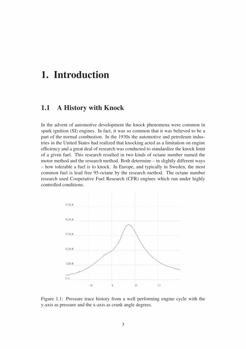
Figure 1.1: Pressure trace history from a well performing engine cycle with the

y-axis as pressure and the x-axis as crank angle degrees.

3

With variable compression ratio – a specific feature of the CFR engine – octane

numbers are determined by comparing the fuel ignition time delay – time between

spark and start of combustion – with two predefined reference fuels of octane num-

ber 0 and 100. Even though octane numbers describe how resilient a fuel is against

knock, the complete physical in-cylinder phenomena during combustion in an SI

engine is complex and the octane number alone can not provide the information

necessary to decide when and why knocking occur.

Engine knock is considered to be one main reason of increased engine wear down.

It has been proved experimentally that engines running under knocking conditions

tend to have more erosion on the piston close to the first piston ring than well tuned

and well performing engines (Johansson, 2006). There is also the risk that eroded

particles mixed with the lubricating oil increase friction in other parts of the engine,

grinding metal until the particles are cleaned up by the oil filter. Engines running

with heavy knock might even suffer immediate failure due to the high level of me-

chanical stress – higher than the designed tolerance of some engine components –

due to pressure oscillations. In modern concepts of engines, down-sizing among

others, aim to increase fuel efficiency. Down-sizing is an example where more fuel

efficient turbo-charged engines with reduced size work under higher pressures. Un-

fortunately down-sizing have the disadvantage of being highly limited by knock.

These limiting properties of knock showed for the importance of understanding

auto-ignition – the actual abnormal combustion that creates the metallic knocking

sound – in detail. Modeling knock has proved to be a daunting task and a continuous

increase of research in the area has been conducted since the late 1950s.

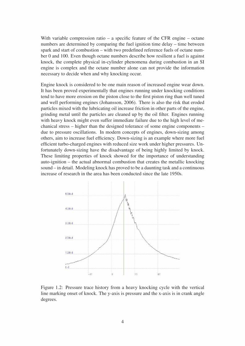
Figure 1.2: Pressure trace history from a heavy knocking cycle with the vertical

line marking onset of knock. The y-axis is pressure and the x-axis is in crank angle

degrees.

4

1.2 The Knock Phenomena

Ideal combustion starts with controlled ignition, usually somewhere around 10–40

crank angle degrees (CAD) before top dead center (BTDC). The choice of spark

advance depends on, for example, engine speed and load, for maximum efficiency

to be maintained. Pressure and temperature rise smoothly as the flame front propa-

gates trough the cylinder with a turbulent surface much larger than one of spherical

shape. At optimal combustion, peak pressure is positioned a few crank angle de-

grees after top dead center (ATDC) in order to deliver maximum mechanical work

on the piston as hot gas expands within the cylinder. Probabilities of auto-ignition

in an SI engine increases as the operating conditions tend towards what is consid-

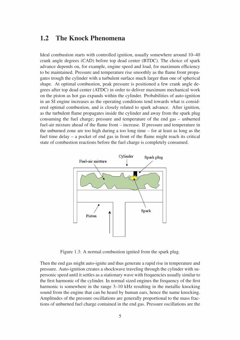
ered optimal combustion, and is closely related to spark advance. After ignition,

as the turbulent flame propagates inside the cylinder and away from the spark plug

consuming the fuel charge; pressure and temperature of the end gas – unburned

fuel-air mixture ahead of the flame front – increase. If pressure and temperature in

the unburned zone are too high during a too long time – for at least as long as the

fuel time delay – a pocket of end gas in front of the flame might reach its critical

state of combustion reactions before the fuel charge is completely consumed.

Figure 1.3: A normal combustion ignited from the spark plug.

Then the end gas might auto-ignite and thus generate a rapid rise in temperature and

pressure. Auto-ignition creates a shockwave traveling through the cylinder with su-

personic speed until it settles as a stationary wave with frequencies usually similar to

the first harmonic of the cylinder. In normal sized engines the frequency of the first

harmonic is somewhere in the range 3–10 kHz resulting in the metallic knocking

sound from the engine that can be heard by human ears, hence the name knocking.

Amplitudes of the pressure oscillations are generally proportional to the mass frac-

tions of unburned fuel charge contained in the end gas. Pressure oscillations are the

5

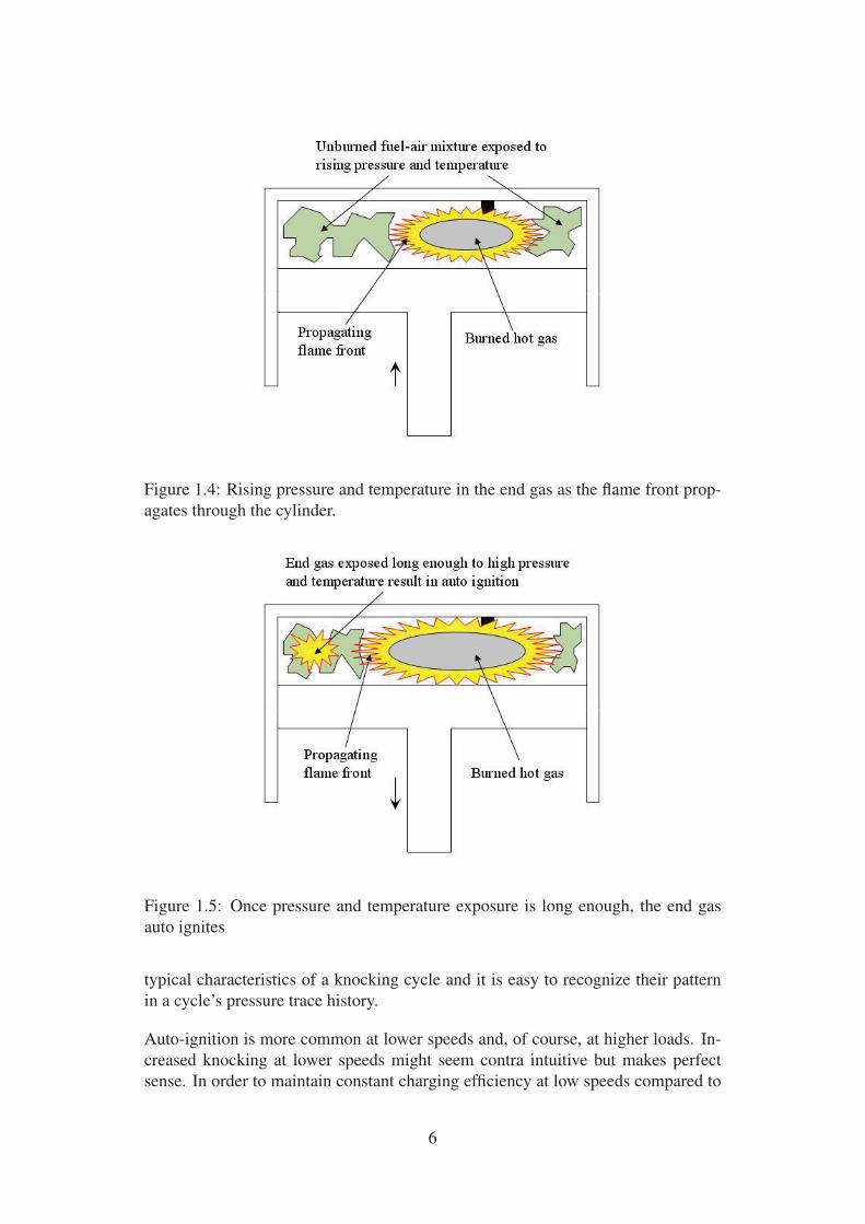
Figure 1.4: Rising pressure and temperature in the end gas as the flame front prop-

agates through the cylinder.

Figure 1.5: Once pressure and temperature exposure is long enough, the end gas

auto ignites

typical characteristics of a knocking cycle and it is easy to recognize their pattern

in a cycle’s pressure trace history.

Auto-ignition is more common at lower speeds and, of course, at higher loads. In-

creased knocking at lower speeds might seem contra intuitive but makes perfect

sense. In order to maintain constant charging efficiency at low speeds compared to

6

high speeds, each cycle needs to burn more fuel during a longer time – seconds,

not crank angle degrees – resulting in more fuel at higher temperatures and pres-

sure during a longer time. In other words, fewer combustions but each with larger

explosions. These are precisely the criterions for auto-ignition to occur.

1.3 Previous Work

Different auto-ignition models developed over the years can be classified in the

groups of detailed chemical kinetic models (Errico et al., 2007), reduced chemical

kinetic models (Noda et al., 2004) and empirical models based on the Arrhenius

equation (Kawai et al., 2009)(Douaud and Eyzat, 1978)(Elmqvist et al., 2003)(By

et al., 1981)(Worret et al., 2002). The chemical kinetic models are extremely com-

plicated and details of hundreds of sub-reactions of the species used must be taken

into account to achieve accuracy. Due to the complexity of these models they are

not suited for fast simulations or online calculations. They are also highly depen-

dent on what fuel is used which reduce their general applicability. Empirical models

based on the Arrhenius equation have proved to be able to predict onset of knock in

simulations within a few crank angle degrees. They are flexible and it is possible to

increase model complexity step-wise as needs of more general use and higher pre-

cision increase. Modern research using and developing similar models often refer

to work made by Douaud and Eyzat (Douaud and Eyzat, 1978) and their findings

of parameter correlations. The same goes for this work where their research lay out

the base line of auto-ignition modeling.

1.4 Motivation

As already mentioned, knocking is more than just a ticking noise. It reduce en-

gine efficiency, hence knocking is also of environmental concern. In the case of

light knocking, it contributes to wear-down of the engine and in the case of heavy

knocking; immediate engine failure might cause more than just material damage.

Calibration of engines under development, to acquire optimal fuel efficiency and

minimal emissions and wear down, is a time-consuming task and an automated

calibration system is a current target of research. One part of calibration would

be to figure out at what spark advance the knock boundary of an engine running

under any given operating conditions is. Also, during the early stages of engine

development, it is important to know – even roughly – where the knock boundary

is so that experiments can be made without risk of damaging neither engineers nor

equipment.

The empirical knock model based on the Arrhenius equation is motivated due to its

simplicity, generality and physical interpretation.

7

1.5 Objectives

Investigate the possibility of using an empirical knock model based on the Arrhenius

equation in engine calibration. The goal is not only to determine onset of knock but

also being able to find the knock boundary with minimal human interference.

1.6 Outline

In chapter 2, experiments made and methods of data gathering are explained. Chap-

ter 3 subsequently describes the three main parts of modeling: knock model, tem-

perature models and the K-value. Chapter 4 describes and discusses methods of

predicting and usage of the model. Chapter 5 discuss the results and future of the

described methods and model. Brief explanations of model implementation and

genetic algorithms can be found in appendix A and B.

1.7 Methods and Tools

The main tool used for all modeling and programming is MATLAB. All experi-

mental data from the engine test bench are gathered with DS-0228 real-time cycle

measuring equipment developed by ONO SOKKI. Also, DS-0228 calculates heat

release and exports pressure data via Microsoft Office Excel to MATLAB. Detecting

knock and calculating knock probabilities at different engine operating conditions

is done with TTDC1 developed Panel 3. In addition, Panel 3 also present data about

charging efficiency and absolute fuel charge injected per stroke. Experiments are

conducted on a Toyota V6 SI gasoline engine and the same engine is used during all

experiments. Unless something else is mentioned, throughout the thesis pressures

are measured in kilopascal [kPa] and temperatures in Kelvin [K].

1.8 Limitations

Experiments at the test bench are limited to run the engine at no higher speeds than

1800 revolutions per minute (RPM). The reason is safety, towards both personnel

and equipment. However this limitation also reduces the validation space of the

model and the results can only be presented within the span of speeds 1000–1800

RPM. All experiments and validations are made on the same engine which also

limits the knowledge of general use of the model. Throughout the thesis only spark

ignition internal combustion engines running the Otto cycle are considered.

1TOYOTA TECHNICAL DEVELOPMENT CORPORATION

8

2. Experiments

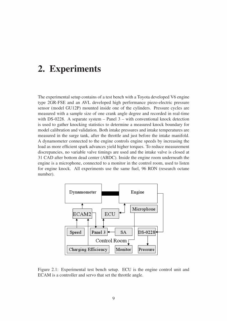
The experimental setup contains of a test bench with a Toyota developed V6 engine

type 2GR-FSE and an AVL developed high performance piezo-electric pressure

sensor (model GU12P) mounted inside one of the cylinders. Pressure cycles are

measured with a sample size of one crank angle degree and recorded in real-time

with DS-0228. A separate system – Panel 3 – with conventional knock detection

is used to gather knocking statistics to determine a measured knock boundary for

model calibration and validation. Both intake pressures and intake temperatures are

measured in the surge tank, after the throttle and just before the intake manifold.

A dynamometer connected to the engine controls engine speeds by increasing the

load as more efficient spark advances yield higher torques. To reduce measurement

discrepancies, no variable valve timings are used and the intake valve is closed at

31 CAD after bottom dead center (ABDC). Inside the engine room underneath the

engine is a microphone, connected to a monitor in the control room, used to listen

for engine knock. All experiments use the same fuel, 96 RON (research octane

number).

Figure 2.1: Experimental test bench setup. ECU is the engine control unit and

ECAM is a controller and servo that set the throttle angle.

9

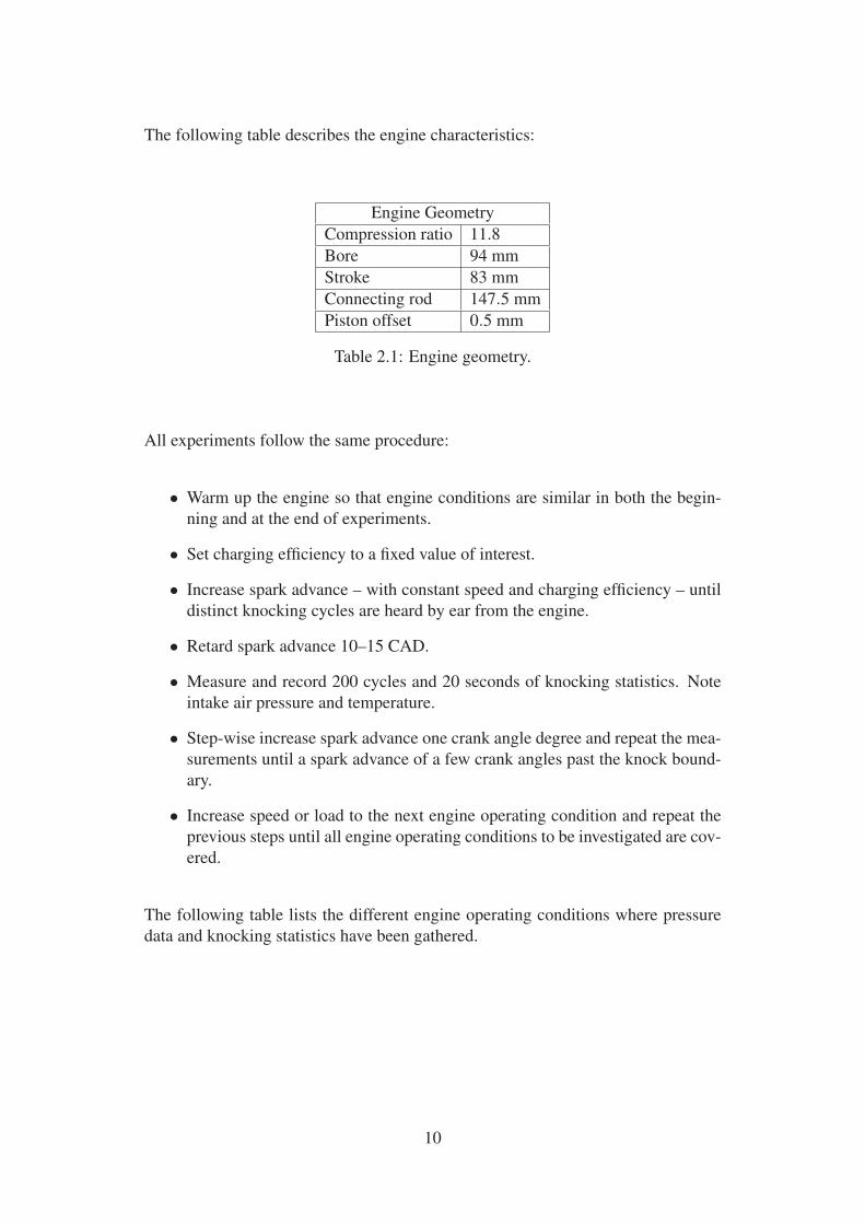
The following table describes the engine characteristics:

Engine Geometry

Compression ratio 11.8

Bore 94 mm

Stroke 83 mm

Connecting rod 147.5 mm

Piston offset 0.5 mm

Table 2.1: Engine geometry.

All experiments follow the same procedure:

• Warm up the engine so that engine conditions are similar in both the begin-

ning and at the end of experiments.

• Set charging efficiency to a fixed value of interest.

• Increase spark advance – with constant speed and charging efficiency – until

distinct knocking cycles are heard by ear from the engine.

• Retard spark advance 10–15 CAD.

• Measure and record 200 cycles and 20 seconds of knocking statistics. Note

intake air pressure and temperature.

• Step-wise increase spark advance one crank angle degree and repeat the mea-

surements until a spark advance of a few crank angles past the knock bound-

ary.

• Increase speed or load to the next engine operating condition and repeat the

previous steps until all engine operating conditions to be investigated are cov-

ered.

The following table lists the different engine operating conditions where pressure

data and knocking statistics have been gathered.

10

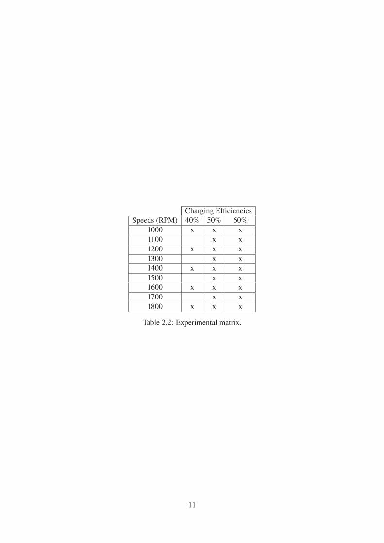
Charging Efficiencies

Speeds (RPM) 40% 50% 60%

1000 x x x

1100 x x

1200 x x x

1300 x x

1400 x x x

1500 x x

1600 x x x

1700 x x

1800 x x x

Table 2.2: Experimental matrix.

11

3. Modeling

Predicting knock requires a few sub models working together. This section de-

scribes in detail the components needed to find the knock boundary.

First, the knock model is described and its similarities to a chemical reaction rate

model known as the Arrhenius equation, which can be related to ignition time delay

of a fuel. Subsequently, a method using the ignition time delay information to

calculate onset of knock is described. In addition to pressure history of an engine

cycle, temperatures of unburned end gas needs to be calculated and implemented

together with the knock model. To achieve increased precision and introduce better

knowledge of when to stop the search of knock onset at any given cycle, the K-value

(Worret et al., 2002) is introduced. In addition, the K-value also opens up for a

method to calculate a distance or size from the current spark advance to the position

where knock occur. This is however described in the next chapter – Prediction –

rather than in the modeling chapter.

3.1 Knock Model

Empirical auto-ignition model

The idea behind the Arrhenius equation that motivates its use – or its cousin’s use

– in the auto-ignition model is its dependencies of the rate constant of chemical

reactions on the temperature and some activation energy. The Arrhenius equation is

commonly expressed as

k = Aexp

(E

RT

)(3.1)

where k is the rate constant, A is a pre-exponential factor, E activation energy, R the

gas constant and T is temperature. The similarities between the Arrhenius equation

and the ignition time delay model is clear, as the latter is modeled as

12

τ = tk − t0 =C1 p−C2 exp

(C3

T

), (3.2)

where p and T are pressures and temperatures of the end gas, tk and t0 the time at

which auto-ignition occur and the ignition timing respectively and C1, C2 and C3 are

model coefficients to be determined (Douaud and Eyzat, 1978). In the cases when

the physical state of the mixture is constant, τ is referred to as ignition time delay.

Under these conditions, and since the unburned gas is compressed and expanded

continuously, it can be assumed that

d

dt

(xxc

)= g

( tτ

), (3.3)

with x as the concentration of reaction components, the constant xc as a critical

concentration leading to auto-ignition and g as a function of time and ignition time

delay (Worret et al., 2002). The function g cannot be determined by ignition time

delay data – fuel octane number – only (Douaud and Eyzat, 1978)so, if it is assumed

that the reaction rate does not change with time during a fixed state process, then

g( t

τ

)=

1

τ. (3.4)

Using equation (3.3) and (3.4) with equation (3.2) and integrating yields

xxc

=

tk∫t0

1

τdt ≡ 1, (3.5)

where xxc

– the critical concentration ratio – equals one if and only if the critical

concentration of the species is reached. The time at where the integral reaches one

is then the timing of knock onset (figure 3.1).

To simplify calculations and increase understanding of the process it is convenient

to transform the integral into crank angles degrees rather than time,

1 =1

6ω

θk∫θ0

1

τdθ , (3.6)

where ω is engine speed in RPM and θ are crank angles; θ0 start of calculations

– which can be chosen arbitrarily – and θk is the crank angle at which knock oc-

cur. The scalars 6 and ω are results of scaling from time in seconds to crank angle

degrees, where one cycle rotates 720 degrees, two whole revolutions. Combining

13

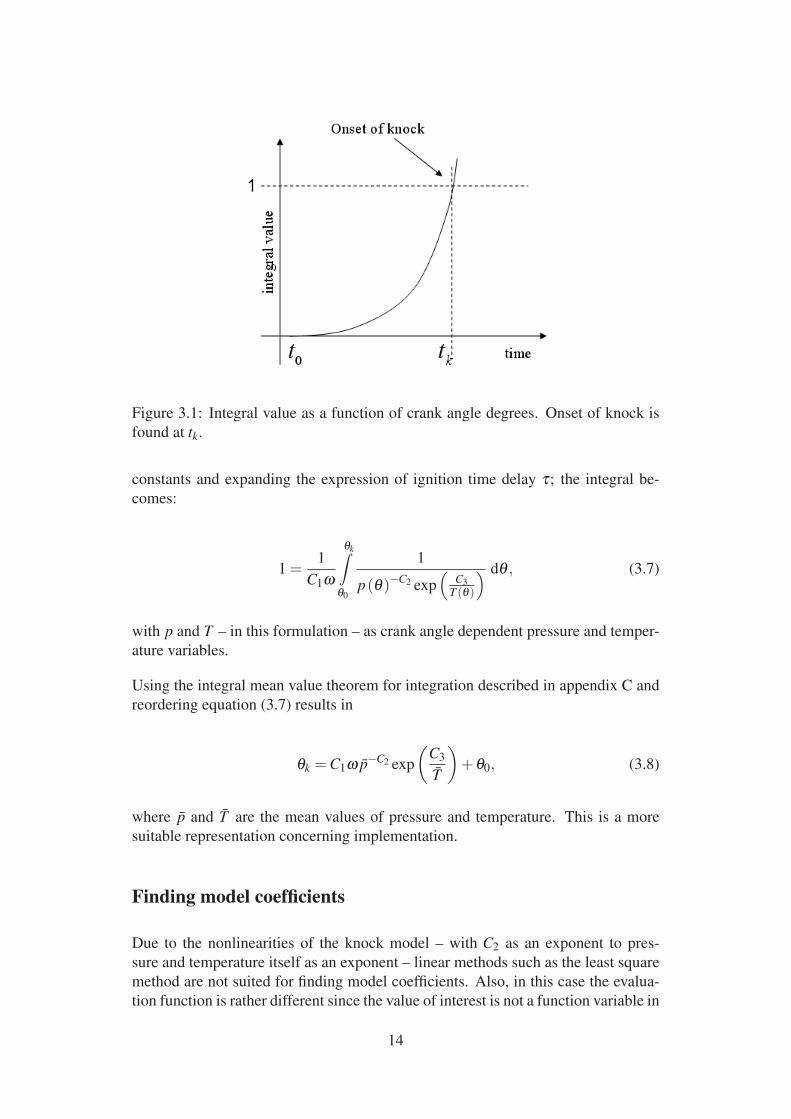
Figure 3.1: Integral value as a function of crank angle degrees. Onset of knock is

found at tk.

constants and expanding the expression of ignition time delay τ; the integral be-

comes:

1 =1

C1ω

θk∫θ0

1

p(θ)−C2 exp(

C3

T (θ)

) dθ , (3.7)

with p and T – in this formulation – as crank angle dependent pressure and temper-

ature variables.

Using the integral mean value theorem for integration described in appendix C and

reordering equation (3.7) results in

θk =C1ω p̄−C2 exp

(C3

T̄

)+θ0, (3.8)

where p̄ and T̄ are the mean values of pressure and temperature. This is a more

suitable representation concerning implementation.

Finding model coefficients

Due to the nonlinearities of the knock model – with C2 as an exponent to pres-

sure and temperature itself as an exponent – linear methods such as the least square

method are not suited for finding model coefficients. Also, in this case the evalua-

tion function is rather different since the value of interest is not a function variable in

14

normal sense, but the upper limit of the integrand interval. Taking this into account

together with the non-linear properties of the knock model motivates a heuristic

coefficient search; and in this thesis a genetic algorithm is implemented and used.

Genetic algorithms are well suited for optimization of non-linear problems, and

even though an optimal solution can not be guaranteed, genetic algorithms have

proven to deliver good results in many applications. Another advantage of genetic

algorithms is the possibility of using almost any function as a fitness function. As

long as it is possible to implement some error measurement, a genetic algorithm is

capable of finding a solution, no matter how the error itself is defined. More details

about genetic algorithms and the implementation of one are found in appendix B.

Steps made to fit the coefficients with help of a genetic algorithm are:

• Measure a few cycles showing light knock at different engine operating con-

ditions. The reason of keeping knocking as light as possible is to achieve high

model sensitivity. Since there are three unknowns in the model at least three

engine operating conditions are needed.

• Measure an average onset of knock at each condition and average the cycles.

• Start the algorithm in a large search space so that the values are not limited

by size; but what is found might be a bit rough.

• Narrow the search space around the new coefficients and repeat the run to

improve precision (this step depends on the implementation and is not always

necessary).

The engine operating conditions used with the genetic algorithm here are 1000 RPM

and 1200 RPM at 40% charging efficiency and 1000 RPM at 50% charging effi-

ciency. The resulting coefficients are shown in table 3.1.

C1 C2 C3

305.731 1.7914 3188.7424

Table 3.1: Static model coefficients.

Unfortunately, investigation found the initial model coefficients to be insufficient.

As speed increased the model seemed to fall behind, never reaching one even though

it should. Because of this, the model could only find the onset of knock at engine

operating conditions close to the once used for finding the model coefficients and

not at all outside of this narrow space. This gave rise to the idea of implementing

adaptation of the model. However, while trying to understand the problem a simpler

solution was found.

15

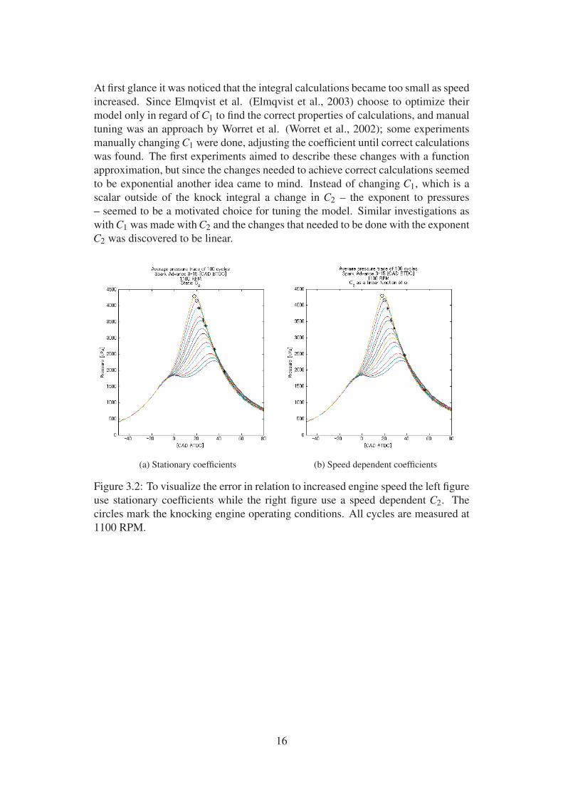
At first glance it was noticed that the integral calculations became too small as speed

increased. Since Elmqvist et al. (Elmqvist et al., 2003) choose to optimize their

model only in regard of C1 to find the correct properties of calculations, and manual

tuning was an approach by Worret et al. (Worret et al., 2002); some experiments

manually changing C1 were done, adjusting the coefficient until correct calculations

was found. The first experiments aimed to describe these changes with a function

approximation, but since the changes needed to achieve correct calculations seemed

to be exponential another idea came to mind. Instead of changing C1, which is a

scalar outside of the knock integral a change in C2 – the exponent to pressures

– seemed to be a motivated choice for tuning the model. Similar investigations as

with C1 was made with C2 and the changes that needed to be done with the exponent

C2 was discovered to be linear.

(a) Stationary coefficients (b) Speed dependent coefficients

Figure 3.2: To visualize the error in relation to increased engine speed the left figure

use stationary coefficients while the right figure use a speed dependent C2. The

circles mark the knocking engine operating conditions. All cycles are measured at

1100 RPM.

16

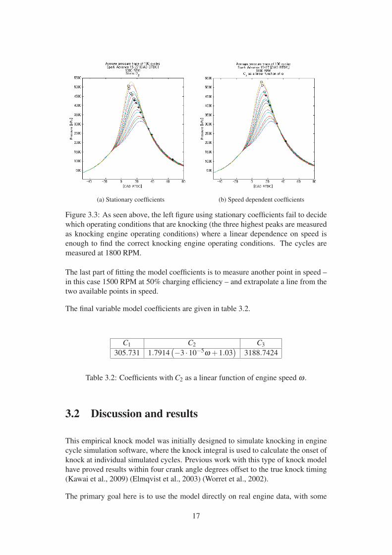
(a) Stationary coefficients (b) Speed dependent coefficients

Figure 3.3: As seen above, the left figure using stationary coefficients fail to decide

which operating conditions that are knocking (the three highest peaks are measured

as knocking engine operating conditions) where a linear dependence on speed is

enough to find the correct knocking engine operating conditions. The cycles are

measured at 1800 RPM.

The last part of fitting the model coefficients is to measure another point in speed –

in this case 1500 RPM at 50% charging efficiency – and extrapolate a line from the

two available points in speed.

The final variable model coefficients are given in table 3.2.

C1 C2 C3

305.731 1.7914(−3 ·10−5ω +1.03

)3188.7424

Table 3.2: Coefficients with C2 as a linear function of engine speed ω .

3.2 Discussion and results

This empirical knock model was initially designed to simulate knocking in engine

cycle simulation software, where the knock integral is used to calculate the onset of

knock at individual simulated cycles. Previous work with this type of knock model

have proved results within four crank angle degrees offset to the true knock timing

(Kawai et al., 2009) (Elmqvist et al., 2003) (Worret et al., 2002).

The primary goal here is to use the model directly on real engine data, with some

17

averaged cycles to get as close as possible to an ideal combustion cycle at the cur-

rent engine operating condition. Applying the model to real data has both its pros

and cons. An advantage is that complexity in combustion that could be lost in sim-

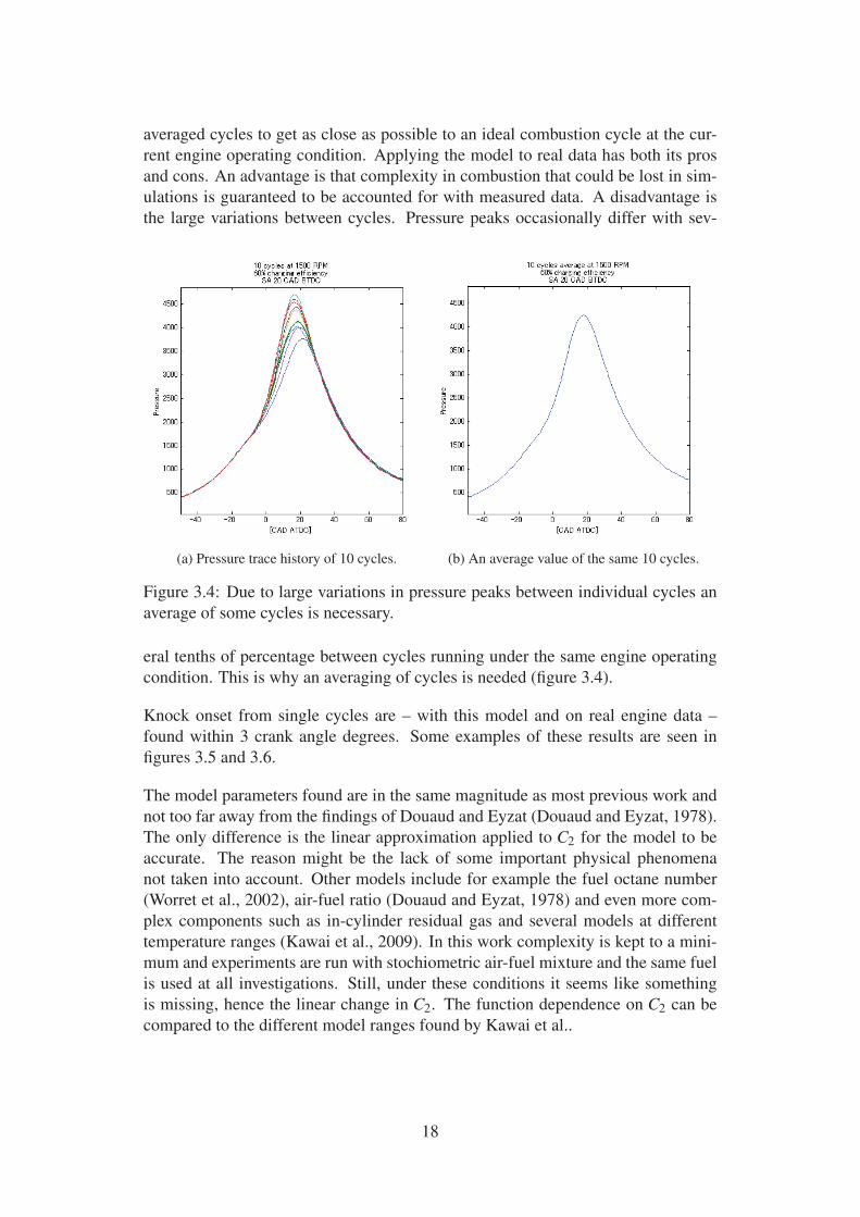
ulations is guaranteed to be accounted for with measured data. A disadvantage is

the large variations between cycles. Pressure peaks occasionally differ with sev-

(a) Pressure trace history of 10 cycles. (b) An average value of the same 10 cycles.

Figure 3.4: Due to large variations in pressure peaks between individual cycles an

average of some cycles is necessary.

eral tenths of percentage between cycles running under the same engine operating

condition. This is why an averaging of cycles is needed (figure 3.4).

Knock onset from single cycles are – with this model and on real engine data –

found within 3 crank angle degrees. Some examples of these results are seen in

figures 3.5 and 3.6.

The model parameters found are in the same magnitude as most previous work and

not too far away from the findings of Douaud and Eyzat (Douaud and Eyzat, 1978).

The only difference is the linear approximation applied to C2 for the model to be

accurate. The reason might be the lack of some important physical phenomena

not taken into account. Other models include for example the fuel octane number

(Worret et al., 2002), air-fuel ratio (Douaud and Eyzat, 1978) and even more com-

plex components such as in-cylinder residual gas and several models at different

temperature ranges (Kawai et al., 2009). In this work complexity is kept to a mini-

mum and experiments are run with stochiometric air-fuel mixture and the same fuel

is used at all investigations. Still, under these conditions it seems like something

is missing, hence the linear change in C2. The function dependence on C2 can be

compared to the different model ranges found by Kawai et al..

18

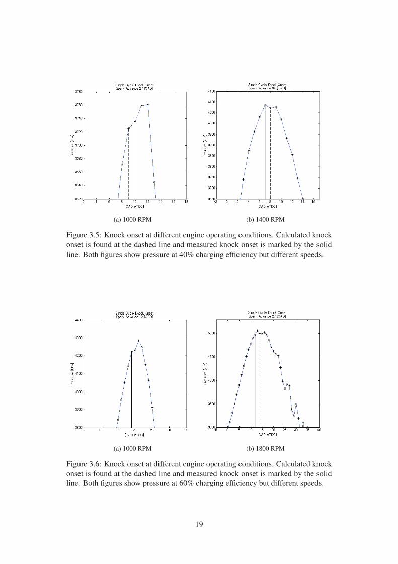
(a) 1000 RPM (b) 1400 RPM

Figure 3.5: Knock onset at different engine operating conditions. Calculated knock

onset is found at the dashed line and measured knock onset is marked by the solid

line. Both figures show pressure at 40% charging efficiency but different speeds.

(a) 1000 RPM (b) 1800 RPM

Figure 3.6: Knock onset at different engine operating conditions. Calculated knock

onset is found at the dashed line and measured knock onset is marked by the solid

line. Both figures show pressure at 60% charging efficiency but different speeds.

19

3.3 Temperature Model

There is more than one approach to model in-cylinder combustion temperatures.

However, in the knock model described in the previous section, there is no interest

in knowing the high temperatures of the hot burned gas. Only temperatures of the

cooler unburned end gas are the necessary temperature information needed.

The temperature model of choice is called a temperature mean value approach

(Klein and Eriksson, 2004)(Eriksson and Andersson, 2002) and contains of a single-

zone mean charge temperature model and a two-zone temperature model.

Single-zone mean charge temperature model

To find the temperature in the single-zone model the state equation

pV = mRT (3.9)

is used under the assumptions that the total mass of charge m and the mass specific

gas constant R are constant,

mR = const. (3.10)

These assumptions are justified by the fact that the molecular weights of the reac-

tants and products are close to equal (Klein and Eriksson, 2004). With equations

(3.9) and (3.10) relations between pressures, volumes and temperatures at two dif-

ferent timings are described by

p1V1

T1=

p2V2

T2. (3.11)

If pressure, volume and temperature are evaluated at a known reference condition –

such as the timing of when the intake valve close (IVC) – the single-zone tempera-

ture Tsz is given by

Tsz =TIVC

pIVCVIVCpV. (3.12)

20

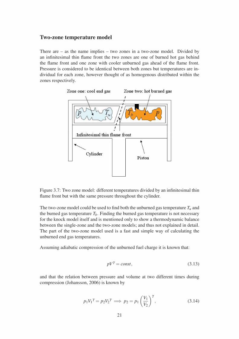
Two-zone temperature model

There are – as the name implies – two zones in a two-zone model. Divided by

an infinitesimal thin flame front the two zones are one of burned hot gas behind

the flame front and one zone with cooler unburned gas ahead of the flame front.

Pressure is considered to be identical between both zones but temperatures are in-

dividual for each zone, however thought of as homogenous distributed within the

zones respectively.

Figure 3.7: Two zone model: different temperatures divided by an infinitesimal thin

flame front but with the same pressure throughout the cylinder.

The two-zone model could be used to find both the unburned gas temperature Tu and

the burned gas temperature Tb. Finding the burned gas temperature is not necessary

for the knock model itself and is mentioned only to show a thermodynamic balance

between the single-zone and the two-zone models; and thus not explained in detail.

The part of the two-zone model used is a fast and simple way of calculating the

unburned end gas temperatures.

Assuming adiabatic compression of the unburned fuel charge it is known that:

pV γ = const, (3.13)

and that the relation between pressure and volume at two different times during

compression (Johansson, 2006) is known by

p1V1γ = p2V2

γ =⇒ p2 = p1

(V1

V2

)γ, (3.14)

21

or what is of interest in this case:

(p1

p2

) 1γ=

V2

V1. (3.15)

The temperatures after compression are given by combining (3.15), the ideal gas

law and adiabatic compression in the following way,

p1V1

T1=

p2V2

T2

V2

V1=

(p1

p2

)γ

⎫⎪⎪⎬⎪⎪⎭

=⇒ T2

T1=

p2

p1

V2

V1=

p2

p1

(p1

p2

) 1γ=

(p1

p2

) 1γ −1

=

(p2

p1

)1− 1γ

(3.16)

and T2 is then given by

T2 = T1

(p2

p1

)1− 1γ. (3.17)

The initial temperature Tu,i of the unburned zone is known from the single-zone

model, evaluated at IVC, and then calculated at start of combustion; in this case at

ignition timing,

Tu,i = Tsz,ig =TIVC

pIVCVIVCpigVig. (3.18)

The unburned zone temperature after ignition is then calculated by combining Tu,iwith equation (3.17),

Tu = Tu,i

(p

pig

)1− 1γ. (3.19)

The complete unburned zone temperature is described by the timings before ignition

and after ignition,

Tu (θ) =

⎧⎪⎨⎪⎩

Tsz (θ) if θ ≤ θig

Tu,i

(p(θ)

p(θig)

)1− 1γ

if θ > θig(3.20)

Finally according to the laws of thermodynamics, the energy balance between the

single-zone model and the two-zone model is described. With subscript b as burned

and u as unburned and with m as mass of gas mixtures the balance becomes,

22

(mb +mu)cvTsz = mbcv,bTb +mucv,uTu, (3.21)

which – if wanted – could be used to calculate the burned zone temperature under

the assumptions that cv = cv,u = cv,b, meaning calorically perfect gas.

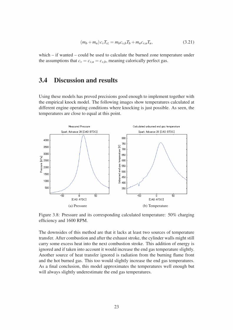
3.4 Discussion and results

Using these models has proved precisions good enough to implement together with

the empirical knock model. The following images show temperatures calculated at

different engine operating conditions where knocking is just possible. As seen, the

temperatures are close to equal at this point.

(a) Pressure (b) Temperature

Figure 3.8: Pressure and its corresponding calculated temperature: 50% charging

efficiency and 1600 RPM.

The downsides of this method are that it lacks at least two sources of temperature

transfer. After combustion and after the exhaust stroke, the cylinder walls might still

carry some excess heat into the next combustion stroke. This addition of energy is

ignored and if taken into account it would increase the end gas temperature slightly.

Another source of heat transfer ignored is radiation from the burning flame front

and the hot burned gas. This too would slightly increase the end gas temperatures.

As a final conclusion, this model approximates the temperatures well enough but

will always slightly underestimate the end gas temperatures.

23

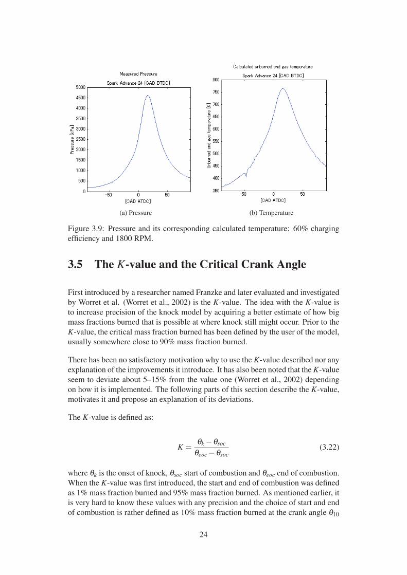
(a) Pressure (b) Temperature

Figure 3.9: Pressure and its corresponding calculated temperature: 60% charging

efficiency and 1800 RPM.

3.5 The K-value and the Critical Crank Angle

First introduced by a researcher named Franzke and later evaluated and investigated

by Worret et al. (Worret et al., 2002) is the K-value. The idea with the K-value is

to increase precision of the knock model by acquiring a better estimate of how big

mass fractions burned that is possible at where knock still might occur. Prior to the

K-value, the critical mass fraction burned has been defined by the user of the model,

usually somewhere close to 90% mass fraction burned.

There has been no satisfactory motivation why to use the K-value described nor any

explanation of the improvements it introduce. It has also been noted that the K-value

seem to deviate about 5–15% from the value one (Worret et al., 2002) depending

on how it is implemented. The following parts of this section describe the K-value,

motivates it and propose an explanation of its deviations.

The K-value is defined as:

K =θk −θsoc

θeoc −θsoc(3.22)

where θk is the onset of knock, θsoc start of combustion and θeoc end of combustion.

When the K-value was first introduced, the start and end of combustion was defined

as 1% mass fraction burned and 95% mass fraction burned. As mentioned earlier, it

is very hard to know these values with any precision and the choice of start and end

of combustion is rather defined as 10% mass fraction burned at the crank angle θ10

24

and 90% mass fraction burned at θ90. The K-value is also proposed to be constant

at the knock boundary which motivates a new model parameter; the critical crank

angle θc. The following transposition of the K-value, with Kre f instead of K and θcinstead of θk yields

θc = θ10 +Kre f (θ90 −θ10) . (3.23)

With the assumption that K is constant on the knock boundary, a reference K-value,

Kre f can be calculated at knock onset from a known knocking cycle. Later, with

cycles at engine operating conditions with unknown knock onset, the critical crank

angle with help of Kre f is calculated as the latest crank angel of where auto-ignition

could possibly occur.

When measuring a new cycle, the knock integral value has to reach one before the

crank angle θc if knock is to occur. The crank angle at where the knock integral

actually do reach one – before θc – is known as the onset of knock.

Regarding the noted deviation in K at different engine operating conditions, it is

here proposed to be a natural cause based on the reasons of auto-ignition. Without

the K-value, the same fixed mass fraction burned is used at all engine operating

conditions to decide whether or not it is possible for knock to occur. However, this

is a faulty assumption since the critical mass of fuel charge left in the engine at a

specific mass fraction burned differs greatly between engine operating conditions.

If the initial fuel charge is large, then 90% mass fractions burned, i.e. 10% mass

fractions fuel charge left in the cylinder is bigger than 10% fuel charge left from

a smaller initial charge. There is only a minor change in the size of fuel charges

between speeds and this difference can safely be ignored. The important changes

are in variations between loads – or rather charging efficiency – where the size of

the fuel charge has to change a lot. The change in K can be seen as a calibration

from mass fractions left in the cylinder to absolute fuel charge left in the engine and

– correctly – result in changes in K at different engine operating conditions.

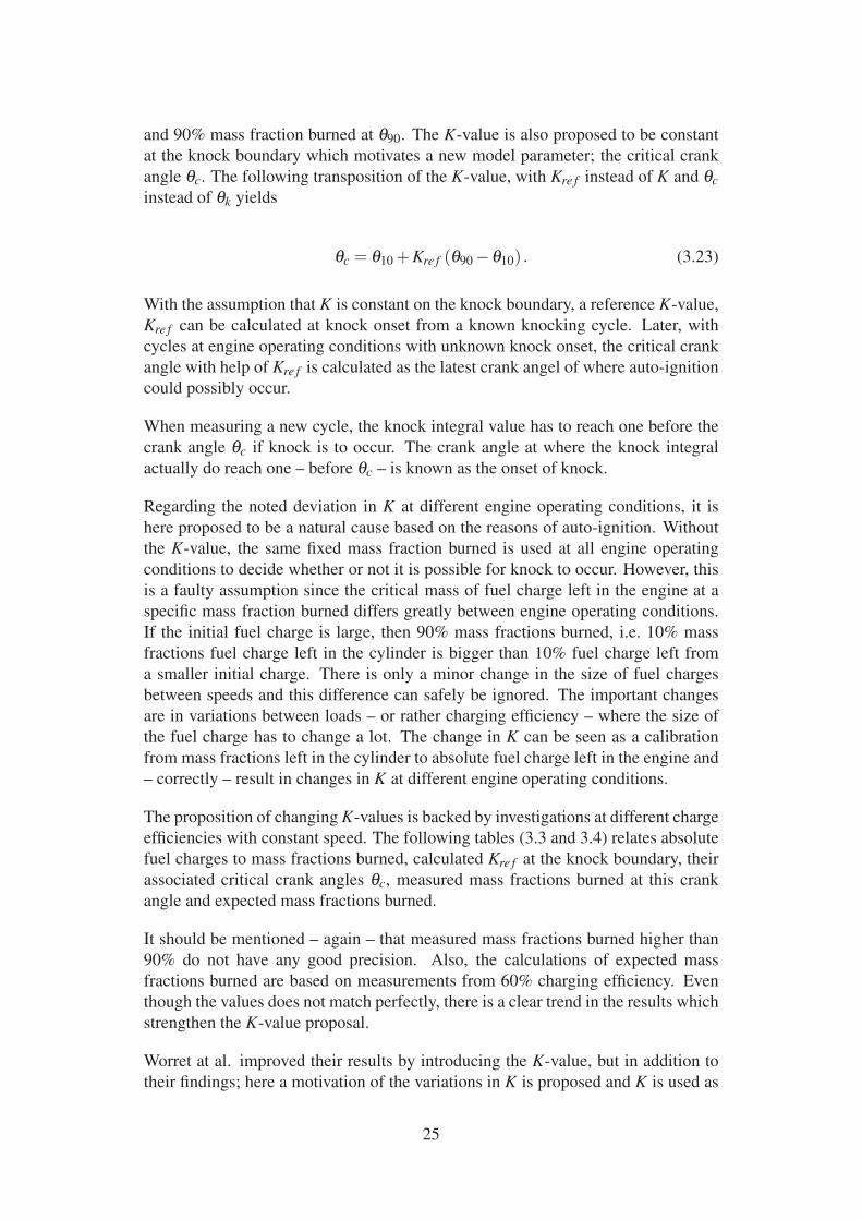
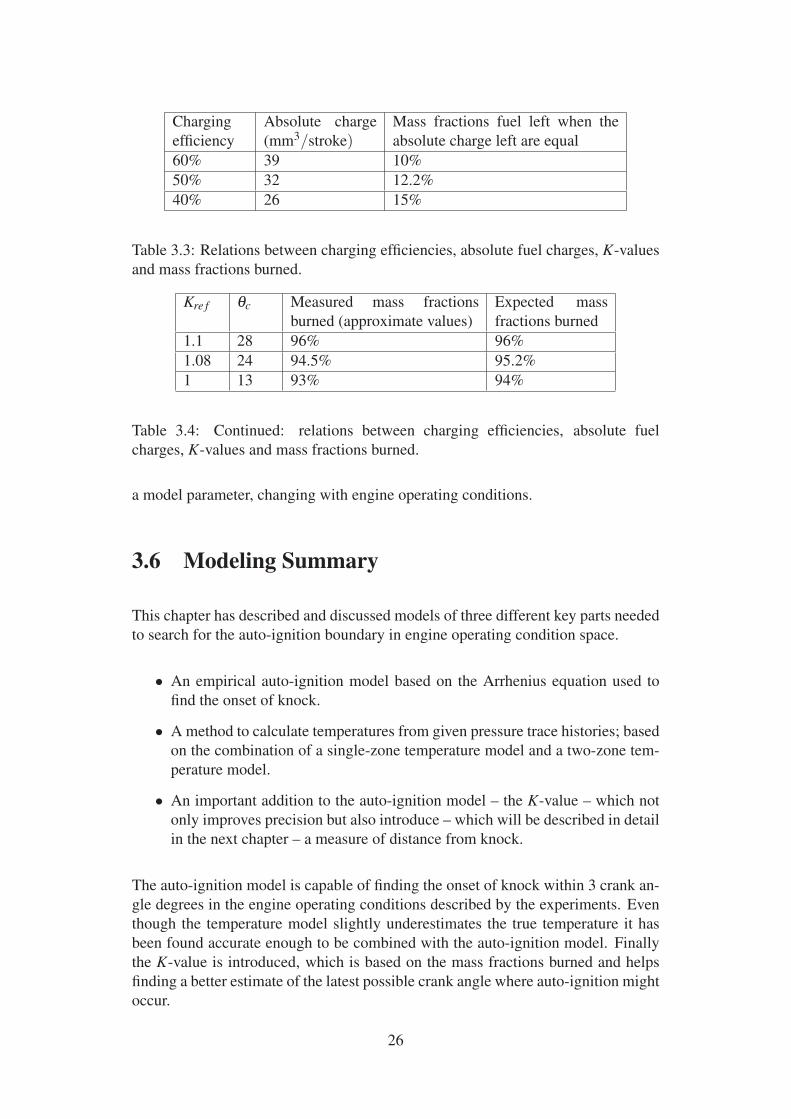
The proposition of changing K-values is backed by investigations at different charge

efficiencies with constant speed. The following tables (3.3 and 3.4) relates absolute

fuel charges to mass fractions burned, calculated Kre f at the knock boundary, their

associated critical crank angles θc, measured mass fractions burned at this crank

angle and expected mass fractions burned.

It should be mentioned – again – that measured mass fractions burned higher than

90% do not have any good precision. Also, the calculations of expected mass

fractions burned are based on measurements from 60% charging efficiency. Even

though the values does not match perfectly, there is a clear trend in the results which

strengthen the K-value proposal.

Worret at al. improved their results by introducing the K-value, but in addition to

their findings; here a motivation of the variations in K is proposed and K is used as

25

Charging

efficiency

Absolute charge

(mm3/stroke)Mass fractions fuel left when the

absolute charge left are equal

60% 39 10%

50% 32 12.2%

40% 26 15%

Table 3.3: Relations between charging efficiencies, absolute fuel charges, K-values

and mass fractions burned.

Kre f θc Measured mass fractions

burned (approximate values)

Expected mass

fractions burned

1.1 28 96% 96%

1.08 24 94.5% 95.2%

1 13 93% 94%

Table 3.4: Continued: relations between charging efficiencies, absolute fuel

charges, K-values and mass fractions burned.

a model parameter, changing with engine operating conditions.

3.6 Modeling Summary

This chapter has described and discussed models of three different key parts needed

to search for the auto-ignition boundary in engine operating condition space.

• An empirical auto-ignition model based on the Arrhenius equation used to

find the onset of knock.

• A method to calculate temperatures from given pressure trace histories; based

on the combination of a single-zone temperature model and a two-zone tem-

perature model.

• An important addition to the auto-ignition model – the K-value – which not

only improves precision but also introduce – which will be described in detail

in the next chapter – a measure of distance from knock.

The auto-ignition model is capable of finding the onset of knock within 3 crank an-

gle degrees in the engine operating conditions described by the experiments. Even

though the temperature model slightly underestimates the true temperature it has

been found accurate enough to be combined with the auto-ignition model. Finally

the K-value is introduced, which is based on the mass fractions burned and helps

finding a better estimate of the latest possible crank angle where auto-ignition might

occur.

26

4. Predicting

If a human were to search for the knock boundary manually the task would be to in-

crease spark advance in each operating condition, listening via a monitor connected

to a microphone in the engine room and trying to identify the sound of auto-ignition.

This method would yield different results depending on the persons who were do-

ing the experiments and it would take a long time to cover all the necessary engine

operating conditions. This chapter explains the distance to knock and discuss how

it might be used to predict the knock boundary. It also investigates and compares

simpler linear searches of spark advance with 10 and 100 averaged cycles respec-

tively.

4.1 Methods

The idea is to use the earlier mentioned distance from knock derived with the K-

value to implement a search scheme with faster than linear search time. Previous

methods of finding the onset of knock has only been concerned about if the integral

value reaches one before a certain percentage mass fractions burned. With the K-

value comes the critical crank angle θc, which has an individual value at each engine

operating condition. In the same way as earlier studies of this model, the integral has

to become one before this specific crank angle is reached. The improvements are

that θc changes with engine operating conditions and it is also possible to continue

the integral calculations until they actually reach one after the critical crank angle.

The value between θc and the crank angle where the integral reach one can be

considered a distance or rather a size, since the function how the size decrease with

spark advance is unknown. The function of size behave in an exponential matter

but it is hard to decide an approximation since its coefficient – whatever they might

be – also change with different engine operating conditions.

The following image (Figure 4.1) visualizes the concept of distance together with

the critical crank angle, spark advance and the knock integral. It can also be noted

that cycles without knock reach one to the right of θc while knocking cycles reach

one precisely on θc or earlier.

The optimal way of finding the knock boundary fast would be to know how the

27

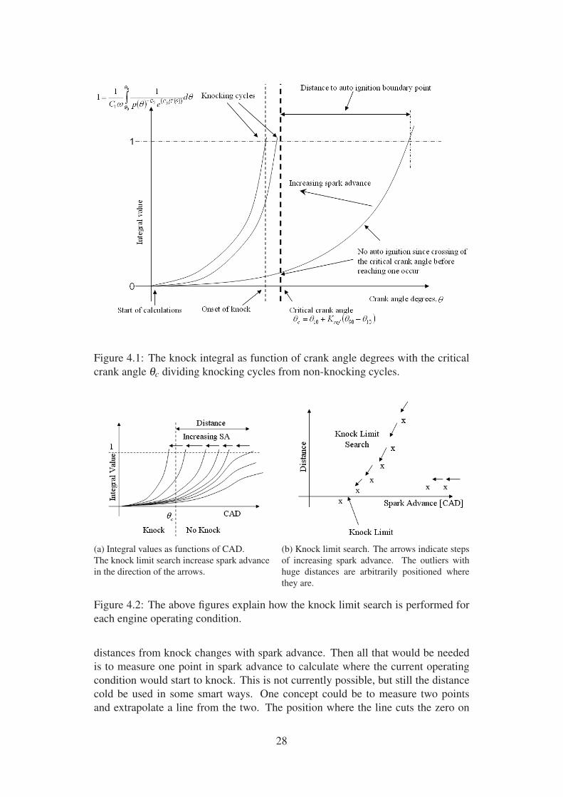
Figure 4.1: The knock integral as function of crank angle degrees with the critical

crank angle θc dividing knocking cycles from non-knocking cycles.

(a) Integral values as functions of CAD.

The knock limit search increase spark advance

in the direction of the arrows.

(b) Knock limit search. The arrows indicate steps

of increasing spark advance. The outliers with

huge distances are arbitrarily positioned where

they are.

Figure 4.2: The above figures explain how the knock limit search is performed for

each engine operating condition.

distances from knock changes with spark advance. Then all that would be needed

is to measure one point in spark advance to calculate where the current operating

condition would start to knock. This is not currently possible, but still the distance

cold be used in some smart ways. One concept could be to measure two points

and extrapolate a line from the two. The position where the line cuts the zero on

28

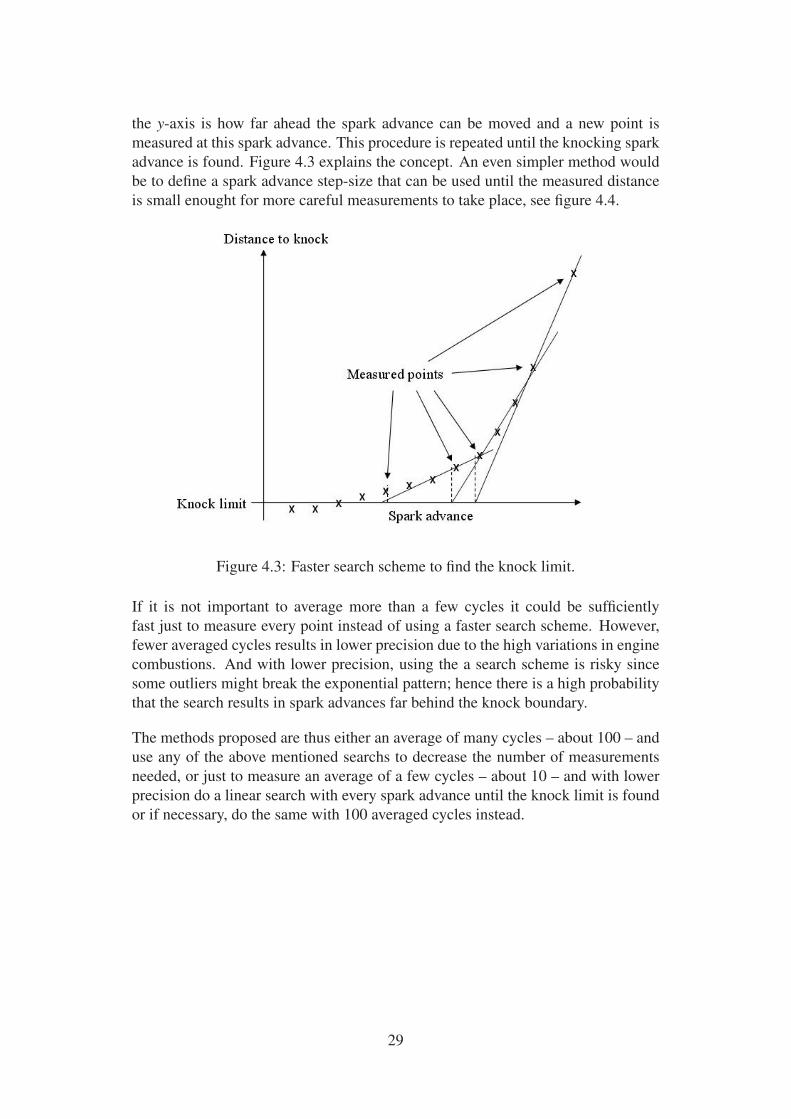
the y-axis is how far ahead the spark advance can be moved and a new point is

measured at this spark advance. This procedure is repeated until the knocking spark

advance is found. Figure 4.3 explains the concept. An even simpler method would

be to define a spark advance step-size that can be used until the measured distance

is small enought for more careful measurements to take place, see figure 4.4.

Figure 4.3: Faster search scheme to find the knock limit.

If it is not important to average more than a few cycles it could be sufficiently

fast just to measure every point instead of using a faster search scheme. However,

fewer averaged cycles results in lower precision due to the high variations in engine

combustions. And with lower precision, using the a search scheme is risky since

some outliers might break the exponential pattern; hence there is a high probability

that the search results in spark advances far behind the knock boundary.

The methods proposed are thus either an average of many cycles – about 100 – and

use any of the above mentioned searchs to decrease the number of measurements

needed, or just to measure an average of a few cycles – about 10 – and with lower

precision do a linear search with every spark advance until the knock limit is found

or if necessary, do the same with 100 averaged cycles instead.

29

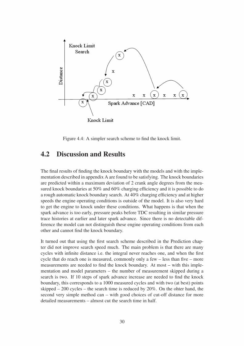
Figure 4.4: A simpler search scheme to find the knock limit.

4.2 Discussion and Results

The final results of finding the knock boundary with the models and with the imple-

mentation described in appendix A are found to be satisfying. The knock boundaries

are predicted within a maximum deviation of 2 crank angle degrees from the mea-

sured knock boundaries at 50% and 60% charging efficiency and it is possible to do

a rough automatic knock boundary search. At 40% charging efficiency and at higher

speeds the engine operating conditions is outside of the model. It is also very hard

to get the engine to knock under these conditions. What happens is that when the

spark advance is too early, pressure peaks before TDC resulting in similar pressure

trace histories at earlier and later spark advance. Since there is no detectable dif-

ference the model can not distinguish these engine operating conditions from each

other and cannot find the knock boundary.

It turned out that using the first search scheme described in the Prediction chap-

ter did not improve search speed much. The main problem is that there are many

cycles with infinite distance i.e. the integral never reaches one, and when the first

cycle that do reach one is measured, commonly only a few – less than five – more

measurements are needed to find the knock boundary. At most – with this imple-

mentation and model parameters – the number of measurement skipped during a

search is two. If 10 steps of spark advance increase are needed to find the knock

boundary, this corresponds to a 1000 measured cycles and with two (at best) points

skipped – 200 cycles – the search time is reduced by 20%. On the ohter hand, the

second very simple method can – with good choices of cut-off distance for more

detailed measurements – almost cut the search time in half.

30

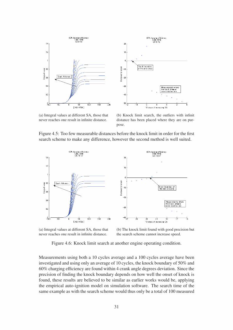
(a) Integral values at different SA, those that

never reaches one result in infinite distance.

(b) Knock limit search, the outliers with infinit

distance has been placed where they are on pur-

pose.

Figure 4.5: Too few measurable distances before the knock limit in order for the first

search scheme to make any difference, however the second method is well suited.

(a) Integral values at different SA, those that

never reaches one result in infinite distance.

(b) The knock limit found with good precision but

the search scheme cannot increase speed.

Figure 4.6: Knock limit search at another engine operating condition.

Measurements using both a 10 cycles average and a 100 cycles average have been

investigated and using only an average of 10 cycles, the knock boundary of 50% and

60% charging efficiency are found within 4 crank angle degrees deviation. Since the

precision of finding the knock boundary depends on how well the onset of knock is

found, these results are believed to be similar as earlier works would be, applying

the empirical auto-ignition model on simulation software. The search time of the

same example as with the search scheme would thus only be a total of 100 measured

31

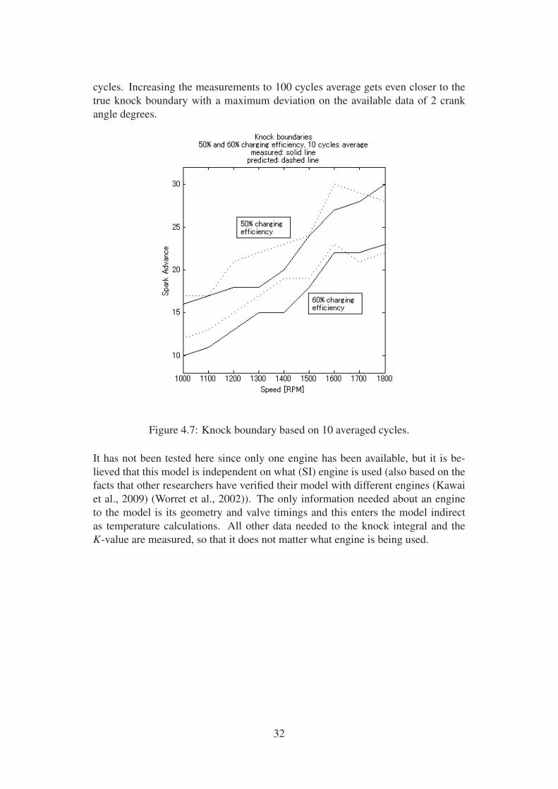
cycles. Increasing the measurements to 100 cycles average gets even closer to the

true knock boundary with a maximum deviation on the available data of 2 crank

angle degrees.

Figure 4.7: Knock boundary based on 10 averaged cycles.

It has not been tested here since only one engine has been available, but it is be-

lieved that this model is independent on what (SI) engine is used (also based on the

facts that other researchers have verified their model with different engines (Kawai

et al., 2009) (Worret et al., 2002)). The only information needed about an engine

to the model is its geometry and valve timings and this enters the model indirect

as temperature calculations. All other data needed to the knock integral and the

K-value are measured, so that it does not matter what engine is being used.

32

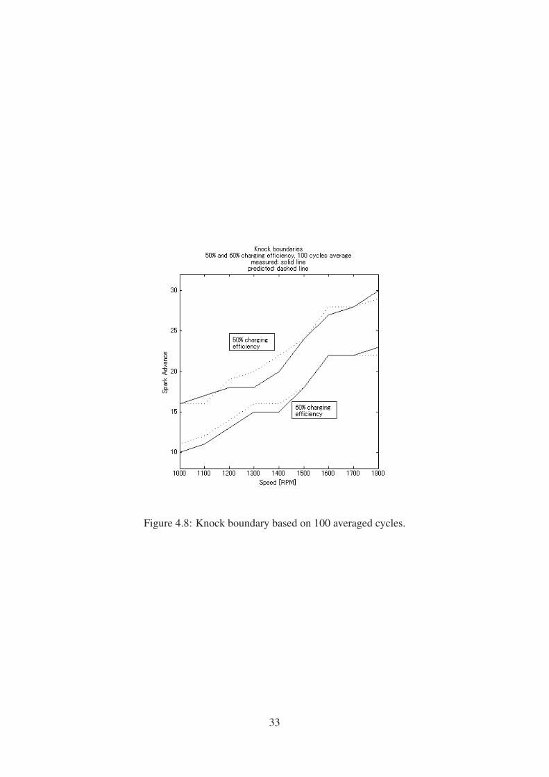
Figure 4.8: Knock boundary based on 100 averaged cycles.

33

5. Conclusions and Future work

The main objective was to be able to find the knock boundary automatically. This

can be done – after model calibration – within a deviation of 2 crank angle degrees,

if an average of 100 cycles is used. The primary improvements from most earlier

works is how the K-value and its related critical crank angle is implemented and

used. Here the K-value is not only used to improve precision of finding onset of

knock but also works as an important part in the methods of finding the knock

boundary by introducing a distance from knock measurement. The distance from

knock, based on the critical crank angle and the position where the knock integral

reaches one can be used by a search scheme to reduce the necessary measurements

and thus reduce the total knock boundary search time.

A future task that would greatly improve the general use of this model would be

to find a method to understand and describe how the K-value changes with engine

operating conditions. Perhaps even include its minor differences between different

speeds to achieve even higher precisions.

It is known that other correlations of knock integral coefficients can be found, and

some of these might have properties so that the problem of infinite distance never

happens. Then the distance to knock could greatly improve the knock boundary

search. In addition to this, understanding or being able to describe the distance

to knock as a function of spark advance would probably be the final goal of this

method. Once this is possible, predicting the knock boundary would be almost

instantaneous with only one – or a few – measurements at each engine operating

condition.

Other improvements are to implement more parameters into the model. This has

already been done by Kawai et al. and even more extensive versions of the model

are under development. To improve model generality it could typically include air-

fuel ratio dependence, fuel octane number and residual gas. If variable valve timing

is used then it has to be implemented as well.

A higher sample frequency is possible since, for example the limit of DS-0228 is

0.5 CAD sample size. Higher sample frequency would not only introduce more

details but also reduce overshoot of the knock integral. Higher sample frequency

has not been used in this thesis to reduce size of the already huge sets of data.

34

A. Implementation

Implementation is mostly straight forward with only a few things to take into extra

consideration.

Even though the model and all calculations are based on the discreet sample of some

crank angle degrees it is important to implement and calculate everything with real

numbers. The critical crank angle θc and the crank angle θk – where the integral

value reach 1 – are highly sensitive to round off errors. If any of these two are

rounded to their closest integer values before all calculations and predictions are

done, the error will be of great significance. Instead, not until a real number of the

knock onset crank angle is found it can be rounded to its closest discreet sample

value.

Another problem is overshoot of the knock integral. Since the samples are only in

one crank angle degree, the integral might be very close to one at a given crank angle

and then greatly overshoot when the next crank angle is included in the calculations.

This is solved by a linear approximation between the two points before and after

crossing 1 on the y-axis, so that the precise real crank angle where the integral

reach one can be determined.

The complete implementation and usage of the model is described in the following

flow chart:

35

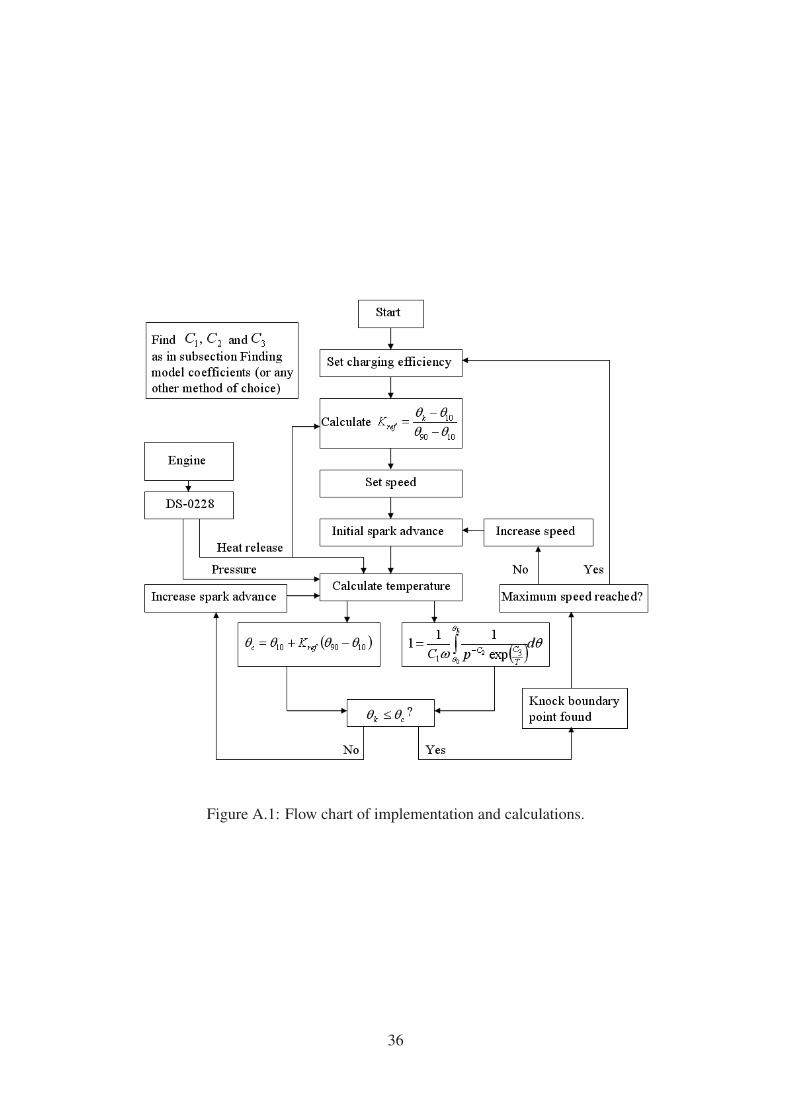
Figure A.1: Flow chart of implementation and calculations.

36

B. Genetic Algorithm

The concept and function of genetic algorithms are based on the biology phenomena

known as evolution and is a type of stochastic search strategy. A more general termi-

nology of genetic algorithms is evolutionary algorithms or in the case of automatic

programming, evolutionary programming. There is a lot of criticism surrounding

evolutionary algorithms. This is due to the fact that it is hard to mathematically

describe their functionality, how they work and how reliable they are; and since

they are heuristic methods, an optimal solution is not guaranteed. There is even

philosophical and metaphysical debate about these methods. Nevertheless evolu-

tionary algorithms continue to deliver great results and have even at some points

outperformed human engineering. One of the most popular examples of programs

outperforming humans is an implementation of genetic programming that designed

a new construction to mount antennas on satellites. It managed to create a weirdly

twisted truss unimaginable to the human mind with increased oscillatory damping

properties and lower weight. More extensive reading about genetic algorithms can

be found in “An introduction to genetic algorithms” (Mitchell, 1998).

Genetic algorithms are based on a population of candidate solutions, also known as

chromosomes. In each iteration – or generation – every chromosome is evaluated

and ranked according to some fitness function and ranking rules. The probability

of reproducing or even surviving to the next generation depends on the ranking of a

chromosome. This process is repeated until some maximum number of generations

is reached or an acceptable solution is found. As long as the solutions can be de-

scribed by a chromosome and it is possible to measure some error with the fitness

function, genetic algorithms are applicable to a wide area of problems.

Chromosomes are constructed by a set of genes and each gene has a number of

loci. Each locus can take a value from the allele of choice, the set of valid values.

Alleles are commonly binary so that the allele – or state – of a locus is zero or

one. The number of loci in a gene needed is a tradeoff between complexity of the

problem, precision and computational efficiency. The same goes for the population

of chromosomes. Initialization of a chromosomes can be either randomly or – if

available – an educated guess.

As an example, the chromosomes of the implementation used to find the knock

integral coefficients have three genes, one for each coefficient. Each gene contains

of 44 loci with the alleles 0 and 1 and describes, with some precision a real number.

37

The size of the population is 150 chromosomes and a typical number of generations

are 50–100.

Evolution of chromosomes is based on genetic operators. The most important and

commonly used operators are crossover, mutation and inversion:

• Crossover can be seen as breeding, where two parents create a child by com-

bining half of their genes respectively into a new chromosome.

• Inversion is a more abstract operator that basically just invert the chromosome

or some chosen subset of the chromosome.

• Mutation is another genetic operator with its foundation in biology. When a

chromosome mutates it simply switch state of a randomly chosen locus.

All operations are based on probability. For example, a mutation can not happen too

often since then the population never gets a chance to converge. However, it has to

mutate some times or else the population will lose its diversity hence not being able

to search the entire problem space. Common probabilities are 0.75 for crossover to

happen, about 0.1 for inversion and 0.001 for mutation.

Finally there is the process of selection. Selection decides which chromosomes that

will survive to the next generation. The decision is made by some sort of battle

between the chromosomes, according to the concept “survival of the fittest”. In this

implementation the roulette wheel method is used and consequently it is the only

method described.

From the fitness value of a chromosome a normalized fitness is calculated and with

that the cumulative norm of each chromosome is created (by calculating the cu-

mulative sum of all the chromosomes normalized fitness). Then a set of random

numbers – as many as there are chromosomes – between 0 and 1 are generated. If

the random value is between the cumulative norm of a given chromosome and the

cumulative norm of the chromosome prior to it in the list of chromosomes, the given

chromosome is allowed to carry on to the next generation. In this process the most

fit chromosomes survive in multiple copies while the worst fitted chromosomes with

time disappear.

38

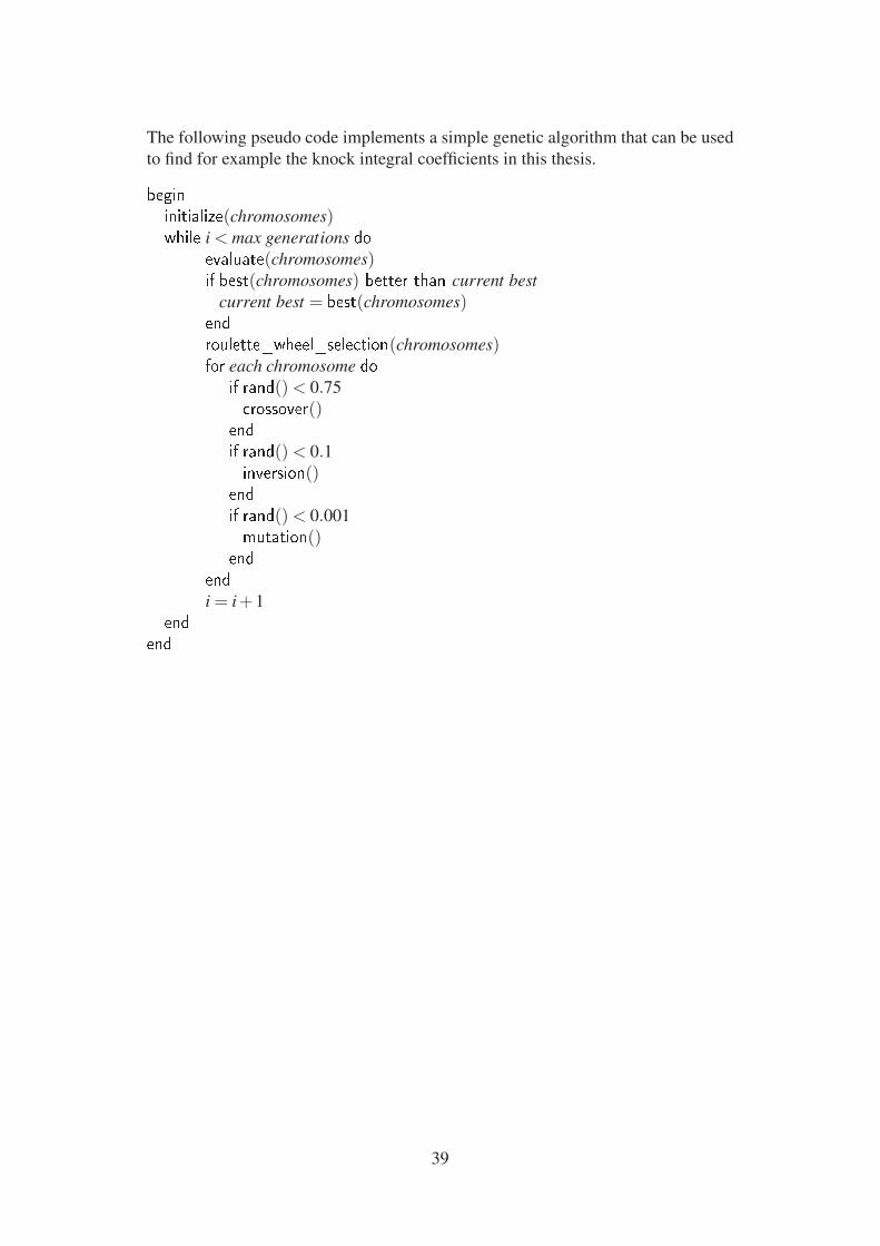
The following pseudo code implements a simple genetic algorithm that can be used

to find for example the knock integral coefficients in this thesis.

��������������(chromosomes)���� i < max generations �

��������(chromosomes)�� ����(chromosomes) ������ ���� current best

current best = ����(chromosomes)���� ������������������� �(chromosomes)� � each chromosome �

�� ����()< 0.75

�� �� ���()����� ����()< 0.1������� �()

����� ����()< 0.001

������ �()���

���i = i+1

������

39

C. Mean value theorem for integrals

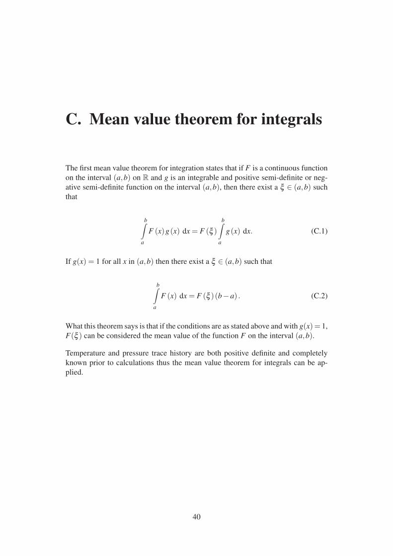
The first mean value theorem for integration states that if F is a continuous function

on the interval (a,b) on R and g is an integrable and positive semi-definite or neg-

ative semi-definite function on the interval (a,b), then there exist a ξ ∈ (a,b) such

that

b∫a

F (x)g(x) dx = F (ξ )b∫

a

g(x) dx. (C.1)

If g(x) = 1 for all x in (a,b) then there exist a ξ ∈ (a,b) such that

b∫a

F (x) dx = F (ξ )(b−a) . (C.2)

What this theorem says is that if the conditions are as stated above and with g(x)= 1,

F(ξ ) can be considered the mean value of the function F on the interval (a,b).

Temperature and pressure trace history are both positive definite and completely

known prior to calculations thus the mean value theorem for integrals can be ap-

plied.

40

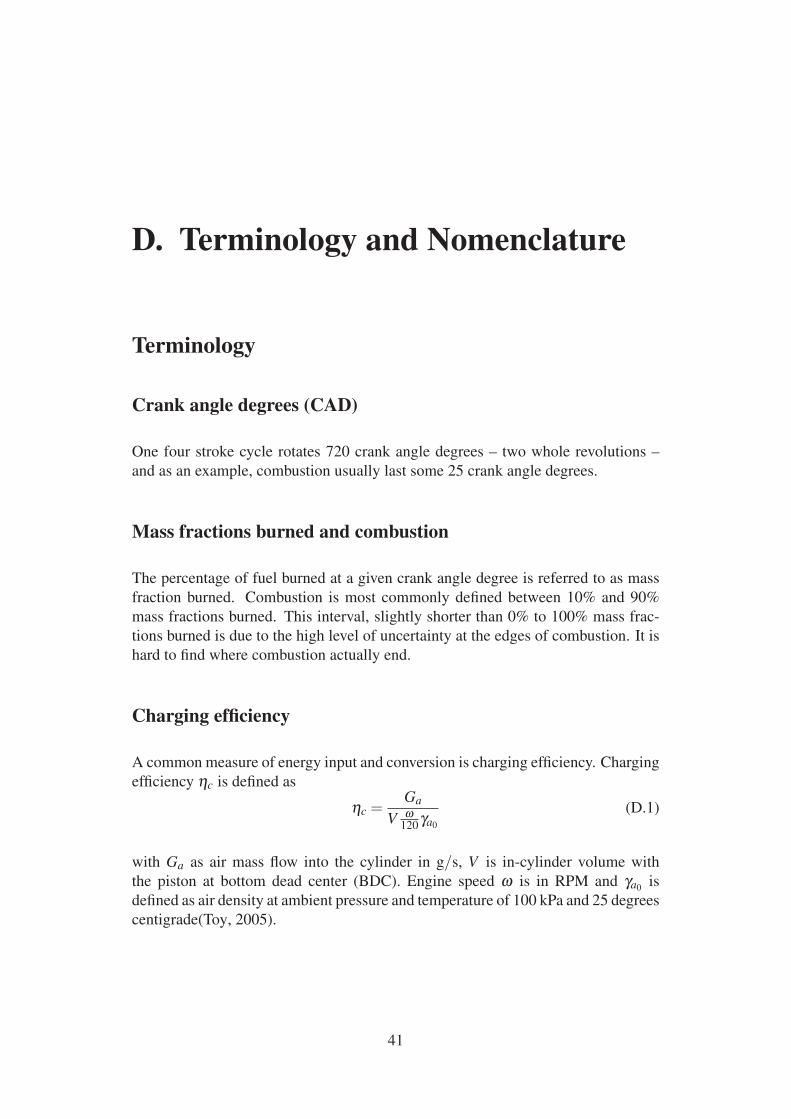
D. Terminology and Nomenclature

Terminology

Crank angle degrees (CAD)

One four stroke cycle rotates 720 crank angle degrees – two whole revolutions –

and as an example, combustion usually last some 25 crank angle degrees.

Mass fractions burned and combustion

The percentage of fuel burned at a given crank angle degree is referred to as mass

fraction burned. Combustion is most commonly defined between 10% and 90%

mass fractions burned. This interval, slightly shorter than 0% to 100% mass frac-

tions burned is due to the high level of uncertainty at the edges of combustion. It is

hard to find where combustion actually end.

Charging efficiency

A common measure of energy input and conversion is charging efficiency. Charging

efficiency ηc is defined as

ηc =Ga

V ω120γa0

(D.1)

with Ga as air mass flow into the cylinder in g/s, V is in-cylinder volume with

the piston at bottom dead center (BDC). Engine speed ω is in RPM and γa0is

defined as air density at ambient pressure and temperature of 100 kPa and 25 degrees

centigrade(Toy, 2005).

41

Spark advance (SA)

Increasing spark advance is defined as moving the ignition point to an earlier posi-

tion (in crank angle degrees) and usually somewhere BTDC; hence it is preferably

expressed in CAD BTDC rather than ATDC (the latter would yield a negative in-

crease in spark advance).

End gas

The term end gas refers to the cooler unburned pockets of gas – as in gasoline and

air mixture – ahead of the combustion flame front.

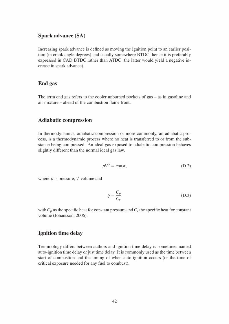
Adiabatic compression

In thermodynamics, adiabatic compression or more commonly, an adiabatic pro-

cess, is a thermodynamic process where no heat is transferred to or from the sub-

stance being compressed. An ideal gas exposed to adiabatic compression behaves

slightly different than the normal ideal gas law,

pV γ = const, (D.2)

where p is pressure, V volume and

γ =Cp

Cv(D.3)

with Cp as the specific heat for constant pressure and Cv the specific heat for constant

volume (Johansson, 2006).

Ignition time delay

Terminology differs between authors and ignition time delay is sometimes named

auto-ignition time delay or just time delay. It is commonly used as the time between

start of combustion and the timing of when auto-ignition occurs (or the time of

critical exposure needed for any fuel to combust).

42

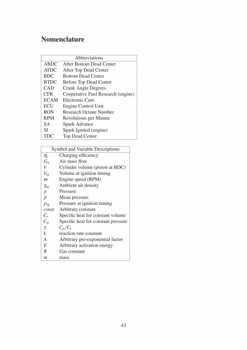
Nomenclature

Abbreviations

ABDC After Bottom Dead Center

ATDC After Top Dead Center

BDC Bottom Dead Center

BTDC Before Top Dead Center

CAD Crank Angle Degrees

CFR Cooperative Fuel Research (engine)

ECAM Electronic Cam

ECU Engine Control Unit

RON Research Octane Number

RPM Revolutions per Minute

SA Spark Advance

SI Spark Ignited (engine)

TDC Top Dead Center

Symbol and Variable Descriptions

ηc Charging efficiency

Ga Air mass flow

V Cylinder volume (piston at BDC)

Vig Volume at ignition timing

ω Engine speed (RPM)

γa0Ambient air density

p Pressure

p̄ Mean pressure

pig Pressure at ignition timing

const Arbitrary constant

Cv Specific heat for constant volume

Cp Specific heat for constant pressure

γ Cp/Cvk reaction rate constant

A Arbitrary pre-exponential factor

E Arbitrary activation energy

R Gas constant

m mass

43

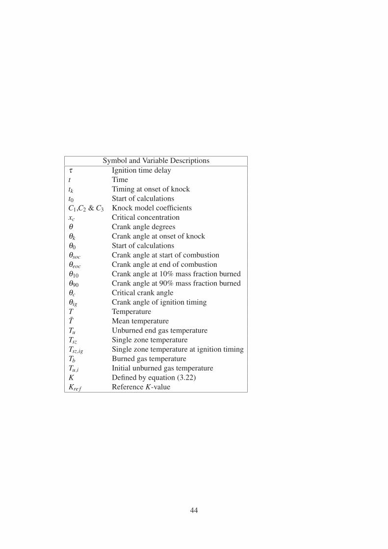
Symbol and Variable Descriptions

τ Ignition time delay

t Time

tk Timing at onset of knock

t0 Start of calculations

C1,C2 & C3 Knock model coefficients

xc Critical concentration

θ Crank angle degrees

θk Crank angle at onset of knock

θ0 Start of calculations

θsoc Crank angle at start of combustion

θeoc Crank angle at end of combustion

θ10 Crank angle at 10% mass fraction burned

θ90 Crank angle at 90% mass fraction burned

θc Critical crank angle

θig Crank angle of ignition timing

T Temperature

T̄ Mean temperature

Tu Unburned end gas temperature

Tsz Single zone temperature

Tsz,ig Single zone temperature at ignition timing

Tb Burned gas temperature

Tu,i Initial unburned gas temperature

K Defined by equation (3.22)

Kre f Reference K-value

44

Bibliography

A. By, B. Kempinski, and J. M. Rife. Knock in Spark Ignition Engines. Technical

report, MIT and Northern Research and Engineering Co., 1981. SAE 810147.

A.M. Douaud and P. Eyzat. Four-Octane-Number Method for Predicting the Anti-

Knock Behavior of Fuels and Engines. Technical report, Institute Francais du

Petrol (France), 1978. SAE 780080.

Christel Elmqvist, Fredrik Lindström, Hans-Erik Ångstrom, Börje Grandin, and

Gautam Kalghatgi. Optimizing Engine Concepts by Using a Simple Model for

Knock Prediction. In Powertrain & Fluid Systems Conference & Exhibition,

Pittsburgh, Pennsylvania USA, 2003. SAE TECHNICAL PAPER SERIES 2003-

01-3123.

Lars Eriksson and Ingemar Andersson. An Analytic Model for Cylinder Pressure

in a Four Stroke SI Engine. Technical report, Vehicular Systems, ISY, Linköping

Universitet and Mecel AB, 2002. SAE 2002-01-0371.

G.D Errico, T. Lucchini, A. Onorati, M. Mehl, T. Faravelli, E. Ranzi, S. Merola,

and B. M. Vaglieco. Development and Experimental Validation of a Combustion

Model with Detailed Chemistry for Knock Predictions. In 2007 World Congress,

Detroit, Michigan USA, 2007. SAE TECHNICAL PAPER SERIES 2007-01-

0938.

Bengt Johansson. Förbränningsmotorns Grunder. Department of Energy Sciences,

Lund Institute of Technology, 2006.

Keisuke Kawai, Junichi Kako, Shinji Kojima, and Tomohiko Jimbo. A Model

Widely Predicting Autoignition Time for Gasoline Engines. Technical report,

TOYOTA CENTRAL R&D LABS. INC. Mechanical Engineering Dept., 2009.

Marcus Klein and Lars Eriksson. A Specific Heat Ratio Model for Single-Zone

Heat Release Models. Technical report, Vehicular Systems, ISY, Linköping Uni-

versitet, 2004. SAE Paper Offer 04P-14.

Melanie Mitchell. An Introduction to Genetic Algorithms. MIT Press, 1998.

45

Toru Noda, Kazuya Hasegawa, Kasaaki Kubo, and Teruyuki Itoh. Development

of Transient Knock Prediction Technique by Using a Zero-Dimensional Knock-

ing Simulation with Chemical Kinetics. In 2004 SAE World Congress, Detroit,

Michigan USA, 2004. SAE TECHNICAL PAPER SERIES 2004-01-0618.

Automotive Dictionary. Toyota Engineering Society, 2005.

R. Worret, S. Bernhardt, F. Schwarz, and U. Spicher. Application of Different

Cylinder Pressure Based Knock Detection Methods in Spark Ignition Engines.

In International Spring Fuels & Lubricants Meeting & Exhibition, Reno, Nevada

USA, 2002. SAE TECHNICAL PAPER SERIES 2002-01-1668.

46