14/10/2008 1

Macroeconomic Policies on Shaky Foundations – Whither Mainstream Economics?

Berlin 31 October – 1 November 2008

Endogenous growth theory twenty years after: a critical assessment

Sergio Cesaratto

University of Siena

Cesaratto@unisi.it

Introduction*

Some years ago I found one ‘key’ of the origins of endogenous growth literature (EGT) in

the dissatisfaction that emerged in the late fifties with one result of the neoclassical growth model

by Robert Solow (1956), that is the independence of the growth rate of the economy from the

saving ratio, the ratio between the (full employment) saving supply and output, a variable subject to

policy influence, e.g. by tax treatment favourable to saving and investment (Cesaratto 1999a,

1999b). I pointed out the difficulties met both by the earlier and the new generations of endogenous

models in trying to relate the growth and saving rates (see also Serrano & Cesaratto, 2002). In the

meanwhile the literature on EGT has been enriched by further models and empirical verifications,

that have been endeavoured to face those difficulties. In this paper I will reassess my early

conclusions about EGT in the light of the most recent contributions. In this paper I shall distinguish

among three generations of EGT models: the old from the sixties; the new from the late eighties;

and the most recent from the second half of the nineties. As we shall see, EGT models can be

divided in two fields: those who defend the Solowian approach (semi-endogenous models) and

those who try to depart from it (full endogenous models).

Quite relevant to corroborate the interpretation of EGT put forward in my earlier

contributions was a paper by Marving Frankel, published in 1962 six months later than the more

well known Arrow’s learning-by-doing model, that I ‘rediscovered’ guided by the key to EGT that

had just come to my mind.1 Frankel observed that in the Harrod-Domar model, where a production

function is used (where is the output-capital ratio), the rate of economic growth depends aKY = a

on the saving ratio according to the well known Harrodian formula , where s vsg /= av /1= . * This is a preliminary and incomplete version. Also the English language has not been revised. 1 I firstly evoked Frankel’s contribution in Cesaratto (1995). Frankel’s forerunner paper was later ‘rediscovered’ by Cannon (2000) who, however, fails to locate Frankel’s original contribution in the context of the troubles met by the old and new EGT.

14/10/2008 2

Economists, he argued, “have found such models attractive because o relatively e

structure, because of the emphasis they give to capital accumulation as an ‘engine of growth’ – an

emphasis with deep routes in economic thought – and because of their pragmatically satisfying

results” (1962, p.996). However, he continued, “the production function aKY = has nothing

interesting to say about resource allocation or income distribution. Worse th as a general

statement of the resources required in production, it is positively wrong, as any one-factor

production function must be” (ibid). On the opposite, the most agreeable Cobb-Douglas production

function, although satisfactory from the point of view of “resource allocation or income

distribution”, in a growth context does lead to a growth rate that depends on the rate of growth of

the labour force and where the investment rate – that in this marginalist context coincides with the

saving rate – does not affect neither the aggregate growth rate nor, through productivity growth, that

of output per worker (ibid, pp.996-997). Labour productivity growth could be introduced into the

model, but its sources remained “exogenous” in the distinctive sense that it does not depend upon

the endogenous saving choices of the community (or of a representative agent)

f their simpl

hip between the investment

(saving

that have passed to new and recent EGT. However, these troubles have not passed unnoticed due in

an this,

2. The same

unhappiness with regard to this specific result of neoclassical Solow’s model was expressed in those

years by other authors (cf. Cesaratto 1999a, 1999b for the references).

In this regard we may start by asking whether the relations

) ration and the growth rate is just a theoretical supposition – although one ‘with deep routes

in [traditional] economic thought’ -, or is also a proved empirical fact. In this respect in section 1 I

shall first consider the recent controversy on the empirical evidence on this relation. It sounds that

most of the results confirm the relation, an outcome unfavourable to Solow’s prediction of its

absence in the secular equilibrium. Solow’s model did not deny it, however, in the transition from

one to another secular equilibrium, so that I will briefly look in section 2 to some recent defences of

Solow’s model based on the length of the transition towards the steady state. Given the frailty of

this defence, we shall then look in section III at proper EGT models recalling Frankel’s and

Arrow’s seminal and archetypal models, not for the sake of history of thought, but since new and

recent EGT has not moved a single step beyond the stage set by those earlier models, if not by

adding further theoretical and empirical considerations to lean in favour of one or the other possible

approaches displayed on that podium. This was one earlier conclusion on EGT, and I shall have not

reasons to change it but just to update in the present work (although I respect to the richness of the

debate over the last twenty years). More importantly, the archetypal models posed some problems

2 It is widely recognised that to get the sense of EGT it is irrelevant if the saving rate is taken as given, or if choices are analysed through a Ramsey model. The latter would just add maths but no substance (see e.g. Mankiw, 1995, pp.279-280).

14/10/2008 3

particular to the influential contributions by Charles Jones that in the light of those difficulties, not

surprisingly, argues in favour of sticking to the traditional Solow’s growth framework. The most

recent generation of EGT models has countered Jones’s criticism by approaches introducing another

battery of ad hoc assumption that, however, also remind to the archetypal, as we shall point out in

section V. After having discussed in section VI Jones’ neo-Solowian perspective, in the final

remarks, I will deal with a methodological defence of the neoclassical growth modelling according

to which one should not be too critical of the analytical or empirical limitation of single models, but

rather pick up the insight provided by each of them. In view of this remark, I will emphasize the

relevance of the Sraffian and Keynesian criticism of neoclassical theory.

I. Econometric growth theory

Recent and earlier presentations of growth theory including Jones (2002) and Solow (1970)

have focused over the explanation of the famous Kaldorian six ‘stylized facts’ of economic growth

that, as they are well known, it is pointless to recall here. To this list, two additional stylised fact

may be added that growth models may aim to explain that are, however, more controversial: a

positive correlation between the investment (saving) rate, that is the ration between investment

(saving) and output, and the rate of economic growth, both in aggregate and per-capita terms,

respectively. Not surprisingly, among those who deny these two additional stylised facts we found

the supporters of the Solowian view and, on the opposite side, those who feel uneasy with this

approach. The debate has focused on the empirical relation between the investment rate ( YI ),

taken in a close economy as a proxy of the saving rate (s),3 and per capita growth rate ( yg ).4 We

shall see that most contributions find an empirical correlation between YI and . Defendants of

Solow’s model have found various ways to shield their master’s results.

In an earlier study, Hill (1964) examined the mentioned relation in a group of industrialised

countries over the period 1954-62 and found a significant correlation

yg

(particularly strong for the

larger economies) between YI and aggregate growth ( Yg ), and also with yg especially once

3 After Feldstein & Horioka (1980) empirical results, some scepticism has emerged amongst neoclassical economists regarding the influence of foreign capital on domestic investment. 4 The fact that neoclassical economists focus upon only one of the two additional stylised facts should not come as a surprise. As known, the aggregate growth rate is given by the summation of the growth rate of the workforce plus labour productivity growth. In a neoclassical full-employment model, the workforce grows at a natural demographic rate n. That the aggregate growth rate should adjust to the (exogenous) growth rate of the workforce irrespective of the investment (saving) rate is something that the neoclassical Weltanschauung cannot put into discussion, so that the discussion centred over the rate of technical change. By contrast, for non orthodox economists it is the aggregate growth rate that is more important since they believe that market economies are not, on average, in full employment. Productivity growth is also important, of course, to measure the competitiveness of a country and as a source of job displacement.

14/10/2008 4

investment in machinery and equipment was considered. M f investment has

been the object of some much quoted papers by De Long and Summers (1991, 1992). They also

found that productivity growth is positively associated to high investment in equipment in a large

sample of rich and developing countries over the Second World War II period.

ore recently, this kind o

92; see also Mankiw 1995)

show t

−

where

5 Abel (1992, p.200)

assigns to De Long-Summers’ finding the status of ‘new stylised fact’.

In their influential paper, Mankiw, Romer and Weil (MRW, 19

hat Solow’s model, once ‘augmented’ to include ‘human capital’, is able to explain a good

deal of the variations among countries in per capita income levels (not growth rates). They propose

a production function like: βα −= 1)( ttttt LAHKY βα

H represents ‘human capital’ and A the traditional exogenous technical progress (hereafter

we shall omit the time subscript in the equations), and 1<+ βα . According to MRW this equation

would lead to good predictions of those variations on Solowian lines, that is based on differences in

the saving rates and in population growth, without recurring to exogenous (or endogenous)

technical change.6

These results concern the differentials in the levels of per capital income, but not the growth

rates. I

run converge towards their common growth rate. Taking advantage of this result, Mankiw (1995,

n this respect MRW acknowledge the lait motive of EGT, that ‘countries with a higher saving

rate grow persistently faster and that they will not converge to a same steady state growth path even

if they have the same technological endowment’ (ibid., p.421-422). Recall that according to

Solow’s model countries with similar s and technology would still show different growth rates

when starting from different initial per capita capital (income) levels, although they will in the long

5 These authors attribute big importance to differences in the price of equipment goods across countries. A high saving ratio associated to a low price of equipment would generate high productivity growth (e.g. De Long & Summers, 1991, pp.484-485). Yet the causes of the low prices of capital equipment are not clearly explored by these authors. They reject an accelerator explanation of growth, whereby it is growth that leads to an high investment shares, because this would be associated, in their view, to a higher equipment price not to the lower one showed by their data (e.g. De Long & Summers, 1991, pp.473-474; 1992, p.176). 6 Without ‘human capital’ the traditional model would only partially explain those inter-country variations (Mankiw 1995, pp.282-284) The reason to include ‘human capital’ is that without it Solow’s model would still well explain the mentioned variations, but with an income share α accruing to capital over two-third (against a usual value of one third). A high value of α would be justified once the returns to educated labour are assimilated to capital’s returns. The economics of the model is that a higher ‘human capital’ component would lead to a higher per capita income and saving supply; the latter does in turn lead to a higher per capita income (MRW, 1992, p.417; Mankiw, 1995, p.290). Although in their model there is a touch of endogenous growth, in the sense that the accumulation of ‘human capital’ is an endogenous decisions, the model is not able to generate endogenous growth (that is the endogenous decisions to accumulate physical of ‘human’ capital do not affect the rate of growth (the model would become a full endogenous model with 1=+ βα , see the production function adopted by endogenous models below in sections III and IV). We put ‘human capital’ in inverted commas given the shaky nature of this magnitude, cf. Steedman 2001).

14/10/2008 5

p.278) maintains that: “The inability of saving to affect steady state growth (…) might appear

inconsistent with the strong correlation between growth and saving across countries. But this

correlation could reflect the transitional dynamics that arise as economies approach their steady

states’.7 In addition, MRW (1992) approvingly quote Barro (1989) that there is no much evidence

of a convergence across countries in the sense that poorer countries (those starting with a lower per

capita capital endowment) do not generally tend to grow faster and catch up richer countries. They

introduce, in this regard, the concept of conditional convergence, thereafter entered in textbook

expositions, that countries do not converge towards a common growth rate, but each one toward her

own one.8 So, they conclude, growth rates can differ both (i) as countries are in ‘transitional

dynamics’, and this may explain the relation between s and yg ; and (ii) because they converge

towards different secular paths, and this is might be explained by the differences in s and population

growth (n) (MRW, 1992, p.423).9

Critical of De Long-Summers results is Jones who argues that whereas in the main

economies the share on GDP of both total and equipment investment has increased, (per capita)

output growth rates ‘have fallen, if anything, over the post-war era’ (Jones, 1995b, p.508). Jones’s

idea seems to be that although De Long-Summers can be right to envisage a cross-country

correlation between YI and yg , for each country over a period of time it is not however true that a

7 The empirical results about convergence towards secular growth reported by these authors (e.g. Mankiw, 1995, pp.284-285) suggest a faster convergence towards the steady state than that predicted by Solow’s model. Assuming a higher value of the capital share α , obtained again by considering part of labour as ‘human capital’, would make the predictions of the ‘augmented’ Solow model closer to those data (ibid, p.291; MRW, 1992, p.428). 8 ‘[T]he neoclassical model predicts that each economy converges to its own steady state, which in turn is determined by its saving and population growth rates’ (Mankiw, 1995, p.284). 9 It should be observed that these authors do not attribute much importance to international differences in technological endowments to explain the divergences of per capita income levels growth across countries, although this sounds strange if we compare the actual techniques in use in poor and rich countries, respectively. They seem to explain this arguing that although the production function is the roughly same in all countries, since ‘knowledge …travels, around the world fairly quickly’ (Mankiw, 1995, pp.300-301) the specific technique - say spades or tractors - used in each country depends on their stage of growth. This, in turn, affects factors’ supply: ‘To use the neoclassical model to explain international variations in growth requires the assumption that different countries use roughly the same production function at a given point in time. …change [of techniques] should be viewed as a movement along the same production function, rather than as a shift to a completely new production function’ (ibid., p.281). The ‘augmented’ Solow model would help again. The different investment in ‘human capital’ would explain the divergent ability across countries to assimilate superior production functions. All neoclassical growth literature never ever mentions that the acquisition of superior foreign technology and education is a costly process in terms of balance of payments. According to non-orthodox theory, what can be called the ‘foreign liquidity constraint’, the necessity to collect enough international currencies to finance the acquisition of foreign embodied and disembodies technology, is one main economic obstacle to economic growth.

14/10/2008 6

increasing YI leads to a hig er yg .h

g-Summers, Blomstrom, Lipsey, Zejan (1996)

find th

10 Critical of Jones is Li (2002) who conducts time-series

regressions over 24 OECD countries over 1950-1992 and five industrialised economies over 1870

to 1987 finding that total investment is positively related to growth in more than half of the cases.

Jones’s outcome would be different since they rely on durable investment only and because the

focus on the U.S. would be misleading (ibid, p.97).

Comparing their results to those by De Lon

at the ‘long term relationship’ between YI and yg ‘were due more to the effect of growth

on capital formation than to the effect of capital forma on on growth’, as argued by De Long-

Summers (ibid, p.269). This sounds of course more in line with less orthodox theory. Vanhoudt

(1998) is not surprised by Bolmstrom et al. results since in Solow model a rise in the saving ratio s

is followed by a sudden rise in the growth rate followed by its decline towards its steady state level.

No surprisingly then, statistical tests would suggest a negative effect of saving on growth.

ti

strongly in favour of a positive

influen

11 A

similar result is obtained by Attanasio, Picci e Scorcu (2000, e.g. pp.198-199),12 while a more

ecumenical outcome is attained by Podrecca and Carmeci (2001) according to whom the causality

can go in both directions. A halfway position is also held by Madsen (2002) whose results on 18

countries over the period 1950-1999 would show that investment in equipment does cause growth,

whereas non-residential investment in buildings and structures is caused by economic growth (this

appears perplexing to a non orthodox economist who would see investment in equipment as demand

induced, and construction works as an autonomous component).

Bernanke and Gurkaynak (2001) present empirical results

ce of YI on yg .13 The two authors also show that the saving rate ( YI ), but also

population growth, are positively correlated with total factor productivity (TFP), contrarily to the

10 Charles Jones was still a student at MIT when, in his Siena doctorate lectures on growth, Solow (1992, p.85) mentioned, not surprisingly approvingly, Jones’ forthcoming results that, he reports, were obtained ‘before [Jones] had read De Long-Summers’s paper’. 11 ‘Since the mentioned Granger causality test control for lagged growth, it is not surprising that positive Granger causality from saving to growth does not show up’ (ibid, p.78. 12 It is impressive how much Keynesian thought has been lost by these economists that explain the ‘dynamic link running from growth to investment’ arguing that ‘[h]igher growth might driven saving up, leading in turn to higher investment’ (ibid, p.183). Elsewhere they admit, and their results do not exclude, a ‘Granger causation running from investment to saving’; however, they continue, ‘the exact mechanisms at work are hard to spell out in detail, if an increased demand for capital goods stimulates saving – maybe through interest rate effects or the endogenous development of the financial instruments that permit the mobilisation of saving – saving might adjust to investment’ (ibidem). No mention by these authors of concepts such as the investment accelerator or the Keynesian multiplier (for a Keynesian adjustment mechanism of saving to investment in a long run framework cf. Garegnani 1992). 13 As MRW (1992), Bernanke and Gurkaynak use the Penn World Tables, a multicountry data set by Heston and Summers (MRW over the years 1960-1985, BG 1960-1995).

14/10/2008 7

Solow model’s prediction that TPF should be exogenous to factor accumulation. This would show

that endogenous mechanism, saving or fertility decisions, have external or scale effects such to

determine endogenous rather than exogenous growth. In their comments David Romer and Mankiw

remark their thesis that economies are not necessarily on their steady state.

While it sounds that most of the empirical outcomes is in favour of a positive association

betwee

. Arrow, Frankel and the AK model.

th theory to endogenise growth? As well

known

e space to

rve the distributive role of the

Cobb-Douglas production function, but in which the growth rate depends on the investment rate as

n the investment (saving) rate and yg (e.g. Mankiw, 1995, p.302), much effort has been paid

by both fronts to check this correlation and see whether other variables would play a more

significant explanatory role. Opinions tend however to converge on the idea that these exercises are

of limited value since they are seriously sensitive to the variables included or excluded, the time

span, the country considered and whatever else.14 We may therefore stand with Mankiw (1995,

p.308) when he argues that: ‘Basic theory, shrewd observation, and common sense are surely more

reliable guides for policy’. Let us therefore go back to ‘basic theory’ starting from the old EGT

models.

II

Which strategies were open to neoclassical grow

, according to Solow’s model the secular growth rate is given by: hngY += ,where n is the

growth rate of the labour force and h is technical change. There is littl endogenise n,

although a number of authors have explored the relation between fertility choices and growth. More

obvious was the exploration of possible relations between saving choices and technical progress.

Clearly, for the neoclassical economists the saving rate was a main determinant of capital

accumulation, but because of the decreasing marginal productivity of capital, for a given a labour

supply, a higher saving rate could not persistently raise the accumulation rate that, at the end, had to

adjust to the exogenous rate of growth of the workforce (in physical or efficiency units). On the

other hand, it was this adjustment that permitted to Solow to conclude that full employment was the

long run rule overcoming the opposite conclusions by the Harrod-Domar (HD) model – who

however, as cleverly pointed out by Frankel, offered a saving-led growth formula. Notably, in the

HD model substitutability amongst ‘production factors’ is ruled out.

Frankel (1962) proposed a new growth model able to prese

14 So we hear Solow saying that: ‘the main fact about these empirical studies’ is that ‘they are not robust’ (1992, p.78, italics in the original). Similarly, Mankiw (1995, pp.307-308) states that: ‘Using these regressions to decide how to foster growth is …most likely a hopeless task. Simultaneity, multicollinearity, and limited degree of freedom are important practical problems for anyone trying to draw inferences from international data. Policy makers who want to promote growth would not go far wrong ignoring most of the vast literature reporting growth regressions’. Other sceptical views include Rodrik (2005), who also quote some other critical surveys, and XXX (2008).

14/10/2008 8

in the HD model. The trick, that has became a sort of cliquet far all the endogenous growth theory

up to now, was to craft a relation between labour augmenting technical change and the saving rate.

In the recent literature this has been done, following Arrow, Phelps, Uzawa and other authors from

the sixties, by linking labour productivity growth to externalities from (the endogenous) capital

accumulation, or by relating it to surrogate saving decisions as those associated to the resources

devoted to R&D or education that also imply diversion of resources from present to future

consumption. In the new EGT literature a short cut has instead been taken by those economists that

have just come back to HD through the so-called AK model, not surprisingly in view of Frankel’s

just recalled account of the neoclassical growth theory dilemma. Frankel’s model is particularly

intriguing in this regard.

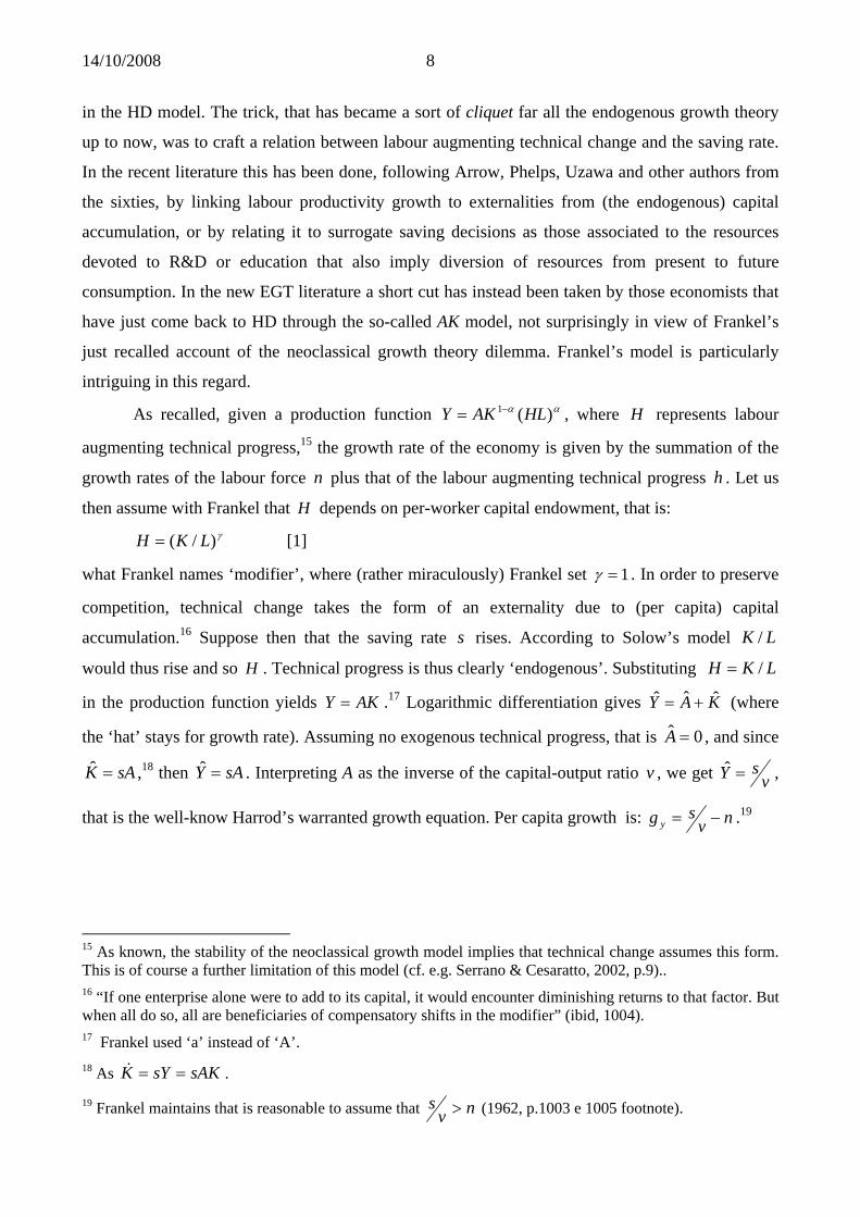
As recalled, given a production function αα )(1 HLAKY −= , where H represents labour

augmenting technical progress,15 the growth rate of mation of the

growth labour augmentin

the economy is given by the sum

rates of the labour force n plus that of the g technic progress h . Let us

then assume with Frankel that

al

H depends on per-worker capital endowment, that is: γ)/( LKH = [1]

what Frankel names ‘modifier’ here (rather miraculously) Frankel set 1=, w γ . In order to preserve

competition, techni chan kes the form of an external capita) capital cal ge ta ity due to (per

accumulation.16 Suppose then that the saving rate s rises. According to Solow’s model LK /

would thus rise and so H . Technical progress is thus clearly ‘endogenous’. Substituting LKH /=

in the production function yields AKY = .17 Logarithmic differentiation gives KAY ˆˆ = (where

the ‘hat’ stays for growth rate). Assuming no exogenous technical progress, that is since

sAK =ˆ ,

ˆ+

and

erpreti t ratio

0ˆ =A ,18 then sAY =ˆ . Int g A as the inverse of the capital-outpu we get n v , v

sY =ˆ ,

that is the well-know Harrod’s warranted growth equation. Per capita growth is: nvysg −= .19

15 As known, the stability of the neoclassical growth model implies that technical change assumes this form. This is of course a further limitation of this model (cf. e.g. Serrano & Cesaratto, 2002, p.9).. 16 “If one enterprise alone were to add to its capital, it would encounter diminishing returns to that factor. But when all do so, all are beneficiaries of compensatory shifts in the modifier” (ibid, 1004). 17 Frankel used ‘a’ instead of ‘A’. 18 As . sAKsYK ==&

19 Frankel maintains that is reasonable to assume that nvs > (1962, p.1003 e 1005 footnote).

14/10/2008 9

Frankel succeeds therefore to retain both the neoclassical production function, with its ‘nice’

distribution properties, and Harrod’s growth equation with its ‘deep routes in economic thought’. Of

course Harrod’s and Frankel’s models are only superficially similar.20

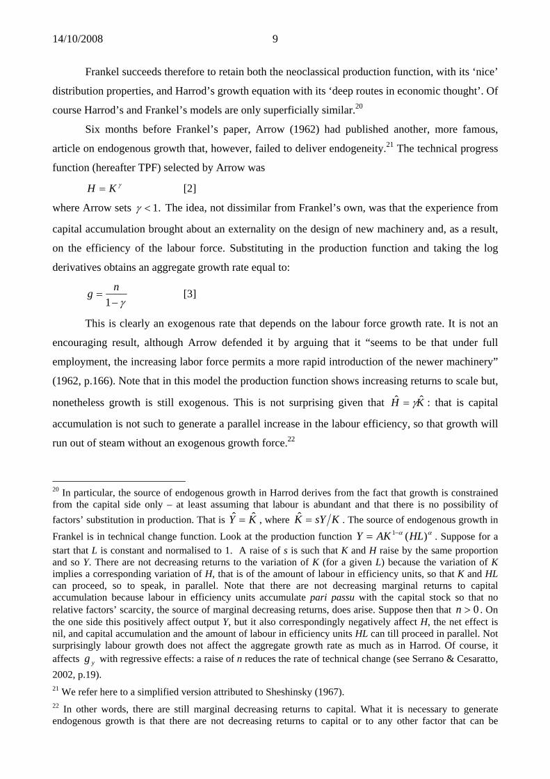
Six months before Frankel’s paper, Arrow (1962) had published another, more famous,

article on endogenous growth that, however, failed to deliver endogeneity.21 The technical progress

function (hereafter TPF) selected by Arrow was γKH = [2]

where Arrow sets .1<γ The idea, not dissimilar from Frankel’s own, was that the experience from

capital accumulation brought about an externality on the design of new machinery and, as a result,

on the efficiency of the labour force. Substituting in the production function and taking the log

derivatives obtains an aggregate growth rate equal to:

γ−=

1ng [3]

This is clearly an exogenous rate that depends on the labour force growth rate. It is not an

encouraging result, although Arrow defended it by arguing that it “seems to be that under full

employment, the increasing labor force permits a more rapid introduction of the newer machinery”

(1962, p.166). Note that in this model the production function shows increasing returns to scale but,

nonetheless growth is still exogenous. This is not surprising given that : that is capital

accumulation is not such to generate a parallel increase in the labour efficiency, so that growth will

run out of steam without an exogenous growth force.

KH ˆˆ γ=

22

20 In particular, the source of endogenous growth in Harrod derives from the fact that growth is constrained from the capital side only – at least assuming that labour is abundant and that there is no possibility of factors’ substitution in production. That is KY ˆˆ = , where KsYK =ˆ . The source of endogenous growth in Frankel is in technical change function. Look at the production function . Suppose for a start that L is constant and normalised to 1. A raise of s is such that K and H raise by the same proportion and so Y. There are not decreasing returns to the variation of K (for a given L) because the variation of K implies a corresponding variation of H, that is of the amount of labour in efficiency units, so that K and HL can proceed, so to speak, in parallel. Note that there are not decreasing marginal returns to capital accumulation because labour in efficiency units accumulate pari passu with the capital stock so that no relative factors’ scarcity, the source of marginal decreasing returns, does arise. Suppose then that . On the one side this positively affect output Y, but it also correspondingly negatively affect H, the net effect is nil, and capital accumulation and the amount of labour in efficiency units HL can till proceed in parallel. Not surprisingly labour growth does not affect the aggregate growth rate as much as in Harrod. Of course, it affects with regressive effects: a raise of n reduces the rate of technical change (see Serrano & Cesaratto, 2002, p.19).

αα )(1 HLAKY −=

0>n

yg

21 We refer here to a simplified version attributed to Sheshinsky (1967). 22 In other words, there are still marginal decreasing returns to capital. What it is necessary to generate endogenous growth is that there are not decreasing returns to capital or to any other factor that can be

14/10/2008 10

While Arrow did not assume 1≥γ then? Suppose that 1=γ . The production function

would then look αAKLY = . Supposing no exogenous technical change ( , the growth

equation would look like . A positive labour growth rate ( would clearly lead the

economy outside a uniform secular growth rate (e.g. Ramanathan, 1982, pp. 95-96, Serrano &

Cesaratto, 2002, p.17). As rather harshly commented by Cesaratto & Serrano (2002, p.18):

‘Therefore if the labour force grows we see here that, rather than accumulate capital more quickly

to seize the externality, what rational agents should do is to save very little and generate a

demographic explosion, which in any case need not be too big because any positive rate of growth

of the population quickly leads the economy to growth rates that tend to infinity! The result is even

more disputable than that of the learning by doing model in which, due to the increasing returns of

the economy, a constant rate of growth of the labour force generates a positive per capita growth

rate. The reason for this even less reasonable result is that the learning by doing model still retains

the decreasing returns to capital, which guaranteed that a constant positive growth rate of the

population failed to accelerate the growth rate continually, since there was a counteracting tendency

for the capital-output ratio to increase.’

)0ˆ =A

nKY α+= ˆˆ )0>n

One can now appreciate why the particular shape of Frankel’s modifier permitted to

preserve the gravitation towards a secular uniform growth even with 1=γ and : while with 1>n

1=γ the externality from capital accumulation is sufficient to determine a parallel raise of labour

in efficiency units, a positive growth in physical labour has no net effect on growth for the reasons

explained above.23

As known, the famous AK model of new EGT can be regarded as an Arrow model with the

strong assumption 1=γ and .0=n 24 In this case we are back again to the HD model since KY ˆˆ =

and , where sAK =ˆK

YA = , that is vssAY ==ˆ . The trenchant comments by Solow were that:

‘The essence here is that there is no primary factor, labor has disappeared’, and ‘It is rather

amazing. …modern literature is in part just a very complicated way of disguising the fact that it is

going back to Domar, and, as with Domar, the rate of growth becomes endogenous’ (1992, p.18 and

32 respectively).

III. Transitional dynamics

accumulated. This can obtained by assuming very strong IRS, or by specific functions that govern the accumulation of the ‘accumulable factor’: capital, ‘knowledge’, or ‘human capital’. 23 An akin ‘modifier’ was advanced by Conlisk (1967): see Cesaratto (1995), fn. 24 and (1999b), pp.251-252. 24 Romer (1987) and Rebelo (1991) are usually quoted in this regard (cf. e.g. Jones, 2002, 162-163).

14/10/2008 11

As seen, MRW and other economists accommodate Solow’s model to the empirical results,

generally favourable to a positive association of YI and , by relying on a sluggish ‘transitional

dynamics’. In the earlier days of neoclassical growth theory a fast time-convergence towards the

steady state was regarded as validating the description of secular growth provided by Solow, while

presently - virtue out of necessity - a slow convergence rate is seen as supporting that model insofar

as during the transition the saving (investment) rate, and the policies that affect it, do influence .

As well known, the seminal contribution of the speed of convergence was Ryuzo Sato (1963) who

showed that it was a slow process. A relevant assumption that affects the sped of adjustment

concerns the capital share (

yg

yg

α ). Having in mind the standard graphical representation of Solow’s

model and using a Cobb-Douglas,25 the curvature of the function hinges on the value of

the capital share

αsksy =

α : given an, say, upsurge in that shift upward the s sy curve, the higher α the

farer away is the new stationary level of from an initial .k 0k 26 As seen above, MRW rely on

‘human capital’ to raise the capital share to two-third of output so as to obtain a slower convergence

rate. An analogous suggestion was advanced by Conlisk (1966, p.553 and passim) who notes:

‘Human capital is accumulated by diverting resources from other uses; and the amount of human

capital accumulated depends on the amount of resources diverted. Hence, logically, human capital

should be included in the factor K, and not in the factor L …If human capital is included in K, then

a substantially larger value of α is called for than if human capital is not included in K ’, as the

numerical examples confirm (see also Ramanathan 1982, pp.245-248, to which we refer for a wider

discussion). More recently, King & Rebelo (1993) have shown that convergence can be faster, so as

to rule out a role for policies in Solow’s model. The intuition is that if an economy is hit by a shock

that reduces her capital stock, the marginal product of capital would be very high. Rational savers

would react by increasing their saving supply thus accelerating accumulation and the convergence

towards the steady state. According to King & Rebelo this result is not favourable to Solow model

in so far as ‘transitional dynamics …cannot account for important part of sustained cross-country

25 As known, given the neoclassical growth equation (standard notation), the secular

equilibrium is were , that is were

knksfk )()( δ+−=&

0=k& knsy )( δ+= . 26 The intuition provided by Ramanathan (1982, p.246) is that when α is high and capital relatively more important in production, if capital (saving) becomes more abundant, the scarce factor, labour, takes more time to limit growth (the marginal product of capital falls more slowly): ‘the exogenous labor input …bottlenecks the growth rate. …if the share of capital is larger, then firms can substitute capital for labor and thus evade the bottleneck for longer period of time’. As noted by Jones (2002, p.159), in the limiting case of 1=α and constant labour, the case of the AK model, the production function is a straight line and the marginal product of capital never falls, so that we have an endless transition, a ‘perfect’ endogenous growth situation.

14/10/2008 12

differences in rates of economic development (ibid., p.929). Slower convergence speeds could be

obtained, but ‘even if one makes agents very unwilling to substitute over time’, at the price of very

high initial marginal product of capital of the order of 500% or more (ibidem).27

To sum up, as often, the conclusions of different authors do strongly depends upon the value

of the chosen analytical functions and on the value attributed to the parameters, while the empirical

tests do not provide unequivocal results. While this would be a cheap criticism, since this happens

in most fields of the discipline, including in non orthodox fields, it is worth noticing the switch of

position in the Solowian camp, from seeing a fast convergence as a confirmation of the practical

relevance of the secular neoclassical path to defending a lethargic gravitation to show the relevance

of policy in a Solowian context. Given the host of special assumptions that EGT models have to

make to bring endogenise growth home, neo-Solowian economists have a point in sticking to their

well established framework stressing the length of the transitional dynamics. There are two

questions, however. A long transition process presupposes a high capital share by including the

accumulation of ‘human capital’ along that of physical capital, what is analytically a shaky

operation if one think of the insurmountable troubles that neoclassical theory has to overcome in

aggregating and measuring in value traditional capital goods. Secondly, as we shortly see, neo-

Solowian models present explanations of the growth sources that may also be considered little

promising.

IV. The new EGT and its neo-Solowian critics

Simplifying a bit, new EGT has taken two roads: one was to follow Arrow’s contribution to

link increasing returns to capital accumulation in a way summarised by the AK model already

mentioned at the bottom of section II. The other was to see the source of EG in the R&D (or

education) effort. The second route was anticipated in the sixties by Phelps, Shell, Uzawa and

others.28 The troubles with both these directions are similar, so it is not really necessary to deal with

them separately. In order to grasp this similarity let us look at the exposition and criticism by

Charles Jones. Jones’ theoretical work on neo-solowian lines has perhaps been the most influential

in the last ten years or so, paralleling the earlier empirical contribution by MRW. Indeed, the first

influential contribution by Jones has been also empirical.

27 In spite of this, Solow (2000, pp.164-165) seems to applaud to King-Rebelo’s point about a fast convergence rate, likely because he regards it as a confirmation of the practical relevance of the secular growth rate predicted by his model. Rather inconsistently, in his Siena doctoral lectures (1992, p.82) Solow argues that De Long-Summers’ results about the influence of the investment rate on growth might be due to a slow convergence path, so as not to disconfirm his model. 28 Cf. Cesaratto (1999a, 1999b), Cesaratto & Serrano (2002).

14/10/2008 13

In a number of papers Jones (1995a; 1995b; 2003) summarized a number of ‘R&D based

models’ (defined ‘R/GH/AH models’) 29 through the following equations:

αα )(1YHLKY −= [4]

λφδ HLHH =& [5]

HY LLL += and LsL HH =

where the symbols are by now obvious to the reader. R/GH/AH models typically assume

1=φ and 1=λ . As it is clear applying these assumptions to the TPF [5],

LsHH

Hδ=&

[6]

The growth rate is endogenous as it hinges upon the term that indicates the choices of the

community between using labour for direct production or for the production of ‘ideas’. The trouble

with equation [6] is that a positive growth in the scale of the R&D labour force, due cet.par. to a

positive growth rate of the labour force, will correspondingly raise the productivity growth rate,

what the good sense would lead to reject. Jones has named this as ‘strong scale effect’ (or ‘growth

scale effect’).

Hs

30 In a particularly influential paper, Jones (1995b) showed that while the U.S. per

capital growth rate had been approx constant over the period 1880-1987 (1.81 % annually), the

number of R&D scientists had increased five-fold. Similar results apply to other OECD countries.

Therefore, Jones concluded: ‘[t]hese models predict that growth rates should be proportional to the

level of R&D, which is clearly falsified by the tremendous rise in R&D over the last 40 tears’

(1995b, p.513). The parallel with Arrow’s (1962) model is clear (Jones 1995a, fn.10; Cesaratto

1995): as much as the assumption of 1=γ in Arrow’s TPF led that model into troubles in that it

could not accommodate a positive growth rate of the labour force, in the present ‘class’ of R&D

models the assumption 1=φ and 1=λ leads to similar difficulties.

V. Modified modifiers

In an exemplary clear paper Jones (1999) summarises his criticism to the R/GH/AH models

and extends it to another ‘class of models’, the Y/P/AH/DT models that has tried to save

29 After the contributions by Romer (1990), Grossman and Helpman (1991), Aghion and Howitt (1992). 30 A definition of strong scale effects is the following: ‘In models that exhibit “strong” scale effects, the growth rate of the economy is an increasing function of scale (which typically means overall population or the population of educated workers)’ (Jones 2004, p.38). We have ‘weak scale effects’ when ‘the level of per capita income long run is increasing function of the size of the economy’ (ibid). The problems with the R/GH/AH models and with some of the earlier generation of EGT models were pointed out in various places of my 1995 paper. Of course these problems were well known before Jones (and me).

14/10/2008 14

endogenous growth without incurring in the ‘scale growth effects’.31 These models are thus

synthesised. Suppose that output Q is composed by a variety B of consumption goods Y, all

produced in the same amount, that is BYQ = .32 Simplifying equation [4], each product is produced

using labour and a stock of ‘ideas’ H: . In turn, the variety YL YLHY σ= B depends on the

population level according to a function like βLB = . Finally, and this is the key assumption, the

stock of ideas evolves according to the TPF:

BL

HH Hδ&

[7]

The rationale of having the term B in the TPF is that population growth has two effects. On

the one hand it has a positive effect on the production of ideas through a larger amount of

labour, but, on the other hand, it also leads to a greater variety of products, so that the amount of

per product line does not increase. As above, the amount of labour devoted to the generation of

ideas depends on the endogenous preferences of the community about the shares of and

respectively: and . The TPF can be therefore written as:

HL

HL

YL HL

sLLH = LsLY )1( −=

βδ −= 1sLg H .

Given these assumptions, the aggregate output growth is given by: . The first

term on the left hand side is

yBq ggg +=

ng B β= . With regard to the second term, since each product grows in

aggregate at a rate: ngg HY += σ , per capita growth will be: HHy gnngg σσ =−+= , or:

. We get therefore an aggregate output growth rate equal to: βδ −= 1sLg y

βσδβ −+= 1sLngq .

If we assume with the Y/P/AH/DT models that 1=β to obtain

sngq σδ+= [8]

we see that growth does depend on the endogenous preferences of the community expressed by the

term s, and growth is positive even with zero population growth. There are no growth scale effects

since the term L has disappeared from the growth equation:

31 After the models by Young (1998), Peretto (1998), Aghion & Howitt (1998), Dinopolous & Thompson (1998) 32 We leave aside aggregation problems and focus only on the assumptions concerning TPFs that assure stable growth. In the specific example, the various goods are produced using labour only, so an aggregation problem does not seem to arise. Otherwise one can maintain that the Ys represents varieties of a same good, say corn.

14/10/2008 15

At this point, watchful readers, having registered that what distinguishes the Y/P/AH/DT’s

TPF from R/GH/AH’s one is the term B, that with 1=β is equal to L, will have noticed that this is

similar to the distinction between Arrow’s and Frankel’s TPFs.33

Jones’s (1999, pp. 142-143) criticism points to the ad hoc nature of the assumption 1=β .

Indeed, with 1<β the number of sectors would grow less than proportionally with population, so

that the model would still exhibit growth scale effects. With 1>β the number of sectors would

grow more than proportionally with population, and this has a negative effect on productivity

growth as a rising workforce would be spread over an even more rapidly rising number of

sectors. Asymptotically growth would then still depend upon population growth. This is indeed the

standard criticism raised against new EGT since its very beginning (Cesaratto 1999b, p.788).

HL

Besides the analogy between Frankel’s and Y/P/AH/DT’s TPF, what Jones fails to notice in

his otherwise illuminating paper is the similarity of Y/P/AH/DT’s equation [8] to the TPF proposed

by Lucas’ (1988) in another seminal paper of the new EGT, in turn similar to Frankel’s modifier as

showed by Serrano & Cesaratto 2002, pp. 22-24).34 In Lucas we find a TPF like:

zHH ϑ=&

where LLz H= is the share of labour devoted to education, R&D or the like. Notably, the

difference with equation [6] is that L appears at the dominator, as much as in Frankel’s equation [1]

and Y/P/AH/DT’s equation [7]. As the latter TPFs, Lucas’ TPF does indeed fit well in the Solow’s

model without perturbing its main features (Lucas 1988, p.19-20). 35 As argued in Serrano & Cesaratto

(2002, p…): in these models ‘the increase of efficiency does not depend on knowledge

33 Respectively: HK = (Arrow with 1=γ ) and

LKH = (Frankel); HL

HH δ=&

(R/GH/AH) and

BL

HH Hδ=&

(Y/P/AH/DT).

34 Jones quotes in passing Frankel in 2002, p.162 ,fn. 5. 35 Jones (1995a, p.762-63; 2004, pp. 42-43) does not regard Lucas’ TPF an appropriate solution since the idea that the absolute number of R&D employees matters for technical progress would be lost in the Lucas’ TPF, only the share on total workforce do indeed matter (we shall come back on this, that Jones names ‘Mozart effect’, soon). In addition, the empirical evidence is that in the U.S. a threefold raise in the R&D effort (z) would have not been followed by a parallel increase in the secular growth rate (the same would apply to other countries).

14/10/2008 16

accumulation itself, but on knowledge accumulation per worker (in close analogy with the Frankel

modifier that enabled efficiency to grow with the quantity of physical capital per worker)’.36

VI. Neo-Solowian (semi-endogenous) models

Having thus pointed out both the troubles with the R/GH/AH models (growth scale effects)

and with Y/P/AH/DT models (ad hoc assumptions in order to avoid the growth scale effects), Jones

proposes a model that avoids the growth scale effects although at the price of sacrificing

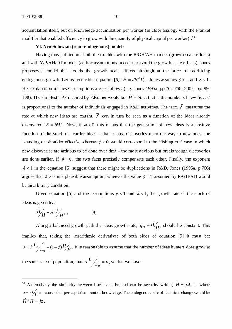
endogenous growth. Let us reconsider equation [5]: . Jones assumes λφδ HLHH =& 1<φ and 1<λ .

His explanation of these assumptions are as follows (e.g. Jones 1995a, pp.764-766; 2002, pp. 99-

100). The simplest TPF inspired by P.Romer would be: HLH δ=& , that is the number of new ‘ideas’

is proportional to the number of individuals engaged in R&D activities. The term δ measures the

rate at which new ideas are caught. δ can in turn be seen as a function of the ideas already

discovered: φδδ H= . Now, if 0>φ this means that the generation of new ideas is a positive

function of the stock of earlier ideas – that is past discoveries open the way to new ones, the

‘standing on shoulder effect’-, whereas 0<φ would correspond to the ‘fishing out’ case in which

new discoveries are arduous to be done over time - the most obvious but breakthrough discoveries

are done earlier. If 0=φ , the two facts precisely compensate each other. Finally, the exponent

1<λ in the equation [5] suggest that there might be duplications in R&D. Jones (1995a, p.766)

argues that 0>φ is a plausible assumption, whereas the value 1=φ assumed by R/GH/AH would

be an arbitrary condition.

Given equation [5] and the assumptions 1<φ and 1<λ , the growth rate of the stock of

ideas is given by:

φλ

δ −= 1HL

HH& [9]

Along a balanced growth path the ideas growth rate, HHg H&= , should be constant. This

implies that, taking the logarithmic derivatives of both sides of equation [9] it must be:

HH

LL

H

H &&)1(0 φλ −−= . It is reasonable to assume that the number of ideas hunters does grow at

the same rate of population, that is nLL

H

H =&

, so that we have:

36 Alternatively the similarity between Lucas and Frankel can be seen by writing , where jzLeH =&

LHe = measures the ‘per capita’ amount of knowledge. The endogenous rate of technical change would be

. jzHH =/&

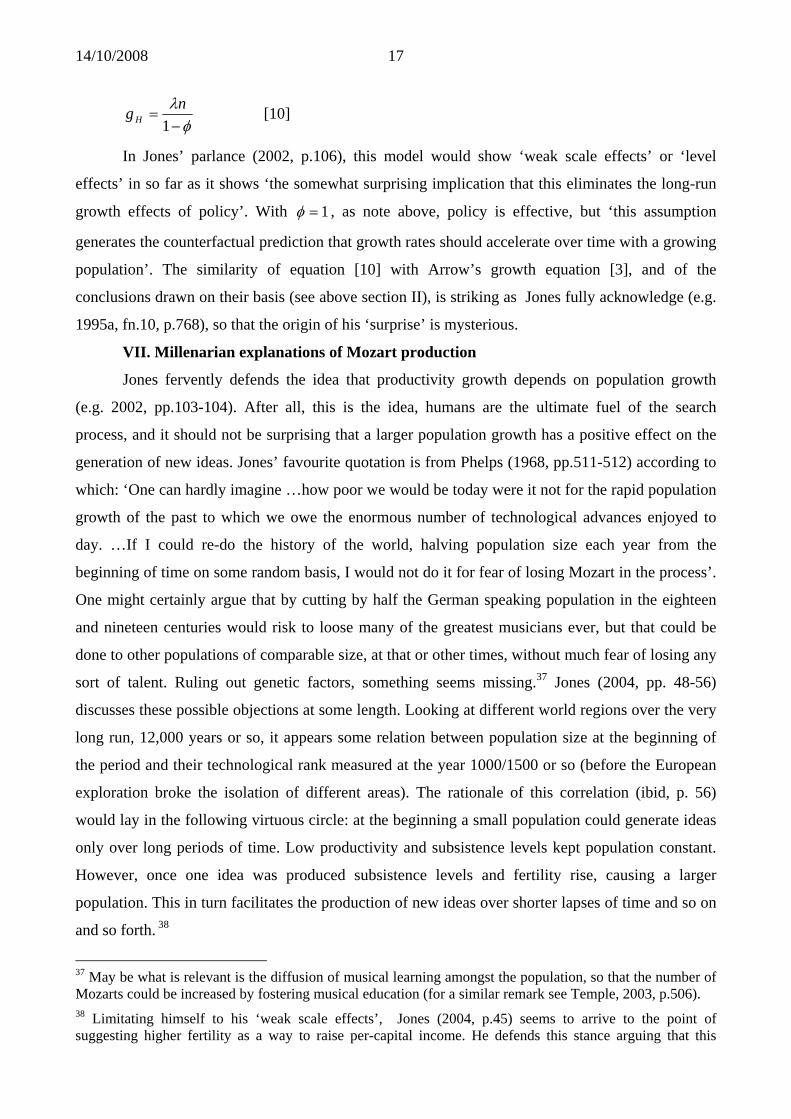
14/10/2008 17

φλ−

=1

ng H [10]

In Jones’ parlance (2002, p.106), this model would show ‘weak scale effects’ or ‘level

effects’ in so far as it shows ‘the somewhat surprising implication that this eliminates the long-run

growth effects of policy’. With 1=φ , as note above, policy is effective, but ‘this assumption

generates the counterfactual prediction that growth rates should accelerate over time with a growing

population’. The similarity of equation [10] with Arrow’s growth equation [3], and of the

conclusions drawn on their basis (see above section II), is striking as Jones fully acknowledge (e.g.

1995a, fn.10, p.768), so that the origin of his ‘surprise’ is mysterious.

VII. Millenarian explanations of Mozart production

Jones fervently defends the idea that productivity growth depends on population growth

(e.g. 2002, pp.103-104). After all, this is the idea, humans are the ultimate fuel of the search

process, and it should not be surprising that a larger population growth has a positive effect on the

generation of new ideas. Jones’ favourite quotation is from Phelps (1968, pp.511-512) according to

which: ‘One can hardly imagine …how poor we would be today were it not for the rapid population

growth of the past to which we owe the enormous number of technological advances enjoyed to

day. …If I could re-do the history of the world, halving population size each year from the

beginning of time on some random basis, I would not do it for fear of losing Mozart in the process’.

One might certainly argue that by cutting by half the German speaking population in the eighteen

and nineteen centuries would risk to loose many of the greatest musicians ever, but that could be

done to other populations of comparable size, at that or other times, without much fear of losing any

sort of talent. Ruling out genetic factors, something seems missing.37 Jones (2004, pp. 48-56)

discusses these possible objections at some length. Looking at different world regions over the very

long run, 12,000 years or so, it appears some relation between population size at the beginning of

the period and their technological rank measured at the year 1000/1500 or so (before the European

exploration broke the isolation of different areas). The rationale of this correlation (ibid, p. 56)

would lay in the following virtuous circle: at the beginning a small population could generate ideas

only over long periods of time. Low productivity and subsistence levels kept population constant.

However, once one idea was produced subsistence levels and fertility rise, causing a larger

population. This in turn facilitates the production of new ideas over shorter lapses of time and so on

and so forth. 38

37 May be what is relevant is the diffusion of musical learning amongst the population, so that the number of Mozarts could be increased by fostering musical education (for a similar remark see Temple, 2003, p.506). 38 Limitating himself to his ‘weak scale effects’, Jones (2004, p.45) seems to arrive to the point of suggesting higher fertility as a way to raise per-capital income. He defends this stance arguing that this

14/10/2008 18

This kind of reasoning certainly facilitate the construction of nice mathematical models,

however it is difficult to think that this kind of explanation can be no more than one aspect of some

more complex historical process.39 In addition, Jones recognises that the most recent experience

seems to disconfirm this explanation since ‘countries with the most rapid rates of population growth

– many in Africa – are among the countries with the slowest rates of per capita income growth’

(Jones, 2004, p.50). This would be due, according to Jones, to the ‘different levels of human capital

and different policies, institutions, and property rights’ and we should rely on ‘econometric

evidence that seeks to neutralize these differences’ (ibidem). Some ‘econometric evidence’ is

presented in order to confirm the idea that one factor to be ‘neutralised’ is openness to international

trade. This in turn would be associated to openness to international ‘flow of ideas’. Once controlled

for both trade and institutional quality, the evidence would suggest a significant elasticity of GDP

per worker with respect to the size of the workforce. In my opinion this is not enough to dissipate

some scepticism with regard to Jones’ thesis. Indeed, one thing is to argue that economic growth is

accompanied by population growth, on the other hand it is difficult to attribute to regard the later as

a main cause of recent episodes of economic development. Over a millennium perspective

population configurations might certainly be a significant factor, amongst others structural factors,

to explain secular backwardness (dispersed population in the vast territory of Africa is quoted in

this respect as an explanation of its backwardness). Whether this is a useful perspective to explain

the secular economic delay of China and her recent rocketing economic growth is doubtful.

Concluding remarks

Modern mainstream growth theory seems therefore split into two camps: those who favour

endogenous models with their policy effectiveness over long-run growth, although at the price of

special assumptions such as the knife-edge value in the exponents of the TPFs, or zero population

growth - this is avoided by the use of the various ad hoc modifiers a là Frankel -; and the neo-

Solowian economists (semi-endogenous models) which limit the policy impact over the transition

periods and attribute a questionable role to population growth in explaining not only aggregate

growth (which sounds quite odd to a Keynesian economist), but even productivity growth. Senior

economists such as Frank Hahn (1994, p.1) have been quite critical of the ‘backward reasoning’

employed by the new EGT in selecting their TPFs: the description of reality is bended in order that

it fits a steady state growth model, and not the other way round as it would appear natural. Indeed,

too much attention is paid to long run ‘balanced’ growth, notes Temple (2003, p.501 and passim) in would be a way to endogenise growth by making it dependent on the policy choices of the community over fertility. 39 An author often quoted for having pointed out a number of material geographical and biological factors that affected the millenarian process of growth differentiation among world regions is Diamond (1997).

14/10/2008 19

an stimulating article, whereas empirically we do not really know whether the economy is moving

along a steady state or, may be, converging to it.40 Balanced growth requires the very peculiar

knife-edge assumptions recalled above even in the exogenous Solowian framework (ibid, pp.499-

500). Temple quotes here a point made by Jones (2004, pp.60-64) that what is required for steady

state growth is the linearity in the TPFs, whether of the exogenous Solowian variety or of the

endogenous species.41 Once we are not obsessed with balanced growth, Temple concludes, these

knife edge assumption my be taken at their face value, as simplifying hypothesis to make theoretical

explorations that provide different perspectives of reality: ‘growth models are often best seen as

laboratories for thought experiments, and apparently competing frameworks can form a useful

complement to one another’ (Temple, 2003, p. 508). This is a sensible position, that may also

explain the sense of accomplishment that, after all, mainstream growth economists display with

regard to the past twenty years of revival of growth theory. Of course, if we pass from the academic

results to the capacity to provide practical policy suggestions the bottle would appear half full, to be

generous, as Temple (ibid, p.501) or Mankiw (1995, p.309) are next to admit.

We may finally ask ourselves if a different approach, alternative to neoclassical theory,

would provide a more satisfactory explanation of economic growth. In this regard should be easily

appreciated by non orthodox economists that neoclassical growth theory – in any of its

ramifications - is the natural victim of the capital theory critique. Alternative theoretical accounts of

capital accumulation appear more amenable to the stylised facts that conventional growth analysis

is at pain to allow for. This is the case of the relation between the investment rate and the growth

rate (cf. Serrano & Cesaratto, pp.25-27). The decisive role of aggregate demand, both in the short

and in the long run periods, as the key of economic growth, is of course the differentia specifica, of

non orthodox schools (Garegnani, 1992). On the supply side, no doubt that the introduction of

technical progress in growth models, including those of non orthodox orientation, is a very artificial

operation that may be useful for some purposes, but that cannot be the basis for a satisfactory

account of a phenomenon whose understanding does require, in my opinion, historical research

rather than economic modelling. But, after all, this true as well with regard to the historical and

geopolitical sources of aggregate demand in the real episodes of economic growth.

40 The only ‘piece of evidence we have for the existence of a balanced growth path is that the real interest rate does not display any clear trend’ (ibid, p.507). Note that it is only within neoclassical theory that a constant real interest rate requires balanced growth, in particular the constancy of the relative proportions of labour (in efficiency units) and capital.

41 Also exogenous technical progress requires a linear TPF, e.g. HHm &= .

14/10/2008 20

References

Rodriguez, F. (2008), What Can We Really Learn from Growth Regressions?, Challenge, 51, pp.55-69.

Abel A.B. (1992), Comment to De Long-Summers (1992), Brookings Papers on Economic Activity, vol. , pp.200-205.

Aghion, P. Howitt, P. (1992), A Model of Growth through Creative Destruction, Econometrica, 60, 323-51.

Aghion P. & Howitt P. (1998), Endogenous Growth Theory, Cambridge (Ma), MIT Press.

Arrow, K.J. The economic implications of Learning by Doing, Review of Economic Studies, vol.29, 1962, 155-73.

Attanasio O.P., Picci L., Scorcu A.E., Saving, Growth, and Investment: A Macroeconomic Analysis Using a Panel of Countries, Review of Economics and Statistics, 82, 182-211.

Barro R.J. (1989), Economic Growth in a Cross Section of Countries, NBER WP 3120.

Bernanke B.S. and Gurkaynak R.S. (2001), Is Growth Exogenous? Taking Mankiw, Romer and Weil Seriously, NBER Macroeconomics Annual 2001, vol.16, pp.11-56

Blomstrom M., Lipsey R.E., Zejan M. (1996), Is Fixed Investment the Key to Economic Growth?, Quarterly Journal of Economics, vol. 111, pp.269-276.

Cannon E.S. 2000, Economies of Scale and Constant Returns to Capital: A Neglected Early Contribution to the Theory of Economic Growth, American Economic Review, 90, pp.292-295.

Cesaratto, S. 1995, Crescita, progresso tecnico e risparmio nella teoria neoclassica: un’analisi critica, Dipartimento di Economia pubblica, Working paper n.7, “La Sapienza”, Roma.

Cesaratto, S. 1999a, New and old neoclassical growth theory: a critical assessment, in G.Mongiovi, F.Petri (eds.), Value, Distribution and Capital: Essays in Honour of Pierangelo Garegnani, Routledge, 1999.

Cesaratto, S. 1999b, Savings and economic growth in neoclassical theory: A critical survey, Cambridge Journal of Economics, vol.23, pp.771-93, 1999.

Conlisk J. (1966), Unemployment in a Neoclassical Growth Model: the Effects on Speed of Adjustment, Economic Journal, vol. 106, pp.550-562.

De Long J.B., Summers, L.H. (1991), Equipment Investment and Economic Growth, Quarterly Journal of Economics, vol. 106, pp.446-502.

De Long J.B., Summers, L.H. (1992), Equipment Investment and Economic Growth: How Strong is the Nexus?, Brookings Papers on Economic Activity, vol. , pp.157-211.

Diamond J. (1997), Guns, Germs, and Steel: The Fates of Human Societies, Norton, New York.

Dinopolous E. & Thompson P. (1998), Schumpeterian Growth without Scale Effects, Journal of Economic Growth, 3, 313-35.

Feldstein M., Horioka (1980), Domestic Saving and International Capital Flows, Economic Journal, 90, 314-329.

Frankel, M. The production Function in Allocation and Growth: A Synthesis, American Economic Review, vol.52, 1962, 995-1002.

Garegnani P., 1992, Some Notes for an Analysis of Accumulation, in J.Halevi, D.Laibman, E.Nell, (eds), Beyond the Steady State, Macmillan, London.

Grossman G., Helpman E. (1991), Innovation and Growth in the Global Economy, Mit Press, Cambridge (Ma.).

14/10/2008 21

Hahn F.H. (1994), On Growth Theory, Quaderni del Dipartimento di Economia Politica, Università di Siena, no. 167.

Hill T.P. (1964) Growth and Investment According to International Comparisons, Economic Journal, vol.74, pp.287-304.

Jones, C.I. 1995a, R&D-based Models of Economic Growth, Journal of Political Economy, 103, pp.759-84.

Jones, C.I. 1995b, Time Series Tests of Endogenous Growth Models, Quarterly Journal of Economics, 110, 495-525.

Jones C. (2002), Introduction to Economic Growth, Norton, New York.

Jones C.I. (2004), Growth and Ideas, NBER Working Papers, no. 10767.

King R.G., Rebelo S.T. (1993), Transitional Dynamics and Economic Growth in the Neoclassical Model, American Economic Review, vol. 83, pp.908-931.

Li D. (2002), Is the AK Model Still Alive? The Long-Run Relation between Growth and Investment Re-examined, Canadian Journal of Economics, vo.35, pp.92-114.

Lucas, R. 1988, On the mechanics of economic development, Journal of Monetary Economics, 22, pp. 3-42, 1988.

Madsen J.B. (2002), The Causality between Investment and Economic Growth, Economics Letters, vol.74, pp.157-163.

Mankiw N.G., Romer D., Weil D.N. (1992), A Contribution to the Empirics of Economic Growth, Quarterly Journal of Economics, vol. 107, pp.407-438.

Mankiw, N.G. 1995, The Growth of Nations, Brookings Papers on Economic Activity, I.

Peretto P. (1998), Technological Change and Population Growth, Journal of Economic Growth, 3, 283-311.

Phelps E.S. (1968), Population Increase, Canadian Journal of Economics, I, 497-518.

Podrecca E., Carmeci G. (2001) Fixed Investment and Economic Growth: New Results on causality, Applied Economics, vol.33, pp.177-182.

Ramanathan R., Introduction to the Theory of Economic Growth, Springer-Verlag, Berlin, 1982

Rebelo S. (1991), Long-Run Policy Analysis and Long-Run Growth, Journal of Political Economy, 99, 500-521.

Rodrik D. (2005), Why We Learn Nothing from Regressing Economic Growth on Policies, Harvard University, mimeo.

Romer P. (1987), Increasing Returns and Long-Run Growth, Journal of Political Economy, 94, 1002-1037.

Romer, P. (1990), Endogenous Technical Change, Journal of Political Economy, 98, S71-S102.

Sato R. (1963), Fiscal Policy in a Neoclassical Growth Model: An Analysis of Time Required for Equilibrating Adjustment’, Review of Economic Studies, 30, pp.16-23.

Serrano F., Cesaratto S. (2002), The Laws of Return in the Neoclassical Theories of Growth: A Sraffian Critique, Working Paper: www.networkideas.org.

Solow, R.M. A Contribution to the Theory of Economic Growth, Quarterly Journal of Economics, vol.70, 1956, 65-94.

Solow, R.M. (1970) Growth Theory: an exposition (Oxford, Clarendon Press).

Solow, R.M. Siena Lectures on Endogenous Growth Theory, Collana Dipartimento di Economia Politica, Università di Siena, vol. 6, 1992.

Steedman, I. "On 'Measuring' Knowledge in New (Endogenous) Growth Theory", Growth Theory

14/10/2008 22

Conference, Pisa, Italy, October 5-7th 2001

Temple J. (2003), The Long-run Implications of Growth Theories, Journal of Economic Surveys, 17, pp.497-510.

Vanhoudt P. (1998), A Fallacy in Causality Research on Growth and Capital Accumulation, Economics Letters, vol.60, pp.77-81.

Young A. (1998), Growth without Scale Effects, Journal of Political Economy, 106, 41-63.