Embed Size (px)
Citation preview

1
ENDOGENOUS SELECTION BIAS: THE PROBLEM OF CONDITIONING ON A
COLLIDER VARIABLE1
Felix Elwert ([email protected])
University of Wisconsin–Madison
Christopher Winship ([email protected])
Harvard University
Forthcoming: Annual Review of Sociology 2014
Penultimate version—prior to proofs
Corresponding Author
Felix Elwert, Dept. of Sociology, University of Wisconsin–Madison, 1180 Observatory Dr.,
Madison, Wi 53706.
Word count: 9,924
1 We thank Miguel Hernán and Jamie Robins for inspiration, Jennie Brand, David Harding,
Kristian Karlson, Therese Leung, Steve Morgan, Robert Mare, Chris Muller, Gabriel Rossman,
Nora Cate Schaeffer, Michael Sobel, Tyler VanderWeele, James Walker, Geoffrey Wodtke, and
Elizabeth Wrigley Field for discussions and advice. Laurie Silverberg, Genevieve Butler, and
Janet Clear provided editorial assistance.

2
1. INTRODUCTION
A large literature in economics, sociology, epidemiology, and statistics deals with sample
selection bias. Sample selection bias occurs when the selection of observations into a sample is
not independent of the outcome (Winship & Mare 1992:328). For example, estimates of the
effect of education on wages will be biased if the sample is restricted to low earners (Hausman &
Wise 1977); and estimates for the effect of motherhood on wages will be biased if the sample is
restricted to employed women (Gronau 1974; Heckman 1974).
Surveys of sample selection bias in sociology tend to emphasize examples where
selection is affected by the treatment or the outcome, i.e., where sample selection occurs after
treatment (Berk 1983; Stolzenberg & Relles 1997; Fu, Winship & Mare 1992; Winship, & Mare
2004). The underlying problem, which we call endogenous selection bias, however, is more
general than this, in two respects. First, bias can also arise if sample selection occurs prior to
treatment. Second, bias can occur from simple conditioning (e.g., controlling or stratifying) on
certain variables even if no observations are discarded from the population (i.e., if no “sample” is
“selected”).
Recognizing endogenous selection bias can be difficult, especially when sample selection
occurs prior to treatment, or when no “selection” (in the sense of discarding observations) takes
place. This article introduces sociologists to a new, purely graphical, way of characterizing
endogenous selection bias that subsumes all of these scenarios. The goal is to facilitate
recognition of the problem in its many forms in practice. In contrast to previous surveys, which
primarily draw on algebraic formulations from econometrics, our presentation draws on
graphical approaches from computer science (Pearl 1995, 2009, 2010) and epidemiology

3
(Greenland, Pearl & Robins 1999; and especially Hernán, Hernández-Diaz, & Robins 2004).
This paper makes five points:
First, we present a definition of endogenous selection bias. Broadly, endogenous
selection bias results from conditioning on a variable that is causally affected by two other
variables along some path connecting treatment and outcome (Hernán et al. 2002, 2004), i.e., a
“common outcome” or “endogenous” variable. An endogenous variable in this sense may occur
before or after the treatment and before or after the outcome.2 In the graphical approach
introduced below, such endogenous variables are called “collider” variables.
Second, we describe the difference between confounding, or omitted variable bias, and
endogenous selection bias (Pearl 1995; Greenland et al. 1999; Hernán et al. 2002, 2004).
Confounding originates from common causes, whereas endogenous selection originates from
common outcomes. Confounding bias results from failing to control for a common cause
variable that one should have controlled for, whereas endogenous selection bias results from
controlling for a common outcome variable that one should not have controlled for.
Third, we highlight the importance of endogenous selection bias for causal inference by
noting that all nonparametric identification problems can be classified as one of three underlying
problems (Pearl 1988): over-control bias, confounding bias, and endogenous selection bias.
2 We avoid the simpler term “selection bias” because it has multiple meanings across literatures.
“Endogenous selection bias” as defined in section 4 of this paper encompasses “sample selection
bias” from econometrics (Vella 1998), and “Berkson’s (1946) bias” and “M-bias” (Greenland
2003) from epidemiology. Our definition is identical to those of “collider stratification bias”
(Greenland 2003), “selection bias” (Hernan et al 2004), “explaining away effect” (Kim & Pearl
1983), and “conditioning bias” (Morgan & Winship 2007).

4
Endogenous selection captures the common underlying structure of a large number of biases
usually known by different names, including selective non-response, ascertainment bias, attrition
bias, informative censoring, Heckman selection bias, sample selection bias, homophily bias, and
others.
Fourth, we illustrate that the commonplace advice not to select (i.e., condition) on the
dependent variable of an analysis is too narrow. Endogenous selection bias can originate in many
places. Endogenous selection can result from conditioning on an outcome, but it can also result
from conditioning on variables that have been affected by the outcome, variables that temporally
precede the outcome, and even variables that temporally precede the treatment (Greenland 2003).
Fifth, and perhaps most importantly, we illustrate the ubiquity of endogenous selection
bias by reviewing numerous examples from stratification research, cultural sociology, social
network analysis, social demography, and the sociology of education.
The specific methodological points of this paper have been made before in various places in
econometrics, statistics, biostatistics, and computer science. Our innovation lies in offering a
unified graphical presentation of these points for sociologists. Specifically, our presentation
relies on direct acyclic graphs (DAGs) (Pearl 1995, 2009; Elwert 2013), a generalization of
conventional linear path diagrams (Blalock 1994; Bollen 1989) that is entirely nonparametric
(making no distributional or functional form assumptions).3 DAGs are formally rigorous yet
accessible because they rely on graphical rules instead of algebra. We hope that this presentation
3 The equivalence of DAGs and nonparametric structural equation models is discussed in Pearl
(2009, 2010). The relationship between DAGs and conventional structural equation models is
discussed by Bollen & Pearl (2013).

5
may empower even sociologists with little mathematical training to recognize and understand
precisely when and why endogenous selection bias may trouble an empirical investigation.
We begin by reviewing the required technical material. Section 2 describes the notion of
nonparametric identification. Section 3 introduces DAGs. Section 4 explains the three structural
sources of association between two variables—causation, confounding, and endogenous
selection—and describes how DAGs can be used to distinguish causal associations from spurious
associations. Section 5—the heart of this article—examines a large number of applied examples
in which endogenous selection is a problem. Section 6 concludes by reflecting on dealing with
endogenous selection bias in practice.
2. IDENTIFICATION VS. ESTIMATION
We investigate endogenous selection bias as a problem for the identification of causal effects.
Following the modern literature on causal inference, we define causal effects as contrasts
between potential outcomes (Rubin 1974, Morgan & Winship 2007). Recovering causal effects
from data is difficult since causal effects can never be observed directly (Holland 1986). Rather,
causal effects have to be inferred from observed associations, which are generally a mixture of
the desired causal effect and various noncausal, or spurious, components. Determining the
possibility of neatly dividing associations into causal and spurious components is the task of
identification analysis. A causal effect is said to be identified if it is possible, with ideal data
(infinite sample size and no measurement error), to purge an observed association of all
noncausal components such that only the causal effect of interest remains.
Identification analysis requires a theory (i.e., a model, or assumptions) of how the data
were generated. Consider, for example, the identification of the causal effect of education on
6
wages. If one assumes that aptitude positively influences both education and wages then the
observed marginal (i.e., unadjusted) association between education and wages does not identify
the causal effect of education on wages. But if one can assume that aptitude is the only factor
influencing both education and wages, then the conditional association between education and
wages after perfectly adjusting for aptitude would identify the causal effect of education on
wages. Unfortunately, the analyst’s theory of data generation can never fully be tested
empirically (Robins & Wasserman 1999). Therefore, it is important that the analyst’s theory of
data generation is stated explicitly for other scholars to inspect and judge. This paper uses DAGs
to clearly state the data-generating model.
Throughout, we focus on nonparametric identification, i.e., identification results that can
be established solely from qualitative causal assumptions about the data-generating process
without relying on parametric assumptions about the distribution of variables or the functional
form of causal effects. We consider this nonparametric focus an important strength since cause-
effect statements are claims about social reality that sociologists deal with on a daily basis,
whereas distributional and functional form assumptions often lack sociological justification.
Identification (assuming ideal data) is a necessary precondition for unbiased estimation
(with real data). Since there is, at present, no universal solution to estimating causal effects in the
presence of endogenous selection (Stolzenberg & Relles 1997:495), we focus here on
identification and deal with estimation only in passing. Reviews of the large econometric
literature on estimating causal effects under various scenarios of endogenous selection can be
found in Pagan & Ullah (1997), Vella (1998), Grasdal (2001), and Christofides et al. (2003),
which cover Hausman & Wise’s (1977) truncated regression model, Heckman’s (1976, 1979)
classic two-step estimator, as well as numerous extensions. Bareinboim & Pearl (2012) discuss
7
estimation under endogenous selection within the graphical framework adopted here. A growing
literature in epidemiology and biostatistics builds on Robins (1984, 1994, 1999) to deal with the
endogenous selection problems that occur with time-varying treatments.
3. DAGS IN BRIEF
DAGs encode the analyst’s qualitative causal assumptions about the data generating process in
the population (thus abstracting from sampling variability).4 Collectively, these assumptions
comprise the model, or theory, on which the analyst can base her identification analysis. DAGs
consist of three elements (Fig. 1). First, letters represent random variables, which may be
observed or unobserved. Variables can have any distribution (continuous or discrete). Second,
arrows represent direct causal effects.5 Direct effects may have any functional form (linear or
nonlinear), they may differ in magnitude across individuals (effect heterogeneity), and—within
certain constraints (Elwert 2013)—they may vary with the value of other variables (effect
interaction or modification). Since the future cannot cause the past, the arrows order pairs of
variables in time such that DAGs do not contain directed cycles. Third, missing arrows represent
the sharp assumption of no causal effect between variables. In the parlance of economics,
missing arrows represent exclusion restrictions. For example, Fig. 1 excludes the arrows U!T
and X!Y among others. Missing arrows are essential for inferring causal information from data.
[FIG. 1 ABOUT HERE]
4 See Pearl (2009) for technical details. This and the following section draw on Elwert’s (2013)
survey of DAGs for social scientists.
5 Strictly speaking, arrows represent possible (rather than certain) causal effects (see Elwert
2013). This distinction is not important for the purposes of this paper and we neglect it below.

8
For clarity, and without infringing upon our conceptual points, we assume that the DAGs
in this paper display all observed and unobserved common causes in the process under
investigation. Note that this assumption implies that all other inputs into variables must be
marginally independent, i.e. all variables have independent error terms. These independent error
terms need not be displayed in the DAG because they never help nonparametric identification
(we occasionally display them below when they harm identification).
A path is a sequence of arrows connecting two variables regardless of the direction of the
arrowheads. A path may traverse a given variable at most once. A causal path between treatment
and outcome is a path in which all arrows point away from the treatment and toward the
outcome. Assessing existence and magnitude of causal paths is the object of causal testing and
causal estimation, respectively. The set of all causal paths between a treatment and an outcome
comprise the total causal effect. Unless specifically stated otherwise, this paper is concerned
with the identification of total causal effects (average or other). In Fig. 1, the total causal effect
of T on Y comprises the causal paths T!Y and T!C!Y. All other paths between treatment
and outcome are called noncausal (or spurious) paths, e.g., T!C"U!Y and T"X"U!Y.
If two arrows along a path both point directly into the same variable, the variable is called
a collider variable on the path (collider, for short). Otherwise, the variable is called a
noncollider. Note that the same variable may be a collider on one path and a noncollider on
another path. In Fig. 1, C is a collider on the path T!C"U and a noncollider on the path
T!C!Y.
We make extensive reference to “conditioning on a variable.” Most broadly, conditioning
refers to introducing information about a variable into the analysis by some means. In sociology,
conditioning usually takes the form of controlling for a variable in a regression model, but it

9
could also take the form of stratifying on a variable, performing a group-specific analysis (thus
conditioning on group membership), or collecting data selectively (e.g., excluding children,
prisoners, retirees, or non-respondents from a survey). We denote conditioning graphically by
drawing a box around the conditioned variable. [EDITOR: WE CANNOT DRAW BOXES IN
THE BODY OF THE TEXT AND USE UNDERSCORE INSTEAD.]
4. SOURCES OF ASSOCIATION: CAUSATION, CONFOUNDING, AND ENDOGENOUS SELECTION
The Building Blocks: Causation, Confounding, and Endogenous Selection
The power of DAGs lies in their ability to reveal all marginal and conditional associations and
independences implied by a qualitative causal model (Pearl 2009). This enables the analyst to
discern which observable associations are solely causal and which ones are not—in other words,
to conduct a formal nonparametric identification analysis. Absent sampling variation (i.e.
chance), all observable associations originate from just three elementary configurations: chains
(A!B, A!C!B, etc), forks (A"C!B), and inverted forks (A!C"B) (Pearl 1988, 2009;
Verma & Pearl 1988). Conveniently, these three configurations correspond exactly to the sources
of causation, confounding bias, and endogenous selection bias. 6
First, two variables are associated if one variable directly or indirectly causes the other.
In Fig. 2a, A indirectly causes B via C. In data generated according to this DAG, the observed
marginal association between A and B would reflect pure causation—in other words, the
marginal association between A and B identifies the causal effect of A on B. By contrast,
6 Deriving the associational implications of causal structures requires two mild assumptions not
discussed here, known as causal Markov assumption and faithfulness. See Glymour & Greenland
(2008) for a non-technical summary. See Pearl (2009) and Spirtes et al. ([1993] 2001) for details.

10
conditioning on the intermediate variable C in Fig. 2b blocks the causal path and hence “controls
away” the causal effect of A on B. Thus, the conditional association between A and B given C
(which is zero in this DAG) does not identify the causal effect of A on B (which is non-zero).
We say that conditioning on a variable on a causal path from treatment to outcome induces over-
control bias.
[FIG. 2 HERE]
Second, two variables are associated if they share a common cause. In Fig. 3a, A and B
are only associated because they are both caused by C. This is the familiar situation of common-
cause confounding—the marginal association between A and B does not identify the causal
effect of A on B. Conditioning on C in Fig. 3b eliminates this spurious association. Therefore,
the conditional association between A and B given C identifies the causal effect of A on B
(which, in this DAG, is zero).
[FIG. 3 HERE]
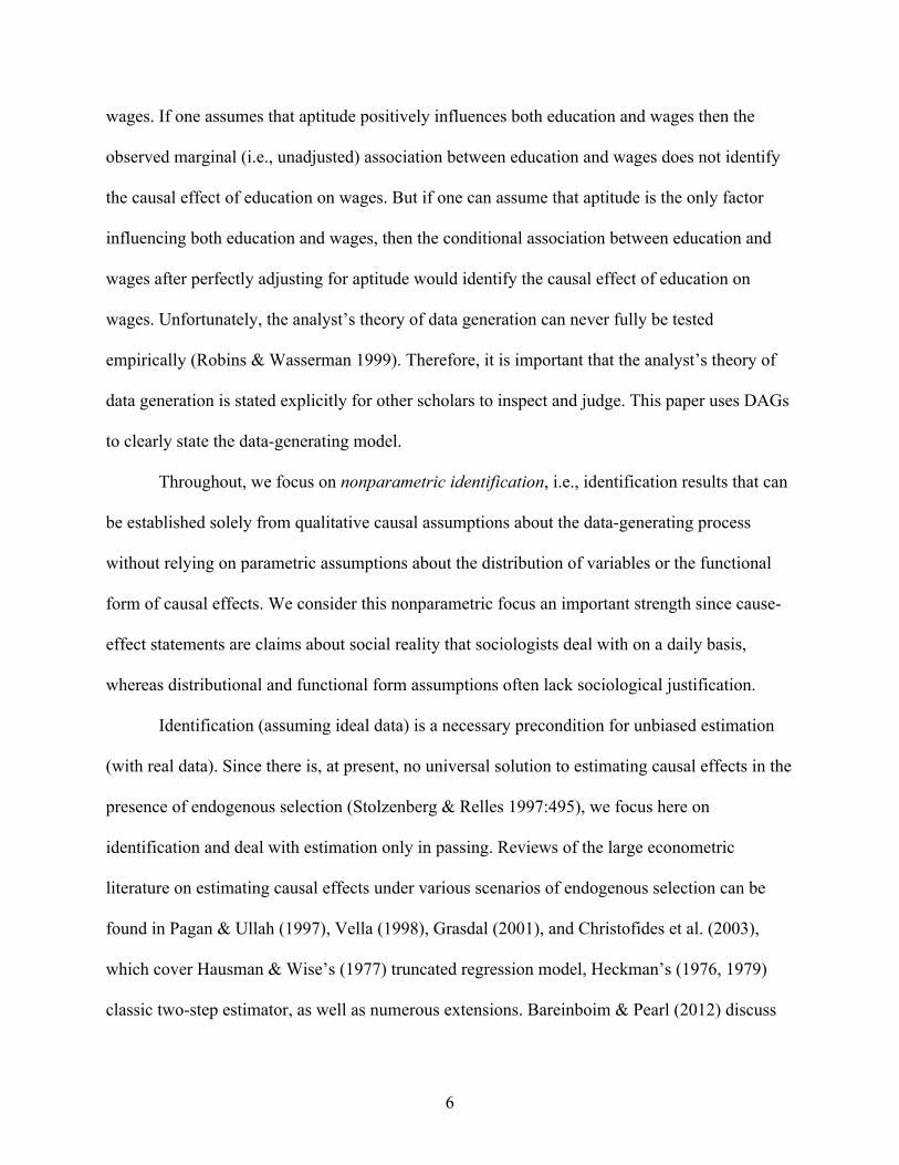
The third reason why two variables may be associated with each other is less widely
known, but it is central to this article: conditioning on the common outcome of two variables
(i.e., a collider) induces a new association between them. We call this phenomenon endogenous
selection. In Fig. 4a, A and B are marginally independent because they do not cause each other
and do not share a common cause. Thus, the marginal association between A and B identifies the
causal effect (which, in this DAG, is zero). In Fig. 4b, by contrast, conditioning on the collider C
induces an association between its causes A and B. Therefore, the conditional association
between A and B given C is biased for the causal effect of A on B. A dotted line denotes the

11
spurious association induced between two variables by conditioning on a collider.7 Conditioning
on a variable that is caused by a collider (a “descendant” of the collider) has qualitatively the
same consequence as conditioning on the collider itself (Fig. 4c) because the descendant is a
proxy measure of the collider.
[FIG. 4 HERE]
Since endogenous selection is not obvious and can be difficult to understand in the
abstract, we first offer an intuitive hypothetical example to illustrate Fig. 4. Consider the
relationships between talent, A, beauty, B, and Hollywood success, C. Suppose, for argument’s
sake, that beauty and talent are unassociated in the general population (i.e., beauty does not cause
talent, talent does not cause beauty, and beauty and talent do not share a common cause).
Suppose further that beauty and talent are separately sufficient for becoming a successful
Hollywood actor. Given these assumptions, success clearly is a collider variable. Now condition
on the collider, for example, by looking at the relationship between beauty and talent only among
successful Hollywood actors. Under our model of success, knowing that a talentless person is a
successful actor implies that the person must be beautiful. Conversely, knowing that a less than
beautiful person is a successful actor implies that the person must be talented. Either way,
conditioning on the collider (success) has created a spurious association between beauty and
talent among the successful. This spurious association is endogenous selection bias.
This example may lack sociological nuance, but it illustrates the logic of endogenous
selection bias that conditioning on a common outcome distorts the association between its
7 This dotted line functions like a regular path segment when tracing paths between variables.
Note that one does not draw a dotted line for the spurious association induced by common-cause
confounding.

12
causes. 8 To achieve greater realism, one could loosen assumptions and, for example, allow that
A causes B (maybe because talented actors invest less in self-beautification). The problem of
endogenous selection, however, would not go away. The observed conditional association
between talent and beauty given Hollywood success would remain biased for the true causal
effect of talent on beauty. (Adding arrows to an existing set of variables never helps
nonparametric identification [Pearl 2009]). Unfortunately, sign and magnitude of endogenous
selection bias cannot generally be predicted outside of constrained settings or without strong
parametric assumptions (Hausman & Wise 1981; Berk 1983; VanderWeele & Robins 2009a).
In sum, over-control bias, confounding bias, and endogenous selection bias are distinct
phenomena: they arise from different causal structures, and they call for different remedies. The
contrast between Figs. 2-4 neatly summarizes this difference. Over-control bias results from
conditioning on a variable on a causal path between treatment and outcome; the remedy is not to
condition on variables on a causal path. Confounding bias arises from failure to condition on a
common cause of treatment and outcome; the remedy is to condition on the common cause.
Finally, endogenous selection bias results from conditioning on a (descendant of a) collider on a
path (causal or noncausal) between treatment and outcome; the remedy is not to condition on
such colliders. All three biases originate from analytical mistakes, albeit from different ones:
8 Conditioning on a collider always changes the association between its causes within at least one
value of the collider, except for pathological situations, e.g., when the two effects going into the
collider cancel each other out exactly. In real life, the probability of exact cancellation is zero,
and we disregard this possibility henceforth. The technical literature refers to this as the
“faithfulness” assumption (Spirtes et al. 1993).

13
with confounding, the analyst did not condition although he should have; and with over-control
and endogenous selection, he did condition although he should not have.
Identification in general DAGs
All DAGs are built from chains, forks, and inverted forks. Therefore, understanding the
associational implications of chains (causation), forks (confounding), and inverted forks
(endogenous selection) is sufficient for conducting nonparametric identification analyses in
arbitrarily complicated DAGs. The so-called d-separation rule summarizes these implications
(Pearl 1988, 1995, Verma & Pearl 1988):
First, note that all associations in a DAG are transmitted along paths, but that not all paths
transmit association. A path between two variables, A and B, does not transmit association and is
said to be blocked, closed, or d-separated if
1. The path contains a noncollider, C, that has been conditioned on, A!C!B, or
A"C!B; or if
2. The path contains a collider, C, and neither the collider nor any of its descendants
have been conditioned on, A!C"B.
Paths that are not d-separated do transmit association and are said to be open, unblocked, or d-
connected. Two variables that are d-separated along all paths are statistically independent.
Conversely, two variables that are d-connected along at least one path are statistically dependent,
i.e., associated (Verma & Pearl 1988).
Note that conditioning on a variable has opposite consequences depending on whether the
variable is a collider or a noncollider: Conditioning on a noncollider blocks the flow of
association along a path, whereas conditioning on a collider opens the flow of association.

14
One way of conducting a formal nonparametric identification analysis then reduces to
blocking all noncausal paths between treatment and outcome (by conditioning on suitably chosen
variables) while keeping all causal paths between treatment and outcome open.9 For example, in
Fig. 1, the total causal effect of T on Y can be identified by conditioning on X because this
blocks the two noncausal paths between T and Y, T"X"U!Y and T"X"U!C!Y that
would otherwise be open. (A third noncausal path between T and Y, T!C"U!Y, is blocked
without conditioning because it contains the collider C. Conditioning on C would ruin
identification for two reasons: first, it would induce endogenous selection bias by opening the
noncausal path T!C"U!Y; second, it would induce over-control bias because C sits on a
causal path from T to Y, T!C!Y)
The motivation for this paper is that it is all too easy to open noncausal paths between
treatment and outcome inadvertently by conditioning on a collider, thus inducing endogenous
selection bias.
5. EXAMPLES OF ENDOGENOUS SELECTION BIAS IN SOCIOLOGY
Endogenous selection bias may originate from conditioning on a collider at any point in a causal
process. Endogenous selection bias can be induced by conditioning on a collider that occurs after
the outcome; by conditioning on a collider that is an intermediate variable that occurs between
the treatment and the outcome; and by conditioning on a collider that occurs before the treatment
9 This is the logic of “identification by adjustment,” which underlies identification in regression
analysis. Pearl’s do-calculus is a complete nonparametric graphical identification criterion built
on d-separation that includes all types of nonparametric identification as special cases (Pearl
1995).

15
(Greenland 2003). Therefore, we organize the following sociological examples of endogenous
selection bias according to the timing of the collider relative to the treatment and the outcome.
Conditioning on a (post-)outcome collider
It is well known that outright selection on the outcome, as well as conditioning on a variable
affected by the outcome, can lead to bias (e.g., Berkson 1946, Gronau 1974; Heckman 1974,
1976, 1979). Nevertheless, both problems continue to occur in empirical sociological research,
where they may result from non-random sampling schemes in the data selection stage of a study
or from seemingly compelling choices in the data analysis stage. Here, we present canonical and
more recent examples, explicating them as endogenous selection bias due to conditioning on a
collider.
Sample Truncation Bias
Hausman & Wise’s (1977) influential discussion of sample truncation bias furnishes a classic
example of endogenous selection bias. They consider the problem of estimating the effect of
education on income from a sample selected (truncated) to contain only low earners. Fig. 5
describes the heart of the problem. Income, I, is affected by education, E, as well as by other
factors traditionally subsumed in the error term, U. Assume, for clarity and without loss of
generality, that E and U are independent in the population (i.e., share no common causes and do
not cause each other). Then, the marginal association between E and I in the population would
identify the causal effect E!I. The DAG shows, however, that I is a collider variable on the path
between treatment and the error term, E!I"U. Restricting the sample to low earners amounts to
conditioning on this collider. As a result, there are now two sources of association between E and

16
I: the causal path E!I, which represents the causal effect of interest, and the newly induced
noncausal path E---U!I. Sample truncation has induced endogenous selection bias so that the
association between E and I in the truncated sample does not identify the causal effect of E on I.
[FIG. 5 ABOUT HERE]
This example illustrates an important general point: if a treatment, T, has an effect on the
outcome, Y, T!Y, then the outcome is a collider variable on the path between the treatment and
the outcome’s error term, U, T!Y" U. Therefore, outright selection on an outcome, or
selection on a variable affected by the outcome, is always potentially problematic.
Nonresponse bias
The same basic causal structure that leads to truncation bias also underlies nonresponse bias in
retrospective studies—except that nonresponse is better understood as conditioning on a variable
affected by the outcome rather than conditioning on the outcome itself. Consider a simplified
version of the example discussed by Lin, Schaeffer, & Seltzer (1999), who investigate the
consequences of nonresponse bias for estimating the effect of divorced fathers’ income on their
child support payments (Fig. 6). Divorced father’s income, I, and the amount of child support he
pays, P, both influence whether a father responds to the study, R. (Without loss of generality, we
neglect that I and P may share common causes). Response behavior thus is a collider along a
noncausal path between treatment and outcome, I!R"P, Analyzing only completed interviews
by dropping nonresponding fathers (listwise deletion) amounts to conditioning on this collider,
which induces a noncausal association between fathers’ income and the child support they pay,
i.e., endogenous selection bias.
[FIG. 6 ABOUT HERE]

17
Ascertainment bias
Sociological research on elite achievement sometimes employs non-random samples when
collecting data on the entire population is too expensive or drawing a random sample is
infeasible. Such studies may sample all individuals, organizations, or cultural products that have
achieved a certain elite status (e.g., sitting on the supreme court, qualifying for the Fortune 500,
or receiving critical accolades) and a control group of individuals, organizations, or cultural
products that have distinguished themselves in some other manner (e.g., sitting on the Federal
bench, posting revenues in excess of $100 million, or being commercially successful). The logic
of this approach is to compare the most outstandingly successful cases to somewhat less
outstandingly successful cases in order to understand what sets them apart. The problem is that
studying the causes of success in a sample selected for success invites endogenous selection bias.
We suspect that this sampling strategy may account for a surprising recent finding about
the determinants of critical success in the music industry (Schmutz 2005; see also Allen and
Lincoln 2004; Schmutz & Faupel 2010). The study aimed, among other goals, to identify the
effects of a music album’s commercial success on its chances of inclusion in Rolling Stone
magazine’s vaunted list of 500 Greatest Albums of All Time. The sample included roughly 1700
albums: all albums in the Rolling Stone 500 and 1200 additional albums, all of which had earned
some other elite distinction, such as topping the Billboard charts or winning a critics’ poll.
Among the tens of thousands of albums released in the United States over the decades, the 1700
sampled albums clearly represent a subset that is heavily selected for success. A priori, one
might expect that outstanding commercial success (i.e., topping the Billboard charts) should
increase an album’s chances of inclusion in the Rolling Stone 500 (because the experts compiling

18
the list can only consider albums that they know, probably know all chart toppers, and cannot
possibly know all albums ever released). Surprisingly, however, a logistic regression of the
analytic sample indicated that topping the Billboard charts was strongly negatively associated
with inclusion in the Rolling Stone 500.
[FIG. 7 ABOUT HERE]
How come? As the authors noted, this result should be interpreted with caution (Schmutz
2005:1520; Schmutz & Faupel 2010:705). We hypothesize that the finding is due to endogenous
selection bias. The DAG in Fig. 7 illustrates the argument. (For clarity, we do not consider
additional explanatory variables in the study.) The outcome is an album’s inclusion in the
Rolling Stone 500, R. The treatment is topping the Billboard charts, B, which presumably has a
positive effect on R in the population of all albums. By construction, both R and B have a strong,
strictly positive effect on inclusion in the sample, S. Analyzing this sample means that the
analysis conditions on inclusion in the sample, S, which is a collider on a noncausal path
between treatment and outcome, B!S"R. Conditioning on this collider changes the association
between its immediate causes, R and B, and induces endogenous selection bias. If the sample is
sufficiently selective of the population of all albums, then the bias may be large enough to
reverse the sign on the estimated effect of B on R, producing a negative estimate for a causal
effect that may in fact be positive.
Table 1 makes the same point. For binary B and R, B=1 denotes topping the Billboard
charts, R=1 denotes inclusion in the Rolling Stone 500, and 0 otherwise. The cell counts a, b, c,
and d, define the population of all albums. In the absence of common-cause confounding (as
encoded in Fig. 7), the population odds ratio ORPopulation = ad/bc gives the true causal effect of B
on R. Now note that the great majority of albums ever released neither topped the charts nor won

19
inclusion in the Rolling Stone 500. In order to reduce the data collection burden, the study then
samples on success by including all albums with R=1 and all albums with B=1 in the analysis
and severely under-samples less successful albums, aSample<a. The odds ratio from the logistic
regression of R on B in this selected sample would then be downward biased compared to the
true population odds ratio, and possibly flip directions, since ORSample = aSample d/bc < ad/bc =
ORPopulation.
[TABLE 1 ABOUT HERE]
We note that the recovery of causal information despite direct selection on the outcome is
sometimes possible if certain constraints can be imposed on the data. This is the domain of the
epidemiological literature on case-control studies (Rothman, Greenland, & Lash 2008) and the
econometric literature on response- or choice-based sampling (Manski 2003: chapter 6). A key
rule in case-control studies, however, is that observations should not be sampled (“ascertained”)
as a function of both the treatment and the outcome. The consequence of violating this rule is
known as ascertainment bias (Rothman et al. 2008). The endogenous selection bias in the
present example is ascertainment bias, because control albums are sampled as a function of (a)
exclusion from the Rolling Stone 500 and (b) commercial success.10
Heckman selection bias
Heckman selection bias—perhaps the best-known selection bias in the social sciences—can be
explicated as endogenous selection bias. A classic example is the effect of motherhood (i.e.,
10 Greenland, Robins & Pearl. (1999) and Hernán et al. (2004) use DAGs to discuss
ascertainment bias as endogenous selection bias in a number of interesting biomedical case-
control studies.

20
having a child), M, on the wages offered to women by potential employers, WO (Gronau 1974,
Heckman 1974). Fig. 8 displays the relevant DAGs. Following standard labor market theory,
assume that motherhood will affect a woman’s reservation wage, WR, i.e., the wage that would
be necessary to draw her out of the home and into the workforce. Employment, E, is a function
both of the wage offer and the reservation wage because a woman will only accept the job if the
wage offer meets or exceeds her reservation wage. Therefore, employment is a collider on the
path M!WR!E"WO between motherhood and offer wages. (For simplicity, assume that M
and WO share no common cause.)
[FIG. 8 ABOUT HERE]
Many social science datasets include information on motherhood, M, but they typically
do not include information on women’s reservation wage, WR. Importantly, the data typically
only include information on offer wages, WO, for those women who are actually employed. If the
analyst restricts the analysis to employed women, he will thus condition on the collider E,
unblock the noncausal path from motherhood to offer wages, M! WR!E"WO, and induce
endogenous selection bias. The analysis would thus indicate an association between motherhood
and wages even if the causal effect of motherhood on wages is in fact zero (Fig. 8a).
If motherhood has no effect on offer wages, as in Fig. 8a, the endogenous selection
problem is bad enough. Further complications are introduced by permitting the possibility that
motherhood may indeed have an effect on offer wages (e.g., because of mothers’ differential
productivity compared to childless women, or because of employer discrimination). This is
shown in Fig. 8b by adding the arrow M!WO. This slight modification of the DAG creates a
second endogenous selection problem. Since, as noted above, all outcomes are colliders on the
path between treatment and the error term if treatment has an effect on the outcome, conditioning

21
on E now further amounts to conditioning on the descendant of the collider WO on the path
M!WO"ε. This induces a noncausal association between motherhood and the error term on
offer wages, M--- ε!WO. Note that this second—but not the first—endogenous selection
problem persists even if the noncollider WR is measured and controlled.
The distinction between these two endogenous selection problems affords a fresh
opportunity for inference that, to our knowledge, has not yet been exploited in the applied
literature on the motherhood wage penalty. In either DAG of Fig. 8, the analyst could test the
causal Null hypothesis of no effect of motherhood on offer wages by observing and controlling
women’s reservation wages: observing that M and WO are not associated after conditioning on
WR and E implies that there is no causal effect of M on WO under the model of Fig. 8.
Nonparametric identification of the magnitude of the causal effect M!WO, however, is made
impossible by its very existence, as seen in Fig. 8.b: even if WR is observed and controlled (thus
blocking the flow of association along the noncausal path M!WR"E!WO), conditioning on E
would still create the noncausal path M--- ε!Y. Therefore, the strength of the association
between M and WO after conditioning on WR and E would be biased for the true strength of the
causal effect.
One can predict the direction of the bias under additional assumptions, specifically that
the causal effects in Fig. 8 are in the same direction for all women (VanderWeele & Robins
2009a). If, for example, motherhood decreases the chances of employment (by increasing
reservation wages), and if higher offer wages increase the chances of accepting employment for
all women, then employed mothers must on average have received higher wage offers than
employed childless women. Consequently, an empirical analysis of motherhood on offer wages
that is restricted to working women would underestimate the motherhood wage penalty. This is

22
exactly what Gangl & Ziefle’s (2009) selectivity-corrected analysis of the motherhood wage
penalty finds.
Conditioning on an intermediate variable
Methodologists have long warned that conditioning on an intermediate variable that has been
affected by the treatment can lead to bias (e.g., Heckman 1976; Berk 1983; Rosenbaum 1984;
Holland 1988; Robins 1989, 2001, 2003; Smith 1990; Angrist & Krueger 1999; Sobel 2008;
Wooldridge 2005). This bias appears in many guises. It is the source of informative censoring
and attrition bias in longitudinal studies, and it is a central problem of mediation analysis in the
search for social mechanisms and the estimation of direct, and indirect effects. Following Pearl
(1998), Robins (2001) and Cole & Hernán (2002), we use DAGs to explicate the problem of
conditioning on intermediate variables as endogenous selection bias.
Informative/dependent censoring and attrition bias in longitudinal studies
Most prospective longitudinal (panel) studies experience attrition over time. Participants that
were enrolled at baseline may die, move away, or simply refuse to answer in subsequent waves
of data collection. Over time, the number of cases available for analysis decreases, sometimes
drastically so (e.g., Behr, Bellgardt, Rendtel 2005; Alderman et al. 2001). When faced with
incomplete follow up, some sociological analyses simply analyze the available cases. Event-
history or survival-analytic approaches follow cases until they drop out (censoring), while other
analytic approaches may disregard incompletely followed cases altogether. Either practice can
lead to endogenous selection bias.
[FIG. 9 ABOUT HERE]

23
Building on Hill’s (1997) analysis of attrition bias, consider estimating the effect of
poverty, P, on divorce, D, in a prospective study with attrition, C. Fig. 9 displays various
assumptions about the attrition process. Fig. 9a shows the most benevolent situation. Here, P
affects D but neither variable is causally related to C—attrition is assumed to be completely
random with respect to both treatment and outcome. If this assumption is correct, then analyzing
complete cases only, i.e., conditioning on not having attrited, is entirely unproblematic—the
causal effect P!D is identified without any adjustments for attrition. In Fig. 9b, poverty is
assumed to affect the risk of dropping out, P!C. Nevertheless, the causal effect of P!D
remains identified. As in Fig. 9a, conditioning on C in Fig. 9b does not lead to bias because
conditioning on C does not open any noncausal paths between P and D.11 If, however, there are
unmeasured factors, such as marital distress, U, that jointly affect attrition and divorce, as in Fig.
9c, then C becomes a collider along the noncausal path between poverty and divorce,
P!C"U!D, and conditioning on C will unblock this path and distort the association between
poverty and divorce. Attrition bias thus is nothing other than endogenous selection bias. Note
that even sizeable attrition per se is not necessarily a problem for the identification of causal
effects. Rather, attrition is problematic if conditioning on attrition opens a noncausal path
between treatment and outcome, as in Fig. 9c.12
11 One may ask whether conditioning on C in Panel (b) would threaten the identification of the
population-average causal effect if the effect of P on D varies in the population. Under the model
of Fig. 9b, this is not the case because the DAG implies that the effect of P on D does not vary
systematically with C (VanderWeele & Robins 2007b).
12 For more elaborate attrition scenarios, see Hernán et al. (2004).

24
Imperfect Proxy Measures Affected by the Treatment
Much social research studies the effects of schooling on outcomes such as cognition (e.g.,
Coleman, Hoffer, & Kilgore et al. 1982), marriage (e.g., Gullickson 2006; Raymo & Iwasawa
2005), and wages (e.g., Grilliches & Mason 1972; Leigh and Ryan 2008; Amin 2011).
Schooling, of course, is not randomly assigned to students: on average, individuals with higher
innate ability are both more likely to obtain more schooling and to achieve more favorable
outcomes later in life regardless of their level of schooling. Absent convincing measures to
control for confounding by innate ability, researchers often resort to proxies for innate ability,
such as IQ-type cognitive test scores. Using DAGs, we elaborate econometric discussions of this
proxy-control strategy (e.g., Angrist and Krueger 1999; Wooldridge 2002:63-70) by
differentiating between three separate problems, including endogenous selection bias.
[FIG. 10 ABOUT HERE]
To be concrete, consider the effect of schooling, S, on wages, W. Fig. 10a starts by
positing the usual assumption that innate ability, U, confounds the effect of schooling on wages
via the unblocked noncausal path S"U!W. Since true innate ability is unobserved, the path
cannot be blocked and the effect S!Y is not identified. Next, one might control for measured
test scores, Q, as a proxy for the unobserved U, as shown in Fig. 10b. To the extent that U
strongly affects Q, Q is a valid proxy for U. But to the extent that Q does not perfectly measure
U, the effect of S on W remains partially confounded—this is the first problem of proxy-control:
the familiar issue of residual confounding when an indicator (i.e., test scores) imperfectly
captures the desired underlying construct (i.e., ability). Nevertheless, under the assumptions of
Fig. 10b, controlling for Q will remove at least some of the confounding bias exerted by U, and
not introduce any new biases.

25
The second problem, endogenous selection bias, enters the picture in Fig. 10c. Cognitive
test scores, Q, are sometimes measured after the onset of schooling. This is a problem because
schooling is known to affect students’ test scores (Winship & Korenman 1997), as indicated by
the addition of the arrow S!Q. This makes Q into collider along the noncausal path from
schooling to wages, S!Q"U!W. Conditioning on Q will open this noncausal path and thus
lead to endogenous selection bias.
The third distinct problem results from the possibility that Q may itself exert a direct
causal effect on W, Q!W, perhaps because employers may use test scores in the hiring process
and reward high test scores with better pay regardless of the applicant’s schooling. If so, the
causal effect of schooling on wages would be partially mediated by test scores along the causal
path S!Q!W, and controlling for Q would block this causal path, leading to over-control bias.
The confluence of these three problems leaves the analyst in a quandary. If Q is measured
after the onset of schooling, should she control for Q to remove (by proxy) some of the
confounding owed to U? Or should she not control for Q to avoid inducing endogenous selection
bias and over-control bias? Absent detailed knowledge of the relative strengths of all effects in
the DAG—which is rarely available, especially where unobserved variables are involved—it is
difficult to determine which problem will dominate empirically, and hence which course of
action should be taken.13
Direct effects, indirect effects, causal mechanisms, and mediation analysis
13 If Q is measured before the onset of schooling, then the analyst can probably assume the DAG
in Fig. 10b (and certainly rule out Figs. 10c and 10d). If Fig. 10b is true, then conditioning on Q
is safe and advisable.

26
Common approaches to estimating direct and indirect effects (Baron & Kenny 1986) are highly
susceptible to endogenous selection bias. We first look at the estimation of direct effects. To fix
ideas, consider an analysis of the Project STAR class-size experiment that asks whether class
size in first grade, T, has a direct effect on high school graduation, Y, via some mechanism other
than boosting student achievement in third grade, M (Finn, Gerber, & Boyd-Zaharias 2005). Fig.
11a gives the basic corresponding DAG. Since class size is randomized, the total effect of
treatment, T, on the outcome, Y, is identified by their marginal association because T and Y
share no common cause. The post-treatment mediator, M, however, is not randomized and may
therefore share an unmeasured cause, U, with the outcome, Y. Candidates for U in the present
example might include parental education, student motivation, and any other confounders of M
and Y not explicitly controlled in the study. The existence of such a variable U would make M a
collider variable along the noncausal path T!M"U!Y between treatment and outcome.
Conditioning on M (e.g., in a regression of Y on T and M) in order to estimate the direct causal
effect T!Y unblocks this noncausal path and induces endogenous selection bias. Hence, the
direct effect of T on Y is not identified.14
[FIG. 11 ABOUT HERE]
Attempts to detect the presence of indirect, or mediated, effects by comparing estimates
for the total effect of T on Y and estimates for the direct effect of T on Y (Baron & Kenny 1986),
are similarly susceptible to endogenous selection bias. Suppose, for argument’s sake, that
14 In this DAG, it is similarly impossible to nonparametrically identify the direct effect T!Y
from an estimate of the total causal effect of T on Y minus estimates for the product of the direct
effects T!M and M!Y. This difference-method would fail because the effect M!Y is
confounded by U and hence not identified in its own right.

27
achievement in third grade has no causal effect on high school graduation (Fig. 11b). The total
effect of T on Y would then be identical with the direct effect of T on Y because no indirect
effect of T on Y via M exists. The total effect is identified by the marginal association between T
and Y. The conditional association between T and Y given M, however, would differ from the
total effect of T on Y because M is a collider, and conditioning on the collider induces a
noncausal association between T and Y via T!M"U!Y. Thus, the (correct) estimate for the
total causal effect and the (naïve and biased) estimate for the direct effect of T on Y would differ,
and the analysts would falsely conclude that an indirect effect exists even if it does not.
The endogenous selection problem of mediation analysis is of particular concern for
current empirical practice in sociology because conventional efforts to control for unobserved
confounding typically focus on the confounders of the main treatment, but not on the
confounders of the mediator. The new literature on causal mediation analysis discusses
estimands and nonparametric identification conditions (Robins & Greenland 1992; Pearl 2001,
2012; Sobel 2008; Shpitser & VanderWeele 2011) as well as parametric and nonparametric
estimation strategies (VanderWeele 2009c, 2011a; Imai, Keele, & Yamamoto 2010; Pearl 2012).
Conditioning on a pre-treatment collider
Controllling for pre-treatment variables can sometimes increase rather than decrease bias. One
class of pre-treatment variables that analysts should approach with caution is pre-treatment
colliders (Pearl 1995; Greenland, Robins & Pearl 1999; Hernán et al. 2002; Greenland 2003;
Hernán et al. 2004; Elwert 2013).
Homophily bias in social network analysis

28
A classic problem of causal inference in social networks is that socially connected individuals
may exhibit similar behaviors not because one individual influences the other (causation) but
because individuals who are similar tend to form social ties with each other (homophily) (Farr
1858). Distinguishing between homophily and interpersonal causal effects (also called peer
effects, social contagion, network influence, induction, or diffusion) is especially challenging if
the sources of homophily are unobserved (latent). Shalizi & Thomas (2011) recently showed that
latent homophily bias constitutes a previously unrecognized example of endogenous selection
bias, where the social tie itself plays the role of the pre-treatment collider.
[FIG. 12 ABOUT HERE]
Consider, for example, the spread of civic engagement between friends in dyads
generically indexed (i,j) (Fig. 12). The question is whether Igor’s civic engagement at time t,
Yi(t) causes Jane’s subsequent civic engagement, Yj(t+1). For expositional clarity, assume that
civic engagement does not spread between friends (i.e., no arrow Yi(t)!Yj(t+1)). Instead, each
person’s civic engagement is caused by their own characteristics, U, such as altruism, which are
at least partially unobserved (giving arrows Yi(t)"Ui!Yi(t+1) and Yj(t)"Uj!Yj(t+1)). Tie
formation is homophilous, such that altruistic people form preferential attachments, Ui!Fij"Uj.
Hence, Fij is a collider. The problem, then, is that the very act of computing the association
between individuals i and j in a sample of dyads (i,j) means that the analysis conditions on the
existence of the social tie, Fij=1. Conditioning on Fij opens a noncausal path between treatment
and outcome, Yi(t)"Ui!Fij"Uj!Yj(t+1), which results in an association between Igor’s and
Jane’s civic engagement even if one does not cause the other.
In sum, if tie formation or tie dissolution are affected by unobserved variables that are,
respectively, associated with the treatment variable in one individual and the outcome variable in

29
another individual, then searching for interpersonal effects will induce a spurious association
between individuals in the network, i.e., endogenous selection bias.
One solution to this problem is to model tie-formation (and dissolution) explicitly
(Shalizi & Thomas 2011). In the model of Fig. 12, this can be accomplished by measuring and
conditioning on the tie-forming characteristics of either Igor, Ui, or Jane, Uj, or both. Other
approaches to latent homophily bias are proliferating in the literature. For example, Elwert &
Christakis (2008) introduce a proxy strategy to measure and subtract homophily bias; Ver Steeg
& Galstyan (2011) develop a formal test for latent homophily; VanderWeele (2011b) introduces
a formal sensitivity analysis; and O’Malley et al. (2013) explore instrumental variables solutions;
VanderWeele & An (2013) provide an extensive survey.
What Pre-Treatment Variables Should be Controlled?
Pre-treatment colliders have practical and conceptual implications beyond social network
analysis. Empirical examples exist where controlling for pre-treatment variables demonstrably
increases rather than decreases bias. For example, Steiner et al. (2010) report a within-study
comparison between an observational study and an experimental benchmark of the effect of an
educational intervention on student test scores. In the observational study, the bias in the
estimated effect of treatment on math scores increased by about 30 percent when controlling only
for pre-treatment psychological disposition or only for pre-treatment vocabulary test scores.
Furthermore, they found that although controlling for additional pre-treatment variables
generally reduced bias, sometimes including additional controls increased bias. It is possible that
these increases in bias resulted from controlling for pre-treatment colliders.

30
This raises larger questions about control-variable selection in observational studies.
Which pre-treatment variables should an analyst control, and which pre-treatment variables are
better left alone? An inspection of the DAGs in Fig. 13 demonstrates that these questions cannot
be settled without recourse to a theory of how the data were generated. Start by comparing the
DAGs in Figs. 13a and 13b. In both models, the pre-treatment variable X meets the
commonsense, purely associational, definition of confounding: (i) X temporally precedes
treatment, T; (ii) X is associated with the treatment; and (iii) X is associated with the outcome,
Y. The conventional advice would be to condition on X in both situations.
But this conventional advice is incorrect. The proper course of action differs sharply
depending on how the data were generated (Greenland & Robins 1986; Weinberg 1993; Cole &
Hernán 2002; Hernán et al. 2002; Pearl 2009). In Fig. 13a, X is indeed a common-cause
confounder as it sits on an open noncausal path between treatment and outcome, T"X!Y.
Conditioning on X will block this noncausal path and identify the causal effect of T on Y. By
contrast, in Fig. 13b, X is a collider that blocks the noncausal path between treatment and
outcome, T"U1!X"U2!Y. Conditioning on X would open this noncausal path and induce
endogenous selection bias. Therefore, the analyst should condition on X if the data were
generated according to Fig. 13a, but she should not condition on X if the data were generated
according to Fig. 13b.
If U1 and U2 are unobserved, the analyst cannot distinguish empirically between Figs. 13a
and 13b because both models have identical observational implications: in both models, all
combinations of X, T, and Y are marginally and conditionally associated with each other.
Therefore, the only way to decide whether or not to control for X is to decide on a priori
grounds, which of the two causal models accurately represents the data-generating process. In

31
other words, the selection of control variables requires a theoretical commitment to a model of
data generation.
In practice, sociologists may lack a fully articulated theory of data generation. It turns
out, however, that partial theory suffices to determine the proper set of pre-treatment control
variables. If the analyst is willing to assume that controlling for some combination of observed
pre-treatment variables is sufficient to identify the total causal effect of treatment, then it is
sufficient to control for all variables that (directly or indirectly) either cause treatment or
outcome or both (VanderWeele & Shpitser 2011).
The virtue of this advice is that it prevents the analyst from conditioning on a pre-
treatment collider. In Fig. 13a, it accurately counsels controlling for X (because X is a cause of
both treatment and outcome), and in Fig. 13b it accurately counsels not controlling for X
(because X causes neither treatment nor outcome).
Nevertheless, the advice is still conditional on some theory of data generation, however
coarsely articulated, specifically that there exists some sufficient set of observed controls. Note
that no such set exists in Fig. 13c. Here, X is both a confounder (on the noncausal paths
T"X"U1!Y and T"X"U2!Y) and a collider (on the noncausal path T"U1!X"U1!Y).
Controlling for X would remove confounding but induce endogenous selection, and not
controlling for X would do the opposite. In short, there exists no set of pre-treatment controls
that is sufficient for identifying the causal effect of T on Y, and hence the VanderWeele-Shpitser
(2011) rule does not apply.

32
When all variables in the DAG are binary, Greenland (2003) suggests that controlling for
a variable that is both a confounder and a collider, as in Fig. 13c, likely (but not necessarily)
removes more bias than it creates.15
6. DISCUSSION AND CONCLUSION
In this paper, we have argued that understanding endogenous selection bias is central for
understanding the identification of causal effects in sociology. Drawing on recent work in
theoretical computer science (Pearl 1995, 2009) and epidemiology (Hernán et al. 2004), we have
explicated endogenous selection as conditioning on a collider variable in a DAG. Interrogating
the simple steps necessary for separating causal from noncausal associations, we next saw that
endogenous selection bias is logically on par with confounding bias and over-control bias in the
sense that all nonparametric identification problems can be reduced to either confounding (i.e.,
not conditioning on a common cause), over-control (i.e., conditioning on a variable on the causal
pathway), or endogenous selection (i.e., conditioning on a collider), or a mixture of the three
(Verma & Pearl 1988).
Methodological warnings are most useful if they are phrased in an accessible language
(Pearl 2009:352). We hope that DAGs may provide such a language because they focus the
analyst’s attention on what matters for nonparametric identification of causal effects: qualitative
assumptions about the causal relationships between variables. This in no way denies the place of 15 Causal inference for time-varying treatments often encounters variables that are both colliders
and confounders (Pearl & Robins 1995). See Elwert (2013), Sharkey & Elwert (2011) and
Wodtke, Harding, & Elwert (2011) for sociological examples from neighborhood effects
research that have statistical solutions (Robins 1999).

33
algebra and parametric assumptions in social science methodology. But inasmuch as algebraic
presentations present themselves as barriers to entry for applied researchers, phrasing
methodological problems graphically may increase awareness of these problems in practice.
In the main part of this paper, we have shown how numerous problems in causal
inference can be explicated as endogenous selection bias. A key insight is that conditioning on an
endogenous variable (a collider variable), no matter where it temporally falls relative to
treatment and outcome, can induce new, noncausal, associations, which are likely to result in
biased estimates. We have distinguished three groups of endogenous selection problems by the
timing of the collider relative to treatment and outcome. The most general advice to be derived
from the first two groups—post-outcome and intermediate collider examples—is
straightforward: when estimating total causal effects, avoid conditioning on post-treatment
variables (Rosenbaum 1984). Of course, this advice can be hard to follow in practice when
conditioning is implicit in the data-collection scheme or the result of selective nonresponse and
attrition. Even where it is easy to follow, it can be hard to swallow if the avowed scientific
interest concerns the identification of causal mechanisms, mediation, direct, or indirect effects,
which require peering into the post-treatment black box. New solutions for the estimation of
causal mechanisms that rely on a combination of great conceptual care, a new awareness of
underlying assumptions, and powerful sensitivity analyses, however, are fast becoming available
(e.g., Robins & Greenland 1992; Pearl 2001; Frangakis & Rubin 2002; Sobel 2008; Imai et al.
2010; VanderWeele 2008b, 2009a, 2010; Shpitser & VanderWeele 2011).
Advice for handling pre-treatment colliders is harder to come by. If it is known that the
pre-treatment collider is not also a confounder then the solution is not to condition on it when
possible (this is not possible in social network analysis where conditioning on the pre-treatment

34
social tie is implicit in the research question). If the pre-treatment collider is also a confounder,
then conditioning on it may, but need not, remove more bias than it induces (Greenland 2003). In
some circumstances, instrumental variable estimation may be feasible, though researchers should
be aware of its limitations (Angrist et al. 1996).
One of the remaining difficulties in dealing with endogenous selection (if it cannot be
entirely avoided) is that sign and size of the bias are difficult to predict. Absent strong parametric
assumptions, size and sign of the bias will depend on the exact structure of the DAG, the sizes of
the effects and their variation across individuals, and the distribution of the variables (Greenland
2003).16 Conventional intuition about size and sign of bias in causal systems can break down in
unpredictable ways outside of the stylized assumptions of linear models.17 Nevertheless,
statisticians have in recent years derived important (and often complicated) results that have
proven quite powerful in applied work. For example, VanderWeele & Robins (2007a, 2009a,
2009b) derive the sign of endogenous selection bias for DAGs with binary variables and
16 The same difficulties pertain to nonparametrically predicting size and sign of confounding bias
(e.g., VanderWeele, Hernán, & Robins 2008; VanderWeele 2008a). The conventional omitted
variables formula in linear regression merely obscures these difficulties via the assumptions of
linearity and constant effects (e.g., Wooldridge 2002).
17 For example, the sign of direct effects is not always transitive (VanderWeele et al. 2008). In
the DAG A!B!C, the average causal effects A!B and the average causal effect B!C may
both be positive and yet the average causal effect A!C could be negative. Sign transitivity in
conventional structural equation models (Alwin & Hauser 1975) relies on linearity and constant
effects.

35
monotonic effects with and without interactions. Hudson et al. (2008) apply these results
productively in a study of familial coaggregation of diseases.
Greenland (2003), in particular, has derived useful analytic results and approximations
for the relative size of endogenous selection bias and confounding bias in DAGs with binary
variables (see also Kaufman, Kaufman, & MacLenose 2009). His three general rules of thumb
match nicely to our examples of post-outcome, intermediate, and pre-treatment colliders. First,
conditioning on post-outcome colliders that are affected by treatment and outcome, T!C"Y
induces the same bias as would the corresponding confounding bias if the direction of the arrows
into the collider were reversed, T"C!Y. Second, conditioning on an intermediate collider may
lead to bias that is larger than the effects pointing into the collider, although the bias will usually
be smaller than those effects if the intermediate collider does not itself exert a causal effect on
the outcome. Finally, conditioning on a pre-treatment collider (as in Figs. 12-13) will usually
lead to a small bias, which is why recognizing latent homophily bias as endogenous selection
bias (as opposed to confounding bias) should be good news to network analysts. Furthermore, if
the pre-treatment variable is both a collider and a confounder (as in Fig. 13c), then conditioning
on it may remove more bias than it induces, even though nonparametric point-identification is
still not feasible. We note, however, that these rules of thumb for binary-variable DAGs do not
necessarily generalize to DAGs with differently distributed variables. More research is needed to
understand the direction and magnitude of endogenous selection bias in realistic social science
settings.
Empirical research in sociology pursues a variety of goals of description, including
interpretation, and causal inference. Since assumption-free causal inference is impossible,
sociologists must rely on theory, prudent substantive judgment, and well-founded prior

36
knowledge to assess the threat of bias. Using DAGs, sociologists can formally analyze the
consequences of their theoretical assumptions and determine whether causal inference is
possible. Such analyses will strengthen confidence in a causal claim when it is warranted and
explicitly indicate sources of potential bias—including endogenous selection bias—when a
causal claim is not appropriate.

37
LITERATURE CITED
Alderman H, Behrman J, Kohler H, Maluccio JA, Watkins SC. 2001. Attrition in longitudinal
household survey data: some tests for three developing-country samples. Demogr. Res.
5:79--124
Allen MP, Lincoln A. 2004. Critical discourse and the cultural consecration of American films.
Soc. Forces 82(3):871--94
Alwin DH, Hauser, RM. 1975. The decomposition of effects in path analysis. Am. Sociol. Rev.
40:37--47
Amin V. 2011. Returns to education: evidence from UK twins: Comment. Am. Econ. Rev.
101(4):1629--35
Angrist JD, Krueger AB. 1999. Empirical strategies in labor economics. In Handbook of Labor
Economics, Vol 3, ed. O Ashenfelter, D Card D, pp. 1277--366. Elsevier.
Angrist JD, Imbens GW, Rubin, DB. 1996. Identification of causal effects using instrumental
variables. J. Am. Stat. Assoc. 8:328--36
Bareinboim E, Pearl J. 2011. Controlling selection bias in causal inference.
UCLA Cognitive Systems Laboratory, Technical Report (R-381)
Baron RM, Kenny DA. 1986. The moderator-mediator variable distinction in social
psychological research: Conceptual, strategic, and statistical considerations. J Personal.
Soc. Psych. 51:1173-82
Behr A, Bellgardt E, Rendtel U. 2005. Extent and determinants of panel attrition in the European
Community Household Panel. Eur. Sociol. Rev. 21(5):489--512
Berk RA. 1983. An introduction to sample selection bias in sociological data. Am. Sociol. Rev.
48(3):386--398

38
Berkson J. 1946. Limitations of the application of fourfold tables to hospital data. Biom. Bull.
2(3):47--53
Blalock H. 1964. Causal Inferences in Nonexperimental Research. Chapel Hill: University of
North Carolina Press
Bollen KA. 1989. Structural Equations with Latent Variables. New York: Wiley.
Christofides LN, Li Q, Liu Z, Min I. 2003. Recent two-stage sample selection procedures with an
application to the gender wage gap. J. Bus. Econ. Stat. 21:396–405
Coleman JS, Hoffer T, Kilgore S. 1982. High School Achievement: Public, Catholic, and Private
Schools Compared. New York: Basic Books
Duncan O. 1975. Introduction to Structural Equation Models. New York: Academic Press
Elwert F. 2013. Graphical causal models. Pp. 245-273 in S. Morgan (ed.), Handbook of Causal
Analysis for Social Research. In Handbook of Causal Analysis for Social Research, ed.
SL Morgan 13:301-28, Dodrecht: Springer
Elwert F, Christakis NA. 2008. Wives and ex-wives: a new test for homogamy bias in the
widowhood effect. Demography 45(4):851--73
Farr W. 1858. Influence of marriage on the mortality of the French people. In Trans. Natl. Assoc.
Promot. Soc. Sci., ed. GW Hastings, pp. 504--13. London: John W. Park & Son
Finn JD, Gerber SB, Boyd-Zaharias J. 2005. Small classes in the early grades, academic
achievement, and graduating from high school. J. Educ. Psychol. 97(2):214--23
Frangakis CE, Rubin DB. 2002. Principal stratification in causal inference. Biometrics 58:21--29
Fu V, Winship C, Mare R. 2004. Sample selection bias models. In Handbook of Data Analysis,
ed. M Hardy, A Bryman, pp. 409--30. London: Sage Publications

39
Gangl M, Ziefle A. 2009. Motherhood, labor force behavior, and women's careers: An empirical
assessment of the wage penalty for motherhood in Britain, Germany, and the United
States. Demography 46(2):341-69
Glymour MM, Greenland S. 2008. Causal diagrams. In Modern Epidemiology, 3rd Edition, ed.
KJ Rothman, S Greenland, T Lash, pp. 183--209. Philadelphia: Lippincott
Grasdal A. 2001. The performance of sample selection estimators to control for attrition bias.
Health Econ. 10(5):385-98.
Greenland S. 2003. Quantifying biases in causal models: classical Confounding versus collider-
stratification bias. Epidemiology 14:300--6.
Greenland S, Robins JM. 1986. Identifiability, exchangeability and epidemiological
confounding. Int. J. Epidemiol. 15:413--19
Greenland S, Pearl J, Robbins JM. 1999. Causal diagrams for epidemiologic research.
Epidemiology 10:37--48
Greenland S, Robins JM, Pearl J. 1999. Confounding and collapsibility in causal inference. Stat.
Sci.14:29--46
Griliches Z, Mason WM. 1972. Education, income, and ability. J. Polit. Econ. 80(3):S74--S103
Gronau R. 1974. Wage comparisons-a selectivity bias. J. Polit. Econ. 82:1119--44
Gullickson A. 2006. Education and black-white interracial marriage. Demography 43(4):673--89
Hausman JA, Wise DA. 1977. Social experimentation, truncated distributions and efficient
estimation. Econometrica 45:919--38
Hausman JA, Wise DA. 1981. Stratification on endogenous variables and estimation. In The
Econometrics of Discrete Data, ed. C Manski, D McFadden, pp. 365--91. Cambridge,
MA: MIT Press

40
Heckman JJ. 1974. Shadow prices, market wages and labor supply. Econometrica 42(4):679--94
Heckman JJ. 1976. The common structure of statistical models of truncation, sample selection,
and limited dependent variables and a simple estimator for such models. Ann. Econ. Soc.
Meas. 5:475--92
Heckman JJ. 1979. Selection bias as a specification error. Econometrica 47:153--61.
Hernán MA, Hernández-Diaz S, Werler MM, Robins JM, Mitchell AA. 2002. Causal knowledge
as a prerequisite of confounding evaluation: an application to birth defects epidemiology.
Am. J. Epidemiol. 155(2):176--84
Hernán MA, Hernández-Diaz S, Robins JM. 2004. A structural approach to section bias.
Epidemiology 15:615--25
Hill DH. 1997. Adjusting for attrition in event-history analysis. Sociol. Methodol.27:393--416
Holland PW. 1986. Statistics and causal inference (with discussion). J. Am. Stat. Assoc. 81:945--
70
Holland PW. 1988. Causal inference, path analysis, and recursive structural equation models.
Sociol. Methodol.18:449--84
Hudson JI, Javaras KN, Laird NM, VanderWeele TJ, Pope HG, et al. 2008. A structural
approach to the familial coaggregation of disorders. Epidemiology 19:431--39
Imai K, Keele L, Yamamoto T. 2010. Identification, inference, and sensitivity analysis for causal
mediation effects. Stat. Sci. 25(1):51--71
Kaufman S, Kaufman J, MacLenose R. 2009. Analytic bounds on causal risk differences in
directed acyclic graphs involving three observed binary variables. J. Stat. Plann.
Inference 139:3473--87
Kim JH, Pearl J. 1983. A computational model for combined causal and diagnostic reasoning in

41
inference systems. In Proceedings of the 8th International Joint Conference on Artificial
Intelligence pp. 190–3. Karlsruhe
Leigh A, Ryan C. 2008. Estimating returns to education using different natural experiment
techniques. Econ. Educ. Rev. 27(2):149--60
Lin I, Schaeffer NC, Seltzer JA. 1999. Causes and effects of nonparticipation in a child support
survey. J. Off. Stat. 15(2):143--66
Manski C. 2003. Partial Identification of Probability Distributions. New York: Springer.
Morgan SL, Winship C. 2007. Counterfactuals and Causal Inference: Methods and Principles
for Social Research. Cambridge: Cambridge University Press
O’Malley AJ, Elwert F, Rosenquist JN, Zaslavsky AM, Christakis NA. 2012. Estimating peer
effects in longitudinal dyadic data using instrumental variables. Work. Pap., Dep. Health
Care Pol., Harvard Univ.
Pagan A, Ullah A. 1997. Nonparametric Econometrics. Cambridge: Cambridge University Press
Pearl J. 1988. Probabilistic reasoning in intelligent systems. San Mateo: Morgan Kaufman
Pearl J. 1995. Causal diagrams for empirical research. Biometrika 82(4):669--710.
Pearl J. 1998. Graphs, causality, and structural equation models. Socio. Meth. Res. 27(2):226–84
Pearl J. 2001. Direct and indirect effects. In Proc. Seventeenth Conf. Uncertain. Artif. Intell., pp.
411--20. San Francisco: Morgan Kaufmann
Pearl J. 2009. Causality: Models, Reasoning, and Inference, 2nd Edition. Cambridge: Cambridge
University Press
Pearl J. 2010a. The foundations of causal inference. Sociol. Methodol. 40:75--149
Pearl J. 2012. The causal mediation formula—a guide to the assessment of pathways and
mechanisms. Prev. Sci. 13(4):426--36

42
Pearl J, Robins JM. 1995. Probabilistic evaluation of sequential plans from causal models with
hidden variables. In Uncertainty in Artificial Intelligence 11, ed. P Besnard, S Hanks, pp.
444--53. San Francisco: Morgan Kaufmann
Raymo JM, Iwasawa M. 2005. Marriage market mismatches in Japan: an alternative view of the
relationship between women's education and marriage. Am. Sociol. Rev. 70(5):801--22
Robins JM. 1986. A new approach to causal inference in mortality studies with a sustained
exposure period: application to the health worker survivor effect. Math. Model. 7:1393—
512
Robins JM. 1989. The control of confounding by intermediate variables. Stat. Med. 8:679—701
Robin JM. 1994. Correcting for noncompliance in randomized trials using structural nested mean
models. Comm. Stat.-Theo. Meth. 23:2379-412.
Robins JM. 1999. Association, causation, and marginal structural models. Synthese 121:151--79
Robins JM. 2001. Data, design, and background knowledge in etiologic inference. Epidemiology
23(3):313--20
Robins JM. 2003. Semantics of causal DAG models and the identification of direct and indirect
effects. In Highly Structured Stochastic Systems, ed. P Green, NL Hjort, S Richardson,
pp. 70--81. New York: Oxford University Press
Robins JM, Greenland S. 1992. Identifiability and exchangeability for direct and indirect effects.
Epidemiology 3:143--55
Robins JM, Wasserman L.1999. On the impossibility of inferring causation from association
without background knowledge. In Computation, Causation, and Discovery, ed. CN
Glymour, GG Cooper, pp. 305--21. Cambridge: AAAI/MIT Press

43
Rosenbaum PR. 1984. The consequences of adjustment for a concomitant variable that has been
affected by the treatment. J. R. Stat. Soc. Series A 147(5):656--66
Rothman KJ, Greenland S, Lash TL. 2008. Case-control studies. In Modern Epidemiology, 3rd
edition, ed. KJ Rothman, S Greenland, TL Lash, pp. 111--27. Philadelphia: Lippincott
Rubin DB. 1974. Estimating causal effects of treatments in randomized and non-randomized
studies. J. Educ. Psychol. 66:688--701
Shalizi CR, Thomas AC. 2011. Homophily and contagion are generically confounded in
observational social network studies. Sociol. Methods Res. 40:211--39.
Schmutz V. 2005. Retrospective cultural Consecration in popular music. Am. Behav. Sci.
48(11):1510--23
Schmutz V, Faupel A. 2010. Gender and cultural consecration in popular music. Soc. Forces
89(2):685--708.
Sharkey P, Elwert F. 2011. The legacy of disadvantage: multigenerational neighborhood effects
on cognitive ability. Am. J. Sociol. 116(6):1934--81
Shpitser I, VanderWeele TJ. 2011. A complete graphical criterion for the adjustment formula in
mediation analysis. Int. J. Biostat. 7, Article 16:1--24
Smith HL. 1990. Specification problems in experimental and nonexperimental social research.
Sociol. Methodol. 20:59--91
Sobel ME. 2008. Identification of causal parameters in randomized studies with mediating
variables. J. Educ. Behav. Stat. 33(2):230--51
Spirtes P, Glymour CN, Scheines R. 1993. Causation, Prediction, and Search. New York:
Springer

44
Steiner PM, Cook TD, Shadish WR, Clark MH. 2010. The importance of covariate selection in
controlling for selection bias in observational studies. Psychol. Methods 15(3):250--67
Stolzenberg RM, Relles DA. 1997. Tools for intuition about sample selection bias and its
correction. Am. Sociol. Rev. 62(3):494--507
VanderWeele TJ. 2008a. The sign of the bias of unmeasured confounding. Biometrics 64:702--6
VanderWeele TJ. 2008b. Simple relations between principal stratification and direct and indirect
effects. Stat. Probab. Lett. 78:2957--62
VanderWeele TJ. 2009a. Mediation and mechanism. Eur. J. Epidemiol. 24:217--24
VanderWeele TJ. 2009b. Sufficient cause interactions and statistical interactions. Epidemiology
20(1):6--13
VanderWeele TJ. 2009c. Marginal structural models for the estimation of direct and indirect
effects. Epidemiology 20:18--26
VanderWeele TJ. 2010. Bias formulas for sensitivity analysis for direct and indirect effects.
Epidemiology 21:540--51
VanderWeele TJ. 2011a. Causal mediation analysis with survival data. Epidemiology 22:582--85
VanderWeele TJ. 2011b. Sensitivity analysis for contagion effects in social networks. Sociol.
Methods Res. 40:240--55
VanderWeele TJ, An W. 2013. Social networks and causal inference. In Handbook of Causal
Analysis for Social Research, ed. SL Morgan, pp. 353--74. Dordrecht: Springer
VanderWeele TJ, Hernán MA, Robins JM. 2008. Causal directed acyclic Graphs and the
direction of unmeasured confounding bias. Epidemiology 19:720--28
VanderWeele TJ, Robins JM. 2007a. Directed acylcic graphs, sufficient causes, and the
properties of conditioning on a common effect. Am. J. Epidemiol. 166(9):1096--04

45
VanderWeele TJ, Robins JM. 2007b. Four types of effect modification: a classification based on
directed acyclic graphs. Epidemiology 18(5):561--68
VanderWeele TJ, Robins JM. 2009a. Properties of monotonic effects on directed acyclic graphs.
J. Mach. Learn. 10:699--718
VanderWeele TJ, Robins JM. 2009b. Minimal sufficient causation and directed acyclic graphs.
Ann. Stat. 37:1437--65
VanderWeele TJ, Shpitser I. 2011. A new criterion for confounder selection. Biometrics
67:1406--13
Vella F. 1998. Estimating models with sample selection bias: A survey. J. Hum. Resour. 33:127–
69
Ver Steeg G, Galstyan A. 2011. A sequence of relaxations constraining hidden variable models.
arXiv: 1106.1636v1
Verma,T, Pearl J. 1988. Causal networks: Semantics and expressiveness. In Proceedings of the
fourth workshop on Uncertainty in Artificial Intelligence pp. 352–9.
Minneapolis/Mountain View: AUAI Press
Weinberg CR. 1993. Towards a clearer definition of confounding. Am. J. Epidemiol. 137:1--8
Winship C, Korenman S. 1997. Does staying in school make you smarter? The effect of
education on IQ in The Bell Curve. In Intelligence and Success: Is It All in the Genes:
Scientists Respond to ‘The Bell Curve’, ed. S Fienberg, D Resnick, B Devlin, K Roeder,
pp. 215--34. New York: Springer.
Winship C, Mare RD. 1992. Models for Sample Selection Bias. Annu. Rev. Sociol. 18:327-50

46
Wodtke G, Harding D, Elwert F. 2011. Neighborhood effects in temporal perspective: the impact
of long-term exposure to concentrated disadvantage on high school graduation. Am.
Sociol. Rev. 76:713--36
Wooldridge J. 2002. Econometric Analysis of Cross Section and Panel Data. Cambridge: MIT
Press
Wooldridge J. 2005. Violating ignorability of treatment by controlling for too many factors.
Econom. Theory 21:1026--28

47
Table of Contents
1. Introduction
2. Identification vs. Estimation
3. DAGs In Brief
4. Sources of Association: Causation, Confounding, and Endogenous Selection
Identification in general DAGs
5. Examples of Endogenous Selection Bias in Sociology
Conditioning on a (post-)outcome collider
Conditioning on an intermediate variable
Conditioning on a pre-treatment collider
6. Discussion and Conclusion

48
Keywords
Causality
Directed acyclic graphs
Identification
Confounding
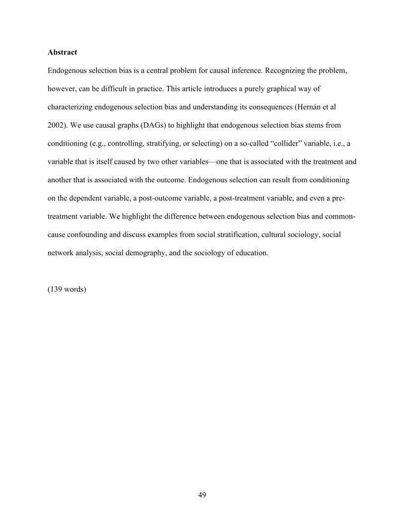
49
Abstract
Endogenous selection bias is a central problem for causal inference. Recognizing the problem,
however, can be difficult in practice. This article introduces a purely graphical way of
characterizing endogenous selection bias and understanding its consequences (Hernán et al
2002). We use causal graphs (DAGs) to highlight that endogenous selection bias stems from
conditioning (e.g., controlling, stratifying, or selecting) on a so-called “collider” variable, i.e., a
variable that is itself caused by two other variables—one that is associated with the treatment and
another that is associated with the outcome. Endogenous selection can result from conditioning
on the dependent variable, a post-outcome variable, a post-treatment variable, and even a pre-
treatment variable. We highlight the difference between endogenous selection bias and common-
cause confounding and discuss examples from social stratification, cultural sociology, social
network analysis, social demography, and the sociology of education.
(139 words)

50
Figure Captions Figure 1. A directed acyclic graph (DAG). Figure 2. (a) A and B are associated by causation. The marginal association between A and B identifies the causal effect of A on B. (b) A and B are conditionally independent given C. The conditional association between A and B given C does not identify the causal effect of A on B (over-control bias). Figure 3. (a) A and B are associated by common cause. The marginal association does not identify the causal effect of A on B (confounding bias). (b) A and B are conditionally independent given C. The conditional association does identify the causal effect of A on B (which is zero in this model). Figure 4. (a) A and B are marginally independent. The marginal association identifies the causal effect of A on B (which is zero in this model). (b) A and B are associated conditional on their common outcome, C (collider). The conditional association between A and B given C does not identify the causal effect of A on B (endogenous selection bias). (c) Conditioning on a descendant, D, of a collider, C, also induces an association between the causes of the collider. Figure 5. Endogenous selection bias due to outcome truncation. E: education (treatment). I: income (outcome, truncated at 1.5 times poverty threshold). U: error term on education. Figure 6. Endogenous selection bias due to listwise deletion. I: father’s income (treatment). P: child support payments (outcome). R: survey response. Conditioning on the post-outcome variable response-behavior R (listwise deletion of missing data) induces a noncausal association between father’s income I and his child support payments P. Figure 7. Endogenous selection bias due sample selection. B: topping the Billboard charts (treatment). R: inclusion in the Rolling Stone 500 (outcome). S: Sample selection. Table 1. Simplified representation of the sampling scheme of a study of the effect of topping the Billboard charts (B) on a record’s inclusion in the Rolling Stone 500 (R). Figure 8. Endogenous selection bias due to sample selection. M: motherhood (treatment). WR: unobserved reservation wage. WO: Offer wage (outcome). E: employment. ε: error term on offer wage. (a) Null model without effect of motherhood on offer wages. (b) Model with effect of motherhood on offer wages. Figure 9. Attrition and dependent/informative censoring in panel studies. P: poverty (treatment); D: divorce (outcome); C: censoring/attrition; U: unmeasured marital distress. (a) Censoring is random with respect to poverty and divorce. (b) Censoring is affected by poverty. (c) Censoring is affected by treatment and shares a common cause with the outcome. Only in (c) does attrition lead to endogenous selection bias.

51
Figure 10. Proxy control. S: schooling (treatment). W: wages (outcome). U: unmeasured ability. Q: test scores. (a) U confounds the effect of S on W. (b) Q is a valid proxy for U. (c) Q is affected by S; conditioning on Q also induces endogenous selection bias. (d) Q is affected by S and affects W; conditioning on Q also induced over-control bias. Figure 11. Endogenous selection bias in mediation analysis. T: class size (randomized treatment); M: student achievement; Y: high school graduation (outcome); U: unobserved factors such as student motivation. (a) M mediates the indirect effect of T on Y. (b) M is not a mediator. Figure 12. Endogenous selection bias due to latent homophily in social network analysis (Shalizi and Thomas 2011). (i,j) index a generic dyad of individuals. Y: civic engagement; U: altruism; F: friendship tie. Figure 13. (a) X is a common cause of the effect of treatment T on outcome Y; conditioning on X removes confounding bias. (b) X is a pre-treatment collider on a noncausal path linking treatment and outcome; conditioning on X induces endogenous selection bias. (c) X is both a confounder and a collider; neither conditioning nor not-conditioning on X identifies the causal effect of T on Y. If U1 and U2 are unobserved, the DAGs in (a-c) are observationally indistinguishable.

52
Figures X T C Y U
Figure 1. A directed acyclic graph (DAG).
(a) (b) A C B A C B Figure 2. (a) A and B are associated by causation. The marginal association between A and B identifies the causal effect of A on B. (b) A and B are conditionally independent given C. The conditional association between A and B given C does not identify the causal effect of A on B (over-control bias).
(a) A (b) A C C B B
Figure 3. (a) A and B are associated by common cause. The marginal association does not identify the causal effect of A on B (confounding bias). (b) A and B are conditionally independent given C. The conditional association does identify the causal effect of A on B (which is zero in this model).
53
(a) (b) (c)
A A A C C C D B B B Figure 4. (a) A and B are marginally independent. The marginal association identifies the causal effect of A on B (which is zero in this model). (b) A and B are associated conditional on their common outcome, C (collider). The conditional association between A and B given C does not identify the causal effect of A on B (endogenous selection bias). (c) Conditioning on a descendant, D, of a collider, C, also induces an association between the causes of the collider. E I U Figure 5. Endogenous selection bias due to outcome truncation. E: education (treatment). I: income (outcome, truncated at 1.5 times poverty threshold). U: error term on education. I R P Figure 6. Endogenous selection bias due to listwise deletion. I: father’s income (treatment). P: child support payments (outcome). R: survey response. Conditioning on the post-outcome variable response-behavior R (listwise deletion of missing data) induces a noncausal association between father’s income I and his child support payments P.

54
B S R Figure 7. Endogenous selection bias due sample selection. B: topping the Billboard charts (treatment). R: inclusion in the Rolling Stone 500 (outcome). S: Sample selection.
!! R=0! R=1!B=0! a! b!B=1! c! d!
Table 1. Simplified representation of the sampling scheme of a study of the effect of topping the Billboard charts (B) on a record’s inclusion in the Rolling Stone 500 (R). (a) (b) M (WR) M (WR)
E E
ε WO ε WO Figure 8. Endogenous selection bias due to sample selection. M: motherhood (treatment). WR: unobserved reservation wage. WO: Offer wage (outcome). E: employment. ε: error term on offer wage. (a) Null model without effect of motherhood on offer wages. (b) Model with effect of motherhood on offer wages. a)

55
P C D (b) P C D (c) P C D U Figure 9. Attrition and dependent/informative censoring in panel studies. P: poverty (treatment); D: divorce (outcome); C: censoring/attrition; U: unmeasured marital distress. (a) Censoring is random with respect to poverty and divorce. (b) Censoring is affected by poverty. (c) Censoring is affected by treatment and shares a common cause with the outcome. Only in (c) does attrition lead to endogenous selection bias.

56
(a)
U S W (b) Q U S W (c) Q U S W (d) Q U S W Figure 10. Proxy control. S: schooling (treatment). W: wages (outcome). U: unmeasured ability. Q: test scores. (a) U confounds the effect of S on W. (b) Q is a valid proxy for U. (c) Q is affected by S; conditioning on Q also induces endogenous selection bias. (d) Q is affected by S and affects W; conditioning on Q also induced over-control bias.
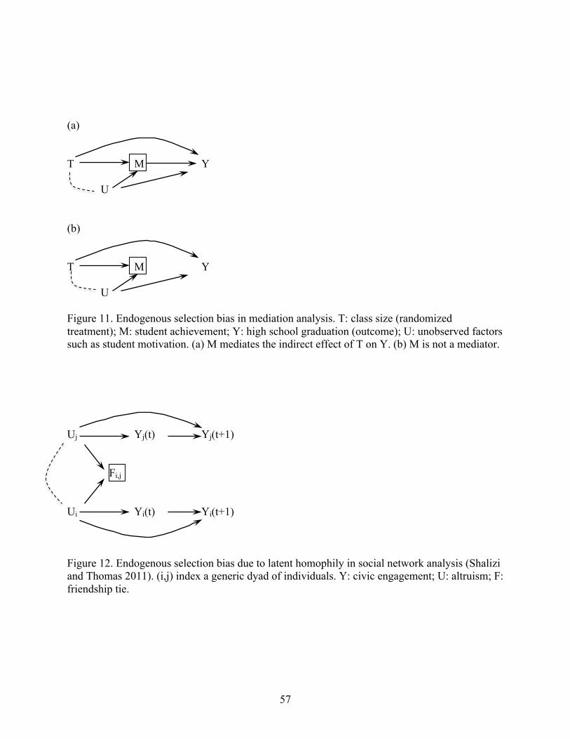
57
(a)
T M Y U (b)
T M Y U Figure 11. Endogenous selection bias in mediation analysis. T: class size (randomized treatment); M: student achievement; Y: high school graduation (outcome); U: unobserved factors such as student motivation. (a) M mediates the indirect effect of T on Y. (b) M is not a mediator. Uj Yj(t) Yj(t+1) Fi,j Ui Yi(t) Yi(t+1) Figure 12. Endogenous selection bias due to latent homophily in social network analysis (Shalizi and Thomas 2011). (i,j) index a generic dyad of individuals. Y: civic engagement; U: altruism; F: friendship tie.

58
(a) X T Y (b) U1 X T Y U2 (c) U1 X T Y U2 Figure 13. (a) X is a common cause of the effect of treatment T on outcome Y; conditioning on X removes confounding bias. (b) X is a pre-treatment collider on a noncausal path linking treatment and outcome; conditioning on X induces endogenous selection bias. (c) X is both a confounder and a collider; neither conditioning nor not-conditioning on X identifies the causal effect of T on Y. If U1 and U2 are unobserved, the DAGs in (a-c) are observationally indistinguishable.