AALTO UNIVERSITY School of Electrical Engineering Department of Communications and Networking Maliha Urooj Jada

Energy Efficiency Techniques amp Challenges for Mobile Access Networks

Masters Thesis submitted in partial fulfillment of the degree of Master of Science in Technology Espoo 6th May 2011 Supervisor Prof Jyri Haumlmaumllaumlinen Aalto University

i

AALTO UNIVERSITY ABSTRACT OF THE MASTERrsquoS THESIS

Author Maliha Urooj Jada

Name of the Thesis Energy Efficiency Techniques amp Challenges for Mobile Access

Networks

Date 6th May 2011 Number of pages 9+ 64

Department Department of Communications and Networking

Professorship Radio Communications

Supervisor Prof Jyri Haumlmaumllaumlinen Aalto University

Energy consumption of mobile access networks has recently received increased attention in

research carried out in both industry and academia The cellular networks do not have

considerable share in the overall energy consumption of the ICT (Information and

Communication Technology) sector However reduction in energy consumption of mobile

networks is of great importance from economical (cost reduction) and environmental

(decreased CO2 emissions) perspective

The Thesis work has investigated the different means to enhance the capacity of evolved

mobile networks and discussed the related challenges from energy consumption perspective

this discussion is followed by a simple radio network power usage model Based on the

model examples are given where two different deployment scenarios have been compared

Further the work focused on the WCDMA energy saving through femtocell deployment A

simple model for the energy consumption per unit area has been derived based on WCDMA

downlink load equations Based on the model two different deployment scenarios have been

compared to make the conclusion from energy consumption perspective

In the end the impact of femtocells to the energy efficiency of the WCDMA network has

been studied under the consideration of a valuable power save feature of femtocell

Keywords Mobile access networks energy and power efficiency scenarios comparisons femtocells load equations idle mode

Language English

ii

Acknowledgments Initially and most importantly I want to thank my supervisor Professor Jyri

Haumlmaumllaumlinen for his endless support worthy guidance and valuable comments on my

work I feel gratitude that with his support and encouragement I am successful in

publishing three research papers I appreciate that he provided several opportunities

for presenting my work in front of audience which has boosted up my confidence

level tremendously

I am also grateful to Professor Riku Jaumlntti for giving valuable advices in thesis work

and also thankful to his doctoral student Aftab Hussain for the grate support while

writing research papers

I would like to thank Edward Mutafungwa one of the senior members of my research

group with excellent English language skills for his help in revising the final draft of

my thesis

Furthermore I am thankful to Sanna Patana (Administrative Services Secretary) and

Sari Kivelio (Department Secretary) for their help in making travel arrangements to

the conference places which I attended to present my accepted research papers

I am extremely thankful to my friends who have kept the entertainment and fun part

active in my life and have been encouraging me throughout my thesis work

Finally I am greatly obliged to my Mother for all the love moral support and

motivation she had been giving me throughout my MSc studies and especially during

my thesis work I owe a great debt of gratitude to my parents for making me a

confident person and developing in me the unquenchable thirst of knowledge

Maliha Urooj Jada

6th May 2011

iii

To my parents amp siblings

iv

Contents Abbreviations v

List of Figures vii

List of Tables viii

1 Introduction 1

11 General Energy Saving Aspects in Mobile Networks 1

12 Energy Consumption in Cellular Network 2

121 Minimizing the BS Energy Consumption 3

122 Minimizing the Base Station density 10

123 Alternative energy resources 10

2 Mobile Network Evolutıon Energy Efficiency challenges 13

21 Introduction 13 22 Network Energy Efficiency 14

23 The Need of Capacity Enhancement Features 15

231 Static Power 15 232 Dynamic Power 15

24 Capacity Enhancement Energy Efficiency Challenges 17

241 Capacity Enhancement Features 18

3 Simple Model for Power Consumption 26

31 Introduction 26 32 Comparison Cases 28

321 First Scenario 29 322 Second Scenario 30

33 Computation of Transmission Power Ratio and Range Ratio 32

34 Examples 33 35 Analysis for Comparison Scenarios 37

4 Energy Efficiency Model for Heterogeneous Network 39

41 Introduction 39 42 Impact of Femtocells to the WCDMA Network Energy Efficiency 40 43 Modeling and Comparison Scenarios 40

431 Load Equations and Dimensioning 41

432 General Energy Usage Model 42

433 Comparison Scenarios 44 44 Numerical Examples 47

441 Numerical comparisons 48 45 Femtocell idle mode and network energy efficiency 51

451 Effect of femtocell idle mode on overall network energy saving 52

452 Energy Savings from the perspective of Green Field Nw Deployment 56

5 Conclusions and Future Work 60

References 62

v

ABBREVIATIONS

BS Base Station CO2 Carbon dioxide ICT Information amp Communication Technology PST Public Switched Telephone PDG Packet Data Gateway GGSN Gateway GPRS Support Node SGSN Serving GPRS Support Node HLR Home Local Register IMS IP Multimedia Subsystem RF Radio Frequency PAR Peak to Average Power Ratio UMTS Universal Mobile Telecommunication System WiMAX Worldwide Interoperability for Microwave Access LTE Long Term Evolution AMAM Amplitude to Amplitude Modulation IBO Input Back Off OBO Output Back Off ET Envelop Tracking PA Power Amplifier WCDMA Wideband Code Division Multiple Access MIMO Multiple Input Multiple Output BBU Base Band Unit DSPs Digital Signal Processors FPGAs Field Programmable Gate Arrays ASICs Application Specific Integrated Circuits UE User Equipment SINR Signal to Interference to Noise Ratio hrs hours OPEX Operational Expenditure CAPEX Capital Expenditure QoS Quality of Service 2G Second Generation 3G Third Generation QoE Quality of Experience EARTH Energy Aware Radio and Network Technologies kwh kilowatt hour SUB Subscribers AMR-HR Adaptive Multi Rate - Half Rate IMT Advanced International Mobile Telecommunications Advanced 3GPP Third Generation Partnership Project SISO Single Input Single Output AWGN Additive White Gaussian Noise SNR Signal to Noise Ratio SIMO Single Input Multiple Output

vi

CDF Cumulative Distribution Function ISD Inter Site Distance WRC World Radio communication Conference IP Internet Protocol HSPA High-Speed Packet Access HSDPA High ndash Speed Downlink Packet Access

vii

L IST OF FIGURES

Figure 1 Energy contribution of main elements of mobile networks 3 Figure 2 Energy consumption in a typical macro BS site 3 Figure 3 A Typical Power Amplifier Response 5 Figure 4 Energy Saving depending on traffic profile for 24 Hours 7 Figure 5 Relation between BS Energy Saving and Load Balancing 8 Figure 6 Hexagonal and crossroad configurations 8 Figure 7 Manhattan configurations linear (top) and squared (bottom) 9 Figure 8 Solar panels deployed at BS 11 Figure 9 Wind Power turbine deployed at BS 12 Figure 10 Enabling energy-efficient growth through capacity enhancement 16 Figure 11 Pictorial representation for First Scenario Network Comparison 29 Figure 12 Pictorial representation for Second Scenario Network Comparison 31 Figure 13 Difference of total power usage in networks 35 Figure 14 Heterogeneous deployment for Energy Efficient Green Networks 39 Figure 15 Macrocell layout Cell range and ISD 41 Figure 16 Network Layout Comparison in first scenario 45 Figure 17 Network Layout Comparison in second scenario 46 Figure 18 Cell range as a function of number of users 48 Figure 19 Flow Chart for the Energy Consumption Algorithm helliphelliphelliphelliphelliphelliphelliphellip 49 Figure 20 Daily energy consumption per square kilometer in the network when assuming second scenario 51 Figure 21 Daily energy saving per km2 in the network for second comparison scenario 54 Figure 22 Reduction in Number of New BSs in comparison to Number of Old BSs 57

viii

L IST OF TABLES

TABLE 1 3GPP PERFORMANCE REQUIREMENTS ON CELL EDGE (CASE 1) 22 TABLE 2 FIRST COMPARISON SCENARIO EXAMPLE POWER RATIOS 34 TABLE 3 SECOND COMPARISON SCENARIO EXAMPLE POWER RATIOS 36 TABLE 4 WCDMA NETWORK PARAMETERS 47 TABLE 5 DAILY ENERGY CONSUMPTION IN THE NETWORK FIRST SCENARIO 50 TABLE 6 DAILY ENERGY CONSUMPTION IN THE NETWORK WHEN DEPLOYED FEMTOCELL POSSESS IDLE MODE FEATURE FIRST SCENARIOhelliphelliphelliphelliphelliphelliphelliphelliphelliphelliphelliphelliphelliphelliphelliphelliphelliphelliphelliphelliphelliphelliphelliphelliphelliphelliphelliphellip52

TABLE 7 DAILY ENERGY CONSUMPTION IN THE NETWORK WHEN DEPLOYED FEMTOCELL DO NOT POSSESS IDLE MODE FEATURE FIRST SCENARIO 53 TABLE 8 TOTAL ENERGY SAVINGS WHEN FEMTOCELLS WITH AND WITHOUT IDLE MODE FEATURE HAVE BEEN USED AND THE REDUCTION IN NUMBER OF NEW BS SITES WRT TO OLD BS SITES 58

1

1 INTRODUCTION

Deployment of increasingly powerful mobile network technologies has taken place

within the last decade Although network efficiency has been growing the higher

access rates have inevitably led to increased energy consumption in base stations

(BSs) and network densities have been constantly growing [1]

Recently the mobile communication community has become aware of the large and

ever-growing energy usage of mobile networks [2] Besides industry the awareness

of the ever-increasing energy consumption has stimulated research in academia

particularly on issues addressing the BS site energy consumption [3] [4] [5] [6] [7]

Yet the work on the reduction of energy consumption has been mostly carried out by

BS manufacturers [8] since high power efficiency provides a competitive advantage

Today one of the most discussed topics is the global warming which is due to

increment of CO2 (Carbon dioxide) and other green house gases concentration levels

in atmosphere To decrease the CO2 emissions the consumption of fossil fuels has to

be decreased [9] [10] Thus the research has been carried out in the ICT (Information

and Communication Technology) sector to reduce the consumption of fossil fuels to

make the environment clean and green

Mobile networks do not have considerable share in the overall energy consumption of

the ICT sector which itself is responsible for 2 to 10 of the world energy

consumption However reduction in energy consumption of mobile networks is of

great importance from economical (cost reduction) and environmental (decreased CO2

emissions) perspective

11 General Energy Saving Aspects in Mobile Networks Two following approaches towards Energy Efficient Mobile Networks are the

following

bull Find appropriate solutions to the energy efficiency challenges for already

existing networks (Brownfield)

2

bull Design future networks from energy (and cost) efficient perspective

(Greenfield perspective)

For the future Telecomrsquos energy consumption difficulties and uncertainties exist in

estimating the potential energy savings due to the different methodologies that is

how to define energy consumption or which elements should be considered in the

energy efficiency calculation [11]

Furthermore energy savings depends significantly on human behavior and utilization

of resulting financial savings as any energy saving is followed by cost savings From

a network operator or infrastructure ownerrsquos business perspective the cost saving

factor in many cases is of more importance than environmental protection Money

saved by reducing energy consumption is available for other expenditures If the

saved cost would be invested in a proper way the low carbon society will be created

Alternatively energy savings could be affected by rebound effect in which the

improper utilization of the saved cost might give unfortunate results of potentially

additional CO2 emissions

Travelling by car is one of the most effective causes of global warming Thus

substitution of the office work with remote work via broadband network connectivity

has the potential to significantly reduce the carbon dioxide emissions [11] In a similar

way business travel can be substituted by videoconferencing and electronic billing

instead of paper bills would also contribute in making an environment green

12 Energy Consumption in Cellular Network A typical mobile network consists of three main elements core network base

stations and mobile terminals as shown in Figure 1 Base stations contribute 60 to

80 of the whole network energy consumption [12] Thus the efforts in the reduction

of energy consumption focus on the BS equipment which includes the minimization

of BS energy consumption minimization of BS density (BS density is inversely

proportion to cell area) and the use of renewable energy sources

3

Figure 1 Energy contribution of main elements of mobile networks

121 Minimizing the BS Energy Consumption

The ways to minimize the BS energy consumption includes improvement in BS

energy efficiency through better performance of BS hardware usage of system level

and software features and usage of BS site solutions [12]

Figure 2 gives some brief idea about the energy consumption in a typical macro BS site

Figure 2 Energy consumption in a typical macro BS site [8]

4

A Base Station Hardware Efficiency

For the improved performance of BS hardware the focus should be on boosting the

efficiency of power amplifier because power amplifier and its associated components

can consume up to 50 of the overall power [13]

The current radio modem design paradigm requires high linearity from the radio

frequency (RF) components which allows one to separate the RF design and digital

signal processing design The classic Class AB amplifier technology offers efficient

operation when the RF envelope waveform is close to peak power Unfortunately

most of the modern waveforms have high peak-to-average power ratio (PAR) forcing

the power amplifier to operate most of the time in less efficient operation point As a

result efficiency around 15-25 has been measured for the waveforms used by the

modern UMTS (Universal Mobile Telecommunication Systems) WiMAX

(Worldwide Interoperability for Microwave Access) and LTE (Long Term Evolution)

systems [13]

Figure 3 shows a typical AMAM response (Amplitude to amplitude modulation The

output power of an RF power amplifier does not keep on increasing without limit

There exists a point when an increase in input power will not produce any significant

increase in output power This is referred to as the saturation point where output

power is not proportional to input power any more In the saturation region of an RF

amplifier response as the input increases the gain becomes compressed This Output

Power versus Input Power characteristic is referred as AM-AM distortion for a High

Power Amplifier with the associated input and output back-off regions (IBO and

OBO respectively) Output Back Off (OBO) induced by PAR means wasted power

5

Figure 3 A Typical Power Amplifier Response

The power efficiency of a High Power Amplifier can be increased by reducing the

PAR of the transmitted signal The average and peak values should be as close

together as possible in order to maximize the efficiency of the power amplifier

It is possible however to achieve a significant improvement in PA efficiency using

envelope tracking (ET) In ET the voltage supplied to the final RF stage power

transistor is changed dynamically synchronized with the RF signal passing through

the device to ensure that the output device remains in its most efficient operating

region close to saturation point In one of the studies (based on the PA efficiency for

BS) 50 efficiency have been reported for WCDMA (Wideband Code Division

Multiple Access) waveforms for ET based PA [14] In recent papers efficiencies close

to 60 has been reported If the energy efficiency of the power amplification can be

drastically increased from the 15-25 range to close to 60 also the energy

consumption of cooling system can be significantly reduced [15][16]

Typically in multi-antenna (MIMO Multiple Input Multiple Output) systems each

antenna has its own power amplifier If the system load is low then energy can be

saved by switching off some of the transmit antennas For instance UMTS supports

6

the use of two transmit antennas In case there are no MIMO capable terminals

present in the system then the base station may switch off the second common pilot

channel transmitted over the second antenna to save energy

The energy efficiency of the base band unit (BBU) of the base station can be further

improved by introducing power save modes to subunits such as channel cards DSPs

(Digital signal processors) FPGAs (Field programmable gate arrays) ASICS

(Application ndashspecific integrated circuits) or even clocks such that they could be

switched on and off based on the base station load

Moreover by using the continuous Phase modulation technique PAR can be reduced

and high efficiency can be achieved in Mobile Station (or User Equipment UE)

transmitter which contributes to the increment in power efficiency of the whole

network

B System Level or Software Feature

The impact of different link budget and network parameters on the network energy

consumption has been investigated in Chapter 2 Results indicate for example that if

transmission power is fixed per BS but cell edge rate requirement is doubled then a

one and a half fold increase in BS density is needed However by introducing multi-

antenna sites there will be an improvement in bandwidth and SINR (Signal to

Interference to Noise Ratio) efficiency which may even fully compensate the need for

increasing BS density In a similar way there also exist more such system level

techniques to reduce energy consumption of radio network One of them is discussed

below

B1 BS switching in conventional macrocell topology

One of the main energy saving approaches is the system level feature in which

underutilized cells (BSrsquos) are switched off whenever traffic load is small as depicted

in Figure 4 The network load in some areas may vary significantly due to the mixed

effect of two traffic properties

bull Daily changes in user data consumption for instance data traffic may be small

at night times

7

bull The user density may greatly vary Office areas may provide heavy load on

day time and very small user load during the night times while load on

residential areas increases during the afternoon as subscribers have returned

from places of work study and so on

Figure 4 Energy Saving depending on traffic profile for 24 Hours

When cells are switched off it is assumed that the radio coverage and feasible service

conditions can be guaranteed by the remaining active cells (BSs) probably with some

increment in the BS transmitting power This increase in transmission power in

remaining active BSs however can be small when compared to the savings achieved

by switching off some BS sites Moreover in order to avoid this increment in

transmission power wireless relays cooperative communication and electrically

tilted antennas can be used to guarantee the radio coverage [5]

Energy saving through BS switching has been under discussion over the last few

years For instance researchers have proposed that power saving algorithms can be

centralized (when all the channel information and traffic requirements are known) or

decentralized (no such information is required) [5] Energy savings are higher in

centralized approach because BS density becomes lower while coverage guarantee is

better in decentralized approach because more BSrsquos stay active In this research the

focus was on the relation between BS energy saving and load balancing The purpose

8

of load balancing is to equally distribute traffic service among BSrsquos to achieve better

coverage whereas the aim in BS energy saving is to concentrate traffic to as few BSrsquos

as possible Through examination it was found out that load balancing appears to be

important BS energy saving algorithm due to its decentralized and dynamic nature

Figure 5 Relation between BS Energy Saving and Load Balancing [6]

Similar approach was applied in other researches whereby focus was on cell layout

[6] To achieve optimal energy saving it was discovered in [6] that in real networks

only a small fraction of cells need to remain on during the night time In [6] few

typical cellular network configurations (Hexagonal Crossroad Manhattanlinear

Manhattansquared as shown in Figures 6 and 7 respectively) had been compared

assuming two different daily traffic patterns symmetric trapezoidal traffic pattern and

asymmetric traffic pattern which is derived from measurements over a real network

Comparison indicates that the best solution is not to switch off the largest possible

number of cells rather it is important to make tradeoff between the night zone period

(low load) and the number of cells that are switched off According to this work the

best performing scheme is switching off 4 cells out of 5 with crossroad configuration

Within the above mentioned network topologies the energy savings of the order of

25-30 are possible to achieve

Figure 6 Hexagonal and crossroad configurations [6]

9

Figure 7 Manhattan configurations linear (top) and squared (bottom) [6]

C Site Solution

Energy efficiency can not only be improved in BS equipment but also certain power

solutions could be adapted on the site level to save the energy These are referred to as

site solutions In [12] the few mentioned site solutions which have the potential for

energy saving are

- Outdoor sites

- Cooling solution for indoor sites

- RF head

- Modular BS

With outdoor sites the cooling requirements can be lowered by raising the allowable

operating temperature range for the BS site wherever possible because the upper limit

set for the temperature is now high so less cooling would be sufficient to keep the

temperature within limits This leads to the reduced energy consumption by the

cooling equipment and thus less CO2 emissions observed With indoor sites the

energy could be saved by utilizing fresh air cooling systems instead of using air

conditioner that consumes energy for its operation With RF head or modular BS the

RF transmitter is located close to BS antenna this way the cable losses decreases and

the network performance is improved Alternatively less transmit power is required

to achieve the same network performance

10

122 Minimizing the Base Station density

The deployment of small low power femto BSs alongside macrocellular BSs is often

believed to reduce the energy consumption of cellular network [17] This idea is

studied in Chapter 4 where analysis is based on WCDMA load equations It has been

demonstrated that when femtocells are introduced to the network they will reduce the

macro BS density Thus reducing the energy consumed by the macrocellular side of

the network But not necessarily the total energy consumed by network due to the lack

of femtocell ability in practical to switch onoff depending upon indoor traffic

(discussed in Chapter 4)

123 Alternative energy resources

Mobile networks can be made much more energy efficient than they are today and

networks may become even fully self-sustainable by using renewable energy

resources which are using natural resources such as sunlight wind tides and

geothermal heat All these resources are regenerative which makes them different

from fossil fuels and thus they will not produce greenhouse gases that is CO2

Currently renewable energy resources are mostly used on sites that are at long

distances from electricity grid or on locations where electricity supply is unreliable

The importance of these renewable energy resources is increasing as the costs of

expanding network into remote areas grow [12]

The most important thing to take into account while planning to operate the BS site by

renewable energy resources is the site location and the energy consumption of the BS

site The availability of energy resources defines the site location and the energy

consumption depends upon the load

The most reasonable renewable energy resources for BS sites are derived from the

main source of energy i-e sun and also wind

A Solar energy

Solar energy is free abundant and inexhaustible It is the source of all forms of

renewable energy supply direct solar power and heat hydro bio mass wind-power

11

and wave power Direct solar power systems are now the subject of intense activity in

different parts of the world Related technology could provide us with electrical

resources totaling up to a thousand times our current demands

For low and medium capacity sites or repeaters sites solar power can be used to

provide virtually free energy at least in terms of OPEX (Operation Expenditure)

While the initial CAPEX (Capital Expenditure) per kilowatt is higher for such

solutions they can provide a positive business case compared with diesel generators

within one or two years of operation

Figure 8 Solar panels deployed at BS For the solar power plant installment near BS more site space is required Moreover

the climate variations in sunshine develop the need of higher energy storage capacity

in solar power plant

On the other hand it is expected for the future network to have a combination of

alternative energy sources to meet the seasonal variation differences [8]

12

B Wind Energy

As with solar power wind power can provide virtually free energy However wind

power industry is constructing very large wind turbine and the challenge is to find a

cost effective solution for BS site (Ericsson)

Figure 9 Wind Power turbine deployed at BS

The advantage of wind power is that it can maintain the BS site at low cost On the

other hand the disadvantage of it is that wind is unpredictable so there must be some

small diesel generator as backup in situations when there is low wind or no wind

Currently the extra site space is required because of the need to install the wind

turbine tower along with the BS tower [8]

13

2 MOBILE NETWORK EVOLUTION ENERGY

EFFICIENCY CHALLENGES

21 Introduction In the last decade we have come across the rapid development of the mobile network

technologies In the establishment of new mobile networks the focus has been shifted

from 2G (Second Generation) mobile network technologies to 3G (Third Generation)

and now beyond 3G (eg LTE) networks which are based on the latest standard and

are being recently commercialized With each new mobile network generation new

services are being introduced and achievable data rates per user are increased

One of the main motivations behind mobile networks evolution is Internet access so

there is a need to constantly increase the user data rates in order to provide the mobile

internet based services with an end-user acceptable quality of experience (QoE) The

internet based services are initially being designed assuming fixed line capabilities

therefore to shift from the fixed line services to mobile services the data rates on

mobile systems have to be increased The large scale deployment of mobile Internet is

ongoing in many countries to fulfill its high demand due to the rapid increment in the

number of mobile data users

Although new networks are more efficient it is expected that increasing demands for

high data rates will cause the constant increase in network densities and thus the

increased energy consumption in the mobile networks Therefore it is of great

importance for network operators to adopt energy efficient techniques while building

the new networks

To provide higher user data rates and serve a growing number of mobile data users

there is a need for higher network capacity There exist several ways to increase the

network capacity which includes wider frequency bandwidths enhanced radio link

technologies higher transmission powers more dense networks and heterogeneous

deployments All of these techniques have been discussed in detail in this chapter

showing the challenges they come across from the energy efficiency perspective

14

Also there exists a need for capacity enhancement features to make the networks

energy efficient that is the capacity enhancement features must provide the reduction

in networkrsquos energy consumption This need for capacity enhancement for having

energy efficient networks has been explained taking into account the power

distribution in the network

22 Network Energy Efficiency Recently several projects in wireless communications (working as consortium of

worldwide renowned companies and research institutes) have been focusing on the

energy efficiency and not on just the reduction of total energy consumed by the

network [10] that is they are concerned about the reduction in energy per bit One of

the proposed units to measure efficiency is Watt per bit And energy efficiency is

considered from network perspective

The formula proposed for the network energy efficiency is

1313 = (1)

bull Growth in the network traffic andor reduction in the power consumed per user

will increase the network energy efficiency

bull Growth in the traffic will increase the revenue from services (Green Services

which focus on energy saving and carbon emission reduction) Traffic is measured

as bits per second

bull Reduction in the power consumption per user will reduce the carbon footprint and

also decrease the operation cost

bull For a given application if QoS is not met then energy efficiency is zero

bull If optical fiber is used instead of wireless the networks will be more energy

efficient but the cost possibly will increase by very large amount

ICT is responsible for 2-10 of worldrsquos energy consumption The research efforts are

also focusing on means to use ICT in order to reduce the remaining 98 of energy

consumption in the world

15

23 The Need of Capacity Enhancement Features To emphasize the need for capacity enhancement features for energy efficient

networks we start by recalling the power usage in base station

Electronic devices consume power when being switched on and in conventional

mobile networks the baseline assumption is that BSs are on all the time Power

supplies basic operation functions and signaling between nodes (between Radio BS

and Mobile BS in idle mode) consume power even when the network is not carrying

any traffic [18]

The BS power usage can be divided into static and dynamic parts [18]

$ = $amp$ + $amp() (2)

231 Static Power

The static power consumption contains both powers that are needed to keep BS site

equipments operable as well as power that is spend on continuous basic radio access

operations such as common channel transmission

Usually power-saving features are designed to lower this static power consumption

There are many features today that monitor network activity and successively shut

down unneeded equipment during times of low traffic without degrading quality of

service [18]

232 Dynamic Power

Dynamic power is a significant portion of power consumed by a network which varies

in direct relationship with the amount of traffic being handled in a network at a given

time

This dynamic part of the power consumption can be made more efficient by employing

capacity-enhancing features so that more traffic can be handled with a given amount

of energy In this regard most network equipment vendors have designed the range of

capacity enhancement features

16

When networks are expanded the large scale deployment of capacity enhancement

solutions would be effective from economical and environmental perspective because

then unnecessary addition of new sites or nodes can be avoided that is the BS density

will not be increased much and energy consumption can be even reduced in the

network

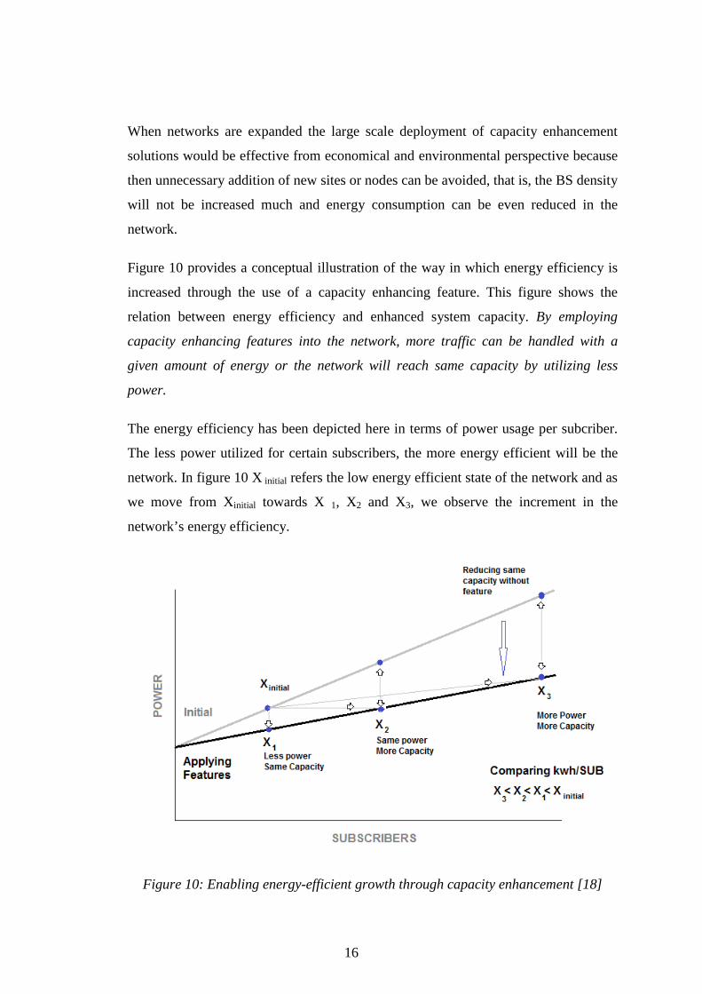
Figure 10 provides a conceptual illustration of the way in which energy efficiency is

increased through the use of a capacity enhancing feature This figure shows the

relation between energy efficiency and enhanced system capacity By employing

capacity enhancing features into the network more traffic can be handled with a

given amount of energy or the network will reach same capacity by utilizing less

power

The energy efficiency has been depicted here in terms of power usage per subcriber

The less power utilized for certain subscribers the more energy efficient will be the

network In figure 10 X initial refers the low energy efficient state of the network and as

we move from Xinitial towards X 1 X2 and X3 we observe the increment in the

networkrsquos energy efficiency

Figure 10 Enabling energy-efficient growth through capacity enhancement [18]

17

The base stations with dynamic power saving features have appeared only very

recently and are not yet widespread in the network [19] Capacity enhancing features

that reduce dynamic part of the used power are physical layer scheduling and MIMO

that both boost the resource usage efficiency Moreover additional examples of

dynamic power reducing features are the use of AMR-HR (Adaptive Multi Rate ndash

Half Rate) in mobile voice networks and higher order modulation schemes for data

transmission [18]

Especially for micro BS power model the dynamic part has significant importance

because for small cell the number of users (load) is statistically varying more than for

large cells [19]

24 Capacity Enhancement Energy Efficiency Challenges The need for expanding system capacity grows with the number of users and with the

amount of information required for a given service But there exist challenges for such

capacity enhancement solutions from an energy perspective

In order to analyze the impact of link budget parameters on the energy consumption

of the network the formulation has been started by understanding the throughput

formula (Shannon capacity formula) To make the network energy efficient the

Shannonrsquos theory can be employed in a novel manner Shannonrsquos theory provides

guidance for discovering and developing new methodologies to maximize energy

efficiency (to reduce energy per data bit) while approaching the Shannon limit of

maximized network capacity [20]

The peak data rates are available only in very good channel conditions and the

practical data rate is limited by the amount of interference and noise in the network

The maximum theoretical data rate with single antenna transmission in static channel

can be derived using the Shannon formula The formula gives the data rate as a

function of two parameters bandwidth and the received signal to noise ratio

The Shannon capacity bound canrsquot be reached in practice due to several

implementation issues To represent these loss mechanisms accurately we use a

modified Shannon capacity formula which has fitting parameters Weff and Γeff

18

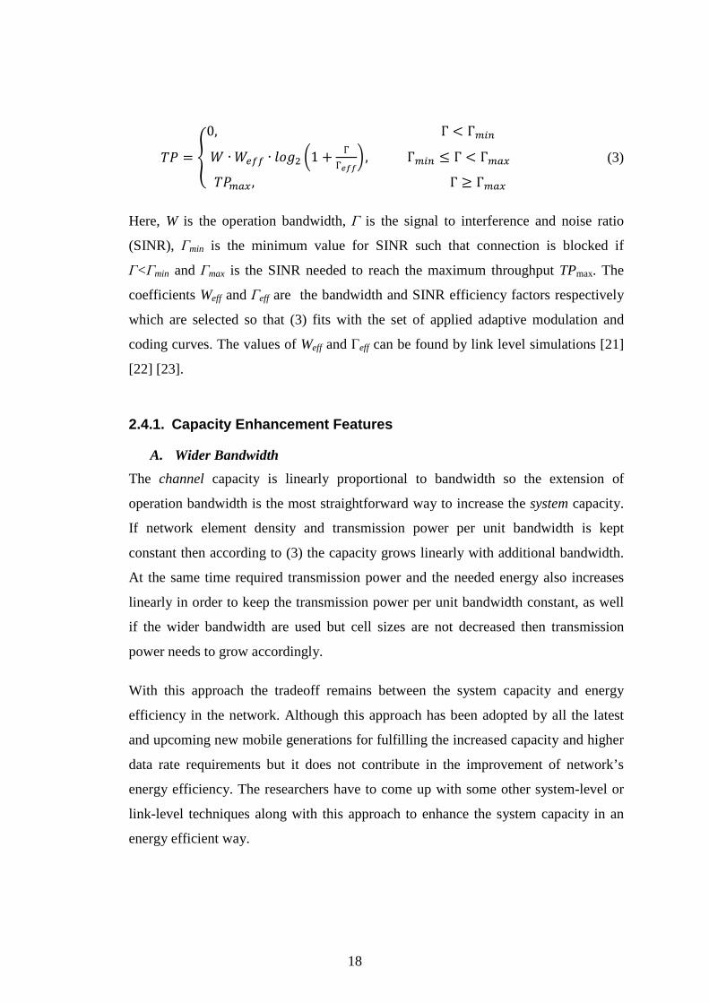
+ = 0Г lt Г)1 ∙ 1 ∙ 34 51 + ГГ7889Г) le Г lt Г+ Г ge Г= (3)

Here W is the operation bandwidth Γ is the signal to interference and noise ratio

(SINR) Γmin is the minimum value for SINR such that connection is blocked if

ΓltΓmin and Γmax is the SINR needed to reach the maximum throughput TPmax The

coefficients Weff and Γeff are the bandwidth and SINR efficiency factors respectively

which are selected so that (3) fits with the set of applied adaptive modulation and

coding curves The values of Weff and Γeff can be found by link level simulations [21]

[22] [23]

241 Capacity Enhancement Features

A Wider Bandwidth

The channel capacity is linearly proportional to bandwidth so the extension of

operation bandwidth is the most straightforward way to increase the system capacity

If network element density and transmission power per unit bandwidth is kept

constant then according to (3) the capacity grows linearly with additional bandwidth

At the same time required transmission power and the needed energy also increases

linearly in order to keep the transmission power per unit bandwidth constant as well

if the wider bandwidth are used but cell sizes are not decreased then transmission

power needs to grow accordingly

With this approach the tradeoff remains between the system capacity and energy

efficiency in the network Although this approach has been adopted by all the latest

and upcoming new mobile generations for fulfilling the increased capacity and higher

data rate requirements but it does not contribute in the improvement of networkrsquos

energy efficiency The researchers have to come up with some other system-level or

link-level techniques along with this approach to enhance the system capacity in an

energy efficient way

19

It is important to note that in (3) the bandwidth efficiency reflects the systemrsquos ability

to utilize the radio spectrum and the upper limit is set by Weff =1

For LTE-Advanced (LTE Releasersquo10) it is expected that operation bandwidth will be

divided to 20 MHz carriers and carrier aggregation over up to five carriers is then

used to reach the data rate targets set by IMT-Advanced (International Mobile

Telecommunications Advanced) (peak rate 1 Gbps data rate in local area) [24]

Following the 3rd Generation Partnership Project (3GPP) recommendations [21] the

maximum BS transmission power is 43 dBm in Wideband Code Division Multiple

Access (WCDMA with 5 MHz channel) 46 dBm in Releasersquo8 LTE (10-20 MHz

channel) and thus LTE-Advanced with carrier aggregation will lead up to five times

higher transmission power than used in Releasersquo8 LTE and up to ten times higher

transmission power than used in WCDMA

B Enhanced radio link technologies

Network operator is interested in the improved network efficiency that is how the

maximum number of users can be served the maximum data rate can be provided and

the BS site density can be decreased The efficiency is considered in the link budget

calculations and in the capacity simulations

The LTE link performance is benchmarked with the theoretical Shannon limit To

guarantee consistent performance 3GPP has defined a set of radio performance

requirements

The radio link efficiency has been improved a lot by setting up the advanced radio

link technologies like multiple-input and multiple-output or MIMO for evolved 3G

networks WCDMA HSPA and recently LTE Releasersquo8

The impact of radio link efficiency is embedded into parameter pair (Weff Γeff) which

are also referred to as the fitting parameters for Shannon performance curve The

higher the efficiency the closer to one are the values of Weff and 1Γeff

LTE is highly efficient and is performing less than 16-2 dB from the Shannon

capacity bound in case of AWGN channel In fading channel the link performance on

20

SISO (Single Input Single Output) is close to Shannon limit that defines fundamental

upper bound However for SISO the best Shannon fit parameters are significantly

worsened compared to AWGN (Additive White Gaussian Noise) the equivalent Weff

(Bandwidth Efficiency) has reduced from 083 to 056 and the Γeff (SNR efficiency)

has been increased from 16-2dB to 2-3dB Whereas for SIMO (Single Input Multiple

Output) the Shannon fit parameters are better than SISO Weff is 062 and Γeff is

18dB Similarly for MIMO the Shannon fit parameters gets better than SIMO Weff is

066 and Γeff is 11dB which makes it closer to Shannon bound and makes the link

performance more efficient in comparison to the cases of SISO and SIMO In MIMO

antenna systems there is more room for optimization but it is well acknowledged that

along with the link performance increase some more solutions are required for future

challenges regarding capacity enhancement [7]

It can be observed that by increasing the number of antennas on the transmitter and

receiver sides the Shannon fit parameters can be further improved leading to higher

spectral efficiency and thus higher throughput With higher spectral efficiencies less

radio resources per information bit are needed and thus the energy could be saved

accordingly However there exist certain limitations on the increment of number of

antennas due to size and cost constraints

C Higher Transmission Powers

In this section SINR has been analyzed in detail to describe the impact of transmission

power in different system environment for increasing system capacity The target

SINR is adjusted according to the transmission power of the signal The idea of this

approach is that communication links in worse propagation conditions have to use

higher transmission power to attain a given target SINR level But for reliable

communication links a small increase in transmission power is sufficient to increase

the SINR value by large amount

To start with the general form of SINR

Г = gt AfraslCDsum gtF AFfraslF (4)

21

where PTxk refers to BS transmission power in kth BS Lk is the related path loss and

PN is the noise power The reference user is assumed to be connected to BS with

index 0

If all BSs apply the same transmission power and we let the power grow without

limit then we have

Г gtrarrHIJJJK Lsum AMAFF (5)

Thus SINR admit an upper limit that depends on the path losses towards BSs If the

network is noise limited that is right side term in (5) is clearly larger than Γmax then

data rates can be improved through higher transmission powers However from (3) it

is obvious that due to logarithm much more power would be required to achieve the

same increase in the capacity as achieved by the increase in the bandwidth Therefore

this strategy is not as energy efficient way to increase capacity as compared to the

strategy where bandwidth is extended If system is interference limited that is if the

right side limit term in (5) is small then large BS transmission powers will waste a lot

of energy and just create more interference to the network

D Impact of cell edge coverage requirement

The cell edge coverage can be defined using a probabilistic throughput requirement

Pr+ lt +)amp = Q (6)

In (6) Prout is the outage probability and TPmin defines the minimum SINR in (3) The

outage probability is an important statistical measure to access the quality of service

provided by the system It is the probability of failing to achieve a specified SINR

value and thus the minimum throughput value which is sufficient for satisfactory

reception

22

Requirement (6) can also be given in terms of spectral efficiency if throughput is

scaled by the used bandwidth

RS lt STUVW le Q (7)

The cell edge user throughput is defined as the 5 point of CDF (Cumulative

Distribution Function) of the user throughput normalized with the overall cell

bandwidth For example LTE-Advanced cell edge throughput requirements have been

given using this approach [25]

TABLE 1 3GPP PERFORMANCE REQUIREMENTS ON CELL EDGE (CASE 1)

For Case1 carrier frequency is 2GHz ISD (Inter Site Distance) is 500 meters

bandwidth is 10MHz path loss is 20dB and user speed is 3 kmh

There are two important parameters in (6) that impact on the cell power usage First

tough coverage constraint with very low outage probability will lead to the need for a

high BS transmission power or dense network Both of these options will mean

increased energy consumption in the network Second if operator plans to improve

the service level in the whole network then it should take into account the minimum

throughput requirement of (6) Another option would be to provide more radio

resources per user which is a possible strategy if network load is not too high or

operator is able to introduce new spectrum resources It is expected that all these

approaches will increase the energy consumption of the network

23

E Impact of carrier frequency and propagation environment

The carrier frequencies tend to increase from 900MHz of first 2G networks the

carrier frequency has been increasing to 1800MHz (2G extension bands) 2100GHz

(main 3G bands) 2600MHz (LTE bands) and it will soon jump up to 3500MHz

(bands granted by World Radio communication Conference WRCrsquo07 for IMT-

Advanced) At the higher carrier frequencies the signal path loss in wireless medium

is stronger which requires either transmission power or network density to be

increased Furthermore while additional carriers and extended bandwidths lead to an

easily predictable increase in energy consumption the effect of higher carrier

frequency can be predicted only when propagation modeling is accurate Since details

of sophisticated propagation models are out of the scope of this thesis we adopt a

simple path loss formula

X = Aamp∙AYZ[ (8)

In (8) L(d) refers to a distance dependent model such as Okumura-Hata LSF is the

lognormal shadowing and G refers to the BS antenna gain We have embedded the

antenna gain into propagation model for simplicity It is recalled that antenna gain

depends on the angle between receiver and antenna main directions Yet in

dimensioning the antenna gain in main direction is applied Since Okumura-Hata

model is a so-called single slope model it admits the form

Xamp = ] ∙ ^ (9)

where parameter α includes the impact from carrier frequency and BS antenna height

while the path loss exponent β depends only on the BS antenna height Let us consider

a simple example Assume that the system carrier frequency is increasing from

21GHz to 26GHz Then according to Okumura-Hata model the path loss increases

round 24dB and thus energy consumption in radio operations increases by factor of

174 If BS range in urban area is for example 1km then path loss from higher carrier

frequency can be compensated on the cell edge by increasing the BS antenna height

from 25m to 38m This might be difficult due to regulations and negative visual

24

impact Finally we note that the propagation environment greatly affects the strength

of the path loss so that in rural environment much larger areas can be covered than in

urban environments with the same BS transmission power

F More dense networks and heterogeneous deployments

The larger operation bandwidth and increased power consumption as well as high

macrocell site costs are driving towards smaller cells which ultimately become part of

heterogeneous networks The deployment of small low power base stations

alongside conventional sites is often believed to greatly lower the energy consumption

of cellular radio network because when communication distance is decreased less

power per bit is needed and available spectrum resources are shared between fewer

users From energy efficiency perspective some of the main challenges in small cells

and heterogeneous deployments are

1) Number of sites follows square law with respect to inverse of the range This puts a

high pressure on the energy efficiency of the small nodes Also the network capital

expenses increase rapidly unless BSsite prices are decreasing proportionally to the

square of inverse of the range

2) Backhaul availability limits the density of small cells and wireless nodes like relays

will spend part of the transmission power on backhaul communication Yet if relays

are used on the cell edge this additional power consumption may be small [26] and

thus the macrocell BS transmission power gets reduced

3) Antennas in small cells are located below the rooftop and therefore coverage areas

of small cells will be fragmented Then coverage holes become more severe and

unnecessary high transmission power might be used to solve the coverage problems

This increases interference which will decrease the system power efficiency

4) Mass deployment of femtocells may lead to a situation where numerous small

access points are turned on and spending energy even when traffic is nonexistent On

the other hand in case of home cellular data transfer becomes highly energy efficient

due to small communication distance

25

5) To avoid high operational expenses and unnecessary power consumption small

cells should support of plug-and-play Thus practically implementable self-

configuration self-optimization and self-healing algorithms should be used to keep

the system efficient

26

3 SIMPLE MODEL FOR POWER CONSUMPTION

31 Introduction

The number of mobile subscribers has increased tremendously during last decade

Along with voice communication the data usage has also grown fast The customers

are used to high data rate performance of fixed line systems so they also expect the

comparable performance from the wireless networks Thus the operators demand high

data capacity with low cost of data delivery which is the main motivation behind the

development of 3GPP LTE [23]

More specifically the motivation of LTE Release 8 includes

bull Wireline capability evolution gives boost to evolution in wireless domain

bull Need for additional wireless capacity ndash to take maximum advantage of

available spectrum and base station sites

o This will put the challenge of reducing the energy consumption while

utilizing capacity enhancement features

bull Need for lower CAPEX and OPEX ndash Flat rate charging model

bull Competition of 3GPP technologies must meet and exceed the competition with

other existing wireless technologies

o When it comes to the competition with other technologies then energy

efficiency become one of the key factor of competition basis

bull Low complexity - Flat IP architecture

As environmental and economic issues have become more important cellular network

operators are paying more attention to environmental issues Power consumption by a

node (Home e Node-B Relay node or Femto node) in such a network can have an

effect on the environment Power generation often requires environmental inputs

Thus reduced power consumption can have an advantageous affect on the

environment as well as reduced overall costs for the network Therefore one of the

main performance targets for LTE includes the surety that the new system could

facilitate lower investment and operating costs compared to earlier systems From this

27

perspective the reduced energy consumption for LTE play an indirect but important

role in reducing the cost and making the technology greener Another main

performance target for LTE is the optimized terminal power efficiency which still

needs improvement

Similarly the need for capacity and coverage of cellular networks is increasing as

more and more people utilize cell phones and other types of wireless communicators

which in turn increase power demand on the overall network Because of the

increased power demand the desire to reduce power consumption (that is save

power) is likewise increasing with regard to systems and nodes It is expected to

increase the energy efficiency of the system by providing cellular service to more

users utilizing the available (limited) power resources

According to big players in the wireless communication industry the focus regarding

Green communication schemes should be mostly on the LTE as they are the most

recent networks and when new sites have to be deployed it is easier to incorporate the

green communication radio solutions into LTE networks rather than for the old

networks (2G and 3G)

- Power Model

Modeling is of great importance because it is useful in making decisions based on

quantitative reasoning and it also helps in performing desired analysis The main goal

of the power consumption model is to make realistic input parameters available for

the simulation of total power consumption in mobile communication networks and

also to compare different network deployments

The total power consumption of the mobile network over some time period can be

expressed in the form

= $ ∙ $ + _ ∙ _ + a (10)

In (10) the first term in the right defines the power consumption in all BSs (NBS and

PBS refer to number of BSs and power consumed by single BS respectively) second

28

term defines the power usage in all User Equipments UEs (NUE and PUE refer to

number of user equipments and power consumed by single UE respectively) and the

last term contains power spent by other mobile network elements such as core

network elements and radio network controllers in WCDMAHSPA High-Speed

Packet Access for example We ignore the second term on the right since terminal

power and energy efficiency has been under extensive investigations for a long time

due to strict battery constraints Therefore recent energy efficiency studies have been

focusing on the network side where more room for notable improvements exists

Furthermore since we concentrate on the energy efficiency of the radio access the last

term in (10) is out of our scope We also recall that BS energy efficiency is of great

importance for operators since BSs form a vast majority of mobile network nodes and

thus they also have largest contribution to the energy consumption of a modern

mobile network creating a significant operational cost factor [27] [28] [29]

To start with we assume an extreme case of full traffic load in BS and express the

power spent by BS in the form

$ = + ) = + gtMbcd (11)

In (11) the term PTxin is the power utilized that is needed to create maximum

transmission power PTxout in the antenna output and η is the efficiency of the

transmission chain Term POper contains all other power that is needed to operate BS

on full load condition

32 Comparison Cases Based on the model we have compared two hypothetical network deployment

scenarios by setting different network parametric assumptions for both Moreover

within these two scenarios we have further compared two networks to estimate how

the change in network configurations will affect the energy consumption in the

modified network (Network 2) wrt the reference network (Network 1) This analysis

will make it visible which network deployment approach is more advantageous in

terms of energy saving

29

We note that first scenario is related to the case where operator is updating BSs in an

existing deployment while second scenario considers Greenfield operator that is

building new network

The goal of this example for comparison scenarios is to make visible the impact of

different link budget and network parameters to the network energy consumption

We will compare power usage in two different networks (network 1 and network 2)

by computing the ratio between powers that are needed in all BSs in the networks

e = fgYh∙gYhfgYi∙gYi (12)

321 First Scenario

Network 1 Network 2

Figure 11 Pictorial representation for First Scenario Network Comparison

In the first scenario case both networks apply the same BS grid (same BS antenna

height same number of BSs etc) that is the inter site distance (ISD) x is fixed as

shown in Figure 11 and the focus is on the difference of BS power between two

networks The BS power varies depending upon the throughput bandwidth efficiency

outage probability and SINR efficiency

According to (11) and (12) the ratio R can be written in the form

30

e = $4$L = 1 + RL) frasl W ∙ R4) L)frasl W1 + L) frasl 13amp

where we have assumed that operation powers are the same for BSs of the first and

second network and difference occurs only between transmission powers Let us

further define

k = gtiUVlm7n o = gthMbcgtiMbc (14)

In (14) parameter ρ refers to the ratio between transmission chain input power and

power spent for all other operations in a BS of the first network We use first network

as a reference and consider impact of changes that reflect only to the required output

transmission power By ν we denote the ratio between maximum output transmission

powers

Using these notations we obtain

e = LDp∙di dhfrasl amp∙qLDp (15)

The idea in expression (15) is that we can separate factor ρ and ratio η2η1 that are

merely product specific from factor ν that reflects the impact of changes in radio

related parameters

322 Second Scenario

In the second scenario the BS output transmission power is fixed that is the BS

output power in both the compared networks remain same However the inter site

distance (ISD) is scaled which reflects to the number of BS sites In this scenario the

cell ranges varies in the second network depending upon the new values of

throughput bandwidth efficiency outage probability SINR efficiency which are set

for second network Thus the ISD varies from x to y as shown in Figure 12 which

will bring change in the BS output power consumption and in the overall power

31

consumption of the modified network (Network 2) with respect to reference network

(Network 1) due to the change in the BS density that is different number of BSs

Network 1 Network 2

Figure 12 Pictorial representation for Second Scenario Network Comparison Here the ratio R is in the form

e = $4$L ∙ 1 + RL) frasl W ∙ R4) L)frasl W1 + L) frasl

(16)

= $4$L ∙ 1 + k ∙ rL r4frasl amp1 + k = 5sLs494 ∙ 1 + k ∙ rL r4frasl amp1 + k

Here D1 and D2 refer to the ranges of the BSs and we have used the fact that number

of BSs in the network is proportional to the square of inverse of the range

Thus in addition to product specific values of ρ η1 and η2 we need in first scenario

the output transmission power ratio ν for fixed BS range and in second scenario we

need the range ratio D1D2 on the condition that output transmission powers are fixed

32

33 Computation of Transmission Power Ratio and Range Ratio Let us start from the coverage requirement (6) By using the formula (3) the

throughput can be expressed in terms of SINR

Г = Г ∙ R2 u∙u788frasl minus 1W (17)

Furthermore the inequality in (6) can be written between SINR and minimum

required SINR

Г le Г) = Г ∙ R2TUV ufrasl ∙u788 minus 1W (18)

Here SINR is given through equations (4) (7) and (9) Let us introduce interference

margin IM through SINR approximation on the cell edge

Г = gt C∙AlampfraslLDsum gtF C∙AFampfraslF asymp gtC∙xy∙Al (19)

This margin is widely used in network dimensioning so that link budgets can be

formed without extensive system simulations After combining (18) (19) and (8) we

get

Xsamp ∙ X$z ge [∙gtC∙xy∙ГTUV = X (20)

In (20) D is the BS range and Lmax refers to the maximum allowed path loss Since

shadow fading is lognormal variable we use decibel scale and write (6) in the form

X$zamp ge Xamp minus RXsampWamp le Q (21)

Furthermore as shadow fading is Gaussian in decibel scale we can use Marqum Q-

function to assume equality for a while and write

|Xamp minus Xsampamp$z ~ = Q22amp

33

In (22) σSF is the standard deviation for the shadow fading Marqum Q-function is

monotonic and it has unique inverse Unfortunately this inverse does not admit

closed-form expression and we can only formally write

Xamp = Xsampamp + $z ∙ LQamp23amp Letrsquos recall the inequality and use again the linear scale Then we obtain the

following requirement for transmission power

ge C∙xy[ ∙ Г ∙ 2 gtTUV∙788 minus 1 ∙ ] ∙ s^ ∙ 10YZ∙inMbcampi 24amp In comparisons we may use minimum power that is defined by equality in (24) Thus

we have

Q = C∙xy[ ∙ Г ∙ 2 gtTUV∙788 minus 1 ∙ ] ∙ s^ ∙ 10YZ∙inMbcampi

(25)

s = gtMbc∙[∙C∙xy∙Г788 ∙ 2 gtTUV∙788 minus 1L ∙ 10YZ∙inMbcampi i

Using these formulae we can compute ν and ratio D1D2 provided that parameters in

(25) are known

34 Examples

We consider a LTE related example where parameters for the reference system are

selected according to [23] Assume first comparison scenario where receiver noise

power interference margin BS antenna gain mean path loss parameters and shadow

fading standard deviation are the same for systems that are compared Then we have

34

o = Г4ГL ∙ 2TUVhu∙u788h minus 1

2 TUViu∙u788i minus 1 ∙ 10YZiRMbchWiRMbciWL 26amp

Equation (26) allows us to track the impact of antenna configuration minimum

throughput requirement and outage probability (Weff Γeff TPmin Prout) Assume

10MHz bandwidth and 8dB standard deviation for shadow fading Then we obtain the

results of Table 2 for different parameter combinations

TABLE 2 FIRST COMPARISON SCENARIO EXAMPLE POWER RATIOS

In Figure 13 we have the ratio R of (13) in decibels It is found that if we increase the

power consumed on the radio side in comparison to the power consumed on the

operation side the total power difference in compared networks increases in a

different way for cases 1 2 3 and 4 depending on the network configurations In

cases 1 and 2 the minimum value of the throughput has been doubled with respect to

the reference network The power difference is larger in case 2 than in case 1 because

the outage probability has been decreased in case 2 Curves show that impact of both

cell edge rate requirement and outage probability are large Yet the power share

between radio and other operations in BS will define the practical cost impact If BS

is using only small portion of the power for keeping BS up and running then changes

in rate requirement and outage probability will have noticeable effect to the operation

costs

Reference parameters (0562005010)

New parameters Value of ν

Case 1 (0562010010) 315 dB

Case 2 (0562010005) 603 dB

Case 3 (0661110010) -020 dB

Case 4 (0661110005) 268 dB

35

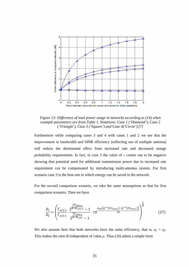
Figure 13 Difference of total power usage in networks according to (14) when example parameters are from Table 1 Notations Case 1 (lsquoDiamondrsquo) Case 2

(lsquoTrianglersquo) Case 3 (lsquoSquarersquo) and Case 4(lsquoCirclersquo)[7]

Furthermore while comparing cases 3 and 4 with cases 1 and 2 we see that the

improvement in bandwidth and SINR efficiency (reflecting use of multiple antenna)

will reduce the detrimental effect from increased rate and decreased outage

probability requirements In fact in case 3 the value of ν comes out to be negative

showing that potential need for additional transmission power due to increased rate

requirement can be compensated by introducing multi-antenna system For first

scenario case 3 is the best one in which energy can be saved in the network

For the second comparison scenario we take the same assumptions as that for first

comparison scenario Then we have

sLs4 = Г4ГL ∙ 2TUVhu∙u788h minus 12TUViu∙u788 minus 1 ∙ 10

YZiRMbchWiRMbciWL L27amp

We also assume here that both networks have the same efficiency that is η1 = η2

This makes the ratio R independent of value ρ Thus (16) admit a simple form

36

e = ih4 (28)

Equation (27) allows us to track the impact of antenna configuration minimum

throughput requirement and outage probability (Weff Γeff TPmin Prout) Assume

10MHz bandwidth 8 dB standard deviation for shadow fading and the path loss

exponent of 376 for LTE framework Then we obtain the results depicted in Table 3

for different network configurations We note that ratio R is now given in both linear

and decibel scale since it indicates both the coverage ratio and the power ratio From

(16) we see that R also points out the ratio between numbers of base stations in

compared deployments

TABLE 3 SECOND COMPARISON SCENARIO EXAMPLE POWER RATIOS

Simulation results for second comparison reveals the fact that changes in rate and

outage requirements may have crucial impact to coverage Doubling the rate

requirement on cell edge will lead to approximately one and a half fold increase in

base station density and if also outage probability is halved then even two fold

increase in base station density is needed Yet this huge cost source can be reduced

by introducing multi-antenna sites Result shows that the Greenfield operator should

be very careful when setting the network parameters requirements for cell edge may

dominate in network power consumption For second scenario also case 3 proves to

be the best case which offers maximum opportunity to save networkrsquos energy Results

Reference parameters (0562005010)

New parameters Value of R

Case 1 (0562010010) 147 (168dB)

Case 2 (0562010005) 210 (322dB)

Case 3 (0661110010) 097 (-010dB)

Case 4 (0661110005) 139 (144dB)

37

show that by improving the bandwidth efficiency and SINR value the operator can

make true savings in network OPEX

35 Analysis for Comparison Scenarios

For both scenarios Case 3 (0661110010) is the only option in which energy could

be saved but in negligible amount For the first scenario the power difference depends

upon the BS power distribution Poper and PTxin

The energy saving increases as PBS distribution changes from 0 to 2 but it is not

sufficient During the whole day the PBS distribution might vary or may remain fixed

but it could be of any value in the network So we calculated the energy decrement

percentage (for modified network 2 in comparison to reference network 1) for every

value of PBS distribution and on averaging it over the whole PBS distribution range

which varies from 0 to 2 we see the decrement in the energy consumption by 207

only

However in second scenario the power difference does not depend on the PBS

distribution for all the cases But energy saving is possible only in case 3 as in

scenario 1 In case 3 the energy saving remains same independent of the PBS

distribution so there is a constant 227 of energy consumption decrement So there

is a very minute difference between the energy decrement of both scenarios for case

3

The situation is the same for cases 1 2 and 4 but all these cases show that the energy

consumption has been increased in modified network with respect to reference

network In scenario 1 the maximum energy consumption at Pradio=2 Poper is more in

comparison to the constant energy consumption values for scenario 2

The averages taken for the total energy consumption in modified network 2 (in

comparison to reference network 1) for every distinct value of the PBS distribution

which varies from 0 to 2 are Case 1 Average P2=148P1 Case 2 Average P2=235P1

and Case 4 Average P2=138P1 If we compare these average powers with the constant

38

power consumption of scenario 2 we will observe very minute difference again as was

for case 3

Hence scenario 1 is the preferred approach for almost all the cases (that is for all

different network parameter settings)

Only in case 3 scenario 2 shows more energy saving than scenario 1 but with very

minute difference so even such network parametric setting shows that it would be

preferable to adopt an approach of updating BS in an existing network deployment

rather than going for building new network which has possibility of saving energy

with very insufficient amount but will enough increase the cost of the network

39

4 ENERGY EFFICIENCY MODEL FOR WIRELESS

HETEROGENEOUS NETWORK

41 Introduction In mobile communications small cells are potentially more energy efficient than usual

macrocells due to the high path loss between users and macro base stations Also

heterogeneous deployments of both cell types can be used to optimize the network

energy efficiency The power consumption of each individual network element has an

impact on the energy efficiency of any deployment The network energy efficiency

also depends on the required transmit power and load

This chapter constitutes my two publications [30] [34] It discusses the impact of

femtocells to the WCDMA network energy efficiency and the importance of

femtocell feature (idle mode) from the perspective of energy saving

Figure 14 Heterogeneous deployment for Energy Efficient Green Networks

40

42 Impact of Femtocells to the WCDMA Network Energy Efficiency To see the impact of load (network traffic) on the networkrsquos energy consumption we

have considered the Wideband Code Division Multiple Access (WCDMA) system

because it is easy to take advantage of the downlink load equations of WCDMA for

developing the model of energy consumption Moreover all the link level parameters

can be easily tracked from deduced formulae (analytical model)

To that end we derive power model for heterogeneous network consisting of

WCDMA macrocells and femtocells deployed in a common service areas The power

model is used to investigate the impact of load sharing between femtocells and

macrocells on the overall energy consumption

Specifically we have focused on analyzing the potential of energy saving in

WCDMA networks through small low power femto BS deployment alongside

macrocellular BSs In WCDMA networks offloading from macrocells to femtocells

results in decreased macrocell loads which in turn can be utilized through cell

breathing so that inter-site distance (ISD) between active macrocells is increasing and

the overall energy consumption by macrocellular system decreases However the

reduced energy consumption by macrocellular infrastructure will be offset by the

increasing energy consumption of the dense femtocell deployment

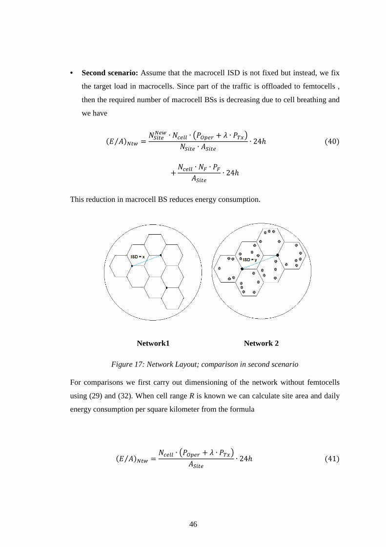
For this study we have considered the following two network deployment scenarios

a First scenario is based on the case where operator is upgrading cell sites in an

existing deployment

b Second scenario considers either Greenfield deployments of new cell sites or

to adopt the approach of switching Macro BSs off whenever traffic load in macrocell

is small due to the offloading to femtocell

43 Modeling and Comparison Scenarios We first recall WCDMA downlink load equations [31] [32] Then we introduce

modeling for performance comparisons and show how load equations can be utilized

in this context

41

431 Load Equations and Dimensioning

The cell range and ISD are defined using the layout of Figure 15 Thus the area

covered by a three-sector site is given by ASite= 94R2 = ISD2 In the following we

simplify the load equations by assuming that dimensioning is done based on a certain

service Then we can start from a simplified form of the well known WCDMA

downlink mean load equation [31] [32]

= +Q ∙ _ fMfrasl amp∙∙qu ∙ R1 minus ] + 3W (29)

Figure 15 Macrocell layout Cell range and ISD

In formula (29) parameter λ0 refers to the minimum load due to control signaling Nuser

is the number of users in the cell EbN0 is the energy per user bit divided by the noise

spectral density Rd is the user bit rate ν is the connection activity factor BW is the

system chip rate α is the spreading code orthogonality factor and i is the other to own

cell interference factor We note that we have considered the mean load that is

depending on the expected α and i over the whole cell

Moreover for the mean output power in BS transmission we have

Q = )Z∙A∙fb7n∙_ fMfrasl amp∙∙qL (30)

where nRF is the noise spectral density of the receiver front end We note that part of

the transmission power is used for control overhead

42

After combining (29) and (30) we can express the mean signal loss as follows

X = Q ∙ LMfb7n∙R CMfrasl Wg ∙∙q∙LDamp)Z∙fb7n∙_ fMfrasl amp∙∙q (31)

We note that mean signal loss is usually 6 dB less than maximum signal loss in the

cell edge [31] so that in dimensioning we need to take into account the corresponding

value in (31) Furthermore the mean signal loss should include impact of distance

dependent path loss shadow fading loss and interference margin If single slope

model aRb for distance dependent path loss is used then we can express the

macrocell range as follows

e = gtMbc∙LMfb7n∙R CMfrasl Wg ∙∙q∙LDDamp∙A∙)Z∙fb7n∙_ fMfrasl amp∙∙q iexcli (32)

Here dL contains the impact of signal loss averaging as well as shadow fading and

indoor penetration margins

In simplest form of network dimensioning a target load for a certain service is first

selected Then number of supported users can be calculated from (29) and

corresponding macrocell range from (32) Other information besides service rate and

load in (29) and (32) can be obtained from link budget

432 General Energy Usage Model

We start from a simple model that was previously applied in [4] [7] to describe the

macrocell base station power sharing between load independent and load dependent

operations

= + ∙ (33)

Here term PTx is the power that is needed to create required transmission power in the

antenna output and λ is the cell load that may vary between 01 and 09 depending on

43

the users load and radio interface configuration Term POper contains all load

independent power that is needed to operate the BS

The equation (33) defines the cell power while sites are usually composed by three or

more sectors that each form a logical cell Therefore the power consumed in site is of

the form

= ∙ R + ∙ W34amp where NCell refer to the number of cells in the site Then the site energy consumption

over a certain time period T is of the form

cent$ = ∙ R + ∙ W ∙ +35amp Although network adaptation to temporal variations of the load is an important topic

we ignore it in this paper since our focus is in the impact of femtocells Impact of

temporal load variations has been investigated in eg [3]

The energy usage over time T in a macrocell network is given by

centf = $ ∙ cent$ + _ ∙ cent_ + cent`a36amp

In (36) the first term in the right defines the energy consumption in all macrocell BSs

(Nsite and Esite refer to number of BS sites and energy consumed by single BS site

respectively) second term defines the energy usage in all UEs (NUE and EUE refer to

number of user equipments and energy consumed by single UE respectively) and last

term contains energy consumed by other mobile network elements such as core

network elements and radio network controllers in WCDMA

According to the justification made in previous chapter we ignore the second and the

last term in (36)

When femtocells are employed in the network the energy utilized by the network is

given by

44

centf = $ ∙ ∙ cent +z ∙ z ∙ +amp37amp

where NF is the number of femtocells in each macrocell and PF is the femto BS mean

power usage over time T In order to simplify the analysis we do not share femto BS

power between load dependent and independent parts since it is assumed that impact

of load to the femto BS power usage is relatively small

In order to make calculations more concrete we adopt from [4] the UMTS macrocell

base station specific values

= 1371 = 571

which will be then used in comparisons It should be noted that these values do not

include the energy consumption used by other elements at the base station site

mainly antenna feeder cables backhaul cooling and backup Within three sector site

the maximum energy consumption over 24 hours is round 14kWh

For femto BS input power we use two values 2W and 5W The former value is

optimistic but achievable in future while latter value is already reality in commercial

femtocell products [33]

433 Comparison Scenarios

Based on our derived power model we have compared the two network deployment

scenarios by setting different network parametric assumptions for both in order to

make it visible that which network deployment approach is more advantageous in

terms of energy saving Moreover within these two scenarios we have further

compared two hypothetical networks to estimate how the change in network

configurations will affect the energy consumption in the modified network (Network

2) in relation to the reference network (Network 1)

45

As a performance measure we will use the daily energy consumption per square

kilometer in the network expressed as follows

cent currenfrasl ampf = $f ∙ ∙ R + f ∙ W$ ∙ curren$ ∙ 24ℎ38amp + ∙ z ∙ zcurren$ ∙ 24ℎ

Thus dimension for the performance is the kWhkm2 In the above equation number

of sites in new deployment (Nsite)new and corresponding load λNew refer to the new

parametric values of the modified network with respect to the old parametric values of

the reference network We also note that the number of femto BSs is given per

macrocell in reference deployment Either of these changes is expected to take place

in one of the two compared networks depending upon the scenario

bull First scenario We assume that Macrocell Inter Site Distance (ISD) is fixed the

number of macrocells is the same for both networks but load is decreasing with

additional femtocells and we have

cent currenfrasl ampf = ∙ R + f ∙ + z ∙ zWcurren$ ∙ 24ℎ39amp Thus addition of femtocells is only visible in macrocell load factor

Network 1 Network 2

Figure 16 Network Layout comparison in first scenario

46

bull Second scenario Assume that the macrocell ISD is not fixed but instead we fix

the target load in macrocells Since part of the traffic is offloaded to femtocells

then the required number of macrocell BSs is decreasing due to cell breathing and

we have

cent currenfrasl ampf = $f ∙ ∙ R + ∙ W$ ∙ curren$ ∙ 24ℎ40amp + ∙ z ∙ zcurren$ ∙ 24ℎ

This reduction in macrocell BS reduces energy consumption

Network1 Network 2

Figure 17 Network Layout comparison in second scenario

For comparisons we first carry out dimensioning of the network without femtocells

using (29) and (32) When cell range R is known we can calculate site area and daily

energy consumption per square kilometer from the formula

cent currenfrasl ampf = ∙ R + ∙ Wcurren$ ∙ 24ℎ41amp

47

When NF femtocells are added to the system they take a certain portion of the users

say (Rfemto100) of users (Rfemto is the ratio between femtocell and macrocell

connections) Then either load in macrocells (first scenario) or ISD (second scenario)

is decreasing The latter phenomena reflects directly on the number of macrocell

sites

44 Numerical Examples We consider a WCDMA related example where parameters are given in Table 4

TABLE 4 WCDMA NETWORK PARAMETERS

Reference parameters

Parameter Value

Operating frequency 2000MHz

BS antenna height 30m

MS antenna height 15m

Propagation model Okumura-Hata (urban area)

Indoor penetration loss 10dB

BS antenna gain (incl losses) 16dBi

User data rate 64kbps 128kbps 256kbps

EbN0 5dB

Macro BS transmission power 20W

Femto BS input power 5W 2W

Control overhead 15

System chip rate 384Mcps

Shadow fading margin 7dB

Mean α 080

Mean i 065

Activity factor ν 100

Minimum load 010

48

In Figure 18 we have cell ranges as a function of number of users when user data rates

are 256kbps 128kbps and 64kbps If dimensioning is done eg based on 64kbps user

rate and assuming load 08 then cell range is round 600m

Figure 18 Cell range as a function of number of users when user data rates are 256kbps (dotted curve) 128kbps (dashed curve) and 64kbps (solid curve)

441 Numerical comparisons

Consider 64 kbps service and assume that initial system load is 09 We can then solve

number of users from (29) and cell range from (32) Furthermore if femtocells

offload data of RfemtoNusers= NF macrocell users then we can calculate new load λNew

from (29) and daily energy consumption per square kilometer from (39) The

algorithm for calculating the energy consumed considering both scenarios can be

more easily understood through the flow chart in Figure 19

0 2 4 6 8 10 12 14 16 18 200

02

04

06

08

1

12

14

16

18

2

Number of users

Cel

l ran

ge [

km]

49

Figure 19 Flow chart for the energy consumption algorithm

50

Resulting numerical values are given in Table 5

TABLE 5 DAILY ENERGY CONSUMPTION IN THE NETWORK FIRST SCENARIO

From second row of Table 5 we find that energy consumption per square kilometer is

clearly decreasing in macrocells when ratio of femto connections is increasing If

femto BS input power is 5W then the total energy consumption in the network is

growing since the load decay in macrocell load cannot compensate the additional

consumption due to femtocells On the other hand if femto BS input power is only

2W then the total energy consumption is slightly decreasing with additional

femtocells Finally we note that

bull In above calculations it was assumed that femto BSs are turned on only when

there is traffic If a number of femtocells are also active when traffic is

nonexistent then network energy consumption increases accordingly

bull From network operating costs perspective the values on the second row of Table 5

are important since they contribute directly to the energy bill paid by the operator

Results regarding to the second scenario has been plotted in Figure 20 It is found that

energy consumption by macrocells is rapidly decreasing since lower load allows less

dense macrocell grid The decrease in macro BS density is limited by the non-

femtocell users and in practice it is not possible to shutdown all the existing macrocell

sites due to coverage reasons Yet if network is to be built from scratch then second

scenario would be beneficial from energy efficiency perspective

100Rfemto 0 25 50 75

(EA)M [kWhkm2] 2435 2288 2140 1993

(EA)Total [kWhkm2] PF = 5W 2435 2577 2718 2859

(EA)Total [kWhkm2] PF = 2W 2435 2403 2371 2339

51

Figure 20 Daily energy consumption per square kilometer in the network when assuming second scenario No ticks Energy consumption by macrocells only Total

energy consumption when 5W femto BS power (o) and 2W femto BS power (x)

From Figure 20 we see that in case of 50 femtocell (2W) penetration around 63

of energy would be saved and it keeps on increasing as the femtocell penetration

increases Whereas in case of 50 femtocell penetration (5W) the maximum energy

saving would be around 49 and it will not further increase with the increase in

femtocell penetration Practically decrease in macro BS density is limited by the non-

femtocell users In order to fully exploit this gain a Greenfield network should be

built However part of the energy savings can be achieved also in existing networks if

macrocell BSs can be switched off during low load periods

45 Femtocell idle mode and network energy efficiency We discuss the importance of designing a special feature in femtocells which supports

idle mode to achieve significant amount of energy savings in network If femto BSs

are activated all the time then Femto BS energy consumption easily overtakes the

achieved savings on the macrocell side So femto BS should not remain activated if

indoor traffic is non-existent rather should enter sleep mode For this femto BS

should have the traffic sensing ability

0 01 02 03 04 05 06 07 08 09 10

5

10

15

20

25

Ene

rgy

cons

umpt

ion

per

squa

re k

ilom

eter

[kW

h]

Ratio between femtocell and macrocell connections

52

451 Effect of femtocell idle mode on overall network energy saving

When NF femtocells are added to the system they take a certain portion of the users

say (Rfemto100) of users as previuosly discussed where Rfemto is the ratio between

femtocell and macrocell connections Then either load in macrocells (first scenario) or

number of macrocell sites (second scenario) is decreasing thus reducing the energy

consumption of the network When both comparison scenarios are analyzed in case of

the femtocells deployment that do not possess idle mode feature we assume that

there exist fixed amount of active NF in the network already And they keep on getting

utilized along the Rfemto scale (when macrocell users are moved to femtocells) while

the underutilized ones will remain active

We have an assumption that each femto BS will serve a single user Initially we

assume number of active femtocells equivalent to number of users in the macrocell

Then onwards vary the value of active femtocells to see the impact on the total energy

saving in the network We have another two options to take the value of NF either

smaller than Nusers or greater than Nusers Here we have not considered NF to be less

than Nusers because this would mean that some indoor users will not be capable of

being served by femto BS as per our assumption of one to one ratio between NF and

Nusers

Resulting numerical values for 1st comparison scenario are given in Table 6 and

Table 7

TABLE 6 DAILY ENERGY CONSUMPTION IN THE NETWORK WHEN

DEPLOYED FEMTOCELL POSSESS IDLE MODE FEATURE FIRST SCENARIO

100 X Rfemto 0 25 50 75

(EA)M [kWhkm2] 2435 2288 2140 1993

(EA)Total [kWhkm 2] PF = 5W 2435 2577 2718 2859

(EA)Total [kWhkm 2] PF = 2W 2435 2403 2371 2339

53

TABLE 7 DAILY ENERGY CONSUMPTION IN THE NETWORK WHEN

DEPLOYED FEMTOCELL DO NOT POSSESS IDLE MODE FEATURE FIRST

SCENARIO

100 X Rfemto 0 25 50 75

(EA)M [kWhkm2] 2435 2288 2140 1993

(EA)Total [kWhkm 2] PF = 5W 3590 3442 3295 3147

(EA)Total [kWhkm 2] PF = 2W 2897 2749 2602 2455

From second row of Table 6 and 7 we find that energy consumption per square

kilometer is clearly decreasing in macrocells when ratio of femto connections is

increasing For femto BS possessing idle mode feature with input power 5W the total

energy consumption in the network is growing since the load decay on the macrocell

side cannot compensate for the additional energy consumption due to femtocells

Whereas the opposite is true for 5W femto BS that do not possess idle mode feature

Even then femtocell possessing idle mode feature are better because the energy

consumption is approximately 10 kWhkm2 less in comparison to the situation when

femtocell without idle mode feature are deployed in the network On the other hand if

femto BS input power is only 2W then the total energy consumption is slightly

decreasing with additional femtocells for both types (with and without idle mode

feature)

Utilizing equation (40) results regarding second comparison scenario has been

plotted in Figure 21 from energy saving perspective for both types of femto BSs (with

and without idle mode feature) having input power of 2W and 5W Plotted curves

show that total energy saving is more when deployed femto BS possess idle mode

feature in comparison to the situation when they do not have such feature

In Figure 21 different symbols are used to diferentiate the variuos plots depicting total

energy saving in different conditions For the case with NF=Nusers we have used

54

bull Circle for the condition when femto BSs with 2W input power possess idle mode feature

bull Triangle (Up) when femto BSs with 2W input power do not possess idle mode feature

bull Asterisk () when femto BSs with 5W input power possess idle mode feature

bull Traingle (Down) when femto BSs with 5W input power do not possess idle mode feature

Similarly in case of NF=23 x Nusers we have used Square when femto BSs with 2W

input power do not possess the idle mode feature Simple line corresponds to the

reference scenario

Figure 21 Daily energy saving per km2 in the network for second comparison scenario

We observe from plots of both input powers of femto BS when more load out of full

load gets shifted from macrocell to femto BS approximately same amount of energy

can be saved from both types of femto BS deployment (with and without idle mode

feature) This figure explains that femto BSs without idle mode feature would be more

55

unfavourable when not much load of the macrocell is shifted to femto BS (low Rfemto)

that is during situation when there is not much indoor traffic existing in the network

With input power of 2W when femto BSs that do not possess idle mode feature are

deployed in the network there will be extra energy consumed (no energy saving) by

the network until Rfemto reaches 005 since femto BS energy consumption is easily

overtaking the achieved savings on the macrocell side Whereas in case of the 5W

femto BS extra energy is consumed by the network until Rfemto reaches 02 and this

extra energy will be more than the extra energy consumed in case of 2W femto BS

Therefore in case of 2W input power the deployment of femto BSs that do not

possess idle mode feature could be acceptable if femto BSs possessing this feature are

unavailable However in case of 5W input power this femto BS feature is necessarily

required

Moreover we vary the number of active femto BSs (2W) in the network as for

example NF =23 x Nusers then the energy saving is reduced

It is concluded through analysis that the number of femtocells should be limited from

an energy perspective and upper bound is then the number of users in the macrocell

that is NF (Upper bound)= Nusers for both types of femto BSs (with and without the

idle mode feature) Thus the maximum gain in energy saving will be achieved when

NF = Nusers

For NF to be greater than Nusers we have already observed there will be more energy

consumption because of the more femto BS deployment than what is required

Considering the one to one ratio assumption only NF=Nusers option remain where we

can save maximum energy

Even from another perspective we can see from the plot the maximum energy saving

become possible when femto BS (that are being utilized) becomes equivalent to Nusers

(at Rfemto=1) that is all the macro load has been shifted to femto BS

56

452 Energy Savings from the perspective of Green Field Network Deployment (In Practice)

Femtocell deployment can reduce the BS density so it seems that building the new

network site from scratch with lesser number of BS would reduce the total energy

consumption of the network But for such Greenfield network build there might exist

certain periods in a day when the expected indoor traffic is not sufficient as was

expected and we also have the idea of sleep mode when there are underutilized

femtocells in the network in order to save energy So in that case the service will

degrade for outdoor users and there will be some coverage holes in the network

because the lesser amount of macro BSs would not be able to meet the high capacity

requirement (of outdoor traffic)

The penetration rate of femto BSs is equivalent to the percentage of the networkrsquos

indoor traffic because as per assumption one femto BS serves the single user that has

been offloaded from macro to femto BS

In case of the Femto BS (5W) with idle mode feature after 50 of Femto BSs

penetrations into the macro BSs network the energy saving becomes almost constant

that is 1203 kWh even if we keep on increasing the penetration rate uptil 100

From Figure 22 we see that macro BS remains underutilized because of the offloading

of macro BS traffic to Femto BS and therefore should be shutdown The result shows

that with the increase of Femto BS penetration we have to shutdown as many macro

BSs if we want to save sufficient energy (which we achieved for 50 femto BS

penetration) Because with the increase of femto BS usage the energy consumed by

femto BS will get increase so in order to compensate this energy consumption

numerous (in large amount) macro BS has to be shutdown

Hence the maximum energy can be saved with atleast 50 of Femto BS penetration

in the macro network But if for certain network the indoor traffic is more than 50

then no matter how much we have been offloading the macro BS (which turn them to

shutdown state) we would be saving the same maximum energy which we can

achieve for 50 femto BS penetration

57

On the other hand with femto BS which do not possess idle mode feature we would

save less energy as compared to the ones with idle mode feature Although the energy

saving keep on increasing throughout the femto penetration from 20 to 100 but

the macro BSs have to be shutdown with the same rate as in the case of femto BS with

idle mode feature

When there is 100 of femto BS penetration that is the whole network traffic is

originates from indoor UE then this shows that all the existing macro BSs can be

shutdown but practically this is not possible because femto BS are connected to core

network via macro BS Here some kind of a tradeoff has to be made to keep one (or

few) macro BSs On and at the same time save the energy by shutting down few macro

BSs depending upon the network macro load

Figure 22 Reduction in Number of New BSs in comparison to Number of Old BSs

Reduction in number of BSs for new sites in relation with the penetration rate of

femtocells has been shown in Figure 22 and the numerical values has been shown in

58

Table 8 the table also shows the respective energy saved for both types of femtocells

Letrsquos suppose if we assume the approach of building new macro BS site network by

reducing the number of BSs to half the amount of old networkrsquos number of BSs

considering the requirement of femtocells with 21 penetration because of the 21

expected indoor traffic existence then 976kWh energy per unit area could be saved

In this situation if indoor traffic decreases to 10 for such newly build Site network

there will be coverage holes due to the missing one third number of BSs (as for 10

of indoor traffic there is a need of 32 times less number of BSs than the old

networkrsquos BSs) Hence to save the energy and to avoid the service degradation

problem it is good to shut down the underutilized macro BSs when there exist indoor

traffic in the network instead of deploying the new sites with lesser BSs

TABLE 8 TOTAL ENERGY SAVINGS WHEN FEMTOCELLS WITH AND WITHOUT IDLE MODE FEATURE HAVE BEEN USED AND THE

REDUCTION IN NUMBER OF NEW BS SITES WRT TO OLD BS SITES

Penetration rate of femtocells

0

21

40

52

77

100

Reduction in the number of new BS site wrt the old BS site network

1 time

2 times

3 times

4 times

7 times

infin times

Total Energy Saving when femtocells with idle mode feature are used

0

kWh

976 kWh

1167 kWh

1203 kWh

1209 kWh

1280 kWh

Total Energy Saving when femtocells without idle mode feature are used

-115 kWh

0639 kWh

474 kWh

648 kWh

935 kWh

1280 kWh

59

On the other hand it is not convenient to use the dynamic power ONOFF switching

technique to save energy in the operation of the macrocellular BS It will be more

feasible to implement this technique when it is known in advance which periods of

day there is high probability of shutting down the BSs based on predetermined traffic

information This requires the daily traffic patterns (both indoor and outdoor traffic

information) of the network with high accuracy

60

5 CONCLUSIONS AND FUTURE WORK

This thesis work investigated the energy consumption of mobile access networks

which has recently received increased attention in research carried out in both

industry and academia This thesis also contributes to the mainstream discussion on

the importance of reduction in energy consumption to achieve economic and

environmental benefits Particularly it has addressed the possible ways to minimize

the energy consumption on the BS sites

In the thesis some factors in evolution of mobile networks were discussed from

energy and power consumption perspective Based on the discussion a simple

methodology was proposed in order to model the power consumption on network of

base stations To make visible the impact of different link budget and network

parameters two scenarios have introduced Finally to elaborate these scenarios two

simple examples were presented

The thesis work also investigated the potential energy savings when deploying

femtocells along with macro base stations in WCDMA network To find the energy

consumption per unit area WCDMA downlink load equations were used It was

determined how the load sharing between femtocells and macrocells will contribute to

the overall energy consumption of the network

To elaborate introduced scenarios two simple examples were presented In first

scenario the macrocell inter site distance is fixed and different femto base station

penetration ratios are assumed Analytical results show that total energy consumption

in network per unit area was increasing when employing femto base stations that

operate with a 5W input power On the other hand energy consumption was found to

decrease slightly when employing femto base stations that operate with a 2W input

power

In second considered scenario the macrocell inter site distance was not fixed and the

addition of femtocells to the macrocellular system decreased the macrocell base

station density due to the cell breathing phenomenon In this case there was a

61

significant amount of energy saving Achieved gain can be fully exploited in green

field deployments but part of the energy saving potential can be utilized also in

existing networks through macrocell breathing decreased macrocell load due to

femtocells results in larger macrocell coverage and in dense macrocell deployments

part of the base stations can be switched off

Finally the thesis focused on the importance of idle mode feature for femto BS The

number of active femto base stations has significant impact on the network energy

efficiency If femto BSs are on all the time then femto base station energy

consumption easily overtake the achieved savings on the macrocell side Therefore it

is essential to design efficient sleep mode procedures for femto base stations

The analytical results concluded that in order to save the energy and avoid the service

degradation problem it is recommended to shutdown the underutilized BSs instead of

deploying the new networks with less BSs (green field networks) This switching

ONOFF of the BSs should be done based on the already available daily traffic

patterns

For this reason the future work includes taking into account the impact of daily traffic

variations for the shown studies and for that purpose a new performance metrics will

be needed Furthermore the future study includes designing the methodology

(utilizing Shannon equations) for the energy consumption of HSDPA (High Speed

Downlink Packet Access) and LTE (Long Term Evolution) modeling the power

usage of a heterogeneous network element such as Relays This study was based on

uncoordinated femtocellular BSs For further studies to see that how the coordinated

and planned femtocellular BSs would affect the energy efficiency of the network

62

REFERENCES

[1] InStat ldquoWCDMA Base Station Embracing the New Generationrdquo InStat analyst report by F Guan Feb 2007

[2] Emerson ldquoEnergy Logic for Telecommunicationrdquo white paper Ericsson 2008

[3] F Richter A J Fehske G P Fettweis ldquoEnergy Efficiency Aspects of Base Station Deployment Strategies for Cellular Networksrdquo IEEE Vehicular Technology Conference Anchorage USA September 2009

[4] G Micallef P Mogensen H O Scheck ldquoCell Size Breathing and Possibilities to Introduce Cell Sleep Moderdquo European Wireless Conference p 111-115 2010

[5] S Zhou J Gong Z Yang Z Niu P Yang ldquoGreen Mobile Access Network with Dynamic Base Station Energy Savingrdquo MobiComrsquo09 Sept 2009 Beijing China

[6] M A Marsan L Chiaraviglio D Ciullo M Meo ldquoOptimal Energy Savings in Cellular Access NetworksrdquoProc IEEE ICCrsquo09 Workshop GreenComm June 2009

[7] M Jada J Haumlmaumllaumlinen R Jaumlntti M M A Hossain ldquoPower Efficiency Model for Mobile Access Networkrdquo IEEE PIMRCrsquo10 Workshop W-Green September 2010

[8] Ericsson AB ldquoSustainable energy use in mobile communicationsrdquo white paper EAB-07021801 Uen Rev C 2007

[9] httptimeforchangeorgCO2-cause-of-global-warming

[10] httpwwwaccessnetsorgkeynoteshtml EARTH project

[11] Hans-Otto Scheck ldquoICT amp wireless networks and their impact on global warmingrdquo Nokia Siemens Networks Linnoitustie 6 FI-02600 Espoo Finland

[12] JTLouhi ldquoEnergy efficiency of modern cellular base stationsrdquo INTELEC 2007 Rome Italy

[13] G Wimpenny ldquoImroving multi-carrier PA efficiency using envelope trackingrdquo Microwave Journal November 2008

[14] Kimball D Draxler P Jeong J Hsia C Lanfranco S Nagy W Linthicum K Larson L Asbeck P 50 PAE WCDMA basestation amplifier implemented with GaN HFETs Compound Semiconductor Integrated Circuit Symposium 2005 CSIC 05 IEEE vol no pp 4 pp 30 Oct-2 Nov 2005

[15] Jinseong Jeong Kimball DF Myoungbo Kwak Draxler P Chin Hsia Steinbeiser C Landon T Krutko O Larson LE Asbeck PM High-Efficiency WCDMA Envelope Tracking Base-Station Amplifier Implemented With GaAs HVHBTs Solid-State Circuits IEEE Journal of vol44 no10 pp2629-2639 Oct 2009

[16] Jinseong Jeong Kimball DF Myoungbo Kwak Chin Hsia Draxler P Asbeck PM Wideband Envelope Tracking Power Amplifiers With Reduced

63

Bandwidth Power Supply Waveforms and Adaptive Digital Predistortion Techniques Microwave Theory and Techniques IEEE Transactions on vol57 no12 pp3307-3314 Dec 2009

[17] Femtocell Networks A Survey Vikram Chandrasekhar and Jeffrey G Andrews The University of Texas at Austin Alan Gatherer Texas Instruments September 2008 IEEE Communications magazine

[18] Ericsson ldquo Minimizing carbon intensity in telecom networks using TCO techniquesrdquo white paper 284 23-3137 Uen Rev A February 2010

[19] O Arnold F Richter G Fettweis O Blume ldquoPower consumption modelling of different base station types in Heterogeneous Cellular Networksrdquo Future Network and Mobile Summit IIMC International Information Management Corporation 2010

[20] httpwwwgreentouchorgindexphppage=shannons-law-explained

[21] 3GPP Radio frequency (RF) system scenarios (Release 8) 3GPP technical report TR 36942 Ver 820 May 2009

[22] P Mogensen W Na I Z Kovacs F Frederiksen A Pokhariyal K I Pedersen T Kolding K Hugl M Kuusela LTE Capacity Compared to the Shannon Bound IEEE Vehicular Technology Conference April 2007

[23] Harri Holma Antti Toskala ldquoLTE for UMTSOFDMA and SC-FDMA based Radio Accessrdquo John Wiley amp Sons 2009

[24] Preben E Mogensen Tommi Koivisto ldquoLTE-Advanced The Path towards Gigabits in Wireless Mobile Communicationsrdquo IEEE Wireless Communication Vehicular Technology Information Theory and Aerospace amp Electronic Systems Technology 2009

[25] 3GPP ldquoRequirements for further advancements for Evolved Universal Terrestrial Access (E-UTRA)rdquo TR36913 v801 March 2009

[26] A Bou Saleh S Redana J Haumlmaumllaumlinen B Raaf Comparison of Relay and Pico eNB Deployments in LTE-Advanced IEEE Vehicular Technology Conference Anchorage Alaska Fall 2009

[27] Ericsson ST-Ericsson Enhanced network energy efficiency (R1-100062) 3GPP TSG-RAN WG1 Meeting 59bis Valencia Spain January 2010

[28] Nokia Nokia Siemens Networks Discussion on Network Energy Saving in LTE (R1-100587) 3GPP TSG-RAN WG1 Meeting 60 San Francisco USA February 2010

[29] Ericsson ST-Ericsson UTRA Node B energy saving (R1-100598) 3GPP TSG-RAN WG1 Meeting 59bis Valencia Spain January 2010

[30] M Jada J Haumlmaumllaumlinen R Jaumlntti M M A Hossain ldquoImpact of Femtocells to the WCDMA Network Energy Efficiencyrdquo IEEE IC-BNMT China October 2010

[31] H Holma A Toskala rdquoWCDMA for UMTSrsquo Third edition Wiley 2004

64

[32] K Sipilauml Z Honkasalo J Laiho-Steffens A Wacker ldquoEstimation of Capacity and Required Transmission Power of WCDMA Downlink Based on a Downlink Pole Equationrdquo IEEE Vehicular Technology Conference Spring 2000

[33] Press Release on NEC FP 810 femtocell product 2010 httpwwwslashgearcomnec-fp810-femtocell-tiny-but-14-45-7mbps-data-rates-1073529

[34] M Jada J Haumlmaumllaumlinen R Jaumlntti ldquoEnergy savings in mobile networks Case Study on Femtocellsrdquo XXXII Finnish URSI Convention on Radio Sciences Oulu August 2010

i

AALTO UNIVERSITY ABSTRACT OF THE MASTERrsquoS THESIS

Author Maliha Urooj Jada

Name of the Thesis Energy Efficiency Techniques amp Challenges for Mobile Access

Networks

Date 6th May 2011 Number of pages 9+ 64

Department Department of Communications and Networking

Professorship Radio Communications

Supervisor Prof Jyri Haumlmaumllaumlinen Aalto University

Energy consumption of mobile access networks has recently received increased attention in

research carried out in both industry and academia The cellular networks do not have

considerable share in the overall energy consumption of the ICT (Information and

Communication Technology) sector However reduction in energy consumption of mobile

networks is of great importance from economical (cost reduction) and environmental

(decreased CO2 emissions) perspective

The Thesis work has investigated the different means to enhance the capacity of evolved

mobile networks and discussed the related challenges from energy consumption perspective

this discussion is followed by a simple radio network power usage model Based on the

model examples are given where two different deployment scenarios have been compared

Further the work focused on the WCDMA energy saving through femtocell deployment A

simple model for the energy consumption per unit area has been derived based on WCDMA

downlink load equations Based on the model two different deployment scenarios have been

compared to make the conclusion from energy consumption perspective

In the end the impact of femtocells to the energy efficiency of the WCDMA network has

been studied under the consideration of a valuable power save feature of femtocell

Keywords Mobile access networks energy and power efficiency scenarios comparisons femtocells load equations idle mode

Language English

ii

Acknowledgments Initially and most importantly I want to thank my supervisor Professor Jyri

Haumlmaumllaumlinen for his endless support worthy guidance and valuable comments on my

work I feel gratitude that with his support and encouragement I am successful in

publishing three research papers I appreciate that he provided several opportunities

for presenting my work in front of audience which has boosted up my confidence

level tremendously

I am also grateful to Professor Riku Jaumlntti for giving valuable advices in thesis work

and also thankful to his doctoral student Aftab Hussain for the grate support while

writing research papers

I would like to thank Edward Mutafungwa one of the senior members of my research

group with excellent English language skills for his help in revising the final draft of

my thesis

Furthermore I am thankful to Sanna Patana (Administrative Services Secretary) and

Sari Kivelio (Department Secretary) for their help in making travel arrangements to

the conference places which I attended to present my accepted research papers

I am extremely thankful to my friends who have kept the entertainment and fun part

active in my life and have been encouraging me throughout my thesis work

Finally I am greatly obliged to my Mother for all the love moral support and

motivation she had been giving me throughout my MSc studies and especially during

my thesis work I owe a great debt of gratitude to my parents for making me a

confident person and developing in me the unquenchable thirst of knowledge

Maliha Urooj Jada

6th May 2011

iii

To my parents amp siblings

iv

Contents Abbreviations v

List of Figures vii

List of Tables viii

1 Introduction 1

11 General Energy Saving Aspects in Mobile Networks 1

12 Energy Consumption in Cellular Network 2

121 Minimizing the BS Energy Consumption 3

122 Minimizing the Base Station density 10

123 Alternative energy resources 10

2 Mobile Network Evolutıon Energy Efficiency challenges 13

21 Introduction 13 22 Network Energy Efficiency 14

23 The Need of Capacity Enhancement Features 15

231 Static Power 15 232 Dynamic Power 15

24 Capacity Enhancement Energy Efficiency Challenges 17

241 Capacity Enhancement Features 18

3 Simple Model for Power Consumption 26

31 Introduction 26 32 Comparison Cases 28

321 First Scenario 29 322 Second Scenario 30

33 Computation of Transmission Power Ratio and Range Ratio 32

34 Examples 33 35 Analysis for Comparison Scenarios 37

4 Energy Efficiency Model for Heterogeneous Network 39

41 Introduction 39 42 Impact of Femtocells to the WCDMA Network Energy Efficiency 40 43 Modeling and Comparison Scenarios 40

431 Load Equations and Dimensioning 41

432 General Energy Usage Model 42

433 Comparison Scenarios 44 44 Numerical Examples 47

441 Numerical comparisons 48 45 Femtocell idle mode and network energy efficiency 51

451 Effect of femtocell idle mode on overall network energy saving 52

452 Energy Savings from the perspective of Green Field Nw Deployment 56

5 Conclusions and Future Work 60

References 62

v

ABBREVIATIONS

BS Base Station CO2 Carbon dioxide ICT Information amp Communication Technology PST Public Switched Telephone PDG Packet Data Gateway GGSN Gateway GPRS Support Node SGSN Serving GPRS Support Node HLR Home Local Register IMS IP Multimedia Subsystem RF Radio Frequency PAR Peak to Average Power Ratio UMTS Universal Mobile Telecommunication System WiMAX Worldwide Interoperability for Microwave Access LTE Long Term Evolution AMAM Amplitude to Amplitude Modulation IBO Input Back Off OBO Output Back Off ET Envelop Tracking PA Power Amplifier WCDMA Wideband Code Division Multiple Access MIMO Multiple Input Multiple Output BBU Base Band Unit DSPs Digital Signal Processors FPGAs Field Programmable Gate Arrays ASICs Application Specific Integrated Circuits UE User Equipment SINR Signal to Interference to Noise Ratio hrs hours OPEX Operational Expenditure CAPEX Capital Expenditure QoS Quality of Service 2G Second Generation 3G Third Generation QoE Quality of Experience EARTH Energy Aware Radio and Network Technologies kwh kilowatt hour SUB Subscribers AMR-HR Adaptive Multi Rate - Half Rate IMT Advanced International Mobile Telecommunications Advanced 3GPP Third Generation Partnership Project SISO Single Input Single Output AWGN Additive White Gaussian Noise SNR Signal to Noise Ratio SIMO Single Input Multiple Output

vi

CDF Cumulative Distribution Function ISD Inter Site Distance WRC World Radio communication Conference IP Internet Protocol HSPA High-Speed Packet Access HSDPA High ndash Speed Downlink Packet Access

vii

L IST OF FIGURES

Figure 1 Energy contribution of main elements of mobile networks 3 Figure 2 Energy consumption in a typical macro BS site 3 Figure 3 A Typical Power Amplifier Response 5 Figure 4 Energy Saving depending on traffic profile for 24 Hours 7 Figure 5 Relation between BS Energy Saving and Load Balancing 8 Figure 6 Hexagonal and crossroad configurations 8 Figure 7 Manhattan configurations linear (top) and squared (bottom) 9 Figure 8 Solar panels deployed at BS 11 Figure 9 Wind Power turbine deployed at BS 12 Figure 10 Enabling energy-efficient growth through capacity enhancement 16 Figure 11 Pictorial representation for First Scenario Network Comparison 29 Figure 12 Pictorial representation for Second Scenario Network Comparison 31 Figure 13 Difference of total power usage in networks 35 Figure 14 Heterogeneous deployment for Energy Efficient Green Networks 39 Figure 15 Macrocell layout Cell range and ISD 41 Figure 16 Network Layout Comparison in first scenario 45 Figure 17 Network Layout Comparison in second scenario 46 Figure 18 Cell range as a function of number of users 48 Figure 19 Flow Chart for the Energy Consumption Algorithm helliphelliphelliphelliphelliphelliphelliphellip 49 Figure 20 Daily energy consumption per square kilometer in the network when assuming second scenario 51 Figure 21 Daily energy saving per km2 in the network for second comparison scenario 54 Figure 22 Reduction in Number of New BSs in comparison to Number of Old BSs 57

viii

L IST OF TABLES

TABLE 1 3GPP PERFORMANCE REQUIREMENTS ON CELL EDGE (CASE 1) 22 TABLE 2 FIRST COMPARISON SCENARIO EXAMPLE POWER RATIOS 34 TABLE 3 SECOND COMPARISON SCENARIO EXAMPLE POWER RATIOS 36 TABLE 4 WCDMA NETWORK PARAMETERS 47 TABLE 5 DAILY ENERGY CONSUMPTION IN THE NETWORK FIRST SCENARIO 50 TABLE 6 DAILY ENERGY CONSUMPTION IN THE NETWORK WHEN DEPLOYED FEMTOCELL POSSESS IDLE MODE FEATURE FIRST SCENARIOhelliphelliphelliphelliphelliphelliphelliphelliphelliphelliphelliphelliphelliphelliphelliphelliphelliphelliphelliphelliphelliphelliphelliphelliphelliphelliphelliphellip52

TABLE 7 DAILY ENERGY CONSUMPTION IN THE NETWORK WHEN DEPLOYED FEMTOCELL DO NOT POSSESS IDLE MODE FEATURE FIRST SCENARIO 53 TABLE 8 TOTAL ENERGY SAVINGS WHEN FEMTOCELLS WITH AND WITHOUT IDLE MODE FEATURE HAVE BEEN USED AND THE REDUCTION IN NUMBER OF NEW BS SITES WRT TO OLD BS SITES 58

1

1 INTRODUCTION

Deployment of increasingly powerful mobile network technologies has taken place

within the last decade Although network efficiency has been growing the higher

access rates have inevitably led to increased energy consumption in base stations

(BSs) and network densities have been constantly growing [1]

Recently the mobile communication community has become aware of the large and

ever-growing energy usage of mobile networks [2] Besides industry the awareness

of the ever-increasing energy consumption has stimulated research in academia

particularly on issues addressing the BS site energy consumption [3] [4] [5] [6] [7]

Yet the work on the reduction of energy consumption has been mostly carried out by

BS manufacturers [8] since high power efficiency provides a competitive advantage

Today one of the most discussed topics is the global warming which is due to

increment of CO2 (Carbon dioxide) and other green house gases concentration levels

in atmosphere To decrease the CO2 emissions the consumption of fossil fuels has to

be decreased [9] [10] Thus the research has been carried out in the ICT (Information

and Communication Technology) sector to reduce the consumption of fossil fuels to

make the environment clean and green

Mobile networks do not have considerable share in the overall energy consumption of

the ICT sector which itself is responsible for 2 to 10 of the world energy

consumption However reduction in energy consumption of mobile networks is of

great importance from economical (cost reduction) and environmental (decreased CO2

emissions) perspective

11 General Energy Saving Aspects in Mobile Networks Two following approaches towards Energy Efficient Mobile Networks are the

following

bull Find appropriate solutions to the energy efficiency challenges for already

existing networks (Brownfield)

2

bull Design future networks from energy (and cost) efficient perspective

(Greenfield perspective)

For the future Telecomrsquos energy consumption difficulties and uncertainties exist in

estimating the potential energy savings due to the different methodologies that is

how to define energy consumption or which elements should be considered in the

energy efficiency calculation [11]

Furthermore energy savings depends significantly on human behavior and utilization

of resulting financial savings as any energy saving is followed by cost savings From

a network operator or infrastructure ownerrsquos business perspective the cost saving

factor in many cases is of more importance than environmental protection Money

saved by reducing energy consumption is available for other expenditures If the

saved cost would be invested in a proper way the low carbon society will be created

Alternatively energy savings could be affected by rebound effect in which the

improper utilization of the saved cost might give unfortunate results of potentially

additional CO2 emissions

Travelling by car is one of the most effective causes of global warming Thus

substitution of the office work with remote work via broadband network connectivity

has the potential to significantly reduce the carbon dioxide emissions [11] In a similar

way business travel can be substituted by videoconferencing and electronic billing

instead of paper bills would also contribute in making an environment green

12 Energy Consumption in Cellular Network A typical mobile network consists of three main elements core network base

stations and mobile terminals as shown in Figure 1 Base stations contribute 60 to

80 of the whole network energy consumption [12] Thus the efforts in the reduction

of energy consumption focus on the BS equipment which includes the minimization

of BS energy consumption minimization of BS density (BS density is inversely

proportion to cell area) and the use of renewable energy sources

3

Figure 1 Energy contribution of main elements of mobile networks

121 Minimizing the BS Energy Consumption

The ways to minimize the BS energy consumption includes improvement in BS

energy efficiency through better performance of BS hardware usage of system level

and software features and usage of BS site solutions [12]

Figure 2 gives some brief idea about the energy consumption in a typical macro BS site

Figure 2 Energy consumption in a typical macro BS site [8]

4

A Base Station Hardware Efficiency

For the improved performance of BS hardware the focus should be on boosting the

efficiency of power amplifier because power amplifier and its associated components

can consume up to 50 of the overall power [13]

The current radio modem design paradigm requires high linearity from the radio

frequency (RF) components which allows one to separate the RF design and digital

signal processing design The classic Class AB amplifier technology offers efficient

operation when the RF envelope waveform is close to peak power Unfortunately

most of the modern waveforms have high peak-to-average power ratio (PAR) forcing

the power amplifier to operate most of the time in less efficient operation point As a

result efficiency around 15-25 has been measured for the waveforms used by the

modern UMTS (Universal Mobile Telecommunication Systems) WiMAX

(Worldwide Interoperability for Microwave Access) and LTE (Long Term Evolution)

systems [13]

Figure 3 shows a typical AMAM response (Amplitude to amplitude modulation The

output power of an RF power amplifier does not keep on increasing without limit

There exists a point when an increase in input power will not produce any significant

increase in output power This is referred to as the saturation point where output

power is not proportional to input power any more In the saturation region of an RF

amplifier response as the input increases the gain becomes compressed This Output

Power versus Input Power characteristic is referred as AM-AM distortion for a High

Power Amplifier with the associated input and output back-off regions (IBO and

OBO respectively) Output Back Off (OBO) induced by PAR means wasted power

5

Figure 3 A Typical Power Amplifier Response

The power efficiency of a High Power Amplifier can be increased by reducing the

PAR of the transmitted signal The average and peak values should be as close

together as possible in order to maximize the efficiency of the power amplifier

It is possible however to achieve a significant improvement in PA efficiency using

envelope tracking (ET) In ET the voltage supplied to the final RF stage power

transistor is changed dynamically synchronized with the RF signal passing through

the device to ensure that the output device remains in its most efficient operating

region close to saturation point In one of the studies (based on the PA efficiency for

BS) 50 efficiency have been reported for WCDMA (Wideband Code Division

Multiple Access) waveforms for ET based PA [14] In recent papers efficiencies close

to 60 has been reported If the energy efficiency of the power amplification can be

drastically increased from the 15-25 range to close to 60 also the energy

consumption of cooling system can be significantly reduced [15][16]

Typically in multi-antenna (MIMO Multiple Input Multiple Output) systems each

antenna has its own power amplifier If the system load is low then energy can be

saved by switching off some of the transmit antennas For instance UMTS supports

6

the use of two transmit antennas In case there are no MIMO capable terminals

present in the system then the base station may switch off the second common pilot

channel transmitted over the second antenna to save energy

The energy efficiency of the base band unit (BBU) of the base station can be further

improved by introducing power save modes to subunits such as channel cards DSPs

(Digital signal processors) FPGAs (Field programmable gate arrays) ASICS

(Application ndashspecific integrated circuits) or even clocks such that they could be

switched on and off based on the base station load

Moreover by using the continuous Phase modulation technique PAR can be reduced

and high efficiency can be achieved in Mobile Station (or User Equipment UE)

transmitter which contributes to the increment in power efficiency of the whole

network

B System Level or Software Feature

The impact of different link budget and network parameters on the network energy

consumption has been investigated in Chapter 2 Results indicate for example that if

transmission power is fixed per BS but cell edge rate requirement is doubled then a

one and a half fold increase in BS density is needed However by introducing multi-

antenna sites there will be an improvement in bandwidth and SINR (Signal to

Interference to Noise Ratio) efficiency which may even fully compensate the need for

increasing BS density In a similar way there also exist more such system level

techniques to reduce energy consumption of radio network One of them is discussed

below

B1 BS switching in conventional macrocell topology

One of the main energy saving approaches is the system level feature in which

underutilized cells (BSrsquos) are switched off whenever traffic load is small as depicted

in Figure 4 The network load in some areas may vary significantly due to the mixed

effect of two traffic properties

bull Daily changes in user data consumption for instance data traffic may be small

at night times

7

bull The user density may greatly vary Office areas may provide heavy load on

day time and very small user load during the night times while load on

residential areas increases during the afternoon as subscribers have returned

from places of work study and so on

Figure 4 Energy Saving depending on traffic profile for 24 Hours

When cells are switched off it is assumed that the radio coverage and feasible service

conditions can be guaranteed by the remaining active cells (BSs) probably with some

increment in the BS transmitting power This increase in transmission power in

remaining active BSs however can be small when compared to the savings achieved

by switching off some BS sites Moreover in order to avoid this increment in

transmission power wireless relays cooperative communication and electrically

tilted antennas can be used to guarantee the radio coverage [5]

Energy saving through BS switching has been under discussion over the last few

years For instance researchers have proposed that power saving algorithms can be

centralized (when all the channel information and traffic requirements are known) or

decentralized (no such information is required) [5] Energy savings are higher in

centralized approach because BS density becomes lower while coverage guarantee is

better in decentralized approach because more BSrsquos stay active In this research the

focus was on the relation between BS energy saving and load balancing The purpose

8

of load balancing is to equally distribute traffic service among BSrsquos to achieve better

coverage whereas the aim in BS energy saving is to concentrate traffic to as few BSrsquos

as possible Through examination it was found out that load balancing appears to be

important BS energy saving algorithm due to its decentralized and dynamic nature

Figure 5 Relation between BS Energy Saving and Load Balancing [6]

Similar approach was applied in other researches whereby focus was on cell layout

[6] To achieve optimal energy saving it was discovered in [6] that in real networks

only a small fraction of cells need to remain on during the night time In [6] few

typical cellular network configurations (Hexagonal Crossroad Manhattanlinear

Manhattansquared as shown in Figures 6 and 7 respectively) had been compared

assuming two different daily traffic patterns symmetric trapezoidal traffic pattern and

asymmetric traffic pattern which is derived from measurements over a real network

Comparison indicates that the best solution is not to switch off the largest possible

number of cells rather it is important to make tradeoff between the night zone period

(low load) and the number of cells that are switched off According to this work the

best performing scheme is switching off 4 cells out of 5 with crossroad configuration

Within the above mentioned network topologies the energy savings of the order of

25-30 are possible to achieve

Figure 6 Hexagonal and crossroad configurations [6]

9

Figure 7 Manhattan configurations linear (top) and squared (bottom) [6]

C Site Solution

Energy efficiency can not only be improved in BS equipment but also certain power

solutions could be adapted on the site level to save the energy These are referred to as

site solutions In [12] the few mentioned site solutions which have the potential for

energy saving are

- Outdoor sites

- Cooling solution for indoor sites

- RF head

- Modular BS

With outdoor sites the cooling requirements can be lowered by raising the allowable

operating temperature range for the BS site wherever possible because the upper limit

set for the temperature is now high so less cooling would be sufficient to keep the

temperature within limits This leads to the reduced energy consumption by the

cooling equipment and thus less CO2 emissions observed With indoor sites the

energy could be saved by utilizing fresh air cooling systems instead of using air

conditioner that consumes energy for its operation With RF head or modular BS the

RF transmitter is located close to BS antenna this way the cable losses decreases and

the network performance is improved Alternatively less transmit power is required

to achieve the same network performance

10

122 Minimizing the Base Station density

The deployment of small low power femto BSs alongside macrocellular BSs is often

believed to reduce the energy consumption of cellular network [17] This idea is

studied in Chapter 4 where analysis is based on WCDMA load equations It has been

demonstrated that when femtocells are introduced to the network they will reduce the

macro BS density Thus reducing the energy consumed by the macrocellular side of

the network But not necessarily the total energy consumed by network due to the lack

of femtocell ability in practical to switch onoff depending upon indoor traffic

(discussed in Chapter 4)

123 Alternative energy resources

Mobile networks can be made much more energy efficient than they are today and

networks may become even fully self-sustainable by using renewable energy

resources which are using natural resources such as sunlight wind tides and

geothermal heat All these resources are regenerative which makes them different

from fossil fuels and thus they will not produce greenhouse gases that is CO2

Currently renewable energy resources are mostly used on sites that are at long

distances from electricity grid or on locations where electricity supply is unreliable

The importance of these renewable energy resources is increasing as the costs of

expanding network into remote areas grow [12]

The most important thing to take into account while planning to operate the BS site by

renewable energy resources is the site location and the energy consumption of the BS

site The availability of energy resources defines the site location and the energy

consumption depends upon the load

The most reasonable renewable energy resources for BS sites are derived from the

main source of energy i-e sun and also wind

A Solar energy

Solar energy is free abundant and inexhaustible It is the source of all forms of

renewable energy supply direct solar power and heat hydro bio mass wind-power

11

and wave power Direct solar power systems are now the subject of intense activity in

different parts of the world Related technology could provide us with electrical

resources totaling up to a thousand times our current demands

For low and medium capacity sites or repeaters sites solar power can be used to

provide virtually free energy at least in terms of OPEX (Operation Expenditure)

While the initial CAPEX (Capital Expenditure) per kilowatt is higher for such

solutions they can provide a positive business case compared with diesel generators

within one or two years of operation

Figure 8 Solar panels deployed at BS For the solar power plant installment near BS more site space is required Moreover

the climate variations in sunshine develop the need of higher energy storage capacity

in solar power plant

On the other hand it is expected for the future network to have a combination of

alternative energy sources to meet the seasonal variation differences [8]

12

B Wind Energy

As with solar power wind power can provide virtually free energy However wind

power industry is constructing very large wind turbine and the challenge is to find a

cost effective solution for BS site (Ericsson)

Figure 9 Wind Power turbine deployed at BS

The advantage of wind power is that it can maintain the BS site at low cost On the

other hand the disadvantage of it is that wind is unpredictable so there must be some

small diesel generator as backup in situations when there is low wind or no wind

Currently the extra site space is required because of the need to install the wind

turbine tower along with the BS tower [8]

13

2 MOBILE NETWORK EVOLUTION ENERGY

EFFICIENCY CHALLENGES

21 Introduction In the last decade we have come across the rapid development of the mobile network

technologies In the establishment of new mobile networks the focus has been shifted

from 2G (Second Generation) mobile network technologies to 3G (Third Generation)

and now beyond 3G (eg LTE) networks which are based on the latest standard and

are being recently commercialized With each new mobile network generation new

services are being introduced and achievable data rates per user are increased

One of the main motivations behind mobile networks evolution is Internet access so

there is a need to constantly increase the user data rates in order to provide the mobile

internet based services with an end-user acceptable quality of experience (QoE) The

internet based services are initially being designed assuming fixed line capabilities

therefore to shift from the fixed line services to mobile services the data rates on

mobile systems have to be increased The large scale deployment of mobile Internet is

ongoing in many countries to fulfill its high demand due to the rapid increment in the

number of mobile data users

Although new networks are more efficient it is expected that increasing demands for

high data rates will cause the constant increase in network densities and thus the

increased energy consumption in the mobile networks Therefore it is of great

importance for network operators to adopt energy efficient techniques while building

the new networks

To provide higher user data rates and serve a growing number of mobile data users

there is a need for higher network capacity There exist several ways to increase the

network capacity which includes wider frequency bandwidths enhanced radio link

technologies higher transmission powers more dense networks and heterogeneous

deployments All of these techniques have been discussed in detail in this chapter

showing the challenges they come across from the energy efficiency perspective

14

Also there exists a need for capacity enhancement features to make the networks

energy efficient that is the capacity enhancement features must provide the reduction

in networkrsquos energy consumption This need for capacity enhancement for having

energy efficient networks has been explained taking into account the power

distribution in the network

22 Network Energy Efficiency Recently several projects in wireless communications (working as consortium of

worldwide renowned companies and research institutes) have been focusing on the

energy efficiency and not on just the reduction of total energy consumed by the

network [10] that is they are concerned about the reduction in energy per bit One of

the proposed units to measure efficiency is Watt per bit And energy efficiency is

considered from network perspective

The formula proposed for the network energy efficiency is

1313 = (1)

bull Growth in the network traffic andor reduction in the power consumed per user

will increase the network energy efficiency

bull Growth in the traffic will increase the revenue from services (Green Services

which focus on energy saving and carbon emission reduction) Traffic is measured

as bits per second

bull Reduction in the power consumption per user will reduce the carbon footprint and

also decrease the operation cost

bull For a given application if QoS is not met then energy efficiency is zero

bull If optical fiber is used instead of wireless the networks will be more energy

efficient but the cost possibly will increase by very large amount

ICT is responsible for 2-10 of worldrsquos energy consumption The research efforts are

also focusing on means to use ICT in order to reduce the remaining 98 of energy

consumption in the world

15

23 The Need of Capacity Enhancement Features To emphasize the need for capacity enhancement features for energy efficient

networks we start by recalling the power usage in base station

Electronic devices consume power when being switched on and in conventional

mobile networks the baseline assumption is that BSs are on all the time Power

supplies basic operation functions and signaling between nodes (between Radio BS

and Mobile BS in idle mode) consume power even when the network is not carrying

any traffic [18]

The BS power usage can be divided into static and dynamic parts [18]

$ = $amp$ + $amp() (2)

231 Static Power

The static power consumption contains both powers that are needed to keep BS site

equipments operable as well as power that is spend on continuous basic radio access

operations such as common channel transmission

Usually power-saving features are designed to lower this static power consumption

There are many features today that monitor network activity and successively shut

down unneeded equipment during times of low traffic without degrading quality of

service [18]

232 Dynamic Power

Dynamic power is a significant portion of power consumed by a network which varies

in direct relationship with the amount of traffic being handled in a network at a given

time

This dynamic part of the power consumption can be made more efficient by employing

capacity-enhancing features so that more traffic can be handled with a given amount

of energy In this regard most network equipment vendors have designed the range of

capacity enhancement features

16

When networks are expanded the large scale deployment of capacity enhancement

solutions would be effective from economical and environmental perspective because

then unnecessary addition of new sites or nodes can be avoided that is the BS density

will not be increased much and energy consumption can be even reduced in the

network

Figure 10 provides a conceptual illustration of the way in which energy efficiency is

increased through the use of a capacity enhancing feature This figure shows the

relation between energy efficiency and enhanced system capacity By employing

capacity enhancing features into the network more traffic can be handled with a

given amount of energy or the network will reach same capacity by utilizing less

power

The energy efficiency has been depicted here in terms of power usage per subcriber

The less power utilized for certain subscribers the more energy efficient will be the

network In figure 10 X initial refers the low energy efficient state of the network and as

we move from Xinitial towards X 1 X2 and X3 we observe the increment in the

networkrsquos energy efficiency

Figure 10 Enabling energy-efficient growth through capacity enhancement [18]

17

The base stations with dynamic power saving features have appeared only very

recently and are not yet widespread in the network [19] Capacity enhancing features

that reduce dynamic part of the used power are physical layer scheduling and MIMO

that both boost the resource usage efficiency Moreover additional examples of

dynamic power reducing features are the use of AMR-HR (Adaptive Multi Rate ndash

Half Rate) in mobile voice networks and higher order modulation schemes for data

transmission [18]

Especially for micro BS power model the dynamic part has significant importance

because for small cell the number of users (load) is statistically varying more than for

large cells [19]

24 Capacity Enhancement Energy Efficiency Challenges The need for expanding system capacity grows with the number of users and with the

amount of information required for a given service But there exist challenges for such

capacity enhancement solutions from an energy perspective

In order to analyze the impact of link budget parameters on the energy consumption

of the network the formulation has been started by understanding the throughput

formula (Shannon capacity formula) To make the network energy efficient the

Shannonrsquos theory can be employed in a novel manner Shannonrsquos theory provides

guidance for discovering and developing new methodologies to maximize energy

efficiency (to reduce energy per data bit) while approaching the Shannon limit of

maximized network capacity [20]

The peak data rates are available only in very good channel conditions and the

practical data rate is limited by the amount of interference and noise in the network

The maximum theoretical data rate with single antenna transmission in static channel

can be derived using the Shannon formula The formula gives the data rate as a

function of two parameters bandwidth and the received signal to noise ratio

The Shannon capacity bound canrsquot be reached in practice due to several

implementation issues To represent these loss mechanisms accurately we use a

modified Shannon capacity formula which has fitting parameters Weff and Γeff

18

+ = 0Г lt Г)1 ∙ 1 ∙ 34 51 + ГГ7889Г) le Г lt Г+ Г ge Г= (3)

Here W is the operation bandwidth Γ is the signal to interference and noise ratio

(SINR) Γmin is the minimum value for SINR such that connection is blocked if

ΓltΓmin and Γmax is the SINR needed to reach the maximum throughput TPmax The

coefficients Weff and Γeff are the bandwidth and SINR efficiency factors respectively

which are selected so that (3) fits with the set of applied adaptive modulation and

coding curves The values of Weff and Γeff can be found by link level simulations [21]

[22] [23]

241 Capacity Enhancement Features

A Wider Bandwidth

The channel capacity is linearly proportional to bandwidth so the extension of

operation bandwidth is the most straightforward way to increase the system capacity

If network element density and transmission power per unit bandwidth is kept

constant then according to (3) the capacity grows linearly with additional bandwidth

At the same time required transmission power and the needed energy also increases

linearly in order to keep the transmission power per unit bandwidth constant as well

if the wider bandwidth are used but cell sizes are not decreased then transmission

power needs to grow accordingly

With this approach the tradeoff remains between the system capacity and energy

efficiency in the network Although this approach has been adopted by all the latest

and upcoming new mobile generations for fulfilling the increased capacity and higher

data rate requirements but it does not contribute in the improvement of networkrsquos

energy efficiency The researchers have to come up with some other system-level or

link-level techniques along with this approach to enhance the system capacity in an

energy efficient way

19

It is important to note that in (3) the bandwidth efficiency reflects the systemrsquos ability

to utilize the radio spectrum and the upper limit is set by Weff =1

For LTE-Advanced (LTE Releasersquo10) it is expected that operation bandwidth will be

divided to 20 MHz carriers and carrier aggregation over up to five carriers is then

used to reach the data rate targets set by IMT-Advanced (International Mobile

Telecommunications Advanced) (peak rate 1 Gbps data rate in local area) [24]

Following the 3rd Generation Partnership Project (3GPP) recommendations [21] the

maximum BS transmission power is 43 dBm in Wideband Code Division Multiple

Access (WCDMA with 5 MHz channel) 46 dBm in Releasersquo8 LTE (10-20 MHz

channel) and thus LTE-Advanced with carrier aggregation will lead up to five times

higher transmission power than used in Releasersquo8 LTE and up to ten times higher

transmission power than used in WCDMA

B Enhanced radio link technologies

Network operator is interested in the improved network efficiency that is how the

maximum number of users can be served the maximum data rate can be provided and

the BS site density can be decreased The efficiency is considered in the link budget

calculations and in the capacity simulations

The LTE link performance is benchmarked with the theoretical Shannon limit To

guarantee consistent performance 3GPP has defined a set of radio performance

requirements

The radio link efficiency has been improved a lot by setting up the advanced radio

link technologies like multiple-input and multiple-output or MIMO for evolved 3G

networks WCDMA HSPA and recently LTE Releasersquo8

The impact of radio link efficiency is embedded into parameter pair (Weff Γeff) which

are also referred to as the fitting parameters for Shannon performance curve The

higher the efficiency the closer to one are the values of Weff and 1Γeff

LTE is highly efficient and is performing less than 16-2 dB from the Shannon

capacity bound in case of AWGN channel In fading channel the link performance on

20

SISO (Single Input Single Output) is close to Shannon limit that defines fundamental

upper bound However for SISO the best Shannon fit parameters are significantly

worsened compared to AWGN (Additive White Gaussian Noise) the equivalent Weff

(Bandwidth Efficiency) has reduced from 083 to 056 and the Γeff (SNR efficiency)

has been increased from 16-2dB to 2-3dB Whereas for SIMO (Single Input Multiple

Output) the Shannon fit parameters are better than SISO Weff is 062 and Γeff is

18dB Similarly for MIMO the Shannon fit parameters gets better than SIMO Weff is

066 and Γeff is 11dB which makes it closer to Shannon bound and makes the link

performance more efficient in comparison to the cases of SISO and SIMO In MIMO

antenna systems there is more room for optimization but it is well acknowledged that

along with the link performance increase some more solutions are required for future

challenges regarding capacity enhancement [7]

It can be observed that by increasing the number of antennas on the transmitter and

receiver sides the Shannon fit parameters can be further improved leading to higher

spectral efficiency and thus higher throughput With higher spectral efficiencies less

radio resources per information bit are needed and thus the energy could be saved

accordingly However there exist certain limitations on the increment of number of

antennas due to size and cost constraints

C Higher Transmission Powers

In this section SINR has been analyzed in detail to describe the impact of transmission

power in different system environment for increasing system capacity The target

SINR is adjusted according to the transmission power of the signal The idea of this

approach is that communication links in worse propagation conditions have to use

higher transmission power to attain a given target SINR level But for reliable

communication links a small increase in transmission power is sufficient to increase

the SINR value by large amount

To start with the general form of SINR

Г = gt AfraslCDsum gtF AFfraslF (4)

21

where PTxk refers to BS transmission power in kth BS Lk is the related path loss and

PN is the noise power The reference user is assumed to be connected to BS with

index 0

If all BSs apply the same transmission power and we let the power grow without

limit then we have

Г gtrarrHIJJJK Lsum AMAFF (5)

Thus SINR admit an upper limit that depends on the path losses towards BSs If the

network is noise limited that is right side term in (5) is clearly larger than Γmax then

data rates can be improved through higher transmission powers However from (3) it

is obvious that due to logarithm much more power would be required to achieve the

same increase in the capacity as achieved by the increase in the bandwidth Therefore

this strategy is not as energy efficient way to increase capacity as compared to the

strategy where bandwidth is extended If system is interference limited that is if the

right side limit term in (5) is small then large BS transmission powers will waste a lot

of energy and just create more interference to the network

D Impact of cell edge coverage requirement

The cell edge coverage can be defined using a probabilistic throughput requirement

Pr+ lt +)amp = Q (6)

In (6) Prout is the outage probability and TPmin defines the minimum SINR in (3) The

outage probability is an important statistical measure to access the quality of service

provided by the system It is the probability of failing to achieve a specified SINR

value and thus the minimum throughput value which is sufficient for satisfactory

reception

22

Requirement (6) can also be given in terms of spectral efficiency if throughput is

scaled by the used bandwidth

RS lt STUVW le Q (7)

The cell edge user throughput is defined as the 5 point of CDF (Cumulative

Distribution Function) of the user throughput normalized with the overall cell

bandwidth For example LTE-Advanced cell edge throughput requirements have been

given using this approach [25]

TABLE 1 3GPP PERFORMANCE REQUIREMENTS ON CELL EDGE (CASE 1)

For Case1 carrier frequency is 2GHz ISD (Inter Site Distance) is 500 meters

bandwidth is 10MHz path loss is 20dB and user speed is 3 kmh

There are two important parameters in (6) that impact on the cell power usage First

tough coverage constraint with very low outage probability will lead to the need for a

high BS transmission power or dense network Both of these options will mean

increased energy consumption in the network Second if operator plans to improve

the service level in the whole network then it should take into account the minimum

throughput requirement of (6) Another option would be to provide more radio

resources per user which is a possible strategy if network load is not too high or

operator is able to introduce new spectrum resources It is expected that all these

approaches will increase the energy consumption of the network

23

E Impact of carrier frequency and propagation environment

The carrier frequencies tend to increase from 900MHz of first 2G networks the

carrier frequency has been increasing to 1800MHz (2G extension bands) 2100GHz

(main 3G bands) 2600MHz (LTE bands) and it will soon jump up to 3500MHz

(bands granted by World Radio communication Conference WRCrsquo07 for IMT-

Advanced) At the higher carrier frequencies the signal path loss in wireless medium

is stronger which requires either transmission power or network density to be

increased Furthermore while additional carriers and extended bandwidths lead to an

easily predictable increase in energy consumption the effect of higher carrier

frequency can be predicted only when propagation modeling is accurate Since details

of sophisticated propagation models are out of the scope of this thesis we adopt a

simple path loss formula

X = Aamp∙AYZ[ (8)

In (8) L(d) refers to a distance dependent model such as Okumura-Hata LSF is the

lognormal shadowing and G refers to the BS antenna gain We have embedded the

antenna gain into propagation model for simplicity It is recalled that antenna gain

depends on the angle between receiver and antenna main directions Yet in

dimensioning the antenna gain in main direction is applied Since Okumura-Hata

model is a so-called single slope model it admits the form

Xamp = ] ∙ ^ (9)

where parameter α includes the impact from carrier frequency and BS antenna height

while the path loss exponent β depends only on the BS antenna height Let us consider

a simple example Assume that the system carrier frequency is increasing from

21GHz to 26GHz Then according to Okumura-Hata model the path loss increases

round 24dB and thus energy consumption in radio operations increases by factor of

174 If BS range in urban area is for example 1km then path loss from higher carrier

frequency can be compensated on the cell edge by increasing the BS antenna height

from 25m to 38m This might be difficult due to regulations and negative visual

24

impact Finally we note that the propagation environment greatly affects the strength

of the path loss so that in rural environment much larger areas can be covered than in

urban environments with the same BS transmission power

F More dense networks and heterogeneous deployments

The larger operation bandwidth and increased power consumption as well as high

macrocell site costs are driving towards smaller cells which ultimately become part of

heterogeneous networks The deployment of small low power base stations

alongside conventional sites is often believed to greatly lower the energy consumption

of cellular radio network because when communication distance is decreased less

power per bit is needed and available spectrum resources are shared between fewer

users From energy efficiency perspective some of the main challenges in small cells

and heterogeneous deployments are

1) Number of sites follows square law with respect to inverse of the range This puts a

high pressure on the energy efficiency of the small nodes Also the network capital

expenses increase rapidly unless BSsite prices are decreasing proportionally to the

square of inverse of the range

2) Backhaul availability limits the density of small cells and wireless nodes like relays

will spend part of the transmission power on backhaul communication Yet if relays

are used on the cell edge this additional power consumption may be small [26] and

thus the macrocell BS transmission power gets reduced

3) Antennas in small cells are located below the rooftop and therefore coverage areas

of small cells will be fragmented Then coverage holes become more severe and

unnecessary high transmission power might be used to solve the coverage problems

This increases interference which will decrease the system power efficiency

4) Mass deployment of femtocells may lead to a situation where numerous small

access points are turned on and spending energy even when traffic is nonexistent On

the other hand in case of home cellular data transfer becomes highly energy efficient

due to small communication distance

25

5) To avoid high operational expenses and unnecessary power consumption small

cells should support of plug-and-play Thus practically implementable self-

configuration self-optimization and self-healing algorithms should be used to keep

the system efficient

26

3 SIMPLE MODEL FOR POWER CONSUMPTION

31 Introduction

The number of mobile subscribers has increased tremendously during last decade

Along with voice communication the data usage has also grown fast The customers

are used to high data rate performance of fixed line systems so they also expect the

comparable performance from the wireless networks Thus the operators demand high

data capacity with low cost of data delivery which is the main motivation behind the

development of 3GPP LTE [23]

More specifically the motivation of LTE Release 8 includes

bull Wireline capability evolution gives boost to evolution in wireless domain

bull Need for additional wireless capacity ndash to take maximum advantage of

available spectrum and base station sites

o This will put the challenge of reducing the energy consumption while

utilizing capacity enhancement features

bull Need for lower CAPEX and OPEX ndash Flat rate charging model

bull Competition of 3GPP technologies must meet and exceed the competition with

other existing wireless technologies

o When it comes to the competition with other technologies then energy

efficiency become one of the key factor of competition basis

bull Low complexity - Flat IP architecture

As environmental and economic issues have become more important cellular network

operators are paying more attention to environmental issues Power consumption by a

node (Home e Node-B Relay node or Femto node) in such a network can have an

effect on the environment Power generation often requires environmental inputs

Thus reduced power consumption can have an advantageous affect on the

environment as well as reduced overall costs for the network Therefore one of the

main performance targets for LTE includes the surety that the new system could

facilitate lower investment and operating costs compared to earlier systems From this

27

perspective the reduced energy consumption for LTE play an indirect but important

role in reducing the cost and making the technology greener Another main

performance target for LTE is the optimized terminal power efficiency which still

needs improvement

Similarly the need for capacity and coverage of cellular networks is increasing as

more and more people utilize cell phones and other types of wireless communicators

which in turn increase power demand on the overall network Because of the

increased power demand the desire to reduce power consumption (that is save

power) is likewise increasing with regard to systems and nodes It is expected to

increase the energy efficiency of the system by providing cellular service to more

users utilizing the available (limited) power resources

According to big players in the wireless communication industry the focus regarding

Green communication schemes should be mostly on the LTE as they are the most

recent networks and when new sites have to be deployed it is easier to incorporate the

green communication radio solutions into LTE networks rather than for the old

networks (2G and 3G)

- Power Model

Modeling is of great importance because it is useful in making decisions based on

quantitative reasoning and it also helps in performing desired analysis The main goal

of the power consumption model is to make realistic input parameters available for

the simulation of total power consumption in mobile communication networks and

also to compare different network deployments

The total power consumption of the mobile network over some time period can be

expressed in the form

= $ ∙ $ + _ ∙ _ + a (10)

In (10) the first term in the right defines the power consumption in all BSs (NBS and

PBS refer to number of BSs and power consumed by single BS respectively) second

28

term defines the power usage in all User Equipments UEs (NUE and PUE refer to

number of user equipments and power consumed by single UE respectively) and the

last term contains power spent by other mobile network elements such as core

network elements and radio network controllers in WCDMAHSPA High-Speed

Packet Access for example We ignore the second term on the right since terminal

power and energy efficiency has been under extensive investigations for a long time

due to strict battery constraints Therefore recent energy efficiency studies have been

focusing on the network side where more room for notable improvements exists

Furthermore since we concentrate on the energy efficiency of the radio access the last

term in (10) is out of our scope We also recall that BS energy efficiency is of great

importance for operators since BSs form a vast majority of mobile network nodes and

thus they also have largest contribution to the energy consumption of a modern

mobile network creating a significant operational cost factor [27] [28] [29]

To start with we assume an extreme case of full traffic load in BS and express the

power spent by BS in the form

$ = + ) = + gtMbcd (11)

In (11) the term PTxin is the power utilized that is needed to create maximum

transmission power PTxout in the antenna output and η is the efficiency of the

transmission chain Term POper contains all other power that is needed to operate BS

on full load condition

32 Comparison Cases Based on the model we have compared two hypothetical network deployment

scenarios by setting different network parametric assumptions for both Moreover

within these two scenarios we have further compared two networks to estimate how

the change in network configurations will affect the energy consumption in the

modified network (Network 2) wrt the reference network (Network 1) This analysis

will make it visible which network deployment approach is more advantageous in

terms of energy saving

29

We note that first scenario is related to the case where operator is updating BSs in an

existing deployment while second scenario considers Greenfield operator that is

building new network

The goal of this example for comparison scenarios is to make visible the impact of

different link budget and network parameters to the network energy consumption

We will compare power usage in two different networks (network 1 and network 2)

by computing the ratio between powers that are needed in all BSs in the networks

e = fgYh∙gYhfgYi∙gYi (12)

321 First Scenario

Network 1 Network 2

Figure 11 Pictorial representation for First Scenario Network Comparison

In the first scenario case both networks apply the same BS grid (same BS antenna

height same number of BSs etc) that is the inter site distance (ISD) x is fixed as

shown in Figure 11 and the focus is on the difference of BS power between two

networks The BS power varies depending upon the throughput bandwidth efficiency

outage probability and SINR efficiency

According to (11) and (12) the ratio R can be written in the form

30

e = $4$L = 1 + RL) frasl W ∙ R4) L)frasl W1 + L) frasl 13amp

where we have assumed that operation powers are the same for BSs of the first and

second network and difference occurs only between transmission powers Let us

further define

k = gtiUVlm7n o = gthMbcgtiMbc (14)

In (14) parameter ρ refers to the ratio between transmission chain input power and

power spent for all other operations in a BS of the first network We use first network

as a reference and consider impact of changes that reflect only to the required output

transmission power By ν we denote the ratio between maximum output transmission

powers

Using these notations we obtain

e = LDp∙di dhfrasl amp∙qLDp (15)

The idea in expression (15) is that we can separate factor ρ and ratio η2η1 that are

merely product specific from factor ν that reflects the impact of changes in radio

related parameters

322 Second Scenario

In the second scenario the BS output transmission power is fixed that is the BS

output power in both the compared networks remain same However the inter site

distance (ISD) is scaled which reflects to the number of BS sites In this scenario the

cell ranges varies in the second network depending upon the new values of

throughput bandwidth efficiency outage probability SINR efficiency which are set

for second network Thus the ISD varies from x to y as shown in Figure 12 which

will bring change in the BS output power consumption and in the overall power

31

consumption of the modified network (Network 2) with respect to reference network

(Network 1) due to the change in the BS density that is different number of BSs

Network 1 Network 2

Figure 12 Pictorial representation for Second Scenario Network Comparison Here the ratio R is in the form

e = $4$L ∙ 1 + RL) frasl W ∙ R4) L)frasl W1 + L) frasl

(16)

= $4$L ∙ 1 + k ∙ rL r4frasl amp1 + k = 5sLs494 ∙ 1 + k ∙ rL r4frasl amp1 + k

Here D1 and D2 refer to the ranges of the BSs and we have used the fact that number

of BSs in the network is proportional to the square of inverse of the range

Thus in addition to product specific values of ρ η1 and η2 we need in first scenario

the output transmission power ratio ν for fixed BS range and in second scenario we

need the range ratio D1D2 on the condition that output transmission powers are fixed

32

33 Computation of Transmission Power Ratio and Range Ratio Let us start from the coverage requirement (6) By using the formula (3) the

throughput can be expressed in terms of SINR

Г = Г ∙ R2 u∙u788frasl minus 1W (17)

Furthermore the inequality in (6) can be written between SINR and minimum

required SINR

Г le Г) = Г ∙ R2TUV ufrasl ∙u788 minus 1W (18)

Here SINR is given through equations (4) (7) and (9) Let us introduce interference

margin IM through SINR approximation on the cell edge

Г = gt C∙AlampfraslLDsum gtF C∙AFampfraslF asymp gtC∙xy∙Al (19)

This margin is widely used in network dimensioning so that link budgets can be

formed without extensive system simulations After combining (18) (19) and (8) we

get

Xsamp ∙ X$z ge [∙gtC∙xy∙ГTUV = X (20)

In (20) D is the BS range and Lmax refers to the maximum allowed path loss Since

shadow fading is lognormal variable we use decibel scale and write (6) in the form

X$zamp ge Xamp minus RXsampWamp le Q (21)

Furthermore as shadow fading is Gaussian in decibel scale we can use Marqum Q-

function to assume equality for a while and write

|Xamp minus Xsampamp$z ~ = Q22amp

33

In (22) σSF is the standard deviation for the shadow fading Marqum Q-function is

monotonic and it has unique inverse Unfortunately this inverse does not admit

closed-form expression and we can only formally write

Xamp = Xsampamp + $z ∙ LQamp23amp Letrsquos recall the inequality and use again the linear scale Then we obtain the

following requirement for transmission power

ge C∙xy[ ∙ Г ∙ 2 gtTUV∙788 minus 1 ∙ ] ∙ s^ ∙ 10YZ∙inMbcampi 24amp In comparisons we may use minimum power that is defined by equality in (24) Thus

we have

Q = C∙xy[ ∙ Г ∙ 2 gtTUV∙788 minus 1 ∙ ] ∙ s^ ∙ 10YZ∙inMbcampi

(25)

s = gtMbc∙[∙C∙xy∙Г788 ∙ 2 gtTUV∙788 minus 1L ∙ 10YZ∙inMbcampi i

Using these formulae we can compute ν and ratio D1D2 provided that parameters in

(25) are known

34 Examples

We consider a LTE related example where parameters for the reference system are

selected according to [23] Assume first comparison scenario where receiver noise

power interference margin BS antenna gain mean path loss parameters and shadow

fading standard deviation are the same for systems that are compared Then we have

34

o = Г4ГL ∙ 2TUVhu∙u788h minus 1

2 TUViu∙u788i minus 1 ∙ 10YZiRMbchWiRMbciWL 26amp

Equation (26) allows us to track the impact of antenna configuration minimum

throughput requirement and outage probability (Weff Γeff TPmin Prout) Assume

10MHz bandwidth and 8dB standard deviation for shadow fading Then we obtain the

results of Table 2 for different parameter combinations

TABLE 2 FIRST COMPARISON SCENARIO EXAMPLE POWER RATIOS

In Figure 13 we have the ratio R of (13) in decibels It is found that if we increase the

power consumed on the radio side in comparison to the power consumed on the

operation side the total power difference in compared networks increases in a

different way for cases 1 2 3 and 4 depending on the network configurations In

cases 1 and 2 the minimum value of the throughput has been doubled with respect to

the reference network The power difference is larger in case 2 than in case 1 because

the outage probability has been decreased in case 2 Curves show that impact of both

cell edge rate requirement and outage probability are large Yet the power share

between radio and other operations in BS will define the practical cost impact If BS

is using only small portion of the power for keeping BS up and running then changes

in rate requirement and outage probability will have noticeable effect to the operation

costs

Reference parameters (0562005010)

New parameters Value of ν

Case 1 (0562010010) 315 dB

Case 2 (0562010005) 603 dB

Case 3 (0661110010) -020 dB

Case 4 (0661110005) 268 dB

35

Figure 13 Difference of total power usage in networks according to (14) when example parameters are from Table 1 Notations Case 1 (lsquoDiamondrsquo) Case 2

(lsquoTrianglersquo) Case 3 (lsquoSquarersquo) and Case 4(lsquoCirclersquo)[7]

Furthermore while comparing cases 3 and 4 with cases 1 and 2 we see that the

improvement in bandwidth and SINR efficiency (reflecting use of multiple antenna)

will reduce the detrimental effect from increased rate and decreased outage

probability requirements In fact in case 3 the value of ν comes out to be negative

showing that potential need for additional transmission power due to increased rate

requirement can be compensated by introducing multi-antenna system For first

scenario case 3 is the best one in which energy can be saved in the network

For the second comparison scenario we take the same assumptions as that for first

comparison scenario Then we have

sLs4 = Г4ГL ∙ 2TUVhu∙u788h minus 12TUViu∙u788 minus 1 ∙ 10

YZiRMbchWiRMbciWL L27amp

We also assume here that both networks have the same efficiency that is η1 = η2

This makes the ratio R independent of value ρ Thus (16) admit a simple form

36

e = ih4 (28)

Equation (27) allows us to track the impact of antenna configuration minimum

throughput requirement and outage probability (Weff Γeff TPmin Prout) Assume

10MHz bandwidth 8 dB standard deviation for shadow fading and the path loss

exponent of 376 for LTE framework Then we obtain the results depicted in Table 3

for different network configurations We note that ratio R is now given in both linear

and decibel scale since it indicates both the coverage ratio and the power ratio From

(16) we see that R also points out the ratio between numbers of base stations in

compared deployments

TABLE 3 SECOND COMPARISON SCENARIO EXAMPLE POWER RATIOS

Simulation results for second comparison reveals the fact that changes in rate and

outage requirements may have crucial impact to coverage Doubling the rate

requirement on cell edge will lead to approximately one and a half fold increase in

base station density and if also outage probability is halved then even two fold

increase in base station density is needed Yet this huge cost source can be reduced

by introducing multi-antenna sites Result shows that the Greenfield operator should

be very careful when setting the network parameters requirements for cell edge may

dominate in network power consumption For second scenario also case 3 proves to

be the best case which offers maximum opportunity to save networkrsquos energy Results

Reference parameters (0562005010)

New parameters Value of R

Case 1 (0562010010) 147 (168dB)

Case 2 (0562010005) 210 (322dB)

Case 3 (0661110010) 097 (-010dB)

Case 4 (0661110005) 139 (144dB)

37

show that by improving the bandwidth efficiency and SINR value the operator can

make true savings in network OPEX

35 Analysis for Comparison Scenarios

For both scenarios Case 3 (0661110010) is the only option in which energy could

be saved but in negligible amount For the first scenario the power difference depends

upon the BS power distribution Poper and PTxin

The energy saving increases as PBS distribution changes from 0 to 2 but it is not

sufficient During the whole day the PBS distribution might vary or may remain fixed

but it could be of any value in the network So we calculated the energy decrement

percentage (for modified network 2 in comparison to reference network 1) for every

value of PBS distribution and on averaging it over the whole PBS distribution range

which varies from 0 to 2 we see the decrement in the energy consumption by 207

only

However in second scenario the power difference does not depend on the PBS

distribution for all the cases But energy saving is possible only in case 3 as in

scenario 1 In case 3 the energy saving remains same independent of the PBS

distribution so there is a constant 227 of energy consumption decrement So there

is a very minute difference between the energy decrement of both scenarios for case

3

The situation is the same for cases 1 2 and 4 but all these cases show that the energy

consumption has been increased in modified network with respect to reference

network In scenario 1 the maximum energy consumption at Pradio=2 Poper is more in

comparison to the constant energy consumption values for scenario 2

The averages taken for the total energy consumption in modified network 2 (in

comparison to reference network 1) for every distinct value of the PBS distribution

which varies from 0 to 2 are Case 1 Average P2=148P1 Case 2 Average P2=235P1

and Case 4 Average P2=138P1 If we compare these average powers with the constant

38

power consumption of scenario 2 we will observe very minute difference again as was

for case 3

Hence scenario 1 is the preferred approach for almost all the cases (that is for all

different network parameter settings)

Only in case 3 scenario 2 shows more energy saving than scenario 1 but with very

minute difference so even such network parametric setting shows that it would be

preferable to adopt an approach of updating BS in an existing network deployment

rather than going for building new network which has possibility of saving energy

with very insufficient amount but will enough increase the cost of the network

39

4 ENERGY EFFICIENCY MODEL FOR WIRELESS

HETEROGENEOUS NETWORK

41 Introduction In mobile communications small cells are potentially more energy efficient than usual

macrocells due to the high path loss between users and macro base stations Also

heterogeneous deployments of both cell types can be used to optimize the network

energy efficiency The power consumption of each individual network element has an

impact on the energy efficiency of any deployment The network energy efficiency

also depends on the required transmit power and load

This chapter constitutes my two publications [30] [34] It discusses the impact of

femtocells to the WCDMA network energy efficiency and the importance of

femtocell feature (idle mode) from the perspective of energy saving

Figure 14 Heterogeneous deployment for Energy Efficient Green Networks

40

42 Impact of Femtocells to the WCDMA Network Energy Efficiency To see the impact of load (network traffic) on the networkrsquos energy consumption we

have considered the Wideband Code Division Multiple Access (WCDMA) system

because it is easy to take advantage of the downlink load equations of WCDMA for

developing the model of energy consumption Moreover all the link level parameters

can be easily tracked from deduced formulae (analytical model)

To that end we derive power model for heterogeneous network consisting of

WCDMA macrocells and femtocells deployed in a common service areas The power

model is used to investigate the impact of load sharing between femtocells and

macrocells on the overall energy consumption

Specifically we have focused on analyzing the potential of energy saving in

WCDMA networks through small low power femto BS deployment alongside

macrocellular BSs In WCDMA networks offloading from macrocells to femtocells

results in decreased macrocell loads which in turn can be utilized through cell

breathing so that inter-site distance (ISD) between active macrocells is increasing and

the overall energy consumption by macrocellular system decreases However the

reduced energy consumption by macrocellular infrastructure will be offset by the

increasing energy consumption of the dense femtocell deployment

For this study we have considered the following two network deployment scenarios

a First scenario is based on the case where operator is upgrading cell sites in an

existing deployment

b Second scenario considers either Greenfield deployments of new cell sites or

to adopt the approach of switching Macro BSs off whenever traffic load in macrocell

is small due to the offloading to femtocell

43 Modeling and Comparison Scenarios We first recall WCDMA downlink load equations [31] [32] Then we introduce

modeling for performance comparisons and show how load equations can be utilized

in this context

41

431 Load Equations and Dimensioning

The cell range and ISD are defined using the layout of Figure 15 Thus the area

covered by a three-sector site is given by ASite= 94R2 = ISD2 In the following we

simplify the load equations by assuming that dimensioning is done based on a certain

service Then we can start from a simplified form of the well known WCDMA

downlink mean load equation [31] [32]

= +Q ∙ _ fMfrasl amp∙∙qu ∙ R1 minus ] + 3W (29)

Figure 15 Macrocell layout Cell range and ISD

In formula (29) parameter λ0 refers to the minimum load due to control signaling Nuser

is the number of users in the cell EbN0 is the energy per user bit divided by the noise

spectral density Rd is the user bit rate ν is the connection activity factor BW is the

system chip rate α is the spreading code orthogonality factor and i is the other to own

cell interference factor We note that we have considered the mean load that is

depending on the expected α and i over the whole cell

Moreover for the mean output power in BS transmission we have

Q = )Z∙A∙fb7n∙_ fMfrasl amp∙∙qL (30)

where nRF is the noise spectral density of the receiver front end We note that part of

the transmission power is used for control overhead

42

After combining (29) and (30) we can express the mean signal loss as follows

X = Q ∙ LMfb7n∙R CMfrasl Wg ∙∙q∙LDamp)Z∙fb7n∙_ fMfrasl amp∙∙q (31)

We note that mean signal loss is usually 6 dB less than maximum signal loss in the

cell edge [31] so that in dimensioning we need to take into account the corresponding

value in (31) Furthermore the mean signal loss should include impact of distance

dependent path loss shadow fading loss and interference margin If single slope

model aRb for distance dependent path loss is used then we can express the

macrocell range as follows

e = gtMbc∙LMfb7n∙R CMfrasl Wg ∙∙q∙LDDamp∙A∙)Z∙fb7n∙_ fMfrasl amp∙∙q iexcli (32)

Here dL contains the impact of signal loss averaging as well as shadow fading and

indoor penetration margins

In simplest form of network dimensioning a target load for a certain service is first

selected Then number of supported users can be calculated from (29) and

corresponding macrocell range from (32) Other information besides service rate and

load in (29) and (32) can be obtained from link budget

432 General Energy Usage Model

We start from a simple model that was previously applied in [4] [7] to describe the

macrocell base station power sharing between load independent and load dependent

operations

= + ∙ (33)

Here term PTx is the power that is needed to create required transmission power in the

antenna output and λ is the cell load that may vary between 01 and 09 depending on

43

the users load and radio interface configuration Term POper contains all load

independent power that is needed to operate the BS

The equation (33) defines the cell power while sites are usually composed by three or

more sectors that each form a logical cell Therefore the power consumed in site is of

the form

= ∙ R + ∙ W34amp where NCell refer to the number of cells in the site Then the site energy consumption

over a certain time period T is of the form

cent$ = ∙ R + ∙ W ∙ +35amp Although network adaptation to temporal variations of the load is an important topic

we ignore it in this paper since our focus is in the impact of femtocells Impact of

temporal load variations has been investigated in eg [3]

The energy usage over time T in a macrocell network is given by

centf = $ ∙ cent$ + _ ∙ cent_ + cent`a36amp

In (36) the first term in the right defines the energy consumption in all macrocell BSs

(Nsite and Esite refer to number of BS sites and energy consumed by single BS site

respectively) second term defines the energy usage in all UEs (NUE and EUE refer to

number of user equipments and energy consumed by single UE respectively) and last

term contains energy consumed by other mobile network elements such as core

network elements and radio network controllers in WCDMA

According to the justification made in previous chapter we ignore the second and the

last term in (36)

When femtocells are employed in the network the energy utilized by the network is

given by

44

centf = $ ∙ ∙ cent +z ∙ z ∙ +amp37amp

where NF is the number of femtocells in each macrocell and PF is the femto BS mean

power usage over time T In order to simplify the analysis we do not share femto BS

power between load dependent and independent parts since it is assumed that impact

of load to the femto BS power usage is relatively small

In order to make calculations more concrete we adopt from [4] the UMTS macrocell

base station specific values

= 1371 = 571

which will be then used in comparisons It should be noted that these values do not

include the energy consumption used by other elements at the base station site

mainly antenna feeder cables backhaul cooling and backup Within three sector site

the maximum energy consumption over 24 hours is round 14kWh

For femto BS input power we use two values 2W and 5W The former value is

optimistic but achievable in future while latter value is already reality in commercial

femtocell products [33]

433 Comparison Scenarios

Based on our derived power model we have compared the two network deployment

scenarios by setting different network parametric assumptions for both in order to

make it visible that which network deployment approach is more advantageous in

terms of energy saving Moreover within these two scenarios we have further

compared two hypothetical networks to estimate how the change in network

configurations will affect the energy consumption in the modified network (Network

2) in relation to the reference network (Network 1)

45

As a performance measure we will use the daily energy consumption per square

kilometer in the network expressed as follows

cent currenfrasl ampf = $f ∙ ∙ R + f ∙ W$ ∙ curren$ ∙ 24ℎ38amp + ∙ z ∙ zcurren$ ∙ 24ℎ

Thus dimension for the performance is the kWhkm2 In the above equation number

of sites in new deployment (Nsite)new and corresponding load λNew refer to the new

parametric values of the modified network with respect to the old parametric values of

the reference network We also note that the number of femto BSs is given per

macrocell in reference deployment Either of these changes is expected to take place

in one of the two compared networks depending upon the scenario

bull First scenario We assume that Macrocell Inter Site Distance (ISD) is fixed the

number of macrocells is the same for both networks but load is decreasing with

additional femtocells and we have

cent currenfrasl ampf = ∙ R + f ∙ + z ∙ zWcurren$ ∙ 24ℎ39amp Thus addition of femtocells is only visible in macrocell load factor

Network 1 Network 2

Figure 16 Network Layout comparison in first scenario

46

bull Second scenario Assume that the macrocell ISD is not fixed but instead we fix

the target load in macrocells Since part of the traffic is offloaded to femtocells

then the required number of macrocell BSs is decreasing due to cell breathing and

we have

cent currenfrasl ampf = $f ∙ ∙ R + ∙ W$ ∙ curren$ ∙ 24ℎ40amp + ∙ z ∙ zcurren$ ∙ 24ℎ

This reduction in macrocell BS reduces energy consumption

Network1 Network 2

Figure 17 Network Layout comparison in second scenario

For comparisons we first carry out dimensioning of the network without femtocells

using (29) and (32) When cell range R is known we can calculate site area and daily

energy consumption per square kilometer from the formula

cent currenfrasl ampf = ∙ R + ∙ Wcurren$ ∙ 24ℎ41amp

47

When NF femtocells are added to the system they take a certain portion of the users

say (Rfemto100) of users (Rfemto is the ratio between femtocell and macrocell

connections) Then either load in macrocells (first scenario) or ISD (second scenario)

is decreasing The latter phenomena reflects directly on the number of macrocell

sites

44 Numerical Examples We consider a WCDMA related example where parameters are given in Table 4

TABLE 4 WCDMA NETWORK PARAMETERS

Reference parameters

Parameter Value

Operating frequency 2000MHz

BS antenna height 30m

MS antenna height 15m

Propagation model Okumura-Hata (urban area)

Indoor penetration loss 10dB

BS antenna gain (incl losses) 16dBi

User data rate 64kbps 128kbps 256kbps

EbN0 5dB

Macro BS transmission power 20W

Femto BS input power 5W 2W

Control overhead 15

System chip rate 384Mcps

Shadow fading margin 7dB

Mean α 080

Mean i 065

Activity factor ν 100

Minimum load 010

48

In Figure 18 we have cell ranges as a function of number of users when user data rates

are 256kbps 128kbps and 64kbps If dimensioning is done eg based on 64kbps user

rate and assuming load 08 then cell range is round 600m

Figure 18 Cell range as a function of number of users when user data rates are 256kbps (dotted curve) 128kbps (dashed curve) and 64kbps (solid curve)

441 Numerical comparisons

Consider 64 kbps service and assume that initial system load is 09 We can then solve

number of users from (29) and cell range from (32) Furthermore if femtocells

offload data of RfemtoNusers= NF macrocell users then we can calculate new load λNew

from (29) and daily energy consumption per square kilometer from (39) The

algorithm for calculating the energy consumed considering both scenarios can be

more easily understood through the flow chart in Figure 19

0 2 4 6 8 10 12 14 16 18 200

02

04

06

08

1

12

14

16

18

2

Number of users

Cel

l ran

ge [

km]

49

Figure 19 Flow chart for the energy consumption algorithm

50

Resulting numerical values are given in Table 5

TABLE 5 DAILY ENERGY CONSUMPTION IN THE NETWORK FIRST SCENARIO

From second row of Table 5 we find that energy consumption per square kilometer is

clearly decreasing in macrocells when ratio of femto connections is increasing If

femto BS input power is 5W then the total energy consumption in the network is

growing since the load decay in macrocell load cannot compensate the additional

consumption due to femtocells On the other hand if femto BS input power is only

2W then the total energy consumption is slightly decreasing with additional

femtocells Finally we note that

bull In above calculations it was assumed that femto BSs are turned on only when

there is traffic If a number of femtocells are also active when traffic is

nonexistent then network energy consumption increases accordingly

bull From network operating costs perspective the values on the second row of Table 5

are important since they contribute directly to the energy bill paid by the operator

Results regarding to the second scenario has been plotted in Figure 20 It is found that

energy consumption by macrocells is rapidly decreasing since lower load allows less

dense macrocell grid The decrease in macro BS density is limited by the non-

femtocell users and in practice it is not possible to shutdown all the existing macrocell

sites due to coverage reasons Yet if network is to be built from scratch then second

scenario would be beneficial from energy efficiency perspective

100Rfemto 0 25 50 75

(EA)M [kWhkm2] 2435 2288 2140 1993

(EA)Total [kWhkm2] PF = 5W 2435 2577 2718 2859

(EA)Total [kWhkm2] PF = 2W 2435 2403 2371 2339

51

Figure 20 Daily energy consumption per square kilometer in the network when assuming second scenario No ticks Energy consumption by macrocells only Total

energy consumption when 5W femto BS power (o) and 2W femto BS power (x)

From Figure 20 we see that in case of 50 femtocell (2W) penetration around 63

of energy would be saved and it keeps on increasing as the femtocell penetration

increases Whereas in case of 50 femtocell penetration (5W) the maximum energy

saving would be around 49 and it will not further increase with the increase in

femtocell penetration Practically decrease in macro BS density is limited by the non-

femtocell users In order to fully exploit this gain a Greenfield network should be

built However part of the energy savings can be achieved also in existing networks if

macrocell BSs can be switched off during low load periods

45 Femtocell idle mode and network energy efficiency We discuss the importance of designing a special feature in femtocells which supports

idle mode to achieve significant amount of energy savings in network If femto BSs

are activated all the time then Femto BS energy consumption easily overtakes the

achieved savings on the macrocell side So femto BS should not remain activated if

indoor traffic is non-existent rather should enter sleep mode For this femto BS

should have the traffic sensing ability

0 01 02 03 04 05 06 07 08 09 10

5

10

15

20

25

Ene

rgy

cons

umpt

ion

per

squa

re k

ilom

eter

[kW

h]

Ratio between femtocell and macrocell connections

52

451 Effect of femtocell idle mode on overall network energy saving

When NF femtocells are added to the system they take a certain portion of the users

say (Rfemto100) of users as previuosly discussed where Rfemto is the ratio between

femtocell and macrocell connections Then either load in macrocells (first scenario) or

number of macrocell sites (second scenario) is decreasing thus reducing the energy

consumption of the network When both comparison scenarios are analyzed in case of

the femtocells deployment that do not possess idle mode feature we assume that

there exist fixed amount of active NF in the network already And they keep on getting

utilized along the Rfemto scale (when macrocell users are moved to femtocells) while

the underutilized ones will remain active

We have an assumption that each femto BS will serve a single user Initially we

assume number of active femtocells equivalent to number of users in the macrocell

Then onwards vary the value of active femtocells to see the impact on the total energy

saving in the network We have another two options to take the value of NF either

smaller than Nusers or greater than Nusers Here we have not considered NF to be less

than Nusers because this would mean that some indoor users will not be capable of

being served by femto BS as per our assumption of one to one ratio between NF and

Nusers

Resulting numerical values for 1st comparison scenario are given in Table 6 and

Table 7

TABLE 6 DAILY ENERGY CONSUMPTION IN THE NETWORK WHEN

DEPLOYED FEMTOCELL POSSESS IDLE MODE FEATURE FIRST SCENARIO

100 X Rfemto 0 25 50 75

(EA)M [kWhkm2] 2435 2288 2140 1993

(EA)Total [kWhkm 2] PF = 5W 2435 2577 2718 2859

(EA)Total [kWhkm 2] PF = 2W 2435 2403 2371 2339

53

TABLE 7 DAILY ENERGY CONSUMPTION IN THE NETWORK WHEN

DEPLOYED FEMTOCELL DO NOT POSSESS IDLE MODE FEATURE FIRST

SCENARIO

100 X Rfemto 0 25 50 75

(EA)M [kWhkm2] 2435 2288 2140 1993

(EA)Total [kWhkm 2] PF = 5W 3590 3442 3295 3147

(EA)Total [kWhkm 2] PF = 2W 2897 2749 2602 2455

From second row of Table 6 and 7 we find that energy consumption per square

kilometer is clearly decreasing in macrocells when ratio of femto connections is

increasing For femto BS possessing idle mode feature with input power 5W the total

energy consumption in the network is growing since the load decay on the macrocell

side cannot compensate for the additional energy consumption due to femtocells

Whereas the opposite is true for 5W femto BS that do not possess idle mode feature

Even then femtocell possessing idle mode feature are better because the energy

consumption is approximately 10 kWhkm2 less in comparison to the situation when

femtocell without idle mode feature are deployed in the network On the other hand if

femto BS input power is only 2W then the total energy consumption is slightly

decreasing with additional femtocells for both types (with and without idle mode

feature)

Utilizing equation (40) results regarding second comparison scenario has been

plotted in Figure 21 from energy saving perspective for both types of femto BSs (with

and without idle mode feature) having input power of 2W and 5W Plotted curves

show that total energy saving is more when deployed femto BS possess idle mode

feature in comparison to the situation when they do not have such feature

In Figure 21 different symbols are used to diferentiate the variuos plots depicting total

energy saving in different conditions For the case with NF=Nusers we have used

54

bull Circle for the condition when femto BSs with 2W input power possess idle mode feature

bull Triangle (Up) when femto BSs with 2W input power do not possess idle mode feature

bull Asterisk () when femto BSs with 5W input power possess idle mode feature

bull Traingle (Down) when femto BSs with 5W input power do not possess idle mode feature

Similarly in case of NF=23 x Nusers we have used Square when femto BSs with 2W

input power do not possess the idle mode feature Simple line corresponds to the

reference scenario

Figure 21 Daily energy saving per km2 in the network for second comparison scenario

We observe from plots of both input powers of femto BS when more load out of full

load gets shifted from macrocell to femto BS approximately same amount of energy

can be saved from both types of femto BS deployment (with and without idle mode

feature) This figure explains that femto BSs without idle mode feature would be more

55

unfavourable when not much load of the macrocell is shifted to femto BS (low Rfemto)

that is during situation when there is not much indoor traffic existing in the network

With input power of 2W when femto BSs that do not possess idle mode feature are

deployed in the network there will be extra energy consumed (no energy saving) by

the network until Rfemto reaches 005 since femto BS energy consumption is easily

overtaking the achieved savings on the macrocell side Whereas in case of the 5W

femto BS extra energy is consumed by the network until Rfemto reaches 02 and this

extra energy will be more than the extra energy consumed in case of 2W femto BS

Therefore in case of 2W input power the deployment of femto BSs that do not

possess idle mode feature could be acceptable if femto BSs possessing this feature are

unavailable However in case of 5W input power this femto BS feature is necessarily

required

Moreover we vary the number of active femto BSs (2W) in the network as for

example NF =23 x Nusers then the energy saving is reduced

It is concluded through analysis that the number of femtocells should be limited from

an energy perspective and upper bound is then the number of users in the macrocell

that is NF (Upper bound)= Nusers for both types of femto BSs (with and without the

idle mode feature) Thus the maximum gain in energy saving will be achieved when

NF = Nusers

For NF to be greater than Nusers we have already observed there will be more energy

consumption because of the more femto BS deployment than what is required

Considering the one to one ratio assumption only NF=Nusers option remain where we

can save maximum energy

Even from another perspective we can see from the plot the maximum energy saving

become possible when femto BS (that are being utilized) becomes equivalent to Nusers

(at Rfemto=1) that is all the macro load has been shifted to femto BS

56

452 Energy Savings from the perspective of Green Field Network Deployment (In Practice)

Femtocell deployment can reduce the BS density so it seems that building the new

network site from scratch with lesser number of BS would reduce the total energy

consumption of the network But for such Greenfield network build there might exist

certain periods in a day when the expected indoor traffic is not sufficient as was

expected and we also have the idea of sleep mode when there are underutilized

femtocells in the network in order to save energy So in that case the service will

degrade for outdoor users and there will be some coverage holes in the network

because the lesser amount of macro BSs would not be able to meet the high capacity

requirement (of outdoor traffic)

The penetration rate of femto BSs is equivalent to the percentage of the networkrsquos

indoor traffic because as per assumption one femto BS serves the single user that has

been offloaded from macro to femto BS

In case of the Femto BS (5W) with idle mode feature after 50 of Femto BSs

penetrations into the macro BSs network the energy saving becomes almost constant

that is 1203 kWh even if we keep on increasing the penetration rate uptil 100

From Figure 22 we see that macro BS remains underutilized because of the offloading

of macro BS traffic to Femto BS and therefore should be shutdown The result shows

that with the increase of Femto BS penetration we have to shutdown as many macro

BSs if we want to save sufficient energy (which we achieved for 50 femto BS

penetration) Because with the increase of femto BS usage the energy consumed by

femto BS will get increase so in order to compensate this energy consumption

numerous (in large amount) macro BS has to be shutdown

Hence the maximum energy can be saved with atleast 50 of Femto BS penetration

in the macro network But if for certain network the indoor traffic is more than 50

then no matter how much we have been offloading the macro BS (which turn them to

shutdown state) we would be saving the same maximum energy which we can

achieve for 50 femto BS penetration

57

On the other hand with femto BS which do not possess idle mode feature we would

save less energy as compared to the ones with idle mode feature Although the energy

saving keep on increasing throughout the femto penetration from 20 to 100 but

the macro BSs have to be shutdown with the same rate as in the case of femto BS with

idle mode feature

When there is 100 of femto BS penetration that is the whole network traffic is

originates from indoor UE then this shows that all the existing macro BSs can be

shutdown but practically this is not possible because femto BS are connected to core

network via macro BS Here some kind of a tradeoff has to be made to keep one (or

few) macro BSs On and at the same time save the energy by shutting down few macro

BSs depending upon the network macro load

Figure 22 Reduction in Number of New BSs in comparison to Number of Old BSs

Reduction in number of BSs for new sites in relation with the penetration rate of

femtocells has been shown in Figure 22 and the numerical values has been shown in

58

Table 8 the table also shows the respective energy saved for both types of femtocells

Letrsquos suppose if we assume the approach of building new macro BS site network by

reducing the number of BSs to half the amount of old networkrsquos number of BSs

considering the requirement of femtocells with 21 penetration because of the 21

expected indoor traffic existence then 976kWh energy per unit area could be saved

In this situation if indoor traffic decreases to 10 for such newly build Site network

there will be coverage holes due to the missing one third number of BSs (as for 10

of indoor traffic there is a need of 32 times less number of BSs than the old

networkrsquos BSs) Hence to save the energy and to avoid the service degradation

problem it is good to shut down the underutilized macro BSs when there exist indoor

traffic in the network instead of deploying the new sites with lesser BSs

TABLE 8 TOTAL ENERGY SAVINGS WHEN FEMTOCELLS WITH AND WITHOUT IDLE MODE FEATURE HAVE BEEN USED AND THE

REDUCTION IN NUMBER OF NEW BS SITES WRT TO OLD BS SITES

Penetration rate of femtocells

0

21

40

52

77

100

Reduction in the number of new BS site wrt the old BS site network

1 time

2 times

3 times

4 times

7 times

infin times

Total Energy Saving when femtocells with idle mode feature are used

0

kWh

976 kWh

1167 kWh

1203 kWh

1209 kWh

1280 kWh

Total Energy Saving when femtocells without idle mode feature are used

-115 kWh

0639 kWh

474 kWh

648 kWh

935 kWh

1280 kWh

59

On the other hand it is not convenient to use the dynamic power ONOFF switching

technique to save energy in the operation of the macrocellular BS It will be more

feasible to implement this technique when it is known in advance which periods of

day there is high probability of shutting down the BSs based on predetermined traffic

information This requires the daily traffic patterns (both indoor and outdoor traffic

information) of the network with high accuracy

60

5 CONCLUSIONS AND FUTURE WORK

This thesis work investigated the energy consumption of mobile access networks

which has recently received increased attention in research carried out in both

industry and academia This thesis also contributes to the mainstream discussion on

the importance of reduction in energy consumption to achieve economic and

environmental benefits Particularly it has addressed the possible ways to minimize

the energy consumption on the BS sites

In the thesis some factors in evolution of mobile networks were discussed from

energy and power consumption perspective Based on the discussion a simple

methodology was proposed in order to model the power consumption on network of

base stations To make visible the impact of different link budget and network

parameters two scenarios have introduced Finally to elaborate these scenarios two

simple examples were presented

The thesis work also investigated the potential energy savings when deploying

femtocells along with macro base stations in WCDMA network To find the energy

consumption per unit area WCDMA downlink load equations were used It was

determined how the load sharing between femtocells and macrocells will contribute to

the overall energy consumption of the network

To elaborate introduced scenarios two simple examples were presented In first

scenario the macrocell inter site distance is fixed and different femto base station

penetration ratios are assumed Analytical results show that total energy consumption

in network per unit area was increasing when employing femto base stations that

operate with a 5W input power On the other hand energy consumption was found to

decrease slightly when employing femto base stations that operate with a 2W input

power

In second considered scenario the macrocell inter site distance was not fixed and the

addition of femtocells to the macrocellular system decreased the macrocell base

station density due to the cell breathing phenomenon In this case there was a

61

significant amount of energy saving Achieved gain can be fully exploited in green

field deployments but part of the energy saving potential can be utilized also in

existing networks through macrocell breathing decreased macrocell load due to

femtocells results in larger macrocell coverage and in dense macrocell deployments

part of the base stations can be switched off

Finally the thesis focused on the importance of idle mode feature for femto BS The

number of active femto base stations has significant impact on the network energy

efficiency If femto BSs are on all the time then femto base station energy

consumption easily overtake the achieved savings on the macrocell side Therefore it

is essential to design efficient sleep mode procedures for femto base stations

The analytical results concluded that in order to save the energy and avoid the service

degradation problem it is recommended to shutdown the underutilized BSs instead of

deploying the new networks with less BSs (green field networks) This switching

ONOFF of the BSs should be done based on the already available daily traffic

patterns

For this reason the future work includes taking into account the impact of daily traffic

variations for the shown studies and for that purpose a new performance metrics will

be needed Furthermore the future study includes designing the methodology

(utilizing Shannon equations) for the energy consumption of HSDPA (High Speed

Downlink Packet Access) and LTE (Long Term Evolution) modeling the power

usage of a heterogeneous network element such as Relays This study was based on

uncoordinated femtocellular BSs For further studies to see that how the coordinated

and planned femtocellular BSs would affect the energy efficiency of the network

62

REFERENCES

[1] InStat ldquoWCDMA Base Station Embracing the New Generationrdquo InStat analyst report by F Guan Feb 2007

[2] Emerson ldquoEnergy Logic for Telecommunicationrdquo white paper Ericsson 2008

[3] F Richter A J Fehske G P Fettweis ldquoEnergy Efficiency Aspects of Base Station Deployment Strategies for Cellular Networksrdquo IEEE Vehicular Technology Conference Anchorage USA September 2009

[4] G Micallef P Mogensen H O Scheck ldquoCell Size Breathing and Possibilities to Introduce Cell Sleep Moderdquo European Wireless Conference p 111-115 2010

[5] S Zhou J Gong Z Yang Z Niu P Yang ldquoGreen Mobile Access Network with Dynamic Base Station Energy Savingrdquo MobiComrsquo09 Sept 2009 Beijing China

[6] M A Marsan L Chiaraviglio D Ciullo M Meo ldquoOptimal Energy Savings in Cellular Access NetworksrdquoProc IEEE ICCrsquo09 Workshop GreenComm June 2009

[7] M Jada J Haumlmaumllaumlinen R Jaumlntti M M A Hossain ldquoPower Efficiency Model for Mobile Access Networkrdquo IEEE PIMRCrsquo10 Workshop W-Green September 2010

[8] Ericsson AB ldquoSustainable energy use in mobile communicationsrdquo white paper EAB-07021801 Uen Rev C 2007

[9] httptimeforchangeorgCO2-cause-of-global-warming

[10] httpwwwaccessnetsorgkeynoteshtml EARTH project

[11] Hans-Otto Scheck ldquoICT amp wireless networks and their impact on global warmingrdquo Nokia Siemens Networks Linnoitustie 6 FI-02600 Espoo Finland

[12] JTLouhi ldquoEnergy efficiency of modern cellular base stationsrdquo INTELEC 2007 Rome Italy

[13] G Wimpenny ldquoImroving multi-carrier PA efficiency using envelope trackingrdquo Microwave Journal November 2008

[14] Kimball D Draxler P Jeong J Hsia C Lanfranco S Nagy W Linthicum K Larson L Asbeck P 50 PAE WCDMA basestation amplifier implemented with GaN HFETs Compound Semiconductor Integrated Circuit Symposium 2005 CSIC 05 IEEE vol no pp 4 pp 30 Oct-2 Nov 2005

[15] Jinseong Jeong Kimball DF Myoungbo Kwak Draxler P Chin Hsia Steinbeiser C Landon T Krutko O Larson LE Asbeck PM High-Efficiency WCDMA Envelope Tracking Base-Station Amplifier Implemented With GaAs HVHBTs Solid-State Circuits IEEE Journal of vol44 no10 pp2629-2639 Oct 2009

[16] Jinseong Jeong Kimball DF Myoungbo Kwak Chin Hsia Draxler P Asbeck PM Wideband Envelope Tracking Power Amplifiers With Reduced

63

Bandwidth Power Supply Waveforms and Adaptive Digital Predistortion Techniques Microwave Theory and Techniques IEEE Transactions on vol57 no12 pp3307-3314 Dec 2009

[17] Femtocell Networks A Survey Vikram Chandrasekhar and Jeffrey G Andrews The University of Texas at Austin Alan Gatherer Texas Instruments September 2008 IEEE Communications magazine

[18] Ericsson ldquo Minimizing carbon intensity in telecom networks using TCO techniquesrdquo white paper 284 23-3137 Uen Rev A February 2010

[19] O Arnold F Richter G Fettweis O Blume ldquoPower consumption modelling of different base station types in Heterogeneous Cellular Networksrdquo Future Network and Mobile Summit IIMC International Information Management Corporation 2010

[20] httpwwwgreentouchorgindexphppage=shannons-law-explained

[21] 3GPP Radio frequency (RF) system scenarios (Release 8) 3GPP technical report TR 36942 Ver 820 May 2009

[22] P Mogensen W Na I Z Kovacs F Frederiksen A Pokhariyal K I Pedersen T Kolding K Hugl M Kuusela LTE Capacity Compared to the Shannon Bound IEEE Vehicular Technology Conference April 2007

[23] Harri Holma Antti Toskala ldquoLTE for UMTSOFDMA and SC-FDMA based Radio Accessrdquo John Wiley amp Sons 2009

[24] Preben E Mogensen Tommi Koivisto ldquoLTE-Advanced The Path towards Gigabits in Wireless Mobile Communicationsrdquo IEEE Wireless Communication Vehicular Technology Information Theory and Aerospace amp Electronic Systems Technology 2009

[25] 3GPP ldquoRequirements for further advancements for Evolved Universal Terrestrial Access (E-UTRA)rdquo TR36913 v801 March 2009

[26] A Bou Saleh S Redana J Haumlmaumllaumlinen B Raaf Comparison of Relay and Pico eNB Deployments in LTE-Advanced IEEE Vehicular Technology Conference Anchorage Alaska Fall 2009

[27] Ericsson ST-Ericsson Enhanced network energy efficiency (R1-100062) 3GPP TSG-RAN WG1 Meeting 59bis Valencia Spain January 2010

[28] Nokia Nokia Siemens Networks Discussion on Network Energy Saving in LTE (R1-100587) 3GPP TSG-RAN WG1 Meeting 60 San Francisco USA February 2010

[29] Ericsson ST-Ericsson UTRA Node B energy saving (R1-100598) 3GPP TSG-RAN WG1 Meeting 59bis Valencia Spain January 2010

[30] M Jada J Haumlmaumllaumlinen R Jaumlntti M M A Hossain ldquoImpact of Femtocells to the WCDMA Network Energy Efficiencyrdquo IEEE IC-BNMT China October 2010

[31] H Holma A Toskala rdquoWCDMA for UMTSrsquo Third edition Wiley 2004

64

[32] K Sipilauml Z Honkasalo J Laiho-Steffens A Wacker ldquoEstimation of Capacity and Required Transmission Power of WCDMA Downlink Based on a Downlink Pole Equationrdquo IEEE Vehicular Technology Conference Spring 2000

[33] Press Release on NEC FP 810 femtocell product 2010 httpwwwslashgearcomnec-fp810-femtocell-tiny-but-14-45-7mbps-data-rates-1073529

[34] M Jada J Haumlmaumllaumlinen R Jaumlntti ldquoEnergy savings in mobile networks Case Study on Femtocellsrdquo XXXII Finnish URSI Convention on Radio Sciences Oulu August 2010

ii

Acknowledgments Initially and most importantly I want to thank my supervisor Professor Jyri

Haumlmaumllaumlinen for his endless support worthy guidance and valuable comments on my

work I feel gratitude that with his support and encouragement I am successful in

publishing three research papers I appreciate that he provided several opportunities

for presenting my work in front of audience which has boosted up my confidence

level tremendously

I am also grateful to Professor Riku Jaumlntti for giving valuable advices in thesis work

and also thankful to his doctoral student Aftab Hussain for the grate support while

writing research papers

I would like to thank Edward Mutafungwa one of the senior members of my research

group with excellent English language skills for his help in revising the final draft of

my thesis

Furthermore I am thankful to Sanna Patana (Administrative Services Secretary) and

Sari Kivelio (Department Secretary) for their help in making travel arrangements to

the conference places which I attended to present my accepted research papers

I am extremely thankful to my friends who have kept the entertainment and fun part

active in my life and have been encouraging me throughout my thesis work

Finally I am greatly obliged to my Mother for all the love moral support and

motivation she had been giving me throughout my MSc studies and especially during

my thesis work I owe a great debt of gratitude to my parents for making me a

confident person and developing in me the unquenchable thirst of knowledge

Maliha Urooj Jada

6th May 2011

iii

To my parents amp siblings

iv

Contents Abbreviations v

List of Figures vii

List of Tables viii

1 Introduction 1

11 General Energy Saving Aspects in Mobile Networks 1

12 Energy Consumption in Cellular Network 2

121 Minimizing the BS Energy Consumption 3

122 Minimizing the Base Station density 10

123 Alternative energy resources 10

2 Mobile Network Evolutıon Energy Efficiency challenges 13

21 Introduction 13 22 Network Energy Efficiency 14

23 The Need of Capacity Enhancement Features 15

231 Static Power 15 232 Dynamic Power 15

24 Capacity Enhancement Energy Efficiency Challenges 17

241 Capacity Enhancement Features 18

3 Simple Model for Power Consumption 26

31 Introduction 26 32 Comparison Cases 28

321 First Scenario 29 322 Second Scenario 30

33 Computation of Transmission Power Ratio and Range Ratio 32

34 Examples 33 35 Analysis for Comparison Scenarios 37

4 Energy Efficiency Model for Heterogeneous Network 39

41 Introduction 39 42 Impact of Femtocells to the WCDMA Network Energy Efficiency 40 43 Modeling and Comparison Scenarios 40

431 Load Equations and Dimensioning 41

432 General Energy Usage Model 42

433 Comparison Scenarios 44 44 Numerical Examples 47

441 Numerical comparisons 48 45 Femtocell idle mode and network energy efficiency 51

451 Effect of femtocell idle mode on overall network energy saving 52

452 Energy Savings from the perspective of Green Field Nw Deployment 56

5 Conclusions and Future Work 60

References 62

v

ABBREVIATIONS

BS Base Station CO2 Carbon dioxide ICT Information amp Communication Technology PST Public Switched Telephone PDG Packet Data Gateway GGSN Gateway GPRS Support Node SGSN Serving GPRS Support Node HLR Home Local Register IMS IP Multimedia Subsystem RF Radio Frequency PAR Peak to Average Power Ratio UMTS Universal Mobile Telecommunication System WiMAX Worldwide Interoperability for Microwave Access LTE Long Term Evolution AMAM Amplitude to Amplitude Modulation IBO Input Back Off OBO Output Back Off ET Envelop Tracking PA Power Amplifier WCDMA Wideband Code Division Multiple Access MIMO Multiple Input Multiple Output BBU Base Band Unit DSPs Digital Signal Processors FPGAs Field Programmable Gate Arrays ASICs Application Specific Integrated Circuits UE User Equipment SINR Signal to Interference to Noise Ratio hrs hours OPEX Operational Expenditure CAPEX Capital Expenditure QoS Quality of Service 2G Second Generation 3G Third Generation QoE Quality of Experience EARTH Energy Aware Radio and Network Technologies kwh kilowatt hour SUB Subscribers AMR-HR Adaptive Multi Rate - Half Rate IMT Advanced International Mobile Telecommunications Advanced 3GPP Third Generation Partnership Project SISO Single Input Single Output AWGN Additive White Gaussian Noise SNR Signal to Noise Ratio SIMO Single Input Multiple Output

vi

CDF Cumulative Distribution Function ISD Inter Site Distance WRC World Radio communication Conference IP Internet Protocol HSPA High-Speed Packet Access HSDPA High ndash Speed Downlink Packet Access

vii

L IST OF FIGURES

Figure 1 Energy contribution of main elements of mobile networks 3 Figure 2 Energy consumption in a typical macro BS site 3 Figure 3 A Typical Power Amplifier Response 5 Figure 4 Energy Saving depending on traffic profile for 24 Hours 7 Figure 5 Relation between BS Energy Saving and Load Balancing 8 Figure 6 Hexagonal and crossroad configurations 8 Figure 7 Manhattan configurations linear (top) and squared (bottom) 9 Figure 8 Solar panels deployed at BS 11 Figure 9 Wind Power turbine deployed at BS 12 Figure 10 Enabling energy-efficient growth through capacity enhancement 16 Figure 11 Pictorial representation for First Scenario Network Comparison 29 Figure 12 Pictorial representation for Second Scenario Network Comparison 31 Figure 13 Difference of total power usage in networks 35 Figure 14 Heterogeneous deployment for Energy Efficient Green Networks 39 Figure 15 Macrocell layout Cell range and ISD 41 Figure 16 Network Layout Comparison in first scenario 45 Figure 17 Network Layout Comparison in second scenario 46 Figure 18 Cell range as a function of number of users 48 Figure 19 Flow Chart for the Energy Consumption Algorithm helliphelliphelliphelliphelliphelliphelliphellip 49 Figure 20 Daily energy consumption per square kilometer in the network when assuming second scenario 51 Figure 21 Daily energy saving per km2 in the network for second comparison scenario 54 Figure 22 Reduction in Number of New BSs in comparison to Number of Old BSs 57

viii

L IST OF TABLES

TABLE 1 3GPP PERFORMANCE REQUIREMENTS ON CELL EDGE (CASE 1) 22 TABLE 2 FIRST COMPARISON SCENARIO EXAMPLE POWER RATIOS 34 TABLE 3 SECOND COMPARISON SCENARIO EXAMPLE POWER RATIOS 36 TABLE 4 WCDMA NETWORK PARAMETERS 47 TABLE 5 DAILY ENERGY CONSUMPTION IN THE NETWORK FIRST SCENARIO 50 TABLE 6 DAILY ENERGY CONSUMPTION IN THE NETWORK WHEN DEPLOYED FEMTOCELL POSSESS IDLE MODE FEATURE FIRST SCENARIOhelliphelliphelliphelliphelliphelliphelliphelliphelliphelliphelliphelliphelliphelliphelliphelliphelliphelliphelliphelliphelliphelliphelliphelliphelliphelliphelliphellip52

TABLE 7 DAILY ENERGY CONSUMPTION IN THE NETWORK WHEN DEPLOYED FEMTOCELL DO NOT POSSESS IDLE MODE FEATURE FIRST SCENARIO 53 TABLE 8 TOTAL ENERGY SAVINGS WHEN FEMTOCELLS WITH AND WITHOUT IDLE MODE FEATURE HAVE BEEN USED AND THE REDUCTION IN NUMBER OF NEW BS SITES WRT TO OLD BS SITES 58

1

1 INTRODUCTION

Deployment of increasingly powerful mobile network technologies has taken place

within the last decade Although network efficiency has been growing the higher

access rates have inevitably led to increased energy consumption in base stations

(BSs) and network densities have been constantly growing [1]

Recently the mobile communication community has become aware of the large and

ever-growing energy usage of mobile networks [2] Besides industry the awareness

of the ever-increasing energy consumption has stimulated research in academia

particularly on issues addressing the BS site energy consumption [3] [4] [5] [6] [7]

Yet the work on the reduction of energy consumption has been mostly carried out by

BS manufacturers [8] since high power efficiency provides a competitive advantage

Today one of the most discussed topics is the global warming which is due to

increment of CO2 (Carbon dioxide) and other green house gases concentration levels

in atmosphere To decrease the CO2 emissions the consumption of fossil fuels has to

be decreased [9] [10] Thus the research has been carried out in the ICT (Information

and Communication Technology) sector to reduce the consumption of fossil fuels to

make the environment clean and green

Mobile networks do not have considerable share in the overall energy consumption of

the ICT sector which itself is responsible for 2 to 10 of the world energy

consumption However reduction in energy consumption of mobile networks is of

great importance from economical (cost reduction) and environmental (decreased CO2

emissions) perspective

11 General Energy Saving Aspects in Mobile Networks Two following approaches towards Energy Efficient Mobile Networks are the

following

bull Find appropriate solutions to the energy efficiency challenges for already

existing networks (Brownfield)

2

bull Design future networks from energy (and cost) efficient perspective

(Greenfield perspective)

For the future Telecomrsquos energy consumption difficulties and uncertainties exist in

estimating the potential energy savings due to the different methodologies that is

how to define energy consumption or which elements should be considered in the

energy efficiency calculation [11]

Furthermore energy savings depends significantly on human behavior and utilization

of resulting financial savings as any energy saving is followed by cost savings From

a network operator or infrastructure ownerrsquos business perspective the cost saving

factor in many cases is of more importance than environmental protection Money

saved by reducing energy consumption is available for other expenditures If the

saved cost would be invested in a proper way the low carbon society will be created

Alternatively energy savings could be affected by rebound effect in which the

improper utilization of the saved cost might give unfortunate results of potentially

additional CO2 emissions

Travelling by car is one of the most effective causes of global warming Thus

substitution of the office work with remote work via broadband network connectivity

has the potential to significantly reduce the carbon dioxide emissions [11] In a similar

way business travel can be substituted by videoconferencing and electronic billing

instead of paper bills would also contribute in making an environment green

12 Energy Consumption in Cellular Network A typical mobile network consists of three main elements core network base

stations and mobile terminals as shown in Figure 1 Base stations contribute 60 to

80 of the whole network energy consumption [12] Thus the efforts in the reduction

of energy consumption focus on the BS equipment which includes the minimization

of BS energy consumption minimization of BS density (BS density is inversely

proportion to cell area) and the use of renewable energy sources

3

Figure 1 Energy contribution of main elements of mobile networks

121 Minimizing the BS Energy Consumption

The ways to minimize the BS energy consumption includes improvement in BS

energy efficiency through better performance of BS hardware usage of system level

and software features and usage of BS site solutions [12]

Figure 2 gives some brief idea about the energy consumption in a typical macro BS site

Figure 2 Energy consumption in a typical macro BS site [8]

4

A Base Station Hardware Efficiency

For the improved performance of BS hardware the focus should be on boosting the

efficiency of power amplifier because power amplifier and its associated components

can consume up to 50 of the overall power [13]

The current radio modem design paradigm requires high linearity from the radio

frequency (RF) components which allows one to separate the RF design and digital

signal processing design The classic Class AB amplifier technology offers efficient

operation when the RF envelope waveform is close to peak power Unfortunately

most of the modern waveforms have high peak-to-average power ratio (PAR) forcing

the power amplifier to operate most of the time in less efficient operation point As a

result efficiency around 15-25 has been measured for the waveforms used by the

modern UMTS (Universal Mobile Telecommunication Systems) WiMAX

(Worldwide Interoperability for Microwave Access) and LTE (Long Term Evolution)

systems [13]

Figure 3 shows a typical AMAM response (Amplitude to amplitude modulation The

output power of an RF power amplifier does not keep on increasing without limit

There exists a point when an increase in input power will not produce any significant

increase in output power This is referred to as the saturation point where output

power is not proportional to input power any more In the saturation region of an RF

amplifier response as the input increases the gain becomes compressed This Output

Power versus Input Power characteristic is referred as AM-AM distortion for a High

Power Amplifier with the associated input and output back-off regions (IBO and

OBO respectively) Output Back Off (OBO) induced by PAR means wasted power

5

Figure 3 A Typical Power Amplifier Response

The power efficiency of a High Power Amplifier can be increased by reducing the

PAR of the transmitted signal The average and peak values should be as close

together as possible in order to maximize the efficiency of the power amplifier

It is possible however to achieve a significant improvement in PA efficiency using

envelope tracking (ET) In ET the voltage supplied to the final RF stage power

transistor is changed dynamically synchronized with the RF signal passing through

the device to ensure that the output device remains in its most efficient operating

region close to saturation point In one of the studies (based on the PA efficiency for

BS) 50 efficiency have been reported for WCDMA (Wideband Code Division

Multiple Access) waveforms for ET based PA [14] In recent papers efficiencies close

to 60 has been reported If the energy efficiency of the power amplification can be

drastically increased from the 15-25 range to close to 60 also the energy

consumption of cooling system can be significantly reduced [15][16]

Typically in multi-antenna (MIMO Multiple Input Multiple Output) systems each

antenna has its own power amplifier If the system load is low then energy can be

saved by switching off some of the transmit antennas For instance UMTS supports

6

the use of two transmit antennas In case there are no MIMO capable terminals

present in the system then the base station may switch off the second common pilot

channel transmitted over the second antenna to save energy

The energy efficiency of the base band unit (BBU) of the base station can be further

improved by introducing power save modes to subunits such as channel cards DSPs

(Digital signal processors) FPGAs (Field programmable gate arrays) ASICS

(Application ndashspecific integrated circuits) or even clocks such that they could be

switched on and off based on the base station load

Moreover by using the continuous Phase modulation technique PAR can be reduced

and high efficiency can be achieved in Mobile Station (or User Equipment UE)

transmitter which contributes to the increment in power efficiency of the whole

network

B System Level or Software Feature

The impact of different link budget and network parameters on the network energy

consumption has been investigated in Chapter 2 Results indicate for example that if

transmission power is fixed per BS but cell edge rate requirement is doubled then a

one and a half fold increase in BS density is needed However by introducing multi-

antenna sites there will be an improvement in bandwidth and SINR (Signal to

Interference to Noise Ratio) efficiency which may even fully compensate the need for

increasing BS density In a similar way there also exist more such system level

techniques to reduce energy consumption of radio network One of them is discussed

below

B1 BS switching in conventional macrocell topology

One of the main energy saving approaches is the system level feature in which

underutilized cells (BSrsquos) are switched off whenever traffic load is small as depicted

in Figure 4 The network load in some areas may vary significantly due to the mixed

effect of two traffic properties

bull Daily changes in user data consumption for instance data traffic may be small

at night times

7

bull The user density may greatly vary Office areas may provide heavy load on

day time and very small user load during the night times while load on

residential areas increases during the afternoon as subscribers have returned

from places of work study and so on

Figure 4 Energy Saving depending on traffic profile for 24 Hours

When cells are switched off it is assumed that the radio coverage and feasible service

conditions can be guaranteed by the remaining active cells (BSs) probably with some

increment in the BS transmitting power This increase in transmission power in

remaining active BSs however can be small when compared to the savings achieved

by switching off some BS sites Moreover in order to avoid this increment in

transmission power wireless relays cooperative communication and electrically

tilted antennas can be used to guarantee the radio coverage [5]

Energy saving through BS switching has been under discussion over the last few

years For instance researchers have proposed that power saving algorithms can be

centralized (when all the channel information and traffic requirements are known) or

decentralized (no such information is required) [5] Energy savings are higher in

centralized approach because BS density becomes lower while coverage guarantee is

better in decentralized approach because more BSrsquos stay active In this research the

focus was on the relation between BS energy saving and load balancing The purpose

8

of load balancing is to equally distribute traffic service among BSrsquos to achieve better

coverage whereas the aim in BS energy saving is to concentrate traffic to as few BSrsquos

as possible Through examination it was found out that load balancing appears to be

important BS energy saving algorithm due to its decentralized and dynamic nature

Figure 5 Relation between BS Energy Saving and Load Balancing [6]

Similar approach was applied in other researches whereby focus was on cell layout

[6] To achieve optimal energy saving it was discovered in [6] that in real networks

only a small fraction of cells need to remain on during the night time In [6] few

typical cellular network configurations (Hexagonal Crossroad Manhattanlinear

Manhattansquared as shown in Figures 6 and 7 respectively) had been compared

assuming two different daily traffic patterns symmetric trapezoidal traffic pattern and

asymmetric traffic pattern which is derived from measurements over a real network

Comparison indicates that the best solution is not to switch off the largest possible

number of cells rather it is important to make tradeoff between the night zone period

(low load) and the number of cells that are switched off According to this work the

best performing scheme is switching off 4 cells out of 5 with crossroad configuration

Within the above mentioned network topologies the energy savings of the order of

25-30 are possible to achieve

Figure 6 Hexagonal and crossroad configurations [6]

9

Figure 7 Manhattan configurations linear (top) and squared (bottom) [6]

C Site Solution

Energy efficiency can not only be improved in BS equipment but also certain power

solutions could be adapted on the site level to save the energy These are referred to as

site solutions In [12] the few mentioned site solutions which have the potential for

energy saving are

- Outdoor sites

- Cooling solution for indoor sites

- RF head

- Modular BS

With outdoor sites the cooling requirements can be lowered by raising the allowable

operating temperature range for the BS site wherever possible because the upper limit

set for the temperature is now high so less cooling would be sufficient to keep the

temperature within limits This leads to the reduced energy consumption by the

cooling equipment and thus less CO2 emissions observed With indoor sites the

energy could be saved by utilizing fresh air cooling systems instead of using air

conditioner that consumes energy for its operation With RF head or modular BS the

RF transmitter is located close to BS antenna this way the cable losses decreases and

the network performance is improved Alternatively less transmit power is required

to achieve the same network performance

10

122 Minimizing the Base Station density

The deployment of small low power femto BSs alongside macrocellular BSs is often

believed to reduce the energy consumption of cellular network [17] This idea is

studied in Chapter 4 where analysis is based on WCDMA load equations It has been

demonstrated that when femtocells are introduced to the network they will reduce the

macro BS density Thus reducing the energy consumed by the macrocellular side of

the network But not necessarily the total energy consumed by network due to the lack

of femtocell ability in practical to switch onoff depending upon indoor traffic

(discussed in Chapter 4)

123 Alternative energy resources

Mobile networks can be made much more energy efficient than they are today and

networks may become even fully self-sustainable by using renewable energy

resources which are using natural resources such as sunlight wind tides and

geothermal heat All these resources are regenerative which makes them different

from fossil fuels and thus they will not produce greenhouse gases that is CO2

Currently renewable energy resources are mostly used on sites that are at long

distances from electricity grid or on locations where electricity supply is unreliable

The importance of these renewable energy resources is increasing as the costs of

expanding network into remote areas grow [12]

The most important thing to take into account while planning to operate the BS site by

renewable energy resources is the site location and the energy consumption of the BS

site The availability of energy resources defines the site location and the energy

consumption depends upon the load

The most reasonable renewable energy resources for BS sites are derived from the

main source of energy i-e sun and also wind

A Solar energy

Solar energy is free abundant and inexhaustible It is the source of all forms of

renewable energy supply direct solar power and heat hydro bio mass wind-power

11

and wave power Direct solar power systems are now the subject of intense activity in

different parts of the world Related technology could provide us with electrical

resources totaling up to a thousand times our current demands

For low and medium capacity sites or repeaters sites solar power can be used to

provide virtually free energy at least in terms of OPEX (Operation Expenditure)

While the initial CAPEX (Capital Expenditure) per kilowatt is higher for such

solutions they can provide a positive business case compared with diesel generators

within one or two years of operation

Figure 8 Solar panels deployed at BS For the solar power plant installment near BS more site space is required Moreover

the climate variations in sunshine develop the need of higher energy storage capacity

in solar power plant

On the other hand it is expected for the future network to have a combination of

alternative energy sources to meet the seasonal variation differences [8]

12

B Wind Energy

As with solar power wind power can provide virtually free energy However wind

power industry is constructing very large wind turbine and the challenge is to find a

cost effective solution for BS site (Ericsson)

Figure 9 Wind Power turbine deployed at BS

The advantage of wind power is that it can maintain the BS site at low cost On the

other hand the disadvantage of it is that wind is unpredictable so there must be some

small diesel generator as backup in situations when there is low wind or no wind

Currently the extra site space is required because of the need to install the wind

turbine tower along with the BS tower [8]

13

2 MOBILE NETWORK EVOLUTION ENERGY

EFFICIENCY CHALLENGES

21 Introduction In the last decade we have come across the rapid development of the mobile network

technologies In the establishment of new mobile networks the focus has been shifted

from 2G (Second Generation) mobile network technologies to 3G (Third Generation)

and now beyond 3G (eg LTE) networks which are based on the latest standard and

are being recently commercialized With each new mobile network generation new

services are being introduced and achievable data rates per user are increased

One of the main motivations behind mobile networks evolution is Internet access so

there is a need to constantly increase the user data rates in order to provide the mobile

internet based services with an end-user acceptable quality of experience (QoE) The

internet based services are initially being designed assuming fixed line capabilities

therefore to shift from the fixed line services to mobile services the data rates on

mobile systems have to be increased The large scale deployment of mobile Internet is

ongoing in many countries to fulfill its high demand due to the rapid increment in the

number of mobile data users

Although new networks are more efficient it is expected that increasing demands for

high data rates will cause the constant increase in network densities and thus the

increased energy consumption in the mobile networks Therefore it is of great

importance for network operators to adopt energy efficient techniques while building

the new networks

To provide higher user data rates and serve a growing number of mobile data users

there is a need for higher network capacity There exist several ways to increase the

network capacity which includes wider frequency bandwidths enhanced radio link

technologies higher transmission powers more dense networks and heterogeneous

deployments All of these techniques have been discussed in detail in this chapter

showing the challenges they come across from the energy efficiency perspective

14

Also there exists a need for capacity enhancement features to make the networks

energy efficient that is the capacity enhancement features must provide the reduction

in networkrsquos energy consumption This need for capacity enhancement for having

energy efficient networks has been explained taking into account the power

distribution in the network

22 Network Energy Efficiency Recently several projects in wireless communications (working as consortium of

worldwide renowned companies and research institutes) have been focusing on the

energy efficiency and not on just the reduction of total energy consumed by the

network [10] that is they are concerned about the reduction in energy per bit One of

the proposed units to measure efficiency is Watt per bit And energy efficiency is

considered from network perspective

The formula proposed for the network energy efficiency is

1313 = (1)

bull Growth in the network traffic andor reduction in the power consumed per user

will increase the network energy efficiency

bull Growth in the traffic will increase the revenue from services (Green Services

which focus on energy saving and carbon emission reduction) Traffic is measured

as bits per second

bull Reduction in the power consumption per user will reduce the carbon footprint and

also decrease the operation cost

bull For a given application if QoS is not met then energy efficiency is zero

bull If optical fiber is used instead of wireless the networks will be more energy

efficient but the cost possibly will increase by very large amount

ICT is responsible for 2-10 of worldrsquos energy consumption The research efforts are

also focusing on means to use ICT in order to reduce the remaining 98 of energy

consumption in the world

15

23 The Need of Capacity Enhancement Features To emphasize the need for capacity enhancement features for energy efficient

networks we start by recalling the power usage in base station

Electronic devices consume power when being switched on and in conventional

mobile networks the baseline assumption is that BSs are on all the time Power

supplies basic operation functions and signaling between nodes (between Radio BS

and Mobile BS in idle mode) consume power even when the network is not carrying

any traffic [18]

The BS power usage can be divided into static and dynamic parts [18]

$ = $amp$ + $amp() (2)

231 Static Power

The static power consumption contains both powers that are needed to keep BS site

equipments operable as well as power that is spend on continuous basic radio access

operations such as common channel transmission

Usually power-saving features are designed to lower this static power consumption

There are many features today that monitor network activity and successively shut

down unneeded equipment during times of low traffic without degrading quality of

service [18]

232 Dynamic Power

Dynamic power is a significant portion of power consumed by a network which varies

in direct relationship with the amount of traffic being handled in a network at a given

time

This dynamic part of the power consumption can be made more efficient by employing

capacity-enhancing features so that more traffic can be handled with a given amount

of energy In this regard most network equipment vendors have designed the range of

capacity enhancement features

16

When networks are expanded the large scale deployment of capacity enhancement

solutions would be effective from economical and environmental perspective because

then unnecessary addition of new sites or nodes can be avoided that is the BS density

will not be increased much and energy consumption can be even reduced in the

network

Figure 10 provides a conceptual illustration of the way in which energy efficiency is

increased through the use of a capacity enhancing feature This figure shows the

relation between energy efficiency and enhanced system capacity By employing

capacity enhancing features into the network more traffic can be handled with a

given amount of energy or the network will reach same capacity by utilizing less

power

The energy efficiency has been depicted here in terms of power usage per subcriber

The less power utilized for certain subscribers the more energy efficient will be the

network In figure 10 X initial refers the low energy efficient state of the network and as

we move from Xinitial towards X 1 X2 and X3 we observe the increment in the

networkrsquos energy efficiency

Figure 10 Enabling energy-efficient growth through capacity enhancement [18]

17

The base stations with dynamic power saving features have appeared only very

recently and are not yet widespread in the network [19] Capacity enhancing features

that reduce dynamic part of the used power are physical layer scheduling and MIMO

that both boost the resource usage efficiency Moreover additional examples of

dynamic power reducing features are the use of AMR-HR (Adaptive Multi Rate ndash

Half Rate) in mobile voice networks and higher order modulation schemes for data

transmission [18]

Especially for micro BS power model the dynamic part has significant importance

because for small cell the number of users (load) is statistically varying more than for

large cells [19]

24 Capacity Enhancement Energy Efficiency Challenges The need for expanding system capacity grows with the number of users and with the

amount of information required for a given service But there exist challenges for such

capacity enhancement solutions from an energy perspective

In order to analyze the impact of link budget parameters on the energy consumption

of the network the formulation has been started by understanding the throughput

formula (Shannon capacity formula) To make the network energy efficient the

Shannonrsquos theory can be employed in a novel manner Shannonrsquos theory provides

guidance for discovering and developing new methodologies to maximize energy

efficiency (to reduce energy per data bit) while approaching the Shannon limit of

maximized network capacity [20]

The peak data rates are available only in very good channel conditions and the

practical data rate is limited by the amount of interference and noise in the network

The maximum theoretical data rate with single antenna transmission in static channel

can be derived using the Shannon formula The formula gives the data rate as a

function of two parameters bandwidth and the received signal to noise ratio

The Shannon capacity bound canrsquot be reached in practice due to several

implementation issues To represent these loss mechanisms accurately we use a

modified Shannon capacity formula which has fitting parameters Weff and Γeff

18

+ = 0Г lt Г)1 ∙ 1 ∙ 34 51 + ГГ7889Г) le Г lt Г+ Г ge Г= (3)

Here W is the operation bandwidth Γ is the signal to interference and noise ratio

(SINR) Γmin is the minimum value for SINR such that connection is blocked if

ΓltΓmin and Γmax is the SINR needed to reach the maximum throughput TPmax The

coefficients Weff and Γeff are the bandwidth and SINR efficiency factors respectively

which are selected so that (3) fits with the set of applied adaptive modulation and

coding curves The values of Weff and Γeff can be found by link level simulations [21]

[22] [23]

241 Capacity Enhancement Features

A Wider Bandwidth

The channel capacity is linearly proportional to bandwidth so the extension of

operation bandwidth is the most straightforward way to increase the system capacity

If network element density and transmission power per unit bandwidth is kept

constant then according to (3) the capacity grows linearly with additional bandwidth

At the same time required transmission power and the needed energy also increases

linearly in order to keep the transmission power per unit bandwidth constant as well

if the wider bandwidth are used but cell sizes are not decreased then transmission

power needs to grow accordingly

With this approach the tradeoff remains between the system capacity and energy

efficiency in the network Although this approach has been adopted by all the latest

and upcoming new mobile generations for fulfilling the increased capacity and higher

data rate requirements but it does not contribute in the improvement of networkrsquos

energy efficiency The researchers have to come up with some other system-level or

link-level techniques along with this approach to enhance the system capacity in an

energy efficient way

19

It is important to note that in (3) the bandwidth efficiency reflects the systemrsquos ability

to utilize the radio spectrum and the upper limit is set by Weff =1

For LTE-Advanced (LTE Releasersquo10) it is expected that operation bandwidth will be

divided to 20 MHz carriers and carrier aggregation over up to five carriers is then

used to reach the data rate targets set by IMT-Advanced (International Mobile

Telecommunications Advanced) (peak rate 1 Gbps data rate in local area) [24]

Following the 3rd Generation Partnership Project (3GPP) recommendations [21] the

maximum BS transmission power is 43 dBm in Wideband Code Division Multiple

Access (WCDMA with 5 MHz channel) 46 dBm in Releasersquo8 LTE (10-20 MHz

channel) and thus LTE-Advanced with carrier aggregation will lead up to five times

higher transmission power than used in Releasersquo8 LTE and up to ten times higher

transmission power than used in WCDMA

B Enhanced radio link technologies

Network operator is interested in the improved network efficiency that is how the

maximum number of users can be served the maximum data rate can be provided and

the BS site density can be decreased The efficiency is considered in the link budget

calculations and in the capacity simulations

The LTE link performance is benchmarked with the theoretical Shannon limit To

guarantee consistent performance 3GPP has defined a set of radio performance

requirements

The radio link efficiency has been improved a lot by setting up the advanced radio

link technologies like multiple-input and multiple-output or MIMO for evolved 3G

networks WCDMA HSPA and recently LTE Releasersquo8

The impact of radio link efficiency is embedded into parameter pair (Weff Γeff) which

are also referred to as the fitting parameters for Shannon performance curve The

higher the efficiency the closer to one are the values of Weff and 1Γeff

LTE is highly efficient and is performing less than 16-2 dB from the Shannon

capacity bound in case of AWGN channel In fading channel the link performance on

20

SISO (Single Input Single Output) is close to Shannon limit that defines fundamental

upper bound However for SISO the best Shannon fit parameters are significantly

worsened compared to AWGN (Additive White Gaussian Noise) the equivalent Weff

(Bandwidth Efficiency) has reduced from 083 to 056 and the Γeff (SNR efficiency)

has been increased from 16-2dB to 2-3dB Whereas for SIMO (Single Input Multiple

Output) the Shannon fit parameters are better than SISO Weff is 062 and Γeff is

18dB Similarly for MIMO the Shannon fit parameters gets better than SIMO Weff is

066 and Γeff is 11dB which makes it closer to Shannon bound and makes the link

performance more efficient in comparison to the cases of SISO and SIMO In MIMO

antenna systems there is more room for optimization but it is well acknowledged that

along with the link performance increase some more solutions are required for future

challenges regarding capacity enhancement [7]

It can be observed that by increasing the number of antennas on the transmitter and

receiver sides the Shannon fit parameters can be further improved leading to higher

spectral efficiency and thus higher throughput With higher spectral efficiencies less

radio resources per information bit are needed and thus the energy could be saved

accordingly However there exist certain limitations on the increment of number of

antennas due to size and cost constraints

C Higher Transmission Powers

In this section SINR has been analyzed in detail to describe the impact of transmission

power in different system environment for increasing system capacity The target

SINR is adjusted according to the transmission power of the signal The idea of this

approach is that communication links in worse propagation conditions have to use

higher transmission power to attain a given target SINR level But for reliable

communication links a small increase in transmission power is sufficient to increase

the SINR value by large amount

To start with the general form of SINR

Г = gt AfraslCDsum gtF AFfraslF (4)

21

where PTxk refers to BS transmission power in kth BS Lk is the related path loss and

PN is the noise power The reference user is assumed to be connected to BS with

index 0

If all BSs apply the same transmission power and we let the power grow without

limit then we have

Г gtrarrHIJJJK Lsum AMAFF (5)

Thus SINR admit an upper limit that depends on the path losses towards BSs If the

network is noise limited that is right side term in (5) is clearly larger than Γmax then

data rates can be improved through higher transmission powers However from (3) it

is obvious that due to logarithm much more power would be required to achieve the

same increase in the capacity as achieved by the increase in the bandwidth Therefore

this strategy is not as energy efficient way to increase capacity as compared to the

strategy where bandwidth is extended If system is interference limited that is if the

right side limit term in (5) is small then large BS transmission powers will waste a lot

of energy and just create more interference to the network

D Impact of cell edge coverage requirement

The cell edge coverage can be defined using a probabilistic throughput requirement

Pr+ lt +)amp = Q (6)

In (6) Prout is the outage probability and TPmin defines the minimum SINR in (3) The

outage probability is an important statistical measure to access the quality of service

provided by the system It is the probability of failing to achieve a specified SINR

value and thus the minimum throughput value which is sufficient for satisfactory

reception

22

Requirement (6) can also be given in terms of spectral efficiency if throughput is

scaled by the used bandwidth

RS lt STUVW le Q (7)

The cell edge user throughput is defined as the 5 point of CDF (Cumulative

Distribution Function) of the user throughput normalized with the overall cell

bandwidth For example LTE-Advanced cell edge throughput requirements have been

given using this approach [25]

TABLE 1 3GPP PERFORMANCE REQUIREMENTS ON CELL EDGE (CASE 1)

For Case1 carrier frequency is 2GHz ISD (Inter Site Distance) is 500 meters

bandwidth is 10MHz path loss is 20dB and user speed is 3 kmh

There are two important parameters in (6) that impact on the cell power usage First

tough coverage constraint with very low outage probability will lead to the need for a

high BS transmission power or dense network Both of these options will mean

increased energy consumption in the network Second if operator plans to improve

the service level in the whole network then it should take into account the minimum

throughput requirement of (6) Another option would be to provide more radio

resources per user which is a possible strategy if network load is not too high or

operator is able to introduce new spectrum resources It is expected that all these

approaches will increase the energy consumption of the network

23

E Impact of carrier frequency and propagation environment

The carrier frequencies tend to increase from 900MHz of first 2G networks the

carrier frequency has been increasing to 1800MHz (2G extension bands) 2100GHz

(main 3G bands) 2600MHz (LTE bands) and it will soon jump up to 3500MHz

(bands granted by World Radio communication Conference WRCrsquo07 for IMT-

Advanced) At the higher carrier frequencies the signal path loss in wireless medium

is stronger which requires either transmission power or network density to be

increased Furthermore while additional carriers and extended bandwidths lead to an

easily predictable increase in energy consumption the effect of higher carrier

frequency can be predicted only when propagation modeling is accurate Since details

of sophisticated propagation models are out of the scope of this thesis we adopt a

simple path loss formula

X = Aamp∙AYZ[ (8)

In (8) L(d) refers to a distance dependent model such as Okumura-Hata LSF is the

lognormal shadowing and G refers to the BS antenna gain We have embedded the

antenna gain into propagation model for simplicity It is recalled that antenna gain

depends on the angle between receiver and antenna main directions Yet in

dimensioning the antenna gain in main direction is applied Since Okumura-Hata

model is a so-called single slope model it admits the form

Xamp = ] ∙ ^ (9)

where parameter α includes the impact from carrier frequency and BS antenna height

while the path loss exponent β depends only on the BS antenna height Let us consider

a simple example Assume that the system carrier frequency is increasing from

21GHz to 26GHz Then according to Okumura-Hata model the path loss increases

round 24dB and thus energy consumption in radio operations increases by factor of

174 If BS range in urban area is for example 1km then path loss from higher carrier

frequency can be compensated on the cell edge by increasing the BS antenna height

from 25m to 38m This might be difficult due to regulations and negative visual

24

impact Finally we note that the propagation environment greatly affects the strength

of the path loss so that in rural environment much larger areas can be covered than in

urban environments with the same BS transmission power

F More dense networks and heterogeneous deployments

The larger operation bandwidth and increased power consumption as well as high

macrocell site costs are driving towards smaller cells which ultimately become part of

heterogeneous networks The deployment of small low power base stations

alongside conventional sites is often believed to greatly lower the energy consumption

of cellular radio network because when communication distance is decreased less

power per bit is needed and available spectrum resources are shared between fewer

users From energy efficiency perspective some of the main challenges in small cells

and heterogeneous deployments are

1) Number of sites follows square law with respect to inverse of the range This puts a

high pressure on the energy efficiency of the small nodes Also the network capital

expenses increase rapidly unless BSsite prices are decreasing proportionally to the

square of inverse of the range

2) Backhaul availability limits the density of small cells and wireless nodes like relays

will spend part of the transmission power on backhaul communication Yet if relays

are used on the cell edge this additional power consumption may be small [26] and

thus the macrocell BS transmission power gets reduced

3) Antennas in small cells are located below the rooftop and therefore coverage areas

of small cells will be fragmented Then coverage holes become more severe and

unnecessary high transmission power might be used to solve the coverage problems

This increases interference which will decrease the system power efficiency

4) Mass deployment of femtocells may lead to a situation where numerous small

access points are turned on and spending energy even when traffic is nonexistent On

the other hand in case of home cellular data transfer becomes highly energy efficient

due to small communication distance

25

5) To avoid high operational expenses and unnecessary power consumption small

cells should support of plug-and-play Thus practically implementable self-

configuration self-optimization and self-healing algorithms should be used to keep

the system efficient

26

3 SIMPLE MODEL FOR POWER CONSUMPTION

31 Introduction

The number of mobile subscribers has increased tremendously during last decade

Along with voice communication the data usage has also grown fast The customers

are used to high data rate performance of fixed line systems so they also expect the

comparable performance from the wireless networks Thus the operators demand high

data capacity with low cost of data delivery which is the main motivation behind the

development of 3GPP LTE [23]

More specifically the motivation of LTE Release 8 includes

bull Wireline capability evolution gives boost to evolution in wireless domain

bull Need for additional wireless capacity ndash to take maximum advantage of

available spectrum and base station sites

o This will put the challenge of reducing the energy consumption while

utilizing capacity enhancement features

bull Need for lower CAPEX and OPEX ndash Flat rate charging model

bull Competition of 3GPP technologies must meet and exceed the competition with

other existing wireless technologies

o When it comes to the competition with other technologies then energy

efficiency become one of the key factor of competition basis

bull Low complexity - Flat IP architecture

As environmental and economic issues have become more important cellular network

operators are paying more attention to environmental issues Power consumption by a

node (Home e Node-B Relay node or Femto node) in such a network can have an

effect on the environment Power generation often requires environmental inputs

Thus reduced power consumption can have an advantageous affect on the

environment as well as reduced overall costs for the network Therefore one of the

main performance targets for LTE includes the surety that the new system could

facilitate lower investment and operating costs compared to earlier systems From this

27

perspective the reduced energy consumption for LTE play an indirect but important

role in reducing the cost and making the technology greener Another main

performance target for LTE is the optimized terminal power efficiency which still

needs improvement

Similarly the need for capacity and coverage of cellular networks is increasing as

more and more people utilize cell phones and other types of wireless communicators

which in turn increase power demand on the overall network Because of the

increased power demand the desire to reduce power consumption (that is save

power) is likewise increasing with regard to systems and nodes It is expected to

increase the energy efficiency of the system by providing cellular service to more

users utilizing the available (limited) power resources

According to big players in the wireless communication industry the focus regarding

Green communication schemes should be mostly on the LTE as they are the most

recent networks and when new sites have to be deployed it is easier to incorporate the

green communication radio solutions into LTE networks rather than for the old

networks (2G and 3G)

- Power Model

Modeling is of great importance because it is useful in making decisions based on

quantitative reasoning and it also helps in performing desired analysis The main goal

of the power consumption model is to make realistic input parameters available for

the simulation of total power consumption in mobile communication networks and

also to compare different network deployments

The total power consumption of the mobile network over some time period can be

expressed in the form

= $ ∙ $ + _ ∙ _ + a (10)

In (10) the first term in the right defines the power consumption in all BSs (NBS and

PBS refer to number of BSs and power consumed by single BS respectively) second

28

term defines the power usage in all User Equipments UEs (NUE and PUE refer to

number of user equipments and power consumed by single UE respectively) and the

last term contains power spent by other mobile network elements such as core

network elements and radio network controllers in WCDMAHSPA High-Speed

Packet Access for example We ignore the second term on the right since terminal

power and energy efficiency has been under extensive investigations for a long time

due to strict battery constraints Therefore recent energy efficiency studies have been

focusing on the network side where more room for notable improvements exists

Furthermore since we concentrate on the energy efficiency of the radio access the last

term in (10) is out of our scope We also recall that BS energy efficiency is of great

importance for operators since BSs form a vast majority of mobile network nodes and

thus they also have largest contribution to the energy consumption of a modern

mobile network creating a significant operational cost factor [27] [28] [29]

To start with we assume an extreme case of full traffic load in BS and express the

power spent by BS in the form

$ = + ) = + gtMbcd (11)

In (11) the term PTxin is the power utilized that is needed to create maximum

transmission power PTxout in the antenna output and η is the efficiency of the

transmission chain Term POper contains all other power that is needed to operate BS

on full load condition

32 Comparison Cases Based on the model we have compared two hypothetical network deployment

scenarios by setting different network parametric assumptions for both Moreover

within these two scenarios we have further compared two networks to estimate how

the change in network configurations will affect the energy consumption in the

modified network (Network 2) wrt the reference network (Network 1) This analysis

will make it visible which network deployment approach is more advantageous in

terms of energy saving

29

We note that first scenario is related to the case where operator is updating BSs in an

existing deployment while second scenario considers Greenfield operator that is

building new network

The goal of this example for comparison scenarios is to make visible the impact of

different link budget and network parameters to the network energy consumption

We will compare power usage in two different networks (network 1 and network 2)

by computing the ratio between powers that are needed in all BSs in the networks

e = fgYh∙gYhfgYi∙gYi (12)

321 First Scenario

Network 1 Network 2

Figure 11 Pictorial representation for First Scenario Network Comparison

In the first scenario case both networks apply the same BS grid (same BS antenna

height same number of BSs etc) that is the inter site distance (ISD) x is fixed as

shown in Figure 11 and the focus is on the difference of BS power between two

networks The BS power varies depending upon the throughput bandwidth efficiency

outage probability and SINR efficiency

According to (11) and (12) the ratio R can be written in the form

30

e = $4$L = 1 + RL) frasl W ∙ R4) L)frasl W1 + L) frasl 13amp

where we have assumed that operation powers are the same for BSs of the first and

second network and difference occurs only between transmission powers Let us

further define

k = gtiUVlm7n o = gthMbcgtiMbc (14)

In (14) parameter ρ refers to the ratio between transmission chain input power and

power spent for all other operations in a BS of the first network We use first network

as a reference and consider impact of changes that reflect only to the required output

transmission power By ν we denote the ratio between maximum output transmission

powers

Using these notations we obtain

e = LDp∙di dhfrasl amp∙qLDp (15)

The idea in expression (15) is that we can separate factor ρ and ratio η2η1 that are

merely product specific from factor ν that reflects the impact of changes in radio

related parameters

322 Second Scenario

In the second scenario the BS output transmission power is fixed that is the BS

output power in both the compared networks remain same However the inter site

distance (ISD) is scaled which reflects to the number of BS sites In this scenario the

cell ranges varies in the second network depending upon the new values of

throughput bandwidth efficiency outage probability SINR efficiency which are set

for second network Thus the ISD varies from x to y as shown in Figure 12 which

will bring change in the BS output power consumption and in the overall power

31

consumption of the modified network (Network 2) with respect to reference network

(Network 1) due to the change in the BS density that is different number of BSs

Network 1 Network 2

Figure 12 Pictorial representation for Second Scenario Network Comparison Here the ratio R is in the form

e = $4$L ∙ 1 + RL) frasl W ∙ R4) L)frasl W1 + L) frasl

(16)

= $4$L ∙ 1 + k ∙ rL r4frasl amp1 + k = 5sLs494 ∙ 1 + k ∙ rL r4frasl amp1 + k

Here D1 and D2 refer to the ranges of the BSs and we have used the fact that number

of BSs in the network is proportional to the square of inverse of the range

Thus in addition to product specific values of ρ η1 and η2 we need in first scenario

the output transmission power ratio ν for fixed BS range and in second scenario we

need the range ratio D1D2 on the condition that output transmission powers are fixed

32

33 Computation of Transmission Power Ratio and Range Ratio Let us start from the coverage requirement (6) By using the formula (3) the

throughput can be expressed in terms of SINR

Г = Г ∙ R2 u∙u788frasl minus 1W (17)

Furthermore the inequality in (6) can be written between SINR and minimum

required SINR

Г le Г) = Г ∙ R2TUV ufrasl ∙u788 minus 1W (18)

Here SINR is given through equations (4) (7) and (9) Let us introduce interference

margin IM through SINR approximation on the cell edge

Г = gt C∙AlampfraslLDsum gtF C∙AFampfraslF asymp gtC∙xy∙Al (19)

This margin is widely used in network dimensioning so that link budgets can be

formed without extensive system simulations After combining (18) (19) and (8) we

get

Xsamp ∙ X$z ge [∙gtC∙xy∙ГTUV = X (20)

In (20) D is the BS range and Lmax refers to the maximum allowed path loss Since

shadow fading is lognormal variable we use decibel scale and write (6) in the form

X$zamp ge Xamp minus RXsampWamp le Q (21)

Furthermore as shadow fading is Gaussian in decibel scale we can use Marqum Q-

function to assume equality for a while and write

|Xamp minus Xsampamp$z ~ = Q22amp

33

In (22) σSF is the standard deviation for the shadow fading Marqum Q-function is

monotonic and it has unique inverse Unfortunately this inverse does not admit

closed-form expression and we can only formally write

Xamp = Xsampamp + $z ∙ LQamp23amp Letrsquos recall the inequality and use again the linear scale Then we obtain the

following requirement for transmission power

ge C∙xy[ ∙ Г ∙ 2 gtTUV∙788 minus 1 ∙ ] ∙ s^ ∙ 10YZ∙inMbcampi 24amp In comparisons we may use minimum power that is defined by equality in (24) Thus

we have

Q = C∙xy[ ∙ Г ∙ 2 gtTUV∙788 minus 1 ∙ ] ∙ s^ ∙ 10YZ∙inMbcampi

(25)

s = gtMbc∙[∙C∙xy∙Г788 ∙ 2 gtTUV∙788 minus 1L ∙ 10YZ∙inMbcampi i

Using these formulae we can compute ν and ratio D1D2 provided that parameters in

(25) are known

34 Examples

We consider a LTE related example where parameters for the reference system are

selected according to [23] Assume first comparison scenario where receiver noise

power interference margin BS antenna gain mean path loss parameters and shadow

fading standard deviation are the same for systems that are compared Then we have

34

o = Г4ГL ∙ 2TUVhu∙u788h minus 1

2 TUViu∙u788i minus 1 ∙ 10YZiRMbchWiRMbciWL 26amp

Equation (26) allows us to track the impact of antenna configuration minimum

throughput requirement and outage probability (Weff Γeff TPmin Prout) Assume

10MHz bandwidth and 8dB standard deviation for shadow fading Then we obtain the

results of Table 2 for different parameter combinations

TABLE 2 FIRST COMPARISON SCENARIO EXAMPLE POWER RATIOS

In Figure 13 we have the ratio R of (13) in decibels It is found that if we increase the

power consumed on the radio side in comparison to the power consumed on the

operation side the total power difference in compared networks increases in a

different way for cases 1 2 3 and 4 depending on the network configurations In

cases 1 and 2 the minimum value of the throughput has been doubled with respect to

the reference network The power difference is larger in case 2 than in case 1 because

the outage probability has been decreased in case 2 Curves show that impact of both

cell edge rate requirement and outage probability are large Yet the power share

between radio and other operations in BS will define the practical cost impact If BS

is using only small portion of the power for keeping BS up and running then changes

in rate requirement and outage probability will have noticeable effect to the operation

costs

Reference parameters (0562005010)

New parameters Value of ν

Case 1 (0562010010) 315 dB

Case 2 (0562010005) 603 dB

Case 3 (0661110010) -020 dB

Case 4 (0661110005) 268 dB

35

Figure 13 Difference of total power usage in networks according to (14) when example parameters are from Table 1 Notations Case 1 (lsquoDiamondrsquo) Case 2

(lsquoTrianglersquo) Case 3 (lsquoSquarersquo) and Case 4(lsquoCirclersquo)[7]

Furthermore while comparing cases 3 and 4 with cases 1 and 2 we see that the

improvement in bandwidth and SINR efficiency (reflecting use of multiple antenna)

will reduce the detrimental effect from increased rate and decreased outage

probability requirements In fact in case 3 the value of ν comes out to be negative

showing that potential need for additional transmission power due to increased rate

requirement can be compensated by introducing multi-antenna system For first

scenario case 3 is the best one in which energy can be saved in the network

For the second comparison scenario we take the same assumptions as that for first

comparison scenario Then we have

sLs4 = Г4ГL ∙ 2TUVhu∙u788h minus 12TUViu∙u788 minus 1 ∙ 10

YZiRMbchWiRMbciWL L27amp

We also assume here that both networks have the same efficiency that is η1 = η2

This makes the ratio R independent of value ρ Thus (16) admit a simple form

36

e = ih4 (28)

Equation (27) allows us to track the impact of antenna configuration minimum

throughput requirement and outage probability (Weff Γeff TPmin Prout) Assume

10MHz bandwidth 8 dB standard deviation for shadow fading and the path loss

exponent of 376 for LTE framework Then we obtain the results depicted in Table 3

for different network configurations We note that ratio R is now given in both linear

and decibel scale since it indicates both the coverage ratio and the power ratio From

(16) we see that R also points out the ratio between numbers of base stations in

compared deployments

TABLE 3 SECOND COMPARISON SCENARIO EXAMPLE POWER RATIOS

Simulation results for second comparison reveals the fact that changes in rate and

outage requirements may have crucial impact to coverage Doubling the rate

requirement on cell edge will lead to approximately one and a half fold increase in

base station density and if also outage probability is halved then even two fold

increase in base station density is needed Yet this huge cost source can be reduced

by introducing multi-antenna sites Result shows that the Greenfield operator should

be very careful when setting the network parameters requirements for cell edge may

dominate in network power consumption For second scenario also case 3 proves to

be the best case which offers maximum opportunity to save networkrsquos energy Results

Reference parameters (0562005010)

New parameters Value of R

Case 1 (0562010010) 147 (168dB)

Case 2 (0562010005) 210 (322dB)

Case 3 (0661110010) 097 (-010dB)

Case 4 (0661110005) 139 (144dB)

37

show that by improving the bandwidth efficiency and SINR value the operator can

make true savings in network OPEX

35 Analysis for Comparison Scenarios

For both scenarios Case 3 (0661110010) is the only option in which energy could

be saved but in negligible amount For the first scenario the power difference depends

upon the BS power distribution Poper and PTxin

The energy saving increases as PBS distribution changes from 0 to 2 but it is not

sufficient During the whole day the PBS distribution might vary or may remain fixed

but it could be of any value in the network So we calculated the energy decrement

percentage (for modified network 2 in comparison to reference network 1) for every

value of PBS distribution and on averaging it over the whole PBS distribution range

which varies from 0 to 2 we see the decrement in the energy consumption by 207

only

However in second scenario the power difference does not depend on the PBS

distribution for all the cases But energy saving is possible only in case 3 as in

scenario 1 In case 3 the energy saving remains same independent of the PBS

distribution so there is a constant 227 of energy consumption decrement So there

is a very minute difference between the energy decrement of both scenarios for case

3

The situation is the same for cases 1 2 and 4 but all these cases show that the energy

consumption has been increased in modified network with respect to reference

network In scenario 1 the maximum energy consumption at Pradio=2 Poper is more in

comparison to the constant energy consumption values for scenario 2

The averages taken for the total energy consumption in modified network 2 (in

comparison to reference network 1) for every distinct value of the PBS distribution

which varies from 0 to 2 are Case 1 Average P2=148P1 Case 2 Average P2=235P1

and Case 4 Average P2=138P1 If we compare these average powers with the constant

38

power consumption of scenario 2 we will observe very minute difference again as was

for case 3

Hence scenario 1 is the preferred approach for almost all the cases (that is for all

different network parameter settings)

Only in case 3 scenario 2 shows more energy saving than scenario 1 but with very

minute difference so even such network parametric setting shows that it would be

preferable to adopt an approach of updating BS in an existing network deployment

rather than going for building new network which has possibility of saving energy

with very insufficient amount but will enough increase the cost of the network

39

4 ENERGY EFFICIENCY MODEL FOR WIRELESS

HETEROGENEOUS NETWORK

41 Introduction In mobile communications small cells are potentially more energy efficient than usual

macrocells due to the high path loss between users and macro base stations Also

heterogeneous deployments of both cell types can be used to optimize the network

energy efficiency The power consumption of each individual network element has an

impact on the energy efficiency of any deployment The network energy efficiency

also depends on the required transmit power and load

This chapter constitutes my two publications [30] [34] It discusses the impact of

femtocells to the WCDMA network energy efficiency and the importance of

femtocell feature (idle mode) from the perspective of energy saving

Figure 14 Heterogeneous deployment for Energy Efficient Green Networks

40

42 Impact of Femtocells to the WCDMA Network Energy Efficiency To see the impact of load (network traffic) on the networkrsquos energy consumption we

have considered the Wideband Code Division Multiple Access (WCDMA) system

because it is easy to take advantage of the downlink load equations of WCDMA for

developing the model of energy consumption Moreover all the link level parameters

can be easily tracked from deduced formulae (analytical model)

To that end we derive power model for heterogeneous network consisting of

WCDMA macrocells and femtocells deployed in a common service areas The power

model is used to investigate the impact of load sharing between femtocells and

macrocells on the overall energy consumption

Specifically we have focused on analyzing the potential of energy saving in

WCDMA networks through small low power femto BS deployment alongside

macrocellular BSs In WCDMA networks offloading from macrocells to femtocells

results in decreased macrocell loads which in turn can be utilized through cell

breathing so that inter-site distance (ISD) between active macrocells is increasing and

the overall energy consumption by macrocellular system decreases However the

reduced energy consumption by macrocellular infrastructure will be offset by the

increasing energy consumption of the dense femtocell deployment

For this study we have considered the following two network deployment scenarios

a First scenario is based on the case where operator is upgrading cell sites in an

existing deployment

b Second scenario considers either Greenfield deployments of new cell sites or

to adopt the approach of switching Macro BSs off whenever traffic load in macrocell

is small due to the offloading to femtocell

43 Modeling and Comparison Scenarios We first recall WCDMA downlink load equations [31] [32] Then we introduce

modeling for performance comparisons and show how load equations can be utilized

in this context

41

431 Load Equations and Dimensioning

The cell range and ISD are defined using the layout of Figure 15 Thus the area

covered by a three-sector site is given by ASite= 94R2 = ISD2 In the following we

simplify the load equations by assuming that dimensioning is done based on a certain

service Then we can start from a simplified form of the well known WCDMA

downlink mean load equation [31] [32]

= +Q ∙ _ fMfrasl amp∙∙qu ∙ R1 minus ] + 3W (29)

Figure 15 Macrocell layout Cell range and ISD

In formula (29) parameter λ0 refers to the minimum load due to control signaling Nuser

is the number of users in the cell EbN0 is the energy per user bit divided by the noise

spectral density Rd is the user bit rate ν is the connection activity factor BW is the

system chip rate α is the spreading code orthogonality factor and i is the other to own

cell interference factor We note that we have considered the mean load that is

depending on the expected α and i over the whole cell

Moreover for the mean output power in BS transmission we have

Q = )Z∙A∙fb7n∙_ fMfrasl amp∙∙qL (30)

where nRF is the noise spectral density of the receiver front end We note that part of

the transmission power is used for control overhead

42

After combining (29) and (30) we can express the mean signal loss as follows

X = Q ∙ LMfb7n∙R CMfrasl Wg ∙∙q∙LDamp)Z∙fb7n∙_ fMfrasl amp∙∙q (31)

We note that mean signal loss is usually 6 dB less than maximum signal loss in the

cell edge [31] so that in dimensioning we need to take into account the corresponding

value in (31) Furthermore the mean signal loss should include impact of distance

dependent path loss shadow fading loss and interference margin If single slope

model aRb for distance dependent path loss is used then we can express the

macrocell range as follows

e = gtMbc∙LMfb7n∙R CMfrasl Wg ∙∙q∙LDDamp∙A∙)Z∙fb7n∙_ fMfrasl amp∙∙q iexcli (32)

Here dL contains the impact of signal loss averaging as well as shadow fading and

indoor penetration margins

In simplest form of network dimensioning a target load for a certain service is first

selected Then number of supported users can be calculated from (29) and

corresponding macrocell range from (32) Other information besides service rate and

load in (29) and (32) can be obtained from link budget

432 General Energy Usage Model

We start from a simple model that was previously applied in [4] [7] to describe the

macrocell base station power sharing between load independent and load dependent

operations

= + ∙ (33)

Here term PTx is the power that is needed to create required transmission power in the

antenna output and λ is the cell load that may vary between 01 and 09 depending on

43

the users load and radio interface configuration Term POper contains all load

independent power that is needed to operate the BS

The equation (33) defines the cell power while sites are usually composed by three or

more sectors that each form a logical cell Therefore the power consumed in site is of

the form

= ∙ R + ∙ W34amp where NCell refer to the number of cells in the site Then the site energy consumption

over a certain time period T is of the form

cent$ = ∙ R + ∙ W ∙ +35amp Although network adaptation to temporal variations of the load is an important topic

we ignore it in this paper since our focus is in the impact of femtocells Impact of

temporal load variations has been investigated in eg [3]

The energy usage over time T in a macrocell network is given by

centf = $ ∙ cent$ + _ ∙ cent_ + cent`a36amp

In (36) the first term in the right defines the energy consumption in all macrocell BSs

(Nsite and Esite refer to number of BS sites and energy consumed by single BS site

respectively) second term defines the energy usage in all UEs (NUE and EUE refer to

number of user equipments and energy consumed by single UE respectively) and last

term contains energy consumed by other mobile network elements such as core

network elements and radio network controllers in WCDMA

According to the justification made in previous chapter we ignore the second and the

last term in (36)

When femtocells are employed in the network the energy utilized by the network is

given by

44

centf = $ ∙ ∙ cent +z ∙ z ∙ +amp37amp

where NF is the number of femtocells in each macrocell and PF is the femto BS mean

power usage over time T In order to simplify the analysis we do not share femto BS

power between load dependent and independent parts since it is assumed that impact

of load to the femto BS power usage is relatively small

In order to make calculations more concrete we adopt from [4] the UMTS macrocell

base station specific values

= 1371 = 571

which will be then used in comparisons It should be noted that these values do not

include the energy consumption used by other elements at the base station site

mainly antenna feeder cables backhaul cooling and backup Within three sector site

the maximum energy consumption over 24 hours is round 14kWh

For femto BS input power we use two values 2W and 5W The former value is

optimistic but achievable in future while latter value is already reality in commercial

femtocell products [33]

433 Comparison Scenarios

Based on our derived power model we have compared the two network deployment

scenarios by setting different network parametric assumptions for both in order to

make it visible that which network deployment approach is more advantageous in

terms of energy saving Moreover within these two scenarios we have further

compared two hypothetical networks to estimate how the change in network

configurations will affect the energy consumption in the modified network (Network

2) in relation to the reference network (Network 1)

45

As a performance measure we will use the daily energy consumption per square

kilometer in the network expressed as follows

cent currenfrasl ampf = $f ∙ ∙ R + f ∙ W$ ∙ curren$ ∙ 24ℎ38amp + ∙ z ∙ zcurren$ ∙ 24ℎ

Thus dimension for the performance is the kWhkm2 In the above equation number

of sites in new deployment (Nsite)new and corresponding load λNew refer to the new

parametric values of the modified network with respect to the old parametric values of

the reference network We also note that the number of femto BSs is given per

macrocell in reference deployment Either of these changes is expected to take place

in one of the two compared networks depending upon the scenario

bull First scenario We assume that Macrocell Inter Site Distance (ISD) is fixed the

number of macrocells is the same for both networks but load is decreasing with

additional femtocells and we have

cent currenfrasl ampf = ∙ R + f ∙ + z ∙ zWcurren$ ∙ 24ℎ39amp Thus addition of femtocells is only visible in macrocell load factor

Network 1 Network 2

Figure 16 Network Layout comparison in first scenario

46

bull Second scenario Assume that the macrocell ISD is not fixed but instead we fix

the target load in macrocells Since part of the traffic is offloaded to femtocells

then the required number of macrocell BSs is decreasing due to cell breathing and

we have

cent currenfrasl ampf = $f ∙ ∙ R + ∙ W$ ∙ curren$ ∙ 24ℎ40amp + ∙ z ∙ zcurren$ ∙ 24ℎ

This reduction in macrocell BS reduces energy consumption

Network1 Network 2

Figure 17 Network Layout comparison in second scenario

For comparisons we first carry out dimensioning of the network without femtocells

using (29) and (32) When cell range R is known we can calculate site area and daily

energy consumption per square kilometer from the formula

cent currenfrasl ampf = ∙ R + ∙ Wcurren$ ∙ 24ℎ41amp

47

When NF femtocells are added to the system they take a certain portion of the users

say (Rfemto100) of users (Rfemto is the ratio between femtocell and macrocell

connections) Then either load in macrocells (first scenario) or ISD (second scenario)

is decreasing The latter phenomena reflects directly on the number of macrocell

sites

44 Numerical Examples We consider a WCDMA related example where parameters are given in Table 4

TABLE 4 WCDMA NETWORK PARAMETERS

Reference parameters

Parameter Value

Operating frequency 2000MHz

BS antenna height 30m

MS antenna height 15m

Propagation model Okumura-Hata (urban area)

Indoor penetration loss 10dB

BS antenna gain (incl losses) 16dBi

User data rate 64kbps 128kbps 256kbps

EbN0 5dB

Macro BS transmission power 20W

Femto BS input power 5W 2W

Control overhead 15

System chip rate 384Mcps

Shadow fading margin 7dB

Mean α 080

Mean i 065

Activity factor ν 100

Minimum load 010

48

In Figure 18 we have cell ranges as a function of number of users when user data rates

are 256kbps 128kbps and 64kbps If dimensioning is done eg based on 64kbps user

rate and assuming load 08 then cell range is round 600m

Figure 18 Cell range as a function of number of users when user data rates are 256kbps (dotted curve) 128kbps (dashed curve) and 64kbps (solid curve)

441 Numerical comparisons

Consider 64 kbps service and assume that initial system load is 09 We can then solve

number of users from (29) and cell range from (32) Furthermore if femtocells

offload data of RfemtoNusers= NF macrocell users then we can calculate new load λNew

from (29) and daily energy consumption per square kilometer from (39) The

algorithm for calculating the energy consumed considering both scenarios can be

more easily understood through the flow chart in Figure 19

0 2 4 6 8 10 12 14 16 18 200

02

04

06

08

1

12

14

16

18

2

Number of users

Cel

l ran

ge [

km]

49

Figure 19 Flow chart for the energy consumption algorithm

50

Resulting numerical values are given in Table 5

TABLE 5 DAILY ENERGY CONSUMPTION IN THE NETWORK FIRST SCENARIO

From second row of Table 5 we find that energy consumption per square kilometer is

clearly decreasing in macrocells when ratio of femto connections is increasing If

femto BS input power is 5W then the total energy consumption in the network is

growing since the load decay in macrocell load cannot compensate the additional

consumption due to femtocells On the other hand if femto BS input power is only

2W then the total energy consumption is slightly decreasing with additional

femtocells Finally we note that

bull In above calculations it was assumed that femto BSs are turned on only when

there is traffic If a number of femtocells are also active when traffic is

nonexistent then network energy consumption increases accordingly

bull From network operating costs perspective the values on the second row of Table 5

are important since they contribute directly to the energy bill paid by the operator

Results regarding to the second scenario has been plotted in Figure 20 It is found that

energy consumption by macrocells is rapidly decreasing since lower load allows less

dense macrocell grid The decrease in macro BS density is limited by the non-

femtocell users and in practice it is not possible to shutdown all the existing macrocell

sites due to coverage reasons Yet if network is to be built from scratch then second

scenario would be beneficial from energy efficiency perspective

100Rfemto 0 25 50 75

(EA)M [kWhkm2] 2435 2288 2140 1993

(EA)Total [kWhkm2] PF = 5W 2435 2577 2718 2859

(EA)Total [kWhkm2] PF = 2W 2435 2403 2371 2339

51

Figure 20 Daily energy consumption per square kilometer in the network when assuming second scenario No ticks Energy consumption by macrocells only Total

energy consumption when 5W femto BS power (o) and 2W femto BS power (x)

From Figure 20 we see that in case of 50 femtocell (2W) penetration around 63

of energy would be saved and it keeps on increasing as the femtocell penetration

increases Whereas in case of 50 femtocell penetration (5W) the maximum energy

saving would be around 49 and it will not further increase with the increase in

femtocell penetration Practically decrease in macro BS density is limited by the non-

femtocell users In order to fully exploit this gain a Greenfield network should be

built However part of the energy savings can be achieved also in existing networks if

macrocell BSs can be switched off during low load periods

45 Femtocell idle mode and network energy efficiency We discuss the importance of designing a special feature in femtocells which supports

idle mode to achieve significant amount of energy savings in network If femto BSs

are activated all the time then Femto BS energy consumption easily overtakes the

achieved savings on the macrocell side So femto BS should not remain activated if

indoor traffic is non-existent rather should enter sleep mode For this femto BS

should have the traffic sensing ability

0 01 02 03 04 05 06 07 08 09 10

5

10

15

20

25

Ene

rgy

cons

umpt

ion

per

squa

re k

ilom

eter

[kW

h]

Ratio between femtocell and macrocell connections

52

451 Effect of femtocell idle mode on overall network energy saving

When NF femtocells are added to the system they take a certain portion of the users

say (Rfemto100) of users as previuosly discussed where Rfemto is the ratio between

femtocell and macrocell connections Then either load in macrocells (first scenario) or

number of macrocell sites (second scenario) is decreasing thus reducing the energy

consumption of the network When both comparison scenarios are analyzed in case of

the femtocells deployment that do not possess idle mode feature we assume that

there exist fixed amount of active NF in the network already And they keep on getting

utilized along the Rfemto scale (when macrocell users are moved to femtocells) while

the underutilized ones will remain active

We have an assumption that each femto BS will serve a single user Initially we

assume number of active femtocells equivalent to number of users in the macrocell

Then onwards vary the value of active femtocells to see the impact on the total energy

saving in the network We have another two options to take the value of NF either

smaller than Nusers or greater than Nusers Here we have not considered NF to be less

than Nusers because this would mean that some indoor users will not be capable of

being served by femto BS as per our assumption of one to one ratio between NF and

Nusers

Resulting numerical values for 1st comparison scenario are given in Table 6 and

Table 7

TABLE 6 DAILY ENERGY CONSUMPTION IN THE NETWORK WHEN

DEPLOYED FEMTOCELL POSSESS IDLE MODE FEATURE FIRST SCENARIO

100 X Rfemto 0 25 50 75

(EA)M [kWhkm2] 2435 2288 2140 1993

(EA)Total [kWhkm 2] PF = 5W 2435 2577 2718 2859

(EA)Total [kWhkm 2] PF = 2W 2435 2403 2371 2339

53

TABLE 7 DAILY ENERGY CONSUMPTION IN THE NETWORK WHEN

DEPLOYED FEMTOCELL DO NOT POSSESS IDLE MODE FEATURE FIRST

SCENARIO

100 X Rfemto 0 25 50 75

(EA)M [kWhkm2] 2435 2288 2140 1993

(EA)Total [kWhkm 2] PF = 5W 3590 3442 3295 3147

(EA)Total [kWhkm 2] PF = 2W 2897 2749 2602 2455

From second row of Table 6 and 7 we find that energy consumption per square

kilometer is clearly decreasing in macrocells when ratio of femto connections is

increasing For femto BS possessing idle mode feature with input power 5W the total

energy consumption in the network is growing since the load decay on the macrocell

side cannot compensate for the additional energy consumption due to femtocells

Whereas the opposite is true for 5W femto BS that do not possess idle mode feature

Even then femtocell possessing idle mode feature are better because the energy

consumption is approximately 10 kWhkm2 less in comparison to the situation when

femtocell without idle mode feature are deployed in the network On the other hand if

femto BS input power is only 2W then the total energy consumption is slightly

decreasing with additional femtocells for both types (with and without idle mode

feature)

Utilizing equation (40) results regarding second comparison scenario has been

plotted in Figure 21 from energy saving perspective for both types of femto BSs (with

and without idle mode feature) having input power of 2W and 5W Plotted curves

show that total energy saving is more when deployed femto BS possess idle mode

feature in comparison to the situation when they do not have such feature

In Figure 21 different symbols are used to diferentiate the variuos plots depicting total

energy saving in different conditions For the case with NF=Nusers we have used

54

bull Circle for the condition when femto BSs with 2W input power possess idle mode feature

bull Triangle (Up) when femto BSs with 2W input power do not possess idle mode feature

bull Asterisk () when femto BSs with 5W input power possess idle mode feature

bull Traingle (Down) when femto BSs with 5W input power do not possess idle mode feature

Similarly in case of NF=23 x Nusers we have used Square when femto BSs with 2W

input power do not possess the idle mode feature Simple line corresponds to the

reference scenario

Figure 21 Daily energy saving per km2 in the network for second comparison scenario

We observe from plots of both input powers of femto BS when more load out of full

load gets shifted from macrocell to femto BS approximately same amount of energy

can be saved from both types of femto BS deployment (with and without idle mode

feature) This figure explains that femto BSs without idle mode feature would be more

55

unfavourable when not much load of the macrocell is shifted to femto BS (low Rfemto)

that is during situation when there is not much indoor traffic existing in the network

With input power of 2W when femto BSs that do not possess idle mode feature are

deployed in the network there will be extra energy consumed (no energy saving) by

the network until Rfemto reaches 005 since femto BS energy consumption is easily

overtaking the achieved savings on the macrocell side Whereas in case of the 5W

femto BS extra energy is consumed by the network until Rfemto reaches 02 and this

extra energy will be more than the extra energy consumed in case of 2W femto BS

Therefore in case of 2W input power the deployment of femto BSs that do not

possess idle mode feature could be acceptable if femto BSs possessing this feature are

unavailable However in case of 5W input power this femto BS feature is necessarily

required

Moreover we vary the number of active femto BSs (2W) in the network as for

example NF =23 x Nusers then the energy saving is reduced

It is concluded through analysis that the number of femtocells should be limited from

an energy perspective and upper bound is then the number of users in the macrocell

that is NF (Upper bound)= Nusers for both types of femto BSs (with and without the

idle mode feature) Thus the maximum gain in energy saving will be achieved when

NF = Nusers

For NF to be greater than Nusers we have already observed there will be more energy

consumption because of the more femto BS deployment than what is required

Considering the one to one ratio assumption only NF=Nusers option remain where we

can save maximum energy

Even from another perspective we can see from the plot the maximum energy saving

become possible when femto BS (that are being utilized) becomes equivalent to Nusers

(at Rfemto=1) that is all the macro load has been shifted to femto BS

56

452 Energy Savings from the perspective of Green Field Network Deployment (In Practice)

Femtocell deployment can reduce the BS density so it seems that building the new

network site from scratch with lesser number of BS would reduce the total energy

consumption of the network But for such Greenfield network build there might exist

certain periods in a day when the expected indoor traffic is not sufficient as was

expected and we also have the idea of sleep mode when there are underutilized

femtocells in the network in order to save energy So in that case the service will

degrade for outdoor users and there will be some coverage holes in the network

because the lesser amount of macro BSs would not be able to meet the high capacity

requirement (of outdoor traffic)

The penetration rate of femto BSs is equivalent to the percentage of the networkrsquos

indoor traffic because as per assumption one femto BS serves the single user that has

been offloaded from macro to femto BS

In case of the Femto BS (5W) with idle mode feature after 50 of Femto BSs

penetrations into the macro BSs network the energy saving becomes almost constant

that is 1203 kWh even if we keep on increasing the penetration rate uptil 100

From Figure 22 we see that macro BS remains underutilized because of the offloading

of macro BS traffic to Femto BS and therefore should be shutdown The result shows

that with the increase of Femto BS penetration we have to shutdown as many macro

BSs if we want to save sufficient energy (which we achieved for 50 femto BS

penetration) Because with the increase of femto BS usage the energy consumed by

femto BS will get increase so in order to compensate this energy consumption

numerous (in large amount) macro BS has to be shutdown

Hence the maximum energy can be saved with atleast 50 of Femto BS penetration

in the macro network But if for certain network the indoor traffic is more than 50

then no matter how much we have been offloading the macro BS (which turn them to

shutdown state) we would be saving the same maximum energy which we can

achieve for 50 femto BS penetration

57

On the other hand with femto BS which do not possess idle mode feature we would

save less energy as compared to the ones with idle mode feature Although the energy

saving keep on increasing throughout the femto penetration from 20 to 100 but

the macro BSs have to be shutdown with the same rate as in the case of femto BS with

idle mode feature

When there is 100 of femto BS penetration that is the whole network traffic is

originates from indoor UE then this shows that all the existing macro BSs can be

shutdown but practically this is not possible because femto BS are connected to core

network via macro BS Here some kind of a tradeoff has to be made to keep one (or

few) macro BSs On and at the same time save the energy by shutting down few macro

BSs depending upon the network macro load

Figure 22 Reduction in Number of New BSs in comparison to Number of Old BSs

Reduction in number of BSs for new sites in relation with the penetration rate of

femtocells has been shown in Figure 22 and the numerical values has been shown in

58

Table 8 the table also shows the respective energy saved for both types of femtocells

Letrsquos suppose if we assume the approach of building new macro BS site network by

reducing the number of BSs to half the amount of old networkrsquos number of BSs

considering the requirement of femtocells with 21 penetration because of the 21

expected indoor traffic existence then 976kWh energy per unit area could be saved

In this situation if indoor traffic decreases to 10 for such newly build Site network

there will be coverage holes due to the missing one third number of BSs (as for 10

of indoor traffic there is a need of 32 times less number of BSs than the old

networkrsquos BSs) Hence to save the energy and to avoid the service degradation

problem it is good to shut down the underutilized macro BSs when there exist indoor

traffic in the network instead of deploying the new sites with lesser BSs

TABLE 8 TOTAL ENERGY SAVINGS WHEN FEMTOCELLS WITH AND WITHOUT IDLE MODE FEATURE HAVE BEEN USED AND THE

REDUCTION IN NUMBER OF NEW BS SITES WRT TO OLD BS SITES

Penetration rate of femtocells

0

21

40

52

77

100

Reduction in the number of new BS site wrt the old BS site network

1 time

2 times

3 times

4 times

7 times

infin times

Total Energy Saving when femtocells with idle mode feature are used

0

kWh

976 kWh

1167 kWh

1203 kWh

1209 kWh

1280 kWh

Total Energy Saving when femtocells without idle mode feature are used

-115 kWh

0639 kWh

474 kWh

648 kWh

935 kWh

1280 kWh

59

On the other hand it is not convenient to use the dynamic power ONOFF switching

technique to save energy in the operation of the macrocellular BS It will be more

feasible to implement this technique when it is known in advance which periods of

day there is high probability of shutting down the BSs based on predetermined traffic

information This requires the daily traffic patterns (both indoor and outdoor traffic

information) of the network with high accuracy

60

5 CONCLUSIONS AND FUTURE WORK

This thesis work investigated the energy consumption of mobile access networks

which has recently received increased attention in research carried out in both

industry and academia This thesis also contributes to the mainstream discussion on

the importance of reduction in energy consumption to achieve economic and

environmental benefits Particularly it has addressed the possible ways to minimize

the energy consumption on the BS sites

In the thesis some factors in evolution of mobile networks were discussed from

energy and power consumption perspective Based on the discussion a simple

methodology was proposed in order to model the power consumption on network of

base stations To make visible the impact of different link budget and network

parameters two scenarios have introduced Finally to elaborate these scenarios two

simple examples were presented

The thesis work also investigated the potential energy savings when deploying

femtocells along with macro base stations in WCDMA network To find the energy

consumption per unit area WCDMA downlink load equations were used It was

determined how the load sharing between femtocells and macrocells will contribute to

the overall energy consumption of the network

To elaborate introduced scenarios two simple examples were presented In first

scenario the macrocell inter site distance is fixed and different femto base station

penetration ratios are assumed Analytical results show that total energy consumption

in network per unit area was increasing when employing femto base stations that

operate with a 5W input power On the other hand energy consumption was found to

decrease slightly when employing femto base stations that operate with a 2W input

power

In second considered scenario the macrocell inter site distance was not fixed and the

addition of femtocells to the macrocellular system decreased the macrocell base

station density due to the cell breathing phenomenon In this case there was a

61

significant amount of energy saving Achieved gain can be fully exploited in green

field deployments but part of the energy saving potential can be utilized also in

existing networks through macrocell breathing decreased macrocell load due to

femtocells results in larger macrocell coverage and in dense macrocell deployments

part of the base stations can be switched off

Finally the thesis focused on the importance of idle mode feature for femto BS The

number of active femto base stations has significant impact on the network energy

efficiency If femto BSs are on all the time then femto base station energy

consumption easily overtake the achieved savings on the macrocell side Therefore it

is essential to design efficient sleep mode procedures for femto base stations

The analytical results concluded that in order to save the energy and avoid the service

degradation problem it is recommended to shutdown the underutilized BSs instead of

deploying the new networks with less BSs (green field networks) This switching

ONOFF of the BSs should be done based on the already available daily traffic

patterns

For this reason the future work includes taking into account the impact of daily traffic

variations for the shown studies and for that purpose a new performance metrics will

be needed Furthermore the future study includes designing the methodology

(utilizing Shannon equations) for the energy consumption of HSDPA (High Speed

Downlink Packet Access) and LTE (Long Term Evolution) modeling the power

usage of a heterogeneous network element such as Relays This study was based on

uncoordinated femtocellular BSs For further studies to see that how the coordinated

and planned femtocellular BSs would affect the energy efficiency of the network

62

REFERENCES

[1] InStat ldquoWCDMA Base Station Embracing the New Generationrdquo InStat analyst report by F Guan Feb 2007

[2] Emerson ldquoEnergy Logic for Telecommunicationrdquo white paper Ericsson 2008

[3] F Richter A J Fehske G P Fettweis ldquoEnergy Efficiency Aspects of Base Station Deployment Strategies for Cellular Networksrdquo IEEE Vehicular Technology Conference Anchorage USA September 2009

[4] G Micallef P Mogensen H O Scheck ldquoCell Size Breathing and Possibilities to Introduce Cell Sleep Moderdquo European Wireless Conference p 111-115 2010

[5] S Zhou J Gong Z Yang Z Niu P Yang ldquoGreen Mobile Access Network with Dynamic Base Station Energy Savingrdquo MobiComrsquo09 Sept 2009 Beijing China

[6] M A Marsan L Chiaraviglio D Ciullo M Meo ldquoOptimal Energy Savings in Cellular Access NetworksrdquoProc IEEE ICCrsquo09 Workshop GreenComm June 2009

[7] M Jada J Haumlmaumllaumlinen R Jaumlntti M M A Hossain ldquoPower Efficiency Model for Mobile Access Networkrdquo IEEE PIMRCrsquo10 Workshop W-Green September 2010

[8] Ericsson AB ldquoSustainable energy use in mobile communicationsrdquo white paper EAB-07021801 Uen Rev C 2007

[9] httptimeforchangeorgCO2-cause-of-global-warming

[10] httpwwwaccessnetsorgkeynoteshtml EARTH project

[11] Hans-Otto Scheck ldquoICT amp wireless networks and their impact on global warmingrdquo Nokia Siemens Networks Linnoitustie 6 FI-02600 Espoo Finland

[12] JTLouhi ldquoEnergy efficiency of modern cellular base stationsrdquo INTELEC 2007 Rome Italy

[13] G Wimpenny ldquoImroving multi-carrier PA efficiency using envelope trackingrdquo Microwave Journal November 2008

[14] Kimball D Draxler P Jeong J Hsia C Lanfranco S Nagy W Linthicum K Larson L Asbeck P 50 PAE WCDMA basestation amplifier implemented with GaN HFETs Compound Semiconductor Integrated Circuit Symposium 2005 CSIC 05 IEEE vol no pp 4 pp 30 Oct-2 Nov 2005

[15] Jinseong Jeong Kimball DF Myoungbo Kwak Draxler P Chin Hsia Steinbeiser C Landon T Krutko O Larson LE Asbeck PM High-Efficiency WCDMA Envelope Tracking Base-Station Amplifier Implemented With GaAs HVHBTs Solid-State Circuits IEEE Journal of vol44 no10 pp2629-2639 Oct 2009

[16] Jinseong Jeong Kimball DF Myoungbo Kwak Chin Hsia Draxler P Asbeck PM Wideband Envelope Tracking Power Amplifiers With Reduced

63

Bandwidth Power Supply Waveforms and Adaptive Digital Predistortion Techniques Microwave Theory and Techniques IEEE Transactions on vol57 no12 pp3307-3314 Dec 2009

[17] Femtocell Networks A Survey Vikram Chandrasekhar and Jeffrey G Andrews The University of Texas at Austin Alan Gatherer Texas Instruments September 2008 IEEE Communications magazine

[18] Ericsson ldquo Minimizing carbon intensity in telecom networks using TCO techniquesrdquo white paper 284 23-3137 Uen Rev A February 2010

[19] O Arnold F Richter G Fettweis O Blume ldquoPower consumption modelling of different base station types in Heterogeneous Cellular Networksrdquo Future Network and Mobile Summit IIMC International Information Management Corporation 2010

[20] httpwwwgreentouchorgindexphppage=shannons-law-explained

[21] 3GPP Radio frequency (RF) system scenarios (Release 8) 3GPP technical report TR 36942 Ver 820 May 2009

[22] P Mogensen W Na I Z Kovacs F Frederiksen A Pokhariyal K I Pedersen T Kolding K Hugl M Kuusela LTE Capacity Compared to the Shannon Bound IEEE Vehicular Technology Conference April 2007

[23] Harri Holma Antti Toskala ldquoLTE for UMTSOFDMA and SC-FDMA based Radio Accessrdquo John Wiley amp Sons 2009

[24] Preben E Mogensen Tommi Koivisto ldquoLTE-Advanced The Path towards Gigabits in Wireless Mobile Communicationsrdquo IEEE Wireless Communication Vehicular Technology Information Theory and Aerospace amp Electronic Systems Technology 2009

[25] 3GPP ldquoRequirements for further advancements for Evolved Universal Terrestrial Access (E-UTRA)rdquo TR36913 v801 March 2009

[26] A Bou Saleh S Redana J Haumlmaumllaumlinen B Raaf Comparison of Relay and Pico eNB Deployments in LTE-Advanced IEEE Vehicular Technology Conference Anchorage Alaska Fall 2009

[27] Ericsson ST-Ericsson Enhanced network energy efficiency (R1-100062) 3GPP TSG-RAN WG1 Meeting 59bis Valencia Spain January 2010

[28] Nokia Nokia Siemens Networks Discussion on Network Energy Saving in LTE (R1-100587) 3GPP TSG-RAN WG1 Meeting 60 San Francisco USA February 2010

[29] Ericsson ST-Ericsson UTRA Node B energy saving (R1-100598) 3GPP TSG-RAN WG1 Meeting 59bis Valencia Spain January 2010

[30] M Jada J Haumlmaumllaumlinen R Jaumlntti M M A Hossain ldquoImpact of Femtocells to the WCDMA Network Energy Efficiencyrdquo IEEE IC-BNMT China October 2010

[31] H Holma A Toskala rdquoWCDMA for UMTSrsquo Third edition Wiley 2004

64

[32] K Sipilauml Z Honkasalo J Laiho-Steffens A Wacker ldquoEstimation of Capacity and Required Transmission Power of WCDMA Downlink Based on a Downlink Pole Equationrdquo IEEE Vehicular Technology Conference Spring 2000

[33] Press Release on NEC FP 810 femtocell product 2010 httpwwwslashgearcomnec-fp810-femtocell-tiny-but-14-45-7mbps-data-rates-1073529

[34] M Jada J Haumlmaumllaumlinen R Jaumlntti ldquoEnergy savings in mobile networks Case Study on Femtocellsrdquo XXXII Finnish URSI Convention on Radio Sciences Oulu August 2010

iii

To my parents amp siblings

iv

Contents Abbreviations v

List of Figures vii

List of Tables viii

1 Introduction 1

11 General Energy Saving Aspects in Mobile Networks 1

12 Energy Consumption in Cellular Network 2

121 Minimizing the BS Energy Consumption 3

122 Minimizing the Base Station density 10

123 Alternative energy resources 10

2 Mobile Network Evolutıon Energy Efficiency challenges 13

21 Introduction 13 22 Network Energy Efficiency 14

23 The Need of Capacity Enhancement Features 15

231 Static Power 15 232 Dynamic Power 15

24 Capacity Enhancement Energy Efficiency Challenges 17

241 Capacity Enhancement Features 18

3 Simple Model for Power Consumption 26

31 Introduction 26 32 Comparison Cases 28

321 First Scenario 29 322 Second Scenario 30

33 Computation of Transmission Power Ratio and Range Ratio 32

34 Examples 33 35 Analysis for Comparison Scenarios 37

4 Energy Efficiency Model for Heterogeneous Network 39

41 Introduction 39 42 Impact of Femtocells to the WCDMA Network Energy Efficiency 40 43 Modeling and Comparison Scenarios 40

431 Load Equations and Dimensioning 41

432 General Energy Usage Model 42

433 Comparison Scenarios 44 44 Numerical Examples 47

441 Numerical comparisons 48 45 Femtocell idle mode and network energy efficiency 51

451 Effect of femtocell idle mode on overall network energy saving 52

452 Energy Savings from the perspective of Green Field Nw Deployment 56

5 Conclusions and Future Work 60

References 62

v

ABBREVIATIONS

BS Base Station CO2 Carbon dioxide ICT Information amp Communication Technology PST Public Switched Telephone PDG Packet Data Gateway GGSN Gateway GPRS Support Node SGSN Serving GPRS Support Node HLR Home Local Register IMS IP Multimedia Subsystem RF Radio Frequency PAR Peak to Average Power Ratio UMTS Universal Mobile Telecommunication System WiMAX Worldwide Interoperability for Microwave Access LTE Long Term Evolution AMAM Amplitude to Amplitude Modulation IBO Input Back Off OBO Output Back Off ET Envelop Tracking PA Power Amplifier WCDMA Wideband Code Division Multiple Access MIMO Multiple Input Multiple Output BBU Base Band Unit DSPs Digital Signal Processors FPGAs Field Programmable Gate Arrays ASICs Application Specific Integrated Circuits UE User Equipment SINR Signal to Interference to Noise Ratio hrs hours OPEX Operational Expenditure CAPEX Capital Expenditure QoS Quality of Service 2G Second Generation 3G Third Generation QoE Quality of Experience EARTH Energy Aware Radio and Network Technologies kwh kilowatt hour SUB Subscribers AMR-HR Adaptive Multi Rate - Half Rate IMT Advanced International Mobile Telecommunications Advanced 3GPP Third Generation Partnership Project SISO Single Input Single Output AWGN Additive White Gaussian Noise SNR Signal to Noise Ratio SIMO Single Input Multiple Output

vi

CDF Cumulative Distribution Function ISD Inter Site Distance WRC World Radio communication Conference IP Internet Protocol HSPA High-Speed Packet Access HSDPA High ndash Speed Downlink Packet Access

vii

L IST OF FIGURES

Figure 1 Energy contribution of main elements of mobile networks 3 Figure 2 Energy consumption in a typical macro BS site 3 Figure 3 A Typical Power Amplifier Response 5 Figure 4 Energy Saving depending on traffic profile for 24 Hours 7 Figure 5 Relation between BS Energy Saving and Load Balancing 8 Figure 6 Hexagonal and crossroad configurations 8 Figure 7 Manhattan configurations linear (top) and squared (bottom) 9 Figure 8 Solar panels deployed at BS 11 Figure 9 Wind Power turbine deployed at BS 12 Figure 10 Enabling energy-efficient growth through capacity enhancement 16 Figure 11 Pictorial representation for First Scenario Network Comparison 29 Figure 12 Pictorial representation for Second Scenario Network Comparison 31 Figure 13 Difference of total power usage in networks 35 Figure 14 Heterogeneous deployment for Energy Efficient Green Networks 39 Figure 15 Macrocell layout Cell range and ISD 41 Figure 16 Network Layout Comparison in first scenario 45 Figure 17 Network Layout Comparison in second scenario 46 Figure 18 Cell range as a function of number of users 48 Figure 19 Flow Chart for the Energy Consumption Algorithm helliphelliphelliphelliphelliphelliphelliphellip 49 Figure 20 Daily energy consumption per square kilometer in the network when assuming second scenario 51 Figure 21 Daily energy saving per km2 in the network for second comparison scenario 54 Figure 22 Reduction in Number of New BSs in comparison to Number of Old BSs 57

viii

L IST OF TABLES

TABLE 1 3GPP PERFORMANCE REQUIREMENTS ON CELL EDGE (CASE 1) 22 TABLE 2 FIRST COMPARISON SCENARIO EXAMPLE POWER RATIOS 34 TABLE 3 SECOND COMPARISON SCENARIO EXAMPLE POWER RATIOS 36 TABLE 4 WCDMA NETWORK PARAMETERS 47 TABLE 5 DAILY ENERGY CONSUMPTION IN THE NETWORK FIRST SCENARIO 50 TABLE 6 DAILY ENERGY CONSUMPTION IN THE NETWORK WHEN DEPLOYED FEMTOCELL POSSESS IDLE MODE FEATURE FIRST SCENARIOhelliphelliphelliphelliphelliphelliphelliphelliphelliphelliphelliphelliphelliphelliphelliphelliphelliphelliphelliphelliphelliphelliphelliphelliphelliphelliphelliphellip52

TABLE 7 DAILY ENERGY CONSUMPTION IN THE NETWORK WHEN DEPLOYED FEMTOCELL DO NOT POSSESS IDLE MODE FEATURE FIRST SCENARIO 53 TABLE 8 TOTAL ENERGY SAVINGS WHEN FEMTOCELLS WITH AND WITHOUT IDLE MODE FEATURE HAVE BEEN USED AND THE REDUCTION IN NUMBER OF NEW BS SITES WRT TO OLD BS SITES 58

1

1 INTRODUCTION

Deployment of increasingly powerful mobile network technologies has taken place

within the last decade Although network efficiency has been growing the higher

access rates have inevitably led to increased energy consumption in base stations

(BSs) and network densities have been constantly growing [1]

Recently the mobile communication community has become aware of the large and

ever-growing energy usage of mobile networks [2] Besides industry the awareness

of the ever-increasing energy consumption has stimulated research in academia

particularly on issues addressing the BS site energy consumption [3] [4] [5] [6] [7]

Yet the work on the reduction of energy consumption has been mostly carried out by

BS manufacturers [8] since high power efficiency provides a competitive advantage

Today one of the most discussed topics is the global warming which is due to

increment of CO2 (Carbon dioxide) and other green house gases concentration levels

in atmosphere To decrease the CO2 emissions the consumption of fossil fuels has to

be decreased [9] [10] Thus the research has been carried out in the ICT (Information

and Communication Technology) sector to reduce the consumption of fossil fuels to

make the environment clean and green

Mobile networks do not have considerable share in the overall energy consumption of

the ICT sector which itself is responsible for 2 to 10 of the world energy

consumption However reduction in energy consumption of mobile networks is of

great importance from economical (cost reduction) and environmental (decreased CO2

emissions) perspective

11 General Energy Saving Aspects in Mobile Networks Two following approaches towards Energy Efficient Mobile Networks are the

following

bull Find appropriate solutions to the energy efficiency challenges for already

existing networks (Brownfield)

2

bull Design future networks from energy (and cost) efficient perspective

(Greenfield perspective)

For the future Telecomrsquos energy consumption difficulties and uncertainties exist in

estimating the potential energy savings due to the different methodologies that is

how to define energy consumption or which elements should be considered in the

energy efficiency calculation [11]

Furthermore energy savings depends significantly on human behavior and utilization

of resulting financial savings as any energy saving is followed by cost savings From

a network operator or infrastructure ownerrsquos business perspective the cost saving

factor in many cases is of more importance than environmental protection Money

saved by reducing energy consumption is available for other expenditures If the

saved cost would be invested in a proper way the low carbon society will be created

Alternatively energy savings could be affected by rebound effect in which the

improper utilization of the saved cost might give unfortunate results of potentially

additional CO2 emissions

Travelling by car is one of the most effective causes of global warming Thus

substitution of the office work with remote work via broadband network connectivity

has the potential to significantly reduce the carbon dioxide emissions [11] In a similar

way business travel can be substituted by videoconferencing and electronic billing

instead of paper bills would also contribute in making an environment green

12 Energy Consumption in Cellular Network A typical mobile network consists of three main elements core network base

stations and mobile terminals as shown in Figure 1 Base stations contribute 60 to

80 of the whole network energy consumption [12] Thus the efforts in the reduction

of energy consumption focus on the BS equipment which includes the minimization

of BS energy consumption minimization of BS density (BS density is inversely

proportion to cell area) and the use of renewable energy sources

3

Figure 1 Energy contribution of main elements of mobile networks

121 Minimizing the BS Energy Consumption

The ways to minimize the BS energy consumption includes improvement in BS

energy efficiency through better performance of BS hardware usage of system level

and software features and usage of BS site solutions [12]

Figure 2 gives some brief idea about the energy consumption in a typical macro BS site

Figure 2 Energy consumption in a typical macro BS site [8]

4

A Base Station Hardware Efficiency

For the improved performance of BS hardware the focus should be on boosting the

efficiency of power amplifier because power amplifier and its associated components

can consume up to 50 of the overall power [13]

The current radio modem design paradigm requires high linearity from the radio

frequency (RF) components which allows one to separate the RF design and digital

signal processing design The classic Class AB amplifier technology offers efficient

operation when the RF envelope waveform is close to peak power Unfortunately

most of the modern waveforms have high peak-to-average power ratio (PAR) forcing

the power amplifier to operate most of the time in less efficient operation point As a

result efficiency around 15-25 has been measured for the waveforms used by the

modern UMTS (Universal Mobile Telecommunication Systems) WiMAX

(Worldwide Interoperability for Microwave Access) and LTE (Long Term Evolution)

systems [13]

Figure 3 shows a typical AMAM response (Amplitude to amplitude modulation The

output power of an RF power amplifier does not keep on increasing without limit

There exists a point when an increase in input power will not produce any significant

increase in output power This is referred to as the saturation point where output

power is not proportional to input power any more In the saturation region of an RF

amplifier response as the input increases the gain becomes compressed This Output

Power versus Input Power characteristic is referred as AM-AM distortion for a High

Power Amplifier with the associated input and output back-off regions (IBO and

OBO respectively) Output Back Off (OBO) induced by PAR means wasted power

5

Figure 3 A Typical Power Amplifier Response

The power efficiency of a High Power Amplifier can be increased by reducing the

PAR of the transmitted signal The average and peak values should be as close

together as possible in order to maximize the efficiency of the power amplifier

It is possible however to achieve a significant improvement in PA efficiency using

envelope tracking (ET) In ET the voltage supplied to the final RF stage power

transistor is changed dynamically synchronized with the RF signal passing through

the device to ensure that the output device remains in its most efficient operating

region close to saturation point In one of the studies (based on the PA efficiency for

BS) 50 efficiency have been reported for WCDMA (Wideband Code Division

Multiple Access) waveforms for ET based PA [14] In recent papers efficiencies close

to 60 has been reported If the energy efficiency of the power amplification can be

drastically increased from the 15-25 range to close to 60 also the energy

consumption of cooling system can be significantly reduced [15][16]

Typically in multi-antenna (MIMO Multiple Input Multiple Output) systems each

antenna has its own power amplifier If the system load is low then energy can be

saved by switching off some of the transmit antennas For instance UMTS supports

6

the use of two transmit antennas In case there are no MIMO capable terminals

present in the system then the base station may switch off the second common pilot

channel transmitted over the second antenna to save energy

The energy efficiency of the base band unit (BBU) of the base station can be further

improved by introducing power save modes to subunits such as channel cards DSPs

(Digital signal processors) FPGAs (Field programmable gate arrays) ASICS

(Application ndashspecific integrated circuits) or even clocks such that they could be

switched on and off based on the base station load

Moreover by using the continuous Phase modulation technique PAR can be reduced

and high efficiency can be achieved in Mobile Station (or User Equipment UE)

transmitter which contributes to the increment in power efficiency of the whole

network

B System Level or Software Feature

The impact of different link budget and network parameters on the network energy

consumption has been investigated in Chapter 2 Results indicate for example that if

transmission power is fixed per BS but cell edge rate requirement is doubled then a

one and a half fold increase in BS density is needed However by introducing multi-

antenna sites there will be an improvement in bandwidth and SINR (Signal to

Interference to Noise Ratio) efficiency which may even fully compensate the need for

increasing BS density In a similar way there also exist more such system level

techniques to reduce energy consumption of radio network One of them is discussed

below

B1 BS switching in conventional macrocell topology

One of the main energy saving approaches is the system level feature in which

underutilized cells (BSrsquos) are switched off whenever traffic load is small as depicted

in Figure 4 The network load in some areas may vary significantly due to the mixed

effect of two traffic properties

bull Daily changes in user data consumption for instance data traffic may be small

at night times

7

bull The user density may greatly vary Office areas may provide heavy load on

day time and very small user load during the night times while load on

residential areas increases during the afternoon as subscribers have returned

from places of work study and so on

Figure 4 Energy Saving depending on traffic profile for 24 Hours

When cells are switched off it is assumed that the radio coverage and feasible service

conditions can be guaranteed by the remaining active cells (BSs) probably with some

increment in the BS transmitting power This increase in transmission power in

remaining active BSs however can be small when compared to the savings achieved

by switching off some BS sites Moreover in order to avoid this increment in

transmission power wireless relays cooperative communication and electrically

tilted antennas can be used to guarantee the radio coverage [5]

Energy saving through BS switching has been under discussion over the last few

years For instance researchers have proposed that power saving algorithms can be

centralized (when all the channel information and traffic requirements are known) or

decentralized (no such information is required) [5] Energy savings are higher in

centralized approach because BS density becomes lower while coverage guarantee is

better in decentralized approach because more BSrsquos stay active In this research the

focus was on the relation between BS energy saving and load balancing The purpose

8

of load balancing is to equally distribute traffic service among BSrsquos to achieve better

coverage whereas the aim in BS energy saving is to concentrate traffic to as few BSrsquos

as possible Through examination it was found out that load balancing appears to be

important BS energy saving algorithm due to its decentralized and dynamic nature

Figure 5 Relation between BS Energy Saving and Load Balancing [6]

Similar approach was applied in other researches whereby focus was on cell layout

[6] To achieve optimal energy saving it was discovered in [6] that in real networks

only a small fraction of cells need to remain on during the night time In [6] few

typical cellular network configurations (Hexagonal Crossroad Manhattanlinear

Manhattansquared as shown in Figures 6 and 7 respectively) had been compared

assuming two different daily traffic patterns symmetric trapezoidal traffic pattern and

asymmetric traffic pattern which is derived from measurements over a real network

Comparison indicates that the best solution is not to switch off the largest possible

number of cells rather it is important to make tradeoff between the night zone period

(low load) and the number of cells that are switched off According to this work the

best performing scheme is switching off 4 cells out of 5 with crossroad configuration

Within the above mentioned network topologies the energy savings of the order of

25-30 are possible to achieve

Figure 6 Hexagonal and crossroad configurations [6]

9

Figure 7 Manhattan configurations linear (top) and squared (bottom) [6]

C Site Solution

Energy efficiency can not only be improved in BS equipment but also certain power

solutions could be adapted on the site level to save the energy These are referred to as

site solutions In [12] the few mentioned site solutions which have the potential for

energy saving are

- Outdoor sites

- Cooling solution for indoor sites

- RF head

- Modular BS

With outdoor sites the cooling requirements can be lowered by raising the allowable

operating temperature range for the BS site wherever possible because the upper limit

set for the temperature is now high so less cooling would be sufficient to keep the

temperature within limits This leads to the reduced energy consumption by the

cooling equipment and thus less CO2 emissions observed With indoor sites the

energy could be saved by utilizing fresh air cooling systems instead of using air

conditioner that consumes energy for its operation With RF head or modular BS the

RF transmitter is located close to BS antenna this way the cable losses decreases and

the network performance is improved Alternatively less transmit power is required

to achieve the same network performance

10

122 Minimizing the Base Station density

The deployment of small low power femto BSs alongside macrocellular BSs is often

believed to reduce the energy consumption of cellular network [17] This idea is

studied in Chapter 4 where analysis is based on WCDMA load equations It has been

demonstrated that when femtocells are introduced to the network they will reduce the

macro BS density Thus reducing the energy consumed by the macrocellular side of

the network But not necessarily the total energy consumed by network due to the lack

of femtocell ability in practical to switch onoff depending upon indoor traffic

(discussed in Chapter 4)

123 Alternative energy resources

Mobile networks can be made much more energy efficient than they are today and

networks may become even fully self-sustainable by using renewable energy

resources which are using natural resources such as sunlight wind tides and

geothermal heat All these resources are regenerative which makes them different

from fossil fuels and thus they will not produce greenhouse gases that is CO2

Currently renewable energy resources are mostly used on sites that are at long

distances from electricity grid or on locations where electricity supply is unreliable

The importance of these renewable energy resources is increasing as the costs of

expanding network into remote areas grow [12]

The most important thing to take into account while planning to operate the BS site by

renewable energy resources is the site location and the energy consumption of the BS

site The availability of energy resources defines the site location and the energy

consumption depends upon the load

The most reasonable renewable energy resources for BS sites are derived from the

main source of energy i-e sun and also wind

A Solar energy

Solar energy is free abundant and inexhaustible It is the source of all forms of

renewable energy supply direct solar power and heat hydro bio mass wind-power

11

and wave power Direct solar power systems are now the subject of intense activity in

different parts of the world Related technology could provide us with electrical

resources totaling up to a thousand times our current demands

For low and medium capacity sites or repeaters sites solar power can be used to

provide virtually free energy at least in terms of OPEX (Operation Expenditure)

While the initial CAPEX (Capital Expenditure) per kilowatt is higher for such

solutions they can provide a positive business case compared with diesel generators

within one or two years of operation

Figure 8 Solar panels deployed at BS For the solar power plant installment near BS more site space is required Moreover

the climate variations in sunshine develop the need of higher energy storage capacity

in solar power plant

On the other hand it is expected for the future network to have a combination of

alternative energy sources to meet the seasonal variation differences [8]

12

B Wind Energy

As with solar power wind power can provide virtually free energy However wind

power industry is constructing very large wind turbine and the challenge is to find a

cost effective solution for BS site (Ericsson)

Figure 9 Wind Power turbine deployed at BS

The advantage of wind power is that it can maintain the BS site at low cost On the

other hand the disadvantage of it is that wind is unpredictable so there must be some

small diesel generator as backup in situations when there is low wind or no wind

Currently the extra site space is required because of the need to install the wind

turbine tower along with the BS tower [8]

13

2 MOBILE NETWORK EVOLUTION ENERGY

EFFICIENCY CHALLENGES

21 Introduction In the last decade we have come across the rapid development of the mobile network

technologies In the establishment of new mobile networks the focus has been shifted

from 2G (Second Generation) mobile network technologies to 3G (Third Generation)

and now beyond 3G (eg LTE) networks which are based on the latest standard and

are being recently commercialized With each new mobile network generation new

services are being introduced and achievable data rates per user are increased

One of the main motivations behind mobile networks evolution is Internet access so

there is a need to constantly increase the user data rates in order to provide the mobile

internet based services with an end-user acceptable quality of experience (QoE) The

internet based services are initially being designed assuming fixed line capabilities

therefore to shift from the fixed line services to mobile services the data rates on

mobile systems have to be increased The large scale deployment of mobile Internet is

ongoing in many countries to fulfill its high demand due to the rapid increment in the

number of mobile data users

Although new networks are more efficient it is expected that increasing demands for

high data rates will cause the constant increase in network densities and thus the

increased energy consumption in the mobile networks Therefore it is of great

importance for network operators to adopt energy efficient techniques while building

the new networks

To provide higher user data rates and serve a growing number of mobile data users

there is a need for higher network capacity There exist several ways to increase the

network capacity which includes wider frequency bandwidths enhanced radio link

technologies higher transmission powers more dense networks and heterogeneous

deployments All of these techniques have been discussed in detail in this chapter

showing the challenges they come across from the energy efficiency perspective

14

Also there exists a need for capacity enhancement features to make the networks

energy efficient that is the capacity enhancement features must provide the reduction

in networkrsquos energy consumption This need for capacity enhancement for having

energy efficient networks has been explained taking into account the power

distribution in the network

22 Network Energy Efficiency Recently several projects in wireless communications (working as consortium of

worldwide renowned companies and research institutes) have been focusing on the

energy efficiency and not on just the reduction of total energy consumed by the

network [10] that is they are concerned about the reduction in energy per bit One of

the proposed units to measure efficiency is Watt per bit And energy efficiency is

considered from network perspective

The formula proposed for the network energy efficiency is

1313 = (1)

bull Growth in the network traffic andor reduction in the power consumed per user

will increase the network energy efficiency

bull Growth in the traffic will increase the revenue from services (Green Services

which focus on energy saving and carbon emission reduction) Traffic is measured

as bits per second

bull Reduction in the power consumption per user will reduce the carbon footprint and

also decrease the operation cost

bull For a given application if QoS is not met then energy efficiency is zero

bull If optical fiber is used instead of wireless the networks will be more energy

efficient but the cost possibly will increase by very large amount

ICT is responsible for 2-10 of worldrsquos energy consumption The research efforts are

also focusing on means to use ICT in order to reduce the remaining 98 of energy

consumption in the world

15

23 The Need of Capacity Enhancement Features To emphasize the need for capacity enhancement features for energy efficient

networks we start by recalling the power usage in base station

Electronic devices consume power when being switched on and in conventional

mobile networks the baseline assumption is that BSs are on all the time Power

supplies basic operation functions and signaling between nodes (between Radio BS

and Mobile BS in idle mode) consume power even when the network is not carrying

any traffic [18]

The BS power usage can be divided into static and dynamic parts [18]

$ = $amp$ + $amp() (2)

231 Static Power

The static power consumption contains both powers that are needed to keep BS site

equipments operable as well as power that is spend on continuous basic radio access

operations such as common channel transmission

Usually power-saving features are designed to lower this static power consumption

There are many features today that monitor network activity and successively shut

down unneeded equipment during times of low traffic without degrading quality of

service [18]

232 Dynamic Power

Dynamic power is a significant portion of power consumed by a network which varies

in direct relationship with the amount of traffic being handled in a network at a given

time

This dynamic part of the power consumption can be made more efficient by employing

capacity-enhancing features so that more traffic can be handled with a given amount

of energy In this regard most network equipment vendors have designed the range of

capacity enhancement features

16

When networks are expanded the large scale deployment of capacity enhancement

solutions would be effective from economical and environmental perspective because

then unnecessary addition of new sites or nodes can be avoided that is the BS density

will not be increased much and energy consumption can be even reduced in the

network

Figure 10 provides a conceptual illustration of the way in which energy efficiency is

increased through the use of a capacity enhancing feature This figure shows the

relation between energy efficiency and enhanced system capacity By employing

capacity enhancing features into the network more traffic can be handled with a

given amount of energy or the network will reach same capacity by utilizing less

power

The energy efficiency has been depicted here in terms of power usage per subcriber

The less power utilized for certain subscribers the more energy efficient will be the

network In figure 10 X initial refers the low energy efficient state of the network and as

we move from Xinitial towards X 1 X2 and X3 we observe the increment in the

networkrsquos energy efficiency

Figure 10 Enabling energy-efficient growth through capacity enhancement [18]

17

The base stations with dynamic power saving features have appeared only very

recently and are not yet widespread in the network [19] Capacity enhancing features

that reduce dynamic part of the used power are physical layer scheduling and MIMO

that both boost the resource usage efficiency Moreover additional examples of

dynamic power reducing features are the use of AMR-HR (Adaptive Multi Rate ndash

Half Rate) in mobile voice networks and higher order modulation schemes for data

transmission [18]

Especially for micro BS power model the dynamic part has significant importance

because for small cell the number of users (load) is statistically varying more than for

large cells [19]

24 Capacity Enhancement Energy Efficiency Challenges The need for expanding system capacity grows with the number of users and with the

amount of information required for a given service But there exist challenges for such

capacity enhancement solutions from an energy perspective

In order to analyze the impact of link budget parameters on the energy consumption

of the network the formulation has been started by understanding the throughput

formula (Shannon capacity formula) To make the network energy efficient the

Shannonrsquos theory can be employed in a novel manner Shannonrsquos theory provides

guidance for discovering and developing new methodologies to maximize energy

efficiency (to reduce energy per data bit) while approaching the Shannon limit of

maximized network capacity [20]

The peak data rates are available only in very good channel conditions and the

practical data rate is limited by the amount of interference and noise in the network

The maximum theoretical data rate with single antenna transmission in static channel

can be derived using the Shannon formula The formula gives the data rate as a

function of two parameters bandwidth and the received signal to noise ratio

The Shannon capacity bound canrsquot be reached in practice due to several

implementation issues To represent these loss mechanisms accurately we use a

modified Shannon capacity formula which has fitting parameters Weff and Γeff

18

+ = 0Г lt Г)1 ∙ 1 ∙ 34 51 + ГГ7889Г) le Г lt Г+ Г ge Г= (3)

Here W is the operation bandwidth Γ is the signal to interference and noise ratio

(SINR) Γmin is the minimum value for SINR such that connection is blocked if

ΓltΓmin and Γmax is the SINR needed to reach the maximum throughput TPmax The

coefficients Weff and Γeff are the bandwidth and SINR efficiency factors respectively

which are selected so that (3) fits with the set of applied adaptive modulation and

coding curves The values of Weff and Γeff can be found by link level simulations [21]

[22] [23]

241 Capacity Enhancement Features

A Wider Bandwidth

The channel capacity is linearly proportional to bandwidth so the extension of

operation bandwidth is the most straightforward way to increase the system capacity

If network element density and transmission power per unit bandwidth is kept

constant then according to (3) the capacity grows linearly with additional bandwidth

At the same time required transmission power and the needed energy also increases

linearly in order to keep the transmission power per unit bandwidth constant as well

if the wider bandwidth are used but cell sizes are not decreased then transmission

power needs to grow accordingly

With this approach the tradeoff remains between the system capacity and energy

efficiency in the network Although this approach has been adopted by all the latest

and upcoming new mobile generations for fulfilling the increased capacity and higher

data rate requirements but it does not contribute in the improvement of networkrsquos

energy efficiency The researchers have to come up with some other system-level or

link-level techniques along with this approach to enhance the system capacity in an

energy efficient way

19

It is important to note that in (3) the bandwidth efficiency reflects the systemrsquos ability

to utilize the radio spectrum and the upper limit is set by Weff =1

For LTE-Advanced (LTE Releasersquo10) it is expected that operation bandwidth will be

divided to 20 MHz carriers and carrier aggregation over up to five carriers is then

used to reach the data rate targets set by IMT-Advanced (International Mobile

Telecommunications Advanced) (peak rate 1 Gbps data rate in local area) [24]

Following the 3rd Generation Partnership Project (3GPP) recommendations [21] the

maximum BS transmission power is 43 dBm in Wideband Code Division Multiple

Access (WCDMA with 5 MHz channel) 46 dBm in Releasersquo8 LTE (10-20 MHz

channel) and thus LTE-Advanced with carrier aggregation will lead up to five times

higher transmission power than used in Releasersquo8 LTE and up to ten times higher

transmission power than used in WCDMA

B Enhanced radio link technologies

Network operator is interested in the improved network efficiency that is how the

maximum number of users can be served the maximum data rate can be provided and

the BS site density can be decreased The efficiency is considered in the link budget

calculations and in the capacity simulations

The LTE link performance is benchmarked with the theoretical Shannon limit To

guarantee consistent performance 3GPP has defined a set of radio performance

requirements

The radio link efficiency has been improved a lot by setting up the advanced radio

link technologies like multiple-input and multiple-output or MIMO for evolved 3G

networks WCDMA HSPA and recently LTE Releasersquo8

The impact of radio link efficiency is embedded into parameter pair (Weff Γeff) which

are also referred to as the fitting parameters for Shannon performance curve The

higher the efficiency the closer to one are the values of Weff and 1Γeff

LTE is highly efficient and is performing less than 16-2 dB from the Shannon

capacity bound in case of AWGN channel In fading channel the link performance on

20

SISO (Single Input Single Output) is close to Shannon limit that defines fundamental

upper bound However for SISO the best Shannon fit parameters are significantly

worsened compared to AWGN (Additive White Gaussian Noise) the equivalent Weff

(Bandwidth Efficiency) has reduced from 083 to 056 and the Γeff (SNR efficiency)

has been increased from 16-2dB to 2-3dB Whereas for SIMO (Single Input Multiple

Output) the Shannon fit parameters are better than SISO Weff is 062 and Γeff is

18dB Similarly for MIMO the Shannon fit parameters gets better than SIMO Weff is

066 and Γeff is 11dB which makes it closer to Shannon bound and makes the link

performance more efficient in comparison to the cases of SISO and SIMO In MIMO

antenna systems there is more room for optimization but it is well acknowledged that

along with the link performance increase some more solutions are required for future

challenges regarding capacity enhancement [7]

It can be observed that by increasing the number of antennas on the transmitter and

receiver sides the Shannon fit parameters can be further improved leading to higher

spectral efficiency and thus higher throughput With higher spectral efficiencies less

radio resources per information bit are needed and thus the energy could be saved

accordingly However there exist certain limitations on the increment of number of

antennas due to size and cost constraints

C Higher Transmission Powers

In this section SINR has been analyzed in detail to describe the impact of transmission

power in different system environment for increasing system capacity The target

SINR is adjusted according to the transmission power of the signal The idea of this

approach is that communication links in worse propagation conditions have to use

higher transmission power to attain a given target SINR level But for reliable

communication links a small increase in transmission power is sufficient to increase

the SINR value by large amount

To start with the general form of SINR

Г = gt AfraslCDsum gtF AFfraslF (4)

21

where PTxk refers to BS transmission power in kth BS Lk is the related path loss and

PN is the noise power The reference user is assumed to be connected to BS with

index 0

If all BSs apply the same transmission power and we let the power grow without

limit then we have

Г gtrarrHIJJJK Lsum AMAFF (5)

Thus SINR admit an upper limit that depends on the path losses towards BSs If the

network is noise limited that is right side term in (5) is clearly larger than Γmax then

data rates can be improved through higher transmission powers However from (3) it

is obvious that due to logarithm much more power would be required to achieve the

same increase in the capacity as achieved by the increase in the bandwidth Therefore

this strategy is not as energy efficient way to increase capacity as compared to the

strategy where bandwidth is extended If system is interference limited that is if the

right side limit term in (5) is small then large BS transmission powers will waste a lot

of energy and just create more interference to the network

D Impact of cell edge coverage requirement

The cell edge coverage can be defined using a probabilistic throughput requirement

Pr+ lt +)amp = Q (6)

In (6) Prout is the outage probability and TPmin defines the minimum SINR in (3) The

outage probability is an important statistical measure to access the quality of service

provided by the system It is the probability of failing to achieve a specified SINR

value and thus the minimum throughput value which is sufficient for satisfactory

reception

22

Requirement (6) can also be given in terms of spectral efficiency if throughput is

scaled by the used bandwidth

RS lt STUVW le Q (7)

The cell edge user throughput is defined as the 5 point of CDF (Cumulative

Distribution Function) of the user throughput normalized with the overall cell

bandwidth For example LTE-Advanced cell edge throughput requirements have been

given using this approach [25]

TABLE 1 3GPP PERFORMANCE REQUIREMENTS ON CELL EDGE (CASE 1)

For Case1 carrier frequency is 2GHz ISD (Inter Site Distance) is 500 meters

bandwidth is 10MHz path loss is 20dB and user speed is 3 kmh

There are two important parameters in (6) that impact on the cell power usage First

tough coverage constraint with very low outage probability will lead to the need for a

high BS transmission power or dense network Both of these options will mean

increased energy consumption in the network Second if operator plans to improve

the service level in the whole network then it should take into account the minimum

throughput requirement of (6) Another option would be to provide more radio

resources per user which is a possible strategy if network load is not too high or

operator is able to introduce new spectrum resources It is expected that all these

approaches will increase the energy consumption of the network

23

E Impact of carrier frequency and propagation environment

The carrier frequencies tend to increase from 900MHz of first 2G networks the

carrier frequency has been increasing to 1800MHz (2G extension bands) 2100GHz

(main 3G bands) 2600MHz (LTE bands) and it will soon jump up to 3500MHz

(bands granted by World Radio communication Conference WRCrsquo07 for IMT-

Advanced) At the higher carrier frequencies the signal path loss in wireless medium

is stronger which requires either transmission power or network density to be

increased Furthermore while additional carriers and extended bandwidths lead to an

easily predictable increase in energy consumption the effect of higher carrier

frequency can be predicted only when propagation modeling is accurate Since details

of sophisticated propagation models are out of the scope of this thesis we adopt a

simple path loss formula

X = Aamp∙AYZ[ (8)

In (8) L(d) refers to a distance dependent model such as Okumura-Hata LSF is the

lognormal shadowing and G refers to the BS antenna gain We have embedded the

antenna gain into propagation model for simplicity It is recalled that antenna gain

depends on the angle between receiver and antenna main directions Yet in

dimensioning the antenna gain in main direction is applied Since Okumura-Hata

model is a so-called single slope model it admits the form

Xamp = ] ∙ ^ (9)

where parameter α includes the impact from carrier frequency and BS antenna height

while the path loss exponent β depends only on the BS antenna height Let us consider

a simple example Assume that the system carrier frequency is increasing from

21GHz to 26GHz Then according to Okumura-Hata model the path loss increases

round 24dB and thus energy consumption in radio operations increases by factor of

174 If BS range in urban area is for example 1km then path loss from higher carrier

frequency can be compensated on the cell edge by increasing the BS antenna height

from 25m to 38m This might be difficult due to regulations and negative visual

24

impact Finally we note that the propagation environment greatly affects the strength

of the path loss so that in rural environment much larger areas can be covered than in

urban environments with the same BS transmission power

F More dense networks and heterogeneous deployments

The larger operation bandwidth and increased power consumption as well as high

macrocell site costs are driving towards smaller cells which ultimately become part of

heterogeneous networks The deployment of small low power base stations

alongside conventional sites is often believed to greatly lower the energy consumption

of cellular radio network because when communication distance is decreased less

power per bit is needed and available spectrum resources are shared between fewer

users From energy efficiency perspective some of the main challenges in small cells

and heterogeneous deployments are

1) Number of sites follows square law with respect to inverse of the range This puts a

high pressure on the energy efficiency of the small nodes Also the network capital

expenses increase rapidly unless BSsite prices are decreasing proportionally to the

square of inverse of the range

2) Backhaul availability limits the density of small cells and wireless nodes like relays

will spend part of the transmission power on backhaul communication Yet if relays

are used on the cell edge this additional power consumption may be small [26] and

thus the macrocell BS transmission power gets reduced

3) Antennas in small cells are located below the rooftop and therefore coverage areas

of small cells will be fragmented Then coverage holes become more severe and

unnecessary high transmission power might be used to solve the coverage problems

This increases interference which will decrease the system power efficiency

4) Mass deployment of femtocells may lead to a situation where numerous small

access points are turned on and spending energy even when traffic is nonexistent On

the other hand in case of home cellular data transfer becomes highly energy efficient

due to small communication distance

25

5) To avoid high operational expenses and unnecessary power consumption small

cells should support of plug-and-play Thus practically implementable self-

configuration self-optimization and self-healing algorithms should be used to keep

the system efficient

26

3 SIMPLE MODEL FOR POWER CONSUMPTION

31 Introduction

The number of mobile subscribers has increased tremendously during last decade

Along with voice communication the data usage has also grown fast The customers

are used to high data rate performance of fixed line systems so they also expect the

comparable performance from the wireless networks Thus the operators demand high

data capacity with low cost of data delivery which is the main motivation behind the

development of 3GPP LTE [23]

More specifically the motivation of LTE Release 8 includes

bull Wireline capability evolution gives boost to evolution in wireless domain

bull Need for additional wireless capacity ndash to take maximum advantage of

available spectrum and base station sites

o This will put the challenge of reducing the energy consumption while

utilizing capacity enhancement features

bull Need for lower CAPEX and OPEX ndash Flat rate charging model

bull Competition of 3GPP technologies must meet and exceed the competition with

other existing wireless technologies

o When it comes to the competition with other technologies then energy

efficiency become one of the key factor of competition basis

bull Low complexity - Flat IP architecture

As environmental and economic issues have become more important cellular network

operators are paying more attention to environmental issues Power consumption by a

node (Home e Node-B Relay node or Femto node) in such a network can have an

effect on the environment Power generation often requires environmental inputs

Thus reduced power consumption can have an advantageous affect on the

environment as well as reduced overall costs for the network Therefore one of the

main performance targets for LTE includes the surety that the new system could

facilitate lower investment and operating costs compared to earlier systems From this

27

perspective the reduced energy consumption for LTE play an indirect but important

role in reducing the cost and making the technology greener Another main

performance target for LTE is the optimized terminal power efficiency which still

needs improvement

Similarly the need for capacity and coverage of cellular networks is increasing as

more and more people utilize cell phones and other types of wireless communicators

which in turn increase power demand on the overall network Because of the

increased power demand the desire to reduce power consumption (that is save

power) is likewise increasing with regard to systems and nodes It is expected to

increase the energy efficiency of the system by providing cellular service to more

users utilizing the available (limited) power resources

According to big players in the wireless communication industry the focus regarding

Green communication schemes should be mostly on the LTE as they are the most

recent networks and when new sites have to be deployed it is easier to incorporate the

green communication radio solutions into LTE networks rather than for the old

networks (2G and 3G)

- Power Model

Modeling is of great importance because it is useful in making decisions based on

quantitative reasoning and it also helps in performing desired analysis The main goal

of the power consumption model is to make realistic input parameters available for

the simulation of total power consumption in mobile communication networks and

also to compare different network deployments

The total power consumption of the mobile network over some time period can be

expressed in the form

= $ ∙ $ + _ ∙ _ + a (10)

In (10) the first term in the right defines the power consumption in all BSs (NBS and

PBS refer to number of BSs and power consumed by single BS respectively) second

28

term defines the power usage in all User Equipments UEs (NUE and PUE refer to

number of user equipments and power consumed by single UE respectively) and the

last term contains power spent by other mobile network elements such as core

network elements and radio network controllers in WCDMAHSPA High-Speed

Packet Access for example We ignore the second term on the right since terminal

power and energy efficiency has been under extensive investigations for a long time

due to strict battery constraints Therefore recent energy efficiency studies have been

focusing on the network side where more room for notable improvements exists

Furthermore since we concentrate on the energy efficiency of the radio access the last

term in (10) is out of our scope We also recall that BS energy efficiency is of great

importance for operators since BSs form a vast majority of mobile network nodes and

thus they also have largest contribution to the energy consumption of a modern

mobile network creating a significant operational cost factor [27] [28] [29]

To start with we assume an extreme case of full traffic load in BS and express the

power spent by BS in the form

$ = + ) = + gtMbcd (11)

In (11) the term PTxin is the power utilized that is needed to create maximum

transmission power PTxout in the antenna output and η is the efficiency of the

transmission chain Term POper contains all other power that is needed to operate BS

on full load condition

32 Comparison Cases Based on the model we have compared two hypothetical network deployment

scenarios by setting different network parametric assumptions for both Moreover

within these two scenarios we have further compared two networks to estimate how

the change in network configurations will affect the energy consumption in the

modified network (Network 2) wrt the reference network (Network 1) This analysis

will make it visible which network deployment approach is more advantageous in

terms of energy saving

29

We note that first scenario is related to the case where operator is updating BSs in an

existing deployment while second scenario considers Greenfield operator that is

building new network

The goal of this example for comparison scenarios is to make visible the impact of

different link budget and network parameters to the network energy consumption

We will compare power usage in two different networks (network 1 and network 2)

by computing the ratio between powers that are needed in all BSs in the networks

e = fgYh∙gYhfgYi∙gYi (12)

321 First Scenario

Network 1 Network 2

Figure 11 Pictorial representation for First Scenario Network Comparison

In the first scenario case both networks apply the same BS grid (same BS antenna

height same number of BSs etc) that is the inter site distance (ISD) x is fixed as

shown in Figure 11 and the focus is on the difference of BS power between two

networks The BS power varies depending upon the throughput bandwidth efficiency

outage probability and SINR efficiency

According to (11) and (12) the ratio R can be written in the form

30

e = $4$L = 1 + RL) frasl W ∙ R4) L)frasl W1 + L) frasl 13amp

where we have assumed that operation powers are the same for BSs of the first and

second network and difference occurs only between transmission powers Let us

further define

k = gtiUVlm7n o = gthMbcgtiMbc (14)

In (14) parameter ρ refers to the ratio between transmission chain input power and

power spent for all other operations in a BS of the first network We use first network

as a reference and consider impact of changes that reflect only to the required output

transmission power By ν we denote the ratio between maximum output transmission

powers

Using these notations we obtain

e = LDp∙di dhfrasl amp∙qLDp (15)

The idea in expression (15) is that we can separate factor ρ and ratio η2η1 that are

merely product specific from factor ν that reflects the impact of changes in radio

related parameters

322 Second Scenario

In the second scenario the BS output transmission power is fixed that is the BS

output power in both the compared networks remain same However the inter site

distance (ISD) is scaled which reflects to the number of BS sites In this scenario the

cell ranges varies in the second network depending upon the new values of

throughput bandwidth efficiency outage probability SINR efficiency which are set

for second network Thus the ISD varies from x to y as shown in Figure 12 which

will bring change in the BS output power consumption and in the overall power

31

consumption of the modified network (Network 2) with respect to reference network

(Network 1) due to the change in the BS density that is different number of BSs

Network 1 Network 2

Figure 12 Pictorial representation for Second Scenario Network Comparison Here the ratio R is in the form

e = $4$L ∙ 1 + RL) frasl W ∙ R4) L)frasl W1 + L) frasl

(16)

= $4$L ∙ 1 + k ∙ rL r4frasl amp1 + k = 5sLs494 ∙ 1 + k ∙ rL r4frasl amp1 + k

Here D1 and D2 refer to the ranges of the BSs and we have used the fact that number

of BSs in the network is proportional to the square of inverse of the range

Thus in addition to product specific values of ρ η1 and η2 we need in first scenario

the output transmission power ratio ν for fixed BS range and in second scenario we

need the range ratio D1D2 on the condition that output transmission powers are fixed

32

33 Computation of Transmission Power Ratio and Range Ratio Let us start from the coverage requirement (6) By using the formula (3) the

throughput can be expressed in terms of SINR

Г = Г ∙ R2 u∙u788frasl minus 1W (17)

Furthermore the inequality in (6) can be written between SINR and minimum

required SINR

Г le Г) = Г ∙ R2TUV ufrasl ∙u788 minus 1W (18)

Here SINR is given through equations (4) (7) and (9) Let us introduce interference

margin IM through SINR approximation on the cell edge

Г = gt C∙AlampfraslLDsum gtF C∙AFampfraslF asymp gtC∙xy∙Al (19)

This margin is widely used in network dimensioning so that link budgets can be

formed without extensive system simulations After combining (18) (19) and (8) we

get

Xsamp ∙ X$z ge [∙gtC∙xy∙ГTUV = X (20)

In (20) D is the BS range and Lmax refers to the maximum allowed path loss Since

shadow fading is lognormal variable we use decibel scale and write (6) in the form

X$zamp ge Xamp minus RXsampWamp le Q (21)

Furthermore as shadow fading is Gaussian in decibel scale we can use Marqum Q-

function to assume equality for a while and write

|Xamp minus Xsampamp$z ~ = Q22amp

33

In (22) σSF is the standard deviation for the shadow fading Marqum Q-function is

monotonic and it has unique inverse Unfortunately this inverse does not admit

closed-form expression and we can only formally write

Xamp = Xsampamp + $z ∙ LQamp23amp Letrsquos recall the inequality and use again the linear scale Then we obtain the

following requirement for transmission power

ge C∙xy[ ∙ Г ∙ 2 gtTUV∙788 minus 1 ∙ ] ∙ s^ ∙ 10YZ∙inMbcampi 24amp In comparisons we may use minimum power that is defined by equality in (24) Thus

we have

Q = C∙xy[ ∙ Г ∙ 2 gtTUV∙788 minus 1 ∙ ] ∙ s^ ∙ 10YZ∙inMbcampi

(25)

s = gtMbc∙[∙C∙xy∙Г788 ∙ 2 gtTUV∙788 minus 1L ∙ 10YZ∙inMbcampi i

Using these formulae we can compute ν and ratio D1D2 provided that parameters in

(25) are known

34 Examples

We consider a LTE related example where parameters for the reference system are

selected according to [23] Assume first comparison scenario where receiver noise

power interference margin BS antenna gain mean path loss parameters and shadow

fading standard deviation are the same for systems that are compared Then we have

34

o = Г4ГL ∙ 2TUVhu∙u788h minus 1

2 TUViu∙u788i minus 1 ∙ 10YZiRMbchWiRMbciWL 26amp

Equation (26) allows us to track the impact of antenna configuration minimum

throughput requirement and outage probability (Weff Γeff TPmin Prout) Assume

10MHz bandwidth and 8dB standard deviation for shadow fading Then we obtain the

results of Table 2 for different parameter combinations

TABLE 2 FIRST COMPARISON SCENARIO EXAMPLE POWER RATIOS

In Figure 13 we have the ratio R of (13) in decibels It is found that if we increase the

power consumed on the radio side in comparison to the power consumed on the

operation side the total power difference in compared networks increases in a

different way for cases 1 2 3 and 4 depending on the network configurations In

cases 1 and 2 the minimum value of the throughput has been doubled with respect to

the reference network The power difference is larger in case 2 than in case 1 because

the outage probability has been decreased in case 2 Curves show that impact of both

cell edge rate requirement and outage probability are large Yet the power share

between radio and other operations in BS will define the practical cost impact If BS

is using only small portion of the power for keeping BS up and running then changes

in rate requirement and outage probability will have noticeable effect to the operation

costs

Reference parameters (0562005010)

New parameters Value of ν

Case 1 (0562010010) 315 dB

Case 2 (0562010005) 603 dB

Case 3 (0661110010) -020 dB

Case 4 (0661110005) 268 dB

35

Figure 13 Difference of total power usage in networks according to (14) when example parameters are from Table 1 Notations Case 1 (lsquoDiamondrsquo) Case 2

(lsquoTrianglersquo) Case 3 (lsquoSquarersquo) and Case 4(lsquoCirclersquo)[7]

Furthermore while comparing cases 3 and 4 with cases 1 and 2 we see that the

improvement in bandwidth and SINR efficiency (reflecting use of multiple antenna)

will reduce the detrimental effect from increased rate and decreased outage

probability requirements In fact in case 3 the value of ν comes out to be negative

showing that potential need for additional transmission power due to increased rate

requirement can be compensated by introducing multi-antenna system For first

scenario case 3 is the best one in which energy can be saved in the network

For the second comparison scenario we take the same assumptions as that for first

comparison scenario Then we have

sLs4 = Г4ГL ∙ 2TUVhu∙u788h minus 12TUViu∙u788 minus 1 ∙ 10

YZiRMbchWiRMbciWL L27amp

We also assume here that both networks have the same efficiency that is η1 = η2

This makes the ratio R independent of value ρ Thus (16) admit a simple form

36

e = ih4 (28)

Equation (27) allows us to track the impact of antenna configuration minimum

throughput requirement and outage probability (Weff Γeff TPmin Prout) Assume

10MHz bandwidth 8 dB standard deviation for shadow fading and the path loss

exponent of 376 for LTE framework Then we obtain the results depicted in Table 3

for different network configurations We note that ratio R is now given in both linear

and decibel scale since it indicates both the coverage ratio and the power ratio From

(16) we see that R also points out the ratio between numbers of base stations in

compared deployments

TABLE 3 SECOND COMPARISON SCENARIO EXAMPLE POWER RATIOS

Simulation results for second comparison reveals the fact that changes in rate and

outage requirements may have crucial impact to coverage Doubling the rate

requirement on cell edge will lead to approximately one and a half fold increase in

base station density and if also outage probability is halved then even two fold

increase in base station density is needed Yet this huge cost source can be reduced

by introducing multi-antenna sites Result shows that the Greenfield operator should

be very careful when setting the network parameters requirements for cell edge may

dominate in network power consumption For second scenario also case 3 proves to

be the best case which offers maximum opportunity to save networkrsquos energy Results

Reference parameters (0562005010)

New parameters Value of R

Case 1 (0562010010) 147 (168dB)

Case 2 (0562010005) 210 (322dB)

Case 3 (0661110010) 097 (-010dB)

Case 4 (0661110005) 139 (144dB)

37

show that by improving the bandwidth efficiency and SINR value the operator can

make true savings in network OPEX

35 Analysis for Comparison Scenarios

For both scenarios Case 3 (0661110010) is the only option in which energy could

be saved but in negligible amount For the first scenario the power difference depends

upon the BS power distribution Poper and PTxin

The energy saving increases as PBS distribution changes from 0 to 2 but it is not

sufficient During the whole day the PBS distribution might vary or may remain fixed

but it could be of any value in the network So we calculated the energy decrement

percentage (for modified network 2 in comparison to reference network 1) for every

value of PBS distribution and on averaging it over the whole PBS distribution range

which varies from 0 to 2 we see the decrement in the energy consumption by 207

only

However in second scenario the power difference does not depend on the PBS

distribution for all the cases But energy saving is possible only in case 3 as in

scenario 1 In case 3 the energy saving remains same independent of the PBS

distribution so there is a constant 227 of energy consumption decrement So there

is a very minute difference between the energy decrement of both scenarios for case

3

The situation is the same for cases 1 2 and 4 but all these cases show that the energy

consumption has been increased in modified network with respect to reference

network In scenario 1 the maximum energy consumption at Pradio=2 Poper is more in

comparison to the constant energy consumption values for scenario 2

The averages taken for the total energy consumption in modified network 2 (in

comparison to reference network 1) for every distinct value of the PBS distribution

which varies from 0 to 2 are Case 1 Average P2=148P1 Case 2 Average P2=235P1

and Case 4 Average P2=138P1 If we compare these average powers with the constant

38

power consumption of scenario 2 we will observe very minute difference again as was

for case 3

Hence scenario 1 is the preferred approach for almost all the cases (that is for all

different network parameter settings)

Only in case 3 scenario 2 shows more energy saving than scenario 1 but with very

minute difference so even such network parametric setting shows that it would be

preferable to adopt an approach of updating BS in an existing network deployment

rather than going for building new network which has possibility of saving energy

with very insufficient amount but will enough increase the cost of the network

39

4 ENERGY EFFICIENCY MODEL FOR WIRELESS

HETEROGENEOUS NETWORK

41 Introduction In mobile communications small cells are potentially more energy efficient than usual

macrocells due to the high path loss between users and macro base stations Also

heterogeneous deployments of both cell types can be used to optimize the network

energy efficiency The power consumption of each individual network element has an

impact on the energy efficiency of any deployment The network energy efficiency

also depends on the required transmit power and load

This chapter constitutes my two publications [30] [34] It discusses the impact of

femtocells to the WCDMA network energy efficiency and the importance of

femtocell feature (idle mode) from the perspective of energy saving

Figure 14 Heterogeneous deployment for Energy Efficient Green Networks

40

42 Impact of Femtocells to the WCDMA Network Energy Efficiency To see the impact of load (network traffic) on the networkrsquos energy consumption we

have considered the Wideband Code Division Multiple Access (WCDMA) system

because it is easy to take advantage of the downlink load equations of WCDMA for

developing the model of energy consumption Moreover all the link level parameters

can be easily tracked from deduced formulae (analytical model)

To that end we derive power model for heterogeneous network consisting of

WCDMA macrocells and femtocells deployed in a common service areas The power

model is used to investigate the impact of load sharing between femtocells and

macrocells on the overall energy consumption

Specifically we have focused on analyzing the potential of energy saving in

WCDMA networks through small low power femto BS deployment alongside

macrocellular BSs In WCDMA networks offloading from macrocells to femtocells

results in decreased macrocell loads which in turn can be utilized through cell

breathing so that inter-site distance (ISD) between active macrocells is increasing and

the overall energy consumption by macrocellular system decreases However the

reduced energy consumption by macrocellular infrastructure will be offset by the

increasing energy consumption of the dense femtocell deployment

For this study we have considered the following two network deployment scenarios

a First scenario is based on the case where operator is upgrading cell sites in an

existing deployment

b Second scenario considers either Greenfield deployments of new cell sites or

to adopt the approach of switching Macro BSs off whenever traffic load in macrocell

is small due to the offloading to femtocell

43 Modeling and Comparison Scenarios We first recall WCDMA downlink load equations [31] [32] Then we introduce

modeling for performance comparisons and show how load equations can be utilized

in this context

41

431 Load Equations and Dimensioning

The cell range and ISD are defined using the layout of Figure 15 Thus the area

covered by a three-sector site is given by ASite= 94R2 = ISD2 In the following we

simplify the load equations by assuming that dimensioning is done based on a certain

service Then we can start from a simplified form of the well known WCDMA

downlink mean load equation [31] [32]

= +Q ∙ _ fMfrasl amp∙∙qu ∙ R1 minus ] + 3W (29)

Figure 15 Macrocell layout Cell range and ISD

In formula (29) parameter λ0 refers to the minimum load due to control signaling Nuser

is the number of users in the cell EbN0 is the energy per user bit divided by the noise

spectral density Rd is the user bit rate ν is the connection activity factor BW is the

system chip rate α is the spreading code orthogonality factor and i is the other to own

cell interference factor We note that we have considered the mean load that is

depending on the expected α and i over the whole cell

Moreover for the mean output power in BS transmission we have

Q = )Z∙A∙fb7n∙_ fMfrasl amp∙∙qL (30)

where nRF is the noise spectral density of the receiver front end We note that part of

the transmission power is used for control overhead

42

After combining (29) and (30) we can express the mean signal loss as follows

X = Q ∙ LMfb7n∙R CMfrasl Wg ∙∙q∙LDamp)Z∙fb7n∙_ fMfrasl amp∙∙q (31)

We note that mean signal loss is usually 6 dB less than maximum signal loss in the

cell edge [31] so that in dimensioning we need to take into account the corresponding

value in (31) Furthermore the mean signal loss should include impact of distance

dependent path loss shadow fading loss and interference margin If single slope

model aRb for distance dependent path loss is used then we can express the

macrocell range as follows

e = gtMbc∙LMfb7n∙R CMfrasl Wg ∙∙q∙LDDamp∙A∙)Z∙fb7n∙_ fMfrasl amp∙∙q iexcli (32)

Here dL contains the impact of signal loss averaging as well as shadow fading and

indoor penetration margins

In simplest form of network dimensioning a target load for a certain service is first

selected Then number of supported users can be calculated from (29) and

corresponding macrocell range from (32) Other information besides service rate and

load in (29) and (32) can be obtained from link budget

432 General Energy Usage Model

We start from a simple model that was previously applied in [4] [7] to describe the

macrocell base station power sharing between load independent and load dependent

operations

= + ∙ (33)

Here term PTx is the power that is needed to create required transmission power in the

antenna output and λ is the cell load that may vary between 01 and 09 depending on

43

the users load and radio interface configuration Term POper contains all load

independent power that is needed to operate the BS

The equation (33) defines the cell power while sites are usually composed by three or

more sectors that each form a logical cell Therefore the power consumed in site is of

the form

= ∙ R + ∙ W34amp where NCell refer to the number of cells in the site Then the site energy consumption

over a certain time period T is of the form

cent$ = ∙ R + ∙ W ∙ +35amp Although network adaptation to temporal variations of the load is an important topic

we ignore it in this paper since our focus is in the impact of femtocells Impact of

temporal load variations has been investigated in eg [3]

The energy usage over time T in a macrocell network is given by

centf = $ ∙ cent$ + _ ∙ cent_ + cent`a36amp

In (36) the first term in the right defines the energy consumption in all macrocell BSs

(Nsite and Esite refer to number of BS sites and energy consumed by single BS site

respectively) second term defines the energy usage in all UEs (NUE and EUE refer to

number of user equipments and energy consumed by single UE respectively) and last

term contains energy consumed by other mobile network elements such as core

network elements and radio network controllers in WCDMA

According to the justification made in previous chapter we ignore the second and the

last term in (36)

When femtocells are employed in the network the energy utilized by the network is

given by

44

centf = $ ∙ ∙ cent +z ∙ z ∙ +amp37amp

where NF is the number of femtocells in each macrocell and PF is the femto BS mean

power usage over time T In order to simplify the analysis we do not share femto BS

power between load dependent and independent parts since it is assumed that impact

of load to the femto BS power usage is relatively small

In order to make calculations more concrete we adopt from [4] the UMTS macrocell

base station specific values

= 1371 = 571

which will be then used in comparisons It should be noted that these values do not

include the energy consumption used by other elements at the base station site

mainly antenna feeder cables backhaul cooling and backup Within three sector site

the maximum energy consumption over 24 hours is round 14kWh

For femto BS input power we use two values 2W and 5W The former value is

optimistic but achievable in future while latter value is already reality in commercial

femtocell products [33]

433 Comparison Scenarios

Based on our derived power model we have compared the two network deployment

scenarios by setting different network parametric assumptions for both in order to

make it visible that which network deployment approach is more advantageous in

terms of energy saving Moreover within these two scenarios we have further

compared two hypothetical networks to estimate how the change in network

configurations will affect the energy consumption in the modified network (Network

2) in relation to the reference network (Network 1)

45

As a performance measure we will use the daily energy consumption per square

kilometer in the network expressed as follows

cent currenfrasl ampf = $f ∙ ∙ R + f ∙ W$ ∙ curren$ ∙ 24ℎ38amp + ∙ z ∙ zcurren$ ∙ 24ℎ

Thus dimension for the performance is the kWhkm2 In the above equation number

of sites in new deployment (Nsite)new and corresponding load λNew refer to the new

parametric values of the modified network with respect to the old parametric values of

the reference network We also note that the number of femto BSs is given per

macrocell in reference deployment Either of these changes is expected to take place

in one of the two compared networks depending upon the scenario

bull First scenario We assume that Macrocell Inter Site Distance (ISD) is fixed the

number of macrocells is the same for both networks but load is decreasing with

additional femtocells and we have

cent currenfrasl ampf = ∙ R + f ∙ + z ∙ zWcurren$ ∙ 24ℎ39amp Thus addition of femtocells is only visible in macrocell load factor

Network 1 Network 2

Figure 16 Network Layout comparison in first scenario

46

bull Second scenario Assume that the macrocell ISD is not fixed but instead we fix

the target load in macrocells Since part of the traffic is offloaded to femtocells

then the required number of macrocell BSs is decreasing due to cell breathing and

we have

cent currenfrasl ampf = $f ∙ ∙ R + ∙ W$ ∙ curren$ ∙ 24ℎ40amp + ∙ z ∙ zcurren$ ∙ 24ℎ

This reduction in macrocell BS reduces energy consumption

Network1 Network 2

Figure 17 Network Layout comparison in second scenario

For comparisons we first carry out dimensioning of the network without femtocells

using (29) and (32) When cell range R is known we can calculate site area and daily

energy consumption per square kilometer from the formula

cent currenfrasl ampf = ∙ R + ∙ Wcurren$ ∙ 24ℎ41amp

47

When NF femtocells are added to the system they take a certain portion of the users

say (Rfemto100) of users (Rfemto is the ratio between femtocell and macrocell

connections) Then either load in macrocells (first scenario) or ISD (second scenario)

is decreasing The latter phenomena reflects directly on the number of macrocell

sites

44 Numerical Examples We consider a WCDMA related example where parameters are given in Table 4

TABLE 4 WCDMA NETWORK PARAMETERS

Reference parameters

Parameter Value

Operating frequency 2000MHz

BS antenna height 30m

MS antenna height 15m

Propagation model Okumura-Hata (urban area)

Indoor penetration loss 10dB

BS antenna gain (incl losses) 16dBi

User data rate 64kbps 128kbps 256kbps

EbN0 5dB

Macro BS transmission power 20W

Femto BS input power 5W 2W

Control overhead 15

System chip rate 384Mcps

Shadow fading margin 7dB

Mean α 080

Mean i 065

Activity factor ν 100

Minimum load 010

48

In Figure 18 we have cell ranges as a function of number of users when user data rates

are 256kbps 128kbps and 64kbps If dimensioning is done eg based on 64kbps user

rate and assuming load 08 then cell range is round 600m

Figure 18 Cell range as a function of number of users when user data rates are 256kbps (dotted curve) 128kbps (dashed curve) and 64kbps (solid curve)

441 Numerical comparisons

Consider 64 kbps service and assume that initial system load is 09 We can then solve

number of users from (29) and cell range from (32) Furthermore if femtocells

offload data of RfemtoNusers= NF macrocell users then we can calculate new load λNew

from (29) and daily energy consumption per square kilometer from (39) The

algorithm for calculating the energy consumed considering both scenarios can be

more easily understood through the flow chart in Figure 19

0 2 4 6 8 10 12 14 16 18 200

02

04

06

08

1

12

14

16

18

2

Number of users

Cel

l ran

ge [

km]

49

Figure 19 Flow chart for the energy consumption algorithm

50

Resulting numerical values are given in Table 5

TABLE 5 DAILY ENERGY CONSUMPTION IN THE NETWORK FIRST SCENARIO

From second row of Table 5 we find that energy consumption per square kilometer is

clearly decreasing in macrocells when ratio of femto connections is increasing If

femto BS input power is 5W then the total energy consumption in the network is

growing since the load decay in macrocell load cannot compensate the additional

consumption due to femtocells On the other hand if femto BS input power is only

2W then the total energy consumption is slightly decreasing with additional

femtocells Finally we note that

bull In above calculations it was assumed that femto BSs are turned on only when

there is traffic If a number of femtocells are also active when traffic is

nonexistent then network energy consumption increases accordingly

bull From network operating costs perspective the values on the second row of Table 5

are important since they contribute directly to the energy bill paid by the operator

Results regarding to the second scenario has been plotted in Figure 20 It is found that

energy consumption by macrocells is rapidly decreasing since lower load allows less

dense macrocell grid The decrease in macro BS density is limited by the non-

femtocell users and in practice it is not possible to shutdown all the existing macrocell

sites due to coverage reasons Yet if network is to be built from scratch then second

scenario would be beneficial from energy efficiency perspective

100Rfemto 0 25 50 75

(EA)M [kWhkm2] 2435 2288 2140 1993

(EA)Total [kWhkm2] PF = 5W 2435 2577 2718 2859

(EA)Total [kWhkm2] PF = 2W 2435 2403 2371 2339

51

Figure 20 Daily energy consumption per square kilometer in the network when assuming second scenario No ticks Energy consumption by macrocells only Total

energy consumption when 5W femto BS power (o) and 2W femto BS power (x)

From Figure 20 we see that in case of 50 femtocell (2W) penetration around 63

of energy would be saved and it keeps on increasing as the femtocell penetration

increases Whereas in case of 50 femtocell penetration (5W) the maximum energy

saving would be around 49 and it will not further increase with the increase in

femtocell penetration Practically decrease in macro BS density is limited by the non-

femtocell users In order to fully exploit this gain a Greenfield network should be

built However part of the energy savings can be achieved also in existing networks if

macrocell BSs can be switched off during low load periods

45 Femtocell idle mode and network energy efficiency We discuss the importance of designing a special feature in femtocells which supports

idle mode to achieve significant amount of energy savings in network If femto BSs

are activated all the time then Femto BS energy consumption easily overtakes the

achieved savings on the macrocell side So femto BS should not remain activated if

indoor traffic is non-existent rather should enter sleep mode For this femto BS

should have the traffic sensing ability

0 01 02 03 04 05 06 07 08 09 10

5

10

15

20

25

Ene

rgy

cons

umpt

ion

per

squa

re k

ilom

eter

[kW

h]

Ratio between femtocell and macrocell connections

52

451 Effect of femtocell idle mode on overall network energy saving

When NF femtocells are added to the system they take a certain portion of the users

say (Rfemto100) of users as previuosly discussed where Rfemto is the ratio between

femtocell and macrocell connections Then either load in macrocells (first scenario) or

number of macrocell sites (second scenario) is decreasing thus reducing the energy

consumption of the network When both comparison scenarios are analyzed in case of

the femtocells deployment that do not possess idle mode feature we assume that

there exist fixed amount of active NF in the network already And they keep on getting

utilized along the Rfemto scale (when macrocell users are moved to femtocells) while

the underutilized ones will remain active

We have an assumption that each femto BS will serve a single user Initially we

assume number of active femtocells equivalent to number of users in the macrocell

Then onwards vary the value of active femtocells to see the impact on the total energy

saving in the network We have another two options to take the value of NF either

smaller than Nusers or greater than Nusers Here we have not considered NF to be less

than Nusers because this would mean that some indoor users will not be capable of

being served by femto BS as per our assumption of one to one ratio between NF and

Nusers

Resulting numerical values for 1st comparison scenario are given in Table 6 and

Table 7

TABLE 6 DAILY ENERGY CONSUMPTION IN THE NETWORK WHEN

DEPLOYED FEMTOCELL POSSESS IDLE MODE FEATURE FIRST SCENARIO

100 X Rfemto 0 25 50 75

(EA)M [kWhkm2] 2435 2288 2140 1993

(EA)Total [kWhkm 2] PF = 5W 2435 2577 2718 2859

(EA)Total [kWhkm 2] PF = 2W 2435 2403 2371 2339

53

TABLE 7 DAILY ENERGY CONSUMPTION IN THE NETWORK WHEN

DEPLOYED FEMTOCELL DO NOT POSSESS IDLE MODE FEATURE FIRST

SCENARIO

100 X Rfemto 0 25 50 75

(EA)M [kWhkm2] 2435 2288 2140 1993

(EA)Total [kWhkm 2] PF = 5W 3590 3442 3295 3147

(EA)Total [kWhkm 2] PF = 2W 2897 2749 2602 2455

From second row of Table 6 and 7 we find that energy consumption per square

kilometer is clearly decreasing in macrocells when ratio of femto connections is

increasing For femto BS possessing idle mode feature with input power 5W the total

energy consumption in the network is growing since the load decay on the macrocell

side cannot compensate for the additional energy consumption due to femtocells

Whereas the opposite is true for 5W femto BS that do not possess idle mode feature

Even then femtocell possessing idle mode feature are better because the energy

consumption is approximately 10 kWhkm2 less in comparison to the situation when

femtocell without idle mode feature are deployed in the network On the other hand if

femto BS input power is only 2W then the total energy consumption is slightly

decreasing with additional femtocells for both types (with and without idle mode

feature)

Utilizing equation (40) results regarding second comparison scenario has been

plotted in Figure 21 from energy saving perspective for both types of femto BSs (with

and without idle mode feature) having input power of 2W and 5W Plotted curves

show that total energy saving is more when deployed femto BS possess idle mode

feature in comparison to the situation when they do not have such feature

In Figure 21 different symbols are used to diferentiate the variuos plots depicting total

energy saving in different conditions For the case with NF=Nusers we have used

54

bull Circle for the condition when femto BSs with 2W input power possess idle mode feature

bull Triangle (Up) when femto BSs with 2W input power do not possess idle mode feature

bull Asterisk () when femto BSs with 5W input power possess idle mode feature

bull Traingle (Down) when femto BSs with 5W input power do not possess idle mode feature

Similarly in case of NF=23 x Nusers we have used Square when femto BSs with 2W

input power do not possess the idle mode feature Simple line corresponds to the

reference scenario

Figure 21 Daily energy saving per km2 in the network for second comparison scenario

We observe from plots of both input powers of femto BS when more load out of full

load gets shifted from macrocell to femto BS approximately same amount of energy

can be saved from both types of femto BS deployment (with and without idle mode

feature) This figure explains that femto BSs without idle mode feature would be more

55

unfavourable when not much load of the macrocell is shifted to femto BS (low Rfemto)

that is during situation when there is not much indoor traffic existing in the network

With input power of 2W when femto BSs that do not possess idle mode feature are

deployed in the network there will be extra energy consumed (no energy saving) by

the network until Rfemto reaches 005 since femto BS energy consumption is easily

overtaking the achieved savings on the macrocell side Whereas in case of the 5W

femto BS extra energy is consumed by the network until Rfemto reaches 02 and this

extra energy will be more than the extra energy consumed in case of 2W femto BS

Therefore in case of 2W input power the deployment of femto BSs that do not

possess idle mode feature could be acceptable if femto BSs possessing this feature are

unavailable However in case of 5W input power this femto BS feature is necessarily

required

Moreover we vary the number of active femto BSs (2W) in the network as for

example NF =23 x Nusers then the energy saving is reduced

It is concluded through analysis that the number of femtocells should be limited from

an energy perspective and upper bound is then the number of users in the macrocell

that is NF (Upper bound)= Nusers for both types of femto BSs (with and without the

idle mode feature) Thus the maximum gain in energy saving will be achieved when

NF = Nusers

For NF to be greater than Nusers we have already observed there will be more energy

consumption because of the more femto BS deployment than what is required

Considering the one to one ratio assumption only NF=Nusers option remain where we

can save maximum energy

Even from another perspective we can see from the plot the maximum energy saving

become possible when femto BS (that are being utilized) becomes equivalent to Nusers

(at Rfemto=1) that is all the macro load has been shifted to femto BS

56

452 Energy Savings from the perspective of Green Field Network Deployment (In Practice)

Femtocell deployment can reduce the BS density so it seems that building the new

network site from scratch with lesser number of BS would reduce the total energy

consumption of the network But for such Greenfield network build there might exist

certain periods in a day when the expected indoor traffic is not sufficient as was

expected and we also have the idea of sleep mode when there are underutilized

femtocells in the network in order to save energy So in that case the service will

degrade for outdoor users and there will be some coverage holes in the network

because the lesser amount of macro BSs would not be able to meet the high capacity

requirement (of outdoor traffic)

The penetration rate of femto BSs is equivalent to the percentage of the networkrsquos

indoor traffic because as per assumption one femto BS serves the single user that has

been offloaded from macro to femto BS

In case of the Femto BS (5W) with idle mode feature after 50 of Femto BSs

penetrations into the macro BSs network the energy saving becomes almost constant

that is 1203 kWh even if we keep on increasing the penetration rate uptil 100

From Figure 22 we see that macro BS remains underutilized because of the offloading

of macro BS traffic to Femto BS and therefore should be shutdown The result shows

that with the increase of Femto BS penetration we have to shutdown as many macro

BSs if we want to save sufficient energy (which we achieved for 50 femto BS

penetration) Because with the increase of femto BS usage the energy consumed by

femto BS will get increase so in order to compensate this energy consumption

numerous (in large amount) macro BS has to be shutdown

Hence the maximum energy can be saved with atleast 50 of Femto BS penetration

in the macro network But if for certain network the indoor traffic is more than 50

then no matter how much we have been offloading the macro BS (which turn them to

shutdown state) we would be saving the same maximum energy which we can

achieve for 50 femto BS penetration

57

On the other hand with femto BS which do not possess idle mode feature we would

save less energy as compared to the ones with idle mode feature Although the energy

saving keep on increasing throughout the femto penetration from 20 to 100 but

the macro BSs have to be shutdown with the same rate as in the case of femto BS with

idle mode feature

When there is 100 of femto BS penetration that is the whole network traffic is

originates from indoor UE then this shows that all the existing macro BSs can be

shutdown but practically this is not possible because femto BS are connected to core

network via macro BS Here some kind of a tradeoff has to be made to keep one (or

few) macro BSs On and at the same time save the energy by shutting down few macro

BSs depending upon the network macro load

Figure 22 Reduction in Number of New BSs in comparison to Number of Old BSs

Reduction in number of BSs for new sites in relation with the penetration rate of

femtocells has been shown in Figure 22 and the numerical values has been shown in

58

Table 8 the table also shows the respective energy saved for both types of femtocells

Letrsquos suppose if we assume the approach of building new macro BS site network by

reducing the number of BSs to half the amount of old networkrsquos number of BSs

considering the requirement of femtocells with 21 penetration because of the 21

expected indoor traffic existence then 976kWh energy per unit area could be saved

In this situation if indoor traffic decreases to 10 for such newly build Site network

there will be coverage holes due to the missing one third number of BSs (as for 10

of indoor traffic there is a need of 32 times less number of BSs than the old

networkrsquos BSs) Hence to save the energy and to avoid the service degradation

problem it is good to shut down the underutilized macro BSs when there exist indoor

traffic in the network instead of deploying the new sites with lesser BSs

TABLE 8 TOTAL ENERGY SAVINGS WHEN FEMTOCELLS WITH AND WITHOUT IDLE MODE FEATURE HAVE BEEN USED AND THE

REDUCTION IN NUMBER OF NEW BS SITES WRT TO OLD BS SITES

Penetration rate of femtocells

0

21

40

52

77

100

Reduction in the number of new BS site wrt the old BS site network

1 time

2 times

3 times

4 times

7 times

infin times

Total Energy Saving when femtocells with idle mode feature are used

0

kWh

976 kWh

1167 kWh

1203 kWh

1209 kWh

1280 kWh

Total Energy Saving when femtocells without idle mode feature are used

-115 kWh

0639 kWh

474 kWh

648 kWh

935 kWh

1280 kWh

59

On the other hand it is not convenient to use the dynamic power ONOFF switching

technique to save energy in the operation of the macrocellular BS It will be more

feasible to implement this technique when it is known in advance which periods of

day there is high probability of shutting down the BSs based on predetermined traffic

information This requires the daily traffic patterns (both indoor and outdoor traffic

information) of the network with high accuracy

60

5 CONCLUSIONS AND FUTURE WORK

This thesis work investigated the energy consumption of mobile access networks

which has recently received increased attention in research carried out in both

industry and academia This thesis also contributes to the mainstream discussion on

the importance of reduction in energy consumption to achieve economic and

environmental benefits Particularly it has addressed the possible ways to minimize

the energy consumption on the BS sites

In the thesis some factors in evolution of mobile networks were discussed from

energy and power consumption perspective Based on the discussion a simple

methodology was proposed in order to model the power consumption on network of

base stations To make visible the impact of different link budget and network

parameters two scenarios have introduced Finally to elaborate these scenarios two

simple examples were presented

The thesis work also investigated the potential energy savings when deploying

femtocells along with macro base stations in WCDMA network To find the energy

consumption per unit area WCDMA downlink load equations were used It was

determined how the load sharing between femtocells and macrocells will contribute to

the overall energy consumption of the network

To elaborate introduced scenarios two simple examples were presented In first

scenario the macrocell inter site distance is fixed and different femto base station

penetration ratios are assumed Analytical results show that total energy consumption

in network per unit area was increasing when employing femto base stations that

operate with a 5W input power On the other hand energy consumption was found to

decrease slightly when employing femto base stations that operate with a 2W input

power

In second considered scenario the macrocell inter site distance was not fixed and the

addition of femtocells to the macrocellular system decreased the macrocell base

station density due to the cell breathing phenomenon In this case there was a

61

significant amount of energy saving Achieved gain can be fully exploited in green

field deployments but part of the energy saving potential can be utilized also in

existing networks through macrocell breathing decreased macrocell load due to

femtocells results in larger macrocell coverage and in dense macrocell deployments

part of the base stations can be switched off

Finally the thesis focused on the importance of idle mode feature for femto BS The

number of active femto base stations has significant impact on the network energy

efficiency If femto BSs are on all the time then femto base station energy

consumption easily overtake the achieved savings on the macrocell side Therefore it

is essential to design efficient sleep mode procedures for femto base stations

The analytical results concluded that in order to save the energy and avoid the service

degradation problem it is recommended to shutdown the underutilized BSs instead of

deploying the new networks with less BSs (green field networks) This switching

ONOFF of the BSs should be done based on the already available daily traffic

patterns

For this reason the future work includes taking into account the impact of daily traffic

variations for the shown studies and for that purpose a new performance metrics will

be needed Furthermore the future study includes designing the methodology

(utilizing Shannon equations) for the energy consumption of HSDPA (High Speed

Downlink Packet Access) and LTE (Long Term Evolution) modeling the power

usage of a heterogeneous network element such as Relays This study was based on

uncoordinated femtocellular BSs For further studies to see that how the coordinated

and planned femtocellular BSs would affect the energy efficiency of the network

62

REFERENCES

[1] InStat ldquoWCDMA Base Station Embracing the New Generationrdquo InStat analyst report by F Guan Feb 2007

[2] Emerson ldquoEnergy Logic for Telecommunicationrdquo white paper Ericsson 2008

[3] F Richter A J Fehske G P Fettweis ldquoEnergy Efficiency Aspects of Base Station Deployment Strategies for Cellular Networksrdquo IEEE Vehicular Technology Conference Anchorage USA September 2009

[4] G Micallef P Mogensen H O Scheck ldquoCell Size Breathing and Possibilities to Introduce Cell Sleep Moderdquo European Wireless Conference p 111-115 2010

[5] S Zhou J Gong Z Yang Z Niu P Yang ldquoGreen Mobile Access Network with Dynamic Base Station Energy Savingrdquo MobiComrsquo09 Sept 2009 Beijing China

[6] M A Marsan L Chiaraviglio D Ciullo M Meo ldquoOptimal Energy Savings in Cellular Access NetworksrdquoProc IEEE ICCrsquo09 Workshop GreenComm June 2009

[7] M Jada J Haumlmaumllaumlinen R Jaumlntti M M A Hossain ldquoPower Efficiency Model for Mobile Access Networkrdquo IEEE PIMRCrsquo10 Workshop W-Green September 2010

[8] Ericsson AB ldquoSustainable energy use in mobile communicationsrdquo white paper EAB-07021801 Uen Rev C 2007

[9] httptimeforchangeorgCO2-cause-of-global-warming

[10] httpwwwaccessnetsorgkeynoteshtml EARTH project

[11] Hans-Otto Scheck ldquoICT amp wireless networks and their impact on global warmingrdquo Nokia Siemens Networks Linnoitustie 6 FI-02600 Espoo Finland

[12] JTLouhi ldquoEnergy efficiency of modern cellular base stationsrdquo INTELEC 2007 Rome Italy

[13] G Wimpenny ldquoImroving multi-carrier PA efficiency using envelope trackingrdquo Microwave Journal November 2008

[14] Kimball D Draxler P Jeong J Hsia C Lanfranco S Nagy W Linthicum K Larson L Asbeck P 50 PAE WCDMA basestation amplifier implemented with GaN HFETs Compound Semiconductor Integrated Circuit Symposium 2005 CSIC 05 IEEE vol no pp 4 pp 30 Oct-2 Nov 2005

[15] Jinseong Jeong Kimball DF Myoungbo Kwak Draxler P Chin Hsia Steinbeiser C Landon T Krutko O Larson LE Asbeck PM High-Efficiency WCDMA Envelope Tracking Base-Station Amplifier Implemented With GaAs HVHBTs Solid-State Circuits IEEE Journal of vol44 no10 pp2629-2639 Oct 2009

[16] Jinseong Jeong Kimball DF Myoungbo Kwak Chin Hsia Draxler P Asbeck PM Wideband Envelope Tracking Power Amplifiers With Reduced

63

Bandwidth Power Supply Waveforms and Adaptive Digital Predistortion Techniques Microwave Theory and Techniques IEEE Transactions on vol57 no12 pp3307-3314 Dec 2009

[17] Femtocell Networks A Survey Vikram Chandrasekhar and Jeffrey G Andrews The University of Texas at Austin Alan Gatherer Texas Instruments September 2008 IEEE Communications magazine

[18] Ericsson ldquo Minimizing carbon intensity in telecom networks using TCO techniquesrdquo white paper 284 23-3137 Uen Rev A February 2010

[19] O Arnold F Richter G Fettweis O Blume ldquoPower consumption modelling of different base station types in Heterogeneous Cellular Networksrdquo Future Network and Mobile Summit IIMC International Information Management Corporation 2010

[20] httpwwwgreentouchorgindexphppage=shannons-law-explained

[21] 3GPP Radio frequency (RF) system scenarios (Release 8) 3GPP technical report TR 36942 Ver 820 May 2009

[22] P Mogensen W Na I Z Kovacs F Frederiksen A Pokhariyal K I Pedersen T Kolding K Hugl M Kuusela LTE Capacity Compared to the Shannon Bound IEEE Vehicular Technology Conference April 2007

[23] Harri Holma Antti Toskala ldquoLTE for UMTSOFDMA and SC-FDMA based Radio Accessrdquo John Wiley amp Sons 2009

[24] Preben E Mogensen Tommi Koivisto ldquoLTE-Advanced The Path towards Gigabits in Wireless Mobile Communicationsrdquo IEEE Wireless Communication Vehicular Technology Information Theory and Aerospace amp Electronic Systems Technology 2009

[25] 3GPP ldquoRequirements for further advancements for Evolved Universal Terrestrial Access (E-UTRA)rdquo TR36913 v801 March 2009

[26] A Bou Saleh S Redana J Haumlmaumllaumlinen B Raaf Comparison of Relay and Pico eNB Deployments in LTE-Advanced IEEE Vehicular Technology Conference Anchorage Alaska Fall 2009

[27] Ericsson ST-Ericsson Enhanced network energy efficiency (R1-100062) 3GPP TSG-RAN WG1 Meeting 59bis Valencia Spain January 2010

[28] Nokia Nokia Siemens Networks Discussion on Network Energy Saving in LTE (R1-100587) 3GPP TSG-RAN WG1 Meeting 60 San Francisco USA February 2010

[29] Ericsson ST-Ericsson UTRA Node B energy saving (R1-100598) 3GPP TSG-RAN WG1 Meeting 59bis Valencia Spain January 2010

[30] M Jada J Haumlmaumllaumlinen R Jaumlntti M M A Hossain ldquoImpact of Femtocells to the WCDMA Network Energy Efficiencyrdquo IEEE IC-BNMT China October 2010

[31] H Holma A Toskala rdquoWCDMA for UMTSrsquo Third edition Wiley 2004

64

[32] K Sipilauml Z Honkasalo J Laiho-Steffens A Wacker ldquoEstimation of Capacity and Required Transmission Power of WCDMA Downlink Based on a Downlink Pole Equationrdquo IEEE Vehicular Technology Conference Spring 2000

[33] Press Release on NEC FP 810 femtocell product 2010 httpwwwslashgearcomnec-fp810-femtocell-tiny-but-14-45-7mbps-data-rates-1073529

[34] M Jada J Haumlmaumllaumlinen R Jaumlntti ldquoEnergy savings in mobile networks Case Study on Femtocellsrdquo XXXII Finnish URSI Convention on Radio Sciences Oulu August 2010

iv

Contents Abbreviations v

List of Figures vii

List of Tables viii

1 Introduction 1

11 General Energy Saving Aspects in Mobile Networks 1

12 Energy Consumption in Cellular Network 2

121 Minimizing the BS Energy Consumption 3

122 Minimizing the Base Station density 10

123 Alternative energy resources 10

2 Mobile Network Evolutıon Energy Efficiency challenges 13

21 Introduction 13 22 Network Energy Efficiency 14

23 The Need of Capacity Enhancement Features 15

231 Static Power 15 232 Dynamic Power 15

24 Capacity Enhancement Energy Efficiency Challenges 17

241 Capacity Enhancement Features 18

3 Simple Model for Power Consumption 26

31 Introduction 26 32 Comparison Cases 28

321 First Scenario 29 322 Second Scenario 30

33 Computation of Transmission Power Ratio and Range Ratio 32

34 Examples 33 35 Analysis for Comparison Scenarios 37

4 Energy Efficiency Model for Heterogeneous Network 39

41 Introduction 39 42 Impact of Femtocells to the WCDMA Network Energy Efficiency 40 43 Modeling and Comparison Scenarios 40

431 Load Equations and Dimensioning 41

432 General Energy Usage Model 42

433 Comparison Scenarios 44 44 Numerical Examples 47

441 Numerical comparisons 48 45 Femtocell idle mode and network energy efficiency 51

451 Effect of femtocell idle mode on overall network energy saving 52

452 Energy Savings from the perspective of Green Field Nw Deployment 56

5 Conclusions and Future Work 60

References 62

v

ABBREVIATIONS

BS Base Station CO2 Carbon dioxide ICT Information amp Communication Technology PST Public Switched Telephone PDG Packet Data Gateway GGSN Gateway GPRS Support Node SGSN Serving GPRS Support Node HLR Home Local Register IMS IP Multimedia Subsystem RF Radio Frequency PAR Peak to Average Power Ratio UMTS Universal Mobile Telecommunication System WiMAX Worldwide Interoperability for Microwave Access LTE Long Term Evolution AMAM Amplitude to Amplitude Modulation IBO Input Back Off OBO Output Back Off ET Envelop Tracking PA Power Amplifier WCDMA Wideband Code Division Multiple Access MIMO Multiple Input Multiple Output BBU Base Band Unit DSPs Digital Signal Processors FPGAs Field Programmable Gate Arrays ASICs Application Specific Integrated Circuits UE User Equipment SINR Signal to Interference to Noise Ratio hrs hours OPEX Operational Expenditure CAPEX Capital Expenditure QoS Quality of Service 2G Second Generation 3G Third Generation QoE Quality of Experience EARTH Energy Aware Radio and Network Technologies kwh kilowatt hour SUB Subscribers AMR-HR Adaptive Multi Rate - Half Rate IMT Advanced International Mobile Telecommunications Advanced 3GPP Third Generation Partnership Project SISO Single Input Single Output AWGN Additive White Gaussian Noise SNR Signal to Noise Ratio SIMO Single Input Multiple Output

vi

CDF Cumulative Distribution Function ISD Inter Site Distance WRC World Radio communication Conference IP Internet Protocol HSPA High-Speed Packet Access HSDPA High ndash Speed Downlink Packet Access

vii

L IST OF FIGURES

Figure 1 Energy contribution of main elements of mobile networks 3 Figure 2 Energy consumption in a typical macro BS site 3 Figure 3 A Typical Power Amplifier Response 5 Figure 4 Energy Saving depending on traffic profile for 24 Hours 7 Figure 5 Relation between BS Energy Saving and Load Balancing 8 Figure 6 Hexagonal and crossroad configurations 8 Figure 7 Manhattan configurations linear (top) and squared (bottom) 9 Figure 8 Solar panels deployed at BS 11 Figure 9 Wind Power turbine deployed at BS 12 Figure 10 Enabling energy-efficient growth through capacity enhancement 16 Figure 11 Pictorial representation for First Scenario Network Comparison 29 Figure 12 Pictorial representation for Second Scenario Network Comparison 31 Figure 13 Difference of total power usage in networks 35 Figure 14 Heterogeneous deployment for Energy Efficient Green Networks 39 Figure 15 Macrocell layout Cell range and ISD 41 Figure 16 Network Layout Comparison in first scenario 45 Figure 17 Network Layout Comparison in second scenario 46 Figure 18 Cell range as a function of number of users 48 Figure 19 Flow Chart for the Energy Consumption Algorithm helliphelliphelliphelliphelliphelliphelliphellip 49 Figure 20 Daily energy consumption per square kilometer in the network when assuming second scenario 51 Figure 21 Daily energy saving per km2 in the network for second comparison scenario 54 Figure 22 Reduction in Number of New BSs in comparison to Number of Old BSs 57

viii

L IST OF TABLES

TABLE 1 3GPP PERFORMANCE REQUIREMENTS ON CELL EDGE (CASE 1) 22 TABLE 2 FIRST COMPARISON SCENARIO EXAMPLE POWER RATIOS 34 TABLE 3 SECOND COMPARISON SCENARIO EXAMPLE POWER RATIOS 36 TABLE 4 WCDMA NETWORK PARAMETERS 47 TABLE 5 DAILY ENERGY CONSUMPTION IN THE NETWORK FIRST SCENARIO 50 TABLE 6 DAILY ENERGY CONSUMPTION IN THE NETWORK WHEN DEPLOYED FEMTOCELL POSSESS IDLE MODE FEATURE FIRST SCENARIOhelliphelliphelliphelliphelliphelliphelliphelliphelliphelliphelliphelliphelliphelliphelliphelliphelliphelliphelliphelliphelliphelliphelliphelliphelliphelliphelliphellip52

TABLE 7 DAILY ENERGY CONSUMPTION IN THE NETWORK WHEN DEPLOYED FEMTOCELL DO NOT POSSESS IDLE MODE FEATURE FIRST SCENARIO 53 TABLE 8 TOTAL ENERGY SAVINGS WHEN FEMTOCELLS WITH AND WITHOUT IDLE MODE FEATURE HAVE BEEN USED AND THE REDUCTION IN NUMBER OF NEW BS SITES WRT TO OLD BS SITES 58

1

1 INTRODUCTION

Deployment of increasingly powerful mobile network technologies has taken place

within the last decade Although network efficiency has been growing the higher

access rates have inevitably led to increased energy consumption in base stations

(BSs) and network densities have been constantly growing [1]

Recently the mobile communication community has become aware of the large and

ever-growing energy usage of mobile networks [2] Besides industry the awareness

of the ever-increasing energy consumption has stimulated research in academia

particularly on issues addressing the BS site energy consumption [3] [4] [5] [6] [7]

Yet the work on the reduction of energy consumption has been mostly carried out by

BS manufacturers [8] since high power efficiency provides a competitive advantage

Today one of the most discussed topics is the global warming which is due to

increment of CO2 (Carbon dioxide) and other green house gases concentration levels

in atmosphere To decrease the CO2 emissions the consumption of fossil fuels has to

be decreased [9] [10] Thus the research has been carried out in the ICT (Information

and Communication Technology) sector to reduce the consumption of fossil fuels to

make the environment clean and green

Mobile networks do not have considerable share in the overall energy consumption of

the ICT sector which itself is responsible for 2 to 10 of the world energy

consumption However reduction in energy consumption of mobile networks is of

great importance from economical (cost reduction) and environmental (decreased CO2

emissions) perspective

11 General Energy Saving Aspects in Mobile Networks Two following approaches towards Energy Efficient Mobile Networks are the

following

bull Find appropriate solutions to the energy efficiency challenges for already

existing networks (Brownfield)

2

bull Design future networks from energy (and cost) efficient perspective

(Greenfield perspective)

For the future Telecomrsquos energy consumption difficulties and uncertainties exist in

estimating the potential energy savings due to the different methodologies that is

how to define energy consumption or which elements should be considered in the

energy efficiency calculation [11]

Furthermore energy savings depends significantly on human behavior and utilization

of resulting financial savings as any energy saving is followed by cost savings From

a network operator or infrastructure ownerrsquos business perspective the cost saving

factor in many cases is of more importance than environmental protection Money

saved by reducing energy consumption is available for other expenditures If the

saved cost would be invested in a proper way the low carbon society will be created

Alternatively energy savings could be affected by rebound effect in which the

improper utilization of the saved cost might give unfortunate results of potentially

additional CO2 emissions

Travelling by car is one of the most effective causes of global warming Thus

substitution of the office work with remote work via broadband network connectivity

has the potential to significantly reduce the carbon dioxide emissions [11] In a similar

way business travel can be substituted by videoconferencing and electronic billing

instead of paper bills would also contribute in making an environment green

12 Energy Consumption in Cellular Network A typical mobile network consists of three main elements core network base

stations and mobile terminals as shown in Figure 1 Base stations contribute 60 to

80 of the whole network energy consumption [12] Thus the efforts in the reduction

of energy consumption focus on the BS equipment which includes the minimization

of BS energy consumption minimization of BS density (BS density is inversely

proportion to cell area) and the use of renewable energy sources

3

Figure 1 Energy contribution of main elements of mobile networks

121 Minimizing the BS Energy Consumption

The ways to minimize the BS energy consumption includes improvement in BS

energy efficiency through better performance of BS hardware usage of system level

and software features and usage of BS site solutions [12]

Figure 2 gives some brief idea about the energy consumption in a typical macro BS site

Figure 2 Energy consumption in a typical macro BS site [8]

4

A Base Station Hardware Efficiency

For the improved performance of BS hardware the focus should be on boosting the

efficiency of power amplifier because power amplifier and its associated components

can consume up to 50 of the overall power [13]

The current radio modem design paradigm requires high linearity from the radio

frequency (RF) components which allows one to separate the RF design and digital

signal processing design The classic Class AB amplifier technology offers efficient

operation when the RF envelope waveform is close to peak power Unfortunately

most of the modern waveforms have high peak-to-average power ratio (PAR) forcing

the power amplifier to operate most of the time in less efficient operation point As a

result efficiency around 15-25 has been measured for the waveforms used by the

modern UMTS (Universal Mobile Telecommunication Systems) WiMAX

(Worldwide Interoperability for Microwave Access) and LTE (Long Term Evolution)

systems [13]

Figure 3 shows a typical AMAM response (Amplitude to amplitude modulation The

output power of an RF power amplifier does not keep on increasing without limit

There exists a point when an increase in input power will not produce any significant

increase in output power This is referred to as the saturation point where output

power is not proportional to input power any more In the saturation region of an RF

amplifier response as the input increases the gain becomes compressed This Output

Power versus Input Power characteristic is referred as AM-AM distortion for a High

Power Amplifier with the associated input and output back-off regions (IBO and

OBO respectively) Output Back Off (OBO) induced by PAR means wasted power

5

Figure 3 A Typical Power Amplifier Response

The power efficiency of a High Power Amplifier can be increased by reducing the

PAR of the transmitted signal The average and peak values should be as close

together as possible in order to maximize the efficiency of the power amplifier

It is possible however to achieve a significant improvement in PA efficiency using

envelope tracking (ET) In ET the voltage supplied to the final RF stage power

transistor is changed dynamically synchronized with the RF signal passing through

the device to ensure that the output device remains in its most efficient operating

region close to saturation point In one of the studies (based on the PA efficiency for

BS) 50 efficiency have been reported for WCDMA (Wideband Code Division

Multiple Access) waveforms for ET based PA [14] In recent papers efficiencies close

to 60 has been reported If the energy efficiency of the power amplification can be

drastically increased from the 15-25 range to close to 60 also the energy

consumption of cooling system can be significantly reduced [15][16]

Typically in multi-antenna (MIMO Multiple Input Multiple Output) systems each

antenna has its own power amplifier If the system load is low then energy can be

saved by switching off some of the transmit antennas For instance UMTS supports

6

the use of two transmit antennas In case there are no MIMO capable terminals

present in the system then the base station may switch off the second common pilot

channel transmitted over the second antenna to save energy

The energy efficiency of the base band unit (BBU) of the base station can be further

improved by introducing power save modes to subunits such as channel cards DSPs

(Digital signal processors) FPGAs (Field programmable gate arrays) ASICS

(Application ndashspecific integrated circuits) or even clocks such that they could be

switched on and off based on the base station load

Moreover by using the continuous Phase modulation technique PAR can be reduced

and high efficiency can be achieved in Mobile Station (or User Equipment UE)

transmitter which contributes to the increment in power efficiency of the whole

network

B System Level or Software Feature

The impact of different link budget and network parameters on the network energy

consumption has been investigated in Chapter 2 Results indicate for example that if

transmission power is fixed per BS but cell edge rate requirement is doubled then a

one and a half fold increase in BS density is needed However by introducing multi-

antenna sites there will be an improvement in bandwidth and SINR (Signal to

Interference to Noise Ratio) efficiency which may even fully compensate the need for

increasing BS density In a similar way there also exist more such system level

techniques to reduce energy consumption of radio network One of them is discussed

below

B1 BS switching in conventional macrocell topology

One of the main energy saving approaches is the system level feature in which

underutilized cells (BSrsquos) are switched off whenever traffic load is small as depicted

in Figure 4 The network load in some areas may vary significantly due to the mixed

effect of two traffic properties

bull Daily changes in user data consumption for instance data traffic may be small

at night times

7

bull The user density may greatly vary Office areas may provide heavy load on

day time and very small user load during the night times while load on

residential areas increases during the afternoon as subscribers have returned

from places of work study and so on

Figure 4 Energy Saving depending on traffic profile for 24 Hours

When cells are switched off it is assumed that the radio coverage and feasible service

conditions can be guaranteed by the remaining active cells (BSs) probably with some

increment in the BS transmitting power This increase in transmission power in

remaining active BSs however can be small when compared to the savings achieved

by switching off some BS sites Moreover in order to avoid this increment in

transmission power wireless relays cooperative communication and electrically

tilted antennas can be used to guarantee the radio coverage [5]

Energy saving through BS switching has been under discussion over the last few

years For instance researchers have proposed that power saving algorithms can be

centralized (when all the channel information and traffic requirements are known) or

decentralized (no such information is required) [5] Energy savings are higher in

centralized approach because BS density becomes lower while coverage guarantee is

better in decentralized approach because more BSrsquos stay active In this research the

focus was on the relation between BS energy saving and load balancing The purpose

8

of load balancing is to equally distribute traffic service among BSrsquos to achieve better

coverage whereas the aim in BS energy saving is to concentrate traffic to as few BSrsquos

as possible Through examination it was found out that load balancing appears to be

important BS energy saving algorithm due to its decentralized and dynamic nature

Figure 5 Relation between BS Energy Saving and Load Balancing [6]

Similar approach was applied in other researches whereby focus was on cell layout

[6] To achieve optimal energy saving it was discovered in [6] that in real networks

only a small fraction of cells need to remain on during the night time In [6] few

typical cellular network configurations (Hexagonal Crossroad Manhattanlinear

Manhattansquared as shown in Figures 6 and 7 respectively) had been compared

assuming two different daily traffic patterns symmetric trapezoidal traffic pattern and

asymmetric traffic pattern which is derived from measurements over a real network

Comparison indicates that the best solution is not to switch off the largest possible

number of cells rather it is important to make tradeoff between the night zone period

(low load) and the number of cells that are switched off According to this work the

best performing scheme is switching off 4 cells out of 5 with crossroad configuration

Within the above mentioned network topologies the energy savings of the order of

25-30 are possible to achieve

Figure 6 Hexagonal and crossroad configurations [6]

9

Figure 7 Manhattan configurations linear (top) and squared (bottom) [6]

C Site Solution

Energy efficiency can not only be improved in BS equipment but also certain power

solutions could be adapted on the site level to save the energy These are referred to as

site solutions In [12] the few mentioned site solutions which have the potential for

energy saving are

- Outdoor sites

- Cooling solution for indoor sites

- RF head

- Modular BS

With outdoor sites the cooling requirements can be lowered by raising the allowable

operating temperature range for the BS site wherever possible because the upper limit

set for the temperature is now high so less cooling would be sufficient to keep the

temperature within limits This leads to the reduced energy consumption by the

cooling equipment and thus less CO2 emissions observed With indoor sites the

energy could be saved by utilizing fresh air cooling systems instead of using air

conditioner that consumes energy for its operation With RF head or modular BS the

RF transmitter is located close to BS antenna this way the cable losses decreases and

the network performance is improved Alternatively less transmit power is required

to achieve the same network performance

10

122 Minimizing the Base Station density

The deployment of small low power femto BSs alongside macrocellular BSs is often

believed to reduce the energy consumption of cellular network [17] This idea is

studied in Chapter 4 where analysis is based on WCDMA load equations It has been

demonstrated that when femtocells are introduced to the network they will reduce the

macro BS density Thus reducing the energy consumed by the macrocellular side of

the network But not necessarily the total energy consumed by network due to the lack

of femtocell ability in practical to switch onoff depending upon indoor traffic

(discussed in Chapter 4)

123 Alternative energy resources

Mobile networks can be made much more energy efficient than they are today and

networks may become even fully self-sustainable by using renewable energy

resources which are using natural resources such as sunlight wind tides and

geothermal heat All these resources are regenerative which makes them different

from fossil fuels and thus they will not produce greenhouse gases that is CO2

Currently renewable energy resources are mostly used on sites that are at long

distances from electricity grid or on locations where electricity supply is unreliable

The importance of these renewable energy resources is increasing as the costs of

expanding network into remote areas grow [12]

The most important thing to take into account while planning to operate the BS site by

renewable energy resources is the site location and the energy consumption of the BS

site The availability of energy resources defines the site location and the energy

consumption depends upon the load

The most reasonable renewable energy resources for BS sites are derived from the

main source of energy i-e sun and also wind

A Solar energy

Solar energy is free abundant and inexhaustible It is the source of all forms of

renewable energy supply direct solar power and heat hydro bio mass wind-power

11

and wave power Direct solar power systems are now the subject of intense activity in

different parts of the world Related technology could provide us with electrical

resources totaling up to a thousand times our current demands

For low and medium capacity sites or repeaters sites solar power can be used to

provide virtually free energy at least in terms of OPEX (Operation Expenditure)

While the initial CAPEX (Capital Expenditure) per kilowatt is higher for such

solutions they can provide a positive business case compared with diesel generators

within one or two years of operation

Figure 8 Solar panels deployed at BS For the solar power plant installment near BS more site space is required Moreover

the climate variations in sunshine develop the need of higher energy storage capacity

in solar power plant

On the other hand it is expected for the future network to have a combination of

alternative energy sources to meet the seasonal variation differences [8]

12

B Wind Energy

As with solar power wind power can provide virtually free energy However wind

power industry is constructing very large wind turbine and the challenge is to find a

cost effective solution for BS site (Ericsson)

Figure 9 Wind Power turbine deployed at BS

The advantage of wind power is that it can maintain the BS site at low cost On the

other hand the disadvantage of it is that wind is unpredictable so there must be some

small diesel generator as backup in situations when there is low wind or no wind

Currently the extra site space is required because of the need to install the wind

turbine tower along with the BS tower [8]

13

2 MOBILE NETWORK EVOLUTION ENERGY

EFFICIENCY CHALLENGES

21 Introduction In the last decade we have come across the rapid development of the mobile network

technologies In the establishment of new mobile networks the focus has been shifted

from 2G (Second Generation) mobile network technologies to 3G (Third Generation)

and now beyond 3G (eg LTE) networks which are based on the latest standard and

are being recently commercialized With each new mobile network generation new

services are being introduced and achievable data rates per user are increased

One of the main motivations behind mobile networks evolution is Internet access so

there is a need to constantly increase the user data rates in order to provide the mobile

internet based services with an end-user acceptable quality of experience (QoE) The

internet based services are initially being designed assuming fixed line capabilities

therefore to shift from the fixed line services to mobile services the data rates on

mobile systems have to be increased The large scale deployment of mobile Internet is

ongoing in many countries to fulfill its high demand due to the rapid increment in the

number of mobile data users

Although new networks are more efficient it is expected that increasing demands for

high data rates will cause the constant increase in network densities and thus the

increased energy consumption in the mobile networks Therefore it is of great

importance for network operators to adopt energy efficient techniques while building

the new networks

To provide higher user data rates and serve a growing number of mobile data users

there is a need for higher network capacity There exist several ways to increase the

network capacity which includes wider frequency bandwidths enhanced radio link

technologies higher transmission powers more dense networks and heterogeneous

deployments All of these techniques have been discussed in detail in this chapter

showing the challenges they come across from the energy efficiency perspective

14

Also there exists a need for capacity enhancement features to make the networks

energy efficient that is the capacity enhancement features must provide the reduction

in networkrsquos energy consumption This need for capacity enhancement for having

energy efficient networks has been explained taking into account the power

distribution in the network

22 Network Energy Efficiency Recently several projects in wireless communications (working as consortium of

worldwide renowned companies and research institutes) have been focusing on the

energy efficiency and not on just the reduction of total energy consumed by the

network [10] that is they are concerned about the reduction in energy per bit One of

the proposed units to measure efficiency is Watt per bit And energy efficiency is

considered from network perspective

The formula proposed for the network energy efficiency is

1313 = (1)

bull Growth in the network traffic andor reduction in the power consumed per user

will increase the network energy efficiency

bull Growth in the traffic will increase the revenue from services (Green Services

which focus on energy saving and carbon emission reduction) Traffic is measured

as bits per second

bull Reduction in the power consumption per user will reduce the carbon footprint and

also decrease the operation cost

bull For a given application if QoS is not met then energy efficiency is zero

bull If optical fiber is used instead of wireless the networks will be more energy

efficient but the cost possibly will increase by very large amount

ICT is responsible for 2-10 of worldrsquos energy consumption The research efforts are

also focusing on means to use ICT in order to reduce the remaining 98 of energy

consumption in the world

15

23 The Need of Capacity Enhancement Features To emphasize the need for capacity enhancement features for energy efficient

networks we start by recalling the power usage in base station

Electronic devices consume power when being switched on and in conventional

mobile networks the baseline assumption is that BSs are on all the time Power

supplies basic operation functions and signaling between nodes (between Radio BS

and Mobile BS in idle mode) consume power even when the network is not carrying

any traffic [18]

The BS power usage can be divided into static and dynamic parts [18]

$ = $amp$ + $amp() (2)

231 Static Power

The static power consumption contains both powers that are needed to keep BS site

equipments operable as well as power that is spend on continuous basic radio access

operations such as common channel transmission

Usually power-saving features are designed to lower this static power consumption

There are many features today that monitor network activity and successively shut

down unneeded equipment during times of low traffic without degrading quality of

service [18]

232 Dynamic Power

Dynamic power is a significant portion of power consumed by a network which varies

in direct relationship with the amount of traffic being handled in a network at a given

time

This dynamic part of the power consumption can be made more efficient by employing

capacity-enhancing features so that more traffic can be handled with a given amount

of energy In this regard most network equipment vendors have designed the range of

capacity enhancement features

16

When networks are expanded the large scale deployment of capacity enhancement

solutions would be effective from economical and environmental perspective because

then unnecessary addition of new sites or nodes can be avoided that is the BS density

will not be increased much and energy consumption can be even reduced in the

network

Figure 10 provides a conceptual illustration of the way in which energy efficiency is

increased through the use of a capacity enhancing feature This figure shows the

relation between energy efficiency and enhanced system capacity By employing

capacity enhancing features into the network more traffic can be handled with a

given amount of energy or the network will reach same capacity by utilizing less

power

The energy efficiency has been depicted here in terms of power usage per subcriber

The less power utilized for certain subscribers the more energy efficient will be the

network In figure 10 X initial refers the low energy efficient state of the network and as

we move from Xinitial towards X 1 X2 and X3 we observe the increment in the

networkrsquos energy efficiency

Figure 10 Enabling energy-efficient growth through capacity enhancement [18]

17

The base stations with dynamic power saving features have appeared only very

recently and are not yet widespread in the network [19] Capacity enhancing features

that reduce dynamic part of the used power are physical layer scheduling and MIMO

that both boost the resource usage efficiency Moreover additional examples of

dynamic power reducing features are the use of AMR-HR (Adaptive Multi Rate ndash

Half Rate) in mobile voice networks and higher order modulation schemes for data

transmission [18]

Especially for micro BS power model the dynamic part has significant importance

because for small cell the number of users (load) is statistically varying more than for

large cells [19]

24 Capacity Enhancement Energy Efficiency Challenges The need for expanding system capacity grows with the number of users and with the

amount of information required for a given service But there exist challenges for such

capacity enhancement solutions from an energy perspective

In order to analyze the impact of link budget parameters on the energy consumption

of the network the formulation has been started by understanding the throughput

formula (Shannon capacity formula) To make the network energy efficient the

Shannonrsquos theory can be employed in a novel manner Shannonrsquos theory provides

guidance for discovering and developing new methodologies to maximize energy

efficiency (to reduce energy per data bit) while approaching the Shannon limit of

maximized network capacity [20]

The peak data rates are available only in very good channel conditions and the

practical data rate is limited by the amount of interference and noise in the network

The maximum theoretical data rate with single antenna transmission in static channel

can be derived using the Shannon formula The formula gives the data rate as a

function of two parameters bandwidth and the received signal to noise ratio

The Shannon capacity bound canrsquot be reached in practice due to several

implementation issues To represent these loss mechanisms accurately we use a

modified Shannon capacity formula which has fitting parameters Weff and Γeff

18

+ = 0Г lt Г)1 ∙ 1 ∙ 34 51 + ГГ7889Г) le Г lt Г+ Г ge Г= (3)

Here W is the operation bandwidth Γ is the signal to interference and noise ratio

(SINR) Γmin is the minimum value for SINR such that connection is blocked if

ΓltΓmin and Γmax is the SINR needed to reach the maximum throughput TPmax The

coefficients Weff and Γeff are the bandwidth and SINR efficiency factors respectively

which are selected so that (3) fits with the set of applied adaptive modulation and

coding curves The values of Weff and Γeff can be found by link level simulations [21]

[22] [23]

241 Capacity Enhancement Features

A Wider Bandwidth

The channel capacity is linearly proportional to bandwidth so the extension of

operation bandwidth is the most straightforward way to increase the system capacity

If network element density and transmission power per unit bandwidth is kept

constant then according to (3) the capacity grows linearly with additional bandwidth

At the same time required transmission power and the needed energy also increases

linearly in order to keep the transmission power per unit bandwidth constant as well

if the wider bandwidth are used but cell sizes are not decreased then transmission

power needs to grow accordingly

With this approach the tradeoff remains between the system capacity and energy

efficiency in the network Although this approach has been adopted by all the latest

and upcoming new mobile generations for fulfilling the increased capacity and higher

data rate requirements but it does not contribute in the improvement of networkrsquos

energy efficiency The researchers have to come up with some other system-level or

link-level techniques along with this approach to enhance the system capacity in an

energy efficient way

19

It is important to note that in (3) the bandwidth efficiency reflects the systemrsquos ability

to utilize the radio spectrum and the upper limit is set by Weff =1

For LTE-Advanced (LTE Releasersquo10) it is expected that operation bandwidth will be

divided to 20 MHz carriers and carrier aggregation over up to five carriers is then

used to reach the data rate targets set by IMT-Advanced (International Mobile

Telecommunications Advanced) (peak rate 1 Gbps data rate in local area) [24]

Following the 3rd Generation Partnership Project (3GPP) recommendations [21] the

maximum BS transmission power is 43 dBm in Wideband Code Division Multiple

Access (WCDMA with 5 MHz channel) 46 dBm in Releasersquo8 LTE (10-20 MHz

channel) and thus LTE-Advanced with carrier aggregation will lead up to five times

higher transmission power than used in Releasersquo8 LTE and up to ten times higher

transmission power than used in WCDMA

B Enhanced radio link technologies

Network operator is interested in the improved network efficiency that is how the

maximum number of users can be served the maximum data rate can be provided and

the BS site density can be decreased The efficiency is considered in the link budget

calculations and in the capacity simulations

The LTE link performance is benchmarked with the theoretical Shannon limit To

guarantee consistent performance 3GPP has defined a set of radio performance

requirements

The radio link efficiency has been improved a lot by setting up the advanced radio

link technologies like multiple-input and multiple-output or MIMO for evolved 3G

networks WCDMA HSPA and recently LTE Releasersquo8

The impact of radio link efficiency is embedded into parameter pair (Weff Γeff) which

are also referred to as the fitting parameters for Shannon performance curve The

higher the efficiency the closer to one are the values of Weff and 1Γeff

LTE is highly efficient and is performing less than 16-2 dB from the Shannon

capacity bound in case of AWGN channel In fading channel the link performance on

20

SISO (Single Input Single Output) is close to Shannon limit that defines fundamental

upper bound However for SISO the best Shannon fit parameters are significantly

worsened compared to AWGN (Additive White Gaussian Noise) the equivalent Weff

(Bandwidth Efficiency) has reduced from 083 to 056 and the Γeff (SNR efficiency)

has been increased from 16-2dB to 2-3dB Whereas for SIMO (Single Input Multiple

Output) the Shannon fit parameters are better than SISO Weff is 062 and Γeff is

18dB Similarly for MIMO the Shannon fit parameters gets better than SIMO Weff is

066 and Γeff is 11dB which makes it closer to Shannon bound and makes the link

performance more efficient in comparison to the cases of SISO and SIMO In MIMO

antenna systems there is more room for optimization but it is well acknowledged that

along with the link performance increase some more solutions are required for future

challenges regarding capacity enhancement [7]

It can be observed that by increasing the number of antennas on the transmitter and

receiver sides the Shannon fit parameters can be further improved leading to higher

spectral efficiency and thus higher throughput With higher spectral efficiencies less

radio resources per information bit are needed and thus the energy could be saved

accordingly However there exist certain limitations on the increment of number of

antennas due to size and cost constraints

C Higher Transmission Powers

In this section SINR has been analyzed in detail to describe the impact of transmission

power in different system environment for increasing system capacity The target

SINR is adjusted according to the transmission power of the signal The idea of this

approach is that communication links in worse propagation conditions have to use

higher transmission power to attain a given target SINR level But for reliable

communication links a small increase in transmission power is sufficient to increase

the SINR value by large amount

To start with the general form of SINR

Г = gt AfraslCDsum gtF AFfraslF (4)

21

where PTxk refers to BS transmission power in kth BS Lk is the related path loss and

PN is the noise power The reference user is assumed to be connected to BS with

index 0

If all BSs apply the same transmission power and we let the power grow without

limit then we have

Г gtrarrHIJJJK Lsum AMAFF (5)

Thus SINR admit an upper limit that depends on the path losses towards BSs If the

network is noise limited that is right side term in (5) is clearly larger than Γmax then

data rates can be improved through higher transmission powers However from (3) it

is obvious that due to logarithm much more power would be required to achieve the

same increase in the capacity as achieved by the increase in the bandwidth Therefore

this strategy is not as energy efficient way to increase capacity as compared to the

strategy where bandwidth is extended If system is interference limited that is if the

right side limit term in (5) is small then large BS transmission powers will waste a lot

of energy and just create more interference to the network

D Impact of cell edge coverage requirement

The cell edge coverage can be defined using a probabilistic throughput requirement

Pr+ lt +)amp = Q (6)

In (6) Prout is the outage probability and TPmin defines the minimum SINR in (3) The

outage probability is an important statistical measure to access the quality of service

provided by the system It is the probability of failing to achieve a specified SINR

value and thus the minimum throughput value which is sufficient for satisfactory

reception

22

Requirement (6) can also be given in terms of spectral efficiency if throughput is

scaled by the used bandwidth

RS lt STUVW le Q (7)

The cell edge user throughput is defined as the 5 point of CDF (Cumulative

Distribution Function) of the user throughput normalized with the overall cell

bandwidth For example LTE-Advanced cell edge throughput requirements have been

given using this approach [25]

TABLE 1 3GPP PERFORMANCE REQUIREMENTS ON CELL EDGE (CASE 1)

For Case1 carrier frequency is 2GHz ISD (Inter Site Distance) is 500 meters

bandwidth is 10MHz path loss is 20dB and user speed is 3 kmh

There are two important parameters in (6) that impact on the cell power usage First

tough coverage constraint with very low outage probability will lead to the need for a

high BS transmission power or dense network Both of these options will mean

increased energy consumption in the network Second if operator plans to improve

the service level in the whole network then it should take into account the minimum

throughput requirement of (6) Another option would be to provide more radio

resources per user which is a possible strategy if network load is not too high or

operator is able to introduce new spectrum resources It is expected that all these

approaches will increase the energy consumption of the network

23

E Impact of carrier frequency and propagation environment

The carrier frequencies tend to increase from 900MHz of first 2G networks the

carrier frequency has been increasing to 1800MHz (2G extension bands) 2100GHz

(main 3G bands) 2600MHz (LTE bands) and it will soon jump up to 3500MHz

(bands granted by World Radio communication Conference WRCrsquo07 for IMT-

Advanced) At the higher carrier frequencies the signal path loss in wireless medium

is stronger which requires either transmission power or network density to be

increased Furthermore while additional carriers and extended bandwidths lead to an

easily predictable increase in energy consumption the effect of higher carrier

frequency can be predicted only when propagation modeling is accurate Since details

of sophisticated propagation models are out of the scope of this thesis we adopt a

simple path loss formula

X = Aamp∙AYZ[ (8)

In (8) L(d) refers to a distance dependent model such as Okumura-Hata LSF is the

lognormal shadowing and G refers to the BS antenna gain We have embedded the

antenna gain into propagation model for simplicity It is recalled that antenna gain

depends on the angle between receiver and antenna main directions Yet in

dimensioning the antenna gain in main direction is applied Since Okumura-Hata

model is a so-called single slope model it admits the form

Xamp = ] ∙ ^ (9)

where parameter α includes the impact from carrier frequency and BS antenna height

while the path loss exponent β depends only on the BS antenna height Let us consider

a simple example Assume that the system carrier frequency is increasing from

21GHz to 26GHz Then according to Okumura-Hata model the path loss increases

round 24dB and thus energy consumption in radio operations increases by factor of

174 If BS range in urban area is for example 1km then path loss from higher carrier

frequency can be compensated on the cell edge by increasing the BS antenna height

from 25m to 38m This might be difficult due to regulations and negative visual

24

impact Finally we note that the propagation environment greatly affects the strength

of the path loss so that in rural environment much larger areas can be covered than in

urban environments with the same BS transmission power

F More dense networks and heterogeneous deployments

The larger operation bandwidth and increased power consumption as well as high

macrocell site costs are driving towards smaller cells which ultimately become part of

heterogeneous networks The deployment of small low power base stations

alongside conventional sites is often believed to greatly lower the energy consumption

of cellular radio network because when communication distance is decreased less

power per bit is needed and available spectrum resources are shared between fewer

users From energy efficiency perspective some of the main challenges in small cells

and heterogeneous deployments are

1) Number of sites follows square law with respect to inverse of the range This puts a

high pressure on the energy efficiency of the small nodes Also the network capital

expenses increase rapidly unless BSsite prices are decreasing proportionally to the

square of inverse of the range

2) Backhaul availability limits the density of small cells and wireless nodes like relays

will spend part of the transmission power on backhaul communication Yet if relays

are used on the cell edge this additional power consumption may be small [26] and

thus the macrocell BS transmission power gets reduced

3) Antennas in small cells are located below the rooftop and therefore coverage areas

of small cells will be fragmented Then coverage holes become more severe and

unnecessary high transmission power might be used to solve the coverage problems

This increases interference which will decrease the system power efficiency

4) Mass deployment of femtocells may lead to a situation where numerous small

access points are turned on and spending energy even when traffic is nonexistent On

the other hand in case of home cellular data transfer becomes highly energy efficient

due to small communication distance

25

5) To avoid high operational expenses and unnecessary power consumption small

cells should support of plug-and-play Thus practically implementable self-

configuration self-optimization and self-healing algorithms should be used to keep

the system efficient

26

3 SIMPLE MODEL FOR POWER CONSUMPTION

31 Introduction

The number of mobile subscribers has increased tremendously during last decade

Along with voice communication the data usage has also grown fast The customers

are used to high data rate performance of fixed line systems so they also expect the

comparable performance from the wireless networks Thus the operators demand high

data capacity with low cost of data delivery which is the main motivation behind the

development of 3GPP LTE [23]

More specifically the motivation of LTE Release 8 includes

bull Wireline capability evolution gives boost to evolution in wireless domain

bull Need for additional wireless capacity ndash to take maximum advantage of

available spectrum and base station sites

o This will put the challenge of reducing the energy consumption while

utilizing capacity enhancement features

bull Need for lower CAPEX and OPEX ndash Flat rate charging model

bull Competition of 3GPP technologies must meet and exceed the competition with

other existing wireless technologies

o When it comes to the competition with other technologies then energy

efficiency become one of the key factor of competition basis

bull Low complexity - Flat IP architecture

As environmental and economic issues have become more important cellular network

operators are paying more attention to environmental issues Power consumption by a

node (Home e Node-B Relay node or Femto node) in such a network can have an

effect on the environment Power generation often requires environmental inputs

Thus reduced power consumption can have an advantageous affect on the

environment as well as reduced overall costs for the network Therefore one of the

main performance targets for LTE includes the surety that the new system could

facilitate lower investment and operating costs compared to earlier systems From this

27

perspective the reduced energy consumption for LTE play an indirect but important

role in reducing the cost and making the technology greener Another main

performance target for LTE is the optimized terminal power efficiency which still

needs improvement

Similarly the need for capacity and coverage of cellular networks is increasing as

more and more people utilize cell phones and other types of wireless communicators

which in turn increase power demand on the overall network Because of the

increased power demand the desire to reduce power consumption (that is save

power) is likewise increasing with regard to systems and nodes It is expected to

increase the energy efficiency of the system by providing cellular service to more

users utilizing the available (limited) power resources

According to big players in the wireless communication industry the focus regarding

Green communication schemes should be mostly on the LTE as they are the most

recent networks and when new sites have to be deployed it is easier to incorporate the

green communication radio solutions into LTE networks rather than for the old

networks (2G and 3G)

- Power Model

Modeling is of great importance because it is useful in making decisions based on

quantitative reasoning and it also helps in performing desired analysis The main goal

of the power consumption model is to make realistic input parameters available for

the simulation of total power consumption in mobile communication networks and

also to compare different network deployments

The total power consumption of the mobile network over some time period can be

expressed in the form

= $ ∙ $ + _ ∙ _ + a (10)

In (10) the first term in the right defines the power consumption in all BSs (NBS and

PBS refer to number of BSs and power consumed by single BS respectively) second

28

term defines the power usage in all User Equipments UEs (NUE and PUE refer to

number of user equipments and power consumed by single UE respectively) and the

last term contains power spent by other mobile network elements such as core

network elements and radio network controllers in WCDMAHSPA High-Speed

Packet Access for example We ignore the second term on the right since terminal

power and energy efficiency has been under extensive investigations for a long time

due to strict battery constraints Therefore recent energy efficiency studies have been

focusing on the network side where more room for notable improvements exists

Furthermore since we concentrate on the energy efficiency of the radio access the last

term in (10) is out of our scope We also recall that BS energy efficiency is of great

importance for operators since BSs form a vast majority of mobile network nodes and

thus they also have largest contribution to the energy consumption of a modern

mobile network creating a significant operational cost factor [27] [28] [29]

To start with we assume an extreme case of full traffic load in BS and express the

power spent by BS in the form

$ = + ) = + gtMbcd (11)

In (11) the term PTxin is the power utilized that is needed to create maximum

transmission power PTxout in the antenna output and η is the efficiency of the

transmission chain Term POper contains all other power that is needed to operate BS

on full load condition

32 Comparison Cases Based on the model we have compared two hypothetical network deployment

scenarios by setting different network parametric assumptions for both Moreover

within these two scenarios we have further compared two networks to estimate how

the change in network configurations will affect the energy consumption in the

modified network (Network 2) wrt the reference network (Network 1) This analysis

will make it visible which network deployment approach is more advantageous in

terms of energy saving

29

We note that first scenario is related to the case where operator is updating BSs in an

existing deployment while second scenario considers Greenfield operator that is

building new network

The goal of this example for comparison scenarios is to make visible the impact of

different link budget and network parameters to the network energy consumption

We will compare power usage in two different networks (network 1 and network 2)

by computing the ratio between powers that are needed in all BSs in the networks

e = fgYh∙gYhfgYi∙gYi (12)

321 First Scenario

Network 1 Network 2

Figure 11 Pictorial representation for First Scenario Network Comparison

In the first scenario case both networks apply the same BS grid (same BS antenna

height same number of BSs etc) that is the inter site distance (ISD) x is fixed as

shown in Figure 11 and the focus is on the difference of BS power between two

networks The BS power varies depending upon the throughput bandwidth efficiency

outage probability and SINR efficiency

According to (11) and (12) the ratio R can be written in the form

30

e = $4$L = 1 + RL) frasl W ∙ R4) L)frasl W1 + L) frasl 13amp

where we have assumed that operation powers are the same for BSs of the first and

second network and difference occurs only between transmission powers Let us

further define

k = gtiUVlm7n o = gthMbcgtiMbc (14)

In (14) parameter ρ refers to the ratio between transmission chain input power and

power spent for all other operations in a BS of the first network We use first network

as a reference and consider impact of changes that reflect only to the required output

transmission power By ν we denote the ratio between maximum output transmission

powers

Using these notations we obtain

e = LDp∙di dhfrasl amp∙qLDp (15)

The idea in expression (15) is that we can separate factor ρ and ratio η2η1 that are

merely product specific from factor ν that reflects the impact of changes in radio

related parameters

322 Second Scenario

In the second scenario the BS output transmission power is fixed that is the BS

output power in both the compared networks remain same However the inter site

distance (ISD) is scaled which reflects to the number of BS sites In this scenario the

cell ranges varies in the second network depending upon the new values of

throughput bandwidth efficiency outage probability SINR efficiency which are set

for second network Thus the ISD varies from x to y as shown in Figure 12 which

will bring change in the BS output power consumption and in the overall power

31

consumption of the modified network (Network 2) with respect to reference network

(Network 1) due to the change in the BS density that is different number of BSs

Network 1 Network 2

Figure 12 Pictorial representation for Second Scenario Network Comparison Here the ratio R is in the form

e = $4$L ∙ 1 + RL) frasl W ∙ R4) L)frasl W1 + L) frasl

(16)

= $4$L ∙ 1 + k ∙ rL r4frasl amp1 + k = 5sLs494 ∙ 1 + k ∙ rL r4frasl amp1 + k

Here D1 and D2 refer to the ranges of the BSs and we have used the fact that number

of BSs in the network is proportional to the square of inverse of the range

Thus in addition to product specific values of ρ η1 and η2 we need in first scenario

the output transmission power ratio ν for fixed BS range and in second scenario we

need the range ratio D1D2 on the condition that output transmission powers are fixed

32

33 Computation of Transmission Power Ratio and Range Ratio Let us start from the coverage requirement (6) By using the formula (3) the

throughput can be expressed in terms of SINR

Г = Г ∙ R2 u∙u788frasl minus 1W (17)

Furthermore the inequality in (6) can be written between SINR and minimum

required SINR

Г le Г) = Г ∙ R2TUV ufrasl ∙u788 minus 1W (18)

Here SINR is given through equations (4) (7) and (9) Let us introduce interference

margin IM through SINR approximation on the cell edge

Г = gt C∙AlampfraslLDsum gtF C∙AFampfraslF asymp gtC∙xy∙Al (19)

This margin is widely used in network dimensioning so that link budgets can be

formed without extensive system simulations After combining (18) (19) and (8) we

get

Xsamp ∙ X$z ge [∙gtC∙xy∙ГTUV = X (20)

In (20) D is the BS range and Lmax refers to the maximum allowed path loss Since

shadow fading is lognormal variable we use decibel scale and write (6) in the form

X$zamp ge Xamp minus RXsampWamp le Q (21)

Furthermore as shadow fading is Gaussian in decibel scale we can use Marqum Q-

function to assume equality for a while and write

|Xamp minus Xsampamp$z ~ = Q22amp

33

In (22) σSF is the standard deviation for the shadow fading Marqum Q-function is

monotonic and it has unique inverse Unfortunately this inverse does not admit

closed-form expression and we can only formally write

Xamp = Xsampamp + $z ∙ LQamp23amp Letrsquos recall the inequality and use again the linear scale Then we obtain the

following requirement for transmission power

ge C∙xy[ ∙ Г ∙ 2 gtTUV∙788 minus 1 ∙ ] ∙ s^ ∙ 10YZ∙inMbcampi 24amp In comparisons we may use minimum power that is defined by equality in (24) Thus

we have

Q = C∙xy[ ∙ Г ∙ 2 gtTUV∙788 minus 1 ∙ ] ∙ s^ ∙ 10YZ∙inMbcampi

(25)

s = gtMbc∙[∙C∙xy∙Г788 ∙ 2 gtTUV∙788 minus 1L ∙ 10YZ∙inMbcampi i

Using these formulae we can compute ν and ratio D1D2 provided that parameters in

(25) are known

34 Examples

We consider a LTE related example where parameters for the reference system are

selected according to [23] Assume first comparison scenario where receiver noise

power interference margin BS antenna gain mean path loss parameters and shadow

fading standard deviation are the same for systems that are compared Then we have

34

o = Г4ГL ∙ 2TUVhu∙u788h minus 1

2 TUViu∙u788i minus 1 ∙ 10YZiRMbchWiRMbciWL 26amp

Equation (26) allows us to track the impact of antenna configuration minimum

throughput requirement and outage probability (Weff Γeff TPmin Prout) Assume

10MHz bandwidth and 8dB standard deviation for shadow fading Then we obtain the

results of Table 2 for different parameter combinations

TABLE 2 FIRST COMPARISON SCENARIO EXAMPLE POWER RATIOS

In Figure 13 we have the ratio R of (13) in decibels It is found that if we increase the

power consumed on the radio side in comparison to the power consumed on the

operation side the total power difference in compared networks increases in a

different way for cases 1 2 3 and 4 depending on the network configurations In

cases 1 and 2 the minimum value of the throughput has been doubled with respect to

the reference network The power difference is larger in case 2 than in case 1 because

the outage probability has been decreased in case 2 Curves show that impact of both

cell edge rate requirement and outage probability are large Yet the power share

between radio and other operations in BS will define the practical cost impact If BS

is using only small portion of the power for keeping BS up and running then changes

in rate requirement and outage probability will have noticeable effect to the operation

costs

Reference parameters (0562005010)

New parameters Value of ν

Case 1 (0562010010) 315 dB

Case 2 (0562010005) 603 dB

Case 3 (0661110010) -020 dB

Case 4 (0661110005) 268 dB

35

Figure 13 Difference of total power usage in networks according to (14) when example parameters are from Table 1 Notations Case 1 (lsquoDiamondrsquo) Case 2

(lsquoTrianglersquo) Case 3 (lsquoSquarersquo) and Case 4(lsquoCirclersquo)[7]

Furthermore while comparing cases 3 and 4 with cases 1 and 2 we see that the

improvement in bandwidth and SINR efficiency (reflecting use of multiple antenna)

will reduce the detrimental effect from increased rate and decreased outage

probability requirements In fact in case 3 the value of ν comes out to be negative

showing that potential need for additional transmission power due to increased rate

requirement can be compensated by introducing multi-antenna system For first

scenario case 3 is the best one in which energy can be saved in the network

For the second comparison scenario we take the same assumptions as that for first

comparison scenario Then we have

sLs4 = Г4ГL ∙ 2TUVhu∙u788h minus 12TUViu∙u788 minus 1 ∙ 10

YZiRMbchWiRMbciWL L27amp

We also assume here that both networks have the same efficiency that is η1 = η2

This makes the ratio R independent of value ρ Thus (16) admit a simple form

36

e = ih4 (28)

Equation (27) allows us to track the impact of antenna configuration minimum

throughput requirement and outage probability (Weff Γeff TPmin Prout) Assume

10MHz bandwidth 8 dB standard deviation for shadow fading and the path loss

exponent of 376 for LTE framework Then we obtain the results depicted in Table 3

for different network configurations We note that ratio R is now given in both linear

and decibel scale since it indicates both the coverage ratio and the power ratio From

(16) we see that R also points out the ratio between numbers of base stations in

compared deployments

TABLE 3 SECOND COMPARISON SCENARIO EXAMPLE POWER RATIOS

Simulation results for second comparison reveals the fact that changes in rate and

outage requirements may have crucial impact to coverage Doubling the rate

requirement on cell edge will lead to approximately one and a half fold increase in

base station density and if also outage probability is halved then even two fold

increase in base station density is needed Yet this huge cost source can be reduced

by introducing multi-antenna sites Result shows that the Greenfield operator should

be very careful when setting the network parameters requirements for cell edge may

dominate in network power consumption For second scenario also case 3 proves to

be the best case which offers maximum opportunity to save networkrsquos energy Results

Reference parameters (0562005010)

New parameters Value of R

Case 1 (0562010010) 147 (168dB)

Case 2 (0562010005) 210 (322dB)

Case 3 (0661110010) 097 (-010dB)

Case 4 (0661110005) 139 (144dB)

37

show that by improving the bandwidth efficiency and SINR value the operator can

make true savings in network OPEX

35 Analysis for Comparison Scenarios

For both scenarios Case 3 (0661110010) is the only option in which energy could

be saved but in negligible amount For the first scenario the power difference depends

upon the BS power distribution Poper and PTxin

The energy saving increases as PBS distribution changes from 0 to 2 but it is not

sufficient During the whole day the PBS distribution might vary or may remain fixed

but it could be of any value in the network So we calculated the energy decrement

percentage (for modified network 2 in comparison to reference network 1) for every

value of PBS distribution and on averaging it over the whole PBS distribution range

which varies from 0 to 2 we see the decrement in the energy consumption by 207

only

However in second scenario the power difference does not depend on the PBS

distribution for all the cases But energy saving is possible only in case 3 as in

scenario 1 In case 3 the energy saving remains same independent of the PBS

distribution so there is a constant 227 of energy consumption decrement So there

is a very minute difference between the energy decrement of both scenarios for case

3

The situation is the same for cases 1 2 and 4 but all these cases show that the energy

consumption has been increased in modified network with respect to reference

network In scenario 1 the maximum energy consumption at Pradio=2 Poper is more in

comparison to the constant energy consumption values for scenario 2

The averages taken for the total energy consumption in modified network 2 (in

comparison to reference network 1) for every distinct value of the PBS distribution

which varies from 0 to 2 are Case 1 Average P2=148P1 Case 2 Average P2=235P1

and Case 4 Average P2=138P1 If we compare these average powers with the constant

38

power consumption of scenario 2 we will observe very minute difference again as was

for case 3

Hence scenario 1 is the preferred approach for almost all the cases (that is for all

different network parameter settings)

Only in case 3 scenario 2 shows more energy saving than scenario 1 but with very

minute difference so even such network parametric setting shows that it would be

preferable to adopt an approach of updating BS in an existing network deployment

rather than going for building new network which has possibility of saving energy

with very insufficient amount but will enough increase the cost of the network

39

4 ENERGY EFFICIENCY MODEL FOR WIRELESS

HETEROGENEOUS NETWORK

41 Introduction In mobile communications small cells are potentially more energy efficient than usual

macrocells due to the high path loss between users and macro base stations Also

heterogeneous deployments of both cell types can be used to optimize the network

energy efficiency The power consumption of each individual network element has an

impact on the energy efficiency of any deployment The network energy efficiency

also depends on the required transmit power and load

This chapter constitutes my two publications [30] [34] It discusses the impact of

femtocells to the WCDMA network energy efficiency and the importance of

femtocell feature (idle mode) from the perspective of energy saving

Figure 14 Heterogeneous deployment for Energy Efficient Green Networks

40

42 Impact of Femtocells to the WCDMA Network Energy Efficiency To see the impact of load (network traffic) on the networkrsquos energy consumption we

have considered the Wideband Code Division Multiple Access (WCDMA) system

because it is easy to take advantage of the downlink load equations of WCDMA for

developing the model of energy consumption Moreover all the link level parameters

can be easily tracked from deduced formulae (analytical model)

To that end we derive power model for heterogeneous network consisting of

WCDMA macrocells and femtocells deployed in a common service areas The power

model is used to investigate the impact of load sharing between femtocells and

macrocells on the overall energy consumption

Specifically we have focused on analyzing the potential of energy saving in

WCDMA networks through small low power femto BS deployment alongside

macrocellular BSs In WCDMA networks offloading from macrocells to femtocells

results in decreased macrocell loads which in turn can be utilized through cell

breathing so that inter-site distance (ISD) between active macrocells is increasing and

the overall energy consumption by macrocellular system decreases However the

reduced energy consumption by macrocellular infrastructure will be offset by the

increasing energy consumption of the dense femtocell deployment

For this study we have considered the following two network deployment scenarios

a First scenario is based on the case where operator is upgrading cell sites in an

existing deployment

b Second scenario considers either Greenfield deployments of new cell sites or

to adopt the approach of switching Macro BSs off whenever traffic load in macrocell

is small due to the offloading to femtocell

43 Modeling and Comparison Scenarios We first recall WCDMA downlink load equations [31] [32] Then we introduce

modeling for performance comparisons and show how load equations can be utilized

in this context

41

431 Load Equations and Dimensioning

The cell range and ISD are defined using the layout of Figure 15 Thus the area

covered by a three-sector site is given by ASite= 94R2 = ISD2 In the following we

simplify the load equations by assuming that dimensioning is done based on a certain

service Then we can start from a simplified form of the well known WCDMA

downlink mean load equation [31] [32]

= +Q ∙ _ fMfrasl amp∙∙qu ∙ R1 minus ] + 3W (29)

Figure 15 Macrocell layout Cell range and ISD

In formula (29) parameter λ0 refers to the minimum load due to control signaling Nuser

is the number of users in the cell EbN0 is the energy per user bit divided by the noise

spectral density Rd is the user bit rate ν is the connection activity factor BW is the

system chip rate α is the spreading code orthogonality factor and i is the other to own

cell interference factor We note that we have considered the mean load that is

depending on the expected α and i over the whole cell

Moreover for the mean output power in BS transmission we have

Q = )Z∙A∙fb7n∙_ fMfrasl amp∙∙qL (30)

where nRF is the noise spectral density of the receiver front end We note that part of

the transmission power is used for control overhead

42

After combining (29) and (30) we can express the mean signal loss as follows

X = Q ∙ LMfb7n∙R CMfrasl Wg ∙∙q∙LDamp)Z∙fb7n∙_ fMfrasl amp∙∙q (31)

We note that mean signal loss is usually 6 dB less than maximum signal loss in the

cell edge [31] so that in dimensioning we need to take into account the corresponding

value in (31) Furthermore the mean signal loss should include impact of distance

dependent path loss shadow fading loss and interference margin If single slope

model aRb for distance dependent path loss is used then we can express the

macrocell range as follows

e = gtMbc∙LMfb7n∙R CMfrasl Wg ∙∙q∙LDDamp∙A∙)Z∙fb7n∙_ fMfrasl amp∙∙q iexcli (32)

Here dL contains the impact of signal loss averaging as well as shadow fading and

indoor penetration margins

In simplest form of network dimensioning a target load for a certain service is first

selected Then number of supported users can be calculated from (29) and

corresponding macrocell range from (32) Other information besides service rate and

load in (29) and (32) can be obtained from link budget

432 General Energy Usage Model

We start from a simple model that was previously applied in [4] [7] to describe the

macrocell base station power sharing between load independent and load dependent

operations

= + ∙ (33)

Here term PTx is the power that is needed to create required transmission power in the

antenna output and λ is the cell load that may vary between 01 and 09 depending on

43

the users load and radio interface configuration Term POper contains all load

independent power that is needed to operate the BS

The equation (33) defines the cell power while sites are usually composed by three or

more sectors that each form a logical cell Therefore the power consumed in site is of

the form

= ∙ R + ∙ W34amp where NCell refer to the number of cells in the site Then the site energy consumption

over a certain time period T is of the form

cent$ = ∙ R + ∙ W ∙ +35amp Although network adaptation to temporal variations of the load is an important topic

we ignore it in this paper since our focus is in the impact of femtocells Impact of

temporal load variations has been investigated in eg [3]

The energy usage over time T in a macrocell network is given by

centf = $ ∙ cent$ + _ ∙ cent_ + cent`a36amp

In (36) the first term in the right defines the energy consumption in all macrocell BSs

(Nsite and Esite refer to number of BS sites and energy consumed by single BS site

respectively) second term defines the energy usage in all UEs (NUE and EUE refer to

number of user equipments and energy consumed by single UE respectively) and last

term contains energy consumed by other mobile network elements such as core

network elements and radio network controllers in WCDMA

According to the justification made in previous chapter we ignore the second and the

last term in (36)

When femtocells are employed in the network the energy utilized by the network is

given by

44

centf = $ ∙ ∙ cent +z ∙ z ∙ +amp37amp

where NF is the number of femtocells in each macrocell and PF is the femto BS mean

power usage over time T In order to simplify the analysis we do not share femto BS

power between load dependent and independent parts since it is assumed that impact

of load to the femto BS power usage is relatively small

In order to make calculations more concrete we adopt from [4] the UMTS macrocell

base station specific values

= 1371 = 571

which will be then used in comparisons It should be noted that these values do not

include the energy consumption used by other elements at the base station site

mainly antenna feeder cables backhaul cooling and backup Within three sector site

the maximum energy consumption over 24 hours is round 14kWh

For femto BS input power we use two values 2W and 5W The former value is

optimistic but achievable in future while latter value is already reality in commercial

femtocell products [33]

433 Comparison Scenarios

Based on our derived power model we have compared the two network deployment

scenarios by setting different network parametric assumptions for both in order to

make it visible that which network deployment approach is more advantageous in

terms of energy saving Moreover within these two scenarios we have further

compared two hypothetical networks to estimate how the change in network

configurations will affect the energy consumption in the modified network (Network

2) in relation to the reference network (Network 1)

45

As a performance measure we will use the daily energy consumption per square

kilometer in the network expressed as follows

cent currenfrasl ampf = $f ∙ ∙ R + f ∙ W$ ∙ curren$ ∙ 24ℎ38amp + ∙ z ∙ zcurren$ ∙ 24ℎ

Thus dimension for the performance is the kWhkm2 In the above equation number

of sites in new deployment (Nsite)new and corresponding load λNew refer to the new

parametric values of the modified network with respect to the old parametric values of

the reference network We also note that the number of femto BSs is given per

macrocell in reference deployment Either of these changes is expected to take place

in one of the two compared networks depending upon the scenario

bull First scenario We assume that Macrocell Inter Site Distance (ISD) is fixed the

number of macrocells is the same for both networks but load is decreasing with

additional femtocells and we have

cent currenfrasl ampf = ∙ R + f ∙ + z ∙ zWcurren$ ∙ 24ℎ39amp Thus addition of femtocells is only visible in macrocell load factor

Network 1 Network 2

Figure 16 Network Layout comparison in first scenario

46

bull Second scenario Assume that the macrocell ISD is not fixed but instead we fix

the target load in macrocells Since part of the traffic is offloaded to femtocells

then the required number of macrocell BSs is decreasing due to cell breathing and

we have

cent currenfrasl ampf = $f ∙ ∙ R + ∙ W$ ∙ curren$ ∙ 24ℎ40amp + ∙ z ∙ zcurren$ ∙ 24ℎ

This reduction in macrocell BS reduces energy consumption

Network1 Network 2

Figure 17 Network Layout comparison in second scenario

For comparisons we first carry out dimensioning of the network without femtocells

using (29) and (32) When cell range R is known we can calculate site area and daily

energy consumption per square kilometer from the formula

cent currenfrasl ampf = ∙ R + ∙ Wcurren$ ∙ 24ℎ41amp

47

When NF femtocells are added to the system they take a certain portion of the users

say (Rfemto100) of users (Rfemto is the ratio between femtocell and macrocell

connections) Then either load in macrocells (first scenario) or ISD (second scenario)

is decreasing The latter phenomena reflects directly on the number of macrocell

sites

44 Numerical Examples We consider a WCDMA related example where parameters are given in Table 4

TABLE 4 WCDMA NETWORK PARAMETERS

Reference parameters

Parameter Value

Operating frequency 2000MHz

BS antenna height 30m

MS antenna height 15m

Propagation model Okumura-Hata (urban area)

Indoor penetration loss 10dB

BS antenna gain (incl losses) 16dBi

User data rate 64kbps 128kbps 256kbps

EbN0 5dB

Macro BS transmission power 20W

Femto BS input power 5W 2W

Control overhead 15

System chip rate 384Mcps

Shadow fading margin 7dB

Mean α 080

Mean i 065

Activity factor ν 100

Minimum load 010

48

In Figure 18 we have cell ranges as a function of number of users when user data rates

are 256kbps 128kbps and 64kbps If dimensioning is done eg based on 64kbps user

rate and assuming load 08 then cell range is round 600m

Figure 18 Cell range as a function of number of users when user data rates are 256kbps (dotted curve) 128kbps (dashed curve) and 64kbps (solid curve)

441 Numerical comparisons

Consider 64 kbps service and assume that initial system load is 09 We can then solve

number of users from (29) and cell range from (32) Furthermore if femtocells

offload data of RfemtoNusers= NF macrocell users then we can calculate new load λNew

from (29) and daily energy consumption per square kilometer from (39) The

algorithm for calculating the energy consumed considering both scenarios can be

more easily understood through the flow chart in Figure 19

0 2 4 6 8 10 12 14 16 18 200

02

04

06

08

1

12

14

16

18

2

Number of users

Cel

l ran

ge [

km]

49

Figure 19 Flow chart for the energy consumption algorithm

50

Resulting numerical values are given in Table 5

TABLE 5 DAILY ENERGY CONSUMPTION IN THE NETWORK FIRST SCENARIO

From second row of Table 5 we find that energy consumption per square kilometer is

clearly decreasing in macrocells when ratio of femto connections is increasing If

femto BS input power is 5W then the total energy consumption in the network is

growing since the load decay in macrocell load cannot compensate the additional

consumption due to femtocells On the other hand if femto BS input power is only

2W then the total energy consumption is slightly decreasing with additional

femtocells Finally we note that

bull In above calculations it was assumed that femto BSs are turned on only when

there is traffic If a number of femtocells are also active when traffic is

nonexistent then network energy consumption increases accordingly

bull From network operating costs perspective the values on the second row of Table 5

are important since they contribute directly to the energy bill paid by the operator

Results regarding to the second scenario has been plotted in Figure 20 It is found that

energy consumption by macrocells is rapidly decreasing since lower load allows less

dense macrocell grid The decrease in macro BS density is limited by the non-

femtocell users and in practice it is not possible to shutdown all the existing macrocell

sites due to coverage reasons Yet if network is to be built from scratch then second

scenario would be beneficial from energy efficiency perspective

100Rfemto 0 25 50 75

(EA)M [kWhkm2] 2435 2288 2140 1993

(EA)Total [kWhkm2] PF = 5W 2435 2577 2718 2859

(EA)Total [kWhkm2] PF = 2W 2435 2403 2371 2339

51

Figure 20 Daily energy consumption per square kilometer in the network when assuming second scenario No ticks Energy consumption by macrocells only Total

energy consumption when 5W femto BS power (o) and 2W femto BS power (x)

From Figure 20 we see that in case of 50 femtocell (2W) penetration around 63

of energy would be saved and it keeps on increasing as the femtocell penetration

increases Whereas in case of 50 femtocell penetration (5W) the maximum energy

saving would be around 49 and it will not further increase with the increase in

femtocell penetration Practically decrease in macro BS density is limited by the non-

femtocell users In order to fully exploit this gain a Greenfield network should be

built However part of the energy savings can be achieved also in existing networks if

macrocell BSs can be switched off during low load periods

45 Femtocell idle mode and network energy efficiency We discuss the importance of designing a special feature in femtocells which supports

idle mode to achieve significant amount of energy savings in network If femto BSs

are activated all the time then Femto BS energy consumption easily overtakes the

achieved savings on the macrocell side So femto BS should not remain activated if

indoor traffic is non-existent rather should enter sleep mode For this femto BS

should have the traffic sensing ability

0 01 02 03 04 05 06 07 08 09 10

5

10

15

20

25

Ene

rgy

cons

umpt

ion

per

squa

re k

ilom

eter

[kW

h]

Ratio between femtocell and macrocell connections

52

451 Effect of femtocell idle mode on overall network energy saving

When NF femtocells are added to the system they take a certain portion of the users

say (Rfemto100) of users as previuosly discussed where Rfemto is the ratio between

femtocell and macrocell connections Then either load in macrocells (first scenario) or

number of macrocell sites (second scenario) is decreasing thus reducing the energy

consumption of the network When both comparison scenarios are analyzed in case of

the femtocells deployment that do not possess idle mode feature we assume that

there exist fixed amount of active NF in the network already And they keep on getting

utilized along the Rfemto scale (when macrocell users are moved to femtocells) while

the underutilized ones will remain active

We have an assumption that each femto BS will serve a single user Initially we

assume number of active femtocells equivalent to number of users in the macrocell

Then onwards vary the value of active femtocells to see the impact on the total energy

saving in the network We have another two options to take the value of NF either

smaller than Nusers or greater than Nusers Here we have not considered NF to be less

than Nusers because this would mean that some indoor users will not be capable of

being served by femto BS as per our assumption of one to one ratio between NF and

Nusers

Resulting numerical values for 1st comparison scenario are given in Table 6 and

Table 7

TABLE 6 DAILY ENERGY CONSUMPTION IN THE NETWORK WHEN

DEPLOYED FEMTOCELL POSSESS IDLE MODE FEATURE FIRST SCENARIO

100 X Rfemto 0 25 50 75

(EA)M [kWhkm2] 2435 2288 2140 1993

(EA)Total [kWhkm 2] PF = 5W 2435 2577 2718 2859

(EA)Total [kWhkm 2] PF = 2W 2435 2403 2371 2339

53

TABLE 7 DAILY ENERGY CONSUMPTION IN THE NETWORK WHEN

DEPLOYED FEMTOCELL DO NOT POSSESS IDLE MODE FEATURE FIRST

SCENARIO

100 X Rfemto 0 25 50 75

(EA)M [kWhkm2] 2435 2288 2140 1993

(EA)Total [kWhkm 2] PF = 5W 3590 3442 3295 3147

(EA)Total [kWhkm 2] PF = 2W 2897 2749 2602 2455

From second row of Table 6 and 7 we find that energy consumption per square

kilometer is clearly decreasing in macrocells when ratio of femto connections is

increasing For femto BS possessing idle mode feature with input power 5W the total

energy consumption in the network is growing since the load decay on the macrocell

side cannot compensate for the additional energy consumption due to femtocells

Whereas the opposite is true for 5W femto BS that do not possess idle mode feature

Even then femtocell possessing idle mode feature are better because the energy

consumption is approximately 10 kWhkm2 less in comparison to the situation when

femtocell without idle mode feature are deployed in the network On the other hand if

femto BS input power is only 2W then the total energy consumption is slightly

decreasing with additional femtocells for both types (with and without idle mode

feature)

Utilizing equation (40) results regarding second comparison scenario has been

plotted in Figure 21 from energy saving perspective for both types of femto BSs (with

and without idle mode feature) having input power of 2W and 5W Plotted curves

show that total energy saving is more when deployed femto BS possess idle mode

feature in comparison to the situation when they do not have such feature

In Figure 21 different symbols are used to diferentiate the variuos plots depicting total

energy saving in different conditions For the case with NF=Nusers we have used

54

bull Circle for the condition when femto BSs with 2W input power possess idle mode feature

bull Triangle (Up) when femto BSs with 2W input power do not possess idle mode feature

bull Asterisk () when femto BSs with 5W input power possess idle mode feature

bull Traingle (Down) when femto BSs with 5W input power do not possess idle mode feature

Similarly in case of NF=23 x Nusers we have used Square when femto BSs with 2W

input power do not possess the idle mode feature Simple line corresponds to the

reference scenario

Figure 21 Daily energy saving per km2 in the network for second comparison scenario

We observe from plots of both input powers of femto BS when more load out of full

load gets shifted from macrocell to femto BS approximately same amount of energy

can be saved from both types of femto BS deployment (with and without idle mode

feature) This figure explains that femto BSs without idle mode feature would be more

55

unfavourable when not much load of the macrocell is shifted to femto BS (low Rfemto)

that is during situation when there is not much indoor traffic existing in the network

With input power of 2W when femto BSs that do not possess idle mode feature are

deployed in the network there will be extra energy consumed (no energy saving) by

the network until Rfemto reaches 005 since femto BS energy consumption is easily

overtaking the achieved savings on the macrocell side Whereas in case of the 5W

femto BS extra energy is consumed by the network until Rfemto reaches 02 and this

extra energy will be more than the extra energy consumed in case of 2W femto BS

Therefore in case of 2W input power the deployment of femto BSs that do not

possess idle mode feature could be acceptable if femto BSs possessing this feature are

unavailable However in case of 5W input power this femto BS feature is necessarily

required

Moreover we vary the number of active femto BSs (2W) in the network as for

example NF =23 x Nusers then the energy saving is reduced

It is concluded through analysis that the number of femtocells should be limited from

an energy perspective and upper bound is then the number of users in the macrocell

that is NF (Upper bound)= Nusers for both types of femto BSs (with and without the

idle mode feature) Thus the maximum gain in energy saving will be achieved when

NF = Nusers

For NF to be greater than Nusers we have already observed there will be more energy

consumption because of the more femto BS deployment than what is required

Considering the one to one ratio assumption only NF=Nusers option remain where we

can save maximum energy

Even from another perspective we can see from the plot the maximum energy saving

become possible when femto BS (that are being utilized) becomes equivalent to Nusers

(at Rfemto=1) that is all the macro load has been shifted to femto BS

56

452 Energy Savings from the perspective of Green Field Network Deployment (In Practice)

Femtocell deployment can reduce the BS density so it seems that building the new

network site from scratch with lesser number of BS would reduce the total energy

consumption of the network But for such Greenfield network build there might exist

certain periods in a day when the expected indoor traffic is not sufficient as was

expected and we also have the idea of sleep mode when there are underutilized

femtocells in the network in order to save energy So in that case the service will

degrade for outdoor users and there will be some coverage holes in the network

because the lesser amount of macro BSs would not be able to meet the high capacity

requirement (of outdoor traffic)

The penetration rate of femto BSs is equivalent to the percentage of the networkrsquos

indoor traffic because as per assumption one femto BS serves the single user that has

been offloaded from macro to femto BS

In case of the Femto BS (5W) with idle mode feature after 50 of Femto BSs

penetrations into the macro BSs network the energy saving becomes almost constant

that is 1203 kWh even if we keep on increasing the penetration rate uptil 100

From Figure 22 we see that macro BS remains underutilized because of the offloading

of macro BS traffic to Femto BS and therefore should be shutdown The result shows

that with the increase of Femto BS penetration we have to shutdown as many macro

BSs if we want to save sufficient energy (which we achieved for 50 femto BS

penetration) Because with the increase of femto BS usage the energy consumed by

femto BS will get increase so in order to compensate this energy consumption

numerous (in large amount) macro BS has to be shutdown

Hence the maximum energy can be saved with atleast 50 of Femto BS penetration

in the macro network But if for certain network the indoor traffic is more than 50

then no matter how much we have been offloading the macro BS (which turn them to

shutdown state) we would be saving the same maximum energy which we can

achieve for 50 femto BS penetration

57

On the other hand with femto BS which do not possess idle mode feature we would

save less energy as compared to the ones with idle mode feature Although the energy

saving keep on increasing throughout the femto penetration from 20 to 100 but

the macro BSs have to be shutdown with the same rate as in the case of femto BS with

idle mode feature

When there is 100 of femto BS penetration that is the whole network traffic is

originates from indoor UE then this shows that all the existing macro BSs can be

shutdown but practically this is not possible because femto BS are connected to core

network via macro BS Here some kind of a tradeoff has to be made to keep one (or

few) macro BSs On and at the same time save the energy by shutting down few macro

BSs depending upon the network macro load

Figure 22 Reduction in Number of New BSs in comparison to Number of Old BSs

Reduction in number of BSs for new sites in relation with the penetration rate of

femtocells has been shown in Figure 22 and the numerical values has been shown in

58

Table 8 the table also shows the respective energy saved for both types of femtocells

Letrsquos suppose if we assume the approach of building new macro BS site network by

reducing the number of BSs to half the amount of old networkrsquos number of BSs

considering the requirement of femtocells with 21 penetration because of the 21

expected indoor traffic existence then 976kWh energy per unit area could be saved

In this situation if indoor traffic decreases to 10 for such newly build Site network

there will be coverage holes due to the missing one third number of BSs (as for 10

of indoor traffic there is a need of 32 times less number of BSs than the old

networkrsquos BSs) Hence to save the energy and to avoid the service degradation

problem it is good to shut down the underutilized macro BSs when there exist indoor

traffic in the network instead of deploying the new sites with lesser BSs

TABLE 8 TOTAL ENERGY SAVINGS WHEN FEMTOCELLS WITH AND WITHOUT IDLE MODE FEATURE HAVE BEEN USED AND THE

REDUCTION IN NUMBER OF NEW BS SITES WRT TO OLD BS SITES

Penetration rate of femtocells

0

21

40

52

77

100

Reduction in the number of new BS site wrt the old BS site network

1 time

2 times

3 times

4 times

7 times

infin times

Total Energy Saving when femtocells with idle mode feature are used

0

kWh

976 kWh

1167 kWh

1203 kWh

1209 kWh

1280 kWh

Total Energy Saving when femtocells without idle mode feature are used

-115 kWh

0639 kWh

474 kWh

648 kWh

935 kWh

1280 kWh

59

On the other hand it is not convenient to use the dynamic power ONOFF switching

technique to save energy in the operation of the macrocellular BS It will be more

feasible to implement this technique when it is known in advance which periods of

day there is high probability of shutting down the BSs based on predetermined traffic

information This requires the daily traffic patterns (both indoor and outdoor traffic

information) of the network with high accuracy

60

5 CONCLUSIONS AND FUTURE WORK

This thesis work investigated the energy consumption of mobile access networks

which has recently received increased attention in research carried out in both

industry and academia This thesis also contributes to the mainstream discussion on

the importance of reduction in energy consumption to achieve economic and

environmental benefits Particularly it has addressed the possible ways to minimize

the energy consumption on the BS sites

In the thesis some factors in evolution of mobile networks were discussed from

energy and power consumption perspective Based on the discussion a simple

methodology was proposed in order to model the power consumption on network of

base stations To make visible the impact of different link budget and network

parameters two scenarios have introduced Finally to elaborate these scenarios two

simple examples were presented

The thesis work also investigated the potential energy savings when deploying

femtocells along with macro base stations in WCDMA network To find the energy

consumption per unit area WCDMA downlink load equations were used It was

determined how the load sharing between femtocells and macrocells will contribute to

the overall energy consumption of the network

To elaborate introduced scenarios two simple examples were presented In first

scenario the macrocell inter site distance is fixed and different femto base station

penetration ratios are assumed Analytical results show that total energy consumption

in network per unit area was increasing when employing femto base stations that

operate with a 5W input power On the other hand energy consumption was found to

decrease slightly when employing femto base stations that operate with a 2W input

power

In second considered scenario the macrocell inter site distance was not fixed and the

addition of femtocells to the macrocellular system decreased the macrocell base

station density due to the cell breathing phenomenon In this case there was a

61

significant amount of energy saving Achieved gain can be fully exploited in green

field deployments but part of the energy saving potential can be utilized also in

existing networks through macrocell breathing decreased macrocell load due to

femtocells results in larger macrocell coverage and in dense macrocell deployments

part of the base stations can be switched off

Finally the thesis focused on the importance of idle mode feature for femto BS The

number of active femto base stations has significant impact on the network energy

efficiency If femto BSs are on all the time then femto base station energy

consumption easily overtake the achieved savings on the macrocell side Therefore it

is essential to design efficient sleep mode procedures for femto base stations

The analytical results concluded that in order to save the energy and avoid the service

degradation problem it is recommended to shutdown the underutilized BSs instead of

deploying the new networks with less BSs (green field networks) This switching

ONOFF of the BSs should be done based on the already available daily traffic

patterns

For this reason the future work includes taking into account the impact of daily traffic

variations for the shown studies and for that purpose a new performance metrics will

be needed Furthermore the future study includes designing the methodology

(utilizing Shannon equations) for the energy consumption of HSDPA (High Speed

Downlink Packet Access) and LTE (Long Term Evolution) modeling the power

usage of a heterogeneous network element such as Relays This study was based on

uncoordinated femtocellular BSs For further studies to see that how the coordinated

and planned femtocellular BSs would affect the energy efficiency of the network

62

REFERENCES

[1] InStat ldquoWCDMA Base Station Embracing the New Generationrdquo InStat analyst report by F Guan Feb 2007

[2] Emerson ldquoEnergy Logic for Telecommunicationrdquo white paper Ericsson 2008

[3] F Richter A J Fehske G P Fettweis ldquoEnergy Efficiency Aspects of Base Station Deployment Strategies for Cellular Networksrdquo IEEE Vehicular Technology Conference Anchorage USA September 2009

[4] G Micallef P Mogensen H O Scheck ldquoCell Size Breathing and Possibilities to Introduce Cell Sleep Moderdquo European Wireless Conference p 111-115 2010

[5] S Zhou J Gong Z Yang Z Niu P Yang ldquoGreen Mobile Access Network with Dynamic Base Station Energy Savingrdquo MobiComrsquo09 Sept 2009 Beijing China

[6] M A Marsan L Chiaraviglio D Ciullo M Meo ldquoOptimal Energy Savings in Cellular Access NetworksrdquoProc IEEE ICCrsquo09 Workshop GreenComm June 2009

[7] M Jada J Haumlmaumllaumlinen R Jaumlntti M M A Hossain ldquoPower Efficiency Model for Mobile Access Networkrdquo IEEE PIMRCrsquo10 Workshop W-Green September 2010

[8] Ericsson AB ldquoSustainable energy use in mobile communicationsrdquo white paper EAB-07021801 Uen Rev C 2007

[9] httptimeforchangeorgCO2-cause-of-global-warming

[10] httpwwwaccessnetsorgkeynoteshtml EARTH project

[11] Hans-Otto Scheck ldquoICT amp wireless networks and their impact on global warmingrdquo Nokia Siemens Networks Linnoitustie 6 FI-02600 Espoo Finland

[12] JTLouhi ldquoEnergy efficiency of modern cellular base stationsrdquo INTELEC 2007 Rome Italy

[13] G Wimpenny ldquoImroving multi-carrier PA efficiency using envelope trackingrdquo Microwave Journal November 2008

[14] Kimball D Draxler P Jeong J Hsia C Lanfranco S Nagy W Linthicum K Larson L Asbeck P 50 PAE WCDMA basestation amplifier implemented with GaN HFETs Compound Semiconductor Integrated Circuit Symposium 2005 CSIC 05 IEEE vol no pp 4 pp 30 Oct-2 Nov 2005

[15] Jinseong Jeong Kimball DF Myoungbo Kwak Draxler P Chin Hsia Steinbeiser C Landon T Krutko O Larson LE Asbeck PM High-Efficiency WCDMA Envelope Tracking Base-Station Amplifier Implemented With GaAs HVHBTs Solid-State Circuits IEEE Journal of vol44 no10 pp2629-2639 Oct 2009

[16] Jinseong Jeong Kimball DF Myoungbo Kwak Chin Hsia Draxler P Asbeck PM Wideband Envelope Tracking Power Amplifiers With Reduced

63

Bandwidth Power Supply Waveforms and Adaptive Digital Predistortion Techniques Microwave Theory and Techniques IEEE Transactions on vol57 no12 pp3307-3314 Dec 2009

[17] Femtocell Networks A Survey Vikram Chandrasekhar and Jeffrey G Andrews The University of Texas at Austin Alan Gatherer Texas Instruments September 2008 IEEE Communications magazine

[18] Ericsson ldquo Minimizing carbon intensity in telecom networks using TCO techniquesrdquo white paper 284 23-3137 Uen Rev A February 2010

[19] O Arnold F Richter G Fettweis O Blume ldquoPower consumption modelling of different base station types in Heterogeneous Cellular Networksrdquo Future Network and Mobile Summit IIMC International Information Management Corporation 2010

[20] httpwwwgreentouchorgindexphppage=shannons-law-explained

[21] 3GPP Radio frequency (RF) system scenarios (Release 8) 3GPP technical report TR 36942 Ver 820 May 2009

[22] P Mogensen W Na I Z Kovacs F Frederiksen A Pokhariyal K I Pedersen T Kolding K Hugl M Kuusela LTE Capacity Compared to the Shannon Bound IEEE Vehicular Technology Conference April 2007

[23] Harri Holma Antti Toskala ldquoLTE for UMTSOFDMA and SC-FDMA based Radio Accessrdquo John Wiley amp Sons 2009

[24] Preben E Mogensen Tommi Koivisto ldquoLTE-Advanced The Path towards Gigabits in Wireless Mobile Communicationsrdquo IEEE Wireless Communication Vehicular Technology Information Theory and Aerospace amp Electronic Systems Technology 2009

[25] 3GPP ldquoRequirements for further advancements for Evolved Universal Terrestrial Access (E-UTRA)rdquo TR36913 v801 March 2009

[26] A Bou Saleh S Redana J Haumlmaumllaumlinen B Raaf Comparison of Relay and Pico eNB Deployments in LTE-Advanced IEEE Vehicular Technology Conference Anchorage Alaska Fall 2009

[27] Ericsson ST-Ericsson Enhanced network energy efficiency (R1-100062) 3GPP TSG-RAN WG1 Meeting 59bis Valencia Spain January 2010

[28] Nokia Nokia Siemens Networks Discussion on Network Energy Saving in LTE (R1-100587) 3GPP TSG-RAN WG1 Meeting 60 San Francisco USA February 2010

[29] Ericsson ST-Ericsson UTRA Node B energy saving (R1-100598) 3GPP TSG-RAN WG1 Meeting 59bis Valencia Spain January 2010

[30] M Jada J Haumlmaumllaumlinen R Jaumlntti M M A Hossain ldquoImpact of Femtocells to the WCDMA Network Energy Efficiencyrdquo IEEE IC-BNMT China October 2010

[31] H Holma A Toskala rdquoWCDMA for UMTSrsquo Third edition Wiley 2004

64

[32] K Sipilauml Z Honkasalo J Laiho-Steffens A Wacker ldquoEstimation of Capacity and Required Transmission Power of WCDMA Downlink Based on a Downlink Pole Equationrdquo IEEE Vehicular Technology Conference Spring 2000

[33] Press Release on NEC FP 810 femtocell product 2010 httpwwwslashgearcomnec-fp810-femtocell-tiny-but-14-45-7mbps-data-rates-1073529

[34] M Jada J Haumlmaumllaumlinen R Jaumlntti ldquoEnergy savings in mobile networks Case Study on Femtocellsrdquo XXXII Finnish URSI Convention on Radio Sciences Oulu August 2010

v

ABBREVIATIONS

BS Base Station CO2 Carbon dioxide ICT Information amp Communication Technology PST Public Switched Telephone PDG Packet Data Gateway GGSN Gateway GPRS Support Node SGSN Serving GPRS Support Node HLR Home Local Register IMS IP Multimedia Subsystem RF Radio Frequency PAR Peak to Average Power Ratio UMTS Universal Mobile Telecommunication System WiMAX Worldwide Interoperability for Microwave Access LTE Long Term Evolution AMAM Amplitude to Amplitude Modulation IBO Input Back Off OBO Output Back Off ET Envelop Tracking PA Power Amplifier WCDMA Wideband Code Division Multiple Access MIMO Multiple Input Multiple Output BBU Base Band Unit DSPs Digital Signal Processors FPGAs Field Programmable Gate Arrays ASICs Application Specific Integrated Circuits UE User Equipment SINR Signal to Interference to Noise Ratio hrs hours OPEX Operational Expenditure CAPEX Capital Expenditure QoS Quality of Service 2G Second Generation 3G Third Generation QoE Quality of Experience EARTH Energy Aware Radio and Network Technologies kwh kilowatt hour SUB Subscribers AMR-HR Adaptive Multi Rate - Half Rate IMT Advanced International Mobile Telecommunications Advanced 3GPP Third Generation Partnership Project SISO Single Input Single Output AWGN Additive White Gaussian Noise SNR Signal to Noise Ratio SIMO Single Input Multiple Output

vi

CDF Cumulative Distribution Function ISD Inter Site Distance WRC World Radio communication Conference IP Internet Protocol HSPA High-Speed Packet Access HSDPA High ndash Speed Downlink Packet Access

vii

L IST OF FIGURES

Figure 1 Energy contribution of main elements of mobile networks 3 Figure 2 Energy consumption in a typical macro BS site 3 Figure 3 A Typical Power Amplifier Response 5 Figure 4 Energy Saving depending on traffic profile for 24 Hours 7 Figure 5 Relation between BS Energy Saving and Load Balancing 8 Figure 6 Hexagonal and crossroad configurations 8 Figure 7 Manhattan configurations linear (top) and squared (bottom) 9 Figure 8 Solar panels deployed at BS 11 Figure 9 Wind Power turbine deployed at BS 12 Figure 10 Enabling energy-efficient growth through capacity enhancement 16 Figure 11 Pictorial representation for First Scenario Network Comparison 29 Figure 12 Pictorial representation for Second Scenario Network Comparison 31 Figure 13 Difference of total power usage in networks 35 Figure 14 Heterogeneous deployment for Energy Efficient Green Networks 39 Figure 15 Macrocell layout Cell range and ISD 41 Figure 16 Network Layout Comparison in first scenario 45 Figure 17 Network Layout Comparison in second scenario 46 Figure 18 Cell range as a function of number of users 48 Figure 19 Flow Chart for the Energy Consumption Algorithm helliphelliphelliphelliphelliphelliphelliphellip 49 Figure 20 Daily energy consumption per square kilometer in the network when assuming second scenario 51 Figure 21 Daily energy saving per km2 in the network for second comparison scenario 54 Figure 22 Reduction in Number of New BSs in comparison to Number of Old BSs 57

viii

L IST OF TABLES

TABLE 1 3GPP PERFORMANCE REQUIREMENTS ON CELL EDGE (CASE 1) 22 TABLE 2 FIRST COMPARISON SCENARIO EXAMPLE POWER RATIOS 34 TABLE 3 SECOND COMPARISON SCENARIO EXAMPLE POWER RATIOS 36 TABLE 4 WCDMA NETWORK PARAMETERS 47 TABLE 5 DAILY ENERGY CONSUMPTION IN THE NETWORK FIRST SCENARIO 50 TABLE 6 DAILY ENERGY CONSUMPTION IN THE NETWORK WHEN DEPLOYED FEMTOCELL POSSESS IDLE MODE FEATURE FIRST SCENARIOhelliphelliphelliphelliphelliphelliphelliphelliphelliphelliphelliphelliphelliphelliphelliphelliphelliphelliphelliphelliphelliphelliphelliphelliphelliphelliphelliphellip52

TABLE 7 DAILY ENERGY CONSUMPTION IN THE NETWORK WHEN DEPLOYED FEMTOCELL DO NOT POSSESS IDLE MODE FEATURE FIRST SCENARIO 53 TABLE 8 TOTAL ENERGY SAVINGS WHEN FEMTOCELLS WITH AND WITHOUT IDLE MODE FEATURE HAVE BEEN USED AND THE REDUCTION IN NUMBER OF NEW BS SITES WRT TO OLD BS SITES 58

1

1 INTRODUCTION

Deployment of increasingly powerful mobile network technologies has taken place

within the last decade Although network efficiency has been growing the higher

access rates have inevitably led to increased energy consumption in base stations

(BSs) and network densities have been constantly growing [1]

Recently the mobile communication community has become aware of the large and

ever-growing energy usage of mobile networks [2] Besides industry the awareness

of the ever-increasing energy consumption has stimulated research in academia

particularly on issues addressing the BS site energy consumption [3] [4] [5] [6] [7]

Yet the work on the reduction of energy consumption has been mostly carried out by

BS manufacturers [8] since high power efficiency provides a competitive advantage

Today one of the most discussed topics is the global warming which is due to

increment of CO2 (Carbon dioxide) and other green house gases concentration levels

in atmosphere To decrease the CO2 emissions the consumption of fossil fuels has to

be decreased [9] [10] Thus the research has been carried out in the ICT (Information

and Communication Technology) sector to reduce the consumption of fossil fuels to

make the environment clean and green

Mobile networks do not have considerable share in the overall energy consumption of

the ICT sector which itself is responsible for 2 to 10 of the world energy

consumption However reduction in energy consumption of mobile networks is of

great importance from economical (cost reduction) and environmental (decreased CO2

emissions) perspective

11 General Energy Saving Aspects in Mobile Networks Two following approaches towards Energy Efficient Mobile Networks are the

following

bull Find appropriate solutions to the energy efficiency challenges for already

existing networks (Brownfield)

2

bull Design future networks from energy (and cost) efficient perspective

(Greenfield perspective)

For the future Telecomrsquos energy consumption difficulties and uncertainties exist in

estimating the potential energy savings due to the different methodologies that is

how to define energy consumption or which elements should be considered in the

energy efficiency calculation [11]

Furthermore energy savings depends significantly on human behavior and utilization

of resulting financial savings as any energy saving is followed by cost savings From

a network operator or infrastructure ownerrsquos business perspective the cost saving

factor in many cases is of more importance than environmental protection Money

saved by reducing energy consumption is available for other expenditures If the

saved cost would be invested in a proper way the low carbon society will be created

Alternatively energy savings could be affected by rebound effect in which the

improper utilization of the saved cost might give unfortunate results of potentially

additional CO2 emissions

Travelling by car is one of the most effective causes of global warming Thus

substitution of the office work with remote work via broadband network connectivity

has the potential to significantly reduce the carbon dioxide emissions [11] In a similar

way business travel can be substituted by videoconferencing and electronic billing

instead of paper bills would also contribute in making an environment green

12 Energy Consumption in Cellular Network A typical mobile network consists of three main elements core network base

stations and mobile terminals as shown in Figure 1 Base stations contribute 60 to

80 of the whole network energy consumption [12] Thus the efforts in the reduction

of energy consumption focus on the BS equipment which includes the minimization

of BS energy consumption minimization of BS density (BS density is inversely

proportion to cell area) and the use of renewable energy sources

3

Figure 1 Energy contribution of main elements of mobile networks

121 Minimizing the BS Energy Consumption

The ways to minimize the BS energy consumption includes improvement in BS

energy efficiency through better performance of BS hardware usage of system level

and software features and usage of BS site solutions [12]

Figure 2 gives some brief idea about the energy consumption in a typical macro BS site

Figure 2 Energy consumption in a typical macro BS site [8]

4

A Base Station Hardware Efficiency

For the improved performance of BS hardware the focus should be on boosting the

efficiency of power amplifier because power amplifier and its associated components

can consume up to 50 of the overall power [13]

The current radio modem design paradigm requires high linearity from the radio

frequency (RF) components which allows one to separate the RF design and digital

signal processing design The classic Class AB amplifier technology offers efficient

operation when the RF envelope waveform is close to peak power Unfortunately

most of the modern waveforms have high peak-to-average power ratio (PAR) forcing

the power amplifier to operate most of the time in less efficient operation point As a

result efficiency around 15-25 has been measured for the waveforms used by the

modern UMTS (Universal Mobile Telecommunication Systems) WiMAX

(Worldwide Interoperability for Microwave Access) and LTE (Long Term Evolution)

systems [13]

Figure 3 shows a typical AMAM response (Amplitude to amplitude modulation The

output power of an RF power amplifier does not keep on increasing without limit

There exists a point when an increase in input power will not produce any significant

increase in output power This is referred to as the saturation point where output

power is not proportional to input power any more In the saturation region of an RF

amplifier response as the input increases the gain becomes compressed This Output

Power versus Input Power characteristic is referred as AM-AM distortion for a High

Power Amplifier with the associated input and output back-off regions (IBO and

OBO respectively) Output Back Off (OBO) induced by PAR means wasted power

5

Figure 3 A Typical Power Amplifier Response

The power efficiency of a High Power Amplifier can be increased by reducing the

PAR of the transmitted signal The average and peak values should be as close

together as possible in order to maximize the efficiency of the power amplifier

It is possible however to achieve a significant improvement in PA efficiency using

envelope tracking (ET) In ET the voltage supplied to the final RF stage power

transistor is changed dynamically synchronized with the RF signal passing through

the device to ensure that the output device remains in its most efficient operating

region close to saturation point In one of the studies (based on the PA efficiency for

BS) 50 efficiency have been reported for WCDMA (Wideband Code Division

Multiple Access) waveforms for ET based PA [14] In recent papers efficiencies close

to 60 has been reported If the energy efficiency of the power amplification can be

drastically increased from the 15-25 range to close to 60 also the energy

consumption of cooling system can be significantly reduced [15][16]

Typically in multi-antenna (MIMO Multiple Input Multiple Output) systems each

antenna has its own power amplifier If the system load is low then energy can be

saved by switching off some of the transmit antennas For instance UMTS supports

6

the use of two transmit antennas In case there are no MIMO capable terminals

present in the system then the base station may switch off the second common pilot

channel transmitted over the second antenna to save energy

The energy efficiency of the base band unit (BBU) of the base station can be further

improved by introducing power save modes to subunits such as channel cards DSPs

(Digital signal processors) FPGAs (Field programmable gate arrays) ASICS

(Application ndashspecific integrated circuits) or even clocks such that they could be

switched on and off based on the base station load

Moreover by using the continuous Phase modulation technique PAR can be reduced

and high efficiency can be achieved in Mobile Station (or User Equipment UE)

transmitter which contributes to the increment in power efficiency of the whole

network

B System Level or Software Feature

The impact of different link budget and network parameters on the network energy

consumption has been investigated in Chapter 2 Results indicate for example that if

transmission power is fixed per BS but cell edge rate requirement is doubled then a

one and a half fold increase in BS density is needed However by introducing multi-

antenna sites there will be an improvement in bandwidth and SINR (Signal to

Interference to Noise Ratio) efficiency which may even fully compensate the need for

increasing BS density In a similar way there also exist more such system level

techniques to reduce energy consumption of radio network One of them is discussed

below

B1 BS switching in conventional macrocell topology

One of the main energy saving approaches is the system level feature in which

underutilized cells (BSrsquos) are switched off whenever traffic load is small as depicted

in Figure 4 The network load in some areas may vary significantly due to the mixed

effect of two traffic properties

bull Daily changes in user data consumption for instance data traffic may be small

at night times

7

bull The user density may greatly vary Office areas may provide heavy load on

day time and very small user load during the night times while load on

residential areas increases during the afternoon as subscribers have returned

from places of work study and so on

Figure 4 Energy Saving depending on traffic profile for 24 Hours

When cells are switched off it is assumed that the radio coverage and feasible service

conditions can be guaranteed by the remaining active cells (BSs) probably with some

increment in the BS transmitting power This increase in transmission power in

remaining active BSs however can be small when compared to the savings achieved

by switching off some BS sites Moreover in order to avoid this increment in

transmission power wireless relays cooperative communication and electrically

tilted antennas can be used to guarantee the radio coverage [5]

Energy saving through BS switching has been under discussion over the last few

years For instance researchers have proposed that power saving algorithms can be

centralized (when all the channel information and traffic requirements are known) or

decentralized (no such information is required) [5] Energy savings are higher in

centralized approach because BS density becomes lower while coverage guarantee is

better in decentralized approach because more BSrsquos stay active In this research the

focus was on the relation between BS energy saving and load balancing The purpose

8

of load balancing is to equally distribute traffic service among BSrsquos to achieve better

coverage whereas the aim in BS energy saving is to concentrate traffic to as few BSrsquos

as possible Through examination it was found out that load balancing appears to be

important BS energy saving algorithm due to its decentralized and dynamic nature

Figure 5 Relation between BS Energy Saving and Load Balancing [6]

Similar approach was applied in other researches whereby focus was on cell layout

[6] To achieve optimal energy saving it was discovered in [6] that in real networks

only a small fraction of cells need to remain on during the night time In [6] few

typical cellular network configurations (Hexagonal Crossroad Manhattanlinear

Manhattansquared as shown in Figures 6 and 7 respectively) had been compared

assuming two different daily traffic patterns symmetric trapezoidal traffic pattern and

asymmetric traffic pattern which is derived from measurements over a real network

Comparison indicates that the best solution is not to switch off the largest possible

number of cells rather it is important to make tradeoff between the night zone period

(low load) and the number of cells that are switched off According to this work the

best performing scheme is switching off 4 cells out of 5 with crossroad configuration

Within the above mentioned network topologies the energy savings of the order of

25-30 are possible to achieve

Figure 6 Hexagonal and crossroad configurations [6]

9

Figure 7 Manhattan configurations linear (top) and squared (bottom) [6]

C Site Solution

Energy efficiency can not only be improved in BS equipment but also certain power

solutions could be adapted on the site level to save the energy These are referred to as

site solutions In [12] the few mentioned site solutions which have the potential for

energy saving are

- Outdoor sites

- Cooling solution for indoor sites

- RF head

- Modular BS

With outdoor sites the cooling requirements can be lowered by raising the allowable

operating temperature range for the BS site wherever possible because the upper limit

set for the temperature is now high so less cooling would be sufficient to keep the

temperature within limits This leads to the reduced energy consumption by the

cooling equipment and thus less CO2 emissions observed With indoor sites the

energy could be saved by utilizing fresh air cooling systems instead of using air

conditioner that consumes energy for its operation With RF head or modular BS the

RF transmitter is located close to BS antenna this way the cable losses decreases and

the network performance is improved Alternatively less transmit power is required

to achieve the same network performance

10

122 Minimizing the Base Station density

The deployment of small low power femto BSs alongside macrocellular BSs is often

believed to reduce the energy consumption of cellular network [17] This idea is

studied in Chapter 4 where analysis is based on WCDMA load equations It has been

demonstrated that when femtocells are introduced to the network they will reduce the

macro BS density Thus reducing the energy consumed by the macrocellular side of

the network But not necessarily the total energy consumed by network due to the lack

of femtocell ability in practical to switch onoff depending upon indoor traffic

(discussed in Chapter 4)

123 Alternative energy resources

Mobile networks can be made much more energy efficient than they are today and

networks may become even fully self-sustainable by using renewable energy

resources which are using natural resources such as sunlight wind tides and

geothermal heat All these resources are regenerative which makes them different

from fossil fuels and thus they will not produce greenhouse gases that is CO2

Currently renewable energy resources are mostly used on sites that are at long

distances from electricity grid or on locations where electricity supply is unreliable

The importance of these renewable energy resources is increasing as the costs of

expanding network into remote areas grow [12]

The most important thing to take into account while planning to operate the BS site by

renewable energy resources is the site location and the energy consumption of the BS

site The availability of energy resources defines the site location and the energy

consumption depends upon the load

The most reasonable renewable energy resources for BS sites are derived from the

main source of energy i-e sun and also wind

A Solar energy

Solar energy is free abundant and inexhaustible It is the source of all forms of

renewable energy supply direct solar power and heat hydro bio mass wind-power

11

and wave power Direct solar power systems are now the subject of intense activity in

different parts of the world Related technology could provide us with electrical

resources totaling up to a thousand times our current demands

For low and medium capacity sites or repeaters sites solar power can be used to

provide virtually free energy at least in terms of OPEX (Operation Expenditure)

While the initial CAPEX (Capital Expenditure) per kilowatt is higher for such

solutions they can provide a positive business case compared with diesel generators

within one or two years of operation

Figure 8 Solar panels deployed at BS For the solar power plant installment near BS more site space is required Moreover

the climate variations in sunshine develop the need of higher energy storage capacity

in solar power plant

On the other hand it is expected for the future network to have a combination of

alternative energy sources to meet the seasonal variation differences [8]

12

B Wind Energy

As with solar power wind power can provide virtually free energy However wind

power industry is constructing very large wind turbine and the challenge is to find a

cost effective solution for BS site (Ericsson)

Figure 9 Wind Power turbine deployed at BS

The advantage of wind power is that it can maintain the BS site at low cost On the

other hand the disadvantage of it is that wind is unpredictable so there must be some

small diesel generator as backup in situations when there is low wind or no wind

Currently the extra site space is required because of the need to install the wind

turbine tower along with the BS tower [8]

13

2 MOBILE NETWORK EVOLUTION ENERGY

EFFICIENCY CHALLENGES

21 Introduction In the last decade we have come across the rapid development of the mobile network

technologies In the establishment of new mobile networks the focus has been shifted

from 2G (Second Generation) mobile network technologies to 3G (Third Generation)

and now beyond 3G (eg LTE) networks which are based on the latest standard and

are being recently commercialized With each new mobile network generation new

services are being introduced and achievable data rates per user are increased

One of the main motivations behind mobile networks evolution is Internet access so

there is a need to constantly increase the user data rates in order to provide the mobile

internet based services with an end-user acceptable quality of experience (QoE) The

internet based services are initially being designed assuming fixed line capabilities

therefore to shift from the fixed line services to mobile services the data rates on

mobile systems have to be increased The large scale deployment of mobile Internet is

ongoing in many countries to fulfill its high demand due to the rapid increment in the

number of mobile data users

Although new networks are more efficient it is expected that increasing demands for

high data rates will cause the constant increase in network densities and thus the

increased energy consumption in the mobile networks Therefore it is of great

importance for network operators to adopt energy efficient techniques while building

the new networks

To provide higher user data rates and serve a growing number of mobile data users

there is a need for higher network capacity There exist several ways to increase the

network capacity which includes wider frequency bandwidths enhanced radio link

technologies higher transmission powers more dense networks and heterogeneous

deployments All of these techniques have been discussed in detail in this chapter

showing the challenges they come across from the energy efficiency perspective

14

Also there exists a need for capacity enhancement features to make the networks

energy efficient that is the capacity enhancement features must provide the reduction

in networkrsquos energy consumption This need for capacity enhancement for having

energy efficient networks has been explained taking into account the power

distribution in the network

22 Network Energy Efficiency Recently several projects in wireless communications (working as consortium of

worldwide renowned companies and research institutes) have been focusing on the

energy efficiency and not on just the reduction of total energy consumed by the

network [10] that is they are concerned about the reduction in energy per bit One of

the proposed units to measure efficiency is Watt per bit And energy efficiency is

considered from network perspective

The formula proposed for the network energy efficiency is

1313 = (1)

bull Growth in the network traffic andor reduction in the power consumed per user

will increase the network energy efficiency

bull Growth in the traffic will increase the revenue from services (Green Services

which focus on energy saving and carbon emission reduction) Traffic is measured

as bits per second

bull Reduction in the power consumption per user will reduce the carbon footprint and

also decrease the operation cost

bull For a given application if QoS is not met then energy efficiency is zero

bull If optical fiber is used instead of wireless the networks will be more energy

efficient but the cost possibly will increase by very large amount

ICT is responsible for 2-10 of worldrsquos energy consumption The research efforts are

also focusing on means to use ICT in order to reduce the remaining 98 of energy

consumption in the world

15

23 The Need of Capacity Enhancement Features To emphasize the need for capacity enhancement features for energy efficient

networks we start by recalling the power usage in base station

Electronic devices consume power when being switched on and in conventional

mobile networks the baseline assumption is that BSs are on all the time Power

supplies basic operation functions and signaling between nodes (between Radio BS

and Mobile BS in idle mode) consume power even when the network is not carrying

any traffic [18]

The BS power usage can be divided into static and dynamic parts [18]

$ = $amp$ + $amp() (2)

231 Static Power

The static power consumption contains both powers that are needed to keep BS site

equipments operable as well as power that is spend on continuous basic radio access

operations such as common channel transmission

Usually power-saving features are designed to lower this static power consumption

There are many features today that monitor network activity and successively shut

down unneeded equipment during times of low traffic without degrading quality of

service [18]

232 Dynamic Power

Dynamic power is a significant portion of power consumed by a network which varies

in direct relationship with the amount of traffic being handled in a network at a given

time

This dynamic part of the power consumption can be made more efficient by employing

capacity-enhancing features so that more traffic can be handled with a given amount

of energy In this regard most network equipment vendors have designed the range of

capacity enhancement features

16

When networks are expanded the large scale deployment of capacity enhancement

solutions would be effective from economical and environmental perspective because

then unnecessary addition of new sites or nodes can be avoided that is the BS density

will not be increased much and energy consumption can be even reduced in the

network

Figure 10 provides a conceptual illustration of the way in which energy efficiency is

increased through the use of a capacity enhancing feature This figure shows the

relation between energy efficiency and enhanced system capacity By employing

capacity enhancing features into the network more traffic can be handled with a

given amount of energy or the network will reach same capacity by utilizing less

power

The energy efficiency has been depicted here in terms of power usage per subcriber

The less power utilized for certain subscribers the more energy efficient will be the

network In figure 10 X initial refers the low energy efficient state of the network and as

we move from Xinitial towards X 1 X2 and X3 we observe the increment in the

networkrsquos energy efficiency

Figure 10 Enabling energy-efficient growth through capacity enhancement [18]

17

The base stations with dynamic power saving features have appeared only very

recently and are not yet widespread in the network [19] Capacity enhancing features

that reduce dynamic part of the used power are physical layer scheduling and MIMO

that both boost the resource usage efficiency Moreover additional examples of

dynamic power reducing features are the use of AMR-HR (Adaptive Multi Rate ndash

Half Rate) in mobile voice networks and higher order modulation schemes for data

transmission [18]

Especially for micro BS power model the dynamic part has significant importance

because for small cell the number of users (load) is statistically varying more than for

large cells [19]

24 Capacity Enhancement Energy Efficiency Challenges The need for expanding system capacity grows with the number of users and with the

amount of information required for a given service But there exist challenges for such

capacity enhancement solutions from an energy perspective

In order to analyze the impact of link budget parameters on the energy consumption

of the network the formulation has been started by understanding the throughput

formula (Shannon capacity formula) To make the network energy efficient the

Shannonrsquos theory can be employed in a novel manner Shannonrsquos theory provides

guidance for discovering and developing new methodologies to maximize energy

efficiency (to reduce energy per data bit) while approaching the Shannon limit of

maximized network capacity [20]

The peak data rates are available only in very good channel conditions and the

practical data rate is limited by the amount of interference and noise in the network

The maximum theoretical data rate with single antenna transmission in static channel

can be derived using the Shannon formula The formula gives the data rate as a

function of two parameters bandwidth and the received signal to noise ratio

The Shannon capacity bound canrsquot be reached in practice due to several

implementation issues To represent these loss mechanisms accurately we use a

modified Shannon capacity formula which has fitting parameters Weff and Γeff

18

+ = 0Г lt Г)1 ∙ 1 ∙ 34 51 + ГГ7889Г) le Г lt Г+ Г ge Г= (3)

Here W is the operation bandwidth Γ is the signal to interference and noise ratio

(SINR) Γmin is the minimum value for SINR such that connection is blocked if

ΓltΓmin and Γmax is the SINR needed to reach the maximum throughput TPmax The

coefficients Weff and Γeff are the bandwidth and SINR efficiency factors respectively

which are selected so that (3) fits with the set of applied adaptive modulation and

coding curves The values of Weff and Γeff can be found by link level simulations [21]

[22] [23]

241 Capacity Enhancement Features

A Wider Bandwidth

The channel capacity is linearly proportional to bandwidth so the extension of

operation bandwidth is the most straightforward way to increase the system capacity

If network element density and transmission power per unit bandwidth is kept

constant then according to (3) the capacity grows linearly with additional bandwidth

At the same time required transmission power and the needed energy also increases

linearly in order to keep the transmission power per unit bandwidth constant as well

if the wider bandwidth are used but cell sizes are not decreased then transmission

power needs to grow accordingly

With this approach the tradeoff remains between the system capacity and energy

efficiency in the network Although this approach has been adopted by all the latest

and upcoming new mobile generations for fulfilling the increased capacity and higher

data rate requirements but it does not contribute in the improvement of networkrsquos

energy efficiency The researchers have to come up with some other system-level or

link-level techniques along with this approach to enhance the system capacity in an

energy efficient way

19

It is important to note that in (3) the bandwidth efficiency reflects the systemrsquos ability

to utilize the radio spectrum and the upper limit is set by Weff =1

For LTE-Advanced (LTE Releasersquo10) it is expected that operation bandwidth will be

divided to 20 MHz carriers and carrier aggregation over up to five carriers is then

used to reach the data rate targets set by IMT-Advanced (International Mobile

Telecommunications Advanced) (peak rate 1 Gbps data rate in local area) [24]

Following the 3rd Generation Partnership Project (3GPP) recommendations [21] the

maximum BS transmission power is 43 dBm in Wideband Code Division Multiple

Access (WCDMA with 5 MHz channel) 46 dBm in Releasersquo8 LTE (10-20 MHz

channel) and thus LTE-Advanced with carrier aggregation will lead up to five times

higher transmission power than used in Releasersquo8 LTE and up to ten times higher

transmission power than used in WCDMA

B Enhanced radio link technologies

Network operator is interested in the improved network efficiency that is how the

maximum number of users can be served the maximum data rate can be provided and

the BS site density can be decreased The efficiency is considered in the link budget

calculations and in the capacity simulations

The LTE link performance is benchmarked with the theoretical Shannon limit To

guarantee consistent performance 3GPP has defined a set of radio performance

requirements

The radio link efficiency has been improved a lot by setting up the advanced radio

link technologies like multiple-input and multiple-output or MIMO for evolved 3G

networks WCDMA HSPA and recently LTE Releasersquo8

The impact of radio link efficiency is embedded into parameter pair (Weff Γeff) which

are also referred to as the fitting parameters for Shannon performance curve The

higher the efficiency the closer to one are the values of Weff and 1Γeff

LTE is highly efficient and is performing less than 16-2 dB from the Shannon

capacity bound in case of AWGN channel In fading channel the link performance on

20

SISO (Single Input Single Output) is close to Shannon limit that defines fundamental

upper bound However for SISO the best Shannon fit parameters are significantly

worsened compared to AWGN (Additive White Gaussian Noise) the equivalent Weff

(Bandwidth Efficiency) has reduced from 083 to 056 and the Γeff (SNR efficiency)

has been increased from 16-2dB to 2-3dB Whereas for SIMO (Single Input Multiple

Output) the Shannon fit parameters are better than SISO Weff is 062 and Γeff is

18dB Similarly for MIMO the Shannon fit parameters gets better than SIMO Weff is

066 and Γeff is 11dB which makes it closer to Shannon bound and makes the link

performance more efficient in comparison to the cases of SISO and SIMO In MIMO

antenna systems there is more room for optimization but it is well acknowledged that

along with the link performance increase some more solutions are required for future

challenges regarding capacity enhancement [7]

It can be observed that by increasing the number of antennas on the transmitter and

receiver sides the Shannon fit parameters can be further improved leading to higher

spectral efficiency and thus higher throughput With higher spectral efficiencies less

radio resources per information bit are needed and thus the energy could be saved

accordingly However there exist certain limitations on the increment of number of

antennas due to size and cost constraints

C Higher Transmission Powers

In this section SINR has been analyzed in detail to describe the impact of transmission

power in different system environment for increasing system capacity The target

SINR is adjusted according to the transmission power of the signal The idea of this

approach is that communication links in worse propagation conditions have to use

higher transmission power to attain a given target SINR level But for reliable

communication links a small increase in transmission power is sufficient to increase

the SINR value by large amount

To start with the general form of SINR

Г = gt AfraslCDsum gtF AFfraslF (4)

21

where PTxk refers to BS transmission power in kth BS Lk is the related path loss and

PN is the noise power The reference user is assumed to be connected to BS with

index 0

If all BSs apply the same transmission power and we let the power grow without

limit then we have

Г gtrarrHIJJJK Lsum AMAFF (5)

Thus SINR admit an upper limit that depends on the path losses towards BSs If the

network is noise limited that is right side term in (5) is clearly larger than Γmax then

data rates can be improved through higher transmission powers However from (3) it

is obvious that due to logarithm much more power would be required to achieve the

same increase in the capacity as achieved by the increase in the bandwidth Therefore

this strategy is not as energy efficient way to increase capacity as compared to the

strategy where bandwidth is extended If system is interference limited that is if the

right side limit term in (5) is small then large BS transmission powers will waste a lot

of energy and just create more interference to the network

D Impact of cell edge coverage requirement

The cell edge coverage can be defined using a probabilistic throughput requirement

Pr+ lt +)amp = Q (6)

In (6) Prout is the outage probability and TPmin defines the minimum SINR in (3) The

outage probability is an important statistical measure to access the quality of service

provided by the system It is the probability of failing to achieve a specified SINR

value and thus the minimum throughput value which is sufficient for satisfactory

reception

22

Requirement (6) can also be given in terms of spectral efficiency if throughput is

scaled by the used bandwidth

RS lt STUVW le Q (7)

The cell edge user throughput is defined as the 5 point of CDF (Cumulative

Distribution Function) of the user throughput normalized with the overall cell

bandwidth For example LTE-Advanced cell edge throughput requirements have been

given using this approach [25]

TABLE 1 3GPP PERFORMANCE REQUIREMENTS ON CELL EDGE (CASE 1)

For Case1 carrier frequency is 2GHz ISD (Inter Site Distance) is 500 meters

bandwidth is 10MHz path loss is 20dB and user speed is 3 kmh

There are two important parameters in (6) that impact on the cell power usage First

tough coverage constraint with very low outage probability will lead to the need for a

high BS transmission power or dense network Both of these options will mean

increased energy consumption in the network Second if operator plans to improve

the service level in the whole network then it should take into account the minimum

throughput requirement of (6) Another option would be to provide more radio

resources per user which is a possible strategy if network load is not too high or

operator is able to introduce new spectrum resources It is expected that all these

approaches will increase the energy consumption of the network

23

E Impact of carrier frequency and propagation environment

The carrier frequencies tend to increase from 900MHz of first 2G networks the

carrier frequency has been increasing to 1800MHz (2G extension bands) 2100GHz

(main 3G bands) 2600MHz (LTE bands) and it will soon jump up to 3500MHz

(bands granted by World Radio communication Conference WRCrsquo07 for IMT-

Advanced) At the higher carrier frequencies the signal path loss in wireless medium

is stronger which requires either transmission power or network density to be

increased Furthermore while additional carriers and extended bandwidths lead to an

easily predictable increase in energy consumption the effect of higher carrier

frequency can be predicted only when propagation modeling is accurate Since details

of sophisticated propagation models are out of the scope of this thesis we adopt a

simple path loss formula

X = Aamp∙AYZ[ (8)

In (8) L(d) refers to a distance dependent model such as Okumura-Hata LSF is the

lognormal shadowing and G refers to the BS antenna gain We have embedded the

antenna gain into propagation model for simplicity It is recalled that antenna gain

depends on the angle between receiver and antenna main directions Yet in

dimensioning the antenna gain in main direction is applied Since Okumura-Hata

model is a so-called single slope model it admits the form

Xamp = ] ∙ ^ (9)

where parameter α includes the impact from carrier frequency and BS antenna height

while the path loss exponent β depends only on the BS antenna height Let us consider

a simple example Assume that the system carrier frequency is increasing from

21GHz to 26GHz Then according to Okumura-Hata model the path loss increases

round 24dB and thus energy consumption in radio operations increases by factor of

174 If BS range in urban area is for example 1km then path loss from higher carrier

frequency can be compensated on the cell edge by increasing the BS antenna height

from 25m to 38m This might be difficult due to regulations and negative visual

24

impact Finally we note that the propagation environment greatly affects the strength

of the path loss so that in rural environment much larger areas can be covered than in

urban environments with the same BS transmission power

F More dense networks and heterogeneous deployments

The larger operation bandwidth and increased power consumption as well as high

macrocell site costs are driving towards smaller cells which ultimately become part of

heterogeneous networks The deployment of small low power base stations

alongside conventional sites is often believed to greatly lower the energy consumption

of cellular radio network because when communication distance is decreased less

power per bit is needed and available spectrum resources are shared between fewer

users From energy efficiency perspective some of the main challenges in small cells

and heterogeneous deployments are

1) Number of sites follows square law with respect to inverse of the range This puts a

high pressure on the energy efficiency of the small nodes Also the network capital

expenses increase rapidly unless BSsite prices are decreasing proportionally to the

square of inverse of the range

2) Backhaul availability limits the density of small cells and wireless nodes like relays

will spend part of the transmission power on backhaul communication Yet if relays

are used on the cell edge this additional power consumption may be small [26] and

thus the macrocell BS transmission power gets reduced

3) Antennas in small cells are located below the rooftop and therefore coverage areas

of small cells will be fragmented Then coverage holes become more severe and

unnecessary high transmission power might be used to solve the coverage problems

This increases interference which will decrease the system power efficiency

4) Mass deployment of femtocells may lead to a situation where numerous small

access points are turned on and spending energy even when traffic is nonexistent On

the other hand in case of home cellular data transfer becomes highly energy efficient

due to small communication distance

25

5) To avoid high operational expenses and unnecessary power consumption small

cells should support of plug-and-play Thus practically implementable self-

configuration self-optimization and self-healing algorithms should be used to keep

the system efficient

26

3 SIMPLE MODEL FOR POWER CONSUMPTION

31 Introduction

The number of mobile subscribers has increased tremendously during last decade

Along with voice communication the data usage has also grown fast The customers

are used to high data rate performance of fixed line systems so they also expect the

comparable performance from the wireless networks Thus the operators demand high

data capacity with low cost of data delivery which is the main motivation behind the

development of 3GPP LTE [23]

More specifically the motivation of LTE Release 8 includes

bull Wireline capability evolution gives boost to evolution in wireless domain

bull Need for additional wireless capacity ndash to take maximum advantage of

available spectrum and base station sites

o This will put the challenge of reducing the energy consumption while

utilizing capacity enhancement features

bull Need for lower CAPEX and OPEX ndash Flat rate charging model

bull Competition of 3GPP technologies must meet and exceed the competition with

other existing wireless technologies

o When it comes to the competition with other technologies then energy

efficiency become one of the key factor of competition basis

bull Low complexity - Flat IP architecture

As environmental and economic issues have become more important cellular network

operators are paying more attention to environmental issues Power consumption by a

node (Home e Node-B Relay node or Femto node) in such a network can have an

effect on the environment Power generation often requires environmental inputs

Thus reduced power consumption can have an advantageous affect on the

environment as well as reduced overall costs for the network Therefore one of the

main performance targets for LTE includes the surety that the new system could

facilitate lower investment and operating costs compared to earlier systems From this

27

perspective the reduced energy consumption for LTE play an indirect but important

role in reducing the cost and making the technology greener Another main

performance target for LTE is the optimized terminal power efficiency which still

needs improvement

Similarly the need for capacity and coverage of cellular networks is increasing as

more and more people utilize cell phones and other types of wireless communicators

which in turn increase power demand on the overall network Because of the

increased power demand the desire to reduce power consumption (that is save

power) is likewise increasing with regard to systems and nodes It is expected to

increase the energy efficiency of the system by providing cellular service to more

users utilizing the available (limited) power resources

According to big players in the wireless communication industry the focus regarding

Green communication schemes should be mostly on the LTE as they are the most

recent networks and when new sites have to be deployed it is easier to incorporate the

green communication radio solutions into LTE networks rather than for the old

networks (2G and 3G)

- Power Model

Modeling is of great importance because it is useful in making decisions based on

quantitative reasoning and it also helps in performing desired analysis The main goal

of the power consumption model is to make realistic input parameters available for

the simulation of total power consumption in mobile communication networks and

also to compare different network deployments

The total power consumption of the mobile network over some time period can be

expressed in the form

= $ ∙ $ + _ ∙ _ + a (10)

In (10) the first term in the right defines the power consumption in all BSs (NBS and

PBS refer to number of BSs and power consumed by single BS respectively) second

28

term defines the power usage in all User Equipments UEs (NUE and PUE refer to

number of user equipments and power consumed by single UE respectively) and the

last term contains power spent by other mobile network elements such as core

network elements and radio network controllers in WCDMAHSPA High-Speed

Packet Access for example We ignore the second term on the right since terminal

power and energy efficiency has been under extensive investigations for a long time

due to strict battery constraints Therefore recent energy efficiency studies have been

focusing on the network side where more room for notable improvements exists

Furthermore since we concentrate on the energy efficiency of the radio access the last

term in (10) is out of our scope We also recall that BS energy efficiency is of great

importance for operators since BSs form a vast majority of mobile network nodes and

thus they also have largest contribution to the energy consumption of a modern

mobile network creating a significant operational cost factor [27] [28] [29]

To start with we assume an extreme case of full traffic load in BS and express the

power spent by BS in the form

$ = + ) = + gtMbcd (11)

In (11) the term PTxin is the power utilized that is needed to create maximum

transmission power PTxout in the antenna output and η is the efficiency of the

transmission chain Term POper contains all other power that is needed to operate BS

on full load condition

32 Comparison Cases Based on the model we have compared two hypothetical network deployment

scenarios by setting different network parametric assumptions for both Moreover

within these two scenarios we have further compared two networks to estimate how

the change in network configurations will affect the energy consumption in the

modified network (Network 2) wrt the reference network (Network 1) This analysis

will make it visible which network deployment approach is more advantageous in

terms of energy saving

29

We note that first scenario is related to the case where operator is updating BSs in an

existing deployment while second scenario considers Greenfield operator that is

building new network

The goal of this example for comparison scenarios is to make visible the impact of

different link budget and network parameters to the network energy consumption

We will compare power usage in two different networks (network 1 and network 2)

by computing the ratio between powers that are needed in all BSs in the networks

e = fgYh∙gYhfgYi∙gYi (12)

321 First Scenario

Network 1 Network 2

Figure 11 Pictorial representation for First Scenario Network Comparison

In the first scenario case both networks apply the same BS grid (same BS antenna

height same number of BSs etc) that is the inter site distance (ISD) x is fixed as

shown in Figure 11 and the focus is on the difference of BS power between two

networks The BS power varies depending upon the throughput bandwidth efficiency

outage probability and SINR efficiency

According to (11) and (12) the ratio R can be written in the form

30

e = $4$L = 1 + RL) frasl W ∙ R4) L)frasl W1 + L) frasl 13amp

where we have assumed that operation powers are the same for BSs of the first and

second network and difference occurs only between transmission powers Let us

further define

k = gtiUVlm7n o = gthMbcgtiMbc (14)

In (14) parameter ρ refers to the ratio between transmission chain input power and

power spent for all other operations in a BS of the first network We use first network

as a reference and consider impact of changes that reflect only to the required output

transmission power By ν we denote the ratio between maximum output transmission

powers

Using these notations we obtain

e = LDp∙di dhfrasl amp∙qLDp (15)

The idea in expression (15) is that we can separate factor ρ and ratio η2η1 that are

merely product specific from factor ν that reflects the impact of changes in radio

related parameters

322 Second Scenario

In the second scenario the BS output transmission power is fixed that is the BS

output power in both the compared networks remain same However the inter site

distance (ISD) is scaled which reflects to the number of BS sites In this scenario the

cell ranges varies in the second network depending upon the new values of

throughput bandwidth efficiency outage probability SINR efficiency which are set

for second network Thus the ISD varies from x to y as shown in Figure 12 which

will bring change in the BS output power consumption and in the overall power

31

consumption of the modified network (Network 2) with respect to reference network

(Network 1) due to the change in the BS density that is different number of BSs

Network 1 Network 2

Figure 12 Pictorial representation for Second Scenario Network Comparison Here the ratio R is in the form

e = $4$L ∙ 1 + RL) frasl W ∙ R4) L)frasl W1 + L) frasl

(16)

= $4$L ∙ 1 + k ∙ rL r4frasl amp1 + k = 5sLs494 ∙ 1 + k ∙ rL r4frasl amp1 + k

Here D1 and D2 refer to the ranges of the BSs and we have used the fact that number

of BSs in the network is proportional to the square of inverse of the range

Thus in addition to product specific values of ρ η1 and η2 we need in first scenario

the output transmission power ratio ν for fixed BS range and in second scenario we

need the range ratio D1D2 on the condition that output transmission powers are fixed

32

33 Computation of Transmission Power Ratio and Range Ratio Let us start from the coverage requirement (6) By using the formula (3) the

throughput can be expressed in terms of SINR

Г = Г ∙ R2 u∙u788frasl minus 1W (17)

Furthermore the inequality in (6) can be written between SINR and minimum

required SINR

Г le Г) = Г ∙ R2TUV ufrasl ∙u788 minus 1W (18)

Here SINR is given through equations (4) (7) and (9) Let us introduce interference

margin IM through SINR approximation on the cell edge

Г = gt C∙AlampfraslLDsum gtF C∙AFampfraslF asymp gtC∙xy∙Al (19)

This margin is widely used in network dimensioning so that link budgets can be

formed without extensive system simulations After combining (18) (19) and (8) we

get

Xsamp ∙ X$z ge [∙gtC∙xy∙ГTUV = X (20)

In (20) D is the BS range and Lmax refers to the maximum allowed path loss Since

shadow fading is lognormal variable we use decibel scale and write (6) in the form

X$zamp ge Xamp minus RXsampWamp le Q (21)

Furthermore as shadow fading is Gaussian in decibel scale we can use Marqum Q-

function to assume equality for a while and write

|Xamp minus Xsampamp$z ~ = Q22amp

33

In (22) σSF is the standard deviation for the shadow fading Marqum Q-function is

monotonic and it has unique inverse Unfortunately this inverse does not admit

closed-form expression and we can only formally write

Xamp = Xsampamp + $z ∙ LQamp23amp Letrsquos recall the inequality and use again the linear scale Then we obtain the

following requirement for transmission power

ge C∙xy[ ∙ Г ∙ 2 gtTUV∙788 minus 1 ∙ ] ∙ s^ ∙ 10YZ∙inMbcampi 24amp In comparisons we may use minimum power that is defined by equality in (24) Thus

we have

Q = C∙xy[ ∙ Г ∙ 2 gtTUV∙788 minus 1 ∙ ] ∙ s^ ∙ 10YZ∙inMbcampi

(25)

s = gtMbc∙[∙C∙xy∙Г788 ∙ 2 gtTUV∙788 minus 1L ∙ 10YZ∙inMbcampi i

Using these formulae we can compute ν and ratio D1D2 provided that parameters in

(25) are known

34 Examples

We consider a LTE related example where parameters for the reference system are

selected according to [23] Assume first comparison scenario where receiver noise

power interference margin BS antenna gain mean path loss parameters and shadow

fading standard deviation are the same for systems that are compared Then we have

34

o = Г4ГL ∙ 2TUVhu∙u788h minus 1

2 TUViu∙u788i minus 1 ∙ 10YZiRMbchWiRMbciWL 26amp

Equation (26) allows us to track the impact of antenna configuration minimum

throughput requirement and outage probability (Weff Γeff TPmin Prout) Assume

10MHz bandwidth and 8dB standard deviation for shadow fading Then we obtain the

results of Table 2 for different parameter combinations

TABLE 2 FIRST COMPARISON SCENARIO EXAMPLE POWER RATIOS

In Figure 13 we have the ratio R of (13) in decibels It is found that if we increase the

power consumed on the radio side in comparison to the power consumed on the

operation side the total power difference in compared networks increases in a

different way for cases 1 2 3 and 4 depending on the network configurations In

cases 1 and 2 the minimum value of the throughput has been doubled with respect to

the reference network The power difference is larger in case 2 than in case 1 because

the outage probability has been decreased in case 2 Curves show that impact of both

cell edge rate requirement and outage probability are large Yet the power share

between radio and other operations in BS will define the practical cost impact If BS

is using only small portion of the power for keeping BS up and running then changes

in rate requirement and outage probability will have noticeable effect to the operation

costs

Reference parameters (0562005010)

New parameters Value of ν

Case 1 (0562010010) 315 dB

Case 2 (0562010005) 603 dB

Case 3 (0661110010) -020 dB

Case 4 (0661110005) 268 dB

35

Figure 13 Difference of total power usage in networks according to (14) when example parameters are from Table 1 Notations Case 1 (lsquoDiamondrsquo) Case 2

(lsquoTrianglersquo) Case 3 (lsquoSquarersquo) and Case 4(lsquoCirclersquo)[7]

Furthermore while comparing cases 3 and 4 with cases 1 and 2 we see that the

improvement in bandwidth and SINR efficiency (reflecting use of multiple antenna)

will reduce the detrimental effect from increased rate and decreased outage

probability requirements In fact in case 3 the value of ν comes out to be negative

showing that potential need for additional transmission power due to increased rate

requirement can be compensated by introducing multi-antenna system For first

scenario case 3 is the best one in which energy can be saved in the network

For the second comparison scenario we take the same assumptions as that for first

comparison scenario Then we have

sLs4 = Г4ГL ∙ 2TUVhu∙u788h minus 12TUViu∙u788 minus 1 ∙ 10

YZiRMbchWiRMbciWL L27amp

We also assume here that both networks have the same efficiency that is η1 = η2

This makes the ratio R independent of value ρ Thus (16) admit a simple form

36

e = ih4 (28)

Equation (27) allows us to track the impact of antenna configuration minimum

throughput requirement and outage probability (Weff Γeff TPmin Prout) Assume

10MHz bandwidth 8 dB standard deviation for shadow fading and the path loss

exponent of 376 for LTE framework Then we obtain the results depicted in Table 3

for different network configurations We note that ratio R is now given in both linear

and decibel scale since it indicates both the coverage ratio and the power ratio From

(16) we see that R also points out the ratio between numbers of base stations in

compared deployments

TABLE 3 SECOND COMPARISON SCENARIO EXAMPLE POWER RATIOS

Simulation results for second comparison reveals the fact that changes in rate and

outage requirements may have crucial impact to coverage Doubling the rate

requirement on cell edge will lead to approximately one and a half fold increase in

base station density and if also outage probability is halved then even two fold

increase in base station density is needed Yet this huge cost source can be reduced

by introducing multi-antenna sites Result shows that the Greenfield operator should

be very careful when setting the network parameters requirements for cell edge may

dominate in network power consumption For second scenario also case 3 proves to

be the best case which offers maximum opportunity to save networkrsquos energy Results

Reference parameters (0562005010)

New parameters Value of R

Case 1 (0562010010) 147 (168dB)

Case 2 (0562010005) 210 (322dB)

Case 3 (0661110010) 097 (-010dB)

Case 4 (0661110005) 139 (144dB)

37

show that by improving the bandwidth efficiency and SINR value the operator can

make true savings in network OPEX

35 Analysis for Comparison Scenarios

For both scenarios Case 3 (0661110010) is the only option in which energy could

be saved but in negligible amount For the first scenario the power difference depends

upon the BS power distribution Poper and PTxin

The energy saving increases as PBS distribution changes from 0 to 2 but it is not

sufficient During the whole day the PBS distribution might vary or may remain fixed

but it could be of any value in the network So we calculated the energy decrement

percentage (for modified network 2 in comparison to reference network 1) for every

value of PBS distribution and on averaging it over the whole PBS distribution range

which varies from 0 to 2 we see the decrement in the energy consumption by 207

only

However in second scenario the power difference does not depend on the PBS

distribution for all the cases But energy saving is possible only in case 3 as in

scenario 1 In case 3 the energy saving remains same independent of the PBS

distribution so there is a constant 227 of energy consumption decrement So there

is a very minute difference between the energy decrement of both scenarios for case

3

The situation is the same for cases 1 2 and 4 but all these cases show that the energy

consumption has been increased in modified network with respect to reference

network In scenario 1 the maximum energy consumption at Pradio=2 Poper is more in

comparison to the constant energy consumption values for scenario 2

The averages taken for the total energy consumption in modified network 2 (in

comparison to reference network 1) for every distinct value of the PBS distribution

which varies from 0 to 2 are Case 1 Average P2=148P1 Case 2 Average P2=235P1

and Case 4 Average P2=138P1 If we compare these average powers with the constant

38

power consumption of scenario 2 we will observe very minute difference again as was

for case 3

Hence scenario 1 is the preferred approach for almost all the cases (that is for all

different network parameter settings)

Only in case 3 scenario 2 shows more energy saving than scenario 1 but with very

minute difference so even such network parametric setting shows that it would be

preferable to adopt an approach of updating BS in an existing network deployment

rather than going for building new network which has possibility of saving energy

with very insufficient amount but will enough increase the cost of the network

39

4 ENERGY EFFICIENCY MODEL FOR WIRELESS

HETEROGENEOUS NETWORK

41 Introduction In mobile communications small cells are potentially more energy efficient than usual

macrocells due to the high path loss between users and macro base stations Also

heterogeneous deployments of both cell types can be used to optimize the network

energy efficiency The power consumption of each individual network element has an

impact on the energy efficiency of any deployment The network energy efficiency

also depends on the required transmit power and load

This chapter constitutes my two publications [30] [34] It discusses the impact of

femtocells to the WCDMA network energy efficiency and the importance of

femtocell feature (idle mode) from the perspective of energy saving

Figure 14 Heterogeneous deployment for Energy Efficient Green Networks

40

42 Impact of Femtocells to the WCDMA Network Energy Efficiency To see the impact of load (network traffic) on the networkrsquos energy consumption we

have considered the Wideband Code Division Multiple Access (WCDMA) system

because it is easy to take advantage of the downlink load equations of WCDMA for

developing the model of energy consumption Moreover all the link level parameters

can be easily tracked from deduced formulae (analytical model)

To that end we derive power model for heterogeneous network consisting of

WCDMA macrocells and femtocells deployed in a common service areas The power

model is used to investigate the impact of load sharing between femtocells and

macrocells on the overall energy consumption

Specifically we have focused on analyzing the potential of energy saving in

WCDMA networks through small low power femto BS deployment alongside

macrocellular BSs In WCDMA networks offloading from macrocells to femtocells

results in decreased macrocell loads which in turn can be utilized through cell

breathing so that inter-site distance (ISD) between active macrocells is increasing and

the overall energy consumption by macrocellular system decreases However the

reduced energy consumption by macrocellular infrastructure will be offset by the

increasing energy consumption of the dense femtocell deployment

For this study we have considered the following two network deployment scenarios

a First scenario is based on the case where operator is upgrading cell sites in an

existing deployment

b Second scenario considers either Greenfield deployments of new cell sites or

to adopt the approach of switching Macro BSs off whenever traffic load in macrocell

is small due to the offloading to femtocell

43 Modeling and Comparison Scenarios We first recall WCDMA downlink load equations [31] [32] Then we introduce

modeling for performance comparisons and show how load equations can be utilized

in this context

41

431 Load Equations and Dimensioning

The cell range and ISD are defined using the layout of Figure 15 Thus the area

covered by a three-sector site is given by ASite= 94R2 = ISD2 In the following we

simplify the load equations by assuming that dimensioning is done based on a certain

service Then we can start from a simplified form of the well known WCDMA

downlink mean load equation [31] [32]

= +Q ∙ _ fMfrasl amp∙∙qu ∙ R1 minus ] + 3W (29)

Figure 15 Macrocell layout Cell range and ISD

In formula (29) parameter λ0 refers to the minimum load due to control signaling Nuser

is the number of users in the cell EbN0 is the energy per user bit divided by the noise

spectral density Rd is the user bit rate ν is the connection activity factor BW is the

system chip rate α is the spreading code orthogonality factor and i is the other to own

cell interference factor We note that we have considered the mean load that is

depending on the expected α and i over the whole cell

Moreover for the mean output power in BS transmission we have

Q = )Z∙A∙fb7n∙_ fMfrasl amp∙∙qL (30)

where nRF is the noise spectral density of the receiver front end We note that part of

the transmission power is used for control overhead

42

After combining (29) and (30) we can express the mean signal loss as follows

X = Q ∙ LMfb7n∙R CMfrasl Wg ∙∙q∙LDamp)Z∙fb7n∙_ fMfrasl amp∙∙q (31)

We note that mean signal loss is usually 6 dB less than maximum signal loss in the

cell edge [31] so that in dimensioning we need to take into account the corresponding

value in (31) Furthermore the mean signal loss should include impact of distance

dependent path loss shadow fading loss and interference margin If single slope

model aRb for distance dependent path loss is used then we can express the

macrocell range as follows

e = gtMbc∙LMfb7n∙R CMfrasl Wg ∙∙q∙LDDamp∙A∙)Z∙fb7n∙_ fMfrasl amp∙∙q iexcli (32)

Here dL contains the impact of signal loss averaging as well as shadow fading and

indoor penetration margins

In simplest form of network dimensioning a target load for a certain service is first

selected Then number of supported users can be calculated from (29) and

corresponding macrocell range from (32) Other information besides service rate and

load in (29) and (32) can be obtained from link budget

432 General Energy Usage Model

We start from a simple model that was previously applied in [4] [7] to describe the

macrocell base station power sharing between load independent and load dependent

operations

= + ∙ (33)

Here term PTx is the power that is needed to create required transmission power in the

antenna output and λ is the cell load that may vary between 01 and 09 depending on

43

the users load and radio interface configuration Term POper contains all load

independent power that is needed to operate the BS

The equation (33) defines the cell power while sites are usually composed by three or

more sectors that each form a logical cell Therefore the power consumed in site is of

the form

= ∙ R + ∙ W34amp where NCell refer to the number of cells in the site Then the site energy consumption

over a certain time period T is of the form

cent$ = ∙ R + ∙ W ∙ +35amp Although network adaptation to temporal variations of the load is an important topic

we ignore it in this paper since our focus is in the impact of femtocells Impact of

temporal load variations has been investigated in eg [3]

The energy usage over time T in a macrocell network is given by

centf = $ ∙ cent$ + _ ∙ cent_ + cent`a36amp

In (36) the first term in the right defines the energy consumption in all macrocell BSs

(Nsite and Esite refer to number of BS sites and energy consumed by single BS site

respectively) second term defines the energy usage in all UEs (NUE and EUE refer to

number of user equipments and energy consumed by single UE respectively) and last

term contains energy consumed by other mobile network elements such as core

network elements and radio network controllers in WCDMA

According to the justification made in previous chapter we ignore the second and the

last term in (36)

When femtocells are employed in the network the energy utilized by the network is

given by

44

centf = $ ∙ ∙ cent +z ∙ z ∙ +amp37amp

where NF is the number of femtocells in each macrocell and PF is the femto BS mean

power usage over time T In order to simplify the analysis we do not share femto BS

power between load dependent and independent parts since it is assumed that impact

of load to the femto BS power usage is relatively small

In order to make calculations more concrete we adopt from [4] the UMTS macrocell

base station specific values

= 1371 = 571

which will be then used in comparisons It should be noted that these values do not

include the energy consumption used by other elements at the base station site

mainly antenna feeder cables backhaul cooling and backup Within three sector site

the maximum energy consumption over 24 hours is round 14kWh

For femto BS input power we use two values 2W and 5W The former value is

optimistic but achievable in future while latter value is already reality in commercial

femtocell products [33]

433 Comparison Scenarios

Based on our derived power model we have compared the two network deployment

scenarios by setting different network parametric assumptions for both in order to

make it visible that which network deployment approach is more advantageous in

terms of energy saving Moreover within these two scenarios we have further

compared two hypothetical networks to estimate how the change in network

configurations will affect the energy consumption in the modified network (Network

2) in relation to the reference network (Network 1)

45

As a performance measure we will use the daily energy consumption per square

kilometer in the network expressed as follows

cent currenfrasl ampf = $f ∙ ∙ R + f ∙ W$ ∙ curren$ ∙ 24ℎ38amp + ∙ z ∙ zcurren$ ∙ 24ℎ

Thus dimension for the performance is the kWhkm2 In the above equation number

of sites in new deployment (Nsite)new and corresponding load λNew refer to the new

parametric values of the modified network with respect to the old parametric values of

the reference network We also note that the number of femto BSs is given per

macrocell in reference deployment Either of these changes is expected to take place

in one of the two compared networks depending upon the scenario

bull First scenario We assume that Macrocell Inter Site Distance (ISD) is fixed the

number of macrocells is the same for both networks but load is decreasing with

additional femtocells and we have

cent currenfrasl ampf = ∙ R + f ∙ + z ∙ zWcurren$ ∙ 24ℎ39amp Thus addition of femtocells is only visible in macrocell load factor

Network 1 Network 2

Figure 16 Network Layout comparison in first scenario

46

bull Second scenario Assume that the macrocell ISD is not fixed but instead we fix

the target load in macrocells Since part of the traffic is offloaded to femtocells

then the required number of macrocell BSs is decreasing due to cell breathing and

we have

cent currenfrasl ampf = $f ∙ ∙ R + ∙ W$ ∙ curren$ ∙ 24ℎ40amp + ∙ z ∙ zcurren$ ∙ 24ℎ

This reduction in macrocell BS reduces energy consumption

Network1 Network 2

Figure 17 Network Layout comparison in second scenario

For comparisons we first carry out dimensioning of the network without femtocells

using (29) and (32) When cell range R is known we can calculate site area and daily

energy consumption per square kilometer from the formula

cent currenfrasl ampf = ∙ R + ∙ Wcurren$ ∙ 24ℎ41amp

47

When NF femtocells are added to the system they take a certain portion of the users

say (Rfemto100) of users (Rfemto is the ratio between femtocell and macrocell

connections) Then either load in macrocells (first scenario) or ISD (second scenario)

is decreasing The latter phenomena reflects directly on the number of macrocell

sites

44 Numerical Examples We consider a WCDMA related example where parameters are given in Table 4

TABLE 4 WCDMA NETWORK PARAMETERS

Reference parameters

Parameter Value

Operating frequency 2000MHz

BS antenna height 30m

MS antenna height 15m

Propagation model Okumura-Hata (urban area)

Indoor penetration loss 10dB

BS antenna gain (incl losses) 16dBi

User data rate 64kbps 128kbps 256kbps

EbN0 5dB

Macro BS transmission power 20W

Femto BS input power 5W 2W

Control overhead 15

System chip rate 384Mcps

Shadow fading margin 7dB

Mean α 080

Mean i 065

Activity factor ν 100

Minimum load 010

48

In Figure 18 we have cell ranges as a function of number of users when user data rates

are 256kbps 128kbps and 64kbps If dimensioning is done eg based on 64kbps user

rate and assuming load 08 then cell range is round 600m

Figure 18 Cell range as a function of number of users when user data rates are 256kbps (dotted curve) 128kbps (dashed curve) and 64kbps (solid curve)

441 Numerical comparisons

Consider 64 kbps service and assume that initial system load is 09 We can then solve

number of users from (29) and cell range from (32) Furthermore if femtocells

offload data of RfemtoNusers= NF macrocell users then we can calculate new load λNew

from (29) and daily energy consumption per square kilometer from (39) The

algorithm for calculating the energy consumed considering both scenarios can be

more easily understood through the flow chart in Figure 19

0 2 4 6 8 10 12 14 16 18 200

02

04

06

08

1

12

14

16

18

2

Number of users

Cel

l ran

ge [

km]

49

Figure 19 Flow chart for the energy consumption algorithm

50

Resulting numerical values are given in Table 5

TABLE 5 DAILY ENERGY CONSUMPTION IN THE NETWORK FIRST SCENARIO

From second row of Table 5 we find that energy consumption per square kilometer is

clearly decreasing in macrocells when ratio of femto connections is increasing If

femto BS input power is 5W then the total energy consumption in the network is

growing since the load decay in macrocell load cannot compensate the additional

consumption due to femtocells On the other hand if femto BS input power is only

2W then the total energy consumption is slightly decreasing with additional

femtocells Finally we note that

bull In above calculations it was assumed that femto BSs are turned on only when

there is traffic If a number of femtocells are also active when traffic is

nonexistent then network energy consumption increases accordingly

bull From network operating costs perspective the values on the second row of Table 5

are important since they contribute directly to the energy bill paid by the operator

Results regarding to the second scenario has been plotted in Figure 20 It is found that

energy consumption by macrocells is rapidly decreasing since lower load allows less

dense macrocell grid The decrease in macro BS density is limited by the non-

femtocell users and in practice it is not possible to shutdown all the existing macrocell

sites due to coverage reasons Yet if network is to be built from scratch then second

scenario would be beneficial from energy efficiency perspective

100Rfemto 0 25 50 75

(EA)M [kWhkm2] 2435 2288 2140 1993

(EA)Total [kWhkm2] PF = 5W 2435 2577 2718 2859

(EA)Total [kWhkm2] PF = 2W 2435 2403 2371 2339

51

Figure 20 Daily energy consumption per square kilometer in the network when assuming second scenario No ticks Energy consumption by macrocells only Total

energy consumption when 5W femto BS power (o) and 2W femto BS power (x)

From Figure 20 we see that in case of 50 femtocell (2W) penetration around 63

of energy would be saved and it keeps on increasing as the femtocell penetration

increases Whereas in case of 50 femtocell penetration (5W) the maximum energy

saving would be around 49 and it will not further increase with the increase in

femtocell penetration Practically decrease in macro BS density is limited by the non-

femtocell users In order to fully exploit this gain a Greenfield network should be

built However part of the energy savings can be achieved also in existing networks if

macrocell BSs can be switched off during low load periods

45 Femtocell idle mode and network energy efficiency We discuss the importance of designing a special feature in femtocells which supports

idle mode to achieve significant amount of energy savings in network If femto BSs

are activated all the time then Femto BS energy consumption easily overtakes the

achieved savings on the macrocell side So femto BS should not remain activated if

indoor traffic is non-existent rather should enter sleep mode For this femto BS

should have the traffic sensing ability

0 01 02 03 04 05 06 07 08 09 10

5

10

15

20

25

Ene

rgy

cons

umpt

ion

per

squa

re k

ilom

eter

[kW

h]

Ratio between femtocell and macrocell connections

52

451 Effect of femtocell idle mode on overall network energy saving

When NF femtocells are added to the system they take a certain portion of the users

say (Rfemto100) of users as previuosly discussed where Rfemto is the ratio between

femtocell and macrocell connections Then either load in macrocells (first scenario) or

number of macrocell sites (second scenario) is decreasing thus reducing the energy

consumption of the network When both comparison scenarios are analyzed in case of

the femtocells deployment that do not possess idle mode feature we assume that

there exist fixed amount of active NF in the network already And they keep on getting

utilized along the Rfemto scale (when macrocell users are moved to femtocells) while

the underutilized ones will remain active

We have an assumption that each femto BS will serve a single user Initially we

assume number of active femtocells equivalent to number of users in the macrocell

Then onwards vary the value of active femtocells to see the impact on the total energy

saving in the network We have another two options to take the value of NF either

smaller than Nusers or greater than Nusers Here we have not considered NF to be less

than Nusers because this would mean that some indoor users will not be capable of

being served by femto BS as per our assumption of one to one ratio between NF and

Nusers

Resulting numerical values for 1st comparison scenario are given in Table 6 and

Table 7

TABLE 6 DAILY ENERGY CONSUMPTION IN THE NETWORK WHEN

DEPLOYED FEMTOCELL POSSESS IDLE MODE FEATURE FIRST SCENARIO

100 X Rfemto 0 25 50 75

(EA)M [kWhkm2] 2435 2288 2140 1993

(EA)Total [kWhkm 2] PF = 5W 2435 2577 2718 2859

(EA)Total [kWhkm 2] PF = 2W 2435 2403 2371 2339

53

TABLE 7 DAILY ENERGY CONSUMPTION IN THE NETWORK WHEN

DEPLOYED FEMTOCELL DO NOT POSSESS IDLE MODE FEATURE FIRST

SCENARIO

100 X Rfemto 0 25 50 75

(EA)M [kWhkm2] 2435 2288 2140 1993

(EA)Total [kWhkm 2] PF = 5W 3590 3442 3295 3147

(EA)Total [kWhkm 2] PF = 2W 2897 2749 2602 2455

From second row of Table 6 and 7 we find that energy consumption per square

kilometer is clearly decreasing in macrocells when ratio of femto connections is

increasing For femto BS possessing idle mode feature with input power 5W the total

energy consumption in the network is growing since the load decay on the macrocell

side cannot compensate for the additional energy consumption due to femtocells

Whereas the opposite is true for 5W femto BS that do not possess idle mode feature

Even then femtocell possessing idle mode feature are better because the energy

consumption is approximately 10 kWhkm2 less in comparison to the situation when

femtocell without idle mode feature are deployed in the network On the other hand if

femto BS input power is only 2W then the total energy consumption is slightly

decreasing with additional femtocells for both types (with and without idle mode

feature)

Utilizing equation (40) results regarding second comparison scenario has been

plotted in Figure 21 from energy saving perspective for both types of femto BSs (with

and without idle mode feature) having input power of 2W and 5W Plotted curves

show that total energy saving is more when deployed femto BS possess idle mode

feature in comparison to the situation when they do not have such feature

In Figure 21 different symbols are used to diferentiate the variuos plots depicting total

energy saving in different conditions For the case with NF=Nusers we have used

54

bull Circle for the condition when femto BSs with 2W input power possess idle mode feature

bull Triangle (Up) when femto BSs with 2W input power do not possess idle mode feature

bull Asterisk () when femto BSs with 5W input power possess idle mode feature

bull Traingle (Down) when femto BSs with 5W input power do not possess idle mode feature

Similarly in case of NF=23 x Nusers we have used Square when femto BSs with 2W

input power do not possess the idle mode feature Simple line corresponds to the

reference scenario

Figure 21 Daily energy saving per km2 in the network for second comparison scenario

We observe from plots of both input powers of femto BS when more load out of full

load gets shifted from macrocell to femto BS approximately same amount of energy

can be saved from both types of femto BS deployment (with and without idle mode

feature) This figure explains that femto BSs without idle mode feature would be more

55

unfavourable when not much load of the macrocell is shifted to femto BS (low Rfemto)

that is during situation when there is not much indoor traffic existing in the network

With input power of 2W when femto BSs that do not possess idle mode feature are

deployed in the network there will be extra energy consumed (no energy saving) by

the network until Rfemto reaches 005 since femto BS energy consumption is easily

overtaking the achieved savings on the macrocell side Whereas in case of the 5W

femto BS extra energy is consumed by the network until Rfemto reaches 02 and this

extra energy will be more than the extra energy consumed in case of 2W femto BS

Therefore in case of 2W input power the deployment of femto BSs that do not

possess idle mode feature could be acceptable if femto BSs possessing this feature are

unavailable However in case of 5W input power this femto BS feature is necessarily

required

Moreover we vary the number of active femto BSs (2W) in the network as for

example NF =23 x Nusers then the energy saving is reduced

It is concluded through analysis that the number of femtocells should be limited from

an energy perspective and upper bound is then the number of users in the macrocell

that is NF (Upper bound)= Nusers for both types of femto BSs (with and without the

idle mode feature) Thus the maximum gain in energy saving will be achieved when

NF = Nusers

For NF to be greater than Nusers we have already observed there will be more energy

consumption because of the more femto BS deployment than what is required

Considering the one to one ratio assumption only NF=Nusers option remain where we

can save maximum energy

Even from another perspective we can see from the plot the maximum energy saving

become possible when femto BS (that are being utilized) becomes equivalent to Nusers

(at Rfemto=1) that is all the macro load has been shifted to femto BS

56

452 Energy Savings from the perspective of Green Field Network Deployment (In Practice)

Femtocell deployment can reduce the BS density so it seems that building the new

network site from scratch with lesser number of BS would reduce the total energy

consumption of the network But for such Greenfield network build there might exist

certain periods in a day when the expected indoor traffic is not sufficient as was

expected and we also have the idea of sleep mode when there are underutilized

femtocells in the network in order to save energy So in that case the service will

degrade for outdoor users and there will be some coverage holes in the network

because the lesser amount of macro BSs would not be able to meet the high capacity

requirement (of outdoor traffic)

The penetration rate of femto BSs is equivalent to the percentage of the networkrsquos

indoor traffic because as per assumption one femto BS serves the single user that has

been offloaded from macro to femto BS

In case of the Femto BS (5W) with idle mode feature after 50 of Femto BSs

penetrations into the macro BSs network the energy saving becomes almost constant

that is 1203 kWh even if we keep on increasing the penetration rate uptil 100

From Figure 22 we see that macro BS remains underutilized because of the offloading

of macro BS traffic to Femto BS and therefore should be shutdown The result shows

that with the increase of Femto BS penetration we have to shutdown as many macro

BSs if we want to save sufficient energy (which we achieved for 50 femto BS

penetration) Because with the increase of femto BS usage the energy consumed by

femto BS will get increase so in order to compensate this energy consumption

numerous (in large amount) macro BS has to be shutdown

Hence the maximum energy can be saved with atleast 50 of Femto BS penetration

in the macro network But if for certain network the indoor traffic is more than 50

then no matter how much we have been offloading the macro BS (which turn them to

shutdown state) we would be saving the same maximum energy which we can

achieve for 50 femto BS penetration

57

On the other hand with femto BS which do not possess idle mode feature we would

save less energy as compared to the ones with idle mode feature Although the energy

saving keep on increasing throughout the femto penetration from 20 to 100 but

the macro BSs have to be shutdown with the same rate as in the case of femto BS with

idle mode feature

When there is 100 of femto BS penetration that is the whole network traffic is

originates from indoor UE then this shows that all the existing macro BSs can be

shutdown but practically this is not possible because femto BS are connected to core

network via macro BS Here some kind of a tradeoff has to be made to keep one (or

few) macro BSs On and at the same time save the energy by shutting down few macro

BSs depending upon the network macro load

Figure 22 Reduction in Number of New BSs in comparison to Number of Old BSs

Reduction in number of BSs for new sites in relation with the penetration rate of

femtocells has been shown in Figure 22 and the numerical values has been shown in

58

Table 8 the table also shows the respective energy saved for both types of femtocells

Letrsquos suppose if we assume the approach of building new macro BS site network by

reducing the number of BSs to half the amount of old networkrsquos number of BSs

considering the requirement of femtocells with 21 penetration because of the 21

expected indoor traffic existence then 976kWh energy per unit area could be saved

In this situation if indoor traffic decreases to 10 for such newly build Site network

there will be coverage holes due to the missing one third number of BSs (as for 10

of indoor traffic there is a need of 32 times less number of BSs than the old

networkrsquos BSs) Hence to save the energy and to avoid the service degradation

problem it is good to shut down the underutilized macro BSs when there exist indoor

traffic in the network instead of deploying the new sites with lesser BSs

TABLE 8 TOTAL ENERGY SAVINGS WHEN FEMTOCELLS WITH AND WITHOUT IDLE MODE FEATURE HAVE BEEN USED AND THE

REDUCTION IN NUMBER OF NEW BS SITES WRT TO OLD BS SITES

Penetration rate of femtocells

0

21

40

52

77

100

Reduction in the number of new BS site wrt the old BS site network

1 time

2 times

3 times

4 times

7 times

infin times

Total Energy Saving when femtocells with idle mode feature are used

0

kWh

976 kWh

1167 kWh

1203 kWh

1209 kWh

1280 kWh

Total Energy Saving when femtocells without idle mode feature are used

-115 kWh

0639 kWh

474 kWh

648 kWh

935 kWh

1280 kWh

59

On the other hand it is not convenient to use the dynamic power ONOFF switching

technique to save energy in the operation of the macrocellular BS It will be more

feasible to implement this technique when it is known in advance which periods of

day there is high probability of shutting down the BSs based on predetermined traffic

information This requires the daily traffic patterns (both indoor and outdoor traffic

information) of the network with high accuracy

60

5 CONCLUSIONS AND FUTURE WORK

This thesis work investigated the energy consumption of mobile access networks

which has recently received increased attention in research carried out in both

industry and academia This thesis also contributes to the mainstream discussion on

the importance of reduction in energy consumption to achieve economic and

environmental benefits Particularly it has addressed the possible ways to minimize

the energy consumption on the BS sites

In the thesis some factors in evolution of mobile networks were discussed from

energy and power consumption perspective Based on the discussion a simple

methodology was proposed in order to model the power consumption on network of

base stations To make visible the impact of different link budget and network

parameters two scenarios have introduced Finally to elaborate these scenarios two

simple examples were presented

The thesis work also investigated the potential energy savings when deploying

femtocells along with macro base stations in WCDMA network To find the energy

consumption per unit area WCDMA downlink load equations were used It was

determined how the load sharing between femtocells and macrocells will contribute to

the overall energy consumption of the network

To elaborate introduced scenarios two simple examples were presented In first

scenario the macrocell inter site distance is fixed and different femto base station

penetration ratios are assumed Analytical results show that total energy consumption

in network per unit area was increasing when employing femto base stations that

operate with a 5W input power On the other hand energy consumption was found to

decrease slightly when employing femto base stations that operate with a 2W input

power

In second considered scenario the macrocell inter site distance was not fixed and the

addition of femtocells to the macrocellular system decreased the macrocell base

station density due to the cell breathing phenomenon In this case there was a

61

significant amount of energy saving Achieved gain can be fully exploited in green

field deployments but part of the energy saving potential can be utilized also in

existing networks through macrocell breathing decreased macrocell load due to

femtocells results in larger macrocell coverage and in dense macrocell deployments

part of the base stations can be switched off

Finally the thesis focused on the importance of idle mode feature for femto BS The

number of active femto base stations has significant impact on the network energy

efficiency If femto BSs are on all the time then femto base station energy

consumption easily overtake the achieved savings on the macrocell side Therefore it

is essential to design efficient sleep mode procedures for femto base stations

The analytical results concluded that in order to save the energy and avoid the service

degradation problem it is recommended to shutdown the underutilized BSs instead of

deploying the new networks with less BSs (green field networks) This switching

ONOFF of the BSs should be done based on the already available daily traffic

patterns

For this reason the future work includes taking into account the impact of daily traffic

variations for the shown studies and for that purpose a new performance metrics will

be needed Furthermore the future study includes designing the methodology

(utilizing Shannon equations) for the energy consumption of HSDPA (High Speed

Downlink Packet Access) and LTE (Long Term Evolution) modeling the power

usage of a heterogeneous network element such as Relays This study was based on

uncoordinated femtocellular BSs For further studies to see that how the coordinated

and planned femtocellular BSs would affect the energy efficiency of the network

62

REFERENCES

[1] InStat ldquoWCDMA Base Station Embracing the New Generationrdquo InStat analyst report by F Guan Feb 2007

[2] Emerson ldquoEnergy Logic for Telecommunicationrdquo white paper Ericsson 2008

[3] F Richter A J Fehske G P Fettweis ldquoEnergy Efficiency Aspects of Base Station Deployment Strategies for Cellular Networksrdquo IEEE Vehicular Technology Conference Anchorage USA September 2009

[4] G Micallef P Mogensen H O Scheck ldquoCell Size Breathing and Possibilities to Introduce Cell Sleep Moderdquo European Wireless Conference p 111-115 2010

[5] S Zhou J Gong Z Yang Z Niu P Yang ldquoGreen Mobile Access Network with Dynamic Base Station Energy Savingrdquo MobiComrsquo09 Sept 2009 Beijing China

[6] M A Marsan L Chiaraviglio D Ciullo M Meo ldquoOptimal Energy Savings in Cellular Access NetworksrdquoProc IEEE ICCrsquo09 Workshop GreenComm June 2009

[7] M Jada J Haumlmaumllaumlinen R Jaumlntti M M A Hossain ldquoPower Efficiency Model for Mobile Access Networkrdquo IEEE PIMRCrsquo10 Workshop W-Green September 2010

[8] Ericsson AB ldquoSustainable energy use in mobile communicationsrdquo white paper EAB-07021801 Uen Rev C 2007

[9] httptimeforchangeorgCO2-cause-of-global-warming

[10] httpwwwaccessnetsorgkeynoteshtml EARTH project

[11] Hans-Otto Scheck ldquoICT amp wireless networks and their impact on global warmingrdquo Nokia Siemens Networks Linnoitustie 6 FI-02600 Espoo Finland

[12] JTLouhi ldquoEnergy efficiency of modern cellular base stationsrdquo INTELEC 2007 Rome Italy

[13] G Wimpenny ldquoImroving multi-carrier PA efficiency using envelope trackingrdquo Microwave Journal November 2008

[14] Kimball D Draxler P Jeong J Hsia C Lanfranco S Nagy W Linthicum K Larson L Asbeck P 50 PAE WCDMA basestation amplifier implemented with GaN HFETs Compound Semiconductor Integrated Circuit Symposium 2005 CSIC 05 IEEE vol no pp 4 pp 30 Oct-2 Nov 2005

[15] Jinseong Jeong Kimball DF Myoungbo Kwak Draxler P Chin Hsia Steinbeiser C Landon T Krutko O Larson LE Asbeck PM High-Efficiency WCDMA Envelope Tracking Base-Station Amplifier Implemented With GaAs HVHBTs Solid-State Circuits IEEE Journal of vol44 no10 pp2629-2639 Oct 2009

[16] Jinseong Jeong Kimball DF Myoungbo Kwak Chin Hsia Draxler P Asbeck PM Wideband Envelope Tracking Power Amplifiers With Reduced

63

Bandwidth Power Supply Waveforms and Adaptive Digital Predistortion Techniques Microwave Theory and Techniques IEEE Transactions on vol57 no12 pp3307-3314 Dec 2009

[17] Femtocell Networks A Survey Vikram Chandrasekhar and Jeffrey G Andrews The University of Texas at Austin Alan Gatherer Texas Instruments September 2008 IEEE Communications magazine

[18] Ericsson ldquo Minimizing carbon intensity in telecom networks using TCO techniquesrdquo white paper 284 23-3137 Uen Rev A February 2010

[19] O Arnold F Richter G Fettweis O Blume ldquoPower consumption modelling of different base station types in Heterogeneous Cellular Networksrdquo Future Network and Mobile Summit IIMC International Information Management Corporation 2010

[20] httpwwwgreentouchorgindexphppage=shannons-law-explained

[21] 3GPP Radio frequency (RF) system scenarios (Release 8) 3GPP technical report TR 36942 Ver 820 May 2009

[22] P Mogensen W Na I Z Kovacs F Frederiksen A Pokhariyal K I Pedersen T Kolding K Hugl M Kuusela LTE Capacity Compared to the Shannon Bound IEEE Vehicular Technology Conference April 2007

[23] Harri Holma Antti Toskala ldquoLTE for UMTSOFDMA and SC-FDMA based Radio Accessrdquo John Wiley amp Sons 2009

[24] Preben E Mogensen Tommi Koivisto ldquoLTE-Advanced The Path towards Gigabits in Wireless Mobile Communicationsrdquo IEEE Wireless Communication Vehicular Technology Information Theory and Aerospace amp Electronic Systems Technology 2009

[25] 3GPP ldquoRequirements for further advancements for Evolved Universal Terrestrial Access (E-UTRA)rdquo TR36913 v801 March 2009

[26] A Bou Saleh S Redana J Haumlmaumllaumlinen B Raaf Comparison of Relay and Pico eNB Deployments in LTE-Advanced IEEE Vehicular Technology Conference Anchorage Alaska Fall 2009

[27] Ericsson ST-Ericsson Enhanced network energy efficiency (R1-100062) 3GPP TSG-RAN WG1 Meeting 59bis Valencia Spain January 2010

[28] Nokia Nokia Siemens Networks Discussion on Network Energy Saving in LTE (R1-100587) 3GPP TSG-RAN WG1 Meeting 60 San Francisco USA February 2010

[29] Ericsson ST-Ericsson UTRA Node B energy saving (R1-100598) 3GPP TSG-RAN WG1 Meeting 59bis Valencia Spain January 2010

[30] M Jada J Haumlmaumllaumlinen R Jaumlntti M M A Hossain ldquoImpact of Femtocells to the WCDMA Network Energy Efficiencyrdquo IEEE IC-BNMT China October 2010

[31] H Holma A Toskala rdquoWCDMA for UMTSrsquo Third edition Wiley 2004

64

[32] K Sipilauml Z Honkasalo J Laiho-Steffens A Wacker ldquoEstimation of Capacity and Required Transmission Power of WCDMA Downlink Based on a Downlink Pole Equationrdquo IEEE Vehicular Technology Conference Spring 2000

[33] Press Release on NEC FP 810 femtocell product 2010 httpwwwslashgearcomnec-fp810-femtocell-tiny-but-14-45-7mbps-data-rates-1073529

[34] M Jada J Haumlmaumllaumlinen R Jaumlntti ldquoEnergy savings in mobile networks Case Study on Femtocellsrdquo XXXII Finnish URSI Convention on Radio Sciences Oulu August 2010

vi

CDF Cumulative Distribution Function ISD Inter Site Distance WRC World Radio communication Conference IP Internet Protocol HSPA High-Speed Packet Access HSDPA High ndash Speed Downlink Packet Access

vii

L IST OF FIGURES

Figure 1 Energy contribution of main elements of mobile networks 3 Figure 2 Energy consumption in a typical macro BS site 3 Figure 3 A Typical Power Amplifier Response 5 Figure 4 Energy Saving depending on traffic profile for 24 Hours 7 Figure 5 Relation between BS Energy Saving and Load Balancing 8 Figure 6 Hexagonal and crossroad configurations 8 Figure 7 Manhattan configurations linear (top) and squared (bottom) 9 Figure 8 Solar panels deployed at BS 11 Figure 9 Wind Power turbine deployed at BS 12 Figure 10 Enabling energy-efficient growth through capacity enhancement 16 Figure 11 Pictorial representation for First Scenario Network Comparison 29 Figure 12 Pictorial representation for Second Scenario Network Comparison 31 Figure 13 Difference of total power usage in networks 35 Figure 14 Heterogeneous deployment for Energy Efficient Green Networks 39 Figure 15 Macrocell layout Cell range and ISD 41 Figure 16 Network Layout Comparison in first scenario 45 Figure 17 Network Layout Comparison in second scenario 46 Figure 18 Cell range as a function of number of users 48 Figure 19 Flow Chart for the Energy Consumption Algorithm helliphelliphelliphelliphelliphelliphelliphellip 49 Figure 20 Daily energy consumption per square kilometer in the network when assuming second scenario 51 Figure 21 Daily energy saving per km2 in the network for second comparison scenario 54 Figure 22 Reduction in Number of New BSs in comparison to Number of Old BSs 57

viii

L IST OF TABLES

TABLE 1 3GPP PERFORMANCE REQUIREMENTS ON CELL EDGE (CASE 1) 22 TABLE 2 FIRST COMPARISON SCENARIO EXAMPLE POWER RATIOS 34 TABLE 3 SECOND COMPARISON SCENARIO EXAMPLE POWER RATIOS 36 TABLE 4 WCDMA NETWORK PARAMETERS 47 TABLE 5 DAILY ENERGY CONSUMPTION IN THE NETWORK FIRST SCENARIO 50 TABLE 6 DAILY ENERGY CONSUMPTION IN THE NETWORK WHEN DEPLOYED FEMTOCELL POSSESS IDLE MODE FEATURE FIRST SCENARIOhelliphelliphelliphelliphelliphelliphelliphelliphelliphelliphelliphelliphelliphelliphelliphelliphelliphelliphelliphelliphelliphelliphelliphelliphelliphelliphelliphellip52

TABLE 7 DAILY ENERGY CONSUMPTION IN THE NETWORK WHEN DEPLOYED FEMTOCELL DO NOT POSSESS IDLE MODE FEATURE FIRST SCENARIO 53 TABLE 8 TOTAL ENERGY SAVINGS WHEN FEMTOCELLS WITH AND WITHOUT IDLE MODE FEATURE HAVE BEEN USED AND THE REDUCTION IN NUMBER OF NEW BS SITES WRT TO OLD BS SITES 58

1

1 INTRODUCTION

Deployment of increasingly powerful mobile network technologies has taken place

within the last decade Although network efficiency has been growing the higher

access rates have inevitably led to increased energy consumption in base stations

(BSs) and network densities have been constantly growing [1]

Recently the mobile communication community has become aware of the large and

ever-growing energy usage of mobile networks [2] Besides industry the awareness

of the ever-increasing energy consumption has stimulated research in academia

particularly on issues addressing the BS site energy consumption [3] [4] [5] [6] [7]

Yet the work on the reduction of energy consumption has been mostly carried out by

BS manufacturers [8] since high power efficiency provides a competitive advantage

Today one of the most discussed topics is the global warming which is due to

increment of CO2 (Carbon dioxide) and other green house gases concentration levels

in atmosphere To decrease the CO2 emissions the consumption of fossil fuels has to

be decreased [9] [10] Thus the research has been carried out in the ICT (Information

and Communication Technology) sector to reduce the consumption of fossil fuels to

make the environment clean and green

Mobile networks do not have considerable share in the overall energy consumption of

the ICT sector which itself is responsible for 2 to 10 of the world energy

consumption However reduction in energy consumption of mobile networks is of

great importance from economical (cost reduction) and environmental (decreased CO2

emissions) perspective

11 General Energy Saving Aspects in Mobile Networks Two following approaches towards Energy Efficient Mobile Networks are the

following

bull Find appropriate solutions to the energy efficiency challenges for already

existing networks (Brownfield)

2

bull Design future networks from energy (and cost) efficient perspective

(Greenfield perspective)

For the future Telecomrsquos energy consumption difficulties and uncertainties exist in

estimating the potential energy savings due to the different methodologies that is

how to define energy consumption or which elements should be considered in the

energy efficiency calculation [11]

Furthermore energy savings depends significantly on human behavior and utilization

of resulting financial savings as any energy saving is followed by cost savings From

a network operator or infrastructure ownerrsquos business perspective the cost saving

factor in many cases is of more importance than environmental protection Money

saved by reducing energy consumption is available for other expenditures If the

saved cost would be invested in a proper way the low carbon society will be created

Alternatively energy savings could be affected by rebound effect in which the

improper utilization of the saved cost might give unfortunate results of potentially

additional CO2 emissions

Travelling by car is one of the most effective causes of global warming Thus

substitution of the office work with remote work via broadband network connectivity

has the potential to significantly reduce the carbon dioxide emissions [11] In a similar

way business travel can be substituted by videoconferencing and electronic billing

instead of paper bills would also contribute in making an environment green

12 Energy Consumption in Cellular Network A typical mobile network consists of three main elements core network base

stations and mobile terminals as shown in Figure 1 Base stations contribute 60 to

80 of the whole network energy consumption [12] Thus the efforts in the reduction

of energy consumption focus on the BS equipment which includes the minimization

of BS energy consumption minimization of BS density (BS density is inversely

proportion to cell area) and the use of renewable energy sources

3

Figure 1 Energy contribution of main elements of mobile networks

121 Minimizing the BS Energy Consumption

The ways to minimize the BS energy consumption includes improvement in BS

energy efficiency through better performance of BS hardware usage of system level

and software features and usage of BS site solutions [12]

Figure 2 gives some brief idea about the energy consumption in a typical macro BS site

Figure 2 Energy consumption in a typical macro BS site [8]

4

A Base Station Hardware Efficiency

For the improved performance of BS hardware the focus should be on boosting the

efficiency of power amplifier because power amplifier and its associated components

can consume up to 50 of the overall power [13]

The current radio modem design paradigm requires high linearity from the radio

frequency (RF) components which allows one to separate the RF design and digital

signal processing design The classic Class AB amplifier technology offers efficient

operation when the RF envelope waveform is close to peak power Unfortunately

most of the modern waveforms have high peak-to-average power ratio (PAR) forcing

the power amplifier to operate most of the time in less efficient operation point As a

result efficiency around 15-25 has been measured for the waveforms used by the

modern UMTS (Universal Mobile Telecommunication Systems) WiMAX

(Worldwide Interoperability for Microwave Access) and LTE (Long Term Evolution)

systems [13]

Figure 3 shows a typical AMAM response (Amplitude to amplitude modulation The

output power of an RF power amplifier does not keep on increasing without limit

There exists a point when an increase in input power will not produce any significant

increase in output power This is referred to as the saturation point where output

power is not proportional to input power any more In the saturation region of an RF

amplifier response as the input increases the gain becomes compressed This Output

Power versus Input Power characteristic is referred as AM-AM distortion for a High

Power Amplifier with the associated input and output back-off regions (IBO and

OBO respectively) Output Back Off (OBO) induced by PAR means wasted power

5

Figure 3 A Typical Power Amplifier Response

The power efficiency of a High Power Amplifier can be increased by reducing the

PAR of the transmitted signal The average and peak values should be as close

together as possible in order to maximize the efficiency of the power amplifier

It is possible however to achieve a significant improvement in PA efficiency using

envelope tracking (ET) In ET the voltage supplied to the final RF stage power

transistor is changed dynamically synchronized with the RF signal passing through

the device to ensure that the output device remains in its most efficient operating

region close to saturation point In one of the studies (based on the PA efficiency for

BS) 50 efficiency have been reported for WCDMA (Wideband Code Division

Multiple Access) waveforms for ET based PA [14] In recent papers efficiencies close

to 60 has been reported If the energy efficiency of the power amplification can be

drastically increased from the 15-25 range to close to 60 also the energy

consumption of cooling system can be significantly reduced [15][16]

Typically in multi-antenna (MIMO Multiple Input Multiple Output) systems each

antenna has its own power amplifier If the system load is low then energy can be

saved by switching off some of the transmit antennas For instance UMTS supports

6

the use of two transmit antennas In case there are no MIMO capable terminals

present in the system then the base station may switch off the second common pilot

channel transmitted over the second antenna to save energy

The energy efficiency of the base band unit (BBU) of the base station can be further

improved by introducing power save modes to subunits such as channel cards DSPs

(Digital signal processors) FPGAs (Field programmable gate arrays) ASICS

(Application ndashspecific integrated circuits) or even clocks such that they could be

switched on and off based on the base station load

Moreover by using the continuous Phase modulation technique PAR can be reduced

and high efficiency can be achieved in Mobile Station (or User Equipment UE)

transmitter which contributes to the increment in power efficiency of the whole

network

B System Level or Software Feature

The impact of different link budget and network parameters on the network energy

consumption has been investigated in Chapter 2 Results indicate for example that if

transmission power is fixed per BS but cell edge rate requirement is doubled then a

one and a half fold increase in BS density is needed However by introducing multi-

antenna sites there will be an improvement in bandwidth and SINR (Signal to

Interference to Noise Ratio) efficiency which may even fully compensate the need for

increasing BS density In a similar way there also exist more such system level

techniques to reduce energy consumption of radio network One of them is discussed

below

B1 BS switching in conventional macrocell topology

One of the main energy saving approaches is the system level feature in which

underutilized cells (BSrsquos) are switched off whenever traffic load is small as depicted

in Figure 4 The network load in some areas may vary significantly due to the mixed

effect of two traffic properties

bull Daily changes in user data consumption for instance data traffic may be small

at night times

7

bull The user density may greatly vary Office areas may provide heavy load on

day time and very small user load during the night times while load on

residential areas increases during the afternoon as subscribers have returned

from places of work study and so on

Figure 4 Energy Saving depending on traffic profile for 24 Hours

When cells are switched off it is assumed that the radio coverage and feasible service

conditions can be guaranteed by the remaining active cells (BSs) probably with some

increment in the BS transmitting power This increase in transmission power in

remaining active BSs however can be small when compared to the savings achieved

by switching off some BS sites Moreover in order to avoid this increment in

transmission power wireless relays cooperative communication and electrically

tilted antennas can be used to guarantee the radio coverage [5]

Energy saving through BS switching has been under discussion over the last few

years For instance researchers have proposed that power saving algorithms can be

centralized (when all the channel information and traffic requirements are known) or

decentralized (no such information is required) [5] Energy savings are higher in

centralized approach because BS density becomes lower while coverage guarantee is

better in decentralized approach because more BSrsquos stay active In this research the

focus was on the relation between BS energy saving and load balancing The purpose

8

of load balancing is to equally distribute traffic service among BSrsquos to achieve better

coverage whereas the aim in BS energy saving is to concentrate traffic to as few BSrsquos

as possible Through examination it was found out that load balancing appears to be

important BS energy saving algorithm due to its decentralized and dynamic nature

Figure 5 Relation between BS Energy Saving and Load Balancing [6]

Similar approach was applied in other researches whereby focus was on cell layout

[6] To achieve optimal energy saving it was discovered in [6] that in real networks

only a small fraction of cells need to remain on during the night time In [6] few

typical cellular network configurations (Hexagonal Crossroad Manhattanlinear

Manhattansquared as shown in Figures 6 and 7 respectively) had been compared

assuming two different daily traffic patterns symmetric trapezoidal traffic pattern and

asymmetric traffic pattern which is derived from measurements over a real network

Comparison indicates that the best solution is not to switch off the largest possible

number of cells rather it is important to make tradeoff between the night zone period

(low load) and the number of cells that are switched off According to this work the

best performing scheme is switching off 4 cells out of 5 with crossroad configuration

Within the above mentioned network topologies the energy savings of the order of

25-30 are possible to achieve

Figure 6 Hexagonal and crossroad configurations [6]

9

Figure 7 Manhattan configurations linear (top) and squared (bottom) [6]

C Site Solution

Energy efficiency can not only be improved in BS equipment but also certain power

solutions could be adapted on the site level to save the energy These are referred to as

site solutions In [12] the few mentioned site solutions which have the potential for

energy saving are

- Outdoor sites

- Cooling solution for indoor sites

- RF head

- Modular BS

With outdoor sites the cooling requirements can be lowered by raising the allowable

operating temperature range for the BS site wherever possible because the upper limit

set for the temperature is now high so less cooling would be sufficient to keep the

temperature within limits This leads to the reduced energy consumption by the

cooling equipment and thus less CO2 emissions observed With indoor sites the

energy could be saved by utilizing fresh air cooling systems instead of using air

conditioner that consumes energy for its operation With RF head or modular BS the

RF transmitter is located close to BS antenna this way the cable losses decreases and

the network performance is improved Alternatively less transmit power is required

to achieve the same network performance

10

122 Minimizing the Base Station density

The deployment of small low power femto BSs alongside macrocellular BSs is often

believed to reduce the energy consumption of cellular network [17] This idea is

studied in Chapter 4 where analysis is based on WCDMA load equations It has been

demonstrated that when femtocells are introduced to the network they will reduce the

macro BS density Thus reducing the energy consumed by the macrocellular side of

the network But not necessarily the total energy consumed by network due to the lack

of femtocell ability in practical to switch onoff depending upon indoor traffic

(discussed in Chapter 4)

123 Alternative energy resources

Mobile networks can be made much more energy efficient than they are today and

networks may become even fully self-sustainable by using renewable energy

resources which are using natural resources such as sunlight wind tides and

geothermal heat All these resources are regenerative which makes them different

from fossil fuels and thus they will not produce greenhouse gases that is CO2

Currently renewable energy resources are mostly used on sites that are at long

distances from electricity grid or on locations where electricity supply is unreliable

The importance of these renewable energy resources is increasing as the costs of

expanding network into remote areas grow [12]

The most important thing to take into account while planning to operate the BS site by

renewable energy resources is the site location and the energy consumption of the BS

site The availability of energy resources defines the site location and the energy

consumption depends upon the load

The most reasonable renewable energy resources for BS sites are derived from the

main source of energy i-e sun and also wind

A Solar energy

Solar energy is free abundant and inexhaustible It is the source of all forms of

renewable energy supply direct solar power and heat hydro bio mass wind-power

11

and wave power Direct solar power systems are now the subject of intense activity in

different parts of the world Related technology could provide us with electrical

resources totaling up to a thousand times our current demands

For low and medium capacity sites or repeaters sites solar power can be used to

provide virtually free energy at least in terms of OPEX (Operation Expenditure)

While the initial CAPEX (Capital Expenditure) per kilowatt is higher for such

solutions they can provide a positive business case compared with diesel generators

within one or two years of operation

Figure 8 Solar panels deployed at BS For the solar power plant installment near BS more site space is required Moreover

the climate variations in sunshine develop the need of higher energy storage capacity

in solar power plant

On the other hand it is expected for the future network to have a combination of

alternative energy sources to meet the seasonal variation differences [8]

12

B Wind Energy

As with solar power wind power can provide virtually free energy However wind

power industry is constructing very large wind turbine and the challenge is to find a

cost effective solution for BS site (Ericsson)

Figure 9 Wind Power turbine deployed at BS

The advantage of wind power is that it can maintain the BS site at low cost On the

other hand the disadvantage of it is that wind is unpredictable so there must be some

small diesel generator as backup in situations when there is low wind or no wind

Currently the extra site space is required because of the need to install the wind

turbine tower along with the BS tower [8]

13

2 MOBILE NETWORK EVOLUTION ENERGY

EFFICIENCY CHALLENGES

21 Introduction In the last decade we have come across the rapid development of the mobile network

technologies In the establishment of new mobile networks the focus has been shifted

from 2G (Second Generation) mobile network technologies to 3G (Third Generation)

and now beyond 3G (eg LTE) networks which are based on the latest standard and

are being recently commercialized With each new mobile network generation new

services are being introduced and achievable data rates per user are increased

One of the main motivations behind mobile networks evolution is Internet access so

there is a need to constantly increase the user data rates in order to provide the mobile

internet based services with an end-user acceptable quality of experience (QoE) The

internet based services are initially being designed assuming fixed line capabilities

therefore to shift from the fixed line services to mobile services the data rates on

mobile systems have to be increased The large scale deployment of mobile Internet is

ongoing in many countries to fulfill its high demand due to the rapid increment in the

number of mobile data users

Although new networks are more efficient it is expected that increasing demands for

high data rates will cause the constant increase in network densities and thus the

increased energy consumption in the mobile networks Therefore it is of great

importance for network operators to adopt energy efficient techniques while building

the new networks

To provide higher user data rates and serve a growing number of mobile data users

there is a need for higher network capacity There exist several ways to increase the

network capacity which includes wider frequency bandwidths enhanced radio link

technologies higher transmission powers more dense networks and heterogeneous

deployments All of these techniques have been discussed in detail in this chapter

showing the challenges they come across from the energy efficiency perspective

14

Also there exists a need for capacity enhancement features to make the networks

energy efficient that is the capacity enhancement features must provide the reduction

in networkrsquos energy consumption This need for capacity enhancement for having

energy efficient networks has been explained taking into account the power

distribution in the network

22 Network Energy Efficiency Recently several projects in wireless communications (working as consortium of

worldwide renowned companies and research institutes) have been focusing on the

energy efficiency and not on just the reduction of total energy consumed by the

network [10] that is they are concerned about the reduction in energy per bit One of

the proposed units to measure efficiency is Watt per bit And energy efficiency is

considered from network perspective

The formula proposed for the network energy efficiency is

1313 = (1)

bull Growth in the network traffic andor reduction in the power consumed per user

will increase the network energy efficiency

bull Growth in the traffic will increase the revenue from services (Green Services

which focus on energy saving and carbon emission reduction) Traffic is measured

as bits per second

bull Reduction in the power consumption per user will reduce the carbon footprint and

also decrease the operation cost

bull For a given application if QoS is not met then energy efficiency is zero

bull If optical fiber is used instead of wireless the networks will be more energy

efficient but the cost possibly will increase by very large amount

ICT is responsible for 2-10 of worldrsquos energy consumption The research efforts are

also focusing on means to use ICT in order to reduce the remaining 98 of energy

consumption in the world

15

23 The Need of Capacity Enhancement Features To emphasize the need for capacity enhancement features for energy efficient

networks we start by recalling the power usage in base station

Electronic devices consume power when being switched on and in conventional

mobile networks the baseline assumption is that BSs are on all the time Power

supplies basic operation functions and signaling between nodes (between Radio BS

and Mobile BS in idle mode) consume power even when the network is not carrying

any traffic [18]

The BS power usage can be divided into static and dynamic parts [18]

$ = $amp$ + $amp() (2)

231 Static Power

The static power consumption contains both powers that are needed to keep BS site

equipments operable as well as power that is spend on continuous basic radio access

operations such as common channel transmission

Usually power-saving features are designed to lower this static power consumption

There are many features today that monitor network activity and successively shut

down unneeded equipment during times of low traffic without degrading quality of

service [18]

232 Dynamic Power

Dynamic power is a significant portion of power consumed by a network which varies

in direct relationship with the amount of traffic being handled in a network at a given

time

This dynamic part of the power consumption can be made more efficient by employing

capacity-enhancing features so that more traffic can be handled with a given amount

of energy In this regard most network equipment vendors have designed the range of

capacity enhancement features

16

When networks are expanded the large scale deployment of capacity enhancement

solutions would be effective from economical and environmental perspective because

then unnecessary addition of new sites or nodes can be avoided that is the BS density

will not be increased much and energy consumption can be even reduced in the

network

Figure 10 provides a conceptual illustration of the way in which energy efficiency is

increased through the use of a capacity enhancing feature This figure shows the

relation between energy efficiency and enhanced system capacity By employing

capacity enhancing features into the network more traffic can be handled with a

given amount of energy or the network will reach same capacity by utilizing less

power

The energy efficiency has been depicted here in terms of power usage per subcriber

The less power utilized for certain subscribers the more energy efficient will be the

network In figure 10 X initial refers the low energy efficient state of the network and as

we move from Xinitial towards X 1 X2 and X3 we observe the increment in the

networkrsquos energy efficiency

Figure 10 Enabling energy-efficient growth through capacity enhancement [18]

17

The base stations with dynamic power saving features have appeared only very

recently and are not yet widespread in the network [19] Capacity enhancing features

that reduce dynamic part of the used power are physical layer scheduling and MIMO

that both boost the resource usage efficiency Moreover additional examples of

dynamic power reducing features are the use of AMR-HR (Adaptive Multi Rate ndash

Half Rate) in mobile voice networks and higher order modulation schemes for data

transmission [18]

Especially for micro BS power model the dynamic part has significant importance

because for small cell the number of users (load) is statistically varying more than for

large cells [19]

24 Capacity Enhancement Energy Efficiency Challenges The need for expanding system capacity grows with the number of users and with the

amount of information required for a given service But there exist challenges for such

capacity enhancement solutions from an energy perspective

In order to analyze the impact of link budget parameters on the energy consumption

of the network the formulation has been started by understanding the throughput

formula (Shannon capacity formula) To make the network energy efficient the

Shannonrsquos theory can be employed in a novel manner Shannonrsquos theory provides

guidance for discovering and developing new methodologies to maximize energy

efficiency (to reduce energy per data bit) while approaching the Shannon limit of

maximized network capacity [20]

The peak data rates are available only in very good channel conditions and the

practical data rate is limited by the amount of interference and noise in the network

The maximum theoretical data rate with single antenna transmission in static channel

can be derived using the Shannon formula The formula gives the data rate as a

function of two parameters bandwidth and the received signal to noise ratio

The Shannon capacity bound canrsquot be reached in practice due to several

implementation issues To represent these loss mechanisms accurately we use a

modified Shannon capacity formula which has fitting parameters Weff and Γeff

18

+ = 0Г lt Г)1 ∙ 1 ∙ 34 51 + ГГ7889Г) le Г lt Г+ Г ge Г= (3)

Here W is the operation bandwidth Γ is the signal to interference and noise ratio

(SINR) Γmin is the minimum value for SINR such that connection is blocked if

ΓltΓmin and Γmax is the SINR needed to reach the maximum throughput TPmax The

coefficients Weff and Γeff are the bandwidth and SINR efficiency factors respectively

which are selected so that (3) fits with the set of applied adaptive modulation and

coding curves The values of Weff and Γeff can be found by link level simulations [21]

[22] [23]

241 Capacity Enhancement Features

A Wider Bandwidth

The channel capacity is linearly proportional to bandwidth so the extension of

operation bandwidth is the most straightforward way to increase the system capacity

If network element density and transmission power per unit bandwidth is kept

constant then according to (3) the capacity grows linearly with additional bandwidth

At the same time required transmission power and the needed energy also increases

linearly in order to keep the transmission power per unit bandwidth constant as well

if the wider bandwidth are used but cell sizes are not decreased then transmission

power needs to grow accordingly

With this approach the tradeoff remains between the system capacity and energy

efficiency in the network Although this approach has been adopted by all the latest

and upcoming new mobile generations for fulfilling the increased capacity and higher

data rate requirements but it does not contribute in the improvement of networkrsquos

energy efficiency The researchers have to come up with some other system-level or

link-level techniques along with this approach to enhance the system capacity in an

energy efficient way

19

It is important to note that in (3) the bandwidth efficiency reflects the systemrsquos ability

to utilize the radio spectrum and the upper limit is set by Weff =1

For LTE-Advanced (LTE Releasersquo10) it is expected that operation bandwidth will be

divided to 20 MHz carriers and carrier aggregation over up to five carriers is then

used to reach the data rate targets set by IMT-Advanced (International Mobile

Telecommunications Advanced) (peak rate 1 Gbps data rate in local area) [24]

Following the 3rd Generation Partnership Project (3GPP) recommendations [21] the

maximum BS transmission power is 43 dBm in Wideband Code Division Multiple

Access (WCDMA with 5 MHz channel) 46 dBm in Releasersquo8 LTE (10-20 MHz

channel) and thus LTE-Advanced with carrier aggregation will lead up to five times

higher transmission power than used in Releasersquo8 LTE and up to ten times higher

transmission power than used in WCDMA

B Enhanced radio link technologies

Network operator is interested in the improved network efficiency that is how the

maximum number of users can be served the maximum data rate can be provided and

the BS site density can be decreased The efficiency is considered in the link budget

calculations and in the capacity simulations

The LTE link performance is benchmarked with the theoretical Shannon limit To

guarantee consistent performance 3GPP has defined a set of radio performance

requirements

The radio link efficiency has been improved a lot by setting up the advanced radio

link technologies like multiple-input and multiple-output or MIMO for evolved 3G

networks WCDMA HSPA and recently LTE Releasersquo8

The impact of radio link efficiency is embedded into parameter pair (Weff Γeff) which

are also referred to as the fitting parameters for Shannon performance curve The

higher the efficiency the closer to one are the values of Weff and 1Γeff

LTE is highly efficient and is performing less than 16-2 dB from the Shannon

capacity bound in case of AWGN channel In fading channel the link performance on

20

SISO (Single Input Single Output) is close to Shannon limit that defines fundamental

upper bound However for SISO the best Shannon fit parameters are significantly

worsened compared to AWGN (Additive White Gaussian Noise) the equivalent Weff

(Bandwidth Efficiency) has reduced from 083 to 056 and the Γeff (SNR efficiency)

has been increased from 16-2dB to 2-3dB Whereas for SIMO (Single Input Multiple

Output) the Shannon fit parameters are better than SISO Weff is 062 and Γeff is

18dB Similarly for MIMO the Shannon fit parameters gets better than SIMO Weff is

066 and Γeff is 11dB which makes it closer to Shannon bound and makes the link

performance more efficient in comparison to the cases of SISO and SIMO In MIMO

antenna systems there is more room for optimization but it is well acknowledged that

along with the link performance increase some more solutions are required for future

challenges regarding capacity enhancement [7]

It can be observed that by increasing the number of antennas on the transmitter and

receiver sides the Shannon fit parameters can be further improved leading to higher

spectral efficiency and thus higher throughput With higher spectral efficiencies less

radio resources per information bit are needed and thus the energy could be saved

accordingly However there exist certain limitations on the increment of number of

antennas due to size and cost constraints

C Higher Transmission Powers

In this section SINR has been analyzed in detail to describe the impact of transmission

power in different system environment for increasing system capacity The target

SINR is adjusted according to the transmission power of the signal The idea of this

approach is that communication links in worse propagation conditions have to use

higher transmission power to attain a given target SINR level But for reliable

communication links a small increase in transmission power is sufficient to increase

the SINR value by large amount

To start with the general form of SINR

Г = gt AfraslCDsum gtF AFfraslF (4)

21

where PTxk refers to BS transmission power in kth BS Lk is the related path loss and

PN is the noise power The reference user is assumed to be connected to BS with

index 0

If all BSs apply the same transmission power and we let the power grow without

limit then we have

Г gtrarrHIJJJK Lsum AMAFF (5)

Thus SINR admit an upper limit that depends on the path losses towards BSs If the

network is noise limited that is right side term in (5) is clearly larger than Γmax then

data rates can be improved through higher transmission powers However from (3) it

is obvious that due to logarithm much more power would be required to achieve the

same increase in the capacity as achieved by the increase in the bandwidth Therefore

this strategy is not as energy efficient way to increase capacity as compared to the

strategy where bandwidth is extended If system is interference limited that is if the

right side limit term in (5) is small then large BS transmission powers will waste a lot

of energy and just create more interference to the network

D Impact of cell edge coverage requirement

The cell edge coverage can be defined using a probabilistic throughput requirement

Pr+ lt +)amp = Q (6)

In (6) Prout is the outage probability and TPmin defines the minimum SINR in (3) The

outage probability is an important statistical measure to access the quality of service

provided by the system It is the probability of failing to achieve a specified SINR

value and thus the minimum throughput value which is sufficient for satisfactory

reception

22

Requirement (6) can also be given in terms of spectral efficiency if throughput is

scaled by the used bandwidth

RS lt STUVW le Q (7)

The cell edge user throughput is defined as the 5 point of CDF (Cumulative

Distribution Function) of the user throughput normalized with the overall cell

bandwidth For example LTE-Advanced cell edge throughput requirements have been

given using this approach [25]

TABLE 1 3GPP PERFORMANCE REQUIREMENTS ON CELL EDGE (CASE 1)

For Case1 carrier frequency is 2GHz ISD (Inter Site Distance) is 500 meters

bandwidth is 10MHz path loss is 20dB and user speed is 3 kmh

There are two important parameters in (6) that impact on the cell power usage First

tough coverage constraint with very low outage probability will lead to the need for a

high BS transmission power or dense network Both of these options will mean

increased energy consumption in the network Second if operator plans to improve

the service level in the whole network then it should take into account the minimum

throughput requirement of (6) Another option would be to provide more radio

resources per user which is a possible strategy if network load is not too high or

operator is able to introduce new spectrum resources It is expected that all these

approaches will increase the energy consumption of the network

23

E Impact of carrier frequency and propagation environment

The carrier frequencies tend to increase from 900MHz of first 2G networks the

carrier frequency has been increasing to 1800MHz (2G extension bands) 2100GHz

(main 3G bands) 2600MHz (LTE bands) and it will soon jump up to 3500MHz

(bands granted by World Radio communication Conference WRCrsquo07 for IMT-

Advanced) At the higher carrier frequencies the signal path loss in wireless medium

is stronger which requires either transmission power or network density to be

increased Furthermore while additional carriers and extended bandwidths lead to an

easily predictable increase in energy consumption the effect of higher carrier

frequency can be predicted only when propagation modeling is accurate Since details

of sophisticated propagation models are out of the scope of this thesis we adopt a

simple path loss formula

X = Aamp∙AYZ[ (8)

In (8) L(d) refers to a distance dependent model such as Okumura-Hata LSF is the

lognormal shadowing and G refers to the BS antenna gain We have embedded the

antenna gain into propagation model for simplicity It is recalled that antenna gain

depends on the angle between receiver and antenna main directions Yet in

dimensioning the antenna gain in main direction is applied Since Okumura-Hata

model is a so-called single slope model it admits the form

Xamp = ] ∙ ^ (9)

where parameter α includes the impact from carrier frequency and BS antenna height

while the path loss exponent β depends only on the BS antenna height Let us consider

a simple example Assume that the system carrier frequency is increasing from

21GHz to 26GHz Then according to Okumura-Hata model the path loss increases

round 24dB and thus energy consumption in radio operations increases by factor of

174 If BS range in urban area is for example 1km then path loss from higher carrier

frequency can be compensated on the cell edge by increasing the BS antenna height

from 25m to 38m This might be difficult due to regulations and negative visual

24

impact Finally we note that the propagation environment greatly affects the strength

of the path loss so that in rural environment much larger areas can be covered than in

urban environments with the same BS transmission power

F More dense networks and heterogeneous deployments

The larger operation bandwidth and increased power consumption as well as high

macrocell site costs are driving towards smaller cells which ultimately become part of

heterogeneous networks The deployment of small low power base stations

alongside conventional sites is often believed to greatly lower the energy consumption

of cellular radio network because when communication distance is decreased less

power per bit is needed and available spectrum resources are shared between fewer

users From energy efficiency perspective some of the main challenges in small cells

and heterogeneous deployments are

1) Number of sites follows square law with respect to inverse of the range This puts a

high pressure on the energy efficiency of the small nodes Also the network capital

expenses increase rapidly unless BSsite prices are decreasing proportionally to the

square of inverse of the range

2) Backhaul availability limits the density of small cells and wireless nodes like relays

will spend part of the transmission power on backhaul communication Yet if relays

are used on the cell edge this additional power consumption may be small [26] and

thus the macrocell BS transmission power gets reduced

3) Antennas in small cells are located below the rooftop and therefore coverage areas

of small cells will be fragmented Then coverage holes become more severe and

unnecessary high transmission power might be used to solve the coverage problems

This increases interference which will decrease the system power efficiency

4) Mass deployment of femtocells may lead to a situation where numerous small

access points are turned on and spending energy even when traffic is nonexistent On

the other hand in case of home cellular data transfer becomes highly energy efficient

due to small communication distance

25

5) To avoid high operational expenses and unnecessary power consumption small

cells should support of plug-and-play Thus practically implementable self-

configuration self-optimization and self-healing algorithms should be used to keep

the system efficient

26

3 SIMPLE MODEL FOR POWER CONSUMPTION

31 Introduction

The number of mobile subscribers has increased tremendously during last decade

Along with voice communication the data usage has also grown fast The customers

are used to high data rate performance of fixed line systems so they also expect the

comparable performance from the wireless networks Thus the operators demand high

data capacity with low cost of data delivery which is the main motivation behind the

development of 3GPP LTE [23]

More specifically the motivation of LTE Release 8 includes

bull Wireline capability evolution gives boost to evolution in wireless domain

bull Need for additional wireless capacity ndash to take maximum advantage of

available spectrum and base station sites

o This will put the challenge of reducing the energy consumption while

utilizing capacity enhancement features

bull Need for lower CAPEX and OPEX ndash Flat rate charging model

bull Competition of 3GPP technologies must meet and exceed the competition with

other existing wireless technologies

o When it comes to the competition with other technologies then energy

efficiency become one of the key factor of competition basis

bull Low complexity - Flat IP architecture

As environmental and economic issues have become more important cellular network

operators are paying more attention to environmental issues Power consumption by a

node (Home e Node-B Relay node or Femto node) in such a network can have an

effect on the environment Power generation often requires environmental inputs

Thus reduced power consumption can have an advantageous affect on the

environment as well as reduced overall costs for the network Therefore one of the

main performance targets for LTE includes the surety that the new system could

facilitate lower investment and operating costs compared to earlier systems From this

27

perspective the reduced energy consumption for LTE play an indirect but important

role in reducing the cost and making the technology greener Another main

performance target for LTE is the optimized terminal power efficiency which still

needs improvement

Similarly the need for capacity and coverage of cellular networks is increasing as

more and more people utilize cell phones and other types of wireless communicators

which in turn increase power demand on the overall network Because of the

increased power demand the desire to reduce power consumption (that is save

power) is likewise increasing with regard to systems and nodes It is expected to

increase the energy efficiency of the system by providing cellular service to more

users utilizing the available (limited) power resources

According to big players in the wireless communication industry the focus regarding

Green communication schemes should be mostly on the LTE as they are the most

recent networks and when new sites have to be deployed it is easier to incorporate the

green communication radio solutions into LTE networks rather than for the old

networks (2G and 3G)

- Power Model

Modeling is of great importance because it is useful in making decisions based on

quantitative reasoning and it also helps in performing desired analysis The main goal

of the power consumption model is to make realistic input parameters available for

the simulation of total power consumption in mobile communication networks and

also to compare different network deployments

The total power consumption of the mobile network over some time period can be

expressed in the form

= $ ∙ $ + _ ∙ _ + a (10)

In (10) the first term in the right defines the power consumption in all BSs (NBS and

PBS refer to number of BSs and power consumed by single BS respectively) second

28

term defines the power usage in all User Equipments UEs (NUE and PUE refer to

number of user equipments and power consumed by single UE respectively) and the

last term contains power spent by other mobile network elements such as core

network elements and radio network controllers in WCDMAHSPA High-Speed

Packet Access for example We ignore the second term on the right since terminal

power and energy efficiency has been under extensive investigations for a long time

due to strict battery constraints Therefore recent energy efficiency studies have been

focusing on the network side where more room for notable improvements exists

Furthermore since we concentrate on the energy efficiency of the radio access the last

term in (10) is out of our scope We also recall that BS energy efficiency is of great

importance for operators since BSs form a vast majority of mobile network nodes and

thus they also have largest contribution to the energy consumption of a modern

mobile network creating a significant operational cost factor [27] [28] [29]

To start with we assume an extreme case of full traffic load in BS and express the

power spent by BS in the form

$ = + ) = + gtMbcd (11)

In (11) the term PTxin is the power utilized that is needed to create maximum

transmission power PTxout in the antenna output and η is the efficiency of the

transmission chain Term POper contains all other power that is needed to operate BS

on full load condition

32 Comparison Cases Based on the model we have compared two hypothetical network deployment

scenarios by setting different network parametric assumptions for both Moreover

within these two scenarios we have further compared two networks to estimate how

the change in network configurations will affect the energy consumption in the

modified network (Network 2) wrt the reference network (Network 1) This analysis

will make it visible which network deployment approach is more advantageous in

terms of energy saving

29

We note that first scenario is related to the case where operator is updating BSs in an

existing deployment while second scenario considers Greenfield operator that is

building new network

The goal of this example for comparison scenarios is to make visible the impact of

different link budget and network parameters to the network energy consumption

We will compare power usage in two different networks (network 1 and network 2)

by computing the ratio between powers that are needed in all BSs in the networks

e = fgYh∙gYhfgYi∙gYi (12)

321 First Scenario

Network 1 Network 2

Figure 11 Pictorial representation for First Scenario Network Comparison

In the first scenario case both networks apply the same BS grid (same BS antenna

height same number of BSs etc) that is the inter site distance (ISD) x is fixed as

shown in Figure 11 and the focus is on the difference of BS power between two

networks The BS power varies depending upon the throughput bandwidth efficiency

outage probability and SINR efficiency

According to (11) and (12) the ratio R can be written in the form

30

e = $4$L = 1 + RL) frasl W ∙ R4) L)frasl W1 + L) frasl 13amp

where we have assumed that operation powers are the same for BSs of the first and

second network and difference occurs only between transmission powers Let us

further define

k = gtiUVlm7n o = gthMbcgtiMbc (14)

In (14) parameter ρ refers to the ratio between transmission chain input power and

power spent for all other operations in a BS of the first network We use first network

as a reference and consider impact of changes that reflect only to the required output

transmission power By ν we denote the ratio between maximum output transmission

powers

Using these notations we obtain

e = LDp∙di dhfrasl amp∙qLDp (15)

The idea in expression (15) is that we can separate factor ρ and ratio η2η1 that are

merely product specific from factor ν that reflects the impact of changes in radio

related parameters

322 Second Scenario

In the second scenario the BS output transmission power is fixed that is the BS

output power in both the compared networks remain same However the inter site

distance (ISD) is scaled which reflects to the number of BS sites In this scenario the

cell ranges varies in the second network depending upon the new values of

throughput bandwidth efficiency outage probability SINR efficiency which are set

for second network Thus the ISD varies from x to y as shown in Figure 12 which

will bring change in the BS output power consumption and in the overall power

31

consumption of the modified network (Network 2) with respect to reference network

(Network 1) due to the change in the BS density that is different number of BSs

Network 1 Network 2

Figure 12 Pictorial representation for Second Scenario Network Comparison Here the ratio R is in the form

e = $4$L ∙ 1 + RL) frasl W ∙ R4) L)frasl W1 + L) frasl

(16)

= $4$L ∙ 1 + k ∙ rL r4frasl amp1 + k = 5sLs494 ∙ 1 + k ∙ rL r4frasl amp1 + k

Here D1 and D2 refer to the ranges of the BSs and we have used the fact that number

of BSs in the network is proportional to the square of inverse of the range

Thus in addition to product specific values of ρ η1 and η2 we need in first scenario

the output transmission power ratio ν for fixed BS range and in second scenario we

need the range ratio D1D2 on the condition that output transmission powers are fixed

32

33 Computation of Transmission Power Ratio and Range Ratio Let us start from the coverage requirement (6) By using the formula (3) the

throughput can be expressed in terms of SINR

Г = Г ∙ R2 u∙u788frasl minus 1W (17)

Furthermore the inequality in (6) can be written between SINR and minimum

required SINR

Г le Г) = Г ∙ R2TUV ufrasl ∙u788 minus 1W (18)

Here SINR is given through equations (4) (7) and (9) Let us introduce interference

margin IM through SINR approximation on the cell edge

Г = gt C∙AlampfraslLDsum gtF C∙AFampfraslF asymp gtC∙xy∙Al (19)

This margin is widely used in network dimensioning so that link budgets can be

formed without extensive system simulations After combining (18) (19) and (8) we

get

Xsamp ∙ X$z ge [∙gtC∙xy∙ГTUV = X (20)

In (20) D is the BS range and Lmax refers to the maximum allowed path loss Since

shadow fading is lognormal variable we use decibel scale and write (6) in the form

X$zamp ge Xamp minus RXsampWamp le Q (21)

Furthermore as shadow fading is Gaussian in decibel scale we can use Marqum Q-

function to assume equality for a while and write

|Xamp minus Xsampamp$z ~ = Q22amp

33

In (22) σSF is the standard deviation for the shadow fading Marqum Q-function is

monotonic and it has unique inverse Unfortunately this inverse does not admit

closed-form expression and we can only formally write

Xamp = Xsampamp + $z ∙ LQamp23amp Letrsquos recall the inequality and use again the linear scale Then we obtain the

following requirement for transmission power

ge C∙xy[ ∙ Г ∙ 2 gtTUV∙788 minus 1 ∙ ] ∙ s^ ∙ 10YZ∙inMbcampi 24amp In comparisons we may use minimum power that is defined by equality in (24) Thus

we have

Q = C∙xy[ ∙ Г ∙ 2 gtTUV∙788 minus 1 ∙ ] ∙ s^ ∙ 10YZ∙inMbcampi

(25)

s = gtMbc∙[∙C∙xy∙Г788 ∙ 2 gtTUV∙788 minus 1L ∙ 10YZ∙inMbcampi i

Using these formulae we can compute ν and ratio D1D2 provided that parameters in

(25) are known

34 Examples

We consider a LTE related example where parameters for the reference system are

selected according to [23] Assume first comparison scenario where receiver noise

power interference margin BS antenna gain mean path loss parameters and shadow

fading standard deviation are the same for systems that are compared Then we have

34

o = Г4ГL ∙ 2TUVhu∙u788h minus 1

2 TUViu∙u788i minus 1 ∙ 10YZiRMbchWiRMbciWL 26amp

Equation (26) allows us to track the impact of antenna configuration minimum

throughput requirement and outage probability (Weff Γeff TPmin Prout) Assume

10MHz bandwidth and 8dB standard deviation for shadow fading Then we obtain the

results of Table 2 for different parameter combinations

TABLE 2 FIRST COMPARISON SCENARIO EXAMPLE POWER RATIOS

In Figure 13 we have the ratio R of (13) in decibels It is found that if we increase the

power consumed on the radio side in comparison to the power consumed on the

operation side the total power difference in compared networks increases in a

different way for cases 1 2 3 and 4 depending on the network configurations In

cases 1 and 2 the minimum value of the throughput has been doubled with respect to

the reference network The power difference is larger in case 2 than in case 1 because

the outage probability has been decreased in case 2 Curves show that impact of both

cell edge rate requirement and outage probability are large Yet the power share

between radio and other operations in BS will define the practical cost impact If BS

is using only small portion of the power for keeping BS up and running then changes

in rate requirement and outage probability will have noticeable effect to the operation

costs

Reference parameters (0562005010)

New parameters Value of ν

Case 1 (0562010010) 315 dB

Case 2 (0562010005) 603 dB

Case 3 (0661110010) -020 dB

Case 4 (0661110005) 268 dB

35

Figure 13 Difference of total power usage in networks according to (14) when example parameters are from Table 1 Notations Case 1 (lsquoDiamondrsquo) Case 2

(lsquoTrianglersquo) Case 3 (lsquoSquarersquo) and Case 4(lsquoCirclersquo)[7]

Furthermore while comparing cases 3 and 4 with cases 1 and 2 we see that the

improvement in bandwidth and SINR efficiency (reflecting use of multiple antenna)

will reduce the detrimental effect from increased rate and decreased outage

probability requirements In fact in case 3 the value of ν comes out to be negative

showing that potential need for additional transmission power due to increased rate

requirement can be compensated by introducing multi-antenna system For first

scenario case 3 is the best one in which energy can be saved in the network

For the second comparison scenario we take the same assumptions as that for first

comparison scenario Then we have

sLs4 = Г4ГL ∙ 2TUVhu∙u788h minus 12TUViu∙u788 minus 1 ∙ 10

YZiRMbchWiRMbciWL L27amp

We also assume here that both networks have the same efficiency that is η1 = η2

This makes the ratio R independent of value ρ Thus (16) admit a simple form

36

e = ih4 (28)

Equation (27) allows us to track the impact of antenna configuration minimum

throughput requirement and outage probability (Weff Γeff TPmin Prout) Assume

10MHz bandwidth 8 dB standard deviation for shadow fading and the path loss

exponent of 376 for LTE framework Then we obtain the results depicted in Table 3

for different network configurations We note that ratio R is now given in both linear

and decibel scale since it indicates both the coverage ratio and the power ratio From

(16) we see that R also points out the ratio between numbers of base stations in

compared deployments

TABLE 3 SECOND COMPARISON SCENARIO EXAMPLE POWER RATIOS

Simulation results for second comparison reveals the fact that changes in rate and

outage requirements may have crucial impact to coverage Doubling the rate

requirement on cell edge will lead to approximately one and a half fold increase in

base station density and if also outage probability is halved then even two fold

increase in base station density is needed Yet this huge cost source can be reduced

by introducing multi-antenna sites Result shows that the Greenfield operator should

be very careful when setting the network parameters requirements for cell edge may

dominate in network power consumption For second scenario also case 3 proves to

be the best case which offers maximum opportunity to save networkrsquos energy Results

Reference parameters (0562005010)

New parameters Value of R

Case 1 (0562010010) 147 (168dB)

Case 2 (0562010005) 210 (322dB)

Case 3 (0661110010) 097 (-010dB)

Case 4 (0661110005) 139 (144dB)

37

show that by improving the bandwidth efficiency and SINR value the operator can

make true savings in network OPEX

35 Analysis for Comparison Scenarios

For both scenarios Case 3 (0661110010) is the only option in which energy could

be saved but in negligible amount For the first scenario the power difference depends

upon the BS power distribution Poper and PTxin

The energy saving increases as PBS distribution changes from 0 to 2 but it is not

sufficient During the whole day the PBS distribution might vary or may remain fixed

but it could be of any value in the network So we calculated the energy decrement

percentage (for modified network 2 in comparison to reference network 1) for every

value of PBS distribution and on averaging it over the whole PBS distribution range

which varies from 0 to 2 we see the decrement in the energy consumption by 207

only

However in second scenario the power difference does not depend on the PBS

distribution for all the cases But energy saving is possible only in case 3 as in

scenario 1 In case 3 the energy saving remains same independent of the PBS

distribution so there is a constant 227 of energy consumption decrement So there

is a very minute difference between the energy decrement of both scenarios for case

3

The situation is the same for cases 1 2 and 4 but all these cases show that the energy

consumption has been increased in modified network with respect to reference

network In scenario 1 the maximum energy consumption at Pradio=2 Poper is more in

comparison to the constant energy consumption values for scenario 2

The averages taken for the total energy consumption in modified network 2 (in

comparison to reference network 1) for every distinct value of the PBS distribution

which varies from 0 to 2 are Case 1 Average P2=148P1 Case 2 Average P2=235P1

and Case 4 Average P2=138P1 If we compare these average powers with the constant

38

power consumption of scenario 2 we will observe very minute difference again as was

for case 3

Hence scenario 1 is the preferred approach for almost all the cases (that is for all

different network parameter settings)

Only in case 3 scenario 2 shows more energy saving than scenario 1 but with very

minute difference so even such network parametric setting shows that it would be

preferable to adopt an approach of updating BS in an existing network deployment

rather than going for building new network which has possibility of saving energy

with very insufficient amount but will enough increase the cost of the network

39

4 ENERGY EFFICIENCY MODEL FOR WIRELESS

HETEROGENEOUS NETWORK

41 Introduction In mobile communications small cells are potentially more energy efficient than usual

macrocells due to the high path loss between users and macro base stations Also

heterogeneous deployments of both cell types can be used to optimize the network

energy efficiency The power consumption of each individual network element has an

impact on the energy efficiency of any deployment The network energy efficiency

also depends on the required transmit power and load

This chapter constitutes my two publications [30] [34] It discusses the impact of

femtocells to the WCDMA network energy efficiency and the importance of

femtocell feature (idle mode) from the perspective of energy saving

Figure 14 Heterogeneous deployment for Energy Efficient Green Networks

40

42 Impact of Femtocells to the WCDMA Network Energy Efficiency To see the impact of load (network traffic) on the networkrsquos energy consumption we

have considered the Wideband Code Division Multiple Access (WCDMA) system

because it is easy to take advantage of the downlink load equations of WCDMA for

developing the model of energy consumption Moreover all the link level parameters

can be easily tracked from deduced formulae (analytical model)

To that end we derive power model for heterogeneous network consisting of

WCDMA macrocells and femtocells deployed in a common service areas The power

model is used to investigate the impact of load sharing between femtocells and

macrocells on the overall energy consumption

Specifically we have focused on analyzing the potential of energy saving in

WCDMA networks through small low power femto BS deployment alongside

macrocellular BSs In WCDMA networks offloading from macrocells to femtocells

results in decreased macrocell loads which in turn can be utilized through cell

breathing so that inter-site distance (ISD) between active macrocells is increasing and

the overall energy consumption by macrocellular system decreases However the

reduced energy consumption by macrocellular infrastructure will be offset by the

increasing energy consumption of the dense femtocell deployment

For this study we have considered the following two network deployment scenarios

a First scenario is based on the case where operator is upgrading cell sites in an

existing deployment

b Second scenario considers either Greenfield deployments of new cell sites or

to adopt the approach of switching Macro BSs off whenever traffic load in macrocell

is small due to the offloading to femtocell

43 Modeling and Comparison Scenarios We first recall WCDMA downlink load equations [31] [32] Then we introduce

modeling for performance comparisons and show how load equations can be utilized

in this context

41

431 Load Equations and Dimensioning

The cell range and ISD are defined using the layout of Figure 15 Thus the area

covered by a three-sector site is given by ASite= 94R2 = ISD2 In the following we

simplify the load equations by assuming that dimensioning is done based on a certain

service Then we can start from a simplified form of the well known WCDMA

downlink mean load equation [31] [32]

= +Q ∙ _ fMfrasl amp∙∙qu ∙ R1 minus ] + 3W (29)

Figure 15 Macrocell layout Cell range and ISD

In formula (29) parameter λ0 refers to the minimum load due to control signaling Nuser

is the number of users in the cell EbN0 is the energy per user bit divided by the noise

spectral density Rd is the user bit rate ν is the connection activity factor BW is the

system chip rate α is the spreading code orthogonality factor and i is the other to own

cell interference factor We note that we have considered the mean load that is

depending on the expected α and i over the whole cell

Moreover for the mean output power in BS transmission we have

Q = )Z∙A∙fb7n∙_ fMfrasl amp∙∙qL (30)

where nRF is the noise spectral density of the receiver front end We note that part of

the transmission power is used for control overhead

42

After combining (29) and (30) we can express the mean signal loss as follows

X = Q ∙ LMfb7n∙R CMfrasl Wg ∙∙q∙LDamp)Z∙fb7n∙_ fMfrasl amp∙∙q (31)

We note that mean signal loss is usually 6 dB less than maximum signal loss in the

cell edge [31] so that in dimensioning we need to take into account the corresponding

value in (31) Furthermore the mean signal loss should include impact of distance

dependent path loss shadow fading loss and interference margin If single slope

model aRb for distance dependent path loss is used then we can express the

macrocell range as follows

e = gtMbc∙LMfb7n∙R CMfrasl Wg ∙∙q∙LDDamp∙A∙)Z∙fb7n∙_ fMfrasl amp∙∙q iexcli (32)

Here dL contains the impact of signal loss averaging as well as shadow fading and

indoor penetration margins

In simplest form of network dimensioning a target load for a certain service is first

selected Then number of supported users can be calculated from (29) and

corresponding macrocell range from (32) Other information besides service rate and

load in (29) and (32) can be obtained from link budget

432 General Energy Usage Model

We start from a simple model that was previously applied in [4] [7] to describe the

macrocell base station power sharing between load independent and load dependent

operations

= + ∙ (33)

Here term PTx is the power that is needed to create required transmission power in the

antenna output and λ is the cell load that may vary between 01 and 09 depending on

43

the users load and radio interface configuration Term POper contains all load

independent power that is needed to operate the BS

The equation (33) defines the cell power while sites are usually composed by three or

more sectors that each form a logical cell Therefore the power consumed in site is of

the form

= ∙ R + ∙ W34amp where NCell refer to the number of cells in the site Then the site energy consumption

over a certain time period T is of the form

cent$ = ∙ R + ∙ W ∙ +35amp Although network adaptation to temporal variations of the load is an important topic

we ignore it in this paper since our focus is in the impact of femtocells Impact of

temporal load variations has been investigated in eg [3]

The energy usage over time T in a macrocell network is given by

centf = $ ∙ cent$ + _ ∙ cent_ + cent`a36amp

In (36) the first term in the right defines the energy consumption in all macrocell BSs

(Nsite and Esite refer to number of BS sites and energy consumed by single BS site

respectively) second term defines the energy usage in all UEs (NUE and EUE refer to

number of user equipments and energy consumed by single UE respectively) and last

term contains energy consumed by other mobile network elements such as core

network elements and radio network controllers in WCDMA

According to the justification made in previous chapter we ignore the second and the

last term in (36)

When femtocells are employed in the network the energy utilized by the network is

given by

44

centf = $ ∙ ∙ cent +z ∙ z ∙ +amp37amp

where NF is the number of femtocells in each macrocell and PF is the femto BS mean

power usage over time T In order to simplify the analysis we do not share femto BS

power between load dependent and independent parts since it is assumed that impact

of load to the femto BS power usage is relatively small

In order to make calculations more concrete we adopt from [4] the UMTS macrocell

base station specific values

= 1371 = 571

which will be then used in comparisons It should be noted that these values do not

include the energy consumption used by other elements at the base station site

mainly antenna feeder cables backhaul cooling and backup Within three sector site

the maximum energy consumption over 24 hours is round 14kWh

For femto BS input power we use two values 2W and 5W The former value is

optimistic but achievable in future while latter value is already reality in commercial

femtocell products [33]

433 Comparison Scenarios

Based on our derived power model we have compared the two network deployment

scenarios by setting different network parametric assumptions for both in order to

make it visible that which network deployment approach is more advantageous in

terms of energy saving Moreover within these two scenarios we have further

compared two hypothetical networks to estimate how the change in network

configurations will affect the energy consumption in the modified network (Network

2) in relation to the reference network (Network 1)

45

As a performance measure we will use the daily energy consumption per square

kilometer in the network expressed as follows

cent currenfrasl ampf = $f ∙ ∙ R + f ∙ W$ ∙ curren$ ∙ 24ℎ38amp + ∙ z ∙ zcurren$ ∙ 24ℎ

Thus dimension for the performance is the kWhkm2 In the above equation number

of sites in new deployment (Nsite)new and corresponding load λNew refer to the new

parametric values of the modified network with respect to the old parametric values of

the reference network We also note that the number of femto BSs is given per

macrocell in reference deployment Either of these changes is expected to take place

in one of the two compared networks depending upon the scenario

bull First scenario We assume that Macrocell Inter Site Distance (ISD) is fixed the

number of macrocells is the same for both networks but load is decreasing with

additional femtocells and we have

cent currenfrasl ampf = ∙ R + f ∙ + z ∙ zWcurren$ ∙ 24ℎ39amp Thus addition of femtocells is only visible in macrocell load factor

Network 1 Network 2

Figure 16 Network Layout comparison in first scenario

46

bull Second scenario Assume that the macrocell ISD is not fixed but instead we fix

the target load in macrocells Since part of the traffic is offloaded to femtocells

then the required number of macrocell BSs is decreasing due to cell breathing and

we have

cent currenfrasl ampf = $f ∙ ∙ R + ∙ W$ ∙ curren$ ∙ 24ℎ40amp + ∙ z ∙ zcurren$ ∙ 24ℎ

This reduction in macrocell BS reduces energy consumption

Network1 Network 2

Figure 17 Network Layout comparison in second scenario

For comparisons we first carry out dimensioning of the network without femtocells

using (29) and (32) When cell range R is known we can calculate site area and daily

energy consumption per square kilometer from the formula

cent currenfrasl ampf = ∙ R + ∙ Wcurren$ ∙ 24ℎ41amp

47

When NF femtocells are added to the system they take a certain portion of the users

say (Rfemto100) of users (Rfemto is the ratio between femtocell and macrocell

connections) Then either load in macrocells (first scenario) or ISD (second scenario)

is decreasing The latter phenomena reflects directly on the number of macrocell

sites

44 Numerical Examples We consider a WCDMA related example where parameters are given in Table 4

TABLE 4 WCDMA NETWORK PARAMETERS

Reference parameters

Parameter Value

Operating frequency 2000MHz

BS antenna height 30m

MS antenna height 15m

Propagation model Okumura-Hata (urban area)

Indoor penetration loss 10dB

BS antenna gain (incl losses) 16dBi

User data rate 64kbps 128kbps 256kbps

EbN0 5dB

Macro BS transmission power 20W

Femto BS input power 5W 2W

Control overhead 15

System chip rate 384Mcps

Shadow fading margin 7dB

Mean α 080

Mean i 065

Activity factor ν 100

Minimum load 010

48

In Figure 18 we have cell ranges as a function of number of users when user data rates

are 256kbps 128kbps and 64kbps If dimensioning is done eg based on 64kbps user

rate and assuming load 08 then cell range is round 600m

Figure 18 Cell range as a function of number of users when user data rates are 256kbps (dotted curve) 128kbps (dashed curve) and 64kbps (solid curve)

441 Numerical comparisons

Consider 64 kbps service and assume that initial system load is 09 We can then solve

number of users from (29) and cell range from (32) Furthermore if femtocells

offload data of RfemtoNusers= NF macrocell users then we can calculate new load λNew

from (29) and daily energy consumption per square kilometer from (39) The

algorithm for calculating the energy consumed considering both scenarios can be

more easily understood through the flow chart in Figure 19

0 2 4 6 8 10 12 14 16 18 200

02

04

06

08

1

12

14

16

18

2

Number of users

Cel

l ran

ge [

km]

49

Figure 19 Flow chart for the energy consumption algorithm

50

Resulting numerical values are given in Table 5

TABLE 5 DAILY ENERGY CONSUMPTION IN THE NETWORK FIRST SCENARIO

From second row of Table 5 we find that energy consumption per square kilometer is

clearly decreasing in macrocells when ratio of femto connections is increasing If

femto BS input power is 5W then the total energy consumption in the network is

growing since the load decay in macrocell load cannot compensate the additional

consumption due to femtocells On the other hand if femto BS input power is only

2W then the total energy consumption is slightly decreasing with additional

femtocells Finally we note that

bull In above calculations it was assumed that femto BSs are turned on only when

there is traffic If a number of femtocells are also active when traffic is

nonexistent then network energy consumption increases accordingly

bull From network operating costs perspective the values on the second row of Table 5

are important since they contribute directly to the energy bill paid by the operator

Results regarding to the second scenario has been plotted in Figure 20 It is found that

energy consumption by macrocells is rapidly decreasing since lower load allows less

dense macrocell grid The decrease in macro BS density is limited by the non-

femtocell users and in practice it is not possible to shutdown all the existing macrocell

sites due to coverage reasons Yet if network is to be built from scratch then second

scenario would be beneficial from energy efficiency perspective

100Rfemto 0 25 50 75

(EA)M [kWhkm2] 2435 2288 2140 1993

(EA)Total [kWhkm2] PF = 5W 2435 2577 2718 2859

(EA)Total [kWhkm2] PF = 2W 2435 2403 2371 2339

51

Figure 20 Daily energy consumption per square kilometer in the network when assuming second scenario No ticks Energy consumption by macrocells only Total

energy consumption when 5W femto BS power (o) and 2W femto BS power (x)

From Figure 20 we see that in case of 50 femtocell (2W) penetration around 63

of energy would be saved and it keeps on increasing as the femtocell penetration

increases Whereas in case of 50 femtocell penetration (5W) the maximum energy

saving would be around 49 and it will not further increase with the increase in

femtocell penetration Practically decrease in macro BS density is limited by the non-

femtocell users In order to fully exploit this gain a Greenfield network should be

built However part of the energy savings can be achieved also in existing networks if

macrocell BSs can be switched off during low load periods

45 Femtocell idle mode and network energy efficiency We discuss the importance of designing a special feature in femtocells which supports

idle mode to achieve significant amount of energy savings in network If femto BSs

are activated all the time then Femto BS energy consumption easily overtakes the

achieved savings on the macrocell side So femto BS should not remain activated if

indoor traffic is non-existent rather should enter sleep mode For this femto BS

should have the traffic sensing ability

0 01 02 03 04 05 06 07 08 09 10

5

10

15

20

25

Ene

rgy

cons

umpt

ion

per

squa

re k

ilom

eter

[kW

h]

Ratio between femtocell and macrocell connections

52

451 Effect of femtocell idle mode on overall network energy saving

When NF femtocells are added to the system they take a certain portion of the users

say (Rfemto100) of users as previuosly discussed where Rfemto is the ratio between

femtocell and macrocell connections Then either load in macrocells (first scenario) or

number of macrocell sites (second scenario) is decreasing thus reducing the energy

consumption of the network When both comparison scenarios are analyzed in case of

the femtocells deployment that do not possess idle mode feature we assume that

there exist fixed amount of active NF in the network already And they keep on getting

utilized along the Rfemto scale (when macrocell users are moved to femtocells) while

the underutilized ones will remain active

We have an assumption that each femto BS will serve a single user Initially we

assume number of active femtocells equivalent to number of users in the macrocell

Then onwards vary the value of active femtocells to see the impact on the total energy

saving in the network We have another two options to take the value of NF either

smaller than Nusers or greater than Nusers Here we have not considered NF to be less

than Nusers because this would mean that some indoor users will not be capable of

being served by femto BS as per our assumption of one to one ratio between NF and

Nusers

Resulting numerical values for 1st comparison scenario are given in Table 6 and

Table 7

TABLE 6 DAILY ENERGY CONSUMPTION IN THE NETWORK WHEN

DEPLOYED FEMTOCELL POSSESS IDLE MODE FEATURE FIRST SCENARIO

100 X Rfemto 0 25 50 75

(EA)M [kWhkm2] 2435 2288 2140 1993

(EA)Total [kWhkm 2] PF = 5W 2435 2577 2718 2859

(EA)Total [kWhkm 2] PF = 2W 2435 2403 2371 2339

53

TABLE 7 DAILY ENERGY CONSUMPTION IN THE NETWORK WHEN

DEPLOYED FEMTOCELL DO NOT POSSESS IDLE MODE FEATURE FIRST

SCENARIO

100 X Rfemto 0 25 50 75

(EA)M [kWhkm2] 2435 2288 2140 1993

(EA)Total [kWhkm 2] PF = 5W 3590 3442 3295 3147

(EA)Total [kWhkm 2] PF = 2W 2897 2749 2602 2455

From second row of Table 6 and 7 we find that energy consumption per square

kilometer is clearly decreasing in macrocells when ratio of femto connections is

increasing For femto BS possessing idle mode feature with input power 5W the total

energy consumption in the network is growing since the load decay on the macrocell

side cannot compensate for the additional energy consumption due to femtocells

Whereas the opposite is true for 5W femto BS that do not possess idle mode feature

Even then femtocell possessing idle mode feature are better because the energy

consumption is approximately 10 kWhkm2 less in comparison to the situation when

femtocell without idle mode feature are deployed in the network On the other hand if

femto BS input power is only 2W then the total energy consumption is slightly

decreasing with additional femtocells for both types (with and without idle mode

feature)

Utilizing equation (40) results regarding second comparison scenario has been

plotted in Figure 21 from energy saving perspective for both types of femto BSs (with

and without idle mode feature) having input power of 2W and 5W Plotted curves

show that total energy saving is more when deployed femto BS possess idle mode

feature in comparison to the situation when they do not have such feature

In Figure 21 different symbols are used to diferentiate the variuos plots depicting total

energy saving in different conditions For the case with NF=Nusers we have used

54

bull Circle for the condition when femto BSs with 2W input power possess idle mode feature

bull Triangle (Up) when femto BSs with 2W input power do not possess idle mode feature

bull Asterisk () when femto BSs with 5W input power possess idle mode feature

bull Traingle (Down) when femto BSs with 5W input power do not possess idle mode feature

Similarly in case of NF=23 x Nusers we have used Square when femto BSs with 2W

input power do not possess the idle mode feature Simple line corresponds to the

reference scenario

Figure 21 Daily energy saving per km2 in the network for second comparison scenario

We observe from plots of both input powers of femto BS when more load out of full

load gets shifted from macrocell to femto BS approximately same amount of energy

can be saved from both types of femto BS deployment (with and without idle mode

feature) This figure explains that femto BSs without idle mode feature would be more

55

unfavourable when not much load of the macrocell is shifted to femto BS (low Rfemto)

that is during situation when there is not much indoor traffic existing in the network

With input power of 2W when femto BSs that do not possess idle mode feature are

deployed in the network there will be extra energy consumed (no energy saving) by

the network until Rfemto reaches 005 since femto BS energy consumption is easily

overtaking the achieved savings on the macrocell side Whereas in case of the 5W

femto BS extra energy is consumed by the network until Rfemto reaches 02 and this

extra energy will be more than the extra energy consumed in case of 2W femto BS

Therefore in case of 2W input power the deployment of femto BSs that do not

possess idle mode feature could be acceptable if femto BSs possessing this feature are

unavailable However in case of 5W input power this femto BS feature is necessarily

required

Moreover we vary the number of active femto BSs (2W) in the network as for

example NF =23 x Nusers then the energy saving is reduced

It is concluded through analysis that the number of femtocells should be limited from

an energy perspective and upper bound is then the number of users in the macrocell

that is NF (Upper bound)= Nusers for both types of femto BSs (with and without the

idle mode feature) Thus the maximum gain in energy saving will be achieved when

NF = Nusers

For NF to be greater than Nusers we have already observed there will be more energy

consumption because of the more femto BS deployment than what is required

Considering the one to one ratio assumption only NF=Nusers option remain where we

can save maximum energy

Even from another perspective we can see from the plot the maximum energy saving

become possible when femto BS (that are being utilized) becomes equivalent to Nusers

(at Rfemto=1) that is all the macro load has been shifted to femto BS

56

452 Energy Savings from the perspective of Green Field Network Deployment (In Practice)

Femtocell deployment can reduce the BS density so it seems that building the new

network site from scratch with lesser number of BS would reduce the total energy

consumption of the network But for such Greenfield network build there might exist

certain periods in a day when the expected indoor traffic is not sufficient as was

expected and we also have the idea of sleep mode when there are underutilized

femtocells in the network in order to save energy So in that case the service will

degrade for outdoor users and there will be some coverage holes in the network

because the lesser amount of macro BSs would not be able to meet the high capacity

requirement (of outdoor traffic)

The penetration rate of femto BSs is equivalent to the percentage of the networkrsquos

indoor traffic because as per assumption one femto BS serves the single user that has

been offloaded from macro to femto BS

In case of the Femto BS (5W) with idle mode feature after 50 of Femto BSs

penetrations into the macro BSs network the energy saving becomes almost constant

that is 1203 kWh even if we keep on increasing the penetration rate uptil 100

From Figure 22 we see that macro BS remains underutilized because of the offloading

of macro BS traffic to Femto BS and therefore should be shutdown The result shows

that with the increase of Femto BS penetration we have to shutdown as many macro

BSs if we want to save sufficient energy (which we achieved for 50 femto BS

penetration) Because with the increase of femto BS usage the energy consumed by

femto BS will get increase so in order to compensate this energy consumption

numerous (in large amount) macro BS has to be shutdown

Hence the maximum energy can be saved with atleast 50 of Femto BS penetration

in the macro network But if for certain network the indoor traffic is more than 50

then no matter how much we have been offloading the macro BS (which turn them to

shutdown state) we would be saving the same maximum energy which we can

achieve for 50 femto BS penetration

57

On the other hand with femto BS which do not possess idle mode feature we would

save less energy as compared to the ones with idle mode feature Although the energy

saving keep on increasing throughout the femto penetration from 20 to 100 but

the macro BSs have to be shutdown with the same rate as in the case of femto BS with

idle mode feature

When there is 100 of femto BS penetration that is the whole network traffic is

originates from indoor UE then this shows that all the existing macro BSs can be

shutdown but practically this is not possible because femto BS are connected to core

network via macro BS Here some kind of a tradeoff has to be made to keep one (or

few) macro BSs On and at the same time save the energy by shutting down few macro

BSs depending upon the network macro load

Figure 22 Reduction in Number of New BSs in comparison to Number of Old BSs

Reduction in number of BSs for new sites in relation with the penetration rate of

femtocells has been shown in Figure 22 and the numerical values has been shown in

58

Table 8 the table also shows the respective energy saved for both types of femtocells

Letrsquos suppose if we assume the approach of building new macro BS site network by

reducing the number of BSs to half the amount of old networkrsquos number of BSs

considering the requirement of femtocells with 21 penetration because of the 21

expected indoor traffic existence then 976kWh energy per unit area could be saved

In this situation if indoor traffic decreases to 10 for such newly build Site network

there will be coverage holes due to the missing one third number of BSs (as for 10

of indoor traffic there is a need of 32 times less number of BSs than the old

networkrsquos BSs) Hence to save the energy and to avoid the service degradation

problem it is good to shut down the underutilized macro BSs when there exist indoor

traffic in the network instead of deploying the new sites with lesser BSs

TABLE 8 TOTAL ENERGY SAVINGS WHEN FEMTOCELLS WITH AND WITHOUT IDLE MODE FEATURE HAVE BEEN USED AND THE

REDUCTION IN NUMBER OF NEW BS SITES WRT TO OLD BS SITES

Penetration rate of femtocells

0

21

40

52

77

100

Reduction in the number of new BS site wrt the old BS site network

1 time

2 times

3 times

4 times

7 times

infin times

Total Energy Saving when femtocells with idle mode feature are used

0

kWh

976 kWh

1167 kWh

1203 kWh

1209 kWh

1280 kWh

Total Energy Saving when femtocells without idle mode feature are used

-115 kWh

0639 kWh

474 kWh

648 kWh

935 kWh

1280 kWh

59

On the other hand it is not convenient to use the dynamic power ONOFF switching

technique to save energy in the operation of the macrocellular BS It will be more

feasible to implement this technique when it is known in advance which periods of

day there is high probability of shutting down the BSs based on predetermined traffic

information This requires the daily traffic patterns (both indoor and outdoor traffic

information) of the network with high accuracy

60

5 CONCLUSIONS AND FUTURE WORK

This thesis work investigated the energy consumption of mobile access networks

which has recently received increased attention in research carried out in both

industry and academia This thesis also contributes to the mainstream discussion on

the importance of reduction in energy consumption to achieve economic and

environmental benefits Particularly it has addressed the possible ways to minimize

the energy consumption on the BS sites

In the thesis some factors in evolution of mobile networks were discussed from

energy and power consumption perspective Based on the discussion a simple

methodology was proposed in order to model the power consumption on network of

base stations To make visible the impact of different link budget and network

parameters two scenarios have introduced Finally to elaborate these scenarios two

simple examples were presented

The thesis work also investigated the potential energy savings when deploying

femtocells along with macro base stations in WCDMA network To find the energy

consumption per unit area WCDMA downlink load equations were used It was

determined how the load sharing between femtocells and macrocells will contribute to

the overall energy consumption of the network

To elaborate introduced scenarios two simple examples were presented In first

scenario the macrocell inter site distance is fixed and different femto base station

penetration ratios are assumed Analytical results show that total energy consumption

in network per unit area was increasing when employing femto base stations that

operate with a 5W input power On the other hand energy consumption was found to

decrease slightly when employing femto base stations that operate with a 2W input

power

In second considered scenario the macrocell inter site distance was not fixed and the

addition of femtocells to the macrocellular system decreased the macrocell base

station density due to the cell breathing phenomenon In this case there was a

61

significant amount of energy saving Achieved gain can be fully exploited in green

field deployments but part of the energy saving potential can be utilized also in

existing networks through macrocell breathing decreased macrocell load due to

femtocells results in larger macrocell coverage and in dense macrocell deployments

part of the base stations can be switched off

Finally the thesis focused on the importance of idle mode feature for femto BS The

number of active femto base stations has significant impact on the network energy

efficiency If femto BSs are on all the time then femto base station energy

consumption easily overtake the achieved savings on the macrocell side Therefore it

is essential to design efficient sleep mode procedures for femto base stations

The analytical results concluded that in order to save the energy and avoid the service

degradation problem it is recommended to shutdown the underutilized BSs instead of

deploying the new networks with less BSs (green field networks) This switching

ONOFF of the BSs should be done based on the already available daily traffic

patterns

For this reason the future work includes taking into account the impact of daily traffic

variations for the shown studies and for that purpose a new performance metrics will

be needed Furthermore the future study includes designing the methodology

(utilizing Shannon equations) for the energy consumption of HSDPA (High Speed

Downlink Packet Access) and LTE (Long Term Evolution) modeling the power

usage of a heterogeneous network element such as Relays This study was based on

uncoordinated femtocellular BSs For further studies to see that how the coordinated

and planned femtocellular BSs would affect the energy efficiency of the network

62

REFERENCES

[1] InStat ldquoWCDMA Base Station Embracing the New Generationrdquo InStat analyst report by F Guan Feb 2007

[2] Emerson ldquoEnergy Logic for Telecommunicationrdquo white paper Ericsson 2008

[3] F Richter A J Fehske G P Fettweis ldquoEnergy Efficiency Aspects of Base Station Deployment Strategies for Cellular Networksrdquo IEEE Vehicular Technology Conference Anchorage USA September 2009

[4] G Micallef P Mogensen H O Scheck ldquoCell Size Breathing and Possibilities to Introduce Cell Sleep Moderdquo European Wireless Conference p 111-115 2010

[5] S Zhou J Gong Z Yang Z Niu P Yang ldquoGreen Mobile Access Network with Dynamic Base Station Energy Savingrdquo MobiComrsquo09 Sept 2009 Beijing China

[6] M A Marsan L Chiaraviglio D Ciullo M Meo ldquoOptimal Energy Savings in Cellular Access NetworksrdquoProc IEEE ICCrsquo09 Workshop GreenComm June 2009

[7] M Jada J Haumlmaumllaumlinen R Jaumlntti M M A Hossain ldquoPower Efficiency Model for Mobile Access Networkrdquo IEEE PIMRCrsquo10 Workshop W-Green September 2010

[8] Ericsson AB ldquoSustainable energy use in mobile communicationsrdquo white paper EAB-07021801 Uen Rev C 2007

[9] httptimeforchangeorgCO2-cause-of-global-warming

[10] httpwwwaccessnetsorgkeynoteshtml EARTH project

[11] Hans-Otto Scheck ldquoICT amp wireless networks and their impact on global warmingrdquo Nokia Siemens Networks Linnoitustie 6 FI-02600 Espoo Finland

[12] JTLouhi ldquoEnergy efficiency of modern cellular base stationsrdquo INTELEC 2007 Rome Italy

[13] G Wimpenny ldquoImroving multi-carrier PA efficiency using envelope trackingrdquo Microwave Journal November 2008

[14] Kimball D Draxler P Jeong J Hsia C Lanfranco S Nagy W Linthicum K Larson L Asbeck P 50 PAE WCDMA basestation amplifier implemented with GaN HFETs Compound Semiconductor Integrated Circuit Symposium 2005 CSIC 05 IEEE vol no pp 4 pp 30 Oct-2 Nov 2005

[15] Jinseong Jeong Kimball DF Myoungbo Kwak Draxler P Chin Hsia Steinbeiser C Landon T Krutko O Larson LE Asbeck PM High-Efficiency WCDMA Envelope Tracking Base-Station Amplifier Implemented With GaAs HVHBTs Solid-State Circuits IEEE Journal of vol44 no10 pp2629-2639 Oct 2009

[16] Jinseong Jeong Kimball DF Myoungbo Kwak Chin Hsia Draxler P Asbeck PM Wideband Envelope Tracking Power Amplifiers With Reduced

63

Bandwidth Power Supply Waveforms and Adaptive Digital Predistortion Techniques Microwave Theory and Techniques IEEE Transactions on vol57 no12 pp3307-3314 Dec 2009

[17] Femtocell Networks A Survey Vikram Chandrasekhar and Jeffrey G Andrews The University of Texas at Austin Alan Gatherer Texas Instruments September 2008 IEEE Communications magazine

[18] Ericsson ldquo Minimizing carbon intensity in telecom networks using TCO techniquesrdquo white paper 284 23-3137 Uen Rev A February 2010

[19] O Arnold F Richter G Fettweis O Blume ldquoPower consumption modelling of different base station types in Heterogeneous Cellular Networksrdquo Future Network and Mobile Summit IIMC International Information Management Corporation 2010

[20] httpwwwgreentouchorgindexphppage=shannons-law-explained

[21] 3GPP Radio frequency (RF) system scenarios (Release 8) 3GPP technical report TR 36942 Ver 820 May 2009

[22] P Mogensen W Na I Z Kovacs F Frederiksen A Pokhariyal K I Pedersen T Kolding K Hugl M Kuusela LTE Capacity Compared to the Shannon Bound IEEE Vehicular Technology Conference April 2007

[23] Harri Holma Antti Toskala ldquoLTE for UMTSOFDMA and SC-FDMA based Radio Accessrdquo John Wiley amp Sons 2009

[24] Preben E Mogensen Tommi Koivisto ldquoLTE-Advanced The Path towards Gigabits in Wireless Mobile Communicationsrdquo IEEE Wireless Communication Vehicular Technology Information Theory and Aerospace amp Electronic Systems Technology 2009

[25] 3GPP ldquoRequirements for further advancements for Evolved Universal Terrestrial Access (E-UTRA)rdquo TR36913 v801 March 2009

[26] A Bou Saleh S Redana J Haumlmaumllaumlinen B Raaf Comparison of Relay and Pico eNB Deployments in LTE-Advanced IEEE Vehicular Technology Conference Anchorage Alaska Fall 2009

[27] Ericsson ST-Ericsson Enhanced network energy efficiency (R1-100062) 3GPP TSG-RAN WG1 Meeting 59bis Valencia Spain January 2010

[28] Nokia Nokia Siemens Networks Discussion on Network Energy Saving in LTE (R1-100587) 3GPP TSG-RAN WG1 Meeting 60 San Francisco USA February 2010

[29] Ericsson ST-Ericsson UTRA Node B energy saving (R1-100598) 3GPP TSG-RAN WG1 Meeting 59bis Valencia Spain January 2010

[30] M Jada J Haumlmaumllaumlinen R Jaumlntti M M A Hossain ldquoImpact of Femtocells to the WCDMA Network Energy Efficiencyrdquo IEEE IC-BNMT China October 2010

[31] H Holma A Toskala rdquoWCDMA for UMTSrsquo Third edition Wiley 2004

64

[32] K Sipilauml Z Honkasalo J Laiho-Steffens A Wacker ldquoEstimation of Capacity and Required Transmission Power of WCDMA Downlink Based on a Downlink Pole Equationrdquo IEEE Vehicular Technology Conference Spring 2000

[33] Press Release on NEC FP 810 femtocell product 2010 httpwwwslashgearcomnec-fp810-femtocell-tiny-but-14-45-7mbps-data-rates-1073529

[34] M Jada J Haumlmaumllaumlinen R Jaumlntti ldquoEnergy savings in mobile networks Case Study on Femtocellsrdquo XXXII Finnish URSI Convention on Radio Sciences Oulu August 2010

vii

L IST OF FIGURES

Figure 1 Energy contribution of main elements of mobile networks 3 Figure 2 Energy consumption in a typical macro BS site 3 Figure 3 A Typical Power Amplifier Response 5 Figure 4 Energy Saving depending on traffic profile for 24 Hours 7 Figure 5 Relation between BS Energy Saving and Load Balancing 8 Figure 6 Hexagonal and crossroad configurations 8 Figure 7 Manhattan configurations linear (top) and squared (bottom) 9 Figure 8 Solar panels deployed at BS 11 Figure 9 Wind Power turbine deployed at BS 12 Figure 10 Enabling energy-efficient growth through capacity enhancement 16 Figure 11 Pictorial representation for First Scenario Network Comparison 29 Figure 12 Pictorial representation for Second Scenario Network Comparison 31 Figure 13 Difference of total power usage in networks 35 Figure 14 Heterogeneous deployment for Energy Efficient Green Networks 39 Figure 15 Macrocell layout Cell range and ISD 41 Figure 16 Network Layout Comparison in first scenario 45 Figure 17 Network Layout Comparison in second scenario 46 Figure 18 Cell range as a function of number of users 48 Figure 19 Flow Chart for the Energy Consumption Algorithm helliphelliphelliphelliphelliphelliphelliphellip 49 Figure 20 Daily energy consumption per square kilometer in the network when assuming second scenario 51 Figure 21 Daily energy saving per km2 in the network for second comparison scenario 54 Figure 22 Reduction in Number of New BSs in comparison to Number of Old BSs 57

viii

L IST OF TABLES

TABLE 1 3GPP PERFORMANCE REQUIREMENTS ON CELL EDGE (CASE 1) 22 TABLE 2 FIRST COMPARISON SCENARIO EXAMPLE POWER RATIOS 34 TABLE 3 SECOND COMPARISON SCENARIO EXAMPLE POWER RATIOS 36 TABLE 4 WCDMA NETWORK PARAMETERS 47 TABLE 5 DAILY ENERGY CONSUMPTION IN THE NETWORK FIRST SCENARIO 50 TABLE 6 DAILY ENERGY CONSUMPTION IN THE NETWORK WHEN DEPLOYED FEMTOCELL POSSESS IDLE MODE FEATURE FIRST SCENARIOhelliphelliphelliphelliphelliphelliphelliphelliphelliphelliphelliphelliphelliphelliphelliphelliphelliphelliphelliphelliphelliphelliphelliphelliphelliphelliphelliphellip52

TABLE 7 DAILY ENERGY CONSUMPTION IN THE NETWORK WHEN DEPLOYED FEMTOCELL DO NOT POSSESS IDLE MODE FEATURE FIRST SCENARIO 53 TABLE 8 TOTAL ENERGY SAVINGS WHEN FEMTOCELLS WITH AND WITHOUT IDLE MODE FEATURE HAVE BEEN USED AND THE REDUCTION IN NUMBER OF NEW BS SITES WRT TO OLD BS SITES 58

1

1 INTRODUCTION

Deployment of increasingly powerful mobile network technologies has taken place

within the last decade Although network efficiency has been growing the higher

access rates have inevitably led to increased energy consumption in base stations

(BSs) and network densities have been constantly growing [1]

Recently the mobile communication community has become aware of the large and

ever-growing energy usage of mobile networks [2] Besides industry the awareness

of the ever-increasing energy consumption has stimulated research in academia

particularly on issues addressing the BS site energy consumption [3] [4] [5] [6] [7]

Yet the work on the reduction of energy consumption has been mostly carried out by

BS manufacturers [8] since high power efficiency provides a competitive advantage

Today one of the most discussed topics is the global warming which is due to

increment of CO2 (Carbon dioxide) and other green house gases concentration levels

in atmosphere To decrease the CO2 emissions the consumption of fossil fuels has to

be decreased [9] [10] Thus the research has been carried out in the ICT (Information

and Communication Technology) sector to reduce the consumption of fossil fuels to

make the environment clean and green

Mobile networks do not have considerable share in the overall energy consumption of

the ICT sector which itself is responsible for 2 to 10 of the world energy

consumption However reduction in energy consumption of mobile networks is of

great importance from economical (cost reduction) and environmental (decreased CO2

emissions) perspective

11 General Energy Saving Aspects in Mobile Networks Two following approaches towards Energy Efficient Mobile Networks are the

following

bull Find appropriate solutions to the energy efficiency challenges for already

existing networks (Brownfield)

2

bull Design future networks from energy (and cost) efficient perspective

(Greenfield perspective)

For the future Telecomrsquos energy consumption difficulties and uncertainties exist in

estimating the potential energy savings due to the different methodologies that is

how to define energy consumption or which elements should be considered in the

energy efficiency calculation [11]

Furthermore energy savings depends significantly on human behavior and utilization

of resulting financial savings as any energy saving is followed by cost savings From

a network operator or infrastructure ownerrsquos business perspective the cost saving

factor in many cases is of more importance than environmental protection Money

saved by reducing energy consumption is available for other expenditures If the

saved cost would be invested in a proper way the low carbon society will be created

Alternatively energy savings could be affected by rebound effect in which the

improper utilization of the saved cost might give unfortunate results of potentially

additional CO2 emissions

Travelling by car is one of the most effective causes of global warming Thus

substitution of the office work with remote work via broadband network connectivity

has the potential to significantly reduce the carbon dioxide emissions [11] In a similar

way business travel can be substituted by videoconferencing and electronic billing

instead of paper bills would also contribute in making an environment green

12 Energy Consumption in Cellular Network A typical mobile network consists of three main elements core network base

stations and mobile terminals as shown in Figure 1 Base stations contribute 60 to

80 of the whole network energy consumption [12] Thus the efforts in the reduction

of energy consumption focus on the BS equipment which includes the minimization

of BS energy consumption minimization of BS density (BS density is inversely

proportion to cell area) and the use of renewable energy sources

3

Figure 1 Energy contribution of main elements of mobile networks

121 Minimizing the BS Energy Consumption

The ways to minimize the BS energy consumption includes improvement in BS

energy efficiency through better performance of BS hardware usage of system level

and software features and usage of BS site solutions [12]

Figure 2 gives some brief idea about the energy consumption in a typical macro BS site

Figure 2 Energy consumption in a typical macro BS site [8]

4

A Base Station Hardware Efficiency

For the improved performance of BS hardware the focus should be on boosting the

efficiency of power amplifier because power amplifier and its associated components

can consume up to 50 of the overall power [13]

The current radio modem design paradigm requires high linearity from the radio

frequency (RF) components which allows one to separate the RF design and digital

signal processing design The classic Class AB amplifier technology offers efficient

operation when the RF envelope waveform is close to peak power Unfortunately

most of the modern waveforms have high peak-to-average power ratio (PAR) forcing

the power amplifier to operate most of the time in less efficient operation point As a

result efficiency around 15-25 has been measured for the waveforms used by the

modern UMTS (Universal Mobile Telecommunication Systems) WiMAX

(Worldwide Interoperability for Microwave Access) and LTE (Long Term Evolution)

systems [13]

Figure 3 shows a typical AMAM response (Amplitude to amplitude modulation The

output power of an RF power amplifier does not keep on increasing without limit

There exists a point when an increase in input power will not produce any significant

increase in output power This is referred to as the saturation point where output

power is not proportional to input power any more In the saturation region of an RF

amplifier response as the input increases the gain becomes compressed This Output

Power versus Input Power characteristic is referred as AM-AM distortion for a High

Power Amplifier with the associated input and output back-off regions (IBO and

OBO respectively) Output Back Off (OBO) induced by PAR means wasted power

5

Figure 3 A Typical Power Amplifier Response

The power efficiency of a High Power Amplifier can be increased by reducing the

PAR of the transmitted signal The average and peak values should be as close

together as possible in order to maximize the efficiency of the power amplifier

It is possible however to achieve a significant improvement in PA efficiency using

envelope tracking (ET) In ET the voltage supplied to the final RF stage power

transistor is changed dynamically synchronized with the RF signal passing through

the device to ensure that the output device remains in its most efficient operating

region close to saturation point In one of the studies (based on the PA efficiency for

BS) 50 efficiency have been reported for WCDMA (Wideband Code Division

Multiple Access) waveforms for ET based PA [14] In recent papers efficiencies close

to 60 has been reported If the energy efficiency of the power amplification can be

drastically increased from the 15-25 range to close to 60 also the energy

consumption of cooling system can be significantly reduced [15][16]

Typically in multi-antenna (MIMO Multiple Input Multiple Output) systems each

antenna has its own power amplifier If the system load is low then energy can be

saved by switching off some of the transmit antennas For instance UMTS supports

6

the use of two transmit antennas In case there are no MIMO capable terminals

present in the system then the base station may switch off the second common pilot

channel transmitted over the second antenna to save energy

The energy efficiency of the base band unit (BBU) of the base station can be further

improved by introducing power save modes to subunits such as channel cards DSPs

(Digital signal processors) FPGAs (Field programmable gate arrays) ASICS

(Application ndashspecific integrated circuits) or even clocks such that they could be

switched on and off based on the base station load

Moreover by using the continuous Phase modulation technique PAR can be reduced

and high efficiency can be achieved in Mobile Station (or User Equipment UE)

transmitter which contributes to the increment in power efficiency of the whole

network

B System Level or Software Feature

The impact of different link budget and network parameters on the network energy

consumption has been investigated in Chapter 2 Results indicate for example that if

transmission power is fixed per BS but cell edge rate requirement is doubled then a

one and a half fold increase in BS density is needed However by introducing multi-

antenna sites there will be an improvement in bandwidth and SINR (Signal to

Interference to Noise Ratio) efficiency which may even fully compensate the need for

increasing BS density In a similar way there also exist more such system level

techniques to reduce energy consumption of radio network One of them is discussed

below

B1 BS switching in conventional macrocell topology

One of the main energy saving approaches is the system level feature in which

underutilized cells (BSrsquos) are switched off whenever traffic load is small as depicted

in Figure 4 The network load in some areas may vary significantly due to the mixed

effect of two traffic properties

bull Daily changes in user data consumption for instance data traffic may be small

at night times

7

bull The user density may greatly vary Office areas may provide heavy load on

day time and very small user load during the night times while load on

residential areas increases during the afternoon as subscribers have returned

from places of work study and so on

Figure 4 Energy Saving depending on traffic profile for 24 Hours

When cells are switched off it is assumed that the radio coverage and feasible service

conditions can be guaranteed by the remaining active cells (BSs) probably with some

increment in the BS transmitting power This increase in transmission power in

remaining active BSs however can be small when compared to the savings achieved

by switching off some BS sites Moreover in order to avoid this increment in

transmission power wireless relays cooperative communication and electrically

tilted antennas can be used to guarantee the radio coverage [5]

Energy saving through BS switching has been under discussion over the last few

years For instance researchers have proposed that power saving algorithms can be

centralized (when all the channel information and traffic requirements are known) or

decentralized (no such information is required) [5] Energy savings are higher in

centralized approach because BS density becomes lower while coverage guarantee is

better in decentralized approach because more BSrsquos stay active In this research the

focus was on the relation between BS energy saving and load balancing The purpose

8

of load balancing is to equally distribute traffic service among BSrsquos to achieve better

coverage whereas the aim in BS energy saving is to concentrate traffic to as few BSrsquos

as possible Through examination it was found out that load balancing appears to be

important BS energy saving algorithm due to its decentralized and dynamic nature

Figure 5 Relation between BS Energy Saving and Load Balancing [6]

Similar approach was applied in other researches whereby focus was on cell layout

[6] To achieve optimal energy saving it was discovered in [6] that in real networks

only a small fraction of cells need to remain on during the night time In [6] few

typical cellular network configurations (Hexagonal Crossroad Manhattanlinear

Manhattansquared as shown in Figures 6 and 7 respectively) had been compared

assuming two different daily traffic patterns symmetric trapezoidal traffic pattern and

asymmetric traffic pattern which is derived from measurements over a real network

Comparison indicates that the best solution is not to switch off the largest possible

number of cells rather it is important to make tradeoff between the night zone period

(low load) and the number of cells that are switched off According to this work the

best performing scheme is switching off 4 cells out of 5 with crossroad configuration

Within the above mentioned network topologies the energy savings of the order of

25-30 are possible to achieve

Figure 6 Hexagonal and crossroad configurations [6]

9

Figure 7 Manhattan configurations linear (top) and squared (bottom) [6]

C Site Solution

Energy efficiency can not only be improved in BS equipment but also certain power

solutions could be adapted on the site level to save the energy These are referred to as

site solutions In [12] the few mentioned site solutions which have the potential for

energy saving are

- Outdoor sites

- Cooling solution for indoor sites

- RF head

- Modular BS

With outdoor sites the cooling requirements can be lowered by raising the allowable

operating temperature range for the BS site wherever possible because the upper limit

set for the temperature is now high so less cooling would be sufficient to keep the

temperature within limits This leads to the reduced energy consumption by the

cooling equipment and thus less CO2 emissions observed With indoor sites the

energy could be saved by utilizing fresh air cooling systems instead of using air

conditioner that consumes energy for its operation With RF head or modular BS the

RF transmitter is located close to BS antenna this way the cable losses decreases and

the network performance is improved Alternatively less transmit power is required

to achieve the same network performance

10

122 Minimizing the Base Station density

The deployment of small low power femto BSs alongside macrocellular BSs is often

believed to reduce the energy consumption of cellular network [17] This idea is

studied in Chapter 4 where analysis is based on WCDMA load equations It has been

demonstrated that when femtocells are introduced to the network they will reduce the

macro BS density Thus reducing the energy consumed by the macrocellular side of

the network But not necessarily the total energy consumed by network due to the lack

of femtocell ability in practical to switch onoff depending upon indoor traffic

(discussed in Chapter 4)

123 Alternative energy resources

Mobile networks can be made much more energy efficient than they are today and

networks may become even fully self-sustainable by using renewable energy

resources which are using natural resources such as sunlight wind tides and

geothermal heat All these resources are regenerative which makes them different

from fossil fuels and thus they will not produce greenhouse gases that is CO2

Currently renewable energy resources are mostly used on sites that are at long

distances from electricity grid or on locations where electricity supply is unreliable

The importance of these renewable energy resources is increasing as the costs of

expanding network into remote areas grow [12]

The most important thing to take into account while planning to operate the BS site by

renewable energy resources is the site location and the energy consumption of the BS

site The availability of energy resources defines the site location and the energy

consumption depends upon the load

The most reasonable renewable energy resources for BS sites are derived from the

main source of energy i-e sun and also wind

A Solar energy

Solar energy is free abundant and inexhaustible It is the source of all forms of

renewable energy supply direct solar power and heat hydro bio mass wind-power

11

and wave power Direct solar power systems are now the subject of intense activity in

different parts of the world Related technology could provide us with electrical

resources totaling up to a thousand times our current demands

For low and medium capacity sites or repeaters sites solar power can be used to

provide virtually free energy at least in terms of OPEX (Operation Expenditure)

While the initial CAPEX (Capital Expenditure) per kilowatt is higher for such

solutions they can provide a positive business case compared with diesel generators

within one or two years of operation

Figure 8 Solar panels deployed at BS For the solar power plant installment near BS more site space is required Moreover

the climate variations in sunshine develop the need of higher energy storage capacity

in solar power plant

On the other hand it is expected for the future network to have a combination of

alternative energy sources to meet the seasonal variation differences [8]

12

B Wind Energy

As with solar power wind power can provide virtually free energy However wind

power industry is constructing very large wind turbine and the challenge is to find a

cost effective solution for BS site (Ericsson)

Figure 9 Wind Power turbine deployed at BS

The advantage of wind power is that it can maintain the BS site at low cost On the

other hand the disadvantage of it is that wind is unpredictable so there must be some

small diesel generator as backup in situations when there is low wind or no wind

Currently the extra site space is required because of the need to install the wind

turbine tower along with the BS tower [8]

13

2 MOBILE NETWORK EVOLUTION ENERGY

EFFICIENCY CHALLENGES

21 Introduction In the last decade we have come across the rapid development of the mobile network

technologies In the establishment of new mobile networks the focus has been shifted

from 2G (Second Generation) mobile network technologies to 3G (Third Generation)

and now beyond 3G (eg LTE) networks which are based on the latest standard and

are being recently commercialized With each new mobile network generation new

services are being introduced and achievable data rates per user are increased

One of the main motivations behind mobile networks evolution is Internet access so

there is a need to constantly increase the user data rates in order to provide the mobile

internet based services with an end-user acceptable quality of experience (QoE) The

internet based services are initially being designed assuming fixed line capabilities

therefore to shift from the fixed line services to mobile services the data rates on

mobile systems have to be increased The large scale deployment of mobile Internet is

ongoing in many countries to fulfill its high demand due to the rapid increment in the

number of mobile data users

Although new networks are more efficient it is expected that increasing demands for

high data rates will cause the constant increase in network densities and thus the

increased energy consumption in the mobile networks Therefore it is of great

importance for network operators to adopt energy efficient techniques while building

the new networks

To provide higher user data rates and serve a growing number of mobile data users

there is a need for higher network capacity There exist several ways to increase the

network capacity which includes wider frequency bandwidths enhanced radio link

technologies higher transmission powers more dense networks and heterogeneous

deployments All of these techniques have been discussed in detail in this chapter

showing the challenges they come across from the energy efficiency perspective

14

Also there exists a need for capacity enhancement features to make the networks

energy efficient that is the capacity enhancement features must provide the reduction

in networkrsquos energy consumption This need for capacity enhancement for having

energy efficient networks has been explained taking into account the power

distribution in the network

22 Network Energy Efficiency Recently several projects in wireless communications (working as consortium of

worldwide renowned companies and research institutes) have been focusing on the

energy efficiency and not on just the reduction of total energy consumed by the

network [10] that is they are concerned about the reduction in energy per bit One of

the proposed units to measure efficiency is Watt per bit And energy efficiency is

considered from network perspective

The formula proposed for the network energy efficiency is

1313 = (1)

bull Growth in the network traffic andor reduction in the power consumed per user

will increase the network energy efficiency

bull Growth in the traffic will increase the revenue from services (Green Services

which focus on energy saving and carbon emission reduction) Traffic is measured

as bits per second

bull Reduction in the power consumption per user will reduce the carbon footprint and

also decrease the operation cost

bull For a given application if QoS is not met then energy efficiency is zero

bull If optical fiber is used instead of wireless the networks will be more energy

efficient but the cost possibly will increase by very large amount

ICT is responsible for 2-10 of worldrsquos energy consumption The research efforts are

also focusing on means to use ICT in order to reduce the remaining 98 of energy

consumption in the world

15

23 The Need of Capacity Enhancement Features To emphasize the need for capacity enhancement features for energy efficient

networks we start by recalling the power usage in base station

Electronic devices consume power when being switched on and in conventional

mobile networks the baseline assumption is that BSs are on all the time Power

supplies basic operation functions and signaling between nodes (between Radio BS

and Mobile BS in idle mode) consume power even when the network is not carrying

any traffic [18]

The BS power usage can be divided into static and dynamic parts [18]

$ = $amp$ + $amp() (2)

231 Static Power

The static power consumption contains both powers that are needed to keep BS site

equipments operable as well as power that is spend on continuous basic radio access

operations such as common channel transmission

Usually power-saving features are designed to lower this static power consumption

There are many features today that monitor network activity and successively shut

down unneeded equipment during times of low traffic without degrading quality of

service [18]

232 Dynamic Power

Dynamic power is a significant portion of power consumed by a network which varies

in direct relationship with the amount of traffic being handled in a network at a given

time

This dynamic part of the power consumption can be made more efficient by employing

capacity-enhancing features so that more traffic can be handled with a given amount

of energy In this regard most network equipment vendors have designed the range of

capacity enhancement features

16

When networks are expanded the large scale deployment of capacity enhancement

solutions would be effective from economical and environmental perspective because

then unnecessary addition of new sites or nodes can be avoided that is the BS density

will not be increased much and energy consumption can be even reduced in the

network

Figure 10 provides a conceptual illustration of the way in which energy efficiency is

increased through the use of a capacity enhancing feature This figure shows the

relation between energy efficiency and enhanced system capacity By employing

capacity enhancing features into the network more traffic can be handled with a

given amount of energy or the network will reach same capacity by utilizing less

power

The energy efficiency has been depicted here in terms of power usage per subcriber

The less power utilized for certain subscribers the more energy efficient will be the

network In figure 10 X initial refers the low energy efficient state of the network and as

we move from Xinitial towards X 1 X2 and X3 we observe the increment in the

networkrsquos energy efficiency

Figure 10 Enabling energy-efficient growth through capacity enhancement [18]

17

The base stations with dynamic power saving features have appeared only very

recently and are not yet widespread in the network [19] Capacity enhancing features

that reduce dynamic part of the used power are physical layer scheduling and MIMO

that both boost the resource usage efficiency Moreover additional examples of

dynamic power reducing features are the use of AMR-HR (Adaptive Multi Rate ndash

Half Rate) in mobile voice networks and higher order modulation schemes for data

transmission [18]

Especially for micro BS power model the dynamic part has significant importance

because for small cell the number of users (load) is statistically varying more than for

large cells [19]

24 Capacity Enhancement Energy Efficiency Challenges The need for expanding system capacity grows with the number of users and with the

amount of information required for a given service But there exist challenges for such

capacity enhancement solutions from an energy perspective

In order to analyze the impact of link budget parameters on the energy consumption

of the network the formulation has been started by understanding the throughput

formula (Shannon capacity formula) To make the network energy efficient the

Shannonrsquos theory can be employed in a novel manner Shannonrsquos theory provides

guidance for discovering and developing new methodologies to maximize energy

efficiency (to reduce energy per data bit) while approaching the Shannon limit of

maximized network capacity [20]

The peak data rates are available only in very good channel conditions and the

practical data rate is limited by the amount of interference and noise in the network

The maximum theoretical data rate with single antenna transmission in static channel

can be derived using the Shannon formula The formula gives the data rate as a

function of two parameters bandwidth and the received signal to noise ratio

The Shannon capacity bound canrsquot be reached in practice due to several

implementation issues To represent these loss mechanisms accurately we use a

modified Shannon capacity formula which has fitting parameters Weff and Γeff

18

+ = 0Г lt Г)1 ∙ 1 ∙ 34 51 + ГГ7889Г) le Г lt Г+ Г ge Г= (3)

Here W is the operation bandwidth Γ is the signal to interference and noise ratio

(SINR) Γmin is the minimum value for SINR such that connection is blocked if

ΓltΓmin and Γmax is the SINR needed to reach the maximum throughput TPmax The

coefficients Weff and Γeff are the bandwidth and SINR efficiency factors respectively

which are selected so that (3) fits with the set of applied adaptive modulation and

coding curves The values of Weff and Γeff can be found by link level simulations [21]

[22] [23]

241 Capacity Enhancement Features

A Wider Bandwidth

The channel capacity is linearly proportional to bandwidth so the extension of

operation bandwidth is the most straightforward way to increase the system capacity

If network element density and transmission power per unit bandwidth is kept

constant then according to (3) the capacity grows linearly with additional bandwidth

At the same time required transmission power and the needed energy also increases

linearly in order to keep the transmission power per unit bandwidth constant as well

if the wider bandwidth are used but cell sizes are not decreased then transmission

power needs to grow accordingly

With this approach the tradeoff remains between the system capacity and energy

efficiency in the network Although this approach has been adopted by all the latest

and upcoming new mobile generations for fulfilling the increased capacity and higher

data rate requirements but it does not contribute in the improvement of networkrsquos

energy efficiency The researchers have to come up with some other system-level or

link-level techniques along with this approach to enhance the system capacity in an

energy efficient way

19

It is important to note that in (3) the bandwidth efficiency reflects the systemrsquos ability

to utilize the radio spectrum and the upper limit is set by Weff =1

For LTE-Advanced (LTE Releasersquo10) it is expected that operation bandwidth will be

divided to 20 MHz carriers and carrier aggregation over up to five carriers is then

used to reach the data rate targets set by IMT-Advanced (International Mobile

Telecommunications Advanced) (peak rate 1 Gbps data rate in local area) [24]

Following the 3rd Generation Partnership Project (3GPP) recommendations [21] the

maximum BS transmission power is 43 dBm in Wideband Code Division Multiple

Access (WCDMA with 5 MHz channel) 46 dBm in Releasersquo8 LTE (10-20 MHz

channel) and thus LTE-Advanced with carrier aggregation will lead up to five times

higher transmission power than used in Releasersquo8 LTE and up to ten times higher

transmission power than used in WCDMA

B Enhanced radio link technologies

Network operator is interested in the improved network efficiency that is how the

maximum number of users can be served the maximum data rate can be provided and

the BS site density can be decreased The efficiency is considered in the link budget

calculations and in the capacity simulations

The LTE link performance is benchmarked with the theoretical Shannon limit To

guarantee consistent performance 3GPP has defined a set of radio performance

requirements

The radio link efficiency has been improved a lot by setting up the advanced radio

link technologies like multiple-input and multiple-output or MIMO for evolved 3G

networks WCDMA HSPA and recently LTE Releasersquo8

The impact of radio link efficiency is embedded into parameter pair (Weff Γeff) which

are also referred to as the fitting parameters for Shannon performance curve The

higher the efficiency the closer to one are the values of Weff and 1Γeff

LTE is highly efficient and is performing less than 16-2 dB from the Shannon

capacity bound in case of AWGN channel In fading channel the link performance on

20

SISO (Single Input Single Output) is close to Shannon limit that defines fundamental

upper bound However for SISO the best Shannon fit parameters are significantly

worsened compared to AWGN (Additive White Gaussian Noise) the equivalent Weff

(Bandwidth Efficiency) has reduced from 083 to 056 and the Γeff (SNR efficiency)

has been increased from 16-2dB to 2-3dB Whereas for SIMO (Single Input Multiple

Output) the Shannon fit parameters are better than SISO Weff is 062 and Γeff is

18dB Similarly for MIMO the Shannon fit parameters gets better than SIMO Weff is

066 and Γeff is 11dB which makes it closer to Shannon bound and makes the link

performance more efficient in comparison to the cases of SISO and SIMO In MIMO

antenna systems there is more room for optimization but it is well acknowledged that

along with the link performance increase some more solutions are required for future

challenges regarding capacity enhancement [7]

It can be observed that by increasing the number of antennas on the transmitter and

receiver sides the Shannon fit parameters can be further improved leading to higher

spectral efficiency and thus higher throughput With higher spectral efficiencies less

radio resources per information bit are needed and thus the energy could be saved

accordingly However there exist certain limitations on the increment of number of

antennas due to size and cost constraints

C Higher Transmission Powers

In this section SINR has been analyzed in detail to describe the impact of transmission

power in different system environment for increasing system capacity The target

SINR is adjusted according to the transmission power of the signal The idea of this

approach is that communication links in worse propagation conditions have to use

higher transmission power to attain a given target SINR level But for reliable

communication links a small increase in transmission power is sufficient to increase

the SINR value by large amount

To start with the general form of SINR

Г = gt AfraslCDsum gtF AFfraslF (4)

21

where PTxk refers to BS transmission power in kth BS Lk is the related path loss and

PN is the noise power The reference user is assumed to be connected to BS with

index 0

If all BSs apply the same transmission power and we let the power grow without

limit then we have

Г gtrarrHIJJJK Lsum AMAFF (5)

Thus SINR admit an upper limit that depends on the path losses towards BSs If the

network is noise limited that is right side term in (5) is clearly larger than Γmax then

data rates can be improved through higher transmission powers However from (3) it

is obvious that due to logarithm much more power would be required to achieve the

same increase in the capacity as achieved by the increase in the bandwidth Therefore

this strategy is not as energy efficient way to increase capacity as compared to the

strategy where bandwidth is extended If system is interference limited that is if the

right side limit term in (5) is small then large BS transmission powers will waste a lot

of energy and just create more interference to the network

D Impact of cell edge coverage requirement

The cell edge coverage can be defined using a probabilistic throughput requirement

Pr+ lt +)amp = Q (6)

In (6) Prout is the outage probability and TPmin defines the minimum SINR in (3) The

outage probability is an important statistical measure to access the quality of service

provided by the system It is the probability of failing to achieve a specified SINR

value and thus the minimum throughput value which is sufficient for satisfactory

reception

22

Requirement (6) can also be given in terms of spectral efficiency if throughput is

scaled by the used bandwidth

RS lt STUVW le Q (7)

The cell edge user throughput is defined as the 5 point of CDF (Cumulative

Distribution Function) of the user throughput normalized with the overall cell

bandwidth For example LTE-Advanced cell edge throughput requirements have been

given using this approach [25]

TABLE 1 3GPP PERFORMANCE REQUIREMENTS ON CELL EDGE (CASE 1)

For Case1 carrier frequency is 2GHz ISD (Inter Site Distance) is 500 meters

bandwidth is 10MHz path loss is 20dB and user speed is 3 kmh

There are two important parameters in (6) that impact on the cell power usage First

tough coverage constraint with very low outage probability will lead to the need for a

high BS transmission power or dense network Both of these options will mean

increased energy consumption in the network Second if operator plans to improve

the service level in the whole network then it should take into account the minimum

throughput requirement of (6) Another option would be to provide more radio

resources per user which is a possible strategy if network load is not too high or

operator is able to introduce new spectrum resources It is expected that all these

approaches will increase the energy consumption of the network

23

E Impact of carrier frequency and propagation environment

The carrier frequencies tend to increase from 900MHz of first 2G networks the

carrier frequency has been increasing to 1800MHz (2G extension bands) 2100GHz

(main 3G bands) 2600MHz (LTE bands) and it will soon jump up to 3500MHz

(bands granted by World Radio communication Conference WRCrsquo07 for IMT-

Advanced) At the higher carrier frequencies the signal path loss in wireless medium

is stronger which requires either transmission power or network density to be

increased Furthermore while additional carriers and extended bandwidths lead to an

easily predictable increase in energy consumption the effect of higher carrier

frequency can be predicted only when propagation modeling is accurate Since details

of sophisticated propagation models are out of the scope of this thesis we adopt a

simple path loss formula

X = Aamp∙AYZ[ (8)

In (8) L(d) refers to a distance dependent model such as Okumura-Hata LSF is the

lognormal shadowing and G refers to the BS antenna gain We have embedded the

antenna gain into propagation model for simplicity It is recalled that antenna gain

depends on the angle between receiver and antenna main directions Yet in

dimensioning the antenna gain in main direction is applied Since Okumura-Hata

model is a so-called single slope model it admits the form

Xamp = ] ∙ ^ (9)

where parameter α includes the impact from carrier frequency and BS antenna height

while the path loss exponent β depends only on the BS antenna height Let us consider

a simple example Assume that the system carrier frequency is increasing from

21GHz to 26GHz Then according to Okumura-Hata model the path loss increases

round 24dB and thus energy consumption in radio operations increases by factor of

174 If BS range in urban area is for example 1km then path loss from higher carrier

frequency can be compensated on the cell edge by increasing the BS antenna height

from 25m to 38m This might be difficult due to regulations and negative visual

24

impact Finally we note that the propagation environment greatly affects the strength

of the path loss so that in rural environment much larger areas can be covered than in

urban environments with the same BS transmission power

F More dense networks and heterogeneous deployments

The larger operation bandwidth and increased power consumption as well as high

macrocell site costs are driving towards smaller cells which ultimately become part of

heterogeneous networks The deployment of small low power base stations

alongside conventional sites is often believed to greatly lower the energy consumption

of cellular radio network because when communication distance is decreased less

power per bit is needed and available spectrum resources are shared between fewer

users From energy efficiency perspective some of the main challenges in small cells

and heterogeneous deployments are

1) Number of sites follows square law with respect to inverse of the range This puts a

high pressure on the energy efficiency of the small nodes Also the network capital

expenses increase rapidly unless BSsite prices are decreasing proportionally to the

square of inverse of the range

2) Backhaul availability limits the density of small cells and wireless nodes like relays

will spend part of the transmission power on backhaul communication Yet if relays

are used on the cell edge this additional power consumption may be small [26] and

thus the macrocell BS transmission power gets reduced

3) Antennas in small cells are located below the rooftop and therefore coverage areas

of small cells will be fragmented Then coverage holes become more severe and

unnecessary high transmission power might be used to solve the coverage problems

This increases interference which will decrease the system power efficiency

4) Mass deployment of femtocells may lead to a situation where numerous small

access points are turned on and spending energy even when traffic is nonexistent On

the other hand in case of home cellular data transfer becomes highly energy efficient

due to small communication distance

25

5) To avoid high operational expenses and unnecessary power consumption small

cells should support of plug-and-play Thus practically implementable self-

configuration self-optimization and self-healing algorithms should be used to keep

the system efficient

26

3 SIMPLE MODEL FOR POWER CONSUMPTION

31 Introduction

The number of mobile subscribers has increased tremendously during last decade

Along with voice communication the data usage has also grown fast The customers

are used to high data rate performance of fixed line systems so they also expect the

comparable performance from the wireless networks Thus the operators demand high

data capacity with low cost of data delivery which is the main motivation behind the

development of 3GPP LTE [23]

More specifically the motivation of LTE Release 8 includes

bull Wireline capability evolution gives boost to evolution in wireless domain

bull Need for additional wireless capacity ndash to take maximum advantage of

available spectrum and base station sites

o This will put the challenge of reducing the energy consumption while

utilizing capacity enhancement features

bull Need for lower CAPEX and OPEX ndash Flat rate charging model

bull Competition of 3GPP technologies must meet and exceed the competition with

other existing wireless technologies

o When it comes to the competition with other technologies then energy

efficiency become one of the key factor of competition basis

bull Low complexity - Flat IP architecture

As environmental and economic issues have become more important cellular network

operators are paying more attention to environmental issues Power consumption by a

node (Home e Node-B Relay node or Femto node) in such a network can have an

effect on the environment Power generation often requires environmental inputs

Thus reduced power consumption can have an advantageous affect on the

environment as well as reduced overall costs for the network Therefore one of the

main performance targets for LTE includes the surety that the new system could

facilitate lower investment and operating costs compared to earlier systems From this

27

perspective the reduced energy consumption for LTE play an indirect but important

role in reducing the cost and making the technology greener Another main

performance target for LTE is the optimized terminal power efficiency which still

needs improvement

Similarly the need for capacity and coverage of cellular networks is increasing as

more and more people utilize cell phones and other types of wireless communicators

which in turn increase power demand on the overall network Because of the

increased power demand the desire to reduce power consumption (that is save

power) is likewise increasing with regard to systems and nodes It is expected to

increase the energy efficiency of the system by providing cellular service to more

users utilizing the available (limited) power resources

According to big players in the wireless communication industry the focus regarding

Green communication schemes should be mostly on the LTE as they are the most

recent networks and when new sites have to be deployed it is easier to incorporate the

green communication radio solutions into LTE networks rather than for the old

networks (2G and 3G)

- Power Model

Modeling is of great importance because it is useful in making decisions based on

quantitative reasoning and it also helps in performing desired analysis The main goal

of the power consumption model is to make realistic input parameters available for

the simulation of total power consumption in mobile communication networks and

also to compare different network deployments

The total power consumption of the mobile network over some time period can be

expressed in the form

= $ ∙ $ + _ ∙ _ + a (10)

In (10) the first term in the right defines the power consumption in all BSs (NBS and

PBS refer to number of BSs and power consumed by single BS respectively) second

28

term defines the power usage in all User Equipments UEs (NUE and PUE refer to

number of user equipments and power consumed by single UE respectively) and the

last term contains power spent by other mobile network elements such as core

network elements and radio network controllers in WCDMAHSPA High-Speed

Packet Access for example We ignore the second term on the right since terminal

power and energy efficiency has been under extensive investigations for a long time

due to strict battery constraints Therefore recent energy efficiency studies have been

focusing on the network side where more room for notable improvements exists

Furthermore since we concentrate on the energy efficiency of the radio access the last

term in (10) is out of our scope We also recall that BS energy efficiency is of great

importance for operators since BSs form a vast majority of mobile network nodes and

thus they also have largest contribution to the energy consumption of a modern

mobile network creating a significant operational cost factor [27] [28] [29]

To start with we assume an extreme case of full traffic load in BS and express the

power spent by BS in the form

$ = + ) = + gtMbcd (11)

In (11) the term PTxin is the power utilized that is needed to create maximum

transmission power PTxout in the antenna output and η is the efficiency of the

transmission chain Term POper contains all other power that is needed to operate BS

on full load condition

32 Comparison Cases Based on the model we have compared two hypothetical network deployment

scenarios by setting different network parametric assumptions for both Moreover

within these two scenarios we have further compared two networks to estimate how

the change in network configurations will affect the energy consumption in the

modified network (Network 2) wrt the reference network (Network 1) This analysis

will make it visible which network deployment approach is more advantageous in

terms of energy saving

29

We note that first scenario is related to the case where operator is updating BSs in an

existing deployment while second scenario considers Greenfield operator that is

building new network

The goal of this example for comparison scenarios is to make visible the impact of

different link budget and network parameters to the network energy consumption

We will compare power usage in two different networks (network 1 and network 2)

by computing the ratio between powers that are needed in all BSs in the networks

e = fgYh∙gYhfgYi∙gYi (12)

321 First Scenario

Network 1 Network 2

Figure 11 Pictorial representation for First Scenario Network Comparison

In the first scenario case both networks apply the same BS grid (same BS antenna

height same number of BSs etc) that is the inter site distance (ISD) x is fixed as

shown in Figure 11 and the focus is on the difference of BS power between two

networks The BS power varies depending upon the throughput bandwidth efficiency

outage probability and SINR efficiency

According to (11) and (12) the ratio R can be written in the form

30

e = $4$L = 1 + RL) frasl W ∙ R4) L)frasl W1 + L) frasl 13amp

where we have assumed that operation powers are the same for BSs of the first and

second network and difference occurs only between transmission powers Let us

further define

k = gtiUVlm7n o = gthMbcgtiMbc (14)

In (14) parameter ρ refers to the ratio between transmission chain input power and

power spent for all other operations in a BS of the first network We use first network

as a reference and consider impact of changes that reflect only to the required output

transmission power By ν we denote the ratio between maximum output transmission

powers

Using these notations we obtain

e = LDp∙di dhfrasl amp∙qLDp (15)

The idea in expression (15) is that we can separate factor ρ and ratio η2η1 that are

merely product specific from factor ν that reflects the impact of changes in radio

related parameters

322 Second Scenario

In the second scenario the BS output transmission power is fixed that is the BS

output power in both the compared networks remain same However the inter site

distance (ISD) is scaled which reflects to the number of BS sites In this scenario the

cell ranges varies in the second network depending upon the new values of

throughput bandwidth efficiency outage probability SINR efficiency which are set

for second network Thus the ISD varies from x to y as shown in Figure 12 which

will bring change in the BS output power consumption and in the overall power

31

consumption of the modified network (Network 2) with respect to reference network

(Network 1) due to the change in the BS density that is different number of BSs

Network 1 Network 2

Figure 12 Pictorial representation for Second Scenario Network Comparison Here the ratio R is in the form

e = $4$L ∙ 1 + RL) frasl W ∙ R4) L)frasl W1 + L) frasl

(16)

= $4$L ∙ 1 + k ∙ rL r4frasl amp1 + k = 5sLs494 ∙ 1 + k ∙ rL r4frasl amp1 + k

Here D1 and D2 refer to the ranges of the BSs and we have used the fact that number

of BSs in the network is proportional to the square of inverse of the range

Thus in addition to product specific values of ρ η1 and η2 we need in first scenario

the output transmission power ratio ν for fixed BS range and in second scenario we

need the range ratio D1D2 on the condition that output transmission powers are fixed

32

33 Computation of Transmission Power Ratio and Range Ratio Let us start from the coverage requirement (6) By using the formula (3) the

throughput can be expressed in terms of SINR

Г = Г ∙ R2 u∙u788frasl minus 1W (17)

Furthermore the inequality in (6) can be written between SINR and minimum

required SINR

Г le Г) = Г ∙ R2TUV ufrasl ∙u788 minus 1W (18)

Here SINR is given through equations (4) (7) and (9) Let us introduce interference

margin IM through SINR approximation on the cell edge

Г = gt C∙AlampfraslLDsum gtF C∙AFampfraslF asymp gtC∙xy∙Al (19)

This margin is widely used in network dimensioning so that link budgets can be

formed without extensive system simulations After combining (18) (19) and (8) we

get

Xsamp ∙ X$z ge [∙gtC∙xy∙ГTUV = X (20)

In (20) D is the BS range and Lmax refers to the maximum allowed path loss Since

shadow fading is lognormal variable we use decibel scale and write (6) in the form

X$zamp ge Xamp minus RXsampWamp le Q (21)

Furthermore as shadow fading is Gaussian in decibel scale we can use Marqum Q-

function to assume equality for a while and write

|Xamp minus Xsampamp$z ~ = Q22amp

33

In (22) σSF is the standard deviation for the shadow fading Marqum Q-function is

monotonic and it has unique inverse Unfortunately this inverse does not admit

closed-form expression and we can only formally write

Xamp = Xsampamp + $z ∙ LQamp23amp Letrsquos recall the inequality and use again the linear scale Then we obtain the

following requirement for transmission power

ge C∙xy[ ∙ Г ∙ 2 gtTUV∙788 minus 1 ∙ ] ∙ s^ ∙ 10YZ∙inMbcampi 24amp In comparisons we may use minimum power that is defined by equality in (24) Thus

we have

Q = C∙xy[ ∙ Г ∙ 2 gtTUV∙788 minus 1 ∙ ] ∙ s^ ∙ 10YZ∙inMbcampi

(25)

s = gtMbc∙[∙C∙xy∙Г788 ∙ 2 gtTUV∙788 minus 1L ∙ 10YZ∙inMbcampi i

Using these formulae we can compute ν and ratio D1D2 provided that parameters in

(25) are known

34 Examples

We consider a LTE related example where parameters for the reference system are

selected according to [23] Assume first comparison scenario where receiver noise

power interference margin BS antenna gain mean path loss parameters and shadow

fading standard deviation are the same for systems that are compared Then we have

34

o = Г4ГL ∙ 2TUVhu∙u788h minus 1

2 TUViu∙u788i minus 1 ∙ 10YZiRMbchWiRMbciWL 26amp

Equation (26) allows us to track the impact of antenna configuration minimum

throughput requirement and outage probability (Weff Γeff TPmin Prout) Assume

10MHz bandwidth and 8dB standard deviation for shadow fading Then we obtain the

results of Table 2 for different parameter combinations

TABLE 2 FIRST COMPARISON SCENARIO EXAMPLE POWER RATIOS

In Figure 13 we have the ratio R of (13) in decibels It is found that if we increase the

power consumed on the radio side in comparison to the power consumed on the

operation side the total power difference in compared networks increases in a

different way for cases 1 2 3 and 4 depending on the network configurations In

cases 1 and 2 the minimum value of the throughput has been doubled with respect to

the reference network The power difference is larger in case 2 than in case 1 because

the outage probability has been decreased in case 2 Curves show that impact of both

cell edge rate requirement and outage probability are large Yet the power share

between radio and other operations in BS will define the practical cost impact If BS

is using only small portion of the power for keeping BS up and running then changes

in rate requirement and outage probability will have noticeable effect to the operation

costs

Reference parameters (0562005010)

New parameters Value of ν

Case 1 (0562010010) 315 dB

Case 2 (0562010005) 603 dB

Case 3 (0661110010) -020 dB

Case 4 (0661110005) 268 dB

35

Figure 13 Difference of total power usage in networks according to (14) when example parameters are from Table 1 Notations Case 1 (lsquoDiamondrsquo) Case 2

(lsquoTrianglersquo) Case 3 (lsquoSquarersquo) and Case 4(lsquoCirclersquo)[7]

Furthermore while comparing cases 3 and 4 with cases 1 and 2 we see that the

improvement in bandwidth and SINR efficiency (reflecting use of multiple antenna)

will reduce the detrimental effect from increased rate and decreased outage

probability requirements In fact in case 3 the value of ν comes out to be negative

showing that potential need for additional transmission power due to increased rate

requirement can be compensated by introducing multi-antenna system For first

scenario case 3 is the best one in which energy can be saved in the network

For the second comparison scenario we take the same assumptions as that for first

comparison scenario Then we have

sLs4 = Г4ГL ∙ 2TUVhu∙u788h minus 12TUViu∙u788 minus 1 ∙ 10

YZiRMbchWiRMbciWL L27amp

We also assume here that both networks have the same efficiency that is η1 = η2

This makes the ratio R independent of value ρ Thus (16) admit a simple form

36

e = ih4 (28)

Equation (27) allows us to track the impact of antenna configuration minimum

throughput requirement and outage probability (Weff Γeff TPmin Prout) Assume

10MHz bandwidth 8 dB standard deviation for shadow fading and the path loss

exponent of 376 for LTE framework Then we obtain the results depicted in Table 3

for different network configurations We note that ratio R is now given in both linear

and decibel scale since it indicates both the coverage ratio and the power ratio From

(16) we see that R also points out the ratio between numbers of base stations in

compared deployments

TABLE 3 SECOND COMPARISON SCENARIO EXAMPLE POWER RATIOS

Simulation results for second comparison reveals the fact that changes in rate and

outage requirements may have crucial impact to coverage Doubling the rate

requirement on cell edge will lead to approximately one and a half fold increase in

base station density and if also outage probability is halved then even two fold

increase in base station density is needed Yet this huge cost source can be reduced

by introducing multi-antenna sites Result shows that the Greenfield operator should

be very careful when setting the network parameters requirements for cell edge may

dominate in network power consumption For second scenario also case 3 proves to

be the best case which offers maximum opportunity to save networkrsquos energy Results

Reference parameters (0562005010)

New parameters Value of R

Case 1 (0562010010) 147 (168dB)

Case 2 (0562010005) 210 (322dB)

Case 3 (0661110010) 097 (-010dB)

Case 4 (0661110005) 139 (144dB)

37

show that by improving the bandwidth efficiency and SINR value the operator can

make true savings in network OPEX

35 Analysis for Comparison Scenarios

For both scenarios Case 3 (0661110010) is the only option in which energy could

be saved but in negligible amount For the first scenario the power difference depends

upon the BS power distribution Poper and PTxin

The energy saving increases as PBS distribution changes from 0 to 2 but it is not

sufficient During the whole day the PBS distribution might vary or may remain fixed

but it could be of any value in the network So we calculated the energy decrement

percentage (for modified network 2 in comparison to reference network 1) for every

value of PBS distribution and on averaging it over the whole PBS distribution range

which varies from 0 to 2 we see the decrement in the energy consumption by 207

only

However in second scenario the power difference does not depend on the PBS

distribution for all the cases But energy saving is possible only in case 3 as in

scenario 1 In case 3 the energy saving remains same independent of the PBS

distribution so there is a constant 227 of energy consumption decrement So there

is a very minute difference between the energy decrement of both scenarios for case

3

The situation is the same for cases 1 2 and 4 but all these cases show that the energy

consumption has been increased in modified network with respect to reference

network In scenario 1 the maximum energy consumption at Pradio=2 Poper is more in

comparison to the constant energy consumption values for scenario 2

The averages taken for the total energy consumption in modified network 2 (in

comparison to reference network 1) for every distinct value of the PBS distribution

which varies from 0 to 2 are Case 1 Average P2=148P1 Case 2 Average P2=235P1

and Case 4 Average P2=138P1 If we compare these average powers with the constant

38

power consumption of scenario 2 we will observe very minute difference again as was

for case 3

Hence scenario 1 is the preferred approach for almost all the cases (that is for all

different network parameter settings)

Only in case 3 scenario 2 shows more energy saving than scenario 1 but with very

minute difference so even such network parametric setting shows that it would be

preferable to adopt an approach of updating BS in an existing network deployment

rather than going for building new network which has possibility of saving energy

with very insufficient amount but will enough increase the cost of the network

39

4 ENERGY EFFICIENCY MODEL FOR WIRELESS

HETEROGENEOUS NETWORK

41 Introduction In mobile communications small cells are potentially more energy efficient than usual

macrocells due to the high path loss between users and macro base stations Also

heterogeneous deployments of both cell types can be used to optimize the network

energy efficiency The power consumption of each individual network element has an

impact on the energy efficiency of any deployment The network energy efficiency

also depends on the required transmit power and load

This chapter constitutes my two publications [30] [34] It discusses the impact of

femtocells to the WCDMA network energy efficiency and the importance of

femtocell feature (idle mode) from the perspective of energy saving

Figure 14 Heterogeneous deployment for Energy Efficient Green Networks

40

42 Impact of Femtocells to the WCDMA Network Energy Efficiency To see the impact of load (network traffic) on the networkrsquos energy consumption we

have considered the Wideband Code Division Multiple Access (WCDMA) system

because it is easy to take advantage of the downlink load equations of WCDMA for

developing the model of energy consumption Moreover all the link level parameters

can be easily tracked from deduced formulae (analytical model)

To that end we derive power model for heterogeneous network consisting of

WCDMA macrocells and femtocells deployed in a common service areas The power

model is used to investigate the impact of load sharing between femtocells and

macrocells on the overall energy consumption

Specifically we have focused on analyzing the potential of energy saving in

WCDMA networks through small low power femto BS deployment alongside

macrocellular BSs In WCDMA networks offloading from macrocells to femtocells

results in decreased macrocell loads which in turn can be utilized through cell

breathing so that inter-site distance (ISD) between active macrocells is increasing and

the overall energy consumption by macrocellular system decreases However the

reduced energy consumption by macrocellular infrastructure will be offset by the

increasing energy consumption of the dense femtocell deployment

For this study we have considered the following two network deployment scenarios

a First scenario is based on the case where operator is upgrading cell sites in an

existing deployment

b Second scenario considers either Greenfield deployments of new cell sites or

to adopt the approach of switching Macro BSs off whenever traffic load in macrocell

is small due to the offloading to femtocell

43 Modeling and Comparison Scenarios We first recall WCDMA downlink load equations [31] [32] Then we introduce

modeling for performance comparisons and show how load equations can be utilized

in this context

41

431 Load Equations and Dimensioning

The cell range and ISD are defined using the layout of Figure 15 Thus the area

covered by a three-sector site is given by ASite= 94R2 = ISD2 In the following we

simplify the load equations by assuming that dimensioning is done based on a certain

service Then we can start from a simplified form of the well known WCDMA

downlink mean load equation [31] [32]

= +Q ∙ _ fMfrasl amp∙∙qu ∙ R1 minus ] + 3W (29)

Figure 15 Macrocell layout Cell range and ISD

In formula (29) parameter λ0 refers to the minimum load due to control signaling Nuser

is the number of users in the cell EbN0 is the energy per user bit divided by the noise

spectral density Rd is the user bit rate ν is the connection activity factor BW is the

system chip rate α is the spreading code orthogonality factor and i is the other to own

cell interference factor We note that we have considered the mean load that is

depending on the expected α and i over the whole cell

Moreover for the mean output power in BS transmission we have

Q = )Z∙A∙fb7n∙_ fMfrasl amp∙∙qL (30)

where nRF is the noise spectral density of the receiver front end We note that part of

the transmission power is used for control overhead

42

After combining (29) and (30) we can express the mean signal loss as follows

X = Q ∙ LMfb7n∙R CMfrasl Wg ∙∙q∙LDamp)Z∙fb7n∙_ fMfrasl amp∙∙q (31)

We note that mean signal loss is usually 6 dB less than maximum signal loss in the

cell edge [31] so that in dimensioning we need to take into account the corresponding

value in (31) Furthermore the mean signal loss should include impact of distance

dependent path loss shadow fading loss and interference margin If single slope

model aRb for distance dependent path loss is used then we can express the

macrocell range as follows

e = gtMbc∙LMfb7n∙R CMfrasl Wg ∙∙q∙LDDamp∙A∙)Z∙fb7n∙_ fMfrasl amp∙∙q iexcli (32)

Here dL contains the impact of signal loss averaging as well as shadow fading and

indoor penetration margins

In simplest form of network dimensioning a target load for a certain service is first

selected Then number of supported users can be calculated from (29) and

corresponding macrocell range from (32) Other information besides service rate and

load in (29) and (32) can be obtained from link budget

432 General Energy Usage Model

We start from a simple model that was previously applied in [4] [7] to describe the

macrocell base station power sharing between load independent and load dependent

operations

= + ∙ (33)

Here term PTx is the power that is needed to create required transmission power in the

antenna output and λ is the cell load that may vary between 01 and 09 depending on

43

the users load and radio interface configuration Term POper contains all load

independent power that is needed to operate the BS

The equation (33) defines the cell power while sites are usually composed by three or

more sectors that each form a logical cell Therefore the power consumed in site is of

the form

= ∙ R + ∙ W34amp where NCell refer to the number of cells in the site Then the site energy consumption

over a certain time period T is of the form

cent$ = ∙ R + ∙ W ∙ +35amp Although network adaptation to temporal variations of the load is an important topic

we ignore it in this paper since our focus is in the impact of femtocells Impact of

temporal load variations has been investigated in eg [3]

The energy usage over time T in a macrocell network is given by

centf = $ ∙ cent$ + _ ∙ cent_ + cent`a36amp

In (36) the first term in the right defines the energy consumption in all macrocell BSs

(Nsite and Esite refer to number of BS sites and energy consumed by single BS site

respectively) second term defines the energy usage in all UEs (NUE and EUE refer to

number of user equipments and energy consumed by single UE respectively) and last

term contains energy consumed by other mobile network elements such as core

network elements and radio network controllers in WCDMA

According to the justification made in previous chapter we ignore the second and the

last term in (36)

When femtocells are employed in the network the energy utilized by the network is

given by

44

centf = $ ∙ ∙ cent +z ∙ z ∙ +amp37amp

where NF is the number of femtocells in each macrocell and PF is the femto BS mean

power usage over time T In order to simplify the analysis we do not share femto BS

power between load dependent and independent parts since it is assumed that impact

of load to the femto BS power usage is relatively small

In order to make calculations more concrete we adopt from [4] the UMTS macrocell

base station specific values

= 1371 = 571

which will be then used in comparisons It should be noted that these values do not

include the energy consumption used by other elements at the base station site

mainly antenna feeder cables backhaul cooling and backup Within three sector site

the maximum energy consumption over 24 hours is round 14kWh

For femto BS input power we use two values 2W and 5W The former value is

optimistic but achievable in future while latter value is already reality in commercial

femtocell products [33]

433 Comparison Scenarios

Based on our derived power model we have compared the two network deployment

scenarios by setting different network parametric assumptions for both in order to

make it visible that which network deployment approach is more advantageous in

terms of energy saving Moreover within these two scenarios we have further

compared two hypothetical networks to estimate how the change in network

configurations will affect the energy consumption in the modified network (Network

2) in relation to the reference network (Network 1)

45

As a performance measure we will use the daily energy consumption per square

kilometer in the network expressed as follows

cent currenfrasl ampf = $f ∙ ∙ R + f ∙ W$ ∙ curren$ ∙ 24ℎ38amp + ∙ z ∙ zcurren$ ∙ 24ℎ

Thus dimension for the performance is the kWhkm2 In the above equation number

of sites in new deployment (Nsite)new and corresponding load λNew refer to the new

parametric values of the modified network with respect to the old parametric values of

the reference network We also note that the number of femto BSs is given per

macrocell in reference deployment Either of these changes is expected to take place

in one of the two compared networks depending upon the scenario

bull First scenario We assume that Macrocell Inter Site Distance (ISD) is fixed the

number of macrocells is the same for both networks but load is decreasing with

additional femtocells and we have

cent currenfrasl ampf = ∙ R + f ∙ + z ∙ zWcurren$ ∙ 24ℎ39amp Thus addition of femtocells is only visible in macrocell load factor

Network 1 Network 2

Figure 16 Network Layout comparison in first scenario

46

bull Second scenario Assume that the macrocell ISD is not fixed but instead we fix

the target load in macrocells Since part of the traffic is offloaded to femtocells

then the required number of macrocell BSs is decreasing due to cell breathing and

we have

cent currenfrasl ampf = $f ∙ ∙ R + ∙ W$ ∙ curren$ ∙ 24ℎ40amp + ∙ z ∙ zcurren$ ∙ 24ℎ

This reduction in macrocell BS reduces energy consumption

Network1 Network 2

Figure 17 Network Layout comparison in second scenario

For comparisons we first carry out dimensioning of the network without femtocells

using (29) and (32) When cell range R is known we can calculate site area and daily

energy consumption per square kilometer from the formula

cent currenfrasl ampf = ∙ R + ∙ Wcurren$ ∙ 24ℎ41amp

47

When NF femtocells are added to the system they take a certain portion of the users

say (Rfemto100) of users (Rfemto is the ratio between femtocell and macrocell

connections) Then either load in macrocells (first scenario) or ISD (second scenario)

is decreasing The latter phenomena reflects directly on the number of macrocell

sites

44 Numerical Examples We consider a WCDMA related example where parameters are given in Table 4

TABLE 4 WCDMA NETWORK PARAMETERS

Reference parameters

Parameter Value

Operating frequency 2000MHz

BS antenna height 30m

MS antenna height 15m

Propagation model Okumura-Hata (urban area)

Indoor penetration loss 10dB

BS antenna gain (incl losses) 16dBi

User data rate 64kbps 128kbps 256kbps

EbN0 5dB

Macro BS transmission power 20W

Femto BS input power 5W 2W

Control overhead 15

System chip rate 384Mcps

Shadow fading margin 7dB

Mean α 080

Mean i 065

Activity factor ν 100

Minimum load 010

48

In Figure 18 we have cell ranges as a function of number of users when user data rates

are 256kbps 128kbps and 64kbps If dimensioning is done eg based on 64kbps user

rate and assuming load 08 then cell range is round 600m

Figure 18 Cell range as a function of number of users when user data rates are 256kbps (dotted curve) 128kbps (dashed curve) and 64kbps (solid curve)

441 Numerical comparisons

Consider 64 kbps service and assume that initial system load is 09 We can then solve

number of users from (29) and cell range from (32) Furthermore if femtocells

offload data of RfemtoNusers= NF macrocell users then we can calculate new load λNew

from (29) and daily energy consumption per square kilometer from (39) The

algorithm for calculating the energy consumed considering both scenarios can be

more easily understood through the flow chart in Figure 19

0 2 4 6 8 10 12 14 16 18 200

02

04

06

08

1

12

14

16

18

2

Number of users

Cel

l ran

ge [

km]

49

Figure 19 Flow chart for the energy consumption algorithm

50

Resulting numerical values are given in Table 5

TABLE 5 DAILY ENERGY CONSUMPTION IN THE NETWORK FIRST SCENARIO

From second row of Table 5 we find that energy consumption per square kilometer is

clearly decreasing in macrocells when ratio of femto connections is increasing If

femto BS input power is 5W then the total energy consumption in the network is

growing since the load decay in macrocell load cannot compensate the additional

consumption due to femtocells On the other hand if femto BS input power is only

2W then the total energy consumption is slightly decreasing with additional

femtocells Finally we note that

bull In above calculations it was assumed that femto BSs are turned on only when

there is traffic If a number of femtocells are also active when traffic is

nonexistent then network energy consumption increases accordingly

bull From network operating costs perspective the values on the second row of Table 5

are important since they contribute directly to the energy bill paid by the operator

Results regarding to the second scenario has been plotted in Figure 20 It is found that

energy consumption by macrocells is rapidly decreasing since lower load allows less

dense macrocell grid The decrease in macro BS density is limited by the non-

femtocell users and in practice it is not possible to shutdown all the existing macrocell

sites due to coverage reasons Yet if network is to be built from scratch then second

scenario would be beneficial from energy efficiency perspective

100Rfemto 0 25 50 75

(EA)M [kWhkm2] 2435 2288 2140 1993

(EA)Total [kWhkm2] PF = 5W 2435 2577 2718 2859

(EA)Total [kWhkm2] PF = 2W 2435 2403 2371 2339

51

Figure 20 Daily energy consumption per square kilometer in the network when assuming second scenario No ticks Energy consumption by macrocells only Total

energy consumption when 5W femto BS power (o) and 2W femto BS power (x)

From Figure 20 we see that in case of 50 femtocell (2W) penetration around 63

of energy would be saved and it keeps on increasing as the femtocell penetration

increases Whereas in case of 50 femtocell penetration (5W) the maximum energy

saving would be around 49 and it will not further increase with the increase in

femtocell penetration Practically decrease in macro BS density is limited by the non-

femtocell users In order to fully exploit this gain a Greenfield network should be

built However part of the energy savings can be achieved also in existing networks if

macrocell BSs can be switched off during low load periods

45 Femtocell idle mode and network energy efficiency We discuss the importance of designing a special feature in femtocells which supports

idle mode to achieve significant amount of energy savings in network If femto BSs

are activated all the time then Femto BS energy consumption easily overtakes the

achieved savings on the macrocell side So femto BS should not remain activated if

indoor traffic is non-existent rather should enter sleep mode For this femto BS

should have the traffic sensing ability

0 01 02 03 04 05 06 07 08 09 10

5

10

15

20

25

Ene

rgy

cons

umpt

ion

per

squa

re k

ilom

eter

[kW

h]

Ratio between femtocell and macrocell connections

52

451 Effect of femtocell idle mode on overall network energy saving

When NF femtocells are added to the system they take a certain portion of the users

say (Rfemto100) of users as previuosly discussed where Rfemto is the ratio between

femtocell and macrocell connections Then either load in macrocells (first scenario) or

number of macrocell sites (second scenario) is decreasing thus reducing the energy

consumption of the network When both comparison scenarios are analyzed in case of

the femtocells deployment that do not possess idle mode feature we assume that

there exist fixed amount of active NF in the network already And they keep on getting

utilized along the Rfemto scale (when macrocell users are moved to femtocells) while

the underutilized ones will remain active

We have an assumption that each femto BS will serve a single user Initially we

assume number of active femtocells equivalent to number of users in the macrocell

Then onwards vary the value of active femtocells to see the impact on the total energy

saving in the network We have another two options to take the value of NF either

smaller than Nusers or greater than Nusers Here we have not considered NF to be less

than Nusers because this would mean that some indoor users will not be capable of

being served by femto BS as per our assumption of one to one ratio between NF and

Nusers

Resulting numerical values for 1st comparison scenario are given in Table 6 and

Table 7

TABLE 6 DAILY ENERGY CONSUMPTION IN THE NETWORK WHEN

DEPLOYED FEMTOCELL POSSESS IDLE MODE FEATURE FIRST SCENARIO

100 X Rfemto 0 25 50 75

(EA)M [kWhkm2] 2435 2288 2140 1993

(EA)Total [kWhkm 2] PF = 5W 2435 2577 2718 2859

(EA)Total [kWhkm 2] PF = 2W 2435 2403 2371 2339

53

TABLE 7 DAILY ENERGY CONSUMPTION IN THE NETWORK WHEN

DEPLOYED FEMTOCELL DO NOT POSSESS IDLE MODE FEATURE FIRST

SCENARIO

100 X Rfemto 0 25 50 75

(EA)M [kWhkm2] 2435 2288 2140 1993

(EA)Total [kWhkm 2] PF = 5W 3590 3442 3295 3147

(EA)Total [kWhkm 2] PF = 2W 2897 2749 2602 2455

From second row of Table 6 and 7 we find that energy consumption per square

kilometer is clearly decreasing in macrocells when ratio of femto connections is

increasing For femto BS possessing idle mode feature with input power 5W the total

energy consumption in the network is growing since the load decay on the macrocell

side cannot compensate for the additional energy consumption due to femtocells

Whereas the opposite is true for 5W femto BS that do not possess idle mode feature

Even then femtocell possessing idle mode feature are better because the energy

consumption is approximately 10 kWhkm2 less in comparison to the situation when

femtocell without idle mode feature are deployed in the network On the other hand if

femto BS input power is only 2W then the total energy consumption is slightly

decreasing with additional femtocells for both types (with and without idle mode

feature)

Utilizing equation (40) results regarding second comparison scenario has been

plotted in Figure 21 from energy saving perspective for both types of femto BSs (with

and without idle mode feature) having input power of 2W and 5W Plotted curves

show that total energy saving is more when deployed femto BS possess idle mode

feature in comparison to the situation when they do not have such feature

In Figure 21 different symbols are used to diferentiate the variuos plots depicting total

energy saving in different conditions For the case with NF=Nusers we have used

54

bull Circle for the condition when femto BSs with 2W input power possess idle mode feature

bull Triangle (Up) when femto BSs with 2W input power do not possess idle mode feature

bull Asterisk () when femto BSs with 5W input power possess idle mode feature

bull Traingle (Down) when femto BSs with 5W input power do not possess idle mode feature

Similarly in case of NF=23 x Nusers we have used Square when femto BSs with 2W

input power do not possess the idle mode feature Simple line corresponds to the

reference scenario

Figure 21 Daily energy saving per km2 in the network for second comparison scenario

We observe from plots of both input powers of femto BS when more load out of full

load gets shifted from macrocell to femto BS approximately same amount of energy

can be saved from both types of femto BS deployment (with and without idle mode

feature) This figure explains that femto BSs without idle mode feature would be more

55

unfavourable when not much load of the macrocell is shifted to femto BS (low Rfemto)

that is during situation when there is not much indoor traffic existing in the network

With input power of 2W when femto BSs that do not possess idle mode feature are

deployed in the network there will be extra energy consumed (no energy saving) by

the network until Rfemto reaches 005 since femto BS energy consumption is easily

overtaking the achieved savings on the macrocell side Whereas in case of the 5W

femto BS extra energy is consumed by the network until Rfemto reaches 02 and this

extra energy will be more than the extra energy consumed in case of 2W femto BS

Therefore in case of 2W input power the deployment of femto BSs that do not

possess idle mode feature could be acceptable if femto BSs possessing this feature are

unavailable However in case of 5W input power this femto BS feature is necessarily

required

Moreover we vary the number of active femto BSs (2W) in the network as for

example NF =23 x Nusers then the energy saving is reduced

It is concluded through analysis that the number of femtocells should be limited from

an energy perspective and upper bound is then the number of users in the macrocell

that is NF (Upper bound)= Nusers for both types of femto BSs (with and without the

idle mode feature) Thus the maximum gain in energy saving will be achieved when

NF = Nusers

For NF to be greater than Nusers we have already observed there will be more energy

consumption because of the more femto BS deployment than what is required

Considering the one to one ratio assumption only NF=Nusers option remain where we

can save maximum energy

Even from another perspective we can see from the plot the maximum energy saving

become possible when femto BS (that are being utilized) becomes equivalent to Nusers

(at Rfemto=1) that is all the macro load has been shifted to femto BS

56

452 Energy Savings from the perspective of Green Field Network Deployment (In Practice)

Femtocell deployment can reduce the BS density so it seems that building the new

network site from scratch with lesser number of BS would reduce the total energy

consumption of the network But for such Greenfield network build there might exist

certain periods in a day when the expected indoor traffic is not sufficient as was

expected and we also have the idea of sleep mode when there are underutilized

femtocells in the network in order to save energy So in that case the service will

degrade for outdoor users and there will be some coverage holes in the network

because the lesser amount of macro BSs would not be able to meet the high capacity

requirement (of outdoor traffic)

The penetration rate of femto BSs is equivalent to the percentage of the networkrsquos

indoor traffic because as per assumption one femto BS serves the single user that has

been offloaded from macro to femto BS

In case of the Femto BS (5W) with idle mode feature after 50 of Femto BSs

penetrations into the macro BSs network the energy saving becomes almost constant

that is 1203 kWh even if we keep on increasing the penetration rate uptil 100

From Figure 22 we see that macro BS remains underutilized because of the offloading

of macro BS traffic to Femto BS and therefore should be shutdown The result shows

that with the increase of Femto BS penetration we have to shutdown as many macro

BSs if we want to save sufficient energy (which we achieved for 50 femto BS

penetration) Because with the increase of femto BS usage the energy consumed by

femto BS will get increase so in order to compensate this energy consumption

numerous (in large amount) macro BS has to be shutdown

Hence the maximum energy can be saved with atleast 50 of Femto BS penetration

in the macro network But if for certain network the indoor traffic is more than 50

then no matter how much we have been offloading the macro BS (which turn them to

shutdown state) we would be saving the same maximum energy which we can

achieve for 50 femto BS penetration

57

On the other hand with femto BS which do not possess idle mode feature we would

save less energy as compared to the ones with idle mode feature Although the energy

saving keep on increasing throughout the femto penetration from 20 to 100 but

the macro BSs have to be shutdown with the same rate as in the case of femto BS with

idle mode feature

When there is 100 of femto BS penetration that is the whole network traffic is

originates from indoor UE then this shows that all the existing macro BSs can be

shutdown but practically this is not possible because femto BS are connected to core

network via macro BS Here some kind of a tradeoff has to be made to keep one (or

few) macro BSs On and at the same time save the energy by shutting down few macro

BSs depending upon the network macro load

Figure 22 Reduction in Number of New BSs in comparison to Number of Old BSs

Reduction in number of BSs for new sites in relation with the penetration rate of

femtocells has been shown in Figure 22 and the numerical values has been shown in

58

Table 8 the table also shows the respective energy saved for both types of femtocells

Letrsquos suppose if we assume the approach of building new macro BS site network by

reducing the number of BSs to half the amount of old networkrsquos number of BSs

considering the requirement of femtocells with 21 penetration because of the 21

expected indoor traffic existence then 976kWh energy per unit area could be saved

In this situation if indoor traffic decreases to 10 for such newly build Site network

there will be coverage holes due to the missing one third number of BSs (as for 10

of indoor traffic there is a need of 32 times less number of BSs than the old

networkrsquos BSs) Hence to save the energy and to avoid the service degradation

problem it is good to shut down the underutilized macro BSs when there exist indoor

traffic in the network instead of deploying the new sites with lesser BSs

TABLE 8 TOTAL ENERGY SAVINGS WHEN FEMTOCELLS WITH AND WITHOUT IDLE MODE FEATURE HAVE BEEN USED AND THE

REDUCTION IN NUMBER OF NEW BS SITES WRT TO OLD BS SITES

Penetration rate of femtocells

0

21

40

52

77

100

Reduction in the number of new BS site wrt the old BS site network

1 time

2 times

3 times

4 times

7 times

infin times

Total Energy Saving when femtocells with idle mode feature are used

0

kWh

976 kWh

1167 kWh

1203 kWh

1209 kWh

1280 kWh

Total Energy Saving when femtocells without idle mode feature are used

-115 kWh

0639 kWh

474 kWh

648 kWh

935 kWh

1280 kWh

59

On the other hand it is not convenient to use the dynamic power ONOFF switching

technique to save energy in the operation of the macrocellular BS It will be more

feasible to implement this technique when it is known in advance which periods of

day there is high probability of shutting down the BSs based on predetermined traffic

information This requires the daily traffic patterns (both indoor and outdoor traffic

information) of the network with high accuracy

60

5 CONCLUSIONS AND FUTURE WORK

This thesis work investigated the energy consumption of mobile access networks

which has recently received increased attention in research carried out in both

industry and academia This thesis also contributes to the mainstream discussion on

the importance of reduction in energy consumption to achieve economic and

environmental benefits Particularly it has addressed the possible ways to minimize

the energy consumption on the BS sites

In the thesis some factors in evolution of mobile networks were discussed from

energy and power consumption perspective Based on the discussion a simple

methodology was proposed in order to model the power consumption on network of

base stations To make visible the impact of different link budget and network

parameters two scenarios have introduced Finally to elaborate these scenarios two

simple examples were presented

The thesis work also investigated the potential energy savings when deploying

femtocells along with macro base stations in WCDMA network To find the energy

consumption per unit area WCDMA downlink load equations were used It was

determined how the load sharing between femtocells and macrocells will contribute to

the overall energy consumption of the network

To elaborate introduced scenarios two simple examples were presented In first

scenario the macrocell inter site distance is fixed and different femto base station

penetration ratios are assumed Analytical results show that total energy consumption

in network per unit area was increasing when employing femto base stations that

operate with a 5W input power On the other hand energy consumption was found to

decrease slightly when employing femto base stations that operate with a 2W input

power

In second considered scenario the macrocell inter site distance was not fixed and the

addition of femtocells to the macrocellular system decreased the macrocell base

station density due to the cell breathing phenomenon In this case there was a

61

significant amount of energy saving Achieved gain can be fully exploited in green

field deployments but part of the energy saving potential can be utilized also in

existing networks through macrocell breathing decreased macrocell load due to

femtocells results in larger macrocell coverage and in dense macrocell deployments

part of the base stations can be switched off

Finally the thesis focused on the importance of idle mode feature for femto BS The

number of active femto base stations has significant impact on the network energy

efficiency If femto BSs are on all the time then femto base station energy

consumption easily overtake the achieved savings on the macrocell side Therefore it

is essential to design efficient sleep mode procedures for femto base stations

The analytical results concluded that in order to save the energy and avoid the service

degradation problem it is recommended to shutdown the underutilized BSs instead of

deploying the new networks with less BSs (green field networks) This switching

ONOFF of the BSs should be done based on the already available daily traffic

patterns

For this reason the future work includes taking into account the impact of daily traffic

variations for the shown studies and for that purpose a new performance metrics will

be needed Furthermore the future study includes designing the methodology

(utilizing Shannon equations) for the energy consumption of HSDPA (High Speed

Downlink Packet Access) and LTE (Long Term Evolution) modeling the power

usage of a heterogeneous network element such as Relays This study was based on

uncoordinated femtocellular BSs For further studies to see that how the coordinated

and planned femtocellular BSs would affect the energy efficiency of the network

62

REFERENCES

[1] InStat ldquoWCDMA Base Station Embracing the New Generationrdquo InStat analyst report by F Guan Feb 2007

[2] Emerson ldquoEnergy Logic for Telecommunicationrdquo white paper Ericsson 2008

[3] F Richter A J Fehske G P Fettweis ldquoEnergy Efficiency Aspects of Base Station Deployment Strategies for Cellular Networksrdquo IEEE Vehicular Technology Conference Anchorage USA September 2009

[4] G Micallef P Mogensen H O Scheck ldquoCell Size Breathing and Possibilities to Introduce Cell Sleep Moderdquo European Wireless Conference p 111-115 2010

[5] S Zhou J Gong Z Yang Z Niu P Yang ldquoGreen Mobile Access Network with Dynamic Base Station Energy Savingrdquo MobiComrsquo09 Sept 2009 Beijing China

[6] M A Marsan L Chiaraviglio D Ciullo M Meo ldquoOptimal Energy Savings in Cellular Access NetworksrdquoProc IEEE ICCrsquo09 Workshop GreenComm June 2009

[7] M Jada J Haumlmaumllaumlinen R Jaumlntti M M A Hossain ldquoPower Efficiency Model for Mobile Access Networkrdquo IEEE PIMRCrsquo10 Workshop W-Green September 2010

[8] Ericsson AB ldquoSustainable energy use in mobile communicationsrdquo white paper EAB-07021801 Uen Rev C 2007

[9] httptimeforchangeorgCO2-cause-of-global-warming

[10] httpwwwaccessnetsorgkeynoteshtml EARTH project

[11] Hans-Otto Scheck ldquoICT amp wireless networks and their impact on global warmingrdquo Nokia Siemens Networks Linnoitustie 6 FI-02600 Espoo Finland

[12] JTLouhi ldquoEnergy efficiency of modern cellular base stationsrdquo INTELEC 2007 Rome Italy

[13] G Wimpenny ldquoImroving multi-carrier PA efficiency using envelope trackingrdquo Microwave Journal November 2008

[14] Kimball D Draxler P Jeong J Hsia C Lanfranco S Nagy W Linthicum K Larson L Asbeck P 50 PAE WCDMA basestation amplifier implemented with GaN HFETs Compound Semiconductor Integrated Circuit Symposium 2005 CSIC 05 IEEE vol no pp 4 pp 30 Oct-2 Nov 2005

[15] Jinseong Jeong Kimball DF Myoungbo Kwak Draxler P Chin Hsia Steinbeiser C Landon T Krutko O Larson LE Asbeck PM High-Efficiency WCDMA Envelope Tracking Base-Station Amplifier Implemented With GaAs HVHBTs Solid-State Circuits IEEE Journal of vol44 no10 pp2629-2639 Oct 2009

[16] Jinseong Jeong Kimball DF Myoungbo Kwak Chin Hsia Draxler P Asbeck PM Wideband Envelope Tracking Power Amplifiers With Reduced

63

Bandwidth Power Supply Waveforms and Adaptive Digital Predistortion Techniques Microwave Theory and Techniques IEEE Transactions on vol57 no12 pp3307-3314 Dec 2009

[17] Femtocell Networks A Survey Vikram Chandrasekhar and Jeffrey G Andrews The University of Texas at Austin Alan Gatherer Texas Instruments September 2008 IEEE Communications magazine

[18] Ericsson ldquo Minimizing carbon intensity in telecom networks using TCO techniquesrdquo white paper 284 23-3137 Uen Rev A February 2010

[19] O Arnold F Richter G Fettweis O Blume ldquoPower consumption modelling of different base station types in Heterogeneous Cellular Networksrdquo Future Network and Mobile Summit IIMC International Information Management Corporation 2010

[20] httpwwwgreentouchorgindexphppage=shannons-law-explained

[21] 3GPP Radio frequency (RF) system scenarios (Release 8) 3GPP technical report TR 36942 Ver 820 May 2009

[22] P Mogensen W Na I Z Kovacs F Frederiksen A Pokhariyal K I Pedersen T Kolding K Hugl M Kuusela LTE Capacity Compared to the Shannon Bound IEEE Vehicular Technology Conference April 2007

[23] Harri Holma Antti Toskala ldquoLTE for UMTSOFDMA and SC-FDMA based Radio Accessrdquo John Wiley amp Sons 2009

[24] Preben E Mogensen Tommi Koivisto ldquoLTE-Advanced The Path towards Gigabits in Wireless Mobile Communicationsrdquo IEEE Wireless Communication Vehicular Technology Information Theory and Aerospace amp Electronic Systems Technology 2009

[25] 3GPP ldquoRequirements for further advancements for Evolved Universal Terrestrial Access (E-UTRA)rdquo TR36913 v801 March 2009

[26] A Bou Saleh S Redana J Haumlmaumllaumlinen B Raaf Comparison of Relay and Pico eNB Deployments in LTE-Advanced IEEE Vehicular Technology Conference Anchorage Alaska Fall 2009

[27] Ericsson ST-Ericsson Enhanced network energy efficiency (R1-100062) 3GPP TSG-RAN WG1 Meeting 59bis Valencia Spain January 2010

[28] Nokia Nokia Siemens Networks Discussion on Network Energy Saving in LTE (R1-100587) 3GPP TSG-RAN WG1 Meeting 60 San Francisco USA February 2010

[29] Ericsson ST-Ericsson UTRA Node B energy saving (R1-100598) 3GPP TSG-RAN WG1 Meeting 59bis Valencia Spain January 2010

[30] M Jada J Haumlmaumllaumlinen R Jaumlntti M M A Hossain ldquoImpact of Femtocells to the WCDMA Network Energy Efficiencyrdquo IEEE IC-BNMT China October 2010

[31] H Holma A Toskala rdquoWCDMA for UMTSrsquo Third edition Wiley 2004

64

[32] K Sipilauml Z Honkasalo J Laiho-Steffens A Wacker ldquoEstimation of Capacity and Required Transmission Power of WCDMA Downlink Based on a Downlink Pole Equationrdquo IEEE Vehicular Technology Conference Spring 2000

[33] Press Release on NEC FP 810 femtocell product 2010 httpwwwslashgearcomnec-fp810-femtocell-tiny-but-14-45-7mbps-data-rates-1073529

[34] M Jada J Haumlmaumllaumlinen R Jaumlntti ldquoEnergy savings in mobile networks Case Study on Femtocellsrdquo XXXII Finnish URSI Convention on Radio Sciences Oulu August 2010

viii

L IST OF TABLES

TABLE 1 3GPP PERFORMANCE REQUIREMENTS ON CELL EDGE (CASE 1) 22 TABLE 2 FIRST COMPARISON SCENARIO EXAMPLE POWER RATIOS 34 TABLE 3 SECOND COMPARISON SCENARIO EXAMPLE POWER RATIOS 36 TABLE 4 WCDMA NETWORK PARAMETERS 47 TABLE 5 DAILY ENERGY CONSUMPTION IN THE NETWORK FIRST SCENARIO 50 TABLE 6 DAILY ENERGY CONSUMPTION IN THE NETWORK WHEN DEPLOYED FEMTOCELL POSSESS IDLE MODE FEATURE FIRST SCENARIOhelliphelliphelliphelliphelliphelliphelliphelliphelliphelliphelliphelliphelliphelliphelliphelliphelliphelliphelliphelliphelliphelliphelliphelliphelliphelliphelliphellip52

TABLE 7 DAILY ENERGY CONSUMPTION IN THE NETWORK WHEN DEPLOYED FEMTOCELL DO NOT POSSESS IDLE MODE FEATURE FIRST SCENARIO 53 TABLE 8 TOTAL ENERGY SAVINGS WHEN FEMTOCELLS WITH AND WITHOUT IDLE MODE FEATURE HAVE BEEN USED AND THE REDUCTION IN NUMBER OF NEW BS SITES WRT TO OLD BS SITES 58

1

1 INTRODUCTION

Deployment of increasingly powerful mobile network technologies has taken place

within the last decade Although network efficiency has been growing the higher

access rates have inevitably led to increased energy consumption in base stations

(BSs) and network densities have been constantly growing [1]

Recently the mobile communication community has become aware of the large and

ever-growing energy usage of mobile networks [2] Besides industry the awareness

of the ever-increasing energy consumption has stimulated research in academia

particularly on issues addressing the BS site energy consumption [3] [4] [5] [6] [7]

Yet the work on the reduction of energy consumption has been mostly carried out by

BS manufacturers [8] since high power efficiency provides a competitive advantage

Today one of the most discussed topics is the global warming which is due to

increment of CO2 (Carbon dioxide) and other green house gases concentration levels

in atmosphere To decrease the CO2 emissions the consumption of fossil fuels has to

be decreased [9] [10] Thus the research has been carried out in the ICT (Information

and Communication Technology) sector to reduce the consumption of fossil fuels to

make the environment clean and green

Mobile networks do not have considerable share in the overall energy consumption of

the ICT sector which itself is responsible for 2 to 10 of the world energy

consumption However reduction in energy consumption of mobile networks is of

great importance from economical (cost reduction) and environmental (decreased CO2

emissions) perspective

11 General Energy Saving Aspects in Mobile Networks Two following approaches towards Energy Efficient Mobile Networks are the

following

bull Find appropriate solutions to the energy efficiency challenges for already

existing networks (Brownfield)

2

bull Design future networks from energy (and cost) efficient perspective

(Greenfield perspective)

For the future Telecomrsquos energy consumption difficulties and uncertainties exist in

estimating the potential energy savings due to the different methodologies that is

how to define energy consumption or which elements should be considered in the

energy efficiency calculation [11]

Furthermore energy savings depends significantly on human behavior and utilization

of resulting financial savings as any energy saving is followed by cost savings From

a network operator or infrastructure ownerrsquos business perspective the cost saving

factor in many cases is of more importance than environmental protection Money

saved by reducing energy consumption is available for other expenditures If the

saved cost would be invested in a proper way the low carbon society will be created

Alternatively energy savings could be affected by rebound effect in which the

improper utilization of the saved cost might give unfortunate results of potentially

additional CO2 emissions

Travelling by car is one of the most effective causes of global warming Thus

substitution of the office work with remote work via broadband network connectivity

has the potential to significantly reduce the carbon dioxide emissions [11] In a similar

way business travel can be substituted by videoconferencing and electronic billing

instead of paper bills would also contribute in making an environment green

12 Energy Consumption in Cellular Network A typical mobile network consists of three main elements core network base

stations and mobile terminals as shown in Figure 1 Base stations contribute 60 to

80 of the whole network energy consumption [12] Thus the efforts in the reduction

of energy consumption focus on the BS equipment which includes the minimization

of BS energy consumption minimization of BS density (BS density is inversely

proportion to cell area) and the use of renewable energy sources

3

Figure 1 Energy contribution of main elements of mobile networks

121 Minimizing the BS Energy Consumption

The ways to minimize the BS energy consumption includes improvement in BS

energy efficiency through better performance of BS hardware usage of system level

and software features and usage of BS site solutions [12]

Figure 2 gives some brief idea about the energy consumption in a typical macro BS site

Figure 2 Energy consumption in a typical macro BS site [8]

4

A Base Station Hardware Efficiency

For the improved performance of BS hardware the focus should be on boosting the

efficiency of power amplifier because power amplifier and its associated components

can consume up to 50 of the overall power [13]

The current radio modem design paradigm requires high linearity from the radio

frequency (RF) components which allows one to separate the RF design and digital

signal processing design The classic Class AB amplifier technology offers efficient

operation when the RF envelope waveform is close to peak power Unfortunately

most of the modern waveforms have high peak-to-average power ratio (PAR) forcing

the power amplifier to operate most of the time in less efficient operation point As a

result efficiency around 15-25 has been measured for the waveforms used by the

modern UMTS (Universal Mobile Telecommunication Systems) WiMAX

(Worldwide Interoperability for Microwave Access) and LTE (Long Term Evolution)

systems [13]

Figure 3 shows a typical AMAM response (Amplitude to amplitude modulation The

output power of an RF power amplifier does not keep on increasing without limit

There exists a point when an increase in input power will not produce any significant

increase in output power This is referred to as the saturation point where output

power is not proportional to input power any more In the saturation region of an RF

amplifier response as the input increases the gain becomes compressed This Output

Power versus Input Power characteristic is referred as AM-AM distortion for a High

Power Amplifier with the associated input and output back-off regions (IBO and

OBO respectively) Output Back Off (OBO) induced by PAR means wasted power

5

Figure 3 A Typical Power Amplifier Response

The power efficiency of a High Power Amplifier can be increased by reducing the

PAR of the transmitted signal The average and peak values should be as close

together as possible in order to maximize the efficiency of the power amplifier

It is possible however to achieve a significant improvement in PA efficiency using

envelope tracking (ET) In ET the voltage supplied to the final RF stage power

transistor is changed dynamically synchronized with the RF signal passing through

the device to ensure that the output device remains in its most efficient operating

region close to saturation point In one of the studies (based on the PA efficiency for

BS) 50 efficiency have been reported for WCDMA (Wideband Code Division

Multiple Access) waveforms for ET based PA [14] In recent papers efficiencies close

to 60 has been reported If the energy efficiency of the power amplification can be

drastically increased from the 15-25 range to close to 60 also the energy

consumption of cooling system can be significantly reduced [15][16]

Typically in multi-antenna (MIMO Multiple Input Multiple Output) systems each

antenna has its own power amplifier If the system load is low then energy can be

saved by switching off some of the transmit antennas For instance UMTS supports

6

the use of two transmit antennas In case there are no MIMO capable terminals

present in the system then the base station may switch off the second common pilot

channel transmitted over the second antenna to save energy

The energy efficiency of the base band unit (BBU) of the base station can be further

improved by introducing power save modes to subunits such as channel cards DSPs

(Digital signal processors) FPGAs (Field programmable gate arrays) ASICS

(Application ndashspecific integrated circuits) or even clocks such that they could be

switched on and off based on the base station load

Moreover by using the continuous Phase modulation technique PAR can be reduced

and high efficiency can be achieved in Mobile Station (or User Equipment UE)

transmitter which contributes to the increment in power efficiency of the whole

network

B System Level or Software Feature

The impact of different link budget and network parameters on the network energy

consumption has been investigated in Chapter 2 Results indicate for example that if

transmission power is fixed per BS but cell edge rate requirement is doubled then a

one and a half fold increase in BS density is needed However by introducing multi-

antenna sites there will be an improvement in bandwidth and SINR (Signal to

Interference to Noise Ratio) efficiency which may even fully compensate the need for

increasing BS density In a similar way there also exist more such system level

techniques to reduce energy consumption of radio network One of them is discussed

below

B1 BS switching in conventional macrocell topology

One of the main energy saving approaches is the system level feature in which

underutilized cells (BSrsquos) are switched off whenever traffic load is small as depicted

in Figure 4 The network load in some areas may vary significantly due to the mixed

effect of two traffic properties

bull Daily changes in user data consumption for instance data traffic may be small

at night times

7

bull The user density may greatly vary Office areas may provide heavy load on

day time and very small user load during the night times while load on

residential areas increases during the afternoon as subscribers have returned

from places of work study and so on

Figure 4 Energy Saving depending on traffic profile for 24 Hours

When cells are switched off it is assumed that the radio coverage and feasible service

conditions can be guaranteed by the remaining active cells (BSs) probably with some

increment in the BS transmitting power This increase in transmission power in

remaining active BSs however can be small when compared to the savings achieved

by switching off some BS sites Moreover in order to avoid this increment in

transmission power wireless relays cooperative communication and electrically

tilted antennas can be used to guarantee the radio coverage [5]

Energy saving through BS switching has been under discussion over the last few

years For instance researchers have proposed that power saving algorithms can be

centralized (when all the channel information and traffic requirements are known) or

decentralized (no such information is required) [5] Energy savings are higher in

centralized approach because BS density becomes lower while coverage guarantee is

better in decentralized approach because more BSrsquos stay active In this research the

focus was on the relation between BS energy saving and load balancing The purpose

8

of load balancing is to equally distribute traffic service among BSrsquos to achieve better

coverage whereas the aim in BS energy saving is to concentrate traffic to as few BSrsquos

as possible Through examination it was found out that load balancing appears to be

important BS energy saving algorithm due to its decentralized and dynamic nature

Figure 5 Relation between BS Energy Saving and Load Balancing [6]

Similar approach was applied in other researches whereby focus was on cell layout

[6] To achieve optimal energy saving it was discovered in [6] that in real networks

only a small fraction of cells need to remain on during the night time In [6] few

typical cellular network configurations (Hexagonal Crossroad Manhattanlinear

Manhattansquared as shown in Figures 6 and 7 respectively) had been compared

assuming two different daily traffic patterns symmetric trapezoidal traffic pattern and

asymmetric traffic pattern which is derived from measurements over a real network

Comparison indicates that the best solution is not to switch off the largest possible

number of cells rather it is important to make tradeoff between the night zone period

(low load) and the number of cells that are switched off According to this work the

best performing scheme is switching off 4 cells out of 5 with crossroad configuration

Within the above mentioned network topologies the energy savings of the order of

25-30 are possible to achieve

Figure 6 Hexagonal and crossroad configurations [6]

9

Figure 7 Manhattan configurations linear (top) and squared (bottom) [6]

C Site Solution

Energy efficiency can not only be improved in BS equipment but also certain power

solutions could be adapted on the site level to save the energy These are referred to as

site solutions In [12] the few mentioned site solutions which have the potential for

energy saving are

- Outdoor sites

- Cooling solution for indoor sites

- RF head

- Modular BS

With outdoor sites the cooling requirements can be lowered by raising the allowable

operating temperature range for the BS site wherever possible because the upper limit

set for the temperature is now high so less cooling would be sufficient to keep the

temperature within limits This leads to the reduced energy consumption by the

cooling equipment and thus less CO2 emissions observed With indoor sites the

energy could be saved by utilizing fresh air cooling systems instead of using air

conditioner that consumes energy for its operation With RF head or modular BS the

RF transmitter is located close to BS antenna this way the cable losses decreases and

the network performance is improved Alternatively less transmit power is required

to achieve the same network performance

10

122 Minimizing the Base Station density

The deployment of small low power femto BSs alongside macrocellular BSs is often

believed to reduce the energy consumption of cellular network [17] This idea is

studied in Chapter 4 where analysis is based on WCDMA load equations It has been

demonstrated that when femtocells are introduced to the network they will reduce the

macro BS density Thus reducing the energy consumed by the macrocellular side of

the network But not necessarily the total energy consumed by network due to the lack

of femtocell ability in practical to switch onoff depending upon indoor traffic

(discussed in Chapter 4)

123 Alternative energy resources

Mobile networks can be made much more energy efficient than they are today and

networks may become even fully self-sustainable by using renewable energy

resources which are using natural resources such as sunlight wind tides and

geothermal heat All these resources are regenerative which makes them different

from fossil fuels and thus they will not produce greenhouse gases that is CO2

Currently renewable energy resources are mostly used on sites that are at long

distances from electricity grid or on locations where electricity supply is unreliable

The importance of these renewable energy resources is increasing as the costs of

expanding network into remote areas grow [12]

The most important thing to take into account while planning to operate the BS site by

renewable energy resources is the site location and the energy consumption of the BS

site The availability of energy resources defines the site location and the energy

consumption depends upon the load

The most reasonable renewable energy resources for BS sites are derived from the

main source of energy i-e sun and also wind

A Solar energy

Solar energy is free abundant and inexhaustible It is the source of all forms of

renewable energy supply direct solar power and heat hydro bio mass wind-power

11

and wave power Direct solar power systems are now the subject of intense activity in

different parts of the world Related technology could provide us with electrical

resources totaling up to a thousand times our current demands

For low and medium capacity sites or repeaters sites solar power can be used to

provide virtually free energy at least in terms of OPEX (Operation Expenditure)

While the initial CAPEX (Capital Expenditure) per kilowatt is higher for such

solutions they can provide a positive business case compared with diesel generators

within one or two years of operation

Figure 8 Solar panels deployed at BS For the solar power plant installment near BS more site space is required Moreover

the climate variations in sunshine develop the need of higher energy storage capacity

in solar power plant

On the other hand it is expected for the future network to have a combination of

alternative energy sources to meet the seasonal variation differences [8]

12

B Wind Energy

As with solar power wind power can provide virtually free energy However wind

power industry is constructing very large wind turbine and the challenge is to find a

cost effective solution for BS site (Ericsson)

Figure 9 Wind Power turbine deployed at BS

The advantage of wind power is that it can maintain the BS site at low cost On the

other hand the disadvantage of it is that wind is unpredictable so there must be some

small diesel generator as backup in situations when there is low wind or no wind

Currently the extra site space is required because of the need to install the wind

turbine tower along with the BS tower [8]

13

2 MOBILE NETWORK EVOLUTION ENERGY

EFFICIENCY CHALLENGES

21 Introduction In the last decade we have come across the rapid development of the mobile network

technologies In the establishment of new mobile networks the focus has been shifted

from 2G (Second Generation) mobile network technologies to 3G (Third Generation)

and now beyond 3G (eg LTE) networks which are based on the latest standard and

are being recently commercialized With each new mobile network generation new

services are being introduced and achievable data rates per user are increased

One of the main motivations behind mobile networks evolution is Internet access so

there is a need to constantly increase the user data rates in order to provide the mobile

internet based services with an end-user acceptable quality of experience (QoE) The

internet based services are initially being designed assuming fixed line capabilities

therefore to shift from the fixed line services to mobile services the data rates on

mobile systems have to be increased The large scale deployment of mobile Internet is

ongoing in many countries to fulfill its high demand due to the rapid increment in the

number of mobile data users

Although new networks are more efficient it is expected that increasing demands for

high data rates will cause the constant increase in network densities and thus the

increased energy consumption in the mobile networks Therefore it is of great

importance for network operators to adopt energy efficient techniques while building

the new networks

To provide higher user data rates and serve a growing number of mobile data users

there is a need for higher network capacity There exist several ways to increase the

network capacity which includes wider frequency bandwidths enhanced radio link

technologies higher transmission powers more dense networks and heterogeneous

deployments All of these techniques have been discussed in detail in this chapter

showing the challenges they come across from the energy efficiency perspective

14

Also there exists a need for capacity enhancement features to make the networks

energy efficient that is the capacity enhancement features must provide the reduction

in networkrsquos energy consumption This need for capacity enhancement for having

energy efficient networks has been explained taking into account the power

distribution in the network

22 Network Energy Efficiency Recently several projects in wireless communications (working as consortium of

worldwide renowned companies and research institutes) have been focusing on the

energy efficiency and not on just the reduction of total energy consumed by the

network [10] that is they are concerned about the reduction in energy per bit One of

the proposed units to measure efficiency is Watt per bit And energy efficiency is

considered from network perspective

The formula proposed for the network energy efficiency is

1313 = (1)

bull Growth in the network traffic andor reduction in the power consumed per user

will increase the network energy efficiency

bull Growth in the traffic will increase the revenue from services (Green Services

which focus on energy saving and carbon emission reduction) Traffic is measured

as bits per second

bull Reduction in the power consumption per user will reduce the carbon footprint and

also decrease the operation cost

bull For a given application if QoS is not met then energy efficiency is zero

bull If optical fiber is used instead of wireless the networks will be more energy

efficient but the cost possibly will increase by very large amount

ICT is responsible for 2-10 of worldrsquos energy consumption The research efforts are

also focusing on means to use ICT in order to reduce the remaining 98 of energy

consumption in the world

15

23 The Need of Capacity Enhancement Features To emphasize the need for capacity enhancement features for energy efficient

networks we start by recalling the power usage in base station

Electronic devices consume power when being switched on and in conventional

mobile networks the baseline assumption is that BSs are on all the time Power

supplies basic operation functions and signaling between nodes (between Radio BS

and Mobile BS in idle mode) consume power even when the network is not carrying

any traffic [18]

The BS power usage can be divided into static and dynamic parts [18]

$ = $amp$ + $amp() (2)

231 Static Power

The static power consumption contains both powers that are needed to keep BS site

equipments operable as well as power that is spend on continuous basic radio access

operations such as common channel transmission

Usually power-saving features are designed to lower this static power consumption

There are many features today that monitor network activity and successively shut

down unneeded equipment during times of low traffic without degrading quality of

service [18]

232 Dynamic Power

Dynamic power is a significant portion of power consumed by a network which varies

in direct relationship with the amount of traffic being handled in a network at a given

time

This dynamic part of the power consumption can be made more efficient by employing

capacity-enhancing features so that more traffic can be handled with a given amount

of energy In this regard most network equipment vendors have designed the range of

capacity enhancement features

16

When networks are expanded the large scale deployment of capacity enhancement

solutions would be effective from economical and environmental perspective because

then unnecessary addition of new sites or nodes can be avoided that is the BS density

will not be increased much and energy consumption can be even reduced in the

network

Figure 10 provides a conceptual illustration of the way in which energy efficiency is

increased through the use of a capacity enhancing feature This figure shows the

relation between energy efficiency and enhanced system capacity By employing

capacity enhancing features into the network more traffic can be handled with a

given amount of energy or the network will reach same capacity by utilizing less

power

The energy efficiency has been depicted here in terms of power usage per subcriber

The less power utilized for certain subscribers the more energy efficient will be the

network In figure 10 X initial refers the low energy efficient state of the network and as

we move from Xinitial towards X 1 X2 and X3 we observe the increment in the

networkrsquos energy efficiency

Figure 10 Enabling energy-efficient growth through capacity enhancement [18]

17

The base stations with dynamic power saving features have appeared only very

recently and are not yet widespread in the network [19] Capacity enhancing features

that reduce dynamic part of the used power are physical layer scheduling and MIMO

that both boost the resource usage efficiency Moreover additional examples of

dynamic power reducing features are the use of AMR-HR (Adaptive Multi Rate ndash

Half Rate) in mobile voice networks and higher order modulation schemes for data

transmission [18]

Especially for micro BS power model the dynamic part has significant importance

because for small cell the number of users (load) is statistically varying more than for

large cells [19]

24 Capacity Enhancement Energy Efficiency Challenges The need for expanding system capacity grows with the number of users and with the

amount of information required for a given service But there exist challenges for such

capacity enhancement solutions from an energy perspective

In order to analyze the impact of link budget parameters on the energy consumption

of the network the formulation has been started by understanding the throughput

formula (Shannon capacity formula) To make the network energy efficient the

Shannonrsquos theory can be employed in a novel manner Shannonrsquos theory provides

guidance for discovering and developing new methodologies to maximize energy

efficiency (to reduce energy per data bit) while approaching the Shannon limit of

maximized network capacity [20]

The peak data rates are available only in very good channel conditions and the

practical data rate is limited by the amount of interference and noise in the network

The maximum theoretical data rate with single antenna transmission in static channel

can be derived using the Shannon formula The formula gives the data rate as a

function of two parameters bandwidth and the received signal to noise ratio

The Shannon capacity bound canrsquot be reached in practice due to several

implementation issues To represent these loss mechanisms accurately we use a

modified Shannon capacity formula which has fitting parameters Weff and Γeff

18

+ = 0Г lt Г)1 ∙ 1 ∙ 34 51 + ГГ7889Г) le Г lt Г+ Г ge Г= (3)

Here W is the operation bandwidth Γ is the signal to interference and noise ratio

(SINR) Γmin is the minimum value for SINR such that connection is blocked if

ΓltΓmin and Γmax is the SINR needed to reach the maximum throughput TPmax The

coefficients Weff and Γeff are the bandwidth and SINR efficiency factors respectively

which are selected so that (3) fits with the set of applied adaptive modulation and

coding curves The values of Weff and Γeff can be found by link level simulations [21]

[22] [23]

241 Capacity Enhancement Features

A Wider Bandwidth

The channel capacity is linearly proportional to bandwidth so the extension of

operation bandwidth is the most straightforward way to increase the system capacity

If network element density and transmission power per unit bandwidth is kept

constant then according to (3) the capacity grows linearly with additional bandwidth

At the same time required transmission power and the needed energy also increases

linearly in order to keep the transmission power per unit bandwidth constant as well

if the wider bandwidth are used but cell sizes are not decreased then transmission

power needs to grow accordingly

With this approach the tradeoff remains between the system capacity and energy

efficiency in the network Although this approach has been adopted by all the latest

and upcoming new mobile generations for fulfilling the increased capacity and higher

data rate requirements but it does not contribute in the improvement of networkrsquos

energy efficiency The researchers have to come up with some other system-level or

link-level techniques along with this approach to enhance the system capacity in an

energy efficient way

19

It is important to note that in (3) the bandwidth efficiency reflects the systemrsquos ability

to utilize the radio spectrum and the upper limit is set by Weff =1

For LTE-Advanced (LTE Releasersquo10) it is expected that operation bandwidth will be

divided to 20 MHz carriers and carrier aggregation over up to five carriers is then

used to reach the data rate targets set by IMT-Advanced (International Mobile

Telecommunications Advanced) (peak rate 1 Gbps data rate in local area) [24]

Following the 3rd Generation Partnership Project (3GPP) recommendations [21] the

maximum BS transmission power is 43 dBm in Wideband Code Division Multiple

Access (WCDMA with 5 MHz channel) 46 dBm in Releasersquo8 LTE (10-20 MHz

channel) and thus LTE-Advanced with carrier aggregation will lead up to five times

higher transmission power than used in Releasersquo8 LTE and up to ten times higher

transmission power than used in WCDMA

B Enhanced radio link technologies

Network operator is interested in the improved network efficiency that is how the

maximum number of users can be served the maximum data rate can be provided and

the BS site density can be decreased The efficiency is considered in the link budget

calculations and in the capacity simulations

The LTE link performance is benchmarked with the theoretical Shannon limit To

guarantee consistent performance 3GPP has defined a set of radio performance

requirements

The radio link efficiency has been improved a lot by setting up the advanced radio

link technologies like multiple-input and multiple-output or MIMO for evolved 3G

networks WCDMA HSPA and recently LTE Releasersquo8

The impact of radio link efficiency is embedded into parameter pair (Weff Γeff) which

are also referred to as the fitting parameters for Shannon performance curve The

higher the efficiency the closer to one are the values of Weff and 1Γeff

LTE is highly efficient and is performing less than 16-2 dB from the Shannon

capacity bound in case of AWGN channel In fading channel the link performance on

20

SISO (Single Input Single Output) is close to Shannon limit that defines fundamental

upper bound However for SISO the best Shannon fit parameters are significantly

worsened compared to AWGN (Additive White Gaussian Noise) the equivalent Weff

(Bandwidth Efficiency) has reduced from 083 to 056 and the Γeff (SNR efficiency)

has been increased from 16-2dB to 2-3dB Whereas for SIMO (Single Input Multiple

Output) the Shannon fit parameters are better than SISO Weff is 062 and Γeff is

18dB Similarly for MIMO the Shannon fit parameters gets better than SIMO Weff is

066 and Γeff is 11dB which makes it closer to Shannon bound and makes the link

performance more efficient in comparison to the cases of SISO and SIMO In MIMO

antenna systems there is more room for optimization but it is well acknowledged that

along with the link performance increase some more solutions are required for future

challenges regarding capacity enhancement [7]

It can be observed that by increasing the number of antennas on the transmitter and

receiver sides the Shannon fit parameters can be further improved leading to higher

spectral efficiency and thus higher throughput With higher spectral efficiencies less

radio resources per information bit are needed and thus the energy could be saved

accordingly However there exist certain limitations on the increment of number of

antennas due to size and cost constraints

C Higher Transmission Powers

In this section SINR has been analyzed in detail to describe the impact of transmission

power in different system environment for increasing system capacity The target

SINR is adjusted according to the transmission power of the signal The idea of this

approach is that communication links in worse propagation conditions have to use

higher transmission power to attain a given target SINR level But for reliable

communication links a small increase in transmission power is sufficient to increase

the SINR value by large amount

To start with the general form of SINR

Г = gt AfraslCDsum gtF AFfraslF (4)

21

where PTxk refers to BS transmission power in kth BS Lk is the related path loss and

PN is the noise power The reference user is assumed to be connected to BS with

index 0

If all BSs apply the same transmission power and we let the power grow without

limit then we have

Г gtrarrHIJJJK Lsum AMAFF (5)

Thus SINR admit an upper limit that depends on the path losses towards BSs If the

network is noise limited that is right side term in (5) is clearly larger than Γmax then

data rates can be improved through higher transmission powers However from (3) it

is obvious that due to logarithm much more power would be required to achieve the

same increase in the capacity as achieved by the increase in the bandwidth Therefore

this strategy is not as energy efficient way to increase capacity as compared to the

strategy where bandwidth is extended If system is interference limited that is if the

right side limit term in (5) is small then large BS transmission powers will waste a lot

of energy and just create more interference to the network

D Impact of cell edge coverage requirement

The cell edge coverage can be defined using a probabilistic throughput requirement

Pr+ lt +)amp = Q (6)

In (6) Prout is the outage probability and TPmin defines the minimum SINR in (3) The

outage probability is an important statistical measure to access the quality of service

provided by the system It is the probability of failing to achieve a specified SINR

value and thus the minimum throughput value which is sufficient for satisfactory

reception

22

Requirement (6) can also be given in terms of spectral efficiency if throughput is

scaled by the used bandwidth

RS lt STUVW le Q (7)

The cell edge user throughput is defined as the 5 point of CDF (Cumulative

Distribution Function) of the user throughput normalized with the overall cell

bandwidth For example LTE-Advanced cell edge throughput requirements have been

given using this approach [25]

TABLE 1 3GPP PERFORMANCE REQUIREMENTS ON CELL EDGE (CASE 1)

For Case1 carrier frequency is 2GHz ISD (Inter Site Distance) is 500 meters

bandwidth is 10MHz path loss is 20dB and user speed is 3 kmh

There are two important parameters in (6) that impact on the cell power usage First

tough coverage constraint with very low outage probability will lead to the need for a

high BS transmission power or dense network Both of these options will mean

increased energy consumption in the network Second if operator plans to improve

the service level in the whole network then it should take into account the minimum

throughput requirement of (6) Another option would be to provide more radio

resources per user which is a possible strategy if network load is not too high or

operator is able to introduce new spectrum resources It is expected that all these

approaches will increase the energy consumption of the network

23

E Impact of carrier frequency and propagation environment

The carrier frequencies tend to increase from 900MHz of first 2G networks the

carrier frequency has been increasing to 1800MHz (2G extension bands) 2100GHz

(main 3G bands) 2600MHz (LTE bands) and it will soon jump up to 3500MHz

(bands granted by World Radio communication Conference WRCrsquo07 for IMT-

Advanced) At the higher carrier frequencies the signal path loss in wireless medium

is stronger which requires either transmission power or network density to be

increased Furthermore while additional carriers and extended bandwidths lead to an

easily predictable increase in energy consumption the effect of higher carrier

frequency can be predicted only when propagation modeling is accurate Since details

of sophisticated propagation models are out of the scope of this thesis we adopt a

simple path loss formula

X = Aamp∙AYZ[ (8)

In (8) L(d) refers to a distance dependent model such as Okumura-Hata LSF is the

lognormal shadowing and G refers to the BS antenna gain We have embedded the

antenna gain into propagation model for simplicity It is recalled that antenna gain

depends on the angle between receiver and antenna main directions Yet in

dimensioning the antenna gain in main direction is applied Since Okumura-Hata

model is a so-called single slope model it admits the form

Xamp = ] ∙ ^ (9)

where parameter α includes the impact from carrier frequency and BS antenna height

while the path loss exponent β depends only on the BS antenna height Let us consider

a simple example Assume that the system carrier frequency is increasing from

21GHz to 26GHz Then according to Okumura-Hata model the path loss increases

round 24dB and thus energy consumption in radio operations increases by factor of

174 If BS range in urban area is for example 1km then path loss from higher carrier

frequency can be compensated on the cell edge by increasing the BS antenna height

from 25m to 38m This might be difficult due to regulations and negative visual

24

impact Finally we note that the propagation environment greatly affects the strength

of the path loss so that in rural environment much larger areas can be covered than in

urban environments with the same BS transmission power

F More dense networks and heterogeneous deployments

The larger operation bandwidth and increased power consumption as well as high

macrocell site costs are driving towards smaller cells which ultimately become part of

heterogeneous networks The deployment of small low power base stations

alongside conventional sites is often believed to greatly lower the energy consumption

of cellular radio network because when communication distance is decreased less

power per bit is needed and available spectrum resources are shared between fewer

users From energy efficiency perspective some of the main challenges in small cells

and heterogeneous deployments are

1) Number of sites follows square law with respect to inverse of the range This puts a

high pressure on the energy efficiency of the small nodes Also the network capital

expenses increase rapidly unless BSsite prices are decreasing proportionally to the

square of inverse of the range

2) Backhaul availability limits the density of small cells and wireless nodes like relays

will spend part of the transmission power on backhaul communication Yet if relays

are used on the cell edge this additional power consumption may be small [26] and

thus the macrocell BS transmission power gets reduced

3) Antennas in small cells are located below the rooftop and therefore coverage areas

of small cells will be fragmented Then coverage holes become more severe and

unnecessary high transmission power might be used to solve the coverage problems

This increases interference which will decrease the system power efficiency

4) Mass deployment of femtocells may lead to a situation where numerous small

access points are turned on and spending energy even when traffic is nonexistent On

the other hand in case of home cellular data transfer becomes highly energy efficient

due to small communication distance

25

5) To avoid high operational expenses and unnecessary power consumption small

cells should support of plug-and-play Thus practically implementable self-

configuration self-optimization and self-healing algorithms should be used to keep

the system efficient

26

3 SIMPLE MODEL FOR POWER CONSUMPTION

31 Introduction

The number of mobile subscribers has increased tremendously during last decade

Along with voice communication the data usage has also grown fast The customers

are used to high data rate performance of fixed line systems so they also expect the

comparable performance from the wireless networks Thus the operators demand high

data capacity with low cost of data delivery which is the main motivation behind the

development of 3GPP LTE [23]

More specifically the motivation of LTE Release 8 includes

bull Wireline capability evolution gives boost to evolution in wireless domain

bull Need for additional wireless capacity ndash to take maximum advantage of

available spectrum and base station sites

o This will put the challenge of reducing the energy consumption while

utilizing capacity enhancement features

bull Need for lower CAPEX and OPEX ndash Flat rate charging model

bull Competition of 3GPP technologies must meet and exceed the competition with

other existing wireless technologies

o When it comes to the competition with other technologies then energy

efficiency become one of the key factor of competition basis

bull Low complexity - Flat IP architecture

As environmental and economic issues have become more important cellular network

operators are paying more attention to environmental issues Power consumption by a

node (Home e Node-B Relay node or Femto node) in such a network can have an

effect on the environment Power generation often requires environmental inputs

Thus reduced power consumption can have an advantageous affect on the

environment as well as reduced overall costs for the network Therefore one of the

main performance targets for LTE includes the surety that the new system could

facilitate lower investment and operating costs compared to earlier systems From this

27

perspective the reduced energy consumption for LTE play an indirect but important

role in reducing the cost and making the technology greener Another main

performance target for LTE is the optimized terminal power efficiency which still

needs improvement

Similarly the need for capacity and coverage of cellular networks is increasing as

more and more people utilize cell phones and other types of wireless communicators

which in turn increase power demand on the overall network Because of the

increased power demand the desire to reduce power consumption (that is save

power) is likewise increasing with regard to systems and nodes It is expected to

increase the energy efficiency of the system by providing cellular service to more

users utilizing the available (limited) power resources

According to big players in the wireless communication industry the focus regarding

Green communication schemes should be mostly on the LTE as they are the most

recent networks and when new sites have to be deployed it is easier to incorporate the

green communication radio solutions into LTE networks rather than for the old

networks (2G and 3G)

- Power Model

Modeling is of great importance because it is useful in making decisions based on

quantitative reasoning and it also helps in performing desired analysis The main goal

of the power consumption model is to make realistic input parameters available for

the simulation of total power consumption in mobile communication networks and

also to compare different network deployments

The total power consumption of the mobile network over some time period can be

expressed in the form

= $ ∙ $ + _ ∙ _ + a (10)

In (10) the first term in the right defines the power consumption in all BSs (NBS and

PBS refer to number of BSs and power consumed by single BS respectively) second

28

term defines the power usage in all User Equipments UEs (NUE and PUE refer to

number of user equipments and power consumed by single UE respectively) and the

last term contains power spent by other mobile network elements such as core

network elements and radio network controllers in WCDMAHSPA High-Speed

Packet Access for example We ignore the second term on the right since terminal

power and energy efficiency has been under extensive investigations for a long time

due to strict battery constraints Therefore recent energy efficiency studies have been

focusing on the network side where more room for notable improvements exists

Furthermore since we concentrate on the energy efficiency of the radio access the last

term in (10) is out of our scope We also recall that BS energy efficiency is of great

importance for operators since BSs form a vast majority of mobile network nodes and

thus they also have largest contribution to the energy consumption of a modern

mobile network creating a significant operational cost factor [27] [28] [29]

To start with we assume an extreme case of full traffic load in BS and express the

power spent by BS in the form

$ = + ) = + gtMbcd (11)

In (11) the term PTxin is the power utilized that is needed to create maximum

transmission power PTxout in the antenna output and η is the efficiency of the

transmission chain Term POper contains all other power that is needed to operate BS

on full load condition

32 Comparison Cases Based on the model we have compared two hypothetical network deployment

scenarios by setting different network parametric assumptions for both Moreover

within these two scenarios we have further compared two networks to estimate how

the change in network configurations will affect the energy consumption in the

modified network (Network 2) wrt the reference network (Network 1) This analysis

will make it visible which network deployment approach is more advantageous in

terms of energy saving

29

We note that first scenario is related to the case where operator is updating BSs in an

existing deployment while second scenario considers Greenfield operator that is

building new network

The goal of this example for comparison scenarios is to make visible the impact of

different link budget and network parameters to the network energy consumption

We will compare power usage in two different networks (network 1 and network 2)

by computing the ratio between powers that are needed in all BSs in the networks

e = fgYh∙gYhfgYi∙gYi (12)

321 First Scenario

Network 1 Network 2

Figure 11 Pictorial representation for First Scenario Network Comparison

In the first scenario case both networks apply the same BS grid (same BS antenna

height same number of BSs etc) that is the inter site distance (ISD) x is fixed as

shown in Figure 11 and the focus is on the difference of BS power between two

networks The BS power varies depending upon the throughput bandwidth efficiency

outage probability and SINR efficiency

According to (11) and (12) the ratio R can be written in the form

30

e = $4$L = 1 + RL) frasl W ∙ R4) L)frasl W1 + L) frasl 13amp

where we have assumed that operation powers are the same for BSs of the first and

second network and difference occurs only between transmission powers Let us

further define

k = gtiUVlm7n o = gthMbcgtiMbc (14)

In (14) parameter ρ refers to the ratio between transmission chain input power and

power spent for all other operations in a BS of the first network We use first network

as a reference and consider impact of changes that reflect only to the required output

transmission power By ν we denote the ratio between maximum output transmission

powers

Using these notations we obtain

e = LDp∙di dhfrasl amp∙qLDp (15)

The idea in expression (15) is that we can separate factor ρ and ratio η2η1 that are

merely product specific from factor ν that reflects the impact of changes in radio

related parameters

322 Second Scenario

In the second scenario the BS output transmission power is fixed that is the BS

output power in both the compared networks remain same However the inter site

distance (ISD) is scaled which reflects to the number of BS sites In this scenario the

cell ranges varies in the second network depending upon the new values of

throughput bandwidth efficiency outage probability SINR efficiency which are set

for second network Thus the ISD varies from x to y as shown in Figure 12 which

will bring change in the BS output power consumption and in the overall power

31

consumption of the modified network (Network 2) with respect to reference network

(Network 1) due to the change in the BS density that is different number of BSs

Network 1 Network 2

Figure 12 Pictorial representation for Second Scenario Network Comparison Here the ratio R is in the form

e = $4$L ∙ 1 + RL) frasl W ∙ R4) L)frasl W1 + L) frasl

(16)

= $4$L ∙ 1 + k ∙ rL r4frasl amp1 + k = 5sLs494 ∙ 1 + k ∙ rL r4frasl amp1 + k

Here D1 and D2 refer to the ranges of the BSs and we have used the fact that number

of BSs in the network is proportional to the square of inverse of the range

Thus in addition to product specific values of ρ η1 and η2 we need in first scenario

the output transmission power ratio ν for fixed BS range and in second scenario we

need the range ratio D1D2 on the condition that output transmission powers are fixed

32

33 Computation of Transmission Power Ratio and Range Ratio Let us start from the coverage requirement (6) By using the formula (3) the

throughput can be expressed in terms of SINR

Г = Г ∙ R2 u∙u788frasl minus 1W (17)

Furthermore the inequality in (6) can be written between SINR and minimum

required SINR

Г le Г) = Г ∙ R2TUV ufrasl ∙u788 minus 1W (18)

Here SINR is given through equations (4) (7) and (9) Let us introduce interference

margin IM through SINR approximation on the cell edge

Г = gt C∙AlampfraslLDsum gtF C∙AFampfraslF asymp gtC∙xy∙Al (19)

This margin is widely used in network dimensioning so that link budgets can be

formed without extensive system simulations After combining (18) (19) and (8) we

get

Xsamp ∙ X$z ge [∙gtC∙xy∙ГTUV = X (20)

In (20) D is the BS range and Lmax refers to the maximum allowed path loss Since

shadow fading is lognormal variable we use decibel scale and write (6) in the form

X$zamp ge Xamp minus RXsampWamp le Q (21)

Furthermore as shadow fading is Gaussian in decibel scale we can use Marqum Q-

function to assume equality for a while and write

|Xamp minus Xsampamp$z ~ = Q22amp

33

In (22) σSF is the standard deviation for the shadow fading Marqum Q-function is

monotonic and it has unique inverse Unfortunately this inverse does not admit

closed-form expression and we can only formally write

Xamp = Xsampamp + $z ∙ LQamp23amp Letrsquos recall the inequality and use again the linear scale Then we obtain the

following requirement for transmission power

ge C∙xy[ ∙ Г ∙ 2 gtTUV∙788 minus 1 ∙ ] ∙ s^ ∙ 10YZ∙inMbcampi 24amp In comparisons we may use minimum power that is defined by equality in (24) Thus

we have

Q = C∙xy[ ∙ Г ∙ 2 gtTUV∙788 minus 1 ∙ ] ∙ s^ ∙ 10YZ∙inMbcampi

(25)

s = gtMbc∙[∙C∙xy∙Г788 ∙ 2 gtTUV∙788 minus 1L ∙ 10YZ∙inMbcampi i

Using these formulae we can compute ν and ratio D1D2 provided that parameters in

(25) are known

34 Examples

We consider a LTE related example where parameters for the reference system are

selected according to [23] Assume first comparison scenario where receiver noise

power interference margin BS antenna gain mean path loss parameters and shadow

fading standard deviation are the same for systems that are compared Then we have

34

o = Г4ГL ∙ 2TUVhu∙u788h minus 1

2 TUViu∙u788i minus 1 ∙ 10YZiRMbchWiRMbciWL 26amp

Equation (26) allows us to track the impact of antenna configuration minimum

throughput requirement and outage probability (Weff Γeff TPmin Prout) Assume

10MHz bandwidth and 8dB standard deviation for shadow fading Then we obtain the

results of Table 2 for different parameter combinations

TABLE 2 FIRST COMPARISON SCENARIO EXAMPLE POWER RATIOS

In Figure 13 we have the ratio R of (13) in decibels It is found that if we increase the

power consumed on the radio side in comparison to the power consumed on the

operation side the total power difference in compared networks increases in a

different way for cases 1 2 3 and 4 depending on the network configurations In

cases 1 and 2 the minimum value of the throughput has been doubled with respect to

the reference network The power difference is larger in case 2 than in case 1 because

the outage probability has been decreased in case 2 Curves show that impact of both

cell edge rate requirement and outage probability are large Yet the power share

between radio and other operations in BS will define the practical cost impact If BS

is using only small portion of the power for keeping BS up and running then changes

in rate requirement and outage probability will have noticeable effect to the operation

costs

Reference parameters (0562005010)

New parameters Value of ν

Case 1 (0562010010) 315 dB

Case 2 (0562010005) 603 dB

Case 3 (0661110010) -020 dB

Case 4 (0661110005) 268 dB

35

Figure 13 Difference of total power usage in networks according to (14) when example parameters are from Table 1 Notations Case 1 (lsquoDiamondrsquo) Case 2

(lsquoTrianglersquo) Case 3 (lsquoSquarersquo) and Case 4(lsquoCirclersquo)[7]

Furthermore while comparing cases 3 and 4 with cases 1 and 2 we see that the

improvement in bandwidth and SINR efficiency (reflecting use of multiple antenna)

will reduce the detrimental effect from increased rate and decreased outage

probability requirements In fact in case 3 the value of ν comes out to be negative

showing that potential need for additional transmission power due to increased rate

requirement can be compensated by introducing multi-antenna system For first

scenario case 3 is the best one in which energy can be saved in the network

For the second comparison scenario we take the same assumptions as that for first

comparison scenario Then we have

sLs4 = Г4ГL ∙ 2TUVhu∙u788h minus 12TUViu∙u788 minus 1 ∙ 10

YZiRMbchWiRMbciWL L27amp

We also assume here that both networks have the same efficiency that is η1 = η2

This makes the ratio R independent of value ρ Thus (16) admit a simple form

36

e = ih4 (28)

Equation (27) allows us to track the impact of antenna configuration minimum

throughput requirement and outage probability (Weff Γeff TPmin Prout) Assume

10MHz bandwidth 8 dB standard deviation for shadow fading and the path loss

exponent of 376 for LTE framework Then we obtain the results depicted in Table 3

for different network configurations We note that ratio R is now given in both linear

and decibel scale since it indicates both the coverage ratio and the power ratio From

(16) we see that R also points out the ratio between numbers of base stations in

compared deployments

TABLE 3 SECOND COMPARISON SCENARIO EXAMPLE POWER RATIOS

Simulation results for second comparison reveals the fact that changes in rate and

outage requirements may have crucial impact to coverage Doubling the rate

requirement on cell edge will lead to approximately one and a half fold increase in

base station density and if also outage probability is halved then even two fold

increase in base station density is needed Yet this huge cost source can be reduced

by introducing multi-antenna sites Result shows that the Greenfield operator should

be very careful when setting the network parameters requirements for cell edge may

dominate in network power consumption For second scenario also case 3 proves to

be the best case which offers maximum opportunity to save networkrsquos energy Results

Reference parameters (0562005010)

New parameters Value of R

Case 1 (0562010010) 147 (168dB)

Case 2 (0562010005) 210 (322dB)

Case 3 (0661110010) 097 (-010dB)

Case 4 (0661110005) 139 (144dB)

37

show that by improving the bandwidth efficiency and SINR value the operator can

make true savings in network OPEX

35 Analysis for Comparison Scenarios

For both scenarios Case 3 (0661110010) is the only option in which energy could

be saved but in negligible amount For the first scenario the power difference depends

upon the BS power distribution Poper and PTxin

The energy saving increases as PBS distribution changes from 0 to 2 but it is not

sufficient During the whole day the PBS distribution might vary or may remain fixed

but it could be of any value in the network So we calculated the energy decrement

percentage (for modified network 2 in comparison to reference network 1) for every

value of PBS distribution and on averaging it over the whole PBS distribution range

which varies from 0 to 2 we see the decrement in the energy consumption by 207

only

However in second scenario the power difference does not depend on the PBS

distribution for all the cases But energy saving is possible only in case 3 as in

scenario 1 In case 3 the energy saving remains same independent of the PBS

distribution so there is a constant 227 of energy consumption decrement So there

is a very minute difference between the energy decrement of both scenarios for case

3

The situation is the same for cases 1 2 and 4 but all these cases show that the energy

consumption has been increased in modified network with respect to reference

network In scenario 1 the maximum energy consumption at Pradio=2 Poper is more in

comparison to the constant energy consumption values for scenario 2

The averages taken for the total energy consumption in modified network 2 (in

comparison to reference network 1) for every distinct value of the PBS distribution

which varies from 0 to 2 are Case 1 Average P2=148P1 Case 2 Average P2=235P1

and Case 4 Average P2=138P1 If we compare these average powers with the constant

38

power consumption of scenario 2 we will observe very minute difference again as was

for case 3

Hence scenario 1 is the preferred approach for almost all the cases (that is for all

different network parameter settings)

Only in case 3 scenario 2 shows more energy saving than scenario 1 but with very

minute difference so even such network parametric setting shows that it would be

preferable to adopt an approach of updating BS in an existing network deployment

rather than going for building new network which has possibility of saving energy

with very insufficient amount but will enough increase the cost of the network

39

4 ENERGY EFFICIENCY MODEL FOR WIRELESS

HETEROGENEOUS NETWORK

41 Introduction In mobile communications small cells are potentially more energy efficient than usual

macrocells due to the high path loss between users and macro base stations Also

heterogeneous deployments of both cell types can be used to optimize the network

energy efficiency The power consumption of each individual network element has an

impact on the energy efficiency of any deployment The network energy efficiency

also depends on the required transmit power and load

This chapter constitutes my two publications [30] [34] It discusses the impact of

femtocells to the WCDMA network energy efficiency and the importance of

femtocell feature (idle mode) from the perspective of energy saving

Figure 14 Heterogeneous deployment for Energy Efficient Green Networks

40

42 Impact of Femtocells to the WCDMA Network Energy Efficiency To see the impact of load (network traffic) on the networkrsquos energy consumption we

have considered the Wideband Code Division Multiple Access (WCDMA) system

because it is easy to take advantage of the downlink load equations of WCDMA for

developing the model of energy consumption Moreover all the link level parameters

can be easily tracked from deduced formulae (analytical model)

To that end we derive power model for heterogeneous network consisting of

WCDMA macrocells and femtocells deployed in a common service areas The power

model is used to investigate the impact of load sharing between femtocells and

macrocells on the overall energy consumption

Specifically we have focused on analyzing the potential of energy saving in

WCDMA networks through small low power femto BS deployment alongside

macrocellular BSs In WCDMA networks offloading from macrocells to femtocells

results in decreased macrocell loads which in turn can be utilized through cell

breathing so that inter-site distance (ISD) between active macrocells is increasing and

the overall energy consumption by macrocellular system decreases However the

reduced energy consumption by macrocellular infrastructure will be offset by the

increasing energy consumption of the dense femtocell deployment

For this study we have considered the following two network deployment scenarios

a First scenario is based on the case where operator is upgrading cell sites in an

existing deployment

b Second scenario considers either Greenfield deployments of new cell sites or

to adopt the approach of switching Macro BSs off whenever traffic load in macrocell

is small due to the offloading to femtocell

43 Modeling and Comparison Scenarios We first recall WCDMA downlink load equations [31] [32] Then we introduce

modeling for performance comparisons and show how load equations can be utilized

in this context

41

431 Load Equations and Dimensioning

The cell range and ISD are defined using the layout of Figure 15 Thus the area

covered by a three-sector site is given by ASite= 94R2 = ISD2 In the following we

simplify the load equations by assuming that dimensioning is done based on a certain

service Then we can start from a simplified form of the well known WCDMA

downlink mean load equation [31] [32]

= +Q ∙ _ fMfrasl amp∙∙qu ∙ R1 minus ] + 3W (29)

Figure 15 Macrocell layout Cell range and ISD

In formula (29) parameter λ0 refers to the minimum load due to control signaling Nuser

is the number of users in the cell EbN0 is the energy per user bit divided by the noise

spectral density Rd is the user bit rate ν is the connection activity factor BW is the

system chip rate α is the spreading code orthogonality factor and i is the other to own

cell interference factor We note that we have considered the mean load that is

depending on the expected α and i over the whole cell

Moreover for the mean output power in BS transmission we have

Q = )Z∙A∙fb7n∙_ fMfrasl amp∙∙qL (30)

where nRF is the noise spectral density of the receiver front end We note that part of

the transmission power is used for control overhead

42

After combining (29) and (30) we can express the mean signal loss as follows

X = Q ∙ LMfb7n∙R CMfrasl Wg ∙∙q∙LDamp)Z∙fb7n∙_ fMfrasl amp∙∙q (31)

We note that mean signal loss is usually 6 dB less than maximum signal loss in the

cell edge [31] so that in dimensioning we need to take into account the corresponding

value in (31) Furthermore the mean signal loss should include impact of distance

dependent path loss shadow fading loss and interference margin If single slope

model aRb for distance dependent path loss is used then we can express the

macrocell range as follows

e = gtMbc∙LMfb7n∙R CMfrasl Wg ∙∙q∙LDDamp∙A∙)Z∙fb7n∙_ fMfrasl amp∙∙q iexcli (32)

Here dL contains the impact of signal loss averaging as well as shadow fading and

indoor penetration margins

In simplest form of network dimensioning a target load for a certain service is first

selected Then number of supported users can be calculated from (29) and

corresponding macrocell range from (32) Other information besides service rate and

load in (29) and (32) can be obtained from link budget

432 General Energy Usage Model

We start from a simple model that was previously applied in [4] [7] to describe the

macrocell base station power sharing between load independent and load dependent

operations

= + ∙ (33)

Here term PTx is the power that is needed to create required transmission power in the

antenna output and λ is the cell load that may vary between 01 and 09 depending on

43

the users load and radio interface configuration Term POper contains all load

independent power that is needed to operate the BS

The equation (33) defines the cell power while sites are usually composed by three or

more sectors that each form a logical cell Therefore the power consumed in site is of

the form

= ∙ R + ∙ W34amp where NCell refer to the number of cells in the site Then the site energy consumption

over a certain time period T is of the form

cent$ = ∙ R + ∙ W ∙ +35amp Although network adaptation to temporal variations of the load is an important topic

we ignore it in this paper since our focus is in the impact of femtocells Impact of

temporal load variations has been investigated in eg [3]

The energy usage over time T in a macrocell network is given by

centf = $ ∙ cent$ + _ ∙ cent_ + cent`a36amp

In (36) the first term in the right defines the energy consumption in all macrocell BSs

(Nsite and Esite refer to number of BS sites and energy consumed by single BS site

respectively) second term defines the energy usage in all UEs (NUE and EUE refer to

number of user equipments and energy consumed by single UE respectively) and last

term contains energy consumed by other mobile network elements such as core

network elements and radio network controllers in WCDMA

According to the justification made in previous chapter we ignore the second and the

last term in (36)

When femtocells are employed in the network the energy utilized by the network is

given by

44

centf = $ ∙ ∙ cent +z ∙ z ∙ +amp37amp

where NF is the number of femtocells in each macrocell and PF is the femto BS mean

power usage over time T In order to simplify the analysis we do not share femto BS

power between load dependent and independent parts since it is assumed that impact

of load to the femto BS power usage is relatively small

In order to make calculations more concrete we adopt from [4] the UMTS macrocell

base station specific values

= 1371 = 571

which will be then used in comparisons It should be noted that these values do not

include the energy consumption used by other elements at the base station site

mainly antenna feeder cables backhaul cooling and backup Within three sector site

the maximum energy consumption over 24 hours is round 14kWh

For femto BS input power we use two values 2W and 5W The former value is

optimistic but achievable in future while latter value is already reality in commercial

femtocell products [33]

433 Comparison Scenarios

Based on our derived power model we have compared the two network deployment

scenarios by setting different network parametric assumptions for both in order to

make it visible that which network deployment approach is more advantageous in

terms of energy saving Moreover within these two scenarios we have further

compared two hypothetical networks to estimate how the change in network

configurations will affect the energy consumption in the modified network (Network

2) in relation to the reference network (Network 1)

45

As a performance measure we will use the daily energy consumption per square

kilometer in the network expressed as follows

cent currenfrasl ampf = $f ∙ ∙ R + f ∙ W$ ∙ curren$ ∙ 24ℎ38amp + ∙ z ∙ zcurren$ ∙ 24ℎ

Thus dimension for the performance is the kWhkm2 In the above equation number

of sites in new deployment (Nsite)new and corresponding load λNew refer to the new

parametric values of the modified network with respect to the old parametric values of

the reference network We also note that the number of femto BSs is given per

macrocell in reference deployment Either of these changes is expected to take place

in one of the two compared networks depending upon the scenario

bull First scenario We assume that Macrocell Inter Site Distance (ISD) is fixed the

number of macrocells is the same for both networks but load is decreasing with

additional femtocells and we have

cent currenfrasl ampf = ∙ R + f ∙ + z ∙ zWcurren$ ∙ 24ℎ39amp Thus addition of femtocells is only visible in macrocell load factor

Network 1 Network 2

Figure 16 Network Layout comparison in first scenario

46

bull Second scenario Assume that the macrocell ISD is not fixed but instead we fix

the target load in macrocells Since part of the traffic is offloaded to femtocells

then the required number of macrocell BSs is decreasing due to cell breathing and

we have

cent currenfrasl ampf = $f ∙ ∙ R + ∙ W$ ∙ curren$ ∙ 24ℎ40amp + ∙ z ∙ zcurren$ ∙ 24ℎ

This reduction in macrocell BS reduces energy consumption

Network1 Network 2

Figure 17 Network Layout comparison in second scenario

For comparisons we first carry out dimensioning of the network without femtocells

using (29) and (32) When cell range R is known we can calculate site area and daily

energy consumption per square kilometer from the formula

cent currenfrasl ampf = ∙ R + ∙ Wcurren$ ∙ 24ℎ41amp

47

When NF femtocells are added to the system they take a certain portion of the users

say (Rfemto100) of users (Rfemto is the ratio between femtocell and macrocell

connections) Then either load in macrocells (first scenario) or ISD (second scenario)

is decreasing The latter phenomena reflects directly on the number of macrocell

sites

44 Numerical Examples We consider a WCDMA related example where parameters are given in Table 4

TABLE 4 WCDMA NETWORK PARAMETERS

Reference parameters

Parameter Value

Operating frequency 2000MHz

BS antenna height 30m

MS antenna height 15m

Propagation model Okumura-Hata (urban area)

Indoor penetration loss 10dB

BS antenna gain (incl losses) 16dBi

User data rate 64kbps 128kbps 256kbps

EbN0 5dB

Macro BS transmission power 20W

Femto BS input power 5W 2W

Control overhead 15

System chip rate 384Mcps

Shadow fading margin 7dB

Mean α 080

Mean i 065

Activity factor ν 100

Minimum load 010

48

In Figure 18 we have cell ranges as a function of number of users when user data rates

are 256kbps 128kbps and 64kbps If dimensioning is done eg based on 64kbps user

rate and assuming load 08 then cell range is round 600m

Figure 18 Cell range as a function of number of users when user data rates are 256kbps (dotted curve) 128kbps (dashed curve) and 64kbps (solid curve)

441 Numerical comparisons

Consider 64 kbps service and assume that initial system load is 09 We can then solve

number of users from (29) and cell range from (32) Furthermore if femtocells

offload data of RfemtoNusers= NF macrocell users then we can calculate new load λNew

from (29) and daily energy consumption per square kilometer from (39) The

algorithm for calculating the energy consumed considering both scenarios can be

more easily understood through the flow chart in Figure 19

0 2 4 6 8 10 12 14 16 18 200

02

04

06

08

1

12

14

16

18

2

Number of users

Cel

l ran

ge [

km]

49

Figure 19 Flow chart for the energy consumption algorithm

50

Resulting numerical values are given in Table 5

TABLE 5 DAILY ENERGY CONSUMPTION IN THE NETWORK FIRST SCENARIO

From second row of Table 5 we find that energy consumption per square kilometer is

clearly decreasing in macrocells when ratio of femto connections is increasing If

femto BS input power is 5W then the total energy consumption in the network is

growing since the load decay in macrocell load cannot compensate the additional

consumption due to femtocells On the other hand if femto BS input power is only

2W then the total energy consumption is slightly decreasing with additional

femtocells Finally we note that

bull In above calculations it was assumed that femto BSs are turned on only when

there is traffic If a number of femtocells are also active when traffic is

nonexistent then network energy consumption increases accordingly

bull From network operating costs perspective the values on the second row of Table 5

are important since they contribute directly to the energy bill paid by the operator

Results regarding to the second scenario has been plotted in Figure 20 It is found that

energy consumption by macrocells is rapidly decreasing since lower load allows less

dense macrocell grid The decrease in macro BS density is limited by the non-

femtocell users and in practice it is not possible to shutdown all the existing macrocell

sites due to coverage reasons Yet if network is to be built from scratch then second

scenario would be beneficial from energy efficiency perspective

100Rfemto 0 25 50 75

(EA)M [kWhkm2] 2435 2288 2140 1993

(EA)Total [kWhkm2] PF = 5W 2435 2577 2718 2859

(EA)Total [kWhkm2] PF = 2W 2435 2403 2371 2339

51

Figure 20 Daily energy consumption per square kilometer in the network when assuming second scenario No ticks Energy consumption by macrocells only Total

energy consumption when 5W femto BS power (o) and 2W femto BS power (x)

From Figure 20 we see that in case of 50 femtocell (2W) penetration around 63

of energy would be saved and it keeps on increasing as the femtocell penetration

increases Whereas in case of 50 femtocell penetration (5W) the maximum energy

saving would be around 49 and it will not further increase with the increase in

femtocell penetration Practically decrease in macro BS density is limited by the non-

femtocell users In order to fully exploit this gain a Greenfield network should be

built However part of the energy savings can be achieved also in existing networks if

macrocell BSs can be switched off during low load periods

45 Femtocell idle mode and network energy efficiency We discuss the importance of designing a special feature in femtocells which supports

idle mode to achieve significant amount of energy savings in network If femto BSs

are activated all the time then Femto BS energy consumption easily overtakes the

achieved savings on the macrocell side So femto BS should not remain activated if

indoor traffic is non-existent rather should enter sleep mode For this femto BS

should have the traffic sensing ability

0 01 02 03 04 05 06 07 08 09 10

5

10

15

20

25

Ene

rgy

cons

umpt

ion

per

squa

re k

ilom

eter

[kW

h]

Ratio between femtocell and macrocell connections

52

451 Effect of femtocell idle mode on overall network energy saving

When NF femtocells are added to the system they take a certain portion of the users

say (Rfemto100) of users as previuosly discussed where Rfemto is the ratio between

femtocell and macrocell connections Then either load in macrocells (first scenario) or

number of macrocell sites (second scenario) is decreasing thus reducing the energy

consumption of the network When both comparison scenarios are analyzed in case of

the femtocells deployment that do not possess idle mode feature we assume that

there exist fixed amount of active NF in the network already And they keep on getting

utilized along the Rfemto scale (when macrocell users are moved to femtocells) while

the underutilized ones will remain active

We have an assumption that each femto BS will serve a single user Initially we

assume number of active femtocells equivalent to number of users in the macrocell

Then onwards vary the value of active femtocells to see the impact on the total energy

saving in the network We have another two options to take the value of NF either

smaller than Nusers or greater than Nusers Here we have not considered NF to be less

than Nusers because this would mean that some indoor users will not be capable of

being served by femto BS as per our assumption of one to one ratio between NF and

Nusers

Resulting numerical values for 1st comparison scenario are given in Table 6 and

Table 7

TABLE 6 DAILY ENERGY CONSUMPTION IN THE NETWORK WHEN

DEPLOYED FEMTOCELL POSSESS IDLE MODE FEATURE FIRST SCENARIO

100 X Rfemto 0 25 50 75

(EA)M [kWhkm2] 2435 2288 2140 1993

(EA)Total [kWhkm 2] PF = 5W 2435 2577 2718 2859

(EA)Total [kWhkm 2] PF = 2W 2435 2403 2371 2339

53

TABLE 7 DAILY ENERGY CONSUMPTION IN THE NETWORK WHEN

DEPLOYED FEMTOCELL DO NOT POSSESS IDLE MODE FEATURE FIRST

SCENARIO

100 X Rfemto 0 25 50 75

(EA)M [kWhkm2] 2435 2288 2140 1993

(EA)Total [kWhkm 2] PF = 5W 3590 3442 3295 3147

(EA)Total [kWhkm 2] PF = 2W 2897 2749 2602 2455

From second row of Table 6 and 7 we find that energy consumption per square

kilometer is clearly decreasing in macrocells when ratio of femto connections is

increasing For femto BS possessing idle mode feature with input power 5W the total

energy consumption in the network is growing since the load decay on the macrocell

side cannot compensate for the additional energy consumption due to femtocells

Whereas the opposite is true for 5W femto BS that do not possess idle mode feature

Even then femtocell possessing idle mode feature are better because the energy

consumption is approximately 10 kWhkm2 less in comparison to the situation when

femtocell without idle mode feature are deployed in the network On the other hand if

femto BS input power is only 2W then the total energy consumption is slightly

decreasing with additional femtocells for both types (with and without idle mode

feature)

Utilizing equation (40) results regarding second comparison scenario has been

plotted in Figure 21 from energy saving perspective for both types of femto BSs (with

and without idle mode feature) having input power of 2W and 5W Plotted curves

show that total energy saving is more when deployed femto BS possess idle mode

feature in comparison to the situation when they do not have such feature

In Figure 21 different symbols are used to diferentiate the variuos plots depicting total

energy saving in different conditions For the case with NF=Nusers we have used

54

bull Circle for the condition when femto BSs with 2W input power possess idle mode feature

bull Triangle (Up) when femto BSs with 2W input power do not possess idle mode feature

bull Asterisk () when femto BSs with 5W input power possess idle mode feature

bull Traingle (Down) when femto BSs with 5W input power do not possess idle mode feature

Similarly in case of NF=23 x Nusers we have used Square when femto BSs with 2W

input power do not possess the idle mode feature Simple line corresponds to the

reference scenario

Figure 21 Daily energy saving per km2 in the network for second comparison scenario

We observe from plots of both input powers of femto BS when more load out of full

load gets shifted from macrocell to femto BS approximately same amount of energy

can be saved from both types of femto BS deployment (with and without idle mode

feature) This figure explains that femto BSs without idle mode feature would be more

55

unfavourable when not much load of the macrocell is shifted to femto BS (low Rfemto)

that is during situation when there is not much indoor traffic existing in the network

With input power of 2W when femto BSs that do not possess idle mode feature are

deployed in the network there will be extra energy consumed (no energy saving) by

the network until Rfemto reaches 005 since femto BS energy consumption is easily

overtaking the achieved savings on the macrocell side Whereas in case of the 5W

femto BS extra energy is consumed by the network until Rfemto reaches 02 and this

extra energy will be more than the extra energy consumed in case of 2W femto BS

Therefore in case of 2W input power the deployment of femto BSs that do not

possess idle mode feature could be acceptable if femto BSs possessing this feature are

unavailable However in case of 5W input power this femto BS feature is necessarily

required

Moreover we vary the number of active femto BSs (2W) in the network as for

example NF =23 x Nusers then the energy saving is reduced

It is concluded through analysis that the number of femtocells should be limited from

an energy perspective and upper bound is then the number of users in the macrocell

that is NF (Upper bound)= Nusers for both types of femto BSs (with and without the

idle mode feature) Thus the maximum gain in energy saving will be achieved when

NF = Nusers

For NF to be greater than Nusers we have already observed there will be more energy

consumption because of the more femto BS deployment than what is required

Considering the one to one ratio assumption only NF=Nusers option remain where we

can save maximum energy

Even from another perspective we can see from the plot the maximum energy saving

become possible when femto BS (that are being utilized) becomes equivalent to Nusers

(at Rfemto=1) that is all the macro load has been shifted to femto BS

56

452 Energy Savings from the perspective of Green Field Network Deployment (In Practice)

Femtocell deployment can reduce the BS density so it seems that building the new

network site from scratch with lesser number of BS would reduce the total energy

consumption of the network But for such Greenfield network build there might exist

certain periods in a day when the expected indoor traffic is not sufficient as was

expected and we also have the idea of sleep mode when there are underutilized

femtocells in the network in order to save energy So in that case the service will

degrade for outdoor users and there will be some coverage holes in the network

because the lesser amount of macro BSs would not be able to meet the high capacity

requirement (of outdoor traffic)

The penetration rate of femto BSs is equivalent to the percentage of the networkrsquos

indoor traffic because as per assumption one femto BS serves the single user that has

been offloaded from macro to femto BS

In case of the Femto BS (5W) with idle mode feature after 50 of Femto BSs

penetrations into the macro BSs network the energy saving becomes almost constant

that is 1203 kWh even if we keep on increasing the penetration rate uptil 100

From Figure 22 we see that macro BS remains underutilized because of the offloading

of macro BS traffic to Femto BS and therefore should be shutdown The result shows

that with the increase of Femto BS penetration we have to shutdown as many macro

BSs if we want to save sufficient energy (which we achieved for 50 femto BS

penetration) Because with the increase of femto BS usage the energy consumed by

femto BS will get increase so in order to compensate this energy consumption

numerous (in large amount) macro BS has to be shutdown

Hence the maximum energy can be saved with atleast 50 of Femto BS penetration

in the macro network But if for certain network the indoor traffic is more than 50

then no matter how much we have been offloading the macro BS (which turn them to

shutdown state) we would be saving the same maximum energy which we can

achieve for 50 femto BS penetration

57

On the other hand with femto BS which do not possess idle mode feature we would

save less energy as compared to the ones with idle mode feature Although the energy

saving keep on increasing throughout the femto penetration from 20 to 100 but

the macro BSs have to be shutdown with the same rate as in the case of femto BS with

idle mode feature

When there is 100 of femto BS penetration that is the whole network traffic is

originates from indoor UE then this shows that all the existing macro BSs can be

shutdown but practically this is not possible because femto BS are connected to core

network via macro BS Here some kind of a tradeoff has to be made to keep one (or

few) macro BSs On and at the same time save the energy by shutting down few macro

BSs depending upon the network macro load

Figure 22 Reduction in Number of New BSs in comparison to Number of Old BSs

Reduction in number of BSs for new sites in relation with the penetration rate of

femtocells has been shown in Figure 22 and the numerical values has been shown in

58

Table 8 the table also shows the respective energy saved for both types of femtocells

Letrsquos suppose if we assume the approach of building new macro BS site network by

reducing the number of BSs to half the amount of old networkrsquos number of BSs

considering the requirement of femtocells with 21 penetration because of the 21

expected indoor traffic existence then 976kWh energy per unit area could be saved

In this situation if indoor traffic decreases to 10 for such newly build Site network

there will be coverage holes due to the missing one third number of BSs (as for 10

of indoor traffic there is a need of 32 times less number of BSs than the old

networkrsquos BSs) Hence to save the energy and to avoid the service degradation

problem it is good to shut down the underutilized macro BSs when there exist indoor

traffic in the network instead of deploying the new sites with lesser BSs

TABLE 8 TOTAL ENERGY SAVINGS WHEN FEMTOCELLS WITH AND WITHOUT IDLE MODE FEATURE HAVE BEEN USED AND THE

REDUCTION IN NUMBER OF NEW BS SITES WRT TO OLD BS SITES

Penetration rate of femtocells

0

21

40

52

77

100

Reduction in the number of new BS site wrt the old BS site network

1 time

2 times

3 times

4 times

7 times

infin times

Total Energy Saving when femtocells with idle mode feature are used

0

kWh

976 kWh

1167 kWh

1203 kWh

1209 kWh

1280 kWh

Total Energy Saving when femtocells without idle mode feature are used

-115 kWh

0639 kWh

474 kWh

648 kWh

935 kWh

1280 kWh

59

On the other hand it is not convenient to use the dynamic power ONOFF switching

technique to save energy in the operation of the macrocellular BS It will be more

feasible to implement this technique when it is known in advance which periods of

day there is high probability of shutting down the BSs based on predetermined traffic

information This requires the daily traffic patterns (both indoor and outdoor traffic

information) of the network with high accuracy

60

5 CONCLUSIONS AND FUTURE WORK

This thesis work investigated the energy consumption of mobile access networks

which has recently received increased attention in research carried out in both

industry and academia This thesis also contributes to the mainstream discussion on

the importance of reduction in energy consumption to achieve economic and

environmental benefits Particularly it has addressed the possible ways to minimize

the energy consumption on the BS sites

In the thesis some factors in evolution of mobile networks were discussed from

energy and power consumption perspective Based on the discussion a simple

methodology was proposed in order to model the power consumption on network of

base stations To make visible the impact of different link budget and network

parameters two scenarios have introduced Finally to elaborate these scenarios two

simple examples were presented

The thesis work also investigated the potential energy savings when deploying

femtocells along with macro base stations in WCDMA network To find the energy

consumption per unit area WCDMA downlink load equations were used It was

determined how the load sharing between femtocells and macrocells will contribute to

the overall energy consumption of the network

To elaborate introduced scenarios two simple examples were presented In first

scenario the macrocell inter site distance is fixed and different femto base station

penetration ratios are assumed Analytical results show that total energy consumption

in network per unit area was increasing when employing femto base stations that

operate with a 5W input power On the other hand energy consumption was found to

decrease slightly when employing femto base stations that operate with a 2W input

power

In second considered scenario the macrocell inter site distance was not fixed and the

addition of femtocells to the macrocellular system decreased the macrocell base

station density due to the cell breathing phenomenon In this case there was a

61

significant amount of energy saving Achieved gain can be fully exploited in green

field deployments but part of the energy saving potential can be utilized also in

existing networks through macrocell breathing decreased macrocell load due to

femtocells results in larger macrocell coverage and in dense macrocell deployments

part of the base stations can be switched off

Finally the thesis focused on the importance of idle mode feature for femto BS The

number of active femto base stations has significant impact on the network energy

efficiency If femto BSs are on all the time then femto base station energy

consumption easily overtake the achieved savings on the macrocell side Therefore it

is essential to design efficient sleep mode procedures for femto base stations

The analytical results concluded that in order to save the energy and avoid the service

degradation problem it is recommended to shutdown the underutilized BSs instead of

deploying the new networks with less BSs (green field networks) This switching

ONOFF of the BSs should be done based on the already available daily traffic

patterns

For this reason the future work includes taking into account the impact of daily traffic

variations for the shown studies and for that purpose a new performance metrics will

be needed Furthermore the future study includes designing the methodology

(utilizing Shannon equations) for the energy consumption of HSDPA (High Speed

Downlink Packet Access) and LTE (Long Term Evolution) modeling the power

usage of a heterogeneous network element such as Relays This study was based on

uncoordinated femtocellular BSs For further studies to see that how the coordinated

and planned femtocellular BSs would affect the energy efficiency of the network

62

REFERENCES

[1] InStat ldquoWCDMA Base Station Embracing the New Generationrdquo InStat analyst report by F Guan Feb 2007

[2] Emerson ldquoEnergy Logic for Telecommunicationrdquo white paper Ericsson 2008

[3] F Richter A J Fehske G P Fettweis ldquoEnergy Efficiency Aspects of Base Station Deployment Strategies for Cellular Networksrdquo IEEE Vehicular Technology Conference Anchorage USA September 2009

[4] G Micallef P Mogensen H O Scheck ldquoCell Size Breathing and Possibilities to Introduce Cell Sleep Moderdquo European Wireless Conference p 111-115 2010

[5] S Zhou J Gong Z Yang Z Niu P Yang ldquoGreen Mobile Access Network with Dynamic Base Station Energy Savingrdquo MobiComrsquo09 Sept 2009 Beijing China

[6] M A Marsan L Chiaraviglio D Ciullo M Meo ldquoOptimal Energy Savings in Cellular Access NetworksrdquoProc IEEE ICCrsquo09 Workshop GreenComm June 2009

[7] M Jada J Haumlmaumllaumlinen R Jaumlntti M M A Hossain ldquoPower Efficiency Model for Mobile Access Networkrdquo IEEE PIMRCrsquo10 Workshop W-Green September 2010

[8] Ericsson AB ldquoSustainable energy use in mobile communicationsrdquo white paper EAB-07021801 Uen Rev C 2007

[9] httptimeforchangeorgCO2-cause-of-global-warming

[10] httpwwwaccessnetsorgkeynoteshtml EARTH project

[11] Hans-Otto Scheck ldquoICT amp wireless networks and their impact on global warmingrdquo Nokia Siemens Networks Linnoitustie 6 FI-02600 Espoo Finland

[12] JTLouhi ldquoEnergy efficiency of modern cellular base stationsrdquo INTELEC 2007 Rome Italy

[13] G Wimpenny ldquoImroving multi-carrier PA efficiency using envelope trackingrdquo Microwave Journal November 2008

[14] Kimball D Draxler P Jeong J Hsia C Lanfranco S Nagy W Linthicum K Larson L Asbeck P 50 PAE WCDMA basestation amplifier implemented with GaN HFETs Compound Semiconductor Integrated Circuit Symposium 2005 CSIC 05 IEEE vol no pp 4 pp 30 Oct-2 Nov 2005

[15] Jinseong Jeong Kimball DF Myoungbo Kwak Draxler P Chin Hsia Steinbeiser C Landon T Krutko O Larson LE Asbeck PM High-Efficiency WCDMA Envelope Tracking Base-Station Amplifier Implemented With GaAs HVHBTs Solid-State Circuits IEEE Journal of vol44 no10 pp2629-2639 Oct 2009

[16] Jinseong Jeong Kimball DF Myoungbo Kwak Chin Hsia Draxler P Asbeck PM Wideband Envelope Tracking Power Amplifiers With Reduced

63

Bandwidth Power Supply Waveforms and Adaptive Digital Predistortion Techniques Microwave Theory and Techniques IEEE Transactions on vol57 no12 pp3307-3314 Dec 2009

[17] Femtocell Networks A Survey Vikram Chandrasekhar and Jeffrey G Andrews The University of Texas at Austin Alan Gatherer Texas Instruments September 2008 IEEE Communications magazine

[18] Ericsson ldquo Minimizing carbon intensity in telecom networks using TCO techniquesrdquo white paper 284 23-3137 Uen Rev A February 2010

[19] O Arnold F Richter G Fettweis O Blume ldquoPower consumption modelling of different base station types in Heterogeneous Cellular Networksrdquo Future Network and Mobile Summit IIMC International Information Management Corporation 2010

[20] httpwwwgreentouchorgindexphppage=shannons-law-explained

[21] 3GPP Radio frequency (RF) system scenarios (Release 8) 3GPP technical report TR 36942 Ver 820 May 2009

[22] P Mogensen W Na I Z Kovacs F Frederiksen A Pokhariyal K I Pedersen T Kolding K Hugl M Kuusela LTE Capacity Compared to the Shannon Bound IEEE Vehicular Technology Conference April 2007

[23] Harri Holma Antti Toskala ldquoLTE for UMTSOFDMA and SC-FDMA based Radio Accessrdquo John Wiley amp Sons 2009

[24] Preben E Mogensen Tommi Koivisto ldquoLTE-Advanced The Path towards Gigabits in Wireless Mobile Communicationsrdquo IEEE Wireless Communication Vehicular Technology Information Theory and Aerospace amp Electronic Systems Technology 2009

[25] 3GPP ldquoRequirements for further advancements for Evolved Universal Terrestrial Access (E-UTRA)rdquo TR36913 v801 March 2009

[26] A Bou Saleh S Redana J Haumlmaumllaumlinen B Raaf Comparison of Relay and Pico eNB Deployments in LTE-Advanced IEEE Vehicular Technology Conference Anchorage Alaska Fall 2009

[27] Ericsson ST-Ericsson Enhanced network energy efficiency (R1-100062) 3GPP TSG-RAN WG1 Meeting 59bis Valencia Spain January 2010

[28] Nokia Nokia Siemens Networks Discussion on Network Energy Saving in LTE (R1-100587) 3GPP TSG-RAN WG1 Meeting 60 San Francisco USA February 2010

[29] Ericsson ST-Ericsson UTRA Node B energy saving (R1-100598) 3GPP TSG-RAN WG1 Meeting 59bis Valencia Spain January 2010

[30] M Jada J Haumlmaumllaumlinen R Jaumlntti M M A Hossain ldquoImpact of Femtocells to the WCDMA Network Energy Efficiencyrdquo IEEE IC-BNMT China October 2010

[31] H Holma A Toskala rdquoWCDMA for UMTSrsquo Third edition Wiley 2004

64

[32] K Sipilauml Z Honkasalo J Laiho-Steffens A Wacker ldquoEstimation of Capacity and Required Transmission Power of WCDMA Downlink Based on a Downlink Pole Equationrdquo IEEE Vehicular Technology Conference Spring 2000

[33] Press Release on NEC FP 810 femtocell product 2010 httpwwwslashgearcomnec-fp810-femtocell-tiny-but-14-45-7mbps-data-rates-1073529

[34] M Jada J Haumlmaumllaumlinen R Jaumlntti ldquoEnergy savings in mobile networks Case Study on Femtocellsrdquo XXXII Finnish URSI Convention on Radio Sciences Oulu August 2010

1

1 INTRODUCTION

Deployment of increasingly powerful mobile network technologies has taken place

within the last decade Although network efficiency has been growing the higher

access rates have inevitably led to increased energy consumption in base stations

(BSs) and network densities have been constantly growing [1]

Recently the mobile communication community has become aware of the large and

ever-growing energy usage of mobile networks [2] Besides industry the awareness

of the ever-increasing energy consumption has stimulated research in academia

particularly on issues addressing the BS site energy consumption [3] [4] [5] [6] [7]

Yet the work on the reduction of energy consumption has been mostly carried out by

BS manufacturers [8] since high power efficiency provides a competitive advantage

Today one of the most discussed topics is the global warming which is due to

increment of CO2 (Carbon dioxide) and other green house gases concentration levels

in atmosphere To decrease the CO2 emissions the consumption of fossil fuels has to

be decreased [9] [10] Thus the research has been carried out in the ICT (Information

and Communication Technology) sector to reduce the consumption of fossil fuels to

make the environment clean and green

Mobile networks do not have considerable share in the overall energy consumption of

the ICT sector which itself is responsible for 2 to 10 of the world energy

consumption However reduction in energy consumption of mobile networks is of

great importance from economical (cost reduction) and environmental (decreased CO2

emissions) perspective

11 General Energy Saving Aspects in Mobile Networks Two following approaches towards Energy Efficient Mobile Networks are the

following

bull Find appropriate solutions to the energy efficiency challenges for already

existing networks (Brownfield)

2

bull Design future networks from energy (and cost) efficient perspective

(Greenfield perspective)

For the future Telecomrsquos energy consumption difficulties and uncertainties exist in

estimating the potential energy savings due to the different methodologies that is

how to define energy consumption or which elements should be considered in the

energy efficiency calculation [11]

Furthermore energy savings depends significantly on human behavior and utilization

of resulting financial savings as any energy saving is followed by cost savings From

a network operator or infrastructure ownerrsquos business perspective the cost saving

factor in many cases is of more importance than environmental protection Money

saved by reducing energy consumption is available for other expenditures If the

saved cost would be invested in a proper way the low carbon society will be created

Alternatively energy savings could be affected by rebound effect in which the

improper utilization of the saved cost might give unfortunate results of potentially

additional CO2 emissions

Travelling by car is one of the most effective causes of global warming Thus

substitution of the office work with remote work via broadband network connectivity

has the potential to significantly reduce the carbon dioxide emissions [11] In a similar

way business travel can be substituted by videoconferencing and electronic billing

instead of paper bills would also contribute in making an environment green

12 Energy Consumption in Cellular Network A typical mobile network consists of three main elements core network base

stations and mobile terminals as shown in Figure 1 Base stations contribute 60 to

80 of the whole network energy consumption [12] Thus the efforts in the reduction

of energy consumption focus on the BS equipment which includes the minimization

of BS energy consumption minimization of BS density (BS density is inversely

proportion to cell area) and the use of renewable energy sources

3

Figure 1 Energy contribution of main elements of mobile networks

121 Minimizing the BS Energy Consumption

The ways to minimize the BS energy consumption includes improvement in BS

energy efficiency through better performance of BS hardware usage of system level

and software features and usage of BS site solutions [12]

Figure 2 gives some brief idea about the energy consumption in a typical macro BS site

Figure 2 Energy consumption in a typical macro BS site [8]

4

A Base Station Hardware Efficiency

For the improved performance of BS hardware the focus should be on boosting the

efficiency of power amplifier because power amplifier and its associated components

can consume up to 50 of the overall power [13]

The current radio modem design paradigm requires high linearity from the radio

frequency (RF) components which allows one to separate the RF design and digital

signal processing design The classic Class AB amplifier technology offers efficient

operation when the RF envelope waveform is close to peak power Unfortunately

most of the modern waveforms have high peak-to-average power ratio (PAR) forcing

the power amplifier to operate most of the time in less efficient operation point As a

result efficiency around 15-25 has been measured for the waveforms used by the

modern UMTS (Universal Mobile Telecommunication Systems) WiMAX

(Worldwide Interoperability for Microwave Access) and LTE (Long Term Evolution)

systems [13]

Figure 3 shows a typical AMAM response (Amplitude to amplitude modulation The

output power of an RF power amplifier does not keep on increasing without limit

There exists a point when an increase in input power will not produce any significant

increase in output power This is referred to as the saturation point where output

power is not proportional to input power any more In the saturation region of an RF

amplifier response as the input increases the gain becomes compressed This Output

Power versus Input Power characteristic is referred as AM-AM distortion for a High

Power Amplifier with the associated input and output back-off regions (IBO and

OBO respectively) Output Back Off (OBO) induced by PAR means wasted power

5

Figure 3 A Typical Power Amplifier Response

The power efficiency of a High Power Amplifier can be increased by reducing the

PAR of the transmitted signal The average and peak values should be as close

together as possible in order to maximize the efficiency of the power amplifier

It is possible however to achieve a significant improvement in PA efficiency using

envelope tracking (ET) In ET the voltage supplied to the final RF stage power

transistor is changed dynamically synchronized with the RF signal passing through

the device to ensure that the output device remains in its most efficient operating

region close to saturation point In one of the studies (based on the PA efficiency for

BS) 50 efficiency have been reported for WCDMA (Wideband Code Division

Multiple Access) waveforms for ET based PA [14] In recent papers efficiencies close

to 60 has been reported If the energy efficiency of the power amplification can be

drastically increased from the 15-25 range to close to 60 also the energy

consumption of cooling system can be significantly reduced [15][16]

Typically in multi-antenna (MIMO Multiple Input Multiple Output) systems each

antenna has its own power amplifier If the system load is low then energy can be

saved by switching off some of the transmit antennas For instance UMTS supports

6

the use of two transmit antennas In case there are no MIMO capable terminals

present in the system then the base station may switch off the second common pilot

channel transmitted over the second antenna to save energy

The energy efficiency of the base band unit (BBU) of the base station can be further

improved by introducing power save modes to subunits such as channel cards DSPs

(Digital signal processors) FPGAs (Field programmable gate arrays) ASICS

(Application ndashspecific integrated circuits) or even clocks such that they could be

switched on and off based on the base station load

Moreover by using the continuous Phase modulation technique PAR can be reduced

and high efficiency can be achieved in Mobile Station (or User Equipment UE)

transmitter which contributes to the increment in power efficiency of the whole

network

B System Level or Software Feature

The impact of different link budget and network parameters on the network energy

consumption has been investigated in Chapter 2 Results indicate for example that if

transmission power is fixed per BS but cell edge rate requirement is doubled then a

one and a half fold increase in BS density is needed However by introducing multi-

antenna sites there will be an improvement in bandwidth and SINR (Signal to

Interference to Noise Ratio) efficiency which may even fully compensate the need for

increasing BS density In a similar way there also exist more such system level

techniques to reduce energy consumption of radio network One of them is discussed

below

B1 BS switching in conventional macrocell topology

One of the main energy saving approaches is the system level feature in which

underutilized cells (BSrsquos) are switched off whenever traffic load is small as depicted

in Figure 4 The network load in some areas may vary significantly due to the mixed

effect of two traffic properties

bull Daily changes in user data consumption for instance data traffic may be small

at night times

7

bull The user density may greatly vary Office areas may provide heavy load on

day time and very small user load during the night times while load on

residential areas increases during the afternoon as subscribers have returned

from places of work study and so on

Figure 4 Energy Saving depending on traffic profile for 24 Hours

When cells are switched off it is assumed that the radio coverage and feasible service

conditions can be guaranteed by the remaining active cells (BSs) probably with some

increment in the BS transmitting power This increase in transmission power in

remaining active BSs however can be small when compared to the savings achieved

by switching off some BS sites Moreover in order to avoid this increment in

transmission power wireless relays cooperative communication and electrically

tilted antennas can be used to guarantee the radio coverage [5]

Energy saving through BS switching has been under discussion over the last few

years For instance researchers have proposed that power saving algorithms can be

centralized (when all the channel information and traffic requirements are known) or

decentralized (no such information is required) [5] Energy savings are higher in

centralized approach because BS density becomes lower while coverage guarantee is

better in decentralized approach because more BSrsquos stay active In this research the

focus was on the relation between BS energy saving and load balancing The purpose

8

of load balancing is to equally distribute traffic service among BSrsquos to achieve better

coverage whereas the aim in BS energy saving is to concentrate traffic to as few BSrsquos

as possible Through examination it was found out that load balancing appears to be

important BS energy saving algorithm due to its decentralized and dynamic nature

Figure 5 Relation between BS Energy Saving and Load Balancing [6]

Similar approach was applied in other researches whereby focus was on cell layout

[6] To achieve optimal energy saving it was discovered in [6] that in real networks

only a small fraction of cells need to remain on during the night time In [6] few

typical cellular network configurations (Hexagonal Crossroad Manhattanlinear

Manhattansquared as shown in Figures 6 and 7 respectively) had been compared

assuming two different daily traffic patterns symmetric trapezoidal traffic pattern and

asymmetric traffic pattern which is derived from measurements over a real network

Comparison indicates that the best solution is not to switch off the largest possible

number of cells rather it is important to make tradeoff between the night zone period

(low load) and the number of cells that are switched off According to this work the

best performing scheme is switching off 4 cells out of 5 with crossroad configuration

Within the above mentioned network topologies the energy savings of the order of

25-30 are possible to achieve

Figure 6 Hexagonal and crossroad configurations [6]

9

Figure 7 Manhattan configurations linear (top) and squared (bottom) [6]

C Site Solution

Energy efficiency can not only be improved in BS equipment but also certain power

solutions could be adapted on the site level to save the energy These are referred to as

site solutions In [12] the few mentioned site solutions which have the potential for

energy saving are

- Outdoor sites

- Cooling solution for indoor sites

- RF head

- Modular BS

With outdoor sites the cooling requirements can be lowered by raising the allowable

operating temperature range for the BS site wherever possible because the upper limit

set for the temperature is now high so less cooling would be sufficient to keep the

temperature within limits This leads to the reduced energy consumption by the

cooling equipment and thus less CO2 emissions observed With indoor sites the

energy could be saved by utilizing fresh air cooling systems instead of using air

conditioner that consumes energy for its operation With RF head or modular BS the

RF transmitter is located close to BS antenna this way the cable losses decreases and

the network performance is improved Alternatively less transmit power is required

to achieve the same network performance

10

122 Minimizing the Base Station density

The deployment of small low power femto BSs alongside macrocellular BSs is often

believed to reduce the energy consumption of cellular network [17] This idea is

studied in Chapter 4 where analysis is based on WCDMA load equations It has been

demonstrated that when femtocells are introduced to the network they will reduce the

macro BS density Thus reducing the energy consumed by the macrocellular side of

the network But not necessarily the total energy consumed by network due to the lack

of femtocell ability in practical to switch onoff depending upon indoor traffic

(discussed in Chapter 4)

123 Alternative energy resources

Mobile networks can be made much more energy efficient than they are today and

networks may become even fully self-sustainable by using renewable energy

resources which are using natural resources such as sunlight wind tides and

geothermal heat All these resources are regenerative which makes them different

from fossil fuels and thus they will not produce greenhouse gases that is CO2

Currently renewable energy resources are mostly used on sites that are at long

distances from electricity grid or on locations where electricity supply is unreliable

The importance of these renewable energy resources is increasing as the costs of

expanding network into remote areas grow [12]

The most important thing to take into account while planning to operate the BS site by

renewable energy resources is the site location and the energy consumption of the BS

site The availability of energy resources defines the site location and the energy

consumption depends upon the load

The most reasonable renewable energy resources for BS sites are derived from the

main source of energy i-e sun and also wind

A Solar energy

Solar energy is free abundant and inexhaustible It is the source of all forms of

renewable energy supply direct solar power and heat hydro bio mass wind-power

11

and wave power Direct solar power systems are now the subject of intense activity in

different parts of the world Related technology could provide us with electrical

resources totaling up to a thousand times our current demands

For low and medium capacity sites or repeaters sites solar power can be used to

provide virtually free energy at least in terms of OPEX (Operation Expenditure)

While the initial CAPEX (Capital Expenditure) per kilowatt is higher for such

solutions they can provide a positive business case compared with diesel generators

within one or two years of operation

Figure 8 Solar panels deployed at BS For the solar power plant installment near BS more site space is required Moreover

the climate variations in sunshine develop the need of higher energy storage capacity

in solar power plant

On the other hand it is expected for the future network to have a combination of

alternative energy sources to meet the seasonal variation differences [8]

12

B Wind Energy

As with solar power wind power can provide virtually free energy However wind

power industry is constructing very large wind turbine and the challenge is to find a

cost effective solution for BS site (Ericsson)

Figure 9 Wind Power turbine deployed at BS

The advantage of wind power is that it can maintain the BS site at low cost On the

other hand the disadvantage of it is that wind is unpredictable so there must be some

small diesel generator as backup in situations when there is low wind or no wind

Currently the extra site space is required because of the need to install the wind

turbine tower along with the BS tower [8]

13

2 MOBILE NETWORK EVOLUTION ENERGY

EFFICIENCY CHALLENGES

21 Introduction In the last decade we have come across the rapid development of the mobile network

technologies In the establishment of new mobile networks the focus has been shifted

from 2G (Second Generation) mobile network technologies to 3G (Third Generation)

and now beyond 3G (eg LTE) networks which are based on the latest standard and

are being recently commercialized With each new mobile network generation new

services are being introduced and achievable data rates per user are increased

One of the main motivations behind mobile networks evolution is Internet access so

there is a need to constantly increase the user data rates in order to provide the mobile

internet based services with an end-user acceptable quality of experience (QoE) The

internet based services are initially being designed assuming fixed line capabilities

therefore to shift from the fixed line services to mobile services the data rates on

mobile systems have to be increased The large scale deployment of mobile Internet is

ongoing in many countries to fulfill its high demand due to the rapid increment in the

number of mobile data users

Although new networks are more efficient it is expected that increasing demands for

high data rates will cause the constant increase in network densities and thus the

increased energy consumption in the mobile networks Therefore it is of great

importance for network operators to adopt energy efficient techniques while building

the new networks

To provide higher user data rates and serve a growing number of mobile data users

there is a need for higher network capacity There exist several ways to increase the

network capacity which includes wider frequency bandwidths enhanced radio link

technologies higher transmission powers more dense networks and heterogeneous

deployments All of these techniques have been discussed in detail in this chapter

showing the challenges they come across from the energy efficiency perspective

14

Also there exists a need for capacity enhancement features to make the networks

energy efficient that is the capacity enhancement features must provide the reduction

in networkrsquos energy consumption This need for capacity enhancement for having

energy efficient networks has been explained taking into account the power

distribution in the network

22 Network Energy Efficiency Recently several projects in wireless communications (working as consortium of

worldwide renowned companies and research institutes) have been focusing on the

energy efficiency and not on just the reduction of total energy consumed by the

network [10] that is they are concerned about the reduction in energy per bit One of

the proposed units to measure efficiency is Watt per bit And energy efficiency is

considered from network perspective

The formula proposed for the network energy efficiency is

1313 = (1)

bull Growth in the network traffic andor reduction in the power consumed per user

will increase the network energy efficiency

bull Growth in the traffic will increase the revenue from services (Green Services

which focus on energy saving and carbon emission reduction) Traffic is measured

as bits per second

bull Reduction in the power consumption per user will reduce the carbon footprint and

also decrease the operation cost

bull For a given application if QoS is not met then energy efficiency is zero

bull If optical fiber is used instead of wireless the networks will be more energy

efficient but the cost possibly will increase by very large amount

ICT is responsible for 2-10 of worldrsquos energy consumption The research efforts are

also focusing on means to use ICT in order to reduce the remaining 98 of energy

consumption in the world

15

23 The Need of Capacity Enhancement Features To emphasize the need for capacity enhancement features for energy efficient

networks we start by recalling the power usage in base station

Electronic devices consume power when being switched on and in conventional

mobile networks the baseline assumption is that BSs are on all the time Power

supplies basic operation functions and signaling between nodes (between Radio BS

and Mobile BS in idle mode) consume power even when the network is not carrying

any traffic [18]

The BS power usage can be divided into static and dynamic parts [18]

$ = $amp$ + $amp() (2)

231 Static Power

The static power consumption contains both powers that are needed to keep BS site

equipments operable as well as power that is spend on continuous basic radio access

operations such as common channel transmission

Usually power-saving features are designed to lower this static power consumption

There are many features today that monitor network activity and successively shut

down unneeded equipment during times of low traffic without degrading quality of

service [18]

232 Dynamic Power

Dynamic power is a significant portion of power consumed by a network which varies

in direct relationship with the amount of traffic being handled in a network at a given

time

This dynamic part of the power consumption can be made more efficient by employing

capacity-enhancing features so that more traffic can be handled with a given amount

of energy In this regard most network equipment vendors have designed the range of

capacity enhancement features

16

When networks are expanded the large scale deployment of capacity enhancement

solutions would be effective from economical and environmental perspective because

then unnecessary addition of new sites or nodes can be avoided that is the BS density

will not be increased much and energy consumption can be even reduced in the

network

Figure 10 provides a conceptual illustration of the way in which energy efficiency is

increased through the use of a capacity enhancing feature This figure shows the

relation between energy efficiency and enhanced system capacity By employing

capacity enhancing features into the network more traffic can be handled with a

given amount of energy or the network will reach same capacity by utilizing less

power

The energy efficiency has been depicted here in terms of power usage per subcriber

The less power utilized for certain subscribers the more energy efficient will be the

network In figure 10 X initial refers the low energy efficient state of the network and as

we move from Xinitial towards X 1 X2 and X3 we observe the increment in the

networkrsquos energy efficiency

Figure 10 Enabling energy-efficient growth through capacity enhancement [18]

17

The base stations with dynamic power saving features have appeared only very

recently and are not yet widespread in the network [19] Capacity enhancing features

that reduce dynamic part of the used power are physical layer scheduling and MIMO

that both boost the resource usage efficiency Moreover additional examples of

dynamic power reducing features are the use of AMR-HR (Adaptive Multi Rate ndash

Half Rate) in mobile voice networks and higher order modulation schemes for data

transmission [18]

Especially for micro BS power model the dynamic part has significant importance

because for small cell the number of users (load) is statistically varying more than for

large cells [19]

24 Capacity Enhancement Energy Efficiency Challenges The need for expanding system capacity grows with the number of users and with the

amount of information required for a given service But there exist challenges for such

capacity enhancement solutions from an energy perspective

In order to analyze the impact of link budget parameters on the energy consumption

of the network the formulation has been started by understanding the throughput

formula (Shannon capacity formula) To make the network energy efficient the

Shannonrsquos theory can be employed in a novel manner Shannonrsquos theory provides

guidance for discovering and developing new methodologies to maximize energy

efficiency (to reduce energy per data bit) while approaching the Shannon limit of

maximized network capacity [20]

The peak data rates are available only in very good channel conditions and the

practical data rate is limited by the amount of interference and noise in the network

The maximum theoretical data rate with single antenna transmission in static channel

can be derived using the Shannon formula The formula gives the data rate as a

function of two parameters bandwidth and the received signal to noise ratio

The Shannon capacity bound canrsquot be reached in practice due to several

implementation issues To represent these loss mechanisms accurately we use a

modified Shannon capacity formula which has fitting parameters Weff and Γeff

18

+ = 0Г lt Г)1 ∙ 1 ∙ 34 51 + ГГ7889Г) le Г lt Г+ Г ge Г= (3)

Here W is the operation bandwidth Γ is the signal to interference and noise ratio

(SINR) Γmin is the minimum value for SINR such that connection is blocked if

ΓltΓmin and Γmax is the SINR needed to reach the maximum throughput TPmax The

coefficients Weff and Γeff are the bandwidth and SINR efficiency factors respectively

which are selected so that (3) fits with the set of applied adaptive modulation and

coding curves The values of Weff and Γeff can be found by link level simulations [21]

[22] [23]

241 Capacity Enhancement Features

A Wider Bandwidth

The channel capacity is linearly proportional to bandwidth so the extension of

operation bandwidth is the most straightforward way to increase the system capacity

If network element density and transmission power per unit bandwidth is kept

constant then according to (3) the capacity grows linearly with additional bandwidth

At the same time required transmission power and the needed energy also increases

linearly in order to keep the transmission power per unit bandwidth constant as well

if the wider bandwidth are used but cell sizes are not decreased then transmission

power needs to grow accordingly

With this approach the tradeoff remains between the system capacity and energy

efficiency in the network Although this approach has been adopted by all the latest

and upcoming new mobile generations for fulfilling the increased capacity and higher

data rate requirements but it does not contribute in the improvement of networkrsquos

energy efficiency The researchers have to come up with some other system-level or

link-level techniques along with this approach to enhance the system capacity in an

energy efficient way

19

It is important to note that in (3) the bandwidth efficiency reflects the systemrsquos ability

to utilize the radio spectrum and the upper limit is set by Weff =1

For LTE-Advanced (LTE Releasersquo10) it is expected that operation bandwidth will be

divided to 20 MHz carriers and carrier aggregation over up to five carriers is then

used to reach the data rate targets set by IMT-Advanced (International Mobile

Telecommunications Advanced) (peak rate 1 Gbps data rate in local area) [24]

Following the 3rd Generation Partnership Project (3GPP) recommendations [21] the

maximum BS transmission power is 43 dBm in Wideband Code Division Multiple

Access (WCDMA with 5 MHz channel) 46 dBm in Releasersquo8 LTE (10-20 MHz

channel) and thus LTE-Advanced with carrier aggregation will lead up to five times

higher transmission power than used in Releasersquo8 LTE and up to ten times higher

transmission power than used in WCDMA

B Enhanced radio link technologies

Network operator is interested in the improved network efficiency that is how the

maximum number of users can be served the maximum data rate can be provided and

the BS site density can be decreased The efficiency is considered in the link budget

calculations and in the capacity simulations

The LTE link performance is benchmarked with the theoretical Shannon limit To

guarantee consistent performance 3GPP has defined a set of radio performance

requirements

The radio link efficiency has been improved a lot by setting up the advanced radio

link technologies like multiple-input and multiple-output or MIMO for evolved 3G

networks WCDMA HSPA and recently LTE Releasersquo8

The impact of radio link efficiency is embedded into parameter pair (Weff Γeff) which

are also referred to as the fitting parameters for Shannon performance curve The

higher the efficiency the closer to one are the values of Weff and 1Γeff

LTE is highly efficient and is performing less than 16-2 dB from the Shannon

capacity bound in case of AWGN channel In fading channel the link performance on

20

SISO (Single Input Single Output) is close to Shannon limit that defines fundamental

upper bound However for SISO the best Shannon fit parameters are significantly

worsened compared to AWGN (Additive White Gaussian Noise) the equivalent Weff

(Bandwidth Efficiency) has reduced from 083 to 056 and the Γeff (SNR efficiency)

has been increased from 16-2dB to 2-3dB Whereas for SIMO (Single Input Multiple

Output) the Shannon fit parameters are better than SISO Weff is 062 and Γeff is

18dB Similarly for MIMO the Shannon fit parameters gets better than SIMO Weff is

066 and Γeff is 11dB which makes it closer to Shannon bound and makes the link

performance more efficient in comparison to the cases of SISO and SIMO In MIMO

antenna systems there is more room for optimization but it is well acknowledged that

along with the link performance increase some more solutions are required for future

challenges regarding capacity enhancement [7]

It can be observed that by increasing the number of antennas on the transmitter and

receiver sides the Shannon fit parameters can be further improved leading to higher

spectral efficiency and thus higher throughput With higher spectral efficiencies less

radio resources per information bit are needed and thus the energy could be saved

accordingly However there exist certain limitations on the increment of number of

antennas due to size and cost constraints

C Higher Transmission Powers

In this section SINR has been analyzed in detail to describe the impact of transmission

power in different system environment for increasing system capacity The target

SINR is adjusted according to the transmission power of the signal The idea of this

approach is that communication links in worse propagation conditions have to use

higher transmission power to attain a given target SINR level But for reliable

communication links a small increase in transmission power is sufficient to increase

the SINR value by large amount

To start with the general form of SINR

Г = gt AfraslCDsum gtF AFfraslF (4)

21

where PTxk refers to BS transmission power in kth BS Lk is the related path loss and

PN is the noise power The reference user is assumed to be connected to BS with

index 0

If all BSs apply the same transmission power and we let the power grow without

limit then we have

Г gtrarrHIJJJK Lsum AMAFF (5)

Thus SINR admit an upper limit that depends on the path losses towards BSs If the

network is noise limited that is right side term in (5) is clearly larger than Γmax then

data rates can be improved through higher transmission powers However from (3) it

is obvious that due to logarithm much more power would be required to achieve the

same increase in the capacity as achieved by the increase in the bandwidth Therefore

this strategy is not as energy efficient way to increase capacity as compared to the

strategy where bandwidth is extended If system is interference limited that is if the

right side limit term in (5) is small then large BS transmission powers will waste a lot

of energy and just create more interference to the network

D Impact of cell edge coverage requirement

The cell edge coverage can be defined using a probabilistic throughput requirement

Pr+ lt +)amp = Q (6)

In (6) Prout is the outage probability and TPmin defines the minimum SINR in (3) The

outage probability is an important statistical measure to access the quality of service

provided by the system It is the probability of failing to achieve a specified SINR

value and thus the minimum throughput value which is sufficient for satisfactory

reception

22

Requirement (6) can also be given in terms of spectral efficiency if throughput is

scaled by the used bandwidth

RS lt STUVW le Q (7)

The cell edge user throughput is defined as the 5 point of CDF (Cumulative

Distribution Function) of the user throughput normalized with the overall cell

bandwidth For example LTE-Advanced cell edge throughput requirements have been

given using this approach [25]

TABLE 1 3GPP PERFORMANCE REQUIREMENTS ON CELL EDGE (CASE 1)

For Case1 carrier frequency is 2GHz ISD (Inter Site Distance) is 500 meters

bandwidth is 10MHz path loss is 20dB and user speed is 3 kmh

There are two important parameters in (6) that impact on the cell power usage First

tough coverage constraint with very low outage probability will lead to the need for a

high BS transmission power or dense network Both of these options will mean

increased energy consumption in the network Second if operator plans to improve

the service level in the whole network then it should take into account the minimum

throughput requirement of (6) Another option would be to provide more radio

resources per user which is a possible strategy if network load is not too high or

operator is able to introduce new spectrum resources It is expected that all these

approaches will increase the energy consumption of the network

23

E Impact of carrier frequency and propagation environment

The carrier frequencies tend to increase from 900MHz of first 2G networks the

carrier frequency has been increasing to 1800MHz (2G extension bands) 2100GHz

(main 3G bands) 2600MHz (LTE bands) and it will soon jump up to 3500MHz

(bands granted by World Radio communication Conference WRCrsquo07 for IMT-

Advanced) At the higher carrier frequencies the signal path loss in wireless medium

is stronger which requires either transmission power or network density to be

increased Furthermore while additional carriers and extended bandwidths lead to an

easily predictable increase in energy consumption the effect of higher carrier

frequency can be predicted only when propagation modeling is accurate Since details

of sophisticated propagation models are out of the scope of this thesis we adopt a

simple path loss formula

X = Aamp∙AYZ[ (8)

In (8) L(d) refers to a distance dependent model such as Okumura-Hata LSF is the

lognormal shadowing and G refers to the BS antenna gain We have embedded the

antenna gain into propagation model for simplicity It is recalled that antenna gain

depends on the angle between receiver and antenna main directions Yet in

dimensioning the antenna gain in main direction is applied Since Okumura-Hata

model is a so-called single slope model it admits the form

Xamp = ] ∙ ^ (9)

where parameter α includes the impact from carrier frequency and BS antenna height

while the path loss exponent β depends only on the BS antenna height Let us consider

a simple example Assume that the system carrier frequency is increasing from

21GHz to 26GHz Then according to Okumura-Hata model the path loss increases

round 24dB and thus energy consumption in radio operations increases by factor of

174 If BS range in urban area is for example 1km then path loss from higher carrier

frequency can be compensated on the cell edge by increasing the BS antenna height

from 25m to 38m This might be difficult due to regulations and negative visual

24

impact Finally we note that the propagation environment greatly affects the strength

of the path loss so that in rural environment much larger areas can be covered than in

urban environments with the same BS transmission power

F More dense networks and heterogeneous deployments

The larger operation bandwidth and increased power consumption as well as high

macrocell site costs are driving towards smaller cells which ultimately become part of

heterogeneous networks The deployment of small low power base stations

alongside conventional sites is often believed to greatly lower the energy consumption

of cellular radio network because when communication distance is decreased less

power per bit is needed and available spectrum resources are shared between fewer

users From energy efficiency perspective some of the main challenges in small cells

and heterogeneous deployments are

1) Number of sites follows square law with respect to inverse of the range This puts a

high pressure on the energy efficiency of the small nodes Also the network capital

expenses increase rapidly unless BSsite prices are decreasing proportionally to the

square of inverse of the range

2) Backhaul availability limits the density of small cells and wireless nodes like relays

will spend part of the transmission power on backhaul communication Yet if relays

are used on the cell edge this additional power consumption may be small [26] and

thus the macrocell BS transmission power gets reduced

3) Antennas in small cells are located below the rooftop and therefore coverage areas

of small cells will be fragmented Then coverage holes become more severe and

unnecessary high transmission power might be used to solve the coverage problems

This increases interference which will decrease the system power efficiency

4) Mass deployment of femtocells may lead to a situation where numerous small

access points are turned on and spending energy even when traffic is nonexistent On

the other hand in case of home cellular data transfer becomes highly energy efficient

due to small communication distance

25

5) To avoid high operational expenses and unnecessary power consumption small

cells should support of plug-and-play Thus practically implementable self-

configuration self-optimization and self-healing algorithms should be used to keep

the system efficient

26

3 SIMPLE MODEL FOR POWER CONSUMPTION

31 Introduction

The number of mobile subscribers has increased tremendously during last decade

Along with voice communication the data usage has also grown fast The customers

are used to high data rate performance of fixed line systems so they also expect the

comparable performance from the wireless networks Thus the operators demand high

data capacity with low cost of data delivery which is the main motivation behind the

development of 3GPP LTE [23]

More specifically the motivation of LTE Release 8 includes

bull Wireline capability evolution gives boost to evolution in wireless domain

bull Need for additional wireless capacity ndash to take maximum advantage of

available spectrum and base station sites

o This will put the challenge of reducing the energy consumption while

utilizing capacity enhancement features

bull Need for lower CAPEX and OPEX ndash Flat rate charging model

bull Competition of 3GPP technologies must meet and exceed the competition with

other existing wireless technologies

o When it comes to the competition with other technologies then energy

efficiency become one of the key factor of competition basis

bull Low complexity - Flat IP architecture

As environmental and economic issues have become more important cellular network

operators are paying more attention to environmental issues Power consumption by a

node (Home e Node-B Relay node or Femto node) in such a network can have an

effect on the environment Power generation often requires environmental inputs

Thus reduced power consumption can have an advantageous affect on the

environment as well as reduced overall costs for the network Therefore one of the

main performance targets for LTE includes the surety that the new system could

facilitate lower investment and operating costs compared to earlier systems From this

27

perspective the reduced energy consumption for LTE play an indirect but important

role in reducing the cost and making the technology greener Another main

performance target for LTE is the optimized terminal power efficiency which still

needs improvement

Similarly the need for capacity and coverage of cellular networks is increasing as

more and more people utilize cell phones and other types of wireless communicators

which in turn increase power demand on the overall network Because of the

increased power demand the desire to reduce power consumption (that is save

power) is likewise increasing with regard to systems and nodes It is expected to

increase the energy efficiency of the system by providing cellular service to more

users utilizing the available (limited) power resources

According to big players in the wireless communication industry the focus regarding

Green communication schemes should be mostly on the LTE as they are the most

recent networks and when new sites have to be deployed it is easier to incorporate the

green communication radio solutions into LTE networks rather than for the old

networks (2G and 3G)

- Power Model

Modeling is of great importance because it is useful in making decisions based on

quantitative reasoning and it also helps in performing desired analysis The main goal

of the power consumption model is to make realistic input parameters available for

the simulation of total power consumption in mobile communication networks and

also to compare different network deployments

The total power consumption of the mobile network over some time period can be

expressed in the form

= $ ∙ $ + _ ∙ _ + a (10)

In (10) the first term in the right defines the power consumption in all BSs (NBS and

PBS refer to number of BSs and power consumed by single BS respectively) second

28

term defines the power usage in all User Equipments UEs (NUE and PUE refer to

number of user equipments and power consumed by single UE respectively) and the

last term contains power spent by other mobile network elements such as core

network elements and radio network controllers in WCDMAHSPA High-Speed

Packet Access for example We ignore the second term on the right since terminal

power and energy efficiency has been under extensive investigations for a long time

due to strict battery constraints Therefore recent energy efficiency studies have been

focusing on the network side where more room for notable improvements exists

Furthermore since we concentrate on the energy efficiency of the radio access the last

term in (10) is out of our scope We also recall that BS energy efficiency is of great

importance for operators since BSs form a vast majority of mobile network nodes and

thus they also have largest contribution to the energy consumption of a modern

mobile network creating a significant operational cost factor [27] [28] [29]

To start with we assume an extreme case of full traffic load in BS and express the

power spent by BS in the form

$ = + ) = + gtMbcd (11)

In (11) the term PTxin is the power utilized that is needed to create maximum

transmission power PTxout in the antenna output and η is the efficiency of the

transmission chain Term POper contains all other power that is needed to operate BS

on full load condition

32 Comparison Cases Based on the model we have compared two hypothetical network deployment

scenarios by setting different network parametric assumptions for both Moreover

within these two scenarios we have further compared two networks to estimate how

the change in network configurations will affect the energy consumption in the

modified network (Network 2) wrt the reference network (Network 1) This analysis

will make it visible which network deployment approach is more advantageous in

terms of energy saving

29

We note that first scenario is related to the case where operator is updating BSs in an

existing deployment while second scenario considers Greenfield operator that is

building new network

The goal of this example for comparison scenarios is to make visible the impact of

different link budget and network parameters to the network energy consumption

We will compare power usage in two different networks (network 1 and network 2)

by computing the ratio between powers that are needed in all BSs in the networks

e = fgYh∙gYhfgYi∙gYi (12)

321 First Scenario

Network 1 Network 2

Figure 11 Pictorial representation for First Scenario Network Comparison

In the first scenario case both networks apply the same BS grid (same BS antenna

height same number of BSs etc) that is the inter site distance (ISD) x is fixed as

shown in Figure 11 and the focus is on the difference of BS power between two

networks The BS power varies depending upon the throughput bandwidth efficiency

outage probability and SINR efficiency

According to (11) and (12) the ratio R can be written in the form

30

e = $4$L = 1 + RL) frasl W ∙ R4) L)frasl W1 + L) frasl 13amp

where we have assumed that operation powers are the same for BSs of the first and

second network and difference occurs only between transmission powers Let us

further define

k = gtiUVlm7n o = gthMbcgtiMbc (14)

In (14) parameter ρ refers to the ratio between transmission chain input power and

power spent for all other operations in a BS of the first network We use first network

as a reference and consider impact of changes that reflect only to the required output

transmission power By ν we denote the ratio between maximum output transmission

powers

Using these notations we obtain

e = LDp∙di dhfrasl amp∙qLDp (15)

The idea in expression (15) is that we can separate factor ρ and ratio η2η1 that are

merely product specific from factor ν that reflects the impact of changes in radio

related parameters

322 Second Scenario

In the second scenario the BS output transmission power is fixed that is the BS

output power in both the compared networks remain same However the inter site

distance (ISD) is scaled which reflects to the number of BS sites In this scenario the

cell ranges varies in the second network depending upon the new values of

throughput bandwidth efficiency outage probability SINR efficiency which are set

for second network Thus the ISD varies from x to y as shown in Figure 12 which

will bring change in the BS output power consumption and in the overall power

31

consumption of the modified network (Network 2) with respect to reference network

(Network 1) due to the change in the BS density that is different number of BSs

Network 1 Network 2

Figure 12 Pictorial representation for Second Scenario Network Comparison Here the ratio R is in the form

e = $4$L ∙ 1 + RL) frasl W ∙ R4) L)frasl W1 + L) frasl

(16)

= $4$L ∙ 1 + k ∙ rL r4frasl amp1 + k = 5sLs494 ∙ 1 + k ∙ rL r4frasl amp1 + k

Here D1 and D2 refer to the ranges of the BSs and we have used the fact that number

of BSs in the network is proportional to the square of inverse of the range

Thus in addition to product specific values of ρ η1 and η2 we need in first scenario

the output transmission power ratio ν for fixed BS range and in second scenario we

need the range ratio D1D2 on the condition that output transmission powers are fixed

32

33 Computation of Transmission Power Ratio and Range Ratio Let us start from the coverage requirement (6) By using the formula (3) the

throughput can be expressed in terms of SINR

Г = Г ∙ R2 u∙u788frasl minus 1W (17)

Furthermore the inequality in (6) can be written between SINR and minimum

required SINR

Г le Г) = Г ∙ R2TUV ufrasl ∙u788 minus 1W (18)

Here SINR is given through equations (4) (7) and (9) Let us introduce interference

margin IM through SINR approximation on the cell edge

Г = gt C∙AlampfraslLDsum gtF C∙AFampfraslF asymp gtC∙xy∙Al (19)

This margin is widely used in network dimensioning so that link budgets can be

formed without extensive system simulations After combining (18) (19) and (8) we

get

Xsamp ∙ X$z ge [∙gtC∙xy∙ГTUV = X (20)

In (20) D is the BS range and Lmax refers to the maximum allowed path loss Since

shadow fading is lognormal variable we use decibel scale and write (6) in the form

X$zamp ge Xamp minus RXsampWamp le Q (21)

Furthermore as shadow fading is Gaussian in decibel scale we can use Marqum Q-

function to assume equality for a while and write

|Xamp minus Xsampamp$z ~ = Q22amp

33

In (22) σSF is the standard deviation for the shadow fading Marqum Q-function is

monotonic and it has unique inverse Unfortunately this inverse does not admit

closed-form expression and we can only formally write

Xamp = Xsampamp + $z ∙ LQamp23amp Letrsquos recall the inequality and use again the linear scale Then we obtain the

following requirement for transmission power

ge C∙xy[ ∙ Г ∙ 2 gtTUV∙788 minus 1 ∙ ] ∙ s^ ∙ 10YZ∙inMbcampi 24amp In comparisons we may use minimum power that is defined by equality in (24) Thus

we have

Q = C∙xy[ ∙ Г ∙ 2 gtTUV∙788 minus 1 ∙ ] ∙ s^ ∙ 10YZ∙inMbcampi

(25)

s = gtMbc∙[∙C∙xy∙Г788 ∙ 2 gtTUV∙788 minus 1L ∙ 10YZ∙inMbcampi i

Using these formulae we can compute ν and ratio D1D2 provided that parameters in

(25) are known

34 Examples

We consider a LTE related example where parameters for the reference system are

selected according to [23] Assume first comparison scenario where receiver noise

power interference margin BS antenna gain mean path loss parameters and shadow

fading standard deviation are the same for systems that are compared Then we have

34

o = Г4ГL ∙ 2TUVhu∙u788h minus 1

2 TUViu∙u788i minus 1 ∙ 10YZiRMbchWiRMbciWL 26amp

Equation (26) allows us to track the impact of antenna configuration minimum

throughput requirement and outage probability (Weff Γeff TPmin Prout) Assume

10MHz bandwidth and 8dB standard deviation for shadow fading Then we obtain the

results of Table 2 for different parameter combinations

TABLE 2 FIRST COMPARISON SCENARIO EXAMPLE POWER RATIOS

In Figure 13 we have the ratio R of (13) in decibels It is found that if we increase the

power consumed on the radio side in comparison to the power consumed on the

operation side the total power difference in compared networks increases in a

different way for cases 1 2 3 and 4 depending on the network configurations In

cases 1 and 2 the minimum value of the throughput has been doubled with respect to

the reference network The power difference is larger in case 2 than in case 1 because

the outage probability has been decreased in case 2 Curves show that impact of both

cell edge rate requirement and outage probability are large Yet the power share

between radio and other operations in BS will define the practical cost impact If BS

is using only small portion of the power for keeping BS up and running then changes

in rate requirement and outage probability will have noticeable effect to the operation

costs

Reference parameters (0562005010)

New parameters Value of ν

Case 1 (0562010010) 315 dB

Case 2 (0562010005) 603 dB

Case 3 (0661110010) -020 dB

Case 4 (0661110005) 268 dB

35

Figure 13 Difference of total power usage in networks according to (14) when example parameters are from Table 1 Notations Case 1 (lsquoDiamondrsquo) Case 2

(lsquoTrianglersquo) Case 3 (lsquoSquarersquo) and Case 4(lsquoCirclersquo)[7]

Furthermore while comparing cases 3 and 4 with cases 1 and 2 we see that the

improvement in bandwidth and SINR efficiency (reflecting use of multiple antenna)

will reduce the detrimental effect from increased rate and decreased outage

probability requirements In fact in case 3 the value of ν comes out to be negative

showing that potential need for additional transmission power due to increased rate

requirement can be compensated by introducing multi-antenna system For first

scenario case 3 is the best one in which energy can be saved in the network

For the second comparison scenario we take the same assumptions as that for first

comparison scenario Then we have

sLs4 = Г4ГL ∙ 2TUVhu∙u788h minus 12TUViu∙u788 minus 1 ∙ 10

YZiRMbchWiRMbciWL L27amp

We also assume here that both networks have the same efficiency that is η1 = η2

This makes the ratio R independent of value ρ Thus (16) admit a simple form

36

e = ih4 (28)

Equation (27) allows us to track the impact of antenna configuration minimum

throughput requirement and outage probability (Weff Γeff TPmin Prout) Assume

10MHz bandwidth 8 dB standard deviation for shadow fading and the path loss

exponent of 376 for LTE framework Then we obtain the results depicted in Table 3

for different network configurations We note that ratio R is now given in both linear

and decibel scale since it indicates both the coverage ratio and the power ratio From

(16) we see that R also points out the ratio between numbers of base stations in

compared deployments

TABLE 3 SECOND COMPARISON SCENARIO EXAMPLE POWER RATIOS

Simulation results for second comparison reveals the fact that changes in rate and

outage requirements may have crucial impact to coverage Doubling the rate

requirement on cell edge will lead to approximately one and a half fold increase in

base station density and if also outage probability is halved then even two fold

increase in base station density is needed Yet this huge cost source can be reduced

by introducing multi-antenna sites Result shows that the Greenfield operator should

be very careful when setting the network parameters requirements for cell edge may

dominate in network power consumption For second scenario also case 3 proves to

be the best case which offers maximum opportunity to save networkrsquos energy Results

Reference parameters (0562005010)

New parameters Value of R

Case 1 (0562010010) 147 (168dB)

Case 2 (0562010005) 210 (322dB)

Case 3 (0661110010) 097 (-010dB)

Case 4 (0661110005) 139 (144dB)

37

show that by improving the bandwidth efficiency and SINR value the operator can

make true savings in network OPEX

35 Analysis for Comparison Scenarios

For both scenarios Case 3 (0661110010) is the only option in which energy could

be saved but in negligible amount For the first scenario the power difference depends

upon the BS power distribution Poper and PTxin

The energy saving increases as PBS distribution changes from 0 to 2 but it is not

sufficient During the whole day the PBS distribution might vary or may remain fixed

but it could be of any value in the network So we calculated the energy decrement

percentage (for modified network 2 in comparison to reference network 1) for every

value of PBS distribution and on averaging it over the whole PBS distribution range

which varies from 0 to 2 we see the decrement in the energy consumption by 207

only

However in second scenario the power difference does not depend on the PBS

distribution for all the cases But energy saving is possible only in case 3 as in

scenario 1 In case 3 the energy saving remains same independent of the PBS

distribution so there is a constant 227 of energy consumption decrement So there

is a very minute difference between the energy decrement of both scenarios for case

3

The situation is the same for cases 1 2 and 4 but all these cases show that the energy

consumption has been increased in modified network with respect to reference

network In scenario 1 the maximum energy consumption at Pradio=2 Poper is more in

comparison to the constant energy consumption values for scenario 2

The averages taken for the total energy consumption in modified network 2 (in

comparison to reference network 1) for every distinct value of the PBS distribution

which varies from 0 to 2 are Case 1 Average P2=148P1 Case 2 Average P2=235P1

and Case 4 Average P2=138P1 If we compare these average powers with the constant

38

power consumption of scenario 2 we will observe very minute difference again as was

for case 3

Hence scenario 1 is the preferred approach for almost all the cases (that is for all

different network parameter settings)

Only in case 3 scenario 2 shows more energy saving than scenario 1 but with very

minute difference so even such network parametric setting shows that it would be

preferable to adopt an approach of updating BS in an existing network deployment

rather than going for building new network which has possibility of saving energy

with very insufficient amount but will enough increase the cost of the network

39

4 ENERGY EFFICIENCY MODEL FOR WIRELESS

HETEROGENEOUS NETWORK

41 Introduction In mobile communications small cells are potentially more energy efficient than usual

macrocells due to the high path loss between users and macro base stations Also

heterogeneous deployments of both cell types can be used to optimize the network

energy efficiency The power consumption of each individual network element has an

impact on the energy efficiency of any deployment The network energy efficiency

also depends on the required transmit power and load

This chapter constitutes my two publications [30] [34] It discusses the impact of

femtocells to the WCDMA network energy efficiency and the importance of

femtocell feature (idle mode) from the perspective of energy saving

Figure 14 Heterogeneous deployment for Energy Efficient Green Networks

40

42 Impact of Femtocells to the WCDMA Network Energy Efficiency To see the impact of load (network traffic) on the networkrsquos energy consumption we

have considered the Wideband Code Division Multiple Access (WCDMA) system

because it is easy to take advantage of the downlink load equations of WCDMA for

developing the model of energy consumption Moreover all the link level parameters

can be easily tracked from deduced formulae (analytical model)

To that end we derive power model for heterogeneous network consisting of

WCDMA macrocells and femtocells deployed in a common service areas The power

model is used to investigate the impact of load sharing between femtocells and

macrocells on the overall energy consumption

Specifically we have focused on analyzing the potential of energy saving in

WCDMA networks through small low power femto BS deployment alongside

macrocellular BSs In WCDMA networks offloading from macrocells to femtocells

results in decreased macrocell loads which in turn can be utilized through cell

breathing so that inter-site distance (ISD) between active macrocells is increasing and

the overall energy consumption by macrocellular system decreases However the

reduced energy consumption by macrocellular infrastructure will be offset by the

increasing energy consumption of the dense femtocell deployment

For this study we have considered the following two network deployment scenarios

a First scenario is based on the case where operator is upgrading cell sites in an

existing deployment

b Second scenario considers either Greenfield deployments of new cell sites or

to adopt the approach of switching Macro BSs off whenever traffic load in macrocell

is small due to the offloading to femtocell

43 Modeling and Comparison Scenarios We first recall WCDMA downlink load equations [31] [32] Then we introduce

modeling for performance comparisons and show how load equations can be utilized

in this context

41

431 Load Equations and Dimensioning

The cell range and ISD are defined using the layout of Figure 15 Thus the area

covered by a three-sector site is given by ASite= 94R2 = ISD2 In the following we

simplify the load equations by assuming that dimensioning is done based on a certain

service Then we can start from a simplified form of the well known WCDMA

downlink mean load equation [31] [32]

= +Q ∙ _ fMfrasl amp∙∙qu ∙ R1 minus ] + 3W (29)

Figure 15 Macrocell layout Cell range and ISD

In formula (29) parameter λ0 refers to the minimum load due to control signaling Nuser

is the number of users in the cell EbN0 is the energy per user bit divided by the noise

spectral density Rd is the user bit rate ν is the connection activity factor BW is the

system chip rate α is the spreading code orthogonality factor and i is the other to own

cell interference factor We note that we have considered the mean load that is

depending on the expected α and i over the whole cell

Moreover for the mean output power in BS transmission we have

Q = )Z∙A∙fb7n∙_ fMfrasl amp∙∙qL (30)

where nRF is the noise spectral density of the receiver front end We note that part of

the transmission power is used for control overhead

42

After combining (29) and (30) we can express the mean signal loss as follows

X = Q ∙ LMfb7n∙R CMfrasl Wg ∙∙q∙LDamp)Z∙fb7n∙_ fMfrasl amp∙∙q (31)

We note that mean signal loss is usually 6 dB less than maximum signal loss in the

cell edge [31] so that in dimensioning we need to take into account the corresponding

value in (31) Furthermore the mean signal loss should include impact of distance

dependent path loss shadow fading loss and interference margin If single slope

model aRb for distance dependent path loss is used then we can express the

macrocell range as follows

e = gtMbc∙LMfb7n∙R CMfrasl Wg ∙∙q∙LDDamp∙A∙)Z∙fb7n∙_ fMfrasl amp∙∙q iexcli (32)

Here dL contains the impact of signal loss averaging as well as shadow fading and

indoor penetration margins

In simplest form of network dimensioning a target load for a certain service is first

selected Then number of supported users can be calculated from (29) and

corresponding macrocell range from (32) Other information besides service rate and

load in (29) and (32) can be obtained from link budget

432 General Energy Usage Model

We start from a simple model that was previously applied in [4] [7] to describe the

macrocell base station power sharing between load independent and load dependent

operations

= + ∙ (33)

Here term PTx is the power that is needed to create required transmission power in the

antenna output and λ is the cell load that may vary between 01 and 09 depending on

43

the users load and radio interface configuration Term POper contains all load

independent power that is needed to operate the BS

The equation (33) defines the cell power while sites are usually composed by three or

more sectors that each form a logical cell Therefore the power consumed in site is of

the form

= ∙ R + ∙ W34amp where NCell refer to the number of cells in the site Then the site energy consumption

over a certain time period T is of the form

cent$ = ∙ R + ∙ W ∙ +35amp Although network adaptation to temporal variations of the load is an important topic

we ignore it in this paper since our focus is in the impact of femtocells Impact of

temporal load variations has been investigated in eg [3]

The energy usage over time T in a macrocell network is given by

centf = $ ∙ cent$ + _ ∙ cent_ + cent`a36amp

In (36) the first term in the right defines the energy consumption in all macrocell BSs

(Nsite and Esite refer to number of BS sites and energy consumed by single BS site

respectively) second term defines the energy usage in all UEs (NUE and EUE refer to

number of user equipments and energy consumed by single UE respectively) and last

term contains energy consumed by other mobile network elements such as core

network elements and radio network controllers in WCDMA

According to the justification made in previous chapter we ignore the second and the

last term in (36)

When femtocells are employed in the network the energy utilized by the network is

given by

44

centf = $ ∙ ∙ cent +z ∙ z ∙ +amp37amp

where NF is the number of femtocells in each macrocell and PF is the femto BS mean

power usage over time T In order to simplify the analysis we do not share femto BS

power between load dependent and independent parts since it is assumed that impact

of load to the femto BS power usage is relatively small

In order to make calculations more concrete we adopt from [4] the UMTS macrocell

base station specific values

= 1371 = 571

which will be then used in comparisons It should be noted that these values do not

include the energy consumption used by other elements at the base station site

mainly antenna feeder cables backhaul cooling and backup Within three sector site

the maximum energy consumption over 24 hours is round 14kWh

For femto BS input power we use two values 2W and 5W The former value is

optimistic but achievable in future while latter value is already reality in commercial

femtocell products [33]

433 Comparison Scenarios

Based on our derived power model we have compared the two network deployment

scenarios by setting different network parametric assumptions for both in order to

make it visible that which network deployment approach is more advantageous in

terms of energy saving Moreover within these two scenarios we have further

compared two hypothetical networks to estimate how the change in network

configurations will affect the energy consumption in the modified network (Network

2) in relation to the reference network (Network 1)

45

As a performance measure we will use the daily energy consumption per square

kilometer in the network expressed as follows

cent currenfrasl ampf = $f ∙ ∙ R + f ∙ W$ ∙ curren$ ∙ 24ℎ38amp + ∙ z ∙ zcurren$ ∙ 24ℎ

Thus dimension for the performance is the kWhkm2 In the above equation number

of sites in new deployment (Nsite)new and corresponding load λNew refer to the new

parametric values of the modified network with respect to the old parametric values of

the reference network We also note that the number of femto BSs is given per

macrocell in reference deployment Either of these changes is expected to take place

in one of the two compared networks depending upon the scenario

bull First scenario We assume that Macrocell Inter Site Distance (ISD) is fixed the

number of macrocells is the same for both networks but load is decreasing with

additional femtocells and we have

cent currenfrasl ampf = ∙ R + f ∙ + z ∙ zWcurren$ ∙ 24ℎ39amp Thus addition of femtocells is only visible in macrocell load factor

Network 1 Network 2

Figure 16 Network Layout comparison in first scenario

46

bull Second scenario Assume that the macrocell ISD is not fixed but instead we fix

the target load in macrocells Since part of the traffic is offloaded to femtocells

then the required number of macrocell BSs is decreasing due to cell breathing and

we have

cent currenfrasl ampf = $f ∙ ∙ R + ∙ W$ ∙ curren$ ∙ 24ℎ40amp + ∙ z ∙ zcurren$ ∙ 24ℎ

This reduction in macrocell BS reduces energy consumption

Network1 Network 2

Figure 17 Network Layout comparison in second scenario

For comparisons we first carry out dimensioning of the network without femtocells

using (29) and (32) When cell range R is known we can calculate site area and daily

energy consumption per square kilometer from the formula

cent currenfrasl ampf = ∙ R + ∙ Wcurren$ ∙ 24ℎ41amp

47

When NF femtocells are added to the system they take a certain portion of the users

say (Rfemto100) of users (Rfemto is the ratio between femtocell and macrocell

connections) Then either load in macrocells (first scenario) or ISD (second scenario)

is decreasing The latter phenomena reflects directly on the number of macrocell

sites

44 Numerical Examples We consider a WCDMA related example where parameters are given in Table 4

TABLE 4 WCDMA NETWORK PARAMETERS

Reference parameters

Parameter Value

Operating frequency 2000MHz

BS antenna height 30m

MS antenna height 15m

Propagation model Okumura-Hata (urban area)

Indoor penetration loss 10dB

BS antenna gain (incl losses) 16dBi

User data rate 64kbps 128kbps 256kbps

EbN0 5dB

Macro BS transmission power 20W

Femto BS input power 5W 2W

Control overhead 15

System chip rate 384Mcps

Shadow fading margin 7dB

Mean α 080

Mean i 065

Activity factor ν 100

Minimum load 010

48

In Figure 18 we have cell ranges as a function of number of users when user data rates

are 256kbps 128kbps and 64kbps If dimensioning is done eg based on 64kbps user

rate and assuming load 08 then cell range is round 600m

Figure 18 Cell range as a function of number of users when user data rates are 256kbps (dotted curve) 128kbps (dashed curve) and 64kbps (solid curve)

441 Numerical comparisons

Consider 64 kbps service and assume that initial system load is 09 We can then solve

number of users from (29) and cell range from (32) Furthermore if femtocells

offload data of RfemtoNusers= NF macrocell users then we can calculate new load λNew

from (29) and daily energy consumption per square kilometer from (39) The

algorithm for calculating the energy consumed considering both scenarios can be

more easily understood through the flow chart in Figure 19

0 2 4 6 8 10 12 14 16 18 200

02

04

06

08

1

12

14

16

18

2

Number of users

Cel

l ran

ge [

km]

49

Figure 19 Flow chart for the energy consumption algorithm

50

Resulting numerical values are given in Table 5

TABLE 5 DAILY ENERGY CONSUMPTION IN THE NETWORK FIRST SCENARIO

From second row of Table 5 we find that energy consumption per square kilometer is

clearly decreasing in macrocells when ratio of femto connections is increasing If

femto BS input power is 5W then the total energy consumption in the network is

growing since the load decay in macrocell load cannot compensate the additional

consumption due to femtocells On the other hand if femto BS input power is only

2W then the total energy consumption is slightly decreasing with additional

femtocells Finally we note that

bull In above calculations it was assumed that femto BSs are turned on only when

there is traffic If a number of femtocells are also active when traffic is

nonexistent then network energy consumption increases accordingly

bull From network operating costs perspective the values on the second row of Table 5

are important since they contribute directly to the energy bill paid by the operator

Results regarding to the second scenario has been plotted in Figure 20 It is found that

energy consumption by macrocells is rapidly decreasing since lower load allows less

dense macrocell grid The decrease in macro BS density is limited by the non-

femtocell users and in practice it is not possible to shutdown all the existing macrocell

sites due to coverage reasons Yet if network is to be built from scratch then second

scenario would be beneficial from energy efficiency perspective

100Rfemto 0 25 50 75

(EA)M [kWhkm2] 2435 2288 2140 1993

(EA)Total [kWhkm2] PF = 5W 2435 2577 2718 2859

(EA)Total [kWhkm2] PF = 2W 2435 2403 2371 2339

51

Figure 20 Daily energy consumption per square kilometer in the network when assuming second scenario No ticks Energy consumption by macrocells only Total

energy consumption when 5W femto BS power (o) and 2W femto BS power (x)

From Figure 20 we see that in case of 50 femtocell (2W) penetration around 63

of energy would be saved and it keeps on increasing as the femtocell penetration

increases Whereas in case of 50 femtocell penetration (5W) the maximum energy

saving would be around 49 and it will not further increase with the increase in

femtocell penetration Practically decrease in macro BS density is limited by the non-

femtocell users In order to fully exploit this gain a Greenfield network should be

built However part of the energy savings can be achieved also in existing networks if

macrocell BSs can be switched off during low load periods

45 Femtocell idle mode and network energy efficiency We discuss the importance of designing a special feature in femtocells which supports

idle mode to achieve significant amount of energy savings in network If femto BSs

are activated all the time then Femto BS energy consumption easily overtakes the

achieved savings on the macrocell side So femto BS should not remain activated if

indoor traffic is non-existent rather should enter sleep mode For this femto BS

should have the traffic sensing ability

0 01 02 03 04 05 06 07 08 09 10

5

10

15

20

25

Ene

rgy

cons

umpt

ion

per

squa

re k

ilom

eter

[kW

h]

Ratio between femtocell and macrocell connections

52

451 Effect of femtocell idle mode on overall network energy saving

When NF femtocells are added to the system they take a certain portion of the users

say (Rfemto100) of users as previuosly discussed where Rfemto is the ratio between

femtocell and macrocell connections Then either load in macrocells (first scenario) or

number of macrocell sites (second scenario) is decreasing thus reducing the energy

consumption of the network When both comparison scenarios are analyzed in case of

the femtocells deployment that do not possess idle mode feature we assume that

there exist fixed amount of active NF in the network already And they keep on getting

utilized along the Rfemto scale (when macrocell users are moved to femtocells) while

the underutilized ones will remain active

We have an assumption that each femto BS will serve a single user Initially we

assume number of active femtocells equivalent to number of users in the macrocell

Then onwards vary the value of active femtocells to see the impact on the total energy

saving in the network We have another two options to take the value of NF either

smaller than Nusers or greater than Nusers Here we have not considered NF to be less

than Nusers because this would mean that some indoor users will not be capable of

being served by femto BS as per our assumption of one to one ratio between NF and

Nusers

Resulting numerical values for 1st comparison scenario are given in Table 6 and

Table 7

TABLE 6 DAILY ENERGY CONSUMPTION IN THE NETWORK WHEN

DEPLOYED FEMTOCELL POSSESS IDLE MODE FEATURE FIRST SCENARIO

100 X Rfemto 0 25 50 75

(EA)M [kWhkm2] 2435 2288 2140 1993

(EA)Total [kWhkm 2] PF = 5W 2435 2577 2718 2859

(EA)Total [kWhkm 2] PF = 2W 2435 2403 2371 2339

53

TABLE 7 DAILY ENERGY CONSUMPTION IN THE NETWORK WHEN

DEPLOYED FEMTOCELL DO NOT POSSESS IDLE MODE FEATURE FIRST

SCENARIO

100 X Rfemto 0 25 50 75

(EA)M [kWhkm2] 2435 2288 2140 1993

(EA)Total [kWhkm 2] PF = 5W 3590 3442 3295 3147

(EA)Total [kWhkm 2] PF = 2W 2897 2749 2602 2455

From second row of Table 6 and 7 we find that energy consumption per square

kilometer is clearly decreasing in macrocells when ratio of femto connections is

increasing For femto BS possessing idle mode feature with input power 5W the total

energy consumption in the network is growing since the load decay on the macrocell

side cannot compensate for the additional energy consumption due to femtocells

Whereas the opposite is true for 5W femto BS that do not possess idle mode feature

Even then femtocell possessing idle mode feature are better because the energy

consumption is approximately 10 kWhkm2 less in comparison to the situation when

femtocell without idle mode feature are deployed in the network On the other hand if

femto BS input power is only 2W then the total energy consumption is slightly

decreasing with additional femtocells for both types (with and without idle mode

feature)

Utilizing equation (40) results regarding second comparison scenario has been

plotted in Figure 21 from energy saving perspective for both types of femto BSs (with

and without idle mode feature) having input power of 2W and 5W Plotted curves

show that total energy saving is more when deployed femto BS possess idle mode

feature in comparison to the situation when they do not have such feature

In Figure 21 different symbols are used to diferentiate the variuos plots depicting total

energy saving in different conditions For the case with NF=Nusers we have used

54

bull Circle for the condition when femto BSs with 2W input power possess idle mode feature

bull Triangle (Up) when femto BSs with 2W input power do not possess idle mode feature

bull Asterisk () when femto BSs with 5W input power possess idle mode feature

bull Traingle (Down) when femto BSs with 5W input power do not possess idle mode feature

Similarly in case of NF=23 x Nusers we have used Square when femto BSs with 2W

input power do not possess the idle mode feature Simple line corresponds to the

reference scenario

Figure 21 Daily energy saving per km2 in the network for second comparison scenario

We observe from plots of both input powers of femto BS when more load out of full

load gets shifted from macrocell to femto BS approximately same amount of energy

can be saved from both types of femto BS deployment (with and without idle mode

feature) This figure explains that femto BSs without idle mode feature would be more

55

unfavourable when not much load of the macrocell is shifted to femto BS (low Rfemto)

that is during situation when there is not much indoor traffic existing in the network

With input power of 2W when femto BSs that do not possess idle mode feature are

deployed in the network there will be extra energy consumed (no energy saving) by

the network until Rfemto reaches 005 since femto BS energy consumption is easily

overtaking the achieved savings on the macrocell side Whereas in case of the 5W

femto BS extra energy is consumed by the network until Rfemto reaches 02 and this

extra energy will be more than the extra energy consumed in case of 2W femto BS

Therefore in case of 2W input power the deployment of femto BSs that do not

possess idle mode feature could be acceptable if femto BSs possessing this feature are

unavailable However in case of 5W input power this femto BS feature is necessarily

required

Moreover we vary the number of active femto BSs (2W) in the network as for

example NF =23 x Nusers then the energy saving is reduced

It is concluded through analysis that the number of femtocells should be limited from

an energy perspective and upper bound is then the number of users in the macrocell

that is NF (Upper bound)= Nusers for both types of femto BSs (with and without the

idle mode feature) Thus the maximum gain in energy saving will be achieved when

NF = Nusers

For NF to be greater than Nusers we have already observed there will be more energy

consumption because of the more femto BS deployment than what is required

Considering the one to one ratio assumption only NF=Nusers option remain where we

can save maximum energy

Even from another perspective we can see from the plot the maximum energy saving

become possible when femto BS (that are being utilized) becomes equivalent to Nusers

(at Rfemto=1) that is all the macro load has been shifted to femto BS

56

452 Energy Savings from the perspective of Green Field Network Deployment (In Practice)

Femtocell deployment can reduce the BS density so it seems that building the new

network site from scratch with lesser number of BS would reduce the total energy

consumption of the network But for such Greenfield network build there might exist

certain periods in a day when the expected indoor traffic is not sufficient as was

expected and we also have the idea of sleep mode when there are underutilized

femtocells in the network in order to save energy So in that case the service will

degrade for outdoor users and there will be some coverage holes in the network

because the lesser amount of macro BSs would not be able to meet the high capacity

requirement (of outdoor traffic)

The penetration rate of femto BSs is equivalent to the percentage of the networkrsquos

indoor traffic because as per assumption one femto BS serves the single user that has

been offloaded from macro to femto BS

In case of the Femto BS (5W) with idle mode feature after 50 of Femto BSs

penetrations into the macro BSs network the energy saving becomes almost constant

that is 1203 kWh even if we keep on increasing the penetration rate uptil 100

From Figure 22 we see that macro BS remains underutilized because of the offloading

of macro BS traffic to Femto BS and therefore should be shutdown The result shows

that with the increase of Femto BS penetration we have to shutdown as many macro

BSs if we want to save sufficient energy (which we achieved for 50 femto BS

penetration) Because with the increase of femto BS usage the energy consumed by

femto BS will get increase so in order to compensate this energy consumption

numerous (in large amount) macro BS has to be shutdown

Hence the maximum energy can be saved with atleast 50 of Femto BS penetration

in the macro network But if for certain network the indoor traffic is more than 50

then no matter how much we have been offloading the macro BS (which turn them to

shutdown state) we would be saving the same maximum energy which we can

achieve for 50 femto BS penetration

57

On the other hand with femto BS which do not possess idle mode feature we would

save less energy as compared to the ones with idle mode feature Although the energy

saving keep on increasing throughout the femto penetration from 20 to 100 but

the macro BSs have to be shutdown with the same rate as in the case of femto BS with

idle mode feature

When there is 100 of femto BS penetration that is the whole network traffic is

originates from indoor UE then this shows that all the existing macro BSs can be

shutdown but practically this is not possible because femto BS are connected to core

network via macro BS Here some kind of a tradeoff has to be made to keep one (or

few) macro BSs On and at the same time save the energy by shutting down few macro

BSs depending upon the network macro load

Figure 22 Reduction in Number of New BSs in comparison to Number of Old BSs

Reduction in number of BSs for new sites in relation with the penetration rate of

femtocells has been shown in Figure 22 and the numerical values has been shown in

58

Table 8 the table also shows the respective energy saved for both types of femtocells

Letrsquos suppose if we assume the approach of building new macro BS site network by

reducing the number of BSs to half the amount of old networkrsquos number of BSs

considering the requirement of femtocells with 21 penetration because of the 21

expected indoor traffic existence then 976kWh energy per unit area could be saved

In this situation if indoor traffic decreases to 10 for such newly build Site network

there will be coverage holes due to the missing one third number of BSs (as for 10

of indoor traffic there is a need of 32 times less number of BSs than the old

networkrsquos BSs) Hence to save the energy and to avoid the service degradation

problem it is good to shut down the underutilized macro BSs when there exist indoor

traffic in the network instead of deploying the new sites with lesser BSs

TABLE 8 TOTAL ENERGY SAVINGS WHEN FEMTOCELLS WITH AND WITHOUT IDLE MODE FEATURE HAVE BEEN USED AND THE

REDUCTION IN NUMBER OF NEW BS SITES WRT TO OLD BS SITES

Penetration rate of femtocells

0

21

40

52

77

100

Reduction in the number of new BS site wrt the old BS site network

1 time

2 times

3 times

4 times

7 times

infin times

Total Energy Saving when femtocells with idle mode feature are used

0

kWh

976 kWh

1167 kWh

1203 kWh

1209 kWh

1280 kWh

Total Energy Saving when femtocells without idle mode feature are used

-115 kWh

0639 kWh

474 kWh

648 kWh

935 kWh

1280 kWh

59

On the other hand it is not convenient to use the dynamic power ONOFF switching

technique to save energy in the operation of the macrocellular BS It will be more

feasible to implement this technique when it is known in advance which periods of

day there is high probability of shutting down the BSs based on predetermined traffic

information This requires the daily traffic patterns (both indoor and outdoor traffic

information) of the network with high accuracy

60

5 CONCLUSIONS AND FUTURE WORK

This thesis work investigated the energy consumption of mobile access networks

which has recently received increased attention in research carried out in both

industry and academia This thesis also contributes to the mainstream discussion on

the importance of reduction in energy consumption to achieve economic and

environmental benefits Particularly it has addressed the possible ways to minimize

the energy consumption on the BS sites

In the thesis some factors in evolution of mobile networks were discussed from

energy and power consumption perspective Based on the discussion a simple

methodology was proposed in order to model the power consumption on network of

base stations To make visible the impact of different link budget and network

parameters two scenarios have introduced Finally to elaborate these scenarios two

simple examples were presented

The thesis work also investigated the potential energy savings when deploying

femtocells along with macro base stations in WCDMA network To find the energy

consumption per unit area WCDMA downlink load equations were used It was

determined how the load sharing between femtocells and macrocells will contribute to

the overall energy consumption of the network

To elaborate introduced scenarios two simple examples were presented In first

scenario the macrocell inter site distance is fixed and different femto base station

penetration ratios are assumed Analytical results show that total energy consumption

in network per unit area was increasing when employing femto base stations that

operate with a 5W input power On the other hand energy consumption was found to

decrease slightly when employing femto base stations that operate with a 2W input

power

In second considered scenario the macrocell inter site distance was not fixed and the

addition of femtocells to the macrocellular system decreased the macrocell base

station density due to the cell breathing phenomenon In this case there was a

61

significant amount of energy saving Achieved gain can be fully exploited in green

field deployments but part of the energy saving potential can be utilized also in

existing networks through macrocell breathing decreased macrocell load due to

femtocells results in larger macrocell coverage and in dense macrocell deployments

part of the base stations can be switched off

Finally the thesis focused on the importance of idle mode feature for femto BS The

number of active femto base stations has significant impact on the network energy

efficiency If femto BSs are on all the time then femto base station energy

consumption easily overtake the achieved savings on the macrocell side Therefore it

is essential to design efficient sleep mode procedures for femto base stations

The analytical results concluded that in order to save the energy and avoid the service

degradation problem it is recommended to shutdown the underutilized BSs instead of

deploying the new networks with less BSs (green field networks) This switching

ONOFF of the BSs should be done based on the already available daily traffic

patterns

For this reason the future work includes taking into account the impact of daily traffic

variations for the shown studies and for that purpose a new performance metrics will

be needed Furthermore the future study includes designing the methodology

(utilizing Shannon equations) for the energy consumption of HSDPA (High Speed

Downlink Packet Access) and LTE (Long Term Evolution) modeling the power

usage of a heterogeneous network element such as Relays This study was based on

uncoordinated femtocellular BSs For further studies to see that how the coordinated

and planned femtocellular BSs would affect the energy efficiency of the network

62

REFERENCES

[1] InStat ldquoWCDMA Base Station Embracing the New Generationrdquo InStat analyst report by F Guan Feb 2007

[2] Emerson ldquoEnergy Logic for Telecommunicationrdquo white paper Ericsson 2008

[3] F Richter A J Fehske G P Fettweis ldquoEnergy Efficiency Aspects of Base Station Deployment Strategies for Cellular Networksrdquo IEEE Vehicular Technology Conference Anchorage USA September 2009

[4] G Micallef P Mogensen H O Scheck ldquoCell Size Breathing and Possibilities to Introduce Cell Sleep Moderdquo European Wireless Conference p 111-115 2010

[5] S Zhou J Gong Z Yang Z Niu P Yang ldquoGreen Mobile Access Network with Dynamic Base Station Energy Savingrdquo MobiComrsquo09 Sept 2009 Beijing China

[6] M A Marsan L Chiaraviglio D Ciullo M Meo ldquoOptimal Energy Savings in Cellular Access NetworksrdquoProc IEEE ICCrsquo09 Workshop GreenComm June 2009

[7] M Jada J Haumlmaumllaumlinen R Jaumlntti M M A Hossain ldquoPower Efficiency Model for Mobile Access Networkrdquo IEEE PIMRCrsquo10 Workshop W-Green September 2010

[8] Ericsson AB ldquoSustainable energy use in mobile communicationsrdquo white paper EAB-07021801 Uen Rev C 2007

[9] httptimeforchangeorgCO2-cause-of-global-warming

[10] httpwwwaccessnetsorgkeynoteshtml EARTH project

[11] Hans-Otto Scheck ldquoICT amp wireless networks and their impact on global warmingrdquo Nokia Siemens Networks Linnoitustie 6 FI-02600 Espoo Finland

[12] JTLouhi ldquoEnergy efficiency of modern cellular base stationsrdquo INTELEC 2007 Rome Italy

[13] G Wimpenny ldquoImroving multi-carrier PA efficiency using envelope trackingrdquo Microwave Journal November 2008

[14] Kimball D Draxler P Jeong J Hsia C Lanfranco S Nagy W Linthicum K Larson L Asbeck P 50 PAE WCDMA basestation amplifier implemented with GaN HFETs Compound Semiconductor Integrated Circuit Symposium 2005 CSIC 05 IEEE vol no pp 4 pp 30 Oct-2 Nov 2005

[15] Jinseong Jeong Kimball DF Myoungbo Kwak Draxler P Chin Hsia Steinbeiser C Landon T Krutko O Larson LE Asbeck PM High-Efficiency WCDMA Envelope Tracking Base-Station Amplifier Implemented With GaAs HVHBTs Solid-State Circuits IEEE Journal of vol44 no10 pp2629-2639 Oct 2009

[16] Jinseong Jeong Kimball DF Myoungbo Kwak Chin Hsia Draxler P Asbeck PM Wideband Envelope Tracking Power Amplifiers With Reduced

63

Bandwidth Power Supply Waveforms and Adaptive Digital Predistortion Techniques Microwave Theory and Techniques IEEE Transactions on vol57 no12 pp3307-3314 Dec 2009

[17] Femtocell Networks A Survey Vikram Chandrasekhar and Jeffrey G Andrews The University of Texas at Austin Alan Gatherer Texas Instruments September 2008 IEEE Communications magazine

[18] Ericsson ldquo Minimizing carbon intensity in telecom networks using TCO techniquesrdquo white paper 284 23-3137 Uen Rev A February 2010

[19] O Arnold F Richter G Fettweis O Blume ldquoPower consumption modelling of different base station types in Heterogeneous Cellular Networksrdquo Future Network and Mobile Summit IIMC International Information Management Corporation 2010

[20] httpwwwgreentouchorgindexphppage=shannons-law-explained

[21] 3GPP Radio frequency (RF) system scenarios (Release 8) 3GPP technical report TR 36942 Ver 820 May 2009

[22] P Mogensen W Na I Z Kovacs F Frederiksen A Pokhariyal K I Pedersen T Kolding K Hugl M Kuusela LTE Capacity Compared to the Shannon Bound IEEE Vehicular Technology Conference April 2007

[23] Harri Holma Antti Toskala ldquoLTE for UMTSOFDMA and SC-FDMA based Radio Accessrdquo John Wiley amp Sons 2009

[24] Preben E Mogensen Tommi Koivisto ldquoLTE-Advanced The Path towards Gigabits in Wireless Mobile Communicationsrdquo IEEE Wireless Communication Vehicular Technology Information Theory and Aerospace amp Electronic Systems Technology 2009

[25] 3GPP ldquoRequirements for further advancements for Evolved Universal Terrestrial Access (E-UTRA)rdquo TR36913 v801 March 2009

[26] A Bou Saleh S Redana J Haumlmaumllaumlinen B Raaf Comparison of Relay and Pico eNB Deployments in LTE-Advanced IEEE Vehicular Technology Conference Anchorage Alaska Fall 2009

[27] Ericsson ST-Ericsson Enhanced network energy efficiency (R1-100062) 3GPP TSG-RAN WG1 Meeting 59bis Valencia Spain January 2010

[28] Nokia Nokia Siemens Networks Discussion on Network Energy Saving in LTE (R1-100587) 3GPP TSG-RAN WG1 Meeting 60 San Francisco USA February 2010

[29] Ericsson ST-Ericsson UTRA Node B energy saving (R1-100598) 3GPP TSG-RAN WG1 Meeting 59bis Valencia Spain January 2010

[30] M Jada J Haumlmaumllaumlinen R Jaumlntti M M A Hossain ldquoImpact of Femtocells to the WCDMA Network Energy Efficiencyrdquo IEEE IC-BNMT China October 2010

[31] H Holma A Toskala rdquoWCDMA for UMTSrsquo Third edition Wiley 2004

64

[32] K Sipilauml Z Honkasalo J Laiho-Steffens A Wacker ldquoEstimation of Capacity and Required Transmission Power of WCDMA Downlink Based on a Downlink Pole Equationrdquo IEEE Vehicular Technology Conference Spring 2000

[33] Press Release on NEC FP 810 femtocell product 2010 httpwwwslashgearcomnec-fp810-femtocell-tiny-but-14-45-7mbps-data-rates-1073529

[34] M Jada J Haumlmaumllaumlinen R Jaumlntti ldquoEnergy savings in mobile networks Case Study on Femtocellsrdquo XXXII Finnish URSI Convention on Radio Sciences Oulu August 2010

2

bull Design future networks from energy (and cost) efficient perspective

(Greenfield perspective)

For the future Telecomrsquos energy consumption difficulties and uncertainties exist in

estimating the potential energy savings due to the different methodologies that is

how to define energy consumption or which elements should be considered in the

energy efficiency calculation [11]

Furthermore energy savings depends significantly on human behavior and utilization

of resulting financial savings as any energy saving is followed by cost savings From

a network operator or infrastructure ownerrsquos business perspective the cost saving

factor in many cases is of more importance than environmental protection Money

saved by reducing energy consumption is available for other expenditures If the

saved cost would be invested in a proper way the low carbon society will be created

Alternatively energy savings could be affected by rebound effect in which the

improper utilization of the saved cost might give unfortunate results of potentially

additional CO2 emissions

Travelling by car is one of the most effective causes of global warming Thus

substitution of the office work with remote work via broadband network connectivity

has the potential to significantly reduce the carbon dioxide emissions [11] In a similar

way business travel can be substituted by videoconferencing and electronic billing

instead of paper bills would also contribute in making an environment green

12 Energy Consumption in Cellular Network A typical mobile network consists of three main elements core network base

stations and mobile terminals as shown in Figure 1 Base stations contribute 60 to

80 of the whole network energy consumption [12] Thus the efforts in the reduction

of energy consumption focus on the BS equipment which includes the minimization

of BS energy consumption minimization of BS density (BS density is inversely

proportion to cell area) and the use of renewable energy sources

3

Figure 1 Energy contribution of main elements of mobile networks

121 Minimizing the BS Energy Consumption

The ways to minimize the BS energy consumption includes improvement in BS

energy efficiency through better performance of BS hardware usage of system level

and software features and usage of BS site solutions [12]

Figure 2 gives some brief idea about the energy consumption in a typical macro BS site

Figure 2 Energy consumption in a typical macro BS site [8]

4

A Base Station Hardware Efficiency

For the improved performance of BS hardware the focus should be on boosting the

efficiency of power amplifier because power amplifier and its associated components

can consume up to 50 of the overall power [13]

The current radio modem design paradigm requires high linearity from the radio

frequency (RF) components which allows one to separate the RF design and digital

signal processing design The classic Class AB amplifier technology offers efficient

operation when the RF envelope waveform is close to peak power Unfortunately

most of the modern waveforms have high peak-to-average power ratio (PAR) forcing

the power amplifier to operate most of the time in less efficient operation point As a

result efficiency around 15-25 has been measured for the waveforms used by the

modern UMTS (Universal Mobile Telecommunication Systems) WiMAX

(Worldwide Interoperability for Microwave Access) and LTE (Long Term Evolution)

systems [13]

Figure 3 shows a typical AMAM response (Amplitude to amplitude modulation The

output power of an RF power amplifier does not keep on increasing without limit

There exists a point when an increase in input power will not produce any significant

increase in output power This is referred to as the saturation point where output

power is not proportional to input power any more In the saturation region of an RF

amplifier response as the input increases the gain becomes compressed This Output

Power versus Input Power characteristic is referred as AM-AM distortion for a High

Power Amplifier with the associated input and output back-off regions (IBO and

OBO respectively) Output Back Off (OBO) induced by PAR means wasted power

5

Figure 3 A Typical Power Amplifier Response

The power efficiency of a High Power Amplifier can be increased by reducing the

PAR of the transmitted signal The average and peak values should be as close

together as possible in order to maximize the efficiency of the power amplifier

It is possible however to achieve a significant improvement in PA efficiency using

envelope tracking (ET) In ET the voltage supplied to the final RF stage power

transistor is changed dynamically synchronized with the RF signal passing through

the device to ensure that the output device remains in its most efficient operating

region close to saturation point In one of the studies (based on the PA efficiency for

BS) 50 efficiency have been reported for WCDMA (Wideband Code Division

Multiple Access) waveforms for ET based PA [14] In recent papers efficiencies close

to 60 has been reported If the energy efficiency of the power amplification can be

drastically increased from the 15-25 range to close to 60 also the energy

consumption of cooling system can be significantly reduced [15][16]

Typically in multi-antenna (MIMO Multiple Input Multiple Output) systems each

antenna has its own power amplifier If the system load is low then energy can be

saved by switching off some of the transmit antennas For instance UMTS supports

6

the use of two transmit antennas In case there are no MIMO capable terminals

present in the system then the base station may switch off the second common pilot

channel transmitted over the second antenna to save energy

The energy efficiency of the base band unit (BBU) of the base station can be further

improved by introducing power save modes to subunits such as channel cards DSPs

(Digital signal processors) FPGAs (Field programmable gate arrays) ASICS

(Application ndashspecific integrated circuits) or even clocks such that they could be

switched on and off based on the base station load

Moreover by using the continuous Phase modulation technique PAR can be reduced

and high efficiency can be achieved in Mobile Station (or User Equipment UE)

transmitter which contributes to the increment in power efficiency of the whole

network

B System Level or Software Feature

The impact of different link budget and network parameters on the network energy

consumption has been investigated in Chapter 2 Results indicate for example that if

transmission power is fixed per BS but cell edge rate requirement is doubled then a

one and a half fold increase in BS density is needed However by introducing multi-

antenna sites there will be an improvement in bandwidth and SINR (Signal to

Interference to Noise Ratio) efficiency which may even fully compensate the need for

increasing BS density In a similar way there also exist more such system level

techniques to reduce energy consumption of radio network One of them is discussed

below

B1 BS switching in conventional macrocell topology

One of the main energy saving approaches is the system level feature in which

underutilized cells (BSrsquos) are switched off whenever traffic load is small as depicted

in Figure 4 The network load in some areas may vary significantly due to the mixed

effect of two traffic properties

bull Daily changes in user data consumption for instance data traffic may be small

at night times

7

bull The user density may greatly vary Office areas may provide heavy load on

day time and very small user load during the night times while load on

residential areas increases during the afternoon as subscribers have returned

from places of work study and so on

Figure 4 Energy Saving depending on traffic profile for 24 Hours

When cells are switched off it is assumed that the radio coverage and feasible service

conditions can be guaranteed by the remaining active cells (BSs) probably with some

increment in the BS transmitting power This increase in transmission power in

remaining active BSs however can be small when compared to the savings achieved

by switching off some BS sites Moreover in order to avoid this increment in

transmission power wireless relays cooperative communication and electrically

tilted antennas can be used to guarantee the radio coverage [5]

Energy saving through BS switching has been under discussion over the last few

years For instance researchers have proposed that power saving algorithms can be

centralized (when all the channel information and traffic requirements are known) or

decentralized (no such information is required) [5] Energy savings are higher in

centralized approach because BS density becomes lower while coverage guarantee is

better in decentralized approach because more BSrsquos stay active In this research the

focus was on the relation between BS energy saving and load balancing The purpose

8

of load balancing is to equally distribute traffic service among BSrsquos to achieve better

coverage whereas the aim in BS energy saving is to concentrate traffic to as few BSrsquos

as possible Through examination it was found out that load balancing appears to be

important BS energy saving algorithm due to its decentralized and dynamic nature

Figure 5 Relation between BS Energy Saving and Load Balancing [6]

Similar approach was applied in other researches whereby focus was on cell layout

[6] To achieve optimal energy saving it was discovered in [6] that in real networks

only a small fraction of cells need to remain on during the night time In [6] few

typical cellular network configurations (Hexagonal Crossroad Manhattanlinear

Manhattansquared as shown in Figures 6 and 7 respectively) had been compared

assuming two different daily traffic patterns symmetric trapezoidal traffic pattern and

asymmetric traffic pattern which is derived from measurements over a real network

Comparison indicates that the best solution is not to switch off the largest possible

number of cells rather it is important to make tradeoff between the night zone period

(low load) and the number of cells that are switched off According to this work the

best performing scheme is switching off 4 cells out of 5 with crossroad configuration

Within the above mentioned network topologies the energy savings of the order of

25-30 are possible to achieve

Figure 6 Hexagonal and crossroad configurations [6]

9

Figure 7 Manhattan configurations linear (top) and squared (bottom) [6]

C Site Solution

Energy efficiency can not only be improved in BS equipment but also certain power

solutions could be adapted on the site level to save the energy These are referred to as

site solutions In [12] the few mentioned site solutions which have the potential for

energy saving are

- Outdoor sites

- Cooling solution for indoor sites

- RF head

- Modular BS

With outdoor sites the cooling requirements can be lowered by raising the allowable

operating temperature range for the BS site wherever possible because the upper limit

set for the temperature is now high so less cooling would be sufficient to keep the

temperature within limits This leads to the reduced energy consumption by the

cooling equipment and thus less CO2 emissions observed With indoor sites the

energy could be saved by utilizing fresh air cooling systems instead of using air

conditioner that consumes energy for its operation With RF head or modular BS the

RF transmitter is located close to BS antenna this way the cable losses decreases and

the network performance is improved Alternatively less transmit power is required

to achieve the same network performance

10

122 Minimizing the Base Station density

The deployment of small low power femto BSs alongside macrocellular BSs is often

believed to reduce the energy consumption of cellular network [17] This idea is

studied in Chapter 4 where analysis is based on WCDMA load equations It has been

demonstrated that when femtocells are introduced to the network they will reduce the

macro BS density Thus reducing the energy consumed by the macrocellular side of

the network But not necessarily the total energy consumed by network due to the lack

of femtocell ability in practical to switch onoff depending upon indoor traffic

(discussed in Chapter 4)

123 Alternative energy resources

Mobile networks can be made much more energy efficient than they are today and

networks may become even fully self-sustainable by using renewable energy

resources which are using natural resources such as sunlight wind tides and

geothermal heat All these resources are regenerative which makes them different

from fossil fuels and thus they will not produce greenhouse gases that is CO2

Currently renewable energy resources are mostly used on sites that are at long

distances from electricity grid or on locations where electricity supply is unreliable

The importance of these renewable energy resources is increasing as the costs of

expanding network into remote areas grow [12]

The most important thing to take into account while planning to operate the BS site by

renewable energy resources is the site location and the energy consumption of the BS

site The availability of energy resources defines the site location and the energy

consumption depends upon the load

The most reasonable renewable energy resources for BS sites are derived from the

main source of energy i-e sun and also wind

A Solar energy

Solar energy is free abundant and inexhaustible It is the source of all forms of

renewable energy supply direct solar power and heat hydro bio mass wind-power

11

and wave power Direct solar power systems are now the subject of intense activity in

different parts of the world Related technology could provide us with electrical

resources totaling up to a thousand times our current demands

For low and medium capacity sites or repeaters sites solar power can be used to

provide virtually free energy at least in terms of OPEX (Operation Expenditure)

While the initial CAPEX (Capital Expenditure) per kilowatt is higher for such

solutions they can provide a positive business case compared with diesel generators

within one or two years of operation

Figure 8 Solar panels deployed at BS For the solar power plant installment near BS more site space is required Moreover

the climate variations in sunshine develop the need of higher energy storage capacity

in solar power plant

On the other hand it is expected for the future network to have a combination of

alternative energy sources to meet the seasonal variation differences [8]

12

B Wind Energy

As with solar power wind power can provide virtually free energy However wind

power industry is constructing very large wind turbine and the challenge is to find a

cost effective solution for BS site (Ericsson)

Figure 9 Wind Power turbine deployed at BS

The advantage of wind power is that it can maintain the BS site at low cost On the

other hand the disadvantage of it is that wind is unpredictable so there must be some

small diesel generator as backup in situations when there is low wind or no wind

Currently the extra site space is required because of the need to install the wind

turbine tower along with the BS tower [8]

13

2 MOBILE NETWORK EVOLUTION ENERGY

EFFICIENCY CHALLENGES

21 Introduction In the last decade we have come across the rapid development of the mobile network

technologies In the establishment of new mobile networks the focus has been shifted

from 2G (Second Generation) mobile network technologies to 3G (Third Generation)

and now beyond 3G (eg LTE) networks which are based on the latest standard and

are being recently commercialized With each new mobile network generation new

services are being introduced and achievable data rates per user are increased

One of the main motivations behind mobile networks evolution is Internet access so

there is a need to constantly increase the user data rates in order to provide the mobile

internet based services with an end-user acceptable quality of experience (QoE) The

internet based services are initially being designed assuming fixed line capabilities

therefore to shift from the fixed line services to mobile services the data rates on

mobile systems have to be increased The large scale deployment of mobile Internet is

ongoing in many countries to fulfill its high demand due to the rapid increment in the

number of mobile data users

Although new networks are more efficient it is expected that increasing demands for

high data rates will cause the constant increase in network densities and thus the

increased energy consumption in the mobile networks Therefore it is of great

importance for network operators to adopt energy efficient techniques while building

the new networks

To provide higher user data rates and serve a growing number of mobile data users

there is a need for higher network capacity There exist several ways to increase the

network capacity which includes wider frequency bandwidths enhanced radio link

technologies higher transmission powers more dense networks and heterogeneous

deployments All of these techniques have been discussed in detail in this chapter

showing the challenges they come across from the energy efficiency perspective

14

Also there exists a need for capacity enhancement features to make the networks

energy efficient that is the capacity enhancement features must provide the reduction

in networkrsquos energy consumption This need for capacity enhancement for having

energy efficient networks has been explained taking into account the power

distribution in the network

22 Network Energy Efficiency Recently several projects in wireless communications (working as consortium of

worldwide renowned companies and research institutes) have been focusing on the

energy efficiency and not on just the reduction of total energy consumed by the

network [10] that is they are concerned about the reduction in energy per bit One of

the proposed units to measure efficiency is Watt per bit And energy efficiency is

considered from network perspective

The formula proposed for the network energy efficiency is

1313 = (1)

bull Growth in the network traffic andor reduction in the power consumed per user

will increase the network energy efficiency

bull Growth in the traffic will increase the revenue from services (Green Services

which focus on energy saving and carbon emission reduction) Traffic is measured

as bits per second

bull Reduction in the power consumption per user will reduce the carbon footprint and

also decrease the operation cost

bull For a given application if QoS is not met then energy efficiency is zero

bull If optical fiber is used instead of wireless the networks will be more energy

efficient but the cost possibly will increase by very large amount

ICT is responsible for 2-10 of worldrsquos energy consumption The research efforts are

also focusing on means to use ICT in order to reduce the remaining 98 of energy

consumption in the world

15

23 The Need of Capacity Enhancement Features To emphasize the need for capacity enhancement features for energy efficient

networks we start by recalling the power usage in base station

Electronic devices consume power when being switched on and in conventional

mobile networks the baseline assumption is that BSs are on all the time Power

supplies basic operation functions and signaling between nodes (between Radio BS

and Mobile BS in idle mode) consume power even when the network is not carrying

any traffic [18]

The BS power usage can be divided into static and dynamic parts [18]

$ = $amp$ + $amp() (2)

231 Static Power

The static power consumption contains both powers that are needed to keep BS site

equipments operable as well as power that is spend on continuous basic radio access

operations such as common channel transmission

Usually power-saving features are designed to lower this static power consumption

There are many features today that monitor network activity and successively shut

down unneeded equipment during times of low traffic without degrading quality of

service [18]

232 Dynamic Power

Dynamic power is a significant portion of power consumed by a network which varies

in direct relationship with the amount of traffic being handled in a network at a given

time

This dynamic part of the power consumption can be made more efficient by employing

capacity-enhancing features so that more traffic can be handled with a given amount

of energy In this regard most network equipment vendors have designed the range of

capacity enhancement features

16

When networks are expanded the large scale deployment of capacity enhancement

solutions would be effective from economical and environmental perspective because

then unnecessary addition of new sites or nodes can be avoided that is the BS density

will not be increased much and energy consumption can be even reduced in the

network

Figure 10 provides a conceptual illustration of the way in which energy efficiency is

increased through the use of a capacity enhancing feature This figure shows the

relation between energy efficiency and enhanced system capacity By employing

capacity enhancing features into the network more traffic can be handled with a

given amount of energy or the network will reach same capacity by utilizing less

power

The energy efficiency has been depicted here in terms of power usage per subcriber

The less power utilized for certain subscribers the more energy efficient will be the

network In figure 10 X initial refers the low energy efficient state of the network and as

we move from Xinitial towards X 1 X2 and X3 we observe the increment in the

networkrsquos energy efficiency

Figure 10 Enabling energy-efficient growth through capacity enhancement [18]

17

The base stations with dynamic power saving features have appeared only very

recently and are not yet widespread in the network [19] Capacity enhancing features

that reduce dynamic part of the used power are physical layer scheduling and MIMO

that both boost the resource usage efficiency Moreover additional examples of

dynamic power reducing features are the use of AMR-HR (Adaptive Multi Rate ndash

Half Rate) in mobile voice networks and higher order modulation schemes for data

transmission [18]

Especially for micro BS power model the dynamic part has significant importance

because for small cell the number of users (load) is statistically varying more than for

large cells [19]

24 Capacity Enhancement Energy Efficiency Challenges The need for expanding system capacity grows with the number of users and with the

amount of information required for a given service But there exist challenges for such

capacity enhancement solutions from an energy perspective

In order to analyze the impact of link budget parameters on the energy consumption

of the network the formulation has been started by understanding the throughput

formula (Shannon capacity formula) To make the network energy efficient the

Shannonrsquos theory can be employed in a novel manner Shannonrsquos theory provides

guidance for discovering and developing new methodologies to maximize energy

efficiency (to reduce energy per data bit) while approaching the Shannon limit of

maximized network capacity [20]

The peak data rates are available only in very good channel conditions and the

practical data rate is limited by the amount of interference and noise in the network

The maximum theoretical data rate with single antenna transmission in static channel

can be derived using the Shannon formula The formula gives the data rate as a

function of two parameters bandwidth and the received signal to noise ratio

The Shannon capacity bound canrsquot be reached in practice due to several

implementation issues To represent these loss mechanisms accurately we use a

modified Shannon capacity formula which has fitting parameters Weff and Γeff

18

+ = 0Г lt Г)1 ∙ 1 ∙ 34 51 + ГГ7889Г) le Г lt Г+ Г ge Г= (3)

Here W is the operation bandwidth Γ is the signal to interference and noise ratio

(SINR) Γmin is the minimum value for SINR such that connection is blocked if

ΓltΓmin and Γmax is the SINR needed to reach the maximum throughput TPmax The

coefficients Weff and Γeff are the bandwidth and SINR efficiency factors respectively

which are selected so that (3) fits with the set of applied adaptive modulation and

coding curves The values of Weff and Γeff can be found by link level simulations [21]

[22] [23]

241 Capacity Enhancement Features

A Wider Bandwidth

The channel capacity is linearly proportional to bandwidth so the extension of

operation bandwidth is the most straightforward way to increase the system capacity

If network element density and transmission power per unit bandwidth is kept

constant then according to (3) the capacity grows linearly with additional bandwidth

At the same time required transmission power and the needed energy also increases

linearly in order to keep the transmission power per unit bandwidth constant as well

if the wider bandwidth are used but cell sizes are not decreased then transmission

power needs to grow accordingly

With this approach the tradeoff remains between the system capacity and energy

efficiency in the network Although this approach has been adopted by all the latest

and upcoming new mobile generations for fulfilling the increased capacity and higher

data rate requirements but it does not contribute in the improvement of networkrsquos

energy efficiency The researchers have to come up with some other system-level or

link-level techniques along with this approach to enhance the system capacity in an

energy efficient way

19

It is important to note that in (3) the bandwidth efficiency reflects the systemrsquos ability

to utilize the radio spectrum and the upper limit is set by Weff =1

For LTE-Advanced (LTE Releasersquo10) it is expected that operation bandwidth will be

divided to 20 MHz carriers and carrier aggregation over up to five carriers is then

used to reach the data rate targets set by IMT-Advanced (International Mobile

Telecommunications Advanced) (peak rate 1 Gbps data rate in local area) [24]

Following the 3rd Generation Partnership Project (3GPP) recommendations [21] the

maximum BS transmission power is 43 dBm in Wideband Code Division Multiple

Access (WCDMA with 5 MHz channel) 46 dBm in Releasersquo8 LTE (10-20 MHz

channel) and thus LTE-Advanced with carrier aggregation will lead up to five times

higher transmission power than used in Releasersquo8 LTE and up to ten times higher

transmission power than used in WCDMA

B Enhanced radio link technologies

Network operator is interested in the improved network efficiency that is how the

maximum number of users can be served the maximum data rate can be provided and

the BS site density can be decreased The efficiency is considered in the link budget

calculations and in the capacity simulations

The LTE link performance is benchmarked with the theoretical Shannon limit To

guarantee consistent performance 3GPP has defined a set of radio performance

requirements

The radio link efficiency has been improved a lot by setting up the advanced radio

link technologies like multiple-input and multiple-output or MIMO for evolved 3G

networks WCDMA HSPA and recently LTE Releasersquo8

The impact of radio link efficiency is embedded into parameter pair (Weff Γeff) which

are also referred to as the fitting parameters for Shannon performance curve The

higher the efficiency the closer to one are the values of Weff and 1Γeff

LTE is highly efficient and is performing less than 16-2 dB from the Shannon

capacity bound in case of AWGN channel In fading channel the link performance on

20

SISO (Single Input Single Output) is close to Shannon limit that defines fundamental

upper bound However for SISO the best Shannon fit parameters are significantly

worsened compared to AWGN (Additive White Gaussian Noise) the equivalent Weff

(Bandwidth Efficiency) has reduced from 083 to 056 and the Γeff (SNR efficiency)

has been increased from 16-2dB to 2-3dB Whereas for SIMO (Single Input Multiple

Output) the Shannon fit parameters are better than SISO Weff is 062 and Γeff is

18dB Similarly for MIMO the Shannon fit parameters gets better than SIMO Weff is

066 and Γeff is 11dB which makes it closer to Shannon bound and makes the link

performance more efficient in comparison to the cases of SISO and SIMO In MIMO

antenna systems there is more room for optimization but it is well acknowledged that

along with the link performance increase some more solutions are required for future

challenges regarding capacity enhancement [7]

It can be observed that by increasing the number of antennas on the transmitter and

receiver sides the Shannon fit parameters can be further improved leading to higher

spectral efficiency and thus higher throughput With higher spectral efficiencies less

radio resources per information bit are needed and thus the energy could be saved

accordingly However there exist certain limitations on the increment of number of

antennas due to size and cost constraints

C Higher Transmission Powers

In this section SINR has been analyzed in detail to describe the impact of transmission

power in different system environment for increasing system capacity The target

SINR is adjusted according to the transmission power of the signal The idea of this

approach is that communication links in worse propagation conditions have to use

higher transmission power to attain a given target SINR level But for reliable

communication links a small increase in transmission power is sufficient to increase

the SINR value by large amount

To start with the general form of SINR

Г = gt AfraslCDsum gtF AFfraslF (4)

21

where PTxk refers to BS transmission power in kth BS Lk is the related path loss and

PN is the noise power The reference user is assumed to be connected to BS with

index 0

If all BSs apply the same transmission power and we let the power grow without

limit then we have

Г gtrarrHIJJJK Lsum AMAFF (5)

Thus SINR admit an upper limit that depends on the path losses towards BSs If the

network is noise limited that is right side term in (5) is clearly larger than Γmax then

data rates can be improved through higher transmission powers However from (3) it

is obvious that due to logarithm much more power would be required to achieve the

same increase in the capacity as achieved by the increase in the bandwidth Therefore

this strategy is not as energy efficient way to increase capacity as compared to the

strategy where bandwidth is extended If system is interference limited that is if the

right side limit term in (5) is small then large BS transmission powers will waste a lot

of energy and just create more interference to the network

D Impact of cell edge coverage requirement

The cell edge coverage can be defined using a probabilistic throughput requirement

Pr+ lt +)amp = Q (6)

In (6) Prout is the outage probability and TPmin defines the minimum SINR in (3) The

outage probability is an important statistical measure to access the quality of service

provided by the system It is the probability of failing to achieve a specified SINR

value and thus the minimum throughput value which is sufficient for satisfactory

reception

22

Requirement (6) can also be given in terms of spectral efficiency if throughput is

scaled by the used bandwidth

RS lt STUVW le Q (7)

The cell edge user throughput is defined as the 5 point of CDF (Cumulative

Distribution Function) of the user throughput normalized with the overall cell

bandwidth For example LTE-Advanced cell edge throughput requirements have been

given using this approach [25]

TABLE 1 3GPP PERFORMANCE REQUIREMENTS ON CELL EDGE (CASE 1)

For Case1 carrier frequency is 2GHz ISD (Inter Site Distance) is 500 meters

bandwidth is 10MHz path loss is 20dB and user speed is 3 kmh

There are two important parameters in (6) that impact on the cell power usage First

tough coverage constraint with very low outage probability will lead to the need for a

high BS transmission power or dense network Both of these options will mean

increased energy consumption in the network Second if operator plans to improve

the service level in the whole network then it should take into account the minimum

throughput requirement of (6) Another option would be to provide more radio

resources per user which is a possible strategy if network load is not too high or

operator is able to introduce new spectrum resources It is expected that all these

approaches will increase the energy consumption of the network

23

E Impact of carrier frequency and propagation environment

The carrier frequencies tend to increase from 900MHz of first 2G networks the

carrier frequency has been increasing to 1800MHz (2G extension bands) 2100GHz

(main 3G bands) 2600MHz (LTE bands) and it will soon jump up to 3500MHz

(bands granted by World Radio communication Conference WRCrsquo07 for IMT-

Advanced) At the higher carrier frequencies the signal path loss in wireless medium

is stronger which requires either transmission power or network density to be

increased Furthermore while additional carriers and extended bandwidths lead to an

easily predictable increase in energy consumption the effect of higher carrier

frequency can be predicted only when propagation modeling is accurate Since details

of sophisticated propagation models are out of the scope of this thesis we adopt a

simple path loss formula

X = Aamp∙AYZ[ (8)

In (8) L(d) refers to a distance dependent model such as Okumura-Hata LSF is the

lognormal shadowing and G refers to the BS antenna gain We have embedded the

antenna gain into propagation model for simplicity It is recalled that antenna gain

depends on the angle between receiver and antenna main directions Yet in

dimensioning the antenna gain in main direction is applied Since Okumura-Hata

model is a so-called single slope model it admits the form

Xamp = ] ∙ ^ (9)

where parameter α includes the impact from carrier frequency and BS antenna height

while the path loss exponent β depends only on the BS antenna height Let us consider

a simple example Assume that the system carrier frequency is increasing from

21GHz to 26GHz Then according to Okumura-Hata model the path loss increases

round 24dB and thus energy consumption in radio operations increases by factor of

174 If BS range in urban area is for example 1km then path loss from higher carrier

frequency can be compensated on the cell edge by increasing the BS antenna height

from 25m to 38m This might be difficult due to regulations and negative visual

24

impact Finally we note that the propagation environment greatly affects the strength

of the path loss so that in rural environment much larger areas can be covered than in

urban environments with the same BS transmission power

F More dense networks and heterogeneous deployments

The larger operation bandwidth and increased power consumption as well as high

macrocell site costs are driving towards smaller cells which ultimately become part of

heterogeneous networks The deployment of small low power base stations

alongside conventional sites is often believed to greatly lower the energy consumption

of cellular radio network because when communication distance is decreased less

power per bit is needed and available spectrum resources are shared between fewer

users From energy efficiency perspective some of the main challenges in small cells

and heterogeneous deployments are

1) Number of sites follows square law with respect to inverse of the range This puts a

high pressure on the energy efficiency of the small nodes Also the network capital

expenses increase rapidly unless BSsite prices are decreasing proportionally to the

square of inverse of the range

2) Backhaul availability limits the density of small cells and wireless nodes like relays

will spend part of the transmission power on backhaul communication Yet if relays

are used on the cell edge this additional power consumption may be small [26] and

thus the macrocell BS transmission power gets reduced

3) Antennas in small cells are located below the rooftop and therefore coverage areas

of small cells will be fragmented Then coverage holes become more severe and

unnecessary high transmission power might be used to solve the coverage problems

This increases interference which will decrease the system power efficiency

4) Mass deployment of femtocells may lead to a situation where numerous small

access points are turned on and spending energy even when traffic is nonexistent On

the other hand in case of home cellular data transfer becomes highly energy efficient

due to small communication distance

25

5) To avoid high operational expenses and unnecessary power consumption small

cells should support of plug-and-play Thus practically implementable self-

configuration self-optimization and self-healing algorithms should be used to keep

the system efficient

26

3 SIMPLE MODEL FOR POWER CONSUMPTION

31 Introduction

The number of mobile subscribers has increased tremendously during last decade

Along with voice communication the data usage has also grown fast The customers

are used to high data rate performance of fixed line systems so they also expect the

comparable performance from the wireless networks Thus the operators demand high

data capacity with low cost of data delivery which is the main motivation behind the

development of 3GPP LTE [23]

More specifically the motivation of LTE Release 8 includes

bull Wireline capability evolution gives boost to evolution in wireless domain

bull Need for additional wireless capacity ndash to take maximum advantage of

available spectrum and base station sites

o This will put the challenge of reducing the energy consumption while

utilizing capacity enhancement features

bull Need for lower CAPEX and OPEX ndash Flat rate charging model

bull Competition of 3GPP technologies must meet and exceed the competition with

other existing wireless technologies

o When it comes to the competition with other technologies then energy

efficiency become one of the key factor of competition basis

bull Low complexity - Flat IP architecture

As environmental and economic issues have become more important cellular network

operators are paying more attention to environmental issues Power consumption by a

node (Home e Node-B Relay node or Femto node) in such a network can have an

effect on the environment Power generation often requires environmental inputs

Thus reduced power consumption can have an advantageous affect on the

environment as well as reduced overall costs for the network Therefore one of the

main performance targets for LTE includes the surety that the new system could

facilitate lower investment and operating costs compared to earlier systems From this

27

perspective the reduced energy consumption for LTE play an indirect but important

role in reducing the cost and making the technology greener Another main

performance target for LTE is the optimized terminal power efficiency which still

needs improvement

Similarly the need for capacity and coverage of cellular networks is increasing as

more and more people utilize cell phones and other types of wireless communicators

which in turn increase power demand on the overall network Because of the

increased power demand the desire to reduce power consumption (that is save

power) is likewise increasing with regard to systems and nodes It is expected to

increase the energy efficiency of the system by providing cellular service to more

users utilizing the available (limited) power resources

According to big players in the wireless communication industry the focus regarding

Green communication schemes should be mostly on the LTE as they are the most

recent networks and when new sites have to be deployed it is easier to incorporate the

green communication radio solutions into LTE networks rather than for the old

networks (2G and 3G)

- Power Model

Modeling is of great importance because it is useful in making decisions based on

quantitative reasoning and it also helps in performing desired analysis The main goal

of the power consumption model is to make realistic input parameters available for

the simulation of total power consumption in mobile communication networks and

also to compare different network deployments

The total power consumption of the mobile network over some time period can be

expressed in the form

= $ ∙ $ + _ ∙ _ + a (10)

In (10) the first term in the right defines the power consumption in all BSs (NBS and

PBS refer to number of BSs and power consumed by single BS respectively) second

28

term defines the power usage in all User Equipments UEs (NUE and PUE refer to

number of user equipments and power consumed by single UE respectively) and the

last term contains power spent by other mobile network elements such as core

network elements and radio network controllers in WCDMAHSPA High-Speed

Packet Access for example We ignore the second term on the right since terminal

power and energy efficiency has been under extensive investigations for a long time

due to strict battery constraints Therefore recent energy efficiency studies have been

focusing on the network side where more room for notable improvements exists

Furthermore since we concentrate on the energy efficiency of the radio access the last

term in (10) is out of our scope We also recall that BS energy efficiency is of great

importance for operators since BSs form a vast majority of mobile network nodes and

thus they also have largest contribution to the energy consumption of a modern

mobile network creating a significant operational cost factor [27] [28] [29]

To start with we assume an extreme case of full traffic load in BS and express the

power spent by BS in the form

$ = + ) = + gtMbcd (11)

In (11) the term PTxin is the power utilized that is needed to create maximum

transmission power PTxout in the antenna output and η is the efficiency of the

transmission chain Term POper contains all other power that is needed to operate BS

on full load condition

32 Comparison Cases Based on the model we have compared two hypothetical network deployment

scenarios by setting different network parametric assumptions for both Moreover

within these two scenarios we have further compared two networks to estimate how

the change in network configurations will affect the energy consumption in the

modified network (Network 2) wrt the reference network (Network 1) This analysis

will make it visible which network deployment approach is more advantageous in

terms of energy saving

29

We note that first scenario is related to the case where operator is updating BSs in an

existing deployment while second scenario considers Greenfield operator that is

building new network

The goal of this example for comparison scenarios is to make visible the impact of

different link budget and network parameters to the network energy consumption

We will compare power usage in two different networks (network 1 and network 2)

by computing the ratio between powers that are needed in all BSs in the networks

e = fgYh∙gYhfgYi∙gYi (12)

321 First Scenario

Network 1 Network 2

Figure 11 Pictorial representation for First Scenario Network Comparison

In the first scenario case both networks apply the same BS grid (same BS antenna

height same number of BSs etc) that is the inter site distance (ISD) x is fixed as

shown in Figure 11 and the focus is on the difference of BS power between two

networks The BS power varies depending upon the throughput bandwidth efficiency

outage probability and SINR efficiency

According to (11) and (12) the ratio R can be written in the form

30

e = $4$L = 1 + RL) frasl W ∙ R4) L)frasl W1 + L) frasl 13amp

where we have assumed that operation powers are the same for BSs of the first and

second network and difference occurs only between transmission powers Let us

further define

k = gtiUVlm7n o = gthMbcgtiMbc (14)

In (14) parameter ρ refers to the ratio between transmission chain input power and

power spent for all other operations in a BS of the first network We use first network

as a reference and consider impact of changes that reflect only to the required output

transmission power By ν we denote the ratio between maximum output transmission

powers

Using these notations we obtain

e = LDp∙di dhfrasl amp∙qLDp (15)

The idea in expression (15) is that we can separate factor ρ and ratio η2η1 that are

merely product specific from factor ν that reflects the impact of changes in radio

related parameters

322 Second Scenario

In the second scenario the BS output transmission power is fixed that is the BS

output power in both the compared networks remain same However the inter site

distance (ISD) is scaled which reflects to the number of BS sites In this scenario the

cell ranges varies in the second network depending upon the new values of

throughput bandwidth efficiency outage probability SINR efficiency which are set

for second network Thus the ISD varies from x to y as shown in Figure 12 which

will bring change in the BS output power consumption and in the overall power

31

consumption of the modified network (Network 2) with respect to reference network

(Network 1) due to the change in the BS density that is different number of BSs

Network 1 Network 2

Figure 12 Pictorial representation for Second Scenario Network Comparison Here the ratio R is in the form

e = $4$L ∙ 1 + RL) frasl W ∙ R4) L)frasl W1 + L) frasl

(16)

= $4$L ∙ 1 + k ∙ rL r4frasl amp1 + k = 5sLs494 ∙ 1 + k ∙ rL r4frasl amp1 + k

Here D1 and D2 refer to the ranges of the BSs and we have used the fact that number

of BSs in the network is proportional to the square of inverse of the range

Thus in addition to product specific values of ρ η1 and η2 we need in first scenario

the output transmission power ratio ν for fixed BS range and in second scenario we

need the range ratio D1D2 on the condition that output transmission powers are fixed

32

33 Computation of Transmission Power Ratio and Range Ratio Let us start from the coverage requirement (6) By using the formula (3) the

throughput can be expressed in terms of SINR

Г = Г ∙ R2 u∙u788frasl minus 1W (17)

Furthermore the inequality in (6) can be written between SINR and minimum

required SINR

Г le Г) = Г ∙ R2TUV ufrasl ∙u788 minus 1W (18)

Here SINR is given through equations (4) (7) and (9) Let us introduce interference

margin IM through SINR approximation on the cell edge

Г = gt C∙AlampfraslLDsum gtF C∙AFampfraslF asymp gtC∙xy∙Al (19)

This margin is widely used in network dimensioning so that link budgets can be

formed without extensive system simulations After combining (18) (19) and (8) we

get

Xsamp ∙ X$z ge [∙gtC∙xy∙ГTUV = X (20)

In (20) D is the BS range and Lmax refers to the maximum allowed path loss Since

shadow fading is lognormal variable we use decibel scale and write (6) in the form

X$zamp ge Xamp minus RXsampWamp le Q (21)

Furthermore as shadow fading is Gaussian in decibel scale we can use Marqum Q-

function to assume equality for a while and write

|Xamp minus Xsampamp$z ~ = Q22amp

33

In (22) σSF is the standard deviation for the shadow fading Marqum Q-function is

monotonic and it has unique inverse Unfortunately this inverse does not admit

closed-form expression and we can only formally write

Xamp = Xsampamp + $z ∙ LQamp23amp Letrsquos recall the inequality and use again the linear scale Then we obtain the

following requirement for transmission power

ge C∙xy[ ∙ Г ∙ 2 gtTUV∙788 minus 1 ∙ ] ∙ s^ ∙ 10YZ∙inMbcampi 24amp In comparisons we may use minimum power that is defined by equality in (24) Thus

we have

Q = C∙xy[ ∙ Г ∙ 2 gtTUV∙788 minus 1 ∙ ] ∙ s^ ∙ 10YZ∙inMbcampi

(25)

s = gtMbc∙[∙C∙xy∙Г788 ∙ 2 gtTUV∙788 minus 1L ∙ 10YZ∙inMbcampi i

Using these formulae we can compute ν and ratio D1D2 provided that parameters in

(25) are known

34 Examples

We consider a LTE related example where parameters for the reference system are

selected according to [23] Assume first comparison scenario where receiver noise

power interference margin BS antenna gain mean path loss parameters and shadow

fading standard deviation are the same for systems that are compared Then we have

34

o = Г4ГL ∙ 2TUVhu∙u788h minus 1

2 TUViu∙u788i minus 1 ∙ 10YZiRMbchWiRMbciWL 26amp

Equation (26) allows us to track the impact of antenna configuration minimum

throughput requirement and outage probability (Weff Γeff TPmin Prout) Assume

10MHz bandwidth and 8dB standard deviation for shadow fading Then we obtain the

results of Table 2 for different parameter combinations

TABLE 2 FIRST COMPARISON SCENARIO EXAMPLE POWER RATIOS

In Figure 13 we have the ratio R of (13) in decibels It is found that if we increase the

power consumed on the radio side in comparison to the power consumed on the

operation side the total power difference in compared networks increases in a

different way for cases 1 2 3 and 4 depending on the network configurations In

cases 1 and 2 the minimum value of the throughput has been doubled with respect to

the reference network The power difference is larger in case 2 than in case 1 because

the outage probability has been decreased in case 2 Curves show that impact of both

cell edge rate requirement and outage probability are large Yet the power share

between radio and other operations in BS will define the practical cost impact If BS

is using only small portion of the power for keeping BS up and running then changes

in rate requirement and outage probability will have noticeable effect to the operation

costs

Reference parameters (0562005010)

New parameters Value of ν

Case 1 (0562010010) 315 dB

Case 2 (0562010005) 603 dB

Case 3 (0661110010) -020 dB

Case 4 (0661110005) 268 dB

35

Figure 13 Difference of total power usage in networks according to (14) when example parameters are from Table 1 Notations Case 1 (lsquoDiamondrsquo) Case 2

(lsquoTrianglersquo) Case 3 (lsquoSquarersquo) and Case 4(lsquoCirclersquo)[7]

Furthermore while comparing cases 3 and 4 with cases 1 and 2 we see that the

improvement in bandwidth and SINR efficiency (reflecting use of multiple antenna)

will reduce the detrimental effect from increased rate and decreased outage

probability requirements In fact in case 3 the value of ν comes out to be negative

showing that potential need for additional transmission power due to increased rate

requirement can be compensated by introducing multi-antenna system For first

scenario case 3 is the best one in which energy can be saved in the network

For the second comparison scenario we take the same assumptions as that for first

comparison scenario Then we have

sLs4 = Г4ГL ∙ 2TUVhu∙u788h minus 12TUViu∙u788 minus 1 ∙ 10

YZiRMbchWiRMbciWL L27amp

We also assume here that both networks have the same efficiency that is η1 = η2

This makes the ratio R independent of value ρ Thus (16) admit a simple form

36

e = ih4 (28)

Equation (27) allows us to track the impact of antenna configuration minimum

throughput requirement and outage probability (Weff Γeff TPmin Prout) Assume

10MHz bandwidth 8 dB standard deviation for shadow fading and the path loss

exponent of 376 for LTE framework Then we obtain the results depicted in Table 3

for different network configurations We note that ratio R is now given in both linear

and decibel scale since it indicates both the coverage ratio and the power ratio From

(16) we see that R also points out the ratio between numbers of base stations in

compared deployments

TABLE 3 SECOND COMPARISON SCENARIO EXAMPLE POWER RATIOS

Simulation results for second comparison reveals the fact that changes in rate and

outage requirements may have crucial impact to coverage Doubling the rate

requirement on cell edge will lead to approximately one and a half fold increase in

base station density and if also outage probability is halved then even two fold

increase in base station density is needed Yet this huge cost source can be reduced

by introducing multi-antenna sites Result shows that the Greenfield operator should

be very careful when setting the network parameters requirements for cell edge may

dominate in network power consumption For second scenario also case 3 proves to

be the best case which offers maximum opportunity to save networkrsquos energy Results

Reference parameters (0562005010)

New parameters Value of R

Case 1 (0562010010) 147 (168dB)

Case 2 (0562010005) 210 (322dB)

Case 3 (0661110010) 097 (-010dB)

Case 4 (0661110005) 139 (144dB)

37

show that by improving the bandwidth efficiency and SINR value the operator can

make true savings in network OPEX

35 Analysis for Comparison Scenarios

For both scenarios Case 3 (0661110010) is the only option in which energy could

be saved but in negligible amount For the first scenario the power difference depends

upon the BS power distribution Poper and PTxin

The energy saving increases as PBS distribution changes from 0 to 2 but it is not

sufficient During the whole day the PBS distribution might vary or may remain fixed

but it could be of any value in the network So we calculated the energy decrement

percentage (for modified network 2 in comparison to reference network 1) for every

value of PBS distribution and on averaging it over the whole PBS distribution range

which varies from 0 to 2 we see the decrement in the energy consumption by 207

only

However in second scenario the power difference does not depend on the PBS

distribution for all the cases But energy saving is possible only in case 3 as in

scenario 1 In case 3 the energy saving remains same independent of the PBS

distribution so there is a constant 227 of energy consumption decrement So there

is a very minute difference between the energy decrement of both scenarios for case

3

The situation is the same for cases 1 2 and 4 but all these cases show that the energy

consumption has been increased in modified network with respect to reference

network In scenario 1 the maximum energy consumption at Pradio=2 Poper is more in

comparison to the constant energy consumption values for scenario 2

The averages taken for the total energy consumption in modified network 2 (in

comparison to reference network 1) for every distinct value of the PBS distribution

which varies from 0 to 2 are Case 1 Average P2=148P1 Case 2 Average P2=235P1

and Case 4 Average P2=138P1 If we compare these average powers with the constant

38

power consumption of scenario 2 we will observe very minute difference again as was

for case 3

Hence scenario 1 is the preferred approach for almost all the cases (that is for all

different network parameter settings)

Only in case 3 scenario 2 shows more energy saving than scenario 1 but with very

minute difference so even such network parametric setting shows that it would be

preferable to adopt an approach of updating BS in an existing network deployment

rather than going for building new network which has possibility of saving energy

with very insufficient amount but will enough increase the cost of the network

39

4 ENERGY EFFICIENCY MODEL FOR WIRELESS

HETEROGENEOUS NETWORK

41 Introduction In mobile communications small cells are potentially more energy efficient than usual

macrocells due to the high path loss between users and macro base stations Also

heterogeneous deployments of both cell types can be used to optimize the network

energy efficiency The power consumption of each individual network element has an

impact on the energy efficiency of any deployment The network energy efficiency

also depends on the required transmit power and load

This chapter constitutes my two publications [30] [34] It discusses the impact of

femtocells to the WCDMA network energy efficiency and the importance of

femtocell feature (idle mode) from the perspective of energy saving

Figure 14 Heterogeneous deployment for Energy Efficient Green Networks

40

42 Impact of Femtocells to the WCDMA Network Energy Efficiency To see the impact of load (network traffic) on the networkrsquos energy consumption we

have considered the Wideband Code Division Multiple Access (WCDMA) system

because it is easy to take advantage of the downlink load equations of WCDMA for

developing the model of energy consumption Moreover all the link level parameters

can be easily tracked from deduced formulae (analytical model)

To that end we derive power model for heterogeneous network consisting of

WCDMA macrocells and femtocells deployed in a common service areas The power

model is used to investigate the impact of load sharing between femtocells and

macrocells on the overall energy consumption

Specifically we have focused on analyzing the potential of energy saving in

WCDMA networks through small low power femto BS deployment alongside

macrocellular BSs In WCDMA networks offloading from macrocells to femtocells

results in decreased macrocell loads which in turn can be utilized through cell

breathing so that inter-site distance (ISD) between active macrocells is increasing and

the overall energy consumption by macrocellular system decreases However the

reduced energy consumption by macrocellular infrastructure will be offset by the

increasing energy consumption of the dense femtocell deployment

For this study we have considered the following two network deployment scenarios

a First scenario is based on the case where operator is upgrading cell sites in an

existing deployment

b Second scenario considers either Greenfield deployments of new cell sites or

to adopt the approach of switching Macro BSs off whenever traffic load in macrocell

is small due to the offloading to femtocell

43 Modeling and Comparison Scenarios We first recall WCDMA downlink load equations [31] [32] Then we introduce

modeling for performance comparisons and show how load equations can be utilized

in this context

41

431 Load Equations and Dimensioning

The cell range and ISD are defined using the layout of Figure 15 Thus the area

covered by a three-sector site is given by ASite= 94R2 = ISD2 In the following we

simplify the load equations by assuming that dimensioning is done based on a certain

service Then we can start from a simplified form of the well known WCDMA

downlink mean load equation [31] [32]

= +Q ∙ _ fMfrasl amp∙∙qu ∙ R1 minus ] + 3W (29)

Figure 15 Macrocell layout Cell range and ISD

In formula (29) parameter λ0 refers to the minimum load due to control signaling Nuser

is the number of users in the cell EbN0 is the energy per user bit divided by the noise

spectral density Rd is the user bit rate ν is the connection activity factor BW is the

system chip rate α is the spreading code orthogonality factor and i is the other to own

cell interference factor We note that we have considered the mean load that is

depending on the expected α and i over the whole cell

Moreover for the mean output power in BS transmission we have

Q = )Z∙A∙fb7n∙_ fMfrasl amp∙∙qL (30)

where nRF is the noise spectral density of the receiver front end We note that part of

the transmission power is used for control overhead

42

After combining (29) and (30) we can express the mean signal loss as follows

X = Q ∙ LMfb7n∙R CMfrasl Wg ∙∙q∙LDamp)Z∙fb7n∙_ fMfrasl amp∙∙q (31)

We note that mean signal loss is usually 6 dB less than maximum signal loss in the

cell edge [31] so that in dimensioning we need to take into account the corresponding

value in (31) Furthermore the mean signal loss should include impact of distance

dependent path loss shadow fading loss and interference margin If single slope

model aRb for distance dependent path loss is used then we can express the

macrocell range as follows

e = gtMbc∙LMfb7n∙R CMfrasl Wg ∙∙q∙LDDamp∙A∙)Z∙fb7n∙_ fMfrasl amp∙∙q iexcli (32)

Here dL contains the impact of signal loss averaging as well as shadow fading and

indoor penetration margins

In simplest form of network dimensioning a target load for a certain service is first

selected Then number of supported users can be calculated from (29) and

corresponding macrocell range from (32) Other information besides service rate and

load in (29) and (32) can be obtained from link budget

432 General Energy Usage Model

We start from a simple model that was previously applied in [4] [7] to describe the

macrocell base station power sharing between load independent and load dependent

operations

= + ∙ (33)

Here term PTx is the power that is needed to create required transmission power in the

antenna output and λ is the cell load that may vary between 01 and 09 depending on

43

the users load and radio interface configuration Term POper contains all load

independent power that is needed to operate the BS

The equation (33) defines the cell power while sites are usually composed by three or

more sectors that each form a logical cell Therefore the power consumed in site is of

the form

= ∙ R + ∙ W34amp where NCell refer to the number of cells in the site Then the site energy consumption

over a certain time period T is of the form

cent$ = ∙ R + ∙ W ∙ +35amp Although network adaptation to temporal variations of the load is an important topic

we ignore it in this paper since our focus is in the impact of femtocells Impact of

temporal load variations has been investigated in eg [3]

The energy usage over time T in a macrocell network is given by

centf = $ ∙ cent$ + _ ∙ cent_ + cent`a36amp

In (36) the first term in the right defines the energy consumption in all macrocell BSs

(Nsite and Esite refer to number of BS sites and energy consumed by single BS site

respectively) second term defines the energy usage in all UEs (NUE and EUE refer to

number of user equipments and energy consumed by single UE respectively) and last

term contains energy consumed by other mobile network elements such as core

network elements and radio network controllers in WCDMA

According to the justification made in previous chapter we ignore the second and the

last term in (36)

When femtocells are employed in the network the energy utilized by the network is

given by

44

centf = $ ∙ ∙ cent +z ∙ z ∙ +amp37amp

where NF is the number of femtocells in each macrocell and PF is the femto BS mean

power usage over time T In order to simplify the analysis we do not share femto BS

power between load dependent and independent parts since it is assumed that impact

of load to the femto BS power usage is relatively small

In order to make calculations more concrete we adopt from [4] the UMTS macrocell

base station specific values

= 1371 = 571

which will be then used in comparisons It should be noted that these values do not

include the energy consumption used by other elements at the base station site

mainly antenna feeder cables backhaul cooling and backup Within three sector site

the maximum energy consumption over 24 hours is round 14kWh

For femto BS input power we use two values 2W and 5W The former value is

optimistic but achievable in future while latter value is already reality in commercial

femtocell products [33]

433 Comparison Scenarios

Based on our derived power model we have compared the two network deployment

scenarios by setting different network parametric assumptions for both in order to

make it visible that which network deployment approach is more advantageous in

terms of energy saving Moreover within these two scenarios we have further

compared two hypothetical networks to estimate how the change in network

configurations will affect the energy consumption in the modified network (Network

2) in relation to the reference network (Network 1)

45

As a performance measure we will use the daily energy consumption per square

kilometer in the network expressed as follows

cent currenfrasl ampf = $f ∙ ∙ R + f ∙ W$ ∙ curren$ ∙ 24ℎ38amp + ∙ z ∙ zcurren$ ∙ 24ℎ

Thus dimension for the performance is the kWhkm2 In the above equation number

of sites in new deployment (Nsite)new and corresponding load λNew refer to the new

parametric values of the modified network with respect to the old parametric values of

the reference network We also note that the number of femto BSs is given per

macrocell in reference deployment Either of these changes is expected to take place

in one of the two compared networks depending upon the scenario

bull First scenario We assume that Macrocell Inter Site Distance (ISD) is fixed the

number of macrocells is the same for both networks but load is decreasing with

additional femtocells and we have

cent currenfrasl ampf = ∙ R + f ∙ + z ∙ zWcurren$ ∙ 24ℎ39amp Thus addition of femtocells is only visible in macrocell load factor

Network 1 Network 2

Figure 16 Network Layout comparison in first scenario

46

bull Second scenario Assume that the macrocell ISD is not fixed but instead we fix

the target load in macrocells Since part of the traffic is offloaded to femtocells

then the required number of macrocell BSs is decreasing due to cell breathing and

we have

cent currenfrasl ampf = $f ∙ ∙ R + ∙ W$ ∙ curren$ ∙ 24ℎ40amp + ∙ z ∙ zcurren$ ∙ 24ℎ

This reduction in macrocell BS reduces energy consumption

Network1 Network 2

Figure 17 Network Layout comparison in second scenario

For comparisons we first carry out dimensioning of the network without femtocells

using (29) and (32) When cell range R is known we can calculate site area and daily

energy consumption per square kilometer from the formula

cent currenfrasl ampf = ∙ R + ∙ Wcurren$ ∙ 24ℎ41amp

47

When NF femtocells are added to the system they take a certain portion of the users

say (Rfemto100) of users (Rfemto is the ratio between femtocell and macrocell

connections) Then either load in macrocells (first scenario) or ISD (second scenario)

is decreasing The latter phenomena reflects directly on the number of macrocell

sites

44 Numerical Examples We consider a WCDMA related example where parameters are given in Table 4

TABLE 4 WCDMA NETWORK PARAMETERS

Reference parameters

Parameter Value

Operating frequency 2000MHz

BS antenna height 30m

MS antenna height 15m

Propagation model Okumura-Hata (urban area)

Indoor penetration loss 10dB

BS antenna gain (incl losses) 16dBi

User data rate 64kbps 128kbps 256kbps

EbN0 5dB

Macro BS transmission power 20W

Femto BS input power 5W 2W

Control overhead 15

System chip rate 384Mcps

Shadow fading margin 7dB

Mean α 080

Mean i 065

Activity factor ν 100

Minimum load 010

48

In Figure 18 we have cell ranges as a function of number of users when user data rates

are 256kbps 128kbps and 64kbps If dimensioning is done eg based on 64kbps user

rate and assuming load 08 then cell range is round 600m

Figure 18 Cell range as a function of number of users when user data rates are 256kbps (dotted curve) 128kbps (dashed curve) and 64kbps (solid curve)

441 Numerical comparisons

Consider 64 kbps service and assume that initial system load is 09 We can then solve

number of users from (29) and cell range from (32) Furthermore if femtocells

offload data of RfemtoNusers= NF macrocell users then we can calculate new load λNew

from (29) and daily energy consumption per square kilometer from (39) The

algorithm for calculating the energy consumed considering both scenarios can be

more easily understood through the flow chart in Figure 19

0 2 4 6 8 10 12 14 16 18 200

02

04

06

08

1

12

14

16

18

2

Number of users

Cel

l ran

ge [

km]

49

Figure 19 Flow chart for the energy consumption algorithm

50

Resulting numerical values are given in Table 5

TABLE 5 DAILY ENERGY CONSUMPTION IN THE NETWORK FIRST SCENARIO

From second row of Table 5 we find that energy consumption per square kilometer is

clearly decreasing in macrocells when ratio of femto connections is increasing If

femto BS input power is 5W then the total energy consumption in the network is

growing since the load decay in macrocell load cannot compensate the additional

consumption due to femtocells On the other hand if femto BS input power is only

2W then the total energy consumption is slightly decreasing with additional

femtocells Finally we note that

bull In above calculations it was assumed that femto BSs are turned on only when

there is traffic If a number of femtocells are also active when traffic is

nonexistent then network energy consumption increases accordingly

bull From network operating costs perspective the values on the second row of Table 5

are important since they contribute directly to the energy bill paid by the operator

Results regarding to the second scenario has been plotted in Figure 20 It is found that

energy consumption by macrocells is rapidly decreasing since lower load allows less

dense macrocell grid The decrease in macro BS density is limited by the non-

femtocell users and in practice it is not possible to shutdown all the existing macrocell

sites due to coverage reasons Yet if network is to be built from scratch then second

scenario would be beneficial from energy efficiency perspective

100Rfemto 0 25 50 75

(EA)M [kWhkm2] 2435 2288 2140 1993

(EA)Total [kWhkm2] PF = 5W 2435 2577 2718 2859

(EA)Total [kWhkm2] PF = 2W 2435 2403 2371 2339

51

Figure 20 Daily energy consumption per square kilometer in the network when assuming second scenario No ticks Energy consumption by macrocells only Total

energy consumption when 5W femto BS power (o) and 2W femto BS power (x)

From Figure 20 we see that in case of 50 femtocell (2W) penetration around 63

of energy would be saved and it keeps on increasing as the femtocell penetration

increases Whereas in case of 50 femtocell penetration (5W) the maximum energy

saving would be around 49 and it will not further increase with the increase in

femtocell penetration Practically decrease in macro BS density is limited by the non-

femtocell users In order to fully exploit this gain a Greenfield network should be

built However part of the energy savings can be achieved also in existing networks if

macrocell BSs can be switched off during low load periods

45 Femtocell idle mode and network energy efficiency We discuss the importance of designing a special feature in femtocells which supports

idle mode to achieve significant amount of energy savings in network If femto BSs

are activated all the time then Femto BS energy consumption easily overtakes the

achieved savings on the macrocell side So femto BS should not remain activated if

indoor traffic is non-existent rather should enter sleep mode For this femto BS

should have the traffic sensing ability

0 01 02 03 04 05 06 07 08 09 10

5

10

15

20

25

Ene

rgy

cons

umpt

ion

per

squa

re k

ilom

eter

[kW

h]

Ratio between femtocell and macrocell connections

52

451 Effect of femtocell idle mode on overall network energy saving

When NF femtocells are added to the system they take a certain portion of the users

say (Rfemto100) of users as previuosly discussed where Rfemto is the ratio between

femtocell and macrocell connections Then either load in macrocells (first scenario) or

number of macrocell sites (second scenario) is decreasing thus reducing the energy

consumption of the network When both comparison scenarios are analyzed in case of

the femtocells deployment that do not possess idle mode feature we assume that

there exist fixed amount of active NF in the network already And they keep on getting

utilized along the Rfemto scale (when macrocell users are moved to femtocells) while

the underutilized ones will remain active

We have an assumption that each femto BS will serve a single user Initially we

assume number of active femtocells equivalent to number of users in the macrocell

Then onwards vary the value of active femtocells to see the impact on the total energy

saving in the network We have another two options to take the value of NF either

smaller than Nusers or greater than Nusers Here we have not considered NF to be less

than Nusers because this would mean that some indoor users will not be capable of

being served by femto BS as per our assumption of one to one ratio between NF and

Nusers

Resulting numerical values for 1st comparison scenario are given in Table 6 and

Table 7

TABLE 6 DAILY ENERGY CONSUMPTION IN THE NETWORK WHEN

DEPLOYED FEMTOCELL POSSESS IDLE MODE FEATURE FIRST SCENARIO

100 X Rfemto 0 25 50 75

(EA)M [kWhkm2] 2435 2288 2140 1993

(EA)Total [kWhkm 2] PF = 5W 2435 2577 2718 2859

(EA)Total [kWhkm 2] PF = 2W 2435 2403 2371 2339

53

TABLE 7 DAILY ENERGY CONSUMPTION IN THE NETWORK WHEN

DEPLOYED FEMTOCELL DO NOT POSSESS IDLE MODE FEATURE FIRST

SCENARIO

100 X Rfemto 0 25 50 75

(EA)M [kWhkm2] 2435 2288 2140 1993

(EA)Total [kWhkm 2] PF = 5W 3590 3442 3295 3147

(EA)Total [kWhkm 2] PF = 2W 2897 2749 2602 2455

From second row of Table 6 and 7 we find that energy consumption per square

kilometer is clearly decreasing in macrocells when ratio of femto connections is

increasing For femto BS possessing idle mode feature with input power 5W the total

energy consumption in the network is growing since the load decay on the macrocell

side cannot compensate for the additional energy consumption due to femtocells

Whereas the opposite is true for 5W femto BS that do not possess idle mode feature

Even then femtocell possessing idle mode feature are better because the energy

consumption is approximately 10 kWhkm2 less in comparison to the situation when

femtocell without idle mode feature are deployed in the network On the other hand if

femto BS input power is only 2W then the total energy consumption is slightly

decreasing with additional femtocells for both types (with and without idle mode

feature)

Utilizing equation (40) results regarding second comparison scenario has been

plotted in Figure 21 from energy saving perspective for both types of femto BSs (with

and without idle mode feature) having input power of 2W and 5W Plotted curves

show that total energy saving is more when deployed femto BS possess idle mode

feature in comparison to the situation when they do not have such feature

In Figure 21 different symbols are used to diferentiate the variuos plots depicting total

energy saving in different conditions For the case with NF=Nusers we have used

54

bull Circle for the condition when femto BSs with 2W input power possess idle mode feature

bull Triangle (Up) when femto BSs with 2W input power do not possess idle mode feature

bull Asterisk () when femto BSs with 5W input power possess idle mode feature

bull Traingle (Down) when femto BSs with 5W input power do not possess idle mode feature

Similarly in case of NF=23 x Nusers we have used Square when femto BSs with 2W

input power do not possess the idle mode feature Simple line corresponds to the

reference scenario

Figure 21 Daily energy saving per km2 in the network for second comparison scenario

We observe from plots of both input powers of femto BS when more load out of full

load gets shifted from macrocell to femto BS approximately same amount of energy

can be saved from both types of femto BS deployment (with and without idle mode

feature) This figure explains that femto BSs without idle mode feature would be more

55

unfavourable when not much load of the macrocell is shifted to femto BS (low Rfemto)

that is during situation when there is not much indoor traffic existing in the network

With input power of 2W when femto BSs that do not possess idle mode feature are

deployed in the network there will be extra energy consumed (no energy saving) by

the network until Rfemto reaches 005 since femto BS energy consumption is easily

overtaking the achieved savings on the macrocell side Whereas in case of the 5W

femto BS extra energy is consumed by the network until Rfemto reaches 02 and this

extra energy will be more than the extra energy consumed in case of 2W femto BS

Therefore in case of 2W input power the deployment of femto BSs that do not

possess idle mode feature could be acceptable if femto BSs possessing this feature are

unavailable However in case of 5W input power this femto BS feature is necessarily

required

Moreover we vary the number of active femto BSs (2W) in the network as for

example NF =23 x Nusers then the energy saving is reduced

It is concluded through analysis that the number of femtocells should be limited from

an energy perspective and upper bound is then the number of users in the macrocell

that is NF (Upper bound)= Nusers for both types of femto BSs (with and without the

idle mode feature) Thus the maximum gain in energy saving will be achieved when

NF = Nusers

For NF to be greater than Nusers we have already observed there will be more energy

consumption because of the more femto BS deployment than what is required

Considering the one to one ratio assumption only NF=Nusers option remain where we

can save maximum energy

Even from another perspective we can see from the plot the maximum energy saving

become possible when femto BS (that are being utilized) becomes equivalent to Nusers

(at Rfemto=1) that is all the macro load has been shifted to femto BS

56

452 Energy Savings from the perspective of Green Field Network Deployment (In Practice)

Femtocell deployment can reduce the BS density so it seems that building the new

network site from scratch with lesser number of BS would reduce the total energy

consumption of the network But for such Greenfield network build there might exist

certain periods in a day when the expected indoor traffic is not sufficient as was

expected and we also have the idea of sleep mode when there are underutilized

femtocells in the network in order to save energy So in that case the service will

degrade for outdoor users and there will be some coverage holes in the network

because the lesser amount of macro BSs would not be able to meet the high capacity

requirement (of outdoor traffic)

The penetration rate of femto BSs is equivalent to the percentage of the networkrsquos

indoor traffic because as per assumption one femto BS serves the single user that has

been offloaded from macro to femto BS

In case of the Femto BS (5W) with idle mode feature after 50 of Femto BSs

penetrations into the macro BSs network the energy saving becomes almost constant

that is 1203 kWh even if we keep on increasing the penetration rate uptil 100

From Figure 22 we see that macro BS remains underutilized because of the offloading

of macro BS traffic to Femto BS and therefore should be shutdown The result shows

that with the increase of Femto BS penetration we have to shutdown as many macro

BSs if we want to save sufficient energy (which we achieved for 50 femto BS

penetration) Because with the increase of femto BS usage the energy consumed by

femto BS will get increase so in order to compensate this energy consumption

numerous (in large amount) macro BS has to be shutdown

Hence the maximum energy can be saved with atleast 50 of Femto BS penetration

in the macro network But if for certain network the indoor traffic is more than 50

then no matter how much we have been offloading the macro BS (which turn them to

shutdown state) we would be saving the same maximum energy which we can

achieve for 50 femto BS penetration

57

On the other hand with femto BS which do not possess idle mode feature we would

save less energy as compared to the ones with idle mode feature Although the energy

saving keep on increasing throughout the femto penetration from 20 to 100 but

the macro BSs have to be shutdown with the same rate as in the case of femto BS with

idle mode feature

When there is 100 of femto BS penetration that is the whole network traffic is

originates from indoor UE then this shows that all the existing macro BSs can be

shutdown but practically this is not possible because femto BS are connected to core

network via macro BS Here some kind of a tradeoff has to be made to keep one (or

few) macro BSs On and at the same time save the energy by shutting down few macro

BSs depending upon the network macro load

Figure 22 Reduction in Number of New BSs in comparison to Number of Old BSs

Reduction in number of BSs for new sites in relation with the penetration rate of

femtocells has been shown in Figure 22 and the numerical values has been shown in

58

Table 8 the table also shows the respective energy saved for both types of femtocells

Letrsquos suppose if we assume the approach of building new macro BS site network by

reducing the number of BSs to half the amount of old networkrsquos number of BSs

considering the requirement of femtocells with 21 penetration because of the 21

expected indoor traffic existence then 976kWh energy per unit area could be saved

In this situation if indoor traffic decreases to 10 for such newly build Site network

there will be coverage holes due to the missing one third number of BSs (as for 10

of indoor traffic there is a need of 32 times less number of BSs than the old

networkrsquos BSs) Hence to save the energy and to avoid the service degradation

problem it is good to shut down the underutilized macro BSs when there exist indoor

traffic in the network instead of deploying the new sites with lesser BSs

TABLE 8 TOTAL ENERGY SAVINGS WHEN FEMTOCELLS WITH AND WITHOUT IDLE MODE FEATURE HAVE BEEN USED AND THE

REDUCTION IN NUMBER OF NEW BS SITES WRT TO OLD BS SITES

Penetration rate of femtocells

0

21

40

52

77

100

Reduction in the number of new BS site wrt the old BS site network

1 time

2 times

3 times

4 times

7 times

infin times

Total Energy Saving when femtocells with idle mode feature are used

0

kWh

976 kWh

1167 kWh

1203 kWh

1209 kWh

1280 kWh

Total Energy Saving when femtocells without idle mode feature are used

-115 kWh

0639 kWh

474 kWh

648 kWh

935 kWh

1280 kWh

59

On the other hand it is not convenient to use the dynamic power ONOFF switching

technique to save energy in the operation of the macrocellular BS It will be more

feasible to implement this technique when it is known in advance which periods of

day there is high probability of shutting down the BSs based on predetermined traffic

information This requires the daily traffic patterns (both indoor and outdoor traffic

information) of the network with high accuracy

60

5 CONCLUSIONS AND FUTURE WORK

This thesis work investigated the energy consumption of mobile access networks

which has recently received increased attention in research carried out in both

industry and academia This thesis also contributes to the mainstream discussion on

the importance of reduction in energy consumption to achieve economic and

environmental benefits Particularly it has addressed the possible ways to minimize

the energy consumption on the BS sites

In the thesis some factors in evolution of mobile networks were discussed from

energy and power consumption perspective Based on the discussion a simple

methodology was proposed in order to model the power consumption on network of

base stations To make visible the impact of different link budget and network

parameters two scenarios have introduced Finally to elaborate these scenarios two

simple examples were presented

The thesis work also investigated the potential energy savings when deploying

femtocells along with macro base stations in WCDMA network To find the energy

consumption per unit area WCDMA downlink load equations were used It was

determined how the load sharing between femtocells and macrocells will contribute to

the overall energy consumption of the network

To elaborate introduced scenarios two simple examples were presented In first

scenario the macrocell inter site distance is fixed and different femto base station

penetration ratios are assumed Analytical results show that total energy consumption

in network per unit area was increasing when employing femto base stations that

operate with a 5W input power On the other hand energy consumption was found to

decrease slightly when employing femto base stations that operate with a 2W input

power

In second considered scenario the macrocell inter site distance was not fixed and the

addition of femtocells to the macrocellular system decreased the macrocell base

station density due to the cell breathing phenomenon In this case there was a

61

significant amount of energy saving Achieved gain can be fully exploited in green

field deployments but part of the energy saving potential can be utilized also in

existing networks through macrocell breathing decreased macrocell load due to

femtocells results in larger macrocell coverage and in dense macrocell deployments

part of the base stations can be switched off

Finally the thesis focused on the importance of idle mode feature for femto BS The

number of active femto base stations has significant impact on the network energy

efficiency If femto BSs are on all the time then femto base station energy

consumption easily overtake the achieved savings on the macrocell side Therefore it

is essential to design efficient sleep mode procedures for femto base stations

The analytical results concluded that in order to save the energy and avoid the service

degradation problem it is recommended to shutdown the underutilized BSs instead of

deploying the new networks with less BSs (green field networks) This switching

ONOFF of the BSs should be done based on the already available daily traffic

patterns

For this reason the future work includes taking into account the impact of daily traffic

variations for the shown studies and for that purpose a new performance metrics will

be needed Furthermore the future study includes designing the methodology

(utilizing Shannon equations) for the energy consumption of HSDPA (High Speed

Downlink Packet Access) and LTE (Long Term Evolution) modeling the power

usage of a heterogeneous network element such as Relays This study was based on

uncoordinated femtocellular BSs For further studies to see that how the coordinated

and planned femtocellular BSs would affect the energy efficiency of the network

62

REFERENCES

[1] InStat ldquoWCDMA Base Station Embracing the New Generationrdquo InStat analyst report by F Guan Feb 2007

[2] Emerson ldquoEnergy Logic for Telecommunicationrdquo white paper Ericsson 2008

[3] F Richter A J Fehske G P Fettweis ldquoEnergy Efficiency Aspects of Base Station Deployment Strategies for Cellular Networksrdquo IEEE Vehicular Technology Conference Anchorage USA September 2009

[4] G Micallef P Mogensen H O Scheck ldquoCell Size Breathing and Possibilities to Introduce Cell Sleep Moderdquo European Wireless Conference p 111-115 2010

[5] S Zhou J Gong Z Yang Z Niu P Yang ldquoGreen Mobile Access Network with Dynamic Base Station Energy Savingrdquo MobiComrsquo09 Sept 2009 Beijing China

[6] M A Marsan L Chiaraviglio D Ciullo M Meo ldquoOptimal Energy Savings in Cellular Access NetworksrdquoProc IEEE ICCrsquo09 Workshop GreenComm June 2009

[7] M Jada J Haumlmaumllaumlinen R Jaumlntti M M A Hossain ldquoPower Efficiency Model for Mobile Access Networkrdquo IEEE PIMRCrsquo10 Workshop W-Green September 2010

[8] Ericsson AB ldquoSustainable energy use in mobile communicationsrdquo white paper EAB-07021801 Uen Rev C 2007

[9] httptimeforchangeorgCO2-cause-of-global-warming

[10] httpwwwaccessnetsorgkeynoteshtml EARTH project

[11] Hans-Otto Scheck ldquoICT amp wireless networks and their impact on global warmingrdquo Nokia Siemens Networks Linnoitustie 6 FI-02600 Espoo Finland

[12] JTLouhi ldquoEnergy efficiency of modern cellular base stationsrdquo INTELEC 2007 Rome Italy

[13] G Wimpenny ldquoImroving multi-carrier PA efficiency using envelope trackingrdquo Microwave Journal November 2008

[14] Kimball D Draxler P Jeong J Hsia C Lanfranco S Nagy W Linthicum K Larson L Asbeck P 50 PAE WCDMA basestation amplifier implemented with GaN HFETs Compound Semiconductor Integrated Circuit Symposium 2005 CSIC 05 IEEE vol no pp 4 pp 30 Oct-2 Nov 2005

[15] Jinseong Jeong Kimball DF Myoungbo Kwak Draxler P Chin Hsia Steinbeiser C Landon T Krutko O Larson LE Asbeck PM High-Efficiency WCDMA Envelope Tracking Base-Station Amplifier Implemented With GaAs HVHBTs Solid-State Circuits IEEE Journal of vol44 no10 pp2629-2639 Oct 2009

[16] Jinseong Jeong Kimball DF Myoungbo Kwak Chin Hsia Draxler P Asbeck PM Wideband Envelope Tracking Power Amplifiers With Reduced

63

Bandwidth Power Supply Waveforms and Adaptive Digital Predistortion Techniques Microwave Theory and Techniques IEEE Transactions on vol57 no12 pp3307-3314 Dec 2009

[17] Femtocell Networks A Survey Vikram Chandrasekhar and Jeffrey G Andrews The University of Texas at Austin Alan Gatherer Texas Instruments September 2008 IEEE Communications magazine

[18] Ericsson ldquo Minimizing carbon intensity in telecom networks using TCO techniquesrdquo white paper 284 23-3137 Uen Rev A February 2010

[19] O Arnold F Richter G Fettweis O Blume ldquoPower consumption modelling of different base station types in Heterogeneous Cellular Networksrdquo Future Network and Mobile Summit IIMC International Information Management Corporation 2010

[20] httpwwwgreentouchorgindexphppage=shannons-law-explained

[21] 3GPP Radio frequency (RF) system scenarios (Release 8) 3GPP technical report TR 36942 Ver 820 May 2009

[22] P Mogensen W Na I Z Kovacs F Frederiksen A Pokhariyal K I Pedersen T Kolding K Hugl M Kuusela LTE Capacity Compared to the Shannon Bound IEEE Vehicular Technology Conference April 2007

[23] Harri Holma Antti Toskala ldquoLTE for UMTSOFDMA and SC-FDMA based Radio Accessrdquo John Wiley amp Sons 2009

[24] Preben E Mogensen Tommi Koivisto ldquoLTE-Advanced The Path towards Gigabits in Wireless Mobile Communicationsrdquo IEEE Wireless Communication Vehicular Technology Information Theory and Aerospace amp Electronic Systems Technology 2009

[25] 3GPP ldquoRequirements for further advancements for Evolved Universal Terrestrial Access (E-UTRA)rdquo TR36913 v801 March 2009

[26] A Bou Saleh S Redana J Haumlmaumllaumlinen B Raaf Comparison of Relay and Pico eNB Deployments in LTE-Advanced IEEE Vehicular Technology Conference Anchorage Alaska Fall 2009

[27] Ericsson ST-Ericsson Enhanced network energy efficiency (R1-100062) 3GPP TSG-RAN WG1 Meeting 59bis Valencia Spain January 2010

[28] Nokia Nokia Siemens Networks Discussion on Network Energy Saving in LTE (R1-100587) 3GPP TSG-RAN WG1 Meeting 60 San Francisco USA February 2010

[29] Ericsson ST-Ericsson UTRA Node B energy saving (R1-100598) 3GPP TSG-RAN WG1 Meeting 59bis Valencia Spain January 2010

[30] M Jada J Haumlmaumllaumlinen R Jaumlntti M M A Hossain ldquoImpact of Femtocells to the WCDMA Network Energy Efficiencyrdquo IEEE IC-BNMT China October 2010

[31] H Holma A Toskala rdquoWCDMA for UMTSrsquo Third edition Wiley 2004

64

[32] K Sipilauml Z Honkasalo J Laiho-Steffens A Wacker ldquoEstimation of Capacity and Required Transmission Power of WCDMA Downlink Based on a Downlink Pole Equationrdquo IEEE Vehicular Technology Conference Spring 2000

[33] Press Release on NEC FP 810 femtocell product 2010 httpwwwslashgearcomnec-fp810-femtocell-tiny-but-14-45-7mbps-data-rates-1073529

[34] M Jada J Haumlmaumllaumlinen R Jaumlntti ldquoEnergy savings in mobile networks Case Study on Femtocellsrdquo XXXII Finnish URSI Convention on Radio Sciences Oulu August 2010

3

Figure 1 Energy contribution of main elements of mobile networks

121 Minimizing the BS Energy Consumption

The ways to minimize the BS energy consumption includes improvement in BS

energy efficiency through better performance of BS hardware usage of system level

and software features and usage of BS site solutions [12]

Figure 2 gives some brief idea about the energy consumption in a typical macro BS site

Figure 2 Energy consumption in a typical macro BS site [8]

4

A Base Station Hardware Efficiency

For the improved performance of BS hardware the focus should be on boosting the

efficiency of power amplifier because power amplifier and its associated components

can consume up to 50 of the overall power [13]

The current radio modem design paradigm requires high linearity from the radio

frequency (RF) components which allows one to separate the RF design and digital

signal processing design The classic Class AB amplifier technology offers efficient

operation when the RF envelope waveform is close to peak power Unfortunately

most of the modern waveforms have high peak-to-average power ratio (PAR) forcing

the power amplifier to operate most of the time in less efficient operation point As a

result efficiency around 15-25 has been measured for the waveforms used by the

modern UMTS (Universal Mobile Telecommunication Systems) WiMAX

(Worldwide Interoperability for Microwave Access) and LTE (Long Term Evolution)

systems [13]

Figure 3 shows a typical AMAM response (Amplitude to amplitude modulation The

output power of an RF power amplifier does not keep on increasing without limit

There exists a point when an increase in input power will not produce any significant

increase in output power This is referred to as the saturation point where output

power is not proportional to input power any more In the saturation region of an RF

amplifier response as the input increases the gain becomes compressed This Output

Power versus Input Power characteristic is referred as AM-AM distortion for a High

Power Amplifier with the associated input and output back-off regions (IBO and

OBO respectively) Output Back Off (OBO) induced by PAR means wasted power

5

Figure 3 A Typical Power Amplifier Response

The power efficiency of a High Power Amplifier can be increased by reducing the

PAR of the transmitted signal The average and peak values should be as close

together as possible in order to maximize the efficiency of the power amplifier

It is possible however to achieve a significant improvement in PA efficiency using

envelope tracking (ET) In ET the voltage supplied to the final RF stage power

transistor is changed dynamically synchronized with the RF signal passing through

the device to ensure that the output device remains in its most efficient operating

region close to saturation point In one of the studies (based on the PA efficiency for

BS) 50 efficiency have been reported for WCDMA (Wideband Code Division

Multiple Access) waveforms for ET based PA [14] In recent papers efficiencies close

to 60 has been reported If the energy efficiency of the power amplification can be

drastically increased from the 15-25 range to close to 60 also the energy

consumption of cooling system can be significantly reduced [15][16]

Typically in multi-antenna (MIMO Multiple Input Multiple Output) systems each

antenna has its own power amplifier If the system load is low then energy can be

saved by switching off some of the transmit antennas For instance UMTS supports

6

the use of two transmit antennas In case there are no MIMO capable terminals

present in the system then the base station may switch off the second common pilot

channel transmitted over the second antenna to save energy

The energy efficiency of the base band unit (BBU) of the base station can be further

improved by introducing power save modes to subunits such as channel cards DSPs

(Digital signal processors) FPGAs (Field programmable gate arrays) ASICS

(Application ndashspecific integrated circuits) or even clocks such that they could be

switched on and off based on the base station load

Moreover by using the continuous Phase modulation technique PAR can be reduced

and high efficiency can be achieved in Mobile Station (or User Equipment UE)

transmitter which contributes to the increment in power efficiency of the whole

network

B System Level or Software Feature

The impact of different link budget and network parameters on the network energy

consumption has been investigated in Chapter 2 Results indicate for example that if

transmission power is fixed per BS but cell edge rate requirement is doubled then a

one and a half fold increase in BS density is needed However by introducing multi-

antenna sites there will be an improvement in bandwidth and SINR (Signal to

Interference to Noise Ratio) efficiency which may even fully compensate the need for

increasing BS density In a similar way there also exist more such system level

techniques to reduce energy consumption of radio network One of them is discussed

below

B1 BS switching in conventional macrocell topology

One of the main energy saving approaches is the system level feature in which

underutilized cells (BSrsquos) are switched off whenever traffic load is small as depicted

in Figure 4 The network load in some areas may vary significantly due to the mixed

effect of two traffic properties

bull Daily changes in user data consumption for instance data traffic may be small

at night times

7

bull The user density may greatly vary Office areas may provide heavy load on

day time and very small user load during the night times while load on

residential areas increases during the afternoon as subscribers have returned

from places of work study and so on

Figure 4 Energy Saving depending on traffic profile for 24 Hours

When cells are switched off it is assumed that the radio coverage and feasible service

conditions can be guaranteed by the remaining active cells (BSs) probably with some

increment in the BS transmitting power This increase in transmission power in

remaining active BSs however can be small when compared to the savings achieved

by switching off some BS sites Moreover in order to avoid this increment in

transmission power wireless relays cooperative communication and electrically

tilted antennas can be used to guarantee the radio coverage [5]

Energy saving through BS switching has been under discussion over the last few

years For instance researchers have proposed that power saving algorithms can be

centralized (when all the channel information and traffic requirements are known) or

decentralized (no such information is required) [5] Energy savings are higher in

centralized approach because BS density becomes lower while coverage guarantee is

better in decentralized approach because more BSrsquos stay active In this research the

focus was on the relation between BS energy saving and load balancing The purpose

8

of load balancing is to equally distribute traffic service among BSrsquos to achieve better

coverage whereas the aim in BS energy saving is to concentrate traffic to as few BSrsquos

as possible Through examination it was found out that load balancing appears to be

important BS energy saving algorithm due to its decentralized and dynamic nature

Figure 5 Relation between BS Energy Saving and Load Balancing [6]

Similar approach was applied in other researches whereby focus was on cell layout

[6] To achieve optimal energy saving it was discovered in [6] that in real networks

only a small fraction of cells need to remain on during the night time In [6] few

typical cellular network configurations (Hexagonal Crossroad Manhattanlinear

Manhattansquared as shown in Figures 6 and 7 respectively) had been compared

assuming two different daily traffic patterns symmetric trapezoidal traffic pattern and

asymmetric traffic pattern which is derived from measurements over a real network

Comparison indicates that the best solution is not to switch off the largest possible

number of cells rather it is important to make tradeoff between the night zone period

(low load) and the number of cells that are switched off According to this work the

best performing scheme is switching off 4 cells out of 5 with crossroad configuration

Within the above mentioned network topologies the energy savings of the order of

25-30 are possible to achieve

Figure 6 Hexagonal and crossroad configurations [6]

9

Figure 7 Manhattan configurations linear (top) and squared (bottom) [6]

C Site Solution

Energy efficiency can not only be improved in BS equipment but also certain power

solutions could be adapted on the site level to save the energy These are referred to as

site solutions In [12] the few mentioned site solutions which have the potential for

energy saving are

- Outdoor sites

- Cooling solution for indoor sites

- RF head

- Modular BS

With outdoor sites the cooling requirements can be lowered by raising the allowable

operating temperature range for the BS site wherever possible because the upper limit

set for the temperature is now high so less cooling would be sufficient to keep the

temperature within limits This leads to the reduced energy consumption by the

cooling equipment and thus less CO2 emissions observed With indoor sites the

energy could be saved by utilizing fresh air cooling systems instead of using air

conditioner that consumes energy for its operation With RF head or modular BS the

RF transmitter is located close to BS antenna this way the cable losses decreases and

the network performance is improved Alternatively less transmit power is required

to achieve the same network performance

10

122 Minimizing the Base Station density

The deployment of small low power femto BSs alongside macrocellular BSs is often

believed to reduce the energy consumption of cellular network [17] This idea is

studied in Chapter 4 where analysis is based on WCDMA load equations It has been

demonstrated that when femtocells are introduced to the network they will reduce the

macro BS density Thus reducing the energy consumed by the macrocellular side of

the network But not necessarily the total energy consumed by network due to the lack

of femtocell ability in practical to switch onoff depending upon indoor traffic

(discussed in Chapter 4)

123 Alternative energy resources

Mobile networks can be made much more energy efficient than they are today and

networks may become even fully self-sustainable by using renewable energy

resources which are using natural resources such as sunlight wind tides and

geothermal heat All these resources are regenerative which makes them different

from fossil fuels and thus they will not produce greenhouse gases that is CO2

Currently renewable energy resources are mostly used on sites that are at long

distances from electricity grid or on locations where electricity supply is unreliable

The importance of these renewable energy resources is increasing as the costs of

expanding network into remote areas grow [12]

The most important thing to take into account while planning to operate the BS site by

renewable energy resources is the site location and the energy consumption of the BS

site The availability of energy resources defines the site location and the energy

consumption depends upon the load

The most reasonable renewable energy resources for BS sites are derived from the

main source of energy i-e sun and also wind

A Solar energy

Solar energy is free abundant and inexhaustible It is the source of all forms of

renewable energy supply direct solar power and heat hydro bio mass wind-power

11

and wave power Direct solar power systems are now the subject of intense activity in

different parts of the world Related technology could provide us with electrical

resources totaling up to a thousand times our current demands

For low and medium capacity sites or repeaters sites solar power can be used to

provide virtually free energy at least in terms of OPEX (Operation Expenditure)

While the initial CAPEX (Capital Expenditure) per kilowatt is higher for such

solutions they can provide a positive business case compared with diesel generators

within one or two years of operation

Figure 8 Solar panels deployed at BS For the solar power plant installment near BS more site space is required Moreover

the climate variations in sunshine develop the need of higher energy storage capacity

in solar power plant

On the other hand it is expected for the future network to have a combination of

alternative energy sources to meet the seasonal variation differences [8]

12

B Wind Energy

As with solar power wind power can provide virtually free energy However wind

power industry is constructing very large wind turbine and the challenge is to find a

cost effective solution for BS site (Ericsson)

Figure 9 Wind Power turbine deployed at BS

The advantage of wind power is that it can maintain the BS site at low cost On the

other hand the disadvantage of it is that wind is unpredictable so there must be some

small diesel generator as backup in situations when there is low wind or no wind

Currently the extra site space is required because of the need to install the wind

turbine tower along with the BS tower [8]

13

2 MOBILE NETWORK EVOLUTION ENERGY

EFFICIENCY CHALLENGES

21 Introduction In the last decade we have come across the rapid development of the mobile network

technologies In the establishment of new mobile networks the focus has been shifted

from 2G (Second Generation) mobile network technologies to 3G (Third Generation)

and now beyond 3G (eg LTE) networks which are based on the latest standard and

are being recently commercialized With each new mobile network generation new

services are being introduced and achievable data rates per user are increased

One of the main motivations behind mobile networks evolution is Internet access so

there is a need to constantly increase the user data rates in order to provide the mobile

internet based services with an end-user acceptable quality of experience (QoE) The

internet based services are initially being designed assuming fixed line capabilities

therefore to shift from the fixed line services to mobile services the data rates on

mobile systems have to be increased The large scale deployment of mobile Internet is

ongoing in many countries to fulfill its high demand due to the rapid increment in the

number of mobile data users

Although new networks are more efficient it is expected that increasing demands for

high data rates will cause the constant increase in network densities and thus the

increased energy consumption in the mobile networks Therefore it is of great

importance for network operators to adopt energy efficient techniques while building

the new networks

To provide higher user data rates and serve a growing number of mobile data users

there is a need for higher network capacity There exist several ways to increase the

network capacity which includes wider frequency bandwidths enhanced radio link

technologies higher transmission powers more dense networks and heterogeneous

deployments All of these techniques have been discussed in detail in this chapter

showing the challenges they come across from the energy efficiency perspective

14

Also there exists a need for capacity enhancement features to make the networks

energy efficient that is the capacity enhancement features must provide the reduction

in networkrsquos energy consumption This need for capacity enhancement for having

energy efficient networks has been explained taking into account the power

distribution in the network

22 Network Energy Efficiency Recently several projects in wireless communications (working as consortium of

worldwide renowned companies and research institutes) have been focusing on the

energy efficiency and not on just the reduction of total energy consumed by the

network [10] that is they are concerned about the reduction in energy per bit One of

the proposed units to measure efficiency is Watt per bit And energy efficiency is

considered from network perspective

The formula proposed for the network energy efficiency is

1313 = (1)

bull Growth in the network traffic andor reduction in the power consumed per user

will increase the network energy efficiency

bull Growth in the traffic will increase the revenue from services (Green Services

which focus on energy saving and carbon emission reduction) Traffic is measured

as bits per second

bull Reduction in the power consumption per user will reduce the carbon footprint and

also decrease the operation cost

bull For a given application if QoS is not met then energy efficiency is zero

bull If optical fiber is used instead of wireless the networks will be more energy

efficient but the cost possibly will increase by very large amount

ICT is responsible for 2-10 of worldrsquos energy consumption The research efforts are

also focusing on means to use ICT in order to reduce the remaining 98 of energy

consumption in the world

15

23 The Need of Capacity Enhancement Features To emphasize the need for capacity enhancement features for energy efficient

networks we start by recalling the power usage in base station

Electronic devices consume power when being switched on and in conventional

mobile networks the baseline assumption is that BSs are on all the time Power

supplies basic operation functions and signaling between nodes (between Radio BS

and Mobile BS in idle mode) consume power even when the network is not carrying

any traffic [18]

The BS power usage can be divided into static and dynamic parts [18]

$ = $amp$ + $amp() (2)

231 Static Power

The static power consumption contains both powers that are needed to keep BS site

equipments operable as well as power that is spend on continuous basic radio access

operations such as common channel transmission

Usually power-saving features are designed to lower this static power consumption

There are many features today that monitor network activity and successively shut

down unneeded equipment during times of low traffic without degrading quality of

service [18]

232 Dynamic Power

Dynamic power is a significant portion of power consumed by a network which varies

in direct relationship with the amount of traffic being handled in a network at a given

time

This dynamic part of the power consumption can be made more efficient by employing

capacity-enhancing features so that more traffic can be handled with a given amount

of energy In this regard most network equipment vendors have designed the range of

capacity enhancement features

16

When networks are expanded the large scale deployment of capacity enhancement

solutions would be effective from economical and environmental perspective because

then unnecessary addition of new sites or nodes can be avoided that is the BS density

will not be increased much and energy consumption can be even reduced in the

network

Figure 10 provides a conceptual illustration of the way in which energy efficiency is

increased through the use of a capacity enhancing feature This figure shows the

relation between energy efficiency and enhanced system capacity By employing

capacity enhancing features into the network more traffic can be handled with a

given amount of energy or the network will reach same capacity by utilizing less

power

The energy efficiency has been depicted here in terms of power usage per subcriber

The less power utilized for certain subscribers the more energy efficient will be the

network In figure 10 X initial refers the low energy efficient state of the network and as

we move from Xinitial towards X 1 X2 and X3 we observe the increment in the

networkrsquos energy efficiency

Figure 10 Enabling energy-efficient growth through capacity enhancement [18]

17

The base stations with dynamic power saving features have appeared only very

recently and are not yet widespread in the network [19] Capacity enhancing features

that reduce dynamic part of the used power are physical layer scheduling and MIMO

that both boost the resource usage efficiency Moreover additional examples of

dynamic power reducing features are the use of AMR-HR (Adaptive Multi Rate ndash

Half Rate) in mobile voice networks and higher order modulation schemes for data

transmission [18]

Especially for micro BS power model the dynamic part has significant importance

because for small cell the number of users (load) is statistically varying more than for

large cells [19]

24 Capacity Enhancement Energy Efficiency Challenges The need for expanding system capacity grows with the number of users and with the

amount of information required for a given service But there exist challenges for such

capacity enhancement solutions from an energy perspective

In order to analyze the impact of link budget parameters on the energy consumption

of the network the formulation has been started by understanding the throughput

formula (Shannon capacity formula) To make the network energy efficient the

Shannonrsquos theory can be employed in a novel manner Shannonrsquos theory provides

guidance for discovering and developing new methodologies to maximize energy

efficiency (to reduce energy per data bit) while approaching the Shannon limit of

maximized network capacity [20]

The peak data rates are available only in very good channel conditions and the

practical data rate is limited by the amount of interference and noise in the network

The maximum theoretical data rate with single antenna transmission in static channel

can be derived using the Shannon formula The formula gives the data rate as a

function of two parameters bandwidth and the received signal to noise ratio

The Shannon capacity bound canrsquot be reached in practice due to several

implementation issues To represent these loss mechanisms accurately we use a

modified Shannon capacity formula which has fitting parameters Weff and Γeff

18

+ = 0Г lt Г)1 ∙ 1 ∙ 34 51 + ГГ7889Г) le Г lt Г+ Г ge Г= (3)

Here W is the operation bandwidth Γ is the signal to interference and noise ratio

(SINR) Γmin is the minimum value for SINR such that connection is blocked if

ΓltΓmin and Γmax is the SINR needed to reach the maximum throughput TPmax The

coefficients Weff and Γeff are the bandwidth and SINR efficiency factors respectively

which are selected so that (3) fits with the set of applied adaptive modulation and

coding curves The values of Weff and Γeff can be found by link level simulations [21]

[22] [23]

241 Capacity Enhancement Features

A Wider Bandwidth

The channel capacity is linearly proportional to bandwidth so the extension of

operation bandwidth is the most straightforward way to increase the system capacity

If network element density and transmission power per unit bandwidth is kept

constant then according to (3) the capacity grows linearly with additional bandwidth

At the same time required transmission power and the needed energy also increases

linearly in order to keep the transmission power per unit bandwidth constant as well

if the wider bandwidth are used but cell sizes are not decreased then transmission

power needs to grow accordingly

With this approach the tradeoff remains between the system capacity and energy

efficiency in the network Although this approach has been adopted by all the latest

and upcoming new mobile generations for fulfilling the increased capacity and higher

data rate requirements but it does not contribute in the improvement of networkrsquos

energy efficiency The researchers have to come up with some other system-level or

link-level techniques along with this approach to enhance the system capacity in an

energy efficient way

19

It is important to note that in (3) the bandwidth efficiency reflects the systemrsquos ability

to utilize the radio spectrum and the upper limit is set by Weff =1

For LTE-Advanced (LTE Releasersquo10) it is expected that operation bandwidth will be

divided to 20 MHz carriers and carrier aggregation over up to five carriers is then

used to reach the data rate targets set by IMT-Advanced (International Mobile

Telecommunications Advanced) (peak rate 1 Gbps data rate in local area) [24]

Following the 3rd Generation Partnership Project (3GPP) recommendations [21] the

maximum BS transmission power is 43 dBm in Wideband Code Division Multiple

Access (WCDMA with 5 MHz channel) 46 dBm in Releasersquo8 LTE (10-20 MHz

channel) and thus LTE-Advanced with carrier aggregation will lead up to five times

higher transmission power than used in Releasersquo8 LTE and up to ten times higher

transmission power than used in WCDMA

B Enhanced radio link technologies

Network operator is interested in the improved network efficiency that is how the

maximum number of users can be served the maximum data rate can be provided and

the BS site density can be decreased The efficiency is considered in the link budget

calculations and in the capacity simulations

The LTE link performance is benchmarked with the theoretical Shannon limit To

guarantee consistent performance 3GPP has defined a set of radio performance

requirements

The radio link efficiency has been improved a lot by setting up the advanced radio

link technologies like multiple-input and multiple-output or MIMO for evolved 3G

networks WCDMA HSPA and recently LTE Releasersquo8

The impact of radio link efficiency is embedded into parameter pair (Weff Γeff) which

are also referred to as the fitting parameters for Shannon performance curve The

higher the efficiency the closer to one are the values of Weff and 1Γeff

LTE is highly efficient and is performing less than 16-2 dB from the Shannon

capacity bound in case of AWGN channel In fading channel the link performance on

20

SISO (Single Input Single Output) is close to Shannon limit that defines fundamental

upper bound However for SISO the best Shannon fit parameters are significantly

worsened compared to AWGN (Additive White Gaussian Noise) the equivalent Weff

(Bandwidth Efficiency) has reduced from 083 to 056 and the Γeff (SNR efficiency)

has been increased from 16-2dB to 2-3dB Whereas for SIMO (Single Input Multiple

Output) the Shannon fit parameters are better than SISO Weff is 062 and Γeff is

18dB Similarly for MIMO the Shannon fit parameters gets better than SIMO Weff is

066 and Γeff is 11dB which makes it closer to Shannon bound and makes the link

performance more efficient in comparison to the cases of SISO and SIMO In MIMO

antenna systems there is more room for optimization but it is well acknowledged that

along with the link performance increase some more solutions are required for future

challenges regarding capacity enhancement [7]

It can be observed that by increasing the number of antennas on the transmitter and

receiver sides the Shannon fit parameters can be further improved leading to higher

spectral efficiency and thus higher throughput With higher spectral efficiencies less

radio resources per information bit are needed and thus the energy could be saved

accordingly However there exist certain limitations on the increment of number of

antennas due to size and cost constraints

C Higher Transmission Powers

In this section SINR has been analyzed in detail to describe the impact of transmission

power in different system environment for increasing system capacity The target

SINR is adjusted according to the transmission power of the signal The idea of this

approach is that communication links in worse propagation conditions have to use

higher transmission power to attain a given target SINR level But for reliable

communication links a small increase in transmission power is sufficient to increase

the SINR value by large amount

To start with the general form of SINR

Г = gt AfraslCDsum gtF AFfraslF (4)

21

where PTxk refers to BS transmission power in kth BS Lk is the related path loss and

PN is the noise power The reference user is assumed to be connected to BS with

index 0

If all BSs apply the same transmission power and we let the power grow without

limit then we have

Г gtrarrHIJJJK Lsum AMAFF (5)

Thus SINR admit an upper limit that depends on the path losses towards BSs If the

network is noise limited that is right side term in (5) is clearly larger than Γmax then

data rates can be improved through higher transmission powers However from (3) it

is obvious that due to logarithm much more power would be required to achieve the

same increase in the capacity as achieved by the increase in the bandwidth Therefore

this strategy is not as energy efficient way to increase capacity as compared to the

strategy where bandwidth is extended If system is interference limited that is if the

right side limit term in (5) is small then large BS transmission powers will waste a lot

of energy and just create more interference to the network

D Impact of cell edge coverage requirement

The cell edge coverage can be defined using a probabilistic throughput requirement

Pr+ lt +)amp = Q (6)

In (6) Prout is the outage probability and TPmin defines the minimum SINR in (3) The

outage probability is an important statistical measure to access the quality of service

provided by the system It is the probability of failing to achieve a specified SINR

value and thus the minimum throughput value which is sufficient for satisfactory

reception

22

Requirement (6) can also be given in terms of spectral efficiency if throughput is

scaled by the used bandwidth

RS lt STUVW le Q (7)

The cell edge user throughput is defined as the 5 point of CDF (Cumulative

Distribution Function) of the user throughput normalized with the overall cell

bandwidth For example LTE-Advanced cell edge throughput requirements have been

given using this approach [25]

TABLE 1 3GPP PERFORMANCE REQUIREMENTS ON CELL EDGE (CASE 1)

For Case1 carrier frequency is 2GHz ISD (Inter Site Distance) is 500 meters

bandwidth is 10MHz path loss is 20dB and user speed is 3 kmh

There are two important parameters in (6) that impact on the cell power usage First

tough coverage constraint with very low outage probability will lead to the need for a

high BS transmission power or dense network Both of these options will mean

increased energy consumption in the network Second if operator plans to improve

the service level in the whole network then it should take into account the minimum

throughput requirement of (6) Another option would be to provide more radio

resources per user which is a possible strategy if network load is not too high or

operator is able to introduce new spectrum resources It is expected that all these

approaches will increase the energy consumption of the network

23

E Impact of carrier frequency and propagation environment

The carrier frequencies tend to increase from 900MHz of first 2G networks the

carrier frequency has been increasing to 1800MHz (2G extension bands) 2100GHz

(main 3G bands) 2600MHz (LTE bands) and it will soon jump up to 3500MHz

(bands granted by World Radio communication Conference WRCrsquo07 for IMT-

Advanced) At the higher carrier frequencies the signal path loss in wireless medium

is stronger which requires either transmission power or network density to be

increased Furthermore while additional carriers and extended bandwidths lead to an

easily predictable increase in energy consumption the effect of higher carrier

frequency can be predicted only when propagation modeling is accurate Since details

of sophisticated propagation models are out of the scope of this thesis we adopt a

simple path loss formula

X = Aamp∙AYZ[ (8)

In (8) L(d) refers to a distance dependent model such as Okumura-Hata LSF is the

lognormal shadowing and G refers to the BS antenna gain We have embedded the

antenna gain into propagation model for simplicity It is recalled that antenna gain

depends on the angle between receiver and antenna main directions Yet in

dimensioning the antenna gain in main direction is applied Since Okumura-Hata

model is a so-called single slope model it admits the form

Xamp = ] ∙ ^ (9)

where parameter α includes the impact from carrier frequency and BS antenna height

while the path loss exponent β depends only on the BS antenna height Let us consider

a simple example Assume that the system carrier frequency is increasing from

21GHz to 26GHz Then according to Okumura-Hata model the path loss increases

round 24dB and thus energy consumption in radio operations increases by factor of

174 If BS range in urban area is for example 1km then path loss from higher carrier

frequency can be compensated on the cell edge by increasing the BS antenna height

from 25m to 38m This might be difficult due to regulations and negative visual

24

impact Finally we note that the propagation environment greatly affects the strength

of the path loss so that in rural environment much larger areas can be covered than in

urban environments with the same BS transmission power

F More dense networks and heterogeneous deployments

The larger operation bandwidth and increased power consumption as well as high

macrocell site costs are driving towards smaller cells which ultimately become part of

heterogeneous networks The deployment of small low power base stations

alongside conventional sites is often believed to greatly lower the energy consumption

of cellular radio network because when communication distance is decreased less

power per bit is needed and available spectrum resources are shared between fewer

users From energy efficiency perspective some of the main challenges in small cells

and heterogeneous deployments are

1) Number of sites follows square law with respect to inverse of the range This puts a

high pressure on the energy efficiency of the small nodes Also the network capital

expenses increase rapidly unless BSsite prices are decreasing proportionally to the

square of inverse of the range

2) Backhaul availability limits the density of small cells and wireless nodes like relays

will spend part of the transmission power on backhaul communication Yet if relays

are used on the cell edge this additional power consumption may be small [26] and

thus the macrocell BS transmission power gets reduced

3) Antennas in small cells are located below the rooftop and therefore coverage areas

of small cells will be fragmented Then coverage holes become more severe and

unnecessary high transmission power might be used to solve the coverage problems

This increases interference which will decrease the system power efficiency

4) Mass deployment of femtocells may lead to a situation where numerous small

access points are turned on and spending energy even when traffic is nonexistent On

the other hand in case of home cellular data transfer becomes highly energy efficient

due to small communication distance

25

5) To avoid high operational expenses and unnecessary power consumption small

cells should support of plug-and-play Thus practically implementable self-

configuration self-optimization and self-healing algorithms should be used to keep

the system efficient

26

3 SIMPLE MODEL FOR POWER CONSUMPTION

31 Introduction

The number of mobile subscribers has increased tremendously during last decade

Along with voice communication the data usage has also grown fast The customers

are used to high data rate performance of fixed line systems so they also expect the

comparable performance from the wireless networks Thus the operators demand high

data capacity with low cost of data delivery which is the main motivation behind the

development of 3GPP LTE [23]

More specifically the motivation of LTE Release 8 includes

bull Wireline capability evolution gives boost to evolution in wireless domain

bull Need for additional wireless capacity ndash to take maximum advantage of

available spectrum and base station sites

o This will put the challenge of reducing the energy consumption while

utilizing capacity enhancement features

bull Need for lower CAPEX and OPEX ndash Flat rate charging model

bull Competition of 3GPP technologies must meet and exceed the competition with

other existing wireless technologies

o When it comes to the competition with other technologies then energy

efficiency become one of the key factor of competition basis

bull Low complexity - Flat IP architecture

As environmental and economic issues have become more important cellular network

operators are paying more attention to environmental issues Power consumption by a

node (Home e Node-B Relay node or Femto node) in such a network can have an

effect on the environment Power generation often requires environmental inputs

Thus reduced power consumption can have an advantageous affect on the

environment as well as reduced overall costs for the network Therefore one of the

main performance targets for LTE includes the surety that the new system could

facilitate lower investment and operating costs compared to earlier systems From this

27

perspective the reduced energy consumption for LTE play an indirect but important

role in reducing the cost and making the technology greener Another main

performance target for LTE is the optimized terminal power efficiency which still

needs improvement

Similarly the need for capacity and coverage of cellular networks is increasing as

more and more people utilize cell phones and other types of wireless communicators

which in turn increase power demand on the overall network Because of the

increased power demand the desire to reduce power consumption (that is save

power) is likewise increasing with regard to systems and nodes It is expected to

increase the energy efficiency of the system by providing cellular service to more

users utilizing the available (limited) power resources

According to big players in the wireless communication industry the focus regarding

Green communication schemes should be mostly on the LTE as they are the most

recent networks and when new sites have to be deployed it is easier to incorporate the

green communication radio solutions into LTE networks rather than for the old

networks (2G and 3G)

- Power Model

Modeling is of great importance because it is useful in making decisions based on

quantitative reasoning and it also helps in performing desired analysis The main goal

of the power consumption model is to make realistic input parameters available for

the simulation of total power consumption in mobile communication networks and

also to compare different network deployments

The total power consumption of the mobile network over some time period can be

expressed in the form

= $ ∙ $ + _ ∙ _ + a (10)

In (10) the first term in the right defines the power consumption in all BSs (NBS and

PBS refer to number of BSs and power consumed by single BS respectively) second

28

term defines the power usage in all User Equipments UEs (NUE and PUE refer to

number of user equipments and power consumed by single UE respectively) and the

last term contains power spent by other mobile network elements such as core

network elements and radio network controllers in WCDMAHSPA High-Speed

Packet Access for example We ignore the second term on the right since terminal

power and energy efficiency has been under extensive investigations for a long time

due to strict battery constraints Therefore recent energy efficiency studies have been

focusing on the network side where more room for notable improvements exists

Furthermore since we concentrate on the energy efficiency of the radio access the last

term in (10) is out of our scope We also recall that BS energy efficiency is of great

importance for operators since BSs form a vast majority of mobile network nodes and

thus they also have largest contribution to the energy consumption of a modern

mobile network creating a significant operational cost factor [27] [28] [29]

To start with we assume an extreme case of full traffic load in BS and express the

power spent by BS in the form

$ = + ) = + gtMbcd (11)

In (11) the term PTxin is the power utilized that is needed to create maximum

transmission power PTxout in the antenna output and η is the efficiency of the

transmission chain Term POper contains all other power that is needed to operate BS

on full load condition

32 Comparison Cases Based on the model we have compared two hypothetical network deployment

scenarios by setting different network parametric assumptions for both Moreover

within these two scenarios we have further compared two networks to estimate how

the change in network configurations will affect the energy consumption in the

modified network (Network 2) wrt the reference network (Network 1) This analysis

will make it visible which network deployment approach is more advantageous in

terms of energy saving

29

We note that first scenario is related to the case where operator is updating BSs in an

existing deployment while second scenario considers Greenfield operator that is

building new network

The goal of this example for comparison scenarios is to make visible the impact of

different link budget and network parameters to the network energy consumption

We will compare power usage in two different networks (network 1 and network 2)

by computing the ratio between powers that are needed in all BSs in the networks

e = fgYh∙gYhfgYi∙gYi (12)

321 First Scenario

Network 1 Network 2

Figure 11 Pictorial representation for First Scenario Network Comparison

In the first scenario case both networks apply the same BS grid (same BS antenna

height same number of BSs etc) that is the inter site distance (ISD) x is fixed as

shown in Figure 11 and the focus is on the difference of BS power between two

networks The BS power varies depending upon the throughput bandwidth efficiency

outage probability and SINR efficiency

According to (11) and (12) the ratio R can be written in the form

30

e = $4$L = 1 + RL) frasl W ∙ R4) L)frasl W1 + L) frasl 13amp

where we have assumed that operation powers are the same for BSs of the first and

second network and difference occurs only between transmission powers Let us

further define

k = gtiUVlm7n o = gthMbcgtiMbc (14)

In (14) parameter ρ refers to the ratio between transmission chain input power and

power spent for all other operations in a BS of the first network We use first network

as a reference and consider impact of changes that reflect only to the required output

transmission power By ν we denote the ratio between maximum output transmission

powers

Using these notations we obtain

e = LDp∙di dhfrasl amp∙qLDp (15)

The idea in expression (15) is that we can separate factor ρ and ratio η2η1 that are

merely product specific from factor ν that reflects the impact of changes in radio

related parameters

322 Second Scenario

In the second scenario the BS output transmission power is fixed that is the BS

output power in both the compared networks remain same However the inter site

distance (ISD) is scaled which reflects to the number of BS sites In this scenario the

cell ranges varies in the second network depending upon the new values of

throughput bandwidth efficiency outage probability SINR efficiency which are set

for second network Thus the ISD varies from x to y as shown in Figure 12 which

will bring change in the BS output power consumption and in the overall power

31

consumption of the modified network (Network 2) with respect to reference network

(Network 1) due to the change in the BS density that is different number of BSs

Network 1 Network 2

Figure 12 Pictorial representation for Second Scenario Network Comparison Here the ratio R is in the form

e = $4$L ∙ 1 + RL) frasl W ∙ R4) L)frasl W1 + L) frasl

(16)

= $4$L ∙ 1 + k ∙ rL r4frasl amp1 + k = 5sLs494 ∙ 1 + k ∙ rL r4frasl amp1 + k

Here D1 and D2 refer to the ranges of the BSs and we have used the fact that number

of BSs in the network is proportional to the square of inverse of the range

Thus in addition to product specific values of ρ η1 and η2 we need in first scenario

the output transmission power ratio ν for fixed BS range and in second scenario we

need the range ratio D1D2 on the condition that output transmission powers are fixed

32

33 Computation of Transmission Power Ratio and Range Ratio Let us start from the coverage requirement (6) By using the formula (3) the

throughput can be expressed in terms of SINR

Г = Г ∙ R2 u∙u788frasl minus 1W (17)

Furthermore the inequality in (6) can be written between SINR and minimum

required SINR

Г le Г) = Г ∙ R2TUV ufrasl ∙u788 minus 1W (18)

Here SINR is given through equations (4) (7) and (9) Let us introduce interference

margin IM through SINR approximation on the cell edge

Г = gt C∙AlampfraslLDsum gtF C∙AFampfraslF asymp gtC∙xy∙Al (19)

This margin is widely used in network dimensioning so that link budgets can be

formed without extensive system simulations After combining (18) (19) and (8) we

get

Xsamp ∙ X$z ge [∙gtC∙xy∙ГTUV = X (20)

In (20) D is the BS range and Lmax refers to the maximum allowed path loss Since

shadow fading is lognormal variable we use decibel scale and write (6) in the form

X$zamp ge Xamp minus RXsampWamp le Q (21)

Furthermore as shadow fading is Gaussian in decibel scale we can use Marqum Q-

function to assume equality for a while and write

|Xamp minus Xsampamp$z ~ = Q22amp

33

In (22) σSF is the standard deviation for the shadow fading Marqum Q-function is

monotonic and it has unique inverse Unfortunately this inverse does not admit

closed-form expression and we can only formally write

Xamp = Xsampamp + $z ∙ LQamp23amp Letrsquos recall the inequality and use again the linear scale Then we obtain the

following requirement for transmission power

ge C∙xy[ ∙ Г ∙ 2 gtTUV∙788 minus 1 ∙ ] ∙ s^ ∙ 10YZ∙inMbcampi 24amp In comparisons we may use minimum power that is defined by equality in (24) Thus

we have

Q = C∙xy[ ∙ Г ∙ 2 gtTUV∙788 minus 1 ∙ ] ∙ s^ ∙ 10YZ∙inMbcampi

(25)

s = gtMbc∙[∙C∙xy∙Г788 ∙ 2 gtTUV∙788 minus 1L ∙ 10YZ∙inMbcampi i

Using these formulae we can compute ν and ratio D1D2 provided that parameters in

(25) are known

34 Examples

We consider a LTE related example where parameters for the reference system are

selected according to [23] Assume first comparison scenario where receiver noise

power interference margin BS antenna gain mean path loss parameters and shadow

fading standard deviation are the same for systems that are compared Then we have

34

o = Г4ГL ∙ 2TUVhu∙u788h minus 1

2 TUViu∙u788i minus 1 ∙ 10YZiRMbchWiRMbciWL 26amp

Equation (26) allows us to track the impact of antenna configuration minimum

throughput requirement and outage probability (Weff Γeff TPmin Prout) Assume

10MHz bandwidth and 8dB standard deviation for shadow fading Then we obtain the

results of Table 2 for different parameter combinations

TABLE 2 FIRST COMPARISON SCENARIO EXAMPLE POWER RATIOS

In Figure 13 we have the ratio R of (13) in decibels It is found that if we increase the

power consumed on the radio side in comparison to the power consumed on the

operation side the total power difference in compared networks increases in a

different way for cases 1 2 3 and 4 depending on the network configurations In

cases 1 and 2 the minimum value of the throughput has been doubled with respect to

the reference network The power difference is larger in case 2 than in case 1 because

the outage probability has been decreased in case 2 Curves show that impact of both

cell edge rate requirement and outage probability are large Yet the power share

between radio and other operations in BS will define the practical cost impact If BS

is using only small portion of the power for keeping BS up and running then changes

in rate requirement and outage probability will have noticeable effect to the operation

costs

Reference parameters (0562005010)

New parameters Value of ν

Case 1 (0562010010) 315 dB

Case 2 (0562010005) 603 dB

Case 3 (0661110010) -020 dB

Case 4 (0661110005) 268 dB

35

Figure 13 Difference of total power usage in networks according to (14) when example parameters are from Table 1 Notations Case 1 (lsquoDiamondrsquo) Case 2

(lsquoTrianglersquo) Case 3 (lsquoSquarersquo) and Case 4(lsquoCirclersquo)[7]

Furthermore while comparing cases 3 and 4 with cases 1 and 2 we see that the

improvement in bandwidth and SINR efficiency (reflecting use of multiple antenna)

will reduce the detrimental effect from increased rate and decreased outage

probability requirements In fact in case 3 the value of ν comes out to be negative

showing that potential need for additional transmission power due to increased rate

requirement can be compensated by introducing multi-antenna system For first

scenario case 3 is the best one in which energy can be saved in the network

For the second comparison scenario we take the same assumptions as that for first

comparison scenario Then we have

sLs4 = Г4ГL ∙ 2TUVhu∙u788h minus 12TUViu∙u788 minus 1 ∙ 10

YZiRMbchWiRMbciWL L27amp

We also assume here that both networks have the same efficiency that is η1 = η2

This makes the ratio R independent of value ρ Thus (16) admit a simple form

36

e = ih4 (28)

Equation (27) allows us to track the impact of antenna configuration minimum

throughput requirement and outage probability (Weff Γeff TPmin Prout) Assume

10MHz bandwidth 8 dB standard deviation for shadow fading and the path loss

exponent of 376 for LTE framework Then we obtain the results depicted in Table 3

for different network configurations We note that ratio R is now given in both linear

and decibel scale since it indicates both the coverage ratio and the power ratio From

(16) we see that R also points out the ratio between numbers of base stations in

compared deployments

TABLE 3 SECOND COMPARISON SCENARIO EXAMPLE POWER RATIOS

Simulation results for second comparison reveals the fact that changes in rate and

outage requirements may have crucial impact to coverage Doubling the rate

requirement on cell edge will lead to approximately one and a half fold increase in

base station density and if also outage probability is halved then even two fold

increase in base station density is needed Yet this huge cost source can be reduced

by introducing multi-antenna sites Result shows that the Greenfield operator should

be very careful when setting the network parameters requirements for cell edge may

dominate in network power consumption For second scenario also case 3 proves to

be the best case which offers maximum opportunity to save networkrsquos energy Results

Reference parameters (0562005010)

New parameters Value of R

Case 1 (0562010010) 147 (168dB)

Case 2 (0562010005) 210 (322dB)

Case 3 (0661110010) 097 (-010dB)

Case 4 (0661110005) 139 (144dB)

37

show that by improving the bandwidth efficiency and SINR value the operator can

make true savings in network OPEX

35 Analysis for Comparison Scenarios

For both scenarios Case 3 (0661110010) is the only option in which energy could

be saved but in negligible amount For the first scenario the power difference depends

upon the BS power distribution Poper and PTxin

The energy saving increases as PBS distribution changes from 0 to 2 but it is not

sufficient During the whole day the PBS distribution might vary or may remain fixed

but it could be of any value in the network So we calculated the energy decrement

percentage (for modified network 2 in comparison to reference network 1) for every

value of PBS distribution and on averaging it over the whole PBS distribution range

which varies from 0 to 2 we see the decrement in the energy consumption by 207

only

However in second scenario the power difference does not depend on the PBS

distribution for all the cases But energy saving is possible only in case 3 as in

scenario 1 In case 3 the energy saving remains same independent of the PBS

distribution so there is a constant 227 of energy consumption decrement So there

is a very minute difference between the energy decrement of both scenarios for case

3

The situation is the same for cases 1 2 and 4 but all these cases show that the energy

consumption has been increased in modified network with respect to reference

network In scenario 1 the maximum energy consumption at Pradio=2 Poper is more in

comparison to the constant energy consumption values for scenario 2

The averages taken for the total energy consumption in modified network 2 (in

comparison to reference network 1) for every distinct value of the PBS distribution

which varies from 0 to 2 are Case 1 Average P2=148P1 Case 2 Average P2=235P1

and Case 4 Average P2=138P1 If we compare these average powers with the constant

38

power consumption of scenario 2 we will observe very minute difference again as was

for case 3

Hence scenario 1 is the preferred approach for almost all the cases (that is for all

different network parameter settings)

Only in case 3 scenario 2 shows more energy saving than scenario 1 but with very

minute difference so even such network parametric setting shows that it would be

preferable to adopt an approach of updating BS in an existing network deployment

rather than going for building new network which has possibility of saving energy

with very insufficient amount but will enough increase the cost of the network

39

4 ENERGY EFFICIENCY MODEL FOR WIRELESS

HETEROGENEOUS NETWORK

41 Introduction In mobile communications small cells are potentially more energy efficient than usual

macrocells due to the high path loss between users and macro base stations Also

heterogeneous deployments of both cell types can be used to optimize the network

energy efficiency The power consumption of each individual network element has an

impact on the energy efficiency of any deployment The network energy efficiency

also depends on the required transmit power and load

This chapter constitutes my two publications [30] [34] It discusses the impact of

femtocells to the WCDMA network energy efficiency and the importance of

femtocell feature (idle mode) from the perspective of energy saving

Figure 14 Heterogeneous deployment for Energy Efficient Green Networks

40

42 Impact of Femtocells to the WCDMA Network Energy Efficiency To see the impact of load (network traffic) on the networkrsquos energy consumption we

have considered the Wideband Code Division Multiple Access (WCDMA) system

because it is easy to take advantage of the downlink load equations of WCDMA for

developing the model of energy consumption Moreover all the link level parameters

can be easily tracked from deduced formulae (analytical model)

To that end we derive power model for heterogeneous network consisting of

WCDMA macrocells and femtocells deployed in a common service areas The power

model is used to investigate the impact of load sharing between femtocells and

macrocells on the overall energy consumption

Specifically we have focused on analyzing the potential of energy saving in

WCDMA networks through small low power femto BS deployment alongside

macrocellular BSs In WCDMA networks offloading from macrocells to femtocells

results in decreased macrocell loads which in turn can be utilized through cell

breathing so that inter-site distance (ISD) between active macrocells is increasing and

the overall energy consumption by macrocellular system decreases However the

reduced energy consumption by macrocellular infrastructure will be offset by the

increasing energy consumption of the dense femtocell deployment

For this study we have considered the following two network deployment scenarios

a First scenario is based on the case where operator is upgrading cell sites in an

existing deployment

b Second scenario considers either Greenfield deployments of new cell sites or

to adopt the approach of switching Macro BSs off whenever traffic load in macrocell

is small due to the offloading to femtocell

43 Modeling and Comparison Scenarios We first recall WCDMA downlink load equations [31] [32] Then we introduce

modeling for performance comparisons and show how load equations can be utilized

in this context

41

431 Load Equations and Dimensioning

The cell range and ISD are defined using the layout of Figure 15 Thus the area

covered by a three-sector site is given by ASite= 94R2 = ISD2 In the following we

simplify the load equations by assuming that dimensioning is done based on a certain

service Then we can start from a simplified form of the well known WCDMA

downlink mean load equation [31] [32]

= +Q ∙ _ fMfrasl amp∙∙qu ∙ R1 minus ] + 3W (29)

Figure 15 Macrocell layout Cell range and ISD

In formula (29) parameter λ0 refers to the minimum load due to control signaling Nuser

is the number of users in the cell EbN0 is the energy per user bit divided by the noise

spectral density Rd is the user bit rate ν is the connection activity factor BW is the

system chip rate α is the spreading code orthogonality factor and i is the other to own

cell interference factor We note that we have considered the mean load that is

depending on the expected α and i over the whole cell

Moreover for the mean output power in BS transmission we have

Q = )Z∙A∙fb7n∙_ fMfrasl amp∙∙qL (30)

where nRF is the noise spectral density of the receiver front end We note that part of

the transmission power is used for control overhead

42

After combining (29) and (30) we can express the mean signal loss as follows

X = Q ∙ LMfb7n∙R CMfrasl Wg ∙∙q∙LDamp)Z∙fb7n∙_ fMfrasl amp∙∙q (31)

We note that mean signal loss is usually 6 dB less than maximum signal loss in the

cell edge [31] so that in dimensioning we need to take into account the corresponding

value in (31) Furthermore the mean signal loss should include impact of distance

dependent path loss shadow fading loss and interference margin If single slope

model aRb for distance dependent path loss is used then we can express the

macrocell range as follows

e = gtMbc∙LMfb7n∙R CMfrasl Wg ∙∙q∙LDDamp∙A∙)Z∙fb7n∙_ fMfrasl amp∙∙q iexcli (32)

Here dL contains the impact of signal loss averaging as well as shadow fading and

indoor penetration margins

In simplest form of network dimensioning a target load for a certain service is first

selected Then number of supported users can be calculated from (29) and

corresponding macrocell range from (32) Other information besides service rate and

load in (29) and (32) can be obtained from link budget

432 General Energy Usage Model

We start from a simple model that was previously applied in [4] [7] to describe the

macrocell base station power sharing between load independent and load dependent

operations

= + ∙ (33)

Here term PTx is the power that is needed to create required transmission power in the

antenna output and λ is the cell load that may vary between 01 and 09 depending on

43

the users load and radio interface configuration Term POper contains all load

independent power that is needed to operate the BS

The equation (33) defines the cell power while sites are usually composed by three or

more sectors that each form a logical cell Therefore the power consumed in site is of

the form

= ∙ R + ∙ W34amp where NCell refer to the number of cells in the site Then the site energy consumption

over a certain time period T is of the form

cent$ = ∙ R + ∙ W ∙ +35amp Although network adaptation to temporal variations of the load is an important topic

we ignore it in this paper since our focus is in the impact of femtocells Impact of

temporal load variations has been investigated in eg [3]

The energy usage over time T in a macrocell network is given by

centf = $ ∙ cent$ + _ ∙ cent_ + cent`a36amp

In (36) the first term in the right defines the energy consumption in all macrocell BSs

(Nsite and Esite refer to number of BS sites and energy consumed by single BS site

respectively) second term defines the energy usage in all UEs (NUE and EUE refer to

number of user equipments and energy consumed by single UE respectively) and last

term contains energy consumed by other mobile network elements such as core

network elements and radio network controllers in WCDMA

According to the justification made in previous chapter we ignore the second and the

last term in (36)

When femtocells are employed in the network the energy utilized by the network is

given by

44

centf = $ ∙ ∙ cent +z ∙ z ∙ +amp37amp

where NF is the number of femtocells in each macrocell and PF is the femto BS mean

power usage over time T In order to simplify the analysis we do not share femto BS

power between load dependent and independent parts since it is assumed that impact

of load to the femto BS power usage is relatively small

In order to make calculations more concrete we adopt from [4] the UMTS macrocell

base station specific values

= 1371 = 571

which will be then used in comparisons It should be noted that these values do not

include the energy consumption used by other elements at the base station site

mainly antenna feeder cables backhaul cooling and backup Within three sector site

the maximum energy consumption over 24 hours is round 14kWh

For femto BS input power we use two values 2W and 5W The former value is

optimistic but achievable in future while latter value is already reality in commercial

femtocell products [33]

433 Comparison Scenarios

Based on our derived power model we have compared the two network deployment

scenarios by setting different network parametric assumptions for both in order to

make it visible that which network deployment approach is more advantageous in

terms of energy saving Moreover within these two scenarios we have further

compared two hypothetical networks to estimate how the change in network

configurations will affect the energy consumption in the modified network (Network

2) in relation to the reference network (Network 1)

45

As a performance measure we will use the daily energy consumption per square

kilometer in the network expressed as follows

cent currenfrasl ampf = $f ∙ ∙ R + f ∙ W$ ∙ curren$ ∙ 24ℎ38amp + ∙ z ∙ zcurren$ ∙ 24ℎ

Thus dimension for the performance is the kWhkm2 In the above equation number

of sites in new deployment (Nsite)new and corresponding load λNew refer to the new

parametric values of the modified network with respect to the old parametric values of

the reference network We also note that the number of femto BSs is given per

macrocell in reference deployment Either of these changes is expected to take place

in one of the two compared networks depending upon the scenario

bull First scenario We assume that Macrocell Inter Site Distance (ISD) is fixed the

number of macrocells is the same for both networks but load is decreasing with

additional femtocells and we have

cent currenfrasl ampf = ∙ R + f ∙ + z ∙ zWcurren$ ∙ 24ℎ39amp Thus addition of femtocells is only visible in macrocell load factor

Network 1 Network 2

Figure 16 Network Layout comparison in first scenario

46

bull Second scenario Assume that the macrocell ISD is not fixed but instead we fix

the target load in macrocells Since part of the traffic is offloaded to femtocells

then the required number of macrocell BSs is decreasing due to cell breathing and

we have

cent currenfrasl ampf = $f ∙ ∙ R + ∙ W$ ∙ curren$ ∙ 24ℎ40amp + ∙ z ∙ zcurren$ ∙ 24ℎ

This reduction in macrocell BS reduces energy consumption

Network1 Network 2

Figure 17 Network Layout comparison in second scenario

For comparisons we first carry out dimensioning of the network without femtocells

using (29) and (32) When cell range R is known we can calculate site area and daily

energy consumption per square kilometer from the formula

cent currenfrasl ampf = ∙ R + ∙ Wcurren$ ∙ 24ℎ41amp

47

When NF femtocells are added to the system they take a certain portion of the users

say (Rfemto100) of users (Rfemto is the ratio between femtocell and macrocell

connections) Then either load in macrocells (first scenario) or ISD (second scenario)

is decreasing The latter phenomena reflects directly on the number of macrocell

sites

44 Numerical Examples We consider a WCDMA related example where parameters are given in Table 4

TABLE 4 WCDMA NETWORK PARAMETERS

Reference parameters

Parameter Value

Operating frequency 2000MHz

BS antenna height 30m

MS antenna height 15m

Propagation model Okumura-Hata (urban area)

Indoor penetration loss 10dB

BS antenna gain (incl losses) 16dBi

User data rate 64kbps 128kbps 256kbps

EbN0 5dB

Macro BS transmission power 20W

Femto BS input power 5W 2W

Control overhead 15

System chip rate 384Mcps

Shadow fading margin 7dB

Mean α 080

Mean i 065

Activity factor ν 100

Minimum load 010

48

In Figure 18 we have cell ranges as a function of number of users when user data rates

are 256kbps 128kbps and 64kbps If dimensioning is done eg based on 64kbps user

rate and assuming load 08 then cell range is round 600m

Figure 18 Cell range as a function of number of users when user data rates are 256kbps (dotted curve) 128kbps (dashed curve) and 64kbps (solid curve)

441 Numerical comparisons

Consider 64 kbps service and assume that initial system load is 09 We can then solve

number of users from (29) and cell range from (32) Furthermore if femtocells

offload data of RfemtoNusers= NF macrocell users then we can calculate new load λNew

from (29) and daily energy consumption per square kilometer from (39) The

algorithm for calculating the energy consumed considering both scenarios can be

more easily understood through the flow chart in Figure 19

0 2 4 6 8 10 12 14 16 18 200

02

04

06

08

1

12

14

16

18

2

Number of users

Cel

l ran

ge [

km]

49

Figure 19 Flow chart for the energy consumption algorithm

50

Resulting numerical values are given in Table 5

TABLE 5 DAILY ENERGY CONSUMPTION IN THE NETWORK FIRST SCENARIO

From second row of Table 5 we find that energy consumption per square kilometer is

clearly decreasing in macrocells when ratio of femto connections is increasing If

femto BS input power is 5W then the total energy consumption in the network is

growing since the load decay in macrocell load cannot compensate the additional

consumption due to femtocells On the other hand if femto BS input power is only

2W then the total energy consumption is slightly decreasing with additional

femtocells Finally we note that

bull In above calculations it was assumed that femto BSs are turned on only when

there is traffic If a number of femtocells are also active when traffic is

nonexistent then network energy consumption increases accordingly

bull From network operating costs perspective the values on the second row of Table 5

are important since they contribute directly to the energy bill paid by the operator

Results regarding to the second scenario has been plotted in Figure 20 It is found that

energy consumption by macrocells is rapidly decreasing since lower load allows less

dense macrocell grid The decrease in macro BS density is limited by the non-

femtocell users and in practice it is not possible to shutdown all the existing macrocell

sites due to coverage reasons Yet if network is to be built from scratch then second

scenario would be beneficial from energy efficiency perspective

100Rfemto 0 25 50 75

(EA)M [kWhkm2] 2435 2288 2140 1993

(EA)Total [kWhkm2] PF = 5W 2435 2577 2718 2859

(EA)Total [kWhkm2] PF = 2W 2435 2403 2371 2339

51

Figure 20 Daily energy consumption per square kilometer in the network when assuming second scenario No ticks Energy consumption by macrocells only Total

energy consumption when 5W femto BS power (o) and 2W femto BS power (x)

From Figure 20 we see that in case of 50 femtocell (2W) penetration around 63

of energy would be saved and it keeps on increasing as the femtocell penetration

increases Whereas in case of 50 femtocell penetration (5W) the maximum energy

saving would be around 49 and it will not further increase with the increase in

femtocell penetration Practically decrease in macro BS density is limited by the non-

femtocell users In order to fully exploit this gain a Greenfield network should be

built However part of the energy savings can be achieved also in existing networks if

macrocell BSs can be switched off during low load periods

45 Femtocell idle mode and network energy efficiency We discuss the importance of designing a special feature in femtocells which supports

idle mode to achieve significant amount of energy savings in network If femto BSs

are activated all the time then Femto BS energy consumption easily overtakes the

achieved savings on the macrocell side So femto BS should not remain activated if

indoor traffic is non-existent rather should enter sleep mode For this femto BS

should have the traffic sensing ability

0 01 02 03 04 05 06 07 08 09 10

5

10

15

20

25

Ene

rgy

cons

umpt

ion

per

squa

re k

ilom

eter

[kW

h]

Ratio between femtocell and macrocell connections

52

451 Effect of femtocell idle mode on overall network energy saving

When NF femtocells are added to the system they take a certain portion of the users

say (Rfemto100) of users as previuosly discussed where Rfemto is the ratio between

femtocell and macrocell connections Then either load in macrocells (first scenario) or

number of macrocell sites (second scenario) is decreasing thus reducing the energy

consumption of the network When both comparison scenarios are analyzed in case of

the femtocells deployment that do not possess idle mode feature we assume that

there exist fixed amount of active NF in the network already And they keep on getting

utilized along the Rfemto scale (when macrocell users are moved to femtocells) while

the underutilized ones will remain active

We have an assumption that each femto BS will serve a single user Initially we

assume number of active femtocells equivalent to number of users in the macrocell

Then onwards vary the value of active femtocells to see the impact on the total energy

saving in the network We have another two options to take the value of NF either

smaller than Nusers or greater than Nusers Here we have not considered NF to be less

than Nusers because this would mean that some indoor users will not be capable of

being served by femto BS as per our assumption of one to one ratio between NF and

Nusers

Resulting numerical values for 1st comparison scenario are given in Table 6 and

Table 7

TABLE 6 DAILY ENERGY CONSUMPTION IN THE NETWORK WHEN

DEPLOYED FEMTOCELL POSSESS IDLE MODE FEATURE FIRST SCENARIO

100 X Rfemto 0 25 50 75

(EA)M [kWhkm2] 2435 2288 2140 1993

(EA)Total [kWhkm 2] PF = 5W 2435 2577 2718 2859

(EA)Total [kWhkm 2] PF = 2W 2435 2403 2371 2339

53

TABLE 7 DAILY ENERGY CONSUMPTION IN THE NETWORK WHEN

DEPLOYED FEMTOCELL DO NOT POSSESS IDLE MODE FEATURE FIRST

SCENARIO

100 X Rfemto 0 25 50 75

(EA)M [kWhkm2] 2435 2288 2140 1993

(EA)Total [kWhkm 2] PF = 5W 3590 3442 3295 3147

(EA)Total [kWhkm 2] PF = 2W 2897 2749 2602 2455

From second row of Table 6 and 7 we find that energy consumption per square

kilometer is clearly decreasing in macrocells when ratio of femto connections is

increasing For femto BS possessing idle mode feature with input power 5W the total

energy consumption in the network is growing since the load decay on the macrocell

side cannot compensate for the additional energy consumption due to femtocells

Whereas the opposite is true for 5W femto BS that do not possess idle mode feature

Even then femtocell possessing idle mode feature are better because the energy

consumption is approximately 10 kWhkm2 less in comparison to the situation when

femtocell without idle mode feature are deployed in the network On the other hand if

femto BS input power is only 2W then the total energy consumption is slightly

decreasing with additional femtocells for both types (with and without idle mode

feature)

Utilizing equation (40) results regarding second comparison scenario has been

plotted in Figure 21 from energy saving perspective for both types of femto BSs (with

and without idle mode feature) having input power of 2W and 5W Plotted curves

show that total energy saving is more when deployed femto BS possess idle mode

feature in comparison to the situation when they do not have such feature

In Figure 21 different symbols are used to diferentiate the variuos plots depicting total

energy saving in different conditions For the case with NF=Nusers we have used

54

bull Circle for the condition when femto BSs with 2W input power possess idle mode feature

bull Triangle (Up) when femto BSs with 2W input power do not possess idle mode feature

bull Asterisk () when femto BSs with 5W input power possess idle mode feature

bull Traingle (Down) when femto BSs with 5W input power do not possess idle mode feature

Similarly in case of NF=23 x Nusers we have used Square when femto BSs with 2W

input power do not possess the idle mode feature Simple line corresponds to the

reference scenario

Figure 21 Daily energy saving per km2 in the network for second comparison scenario

We observe from plots of both input powers of femto BS when more load out of full

load gets shifted from macrocell to femto BS approximately same amount of energy

can be saved from both types of femto BS deployment (with and without idle mode

feature) This figure explains that femto BSs without idle mode feature would be more

55

unfavourable when not much load of the macrocell is shifted to femto BS (low Rfemto)

that is during situation when there is not much indoor traffic existing in the network

With input power of 2W when femto BSs that do not possess idle mode feature are

deployed in the network there will be extra energy consumed (no energy saving) by

the network until Rfemto reaches 005 since femto BS energy consumption is easily

overtaking the achieved savings on the macrocell side Whereas in case of the 5W

femto BS extra energy is consumed by the network until Rfemto reaches 02 and this

extra energy will be more than the extra energy consumed in case of 2W femto BS

Therefore in case of 2W input power the deployment of femto BSs that do not

possess idle mode feature could be acceptable if femto BSs possessing this feature are

unavailable However in case of 5W input power this femto BS feature is necessarily

required

Moreover we vary the number of active femto BSs (2W) in the network as for

example NF =23 x Nusers then the energy saving is reduced

It is concluded through analysis that the number of femtocells should be limited from

an energy perspective and upper bound is then the number of users in the macrocell

that is NF (Upper bound)= Nusers for both types of femto BSs (with and without the

idle mode feature) Thus the maximum gain in energy saving will be achieved when

NF = Nusers

For NF to be greater than Nusers we have already observed there will be more energy

consumption because of the more femto BS deployment than what is required

Considering the one to one ratio assumption only NF=Nusers option remain where we

can save maximum energy

Even from another perspective we can see from the plot the maximum energy saving

become possible when femto BS (that are being utilized) becomes equivalent to Nusers

(at Rfemto=1) that is all the macro load has been shifted to femto BS

56

452 Energy Savings from the perspective of Green Field Network Deployment (In Practice)

Femtocell deployment can reduce the BS density so it seems that building the new

network site from scratch with lesser number of BS would reduce the total energy

consumption of the network But for such Greenfield network build there might exist

certain periods in a day when the expected indoor traffic is not sufficient as was

expected and we also have the idea of sleep mode when there are underutilized

femtocells in the network in order to save energy So in that case the service will

degrade for outdoor users and there will be some coverage holes in the network

because the lesser amount of macro BSs would not be able to meet the high capacity

requirement (of outdoor traffic)

The penetration rate of femto BSs is equivalent to the percentage of the networkrsquos

indoor traffic because as per assumption one femto BS serves the single user that has

been offloaded from macro to femto BS

In case of the Femto BS (5W) with idle mode feature after 50 of Femto BSs

penetrations into the macro BSs network the energy saving becomes almost constant

that is 1203 kWh even if we keep on increasing the penetration rate uptil 100

From Figure 22 we see that macro BS remains underutilized because of the offloading

of macro BS traffic to Femto BS and therefore should be shutdown The result shows

that with the increase of Femto BS penetration we have to shutdown as many macro

BSs if we want to save sufficient energy (which we achieved for 50 femto BS

penetration) Because with the increase of femto BS usage the energy consumed by

femto BS will get increase so in order to compensate this energy consumption

numerous (in large amount) macro BS has to be shutdown

Hence the maximum energy can be saved with atleast 50 of Femto BS penetration

in the macro network But if for certain network the indoor traffic is more than 50

then no matter how much we have been offloading the macro BS (which turn them to

shutdown state) we would be saving the same maximum energy which we can

achieve for 50 femto BS penetration

57

On the other hand with femto BS which do not possess idle mode feature we would

save less energy as compared to the ones with idle mode feature Although the energy

saving keep on increasing throughout the femto penetration from 20 to 100 but

the macro BSs have to be shutdown with the same rate as in the case of femto BS with

idle mode feature

When there is 100 of femto BS penetration that is the whole network traffic is

originates from indoor UE then this shows that all the existing macro BSs can be

shutdown but practically this is not possible because femto BS are connected to core

network via macro BS Here some kind of a tradeoff has to be made to keep one (or

few) macro BSs On and at the same time save the energy by shutting down few macro

BSs depending upon the network macro load

Figure 22 Reduction in Number of New BSs in comparison to Number of Old BSs

Reduction in number of BSs for new sites in relation with the penetration rate of

femtocells has been shown in Figure 22 and the numerical values has been shown in

58

Table 8 the table also shows the respective energy saved for both types of femtocells

Letrsquos suppose if we assume the approach of building new macro BS site network by

reducing the number of BSs to half the amount of old networkrsquos number of BSs

considering the requirement of femtocells with 21 penetration because of the 21

expected indoor traffic existence then 976kWh energy per unit area could be saved

In this situation if indoor traffic decreases to 10 for such newly build Site network

there will be coverage holes due to the missing one third number of BSs (as for 10

of indoor traffic there is a need of 32 times less number of BSs than the old

networkrsquos BSs) Hence to save the energy and to avoid the service degradation

problem it is good to shut down the underutilized macro BSs when there exist indoor

traffic in the network instead of deploying the new sites with lesser BSs

TABLE 8 TOTAL ENERGY SAVINGS WHEN FEMTOCELLS WITH AND WITHOUT IDLE MODE FEATURE HAVE BEEN USED AND THE

REDUCTION IN NUMBER OF NEW BS SITES WRT TO OLD BS SITES

Penetration rate of femtocells

0

21

40

52

77

100

Reduction in the number of new BS site wrt the old BS site network

1 time

2 times

3 times

4 times

7 times

infin times

Total Energy Saving when femtocells with idle mode feature are used

0

kWh

976 kWh

1167 kWh

1203 kWh

1209 kWh

1280 kWh

Total Energy Saving when femtocells without idle mode feature are used

-115 kWh

0639 kWh

474 kWh

648 kWh

935 kWh

1280 kWh

59

On the other hand it is not convenient to use the dynamic power ONOFF switching

technique to save energy in the operation of the macrocellular BS It will be more

feasible to implement this technique when it is known in advance which periods of

day there is high probability of shutting down the BSs based on predetermined traffic

information This requires the daily traffic patterns (both indoor and outdoor traffic

information) of the network with high accuracy

60

5 CONCLUSIONS AND FUTURE WORK

This thesis work investigated the energy consumption of mobile access networks

which has recently received increased attention in research carried out in both

industry and academia This thesis also contributes to the mainstream discussion on

the importance of reduction in energy consumption to achieve economic and

environmental benefits Particularly it has addressed the possible ways to minimize

the energy consumption on the BS sites

In the thesis some factors in evolution of mobile networks were discussed from

energy and power consumption perspective Based on the discussion a simple

methodology was proposed in order to model the power consumption on network of

base stations To make visible the impact of different link budget and network

parameters two scenarios have introduced Finally to elaborate these scenarios two

simple examples were presented

The thesis work also investigated the potential energy savings when deploying

femtocells along with macro base stations in WCDMA network To find the energy

consumption per unit area WCDMA downlink load equations were used It was

determined how the load sharing between femtocells and macrocells will contribute to

the overall energy consumption of the network

To elaborate introduced scenarios two simple examples were presented In first

scenario the macrocell inter site distance is fixed and different femto base station

penetration ratios are assumed Analytical results show that total energy consumption

in network per unit area was increasing when employing femto base stations that

operate with a 5W input power On the other hand energy consumption was found to

decrease slightly when employing femto base stations that operate with a 2W input

power

In second considered scenario the macrocell inter site distance was not fixed and the

addition of femtocells to the macrocellular system decreased the macrocell base

station density due to the cell breathing phenomenon In this case there was a

61

significant amount of energy saving Achieved gain can be fully exploited in green

field deployments but part of the energy saving potential can be utilized also in

existing networks through macrocell breathing decreased macrocell load due to

femtocells results in larger macrocell coverage and in dense macrocell deployments

part of the base stations can be switched off

Finally the thesis focused on the importance of idle mode feature for femto BS The

number of active femto base stations has significant impact on the network energy

efficiency If femto BSs are on all the time then femto base station energy

consumption easily overtake the achieved savings on the macrocell side Therefore it

is essential to design efficient sleep mode procedures for femto base stations

The analytical results concluded that in order to save the energy and avoid the service

degradation problem it is recommended to shutdown the underutilized BSs instead of

deploying the new networks with less BSs (green field networks) This switching

ONOFF of the BSs should be done based on the already available daily traffic

patterns

For this reason the future work includes taking into account the impact of daily traffic

variations for the shown studies and for that purpose a new performance metrics will

be needed Furthermore the future study includes designing the methodology

(utilizing Shannon equations) for the energy consumption of HSDPA (High Speed

Downlink Packet Access) and LTE (Long Term Evolution) modeling the power

usage of a heterogeneous network element such as Relays This study was based on

uncoordinated femtocellular BSs For further studies to see that how the coordinated

and planned femtocellular BSs would affect the energy efficiency of the network

62

REFERENCES

[1] InStat ldquoWCDMA Base Station Embracing the New Generationrdquo InStat analyst report by F Guan Feb 2007

[2] Emerson ldquoEnergy Logic for Telecommunicationrdquo white paper Ericsson 2008

[3] F Richter A J Fehske G P Fettweis ldquoEnergy Efficiency Aspects of Base Station Deployment Strategies for Cellular Networksrdquo IEEE Vehicular Technology Conference Anchorage USA September 2009

[4] G Micallef P Mogensen H O Scheck ldquoCell Size Breathing and Possibilities to Introduce Cell Sleep Moderdquo European Wireless Conference p 111-115 2010

[5] S Zhou J Gong Z Yang Z Niu P Yang ldquoGreen Mobile Access Network with Dynamic Base Station Energy Savingrdquo MobiComrsquo09 Sept 2009 Beijing China

[6] M A Marsan L Chiaraviglio D Ciullo M Meo ldquoOptimal Energy Savings in Cellular Access NetworksrdquoProc IEEE ICCrsquo09 Workshop GreenComm June 2009

[7] M Jada J Haumlmaumllaumlinen R Jaumlntti M M A Hossain ldquoPower Efficiency Model for Mobile Access Networkrdquo IEEE PIMRCrsquo10 Workshop W-Green September 2010

[8] Ericsson AB ldquoSustainable energy use in mobile communicationsrdquo white paper EAB-07021801 Uen Rev C 2007

[9] httptimeforchangeorgCO2-cause-of-global-warming

[10] httpwwwaccessnetsorgkeynoteshtml EARTH project

[11] Hans-Otto Scheck ldquoICT amp wireless networks and their impact on global warmingrdquo Nokia Siemens Networks Linnoitustie 6 FI-02600 Espoo Finland

[12] JTLouhi ldquoEnergy efficiency of modern cellular base stationsrdquo INTELEC 2007 Rome Italy

[13] G Wimpenny ldquoImroving multi-carrier PA efficiency using envelope trackingrdquo Microwave Journal November 2008

[14] Kimball D Draxler P Jeong J Hsia C Lanfranco S Nagy W Linthicum K Larson L Asbeck P 50 PAE WCDMA basestation amplifier implemented with GaN HFETs Compound Semiconductor Integrated Circuit Symposium 2005 CSIC 05 IEEE vol no pp 4 pp 30 Oct-2 Nov 2005

[15] Jinseong Jeong Kimball DF Myoungbo Kwak Draxler P Chin Hsia Steinbeiser C Landon T Krutko O Larson LE Asbeck PM High-Efficiency WCDMA Envelope Tracking Base-Station Amplifier Implemented With GaAs HVHBTs Solid-State Circuits IEEE Journal of vol44 no10 pp2629-2639 Oct 2009

[16] Jinseong Jeong Kimball DF Myoungbo Kwak Chin Hsia Draxler P Asbeck PM Wideband Envelope Tracking Power Amplifiers With Reduced

63

Bandwidth Power Supply Waveforms and Adaptive Digital Predistortion Techniques Microwave Theory and Techniques IEEE Transactions on vol57 no12 pp3307-3314 Dec 2009

[17] Femtocell Networks A Survey Vikram Chandrasekhar and Jeffrey G Andrews The University of Texas at Austin Alan Gatherer Texas Instruments September 2008 IEEE Communications magazine

[18] Ericsson ldquo Minimizing carbon intensity in telecom networks using TCO techniquesrdquo white paper 284 23-3137 Uen Rev A February 2010

[19] O Arnold F Richter G Fettweis O Blume ldquoPower consumption modelling of different base station types in Heterogeneous Cellular Networksrdquo Future Network and Mobile Summit IIMC International Information Management Corporation 2010

[20] httpwwwgreentouchorgindexphppage=shannons-law-explained

[21] 3GPP Radio frequency (RF) system scenarios (Release 8) 3GPP technical report TR 36942 Ver 820 May 2009

[22] P Mogensen W Na I Z Kovacs F Frederiksen A Pokhariyal K I Pedersen T Kolding K Hugl M Kuusela LTE Capacity Compared to the Shannon Bound IEEE Vehicular Technology Conference April 2007

[23] Harri Holma Antti Toskala ldquoLTE for UMTSOFDMA and SC-FDMA based Radio Accessrdquo John Wiley amp Sons 2009

[24] Preben E Mogensen Tommi Koivisto ldquoLTE-Advanced The Path towards Gigabits in Wireless Mobile Communicationsrdquo IEEE Wireless Communication Vehicular Technology Information Theory and Aerospace amp Electronic Systems Technology 2009

[25] 3GPP ldquoRequirements for further advancements for Evolved Universal Terrestrial Access (E-UTRA)rdquo TR36913 v801 March 2009

[26] A Bou Saleh S Redana J Haumlmaumllaumlinen B Raaf Comparison of Relay and Pico eNB Deployments in LTE-Advanced IEEE Vehicular Technology Conference Anchorage Alaska Fall 2009

[27] Ericsson ST-Ericsson Enhanced network energy efficiency (R1-100062) 3GPP TSG-RAN WG1 Meeting 59bis Valencia Spain January 2010

[28] Nokia Nokia Siemens Networks Discussion on Network Energy Saving in LTE (R1-100587) 3GPP TSG-RAN WG1 Meeting 60 San Francisco USA February 2010

[29] Ericsson ST-Ericsson UTRA Node B energy saving (R1-100598) 3GPP TSG-RAN WG1 Meeting 59bis Valencia Spain January 2010

[30] M Jada J Haumlmaumllaumlinen R Jaumlntti M M A Hossain ldquoImpact of Femtocells to the WCDMA Network Energy Efficiencyrdquo IEEE IC-BNMT China October 2010

[31] H Holma A Toskala rdquoWCDMA for UMTSrsquo Third edition Wiley 2004

64

[32] K Sipilauml Z Honkasalo J Laiho-Steffens A Wacker ldquoEstimation of Capacity and Required Transmission Power of WCDMA Downlink Based on a Downlink Pole Equationrdquo IEEE Vehicular Technology Conference Spring 2000

[33] Press Release on NEC FP 810 femtocell product 2010 httpwwwslashgearcomnec-fp810-femtocell-tiny-but-14-45-7mbps-data-rates-1073529

[34] M Jada J Haumlmaumllaumlinen R Jaumlntti ldquoEnergy savings in mobile networks Case Study on Femtocellsrdquo XXXII Finnish URSI Convention on Radio Sciences Oulu August 2010

4

A Base Station Hardware Efficiency

For the improved performance of BS hardware the focus should be on boosting the

efficiency of power amplifier because power amplifier and its associated components

can consume up to 50 of the overall power [13]

The current radio modem design paradigm requires high linearity from the radio

frequency (RF) components which allows one to separate the RF design and digital

signal processing design The classic Class AB amplifier technology offers efficient

operation when the RF envelope waveform is close to peak power Unfortunately

most of the modern waveforms have high peak-to-average power ratio (PAR) forcing

the power amplifier to operate most of the time in less efficient operation point As a

result efficiency around 15-25 has been measured for the waveforms used by the

modern UMTS (Universal Mobile Telecommunication Systems) WiMAX

(Worldwide Interoperability for Microwave Access) and LTE (Long Term Evolution)

systems [13]

Figure 3 shows a typical AMAM response (Amplitude to amplitude modulation The

output power of an RF power amplifier does not keep on increasing without limit

There exists a point when an increase in input power will not produce any significant

increase in output power This is referred to as the saturation point where output

power is not proportional to input power any more In the saturation region of an RF

amplifier response as the input increases the gain becomes compressed This Output

Power versus Input Power characteristic is referred as AM-AM distortion for a High

Power Amplifier with the associated input and output back-off regions (IBO and

OBO respectively) Output Back Off (OBO) induced by PAR means wasted power

5

Figure 3 A Typical Power Amplifier Response

The power efficiency of a High Power Amplifier can be increased by reducing the

PAR of the transmitted signal The average and peak values should be as close

together as possible in order to maximize the efficiency of the power amplifier

It is possible however to achieve a significant improvement in PA efficiency using

envelope tracking (ET) In ET the voltage supplied to the final RF stage power

transistor is changed dynamically synchronized with the RF signal passing through

the device to ensure that the output device remains in its most efficient operating

region close to saturation point In one of the studies (based on the PA efficiency for

BS) 50 efficiency have been reported for WCDMA (Wideband Code Division

Multiple Access) waveforms for ET based PA [14] In recent papers efficiencies close

to 60 has been reported If the energy efficiency of the power amplification can be

drastically increased from the 15-25 range to close to 60 also the energy

consumption of cooling system can be significantly reduced [15][16]

Typically in multi-antenna (MIMO Multiple Input Multiple Output) systems each

antenna has its own power amplifier If the system load is low then energy can be

saved by switching off some of the transmit antennas For instance UMTS supports

6

the use of two transmit antennas In case there are no MIMO capable terminals

present in the system then the base station may switch off the second common pilot

channel transmitted over the second antenna to save energy

The energy efficiency of the base band unit (BBU) of the base station can be further

improved by introducing power save modes to subunits such as channel cards DSPs

(Digital signal processors) FPGAs (Field programmable gate arrays) ASICS

(Application ndashspecific integrated circuits) or even clocks such that they could be

switched on and off based on the base station load

Moreover by using the continuous Phase modulation technique PAR can be reduced

and high efficiency can be achieved in Mobile Station (or User Equipment UE)

transmitter which contributes to the increment in power efficiency of the whole

network

B System Level or Software Feature

The impact of different link budget and network parameters on the network energy

consumption has been investigated in Chapter 2 Results indicate for example that if

transmission power is fixed per BS but cell edge rate requirement is doubled then a

one and a half fold increase in BS density is needed However by introducing multi-

antenna sites there will be an improvement in bandwidth and SINR (Signal to

Interference to Noise Ratio) efficiency which may even fully compensate the need for

increasing BS density In a similar way there also exist more such system level

techniques to reduce energy consumption of radio network One of them is discussed

below

B1 BS switching in conventional macrocell topology

One of the main energy saving approaches is the system level feature in which

underutilized cells (BSrsquos) are switched off whenever traffic load is small as depicted

in Figure 4 The network load in some areas may vary significantly due to the mixed

effect of two traffic properties

bull Daily changes in user data consumption for instance data traffic may be small

at night times

7

bull The user density may greatly vary Office areas may provide heavy load on

day time and very small user load during the night times while load on

residential areas increases during the afternoon as subscribers have returned

from places of work study and so on

Figure 4 Energy Saving depending on traffic profile for 24 Hours

When cells are switched off it is assumed that the radio coverage and feasible service

conditions can be guaranteed by the remaining active cells (BSs) probably with some

increment in the BS transmitting power This increase in transmission power in

remaining active BSs however can be small when compared to the savings achieved

by switching off some BS sites Moreover in order to avoid this increment in

transmission power wireless relays cooperative communication and electrically

tilted antennas can be used to guarantee the radio coverage [5]

Energy saving through BS switching has been under discussion over the last few

years For instance researchers have proposed that power saving algorithms can be

centralized (when all the channel information and traffic requirements are known) or

decentralized (no such information is required) [5] Energy savings are higher in

centralized approach because BS density becomes lower while coverage guarantee is

better in decentralized approach because more BSrsquos stay active In this research the

focus was on the relation between BS energy saving and load balancing The purpose

8

of load balancing is to equally distribute traffic service among BSrsquos to achieve better

coverage whereas the aim in BS energy saving is to concentrate traffic to as few BSrsquos

as possible Through examination it was found out that load balancing appears to be

important BS energy saving algorithm due to its decentralized and dynamic nature

Figure 5 Relation between BS Energy Saving and Load Balancing [6]

Similar approach was applied in other researches whereby focus was on cell layout

[6] To achieve optimal energy saving it was discovered in [6] that in real networks

only a small fraction of cells need to remain on during the night time In [6] few

typical cellular network configurations (Hexagonal Crossroad Manhattanlinear

Manhattansquared as shown in Figures 6 and 7 respectively) had been compared

assuming two different daily traffic patterns symmetric trapezoidal traffic pattern and

asymmetric traffic pattern which is derived from measurements over a real network

Comparison indicates that the best solution is not to switch off the largest possible

number of cells rather it is important to make tradeoff between the night zone period

(low load) and the number of cells that are switched off According to this work the

best performing scheme is switching off 4 cells out of 5 with crossroad configuration

Within the above mentioned network topologies the energy savings of the order of

25-30 are possible to achieve

Figure 6 Hexagonal and crossroad configurations [6]

9

Figure 7 Manhattan configurations linear (top) and squared (bottom) [6]

C Site Solution

Energy efficiency can not only be improved in BS equipment but also certain power

solutions could be adapted on the site level to save the energy These are referred to as

site solutions In [12] the few mentioned site solutions which have the potential for

energy saving are

- Outdoor sites

- Cooling solution for indoor sites

- RF head

- Modular BS

With outdoor sites the cooling requirements can be lowered by raising the allowable

operating temperature range for the BS site wherever possible because the upper limit

set for the temperature is now high so less cooling would be sufficient to keep the

temperature within limits This leads to the reduced energy consumption by the

cooling equipment and thus less CO2 emissions observed With indoor sites the

energy could be saved by utilizing fresh air cooling systems instead of using air

conditioner that consumes energy for its operation With RF head or modular BS the

RF transmitter is located close to BS antenna this way the cable losses decreases and

the network performance is improved Alternatively less transmit power is required

to achieve the same network performance

10

122 Minimizing the Base Station density

The deployment of small low power femto BSs alongside macrocellular BSs is often

believed to reduce the energy consumption of cellular network [17] This idea is

studied in Chapter 4 where analysis is based on WCDMA load equations It has been

demonstrated that when femtocells are introduced to the network they will reduce the

macro BS density Thus reducing the energy consumed by the macrocellular side of

the network But not necessarily the total energy consumed by network due to the lack

of femtocell ability in practical to switch onoff depending upon indoor traffic

(discussed in Chapter 4)

123 Alternative energy resources

Mobile networks can be made much more energy efficient than they are today and

networks may become even fully self-sustainable by using renewable energy

resources which are using natural resources such as sunlight wind tides and

geothermal heat All these resources are regenerative which makes them different

from fossil fuels and thus they will not produce greenhouse gases that is CO2

Currently renewable energy resources are mostly used on sites that are at long

distances from electricity grid or on locations where electricity supply is unreliable

The importance of these renewable energy resources is increasing as the costs of

expanding network into remote areas grow [12]

The most important thing to take into account while planning to operate the BS site by

renewable energy resources is the site location and the energy consumption of the BS

site The availability of energy resources defines the site location and the energy

consumption depends upon the load

The most reasonable renewable energy resources for BS sites are derived from the

main source of energy i-e sun and also wind

A Solar energy

Solar energy is free abundant and inexhaustible It is the source of all forms of

renewable energy supply direct solar power and heat hydro bio mass wind-power

11

and wave power Direct solar power systems are now the subject of intense activity in

different parts of the world Related technology could provide us with electrical

resources totaling up to a thousand times our current demands

For low and medium capacity sites or repeaters sites solar power can be used to

provide virtually free energy at least in terms of OPEX (Operation Expenditure)

While the initial CAPEX (Capital Expenditure) per kilowatt is higher for such

solutions they can provide a positive business case compared with diesel generators

within one or two years of operation

Figure 8 Solar panels deployed at BS For the solar power plant installment near BS more site space is required Moreover

the climate variations in sunshine develop the need of higher energy storage capacity

in solar power plant

On the other hand it is expected for the future network to have a combination of

alternative energy sources to meet the seasonal variation differences [8]

12

B Wind Energy

As with solar power wind power can provide virtually free energy However wind

power industry is constructing very large wind turbine and the challenge is to find a

cost effective solution for BS site (Ericsson)

Figure 9 Wind Power turbine deployed at BS

The advantage of wind power is that it can maintain the BS site at low cost On the

other hand the disadvantage of it is that wind is unpredictable so there must be some

small diesel generator as backup in situations when there is low wind or no wind

Currently the extra site space is required because of the need to install the wind

turbine tower along with the BS tower [8]

13

2 MOBILE NETWORK EVOLUTION ENERGY

EFFICIENCY CHALLENGES

21 Introduction In the last decade we have come across the rapid development of the mobile network

technologies In the establishment of new mobile networks the focus has been shifted

from 2G (Second Generation) mobile network technologies to 3G (Third Generation)

and now beyond 3G (eg LTE) networks which are based on the latest standard and

are being recently commercialized With each new mobile network generation new

services are being introduced and achievable data rates per user are increased

One of the main motivations behind mobile networks evolution is Internet access so

there is a need to constantly increase the user data rates in order to provide the mobile

internet based services with an end-user acceptable quality of experience (QoE) The

internet based services are initially being designed assuming fixed line capabilities

therefore to shift from the fixed line services to mobile services the data rates on

mobile systems have to be increased The large scale deployment of mobile Internet is

ongoing in many countries to fulfill its high demand due to the rapid increment in the

number of mobile data users

Although new networks are more efficient it is expected that increasing demands for

high data rates will cause the constant increase in network densities and thus the

increased energy consumption in the mobile networks Therefore it is of great

importance for network operators to adopt energy efficient techniques while building

the new networks

To provide higher user data rates and serve a growing number of mobile data users

there is a need for higher network capacity There exist several ways to increase the

network capacity which includes wider frequency bandwidths enhanced radio link

technologies higher transmission powers more dense networks and heterogeneous

deployments All of these techniques have been discussed in detail in this chapter

showing the challenges they come across from the energy efficiency perspective

14

Also there exists a need for capacity enhancement features to make the networks

energy efficient that is the capacity enhancement features must provide the reduction

in networkrsquos energy consumption This need for capacity enhancement for having

energy efficient networks has been explained taking into account the power

distribution in the network

22 Network Energy Efficiency Recently several projects in wireless communications (working as consortium of

worldwide renowned companies and research institutes) have been focusing on the

energy efficiency and not on just the reduction of total energy consumed by the

network [10] that is they are concerned about the reduction in energy per bit One of

the proposed units to measure efficiency is Watt per bit And energy efficiency is

considered from network perspective

The formula proposed for the network energy efficiency is

1313 = (1)

bull Growth in the network traffic andor reduction in the power consumed per user

will increase the network energy efficiency

bull Growth in the traffic will increase the revenue from services (Green Services

which focus on energy saving and carbon emission reduction) Traffic is measured

as bits per second

bull Reduction in the power consumption per user will reduce the carbon footprint and

also decrease the operation cost

bull For a given application if QoS is not met then energy efficiency is zero

bull If optical fiber is used instead of wireless the networks will be more energy

efficient but the cost possibly will increase by very large amount

ICT is responsible for 2-10 of worldrsquos energy consumption The research efforts are

also focusing on means to use ICT in order to reduce the remaining 98 of energy

consumption in the world

15

23 The Need of Capacity Enhancement Features To emphasize the need for capacity enhancement features for energy efficient

networks we start by recalling the power usage in base station

Electronic devices consume power when being switched on and in conventional

mobile networks the baseline assumption is that BSs are on all the time Power

supplies basic operation functions and signaling between nodes (between Radio BS

and Mobile BS in idle mode) consume power even when the network is not carrying

any traffic [18]

The BS power usage can be divided into static and dynamic parts [18]

$ = $amp$ + $amp() (2)

231 Static Power

The static power consumption contains both powers that are needed to keep BS site

equipments operable as well as power that is spend on continuous basic radio access

operations such as common channel transmission

Usually power-saving features are designed to lower this static power consumption

There are many features today that monitor network activity and successively shut

down unneeded equipment during times of low traffic without degrading quality of

service [18]

232 Dynamic Power

Dynamic power is a significant portion of power consumed by a network which varies

in direct relationship with the amount of traffic being handled in a network at a given

time

This dynamic part of the power consumption can be made more efficient by employing

capacity-enhancing features so that more traffic can be handled with a given amount

of energy In this regard most network equipment vendors have designed the range of

capacity enhancement features

16

When networks are expanded the large scale deployment of capacity enhancement

solutions would be effective from economical and environmental perspective because

then unnecessary addition of new sites or nodes can be avoided that is the BS density

will not be increased much and energy consumption can be even reduced in the

network

Figure 10 provides a conceptual illustration of the way in which energy efficiency is

increased through the use of a capacity enhancing feature This figure shows the

relation between energy efficiency and enhanced system capacity By employing

capacity enhancing features into the network more traffic can be handled with a

given amount of energy or the network will reach same capacity by utilizing less

power

The energy efficiency has been depicted here in terms of power usage per subcriber

The less power utilized for certain subscribers the more energy efficient will be the

network In figure 10 X initial refers the low energy efficient state of the network and as

we move from Xinitial towards X 1 X2 and X3 we observe the increment in the

networkrsquos energy efficiency

Figure 10 Enabling energy-efficient growth through capacity enhancement [18]

17

The base stations with dynamic power saving features have appeared only very

recently and are not yet widespread in the network [19] Capacity enhancing features

that reduce dynamic part of the used power are physical layer scheduling and MIMO

that both boost the resource usage efficiency Moreover additional examples of

dynamic power reducing features are the use of AMR-HR (Adaptive Multi Rate ndash

Half Rate) in mobile voice networks and higher order modulation schemes for data

transmission [18]

Especially for micro BS power model the dynamic part has significant importance

because for small cell the number of users (load) is statistically varying more than for

large cells [19]

24 Capacity Enhancement Energy Efficiency Challenges The need for expanding system capacity grows with the number of users and with the

amount of information required for a given service But there exist challenges for such

capacity enhancement solutions from an energy perspective

In order to analyze the impact of link budget parameters on the energy consumption

of the network the formulation has been started by understanding the throughput

formula (Shannon capacity formula) To make the network energy efficient the

Shannonrsquos theory can be employed in a novel manner Shannonrsquos theory provides

guidance for discovering and developing new methodologies to maximize energy

efficiency (to reduce energy per data bit) while approaching the Shannon limit of

maximized network capacity [20]

The peak data rates are available only in very good channel conditions and the

practical data rate is limited by the amount of interference and noise in the network

The maximum theoretical data rate with single antenna transmission in static channel

can be derived using the Shannon formula The formula gives the data rate as a

function of two parameters bandwidth and the received signal to noise ratio

The Shannon capacity bound canrsquot be reached in practice due to several

implementation issues To represent these loss mechanisms accurately we use a

modified Shannon capacity formula which has fitting parameters Weff and Γeff

18

+ = 0Г lt Г)1 ∙ 1 ∙ 34 51 + ГГ7889Г) le Г lt Г+ Г ge Г= (3)

Here W is the operation bandwidth Γ is the signal to interference and noise ratio

(SINR) Γmin is the minimum value for SINR such that connection is blocked if

ΓltΓmin and Γmax is the SINR needed to reach the maximum throughput TPmax The

coefficients Weff and Γeff are the bandwidth and SINR efficiency factors respectively

which are selected so that (3) fits with the set of applied adaptive modulation and

coding curves The values of Weff and Γeff can be found by link level simulations [21]

[22] [23]

241 Capacity Enhancement Features

A Wider Bandwidth

The channel capacity is linearly proportional to bandwidth so the extension of

operation bandwidth is the most straightforward way to increase the system capacity

If network element density and transmission power per unit bandwidth is kept

constant then according to (3) the capacity grows linearly with additional bandwidth

At the same time required transmission power and the needed energy also increases

linearly in order to keep the transmission power per unit bandwidth constant as well

if the wider bandwidth are used but cell sizes are not decreased then transmission

power needs to grow accordingly

With this approach the tradeoff remains between the system capacity and energy

efficiency in the network Although this approach has been adopted by all the latest

and upcoming new mobile generations for fulfilling the increased capacity and higher

data rate requirements but it does not contribute in the improvement of networkrsquos

energy efficiency The researchers have to come up with some other system-level or

link-level techniques along with this approach to enhance the system capacity in an

energy efficient way

19

It is important to note that in (3) the bandwidth efficiency reflects the systemrsquos ability

to utilize the radio spectrum and the upper limit is set by Weff =1

For LTE-Advanced (LTE Releasersquo10) it is expected that operation bandwidth will be

divided to 20 MHz carriers and carrier aggregation over up to five carriers is then

used to reach the data rate targets set by IMT-Advanced (International Mobile

Telecommunications Advanced) (peak rate 1 Gbps data rate in local area) [24]

Following the 3rd Generation Partnership Project (3GPP) recommendations [21] the

maximum BS transmission power is 43 dBm in Wideband Code Division Multiple

Access (WCDMA with 5 MHz channel) 46 dBm in Releasersquo8 LTE (10-20 MHz

channel) and thus LTE-Advanced with carrier aggregation will lead up to five times

higher transmission power than used in Releasersquo8 LTE and up to ten times higher

transmission power than used in WCDMA

B Enhanced radio link technologies

Network operator is interested in the improved network efficiency that is how the

maximum number of users can be served the maximum data rate can be provided and

the BS site density can be decreased The efficiency is considered in the link budget

calculations and in the capacity simulations

The LTE link performance is benchmarked with the theoretical Shannon limit To

guarantee consistent performance 3GPP has defined a set of radio performance

requirements

The radio link efficiency has been improved a lot by setting up the advanced radio

link technologies like multiple-input and multiple-output or MIMO for evolved 3G

networks WCDMA HSPA and recently LTE Releasersquo8

The impact of radio link efficiency is embedded into parameter pair (Weff Γeff) which

are also referred to as the fitting parameters for Shannon performance curve The

higher the efficiency the closer to one are the values of Weff and 1Γeff

LTE is highly efficient and is performing less than 16-2 dB from the Shannon

capacity bound in case of AWGN channel In fading channel the link performance on

20

SISO (Single Input Single Output) is close to Shannon limit that defines fundamental

upper bound However for SISO the best Shannon fit parameters are significantly

worsened compared to AWGN (Additive White Gaussian Noise) the equivalent Weff

(Bandwidth Efficiency) has reduced from 083 to 056 and the Γeff (SNR efficiency)

has been increased from 16-2dB to 2-3dB Whereas for SIMO (Single Input Multiple

Output) the Shannon fit parameters are better than SISO Weff is 062 and Γeff is

18dB Similarly for MIMO the Shannon fit parameters gets better than SIMO Weff is

066 and Γeff is 11dB which makes it closer to Shannon bound and makes the link

performance more efficient in comparison to the cases of SISO and SIMO In MIMO

antenna systems there is more room for optimization but it is well acknowledged that

along with the link performance increase some more solutions are required for future

challenges regarding capacity enhancement [7]

It can be observed that by increasing the number of antennas on the transmitter and

receiver sides the Shannon fit parameters can be further improved leading to higher

spectral efficiency and thus higher throughput With higher spectral efficiencies less

radio resources per information bit are needed and thus the energy could be saved

accordingly However there exist certain limitations on the increment of number of

antennas due to size and cost constraints

C Higher Transmission Powers

In this section SINR has been analyzed in detail to describe the impact of transmission

power in different system environment for increasing system capacity The target

SINR is adjusted according to the transmission power of the signal The idea of this

approach is that communication links in worse propagation conditions have to use

higher transmission power to attain a given target SINR level But for reliable

communication links a small increase in transmission power is sufficient to increase

the SINR value by large amount

To start with the general form of SINR

Г = gt AfraslCDsum gtF AFfraslF (4)

21

where PTxk refers to BS transmission power in kth BS Lk is the related path loss and

PN is the noise power The reference user is assumed to be connected to BS with

index 0

If all BSs apply the same transmission power and we let the power grow without

limit then we have

Г gtrarrHIJJJK Lsum AMAFF (5)

Thus SINR admit an upper limit that depends on the path losses towards BSs If the

network is noise limited that is right side term in (5) is clearly larger than Γmax then

data rates can be improved through higher transmission powers However from (3) it

is obvious that due to logarithm much more power would be required to achieve the

same increase in the capacity as achieved by the increase in the bandwidth Therefore

this strategy is not as energy efficient way to increase capacity as compared to the

strategy where bandwidth is extended If system is interference limited that is if the

right side limit term in (5) is small then large BS transmission powers will waste a lot

of energy and just create more interference to the network

D Impact of cell edge coverage requirement

The cell edge coverage can be defined using a probabilistic throughput requirement

Pr+ lt +)amp = Q (6)

In (6) Prout is the outage probability and TPmin defines the minimum SINR in (3) The

outage probability is an important statistical measure to access the quality of service

provided by the system It is the probability of failing to achieve a specified SINR

value and thus the minimum throughput value which is sufficient for satisfactory

reception

22

Requirement (6) can also be given in terms of spectral efficiency if throughput is

scaled by the used bandwidth

RS lt STUVW le Q (7)

The cell edge user throughput is defined as the 5 point of CDF (Cumulative

Distribution Function) of the user throughput normalized with the overall cell

bandwidth For example LTE-Advanced cell edge throughput requirements have been

given using this approach [25]

TABLE 1 3GPP PERFORMANCE REQUIREMENTS ON CELL EDGE (CASE 1)

For Case1 carrier frequency is 2GHz ISD (Inter Site Distance) is 500 meters

bandwidth is 10MHz path loss is 20dB and user speed is 3 kmh

There are two important parameters in (6) that impact on the cell power usage First

tough coverage constraint with very low outage probability will lead to the need for a

high BS transmission power or dense network Both of these options will mean

increased energy consumption in the network Second if operator plans to improve

the service level in the whole network then it should take into account the minimum

throughput requirement of (6) Another option would be to provide more radio

resources per user which is a possible strategy if network load is not too high or

operator is able to introduce new spectrum resources It is expected that all these

approaches will increase the energy consumption of the network

23

E Impact of carrier frequency and propagation environment

The carrier frequencies tend to increase from 900MHz of first 2G networks the

carrier frequency has been increasing to 1800MHz (2G extension bands) 2100GHz

(main 3G bands) 2600MHz (LTE bands) and it will soon jump up to 3500MHz

(bands granted by World Radio communication Conference WRCrsquo07 for IMT-

Advanced) At the higher carrier frequencies the signal path loss in wireless medium

is stronger which requires either transmission power or network density to be

increased Furthermore while additional carriers and extended bandwidths lead to an

easily predictable increase in energy consumption the effect of higher carrier

frequency can be predicted only when propagation modeling is accurate Since details

of sophisticated propagation models are out of the scope of this thesis we adopt a

simple path loss formula

X = Aamp∙AYZ[ (8)

In (8) L(d) refers to a distance dependent model such as Okumura-Hata LSF is the

lognormal shadowing and G refers to the BS antenna gain We have embedded the

antenna gain into propagation model for simplicity It is recalled that antenna gain

depends on the angle between receiver and antenna main directions Yet in

dimensioning the antenna gain in main direction is applied Since Okumura-Hata

model is a so-called single slope model it admits the form

Xamp = ] ∙ ^ (9)

where parameter α includes the impact from carrier frequency and BS antenna height

while the path loss exponent β depends only on the BS antenna height Let us consider

a simple example Assume that the system carrier frequency is increasing from

21GHz to 26GHz Then according to Okumura-Hata model the path loss increases

round 24dB and thus energy consumption in radio operations increases by factor of

174 If BS range in urban area is for example 1km then path loss from higher carrier

frequency can be compensated on the cell edge by increasing the BS antenna height

from 25m to 38m This might be difficult due to regulations and negative visual

24

impact Finally we note that the propagation environment greatly affects the strength

of the path loss so that in rural environment much larger areas can be covered than in

urban environments with the same BS transmission power

F More dense networks and heterogeneous deployments

The larger operation bandwidth and increased power consumption as well as high

macrocell site costs are driving towards smaller cells which ultimately become part of

heterogeneous networks The deployment of small low power base stations

alongside conventional sites is often believed to greatly lower the energy consumption

of cellular radio network because when communication distance is decreased less

power per bit is needed and available spectrum resources are shared between fewer

users From energy efficiency perspective some of the main challenges in small cells

and heterogeneous deployments are

1) Number of sites follows square law with respect to inverse of the range This puts a

high pressure on the energy efficiency of the small nodes Also the network capital

expenses increase rapidly unless BSsite prices are decreasing proportionally to the

square of inverse of the range

2) Backhaul availability limits the density of small cells and wireless nodes like relays

will spend part of the transmission power on backhaul communication Yet if relays

are used on the cell edge this additional power consumption may be small [26] and

thus the macrocell BS transmission power gets reduced

3) Antennas in small cells are located below the rooftop and therefore coverage areas

of small cells will be fragmented Then coverage holes become more severe and

unnecessary high transmission power might be used to solve the coverage problems

This increases interference which will decrease the system power efficiency

4) Mass deployment of femtocells may lead to a situation where numerous small

access points are turned on and spending energy even when traffic is nonexistent On

the other hand in case of home cellular data transfer becomes highly energy efficient

due to small communication distance

25

5) To avoid high operational expenses and unnecessary power consumption small

cells should support of plug-and-play Thus practically implementable self-

configuration self-optimization and self-healing algorithms should be used to keep

the system efficient

26

3 SIMPLE MODEL FOR POWER CONSUMPTION

31 Introduction

The number of mobile subscribers has increased tremendously during last decade

Along with voice communication the data usage has also grown fast The customers

are used to high data rate performance of fixed line systems so they also expect the

comparable performance from the wireless networks Thus the operators demand high

data capacity with low cost of data delivery which is the main motivation behind the

development of 3GPP LTE [23]

More specifically the motivation of LTE Release 8 includes

bull Wireline capability evolution gives boost to evolution in wireless domain

bull Need for additional wireless capacity ndash to take maximum advantage of

available spectrum and base station sites

o This will put the challenge of reducing the energy consumption while

utilizing capacity enhancement features

bull Need for lower CAPEX and OPEX ndash Flat rate charging model

bull Competition of 3GPP technologies must meet and exceed the competition with

other existing wireless technologies

o When it comes to the competition with other technologies then energy

efficiency become one of the key factor of competition basis

bull Low complexity - Flat IP architecture

As environmental and economic issues have become more important cellular network

operators are paying more attention to environmental issues Power consumption by a

node (Home e Node-B Relay node or Femto node) in such a network can have an

effect on the environment Power generation often requires environmental inputs

Thus reduced power consumption can have an advantageous affect on the

environment as well as reduced overall costs for the network Therefore one of the

main performance targets for LTE includes the surety that the new system could

facilitate lower investment and operating costs compared to earlier systems From this

27

perspective the reduced energy consumption for LTE play an indirect but important

role in reducing the cost and making the technology greener Another main

performance target for LTE is the optimized terminal power efficiency which still

needs improvement

Similarly the need for capacity and coverage of cellular networks is increasing as

more and more people utilize cell phones and other types of wireless communicators

which in turn increase power demand on the overall network Because of the

increased power demand the desire to reduce power consumption (that is save

power) is likewise increasing with regard to systems and nodes It is expected to

increase the energy efficiency of the system by providing cellular service to more

users utilizing the available (limited) power resources

According to big players in the wireless communication industry the focus regarding

Green communication schemes should be mostly on the LTE as they are the most

recent networks and when new sites have to be deployed it is easier to incorporate the

green communication radio solutions into LTE networks rather than for the old

networks (2G and 3G)

- Power Model

Modeling is of great importance because it is useful in making decisions based on

quantitative reasoning and it also helps in performing desired analysis The main goal

of the power consumption model is to make realistic input parameters available for

the simulation of total power consumption in mobile communication networks and

also to compare different network deployments

The total power consumption of the mobile network over some time period can be

expressed in the form

= $ ∙ $ + _ ∙ _ + a (10)

In (10) the first term in the right defines the power consumption in all BSs (NBS and

PBS refer to number of BSs and power consumed by single BS respectively) second

28

term defines the power usage in all User Equipments UEs (NUE and PUE refer to

number of user equipments and power consumed by single UE respectively) and the

last term contains power spent by other mobile network elements such as core

network elements and radio network controllers in WCDMAHSPA High-Speed

Packet Access for example We ignore the second term on the right since terminal

power and energy efficiency has been under extensive investigations for a long time

due to strict battery constraints Therefore recent energy efficiency studies have been

focusing on the network side where more room for notable improvements exists

Furthermore since we concentrate on the energy efficiency of the radio access the last

term in (10) is out of our scope We also recall that BS energy efficiency is of great

importance for operators since BSs form a vast majority of mobile network nodes and

thus they also have largest contribution to the energy consumption of a modern

mobile network creating a significant operational cost factor [27] [28] [29]

To start with we assume an extreme case of full traffic load in BS and express the

power spent by BS in the form

$ = + ) = + gtMbcd (11)

In (11) the term PTxin is the power utilized that is needed to create maximum

transmission power PTxout in the antenna output and η is the efficiency of the

transmission chain Term POper contains all other power that is needed to operate BS

on full load condition

32 Comparison Cases Based on the model we have compared two hypothetical network deployment

scenarios by setting different network parametric assumptions for both Moreover

within these two scenarios we have further compared two networks to estimate how

the change in network configurations will affect the energy consumption in the

modified network (Network 2) wrt the reference network (Network 1) This analysis

will make it visible which network deployment approach is more advantageous in

terms of energy saving

29

We note that first scenario is related to the case where operator is updating BSs in an

existing deployment while second scenario considers Greenfield operator that is

building new network

The goal of this example for comparison scenarios is to make visible the impact of

different link budget and network parameters to the network energy consumption

We will compare power usage in two different networks (network 1 and network 2)

by computing the ratio between powers that are needed in all BSs in the networks

e = fgYh∙gYhfgYi∙gYi (12)

321 First Scenario

Network 1 Network 2

Figure 11 Pictorial representation for First Scenario Network Comparison

In the first scenario case both networks apply the same BS grid (same BS antenna

height same number of BSs etc) that is the inter site distance (ISD) x is fixed as

shown in Figure 11 and the focus is on the difference of BS power between two

networks The BS power varies depending upon the throughput bandwidth efficiency

outage probability and SINR efficiency

According to (11) and (12) the ratio R can be written in the form

30

e = $4$L = 1 + RL) frasl W ∙ R4) L)frasl W1 + L) frasl 13amp

where we have assumed that operation powers are the same for BSs of the first and

second network and difference occurs only between transmission powers Let us

further define

k = gtiUVlm7n o = gthMbcgtiMbc (14)

In (14) parameter ρ refers to the ratio between transmission chain input power and

power spent for all other operations in a BS of the first network We use first network

as a reference and consider impact of changes that reflect only to the required output

transmission power By ν we denote the ratio between maximum output transmission

powers

Using these notations we obtain

e = LDp∙di dhfrasl amp∙qLDp (15)

The idea in expression (15) is that we can separate factor ρ and ratio η2η1 that are

merely product specific from factor ν that reflects the impact of changes in radio

related parameters

322 Second Scenario

In the second scenario the BS output transmission power is fixed that is the BS

output power in both the compared networks remain same However the inter site

distance (ISD) is scaled which reflects to the number of BS sites In this scenario the

cell ranges varies in the second network depending upon the new values of

throughput bandwidth efficiency outage probability SINR efficiency which are set

for second network Thus the ISD varies from x to y as shown in Figure 12 which

will bring change in the BS output power consumption and in the overall power

31

consumption of the modified network (Network 2) with respect to reference network

(Network 1) due to the change in the BS density that is different number of BSs

Network 1 Network 2

Figure 12 Pictorial representation for Second Scenario Network Comparison Here the ratio R is in the form

e = $4$L ∙ 1 + RL) frasl W ∙ R4) L)frasl W1 + L) frasl

(16)

= $4$L ∙ 1 + k ∙ rL r4frasl amp1 + k = 5sLs494 ∙ 1 + k ∙ rL r4frasl amp1 + k

Here D1 and D2 refer to the ranges of the BSs and we have used the fact that number

of BSs in the network is proportional to the square of inverse of the range

Thus in addition to product specific values of ρ η1 and η2 we need in first scenario

the output transmission power ratio ν for fixed BS range and in second scenario we

need the range ratio D1D2 on the condition that output transmission powers are fixed

32

33 Computation of Transmission Power Ratio and Range Ratio Let us start from the coverage requirement (6) By using the formula (3) the

throughput can be expressed in terms of SINR

Г = Г ∙ R2 u∙u788frasl minus 1W (17)

Furthermore the inequality in (6) can be written between SINR and minimum

required SINR

Г le Г) = Г ∙ R2TUV ufrasl ∙u788 minus 1W (18)

Here SINR is given through equations (4) (7) and (9) Let us introduce interference

margin IM through SINR approximation on the cell edge

Г = gt C∙AlampfraslLDsum gtF C∙AFampfraslF asymp gtC∙xy∙Al (19)

This margin is widely used in network dimensioning so that link budgets can be

formed without extensive system simulations After combining (18) (19) and (8) we

get

Xsamp ∙ X$z ge [∙gtC∙xy∙ГTUV = X (20)

In (20) D is the BS range and Lmax refers to the maximum allowed path loss Since

shadow fading is lognormal variable we use decibel scale and write (6) in the form

X$zamp ge Xamp minus RXsampWamp le Q (21)

Furthermore as shadow fading is Gaussian in decibel scale we can use Marqum Q-

function to assume equality for a while and write

|Xamp minus Xsampamp$z ~ = Q22amp

33

In (22) σSF is the standard deviation for the shadow fading Marqum Q-function is

monotonic and it has unique inverse Unfortunately this inverse does not admit

closed-form expression and we can only formally write

Xamp = Xsampamp + $z ∙ LQamp23amp Letrsquos recall the inequality and use again the linear scale Then we obtain the

following requirement for transmission power

ge C∙xy[ ∙ Г ∙ 2 gtTUV∙788 minus 1 ∙ ] ∙ s^ ∙ 10YZ∙inMbcampi 24amp In comparisons we may use minimum power that is defined by equality in (24) Thus

we have

Q = C∙xy[ ∙ Г ∙ 2 gtTUV∙788 minus 1 ∙ ] ∙ s^ ∙ 10YZ∙inMbcampi

(25)

s = gtMbc∙[∙C∙xy∙Г788 ∙ 2 gtTUV∙788 minus 1L ∙ 10YZ∙inMbcampi i

Using these formulae we can compute ν and ratio D1D2 provided that parameters in

(25) are known

34 Examples

We consider a LTE related example where parameters for the reference system are

selected according to [23] Assume first comparison scenario where receiver noise

power interference margin BS antenna gain mean path loss parameters and shadow

fading standard deviation are the same for systems that are compared Then we have

34

o = Г4ГL ∙ 2TUVhu∙u788h minus 1

2 TUViu∙u788i minus 1 ∙ 10YZiRMbchWiRMbciWL 26amp

Equation (26) allows us to track the impact of antenna configuration minimum

throughput requirement and outage probability (Weff Γeff TPmin Prout) Assume

10MHz bandwidth and 8dB standard deviation for shadow fading Then we obtain the

results of Table 2 for different parameter combinations

TABLE 2 FIRST COMPARISON SCENARIO EXAMPLE POWER RATIOS

In Figure 13 we have the ratio R of (13) in decibels It is found that if we increase the

power consumed on the radio side in comparison to the power consumed on the

operation side the total power difference in compared networks increases in a

different way for cases 1 2 3 and 4 depending on the network configurations In

cases 1 and 2 the minimum value of the throughput has been doubled with respect to

the reference network The power difference is larger in case 2 than in case 1 because

the outage probability has been decreased in case 2 Curves show that impact of both

cell edge rate requirement and outage probability are large Yet the power share

between radio and other operations in BS will define the practical cost impact If BS

is using only small portion of the power for keeping BS up and running then changes

in rate requirement and outage probability will have noticeable effect to the operation

costs

Reference parameters (0562005010)

New parameters Value of ν

Case 1 (0562010010) 315 dB

Case 2 (0562010005) 603 dB

Case 3 (0661110010) -020 dB

Case 4 (0661110005) 268 dB

35

Figure 13 Difference of total power usage in networks according to (14) when example parameters are from Table 1 Notations Case 1 (lsquoDiamondrsquo) Case 2

(lsquoTrianglersquo) Case 3 (lsquoSquarersquo) and Case 4(lsquoCirclersquo)[7]

Furthermore while comparing cases 3 and 4 with cases 1 and 2 we see that the

improvement in bandwidth and SINR efficiency (reflecting use of multiple antenna)

will reduce the detrimental effect from increased rate and decreased outage

probability requirements In fact in case 3 the value of ν comes out to be negative

showing that potential need for additional transmission power due to increased rate

requirement can be compensated by introducing multi-antenna system For first

scenario case 3 is the best one in which energy can be saved in the network

For the second comparison scenario we take the same assumptions as that for first

comparison scenario Then we have

sLs4 = Г4ГL ∙ 2TUVhu∙u788h minus 12TUViu∙u788 minus 1 ∙ 10

YZiRMbchWiRMbciWL L27amp

We also assume here that both networks have the same efficiency that is η1 = η2

This makes the ratio R independent of value ρ Thus (16) admit a simple form

36

e = ih4 (28)

Equation (27) allows us to track the impact of antenna configuration minimum

throughput requirement and outage probability (Weff Γeff TPmin Prout) Assume

10MHz bandwidth 8 dB standard deviation for shadow fading and the path loss

exponent of 376 for LTE framework Then we obtain the results depicted in Table 3

for different network configurations We note that ratio R is now given in both linear

and decibel scale since it indicates both the coverage ratio and the power ratio From

(16) we see that R also points out the ratio between numbers of base stations in

compared deployments

TABLE 3 SECOND COMPARISON SCENARIO EXAMPLE POWER RATIOS

Simulation results for second comparison reveals the fact that changes in rate and

outage requirements may have crucial impact to coverage Doubling the rate

requirement on cell edge will lead to approximately one and a half fold increase in

base station density and if also outage probability is halved then even two fold

increase in base station density is needed Yet this huge cost source can be reduced

by introducing multi-antenna sites Result shows that the Greenfield operator should

be very careful when setting the network parameters requirements for cell edge may

dominate in network power consumption For second scenario also case 3 proves to

be the best case which offers maximum opportunity to save networkrsquos energy Results

Reference parameters (0562005010)

New parameters Value of R

Case 1 (0562010010) 147 (168dB)

Case 2 (0562010005) 210 (322dB)

Case 3 (0661110010) 097 (-010dB)

Case 4 (0661110005) 139 (144dB)

37

show that by improving the bandwidth efficiency and SINR value the operator can

make true savings in network OPEX

35 Analysis for Comparison Scenarios

For both scenarios Case 3 (0661110010) is the only option in which energy could

be saved but in negligible amount For the first scenario the power difference depends

upon the BS power distribution Poper and PTxin

The energy saving increases as PBS distribution changes from 0 to 2 but it is not

sufficient During the whole day the PBS distribution might vary or may remain fixed

but it could be of any value in the network So we calculated the energy decrement

percentage (for modified network 2 in comparison to reference network 1) for every

value of PBS distribution and on averaging it over the whole PBS distribution range

which varies from 0 to 2 we see the decrement in the energy consumption by 207

only

However in second scenario the power difference does not depend on the PBS

distribution for all the cases But energy saving is possible only in case 3 as in

scenario 1 In case 3 the energy saving remains same independent of the PBS

distribution so there is a constant 227 of energy consumption decrement So there

is a very minute difference between the energy decrement of both scenarios for case

3

The situation is the same for cases 1 2 and 4 but all these cases show that the energy

consumption has been increased in modified network with respect to reference

network In scenario 1 the maximum energy consumption at Pradio=2 Poper is more in

comparison to the constant energy consumption values for scenario 2

The averages taken for the total energy consumption in modified network 2 (in

comparison to reference network 1) for every distinct value of the PBS distribution

which varies from 0 to 2 are Case 1 Average P2=148P1 Case 2 Average P2=235P1

and Case 4 Average P2=138P1 If we compare these average powers with the constant

38

power consumption of scenario 2 we will observe very minute difference again as was

for case 3

Hence scenario 1 is the preferred approach for almost all the cases (that is for all

different network parameter settings)

Only in case 3 scenario 2 shows more energy saving than scenario 1 but with very

minute difference so even such network parametric setting shows that it would be

preferable to adopt an approach of updating BS in an existing network deployment

rather than going for building new network which has possibility of saving energy

with very insufficient amount but will enough increase the cost of the network

39

4 ENERGY EFFICIENCY MODEL FOR WIRELESS

HETEROGENEOUS NETWORK

41 Introduction In mobile communications small cells are potentially more energy efficient than usual

macrocells due to the high path loss between users and macro base stations Also

heterogeneous deployments of both cell types can be used to optimize the network

energy efficiency The power consumption of each individual network element has an

impact on the energy efficiency of any deployment The network energy efficiency

also depends on the required transmit power and load

This chapter constitutes my two publications [30] [34] It discusses the impact of

femtocells to the WCDMA network energy efficiency and the importance of

femtocell feature (idle mode) from the perspective of energy saving

Figure 14 Heterogeneous deployment for Energy Efficient Green Networks

40

42 Impact of Femtocells to the WCDMA Network Energy Efficiency To see the impact of load (network traffic) on the networkrsquos energy consumption we

have considered the Wideband Code Division Multiple Access (WCDMA) system

because it is easy to take advantage of the downlink load equations of WCDMA for

developing the model of energy consumption Moreover all the link level parameters

can be easily tracked from deduced formulae (analytical model)

To that end we derive power model for heterogeneous network consisting of

WCDMA macrocells and femtocells deployed in a common service areas The power

model is used to investigate the impact of load sharing between femtocells and

macrocells on the overall energy consumption

Specifically we have focused on analyzing the potential of energy saving in

WCDMA networks through small low power femto BS deployment alongside

macrocellular BSs In WCDMA networks offloading from macrocells to femtocells

results in decreased macrocell loads which in turn can be utilized through cell

breathing so that inter-site distance (ISD) between active macrocells is increasing and

the overall energy consumption by macrocellular system decreases However the

reduced energy consumption by macrocellular infrastructure will be offset by the

increasing energy consumption of the dense femtocell deployment

For this study we have considered the following two network deployment scenarios

a First scenario is based on the case where operator is upgrading cell sites in an

existing deployment

b Second scenario considers either Greenfield deployments of new cell sites or

to adopt the approach of switching Macro BSs off whenever traffic load in macrocell

is small due to the offloading to femtocell

43 Modeling and Comparison Scenarios We first recall WCDMA downlink load equations [31] [32] Then we introduce

modeling for performance comparisons and show how load equations can be utilized

in this context

41

431 Load Equations and Dimensioning

The cell range and ISD are defined using the layout of Figure 15 Thus the area

covered by a three-sector site is given by ASite= 94R2 = ISD2 In the following we

simplify the load equations by assuming that dimensioning is done based on a certain

service Then we can start from a simplified form of the well known WCDMA

downlink mean load equation [31] [32]

= +Q ∙ _ fMfrasl amp∙∙qu ∙ R1 minus ] + 3W (29)

Figure 15 Macrocell layout Cell range and ISD

In formula (29) parameter λ0 refers to the minimum load due to control signaling Nuser

is the number of users in the cell EbN0 is the energy per user bit divided by the noise

spectral density Rd is the user bit rate ν is the connection activity factor BW is the

system chip rate α is the spreading code orthogonality factor and i is the other to own

cell interference factor We note that we have considered the mean load that is

depending on the expected α and i over the whole cell

Moreover for the mean output power in BS transmission we have

Q = )Z∙A∙fb7n∙_ fMfrasl amp∙∙qL (30)

where nRF is the noise spectral density of the receiver front end We note that part of

the transmission power is used for control overhead

42

After combining (29) and (30) we can express the mean signal loss as follows

X = Q ∙ LMfb7n∙R CMfrasl Wg ∙∙q∙LDamp)Z∙fb7n∙_ fMfrasl amp∙∙q (31)

We note that mean signal loss is usually 6 dB less than maximum signal loss in the

cell edge [31] so that in dimensioning we need to take into account the corresponding

value in (31) Furthermore the mean signal loss should include impact of distance

dependent path loss shadow fading loss and interference margin If single slope

model aRb for distance dependent path loss is used then we can express the

macrocell range as follows

e = gtMbc∙LMfb7n∙R CMfrasl Wg ∙∙q∙LDDamp∙A∙)Z∙fb7n∙_ fMfrasl amp∙∙q iexcli (32)

Here dL contains the impact of signal loss averaging as well as shadow fading and

indoor penetration margins

In simplest form of network dimensioning a target load for a certain service is first

selected Then number of supported users can be calculated from (29) and

corresponding macrocell range from (32) Other information besides service rate and

load in (29) and (32) can be obtained from link budget

432 General Energy Usage Model

We start from a simple model that was previously applied in [4] [7] to describe the

macrocell base station power sharing between load independent and load dependent

operations

= + ∙ (33)

Here term PTx is the power that is needed to create required transmission power in the

antenna output and λ is the cell load that may vary between 01 and 09 depending on

43

the users load and radio interface configuration Term POper contains all load

independent power that is needed to operate the BS

The equation (33) defines the cell power while sites are usually composed by three or

more sectors that each form a logical cell Therefore the power consumed in site is of

the form

= ∙ R + ∙ W34amp where NCell refer to the number of cells in the site Then the site energy consumption

over a certain time period T is of the form

cent$ = ∙ R + ∙ W ∙ +35amp Although network adaptation to temporal variations of the load is an important topic

we ignore it in this paper since our focus is in the impact of femtocells Impact of

temporal load variations has been investigated in eg [3]

The energy usage over time T in a macrocell network is given by

centf = $ ∙ cent$ + _ ∙ cent_ + cent`a36amp

In (36) the first term in the right defines the energy consumption in all macrocell BSs

(Nsite and Esite refer to number of BS sites and energy consumed by single BS site

respectively) second term defines the energy usage in all UEs (NUE and EUE refer to

number of user equipments and energy consumed by single UE respectively) and last

term contains energy consumed by other mobile network elements such as core

network elements and radio network controllers in WCDMA

According to the justification made in previous chapter we ignore the second and the

last term in (36)

When femtocells are employed in the network the energy utilized by the network is

given by

44

centf = $ ∙ ∙ cent +z ∙ z ∙ +amp37amp

where NF is the number of femtocells in each macrocell and PF is the femto BS mean

power usage over time T In order to simplify the analysis we do not share femto BS

power between load dependent and independent parts since it is assumed that impact

of load to the femto BS power usage is relatively small

In order to make calculations more concrete we adopt from [4] the UMTS macrocell

base station specific values

= 1371 = 571

which will be then used in comparisons It should be noted that these values do not

include the energy consumption used by other elements at the base station site

mainly antenna feeder cables backhaul cooling and backup Within three sector site

the maximum energy consumption over 24 hours is round 14kWh

For femto BS input power we use two values 2W and 5W The former value is

optimistic but achievable in future while latter value is already reality in commercial

femtocell products [33]

433 Comparison Scenarios

Based on our derived power model we have compared the two network deployment

scenarios by setting different network parametric assumptions for both in order to

make it visible that which network deployment approach is more advantageous in

terms of energy saving Moreover within these two scenarios we have further

compared two hypothetical networks to estimate how the change in network

configurations will affect the energy consumption in the modified network (Network

2) in relation to the reference network (Network 1)

45

As a performance measure we will use the daily energy consumption per square

kilometer in the network expressed as follows

cent currenfrasl ampf = $f ∙ ∙ R + f ∙ W$ ∙ curren$ ∙ 24ℎ38amp + ∙ z ∙ zcurren$ ∙ 24ℎ

Thus dimension for the performance is the kWhkm2 In the above equation number

of sites in new deployment (Nsite)new and corresponding load λNew refer to the new

parametric values of the modified network with respect to the old parametric values of

the reference network We also note that the number of femto BSs is given per

macrocell in reference deployment Either of these changes is expected to take place

in one of the two compared networks depending upon the scenario

bull First scenario We assume that Macrocell Inter Site Distance (ISD) is fixed the

number of macrocells is the same for both networks but load is decreasing with

additional femtocells and we have

cent currenfrasl ampf = ∙ R + f ∙ + z ∙ zWcurren$ ∙ 24ℎ39amp Thus addition of femtocells is only visible in macrocell load factor

Network 1 Network 2

Figure 16 Network Layout comparison in first scenario

46

bull Second scenario Assume that the macrocell ISD is not fixed but instead we fix

the target load in macrocells Since part of the traffic is offloaded to femtocells

then the required number of macrocell BSs is decreasing due to cell breathing and

we have

cent currenfrasl ampf = $f ∙ ∙ R + ∙ W$ ∙ curren$ ∙ 24ℎ40amp + ∙ z ∙ zcurren$ ∙ 24ℎ

This reduction in macrocell BS reduces energy consumption

Network1 Network 2

Figure 17 Network Layout comparison in second scenario

For comparisons we first carry out dimensioning of the network without femtocells

using (29) and (32) When cell range R is known we can calculate site area and daily

energy consumption per square kilometer from the formula

cent currenfrasl ampf = ∙ R + ∙ Wcurren$ ∙ 24ℎ41amp

47

When NF femtocells are added to the system they take a certain portion of the users

say (Rfemto100) of users (Rfemto is the ratio between femtocell and macrocell

connections) Then either load in macrocells (first scenario) or ISD (second scenario)

is decreasing The latter phenomena reflects directly on the number of macrocell

sites

44 Numerical Examples We consider a WCDMA related example where parameters are given in Table 4

TABLE 4 WCDMA NETWORK PARAMETERS

Reference parameters

Parameter Value

Operating frequency 2000MHz

BS antenna height 30m

MS antenna height 15m

Propagation model Okumura-Hata (urban area)

Indoor penetration loss 10dB

BS antenna gain (incl losses) 16dBi

User data rate 64kbps 128kbps 256kbps

EbN0 5dB

Macro BS transmission power 20W

Femto BS input power 5W 2W

Control overhead 15

System chip rate 384Mcps

Shadow fading margin 7dB

Mean α 080

Mean i 065

Activity factor ν 100

Minimum load 010

48

In Figure 18 we have cell ranges as a function of number of users when user data rates

are 256kbps 128kbps and 64kbps If dimensioning is done eg based on 64kbps user

rate and assuming load 08 then cell range is round 600m

Figure 18 Cell range as a function of number of users when user data rates are 256kbps (dotted curve) 128kbps (dashed curve) and 64kbps (solid curve)

441 Numerical comparisons

Consider 64 kbps service and assume that initial system load is 09 We can then solve

number of users from (29) and cell range from (32) Furthermore if femtocells

offload data of RfemtoNusers= NF macrocell users then we can calculate new load λNew

from (29) and daily energy consumption per square kilometer from (39) The

algorithm for calculating the energy consumed considering both scenarios can be

more easily understood through the flow chart in Figure 19

0 2 4 6 8 10 12 14 16 18 200

02

04

06

08

1

12

14

16

18

2

Number of users

Cel

l ran

ge [

km]

49

Figure 19 Flow chart for the energy consumption algorithm

50

Resulting numerical values are given in Table 5

TABLE 5 DAILY ENERGY CONSUMPTION IN THE NETWORK FIRST SCENARIO

From second row of Table 5 we find that energy consumption per square kilometer is

clearly decreasing in macrocells when ratio of femto connections is increasing If

femto BS input power is 5W then the total energy consumption in the network is

growing since the load decay in macrocell load cannot compensate the additional

consumption due to femtocells On the other hand if femto BS input power is only

2W then the total energy consumption is slightly decreasing with additional

femtocells Finally we note that

bull In above calculations it was assumed that femto BSs are turned on only when

there is traffic If a number of femtocells are also active when traffic is

nonexistent then network energy consumption increases accordingly

bull From network operating costs perspective the values on the second row of Table 5

are important since they contribute directly to the energy bill paid by the operator

Results regarding to the second scenario has been plotted in Figure 20 It is found that

energy consumption by macrocells is rapidly decreasing since lower load allows less

dense macrocell grid The decrease in macro BS density is limited by the non-

femtocell users and in practice it is not possible to shutdown all the existing macrocell

sites due to coverage reasons Yet if network is to be built from scratch then second

scenario would be beneficial from energy efficiency perspective

100Rfemto 0 25 50 75

(EA)M [kWhkm2] 2435 2288 2140 1993

(EA)Total [kWhkm2] PF = 5W 2435 2577 2718 2859

(EA)Total [kWhkm2] PF = 2W 2435 2403 2371 2339

51

Figure 20 Daily energy consumption per square kilometer in the network when assuming second scenario No ticks Energy consumption by macrocells only Total

energy consumption when 5W femto BS power (o) and 2W femto BS power (x)

From Figure 20 we see that in case of 50 femtocell (2W) penetration around 63

of energy would be saved and it keeps on increasing as the femtocell penetration

increases Whereas in case of 50 femtocell penetration (5W) the maximum energy

saving would be around 49 and it will not further increase with the increase in

femtocell penetration Practically decrease in macro BS density is limited by the non-

femtocell users In order to fully exploit this gain a Greenfield network should be

built However part of the energy savings can be achieved also in existing networks if

macrocell BSs can be switched off during low load periods

45 Femtocell idle mode and network energy efficiency We discuss the importance of designing a special feature in femtocells which supports

idle mode to achieve significant amount of energy savings in network If femto BSs

are activated all the time then Femto BS energy consumption easily overtakes the

achieved savings on the macrocell side So femto BS should not remain activated if

indoor traffic is non-existent rather should enter sleep mode For this femto BS

should have the traffic sensing ability

0 01 02 03 04 05 06 07 08 09 10

5

10

15

20

25

Ene

rgy

cons

umpt

ion

per

squa

re k

ilom

eter

[kW

h]

Ratio between femtocell and macrocell connections

52

451 Effect of femtocell idle mode on overall network energy saving

When NF femtocells are added to the system they take a certain portion of the users

say (Rfemto100) of users as previuosly discussed where Rfemto is the ratio between

femtocell and macrocell connections Then either load in macrocells (first scenario) or

number of macrocell sites (second scenario) is decreasing thus reducing the energy

consumption of the network When both comparison scenarios are analyzed in case of

the femtocells deployment that do not possess idle mode feature we assume that

there exist fixed amount of active NF in the network already And they keep on getting

utilized along the Rfemto scale (when macrocell users are moved to femtocells) while

the underutilized ones will remain active

We have an assumption that each femto BS will serve a single user Initially we

assume number of active femtocells equivalent to number of users in the macrocell

Then onwards vary the value of active femtocells to see the impact on the total energy

saving in the network We have another two options to take the value of NF either

smaller than Nusers or greater than Nusers Here we have not considered NF to be less

than Nusers because this would mean that some indoor users will not be capable of

being served by femto BS as per our assumption of one to one ratio between NF and

Nusers

Resulting numerical values for 1st comparison scenario are given in Table 6 and

Table 7

TABLE 6 DAILY ENERGY CONSUMPTION IN THE NETWORK WHEN

DEPLOYED FEMTOCELL POSSESS IDLE MODE FEATURE FIRST SCENARIO

100 X Rfemto 0 25 50 75

(EA)M [kWhkm2] 2435 2288 2140 1993

(EA)Total [kWhkm 2] PF = 5W 2435 2577 2718 2859

(EA)Total [kWhkm 2] PF = 2W 2435 2403 2371 2339

53

TABLE 7 DAILY ENERGY CONSUMPTION IN THE NETWORK WHEN

DEPLOYED FEMTOCELL DO NOT POSSESS IDLE MODE FEATURE FIRST

SCENARIO

100 X Rfemto 0 25 50 75

(EA)M [kWhkm2] 2435 2288 2140 1993

(EA)Total [kWhkm 2] PF = 5W 3590 3442 3295 3147

(EA)Total [kWhkm 2] PF = 2W 2897 2749 2602 2455

From second row of Table 6 and 7 we find that energy consumption per square

kilometer is clearly decreasing in macrocells when ratio of femto connections is

increasing For femto BS possessing idle mode feature with input power 5W the total

energy consumption in the network is growing since the load decay on the macrocell

side cannot compensate for the additional energy consumption due to femtocells

Whereas the opposite is true for 5W femto BS that do not possess idle mode feature

Even then femtocell possessing idle mode feature are better because the energy

consumption is approximately 10 kWhkm2 less in comparison to the situation when

femtocell without idle mode feature are deployed in the network On the other hand if

femto BS input power is only 2W then the total energy consumption is slightly

decreasing with additional femtocells for both types (with and without idle mode

feature)

Utilizing equation (40) results regarding second comparison scenario has been

plotted in Figure 21 from energy saving perspective for both types of femto BSs (with

and without idle mode feature) having input power of 2W and 5W Plotted curves

show that total energy saving is more when deployed femto BS possess idle mode

feature in comparison to the situation when they do not have such feature

In Figure 21 different symbols are used to diferentiate the variuos plots depicting total

energy saving in different conditions For the case with NF=Nusers we have used

54

bull Circle for the condition when femto BSs with 2W input power possess idle mode feature

bull Triangle (Up) when femto BSs with 2W input power do not possess idle mode feature

bull Asterisk () when femto BSs with 5W input power possess idle mode feature

bull Traingle (Down) when femto BSs with 5W input power do not possess idle mode feature

Similarly in case of NF=23 x Nusers we have used Square when femto BSs with 2W

input power do not possess the idle mode feature Simple line corresponds to the

reference scenario

Figure 21 Daily energy saving per km2 in the network for second comparison scenario

We observe from plots of both input powers of femto BS when more load out of full

load gets shifted from macrocell to femto BS approximately same amount of energy

can be saved from both types of femto BS deployment (with and without idle mode

feature) This figure explains that femto BSs without idle mode feature would be more

55

unfavourable when not much load of the macrocell is shifted to femto BS (low Rfemto)

that is during situation when there is not much indoor traffic existing in the network

With input power of 2W when femto BSs that do not possess idle mode feature are

deployed in the network there will be extra energy consumed (no energy saving) by

the network until Rfemto reaches 005 since femto BS energy consumption is easily

overtaking the achieved savings on the macrocell side Whereas in case of the 5W

femto BS extra energy is consumed by the network until Rfemto reaches 02 and this

extra energy will be more than the extra energy consumed in case of 2W femto BS

Therefore in case of 2W input power the deployment of femto BSs that do not

possess idle mode feature could be acceptable if femto BSs possessing this feature are

unavailable However in case of 5W input power this femto BS feature is necessarily

required

Moreover we vary the number of active femto BSs (2W) in the network as for

example NF =23 x Nusers then the energy saving is reduced

It is concluded through analysis that the number of femtocells should be limited from

an energy perspective and upper bound is then the number of users in the macrocell

that is NF (Upper bound)= Nusers for both types of femto BSs (with and without the

idle mode feature) Thus the maximum gain in energy saving will be achieved when

NF = Nusers

For NF to be greater than Nusers we have already observed there will be more energy

consumption because of the more femto BS deployment than what is required

Considering the one to one ratio assumption only NF=Nusers option remain where we

can save maximum energy

Even from another perspective we can see from the plot the maximum energy saving

become possible when femto BS (that are being utilized) becomes equivalent to Nusers

(at Rfemto=1) that is all the macro load has been shifted to femto BS

56

452 Energy Savings from the perspective of Green Field Network Deployment (In Practice)

Femtocell deployment can reduce the BS density so it seems that building the new

network site from scratch with lesser number of BS would reduce the total energy

consumption of the network But for such Greenfield network build there might exist

certain periods in a day when the expected indoor traffic is not sufficient as was

expected and we also have the idea of sleep mode when there are underutilized

femtocells in the network in order to save energy So in that case the service will

degrade for outdoor users and there will be some coverage holes in the network

because the lesser amount of macro BSs would not be able to meet the high capacity

requirement (of outdoor traffic)

The penetration rate of femto BSs is equivalent to the percentage of the networkrsquos

indoor traffic because as per assumption one femto BS serves the single user that has

been offloaded from macro to femto BS

In case of the Femto BS (5W) with idle mode feature after 50 of Femto BSs

penetrations into the macro BSs network the energy saving becomes almost constant

that is 1203 kWh even if we keep on increasing the penetration rate uptil 100

From Figure 22 we see that macro BS remains underutilized because of the offloading

of macro BS traffic to Femto BS and therefore should be shutdown The result shows

that with the increase of Femto BS penetration we have to shutdown as many macro

BSs if we want to save sufficient energy (which we achieved for 50 femto BS

penetration) Because with the increase of femto BS usage the energy consumed by

femto BS will get increase so in order to compensate this energy consumption

numerous (in large amount) macro BS has to be shutdown

Hence the maximum energy can be saved with atleast 50 of Femto BS penetration

in the macro network But if for certain network the indoor traffic is more than 50

then no matter how much we have been offloading the macro BS (which turn them to

shutdown state) we would be saving the same maximum energy which we can

achieve for 50 femto BS penetration

57

On the other hand with femto BS which do not possess idle mode feature we would

save less energy as compared to the ones with idle mode feature Although the energy

saving keep on increasing throughout the femto penetration from 20 to 100 but

the macro BSs have to be shutdown with the same rate as in the case of femto BS with

idle mode feature

When there is 100 of femto BS penetration that is the whole network traffic is

originates from indoor UE then this shows that all the existing macro BSs can be

shutdown but practically this is not possible because femto BS are connected to core

network via macro BS Here some kind of a tradeoff has to be made to keep one (or

few) macro BSs On and at the same time save the energy by shutting down few macro

BSs depending upon the network macro load

Figure 22 Reduction in Number of New BSs in comparison to Number of Old BSs

Reduction in number of BSs for new sites in relation with the penetration rate of

femtocells has been shown in Figure 22 and the numerical values has been shown in

58

Table 8 the table also shows the respective energy saved for both types of femtocells

Letrsquos suppose if we assume the approach of building new macro BS site network by

reducing the number of BSs to half the amount of old networkrsquos number of BSs

considering the requirement of femtocells with 21 penetration because of the 21

expected indoor traffic existence then 976kWh energy per unit area could be saved

In this situation if indoor traffic decreases to 10 for such newly build Site network

there will be coverage holes due to the missing one third number of BSs (as for 10

of indoor traffic there is a need of 32 times less number of BSs than the old

networkrsquos BSs) Hence to save the energy and to avoid the service degradation

problem it is good to shut down the underutilized macro BSs when there exist indoor

traffic in the network instead of deploying the new sites with lesser BSs

TABLE 8 TOTAL ENERGY SAVINGS WHEN FEMTOCELLS WITH AND WITHOUT IDLE MODE FEATURE HAVE BEEN USED AND THE

REDUCTION IN NUMBER OF NEW BS SITES WRT TO OLD BS SITES

Penetration rate of femtocells

0

21

40

52

77

100

Reduction in the number of new BS site wrt the old BS site network

1 time

2 times

3 times

4 times

7 times

infin times

Total Energy Saving when femtocells with idle mode feature are used

0

kWh

976 kWh

1167 kWh

1203 kWh

1209 kWh

1280 kWh

Total Energy Saving when femtocells without idle mode feature are used

-115 kWh

0639 kWh

474 kWh

648 kWh

935 kWh

1280 kWh

59

On the other hand it is not convenient to use the dynamic power ONOFF switching

technique to save energy in the operation of the macrocellular BS It will be more

feasible to implement this technique when it is known in advance which periods of

day there is high probability of shutting down the BSs based on predetermined traffic

information This requires the daily traffic patterns (both indoor and outdoor traffic

information) of the network with high accuracy

60

5 CONCLUSIONS AND FUTURE WORK

This thesis work investigated the energy consumption of mobile access networks

which has recently received increased attention in research carried out in both

industry and academia This thesis also contributes to the mainstream discussion on

the importance of reduction in energy consumption to achieve economic and

environmental benefits Particularly it has addressed the possible ways to minimize

the energy consumption on the BS sites

In the thesis some factors in evolution of mobile networks were discussed from

energy and power consumption perspective Based on the discussion a simple

methodology was proposed in order to model the power consumption on network of

base stations To make visible the impact of different link budget and network

parameters two scenarios have introduced Finally to elaborate these scenarios two

simple examples were presented

The thesis work also investigated the potential energy savings when deploying

femtocells along with macro base stations in WCDMA network To find the energy

consumption per unit area WCDMA downlink load equations were used It was

determined how the load sharing between femtocells and macrocells will contribute to

the overall energy consumption of the network

To elaborate introduced scenarios two simple examples were presented In first

scenario the macrocell inter site distance is fixed and different femto base station

penetration ratios are assumed Analytical results show that total energy consumption

in network per unit area was increasing when employing femto base stations that

operate with a 5W input power On the other hand energy consumption was found to

decrease slightly when employing femto base stations that operate with a 2W input

power

In second considered scenario the macrocell inter site distance was not fixed and the

addition of femtocells to the macrocellular system decreased the macrocell base

station density due to the cell breathing phenomenon In this case there was a

61

significant amount of energy saving Achieved gain can be fully exploited in green

field deployments but part of the energy saving potential can be utilized also in

existing networks through macrocell breathing decreased macrocell load due to

femtocells results in larger macrocell coverage and in dense macrocell deployments

part of the base stations can be switched off

Finally the thesis focused on the importance of idle mode feature for femto BS The

number of active femto base stations has significant impact on the network energy

efficiency If femto BSs are on all the time then femto base station energy

consumption easily overtake the achieved savings on the macrocell side Therefore it

is essential to design efficient sleep mode procedures for femto base stations

The analytical results concluded that in order to save the energy and avoid the service

degradation problem it is recommended to shutdown the underutilized BSs instead of

deploying the new networks with less BSs (green field networks) This switching

ONOFF of the BSs should be done based on the already available daily traffic

patterns

For this reason the future work includes taking into account the impact of daily traffic

variations for the shown studies and for that purpose a new performance metrics will

be needed Furthermore the future study includes designing the methodology

(utilizing Shannon equations) for the energy consumption of HSDPA (High Speed

Downlink Packet Access) and LTE (Long Term Evolution) modeling the power

usage of a heterogeneous network element such as Relays This study was based on

uncoordinated femtocellular BSs For further studies to see that how the coordinated

and planned femtocellular BSs would affect the energy efficiency of the network

62

REFERENCES

[1] InStat ldquoWCDMA Base Station Embracing the New Generationrdquo InStat analyst report by F Guan Feb 2007

[2] Emerson ldquoEnergy Logic for Telecommunicationrdquo white paper Ericsson 2008

[3] F Richter A J Fehske G P Fettweis ldquoEnergy Efficiency Aspects of Base Station Deployment Strategies for Cellular Networksrdquo IEEE Vehicular Technology Conference Anchorage USA September 2009

[4] G Micallef P Mogensen H O Scheck ldquoCell Size Breathing and Possibilities to Introduce Cell Sleep Moderdquo European Wireless Conference p 111-115 2010

[5] S Zhou J Gong Z Yang Z Niu P Yang ldquoGreen Mobile Access Network with Dynamic Base Station Energy Savingrdquo MobiComrsquo09 Sept 2009 Beijing China

[6] M A Marsan L Chiaraviglio D Ciullo M Meo ldquoOptimal Energy Savings in Cellular Access NetworksrdquoProc IEEE ICCrsquo09 Workshop GreenComm June 2009

[7] M Jada J Haumlmaumllaumlinen R Jaumlntti M M A Hossain ldquoPower Efficiency Model for Mobile Access Networkrdquo IEEE PIMRCrsquo10 Workshop W-Green September 2010

[8] Ericsson AB ldquoSustainable energy use in mobile communicationsrdquo white paper EAB-07021801 Uen Rev C 2007

[9] httptimeforchangeorgCO2-cause-of-global-warming

[10] httpwwwaccessnetsorgkeynoteshtml EARTH project

[11] Hans-Otto Scheck ldquoICT amp wireless networks and their impact on global warmingrdquo Nokia Siemens Networks Linnoitustie 6 FI-02600 Espoo Finland

[12] JTLouhi ldquoEnergy efficiency of modern cellular base stationsrdquo INTELEC 2007 Rome Italy

[13] G Wimpenny ldquoImroving multi-carrier PA efficiency using envelope trackingrdquo Microwave Journal November 2008

[14] Kimball D Draxler P Jeong J Hsia C Lanfranco S Nagy W Linthicum K Larson L Asbeck P 50 PAE WCDMA basestation amplifier implemented with GaN HFETs Compound Semiconductor Integrated Circuit Symposium 2005 CSIC 05 IEEE vol no pp 4 pp 30 Oct-2 Nov 2005

[15] Jinseong Jeong Kimball DF Myoungbo Kwak Draxler P Chin Hsia Steinbeiser C Landon T Krutko O Larson LE Asbeck PM High-Efficiency WCDMA Envelope Tracking Base-Station Amplifier Implemented With GaAs HVHBTs Solid-State Circuits IEEE Journal of vol44 no10 pp2629-2639 Oct 2009

[16] Jinseong Jeong Kimball DF Myoungbo Kwak Chin Hsia Draxler P Asbeck PM Wideband Envelope Tracking Power Amplifiers With Reduced

63

Bandwidth Power Supply Waveforms and Adaptive Digital Predistortion Techniques Microwave Theory and Techniques IEEE Transactions on vol57 no12 pp3307-3314 Dec 2009

[17] Femtocell Networks A Survey Vikram Chandrasekhar and Jeffrey G Andrews The University of Texas at Austin Alan Gatherer Texas Instruments September 2008 IEEE Communications magazine

[18] Ericsson ldquo Minimizing carbon intensity in telecom networks using TCO techniquesrdquo white paper 284 23-3137 Uen Rev A February 2010

[19] O Arnold F Richter G Fettweis O Blume ldquoPower consumption modelling of different base station types in Heterogeneous Cellular Networksrdquo Future Network and Mobile Summit IIMC International Information Management Corporation 2010

[20] httpwwwgreentouchorgindexphppage=shannons-law-explained

[21] 3GPP Radio frequency (RF) system scenarios (Release 8) 3GPP technical report TR 36942 Ver 820 May 2009

[22] P Mogensen W Na I Z Kovacs F Frederiksen A Pokhariyal K I Pedersen T Kolding K Hugl M Kuusela LTE Capacity Compared to the Shannon Bound IEEE Vehicular Technology Conference April 2007

[23] Harri Holma Antti Toskala ldquoLTE for UMTSOFDMA and SC-FDMA based Radio Accessrdquo John Wiley amp Sons 2009

[24] Preben E Mogensen Tommi Koivisto ldquoLTE-Advanced The Path towards Gigabits in Wireless Mobile Communicationsrdquo IEEE Wireless Communication Vehicular Technology Information Theory and Aerospace amp Electronic Systems Technology 2009

[25] 3GPP ldquoRequirements for further advancements for Evolved Universal Terrestrial Access (E-UTRA)rdquo TR36913 v801 March 2009

[26] A Bou Saleh S Redana J Haumlmaumllaumlinen B Raaf Comparison of Relay and Pico eNB Deployments in LTE-Advanced IEEE Vehicular Technology Conference Anchorage Alaska Fall 2009

[27] Ericsson ST-Ericsson Enhanced network energy efficiency (R1-100062) 3GPP TSG-RAN WG1 Meeting 59bis Valencia Spain January 2010

[28] Nokia Nokia Siemens Networks Discussion on Network Energy Saving in LTE (R1-100587) 3GPP TSG-RAN WG1 Meeting 60 San Francisco USA February 2010

[29] Ericsson ST-Ericsson UTRA Node B energy saving (R1-100598) 3GPP TSG-RAN WG1 Meeting 59bis Valencia Spain January 2010

[30] M Jada J Haumlmaumllaumlinen R Jaumlntti M M A Hossain ldquoImpact of Femtocells to the WCDMA Network Energy Efficiencyrdquo IEEE IC-BNMT China October 2010

[31] H Holma A Toskala rdquoWCDMA for UMTSrsquo Third edition Wiley 2004

64

[32] K Sipilauml Z Honkasalo J Laiho-Steffens A Wacker ldquoEstimation of Capacity and Required Transmission Power of WCDMA Downlink Based on a Downlink Pole Equationrdquo IEEE Vehicular Technology Conference Spring 2000

[33] Press Release on NEC FP 810 femtocell product 2010 httpwwwslashgearcomnec-fp810-femtocell-tiny-but-14-45-7mbps-data-rates-1073529

[34] M Jada J Haumlmaumllaumlinen R Jaumlntti ldquoEnergy savings in mobile networks Case Study on Femtocellsrdquo XXXII Finnish URSI Convention on Radio Sciences Oulu August 2010

5

Figure 3 A Typical Power Amplifier Response

The power efficiency of a High Power Amplifier can be increased by reducing the

PAR of the transmitted signal The average and peak values should be as close

together as possible in order to maximize the efficiency of the power amplifier

It is possible however to achieve a significant improvement in PA efficiency using

envelope tracking (ET) In ET the voltage supplied to the final RF stage power

transistor is changed dynamically synchronized with the RF signal passing through

the device to ensure that the output device remains in its most efficient operating

region close to saturation point In one of the studies (based on the PA efficiency for

BS) 50 efficiency have been reported for WCDMA (Wideband Code Division

Multiple Access) waveforms for ET based PA [14] In recent papers efficiencies close

to 60 has been reported If the energy efficiency of the power amplification can be

drastically increased from the 15-25 range to close to 60 also the energy

consumption of cooling system can be significantly reduced [15][16]

Typically in multi-antenna (MIMO Multiple Input Multiple Output) systems each

antenna has its own power amplifier If the system load is low then energy can be

saved by switching off some of the transmit antennas For instance UMTS supports

6

the use of two transmit antennas In case there are no MIMO capable terminals

present in the system then the base station may switch off the second common pilot

channel transmitted over the second antenna to save energy

The energy efficiency of the base band unit (BBU) of the base station can be further

improved by introducing power save modes to subunits such as channel cards DSPs

(Digital signal processors) FPGAs (Field programmable gate arrays) ASICS

(Application ndashspecific integrated circuits) or even clocks such that they could be

switched on and off based on the base station load

Moreover by using the continuous Phase modulation technique PAR can be reduced

and high efficiency can be achieved in Mobile Station (or User Equipment UE)

transmitter which contributes to the increment in power efficiency of the whole

network

B System Level or Software Feature

The impact of different link budget and network parameters on the network energy

consumption has been investigated in Chapter 2 Results indicate for example that if

transmission power is fixed per BS but cell edge rate requirement is doubled then a

one and a half fold increase in BS density is needed However by introducing multi-

antenna sites there will be an improvement in bandwidth and SINR (Signal to

Interference to Noise Ratio) efficiency which may even fully compensate the need for

increasing BS density In a similar way there also exist more such system level

techniques to reduce energy consumption of radio network One of them is discussed

below

B1 BS switching in conventional macrocell topology

One of the main energy saving approaches is the system level feature in which

underutilized cells (BSrsquos) are switched off whenever traffic load is small as depicted

in Figure 4 The network load in some areas may vary significantly due to the mixed

effect of two traffic properties

bull Daily changes in user data consumption for instance data traffic may be small

at night times

7

bull The user density may greatly vary Office areas may provide heavy load on

day time and very small user load during the night times while load on

residential areas increases during the afternoon as subscribers have returned

from places of work study and so on

Figure 4 Energy Saving depending on traffic profile for 24 Hours

When cells are switched off it is assumed that the radio coverage and feasible service

conditions can be guaranteed by the remaining active cells (BSs) probably with some

increment in the BS transmitting power This increase in transmission power in

remaining active BSs however can be small when compared to the savings achieved

by switching off some BS sites Moreover in order to avoid this increment in

transmission power wireless relays cooperative communication and electrically

tilted antennas can be used to guarantee the radio coverage [5]

Energy saving through BS switching has been under discussion over the last few

years For instance researchers have proposed that power saving algorithms can be

centralized (when all the channel information and traffic requirements are known) or

decentralized (no such information is required) [5] Energy savings are higher in

centralized approach because BS density becomes lower while coverage guarantee is

better in decentralized approach because more BSrsquos stay active In this research the

focus was on the relation between BS energy saving and load balancing The purpose

8

of load balancing is to equally distribute traffic service among BSrsquos to achieve better

coverage whereas the aim in BS energy saving is to concentrate traffic to as few BSrsquos

as possible Through examination it was found out that load balancing appears to be

important BS energy saving algorithm due to its decentralized and dynamic nature

Figure 5 Relation between BS Energy Saving and Load Balancing [6]

Similar approach was applied in other researches whereby focus was on cell layout

[6] To achieve optimal energy saving it was discovered in [6] that in real networks

only a small fraction of cells need to remain on during the night time In [6] few

typical cellular network configurations (Hexagonal Crossroad Manhattanlinear

Manhattansquared as shown in Figures 6 and 7 respectively) had been compared

assuming two different daily traffic patterns symmetric trapezoidal traffic pattern and

asymmetric traffic pattern which is derived from measurements over a real network

Comparison indicates that the best solution is not to switch off the largest possible

number of cells rather it is important to make tradeoff between the night zone period

(low load) and the number of cells that are switched off According to this work the

best performing scheme is switching off 4 cells out of 5 with crossroad configuration

Within the above mentioned network topologies the energy savings of the order of

25-30 are possible to achieve

Figure 6 Hexagonal and crossroad configurations [6]

9

Figure 7 Manhattan configurations linear (top) and squared (bottom) [6]

C Site Solution

Energy efficiency can not only be improved in BS equipment but also certain power

solutions could be adapted on the site level to save the energy These are referred to as

site solutions In [12] the few mentioned site solutions which have the potential for

energy saving are

- Outdoor sites

- Cooling solution for indoor sites

- RF head

- Modular BS

With outdoor sites the cooling requirements can be lowered by raising the allowable

operating temperature range for the BS site wherever possible because the upper limit

set for the temperature is now high so less cooling would be sufficient to keep the

temperature within limits This leads to the reduced energy consumption by the

cooling equipment and thus less CO2 emissions observed With indoor sites the

energy could be saved by utilizing fresh air cooling systems instead of using air

conditioner that consumes energy for its operation With RF head or modular BS the

RF transmitter is located close to BS antenna this way the cable losses decreases and

the network performance is improved Alternatively less transmit power is required

to achieve the same network performance

10

122 Minimizing the Base Station density

The deployment of small low power femto BSs alongside macrocellular BSs is often

believed to reduce the energy consumption of cellular network [17] This idea is

studied in Chapter 4 where analysis is based on WCDMA load equations It has been

demonstrated that when femtocells are introduced to the network they will reduce the

macro BS density Thus reducing the energy consumed by the macrocellular side of

the network But not necessarily the total energy consumed by network due to the lack

of femtocell ability in practical to switch onoff depending upon indoor traffic

(discussed in Chapter 4)

123 Alternative energy resources

Mobile networks can be made much more energy efficient than they are today and

networks may become even fully self-sustainable by using renewable energy

resources which are using natural resources such as sunlight wind tides and

geothermal heat All these resources are regenerative which makes them different

from fossil fuels and thus they will not produce greenhouse gases that is CO2

Currently renewable energy resources are mostly used on sites that are at long

distances from electricity grid or on locations where electricity supply is unreliable

The importance of these renewable energy resources is increasing as the costs of

expanding network into remote areas grow [12]

The most important thing to take into account while planning to operate the BS site by

renewable energy resources is the site location and the energy consumption of the BS

site The availability of energy resources defines the site location and the energy

consumption depends upon the load

The most reasonable renewable energy resources for BS sites are derived from the

main source of energy i-e sun and also wind

A Solar energy

Solar energy is free abundant and inexhaustible It is the source of all forms of

renewable energy supply direct solar power and heat hydro bio mass wind-power

11

and wave power Direct solar power systems are now the subject of intense activity in

different parts of the world Related technology could provide us with electrical

resources totaling up to a thousand times our current demands

For low and medium capacity sites or repeaters sites solar power can be used to

provide virtually free energy at least in terms of OPEX (Operation Expenditure)

While the initial CAPEX (Capital Expenditure) per kilowatt is higher for such

solutions they can provide a positive business case compared with diesel generators

within one or two years of operation

Figure 8 Solar panels deployed at BS For the solar power plant installment near BS more site space is required Moreover

the climate variations in sunshine develop the need of higher energy storage capacity

in solar power plant

On the other hand it is expected for the future network to have a combination of

alternative energy sources to meet the seasonal variation differences [8]

12

B Wind Energy

As with solar power wind power can provide virtually free energy However wind

power industry is constructing very large wind turbine and the challenge is to find a

cost effective solution for BS site (Ericsson)

Figure 9 Wind Power turbine deployed at BS

The advantage of wind power is that it can maintain the BS site at low cost On the

other hand the disadvantage of it is that wind is unpredictable so there must be some

small diesel generator as backup in situations when there is low wind or no wind

Currently the extra site space is required because of the need to install the wind

turbine tower along with the BS tower [8]

13

2 MOBILE NETWORK EVOLUTION ENERGY

EFFICIENCY CHALLENGES

21 Introduction In the last decade we have come across the rapid development of the mobile network

technologies In the establishment of new mobile networks the focus has been shifted

from 2G (Second Generation) mobile network technologies to 3G (Third Generation)

and now beyond 3G (eg LTE) networks which are based on the latest standard and

are being recently commercialized With each new mobile network generation new

services are being introduced and achievable data rates per user are increased

One of the main motivations behind mobile networks evolution is Internet access so

there is a need to constantly increase the user data rates in order to provide the mobile

internet based services with an end-user acceptable quality of experience (QoE) The

internet based services are initially being designed assuming fixed line capabilities

therefore to shift from the fixed line services to mobile services the data rates on

mobile systems have to be increased The large scale deployment of mobile Internet is

ongoing in many countries to fulfill its high demand due to the rapid increment in the

number of mobile data users

Although new networks are more efficient it is expected that increasing demands for

high data rates will cause the constant increase in network densities and thus the

increased energy consumption in the mobile networks Therefore it is of great

importance for network operators to adopt energy efficient techniques while building

the new networks

To provide higher user data rates and serve a growing number of mobile data users

there is a need for higher network capacity There exist several ways to increase the

network capacity which includes wider frequency bandwidths enhanced radio link

technologies higher transmission powers more dense networks and heterogeneous

deployments All of these techniques have been discussed in detail in this chapter

showing the challenges they come across from the energy efficiency perspective

14

Also there exists a need for capacity enhancement features to make the networks

energy efficient that is the capacity enhancement features must provide the reduction

in networkrsquos energy consumption This need for capacity enhancement for having

energy efficient networks has been explained taking into account the power

distribution in the network

22 Network Energy Efficiency Recently several projects in wireless communications (working as consortium of

worldwide renowned companies and research institutes) have been focusing on the

energy efficiency and not on just the reduction of total energy consumed by the

network [10] that is they are concerned about the reduction in energy per bit One of

the proposed units to measure efficiency is Watt per bit And energy efficiency is

considered from network perspective

The formula proposed for the network energy efficiency is

1313 = (1)

bull Growth in the network traffic andor reduction in the power consumed per user

will increase the network energy efficiency

bull Growth in the traffic will increase the revenue from services (Green Services

which focus on energy saving and carbon emission reduction) Traffic is measured

as bits per second

bull Reduction in the power consumption per user will reduce the carbon footprint and

also decrease the operation cost

bull For a given application if QoS is not met then energy efficiency is zero

bull If optical fiber is used instead of wireless the networks will be more energy

efficient but the cost possibly will increase by very large amount

ICT is responsible for 2-10 of worldrsquos energy consumption The research efforts are

also focusing on means to use ICT in order to reduce the remaining 98 of energy

consumption in the world

15

23 The Need of Capacity Enhancement Features To emphasize the need for capacity enhancement features for energy efficient

networks we start by recalling the power usage in base station

Electronic devices consume power when being switched on and in conventional

mobile networks the baseline assumption is that BSs are on all the time Power

supplies basic operation functions and signaling between nodes (between Radio BS

and Mobile BS in idle mode) consume power even when the network is not carrying

any traffic [18]

The BS power usage can be divided into static and dynamic parts [18]

$ = $amp$ + $amp() (2)

231 Static Power

The static power consumption contains both powers that are needed to keep BS site

equipments operable as well as power that is spend on continuous basic radio access

operations such as common channel transmission

Usually power-saving features are designed to lower this static power consumption

There are many features today that monitor network activity and successively shut

down unneeded equipment during times of low traffic without degrading quality of

service [18]

232 Dynamic Power

Dynamic power is a significant portion of power consumed by a network which varies

in direct relationship with the amount of traffic being handled in a network at a given

time

This dynamic part of the power consumption can be made more efficient by employing

capacity-enhancing features so that more traffic can be handled with a given amount

of energy In this regard most network equipment vendors have designed the range of

capacity enhancement features

16

When networks are expanded the large scale deployment of capacity enhancement

solutions would be effective from economical and environmental perspective because

then unnecessary addition of new sites or nodes can be avoided that is the BS density

will not be increased much and energy consumption can be even reduced in the

network

Figure 10 provides a conceptual illustration of the way in which energy efficiency is

increased through the use of a capacity enhancing feature This figure shows the

relation between energy efficiency and enhanced system capacity By employing

capacity enhancing features into the network more traffic can be handled with a

given amount of energy or the network will reach same capacity by utilizing less

power

The energy efficiency has been depicted here in terms of power usage per subcriber

The less power utilized for certain subscribers the more energy efficient will be the

network In figure 10 X initial refers the low energy efficient state of the network and as

we move from Xinitial towards X 1 X2 and X3 we observe the increment in the

networkrsquos energy efficiency

Figure 10 Enabling energy-efficient growth through capacity enhancement [18]

17

The base stations with dynamic power saving features have appeared only very

recently and are not yet widespread in the network [19] Capacity enhancing features

that reduce dynamic part of the used power are physical layer scheduling and MIMO

that both boost the resource usage efficiency Moreover additional examples of

dynamic power reducing features are the use of AMR-HR (Adaptive Multi Rate ndash

Half Rate) in mobile voice networks and higher order modulation schemes for data

transmission [18]

Especially for micro BS power model the dynamic part has significant importance

because for small cell the number of users (load) is statistically varying more than for

large cells [19]

24 Capacity Enhancement Energy Efficiency Challenges The need for expanding system capacity grows with the number of users and with the

amount of information required for a given service But there exist challenges for such

capacity enhancement solutions from an energy perspective

In order to analyze the impact of link budget parameters on the energy consumption

of the network the formulation has been started by understanding the throughput

formula (Shannon capacity formula) To make the network energy efficient the

Shannonrsquos theory can be employed in a novel manner Shannonrsquos theory provides

guidance for discovering and developing new methodologies to maximize energy

efficiency (to reduce energy per data bit) while approaching the Shannon limit of

maximized network capacity [20]

The peak data rates are available only in very good channel conditions and the

practical data rate is limited by the amount of interference and noise in the network

The maximum theoretical data rate with single antenna transmission in static channel

can be derived using the Shannon formula The formula gives the data rate as a

function of two parameters bandwidth and the received signal to noise ratio

The Shannon capacity bound canrsquot be reached in practice due to several

implementation issues To represent these loss mechanisms accurately we use a

modified Shannon capacity formula which has fitting parameters Weff and Γeff

18

+ = 0Г lt Г)1 ∙ 1 ∙ 34 51 + ГГ7889Г) le Г lt Г+ Г ge Г= (3)

Here W is the operation bandwidth Γ is the signal to interference and noise ratio

(SINR) Γmin is the minimum value for SINR such that connection is blocked if

ΓltΓmin and Γmax is the SINR needed to reach the maximum throughput TPmax The

coefficients Weff and Γeff are the bandwidth and SINR efficiency factors respectively

which are selected so that (3) fits with the set of applied adaptive modulation and

coding curves The values of Weff and Γeff can be found by link level simulations [21]

[22] [23]

241 Capacity Enhancement Features

A Wider Bandwidth

The channel capacity is linearly proportional to bandwidth so the extension of

operation bandwidth is the most straightforward way to increase the system capacity

If network element density and transmission power per unit bandwidth is kept

constant then according to (3) the capacity grows linearly with additional bandwidth

At the same time required transmission power and the needed energy also increases

linearly in order to keep the transmission power per unit bandwidth constant as well

if the wider bandwidth are used but cell sizes are not decreased then transmission

power needs to grow accordingly

With this approach the tradeoff remains between the system capacity and energy

efficiency in the network Although this approach has been adopted by all the latest

and upcoming new mobile generations for fulfilling the increased capacity and higher

data rate requirements but it does not contribute in the improvement of networkrsquos

energy efficiency The researchers have to come up with some other system-level or

link-level techniques along with this approach to enhance the system capacity in an

energy efficient way

19

It is important to note that in (3) the bandwidth efficiency reflects the systemrsquos ability

to utilize the radio spectrum and the upper limit is set by Weff =1

For LTE-Advanced (LTE Releasersquo10) it is expected that operation bandwidth will be

divided to 20 MHz carriers and carrier aggregation over up to five carriers is then

used to reach the data rate targets set by IMT-Advanced (International Mobile

Telecommunications Advanced) (peak rate 1 Gbps data rate in local area) [24]

Following the 3rd Generation Partnership Project (3GPP) recommendations [21] the

maximum BS transmission power is 43 dBm in Wideband Code Division Multiple

Access (WCDMA with 5 MHz channel) 46 dBm in Releasersquo8 LTE (10-20 MHz

channel) and thus LTE-Advanced with carrier aggregation will lead up to five times

higher transmission power than used in Releasersquo8 LTE and up to ten times higher

transmission power than used in WCDMA

B Enhanced radio link technologies

Network operator is interested in the improved network efficiency that is how the

maximum number of users can be served the maximum data rate can be provided and

the BS site density can be decreased The efficiency is considered in the link budget

calculations and in the capacity simulations

The LTE link performance is benchmarked with the theoretical Shannon limit To

guarantee consistent performance 3GPP has defined a set of radio performance

requirements

The radio link efficiency has been improved a lot by setting up the advanced radio

link technologies like multiple-input and multiple-output or MIMO for evolved 3G

networks WCDMA HSPA and recently LTE Releasersquo8

The impact of radio link efficiency is embedded into parameter pair (Weff Γeff) which

are also referred to as the fitting parameters for Shannon performance curve The

higher the efficiency the closer to one are the values of Weff and 1Γeff

LTE is highly efficient and is performing less than 16-2 dB from the Shannon

capacity bound in case of AWGN channel In fading channel the link performance on

20

SISO (Single Input Single Output) is close to Shannon limit that defines fundamental

upper bound However for SISO the best Shannon fit parameters are significantly

worsened compared to AWGN (Additive White Gaussian Noise) the equivalent Weff

(Bandwidth Efficiency) has reduced from 083 to 056 and the Γeff (SNR efficiency)

has been increased from 16-2dB to 2-3dB Whereas for SIMO (Single Input Multiple

Output) the Shannon fit parameters are better than SISO Weff is 062 and Γeff is

18dB Similarly for MIMO the Shannon fit parameters gets better than SIMO Weff is

066 and Γeff is 11dB which makes it closer to Shannon bound and makes the link

performance more efficient in comparison to the cases of SISO and SIMO In MIMO

antenna systems there is more room for optimization but it is well acknowledged that

along with the link performance increase some more solutions are required for future

challenges regarding capacity enhancement [7]

It can be observed that by increasing the number of antennas on the transmitter and

receiver sides the Shannon fit parameters can be further improved leading to higher

spectral efficiency and thus higher throughput With higher spectral efficiencies less

radio resources per information bit are needed and thus the energy could be saved

accordingly However there exist certain limitations on the increment of number of

antennas due to size and cost constraints

C Higher Transmission Powers

In this section SINR has been analyzed in detail to describe the impact of transmission

power in different system environment for increasing system capacity The target

SINR is adjusted according to the transmission power of the signal The idea of this

approach is that communication links in worse propagation conditions have to use

higher transmission power to attain a given target SINR level But for reliable

communication links a small increase in transmission power is sufficient to increase

the SINR value by large amount

To start with the general form of SINR

Г = gt AfraslCDsum gtF AFfraslF (4)

21

where PTxk refers to BS transmission power in kth BS Lk is the related path loss and

PN is the noise power The reference user is assumed to be connected to BS with

index 0

If all BSs apply the same transmission power and we let the power grow without

limit then we have

Г gtrarrHIJJJK Lsum AMAFF (5)

Thus SINR admit an upper limit that depends on the path losses towards BSs If the

network is noise limited that is right side term in (5) is clearly larger than Γmax then

data rates can be improved through higher transmission powers However from (3) it

is obvious that due to logarithm much more power would be required to achieve the

same increase in the capacity as achieved by the increase in the bandwidth Therefore

this strategy is not as energy efficient way to increase capacity as compared to the

strategy where bandwidth is extended If system is interference limited that is if the

right side limit term in (5) is small then large BS transmission powers will waste a lot

of energy and just create more interference to the network

D Impact of cell edge coverage requirement

The cell edge coverage can be defined using a probabilistic throughput requirement

Pr+ lt +)amp = Q (6)

In (6) Prout is the outage probability and TPmin defines the minimum SINR in (3) The

outage probability is an important statistical measure to access the quality of service

provided by the system It is the probability of failing to achieve a specified SINR

value and thus the minimum throughput value which is sufficient for satisfactory

reception

22

Requirement (6) can also be given in terms of spectral efficiency if throughput is

scaled by the used bandwidth

RS lt STUVW le Q (7)

The cell edge user throughput is defined as the 5 point of CDF (Cumulative

Distribution Function) of the user throughput normalized with the overall cell

bandwidth For example LTE-Advanced cell edge throughput requirements have been

given using this approach [25]

TABLE 1 3GPP PERFORMANCE REQUIREMENTS ON CELL EDGE (CASE 1)

For Case1 carrier frequency is 2GHz ISD (Inter Site Distance) is 500 meters

bandwidth is 10MHz path loss is 20dB and user speed is 3 kmh

There are two important parameters in (6) that impact on the cell power usage First

tough coverage constraint with very low outage probability will lead to the need for a

high BS transmission power or dense network Both of these options will mean

increased energy consumption in the network Second if operator plans to improve

the service level in the whole network then it should take into account the minimum

throughput requirement of (6) Another option would be to provide more radio

resources per user which is a possible strategy if network load is not too high or

operator is able to introduce new spectrum resources It is expected that all these

approaches will increase the energy consumption of the network

23

E Impact of carrier frequency and propagation environment

The carrier frequencies tend to increase from 900MHz of first 2G networks the

carrier frequency has been increasing to 1800MHz (2G extension bands) 2100GHz

(main 3G bands) 2600MHz (LTE bands) and it will soon jump up to 3500MHz

(bands granted by World Radio communication Conference WRCrsquo07 for IMT-

Advanced) At the higher carrier frequencies the signal path loss in wireless medium

is stronger which requires either transmission power or network density to be

increased Furthermore while additional carriers and extended bandwidths lead to an

easily predictable increase in energy consumption the effect of higher carrier

frequency can be predicted only when propagation modeling is accurate Since details

of sophisticated propagation models are out of the scope of this thesis we adopt a

simple path loss formula

X = Aamp∙AYZ[ (8)

In (8) L(d) refers to a distance dependent model such as Okumura-Hata LSF is the

lognormal shadowing and G refers to the BS antenna gain We have embedded the

antenna gain into propagation model for simplicity It is recalled that antenna gain

depends on the angle between receiver and antenna main directions Yet in

dimensioning the antenna gain in main direction is applied Since Okumura-Hata

model is a so-called single slope model it admits the form

Xamp = ] ∙ ^ (9)

where parameter α includes the impact from carrier frequency and BS antenna height

while the path loss exponent β depends only on the BS antenna height Let us consider

a simple example Assume that the system carrier frequency is increasing from

21GHz to 26GHz Then according to Okumura-Hata model the path loss increases

round 24dB and thus energy consumption in radio operations increases by factor of

174 If BS range in urban area is for example 1km then path loss from higher carrier

frequency can be compensated on the cell edge by increasing the BS antenna height

from 25m to 38m This might be difficult due to regulations and negative visual

24

impact Finally we note that the propagation environment greatly affects the strength

of the path loss so that in rural environment much larger areas can be covered than in

urban environments with the same BS transmission power

F More dense networks and heterogeneous deployments

The larger operation bandwidth and increased power consumption as well as high

macrocell site costs are driving towards smaller cells which ultimately become part of

heterogeneous networks The deployment of small low power base stations

alongside conventional sites is often believed to greatly lower the energy consumption

of cellular radio network because when communication distance is decreased less

power per bit is needed and available spectrum resources are shared between fewer

users From energy efficiency perspective some of the main challenges in small cells

and heterogeneous deployments are

1) Number of sites follows square law with respect to inverse of the range This puts a

high pressure on the energy efficiency of the small nodes Also the network capital

expenses increase rapidly unless BSsite prices are decreasing proportionally to the

square of inverse of the range

2) Backhaul availability limits the density of small cells and wireless nodes like relays

will spend part of the transmission power on backhaul communication Yet if relays

are used on the cell edge this additional power consumption may be small [26] and

thus the macrocell BS transmission power gets reduced

3) Antennas in small cells are located below the rooftop and therefore coverage areas

of small cells will be fragmented Then coverage holes become more severe and

unnecessary high transmission power might be used to solve the coverage problems

This increases interference which will decrease the system power efficiency

4) Mass deployment of femtocells may lead to a situation where numerous small

access points are turned on and spending energy even when traffic is nonexistent On

the other hand in case of home cellular data transfer becomes highly energy efficient

due to small communication distance

25

5) To avoid high operational expenses and unnecessary power consumption small

cells should support of plug-and-play Thus practically implementable self-

configuration self-optimization and self-healing algorithms should be used to keep

the system efficient

26

3 SIMPLE MODEL FOR POWER CONSUMPTION

31 Introduction

The number of mobile subscribers has increased tremendously during last decade

Along with voice communication the data usage has also grown fast The customers

are used to high data rate performance of fixed line systems so they also expect the

comparable performance from the wireless networks Thus the operators demand high

data capacity with low cost of data delivery which is the main motivation behind the

development of 3GPP LTE [23]

More specifically the motivation of LTE Release 8 includes

bull Wireline capability evolution gives boost to evolution in wireless domain

bull Need for additional wireless capacity ndash to take maximum advantage of

available spectrum and base station sites

o This will put the challenge of reducing the energy consumption while

utilizing capacity enhancement features

bull Need for lower CAPEX and OPEX ndash Flat rate charging model

bull Competition of 3GPP technologies must meet and exceed the competition with

other existing wireless technologies

o When it comes to the competition with other technologies then energy

efficiency become one of the key factor of competition basis

bull Low complexity - Flat IP architecture

As environmental and economic issues have become more important cellular network

operators are paying more attention to environmental issues Power consumption by a

node (Home e Node-B Relay node or Femto node) in such a network can have an

effect on the environment Power generation often requires environmental inputs

Thus reduced power consumption can have an advantageous affect on the

environment as well as reduced overall costs for the network Therefore one of the

main performance targets for LTE includes the surety that the new system could

facilitate lower investment and operating costs compared to earlier systems From this

27

perspective the reduced energy consumption for LTE play an indirect but important

role in reducing the cost and making the technology greener Another main

performance target for LTE is the optimized terminal power efficiency which still

needs improvement

Similarly the need for capacity and coverage of cellular networks is increasing as

more and more people utilize cell phones and other types of wireless communicators

which in turn increase power demand on the overall network Because of the

increased power demand the desire to reduce power consumption (that is save

power) is likewise increasing with regard to systems and nodes It is expected to

increase the energy efficiency of the system by providing cellular service to more

users utilizing the available (limited) power resources

According to big players in the wireless communication industry the focus regarding

Green communication schemes should be mostly on the LTE as they are the most

recent networks and when new sites have to be deployed it is easier to incorporate the

green communication radio solutions into LTE networks rather than for the old

networks (2G and 3G)

- Power Model

Modeling is of great importance because it is useful in making decisions based on

quantitative reasoning and it also helps in performing desired analysis The main goal

of the power consumption model is to make realistic input parameters available for

the simulation of total power consumption in mobile communication networks and

also to compare different network deployments

The total power consumption of the mobile network over some time period can be

expressed in the form

= $ ∙ $ + _ ∙ _ + a (10)

In (10) the first term in the right defines the power consumption in all BSs (NBS and

PBS refer to number of BSs and power consumed by single BS respectively) second

28

term defines the power usage in all User Equipments UEs (NUE and PUE refer to

number of user equipments and power consumed by single UE respectively) and the

last term contains power spent by other mobile network elements such as core

network elements and radio network controllers in WCDMAHSPA High-Speed

Packet Access for example We ignore the second term on the right since terminal

power and energy efficiency has been under extensive investigations for a long time

due to strict battery constraints Therefore recent energy efficiency studies have been

focusing on the network side where more room for notable improvements exists

Furthermore since we concentrate on the energy efficiency of the radio access the last

term in (10) is out of our scope We also recall that BS energy efficiency is of great

importance for operators since BSs form a vast majority of mobile network nodes and

thus they also have largest contribution to the energy consumption of a modern

mobile network creating a significant operational cost factor [27] [28] [29]

To start with we assume an extreme case of full traffic load in BS and express the

power spent by BS in the form

$ = + ) = + gtMbcd (11)

In (11) the term PTxin is the power utilized that is needed to create maximum

transmission power PTxout in the antenna output and η is the efficiency of the

transmission chain Term POper contains all other power that is needed to operate BS

on full load condition

32 Comparison Cases Based on the model we have compared two hypothetical network deployment

scenarios by setting different network parametric assumptions for both Moreover

within these two scenarios we have further compared two networks to estimate how

the change in network configurations will affect the energy consumption in the

modified network (Network 2) wrt the reference network (Network 1) This analysis

will make it visible which network deployment approach is more advantageous in

terms of energy saving

29

We note that first scenario is related to the case where operator is updating BSs in an

existing deployment while second scenario considers Greenfield operator that is

building new network

The goal of this example for comparison scenarios is to make visible the impact of

different link budget and network parameters to the network energy consumption

We will compare power usage in two different networks (network 1 and network 2)

by computing the ratio between powers that are needed in all BSs in the networks

e = fgYh∙gYhfgYi∙gYi (12)

321 First Scenario

Network 1 Network 2

Figure 11 Pictorial representation for First Scenario Network Comparison

In the first scenario case both networks apply the same BS grid (same BS antenna

height same number of BSs etc) that is the inter site distance (ISD) x is fixed as

shown in Figure 11 and the focus is on the difference of BS power between two

networks The BS power varies depending upon the throughput bandwidth efficiency

outage probability and SINR efficiency

According to (11) and (12) the ratio R can be written in the form

30

e = $4$L = 1 + RL) frasl W ∙ R4) L)frasl W1 + L) frasl 13amp

where we have assumed that operation powers are the same for BSs of the first and

second network and difference occurs only between transmission powers Let us

further define

k = gtiUVlm7n o = gthMbcgtiMbc (14)

In (14) parameter ρ refers to the ratio between transmission chain input power and

power spent for all other operations in a BS of the first network We use first network

as a reference and consider impact of changes that reflect only to the required output

transmission power By ν we denote the ratio between maximum output transmission

powers

Using these notations we obtain

e = LDp∙di dhfrasl amp∙qLDp (15)

The idea in expression (15) is that we can separate factor ρ and ratio η2η1 that are

merely product specific from factor ν that reflects the impact of changes in radio

related parameters

322 Second Scenario

In the second scenario the BS output transmission power is fixed that is the BS

output power in both the compared networks remain same However the inter site

distance (ISD) is scaled which reflects to the number of BS sites In this scenario the

cell ranges varies in the second network depending upon the new values of

throughput bandwidth efficiency outage probability SINR efficiency which are set

for second network Thus the ISD varies from x to y as shown in Figure 12 which

will bring change in the BS output power consumption and in the overall power

31

consumption of the modified network (Network 2) with respect to reference network

(Network 1) due to the change in the BS density that is different number of BSs

Network 1 Network 2

Figure 12 Pictorial representation for Second Scenario Network Comparison Here the ratio R is in the form

e = $4$L ∙ 1 + RL) frasl W ∙ R4) L)frasl W1 + L) frasl

(16)

= $4$L ∙ 1 + k ∙ rL r4frasl amp1 + k = 5sLs494 ∙ 1 + k ∙ rL r4frasl amp1 + k

Here D1 and D2 refer to the ranges of the BSs and we have used the fact that number

of BSs in the network is proportional to the square of inverse of the range

Thus in addition to product specific values of ρ η1 and η2 we need in first scenario

the output transmission power ratio ν for fixed BS range and in second scenario we

need the range ratio D1D2 on the condition that output transmission powers are fixed

32

33 Computation of Transmission Power Ratio and Range Ratio Let us start from the coverage requirement (6) By using the formula (3) the

throughput can be expressed in terms of SINR

Г = Г ∙ R2 u∙u788frasl minus 1W (17)

Furthermore the inequality in (6) can be written between SINR and minimum

required SINR

Г le Г) = Г ∙ R2TUV ufrasl ∙u788 minus 1W (18)

Here SINR is given through equations (4) (7) and (9) Let us introduce interference

margin IM through SINR approximation on the cell edge

Г = gt C∙AlampfraslLDsum gtF C∙AFampfraslF asymp gtC∙xy∙Al (19)

This margin is widely used in network dimensioning so that link budgets can be

formed without extensive system simulations After combining (18) (19) and (8) we

get

Xsamp ∙ X$z ge [∙gtC∙xy∙ГTUV = X (20)

In (20) D is the BS range and Lmax refers to the maximum allowed path loss Since

shadow fading is lognormal variable we use decibel scale and write (6) in the form

X$zamp ge Xamp minus RXsampWamp le Q (21)

Furthermore as shadow fading is Gaussian in decibel scale we can use Marqum Q-

function to assume equality for a while and write

|Xamp minus Xsampamp$z ~ = Q22amp

33

In (22) σSF is the standard deviation for the shadow fading Marqum Q-function is

monotonic and it has unique inverse Unfortunately this inverse does not admit

closed-form expression and we can only formally write

Xamp = Xsampamp + $z ∙ LQamp23amp Letrsquos recall the inequality and use again the linear scale Then we obtain the

following requirement for transmission power

ge C∙xy[ ∙ Г ∙ 2 gtTUV∙788 minus 1 ∙ ] ∙ s^ ∙ 10YZ∙inMbcampi 24amp In comparisons we may use minimum power that is defined by equality in (24) Thus

we have

Q = C∙xy[ ∙ Г ∙ 2 gtTUV∙788 minus 1 ∙ ] ∙ s^ ∙ 10YZ∙inMbcampi

(25)

s = gtMbc∙[∙C∙xy∙Г788 ∙ 2 gtTUV∙788 minus 1L ∙ 10YZ∙inMbcampi i

Using these formulae we can compute ν and ratio D1D2 provided that parameters in

(25) are known

34 Examples

We consider a LTE related example where parameters for the reference system are

selected according to [23] Assume first comparison scenario where receiver noise

power interference margin BS antenna gain mean path loss parameters and shadow

fading standard deviation are the same for systems that are compared Then we have

34

o = Г4ГL ∙ 2TUVhu∙u788h minus 1

2 TUViu∙u788i minus 1 ∙ 10YZiRMbchWiRMbciWL 26amp

Equation (26) allows us to track the impact of antenna configuration minimum

throughput requirement and outage probability (Weff Γeff TPmin Prout) Assume

10MHz bandwidth and 8dB standard deviation for shadow fading Then we obtain the

results of Table 2 for different parameter combinations

TABLE 2 FIRST COMPARISON SCENARIO EXAMPLE POWER RATIOS

In Figure 13 we have the ratio R of (13) in decibels It is found that if we increase the

power consumed on the radio side in comparison to the power consumed on the

operation side the total power difference in compared networks increases in a

different way for cases 1 2 3 and 4 depending on the network configurations In

cases 1 and 2 the minimum value of the throughput has been doubled with respect to

the reference network The power difference is larger in case 2 than in case 1 because

the outage probability has been decreased in case 2 Curves show that impact of both

cell edge rate requirement and outage probability are large Yet the power share

between radio and other operations in BS will define the practical cost impact If BS

is using only small portion of the power for keeping BS up and running then changes

in rate requirement and outage probability will have noticeable effect to the operation

costs

Reference parameters (0562005010)

New parameters Value of ν

Case 1 (0562010010) 315 dB

Case 2 (0562010005) 603 dB

Case 3 (0661110010) -020 dB

Case 4 (0661110005) 268 dB

35

Figure 13 Difference of total power usage in networks according to (14) when example parameters are from Table 1 Notations Case 1 (lsquoDiamondrsquo) Case 2

(lsquoTrianglersquo) Case 3 (lsquoSquarersquo) and Case 4(lsquoCirclersquo)[7]

Furthermore while comparing cases 3 and 4 with cases 1 and 2 we see that the

improvement in bandwidth and SINR efficiency (reflecting use of multiple antenna)

will reduce the detrimental effect from increased rate and decreased outage

probability requirements In fact in case 3 the value of ν comes out to be negative

showing that potential need for additional transmission power due to increased rate

requirement can be compensated by introducing multi-antenna system For first

scenario case 3 is the best one in which energy can be saved in the network

For the second comparison scenario we take the same assumptions as that for first

comparison scenario Then we have

sLs4 = Г4ГL ∙ 2TUVhu∙u788h minus 12TUViu∙u788 minus 1 ∙ 10

YZiRMbchWiRMbciWL L27amp

We also assume here that both networks have the same efficiency that is η1 = η2

This makes the ratio R independent of value ρ Thus (16) admit a simple form

36

e = ih4 (28)

Equation (27) allows us to track the impact of antenna configuration minimum

throughput requirement and outage probability (Weff Γeff TPmin Prout) Assume

10MHz bandwidth 8 dB standard deviation for shadow fading and the path loss

exponent of 376 for LTE framework Then we obtain the results depicted in Table 3

for different network configurations We note that ratio R is now given in both linear

and decibel scale since it indicates both the coverage ratio and the power ratio From

(16) we see that R also points out the ratio between numbers of base stations in

compared deployments

TABLE 3 SECOND COMPARISON SCENARIO EXAMPLE POWER RATIOS

Simulation results for second comparison reveals the fact that changes in rate and

outage requirements may have crucial impact to coverage Doubling the rate

requirement on cell edge will lead to approximately one and a half fold increase in

base station density and if also outage probability is halved then even two fold

increase in base station density is needed Yet this huge cost source can be reduced

by introducing multi-antenna sites Result shows that the Greenfield operator should

be very careful when setting the network parameters requirements for cell edge may

dominate in network power consumption For second scenario also case 3 proves to

be the best case which offers maximum opportunity to save networkrsquos energy Results

Reference parameters (0562005010)

New parameters Value of R

Case 1 (0562010010) 147 (168dB)

Case 2 (0562010005) 210 (322dB)

Case 3 (0661110010) 097 (-010dB)

Case 4 (0661110005) 139 (144dB)

37

show that by improving the bandwidth efficiency and SINR value the operator can

make true savings in network OPEX

35 Analysis for Comparison Scenarios

For both scenarios Case 3 (0661110010) is the only option in which energy could

be saved but in negligible amount For the first scenario the power difference depends

upon the BS power distribution Poper and PTxin

The energy saving increases as PBS distribution changes from 0 to 2 but it is not

sufficient During the whole day the PBS distribution might vary or may remain fixed

but it could be of any value in the network So we calculated the energy decrement

percentage (for modified network 2 in comparison to reference network 1) for every

value of PBS distribution and on averaging it over the whole PBS distribution range

which varies from 0 to 2 we see the decrement in the energy consumption by 207

only

However in second scenario the power difference does not depend on the PBS

distribution for all the cases But energy saving is possible only in case 3 as in

scenario 1 In case 3 the energy saving remains same independent of the PBS

distribution so there is a constant 227 of energy consumption decrement So there

is a very minute difference between the energy decrement of both scenarios for case

3

The situation is the same for cases 1 2 and 4 but all these cases show that the energy

consumption has been increased in modified network with respect to reference

network In scenario 1 the maximum energy consumption at Pradio=2 Poper is more in

comparison to the constant energy consumption values for scenario 2

The averages taken for the total energy consumption in modified network 2 (in

comparison to reference network 1) for every distinct value of the PBS distribution

which varies from 0 to 2 are Case 1 Average P2=148P1 Case 2 Average P2=235P1

and Case 4 Average P2=138P1 If we compare these average powers with the constant

38

power consumption of scenario 2 we will observe very minute difference again as was

for case 3

Hence scenario 1 is the preferred approach for almost all the cases (that is for all

different network parameter settings)

Only in case 3 scenario 2 shows more energy saving than scenario 1 but with very

minute difference so even such network parametric setting shows that it would be

preferable to adopt an approach of updating BS in an existing network deployment

rather than going for building new network which has possibility of saving energy

with very insufficient amount but will enough increase the cost of the network

39

4 ENERGY EFFICIENCY MODEL FOR WIRELESS

HETEROGENEOUS NETWORK

41 Introduction In mobile communications small cells are potentially more energy efficient than usual

macrocells due to the high path loss between users and macro base stations Also

heterogeneous deployments of both cell types can be used to optimize the network

energy efficiency The power consumption of each individual network element has an

impact on the energy efficiency of any deployment The network energy efficiency

also depends on the required transmit power and load

This chapter constitutes my two publications [30] [34] It discusses the impact of

femtocells to the WCDMA network energy efficiency and the importance of

femtocell feature (idle mode) from the perspective of energy saving

Figure 14 Heterogeneous deployment for Energy Efficient Green Networks

40

42 Impact of Femtocells to the WCDMA Network Energy Efficiency To see the impact of load (network traffic) on the networkrsquos energy consumption we

have considered the Wideband Code Division Multiple Access (WCDMA) system

because it is easy to take advantage of the downlink load equations of WCDMA for

developing the model of energy consumption Moreover all the link level parameters

can be easily tracked from deduced formulae (analytical model)

To that end we derive power model for heterogeneous network consisting of

WCDMA macrocells and femtocells deployed in a common service areas The power

model is used to investigate the impact of load sharing between femtocells and

macrocells on the overall energy consumption

Specifically we have focused on analyzing the potential of energy saving in

WCDMA networks through small low power femto BS deployment alongside

macrocellular BSs In WCDMA networks offloading from macrocells to femtocells

results in decreased macrocell loads which in turn can be utilized through cell

breathing so that inter-site distance (ISD) between active macrocells is increasing and

the overall energy consumption by macrocellular system decreases However the

reduced energy consumption by macrocellular infrastructure will be offset by the

increasing energy consumption of the dense femtocell deployment

For this study we have considered the following two network deployment scenarios

a First scenario is based on the case where operator is upgrading cell sites in an

existing deployment

b Second scenario considers either Greenfield deployments of new cell sites or

to adopt the approach of switching Macro BSs off whenever traffic load in macrocell

is small due to the offloading to femtocell

43 Modeling and Comparison Scenarios We first recall WCDMA downlink load equations [31] [32] Then we introduce

modeling for performance comparisons and show how load equations can be utilized

in this context

41

431 Load Equations and Dimensioning

The cell range and ISD are defined using the layout of Figure 15 Thus the area

covered by a three-sector site is given by ASite= 94R2 = ISD2 In the following we

simplify the load equations by assuming that dimensioning is done based on a certain

service Then we can start from a simplified form of the well known WCDMA

downlink mean load equation [31] [32]

= +Q ∙ _ fMfrasl amp∙∙qu ∙ R1 minus ] + 3W (29)

Figure 15 Macrocell layout Cell range and ISD

In formula (29) parameter λ0 refers to the minimum load due to control signaling Nuser

is the number of users in the cell EbN0 is the energy per user bit divided by the noise

spectral density Rd is the user bit rate ν is the connection activity factor BW is the

system chip rate α is the spreading code orthogonality factor and i is the other to own

cell interference factor We note that we have considered the mean load that is

depending on the expected α and i over the whole cell

Moreover for the mean output power in BS transmission we have

Q = )Z∙A∙fb7n∙_ fMfrasl amp∙∙qL (30)

where nRF is the noise spectral density of the receiver front end We note that part of

the transmission power is used for control overhead

42

After combining (29) and (30) we can express the mean signal loss as follows

X = Q ∙ LMfb7n∙R CMfrasl Wg ∙∙q∙LDamp)Z∙fb7n∙_ fMfrasl amp∙∙q (31)

We note that mean signal loss is usually 6 dB less than maximum signal loss in the

cell edge [31] so that in dimensioning we need to take into account the corresponding

value in (31) Furthermore the mean signal loss should include impact of distance

dependent path loss shadow fading loss and interference margin If single slope

model aRb for distance dependent path loss is used then we can express the

macrocell range as follows

e = gtMbc∙LMfb7n∙R CMfrasl Wg ∙∙q∙LDDamp∙A∙)Z∙fb7n∙_ fMfrasl amp∙∙q iexcli (32)

Here dL contains the impact of signal loss averaging as well as shadow fading and

indoor penetration margins

In simplest form of network dimensioning a target load for a certain service is first

selected Then number of supported users can be calculated from (29) and

corresponding macrocell range from (32) Other information besides service rate and

load in (29) and (32) can be obtained from link budget

432 General Energy Usage Model

We start from a simple model that was previously applied in [4] [7] to describe the

macrocell base station power sharing between load independent and load dependent

operations

= + ∙ (33)

Here term PTx is the power that is needed to create required transmission power in the

antenna output and λ is the cell load that may vary between 01 and 09 depending on

43

the users load and radio interface configuration Term POper contains all load

independent power that is needed to operate the BS

The equation (33) defines the cell power while sites are usually composed by three or

more sectors that each form a logical cell Therefore the power consumed in site is of

the form

= ∙ R + ∙ W34amp where NCell refer to the number of cells in the site Then the site energy consumption

over a certain time period T is of the form

cent$ = ∙ R + ∙ W ∙ +35amp Although network adaptation to temporal variations of the load is an important topic

we ignore it in this paper since our focus is in the impact of femtocells Impact of

temporal load variations has been investigated in eg [3]

The energy usage over time T in a macrocell network is given by

centf = $ ∙ cent$ + _ ∙ cent_ + cent`a36amp

In (36) the first term in the right defines the energy consumption in all macrocell BSs

(Nsite and Esite refer to number of BS sites and energy consumed by single BS site

respectively) second term defines the energy usage in all UEs (NUE and EUE refer to

number of user equipments and energy consumed by single UE respectively) and last

term contains energy consumed by other mobile network elements such as core

network elements and radio network controllers in WCDMA

According to the justification made in previous chapter we ignore the second and the

last term in (36)

When femtocells are employed in the network the energy utilized by the network is

given by

44

centf = $ ∙ ∙ cent +z ∙ z ∙ +amp37amp

where NF is the number of femtocells in each macrocell and PF is the femto BS mean

power usage over time T In order to simplify the analysis we do not share femto BS

power between load dependent and independent parts since it is assumed that impact

of load to the femto BS power usage is relatively small

In order to make calculations more concrete we adopt from [4] the UMTS macrocell

base station specific values

= 1371 = 571

which will be then used in comparisons It should be noted that these values do not

include the energy consumption used by other elements at the base station site

mainly antenna feeder cables backhaul cooling and backup Within three sector site

the maximum energy consumption over 24 hours is round 14kWh

For femto BS input power we use two values 2W and 5W The former value is

optimistic but achievable in future while latter value is already reality in commercial

femtocell products [33]

433 Comparison Scenarios

Based on our derived power model we have compared the two network deployment

scenarios by setting different network parametric assumptions for both in order to

make it visible that which network deployment approach is more advantageous in

terms of energy saving Moreover within these two scenarios we have further

compared two hypothetical networks to estimate how the change in network

configurations will affect the energy consumption in the modified network (Network

2) in relation to the reference network (Network 1)

45

As a performance measure we will use the daily energy consumption per square

kilometer in the network expressed as follows

cent currenfrasl ampf = $f ∙ ∙ R + f ∙ W$ ∙ curren$ ∙ 24ℎ38amp + ∙ z ∙ zcurren$ ∙ 24ℎ

Thus dimension for the performance is the kWhkm2 In the above equation number

of sites in new deployment (Nsite)new and corresponding load λNew refer to the new

parametric values of the modified network with respect to the old parametric values of

the reference network We also note that the number of femto BSs is given per

macrocell in reference deployment Either of these changes is expected to take place

in one of the two compared networks depending upon the scenario

bull First scenario We assume that Macrocell Inter Site Distance (ISD) is fixed the

number of macrocells is the same for both networks but load is decreasing with

additional femtocells and we have

cent currenfrasl ampf = ∙ R + f ∙ + z ∙ zWcurren$ ∙ 24ℎ39amp Thus addition of femtocells is only visible in macrocell load factor

Network 1 Network 2

Figure 16 Network Layout comparison in first scenario

46

bull Second scenario Assume that the macrocell ISD is not fixed but instead we fix

the target load in macrocells Since part of the traffic is offloaded to femtocells

then the required number of macrocell BSs is decreasing due to cell breathing and

we have

cent currenfrasl ampf = $f ∙ ∙ R + ∙ W$ ∙ curren$ ∙ 24ℎ40amp + ∙ z ∙ zcurren$ ∙ 24ℎ

This reduction in macrocell BS reduces energy consumption

Network1 Network 2

Figure 17 Network Layout comparison in second scenario

For comparisons we first carry out dimensioning of the network without femtocells

using (29) and (32) When cell range R is known we can calculate site area and daily

energy consumption per square kilometer from the formula

cent currenfrasl ampf = ∙ R + ∙ Wcurren$ ∙ 24ℎ41amp

47

When NF femtocells are added to the system they take a certain portion of the users

say (Rfemto100) of users (Rfemto is the ratio between femtocell and macrocell

connections) Then either load in macrocells (first scenario) or ISD (second scenario)

is decreasing The latter phenomena reflects directly on the number of macrocell

sites

44 Numerical Examples We consider a WCDMA related example where parameters are given in Table 4

TABLE 4 WCDMA NETWORK PARAMETERS

Reference parameters

Parameter Value

Operating frequency 2000MHz

BS antenna height 30m

MS antenna height 15m

Propagation model Okumura-Hata (urban area)

Indoor penetration loss 10dB

BS antenna gain (incl losses) 16dBi

User data rate 64kbps 128kbps 256kbps

EbN0 5dB

Macro BS transmission power 20W

Femto BS input power 5W 2W

Control overhead 15

System chip rate 384Mcps

Shadow fading margin 7dB

Mean α 080

Mean i 065

Activity factor ν 100

Minimum load 010

48

In Figure 18 we have cell ranges as a function of number of users when user data rates

are 256kbps 128kbps and 64kbps If dimensioning is done eg based on 64kbps user

rate and assuming load 08 then cell range is round 600m

Figure 18 Cell range as a function of number of users when user data rates are 256kbps (dotted curve) 128kbps (dashed curve) and 64kbps (solid curve)

441 Numerical comparisons

Consider 64 kbps service and assume that initial system load is 09 We can then solve

number of users from (29) and cell range from (32) Furthermore if femtocells

offload data of RfemtoNusers= NF macrocell users then we can calculate new load λNew

from (29) and daily energy consumption per square kilometer from (39) The

algorithm for calculating the energy consumed considering both scenarios can be

more easily understood through the flow chart in Figure 19

0 2 4 6 8 10 12 14 16 18 200

02

04

06

08

1

12

14

16

18

2

Number of users

Cel

l ran

ge [

km]

49

Figure 19 Flow chart for the energy consumption algorithm

50

Resulting numerical values are given in Table 5

TABLE 5 DAILY ENERGY CONSUMPTION IN THE NETWORK FIRST SCENARIO

From second row of Table 5 we find that energy consumption per square kilometer is

clearly decreasing in macrocells when ratio of femto connections is increasing If

femto BS input power is 5W then the total energy consumption in the network is

growing since the load decay in macrocell load cannot compensate the additional

consumption due to femtocells On the other hand if femto BS input power is only

2W then the total energy consumption is slightly decreasing with additional

femtocells Finally we note that

bull In above calculations it was assumed that femto BSs are turned on only when

there is traffic If a number of femtocells are also active when traffic is

nonexistent then network energy consumption increases accordingly

bull From network operating costs perspective the values on the second row of Table 5

are important since they contribute directly to the energy bill paid by the operator

Results regarding to the second scenario has been plotted in Figure 20 It is found that

energy consumption by macrocells is rapidly decreasing since lower load allows less

dense macrocell grid The decrease in macro BS density is limited by the non-

femtocell users and in practice it is not possible to shutdown all the existing macrocell

sites due to coverage reasons Yet if network is to be built from scratch then second

scenario would be beneficial from energy efficiency perspective

100Rfemto 0 25 50 75

(EA)M [kWhkm2] 2435 2288 2140 1993

(EA)Total [kWhkm2] PF = 5W 2435 2577 2718 2859

(EA)Total [kWhkm2] PF = 2W 2435 2403 2371 2339

51

Figure 20 Daily energy consumption per square kilometer in the network when assuming second scenario No ticks Energy consumption by macrocells only Total

energy consumption when 5W femto BS power (o) and 2W femto BS power (x)

From Figure 20 we see that in case of 50 femtocell (2W) penetration around 63

of energy would be saved and it keeps on increasing as the femtocell penetration

increases Whereas in case of 50 femtocell penetration (5W) the maximum energy

saving would be around 49 and it will not further increase with the increase in

femtocell penetration Practically decrease in macro BS density is limited by the non-

femtocell users In order to fully exploit this gain a Greenfield network should be

built However part of the energy savings can be achieved also in existing networks if

macrocell BSs can be switched off during low load periods

45 Femtocell idle mode and network energy efficiency We discuss the importance of designing a special feature in femtocells which supports

idle mode to achieve significant amount of energy savings in network If femto BSs

are activated all the time then Femto BS energy consumption easily overtakes the

achieved savings on the macrocell side So femto BS should not remain activated if

indoor traffic is non-existent rather should enter sleep mode For this femto BS

should have the traffic sensing ability

0 01 02 03 04 05 06 07 08 09 10

5

10

15

20

25

Ene

rgy

cons

umpt

ion

per

squa

re k

ilom

eter

[kW

h]

Ratio between femtocell and macrocell connections

52

451 Effect of femtocell idle mode on overall network energy saving

When NF femtocells are added to the system they take a certain portion of the users

say (Rfemto100) of users as previuosly discussed where Rfemto is the ratio between

femtocell and macrocell connections Then either load in macrocells (first scenario) or

number of macrocell sites (second scenario) is decreasing thus reducing the energy

consumption of the network When both comparison scenarios are analyzed in case of

the femtocells deployment that do not possess idle mode feature we assume that

there exist fixed amount of active NF in the network already And they keep on getting

utilized along the Rfemto scale (when macrocell users are moved to femtocells) while

the underutilized ones will remain active

We have an assumption that each femto BS will serve a single user Initially we

assume number of active femtocells equivalent to number of users in the macrocell

Then onwards vary the value of active femtocells to see the impact on the total energy

saving in the network We have another two options to take the value of NF either

smaller than Nusers or greater than Nusers Here we have not considered NF to be less

than Nusers because this would mean that some indoor users will not be capable of

being served by femto BS as per our assumption of one to one ratio between NF and

Nusers

Resulting numerical values for 1st comparison scenario are given in Table 6 and

Table 7

TABLE 6 DAILY ENERGY CONSUMPTION IN THE NETWORK WHEN

DEPLOYED FEMTOCELL POSSESS IDLE MODE FEATURE FIRST SCENARIO

100 X Rfemto 0 25 50 75

(EA)M [kWhkm2] 2435 2288 2140 1993

(EA)Total [kWhkm 2] PF = 5W 2435 2577 2718 2859

(EA)Total [kWhkm 2] PF = 2W 2435 2403 2371 2339

53

TABLE 7 DAILY ENERGY CONSUMPTION IN THE NETWORK WHEN

DEPLOYED FEMTOCELL DO NOT POSSESS IDLE MODE FEATURE FIRST

SCENARIO

100 X Rfemto 0 25 50 75

(EA)M [kWhkm2] 2435 2288 2140 1993

(EA)Total [kWhkm 2] PF = 5W 3590 3442 3295 3147

(EA)Total [kWhkm 2] PF = 2W 2897 2749 2602 2455

From second row of Table 6 and 7 we find that energy consumption per square

kilometer is clearly decreasing in macrocells when ratio of femto connections is

increasing For femto BS possessing idle mode feature with input power 5W the total

energy consumption in the network is growing since the load decay on the macrocell

side cannot compensate for the additional energy consumption due to femtocells

Whereas the opposite is true for 5W femto BS that do not possess idle mode feature

Even then femtocell possessing idle mode feature are better because the energy

consumption is approximately 10 kWhkm2 less in comparison to the situation when

femtocell without idle mode feature are deployed in the network On the other hand if

femto BS input power is only 2W then the total energy consumption is slightly

decreasing with additional femtocells for both types (with and without idle mode

feature)

Utilizing equation (40) results regarding second comparison scenario has been

plotted in Figure 21 from energy saving perspective for both types of femto BSs (with

and without idle mode feature) having input power of 2W and 5W Plotted curves

show that total energy saving is more when deployed femto BS possess idle mode

feature in comparison to the situation when they do not have such feature

In Figure 21 different symbols are used to diferentiate the variuos plots depicting total

energy saving in different conditions For the case with NF=Nusers we have used

54

bull Circle for the condition when femto BSs with 2W input power possess idle mode feature

bull Triangle (Up) when femto BSs with 2W input power do not possess idle mode feature

bull Asterisk () when femto BSs with 5W input power possess idle mode feature

bull Traingle (Down) when femto BSs with 5W input power do not possess idle mode feature

Similarly in case of NF=23 x Nusers we have used Square when femto BSs with 2W

input power do not possess the idle mode feature Simple line corresponds to the

reference scenario

Figure 21 Daily energy saving per km2 in the network for second comparison scenario

We observe from plots of both input powers of femto BS when more load out of full

load gets shifted from macrocell to femto BS approximately same amount of energy

can be saved from both types of femto BS deployment (with and without idle mode

feature) This figure explains that femto BSs without idle mode feature would be more

55

unfavourable when not much load of the macrocell is shifted to femto BS (low Rfemto)

that is during situation when there is not much indoor traffic existing in the network

With input power of 2W when femto BSs that do not possess idle mode feature are

deployed in the network there will be extra energy consumed (no energy saving) by

the network until Rfemto reaches 005 since femto BS energy consumption is easily

overtaking the achieved savings on the macrocell side Whereas in case of the 5W

femto BS extra energy is consumed by the network until Rfemto reaches 02 and this

extra energy will be more than the extra energy consumed in case of 2W femto BS

Therefore in case of 2W input power the deployment of femto BSs that do not

possess idle mode feature could be acceptable if femto BSs possessing this feature are

unavailable However in case of 5W input power this femto BS feature is necessarily

required

Moreover we vary the number of active femto BSs (2W) in the network as for

example NF =23 x Nusers then the energy saving is reduced

It is concluded through analysis that the number of femtocells should be limited from

an energy perspective and upper bound is then the number of users in the macrocell

that is NF (Upper bound)= Nusers for both types of femto BSs (with and without the

idle mode feature) Thus the maximum gain in energy saving will be achieved when

NF = Nusers

For NF to be greater than Nusers we have already observed there will be more energy

consumption because of the more femto BS deployment than what is required

Considering the one to one ratio assumption only NF=Nusers option remain where we

can save maximum energy

Even from another perspective we can see from the plot the maximum energy saving

become possible when femto BS (that are being utilized) becomes equivalent to Nusers

(at Rfemto=1) that is all the macro load has been shifted to femto BS

56

452 Energy Savings from the perspective of Green Field Network Deployment (In Practice)

Femtocell deployment can reduce the BS density so it seems that building the new

network site from scratch with lesser number of BS would reduce the total energy

consumption of the network But for such Greenfield network build there might exist

certain periods in a day when the expected indoor traffic is not sufficient as was

expected and we also have the idea of sleep mode when there are underutilized

femtocells in the network in order to save energy So in that case the service will

degrade for outdoor users and there will be some coverage holes in the network

because the lesser amount of macro BSs would not be able to meet the high capacity

requirement (of outdoor traffic)

The penetration rate of femto BSs is equivalent to the percentage of the networkrsquos

indoor traffic because as per assumption one femto BS serves the single user that has

been offloaded from macro to femto BS

In case of the Femto BS (5W) with idle mode feature after 50 of Femto BSs

penetrations into the macro BSs network the energy saving becomes almost constant

that is 1203 kWh even if we keep on increasing the penetration rate uptil 100

From Figure 22 we see that macro BS remains underutilized because of the offloading

of macro BS traffic to Femto BS and therefore should be shutdown The result shows

that with the increase of Femto BS penetration we have to shutdown as many macro

BSs if we want to save sufficient energy (which we achieved for 50 femto BS

penetration) Because with the increase of femto BS usage the energy consumed by

femto BS will get increase so in order to compensate this energy consumption

numerous (in large amount) macro BS has to be shutdown

Hence the maximum energy can be saved with atleast 50 of Femto BS penetration

in the macro network But if for certain network the indoor traffic is more than 50

then no matter how much we have been offloading the macro BS (which turn them to

shutdown state) we would be saving the same maximum energy which we can

achieve for 50 femto BS penetration

57

On the other hand with femto BS which do not possess idle mode feature we would

save less energy as compared to the ones with idle mode feature Although the energy

saving keep on increasing throughout the femto penetration from 20 to 100 but

the macro BSs have to be shutdown with the same rate as in the case of femto BS with

idle mode feature

When there is 100 of femto BS penetration that is the whole network traffic is

originates from indoor UE then this shows that all the existing macro BSs can be

shutdown but practically this is not possible because femto BS are connected to core

network via macro BS Here some kind of a tradeoff has to be made to keep one (or

few) macro BSs On and at the same time save the energy by shutting down few macro

BSs depending upon the network macro load

Figure 22 Reduction in Number of New BSs in comparison to Number of Old BSs

Reduction in number of BSs for new sites in relation with the penetration rate of

femtocells has been shown in Figure 22 and the numerical values has been shown in

58

Table 8 the table also shows the respective energy saved for both types of femtocells

Letrsquos suppose if we assume the approach of building new macro BS site network by

reducing the number of BSs to half the amount of old networkrsquos number of BSs

considering the requirement of femtocells with 21 penetration because of the 21

expected indoor traffic existence then 976kWh energy per unit area could be saved

In this situation if indoor traffic decreases to 10 for such newly build Site network

there will be coverage holes due to the missing one third number of BSs (as for 10

of indoor traffic there is a need of 32 times less number of BSs than the old

networkrsquos BSs) Hence to save the energy and to avoid the service degradation

problem it is good to shut down the underutilized macro BSs when there exist indoor

traffic in the network instead of deploying the new sites with lesser BSs

TABLE 8 TOTAL ENERGY SAVINGS WHEN FEMTOCELLS WITH AND WITHOUT IDLE MODE FEATURE HAVE BEEN USED AND THE

REDUCTION IN NUMBER OF NEW BS SITES WRT TO OLD BS SITES

Penetration rate of femtocells

0

21

40

52

77

100

Reduction in the number of new BS site wrt the old BS site network

1 time

2 times

3 times

4 times

7 times

infin times

Total Energy Saving when femtocells with idle mode feature are used

0

kWh

976 kWh

1167 kWh

1203 kWh

1209 kWh

1280 kWh

Total Energy Saving when femtocells without idle mode feature are used

-115 kWh

0639 kWh

474 kWh

648 kWh

935 kWh

1280 kWh

59

On the other hand it is not convenient to use the dynamic power ONOFF switching

technique to save energy in the operation of the macrocellular BS It will be more

feasible to implement this technique when it is known in advance which periods of

day there is high probability of shutting down the BSs based on predetermined traffic

information This requires the daily traffic patterns (both indoor and outdoor traffic

information) of the network with high accuracy

60

5 CONCLUSIONS AND FUTURE WORK

This thesis work investigated the energy consumption of mobile access networks

which has recently received increased attention in research carried out in both

industry and academia This thesis also contributes to the mainstream discussion on

the importance of reduction in energy consumption to achieve economic and

environmental benefits Particularly it has addressed the possible ways to minimize

the energy consumption on the BS sites

In the thesis some factors in evolution of mobile networks were discussed from

energy and power consumption perspective Based on the discussion a simple

methodology was proposed in order to model the power consumption on network of

base stations To make visible the impact of different link budget and network

parameters two scenarios have introduced Finally to elaborate these scenarios two

simple examples were presented

The thesis work also investigated the potential energy savings when deploying

femtocells along with macro base stations in WCDMA network To find the energy

consumption per unit area WCDMA downlink load equations were used It was

determined how the load sharing between femtocells and macrocells will contribute to

the overall energy consumption of the network

To elaborate introduced scenarios two simple examples were presented In first

scenario the macrocell inter site distance is fixed and different femto base station

penetration ratios are assumed Analytical results show that total energy consumption

in network per unit area was increasing when employing femto base stations that

operate with a 5W input power On the other hand energy consumption was found to

decrease slightly when employing femto base stations that operate with a 2W input

power

In second considered scenario the macrocell inter site distance was not fixed and the

addition of femtocells to the macrocellular system decreased the macrocell base

station density due to the cell breathing phenomenon In this case there was a

61

significant amount of energy saving Achieved gain can be fully exploited in green

field deployments but part of the energy saving potential can be utilized also in

existing networks through macrocell breathing decreased macrocell load due to

femtocells results in larger macrocell coverage and in dense macrocell deployments

part of the base stations can be switched off

Finally the thesis focused on the importance of idle mode feature for femto BS The

number of active femto base stations has significant impact on the network energy

efficiency If femto BSs are on all the time then femto base station energy

consumption easily overtake the achieved savings on the macrocell side Therefore it

is essential to design efficient sleep mode procedures for femto base stations

The analytical results concluded that in order to save the energy and avoid the service

degradation problem it is recommended to shutdown the underutilized BSs instead of

deploying the new networks with less BSs (green field networks) This switching

ONOFF of the BSs should be done based on the already available daily traffic

patterns

For this reason the future work includes taking into account the impact of daily traffic

variations for the shown studies and for that purpose a new performance metrics will

be needed Furthermore the future study includes designing the methodology

(utilizing Shannon equations) for the energy consumption of HSDPA (High Speed

Downlink Packet Access) and LTE (Long Term Evolution) modeling the power

usage of a heterogeneous network element such as Relays This study was based on

uncoordinated femtocellular BSs For further studies to see that how the coordinated

and planned femtocellular BSs would affect the energy efficiency of the network

62

REFERENCES

[1] InStat ldquoWCDMA Base Station Embracing the New Generationrdquo InStat analyst report by F Guan Feb 2007

[2] Emerson ldquoEnergy Logic for Telecommunicationrdquo white paper Ericsson 2008

[3] F Richter A J Fehske G P Fettweis ldquoEnergy Efficiency Aspects of Base Station Deployment Strategies for Cellular Networksrdquo IEEE Vehicular Technology Conference Anchorage USA September 2009

[4] G Micallef P Mogensen H O Scheck ldquoCell Size Breathing and Possibilities to Introduce Cell Sleep Moderdquo European Wireless Conference p 111-115 2010

[5] S Zhou J Gong Z Yang Z Niu P Yang ldquoGreen Mobile Access Network with Dynamic Base Station Energy Savingrdquo MobiComrsquo09 Sept 2009 Beijing China

[6] M A Marsan L Chiaraviglio D Ciullo M Meo ldquoOptimal Energy Savings in Cellular Access NetworksrdquoProc IEEE ICCrsquo09 Workshop GreenComm June 2009

[7] M Jada J Haumlmaumllaumlinen R Jaumlntti M M A Hossain ldquoPower Efficiency Model for Mobile Access Networkrdquo IEEE PIMRCrsquo10 Workshop W-Green September 2010

[8] Ericsson AB ldquoSustainable energy use in mobile communicationsrdquo white paper EAB-07021801 Uen Rev C 2007

[9] httptimeforchangeorgCO2-cause-of-global-warming

[10] httpwwwaccessnetsorgkeynoteshtml EARTH project

[11] Hans-Otto Scheck ldquoICT amp wireless networks and their impact on global warmingrdquo Nokia Siemens Networks Linnoitustie 6 FI-02600 Espoo Finland

[12] JTLouhi ldquoEnergy efficiency of modern cellular base stationsrdquo INTELEC 2007 Rome Italy

[13] G Wimpenny ldquoImroving multi-carrier PA efficiency using envelope trackingrdquo Microwave Journal November 2008

[14] Kimball D Draxler P Jeong J Hsia C Lanfranco S Nagy W Linthicum K Larson L Asbeck P 50 PAE WCDMA basestation amplifier implemented with GaN HFETs Compound Semiconductor Integrated Circuit Symposium 2005 CSIC 05 IEEE vol no pp 4 pp 30 Oct-2 Nov 2005

[15] Jinseong Jeong Kimball DF Myoungbo Kwak Draxler P Chin Hsia Steinbeiser C Landon T Krutko O Larson LE Asbeck PM High-Efficiency WCDMA Envelope Tracking Base-Station Amplifier Implemented With GaAs HVHBTs Solid-State Circuits IEEE Journal of vol44 no10 pp2629-2639 Oct 2009

[16] Jinseong Jeong Kimball DF Myoungbo Kwak Chin Hsia Draxler P Asbeck PM Wideband Envelope Tracking Power Amplifiers With Reduced

63

Bandwidth Power Supply Waveforms and Adaptive Digital Predistortion Techniques Microwave Theory and Techniques IEEE Transactions on vol57 no12 pp3307-3314 Dec 2009

[17] Femtocell Networks A Survey Vikram Chandrasekhar and Jeffrey G Andrews The University of Texas at Austin Alan Gatherer Texas Instruments September 2008 IEEE Communications magazine

[18] Ericsson ldquo Minimizing carbon intensity in telecom networks using TCO techniquesrdquo white paper 284 23-3137 Uen Rev A February 2010

[19] O Arnold F Richter G Fettweis O Blume ldquoPower consumption modelling of different base station types in Heterogeneous Cellular Networksrdquo Future Network and Mobile Summit IIMC International Information Management Corporation 2010

[20] httpwwwgreentouchorgindexphppage=shannons-law-explained

[21] 3GPP Radio frequency (RF) system scenarios (Release 8) 3GPP technical report TR 36942 Ver 820 May 2009

[22] P Mogensen W Na I Z Kovacs F Frederiksen A Pokhariyal K I Pedersen T Kolding K Hugl M Kuusela LTE Capacity Compared to the Shannon Bound IEEE Vehicular Technology Conference April 2007

[23] Harri Holma Antti Toskala ldquoLTE for UMTSOFDMA and SC-FDMA based Radio Accessrdquo John Wiley amp Sons 2009

[24] Preben E Mogensen Tommi Koivisto ldquoLTE-Advanced The Path towards Gigabits in Wireless Mobile Communicationsrdquo IEEE Wireless Communication Vehicular Technology Information Theory and Aerospace amp Electronic Systems Technology 2009

[25] 3GPP ldquoRequirements for further advancements for Evolved Universal Terrestrial Access (E-UTRA)rdquo TR36913 v801 March 2009

[26] A Bou Saleh S Redana J Haumlmaumllaumlinen B Raaf Comparison of Relay and Pico eNB Deployments in LTE-Advanced IEEE Vehicular Technology Conference Anchorage Alaska Fall 2009

[27] Ericsson ST-Ericsson Enhanced network energy efficiency (R1-100062) 3GPP TSG-RAN WG1 Meeting 59bis Valencia Spain January 2010

[28] Nokia Nokia Siemens Networks Discussion on Network Energy Saving in LTE (R1-100587) 3GPP TSG-RAN WG1 Meeting 60 San Francisco USA February 2010

[29] Ericsson ST-Ericsson UTRA Node B energy saving (R1-100598) 3GPP TSG-RAN WG1 Meeting 59bis Valencia Spain January 2010

[30] M Jada J Haumlmaumllaumlinen R Jaumlntti M M A Hossain ldquoImpact of Femtocells to the WCDMA Network Energy Efficiencyrdquo IEEE IC-BNMT China October 2010

[31] H Holma A Toskala rdquoWCDMA for UMTSrsquo Third edition Wiley 2004

64

[32] K Sipilauml Z Honkasalo J Laiho-Steffens A Wacker ldquoEstimation of Capacity and Required Transmission Power of WCDMA Downlink Based on a Downlink Pole Equationrdquo IEEE Vehicular Technology Conference Spring 2000

[33] Press Release on NEC FP 810 femtocell product 2010 httpwwwslashgearcomnec-fp810-femtocell-tiny-but-14-45-7mbps-data-rates-1073529

[34] M Jada J Haumlmaumllaumlinen R Jaumlntti ldquoEnergy savings in mobile networks Case Study on Femtocellsrdquo XXXII Finnish URSI Convention on Radio Sciences Oulu August 2010

6

the use of two transmit antennas In case there are no MIMO capable terminals

present in the system then the base station may switch off the second common pilot

channel transmitted over the second antenna to save energy

The energy efficiency of the base band unit (BBU) of the base station can be further

improved by introducing power save modes to subunits such as channel cards DSPs

(Digital signal processors) FPGAs (Field programmable gate arrays) ASICS

(Application ndashspecific integrated circuits) or even clocks such that they could be

switched on and off based on the base station load

Moreover by using the continuous Phase modulation technique PAR can be reduced

and high efficiency can be achieved in Mobile Station (or User Equipment UE)

transmitter which contributes to the increment in power efficiency of the whole

network

B System Level or Software Feature

The impact of different link budget and network parameters on the network energy

consumption has been investigated in Chapter 2 Results indicate for example that if

transmission power is fixed per BS but cell edge rate requirement is doubled then a

one and a half fold increase in BS density is needed However by introducing multi-

antenna sites there will be an improvement in bandwidth and SINR (Signal to

Interference to Noise Ratio) efficiency which may even fully compensate the need for

increasing BS density In a similar way there also exist more such system level

techniques to reduce energy consumption of radio network One of them is discussed

below

B1 BS switching in conventional macrocell topology

One of the main energy saving approaches is the system level feature in which

underutilized cells (BSrsquos) are switched off whenever traffic load is small as depicted

in Figure 4 The network load in some areas may vary significantly due to the mixed

effect of two traffic properties

bull Daily changes in user data consumption for instance data traffic may be small

at night times

7

bull The user density may greatly vary Office areas may provide heavy load on

day time and very small user load during the night times while load on

residential areas increases during the afternoon as subscribers have returned

from places of work study and so on

Figure 4 Energy Saving depending on traffic profile for 24 Hours

When cells are switched off it is assumed that the radio coverage and feasible service

conditions can be guaranteed by the remaining active cells (BSs) probably with some

increment in the BS transmitting power This increase in transmission power in

remaining active BSs however can be small when compared to the savings achieved

by switching off some BS sites Moreover in order to avoid this increment in

transmission power wireless relays cooperative communication and electrically

tilted antennas can be used to guarantee the radio coverage [5]

Energy saving through BS switching has been under discussion over the last few

years For instance researchers have proposed that power saving algorithms can be

centralized (when all the channel information and traffic requirements are known) or

decentralized (no such information is required) [5] Energy savings are higher in

centralized approach because BS density becomes lower while coverage guarantee is

better in decentralized approach because more BSrsquos stay active In this research the

focus was on the relation between BS energy saving and load balancing The purpose

8

of load balancing is to equally distribute traffic service among BSrsquos to achieve better

coverage whereas the aim in BS energy saving is to concentrate traffic to as few BSrsquos

as possible Through examination it was found out that load balancing appears to be

important BS energy saving algorithm due to its decentralized and dynamic nature

Figure 5 Relation between BS Energy Saving and Load Balancing [6]

Similar approach was applied in other researches whereby focus was on cell layout

[6] To achieve optimal energy saving it was discovered in [6] that in real networks

only a small fraction of cells need to remain on during the night time In [6] few

typical cellular network configurations (Hexagonal Crossroad Manhattanlinear

Manhattansquared as shown in Figures 6 and 7 respectively) had been compared

assuming two different daily traffic patterns symmetric trapezoidal traffic pattern and

asymmetric traffic pattern which is derived from measurements over a real network

Comparison indicates that the best solution is not to switch off the largest possible

number of cells rather it is important to make tradeoff between the night zone period

(low load) and the number of cells that are switched off According to this work the

best performing scheme is switching off 4 cells out of 5 with crossroad configuration

Within the above mentioned network topologies the energy savings of the order of

25-30 are possible to achieve

Figure 6 Hexagonal and crossroad configurations [6]

9

Figure 7 Manhattan configurations linear (top) and squared (bottom) [6]

C Site Solution

Energy efficiency can not only be improved in BS equipment but also certain power

solutions could be adapted on the site level to save the energy These are referred to as

site solutions In [12] the few mentioned site solutions which have the potential for

energy saving are

- Outdoor sites

- Cooling solution for indoor sites

- RF head

- Modular BS

With outdoor sites the cooling requirements can be lowered by raising the allowable

operating temperature range for the BS site wherever possible because the upper limit

set for the temperature is now high so less cooling would be sufficient to keep the

temperature within limits This leads to the reduced energy consumption by the

cooling equipment and thus less CO2 emissions observed With indoor sites the

energy could be saved by utilizing fresh air cooling systems instead of using air

conditioner that consumes energy for its operation With RF head or modular BS the

RF transmitter is located close to BS antenna this way the cable losses decreases and

the network performance is improved Alternatively less transmit power is required

to achieve the same network performance

10

122 Minimizing the Base Station density

The deployment of small low power femto BSs alongside macrocellular BSs is often

believed to reduce the energy consumption of cellular network [17] This idea is

studied in Chapter 4 where analysis is based on WCDMA load equations It has been

demonstrated that when femtocells are introduced to the network they will reduce the

macro BS density Thus reducing the energy consumed by the macrocellular side of

the network But not necessarily the total energy consumed by network due to the lack

of femtocell ability in practical to switch onoff depending upon indoor traffic

(discussed in Chapter 4)

123 Alternative energy resources

Mobile networks can be made much more energy efficient than they are today and

networks may become even fully self-sustainable by using renewable energy

resources which are using natural resources such as sunlight wind tides and

geothermal heat All these resources are regenerative which makes them different

from fossil fuels and thus they will not produce greenhouse gases that is CO2

Currently renewable energy resources are mostly used on sites that are at long

distances from electricity grid or on locations where electricity supply is unreliable

The importance of these renewable energy resources is increasing as the costs of

expanding network into remote areas grow [12]

The most important thing to take into account while planning to operate the BS site by

renewable energy resources is the site location and the energy consumption of the BS

site The availability of energy resources defines the site location and the energy

consumption depends upon the load

The most reasonable renewable energy resources for BS sites are derived from the

main source of energy i-e sun and also wind

A Solar energy

Solar energy is free abundant and inexhaustible It is the source of all forms of

renewable energy supply direct solar power and heat hydro bio mass wind-power

11

and wave power Direct solar power systems are now the subject of intense activity in

different parts of the world Related technology could provide us with electrical

resources totaling up to a thousand times our current demands

For low and medium capacity sites or repeaters sites solar power can be used to

provide virtually free energy at least in terms of OPEX (Operation Expenditure)

While the initial CAPEX (Capital Expenditure) per kilowatt is higher for such

solutions they can provide a positive business case compared with diesel generators

within one or two years of operation

Figure 8 Solar panels deployed at BS For the solar power plant installment near BS more site space is required Moreover

the climate variations in sunshine develop the need of higher energy storage capacity

in solar power plant

On the other hand it is expected for the future network to have a combination of

alternative energy sources to meet the seasonal variation differences [8]

12

B Wind Energy

As with solar power wind power can provide virtually free energy However wind

power industry is constructing very large wind turbine and the challenge is to find a

cost effective solution for BS site (Ericsson)

Figure 9 Wind Power turbine deployed at BS

The advantage of wind power is that it can maintain the BS site at low cost On the

other hand the disadvantage of it is that wind is unpredictable so there must be some

small diesel generator as backup in situations when there is low wind or no wind

Currently the extra site space is required because of the need to install the wind

turbine tower along with the BS tower [8]

13

2 MOBILE NETWORK EVOLUTION ENERGY

EFFICIENCY CHALLENGES

21 Introduction In the last decade we have come across the rapid development of the mobile network

technologies In the establishment of new mobile networks the focus has been shifted

from 2G (Second Generation) mobile network technologies to 3G (Third Generation)

and now beyond 3G (eg LTE) networks which are based on the latest standard and

are being recently commercialized With each new mobile network generation new

services are being introduced and achievable data rates per user are increased

One of the main motivations behind mobile networks evolution is Internet access so

there is a need to constantly increase the user data rates in order to provide the mobile

internet based services with an end-user acceptable quality of experience (QoE) The

internet based services are initially being designed assuming fixed line capabilities

therefore to shift from the fixed line services to mobile services the data rates on

mobile systems have to be increased The large scale deployment of mobile Internet is

ongoing in many countries to fulfill its high demand due to the rapid increment in the

number of mobile data users

Although new networks are more efficient it is expected that increasing demands for

high data rates will cause the constant increase in network densities and thus the

increased energy consumption in the mobile networks Therefore it is of great

importance for network operators to adopt energy efficient techniques while building

the new networks

To provide higher user data rates and serve a growing number of mobile data users

there is a need for higher network capacity There exist several ways to increase the

network capacity which includes wider frequency bandwidths enhanced radio link

technologies higher transmission powers more dense networks and heterogeneous

deployments All of these techniques have been discussed in detail in this chapter

showing the challenges they come across from the energy efficiency perspective

14

Also there exists a need for capacity enhancement features to make the networks

energy efficient that is the capacity enhancement features must provide the reduction

in networkrsquos energy consumption This need for capacity enhancement for having

energy efficient networks has been explained taking into account the power

distribution in the network

22 Network Energy Efficiency Recently several projects in wireless communications (working as consortium of

worldwide renowned companies and research institutes) have been focusing on the

energy efficiency and not on just the reduction of total energy consumed by the

network [10] that is they are concerned about the reduction in energy per bit One of

the proposed units to measure efficiency is Watt per bit And energy efficiency is

considered from network perspective

The formula proposed for the network energy efficiency is

1313 = (1)

bull Growth in the network traffic andor reduction in the power consumed per user

will increase the network energy efficiency

bull Growth in the traffic will increase the revenue from services (Green Services

which focus on energy saving and carbon emission reduction) Traffic is measured

as bits per second

bull Reduction in the power consumption per user will reduce the carbon footprint and

also decrease the operation cost

bull For a given application if QoS is not met then energy efficiency is zero

bull If optical fiber is used instead of wireless the networks will be more energy

efficient but the cost possibly will increase by very large amount

ICT is responsible for 2-10 of worldrsquos energy consumption The research efforts are

also focusing on means to use ICT in order to reduce the remaining 98 of energy

consumption in the world

15

23 The Need of Capacity Enhancement Features To emphasize the need for capacity enhancement features for energy efficient

networks we start by recalling the power usage in base station

Electronic devices consume power when being switched on and in conventional

mobile networks the baseline assumption is that BSs are on all the time Power

supplies basic operation functions and signaling between nodes (between Radio BS

and Mobile BS in idle mode) consume power even when the network is not carrying

any traffic [18]

The BS power usage can be divided into static and dynamic parts [18]

$ = $amp$ + $amp() (2)

231 Static Power

The static power consumption contains both powers that are needed to keep BS site

equipments operable as well as power that is spend on continuous basic radio access

operations such as common channel transmission

Usually power-saving features are designed to lower this static power consumption

There are many features today that monitor network activity and successively shut

down unneeded equipment during times of low traffic without degrading quality of

service [18]

232 Dynamic Power

Dynamic power is a significant portion of power consumed by a network which varies

in direct relationship with the amount of traffic being handled in a network at a given

time

This dynamic part of the power consumption can be made more efficient by employing

capacity-enhancing features so that more traffic can be handled with a given amount

of energy In this regard most network equipment vendors have designed the range of

capacity enhancement features

16

When networks are expanded the large scale deployment of capacity enhancement

solutions would be effective from economical and environmental perspective because

then unnecessary addition of new sites or nodes can be avoided that is the BS density

will not be increased much and energy consumption can be even reduced in the

network

Figure 10 provides a conceptual illustration of the way in which energy efficiency is

increased through the use of a capacity enhancing feature This figure shows the

relation between energy efficiency and enhanced system capacity By employing

capacity enhancing features into the network more traffic can be handled with a

given amount of energy or the network will reach same capacity by utilizing less

power

The energy efficiency has been depicted here in terms of power usage per subcriber

The less power utilized for certain subscribers the more energy efficient will be the

network In figure 10 X initial refers the low energy efficient state of the network and as

we move from Xinitial towards X 1 X2 and X3 we observe the increment in the

networkrsquos energy efficiency

Figure 10 Enabling energy-efficient growth through capacity enhancement [18]

17

The base stations with dynamic power saving features have appeared only very

recently and are not yet widespread in the network [19] Capacity enhancing features

that reduce dynamic part of the used power are physical layer scheduling and MIMO

that both boost the resource usage efficiency Moreover additional examples of

dynamic power reducing features are the use of AMR-HR (Adaptive Multi Rate ndash

Half Rate) in mobile voice networks and higher order modulation schemes for data

transmission [18]

Especially for micro BS power model the dynamic part has significant importance

because for small cell the number of users (load) is statistically varying more than for

large cells [19]

24 Capacity Enhancement Energy Efficiency Challenges The need for expanding system capacity grows with the number of users and with the

amount of information required for a given service But there exist challenges for such

capacity enhancement solutions from an energy perspective

In order to analyze the impact of link budget parameters on the energy consumption

of the network the formulation has been started by understanding the throughput

formula (Shannon capacity formula) To make the network energy efficient the

Shannonrsquos theory can be employed in a novel manner Shannonrsquos theory provides

guidance for discovering and developing new methodologies to maximize energy

efficiency (to reduce energy per data bit) while approaching the Shannon limit of

maximized network capacity [20]

The peak data rates are available only in very good channel conditions and the

practical data rate is limited by the amount of interference and noise in the network

The maximum theoretical data rate with single antenna transmission in static channel

can be derived using the Shannon formula The formula gives the data rate as a

function of two parameters bandwidth and the received signal to noise ratio

The Shannon capacity bound canrsquot be reached in practice due to several

implementation issues To represent these loss mechanisms accurately we use a

modified Shannon capacity formula which has fitting parameters Weff and Γeff

18

+ = 0Г lt Г)1 ∙ 1 ∙ 34 51 + ГГ7889Г) le Г lt Г+ Г ge Г= (3)

Here W is the operation bandwidth Γ is the signal to interference and noise ratio

(SINR) Γmin is the minimum value for SINR such that connection is blocked if

ΓltΓmin and Γmax is the SINR needed to reach the maximum throughput TPmax The

coefficients Weff and Γeff are the bandwidth and SINR efficiency factors respectively

which are selected so that (3) fits with the set of applied adaptive modulation and

coding curves The values of Weff and Γeff can be found by link level simulations [21]

[22] [23]

241 Capacity Enhancement Features

A Wider Bandwidth

The channel capacity is linearly proportional to bandwidth so the extension of

operation bandwidth is the most straightforward way to increase the system capacity

If network element density and transmission power per unit bandwidth is kept

constant then according to (3) the capacity grows linearly with additional bandwidth

At the same time required transmission power and the needed energy also increases

linearly in order to keep the transmission power per unit bandwidth constant as well

if the wider bandwidth are used but cell sizes are not decreased then transmission

power needs to grow accordingly

With this approach the tradeoff remains between the system capacity and energy

efficiency in the network Although this approach has been adopted by all the latest

and upcoming new mobile generations for fulfilling the increased capacity and higher

data rate requirements but it does not contribute in the improvement of networkrsquos

energy efficiency The researchers have to come up with some other system-level or

link-level techniques along with this approach to enhance the system capacity in an

energy efficient way

19

It is important to note that in (3) the bandwidth efficiency reflects the systemrsquos ability

to utilize the radio spectrum and the upper limit is set by Weff =1

For LTE-Advanced (LTE Releasersquo10) it is expected that operation bandwidth will be

divided to 20 MHz carriers and carrier aggregation over up to five carriers is then

used to reach the data rate targets set by IMT-Advanced (International Mobile

Telecommunications Advanced) (peak rate 1 Gbps data rate in local area) [24]

Following the 3rd Generation Partnership Project (3GPP) recommendations [21] the

maximum BS transmission power is 43 dBm in Wideband Code Division Multiple

Access (WCDMA with 5 MHz channel) 46 dBm in Releasersquo8 LTE (10-20 MHz

channel) and thus LTE-Advanced with carrier aggregation will lead up to five times

higher transmission power than used in Releasersquo8 LTE and up to ten times higher

transmission power than used in WCDMA

B Enhanced radio link technologies

Network operator is interested in the improved network efficiency that is how the

maximum number of users can be served the maximum data rate can be provided and

the BS site density can be decreased The efficiency is considered in the link budget

calculations and in the capacity simulations

The LTE link performance is benchmarked with the theoretical Shannon limit To

guarantee consistent performance 3GPP has defined a set of radio performance

requirements

The radio link efficiency has been improved a lot by setting up the advanced radio

link technologies like multiple-input and multiple-output or MIMO for evolved 3G

networks WCDMA HSPA and recently LTE Releasersquo8

The impact of radio link efficiency is embedded into parameter pair (Weff Γeff) which

are also referred to as the fitting parameters for Shannon performance curve The

higher the efficiency the closer to one are the values of Weff and 1Γeff

LTE is highly efficient and is performing less than 16-2 dB from the Shannon

capacity bound in case of AWGN channel In fading channel the link performance on

20

SISO (Single Input Single Output) is close to Shannon limit that defines fundamental

upper bound However for SISO the best Shannon fit parameters are significantly

worsened compared to AWGN (Additive White Gaussian Noise) the equivalent Weff

(Bandwidth Efficiency) has reduced from 083 to 056 and the Γeff (SNR efficiency)

has been increased from 16-2dB to 2-3dB Whereas for SIMO (Single Input Multiple

Output) the Shannon fit parameters are better than SISO Weff is 062 and Γeff is

18dB Similarly for MIMO the Shannon fit parameters gets better than SIMO Weff is

066 and Γeff is 11dB which makes it closer to Shannon bound and makes the link

performance more efficient in comparison to the cases of SISO and SIMO In MIMO

antenna systems there is more room for optimization but it is well acknowledged that

along with the link performance increase some more solutions are required for future

challenges regarding capacity enhancement [7]

It can be observed that by increasing the number of antennas on the transmitter and

receiver sides the Shannon fit parameters can be further improved leading to higher

spectral efficiency and thus higher throughput With higher spectral efficiencies less

radio resources per information bit are needed and thus the energy could be saved

accordingly However there exist certain limitations on the increment of number of

antennas due to size and cost constraints

C Higher Transmission Powers

In this section SINR has been analyzed in detail to describe the impact of transmission

power in different system environment for increasing system capacity The target

SINR is adjusted according to the transmission power of the signal The idea of this

approach is that communication links in worse propagation conditions have to use

higher transmission power to attain a given target SINR level But for reliable

communication links a small increase in transmission power is sufficient to increase

the SINR value by large amount

To start with the general form of SINR

Г = gt AfraslCDsum gtF AFfraslF (4)

21

where PTxk refers to BS transmission power in kth BS Lk is the related path loss and

PN is the noise power The reference user is assumed to be connected to BS with

index 0

If all BSs apply the same transmission power and we let the power grow without

limit then we have

Г gtrarrHIJJJK Lsum AMAFF (5)

Thus SINR admit an upper limit that depends on the path losses towards BSs If the

network is noise limited that is right side term in (5) is clearly larger than Γmax then

data rates can be improved through higher transmission powers However from (3) it

is obvious that due to logarithm much more power would be required to achieve the

same increase in the capacity as achieved by the increase in the bandwidth Therefore

this strategy is not as energy efficient way to increase capacity as compared to the

strategy where bandwidth is extended If system is interference limited that is if the

right side limit term in (5) is small then large BS transmission powers will waste a lot

of energy and just create more interference to the network

D Impact of cell edge coverage requirement

The cell edge coverage can be defined using a probabilistic throughput requirement

Pr+ lt +)amp = Q (6)

In (6) Prout is the outage probability and TPmin defines the minimum SINR in (3) The

outage probability is an important statistical measure to access the quality of service

provided by the system It is the probability of failing to achieve a specified SINR

value and thus the minimum throughput value which is sufficient for satisfactory

reception

22

Requirement (6) can also be given in terms of spectral efficiency if throughput is

scaled by the used bandwidth

RS lt STUVW le Q (7)

The cell edge user throughput is defined as the 5 point of CDF (Cumulative

Distribution Function) of the user throughput normalized with the overall cell

bandwidth For example LTE-Advanced cell edge throughput requirements have been

given using this approach [25]

TABLE 1 3GPP PERFORMANCE REQUIREMENTS ON CELL EDGE (CASE 1)

For Case1 carrier frequency is 2GHz ISD (Inter Site Distance) is 500 meters

bandwidth is 10MHz path loss is 20dB and user speed is 3 kmh

There are two important parameters in (6) that impact on the cell power usage First

tough coverage constraint with very low outage probability will lead to the need for a

high BS transmission power or dense network Both of these options will mean

increased energy consumption in the network Second if operator plans to improve

the service level in the whole network then it should take into account the minimum

throughput requirement of (6) Another option would be to provide more radio

resources per user which is a possible strategy if network load is not too high or

operator is able to introduce new spectrum resources It is expected that all these

approaches will increase the energy consumption of the network

23

E Impact of carrier frequency and propagation environment

The carrier frequencies tend to increase from 900MHz of first 2G networks the

carrier frequency has been increasing to 1800MHz (2G extension bands) 2100GHz

(main 3G bands) 2600MHz (LTE bands) and it will soon jump up to 3500MHz

(bands granted by World Radio communication Conference WRCrsquo07 for IMT-

Advanced) At the higher carrier frequencies the signal path loss in wireless medium

is stronger which requires either transmission power or network density to be

increased Furthermore while additional carriers and extended bandwidths lead to an

easily predictable increase in energy consumption the effect of higher carrier

frequency can be predicted only when propagation modeling is accurate Since details

of sophisticated propagation models are out of the scope of this thesis we adopt a

simple path loss formula

X = Aamp∙AYZ[ (8)

In (8) L(d) refers to a distance dependent model such as Okumura-Hata LSF is the

lognormal shadowing and G refers to the BS antenna gain We have embedded the

antenna gain into propagation model for simplicity It is recalled that antenna gain

depends on the angle between receiver and antenna main directions Yet in

dimensioning the antenna gain in main direction is applied Since Okumura-Hata

model is a so-called single slope model it admits the form

Xamp = ] ∙ ^ (9)

where parameter α includes the impact from carrier frequency and BS antenna height

while the path loss exponent β depends only on the BS antenna height Let us consider

a simple example Assume that the system carrier frequency is increasing from

21GHz to 26GHz Then according to Okumura-Hata model the path loss increases

round 24dB and thus energy consumption in radio operations increases by factor of

174 If BS range in urban area is for example 1km then path loss from higher carrier

frequency can be compensated on the cell edge by increasing the BS antenna height

from 25m to 38m This might be difficult due to regulations and negative visual

24

impact Finally we note that the propagation environment greatly affects the strength

of the path loss so that in rural environment much larger areas can be covered than in

urban environments with the same BS transmission power

F More dense networks and heterogeneous deployments

The larger operation bandwidth and increased power consumption as well as high

macrocell site costs are driving towards smaller cells which ultimately become part of

heterogeneous networks The deployment of small low power base stations

alongside conventional sites is often believed to greatly lower the energy consumption

of cellular radio network because when communication distance is decreased less

power per bit is needed and available spectrum resources are shared between fewer

users From energy efficiency perspective some of the main challenges in small cells

and heterogeneous deployments are

1) Number of sites follows square law with respect to inverse of the range This puts a

high pressure on the energy efficiency of the small nodes Also the network capital

expenses increase rapidly unless BSsite prices are decreasing proportionally to the

square of inverse of the range

2) Backhaul availability limits the density of small cells and wireless nodes like relays

will spend part of the transmission power on backhaul communication Yet if relays

are used on the cell edge this additional power consumption may be small [26] and

thus the macrocell BS transmission power gets reduced

3) Antennas in small cells are located below the rooftop and therefore coverage areas

of small cells will be fragmented Then coverage holes become more severe and

unnecessary high transmission power might be used to solve the coverage problems

This increases interference which will decrease the system power efficiency

4) Mass deployment of femtocells may lead to a situation where numerous small

access points are turned on and spending energy even when traffic is nonexistent On

the other hand in case of home cellular data transfer becomes highly energy efficient

due to small communication distance

25

5) To avoid high operational expenses and unnecessary power consumption small

cells should support of plug-and-play Thus practically implementable self-

configuration self-optimization and self-healing algorithms should be used to keep

the system efficient

26

3 SIMPLE MODEL FOR POWER CONSUMPTION

31 Introduction

The number of mobile subscribers has increased tremendously during last decade

Along with voice communication the data usage has also grown fast The customers

are used to high data rate performance of fixed line systems so they also expect the

comparable performance from the wireless networks Thus the operators demand high

data capacity with low cost of data delivery which is the main motivation behind the

development of 3GPP LTE [23]

More specifically the motivation of LTE Release 8 includes

bull Wireline capability evolution gives boost to evolution in wireless domain

bull Need for additional wireless capacity ndash to take maximum advantage of

available spectrum and base station sites

o This will put the challenge of reducing the energy consumption while

utilizing capacity enhancement features

bull Need for lower CAPEX and OPEX ndash Flat rate charging model

bull Competition of 3GPP technologies must meet and exceed the competition with

other existing wireless technologies

o When it comes to the competition with other technologies then energy

efficiency become one of the key factor of competition basis

bull Low complexity - Flat IP architecture

As environmental and economic issues have become more important cellular network

operators are paying more attention to environmental issues Power consumption by a

node (Home e Node-B Relay node or Femto node) in such a network can have an

effect on the environment Power generation often requires environmental inputs

Thus reduced power consumption can have an advantageous affect on the

environment as well as reduced overall costs for the network Therefore one of the

main performance targets for LTE includes the surety that the new system could

facilitate lower investment and operating costs compared to earlier systems From this

27

perspective the reduced energy consumption for LTE play an indirect but important

role in reducing the cost and making the technology greener Another main

performance target for LTE is the optimized terminal power efficiency which still

needs improvement

Similarly the need for capacity and coverage of cellular networks is increasing as

more and more people utilize cell phones and other types of wireless communicators

which in turn increase power demand on the overall network Because of the

increased power demand the desire to reduce power consumption (that is save

power) is likewise increasing with regard to systems and nodes It is expected to

increase the energy efficiency of the system by providing cellular service to more

users utilizing the available (limited) power resources

According to big players in the wireless communication industry the focus regarding

Green communication schemes should be mostly on the LTE as they are the most

recent networks and when new sites have to be deployed it is easier to incorporate the

green communication radio solutions into LTE networks rather than for the old

networks (2G and 3G)

- Power Model

Modeling is of great importance because it is useful in making decisions based on

quantitative reasoning and it also helps in performing desired analysis The main goal

of the power consumption model is to make realistic input parameters available for

the simulation of total power consumption in mobile communication networks and

also to compare different network deployments

The total power consumption of the mobile network over some time period can be

expressed in the form

= $ ∙ $ + _ ∙ _ + a (10)

In (10) the first term in the right defines the power consumption in all BSs (NBS and

PBS refer to number of BSs and power consumed by single BS respectively) second

28

term defines the power usage in all User Equipments UEs (NUE and PUE refer to

number of user equipments and power consumed by single UE respectively) and the

last term contains power spent by other mobile network elements such as core

network elements and radio network controllers in WCDMAHSPA High-Speed

Packet Access for example We ignore the second term on the right since terminal

power and energy efficiency has been under extensive investigations for a long time

due to strict battery constraints Therefore recent energy efficiency studies have been

focusing on the network side where more room for notable improvements exists

Furthermore since we concentrate on the energy efficiency of the radio access the last

term in (10) is out of our scope We also recall that BS energy efficiency is of great

importance for operators since BSs form a vast majority of mobile network nodes and

thus they also have largest contribution to the energy consumption of a modern

mobile network creating a significant operational cost factor [27] [28] [29]

To start with we assume an extreme case of full traffic load in BS and express the

power spent by BS in the form

$ = + ) = + gtMbcd (11)

In (11) the term PTxin is the power utilized that is needed to create maximum

transmission power PTxout in the antenna output and η is the efficiency of the

transmission chain Term POper contains all other power that is needed to operate BS

on full load condition

32 Comparison Cases Based on the model we have compared two hypothetical network deployment

scenarios by setting different network parametric assumptions for both Moreover

within these two scenarios we have further compared two networks to estimate how

the change in network configurations will affect the energy consumption in the

modified network (Network 2) wrt the reference network (Network 1) This analysis

will make it visible which network deployment approach is more advantageous in

terms of energy saving

29

We note that first scenario is related to the case where operator is updating BSs in an

existing deployment while second scenario considers Greenfield operator that is

building new network

The goal of this example for comparison scenarios is to make visible the impact of

different link budget and network parameters to the network energy consumption

We will compare power usage in two different networks (network 1 and network 2)

by computing the ratio between powers that are needed in all BSs in the networks

e = fgYh∙gYhfgYi∙gYi (12)

321 First Scenario

Network 1 Network 2

Figure 11 Pictorial representation for First Scenario Network Comparison

In the first scenario case both networks apply the same BS grid (same BS antenna

height same number of BSs etc) that is the inter site distance (ISD) x is fixed as

shown in Figure 11 and the focus is on the difference of BS power between two

networks The BS power varies depending upon the throughput bandwidth efficiency

outage probability and SINR efficiency

According to (11) and (12) the ratio R can be written in the form

30

e = $4$L = 1 + RL) frasl W ∙ R4) L)frasl W1 + L) frasl 13amp

where we have assumed that operation powers are the same for BSs of the first and

second network and difference occurs only between transmission powers Let us

further define

k = gtiUVlm7n o = gthMbcgtiMbc (14)

In (14) parameter ρ refers to the ratio between transmission chain input power and

power spent for all other operations in a BS of the first network We use first network

as a reference and consider impact of changes that reflect only to the required output

transmission power By ν we denote the ratio between maximum output transmission

powers

Using these notations we obtain

e = LDp∙di dhfrasl amp∙qLDp (15)

The idea in expression (15) is that we can separate factor ρ and ratio η2η1 that are

merely product specific from factor ν that reflects the impact of changes in radio

related parameters

322 Second Scenario

In the second scenario the BS output transmission power is fixed that is the BS

output power in both the compared networks remain same However the inter site

distance (ISD) is scaled which reflects to the number of BS sites In this scenario the

cell ranges varies in the second network depending upon the new values of

throughput bandwidth efficiency outage probability SINR efficiency which are set

for second network Thus the ISD varies from x to y as shown in Figure 12 which

will bring change in the BS output power consumption and in the overall power

31

consumption of the modified network (Network 2) with respect to reference network

(Network 1) due to the change in the BS density that is different number of BSs

Network 1 Network 2

Figure 12 Pictorial representation for Second Scenario Network Comparison Here the ratio R is in the form

e = $4$L ∙ 1 + RL) frasl W ∙ R4) L)frasl W1 + L) frasl

(16)

= $4$L ∙ 1 + k ∙ rL r4frasl amp1 + k = 5sLs494 ∙ 1 + k ∙ rL r4frasl amp1 + k

Here D1 and D2 refer to the ranges of the BSs and we have used the fact that number

of BSs in the network is proportional to the square of inverse of the range

Thus in addition to product specific values of ρ η1 and η2 we need in first scenario

the output transmission power ratio ν for fixed BS range and in second scenario we

need the range ratio D1D2 on the condition that output transmission powers are fixed

32

33 Computation of Transmission Power Ratio and Range Ratio Let us start from the coverage requirement (6) By using the formula (3) the

throughput can be expressed in terms of SINR

Г = Г ∙ R2 u∙u788frasl minus 1W (17)

Furthermore the inequality in (6) can be written between SINR and minimum

required SINR

Г le Г) = Г ∙ R2TUV ufrasl ∙u788 minus 1W (18)

Here SINR is given through equations (4) (7) and (9) Let us introduce interference

margin IM through SINR approximation on the cell edge

Г = gt C∙AlampfraslLDsum gtF C∙AFampfraslF asymp gtC∙xy∙Al (19)

This margin is widely used in network dimensioning so that link budgets can be

formed without extensive system simulations After combining (18) (19) and (8) we

get

Xsamp ∙ X$z ge [∙gtC∙xy∙ГTUV = X (20)

In (20) D is the BS range and Lmax refers to the maximum allowed path loss Since

shadow fading is lognormal variable we use decibel scale and write (6) in the form

X$zamp ge Xamp minus RXsampWamp le Q (21)

Furthermore as shadow fading is Gaussian in decibel scale we can use Marqum Q-

function to assume equality for a while and write

|Xamp minus Xsampamp$z ~ = Q22amp

33

In (22) σSF is the standard deviation for the shadow fading Marqum Q-function is

monotonic and it has unique inverse Unfortunately this inverse does not admit

closed-form expression and we can only formally write

Xamp = Xsampamp + $z ∙ LQamp23amp Letrsquos recall the inequality and use again the linear scale Then we obtain the

following requirement for transmission power

ge C∙xy[ ∙ Г ∙ 2 gtTUV∙788 minus 1 ∙ ] ∙ s^ ∙ 10YZ∙inMbcampi 24amp In comparisons we may use minimum power that is defined by equality in (24) Thus

we have

Q = C∙xy[ ∙ Г ∙ 2 gtTUV∙788 minus 1 ∙ ] ∙ s^ ∙ 10YZ∙inMbcampi

(25)

s = gtMbc∙[∙C∙xy∙Г788 ∙ 2 gtTUV∙788 minus 1L ∙ 10YZ∙inMbcampi i

Using these formulae we can compute ν and ratio D1D2 provided that parameters in

(25) are known

34 Examples

We consider a LTE related example where parameters for the reference system are

selected according to [23] Assume first comparison scenario where receiver noise

power interference margin BS antenna gain mean path loss parameters and shadow

fading standard deviation are the same for systems that are compared Then we have

34

o = Г4ГL ∙ 2TUVhu∙u788h minus 1

2 TUViu∙u788i minus 1 ∙ 10YZiRMbchWiRMbciWL 26amp

Equation (26) allows us to track the impact of antenna configuration minimum

throughput requirement and outage probability (Weff Γeff TPmin Prout) Assume

10MHz bandwidth and 8dB standard deviation for shadow fading Then we obtain the

results of Table 2 for different parameter combinations

TABLE 2 FIRST COMPARISON SCENARIO EXAMPLE POWER RATIOS

In Figure 13 we have the ratio R of (13) in decibels It is found that if we increase the

power consumed on the radio side in comparison to the power consumed on the

operation side the total power difference in compared networks increases in a

different way for cases 1 2 3 and 4 depending on the network configurations In

cases 1 and 2 the minimum value of the throughput has been doubled with respect to

the reference network The power difference is larger in case 2 than in case 1 because

the outage probability has been decreased in case 2 Curves show that impact of both

cell edge rate requirement and outage probability are large Yet the power share

between radio and other operations in BS will define the practical cost impact If BS

is using only small portion of the power for keeping BS up and running then changes

in rate requirement and outage probability will have noticeable effect to the operation

costs

Reference parameters (0562005010)

New parameters Value of ν

Case 1 (0562010010) 315 dB

Case 2 (0562010005) 603 dB

Case 3 (0661110010) -020 dB

Case 4 (0661110005) 268 dB

35

Figure 13 Difference of total power usage in networks according to (14) when example parameters are from Table 1 Notations Case 1 (lsquoDiamondrsquo) Case 2

(lsquoTrianglersquo) Case 3 (lsquoSquarersquo) and Case 4(lsquoCirclersquo)[7]

Furthermore while comparing cases 3 and 4 with cases 1 and 2 we see that the

improvement in bandwidth and SINR efficiency (reflecting use of multiple antenna)

will reduce the detrimental effect from increased rate and decreased outage

probability requirements In fact in case 3 the value of ν comes out to be negative

showing that potential need for additional transmission power due to increased rate

requirement can be compensated by introducing multi-antenna system For first

scenario case 3 is the best one in which energy can be saved in the network

For the second comparison scenario we take the same assumptions as that for first

comparison scenario Then we have

sLs4 = Г4ГL ∙ 2TUVhu∙u788h minus 12TUViu∙u788 minus 1 ∙ 10

YZiRMbchWiRMbciWL L27amp

We also assume here that both networks have the same efficiency that is η1 = η2

This makes the ratio R independent of value ρ Thus (16) admit a simple form

36

e = ih4 (28)

Equation (27) allows us to track the impact of antenna configuration minimum

throughput requirement and outage probability (Weff Γeff TPmin Prout) Assume

10MHz bandwidth 8 dB standard deviation for shadow fading and the path loss

exponent of 376 for LTE framework Then we obtain the results depicted in Table 3

for different network configurations We note that ratio R is now given in both linear

and decibel scale since it indicates both the coverage ratio and the power ratio From

(16) we see that R also points out the ratio between numbers of base stations in

compared deployments

TABLE 3 SECOND COMPARISON SCENARIO EXAMPLE POWER RATIOS

Simulation results for second comparison reveals the fact that changes in rate and

outage requirements may have crucial impact to coverage Doubling the rate

requirement on cell edge will lead to approximately one and a half fold increase in

base station density and if also outage probability is halved then even two fold

increase in base station density is needed Yet this huge cost source can be reduced

by introducing multi-antenna sites Result shows that the Greenfield operator should

be very careful when setting the network parameters requirements for cell edge may

dominate in network power consumption For second scenario also case 3 proves to

be the best case which offers maximum opportunity to save networkrsquos energy Results

Reference parameters (0562005010)

New parameters Value of R

Case 1 (0562010010) 147 (168dB)

Case 2 (0562010005) 210 (322dB)

Case 3 (0661110010) 097 (-010dB)

Case 4 (0661110005) 139 (144dB)

37

show that by improving the bandwidth efficiency and SINR value the operator can

make true savings in network OPEX

35 Analysis for Comparison Scenarios

For both scenarios Case 3 (0661110010) is the only option in which energy could

be saved but in negligible amount For the first scenario the power difference depends

upon the BS power distribution Poper and PTxin

The energy saving increases as PBS distribution changes from 0 to 2 but it is not

sufficient During the whole day the PBS distribution might vary or may remain fixed

but it could be of any value in the network So we calculated the energy decrement

percentage (for modified network 2 in comparison to reference network 1) for every

value of PBS distribution and on averaging it over the whole PBS distribution range

which varies from 0 to 2 we see the decrement in the energy consumption by 207

only

However in second scenario the power difference does not depend on the PBS

distribution for all the cases But energy saving is possible only in case 3 as in

scenario 1 In case 3 the energy saving remains same independent of the PBS

distribution so there is a constant 227 of energy consumption decrement So there

is a very minute difference between the energy decrement of both scenarios for case

3

The situation is the same for cases 1 2 and 4 but all these cases show that the energy

consumption has been increased in modified network with respect to reference

network In scenario 1 the maximum energy consumption at Pradio=2 Poper is more in

comparison to the constant energy consumption values for scenario 2

The averages taken for the total energy consumption in modified network 2 (in

comparison to reference network 1) for every distinct value of the PBS distribution

which varies from 0 to 2 are Case 1 Average P2=148P1 Case 2 Average P2=235P1

and Case 4 Average P2=138P1 If we compare these average powers with the constant

38

power consumption of scenario 2 we will observe very minute difference again as was

for case 3

Hence scenario 1 is the preferred approach for almost all the cases (that is for all

different network parameter settings)

Only in case 3 scenario 2 shows more energy saving than scenario 1 but with very

minute difference so even such network parametric setting shows that it would be

preferable to adopt an approach of updating BS in an existing network deployment

rather than going for building new network which has possibility of saving energy

with very insufficient amount but will enough increase the cost of the network

39

4 ENERGY EFFICIENCY MODEL FOR WIRELESS

HETEROGENEOUS NETWORK

41 Introduction In mobile communications small cells are potentially more energy efficient than usual

macrocells due to the high path loss between users and macro base stations Also

heterogeneous deployments of both cell types can be used to optimize the network

energy efficiency The power consumption of each individual network element has an

impact on the energy efficiency of any deployment The network energy efficiency

also depends on the required transmit power and load

This chapter constitutes my two publications [30] [34] It discusses the impact of

femtocells to the WCDMA network energy efficiency and the importance of

femtocell feature (idle mode) from the perspective of energy saving

Figure 14 Heterogeneous deployment for Energy Efficient Green Networks

40

42 Impact of Femtocells to the WCDMA Network Energy Efficiency To see the impact of load (network traffic) on the networkrsquos energy consumption we

have considered the Wideband Code Division Multiple Access (WCDMA) system

because it is easy to take advantage of the downlink load equations of WCDMA for

developing the model of energy consumption Moreover all the link level parameters

can be easily tracked from deduced formulae (analytical model)

To that end we derive power model for heterogeneous network consisting of

WCDMA macrocells and femtocells deployed in a common service areas The power

model is used to investigate the impact of load sharing between femtocells and

macrocells on the overall energy consumption

Specifically we have focused on analyzing the potential of energy saving in

WCDMA networks through small low power femto BS deployment alongside

macrocellular BSs In WCDMA networks offloading from macrocells to femtocells

results in decreased macrocell loads which in turn can be utilized through cell

breathing so that inter-site distance (ISD) between active macrocells is increasing and

the overall energy consumption by macrocellular system decreases However the

reduced energy consumption by macrocellular infrastructure will be offset by the

increasing energy consumption of the dense femtocell deployment

For this study we have considered the following two network deployment scenarios

a First scenario is based on the case where operator is upgrading cell sites in an

existing deployment

b Second scenario considers either Greenfield deployments of new cell sites or

to adopt the approach of switching Macro BSs off whenever traffic load in macrocell

is small due to the offloading to femtocell

43 Modeling and Comparison Scenarios We first recall WCDMA downlink load equations [31] [32] Then we introduce

modeling for performance comparisons and show how load equations can be utilized

in this context

41

431 Load Equations and Dimensioning

The cell range and ISD are defined using the layout of Figure 15 Thus the area

covered by a three-sector site is given by ASite= 94R2 = ISD2 In the following we

simplify the load equations by assuming that dimensioning is done based on a certain

service Then we can start from a simplified form of the well known WCDMA

downlink mean load equation [31] [32]

= +Q ∙ _ fMfrasl amp∙∙qu ∙ R1 minus ] + 3W (29)

Figure 15 Macrocell layout Cell range and ISD

In formula (29) parameter λ0 refers to the minimum load due to control signaling Nuser

is the number of users in the cell EbN0 is the energy per user bit divided by the noise

spectral density Rd is the user bit rate ν is the connection activity factor BW is the

system chip rate α is the spreading code orthogonality factor and i is the other to own

cell interference factor We note that we have considered the mean load that is

depending on the expected α and i over the whole cell

Moreover for the mean output power in BS transmission we have

Q = )Z∙A∙fb7n∙_ fMfrasl amp∙∙qL (30)

where nRF is the noise spectral density of the receiver front end We note that part of

the transmission power is used for control overhead

42

After combining (29) and (30) we can express the mean signal loss as follows

X = Q ∙ LMfb7n∙R CMfrasl Wg ∙∙q∙LDamp)Z∙fb7n∙_ fMfrasl amp∙∙q (31)

We note that mean signal loss is usually 6 dB less than maximum signal loss in the

cell edge [31] so that in dimensioning we need to take into account the corresponding

value in (31) Furthermore the mean signal loss should include impact of distance

dependent path loss shadow fading loss and interference margin If single slope

model aRb for distance dependent path loss is used then we can express the

macrocell range as follows

e = gtMbc∙LMfb7n∙R CMfrasl Wg ∙∙q∙LDDamp∙A∙)Z∙fb7n∙_ fMfrasl amp∙∙q iexcli (32)

Here dL contains the impact of signal loss averaging as well as shadow fading and

indoor penetration margins

In simplest form of network dimensioning a target load for a certain service is first

selected Then number of supported users can be calculated from (29) and

corresponding macrocell range from (32) Other information besides service rate and

load in (29) and (32) can be obtained from link budget

432 General Energy Usage Model

We start from a simple model that was previously applied in [4] [7] to describe the

macrocell base station power sharing between load independent and load dependent

operations

= + ∙ (33)

Here term PTx is the power that is needed to create required transmission power in the

antenna output and λ is the cell load that may vary between 01 and 09 depending on

43

the users load and radio interface configuration Term POper contains all load

independent power that is needed to operate the BS

The equation (33) defines the cell power while sites are usually composed by three or

more sectors that each form a logical cell Therefore the power consumed in site is of

the form

= ∙ R + ∙ W34amp where NCell refer to the number of cells in the site Then the site energy consumption

over a certain time period T is of the form

cent$ = ∙ R + ∙ W ∙ +35amp Although network adaptation to temporal variations of the load is an important topic

we ignore it in this paper since our focus is in the impact of femtocells Impact of

temporal load variations has been investigated in eg [3]

The energy usage over time T in a macrocell network is given by

centf = $ ∙ cent$ + _ ∙ cent_ + cent`a36amp

In (36) the first term in the right defines the energy consumption in all macrocell BSs

(Nsite and Esite refer to number of BS sites and energy consumed by single BS site

respectively) second term defines the energy usage in all UEs (NUE and EUE refer to

number of user equipments and energy consumed by single UE respectively) and last

term contains energy consumed by other mobile network elements such as core

network elements and radio network controllers in WCDMA

According to the justification made in previous chapter we ignore the second and the

last term in (36)

When femtocells are employed in the network the energy utilized by the network is

given by

44

centf = $ ∙ ∙ cent +z ∙ z ∙ +amp37amp

where NF is the number of femtocells in each macrocell and PF is the femto BS mean

power usage over time T In order to simplify the analysis we do not share femto BS

power between load dependent and independent parts since it is assumed that impact

of load to the femto BS power usage is relatively small

In order to make calculations more concrete we adopt from [4] the UMTS macrocell

base station specific values

= 1371 = 571

which will be then used in comparisons It should be noted that these values do not

include the energy consumption used by other elements at the base station site

mainly antenna feeder cables backhaul cooling and backup Within three sector site

the maximum energy consumption over 24 hours is round 14kWh

For femto BS input power we use two values 2W and 5W The former value is

optimistic but achievable in future while latter value is already reality in commercial

femtocell products [33]

433 Comparison Scenarios

Based on our derived power model we have compared the two network deployment

scenarios by setting different network parametric assumptions for both in order to

make it visible that which network deployment approach is more advantageous in

terms of energy saving Moreover within these two scenarios we have further

compared two hypothetical networks to estimate how the change in network

configurations will affect the energy consumption in the modified network (Network

2) in relation to the reference network (Network 1)

45

As a performance measure we will use the daily energy consumption per square

kilometer in the network expressed as follows

cent currenfrasl ampf = $f ∙ ∙ R + f ∙ W$ ∙ curren$ ∙ 24ℎ38amp + ∙ z ∙ zcurren$ ∙ 24ℎ

Thus dimension for the performance is the kWhkm2 In the above equation number

of sites in new deployment (Nsite)new and corresponding load λNew refer to the new

parametric values of the modified network with respect to the old parametric values of

the reference network We also note that the number of femto BSs is given per

macrocell in reference deployment Either of these changes is expected to take place

in one of the two compared networks depending upon the scenario

bull First scenario We assume that Macrocell Inter Site Distance (ISD) is fixed the

number of macrocells is the same for both networks but load is decreasing with

additional femtocells and we have

cent currenfrasl ampf = ∙ R + f ∙ + z ∙ zWcurren$ ∙ 24ℎ39amp Thus addition of femtocells is only visible in macrocell load factor

Network 1 Network 2

Figure 16 Network Layout comparison in first scenario

46

bull Second scenario Assume that the macrocell ISD is not fixed but instead we fix

the target load in macrocells Since part of the traffic is offloaded to femtocells

then the required number of macrocell BSs is decreasing due to cell breathing and

we have

cent currenfrasl ampf = $f ∙ ∙ R + ∙ W$ ∙ curren$ ∙ 24ℎ40amp + ∙ z ∙ zcurren$ ∙ 24ℎ

This reduction in macrocell BS reduces energy consumption

Network1 Network 2

Figure 17 Network Layout comparison in second scenario

For comparisons we first carry out dimensioning of the network without femtocells

using (29) and (32) When cell range R is known we can calculate site area and daily

energy consumption per square kilometer from the formula

cent currenfrasl ampf = ∙ R + ∙ Wcurren$ ∙ 24ℎ41amp

47

When NF femtocells are added to the system they take a certain portion of the users

say (Rfemto100) of users (Rfemto is the ratio between femtocell and macrocell

connections) Then either load in macrocells (first scenario) or ISD (second scenario)

is decreasing The latter phenomena reflects directly on the number of macrocell

sites

44 Numerical Examples We consider a WCDMA related example where parameters are given in Table 4

TABLE 4 WCDMA NETWORK PARAMETERS

Reference parameters

Parameter Value

Operating frequency 2000MHz

BS antenna height 30m

MS antenna height 15m

Propagation model Okumura-Hata (urban area)

Indoor penetration loss 10dB

BS antenna gain (incl losses) 16dBi

User data rate 64kbps 128kbps 256kbps

EbN0 5dB

Macro BS transmission power 20W

Femto BS input power 5W 2W

Control overhead 15

System chip rate 384Mcps

Shadow fading margin 7dB

Mean α 080

Mean i 065

Activity factor ν 100

Minimum load 010

48

In Figure 18 we have cell ranges as a function of number of users when user data rates

are 256kbps 128kbps and 64kbps If dimensioning is done eg based on 64kbps user

rate and assuming load 08 then cell range is round 600m

Figure 18 Cell range as a function of number of users when user data rates are 256kbps (dotted curve) 128kbps (dashed curve) and 64kbps (solid curve)

441 Numerical comparisons

Consider 64 kbps service and assume that initial system load is 09 We can then solve

number of users from (29) and cell range from (32) Furthermore if femtocells

offload data of RfemtoNusers= NF macrocell users then we can calculate new load λNew

from (29) and daily energy consumption per square kilometer from (39) The

algorithm for calculating the energy consumed considering both scenarios can be

more easily understood through the flow chart in Figure 19

0 2 4 6 8 10 12 14 16 18 200

02

04

06

08

1

12

14

16

18

2

Number of users

Cel

l ran

ge [

km]

49

Figure 19 Flow chart for the energy consumption algorithm

50

Resulting numerical values are given in Table 5

TABLE 5 DAILY ENERGY CONSUMPTION IN THE NETWORK FIRST SCENARIO

From second row of Table 5 we find that energy consumption per square kilometer is

clearly decreasing in macrocells when ratio of femto connections is increasing If

femto BS input power is 5W then the total energy consumption in the network is

growing since the load decay in macrocell load cannot compensate the additional

consumption due to femtocells On the other hand if femto BS input power is only

2W then the total energy consumption is slightly decreasing with additional

femtocells Finally we note that

bull In above calculations it was assumed that femto BSs are turned on only when

there is traffic If a number of femtocells are also active when traffic is

nonexistent then network energy consumption increases accordingly

bull From network operating costs perspective the values on the second row of Table 5

are important since they contribute directly to the energy bill paid by the operator

Results regarding to the second scenario has been plotted in Figure 20 It is found that

energy consumption by macrocells is rapidly decreasing since lower load allows less

dense macrocell grid The decrease in macro BS density is limited by the non-

femtocell users and in practice it is not possible to shutdown all the existing macrocell

sites due to coverage reasons Yet if network is to be built from scratch then second

scenario would be beneficial from energy efficiency perspective

100Rfemto 0 25 50 75

(EA)M [kWhkm2] 2435 2288 2140 1993

(EA)Total [kWhkm2] PF = 5W 2435 2577 2718 2859

(EA)Total [kWhkm2] PF = 2W 2435 2403 2371 2339

51

Figure 20 Daily energy consumption per square kilometer in the network when assuming second scenario No ticks Energy consumption by macrocells only Total

energy consumption when 5W femto BS power (o) and 2W femto BS power (x)

From Figure 20 we see that in case of 50 femtocell (2W) penetration around 63

of energy would be saved and it keeps on increasing as the femtocell penetration

increases Whereas in case of 50 femtocell penetration (5W) the maximum energy

saving would be around 49 and it will not further increase with the increase in

femtocell penetration Practically decrease in macro BS density is limited by the non-

femtocell users In order to fully exploit this gain a Greenfield network should be

built However part of the energy savings can be achieved also in existing networks if

macrocell BSs can be switched off during low load periods

45 Femtocell idle mode and network energy efficiency We discuss the importance of designing a special feature in femtocells which supports

idle mode to achieve significant amount of energy savings in network If femto BSs

are activated all the time then Femto BS energy consumption easily overtakes the

achieved savings on the macrocell side So femto BS should not remain activated if

indoor traffic is non-existent rather should enter sleep mode For this femto BS

should have the traffic sensing ability

0 01 02 03 04 05 06 07 08 09 10

5

10

15

20

25

Ene

rgy

cons

umpt

ion

per

squa

re k

ilom

eter

[kW

h]

Ratio between femtocell and macrocell connections

52

451 Effect of femtocell idle mode on overall network energy saving

When NF femtocells are added to the system they take a certain portion of the users

say (Rfemto100) of users as previuosly discussed where Rfemto is the ratio between

femtocell and macrocell connections Then either load in macrocells (first scenario) or

number of macrocell sites (second scenario) is decreasing thus reducing the energy

consumption of the network When both comparison scenarios are analyzed in case of

the femtocells deployment that do not possess idle mode feature we assume that

there exist fixed amount of active NF in the network already And they keep on getting

utilized along the Rfemto scale (when macrocell users are moved to femtocells) while

the underutilized ones will remain active

We have an assumption that each femto BS will serve a single user Initially we

assume number of active femtocells equivalent to number of users in the macrocell

Then onwards vary the value of active femtocells to see the impact on the total energy

saving in the network We have another two options to take the value of NF either

smaller than Nusers or greater than Nusers Here we have not considered NF to be less

than Nusers because this would mean that some indoor users will not be capable of

being served by femto BS as per our assumption of one to one ratio between NF and

Nusers

Resulting numerical values for 1st comparison scenario are given in Table 6 and

Table 7

TABLE 6 DAILY ENERGY CONSUMPTION IN THE NETWORK WHEN

DEPLOYED FEMTOCELL POSSESS IDLE MODE FEATURE FIRST SCENARIO

100 X Rfemto 0 25 50 75

(EA)M [kWhkm2] 2435 2288 2140 1993

(EA)Total [kWhkm 2] PF = 5W 2435 2577 2718 2859

(EA)Total [kWhkm 2] PF = 2W 2435 2403 2371 2339

53

TABLE 7 DAILY ENERGY CONSUMPTION IN THE NETWORK WHEN

DEPLOYED FEMTOCELL DO NOT POSSESS IDLE MODE FEATURE FIRST

SCENARIO

100 X Rfemto 0 25 50 75

(EA)M [kWhkm2] 2435 2288 2140 1993

(EA)Total [kWhkm 2] PF = 5W 3590 3442 3295 3147

(EA)Total [kWhkm 2] PF = 2W 2897 2749 2602 2455

From second row of Table 6 and 7 we find that energy consumption per square

kilometer is clearly decreasing in macrocells when ratio of femto connections is

increasing For femto BS possessing idle mode feature with input power 5W the total

energy consumption in the network is growing since the load decay on the macrocell

side cannot compensate for the additional energy consumption due to femtocells

Whereas the opposite is true for 5W femto BS that do not possess idle mode feature

Even then femtocell possessing idle mode feature are better because the energy

consumption is approximately 10 kWhkm2 less in comparison to the situation when

femtocell without idle mode feature are deployed in the network On the other hand if

femto BS input power is only 2W then the total energy consumption is slightly

decreasing with additional femtocells for both types (with and without idle mode

feature)

Utilizing equation (40) results regarding second comparison scenario has been

plotted in Figure 21 from energy saving perspective for both types of femto BSs (with

and without idle mode feature) having input power of 2W and 5W Plotted curves

show that total energy saving is more when deployed femto BS possess idle mode

feature in comparison to the situation when they do not have such feature

In Figure 21 different symbols are used to diferentiate the variuos plots depicting total

energy saving in different conditions For the case with NF=Nusers we have used

54

bull Circle for the condition when femto BSs with 2W input power possess idle mode feature

bull Triangle (Up) when femto BSs with 2W input power do not possess idle mode feature

bull Asterisk () when femto BSs with 5W input power possess idle mode feature

bull Traingle (Down) when femto BSs with 5W input power do not possess idle mode feature

Similarly in case of NF=23 x Nusers we have used Square when femto BSs with 2W

input power do not possess the idle mode feature Simple line corresponds to the

reference scenario

Figure 21 Daily energy saving per km2 in the network for second comparison scenario

We observe from plots of both input powers of femto BS when more load out of full

load gets shifted from macrocell to femto BS approximately same amount of energy

can be saved from both types of femto BS deployment (with and without idle mode

feature) This figure explains that femto BSs without idle mode feature would be more

55

unfavourable when not much load of the macrocell is shifted to femto BS (low Rfemto)

that is during situation when there is not much indoor traffic existing in the network

With input power of 2W when femto BSs that do not possess idle mode feature are

deployed in the network there will be extra energy consumed (no energy saving) by

the network until Rfemto reaches 005 since femto BS energy consumption is easily

overtaking the achieved savings on the macrocell side Whereas in case of the 5W

femto BS extra energy is consumed by the network until Rfemto reaches 02 and this

extra energy will be more than the extra energy consumed in case of 2W femto BS

Therefore in case of 2W input power the deployment of femto BSs that do not

possess idle mode feature could be acceptable if femto BSs possessing this feature are

unavailable However in case of 5W input power this femto BS feature is necessarily

required

Moreover we vary the number of active femto BSs (2W) in the network as for

example NF =23 x Nusers then the energy saving is reduced

It is concluded through analysis that the number of femtocells should be limited from

an energy perspective and upper bound is then the number of users in the macrocell

that is NF (Upper bound)= Nusers for both types of femto BSs (with and without the

idle mode feature) Thus the maximum gain in energy saving will be achieved when

NF = Nusers

For NF to be greater than Nusers we have already observed there will be more energy

consumption because of the more femto BS deployment than what is required

Considering the one to one ratio assumption only NF=Nusers option remain where we

can save maximum energy

Even from another perspective we can see from the plot the maximum energy saving

become possible when femto BS (that are being utilized) becomes equivalent to Nusers

(at Rfemto=1) that is all the macro load has been shifted to femto BS

56

452 Energy Savings from the perspective of Green Field Network Deployment (In Practice)

Femtocell deployment can reduce the BS density so it seems that building the new

network site from scratch with lesser number of BS would reduce the total energy

consumption of the network But for such Greenfield network build there might exist

certain periods in a day when the expected indoor traffic is not sufficient as was

expected and we also have the idea of sleep mode when there are underutilized

femtocells in the network in order to save energy So in that case the service will

degrade for outdoor users and there will be some coverage holes in the network

because the lesser amount of macro BSs would not be able to meet the high capacity

requirement (of outdoor traffic)

The penetration rate of femto BSs is equivalent to the percentage of the networkrsquos

indoor traffic because as per assumption one femto BS serves the single user that has

been offloaded from macro to femto BS

In case of the Femto BS (5W) with idle mode feature after 50 of Femto BSs

penetrations into the macro BSs network the energy saving becomes almost constant

that is 1203 kWh even if we keep on increasing the penetration rate uptil 100

From Figure 22 we see that macro BS remains underutilized because of the offloading

of macro BS traffic to Femto BS and therefore should be shutdown The result shows

that with the increase of Femto BS penetration we have to shutdown as many macro

BSs if we want to save sufficient energy (which we achieved for 50 femto BS

penetration) Because with the increase of femto BS usage the energy consumed by

femto BS will get increase so in order to compensate this energy consumption

numerous (in large amount) macro BS has to be shutdown

Hence the maximum energy can be saved with atleast 50 of Femto BS penetration

in the macro network But if for certain network the indoor traffic is more than 50

then no matter how much we have been offloading the macro BS (which turn them to

shutdown state) we would be saving the same maximum energy which we can

achieve for 50 femto BS penetration

57

On the other hand with femto BS which do not possess idle mode feature we would

save less energy as compared to the ones with idle mode feature Although the energy

saving keep on increasing throughout the femto penetration from 20 to 100 but

the macro BSs have to be shutdown with the same rate as in the case of femto BS with

idle mode feature

When there is 100 of femto BS penetration that is the whole network traffic is

originates from indoor UE then this shows that all the existing macro BSs can be

shutdown but practically this is not possible because femto BS are connected to core

network via macro BS Here some kind of a tradeoff has to be made to keep one (or

few) macro BSs On and at the same time save the energy by shutting down few macro

BSs depending upon the network macro load

Figure 22 Reduction in Number of New BSs in comparison to Number of Old BSs

Reduction in number of BSs for new sites in relation with the penetration rate of

femtocells has been shown in Figure 22 and the numerical values has been shown in

58

Table 8 the table also shows the respective energy saved for both types of femtocells

Letrsquos suppose if we assume the approach of building new macro BS site network by

reducing the number of BSs to half the amount of old networkrsquos number of BSs

considering the requirement of femtocells with 21 penetration because of the 21

expected indoor traffic existence then 976kWh energy per unit area could be saved

In this situation if indoor traffic decreases to 10 for such newly build Site network

there will be coverage holes due to the missing one third number of BSs (as for 10

of indoor traffic there is a need of 32 times less number of BSs than the old

networkrsquos BSs) Hence to save the energy and to avoid the service degradation

problem it is good to shut down the underutilized macro BSs when there exist indoor

traffic in the network instead of deploying the new sites with lesser BSs

TABLE 8 TOTAL ENERGY SAVINGS WHEN FEMTOCELLS WITH AND WITHOUT IDLE MODE FEATURE HAVE BEEN USED AND THE

REDUCTION IN NUMBER OF NEW BS SITES WRT TO OLD BS SITES

Penetration rate of femtocells

0

21

40

52

77

100

Reduction in the number of new BS site wrt the old BS site network

1 time

2 times

3 times

4 times

7 times

infin times

Total Energy Saving when femtocells with idle mode feature are used

0

kWh

976 kWh

1167 kWh

1203 kWh

1209 kWh

1280 kWh

Total Energy Saving when femtocells without idle mode feature are used

-115 kWh

0639 kWh

474 kWh

648 kWh

935 kWh

1280 kWh

59

On the other hand it is not convenient to use the dynamic power ONOFF switching

technique to save energy in the operation of the macrocellular BS It will be more

feasible to implement this technique when it is known in advance which periods of

day there is high probability of shutting down the BSs based on predetermined traffic

information This requires the daily traffic patterns (both indoor and outdoor traffic

information) of the network with high accuracy

60

5 CONCLUSIONS AND FUTURE WORK

This thesis work investigated the energy consumption of mobile access networks

which has recently received increased attention in research carried out in both

industry and academia This thesis also contributes to the mainstream discussion on

the importance of reduction in energy consumption to achieve economic and

environmental benefits Particularly it has addressed the possible ways to minimize

the energy consumption on the BS sites

In the thesis some factors in evolution of mobile networks were discussed from

energy and power consumption perspective Based on the discussion a simple

methodology was proposed in order to model the power consumption on network of

base stations To make visible the impact of different link budget and network

parameters two scenarios have introduced Finally to elaborate these scenarios two

simple examples were presented

The thesis work also investigated the potential energy savings when deploying

femtocells along with macro base stations in WCDMA network To find the energy

consumption per unit area WCDMA downlink load equations were used It was

determined how the load sharing between femtocells and macrocells will contribute to

the overall energy consumption of the network

To elaborate introduced scenarios two simple examples were presented In first

scenario the macrocell inter site distance is fixed and different femto base station

penetration ratios are assumed Analytical results show that total energy consumption

in network per unit area was increasing when employing femto base stations that

operate with a 5W input power On the other hand energy consumption was found to

decrease slightly when employing femto base stations that operate with a 2W input

power

In second considered scenario the macrocell inter site distance was not fixed and the

addition of femtocells to the macrocellular system decreased the macrocell base

station density due to the cell breathing phenomenon In this case there was a

61

significant amount of energy saving Achieved gain can be fully exploited in green

field deployments but part of the energy saving potential can be utilized also in

existing networks through macrocell breathing decreased macrocell load due to

femtocells results in larger macrocell coverage and in dense macrocell deployments

part of the base stations can be switched off

Finally the thesis focused on the importance of idle mode feature for femto BS The

number of active femto base stations has significant impact on the network energy

efficiency If femto BSs are on all the time then femto base station energy

consumption easily overtake the achieved savings on the macrocell side Therefore it

is essential to design efficient sleep mode procedures for femto base stations

The analytical results concluded that in order to save the energy and avoid the service

degradation problem it is recommended to shutdown the underutilized BSs instead of

deploying the new networks with less BSs (green field networks) This switching

ONOFF of the BSs should be done based on the already available daily traffic

patterns

For this reason the future work includes taking into account the impact of daily traffic

variations for the shown studies and for that purpose a new performance metrics will

be needed Furthermore the future study includes designing the methodology

(utilizing Shannon equations) for the energy consumption of HSDPA (High Speed

Downlink Packet Access) and LTE (Long Term Evolution) modeling the power

usage of a heterogeneous network element such as Relays This study was based on

uncoordinated femtocellular BSs For further studies to see that how the coordinated

and planned femtocellular BSs would affect the energy efficiency of the network

62

REFERENCES

[1] InStat ldquoWCDMA Base Station Embracing the New Generationrdquo InStat analyst report by F Guan Feb 2007

[2] Emerson ldquoEnergy Logic for Telecommunicationrdquo white paper Ericsson 2008

[3] F Richter A J Fehske G P Fettweis ldquoEnergy Efficiency Aspects of Base Station Deployment Strategies for Cellular Networksrdquo IEEE Vehicular Technology Conference Anchorage USA September 2009

[4] G Micallef P Mogensen H O Scheck ldquoCell Size Breathing and Possibilities to Introduce Cell Sleep Moderdquo European Wireless Conference p 111-115 2010

[5] S Zhou J Gong Z Yang Z Niu P Yang ldquoGreen Mobile Access Network with Dynamic Base Station Energy Savingrdquo MobiComrsquo09 Sept 2009 Beijing China

[6] M A Marsan L Chiaraviglio D Ciullo M Meo ldquoOptimal Energy Savings in Cellular Access NetworksrdquoProc IEEE ICCrsquo09 Workshop GreenComm June 2009

[7] M Jada J Haumlmaumllaumlinen R Jaumlntti M M A Hossain ldquoPower Efficiency Model for Mobile Access Networkrdquo IEEE PIMRCrsquo10 Workshop W-Green September 2010

[8] Ericsson AB ldquoSustainable energy use in mobile communicationsrdquo white paper EAB-07021801 Uen Rev C 2007

[9] httptimeforchangeorgCO2-cause-of-global-warming

[10] httpwwwaccessnetsorgkeynoteshtml EARTH project

[11] Hans-Otto Scheck ldquoICT amp wireless networks and their impact on global warmingrdquo Nokia Siemens Networks Linnoitustie 6 FI-02600 Espoo Finland

[12] JTLouhi ldquoEnergy efficiency of modern cellular base stationsrdquo INTELEC 2007 Rome Italy

[13] G Wimpenny ldquoImroving multi-carrier PA efficiency using envelope trackingrdquo Microwave Journal November 2008

[14] Kimball D Draxler P Jeong J Hsia C Lanfranco S Nagy W Linthicum K Larson L Asbeck P 50 PAE WCDMA basestation amplifier implemented with GaN HFETs Compound Semiconductor Integrated Circuit Symposium 2005 CSIC 05 IEEE vol no pp 4 pp 30 Oct-2 Nov 2005

[15] Jinseong Jeong Kimball DF Myoungbo Kwak Draxler P Chin Hsia Steinbeiser C Landon T Krutko O Larson LE Asbeck PM High-Efficiency WCDMA Envelope Tracking Base-Station Amplifier Implemented With GaAs HVHBTs Solid-State Circuits IEEE Journal of vol44 no10 pp2629-2639 Oct 2009

[16] Jinseong Jeong Kimball DF Myoungbo Kwak Chin Hsia Draxler P Asbeck PM Wideband Envelope Tracking Power Amplifiers With Reduced

63

Bandwidth Power Supply Waveforms and Adaptive Digital Predistortion Techniques Microwave Theory and Techniques IEEE Transactions on vol57 no12 pp3307-3314 Dec 2009

[17] Femtocell Networks A Survey Vikram Chandrasekhar and Jeffrey G Andrews The University of Texas at Austin Alan Gatherer Texas Instruments September 2008 IEEE Communications magazine

[18] Ericsson ldquo Minimizing carbon intensity in telecom networks using TCO techniquesrdquo white paper 284 23-3137 Uen Rev A February 2010

[19] O Arnold F Richter G Fettweis O Blume ldquoPower consumption modelling of different base station types in Heterogeneous Cellular Networksrdquo Future Network and Mobile Summit IIMC International Information Management Corporation 2010

[20] httpwwwgreentouchorgindexphppage=shannons-law-explained

[21] 3GPP Radio frequency (RF) system scenarios (Release 8) 3GPP technical report TR 36942 Ver 820 May 2009

[22] P Mogensen W Na I Z Kovacs F Frederiksen A Pokhariyal K I Pedersen T Kolding K Hugl M Kuusela LTE Capacity Compared to the Shannon Bound IEEE Vehicular Technology Conference April 2007

[23] Harri Holma Antti Toskala ldquoLTE for UMTSOFDMA and SC-FDMA based Radio Accessrdquo John Wiley amp Sons 2009

[24] Preben E Mogensen Tommi Koivisto ldquoLTE-Advanced The Path towards Gigabits in Wireless Mobile Communicationsrdquo IEEE Wireless Communication Vehicular Technology Information Theory and Aerospace amp Electronic Systems Technology 2009

[25] 3GPP ldquoRequirements for further advancements for Evolved Universal Terrestrial Access (E-UTRA)rdquo TR36913 v801 March 2009

[26] A Bou Saleh S Redana J Haumlmaumllaumlinen B Raaf Comparison of Relay and Pico eNB Deployments in LTE-Advanced IEEE Vehicular Technology Conference Anchorage Alaska Fall 2009

[27] Ericsson ST-Ericsson Enhanced network energy efficiency (R1-100062) 3GPP TSG-RAN WG1 Meeting 59bis Valencia Spain January 2010

[28] Nokia Nokia Siemens Networks Discussion on Network Energy Saving in LTE (R1-100587) 3GPP TSG-RAN WG1 Meeting 60 San Francisco USA February 2010

[29] Ericsson ST-Ericsson UTRA Node B energy saving (R1-100598) 3GPP TSG-RAN WG1 Meeting 59bis Valencia Spain January 2010

[30] M Jada J Haumlmaumllaumlinen R Jaumlntti M M A Hossain ldquoImpact of Femtocells to the WCDMA Network Energy Efficiencyrdquo IEEE IC-BNMT China October 2010

[31] H Holma A Toskala rdquoWCDMA for UMTSrsquo Third edition Wiley 2004

64

[32] K Sipilauml Z Honkasalo J Laiho-Steffens A Wacker ldquoEstimation of Capacity and Required Transmission Power of WCDMA Downlink Based on a Downlink Pole Equationrdquo IEEE Vehicular Technology Conference Spring 2000

[33] Press Release on NEC FP 810 femtocell product 2010 httpwwwslashgearcomnec-fp810-femtocell-tiny-but-14-45-7mbps-data-rates-1073529

[34] M Jada J Haumlmaumllaumlinen R Jaumlntti ldquoEnergy savings in mobile networks Case Study on Femtocellsrdquo XXXII Finnish URSI Convention on Radio Sciences Oulu August 2010

7

bull The user density may greatly vary Office areas may provide heavy load on

day time and very small user load during the night times while load on

residential areas increases during the afternoon as subscribers have returned

from places of work study and so on

Figure 4 Energy Saving depending on traffic profile for 24 Hours

When cells are switched off it is assumed that the radio coverage and feasible service

conditions can be guaranteed by the remaining active cells (BSs) probably with some

increment in the BS transmitting power This increase in transmission power in

remaining active BSs however can be small when compared to the savings achieved

by switching off some BS sites Moreover in order to avoid this increment in

transmission power wireless relays cooperative communication and electrically

tilted antennas can be used to guarantee the radio coverage [5]

Energy saving through BS switching has been under discussion over the last few

years For instance researchers have proposed that power saving algorithms can be

centralized (when all the channel information and traffic requirements are known) or

decentralized (no such information is required) [5] Energy savings are higher in

centralized approach because BS density becomes lower while coverage guarantee is

better in decentralized approach because more BSrsquos stay active In this research the

focus was on the relation between BS energy saving and load balancing The purpose

8

of load balancing is to equally distribute traffic service among BSrsquos to achieve better

coverage whereas the aim in BS energy saving is to concentrate traffic to as few BSrsquos

as possible Through examination it was found out that load balancing appears to be

important BS energy saving algorithm due to its decentralized and dynamic nature

Figure 5 Relation between BS Energy Saving and Load Balancing [6]

Similar approach was applied in other researches whereby focus was on cell layout

[6] To achieve optimal energy saving it was discovered in [6] that in real networks

only a small fraction of cells need to remain on during the night time In [6] few

typical cellular network configurations (Hexagonal Crossroad Manhattanlinear

Manhattansquared as shown in Figures 6 and 7 respectively) had been compared

assuming two different daily traffic patterns symmetric trapezoidal traffic pattern and

asymmetric traffic pattern which is derived from measurements over a real network

Comparison indicates that the best solution is not to switch off the largest possible

number of cells rather it is important to make tradeoff between the night zone period

(low load) and the number of cells that are switched off According to this work the

best performing scheme is switching off 4 cells out of 5 with crossroad configuration

Within the above mentioned network topologies the energy savings of the order of

25-30 are possible to achieve

Figure 6 Hexagonal and crossroad configurations [6]

9

Figure 7 Manhattan configurations linear (top) and squared (bottom) [6]

C Site Solution

Energy efficiency can not only be improved in BS equipment but also certain power

solutions could be adapted on the site level to save the energy These are referred to as

site solutions In [12] the few mentioned site solutions which have the potential for

energy saving are

- Outdoor sites

- Cooling solution for indoor sites

- RF head

- Modular BS

With outdoor sites the cooling requirements can be lowered by raising the allowable

operating temperature range for the BS site wherever possible because the upper limit

set for the temperature is now high so less cooling would be sufficient to keep the

temperature within limits This leads to the reduced energy consumption by the

cooling equipment and thus less CO2 emissions observed With indoor sites the

energy could be saved by utilizing fresh air cooling systems instead of using air

conditioner that consumes energy for its operation With RF head or modular BS the

RF transmitter is located close to BS antenna this way the cable losses decreases and

the network performance is improved Alternatively less transmit power is required

to achieve the same network performance

10

122 Minimizing the Base Station density

The deployment of small low power femto BSs alongside macrocellular BSs is often

believed to reduce the energy consumption of cellular network [17] This idea is

studied in Chapter 4 where analysis is based on WCDMA load equations It has been

demonstrated that when femtocells are introduced to the network they will reduce the

macro BS density Thus reducing the energy consumed by the macrocellular side of

the network But not necessarily the total energy consumed by network due to the lack

of femtocell ability in practical to switch onoff depending upon indoor traffic

(discussed in Chapter 4)

123 Alternative energy resources

Mobile networks can be made much more energy efficient than they are today and

networks may become even fully self-sustainable by using renewable energy

resources which are using natural resources such as sunlight wind tides and

geothermal heat All these resources are regenerative which makes them different

from fossil fuels and thus they will not produce greenhouse gases that is CO2

Currently renewable energy resources are mostly used on sites that are at long

distances from electricity grid or on locations where electricity supply is unreliable

The importance of these renewable energy resources is increasing as the costs of

expanding network into remote areas grow [12]

The most important thing to take into account while planning to operate the BS site by

renewable energy resources is the site location and the energy consumption of the BS

site The availability of energy resources defines the site location and the energy

consumption depends upon the load

The most reasonable renewable energy resources for BS sites are derived from the

main source of energy i-e sun and also wind

A Solar energy

Solar energy is free abundant and inexhaustible It is the source of all forms of

renewable energy supply direct solar power and heat hydro bio mass wind-power

11

and wave power Direct solar power systems are now the subject of intense activity in

different parts of the world Related technology could provide us with electrical

resources totaling up to a thousand times our current demands

For low and medium capacity sites or repeaters sites solar power can be used to

provide virtually free energy at least in terms of OPEX (Operation Expenditure)

While the initial CAPEX (Capital Expenditure) per kilowatt is higher for such

solutions they can provide a positive business case compared with diesel generators

within one or two years of operation

Figure 8 Solar panels deployed at BS For the solar power plant installment near BS more site space is required Moreover

the climate variations in sunshine develop the need of higher energy storage capacity

in solar power plant

On the other hand it is expected for the future network to have a combination of

alternative energy sources to meet the seasonal variation differences [8]

12

B Wind Energy

As with solar power wind power can provide virtually free energy However wind

power industry is constructing very large wind turbine and the challenge is to find a

cost effective solution for BS site (Ericsson)

Figure 9 Wind Power turbine deployed at BS

The advantage of wind power is that it can maintain the BS site at low cost On the

other hand the disadvantage of it is that wind is unpredictable so there must be some

small diesel generator as backup in situations when there is low wind or no wind

Currently the extra site space is required because of the need to install the wind

turbine tower along with the BS tower [8]

13

2 MOBILE NETWORK EVOLUTION ENERGY

EFFICIENCY CHALLENGES

21 Introduction In the last decade we have come across the rapid development of the mobile network

technologies In the establishment of new mobile networks the focus has been shifted

from 2G (Second Generation) mobile network technologies to 3G (Third Generation)

and now beyond 3G (eg LTE) networks which are based on the latest standard and

are being recently commercialized With each new mobile network generation new

services are being introduced and achievable data rates per user are increased

One of the main motivations behind mobile networks evolution is Internet access so

there is a need to constantly increase the user data rates in order to provide the mobile

internet based services with an end-user acceptable quality of experience (QoE) The

internet based services are initially being designed assuming fixed line capabilities

therefore to shift from the fixed line services to mobile services the data rates on

mobile systems have to be increased The large scale deployment of mobile Internet is

ongoing in many countries to fulfill its high demand due to the rapid increment in the

number of mobile data users

Although new networks are more efficient it is expected that increasing demands for

high data rates will cause the constant increase in network densities and thus the

increased energy consumption in the mobile networks Therefore it is of great

importance for network operators to adopt energy efficient techniques while building

the new networks

To provide higher user data rates and serve a growing number of mobile data users

there is a need for higher network capacity There exist several ways to increase the

network capacity which includes wider frequency bandwidths enhanced radio link

technologies higher transmission powers more dense networks and heterogeneous

deployments All of these techniques have been discussed in detail in this chapter

showing the challenges they come across from the energy efficiency perspective

14

Also there exists a need for capacity enhancement features to make the networks

energy efficient that is the capacity enhancement features must provide the reduction

in networkrsquos energy consumption This need for capacity enhancement for having

energy efficient networks has been explained taking into account the power

distribution in the network

22 Network Energy Efficiency Recently several projects in wireless communications (working as consortium of

worldwide renowned companies and research institutes) have been focusing on the

energy efficiency and not on just the reduction of total energy consumed by the

network [10] that is they are concerned about the reduction in energy per bit One of

the proposed units to measure efficiency is Watt per bit And energy efficiency is

considered from network perspective

The formula proposed for the network energy efficiency is

1313 = (1)

bull Growth in the network traffic andor reduction in the power consumed per user

will increase the network energy efficiency

bull Growth in the traffic will increase the revenue from services (Green Services

which focus on energy saving and carbon emission reduction) Traffic is measured

as bits per second

bull Reduction in the power consumption per user will reduce the carbon footprint and

also decrease the operation cost

bull For a given application if QoS is not met then energy efficiency is zero

bull If optical fiber is used instead of wireless the networks will be more energy

efficient but the cost possibly will increase by very large amount

ICT is responsible for 2-10 of worldrsquos energy consumption The research efforts are

also focusing on means to use ICT in order to reduce the remaining 98 of energy

consumption in the world

15

23 The Need of Capacity Enhancement Features To emphasize the need for capacity enhancement features for energy efficient

networks we start by recalling the power usage in base station

Electronic devices consume power when being switched on and in conventional

mobile networks the baseline assumption is that BSs are on all the time Power

supplies basic operation functions and signaling between nodes (between Radio BS

and Mobile BS in idle mode) consume power even when the network is not carrying

any traffic [18]

The BS power usage can be divided into static and dynamic parts [18]

$ = $amp$ + $amp() (2)

231 Static Power

The static power consumption contains both powers that are needed to keep BS site

equipments operable as well as power that is spend on continuous basic radio access

operations such as common channel transmission

Usually power-saving features are designed to lower this static power consumption

There are many features today that monitor network activity and successively shut

down unneeded equipment during times of low traffic without degrading quality of

service [18]

232 Dynamic Power

Dynamic power is a significant portion of power consumed by a network which varies

in direct relationship with the amount of traffic being handled in a network at a given

time

This dynamic part of the power consumption can be made more efficient by employing

capacity-enhancing features so that more traffic can be handled with a given amount

of energy In this regard most network equipment vendors have designed the range of

capacity enhancement features

16

When networks are expanded the large scale deployment of capacity enhancement

solutions would be effective from economical and environmental perspective because

then unnecessary addition of new sites or nodes can be avoided that is the BS density

will not be increased much and energy consumption can be even reduced in the

network

Figure 10 provides a conceptual illustration of the way in which energy efficiency is

increased through the use of a capacity enhancing feature This figure shows the

relation between energy efficiency and enhanced system capacity By employing

capacity enhancing features into the network more traffic can be handled with a

given amount of energy or the network will reach same capacity by utilizing less

power

The energy efficiency has been depicted here in terms of power usage per subcriber

The less power utilized for certain subscribers the more energy efficient will be the

network In figure 10 X initial refers the low energy efficient state of the network and as

we move from Xinitial towards X 1 X2 and X3 we observe the increment in the

networkrsquos energy efficiency

Figure 10 Enabling energy-efficient growth through capacity enhancement [18]

17

The base stations with dynamic power saving features have appeared only very

recently and are not yet widespread in the network [19] Capacity enhancing features

that reduce dynamic part of the used power are physical layer scheduling and MIMO

that both boost the resource usage efficiency Moreover additional examples of

dynamic power reducing features are the use of AMR-HR (Adaptive Multi Rate ndash

Half Rate) in mobile voice networks and higher order modulation schemes for data

transmission [18]

Especially for micro BS power model the dynamic part has significant importance

because for small cell the number of users (load) is statistically varying more than for

large cells [19]

24 Capacity Enhancement Energy Efficiency Challenges The need for expanding system capacity grows with the number of users and with the

amount of information required for a given service But there exist challenges for such

capacity enhancement solutions from an energy perspective

In order to analyze the impact of link budget parameters on the energy consumption

of the network the formulation has been started by understanding the throughput

formula (Shannon capacity formula) To make the network energy efficient the

Shannonrsquos theory can be employed in a novel manner Shannonrsquos theory provides

guidance for discovering and developing new methodologies to maximize energy

efficiency (to reduce energy per data bit) while approaching the Shannon limit of

maximized network capacity [20]

The peak data rates are available only in very good channel conditions and the

practical data rate is limited by the amount of interference and noise in the network

The maximum theoretical data rate with single antenna transmission in static channel

can be derived using the Shannon formula The formula gives the data rate as a

function of two parameters bandwidth and the received signal to noise ratio

The Shannon capacity bound canrsquot be reached in practice due to several

implementation issues To represent these loss mechanisms accurately we use a

modified Shannon capacity formula which has fitting parameters Weff and Γeff

18

+ = 0Г lt Г)1 ∙ 1 ∙ 34 51 + ГГ7889Г) le Г lt Г+ Г ge Г= (3)

Here W is the operation bandwidth Γ is the signal to interference and noise ratio

(SINR) Γmin is the minimum value for SINR such that connection is blocked if

ΓltΓmin and Γmax is the SINR needed to reach the maximum throughput TPmax The

coefficients Weff and Γeff are the bandwidth and SINR efficiency factors respectively

which are selected so that (3) fits with the set of applied adaptive modulation and

coding curves The values of Weff and Γeff can be found by link level simulations [21]

[22] [23]

241 Capacity Enhancement Features

A Wider Bandwidth

The channel capacity is linearly proportional to bandwidth so the extension of

operation bandwidth is the most straightforward way to increase the system capacity

If network element density and transmission power per unit bandwidth is kept

constant then according to (3) the capacity grows linearly with additional bandwidth

At the same time required transmission power and the needed energy also increases

linearly in order to keep the transmission power per unit bandwidth constant as well

if the wider bandwidth are used but cell sizes are not decreased then transmission

power needs to grow accordingly

With this approach the tradeoff remains between the system capacity and energy

efficiency in the network Although this approach has been adopted by all the latest

and upcoming new mobile generations for fulfilling the increased capacity and higher

data rate requirements but it does not contribute in the improvement of networkrsquos

energy efficiency The researchers have to come up with some other system-level or

link-level techniques along with this approach to enhance the system capacity in an

energy efficient way

19

It is important to note that in (3) the bandwidth efficiency reflects the systemrsquos ability

to utilize the radio spectrum and the upper limit is set by Weff =1

For LTE-Advanced (LTE Releasersquo10) it is expected that operation bandwidth will be

divided to 20 MHz carriers and carrier aggregation over up to five carriers is then

used to reach the data rate targets set by IMT-Advanced (International Mobile

Telecommunications Advanced) (peak rate 1 Gbps data rate in local area) [24]

Following the 3rd Generation Partnership Project (3GPP) recommendations [21] the

maximum BS transmission power is 43 dBm in Wideband Code Division Multiple

Access (WCDMA with 5 MHz channel) 46 dBm in Releasersquo8 LTE (10-20 MHz

channel) and thus LTE-Advanced with carrier aggregation will lead up to five times

higher transmission power than used in Releasersquo8 LTE and up to ten times higher

transmission power than used in WCDMA

B Enhanced radio link technologies

Network operator is interested in the improved network efficiency that is how the

maximum number of users can be served the maximum data rate can be provided and

the BS site density can be decreased The efficiency is considered in the link budget

calculations and in the capacity simulations

The LTE link performance is benchmarked with the theoretical Shannon limit To

guarantee consistent performance 3GPP has defined a set of radio performance

requirements

The radio link efficiency has been improved a lot by setting up the advanced radio

link technologies like multiple-input and multiple-output or MIMO for evolved 3G

networks WCDMA HSPA and recently LTE Releasersquo8

The impact of radio link efficiency is embedded into parameter pair (Weff Γeff) which

are also referred to as the fitting parameters for Shannon performance curve The

higher the efficiency the closer to one are the values of Weff and 1Γeff

LTE is highly efficient and is performing less than 16-2 dB from the Shannon

capacity bound in case of AWGN channel In fading channel the link performance on

20

SISO (Single Input Single Output) is close to Shannon limit that defines fundamental

upper bound However for SISO the best Shannon fit parameters are significantly

worsened compared to AWGN (Additive White Gaussian Noise) the equivalent Weff

(Bandwidth Efficiency) has reduced from 083 to 056 and the Γeff (SNR efficiency)

has been increased from 16-2dB to 2-3dB Whereas for SIMO (Single Input Multiple

Output) the Shannon fit parameters are better than SISO Weff is 062 and Γeff is

18dB Similarly for MIMO the Shannon fit parameters gets better than SIMO Weff is

066 and Γeff is 11dB which makes it closer to Shannon bound and makes the link

performance more efficient in comparison to the cases of SISO and SIMO In MIMO

antenna systems there is more room for optimization but it is well acknowledged that

along with the link performance increase some more solutions are required for future

challenges regarding capacity enhancement [7]

It can be observed that by increasing the number of antennas on the transmitter and

receiver sides the Shannon fit parameters can be further improved leading to higher

spectral efficiency and thus higher throughput With higher spectral efficiencies less

radio resources per information bit are needed and thus the energy could be saved

accordingly However there exist certain limitations on the increment of number of

antennas due to size and cost constraints

C Higher Transmission Powers

In this section SINR has been analyzed in detail to describe the impact of transmission

power in different system environment for increasing system capacity The target

SINR is adjusted according to the transmission power of the signal The idea of this

approach is that communication links in worse propagation conditions have to use

higher transmission power to attain a given target SINR level But for reliable

communication links a small increase in transmission power is sufficient to increase

the SINR value by large amount

To start with the general form of SINR

Г = gt AfraslCDsum gtF AFfraslF (4)

21

where PTxk refers to BS transmission power in kth BS Lk is the related path loss and

PN is the noise power The reference user is assumed to be connected to BS with

index 0

If all BSs apply the same transmission power and we let the power grow without

limit then we have

Г gtrarrHIJJJK Lsum AMAFF (5)

Thus SINR admit an upper limit that depends on the path losses towards BSs If the

network is noise limited that is right side term in (5) is clearly larger than Γmax then

data rates can be improved through higher transmission powers However from (3) it

is obvious that due to logarithm much more power would be required to achieve the

same increase in the capacity as achieved by the increase in the bandwidth Therefore

this strategy is not as energy efficient way to increase capacity as compared to the

strategy where bandwidth is extended If system is interference limited that is if the

right side limit term in (5) is small then large BS transmission powers will waste a lot

of energy and just create more interference to the network

D Impact of cell edge coverage requirement

The cell edge coverage can be defined using a probabilistic throughput requirement

Pr+ lt +)amp = Q (6)

In (6) Prout is the outage probability and TPmin defines the minimum SINR in (3) The

outage probability is an important statistical measure to access the quality of service

provided by the system It is the probability of failing to achieve a specified SINR

value and thus the minimum throughput value which is sufficient for satisfactory

reception

22

Requirement (6) can also be given in terms of spectral efficiency if throughput is

scaled by the used bandwidth

RS lt STUVW le Q (7)

The cell edge user throughput is defined as the 5 point of CDF (Cumulative

Distribution Function) of the user throughput normalized with the overall cell

bandwidth For example LTE-Advanced cell edge throughput requirements have been

given using this approach [25]

TABLE 1 3GPP PERFORMANCE REQUIREMENTS ON CELL EDGE (CASE 1)

For Case1 carrier frequency is 2GHz ISD (Inter Site Distance) is 500 meters

bandwidth is 10MHz path loss is 20dB and user speed is 3 kmh

There are two important parameters in (6) that impact on the cell power usage First

tough coverage constraint with very low outage probability will lead to the need for a

high BS transmission power or dense network Both of these options will mean

increased energy consumption in the network Second if operator plans to improve

the service level in the whole network then it should take into account the minimum

throughput requirement of (6) Another option would be to provide more radio

resources per user which is a possible strategy if network load is not too high or

operator is able to introduce new spectrum resources It is expected that all these

approaches will increase the energy consumption of the network

23

E Impact of carrier frequency and propagation environment

The carrier frequencies tend to increase from 900MHz of first 2G networks the

carrier frequency has been increasing to 1800MHz (2G extension bands) 2100GHz

(main 3G bands) 2600MHz (LTE bands) and it will soon jump up to 3500MHz

(bands granted by World Radio communication Conference WRCrsquo07 for IMT-

Advanced) At the higher carrier frequencies the signal path loss in wireless medium

is stronger which requires either transmission power or network density to be

increased Furthermore while additional carriers and extended bandwidths lead to an

easily predictable increase in energy consumption the effect of higher carrier

frequency can be predicted only when propagation modeling is accurate Since details

of sophisticated propagation models are out of the scope of this thesis we adopt a

simple path loss formula

X = Aamp∙AYZ[ (8)

In (8) L(d) refers to a distance dependent model such as Okumura-Hata LSF is the

lognormal shadowing and G refers to the BS antenna gain We have embedded the

antenna gain into propagation model for simplicity It is recalled that antenna gain

depends on the angle between receiver and antenna main directions Yet in

dimensioning the antenna gain in main direction is applied Since Okumura-Hata

model is a so-called single slope model it admits the form

Xamp = ] ∙ ^ (9)

where parameter α includes the impact from carrier frequency and BS antenna height

while the path loss exponent β depends only on the BS antenna height Let us consider

a simple example Assume that the system carrier frequency is increasing from

21GHz to 26GHz Then according to Okumura-Hata model the path loss increases

round 24dB and thus energy consumption in radio operations increases by factor of

174 If BS range in urban area is for example 1km then path loss from higher carrier

frequency can be compensated on the cell edge by increasing the BS antenna height

from 25m to 38m This might be difficult due to regulations and negative visual

24

impact Finally we note that the propagation environment greatly affects the strength

of the path loss so that in rural environment much larger areas can be covered than in

urban environments with the same BS transmission power

F More dense networks and heterogeneous deployments

The larger operation bandwidth and increased power consumption as well as high

macrocell site costs are driving towards smaller cells which ultimately become part of

heterogeneous networks The deployment of small low power base stations

alongside conventional sites is often believed to greatly lower the energy consumption

of cellular radio network because when communication distance is decreased less

power per bit is needed and available spectrum resources are shared between fewer

users From energy efficiency perspective some of the main challenges in small cells

and heterogeneous deployments are

1) Number of sites follows square law with respect to inverse of the range This puts a

high pressure on the energy efficiency of the small nodes Also the network capital

expenses increase rapidly unless BSsite prices are decreasing proportionally to the

square of inverse of the range

2) Backhaul availability limits the density of small cells and wireless nodes like relays

will spend part of the transmission power on backhaul communication Yet if relays

are used on the cell edge this additional power consumption may be small [26] and

thus the macrocell BS transmission power gets reduced

3) Antennas in small cells are located below the rooftop and therefore coverage areas

of small cells will be fragmented Then coverage holes become more severe and

unnecessary high transmission power might be used to solve the coverage problems

This increases interference which will decrease the system power efficiency

4) Mass deployment of femtocells may lead to a situation where numerous small

access points are turned on and spending energy even when traffic is nonexistent On

the other hand in case of home cellular data transfer becomes highly energy efficient

due to small communication distance

25

5) To avoid high operational expenses and unnecessary power consumption small

cells should support of plug-and-play Thus practically implementable self-

configuration self-optimization and self-healing algorithms should be used to keep

the system efficient

26

3 SIMPLE MODEL FOR POWER CONSUMPTION

31 Introduction

The number of mobile subscribers has increased tremendously during last decade

Along with voice communication the data usage has also grown fast The customers

are used to high data rate performance of fixed line systems so they also expect the

comparable performance from the wireless networks Thus the operators demand high

data capacity with low cost of data delivery which is the main motivation behind the

development of 3GPP LTE [23]

More specifically the motivation of LTE Release 8 includes

bull Wireline capability evolution gives boost to evolution in wireless domain

bull Need for additional wireless capacity ndash to take maximum advantage of

available spectrum and base station sites

o This will put the challenge of reducing the energy consumption while

utilizing capacity enhancement features

bull Need for lower CAPEX and OPEX ndash Flat rate charging model

bull Competition of 3GPP technologies must meet and exceed the competition with

other existing wireless technologies

o When it comes to the competition with other technologies then energy

efficiency become one of the key factor of competition basis

bull Low complexity - Flat IP architecture

As environmental and economic issues have become more important cellular network

operators are paying more attention to environmental issues Power consumption by a

node (Home e Node-B Relay node or Femto node) in such a network can have an

effect on the environment Power generation often requires environmental inputs

Thus reduced power consumption can have an advantageous affect on the

environment as well as reduced overall costs for the network Therefore one of the

main performance targets for LTE includes the surety that the new system could

facilitate lower investment and operating costs compared to earlier systems From this

27

perspective the reduced energy consumption for LTE play an indirect but important

role in reducing the cost and making the technology greener Another main

performance target for LTE is the optimized terminal power efficiency which still

needs improvement

Similarly the need for capacity and coverage of cellular networks is increasing as

more and more people utilize cell phones and other types of wireless communicators

which in turn increase power demand on the overall network Because of the

increased power demand the desire to reduce power consumption (that is save

power) is likewise increasing with regard to systems and nodes It is expected to

increase the energy efficiency of the system by providing cellular service to more

users utilizing the available (limited) power resources

According to big players in the wireless communication industry the focus regarding

Green communication schemes should be mostly on the LTE as they are the most

recent networks and when new sites have to be deployed it is easier to incorporate the

green communication radio solutions into LTE networks rather than for the old

networks (2G and 3G)

- Power Model

Modeling is of great importance because it is useful in making decisions based on

quantitative reasoning and it also helps in performing desired analysis The main goal

of the power consumption model is to make realistic input parameters available for

the simulation of total power consumption in mobile communication networks and

also to compare different network deployments

The total power consumption of the mobile network over some time period can be

expressed in the form

= $ ∙ $ + _ ∙ _ + a (10)

In (10) the first term in the right defines the power consumption in all BSs (NBS and

PBS refer to number of BSs and power consumed by single BS respectively) second

28

term defines the power usage in all User Equipments UEs (NUE and PUE refer to

number of user equipments and power consumed by single UE respectively) and the

last term contains power spent by other mobile network elements such as core

network elements and radio network controllers in WCDMAHSPA High-Speed

Packet Access for example We ignore the second term on the right since terminal

power and energy efficiency has been under extensive investigations for a long time

due to strict battery constraints Therefore recent energy efficiency studies have been

focusing on the network side where more room for notable improvements exists

Furthermore since we concentrate on the energy efficiency of the radio access the last

term in (10) is out of our scope We also recall that BS energy efficiency is of great

importance for operators since BSs form a vast majority of mobile network nodes and

thus they also have largest contribution to the energy consumption of a modern

mobile network creating a significant operational cost factor [27] [28] [29]

To start with we assume an extreme case of full traffic load in BS and express the

power spent by BS in the form

$ = + ) = + gtMbcd (11)

In (11) the term PTxin is the power utilized that is needed to create maximum

transmission power PTxout in the antenna output and η is the efficiency of the

transmission chain Term POper contains all other power that is needed to operate BS

on full load condition

32 Comparison Cases Based on the model we have compared two hypothetical network deployment

scenarios by setting different network parametric assumptions for both Moreover

within these two scenarios we have further compared two networks to estimate how

the change in network configurations will affect the energy consumption in the

modified network (Network 2) wrt the reference network (Network 1) This analysis

will make it visible which network deployment approach is more advantageous in

terms of energy saving

29

We note that first scenario is related to the case where operator is updating BSs in an

existing deployment while second scenario considers Greenfield operator that is

building new network

The goal of this example for comparison scenarios is to make visible the impact of

different link budget and network parameters to the network energy consumption

We will compare power usage in two different networks (network 1 and network 2)

by computing the ratio between powers that are needed in all BSs in the networks

e = fgYh∙gYhfgYi∙gYi (12)

321 First Scenario

Network 1 Network 2

Figure 11 Pictorial representation for First Scenario Network Comparison

In the first scenario case both networks apply the same BS grid (same BS antenna

height same number of BSs etc) that is the inter site distance (ISD) x is fixed as

shown in Figure 11 and the focus is on the difference of BS power between two

networks The BS power varies depending upon the throughput bandwidth efficiency

outage probability and SINR efficiency

According to (11) and (12) the ratio R can be written in the form

30

e = $4$L = 1 + RL) frasl W ∙ R4) L)frasl W1 + L) frasl 13amp

where we have assumed that operation powers are the same for BSs of the first and

second network and difference occurs only between transmission powers Let us

further define

k = gtiUVlm7n o = gthMbcgtiMbc (14)

In (14) parameter ρ refers to the ratio between transmission chain input power and

power spent for all other operations in a BS of the first network We use first network

as a reference and consider impact of changes that reflect only to the required output

transmission power By ν we denote the ratio between maximum output transmission

powers

Using these notations we obtain

e = LDp∙di dhfrasl amp∙qLDp (15)

The idea in expression (15) is that we can separate factor ρ and ratio η2η1 that are

merely product specific from factor ν that reflects the impact of changes in radio

related parameters

322 Second Scenario

In the second scenario the BS output transmission power is fixed that is the BS

output power in both the compared networks remain same However the inter site

distance (ISD) is scaled which reflects to the number of BS sites In this scenario the

cell ranges varies in the second network depending upon the new values of

throughput bandwidth efficiency outage probability SINR efficiency which are set

for second network Thus the ISD varies from x to y as shown in Figure 12 which

will bring change in the BS output power consumption and in the overall power

31

consumption of the modified network (Network 2) with respect to reference network

(Network 1) due to the change in the BS density that is different number of BSs

Network 1 Network 2

Figure 12 Pictorial representation for Second Scenario Network Comparison Here the ratio R is in the form

e = $4$L ∙ 1 + RL) frasl W ∙ R4) L)frasl W1 + L) frasl

(16)

= $4$L ∙ 1 + k ∙ rL r4frasl amp1 + k = 5sLs494 ∙ 1 + k ∙ rL r4frasl amp1 + k

Here D1 and D2 refer to the ranges of the BSs and we have used the fact that number

of BSs in the network is proportional to the square of inverse of the range

Thus in addition to product specific values of ρ η1 and η2 we need in first scenario

the output transmission power ratio ν for fixed BS range and in second scenario we

need the range ratio D1D2 on the condition that output transmission powers are fixed

32

33 Computation of Transmission Power Ratio and Range Ratio Let us start from the coverage requirement (6) By using the formula (3) the

throughput can be expressed in terms of SINR

Г = Г ∙ R2 u∙u788frasl minus 1W (17)

Furthermore the inequality in (6) can be written between SINR and minimum

required SINR

Г le Г) = Г ∙ R2TUV ufrasl ∙u788 minus 1W (18)

Here SINR is given through equations (4) (7) and (9) Let us introduce interference

margin IM through SINR approximation on the cell edge

Г = gt C∙AlampfraslLDsum gtF C∙AFampfraslF asymp gtC∙xy∙Al (19)

This margin is widely used in network dimensioning so that link budgets can be

formed without extensive system simulations After combining (18) (19) and (8) we

get

Xsamp ∙ X$z ge [∙gtC∙xy∙ГTUV = X (20)

In (20) D is the BS range and Lmax refers to the maximum allowed path loss Since

shadow fading is lognormal variable we use decibel scale and write (6) in the form

X$zamp ge Xamp minus RXsampWamp le Q (21)

Furthermore as shadow fading is Gaussian in decibel scale we can use Marqum Q-

function to assume equality for a while and write

|Xamp minus Xsampamp$z ~ = Q22amp

33

In (22) σSF is the standard deviation for the shadow fading Marqum Q-function is

monotonic and it has unique inverse Unfortunately this inverse does not admit

closed-form expression and we can only formally write

Xamp = Xsampamp + $z ∙ LQamp23amp Letrsquos recall the inequality and use again the linear scale Then we obtain the

following requirement for transmission power

ge C∙xy[ ∙ Г ∙ 2 gtTUV∙788 minus 1 ∙ ] ∙ s^ ∙ 10YZ∙inMbcampi 24amp In comparisons we may use minimum power that is defined by equality in (24) Thus

we have

Q = C∙xy[ ∙ Г ∙ 2 gtTUV∙788 minus 1 ∙ ] ∙ s^ ∙ 10YZ∙inMbcampi

(25)

s = gtMbc∙[∙C∙xy∙Г788 ∙ 2 gtTUV∙788 minus 1L ∙ 10YZ∙inMbcampi i

Using these formulae we can compute ν and ratio D1D2 provided that parameters in

(25) are known

34 Examples

We consider a LTE related example where parameters for the reference system are

selected according to [23] Assume first comparison scenario where receiver noise

power interference margin BS antenna gain mean path loss parameters and shadow

fading standard deviation are the same for systems that are compared Then we have

34

o = Г4ГL ∙ 2TUVhu∙u788h minus 1

2 TUViu∙u788i minus 1 ∙ 10YZiRMbchWiRMbciWL 26amp

Equation (26) allows us to track the impact of antenna configuration minimum

throughput requirement and outage probability (Weff Γeff TPmin Prout) Assume

10MHz bandwidth and 8dB standard deviation for shadow fading Then we obtain the

results of Table 2 for different parameter combinations

TABLE 2 FIRST COMPARISON SCENARIO EXAMPLE POWER RATIOS

In Figure 13 we have the ratio R of (13) in decibels It is found that if we increase the

power consumed on the radio side in comparison to the power consumed on the

operation side the total power difference in compared networks increases in a

different way for cases 1 2 3 and 4 depending on the network configurations In

cases 1 and 2 the minimum value of the throughput has been doubled with respect to

the reference network The power difference is larger in case 2 than in case 1 because

the outage probability has been decreased in case 2 Curves show that impact of both

cell edge rate requirement and outage probability are large Yet the power share

between radio and other operations in BS will define the practical cost impact If BS

is using only small portion of the power for keeping BS up and running then changes

in rate requirement and outage probability will have noticeable effect to the operation

costs

Reference parameters (0562005010)

New parameters Value of ν

Case 1 (0562010010) 315 dB

Case 2 (0562010005) 603 dB

Case 3 (0661110010) -020 dB

Case 4 (0661110005) 268 dB

35

Figure 13 Difference of total power usage in networks according to (14) when example parameters are from Table 1 Notations Case 1 (lsquoDiamondrsquo) Case 2

(lsquoTrianglersquo) Case 3 (lsquoSquarersquo) and Case 4(lsquoCirclersquo)[7]

Furthermore while comparing cases 3 and 4 with cases 1 and 2 we see that the

improvement in bandwidth and SINR efficiency (reflecting use of multiple antenna)

will reduce the detrimental effect from increased rate and decreased outage

probability requirements In fact in case 3 the value of ν comes out to be negative

showing that potential need for additional transmission power due to increased rate

requirement can be compensated by introducing multi-antenna system For first

scenario case 3 is the best one in which energy can be saved in the network

For the second comparison scenario we take the same assumptions as that for first

comparison scenario Then we have

sLs4 = Г4ГL ∙ 2TUVhu∙u788h minus 12TUViu∙u788 minus 1 ∙ 10

YZiRMbchWiRMbciWL L27amp

We also assume here that both networks have the same efficiency that is η1 = η2

This makes the ratio R independent of value ρ Thus (16) admit a simple form

36

e = ih4 (28)

Equation (27) allows us to track the impact of antenna configuration minimum

throughput requirement and outage probability (Weff Γeff TPmin Prout) Assume

10MHz bandwidth 8 dB standard deviation for shadow fading and the path loss

exponent of 376 for LTE framework Then we obtain the results depicted in Table 3

for different network configurations We note that ratio R is now given in both linear

and decibel scale since it indicates both the coverage ratio and the power ratio From

(16) we see that R also points out the ratio between numbers of base stations in

compared deployments

TABLE 3 SECOND COMPARISON SCENARIO EXAMPLE POWER RATIOS

Simulation results for second comparison reveals the fact that changes in rate and

outage requirements may have crucial impact to coverage Doubling the rate

requirement on cell edge will lead to approximately one and a half fold increase in

base station density and if also outage probability is halved then even two fold

increase in base station density is needed Yet this huge cost source can be reduced

by introducing multi-antenna sites Result shows that the Greenfield operator should

be very careful when setting the network parameters requirements for cell edge may

dominate in network power consumption For second scenario also case 3 proves to

be the best case which offers maximum opportunity to save networkrsquos energy Results

Reference parameters (0562005010)

New parameters Value of R

Case 1 (0562010010) 147 (168dB)

Case 2 (0562010005) 210 (322dB)

Case 3 (0661110010) 097 (-010dB)

Case 4 (0661110005) 139 (144dB)

37

show that by improving the bandwidth efficiency and SINR value the operator can

make true savings in network OPEX

35 Analysis for Comparison Scenarios

For both scenarios Case 3 (0661110010) is the only option in which energy could

be saved but in negligible amount For the first scenario the power difference depends

upon the BS power distribution Poper and PTxin

The energy saving increases as PBS distribution changes from 0 to 2 but it is not

sufficient During the whole day the PBS distribution might vary or may remain fixed

but it could be of any value in the network So we calculated the energy decrement

percentage (for modified network 2 in comparison to reference network 1) for every

value of PBS distribution and on averaging it over the whole PBS distribution range

which varies from 0 to 2 we see the decrement in the energy consumption by 207

only

However in second scenario the power difference does not depend on the PBS

distribution for all the cases But energy saving is possible only in case 3 as in

scenario 1 In case 3 the energy saving remains same independent of the PBS

distribution so there is a constant 227 of energy consumption decrement So there

is a very minute difference between the energy decrement of both scenarios for case

3

The situation is the same for cases 1 2 and 4 but all these cases show that the energy

consumption has been increased in modified network with respect to reference

network In scenario 1 the maximum energy consumption at Pradio=2 Poper is more in

comparison to the constant energy consumption values for scenario 2

The averages taken for the total energy consumption in modified network 2 (in

comparison to reference network 1) for every distinct value of the PBS distribution

which varies from 0 to 2 are Case 1 Average P2=148P1 Case 2 Average P2=235P1

and Case 4 Average P2=138P1 If we compare these average powers with the constant

38

power consumption of scenario 2 we will observe very minute difference again as was

for case 3

Hence scenario 1 is the preferred approach for almost all the cases (that is for all

different network parameter settings)

Only in case 3 scenario 2 shows more energy saving than scenario 1 but with very

minute difference so even such network parametric setting shows that it would be

preferable to adopt an approach of updating BS in an existing network deployment

rather than going for building new network which has possibility of saving energy

with very insufficient amount but will enough increase the cost of the network

39

4 ENERGY EFFICIENCY MODEL FOR WIRELESS

HETEROGENEOUS NETWORK

41 Introduction In mobile communications small cells are potentially more energy efficient than usual

macrocells due to the high path loss between users and macro base stations Also

heterogeneous deployments of both cell types can be used to optimize the network

energy efficiency The power consumption of each individual network element has an

impact on the energy efficiency of any deployment The network energy efficiency

also depends on the required transmit power and load

This chapter constitutes my two publications [30] [34] It discusses the impact of

femtocells to the WCDMA network energy efficiency and the importance of

femtocell feature (idle mode) from the perspective of energy saving

Figure 14 Heterogeneous deployment for Energy Efficient Green Networks

40

42 Impact of Femtocells to the WCDMA Network Energy Efficiency To see the impact of load (network traffic) on the networkrsquos energy consumption we

have considered the Wideband Code Division Multiple Access (WCDMA) system

because it is easy to take advantage of the downlink load equations of WCDMA for

developing the model of energy consumption Moreover all the link level parameters

can be easily tracked from deduced formulae (analytical model)

To that end we derive power model for heterogeneous network consisting of

WCDMA macrocells and femtocells deployed in a common service areas The power

model is used to investigate the impact of load sharing between femtocells and

macrocells on the overall energy consumption

Specifically we have focused on analyzing the potential of energy saving in

WCDMA networks through small low power femto BS deployment alongside

macrocellular BSs In WCDMA networks offloading from macrocells to femtocells

results in decreased macrocell loads which in turn can be utilized through cell

breathing so that inter-site distance (ISD) between active macrocells is increasing and

the overall energy consumption by macrocellular system decreases However the

reduced energy consumption by macrocellular infrastructure will be offset by the

increasing energy consumption of the dense femtocell deployment

For this study we have considered the following two network deployment scenarios

a First scenario is based on the case where operator is upgrading cell sites in an

existing deployment

b Second scenario considers either Greenfield deployments of new cell sites or

to adopt the approach of switching Macro BSs off whenever traffic load in macrocell

is small due to the offloading to femtocell

43 Modeling and Comparison Scenarios We first recall WCDMA downlink load equations [31] [32] Then we introduce

modeling for performance comparisons and show how load equations can be utilized

in this context

41

431 Load Equations and Dimensioning

The cell range and ISD are defined using the layout of Figure 15 Thus the area

covered by a three-sector site is given by ASite= 94R2 = ISD2 In the following we

simplify the load equations by assuming that dimensioning is done based on a certain

service Then we can start from a simplified form of the well known WCDMA

downlink mean load equation [31] [32]

= +Q ∙ _ fMfrasl amp∙∙qu ∙ R1 minus ] + 3W (29)

Figure 15 Macrocell layout Cell range and ISD

In formula (29) parameter λ0 refers to the minimum load due to control signaling Nuser

is the number of users in the cell EbN0 is the energy per user bit divided by the noise

spectral density Rd is the user bit rate ν is the connection activity factor BW is the

system chip rate α is the spreading code orthogonality factor and i is the other to own

cell interference factor We note that we have considered the mean load that is

depending on the expected α and i over the whole cell

Moreover for the mean output power in BS transmission we have

Q = )Z∙A∙fb7n∙_ fMfrasl amp∙∙qL (30)

where nRF is the noise spectral density of the receiver front end We note that part of

the transmission power is used for control overhead

42

After combining (29) and (30) we can express the mean signal loss as follows

X = Q ∙ LMfb7n∙R CMfrasl Wg ∙∙q∙LDamp)Z∙fb7n∙_ fMfrasl amp∙∙q (31)

We note that mean signal loss is usually 6 dB less than maximum signal loss in the

cell edge [31] so that in dimensioning we need to take into account the corresponding

value in (31) Furthermore the mean signal loss should include impact of distance

dependent path loss shadow fading loss and interference margin If single slope

model aRb for distance dependent path loss is used then we can express the

macrocell range as follows

e = gtMbc∙LMfb7n∙R CMfrasl Wg ∙∙q∙LDDamp∙A∙)Z∙fb7n∙_ fMfrasl amp∙∙q iexcli (32)

Here dL contains the impact of signal loss averaging as well as shadow fading and

indoor penetration margins

In simplest form of network dimensioning a target load for a certain service is first

selected Then number of supported users can be calculated from (29) and

corresponding macrocell range from (32) Other information besides service rate and

load in (29) and (32) can be obtained from link budget

432 General Energy Usage Model

We start from a simple model that was previously applied in [4] [7] to describe the

macrocell base station power sharing between load independent and load dependent

operations

= + ∙ (33)

Here term PTx is the power that is needed to create required transmission power in the

antenna output and λ is the cell load that may vary between 01 and 09 depending on

43

the users load and radio interface configuration Term POper contains all load

independent power that is needed to operate the BS

The equation (33) defines the cell power while sites are usually composed by three or

more sectors that each form a logical cell Therefore the power consumed in site is of

the form

= ∙ R + ∙ W34amp where NCell refer to the number of cells in the site Then the site energy consumption

over a certain time period T is of the form

cent$ = ∙ R + ∙ W ∙ +35amp Although network adaptation to temporal variations of the load is an important topic

we ignore it in this paper since our focus is in the impact of femtocells Impact of

temporal load variations has been investigated in eg [3]

The energy usage over time T in a macrocell network is given by

centf = $ ∙ cent$ + _ ∙ cent_ + cent`a36amp

In (36) the first term in the right defines the energy consumption in all macrocell BSs

(Nsite and Esite refer to number of BS sites and energy consumed by single BS site

respectively) second term defines the energy usage in all UEs (NUE and EUE refer to

number of user equipments and energy consumed by single UE respectively) and last

term contains energy consumed by other mobile network elements such as core

network elements and radio network controllers in WCDMA

According to the justification made in previous chapter we ignore the second and the

last term in (36)

When femtocells are employed in the network the energy utilized by the network is

given by

44

centf = $ ∙ ∙ cent +z ∙ z ∙ +amp37amp

where NF is the number of femtocells in each macrocell and PF is the femto BS mean

power usage over time T In order to simplify the analysis we do not share femto BS

power between load dependent and independent parts since it is assumed that impact

of load to the femto BS power usage is relatively small

In order to make calculations more concrete we adopt from [4] the UMTS macrocell

base station specific values

= 1371 = 571

which will be then used in comparisons It should be noted that these values do not

include the energy consumption used by other elements at the base station site

mainly antenna feeder cables backhaul cooling and backup Within three sector site

the maximum energy consumption over 24 hours is round 14kWh

For femto BS input power we use two values 2W and 5W The former value is

optimistic but achievable in future while latter value is already reality in commercial

femtocell products [33]

433 Comparison Scenarios

Based on our derived power model we have compared the two network deployment

scenarios by setting different network parametric assumptions for both in order to

make it visible that which network deployment approach is more advantageous in

terms of energy saving Moreover within these two scenarios we have further

compared two hypothetical networks to estimate how the change in network

configurations will affect the energy consumption in the modified network (Network

2) in relation to the reference network (Network 1)

45

As a performance measure we will use the daily energy consumption per square

kilometer in the network expressed as follows

cent currenfrasl ampf = $f ∙ ∙ R + f ∙ W$ ∙ curren$ ∙ 24ℎ38amp + ∙ z ∙ zcurren$ ∙ 24ℎ

Thus dimension for the performance is the kWhkm2 In the above equation number

of sites in new deployment (Nsite)new and corresponding load λNew refer to the new

parametric values of the modified network with respect to the old parametric values of

the reference network We also note that the number of femto BSs is given per

macrocell in reference deployment Either of these changes is expected to take place

in one of the two compared networks depending upon the scenario

bull First scenario We assume that Macrocell Inter Site Distance (ISD) is fixed the

number of macrocells is the same for both networks but load is decreasing with

additional femtocells and we have

cent currenfrasl ampf = ∙ R + f ∙ + z ∙ zWcurren$ ∙ 24ℎ39amp Thus addition of femtocells is only visible in macrocell load factor

Network 1 Network 2

Figure 16 Network Layout comparison in first scenario

46

bull Second scenario Assume that the macrocell ISD is not fixed but instead we fix

the target load in macrocells Since part of the traffic is offloaded to femtocells

then the required number of macrocell BSs is decreasing due to cell breathing and

we have

cent currenfrasl ampf = $f ∙ ∙ R + ∙ W$ ∙ curren$ ∙ 24ℎ40amp + ∙ z ∙ zcurren$ ∙ 24ℎ

This reduction in macrocell BS reduces energy consumption

Network1 Network 2

Figure 17 Network Layout comparison in second scenario

For comparisons we first carry out dimensioning of the network without femtocells

using (29) and (32) When cell range R is known we can calculate site area and daily

energy consumption per square kilometer from the formula

cent currenfrasl ampf = ∙ R + ∙ Wcurren$ ∙ 24ℎ41amp

47

When NF femtocells are added to the system they take a certain portion of the users

say (Rfemto100) of users (Rfemto is the ratio between femtocell and macrocell

connections) Then either load in macrocells (first scenario) or ISD (second scenario)

is decreasing The latter phenomena reflects directly on the number of macrocell

sites

44 Numerical Examples We consider a WCDMA related example where parameters are given in Table 4

TABLE 4 WCDMA NETWORK PARAMETERS

Reference parameters

Parameter Value

Operating frequency 2000MHz

BS antenna height 30m

MS antenna height 15m

Propagation model Okumura-Hata (urban area)

Indoor penetration loss 10dB

BS antenna gain (incl losses) 16dBi

User data rate 64kbps 128kbps 256kbps

EbN0 5dB

Macro BS transmission power 20W

Femto BS input power 5W 2W

Control overhead 15

System chip rate 384Mcps

Shadow fading margin 7dB

Mean α 080

Mean i 065

Activity factor ν 100

Minimum load 010

48

In Figure 18 we have cell ranges as a function of number of users when user data rates

are 256kbps 128kbps and 64kbps If dimensioning is done eg based on 64kbps user

rate and assuming load 08 then cell range is round 600m

Figure 18 Cell range as a function of number of users when user data rates are 256kbps (dotted curve) 128kbps (dashed curve) and 64kbps (solid curve)

441 Numerical comparisons

Consider 64 kbps service and assume that initial system load is 09 We can then solve

number of users from (29) and cell range from (32) Furthermore if femtocells

offload data of RfemtoNusers= NF macrocell users then we can calculate new load λNew

from (29) and daily energy consumption per square kilometer from (39) The

algorithm for calculating the energy consumed considering both scenarios can be

more easily understood through the flow chart in Figure 19

0 2 4 6 8 10 12 14 16 18 200

02

04

06

08

1

12

14

16

18

2

Number of users

Cel

l ran

ge [

km]

49

Figure 19 Flow chart for the energy consumption algorithm

50

Resulting numerical values are given in Table 5

TABLE 5 DAILY ENERGY CONSUMPTION IN THE NETWORK FIRST SCENARIO

From second row of Table 5 we find that energy consumption per square kilometer is

clearly decreasing in macrocells when ratio of femto connections is increasing If

femto BS input power is 5W then the total energy consumption in the network is

growing since the load decay in macrocell load cannot compensate the additional

consumption due to femtocells On the other hand if femto BS input power is only

2W then the total energy consumption is slightly decreasing with additional

femtocells Finally we note that

bull In above calculations it was assumed that femto BSs are turned on only when

there is traffic If a number of femtocells are also active when traffic is

nonexistent then network energy consumption increases accordingly

bull From network operating costs perspective the values on the second row of Table 5

are important since they contribute directly to the energy bill paid by the operator

Results regarding to the second scenario has been plotted in Figure 20 It is found that

energy consumption by macrocells is rapidly decreasing since lower load allows less

dense macrocell grid The decrease in macro BS density is limited by the non-

femtocell users and in practice it is not possible to shutdown all the existing macrocell

sites due to coverage reasons Yet if network is to be built from scratch then second

scenario would be beneficial from energy efficiency perspective

100Rfemto 0 25 50 75

(EA)M [kWhkm2] 2435 2288 2140 1993

(EA)Total [kWhkm2] PF = 5W 2435 2577 2718 2859

(EA)Total [kWhkm2] PF = 2W 2435 2403 2371 2339

51

Figure 20 Daily energy consumption per square kilometer in the network when assuming second scenario No ticks Energy consumption by macrocells only Total

energy consumption when 5W femto BS power (o) and 2W femto BS power (x)

From Figure 20 we see that in case of 50 femtocell (2W) penetration around 63

of energy would be saved and it keeps on increasing as the femtocell penetration

increases Whereas in case of 50 femtocell penetration (5W) the maximum energy

saving would be around 49 and it will not further increase with the increase in

femtocell penetration Practically decrease in macro BS density is limited by the non-

femtocell users In order to fully exploit this gain a Greenfield network should be

built However part of the energy savings can be achieved also in existing networks if

macrocell BSs can be switched off during low load periods

45 Femtocell idle mode and network energy efficiency We discuss the importance of designing a special feature in femtocells which supports

idle mode to achieve significant amount of energy savings in network If femto BSs

are activated all the time then Femto BS energy consumption easily overtakes the

achieved savings on the macrocell side So femto BS should not remain activated if

indoor traffic is non-existent rather should enter sleep mode For this femto BS

should have the traffic sensing ability

0 01 02 03 04 05 06 07 08 09 10

5

10

15

20

25

Ene

rgy

cons

umpt

ion

per

squa

re k

ilom

eter

[kW

h]

Ratio between femtocell and macrocell connections

52

451 Effect of femtocell idle mode on overall network energy saving

When NF femtocells are added to the system they take a certain portion of the users

say (Rfemto100) of users as previuosly discussed where Rfemto is the ratio between

femtocell and macrocell connections Then either load in macrocells (first scenario) or

number of macrocell sites (second scenario) is decreasing thus reducing the energy

consumption of the network When both comparison scenarios are analyzed in case of

the femtocells deployment that do not possess idle mode feature we assume that

there exist fixed amount of active NF in the network already And they keep on getting

utilized along the Rfemto scale (when macrocell users are moved to femtocells) while

the underutilized ones will remain active

We have an assumption that each femto BS will serve a single user Initially we

assume number of active femtocells equivalent to number of users in the macrocell

Then onwards vary the value of active femtocells to see the impact on the total energy

saving in the network We have another two options to take the value of NF either

smaller than Nusers or greater than Nusers Here we have not considered NF to be less

than Nusers because this would mean that some indoor users will not be capable of

being served by femto BS as per our assumption of one to one ratio between NF and

Nusers

Resulting numerical values for 1st comparison scenario are given in Table 6 and

Table 7

TABLE 6 DAILY ENERGY CONSUMPTION IN THE NETWORK WHEN

DEPLOYED FEMTOCELL POSSESS IDLE MODE FEATURE FIRST SCENARIO

100 X Rfemto 0 25 50 75

(EA)M [kWhkm2] 2435 2288 2140 1993

(EA)Total [kWhkm 2] PF = 5W 2435 2577 2718 2859

(EA)Total [kWhkm 2] PF = 2W 2435 2403 2371 2339

53

TABLE 7 DAILY ENERGY CONSUMPTION IN THE NETWORK WHEN

DEPLOYED FEMTOCELL DO NOT POSSESS IDLE MODE FEATURE FIRST

SCENARIO

100 X Rfemto 0 25 50 75

(EA)M [kWhkm2] 2435 2288 2140 1993

(EA)Total [kWhkm 2] PF = 5W 3590 3442 3295 3147

(EA)Total [kWhkm 2] PF = 2W 2897 2749 2602 2455

From second row of Table 6 and 7 we find that energy consumption per square

kilometer is clearly decreasing in macrocells when ratio of femto connections is

increasing For femto BS possessing idle mode feature with input power 5W the total

energy consumption in the network is growing since the load decay on the macrocell

side cannot compensate for the additional energy consumption due to femtocells

Whereas the opposite is true for 5W femto BS that do not possess idle mode feature

Even then femtocell possessing idle mode feature are better because the energy

consumption is approximately 10 kWhkm2 less in comparison to the situation when

femtocell without idle mode feature are deployed in the network On the other hand if

femto BS input power is only 2W then the total energy consumption is slightly

decreasing with additional femtocells for both types (with and without idle mode

feature)

Utilizing equation (40) results regarding second comparison scenario has been

plotted in Figure 21 from energy saving perspective for both types of femto BSs (with

and without idle mode feature) having input power of 2W and 5W Plotted curves

show that total energy saving is more when deployed femto BS possess idle mode

feature in comparison to the situation when they do not have such feature

In Figure 21 different symbols are used to diferentiate the variuos plots depicting total

energy saving in different conditions For the case with NF=Nusers we have used

54

bull Circle for the condition when femto BSs with 2W input power possess idle mode feature

bull Triangle (Up) when femto BSs with 2W input power do not possess idle mode feature

bull Asterisk () when femto BSs with 5W input power possess idle mode feature

bull Traingle (Down) when femto BSs with 5W input power do not possess idle mode feature

Similarly in case of NF=23 x Nusers we have used Square when femto BSs with 2W

input power do not possess the idle mode feature Simple line corresponds to the

reference scenario

Figure 21 Daily energy saving per km2 in the network for second comparison scenario

We observe from plots of both input powers of femto BS when more load out of full

load gets shifted from macrocell to femto BS approximately same amount of energy

can be saved from both types of femto BS deployment (with and without idle mode

feature) This figure explains that femto BSs without idle mode feature would be more

55

unfavourable when not much load of the macrocell is shifted to femto BS (low Rfemto)

that is during situation when there is not much indoor traffic existing in the network

With input power of 2W when femto BSs that do not possess idle mode feature are

deployed in the network there will be extra energy consumed (no energy saving) by

the network until Rfemto reaches 005 since femto BS energy consumption is easily

overtaking the achieved savings on the macrocell side Whereas in case of the 5W

femto BS extra energy is consumed by the network until Rfemto reaches 02 and this

extra energy will be more than the extra energy consumed in case of 2W femto BS

Therefore in case of 2W input power the deployment of femto BSs that do not

possess idle mode feature could be acceptable if femto BSs possessing this feature are

unavailable However in case of 5W input power this femto BS feature is necessarily

required

Moreover we vary the number of active femto BSs (2W) in the network as for

example NF =23 x Nusers then the energy saving is reduced

It is concluded through analysis that the number of femtocells should be limited from

an energy perspective and upper bound is then the number of users in the macrocell

that is NF (Upper bound)= Nusers for both types of femto BSs (with and without the

idle mode feature) Thus the maximum gain in energy saving will be achieved when

NF = Nusers

For NF to be greater than Nusers we have already observed there will be more energy

consumption because of the more femto BS deployment than what is required

Considering the one to one ratio assumption only NF=Nusers option remain where we

can save maximum energy

Even from another perspective we can see from the plot the maximum energy saving

become possible when femto BS (that are being utilized) becomes equivalent to Nusers

(at Rfemto=1) that is all the macro load has been shifted to femto BS

56

452 Energy Savings from the perspective of Green Field Network Deployment (In Practice)

Femtocell deployment can reduce the BS density so it seems that building the new

network site from scratch with lesser number of BS would reduce the total energy

consumption of the network But for such Greenfield network build there might exist

certain periods in a day when the expected indoor traffic is not sufficient as was

expected and we also have the idea of sleep mode when there are underutilized

femtocells in the network in order to save energy So in that case the service will

degrade for outdoor users and there will be some coverage holes in the network

because the lesser amount of macro BSs would not be able to meet the high capacity

requirement (of outdoor traffic)

The penetration rate of femto BSs is equivalent to the percentage of the networkrsquos

indoor traffic because as per assumption one femto BS serves the single user that has

been offloaded from macro to femto BS

In case of the Femto BS (5W) with idle mode feature after 50 of Femto BSs

penetrations into the macro BSs network the energy saving becomes almost constant

that is 1203 kWh even if we keep on increasing the penetration rate uptil 100

From Figure 22 we see that macro BS remains underutilized because of the offloading

of macro BS traffic to Femto BS and therefore should be shutdown The result shows

that with the increase of Femto BS penetration we have to shutdown as many macro

BSs if we want to save sufficient energy (which we achieved for 50 femto BS

penetration) Because with the increase of femto BS usage the energy consumed by

femto BS will get increase so in order to compensate this energy consumption

numerous (in large amount) macro BS has to be shutdown

Hence the maximum energy can be saved with atleast 50 of Femto BS penetration

in the macro network But if for certain network the indoor traffic is more than 50

then no matter how much we have been offloading the macro BS (which turn them to

shutdown state) we would be saving the same maximum energy which we can

achieve for 50 femto BS penetration

57

On the other hand with femto BS which do not possess idle mode feature we would

save less energy as compared to the ones with idle mode feature Although the energy

saving keep on increasing throughout the femto penetration from 20 to 100 but

the macro BSs have to be shutdown with the same rate as in the case of femto BS with

idle mode feature

When there is 100 of femto BS penetration that is the whole network traffic is

originates from indoor UE then this shows that all the existing macro BSs can be

shutdown but practically this is not possible because femto BS are connected to core

network via macro BS Here some kind of a tradeoff has to be made to keep one (or

few) macro BSs On and at the same time save the energy by shutting down few macro

BSs depending upon the network macro load

Figure 22 Reduction in Number of New BSs in comparison to Number of Old BSs

Reduction in number of BSs for new sites in relation with the penetration rate of

femtocells has been shown in Figure 22 and the numerical values has been shown in

58

Table 8 the table also shows the respective energy saved for both types of femtocells

Letrsquos suppose if we assume the approach of building new macro BS site network by

reducing the number of BSs to half the amount of old networkrsquos number of BSs

considering the requirement of femtocells with 21 penetration because of the 21

expected indoor traffic existence then 976kWh energy per unit area could be saved

In this situation if indoor traffic decreases to 10 for such newly build Site network

there will be coverage holes due to the missing one third number of BSs (as for 10

of indoor traffic there is a need of 32 times less number of BSs than the old

networkrsquos BSs) Hence to save the energy and to avoid the service degradation

problem it is good to shut down the underutilized macro BSs when there exist indoor

traffic in the network instead of deploying the new sites with lesser BSs

TABLE 8 TOTAL ENERGY SAVINGS WHEN FEMTOCELLS WITH AND WITHOUT IDLE MODE FEATURE HAVE BEEN USED AND THE

REDUCTION IN NUMBER OF NEW BS SITES WRT TO OLD BS SITES

Penetration rate of femtocells

0

21

40

52

77

100

Reduction in the number of new BS site wrt the old BS site network

1 time

2 times

3 times

4 times

7 times

infin times

Total Energy Saving when femtocells with idle mode feature are used

0

kWh

976 kWh

1167 kWh

1203 kWh

1209 kWh

1280 kWh

Total Energy Saving when femtocells without idle mode feature are used

-115 kWh

0639 kWh

474 kWh

648 kWh

935 kWh

1280 kWh

59

On the other hand it is not convenient to use the dynamic power ONOFF switching

technique to save energy in the operation of the macrocellular BS It will be more

feasible to implement this technique when it is known in advance which periods of

day there is high probability of shutting down the BSs based on predetermined traffic

information This requires the daily traffic patterns (both indoor and outdoor traffic

information) of the network with high accuracy

60

5 CONCLUSIONS AND FUTURE WORK

This thesis work investigated the energy consumption of mobile access networks

which has recently received increased attention in research carried out in both

industry and academia This thesis also contributes to the mainstream discussion on

the importance of reduction in energy consumption to achieve economic and

environmental benefits Particularly it has addressed the possible ways to minimize

the energy consumption on the BS sites

In the thesis some factors in evolution of mobile networks were discussed from

energy and power consumption perspective Based on the discussion a simple

methodology was proposed in order to model the power consumption on network of

base stations To make visible the impact of different link budget and network

parameters two scenarios have introduced Finally to elaborate these scenarios two

simple examples were presented

The thesis work also investigated the potential energy savings when deploying

femtocells along with macro base stations in WCDMA network To find the energy

consumption per unit area WCDMA downlink load equations were used It was

determined how the load sharing between femtocells and macrocells will contribute to

the overall energy consumption of the network

To elaborate introduced scenarios two simple examples were presented In first

scenario the macrocell inter site distance is fixed and different femto base station

penetration ratios are assumed Analytical results show that total energy consumption

in network per unit area was increasing when employing femto base stations that

operate with a 5W input power On the other hand energy consumption was found to

decrease slightly when employing femto base stations that operate with a 2W input

power

In second considered scenario the macrocell inter site distance was not fixed and the

addition of femtocells to the macrocellular system decreased the macrocell base

station density due to the cell breathing phenomenon In this case there was a

61

significant amount of energy saving Achieved gain can be fully exploited in green

field deployments but part of the energy saving potential can be utilized also in

existing networks through macrocell breathing decreased macrocell load due to

femtocells results in larger macrocell coverage and in dense macrocell deployments

part of the base stations can be switched off

Finally the thesis focused on the importance of idle mode feature for femto BS The

number of active femto base stations has significant impact on the network energy

efficiency If femto BSs are on all the time then femto base station energy

consumption easily overtake the achieved savings on the macrocell side Therefore it

is essential to design efficient sleep mode procedures for femto base stations

The analytical results concluded that in order to save the energy and avoid the service

degradation problem it is recommended to shutdown the underutilized BSs instead of

deploying the new networks with less BSs (green field networks) This switching

ONOFF of the BSs should be done based on the already available daily traffic

patterns

For this reason the future work includes taking into account the impact of daily traffic

variations for the shown studies and for that purpose a new performance metrics will

be needed Furthermore the future study includes designing the methodology

(utilizing Shannon equations) for the energy consumption of HSDPA (High Speed

Downlink Packet Access) and LTE (Long Term Evolution) modeling the power

usage of a heterogeneous network element such as Relays This study was based on

uncoordinated femtocellular BSs For further studies to see that how the coordinated

and planned femtocellular BSs would affect the energy efficiency of the network

62

REFERENCES

[1] InStat ldquoWCDMA Base Station Embracing the New Generationrdquo InStat analyst report by F Guan Feb 2007

[2] Emerson ldquoEnergy Logic for Telecommunicationrdquo white paper Ericsson 2008

[3] F Richter A J Fehske G P Fettweis ldquoEnergy Efficiency Aspects of Base Station Deployment Strategies for Cellular Networksrdquo IEEE Vehicular Technology Conference Anchorage USA September 2009

[4] G Micallef P Mogensen H O Scheck ldquoCell Size Breathing and Possibilities to Introduce Cell Sleep Moderdquo European Wireless Conference p 111-115 2010

[5] S Zhou J Gong Z Yang Z Niu P Yang ldquoGreen Mobile Access Network with Dynamic Base Station Energy Savingrdquo MobiComrsquo09 Sept 2009 Beijing China

[6] M A Marsan L Chiaraviglio D Ciullo M Meo ldquoOptimal Energy Savings in Cellular Access NetworksrdquoProc IEEE ICCrsquo09 Workshop GreenComm June 2009

[7] M Jada J Haumlmaumllaumlinen R Jaumlntti M M A Hossain ldquoPower Efficiency Model for Mobile Access Networkrdquo IEEE PIMRCrsquo10 Workshop W-Green September 2010

[8] Ericsson AB ldquoSustainable energy use in mobile communicationsrdquo white paper EAB-07021801 Uen Rev C 2007

[9] httptimeforchangeorgCO2-cause-of-global-warming

[10] httpwwwaccessnetsorgkeynoteshtml EARTH project

[11] Hans-Otto Scheck ldquoICT amp wireless networks and their impact on global warmingrdquo Nokia Siemens Networks Linnoitustie 6 FI-02600 Espoo Finland

[12] JTLouhi ldquoEnergy efficiency of modern cellular base stationsrdquo INTELEC 2007 Rome Italy

[13] G Wimpenny ldquoImroving multi-carrier PA efficiency using envelope trackingrdquo Microwave Journal November 2008

[14] Kimball D Draxler P Jeong J Hsia C Lanfranco S Nagy W Linthicum K Larson L Asbeck P 50 PAE WCDMA basestation amplifier implemented with GaN HFETs Compound Semiconductor Integrated Circuit Symposium 2005 CSIC 05 IEEE vol no pp 4 pp 30 Oct-2 Nov 2005

[15] Jinseong Jeong Kimball DF Myoungbo Kwak Draxler P Chin Hsia Steinbeiser C Landon T Krutko O Larson LE Asbeck PM High-Efficiency WCDMA Envelope Tracking Base-Station Amplifier Implemented With GaAs HVHBTs Solid-State Circuits IEEE Journal of vol44 no10 pp2629-2639 Oct 2009

[16] Jinseong Jeong Kimball DF Myoungbo Kwak Chin Hsia Draxler P Asbeck PM Wideband Envelope Tracking Power Amplifiers With Reduced

63

Bandwidth Power Supply Waveforms and Adaptive Digital Predistortion Techniques Microwave Theory and Techniques IEEE Transactions on vol57 no12 pp3307-3314 Dec 2009

[17] Femtocell Networks A Survey Vikram Chandrasekhar and Jeffrey G Andrews The University of Texas at Austin Alan Gatherer Texas Instruments September 2008 IEEE Communications magazine

[18] Ericsson ldquo Minimizing carbon intensity in telecom networks using TCO techniquesrdquo white paper 284 23-3137 Uen Rev A February 2010

[19] O Arnold F Richter G Fettweis O Blume ldquoPower consumption modelling of different base station types in Heterogeneous Cellular Networksrdquo Future Network and Mobile Summit IIMC International Information Management Corporation 2010

[20] httpwwwgreentouchorgindexphppage=shannons-law-explained

[21] 3GPP Radio frequency (RF) system scenarios (Release 8) 3GPP technical report TR 36942 Ver 820 May 2009

[22] P Mogensen W Na I Z Kovacs F Frederiksen A Pokhariyal K I Pedersen T Kolding K Hugl M Kuusela LTE Capacity Compared to the Shannon Bound IEEE Vehicular Technology Conference April 2007

[23] Harri Holma Antti Toskala ldquoLTE for UMTSOFDMA and SC-FDMA based Radio Accessrdquo John Wiley amp Sons 2009

[24] Preben E Mogensen Tommi Koivisto ldquoLTE-Advanced The Path towards Gigabits in Wireless Mobile Communicationsrdquo IEEE Wireless Communication Vehicular Technology Information Theory and Aerospace amp Electronic Systems Technology 2009

[25] 3GPP ldquoRequirements for further advancements for Evolved Universal Terrestrial Access (E-UTRA)rdquo TR36913 v801 March 2009

[26] A Bou Saleh S Redana J Haumlmaumllaumlinen B Raaf Comparison of Relay and Pico eNB Deployments in LTE-Advanced IEEE Vehicular Technology Conference Anchorage Alaska Fall 2009

[27] Ericsson ST-Ericsson Enhanced network energy efficiency (R1-100062) 3GPP TSG-RAN WG1 Meeting 59bis Valencia Spain January 2010

[28] Nokia Nokia Siemens Networks Discussion on Network Energy Saving in LTE (R1-100587) 3GPP TSG-RAN WG1 Meeting 60 San Francisco USA February 2010

[29] Ericsson ST-Ericsson UTRA Node B energy saving (R1-100598) 3GPP TSG-RAN WG1 Meeting 59bis Valencia Spain January 2010

[30] M Jada J Haumlmaumllaumlinen R Jaumlntti M M A Hossain ldquoImpact of Femtocells to the WCDMA Network Energy Efficiencyrdquo IEEE IC-BNMT China October 2010

[31] H Holma A Toskala rdquoWCDMA for UMTSrsquo Third edition Wiley 2004

64

[32] K Sipilauml Z Honkasalo J Laiho-Steffens A Wacker ldquoEstimation of Capacity and Required Transmission Power of WCDMA Downlink Based on a Downlink Pole Equationrdquo IEEE Vehicular Technology Conference Spring 2000

[33] Press Release on NEC FP 810 femtocell product 2010 httpwwwslashgearcomnec-fp810-femtocell-tiny-but-14-45-7mbps-data-rates-1073529

[34] M Jada J Haumlmaumllaumlinen R Jaumlntti ldquoEnergy savings in mobile networks Case Study on Femtocellsrdquo XXXII Finnish URSI Convention on Radio Sciences Oulu August 2010

8

of load balancing is to equally distribute traffic service among BSrsquos to achieve better

coverage whereas the aim in BS energy saving is to concentrate traffic to as few BSrsquos

as possible Through examination it was found out that load balancing appears to be

important BS energy saving algorithm due to its decentralized and dynamic nature

Figure 5 Relation between BS Energy Saving and Load Balancing [6]

Similar approach was applied in other researches whereby focus was on cell layout

[6] To achieve optimal energy saving it was discovered in [6] that in real networks

only a small fraction of cells need to remain on during the night time In [6] few

typical cellular network configurations (Hexagonal Crossroad Manhattanlinear

Manhattansquared as shown in Figures 6 and 7 respectively) had been compared

assuming two different daily traffic patterns symmetric trapezoidal traffic pattern and

asymmetric traffic pattern which is derived from measurements over a real network

Comparison indicates that the best solution is not to switch off the largest possible

number of cells rather it is important to make tradeoff between the night zone period

(low load) and the number of cells that are switched off According to this work the

best performing scheme is switching off 4 cells out of 5 with crossroad configuration

Within the above mentioned network topologies the energy savings of the order of

25-30 are possible to achieve

Figure 6 Hexagonal and crossroad configurations [6]

9

Figure 7 Manhattan configurations linear (top) and squared (bottom) [6]

C Site Solution

Energy efficiency can not only be improved in BS equipment but also certain power

solutions could be adapted on the site level to save the energy These are referred to as

site solutions In [12] the few mentioned site solutions which have the potential for

energy saving are

- Outdoor sites

- Cooling solution for indoor sites

- RF head

- Modular BS

With outdoor sites the cooling requirements can be lowered by raising the allowable

operating temperature range for the BS site wherever possible because the upper limit

set for the temperature is now high so less cooling would be sufficient to keep the

temperature within limits This leads to the reduced energy consumption by the

cooling equipment and thus less CO2 emissions observed With indoor sites the

energy could be saved by utilizing fresh air cooling systems instead of using air

conditioner that consumes energy for its operation With RF head or modular BS the

RF transmitter is located close to BS antenna this way the cable losses decreases and

the network performance is improved Alternatively less transmit power is required

to achieve the same network performance

10

122 Minimizing the Base Station density

The deployment of small low power femto BSs alongside macrocellular BSs is often

believed to reduce the energy consumption of cellular network [17] This idea is

studied in Chapter 4 where analysis is based on WCDMA load equations It has been

demonstrated that when femtocells are introduced to the network they will reduce the

macro BS density Thus reducing the energy consumed by the macrocellular side of

the network But not necessarily the total energy consumed by network due to the lack

of femtocell ability in practical to switch onoff depending upon indoor traffic

(discussed in Chapter 4)

123 Alternative energy resources

Mobile networks can be made much more energy efficient than they are today and

networks may become even fully self-sustainable by using renewable energy

resources which are using natural resources such as sunlight wind tides and

geothermal heat All these resources are regenerative which makes them different

from fossil fuels and thus they will not produce greenhouse gases that is CO2

Currently renewable energy resources are mostly used on sites that are at long

distances from electricity grid or on locations where electricity supply is unreliable

The importance of these renewable energy resources is increasing as the costs of

expanding network into remote areas grow [12]

The most important thing to take into account while planning to operate the BS site by

renewable energy resources is the site location and the energy consumption of the BS

site The availability of energy resources defines the site location and the energy

consumption depends upon the load

The most reasonable renewable energy resources for BS sites are derived from the

main source of energy i-e sun and also wind

A Solar energy

Solar energy is free abundant and inexhaustible It is the source of all forms of

renewable energy supply direct solar power and heat hydro bio mass wind-power

11

and wave power Direct solar power systems are now the subject of intense activity in

different parts of the world Related technology could provide us with electrical

resources totaling up to a thousand times our current demands

For low and medium capacity sites or repeaters sites solar power can be used to

provide virtually free energy at least in terms of OPEX (Operation Expenditure)

While the initial CAPEX (Capital Expenditure) per kilowatt is higher for such

solutions they can provide a positive business case compared with diesel generators

within one or two years of operation

Figure 8 Solar panels deployed at BS For the solar power plant installment near BS more site space is required Moreover

the climate variations in sunshine develop the need of higher energy storage capacity

in solar power plant

On the other hand it is expected for the future network to have a combination of

alternative energy sources to meet the seasonal variation differences [8]

12

B Wind Energy

As with solar power wind power can provide virtually free energy However wind

power industry is constructing very large wind turbine and the challenge is to find a

cost effective solution for BS site (Ericsson)

Figure 9 Wind Power turbine deployed at BS

The advantage of wind power is that it can maintain the BS site at low cost On the

other hand the disadvantage of it is that wind is unpredictable so there must be some

small diesel generator as backup in situations when there is low wind or no wind

Currently the extra site space is required because of the need to install the wind

turbine tower along with the BS tower [8]

13

2 MOBILE NETWORK EVOLUTION ENERGY

EFFICIENCY CHALLENGES

21 Introduction In the last decade we have come across the rapid development of the mobile network

technologies In the establishment of new mobile networks the focus has been shifted

from 2G (Second Generation) mobile network technologies to 3G (Third Generation)

and now beyond 3G (eg LTE) networks which are based on the latest standard and

are being recently commercialized With each new mobile network generation new

services are being introduced and achievable data rates per user are increased

One of the main motivations behind mobile networks evolution is Internet access so

there is a need to constantly increase the user data rates in order to provide the mobile

internet based services with an end-user acceptable quality of experience (QoE) The

internet based services are initially being designed assuming fixed line capabilities

therefore to shift from the fixed line services to mobile services the data rates on

mobile systems have to be increased The large scale deployment of mobile Internet is

ongoing in many countries to fulfill its high demand due to the rapid increment in the

number of mobile data users

Although new networks are more efficient it is expected that increasing demands for

high data rates will cause the constant increase in network densities and thus the

increased energy consumption in the mobile networks Therefore it is of great

importance for network operators to adopt energy efficient techniques while building

the new networks

To provide higher user data rates and serve a growing number of mobile data users

there is a need for higher network capacity There exist several ways to increase the

network capacity which includes wider frequency bandwidths enhanced radio link

technologies higher transmission powers more dense networks and heterogeneous

deployments All of these techniques have been discussed in detail in this chapter

showing the challenges they come across from the energy efficiency perspective

14

Also there exists a need for capacity enhancement features to make the networks

energy efficient that is the capacity enhancement features must provide the reduction

in networkrsquos energy consumption This need for capacity enhancement for having

energy efficient networks has been explained taking into account the power

distribution in the network

22 Network Energy Efficiency Recently several projects in wireless communications (working as consortium of

worldwide renowned companies and research institutes) have been focusing on the

energy efficiency and not on just the reduction of total energy consumed by the

network [10] that is they are concerned about the reduction in energy per bit One of

the proposed units to measure efficiency is Watt per bit And energy efficiency is

considered from network perspective

The formula proposed for the network energy efficiency is

1313 = (1)

bull Growth in the network traffic andor reduction in the power consumed per user

will increase the network energy efficiency

bull Growth in the traffic will increase the revenue from services (Green Services

which focus on energy saving and carbon emission reduction) Traffic is measured

as bits per second

bull Reduction in the power consumption per user will reduce the carbon footprint and

also decrease the operation cost

bull For a given application if QoS is not met then energy efficiency is zero

bull If optical fiber is used instead of wireless the networks will be more energy

efficient but the cost possibly will increase by very large amount

ICT is responsible for 2-10 of worldrsquos energy consumption The research efforts are

also focusing on means to use ICT in order to reduce the remaining 98 of energy

consumption in the world

15

23 The Need of Capacity Enhancement Features To emphasize the need for capacity enhancement features for energy efficient

networks we start by recalling the power usage in base station

Electronic devices consume power when being switched on and in conventional

mobile networks the baseline assumption is that BSs are on all the time Power

supplies basic operation functions and signaling between nodes (between Radio BS

and Mobile BS in idle mode) consume power even when the network is not carrying

any traffic [18]

The BS power usage can be divided into static and dynamic parts [18]

$ = $amp$ + $amp() (2)

231 Static Power

The static power consumption contains both powers that are needed to keep BS site

equipments operable as well as power that is spend on continuous basic radio access

operations such as common channel transmission

Usually power-saving features are designed to lower this static power consumption

There are many features today that monitor network activity and successively shut

down unneeded equipment during times of low traffic without degrading quality of

service [18]

232 Dynamic Power

Dynamic power is a significant portion of power consumed by a network which varies

in direct relationship with the amount of traffic being handled in a network at a given

time

This dynamic part of the power consumption can be made more efficient by employing

capacity-enhancing features so that more traffic can be handled with a given amount

of energy In this regard most network equipment vendors have designed the range of

capacity enhancement features

16

When networks are expanded the large scale deployment of capacity enhancement

solutions would be effective from economical and environmental perspective because

then unnecessary addition of new sites or nodes can be avoided that is the BS density

will not be increased much and energy consumption can be even reduced in the

network

Figure 10 provides a conceptual illustration of the way in which energy efficiency is

increased through the use of a capacity enhancing feature This figure shows the

relation between energy efficiency and enhanced system capacity By employing

capacity enhancing features into the network more traffic can be handled with a

given amount of energy or the network will reach same capacity by utilizing less

power

The energy efficiency has been depicted here in terms of power usage per subcriber

The less power utilized for certain subscribers the more energy efficient will be the

network In figure 10 X initial refers the low energy efficient state of the network and as

we move from Xinitial towards X 1 X2 and X3 we observe the increment in the

networkrsquos energy efficiency

Figure 10 Enabling energy-efficient growth through capacity enhancement [18]

17

The base stations with dynamic power saving features have appeared only very

recently and are not yet widespread in the network [19] Capacity enhancing features

that reduce dynamic part of the used power are physical layer scheduling and MIMO

that both boost the resource usage efficiency Moreover additional examples of

dynamic power reducing features are the use of AMR-HR (Adaptive Multi Rate ndash

Half Rate) in mobile voice networks and higher order modulation schemes for data

transmission [18]

Especially for micro BS power model the dynamic part has significant importance

because for small cell the number of users (load) is statistically varying more than for

large cells [19]

24 Capacity Enhancement Energy Efficiency Challenges The need for expanding system capacity grows with the number of users and with the

amount of information required for a given service But there exist challenges for such

capacity enhancement solutions from an energy perspective

In order to analyze the impact of link budget parameters on the energy consumption

of the network the formulation has been started by understanding the throughput

formula (Shannon capacity formula) To make the network energy efficient the

Shannonrsquos theory can be employed in a novel manner Shannonrsquos theory provides

guidance for discovering and developing new methodologies to maximize energy

efficiency (to reduce energy per data bit) while approaching the Shannon limit of

maximized network capacity [20]

The peak data rates are available only in very good channel conditions and the

practical data rate is limited by the amount of interference and noise in the network

The maximum theoretical data rate with single antenna transmission in static channel

can be derived using the Shannon formula The formula gives the data rate as a

function of two parameters bandwidth and the received signal to noise ratio

The Shannon capacity bound canrsquot be reached in practice due to several

implementation issues To represent these loss mechanisms accurately we use a

modified Shannon capacity formula which has fitting parameters Weff and Γeff

18

+ = 0Г lt Г)1 ∙ 1 ∙ 34 51 + ГГ7889Г) le Г lt Г+ Г ge Г= (3)

Here W is the operation bandwidth Γ is the signal to interference and noise ratio

(SINR) Γmin is the minimum value for SINR such that connection is blocked if

ΓltΓmin and Γmax is the SINR needed to reach the maximum throughput TPmax The

coefficients Weff and Γeff are the bandwidth and SINR efficiency factors respectively

which are selected so that (3) fits with the set of applied adaptive modulation and

coding curves The values of Weff and Γeff can be found by link level simulations [21]

[22] [23]

241 Capacity Enhancement Features

A Wider Bandwidth

The channel capacity is linearly proportional to bandwidth so the extension of

operation bandwidth is the most straightforward way to increase the system capacity

If network element density and transmission power per unit bandwidth is kept

constant then according to (3) the capacity grows linearly with additional bandwidth

At the same time required transmission power and the needed energy also increases

linearly in order to keep the transmission power per unit bandwidth constant as well

if the wider bandwidth are used but cell sizes are not decreased then transmission

power needs to grow accordingly

With this approach the tradeoff remains between the system capacity and energy

efficiency in the network Although this approach has been adopted by all the latest

and upcoming new mobile generations for fulfilling the increased capacity and higher

data rate requirements but it does not contribute in the improvement of networkrsquos

energy efficiency The researchers have to come up with some other system-level or

link-level techniques along with this approach to enhance the system capacity in an

energy efficient way

19

It is important to note that in (3) the bandwidth efficiency reflects the systemrsquos ability

to utilize the radio spectrum and the upper limit is set by Weff =1

For LTE-Advanced (LTE Releasersquo10) it is expected that operation bandwidth will be

divided to 20 MHz carriers and carrier aggregation over up to five carriers is then

used to reach the data rate targets set by IMT-Advanced (International Mobile

Telecommunications Advanced) (peak rate 1 Gbps data rate in local area) [24]

Following the 3rd Generation Partnership Project (3GPP) recommendations [21] the

maximum BS transmission power is 43 dBm in Wideband Code Division Multiple

Access (WCDMA with 5 MHz channel) 46 dBm in Releasersquo8 LTE (10-20 MHz

channel) and thus LTE-Advanced with carrier aggregation will lead up to five times

higher transmission power than used in Releasersquo8 LTE and up to ten times higher

transmission power than used in WCDMA

B Enhanced radio link technologies

Network operator is interested in the improved network efficiency that is how the

maximum number of users can be served the maximum data rate can be provided and

the BS site density can be decreased The efficiency is considered in the link budget

calculations and in the capacity simulations

The LTE link performance is benchmarked with the theoretical Shannon limit To

guarantee consistent performance 3GPP has defined a set of radio performance

requirements

The radio link efficiency has been improved a lot by setting up the advanced radio

link technologies like multiple-input and multiple-output or MIMO for evolved 3G

networks WCDMA HSPA and recently LTE Releasersquo8

The impact of radio link efficiency is embedded into parameter pair (Weff Γeff) which

are also referred to as the fitting parameters for Shannon performance curve The

higher the efficiency the closer to one are the values of Weff and 1Γeff

LTE is highly efficient and is performing less than 16-2 dB from the Shannon

capacity bound in case of AWGN channel In fading channel the link performance on

20

SISO (Single Input Single Output) is close to Shannon limit that defines fundamental

upper bound However for SISO the best Shannon fit parameters are significantly

worsened compared to AWGN (Additive White Gaussian Noise) the equivalent Weff

(Bandwidth Efficiency) has reduced from 083 to 056 and the Γeff (SNR efficiency)

has been increased from 16-2dB to 2-3dB Whereas for SIMO (Single Input Multiple

Output) the Shannon fit parameters are better than SISO Weff is 062 and Γeff is

18dB Similarly for MIMO the Shannon fit parameters gets better than SIMO Weff is

066 and Γeff is 11dB which makes it closer to Shannon bound and makes the link

performance more efficient in comparison to the cases of SISO and SIMO In MIMO

antenna systems there is more room for optimization but it is well acknowledged that

along with the link performance increase some more solutions are required for future

challenges regarding capacity enhancement [7]

It can be observed that by increasing the number of antennas on the transmitter and

receiver sides the Shannon fit parameters can be further improved leading to higher

spectral efficiency and thus higher throughput With higher spectral efficiencies less

radio resources per information bit are needed and thus the energy could be saved

accordingly However there exist certain limitations on the increment of number of

antennas due to size and cost constraints

C Higher Transmission Powers

In this section SINR has been analyzed in detail to describe the impact of transmission

power in different system environment for increasing system capacity The target

SINR is adjusted according to the transmission power of the signal The idea of this

approach is that communication links in worse propagation conditions have to use

higher transmission power to attain a given target SINR level But for reliable

communication links a small increase in transmission power is sufficient to increase

the SINR value by large amount

To start with the general form of SINR

Г = gt AfraslCDsum gtF AFfraslF (4)

21

where PTxk refers to BS transmission power in kth BS Lk is the related path loss and

PN is the noise power The reference user is assumed to be connected to BS with

index 0

If all BSs apply the same transmission power and we let the power grow without

limit then we have

Г gtrarrHIJJJK Lsum AMAFF (5)

Thus SINR admit an upper limit that depends on the path losses towards BSs If the

network is noise limited that is right side term in (5) is clearly larger than Γmax then

data rates can be improved through higher transmission powers However from (3) it

is obvious that due to logarithm much more power would be required to achieve the

same increase in the capacity as achieved by the increase in the bandwidth Therefore

this strategy is not as energy efficient way to increase capacity as compared to the

strategy where bandwidth is extended If system is interference limited that is if the

right side limit term in (5) is small then large BS transmission powers will waste a lot

of energy and just create more interference to the network

D Impact of cell edge coverage requirement

The cell edge coverage can be defined using a probabilistic throughput requirement

Pr+ lt +)amp = Q (6)

In (6) Prout is the outage probability and TPmin defines the minimum SINR in (3) The

outage probability is an important statistical measure to access the quality of service

provided by the system It is the probability of failing to achieve a specified SINR

value and thus the minimum throughput value which is sufficient for satisfactory

reception

22

Requirement (6) can also be given in terms of spectral efficiency if throughput is

scaled by the used bandwidth

RS lt STUVW le Q (7)

The cell edge user throughput is defined as the 5 point of CDF (Cumulative

Distribution Function) of the user throughput normalized with the overall cell

bandwidth For example LTE-Advanced cell edge throughput requirements have been

given using this approach [25]

TABLE 1 3GPP PERFORMANCE REQUIREMENTS ON CELL EDGE (CASE 1)

For Case1 carrier frequency is 2GHz ISD (Inter Site Distance) is 500 meters

bandwidth is 10MHz path loss is 20dB and user speed is 3 kmh

There are two important parameters in (6) that impact on the cell power usage First

tough coverage constraint with very low outage probability will lead to the need for a

high BS transmission power or dense network Both of these options will mean

increased energy consumption in the network Second if operator plans to improve

the service level in the whole network then it should take into account the minimum

throughput requirement of (6) Another option would be to provide more radio

resources per user which is a possible strategy if network load is not too high or

operator is able to introduce new spectrum resources It is expected that all these

approaches will increase the energy consumption of the network

23

E Impact of carrier frequency and propagation environment

The carrier frequencies tend to increase from 900MHz of first 2G networks the

carrier frequency has been increasing to 1800MHz (2G extension bands) 2100GHz

(main 3G bands) 2600MHz (LTE bands) and it will soon jump up to 3500MHz

(bands granted by World Radio communication Conference WRCrsquo07 for IMT-

Advanced) At the higher carrier frequencies the signal path loss in wireless medium

is stronger which requires either transmission power or network density to be

increased Furthermore while additional carriers and extended bandwidths lead to an

easily predictable increase in energy consumption the effect of higher carrier

frequency can be predicted only when propagation modeling is accurate Since details

of sophisticated propagation models are out of the scope of this thesis we adopt a

simple path loss formula

X = Aamp∙AYZ[ (8)

In (8) L(d) refers to a distance dependent model such as Okumura-Hata LSF is the

lognormal shadowing and G refers to the BS antenna gain We have embedded the

antenna gain into propagation model for simplicity It is recalled that antenna gain

depends on the angle between receiver and antenna main directions Yet in

dimensioning the antenna gain in main direction is applied Since Okumura-Hata

model is a so-called single slope model it admits the form

Xamp = ] ∙ ^ (9)

where parameter α includes the impact from carrier frequency and BS antenna height

while the path loss exponent β depends only on the BS antenna height Let us consider

a simple example Assume that the system carrier frequency is increasing from

21GHz to 26GHz Then according to Okumura-Hata model the path loss increases

round 24dB and thus energy consumption in radio operations increases by factor of

174 If BS range in urban area is for example 1km then path loss from higher carrier

frequency can be compensated on the cell edge by increasing the BS antenna height

from 25m to 38m This might be difficult due to regulations and negative visual

24

impact Finally we note that the propagation environment greatly affects the strength

of the path loss so that in rural environment much larger areas can be covered than in

urban environments with the same BS transmission power

F More dense networks and heterogeneous deployments

The larger operation bandwidth and increased power consumption as well as high

macrocell site costs are driving towards smaller cells which ultimately become part of

heterogeneous networks The deployment of small low power base stations

alongside conventional sites is often believed to greatly lower the energy consumption

of cellular radio network because when communication distance is decreased less

power per bit is needed and available spectrum resources are shared between fewer

users From energy efficiency perspective some of the main challenges in small cells

and heterogeneous deployments are

1) Number of sites follows square law with respect to inverse of the range This puts a

high pressure on the energy efficiency of the small nodes Also the network capital

expenses increase rapidly unless BSsite prices are decreasing proportionally to the

square of inverse of the range

2) Backhaul availability limits the density of small cells and wireless nodes like relays

will spend part of the transmission power on backhaul communication Yet if relays

are used on the cell edge this additional power consumption may be small [26] and

thus the macrocell BS transmission power gets reduced

3) Antennas in small cells are located below the rooftop and therefore coverage areas

of small cells will be fragmented Then coverage holes become more severe and

unnecessary high transmission power might be used to solve the coverage problems

This increases interference which will decrease the system power efficiency

4) Mass deployment of femtocells may lead to a situation where numerous small

access points are turned on and spending energy even when traffic is nonexistent On

the other hand in case of home cellular data transfer becomes highly energy efficient

due to small communication distance

25

5) To avoid high operational expenses and unnecessary power consumption small

cells should support of plug-and-play Thus practically implementable self-

configuration self-optimization and self-healing algorithms should be used to keep

the system efficient

26

3 SIMPLE MODEL FOR POWER CONSUMPTION

31 Introduction

The number of mobile subscribers has increased tremendously during last decade

Along with voice communication the data usage has also grown fast The customers

are used to high data rate performance of fixed line systems so they also expect the

comparable performance from the wireless networks Thus the operators demand high

data capacity with low cost of data delivery which is the main motivation behind the

development of 3GPP LTE [23]

More specifically the motivation of LTE Release 8 includes

bull Wireline capability evolution gives boost to evolution in wireless domain

bull Need for additional wireless capacity ndash to take maximum advantage of

available spectrum and base station sites

o This will put the challenge of reducing the energy consumption while

utilizing capacity enhancement features

bull Need for lower CAPEX and OPEX ndash Flat rate charging model

bull Competition of 3GPP technologies must meet and exceed the competition with

other existing wireless technologies

o When it comes to the competition with other technologies then energy

efficiency become one of the key factor of competition basis

bull Low complexity - Flat IP architecture

As environmental and economic issues have become more important cellular network

operators are paying more attention to environmental issues Power consumption by a

node (Home e Node-B Relay node or Femto node) in such a network can have an

effect on the environment Power generation often requires environmental inputs

Thus reduced power consumption can have an advantageous affect on the

environment as well as reduced overall costs for the network Therefore one of the

main performance targets for LTE includes the surety that the new system could

facilitate lower investment and operating costs compared to earlier systems From this

27

perspective the reduced energy consumption for LTE play an indirect but important

role in reducing the cost and making the technology greener Another main

performance target for LTE is the optimized terminal power efficiency which still

needs improvement

Similarly the need for capacity and coverage of cellular networks is increasing as

more and more people utilize cell phones and other types of wireless communicators

which in turn increase power demand on the overall network Because of the

increased power demand the desire to reduce power consumption (that is save

power) is likewise increasing with regard to systems and nodes It is expected to

increase the energy efficiency of the system by providing cellular service to more

users utilizing the available (limited) power resources

According to big players in the wireless communication industry the focus regarding

Green communication schemes should be mostly on the LTE as they are the most

recent networks and when new sites have to be deployed it is easier to incorporate the

green communication radio solutions into LTE networks rather than for the old

networks (2G and 3G)

- Power Model

Modeling is of great importance because it is useful in making decisions based on

quantitative reasoning and it also helps in performing desired analysis The main goal

of the power consumption model is to make realistic input parameters available for

the simulation of total power consumption in mobile communication networks and

also to compare different network deployments

The total power consumption of the mobile network over some time period can be

expressed in the form

= $ ∙ $ + _ ∙ _ + a (10)

In (10) the first term in the right defines the power consumption in all BSs (NBS and

PBS refer to number of BSs and power consumed by single BS respectively) second

28

term defines the power usage in all User Equipments UEs (NUE and PUE refer to

number of user equipments and power consumed by single UE respectively) and the

last term contains power spent by other mobile network elements such as core

network elements and radio network controllers in WCDMAHSPA High-Speed

Packet Access for example We ignore the second term on the right since terminal

power and energy efficiency has been under extensive investigations for a long time

due to strict battery constraints Therefore recent energy efficiency studies have been

focusing on the network side where more room for notable improvements exists

Furthermore since we concentrate on the energy efficiency of the radio access the last

term in (10) is out of our scope We also recall that BS energy efficiency is of great

importance for operators since BSs form a vast majority of mobile network nodes and

thus they also have largest contribution to the energy consumption of a modern

mobile network creating a significant operational cost factor [27] [28] [29]

To start with we assume an extreme case of full traffic load in BS and express the

power spent by BS in the form

$ = + ) = + gtMbcd (11)

In (11) the term PTxin is the power utilized that is needed to create maximum

transmission power PTxout in the antenna output and η is the efficiency of the

transmission chain Term POper contains all other power that is needed to operate BS

on full load condition

32 Comparison Cases Based on the model we have compared two hypothetical network deployment

scenarios by setting different network parametric assumptions for both Moreover

within these two scenarios we have further compared two networks to estimate how

the change in network configurations will affect the energy consumption in the

modified network (Network 2) wrt the reference network (Network 1) This analysis

will make it visible which network deployment approach is more advantageous in

terms of energy saving

29

We note that first scenario is related to the case where operator is updating BSs in an

existing deployment while second scenario considers Greenfield operator that is

building new network

The goal of this example for comparison scenarios is to make visible the impact of

different link budget and network parameters to the network energy consumption

We will compare power usage in two different networks (network 1 and network 2)

by computing the ratio between powers that are needed in all BSs in the networks

e = fgYh∙gYhfgYi∙gYi (12)

321 First Scenario

Network 1 Network 2

Figure 11 Pictorial representation for First Scenario Network Comparison

In the first scenario case both networks apply the same BS grid (same BS antenna

height same number of BSs etc) that is the inter site distance (ISD) x is fixed as

shown in Figure 11 and the focus is on the difference of BS power between two

networks The BS power varies depending upon the throughput bandwidth efficiency

outage probability and SINR efficiency

According to (11) and (12) the ratio R can be written in the form

30

e = $4$L = 1 + RL) frasl W ∙ R4) L)frasl W1 + L) frasl 13amp

where we have assumed that operation powers are the same for BSs of the first and

second network and difference occurs only between transmission powers Let us

further define

k = gtiUVlm7n o = gthMbcgtiMbc (14)

In (14) parameter ρ refers to the ratio between transmission chain input power and

power spent for all other operations in a BS of the first network We use first network

as a reference and consider impact of changes that reflect only to the required output

transmission power By ν we denote the ratio between maximum output transmission

powers

Using these notations we obtain

e = LDp∙di dhfrasl amp∙qLDp (15)

The idea in expression (15) is that we can separate factor ρ and ratio η2η1 that are

merely product specific from factor ν that reflects the impact of changes in radio

related parameters

322 Second Scenario

In the second scenario the BS output transmission power is fixed that is the BS

output power in both the compared networks remain same However the inter site

distance (ISD) is scaled which reflects to the number of BS sites In this scenario the

cell ranges varies in the second network depending upon the new values of

throughput bandwidth efficiency outage probability SINR efficiency which are set

for second network Thus the ISD varies from x to y as shown in Figure 12 which

will bring change in the BS output power consumption and in the overall power

31

consumption of the modified network (Network 2) with respect to reference network

(Network 1) due to the change in the BS density that is different number of BSs

Network 1 Network 2

Figure 12 Pictorial representation for Second Scenario Network Comparison Here the ratio R is in the form

e = $4$L ∙ 1 + RL) frasl W ∙ R4) L)frasl W1 + L) frasl

(16)

= $4$L ∙ 1 + k ∙ rL r4frasl amp1 + k = 5sLs494 ∙ 1 + k ∙ rL r4frasl amp1 + k

Here D1 and D2 refer to the ranges of the BSs and we have used the fact that number

of BSs in the network is proportional to the square of inverse of the range

Thus in addition to product specific values of ρ η1 and η2 we need in first scenario

the output transmission power ratio ν for fixed BS range and in second scenario we

need the range ratio D1D2 on the condition that output transmission powers are fixed

32

33 Computation of Transmission Power Ratio and Range Ratio Let us start from the coverage requirement (6) By using the formula (3) the

throughput can be expressed in terms of SINR

Г = Г ∙ R2 u∙u788frasl minus 1W (17)

Furthermore the inequality in (6) can be written between SINR and minimum

required SINR

Г le Г) = Г ∙ R2TUV ufrasl ∙u788 minus 1W (18)

Here SINR is given through equations (4) (7) and (9) Let us introduce interference

margin IM through SINR approximation on the cell edge

Г = gt C∙AlampfraslLDsum gtF C∙AFampfraslF asymp gtC∙xy∙Al (19)

This margin is widely used in network dimensioning so that link budgets can be

formed without extensive system simulations After combining (18) (19) and (8) we

get

Xsamp ∙ X$z ge [∙gtC∙xy∙ГTUV = X (20)

In (20) D is the BS range and Lmax refers to the maximum allowed path loss Since

shadow fading is lognormal variable we use decibel scale and write (6) in the form

X$zamp ge Xamp minus RXsampWamp le Q (21)

Furthermore as shadow fading is Gaussian in decibel scale we can use Marqum Q-

function to assume equality for a while and write

|Xamp minus Xsampamp$z ~ = Q22amp

33

In (22) σSF is the standard deviation for the shadow fading Marqum Q-function is

monotonic and it has unique inverse Unfortunately this inverse does not admit

closed-form expression and we can only formally write

Xamp = Xsampamp + $z ∙ LQamp23amp Letrsquos recall the inequality and use again the linear scale Then we obtain the

following requirement for transmission power

ge C∙xy[ ∙ Г ∙ 2 gtTUV∙788 minus 1 ∙ ] ∙ s^ ∙ 10YZ∙inMbcampi 24amp In comparisons we may use minimum power that is defined by equality in (24) Thus

we have

Q = C∙xy[ ∙ Г ∙ 2 gtTUV∙788 minus 1 ∙ ] ∙ s^ ∙ 10YZ∙inMbcampi

(25)

s = gtMbc∙[∙C∙xy∙Г788 ∙ 2 gtTUV∙788 minus 1L ∙ 10YZ∙inMbcampi i

Using these formulae we can compute ν and ratio D1D2 provided that parameters in

(25) are known

34 Examples

We consider a LTE related example where parameters for the reference system are

selected according to [23] Assume first comparison scenario where receiver noise

power interference margin BS antenna gain mean path loss parameters and shadow

fading standard deviation are the same for systems that are compared Then we have

34

o = Г4ГL ∙ 2TUVhu∙u788h minus 1

2 TUViu∙u788i minus 1 ∙ 10YZiRMbchWiRMbciWL 26amp

Equation (26) allows us to track the impact of antenna configuration minimum

throughput requirement and outage probability (Weff Γeff TPmin Prout) Assume

10MHz bandwidth and 8dB standard deviation for shadow fading Then we obtain the

results of Table 2 for different parameter combinations

TABLE 2 FIRST COMPARISON SCENARIO EXAMPLE POWER RATIOS

In Figure 13 we have the ratio R of (13) in decibels It is found that if we increase the

power consumed on the radio side in comparison to the power consumed on the

operation side the total power difference in compared networks increases in a

different way for cases 1 2 3 and 4 depending on the network configurations In

cases 1 and 2 the minimum value of the throughput has been doubled with respect to

the reference network The power difference is larger in case 2 than in case 1 because

the outage probability has been decreased in case 2 Curves show that impact of both

cell edge rate requirement and outage probability are large Yet the power share

between radio and other operations in BS will define the practical cost impact If BS

is using only small portion of the power for keeping BS up and running then changes

in rate requirement and outage probability will have noticeable effect to the operation

costs

Reference parameters (0562005010)

New parameters Value of ν

Case 1 (0562010010) 315 dB

Case 2 (0562010005) 603 dB

Case 3 (0661110010) -020 dB

Case 4 (0661110005) 268 dB

35

Figure 13 Difference of total power usage in networks according to (14) when example parameters are from Table 1 Notations Case 1 (lsquoDiamondrsquo) Case 2

(lsquoTrianglersquo) Case 3 (lsquoSquarersquo) and Case 4(lsquoCirclersquo)[7]

Furthermore while comparing cases 3 and 4 with cases 1 and 2 we see that the

improvement in bandwidth and SINR efficiency (reflecting use of multiple antenna)

will reduce the detrimental effect from increased rate and decreased outage

probability requirements In fact in case 3 the value of ν comes out to be negative

showing that potential need for additional transmission power due to increased rate

requirement can be compensated by introducing multi-antenna system For first

scenario case 3 is the best one in which energy can be saved in the network

For the second comparison scenario we take the same assumptions as that for first

comparison scenario Then we have

sLs4 = Г4ГL ∙ 2TUVhu∙u788h minus 12TUViu∙u788 minus 1 ∙ 10

YZiRMbchWiRMbciWL L27amp

We also assume here that both networks have the same efficiency that is η1 = η2

This makes the ratio R independent of value ρ Thus (16) admit a simple form

36

e = ih4 (28)

Equation (27) allows us to track the impact of antenna configuration minimum

throughput requirement and outage probability (Weff Γeff TPmin Prout) Assume

10MHz bandwidth 8 dB standard deviation for shadow fading and the path loss

exponent of 376 for LTE framework Then we obtain the results depicted in Table 3

for different network configurations We note that ratio R is now given in both linear

and decibel scale since it indicates both the coverage ratio and the power ratio From

(16) we see that R also points out the ratio between numbers of base stations in

compared deployments

TABLE 3 SECOND COMPARISON SCENARIO EXAMPLE POWER RATIOS

Simulation results for second comparison reveals the fact that changes in rate and

outage requirements may have crucial impact to coverage Doubling the rate

requirement on cell edge will lead to approximately one and a half fold increase in

base station density and if also outage probability is halved then even two fold

increase in base station density is needed Yet this huge cost source can be reduced

by introducing multi-antenna sites Result shows that the Greenfield operator should

be very careful when setting the network parameters requirements for cell edge may

dominate in network power consumption For second scenario also case 3 proves to

be the best case which offers maximum opportunity to save networkrsquos energy Results

Reference parameters (0562005010)

New parameters Value of R

Case 1 (0562010010) 147 (168dB)

Case 2 (0562010005) 210 (322dB)

Case 3 (0661110010) 097 (-010dB)

Case 4 (0661110005) 139 (144dB)

37

show that by improving the bandwidth efficiency and SINR value the operator can

make true savings in network OPEX

35 Analysis for Comparison Scenarios

For both scenarios Case 3 (0661110010) is the only option in which energy could

be saved but in negligible amount For the first scenario the power difference depends

upon the BS power distribution Poper and PTxin

The energy saving increases as PBS distribution changes from 0 to 2 but it is not

sufficient During the whole day the PBS distribution might vary or may remain fixed

but it could be of any value in the network So we calculated the energy decrement

percentage (for modified network 2 in comparison to reference network 1) for every

value of PBS distribution and on averaging it over the whole PBS distribution range

which varies from 0 to 2 we see the decrement in the energy consumption by 207

only

However in second scenario the power difference does not depend on the PBS

distribution for all the cases But energy saving is possible only in case 3 as in

scenario 1 In case 3 the energy saving remains same independent of the PBS

distribution so there is a constant 227 of energy consumption decrement So there

is a very minute difference between the energy decrement of both scenarios for case

3

The situation is the same for cases 1 2 and 4 but all these cases show that the energy

consumption has been increased in modified network with respect to reference

network In scenario 1 the maximum energy consumption at Pradio=2 Poper is more in

comparison to the constant energy consumption values for scenario 2

The averages taken for the total energy consumption in modified network 2 (in

comparison to reference network 1) for every distinct value of the PBS distribution

which varies from 0 to 2 are Case 1 Average P2=148P1 Case 2 Average P2=235P1

and Case 4 Average P2=138P1 If we compare these average powers with the constant

38

power consumption of scenario 2 we will observe very minute difference again as was

for case 3

Hence scenario 1 is the preferred approach for almost all the cases (that is for all

different network parameter settings)

Only in case 3 scenario 2 shows more energy saving than scenario 1 but with very

minute difference so even such network parametric setting shows that it would be

preferable to adopt an approach of updating BS in an existing network deployment

rather than going for building new network which has possibility of saving energy

with very insufficient amount but will enough increase the cost of the network

39

4 ENERGY EFFICIENCY MODEL FOR WIRELESS

HETEROGENEOUS NETWORK

41 Introduction In mobile communications small cells are potentially more energy efficient than usual

macrocells due to the high path loss between users and macro base stations Also

heterogeneous deployments of both cell types can be used to optimize the network

energy efficiency The power consumption of each individual network element has an

impact on the energy efficiency of any deployment The network energy efficiency

also depends on the required transmit power and load

This chapter constitutes my two publications [30] [34] It discusses the impact of

femtocells to the WCDMA network energy efficiency and the importance of

femtocell feature (idle mode) from the perspective of energy saving

Figure 14 Heterogeneous deployment for Energy Efficient Green Networks

40

42 Impact of Femtocells to the WCDMA Network Energy Efficiency To see the impact of load (network traffic) on the networkrsquos energy consumption we

have considered the Wideband Code Division Multiple Access (WCDMA) system

because it is easy to take advantage of the downlink load equations of WCDMA for

developing the model of energy consumption Moreover all the link level parameters

can be easily tracked from deduced formulae (analytical model)

To that end we derive power model for heterogeneous network consisting of

WCDMA macrocells and femtocells deployed in a common service areas The power

model is used to investigate the impact of load sharing between femtocells and

macrocells on the overall energy consumption

Specifically we have focused on analyzing the potential of energy saving in

WCDMA networks through small low power femto BS deployment alongside

macrocellular BSs In WCDMA networks offloading from macrocells to femtocells

results in decreased macrocell loads which in turn can be utilized through cell

breathing so that inter-site distance (ISD) between active macrocells is increasing and

the overall energy consumption by macrocellular system decreases However the

reduced energy consumption by macrocellular infrastructure will be offset by the

increasing energy consumption of the dense femtocell deployment

For this study we have considered the following two network deployment scenarios

a First scenario is based on the case where operator is upgrading cell sites in an

existing deployment

b Second scenario considers either Greenfield deployments of new cell sites or

to adopt the approach of switching Macro BSs off whenever traffic load in macrocell

is small due to the offloading to femtocell

43 Modeling and Comparison Scenarios We first recall WCDMA downlink load equations [31] [32] Then we introduce

modeling for performance comparisons and show how load equations can be utilized

in this context

41

431 Load Equations and Dimensioning

The cell range and ISD are defined using the layout of Figure 15 Thus the area

covered by a three-sector site is given by ASite= 94R2 = ISD2 In the following we

simplify the load equations by assuming that dimensioning is done based on a certain

service Then we can start from a simplified form of the well known WCDMA

downlink mean load equation [31] [32]

= +Q ∙ _ fMfrasl amp∙∙qu ∙ R1 minus ] + 3W (29)

Figure 15 Macrocell layout Cell range and ISD

In formula (29) parameter λ0 refers to the minimum load due to control signaling Nuser

is the number of users in the cell EbN0 is the energy per user bit divided by the noise

spectral density Rd is the user bit rate ν is the connection activity factor BW is the

system chip rate α is the spreading code orthogonality factor and i is the other to own

cell interference factor We note that we have considered the mean load that is

depending on the expected α and i over the whole cell

Moreover for the mean output power in BS transmission we have

Q = )Z∙A∙fb7n∙_ fMfrasl amp∙∙qL (30)

where nRF is the noise spectral density of the receiver front end We note that part of

the transmission power is used for control overhead

42

After combining (29) and (30) we can express the mean signal loss as follows

X = Q ∙ LMfb7n∙R CMfrasl Wg ∙∙q∙LDamp)Z∙fb7n∙_ fMfrasl amp∙∙q (31)

We note that mean signal loss is usually 6 dB less than maximum signal loss in the

cell edge [31] so that in dimensioning we need to take into account the corresponding

value in (31) Furthermore the mean signal loss should include impact of distance

dependent path loss shadow fading loss and interference margin If single slope

model aRb for distance dependent path loss is used then we can express the

macrocell range as follows

e = gtMbc∙LMfb7n∙R CMfrasl Wg ∙∙q∙LDDamp∙A∙)Z∙fb7n∙_ fMfrasl amp∙∙q iexcli (32)

Here dL contains the impact of signal loss averaging as well as shadow fading and

indoor penetration margins

In simplest form of network dimensioning a target load for a certain service is first

selected Then number of supported users can be calculated from (29) and

corresponding macrocell range from (32) Other information besides service rate and

load in (29) and (32) can be obtained from link budget

432 General Energy Usage Model

We start from a simple model that was previously applied in [4] [7] to describe the

macrocell base station power sharing between load independent and load dependent

operations

= + ∙ (33)

Here term PTx is the power that is needed to create required transmission power in the

antenna output and λ is the cell load that may vary between 01 and 09 depending on

43

the users load and radio interface configuration Term POper contains all load

independent power that is needed to operate the BS

The equation (33) defines the cell power while sites are usually composed by three or

more sectors that each form a logical cell Therefore the power consumed in site is of

the form

= ∙ R + ∙ W34amp where NCell refer to the number of cells in the site Then the site energy consumption

over a certain time period T is of the form

cent$ = ∙ R + ∙ W ∙ +35amp Although network adaptation to temporal variations of the load is an important topic

we ignore it in this paper since our focus is in the impact of femtocells Impact of

temporal load variations has been investigated in eg [3]

The energy usage over time T in a macrocell network is given by

centf = $ ∙ cent$ + _ ∙ cent_ + cent`a36amp

In (36) the first term in the right defines the energy consumption in all macrocell BSs

(Nsite and Esite refer to number of BS sites and energy consumed by single BS site

respectively) second term defines the energy usage in all UEs (NUE and EUE refer to

number of user equipments and energy consumed by single UE respectively) and last

term contains energy consumed by other mobile network elements such as core

network elements and radio network controllers in WCDMA

According to the justification made in previous chapter we ignore the second and the

last term in (36)

When femtocells are employed in the network the energy utilized by the network is

given by

44

centf = $ ∙ ∙ cent +z ∙ z ∙ +amp37amp

where NF is the number of femtocells in each macrocell and PF is the femto BS mean

power usage over time T In order to simplify the analysis we do not share femto BS

power between load dependent and independent parts since it is assumed that impact

of load to the femto BS power usage is relatively small

In order to make calculations more concrete we adopt from [4] the UMTS macrocell

base station specific values

= 1371 = 571

which will be then used in comparisons It should be noted that these values do not

include the energy consumption used by other elements at the base station site

mainly antenna feeder cables backhaul cooling and backup Within three sector site

the maximum energy consumption over 24 hours is round 14kWh

For femto BS input power we use two values 2W and 5W The former value is

optimistic but achievable in future while latter value is already reality in commercial

femtocell products [33]

433 Comparison Scenarios

Based on our derived power model we have compared the two network deployment

scenarios by setting different network parametric assumptions for both in order to

make it visible that which network deployment approach is more advantageous in

terms of energy saving Moreover within these two scenarios we have further

compared two hypothetical networks to estimate how the change in network

configurations will affect the energy consumption in the modified network (Network

2) in relation to the reference network (Network 1)

45

As a performance measure we will use the daily energy consumption per square

kilometer in the network expressed as follows

cent currenfrasl ampf = $f ∙ ∙ R + f ∙ W$ ∙ curren$ ∙ 24ℎ38amp + ∙ z ∙ zcurren$ ∙ 24ℎ

Thus dimension for the performance is the kWhkm2 In the above equation number

of sites in new deployment (Nsite)new and corresponding load λNew refer to the new

parametric values of the modified network with respect to the old parametric values of

the reference network We also note that the number of femto BSs is given per

macrocell in reference deployment Either of these changes is expected to take place

in one of the two compared networks depending upon the scenario

bull First scenario We assume that Macrocell Inter Site Distance (ISD) is fixed the

number of macrocells is the same for both networks but load is decreasing with

additional femtocells and we have

cent currenfrasl ampf = ∙ R + f ∙ + z ∙ zWcurren$ ∙ 24ℎ39amp Thus addition of femtocells is only visible in macrocell load factor

Network 1 Network 2

Figure 16 Network Layout comparison in first scenario

46

bull Second scenario Assume that the macrocell ISD is not fixed but instead we fix

the target load in macrocells Since part of the traffic is offloaded to femtocells

then the required number of macrocell BSs is decreasing due to cell breathing and

we have

cent currenfrasl ampf = $f ∙ ∙ R + ∙ W$ ∙ curren$ ∙ 24ℎ40amp + ∙ z ∙ zcurren$ ∙ 24ℎ

This reduction in macrocell BS reduces energy consumption

Network1 Network 2

Figure 17 Network Layout comparison in second scenario

For comparisons we first carry out dimensioning of the network without femtocells

using (29) and (32) When cell range R is known we can calculate site area and daily

energy consumption per square kilometer from the formula

cent currenfrasl ampf = ∙ R + ∙ Wcurren$ ∙ 24ℎ41amp

47

When NF femtocells are added to the system they take a certain portion of the users

say (Rfemto100) of users (Rfemto is the ratio between femtocell and macrocell

connections) Then either load in macrocells (first scenario) or ISD (second scenario)

is decreasing The latter phenomena reflects directly on the number of macrocell

sites

44 Numerical Examples We consider a WCDMA related example where parameters are given in Table 4

TABLE 4 WCDMA NETWORK PARAMETERS

Reference parameters

Parameter Value

Operating frequency 2000MHz

BS antenna height 30m

MS antenna height 15m

Propagation model Okumura-Hata (urban area)

Indoor penetration loss 10dB

BS antenna gain (incl losses) 16dBi

User data rate 64kbps 128kbps 256kbps

EbN0 5dB

Macro BS transmission power 20W

Femto BS input power 5W 2W

Control overhead 15

System chip rate 384Mcps

Shadow fading margin 7dB

Mean α 080

Mean i 065

Activity factor ν 100

Minimum load 010

48

In Figure 18 we have cell ranges as a function of number of users when user data rates

are 256kbps 128kbps and 64kbps If dimensioning is done eg based on 64kbps user

rate and assuming load 08 then cell range is round 600m

Figure 18 Cell range as a function of number of users when user data rates are 256kbps (dotted curve) 128kbps (dashed curve) and 64kbps (solid curve)

441 Numerical comparisons

Consider 64 kbps service and assume that initial system load is 09 We can then solve

number of users from (29) and cell range from (32) Furthermore if femtocells

offload data of RfemtoNusers= NF macrocell users then we can calculate new load λNew

from (29) and daily energy consumption per square kilometer from (39) The

algorithm for calculating the energy consumed considering both scenarios can be

more easily understood through the flow chart in Figure 19

0 2 4 6 8 10 12 14 16 18 200

02

04

06

08

1

12

14

16

18

2

Number of users

Cel

l ran

ge [

km]

49

Figure 19 Flow chart for the energy consumption algorithm

50

Resulting numerical values are given in Table 5

TABLE 5 DAILY ENERGY CONSUMPTION IN THE NETWORK FIRST SCENARIO

From second row of Table 5 we find that energy consumption per square kilometer is

clearly decreasing in macrocells when ratio of femto connections is increasing If

femto BS input power is 5W then the total energy consumption in the network is

growing since the load decay in macrocell load cannot compensate the additional

consumption due to femtocells On the other hand if femto BS input power is only

2W then the total energy consumption is slightly decreasing with additional

femtocells Finally we note that

bull In above calculations it was assumed that femto BSs are turned on only when

there is traffic If a number of femtocells are also active when traffic is

nonexistent then network energy consumption increases accordingly

bull From network operating costs perspective the values on the second row of Table 5

are important since they contribute directly to the energy bill paid by the operator

Results regarding to the second scenario has been plotted in Figure 20 It is found that

energy consumption by macrocells is rapidly decreasing since lower load allows less

dense macrocell grid The decrease in macro BS density is limited by the non-

femtocell users and in practice it is not possible to shutdown all the existing macrocell

sites due to coverage reasons Yet if network is to be built from scratch then second

scenario would be beneficial from energy efficiency perspective

100Rfemto 0 25 50 75

(EA)M [kWhkm2] 2435 2288 2140 1993

(EA)Total [kWhkm2] PF = 5W 2435 2577 2718 2859

(EA)Total [kWhkm2] PF = 2W 2435 2403 2371 2339

51

Figure 20 Daily energy consumption per square kilometer in the network when assuming second scenario No ticks Energy consumption by macrocells only Total

energy consumption when 5W femto BS power (o) and 2W femto BS power (x)

From Figure 20 we see that in case of 50 femtocell (2W) penetration around 63

of energy would be saved and it keeps on increasing as the femtocell penetration

increases Whereas in case of 50 femtocell penetration (5W) the maximum energy

saving would be around 49 and it will not further increase with the increase in

femtocell penetration Practically decrease in macro BS density is limited by the non-

femtocell users In order to fully exploit this gain a Greenfield network should be

built However part of the energy savings can be achieved also in existing networks if

macrocell BSs can be switched off during low load periods

45 Femtocell idle mode and network energy efficiency We discuss the importance of designing a special feature in femtocells which supports

idle mode to achieve significant amount of energy savings in network If femto BSs

are activated all the time then Femto BS energy consumption easily overtakes the

achieved savings on the macrocell side So femto BS should not remain activated if

indoor traffic is non-existent rather should enter sleep mode For this femto BS

should have the traffic sensing ability

0 01 02 03 04 05 06 07 08 09 10

5

10

15

20

25

Ene

rgy

cons

umpt

ion

per

squa

re k

ilom

eter

[kW

h]

Ratio between femtocell and macrocell connections

52

451 Effect of femtocell idle mode on overall network energy saving

When NF femtocells are added to the system they take a certain portion of the users

say (Rfemto100) of users as previuosly discussed where Rfemto is the ratio between

femtocell and macrocell connections Then either load in macrocells (first scenario) or

number of macrocell sites (second scenario) is decreasing thus reducing the energy

consumption of the network When both comparison scenarios are analyzed in case of

the femtocells deployment that do not possess idle mode feature we assume that

there exist fixed amount of active NF in the network already And they keep on getting

utilized along the Rfemto scale (when macrocell users are moved to femtocells) while

the underutilized ones will remain active

We have an assumption that each femto BS will serve a single user Initially we

assume number of active femtocells equivalent to number of users in the macrocell

Then onwards vary the value of active femtocells to see the impact on the total energy

saving in the network We have another two options to take the value of NF either

smaller than Nusers or greater than Nusers Here we have not considered NF to be less

than Nusers because this would mean that some indoor users will not be capable of

being served by femto BS as per our assumption of one to one ratio between NF and

Nusers

Resulting numerical values for 1st comparison scenario are given in Table 6 and

Table 7

TABLE 6 DAILY ENERGY CONSUMPTION IN THE NETWORK WHEN

DEPLOYED FEMTOCELL POSSESS IDLE MODE FEATURE FIRST SCENARIO

100 X Rfemto 0 25 50 75

(EA)M [kWhkm2] 2435 2288 2140 1993

(EA)Total [kWhkm 2] PF = 5W 2435 2577 2718 2859

(EA)Total [kWhkm 2] PF = 2W 2435 2403 2371 2339

53

TABLE 7 DAILY ENERGY CONSUMPTION IN THE NETWORK WHEN

DEPLOYED FEMTOCELL DO NOT POSSESS IDLE MODE FEATURE FIRST

SCENARIO

100 X Rfemto 0 25 50 75

(EA)M [kWhkm2] 2435 2288 2140 1993

(EA)Total [kWhkm 2] PF = 5W 3590 3442 3295 3147

(EA)Total [kWhkm 2] PF = 2W 2897 2749 2602 2455

From second row of Table 6 and 7 we find that energy consumption per square

kilometer is clearly decreasing in macrocells when ratio of femto connections is

increasing For femto BS possessing idle mode feature with input power 5W the total

energy consumption in the network is growing since the load decay on the macrocell

side cannot compensate for the additional energy consumption due to femtocells

Whereas the opposite is true for 5W femto BS that do not possess idle mode feature

Even then femtocell possessing idle mode feature are better because the energy

consumption is approximately 10 kWhkm2 less in comparison to the situation when

femtocell without idle mode feature are deployed in the network On the other hand if

femto BS input power is only 2W then the total energy consumption is slightly

decreasing with additional femtocells for both types (with and without idle mode

feature)

Utilizing equation (40) results regarding second comparison scenario has been

plotted in Figure 21 from energy saving perspective for both types of femto BSs (with

and without idle mode feature) having input power of 2W and 5W Plotted curves

show that total energy saving is more when deployed femto BS possess idle mode

feature in comparison to the situation when they do not have such feature

In Figure 21 different symbols are used to diferentiate the variuos plots depicting total

energy saving in different conditions For the case with NF=Nusers we have used

54

bull Circle for the condition when femto BSs with 2W input power possess idle mode feature

bull Triangle (Up) when femto BSs with 2W input power do not possess idle mode feature

bull Asterisk () when femto BSs with 5W input power possess idle mode feature

bull Traingle (Down) when femto BSs with 5W input power do not possess idle mode feature

Similarly in case of NF=23 x Nusers we have used Square when femto BSs with 2W

input power do not possess the idle mode feature Simple line corresponds to the

reference scenario

Figure 21 Daily energy saving per km2 in the network for second comparison scenario

We observe from plots of both input powers of femto BS when more load out of full

load gets shifted from macrocell to femto BS approximately same amount of energy

can be saved from both types of femto BS deployment (with and without idle mode

feature) This figure explains that femto BSs without idle mode feature would be more

55

unfavourable when not much load of the macrocell is shifted to femto BS (low Rfemto)

that is during situation when there is not much indoor traffic existing in the network

With input power of 2W when femto BSs that do not possess idle mode feature are

deployed in the network there will be extra energy consumed (no energy saving) by

the network until Rfemto reaches 005 since femto BS energy consumption is easily

overtaking the achieved savings on the macrocell side Whereas in case of the 5W

femto BS extra energy is consumed by the network until Rfemto reaches 02 and this

extra energy will be more than the extra energy consumed in case of 2W femto BS

Therefore in case of 2W input power the deployment of femto BSs that do not

possess idle mode feature could be acceptable if femto BSs possessing this feature are

unavailable However in case of 5W input power this femto BS feature is necessarily

required

Moreover we vary the number of active femto BSs (2W) in the network as for

example NF =23 x Nusers then the energy saving is reduced

It is concluded through analysis that the number of femtocells should be limited from

an energy perspective and upper bound is then the number of users in the macrocell

that is NF (Upper bound)= Nusers for both types of femto BSs (with and without the

idle mode feature) Thus the maximum gain in energy saving will be achieved when

NF = Nusers

For NF to be greater than Nusers we have already observed there will be more energy

consumption because of the more femto BS deployment than what is required

Considering the one to one ratio assumption only NF=Nusers option remain where we

can save maximum energy

Even from another perspective we can see from the plot the maximum energy saving

become possible when femto BS (that are being utilized) becomes equivalent to Nusers

(at Rfemto=1) that is all the macro load has been shifted to femto BS

56

452 Energy Savings from the perspective of Green Field Network Deployment (In Practice)

Femtocell deployment can reduce the BS density so it seems that building the new

network site from scratch with lesser number of BS would reduce the total energy

consumption of the network But for such Greenfield network build there might exist

certain periods in a day when the expected indoor traffic is not sufficient as was

expected and we also have the idea of sleep mode when there are underutilized

femtocells in the network in order to save energy So in that case the service will

degrade for outdoor users and there will be some coverage holes in the network

because the lesser amount of macro BSs would not be able to meet the high capacity

requirement (of outdoor traffic)

The penetration rate of femto BSs is equivalent to the percentage of the networkrsquos

indoor traffic because as per assumption one femto BS serves the single user that has

been offloaded from macro to femto BS

In case of the Femto BS (5W) with idle mode feature after 50 of Femto BSs

penetrations into the macro BSs network the energy saving becomes almost constant

that is 1203 kWh even if we keep on increasing the penetration rate uptil 100

From Figure 22 we see that macro BS remains underutilized because of the offloading

of macro BS traffic to Femto BS and therefore should be shutdown The result shows

that with the increase of Femto BS penetration we have to shutdown as many macro

BSs if we want to save sufficient energy (which we achieved for 50 femto BS

penetration) Because with the increase of femto BS usage the energy consumed by

femto BS will get increase so in order to compensate this energy consumption

numerous (in large amount) macro BS has to be shutdown

Hence the maximum energy can be saved with atleast 50 of Femto BS penetration

in the macro network But if for certain network the indoor traffic is more than 50

then no matter how much we have been offloading the macro BS (which turn them to

shutdown state) we would be saving the same maximum energy which we can

achieve for 50 femto BS penetration

57

On the other hand with femto BS which do not possess idle mode feature we would

save less energy as compared to the ones with idle mode feature Although the energy

saving keep on increasing throughout the femto penetration from 20 to 100 but

the macro BSs have to be shutdown with the same rate as in the case of femto BS with

idle mode feature

When there is 100 of femto BS penetration that is the whole network traffic is

originates from indoor UE then this shows that all the existing macro BSs can be

shutdown but practically this is not possible because femto BS are connected to core

network via macro BS Here some kind of a tradeoff has to be made to keep one (or

few) macro BSs On and at the same time save the energy by shutting down few macro

BSs depending upon the network macro load

Figure 22 Reduction in Number of New BSs in comparison to Number of Old BSs

Reduction in number of BSs for new sites in relation with the penetration rate of

femtocells has been shown in Figure 22 and the numerical values has been shown in

58

Table 8 the table also shows the respective energy saved for both types of femtocells

Letrsquos suppose if we assume the approach of building new macro BS site network by

reducing the number of BSs to half the amount of old networkrsquos number of BSs

considering the requirement of femtocells with 21 penetration because of the 21

expected indoor traffic existence then 976kWh energy per unit area could be saved

In this situation if indoor traffic decreases to 10 for such newly build Site network

there will be coverage holes due to the missing one third number of BSs (as for 10

of indoor traffic there is a need of 32 times less number of BSs than the old

networkrsquos BSs) Hence to save the energy and to avoid the service degradation

problem it is good to shut down the underutilized macro BSs when there exist indoor

traffic in the network instead of deploying the new sites with lesser BSs

TABLE 8 TOTAL ENERGY SAVINGS WHEN FEMTOCELLS WITH AND WITHOUT IDLE MODE FEATURE HAVE BEEN USED AND THE

REDUCTION IN NUMBER OF NEW BS SITES WRT TO OLD BS SITES

Penetration rate of femtocells

0

21

40

52

77

100

Reduction in the number of new BS site wrt the old BS site network

1 time

2 times

3 times

4 times

7 times

infin times

Total Energy Saving when femtocells with idle mode feature are used

0

kWh

976 kWh

1167 kWh

1203 kWh

1209 kWh

1280 kWh

Total Energy Saving when femtocells without idle mode feature are used

-115 kWh

0639 kWh

474 kWh

648 kWh

935 kWh

1280 kWh

59

On the other hand it is not convenient to use the dynamic power ONOFF switching

technique to save energy in the operation of the macrocellular BS It will be more

feasible to implement this technique when it is known in advance which periods of

day there is high probability of shutting down the BSs based on predetermined traffic

information This requires the daily traffic patterns (both indoor and outdoor traffic

information) of the network with high accuracy

60

5 CONCLUSIONS AND FUTURE WORK

This thesis work investigated the energy consumption of mobile access networks

which has recently received increased attention in research carried out in both

industry and academia This thesis also contributes to the mainstream discussion on

the importance of reduction in energy consumption to achieve economic and

environmental benefits Particularly it has addressed the possible ways to minimize

the energy consumption on the BS sites

In the thesis some factors in evolution of mobile networks were discussed from

energy and power consumption perspective Based on the discussion a simple

methodology was proposed in order to model the power consumption on network of

base stations To make visible the impact of different link budget and network

parameters two scenarios have introduced Finally to elaborate these scenarios two

simple examples were presented

The thesis work also investigated the potential energy savings when deploying

femtocells along with macro base stations in WCDMA network To find the energy

consumption per unit area WCDMA downlink load equations were used It was

determined how the load sharing between femtocells and macrocells will contribute to

the overall energy consumption of the network

To elaborate introduced scenarios two simple examples were presented In first

scenario the macrocell inter site distance is fixed and different femto base station

penetration ratios are assumed Analytical results show that total energy consumption

in network per unit area was increasing when employing femto base stations that

operate with a 5W input power On the other hand energy consumption was found to

decrease slightly when employing femto base stations that operate with a 2W input

power

In second considered scenario the macrocell inter site distance was not fixed and the

addition of femtocells to the macrocellular system decreased the macrocell base

station density due to the cell breathing phenomenon In this case there was a

61

significant amount of energy saving Achieved gain can be fully exploited in green

field deployments but part of the energy saving potential can be utilized also in

existing networks through macrocell breathing decreased macrocell load due to

femtocells results in larger macrocell coverage and in dense macrocell deployments

part of the base stations can be switched off

Finally the thesis focused on the importance of idle mode feature for femto BS The

number of active femto base stations has significant impact on the network energy

efficiency If femto BSs are on all the time then femto base station energy

consumption easily overtake the achieved savings on the macrocell side Therefore it

is essential to design efficient sleep mode procedures for femto base stations

The analytical results concluded that in order to save the energy and avoid the service

degradation problem it is recommended to shutdown the underutilized BSs instead of

deploying the new networks with less BSs (green field networks) This switching

ONOFF of the BSs should be done based on the already available daily traffic

patterns

For this reason the future work includes taking into account the impact of daily traffic

variations for the shown studies and for that purpose a new performance metrics will

be needed Furthermore the future study includes designing the methodology

(utilizing Shannon equations) for the energy consumption of HSDPA (High Speed

Downlink Packet Access) and LTE (Long Term Evolution) modeling the power

usage of a heterogeneous network element such as Relays This study was based on

uncoordinated femtocellular BSs For further studies to see that how the coordinated

and planned femtocellular BSs would affect the energy efficiency of the network

62

REFERENCES

[1] InStat ldquoWCDMA Base Station Embracing the New Generationrdquo InStat analyst report by F Guan Feb 2007

[2] Emerson ldquoEnergy Logic for Telecommunicationrdquo white paper Ericsson 2008

[3] F Richter A J Fehske G P Fettweis ldquoEnergy Efficiency Aspects of Base Station Deployment Strategies for Cellular Networksrdquo IEEE Vehicular Technology Conference Anchorage USA September 2009

[4] G Micallef P Mogensen H O Scheck ldquoCell Size Breathing and Possibilities to Introduce Cell Sleep Moderdquo European Wireless Conference p 111-115 2010

[5] S Zhou J Gong Z Yang Z Niu P Yang ldquoGreen Mobile Access Network with Dynamic Base Station Energy Savingrdquo MobiComrsquo09 Sept 2009 Beijing China

[6] M A Marsan L Chiaraviglio D Ciullo M Meo ldquoOptimal Energy Savings in Cellular Access NetworksrdquoProc IEEE ICCrsquo09 Workshop GreenComm June 2009

[7] M Jada J Haumlmaumllaumlinen R Jaumlntti M M A Hossain ldquoPower Efficiency Model for Mobile Access Networkrdquo IEEE PIMRCrsquo10 Workshop W-Green September 2010

[8] Ericsson AB ldquoSustainable energy use in mobile communicationsrdquo white paper EAB-07021801 Uen Rev C 2007

[9] httptimeforchangeorgCO2-cause-of-global-warming

[10] httpwwwaccessnetsorgkeynoteshtml EARTH project

[11] Hans-Otto Scheck ldquoICT amp wireless networks and their impact on global warmingrdquo Nokia Siemens Networks Linnoitustie 6 FI-02600 Espoo Finland

[12] JTLouhi ldquoEnergy efficiency of modern cellular base stationsrdquo INTELEC 2007 Rome Italy

[13] G Wimpenny ldquoImroving multi-carrier PA efficiency using envelope trackingrdquo Microwave Journal November 2008

[14] Kimball D Draxler P Jeong J Hsia C Lanfranco S Nagy W Linthicum K Larson L Asbeck P 50 PAE WCDMA basestation amplifier implemented with GaN HFETs Compound Semiconductor Integrated Circuit Symposium 2005 CSIC 05 IEEE vol no pp 4 pp 30 Oct-2 Nov 2005

[15] Jinseong Jeong Kimball DF Myoungbo Kwak Draxler P Chin Hsia Steinbeiser C Landon T Krutko O Larson LE Asbeck PM High-Efficiency WCDMA Envelope Tracking Base-Station Amplifier Implemented With GaAs HVHBTs Solid-State Circuits IEEE Journal of vol44 no10 pp2629-2639 Oct 2009

[16] Jinseong Jeong Kimball DF Myoungbo Kwak Chin Hsia Draxler P Asbeck PM Wideband Envelope Tracking Power Amplifiers With Reduced

63

Bandwidth Power Supply Waveforms and Adaptive Digital Predistortion Techniques Microwave Theory and Techniques IEEE Transactions on vol57 no12 pp3307-3314 Dec 2009

[17] Femtocell Networks A Survey Vikram Chandrasekhar and Jeffrey G Andrews The University of Texas at Austin Alan Gatherer Texas Instruments September 2008 IEEE Communications magazine

[18] Ericsson ldquo Minimizing carbon intensity in telecom networks using TCO techniquesrdquo white paper 284 23-3137 Uen Rev A February 2010

[19] O Arnold F Richter G Fettweis O Blume ldquoPower consumption modelling of different base station types in Heterogeneous Cellular Networksrdquo Future Network and Mobile Summit IIMC International Information Management Corporation 2010

[20] httpwwwgreentouchorgindexphppage=shannons-law-explained

[21] 3GPP Radio frequency (RF) system scenarios (Release 8) 3GPP technical report TR 36942 Ver 820 May 2009

[22] P Mogensen W Na I Z Kovacs F Frederiksen A Pokhariyal K I Pedersen T Kolding K Hugl M Kuusela LTE Capacity Compared to the Shannon Bound IEEE Vehicular Technology Conference April 2007

[23] Harri Holma Antti Toskala ldquoLTE for UMTSOFDMA and SC-FDMA based Radio Accessrdquo John Wiley amp Sons 2009

[24] Preben E Mogensen Tommi Koivisto ldquoLTE-Advanced The Path towards Gigabits in Wireless Mobile Communicationsrdquo IEEE Wireless Communication Vehicular Technology Information Theory and Aerospace amp Electronic Systems Technology 2009

[25] 3GPP ldquoRequirements for further advancements for Evolved Universal Terrestrial Access (E-UTRA)rdquo TR36913 v801 March 2009

[26] A Bou Saleh S Redana J Haumlmaumllaumlinen B Raaf Comparison of Relay and Pico eNB Deployments in LTE-Advanced IEEE Vehicular Technology Conference Anchorage Alaska Fall 2009

[27] Ericsson ST-Ericsson Enhanced network energy efficiency (R1-100062) 3GPP TSG-RAN WG1 Meeting 59bis Valencia Spain January 2010

[28] Nokia Nokia Siemens Networks Discussion on Network Energy Saving in LTE (R1-100587) 3GPP TSG-RAN WG1 Meeting 60 San Francisco USA February 2010

[29] Ericsson ST-Ericsson UTRA Node B energy saving (R1-100598) 3GPP TSG-RAN WG1 Meeting 59bis Valencia Spain January 2010

[30] M Jada J Haumlmaumllaumlinen R Jaumlntti M M A Hossain ldquoImpact of Femtocells to the WCDMA Network Energy Efficiencyrdquo IEEE IC-BNMT China October 2010

[31] H Holma A Toskala rdquoWCDMA for UMTSrsquo Third edition Wiley 2004

64

[32] K Sipilauml Z Honkasalo J Laiho-Steffens A Wacker ldquoEstimation of Capacity and Required Transmission Power of WCDMA Downlink Based on a Downlink Pole Equationrdquo IEEE Vehicular Technology Conference Spring 2000

[33] Press Release on NEC FP 810 femtocell product 2010 httpwwwslashgearcomnec-fp810-femtocell-tiny-but-14-45-7mbps-data-rates-1073529

[34] M Jada J Haumlmaumllaumlinen R Jaumlntti ldquoEnergy savings in mobile networks Case Study on Femtocellsrdquo XXXII Finnish URSI Convention on Radio Sciences Oulu August 2010

9

Figure 7 Manhattan configurations linear (top) and squared (bottom) [6]

C Site Solution

Energy efficiency can not only be improved in BS equipment but also certain power

solutions could be adapted on the site level to save the energy These are referred to as

site solutions In [12] the few mentioned site solutions which have the potential for

energy saving are

- Outdoor sites

- Cooling solution for indoor sites

- RF head

- Modular BS

With outdoor sites the cooling requirements can be lowered by raising the allowable

operating temperature range for the BS site wherever possible because the upper limit

set for the temperature is now high so less cooling would be sufficient to keep the

temperature within limits This leads to the reduced energy consumption by the

cooling equipment and thus less CO2 emissions observed With indoor sites the

energy could be saved by utilizing fresh air cooling systems instead of using air

conditioner that consumes energy for its operation With RF head or modular BS the

RF transmitter is located close to BS antenna this way the cable losses decreases and

the network performance is improved Alternatively less transmit power is required

to achieve the same network performance

10

122 Minimizing the Base Station density

The deployment of small low power femto BSs alongside macrocellular BSs is often

believed to reduce the energy consumption of cellular network [17] This idea is

studied in Chapter 4 where analysis is based on WCDMA load equations It has been

demonstrated that when femtocells are introduced to the network they will reduce the

macro BS density Thus reducing the energy consumed by the macrocellular side of

the network But not necessarily the total energy consumed by network due to the lack

of femtocell ability in practical to switch onoff depending upon indoor traffic

(discussed in Chapter 4)

123 Alternative energy resources

Mobile networks can be made much more energy efficient than they are today and

networks may become even fully self-sustainable by using renewable energy

resources which are using natural resources such as sunlight wind tides and

geothermal heat All these resources are regenerative which makes them different

from fossil fuels and thus they will not produce greenhouse gases that is CO2

Currently renewable energy resources are mostly used on sites that are at long

distances from electricity grid or on locations where electricity supply is unreliable

The importance of these renewable energy resources is increasing as the costs of

expanding network into remote areas grow [12]

The most important thing to take into account while planning to operate the BS site by

renewable energy resources is the site location and the energy consumption of the BS

site The availability of energy resources defines the site location and the energy

consumption depends upon the load

The most reasonable renewable energy resources for BS sites are derived from the

main source of energy i-e sun and also wind

A Solar energy

Solar energy is free abundant and inexhaustible It is the source of all forms of

renewable energy supply direct solar power and heat hydro bio mass wind-power

11

and wave power Direct solar power systems are now the subject of intense activity in

different parts of the world Related technology could provide us with electrical

resources totaling up to a thousand times our current demands

For low and medium capacity sites or repeaters sites solar power can be used to

provide virtually free energy at least in terms of OPEX (Operation Expenditure)

While the initial CAPEX (Capital Expenditure) per kilowatt is higher for such

solutions they can provide a positive business case compared with diesel generators

within one or two years of operation

Figure 8 Solar panels deployed at BS For the solar power plant installment near BS more site space is required Moreover

the climate variations in sunshine develop the need of higher energy storage capacity

in solar power plant

On the other hand it is expected for the future network to have a combination of

alternative energy sources to meet the seasonal variation differences [8]

12

B Wind Energy

As with solar power wind power can provide virtually free energy However wind

power industry is constructing very large wind turbine and the challenge is to find a

cost effective solution for BS site (Ericsson)

Figure 9 Wind Power turbine deployed at BS

The advantage of wind power is that it can maintain the BS site at low cost On the

other hand the disadvantage of it is that wind is unpredictable so there must be some

small diesel generator as backup in situations when there is low wind or no wind

Currently the extra site space is required because of the need to install the wind

turbine tower along with the BS tower [8]

13

2 MOBILE NETWORK EVOLUTION ENERGY

EFFICIENCY CHALLENGES

21 Introduction In the last decade we have come across the rapid development of the mobile network

technologies In the establishment of new mobile networks the focus has been shifted

from 2G (Second Generation) mobile network technologies to 3G (Third Generation)

and now beyond 3G (eg LTE) networks which are based on the latest standard and

are being recently commercialized With each new mobile network generation new

services are being introduced and achievable data rates per user are increased

One of the main motivations behind mobile networks evolution is Internet access so

there is a need to constantly increase the user data rates in order to provide the mobile

internet based services with an end-user acceptable quality of experience (QoE) The

internet based services are initially being designed assuming fixed line capabilities

therefore to shift from the fixed line services to mobile services the data rates on

mobile systems have to be increased The large scale deployment of mobile Internet is

ongoing in many countries to fulfill its high demand due to the rapid increment in the

number of mobile data users

Although new networks are more efficient it is expected that increasing demands for

high data rates will cause the constant increase in network densities and thus the

increased energy consumption in the mobile networks Therefore it is of great

importance for network operators to adopt energy efficient techniques while building

the new networks

To provide higher user data rates and serve a growing number of mobile data users

there is a need for higher network capacity There exist several ways to increase the

network capacity which includes wider frequency bandwidths enhanced radio link

technologies higher transmission powers more dense networks and heterogeneous

deployments All of these techniques have been discussed in detail in this chapter

showing the challenges they come across from the energy efficiency perspective

14

Also there exists a need for capacity enhancement features to make the networks

energy efficient that is the capacity enhancement features must provide the reduction

in networkrsquos energy consumption This need for capacity enhancement for having

energy efficient networks has been explained taking into account the power

distribution in the network

22 Network Energy Efficiency Recently several projects in wireless communications (working as consortium of

worldwide renowned companies and research institutes) have been focusing on the

energy efficiency and not on just the reduction of total energy consumed by the

network [10] that is they are concerned about the reduction in energy per bit One of

the proposed units to measure efficiency is Watt per bit And energy efficiency is

considered from network perspective

The formula proposed for the network energy efficiency is

1313 = (1)

bull Growth in the network traffic andor reduction in the power consumed per user

will increase the network energy efficiency

bull Growth in the traffic will increase the revenue from services (Green Services

which focus on energy saving and carbon emission reduction) Traffic is measured

as bits per second

bull Reduction in the power consumption per user will reduce the carbon footprint and

also decrease the operation cost

bull For a given application if QoS is not met then energy efficiency is zero

bull If optical fiber is used instead of wireless the networks will be more energy

efficient but the cost possibly will increase by very large amount

ICT is responsible for 2-10 of worldrsquos energy consumption The research efforts are

also focusing on means to use ICT in order to reduce the remaining 98 of energy

consumption in the world

15

23 The Need of Capacity Enhancement Features To emphasize the need for capacity enhancement features for energy efficient

networks we start by recalling the power usage in base station

Electronic devices consume power when being switched on and in conventional

mobile networks the baseline assumption is that BSs are on all the time Power

supplies basic operation functions and signaling between nodes (between Radio BS

and Mobile BS in idle mode) consume power even when the network is not carrying

any traffic [18]

The BS power usage can be divided into static and dynamic parts [18]

$ = $amp$ + $amp() (2)

231 Static Power

The static power consumption contains both powers that are needed to keep BS site

equipments operable as well as power that is spend on continuous basic radio access

operations such as common channel transmission

Usually power-saving features are designed to lower this static power consumption

There are many features today that monitor network activity and successively shut

down unneeded equipment during times of low traffic without degrading quality of

service [18]

232 Dynamic Power

Dynamic power is a significant portion of power consumed by a network which varies

in direct relationship with the amount of traffic being handled in a network at a given

time

This dynamic part of the power consumption can be made more efficient by employing

capacity-enhancing features so that more traffic can be handled with a given amount

of energy In this regard most network equipment vendors have designed the range of

capacity enhancement features

16

When networks are expanded the large scale deployment of capacity enhancement

solutions would be effective from economical and environmental perspective because

then unnecessary addition of new sites or nodes can be avoided that is the BS density

will not be increased much and energy consumption can be even reduced in the

network

Figure 10 provides a conceptual illustration of the way in which energy efficiency is

increased through the use of a capacity enhancing feature This figure shows the

relation between energy efficiency and enhanced system capacity By employing

capacity enhancing features into the network more traffic can be handled with a

given amount of energy or the network will reach same capacity by utilizing less

power

The energy efficiency has been depicted here in terms of power usage per subcriber

The less power utilized for certain subscribers the more energy efficient will be the

network In figure 10 X initial refers the low energy efficient state of the network and as

we move from Xinitial towards X 1 X2 and X3 we observe the increment in the

networkrsquos energy efficiency

Figure 10 Enabling energy-efficient growth through capacity enhancement [18]

17

The base stations with dynamic power saving features have appeared only very

recently and are not yet widespread in the network [19] Capacity enhancing features

that reduce dynamic part of the used power are physical layer scheduling and MIMO

that both boost the resource usage efficiency Moreover additional examples of

dynamic power reducing features are the use of AMR-HR (Adaptive Multi Rate ndash

Half Rate) in mobile voice networks and higher order modulation schemes for data

transmission [18]

Especially for micro BS power model the dynamic part has significant importance

because for small cell the number of users (load) is statistically varying more than for

large cells [19]

24 Capacity Enhancement Energy Efficiency Challenges The need for expanding system capacity grows with the number of users and with the

amount of information required for a given service But there exist challenges for such

capacity enhancement solutions from an energy perspective

In order to analyze the impact of link budget parameters on the energy consumption

of the network the formulation has been started by understanding the throughput

formula (Shannon capacity formula) To make the network energy efficient the

Shannonrsquos theory can be employed in a novel manner Shannonrsquos theory provides

guidance for discovering and developing new methodologies to maximize energy

efficiency (to reduce energy per data bit) while approaching the Shannon limit of

maximized network capacity [20]

The peak data rates are available only in very good channel conditions and the

practical data rate is limited by the amount of interference and noise in the network

The maximum theoretical data rate with single antenna transmission in static channel

can be derived using the Shannon formula The formula gives the data rate as a

function of two parameters bandwidth and the received signal to noise ratio

The Shannon capacity bound canrsquot be reached in practice due to several

implementation issues To represent these loss mechanisms accurately we use a

modified Shannon capacity formula which has fitting parameters Weff and Γeff

18

+ = 0Г lt Г)1 ∙ 1 ∙ 34 51 + ГГ7889Г) le Г lt Г+ Г ge Г= (3)

Here W is the operation bandwidth Γ is the signal to interference and noise ratio

(SINR) Γmin is the minimum value for SINR such that connection is blocked if

ΓltΓmin and Γmax is the SINR needed to reach the maximum throughput TPmax The

coefficients Weff and Γeff are the bandwidth and SINR efficiency factors respectively

which are selected so that (3) fits with the set of applied adaptive modulation and

coding curves The values of Weff and Γeff can be found by link level simulations [21]

[22] [23]

241 Capacity Enhancement Features

A Wider Bandwidth

The channel capacity is linearly proportional to bandwidth so the extension of

operation bandwidth is the most straightforward way to increase the system capacity

If network element density and transmission power per unit bandwidth is kept

constant then according to (3) the capacity grows linearly with additional bandwidth

At the same time required transmission power and the needed energy also increases

linearly in order to keep the transmission power per unit bandwidth constant as well

if the wider bandwidth are used but cell sizes are not decreased then transmission

power needs to grow accordingly

With this approach the tradeoff remains between the system capacity and energy

efficiency in the network Although this approach has been adopted by all the latest

and upcoming new mobile generations for fulfilling the increased capacity and higher

data rate requirements but it does not contribute in the improvement of networkrsquos

energy efficiency The researchers have to come up with some other system-level or

link-level techniques along with this approach to enhance the system capacity in an

energy efficient way

19

It is important to note that in (3) the bandwidth efficiency reflects the systemrsquos ability

to utilize the radio spectrum and the upper limit is set by Weff =1

For LTE-Advanced (LTE Releasersquo10) it is expected that operation bandwidth will be

divided to 20 MHz carriers and carrier aggregation over up to five carriers is then

used to reach the data rate targets set by IMT-Advanced (International Mobile

Telecommunications Advanced) (peak rate 1 Gbps data rate in local area) [24]

Following the 3rd Generation Partnership Project (3GPP) recommendations [21] the

maximum BS transmission power is 43 dBm in Wideband Code Division Multiple

Access (WCDMA with 5 MHz channel) 46 dBm in Releasersquo8 LTE (10-20 MHz

channel) and thus LTE-Advanced with carrier aggregation will lead up to five times

higher transmission power than used in Releasersquo8 LTE and up to ten times higher

transmission power than used in WCDMA

B Enhanced radio link technologies

Network operator is interested in the improved network efficiency that is how the

maximum number of users can be served the maximum data rate can be provided and

the BS site density can be decreased The efficiency is considered in the link budget

calculations and in the capacity simulations

The LTE link performance is benchmarked with the theoretical Shannon limit To

guarantee consistent performance 3GPP has defined a set of radio performance

requirements

The radio link efficiency has been improved a lot by setting up the advanced radio

link technologies like multiple-input and multiple-output or MIMO for evolved 3G

networks WCDMA HSPA and recently LTE Releasersquo8

The impact of radio link efficiency is embedded into parameter pair (Weff Γeff) which

are also referred to as the fitting parameters for Shannon performance curve The

higher the efficiency the closer to one are the values of Weff and 1Γeff

LTE is highly efficient and is performing less than 16-2 dB from the Shannon

capacity bound in case of AWGN channel In fading channel the link performance on

20

SISO (Single Input Single Output) is close to Shannon limit that defines fundamental

upper bound However for SISO the best Shannon fit parameters are significantly

worsened compared to AWGN (Additive White Gaussian Noise) the equivalent Weff

(Bandwidth Efficiency) has reduced from 083 to 056 and the Γeff (SNR efficiency)

has been increased from 16-2dB to 2-3dB Whereas for SIMO (Single Input Multiple

Output) the Shannon fit parameters are better than SISO Weff is 062 and Γeff is

18dB Similarly for MIMO the Shannon fit parameters gets better than SIMO Weff is

066 and Γeff is 11dB which makes it closer to Shannon bound and makes the link

performance more efficient in comparison to the cases of SISO and SIMO In MIMO

antenna systems there is more room for optimization but it is well acknowledged that

along with the link performance increase some more solutions are required for future

challenges regarding capacity enhancement [7]

It can be observed that by increasing the number of antennas on the transmitter and

receiver sides the Shannon fit parameters can be further improved leading to higher

spectral efficiency and thus higher throughput With higher spectral efficiencies less

radio resources per information bit are needed and thus the energy could be saved

accordingly However there exist certain limitations on the increment of number of

antennas due to size and cost constraints

C Higher Transmission Powers

In this section SINR has been analyzed in detail to describe the impact of transmission

power in different system environment for increasing system capacity The target

SINR is adjusted according to the transmission power of the signal The idea of this

approach is that communication links in worse propagation conditions have to use

higher transmission power to attain a given target SINR level But for reliable

communication links a small increase in transmission power is sufficient to increase

the SINR value by large amount

To start with the general form of SINR

Г = gt AfraslCDsum gtF AFfraslF (4)

21

where PTxk refers to BS transmission power in kth BS Lk is the related path loss and

PN is the noise power The reference user is assumed to be connected to BS with

index 0

If all BSs apply the same transmission power and we let the power grow without

limit then we have

Г gtrarrHIJJJK Lsum AMAFF (5)

Thus SINR admit an upper limit that depends on the path losses towards BSs If the

network is noise limited that is right side term in (5) is clearly larger than Γmax then

data rates can be improved through higher transmission powers However from (3) it

is obvious that due to logarithm much more power would be required to achieve the

same increase in the capacity as achieved by the increase in the bandwidth Therefore

this strategy is not as energy efficient way to increase capacity as compared to the

strategy where bandwidth is extended If system is interference limited that is if the

right side limit term in (5) is small then large BS transmission powers will waste a lot

of energy and just create more interference to the network

D Impact of cell edge coverage requirement

The cell edge coverage can be defined using a probabilistic throughput requirement

Pr+ lt +)amp = Q (6)

In (6) Prout is the outage probability and TPmin defines the minimum SINR in (3) The

outage probability is an important statistical measure to access the quality of service

provided by the system It is the probability of failing to achieve a specified SINR

value and thus the minimum throughput value which is sufficient for satisfactory

reception

22

Requirement (6) can also be given in terms of spectral efficiency if throughput is

scaled by the used bandwidth

RS lt STUVW le Q (7)

The cell edge user throughput is defined as the 5 point of CDF (Cumulative

Distribution Function) of the user throughput normalized with the overall cell

bandwidth For example LTE-Advanced cell edge throughput requirements have been

given using this approach [25]

TABLE 1 3GPP PERFORMANCE REQUIREMENTS ON CELL EDGE (CASE 1)

For Case1 carrier frequency is 2GHz ISD (Inter Site Distance) is 500 meters

bandwidth is 10MHz path loss is 20dB and user speed is 3 kmh

There are two important parameters in (6) that impact on the cell power usage First

tough coverage constraint with very low outage probability will lead to the need for a

high BS transmission power or dense network Both of these options will mean

increased energy consumption in the network Second if operator plans to improve

the service level in the whole network then it should take into account the minimum

throughput requirement of (6) Another option would be to provide more radio

resources per user which is a possible strategy if network load is not too high or

operator is able to introduce new spectrum resources It is expected that all these

approaches will increase the energy consumption of the network

23

E Impact of carrier frequency and propagation environment

The carrier frequencies tend to increase from 900MHz of first 2G networks the

carrier frequency has been increasing to 1800MHz (2G extension bands) 2100GHz

(main 3G bands) 2600MHz (LTE bands) and it will soon jump up to 3500MHz

(bands granted by World Radio communication Conference WRCrsquo07 for IMT-

Advanced) At the higher carrier frequencies the signal path loss in wireless medium

is stronger which requires either transmission power or network density to be

increased Furthermore while additional carriers and extended bandwidths lead to an

easily predictable increase in energy consumption the effect of higher carrier

frequency can be predicted only when propagation modeling is accurate Since details

of sophisticated propagation models are out of the scope of this thesis we adopt a

simple path loss formula

X = Aamp∙AYZ[ (8)

In (8) L(d) refers to a distance dependent model such as Okumura-Hata LSF is the

lognormal shadowing and G refers to the BS antenna gain We have embedded the

antenna gain into propagation model for simplicity It is recalled that antenna gain

depends on the angle between receiver and antenna main directions Yet in

dimensioning the antenna gain in main direction is applied Since Okumura-Hata

model is a so-called single slope model it admits the form

Xamp = ] ∙ ^ (9)

where parameter α includes the impact from carrier frequency and BS antenna height

while the path loss exponent β depends only on the BS antenna height Let us consider

a simple example Assume that the system carrier frequency is increasing from

21GHz to 26GHz Then according to Okumura-Hata model the path loss increases

round 24dB and thus energy consumption in radio operations increases by factor of

174 If BS range in urban area is for example 1km then path loss from higher carrier

frequency can be compensated on the cell edge by increasing the BS antenna height

from 25m to 38m This might be difficult due to regulations and negative visual

24

impact Finally we note that the propagation environment greatly affects the strength

of the path loss so that in rural environment much larger areas can be covered than in

urban environments with the same BS transmission power

F More dense networks and heterogeneous deployments

The larger operation bandwidth and increased power consumption as well as high

macrocell site costs are driving towards smaller cells which ultimately become part of

heterogeneous networks The deployment of small low power base stations

alongside conventional sites is often believed to greatly lower the energy consumption

of cellular radio network because when communication distance is decreased less

power per bit is needed and available spectrum resources are shared between fewer

users From energy efficiency perspective some of the main challenges in small cells

and heterogeneous deployments are

1) Number of sites follows square law with respect to inverse of the range This puts a

high pressure on the energy efficiency of the small nodes Also the network capital

expenses increase rapidly unless BSsite prices are decreasing proportionally to the

square of inverse of the range

2) Backhaul availability limits the density of small cells and wireless nodes like relays

will spend part of the transmission power on backhaul communication Yet if relays

are used on the cell edge this additional power consumption may be small [26] and

thus the macrocell BS transmission power gets reduced

3) Antennas in small cells are located below the rooftop and therefore coverage areas

of small cells will be fragmented Then coverage holes become more severe and

unnecessary high transmission power might be used to solve the coverage problems

This increases interference which will decrease the system power efficiency

4) Mass deployment of femtocells may lead to a situation where numerous small

access points are turned on and spending energy even when traffic is nonexistent On

the other hand in case of home cellular data transfer becomes highly energy efficient

due to small communication distance

25

5) To avoid high operational expenses and unnecessary power consumption small

cells should support of plug-and-play Thus practically implementable self-

configuration self-optimization and self-healing algorithms should be used to keep

the system efficient

26

3 SIMPLE MODEL FOR POWER CONSUMPTION

31 Introduction

The number of mobile subscribers has increased tremendously during last decade

Along with voice communication the data usage has also grown fast The customers

are used to high data rate performance of fixed line systems so they also expect the

comparable performance from the wireless networks Thus the operators demand high

data capacity with low cost of data delivery which is the main motivation behind the

development of 3GPP LTE [23]

More specifically the motivation of LTE Release 8 includes

bull Wireline capability evolution gives boost to evolution in wireless domain

bull Need for additional wireless capacity ndash to take maximum advantage of

available spectrum and base station sites

o This will put the challenge of reducing the energy consumption while

utilizing capacity enhancement features

bull Need for lower CAPEX and OPEX ndash Flat rate charging model

bull Competition of 3GPP technologies must meet and exceed the competition with

other existing wireless technologies

o When it comes to the competition with other technologies then energy

efficiency become one of the key factor of competition basis

bull Low complexity - Flat IP architecture

As environmental and economic issues have become more important cellular network

operators are paying more attention to environmental issues Power consumption by a

node (Home e Node-B Relay node or Femto node) in such a network can have an

effect on the environment Power generation often requires environmental inputs

Thus reduced power consumption can have an advantageous affect on the

environment as well as reduced overall costs for the network Therefore one of the

main performance targets for LTE includes the surety that the new system could

facilitate lower investment and operating costs compared to earlier systems From this

27

perspective the reduced energy consumption for LTE play an indirect but important

role in reducing the cost and making the technology greener Another main

performance target for LTE is the optimized terminal power efficiency which still

needs improvement

Similarly the need for capacity and coverage of cellular networks is increasing as

more and more people utilize cell phones and other types of wireless communicators

which in turn increase power demand on the overall network Because of the

increased power demand the desire to reduce power consumption (that is save

power) is likewise increasing with regard to systems and nodes It is expected to

increase the energy efficiency of the system by providing cellular service to more

users utilizing the available (limited) power resources

According to big players in the wireless communication industry the focus regarding

Green communication schemes should be mostly on the LTE as they are the most

recent networks and when new sites have to be deployed it is easier to incorporate the

green communication radio solutions into LTE networks rather than for the old

networks (2G and 3G)

- Power Model

Modeling is of great importance because it is useful in making decisions based on

quantitative reasoning and it also helps in performing desired analysis The main goal

of the power consumption model is to make realistic input parameters available for

the simulation of total power consumption in mobile communication networks and

also to compare different network deployments

The total power consumption of the mobile network over some time period can be

expressed in the form

= $ ∙ $ + _ ∙ _ + a (10)

In (10) the first term in the right defines the power consumption in all BSs (NBS and

PBS refer to number of BSs and power consumed by single BS respectively) second

28

term defines the power usage in all User Equipments UEs (NUE and PUE refer to

number of user equipments and power consumed by single UE respectively) and the

last term contains power spent by other mobile network elements such as core

network elements and radio network controllers in WCDMAHSPA High-Speed

Packet Access for example We ignore the second term on the right since terminal

power and energy efficiency has been under extensive investigations for a long time

due to strict battery constraints Therefore recent energy efficiency studies have been

focusing on the network side where more room for notable improvements exists

Furthermore since we concentrate on the energy efficiency of the radio access the last

term in (10) is out of our scope We also recall that BS energy efficiency is of great

importance for operators since BSs form a vast majority of mobile network nodes and

thus they also have largest contribution to the energy consumption of a modern

mobile network creating a significant operational cost factor [27] [28] [29]

To start with we assume an extreme case of full traffic load in BS and express the

power spent by BS in the form

$ = + ) = + gtMbcd (11)

In (11) the term PTxin is the power utilized that is needed to create maximum

transmission power PTxout in the antenna output and η is the efficiency of the

transmission chain Term POper contains all other power that is needed to operate BS

on full load condition

32 Comparison Cases Based on the model we have compared two hypothetical network deployment

scenarios by setting different network parametric assumptions for both Moreover

within these two scenarios we have further compared two networks to estimate how

the change in network configurations will affect the energy consumption in the

modified network (Network 2) wrt the reference network (Network 1) This analysis

will make it visible which network deployment approach is more advantageous in

terms of energy saving

29

We note that first scenario is related to the case where operator is updating BSs in an

existing deployment while second scenario considers Greenfield operator that is

building new network

The goal of this example for comparison scenarios is to make visible the impact of

different link budget and network parameters to the network energy consumption

We will compare power usage in two different networks (network 1 and network 2)

by computing the ratio between powers that are needed in all BSs in the networks

e = fgYh∙gYhfgYi∙gYi (12)

321 First Scenario

Network 1 Network 2

Figure 11 Pictorial representation for First Scenario Network Comparison

In the first scenario case both networks apply the same BS grid (same BS antenna

height same number of BSs etc) that is the inter site distance (ISD) x is fixed as

shown in Figure 11 and the focus is on the difference of BS power between two

networks The BS power varies depending upon the throughput bandwidth efficiency

outage probability and SINR efficiency

According to (11) and (12) the ratio R can be written in the form

30

e = $4$L = 1 + RL) frasl W ∙ R4) L)frasl W1 + L) frasl 13amp

where we have assumed that operation powers are the same for BSs of the first and

second network and difference occurs only between transmission powers Let us

further define

k = gtiUVlm7n o = gthMbcgtiMbc (14)

In (14) parameter ρ refers to the ratio between transmission chain input power and

power spent for all other operations in a BS of the first network We use first network

as a reference and consider impact of changes that reflect only to the required output

transmission power By ν we denote the ratio between maximum output transmission

powers

Using these notations we obtain

e = LDp∙di dhfrasl amp∙qLDp (15)

The idea in expression (15) is that we can separate factor ρ and ratio η2η1 that are

merely product specific from factor ν that reflects the impact of changes in radio

related parameters

322 Second Scenario

In the second scenario the BS output transmission power is fixed that is the BS

output power in both the compared networks remain same However the inter site

distance (ISD) is scaled which reflects to the number of BS sites In this scenario the

cell ranges varies in the second network depending upon the new values of

throughput bandwidth efficiency outage probability SINR efficiency which are set

for second network Thus the ISD varies from x to y as shown in Figure 12 which

will bring change in the BS output power consumption and in the overall power

31

consumption of the modified network (Network 2) with respect to reference network

(Network 1) due to the change in the BS density that is different number of BSs

Network 1 Network 2

Figure 12 Pictorial representation for Second Scenario Network Comparison Here the ratio R is in the form

e = $4$L ∙ 1 + RL) frasl W ∙ R4) L)frasl W1 + L) frasl

(16)

= $4$L ∙ 1 + k ∙ rL r4frasl amp1 + k = 5sLs494 ∙ 1 + k ∙ rL r4frasl amp1 + k

Here D1 and D2 refer to the ranges of the BSs and we have used the fact that number

of BSs in the network is proportional to the square of inverse of the range

Thus in addition to product specific values of ρ η1 and η2 we need in first scenario

the output transmission power ratio ν for fixed BS range and in second scenario we

need the range ratio D1D2 on the condition that output transmission powers are fixed

32

33 Computation of Transmission Power Ratio and Range Ratio Let us start from the coverage requirement (6) By using the formula (3) the

throughput can be expressed in terms of SINR

Г = Г ∙ R2 u∙u788frasl minus 1W (17)

Furthermore the inequality in (6) can be written between SINR and minimum

required SINR

Г le Г) = Г ∙ R2TUV ufrasl ∙u788 minus 1W (18)

Here SINR is given through equations (4) (7) and (9) Let us introduce interference

margin IM through SINR approximation on the cell edge

Г = gt C∙AlampfraslLDsum gtF C∙AFampfraslF asymp gtC∙xy∙Al (19)

This margin is widely used in network dimensioning so that link budgets can be

formed without extensive system simulations After combining (18) (19) and (8) we

get

Xsamp ∙ X$z ge [∙gtC∙xy∙ГTUV = X (20)

In (20) D is the BS range and Lmax refers to the maximum allowed path loss Since

shadow fading is lognormal variable we use decibel scale and write (6) in the form

X$zamp ge Xamp minus RXsampWamp le Q (21)

Furthermore as shadow fading is Gaussian in decibel scale we can use Marqum Q-

function to assume equality for a while and write

|Xamp minus Xsampamp$z ~ = Q22amp

33

In (22) σSF is the standard deviation for the shadow fading Marqum Q-function is

monotonic and it has unique inverse Unfortunately this inverse does not admit

closed-form expression and we can only formally write

Xamp = Xsampamp + $z ∙ LQamp23amp Letrsquos recall the inequality and use again the linear scale Then we obtain the

following requirement for transmission power

ge C∙xy[ ∙ Г ∙ 2 gtTUV∙788 minus 1 ∙ ] ∙ s^ ∙ 10YZ∙inMbcampi 24amp In comparisons we may use minimum power that is defined by equality in (24) Thus

we have

Q = C∙xy[ ∙ Г ∙ 2 gtTUV∙788 minus 1 ∙ ] ∙ s^ ∙ 10YZ∙inMbcampi

(25)

s = gtMbc∙[∙C∙xy∙Г788 ∙ 2 gtTUV∙788 minus 1L ∙ 10YZ∙inMbcampi i

Using these formulae we can compute ν and ratio D1D2 provided that parameters in

(25) are known

34 Examples

We consider a LTE related example where parameters for the reference system are

selected according to [23] Assume first comparison scenario where receiver noise

power interference margin BS antenna gain mean path loss parameters and shadow

fading standard deviation are the same for systems that are compared Then we have

34

o = Г4ГL ∙ 2TUVhu∙u788h minus 1

2 TUViu∙u788i minus 1 ∙ 10YZiRMbchWiRMbciWL 26amp

Equation (26) allows us to track the impact of antenna configuration minimum

throughput requirement and outage probability (Weff Γeff TPmin Prout) Assume

10MHz bandwidth and 8dB standard deviation for shadow fading Then we obtain the

results of Table 2 for different parameter combinations

TABLE 2 FIRST COMPARISON SCENARIO EXAMPLE POWER RATIOS

In Figure 13 we have the ratio R of (13) in decibels It is found that if we increase the

power consumed on the radio side in comparison to the power consumed on the

operation side the total power difference in compared networks increases in a

different way for cases 1 2 3 and 4 depending on the network configurations In

cases 1 and 2 the minimum value of the throughput has been doubled with respect to

the reference network The power difference is larger in case 2 than in case 1 because

the outage probability has been decreased in case 2 Curves show that impact of both

cell edge rate requirement and outage probability are large Yet the power share

between radio and other operations in BS will define the practical cost impact If BS

is using only small portion of the power for keeping BS up and running then changes

in rate requirement and outage probability will have noticeable effect to the operation

costs

Reference parameters (0562005010)

New parameters Value of ν

Case 1 (0562010010) 315 dB

Case 2 (0562010005) 603 dB

Case 3 (0661110010) -020 dB

Case 4 (0661110005) 268 dB

35

Figure 13 Difference of total power usage in networks according to (14) when example parameters are from Table 1 Notations Case 1 (lsquoDiamondrsquo) Case 2

(lsquoTrianglersquo) Case 3 (lsquoSquarersquo) and Case 4(lsquoCirclersquo)[7]

Furthermore while comparing cases 3 and 4 with cases 1 and 2 we see that the

improvement in bandwidth and SINR efficiency (reflecting use of multiple antenna)

will reduce the detrimental effect from increased rate and decreased outage

probability requirements In fact in case 3 the value of ν comes out to be negative

showing that potential need for additional transmission power due to increased rate

requirement can be compensated by introducing multi-antenna system For first

scenario case 3 is the best one in which energy can be saved in the network

For the second comparison scenario we take the same assumptions as that for first

comparison scenario Then we have

sLs4 = Г4ГL ∙ 2TUVhu∙u788h minus 12TUViu∙u788 minus 1 ∙ 10

YZiRMbchWiRMbciWL L27amp

We also assume here that both networks have the same efficiency that is η1 = η2

This makes the ratio R independent of value ρ Thus (16) admit a simple form

36

e = ih4 (28)

Equation (27) allows us to track the impact of antenna configuration minimum

throughput requirement and outage probability (Weff Γeff TPmin Prout) Assume

10MHz bandwidth 8 dB standard deviation for shadow fading and the path loss

exponent of 376 for LTE framework Then we obtain the results depicted in Table 3

for different network configurations We note that ratio R is now given in both linear

and decibel scale since it indicates both the coverage ratio and the power ratio From

(16) we see that R also points out the ratio between numbers of base stations in

compared deployments

TABLE 3 SECOND COMPARISON SCENARIO EXAMPLE POWER RATIOS

Simulation results for second comparison reveals the fact that changes in rate and

outage requirements may have crucial impact to coverage Doubling the rate

requirement on cell edge will lead to approximately one and a half fold increase in

base station density and if also outage probability is halved then even two fold

increase in base station density is needed Yet this huge cost source can be reduced

by introducing multi-antenna sites Result shows that the Greenfield operator should

be very careful when setting the network parameters requirements for cell edge may

dominate in network power consumption For second scenario also case 3 proves to

be the best case which offers maximum opportunity to save networkrsquos energy Results

Reference parameters (0562005010)

New parameters Value of R

Case 1 (0562010010) 147 (168dB)

Case 2 (0562010005) 210 (322dB)

Case 3 (0661110010) 097 (-010dB)

Case 4 (0661110005) 139 (144dB)

37

show that by improving the bandwidth efficiency and SINR value the operator can

make true savings in network OPEX

35 Analysis for Comparison Scenarios

For both scenarios Case 3 (0661110010) is the only option in which energy could

be saved but in negligible amount For the first scenario the power difference depends

upon the BS power distribution Poper and PTxin

The energy saving increases as PBS distribution changes from 0 to 2 but it is not

sufficient During the whole day the PBS distribution might vary or may remain fixed

but it could be of any value in the network So we calculated the energy decrement

percentage (for modified network 2 in comparison to reference network 1) for every

value of PBS distribution and on averaging it over the whole PBS distribution range

which varies from 0 to 2 we see the decrement in the energy consumption by 207

only

However in second scenario the power difference does not depend on the PBS

distribution for all the cases But energy saving is possible only in case 3 as in

scenario 1 In case 3 the energy saving remains same independent of the PBS

distribution so there is a constant 227 of energy consumption decrement So there

is a very minute difference between the energy decrement of both scenarios for case

3

The situation is the same for cases 1 2 and 4 but all these cases show that the energy

consumption has been increased in modified network with respect to reference

network In scenario 1 the maximum energy consumption at Pradio=2 Poper is more in

comparison to the constant energy consumption values for scenario 2

The averages taken for the total energy consumption in modified network 2 (in

comparison to reference network 1) for every distinct value of the PBS distribution

which varies from 0 to 2 are Case 1 Average P2=148P1 Case 2 Average P2=235P1

and Case 4 Average P2=138P1 If we compare these average powers with the constant

38

power consumption of scenario 2 we will observe very minute difference again as was

for case 3

Hence scenario 1 is the preferred approach for almost all the cases (that is for all

different network parameter settings)

Only in case 3 scenario 2 shows more energy saving than scenario 1 but with very

minute difference so even such network parametric setting shows that it would be

preferable to adopt an approach of updating BS in an existing network deployment

rather than going for building new network which has possibility of saving energy

with very insufficient amount but will enough increase the cost of the network

39

4 ENERGY EFFICIENCY MODEL FOR WIRELESS

HETEROGENEOUS NETWORK

41 Introduction In mobile communications small cells are potentially more energy efficient than usual

macrocells due to the high path loss between users and macro base stations Also

heterogeneous deployments of both cell types can be used to optimize the network

energy efficiency The power consumption of each individual network element has an

impact on the energy efficiency of any deployment The network energy efficiency

also depends on the required transmit power and load

This chapter constitutes my two publications [30] [34] It discusses the impact of

femtocells to the WCDMA network energy efficiency and the importance of

femtocell feature (idle mode) from the perspective of energy saving

Figure 14 Heterogeneous deployment for Energy Efficient Green Networks

40

42 Impact of Femtocells to the WCDMA Network Energy Efficiency To see the impact of load (network traffic) on the networkrsquos energy consumption we

have considered the Wideband Code Division Multiple Access (WCDMA) system

because it is easy to take advantage of the downlink load equations of WCDMA for

developing the model of energy consumption Moreover all the link level parameters

can be easily tracked from deduced formulae (analytical model)

To that end we derive power model for heterogeneous network consisting of

WCDMA macrocells and femtocells deployed in a common service areas The power

model is used to investigate the impact of load sharing between femtocells and

macrocells on the overall energy consumption

Specifically we have focused on analyzing the potential of energy saving in

WCDMA networks through small low power femto BS deployment alongside

macrocellular BSs In WCDMA networks offloading from macrocells to femtocells

results in decreased macrocell loads which in turn can be utilized through cell

breathing so that inter-site distance (ISD) between active macrocells is increasing and

the overall energy consumption by macrocellular system decreases However the

reduced energy consumption by macrocellular infrastructure will be offset by the

increasing energy consumption of the dense femtocell deployment

For this study we have considered the following two network deployment scenarios

a First scenario is based on the case where operator is upgrading cell sites in an

existing deployment

b Second scenario considers either Greenfield deployments of new cell sites or

to adopt the approach of switching Macro BSs off whenever traffic load in macrocell

is small due to the offloading to femtocell

43 Modeling and Comparison Scenarios We first recall WCDMA downlink load equations [31] [32] Then we introduce

modeling for performance comparisons and show how load equations can be utilized

in this context

41

431 Load Equations and Dimensioning

The cell range and ISD are defined using the layout of Figure 15 Thus the area

covered by a three-sector site is given by ASite= 94R2 = ISD2 In the following we

simplify the load equations by assuming that dimensioning is done based on a certain

service Then we can start from a simplified form of the well known WCDMA

downlink mean load equation [31] [32]

= +Q ∙ _ fMfrasl amp∙∙qu ∙ R1 minus ] + 3W (29)

Figure 15 Macrocell layout Cell range and ISD

In formula (29) parameter λ0 refers to the minimum load due to control signaling Nuser

is the number of users in the cell EbN0 is the energy per user bit divided by the noise

spectral density Rd is the user bit rate ν is the connection activity factor BW is the

system chip rate α is the spreading code orthogonality factor and i is the other to own

cell interference factor We note that we have considered the mean load that is

depending on the expected α and i over the whole cell

Moreover for the mean output power in BS transmission we have

Q = )Z∙A∙fb7n∙_ fMfrasl amp∙∙qL (30)

where nRF is the noise spectral density of the receiver front end We note that part of

the transmission power is used for control overhead

42

After combining (29) and (30) we can express the mean signal loss as follows

X = Q ∙ LMfb7n∙R CMfrasl Wg ∙∙q∙LDamp)Z∙fb7n∙_ fMfrasl amp∙∙q (31)

We note that mean signal loss is usually 6 dB less than maximum signal loss in the

cell edge [31] so that in dimensioning we need to take into account the corresponding

value in (31) Furthermore the mean signal loss should include impact of distance

dependent path loss shadow fading loss and interference margin If single slope

model aRb for distance dependent path loss is used then we can express the

macrocell range as follows

e = gtMbc∙LMfb7n∙R CMfrasl Wg ∙∙q∙LDDamp∙A∙)Z∙fb7n∙_ fMfrasl amp∙∙q iexcli (32)

Here dL contains the impact of signal loss averaging as well as shadow fading and

indoor penetration margins

In simplest form of network dimensioning a target load for a certain service is first

selected Then number of supported users can be calculated from (29) and

corresponding macrocell range from (32) Other information besides service rate and

load in (29) and (32) can be obtained from link budget

432 General Energy Usage Model

We start from a simple model that was previously applied in [4] [7] to describe the

macrocell base station power sharing between load independent and load dependent

operations

= + ∙ (33)

Here term PTx is the power that is needed to create required transmission power in the

antenna output and λ is the cell load that may vary between 01 and 09 depending on

43

the users load and radio interface configuration Term POper contains all load

independent power that is needed to operate the BS

The equation (33) defines the cell power while sites are usually composed by three or

more sectors that each form a logical cell Therefore the power consumed in site is of

the form

= ∙ R + ∙ W34amp where NCell refer to the number of cells in the site Then the site energy consumption

over a certain time period T is of the form

cent$ = ∙ R + ∙ W ∙ +35amp Although network adaptation to temporal variations of the load is an important topic

we ignore it in this paper since our focus is in the impact of femtocells Impact of

temporal load variations has been investigated in eg [3]

The energy usage over time T in a macrocell network is given by

centf = $ ∙ cent$ + _ ∙ cent_ + cent`a36amp

In (36) the first term in the right defines the energy consumption in all macrocell BSs

(Nsite and Esite refer to number of BS sites and energy consumed by single BS site

respectively) second term defines the energy usage in all UEs (NUE and EUE refer to

number of user equipments and energy consumed by single UE respectively) and last

term contains energy consumed by other mobile network elements such as core

network elements and radio network controllers in WCDMA

According to the justification made in previous chapter we ignore the second and the

last term in (36)

When femtocells are employed in the network the energy utilized by the network is

given by

44

centf = $ ∙ ∙ cent +z ∙ z ∙ +amp37amp

where NF is the number of femtocells in each macrocell and PF is the femto BS mean

power usage over time T In order to simplify the analysis we do not share femto BS

power between load dependent and independent parts since it is assumed that impact

of load to the femto BS power usage is relatively small

In order to make calculations more concrete we adopt from [4] the UMTS macrocell

base station specific values

= 1371 = 571

which will be then used in comparisons It should be noted that these values do not

include the energy consumption used by other elements at the base station site

mainly antenna feeder cables backhaul cooling and backup Within three sector site

the maximum energy consumption over 24 hours is round 14kWh

For femto BS input power we use two values 2W and 5W The former value is

optimistic but achievable in future while latter value is already reality in commercial

femtocell products [33]

433 Comparison Scenarios

Based on our derived power model we have compared the two network deployment

scenarios by setting different network parametric assumptions for both in order to

make it visible that which network deployment approach is more advantageous in

terms of energy saving Moreover within these two scenarios we have further

compared two hypothetical networks to estimate how the change in network

configurations will affect the energy consumption in the modified network (Network

2) in relation to the reference network (Network 1)

45

As a performance measure we will use the daily energy consumption per square

kilometer in the network expressed as follows

cent currenfrasl ampf = $f ∙ ∙ R + f ∙ W$ ∙ curren$ ∙ 24ℎ38amp + ∙ z ∙ zcurren$ ∙ 24ℎ

Thus dimension for the performance is the kWhkm2 In the above equation number

of sites in new deployment (Nsite)new and corresponding load λNew refer to the new

parametric values of the modified network with respect to the old parametric values of

the reference network We also note that the number of femto BSs is given per

macrocell in reference deployment Either of these changes is expected to take place

in one of the two compared networks depending upon the scenario

bull First scenario We assume that Macrocell Inter Site Distance (ISD) is fixed the

number of macrocells is the same for both networks but load is decreasing with

additional femtocells and we have

cent currenfrasl ampf = ∙ R + f ∙ + z ∙ zWcurren$ ∙ 24ℎ39amp Thus addition of femtocells is only visible in macrocell load factor

Network 1 Network 2

Figure 16 Network Layout comparison in first scenario

46

bull Second scenario Assume that the macrocell ISD is not fixed but instead we fix

the target load in macrocells Since part of the traffic is offloaded to femtocells

then the required number of macrocell BSs is decreasing due to cell breathing and

we have

cent currenfrasl ampf = $f ∙ ∙ R + ∙ W$ ∙ curren$ ∙ 24ℎ40amp + ∙ z ∙ zcurren$ ∙ 24ℎ

This reduction in macrocell BS reduces energy consumption

Network1 Network 2

Figure 17 Network Layout comparison in second scenario

For comparisons we first carry out dimensioning of the network without femtocells

using (29) and (32) When cell range R is known we can calculate site area and daily

energy consumption per square kilometer from the formula

cent currenfrasl ampf = ∙ R + ∙ Wcurren$ ∙ 24ℎ41amp

47

When NF femtocells are added to the system they take a certain portion of the users

say (Rfemto100) of users (Rfemto is the ratio between femtocell and macrocell

connections) Then either load in macrocells (first scenario) or ISD (second scenario)

is decreasing The latter phenomena reflects directly on the number of macrocell

sites

44 Numerical Examples We consider a WCDMA related example where parameters are given in Table 4

TABLE 4 WCDMA NETWORK PARAMETERS

Reference parameters

Parameter Value

Operating frequency 2000MHz

BS antenna height 30m

MS antenna height 15m

Propagation model Okumura-Hata (urban area)

Indoor penetration loss 10dB

BS antenna gain (incl losses) 16dBi

User data rate 64kbps 128kbps 256kbps

EbN0 5dB

Macro BS transmission power 20W

Femto BS input power 5W 2W

Control overhead 15

System chip rate 384Mcps

Shadow fading margin 7dB

Mean α 080

Mean i 065

Activity factor ν 100

Minimum load 010

48

In Figure 18 we have cell ranges as a function of number of users when user data rates

are 256kbps 128kbps and 64kbps If dimensioning is done eg based on 64kbps user

rate and assuming load 08 then cell range is round 600m

Figure 18 Cell range as a function of number of users when user data rates are 256kbps (dotted curve) 128kbps (dashed curve) and 64kbps (solid curve)

441 Numerical comparisons

Consider 64 kbps service and assume that initial system load is 09 We can then solve

number of users from (29) and cell range from (32) Furthermore if femtocells

offload data of RfemtoNusers= NF macrocell users then we can calculate new load λNew

from (29) and daily energy consumption per square kilometer from (39) The

algorithm for calculating the energy consumed considering both scenarios can be

more easily understood through the flow chart in Figure 19

0 2 4 6 8 10 12 14 16 18 200

02

04

06

08

1

12

14

16

18

2

Number of users

Cel

l ran

ge [

km]

49

Figure 19 Flow chart for the energy consumption algorithm

50

Resulting numerical values are given in Table 5

TABLE 5 DAILY ENERGY CONSUMPTION IN THE NETWORK FIRST SCENARIO

From second row of Table 5 we find that energy consumption per square kilometer is

clearly decreasing in macrocells when ratio of femto connections is increasing If

femto BS input power is 5W then the total energy consumption in the network is

growing since the load decay in macrocell load cannot compensate the additional

consumption due to femtocells On the other hand if femto BS input power is only

2W then the total energy consumption is slightly decreasing with additional

femtocells Finally we note that

bull In above calculations it was assumed that femto BSs are turned on only when

there is traffic If a number of femtocells are also active when traffic is

nonexistent then network energy consumption increases accordingly

bull From network operating costs perspective the values on the second row of Table 5

are important since they contribute directly to the energy bill paid by the operator

Results regarding to the second scenario has been plotted in Figure 20 It is found that

energy consumption by macrocells is rapidly decreasing since lower load allows less

dense macrocell grid The decrease in macro BS density is limited by the non-

femtocell users and in practice it is not possible to shutdown all the existing macrocell

sites due to coverage reasons Yet if network is to be built from scratch then second

scenario would be beneficial from energy efficiency perspective

100Rfemto 0 25 50 75

(EA)M [kWhkm2] 2435 2288 2140 1993

(EA)Total [kWhkm2] PF = 5W 2435 2577 2718 2859

(EA)Total [kWhkm2] PF = 2W 2435 2403 2371 2339

51

Figure 20 Daily energy consumption per square kilometer in the network when assuming second scenario No ticks Energy consumption by macrocells only Total

energy consumption when 5W femto BS power (o) and 2W femto BS power (x)

From Figure 20 we see that in case of 50 femtocell (2W) penetration around 63

of energy would be saved and it keeps on increasing as the femtocell penetration

increases Whereas in case of 50 femtocell penetration (5W) the maximum energy

saving would be around 49 and it will not further increase with the increase in

femtocell penetration Practically decrease in macro BS density is limited by the non-

femtocell users In order to fully exploit this gain a Greenfield network should be

built However part of the energy savings can be achieved also in existing networks if

macrocell BSs can be switched off during low load periods

45 Femtocell idle mode and network energy efficiency We discuss the importance of designing a special feature in femtocells which supports

idle mode to achieve significant amount of energy savings in network If femto BSs

are activated all the time then Femto BS energy consumption easily overtakes the

achieved savings on the macrocell side So femto BS should not remain activated if

indoor traffic is non-existent rather should enter sleep mode For this femto BS

should have the traffic sensing ability

0 01 02 03 04 05 06 07 08 09 10

5

10

15

20

25

Ene

rgy

cons

umpt

ion

per

squa

re k

ilom

eter

[kW

h]

Ratio between femtocell and macrocell connections

52

451 Effect of femtocell idle mode on overall network energy saving

When NF femtocells are added to the system they take a certain portion of the users

say (Rfemto100) of users as previuosly discussed where Rfemto is the ratio between

femtocell and macrocell connections Then either load in macrocells (first scenario) or

number of macrocell sites (second scenario) is decreasing thus reducing the energy

consumption of the network When both comparison scenarios are analyzed in case of

the femtocells deployment that do not possess idle mode feature we assume that

there exist fixed amount of active NF in the network already And they keep on getting

utilized along the Rfemto scale (when macrocell users are moved to femtocells) while

the underutilized ones will remain active

We have an assumption that each femto BS will serve a single user Initially we

assume number of active femtocells equivalent to number of users in the macrocell

Then onwards vary the value of active femtocells to see the impact on the total energy

saving in the network We have another two options to take the value of NF either

smaller than Nusers or greater than Nusers Here we have not considered NF to be less

than Nusers because this would mean that some indoor users will not be capable of

being served by femto BS as per our assumption of one to one ratio between NF and

Nusers

Resulting numerical values for 1st comparison scenario are given in Table 6 and

Table 7

TABLE 6 DAILY ENERGY CONSUMPTION IN THE NETWORK WHEN

DEPLOYED FEMTOCELL POSSESS IDLE MODE FEATURE FIRST SCENARIO

100 X Rfemto 0 25 50 75

(EA)M [kWhkm2] 2435 2288 2140 1993

(EA)Total [kWhkm 2] PF = 5W 2435 2577 2718 2859

(EA)Total [kWhkm 2] PF = 2W 2435 2403 2371 2339

53

TABLE 7 DAILY ENERGY CONSUMPTION IN THE NETWORK WHEN

DEPLOYED FEMTOCELL DO NOT POSSESS IDLE MODE FEATURE FIRST

SCENARIO

100 X Rfemto 0 25 50 75

(EA)M [kWhkm2] 2435 2288 2140 1993

(EA)Total [kWhkm 2] PF = 5W 3590 3442 3295 3147

(EA)Total [kWhkm 2] PF = 2W 2897 2749 2602 2455

From second row of Table 6 and 7 we find that energy consumption per square

kilometer is clearly decreasing in macrocells when ratio of femto connections is

increasing For femto BS possessing idle mode feature with input power 5W the total

energy consumption in the network is growing since the load decay on the macrocell

side cannot compensate for the additional energy consumption due to femtocells

Whereas the opposite is true for 5W femto BS that do not possess idle mode feature

Even then femtocell possessing idle mode feature are better because the energy

consumption is approximately 10 kWhkm2 less in comparison to the situation when

femtocell without idle mode feature are deployed in the network On the other hand if

femto BS input power is only 2W then the total energy consumption is slightly

decreasing with additional femtocells for both types (with and without idle mode

feature)

Utilizing equation (40) results regarding second comparison scenario has been

plotted in Figure 21 from energy saving perspective for both types of femto BSs (with

and without idle mode feature) having input power of 2W and 5W Plotted curves

show that total energy saving is more when deployed femto BS possess idle mode

feature in comparison to the situation when they do not have such feature

In Figure 21 different symbols are used to diferentiate the variuos plots depicting total

energy saving in different conditions For the case with NF=Nusers we have used

54

bull Circle for the condition when femto BSs with 2W input power possess idle mode feature

bull Triangle (Up) when femto BSs with 2W input power do not possess idle mode feature

bull Asterisk () when femto BSs with 5W input power possess idle mode feature

bull Traingle (Down) when femto BSs with 5W input power do not possess idle mode feature

Similarly in case of NF=23 x Nusers we have used Square when femto BSs with 2W

input power do not possess the idle mode feature Simple line corresponds to the

reference scenario

Figure 21 Daily energy saving per km2 in the network for second comparison scenario

We observe from plots of both input powers of femto BS when more load out of full

load gets shifted from macrocell to femto BS approximately same amount of energy

can be saved from both types of femto BS deployment (with and without idle mode

feature) This figure explains that femto BSs without idle mode feature would be more

55

unfavourable when not much load of the macrocell is shifted to femto BS (low Rfemto)

that is during situation when there is not much indoor traffic existing in the network

With input power of 2W when femto BSs that do not possess idle mode feature are

deployed in the network there will be extra energy consumed (no energy saving) by

the network until Rfemto reaches 005 since femto BS energy consumption is easily

overtaking the achieved savings on the macrocell side Whereas in case of the 5W

femto BS extra energy is consumed by the network until Rfemto reaches 02 and this

extra energy will be more than the extra energy consumed in case of 2W femto BS

Therefore in case of 2W input power the deployment of femto BSs that do not

possess idle mode feature could be acceptable if femto BSs possessing this feature are

unavailable However in case of 5W input power this femto BS feature is necessarily

required

Moreover we vary the number of active femto BSs (2W) in the network as for

example NF =23 x Nusers then the energy saving is reduced

It is concluded through analysis that the number of femtocells should be limited from

an energy perspective and upper bound is then the number of users in the macrocell

that is NF (Upper bound)= Nusers for both types of femto BSs (with and without the

idle mode feature) Thus the maximum gain in energy saving will be achieved when

NF = Nusers

For NF to be greater than Nusers we have already observed there will be more energy

consumption because of the more femto BS deployment than what is required

Considering the one to one ratio assumption only NF=Nusers option remain where we

can save maximum energy

Even from another perspective we can see from the plot the maximum energy saving

become possible when femto BS (that are being utilized) becomes equivalent to Nusers

(at Rfemto=1) that is all the macro load has been shifted to femto BS

56

452 Energy Savings from the perspective of Green Field Network Deployment (In Practice)

Femtocell deployment can reduce the BS density so it seems that building the new

network site from scratch with lesser number of BS would reduce the total energy

consumption of the network But for such Greenfield network build there might exist

certain periods in a day when the expected indoor traffic is not sufficient as was

expected and we also have the idea of sleep mode when there are underutilized

femtocells in the network in order to save energy So in that case the service will

degrade for outdoor users and there will be some coverage holes in the network

because the lesser amount of macro BSs would not be able to meet the high capacity

requirement (of outdoor traffic)

The penetration rate of femto BSs is equivalent to the percentage of the networkrsquos

indoor traffic because as per assumption one femto BS serves the single user that has

been offloaded from macro to femto BS

In case of the Femto BS (5W) with idle mode feature after 50 of Femto BSs

penetrations into the macro BSs network the energy saving becomes almost constant

that is 1203 kWh even if we keep on increasing the penetration rate uptil 100

From Figure 22 we see that macro BS remains underutilized because of the offloading

of macro BS traffic to Femto BS and therefore should be shutdown The result shows

that with the increase of Femto BS penetration we have to shutdown as many macro

BSs if we want to save sufficient energy (which we achieved for 50 femto BS

penetration) Because with the increase of femto BS usage the energy consumed by

femto BS will get increase so in order to compensate this energy consumption

numerous (in large amount) macro BS has to be shutdown

Hence the maximum energy can be saved with atleast 50 of Femto BS penetration

in the macro network But if for certain network the indoor traffic is more than 50

then no matter how much we have been offloading the macro BS (which turn them to

shutdown state) we would be saving the same maximum energy which we can

achieve for 50 femto BS penetration

57

On the other hand with femto BS which do not possess idle mode feature we would

save less energy as compared to the ones with idle mode feature Although the energy

saving keep on increasing throughout the femto penetration from 20 to 100 but

the macro BSs have to be shutdown with the same rate as in the case of femto BS with

idle mode feature

When there is 100 of femto BS penetration that is the whole network traffic is

originates from indoor UE then this shows that all the existing macro BSs can be

shutdown but practically this is not possible because femto BS are connected to core

network via macro BS Here some kind of a tradeoff has to be made to keep one (or

few) macro BSs On and at the same time save the energy by shutting down few macro

BSs depending upon the network macro load

Figure 22 Reduction in Number of New BSs in comparison to Number of Old BSs

Reduction in number of BSs for new sites in relation with the penetration rate of

femtocells has been shown in Figure 22 and the numerical values has been shown in

58

Table 8 the table also shows the respective energy saved for both types of femtocells

Letrsquos suppose if we assume the approach of building new macro BS site network by

reducing the number of BSs to half the amount of old networkrsquos number of BSs

considering the requirement of femtocells with 21 penetration because of the 21

expected indoor traffic existence then 976kWh energy per unit area could be saved

In this situation if indoor traffic decreases to 10 for such newly build Site network

there will be coverage holes due to the missing one third number of BSs (as for 10

of indoor traffic there is a need of 32 times less number of BSs than the old

networkrsquos BSs) Hence to save the energy and to avoid the service degradation

problem it is good to shut down the underutilized macro BSs when there exist indoor

traffic in the network instead of deploying the new sites with lesser BSs

TABLE 8 TOTAL ENERGY SAVINGS WHEN FEMTOCELLS WITH AND WITHOUT IDLE MODE FEATURE HAVE BEEN USED AND THE

REDUCTION IN NUMBER OF NEW BS SITES WRT TO OLD BS SITES

Penetration rate of femtocells

0

21

40

52

77

100

Reduction in the number of new BS site wrt the old BS site network

1 time

2 times

3 times

4 times

7 times

infin times

Total Energy Saving when femtocells with idle mode feature are used

0

kWh

976 kWh

1167 kWh

1203 kWh

1209 kWh

1280 kWh

Total Energy Saving when femtocells without idle mode feature are used

-115 kWh

0639 kWh

474 kWh

648 kWh

935 kWh

1280 kWh

59

On the other hand it is not convenient to use the dynamic power ONOFF switching

technique to save energy in the operation of the macrocellular BS It will be more

feasible to implement this technique when it is known in advance which periods of

day there is high probability of shutting down the BSs based on predetermined traffic

information This requires the daily traffic patterns (both indoor and outdoor traffic

information) of the network with high accuracy

60

5 CONCLUSIONS AND FUTURE WORK

This thesis work investigated the energy consumption of mobile access networks

which has recently received increased attention in research carried out in both

industry and academia This thesis also contributes to the mainstream discussion on

the importance of reduction in energy consumption to achieve economic and

environmental benefits Particularly it has addressed the possible ways to minimize

the energy consumption on the BS sites

In the thesis some factors in evolution of mobile networks were discussed from

energy and power consumption perspective Based on the discussion a simple

methodology was proposed in order to model the power consumption on network of

base stations To make visible the impact of different link budget and network

parameters two scenarios have introduced Finally to elaborate these scenarios two

simple examples were presented

The thesis work also investigated the potential energy savings when deploying

femtocells along with macro base stations in WCDMA network To find the energy

consumption per unit area WCDMA downlink load equations were used It was

determined how the load sharing between femtocells and macrocells will contribute to

the overall energy consumption of the network

To elaborate introduced scenarios two simple examples were presented In first

scenario the macrocell inter site distance is fixed and different femto base station

penetration ratios are assumed Analytical results show that total energy consumption

in network per unit area was increasing when employing femto base stations that

operate with a 5W input power On the other hand energy consumption was found to

decrease slightly when employing femto base stations that operate with a 2W input

power

In second considered scenario the macrocell inter site distance was not fixed and the

addition of femtocells to the macrocellular system decreased the macrocell base

station density due to the cell breathing phenomenon In this case there was a

61

significant amount of energy saving Achieved gain can be fully exploited in green

field deployments but part of the energy saving potential can be utilized also in

existing networks through macrocell breathing decreased macrocell load due to

femtocells results in larger macrocell coverage and in dense macrocell deployments

part of the base stations can be switched off

Finally the thesis focused on the importance of idle mode feature for femto BS The

number of active femto base stations has significant impact on the network energy

efficiency If femto BSs are on all the time then femto base station energy

consumption easily overtake the achieved savings on the macrocell side Therefore it

is essential to design efficient sleep mode procedures for femto base stations

The analytical results concluded that in order to save the energy and avoid the service

degradation problem it is recommended to shutdown the underutilized BSs instead of

deploying the new networks with less BSs (green field networks) This switching

ONOFF of the BSs should be done based on the already available daily traffic

patterns

For this reason the future work includes taking into account the impact of daily traffic

variations for the shown studies and for that purpose a new performance metrics will

be needed Furthermore the future study includes designing the methodology

(utilizing Shannon equations) for the energy consumption of HSDPA (High Speed

Downlink Packet Access) and LTE (Long Term Evolution) modeling the power

usage of a heterogeneous network element such as Relays This study was based on

uncoordinated femtocellular BSs For further studies to see that how the coordinated

and planned femtocellular BSs would affect the energy efficiency of the network

62

REFERENCES

[1] InStat ldquoWCDMA Base Station Embracing the New Generationrdquo InStat analyst report by F Guan Feb 2007

[2] Emerson ldquoEnergy Logic for Telecommunicationrdquo white paper Ericsson 2008

[3] F Richter A J Fehske G P Fettweis ldquoEnergy Efficiency Aspects of Base Station Deployment Strategies for Cellular Networksrdquo IEEE Vehicular Technology Conference Anchorage USA September 2009

[4] G Micallef P Mogensen H O Scheck ldquoCell Size Breathing and Possibilities to Introduce Cell Sleep Moderdquo European Wireless Conference p 111-115 2010

[5] S Zhou J Gong Z Yang Z Niu P Yang ldquoGreen Mobile Access Network with Dynamic Base Station Energy Savingrdquo MobiComrsquo09 Sept 2009 Beijing China

[6] M A Marsan L Chiaraviglio D Ciullo M Meo ldquoOptimal Energy Savings in Cellular Access NetworksrdquoProc IEEE ICCrsquo09 Workshop GreenComm June 2009

[7] M Jada J Haumlmaumllaumlinen R Jaumlntti M M A Hossain ldquoPower Efficiency Model for Mobile Access Networkrdquo IEEE PIMRCrsquo10 Workshop W-Green September 2010

[8] Ericsson AB ldquoSustainable energy use in mobile communicationsrdquo white paper EAB-07021801 Uen Rev C 2007

[9] httptimeforchangeorgCO2-cause-of-global-warming

[10] httpwwwaccessnetsorgkeynoteshtml EARTH project

[11] Hans-Otto Scheck ldquoICT amp wireless networks and their impact on global warmingrdquo Nokia Siemens Networks Linnoitustie 6 FI-02600 Espoo Finland

[12] JTLouhi ldquoEnergy efficiency of modern cellular base stationsrdquo INTELEC 2007 Rome Italy

[13] G Wimpenny ldquoImroving multi-carrier PA efficiency using envelope trackingrdquo Microwave Journal November 2008

[14] Kimball D Draxler P Jeong J Hsia C Lanfranco S Nagy W Linthicum K Larson L Asbeck P 50 PAE WCDMA basestation amplifier implemented with GaN HFETs Compound Semiconductor Integrated Circuit Symposium 2005 CSIC 05 IEEE vol no pp 4 pp 30 Oct-2 Nov 2005

[15] Jinseong Jeong Kimball DF Myoungbo Kwak Draxler P Chin Hsia Steinbeiser C Landon T Krutko O Larson LE Asbeck PM High-Efficiency WCDMA Envelope Tracking Base-Station Amplifier Implemented With GaAs HVHBTs Solid-State Circuits IEEE Journal of vol44 no10 pp2629-2639 Oct 2009

[16] Jinseong Jeong Kimball DF Myoungbo Kwak Chin Hsia Draxler P Asbeck PM Wideband Envelope Tracking Power Amplifiers With Reduced

63

Bandwidth Power Supply Waveforms and Adaptive Digital Predistortion Techniques Microwave Theory and Techniques IEEE Transactions on vol57 no12 pp3307-3314 Dec 2009

[17] Femtocell Networks A Survey Vikram Chandrasekhar and Jeffrey G Andrews The University of Texas at Austin Alan Gatherer Texas Instruments September 2008 IEEE Communications magazine

[18] Ericsson ldquo Minimizing carbon intensity in telecom networks using TCO techniquesrdquo white paper 284 23-3137 Uen Rev A February 2010

[19] O Arnold F Richter G Fettweis O Blume ldquoPower consumption modelling of different base station types in Heterogeneous Cellular Networksrdquo Future Network and Mobile Summit IIMC International Information Management Corporation 2010

[20] httpwwwgreentouchorgindexphppage=shannons-law-explained

[21] 3GPP Radio frequency (RF) system scenarios (Release 8) 3GPP technical report TR 36942 Ver 820 May 2009

[22] P Mogensen W Na I Z Kovacs F Frederiksen A Pokhariyal K I Pedersen T Kolding K Hugl M Kuusela LTE Capacity Compared to the Shannon Bound IEEE Vehicular Technology Conference April 2007

[23] Harri Holma Antti Toskala ldquoLTE for UMTSOFDMA and SC-FDMA based Radio Accessrdquo John Wiley amp Sons 2009

[24] Preben E Mogensen Tommi Koivisto ldquoLTE-Advanced The Path towards Gigabits in Wireless Mobile Communicationsrdquo IEEE Wireless Communication Vehicular Technology Information Theory and Aerospace amp Electronic Systems Technology 2009

[25] 3GPP ldquoRequirements for further advancements for Evolved Universal Terrestrial Access (E-UTRA)rdquo TR36913 v801 March 2009

[26] A Bou Saleh S Redana J Haumlmaumllaumlinen B Raaf Comparison of Relay and Pico eNB Deployments in LTE-Advanced IEEE Vehicular Technology Conference Anchorage Alaska Fall 2009

[27] Ericsson ST-Ericsson Enhanced network energy efficiency (R1-100062) 3GPP TSG-RAN WG1 Meeting 59bis Valencia Spain January 2010

[28] Nokia Nokia Siemens Networks Discussion on Network Energy Saving in LTE (R1-100587) 3GPP TSG-RAN WG1 Meeting 60 San Francisco USA February 2010

[29] Ericsson ST-Ericsson UTRA Node B energy saving (R1-100598) 3GPP TSG-RAN WG1 Meeting 59bis Valencia Spain January 2010

[30] M Jada J Haumlmaumllaumlinen R Jaumlntti M M A Hossain ldquoImpact of Femtocells to the WCDMA Network Energy Efficiencyrdquo IEEE IC-BNMT China October 2010

[31] H Holma A Toskala rdquoWCDMA for UMTSrsquo Third edition Wiley 2004

64

[32] K Sipilauml Z Honkasalo J Laiho-Steffens A Wacker ldquoEstimation of Capacity and Required Transmission Power of WCDMA Downlink Based on a Downlink Pole Equationrdquo IEEE Vehicular Technology Conference Spring 2000

[33] Press Release on NEC FP 810 femtocell product 2010 httpwwwslashgearcomnec-fp810-femtocell-tiny-but-14-45-7mbps-data-rates-1073529

[34] M Jada J Haumlmaumllaumlinen R Jaumlntti ldquoEnergy savings in mobile networks Case Study on Femtocellsrdquo XXXII Finnish URSI Convention on Radio Sciences Oulu August 2010

10

122 Minimizing the Base Station density

The deployment of small low power femto BSs alongside macrocellular BSs is often

believed to reduce the energy consumption of cellular network [17] This idea is

studied in Chapter 4 where analysis is based on WCDMA load equations It has been

demonstrated that when femtocells are introduced to the network they will reduce the

macro BS density Thus reducing the energy consumed by the macrocellular side of

the network But not necessarily the total energy consumed by network due to the lack

of femtocell ability in practical to switch onoff depending upon indoor traffic

(discussed in Chapter 4)

123 Alternative energy resources

Mobile networks can be made much more energy efficient than they are today and

networks may become even fully self-sustainable by using renewable energy

resources which are using natural resources such as sunlight wind tides and

geothermal heat All these resources are regenerative which makes them different

from fossil fuels and thus they will not produce greenhouse gases that is CO2

Currently renewable energy resources are mostly used on sites that are at long

distances from electricity grid or on locations where electricity supply is unreliable

The importance of these renewable energy resources is increasing as the costs of

expanding network into remote areas grow [12]

The most important thing to take into account while planning to operate the BS site by

renewable energy resources is the site location and the energy consumption of the BS

site The availability of energy resources defines the site location and the energy

consumption depends upon the load

The most reasonable renewable energy resources for BS sites are derived from the

main source of energy i-e sun and also wind

A Solar energy

Solar energy is free abundant and inexhaustible It is the source of all forms of

renewable energy supply direct solar power and heat hydro bio mass wind-power

11

and wave power Direct solar power systems are now the subject of intense activity in

different parts of the world Related technology could provide us with electrical

resources totaling up to a thousand times our current demands

For low and medium capacity sites or repeaters sites solar power can be used to

provide virtually free energy at least in terms of OPEX (Operation Expenditure)

While the initial CAPEX (Capital Expenditure) per kilowatt is higher for such

solutions they can provide a positive business case compared with diesel generators

within one or two years of operation

Figure 8 Solar panels deployed at BS For the solar power plant installment near BS more site space is required Moreover

the climate variations in sunshine develop the need of higher energy storage capacity

in solar power plant

On the other hand it is expected for the future network to have a combination of

alternative energy sources to meet the seasonal variation differences [8]

12

B Wind Energy

As with solar power wind power can provide virtually free energy However wind

power industry is constructing very large wind turbine and the challenge is to find a

cost effective solution for BS site (Ericsson)

Figure 9 Wind Power turbine deployed at BS

The advantage of wind power is that it can maintain the BS site at low cost On the

other hand the disadvantage of it is that wind is unpredictable so there must be some

small diesel generator as backup in situations when there is low wind or no wind

Currently the extra site space is required because of the need to install the wind

turbine tower along with the BS tower [8]

13

2 MOBILE NETWORK EVOLUTION ENERGY

EFFICIENCY CHALLENGES

21 Introduction In the last decade we have come across the rapid development of the mobile network

technologies In the establishment of new mobile networks the focus has been shifted

from 2G (Second Generation) mobile network technologies to 3G (Third Generation)

and now beyond 3G (eg LTE) networks which are based on the latest standard and

are being recently commercialized With each new mobile network generation new

services are being introduced and achievable data rates per user are increased

One of the main motivations behind mobile networks evolution is Internet access so

there is a need to constantly increase the user data rates in order to provide the mobile

internet based services with an end-user acceptable quality of experience (QoE) The

internet based services are initially being designed assuming fixed line capabilities

therefore to shift from the fixed line services to mobile services the data rates on

mobile systems have to be increased The large scale deployment of mobile Internet is

ongoing in many countries to fulfill its high demand due to the rapid increment in the

number of mobile data users

Although new networks are more efficient it is expected that increasing demands for

high data rates will cause the constant increase in network densities and thus the

increased energy consumption in the mobile networks Therefore it is of great

importance for network operators to adopt energy efficient techniques while building

the new networks

To provide higher user data rates and serve a growing number of mobile data users

there is a need for higher network capacity There exist several ways to increase the

network capacity which includes wider frequency bandwidths enhanced radio link

technologies higher transmission powers more dense networks and heterogeneous

deployments All of these techniques have been discussed in detail in this chapter

showing the challenges they come across from the energy efficiency perspective

14

Also there exists a need for capacity enhancement features to make the networks

energy efficient that is the capacity enhancement features must provide the reduction

in networkrsquos energy consumption This need for capacity enhancement for having

energy efficient networks has been explained taking into account the power

distribution in the network

22 Network Energy Efficiency Recently several projects in wireless communications (working as consortium of

worldwide renowned companies and research institutes) have been focusing on the

energy efficiency and not on just the reduction of total energy consumed by the

network [10] that is they are concerned about the reduction in energy per bit One of

the proposed units to measure efficiency is Watt per bit And energy efficiency is

considered from network perspective

The formula proposed for the network energy efficiency is

1313 = (1)

bull Growth in the network traffic andor reduction in the power consumed per user

will increase the network energy efficiency

bull Growth in the traffic will increase the revenue from services (Green Services

which focus on energy saving and carbon emission reduction) Traffic is measured

as bits per second

bull Reduction in the power consumption per user will reduce the carbon footprint and

also decrease the operation cost

bull For a given application if QoS is not met then energy efficiency is zero

bull If optical fiber is used instead of wireless the networks will be more energy

efficient but the cost possibly will increase by very large amount

ICT is responsible for 2-10 of worldrsquos energy consumption The research efforts are

also focusing on means to use ICT in order to reduce the remaining 98 of energy

consumption in the world

15

23 The Need of Capacity Enhancement Features To emphasize the need for capacity enhancement features for energy efficient

networks we start by recalling the power usage in base station

Electronic devices consume power when being switched on and in conventional

mobile networks the baseline assumption is that BSs are on all the time Power

supplies basic operation functions and signaling between nodes (between Radio BS

and Mobile BS in idle mode) consume power even when the network is not carrying

any traffic [18]

The BS power usage can be divided into static and dynamic parts [18]

$ = $amp$ + $amp() (2)

231 Static Power

The static power consumption contains both powers that are needed to keep BS site

equipments operable as well as power that is spend on continuous basic radio access

operations such as common channel transmission

Usually power-saving features are designed to lower this static power consumption

There are many features today that monitor network activity and successively shut

down unneeded equipment during times of low traffic without degrading quality of

service [18]

232 Dynamic Power

Dynamic power is a significant portion of power consumed by a network which varies

in direct relationship with the amount of traffic being handled in a network at a given

time

This dynamic part of the power consumption can be made more efficient by employing

capacity-enhancing features so that more traffic can be handled with a given amount

of energy In this regard most network equipment vendors have designed the range of

capacity enhancement features

16

When networks are expanded the large scale deployment of capacity enhancement

solutions would be effective from economical and environmental perspective because

then unnecessary addition of new sites or nodes can be avoided that is the BS density

will not be increased much and energy consumption can be even reduced in the

network

Figure 10 provides a conceptual illustration of the way in which energy efficiency is

increased through the use of a capacity enhancing feature This figure shows the

relation between energy efficiency and enhanced system capacity By employing

capacity enhancing features into the network more traffic can be handled with a

given amount of energy or the network will reach same capacity by utilizing less

power

The energy efficiency has been depicted here in terms of power usage per subcriber

The less power utilized for certain subscribers the more energy efficient will be the

network In figure 10 X initial refers the low energy efficient state of the network and as

we move from Xinitial towards X 1 X2 and X3 we observe the increment in the

networkrsquos energy efficiency

Figure 10 Enabling energy-efficient growth through capacity enhancement [18]

17

The base stations with dynamic power saving features have appeared only very

recently and are not yet widespread in the network [19] Capacity enhancing features

that reduce dynamic part of the used power are physical layer scheduling and MIMO

that both boost the resource usage efficiency Moreover additional examples of

dynamic power reducing features are the use of AMR-HR (Adaptive Multi Rate ndash

Half Rate) in mobile voice networks and higher order modulation schemes for data

transmission [18]

Especially for micro BS power model the dynamic part has significant importance

because for small cell the number of users (load) is statistically varying more than for

large cells [19]

24 Capacity Enhancement Energy Efficiency Challenges The need for expanding system capacity grows with the number of users and with the

amount of information required for a given service But there exist challenges for such

capacity enhancement solutions from an energy perspective

In order to analyze the impact of link budget parameters on the energy consumption

of the network the formulation has been started by understanding the throughput

formula (Shannon capacity formula) To make the network energy efficient the

Shannonrsquos theory can be employed in a novel manner Shannonrsquos theory provides

guidance for discovering and developing new methodologies to maximize energy

efficiency (to reduce energy per data bit) while approaching the Shannon limit of

maximized network capacity [20]

The peak data rates are available only in very good channel conditions and the

practical data rate is limited by the amount of interference and noise in the network

The maximum theoretical data rate with single antenna transmission in static channel

can be derived using the Shannon formula The formula gives the data rate as a

function of two parameters bandwidth and the received signal to noise ratio

The Shannon capacity bound canrsquot be reached in practice due to several

implementation issues To represent these loss mechanisms accurately we use a

modified Shannon capacity formula which has fitting parameters Weff and Γeff

18

+ = 0Г lt Г)1 ∙ 1 ∙ 34 51 + ГГ7889Г) le Г lt Г+ Г ge Г= (3)

Here W is the operation bandwidth Γ is the signal to interference and noise ratio

(SINR) Γmin is the minimum value for SINR such that connection is blocked if

ΓltΓmin and Γmax is the SINR needed to reach the maximum throughput TPmax The

coefficients Weff and Γeff are the bandwidth and SINR efficiency factors respectively

which are selected so that (3) fits with the set of applied adaptive modulation and

coding curves The values of Weff and Γeff can be found by link level simulations [21]

[22] [23]

241 Capacity Enhancement Features

A Wider Bandwidth

The channel capacity is linearly proportional to bandwidth so the extension of

operation bandwidth is the most straightforward way to increase the system capacity

If network element density and transmission power per unit bandwidth is kept

constant then according to (3) the capacity grows linearly with additional bandwidth

At the same time required transmission power and the needed energy also increases

linearly in order to keep the transmission power per unit bandwidth constant as well

if the wider bandwidth are used but cell sizes are not decreased then transmission

power needs to grow accordingly

With this approach the tradeoff remains between the system capacity and energy

efficiency in the network Although this approach has been adopted by all the latest

and upcoming new mobile generations for fulfilling the increased capacity and higher

data rate requirements but it does not contribute in the improvement of networkrsquos

energy efficiency The researchers have to come up with some other system-level or

link-level techniques along with this approach to enhance the system capacity in an

energy efficient way

19

It is important to note that in (3) the bandwidth efficiency reflects the systemrsquos ability

to utilize the radio spectrum and the upper limit is set by Weff =1

For LTE-Advanced (LTE Releasersquo10) it is expected that operation bandwidth will be

divided to 20 MHz carriers and carrier aggregation over up to five carriers is then

used to reach the data rate targets set by IMT-Advanced (International Mobile

Telecommunications Advanced) (peak rate 1 Gbps data rate in local area) [24]

Following the 3rd Generation Partnership Project (3GPP) recommendations [21] the

maximum BS transmission power is 43 dBm in Wideband Code Division Multiple

Access (WCDMA with 5 MHz channel) 46 dBm in Releasersquo8 LTE (10-20 MHz

channel) and thus LTE-Advanced with carrier aggregation will lead up to five times

higher transmission power than used in Releasersquo8 LTE and up to ten times higher

transmission power than used in WCDMA

B Enhanced radio link technologies

Network operator is interested in the improved network efficiency that is how the

maximum number of users can be served the maximum data rate can be provided and

the BS site density can be decreased The efficiency is considered in the link budget

calculations and in the capacity simulations

The LTE link performance is benchmarked with the theoretical Shannon limit To

guarantee consistent performance 3GPP has defined a set of radio performance

requirements

The radio link efficiency has been improved a lot by setting up the advanced radio

link technologies like multiple-input and multiple-output or MIMO for evolved 3G

networks WCDMA HSPA and recently LTE Releasersquo8

The impact of radio link efficiency is embedded into parameter pair (Weff Γeff) which

are also referred to as the fitting parameters for Shannon performance curve The

higher the efficiency the closer to one are the values of Weff and 1Γeff

LTE is highly efficient and is performing less than 16-2 dB from the Shannon

capacity bound in case of AWGN channel In fading channel the link performance on

20

SISO (Single Input Single Output) is close to Shannon limit that defines fundamental

upper bound However for SISO the best Shannon fit parameters are significantly

worsened compared to AWGN (Additive White Gaussian Noise) the equivalent Weff

(Bandwidth Efficiency) has reduced from 083 to 056 and the Γeff (SNR efficiency)

has been increased from 16-2dB to 2-3dB Whereas for SIMO (Single Input Multiple

Output) the Shannon fit parameters are better than SISO Weff is 062 and Γeff is

18dB Similarly for MIMO the Shannon fit parameters gets better than SIMO Weff is

066 and Γeff is 11dB which makes it closer to Shannon bound and makes the link

performance more efficient in comparison to the cases of SISO and SIMO In MIMO

antenna systems there is more room for optimization but it is well acknowledged that

along with the link performance increase some more solutions are required for future

challenges regarding capacity enhancement [7]

It can be observed that by increasing the number of antennas on the transmitter and

receiver sides the Shannon fit parameters can be further improved leading to higher

spectral efficiency and thus higher throughput With higher spectral efficiencies less

radio resources per information bit are needed and thus the energy could be saved

accordingly However there exist certain limitations on the increment of number of

antennas due to size and cost constraints

C Higher Transmission Powers

In this section SINR has been analyzed in detail to describe the impact of transmission

power in different system environment for increasing system capacity The target

SINR is adjusted according to the transmission power of the signal The idea of this

approach is that communication links in worse propagation conditions have to use

higher transmission power to attain a given target SINR level But for reliable

communication links a small increase in transmission power is sufficient to increase

the SINR value by large amount

To start with the general form of SINR

Г = gt AfraslCDsum gtF AFfraslF (4)

21

where PTxk refers to BS transmission power in kth BS Lk is the related path loss and

PN is the noise power The reference user is assumed to be connected to BS with

index 0

If all BSs apply the same transmission power and we let the power grow without

limit then we have

Г gtrarrHIJJJK Lsum AMAFF (5)

Thus SINR admit an upper limit that depends on the path losses towards BSs If the

network is noise limited that is right side term in (5) is clearly larger than Γmax then

data rates can be improved through higher transmission powers However from (3) it

is obvious that due to logarithm much more power would be required to achieve the

same increase in the capacity as achieved by the increase in the bandwidth Therefore

this strategy is not as energy efficient way to increase capacity as compared to the

strategy where bandwidth is extended If system is interference limited that is if the

right side limit term in (5) is small then large BS transmission powers will waste a lot

of energy and just create more interference to the network

D Impact of cell edge coverage requirement

The cell edge coverage can be defined using a probabilistic throughput requirement

Pr+ lt +)amp = Q (6)

In (6) Prout is the outage probability and TPmin defines the minimum SINR in (3) The

outage probability is an important statistical measure to access the quality of service

provided by the system It is the probability of failing to achieve a specified SINR

value and thus the minimum throughput value which is sufficient for satisfactory

reception

22

Requirement (6) can also be given in terms of spectral efficiency if throughput is

scaled by the used bandwidth

RS lt STUVW le Q (7)

The cell edge user throughput is defined as the 5 point of CDF (Cumulative

Distribution Function) of the user throughput normalized with the overall cell

bandwidth For example LTE-Advanced cell edge throughput requirements have been

given using this approach [25]

TABLE 1 3GPP PERFORMANCE REQUIREMENTS ON CELL EDGE (CASE 1)

For Case1 carrier frequency is 2GHz ISD (Inter Site Distance) is 500 meters

bandwidth is 10MHz path loss is 20dB and user speed is 3 kmh

There are two important parameters in (6) that impact on the cell power usage First

tough coverage constraint with very low outage probability will lead to the need for a

high BS transmission power or dense network Both of these options will mean

increased energy consumption in the network Second if operator plans to improve

the service level in the whole network then it should take into account the minimum

throughput requirement of (6) Another option would be to provide more radio

resources per user which is a possible strategy if network load is not too high or

operator is able to introduce new spectrum resources It is expected that all these

approaches will increase the energy consumption of the network

23

E Impact of carrier frequency and propagation environment

The carrier frequencies tend to increase from 900MHz of first 2G networks the

carrier frequency has been increasing to 1800MHz (2G extension bands) 2100GHz

(main 3G bands) 2600MHz (LTE bands) and it will soon jump up to 3500MHz

(bands granted by World Radio communication Conference WRCrsquo07 for IMT-

Advanced) At the higher carrier frequencies the signal path loss in wireless medium

is stronger which requires either transmission power or network density to be

increased Furthermore while additional carriers and extended bandwidths lead to an

easily predictable increase in energy consumption the effect of higher carrier

frequency can be predicted only when propagation modeling is accurate Since details

of sophisticated propagation models are out of the scope of this thesis we adopt a

simple path loss formula

X = Aamp∙AYZ[ (8)

In (8) L(d) refers to a distance dependent model such as Okumura-Hata LSF is the

lognormal shadowing and G refers to the BS antenna gain We have embedded the

antenna gain into propagation model for simplicity It is recalled that antenna gain

depends on the angle between receiver and antenna main directions Yet in

dimensioning the antenna gain in main direction is applied Since Okumura-Hata

model is a so-called single slope model it admits the form

Xamp = ] ∙ ^ (9)

where parameter α includes the impact from carrier frequency and BS antenna height

while the path loss exponent β depends only on the BS antenna height Let us consider

a simple example Assume that the system carrier frequency is increasing from

21GHz to 26GHz Then according to Okumura-Hata model the path loss increases

round 24dB and thus energy consumption in radio operations increases by factor of

174 If BS range in urban area is for example 1km then path loss from higher carrier

frequency can be compensated on the cell edge by increasing the BS antenna height

from 25m to 38m This might be difficult due to regulations and negative visual

24

impact Finally we note that the propagation environment greatly affects the strength

of the path loss so that in rural environment much larger areas can be covered than in

urban environments with the same BS transmission power

F More dense networks and heterogeneous deployments

The larger operation bandwidth and increased power consumption as well as high

macrocell site costs are driving towards smaller cells which ultimately become part of

heterogeneous networks The deployment of small low power base stations

alongside conventional sites is often believed to greatly lower the energy consumption

of cellular radio network because when communication distance is decreased less

power per bit is needed and available spectrum resources are shared between fewer

users From energy efficiency perspective some of the main challenges in small cells

and heterogeneous deployments are

1) Number of sites follows square law with respect to inverse of the range This puts a

high pressure on the energy efficiency of the small nodes Also the network capital

expenses increase rapidly unless BSsite prices are decreasing proportionally to the

square of inverse of the range

2) Backhaul availability limits the density of small cells and wireless nodes like relays

will spend part of the transmission power on backhaul communication Yet if relays

are used on the cell edge this additional power consumption may be small [26] and

thus the macrocell BS transmission power gets reduced

3) Antennas in small cells are located below the rooftop and therefore coverage areas

of small cells will be fragmented Then coverage holes become more severe and

unnecessary high transmission power might be used to solve the coverage problems

This increases interference which will decrease the system power efficiency

4) Mass deployment of femtocells may lead to a situation where numerous small

access points are turned on and spending energy even when traffic is nonexistent On

the other hand in case of home cellular data transfer becomes highly energy efficient

due to small communication distance

25

5) To avoid high operational expenses and unnecessary power consumption small

cells should support of plug-and-play Thus practically implementable self-

configuration self-optimization and self-healing algorithms should be used to keep

the system efficient

26

3 SIMPLE MODEL FOR POWER CONSUMPTION

31 Introduction

The number of mobile subscribers has increased tremendously during last decade

Along with voice communication the data usage has also grown fast The customers

are used to high data rate performance of fixed line systems so they also expect the

comparable performance from the wireless networks Thus the operators demand high

data capacity with low cost of data delivery which is the main motivation behind the

development of 3GPP LTE [23]

More specifically the motivation of LTE Release 8 includes

bull Wireline capability evolution gives boost to evolution in wireless domain

bull Need for additional wireless capacity ndash to take maximum advantage of

available spectrum and base station sites

o This will put the challenge of reducing the energy consumption while

utilizing capacity enhancement features

bull Need for lower CAPEX and OPEX ndash Flat rate charging model

bull Competition of 3GPP technologies must meet and exceed the competition with

other existing wireless technologies

o When it comes to the competition with other technologies then energy

efficiency become one of the key factor of competition basis

bull Low complexity - Flat IP architecture

As environmental and economic issues have become more important cellular network

operators are paying more attention to environmental issues Power consumption by a

node (Home e Node-B Relay node or Femto node) in such a network can have an

effect on the environment Power generation often requires environmental inputs

Thus reduced power consumption can have an advantageous affect on the

environment as well as reduced overall costs for the network Therefore one of the

main performance targets for LTE includes the surety that the new system could

facilitate lower investment and operating costs compared to earlier systems From this

27

perspective the reduced energy consumption for LTE play an indirect but important

role in reducing the cost and making the technology greener Another main

performance target for LTE is the optimized terminal power efficiency which still

needs improvement

Similarly the need for capacity and coverage of cellular networks is increasing as

more and more people utilize cell phones and other types of wireless communicators

which in turn increase power demand on the overall network Because of the

increased power demand the desire to reduce power consumption (that is save

power) is likewise increasing with regard to systems and nodes It is expected to

increase the energy efficiency of the system by providing cellular service to more

users utilizing the available (limited) power resources

According to big players in the wireless communication industry the focus regarding

Green communication schemes should be mostly on the LTE as they are the most

recent networks and when new sites have to be deployed it is easier to incorporate the

green communication radio solutions into LTE networks rather than for the old

networks (2G and 3G)

- Power Model

Modeling is of great importance because it is useful in making decisions based on

quantitative reasoning and it also helps in performing desired analysis The main goal

of the power consumption model is to make realistic input parameters available for

the simulation of total power consumption in mobile communication networks and

also to compare different network deployments

The total power consumption of the mobile network over some time period can be

expressed in the form

= $ ∙ $ + _ ∙ _ + a (10)

In (10) the first term in the right defines the power consumption in all BSs (NBS and

PBS refer to number of BSs and power consumed by single BS respectively) second

28

term defines the power usage in all User Equipments UEs (NUE and PUE refer to

number of user equipments and power consumed by single UE respectively) and the

last term contains power spent by other mobile network elements such as core

network elements and radio network controllers in WCDMAHSPA High-Speed

Packet Access for example We ignore the second term on the right since terminal

power and energy efficiency has been under extensive investigations for a long time

due to strict battery constraints Therefore recent energy efficiency studies have been

focusing on the network side where more room for notable improvements exists

Furthermore since we concentrate on the energy efficiency of the radio access the last

term in (10) is out of our scope We also recall that BS energy efficiency is of great

importance for operators since BSs form a vast majority of mobile network nodes and

thus they also have largest contribution to the energy consumption of a modern

mobile network creating a significant operational cost factor [27] [28] [29]

To start with we assume an extreme case of full traffic load in BS and express the

power spent by BS in the form

$ = + ) = + gtMbcd (11)

In (11) the term PTxin is the power utilized that is needed to create maximum

transmission power PTxout in the antenna output and η is the efficiency of the

transmission chain Term POper contains all other power that is needed to operate BS

on full load condition

32 Comparison Cases Based on the model we have compared two hypothetical network deployment

scenarios by setting different network parametric assumptions for both Moreover

within these two scenarios we have further compared two networks to estimate how

the change in network configurations will affect the energy consumption in the

modified network (Network 2) wrt the reference network (Network 1) This analysis

will make it visible which network deployment approach is more advantageous in

terms of energy saving

29

We note that first scenario is related to the case where operator is updating BSs in an

existing deployment while second scenario considers Greenfield operator that is

building new network

The goal of this example for comparison scenarios is to make visible the impact of

different link budget and network parameters to the network energy consumption

We will compare power usage in two different networks (network 1 and network 2)

by computing the ratio between powers that are needed in all BSs in the networks

e = fgYh∙gYhfgYi∙gYi (12)

321 First Scenario

Network 1 Network 2

Figure 11 Pictorial representation for First Scenario Network Comparison

In the first scenario case both networks apply the same BS grid (same BS antenna

height same number of BSs etc) that is the inter site distance (ISD) x is fixed as

shown in Figure 11 and the focus is on the difference of BS power between two

networks The BS power varies depending upon the throughput bandwidth efficiency

outage probability and SINR efficiency

According to (11) and (12) the ratio R can be written in the form

30

e = $4$L = 1 + RL) frasl W ∙ R4) L)frasl W1 + L) frasl 13amp

where we have assumed that operation powers are the same for BSs of the first and

second network and difference occurs only between transmission powers Let us

further define

k = gtiUVlm7n o = gthMbcgtiMbc (14)

In (14) parameter ρ refers to the ratio between transmission chain input power and

power spent for all other operations in a BS of the first network We use first network

as a reference and consider impact of changes that reflect only to the required output

transmission power By ν we denote the ratio between maximum output transmission

powers

Using these notations we obtain

e = LDp∙di dhfrasl amp∙qLDp (15)

The idea in expression (15) is that we can separate factor ρ and ratio η2η1 that are

merely product specific from factor ν that reflects the impact of changes in radio

related parameters

322 Second Scenario

In the second scenario the BS output transmission power is fixed that is the BS

output power in both the compared networks remain same However the inter site

distance (ISD) is scaled which reflects to the number of BS sites In this scenario the

cell ranges varies in the second network depending upon the new values of

throughput bandwidth efficiency outage probability SINR efficiency which are set

for second network Thus the ISD varies from x to y as shown in Figure 12 which

will bring change in the BS output power consumption and in the overall power

31

consumption of the modified network (Network 2) with respect to reference network

(Network 1) due to the change in the BS density that is different number of BSs

Network 1 Network 2

Figure 12 Pictorial representation for Second Scenario Network Comparison Here the ratio R is in the form

e = $4$L ∙ 1 + RL) frasl W ∙ R4) L)frasl W1 + L) frasl

(16)

= $4$L ∙ 1 + k ∙ rL r4frasl amp1 + k = 5sLs494 ∙ 1 + k ∙ rL r4frasl amp1 + k

Here D1 and D2 refer to the ranges of the BSs and we have used the fact that number

of BSs in the network is proportional to the square of inverse of the range

Thus in addition to product specific values of ρ η1 and η2 we need in first scenario

the output transmission power ratio ν for fixed BS range and in second scenario we

need the range ratio D1D2 on the condition that output transmission powers are fixed

32

33 Computation of Transmission Power Ratio and Range Ratio Let us start from the coverage requirement (6) By using the formula (3) the

throughput can be expressed in terms of SINR

Г = Г ∙ R2 u∙u788frasl minus 1W (17)

Furthermore the inequality in (6) can be written between SINR and minimum

required SINR

Г le Г) = Г ∙ R2TUV ufrasl ∙u788 minus 1W (18)

Here SINR is given through equations (4) (7) and (9) Let us introduce interference

margin IM through SINR approximation on the cell edge

Г = gt C∙AlampfraslLDsum gtF C∙AFampfraslF asymp gtC∙xy∙Al (19)

This margin is widely used in network dimensioning so that link budgets can be

formed without extensive system simulations After combining (18) (19) and (8) we

get

Xsamp ∙ X$z ge [∙gtC∙xy∙ГTUV = X (20)

In (20) D is the BS range and Lmax refers to the maximum allowed path loss Since

shadow fading is lognormal variable we use decibel scale and write (6) in the form

X$zamp ge Xamp minus RXsampWamp le Q (21)

Furthermore as shadow fading is Gaussian in decibel scale we can use Marqum Q-

function to assume equality for a while and write

|Xamp minus Xsampamp$z ~ = Q22amp

33

In (22) σSF is the standard deviation for the shadow fading Marqum Q-function is

monotonic and it has unique inverse Unfortunately this inverse does not admit

closed-form expression and we can only formally write

Xamp = Xsampamp + $z ∙ LQamp23amp Letrsquos recall the inequality and use again the linear scale Then we obtain the

following requirement for transmission power

ge C∙xy[ ∙ Г ∙ 2 gtTUV∙788 minus 1 ∙ ] ∙ s^ ∙ 10YZ∙inMbcampi 24amp In comparisons we may use minimum power that is defined by equality in (24) Thus

we have

Q = C∙xy[ ∙ Г ∙ 2 gtTUV∙788 minus 1 ∙ ] ∙ s^ ∙ 10YZ∙inMbcampi

(25)

s = gtMbc∙[∙C∙xy∙Г788 ∙ 2 gtTUV∙788 minus 1L ∙ 10YZ∙inMbcampi i

Using these formulae we can compute ν and ratio D1D2 provided that parameters in

(25) are known

34 Examples

We consider a LTE related example where parameters for the reference system are

selected according to [23] Assume first comparison scenario where receiver noise

power interference margin BS antenna gain mean path loss parameters and shadow

fading standard deviation are the same for systems that are compared Then we have

34

o = Г4ГL ∙ 2TUVhu∙u788h minus 1

2 TUViu∙u788i minus 1 ∙ 10YZiRMbchWiRMbciWL 26amp

Equation (26) allows us to track the impact of antenna configuration minimum

throughput requirement and outage probability (Weff Γeff TPmin Prout) Assume

10MHz bandwidth and 8dB standard deviation for shadow fading Then we obtain the

results of Table 2 for different parameter combinations

TABLE 2 FIRST COMPARISON SCENARIO EXAMPLE POWER RATIOS

In Figure 13 we have the ratio R of (13) in decibels It is found that if we increase the

power consumed on the radio side in comparison to the power consumed on the

operation side the total power difference in compared networks increases in a

different way for cases 1 2 3 and 4 depending on the network configurations In

cases 1 and 2 the minimum value of the throughput has been doubled with respect to

the reference network The power difference is larger in case 2 than in case 1 because

the outage probability has been decreased in case 2 Curves show that impact of both

cell edge rate requirement and outage probability are large Yet the power share

between radio and other operations in BS will define the practical cost impact If BS

is using only small portion of the power for keeping BS up and running then changes

in rate requirement and outage probability will have noticeable effect to the operation

costs

Reference parameters (0562005010)

New parameters Value of ν

Case 1 (0562010010) 315 dB

Case 2 (0562010005) 603 dB

Case 3 (0661110010) -020 dB

Case 4 (0661110005) 268 dB

35

Figure 13 Difference of total power usage in networks according to (14) when example parameters are from Table 1 Notations Case 1 (lsquoDiamondrsquo) Case 2

(lsquoTrianglersquo) Case 3 (lsquoSquarersquo) and Case 4(lsquoCirclersquo)[7]

Furthermore while comparing cases 3 and 4 with cases 1 and 2 we see that the

improvement in bandwidth and SINR efficiency (reflecting use of multiple antenna)

will reduce the detrimental effect from increased rate and decreased outage

probability requirements In fact in case 3 the value of ν comes out to be negative

showing that potential need for additional transmission power due to increased rate

requirement can be compensated by introducing multi-antenna system For first

scenario case 3 is the best one in which energy can be saved in the network

For the second comparison scenario we take the same assumptions as that for first

comparison scenario Then we have

sLs4 = Г4ГL ∙ 2TUVhu∙u788h minus 12TUViu∙u788 minus 1 ∙ 10

YZiRMbchWiRMbciWL L27amp

We also assume here that both networks have the same efficiency that is η1 = η2

This makes the ratio R independent of value ρ Thus (16) admit a simple form

36

e = ih4 (28)

Equation (27) allows us to track the impact of antenna configuration minimum

throughput requirement and outage probability (Weff Γeff TPmin Prout) Assume

10MHz bandwidth 8 dB standard deviation for shadow fading and the path loss

exponent of 376 for LTE framework Then we obtain the results depicted in Table 3

for different network configurations We note that ratio R is now given in both linear

and decibel scale since it indicates both the coverage ratio and the power ratio From

(16) we see that R also points out the ratio between numbers of base stations in

compared deployments

TABLE 3 SECOND COMPARISON SCENARIO EXAMPLE POWER RATIOS

Simulation results for second comparison reveals the fact that changes in rate and

outage requirements may have crucial impact to coverage Doubling the rate

requirement on cell edge will lead to approximately one and a half fold increase in

base station density and if also outage probability is halved then even two fold

increase in base station density is needed Yet this huge cost source can be reduced

by introducing multi-antenna sites Result shows that the Greenfield operator should

be very careful when setting the network parameters requirements for cell edge may

dominate in network power consumption For second scenario also case 3 proves to

be the best case which offers maximum opportunity to save networkrsquos energy Results

Reference parameters (0562005010)

New parameters Value of R

Case 1 (0562010010) 147 (168dB)

Case 2 (0562010005) 210 (322dB)

Case 3 (0661110010) 097 (-010dB)

Case 4 (0661110005) 139 (144dB)

37

show that by improving the bandwidth efficiency and SINR value the operator can

make true savings in network OPEX

35 Analysis for Comparison Scenarios

For both scenarios Case 3 (0661110010) is the only option in which energy could

be saved but in negligible amount For the first scenario the power difference depends

upon the BS power distribution Poper and PTxin

The energy saving increases as PBS distribution changes from 0 to 2 but it is not

sufficient During the whole day the PBS distribution might vary or may remain fixed

but it could be of any value in the network So we calculated the energy decrement

percentage (for modified network 2 in comparison to reference network 1) for every

value of PBS distribution and on averaging it over the whole PBS distribution range

which varies from 0 to 2 we see the decrement in the energy consumption by 207

only

However in second scenario the power difference does not depend on the PBS

distribution for all the cases But energy saving is possible only in case 3 as in

scenario 1 In case 3 the energy saving remains same independent of the PBS

distribution so there is a constant 227 of energy consumption decrement So there

is a very minute difference between the energy decrement of both scenarios for case

3

The situation is the same for cases 1 2 and 4 but all these cases show that the energy

consumption has been increased in modified network with respect to reference

network In scenario 1 the maximum energy consumption at Pradio=2 Poper is more in

comparison to the constant energy consumption values for scenario 2

The averages taken for the total energy consumption in modified network 2 (in

comparison to reference network 1) for every distinct value of the PBS distribution

which varies from 0 to 2 are Case 1 Average P2=148P1 Case 2 Average P2=235P1

and Case 4 Average P2=138P1 If we compare these average powers with the constant

38

power consumption of scenario 2 we will observe very minute difference again as was

for case 3

Hence scenario 1 is the preferred approach for almost all the cases (that is for all

different network parameter settings)

Only in case 3 scenario 2 shows more energy saving than scenario 1 but with very

minute difference so even such network parametric setting shows that it would be

preferable to adopt an approach of updating BS in an existing network deployment

rather than going for building new network which has possibility of saving energy

with very insufficient amount but will enough increase the cost of the network

39

4 ENERGY EFFICIENCY MODEL FOR WIRELESS

HETEROGENEOUS NETWORK

41 Introduction In mobile communications small cells are potentially more energy efficient than usual

macrocells due to the high path loss between users and macro base stations Also

heterogeneous deployments of both cell types can be used to optimize the network

energy efficiency The power consumption of each individual network element has an

impact on the energy efficiency of any deployment The network energy efficiency

also depends on the required transmit power and load

This chapter constitutes my two publications [30] [34] It discusses the impact of

femtocells to the WCDMA network energy efficiency and the importance of

femtocell feature (idle mode) from the perspective of energy saving

Figure 14 Heterogeneous deployment for Energy Efficient Green Networks

40

42 Impact of Femtocells to the WCDMA Network Energy Efficiency To see the impact of load (network traffic) on the networkrsquos energy consumption we

have considered the Wideband Code Division Multiple Access (WCDMA) system

because it is easy to take advantage of the downlink load equations of WCDMA for

developing the model of energy consumption Moreover all the link level parameters

can be easily tracked from deduced formulae (analytical model)

To that end we derive power model for heterogeneous network consisting of

WCDMA macrocells and femtocells deployed in a common service areas The power

model is used to investigate the impact of load sharing between femtocells and

macrocells on the overall energy consumption

Specifically we have focused on analyzing the potential of energy saving in

WCDMA networks through small low power femto BS deployment alongside

macrocellular BSs In WCDMA networks offloading from macrocells to femtocells

results in decreased macrocell loads which in turn can be utilized through cell

breathing so that inter-site distance (ISD) between active macrocells is increasing and

the overall energy consumption by macrocellular system decreases However the

reduced energy consumption by macrocellular infrastructure will be offset by the

increasing energy consumption of the dense femtocell deployment

For this study we have considered the following two network deployment scenarios

a First scenario is based on the case where operator is upgrading cell sites in an

existing deployment

b Second scenario considers either Greenfield deployments of new cell sites or

to adopt the approach of switching Macro BSs off whenever traffic load in macrocell

is small due to the offloading to femtocell

43 Modeling and Comparison Scenarios We first recall WCDMA downlink load equations [31] [32] Then we introduce

modeling for performance comparisons and show how load equations can be utilized

in this context

41

431 Load Equations and Dimensioning

The cell range and ISD are defined using the layout of Figure 15 Thus the area

covered by a three-sector site is given by ASite= 94R2 = ISD2 In the following we

simplify the load equations by assuming that dimensioning is done based on a certain

service Then we can start from a simplified form of the well known WCDMA

downlink mean load equation [31] [32]

= +Q ∙ _ fMfrasl amp∙∙qu ∙ R1 minus ] + 3W (29)

Figure 15 Macrocell layout Cell range and ISD

In formula (29) parameter λ0 refers to the minimum load due to control signaling Nuser

is the number of users in the cell EbN0 is the energy per user bit divided by the noise

spectral density Rd is the user bit rate ν is the connection activity factor BW is the

system chip rate α is the spreading code orthogonality factor and i is the other to own

cell interference factor We note that we have considered the mean load that is

depending on the expected α and i over the whole cell

Moreover for the mean output power in BS transmission we have

Q = )Z∙A∙fb7n∙_ fMfrasl amp∙∙qL (30)

where nRF is the noise spectral density of the receiver front end We note that part of

the transmission power is used for control overhead

42

After combining (29) and (30) we can express the mean signal loss as follows

X = Q ∙ LMfb7n∙R CMfrasl Wg ∙∙q∙LDamp)Z∙fb7n∙_ fMfrasl amp∙∙q (31)

We note that mean signal loss is usually 6 dB less than maximum signal loss in the

cell edge [31] so that in dimensioning we need to take into account the corresponding

value in (31) Furthermore the mean signal loss should include impact of distance

dependent path loss shadow fading loss and interference margin If single slope

model aRb for distance dependent path loss is used then we can express the

macrocell range as follows

e = gtMbc∙LMfb7n∙R CMfrasl Wg ∙∙q∙LDDamp∙A∙)Z∙fb7n∙_ fMfrasl amp∙∙q iexcli (32)

Here dL contains the impact of signal loss averaging as well as shadow fading and

indoor penetration margins

In simplest form of network dimensioning a target load for a certain service is first

selected Then number of supported users can be calculated from (29) and

corresponding macrocell range from (32) Other information besides service rate and

load in (29) and (32) can be obtained from link budget

432 General Energy Usage Model

We start from a simple model that was previously applied in [4] [7] to describe the

macrocell base station power sharing between load independent and load dependent

operations

= + ∙ (33)

Here term PTx is the power that is needed to create required transmission power in the

antenna output and λ is the cell load that may vary between 01 and 09 depending on

43

the users load and radio interface configuration Term POper contains all load

independent power that is needed to operate the BS

The equation (33) defines the cell power while sites are usually composed by three or

more sectors that each form a logical cell Therefore the power consumed in site is of

the form

= ∙ R + ∙ W34amp where NCell refer to the number of cells in the site Then the site energy consumption

over a certain time period T is of the form

cent$ = ∙ R + ∙ W ∙ +35amp Although network adaptation to temporal variations of the load is an important topic

we ignore it in this paper since our focus is in the impact of femtocells Impact of

temporal load variations has been investigated in eg [3]

The energy usage over time T in a macrocell network is given by

centf = $ ∙ cent$ + _ ∙ cent_ + cent`a36amp

In (36) the first term in the right defines the energy consumption in all macrocell BSs

(Nsite and Esite refer to number of BS sites and energy consumed by single BS site

respectively) second term defines the energy usage in all UEs (NUE and EUE refer to

number of user equipments and energy consumed by single UE respectively) and last

term contains energy consumed by other mobile network elements such as core

network elements and radio network controllers in WCDMA

According to the justification made in previous chapter we ignore the second and the

last term in (36)

When femtocells are employed in the network the energy utilized by the network is

given by

44

centf = $ ∙ ∙ cent +z ∙ z ∙ +amp37amp

where NF is the number of femtocells in each macrocell and PF is the femto BS mean

power usage over time T In order to simplify the analysis we do not share femto BS

power between load dependent and independent parts since it is assumed that impact

of load to the femto BS power usage is relatively small

In order to make calculations more concrete we adopt from [4] the UMTS macrocell

base station specific values

= 1371 = 571

which will be then used in comparisons It should be noted that these values do not

include the energy consumption used by other elements at the base station site

mainly antenna feeder cables backhaul cooling and backup Within three sector site

the maximum energy consumption over 24 hours is round 14kWh

For femto BS input power we use two values 2W and 5W The former value is

optimistic but achievable in future while latter value is already reality in commercial

femtocell products [33]

433 Comparison Scenarios

Based on our derived power model we have compared the two network deployment

scenarios by setting different network parametric assumptions for both in order to

make it visible that which network deployment approach is more advantageous in

terms of energy saving Moreover within these two scenarios we have further

compared two hypothetical networks to estimate how the change in network

configurations will affect the energy consumption in the modified network (Network

2) in relation to the reference network (Network 1)

45

As a performance measure we will use the daily energy consumption per square

kilometer in the network expressed as follows

cent currenfrasl ampf = $f ∙ ∙ R + f ∙ W$ ∙ curren$ ∙ 24ℎ38amp + ∙ z ∙ zcurren$ ∙ 24ℎ

Thus dimension for the performance is the kWhkm2 In the above equation number

of sites in new deployment (Nsite)new and corresponding load λNew refer to the new

parametric values of the modified network with respect to the old parametric values of

the reference network We also note that the number of femto BSs is given per

macrocell in reference deployment Either of these changes is expected to take place

in one of the two compared networks depending upon the scenario

bull First scenario We assume that Macrocell Inter Site Distance (ISD) is fixed the

number of macrocells is the same for both networks but load is decreasing with

additional femtocells and we have

cent currenfrasl ampf = ∙ R + f ∙ + z ∙ zWcurren$ ∙ 24ℎ39amp Thus addition of femtocells is only visible in macrocell load factor

Network 1 Network 2

Figure 16 Network Layout comparison in first scenario

46

bull Second scenario Assume that the macrocell ISD is not fixed but instead we fix

the target load in macrocells Since part of the traffic is offloaded to femtocells

then the required number of macrocell BSs is decreasing due to cell breathing and

we have

cent currenfrasl ampf = $f ∙ ∙ R + ∙ W$ ∙ curren$ ∙ 24ℎ40amp + ∙ z ∙ zcurren$ ∙ 24ℎ

This reduction in macrocell BS reduces energy consumption

Network1 Network 2

Figure 17 Network Layout comparison in second scenario

For comparisons we first carry out dimensioning of the network without femtocells

using (29) and (32) When cell range R is known we can calculate site area and daily

energy consumption per square kilometer from the formula

cent currenfrasl ampf = ∙ R + ∙ Wcurren$ ∙ 24ℎ41amp

47

When NF femtocells are added to the system they take a certain portion of the users

say (Rfemto100) of users (Rfemto is the ratio between femtocell and macrocell

connections) Then either load in macrocells (first scenario) or ISD (second scenario)

is decreasing The latter phenomena reflects directly on the number of macrocell

sites

44 Numerical Examples We consider a WCDMA related example where parameters are given in Table 4

TABLE 4 WCDMA NETWORK PARAMETERS

Reference parameters

Parameter Value

Operating frequency 2000MHz

BS antenna height 30m

MS antenna height 15m

Propagation model Okumura-Hata (urban area)

Indoor penetration loss 10dB

BS antenna gain (incl losses) 16dBi

User data rate 64kbps 128kbps 256kbps

EbN0 5dB

Macro BS transmission power 20W

Femto BS input power 5W 2W

Control overhead 15

System chip rate 384Mcps

Shadow fading margin 7dB

Mean α 080

Mean i 065

Activity factor ν 100

Minimum load 010

48

In Figure 18 we have cell ranges as a function of number of users when user data rates

are 256kbps 128kbps and 64kbps If dimensioning is done eg based on 64kbps user

rate and assuming load 08 then cell range is round 600m

Figure 18 Cell range as a function of number of users when user data rates are 256kbps (dotted curve) 128kbps (dashed curve) and 64kbps (solid curve)

441 Numerical comparisons

Consider 64 kbps service and assume that initial system load is 09 We can then solve

number of users from (29) and cell range from (32) Furthermore if femtocells

offload data of RfemtoNusers= NF macrocell users then we can calculate new load λNew

from (29) and daily energy consumption per square kilometer from (39) The

algorithm for calculating the energy consumed considering both scenarios can be

more easily understood through the flow chart in Figure 19

0 2 4 6 8 10 12 14 16 18 200

02

04

06

08

1

12

14

16

18

2

Number of users

Cel

l ran

ge [

km]

49

Figure 19 Flow chart for the energy consumption algorithm

50

Resulting numerical values are given in Table 5

TABLE 5 DAILY ENERGY CONSUMPTION IN THE NETWORK FIRST SCENARIO

From second row of Table 5 we find that energy consumption per square kilometer is

clearly decreasing in macrocells when ratio of femto connections is increasing If

femto BS input power is 5W then the total energy consumption in the network is

growing since the load decay in macrocell load cannot compensate the additional

consumption due to femtocells On the other hand if femto BS input power is only

2W then the total energy consumption is slightly decreasing with additional

femtocells Finally we note that

bull In above calculations it was assumed that femto BSs are turned on only when

there is traffic If a number of femtocells are also active when traffic is

nonexistent then network energy consumption increases accordingly

bull From network operating costs perspective the values on the second row of Table 5

are important since they contribute directly to the energy bill paid by the operator

Results regarding to the second scenario has been plotted in Figure 20 It is found that

energy consumption by macrocells is rapidly decreasing since lower load allows less

dense macrocell grid The decrease in macro BS density is limited by the non-

femtocell users and in practice it is not possible to shutdown all the existing macrocell

sites due to coverage reasons Yet if network is to be built from scratch then second

scenario would be beneficial from energy efficiency perspective

100Rfemto 0 25 50 75

(EA)M [kWhkm2] 2435 2288 2140 1993

(EA)Total [kWhkm2] PF = 5W 2435 2577 2718 2859

(EA)Total [kWhkm2] PF = 2W 2435 2403 2371 2339

51

Figure 20 Daily energy consumption per square kilometer in the network when assuming second scenario No ticks Energy consumption by macrocells only Total

energy consumption when 5W femto BS power (o) and 2W femto BS power (x)

From Figure 20 we see that in case of 50 femtocell (2W) penetration around 63

of energy would be saved and it keeps on increasing as the femtocell penetration

increases Whereas in case of 50 femtocell penetration (5W) the maximum energy

saving would be around 49 and it will not further increase with the increase in

femtocell penetration Practically decrease in macro BS density is limited by the non-

femtocell users In order to fully exploit this gain a Greenfield network should be

built However part of the energy savings can be achieved also in existing networks if

macrocell BSs can be switched off during low load periods

45 Femtocell idle mode and network energy efficiency We discuss the importance of designing a special feature in femtocells which supports

idle mode to achieve significant amount of energy savings in network If femto BSs

are activated all the time then Femto BS energy consumption easily overtakes the

achieved savings on the macrocell side So femto BS should not remain activated if

indoor traffic is non-existent rather should enter sleep mode For this femto BS

should have the traffic sensing ability

0 01 02 03 04 05 06 07 08 09 10

5

10

15

20

25

Ene

rgy

cons

umpt

ion

per

squa

re k

ilom

eter

[kW

h]

Ratio between femtocell and macrocell connections

52

451 Effect of femtocell idle mode on overall network energy saving

When NF femtocells are added to the system they take a certain portion of the users

say (Rfemto100) of users as previuosly discussed where Rfemto is the ratio between

femtocell and macrocell connections Then either load in macrocells (first scenario) or

number of macrocell sites (second scenario) is decreasing thus reducing the energy

consumption of the network When both comparison scenarios are analyzed in case of

the femtocells deployment that do not possess idle mode feature we assume that

there exist fixed amount of active NF in the network already And they keep on getting

utilized along the Rfemto scale (when macrocell users are moved to femtocells) while

the underutilized ones will remain active

We have an assumption that each femto BS will serve a single user Initially we

assume number of active femtocells equivalent to number of users in the macrocell

Then onwards vary the value of active femtocells to see the impact on the total energy

saving in the network We have another two options to take the value of NF either

smaller than Nusers or greater than Nusers Here we have not considered NF to be less

than Nusers because this would mean that some indoor users will not be capable of

being served by femto BS as per our assumption of one to one ratio between NF and

Nusers

Resulting numerical values for 1st comparison scenario are given in Table 6 and

Table 7

TABLE 6 DAILY ENERGY CONSUMPTION IN THE NETWORK WHEN

DEPLOYED FEMTOCELL POSSESS IDLE MODE FEATURE FIRST SCENARIO

100 X Rfemto 0 25 50 75

(EA)M [kWhkm2] 2435 2288 2140 1993

(EA)Total [kWhkm 2] PF = 5W 2435 2577 2718 2859

(EA)Total [kWhkm 2] PF = 2W 2435 2403 2371 2339

53

TABLE 7 DAILY ENERGY CONSUMPTION IN THE NETWORK WHEN

DEPLOYED FEMTOCELL DO NOT POSSESS IDLE MODE FEATURE FIRST

SCENARIO

100 X Rfemto 0 25 50 75

(EA)M [kWhkm2] 2435 2288 2140 1993

(EA)Total [kWhkm 2] PF = 5W 3590 3442 3295 3147

(EA)Total [kWhkm 2] PF = 2W 2897 2749 2602 2455

From second row of Table 6 and 7 we find that energy consumption per square

kilometer is clearly decreasing in macrocells when ratio of femto connections is

increasing For femto BS possessing idle mode feature with input power 5W the total

energy consumption in the network is growing since the load decay on the macrocell

side cannot compensate for the additional energy consumption due to femtocells

Whereas the opposite is true for 5W femto BS that do not possess idle mode feature

Even then femtocell possessing idle mode feature are better because the energy

consumption is approximately 10 kWhkm2 less in comparison to the situation when

femtocell without idle mode feature are deployed in the network On the other hand if

femto BS input power is only 2W then the total energy consumption is slightly

decreasing with additional femtocells for both types (with and without idle mode

feature)

Utilizing equation (40) results regarding second comparison scenario has been

plotted in Figure 21 from energy saving perspective for both types of femto BSs (with

and without idle mode feature) having input power of 2W and 5W Plotted curves

show that total energy saving is more when deployed femto BS possess idle mode

feature in comparison to the situation when they do not have such feature

In Figure 21 different symbols are used to diferentiate the variuos plots depicting total

energy saving in different conditions For the case with NF=Nusers we have used

54

bull Circle for the condition when femto BSs with 2W input power possess idle mode feature

bull Triangle (Up) when femto BSs with 2W input power do not possess idle mode feature

bull Asterisk () when femto BSs with 5W input power possess idle mode feature

bull Traingle (Down) when femto BSs with 5W input power do not possess idle mode feature

Similarly in case of NF=23 x Nusers we have used Square when femto BSs with 2W

input power do not possess the idle mode feature Simple line corresponds to the

reference scenario

Figure 21 Daily energy saving per km2 in the network for second comparison scenario

We observe from plots of both input powers of femto BS when more load out of full

load gets shifted from macrocell to femto BS approximately same amount of energy

can be saved from both types of femto BS deployment (with and without idle mode

feature) This figure explains that femto BSs without idle mode feature would be more

55

unfavourable when not much load of the macrocell is shifted to femto BS (low Rfemto)

that is during situation when there is not much indoor traffic existing in the network

With input power of 2W when femto BSs that do not possess idle mode feature are

deployed in the network there will be extra energy consumed (no energy saving) by

the network until Rfemto reaches 005 since femto BS energy consumption is easily

overtaking the achieved savings on the macrocell side Whereas in case of the 5W

femto BS extra energy is consumed by the network until Rfemto reaches 02 and this

extra energy will be more than the extra energy consumed in case of 2W femto BS

Therefore in case of 2W input power the deployment of femto BSs that do not

possess idle mode feature could be acceptable if femto BSs possessing this feature are

unavailable However in case of 5W input power this femto BS feature is necessarily

required

Moreover we vary the number of active femto BSs (2W) in the network as for

example NF =23 x Nusers then the energy saving is reduced

It is concluded through analysis that the number of femtocells should be limited from

an energy perspective and upper bound is then the number of users in the macrocell

that is NF (Upper bound)= Nusers for both types of femto BSs (with and without the

idle mode feature) Thus the maximum gain in energy saving will be achieved when

NF = Nusers

For NF to be greater than Nusers we have already observed there will be more energy

consumption because of the more femto BS deployment than what is required

Considering the one to one ratio assumption only NF=Nusers option remain where we

can save maximum energy

Even from another perspective we can see from the plot the maximum energy saving

become possible when femto BS (that are being utilized) becomes equivalent to Nusers

(at Rfemto=1) that is all the macro load has been shifted to femto BS

56

452 Energy Savings from the perspective of Green Field Network Deployment (In Practice)

Femtocell deployment can reduce the BS density so it seems that building the new

network site from scratch with lesser number of BS would reduce the total energy

consumption of the network But for such Greenfield network build there might exist

certain periods in a day when the expected indoor traffic is not sufficient as was

expected and we also have the idea of sleep mode when there are underutilized

femtocells in the network in order to save energy So in that case the service will

degrade for outdoor users and there will be some coverage holes in the network

because the lesser amount of macro BSs would not be able to meet the high capacity

requirement (of outdoor traffic)

The penetration rate of femto BSs is equivalent to the percentage of the networkrsquos

indoor traffic because as per assumption one femto BS serves the single user that has

been offloaded from macro to femto BS

In case of the Femto BS (5W) with idle mode feature after 50 of Femto BSs

penetrations into the macro BSs network the energy saving becomes almost constant

that is 1203 kWh even if we keep on increasing the penetration rate uptil 100

From Figure 22 we see that macro BS remains underutilized because of the offloading

of macro BS traffic to Femto BS and therefore should be shutdown The result shows

that with the increase of Femto BS penetration we have to shutdown as many macro

BSs if we want to save sufficient energy (which we achieved for 50 femto BS

penetration) Because with the increase of femto BS usage the energy consumed by

femto BS will get increase so in order to compensate this energy consumption

numerous (in large amount) macro BS has to be shutdown

Hence the maximum energy can be saved with atleast 50 of Femto BS penetration

in the macro network But if for certain network the indoor traffic is more than 50

then no matter how much we have been offloading the macro BS (which turn them to

shutdown state) we would be saving the same maximum energy which we can

achieve for 50 femto BS penetration

57

On the other hand with femto BS which do not possess idle mode feature we would

save less energy as compared to the ones with idle mode feature Although the energy

saving keep on increasing throughout the femto penetration from 20 to 100 but

the macro BSs have to be shutdown with the same rate as in the case of femto BS with

idle mode feature

When there is 100 of femto BS penetration that is the whole network traffic is

originates from indoor UE then this shows that all the existing macro BSs can be

shutdown but practically this is not possible because femto BS are connected to core

network via macro BS Here some kind of a tradeoff has to be made to keep one (or

few) macro BSs On and at the same time save the energy by shutting down few macro

BSs depending upon the network macro load

Figure 22 Reduction in Number of New BSs in comparison to Number of Old BSs

Reduction in number of BSs for new sites in relation with the penetration rate of

femtocells has been shown in Figure 22 and the numerical values has been shown in

58

Table 8 the table also shows the respective energy saved for both types of femtocells

Letrsquos suppose if we assume the approach of building new macro BS site network by

reducing the number of BSs to half the amount of old networkrsquos number of BSs

considering the requirement of femtocells with 21 penetration because of the 21

expected indoor traffic existence then 976kWh energy per unit area could be saved

In this situation if indoor traffic decreases to 10 for such newly build Site network

there will be coverage holes due to the missing one third number of BSs (as for 10

of indoor traffic there is a need of 32 times less number of BSs than the old

networkrsquos BSs) Hence to save the energy and to avoid the service degradation

problem it is good to shut down the underutilized macro BSs when there exist indoor

traffic in the network instead of deploying the new sites with lesser BSs

TABLE 8 TOTAL ENERGY SAVINGS WHEN FEMTOCELLS WITH AND WITHOUT IDLE MODE FEATURE HAVE BEEN USED AND THE

REDUCTION IN NUMBER OF NEW BS SITES WRT TO OLD BS SITES

Penetration rate of femtocells

0

21

40

52

77

100

Reduction in the number of new BS site wrt the old BS site network

1 time

2 times

3 times

4 times

7 times

infin times

Total Energy Saving when femtocells with idle mode feature are used

0

kWh

976 kWh

1167 kWh

1203 kWh

1209 kWh

1280 kWh

Total Energy Saving when femtocells without idle mode feature are used

-115 kWh

0639 kWh

474 kWh

648 kWh

935 kWh

1280 kWh

59

On the other hand it is not convenient to use the dynamic power ONOFF switching

technique to save energy in the operation of the macrocellular BS It will be more

feasible to implement this technique when it is known in advance which periods of

day there is high probability of shutting down the BSs based on predetermined traffic

information This requires the daily traffic patterns (both indoor and outdoor traffic

information) of the network with high accuracy

60

5 CONCLUSIONS AND FUTURE WORK

This thesis work investigated the energy consumption of mobile access networks

which has recently received increased attention in research carried out in both

industry and academia This thesis also contributes to the mainstream discussion on

the importance of reduction in energy consumption to achieve economic and

environmental benefits Particularly it has addressed the possible ways to minimize

the energy consumption on the BS sites

In the thesis some factors in evolution of mobile networks were discussed from

energy and power consumption perspective Based on the discussion a simple

methodology was proposed in order to model the power consumption on network of

base stations To make visible the impact of different link budget and network

parameters two scenarios have introduced Finally to elaborate these scenarios two

simple examples were presented

The thesis work also investigated the potential energy savings when deploying

femtocells along with macro base stations in WCDMA network To find the energy

consumption per unit area WCDMA downlink load equations were used It was

determined how the load sharing between femtocells and macrocells will contribute to

the overall energy consumption of the network

To elaborate introduced scenarios two simple examples were presented In first

scenario the macrocell inter site distance is fixed and different femto base station

penetration ratios are assumed Analytical results show that total energy consumption

in network per unit area was increasing when employing femto base stations that

operate with a 5W input power On the other hand energy consumption was found to

decrease slightly when employing femto base stations that operate with a 2W input

power

In second considered scenario the macrocell inter site distance was not fixed and the

addition of femtocells to the macrocellular system decreased the macrocell base

station density due to the cell breathing phenomenon In this case there was a

61

significant amount of energy saving Achieved gain can be fully exploited in green

field deployments but part of the energy saving potential can be utilized also in

existing networks through macrocell breathing decreased macrocell load due to

femtocells results in larger macrocell coverage and in dense macrocell deployments

part of the base stations can be switched off

Finally the thesis focused on the importance of idle mode feature for femto BS The

number of active femto base stations has significant impact on the network energy

efficiency If femto BSs are on all the time then femto base station energy

consumption easily overtake the achieved savings on the macrocell side Therefore it

is essential to design efficient sleep mode procedures for femto base stations

The analytical results concluded that in order to save the energy and avoid the service

degradation problem it is recommended to shutdown the underutilized BSs instead of

deploying the new networks with less BSs (green field networks) This switching

ONOFF of the BSs should be done based on the already available daily traffic

patterns

For this reason the future work includes taking into account the impact of daily traffic

variations for the shown studies and for that purpose a new performance metrics will

be needed Furthermore the future study includes designing the methodology

(utilizing Shannon equations) for the energy consumption of HSDPA (High Speed

Downlink Packet Access) and LTE (Long Term Evolution) modeling the power

usage of a heterogeneous network element such as Relays This study was based on

uncoordinated femtocellular BSs For further studies to see that how the coordinated

and planned femtocellular BSs would affect the energy efficiency of the network

62

REFERENCES

[1] InStat ldquoWCDMA Base Station Embracing the New Generationrdquo InStat analyst report by F Guan Feb 2007

[2] Emerson ldquoEnergy Logic for Telecommunicationrdquo white paper Ericsson 2008

[3] F Richter A J Fehske G P Fettweis ldquoEnergy Efficiency Aspects of Base Station Deployment Strategies for Cellular Networksrdquo IEEE Vehicular Technology Conference Anchorage USA September 2009

[4] G Micallef P Mogensen H O Scheck ldquoCell Size Breathing and Possibilities to Introduce Cell Sleep Moderdquo European Wireless Conference p 111-115 2010

[5] S Zhou J Gong Z Yang Z Niu P Yang ldquoGreen Mobile Access Network with Dynamic Base Station Energy Savingrdquo MobiComrsquo09 Sept 2009 Beijing China

[6] M A Marsan L Chiaraviglio D Ciullo M Meo ldquoOptimal Energy Savings in Cellular Access NetworksrdquoProc IEEE ICCrsquo09 Workshop GreenComm June 2009

[7] M Jada J Haumlmaumllaumlinen R Jaumlntti M M A Hossain ldquoPower Efficiency Model for Mobile Access Networkrdquo IEEE PIMRCrsquo10 Workshop W-Green September 2010

[8] Ericsson AB ldquoSustainable energy use in mobile communicationsrdquo white paper EAB-07021801 Uen Rev C 2007

[9] httptimeforchangeorgCO2-cause-of-global-warming

[10] httpwwwaccessnetsorgkeynoteshtml EARTH project

[11] Hans-Otto Scheck ldquoICT amp wireless networks and their impact on global warmingrdquo Nokia Siemens Networks Linnoitustie 6 FI-02600 Espoo Finland

[12] JTLouhi ldquoEnergy efficiency of modern cellular base stationsrdquo INTELEC 2007 Rome Italy

[13] G Wimpenny ldquoImroving multi-carrier PA efficiency using envelope trackingrdquo Microwave Journal November 2008

[14] Kimball D Draxler P Jeong J Hsia C Lanfranco S Nagy W Linthicum K Larson L Asbeck P 50 PAE WCDMA basestation amplifier implemented with GaN HFETs Compound Semiconductor Integrated Circuit Symposium 2005 CSIC 05 IEEE vol no pp 4 pp 30 Oct-2 Nov 2005

[15] Jinseong Jeong Kimball DF Myoungbo Kwak Draxler P Chin Hsia Steinbeiser C Landon T Krutko O Larson LE Asbeck PM High-Efficiency WCDMA Envelope Tracking Base-Station Amplifier Implemented With GaAs HVHBTs Solid-State Circuits IEEE Journal of vol44 no10 pp2629-2639 Oct 2009

[16] Jinseong Jeong Kimball DF Myoungbo Kwak Chin Hsia Draxler P Asbeck PM Wideband Envelope Tracking Power Amplifiers With Reduced

63

Bandwidth Power Supply Waveforms and Adaptive Digital Predistortion Techniques Microwave Theory and Techniques IEEE Transactions on vol57 no12 pp3307-3314 Dec 2009

[17] Femtocell Networks A Survey Vikram Chandrasekhar and Jeffrey G Andrews The University of Texas at Austin Alan Gatherer Texas Instruments September 2008 IEEE Communications magazine

[18] Ericsson ldquo Minimizing carbon intensity in telecom networks using TCO techniquesrdquo white paper 284 23-3137 Uen Rev A February 2010

[19] O Arnold F Richter G Fettweis O Blume ldquoPower consumption modelling of different base station types in Heterogeneous Cellular Networksrdquo Future Network and Mobile Summit IIMC International Information Management Corporation 2010

[20] httpwwwgreentouchorgindexphppage=shannons-law-explained

[21] 3GPP Radio frequency (RF) system scenarios (Release 8) 3GPP technical report TR 36942 Ver 820 May 2009

[22] P Mogensen W Na I Z Kovacs F Frederiksen A Pokhariyal K I Pedersen T Kolding K Hugl M Kuusela LTE Capacity Compared to the Shannon Bound IEEE Vehicular Technology Conference April 2007

[23] Harri Holma Antti Toskala ldquoLTE for UMTSOFDMA and SC-FDMA based Radio Accessrdquo John Wiley amp Sons 2009

[24] Preben E Mogensen Tommi Koivisto ldquoLTE-Advanced The Path towards Gigabits in Wireless Mobile Communicationsrdquo IEEE Wireless Communication Vehicular Technology Information Theory and Aerospace amp Electronic Systems Technology 2009

[25] 3GPP ldquoRequirements for further advancements for Evolved Universal Terrestrial Access (E-UTRA)rdquo TR36913 v801 March 2009

[26] A Bou Saleh S Redana J Haumlmaumllaumlinen B Raaf Comparison of Relay and Pico eNB Deployments in LTE-Advanced IEEE Vehicular Technology Conference Anchorage Alaska Fall 2009

[27] Ericsson ST-Ericsson Enhanced network energy efficiency (R1-100062) 3GPP TSG-RAN WG1 Meeting 59bis Valencia Spain January 2010

[28] Nokia Nokia Siemens Networks Discussion on Network Energy Saving in LTE (R1-100587) 3GPP TSG-RAN WG1 Meeting 60 San Francisco USA February 2010

[29] Ericsson ST-Ericsson UTRA Node B energy saving (R1-100598) 3GPP TSG-RAN WG1 Meeting 59bis Valencia Spain January 2010

[30] M Jada J Haumlmaumllaumlinen R Jaumlntti M M A Hossain ldquoImpact of Femtocells to the WCDMA Network Energy Efficiencyrdquo IEEE IC-BNMT China October 2010

[31] H Holma A Toskala rdquoWCDMA for UMTSrsquo Third edition Wiley 2004

64

[32] K Sipilauml Z Honkasalo J Laiho-Steffens A Wacker ldquoEstimation of Capacity and Required Transmission Power of WCDMA Downlink Based on a Downlink Pole Equationrdquo IEEE Vehicular Technology Conference Spring 2000

[33] Press Release on NEC FP 810 femtocell product 2010 httpwwwslashgearcomnec-fp810-femtocell-tiny-but-14-45-7mbps-data-rates-1073529

[34] M Jada J Haumlmaumllaumlinen R Jaumlntti ldquoEnergy savings in mobile networks Case Study on Femtocellsrdquo XXXII Finnish URSI Convention on Radio Sciences Oulu August 2010

11

and wave power Direct solar power systems are now the subject of intense activity in

different parts of the world Related technology could provide us with electrical

resources totaling up to a thousand times our current demands

For low and medium capacity sites or repeaters sites solar power can be used to

provide virtually free energy at least in terms of OPEX (Operation Expenditure)

While the initial CAPEX (Capital Expenditure) per kilowatt is higher for such

solutions they can provide a positive business case compared with diesel generators

within one or two years of operation

Figure 8 Solar panels deployed at BS For the solar power plant installment near BS more site space is required Moreover

the climate variations in sunshine develop the need of higher energy storage capacity

in solar power plant

On the other hand it is expected for the future network to have a combination of

alternative energy sources to meet the seasonal variation differences [8]

12

B Wind Energy

As with solar power wind power can provide virtually free energy However wind

power industry is constructing very large wind turbine and the challenge is to find a

cost effective solution for BS site (Ericsson)

Figure 9 Wind Power turbine deployed at BS

The advantage of wind power is that it can maintain the BS site at low cost On the

other hand the disadvantage of it is that wind is unpredictable so there must be some

small diesel generator as backup in situations when there is low wind or no wind

Currently the extra site space is required because of the need to install the wind

turbine tower along with the BS tower [8]

13

2 MOBILE NETWORK EVOLUTION ENERGY

EFFICIENCY CHALLENGES

21 Introduction In the last decade we have come across the rapid development of the mobile network

technologies In the establishment of new mobile networks the focus has been shifted

from 2G (Second Generation) mobile network technologies to 3G (Third Generation)

and now beyond 3G (eg LTE) networks which are based on the latest standard and

are being recently commercialized With each new mobile network generation new

services are being introduced and achievable data rates per user are increased

One of the main motivations behind mobile networks evolution is Internet access so

there is a need to constantly increase the user data rates in order to provide the mobile

internet based services with an end-user acceptable quality of experience (QoE) The

internet based services are initially being designed assuming fixed line capabilities

therefore to shift from the fixed line services to mobile services the data rates on

mobile systems have to be increased The large scale deployment of mobile Internet is

ongoing in many countries to fulfill its high demand due to the rapid increment in the

number of mobile data users

Although new networks are more efficient it is expected that increasing demands for

high data rates will cause the constant increase in network densities and thus the

increased energy consumption in the mobile networks Therefore it is of great

importance for network operators to adopt energy efficient techniques while building

the new networks

To provide higher user data rates and serve a growing number of mobile data users

there is a need for higher network capacity There exist several ways to increase the

network capacity which includes wider frequency bandwidths enhanced radio link

technologies higher transmission powers more dense networks and heterogeneous

deployments All of these techniques have been discussed in detail in this chapter

showing the challenges they come across from the energy efficiency perspective

14

Also there exists a need for capacity enhancement features to make the networks

energy efficient that is the capacity enhancement features must provide the reduction

in networkrsquos energy consumption This need for capacity enhancement for having

energy efficient networks has been explained taking into account the power

distribution in the network

22 Network Energy Efficiency Recently several projects in wireless communications (working as consortium of

worldwide renowned companies and research institutes) have been focusing on the

energy efficiency and not on just the reduction of total energy consumed by the

network [10] that is they are concerned about the reduction in energy per bit One of

the proposed units to measure efficiency is Watt per bit And energy efficiency is

considered from network perspective

The formula proposed for the network energy efficiency is

1313 = (1)

bull Growth in the network traffic andor reduction in the power consumed per user

will increase the network energy efficiency

bull Growth in the traffic will increase the revenue from services (Green Services

which focus on energy saving and carbon emission reduction) Traffic is measured

as bits per second

bull Reduction in the power consumption per user will reduce the carbon footprint and

also decrease the operation cost

bull For a given application if QoS is not met then energy efficiency is zero

bull If optical fiber is used instead of wireless the networks will be more energy

efficient but the cost possibly will increase by very large amount

ICT is responsible for 2-10 of worldrsquos energy consumption The research efforts are

also focusing on means to use ICT in order to reduce the remaining 98 of energy

consumption in the world

15

23 The Need of Capacity Enhancement Features To emphasize the need for capacity enhancement features for energy efficient

networks we start by recalling the power usage in base station

Electronic devices consume power when being switched on and in conventional

mobile networks the baseline assumption is that BSs are on all the time Power

supplies basic operation functions and signaling between nodes (between Radio BS

and Mobile BS in idle mode) consume power even when the network is not carrying

any traffic [18]

The BS power usage can be divided into static and dynamic parts [18]

$ = $amp$ + $amp() (2)

231 Static Power

The static power consumption contains both powers that are needed to keep BS site

equipments operable as well as power that is spend on continuous basic radio access

operations such as common channel transmission

Usually power-saving features are designed to lower this static power consumption

There are many features today that monitor network activity and successively shut

down unneeded equipment during times of low traffic without degrading quality of

service [18]

232 Dynamic Power

Dynamic power is a significant portion of power consumed by a network which varies

in direct relationship with the amount of traffic being handled in a network at a given

time

This dynamic part of the power consumption can be made more efficient by employing

capacity-enhancing features so that more traffic can be handled with a given amount

of energy In this regard most network equipment vendors have designed the range of

capacity enhancement features

16

When networks are expanded the large scale deployment of capacity enhancement

solutions would be effective from economical and environmental perspective because

then unnecessary addition of new sites or nodes can be avoided that is the BS density

will not be increased much and energy consumption can be even reduced in the

network

Figure 10 provides a conceptual illustration of the way in which energy efficiency is

increased through the use of a capacity enhancing feature This figure shows the

relation between energy efficiency and enhanced system capacity By employing

capacity enhancing features into the network more traffic can be handled with a

given amount of energy or the network will reach same capacity by utilizing less

power

The energy efficiency has been depicted here in terms of power usage per subcriber

The less power utilized for certain subscribers the more energy efficient will be the

network In figure 10 X initial refers the low energy efficient state of the network and as

we move from Xinitial towards X 1 X2 and X3 we observe the increment in the

networkrsquos energy efficiency

Figure 10 Enabling energy-efficient growth through capacity enhancement [18]

17

The base stations with dynamic power saving features have appeared only very

recently and are not yet widespread in the network [19] Capacity enhancing features

that reduce dynamic part of the used power are physical layer scheduling and MIMO

that both boost the resource usage efficiency Moreover additional examples of

dynamic power reducing features are the use of AMR-HR (Adaptive Multi Rate ndash

Half Rate) in mobile voice networks and higher order modulation schemes for data

transmission [18]

Especially for micro BS power model the dynamic part has significant importance

because for small cell the number of users (load) is statistically varying more than for

large cells [19]

24 Capacity Enhancement Energy Efficiency Challenges The need for expanding system capacity grows with the number of users and with the

amount of information required for a given service But there exist challenges for such

capacity enhancement solutions from an energy perspective

In order to analyze the impact of link budget parameters on the energy consumption

of the network the formulation has been started by understanding the throughput

formula (Shannon capacity formula) To make the network energy efficient the

Shannonrsquos theory can be employed in a novel manner Shannonrsquos theory provides

guidance for discovering and developing new methodologies to maximize energy

efficiency (to reduce energy per data bit) while approaching the Shannon limit of

maximized network capacity [20]

The peak data rates are available only in very good channel conditions and the

practical data rate is limited by the amount of interference and noise in the network

The maximum theoretical data rate with single antenna transmission in static channel

can be derived using the Shannon formula The formula gives the data rate as a

function of two parameters bandwidth and the received signal to noise ratio

The Shannon capacity bound canrsquot be reached in practice due to several

implementation issues To represent these loss mechanisms accurately we use a

modified Shannon capacity formula which has fitting parameters Weff and Γeff

18

+ = 0Г lt Г)1 ∙ 1 ∙ 34 51 + ГГ7889Г) le Г lt Г+ Г ge Г= (3)

Here W is the operation bandwidth Γ is the signal to interference and noise ratio

(SINR) Γmin is the minimum value for SINR such that connection is blocked if

ΓltΓmin and Γmax is the SINR needed to reach the maximum throughput TPmax The

coefficients Weff and Γeff are the bandwidth and SINR efficiency factors respectively

which are selected so that (3) fits with the set of applied adaptive modulation and

coding curves The values of Weff and Γeff can be found by link level simulations [21]

[22] [23]

241 Capacity Enhancement Features

A Wider Bandwidth

The channel capacity is linearly proportional to bandwidth so the extension of

operation bandwidth is the most straightforward way to increase the system capacity

If network element density and transmission power per unit bandwidth is kept

constant then according to (3) the capacity grows linearly with additional bandwidth

At the same time required transmission power and the needed energy also increases

linearly in order to keep the transmission power per unit bandwidth constant as well

if the wider bandwidth are used but cell sizes are not decreased then transmission

power needs to grow accordingly

With this approach the tradeoff remains between the system capacity and energy

efficiency in the network Although this approach has been adopted by all the latest

and upcoming new mobile generations for fulfilling the increased capacity and higher

data rate requirements but it does not contribute in the improvement of networkrsquos

energy efficiency The researchers have to come up with some other system-level or

link-level techniques along with this approach to enhance the system capacity in an

energy efficient way

19

It is important to note that in (3) the bandwidth efficiency reflects the systemrsquos ability

to utilize the radio spectrum and the upper limit is set by Weff =1

For LTE-Advanced (LTE Releasersquo10) it is expected that operation bandwidth will be

divided to 20 MHz carriers and carrier aggregation over up to five carriers is then

used to reach the data rate targets set by IMT-Advanced (International Mobile

Telecommunications Advanced) (peak rate 1 Gbps data rate in local area) [24]

Following the 3rd Generation Partnership Project (3GPP) recommendations [21] the

maximum BS transmission power is 43 dBm in Wideband Code Division Multiple

Access (WCDMA with 5 MHz channel) 46 dBm in Releasersquo8 LTE (10-20 MHz

channel) and thus LTE-Advanced with carrier aggregation will lead up to five times

higher transmission power than used in Releasersquo8 LTE and up to ten times higher

transmission power than used in WCDMA

B Enhanced radio link technologies

Network operator is interested in the improved network efficiency that is how the

maximum number of users can be served the maximum data rate can be provided and

the BS site density can be decreased The efficiency is considered in the link budget

calculations and in the capacity simulations

The LTE link performance is benchmarked with the theoretical Shannon limit To

guarantee consistent performance 3GPP has defined a set of radio performance

requirements

The radio link efficiency has been improved a lot by setting up the advanced radio

link technologies like multiple-input and multiple-output or MIMO for evolved 3G

networks WCDMA HSPA and recently LTE Releasersquo8

The impact of radio link efficiency is embedded into parameter pair (Weff Γeff) which

are also referred to as the fitting parameters for Shannon performance curve The

higher the efficiency the closer to one are the values of Weff and 1Γeff

LTE is highly efficient and is performing less than 16-2 dB from the Shannon

capacity bound in case of AWGN channel In fading channel the link performance on

20

SISO (Single Input Single Output) is close to Shannon limit that defines fundamental

upper bound However for SISO the best Shannon fit parameters are significantly

worsened compared to AWGN (Additive White Gaussian Noise) the equivalent Weff

(Bandwidth Efficiency) has reduced from 083 to 056 and the Γeff (SNR efficiency)

has been increased from 16-2dB to 2-3dB Whereas for SIMO (Single Input Multiple

Output) the Shannon fit parameters are better than SISO Weff is 062 and Γeff is

18dB Similarly for MIMO the Shannon fit parameters gets better than SIMO Weff is

066 and Γeff is 11dB which makes it closer to Shannon bound and makes the link

performance more efficient in comparison to the cases of SISO and SIMO In MIMO

antenna systems there is more room for optimization but it is well acknowledged that

along with the link performance increase some more solutions are required for future

challenges regarding capacity enhancement [7]

It can be observed that by increasing the number of antennas on the transmitter and

receiver sides the Shannon fit parameters can be further improved leading to higher

spectral efficiency and thus higher throughput With higher spectral efficiencies less

radio resources per information bit are needed and thus the energy could be saved

accordingly However there exist certain limitations on the increment of number of

antennas due to size and cost constraints

C Higher Transmission Powers

In this section SINR has been analyzed in detail to describe the impact of transmission

power in different system environment for increasing system capacity The target

SINR is adjusted according to the transmission power of the signal The idea of this

approach is that communication links in worse propagation conditions have to use

higher transmission power to attain a given target SINR level But for reliable

communication links a small increase in transmission power is sufficient to increase

the SINR value by large amount

To start with the general form of SINR

Г = gt AfraslCDsum gtF AFfraslF (4)

21

where PTxk refers to BS transmission power in kth BS Lk is the related path loss and

PN is the noise power The reference user is assumed to be connected to BS with

index 0

If all BSs apply the same transmission power and we let the power grow without

limit then we have

Г gtrarrHIJJJK Lsum AMAFF (5)

Thus SINR admit an upper limit that depends on the path losses towards BSs If the

network is noise limited that is right side term in (5) is clearly larger than Γmax then

data rates can be improved through higher transmission powers However from (3) it

is obvious that due to logarithm much more power would be required to achieve the

same increase in the capacity as achieved by the increase in the bandwidth Therefore

this strategy is not as energy efficient way to increase capacity as compared to the

strategy where bandwidth is extended If system is interference limited that is if the

right side limit term in (5) is small then large BS transmission powers will waste a lot

of energy and just create more interference to the network

D Impact of cell edge coverage requirement

The cell edge coverage can be defined using a probabilistic throughput requirement

Pr+ lt +)amp = Q (6)

In (6) Prout is the outage probability and TPmin defines the minimum SINR in (3) The

outage probability is an important statistical measure to access the quality of service

provided by the system It is the probability of failing to achieve a specified SINR

value and thus the minimum throughput value which is sufficient for satisfactory

reception

22

Requirement (6) can also be given in terms of spectral efficiency if throughput is

scaled by the used bandwidth

RS lt STUVW le Q (7)

The cell edge user throughput is defined as the 5 point of CDF (Cumulative

Distribution Function) of the user throughput normalized with the overall cell

bandwidth For example LTE-Advanced cell edge throughput requirements have been

given using this approach [25]

TABLE 1 3GPP PERFORMANCE REQUIREMENTS ON CELL EDGE (CASE 1)

For Case1 carrier frequency is 2GHz ISD (Inter Site Distance) is 500 meters

bandwidth is 10MHz path loss is 20dB and user speed is 3 kmh

There are two important parameters in (6) that impact on the cell power usage First

tough coverage constraint with very low outage probability will lead to the need for a

high BS transmission power or dense network Both of these options will mean

increased energy consumption in the network Second if operator plans to improve

the service level in the whole network then it should take into account the minimum

throughput requirement of (6) Another option would be to provide more radio

resources per user which is a possible strategy if network load is not too high or

operator is able to introduce new spectrum resources It is expected that all these

approaches will increase the energy consumption of the network

23

E Impact of carrier frequency and propagation environment

The carrier frequencies tend to increase from 900MHz of first 2G networks the

carrier frequency has been increasing to 1800MHz (2G extension bands) 2100GHz

(main 3G bands) 2600MHz (LTE bands) and it will soon jump up to 3500MHz

(bands granted by World Radio communication Conference WRCrsquo07 for IMT-

Advanced) At the higher carrier frequencies the signal path loss in wireless medium

is stronger which requires either transmission power or network density to be

increased Furthermore while additional carriers and extended bandwidths lead to an

easily predictable increase in energy consumption the effect of higher carrier

frequency can be predicted only when propagation modeling is accurate Since details

of sophisticated propagation models are out of the scope of this thesis we adopt a

simple path loss formula

X = Aamp∙AYZ[ (8)

In (8) L(d) refers to a distance dependent model such as Okumura-Hata LSF is the

lognormal shadowing and G refers to the BS antenna gain We have embedded the

antenna gain into propagation model for simplicity It is recalled that antenna gain

depends on the angle between receiver and antenna main directions Yet in

dimensioning the antenna gain in main direction is applied Since Okumura-Hata

model is a so-called single slope model it admits the form

Xamp = ] ∙ ^ (9)

where parameter α includes the impact from carrier frequency and BS antenna height

while the path loss exponent β depends only on the BS antenna height Let us consider

a simple example Assume that the system carrier frequency is increasing from

21GHz to 26GHz Then according to Okumura-Hata model the path loss increases

round 24dB and thus energy consumption in radio operations increases by factor of

174 If BS range in urban area is for example 1km then path loss from higher carrier

frequency can be compensated on the cell edge by increasing the BS antenna height

from 25m to 38m This might be difficult due to regulations and negative visual

24

impact Finally we note that the propagation environment greatly affects the strength

of the path loss so that in rural environment much larger areas can be covered than in

urban environments with the same BS transmission power

F More dense networks and heterogeneous deployments

The larger operation bandwidth and increased power consumption as well as high

macrocell site costs are driving towards smaller cells which ultimately become part of

heterogeneous networks The deployment of small low power base stations

alongside conventional sites is often believed to greatly lower the energy consumption

of cellular radio network because when communication distance is decreased less

power per bit is needed and available spectrum resources are shared between fewer

users From energy efficiency perspective some of the main challenges in small cells

and heterogeneous deployments are

1) Number of sites follows square law with respect to inverse of the range This puts a

high pressure on the energy efficiency of the small nodes Also the network capital

expenses increase rapidly unless BSsite prices are decreasing proportionally to the

square of inverse of the range

2) Backhaul availability limits the density of small cells and wireless nodes like relays

will spend part of the transmission power on backhaul communication Yet if relays

are used on the cell edge this additional power consumption may be small [26] and

thus the macrocell BS transmission power gets reduced

3) Antennas in small cells are located below the rooftop and therefore coverage areas

of small cells will be fragmented Then coverage holes become more severe and

unnecessary high transmission power might be used to solve the coverage problems

This increases interference which will decrease the system power efficiency

4) Mass deployment of femtocells may lead to a situation where numerous small

access points are turned on and spending energy even when traffic is nonexistent On

the other hand in case of home cellular data transfer becomes highly energy efficient

due to small communication distance

25

5) To avoid high operational expenses and unnecessary power consumption small

cells should support of plug-and-play Thus practically implementable self-

configuration self-optimization and self-healing algorithms should be used to keep

the system efficient

26

3 SIMPLE MODEL FOR POWER CONSUMPTION

31 Introduction

The number of mobile subscribers has increased tremendously during last decade

Along with voice communication the data usage has also grown fast The customers

are used to high data rate performance of fixed line systems so they also expect the

comparable performance from the wireless networks Thus the operators demand high

data capacity with low cost of data delivery which is the main motivation behind the

development of 3GPP LTE [23]

More specifically the motivation of LTE Release 8 includes

bull Wireline capability evolution gives boost to evolution in wireless domain

bull Need for additional wireless capacity ndash to take maximum advantage of

available spectrum and base station sites

o This will put the challenge of reducing the energy consumption while

utilizing capacity enhancement features

bull Need for lower CAPEX and OPEX ndash Flat rate charging model

bull Competition of 3GPP technologies must meet and exceed the competition with

other existing wireless technologies

o When it comes to the competition with other technologies then energy

efficiency become one of the key factor of competition basis

bull Low complexity - Flat IP architecture

As environmental and economic issues have become more important cellular network

operators are paying more attention to environmental issues Power consumption by a

node (Home e Node-B Relay node or Femto node) in such a network can have an

effect on the environment Power generation often requires environmental inputs

Thus reduced power consumption can have an advantageous affect on the

environment as well as reduced overall costs for the network Therefore one of the

main performance targets for LTE includes the surety that the new system could

facilitate lower investment and operating costs compared to earlier systems From this

27

perspective the reduced energy consumption for LTE play an indirect but important

role in reducing the cost and making the technology greener Another main

performance target for LTE is the optimized terminal power efficiency which still

needs improvement

Similarly the need for capacity and coverage of cellular networks is increasing as

more and more people utilize cell phones and other types of wireless communicators

which in turn increase power demand on the overall network Because of the

increased power demand the desire to reduce power consumption (that is save

power) is likewise increasing with regard to systems and nodes It is expected to

increase the energy efficiency of the system by providing cellular service to more

users utilizing the available (limited) power resources

According to big players in the wireless communication industry the focus regarding

Green communication schemes should be mostly on the LTE as they are the most

recent networks and when new sites have to be deployed it is easier to incorporate the

green communication radio solutions into LTE networks rather than for the old

networks (2G and 3G)

- Power Model

Modeling is of great importance because it is useful in making decisions based on

quantitative reasoning and it also helps in performing desired analysis The main goal

of the power consumption model is to make realistic input parameters available for

the simulation of total power consumption in mobile communication networks and

also to compare different network deployments

The total power consumption of the mobile network over some time period can be

expressed in the form

= $ ∙ $ + _ ∙ _ + a (10)

In (10) the first term in the right defines the power consumption in all BSs (NBS and

PBS refer to number of BSs and power consumed by single BS respectively) second

28

term defines the power usage in all User Equipments UEs (NUE and PUE refer to

number of user equipments and power consumed by single UE respectively) and the

last term contains power spent by other mobile network elements such as core

network elements and radio network controllers in WCDMAHSPA High-Speed

Packet Access for example We ignore the second term on the right since terminal

power and energy efficiency has been under extensive investigations for a long time

due to strict battery constraints Therefore recent energy efficiency studies have been

focusing on the network side where more room for notable improvements exists

Furthermore since we concentrate on the energy efficiency of the radio access the last

term in (10) is out of our scope We also recall that BS energy efficiency is of great

importance for operators since BSs form a vast majority of mobile network nodes and

thus they also have largest contribution to the energy consumption of a modern

mobile network creating a significant operational cost factor [27] [28] [29]

To start with we assume an extreme case of full traffic load in BS and express the

power spent by BS in the form

$ = + ) = + gtMbcd (11)

In (11) the term PTxin is the power utilized that is needed to create maximum

transmission power PTxout in the antenna output and η is the efficiency of the

transmission chain Term POper contains all other power that is needed to operate BS

on full load condition

32 Comparison Cases Based on the model we have compared two hypothetical network deployment

scenarios by setting different network parametric assumptions for both Moreover

within these two scenarios we have further compared two networks to estimate how

the change in network configurations will affect the energy consumption in the

modified network (Network 2) wrt the reference network (Network 1) This analysis

will make it visible which network deployment approach is more advantageous in

terms of energy saving

29

We note that first scenario is related to the case where operator is updating BSs in an

existing deployment while second scenario considers Greenfield operator that is

building new network

The goal of this example for comparison scenarios is to make visible the impact of

different link budget and network parameters to the network energy consumption

We will compare power usage in two different networks (network 1 and network 2)

by computing the ratio between powers that are needed in all BSs in the networks

e = fgYh∙gYhfgYi∙gYi (12)

321 First Scenario

Network 1 Network 2

Figure 11 Pictorial representation for First Scenario Network Comparison

In the first scenario case both networks apply the same BS grid (same BS antenna

height same number of BSs etc) that is the inter site distance (ISD) x is fixed as

shown in Figure 11 and the focus is on the difference of BS power between two

networks The BS power varies depending upon the throughput bandwidth efficiency

outage probability and SINR efficiency

According to (11) and (12) the ratio R can be written in the form

30

e = $4$L = 1 + RL) frasl W ∙ R4) L)frasl W1 + L) frasl 13amp

where we have assumed that operation powers are the same for BSs of the first and

second network and difference occurs only between transmission powers Let us

further define

k = gtiUVlm7n o = gthMbcgtiMbc (14)

In (14) parameter ρ refers to the ratio between transmission chain input power and

power spent for all other operations in a BS of the first network We use first network

as a reference and consider impact of changes that reflect only to the required output

transmission power By ν we denote the ratio between maximum output transmission

powers

Using these notations we obtain

e = LDp∙di dhfrasl amp∙qLDp (15)

The idea in expression (15) is that we can separate factor ρ and ratio η2η1 that are

merely product specific from factor ν that reflects the impact of changes in radio

related parameters

322 Second Scenario

In the second scenario the BS output transmission power is fixed that is the BS

output power in both the compared networks remain same However the inter site

distance (ISD) is scaled which reflects to the number of BS sites In this scenario the

cell ranges varies in the second network depending upon the new values of

throughput bandwidth efficiency outage probability SINR efficiency which are set

for second network Thus the ISD varies from x to y as shown in Figure 12 which

will bring change in the BS output power consumption and in the overall power

31

consumption of the modified network (Network 2) with respect to reference network

(Network 1) due to the change in the BS density that is different number of BSs

Network 1 Network 2

Figure 12 Pictorial representation for Second Scenario Network Comparison Here the ratio R is in the form

e = $4$L ∙ 1 + RL) frasl W ∙ R4) L)frasl W1 + L) frasl

(16)

= $4$L ∙ 1 + k ∙ rL r4frasl amp1 + k = 5sLs494 ∙ 1 + k ∙ rL r4frasl amp1 + k

Here D1 and D2 refer to the ranges of the BSs and we have used the fact that number

of BSs in the network is proportional to the square of inverse of the range

Thus in addition to product specific values of ρ η1 and η2 we need in first scenario

the output transmission power ratio ν for fixed BS range and in second scenario we

need the range ratio D1D2 on the condition that output transmission powers are fixed

32

33 Computation of Transmission Power Ratio and Range Ratio Let us start from the coverage requirement (6) By using the formula (3) the

throughput can be expressed in terms of SINR

Г = Г ∙ R2 u∙u788frasl minus 1W (17)

Furthermore the inequality in (6) can be written between SINR and minimum

required SINR

Г le Г) = Г ∙ R2TUV ufrasl ∙u788 minus 1W (18)

Here SINR is given through equations (4) (7) and (9) Let us introduce interference

margin IM through SINR approximation on the cell edge

Г = gt C∙AlampfraslLDsum gtF C∙AFampfraslF asymp gtC∙xy∙Al (19)

This margin is widely used in network dimensioning so that link budgets can be

formed without extensive system simulations After combining (18) (19) and (8) we

get

Xsamp ∙ X$z ge [∙gtC∙xy∙ГTUV = X (20)

In (20) D is the BS range and Lmax refers to the maximum allowed path loss Since

shadow fading is lognormal variable we use decibel scale and write (6) in the form

X$zamp ge Xamp minus RXsampWamp le Q (21)

Furthermore as shadow fading is Gaussian in decibel scale we can use Marqum Q-

function to assume equality for a while and write

|Xamp minus Xsampamp$z ~ = Q22amp

33

In (22) σSF is the standard deviation for the shadow fading Marqum Q-function is

monotonic and it has unique inverse Unfortunately this inverse does not admit

closed-form expression and we can only formally write

Xamp = Xsampamp + $z ∙ LQamp23amp Letrsquos recall the inequality and use again the linear scale Then we obtain the

following requirement for transmission power

ge C∙xy[ ∙ Г ∙ 2 gtTUV∙788 minus 1 ∙ ] ∙ s^ ∙ 10YZ∙inMbcampi 24amp In comparisons we may use minimum power that is defined by equality in (24) Thus

we have

Q = C∙xy[ ∙ Г ∙ 2 gtTUV∙788 minus 1 ∙ ] ∙ s^ ∙ 10YZ∙inMbcampi

(25)

s = gtMbc∙[∙C∙xy∙Г788 ∙ 2 gtTUV∙788 minus 1L ∙ 10YZ∙inMbcampi i

Using these formulae we can compute ν and ratio D1D2 provided that parameters in

(25) are known

34 Examples

We consider a LTE related example where parameters for the reference system are

selected according to [23] Assume first comparison scenario where receiver noise

power interference margin BS antenna gain mean path loss parameters and shadow

fading standard deviation are the same for systems that are compared Then we have

34

o = Г4ГL ∙ 2TUVhu∙u788h minus 1

2 TUViu∙u788i minus 1 ∙ 10YZiRMbchWiRMbciWL 26amp

Equation (26) allows us to track the impact of antenna configuration minimum

throughput requirement and outage probability (Weff Γeff TPmin Prout) Assume

10MHz bandwidth and 8dB standard deviation for shadow fading Then we obtain the

results of Table 2 for different parameter combinations

TABLE 2 FIRST COMPARISON SCENARIO EXAMPLE POWER RATIOS

In Figure 13 we have the ratio R of (13) in decibels It is found that if we increase the

power consumed on the radio side in comparison to the power consumed on the

operation side the total power difference in compared networks increases in a

different way for cases 1 2 3 and 4 depending on the network configurations In

cases 1 and 2 the minimum value of the throughput has been doubled with respect to

the reference network The power difference is larger in case 2 than in case 1 because

the outage probability has been decreased in case 2 Curves show that impact of both

cell edge rate requirement and outage probability are large Yet the power share

between radio and other operations in BS will define the practical cost impact If BS

is using only small portion of the power for keeping BS up and running then changes

in rate requirement and outage probability will have noticeable effect to the operation

costs

Reference parameters (0562005010)

New parameters Value of ν

Case 1 (0562010010) 315 dB

Case 2 (0562010005) 603 dB

Case 3 (0661110010) -020 dB

Case 4 (0661110005) 268 dB

35

Figure 13 Difference of total power usage in networks according to (14) when example parameters are from Table 1 Notations Case 1 (lsquoDiamondrsquo) Case 2

(lsquoTrianglersquo) Case 3 (lsquoSquarersquo) and Case 4(lsquoCirclersquo)[7]

Furthermore while comparing cases 3 and 4 with cases 1 and 2 we see that the

improvement in bandwidth and SINR efficiency (reflecting use of multiple antenna)

will reduce the detrimental effect from increased rate and decreased outage

probability requirements In fact in case 3 the value of ν comes out to be negative

showing that potential need for additional transmission power due to increased rate

requirement can be compensated by introducing multi-antenna system For first

scenario case 3 is the best one in which energy can be saved in the network

For the second comparison scenario we take the same assumptions as that for first

comparison scenario Then we have

sLs4 = Г4ГL ∙ 2TUVhu∙u788h minus 12TUViu∙u788 minus 1 ∙ 10

YZiRMbchWiRMbciWL L27amp

We also assume here that both networks have the same efficiency that is η1 = η2

This makes the ratio R independent of value ρ Thus (16) admit a simple form

36

e = ih4 (28)

Equation (27) allows us to track the impact of antenna configuration minimum

throughput requirement and outage probability (Weff Γeff TPmin Prout) Assume

10MHz bandwidth 8 dB standard deviation for shadow fading and the path loss

exponent of 376 for LTE framework Then we obtain the results depicted in Table 3

for different network configurations We note that ratio R is now given in both linear

and decibel scale since it indicates both the coverage ratio and the power ratio From

(16) we see that R also points out the ratio between numbers of base stations in

compared deployments

TABLE 3 SECOND COMPARISON SCENARIO EXAMPLE POWER RATIOS

Simulation results for second comparison reveals the fact that changes in rate and

outage requirements may have crucial impact to coverage Doubling the rate

requirement on cell edge will lead to approximately one and a half fold increase in

base station density and if also outage probability is halved then even two fold

increase in base station density is needed Yet this huge cost source can be reduced

by introducing multi-antenna sites Result shows that the Greenfield operator should

be very careful when setting the network parameters requirements for cell edge may

dominate in network power consumption For second scenario also case 3 proves to

be the best case which offers maximum opportunity to save networkrsquos energy Results

Reference parameters (0562005010)

New parameters Value of R

Case 1 (0562010010) 147 (168dB)

Case 2 (0562010005) 210 (322dB)

Case 3 (0661110010) 097 (-010dB)

Case 4 (0661110005) 139 (144dB)

37

show that by improving the bandwidth efficiency and SINR value the operator can

make true savings in network OPEX

35 Analysis for Comparison Scenarios

For both scenarios Case 3 (0661110010) is the only option in which energy could

be saved but in negligible amount For the first scenario the power difference depends

upon the BS power distribution Poper and PTxin

The energy saving increases as PBS distribution changes from 0 to 2 but it is not

sufficient During the whole day the PBS distribution might vary or may remain fixed

but it could be of any value in the network So we calculated the energy decrement

percentage (for modified network 2 in comparison to reference network 1) for every

value of PBS distribution and on averaging it over the whole PBS distribution range

which varies from 0 to 2 we see the decrement in the energy consumption by 207

only

However in second scenario the power difference does not depend on the PBS

distribution for all the cases But energy saving is possible only in case 3 as in

scenario 1 In case 3 the energy saving remains same independent of the PBS

distribution so there is a constant 227 of energy consumption decrement So there

is a very minute difference between the energy decrement of both scenarios for case

3

The situation is the same for cases 1 2 and 4 but all these cases show that the energy

consumption has been increased in modified network with respect to reference

network In scenario 1 the maximum energy consumption at Pradio=2 Poper is more in

comparison to the constant energy consumption values for scenario 2

The averages taken for the total energy consumption in modified network 2 (in

comparison to reference network 1) for every distinct value of the PBS distribution

which varies from 0 to 2 are Case 1 Average P2=148P1 Case 2 Average P2=235P1

and Case 4 Average P2=138P1 If we compare these average powers with the constant

38

power consumption of scenario 2 we will observe very minute difference again as was

for case 3

Hence scenario 1 is the preferred approach for almost all the cases (that is for all

different network parameter settings)

Only in case 3 scenario 2 shows more energy saving than scenario 1 but with very

minute difference so even such network parametric setting shows that it would be

preferable to adopt an approach of updating BS in an existing network deployment

rather than going for building new network which has possibility of saving energy

with very insufficient amount but will enough increase the cost of the network

39

4 ENERGY EFFICIENCY MODEL FOR WIRELESS

HETEROGENEOUS NETWORK

41 Introduction In mobile communications small cells are potentially more energy efficient than usual

macrocells due to the high path loss between users and macro base stations Also

heterogeneous deployments of both cell types can be used to optimize the network

energy efficiency The power consumption of each individual network element has an

impact on the energy efficiency of any deployment The network energy efficiency

also depends on the required transmit power and load

This chapter constitutes my two publications [30] [34] It discusses the impact of

femtocells to the WCDMA network energy efficiency and the importance of

femtocell feature (idle mode) from the perspective of energy saving

Figure 14 Heterogeneous deployment for Energy Efficient Green Networks

40

42 Impact of Femtocells to the WCDMA Network Energy Efficiency To see the impact of load (network traffic) on the networkrsquos energy consumption we

have considered the Wideband Code Division Multiple Access (WCDMA) system

because it is easy to take advantage of the downlink load equations of WCDMA for

developing the model of energy consumption Moreover all the link level parameters

can be easily tracked from deduced formulae (analytical model)

To that end we derive power model for heterogeneous network consisting of

WCDMA macrocells and femtocells deployed in a common service areas The power

model is used to investigate the impact of load sharing between femtocells and

macrocells on the overall energy consumption

Specifically we have focused on analyzing the potential of energy saving in

WCDMA networks through small low power femto BS deployment alongside

macrocellular BSs In WCDMA networks offloading from macrocells to femtocells

results in decreased macrocell loads which in turn can be utilized through cell

breathing so that inter-site distance (ISD) between active macrocells is increasing and

the overall energy consumption by macrocellular system decreases However the

reduced energy consumption by macrocellular infrastructure will be offset by the

increasing energy consumption of the dense femtocell deployment

For this study we have considered the following two network deployment scenarios

a First scenario is based on the case where operator is upgrading cell sites in an

existing deployment

b Second scenario considers either Greenfield deployments of new cell sites or

to adopt the approach of switching Macro BSs off whenever traffic load in macrocell

is small due to the offloading to femtocell

43 Modeling and Comparison Scenarios We first recall WCDMA downlink load equations [31] [32] Then we introduce

modeling for performance comparisons and show how load equations can be utilized

in this context

41

431 Load Equations and Dimensioning

The cell range and ISD are defined using the layout of Figure 15 Thus the area

covered by a three-sector site is given by ASite= 94R2 = ISD2 In the following we

simplify the load equations by assuming that dimensioning is done based on a certain

service Then we can start from a simplified form of the well known WCDMA

downlink mean load equation [31] [32]

= +Q ∙ _ fMfrasl amp∙∙qu ∙ R1 minus ] + 3W (29)

Figure 15 Macrocell layout Cell range and ISD

In formula (29) parameter λ0 refers to the minimum load due to control signaling Nuser

is the number of users in the cell EbN0 is the energy per user bit divided by the noise

spectral density Rd is the user bit rate ν is the connection activity factor BW is the

system chip rate α is the spreading code orthogonality factor and i is the other to own

cell interference factor We note that we have considered the mean load that is

depending on the expected α and i over the whole cell

Moreover for the mean output power in BS transmission we have

Q = )Z∙A∙fb7n∙_ fMfrasl amp∙∙qL (30)

where nRF is the noise spectral density of the receiver front end We note that part of

the transmission power is used for control overhead

42

After combining (29) and (30) we can express the mean signal loss as follows

X = Q ∙ LMfb7n∙R CMfrasl Wg ∙∙q∙LDamp)Z∙fb7n∙_ fMfrasl amp∙∙q (31)

We note that mean signal loss is usually 6 dB less than maximum signal loss in the

cell edge [31] so that in dimensioning we need to take into account the corresponding

value in (31) Furthermore the mean signal loss should include impact of distance

dependent path loss shadow fading loss and interference margin If single slope

model aRb for distance dependent path loss is used then we can express the

macrocell range as follows

e = gtMbc∙LMfb7n∙R CMfrasl Wg ∙∙q∙LDDamp∙A∙)Z∙fb7n∙_ fMfrasl amp∙∙q iexcli (32)

Here dL contains the impact of signal loss averaging as well as shadow fading and

indoor penetration margins

In simplest form of network dimensioning a target load for a certain service is first

selected Then number of supported users can be calculated from (29) and

corresponding macrocell range from (32) Other information besides service rate and

load in (29) and (32) can be obtained from link budget

432 General Energy Usage Model

We start from a simple model that was previously applied in [4] [7] to describe the

macrocell base station power sharing between load independent and load dependent

operations

= + ∙ (33)

Here term PTx is the power that is needed to create required transmission power in the

antenna output and λ is the cell load that may vary between 01 and 09 depending on

43

the users load and radio interface configuration Term POper contains all load

independent power that is needed to operate the BS

The equation (33) defines the cell power while sites are usually composed by three or

more sectors that each form a logical cell Therefore the power consumed in site is of

the form

= ∙ R + ∙ W34amp where NCell refer to the number of cells in the site Then the site energy consumption

over a certain time period T is of the form

cent$ = ∙ R + ∙ W ∙ +35amp Although network adaptation to temporal variations of the load is an important topic

we ignore it in this paper since our focus is in the impact of femtocells Impact of

temporal load variations has been investigated in eg [3]

The energy usage over time T in a macrocell network is given by

centf = $ ∙ cent$ + _ ∙ cent_ + cent`a36amp

In (36) the first term in the right defines the energy consumption in all macrocell BSs

(Nsite and Esite refer to number of BS sites and energy consumed by single BS site

respectively) second term defines the energy usage in all UEs (NUE and EUE refer to

number of user equipments and energy consumed by single UE respectively) and last

term contains energy consumed by other mobile network elements such as core

network elements and radio network controllers in WCDMA

According to the justification made in previous chapter we ignore the second and the

last term in (36)

When femtocells are employed in the network the energy utilized by the network is

given by

44

centf = $ ∙ ∙ cent +z ∙ z ∙ +amp37amp

where NF is the number of femtocells in each macrocell and PF is the femto BS mean

power usage over time T In order to simplify the analysis we do not share femto BS

power between load dependent and independent parts since it is assumed that impact

of load to the femto BS power usage is relatively small

In order to make calculations more concrete we adopt from [4] the UMTS macrocell

base station specific values

= 1371 = 571

which will be then used in comparisons It should be noted that these values do not

include the energy consumption used by other elements at the base station site

mainly antenna feeder cables backhaul cooling and backup Within three sector site

the maximum energy consumption over 24 hours is round 14kWh

For femto BS input power we use two values 2W and 5W The former value is

optimistic but achievable in future while latter value is already reality in commercial

femtocell products [33]

433 Comparison Scenarios

Based on our derived power model we have compared the two network deployment

scenarios by setting different network parametric assumptions for both in order to

make it visible that which network deployment approach is more advantageous in

terms of energy saving Moreover within these two scenarios we have further

compared two hypothetical networks to estimate how the change in network

configurations will affect the energy consumption in the modified network (Network

2) in relation to the reference network (Network 1)

45

As a performance measure we will use the daily energy consumption per square

kilometer in the network expressed as follows

cent currenfrasl ampf = $f ∙ ∙ R + f ∙ W$ ∙ curren$ ∙ 24ℎ38amp + ∙ z ∙ zcurren$ ∙ 24ℎ

Thus dimension for the performance is the kWhkm2 In the above equation number

of sites in new deployment (Nsite)new and corresponding load λNew refer to the new

parametric values of the modified network with respect to the old parametric values of

the reference network We also note that the number of femto BSs is given per

macrocell in reference deployment Either of these changes is expected to take place

in one of the two compared networks depending upon the scenario

bull First scenario We assume that Macrocell Inter Site Distance (ISD) is fixed the

number of macrocells is the same for both networks but load is decreasing with

additional femtocells and we have

cent currenfrasl ampf = ∙ R + f ∙ + z ∙ zWcurren$ ∙ 24ℎ39amp Thus addition of femtocells is only visible in macrocell load factor

Network 1 Network 2

Figure 16 Network Layout comparison in first scenario

46

bull Second scenario Assume that the macrocell ISD is not fixed but instead we fix

the target load in macrocells Since part of the traffic is offloaded to femtocells

then the required number of macrocell BSs is decreasing due to cell breathing and

we have

cent currenfrasl ampf = $f ∙ ∙ R + ∙ W$ ∙ curren$ ∙ 24ℎ40amp + ∙ z ∙ zcurren$ ∙ 24ℎ

This reduction in macrocell BS reduces energy consumption

Network1 Network 2

Figure 17 Network Layout comparison in second scenario

For comparisons we first carry out dimensioning of the network without femtocells

using (29) and (32) When cell range R is known we can calculate site area and daily

energy consumption per square kilometer from the formula

cent currenfrasl ampf = ∙ R + ∙ Wcurren$ ∙ 24ℎ41amp

47

When NF femtocells are added to the system they take a certain portion of the users

say (Rfemto100) of users (Rfemto is the ratio between femtocell and macrocell

connections) Then either load in macrocells (first scenario) or ISD (second scenario)

is decreasing The latter phenomena reflects directly on the number of macrocell

sites

44 Numerical Examples We consider a WCDMA related example where parameters are given in Table 4

TABLE 4 WCDMA NETWORK PARAMETERS

Reference parameters

Parameter Value

Operating frequency 2000MHz

BS antenna height 30m

MS antenna height 15m

Propagation model Okumura-Hata (urban area)

Indoor penetration loss 10dB

BS antenna gain (incl losses) 16dBi

User data rate 64kbps 128kbps 256kbps

EbN0 5dB

Macro BS transmission power 20W

Femto BS input power 5W 2W

Control overhead 15

System chip rate 384Mcps

Shadow fading margin 7dB

Mean α 080

Mean i 065

Activity factor ν 100

Minimum load 010

48

In Figure 18 we have cell ranges as a function of number of users when user data rates

are 256kbps 128kbps and 64kbps If dimensioning is done eg based on 64kbps user

rate and assuming load 08 then cell range is round 600m

Figure 18 Cell range as a function of number of users when user data rates are 256kbps (dotted curve) 128kbps (dashed curve) and 64kbps (solid curve)

441 Numerical comparisons

Consider 64 kbps service and assume that initial system load is 09 We can then solve

number of users from (29) and cell range from (32) Furthermore if femtocells

offload data of RfemtoNusers= NF macrocell users then we can calculate new load λNew

from (29) and daily energy consumption per square kilometer from (39) The

algorithm for calculating the energy consumed considering both scenarios can be

more easily understood through the flow chart in Figure 19

0 2 4 6 8 10 12 14 16 18 200

02

04

06

08

1

12

14

16

18

2

Number of users

Cel

l ran

ge [

km]

49

Figure 19 Flow chart for the energy consumption algorithm

50

Resulting numerical values are given in Table 5

TABLE 5 DAILY ENERGY CONSUMPTION IN THE NETWORK FIRST SCENARIO

From second row of Table 5 we find that energy consumption per square kilometer is

clearly decreasing in macrocells when ratio of femto connections is increasing If

femto BS input power is 5W then the total energy consumption in the network is

growing since the load decay in macrocell load cannot compensate the additional

consumption due to femtocells On the other hand if femto BS input power is only

2W then the total energy consumption is slightly decreasing with additional

femtocells Finally we note that

bull In above calculations it was assumed that femto BSs are turned on only when

there is traffic If a number of femtocells are also active when traffic is

nonexistent then network energy consumption increases accordingly

bull From network operating costs perspective the values on the second row of Table 5

are important since they contribute directly to the energy bill paid by the operator

Results regarding to the second scenario has been plotted in Figure 20 It is found that

energy consumption by macrocells is rapidly decreasing since lower load allows less

dense macrocell grid The decrease in macro BS density is limited by the non-

femtocell users and in practice it is not possible to shutdown all the existing macrocell

sites due to coverage reasons Yet if network is to be built from scratch then second

scenario would be beneficial from energy efficiency perspective

100Rfemto 0 25 50 75

(EA)M [kWhkm2] 2435 2288 2140 1993

(EA)Total [kWhkm2] PF = 5W 2435 2577 2718 2859

(EA)Total [kWhkm2] PF = 2W 2435 2403 2371 2339

51

Figure 20 Daily energy consumption per square kilometer in the network when assuming second scenario No ticks Energy consumption by macrocells only Total

energy consumption when 5W femto BS power (o) and 2W femto BS power (x)

From Figure 20 we see that in case of 50 femtocell (2W) penetration around 63

of energy would be saved and it keeps on increasing as the femtocell penetration

increases Whereas in case of 50 femtocell penetration (5W) the maximum energy

saving would be around 49 and it will not further increase with the increase in

femtocell penetration Practically decrease in macro BS density is limited by the non-

femtocell users In order to fully exploit this gain a Greenfield network should be

built However part of the energy savings can be achieved also in existing networks if

macrocell BSs can be switched off during low load periods

45 Femtocell idle mode and network energy efficiency We discuss the importance of designing a special feature in femtocells which supports

idle mode to achieve significant amount of energy savings in network If femto BSs

are activated all the time then Femto BS energy consumption easily overtakes the

achieved savings on the macrocell side So femto BS should not remain activated if

indoor traffic is non-existent rather should enter sleep mode For this femto BS

should have the traffic sensing ability

0 01 02 03 04 05 06 07 08 09 10

5

10

15

20

25

Ene

rgy

cons

umpt

ion

per

squa

re k

ilom

eter

[kW

h]

Ratio between femtocell and macrocell connections

52

451 Effect of femtocell idle mode on overall network energy saving

When NF femtocells are added to the system they take a certain portion of the users

say (Rfemto100) of users as previuosly discussed where Rfemto is the ratio between

femtocell and macrocell connections Then either load in macrocells (first scenario) or

number of macrocell sites (second scenario) is decreasing thus reducing the energy

consumption of the network When both comparison scenarios are analyzed in case of

the femtocells deployment that do not possess idle mode feature we assume that

there exist fixed amount of active NF in the network already And they keep on getting

utilized along the Rfemto scale (when macrocell users are moved to femtocells) while

the underutilized ones will remain active

We have an assumption that each femto BS will serve a single user Initially we

assume number of active femtocells equivalent to number of users in the macrocell

Then onwards vary the value of active femtocells to see the impact on the total energy

saving in the network We have another two options to take the value of NF either

smaller than Nusers or greater than Nusers Here we have not considered NF to be less

than Nusers because this would mean that some indoor users will not be capable of

being served by femto BS as per our assumption of one to one ratio between NF and

Nusers

Resulting numerical values for 1st comparison scenario are given in Table 6 and

Table 7

TABLE 6 DAILY ENERGY CONSUMPTION IN THE NETWORK WHEN

DEPLOYED FEMTOCELL POSSESS IDLE MODE FEATURE FIRST SCENARIO

100 X Rfemto 0 25 50 75

(EA)M [kWhkm2] 2435 2288 2140 1993

(EA)Total [kWhkm 2] PF = 5W 2435 2577 2718 2859

(EA)Total [kWhkm 2] PF = 2W 2435 2403 2371 2339

53

TABLE 7 DAILY ENERGY CONSUMPTION IN THE NETWORK WHEN

DEPLOYED FEMTOCELL DO NOT POSSESS IDLE MODE FEATURE FIRST

SCENARIO

100 X Rfemto 0 25 50 75

(EA)M [kWhkm2] 2435 2288 2140 1993

(EA)Total [kWhkm 2] PF = 5W 3590 3442 3295 3147

(EA)Total [kWhkm 2] PF = 2W 2897 2749 2602 2455

From second row of Table 6 and 7 we find that energy consumption per square

kilometer is clearly decreasing in macrocells when ratio of femto connections is

increasing For femto BS possessing idle mode feature with input power 5W the total

energy consumption in the network is growing since the load decay on the macrocell

side cannot compensate for the additional energy consumption due to femtocells

Whereas the opposite is true for 5W femto BS that do not possess idle mode feature

Even then femtocell possessing idle mode feature are better because the energy

consumption is approximately 10 kWhkm2 less in comparison to the situation when

femtocell without idle mode feature are deployed in the network On the other hand if

femto BS input power is only 2W then the total energy consumption is slightly

decreasing with additional femtocells for both types (with and without idle mode

feature)

Utilizing equation (40) results regarding second comparison scenario has been

plotted in Figure 21 from energy saving perspective for both types of femto BSs (with

and without idle mode feature) having input power of 2W and 5W Plotted curves

show that total energy saving is more when deployed femto BS possess idle mode

feature in comparison to the situation when they do not have such feature

In Figure 21 different symbols are used to diferentiate the variuos plots depicting total

energy saving in different conditions For the case with NF=Nusers we have used

54

bull Circle for the condition when femto BSs with 2W input power possess idle mode feature

bull Triangle (Up) when femto BSs with 2W input power do not possess idle mode feature

bull Asterisk () when femto BSs with 5W input power possess idle mode feature

bull Traingle (Down) when femto BSs with 5W input power do not possess idle mode feature

Similarly in case of NF=23 x Nusers we have used Square when femto BSs with 2W

input power do not possess the idle mode feature Simple line corresponds to the

reference scenario

Figure 21 Daily energy saving per km2 in the network for second comparison scenario

We observe from plots of both input powers of femto BS when more load out of full

load gets shifted from macrocell to femto BS approximately same amount of energy

can be saved from both types of femto BS deployment (with and without idle mode

feature) This figure explains that femto BSs without idle mode feature would be more

55

unfavourable when not much load of the macrocell is shifted to femto BS (low Rfemto)

that is during situation when there is not much indoor traffic existing in the network

With input power of 2W when femto BSs that do not possess idle mode feature are

deployed in the network there will be extra energy consumed (no energy saving) by

the network until Rfemto reaches 005 since femto BS energy consumption is easily

overtaking the achieved savings on the macrocell side Whereas in case of the 5W

femto BS extra energy is consumed by the network until Rfemto reaches 02 and this

extra energy will be more than the extra energy consumed in case of 2W femto BS

Therefore in case of 2W input power the deployment of femto BSs that do not

possess idle mode feature could be acceptable if femto BSs possessing this feature are

unavailable However in case of 5W input power this femto BS feature is necessarily

required

Moreover we vary the number of active femto BSs (2W) in the network as for

example NF =23 x Nusers then the energy saving is reduced

It is concluded through analysis that the number of femtocells should be limited from

an energy perspective and upper bound is then the number of users in the macrocell

that is NF (Upper bound)= Nusers for both types of femto BSs (with and without the

idle mode feature) Thus the maximum gain in energy saving will be achieved when

NF = Nusers

For NF to be greater than Nusers we have already observed there will be more energy

consumption because of the more femto BS deployment than what is required

Considering the one to one ratio assumption only NF=Nusers option remain where we

can save maximum energy

Even from another perspective we can see from the plot the maximum energy saving

become possible when femto BS (that are being utilized) becomes equivalent to Nusers

(at Rfemto=1) that is all the macro load has been shifted to femto BS

56

452 Energy Savings from the perspective of Green Field Network Deployment (In Practice)

Femtocell deployment can reduce the BS density so it seems that building the new

network site from scratch with lesser number of BS would reduce the total energy

consumption of the network But for such Greenfield network build there might exist

certain periods in a day when the expected indoor traffic is not sufficient as was

expected and we also have the idea of sleep mode when there are underutilized

femtocells in the network in order to save energy So in that case the service will

degrade for outdoor users and there will be some coverage holes in the network

because the lesser amount of macro BSs would not be able to meet the high capacity

requirement (of outdoor traffic)

The penetration rate of femto BSs is equivalent to the percentage of the networkrsquos

indoor traffic because as per assumption one femto BS serves the single user that has

been offloaded from macro to femto BS

In case of the Femto BS (5W) with idle mode feature after 50 of Femto BSs

penetrations into the macro BSs network the energy saving becomes almost constant

that is 1203 kWh even if we keep on increasing the penetration rate uptil 100

From Figure 22 we see that macro BS remains underutilized because of the offloading

of macro BS traffic to Femto BS and therefore should be shutdown The result shows

that with the increase of Femto BS penetration we have to shutdown as many macro

BSs if we want to save sufficient energy (which we achieved for 50 femto BS

penetration) Because with the increase of femto BS usage the energy consumed by

femto BS will get increase so in order to compensate this energy consumption

numerous (in large amount) macro BS has to be shutdown

Hence the maximum energy can be saved with atleast 50 of Femto BS penetration

in the macro network But if for certain network the indoor traffic is more than 50

then no matter how much we have been offloading the macro BS (which turn them to

shutdown state) we would be saving the same maximum energy which we can

achieve for 50 femto BS penetration

57

On the other hand with femto BS which do not possess idle mode feature we would

save less energy as compared to the ones with idle mode feature Although the energy

saving keep on increasing throughout the femto penetration from 20 to 100 but

the macro BSs have to be shutdown with the same rate as in the case of femto BS with

idle mode feature

When there is 100 of femto BS penetration that is the whole network traffic is

originates from indoor UE then this shows that all the existing macro BSs can be

shutdown but practically this is not possible because femto BS are connected to core

network via macro BS Here some kind of a tradeoff has to be made to keep one (or

few) macro BSs On and at the same time save the energy by shutting down few macro

BSs depending upon the network macro load

Figure 22 Reduction in Number of New BSs in comparison to Number of Old BSs

Reduction in number of BSs for new sites in relation with the penetration rate of

femtocells has been shown in Figure 22 and the numerical values has been shown in

58

Table 8 the table also shows the respective energy saved for both types of femtocells

Letrsquos suppose if we assume the approach of building new macro BS site network by

reducing the number of BSs to half the amount of old networkrsquos number of BSs

considering the requirement of femtocells with 21 penetration because of the 21

expected indoor traffic existence then 976kWh energy per unit area could be saved

In this situation if indoor traffic decreases to 10 for such newly build Site network

there will be coverage holes due to the missing one third number of BSs (as for 10

of indoor traffic there is a need of 32 times less number of BSs than the old

networkrsquos BSs) Hence to save the energy and to avoid the service degradation

problem it is good to shut down the underutilized macro BSs when there exist indoor

traffic in the network instead of deploying the new sites with lesser BSs

TABLE 8 TOTAL ENERGY SAVINGS WHEN FEMTOCELLS WITH AND WITHOUT IDLE MODE FEATURE HAVE BEEN USED AND THE

REDUCTION IN NUMBER OF NEW BS SITES WRT TO OLD BS SITES

Penetration rate of femtocells

0

21

40

52

77

100

Reduction in the number of new BS site wrt the old BS site network

1 time

2 times

3 times

4 times

7 times

infin times

Total Energy Saving when femtocells with idle mode feature are used

0

kWh

976 kWh

1167 kWh

1203 kWh

1209 kWh

1280 kWh

Total Energy Saving when femtocells without idle mode feature are used

-115 kWh

0639 kWh

474 kWh

648 kWh

935 kWh

1280 kWh

59

On the other hand it is not convenient to use the dynamic power ONOFF switching

technique to save energy in the operation of the macrocellular BS It will be more

feasible to implement this technique when it is known in advance which periods of

day there is high probability of shutting down the BSs based on predetermined traffic

information This requires the daily traffic patterns (both indoor and outdoor traffic

information) of the network with high accuracy

60

5 CONCLUSIONS AND FUTURE WORK

This thesis work investigated the energy consumption of mobile access networks

which has recently received increased attention in research carried out in both

industry and academia This thesis also contributes to the mainstream discussion on

the importance of reduction in energy consumption to achieve economic and

environmental benefits Particularly it has addressed the possible ways to minimize

the energy consumption on the BS sites

In the thesis some factors in evolution of mobile networks were discussed from

energy and power consumption perspective Based on the discussion a simple

methodology was proposed in order to model the power consumption on network of

base stations To make visible the impact of different link budget and network

parameters two scenarios have introduced Finally to elaborate these scenarios two

simple examples were presented

The thesis work also investigated the potential energy savings when deploying

femtocells along with macro base stations in WCDMA network To find the energy

consumption per unit area WCDMA downlink load equations were used It was

determined how the load sharing between femtocells and macrocells will contribute to

the overall energy consumption of the network

To elaborate introduced scenarios two simple examples were presented In first

scenario the macrocell inter site distance is fixed and different femto base station

penetration ratios are assumed Analytical results show that total energy consumption

in network per unit area was increasing when employing femto base stations that

operate with a 5W input power On the other hand energy consumption was found to

decrease slightly when employing femto base stations that operate with a 2W input

power

In second considered scenario the macrocell inter site distance was not fixed and the

addition of femtocells to the macrocellular system decreased the macrocell base

station density due to the cell breathing phenomenon In this case there was a

61

significant amount of energy saving Achieved gain can be fully exploited in green

field deployments but part of the energy saving potential can be utilized also in

existing networks through macrocell breathing decreased macrocell load due to

femtocells results in larger macrocell coverage and in dense macrocell deployments

part of the base stations can be switched off

Finally the thesis focused on the importance of idle mode feature for femto BS The

number of active femto base stations has significant impact on the network energy

efficiency If femto BSs are on all the time then femto base station energy

consumption easily overtake the achieved savings on the macrocell side Therefore it

is essential to design efficient sleep mode procedures for femto base stations

The analytical results concluded that in order to save the energy and avoid the service

degradation problem it is recommended to shutdown the underutilized BSs instead of

deploying the new networks with less BSs (green field networks) This switching

ONOFF of the BSs should be done based on the already available daily traffic

patterns

For this reason the future work includes taking into account the impact of daily traffic

variations for the shown studies and for that purpose a new performance metrics will

be needed Furthermore the future study includes designing the methodology

(utilizing Shannon equations) for the energy consumption of HSDPA (High Speed

Downlink Packet Access) and LTE (Long Term Evolution) modeling the power

usage of a heterogeneous network element such as Relays This study was based on

uncoordinated femtocellular BSs For further studies to see that how the coordinated

and planned femtocellular BSs would affect the energy efficiency of the network

62

REFERENCES

[1] InStat ldquoWCDMA Base Station Embracing the New Generationrdquo InStat analyst report by F Guan Feb 2007

[2] Emerson ldquoEnergy Logic for Telecommunicationrdquo white paper Ericsson 2008

[3] F Richter A J Fehske G P Fettweis ldquoEnergy Efficiency Aspects of Base Station Deployment Strategies for Cellular Networksrdquo IEEE Vehicular Technology Conference Anchorage USA September 2009

[4] G Micallef P Mogensen H O Scheck ldquoCell Size Breathing and Possibilities to Introduce Cell Sleep Moderdquo European Wireless Conference p 111-115 2010

[5] S Zhou J Gong Z Yang Z Niu P Yang ldquoGreen Mobile Access Network with Dynamic Base Station Energy Savingrdquo MobiComrsquo09 Sept 2009 Beijing China

[6] M A Marsan L Chiaraviglio D Ciullo M Meo ldquoOptimal Energy Savings in Cellular Access NetworksrdquoProc IEEE ICCrsquo09 Workshop GreenComm June 2009

[7] M Jada J Haumlmaumllaumlinen R Jaumlntti M M A Hossain ldquoPower Efficiency Model for Mobile Access Networkrdquo IEEE PIMRCrsquo10 Workshop W-Green September 2010

[8] Ericsson AB ldquoSustainable energy use in mobile communicationsrdquo white paper EAB-07021801 Uen Rev C 2007

[9] httptimeforchangeorgCO2-cause-of-global-warming

[10] httpwwwaccessnetsorgkeynoteshtml EARTH project

[11] Hans-Otto Scheck ldquoICT amp wireless networks and their impact on global warmingrdquo Nokia Siemens Networks Linnoitustie 6 FI-02600 Espoo Finland

[12] JTLouhi ldquoEnergy efficiency of modern cellular base stationsrdquo INTELEC 2007 Rome Italy

[13] G Wimpenny ldquoImroving multi-carrier PA efficiency using envelope trackingrdquo Microwave Journal November 2008

[14] Kimball D Draxler P Jeong J Hsia C Lanfranco S Nagy W Linthicum K Larson L Asbeck P 50 PAE WCDMA basestation amplifier implemented with GaN HFETs Compound Semiconductor Integrated Circuit Symposium 2005 CSIC 05 IEEE vol no pp 4 pp 30 Oct-2 Nov 2005

[15] Jinseong Jeong Kimball DF Myoungbo Kwak Draxler P Chin Hsia Steinbeiser C Landon T Krutko O Larson LE Asbeck PM High-Efficiency WCDMA Envelope Tracking Base-Station Amplifier Implemented With GaAs HVHBTs Solid-State Circuits IEEE Journal of vol44 no10 pp2629-2639 Oct 2009

[16] Jinseong Jeong Kimball DF Myoungbo Kwak Chin Hsia Draxler P Asbeck PM Wideband Envelope Tracking Power Amplifiers With Reduced

63

Bandwidth Power Supply Waveforms and Adaptive Digital Predistortion Techniques Microwave Theory and Techniques IEEE Transactions on vol57 no12 pp3307-3314 Dec 2009

[17] Femtocell Networks A Survey Vikram Chandrasekhar and Jeffrey G Andrews The University of Texas at Austin Alan Gatherer Texas Instruments September 2008 IEEE Communications magazine

[18] Ericsson ldquo Minimizing carbon intensity in telecom networks using TCO techniquesrdquo white paper 284 23-3137 Uen Rev A February 2010

[19] O Arnold F Richter G Fettweis O Blume ldquoPower consumption modelling of different base station types in Heterogeneous Cellular Networksrdquo Future Network and Mobile Summit IIMC International Information Management Corporation 2010

[20] httpwwwgreentouchorgindexphppage=shannons-law-explained

[21] 3GPP Radio frequency (RF) system scenarios (Release 8) 3GPP technical report TR 36942 Ver 820 May 2009

[22] P Mogensen W Na I Z Kovacs F Frederiksen A Pokhariyal K I Pedersen T Kolding K Hugl M Kuusela LTE Capacity Compared to the Shannon Bound IEEE Vehicular Technology Conference April 2007

[23] Harri Holma Antti Toskala ldquoLTE for UMTSOFDMA and SC-FDMA based Radio Accessrdquo John Wiley amp Sons 2009

[24] Preben E Mogensen Tommi Koivisto ldquoLTE-Advanced The Path towards Gigabits in Wireless Mobile Communicationsrdquo IEEE Wireless Communication Vehicular Technology Information Theory and Aerospace amp Electronic Systems Technology 2009

[25] 3GPP ldquoRequirements for further advancements for Evolved Universal Terrestrial Access (E-UTRA)rdquo TR36913 v801 March 2009

[26] A Bou Saleh S Redana J Haumlmaumllaumlinen B Raaf Comparison of Relay and Pico eNB Deployments in LTE-Advanced IEEE Vehicular Technology Conference Anchorage Alaska Fall 2009

[27] Ericsson ST-Ericsson Enhanced network energy efficiency (R1-100062) 3GPP TSG-RAN WG1 Meeting 59bis Valencia Spain January 2010

[28] Nokia Nokia Siemens Networks Discussion on Network Energy Saving in LTE (R1-100587) 3GPP TSG-RAN WG1 Meeting 60 San Francisco USA February 2010

[29] Ericsson ST-Ericsson UTRA Node B energy saving (R1-100598) 3GPP TSG-RAN WG1 Meeting 59bis Valencia Spain January 2010

[30] M Jada J Haumlmaumllaumlinen R Jaumlntti M M A Hossain ldquoImpact of Femtocells to the WCDMA Network Energy Efficiencyrdquo IEEE IC-BNMT China October 2010

[31] H Holma A Toskala rdquoWCDMA for UMTSrsquo Third edition Wiley 2004

64

[32] K Sipilauml Z Honkasalo J Laiho-Steffens A Wacker ldquoEstimation of Capacity and Required Transmission Power of WCDMA Downlink Based on a Downlink Pole Equationrdquo IEEE Vehicular Technology Conference Spring 2000

[33] Press Release on NEC FP 810 femtocell product 2010 httpwwwslashgearcomnec-fp810-femtocell-tiny-but-14-45-7mbps-data-rates-1073529

[34] M Jada J Haumlmaumllaumlinen R Jaumlntti ldquoEnergy savings in mobile networks Case Study on Femtocellsrdquo XXXII Finnish URSI Convention on Radio Sciences Oulu August 2010