Embed Size (px)
Citation preview


Energy: Management, Supplyand
Conservation

This book is dedicated to Prem, Lucy and Rachel

Energy: Management, Supplyand
Conservation
Dr Clive Beggs
OXFORD AMSTERDAM BOSTON LONDON NEW YORK PARIS
SAN DIEGO SAN FRANCISCO SINGAPORE SYDNEY TOKYO

Butterworth-Heinemann
An imprint of Elsevier Science
Linacre House, Jordan Hill, Oxford OX2 8DP
225 Wildwood Avenue, Woburn MA 01801–2041
First published 2002
Copyright © 2002, Clive Beggs. All rights reserved
The right of Clive Beggs to be identified as the author of this
work has been asserted in accordance with the Copyright,
Designs and Patents Act 1988
No part of this publication may be reproduced in any material
form (including photocopying or storing in any medium by
electronic means and whether or not transiently or incidentally to
some other use of this publication) without the written permission of
the copyright holder except in accordance with the provisions of the
Copyright, Designs and Patents Act 1988 or under the terms of a licence
issued by the Copyright Licensing Agency Ltd, 90 Tottenham Court Road,
London, England W1T 4LP. Applications for the copyright holder’s written
permission to reproduce any part of this publication should be addressed
to the publisher
British Library Cataloguing in Publication Data
A catalogue record for this book is available from the British Library
Library of Congress Cataloguing in Publication Data
A catalogue record for this book is available from the Library of Congress
ISBN 0 7506 5096 6
For information on all Butterworth-Heinemann publications
visit our website at www.bh.com
Typeset by Integra Software Services Pvt. Ltd, Pondicherry, India
Printed and bound in Great Britain by Martins the Printers Ltd

Contents
1 Energy and the environment . . . . . . . . . . . . . . . . . . . . . . . . . . . . . 1
1.1 Introduction . . . . . . . . . . . . . . . . . . . . . . . . . . . . . . . . . . . 1
1.2 Politics and self-interest . . . . . . . . . . . . . . . . . . . . . . . . . . . . . 3
1.3 What is energy? . . . . . . . . . . . . . . . . . . . . . . . . . . . . . . . . . 4
1.3.1 Units of energy . . . . . . . . . . . . . . . . . . . . . . . . . . . . . . . . 5
1.3.2 The laws of thermodynamics . . . . . . . . . . . . . . . . . . . . . . . . . 6
1.4 Energy consumption and GDP . . . . . . . . . . . . . . . . . . . . . . . . . . 7
1.5 Environmental issues . . . . . . . . . . . . . . . . . . . . . . . . . . . . . . . 10
1.5.1 Global warming . . . . . . . . . . . . . . . . . . . . . . . . . . . . . . . . 10
1.5.2 Carbon intensity of energy supply . . . . . . . . . . . . . . . . . . . . . . 12
1.5.3 Carbon dioxide emissions . . . . . . . . . . . . . . . . . . . . . . . . . . . 13
1.5.4 Depletion of the ozone layer . . . . . . . . . . . . . . . . . . . . . . . . . 14
1.5.5 Intergovernmental action . . . . . . . . . . . . . . . . . . . . . . . . . . . 14
1.5.6 Carbon credits and taxes . . . . . . . . . . . . . . . . . . . . . . . . . . . 15
1.6 Energy consumption . . . . . . . . . . . . . . . . . . . . . . . . . . . . . . . 18
1.7 Energy reserves . . . . . . . . . . . . . . . . . . . . . . . . . . . . . . . . . . 19
2 Utility companies and energy supply . . . . . . . . . . . . . . . . . . . . . . . . 22
2.1 Introduction . . . . . . . . . . . . . . . . . . . . . . . . . . . . . . . . . . . 22
2.2 Primary energy . . . . . . . . . . . . . . . . . . . . . . . . . . . . . . . . . . 23
2.3 Delivered energy . . . . . . . . . . . . . . . . . . . . . . . . . . . . . . . . . 23
2.4 Electricity supply . . . . . . . . . . . . . . . . . . . . . . . . . . . . . . . . . 24
2.4.1 Electricity charges . . . . . . . . . . . . . . . . . . . . . . . . . . . . . . 26
2.4.2 Electricity tariffs . . . . . . . . . . . . . . . . . . . . . . . . . . . . . . . 28
2.5 Natural gas . . . . . . . . . . . . . . . . . . . . . . . . . . . . . . . . . . . . 31
2.5.1 Natural gas production, transmission and distribution . . . . . . . . . . . . 33
2.5.2 Peak demand problems . . . . . . . . . . . . . . . . . . . . . . . . . . . . 33
2.5.3 Gas tariffs . . . . . . . . . . . . . . . . . . . . . . . . . . . . . . . . . . . 34
2.6 Fuel oil . . . . . . . . . . . . . . . . . . . . . . . . . . . . . . . . . . . . . . 35
3 Competition in energy supply . . . . . . . . . . . . . . . . . . . . . . . . . . . . 37
3.1 Introduction . . . . . . . . . . . . . . . . . . . . . . . . . . . . . . . . . . . 37
3.2 The concept of competition . . . . . . . . . . . . . . . . . . . . . . . . . . . 38
3.3 Competition in the electricity supply industry . . . . . . . . . . . . . . . . . . 38
3.4 The UK electricity experience . . . . . . . . . . . . . . . . . . . . . . . . . . 41
3.4.1 The evolution of the UK electricity market . . . . . . . . . . . . . . . . . . 43
3.4.2 The Californian experience . . . . . . . . . . . . . . . . . . . . . . . . . . 44

vi Contents
3.5 Competition in the gas market . . . . . . . . . . . . . . . . . . . . . . . . . . 45
3.6 Load management of electricity . . . . . . . . . . . . . . . . . . . . . . . . . 46
3.7 Supply side and demand side . . . . . . . . . . . . . . . . . . . . . . . . . . 47
3.8 Demand-side management . . . . . . . . . . . . . . . . . . . . . . . . . . . . 48
3.8.1 The USA experience . . . . . . . . . . . . . . . . . . . . . . . . . . . . . . 49
3.8.2 The UK experience . . . . . . . . . . . . . . . . . . . . . . . . . . . . . . 51
4 Energy analysis techniques . . . . . . . . . . . . . . . . . . . . . . . . . . . . . . 55
4.1 Introduction . . . . . . . . . . . . . . . . . . . . . . . . . . . . . . . . . . . 55
4.2 Annual energy consumption . . . . . . . . . . . . . . . . . . . . . . . . . . . 55
4.3 Normalized performance indicators . . . . . . . . . . . . . . . . . . . . . . . 56
4.4 Time-dependent energy analysis . . . . . . . . . . . . . . . . . . . . . . . . . 61
4.5 Linear regression analysis . . . . . . . . . . . . . . . . . . . . . . . . . . . . 63
4.5.1 Single independent variable . . . . . . . . . . . . . . . . . . . . . . . . . 63
4.5.2 Correlation coefficients . . . . . . . . . . . . . . . . . . . . . . . . . . . . 65
4.5.3 Multi-variable analysis . . . . . . . . . . . . . . . . . . . . . . . . . . . . 67
4.6 CUSUM . . . . . . . . . . . . . . . . . . . . . . . . . . . . . . . . . . . . . 67
5 Energy audits and surveys . . . . . . . . . . . . . . . . . . . . . . . . . . . . . . 73
5.1 Introduction . . . . . . . . . . . . . . . . . . . . . . . . . . . . . . . . . . . 73
5.2 Types of energy audit . . . . . . . . . . . . . . . . . . . . . . . . . . . . . . 74
5.2.1 Audit costs . . . . . . . . . . . . . . . . . . . . . . . . . . . . . . . . . . . 75
5.3 Why is energy wasted? . . . . . . . . . . . . . . . . . . . . . . . . . . . . . . 76
5.4 Preliminary energy audits . . . . . . . . . . . . . . . . . . . . . . . . . . . . 77
5.4.1 Electricity invoices . . . . . . . . . . . . . . . . . . . . . . . . . . . . . . 78
5.4.2 Natural gas . . . . . . . . . . . . . . . . . . . . . . . . . . . . . . . . . . 79
5.4.3 Fuel oil . . . . . . . . . . . . . . . . . . . . . . . . . . . . . . . . . . . . 79
5.4.4 Solid fuel . . . . . . . . . . . . . . . . . . . . . . . . . . . . . . . . . . . 80
5.4.5 Heat . . . . . . . . . . . . . . . . . . . . . . . . . . . . . . . . . . . . . . 80
5.4.6 Site records . . . . . . . . . . . . . . . . . . . . . . . . . . . . . . . . . . 80
5.4.7 Data analysis . . . . . . . . . . . . . . . . . . . . . . . . . . . . . . . . . 80
5.5 Comprehensive energy audits . . . . . . . . . . . . . . . . . . . . . . . . . . 85
5.5.1 Portable and temporary sub-metering . . . . . . . . . . . . . . . . . . . . 85
5.5.2 Estimating energy use . . . . . . . . . . . . . . . . . . . . . . . . . . . . . 86
5.6 Energy surveys . . . . . . . . . . . . . . . . . . . . . . . . . . . . . . . . . . 88
5.6.1 Management and operating characteristics . . . . . . . . . . . . . . . . . 88
5.6.2 Energy supply . . . . . . . . . . . . . . . . . . . . . . . . . . . . . . . . . 89
5.6.3 Plant and equipment . . . . . . . . . . . . . . . . . . . . . . . . . . . . . 89
5.6.4 Building fabric . . . . . . . . . . . . . . . . . . . . . . . . . . . . . . . . 90
5.7 Recommendations . . . . . . . . . . . . . . . . . . . . . . . . . . . . . . . . 90
5.8 The audit report . . . . . . . . . . . . . . . . . . . . . . . . . . . . . . . . . 91
6 Project investment appraisal . . . . . . . . . . . . . . . . . . . . . . . . . . . . . 92
6.1 Introduction . . . . . . . . . . . . . . . . . . . . . . . . . . . . . . . . . . . 92
6.2 Fixed and variable costs . . . . . . . . . . . . . . . . . . . . . . . . . . . . . 93
6.3 Interest charges . . . . . . . . . . . . . . . . . . . . . . . . . . . . . . . . . . 94
6.4 Payback period . . . . . . . . . . . . . . . . . . . . . . . . . . . . . . . . . . 95
6.5 Discounted cash flow methods . . . . . . . . . . . . . . . . . . . . . . . . . . 96
6.5.1 Net present value method . . . . . . . . . . . . . . . . . . . . . . . . . . . 96
6.5.2 Internal rate of return method . . . . . . . . . . . . . . . . . . . . . . . . 99
6.5.3 Profitability index . . . . . . . . . . . . . . . . . . . . . . . . . . . . . . . 100
6.6 Factors affecting analysis . . . . . . . . . . . . . . . . . . . . . . . . . . . . 100
6.6.1 Real value . . . . . . . . . . . . . . . . . . . . . . . . . . . . . . . . . . . 101
7 Energy monitoring, targeting and waste avoidance . . . . . . . . . . . . . . . . . 103
7.1 The concept of monitoring and targeting . . . . . . . . . . . . . . . . . . . . 103
7.2 Computer-based monitoring and targeting . . . . . . . . . . . . . . . . . . . . 104
7.3 Monitoring and data collection . . . . . . . . . . . . . . . . . . . . . . . . . . 105
7.3.1 Data from invoices . . . . . . . . . . . . . . . . . . . . . . . . . . . . . . 105
7.3.2 Data from meters . . . . . . . . . . . . . . . . . . . . . . . . . . . . . . . 105
7.4 Energy targets . . . . . . . . . . . . . . . . . . . . . . . . . . . . . . . . . . 106
7.5 Reporting . . . . . . . . . . . . . . . . . . . . . . . . . . . . . . . . . . . . . 107
7.6 Reporting techniques . . . . . . . . . . . . . . . . . . . . . . . . . . . . . . . 109
7.6.1 League tables . . . . . . . . . . . . . . . . . . . . . . . . . . . . . . . . . 109
7.6.2 Graphical techniques . . . . . . . . . . . . . . . . . . . . . . . . . . . . . 110
7.7 Diagnosing changes in energy performance . . . . . . . . . . . . . . . . . . . 111
7.8 Waste avoidance . . . . . . . . . . . . . . . . . . . . . . . . . . . . . . . . . 113
7.9 Causes of avoidable waste . . . . . . . . . . . . . . . . . . . . . . . . . . . . 114
7.10 Prioritizing . . . . . . . . . . . . . . . . . . . . . . . . . . . . . . . . . . . . 115
8 Energy efficient heating . . . . . . . . . . . . . . . . . . . . . . . . . . . . . . . . 117
8.1 Introduction . . . . . . . . . . . . . . . . . . . . . . . . . . . . . . . . . . . 117
8.2 Thermal comfort . . . . . . . . . . . . . . . . . . . . . . . . . . . . . . . . . 118
8.3 Building heat loss . . . . . . . . . . . . . . . . . . . . . . . . . . . . . . . . 120
8.3.1 U values . . . . . . . . . . . . . . . . . . . . . . . . . . . . . . . . . . . . 121
8.3.2 Heat loss calculations . . . . . . . . . . . . . . . . . . . . . . . . . . . . . 126
8.4 Heating energy calculations . . . . . . . . . . . . . . . . . . . . . . . . . . . 131
8.5 Intermittent heating . . . . . . . . . . . . . . . . . . . . . . . . . . . . . . . 135
8.6 Radiant heat . . . . . . . . . . . . . . . . . . . . . . . . . . . . . . . . . . . 136
8.6.1 Radiant heating . . . . . . . . . . . . . . . . . . . . . . . . . . . . . . . . 136
8.6.2 Low emissivity glazing . . . . . . . . . . . . . . . . . . . . . . . . . . . . 137
8.7 Under floor and wall heating . . . . . . . . . . . . . . . . . . . . . . . . . . . 137
8.8 Pipework insulation . . . . . . . . . . . . . . . . . . . . . . . . . . . . . . . 138
8.8.1 Pipework heat loss . . . . . . . . . . . . . . . . . . . . . . . . . . . . . . 139
8.8.2 Economics of pipework insulation . . . . . . . . . . . . . . . . . . . . . . 141
8.9 Boilers . . . . . . . . . . . . . . . . . . . . . . . . . . . . . . . . . . . . . . 143
8.9.1 Flue gas losses . . . . . . . . . . . . . . . . . . . . . . . . . . . . . . . . 143
8.9.2 Other heat losses . . . . . . . . . . . . . . . . . . . . . . . . . . . . . . . 144
8.9.3 Boiler blow-down . . . . . . . . . . . . . . . . . . . . . . . . . . . . . . . 145
8.9.4 Condensing boilers . . . . . . . . . . . . . . . . . . . . . . . . . . . . . . 145
9 Waste heat recovery . . . . . . . . . . . . . . . . . . . . . . . . . . . . . . . . . . 148
9.1 Introduction . . . . . . . . . . . . . . . . . . . . . . . . . . . . . . . . . . . 148
9.2 Recuperative heat exchangers . . . . . . . . . . . . . . . . . . . . . . . . . . 149
9.3 Heat exchanger theory . . . . . . . . . . . . . . . . . . . . . . . . . . . . . . 151
9.3.1 Number of transfer units (NTU) concept . . . . . . . . . . . . . . . . . . . 155
Contents vii

9.4 Run-around coils . . . . . . . . . . . . . . . . . . . . . . . . . . . . . . . . . 157
9.5 Regenerative heat exchangers . . . . . . . . . . . . . . . . . . . . . . . . . . 160
9.6 Heat pumps . . . . . . . . . . . . . . . . . . . . . . . . . . . . . . . . . . . . 164
10 Combined heat and power . . . . . . . . . . . . . . . . . . . . . . . . . . . . . . 170
10.1 The combined heat and power concept . . . . . . . . . . . . . . . . . . . . . 170
10.2 CHP system efficiency . . . . . . . . . . . . . . . . . . . . . . . . . . . . . . 172
10.3 CHP systems . . . . . . . . . . . . . . . . . . . . . . . . . . . . . . . . . . . 173
10.3.1 Internal combustion engines . . . . . . . . . . . . . . . . . . . . . . . . . 173
10.3.2 Gas turbines . . . . . . . . . . . . . . . . . . . . . . . . . . . . . . . . . . 173
10.3.3 Steam turbines . . . . . . . . . . . . . . . . . . . . . . . . . . . . . . . . 174
10.4 Micro-CHP systems . . . . . . . . . . . . . . . . . . . . . . . . . . . . . . . 175
10.5 District heating schemes . . . . . . . . . . . . . . . . . . . . . . . . . . . . . 176
10.6 CHP applications . . . . . . . . . . . . . . . . . . . . . . . . . . . . . . . . . 177
10.7 Operating and capital costs . . . . . . . . . . . . . . . . . . . . . . . . . . . . 178
10.8 CHP plant sizing strategies . . . . . . . . . . . . . . . . . . . . . . . . . . . . 178
10.9 The economics of CHP . . . . . . . . . . . . . . . . . . . . . . . . . . . . . . 180
11 Energy efficient air conditioning and mechanical ventilation . . . . . . . . . . . 186
11.1 The impact of air conditioning . . . . . . . . . . . . . . . . . . . . . . . . . . 186
11.2 Air conditioning systems . . . . . . . . . . . . . . . . . . . . . . . . . . . . . 189
11.3 Refrigeration systems . . . . . . . . . . . . . . . . . . . . . . . . . . . . . . 191
11.4 The problems of the traditional design approach . . . . . . . . . . . . . . . . 194
11.4.1 Building design weaknesses . . . . . . . . . . . . . . . . . . . . . . . . . 195
11.4.2 Refrigeration system weaknesses . . . . . . . . . . . . . . . . . . . . . . . 195
11.4.3 Air system weaknesses . . . . . . . . . . . . . . . . . . . . . . . . . . . . 196
11.5 Alternative approaches . . . . . . . . . . . . . . . . . . . . . . . . . . . . . . 197
11.6 Energy efficient refrigeration . . . . . . . . . . . . . . . . . . . . . . . . . . 198
11.6.1 Evaporators . . . . . . . . . . . . . . . . . . . . . . . . . . . . . . . . . . 198
11.6.2 Condensers . . . . . . . . . . . . . . . . . . . . . . . . . . . . . . . . . . 198
11.6.3 Compressors . . . . . . . . . . . . . . . . . . . . . . . . . . . . . . . . . 199
11.6.4 Expansion devices . . . . . . . . . . . . . . . . . . . . . . . . . . . . . . . 200
11.6.5 Heat recovery . . . . . . . . . . . . . . . . . . . . . . . . . . . . . . . . . 201
11.7 Splitting sensible cooling and ventilation . . . . . . . . . . . . . . . . . . . . 201
11.7.1 Ventilation . . . . . . . . . . . . . . . . . . . . . . . . . . . . . . . . . . . 203
11.8 Fabric thermal storage . . . . . . . . . . . . . . . . . . . . . . . . . . . . . . 204
11.9 Ice thermal storage . . . . . . . . . . . . . . . . . . . . . . . . . . . . . . . . 205
11.9.1 Control strategies . . . . . . . . . . . . . . . . . . . . . . . . . . . . . . . 205
11.9.2 Ice thermal storage systems . . . . . . . . . . . . . . . . . . . . . . . . . . 208
11.9.3 Sizing of ice storage systems . . . . . . . . . . . . . . . . . . . . . . . . . 209
11.10 Evaporative cooling . . . . . . . . . . . . . . . . . . . . . . . . . . . . . . . 213
11.11 Desiccant cooling . . . . . . . . . . . . . . . . . . . . . . . . . . . . . . . . 214
11.11.1 Solar application of desiccant cooling . . . . . . . . . . . . . . . . . . . 217
12 Energy efficient electrical services . . . . . . . . . . . . . . . . . . . . . . . . . . 219
12.1 Introduction . . . . . . . . . . . . . . . . . . . . . . . . . . . . . . . . . . . 219
12.2 Power factor . . . . . . . . . . . . . . . . . . . . . . . . . . . . . . . . . . . 219
viii Contents

12.2.1 Effects of a poor power factor . . . . . . . . . . . . . . . . . . . . . . . . 221
12.2.2 Power factor correction . . . . . . . . . . . . . . . . . . . . . . . . . . . . 222
12.3 Electric motors . . . . . . . . . . . . . . . . . . . . . . . . . . . . . . . . . . 223
12.3.1 Motor sizing . . . . . . . . . . . . . . . . . . . . . . . . . . . . . . . . . . 224
12.4 Variable speed drives (VSD) . . . . . . . . . . . . . . . . . . . . . . . . . . . 225
12.4.1 Principles of VSD operation . . . . . . . . . . . . . . . . . . . . . . . . . 227
12.5 Lighting energy consumption . . . . . . . . . . . . . . . . . . . . . . . . . . 228
12.5.1 Daylighting . . . . . . . . . . . . . . . . . . . . . . . . . . . . . . . . . . 228
12.5.2 Lighting definitions . . . . . . . . . . . . . . . . . . . . . . . . . . . . . . 229
12.6 Artificial lighting design . . . . . . . . . . . . . . . . . . . . . . . . . . . . . 231
12.6.1 Average illuminance (Eav) . . . . . . . . . . . . . . . . . . . . . . . . . . . 232
12.6.2 Lighting design lumens (ø) . . . . . . . . . . . . . . . . . . . . . . . . . . 232
12.6.3 Utilization factor (UF) . . . . . . . . . . . . . . . . . . . . . . . . . . . . 233
12.6.4 Maintenance factor (MF) . . . . . . . . . . . . . . . . . . . . . . . . . . . 233
12.7 Energy efficient lighting . . . . . . . . . . . . . . . . . . . . . . . . . . . . . 237
12.7.1 Lamps . . . . . . . . . . . . . . . . . . . . . . . . . . . . . . . . . . . . . 238
12.7.2 Control gear . . . . . . . . . . . . . . . . . . . . . . . . . . . . . . . . . . 240
12.7.3 Lighting controls . . . . . . . . . . . . . . . . . . . . . . . . . . . . . . . 240
12.7.4 Maintenance . . . . . . . . . . . . . . . . . . . . . . . . . . . . . . . . . 241
13 Passive solar and low energy building design . . . . . . . . . . . . . . . . . . . . 243
13.1 Introduction . . . . . . . . . . . . . . . . . . . . . . . . . . . . . . . . . . . 243
13.2 Passive solar heating . . . . . . . . . . . . . . . . . . . . . . . . . . . . . . . 244
13.2.1 Direct gain techniques . . . . . . . . . . . . . . . . . . . . . . . . . . . . 246
13.2.2 Indirect gain techniques . . . . . . . . . . . . . . . . . . . . . . . . . . . 247
13.2.3 Isolated gain techniques . . . . . . . . . . . . . . . . . . . . . . . . . . . 248
13.2.4 Thermosiphon systems . . . . . . . . . . . . . . . . . . . . . . . . . . . . 249
13.3 Active solar heating . . . . . . . . . . . . . . . . . . . . . . . . . . . . . . . 249
13.4 Photovoltaics . . . . . . . . . . . . . . . . . . . . . . . . . . . . . . . . . . . 251
13.5 Passive solar cooling . . . . . . . . . . . . . . . . . . . . . . . . . . . . . . . 252
13.5.1 Shading techniques . . . . . . . . . . . . . . . . . . . . . . . . . . . . . . 253
13.5.2 Solar control glazing . . . . . . . . . . . . . . . . . . . . . . . . . . . . . 254
13.5.3 Advanced fenestration . . . . . . . . . . . . . . . . . . . . . . . . . . . . 255
13.5.4 Natural ventilation . . . . . . . . . . . . . . . . . . . . . . . . . . . . . . 256
13.5.5 Thermal mass . . . . . . . . . . . . . . . . . . . . . . . . . . . . . . . . . 260
13.5.6 Night venting . . . . . . . . . . . . . . . . . . . . . . . . . . . . . . . . . 261
13.5.7 Termodeck . . . . . . . . . . . . . . . . . . . . . . . . . . . . . . . . . . . 262
13.6 Building form . . . . . . . . . . . . . . . . . . . . . . . . . . . . . . . . . . 263
13.7 Building operation . . . . . . . . . . . . . . . . . . . . . . . . . . . . . . . . 266
Appendix 1 . . . . . . . . . . . . . . . . . . . . . . . . . . . . . . . . . . . . . . . . 271
Appendix 2 . . . . . . . . . . . . . . . . . . . . . . . . . . . . . . . . . . . . . . . . 274
Appendix 3 . . . . . . . . . . . . . . . . . . . . . . . . . . . . . . . . . . . . . . . . 275
Index . . . . . . . . . . . . . . . . . . . . . . . . . . . . . . . . . . . . . . . . . . 277
Contents ix

This Page Intentionally Left Blank

1
Energy and the environment
Society in the developed world is built on the assumption that energy is both freely available
and relatively cheap. However, there are environmental costs associated with the continued
use of fossil fuels and these are causing a reappraisal of the way in which energy is used.
This chapter investigates the global use of energy and its impact on the environment.
1.1 Introduction
Those of us who live in developed countries take energy very much for granted. Although we
may not understand exactly what it is, we certainly know how to use it. Indeed, never before has
there been a society which is so reliant on energy as our own. Consider for a moment the number
of everyday items of equipment, tools and appliances that run on electricity; lamps, washing
machines, televisions, radios, computers and many other ‘essential’ items of equipment all need
a ready supply of electricity in order to function. Imagine what life would be like without
electricity. Both our home and our working lives would be very different. Indeed, our high-tech
computer reliant society would cease to function; our productivity would fall drastically; and our
gross domestic product (GDP) would be greatly reduced; a fact highlighted by the power cuts
that brought California to its knees in 2001 [1]. Similarly, if oil supplies ceased then the fabric
of our society would very quickly fall apart. Those living in the UK may remember the events
of September 2000, when a relatively small number of ‘fuel protesters’ managed to almost
entirely stop petroleum supplies to the UK’s petrol stations, with the result the economy came to
a halt within days; people couldn’t get to work and the supermarkets ran out of food. Those in
the UK with longer memories might also recall how a combination of striking coal miners,
power workers and crude oil price rises in the 1970s brought the UK to a standstill; electricity
power cuts were commonplace, vehicle speed restrictions were introduced, and ultimately the
government was forced to introduce a three-day working week in order to save energy. Clearly,
although it is all too often taken for granted, cheap and available energy is essential to the
running of any so-called advanced industrialized society. Understanding the nature of energy, its
supply, and its utilization is therefore an important subject, for without it we in the developed
world face an uncertain future.

To some of you reading this book, the society which has just been described may seem alien.
Those living in developing countries will be all too aware that energy is a very finite resource.
In many poorer countries, electricity is supplied only to major towns, and even then, power cuts
are commonplace. This not only reduces the quality of life of those living in such countries, but
also hampers productivity and ultimately ensures that those countries have a low GDP. If you
live in one of these poorer nations you are in the majority, a majority of the world’s population
which consumes the minority of its energy. This is indeed, a great paradox. One-third of the
world’s population lives in a consumer society which squanders energy all too easily, while the
other two thirds live in countries which are often unable to secure enough energy to grow eco-
nomically. This is highlighted by the example of the USA which consumes approximately 26%
of the all world’s energy [2], while having only 4.4% of the world’s population.
The inequalities between developed and developing countries are real and should be cause for
great concern to the whole world. Unfortunately, political self-interest is often much stronger than
altruism and the gap between the rich and the poor nations has widened in recent years. However,
when confronted with unpalatable facts about gross inequalities between rich and poor nations, our
usual response is to assume that the problem is altogether too large to solve, and to forget about it.
After all most of us have many other pressing needs and problems to worry about. This of course,
is a very understandable response. However, forgetting about the problem does not mean that it will
go away. In fact, the reality is that as the economies of the developing world grow, so will their
demand for energy [3]. This will increase pressure on the Earth’s dwindling supply of fossil fuel
and will also increase greenhouse gas emissions and atmospheric pollution in general. It is worth
remembering that the Earth is a relatively small place and that atmospheric pollution is no respecter
of national boundaries. Indeed, issues such as climate change and third world debt are now imping-
ing on the comfort and security of the developed world. It is the perceived threat of global climate
change that has been the driving force behind all the intergovernmental environmental summits
of the late twentieth century. In historical terms the summits at Montreal, Rio and Kyoto were
unique, since never before had so many nations sat down together to discuss the impact of humans
on the environment. Indeed, it could truthfully be said that never before in the history of the world
have so many sat down together to discuss the weather! Collectively these summits produced
protocols which set targets for reducing ozone depleting and greenhouse gas emissions, and have
forced governments around the world to reappraise policies on energy supply and consumption.
The collective agreements signed at these summits have impacted, to varying degrees, on the
signatory nations and have manifest themselves in a variety of ways. For example, in the UK a large
proportion of the electricity supply sector has switched from coal, which has a high carbon inten-
sity, to natural gas, which has a much lower carbon content. In the construction industry, so-called
‘green buildings’ are being erected which are passively ventilated and cooled (see Chapter 13) with
the express intention of minimizing energy consumption and eliminating the use of harmful refrig-
erants. In addition, the high profile nature of the various intergovernmental summits has meant that
concern about energy and its utilization is now at the forefront of public consciousness.
Because most lay people focus on the consumption of energy it is often forgotten that the sup-
ply of energy is itself a large and important sector of the world’s economy. For example, the
energy industry in the UK is worth 5% of GDP and employs 4% of the industrial workforce
(1999 data) [4], making it one of the largest industries in the UK. The energy supply sector is
also very multinational in nature. For example, crude oil is transported all around the globe, with
a total of 41 048 barrels being transported daily in 1999 alone [2]. Similarly, large quantities of
natural gas are piped daily over long distances and across many international borders, and
electricity is traded between nations on a daily basis. Given the size of the energy supply
industry, its multinational nature, and its importance to the world economy, it should come as no
2 Energy: Management, Supply and Conservation
Energy and the environment 3
surprise that many parties have a vested interest in promoting energy consumption and that this
often leads to conflict with those driven by environmental considerations.
1.2 Politics and self-interest
Any serious investigation of the subject of energy supply and conservation soon reveals that it is
impossible to separate the ‘technical’ aspects of the subject from the ‘politics’ which surround it.
This is because the two are intertwined; an available energy supply is the cornerstone of any
economy and politicians are extremely interested in how economies perform. Politicians like
short-term solutions and are reluctant to introduce measures which will make them unpopular.
Also, many political parties rely on funding from commercial organizations. Consequently,
political self-interest often runs counter to collective reason. For example, in many countries
(although not all), politicians who put forward policies which promote congestion charging or
petrol price increases become unpopular, and are soon voted out of office. As a result, measures
which might at first sight appear to be extremely sensible are discarded or watered down due to
political self-interest. It is of course far too easy to blame politicians for hypocrisy, while
ignoring the fact that we as individuals are also often culpable. Consider the case of a rapidly
growing large city which has traffic congestion problems; journey times are long and air quality
is poor. Clearly the quality of life of all those in the city is suffering due to the road congestion.
The solution is obvious. People need to stop using their cars and switch to public transport. If
questioned on the subject, car drivers will probably agree that the city is too congested and that
something should be done to reduce the number of cars on the roads. However, when it is
suggested that they, as individuals, should stop using their own cars then self-interest tends to
win over reason; objections are raised, sometimes violently, that such a measure is too extreme
and that the freedom of the individual is being compromised. From this we can only conclude
that it is impossible for politicians alone to bring about change in ‘energy politics’ without
changes in public opinion. In many ways it is true to say we all get the leaders we deserve!
The road congestion example discussed above is a good illustration of the contradiction
between reason and self-interest, which is often manifest within the individual. However, exactly
the same contradiction is often all too evident at a governmental and international level. When it
comes to environmental issues governments often refuse to implement sound policies because in
so doing they might inhibit economic growth. To those concerned with environmental issues, the
idea of putting national ‘self-interest’ before the environmental health of the planet might seem
absurd. However, the issue is not as clear-cut as it would appear at first sight. There is a strong
link between energy consumption and GDP. Without a cheap and available energy supply the
economic growth of many nations will be restricted. Consequently, any enforced reduction in
GDP due to environmental control measures is going to be much more painful to the inhabitants
of poorer countries than an equivalent cut in a developed country. Indeed, to many poorer
nations, the notion of rich developed countries telling them to reduce greenhouse gas emissions
is hypocritical; after all, the advanced nations of North America and western Europe only
became rich through intensive manufacturing. Since the eighteenth century the developed coun-
tries have consumed large amounts of primary energy and produced high levels of pollution. So
in the late twentieth century when – having created many environmental problems – these same
nations turn to their poorer neighbours and expect them to restrict economic growth in the name
of environmentalism, it is not surprising that to many in the developing world this approach
appears high-handed. Therefore, it is up to those of us in the developed world to lead by example
and alter our approach towards energy consumption.

4 Energy: Management, Supply and Conservation
1.3 What is energy?
Before discussing global energy production and consumption, it is perhaps wise to go over some
of the basic physics associated with the study of energy. We are all familiar with the term energy,
but surprisingly few people fully appreciate its true nature. In everyday language the word energy
is used very loosely; words like work, power, fuel and energy are often used interchangeably
and frequently incorrectly. To the physicist or engineer, energy is a very specific term which is
perhaps the best explained by means of an illustration.
Consider a mass of 1 kg which is raised 1 m above a surface on which it was originally resting.
It is easy to appreciate that in order to raise the weight through the distance of 1 m, someone, or
some machine, must have performed some work. In other words work has been put into the
system to raise the mass from a low level to a higher level. This work is the amount of energy
that has been put into the system. So, when the weight is in the raised position, it is at a higher
energy level than when on the surface. Indeed, this illustration forms the basis for the
International System (SI) unit of energy, the ‘joule’, which can be defined as follows.
One joule (J) is the work done when a force of 1 newton (N) acts on an object so that it
moves 1 metre (m) in the direction of the force.
and
One newton (N) is the force required to increase or decrease the velocity of a 1 kg object
by 1 m per second every second.
The number of newtons needed to accelerate an object can be calculated by:
F � m � a (1.1)
where m is the mass of the object (kg), and a is the acceleration (m/s2). Given that the accelera-
tion due to gravity is 9.81 m/s2, a mass of 1 kg will exert a force of 9.81 N (i.e. 1 kg �9.81 m/s2). Therefore the energy required to raise it through 1 m will be 9.81 J.
If the 1 kg mass is released it will fall through a distance of 1 m back to its original position.
In doing so the potential energy stored in the 1 kg mass when it is at the higher level will be
released. Notice that the energy released will be equal to the work put into raising the weight.
For this reason the term work is sometimes used instead of energy. Perhaps a good way of view-
ing energy is to consider it as stored work. Therefore, potential energy represents work that has
already been done and stored for future use. Potential energy can be calculated by:
Potential energy � m � g � h (1.2)
where m is the mass of the object (kg), g is the acceleration due to gravity (i.e. 9.81 m/s2), and
h is the height through which the object has been raised (m).
As the weight falls it will possess energy because of its motion and this is termed kinetic energy.
The kinetic energy of a body is proportional to its mass and to the square of its speed. Kinetic
energy can be calculated by:
Kinetic energy � 0.5 � m � v2 (1.3)
where v is the velocity of the object (m/s)
We can see that during the time the mass takes to fall, its potential energy decreases whilst its
kinetic energy increases. However, the sum of both forms of energy must remain constant during

Energy and the environment 5
the fall. Physicists and engineers express this constancy in the ‘law of conservation of energy’,
which states that the total amount of energy in the system must always be the same.
It should be noted that the amount of energy expended in raising the weight is completely
independent of the time taken to raise the weight. Whether the weight is raised in 1 second or
1 day makes no difference to the energy put into the system. It does however, have an effect on
the ‘power’ of the person or machine performing the work. Clearly, the shorter the duration of
the lift, the more powerful the lifter has to be. Consequently, power is defined as the rate at
which work is done, or alternatively, the rate of producing or using energy. The SI unit of power
is the watt (W). Therefore, a machine requires a power of 1 watt if it uses 1 joule of energy in
1 second (i.e. 1 watt is 1 joule per second). In electrical terms 1 watt is the energy released in
1 second by a current of 1 ampere passing through a resistance of 1 ohm.
It is well known that if two rough surfaces are rubbed together, the work required in over-
coming the friction produces heat. Also, it is known that electricity can be used to perform
mechanical work by utilizing an electric motor. Therefore, it is clear energy can take a number
of forms (e.g. electrical energy, mechanical work and heat) and it can be easily converted
between these various forms. For example, a fossil fuel can be burnt to produce heat energy in a
power station. The heat energy produced is then converted to mechanical energy by a turbine,
which in turn produces electrical energy through a generator. Finally, the electricity is distributed
to homes and factories where it can be converted to mechanical work using electric motors, heat
using resistance elements and light using electric lamps.
1.3.1 Units of energy
For a myriad of reasons (too numerous to mention here), a bizarre array of units for energy has
evolved. Books, articles and papers on energy quote terms such as ‘kWh’, ‘therms’, ‘joules’,
‘calories’, ‘toe’ and many more. This makes things very complicated and confusing for the
reader. This section is, therefore, included to introduce some of the units more commonly in use.
Kilowatt-hour (kWh)
The kilowatt-hour (kWh) is a particularly useful unit of energy which is commonly used in the
electricity supply industry and, to a lesser extent, in the gas supply industry. It refers to the
amount of energy consumed in 1 hour by the operation of an appliance having a power rating of
1 kW. Therefore:
1 kWh � 3.6 � 106 joule
British thermal unit (Btu)
The British thermal unit (Btu) is the old imperial unit of energy. It is still very much in use and
is particularly popular in the USA.
1 Btu � 1.055 � 103 joule
Therme
The therme is a unit that originated in the gas supply industry. It is equivalent to 100 000 Btu.
1 therme � 1.055 � 108 joule

6 Energy: Management, Supply and Conservation
Tonne of oil equivalent (toe)
The ‘tonne of oil equivalent’ (toe) is a unit of energy used in the oil industry.
1 toe � 4.5 � 1010 joule
Barrel
The barrel is another unit of energy used in the oil industry. There are 7.5 barrels in 1 toe.
1 barrel � 6 � 109 joule
Calorie
In the food industry the calorie is the most commonly used unit of energy. It is in fact the amount
of heat energy required to raise 1 gram of water through 1 °C.
1 calorie � 4.2 � 103 joule
1.3.2 The laws of thermodynamics
Thermodynamics is the study of heat and work, and the conversion of energy from one form into
another. There are actually three laws of thermodynamics, although the majority of thermo-
dynamics is based on the first two laws.
The first law of thermodynamics
The first law of thermodynamics is also known as the law of conservation of energy. It states that
the energy in a system can neither be created nor destroyed. Instead, energy is either converted
from one form to another, or transferred from one system to another. The term ‘system’ can refer
to anything from a simple object to a complex machine. If the first law is applied to a heat
engine, such as a gas turbine, where heat energy is converted into mechanical energy, then it tells
us that no matter what the various stages in the process, the total amount of energy in the system
must always remain constant.
The second law of thermodynamics
While the first law of thermodynamics refers to the quantity of energy that is in a system, it says
nothing about the direction in which it flows. It is the second law which deals with the natural
direction of energy processes. For example, according to the second law of thermodynamics,
heat will always flow only from a hot object to a colder object. In another context it explains why
many natural processes occur in the way they do. For example, iron always turns to rust; rust
never becomes pure iron. This is because all processes proceed in a direction which increases the
amount of disorder, or chaos, in the universe. Iron is produced by smelting ore in a foundry, a
process which involves the input of a large amount of heat energy. So, when iron rusts it is revert-
ing back to a ‘low energy’ state. Although it is a difficult concept to grasp, disorder has been
quantified and given the name ‘entropy’. Entropy can be used to quantify the amount of useful
work that can be performed in a system. In simple terms, the more chaotic a system, the more
difficult it is to perform useful work.
In an engineering context it is the second law of thermodynamics that accounts for the fact
that a heat engine can never be 100% efficient. Some of the heat energy from its fuel will be

Energy and the environment 7
transferred to colder objects in the surroundings, with the result that it will not be converted into
mechanical energy.
The third law of thermodynamics
The third law of thermodynamics is concerned with absolute zero (i.e. �273 °C). It simply states
that it is impossible to reduce the temperature of any system to absolute zero.
1.4 Energy consumption and GDP
In the introduction to this chapter it was stated that it is impossible to remove politics from any
discussion or study of energy. This is because the GDP of any nation is related to its energy con-
sumption. Perhaps the best way to illustrate this link is to look at energy consumption from an
historical viewpoint. Table 1.1 shows the estimated average daily consumption of people in
various historical societies.
It can be seen from Table 1.1 that per capita energy consumption has increased (almost
exponentially) as societies have become more advanced and industrialized. The first humans
were simple gatherers who lived off wild fruit, nuts and vegetables. However, as people began
to hunt and live in less hospitable regions, they learnt to use fire for cooking and heating. As time
progressed, societies developed; first came agriculture and then came industrial practices; the
smelting and working of metals and increased trading of goods and materials. With these
technological and social advances came increased energy consumption; buildings needed heat-
ing, food needed cooking and manufacturing processes required fuel. It is estimated that per
capita energy consumption rose from approximately 4000 kilocalories per day, in the age of the
hunter-gatherer, to approximately 21 000 kilocalories per day, in Europe prior to the Industrial
Revolution [5]. The Industrial Revolution, first in Europe and later in North America, resulted in
a rapid increase in per capita energy consumption during the nineteenth century. Populations
Table 1.1 Historical overview of per capita energy consumption [5]
Estimated daily perPeriod and Type of capita energy location society Characteristics consumption
Very early Gatherers Gathered wild fruit, 2 000 kCal (8.2 MJ)
nuts and vegetables
1000 000 BC Hunter-gatherers Gathered wild fruit 4 000 kCal (16.4 MJ)
etc., hunted and
cooked food
4000 BC Settled farmers Sowed crops and 12 000 kCal (49.2 MJ)
Middle East kept animals
AD 1500 Agricultural with Agricultural society 21 000 kCal (88.2 MJ)
Europe small scale with specialized industries
industry producing metal, glass etc.
AD 1900 Industrialized Large scale industry, 90 000 kCal (378 MJ)
Europe society mass production,
large cities
AD 1990 USA, Advanced Consumer society, mass 250 000 kCal (1 GJ)
Western industrialized transport, many labour
Europe etc. society saving devices
8 Energy: Management, Supply and Conservation
grew rapidly and became concentrated in large towns and cities. Mass production became com-
monplace and with it more transportation of goods, raw materials and people. This dramatic
increase in energy consumption continued throughout the twentieth century as more and more
societies became industrialized, to such an extent that in technologically advanced countries
such as the USA, per capita energy consumption has reached approximately 250 000 kilocalo-
ries per day [5].
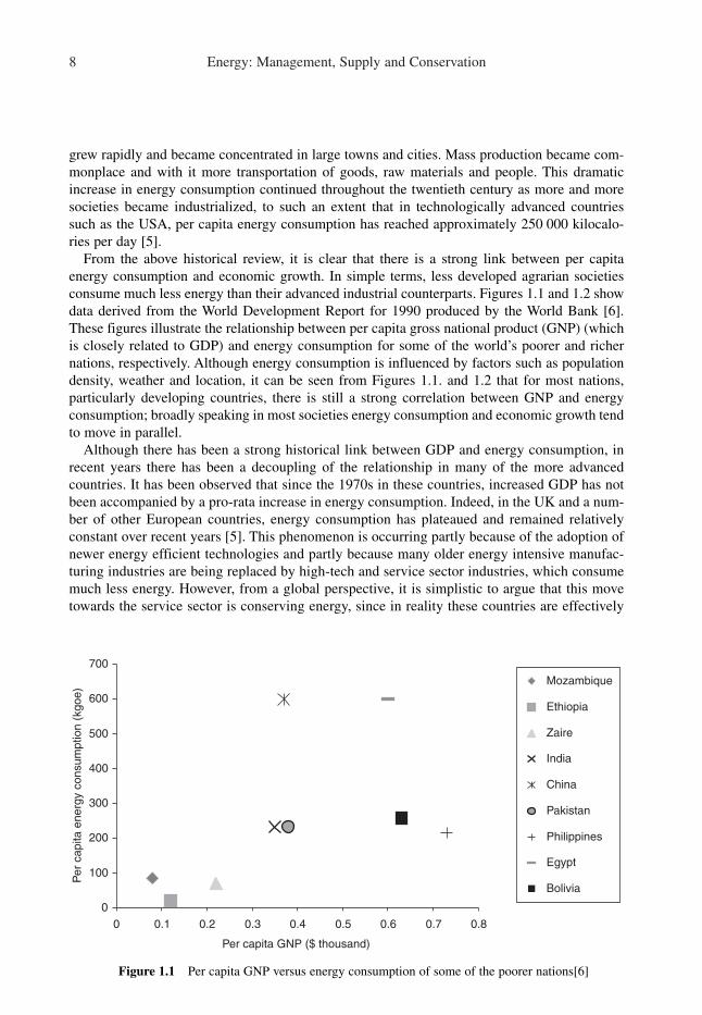
From the above historical review, it is clear that there is a strong link between per capita
energy consumption and economic growth. In simple terms, less developed agrarian societies
consume much less energy than their advanced industrial counterparts. Figures 1.1 and 1.2 show
data derived from the World Development Report for 1990 produced by the World Bank [6].
These figures illustrate the relationship between per capita gross national product (GNP) (which
is closely related to GDP) and energy consumption for some of the world’s poorer and richer
nations, respectively. Although energy consumption is influenced by factors such as population
density, weather and location, it can be seen from Figures 1.1. and 1.2 that for most nations,
particularly developing countries, there is still a strong correlation between GNP and energy
consumption; broadly speaking in most societies energy consumption and economic growth tend
to move in parallel.
Although there has been a strong historical link between GDP and energy consumption, in
recent years there has been a decoupling of the relationship in many of the more advanced
countries. It has been observed that since the 1970s in these countries, increased GDP has not
been accompanied by a pro-rata increase in energy consumption. Indeed, in the UK and a num-
ber of other European countries, energy consumption has plateaued and remained relatively
constant over recent years [5]. This phenomenon is occurring partly because of the adoption of
newer energy efficient technologies and partly because many older energy intensive manufac-
turing industries are being replaced by high-tech and service sector industries, which consume
much less energy. However, from a global perspective, it is simplistic to argue that this move
towards the service sector is conserving energy, since in reality these countries are effectively
0
100
200
300
400
500
600
700
0 0.1 0.2 0.3 0.4 0.5 0.6 0.7 0.8
Per capita GNP ($ thousand)
Per
capita e
nerg
y c
onsum
ption (
kgoe)
Mozambique
Ethiopia
Zaire
India
China
Pakistan
Philippines
Egypt
Bolivia
Figure 1.1 Per capita GNP versus energy consumption of some of the poorer nations[6]

Energy and the environment 9
exporting their manufacturing and heavy industry requirements to other parts of the world
where wage costs are lower. Indeed, there is evidence that many advanced ‘consumer’ nations
are simply exporting their ‘dirty’ energy intensive industries to countries in which environ-
mental legislation is much weaker, with the result that in gross terms environmental pollution
is increasing.
The ratio of energy used to GDP is known as the energy intensity of an economy. It is a
measure of the output of an economy compared with its energy inputs, in effect a measure of the
efficiency with which energy is used. Manufacturing nations, with old or relatively poor
infrastructures, like many of the East European and former Soviet Union (FSU) countries, often
exhibit very high energy intensities, while the more energy efficient ‘post-industrialized’ nations
have much lower intensities. The link between infrastructure and energy intensity is very strong
indeed [7]. In developing countries, development of an infrastructure leads to growth in energy
intensive manufacturing industries. In industrialized economies, energy intensity is strongly
influenced by the efficiency of the infrastructure and capital stock such as power stations, motor
vehicles, manufacturing facilities and end-user appliances. The energy efficiency of capital stock
is, in turn, influenced by the price of energy relative to the cost of labour and the cost of
borrowing capital. If energy costs are high in relation to these other costs, then it is much more
likely that investments will be made in energy-efficient technologies. Conversely, if energy
prices are low, then little incentive exists for investment, or indeed research, in more energy
efficient technologies [7].
While energy intensity is strongly influenced by the price of energy, it is also affected by
factors which are not directly attributable to price effects. For example, changes in technology
and changes in the composition of world trade can influence energy intensity. Geographical
location has a strong influence; cold northerly countries tend to exhibit high energy intensities.
Other factors include changes in fashion and preferences. For example, if the practice of cycling
to work becomes popular with enough people, then it is possible that this will influence the
energy intensity of an economy. In short, there are many factors which influence energy
intensity.
0
2000
4000
6000
8000
10000
12000
0 5 10 15 20 25 30 35
Per capita GNP ($ thousand)
Per
capita e
nerg
y c
onsum
ption (
kgoe) Brazil
Mexico
Hungary
Greece
United Kingdom
Japan
Canada
United States
Switzerland
Figure 1.2 Per capita GNP versus energy consumption of some of the richer nations[6]

1.5 Environmental issues
A full examination of the environmental problems facing the Earth, although very interesting, is
well beyond the scope of this book. However, because environmental considerations, in particu-
lar the perceived threat of global warming, are influential in shaping the energy policy of many
countries, it is essential that the issue be discussed in some detail. It is the perceived threat of
climate change, above any other issue, which is changing the attitudes towards energy
consumption. Although there is much scientific debate on the precise nature and extent of the
twin threats of global warming and ozone depletion, the fact remains that these threats, whether
actual or imaginary, are perceived by many governments to be real, with the result that both
national and international energy policies are now being driven by an environmental agenda. It
is important to have an understanding of pertinent environmental issues. Ignorance of the
facts relating to environmental issues is surprisingly widespread amongst politicians, profes-
sionals and the public at large. Concepts such as global warming and ozone depletion are often
confused and interchanged. Indeed, some individuals committed to environmentally green
lifestyles exhibit very woolly thinking when it comes to the science of the environment. This
section is, therefore, written with the sole intent of presenting the relevant facts and explaining
the pertinent issues relating to global warming and ozone depletion.
1.5.1 Global warming
There is growing scientific evidence that greenhouse gas emissions caused by human activity are
having an effect on the Earth’s climate. The evidence suggests that the Earth’s climate has
warmed by almost 0.7 °C since the end of the nineteenth century [8], and that the pace of this
warming is increasing. Globally, the 1990s were the warmest years on record, with seven of the
ten warmest years being recorded in that decade [8, 9]. Indeed, in 1998 the global temperature
was the highest since 1860 [8] and was the twentieth consecutive year with an above normal
global surface temperature [8]. Figure 1.3 illustrates the steady rise in global temperature.
10 Energy: Management, Supply and Conservation
1995
1990
1985
1980
1975
1970
1965
1960
1955
1950
1945
1940
1935
1930
1925
1920
1915
1910
1905
1900
1895
1890
1885
1880
–0.5
–0.4
–0.3
–0.2
–0.1
0
0.1
0.2
0.3
0.4
0.5
5 y
ear
mean g
lobal te
mpera
ture
(°C
)
Figure 1.3 Global mean temperature change[9]

Energy and the environment 11
It is generally accepted that the rapid rise in global temperature experienced during the latter
part of the twentieth century is due, in part, to atmospheric pollution arising from human activity,
which is accelerating the Earth’s greenhouse effect. The greenhouse effect is a natural phenom-
enon which is essential for preserving the ‘warmth’ of the planet. It is caused by trace gases in
the upper atmosphere trapping long-wave infrared radiation emitted from the Earth’s surface.
The Earth’s atmosphere allows short-wave solar radiation to pass relatively unimpeded.
However, the long-wave radiation produced by the warm surface of the Earth is partially
absorbed and then re-emitted downwards by greenhouse gases in the atmosphere. In this way an
energy balance is set up, which ensures that the Earth is warmer than it would otherwise be.
Without the greenhouse effect it is estimated that the Earth’s surface would be approximately
33 °C cooler [10], and almost uninhabitable. Although the greenhouse effect is essential to the
well being of human populations, if greenhouse gas levels rise above their natural norm, the
consequent additional warming could threaten the sustainability of the planet as a whole.
The main naturally occurring greenhouse gases in the Earth’s atmosphere are water vapour
and CO2. Of these, it is water vapour which has the greatest greenhouse action. While CO2
concentrations are strongly influenced by human activity, atmospheric water vapour is almost
entirely determined by climatic conditions and not human action. Human activity is responsible
for production of a number of other potent greenhouse gases, including methane, nitrous oxide,
chlorofluorocarbons (CFCs) and hydrochlorofluorocarbons (HCFCs). From the late eighteenth
century onwards, concentrations of ‘man-made’ greenhouse gases (with the exception of CFCs
and HCFCs, which were first introduced in the 1930s) have steadily increased. Table 1.2 shows
the pre-industrial and 1990 levels of various greenhouse gases. For each gas it can be seen that
there has been a substantial rise in the atmospheric concentration. For example, CO2 concentra-
tions have grown from 280 ppm in the middle of the eighteenth century, to approximately 353
ppm in 1990: a rise of about 26%, leading to a current rate of increase of about 0.5% a year [10].
Indeed, the Intergovernmental Panel on Climate Change (IPCC) forecast that a likely doubling
of atmospheric CO2 will occur by 2050, leading to an average global temperature increase of
between 1.5 °C and 4.5 °C [10, 11].
Although CO2 is the single ‘man-made’ gas which contributes most towards overall global
warming (i.e. in excess of 50%), it is by no means the most potent of the greenhouse gases.
Methane for example, is approximately 21 times as potent as CO2. In other words, methane has
a relative global warming potential (GWP) of 21 compared with that of CO2, which is 1.
Incredibly, CFC-11 has a GWP of approximately 3500 and CFC-12 has a GWP of approximately
7300 [10], making CFCs the most potent of greenhouse gases. CFCs were first introduced in the
1930s and were widely used as refrigerants, solvents and aerosol propellants, until they were
Table 1.2 Contribution to global warming of various gases [12]
Carbondioxide
equivalent Pre-1800 1990 GrowthGreenhouse per concen- Concen- rate Atmosphericgas molecule tration tration (%/year) life (years)
Carbon dioxide 1 280 ppmv 353 ppmv 0.50 50–200
Methane 21 0.8 ppmv 1.72 ppmv 0.90 10
CFC 12 7300 0.0 ppmv 484 pptv 4.00 130
CFC 11 3500 0.0 ppmv 280 pptv 4.00 65
Nitrous oxide 290 288 ppbv 310 ppbv 0.25 150

withdrawn in the mid-1990s. They are very stable and remain in the upper atmosphere for
considerable periods of time, as much as 130 years in the case of CFC-12 [10]. Given that they
are also potent ozone depletors, it is not surprising that the control and elimination of CFCs
became one of the major environmental targets in the 1990s.
The extent to which global warming is likely to occur as a result of the build-up of greenhouse
gases is a matter of much scientific debate. The Hadley Centre of the UK Meteorological Office
predicts that, under the ‘business as usual’ scenario, the world’s climate will warm by about 3 °C
over the next 100 years [12], which is in keeping with the IPCC’s forecast of a 1.5 °C to 4.5 °C
rise by 2050 [10]. Although there is general agreement that climate change is the most serious
environmental threat facing the world today, the precise nature of this ‘climate change’ is open
to debate. It is predicted that as global warming progresses, sea levels will rise by over 400 mm
by 2080 [12] due to the combined effects of thermal expansion of the oceans and melting of polar
ice. This will put the lives of millions of people at risk, with an additional 80 million people par-
ticularly threatened with flooding in the low lying parts of southern and South-East Asia [12]. It
is probable that droughts will occur due to increased temperatures and that Africa, the Middle
East and India will all experience significant reductions in cereal crop yields [12]. Increased
drought will mean that by 2080 an additional 3 billion people could suffer increased water stress,
with Northern Africa, the Middle East and the Indian subcontinent expected to be the worst
affected [12]. It is ironic that it will be the poorest countries, often ones which have contributed
the least to global warming, which are most likely to be vulnerable to the effects of climate
change.
1.5.2 Carbon intensity of energy supply
Carbon intensity is a measure of the amount of CO2 that is released into the atmosphere for every
unit of energy produced. As such it is wholly dependent on the type of fuel used. For example,
electricity produced from nuclear power plants produces no CO2 emissions, whereas that
produced from coal-fired power station has a high carbon intensity. Table 1.3 shows the relative
carbon intensities for electricity produced from a variety of fuels.
While renewable energy sources such as wind, solar, and hydropower emit no CO2, the carbon
content of fossil fuels varies greatly. It can be seen from Table 1.3 that electricity produced in a
typical coal-fired power station produces approximately 2.4 times as much CO2 as that produced
by a combined cycle gas turbine (CCGT) plant [13]. Indeed, it has been demonstrated that the
carbon intensity of delivered mains electricity is not constant, but varies considerably with time and
with the generation plant mix [14]. For example, in England and Wales, carbon intensity is at its
lowest during the nighttime in summer, when the bulk of the power is produced from nuclear energy.
12 Energy: Management, Supply and Conservation
Table 1.3 CO2 emissions per kWh of delivered electrical energy (compiled from Building Research
Establishment data) [11]
Average Kg of CO2 Kg of CO2 perKg of CO2 gross per GJ kWh ofper GJ of efficiency of delivered delivered primary of electrical electrical
Primary energy power plant energy energy fuel (kg/GJ) (%) (kg/GJ) (kg/kWh)Coal 90.7 35 259.1 0.93
Oil 69.3 32 216.6 0.78
Gas (CCGT) 49.5 46 107.6 0.39

It is possible to achieve significant reductions in carbon intensity simply by switching from a fuel
such as coal, which has a high carbon intensity, to one with a much lower intensity, such as natu-
ral gas. This is in fact what happened in the UK during the 1990s when there was a massive switch
from coal to natural gas as the fuel of choice for electricity generation.
Because carbon intensity is wholly dependent on the type of fuel used, it differs across regions
and also over time. During the 1990s coal became less important as a source of energy in western
Europe, with the shutting down of lignite production in Germany and of hard coal production in
the UK [7]. For example, in England and Wales the switch from coal to natural gas which accom-
panied deregulation of the electricity supply industry meant that coal consumption dropped from
65 million tonnes of oil equivalent (mtoe) in 1989 to only 35.6 mtoe in 1999 [2]. This has resulted
in a 45% decrease in the UK’s carbon intensity from 1980 to 1998 [15]. By contrast in the USA
during the 1990s the electricity generators continued to use coal extensively and as a result the
carbon intensity for western Europe has dropped below that of North America in recent years [7].
1.5.3 Carbon dioxide emissions
It has been estimated that global CO2 emissions will reach approximately 9.8 billion tonnes per
annum by 2020 – 70% above 1990 levels [3]. In the industrialized world it is predicted that CO2
emissions will increase from a 1990 level of 2.9 billion tonnes to 3.9 billion tonnes in 2020
(see Figure 1.4) [3]. Emissions are, however, predicted to grow at a slower rate than primary
energy consumption, mainly because of growth in the use of natural gas relative to coal in the
developed world. However, in the industrialized countries oil is predicted to remain the domi-
nant source of CO2 emissions because of increased automobile use.
In 1990 emissions from the developed countries were approximately twice as much as those
of the developing world [3]. By 2010 it is predicted that CO2 emissions in the developing
countries will surpass those of the industrialized countries (see Figure 1.4) [3]. The rapid growth
in CO2 emissions from the developing world is predicted because high rates of economic growth
are anticipated and also because of the heavy dependence on coal in the developing Asian
Energy and the environment 13
0
50
100
150
Carb
on d
ioxid
e (
bill
ion tonnes)
200
250
300
350
400
450
1970 1980 1990 2000 2010 2020
Industrialized
Eastern Europe andFormer Soviet Union
Developing
Figure 1.4 World carbon dioxide emissions by region[3]

countries. Predictions indicate that China and India alone will account for the majority of the
worldwide increase in coal consumption by 2020 [3].
1.5.4 Depletion of the ozone layer
Ozone (O3) in the Earth’s stratosphere performs the vital function of protecting the surface of the
planet from ultraviolet (UV) radiation which would otherwise be extremely harmful to human
and animal life. The stratosphere is a layer approximately 35 km thick which has its lower limit
at an altitude of 8–16 km. Ozone is produced in the stratosphere by the absorption of solar UV
radiation by oxygen molecules (O2) to produce ozone through a series of complex photochemi-
cal reactions [16]. The ozone produced absorbs both incoming solar UV radiation and also out-
going terrestrial long-wave radiation. In doing so, the ozone in the stratosphere is converted back
to oxygen. The process is, therefore, both continuous and transient, with ozone continually being
created and destroyed. The process is dependent on the amount of solar radiation incident on the
Earth; consequently, ozone levels in the stratosphere are strongly influenced by factors such as
altitude, latitude and season.
In the late 1970s a ‘hole’ was first discovered in the ozone layer above Antarctica [17].
Observations over a number of decades reveal that each September and October up to 60% of
the total ozone above Antarctica is depleted [17]. In addition, progressive thinning of stratos-
pheric ozone in both the northern and the southern hemispheres has been observed, with record
low global ozone levels being recorded in 1992 and 1993 [17]. The average ozone loss across
the globe has totalled about 5% since the mid-1960s, with the greatest losses occurring each year
in the winter and spring [17]. This degradation of the ozone layer has resulted in higher levels of
UV radiation reaching the Earth’s surface. Increased UV radiation in turn leads to a greater inci-
dence of skin cancer, cataracts, and impaired immune systems.
Blame for the recent and rapid deterioration of the ozone layer has been placed on escaping
gases such as CFCs and nitrous oxide. Until recently CFCs were widely used in many applica-
tions including aerosol propellants, refrigerants, solvents and insulation foam. CFCs, especially
CFC-11 and CFC-12, as well as being strong greenhouse gases are also potent ozone depletors.
The lifetime of CFC-11 in the stratosphere is about 65 years, while that for CFC-12 is estimat-
ed to be 130 years [10]. In recent years, intergovernmental agreements, particularly the Montreal
Protocol (1987), have phased out the production and use of CFCs. However CFCs are very long
lived in the stratosphere and hence any reduction in CFC release will have little effect in the
near future. The phasing out of CFCs has caused a greater reliance on HCFCs, in particular
HCFC-22, which although much more ozone friendly is still a potent greenhouse gas. Under
the Montreal Protocol HCFC-22 is being phased out and as a result the chemical companies are
developing new generations of ozone ‘friendly’ refrigerants. Ozone depletion has caused many
designers of buildings in Europe to question the need for vapour compression refrigeration
machines to air condition buildings, with the result that alternative passive ventilation strategies
are now being adopted in many new buildings (see Chapter 13).
1.5.5 Intergovernmental action
In the 1980s governments around the world became aware of some of the environmental prob-
lems associated with atmospheric pollution and the first in a series of intergovernmental sum-
mits was held in a concerted effort to combat the perceived problems. In many ways the
Montreal Protocol, signed in September 1987, marks a turning point in global environmental
policy. The leading industrialized nations signed the Montreal Protocol in September 1987,
with the aim of limiting emissions of certain ozone depleting gases, such as CFCs (i.e. CFC-11,
14 Energy: Management, Supply and Conservation

CFC-12, CFC-113, CFC-114 and CFC-115) and halons (i.e. Halon 1211, Halon 1301 and Halon
2402). The original intention of the Protocol was to reduce consumption of these ozone degrad-
ing gases by 50% below the 1986 level by 1999 [16]. Since its original signing the Protocol has
been reviewed regularly and such has been the concern about ozone depletion that the Protocol
was expanded to cover HCFCs (i.e. HCFC-141b, HCFC-142b and HCFC-22) and the phase out
schedule was also accelerated. In 1992, the parties to the Protocol agreed to accelerate the 100%
phase out of CFCs, carbon tetrachloride, and methyl chloroform to the end of 1995 and halons
to the end of 1993 [18]. The parties to the Protocol also agreed to phase out HCFCs so that a
90% reduction in production would be achieved by 2010 and a complete phase out by 2030 [19].
Having made a concerted effort to tackle the problem of ozone depletion the world’s leading
industrialized nations then turned their attention to the problem of global warming. Through a
series of summits, notably Rio in 1992 and Kyoto in 1997, the nations formulated an interna-
tional framework for reducing global CO2 and other greenhouse gas emissions. At the Kyoto
conference in December 1997, attended by 160 countries, the so-called ‘Annex I’ countries
(which included the USA, Canada, the European Union (EU) countries, Japan, Australia, and
New Zealand) agreed to reduce their emissions of six greenhouse gases (i.e. CO2, nitrous oxide,
methane, hydrofluorocarbon gases (HFCs), perfluorocarbons (PFCs) and sulphur hexafluoride)
by at least 5% compared with 1990 levels between 2008 and 2012 [20]. However, the EU aims
to reduce its emissions of the main six greenhouse gases (from 1990 levels) by 8% by 2012 [21,
22]. In order to meet this target the EU member states have taken various steps, including
tightening building regulations and the introduction of carbon taxes.
1.5.6 Carbon credits and taxes
In order to meet their obligations under the Kyoto agreement a number of countries, notably The
Netherlands, Sweden, Finland, Norway, Denmark and the UK have introduced ‘carbon taxes’.
These taxes are designed to penalize high carbon intensity energy consumption and promote the
use of renewable energy sources. For example, the UK introduced its Climate Change Levy in
2001 with the express intention of increasing the share of its electricity generated by renewables
from 2% to 10% by 2010 [15]. Nevertheless, many economists are sceptical about the use of
carbon taxes, preferring instead a system of tradable emission permits. Under the Kyoto
Protocol, flexibility was introduced into the agreement through ‘Kyoto mechanisms’ which
allow countries to partake in emissions trading. It is argued that tradable permits are superior to
carbon taxes, because unlike carbon taxes, they are a form of rationing which should ensure that
targets are achieved. Permits are also more applicable to the international nature of the problem,
since a regime of international carbon taxes would be extremely difficult to enforce.
The concept of trading in greenhouse gas emissions may seem very strange to many, so
perhaps an analogy would be helpful at this point. Consider the case of a home-owner who
wakes up one morning to find that a pipe has burst and that a flood has occurred [23]. Imagine
also that this particular home-owner runs a profitable law firm and is also very good at mending
burst pipes. The homeowner is, therefore, faced with a dilemma. He can take a day off work to
mend the pipe, or alternatively, he can employ a professional plumber to repair the damaged
pipe. If the home-owner repairs the pipe, then a day’s fees will be lost; it is a much cheaper
option to employ a plumber. Realizing this, the homeowner opts for the financially expedient
solution and employs the plumber. As a result both parties benefit from the transaction; the
plumber gets paid a fee and the lawyer is able to earn more money in court. This analogy is very
similar to trading greenhouse gas emission permits, insomuch as those parties buying emission
permits or credits are actually paying someone else to reduce greenhouse gas emissions who can
Energy and the environment 15
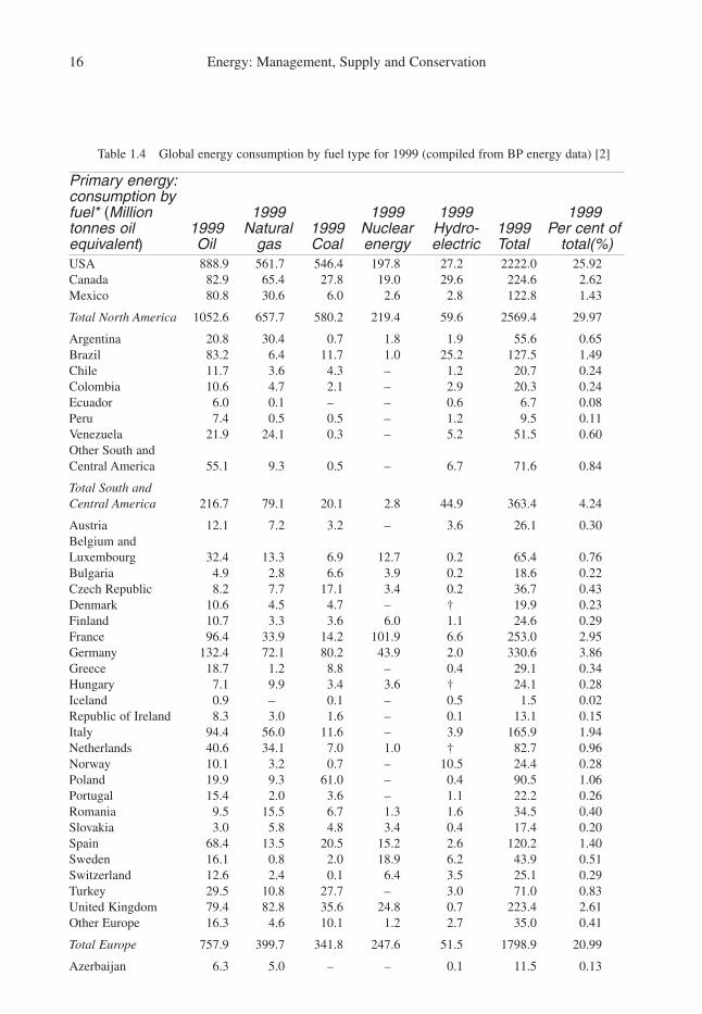
16 Energy: Management, Supply and Conservation
Table 1.4 Global energy consumption by fuel type for 1999 (compiled from BP energy data) [2]
Primary energy:consumption by fuel* (Million 1999 1999 1999 1999tonnes oil 1999 Natural 1999 Nuclear Hydro- 1999 Per cent ofequivalent) Oil gas Coal energy electric Total total(%)
USA 888.9 561.7 546.4 197.8 27.2 2222.0 25.92
Canada 82.9 65.4 27.8 19.0 29.6 224.6 2.62
Mexico 80.8 30.6 6.0 2.6 2.8 122.8 1.43
Total North America 1052.6 657.7 580.2 219.4 59.6 2569.4 29.97
Argentina 20.8 30.4 0.7 1.8 1.9 55.6 0.65
Brazil 83.2 6.4 11.7 1.0 25.2 127.5 1.49
Chile 11.7 3.6 4.3 – 1.2 20.7 0.24
Colombia 10.6 4.7 2.1 – 2.9 20.3 0.24
Ecuador 6.0 0.1 – – 0.6 6.7 0.08
Peru 7.4 0.5 0.5 – 1.2 9.5 0.11
Venezuela 21.9 24.1 0.3 – 5.2 51.5 0.60
Other South and
Central America 55.1 9.3 0.5 – 6.7 71.6 0.84
Total South and
Central America 216.7 79.1 20.1 2.8 44.9 363.4 4.24
Austria 12.1 7.2 3.2 – 3.6 26.1 0.30
Belgium and
Luxembourg 32.4 13.3 6.9 12.7 0.2 65.4 0.76
Bulgaria 4.9 2.8 6.6 3.9 0.2 18.6 0.22
Czech Republic 8.2 7.7 17.1 3.4 0.2 36.7 0.43
Denmark 10.6 4.5 4.7 – † 19.9 0.23
Finland 10.7 3.3 3.6 6.0 1.1 24.6 0.29
France 96.4 33.9 14.2 101.9 6.6 253.0 2.95
Germany 132.4 72.1 80.2 43.9 2.0 330.6 3.86
Greece 18.7 1.2 8.8 – 0.4 29.1 0.34
Hungary 7.1 9.9 3.4 3.6 † 24.1 0.28
Iceland 0.9 – 0.1 – 0.5 1.5 0.02
Republic of Ireland 8.3 3.0 1.6 – 0.1 13.1 0.15
Italy 94.4 56.0 11.6 – 3.9 165.9 1.94
Netherlands 40.6 34.1 7.0 1.0 † 82.7 0.96
Norway 10.1 3.2 0.7 – 10.5 24.4 0.28
Poland 19.9 9.3 61.0 – 0.4 90.5 1.06
Portugal 15.4 2.0 3.6 – 1.1 22.2 0.26
Romania 9.5 15.5 6.7 1.3 1.6 34.5 0.40
Slovakia 3.0 5.8 4.8 3.4 0.4 17.4 0.20
Spain 68.4 13.5 20.5 15.2 2.6 120.2 1.40
Sweden 16.1 0.8 2.0 18.9 6.2 43.9 0.51
Switzerland 12.6 2.4 0.1 6.4 3.5 25.1 0.29
Turkey 29.5 10.8 27.7 – 3.0 71.0 0.83
United Kingdom 79.4 82.8 35.6 24.8 0.7 223.4 2.61
Other Europe 16.3 4.6 10.1 1.2 2.7 35.0 0.41
Total Europe 757.9 399.7 341.8 247.6 51.5 1798.9 20.99
Azerbaijan 6.3 5.0 – – 0.1 11.5 0.13

Energy and the environment 17
Belarus 6.1 13.8 0.1 – † 20.0 0.23
Kazakhstan 6.0 7.1 19.8 – 0.6 33.6 0.39
Lithuania 3.1 2.2 0.1 2.5 0.1 8.0 0.09
Russian Federation 126.2 326.4 109.4 30.9 13.8 606.8 7.08
Turkmenistan 4.5 10.2 – – – 14.7 0.17
Ukraine 13.3 63.6 38.5 18.6 1.0 135.0 1.57
Uzbekistan 7.1 44.3 1.8 – 0.6 53.8 0.63
Other Former
Soviet Union 4.7 7.1 1.0 0.6 3.1 16.4 0.19
Total former
Soviet Union 177.3 479.7 170.7 52.6 19.3 899.8 10.50
Iran 58.4 49.5 1.0 – 0.4 109.3 1.28
Kuwait 8.6 7.8 – – – 16.4 0.19
Qatar 1.1 14.3 – – – 15.4 0.18
Saudi Arabia 60.9 41.6 – – – 102.5 1.20
United Arab Emirates 13.0 28.3 – – – 41.3 0.48
Other Middle East 65.0 19.1 5.7 – 0.3 90.1 1.05
Total Middle East 207.0 160.6 6.7 – 0.7 375 4.37
Algeria 8.1 20.0 0.3 – † 28.4 0.33
Egypt 27.8 12.9 0.9 – 1.1 42.7 0.50
South Africa 21.8 – 82.1 3.5 0.3 107.7 1.26
Other Africa 58.2 14.0 6.8 – 4.9 83.9 0.98
Total Africa 115.9 46.9 90.1 3.5 6.3 262.7 3.06
Australia 38.0 17.8 45.5 – 1.5 102.8 1.20
Bangladesh 3.2 7.5 0.2 – 0.1 10.8 0.13
China 207.2 19.3 512.7 3.8 16.8 759.7 8.86
China Hong
Kong SAR 9.3 2.4 3.9 – – 15.6 0.18
India 95.2 21.4 154.5 3.3 7.1 281.5 3.28
Indonesia 46.8 24.8 10.5 – 0.8 82.9 0.97
Japan 257.3 67.1 91.5 82.0 8.0 505.9 5.90
Malaysia 20.3 17.1 1.2 – 0.4 39.0 0.45
New Zealand 6.3 4.7 1.2 – 2.0 14.1 0.16
Pakistan 18.2 15.6 2.1 † 1.8 37.7 0.44
Philippines 18 † 2.9 – 0.7 21.6 0.25
Singapore 28.3 1.4 – – – 29.6 0.35
South Korea 99.7 16.8 38.2 26.6 0.5 181.9 2.12
Taiwan 39.9 5.6 24.9 9.9 0.8 81.1 0.95
Thailand 35.4 15.6 7.9 – 0.3 59.2 0.69
Other Asia Pacific 18.6 4.4 53.1 – 3.5 79.6 0.93
Total Asia Pacific 941.7 241.5 950.3 125.6 44.3 2303 26.87
Total world 3469.1 2065.2 2159.9 651.5 226.6 8572.2 100.00
Of which: OECD 2178.1 1135.1 1070.2 565.8 118.2 5067.5 59.12
European Union 15 635.9 327.7 203.5 224.4 28.5 1420.1 16.57
Other EMEs‡ 1079.8 421.7 890.8 23.3 84.2 2499.4 29.16* In this Table, primary energy comprises commercially traded fuels only.
† Less than 0.05.
‡ Excludes Central Europe and Former Soviet Union.

18 Energy: Management, Supply and Conservation
do it more cheaply than they can themselves. However, in order for a trading scheme to work
there must be something forcing the participants to make emission reductions, in much the same
way that the home-owner was forced to act because the burst pipe would have created a
considerable amount of damage if left unattended. Therefore, at the heart of any trading scheme
there must be an obligation on the part of the participants to achieve greenhouse gas emission
reductions; the obligations under the Kyoto Protocol are forcing countries to reduce greenhouse
gas emissions. However, it does not matter geographically where these reductions are made. It
is, therefore, possible for participating companies to trade all or part of their obligation without
any detrimental environmental effects. This can be achieved by issuing permits which allow the
holder to emit a given quantity of greenhouse gas.
The rules for any emissions trading system have yet to be fully worked out and there are many
difficult international problems which must be solved, not least technical issues associated with
the administration, verification and enforcement of such a scheme. One possible way in which
such a scheme might work would be to allow permit holders to sell some of their ‘excess capac-
ity’. For example, in 1990 greenhouse gas emissions from many FSU countries were high.
However since the break-up of the Soviet Union there has been a severe decline in economic
activity in this region with the result that by 2000 emission levels were much lower than those in
1990. Under the Kyoto Protocol Russia and Ukraine are required to stabilize greenhouse gas
emissions at a 100% of their 1990 emission levels. It is predicted that by 2010 in these countries
emissions levels will still be below 1990 levels. Consequently, these countries would have a
considerable block of surplus permits to sell. Western European countries might find it cost effec-
tive to purchase some of the ‘excess capacity’ in the FSU countries rather than reduce their own
CO2 emissions. Alternatively, countries with high labour and infrastructure costs could invest in
emission reducing activities in countries with lower costs and claim emission reduction credits for
themselves, thus offsetting their ‘overseas’ activities against their own emission reduction targets.
One possible advantage of tradable emissions permits is that they can be rationed. Permits
could be issued which would give the parties involved in the scheme the right to emit at their
1990 emissions levels for free. If every year a proportion of permits were to be withdrawn and
then sold either by direct sale or by auction, incentives would be created for the participants in
the scheme to reduce emissions. Also, if permits were tradable and banking was to be permitted
then a market would be created. However, it is essential that a single, central authority be created
which could control the system and fine parties who exceeded their quotas.
1.6 Energy consumption
Global energy consumption data for 1999 is presented in Table 1.4 (see pages 16–17). These data
give a detailed breakdown of energy consumption on a country-by-country and fuel-by-fuel
basis. It can be seen from Table 1.4 that in 1999 global energy consumption was approximately
8572 mtoe. Of this total approximately 25.9% was consumed in the USA, 16.6% in the EU and
10.5% in the FSU countries. Indeed, 59.1% of all global energy consumption occurred in the
OECD countries. This demonstrates that currently the major part of global energy consumption
takes place in industrialized countries.
The fuel mix and hence the carbon intensity varies greatly from region to region. In the USA,
for example, the ratio of coal to natural gas consumption is 1:1.03, whereas in the UK the ratio
is 1:2.33, while in China the ratio is only 1:0.04 and in India it is 1:0.14. These figures reflect
the fact that, firstly in the UK during the 1990s there has been a trend away from coal and
towards natural gas, and secondly there is a heavy reliance on coal in China and India.

The Energy Information Administration (EIA) in the USA predicts that in the twenty-first
century there will be substantial increases in energy demand, based mostly on fossil fuels [3].
This is expected to occur mainly because of economic growth in the developing economies of
Asia and South America. In developing countries, energy and economic growth tend to move in
parallel. Economic development is an energy intensive process which ultimately raises living
standards and facilitates broad access to electricity and motorized transportation. Economic
development of the infrastructure also causes growth in energy intensive manufacturing indus-
tries. In contrast to the developing countries, in advanced industrialized countries the link
between economic growth and energy consumption is relatively weak, with energy demand
growth lagging behind economic growth. In advanced economies per capita energy use tends to
be relatively stable, with old energy intensive appliances and equipment often being replaced by
newer more energy efficient equipment. Consequently it is predicted that the percentage growth
in energy demand will be considerably lower in the developed countries compared with the
developing countries.
It is predicted by the EIA that the trend towards the increased use of natural gas in the 1990s
will continue in the twenty-first century [3]. This is because natural gas is increasingly perceived
as the fuel of choice for electricity generation: it has a much lower carbon intensity than coal;
the electricity generation process is more efficient; it is free from the industrial disputes which
are often associated with coal production; and it is much cheaper and quicker to construct gas-
fired power plants. Oil demand is predicted to grow with the increased use of motorized trans-
port in developing countries.
1.7 Energy reserves
One of the major concerns of environmentalists and economists alike is the rate at which ‘pre-
cious’ fossil fuel reserves are being expended. It has been estimated that crude oil could remain
plentiful and cheap for at least 40 years [24]. This prediction ‘assumes that production volumes
will remain constant, and assumes that production rates can be maintained as reserves decline’
[24]; this is an assumption which appears optimistic given that the demand for oil should
increase with economic growth in the developing world. The EIA states:
Worldwide, oil remains the dominant source of energy throughout the projection horizon
[i.e. to 2020], as it has since 1970. Oil’s key role [is] in the transportation sector –
where it does not currently have any serious competition from other energy sources...[3]
Even if oil remains plentiful until the middle of the twenty-first century, geophysical surveys
indicate that massive new oil deposits are unlikely to be found [24]. In future new oil finds are
likely to be much smaller than those already discovered. In other words, the law of diminishing
returns is likely to apply. Consequently there will be a pressing need to find alternative sources
of fuel to replace oil as the choice of fuel for motorized transportation.
Although there is considerable debate about the global oil reserves, it is generally agreed that
conventional oil production outside the Middle East will start to decline before that of the
Middle East, implying a greater reliance on Middle Eastern oil [2]. Table 1.5 shows global
proven energy reserves at the end of 1999. From these data it can be seen that approximately
65% of proven oil reserves are located in the Middle East. It is, therefore, not surprising that as
existing supplies become depleted the rest of the world will become reliant on Middle Eastern
oil suppliers.
Energy and the environment 19

Table 1.5 Proven energy reserves by fuel type (compiled from BP energy data) [2]
Proven reserves at Oil Natural gas Coalthe end of 1999 Thousand Share Trillion Share Share
million of cubic of Million of barrels total(%) metres total(%) tonnes total(%)
Total North America 63.9 6.18 7.31 5 256477 26.10
Total South and
Central America 89.5 8.66 6.31 4.30 21574 2.20
Total Europe 20.7 2.00 5.15 3.50 122032 12.40
Total Former
Soviet Union 65.4 6.32 56.7 38.70 230178 23.40
Total Middle East 675.7 65.35 49.52 33.80 n a n a
Total Africa 74.8 7.23 11.16 7.70 61605* 6.20*
Total Asia Pacific 44.0 4.26 10.28 7.00 292345 29.70
Total World 1034.0 100.00 146.43 100.00 922606 100.00* Includes the Middle East.
20 Energy: Management, Supply and Conservation
It is likely that as global oil stocks become depleted natural gas will replace oil, since gas can
be converted into liquid fuels which can be used for automotive purposes at relatively low cost.
The EIA expects natural gas to be the fastest-growing primary energy source between 1996 and
2020 [3].
References
1. Campbell, D. (2001). Blackouts bring gloom to California. The Guardian, 19th January.
2. BP energy statistics, 2001, BP Website (www.bp.com/downloads/702/BPwebglobal.pdf)
(March 2002).
3. International Energy Outlook 1999 (IEO99) (1999). World Energy Consumption.
DOE/EIA-0484 (99).
4. Digest of United Kingdom Energy Statistics 2000 (2000). DTI.
5. Hill, R., O’Keefe, P. and Snape, C. (1995). The future of energy use. (Chapter 1), Earthscan.
6. World Development Report for 1990 produced by the World Bank.
7. International Energy Outlook 1999 (IEO99) (1999). Environmental Issues and World
Energy Use. DOE/EIA-0484 (99).
8. WMO Annual Statement on the Global Climate, 1998, WHO Website
(www.wmo.ch/web/Press/Press626.html) (March 2002).
9. NASA Goddard Institute for Space Studies, Global Temperature Trends 1998 Summation,
NASA Website (www.giss.nasa.gov/research/observe/surftemp/1998.html) (March 2002).
10. Climate change: The IPCC scientific assessment (1990). WMO/UNP Intergovernmental
panel on climate change.
11. May, R. Global Warming Needs Action (1998). Energy Exploration and Exploitation, 16(1),
93–102.
12. Department of the Environment, Transport and the Regions (2000). Climate Change: Action
to Tackle Global Warming.
13. Shorrock, L. D. and Henderson, G. (1990). Energy use in Buildings and Carbon Dioxide
Emissions. BRE Report.

14. Beggs, C. B. (1996). A method for estimating the time-of-day carbon dioxide emissions per
kWh of delivered electrical energy in England and Wales. Building Services Engineering
Research and Technology, 17(3), 127–34.
15. Energy Information Administration, DOE, USA. September 2001, EIA Website
(www.eia.doe.gov/emeu/cabs/uk.html) (March 2002).
16. Harrison, R. M. (1990). Pollution: causes, effects and control (Chapter 9). Royal Society of
Chemistry.
17. Environmental Indicators: Ozone Depletion (1996). United States Environmental Protection
Agency.
18. The Accelerated Phase out of Class I Ozone-Depleting Substances (1999). United States
Environmental Protection Agency.
19. HCFC Phase out Schedule (1998). United States Environmental Protection Agency.
20. Energy in the 21st-century: The return of geopolitics? (1999). Highlight of the OECD
Information Base, OECD, No. 17, May.
21. Greenhouse gases and climate change – Environment in EU at the turn of the century
(Chapter 3.1) (2001). European Environment Agency.
22. Svendsen, G. T. (1998). Towards a CO2 Market in the EU: the case of electric utilities.
European Environment, 8(4), 121–8.
23. Kopp, R. and Toman, M. (2001). International Emissions Trading: A Primer:
www.weathervane.rff.org/features/feature049.html. (12 July).
24. Campbell, C. J., Laherrère, J. H., George, R. L., Anderson, R. N. and Fouda, S. A. (1998).
Preventing the next oil crunch. Scientific American, 278(3), 59–77.
Bibliography
Climate change: The IPCC scientific assessment (1990). WMO/UNP Intergovernmental panel
on climate change.
Harrison, R. M. (1990). Pollution: Causes, effects and control. (Chapter 9) Royal Society of
Chemistry.
Hill, R., O’Keefe, P. and Snape, C. (1995). The future of energy use. (Chapter 1) Earthscan.
International Energy Outlook 1999 (IEO99) (1999). Environmental Issues and World Energy
Use. DOE/EIA-0484 (99).
International Energy Outlook 1999 (IEO99) (1999). World Energy Consumption. DOE/EIA-
0484 (99).
Energy and the environment 21

2
Utility companies and energy supply
Energy costs are strongly influenced by the policies of utility companies and fuel suppliers.
It is therefore important to have a good understanding of the supply side of the energy
industry. This chapter explains the fundamental issues associated with the supply of fuel and
energy, and explains how utility companies recover their costs.
2.1 Introduction
This chapter is not intended to be a text on the chemical properties of various fuels, or indeed a
work on the geographical aspects of energy supply, rather it is written from the point of view of
the end user, who may also be the energy purchaser. The aim of the chapter is to explain the ways
in which utility companies operate and also to highlight key issues which influence the supply
of fuel and energy.
When investigating the subject of energy supply it is necessary to understand the process by
which energy is delivered to the consumer. In general terms, most facilities consume one or more
of the following ‘fuels’:
• Coal
• Oil
• Natural gas
• Electricity
Natural gas and electricity are delivered to consumers by utility companies via extensive pipe
and cable infrastructures. By contrast, coal and oil are purchased on the open market and require
vehicular delivery and storage facilities. Each ‘fuel’ therefore has its own set of peculiarities and
limitations, and these strongly influence both usage and energy costs. Some fuels, such as natural
gas, are unavailable in many locations because nearby pipelines do not exist. Other fuels, such
as coal and oil, are perceived as dirty and difficult to handle, and also require considerable
storage space. Since all these factors influence energy costs, it is important to be familiar with
the costs associated with each type of fuel. Fuel and energy costs can be categorized as:
• Direct costs associated with the purchase of the ‘fuel’;
• Indirect cost associated with the use of the ‘fuel’; and
• Indirect environmental costs.

Utility companies and energy supply 23
Direct fuel costs are those costs specifically associated with the purchase of the fuel, such as unit
energy charges and standing charges, and indirect costs are those costs associated with the
storage and handling of fuels such as coal and oil. Indirect environmental costs also exist, but the
end user does not always perceive their existence. Environmental costs can take an obvious form,
such as an environmental tax on fossil fuel consumption (see Chapter 1). However, it is more
often the case that environmental costs are absorbed and disguised within other costs. For
example, if an electricity company is required to invest in expensive desulphurization equipment
to clean up its generating plant, it will probably pass this environmental related cost on to its
customers in the form of higher energy prices.
2.2 Primary energy
Three fuels, oil, coal and natural gas dominate the world’s primary energy market. In 1999, 40.6%
of the world’s primary energy came from oil, 25.0% from coal, 24.2% from natural gas, 2.7% from
hydro-electricity and 7.6% from nuclear power [1]. Although oil is currently the principal source
of the world’s energy, consumption is outstripping supply and known oil reserves are dwindling. It
has been estimated that at current rates of consumption, cheap available oil supplies will be
exhausted in approximately 40 years time [2]. However, unlike oil, the Earth’s coal reserves are in
a much healthier state, with worldwide reserves of anthracite and bituminous coal alone exceeding
200 times annual coal consumption [1]. One might therefore assume that coal could fill the
‘vacuum’ which will be created as oil reserves diminish. This however is a simplistic assumption,
since oil is primarily used in the transport sector and coal, unless synthesized, is unsuitable for this
purpose. Also, coal is perceived as being environmentally unfriendly, producing large quantities of
carbon dioxide (CO2) and sulphur dioxide (SO2) when burnt. By contrast natural gas is clean when
burnt and is relatively easily to handle. Consequently, worldwide natural gas consumption is
increasing. For example, in the UK, natural gas consumption rose from 52.4 billion cubic metres
in 1990 to 92.0 billion cubic metres in 1999 [1]. The expansion in the natural gas sector in the UK
was mainly due to the construction of a large number of new combined-cycle gas turbine power
stations in the 1990s. The rise in the UK’s gas consumption was matched by a steep decline in its
coal consumption, which was only 35.6 mtoe in 1999, compared with 64.9 mtoe in 1990 [1]. This
scenario has been matched elsewhere in Europe. In France, for example, coal production fell by
59.0% from 1990 to 1999 [1] and in Germany the corresponding fall was 51.3% [1].
In terms of global energy consumption, natural gas is the fastest growing primary fuel. This is
primarily because natural gas reserves are large and the cost of production is relatively low. In
the FSU countries alone, proven gas reserves are 56.7 trillion cubic metres [1999 data], enough
to supply their own, together with the whole of Europe’s, requirements for at least 50 years [1].
One important attribute of natural gas is that it is very clean compared with more carbon inten-
sive fuels such as oil and coal. Following the 1997 Kyoto agreement many nations have sought
to reduce the CO2 emissions by increased utilization of natural gas. It is also a more manageable
fuel than coal, which has to be mined and involves expensive handling. Consequently, in many
parts of the world electricity companies are turning away from coal and switching to natural gas.
One added bonus to the generating companies is that gas fired power stations are not prone to
industrial action by miners, as coal fired stations are.
2.3 Delivered energy
It is important to appreciate the difference between primary energy and delivered energy. For
example, natural gas is a primary fuel which can be burnt in a power station to produce electricity

24 Energy: Management, Supply and Conservation
(i.e. a ‘secondary’ fuel) or instead piped straight to the consumer as a primary fuel. By contrast,
electricity is always a ‘secondary’ fuel, which is produced from a primary source, often by a very
inefficient conversion process. Therefore for every unit (i.e. kWh) of electricity which is
delivered to a property, several units of primary energy must be consumed.
The price paid by the consumer for energy usually reflects closely the cost of its production and
its general availability. Consider the case of electricity produced from natural gas in a combined-
cycle power station, with thermal efficiency of 47%. It is not difficult to see that the cost to the
utility company of producing the electricity must be over twice the cost of the natural gas. Indeed,
when all the other maintenance, transportation and management costs are factored in, then the
cost of the delivered electricity will much higher. In fact, in the UK the unit price of electricity is
generally three to five times the price of natural gas, depending on the type of consumer.
2.4 Electricity supply
Consider the generic model of an electricity supply network shown in Figure 2.1. The saleable
commodity, electricity, is generated in power stations, from a variety of primary energy sources.
These power stations are all connected to a high voltage transmission grid, which is used to trans-
mit the electricity over long distances. At various points in the system, electricity is drawn from
the transmission grid and distributed to consumers. This involves the use of a local distribution
network which distributes the electricity at a reduced voltage, say 33 kV or 11 kV, to local sub-
stations, where the voltage is further reduced, to say 415 V, before being supplied to the consumer.
Finally, the electricity is sold to consumers and the amount consumed recorded using meters.
In broad terms, the various component parts of an electric supply industry can be categorized
as follows:
(i) The generation process: This takes place in the power stations and involves the conversion
of primary energy from fossil fuels into electricity. It is at the generating stage that all the
Power station
132 kV Distribution Grid
33 kV HeavyIndustry
11 kV LightIndustry240 V
Domestic
400 kV TransmissionGrid
Figure 2.1 A generic electricity supply network

Utility companies and energy supply 25
pollution associated with electricity production is created. Electricity generation is a
complex and costly business, which involves the construction, operation and maintenance
of large power stations and the purchase, transportation and storage of primary fuels.
Because electricity cannot be stored easily it is necessary for the generating companies to
have enough spare capacity to cope with the high peaks in demand which occur at certain
times of the year. Therefore, many smaller and less efficient power stations are rarely used
and only operate when demand on the transmission grid is high. This situation is very
uneconomic because even though these power stations are infrequently used, they still need
to be maintained. Consequently, the generating companies have to recover the cost of
maintaining inactive power stations from the electricity produced by the active ones.
(ii) The transmission process: This is the process whereby electricity is transported through a
transmission grid over long distances around a region or country. The transmission grid is
operated at a very high voltage, for example, 400 kV, in order to minimize the energy
wastage. Operating a transmission grid involves the construction and maintenance of a very
large piece of infrastructure, which may extend for thousands of miles, sometimes over very
inhospitable terrain. Naturally large costs are involved in operating such a network and these
must be recovered from the sale of any electricity which is transmitted through the grid.
(iii) The distribution process: Once electricity has been transmitted over a long distance at high
voltage, it must then be distributed to the various end users. At various points along the
transmission grid electricity will be ‘siphoned’ off into local distribution networks. These
distribution networks are regional grids, operating at a lower voltage (e.g. 132 kV and
33 kV), which distribute the electricity around a city or a particular locality. During the
distribution process the voltage of the electricity is stepped down (through the use of sub-
stations) to the voltage required by the consumers (e.g. 240 V, 415 V or 11 kV). As with the
transmission grid, the costs involved in maintaining and operating a distribution network
must be recouped from the revenue received from the electricity sold.
(iv) The sales process: The sales process is not as easy to identify as the other processes because
it does not involve any obvious hardware, but it is no less important. All utility companies
have to market their product in order to attract customers, and once customers have been
found a utility company must monitor and record all the energy that is consumed, so that
customers can be billed and the revenue collected. There are therefore considerable
administration costs associated in managing each customer’s account. These costs are
usually recovered by levying a periodic standing charge on each customer.
The relationship between the various processes in a typical electricity supply industry is shown
in Figure 2.2.
Although the processes described above are common to all electricity supply industries, the
way in which they are achieved in practice varies considerably around the globe. In some
countries all the four processes are performed by a single vertically integrated utility company,
which generates, transmits and distributes electricity, and bills its own customers. Examples of
vertically integrated utility companies exist in many parts of the USA. In other countries such
as in England and Wales a horizontal structure exists in which the various processes are frag-
mented, with a number of utility companies performing different roles within the whole supply
industry. For example in England and Wales, electricity generation is performed by a number of
competing generating companies such as National Power and PowerGen. Another independent
company, the National Grid Company which levies rental charges for using its power lines,
performs the transmission process. Finally, regional utility companies such as Yorkshire
Electricity and London Electricity purchase electricity from the national grid and distribute it to

26 Energy: Management, Supply and Conservation
their customers. They also read their customers’ meters and invoice them for the electricity
consumed. This horizontal approach can result in extremely complex trading mechanisms (see
Chapter 3). No matter how complex the structure, it is important to understand that the compo-
nent processes described above and their related costs are the same the world over. Consequently
the tariffs levied by all electricity utility companies tend to follow a similar format.
2.4.1 Electricity charges
From the discussion in Section 2.4 it can be seen that many costs are incurred in generating and
supplying electricity, and these must be recovered from the end user. They can be summarized as:
• The cost of purchasing the primary energy and converting it to electricity;
• The cost of transporting electricity around a region or country;
• The cost of distributing electricity to the customer; and
• The cost involved in meter reading, billing and managing customers’ accounts.
Because electricity cannot be stored, the size, and hence the cost, of the supporting infrastruc-
ture is governed by the maximum instantaneous load on the system and not the amount of energy
which is consumed. Consider the electricity demand profiles for 1993 for the national grid in
England and Wales presented in Figure 2.3. It can be seen from these profiles that the greatest
demand for electricity in 1993 occurred in winter, reaching a peak of 48 GW at approximately
18.00 hours on 29th November [3]. However, for most of the year the demand was considerably
less. In fact at 06.00 hours on the 1 August 1993 demand on the grid dropped to a low of approxi-
mately 16 GW. The only conclusion which can be drawn from this is that for most of the year
the transmission and distribution grids are working at a level well below their maximum capac-
ity. Although a considerable amount of generating capacity is idle for much of the year, it still
has to be maintained on stand-by, ready to be used should demand on the grid rise to a high level.
In fact, if excess capacity is not built into the system, when demand for electricity rises to a
higher level, one of two things will happen:
1 There may not be enough generating capacity to meet demand; or
2 The cables in the transmission grid may become overloaded.
If either of these happen, then power cuts will occur, which is highly undesirable. Given this, the
utility companies are faced with a decision, either to:
Electricity generation from:coal, oil, gas, nuclear, hydro
Generation
National orregionaltransmission
Localdistribution
Sales tocustomers
Transmission grid (400kV)
Local distribution network(133kV and 11 kV)
Figure 2.2 Typical structure of an electricity supply network

Utility companies and energy supply 27
• Build more power stations and reinforce their transmission and distribution networks, which
is a very costly solution; or
• Discourage their customers from consuming large amounts of electricity at times when
electricity demand is high.
Given this choice it is not surprising that most electricity utility companies opt for the latter
solution. In practice they discourage high electricity usage by levying large demand charges on
customers who use electricity during periods of peak demand. In northern Europe the period of
peak demand is in the winter months, but in the southern states of the USA the peak occurs in
summer due to the increased use of air conditioning equipment [4]. From this it can be seen that
utility companies can influence demand on their network by altering the charges levied on
customers under tariffs.
Although tariffs can be used to discourage customers, they can also be used to encourage
them. Figure 2.3 demonstrates that electrical demand is much higher in the day time than at
nighttime. Consequently, generating plant is under-utilized at night. In an attempt to remedy this
situation, utility companies often offer nighttime (i.e. off-peak) electricity at a discounted rate as
an incentive to customers to use off-peak electricity. This is a common practice worldwide. Some
utility companies even divide the day into 3 or 4 bands and charge various unit energy rates for
each band, depending on the demand experienced on their network. Utility companies also use
tariffs to discourage building designers from over-designing their electrical installations by levy-
ing availability charges. When a building is constructed the local electrical utility company is
generally obliged to supply it with electricity. This usually involves laying a new power cable to
the building and may involve the construction of a new transformer and sub-station. In some
cases, if the facility is large, it might even involve reinforcing the whole local electrical
distribution network. The capital cost involved in all this work is borne by the utility company.
Not surprisingly the utility company does not look kindly on end users who over-estimate their
power requirements as this results in them incurring large capital costs. One solution is therefore
to levy a supply availability charge on the power demand (i.e. system rated capacity) requested
0
Dem
and o
n G
rid (
GW
)
10
20
30
40
50
60
0.5
1.5
2.5
3.5
4.5
5.5
6.5
7.5
8.5
9.5
10.5
11.5
12.5
13.5
14.5
15.5
16.5
17.5
18.5
19.5
20.5
21.5
22.5
23.5
Time (hours)
29th November 1993
Typical Winter Day 1993
Typical Summer Day 1993
1st August 1993
Figure 2.3 Electricity demand profiles for England and Wales for 1993[3]
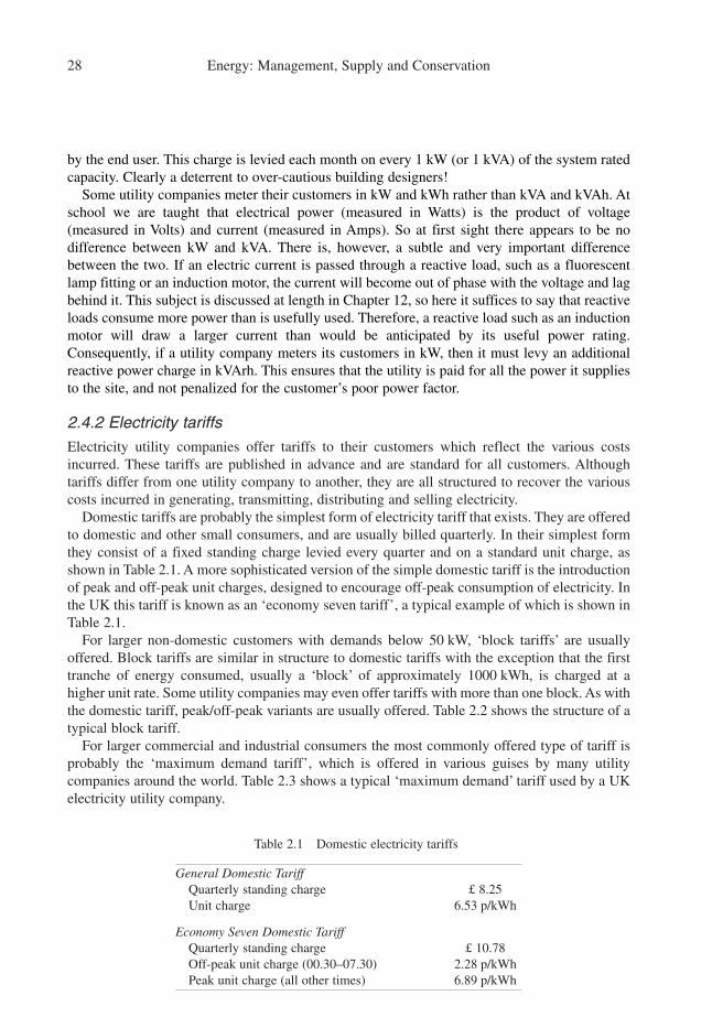
28 Energy: Management, Supply and Conservation
by the end user. This charge is levied each month on every 1 kW (or 1 kVA) of the system rated
capacity. Clearly a deterrent to over-cautious building designers!
Some utility companies meter their customers in kW and kWh rather than kVA and kVAh. At
school we are taught that electrical power (measured in Watts) is the product of voltage
(measured in Volts) and current (measured in Amps). So at first sight there appears to be no
difference between kW and kVA. There is, however, a subtle and very important difference
between the two. If an electric current is passed through a reactive load, such as a fluorescent
lamp fitting or an induction motor, the current will become out of phase with the voltage and lag
behind it. This subject is discussed at length in Chapter 12, so here it suffices to say that reactive
loads consume more power than is usefully used. Therefore, a reactive load such as an induction
motor will draw a larger current than would be anticipated by its useful power rating.
Consequently, if a utility company meters its customers in kW, then it must levy an additional
reactive power charge in kVArh. This ensures that the utility is paid for all the power it supplies
to the site, and not penalized for the customer’s poor power factor.
2.4.2 Electricity tariffs
Electricity utility companies offer tariffs to their customers which reflect the various costs
incurred. These tariffs are published in advance and are standard for all customers. Although
tariffs differ from one utility company to another, they are all structured to recover the various
costs incurred in generating, transmitting, distributing and selling electricity.
Domestic tariffs are probably the simplest form of electricity tariff that exists. They are offered
to domestic and other small consumers, and are usually billed quarterly. In their simplest form
they consist of a fixed standing charge levied every quarter and on a standard unit charge, as
shown in Table 2.1. A more sophisticated version of the simple domestic tariff is the introduction
of peak and off-peak unit charges, designed to encourage off-peak consumption of electricity. In
the UK this tariff is known as an ‘economy seven tariff’, a typical example of which is shown in
Table 2.1.
For larger non-domestic customers with demands below 50 kW, ‘block tariffs’ are usually
offered. Block tariffs are similar in structure to domestic tariffs with the exception that the first
tranche of energy consumed, usually a ‘block’ of approximately 1000 kWh, is charged at a
higher unit rate. Some utility companies may even offer tariffs with more than one block. As with
the domestic tariff, peak/off-peak variants are usually offered. Table 2.2 shows the structure of a
typical block tariff.
For larger commercial and industrial consumers the most commonly offered type of tariff is
probably the ‘maximum demand tariff’, which is offered in various guises by many utility
companies around the world. Table 2.3 shows a typical ‘maximum demand’ tariff used by a UK
electricity utility company.
Table 2.1 Domestic electricity tariffs
General Domestic Tariff
Quarterly standing charge £ 8.25
Unit charge 6.53 p/kWh
Economy Seven Domestic Tariff
Quarterly standing charge £ 10.78
Off-peak unit charge (00.30–07.30) 2.28 p/kWh
Peak unit charge (all other times) 6.89 p/kWh

Utility companies and energy supply 29
Under a maximum demand tariff shown in Table 2.3 the billing and administrative costs are
recovered through a monthly standing charge which is constant and independent of the amount
of electricity consumed. The unit charge covers the cost of providing electrical energy and
therefore is levied on every kVAh of electricity consumed. The unit charge is generally made up
of two components: a larger component, which covers the cost of producing the electricity, and
a smaller component, which covers the operating costs associated with its transmission and
distribution. In order to encourage off-peak electricity consumption, a reduced off-peak unit
charge is offered nightly from 00.30 to 07.30 hours. This encourages customers to load shift and
thus reduce the demand on the network during periods of peak demand.
The capital costs associated with the distribution network are recovered through the maximum
demand charge, which is levied to penalize consumers who have a high power demand (in kW
or kVA) during periods in which demand for electricity is high. In the case of the tariff shown in
Table 2.3, the ‘peak power demand’ period lasts from 1 November to 28 February. During this
period a demand charge is levied on every kVA of the peak instantaneous demand recorded in
any particular month. During the colder months of December and January the charge is £5.40
per kVA. However, this drops to £2.70 per kVA during November and February. For the rest of
the year, no demand charges are levied.
The supply availability charge is designed to deter customers and building designers from
requesting oversized supply cables to their facilities. If a customer over-estimates their required
Table 2.2 Block electricity tariff
General Block Tariff
Quarterly standing charge £ 8.69
Unit charge for the first 1000 kWh consumed 8.94 p/kWh
Unit charge for additional kWh consumed 6.70 p/kWh
Economy Seven Block Tariff
Quarterly standing charge £ 11.22
Off-peak unit charge (00.30–07.30) 2.28 p/kWh
Peak unit charge for the first 1000 kWh consumed 8.94 p/kWh
Peak unit charge for additional kWh consumed 7.05 p/kWh
Table 2.3 Typical maximum demand tariff
Tariff
1. Monthly charge £32.00
2. Supply availability charge per month for each kVA of
chargeable supply capacity £1.40
3. Maximum demand charge per month for each kVA of
monthly maximum demand in the months of:
December and January £5.40
November and February £2.70
4. Unit charges for maximum demand tariffs (p/kVAh)
For each unit supplied 6.15 p
For each unit supplied between the hours of 00.30 and 07.30 each night 2.65 p

30 Energy: Management, Supply and Conservation
supply capacity, then the utility company will incur additional expense. If the customer’s high
demand estimates do not materialize, then the utility company will have spent money which it
cannot recoup through either maximum demand or unit charges. Consequently, an availability
charge is levied monthly on each kVA or kW of the requested supply capacity, in order to penal-
ize over-ambitious customers.
A variation on the maximum demand tariff described above is the seasonal time of day
(STOD) tariff which is illustrated in Table 2.4.
Under a seasonal time of day tariff, monthly standing and availability charges are levied as in
the maximum demand tariff. However, there are no demand charges, and instead the unit charges
reflect the demand on the utility company’s network, penalizing very heavily those customers
who consume electricity during periods of peak demand.
Variations on the tariffs described above can be found throughout the world. One novel
variation occurs in Finland, where IVO, the countries largest supplier, has a triple band tariff.
This reflects the nature of, and the production costs associated with, the various types of
generating plant required to meet demand [5]. The base tariff is linked to hydro and nuclear
power, the middle tariff is related to coal-based power production, and the peak tariff is based on
oil-fired and gas turbine power production. In many hotter regions, such as in the southern states
of the USA, peak demand occurs during the summer months due to the intensive use of air
conditioning plant. Therefore utility companies in these regions levy maximum demand charges
in the summer months and not during the winter.
It should be noted that in many countries some form of ‘value added tax’ (VAT) is levied on
energy consumption. If this applies in a particular region or country, it is important that this is
considered when estimating and analysing electrical energy bills.
The discussion above demonstrates that the overall price per kWh or kVAh paid by the consumer
depends greatly on the end user’s consumption profile. Indeed, in some circumstances it can be
considerably greater than the unit energy charge quoted by a utility company. Example 2.1 illus-
trates the technique which should be used in order to accurately calculate electrical energy costs.
Table 2.4 Typical Seasonal Time of Day Tariff
Tariff
1. Monthly charge £32.00
2. Supply availability charge per month for each kVA of chargeable
supply capacity £1.40
3. Winter unit charges (p/kVAh) (November to March inclusive)
(i) For each unit supplied between 16.00 and 19.00 each day on Mondays
to Fridays inclusive during
(a) December and January 30.50 p
(b) November and February 17.60 p
(ii) For each unit supplied between 08.30 and 20.00 each day on Mondays
to Fridays inclusive during the months of December to February inclusive,
other than charged at rates (i) (a) or (b) above 7.45 p
(iii) For other winter day units supplied between 07.30 and 00.30 5.30 p
(iv) For winter night units supplied between 00.30 and 07.30 2.65 p
4. Summer unit charges (p/kVAh) (April to October inclusive)
(i) For each summer day units supplied between 07.30 and 00.30 4.50 p
(ii) For summer night units supplied between 00.30 and 07.30 1.90 p

Utility companies and energy supply 31
Given that the declared maximum supply capacity of the hotel building is 650 kW and that the
maximum demand tariff shown in Table 2.3 applies, determine the annual electricity bill, and
hence an average price for each unit (kVAh) of electricity consumed (exclusive of VAT).
Solution
Elemental charge Calculation Cost (£)
Monthly standing charge £ 32.00 � 12 384.00
Supply availability charge 650 kVA @ £ 1.40 per kVA � 12 10 920.00
Maximum demand charges
December 623 kVA @ £ 5.40 3 364.20
January 592 kVA @ £ 5.40 3 196.80
November 486 kVA @ £ 2.70 1 312.20
February 552 kVA @ £ 2.70 1 490.40
Energy charges
Peak rate 2 216 345 kVAh @ 6.15 p per kVAh 136 305.22
Off-peak 494 193 kVAh @ 2.65 p per kVAh 13 096.11
Annual electricity cost 170 068.93
Average unit price of electricity � � 6.274 p/kVAh
2.5 Natural gas
Gas utility companies are similar to electricity utility companies insomuch as they both supply
energy directly to buildings via pipes or cables. Both types of utility company have therefore to
construct, operate, and maintain large transmission and distribution networks. In addition, both
types of utility company have to invoice customers and maintain customer accounts. However,
there are some distinct and influential differences between the two ‘fuels’:
170 068.93 � 100
(2 216 345 � 494 193)
Example 2.1
The monthly electricity consumption data for a hotel building for a calendar year is as follows:
Electricity Electricity Monthly maximum
peak units off-peak units demand
Month (kVAh) (kVAh) (kVA)
January 223 475 63 031 592
February 214 718 57 076 552
March 186 845 46 711 476
April 185 513 40 722 471
May 174 103 33 162 427
June 165 988 27 021 381
July 163 181 24 383 365
August 150 089 26 486 372
September 164 746 31 380 410
October 174 983 41 045 452
November 189 752 47 438 486
December 222 952 55 738 623
Totals 2 216 345 494 193 n.a.

32 Energy: Management, Supply and Conservation
• Unlike electricity, natural gas is a primary fuel which must be removed from the ground by
some means;
• Natural gas can be stored in large quantities, while electricity cannot; and
• Unlike electricity, which is required all year round, the market for natural gas is very seasonal
and is weather dependent.
Natural gas consists almost entirely of methane (see Table 2.5) and has a net calorific value of
approximately 38.6 MJ/m3; its density is about 0.73 kg/m3. As such it has a low energy density
compared with oil. In fact, 1 m3 of natural gas contains approximately one-thousandth of the
energy of the same volume of crude oil. Consequently, transportation of natural gas is an expen-
sive and difficult operation, involving substantial networks of large diameter pipelines. Gas
transportation is therefore usually by high-pressure pipeline, although gas can be liquefied and
then transported by ship. Both methods usually require large-scale storage near to consumers to
balance out fluctuations in demand.
Figure 2.4 shows an example of a supply chain for gas produced from an offshore platform
[7]. From the platform the gas is sent through an offshore pipeline to a landing terminal. From
there, it is either sent through transmission pipelines to serve the domestic market, or transferred
to another country via an international transmission pipeline. At some stage the gas will end up
in a regional distribution pipeline before eventually being supplied to domestic users, large
industrial users, or electricity generators.
Table 2.5 Composition of natural gas
Constituent part Percentage by volume (%)
Methane, CH4 92.6
Ethane, C2H6 3.6
Propane, C3H8 0.8
Butane, C4H10 0.3
Nitrogen, N2 2.6
Carbon dioxide, CO2 0.1
From Eastop and Croft (1990) Energy Efficiency for Engineers and Technologists,
© Longman Group Ltd 1990, reprinted by permission of Pearson Education Ltd.
Drilling Platform
Residential/commercial Large industry Power stations
Actors:
1. Producer
2. Pipeline company
3. Transmission andwholesale company
4. Regional distributioncompany
5. End users
Physical links in the chain
1. Wellhead/platform
2. Off-shore pipeline
3. On-shore transmissionpipeline
4. On-shore distributionpipeline
Figure 2.4 Gas chain[7]

Utility companies and energy supply 33
Gas supply chains vary depending on their location and often involve a large number of
parties. The gas producers may not necessarily be the companies who own the offshore pipeline;
similarly the transmission company may not be involved in regional and final distribution.
Therefore as gas flows along a chain, its ownership may be transferred several times.
2.5.1 Natural gas production, transmission and distribution
The gas chain in Figure 2.4 shows that a number of distinct processes are involved in bringing
the finished product to the customer:
(i) Gas gathering pipelines: These link the production fields to the transmission lines and may run
undersea or over land. They transport untreated gas which is not usually of marketable quality.
Untreated gas may be ‘dry’ or ‘wet’. The gathering pipelines for ‘dry gas’, which is relatively
free of liquids, will be much like any other transmission line. ‘Wet gas’ contains substantial
quantities of liquid; if this is to be transported then it must be treated to prevent line clogging.
(ii) Gas treatment: When it is extracted, natural gas is nearly always mixed with impurities such
as water, acid gases, nitrogen and helium [7]. In order to prevent corrosion of transmission
lines, these impurities must be removed. This process usually takes place in an on-shore gas
treatment facility.
(iii) Gas transmission: Gas transmission pipelines ensure an uninterrupted supply of gas at a set
pressure from the gas gathering pipeline to various delivery points. These delivery points
are typically the inlets to local utility distribution systems. At their simplest, transmission
pipelines can simply be a connection between two points. However, it is more common that
transmission pipelines supply several points along their routes, as is the case with the
Russian pipelines, which serve several European countries. In transmission pipelines it is
necessary to boost the gas pressure at regular intervals by using compressors.
(iv) Blending: Depending on their hydrocarbon and nitrogen content, the calorific content of
natural gases from different sources may vary. Many gas appliances are designed to run on
one type of gas and cannot burn a gas with a different calorific value. Consequently,
blending stations are required to mix the various different gases into a blend whose calorific
value is within the tolerance of end users’ appliances.
2.5.2 Peak demand problems
In Europe and North America, where natural gas is predominantly used for space heating,
demand is strongly dependent on outside air temperature. Gas transmission and distribution
systems must therefore cope with large swings in seasonal demand, while still maintaining a
continuous supply to customers. It is particularly important to ensure that all gas pipelines are
maintained well above atmospheric pressure, so that air is not entrained into the system;
otherwise a potentially explosive mixture may be created. In order to overcome the problem of
fluctuating demand, gas utility companies can employ a number of alternative strategies:
• They can construct a transmission infrastructure which is large enough to cope with the
maximum likely demand;
• They can store large reserves of gas near to consumers when gas demand is low, ready for
withdrawal when demand is high;
• They can offer interruptible supply tariffs with discounted unit charges. However, under this
type of tariff, the utility company does not guarantee to supply gas to customers when demand
rises to a high level.

34 Energy: Management, Supply and Conservation
The first solution involves large capital expenditure on infrastructure; an infrastructure which
is inevitably under-utilized for most of its life, with the result that production and transmission
costs are increased. The second solution attempts to balance production and transmission
loads and also provides a measure of security against supply disruption. However, it does
involve capital expenditure on storage facilities. The third solution involves no capital
expenditure and is very popular with utility companies. By offering an interruptible supply to
large customers, the utility company is not guaranteeing a gas supply during periods of peak
demand. Interruptible supplies are popular with organizations that are able to switch at short
notice to another fuel, such as oil, and so are able to reduce the peak demand on the gas
utilities network. In return, consumers who opt for an interruptible supply are offered an
advantageous tariff. In practice, a combination of all three solutions is often employed to
balance a utility company’s supply load.
2.5.3 Gas tariffs
The supply of natural gas to customers involves costs which must be met by the various
companies involved. These can be categorized as:
• The cost of collecting, processing and delivering the gas ‘on-shore’;
• The cost of transporting the gas through the transmission pipelines; and
• The costs involved in marketing, billing and managing customers’ accounts.
One of the most influential factors in determining the price that customers pay for gas is the
transportation levy that gas suppliers have to pay for the use of transmission pipelines. This
transportation levy reflects the costs incurred in constructing and operating the transmission
network, and is generally determined by the length of the pipeline and the maximum gas-flow
rate during periods of peak demand.
Gas tariffs are much simpler than those used for electricity. They tend to follow a fixed pattern
of charges, namely: a fixed quarterly standing charge and a charge for every unit (kWh) of gas
supplied. Unit charges usually incorporate a transportation charge. For smaller consumers unit
charges are generally constant. For larger customers, the unit charge usually decreases as gas
consumption increases. Table 2.6 shows a typical gas tariff for a small customer.
It should be noted that in many countries VAT is levied on gas consumption. A variation on
this gas tariff shown in Table 2.6 is the introduction of a higher unit charge for the first ‘block’
of gas consumed, in a similar manner to an electrical block tariff.
Larger customers tend to be offered monthly tariffs in which the unit charge decreases as gas
consumption increases. They also have the option of negotiating either firm or interruptible
supply contracts. The unit charges associated with an interruptible supply are lower than those
for a firm supply and therefore they are an attractive proposition for some customers.
Interruptible supply contracts can be negotiated in a variety of forms, with a variable interrup-
tion period. Not surprisingly, the longer the permitted period of interruption the lower the unit
price of the gas. With an interruptible supply tariff or contract, the customer is given short
notice that the gas supply is going to be cut and must therefore be prepared to switch over to
another fuel.
Table 2.6 Typical gas tariff for small customer
Standing charge per quarter £ 9.57
Unit charge per kWh supplied 1.52 p/kWh
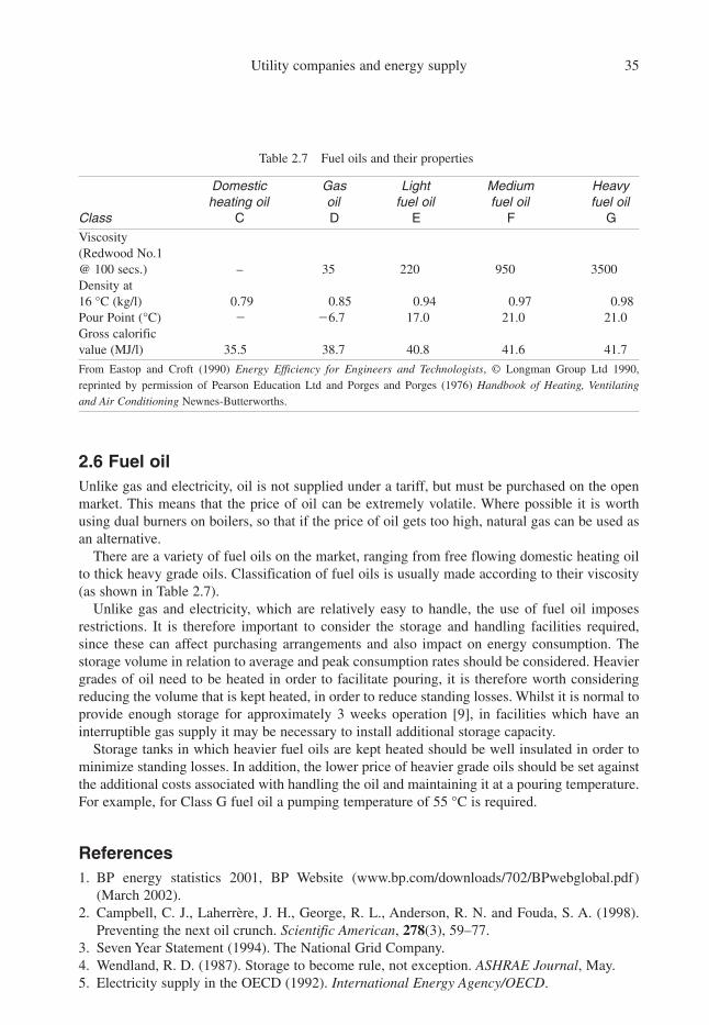
Utility companies and energy supply 35
2.6 Fuel oil
Unlike gas and electricity, oil is not supplied under a tariff, but must be purchased on the open
market. This means that the price of oil can be extremely volatile. Where possible it is worth
using dual burners on boilers, so that if the price of oil gets too high, natural gas can be used as
an alternative.
There are a variety of fuel oils on the market, ranging from free flowing domestic heating oil
to thick heavy grade oils. Classification of fuel oils is usually made according to their viscosity
(as shown in Table 2.7).
Unlike gas and electricity, which are relatively easy to handle, the use of fuel oil imposes
restrictions. It is therefore important to consider the storage and handling facilities required,
since these can affect purchasing arrangements and also impact on energy consumption. The
storage volume in relation to average and peak consumption rates should be considered. Heavier
grades of oil need to be heated in order to facilitate pouring, it is therefore worth considering
reducing the volume that is kept heated, in order to reduce standing losses. Whilst it is normal to
provide enough storage for approximately 3 weeks operation [9], in facilities which have an
interruptible gas supply it may be necessary to install additional storage capacity.
Storage tanks in which heavier fuel oils are kept heated should be well insulated in order to
minimize standing losses. In addition, the lower price of heavier grade oils should be set against
the additional costs associated with handling the oil and maintaining it at a pouring temperature.
For example, for Class G fuel oil a pumping temperature of 55 °C is required.
References
1. BP energy statistics 2001, BP Website (www.bp.com/downloads/702/BPwebglobal.pdf)
(March 2002).
2. Campbell, C. J., Laherrère, J. H., George, R. L., Anderson, R. N. and Fouda, S. A. (1998).
Preventing the next oil crunch. Scientific American, 278(3), 59–77.
3. Seven Year Statement (1994). The National Grid Company.
4. Wendland, R. D. (1987). Storage to become rule, not exception. ASHRAE Journal, May.
5. Electricity supply in the OECD (1992). International Energy Agency/OECD.
Table 2.7 Fuel oils and their properties
Domestic Gas Light Medium Heavy
heating oil oil fuel oil fuel oil fuel oil
Class C D E F G
Viscosity
(Redwood No.1
@ 100 secs.) – 35 220 950 3500
Density at
16 °C (kg/l) 0.79 0.85 0.94 0.97 0.98
Pour Point (°C) � �6.7 17.0 21.0 21.0
Gross calorific
value (MJ/l) 35.5 38.7 40.8 41.6 41.7
From Eastop and Croft (1990) Energy Efficiency for Engineers and Technologists, © Longman Group Ltd 1990,
reprinted by permission of Pearson Education Ltd and Porges and Porges (1976) Handbook of Heating, Ventilating
and Air Conditioning Newnes-Butterworths.

36 Energy: Management, Supply and Conservation
6. Eastop T. D. and Croft D. R. (1990). Energy efficiency for engineers and technologists.
Longman Scientific & Technical.
7. Natural gas transportation: Organisation and regulation. (1994). International Energy
Agency/OECD.
8. Porges, J. and Porges, F. (1976). Handbook of heating, ventilating and air conditioning.
Newnes-Butterworths.
9. Energy audits and surveys (1991). CIBSE Applications Manual AM5.
Bibliography
Eastop, T. D. and Croft, D. R. (1990). Energy efficiency for engineers and technologists. (Chapter 9),
Longman Scientific & Technical.
Economic use of electricity in buildings (1995). Fuel Efficiency Booklet 9. Department of the
Environment.
Energy audits and surveys (1991). CIBSE Applications Manual AM5.
Yuill, D. (1985). Understanding electricity costs. Energy Manager’s Workbook, 2 (Chapter 2),
Energy Publications.

3
Competition in energy supply
In this chapter the concept of competition in the energy sector is examined for both
electricity and gas supply industries and the experience of electricity deregulation in the UK
and USA is discussed in detail. The potential role of demand-side management is also
investigated and comparisons are drawn between experiences in the UK and USA.
3.1 Introduction
It has traditionally been the case that gas and electricity utility companies, irrespective of
ownership (i.e. state or privately owned), are natural monopolies, which are regulated by
legislative measures. These monopolies evolved partly because of the high infrastructure costs
associated with the transmission and distribution of gas and electricity, and partly because it was
easier to manage and regulate utility companies which generated/supplied, transmitted and
distributed electricity or gas. Indeed, it is difficult to imagine anything other than a monopoly,
given that most buildings have only one physical connection to a gas pipe and another to an
electricity cable. However, while monopolistic utility companies are relatively easy to control
and regulate, they prevent competition in the energy market. Consequently, it is not possible to
buy and sell ‘bulk’ energy in the same way other commodities are traded.
In recent years many governments around the world have begun to investigate alternative
solutions which introduce competition into their respective electricity and gas supply industries.
This has become possible because of various technical and financial advances made in the late
1980s and 1990s. The United Kingdom has been at the forefront in pioneering utility deregula-
tion, and has completely restructured its utility sector. During the 1990s the UK deregulated first
its electricity supply industry and then its gas industry, in a long and complex process, which at
time of writing, is still ongoing. Such has been the radical nature of these changes that in many
ways the UK has become the ‘pilot study’ for the rest of the world. Following the UK’s lead a
number of countries, including the USA, have deregulated (at least in part) their electricity sup-
ply industries and are developing new energy trading markets. In addition to the UK electricity
spot market (i.e. the electricity ‘pool’), four other ‘pools’ have so far been created in Europe; the
Amsterdam Power Exchange (covering The Netherlands, Belgium and Germany), the Spanish
Pool, the Swiss Pool and the Nordpool in Scandinavia (covering Norway, Sweden and Finland) [1].
3.2 The concept of competition
Consider the case of an organization which uses oil to heat its buildings. Under normal circum-
stances the organization will have a choice of competing fuel suppliers from whom to purchase oil.
The organization can negotiate a bilateral supply contract with any one of these suppliers. If one
supplier becomes too expensive, then the organization can simply switch to purchase oil from
another supplier. If the general demand for fuel oil is high, then the suppliers will be able to raise
their prices. Conversely, if demand is low then the price of oil will also be low. Thus a competitive
market in fuel oil exists which reflects the demand for oil at any moment in time. As with any other
commodity, the oil price will vary because customers have the ability to switch between suppliers.
In addition, there is no cross-subsidy of one group of customers by another group of customers.
Each fuel supply contract is negotiated on an individual basis between the parties concerned.
Now consider the same organization purchasing electricity under a tariff from a utility
company. Since the electricity is supplied through cables owned by the utility company, the
customer has no choice of alternative supplier and so the organization is compelled to purchase
electricity at a price fixed by the utility company. As a consequence:
• No competition exists: The customer is in a weak position since electricity prices are fixed by
the utility company.
• No market exists: Under a tariff, electricity prices are fixed, with the result that prices do not
accurately reflect the fluctuations in demand for electricity. Although many tariffs do have
reduced ‘off-peak’ elements these are at best only a crude indicator of market demand.
• The potential for cross-subsidy exists: The utility company may decide to offer lower electricity
prices to its large industrial customers, and recoup some of its lost income by increasing the
prices of its smaller domestic and commercial tariff customers. This is termed ‘cross-subsidy’,
and effectively means that one group of customers is subsidizing another group.
While this monopolistic scenario may suit the utility companies, it does not benefit the customer.
The utility companies are in a strong position and the potential exists for artificially high
electricity prices. Lack of competition ultimately leads to:
• Manufacturing industry paying a high price for energy, with the result that the unit cost of
production increases and the industry becomes less competitive.
• Utility companies becoming over-manned and inefficient.
It is therefore easy to see why many governments are reviewing the monopolistic position of
their respective utility companies with a view to introducing a competitive energy market.
3.3 Competition in the electricity supply industry
While it is easy to state that competition in the energy market is a desirable thing, in practice it
is difficult to achieve a truly competitive market amongst utility companies. Utility networks, be
they gas or electricity, lend themselves to monopolies and are not naturally suited to competi-
tion. This is because it is impractical and prohibitively expensive to construct two or more sets
of competing transmission/distribution networks. Given this, the simplest and easiest way to
organize affairs is to have a ‘vertically integrated’ structure in which a single utility company is
responsible for provision of supply. Figure 3.1 shows the structure of a typical vertically
integrated electricity supply industry.
In a vertically integrated electricity supply industry the various utility companies have
monopolies over their ‘franchise’ regions. Within its franchise region a utility company will be
38 Energy: Management, Supply and Conservation

responsible for generating, transmitting, distributing and supplying electricity to all its
customers. Customers in the utility company’s franchise region are forced to purchase their
electricity from the regional utility company. Vertically integrated utility companies can exist in
both the private and the public sectors. Their monopolistic position is derived solely from their
physical location, which excludes competition and means that the utility company has a pro-
tected market. Under this scenario energy prices can easily become over inflated if the utility
company is not tightly regulated.
In order to promote competition in the electricity supply industry it is necessary to create a
market for the commodity which is flexible and yet, still robust enough to cope with wide
fluctuations in demand. The market should:
• Allow various electricity supply companies and generators to compete with each other to sell
electricity direct to customers.
• Allow customers to negotiate electricity supply contracts with various suppliers.
• Be transparent, so that generators, suppliers and customers can see that the market is fair and
equitable.
• Create a ‘spot market’ which accurately reflects both demand for energy and cost of produc-
tion. This spot market then becomes the market indicator of the real cost of production at any
given point in time.
• Facilitate a future’s market in electricity trading.
While the above points are relatively easy to achieve in a normal commodity market, they are
not easily achieved in a market in which electricity is bought and sold. This is because electric-
ity cannot be stored and must be generated only when it can be consumed. Any potential trading
market in electricity must fully accommodate the physical constraints of an electricity supply
system. As a result a truly competitive market in electricity is likely to be much more complex
than a normal commodities market.
It is impossible to achieve a competitive market with a vertically integrated electricity supply
industry. Instead a horizontally integrated structure is required. The introduction of a horizon-
tally integrated electricity supply industry, in which the generating, transmission and distribution
roles are all split up from each other, is the key to facilitating competition. By splitting up the
roles it is possible to create competition between generators, who then have to bid in a ‘spot
market’ for the right to supply electricity to the transmission grid. If the transmission company
acts in a fair and independent manner, purchasing power at ‘least cost’, then any possible cartel
should be eliminated. It then becomes possible for new ‘independent power producers’ to enter
Competition in energy supply 39
Electricity generation from:coal, oil, gas, nuclear, hydro
A single utilitycompanygenerates,transmits,distributesand sellselectricity tocustomers
Transmission grid (400 kV)
Local distribution network(133 kV and 11 kV)
Figure 3.1 A vertically integrated electricity supply industry

the market to compete with existing generators. This should result in a reduced cost to the
customer for each unit of electrical energy produced. Figure 3.2 shows the structure of a typical
horizontally integrated electricity supply industry.
Whilst the spot market described above facilitates competition between generators, it does
not of itself offer the customer a choice of competing suppliers. In order to achieve this the
customer must be allowed to negotiate supply contracts with individual energy suppliers. This
is achieved by allowing ‘second tier’ electricity ‘wholesale’ suppliers to purchase ‘bulk’
electricity from the transmission grid and sell it on directly to customers. Under this arrange-
ment the customer purchases electricity from competing supply companies, who pay a fee to
the relevant distribution companies for the use of their ‘wires’. This ‘line rental’ fee is then
passed onto the customer and included in the unit price paid for the electricity. In order to
ensure that true competition takes place, the ‘line rental’ fees should be transparent and equal
for all potential electricity suppliers. These fees are usually fixed by some form of statutory
regulatory mechanism.
This discussion indicates that facilitating competition in an electricity supply industry
involves the setting-up of a complex structure, with many demarcation boundaries. Indeed,
there is an inherent conflict of interests between the engineering and financial requirements of
a horizontally integrated structure. The transmission company is primarily interested in
procuring enough electrical energy from generators in order to meet the instantaneous demand
on its grid. It seeks to procure this energy from the cheapest power producers and is not
particularly interested in individual supply contracts. Conversely, customers, suppliers and
generators are primarily interested in negotiating contracts which ensure secure supply and
therefore are not interested in the transmission company’s need to meet instantaneous demand.
Satisfying these conflicting needs requires the setting-up of complex bidding, pricing and
settlement mechanisms. It is the specific nature of these mechanisms and the efficiency with
which they are applied which will ultimately determine the success or failure of any electricity
market.
In addition to the complex financial and settlement mechanisms required to operate the market,
suppliers need to know the ‘real-time’ electricity consumption of their contract (i.e. non-domestic)
customers. This involves the installation of ‘smart’ meters which measure electricity usage every
half hour, and can be read remotely and automatically. The data from these meters are transmitted
to remote disseminated centres, from which relevant data are sent to all the parties involved in the
supply contract. Contract customers may purchase or lease their metering equipment, but the
installation and maintenance of these meters should be carried out by approved operators.
40 Energy: Management, Supply and Conservation
Competing generators
Competing suppliers
Customers
Transmission company
Regional distribution network
Figure 3.2 A horizontally integrated electricity supply industry

3.4 The UK electricity experience
Competition in electricity supply is still in its infancy and many protocols are not yet firmly in
place. Most of the electricity power markets which exist around the world are only a few years
old and even the UK market, established in 1990, is still undergoing major revisions. This makes
it difficult to describe general rules which apply to all electricity markets. In the absence of any
firm ‘ground-rules’ it is worthwhile looking in detail at the evolution of the competitive
electricity market in England and Wales (the largest part of the UK), since this has been the
‘template’ for subsequent deregulation schemes in various parts of the world.
In 1990 in England and Wales a daily spot market known as the electricity ‘pool’ was
created. The pool was administered by the National Grid Company (NGC), which owned and
operated the transmission grid in England and Wales. Each morning the competing generating
companies would submit ‘bids’ for their various generating sets to NGC for the following
day’s operation. Each bid included an offer price at which the generating company would be
prepared to operate its various generating units for the following day. It also included a
declaration of availability of generating plant for the following day. Once the generators had
submitted their bids to the pool, the NGC examined its own demand forecast for the follow-
ing day, and ranked each generating unit in order of price (lowest price first), so that finally a
merit schedule was produced. This schedule was then published at approximately 15.00 hours,
so that the generating companies were notified of the generating units required for the
following day. As there was often considerable over-capacity in the system, any generating
units for which the offer price was too high were either placed on standby, or excluded from
the pool and forced to shut down.
As electricity cannot be stored it is essential that the controllers of the national transmission
grid be able to bring on line (or down load) additional generating capacity at very short notice
to cope with fluctuating demand. Figure 3.3 shows the national grid demand profile for a peak
‘winter time’ weekday, 29 November 1993 [2]. This graph shows that demand on that day varied
considerably over the 24 hour period. To cope with increases in demand, generating units had to
Competition in energy supply 41
0
10
0.5 2
3.5 5
6.5 8
9.5 11
12
.5 14
15
.5 17
18
.5 20
21
.5 23
20
30
40
50
60
De
ma
nd
(G
W)
Time (hours)
Figure 3.3 Demand experienced by National Grid, 29 November 1993[2]

be brought on line as and when they were required, but in strict accordance with their ranking in
the daily pool merit schedule. In other words, generating sets which bid a low price were brought
on line first, while the more expensive units had to wait until demand increases before they were
allowed to generate. Consequently the pool price varied for each half hour period throughout the
day. When demand was high, it generally followed that pool price would also be high. In this
way the pool price reflected the demand on the transmission grid.
The bid price submitted for the most expensive generating unit brought on line to meet the
demand in any given half hour period was known as the ‘system marginal price’ (SMP). For
example, if the highest bid price accepted into the pool for the half hour period 11.00 to 11.30
hours was 2.5 p/kWh, then the SMP would be 2.5 p/kWh. It is important to note that it is the
SMP, not the bid prices submitted by the individual generators, which became the basis for the
eventual pool price for any given half hour, and that all the generators on line in that particular
half hour were paid the ‘pool purchase price’ (PPP). Electricity supply companies and large
consumers purchasing from the pool had to pay the ‘pool selling price’ (PSP). Not surprisingly
PSP is always greater than PPP, the difference being an uplift to cover the pool operating costs.
The electricity pool in England and Wales enabled a competitive market to exist amongst
the generators, and gave the market as a whole an indication of the true costs of electricity
production at any given time.
While an electricity pool facilitates competition between the various generators, it does not
on its own provide the mechanism for promoting a competitive market amongst customers.
In order to achieve this, ‘second tier’ electricity ‘wholesale’ supply companies must be
allowed to purchase electricity from the transmission grid and sell it on directly to customers.
These wholesaler suppliers negotiate bilateral contracts with the generating companies to
purchase ‘bulk’ electricity at fixed rates, under a series of contracts for differences (defined
later in this paragraph), and then sell it on to the customer at a marked-up price. These sup-
ply companies make their money by purchasing ‘bulk’ electricity from the generators at a low
price and selling it on to their customers at a higher price. This involves considerable finan-
cial risk and the supply companies must negotiate contracts which ensure that they make a
profit. However, pool price can be extremely volatile, especially in the winter. This volatility
increases the element of risk for the supply companies if they purchase from the pool, with
the result that they may lose money if they purchase at a high price and have to sell at a low
one. The inherent volatility of the pool also makes planning ahead difficult. In an attempt to
hedge against the risk of high pool prices, the supply companies take out ‘contracts for
differences’ with the individual generating companies. The contracts between the supply
companies and the generators operate outside the pool and operate in a similar way to
‘futures contracts’ traded in the world’s commodity markets. Under a typical contract for
differences a supply company would contract with a specific generator to buy electricity at a
fixed price for a specific time period (usually on a daily five time block basis) [3]. This
‘hedges’ against the volatility of the pool, and enables both generators and suppliers to
predict the future financial risk involved in generating and selling electricity with some
degree of confidence. These contracts for differences underpin the electricity market. They
are called contracts for differences because payments are made by the parties involved to
make good the difference between the pool price and the agreed contract price. Under this
system, if the pool price falls below the contract price, the supply company remunerates the
generator for the difference between the two prices, and vice versa if the pool price is above
the contract price. The price of most of the electricity bought and sold is fixed in advance by
contracts for differences. Hence the vast majority of electricity that is traded in England and
Wales is purchased outside of the electricity pool.
42 Energy: Management, Supply and Conservation

3.4.1 The evolution of the UK electricity market
The electricity pool described in Section 3.4 has become the basis for a number of other trading
pools set up during the 1990s in Europe. However in the UK, during the late 1990s concerns
were expressed that the pool system:
• Favoured the large generating companies; indeed there was suspicion that these companies
were able in some way to control the pool price.
• Inhibited the introduction of new independent energy traders into the market.
• Inhibited the negotiation of bilateral electricity supply contracts between various parties.
The last point is an important one. In most trading deals the customer can state the price at which
they wish to purchase a commodity and this has an influence on the overall market price.
However, under the pool system the ‘market price’ (i.e. the pool price) was wholly determined
by the sellers (i.e. the generating companies). The pool could therefore be viewed as being in
some way only ‘half a market’ [4].
As a result of the concerns stated above, the UK completely restructured its electricity trading
arrangements in 2000 and introduced the ‘New Electricity Trading Arrangement’ (NETA) [5].
This new arrangement abolished the old centrally regulated pool in favour of a ‘free-market’
approach which allowed a series of ‘power exchanges’ (i.e. electricity commodity markets) to be
established; the hope being that the exchanges and brokers would create forwards, futures, and
short-term bilateral markets. The intention was that the true price of electricity would become
established through the power exchanges in much the same way that the commodity markets fix
the price of other traded commodities. However, while the power exchanges can facilitate trade
in ‘bulk’ energy, there is no way in which they can satisfy the physical engineering requirements
of NGC (the operators of the transmission grid), who need to predict accurately at any point in
time the demand on their network. Because electricity cannot be stored, the NGC must bring
on-line more generating capacity as demand rises, otherwise power cuts will occur. Clearly, no
commodity market can solve this problem alone! So the NETA arrangements were designed to
operate in parallel with the new power exchanges, so that every time a bilateral contract is signed
between a generator and a supplier they are required to inform NGC (or its settlements agent) of
the quantity of electricity traded and the duration of the contract. It should be noted that parties
are not required to notify NGC of the price paid for the electricity. All the supply companies and
the generating companies are also required to notify NGC in advance of their expected operating
levels for the following day. So by 11.00 hours on the day before trading, both the generators and
the suppliers must submit to NGC their forecasts of demand, on a minute-by-minute basis, for
the day ahead. They can do this because all parties know the quantity of electricity they have
contracted to supply or purchase for the following day. By ‘gate closure’ (i.e. 3.5 hours before
real time) the suppliers and generators must submit finalized demand forecasts to NGC. In this
way NGC can effectively manage the transmission grid and inform the individual generators of
the generating plant that will be required for the following day.
In theory the demand profiles predicted by the supply companies should exactly match the
generation profiles predicted by the generating companies. In reality this never happens because it
is difficult to accurately predict demand for electricity on a daily basis. A large number of factors
influence electricity consumption, including weather and television scheduling. Since many
variables influence electricity consumption, it is inevitable that the true demand for electricity will
vary from the demand predicted by the supply companies. This means that NGC will have to bring
on-line (or take off-line) at short notice, additional generating plant in order to cope with variations
from the predicted values. This of course incurs additional expense on behalf of the generating
Competition in energy supply 43

companies who have either to bring on-line extra plant or lay-off generating plant which it had
planned to operate. These ‘imbalance costs’ (i.e. costs incurred due to deviations from bilateral
supply contracts) are calculated by NGC through a complex series of counter ‘bids’ and ‘offers’
made by both the generators and the suppliers. In this way NETA determines only the unit price of
electricity which is ‘traded’ at the margins (i.e. outside of the power exchanges). It is intended that
the ‘imbalance’ electricity costs will be higher than the ‘bulk’ electricity price, thus encouraging
both the generators and the suppliers accurately to forecast predicted demand.
From the discussion above it is evident that in order to accommodate the engineering
constraints of a transmission grid and facilitate a commodity market in electricity, extremely
complex trading arrangements must be set up. Given this, it is understandable that competition in
the electricity supply sector has been slow to evolve. Indeed, it and would have been impossible
without recent rapid advances in information technology (IT) in general and the Internet in
particular. Without these IT advances, it would be impossible to rapidly transfer the large amounts
of data associated with the bidding process to the many parties involved in a power exchange.
3.4.2 The Californian experience
From the discussion in Section 3.4.1, it is clear that facilitating a true competitive market in
electricity is an extremely complex process. Indeed, the electricity supply industry is of such
strategic importance that if the deregulation process goes wrong, it can have a catastrophic effect
on the whole economy. With this in mind, the experience of the Californian electricity supply
industry should be a salutary lesson to all legislators who might be considering deregulating their
utility sector. In January 2001 large parts of the state of California suffered major power-cuts,
not because of any technical failures, but as a direct result of poorly thought out legislation [6].
In 1996, the California Assembly voted to deregulate the state’s electricity supply industry
and to dismantle what was considered to be a government regulated monopoly [7]. Prior to
deregulation, the state had a vertically integrated electricity supply industry, with a number of
investor-owned utility companies owning and operating their own power stations, transmission
grids and distribution networks. With deregulation, a non-profit making organization, the
California Power Exchange was established and the following changes were made:
• Operational control of the transmission grids was transferred to a single Independent System
Operator who became responsible for the management of the system.
• The investor-owned utility companies, such as Southern California Edison and Pacific Gas
and Electric, were forced to sell most of their power stations to other unregulated private
companies. This forced the major utility companies to purchase wholesale electricity through
the California Power Exchange.
• The California Power Exchange acted as a wholesale commodities market, through which all
the state’s electricity was bought and sold. An auction process therefore set the price of
wholesale electric power.
The investor-owned utility companies did however, retain ownership and control of their
distribution networks.
By making these changes the California legislature created a classic model for a competitive,
deregulated electricity supply industry. However, there were two critical factors which were to
have a significant influence on the events that were to follow:
1 While deregulation forced the utility companies to purchase their power on the open market
and pay market prices, it prevented them from passing on any increases in the cost of whole-
sale electricity to their customers until at least 31 March 2002 [7].
44 Energy: Management, Supply and Conservation

2 Because of environmental concerns the state authorities prevented the building of new power
stations. For 20 years or more, there had been no significant increase in California’s
generating capacity, despite the fact that demand for electricity in the state had been growing
at approximately 2% each year [7].
These two critical factors were to have disastrous consequences for California in general and its
electricity supply industry in particular. What the state legislature had done was to force the utility
companies to buy wholesale electricity on the open market, which can be extremely volatile, while
at the same time effectively fixing the price at which the utilities could sell electricity to their
customers. The failings of this strategy were compounded by the fact that there was little excess
generating capacity in the system. Without excess capacity there was little competitive pressure to
keep wholesale prices low. As a result during the summer of 2000, when demand for power peaked,
the utility companies urgently needed power from the electricity wholesalers and generating
companies, who promptly raised their prices. Bulk electricity prices rose steeply, with the average
price of electricity bought through the Power Exchange rising from approximately $30 per MWh in
January 2000 to $330 in January 2001 [8]. In fact, in December 2000 the price reached a peak of
$1400 per MWh [7]. Unable to recoup these inflated costs from their customers, the utility
companies, not surprisingly, started to lose money. They rapidly ran out of money, with the two largest
utilities, Southern California Edison and Pacific Gas and Electric, claiming that by January 2001 their
combined losses exceeded $9 billion [7]. Indeed, Pacific Gas and Electric filed for bankruptcy in April
2001 [9]. The financial difficulties of the utility companies had two direct consequences:
1 The banks became very reluctant to lend more money to the cash-starved utility companies,
who were rapidly becoming insolvent.
2 The wholesale and generating companies became reluctant to sell electricity to utility com-
panies which were obviously in financial difficulties.
Faced with such high financial losses and not wanting to lose any more money, the utility com-
panies took the only course of action available to them: they stopped purchasing electricity and
the state of California suffered major power-cuts. The state authorities then had to step in and try
to pick up the pieces and sort the mess out.
The sorry state of affairs that occurred in California graphically highlights the major problems
which can occur if all the issues involved in deregulation are not thought out in advance. Clearly,
the combination of a shortage in generating capacity and an unregulated wholesale market,
facilitating what is in effect an energy cartel, is a recipe for disaster.
3.5 Competition in the gas market
In many ways facilitating competition in the gas market is similar to the electricity market. As
with electricity supply, horizontal integration is the key to a competitive gas market. However,
there are a number of fundamental differences which make trading in natural gas much simpler
than trading electricity:
• Natural gas is not generated; it is pumped out of oil and gas fields at sea or on land and sold
to licensed shippers (i.e. wholesale supply companies) who sell it on to customers.
• Unlike electricity, natural gas can be stored to a limited extent.
• Demand for natural gas is very seasonal.
Given the differences between the nature of gas and electricity, a relatively simple horizontally
integrated model is required to facilitate a competitive market in gas (as shown in Figure 3.4).
Competition in energy supply 45

Because there are only three parties involved in the process and also because gas can be stored,
the whole structure is much simpler to control and operate than that of an electricity supply
industry. However, in order to ensure that the system functions in a fair and equitable manner it
is important that the gas transmission company charges equal transportation fees to all suppliers
and that all fees should be transparent.
Under a horizontally integrated gas supply structure, individual customers are free to negotiate
bilateral supply contracts with various competing suppliers. The price paid by the customer is
the price the supplier pays for the gas at the ‘beach head’ plus the cost of transportation plus the
supplier’s profit. However, the price paid by the customer is mainly affected by the cost of gas
at the beach head.
It is the responsibility of the gas transmission company to balance supply and demand on its
network on a continual basis. If too much gas enters the network then it must be stored in under-
ground caverns or gasometers. Conversely, if too little enters the network, then gas from the
storage vessels will have to be utilized. Suppliers therefore have to ensure that the gas they put
into the network is roughly equal to the gas that their customers use. If they miscalculate either
way by too great a margin, then the transmission company will levy a penalty charge on them.
3.6 Load management of electricity
From the discussions in Section 3.4 it can be seen that the ‘true’ cost of electricity production varies
with demand on the network, and that through the use of pricing mechanisms such as the ‘pool’ it
is possible to introduce real-time electricity pricing. Under this scenario when electricity is
consumed becomes as important as how much electricity is consumed. Those customers who have
the ability to manage their electrical load should thus be in a good position to reduce energy costs.
An ability to manage electrical load not only reduces customers’ electrical costs, it also
enables them to negotiate more competitive electricity supply contracts. If a potential customer
wishes to negotiate a supply contract, they will need to furnish potential suppliers with the
following information:
• The annual consumption of electricity in kWh.
• The maximum demand in kW.
• The load factor.
The load factor for any given period represents the percentage of time for which plant and
equipment operates during that period. It can be calculated as follows:
Load factor �Energy consumed (kWh)
Max. demand (kW) � Time period (h)� 100
46 Energy: Management, Supply and Conservation
Gas transmission company
Competing gassuppliers
Customer
Figure 3.4 Horizontally integrated gas supply industry
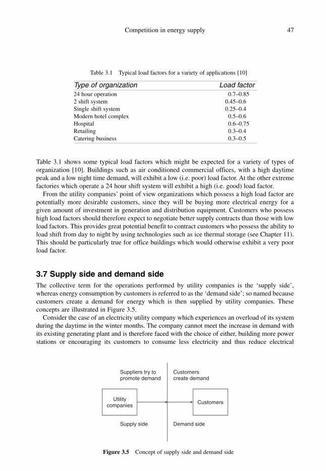
Table 3.1 shows some typical load factors which might be expected for a variety of types of
organization [10]. Buildings such as air conditioned commercial offices, with a high daytime
peak and a low night time demand, will exhibit a low (i.e. poor) load factor. At the other extreme
factories which operate a 24 hour shift system will exhibit a high (i.e. good) load factor.
From the utility companies’ point of view organizations which possess a high load factor are
potentially more desirable customers, since they will be buying more electrical energy for a
given amount of investment in generation and distribution equipment. Customers who possess
high load factors should therefore expect to negotiate better supply contracts than those with low
load factors. This provides great potential benefit to contract customers who possess the ability to
load shift from day to night by using technologies such as ice thermal storage (see Chapter 11).
This should be particularly true for office buildings which would otherwise exhibit a very poor
load factor.
3.7 Supply side and demand side
The collective term for the operations performed by utility companies is the ‘supply side’,
whereas energy consumption by customers is referred to as the ‘demand side’; so named because
customers create a demand for energy which is then supplied by utility companies. These
concepts are illustrated in Figure 3.5.
Consider the case of an electricity utility company which experiences an overload of its system
during the daytime in the winter months. The company cannot meet the increase in demand with
its existing generating plant and is therefore faced with the choice of either, building more power
stations or encouraging its customers to consume less electricity and thus reduce electrical
Competition in energy supply 47
Table 3.1 Typical load factors for a variety of applications [10]
Type of organization Load factor
24 hour operation 0.7–0.85
2 shift system 0.45–0.6
Single shift system 0.25–0.4
Modern hotel complex 0.5–0.6
Hospital 0.6–0.75
Retailing 0.3–0.4
Catering business 0.3–0.5
Suppliers try topromote demand
Supply side Demand side
Customerscreate demand
Utilitycompanies
Customers
Figure 3.5 Concept of supply side and demand side

demand during the daytime. The former solution is a ‘supply-side measure’ since the solution lies
wholly with the utility company (i.e. on the supply side) and the latter is termed a ‘demand-side
measure’ since the solution to the problem lies with the customer. The demand-side solution could
be achieved by introducing an electricity tariff offering lower unit charges to customers who are
prepared to switch their electricity consumption from the daytime to the nighttime. Through
management of the ‘demand side’ in this way it is possible for utility companies to utilize their
resources efficiently and thus achieve substantial cost savings. Demand-side measures are
therefore concerned with direct intervention in the customer’s end use of electricity by the utility
company, in a way which affects the planning of the utility company’s infrastructure.
Traditionally electricity utility companies have tended to rely on supply-side measures to
shape their businesses; that is, the utility companies have tried to influence the way in which
their customers use electricity from the supply side of the meter, and have provided the
infrastructure to meet the predicted demand. However, in recent years, both in the UK and the
USA, there has been increasing interest in the use of demand-side measures.
3.8 Demand-side management
The concept of demand-side management (DSM) (sometimes referred to as ‘least cost plan-
ning’) was pioneered in the USA during the 1980s, where it has since become an influential
force. In some parts of the USA the electrical demand can increase by as much as 40% during
the summer months, due to the use of air conditioning equipment [11]. There is also stiff legis-
lative opposition from the Public Utility Commissioners to the construction of new power sta-
tions. Faced with this situation many USA utility companies have introduced DSM programmes
to encourage customers to conserve energy, and persuade as many as possible to shift their day-
time load to the nighttime. In the USA DSM programmes include such measures as financial
support for feasibility studies, free advice on techniques, capital grants towards the cost of new
equipment, and even the free issue to customers of low energy light bulbs. Many utility compa-
nies in the USA have found it more economical to persuade their customers to conserve energy,
rather than be forced to build new generating plant. A typical example of this is that of Pacific
Gas and Electricity, which in 1985 announced that it intended to ‘build’ a new power plant; a
1000 MW conservation power plant. In other words they intended to buy extra efficiency
improvements which would reduce their peak demand by 1000 MW [12].
Simple analysis of energy consumption demonstrates the great benefit of encouraging energy
conservation over the construction of new generating plant. If it assumed that a typical thermal
power station has an efficiency of 35%, then the overall primary energy saved through the
conservation of 1 kWh of delivered electrical energy is:
From this it is obvious that in energy conservation terms, encouraging customers to conserve
electrical energy makes much sense. Nevertheless, in order to persuade the utility companies
to adopt an energy conservation strategy, it must also make commercial sense. In the late
1980s, Ontario Hydro of Canada estimated that meeting its peak demand obligations through
supply-side measures (i.e. constructing new generating plant and reinforcing transmission and
distribution networks) would cost the utility four times as much as using demand-side meas-
ures. [13] The findings of Ontario Hydro are backed up by Rosenfeld and de la Moriniere [14]
who demonstrated in 1985 the cost of constructing new generating capacity to be in the region
Primary energy saved �1
0.35� 2.86 kWh
48 Energy: Management, Supply and Conservation

of $1200–$1500/kW, which compared very poorly with the maximum of $400/kW of electri-
city saved which could be achieved by using an ice storage system. It is therefore clearly in
the interests of vertically integrated utility companies, such as those that exist in many parts
of the USA and Europe to encourage the installation of DSM technologies. To this end, many
of the utility companies in the USA offer substantial capital incentives to building users to
install technologies such as low energy light fittings and ice thermal storage [12].
Although DSM has become an influential force in the USA, its country of origin, the UK has
been slow to adopt it. The UK does not suffer from a shortage of generating capacity, as is the
case in some parts of the USA. It also experiences a winter peak, unlike many states in the USA.
In addition, in England and Wales the electricity supply industry is not vertically integrated as
much of the USA still is, thus making comparisons between the two countries very difficult.
However, despite the obvious differences between the electricity supply industries in the USA
and England and Wales, the regional distribution companies in the UK have recently become
interested in DSM, since it is one method by which they can significantly reduce the demand on
their cables and transformers, and thus reduce their operating and capital investment costs.
Because of the complex nature of the UK’s horizontally integrated electricity supply industry,
the role of DSM in the UK is somewhat ambiguous. In theory the widespread introduction of
DSM should:
• Produce a reduction in the fuel burnt at power stations.
• Cause the deferral of the capital and financing costs of new power station construction.
• Cause a reduction in distribution losses.
• Result in the possible deferral of distribution reinforcement.
• Cause a reduction in transmission losses.
• Result in the possible deferral of transmission reinforcement associated with both new power
plants and increased loads.
• Lead to a reduction in the emissions of CO2, SO2 and NO2 from power stations.
While at first sight all the above points seem to indicate that there is a strong case for implement-
ing DSM policies in the UK, further analysis casts doubt on the validity of the statement above. In
theory all parties in the UK electricity supply industry benefit from the introduction of DSM. Yet,
because of the fragmentation of the industry due to horizontal integration it is difficult to initiate
and coordinate an effective DSM policy. For example, who will pay for a DSM policy? Are the
regional distribution companies going to pay for a policy which arguably gives greatest benefits to
the generators and the NGC? It is also difficult for the competing generators to initiate DSM, since
they have no ‘captive’ market and they have little direct influence over the end users. Also, the
structure of the electricity market is such that individual generators are always seeking to generate
as much electricity as possible. The benefit to the generators through the implication of a DSM
policy is dubious to say the least, since there is over capacity in the system, and every generator
benefits from higher electricity prices when demand is high. Therefore, for DSM to succeed in the
UK it must benefit both the regional distribution companies and their customers.
3.8.1 The USA experience
The US-based energy research body the Electrical Power Research Institute (EPRI) defines
DSM as:
The planning, implementation and monitoring of utility activities designed to influence
customer use of electricity in ways that will produce desired changes in load shape [15]
Competition in energy supply 49

In the USA, DSM programmes are often initiated by the Public Utility Commissioners who are
intent on minimizing the construction of new generating plant. Utility companies are required to
demonstrate to the Commissioners that their proposed course of action is the least expensive
option for supplying customers with electricity. The onus is therefore on the utility companies to
reduce demand rather than build more power stations. In some states in the USA, utilities are
even being awarded bonuses for implementing DSM programmes.
Although DSM programmes in the USA have been initiated as a result of social concern and
regulatory pressure, it is the potential for profit to the utility companies that has driven such pro-
grammes. In the USA the utilities are permitted to over-recover the costs of DSM programmes
through increases in electricity prices. Consequently, the utilities receive a greater marginal
return from demand-side measures than they would from supply measures. This has resulted in
DSM programmes in North America being used on a large scale. Many North American utility
companies spend more than 5% of their total turnover on investment in DSM. Table 3.2 shows
the investment levels and targeted energy savings for some DSM programmes, operated by a
variety of North American utility companies [16].
Although some of the DSM programmes included in Table 3.2 have not proved to be cost
effective, many of the utility companies have reported that their DSM programmes have proved
less expensive in total cost terms, when compared with the costs avoided on the supply side.
These findings even applied in circumstances where the utility company had an excess of
generating capacity.
When a DSM policy is introduced a utility company avoids generating costs, network losses,
some administration charges, and may avoid capital expenditure on network reinforcement and
expanding generating capacity. However, it also sells less electricity and is therefore liable to a
loss of revenue through implementing a DSM programme. To avoid this situation some form of
‘balancing’ mechanism must be provided to ensure that the utility company does not lose
revenue. In the USA, this balancing mechanism is provided by a regulator, who approves an
50 Energy: Management, Supply and Conservation
Table 3.2 Examples of North American utilities’ expenditure on DSM [16]
Current MW savingsexpend- as % of Target
Utility iture Target GWh Target MW projected year forcompany ($ Millions) savings Savings peak savings
BC Hydro 66 4491 1266 9.4 2000
Hydro Quebec 251 9289 5065 13.2 2000
Manitoba Hydro 8 931 255 4.7 2000
Ontario Hydro 377 14911 5200 16.0 2000
Consolid. Edison 76 7120 2500 22.5 2008
Florida P & L 66 2800 1884 8.7 1999
Long Island 33 2840 589 11.4 2008
Nevada Power 5 190 147 5.2 2007
New York State 25 2790 846 18.9 2004
Niagara Mohawk 37 2680 849 12 2008
Orange & Rock. 8 191 122 7.6 2008
Pacific G & E 120 5760 2270 11.1 2001
Rochester G & E 7 876 186 10.7 2009
Southern Calif. 107 5170 2780 11.2 2009
Wisconsin Elec. 40 1260 290 5.6 2000

increase in tariffs for all customers, subject to the utility company demonstrating that the ‘aver-
age’ customer receives an overall reduction in energy costs [17].
In recent years the electricity supply industry in the USA has undergone major restructuring
in order to facilitate wholesale trading in electricity in a similar way to the industry in the UK
[18]. Despite the uncertainty that surrounds this change, the industry in the USA reported that in
1999, a total of 848 electricity utilities had DSM programmes and of this number the 459 ‘large’
DSM programmes resulted in a 50.6 billion kWh energy saving [19].
3.8.2 The UK experience
Unlike North America, where DSM programmes have become commonplace, DSM in the UK
is still in its infancy. Under the old state-owned electricity supply industry, one of the few exam-
ples of a DSM policy in the UK was the introduction of the Economy 7 tariffs which were used
in conjunction with night storage heaters. Over many years under the nationalized regime, night
storage heaters were heavily marketed, the main objective being:
• To achieve better utilization of the nation’s generating plant.
• To utilize the electricity distribution network more efficiently.
• To raise useful revenue for the regional electricity boards by selling the night storage heaters
to the public.
The marketing of night storage heaters was an extremely successful policy – perhaps too
successful. Analysis of the pool price profile for an average weekday in December 1992 (see
Figure 3.6) shows that the pool selling price for some of the nighttime is actually greater than
the daytime (office hours) price. This was because of the generating capacity required at
nighttime to satisfy night storage heaters. However, this high nighttime pool selling price was
not reflected in the price paid by tariff customers, typically between a third to a half of the day
time price, for both domestic ‘Economy 7’ customers and a commercial maximum demand tariff
customers. In the case of ‘Economy 7’, the off-peak price was set to compete with gas central
heating in the domestic market. As a result the users of night storage heaters were in fact being
subsidized by other customers who have to pay higher daytime prices.
Competition in energy supply 51
Time (Hours)
Pool selli
ng p
rice (p
/kW
h)
0
0.5
1
1.5
2
2.5
3
3.5
4
8 20
Figure 3.6 Average weekday Pool Selling Price December 1992

The intensive marketing of night storage heaters meant that in some areas of the UK, the
regional distribution networks experienced high nighttime peaks. This caused problems and
resulted in a number of regional distribution companies (who were also electricity suppliers)
marketing flexible off-peak domestic tariffs. These flexible off-peak tariffs were designed to
replace the old monolithic ‘Economy 7’ tariff, and offered customers 10 hours of off-peak
electricity compared with the old 7 hour period [20]. A sample of one of these flexible tariffs is
shown in Table 3.3 from which can be seen that the utility company is trying to utilize more
effectively the troughs in the UK’s daily demand profile, which generally correspond to periods
when electricity prices are low.
To the regional distribution companies these flexible tariffs have a number of advantages.
They shift much of the off-peak period from its ‘traditional’ nighttime slot, to the daytime and
evening periods, so that troughs in the daytime demand can be exploited. They also have inherent
flexibility which allows the utility company to control the precise start and stop times of the ‘off-
peak’ periods, and allows these to be varied from day-to-day.
The regional distribution companies receive two major benefits from these flexible tariffs:
1 They achieve better utilization of their distribution networks, and avoid capital expenditure
on network reinforcement.
2 If they are also a supply company, the regional distribution company can purchase electricity
from the generators at periods when prices are low, and sell it on to their customers for heat-
ing purposes at the standard tariff price. Consequently, they have more scope for increasing
profit margins in their supply business.
To implement flexible tariffs such as the one outlined above involves the installation of complex
metering equipment, which is capable of both recording the electricity consumption at the
various periods of the day, and also of receiving switching signals from the utility company
concerned, to activate the ‘off-peak’ period on the meter. To achieve this in the domestic market
the utility companies offering these tariffs have to use a radio tele-switching system.
If the subject of night storage heaters is set aside, DSM in the UK is being driven primarily
by those regional distribution companies which are experiencing network problems [21, 22]. The
position of the generators towards DSM is ambivalent, since it is unclear how they benefit
commercially. Therefore, the potential benefits of DSM in the UK are perceived to lie in
enabling the distribution companies to optimize their existing networks.
Electricity companies always seek to maximize their returns on their investment in generation,
transmission and distribution equipment. In the past, increasing electricity demand has ensured
that whenever a system needed reinforcement in order to maintain security of supply, the capital
52 Energy: Management, Supply and Conservation
Table 3.3 East Midlands electricity ‘heatwise’ tariff 1 May 1992 [20]
Off-peak supply isavailable for 10 hours Monday to Friday Saturday and Sunday
Five hours continuously during night 00.00–7.00 00.00–8.00
Three hours continuously during afternoon 13.00–16.30 13.00–17.30
Two hours continuously during evening 17.30–22.00 17.30–22.00
Standing quarterly charge £3.90
Unit charges:
Off-peak 2.90 p/kWh
Peak 7.64 p/kWh
investment could be recouped from increased electricity sales. Before deregulation, the electric-
ity supply industry used vigorously to promote the use of electricity in the hope of maximizing
sales. This situation has however changed. The electricity market in the UK is a mature one.
Sales of electricity have steadied and predicted growth is low. In some areas electricity sales are
static or even declining. Distribution companies cannot look to increased sales to finance system
reinforcement. Under this scenario DSM becomes an important option which the distribution
companies must consider.
From the position of the competing generators in the UK, it is unlikely that DSM is going to
gain much support. Electricity prices tend to be high when demand is high. Therefore all the
generators benefit from high demand. From a generator’s point of view, DSM can be viewed as
a competitor since it reduces electricity sales.
DSM programmes cost money to implement, especially if they involve capital grants to
customers to purchase energy efficient or load shifting equipment. Therefore the utility
companies need some mechanism to recoup investment costs. In the USA, utility companies are
allowed to increase tariff prices to all their customers to pay for DSM programmes. In effect the
ordinary customers of the utility companies are subsidizing those customers benefiting from the
DSM measure. In the UK the regulatory authorities will not allow this approach to paying for
DSM, since it both distorts the market and is ‘unfair’ on franchise customers. Indeed, the
regulatory authorities in the UK appear to be opposed to the widespread adoption of such
schemes on the grounds that they represent a cross-subsidy between customers. The distribution
companies must therefore recoup their DSM programme costs from those customers who benefit
directly from it.
References
1. European electricity deregulation progress. www.commodities-now.com.
2. National Grid Company (1994). Seven Year Statement.
3. Business focus (1992). National Power Plc. Issue 3, July.
4. Littlechild, S. (1993). Demand side bidding in the Pool. OFFER, 5 May.
5. Haigh, R. (2000). An overview of the New Electricity Trading Arrangements V1.0. OFGEM
and DTI, 31 May.
6. Campbell, D. (2001). Blackouts bring gloom to California. The Guardian, 19 January.
7. Feldman, C. (2001). The California power quagmire CNN.com, January 4. http:
//www.cnn.com/SPECIALS/views/y/2001/01/feldman.power.jan3. 29 March.
8. Feldman, C. (2001). California power crisis sends shock waves nationwide. CNN.com
In-Depth Specials – Power Crisis. http://www.cnn.com/SPECIALS/2001/power.crisis.
29 March.
9. National Energy Information Center Subsequent Events – California’s Energy Crisis (2001).
http://www.eia.doe.gov/cneaf/ electricity/califo rnia/subsequentevents.html. 12 July.
10. Forrester, R. (1993). Hard Bargaining. Electrical Review, 9–29 July, pp. 32–4
11. Wendland, R. D. (1987). Storage to become rule, not exception. ASHRAE Journal, May.
12. Oliver, D. (1986). The Energy Efficient Way of Life. CIBSE Journal, June, p. 40.
13. Redford, S. J. (1995) Demand Side Management – Intervention across the meter. CIBSE
Journal, June, p. 25.
14. Rosenfeld, A. and de la Moriniere (1988). The high cost-effectiveness of cold storage in new
commercial buildings. ASHRAE Transactions, p. 818.
15. Duguid, T. and Mee, C. A. (1994). The drivers behind the UK experience of DSM. Power
Engineering Journal, October, pp. 225–28.
Competition in energy supply 53

16. Demand Side Measures – A report to the Office of Electricity Regulation (1992). LE Energy
Ltd. SRC International ApS, 12 October.
17. Redford, S. J. (1994). The rational for demand-side management. Power Engineering
Journal, October, pp. 211–17.
18. U.S. Electricity utility demand-side management: Trends and analysis. DOE (USA).
19. Electricity utility demand-side management (1999). DOE (USA).
20. Heatwise (1992). East Midlands Electricity Plc. 1 May.
21. Savings on demand. (1995). CIBSE Journal, June, p. 29.
22. Stanway, J. (1994). The Holyhead Experience. Power Engineering Journal, October, p. 221.
54 Energy: Management, Supply and Conservation

4
Energy analysis techniques
Energy data may be collected for buildings either through audits or as a result of continuous
monitoring programmes. However, the data on their own are relatively useless unless they
are interpreted in a correct manner. Analysis must therefore be carried out on any raw data
that are collected in order to identify trends and areas in which improvements can be made.
There are various analysis techniques which can be employed in order to interpret energy data.
This chapter introduces the data analysis techniques which are commonly used in energy
management.
4.1 Introduction
There are a wide variety of statistical and numerical analysis techniques which can be employed
in order to understand why energy is being consumed in a particular fashion. Some of the analy-
sis techniques are fairly simple and can be done using simple hand calculations, while others are
more complex and may require the use of computer software. The purpose of this chapter is to
introduce the various analysis techniques and explain the practice and theory involved in each.
4.2 Annual energy consumption
Probably the simplest analysis that can be undertaken is to produce a percentage breakdown of
annual energy consumption and cost data. This is a useful technique which enables the overall
energy performance of a building quickly and easily to be assessed. The analysis of annual
energy consumption should be performed as follows:
(i) Convert all the energy consumption data into standard units (usually the kWh) using the
standard conversion factors shown in Table 4.1 and the gross calorific values shown in
Table 4.2.
(ii) Produce percentage breakdowns of the total consumption and cost of each energy type, and
determine the average unit cost per kWh for each.
(iii) Compile a table similar to the example shown in Table 4.3 showing the total annual energy
consumption, cost and percentage breakdown of each fuel type.

56 Energy: Management, Supply and Conservation
Table 4.2 Typical gross calorific value of fuels [1]
Fuel type Typical gross calorific value
Electricity 1 kWh
Natural gas 1.01 therms/100 ft3
Gas oil (Class D) 38 MJ/litre
Heavy fuel oil (Class G) 42 MJ/litre
Coal 27–30 GJ/tonne
Propane 92.6 GJ/m3
Butane 49.3 GJ/m3
Table 4.1 Energy conversion factors
From Multiply by factor To
Therms 29.306 kWh
MJ 0.2778 kWh
GJ 277.778 kWh
Table 4.3 Table of annual energy input for 1998/99
Energy Purchased Consumption Costtype units (kWh) (%) (£) (%) (p/kWh)
Electricity 61 500 kWh 61 500.0 26.0 3075.00 52.58 5.00
Gas 146 800 kWh 146 800.0 62.0 2231.36 38.16 1.52
Oil-class D 2700 litres 28 500.0 12.0 541.52 9.26 1.90
Totals – 236 800.0 100.0 5847.88 100.00 2.47 (av.)
(iv) Produce pie charts similar to those shown in Figure 4.1 to show graphically the energy and
cost contributions of each energy type.
(v) Where historical energy data are available, comparisons should be made in order to identify
any trends, as illustrated in Table 4.4.
It is important to note that although the simple analysis described above may produce energy
cost breakdowns and identify possible trends, no allowances have been made for variable factors
such as the weather, which may influence the energy performance of the facility. It should there-
fore be viewed as a rather crude analysis technique, and should not be used when comparing the
energy performance of one building against another. If comparison between buildings is required
then a more sophisticated analysis approach such as that described in Section 4.3 is required.
4.3 Normalized performance indicators
A good indication of the energy performance of a particular building can often be gained sim-
ply by comparing actual annual energy consumption and costs with those achieved by buildings
of a similar type and function. However, there are a number of inherent problems which must be
overcome when comparing the energy performance of one building with another of a similar
type in a different location.

• The buildings may be of different sizes.
• The two locations may have different climates. This will influence the amount of energy
consumed by the two buildings.
• The two buildings may experience different levels of exposure, which will influence building
heat loss.
• The two buildings may experience different operating hours.
In order to overcome these inherent problems it is necessary to correct the building energy
consumption data to allow for variables such as weather and occupancy patterns. The concept of
the ‘normalized performance indicator’ (NPI) was developed to address these problems. NPIs
enable the energy performance of particular buildings to be compared with others of a similar
type and function. They also enable the overall energy performance of a building to be compared
with standard energy ‘yardsticks’ for various building types (see Table 4.6).
Many countries around the world have national energy yardsticks for various building types.
These yardsticks are determined by statistical analysis of the results of surveys of measured
energy consumption. Energy yardsticks are usually quoted in kWh/m2 of floor area per annum,
although some prefer to use kWh/m3 of building volume per annum. Yardsticks provide a useful
guide against which buildings can be measured. It should be noted that yardsticks are designed
to provide useful guidance when establishing priorities; they should not be taken as absolute
values to be achieved. In order to determine the actual potential for improving energy perform-
ance in a particular facility, it is necessary to undertake further detailed energy surveys. It is also
important to remember that performance indicators are only intended to allow comparisons to be
Energy analysis techniques 57
Oil12%
Gas62%
Electricity26%
(a)Oil9%
(b)
Gas38%
Electricity53%
Table 4.4 Changes in annual energy use
Year Consumption (kWh) Change (%)
1994/95 (base) 201 456.4 n.a.
1995/96 197 562.2 �1.9
1996/97 203 216.2 �0.9
1997/98 220 403.5 �9.4
1998/99 236 800.0 �17.5
Figure 4.1 Energy consumption (a) and costs (b)

made between similar types of building. For example, there is little point in comparing the
energy performance of a school with that of a hospital.
The precise energy yardsticks which should be used in various countries will obviously vary
widely with the climate experienced and the nature of the construction used. Nevertheless, the
principles, which underlie the production of NPIs, are generic and can be applied worldwide. For
ease of reference, in this text the energy yardsticks and data applicable to the UK are used to
illustrate the process. In the UK, building energy performance is classified as follows:
• Good: Generally good controls and energy management procedures although further energy
savings are often possible.
• Fair: Reasonable controls and energy management procedures, but significant energy savings
should be achievable.
• Poor: Energy consumption is unnecessarily high and urgent action should be taken to remedy
the situation. Substantial energy savings should result from the introduction of energy
efficiency measures [1].
Buildings which exhibit a ‘poor’ performance are most likely to offer the best energy
management opportunities, but energy improvements should also be possible for those buildings
classified as ‘good’.
These broad categories can be assigned to most buildings for energy performance purposes.
The process whereby NPI can be determined and building energy performance categorized is
based on the CIBSE method [1] and is as follows:
(i) Establish the total building energy use in standard units as described in Section 4.2.
(ii) Ascertain the annual energy use for space heating. This can be determined either by
separate sub-metering (see Chapter 5), or by using the analytical techniques described in
Section 4.5. If this is not possible, the percentage breakdown data shown in Table 4.5 can
be used as an approximate estimation.
58 Energy: Management, Supply and Conservation
Table 4.5 Proportion of fuel used for space heating and hot water production which is assumed to be
attributable to space heating [1]
Proportion of fuel used for space heating and hotBuilding type water attributable to space heating (%)School 75
Hospital, nursing home 50
Other health care 75
Further/higher education 75
Office 75
Sports centre, no pool 75
Sports centre, with pool 65
Swimming pool 55
Library, museum, gallery 70
Church 90
Hotel 60
Bank, agency 75
Entertainment 75
Prison 60
Court, depot, emergency
services building 75
Factory 80

(iii) Once the raw annual space heating energy consumption has been established, it must then
be corrected to compensate for variations in climate and exposure by applying the following
coefficients:
In the UK the standard annual number heating degree days is considered to be 2462 (see
Appendix 1 for an explanation of degree days). This value will vary with the particular
country or region under consideration. Exposure coefficients are as follows:
Weather coefficient �Standard annual heating degree days
Annual heating degree days experienced by building
Energy analysis techniques 59
Exposure Exposure coefficient
Sheltered (city centre) 1.1
Normal (urban/rural) 1.0
Exposed (coastal/hilly site) 0.9
(iv) The next step is to add the non-heating energy consumption to the corrected space heating
energy use to give the raw ‘non-time corrected’ energy consumption.
(v) The raw annual ‘non-time corrected’ energy consumption figure should then be multiplied
by a coefficient to correct for the ‘hours of use’ of the building to give the normalized
annual energy consumption. This can be done as follows:
Typical standard annual hours of use values for the UK are shown in Table 4.6.
(vi) The normalized annual energy consumption should be divided by the building floor area to
give the NPI. The floor area used in this calculation should exclude completely untreated
areas.
(vii) Finally, compare the NPI against the yardsticks given in Table 4.6 and classify the
building’s energy performance.
Example 4.1 demonstrates the technique involved in calculating a normalized performance
indicator for a library building.
Example 4.1
A library building is situated in an urban location, which experiences 2115 heating degree days
per year. It is in use for 2400 hours per year, and consumes 940 000 kWh of natural gas and
28 000 kWh of electricity. If the floor area of the school is 4800 m2, calculate its NPI and assess
its energy performance.
Solution
Electrical energy used � 28 000 kWh
Gas used � 940 000 kWh
Total energy consumed � 28 000 � 940 000 � 968 000 kWh
Table 4.5 shows that 70% of the gas used can be attributed directly to space heating.
Hours of use coefficient �Standard annual hours of use
Actual annual hours of use

Therefore:
Space heating energy consumption � 940 000 � 0.70 � 658 000 kWhkWh
By applying weather and exposure coefficients:
Corrected space heating energy consumption
� 765 955.6 kWh
Non-heating energy consumption � 968 000 � 658 000 � 310 000 kWh
� 658 000 �2462
2115� 1.0
Table 4.6 Yardsticks (kWh/m2 per year) for annual energy consumption of various building types [1]
Standard hours Fair performanceBuilding type of use per year range (kWh/m2)Nursery 2290 370–430
Primary school, no pool 1400 180–240
Primary school with pool 1480 230–310
Secondary school, no pool 1660 190–240
Secondary school, with pool 2000 250–310
Secondary school with sports centre 3690 250–280
Special school, non-residential 1570 250–340
Special school, residential 8760 380–500
Restaurants – 410–430
Public houses – 340–470
Fast-food outlets – 1450–1750
Motorway service area – 880–1200
Department/chain store (mechanically ventilated) – 520–620
Other non-food shops* – 280–320
Superstore/hypermarket (mechanically ventilated)* – 720–830
Supermarket, no bakery (mechanically ventilated)* – 1070–1270
Supermarket, with bakery (mechanically ventilated)* – 1130–1350
Small food shop – general* – 510–580
Small food shop – fruit & veg – 400–450
University 4250 325–355
Colleges of Further Education 3200 230–280
Air conditioned offices, over 2000 m2 2600 250–410
Air conditioned offices, under 2000 m2 2400 220–310
Naturally ventilated offices, over 2000 m2 2600 230–290
Naturally ventilated offices, under 2000 m2 2400 200–250
Computer centres 8760 340–480
Swimming pool 4000 1050–1390
Sports centre with pool 5130 570–840
Sports centre, no pool 4910 200–340
Library 2540 200–280
Small hotel – 240–330
Medium-sized hotel – 310–420
Large hotel – 290–420
Banks 2200 180–240
Museum, art gallery 2540 220–310
Cinema 3080 650–780
Theatre 1150 600–900
*Based on sales area
60 Energy: Management, Supply and Conservation

Energy analysis techniques 61
Therefore:
Corrected total energy consumption � 310 000 � 765 955.6 � 1075 955.6 kWh
and correcting for occupancy (using data from Table 4.6):
Normalized annual energy consumption
Therefore:
NPI
According to Table 4.6 the assessed energy performance of the library building is ‘fair’. In
other words, the building is performing reasonably well, but significant energy saving could still
be made.
4.4 Time-dependent energy analysis
If enough energy data are collected it is possible to produce a simple graph in which energy con-
sumption is plotted against time (see Figure 4.2). Through this type of simple time-dependent
analysis it is possible to identify general trends and seasonal patterns in energy consumption.
This can prove invaluable, since it enables exceptions to the norm to be identified quickly.
Although a useful tool, it is important to understand the limitations of this technique, which is
best used as a comparative tool and not an absolute one.
Consider the case of the office building represented in Figure 4.2. The time-dependent graph
shows monthly gas consumption for the years 1994 and 1995. It can be seen from the graph
that:
• Energy consumption during the months of January, February and March of 1995 is consist-
ently less than in the corresponding period in 1994.
�1138 719.7
4800� 237.2 kWh/m2
� 1075 955.6 �2540
2400� 1138 719.7 kWh
0
10 000
20 000
30 000
40 000
50 000
60 000
70 000
Month
Dec.
Jan.
Feb.
Mar.
Apri
l
May
June
July
Aug.
Sept.
Oct.
Nov.
Dec.
Jan.
Gas
consum
ption k
Wh
1994
1995
Figure 4.2 Office building gas consumption

62 Energy: Management, Supply and Conservation
• The base load consumption is approximately 10 500 kWh/month. This presumably is the gas
consumed in producing domestic hot water and in catering.
• Energy consumption during the months of November and December 1995, and January 1996
appears to have increased significantly compared with the corresponding 1994 figures. This
tends to indicate a loss of control in the heating system, which might have arisen as a result of
an operative altering the control settings at the end of October.
Although energy consumption in January, February and March of 1995 is consistently lower than
that in the corresponding period in 1994, it should be noted that this could be for a variety of
reasons, some of which are as follows:
• Improved operating practices.
• Warmer weather in 1995, compared with 1994.
• Less hours worked by staff in the office. Perhaps during this period in 1994 the office was
open during the weekend, because of a high workload!
It is impossible to identify precisely from Figure 4.2 why the energy consumption for January,
February and March 1995 is lower than for the same period in 1994. In order to do this more
sophisticated analytical techniques are required (see Section 4.5). Notwithstanding this, it is
possible using a time related graph, to plot more than one variable against time, as in Figure 4.3
where the gas energy consumption figures for 1994 are plotted along side the relevant degree
day data.
By generating time-related graphs such as Figure 4.3 it is possible to:
• Identify cyclical patterns which indicate seasonal loads. As the monthly degree day total rises,
so gas consumption should also rise.
• Identify general trends which reflect changes in energy consumption. These may arise because
of changes in load or efficiency, or alternatively they may be due to changes in operating
practice.
• Identify a steady base load, which is the energy consumed when plant is operating at minimum
load. For example, in Figure 4.3 a base load of approximately 10 500 kWh per month occurs
0
10 000
20 000
30 000
40 000
50 000
60 000
Month
Gas
consum
ption k
Wh
0
50
100
150
200
250
300
350
400
Degre
e d
ays
Gas consumption 1994
Degree days
Dec.
Jan.
Feb.
Mar.
Apri
l
May
June
July
Aug.
Sept.
Oct.
Nov.
Dec.
Jan.
Figure 4.3 Comparison of gas consumption and degree days for 1994

Energy analysis techniques 63
in June, July and August when no space heating is required. This base load probably repre-
sents domestic hot water production and catering gas consumption.
• Identify a lack of any clear pattern. This usually represents a system which is suffering from
lack of good control.
• Identify periods of very high or very low energy consumption, which may occur because of
unusual changes in plant operation in a particular month. It should always be remembered that
anomalies might appear because of errors in logging energy input data.
Most building energy management applications use monthly data. It is therefore recommended
that data be based on calendar months, since analysis of data derived from 4- or 5-week periods
might cause errors. When using calendar months, the one or two day differences, which occur
between successive months, can usually be ignored.
4.5 Linear regression analysis
Linear regression analysis is a statistical technique which determines and quantifies the rela-
tionship between variables. It is a widely used energy management tool which enables standard
equations to be established for energy consumption, often from data which would otherwise be
meaningless.
From Section 4.4 it is clear that although time-dependent analysis is a useful comparative
tool, it has its limitations; it is difficult to identify why certain trends occur or indeed, if
perceived trends actually exist at all. Regression analysis overcomes this problem by remov-
ing the ‘time’ element from the analysis and focusing instead on the variables which influence
energy consumption. It is a versatile technique which can be used to analyse a wide variety of
applications. When used as an energy management tool, the variables commonly compared
are [2]:
• Gas consumption versus the number of heating degree days experienced.
• Gas consumption versus the number of units of production.
• Electricity consumption versus the number of units of production.
• Water consumption versus the number of units of production.
• Electricity consumed by lighting versus hours of occupancy.
Regression analysis is very much dependent on the quality of the data used. It should there-
fore be treated with care. If an analysis indicates the absence of a significant relationship (i.e.
P � 0.05) between two variables, it does not necessarily mean that no relationship exists. The
significance of results depends on the quantity and quality of the data used, and indeed, on the
variables used in the analysis. Table 4.7 shows a selection of variables which can influence
energy and water consumption.
4.5.1 Single independent variable
Consider a case where the monthly gas consumption of an office building (i.e. a dependent vari-
able) and the number of heating degree days experienced (i.e. an independent variable) are plot-
ted against each other on a graph. Since it is well known that building heat losses increase as the
outside air temperature gets colder, it is reasonable to expect some sort of relationship between
the two. This relationship is in fact linear and it is possible to derive an equation for the best-fit
straight-line curve through the points plotted on the graph. The best-fit straight-line curve is
determined by summing the squares of the distances from the straight line of the various data

64 Energy: Management, Supply and Conservation
points. Once established, this linear equation can be used to predict future energy consumption.
In addition, it can be used as a standard performance equation for energy monitoring and
targeting purposes (see Chapter 7).
The generic equation for a straight-line graph can be represented as:
y � c � mx (4.1)
Where y is the dependent variable (e.g. energy consumption), x is the independent variable (e.g.
number of degree days), c is the value at which the straight-line curve intersects the ‘y’ axis, and
m is the gradient of the straight-line curve.
If the straight line y � c � mx is best fitted to a set of data sample points;
(x1, y1).(x2, y2) . . . (xn, yn)
it can be shown that
cn � m�x � �y (4.2)
and
c�x � m�x2 � �xy (4.3)
Where n is the number of data points.
These equations are known as the normal equations of the problem and they can be used to
establish the values of c and m, as illustrated in Example 4.2.
Example 4.2
Consider a hospital building which during a monitoring programme produces the following
sample data:
Degree days
experienced per
month (x) 72 88 95 106 169 204 244 265 290 298 332 345
Gas consumption
per month (y) (GJ) 482 520 634 570 671 860 903 940 1007 1210 1020 1131
Table 4.7 Factors which influence energy consumption [2]
Commodity Duty performed Possible factors
Electricity Outside security lighting Hours of darkness
Water Swimming pool make-up Number of bathers
(because of evaporation and water
removed in swimming costumes)
Gas Space heating Heating degree days
Electricity Air conditioning Cooling degree days
Oil Steam-raising in boiler plant Amount of steam generated
Electricity Air compressor Air volume delivered
Diesel road Goods vehicles Tonne-miles hauled
Fuel steam Production process Production volume

Energy analysis techniques 65
Therefore:
x y x 2 xy
72 482 5184 34 704
88 520 7744 45 760
95 634 9025 60 230
106 570 11 236 60 420
169 671 28 561 113 399
204 860 41 616 175 440
244 903 59 536 220 332
265 940 70 225 249 100
290 1007 84 100 292 030
298 1210 88 804 360 580
332 1020 110 224 338 640
345 1131 119 025 390 195
� 2508 9948 635 280 2340 830
Therefore, the normal equations become:
12c � 2508m � 9948
and
2508c � 635 280m � 2340 830
therefore
therefore
therefore
m � 2.355
and
c � 336.73
The best fit straight line curve equation is therefore:
y � 336.73 � 2.355x
From this equation, it can be seen that the theoretical base load for the building is 336.73 GJ.
The graph resulting from the regression analysis is shown in Figure 4.4.
The linear regression curve in Figure 4.4 shows that even when zero degree days are experi-
enced in a particular month, the building still consumes 336.7 GJ of gas. This implies that the
theoretical monthly base load gas consumption for catering and hot water production is 336.7
GJ, and that the annual base load consumption is about 4040.4 GJ (i.e. 12 � 336.7 GJ).
4.5.2 Correlation coefficients
The regression analysis method described in Section 4.5.1 enables a best-fit straight line to be
determined for a sample data set. However, in some circumstances the sample data points may
2508(9948 � 2508m)
12� 635 280m � 2340 830
c �9948 � 2508m
12
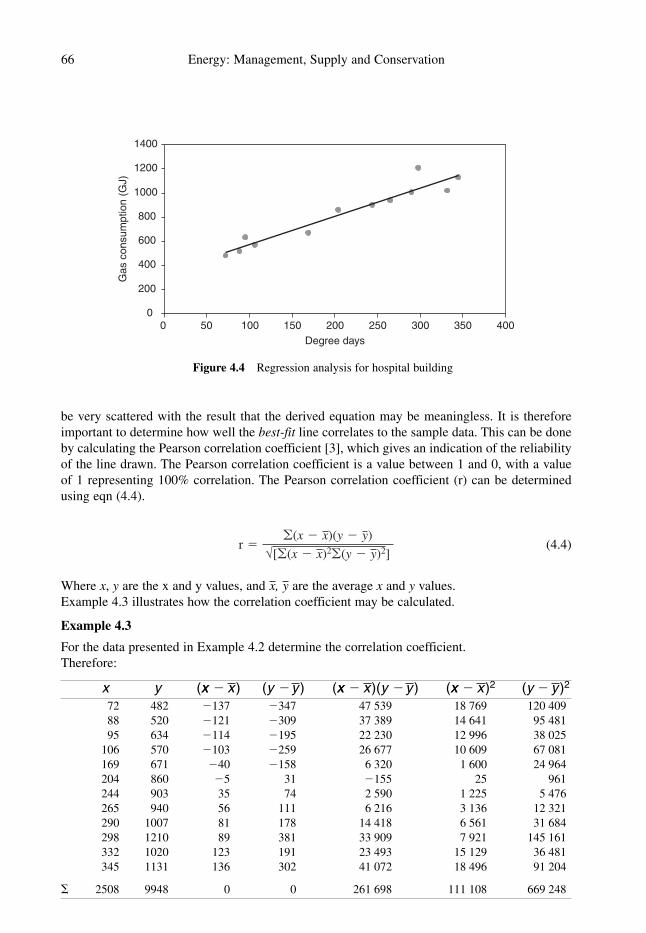
be very scattered with the result that the derived equation may be meaningless. It is therefore
important to determine how well the best-fit line correlates to the sample data. This can be done
by calculating the Pearson correlation coefficient [3], which gives an indication of the reliability
of the line drawn. The Pearson correlation coefficient is a value between 1 and 0, with a value
of 1 representing 100% correlation. The Pearson correlation coefficient (r) can be determined
using eqn (4.4).
(4.4)
Where x, y are the x and y values, and , are the average x and y values.
Example 4.3 illustrates how the correlation coefficient may be calculated.
Example 4.3
For the data presented in Example 4.2 determine the correlation coefficient.
Therefore:
x y (xx � ) (y � ) (xx � )(y � ) (xx � )2 (y � )2
72 482 �137 �347 47 539 18 769 120 409
88 520 �121 �309 37 389 14 641 95 481
95 634 �114 �195 22 230 12 996 38 025
106 570 �103 �259 26 677 10 609 67 081
169 671 �40 �158 6 320 1 600 24 964
204 860 �5 31 �155 25 961
244 903 35 74 2 590 1 225 5 476
265 940 56 111 6 216 3 136 12 321
290 1007 81 178 14 418 6 561 31 684
298 1210 89 381 33 909 7 921 145 161
332 1020 123 191 23 493 15 129 36 481
345 1131 136 302 41 072 18 496 91 204
� 2508 9948 0 0 261 698 111 108 669 248
yxyxyx
yx
r ��(x � x)(y � y)
√[�(x � x)2�(y � y)2]
66 Energy: Management, Supply and Conservation
0
200
400
600
800
1000
1200
1400
Gas c
onsum
ption (
GJ)
0 50 100 150 200 250 300 350 400
Degree days
Figure 4.4 Regression analysis for hospital building
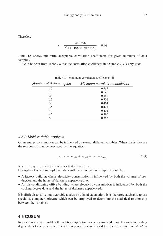
Energy analysis techniques 67
Table 4.8 Minimum correlation coefficients [4]
Number of data samples Minimum correlation coefficient
10 0.767
15 0.641
20 0.561
25 0.506
30 0.464
35 0.425
40 0.402
45 0.380
50 0.362
Therefore:
Table 4.8 shows minimum acceptable correlation coefficients for given numbers of data
samples.
It can be seen from Table 4.8 that the correlation coefficient in Example 4.3 is very good.
r �261 698
√(111 108 � 669 248)� 0.96
4.5.3 Multi-variable analysis
Often energy consumption can be influenced by several different variables. When this is the case
the relationship can be described by the equation:
y � c � m1x1 � m2x2 � . . . � mnxn (4.5)
where x1, x2, . . . ,xn are the variables that influence y.
Examples of where multiple variables influence energy consumption could be:
• A factory building where electricity consumption is influenced by both the volume of pro-
duction and the hours of darkness experienced; or
• An air conditioning office building where electricity consumption is influenced by both the
cooling degree days and the hours of darkness experienced.
It is difficult to solve multivariable analysis by hand calculation. It is therefore advisable to use
specialist computer software which can be employed to determine the statistical relationship
between the variables.
4.6 CUSUM
Regression analysis enables the relationship between energy use and variables such as heating
degree days to be established for a given period. It can be used to establish a base line standard

68 Energy: Management, Supply and Conservation
performance equation, against which subsequent energy consumption can be measured.
One technique that can be employed to assess subsequent energy consumption is known as
CUSUM, which is an acronym for cumulative sum deviation method [2, 5]. It is a measure of the
progressive deviation from a standard consumption pattern. It is simple to calculate and involves
the cumulative summation of the differences between actual energy consumption and target, or
base line, energy consumption. Base line values should be calculated from a standard performance
equation which should be derived through analysis of data collected during a monitoring period
before any interventions are made.
In order to produce a CUSUM plot the following steps should be taken:
(i) Plot a scatter graph of the two variables under consideration (similar to that shown in Figure
4.4) for the ‘base line’ period and derive a standard performance equation as described in
Section 4.5.1.
(ii) Use the standard performance equation to calculate the predicted energy consumption for
each month (including the period covered by the baseline and any subsequent study
months).
(iii) For each data point (i.e. for each month), subtract the predicted consumption from the
actual consumption.
(iv) For each data point, obtain the cumulative total deviation from predicted consumption;
this gives the CUSUM value for each data point.
(v) Plot the CUSUM values against time.
The CUSUM process is illustrated by Example 4.4, which shows the gas consumption for an
office building over a 44 month period.
Example 4.4
An energy audit of an office building for the period August 1989 to December 1990 produced
the following gas consumption data:
Year Month Gas consumed (kWh) Heating degree days
1989 August 15 490 18
September 23 700 36
October 55 673 109
November 94 382 199
December 106 683 239
1990 January 110 745 247
February 96 458 210
March 95 903 207
April 93 265 195
May 60 045 117
June 32 267 58
July 18 849 24
August 12 435 12
September 32 775 60
October 43 924 95
November 95 012 201
December 129 505 280

Energy analysis techniques 69
A subsequent monitoring programme found gas consumption for the period January 1991 to
March 1993 to be as follows:
Year Month Gas consumed (kWh) Heating degree days
1991 January 140 022 308
February 180 034 338
March 118 524 214
April 112 045 201
May 64 045 108
June 37 724 67
July 18 490 24
August 17 045 21
September 22 483 35
October 66 275 140
November 101 040 219
December 120 500 262
1992 January 144 240 323
February 123 140 271
March 91 500 232
April 78 041 195
May 41 004 96
June 20 549 39
July 13 461 18
August 16 062 26
September 28 740 61
October 44 467 103
November 77 206 197
December 112 442 290
1993 January 98 950 260
February 98 399 253
March 97 760 250
Given the information above produce a CUSUM plot for the building.
Solution
Using the linear regression technique described in Section 4.5.1 the standard performance equa-
tion for the base line period is:
Monthly gas consumption � 7744.7 � (427.16 � degree days)
Once this is established it is possible to produce the CUSUM results, as shown in Table 4.9.
From the results in Table 4.9 it is possible to produce the CUSUM plot, as shown in Figure 4.5.
A cursory inspection of the CUSUM graph in Figure 4.5 reveals that two major events
occurred during the monitoring period, one in February 1991 when the energy consumption
dramatically increased, and the other in February 1992 when it started to decrease. In fact further
investigation revealed that:
• In February 1991 the time clock on the heating system was incorrectly set, so that the heating
remained on until 22.00 hours, leading to a dramatic increase in gas consumption.
This problem was spotted and rectified in May 1991, at which point the CUSUM plot returns
to a similar gradient as that experienced during the base line period.
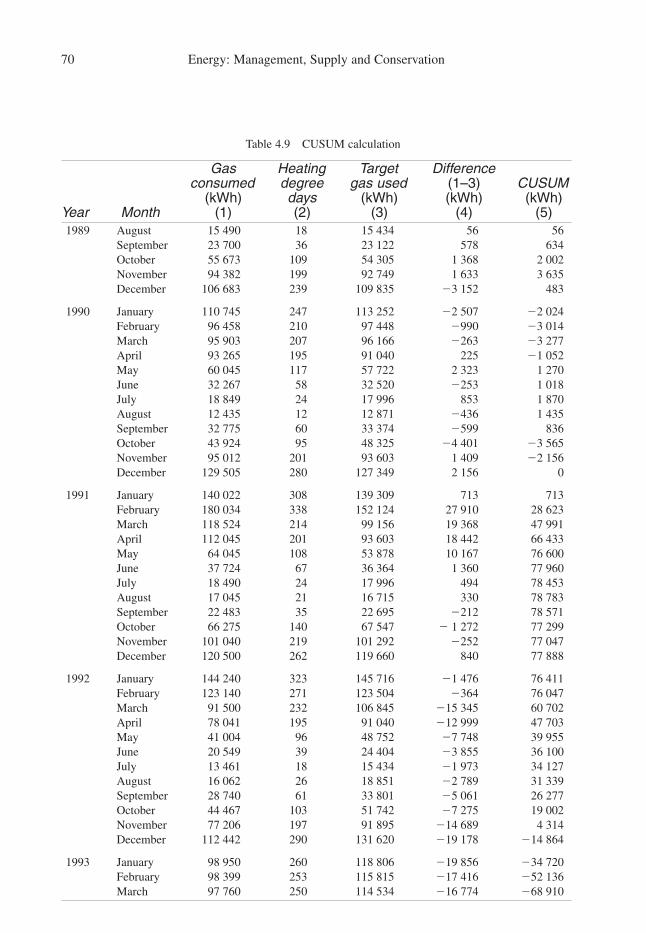
70 Energy: Management, Supply and Conservation
Table 4.9 CUSUM calculation
Gas Heating Target Difference consumed degree gas used (1–3) CUSUM
(kWh) days (kWh) (kWh) (kWh)Year Month (1) (2) (3) (4) (5)1989 August 15 490 18 15 434 56 56
September 23 700 36 23 122 578 634
October 55 673 109 54 305 1 368 2 002
November 94 382 199 92 749 1 633 3 635
December 106 683 239 109 835 �3 152 483
1990 January 110 745 247 113 252 �2 507 �2 024
February 96 458 210 97 448 �990 �3 014
March 95 903 207 96 166 �263 �3 277
April 93 265 195 91 040 225 �1 052
May 60 045 117 57 722 2 323 1 270
June 32 267 58 32 520 �253 1 018
July 18 849 24 17 996 853 1 870
August 12 435 12 12 871 �436 1 435
September 32 775 60 33 374 �599 836
October 43 924 95 48 325 �4 401 �3 565
November 95 012 201 93 603 1 409 �2 156
December 129 505 280 127 349 2 156 0
1991 January 140 022 308 139 309 713 713
February 180 034 338 152 124 27 910 28 623
March 118 524 214 99 156 19 368 47 991
April 112 045 201 93 603 18 442 66 433
May 64 045 108 53 878 10 167 76 600
June 37 724 67 36 364 1 360 77 960
July 18 490 24 17 996 494 78 453
August 17 045 21 16 715 330 78 783
September 22 483 35 22 695 �212 78 571
October 66 275 140 67 547 � 1 272 77 299
November 101 040 219 101 292 �252 77 047
December 120 500 262 119 660 840 77 888
1992 January 144 240 323 145 716 �1 476 76 411
February 123 140 271 123 504 �364 76 047
March 91 500 232 106 845 �15 345 60 702
April 78 041 195 91 040 �12 999 47 703
May 41 004 96 48 752 �7 748 39 955
June 20 549 39 24 404 �3 855 36 100
July 13 461 18 15 434 �1 973 34 127
August 16 062 26 18 851 �2 789 31 339
September 28 740 61 33 801 �5 061 26 277
October 44 467 103 51 742 �7 275 19 002
November 77 206 197 91 895 �14 689 4 314
December 112 442 290 131 620 �19 178 �14 864
1993 January 98 950 260 118 806 �19 856 �34 720
February 98 399 253 115 815 �17 416 �52 136
March 97 760 250 114 534 �16 774 �68 910

• In February 1992 the old single glazing in the office building was replaced by double glazed
window, thus leading to a fall in energy consumption.
It should also be noted that:
• During the summer months the slope of the CUSUM line became less steep, due to the
reduced demand for heating.
• The base line should always be a horizontal line through zero. This is because by definition it
is a best-fit straight line for the data samples occurring during the base line period. The actual
samples during this period may deviate from the predicted base line figures, but the CUSUM
plot will always fluctuate about zero.
• The greater the slope downwards of the CUSUM line, the more energy efficient the process.
References
1. Energy audits and surveys. (1991). CIBSE Applications Manual AM5.
2. Waste avoidance methods. (1995). Fuel Efficiency Booklet 13, Department of the
Environment.
3. Campbell, M. J. and Machin, D. (1999). Medical statistics: a commonsense approach.
Appendix 1. John Wiley and Sons.
4. Measurement of energy consumption: CIBSE Building Energy Code Part 4. (1982). CIBSE.
5. Harris, P. (1985). Monitoring consumption and setting targets. Energy Manager’s Workbook,
2 (Chapter 2), Energy Publications.
Bibliography
Contract energy management. (1991). CIBSE Applications Manual AM6.
Eastop, T. D. and Croft, D. R. (1990). Energy efficiency for engineers and technologists
(Chapters 7 and 9). Longman Scientific & Technical.
Energy analysis techniques 71
–80000
–60000
–40000
–20000
0
20000
40000
60000
80000
100000
CU
SU
M(k
Wh
)F
ebru
ary
Decem
ber
Octo
ber
August
June
April
Decem
ber
Octo
ber
August
June
Febru
ary
April
Febru
ary
Decem
ber
Octo
ber
August
June
April
Febru
ary
Decem
ber
Octo
ber
August
Figure 4.5 CUSUM graph

Energy audits and surveys. (1991). CIBSE Applications Manual AM5.
Harris, P. (1985). Monitoring consumption and setting targets. Energy Manager’s Workbook, 2
(Chapter 2), Energy Publications.
Moss, K. J. (1997). Energy Management and Operating Costs in Buildings (Chapter 10). E&FN
Spon.
72 Energy: Management, Supply and Conservation

5
Energy audits and surveys
Before any energy saving measures can be undertaken within an organization, it is first
necessary to collect comprehensive energy data through an auditing process. This chapter
focuses on the mechanics of energy auditing and describes the procedures involved. The
differences between preliminary, targeted and comprehensive audits are discussed and the
procedures associated with each type highlighted. The subject of energy surveys is also
discussed.
5.1 Introduction
There is a strong analogy between the medical profession and the field of energy management.
If a patient with a medical complaint presents him or herself before a doctor, the doctor must
first accurately diagnose the condition before taking further steps. The doctor should obtain
information from the patient by asking informed questions, possibly carrying out tests, use
knowledge and expertize in order to diagnose the complaint and ultimately prescribe treatment.
In a similar manner, before any energy ‘problems’ can be treated it is first necessary to deter-
mine the current state of a facility’s, or organization’s energy consumption and thus diagnose
any problems that exist. In order to do this, an energy audit must be undertaken and analysis
performed on the data collected.
An energy audit is a feasibility study to establish and quantify the cost of the various energy
inputs to, and flows within, a facility or organization over a given period. The overall aim
of an energy audit is to identify viable and cost effective energy measures which will reduce
operating costs. Energy audits can take a variety of forms, but the process usually involves
collecting data from energy invoices and meters, and undertaking surveys of plant, equipment
and buildings, as well as collecting information from managers and other staff. The auditing
process should identify ways to enhance an organization’s operating efficiency and decrease
its maintenance costs. In addition, the process should help to resolve any occupant comfort
problem which may exist.
An energy audit should be viewed as the ‘foundation’ on which any future energy manage-
ment programme is built. Energy management programmes (discussed in detail in Chapter 7)

involve the continual monitoring and targeting of energy consumption. Before targets can be set,
or effective monitoring undertaken, it is important to establish:
• Baseline energy consumption;
• Patterns of operation and the work practices used;
• The condition of the organization’s buildings, plant and equipment; and
• Energy management opportunities, which will result in energy cost reductions.
This information can only be obtained by carrying out a full energy audit of an organization’s
facilities.
An energy audit should identify those issues which need immediate direct action, as well as
those which require further detailed investigation. It should also produce data which can be used
to justify future capital investment, and raise, within the organization, general awareness of
energy conservation matters. The financial benefits afforded to an organization by an energy
audit are both direct and indirect. The direct benefits are fairly obvious; energy cost savings can
be achieved by reducing consumption, or simply by changing tariff or fuel type. The indirect
benefits are much less obvious; reduced maintenance costs will arise from improved plant
utilization and reduced operating hours. Also, improved plant utilization may result in the
elimination of excess plant capacity and ultimately reduce capital expenditure.
The auditing process should identify energy management opportunities, which when imple-
mented will result in financial benefit to an organization. The magnitude of these financial
benefits is not necessarily dependent on the level of capital investment. In many situations,
major cost savings can be achieved through the implementation of ‘no cost’ or low cost
measures, such as:
• Changing an energy tariff;
• Rescheduling production activities to take advantage of preferential tariffs;
• Adjusting existing controls so that plant operation matches the actual requirements of the
building or manufacturing process;
• Implementing good housekeeping policies, in which staff are encouraged to avoid energy
wasteful practices;
• Investment in small capital items such as thermostats and time switches.
Although much can be achieved through low cost measures, it is sometimes necessary to under-
take more capital-intensive measures, such as replacing worn out plant or installing a building
management system (BMS). Because of the capital involved in such measures, decisions to
invest in them are usually made by senior management (see Chapter 6). In this situation the
results of an energy audit can be used to justify capital investment.
5.2 Types of energy audit
Although there are many variations, energy audits can broadly be classified as preliminary, targeted
and comprehensive audits. Each type is distinguished by the level of detail involved and the depth
of the analysis undertaken. It is important to select the appropriate audit type for the facility
concerned. Comprehensive audits involve detailed energy surveys of plant, equipment and the
fabric of buildings, which is a time consuming and expensive process. They therefore should not
be undertaken lightly. It is often better to focus detailed surveys on problem areas highlighted by a
preliminary energy audit, otherwise much time and money can be wasted. By carrying out a pre-
liminary audit and methodically applying a range of simple analysis techniques it is often possible
to identify major energy problems without the need for expensive and detailed energy surveys.
74 Energy: Management, Supply and Conservation

Preliminary energy audits seek to establish the quantity and cost of each form of energy used
in a facility or in an organization. They are relatively quick and are designed to determine a
project’s potential; more detailed energy audits and surveys can always be undertaken later if so
required. Preliminary audits are primarily concerned with obtaining data from energy invoices
and meter readings for a given period, which often corresponds to the most recent financial year.
Because such audits are primarily concerned with gathering data from bills and invoices, it is
sometimes helpful to think of preliminary audits as being financial energy audits.
Targeted energy audits often result from preliminary audits. They provide data and detailed
analysis on specific targeted projects. For example, an organization may target its lighting
installation or boilers with a view to up-grading these items of equipment. Targeted audits there-
fore involve detailed surveys of the target subjects and analysis of the energy flows and costs
associated with the targets. They should make recommendations regarding action to be taken.
Comprehensive energy audits provide detailed data on the energy inputs to, and energy flows
within, a facility or organization. They should produce detailed energy project implementation
plans. Such audits involve detailed energy surveys and may involve the use of complex energy
simulation computer software.
Although in-house staff can carry out audits, they are generally undertaken by either special-
ist energy consultants or energy service companies. Energy service companies make their money
through performance contracts, which guarantee organizations energy cost savings in return for
negotiated fees. To energy service companies the main interest lies not in the audit itself, but in
installing and managing plant in accordance with their recommendations. Some companies may
even arrange the finance for such projects. When using an energy service company it is thus
important to remember that they have a vested interest in the outcome of any energy audit and
that they may not be totally impartial. By contrast, energy consultants are independent and
therefore should provide objective advice.
5.2.1 Audit costs
Energy audits can be expensive undertakings. Table 5.1 shows data produced by the California
Energy Commission for the cost of performing an energy audit in the USA [1].
It can be seen from Table 5.1 that the more complex the audit, the higher the costs
involved. It is therefore important to select the appropriate level of audit for any particular
application.
Audit costs are affected by the complexity of the facility under consideration. For example,
complex facilities such as hospitals or universities are more costly to audit than say, schools.
The age of the facility may also affect the cost. For example, if a mechanical system is complex
and the ‘as built’ drawings are out of date or not available then the energy auditors may have
to produce schematic drawings. This can be very time consuming and obviously greatly increases
Energy audits and surveys 75
Table 5.1 Energy audit costs in the USA (1997 rates) [1]
Type of energy audit Typical cost ($/sq. ft.) (1997 dollar rate)
Preliminary audit $0.144–$0.333 per m2
Targeted audit $0.333–$0.778 per m2 (lighting projects)
$0.556–$1.00 per m2 (HVAC and controls projects)
Comprehensive audit $2.00–$5.556 per m2 (less than 4500 m2)
Less than $1.333 per m2 (more than 22500 m2)

the audit costs. Given the cost involved, it is important that organizations assist their auditors by
preparing in advance for the audit and providing the auditing team with as much relevant infor-
mation as possible. Energy bills, fuel invoices, meter readings and operational notes should all be
collected, together with any relevant system or building drawings. Organizations should also
inform their management team that an energy audit is being undertaken and arrange for the
auditors to meet with key managers and other relevant staff.
5.3 Why is energy wasted?
Before looking in detail at the processes involved in energy auditing, it is perhaps worth looking
briefly at the reasons why energy is wasted in so many organizations. Energy is often wasted
because of:
• Poorly designed buildings and installations. Buildings may be poorly insulated resulting in
high space heating costs, or mechanical ventilation ducts may be undersized so that fan power
consumption is high.
• Inadequate control systems. Heating systems may be installed without any optimum start
control.
• Poor control settings. Time clock controllers may be incorrectly set so that buildings are
heated when not in use.
• Inefficient plant operation, often arising from the use of old or out of date technology,
a situation often made worse by poor maintenance practices.
• Poor operating and working practices. Lights are often left on in buildings when they should
be switched off.
Although the reasons for energy waste are multifactorial, some of the main reasons are as follows:
• Building designers do not pay energy bills. The design process is closely allied to the
construction process, and designers usually select low capital cost solutions, which often
result in higher operating costs. This situation is made worse by the fact that the budgets for
constructing a facility and running it are usually completely separate.
• Energy consumption is taken for granted. Most building occupants and users do not pay
energy bills. They are concerned with their own personal comfort and are not particularly
interested in how much energy is consumed in achieving a comfortable environment.
• Most organizations do not have a culture of energy efficiency.
• In many countries the cost of energy is low in comparison with labour costs.
The above list demonstrates that much energy wastage arises from poor strategic and operational
management, and also a lack of an energy saving culture amongst staff. Energy can often be
saved at no capital expense simply by improving maintenance procedures and instigating good
work practices. This is often referred to as ‘good housekeeping’, and involves simple measures
such as encouraging personnel to switch off lights when they are not required. Initiating good
maintenance procedures is also important. For example, if filters in ducted air handling systems
are not replaced regularly, then they become dirty with the result that fan energy consumption
increases. It has been estimated that energy bills for organizations can be reduced by approxi-
mately 20% through the use of good energy management practices [2]. It is therefore important
that the human and management aspects of energy consumption are investigated in any energy
audit. Without a supportive management culture it is difficult to make lasting energy savings in
any organization.
76 Energy: Management, Supply and Conservation

5.4 Preliminary energy audits
Preliminary audits seek to quantify and cost each form of energy input to a facility or organiza-
tion over a period of time. They should also identify where the energy is being used within the
organization. The main processes involved in such an audit are:
• Collecting data
• Analysing data
• Presenting data
• Establishing priorities and making recommendations.
At the start of any audit process it is important to gather preliminary data about the geographic
location of the particular facility concerned, together with any relevant distinguishing features
such as its altitude and orientation. Local weather data and degree day data covering the audit
period should also be collected. These data will act as a benchmark reference against which the
facility’s energy consumption can be measured. With manufacturing facilities it will also be
necessary to collect data concerning the production output during the audit period, since this will
have a considerable impact on energy consumption.
Probably the single most important source of energy data is the energy invoice. It is therefore
very important that the audit team has all the relevant energy invoices for the selected audit
period. By compiling data from invoices it is possible to build up a clear picture of the pattern
of energy consumption and the associated costs to a facility of the various energy inputs. In
addition, the total amount spent on energy can be determined from the invoices, thus indicating
the upper limit which can ultimately be saved through energy management measures.
When collecting data from fuel and energy invoices it is important to ensure that copies of all
utility invoices for the audit period are collected rather than simply those for which payments
were made during the audit period. It is also important to collect all the invoices or delivery notes
relating to oil, solid fuel or liquid petroleum gas for the audit period. Due to the time lag between
delivery and consumption, it may also be necessary to include deliveries which occurred before
the start of the audit period. In addition, it is essential that all the metering and supply points are
identified from the invoices, to account for all the energy inputs.
Any estimated meter readings should be identified, since these can result in misleading data.
In order to overcome the problems associated with estimated readings, additional invoices
should be collected which cover the same months as the estimated invoice, but for years prior to
the audit period. These ‘real’ data can then be compared with the estimated data, to establish
realistic data for the audit period. Where possible, data from invoices should be corroborated by
independent meter reading data collected over the audit period.
If invoice data are inadequate or unavailable, then it will be necessary to approach the utility
companies or fuel suppliers for assistance.
Although for most facilities it will be relatively simple to identify the utility metering points,
on large complex sites it may be difficult to account for all the meters. Utility services may come
from a variety of sources and this will be reflected in the invoices. Consider a large supermarket
site which has an 11 kV electricity supply to the main shopping complex and a separate incoming
415 V supply to a remote petrol station owned by the retailer on the same site. Both supplies will
be billed separately, and may be on different tariffs. The two supplies might even come from
different utility companies!
Preliminary analysis of energy invoices can often be very useful in identifying any anomalies
which require further investigation. If a relatively small building on a site consumes as much
gas as one of its much larger neighbours, then it would appear that something is wrong.
Energy audits and surveys 77

Further investigation can then be undertaken, which might reveal that the high gas consumption is
due to the heating plant in the small building operating at nighttime when the building is empty.
Given that the gathering of information from invoices is crucial to the auditing process, it is
important that energy invoices be understood. It is also important to understand the peculiarities
of the various fuel types and utility services, since these can have a bearing on energy
consumption and on the auditing process itself.
5.4.1 Electricity invoices
The precise nature of electricity tariffs and supply contracts is discussed in detail in Chapter 2.
For the purpose of this chapter we will consider only monthly maximum demand tariffs, since
many medium-sized and large organizations use tariffs of a similar nature. Figure 5.1 shows a
simplified electricity invoice, which illustrates many of the features commonly found in monthly
electricity bills.
The monthly electricity invoice shown in Figure 5.1 contains the following information:
• The date of the meter reading.
• The monthly standing charge, which is £30.00 in Figure 5.1.
• The present and previous meter readings with the number of units supplied. These are usually
divided into two sets of meter readings, daytime units (i.e. peak rate) and nighttime units
(i.e. off-peak rate). The difference between the present and previous readings is the units of
electricity consumed in the period since the previous meter reading. With some meters a
constant may be included on the invoice; multiplication of the meter advances by this constant
gives the actual number of units supplied in kVAh or kWh.
• The charges for each unit of electrical energy consumed. These are usually different for the
daytime and nighttime. In Figure 5.1 the peak rate is 6.05 p per kVAh and the off-peak rate is
2.60 p per kVAh. Sometimes blocks of units are charged at different rates. Some tariffs levy a
higher unit charge on the first 1000 kVAh or kWh consumed.
78 Energy: Management, Supply and Conservation
METER READINGS METER READING DATE:23/01/2000
Present Previous Units Consumed
247451184530 (Night)
224520174702 (Night)
229319828 (Night)
MAXIMUM DEMANDTHIS MONTH
270 kVA ANNUAL MAXIMUMDEMAND
300 kVA
DESCRIPTION OFCHARGE
No. OFUNITSOR kVA
RATE AMOUNTEXCLUSIVEOF TAX
TAX(VAT)
%RATE
MONTHLY CHARGEAVAILABILITY CHARGEMAX.DEMAND CHARGEUNIT CHARGENIGHT UNITS
£30.00£1.41£5.35
30.00423.00
1444.50
5.2574.03
252.79
17.5017.5017.50
300.0270.0
229319828
6.05p2.60p
1387.32255.53
242.7844.72
17.5017.50
TOTAL£4159.92
3540.35 619.57TOTAL DUE
Figure 5.1 Monthly electricity bill

• A monthly maximum demand charge for every kW or kVA of the peak power demand occur-
ring during the billing month. Maximum demand charges are designed to penalize users who
make heavy demands on the supply grid during peak periods. They vary throughout the year;
in northern countries such as the UK, they are at their highest in December and January and
very low, or non-existent, during the summer. In hot countries where air conditioning is exten-
sively used, the situation is reversed with the highest demand charges being levied in summer.
Demand charges are often stepped and levied at different rates for various parts of the year.
Figure 5.1 shows a maximum demand of 270 kVA, all of which is charged at £5.35 per kVA.
• The supply capacity, for which a monthly availability charge is levied. In Figure 5.1 charge-
able supply capacity is 300 kVA, all of which is charged at £1.41 per kVA each month.
• The VAT charged on the bill, together with the total cost due.
5.4.2 Natural gas
Natural gas invoices are generally much less complicated than their electricity counterparts.
Figure 5.2 shows a typical example of a monthly gas invoice.
The gas invoices in Figure 5.2 includes the following:
• The date of meter reading or estimate.
• The calorific value of gas (i.e. 39.6 MJ/m3 in Figure 5.2);
• The present and previous readings with the amount of gas used, often presented in cubic feet,
cubic metres or kWh (and sometimes in therms);
• The unit price per kWh of natural gas (i.e. 1.520 p/kWh in Figure 5.2);
• A fixed monthly or quarterly standing charge (i.e. £9.45 per kWh in Figure 5.2).
• The VAT charged on the bill, together with the total cost due.
The unit price of natural gas may be fixed as in Figure 5.2, or it may vary depending on the
volume of gas consumed. In addition, some large sites may have a combination of firm and
interruptible supplies, which may be invoiced separately.
5.4.3 Fuel oil
Fuel oil is measured by volume, which varies with temperature. Delivery invoices for fuel oils
should therefore state the volume corrected to a standard condition of 15.5 °C [3]. They should
also state the date of delivery, the delivery note reference number, the unit cost per standard litre,
Energy audits and surveys 79
DATE OFBILL
03/04/2000 DATE OF METERREADING
16/03/2000 CALORIFIC
VALUE (MJ/m )3
39.6
METER READING GAS USED COSTSPresent Previous Cubic Feet Cubic
MetreskWh
3171 2825 346 979.1 10770 163.70
STANDING CHARGE 9.45£173.15 AT 17.5% VAT 30.30
UNIT CHARGE 1.520p/kWhTOTAL £203.45
Figure 5.2 Typical gas bill

80 Energy: Management, Supply and Conservation
and the VAT charged on the bill. The calorific value of the oil may be included, but if not, this
should be obtained from the supplier. This last point is important because the calorific value
varies with the type of fuel oil used.
5.4.4 Solid fuel
Solid fuel invoices generally state the weight delivered and the cost, but do not always include
data on the calorific value. These data can usually be obtained from the supplier. Solid fuels can
present particular problems to energy auditors because they are often stock piled, making
accurate short-term assessment of solid fuel consumption a difficult task.
5.4.5 Heat
In many parts of northern Europe buildings and whole towns rely on heat produced in cogener-
ation plants. The heat is usually supplied in the form of medium-pressure or high-pressure water
from a district heating main and transferred to individual buildings via heat exchangers. The heat
energy consumption is recorded by heat meters, which record the water flow rate, and the
temperatures of the water entering and leaving the facility, thus determining the energy
consumed in kWh. It is important to note that the accuracy of heat meters can be affected by
variations in temperature and flow rate. At low flow rates or where small temperature differences
occur, metering errors can be significant.
5.4.6 Site records
In larger more complex facilities, especially those which employ an energy manager, it is often
the case that site energy records are kept. These can be an important source of information to an
audit team and can be used to corroborate data collected from energy invoices. In particular,
records of sub-meter readings can be particularly useful, since they give detailed information
about energy flows. However, when using data collected from sub-meters, it is important to know
where the meters are located and to understand what they are measuring. It should be realized that
sub-meters are always ‘subordinate’ to main meters. In other words, the energy consumption
recorded by a sub-meter is always a sub-set of that recorded by the main meter and not additional
energy consumption. Failure to recognize this will result in major errors. One good way of
avoiding these errors is to construct schematic diagrams showing the respective positions of all
the main meters and sub-meters. In addition, it should be remembered that meter records often
contain mistakes (see Chapter 7). Care should therefore be taken to validate meter readings.
5.4.7 Data analysis
The data analysis techniques used in energy audits are described in detail in Chapter 4. For
a preliminary energy audit, analysis should be limited to those techniques which enable the
auditor to determine:
• How much energy is being consumed;
• What type of energy is being consumed;
• The performance of the facility compared with other similar facilities; and
• The characteristic performance of the building.
These outcomes can be achieved by using the percentage breakdown technique (described in
Section 4.2), the NPI technique (described in Section 4.3) and the linear regression technique
(described in Section 4.5).

Energy audits and surveys 81
When all the energy data have been gathered and analysed, they need to be compared
against various ‘yardsticks’ for similar facilities. Table 5.2 gives the NPIs for various building
types in the UK, together with percentage breakdowns for typical energy consumption [3].
Example 5.1 illustrates how the analysis for a preliminary energy audit might be performed.
Example 5.1
A preliminary energy audit of a 5000 m2 air conditioned office building has yielded the follow-
ing energy data:
Heating Gas Electricity Electricitydegree consumption Gas cost consumption cost
Month days (kWh) (£) (kWh) (£)January 267 90 010 1080.12 68 214 3956.41
February 298 97 160 1165.92 60 312 3437.78
March 250 87 058 1044.70 59 645 3280.48
April 176 71 320 855.84 65 045 3382.34
May 69 47 200 566.40 89 234 4550.93
June 30 38 645 463.74 105 932 5296.60
July 12 33 840 406.08 119 237 5961.85
August 20 34 400 412.80 103 247 5265.60
September 50 44 050 528.60 88 235 4588.22
October 208 75 920 911.04 65 023 3446.22
November 215 78 580 942.96 61 567 3447.75
December 337 106 640 1279.68 70 124 4137.32
Totals 1932 804 823 9657.88 955 815 50 751.50
Given that the office building is located in a city centre and is occupied for 2560 hours per year,
perform an analysis which characterizes the building’s energy consumption.
Solution
The annual energy consumption and energy cost breakdowns are shown in Figure 5.3. It can be
seen from the pie charts that although approximately 46% of the energy consumed is natural gas,
it only accounts for 16% of the energy costs.
The raw energy consumption and cost figures per m2 are as follows:
Annual energy Annual energy costFuel consumption per m2 per m2
Natural gas 160.965 kWh per m2 £1.93 per m2
Electricity 191.163 kWh per m2 £10.15 per m2
Using the methodology explained in Section 4.3, the NPI can be established as follows:
Electrical energy used � 955 815 kWh
Gas used � 804 823 kWh
Total energy consumed � 955 815 � 804 823
� 1760 638 kWh

Table 5.2 Energy breakdown figures and normalized performance indicators for various building types in the UK [3]
Fair Space Domestic Air Other OtherBuilding NPI heating hot water Lighting Ventilation conditioning (specified) (unspecified)type (kWh/m2) (%) (%) (%) (%) (%) (%) (%)School with
indoor
swimming pool 190–240 43 20 9 na na 22 (Pool) 6
School without
indoor
swimming pool 250–310 56 25 12 na na na 7
Restaurant 410–430 25 15 15 5 na 40 (Catering)
Public
house 340–470 38 18 12 na na 11 (Catering) 16
Motorway
service area 880–1200 22 32 9 7 na 30 (Catering) na
Fast food outlet 1450–1750 4 24 1 na na 70 (Cooking) 1
Supermarket 23 (includes 50
with bakery 1130–1350 ventilation) 2 11 na na (Refrigeration) 3
Office building 12 (Electrical na
(naturally ventilated) 230–290 60 8 20 na na consumption)
Office building 1 (Office na
(air conditioned) 250–410 48 6 16 na 29 machines)
Sports centre na
(without 11 (Fans,
swimming pool) 200–340 75 3 11 na na pumps, etc.)
Swimming pool 1050–1390 10 3 11 45 na 33 (Pool water na
heating)
Church building 88–169 88 na 6 na na na 6

Libraries, museums
and art galleries 200–280 60 na 18 na 11 na 11
Large hotel 290–420 50 11 9 na na 18 (Catering) 12
Bank
(non-air conditioned) 180–240 67 4 19 na na na 10
Cinema 650–780 77 3 2 15 na 3 (Projection na
equipment)
Bingo hall 631–770 65 5 13 5 na 7 (Catering) 5
Prison 550–689 45 25 10 na na 10 (Catering) 10
Transport depots 311–381 80 4 6 na na 2 (Catering) 8
Law court 219–300 84 5 8 na na 1 (Catering) 2
Factory (excluding
process energy) 261–369 72 3 15 na na na 10
Cold store 500–675 8 na 10 na na 82 (Refrigeration) na
Warehouse 150–269 80 2 8 na na na 10

From Table 4.5 (see pages 82–3) it can be seen that 75% of the gas consumed can be attributed
directly to space heating. Therefore:
Space heating energy consumption � 1760 638 � 0.75
� 1320 478.5 kWh
By applying weather and exposure coefficients:
� 1682 721.6 kWhNon-heating energy consumption kWh � 1760 638 � 1320 478.5
� 440 159.5 kWh
Therefore
Corrected total energy consumption � 440 159.5 � 1682 721.6
� 2122 881.1 kWh
and correcting for occupancy (using data from Table 4.6):
Therefore
Because the calculated NPI of 431.21 kWh/m2 is above the upper limit of the ‘fair’ range
(i.e. 410 kWh/m2 in Table 5.2), for an air conditioned office building, it can be assumed that the
energy performance of the office building is poor.
Using the methodology described in Section 4.5, it is possible to perform a linear regression
analysis of the gas data. When such an analysis is performed it yields the following performance
equation, which may then be used as the standard performance equation for a future monitoring
and targeting programme (see Chapter 7).
Monthly gas consumption (kWh) � 31 521.75 � (220.788 � Degree days)
This equation shows that the monthly gas base-load consumption is 31 521.75 kWh.
NPI �2156 051.1
5000� 431.21 kWh/m2
Normalized annual energy consumption � 2122 881.1 �2600
2560� 2156 051.1 kWh
Corrected space heating energy consumption �1320478.5 � 2462 � 1.0
1932
84 Energy: Management, Supply and Conservation
Energy consumption
Gas46%
Electricity54%
Energy cost
Electricity84%
Gas16%
Figure 5.3 Energy consumption and cost breakdowns

5.5 Comprehensive energy audits
It is clear from the analysis presented in Example 5.1 that a considerable amount of useful infor-
mation can be obtained from a preliminary energy audit. However, without further investigation
it is not possible to determine where in the office building the energy is being consumed. In order
to do this a more comprehensive audit is required. The analysis techniques used for comprehen-
sive energy audits are essentially much the same as those used for preliminary audits, but the
level of detail is much greater. Comprehensive audits require detailed energy surveys to be
undertaken, and they often require the installation of additional sub-metering in order to deter-
mine accurately component energy flows. Example 5.2 illustrates the auditing benefits which
can be gained from installing comprehensive sub-metering.
Example 5.2
Through the installation of sub-meters in the office building in Example 5.1, it has been possible
to establish the following data:
Space Domesticheating hot water Catering Lifts Lighting Air conditioning Other
Month (kWh) (kWh) (kWh) (kWh) (kWh) (kWh) (kWh)January 54 075 13 239 22 696 620 44 016 21 231 2 348
February 61 856 12 924 22 380 610 41 082 16 566 2 054
March 52 888 11 978 22 191 627 33 746 23 659 1 614
April 38 537 11 348 21 435 631 24 942 27 734 11 738
May 12 841 11 663 22 696 636 19 074 68 013 1 511
June 2395 12 293 23 957 640 14 672 88 713 1 907
July 427 11 663 21 750 625 15 112 1011 681 1 819
August 672 10 717 23 011 621 19 074 81 909 1 643
September 14 420 94 57 20 174 615 26 410 59 655 1 555
October 42 507 11 348 22 065 630 32 719 30 134 1 541
November 43 591 11 978 23 011 632 42 549 16 611 1 775
December 67 868 13 554 25 217 628 45 483 21 929 2 083
Totals 392 077 142 163 270 583 7515 358 877 557 835 31 589
From these data it is possible to produce a comprehensive breakdown of annual energy con-
sumption in each of the component areas (see Figure 5.4).
Example 5.2 makes the bold assumption that extensive sub-metering has been installed in the
office building for auditing purposes. While this is possible it would be an expensive option. It
is therefore often better to employ other techniques to estimate individual energy flows. In some
situations it is possible to deduce energy flows by deducting sub-meter readings from main meter
readings. However, other situations may require the members of the auditing team to use their
skill and judgement to estimate energy flows.
5.5.1 Portable and temporary sub-metering
It may be evident from the outset of an auditing project that the installation of additional
sub-metering will yield much useful information about the energy flows within a facility.
For example, by placing sub-meters on the energy input side and heat meters on the output
side, it is possible to determine the efficiency of individual plant items. Sub-metering should
also highlight any imbalances between the consumption recorded by main meters and the
total recorded by the sub-meters. If additional sub-meters are deemed necessary, then the
Energy audits and surveys 85

additional cost can usually be justified for items of plant or areas with high loads, particu-
larly in situations where little information exists on current energy consumption.
The process of assessing a facility for additional sub-metering can also highlight shortcom-
ings in the facility’s existing metering provision. For example, several buildings may be served
off a single electricity meter. In such a situation, it may be worth considering the installation of
permanent sub-meters, since these would support any future energy management programme.
Permanent metering should also be considered when it is less expensive than the cost of hiring,
installing and removing temporary metering equipment. The installation of permanent or
temporary meters is invasive and involves the shutting off of energy supplies, which in many
circumstances is unsatisfactory. Instead, it is worth considering the use of portable non-invasive
metering. Electricity demand profiles can be monitored using portable clamp-on meters and heat
flows in water pipes can be determined by using clamp-on electronic thermometers and portable
ultrasonic flow meters.
5.5.2 Estimating energy use
In many situations it is either impractical or prohibitively expensive to install comprehensive
sub-metering and so it is necessary to estimate the energy consumption of various items of plant
and equipment. Accurate estimation of equipment energy consumption can be a difficult process
and one which relies on skill and judgement. Nevertheless, it is relatively easy to establish an
upper limit for energy consumption by using eqn (5.1).
(5.1)
where Qout is the plant power output (kW), � is the efficiency of plant, and, Th is the number of
operating hours per year.
While eqn (5.1) may give an upper limit on plant energy consumption it does not provide the
actual operating energy consumption. This problem can be overcome by monitoring the actual
plant energy consumption for a short period of time, using meters, and then multiplying the aver-
age measured load by the annual operating time. In the case of electrical equipment this can be
a relatively simple process since the current can be measured using a portable clamp-on meter.
Annual energy consumption (kWh) �Qout
�� Th
86 Energy: Management, Supply and Conservation
Energy consumption
Space heating22%
Domestic hot water8%
Catering15%Lighting
20%
Air conditioning33%
Other2%
Lifts0.4%
Figure 5.4 Energy consumption breakdown for the office building

Space heating energy consumption can be estimated using the heat loss and degree day
methods described in Chapter 8. The energy consumed in producing domestic hot water can be
determined, if the cold feed water is metered, by using eqn (5.2).
(5.2)
where mcf is the mass of cold feed water used annually (kg), cp is the specific heat capacity of
water (i.e. 4.19 kJ/kgK), ts is the hot water storage temperature (e.g. 60 °C), tcf is the cold feed
water temperature (e.g. 10 °C), and �s is the seasonal efficiency of system.
The seasonal efficiencies for various domestic hot water producing systems are given in Table
5.3.
If the cold feed water consumption is not known then it is possible to estimate the energy
consumed in producing hot water by using eqn (5.3) [4].
(5.3)
Where qhws is the mean power requirement (W/m2), Af is the floor area (m2), and Nw is the
number of working days.
The power requirement (qhws) can be determined using Table 5.4. The energy consumed by
lighting can be estimated simply by counting the number of luminaire fittings and noting their
respective power ratings. With all but tungsten filament lamps, allowances should be made for
control gear losses (see Chapter 12). In most buildings lighting energy consumption lies in the
region 10–20 W/m2 [3].
Annual energy consumption (kWh) � 0.024 � qhws � Af � Nw
Annual energy consumption (kWh) �mcf � cp � (ts�tcf)
�s � 3600
Energy audits and surveys 87
Table 5.3 Seasonal efficiencies for water heating systems [3]
System type Seasonal efficiency
Gas heater with storage cylinder 52
Gas or oil fired boiler with storage cylinder 56
Hot water cylinder with immersion heater using off-peak electricity 80
Instantaneous gas multi-point heater 62
District heating with local calorifiers 60
District heating with central calorifiers and distribution 56
Table 5.4 Mean power requirements for domestic hot water [3]
Mean powerBuilding type requirement (qhws) (W/m2)Office (5 day occupancy) 2.0
Office (6 day occupancy) 2.0
Shop (5 day occupancy) 0.5
Shop (6 day occupancy) 1.0
Factory (5 day occupancy: single shift) 9.0
Factory (6 day occupancy: single shift) 11.0
Factory (7 day occupancy: multiple shift) 12.0
Warehouse 1.0
Residential buildings 17.5
Hotels 8.0
Hospitals 29.0
Education 2.0

5.6 Energy surveys
Energy surveys are an integral part of the auditing process. They enable the auditors to understand
the energy flows within facilities and to identify energy wastage. Surveys can be comprehensive,
looking in depth at all aspects of a facility’s energy consumption, or targeted, in which case they
only cover certain specific issues. The main objectives of any energy survey should be to:
• Determine the energy performance of a facility, or in the case of a targeted survey, targeted
items of plant and equipment.
• Identify and quantify the principal energy flows.
• Identify and quantify achievable energy cost savings.
• Produce costed recommendations to achieve energy cost savings.
• Make recommendations on the future energy management of the facility.
Energy surveys, with the exception of specifically targeted surveys, should cover all aspects relat-
ing to a facility’s or organization’s energy consumption. This will involve detailed surveys of:
• The management and operation characteristics of a facility or organization.
• The energy supply to an organization’s various facilities.
• The energy use within a facility.
• The plant and equipment within a facility.
• The fabric of the organization’s buildings.
5.6.1 Management and operating characteristics
The management culture within an organization can have a great influence on energy consump-
tion. It is therefore important to determine the management structure and practices relating
to energy procurement and consumption. In particular, it is important to identify cost centres
clearly, where the managers accountable for operating costs can be made individually
responsible for energy consumption. Maintenance practices can also have a direct influence on
energy consumption, so it is important to establish the frequency and quality of the maintenance
procedures, and to identify new maintenance measures which could improve the energy
performance of plant and equipment.
At the auditing stage it is important to survey the operating practices within an organization
or facility. Detailed data should be gathered on such factors as:
• The use of a particular space or building.
• The mechanical and electrical services within the building.
• The number and type of occupants. Particular attention should be paid to any special charac-
teristics of occupants. For example, in rooms containing smokers, windows are often opened
with the result that space heating costs are increased.
• The occupancy patterns of building or space.
• The environmental conditions within a space or building. This will include air temperature,
dry resultant temperature, relative humidity and illuminance levels.
• The operating practices of major items of plant and equipment.
Knowledge of the above issues will give the auditor a good understanding of how and why
energy is consumed within a facility. Particular attention should be paid to situations where
actual practice deviates from that stated by the management of an organization. For example,
if rooms which are supposed to be heated to 21 °C are in fact heated to 23 °C, then energy is
being wasted on over-heating spaces.
88 Energy: Management, Supply and Conservation

5.6.2 Energy supply
It is important to identify the tariffs and supply contracts under which any organization purchases
its energy. This will enable the energy auditing team to establish whether or not a particular
organization is purchasing energy at a low price. If an organization is paying a higher than nec-
essary price for its energy, then the auditor should recommend a change of tariff or fuel supplier.
Because electricity tariffs usually include some form of demand charge, it is important that an
organization selects the correct electricity tariff to suite its load profile. Therefore, the audit
process should include a survey of the electrical load profile of a facility. For relatively minor
loads it may be sufficient to take meter readings at the beginning and end of a selected period,
with intermediate readings taken during the daytime, nighttime and at the weekend. This will
give a good indication of when electrical energy is being consumed and should assist the audi-
tor in recommending an appropriate tariff. For larger electrical loads, it is important to survey
the load profile accurately. This can be achieved by using a portable meter to determine demand
and consumption at 30-minute intervals over a selected period. Any large peaks in load should
be identified and further investigations made in order to establish their cause.
With electricity supply, it is important to determine the power factor of a facility. Many items of
equipment, such as fluorescent lamps and electric motors, produce a poor power factor (i.e. a
decoupling of the current and the voltage so that they become out of phase with each other). This
results in higher than expected electricity bills. If poor power factors are found in a facility then it
may be worth considering the installation of power factor correction equipment (see Chapter 12).
5.6.3 Plant and equipment
Major items of plant, such as boilers and refrigeration chillers, convert energy from one form to
another. In doing so energy is wasted. For example, in boilers much of the heat produced by the
combustion process can be wasted by allowing it to escape with the flue gases. The more effi-
cient an item of plant, the less energy is wasted. Major items of plant and equipment should
therefore be surveyed in order to determine their operating efficiency. It is also important
to survey their respective pipe distribution networks since these too can be a major source of
energy wastage.
The subjects of energy efficient heating and refrigeration are dealt with in some detail in
Chapters 8 and 11, so the issues involved in a plant survey are only briefly summarized here.
With boilers it is essential that they be ‘tuned’ so that flue gas heat losses are minimized. This
involves sampling the CO2 or O2 content of the flue gases, and adjusting the burner settings
so that excess O2 is minimized, whilst still ensuring that complete combustion takes place.
In addition, it is important to identify whether or not flue gas heat recovery is feasible.
The efficiency of refrigeration plant is measured by its coefficient of performance (COP). The
higher the COP, the greater the efficiency of the machine. COP varies with the cooling load and
the external air conditions. It is therefore necessary to meter the energy input and output over a
period of time, if the average COP is to be identified. Note should be taken of the operating
pattern of refrigeration plant and also of how it is controlled, since this will tell the auditor much
about the operation of the facility. If both boilers and refrigeration chillers are operating at the
same time, it could be that the two systems are fighting each other. If this is the case, then the
control logic and settings of the system will need adjustment. The feasibility of recovering heat
from the hot condenser gases should also be investigated.
In many facilities much energy is wasted from hot water, chilled water and steam distribution
pipework because of inadequate or poor quality insulation. Pipework systems should therefore
be inspected to establish the quality of the insulation and also to identify any leaks.
Energy audits and surveys 89

Plant surveys should allow for the fact that mechanical equipment has a finite working
life and that efficiency often deteriorates badly when plant is old. Therefore one of the impor-
tant outcomes of such a survey should be a recommendation for the planned replacement of
older plant. In many situations it is much more cost effective to replace old plant, rather than
renovate it.
5.6.4 Building fabric
Although the subject of heat loss through building fabric is covered in detail in Chapter 8, a
few words on the subject are timely here. It is important to note the age, size, shape and
orientation of the buildings within a facility, since these are all factors which affect energy
consumption. In particular, areas of greatest heat loss should be identified. Greatest heat loss
will always occur where the building fabric has a high U value (see Chapter 8). If ‘as built’
drawings exist, these can be used to determine elemental U values. The use of portable infra-
red thermography can also be very useful, since this enables areas of high heat loss to be
instantly identified.
When surveying buildings, it should be appreciated that large amounts of heat can be lost by
excess ventilation (see Chapter 8). This is particularly the case in older properties with old fenes-
tration systems. Particular attention should therefore be paid to any poorly fitting window and door
frames, or to any space where windows and outside doors remain open for any length of time.
5.7 Recommendations
The energy auditing process should enable recommendations to be made, which will result in
cost savings. Although the precise nature of these recommendations will depend on the particular
application in question, they can broadly be classified as follows:
(i) Reducing energy costs by tariff negotiation: Electricity and gas are supplied either through
published tariffs or through negotiated supply contracts. Not all tariffs and supply contracts
are suited to every organization and some are better than others. It may therefore be possi-
ble to reduce energy costs simply by changing tariff or negotiating a more beneficial supply
contract.
(ii) Good maintenance and work practices: Energy can often be saved at no capital expense
simply by ‘good housekeeping’ (i.e. improving maintenance procedures and implementing
good work practices).
(iii) Retrofitting and tuning systems: Energy is often wasted as systems age, because
components wear out or become damaged. Also, the controls associated with these systems
are often inappropriate or poorly set-up with the result that systems perform inefficiently.
Significant energy savings can be achieved through modest capital investment to retrofit
and re-tune inefficient installations.
(iv) Capital investment: In many situations the poor condition of plant and infrastructure
makes refurbishment a futile exercise. Under these circumstances major capital invest-
ment is required to replace existing plant. In this case, it is often worthwhile reapprais-
ing the situation to determine whether or not an alternative installation might be more
appropriate. An existing boiler installation could be replaced by a combined heat and
power (CHP) plant, thus reducing the need to buy in electrical power. Such measures
usually involve large capital investment and careful financial appraisal is therefore
required.
90 Energy: Management, Supply and Conservation
5.8 The audit report
The audit process should identify potential energy management opportunities. Since exploitation
of these opportunities often involves capital expenditure, maximum effort should be put into
investigating those measures which will yield the greatest cost savings. Those energy manage-
ment opportunities which result in lesser savings should be given a low priority. However, all
energy management opportunities, identified through the auditing process should be clearly
stated in the final audit report, together with cost benefit calculations to justify them. The final
audit report should include:
• A description of the facility, including layout drawings, construction details, hours of opera-
tion, equipment lists and any relevant materials and product flows.
• A description of the various utility tariffs or contracts used.
• A presentation of all the energy data gathered, together with any relevant analysis.
• A detailed statement of potential energy management opportunities, together with supporting
cost-benefit analysis calculations.
• An energy management action plan for the future operation of the facility. This may include
an implementation schedule for the recommended energy management opportunities and a
programme for the ongoing energy monitoring and targeting of the facility.
Although the audit report should contain detailed technical information, it is important to
remember that its primary purpose is to communicate the principal findings of the audit to an
organization’s senior management, many of whom may have little understanding of energy
matters. It is therefore advisable to include a short executive summary, giving a brief synopsis of
the report and highlighting its major findings and recommendations.
References1. How to hire an energy auditor to identify energy efficiency projects. (2000). California
Energy Commission. January.
2. Aspects of energy management. (1995). General Information Report 12, Department of the
Environment. May.
3. Energy audits and surveys. (1991). CIBSE Applications Manual AM5.
4. Measurement of energy consumption: CIBSE Building Energy Code Part 4. (1982). CIBSE.
Bibliography
Capehurst, B. L., Turner, W. C. and Kennedy, W. J. (1997). Guide to energy management (Chapter
2). The Fairmont Press, Prentice Hall.
Eastop, T. D. and Croft, D. R. (1990). Energy efficiency for engineers and technologists (Chapter
9). Longman Scientific & Technical.
Energy audits and surveys (1991). CIBSE Applications Manual AM5.
Energy audits for buildings, Fuel Efficiency Booklet 1 (1993). Department of the Environment.
How to hire an energy auditor to identify energy efficiency projects (2000). California Energy
Commission. January.
Moss, K. J. (1997). Energy management and operating costs in buildings (Chapter 9). E & FN
Spon.
Thumann, A. and Mehta, P. D. (1997). Handbook of energy engineering (Chapter 3). The
Fairmont Press, Prentice Hall.
Energy audits and surveys 91

6
Project investment appraisal
It is important to justify any capital investment project by carrying out a financial appraisal.
The financial issues associated with capital investment in energy saving projects are
investigated in this chapter. In particular, the discounted cash flow techniques of net present
value and internal rate of return are presented and discussed.
6.1 Introduction
When planning an energy efficiency or energy management project, the costs involved should
always be considered. Therefore, as with any other type of investment, energy management
proposals should show the likely return on any capital that is invested. Consider the case of
an energy consultant who advises the senior management of an organization that capital
should be invested in new boiler plant. Inevitably, the management of the organization would
enquire:
• How much will the proposal cost?
• How much money will be saved by the proposal?
These are, of course, not unreasonable questions, since within any organization there are many
‘worthy causes’, each of which requires funding and it is the job of senior management to invest
capital where it is going to obtain the greatest return. In order to make a decision about any
course of action, management needs to be able to appraise all the costs involved in a project and
determine the potential returns. This however, is not quite as straightforward as it might first
appear. The capital value of plant or equipment usually decreases with time and it often requires
more maintenance as it gets older. If money is borrowed from a bank to finance a project, then
interest will have to be paid on the loan. Inflation too will influence the value of any future
energy savings that might be achieved. It is therefore important that the cost appraisal process
allows for all these factors, with the aim of determining which investments should be
undertaken, and of optimizing the benefits achieved. To this end a number of accounting
and financial appraisal techniques have been developed which help managers make correct and
objective decisions. It is these financial appraisal techniques which are introduced and
discussed in this chapter.

Project investment appraisal 93
6.2 Fixed and variable costs
When appraising the potential costs involved in a project it is important to understand the
difference between fixed and variable costs. Variable costs are those which vary directly with the
output of a particular plant or production process, such as fuel costs. Fixed costs are those costs,
which are not dependent on plant or process output, such as site-rent and insurance. The total
cost of any project is therefore the sum of the fixed and variable costs. Example 6.1 illustrates
how both fixed and variable costs combine to make the total operating cost.
Example 6.1
Determine the total cost of a diesel generator operating over a 5-year period. Assume that the
capital cost of the generator is £15 000, the annual output is 219 MWh, and the maintenance
costs are £500 per annum. The cost of producing each unit of electricity is 3.5 p/kWh.
Solution
Item Type of cost Calculation Cost (£)Capital cost of generator Fixed n.a. 15 000.00
Annual maintenance Fixed £ 500 � 5 2 500.00
Fuel cost Variable 219 000 � 0.035 7 665.00
Total cost � 25 165.00
From Example 6.1 it can be seen that the fixed costs represent 69.5% of the total cost. In fact,
the annual electricity output of 219 MWh assumes that the plant is operating with an average
output of 50 kW. If this output were increased to an average of 70 kW, then the fuel cost would
become £10 731, with the result that the fixed costs would drop to 62% of the total. Clearly, the
average unit cost of production decreases as output increases.
The concept of fixed and variable costs can be used to determine the break-even point for a
proposed project. The break-even point can be determined by using eqn (6.1).
UCutil � Wav � n � FC � (UCprod � Wav � n) (6.1)
where UCutil is the unit cost per kWh of bought in energy (£/kWh), UCprod is the unit cost per
kWh of produced energy (£/kWh), FC is the fixed costs (£), Wav is the average power output
(or consumption) (kW), and n is the number of hours of operation (h).
Example 6.2
Assuming that electricity bought from a local utility company costs an average of 6.1 p/kWh,
determine the break-even point for the generator described in Example 6.1, when:
(i) the average output is 50 kW; and
(ii) the average output is 70 kW.
Solution
(i) Assuming that the average output of the generator is 50 kW.
0.061 � 50 � n � (15 000 � 2500) � (0.035 � 50 � n)
� n � 13 461.5 hours
(ii) Assuming that the average output of the generator is 70 kW.
0.061 � 70 � n � (15 000 � 2500) � (0.035 � 70 � n)
� n � 9615.4 hours
94 Energy: Management, Supply and Conservation
Clearly, increasing the average output of the generator significantly reduces the break-even time
for the project. This is because the capital investment (i.e. the generator) is being better utilized.
6.3 Interest charges
In order to finance projects, organizations often borrow money from banks or other lending
organizations. Projects financed in this way cost more than similar projects financed from an
organization’s own funds, because interest charges must be paid on the loan. It is therefore
important to understand how interest charges are calculated. Interest charges can be calculated
by lending organizations in two different ways: simple interest and compound interest.
(i) Simple interest: If simple interest is applied, then charges are calculated as a fixed percent-
age of the capital that is borrowed. A fixed interest percentage is applied to each year of the
loan and repayments are calculated using eqn (6.2).
(6.2)
where TRV is the total repayment value (£), LV is the value of initial loan (£), IR is the
interest rate (%), and P is the repayment period (years).
(ii) Compound interest: Compound interest is usually calculated annually (although this is not
necessarily the case). The interest charged is calculated as a percentage of the outstanding
loan at the end of each time period. It is termed ‘compound’ because the outstanding loan
is the sum of the unpaid capital and the interest charges up to that point. The value of the
total repayment can be calculated using eqn (6.3).
(6.3)
The techniques involved in calculating simple and compound interest are illustrated in Example 6.3.
Example 6.3
A company borrows £ 50 000 to finance a new boiler installation. If the interest rate is 9.5% per
annum and the repayment period is 5 years, determine the value of the total repayment and the
monthly repayment value, assuming:
(i) that simple interest is applied; and
(ii) that compound interest is applied.
Solution
(i) Assuming simple interest:
(ii) Assuming compound interest:
Repayment at end of year 1 � 50 000 � � 9.5
100� 50 000� � £54 750.00
Monthly repayment �73 750.00
(5 � 12)� £1229.17
Total repayment � 50 000 � � 9.5
100� 50 000 � 5� � £73 750.00
TRV � LV � �1 �IR
100 �P
TRV � LV � � IR
100� LV � P�

Project investment appraisal 95
and
Similarly, the repayments at the end of years 3, 4 and 5 can be calculated:
Repayment at end of year 3 � £ 65 646.62
Repayment at end of year 4 � £ 71 883.05
Repayment at end of year 5 � £ 78 711.94
Alternatively, eqn (6.3) can be used to determine the compound interest repayment value.
It can be seen that by using compound interest, the lender recoups an additional £4962. Not sur-
prisingly lenders usually charge compound interest on loans.
6.4 Payback period
Probably the simplest technique which can be used to appraise a proposal is payback analysis.
The payback period can be defined as ‘the length of time required for the running total of net
savings before depreciation to equal the capital cost of the project’ [1]. In theory, once the pay-
back period has ended, all the project capital costs will have been recouped and any additional
cost savings achieved can be seen as clear ‘profit’. Obviously, the shorter the payback period, the
more attractive the project becomes. The length of the maximum permissible payback period
generally varies with the business culture concerned. In some countries, payback periods in
excess of 5 years are considered acceptable, whereas in other countries, such as the in the UK,
organizations generally impose payback periods of less than 3 years.
The payback period can be calculated using eqn (6.4).
(6.4)
where PB is the payback period (years), CC is the capital cost of the project (£), and AS is the
annual net cost saving achieved (£).
The annual net cost saving (AS) is the cost saving achieved after all the operational costs have
been met.
Example 6.4
A new combined heat and power (CHP) installation is expected to reduce a company’s annual
energy bill by £8100. If the capital cost of the new boiler installation is £37 000, and the annual
maintenance and operating costs are £700, what will be the expected payback period for the
project?
Solution
PB �37 000
8100 � 700� 5.0 years
PB �CC
AS
Monthly repayment �78 711.94
(5 � 12)� £1311.87
Total repayment value � 50 000 � �1 �9.5
100 �5
� £78 711.94
Repayment at end of year 2 � 54 750 � � 9.5
100� 54 750� � £59 951.25

96 Energy: Management, Supply and Conservation
6.5 Discounted cash flow methods
The payback method is a simple technique which can easily be used to provide a quick evalua-
tion of a proposal. However, it has a number of major weaknesses:
• The payback method does not consider savings that are accrued after the payback period has
finished.
• The payback method does not consider the fact that money, which is invested, should accrue
interest as time passes. In simple terms there is a ‘time value’ component to cash flows. Thus
a £100 today is more valuable than £100 in 10 years’ time.
In order to overcome these weaknesses a number of discounted cash flow techniques have been devel-
oped, which are based on the fact that money invested in a bank will accrue annual interest. The two
most commonly used techniques are the ‘net present value’ and the ‘internal rate of return’ methods.
6.5.1 Net present value method
The net present value method considers the fact that a cash saving (often referred to as a ‘cash
flow’) of £1000 in year 10 of a project will be worth less than a cash flow of £1000 in year 2.
The net present value method achieves this by quantifying the impact of time on any particular
future cash flow. This is done by equating each future cash flow to its current value today, in
other words determining the present value of any future cash flow. The present value (PV) is
determined by using an assumed interest rate, usually referred to as a discount rate.
Discounting is the opposite process to compounding. Compounding determines the future value
of present cash flows, whereas discounting determines the present value of future cash flows.
In order to understand the concept of present value, consider the case described in Example
6.4. If instead of installing a new CHP system, the company invested £37 000 in a bank at an
annual interest rate of 8%, then:
The value of the sum at the end of year 1 � 37 000 � (0.08 � 37 000) � £39 960.00
and
The value of the sum at the end of year 2 � 39 960 � (0.08 � 39 960) � £43 156.80
The value of the investment would grow as compound interest is added, until after n years the
value of the sum would be:
(6.5)
where FV is the future value of investment (£), and D is the value of initial deposit
(or investment) (£).
So after 5 years the future value of the investment would be:
So in 5 years the initial investment of £37 000 will accrue £17 365.14 in interest and will be
worth £54 365.14. Alternatively, it could equally be said that £54 365.14 in 5 years time is
worth £37 000 now (assuming an annual interest rate of 8%). In other words the present value
of £54 365.14 in 5 years time is £37 000 now. The present value of an amount of money at any
specified time in the future can be determined by eqn (6.6).
FV � 37 000 � �1 �8
100 �5
� £54 365.14
FV � D � �1 �IR
100 �n

Project investment appraisal 97
where PV is the present value of S in n years time (£), and S is the value of cash flow in n years
time (£).
The net present value method calculates the present value of all the yearly cash flows (i.e.
capital costs and net savings) incurred or accrued throughout the life of a project, and summates
them. Costs are represented as a negative value and savings as a positive value. The sum of all
the present values is known as the net present value (NPV). The higher the net present value, the
more attractive the proposed project.
The present value of a future cash flow can be determined using eqn (6.6). However, it is
common practice to use a discount factor (DF) when calculating present value. The discount
factor is based on an assumed discount rate (i.e. interest rate) and can be determined by using
eqn (6.7).
(6.7)
The product of a particular cash flow and the discount factor is the present value.
PV � S � DF (6.8)
The value of various discount factors computed for a range of discount rates (i.e. interest rates)
is shown in Table 6.1. Example 6.5 illustrates the process involved in a net present value
analysis.
DF � �1 �IR
100 ��n
PV � S � �1 �IR
100 ��n
Table 6.1 Computed discount factors
Discount rate % (or interest rate %)
Year 2 4 6 8 10 12 14 160 1.000 1.000 1.000 1.000 1.000 1.000 1.000 1.000
1 0.980 0.962 0.943 0.926 0.909 0.893 0.877 0.862
2 0.961 0.925 0.890 0.857 0.826 0.797 0.769 0.743
3 0.942 0.889 0.840 0.794 0.751 0.712 0.675 0.641
4 0.924 0.855 0.792 0.735 0.683 0.636 0.592 0.552
5 0.906 0.822 0.747 0.681 0.621 0.567 0.519 0.476
6 0.888 0.790 0.705 0.630 0.564 0.507 0.456 0.410
7 0.871 0.760 0.665 0.583 0.513 0.452 0.400 0.354
8 0.853 0.731 0.627 0.540 0.467 0.404 0.351 0.305
9 0.837 0.703 0.592 0.500 0.424 0.361 0.308 0.263
10 0.820 0.676 0.558 0.463 0.386 0.322 0.270 0.227
11 0.804 0.650 0.527 0.429 0.350 0.287 0.237 0.195
12 0.788 0.625 0.497 0.397 0.319 0.257 0.208 0.168
13 0.773 0.601 0.469 0.368 0.290 0.229 0.182 0.145
14 0.758 0.577 0.442 0.340 0.263 0.205 0.160 0.125
15 0.743 0.555 0.417 0.315 0.239 0.183 0.140 0.108
16 0.728 0.534 0.394 0.292 0.218 0.163 0.123 0.093
17 0.714 0.513 0.371 0.270 0.198 0.146 0.108 0.080
18 0.700 0.494 0.350 0.250 0.180 0.130 0.095 0.069
19 0.686 0.475 0.331 0.232 0.164 0.116 0.083 0.060
20 0.673 0.456 0.312 0.215 0.149 0.104 0.073 0.051

98 Energy: Management, Supply and Conservation
Example 6.5
Using the net present value analysis technique, evaluate the financial merits of the two
proposed projects shown in the table below. Assume an annual discount rate of 8% for each
project.
Project 1 Project 2
Capital cost (£) 30 000.00 30 000.00
Year Net annual saving (£) Net annual saving (£)
1 �6 000.00 �6 600.00
2 �6 000.00 �6 600.00
3 �6 000.00 �6 300.00
4 �6 000.00 �6 300.00
5 �6 000.00 �6 000.00
6 �6 000.00 �6 000.00
7 �6 000.00 �5 700.00
8 �6 000.00 �5 700.00
9 �6 000.00 �5 400.00
10 �6 000.00 �5 400.00
Total net saving at
end of year 10 �60 000.00 �60 000.00
Solution
The annual cash flows should be multiplied by the annual discount factors for a rate of 8% to
determine the annual present values, as shown in the table below.
Discount Project 1 Project 2
factor for Net Present Net Present 8% savings (£) value (£) savings (£) value (£)
Year (a) (b) (a � b) (c) (a � c)
0 1.000 �30 000.00 �30 000.00 �30 000.00 �30 000.00
1 0.926 �6 000.00 �5 556.00 �6 600.00 �6 111.60
2 0.857 �6 000.00 �5 142.00 �6 600.00 �5 656.20
3 0.794 �6 000.00 �4 764.00 �6 300.00 �5 002.20
4 0.735 �6 000.00 �4 410.00 �6 300.00 �4 630.50
5 0.681 �6 000.00 �4 086.00 �6 000.00 �4 086.00
6 0.630 �6 000.00 �3 780.00 �6 000.00 �3 780.00
7 0.583 �6 000.00 �3 498.00 �5 700.00 �3 323.10
8 0.540 �6 000.00 �3 240.00 �5 700.00 �3 078.00
9 0.500 �6 000.00 �3 000.00 �5 400.00 �2 700.00
10 0.463 �6 000.00 �2 778.00 �5 400.00 �2 500.20
NPV � �10 254.00 NPV � �10 867.80
It can be seen that over a 10-year life-span the net present value for Project 1 is £10 254.00,
while for Project 2 it is £10 867.80. Therefore Project 2 is the preferential proposal.
The whole credibility of the net present value method depends on a realistic prediction of
future interest rates, which can often be unpredictable. It is prudent therefore to set the discount
rate slightly above the interest rate at which the capital for the project is borrowed. This will

Project investment appraisal 99
ensure that the overall analysis is slightly pessimistic, thus acting against the inherent uncertain-
ties in predicting future savings.
6.5.2 Internal rate of return method
It can be seen from Example 6.5 that both projects returned a positive net present value over 10
years, at a discount rate of 8%. However, if the discount rate were reduced there would come a
point when the net present value would become zero. It is clear that the discount rate which must
be applied, in order to achieve a net present value of zero, will be higher for Project 2 than for
Project 1. This means that the average rate of return for Project 2 is higher than for Project 1,
with the result that Project 2 is the better proposition. The discount rate which achieves a net
present value of zero is known as the internal rate of return (IRR). The higher the internal rate
of return, the more attractive the project.
Example 6.6 illustrates how an internal rate of return analysis is performed.
Example 6.6
A proposed project requires an initial capital investment of £20 000. The cash flows generated
by the project are shown in the table below.
Year Cash flow (£)0 �20 000.00
1 �6 000.00
2 �5 500.00
3 �5 000.00
4 �4 500.00
5 �4 000.00
6 �4 000.00
Given the above cash flow data determine the internal rate of return for the project.
Solution
The net present value should be calculated for a range of discount rates, as shown below.
8% discount rate 12% discount rate 16% discount rate
Cash Present Present Presentflow Discount value Discount value Discount value
Year (£) factor (£) factor (£) factor (£)0 �20 000 1.000 �20 000 1.000 �20 000 1.000 �20 000
1 6 000 0.926 5 556 0.893 5 358 0.862 5 172
2 5 500 0.857 4 713.5 0.797 4 383.5 0.743 4 086.5
3 5 000 0.794 3 970 0.712 3 560 0.641 3 205
4 4 500 0.735 3 307.5 0.636 2 862 0.552 2 484
5 4 000 0.681 2 724 0.567 2 268 0.476 1 904
6 4 000 0.630 2 520 0.507 2 028 0.410 1 640
NPV � 2 791 NPV � 459.5 NPV � �1 508.5
It can clearly be seen that the discount rate which results in the net present value being zero lies
somewhere between 12% and 16%. The exact internal rate of return can be found by plotting the
net present values on a graph, as shown in Figure 6.1.
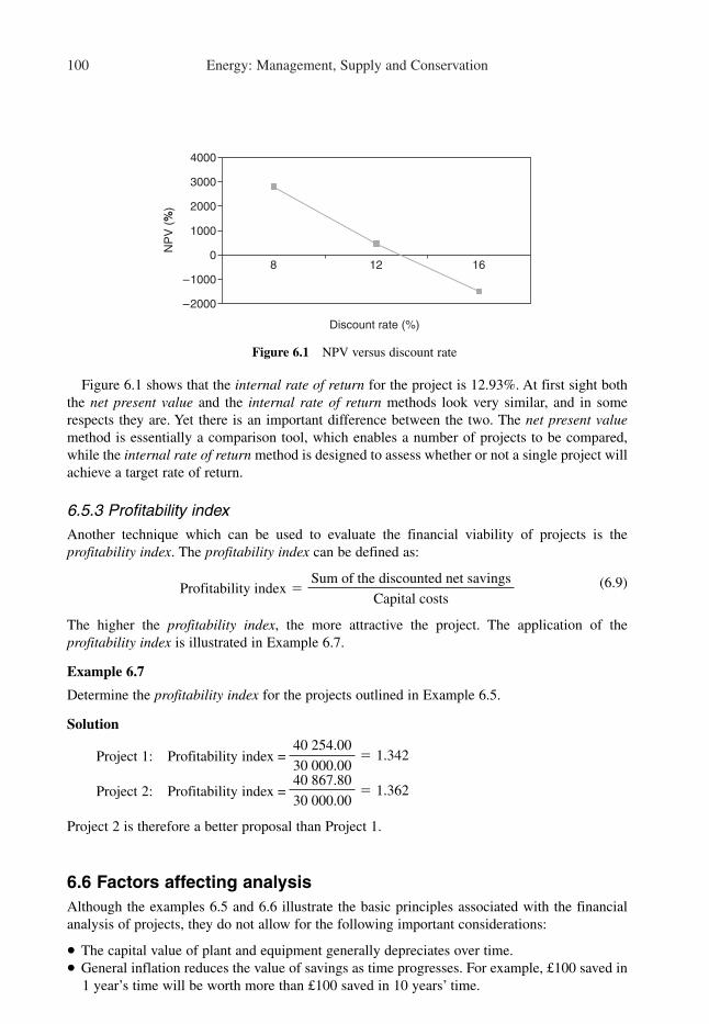
100 Energy: Management, Supply and Conservation
Figure 6.1 shows that the internal rate of return for the project is 12.93%. At first sight both
the net present value and the internal rate of return methods look very similar, and in some
respects they are. Yet there is an important difference between the two. The net present value
method is essentially a comparison tool, which enables a number of projects to be compared,
while the internal rate of return method is designed to assess whether or not a single project will
achieve a target rate of return.
6.5.3 Profitability index
Another technique which can be used to evaluate the financial viability of projects is the
profitability index. The profitability index can be defined as:
(6.9)
The higher the profitability index, the more attractive the project. The application of the
profitability index is illustrated in Example 6.7.
Example 6.7
Determine the profitability index for the projects outlined in Example 6.5.
Solution
Project 1: Profitability index =
Project 2: Profitability index =
Project 2 is therefore a better proposal than Project 1.
6.6 Factors affecting analysis
Although the examples 6.5 and 6.6 illustrate the basic principles associated with the financial
analysis of projects, they do not allow for the following important considerations:
• The capital value of plant and equipment generally depreciates over time.
• General inflation reduces the value of savings as time progresses. For example, £100 saved in
1 year’s time will be worth more than £100 saved in 10 years’ time.
40 867.80
30 000.00� 1.362
40 254.00
30 000.00� 1.342
Profitability index �Sum of the discounted net savings
Capital costs
–2000
–1000
0
1000
2000
3000
4000N
PV
(%
)
8 12 16
Discount rate (%)
%
Figure 6.1 NPV versus discount rate

Project investment appraisal 101
The capital depreciation of an item of equipment can be considered in terms of its salvage value
at the end of the analysis period. Example 6.8 illustrates this point.
Example 6.8
It is proposed to install a heat recovery device in a factory building. The capital cost of installing
the device is £20 000 and after 5 years its salvage value is £1500. If the savings accrued by the
heat recovery device are as shown below, determine the net present value after 5 years. Assume
a discount rate of 8%.
Data:
Year 1 2 3 4 5
Saving (£) 7000 6000 6000 5000 5000
Solution
Discount Capital Net Present factor for investment savings value
8% (£) (£) (£)Year (a) (b) (c) (a) � (b � c)
0 1.000 �20 000.00 �20 000.00
1 0.926 �7000.00 �6 482.00
2 0.857 �6000.00 �5 142.00
3 0.794 �6000.00 �4 764.00
4 0.735 �5000.00 �3 675.00
5 0.681 �1 500.00 �5000.00 �4 426.50
NPV � �4 489.50
It is evident that over a 5-year life-span the net present value of the project is £4489.50. Had the
salvage value of the equipment not been considered, the net present value of the project would
have been only £3468.00.
6.6.1 Real value
Inflation can be defined as the ‘rate of increase in the average price of goods and services’ [1].
In the UK, inflation is expressed in terms of the retail price index (RPI), which is determined
centrally and reflects average inflation over a range of commodities. Because of inflation, the
real value of cash flows decrease with time. The real value of a sum of money (S) realized in n
years time can be determined by using eqn (6.10).
(6.10)
where RV is the real value of S realized in n years time (£), S is the value of cash flow in n years
time (£), and R is the inflation rate (%).
As with the ‘discount factor’ it is common practice to use an ‘inflation factor’ when assessing
the impact of inflation on a project. The inflation factor can be determined by using eqn (6.11).
(6.11)
The product of a particular cash flow and the inflation factor is the real value of the cash flow.
RV � S � IF (6.12)
IF � �1 �R
100 ��n
RV � S � �1 �R
100 ��n

102 Energy: Management, Supply and Conservation
The application of inflation factors is considered in Example 6.9.
Example 6.9
Recalculate the net present value of the energy recovery scheme in Example 6.8, assuming that
the discount rate remains at 8% and that the rate of inflation is 5%.
Solution
Because of inflation;
Real interest rate � Discount rate � Rate of inflation
� Real interest rate � 8 � 5 � 3%
RealCapital Net real Inflation Net real discount Present
investment savings factor savings factor value Year (£) (£) for 5% (£) for 3% (£)0 �20 000.00 1.000 �20 000.00 1.000 �20 000.00
1 �7 000.00 0.952 �6 664.00 0.971 �6 470.74
2 �6 000.00 0.907 �5 442.00 0.943 �5 131.81
3 �6 000.00 0.864 �5 184.00 0.915 �4 743.36
4 �5 000.00 0.823 �4 115.00 0.888 �3 654.12
5 �1 500.00 �5 000.00 0.784 �5 096.00 0.863 �4 397.85
NPV � �4 397.88
Example 6.9 shows that when inflation is assumed to be 5%, the net present value of the project
reduces from £4489.50 to £4397.88. This is to be expected, because general inflation will always
erode the value of future ‘profits’ accrued by a project.
References
1. Eastop, T. D. and Croft, D. R. (1990). Energy efficiency for engineers and technologists
(Chapter 2). Longman Scientific & Technical.
Bibliography
Capehurst, B. L., Turner, W. C. and Kennedy, W. J. (1997). Guide to energy management
(Chapter 4). The Fairmont Press, Prentice Hall.
Eastop, T. D. and Croft, D. R. (1990). Energy efficiency for engineers and technologists (Chapter
2). Longman Scientific & Technical.
Investment appraisal for industrial energy efficiency (1993). Good Practice Guide 69. DOE.
Moss, K. J. (1997). Energy Management and Operating Costs in Buildings (Chapter 8). E & FN
Spon.
Sizer, J. (1979). An Insight into Management Accounting (Chapter 8). Pelican.
Thumann, A. and Mehta, P. D. (1997). Handbook of energy engineering (Chapter 2). The
Fairmont Press, Prentice Hall.

7
Energy monitoring, targeting andwaste avoidance
The concept of monitoring and targeting is discussed in this chapter and techniques for
collecting and analysing energy data are explained. A variety of reporting techniques is also
presented. The subject of waste avoidance is discussed and practical examples given on how
to diagnose and eliminate wasteful energy practices.
7.1 The concept of monitoring and targeting
It is possible to establish the existing energy consumption of a facility or organization
through an energy audit (see Chapter 5). However, this only produces a ‘picture’ of past
energy consumption. In order to keep control of subsequent energy consumption, it is
necessary to initiate a monitoring programme, although by itself it is only of limited value,
as it simply records energy consumption. To achieve improvements in energy performance a
targeting programme, in which targets are set, must accompany the monitoring process and
planned improvements made. The key elements of a monitoring and targeting (M&T)
programme are as follows [1]:
• The establishment of Energy Account Centres (EACs) within an organization. These may be
departments, processes or cost centres. Operational managers should be accountable for the
energy consumption of the EACs for which they are responsible.
• The establishment of standard energy performance benchmarks for each EAC. Standard
energy performance relates energy consumption to a variable, such as degree days or
production output. Standard performance is established through regression analysis of past
energy data (see Chapter 4) and it provides a base line for the assessment of future energy
performance.
• Monitoring the energy consumption of each EAC within an organization. This involves setting
up procedures to ensure the regular collection of reliable energy data.
• The establishment of energy targets for each EAC. Energy cost savings can only be achieved
if improvements are made on standard performance. Achievable targets should therefore be
set which improve on standard performance.

• Energy management reports should be produced for each EAC on a regular basis.
These reports provide the stimulus for improved energy performance, and should also quantify
any improvements that are achieved.
It is important that any proposed M&T programme be designed to suit the needs of its host
organization. From an energy point of view, organizations can be characterized in a variety of
ways. One useful classification method is by the number of sites covered and the level of
metering adopted, as follows [1]:
• Single site with central utility metering;
• Single site with sub-metering;
• Multisite with central utility metering;
• Multisite with sub-metering.
Single sites with central utility metering are probably best treated as a single EAC, while the
introduction of sub-metering enables such sites to be broken-up into a number of separate EACs.
Where organizations have a number of separate properties, each with central utility meters, the
sites should be treated as separate EACs. If organizations have multiple properties, each con-
taining sub-metering, then it should be possible to divide each site into a number of separate EACs.
7.2 Computer-based monitoring and targeting
The use of specially designed computer software is advisable when operating an M&T
programme. Computers should not be seen as a replacement for the energy manager, but simply
as tools which enable large amounts of data to be stored and analysed in a short period of time.
A number of energy management software packages are commercially available, with varying
degrees of complexity (discussion of which is beyond the scope of this book). They all tend to
share the following generic features:
• A database facility, which is capable of storing and organizing large quantities of data collected
over a long period of time.
• The ability to record energy data for all utility types, including data taken from both meters
and invoices.
• The ability to handle complex utility tariffs. Tariffs vary from country to country, and are
becoming increasingly complex as competition is introduced into the utilities sector.
• The ability to handle other variables such as degree days and production data.
• A data analysis facility. This is achieved by incorporating statistical analysis software into the
energy management software.
• A reporting facility, which is capable of quickly producing energy management reports.
With the more sophisticated energy management packages it is possible to interface the software
with Building Management Systems (BMS), so that energy data can be automatically recorded
on a regular basis (e.g. hourly).
One of the great advantages of computer-based systems is their database facility, which
enables historical data and data from many sources to be instantly compared. This facility is
particularly useful when comparing site energy costs on a utility basis and enables energy
managers quickly to assess the relative performance of various EACs. In this way EACs which
are under-performing can be quickly identified and remedial action taken.
104 Energy: Management, Supply and Conservation

7.3 Monitoring and data collection
An integral element of any M&T programme is data collection. Ultimately, the accuracy of an
energy audit or any M&T programme depends on the collection and input of good quality data.
In order to ensure accuracy, robust data collection procedures must be established, but problems
can arise for a variety of reasons. If too few data are used, any analysis will be meaningless. Most
systems therefore require at least 12 sets of data before any meaningful analysis can be carried
out. By contrast, if excessive data are collected it slows down collection and analysis processes,
and leads to an over complex M&T system. In some situations data from various sources may
be incompatible, making comparisons very difficult. For example, utility invoices may be
collected which cover different time periods. In addition, errors may occur when meters are read
incorrectly and also when readings are incorrectly logged.
7.3.1 Data from invoices
In most applications, energy invoices are the primary source of energy data. Data collection from
invoices involves collating various utility and fuel bills, extracting relevant information and
inputting data into a computer. Problems arise when invoices are misplaced. It is therefore
important to establish good collection procedures which ensure that good quality data are
entered into the computer system.
Although an extremely important source of data, in many larger process industries the use of
monthly utility invoices is considered inadequate. This is because the data provided by the
invoices are of insufficient detail and also because the data collection process is too slow, with
the potential for excessive energy wastage. Therefore, in situations where invoice data alone are
considered insufficient, it is necessary to establish more detailed data collection systems.
7.3.2 Data from meters
Meter reading provides another useful source of energy data. Reading of meters should in theory
be a relatively simple task, but unfortunately in practice a number of problems can arise. Some
of the common faults which may arise are as follows [1]:
• Digits may be recorded in the wrong order.
• Too many digits may be inserted in the recorded reading.
• The recorded reading may be wrong by a factor of 10 or even 100.
• Readings may be lost after being recorded.
• The wrong meter may be read.
• Meters may not be read at all.
• Poor writing may be used when recording readings.
Not surprisingly, poorly recorded meter readings can result in much wasted time and effort.
Therefore meter readings should always be validated. Validation checks should include [1]:
• Checking that the correct number of digits is recorded.
• Checking that current readings are higher than previous readings.
• Checking that readings are within predicted energy consumption bands.
• Checking the date of meter readings.
Should a meter reading fail one of the above tests, the most likely source of the discrepancy will
be operator error, although the fault cannot always be attributed to the operator. For example, a
meter may have been changed, or, for some unknown reason, there may have been a period of
Energy monitoring, targeting and waste avoidance 105

abnormally high energy consumption. It is therefore important to establish a robust data valida-
tion system, one that alerts the system user as soon as a potential error is detected. Validation can
take place either when readings are input, or at the initial stages of the data analysis.
The manual reading of meters and the writing down of digits by hand is a time consuming
process which is prone to mistakes. With the advent of smart metering systems, there are a
variety of alternatives to the manual approach. For example, data capture units can be employed.
These are small portable computer units, into which meter readings can be directly entered. The
data collected in this way can later be downloaded to a larger personal computer for analysis.
Data capture units can also be programmed to validate data as it is input. Data capture units thus
improve the quality of manual meter reading, but they still require an operator to visit all the
relevant meters, which is a labour intensive process. By using pulsed output meters it is possible
to carry out remote meter reading automatically. Pulsed output meters send out an electronic
signal which can be automatically monitored by an M&T computer. Many BMS also have the
capability to monitor energy consumption and data can be downloaded to an M&T computer
either as ‘ASCII’ or spreadsheet files.
In situations where existing metering is unable to provide enough detailed information on
energy consumption, it may be necessary to install additional sub-metering (see Chapter 5). This
should improve the overall quality of any M&T programme and result in increased energy
savings. However, additional metering can be expensive and can also lead to a substantial
increase in the quantity data which must be collected and processed. Therefore any additional
metering must be justified, to ensure that potential energy cost savings are not outweighed by the
installation costs.
7.4 Energy targets
At the outset of any M&T programme it is important to set energy targets. Initially, these
should be the standard energy performances which have been established for the respective
EACs [2]. Standard performance can be determined through analysis of past energy
consumption data (see Chapter 4). If these data do not exist, then it will be necessary to
undertake an auditing process to establish credible standard energy performances for the
respective EACs.
Although the standard energy performance is generally used as an initial target, subsequent
energy targets should represent improvements on standard performance. One way of establishing
an improved target is to plot a best-fit straight line through the lower edge of the points on a scatter
diagram (see Figure 7.1). At first sight this might appear as a strange thing to do, but the points
on the lower edge of the scatter diagram represent the historical achievement of least energy
consumption and therefore should be an achievable target. In other words a straight line through
the lower points represents what can actually be achieved in practice and makes an ideal energy
target.
Energy targets should be reappraised on a regular basis. This can be done by defining the best
historical performance as the target in a similar way to that described above, or by basing the
target on an agreed action plan that is designed to achieve energy savings. Both these methods
have the advantage of being based on real data and so should be achievable. A more arbitrary,
and possibly inferior, approach is to set targets based on a percentage improvement on the
current energy performance. No matter the approach chosen, all targets should be realistic and
achievable otherwise they will lose credibility. They should also be reviewed regularly, in order
to maintain pressure to reduce energy consumption.
106 Energy: Management, Supply and Conservation

7.5 Reporting
One of the major outputs of any M&T programme is the production of energy management
reports. These reports perform the vital role of communicating key information to senior and
operational managers, and are therefore the means by which action is initiated within an
organization. In order to ensure that prompt action is taken to minimize wasteful practices,
reports should be as simple as possible and should highlight those areas in which energy wastage
is occurring. Reports should be published regularly so that energy wasteful practices are iden-
tified quickly and not allowed to persist for too long. Reports should be succinct, and conform
to a standard format which should be generated automatically by a computer. This minimizes
preparation time, and also familiarizes managers with the information being communicated.
Figure 7.2 shows an example of a weekly electricity consumption report produced by an M&T
computer program.
Most M&T programmes require reports to be published weekly or monthly. Monthly reports
are usually applicable to large organizations with many sites, with weekly reports being more
suitable to complex high energy consuming facilities. In applications where energy consumption
is particularly high, reports may be produced daily. If the reporting period is too long, energy
may well be needlessly wasted before managers are notified of the problem and remedial action
is taken. Yet, if the reporting period is too short this will lead to an over-complex M&T system
in which too much irrelevant information requires consideration.
The primary purpose of energy management reports is to communicate effectively with
senior and operational managers. They should therefore be tailored to suit the needs of their
readers, with different managers within organizations requiring different levels of report.
Operational managers may need weekly reports, whereas senior management may only require
Energy monitoring, targeting and waste avoidance 107
0
1000
2000
3000
4000
Month
ly g
as c
onsum
ption (
kW
h)
5000
6000
0 50 100 150 200 250 300 350 400 450
Heating degree days
Standard consumption
Target consumption
Linear (standard consumption)
Linear (target consumption)
Figure 7.1 Target curve based on best historical performance

a quarterly review. Figure 7.3 illustrates the relationship between reporting frequency and
managerial status.
One big disadvantage of producing a large number of regular reports is that they can swamp
operational managers with what may appear to be irrelevant information. One good way to get
around this problem is to adopt a reporting by exception system, in which reports are only
generated when energy performance falls outside certain predetermined limits. This system has the
great advantage that managers only receive reports when energy performance is either poor or very
good. In addition, everyone involved in the reporting process benefits from a reduced workload.
108 Energy: Management, Supply and Conservation
Daily Breakdown Report for Stark Cash + Carry
Date Cons
0
10
20
30
0 8 16
kWh
Time
M.D. Time
Weeks Average L.F.
0
10
20
30
0 8 16
kWh
Time
0
10
20
30
0 8 16
kWh
Time
0
10
20
30
0 8 16
kWh
Time
0
10
20
30
0 8 16
kWh
Time
0
10
20
30
0 8 16
kWh
Time
0
10
20
30
0 8 16
kWh
Time
Address:
Utility:Ending:At:
Sun 11/03/01
Salbrook RoadSalfordsSurreyRH1 5DYElectricity18/03/010: 0
Mon 12/03/01 Tue 13/03/01
9971,3051,2411,1561,3751,260
807
Sat 17/03/01
75.0078.6078.4075.6078.0078.2073.00
11:3015:3011:309:309:30
11:3011:00
0.630
Fri 16/03/01Thu 15/03/01Wed 14/03/01
1.000Weeks Average P.F.Night Weekday
Peak Eve & Wkend
11/03/0112/03/0113/03/0114/03/0115/03/0116/03/0117/03/01
Figure 7.2 Weekly electricity consumption report[3]
Level Report frequency
Seniormanagement
Departmenthead
EACmanager
Energymanager
Annual Quarterly
Quarterly
Monthly
Monthly
Weekly
Weekly
Annual
Annual
Annual
Figure 7.3 Relationship between managerial status and report frequency. Crown copyright is repro-
duced with the permission of the Controller of Her Majesty’s Stationery Office and the Queen’s Printer
for Scotland

7.6 Reporting techniques
There are a number of reporting techniques which can help energy managers communicate effec-
tively with operational managers. These include the production of league tables and a variety of
graphical techniques.
7.6.1 League tables
League tables can be a particularly effective way of conveying energy performance information.
They are most useful when comparing a number of similar EACs. Example 7.1 illustrates this
process.
Example 7.1
A retail chain has 12 shops. Table 7.1 shows a league table of the monthly electrical energy con-
sumption and cost of all 12 shops.
From the league table, two issues become obvious:
• The shop at Crewe appears to have an abnormally high electricity consumption compared with
similar sized shops at Bingley, Burnley and Macclesfield. Further investigation is therefore
required to identify the reason for the high electricity consumption.
• The shop at Bingley is paying too much for its electricity, which implies that the tariff needs
to be changed.
If an organization has a number of dissimilar EACs then direct comparison by league table is
meaningless. However, league tables can still be usefully employed if the EACs are ranked on
the basis of variation from target performance, as shown in Table 7.2.
From Table 7.2 it is clear that in energy consumption terms, the Geography Department
is performing poorly, while the Mechanical Engineering Department is performing rela-
tively well.
Energy monitoring, targeting and waste avoidance 109
Table 7.1 League table of shop electrical consumption
Electrical units Electricity Electrical units Average costFloor area consumed cost per m2 per unit
Shop (m2) (kWh) (£) (kWh/m2) (p/kWh)Crewe 6 560 91 906 4374.72 14.01 4.76
Chester 12 000 149 845 6967.79 12.49 4.65
Leeds 13 600 169 400 6860.70 12.46 4.05
Bingley 6 070 73 677 5046.87 12.14 6.85
Macclesfield 6 460 74 823 3165.01 11.58 4.23
Huddersfield 9 470 108 640 5442.86 11.47 5.01
Stockport 10 800 123 892 4943.29 11.47 3.99
Doncaster 12 500 132 345 5426.15 10.59 4.10
Ashbourne 5 780 59 534 2393.27 10.30 4.02
Burnley 7 540 74 943 3050.18 9.94 4.07
Halifax 7 800 72 513 2806.25 9.30 3.87
Stoke 8 670 75 342 3337.65 8.69 4.43

7.6.2 Graphical techniques
Graphical techniques, if used correctly, can be an excellent tool for communicating information
to managers. However, not all graphical techniques are easy to follow and some can be very
misleading. For example, although the scatter diagram is an excellent analysis tool (see Chapter
4), it is a poor communication tool because it gives no historical record of energy consumption.
Since it is unlikely that senior and operational managers will be familiar with energy analysis
techniques, it is important that energy performance graphs be of a type that is easily understood
by non-energy specialists.
There are a number of graphical techniques which can be used to represent historical energy
consumption. Of particular importance are the norm chart, the deviance chart, and the CUSUM
chart. The norm chart is a sequential plot of actual energy consumption overlaid on a plot of
target consumption (see Figure 7.4). It is of little value as an analytical tool, but can be very
110 Energy: Management, Supply and Conservation
Table 7.2 League table of electrical consumption for various university departments
Electrical Excess Variationunits Target Electricity above from
consumed use cost target targetEAC (kWh) (kWh) (£) (kWh) (%)Geography dept 11 780 10 484 565.44 �1296 �12.36
Electrical eng. dept 40 056 37 653 1922.69 �2403 �6.38
Civil eng. dept 50 834 48 801 2440.03 �2033 �4.17
Law dept 8 893 8 982 426.86 �89 �0.99
Chemistry dept 180 567 183 817 8667.22 �3250 �1.77
Mechanical eng. dept 72 004 75 604 3456.19 �3600 �4.76
0
10 000
20 000
30 000
40 000
50 000
60 000
70 000
Gas c
onsum
ption (
kW
h)
Dec. Jan. Feb. Mar. April May June July Aug. Sept. Oct. Nov. Dec. Jan.
Normal
Actual
Figure 7.4 Norm chart for gas consumption

useful for highlighting exceptions and communicating these to managers. Because norm charts
represent a historical record of energy consumption, senior and operational managers find them
relatively easy to understand.
Deviance charts plot the difference between target and actual energy consumption
(see Figure 7.5). If, in any one month, energy consumption is above the target value, then the
consumption is plotted as a positive value; by contrast a negative value is returned if actual
consumption is lower than predicted. When producing a deviance chart it is useful to show on
the graph limits of normal operation, since this helps to distinguish between normal back-
ground ‘noise’ and serious deviations from the norm. Deviance charts are particularly good at
highlighting problems, so that remedial action can be taken. They can also be used to initiate
detailed exception reports.
The concept of the CUSUM is discussed in detail in Chapter 4. CUSUM charts plot the
cumulative sum of the deviation of actual energy consumption from predicted or target
consumption. As such they are a useful tool when identifying trends and diagnosing problems.
They are also useful when assessing the impact of any remedial action which is taken. While
CUSUM charts are a useful diagnostic tool, they can be difficult to understand if not fully
explained. Care is necessary to ensure that managers understand what is being communicated in
a CUSUM chart. Figure 7.6 shows a typical CUSUM chart.
7.7 Diagnosing changes in energy performance
CUSUM charts can be particularly useful when diagnosing why energy wastage is occurring.
This is principally because they identify the date of any change in energy performance. It can be
particularly helpful to know when a problem first occurred, as this helps to pin-point the prob-
lem; further analysis can then be undertaken to determine its cause. The diagnostic use of
CUSUM is illustrated in Example 7.2.
Energy monitoring, targeting and waste avoidance 111
–6000
–4000
–2000
0
2000
4000
6000
8000
10 000
12 000
14 000
Devia
nce in g
as c
onsum
ption (
kW
h)
Deviance
Upper Limit
Jan.
Dec.
Nov.
Oct.
Sept.
Aug.
July
June
May
Apri
l
Mar.
Feb.
Jan.
Dec.
Lower Limit
Figure 7.5 Deviance chart for gas consumption

Example 7.2
Figure 7.6 shows a CUSUM plot of gas consumption for a residential building for the period
January 1997 to May 2001. The CUSUM plot shows that for the period January 1997 to
February 1998 the actual energy consumption conformed to standard energy performance.
However, around March 1998 something happened to change the energy performance of the
building dramatically for the worse and poor performance continued until February 1999 when
the problem was rectified. In May 2000 the energy consumption again took a dramatic turn for
the worse and this continued unresolved until the end of the analysis period.
112 Energy: Management, Supply and Conservation
–2000
0
2000
4000
Apri
l
Jan.
Oct.
July
Apri
l
Jan.
Oct.
July
Apri
l
Jan.
Oct.
July
Apri
l
Jan.
Oct.
July
Apri
l
Jan.
6 000
8000
10 000
12 000
14 000
16 000
Gas c
onsum
ption (
kW
h)
Months
Figure 7.6 CUSUM chart for gas consumption
0
1000
2000
3000
4000
5000
6000
7000
8000
Gas c
onsum
ption (
kW
h)
0 50 100 150 200 250 300 350 400 450
Degree-days
Pre-March 1998
Post-March 1998
Linear (Post-March 1998)
Linear (Pre-March 1998)
Figure 7.7 Performance lines pre- and post- March 1998, indicating that reduced performance is due
to a weather-related matter

In order to determine why the change in performance occurred in March 1998, regression
analysis needs to be carried out for periods ‘pre and post’ the event. Figure 7.7 shows the results
of the regression analysis.
From Figure 7.7 it is clear that there is a change in the slope of the best-fit straight-line curve
which indicates that the increase in energy consumption is weather-related. The point at which
both lines intersect the ‘y’-axis is the same, indicating that base load consumption has not
increased. Possible explanations for the increase in weather-related performance, could be:
• An increase in the space temperature control setting.
• An increase in the ventilation rate. If the building had a central ducted warm air system, this situa-
tion could occur if the fresh air mixing dampers on the main air handling units were incorrectly set.
Now consider the increase in energy consumption which occurred in May 2000. Figure 7.8
shows the regression analysis plot for the periods before and after this date. It can be seen that
the slope of the two ‘best fit’ straight lines is the same. This indicates that the increase in energy
consumption was not a weather-related issue, but rather caused by a significant increase in the
base load. This could have been caused by incorrect setting of the thermostat on the hot water
storage cylinders in the building.
7.8 Waste avoidance
Waste avoidance is a simple concept, which can enable large energy cost savings to be achieved
without significant capital investment. As the name implies, waste avoidance seeks to minimize
avoidable wasted energy. Waste avoidance programmes should be quick and inexpensive to
implement, since their specific objective is cut out waste that can be easily avoided.
Unlike materials wastage, which is usually relatively easy to detect, energy wastage is not at
all easy to spot and identifying it usually requires considerable detective work. It is often the case
that large quantities of energy can be wasted over long periods of time, without anybody being
aware that wastage is occurring. Consider the case of electric frost protection heaters. These are
Energy monitoring, targeting and waste avoidance 113
0
1000
2000
3000
4000
5000
6000
7000
0 100 200 300 400
Degree -days
Ga
sc
on
su
mp
tio
n(k
Wh
)
Pre-May 2000
Post-May 2000
Linear(Post-May 2000)
Linear(Pre-May 2000)
Figure 7.8 Performance lines pre and post May 2000, indicating that reduced performance is due to
an increased base load

switched on in winter to protect control panels and other items of equipment from frost damage.
Although they may be switched on in winter, it is often the case that they are not switched off
when the cold weather has finished. As a result, they remain switched on all year round without
anyone noticing. It is not difficult to see that if something like this is detected early enough, large
energy savings can be made. Early diagnosis is essential, and a waste avoidance programme
utilizing many of the techniques already described in this chapter will facilitate this.
7.9 Causes of avoidable waste
Although facilities and organizations may vary widely, many of the causes of avoidable waste
are generic and common to most applications. These generic causes include the following [2]:
• Frost protection devices frequently remain in operation for long periods when there is no risk
of frost damage. Under-surface heaters often remain on throughout the spring and summer
without any perceptible effect. Similarly, pre-heating coils in air handling units often operate
all the time, without the system operators being aware of the problem.
• The failure of switches can often cause major energy wastage. Switches are often employed
to automatically turn equipment on and off. If for any reason a switch fails in the ‘on’ position,
then the equipment will run continuously, often unnoticed, for a considerable time.
• Time controls can often lead to excessive energy consumption. Time switches are designed to
turn off equipment after a pre-set period of operation. If they fail or are overridden, or indeed,
if they are simply incorrectly set, it can result in extended plant operation and much excess
energy being needlessly consumed.
• Lack of suitable control often results in unnecessarily high energy consumption. Items of
equipment such as luminaires and ventilation fans often have no controls other than a manual
switch. Such items tend to be left on continuously. Remember, staff and operatives, although
quick to switch on items of equipment, often forget to switch them off when they are not
needed.
• Leaks of water or steam from pipes often go unnoticed for long periods, since they usually
occur out of sight.
• Control valves and dampers, if not correctly monitored and controlled, can result in excessive
energy wastage. Air handling systems often employ modulating dampers to vary the quan-
tities of fresh and recirculated air. However, if a damper remains in the ‘full fresh air’ position
for long periods during cold weather, much energy will be wasted in heating up excessive
quantities of cold air.
• With air conditioning systems, much energy can be wasted due to poorly set controls. If the
cooling ‘set-point’ is set below the heating ‘set-point’, then both the cooling and heating coils
will operate at the same time and ‘fight’ each other. This can occur without the building
occupants being aware and always leads to excessive energy consumption.
It should be noted that most of the causes of the energy wastage listed above are due to either
incorrect control setting, control failure, or the use of insufficient controls. These are failures
which can be rectified at relatively little cost.
A good way to detect and solve energy wastage problems is to create checklists which iden-
tify common problem areas. Checklists can also assist in the prioritization of energy conser-
vation measures. They should commence with the more obvious and simple energy saving
measures and progress towards those which are more obscure and which may demand capital
expenditure.
114 Energy: Management, Supply and Conservation

7.10 Prioritizing
Potential energy efficiency measures should be prioritized. This involves identifying and quanti-
fying energy costs, and highlighting those measures which offer the greatest potential savings.
History is littered with schemes which were embarked upon because they were fashionable or
perceived as ‘sexy’ and which in the long run proved to be ineffective, ultimately becoming
‘follies’. Such schemes usually come about because someone at the planning stage did not
correctly quantify the potential gains. Very often it is the mundane measures which yield the best
returns.
One way to prioritize action areas is to produce league tables as discussed in Section 7.5.1.
This enables those EACs requiring most urgent investigation to be identified. When prioritizing
measures it is important to assess both the energy consumption and the energy cost. Consider the
case of a factory building with a gas fired heating system, the annual energy and cost breakdowns
of which are shown in Figure 7.9.
It can be seen from Figure 7.9 that although electrical energy use is 29 per cent of total energy
use, the cost of the electrical energy represents 63 per cent of the total energy bill, 1.7 times the
expenditure on gas. Consequently, priority should be given to reducing electrical consumption
rather than gas consumption.
References
1. Computer-aided monitoring and targeting for industry, Good Practice Guide 31 (1995).
Department of the Environment.
2. Waste avoidance methods, Fuel Efficiency Booklet 13 (1995). Department of the
Environment.
3. Stark energy information systems (2001). http://www.stark.co.uk/, 16 July.
Bibliography
Computer-aided monitoring and targeting for industry, Good Practice Guide 31. (1995).
Department of the Environment.
Energy monitoring, targeting and waste avoidance 115
Energy breakdown
Electricity29%
Heating (gas)67%
Hot water (gas)4%
Energy cost breakdown
Electricity63%
Heating (gas)35%
Hot water (gas)2%
Figure 7.9 Factory unit: annual energy and cost breakdown

Eastop, T. D. and Croft, D. R. (1990). Energy efficiency for engineers and technologists,
(Chapter 9). Longman Scientific & Technical.
Energy audits and surveys (1991). CIBSE Applications Manual AM5.
Moss, K. J. (1997). Energy Management and Operating Costs in Buildings, (Chapter 10).
E & F. N Spon.
Monitoring and targeting in large manufacturing companies, Good Practice Guide 91. (1994).
Department of the Environment.
Waste avoidance methods, Fuel Efficiency Booklet 13 (1995). Department of the Environment.
116 Energy: Management, Supply and Conservation

8
Energy efficient heating
This chapter outlines good practice in the design and operation of building heating systems.
It includes a discussion of the types of heating system that should be selected for particular
applications. In addition, the concept of building heat loss is discussed, and methodologies
presented for predicting heating energy costs and optimizing plant utilization.
8.1 Introduction
For those who live in temperate, cool or cold climates, the provision of adequate heating is
essential for large parts of the year in order to maintain comfort and good health. While some may
consider good ‘central heating’ to be a luxury, a recent epidemiological study undertaken in
several European countries revealed that death rates amongst those over 50 years of age are pro-
portional to the degree of coldness experienced [1]. In fact, in England and Wales there is a 2%
increase in mortality for every 1 °C below an outside temperature of 19 °C [2]. As a result,
weather related mortality rates in the UK are amongst the highest in Europe, with an estimated
40 000 additional deaths occurring during the winter months each year [1]. One major contributory
factor to this sad state of affairs is the poor state of much of the housing stock in the UK [1, 3].
In addition to preserving the good health of building occupants, adequate heating of public,
commercial and industrial buildings is essential to promote efficient and productive work
practices. If people are cold and uncomfortable, they will not perform well and so output will
fall. Clearly it is false economy to save a little on fuel costs and lose much in productivity.
Although a building may be heated to a comfortable level, it does not always mean that it is
efficiently heated. In many buildings large quantities of heat energy are wasted daily due to a
combination of poor design and poor operating and maintenance practices. Broadly speaking,
heat can be wasted by any combination of the following:
• Poorly designed heating systems, which are often wrongly selected for particular applications.
• Poorly designed and insulated building envelopes.
• Poorly insulated heating systems.
• Poorly commissioned and maintained boiler plant.
• Poor controls.
• Poor operating practices.

To understand the reasons why heat is so easily wasted in buildings, it is worth considering the
case of an old poorly maintained church hall with a high roof, which is heated by an old low
temperature hot water (LTHW) radiator system, served by an oil-fired boiler. Let us assume that
the building is used for meetings and social events, mainly in the evenings and at weekends.
Without going into too much detail, there are a number of possible ways in which the heating
system might be considered to be inefficient:
• The building envelope is probably poorly insulated so heat will be easily lost to the outside by
conduction, especially on cold winter nights.
• The building envelope is probably not very well sealed and so large amounts of the warm
heated air will be lost through cracks around doors and window frames.
• In the church hall the warm air heated by the radiators will rise up into the high roof space
where it will stratify. Consequently, any pigeons that might be in the roof space will be warm,
while the occupants at floor level will probably feel cold and uncomfortable.
• The pipework from the boiler to the radiators may not be very well insulated. This will result
in major heat losses if the pipes run through unheated spaces, such as floor voids or in the
boiler room.
• The boiler will probably be poorly maintained, with the result that some of the heat meant to
warm up the water will be lost up the flue with the combustion gases.
• Since the system is old, it is probable that its controls will be inadequate. For example, the
system might have a time clock which turns the boiler and pump on at the same time each day,
whether or not the hall is occupied. Alternatively, the thermostat in the room space may be set
at too high a temperature, so that the hall over-heats and the occupants become uncomfort-
able. It is not uncommon for the occupants of buildings to open windows rather than turn
down thermostats. After all, it is often the case that the occupants of a building are not the ones
paying the fuel bills.
The illustration of the poorly heated church hall, demonstrates four important points:
1 It is essential to take a holistic view when designing a heating system. The building fabric
and the mechanical heating system are equally important.
2 It is important to select the correct heating system for the particular application.
3 It is important to have an adequate control system.
4 It is no use designing and installing an excellent heating system, if the building operatives
and occupants do not understand how to use it correctly.
8.2 Thermal comfort
When an individual is in a room, his/her vital organs are maintained at a temperature of 37.2 °C
through a complex set of heat transfer mechanisms. The person will lose heat to the surrounding
air by convection, and to any cold surfaces within the room space by radiation. However, hot sur-
faces within the room will cause the person to gain heat by radiation. Consider a room in which
the air is maintained at 21 °C by wall-mounted radiators which have a surface temperature of 70 °C.
The occupants of the room will lose heat by convection to the air, because the surface of their
clothes will be at approximately 30 °C. They will also lose heat by radiation to many of the cool
surfaces in the room, most of which will be at a temperature of less than 21 °C. At the same time
they will gain heat by radiation from the hot radiators. The occupants will also lose heat by evap-
oration through exhalation and perspiration. A small amount of heat will also be lost through
their feet by conduction. Consequently, a complex heat balance is set-up, which maintains the
118 Energy: Management, Supply and Conservation

core temperature of the occupant’s bodies at 37.2 °C. If for any reason a person becomes hot or
cold, in other words uncomfortable, then their body will take involuntary action in order to
maintain the core temperature. One such mechanism is perspiration, which increases under
warm conditions, so that increased evaporative cooling occurs. If a person is uncomfortable,
he/she can also take voluntary steps to rectify the situation. For example extra/excess clothing
can be worn or removed. Equation 8.1 expresses the heat balance between the human body and
the surrounding environment [4]. It should be noted that the term for conduction has been
omitted from eqn (8.1) because in most normal situations it is negligible.
(8.1)
where M is the metabolic rate (W), W is the rate at which energy is expended in mechanical work
(W), Qc is the rate of heat transfer by convection (W), Qr is the rate of heat transfer by radiation
(W), Qe is the rate of heat loss by evaporation (W), and S is the rate at which heat is stored in
the body (W).
Food that is digested by the body is converted into energy. Some of this energy is used to
perform mechanical work, but most of it produces heat. In fact, under normal conditions, more
heat is produced by the body than it actually requires to maintain its core temperature. Therefore
heat is lost from the body by convection, radiation and evaporation. The human body can also
gain heat by convection and radiation under hot conditions. It is however, impossible to gain heat
by evaporation, since this is always a cooling mechanism. If a person performs exercises or
mechanical work, then the metabolic rate increases and the body is required to reject more heat,
otherwise it will over heat. Consequently, in rooms such as gymnasia, where vigorous exercise
is performed, it is necessary to have a lower room air temperature to compensate for the
increased heat production rate of the human body. Table 8.1 shows heat outputs for a range of
work rates, together with recommended room temperatures.
The thermal comfort of building occupants can be affected by personal and environmental
factors. Personal factors can be defined as those variables which are directly connected with the
individual. These include:
• Activity: The higher the level of personal activity, the greater the heat output.
• Clothing: The greater the amount of clothing worn, the lower the heat loss.
• Age: The metabolic rate decreases with age.
• Gender: The resting metabolic rate of women is approximately 10% lower than that of men.
• Health: Illness affects the ability of the body to maintain its core temperature at 37.2 °C.
These personal comfort factors should always be considered when designing heating systems for
particular applications. For example, because the metabolic rate of the elderly is lower than that of
younger people, it is important to maintain air temperatures at a higher than normal level in sheltered
M � W � Qe Qc Qr � S
Energy efficient heating 119
Table 8.1 Sensible heat outputs and recommended dry resultant temperatures [5]
Required room Typical dry resultant Sensible heat output
Type of work application temperature (°C) per person (W)Light work Office 20.0 100
Walking slowly Bank 20.0 110
Light bench work Factory 16.0 150*
Heavy work Factory 13.0 200*
* Assumes a dry-bulb temperature of 15 °C.

accommodation for the elderly. Similarly, when designing the foyer of a railway station, where
passengers in transit may be wearing outdoor winter clothes, it is advisable to maintain the air tem-
perature at a lower temperature than, say an office, where indoor clothing would normally be worn.
The environmental parameters which influence thermal comfort are: air temperature, mean
radiant temperature, relative humidity and air velocity. These parameters, in different ways,
influence heat transfer by convection, radiation and evaporation. Convective heat transfer is
influenced by air temperature and air velocity. It takes place continually, although in most build-
ings it is imperceptible because air speeds are low (i.e. below 0.1 m/s). To be perceptible, air
speeds must exceed approximately 0.2 m/s. Radiant heat transfer occurs between the
skin/clothes and those surfaces ‘seen’ by the human body. It is therefore heavily influenced by
the mean radiant temperature (tr) of the surfaces within rooms. For cuboid shaped rooms, the
approximate mean radiant temperature at the centre of the room can be determined by:
(8.2)
where tr is the mean radiant temperature (°C), a1, a2, . . . , are the room component surface areas
(m2), and t1, t2, . . . , are the room component surface temperatures (m2).
Evaporative heat loss is governed by the relative humidity of air, and air velocity. If conditions
are very humid, as in tropical countries, then evaporative heat losses will be low, since any
perspiration produced is unable to evaporate. If, however, the air is dry then evaporation readily
takes place and the body is cooled. Evaporative cooling becomes an important heat transfer
mechanism at air temperatures above 25 °C. At air temperatures above 29 °C almost all heat is
lost from the body by evaporation [6].
Thermal comfort is determined by a number of environmental factors, particularly mean
radiant temperature, air temperature and air velocity. It is thus important that these factors are
considered when designing buildings. The concept of dry resultant temperature (tres) was devel-
oped to make allowances for these considerations. The dry resultant temperature is defined as:
(8.3)
where va is the air velocity (m/s), and ta is the air temperature (°C).
However, in most buildings, because the air velocity is below 0.1 m/s, eqn (8.3) can be
simplified to:
(8.4)
Equation 8.4 tells us that mean radiant temperature is as important as air temperature when
maintaining a comfortable environment within buildings. This explains why on returning to an
unheated house after some days of absence, the rooms will feel cold and uncomfortable, even
though the heating is on and the air up to temperature. The air temperature may be acceptable,
but the dry resultant temperature will still be low because the fabric of the building is still cold.
8.3 Building heat loss
When a building is heated to a steady internal temperature, an equilibrium is established in
which the heat power into the building equals the rate at which heat is lost from the building.
Thus to maintain a comfortable internal environment, the output from any heating system must
tres � 0.5 tr� 0.5 ta
tres �tr � ta√10va
1 � √10va
tr �a1t1�a2t2�a3t3� �antn
a1�a2�a3� �an
120 Energy: Management, Supply and Conservation

be equal to or greater than the combined effect of the heat loss through the building fabric and
the ventilation heat losses. Fabric heat losses are those which occur primarily by conduction
through walls, windows, floors and roofs. Ventilation losses are the convective heat losses which
occur when warm air is lost from a building and replaced by cold air. A good approximation of
the fabric heat losses can be determined using the generic equation:
(8.5)
where Qf is the fabric heat loss rate (W), U is the thermal transmittance (U value) (W/m2K),
A is the area (m2), tai is the internal air temperature (°C), and tao is the external air temperature (°C).
Similarly, the ventilation heat loss can be determined using:
(8.6)
where Qv is the ventilation heat loss rate (W), n is the ventilation rate (air changes per hour),
and V is the volume (m3).
From eqns (8.5) and (8.6) it can be seen that both the fabric and the ventilation heat loss rates
are directly proportional to the difference between the internal and the external air temperatures.
Since the internal air temperature should be maintained at a constant level during the winter, the
heat loss therefore varies with the outside air temperature. Boilers and heat emitters should be
sized for the ‘worst-case’ scenario (i.e. a very cold day) and be capable of maintaining the inter-
nal design temperature under this extreme weather condition. When operating under less extreme
conditions (i.e. under part-load conditions), the output of the heating system can be reduced by
using controls. Table 8.2 gives some sample winter external design conditions for various parts
of the world.
The simplest way to reduce the energy consumed by a heating system is to create a building
envelope which is well insulated and in which ventilation rates are controlled to the minimum
required for healthy living. Achieving this usually involves care and attention during both the
design and the construction stages, together with increased capital outlay. Not surprisingly, many
speculative builders have little incentive to construct energy efficient building envelopes, since
they usually do not pay the fuel bills. Therefore most countries have building regulations, of
varying degrees of rigour, to force developers to conform to certain minimum thermal insulation
standards. Usually these standards are expressed in terms of maximum permissible U values for
glazing, walls, floors and roofs.
8.3.1 U values
Thermal insulation standards are usually expressed in terms of U values. The U value, or thermal
transmittance, is a measure of the overall rate of heat transfer, under standard conditions, through
a particular section of construction. It has units W/m2K and, as can be seen from eqn (8.7), is the
inverse of thermal resistance. The lower the U value of an item of construction, the better its ther-
mal insulation performance.
(8.7)
where �R is the total thermal resistance of the construction (m2K/W).
The thermal resistance of each component layer of any construction can be determined by
using eqn (8.8).
(8.8)R �l
�
U �1
�R
Qv � 0.333 � n � V � (tai � tao)
Qf � U � A � (tai � tao)
Energy efficient heating 121
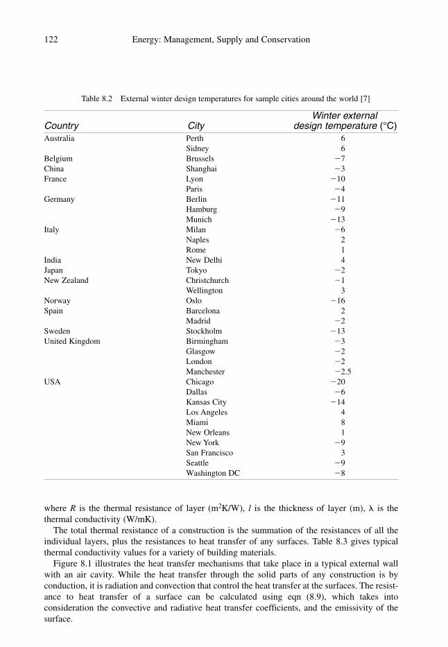
where R is the thermal resistance of layer (m2K/W), l is the thickness of layer (m), � is the
thermal conductivity (W/mK).
The total thermal resistance of a construction is the summation of the resistances of all the
individual layers, plus the resistances to heat transfer of any surfaces. Table 8.3 gives typical
thermal conductivity values for a variety of building materials.
Figure 8.1 illustrates the heat transfer mechanisms that take place in a typical external wall
with an air cavity. While the heat transfer through the solid parts of any construction is by
conduction, it is radiation and convection that control the heat transfer at the surfaces. The resist-
ance to heat transfer of a surface can be calculated using eqn (8.9), which takes into
consideration the convective and radiative heat transfer coefficients, and the emissivity of the
surface.
122 Energy: Management, Supply and Conservation
Table 8.2 External winter design temperatures for sample cities around the world [7]
Winter external Country City design temperature (°C)Australia Perth 6
Sidney 6
Belgium Brussels �7
China Shanghai �3
France Lyon �10
Paris �4
Germany Berlin �11
Hamburg �9
Munich �13
Italy Milan �6
Naples 2
Rome 1
India New Delhi 4
Japan Tokyo �2
New Zealand Christchurch �1
Wellington 3
Norway Oslo �16
Spain Barcelona 2
Madrid �2
Sweden Stockholm �13
United Kingdom Birmingham �3
Glasgow �2
London �2
Manchester �2.5
USA Chicago �20
Dallas �6
Kansas City �14
Los Angeles 4
Miami 8
New Orleans 1
New York �9
San Francisco 3
Seattle �9
Washington DC �8

Energy efficient heating 123
Table 8.3 Thermal conductivity of various materials [8]
Material Density (kg/m3) Thermal conductivity (W/mK)Brickwork (outer leaf) 1700 0.84
Brickwork (inner leaf) 1700 0.62
Cast concrete (dense) 2100 1.40
Cast concrete (lightweight) 1200 0.38
Concrete block (heavyweight) 2300 1.63
Concrete block (medium weight) 1400 0.51
Concrete block (lightweight) 600 0.19
Fibreboard 300 0.06
Plasterboard 950 0.16
Plaster (dense) 1300 0.50
Plaster (lightweight) 600 0.16
External rendering 1300 0.50
Screed 1200 0.41
Asphalt 1700 0.50
Tile 1900 0.84
Wood-wool slab 650 0.14
Expanded polystyrene 25 0.035
Glass fibre slab 25 0.035
Phenolic foam 30 0.040
Inner LeafOuter Leaf
InsideOutside
Radiation Conduction
ConvectionConvection
Conduction RadiationRad.
Conv.
Figure 8.1 Heat transfer through a cavity wall
(8.9)
where Rs is the surface resistance (m2K/W), hc is the convective heat transfer coefficient
(W/m2K), hr is the radiative heat transfer coefficient (W/m2K), and E is the emissivity factor.
The convective heat transfer coefficient is the rate at which heat is transferred to or from a 1 m2
surface by convection, per 1 °C temperature difference between the surface and the neighbouring
fluid (i.e. air). The radiative heat transfer coefficient is the rate of radiant heat transfer to or from a
1 m2 surface of a black body divided by the difference between the mean temperatures of the radi-
ating surface and that of the surrounding surfaces. The term black body refers to a body which
Rs �1
hc � (E � hr)

absorbs all energy incident on it at every wavelength and conversely emits energy at every wave-
length. The emissive power of a black body can be calculated using eqn (8.10).
Eb � � � T4 (8.10)
where Eb is the emissive power (W/m2), � is the Stefan–Boltzmann constant (i.e. 5.67 �10�8 W/m2K4), and T is the absolute temperature of the black body (K).
Of course, black bodies are theoretical and building materials do not emit and absorb energy
at all wavelengths and are therefore non-black bodies. The term emissivity is used to describe the
ratio of the emissive power of a non-black body to that exhibited by a black body. The emissiv-
ity of a black body is 1, while that of all other bodies will be less than one. Dull surfaces, of the
type exhibited by most building materials, have a high emissivity, while shiny metallic surfaces
have a low emissivity. High emissivity surfaces are good emitters and receivers of radiation,
while low emissivity surfaces are not. Table 8.4 gives examples of the emissivity values for
typical building materials.
The emissivity factor (E) referred to in eqn (8.9) allows for the emissivity and geometrical
relationship of both the emitting and the receiving surfaces. The emissivity factor varies with the
specific geometrical arrangement of the surfaces involved, but for most building applications it
can be taken as being approximately 0.9.
The thermal resistance of any surface is strongly influenced by air velocity. However, for most
building applications, room air velocities are not greater than 0.1 m/s and so it is possible to
determine typical values for a variety of surfaces (as shown in Table 8.5). Table 8.5 presents
typical internal surface resistances for both high and low emissivity surfaces.
The resistance of external building surfaces is heavily influenced by wind speed. Table 8.6
gives typical external surface resistances under sheltered, normal and severe conditions.
Unventilated air cavities in walls and roofs offer resistance to heat transfer. For cavities in
walls the thermal resistance increases with thickness up to approximately 25 mm. Thereafter the
124 Energy: Management, Supply and Conservation
Table 8.4 Typical values of emissivity
Surface Emissivity
Black body 1
Black (non-metallic) 0.90–0.98
Concrete 0.85–0.95
White paint 0.85–0.95
Aluminium (dull) 0.20–0.30
Aluminium (polished) 0.02–0.05
From Smith, Phillips and Sweeney (1987) Environmental
Science, © Longman Group UK ltd (1987), reprinted by
permission of Pearson Education Ltd.
Table 8.5 Typical internal surface resistances [8]
Surface resistance (m2K/W)
Building Direction of High emissivity factor Low emissivity factorelement heat flow (E � 0.97) (E � 0.05)Walls Horizontal 0.12 0.30
Ceiling or roofs Upward 0.10 0.22
Ceiling or floors Downward 0.14 0.55

thermal resistance of the air cavity is virtually constant despite any further increase in thickness.
Heat transfer across an air cavity is by convection and radiation. Thus the emissivity of the
cavity surfaces significantly influences the heat transfer. Table 8.7 gives typical thermal
resistances for a variety of air cavities.
Energy efficient heating 125
Table 8.6 Typical external surface resistances [8]
Surface resistance
Building Emissivity (m2K/W)element of surface Sheltered Normal Severe
Wall High 0.08 0.06 0.03
Low 0.11 0.07 0.03
Roof High 0.07 0.04 0.02
Low 0.09 0.05 0.02
Sheltered: Applies up to the third floor in city centres;
Normal: Applies to most suburban and rural areas, and from the fourth to the eighth floors on tall buildings in city
centres; and
Severe: Applies to coastal and hill sites, above the fifth floor in suburban and rural districts and above the ninth in city
centres.
Table 8.7 Typical resistances of unventilated air cavities [8]
Thermal resistance (m2K/W)
Emissivity for stated heat flow direction
Cavity thickness of surface Horizontal Upward Downward
5 mm High 0.10 0.10 0.10
Low 0.18 0.18 0.18
25 mm or greater High 0.18 0.17 0.22
Low 0.35 0.35 1.06
Example 8.1 illustrates how the above equation and data can be used to determine the U value
of an external wall.
Example 8.1
An external wall has the following construction:
Element Thickness (mm) Thermal conductivity (W/mK)Plaster 13 0.500
Concrete block (inner leaf) 100 0.200
Air cavity 50 n.a.
Brick (outer leaf) 102 0.840
Assuming that the air cavity has a thermal resistance of 0.18 m2K/W, the internal surface
resistance is 0.123 m2K/W and the external surface resistance is 0.055 m2K/W, determine:
(i) The U value of the wall; and
(ii) The U value of the wall if the cavity is filled with insulating foam having a thermal
conductivity of 0.036 W/mK.

Solution
Using the above data and eqn (8.8) it is possible to determine the total thermal resistance of the
cavity wall as follows:
Thickness Thermal conductivity Thermal resistanceElement (m) (W/mK) (m2K/W)Internal surface resistance n.a. n.a. 0.123
Plaster 0.013 0.500 0.026
Concrete block (inner leaf) 0.100 0.200 0.500
Air cavity 0.050 n.a. 0.180
Brick (outer leaf) 0.102 0.840 0.121
External surface resistance n.a. n.a. 0.055
Total Resistance � 1.005
(i) Therefore:
U value (existing wall) � 0.995 W/m2K
(ii) If the cavity of the wall is filled with foam, then:
Thermal resistance of foam � 1.389 m2K/W
However, the thermal resistance of 0.18 m2K/W for the air cavity no longer applies, therefore:
New thermal resistance of wall � 1.005 � 1.389 � 0.18 � 2.214 m2K/W
Therefore:
New U value � 0.452 W/m2K
It can be seen from Example 8.1 that by filling the cavity with insulating foam, it has been
possible to reduce the U value of the wall by 54.6%.
8.3.2 Heat loss calculations
If the U values for the various component parts of a building’s fabric are known, then it is
possible using eqns (8.5) and (8.6) to determine, with relative accuracy, the wintertime design
day heat loss rate and thus ultimately size boiler plant and heat emitters. Example 8.2 illustrates
how this calculation should be performed.
Example 8.2
The surface areas and U values of the elements of a building are as follows:
Element Area (m2) U value (W/m2K)Floor 200 0.45
Roof 200 0.28
Single glazing 16 5.60
External doors 8 2.00
External walls 216 0.60
1
2.214�
0.05
0.036�
1
1.005�
126 Energy: Management, Supply and Conservation

If the internal design temperature is 21 °C and the external design temperature is �1 °C,
determine the design day heat loss rate. (Assume that the building experiences 3 air changes per
hour and that its volume is 800 m3.)
Solution
Under the wintertime design condition, the temperature difference between the inside and
outside is 22. Given this, and by applying eqn (8.5) (i.e. Qf � UA(tai � tao)), it is possible to
calculate the heat loss rate through each component element of the building fabric.
Area U value Temperature difference Heat lossElement (m2) (W/m2K) (°C) (W)Floor 200 0.45 22 1980.0
Roof 200 0.28 22 1232.0
Single glazing 16 5.60 22 1971.2
External doors 8 2.00 22 352.0
External walls 216 0.60 22 2851.2
Fabric heat loss � 8386.4
By applying eqn (8.6) it is possible to determine the ventilation heat loss:
Ventilation heat loss � 0.3333 � 3 � 800 � (21 � (�1)) � 17 600 W
Now:
Total heat loss � Fabric loss � Ventilation loss
Therefore:
Total heat loss � 8386.4 � 17 600 � 25 986.4 W
From an energy conservation point of view, one of the advantages of performing a design day
heat loss calculation is that it gives an elemental breakdown of the relative heat losses from the
building, enabling them to be quickly and easily evaluated. From Example 8.2 it can be seen that
1971.2 W is lost through the single glazing (i.e. 7.6% of the total heat loss). However, the
ventilation loss of 17 600 W represents 67.7% of the total heat loss. Given this, it would be folly
to install double glazing without first reducing the ventilation heat loss.
While the use of eqns (8.5) and (8.6) gives a relatively accurate value of the winter design day
heat loss, it can be inaccurate, especially in applications where radiant heating is used. A superior
model, which fully takes into account the radiant heat transfer which occurs within a room space,
is described by eqns (8.11) and (8.12).
(8.11)
and
(8.12)
and
(8.13)
where Qp is the heating plant output (W), tc is the dry resultant temperature in the centre of the
room (°C), and F1, F2 are the characteristic temperature ratios.
Qp � Qf � Qv
Qv � F2 � 0.333 � N � V � (tc � tao)
Qf � F1 � �(AU) � (tc � tao)
Energy efficient heating 127

The temperature ratios, F1 and F2, are defined as:
(8.14)
and
(8.15)
where tei is the internal environmental temperature (°C).
The internal environmental temperature is a theoretical construct which is used to calculate
the radiative and convective heat transfer to the inside surface of an external wall from the other
surfaces in a room. In temperate and hot climates, it can be defined as:
(8.16)
where tm is the mean surface temperature of the room (°C).
The CIBSE publish tables of values for F1 and F2 for various heating systems [10]. Tables 8.8,
8.9 and 8.10 show values of F1 and F2 for a forced warm air system, a panel radiator system, and
a high temperature radiant strip system. In each table values of F1 and F2 are presented against
two variables, �(AU)/�(A) and NV/3�(A).
Once the values of F1 and F2 have been established for any system, it is possible to calculate
the internal environmental temperature and the mean surface temperature of a room by using
eqns (8.17) and (8.18).
(8.17)
(8.18)
Rearranging equation (8.16) gives:
(8.19)tm �3
2 tei �
1
2 tai
tai � (F2 � (tc � tao)) � tao
tei � (F1 � (tc � tao)) � tao
tei �1
3 tai �
2
3 tm
F2 �(tai � tao)
(tc � tao)
F1 �(tei � tao)
(tc � tao)
128 Energy: Management, Supply and Conservation
Table 8.8 F1 and F2 values for 100% convective, 0% radiant heating (i.e. forced warm air heating)[10]
�(AU)/�(A)
0.2 0.4 0.6 0.8
NV/3�(A) F1 F2 F1 F2 F1 F2 F1 F2
0.1 0.99 1.03 0.98 1.07 0.97 1.10 0.96 1.13
0.2 0.99 1.03 0.98 1.07 0.97 1.10 0.96 1.13
0.4 0.99 1.03 0.98 1.07 0.97 1.10 0.96 1.13
0.6 0.99 1.03 0.98 1.07 0.97 1.10 0.96 1.13
0.8 0.99 1.03 0.98 1.07 0.97 1.10 0.96 1.13
1.0 0.99 1.03 0.98 1.07 0.97 1.10 0.96 1.13
1.5 0.99 1.03 0.98 1.07 0.97 1.10 0.96 1.13
2.0 0.99 1.03 0.98 1.07 0.97 1.10 0.96 1.13
3.0 0.99 1.03 0.98 1.07 0.97 1.10 0.96 1.13
4.0 0.99 1.03 0.98 1.07 0.97 1.10 0.96 1.13
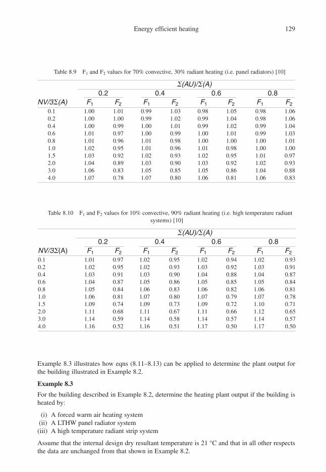
Energy efficient heating 129
Table 8.9 F1 and F2 values for 70% convective, 30% radiant heating (i.e. panel radiators) [10]
�(AU)/�(A)
0.2 0.4 0.6 0.8
NV/3�(A) F1 F2 F1 F2 F1 F2 F1 F2
0.1 1.00 1.01 0.99 1.03 0.98 1.05 0.98 1.06
0.2 1.00 1.00 0.99 1.02 0.99 1.04 0.98 1.06
0.4 1.00 0.99 1.00 1.01 0.99 1.02 0.99 1.04
0.6 1.01 0.97 1.00 0.99 1.00 1.01 0.99 1.03
0.8 1.01 0.96 1.01 0.98 1.00 1.00 1.00 1.01
1.0 1.02 0.95 1.01 0.96 1.01 0.98 1.00 1.00
1.5 1.03 0.92 1.02 0.93 1.02 0.95 1.01 0.97
2.0 1.04 0.89 1.03 0.90 1.03 0.92 1.02 0.93
3.0 1.06 0.83 1.05 0.85 1.05 0.86 1.04 0.88
4.0 1.07 0.78 1.07 0.80 1.06 0.81 1.06 0.83
Table 8.10 F1 and F2 values for 10% convective, 90% radiant heating (i.e. high temperature radiant
systems) [10]
�(AU)/�(A)
0.2 0.4 0.6 0.8
NV/3�(A) F1 F2 F1 F2 F1 F2 F1 F2
0.1 1.01 0.97 1.02 0.95 1.02 0.94 1.02 0.93
0.2 1.02 0.95 1.02 0.93 1.03 0.92 1.03 0.91
0.4 1.03 0.91 1.03 0.90 1.04 0.88 1.04 0.87
0.6 1.04 0.87 1.05 0.86 1.05 0.85 1.05 0.84
0.8 1.05 0.84 1.06 0.83 1.06 0.82 1.06 0.81
1.0 1.06 0.81 1.07 0.80 1.07 0.79 1.07 0.78
1.5 1.09 0.74 1.09 0.73 1.09 0.72 1.10 0.71
2.0 1.11 0.68 1.11 0.67 1.11 0.66 1.12 0.65
3.0 1.14 0.59 1.14 0.58 1.14 0.57 1.14 0.57
4.0 1.16 0.52 1.16 0.51 1.17 0.50 1.17 0.50
Example 8.3 illustrates how eqns (8.11–8.13) can be applied to determine the plant output for
the building illustrated in Example 8.2.
Example 8.3
For the building described in Example 8.2, determine the heating plant output if the building is
heated by:
(i) A forced warm air heating system
(ii) A LTHW panel radiator system
(iii) A high temperature radiant strip system
Assume that the internal design dry resultant temperature is 21 °C and that in all other respects
the data are unchanged from that shown in Example 8.2.

Solution
In order quantify F1 and F2 the values of the following parameters are determined:
.
Therefore
and
By looking-up Tables 8.8, 8.9 and 8.10 the values of F1 and F2 are found to be:
Option Heating type F1 F2
(i) Forced warm air heating 0.970 1.010
(ii) LTHW panel radiator system 1.015 0.965
(iii) High temperature radiant strip system 1.080 0.755
Therefore, using eqns (8.11) and (8.13):
(i) Forced warm air heating:
and
.
Therefore
Using eqns (8.17–8.19) it is possible to determine the internal air and environmental tempera-
tures, and the mean internal surface temperature of the building.
Similarly the plant output for options (ii) and (iii) can be established using the above method-
ology. A summary of the results of the winter design calculation for options (i), (ii) and (iii),
together with the results from Example 8.2 is presented in the table below.
tm �3
2� 20.3 �
1
2� 23.2 � 18.9 C
tai � [1.01 � (21 � (�1))] � (�1) � 23.2 oC
tei � [0.97 � (21 � (�1))] � (�1) � 20.3 oC
Qp � 8134.8 � 19 360 � 27 494.8 W
Qv � 1.10 � 0.333 � 3 � 800 � (21 � (�1)) � 19 360.0 W
Qf � 0.97 � 381.2 � (21 � (�1)) � 8134.8 W
NV
3�(A)� 1.25 W/m2K
�(AU)
�(A)� 0.60 W/m2K
NV/3 � 800 W/K
�(AU) � 381.2 W/K
�(A) � 640 m2
130 Energy: Management, Supply and Conservation

Heating Qf Qv Qp tai tm tei tcOption Type (W) (W) (W) (°C) (°C) (°C) (°C)Example 8.2 Non-specific 8386.4 17 600.0 25 986.4 21.0 n.a. n.a. n.a.
(i) Warm air 8134.8 19 360.0 27 494.8 23.2 18.9 20.3 21.1
(ii) Panel radiators 8512.2 16 983.8 25 496.0 20.2 21.9 21.3 21.1
(iii) High temp. radiant strip 9057.3 13 287.9 22 345.2 15.6 26.3 22.8 21.0
Comparison of the results from Examples 8.2 and 8.3 indicates that the use of the dry resultant
temperature and the F1 and F2 coefficients has some effect on the calculated overall plant output.
It can be seen that the required output of the high temperature radiant strip system is approxi-
mately 5 kW lower than that of the forced warm air system, with the radiator system in the
middle. It should also be noticed that the simple method, based on the indoor air temperature,
produces a plant output which was similar in magnitude to that required for the LTHW panel
radiator system. The margin of error for the less accurate ‘air temperature’ method, was �5.8%
when compared with the warm air system, and �14.0% when compared with the radiant strip
system. It can therefore be concluded that while the simple ‘air temperature’ method is
acceptable for sizing standard wall radiator heating systems, the ‘F1 and F2’ method should be
used when designing systems which are either 100% convective or almost 100% radiative.
8.4 Heating energy calculations
Equations 8.5, 8.6, 8.11 and 8.12 demonstrate that building heat loss is directly proportional to
the difference in temperature between the internal and external environments. It follows
therefore that buildings which experience harsher winters will, not surprisingly, consume more
heating energy during the winter months. It is therefore possible to use the degree day method
(see Appendix 1 for a detailed explanation of degree days) to predict annual heating costs.
For a building which is continuously heated and which experiences no substantial continuous
heat gains, the annual heating energy consumption can be determined by using eqn (8.20) or (8.21).
(8.20)
where E is the energy consumed (kWh), Qp is the heating plant output (kW), D15.5 is the number
of standard degree days (i.e. to the base temperature 15.5 °C), and � is the seasonal efficiency of
heating system.
Typical values of � for various types of boiler plant are shown in Table 8.11. As an alternative
to eqn (8.20), it is possible to use eqn (8.21) to predict heating energy consumption. However,
because eqn (8.21) uses internal air temperature and represents a non-specific heating system,
the results calculated are likely to be less accurate than those determined using eqn (8.20).
Notwithstanding this, eqn (8.21) is reasonably accurate if buildings are well insulated and a
predominantly convective heating system is being used.
(8.21)
When designing building heating systems it is standard practice to ignore any internal heat gains
in the winter design day calculation. In this way the heating system is sized to meet the ‘worst-
case’ scenario (i.e. when the internal heat gain is not present). In reality, if the heating plant is
E �Qp
(tai � tao)� D15.5 � 24 �
1�
E �Qp
(tc � tao)� D15.5 � 24 �
1�
Energy efficient heating 131

132 Energy: Management, Supply and Conservation
over-sized, the heating controls should modulate down the flow water temperature and prevent
the building from over-heating. However, when performing energy prediction calculations,
it may be important to allow for continuous internal heat gains (e.g. from lighting and equip-
ment) in the degree day calculation. This can be achieved by altering the degree day base tem-
perature from 15.5 °C to an appropriate level. Table 8.12 shows various Dd/D15.5 correction
factors for various base temperatures.
Internal heat gains can be allowed for in the degree day calculation by determining the
temperature rise due to internal gains using eqn (8.22).
(8.22)
where d is the average temperature rise which can be maintained by internal heat gains alone (K),
and Qg is the internal heat gain (W).
The new base temperature tb, can then be determined using eqn (8.23).
(8.23)
Equations 8.20 and 8.21 only apply to continuously heated buildings. Most buildings are however,
intermittently occupied and are not heated continuously. When buildings are intermittently occupied
it is necessary to allow for the additional heat energy required to bring the building structure up to
temperature. The amount of pre-heating required depends on the thermal capacity of the building.
tb � tc � d
d �Qg
Qp
� (tc � tao)
Table 8.11 Seasonal heating plant efficiencies [11]
SeasonalType of system efficiency (%)
Continuous space heating
Condenser and conventional boilers with weather compensated system 85
Fully controlled gas or oil fired boiler with radiator system 70
Fully controlled gas or oil fired boiler with radiator system (multiple
modular boilers used with sequence controller) 75
Intermittent space heating
Condenser and conventional boilers with weather compensated system 80
Fully controlled gas or oil fired boiler with radiator system 65
Fully controlled gas or oil fired boiler with radiator system (multiple
modular boilers used with sequence controller) 70
Table 8.12 Dd/D15.5 ratios for various base temperatures [12]
Base temperature (°C) Dd/D15.5
10 0.33
12 0.57
14 0.82
15 0.94
15.5 1.00
16 1.06
17 1.18
18 1.30

Heavy structures require long pre-heat periods and, once heated, retain heat well, while lightweight
structures tend to heat-up and cool quickly. It is therefore impossible to fully consider the impact of
intermittent occupation on energy consumption without considering the thermal capacity of the
building. The CIBSE classification of structures by thermal inertia is presented in Table 8.13.
To allow for intermittent heating when using the degree day method it is necessary to introduce
correction factors for:
• The length of the working week.
• The length of the working day.
• The response of the building and plant.
Tables 8.14, 8.15 and 8.16 set out values for these correction factors. Example 8.4 illustrates how
the annual heating costs for a building can be calculated.
Example 8.4
A three-storey office building, with a total floor area of 2400 m3, is occupied for 5 days per week
and for 8 hours per day. The design day plant output (i.e. heat loss) is calculated to be 190.0 kW
when the external temperature is �3.0 °C and the dry resultant temperature is 21 °C. The build-
ing is heated by a series of gas-fired modular boilers connected to a responsive warm air heating
system with a seasonal efficiency of 70%.
Given that the building is located in a region which experiences 2354 degree days per year and
that the cost of natural gas is 1.5 p/kWh, determine the annual heating fuel cost:
(i) Ignoring any internal heat gains (i.e. assuming a base temperature of 15.5 °C)
(ii) Allowing for an internal heat gain (from lights and equipment) of 20 W/m2.
Solution
(i) Ignoring any internal heat gains: From Table 8.14, the correction factor for length of work-
ing week is 0.85. From Table 8.15, the correction factor for length of working day is 1.00.
From Table 8.16, the correction factor for response of building and plant is 0.85.
Energy efficient heating 133
Table 8.14 Correction factor for length of working week [13]
Occupied days Lightweight Heavyweightper week building building
7 days 1.0 1.0
5 days 0.75 0.85
Table 8.13 CIBSE classification of structures by thermal inertia [12]
Weight Building description
Very heavy Multi-storey buildings with masonry or concrete curtain walling and sub-divided
within by solid partitions.
Heavy Buildings with large window areas but appreciable areas of solid partitions and floors.
Medium Single-storey buildings of masonry or concrete, sub-divided within by solid partitions.
Light Single-storey buildings of a factory type, with little or no solid partitions.
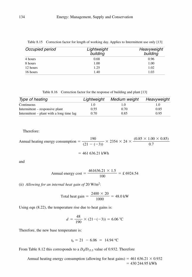
Therefore:
and
(ii) Allowing for an internal heat gain of 20 W/m2:
Using eqn (8.22), the temperature rise due to heat gains is:
Therefore, the new base temperature is:
From Table 8.12 this corresponds to a Dd/D15.5 value of 0.932. Therefore
Annual heating energy consumption (allowing for heat gains) � 461 636.21 � 0.932
� 430 244.95 kWh
tb � 21 � 6.06 � 14.94 oC
d �48
190� (21�(�3)) � 6.06 C
Total heat gain �2400 � 20
1000� 48.0 kW
Annual energy cost �461636.21 � 1.5
100� £ 6924.54
� 461 636.21 kWh
Annual heating energy consumption �190
(21 � (�3))� 2354 � 24 �
(0.85 � 1.00 � 0.85)
0.7
134 Energy: Management, Supply and Conservation
Table 8.16 Correction factor for the response of building and plant [13]
Type of heating Lightweight Medium weight Heavyweight
Continuous 1.0 1.0 1.0
Intermittent – responsive plant 0.55 0.70 0.85
Intermittent – plant with a long time lag 0.70 0.85 0.95
Table 8.15 Correction factor for length of working day. Applies to Intermittent use only [13]
Occupied period Lightweight Heavyweightbuilding building
4 hours 0.68 0.96
8 hours 1.00 1.00
12 hours 1.25 1.02
16 hours 1.40 1.03

Therefore
As well as predicting heating energy costs, it is also possible to use the degree day method to
evaluate proposed energy saving measures. Example 8.5 illustrates how this can be achieved.
Example 8.5
An office building has a roof which has a U value of 1.1 W/m2K. It is proposed that additional
insulation be installed in the roof to bring its U value down to 0.25 W/m2K.
The office building is located in a region which experiences an annual total of 2350 degree
days. Assuming that the efficiency of the building heating system is 70%, the cost of fuel is 1.5
p/kWh and the capital cost of installing the roof insulation is £2.00 per m2, determine the
payback on the investment.
Solution
Therefore
8.5 Intermittent heating
The degree day calculations in Section 8.4, indicate that the intermittent use of heating plant
results in higher energy consumption compared with continuous heating. This is primarily
because intermittently occupied buildings, such as office buildings, require the structure to be
warmed up after it has been allowed to cool over-night and at weekends. Additional heat energy
is therefore required to ‘pre-heat’ the building in the mornings, so that its fabric is brought up to
a temperature which will be comfortable for the occupants. Buildings with a high thermal mass
require greater pre-heating than buildings with a low thermal mass. However, once heated to the
required temperature, heavyweight structures retain their heat for much longer than lightweight
ones.
Payback period �2.00
1.03� 1.94 years
Annual energy cost saving �68.486 � 1.5
100� £1.03 per m2
� 68.486 kWh/m2.
Annual energy saving � (1.1 � 0.25) �2350
100�
24
0.7
Annual energy cost �430 244.95 � 1.5
100� £ 6453.67
Energy efficient heating 135
Table 8.17 Recommended plant ratios for intermittent heating [10]
Lightweight building Heavyweight buildingPlant ratio (F3) pre-heat time (hours) pre-heat time (hours)1.0 Continuous Continuous
1.2 6 Very long
1.5 3 7
2.0 1 4
2.5 0 2
3.0 0 1
The pre-heating of a building structure is achieved by running the heating system at full capac-
ity for a pre-heat period prior to the building’s occupation. The heavier the building structure, the
longer the pre-heat period. The pre-heat period can be reduced in length by over-sizing the boiler
plant and, to some extent, the heat emitters. It is generally considered more energy efficient to
increase the plant margin (i.e. over-size the boiler plant) in order to reduce the pre-heat period
[10]. Table 8.17 gives recommended plant ratios for intermittent heating [10], which should be
used in conjunction with eqn (8.24) to determine the intermittent peak heating load. It should be
noted that the pre-heat times in the table assume the use of plant with a short response time, such
as a warm air heating system. For slow response heating systems such as under-floor heating the
pre-heating period will be longer.
(8.24)
where Qpb is the intermittent peak heating output (W or kW), and F3 is the plant ratio (i.e. Max.
heat output / Design day heat output).
When over-sizing plant it is important to consider both boilers and heat emitters. While
increased boiler capacity may reduce the pre-heat time, it can result in poor part-load perform-
ance and low seasonal boiler efficiency. It should be remembered that for most of the heating
season, the external air temperature will be well above the winter design condition, so for much
of the year the boilers will have plenty of excess capacity. It is therefore wise to consider the use
of modular boilers.
While increased boiler capacity may be advisable, it is not always necessary to increase
individual heat emitters. This is because the following alternative strategies can be employed:
• In buildings which are unoccupied, natural and mechanical ventilation rates can be reduced
during the nighttime. Reduced ventilation rates will occur naturally during the nighttime
because doors and windows usually remain closed. With mechanical ventilation systems it is
also possible to reduce the ventilation load by fully recirculating the air (i.e. reducing the
outside air component of the supply air to 0%) during the pre-heat period.
• It is possible to elevate the water supply temperature to the heat emitters during the pre-heat
period.
Although, a modest over-sizing of heat emitters is recommended by the CIBSE, there is no
strong economic case for considerable over-sizing (i.e. in excess of 25%) of emitter sur-
faces [10].
8.6 Radiant heat
The importance of radiant heat transfer in buildings is often misunderstood with the result that
potential ‘radiant’ energy saving measures are often ignored. It is therefore worth investigating
some of the ‘radiant’ energy saving techniques that exist.
8.6.1 Radiant heating
Equation 8.4 shows that the comfort of building occupants is as dependent on the mean radiant
temperature as it is on air temperature. This fact can be used to great advantage in applications
where a building is poorly insulated and in which ventilation rates are high, such as in old
factories or workshops. In such applications, it is often prohibitively expensive to heat up large
volumes of air, which are then quickly lost to the outside. It is much better to use some form of
Qpb � F3 � Qp
136 Energy: Management, Supply and Conservation

radiant heating to warm up the occupants. By using a high temperature radiant heat source it is
possible to create a heat balance which enables the occupants to feel comfortable whilst still
maintaining the air and fabric at a low temperature.
Radiant heating is particularly well suited to applications in which occupancy is very
intermittent and in which the occupants are located in relatively fixed positions. A church
building is a classic example of such an application. Such a building is occupied for a
relatively short period in every week. Because radiant heating systems react very quickly and
warm the occupants rather than the air, they can achieve a good comfort level without any pre-
heating of the building. For this and the other reasons mentioned, radiant heating systems
are generally considered to incur lower capital costs and lower operating costs than other
comparable systems [13].
In order to achieve high levels of radiant heat transfer it is necessary to have emitters which
are at a high temperature, well above 100 °C. For safety and comfort reasons, these heat emit-
ting panels must be placed at high level, well out of the reach of any of the occupants.
8.6.2 Low emissivity glazing
Glazing is often viewed as a thermal ‘weak-link’, because heat is easily conducted through
glass from the inside to the outside. This perception is broadly, but not wholly, true. It is often
forgotten that much of the heat which is lost through windows occurs because they are, in
effect, large flat high emissivity surfaces which are cold in relation to the other surfaces in a
room. All the other surfaces in the room, especially heated surfaces, such as radiators and warm
bodies, emit long-wave radiation which is readily absorbed by the cool glass. In this way much
heat is lost from buildings. It is possible to minimize this problem by installing low emissivity
glazing which reduces the absorption of long-wave radiation. The low emissivity effect is
achieved during the manufacturing process by applying a microscopically thin (i.e. 0.3–0.4 �m
thick) coating of tin oxide doped with fluorine atoms [14] to the cavity-facing surface of the
inner pane of a double-glazed unit. This significantly reduces the radiative heat loss to the
cavity and thus reduces the U value of a typical double glazed unit from approximately 3
W/m2K to 1.8 W/m2K.
8.7 Under floor and wall heating
It is possible to heat buildings efficiently by using systems which utilize very low water temper-
atures. Two effective low temperature systems which can be used are:
• Under floor heating, which utilizes flow water temperatures in the range 35 °C–50 °C.
• Wall heating, which utilizes flow water temperatures in the range 30 °C–40 °C.
The low water temperatures involved in these systems enable alternative heat sources to be utilized,
such as ground source heat pumps, or even solar energy. Because both wall and under floor heating
systems involve large heated surfaces, the room mean radiant temperature is increased. This makes
it possible to reduce the air temperature within the room space without altering the dry resultant
temperature, enabling energy to be saved whilst still maintaining a comfortable environment.
The maximum permissible surface temperature governs the maximum water flow temperature
which can be used in both wall and under-floor heating installations. In the case of under-floor
heating, occupants feel uncomfortable if the floor surface temperature is above 29 °C. For walls
the maximum safe surface temperature is about 43 °C, since the disassociation temperature for
plaster is approximately 45 °C.
Energy efficient heating 137

Under-floor heating systems are best suited to tall spaces, where the use of a conventional
warm air or radiator system may lead to stratification of the air (i.e. the warm air becoming
trapped at the top of the room space). The use of under-floor heating overcomes this problem
and ensures that the air is warmest at ground level, where the occupants are likely to be located.
Under-floor heating systems often consist of a continuous cross-linked polyethylene, or
polypropylene flexible pipe loop embedded in a floor screed, on top of a structural floor [15].
The screed is usually isolated from the structural floor by rigid insulation slabs, which reduce
the heat transfer through the slab and help to maintain the screed temperature. The nature of the
screed used in under-floor heating systems is of particular importance, since the screed acts as a
thermal resistance to the heat transfer from the pipe to the room space, and also provides the
system with thermal inertia. Screeds can be either cementitious in nature and approximately
75 mm thick, or an anhydrite flowing screed which enables the thickness to be reduced to
approximately 50 mm. The thermal storage capacity and inertia of a floor screed depend on a
number of parameters such as the specific heat capacity, screed thickness, screed density, thermal
conductivity, pipe spacing, and the water flow and return temperatures. It is therefore difficult to
predict exactly how any given floor will perform in practice. However, for a standard 65 mm
thick concrete screed floor, with a flow water temperature of 60 °C, it has been estimated that
the floor screed will take approximately 3 hours to charge, and 3 hours to discharge. At lower
water temperatures the charging process is considerably extended. The long hysteresis effect of
under-floor heating has the disadvantage of being slow to respond and makes it difficult to adjust
to sudden changes in the internal environment. Under-floor heating systems are therefore best
suited to applications in which occupancy is continuous or well-defined and predictable.
Wall heating operates in a similar manner to under floor heating, with the exception that the
pipe coils are generally not located in a material which has a high thermal mass, such as a floor
screed. In a typical wall heating system cross-linked polyethylene pipes are located on the air
cavity side of a dry lined plastered wall. The system can be used either with a wet plastered
board, or alternatively the pipes can be mechanically bonded to plasterboard using notched
battens to make a rigid unit which can then be fixed to the wall. A flexible insulation quilt, such
as rockwool, should be placed between the pipes and the structural wall, so that conduction to
the building structure is minimized. It is advisable where possible to install the wall heating on
internal walls, so that heat losses are minimized.
8.8 Pipework insulation
Considerable amounts of heat energy can be lost through uninsulated or poorly insulated
pipework. It is therefore important to ensure that hot water and steam pipework is properly
138 Energy: Management, Supply and Conservation
Table 8.18 Thermal conductivities of insulating materials [16]
Thermal conductivity (W/mK)Material Density (kg/m3) 50 °C 100 °C 300 °CCalcium silicate 210 0.055 0.058 0.083
Expanded nitrile rubber 65–90 0.039 – –
Mineral wool (glass) 16 0.047 0.065 –
Mineral wool (rock) 100 0.037 0.043 0.088
Magnesia 190 0.055 0.058 0.082
Polyisocyanurate foam 50 0.023 0.026 –

insulated. A range of insulating materials is available and these can be either inorganic, based
on crystalline or amorphous silicon, aluminium or calcium, or organic, based on hydrocarbon
polymers in the form of thermosetting/thermoplastic resins or rubbers [16]. They can be
either flexible or rigid, both types being available in pre-formed pipe sections. Table 8.18 lists
some of the common types of insulation along with some of their thermal properties.
8.8.1 Pipework heat loss
In Section 8.3.1 heat loss through flat surfaces such as walls and roofs is discussed. The geom-
etry of pipework is different from that of flat surfaces, requiring an alternative approach when
calculating the heat loss from sections of pipework. The heat transfer through the wall of a pipe
can be calculated using eqn (8.25).
(8.25)
where � is the thermal conductivity of pipe wall (W/mK), r1 is the internal radius of pipe (m),
and r2 is the external radius of pipe (m).
The thermal resistance of the pipe wall (per unit length of pipe) can be determined by:
(8.26)
As hot fluid flows along a pipe, heat is transferred to the pipe wall. The rate at which this
heat is transferred depends on the thermal resistance of a thin stationary layer of fluid on
the pipe wall surface. The heat transfer rate across this internal surface boundary layer can be
expressed as:
(8.27)
where h is the surface heat transfer coefficient (W/m2K), A is the surface area (m2), and �t is the
temperature difference between the surface and the bulk fluid (°C).
Equation (8.27) can also be applied to the heat transfer across the external surface of a pipe.
Consequently, the internal and external surface resistance per unit length of a pipe can be
expressed as:
(8.28)
The overall resistance per unit length of a typical insulated pipe can therefore be represented by:
(8.29)
where Rt is the total thermal resistance of pipework per unit length (mK/W), Rw is the thermal
resistance of pipe wall per unit length (mK/W), Rins is the thermal resistance of insulation per
unit length (mK/W), Rsi and Rso are the internal and external surface thermal resistances of
insulation per unit length (mK/W).
Once the overall resistance of the pipework is determined, the total heat loss per metre run can
be calculated by dividing the temperature difference between the fluid and ambient air by the
total resistance.
Rt � Rsi � Rw � Rins � Rso
Rso or si �1
h.A (mK/W)
Q � h � A � �t
R �ln(r2/r1)
2�� (mK/W)
Q �2��(t1 � t2)
ln(r2/r1) (W per metre length)
Energy efficient heating 139

(8.30)
Example 8.5
A pipe carries wet steam at 200 °C through a building which has an ambient air temperature of
20 °C. The pipe has an internal diameter of 53.5 mm, a wall thickness of 3.7 mm, and is
insulated to a thickness of 25 mm. The thermal conductivity of the pipe material is 46 W/m K
and the thermal conductivity of the insulating material is 0.033 W/mK. Assuming that the inside
and outside surface heat transfer coefficients are 10 000 W/m2 K and 10 W/m2 K respectively,
determine:
(i) The heat transfer per metre length of pipe;
(ii) The temperature of the outside surface of the insulation;
(iii) The heat loss from an uninsulated pipe, assuming that the external heat transfer coefficient
remains unchanged.
Solution
(i) The total pipework resistance per metre length is:
and
From the above calculation it can be seen that the resistance of the pipe wall is negligible
compared with that of the insulation and the outside surface resistance. In addition the heat trans-
fer coefficient for the internal surface is very high and hence the internal surface resistance is
negligible. Therefore, the total thermal resistance can be assumed to be:
� 3.178 mK/W
Therefore
(ii) The surface temperature can be found by applying the following equation:
Temperature of the outside of the insulation
where ta is the room air temperature (ºC).
� 20 � (0.287 � 56.64) � 36.3 oC
� ta � (Rso � Q)
Q �(200 � 20)
3.178� 56.64 W/m
Rt � Rins � Rso
Rins �ln (55.45/30.45)
2 � � � 0.033� 2.891 mK/W
Rw �ln (30.45/26.75)
2 � � � 46� 0.00045 mK/W
Rso �1
10 � � � 0.1109� 0.287 mK/W
Rsi �1
10000 � � � 0.0535� 0.00059 mK/W
Rt � Rsi � Rw � Rins � Rso
Q ��t
Rt
(W/m)
140 Energy: Management, Supply and Conservation

(iii) For the uninsulated pipe:
therefore
As well as illustrating the mechanics of a pipework heat loss calculation, Example 8.5 illustrates
the great benefit to be derived from insulation, since the 25 mm insulation layer reduced the heat
loss from 625 to 56.6 W/m.
8.8.2 Economics of pipework insulation
It is well known that one of the simplest and most cost effective ways of preventing energy
wastage is to insulate pipework runs. Nevertheless it is not easy to determine to what extent
pipework should be insulated. The capital cost of insulation increases with its thickness and the
financial saving must be off-set against the capital cost. The economic thickness of insulation
should therefore be governed by the pay-back period that is required on the investment, as
illustrated in Example 8.6.
Example 8.6
A steel pipe carries high pressure hot water at 120 °C around a factory building. The owners
of the factory propose to insulate the pipe using rock-wool. Given the data below, determine the
optimum thickness of the insulation and the simple pay-back period for that thickness.
Data:
Pipe outside diameter � 76.6 mm
Heat transfer coefficient for outside surface insulation � 10 W/m2K
Thermal conductivity of insulation � 0.037 W/m K
Water temperature � 120 °C
Temperature of air in factory � 15 °C
Boiler efficiency � 70%
Unit price of gas � 1.52 p/kWh
Boiler operates for 2500 hours per annum
Insulation costs
Thickness of insulation (mm) [20] [25] [32] [38] [50] [60] [75]
Cost per metre length (£/m) 5.00 5.58 6.64 8.01 10.57 13.44 16.68
Assume that the write-off period for the insulation is 5 years.
Solution
Assuming that the thermal resistances of the pipe wall and of the inside surface of the pipe are
both negligible, let
x � thickness of insulation (mm)
Q �(200 � 20)
0.288� 625 W/m
� 0.00059 � 0.00045 � 0.287 � 0.288 mK/W
Rt � Rsi � Rw � Rso
Energy efficient heating 141

142 Energy: Management, Supply and Conservation
Now
and
and
therefore
and
and
The following table can be produced from the above equations:
Insulation Insulation External Heat Annual Totalthickness resistance resistance loss fuel cost annual cost(mm) (mK/W) (mK/W) (W/m) (£/m) (£/m)0 0.00 0.42 252.68 13.72 13.72
20 1.81 0.27 50.47 2.74 3.74
25 2.16 0.25 43.52 2.36 3.48
32 2.61 0.23 36.99 2.01 3.34
38 2.96 0.21 33.09 1.80 3.40
50 3.59 0.18 27.83 1.51 3.62
60 4.05 0.16 24.90 1.35 4.04
75 4.67 0.14 21.85 1.19 4.52
It can be seen that the most economic thickness of insulation is 32 mm, since this has the low-
est annual cost.
Total annual cost � annual fuel cost �capital cost
write-off period
Annual operating cost �Q � 2500 � 1.52
0.7 � 100
Q �(120 � 15)
Rins � Rso
Q ��t
Rt
Rt � Rins � Rso
�1
10 � � � ((76.6 � 2x) � 10�3)
Rso �1
h.A
�ln ((38.3 � x)/38.3)
2 � � � 0.037
Rins �ln(r2/r1)
2��

The pay back period for the 32 mm insulation is:
8.9 Boilers
Most heating systems, although not all, employ boilers to produce hot water or steam. Boiler effi-
ciency therefore has an important influence on heating-related energy costs. The cost savings that
can be achieved by improving overall boiler efficiency can be substantial. Essentially a boiler is a
device in which a fossil fuel is burnt and the heat produced is transferred to water. The more
effective this heat transfer process, the more efficient the boiler. It is therefore important to max-
imize the heat transfer to the water and minimize boiler heat losses. Heat can be lost from boilers
by a variety of methods, including flue gas losses, radiation losses and, in the case of steam boil-
ers, blow-down losses. Although all these various losses have a significant effect on boiler energy
consumption, the major reason for poor boiler performance occurs at the design stage, where the
capacity of boilers is usually oversized and inappropriate boilers are often selected.
Boiler plant which is oversized will operate at part-load for most of the time, resulting in low
seasonal efficiency and high operating costs. It has been estimated that a 15% increase in energy
consumption can occur if a conventional boiler plant is oversized by 150% [17]. Boiler plant
should be considered oversized if under the winter design condition the boilers are able to
maintain an internal air temperature well above the design temperature (e.g. 21 °C). Evidence of
over-sizing can be manifested in a number of ways: fuel bills may be higher than expected;
excessive cycling of boiler plant may be experienced; and in installations equipped with modular
boilers, a large proportion of the boilers may never be used.
Given that for much of the heating season external air temperatures are usually well above the
winter design condition, it is important that any boiler installation be designed so that it operates
efficiently at part load. For most types of conventional boiler, efficiency falls dramatically below
about 30% of rated capacity [18]. Large boilers are therefore at a disadvantage since for most of
the time they will be operating well below their rated capacity. One simple way of overcoming
this problem is to install a large number of small modular boilers with a sequence controller in
preference to a few large boilers. This ensures that under part-load conditions, boilers which are
always operating near their maximum efficiency will provide the bulk of the heating. With such
a multi-boiler plant installation, it is wise to install a boiler sequence control system. This is a
fully automatic microprocessor-controlled system which monitors and sequences on/off
operations of boiler plant according to the demand for heat. This avoids running too many boilers
on part-load and minimizes the number of boilers in operation at any one time.
Another technique which can be employed to ensure good part-load efficiencies is to use
boilers with modulating burners. These burners modulate the fuel and air to provide a variable
output from 20–30% to 100%. With large modulating boilers it is possible to make substantial
energy savings by installing variable speed drives on the combustion air fans. Variable speed
drives reproduce the operating characteristics of fixed speed combustion air fans and
adjustable dampers, whilst reducing the average electrical demand of the fan motor by
approximately 60% [19].
8.9.1 Flue gas losses
All boilers require a minimum amount of air to ensure that complete combustion of the fuel takes
place and that no carbon monoxide is produced. Yet, if too much air is added then heat is wasted
Payback period �6.62
(13.72 � 3.34)� 0.638 years
Energy efficient heating 143

in warming up the excess air, which then escapes through the flue. The amount of combustion
air should therefore be limited to that necessary to ensure complete combustion of the fuel. In
practice some excess air, around 15–25% for oil fired boilers [19], and 15–30% for gas fired
boilers [20] is needed. The actual amount required to give the optimum boiler efficiency depends
on the fuel used and the type of boiler and burner. If the air flow rate to a boiler is too low, then
a proportion of the fuel will remain unburnt and running costs will increase. In the case of oil-
fired plant, incomplete combustion will produce smoke which will be visible. For coal fire plant,
incomplete combustion results in unburnt carbon in the ash. It is therefore essential to maintain
the correct fuel-to-air ratio at all times. With modern microprocessor controlled burners, which
are fitted to fuel valves and air dampers, it is possible to automatically select and maintain
specific fuel-to-air ratios for a variety of fuels. These controllers continually monitor the level of
oxygen in the flue gases, and alter the combustion air supply in order to maintain optimum
conditions.
Flue gas losses are by far the greatest heat losses which occur from boilers. The flue gases
contain considerable sensible heat and also latent heat which is ‘bound up’ in water vapour.
It is possible to determine the amount of heat which is being lost through the flue, by
monitoring the presence of O2 or CO2 in the flue gases. If there is little excess air in the com-
bustion gases, then the percentage of CO2 will be high and the percentage of O2 low.
Conversely, if a large amount of excess air is present, the relationship will be reversed. In a
typical gas-fired shell and tube boiler the flue gases should contain about 9–10% CO2 and
3–5% O2 [20], while for an oil fired boiler the CO2 content of the flue gases should be in the
region of 13–14% [19]. Typical CO2 and O2 flue gas contents for efficient boiler operation
are presented in Table 8.19.
With large boiler plant it is possible to increase boiler efficiency by pre-heating the combus-
tion air. It has been estimated that the thermal efficiency of a boiler can be increased by approx-
imately 1% if the temperature of the combustion air is raised by 20 °C [19, 20]. Any one of the
following sources of heat can be utilized to pre-heat the boiler combustion air:
• Waste heat from the flue gases.
• Drawing high temperature air from the top of the boiler room.
• Recovering waste heat by drawing air over or through the boiler casing.
8.9.2 Other heat losses
With shell and tube boilers it is possible for the ‘smoke’ tubes to become fouled by soot and other
deposits, resulting in a reduction in the amount of heat which is transferred from the hot flue
gases to the water. This increases the temperature of the flue gases and results in greater flue gas
losses. Boiler smoke tubes should therefore be cleaned regularly to minimize the flue gas tem-
perature rise, since it has been estimated that a rise of 17 °C in the flue gas temperature causes
144 Energy: Management, Supply and Conservation
Table 8.19 Typical CO2 and O2 contents by volume expected in flue gas (dry basis) [18]
Min. fire Full fire
Fuel CO2 (%) O2 (%) CO2 (%) O2 (%) CO (ppm)Coal 11.0 8.5 14.0 5.0 2–500
Fuel oils 11.5 5.5 13.5 3.0 –
Butane 9.4 7.0 12.0 3.0 2–400
Propane 9.2 7.0 12.0 3.0 2–400
Natural gas 8.0 7.0 10.0 3.3 2–400

a decrease in efficiency of approximately 1% [19]. Boiler efficiency can also significantly be
reduced by a build-up of scale on the water side of the smoke tubes. Water treatment should
therefore be employed in order to prevent scale formation.
Heat can be lost through the surface casing of boilers. This is generally referred to as radiation
loss, although it includes heat which is lost by convection. With modern boilers radiation losses
are usually not greater than 1% of the maximum rating. On older boilers this figure may be as
high as 10% where the insulation is in poor condition [19, 20].
8.9.3 Boiler blow-down
With steam boilers it is necessary to eject a small proportion of the water regularly in order to
remove sludge and to maintain acceptable levels of total dissolved solids. This process is called
blow-down and it prevents scaling up of the tubes on the water side. Although necessary,
blow-down represents a considerable energy loss and the level of blow-down should be kept to
a minimum while still maintaining the recommended level of dissolved solids.
It is possible to recover waste heat from the blow-down process by collecting the flash steam
which forms as the pressure falls through the blow-down valve. Because the condensate
produced by the blow-down process is both hot and pure, with no dissolved solids, it can be
added directly to the make-up water for the boiler, thus reducing energy consumption.
8.9.4 Condensing boilers
Boiler flue gases are often in excess of 200 °C and as such are a useful source of waste heat
recovery. Heat exchangers can be installed in flues to recover both sensible and latent heat from
the hot products of combustion. However, because of the corrosion problems associated with
sulphur bearing fuels, such as fuel oil, flue gas heat recovery is generally only practised on gas-
fired boilers. Gas-fired boilers which incorporate integral flue gas heat exchangers are known as
condensing boilers. If used correctly, condensing boilers can achieve operating efficiencies in
excess of 90% [18, 21].
With a condensing boiler it is desirable to operate the system so that the return water temper-
ature is as low as possible. This ensures that condensation of the flue gases occurs and that
maximum heat recovery from flue gases is achieved. If a condensing boiler is used in conjunc-
tion with a weather compensating controller, the boiler will move into condensing mode during
the milder part of the season, when return water temperatures are at their lowest. In this way,
high efficiency is maintained under part-load conditions. In multiple boiler installations it is
usually cost effective to install only one condensing boiler. This should always be the lead boiler,
since it exhibits the highest efficiencies. This ensures that good energy utilization will occur
under part-load conditions.
References
1. Keating, W. R. and the Eurowinter Group (1997). Cold exposure and winter mortality from
ischaemic heart disease, cerebrovascular disease, respiratory disease, and all causes in warm
and cold regions of Europe. The Lancet, 349, 1341–6.
2. Forecasting the nation’s health (2000). Met Office Report, November.
3. Wilkinson, P. (2000). Social and environmental determinants of excess winter deaths in
England, 1986–1996. Report for the Joseph Rowntree Foundation, July.
4. Edholm, O. G. (1978). Man – hot and cold (Studies in Biology No. 97) (Chapter 1). Arnold.
Energy efficient heating 145

5. CIBSE Guide A1, Environmental criteria for design (1986).
6. Smith, B. J., Phillips, G. M. and Sweeney, M. (1987). Environmental science (Chapter 2).
Longman Scientific and Technical.
7. CIBSE Guide A2, Weather and solar data (1982).
8. CIBSE Guide A3, Thermal properties of building structures (1980).
9. Smith, B. J., Phillips, G. M. and Sweeney, M. (1987). Environmental science (Chapter 1).
Longman Scientific and Technical.
10. CIBSE Guide A9, Estimation of plant capacity (1983).
11. Moss, K. J. (1997). Energy Management and Operating Costs in Buildings, (Chapter 1).
E & FN Spon.
12. CIBSE Guide B18, Owning and operating costs (1986).
13. Economic use of fired space heaters for industry and commerce, Fuel Efficiency Booklet 3
(1993). Department of the Environment.
14. Enhancing the built environment. Pilkington Plc. website.
15. CIBSE Guide B1, Heating (1986).
16. The economic thickness of insulation for hot pipes, Fuel Efficiency Booklet 8 (1994).
Department of the Environment.
17. Hendrick, R. et al. (1992). Furnace sizing criteria for energy-efficient set back strategies.
ASHRAE Transactions, 98(Part 1), 1239–46.
18. Energy audits and surveys (1991). CIBSE Applications Manual AM5.
19. Economic use of oil-fired boiler plant, Fuel Efficiency Booklet 14 (1993). Department of the
Environment.
20. Economic use of gas-fired boiler plant, Fuel Efficiency Booklet 15 (1994). Department of
the Environment.
21. Condensing Boilers (1989). CIBSE Applications Manual AM3.
Bibliography
CIBSE Guide A1, Environmental criteria for design (1986).
CIBSE Guide A2, Weather and solar data (1982).
CIBSE Guide A3, Thermal properties of building structures (1980).
CIBSE Guide A9, Estimation of plant capacity (1983).
CIBSE Guide B1, Heating (1986).
CIBSE Guide B18, Owning and operating costs (1986).
Degree days, Fuel Efficiency Booklet 7 (1995). Department of the Environment.
Eastop, T. D. and Croft, D. R. (1990). Energy efficiency for engineers and technologists
(Chapters 4 and 5). Longman Scientific & Technical.
Eastop, T. D. and Watson, W. E. (1992). Mechanical services for buildings (Chapter 3). Longman
Scientific & Technical.
Edholm, O. G. (1978). Man – hot and cold (Studies in Biology No. 97) (Chapter 1). Arnold.
Economic use of fired space heaters for industry and commerce. Fuel Efficiency Booklet 3
(1993). Department of the Environment.
Economic use of oil-fired boiler plant, Fuel Efficiency Booklet 14 (1993). Department of the
Environment.
146 Energy: Management, Supply and Conservation

Economic use of gas-fired boiler plant, Fuel Efficiency Booklet 15 (1994). Department of the
Environment.
Levermore, G. J. (1992). Building energy management systems (Chapter 10). E & FN Spon.
Moss, K. J. (1997). Energy Management and Operating Costs in Buildings (Chapters 1 and 3).
E & FN Spon.
Stoecker, W. F. and Jones, J. W. (1982). Refrigeration and air conditioning (Chapters 2 and 4).
McGraw-Hill International Editions.
The economic thickness of insulation for hot pipes, Fuel Efficiency Booklet 8 (1994).
Department of the Environment.
Energy efficient heating 147

9
Waste heat recovery
In many applications there is the potential for recovering heat energy that would otherwise
go to waste. This chapter describes various waste heat recovery technologies and examines
the theoretical principles behind each.
9.1 Introduction
In many applications it is possible to greatly reduce energy costs by employing some form of
waste heat recovery device. However, before investing in such technology it is important to first
consider some generic issues:
• Is there a suitable waste heat source? If the answer to this question is ‘yes’, it is important to
establish that the source is capable of supplying a sufficient ‘quantity’ of heat, and that the heat
is of a good enough ‘quality’ to promote good heat transfer.
• Is there a market or use for the recovered waste heat? It is important to have a use for any
waste heat which may be recovered. In many applications there may be no demand for the
heat that is available, with the result that a large quantity of heat energy is dumped. In other
situations there may be a long time lag between waste heat production and the demand for
heat. Waste heat therefore cannot be utilized unless some form of thermal storage is adopted.
• Will the insertion of a heat recovery device actually save primary energy or reduce energy
costs? Often the insertion of a heat exchanger increases the resistance of the fluid streams,
resulting in fan or pump energy consumption rising. Heat energy is therefore replaced by
electrical energy, which may be produced at an efficiency of less than 35%.
• Will any investment in heat recovery technology be economic? Heat recovery devices can be
expensive to install. It is, therefore, essential that the economic payback period be determined
prior to any investment being undertaken.
Although the questions above may appear obvious, it is not uncommon to find cases where poor
planning and analysis at the design stage has resulted in an installation where the impact of the
heat recovery device is either minimal, or is even increasing energy costs. Consider the case of a
heat exchanger installed in a warm exhaust air stream from a building. The insertion of the device
causes the resistance of the air streams to rise, resulting in greater fan energy consumption. If the

Waste heat recovery 149
unit price of electricity is four times that of gas, then in order to just break even, the heat
exchanger must recover four times the increase in electrical energy consumption, arising from the
increased system resistance. Also, there may well be long periods when the external air tempera-
ture is such that little or no heat can be recovered. If however, the fans run continuously then the
increased electrical energy is being expended for little or no return. Given this, it is not surprising
that many so-called ‘energy recovery’ systems, while appearing to save energy, are in fact
increasing both primary energy consumption and energy costs.
If a strategic decision is made to invest in some form of heat recovery device, then the next
logical step is to select the most appropriate system. There are a wide variety of heat recovery
technologies, which can be divided into the following broad categories:
• Recuperative heat exchanges: where the two fluids involved in the heat exchange, are
separated at all times by a solid barrier.
• Run-around coils: where an independent circulating fluid is used to transport heat between the
hot and cold streams.
• Regenerative heat exchanges: where hot and cold fluids pass alternately across a matrix of
material.
• Heat pumps: where a vapour compression cycle is used to transfer heat between the hot and
cold streams.
In addition to these, there are a few lesser used technologies, such as heat pipes, which are not
covered in this text.
9.2 Recuperative heat exchangers
In a recuperative heat exchanger the two fluids involved in the heat transfer are separated at all
times by a solid barrier. This means that the mechanisms which control the heat transfer are
convection and conduction. The thermal resistance of a heat exchanger can therefore be
expressed as follows:
(9.1)
where R is the thermal resistance of the heat exchanger (m2K/W), Rw is the thermal resistance of
the separating wall (m2K/W), hi and ho are the heat transfer coefficient of internal and external
surfaces (W/m2K), Fi and Fo are the internal and external fouling factors, and U is the overall
heat transfer coefficient (i.e. U value) (W/m2K).
In short this can be written as:
(9.2)
In practice heat exchangers are often over-sized so that even when fouled their performance still
meets design requirements. The degree of over-sizing is achieved by incorporating fouling
factors into the sizing calculation.
Recuperative heat exchangers are the most common type of equipment used for waste heat
recovery. They can only be used in applications where the hot and cold streams can be brought
into close proximity with each other. Although the precise form of a heat exchanger may change
with its particular application, there are three forms which are widely used.
1
Udirty
�1
Uclean
� Fouling factors
R �1
U�
1
hi
� Rw �1
hO
� Fi � FO

150 Energy: Management, Supply and Conservation
(a) Shell and tube heat exchanger: Shell and tube heat exchangers consist of a bundle of tubes
inside a cylindrical shell through which two fluids flow, one through the tubes and the other
through the shell (as shown in Figure 9.1). Heat is exchanged by conduction through the tube
walls. Baffles are often used to direct fluid around the heat exchanger and also to provide
structural support for the tubes.
(b) Plate heat exchanger: Plate heat exchangers consist of a large number of thin metal plates
(usually stainless steel but sometimes titanium or nickel), which are clamped tightly together
and sealed with gaskets (see Figure 9.2). The thin plates are profiled so that ‘flow ways’ are
Cold fluid
Hot fluid
Cold waste fluid Hot waste fluid
Figure 9.1 Shell and tube heat exchanger
Figure 9.2 Plate heat exchanger

Waste heat recovery 151
Cooledexhaust air
Warmedsupply air
Exhaustair outlet Inlet
supply air
Figure 9.3 Flat plate recuperator
created between the plates when they are packed together, and a very large surface area is
created across which heat transfer can take place. Ports located at the corners of the
individual plate separate the ‘hot’ and ‘cold’ fluid flows and direct them to alternate passages
so that no intermixing of the fluids occurs. The whole exchanger experiences a counter-flow
pattern. The maximum operating temperature is usually about 130 °C if rubber sealing
gaskets are fitted, but this can be extended to 200 °C if compressed asbestos fibre seals are
used [1]. Plate heat exchangers have become popular in recent years because they are
extremely compact, and can easily be expanded or contracted to accommodate future system
modification.
(c) Flat plate recuperator: Flat plate recuperators consist of a series of metal (usually alumin-
ium) plates separating ‘hot’ and ‘cold’ air or gas flows, sandwiched in a box-like structure
(see Figure 9.3). The plates are sealed in order to prevent intermixing of the two fluid flows.
They are often used in ducted air conditioning installations to reclaim heat from the exhaust
air stream, without any cross contamination occurring.
9.3 Heat exchanger theory
The two most commonly used heat exchanger flow configurations are counter flow and parallel
flow. These flow patterns are represented in Figures 9.4 and 9.5 respectively, along with their
characteristic temperature profiles.
It should be noted that with the parallel flow configuration the ‘hot’ stream is always warmer
than the ‘cold’ stream. With the counter flow configuration it is possible for the outlet tempera-
ture of the cold fluid to be higher than the outlet temperature of the hot fluid.
The general equations which govern the heat transfer in recuperative heat exchangers are as
follows:
(9.3)Q � �mh ch (th1�th2) � �mc cc (tc1�tc2)

152 Energy: Management, Supply and Conservation
and
(9.4)
where Q is the rate of heat transfer (W), is the mass flow rate of hot fluid (kg/s), is the
mass flow rate of cold fluid (kg/s), ch is the specific heat of hot fluid (J/kgK), cc is the specific
heat of cold fluid (J/kgK), th1 and th2 are the inlet and outlet temperatures of hot fluid (°C), tc1
and tc2 are the outlet and inlet temperatures of cold fluid (°C), U is the overall heat transfer coef-
ficient (i.e. U value) (W/m2K), Ao is the outside surface area of heat exchanger (m2), LMTD is
the logarithmic mean temperature difference (°C), and K is the constant which is dependent on
the type of flow through the heat exchanger (e.g. K � 1 for counter-flow and parallel flow, and
is therefore often ignored).
The logarithmic mean temperature difference (LMTD) can be determined by:
(9.5)
The following examples illustrate how the above equations can be used to design and analyse
heat exchangers:
Example 9.1
A liquid waste stream has a flow rate of 3.5 kg/s and a temperature of 70 °C, with a specific heat
capacity of 4190 J/kgK. Heat recovered from the hot waste stream is used to pre-heat boiler
LMTD ��t1 � �t2
ln (�t1/�t2)
�mc�mh
Q � UAo (LMTD)K
A
B
A B
Temperature
Distance
A
B
A B
Temperature
Distance
Figure 9.4 Counter flow heat exchanger
Figure 9.5 Parallel flow heat exchanger

Waste heat recovery 153
make-up water. The flow rate of the make-up water is 2 kg/s, its temperature is 10 °C and its spe-
cific heat capacity is 4190 J/kgK. The overall heat transfer coefficient of the heat exchanger is
800 W/m2K. If a make-up water exit temperature of 50 °C is required, and assuming that there
are no heat losses from the exchanger, determine:
(i) The heat transfer rate;
(ii) The exit temperature of the effluent; and
(iii) The area of the heat exchanger required.
Solution
(i) Now:
(ii) Now
(iii) Now, because the water outlet temperature is above the outlet temperature of the effluent,
a counter-flow heat exchanger is required.
Now
therefore
Example 9.2
Consider the counter flow heat exchanger shown in Figure 9.6. Given the data below, determine
the overall heat transfer rate for the heat exchanger.
Data:
Length of heat exchanger � 2 m
Internal radius of heat exchanger surface � 10 mm
External radius of heat exchanger surface � 11 mm
Thermal conductivity of heat exchanger surface � 386 W/mK
Heat transfer coefficient of Fluid 1 � 50 W/m2K
Heat transfer coefficient of Fluid 2 � 90 W/m2K
A �335 200
800 � 27.69� 15.13 m2
Q � UA(LMTD)
� 27.69 oC
�((70 � 50) � (47.14 � 10))
ln ((70 � 50)�(47.14 � 10))
LMTD ��t1 � �t2
ln (�t1��t2)
th2 � 47.14 oC
3.5 � 4190 � (70 � th2) � 2 � 4190 � (50 � 10)
�mh ch (th1 � th2) � �mc cc (tc1 � tc2)
� 335 200 W � 335.2 kW
� 2 � 4190 � (50 � 10)
Q � �mc cc (tc1 � tc2)

154 Energy: Management, Supply and Conservation
Solution
By combining eqns (8.26) and (8.28) it can be shown that the total thermal resistance, Rt, of the
heat exchanger is:
where k is the thermal conductivity of the pipe wall (W/mK), r1 is the internal radius of the pipe
(m), r2 is the external radius of the pipe (m), l is the length of the pipe (m), h is the heat transfer
coefficient (W/m2K), and A1 and A2 are the external and internal surface areas (m2)
and using eqn (8.30) the total heat transfer rate can be expressed as:
Now:
A1 � 2� � 0.011 � 2 � 0.138 m2
and
A2 � 2� � 0.01 � 2 � 0.126 m2
therefore
Rt � 0.233 W/K
and
therefore
Q �28.85
0.233� 123.8 W
LMTD �(70 � 30) � (30 � 10)
ln [ (70 � 30)�(30 � 10) ]� 28.85 oC
Rt �1
90 � 0.126�
ln(0.011/0.01)
2π � 386 � 2�
1
50 � 0.138
Q ��t
Rt
(W)
Rt �1
h.A1
�ln(r2/r1)
2πk.1�
1
h.A2
10°C
70°C30°C
30°C Fluid 1
Fluid 2
Figure 9.6 Heat exchanger

Waste heat recovery 155
9.3.1 Number of transfer units (NTU) concept
In some situations only the inlet temperatures and the flow rates of the hot and cold streams are
known. Under these circumstances the use of the LMTD method results in a long and complex
mathematical solution. To simplify such calculations the number of transfer units (NTU) method
was developed [2, 3].
NTU is defined as the ratio of the temperature change of one of the fluids divided by the mean
driving force between the fluids, and can be expressed as:
For the hot fluid:
(9.6)
For the cold fluid:
(9.7)
(NB: For counter flow and parallel flow heat exchangers the K term can be ignored)
Equations (9.6) and (9.7) are more commonly simplified to:
(9.8)
where is the minimum thermal capacity (kW/K).
The ratio of the thermal capacities, R, is defined as:
(9.9)
If both fluids in the heat exchanger have the same thermal capacity then R � 1. At the other
extreme when one of the fluids has an infinite thermal capacity, as in the case of an evaporating
vapour, then R � 0.
Another useful concept is the effectiveness, E, of a heat exchanger. Effectiveness can be
defined as the actual heat transfer divided by the maximum possible heat transfer across the heat
exchanger, and can be expressed as:
(9.10)
It is possible to derive the relationship between E, NTU and R for a variety of heat exchanger appli-
cations. The mathematical expressions for some of the more common applications are given below.
(i) Parallel flow:
(9.11)
(ii) Counter flow:
(9.12)
If R � 1 then this expression simplifies to:
(9.13)E �NTU
1 � NTU
E �1 � e[�NTU (1�R) ]
1 � Re[�NTU (1�R) ]
E �1 � e[�NTU (1�R)]
1 � R
E �Q
Qmax
�Q
( �mc)min(thmax � tcmin)
R �( �mc)min
( �mc)max
( �mc)min
NTU �UAo
( �mc)min
NTUc �(tc1 � tc2)
(LMTD)K�
UA
( �mc)c
NTUh �(th1 � th2)
(LMTD)K�
UAo
( �mc)h

156 Energy: Management, Supply and Conservation
(iii) Heat exchanger with condensing vapour of boiling liquid on one side:
(9.14)
The NTU method for heat exchanger analysis is illustrated in Example 9.3.
Example 9.3
A contaminated water stream from a factory building has a temperature of 80 °C, and has a flow
rate of 6 kg/s and a specific heat capacity of 4.19 kJ/kg K. The incoming water supply to the
manufacturing process is at 10 °C, and has a flow rate of 7 kg/s and a specific heat capacity of
4.19 kJ/kg K. It is proposed to install a counter flow heat exchanger to recover the waste heat. If
the heat exchanger has an overall area of 30 m2 and an overall heat transfer coefficient of 800
W/m2K (assuming that there are no heat losses from the heat exchanger), determine:
(i) The effectiveness of the heat exchanger;
(ii) The heat transfer rate; and
(iii) The exit temperature of the incoming water stream leaving the heat exchanger.
Solution
Now
(m.c)min � 6 � 4.19 � 25.14 kW/K
and
(m.c)max � 7 � 4.19 � 29.33 kW/K.
therefore
and
(i) Therefore
(ii) Now
therefore:
Q � 0.506 � 25.14 � [80 � 10] � 890.46 kW
(iii) Therefore:
890.46 � 29.33 � [toff � 10]
therefore:
toff � 40.4 °C
E �Q
( �mc)min(thmax � tcmin)
E � 0.506
E �1 � e[�0.955 (1�0.857) ]
1 � 0.857 e[�0.955 (1�0.857) ]
NTU �30 � 800
25.14 � 1000� 0.955.
R �25.14
29.33� 0.857
E � 1 � e[�NTU]

Waste heat recovery 157
9.4 Run-around coils
When two recuperative heat exchangers are linked together by a third fluid which transports heat
between them, the system is known as a run-around coil. Run-around coils are often employed
to recover waste heat from exhaust air streams and to pre-heat incoming supply air, thus avoid-
ing the risk of cross-contamination between the two air streams. Such a system is shown in
Figure 9.7. Run-around coils usually employ a glycol/water mixture as the working fluid which
avoids the risk of freezing during the winter.
Run-around coils have the advantage that they can be used in applications where the two fluid
streams are physically too far apart to use a recuperative heat exchanger. Whilst this feature is
usually considered advantageous it does result in increased energy consumption since a pump is
introduced into the system, and may also result in heat loss from the secondary fluid. This makes
it important to insulate the pipework circuit, otherwise the overall effectiveness of the system
will become unacceptably low. Despite these drawbacks, when compared with many other
methods of recovering waste heat, run-around coils are relatively inexpensive to install since
they utilize standard air/water heating coils.
In the case of the system shown in Figure 9.7 the thermal capacity (m.c) of the cold fluid is
equal to that of the hot fluid since the two heat exchangers are identical. Therefore:
(m.c)h � (m
.c)c � (m
.c)s (9.15)
Where (m.c)s is the thermal capacity of the secondary fluid (kW/K).
Consequently, it can be shown that:
and
Where ts1, ts2 are the flow and return temperatures of the secondary fluid (°C), th1, th2 are the tem-
peratures of the hot fluid stream before and after heat exchanger (°C), and tc2, tc1 are the
temperatures of the cold fluid stream before and after heat exchanger (°C).
Also, the overall heat transfer can be defined by
Q � (UA)o (th1 � tc1)
ts2 �(th2 � tc2)
2
ts1 �(th1 � tc1)
2
Run-around Coil
Room space
tc2 tc1
ts2
Heating coil
+
ts1
th2 th1
Figure 9.7 Run-around coil system

158 Energy: Management, Supply and Conservation
and
Q � (UA)h (th1 � ts1)
where (UA)o is the product of U and A for the whole run-around coil (W/K), and (UA)h is the
product of U and A for the heat exchanger in the hot stream (W/K).
Therefore:
so
and since
it can be shown that:
(9.16)
Example 9.4
A run-around coil is applied to a heating and ventilation system as shown in Figure 9.7. Air is
supplied to the room space at 28 °C and leaves at 20 °C. The outside air temperature is �1 °C.
The supply air to the space has a mass flow rate of 3 kg/s and a mean specific heat capacity of
1.012 kJ/kgK. The specific heat of the secondary fluid is 3.6 kJ/kgK, and:
(UA)c � (UA)h � 5 kW/K
Given this information, determine:
(i) The required mass flow rate of the secondary fluid;
(ii) The temperature of the air entering the supply air heating coil; and
(iii) The percentage energy saving achieved by using the run-around coil.
Solution
(i) From eqn (9.15) it can be seen that:
therefore:
(ii) Now:
therefore:
Q �5 � [20 � (�1)]
2 � [5�(3 � 1.012)]� 28.79 kW
Q �(UA)h (th1 � tc2)
2 � [(UA)h�( �mc)c]
�ms �3 � 1.012
3.6� 0.843 kg/s
( �mc)c � ( �mc)s
Q �(UA)h (th1 � tc2)
2 � [(UA)h�( �mc)c]
Q � ( �mc)c � (tc1 � tc2)
Q �(UA)h (th1 � tc1)
2
(UA)o (th1 � tc1) � (UA)h
(th1 � tc1)
2
� (UA)h �th1 �(th1 � tc1)
2 �

Waste heat recovery 159
and since
therefore
(iii) With the run-around coil
Q � 3 � 1.012 � [28 � 8.48] � 59.263 kW
Without run-around coil
Q � 3 � 1.012 � [28 � (�1)] � 88.044 kW
therefore
While it is relatively simple to derive an expression for the heat transfer of a run-around coil
when the thermal capacities of the fluids are equal, it becomes much more complex when the
thermal capacities of the two fluids are different, and the heat exchangers are also different.
However, this problem can be overcome by using the NTU method.
It can be shown that for a run-around coil
(9.17)
and from eqn (9.8)
therefore
(9.18)
Example 9.5 illustrates how the NTU method can be applied to a run-around coil problem.
Example 9.5
It is intended that a run-around coil be installed to recover waste heat from a flue gas stream at
250 °C, and to pre-heat a water stream at 10 °C. The flue gas has a mass flow rate of 4 kg/s and
that of the water is 2 kg/s. The individual heat exchangers used in the system are of a counter
flow type. Given the following data determine:
(i) The overall effectiveness of the run-around coil; and
(ii) The exit temperature of the water stream.
Data:
Specific heat capacity of flue gas � 1.2 kJ/kgK
Specific heat capacity of water � 4.19 kJ/kgK
UA for the flue gas heat exchanger � 5 kW/K
UA for the water heat exchanger � 18 kW/K
Solution
(i) Now
( �mc)min � 4 � 1.2 � 4.8 kW/K
NTU �UAh � UAc
( �mc)min(UAh � UAc)
NTU �UAo
( �mc)min
,
1
(UA)o
�1
(UA)h
�1
(UA)c
Percentage saving �(88.044 � 59.263)
88.044� 100 � 32.7%
tc1 � �1 �28.79
(3 � 1.012)� 8.48 oC.
tc1 � tc2 �Q
( �mc)c
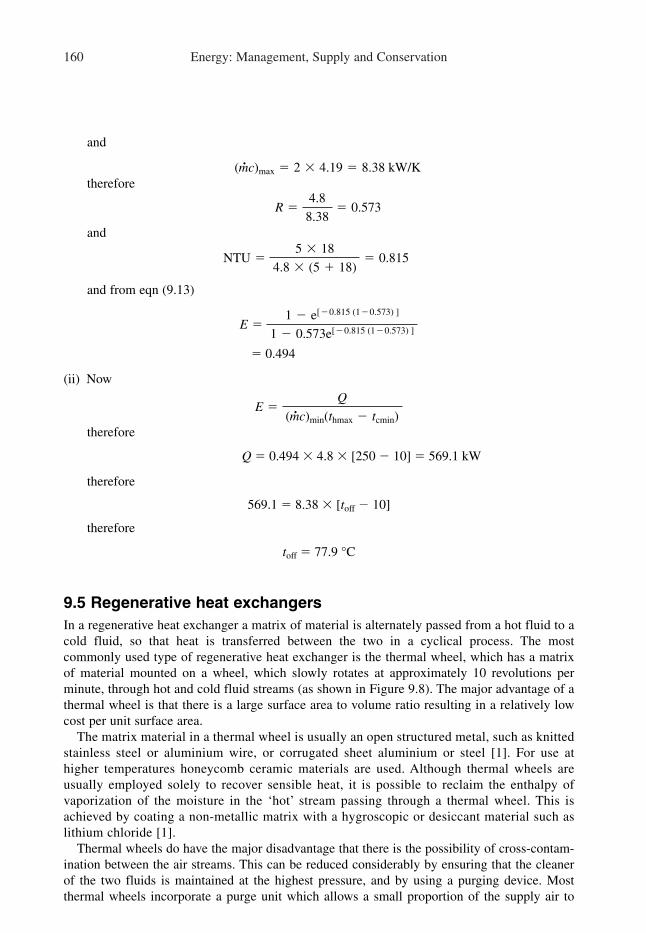
160 Energy: Management, Supply and Conservation
and
therefore
and
and from eqn (9.13)
� 0.494
(ii) Now
therefore
Q � 0.494 � 4.8 � [250 � 10] � 569.1 kW
therefore
569.1 � 8.38 � [toff � 10]
therefore
toff � 77.9 °C
9.5 Regenerative heat exchangers
In a regenerative heat exchanger a matrix of material is alternately passed from a hot fluid to a
cold fluid, so that heat is transferred between the two in a cyclical process. The most
commonly used type of regenerative heat exchanger is the thermal wheel, which has a matrix
of material mounted on a wheel, which slowly rotates at approximately 10 revolutions per
minute, through hot and cold fluid streams (as shown in Figure 9.8). The major advantage of a
thermal wheel is that there is a large surface area to volume ratio resulting in a relatively low
cost per unit surface area.
The matrix material in a thermal wheel is usually an open structured metal, such as knitted
stainless steel or aluminium wire, or corrugated sheet aluminium or steel [1]. For use at
higher temperatures honeycomb ceramic materials are used. Although thermal wheels are
usually employed solely to recover sensible heat, it is possible to reclaim the enthalpy of
vaporization of the moisture in the ‘hot’ stream passing through a thermal wheel. This is
achieved by coating a non-metallic matrix with a hygroscopic or desiccant material such as
lithium chloride [1].
Thermal wheels do have the major disadvantage that there is the possibility of cross-contam-
ination between the air streams. This can be reduced considerably by ensuring that the cleaner
of the two fluids is maintained at the highest pressure, and by using a purging device. Most
thermal wheels incorporate a purge unit which allows a small proportion of the supply air to
E �Q
( �mc)min(thmax � tcmin)
E �1 � e[�0.815 (1�0.573) ]
1 � 0.573e[�0.815 (1�0.573) ]
NTU �5 � 18
4.8 � (5 � 18)� 0.815
R �4.8
8.38� 0.573
( �mc)max � 2 � 4.19 � 8.38 kW/K

Waste heat recovery 161
flush the contaminants from the wheel, thus keeping cross-contamination to a minimum
(e.g. less than 0.04%) [1].
Thermal wheels are often used to recover heat from room ventilation systems such as that
shown in Figure 9.9. In this type of application the thermal efficiency, �t can be defined by:
(9.19)
similarly the overall (total energy) efficiency, �x can be expressed:
(9.20)�x �h2 � h1
h3 � h1
�t �t2 � t1
t3 � t1
Wheel matrix
Warmed supplyair to system
Exhaustinlet
Purgingsector
Cooledexhaustoutlet
Inletsupply air
Figure 9.8 Thermal wheel
Room space
t h1 1
Heating coil
+
t h3 3
t h2 2
Thermalwheel
Figure 9.9 Thermal wheel application

162 Energy: Management, Supply and Conservation
where t1, t2, and t3 are the air temperatures (°C), and h1, h2, and h3 are the air enthalpies (°C).
In a similar manner to a recuperative heat exchanger it can be shown that for a thermal wheel
the relationship between (UA) and (hA) is:
(9.21)
where (UA)o is the product of overall heat transfer coefficient and surface area of matrix, (hA)h
is the product of heat transfer coefficient between the hot fluid and surface area of matrix, and
(hA)c is the product of heat transfer coefficient between the cold fluid and surface area of matrix
and since the matrix area is constant, therefore:
(9.22)
As with recuperative heat exchangers and run-around coils it is possible to use the NTU method
to simplify the analysis of thermal wheels. Kays and London [4] derived the following empiri-
cal formula to describe the effectiveness of thermal wheels.
(9.23)
where
(9.24)
N is the wheel revolutions per second, M is the mass of the matrix (kg), cM is the specific heat
capacity of matrix material (kJ/kgK), and;
where
or
when
Example 9.6
The exhaust air from a factory building is at a temperature of 35 °C and has a flow rate of 6 kg/s
and a specific heat capacity of 1.025 kJ/kg K. The incoming fresh air to the building is at �1 °C,
and has a flow rate of 7 kg/s and a specific heat capacity of 1.025 kJ/kg K. It is proposed to insert
a thermal wheel between the air streams to recover the sensible waste heat. Given the following
information determine:
(i) The effectiveness of the thermal wheel
(ii) The heat transfer rate
(iii) The exit temperature of the fresh air leaving the thermal wheel
(iv) The exit temperature of the fresh air leaving the thermal wheel if its rotational speed is doubled.
Data:
Wheel diameter � 1.2 m
Wheel depth � 0.4 m
Mass of wheel � 140 kg
Surface area to volume ratio � 2500 m2/m3
Specific heat of matrix material � 1.3 kJ/kgK
R � 1Ec �NTU
1 � NTU
R � ( �mc)min� ( �mc)maxEc �1 � e[�NTU(1�R)]
1 � Re[�NTU(1�R)]
( �mc)M � N.M.cM
E � Ec � �1 �1
9[( �mc)M� ( �mc)min]1.93 �
U �h
2
1
(UA)o
�1
(hA)h
�1
(hA)c

Waste heat recovery 163
Wheel speed � 8 rev/min
Heat transfer coefficient for each � 35 W/m2K
air stream
Solution
(i)
therefore
and from eqn (9.21);
therefore
therefore
and
therefore
(ii) Now
therefore
Q � 0.797 � 6.15 � [35 � (�1)] � 176.46 kW
E �Q
( �mc)min (thmax � tcmin)
� 0.797
E � 0.803 � �1 �1
9[24.27 / 6.15]1.93 �
( �mc)M � N.M.cM �8
60� 140 � 1.3 � 24.27 kW� K
Ec �1 � e[�3.215 (1�0.857)]
1 � 0.857 e[�3.215 (1�0.857)]� 0.803
NTU �UAo
( �mc)min
�1130 � 17.5
6.15 � 1000� 3.215
U �h
2�
35
2� 17.5 W�m2K
R �6.15
7.175� 0.857
( �mc)max � 7 � 1.025 � 7.175 kW� K
( �mc)min � 6 � 1.025 � 6.15 kW� K
A � 0.452 � 2500 � 1130 m2
Volume of wheel � 1.13 � 0.4 � 0.452 m3
Face area of wheel �π � 1.22
4� 1.12 m2

164 Energy: Management, Supply and Conservation
(iii) therefore
therefore
(iv) If N � 2 � 8 � 16 rev/min, then
therefore
therefore
therefore
therefore
From this it can be seen that there is very little benefit to be gained from doubling the rotational
speed of the thermal wheel.
9.6 Heat pumps
A heat pump is essentially a vapour compression refrigeration machine which takes heat from a
low temperature source such as air or water, and upgrades it to be used at a higher temperature.
Unlike a conventional refrigeration machine, the heat produced at the condenser is utilized and
not wasted to the atmosphere. Figure 9.10 shows a simple vapour compression heat pump,
together with the relevant pressure/enthalpy diagram.
The performance of the vapour compression refrigeration cycle is quantified by the coefficient
of performance (COP), which can be expressed as:
for a refrigeration machine:
for a heat pump:
COPhp �useful heat rejected from cycle
net work input
COPref �useful refrigeration output
net work input
toff � 23.7 oC
177.34 � 7.175 � [toff � (�1)]
Q � 0.801 � 6.15 � [35 � (�1)] � 177.43 kW
� 0.801
E � 0.803 � �1 �1
9[48.53�6.15]1.93 �
( �mc)M � N.M.cM �16
60� 140 � 1.3 � 48.53 kW� K
toff � 23.6 oC
176.46 � 7.175 � [toff � (�1)]

Waste heat recovery 165
The COP of the vapour compression cycle is usually expressed in terms of a ratio of enthalpy
differences, hence the COP of a refrigeration machine can be expressed as follows (referring to
Figure 9.10):
(9.25)
where:
h � specific enthalpy of refrigerant (kJ/kg)
So, for a heat pump:
(9.26)
from this it can be shown that:
COPhp � COPref � 1 (9.27)
For an ideal heat pump the maximum possible COP is given by the Carnot cycle expression:
(9.28)
where Te is the evaporating absolute temperature (K), and Tc is the condensing absolute temper-
ature (K).
In practice the Carnot COP shown above can never be achieved, but the Carnot equation
shows that the greater the difference between Tc and Te the lower the COP of the heat pump. Heat
pumps are therefore well suited to applications where the evaporating and condensing
temperatures are close together, which is the case when recovering heat from exhaust air in
heating and air conditioning applications. As a result, heat pumps are often used in air
conditioning applications. They are also popular in applications where there is a need for both
dehumidification and heating, such as in warehouses where the occurrence of a high humidity
may cause condensation problems and result in the destruction of valuable stock.
COPhp �Tc
Tc � Te
COPhp �h2 � h3
h2 � h1
COPref �h1 � h4
h2 � h1
+
Condenser
–
Evaporator
Compressor
Thermostaticexpansion valve 14
3 2
Pressure (kPa)
Enthalpy (kJ/kg)
Saturatedliquid
Saturatedvapour
1
2 3
4
Figure 9.10 Vapour compression heat pump

166 Energy: Management, Supply and Conservation
Swimming pool buildings are particularly well suited to the application of heat pumps. In
swimming pools the air leaving the pool hall is very humid and contains large amounts of latent
heat bound up in the water vapour. Heat pumps are particularly well suited to recovering the
enthalpy of vaporization from the moisture in the exhaust air. A typical example of the heat pump
used in combination with a flat plate heat recuperator is shown in Figure 9.11. In this applica-
tion sensible heat is taken from the swimming pool exhaust air by the flat plate recuperator and
used to pre-heat the supply air stream. The evaporator of the heat pump then dehumidifies the
exhaust air stream and recovers the latent heat bound up in the water vapour. The heat pump then
rejects this heat (plus the ‘work’ input by the compressor) through the condenser, and thus heats
the supply air to the pool.
Example 9.7
The heat pump shown in Figure 9.11, operates on refrigerant HCFC 22. Given the following
data, calculate:
(i) The COP of the heat pump
(ii) The electrical energy consumed for each kW of heat produced
Data:
Condensing temperature � 50 °C
Evaporating temperature � 10 °C
Vapour temperature (leaving compressor) � 80 °C
Liquid temperature (leaving condenser) � 40 °C
Combined electrical and mechanical efficiency of motor � 90%
Solution
Using a pressure enthalpy chart (see Appendix 2), or by using thermodynamic tables for
HCFC 22 it is possible to plot the refrigeration process as follows:
(i)
�346 � 150
346 � 315� 6.323
COPhp �h2 � h3
h2 � h1
+–
Evaporator Evaporator
Flat platerecuperator Swimming pool hall
1
6 52
3
4
Figure 9.11 Heat recovery system for a swimming pool building

Waste heat recovery 167
(ii)
Example 9.8
For the heat pump installation shown in Figure 9.11, calculate:
(i) The heat output of the heat pump
(ii) The mass flow rate of refrigerant required in the heat pump circuit
(iii) The power input required to the electric motor
(iv) The specific enthalpy of the air leaving the evaporator coil
Data:
The mass flow rate of supply air � 6 kg/s and
Condition of air leaving pool hall � 29 °C and 70% saturation
Temperature of air supplied to pool hall � 34 °C
Outside air condition � �3 °C and 100% saturation
Effectiveness of flat plate recuperator � 0.7
Solution
Consider first the fresh outside air entering the system and passing through the flat plate recu-
perator. It enters the system at �3 °C and 100% saturation; from a psychrometric chart (see
Appendix 3) or from psychrometric tables, it can be determined that the moisture content of
incoming air stream is 0.0029 kg/kg (dry air) and its specific enthalpy is 4.2 kJ/kg.
Now
Therefore, for the supply air stream, if the maximum theoretical heat transfer occurred,
then it would be heated from �1 °C to 29 °C at a constant moisture content of 0.0029 kg/kg. From
a psychrometric chart or tables, the specific enthalpy of air at 29 °C and 0.0029 kg/kg is 36.6 kJ/kg.
Therefore
The maximum theoretical heat transfer � 36.6 � 4.2
therefore
therefore
Heat transferred (h2 � h1) � 0.7 (36.6 � 4.2) � 22.68 kJ/kg
therefore
h2 � 4.2 � 22.68 kJ/kg
h2 � 22.68 � 4.2 � 26.88 kJ/kg
At a moisture content of 0.0029 kg/kg, h2 equates to an air temperature of 19.3 °C. The heat
pump condenser therefore has to raise the supply air temperature from 19.3 °C to 34 °C, at which
temperature the specific enthalpy is 41.6 kJ/kg.
Effectiveness �Heat transferred
(37.2 � 4.2)
The effectiveness of a flat plate recuperator �Heat transferred
Max. theoretical heat transferred
Electricity consumption per kW of produced �1
6.323 � 0.9� 0.176 kW

168 Energy: Management, Supply and Conservation
(i) Therefore
� 6 � (41.6 � 26.88) � 88.32 kW
and from Example 9.7 it can be seen that for the condenser
(ii)
therefore
(iii) Therefore
(iv) Considering now the exhaust air stream through the flat plate recuperator
Qfpr � � (h2 � h1) � � (h4 � h5)
therefore
Qfpr � 6 � 22.68 � 136.08 kW
Now, the air leaving the pool hall has a moisture content of 0.018 kg/kg and specific enthalpy
(h4) of 75.1 kJ/kg. therefore:
therefore
and from Example 9.7;
Qevap � 0.451 � (315 � 150) � 74.415 kW
and
therefore
Many manufacturers produce machines which have the dual ability to act as both a refrigeration
machine and a heat pump. These machines have twin condensers; an air cooled one for normal
operation, and a water cooled one for the heat pump mode. They are often installed in buildings
and act as air conditioning chillers. When operating in the heat pump mode the waste heat from
the condenser is recovered and used to produce the domestic hot water for the building. This
at first sight would appear to be a classic energy conservation measure. However, such ‘energy
h6 � 52.42 �74.414
6� 40.02 kJ�kg
Qevap � �mair � (h5�h6)
h5 � 75.1 �136.08
6� 52.42 kJ� kg
h5 � h4 �Qfpr
�mair
�mair�mair
Electric power input to compressor �0.451 (346 � 315)
0.9� 15.534 kW
�mref �88.32
346 � 150� 0.451 kg �s
Qcond � �mref � (346 � 150)
Qcond � �mair � (h3 � h2)

Waste heat recovery 169
saving’ measures should be treated with caution since in order to produce the domestic hot water
it may be necessary to raise the condensing pressure considerably, with the result that the COP
may be significantly reduced. When it is also considered that the unit price of electricity is
usually 3 to 4 times that of gas, then the adoption of such a dual purpose machine may not be
quite as advantageous as it appeared originally.
References
1. Cornforth, J. R. (1992). Combustion Engineering and Gas Utilisation (Chapter 7). E & FN Spon.
2. Eastop, T. D. and Croft, D. R. (1990). Energy Efficiency for Engineers and Technologists
(Chapter 5). Longman.
3. Incropera, F. P. and De Witt, D. P. (1990). Fundamentals of heat and mass transfer
(Chapter 11). John Wiley & Sons.
4. Kays, W. M. and London, A. L. (1984). Compact Heat Exchangers. Mc Graw-Hill.
Bibliography
Brookes, G. (1985). Assessing the scope for heat recovery. Energy Manager’s Workbook, 2,
(Chapter 6). Energy Publications.
Cornforth, J. R. (1992). Combustion Engineering and Gas Utilisation (Chapter 7). E & FN
Spon.
Eastop, T. D. and Croft, D. R. (1990). Energy Efficiency for Engineers and Technologists
(Chapter 5). Longman.
McQuiston, F. C. and Parker, J. D. (1994). Heating, ventilating, and air conditioning (Chapter 14).
John Wiley & Sons.
Ozisik, M. N. (1985). Heat transfer: a basic approach (Chapter 11). Mc Graw-Hill.
Stoecker, W. F. and Jones, J. W. (1982). Refrigeration and air conditioning (Chapter 2).
Mc Graw-Hill, 2nd edition.
Thumann, A. and Mehta, D. P. (1997). Handbook of energy engineering (Chapter 5).
The Fairmont Press (Prentice Hall), 4th edition.

10
Combined heat and power
This chapter investigates the subject of combined heat and power (CHP). The general nature of
combined heat and power systems is discussed and the economic benefits appraised. In
particular, CHP plant sizing strategies are evaluated and example design calculations presented.
10.1 The combined heat and power concept
From an energy point of view, the generation of electricity in thermal power stations is an
extremely wasteful process. Most conventional thermal power stations exhibit efficiencies in the
range 30–37% [1], while the newer combined cycle gas turbine stations still only achieve effi-
ciencies in the region of 47% [1]. This means that over 50% of the primary energy consumed in
the generation process is wasted and not converted into delivered electricity. This wasted energy
is converted to heat which is ultimately rejected to the environment. The generation process also
liberates considerable amounts of CO2 into the atmosphere. It has been calculated that in the UK
0.43 kg of CO2 is liberated for every 1 kWh of electrical energy delivered (2001 data) [2].
One easy way to appreciate the inefficiency of the electricity generation cycle is to consider
the theoretical maximum efficiency of the process. The Carnot principle shows that the theoret-
ical maximum thermal efficiency of any heat engine cycle can be determined by:
where T1 is the the maximum temperature available (K), T2 is the the lowest temperature
available (K).
For example, if the maximum temperature in a cycle is 1450 K and the cooling water
minimum temperature is 285 K, then the maximum possible efficiency of the cycle is:
The fact that this level of efficiency is not achieved in practice is due to the high degree
of irreversibility in the process. Consequently, the efficiencies achieved in power stations are
�carnot � 1 �285
1450� 0.803 (or 80.3%)
�carnot � 1 �T2
T1

Combined heat and power 171
very much lower than the theoretical Carnot efficiency and are dependent on the type of prime
mover used.
The low operating efficiencies achieved during the electricity generation process result in a
great amount of energy being lost in the form of waste heat. Given the Earth’s dwindling energy
resources this is not a very satisfactory arrangement. It would be much better to collect the waste
heat from the generation process and use it to heat buildings. By combining the electrical
generation and heat production processes it is possible to produce a highly efficient system
which makes good use of primary energy. It is the combination of the electrical generation and
heat production processes which is the basis of the CHP, or cogeneration, concept. In a typical
CHP installation heat exchangers are used to reclaim waste heat from exhaust gases and other
sources during the electricity generation process. In this way it is possible to achieve overall
efficiencies in the region of 80%, if a system is correctly optimized [3].
CHP systems vary in size from large ‘power stations’ serving whole cities to small micro-CHP
units serving individual buildings. The larger CHP systems tend to use gas or steam turbines,
while smaller systems generally use internal combustion engines converted to run on natural gas.
During the electricity generation process waste heat is recovered from the exhaust gases, or used
steam, and, in the case of micro-CHP systems, also from the engine jacket. Large cogeneration
systems often use recovered heat to produce hot water for use in district heating schemes, while
micro-CHP systems are generally used to heat single buildings.
CHP schemes enable electricity to be generated locally, and eliminate much of the wastage of heat
which normally occurs in conventional power plants. Through the use of CHP it is possible to:
• Improve national energy efficiency and preserve non-renewable energy reserves. This is
particularly important for nations which have limited fossil fuel resources and which are
dependent on imported energy.
• Reduce the cost of transporting electrical energy. The transportation of electricity over long
distances involves the construction of expensive transmission networks (consisting of cables,
pylons, transformers and switchgear). The need for these is reduced by the use of locally-
based CHP schemes. Localized CHP schemes also save energy because they avert the need to
transport electricity over long distances. There is a 4–8% energy loss during the transportation
of electricity over long distances.
• Reduce the amount atmospheric pollution produced, due to more efficient fuel conversion.
Although CHP has many potential benefits, there are a number of problems associated with it,
which have inhibited its widespread use.
• CHP plant requires considerable capital expenditure. This necessitates a full financial appraisal
of future energy demands, fuel prices and maintenance costs. Such an appraisal may only be
accurate in the short term, with the result that organizations often ‘play safe’ and rely on con-
ventional systems with which they are familiar.
• There must be a demand for the heat from any proposed CHP plant. Although in most
applications it is possible to fully utilize the electricity produced by CHP plant, it is often
much more difficult to utilize the heat which is produced. Most building types do not have the
all-year-round demand for heat which is required to successfully employ a CHP plant. On the
contrary many building types require cooling for large parts of the year.
• Back-up plant is often required in CHP installations, in order to ensure security of supply of
electricity and heat. This ‘back-up’ plant adds to the capital cost of the installation.
Given the considerable capital expenditure associated with CHP schemes it is essential that any
proposed CHP application be carefully evaluated to determine its suitability. It should be

172 Energy: Management, Supply and Conservation
remembered with caution that there are many so-called energy saving schemes which have
proved to be expensive liabilities.
10.2 CHP system efficiency
It is possible to illustrate the energy saving merits of CHP systems by comparing the primary
energy consumption of a typical micro-CHP plant with that consumed by a conventional system
in which heat is produced in a boiler and electrical power is purchased from a utility company.
Example 10.1 presents the energy balance for the two alternative systems.
Example 10.1
A building has an electrical power requirement of 80 kWe (i.e. 80 kW of electrical power) and a
heat load of 122 kW. The owners of the building are considering installing a micro-CHP unit
which utilizes an internal combustion engine converted to run on natural gas. Compare the
primary energy consumption and unit energy costs of the CHP scheme compared with a
conventional separate system.
Data:
Efficiency of the conventional electricity supply process � 35%
Efficiency of conventional boiler plant � 70%
Mechanical efficiency of CHP unit � 32%
Efficiency of CHP electricity generator � 95%
Heat recovery efficiency of CHP unit � 68.16%
Unit cost of gas � 0.9 p/kWh
Unit cost of electricity � 5.0 p/kWh
Solution
The two options are considered as follows:
Option 1: conventional system:
and
Therefore
Total primary power input � 228.6 � 174.3 � 402.9 kW
therefore
and
Energy cost for 1 hour's operation �(80 � 5.0) � (174.3 � 0.9)
100� £5.57
Overall system efficiency �80 � 122
402.9� 100 � 50.1%
Power input to boilers �122
0.70� 174.3 kW.
Primary fuel power input to generate electicity �80
0.35� 228.6 kW

Combined heat and power 173
Option 2: CHP System:
The waste heat produced by the CHP unit is passed through a heat exchanger with an efficiency
of 68.16%, therefore:
Recoverable heat power � (263.2 � (1 � 0.32)) � 0.6816 � 122.0 kW
Therefore
and
Energy cost for 1 hour’s operation � (263.2 � 0.9) � £2.37
Example 10.1 clearly shows that there are large potential energy cost savings to be gained
through utilizing CHP in buildings.
10.3 CHP systems
CHP systems can range from small ‘micro’ installations, designed to serve the needs of a single
building, to large systems which satisfy the heating and electrical power requirements of whole
towns. Micro-CHP systems utilizing internal combustion engines tend to be used in applications
where electrical demand does not exceed 1 MWe. Gas turbines are popular on larger installa-
tions, while steam turbines are often used on the largest schemes.
10.3.1 Internal combustion engines
Internal combustion engines are often used to drive small micro-CHP systems. Mechanical
power from this type of engine is used to drive a generator and heat is recovered from the engine
exhaust, jacket water and lubricating oil. Micro-CHP units typically operate in the range 15 kWe
to 1 MWe electrical output. Modified automotive derived engines are the most widely used
systems up to 200 kWe electrical output, whereas more rugged stationary industrial engines are
generally used for higher outputs [3]. The automotive engines used are generally modified lorry
engines, which are converted to run on gas. These engines usually operate at a much slower and
constant speed, typically 1500 rpm, than normal automotive engines. The engine life of a typical
CHP prime mover is thus considerably longer than that of a typical automotive engine. Spark
ignition gas engines tend to exhibit a heat to power ratio around 1.7:1 [3], whereas compression
ignition diesel engines have heat to power ratios nearer 1:1.
10.3.2 Gas turbines
Where a natural gas supply is available, gas turbines are often used as the prime mover for larger
CHP systems. Gas turbines have a relatively low capital cost and are reliable. The peak load
mechanical efficiency of gas turbines is around 30%, which gives an optimum heat to power
ratio of around 3:1 [4]. However, under part-load conditions efficiency can be substantially
reduced. Gas turbines are usually fuelled by natural gas, but oil and pulverized coal have also
been successfully employed.
Overall system efficiency �80 � 122
263.2� 100 � 76.7%
Fuel power input to CHP unit �80
0.32 � 0.95� 263.2 kW
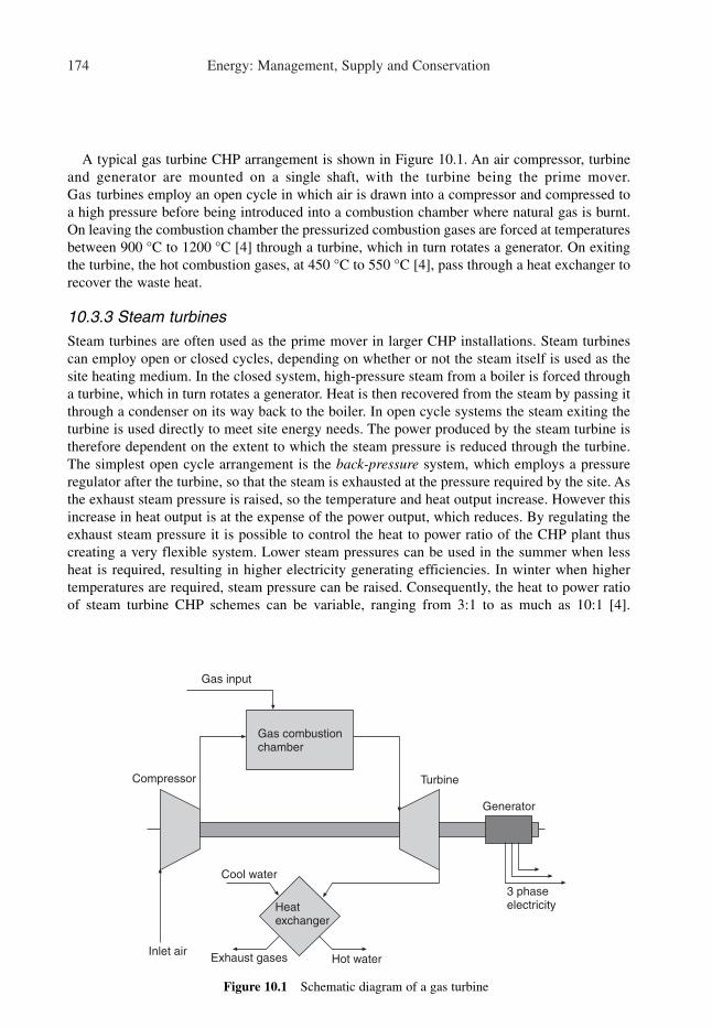
174 Energy: Management, Supply and Conservation
A typical gas turbine CHP arrangement is shown in Figure 10.1. An air compressor, turbine
and generator are mounted on a single shaft, with the turbine being the prime mover.
Gas turbines employ an open cycle in which air is drawn into a compressor and compressed to
a high pressure before being introduced into a combustion chamber where natural gas is burnt.
On leaving the combustion chamber the pressurized combustion gases are forced at temperatures
between 900 °C to 1200 °C [4] through a turbine, which in turn rotates a generator. On exiting
the turbine, the hot combustion gases, at 450 °C to 550 °C [4], pass through a heat exchanger to
recover the waste heat.
10.3.3 Steam turbines
Steam turbines are often used as the prime mover in larger CHP installations. Steam turbines
can employ open or closed cycles, depending on whether or not the steam itself is used as the
site heating medium. In the closed system, high-pressure steam from a boiler is forced through
a turbine, which in turn rotates a generator. Heat is then recovered from the steam by passing it
through a condenser on its way back to the boiler. In open cycle systems the steam exiting the
turbine is used directly to meet site energy needs. The power produced by the steam turbine is
therefore dependent on the extent to which the steam pressure is reduced through the turbine.
The simplest open cycle arrangement is the back-pressure system, which employs a pressure
regulator after the turbine, so that the steam is exhausted at the pressure required by the site. As
the exhaust steam pressure is raised, so the temperature and heat output increase. However this
increase in heat output is at the expense of the power output, which reduces. By regulating the
exhaust steam pressure it is possible to control the heat to power ratio of the CHP plant thus
creating a very flexible system. Lower steam pressures can be used in the summer when less
heat is required, resulting in higher electricity generating efficiencies. In winter when higher
temperatures are required, steam pressure can be raised. Consequently, the heat to power ratio
of steam turbine CHP schemes can be variable, ranging from 3:1 to as much as 10:1 [4].
Gas combustionchamber
Compressor Turbine
Heatexchanger
Inlet air
Cool water
Exhaust gases Hot water
Generator
3 phaseelectricity
Gas input
Figure 10.1 Schematic diagram of a gas turbine

Combined heat and power 175
They are therefore best suited to schemes in which there is a high all-year-round heat require-
ment. A typical back-pressure steam turbine CHP arrangement is shown in Figure 10.2.
Because a boiler is employed to produce the steam to drive a turbine, a wide variety of fuels can
be used, including refuse. Therefore steam turbines are a good solution for waste-to-energy CHP
schemes in which refuse is incinerated and the heat used to produce steam. In Scandinavia it is
common practice to burn the waste products from the timber industry to produce steam in CHP
schemes.
10.4 Micro-CHP systems
Stand-alone micro-CHP units are a popular solution for many small- and medium-sized com-
mercial applications. Micro-CHP units use an internal combustion engine as a prime mover, and
generally comprise an engine, an electricity generator, a heat recovery system, an exhaust, and a
control system (as shown in Figure 10.3).
In a micro-CHP system, optimum efficiency is achieved by maximizing the heat recovered
from the engine and exhaust gases. In theory as much as 90% of the heat produced by the gen-
eration process can be recovered. Achieving this level of heat recovery requires the use of sev-
eral heat exchangers, which makes the capital cost high. It is therefore more typical to recover
around 50 per cent of the fuel input as useful high-grade heat, with a further 10% recovered as
low-grade heat [3]. The high-grade heat can be used to provide heating water in the region of
70–90 °C and the low-grade heat to provide water at 30–40 °C [3]. Most of the heat is recovered
from the engine jacket, which has a temperature of approximately 120 °C, while the rest is
recovered from the exhaust gases, which can be at 650 °C [4]. Both sensible and latent heat can
be recovered from the exhaust gases.
Although most micro-CHP units provide low temperature hot water (LTHW) in the region
70–80 °C, it is equally possible to provide medium temperature hot water (MTHW) (i.e. 90–120 °C).
Boiler
Steamturbine
Heatexchanger
Feedpump
Cool water
Condensate Hot water
Generator
3 phaseelectricityBack-pressure
regulator
Steam
Fuel input
Figure 10.2 Schematic diagram of back-pressure steam turbine CHP system

176 Energy: Management, Supply and Conservation
However, because of the higher water temperatures involved, heat recovery is reduced. Conversely, it
is possible to increase heat recovery and therefore the efficiency of a micro-CHP system, by reduc-
ing the hot water supply temperature to below 70 °C. As most micro-CHP systems are required to
produce domestic hot water (DHW), which must be stored at above 60 °C to prevent the growth of
Legionella spp., in practice the flow water temperature should be 70 °C or above.
Micro-CHP units are often used in conjunction with boilers. In such systems the CHP unit
should satisfy the base heating load, with the boilers only being used during periods of peak
demand. This necessitates coupling the micro-CHP unit to the boilers, so that the two can work
effectively together. In existing installations, where a CHP unit is replacing some old boilers, it
is common practice to connect the CHP unit and boilers in series as this causes minimum
interference to existing systems. In new installations, CHP units are often connected in parallel
with boilers. Figure 10.4 illustrates both arrangements. No matter which arrangement, it is
essential that the CHP unit operates as the lead ‘boiler’, as this maximizes its operating hours.
Many micro-CHP units incorporate a continuous monitoring facility as part of their control
system. This enables building heat and power requirements to be monitored so that optimum
performance of the plant is achieved. It also enables the system to be audited, so that the return
on the capital investment can be calculated.
10.5 District heating schemes
Many larger CHP units are coupled to district heating schemes in which the pipework and
pumping costs are dominant. In such schemes it is important to minimize both pipe diameters
Exhaustgases
Heatexchanger
Cool returnwater
Gas engine
Hot supplywater
Generator
3 phaseelectricity
Gas input
Figure 10.3 Schematic diagram of a micro-CHP unit

Combined heat and power 177
and water flow rates, by operating at a peak flow water temperature of approximately 120 °C,
with a return water temperature of 70 °C. This reduces both capital and operating costs. It is also
common practice to vary supply water temperature with ambient air temperature so that system
heat losses are minimized.
If LTHW is required in individual buildings on a district heating scheme, this can be achieved
by installing remote heat exchangers in each building. This maintains hydraulic separation
between the district heating water and the LTHW and makes the overall system safe and
flexible. In Europe, variable temperature district heating schemes with heat exchangers are very
popular.
10.6 CHP applications
CHP systems are considered to be efficient users of primary energy because the waste heat
produced by the generation process is utilized to satisfy heating requirements. If ‘waste’ heat
cannot be utilized effectively, overall efficiency will drop dramatically. In simple terms, there is
no point in installing a CHP system in an application which does not have an all-year-round
demand for heat. CHP systems are therefore suitable for buildings such as leisure centres, swim-
ming pools, hotels, hospitals, and residential establishments, all of which have extensive DHW
requirements for most or all of the year. Office buildings are generally thought to be unsuitable,
since they frequently have a cooling load for much of the year and are only open during the day
Boilers
Bypass ifrequired
DedicatedCHP pump
CHP
To radiators
Hot watercalorifier
Hot waterto services
3PMV
Cold feed3PDV
Pump
T Co
CHP in bypass toreturn header (series)
Boilers To radiators
Hot watercalorifier
Hot waterto services
3PMV
Cold feed3PDV
Pump
T Co
CHP
DedicatedCHP pump
CHP in parallelwith boilers
Figure 10.4 CHP piping arrangement. Crown copyright is reproduced with the permission of the
Controller of Her Majesty’s Stationery Office and the Queen’s Printer for Scotland [3]

178 Energy: Management, Supply and Conservation
time. If however the heat from a CHP unit is used to drive absorption refrigeration plant, then
CHP can become a feasible option for office buildings.
Although the operational costs associated with CHP systems are low, the capital costs are
high. It is therefore desirable to run a CHP unit for as long as possible in order to achieve the
greatest return on the initial capital investment. It has been calculated that in order to achieve a
simple payback of 3 to 4 years it is necessary to operate a CHP unit between 4500 and 6000
hours per year [3], which is equivalent to approximately 12.3 to 16.5 hours of operation for each
day of the year. It is much better to undersize a CHP unit than to oversize it, since this will ensure
that the unit runs continuously when in operation, with any shortfall in output being made up by
back-up boilers and bought-in electricity. It is therefore common practice to use the CHP unit to
satisfy base heat load requirements. Ideally a CHP unit should be able to supply the entire
summer heat load and a proportion of the winter load. Although it may be relatively small
(possibly with a rated output of only 33–50% of the peak heating demand) it is possible to supply
60–90% of a building’s annual heat requirement with a CHP unit because it supplies the base
heat load.
In certain situations, where a CHP unit generates more electricity than can be consumed on
site, it is possible to export power to the local utility company. This depends on the willingness
of the utility company to purchase the electricity. It also requires the installation of an export
meter. Therefore, for small-scale CHP installations it is not generally considered economic to
export electricity. Micro-CHP units should therefore be sized so as not to exceed the base
electrical load.
It is possible to use a CHP unit as a standby generator if so required. If used in this way its
size will be governed by the required peak emergency electrical load. For normal operation it
will be necessary to modulate down the output to match the reduced heat and power require-
ments, with the result that efficiency will be compromised. In such circumstances it may be more
economical to install two smaller CHP units.
10.7 Operating and capital costs
The capital and installation costs of CHP plant can be significantly higher than those for
conventional boiler plant. One significant cost which can easily be overlooked is the requirement
of CHP systems to be synchronized in parallel with the local utility company’s distribution grid,
so that the grid and the CHP unit can work together to meet peak site electrical demand. This
involves the installation of expensive electrical switching equipment. In contrast to the capital
costs, the operating costs associated with CHP are relatively low and comprise the fuel and
maintenance costs. For micro-CHP units maintenance costs are generally in the range of 0.5–2.0 p
per kWhe of electricity generated [3], with the maintenance cost reducing for larger systems.
Typical capital and maintenance costs for various sized CHP units are shown in Table 10.1.
10.8 CHP plant sizing strategies
In order to correctly size a CHP installation it is important to obtain as much accurate energy
data as possible for the given application. Ideally these data should include:
• Monthly electricity and heat energy consumption data in kWh.
• Base and peak-load demands (in kW) for both electricity and heat.
• The operational characteristics of the particular application.
• Unit cost data for electricity and gas (or oil).

Combined heat and power 179
Because it is important not to oversize a CHP plant it is advisable to undertake all the possible
no-cost and low-cost energy efficiency measures before sizing the plant. This will avoid the CHP
unit being oversized and should reduce the capital cost of the installation.
When determining the size of a CHP unit the most commonly used approach is to size the unit
to meet the base heating load, as shown in Figure 10.5. This ensures that the CHP unit can run
all year round, thus guaranteeing that the payback period on the initial capital investment is short.
Back-up boilers can then be used to meet the peak-load heating requirements. A CHP unit sized
in this way usually generates less electricity than is required to meet the base electrical demand
and therefore additional electrical energy must be purchased all-year-round from the local utility
company. An alternative approach is to size the CHP unit to meet the electrical base load. This
usually means that for part of the year heat will have to be dumped because the heat produced
by the CHP unit will exceed the base-load requirement. However, despite the dumping of heat
this can be the most economic solution, since the unit cost of electricity can be as much as five
times that of a unit of heat.
Table 10.1 CHP installation and maintenance costs (1996 data) [5]
CHP engine size Installed capital cost Maintenance cost (kWe) (£/kWe) (p/kWhe)45 1230 1.04
54 1170 1.02
90 1020 0.98
110 960 0.95
167 810 0.89
210 730 0.85
300 660 0.79
384 605 0.73
600 520 0.62
0
100
200
300
400
500
600
Ave
rage h
eating d
em
and (
kW
)
Dec. Jan. Feb. Mar. April May June July Aug. Sept. Oct. Nov. Dec. Jan.
CHP Boilers
Figure 10.5 Base heat load sizing strategy for CHP plant

180 Energy: Management, Supply and Conservation
10.9 The economics of CHP
For most small-scale CHP applications three factors dominate economic viability. These are:
• The capital cost of the installation.
• The potential number of operating hours per year.
• The relative costs of ‘bought-in’ electricity and gas (or fuel oil).
If any of these three variables are not favourable, then a particular CHP scheme may become
non-viable. Given that fuel prices can be unstable, the last point is of particular importance. If
for example, the unit cost of mains electricity should fall or the cost of gas rise, there will come
a point when a particular CHP unit ceases to be economically viable. Other lesser factors which
may influence the economic performance of a CHP scheme are:
• The heat to power ratio of the particular CHP plant;
• The difference in maintenance costs between a CHP scheme and a conventional scheme;
• The cost of having mains electricity as a back-up system in case of breakdown or maintenance.
Given these costs, it is important to undertake a full economic appraisal of any proposed CHP
scheme. Example 10.2 illustrates how a simple appraisal might be undertaken.
Example 10.2
An existing hotel building has an average electrical demand of 80 kWe and an average combined
heating and hot water demand of 180 kW. The average annual load factor for the building is 0.75.
The heating and hot water demand is currently served by two gas fired boilers and mains
electricity is bought-in. It is proposed to install a micro-CHP plant which will run on gas and have
a heat to power ratio of 1.7:1. The existing boilers will supplement the heat output from the CHP
unit. If the initial cost of the CHP installation is £76 000, determine the simple payback period.
Data:
Efficiency of existing boilers � 70%
CHP unit electric power output � 80 kWe
CHP unit gas power input � 286 kW
Unit price of electricity � 5.0 p/kWh
Unit price of gas � 0.9 p/kWh
Existing plant maintenance cost � £1000 per year
CHP scheme maintenance cost � £5000 per year
Solution
Annual operating hours � load factor � total hours per year
� 0.75 � 8760 � 6570 hours
Considering the present scheme:
and
Maintenance cost � £1000.00
Gas cost �180 � 6570 � 0.9
0.7 � 100� £15 204.86
Electricity cost �80 � 6570 � 5.0
100� £26 280.00

Combined heat and power 181
therefore
Annual cost � 26 280.00 � 15 204.86 � 1000.00
� £ 42 484.86
Considering the proposed CHP scheme:
The average short-fall in CHP heat production � 180 � (80 � 1.7) � 44 kW.
Therefore
and
Maintenance cost � £5000.00
therefore
Annual operating cost � 16 911.18 � 3716.74 � 5000.00 � £25 627.92.
Now
Therefore
� 4.51 years
While the analysis undertaken in Example 10.2 gives some indication of the economic viability
of a CHP scheme, the method used is simplistic and has a number of inherent weaknesses.
It assumes that the electrical and heating demands are constant at 80 kWe and 180 kW
respectively. In reality this will not be the case. For long periods during the year demand will be
higher than this, while at other times it will be lower. This means that during periods of high
electrical demand (i.e. when the electrical demand exceeds 80 kWe), electricity will have to be
purchased from the local utility company. However during periods of low demand the CHP
unit will be producing electricity and heat which cannot be utilized. As a result the analysis
overestimates the potential cost savings achievable through using CHP.
A more sophisticated approach which overcomes some of the short-falls described above is
illustrated in Example 10.3.
Example 10.3
A new sports centre is to be built which will have a predicted annual heat load of 2600 000 kWh
and an annual electrical load of 830 000 kWhe. The peak winter heating and hot water demand
is predicted to be 1000 kW and the base heat demand is 350 kW. The base electrical demand is
130 kWe. The sports centre plant will operate for 5130 hours per year. Given the following data
appraise the financial viability of three proposed schemes:
(a) conventional scheme in which boilers produce all the heat and electricity is purchased from
a utility company.
(b) A CHP scheme in which the CHP plant is sized to meet the base electrical load.
(c) A CHP scheme in which the CHP plant is sized to meet the base heat load.
Pay back �76 000
(42 484.86 � 25 627.92)
Pay back �Capital cost
Annual cost saving.
Annual boiler fuel cost �44 � 6570 � 0.9
0.7 � 100� £3716.74
Annual CHP unit fuel cost �286 � 6570 � 0.9
100� £16 911.18

182 Energy: Management, Supply and Conservation
Data:
Efficiency of boilers � 70%
Mechanical efficiency of CHP unit � 30%
Efficiency of CHP electricity generator � 95%
Heat recovery efficiency of CHP unit � 70%
Unit cost of gas � 0.9 p/kWh
Unit cost of electricity � 5.0 p/kWh
Cost of maintaining boilers � 0.1 p/kWh
CHP scheme maintenance cost � 0.9 p/kWhe
Capital cost of boiler only scheme � £26.50 per kW
Capital cost of CHP scheme � £900 per kWe
Solution
(a) Considering the conventional scheme:
and
Therefore
Annual cost � 41 500.00 � 33 428.57 � 2600.00 � £77 528.57
and
Capital cost � 26.50 � 1000 � £26 500.00.
(b) Considering the CHP scheme, sized to meet the base electrical load:
The waste heat produced by the CHP unit is passed through a heat exchanger with an efficiency
of 70%, therefore:
Recoverable heat power � (456.14 � (1 � 0.3)) � 0.70 � 223.51 kW.
Therefore
Annual electricity produced by CHP unit � 130 � 5130 � 666 900 kWhe
and
Annual heat produced by CHP unit � 223.51 � 5130 � 1146 606.3 kWh
Therefore
Annual CHP unit fuel cost �454.14 � 5130 � 0.9
100� £21 059.98
Fuel power input to CHP unit �130
0.3 � 0.95� 456.14 kW
Maintenance cost �2600 000 � 0.1
100� £2600.00
Gas cost �2600 000 � 0.9
0.7 � 100� £33 428.57
Electricity cost �830 000 � 5.0
100� £41 500.00

Combined heat and power 183
and
Therefore
Annual operating cost � 21 059.98 � 18 686.49 � 8 155.00 � 6002.10
� £53 903.57
and
Capital cost of CHP scheme � 900.00 � 130 � £117 000.00
Therefore
Increased capital expenditure compared with Scheme (a) � 117 000.00 � 26 500.00
� £90 500.00
and
Annual operating cost saving � 77 528.57 � 53 903.57 � £23 625.00
(compared with Scheme (a))
therefore
(c) Considering the CHP scheme, sized to meet the base heat load:
Therefore, the heat to power ratio of the CHP unit is 1.719:1. Assuming that the CHP unit is
sized to meet the base heat load of 350 kW, then:
Unfortunately since the average electrical demand of the building is only 161.79 kWe, the CHP
unit produces more electricity than can be consumed by the building. Unless the electricity can
be exported to the local utility company, the CHP unit will either have to be reduced in size, or
else its output will have to be modulated down considerably.
If it is assumed that electricity can be exported at, say, 3.0 p/kWhe, then:
� £6436.10
and
Annual heat produced by CHP unit � 350 � 5130 � 1795 500 kWh
Annual electricity produced by CHP unit � 161.79 � 5130 � 830 000 k Whe
NB: The CHP unit provides all the electricity for the building.
Annual revenue generated through exporting electricity �(203.61 � 161.79) � 5130 � 3.0
100
Electrical power output from CHP unit �350
1.719� 203.61 kW
Heat produced for each kWe of electrical power generated �223.51
130� 1.719
Pay back on increased Capital expenditure �90 500.00
23 625.00� 3.8 years
Maintenance cost �0.9 � 666 900
100� £6002.10.
Annual cost of electricity purchased �(830 000 � 666 900) � 5.0
100� £8155.00
Annual boiler fuel cost �(2600 000 � 1146 606.3) � 0.9
0.7 � 100� £18 686.49

184 Energy: Management, Supply and Conservation
Therefore
and
Therefore
Annual operating cost � 32 984.77 � 10 343.57 � 9400.67 � 6436.10
� £46 292.91
and
Capital cost of CHP scheme � 900.00 � 203.61 � £183 249.00
Therefore
Increased capital expenditure (compared with Scheme (a)) � 183 249.00 � 26 500.00
� £156 749.00
and
Annual operating cost saving (compared with Scheme (a)) � 77 528.57 � 46 292.91
� £31 235.66
Therefore
Example 10.3 clearly demonstrates that both CHP schemes achieve substantial cost savings
compared with the conventional scheme (a). However, it should be noted that although scheme
(c), sized to meet the base heat load, produces the greatest annual cost savings, scheme (b)
appears to be the more cost effective of the two proposals. This is because:
• The capital cost of scheme (c) is much higher than that of scheme (b); and
• Much of the electricity produced under scheme (c) is under-utilized (i.e. exported for a
relatively low return).
Example 10.3 therefore reinforces the conclusion that it is unwise to oversize a CHP plant and
confirms that it is preferable to size the CHP plant to meet the electrical base load.
References
1. Beggs, C. B. (1996). A method for estimating the time-of-day carbon dioxide emissions per
kWh of delivered electrical energy in England and Wales. Building Services Engineering
Research and Technology, 17, (Number 3), 127–134
Pay back on increased Capital expenditure �156 749.00
31 235.66� 5.02 years
Maintenance cost �0.9 � (203.61 � 5130)
100� £9400.67
Annual boiler fuel cost �(2600 000 � 1795 500) � 0.9
0.7 � 100� £10 343.57
Annual CHP unit fuel cost �714.42 � 5130 � 0.9
100� £32 984.77
Fuel power input to CHP unit �203.61
0.3 � 0.95� 714.42 kW.

Combined heat and power 185
2. Department of the Environment, Transport and the Regions (2001). Environmental
Reporting – Guidelines for Company Reporting on Greenhouse Gas Emissions,
www.detr.gov.uk/ environment/envrp/gas/ 05.htm, 8 May.
3. Department of the Environment (1989). Guidance notes for the implementation of small scale
packaged combined heat and power. Good Practice Guide 1.
4. Department of the Environment (1992). Introduction to large-scale combined heat and power.
Good Practice Guide 43.
5. Williams J., Griffiths, T. and Knight, I. (1996). Sizing chp for new hospitals. Building
Services Journal, November, pp. 41–3.
Bibliography
Cost model: Combined heat and power system analysis (1997). Building Services Journal,
January, pp. 17–19.
Department of the Environment (1989). Guidance notes for the implementation of small scale
packaged combined heat and power. Good Practice Guide 1.
Department of the Environment (1992). Introduction to large-scale combined heat and power.
Good Practice Guide 43.
Eastop, T. D. and Croft, D. R. (1990). Energy efficiency for engineers and technologists,
(Chapter 8). Longman Scientific & Technical.
Williams, J., Griffiths, T. and Knight, I. (1996). Sizing chp for new hospitals. Building Services
Journal, November, pp. 41–3.

11
Energy efficient air conditioning andmechanical ventilation
Much energy is wasted in buildings through the use of inappropriate air conditioning and
mechanical ventilation systems. This situation has arisen because building designers are
often ignorant of the issues associated with air conditioning and also because designers of
air conditioning systems are more interested in minimizing first costs rather than reducing
overall energy consumption. There are, however, a number of new and innovative technolo-
gies, which have the potential to reduce energy consumption greatly. This chapter discusses
the issues associated with the design of air conditioning and mechanical ventilation systems,
and introduces some of these new low energy technologies.
11.1 The impact of air conditioning
Over the last 40 years or so, there has been a trend towards large deep plan buildings with highly
insulated envelopes. This trend, coupled with the increased use of personal computers and the
use of high illumination levels, has meant that many buildings over-heat and thus require cool-
ing for large parts of the year, even in countries which experience cool temperate climates. Over
the years boilers have steadily reduced in size and the use of air conditioning and mechanical
ventilation has increased. When it is also considered that most of the Earth’s population live in
countries which have warm or hot climates, it is not difficult to appreciate that the provision of
adequate cooling and ventilation is a much greater global issue than the provision of adequate
heating. Unfortunately, many building designers are not fully aware of this simple fact, with the
result that a great number of poorly designed buildings are erected, relying on large air condi-
tioning systems in order to maintain a tolerable internal environment.
The contribution of mechanical cooling towards overall global energy consumption should not
be underestimated. In the UK alone, it has been estimated that approximately 10 000 GWh of
electrical energy is consumed per annum by air conditioning equipment [1]. This represents
approximately 14% of all the electrical energy consumed in the commercial and public admin-
istration sectors in the UK. Of this figure, approximately 5853 GWh is consumed solely by
refrigeration plant, the rest being consumed by fans, pumps and controls [2]. In the USA,
the energy consumed by air conditioning equipment is much higher. Indeed, in many of the

Energy efficient air conditioning and mechanical ventilation 187
southern states in the USA, electrical demand increases by 30–40 % during the summer months
solely due to the use of air conditioning equipment [3]. As a result of this, the utility companies
in the southern states of the USA have to install excess generating capacity to meet the summer
peak, even though for most of the year this plant remains idle, which is clearly a very uneco-
nomical situation. The problems faced by the electrical utilities in the USA are typical of many
companies operating in warm climates throughout the world. In some countries, electrical
demand is so high during the summer months that the authorities ration electricity by restricting
the capacity of power cables which enter properties. In doing so they force building owners and
users to utilize low energy design solutions.
It is a common misconception that most of the energy consumed by air conditioning plant is
associated with the operation of refrigeration machines. This is not the case. In reality much
more energy is consumed by air handling plant. A recent study of typical ‘standard’ air condi-
tioned office buildings in the UK found that refrigeration plant consumed 13% of total electricity
consumption, while fans, pumps and controls consumed 26.5% of all the electrical energy
consumed. In this type of office building approximately 35% of the total energy costs were spent
on running the air conditioning and mechanical ventilation systems [4]. A summary of the results
of this study is presented in Table 11.1.
The environmental impact of air conditioning equipment is considerable. Air conditioning is
uniquely catastrophic from an environmental point of view, since it:
• Can contribute directly to atmospheric ozone depletion through the leakage of harmful
refrigerants.
• Contributes directly to global warming through the leakage of refrigerants which are
powerful greenhouse gases.
• Contributes to global warming by consuming large amounts of electricity and indirectly
releases large quantities of CO2 into the atmosphere.
A full discussion of the environmental problems associated with refrigerants is beyond the scope
of this book. Nevertheless, a brief discussion of environmental matters is perhaps relevant here.
Until recently, both CFCs and HCFCs were extensively used as refrigerants. Although CFCs and
HCFCs are known to be potent greenhouse gases, they are much more infamous for being potent
ozone depletors. Indeed, it was the serious threat to the ozone layer which ended production of
CFCs in 1995 under the Montreal Protocol [5]. Since then there has been heavy reliance on the
use of HCFC 22 as an alternative to CFCs. While HCFC 22 is far more ozone friendly than CFC
11 or 12, it is still a potent greenhouse gas, having a GWP of 1700 [6]. However, under the
Montreal Protocol, HCFCs are also being phased-out, with production due to cease completely
by 2030 [7]. Consequently, the chemical manufacturers are currently developing a new genera-
tion of refrigerants, HFCs, to replace the old CFCs and HCFCs. Unfortunately, while HFCs are
ozone benign they are still strong greenhouse gases. Notwithstanding this, the relative effect
which refrigerants have on global warming is often overestimated. The contribution to global
warming made by escaping refrigerants is far outweighed by the indirect CO2 emissions
resulting from the electrical consumption of refrigeration machines. This is graphically illustrated
by Figure 11.1 which shows the relative contribution to global warming of associated CO2
emissions compared with that of a variety of refrigerants [8].
It can be seen from Figure 11.1 that the indirect contribution of air conditioning equipment
towards global warming is considerable. It has been estimated that in the UK alone, 4.2 million
tonnes of CO2 per annum are directly attributable to the use of air conditioning refrigeration
plant [2]. It is therefore not surprising that governments around the world are putting pressure on
building designers to reduce or eliminate the need for mechanical cooling.

Table 11.1 Energy consumption in various UK office buildings [4]
Naturally ventilated Naturally ventilated Air conditioned Air conditionedcellular open-plan standard prestige
Good Good Good Goodpractice Typical practice Typical practice Typical practice Typical(kWh/m2) (kWh/m2) (kWh/m2) (kWh/m2) (kWh/m2) (kWh/m2) (kWh/m2) (kWh/m2)
Heating and hot water (gas or oil) 79 151 79 151 97 178 107 201
Mechanical cooling 0 0 1 2 14 31 21 41
Fans, pumps and controls 2 6 4 8 30 60 36 67
Humidification 0 0 0 0 8 18 12 23
Lighting 14 23 22 38 27 54 29 60
Office equipment 12 18 20 27 23 31 23 32
Catering (gas) 0 0 0 0 0 0 7 9
Catering (electricity) 2 3 3 5 5 6 13 15
Other electricity 3 4 4 5 7 8 13 15
Computer room (where applicable) 0 0 0 0 14 18 87 105
Total gas or oil 79 151 79 151 97 178 114 210
Total electricity 33 54 54 85 128 226 234 358

Energy efficient air conditioning and mechanical ventilation 189
11.2 Air conditioning systems
This chapter is not intended to be a text on the fundamentals of air conditioning design, but rather
a discussion of the application of air conditioning in buildings. Before discussing in detail the
issues which affect the energy consumption of air conditioning systems, it is necessary first to
describe briefly the nature and operation of a generic air conditioning installation. It should be
noted that in this text, for ease of reference, the term air conditioning is used in its loosest sense
to describe any system which employs refrigeration to cool air in buildings.
Figure 11.2 shows a simple air conditioning system which illustrates many generic features.
The system employs an air handling unit (AHU) to blow air at a constant volume flow rate
through ducts to a room space. Stale air is then removed from the room space via an extract duct
using a return fan. In order to save energy, it is common practice to recirculate a large proportion
(e.g. 70%) of the return air stream using mixing dampers located in the AHU. It is also common
practice to propel air along the ducts at velocities in excess of 5 m/s. This ensures that duct-work
sizes are kept to a minimum. Room space temperature is controlled by varying the temperature of
the incoming supply air; in winter, air is supplied at a temperature higher than that of the room
space, while in summer the air is supplied at a temperature lower than that of the room space. In
this way a comfortable environment can be maintained all-year-round in the room space.
The AHU in Figure 11.2 comprises:
• A mixing damper section to mix the incoming fresh air with recirculated air;
• A filter to clean the air;
• A heating coil (usually a hot water coil fed from a boiler but sometimes electric);
• A cooling coil to cool and dehumidify the air;
• A reheat coil to accurately control the air temperature and to compensate for any over-cooling
by the cooling coil; and
• A centrifugal fan to draw the air through the AHU and to push it through the ductwork.
In the case of the AHU shown in Figure 11.2, a direct expansion (DX) refrigeration coil is used
to cool the supply air. This coil is the evaporator of a refrigeration system, and contains liquid
0
20
40
60
80
100
120
140C
om
para
tive
glo
bal w
arm
ing (
%)
CFC 11 CFC 12 HCFC 22 HCFC 123 HFC 134a
Refrigerant
Direct (refrigerant)
Indirect (electricity)
Figure 11.1 Comparison of the direct and indirect contribution of various refrigerant machine types
towards global warming[8]
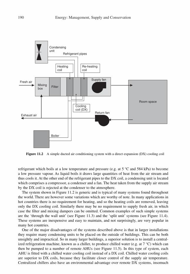
190 Energy: Management, Supply and Conservation
refrigerant which boils at a low temperature and pressure (e.g. at 5 °C and 584 kPa) to become
a low pressure vapour. As liquid boils it draws large quantities of heat from the air stream and
thus cools it. At the other end of the refrigerant pipes to the DX coil, a condensing unit is located
which comprises a compressor, a condenser and a fan. The heat taken from the supply air stream
by the DX coil is rejected at the condenser to the atmosphere.
The system shown in Figure 11.2 is generic and is typical of many systems found throughout
the world. There are however some variations which are worthy of note. In many applications in
hot countries there is no requirement for heating, and so the heating coils are removed, leaving
only the DX cooling coil. Similarly there may be no requirement to supply fresh air, in which
case the filter and mixing dampers can be omitted. Common examples of such simple systems
are the ‘through the wall unit’ (see Figure 11.3) and the ‘split unit’ systems (see Figure 11.4).
These systems are inexpensive and easy to maintain, and not surprisingly, are very popular in
many hot countries.
One of the major disadvantages of the systems described above is that in larger installations
they require many condensing units to be placed on the outside of buildings. This can be both
unsightly and impractical. So in many larger buildings, a superior solution is to install a central-
ized refrigeration machine, known as a chiller, to produce chilled water (e.g. at 7 °C) which can
then be pumped to a number of remote AHUs (see Figure 11.5). In this type of system, each
AHU is fitted with a chilled water cooling coil instead of a DX coil. Chilled water cooling coils
are superior to DX coils, because they facilitate closer control of the supply air temperature.
Centralized chillers also have an environmental advantage over remote DX systems, insomuch
Re-heatingcoil
Heatingcoil
Refrigerant pipes
Condensingunit
Fresh airSupply fan
FilterMixingbox
Exhaust air
Coolingcoil (DX)
Return fan
Room space
Boiler
Figure 11.2 A simple ducted air conditioning system with a direct expansion (DX) cooling coil

Energy efficient air conditioning and mechanical ventilation 191
Warmexhaustair
Return air
Cool supplyair
Evaporator
Condensate
Condenser
Compressor
Outside
Condenser airintake
Figure 11.3 A through the wall air conditioning unit
as there are fewer refrigeration circuits to maintain, resulting in lower risk of refrigerant leaks.
Chillers can utilize either air or water cooled condensers. Water cooled condensers are more
efficient than the air cooled variety, but usually require a cooling tower, and are therefore a
potential Legionella pneumophila hazard. For this reason, air cooled chillers have become more
popular than water cooled chillers, because despite being less efficient they present no health
hazard.
11.3 Refrigeration systems
Most air conditioning plant relies on some form of vapour compression refrigeration machine to
remove heat from air. Figure 11.6 shows a schematic diagram of a simple, single-stage, vapour
compressor refrigeration system, similar to that found in many air conditioning systems.
The vapour compression refrigeration cycle operates as follows:
1 Low pressure liquid refrigerant in the evaporator boils to produce low pressure vapour.
The heat required to boil and vaporize the liquid within the evaporator is taken from an air
or water stream passing over the outside of the evaporator.
2 After leaving the evaporator, the low pressure refrigerant vapour enters the compressor where
both its temperature and its pressure are raised by isentropic compression.
3 The high pressure refrigerant vapour then passes to the condenser where it is cooled and
liquefied. The heat extracted in the condenser is released to the environment either directly
by forcing air over the outside of the condenser, or indirectly using a secondary fluid,
usually water, and a cooling tower.

192 Energy: Management, Supply and Conservation
4 The high pressure liquid refrigerant then passes from the condenser to the expansion valve,
where its pressure is lowered, and approximately 10% of the liquid ‘flashes’ (i.e. instantly
turns from a liquid to a vapour) thus cooling the remainder of the liquid. The cooled low
pressure liquid then flows into the evaporator and the cycle begins all over again.
The boiling point of refrigerants varies with pressure. At low pressures, refrigerants boil at low
temperatures (e.g. 2 °C), while at much higher pressures the boiling point of the refrigerant is
significantly raised (e.g. 35 °C). In this way refrigerants can be vaporized and condensed at
different temperatures, simply by altering system pressure. Since condensing and evaporating
Warmexhaustair
Returnair
Cool supplyair
Evaporator
Condensatepipe
Condenserfan
Compressor
Condenserair intake
Outside
Refrig-erantpipes
Figure 11.4 A split unit air conditioning system

Energy efficient air conditioning and mechanical ventilation 193
temperatures correspond to particular pressures, they are normally ‘measured’ using pressure
gauges located before and after the compressor.
Figure 11.7 shows a plot of the vapour compression cycle on a pressure/enthalpy diagram.
The refrigeration capacity of the system is the amount of cooling which the plant can achieve and
is proportional to the length of the line between points 4 and 1. The power input to the system is
through the compressor drive, and is represented by the line 1 to 2. Line 2 to 3 represents the
heat rejection at the condenser. Line 3 to 4 represents the passage of the refrigerant through the
expansion device and is a constant enthalpy process. It should be noted that the heat rejected by
the condenser is equal to the total energy input at the evaporator and at the compressor. Note also
that as the condensing pressure decreases, so too does the power input from the compressor.
Air cooledchiller unit
7 °C
AHU
AHU
AHU
AHU
Chilled waterpump
12 °C
Figure 11.5 An air cooled chiller system with multiple air handling units
– CondenserEvaporator
Thermostaticexpansion valve
1 2
34
+
High pressureliquid
Low pressureliquid
Low pressurevapour
Compressor High pressurevapour
Figure 11.6 Vapour compression refrigeration cycles

194 Energy: Management, Supply and Conservation
The overall ‘efficiency’ of a vapour compression machine is normally described by the COP.
The COP of a refrigeration machine is the ratio of the refrigeration capacity to the power input
at the compressor. It can be expressed as (referring to Figure 11.7):
(11.1)
where h is the specific enthalpy of refrigerant (kJ/kg).
The higher the COP, the more efficient the refrigeration process. In the UK, refrigeration
machines generally exhibit COPs in the range of 2.0–3.0 [2].
11.4 The problems of the traditional design approach
Having briefly discussed the nature of air conditioning and refrigeration systems, the overall
design of ‘air conditioned’ buildings must now be considered. It is generally the case that in
buildings the air conditioning design is something of an afterthought. In many buildings the form
and the envelope are designed in complete isolation from the mechanical services. Usually, air
conditioning engineers are required to design and install systems which fit unobtrusively into
buildings (i.e. behind suspended ceilings etc.); often these systems are required to overcome the
environmental short-comings of poor envelope design.
The traditional approach to air conditioning is to employ a constant volume flow rate system,
similar to that described in Section 11.2. However, this design approach has a great many
inherent weaknesses, which can loosely be categorized as:
• Weaknesses of the building design;
• Weaknesses of the refrigeration system; and
• Weaknesses of the air system.
COPref �h1 � h4
h2 � h1
14
3 2
Pressure(kPa)
Enthalpy (kJ/kg)
Saturatedliquid
Saturatedvapour
h3 4h h1 h2
Condenserpressure
Evaporatorpressure Evaporation
Compression
Condensation
Expansion
Figure 11.7 Pressure / enthalpy chart of vapour compression process

Energy efficient air conditioning and mechanical ventilation 195
11.4.1 Building design weaknesses
Buildings have to function properly in a great many harsh environments around the world. In
hot desert climates they are required to keep their occupants cool, while in polar regions keeping
warm is the important issue. Buildings should therefore be designed so that the external envelope
is the primary climate modifier, with the internal mechanical services simply fine tuning the
shortcomings of the envelope. This may seem an obvious statement, but clearly it is not one
which is fully understood by many building designers. In Texas, which has a hot arid climate,
there are many glass clad office buildings. It would be intolerable to work in these buildings were
it not for the use of very large air conditioning systems to compensate for the inappropriate
building envelope. This apparently ludicrous situation comes about for three specific reasons:
1 Energy efficiency is often a low priority; minimizing the first cost is usually the prime
consideration.
2 Design professionals often work in isolation from each other, and have little understanding of
building physics, or of how buildings function when occupied.
3 There is great incentive to maintain the status quo. Building services design engineers are usually
paid a fee which is a fixed proportion of the total capital cost of the building services.
Consequently, there is little incentive to reduce the capacity of the mechanical building services.
In order to avoid the creation of energy wasteful buildings, it is important that energy efficiency
be at the forefront of the designer’s mind. Critical decisions made at the design stage have huge
ramifications on both capital and operating costs. If the envelope is a poor climate modifier then
the building will experience high summer heat gains and high winter heat losses, necessitating
the installation of large boilers and refrigeration chillers. These items of equipment may,
however, only operate at peak load for a few hours per year, with the result that for most of the
year they operate very inefficiently at part load. Conversely, if the building envelope success-
fully attenuates the winter and summertime peaks, then the plant sizes can be greatly reduced,
resulting in the plant operating near its rated capacity for a much greater part of the year.
Clearly, the latter situation is a much better utilization of capital expenditure than the former.
11.4.2 Refrigeration system weaknesses
The strategy of installing refrigeration plant to meet the peak summertime cooling load of build-
ings often results in greatly oversized mechanical plant which operates inefficiently, at part load,
for most of the year. It can also result in a greatly oversized electrical installation, since larger
cables, transformers and switchgear must be installed to meet the peak refrigeration capacity.
Not only does a system such as this have a high capital cost, it is also expensive to run since it
uses peak time electricity. In hot countries it may also incur high electrical demand related
charges. Refrigeration chillers are often oversized because:
• System designers overestimate peak building heat gains to ensure that plant is not undersized.
• System designers make design assumptions which are widely inaccurate. For example, in
most buildings the actual cooling load is much less than the design cooling load. This
discrepancy primarily occurs because designers assume very high ‘office equipment’ heat
gains, which in practice rarely materialize.
• Refrigeration chillers are often rated for hot climates such as that found in the USA. So
when these machines are installed in a temperate climate location such as in the UK, their
condensers are oversized and so they operate at part load even when under peak load
conditions.

196 Energy: Management, Supply and Conservation
The general oversizing of refrigeration machines results in very poor overall energy efficiencies.
It has been estimated that of the refrigeration plant currently in operation in the UK, the average
air cooled chiller has a working gross COP of approximately 1.9, while water cooled chillers
exhibit an average gross COP of 3.0 [2]. These low figures are mainly due to the design of most
of the refrigeration chillers used in the UK, namely machines which use thermostatic expansion
valves and maintain a relatively fixed condensing pressure under part load conditions. These
machines display poor COPs under part load conditions, which is unfortunate since for most of
the year they operate in this state.
There are a number of alternative design strategies which can be used dramatically to reduce
the size of refrigeration plant and improve operating costs. These are:
• The use of a solar defensive building envelope, incorporating features such as external shading
and solar reflective glass to reduce the peak cooling load.
• The use of a thermally massive structure to absorb both internal and solar heat gains during
peak periods.
• The use of night ventilation to purge the building structure of heat accumulated during the
daytime.
• The use of ice thermal storage to shift some of the peak time cooling load to the nighttime.
• The use of a floating internal air temperature strategy, which allows internal temperatures to
rise when conditions are exceptionally hot.
11.4.3 Air system weaknesses
The strategy of using an all air system to condition room air has the major disadvantage that it
necessitates the transportation of large volumes of air and is thus inherently inefficient. It is
generally the case that much larger volumes of supply air are required to sensibly cool room
spaces than are required for the purpose of pure ventilation. Consequently, the provision of
sensible cooling using an all air system results in large fans and associated air handling equip-
ment, and also in large ceiling (or floor) voids to accommodate oversized duct work. Although
an expensive solution, resulting in increased energy and capital expenditure, all air systems are
still very popular, despite the existence of superior alternatives which use chilled water to
perform the sensible cooling. One such alternative strategy is the use of chilled ceilings to
perform sensible cooling, while reserving the ductwork system for ventilation purposes only.
This strategy results in greatly reduced fan and ductwork sizes.
Another major draw back of the constant volume approach, described in Section 11.2, is that
air duct and fan sizes are determined by the peak summertime condition which may only last for
a few hours per year. For the rest of the year the fans push large volumes of air around need-
lessly, with the result that energy consumption on air handling is large. Many air conditioning
system designers argue that constant volume systems have the potential to provide large amounts
of free cooling during the spring and autumn seasons. This unfortunately is a misconception
since oversized fans consume such large quantities of electrical energy that any saving in
refrigeration energy is wiped out. The evidence for this can be seen in Table 11.1, where in the
air conditioned buildings almost twice as much electrical energy is consumed by air distribution
systems compared with the refrigeration machines. One alternative strategy which overcomes
this problem is to adopt a variable air volume system in which the quantity of the air handled
reduces with the cooling load.
It is common practice in ducted air systems to size the main ducts assuming air velocities of
4 m/s to 7 m/s. Designers use these relatively high air velocities in order to keep duct sizes to a
minimum. Unfortunately, the use of such high air velocities results in large system resistances.

Energy efficient air conditioning and mechanical ventilation 197
The fan power consumed in a ducted air system can be determined using eqn (11.2). Fan
power,
(11.2)
where is the volume flow rate of air discharged by the fan (m3/s), and �Ptotal is the total system
pressure drop or resistance (Pa).
From eqn (11.2) it can be seen that there is a linear relationship between fan power and sys-
tem resistance; the higher the system resistance, the higher the energy consumed by the fan. The
system resistance is the sum of the system static pressure drop and the velocity pressure drop.
The velocity pressure in particular strongly influences the pressure drop across ductwork bends
and fittings. From eqn (11.3) it can be seen that the pressure drop across a ductwork fitting is a
function of the square of the air velocity.
Pressure drop across ductwork fitting:
(11.3)
where k is the velocity pressure loss factor for fitting, � is the density of air (kg/m3), v is the
velocity of air (m/s), and (0.5 �v2) is the velocity pressure (Pa).
Given eqns (11.2) and (11.3) it is not difficult to see that the use of high air velocities (i.e. in
the region of 5 m/s) results in high fan powers and high energy consumption. However, if air
velocities are reduced to approximately 1 m/s to 2 m/s, as is the case in some low energy build-
ings, then fan energy consumption falls dramatically.
11.5 Alternative approaches
The critique of the traditional approach to the design of air conditioning systems presented in
Section 11.4 highlights its many shortcomings and hints at a number of possible solutions. There
are several alternative low energy strategies which may be employed to overcome the disadvan-
tages of the conventional approach. Although inter-linked, for ease of reference these alternative
strategies can loosely be categorized as follows:
• Using passive solar defensive and natural ventilation measures to reduce the need for air
conditioning;
• Splitting the sensible cooling and ventilation roles into two separate but complementary
systems;
• Using low velocity and variable air volume flow systems;
• Using the thermal mass of buildings to absorb heat which can then be purged by a variety of
ventilation techniques;
• Using thermal storage techniques to shift the peak cooling load to the nighttime;
• Using displacement ventilation techniques;
• Using evaporative cooling; and
• Using desiccant cooling techniques.
Many of the energy conservation techniques listed above are discussed in detail in this chapter.
Some of the techniques which relate specifically to building envelope design are specifically
dealt with in Chapter 13.
�P � k � (0.5 �v2)
.v
W � v � �Ptotal

198 Energy: Management, Supply and Conservation
11.6 Energy efficient refrigeration
Although a number of alternative cooling strategies are discussed in this chapter, there are still
many applications which demand the use of conventional refrigeration plant. It is therefore
necessary to understand the factors which influence the energy consumption of conventional
vapour compression refrigeration machines. The major factors influencing energy performance are:
• The evaporating and condensing temperatures used;
• The type of refrigerant used;
• The type of compressor and condenser used;
• The defrost method used on the evaporator; and
• The system controls.
Each of these factors can have a profound effect on overall energy consumption and are therefore
worthy of further investigation.
11.6.1 Evaporators
The efficiency of vapour compression systems increases as the evaporating temperature increases.
Generally, the higher the evaporating temperature used, the greater the system COP and the
lower the energy consumption. It has been estimated that a rise in the evaporating temperature
of 1 °C results in an operating cost reduction of between 2% and 4% [9]. It is therefore desirable
to maintain the evaporating temperatures as high as is practically possible. Maximum heat
transfer across the evaporator should be achieved in order to prevent the evaporating temperature
from dropping. In practice, this can be achieved by increasing the fluid flow across the evapora-
tor, or by increasing its surface area. Also, in order to ensure high evaporating temperatures it is
essential that good control of the system be maintained.
On air cooling applications where the evaporator may be operating below 0 °C the fin
spacing must allow for ice build-up. In order to maintain an adequate airflow through the evap-
orator it is necessary to defrost the coil periodically. Defrosting techniques involve either the
use of an electric heating element built in to the coil or periodically reversing the refrigeration
cycle so that the evaporator effectively becomes a hot condenser. While essential for the
correct operation of the system, the defrost process can be a potential source of energy
wastage. It is therefore important that the defrost operation only be initiated when absolutely
necessary and that the defrost heat be evenly distributed over the whole of the fin block.
Prolonged defrosting is energy wasteful and therefore the defrost cycle should be stopped as
soon as possible. If not controlled and monitored properly defrost systems can needlessly
waste large amounts of energy.
11.6.2 Condensers
Condensing temperature can have a dramatic influence on system COP, with lower condensing
temperatures usually resulting in lower operating costs. It is estimated that a 1 °C drop in
condensing temperature reduces operating costs by approximately 2–4% [9]. However, if the
condensing pressure fluctuates widely, problems can occur on machines which utilize
thermostatic expansion valves. This is because such valves are unable to reliably control
refrigerant flow at low pressure differentials. In order to overcome this problem, these machines
often employ some form of condenser pressure control to raise the condenser pressure arti-
ficially. This results in unnecessarily high energy consumption, which could be avoided if
electronic expansion devices were used instead.

Energy efficient air conditioning and mechanical ventilation 199
There are three basic condenser systems commonly in use: air-cooled condensers,
water-cooled condensers and evaporative condensers, each of which has its own peculiarities.
Air-cooled condensers are by far the most popular heat rejection system. They generally
comprise a fin and tube heat exchanger in which refrigerant vapour condenses. Air is forced over
the heat exchanger by fans. Well-designed condensers should operate at a temperature no higher
than 14 °C above the ambient air temperature [10]. In larger air cooled systems, condenser
pressure is often controlled by switching off or slowing down fans. Although this practice is
inefficient it does save on energy consumed by the condenser fans. One important advantage of
air-cooled condensers is that they present no Legionella pneumophila risk.
Water-cooled condensers are much more compact than their air-cooled counterparts and
comprise a shell containing refrigerant, through which pass water-filled tubes. Secondary
cooling water flows through these tubes to a cooling tower where the heat is finally rejected
through an evaporative cooling process. In an efficient system, the temperature rise of the water
passing through the condenser should be 5 °C, with a difference of 5 °C existing between the
condensing temperature and the temperature of the water leaving the condenser [10].
Water-cooled systems are considerably more efficient than air cooled systems, with the former
requiring a cooling tower air flow rate of approximately 0.04 m3/s to 0.08 m3/s per kW of
rejected heat and the latter requiring 0.14 m3/s to 0.2 m3/s to perform the same task [11].
However, there is a risk of Legionella pneumophila bacteria breeding in cooling towers, if they
are not monitored and regularly treated with biocides. For this reason water-cooled condensers
have become less popular in recent years.
Evaporative condensers are less popular than either air or water cooled condensers. They
comprise refrigerant condensing tubes which are externally wet and over which air is forced.
Evaporation of the water on the outside of the tubes increases the heat rejection rate and so this
type of condenser is more efficient than its air-cooled counterpart. Evaporative condensers do,
however, pose a Legionella pneumophila risk.
11.6.3 Compressors
The compressor is the only part of a vapour compression system which consumes energy. It is
therefore important that the factors which influence compressor performance are well understood.
The efficiency of a compressor can be expressed in several ways. In terms of overall energy
consumption the most critical ‘efficiency’ is isentropic efficiency, which is defined as follows:
(11.4)
It should be noted that isentropic efficiency does not take into account motor and drive
inefficiencies, which must be allowed for when determining the overall efficiency of a compres-
sor. With most types of compressor, particularly screw and centrifugal compressors, efficiencies
fall dramatically under part-load operation. Compressor motor efficiency also decreases at
part-load. In general therefore, part-load operation should be avoided if high efficiencies are to
be maintained.
Part-load operation is the main reason for poor refrigeration plant efficiency. Many refrig-
eration machines spend less than 20% of the year operating at their nominal design condition.
During the rest of the year they operate at part-load, partly because of cooler ambient
temperatures and partly because of reduced cooling duties. Unless these part-load conditions
are properly allowed for at the design stage, it is likely that overall system COP will be poor.
It is therefore important to select a compressor which exhibits good part-load efficiency.
Isentropic efficiency �ideal 'no loss' power input
actual power input to shaft� 100

200 Energy: Management, Supply and Conservation
Multi-cylinder reciprocating compressors achieve reasonable part-load efficiencies because they
are able to unload cylinders so that output is reduced in steps (e.g. 75, 50 and 25%). Variable
speed drives can also be used. These give good flexible control and can achieve reasonable
efficiencies above 30% of full-load [12].
11.6.4 Expansion devices
In a refrigeration machine the expansion valve is used to reduce the pressure of the returning
liquid refrigerant from the condensing pressure to the evaporating pressure. It also controls the
flow of liquid refrigerant to the evaporator. It is therefore important that expansion valves be
correctly selected and installed, since incorrect operation of the expansion valve can lead to
reduced energy efficiency.
Thermostatic expansion valves are the most commonly used type of refrigerant regulation
device. They regulate the flow of refrigerant through the system by opening and closing a small
orifice using a ‘needle’ connected to a diaphragm (as shown in Figure 11.8). The diaphragm
responds to pressure changes created inside a control phial which senses the temperature of the
refrigerant leaving the evaporator. Both the phial and the valve contain refrigerant. As the load
on the evaporator changes, so the temperature of the refrigerant leaving the evaporator also
changes. The control phial senses these changes in temperature and automatically adjusts the
refrigerant flow to accommodate the load changes.
The major disadvantage of thermostatic valves is that they cannot cope with large pressure
differentials, such as those created when the condensing pressure is allowed to float with ambient
S
D
To distributorand evaporator
Fro
mexpansio
nva
lve
Evaporator(e.g. direct–expansion aircooler coil)
P
Outlet fromevaporator
Distributor
Capillary tube
To c
om
pre
ssor
Fromliquid receiveror condenser
Figure 11.8 Thermostatic expansion device[11]

Energy efficient air conditioning and mechanical ventilation 201
air temperature. Thermostatic expansion valves tend to operate unsatisfactorily at less than 50%
of their rated capacity [13]. Therefore, in refrigerating machines using thermostatic expansion
valves it is often necessary to maintain an artificially high condensing temperature during
conditions of low ambient temperature.
It can be seen from the discussion in Section 11.6.2 that if the condensing pressure is allowed to
fall, the COP increases. Therefore in theory, system efficiency should improve when ambient air
temperature falls. Unfortunately, due to the operational characteristics of thermostatic expansion
valves it is not possible to take advantage of this situation. Thermostatic expansion valves are
therefore inherently inefficient. In recent years an alternative technology has arisen which
overcomes this problem. By using electronic expansion valves it is possible to allow condensing
pressures to drop while still maintaining a constant evaporating pressure. Unlike conventional
thermostatic expansion valves, which operate on the degree of superheating in the evaporator,
electronic expansion valves employ a microprocessor which constantly monitors the position of the
valve, the temperature of the liquid in the evaporator, and the temperature of the vapour leaving the
evaporator. They can therefore respond quickly to fluctuations in load and are not dependent on
large differential pressures between the condenser and the evaporator. Consequently, it is possible
under low ambient conditions to allow the condensing pressure to fall and the COP to improve.
11.6.5 Heat recovery
Vapour compression refrigeration machines are simply a specific form of heat pump. This means
that they reject large quantities of waste heat at the condenser. In many applications, through a
little careful thought at the design stage, it is possible to utilize this waste heat profitably to
reduce energy costs. In refrigeration installations heat can be recovered from:
• The compressor discharge gas, which is generally in the region 70–90 °C, but can be as high
as 150 °C in some installations; and
• The condenser, which is generally 10–30 °C above ambient temperature.
High quality waste heat can be recovered from the compressor discharge gas by using a desuper-
heater heat exchanger. This device recovers heat from the high temperature vapour before it
reaches the condenser. At this point in the cycle the vapour is at its highest temperature and
therefore the heat transfer is at its greatest. It is important to locate desuperheaters above
condensers so that if any refrigerant vapour condenses, the liquid can safely drain away.
Heat may also be recovered at the condenser. However, because condensing temperatures should
ideally be as low as possible, any heat recovered here will inevitably be at a relatively low tempera-
ture. The quality of this heat should however, be sufficient to pre-heat domestic hot water. If higher
condensing temperatures are envisaged as a result of any proposed heat recovery scheme, careful
analysis should be undertaken to ensure that economic benefit will accrue. Remember, there are
many so called ‘energy saving’ schemes in existence which have actually increased energy costs!
11.7 Splitting sensible cooling and ventilation
When considering air conditioning, it is possible to save substantial amounts of energy by
splitting up the sensible cooling and ventilation roles into two separate systems. This also
enables fan and duct sizes to be greatly reduced. One commonly used method of separating these
two roles is to use a fan coil system, which circulates chilled water through water/air heat
exchangers (incorporating recirculation fans) located in room mounted units. Although fan coils
function well in many applications, they can take up valuable room space and also be noisy.

202 Energy: Management, Supply and Conservation
In addition, they utilize recirculation fans which consume energy. A novel alternative approach
is the use of passive chilled ceilings or beams, which comprise a cold surface mounted at high
level within a room space. Chilled ceilings and beams perform room sensible cooling and leave
the ducted air system to perform the ventilation and latent cooling roles.
Chilled ceilings have a very slim profile and usually comprise a metal pipe coil bonded to a
flat metal plate (as shown in Figure 11.9). They can be fixed directly to the soffit of a structural
floor slab, thus eliminating the need for an expensive suspended ceiling. They are usually
designed to have an average surface temperature of approximately 17 °C, which can be achieved
in practice by supplying low grade chilled water at about 13 °C. Because relatively high water
temperatures are used it means that chiller evaporating temperatures can be high, resulting in
very good refrigeration COPs being achieved.
The cooling power of chilled ceilings varies with the individual design used and the extent to
which air turbulence occurs across the heat exchanger surface. In general an output of approxi-
mately 50 W/m2 is considered to be the maximum that can be obtained. This means that chilled
ceilings are not suitable for applications which experience very high internal heat gains. Heat is
transferred to the chilled ceiling by natural convection and radiation. Approximately 50% of the
heat transfer occurs when warm air at the top of the room space comes into contact with the cool
surface. The remaining heat transfer is by radiation from room occupants and other warm sur-
faces within the room space.
The radiative cooling capability of chilled ceilings is of particular importance and is worthy
of further comment. At relative humidities below 70%, the thermal comfort of building occu-
pants is primarily governed by room air temperature and room surface temperature. In order to
assess and quantify relative thermal comfort, a number of thermal comfort indices have been
developed. Although these comfort indices vary slightly from each other, they all seek to
quantify the convective and radiative heat transfer to and from an occupant within a room space.
The most widely used thermal comfort index in the UK is dry resultant temperature. Provided
Metal ceiling tile
Metal chilledwater pipes
Insulation quilt
Figure 11.9 Typical chilled ceiling

Energy efficient air conditioning and mechanical ventilation 203
room air velocities are less than 0.1 m/s (which is usually the case), dry resultant temperature
can be expressed as:
(11.5)
where tr is the mean radiant temperature (°C), and ta is the air temperature (°C).
Mean radiant temperature is the average surface temperature of all the surfaces ‘seen’ in a
room space. It can be either measured indirectly using a globe thermometer or calculated from
surface temperatures. For most cuboid shaped rooms, the mean radiant temperature in the cen-
tre of the room can be expressed as:
(11.6)
where As is the area of each component surface (m2), and ts is the temperature of each component
surface (°C).
By installing a large surface area of chilled ceiling at 17 °C, it is possible to substantially reduce
room mean radiant temperature. Consequently, air temperatures can be allowed to rise to say, 23 °C
or 24 °C without any deterioration in perceived comfort, with the result that energy can be saved.
A variation on the chilled ceiling theme is the passive chilled beam system (see Figure
11.10). Passive chilled beams work on a similar principle to chilled ceilings, but they achieve a
much greater cooling output (e.g. 185 W/m2) and exhibit a much higher convective cooling
component than chilled ceilings (e.g. approximately 85%). However, this can cause problems,
since uncomfortable downdraughts can be created.
11.7.1 Ventilation
By utilizing chilled ceilings or beams, it is possible to free-up ductwork systems to concentrate
solely upon the ventilation and latent cooling tasks. Normally the fresh air requirement of room
occupants is in the region 8 l/s to 12 l/s per person. However, when using chilled ceilings or beams
tr ��(As ts)
�As
tres � 0.5ta � 0.5tr
Heatexchanger
Chilled air
Warm airWarm air
Metal chilledwater pipe
Figure 11.10 Typical chilled beam

204 Energy: Management, Supply and Conservation
the ducted air ventilation system also has to perform all of the room latent cooling. In order to do
this it is common for the ventilation rate to be increased slightly to 18 l/s per person [14].
With chilled ceilings and beams it is important to ensure that the room air moisture content be
maintained at a low level, otherwise condensation may occur on the cool surface and ultimately
‘internal rain’ may be formed. This makes it important to ensure that the incoming ventilation air
is dehumidified, so that the room dew point temperature remains a few degrees below the surface
temperature of the chilled ceilings. An ideal air condition for a room incorporating a chilled
ceiling is 24 °C and 40% relative humidity.
11.8 Fabric thermal storage
Although, a full discussion of the role of fabric thermal storage is contained in Chapter 13, a few
words on the subject are perhaps relevant here. The widespread use of suspended ceilings and
carpets in buildings means that otherwise thermally heavyweight structures are converted into
thermally lightweight ones. These low admittance buildings are not able to absorb much heat and
so surface temperatures tend to rise, with the result that there is a great need to get rid of the heat
gains as they occur. This is one of the main reasons why air conditioning has become such an
essential requirement of so many office buildings. By contrast, if the mass of the building struc-
ture is exposed, then a high admittance environment is formed, and the thermal capacity of the
structure can be utilized successfully to combat overheating.
The creation of a high admittance environment by exposing thermal mass has implications on
the comfort of occupants. It can be seen from the discussion in Section 11.7, that it is the dry
resultant temperature and not the air temperature which is critical when establishing a comfort-
able environment. By exposing the ‘mass’ of a building it is possible to reduce the mean radiant
temperature within the space, and thus the dry resultant temperature. So if an office building
with openable windows and exposed concrete floor soffits has a mean radiant temperature of, for
example, 20 °C and the air temperature in the space is 28 °C, then the perceived temperature
(i.e. the dry resultant temperature) in the space will be only 24 °C. While an internal air
temperature of 28 °C is generally considered unacceptable, a dry resultant temperature of 24 °C
will be perceived as tolerable on hot summer days.
In buildings which employ ‘thermal mass’ to control internal temperatures, it is common
practice to expose concrete floor soffits to create a high admittance environment, as can be seen
in examples such as the Queens Building at De Montfort University [15] and the Elizabeth Fry
Building at the University of East Anglia [16]. While it is possible to create a high admittance
environment by exposing concrete floor soffits, the structure needs to be purged periodically
of heat absorbed over time, otherwise the mean radiant temperature of the room spaces will
steadily rise until conditions become unacceptable. One effective method which can be
employed to purge heat from the structure of buildings is night venting. Night venting involves
passing cool outside air over or under the exposed surface of a concrete floor slab so that it is
purged of the heat accumulated during the day time. This can be done either by natural or
mechanical means. At its most rudimentary night venting may simply entail the opening of
windows at nighttime to induce cross ventilation, while at its most sophisticated it may involve
a dedicated mechanical night ventilation system and the use of floor voids.
When creating a night venting scheme it is important to ensure that good thermal coupling
occurs between the air and the mass of the concrete floor, whilst at the same time ensuring that
fan powers are kept to a minimum. One system which manages to achieve this is the Swedish
Termodeck hollow concrete floor slab system (see Chapter 13). The Termodeck system has been

Energy efficient air conditioning and mechanical ventilation 205
used effectively in many locations, throughout northern Europe and in the UK [16,17] to produce
buildings which are both thermally stable and energy efficient.
11.9 Ice thermal storage
In the exposed concrete soffit system described in Section 11.8, the cooling process is
effectively ‘load shifted’ to the nighttime by using a passive thermal storage technique. While
this can be very effective, the system is limited to cool temperate countries where nighttime
temperatures are low enough to purge accumulated heat. In hotter climates this strategy is
impossible and so an alternative approach to load shifting is required. One alternative tech-
nology is ice thermal storage, which utilizes low cost nighttime electricity to produce a ‘cold
store’ for use during the daytime. The technique involves running refrigeration chillers during
‘off-peak’ hours to produce an ice store. During the daytime when electricity prices are high,
the ice is melted to overcome building or process heat gains. The principal advantages of the
system are as follows:
• Refrigeration energy costs can be significantly reduced, as a substantial portion of the cooling
is undertaken using off-peak electricity.
• The capital cost of the refrigeration plant can be significantly reduced, if both the chillers and
the store combine to satisfy the peak cooling load requirement.
• If an ice store is coupled with a conventional refrigeration plant, then it is possible to run the
chiller constantly at 100% of its rated capacity and thus operate it in an efficient manner.
• If an ice store is coupled with an electronically controlled refrigeration plant, then it is possi-
ble to minimize the refrigeration energy expended. This is because the refrigeration plant will
be running at nighttime when ambient temperatures are low and so operating COPs will be
high.
• Any electricity maximum demand charges incurred by the system will be significantly lower
than those incurred by conventional refrigeration plant.
• By installing additional ice stores it is possible to increase the overall capacity of existing
air conditioning installations without purchasing new chillers or upgrading electrical
systems.
• Ice storage systems enable CO2 emissions to be reduced through load shifting [18] and can
also reduce the quantity of refrigerant used.
Ice storage systems are generally associated with air conditioned commercial or public
buildings. However, ice storage systems have also been used successfully in process industries
which experience large and predictable cooling loads. In this type of application it is often the
case that a relatively small refrigeration machine can, over a long period of time, generate a large
ice store. The ice store can then be melted over a relatively short period of time, to satisfy the
peak cooling load. In this way small refrigeration machines can be used to satisfy very large
cooling loads, with the result large capital savings can be made on refrigeration plant. In
addition, capital cost savings can be made on electrical cables and switch gear, which is of
particular importance for applications in remote locations.
11.9.1 Control strategies
Ice thermal storage systems can be operated in a variety of ways, with the major control
strategies being full storage, partial storage and demand-limited storage.

206 Energy: Management, Supply and Conservation
(a) Full storage: Under a full storage control strategy the total daytime cooling load is shifted
to the nighttime, with the chillers producing an ice store during the period when off-peak
electricity charges apply. During the daytime the ice store is discharged to meet the building
or process cooling load, as shown in Figure 11.11. While being the most effective of all the
control strategies in terms of energy costs, full storage has the major drawback that the ice
store and chiller plant required are much larger than for the other control strategies. Due to
its prohibitively high capital cost full storage is rarely used.
(b) Partial storage: Partial storage is the collective term given to those ice storage control
strategies which require both the chiller plant and the ice store to operate together to satisfy
the daytime cooling load. During periods in which the building or industrial process experi-
ences a cooling load, the ice store and the chiller plant work simultaneously to satisfy the
cooling load. The advantage of partial storage is that both the store and the chiller plant are
substantially smaller than would be the case for a full storage installation and thus the capital
cost is lower. This makes partial storage a very popular option. The umbrella term partial
storage can be sub-divided into two separate and distinct sub-strategies, namely chiller
priority and store priority.
Under a chiller priority control strategy the refrigeration plant runs continuously through
both the ice production and the store discharge periods. During the daytime the refrigeration
plant carries out the base-load cooling and the ice store is used to top-up the refrigeration
capacity of the chiller plant (see Figure 11.12), which would otherwise be unable to cope
with the peak demand.
Under a chiller priority strategy it is possible to achieve reductions in the region of 50 %
in chiller capacity when compared with a conventional refrigeration installation. The capital
cost of installing an ice store can therefore be off-set against the capital cost saving arising
from the reduction in chiller capacity.
The philosophy behind the store priority control strategy is the opposite of the chiller priority
strategy. Under a store priority strategy the ice store is given priority over the chiller during
the daytime (see Figure 11.13). The objective of this strategy is to minimize the operation of
Ice production
Store discharge
700.00
600.00
500.00
400.00
200.00
100.00
0.00
300.00
1 2 3 4 5 6 7 8 9 10 11 12 13 14 15 16 17 18 19 20 21 22 23 24
Time (hours)
Refr
igera
tion load (
kW
)
Figure 11.11 Full storage strategy

Energy efficient air conditioning and mechanical ventilation 207
600.00
500.00
400.00
300.00
100.00
200.00
0.001 2 3 4 5 6 7 8 9 10 11 12 13 14 15 16 17 18 19 20 21 22 23 24
Refr
igera
tion load (
kW
)
Time (hours)
Daytime chiller
Store discharge
Ice production
Figure 11.13 Store priority strategy
the refrigeration plant during periods when electricity prices are high. The refrigeration chiller
is only used to top-up the refrigerating energy released by the ice store.
(c) Demand-limited storage: The object of a demand-limited control strategy is to limit peak
electrical demand by shifting the cooling load out of periods in which the peak demand
naturally occurs (see Figure 11.14). This greatly reduces the overall maximum demand of the
installation and improves the overall load factor of the building, putting the operators in a
stronger position when it comes to negotiating electricity supply contracts with the utility
companies.
Store discharge
Daytime chiller
600.00
500.00
400.00
200.00
100.00
0.00
300.00
1 2 3 4 5 6 7 8 9 10 11 12 13 14 15 16 17 18 19 20 21 22 23 24
Time (hours)
Refr
igera
tion load (
kW
) Ice production
Figure 11.12 Chiller priority strategy

208 Energy: Management, Supply and Conservation
A demand-limited control strategy is particularly useful in situations where a utility company
offers an electricity tariff which has either high unit charges or high demand charges for part of
the daytime (e.g. from 12 am–6 pm), as is often the case in hot countries during the summertime.
Under these circumstances, during the period for which peak charges apply, the cooling load
should be entirely satisfied by the refrigeration energy released from the ice store.
11.9.2 Ice thermal storage systems
In broad terms ice storage systems fall into two main categories, static systems and dynamic
systems. Static systems have the general characteristic that ice is melted in the same location as it is
generated. Unlike static systems where the ice remains in one location throughout the entire oper-
ation of the installation, in dynamic systems the ice, once formed, is transported by some means to
another location where it comes into contact with the working fluid, which is usually water.
The ice bank system shown in Figure 11.15 is typical of a static ice system. It consists of an
insulated water storage tank, which contains a submerged bundle of small tubes. These tubes are
evenly spaced within the tank volume, often in a spiral or serpentine form. During ice production
a glycol/water solution at a sub-zero temperature is circulated through the tubes. This causes the
water in the tank to freeze solid. During the discharge cycle, the ice is melted by the same
glycol/water solution, this time circulating at a temperature above 0°C.
The most widely used dynamic system is the ice harvester. Ice harvesters have been used in the
dairy industry for many years. They consist of an open insulated tank, above which a number of
vertical refrigerant evaporator plates are located. Water is trickled over the surface of the plates so
that it becomes frozen. Typically, within about 20 minutes an 8–10 mm thick layer of ice can be
built up. The ice is harvested by removing it from the evaporator and allowing it to fall into the
tank below. This process is achieved by interrupting the flow of liquid refrigerant through
the evaporator plates and diverting hot discharge gas through them so that their surface tem-
perature reaches approximately 5 °C. A photo-electric switch can be used to stop ice production
when the ice in the sump reaches the required level. To discharge the ice store, system water is
circulated through the ice sump. A typical ice harvester installation is shown in Figure 11.16.
600.00
500.00
400.00
300.00
100.00
200.00
0.001 2 3 4 5 6 7 8 9 10 11 12 13 14 15 16 17 18 19 20 21 22 23 24
Refr
igera
tion load (
kW
)
Time (hours)
Daytime chiller
Store discharge
Ice production
Figure 11.14 Demand limiting strategy

Energy efficient air conditioning and mechanical ventilation 209
11.9.3 Sizing of ice storage systems
The design calculations used to size ice storage systems depend on the precise control strategy
which is adopted [19]. If a chiller priority control strategy is adopted then eqns (11.7–11.13)
should be used. For a store priority strategy eqns (11.14–11.16) should be used.
(11.7)
where Qst is the refrigeration energy contained within the ice store (kWh), Qch is the refrigera-
tion energy produced by chiller plant when operating in the day time (kWh), and Qj is the daily
cooling load (energy) under design condition (kWh).
Under a chiller priority control strategy it is intended that the chiller plant should operate at
full capacity throughout the day time period. However, it is not always possible to achieve this.
A chiller plant will often operate at below its rated capacity for part of the day time.
Consequently, eqn (11.7) must be modified to accommodate this:
(11.8)
where Qu is the unused chiller refrigeration energy (kWh).
The evaporating temperatures experienced by the refrigeration plant are much lower during
the ice production than those experienced during day-time operation. Consequently, during the
store charging period the chiller plant will experience reduced refrigerating capacity. It can
therefore be stated that:
Qch � Pr.H (11.9)
and;
Qst � Pr.kr
.h (11.10)
where Pr is the rated duty of chiller under daytime operation (kW), kr is the reduction factor for
chiller producing ice, H is the duration of daytime chiller operation (hours), and h is the duration
of ice production period (hours).
Qst � Qch � Qj � Qu
Qst � Qch � Qj
Air cooledchiller unit
Ice bank
Ice
Ice makingpump
Glycol/waterpump
Figure 11.15 Ice bank system

210 Energy: Management, Supply and Conservation
Therefore
Qst � Qch � Pr.(H � kr
.h) (11.11)
By combining eqns (11.8) and (11.11) it can be shown that:
(11.12)
By combining eqns (11.8) and (11.9) it can be shown that:
Qst � Qj � Qu – H.Pr (11.13)
In order to derive the plant sizing equations for a store priority control strategy, a slightly
different approach is taken to that for the chiller priority equations. The concept of peak cooling
load (Pm) is introduced. It can therefore be stated that:
Qst � H.Pr � H.Pm – Qv (11.14)
where Pm is the peak cooling load experienced by building (kW), and Qv is the unused ice stor-
age capacity (kWh).
Therefore
Qst � H.Pm � Qv � H.Pr (11.15)
By combining eqns (11.10) and (11.14) the following is produced:
(11.16)Pr �HPm � Qv
H � krh
Pr �Qj � Qu
H � krh
Condensing unit
Ice sump
Evaporator coil
Sump pump
Chilled water
Figure 11.16 Ice harvester system

Energy efficient air conditioning and mechanical ventilation 211
The process involved in sizing ice thermal storage systems is illustrated in Example 11.1.
Example 11.1
An office building has a peak daily cooling load of 5210 kWh, with a maximum instantaneous
cooling duty of 620 kW. Given the following data:
(i) Determine the size of the ice store and chiller plant required for chiller priority, store
priority and full storage control strategies, and for conventional chiller only system.
(ii) Determine the daily costs for the options outlined in (i) above; and
(iii) Determine the system capital costs for the options outlined in (i) above.
Data:
Off-peak electricity period � 00.00–07.00 hours
Peak electricity period � 07.00–24.00 hours
Air conditioning operation period � 08.00–18.00 hours
Day-time average COP � 3.00
Ice production COP � 2.25
Chiller capacity reduction � 0.75
factor for ice production
Peak unit charge � 5.50 p/kWh
Off-peak unit charge � 2.57 p/kWh
Capital cost of ice storage � 25 £/kWh
Capital cost of refrigeration chiller � 240 £/kW
NB: Assume that there is no unused refrigeration energy or ice store capacity in the process.
Solution
(i) Conventional chiller only system: There is no ice store so the chiller must have a refrigera-
tion capacity of 620 kW.
Full storage control strategy: The chiller is not in operation during the daytime and so the ice
store is required to satisfy all the daytime cooling load. Thus a large ice store is required to be
built up over the 7 hour off-peak period. Therefore:
Ice store capacity � 5210 kWh
and
Chiller priority control strategy: The office air conditioning system is operational for
10 hours.
Therefore:
and
Store capacity � 5210 � (10 � 341.6) � 1793.6 kWh
Nominal chiller duty �5210
10 � (0.75 � 7)� 341.6 kW
Nominal chiller duty �5210
7 � 0.75� 992.4 kW

212 Energy: Management, Supply and Conservation
Store priority control strategy: The peak summertime cooling duty is 620 kW. Therefore:
and
(ii) Conventional chiller only system:
Full storage control strategy:
Chiller priority control strategy:
Store priority control strategy:
(iii) Conventional chiller only system:
Full storage control strategy:
Chiller priority control strategy:
Store priority control strategy:
Results summary:
Conventional chiller only
system Chiller priority Store priority Full storage
Chiller duty 620 kW 341.6 kW 406.6 kW 992.4 kW
Store capacity n.a. 1793.6 kWh 2134.4 kWh 5210 kWh
Capital cost £ 148 800 £ 126 824 £ 150 944 £ 368 426
Peak daily cost £95.52 £ 83.11 £ 80.77 £ 59.51
Pay-back period* n.a. �4.85 years 0.40 years 16.71 years
* Indicative payback periods only, since calculated daily costs only apply to the peak summertime day.
Capital cost of installation � (406.6 � 240) � (2134.4 � 25) � £150 944.00
Capital cost of installation � (341.6 � 240) � (1793.6 � 25) � £126 824.00
Capital cost of installation � (992.4 � 240) � (5210 � 25) � £368 426.00
Capital cost of installation � 620 � 240 � £148 800.00
� £80.77
Daily energy cost �2134.4 � 2.57
2.25 � 100�
(5210 � 2134.4) � 5.50
3.0 � 100
� £83.11
Daily energy cost �1793.6 � 2.57
2.25 � 100�
(10 � 341.6) � 5.50
3.0 � 100
Daily energy cost �5210 � 2.57
2.25 � 100� £59.51
Daily energy cost �5210 � 5.50
3.0 � 100� £95.52
Store capacity � (10 � 620) � (10 � 406.6) � 2134.4 kWh
Nominal chiller duty �10 � 620
10 � (0.75 � 7)� 406.6 kW

Energy efficient air conditioning and mechanical ventilation 213
Sump
Open wettedmedia
Pump
Cool humid airHot dry air
Figure 11.17 A direct evaporative cooler
From the results shown in Example 11.1 it can be seen that the initial choice of control strategy
has a huge impact on the economic viability of any ice storage scheme. Given the inordinately
large capital cost associated with full storage systems it is not surprising that these systems are
rarely installed. The most popular strategy used is the chiller priority strategy which, as in the
case in Example 11.1, can result in capital cost savings and a negative payback period.
11.10 Evaporative cooling
So far, most of the cooling techniques discussed in this chapter have utilized the vapour
compression refrigeration cycle to perform air cooling. There are however a number of
alternative technologies, such as evaporative cooling and desiccant cooling which can be utilized
to perform air cooling. Direct evaporative cooling is perhaps the simplest of all the air cooling
techniques and is extremely energy efficient. It relies on an adiabatic heat exchange between air
and water in which the air is both sensibly cooled and humidified. Most direct evaporative
cooling systems comprise an open porous matrix over which water is trickled and through which
air can pass (see Figure 11.17). As air passes over the wetted media, water evaporates and so the
air becomes more humid. In order to evaporate the water needs a ‘package’ of latent heat energy;
this it takes from the air stream, with the result that the air is sensibly cooled. Figure 11.18 shows
the evaporative cooling process on a psychrometric chart. It should be noted that the whole
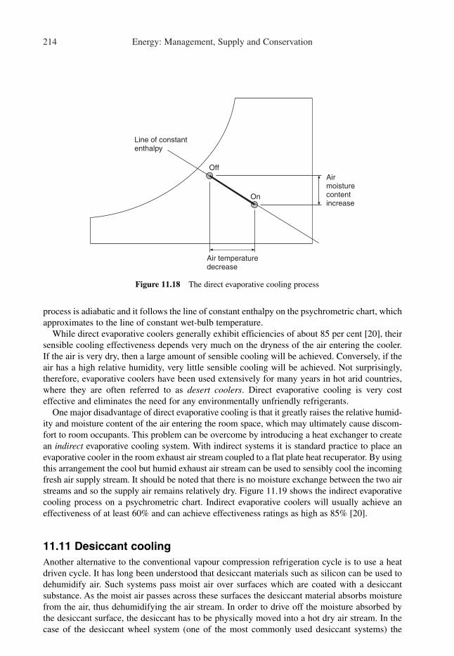
214 Energy: Management, Supply and Conservation
process is adiabatic and it follows the line of constant enthalpy on the psychrometric chart, which
approximates to the line of constant wet-bulb temperature.
While direct evaporative coolers generally exhibit efficiencies of about 85 per cent [20], their
sensible cooling effectiveness depends very much on the dryness of the air entering the cooler.
If the air is very dry, then a large amount of sensible cooling will be achieved. Conversely, if the
air has a high relative humidity, very little sensible cooling will be achieved. Not surprisingly,
therefore, evaporative coolers have been used extensively for many years in hot arid countries,
where they are often referred to as desert coolers. Direct evaporative cooling is very cost
effective and eliminates the need for any environmentally unfriendly refrigerants.
One major disadvantage of direct evaporative cooling is that it greatly raises the relative humid-
ity and moisture content of the air entering the room space, which may ultimately cause discom-
fort to room occupants. This problem can be overcome by introducing a heat exchanger to create
an indirect evaporative cooling system. With indirect systems it is standard practice to place an
evaporative cooler in the room exhaust air stream coupled to a flat plate heat recuperator. By using
this arrangement the cool but humid exhaust air stream can be used to sensibly cool the incoming
fresh air supply stream. It should be noted that there is no moisture exchange between the two air
streams and so the supply air remains relatively dry. Figure 11.19 shows the indirect evaporative
cooling process on a psychrometric chart. Indirect evaporative coolers will usually achieve an
effectiveness of at least 60% and can achieve effectiveness ratings as high as 85% [20].
11.11 Desiccant cooling
Another alternative to the conventional vapour compression refrigeration cycle is to use a heat
driven cycle. It has long been understood that desiccant materials such as silicon can be used to
dehumidify air. Such systems pass moist air over surfaces which are coated with a desiccant
substance. As the moist air passes across these surfaces the desiccant material absorbs moisture
from the air, thus dehumidifying the air stream. In order to drive off the moisture absorbed by
the desiccant surface, the desiccant has to be physically moved into a hot dry air stream. In the
case of the desiccant wheel system (one of the most commonly used desiccant systems) the
Airmoisturecontentincrease
Line of constantenthalpy
Air temperaturedecrease
Off
On
Figure 11.18 The direct evaporative cooling process

Energy efficient air conditioning and mechanical ventilation 215
moisture laden section of the wheel rotates slowly at approximately 16 revs/hour from the moist
air stream to the hot dry air stream where it is regenerated.
Recently desiccant cooling systems have been developed which combine a desiccant wheel
with a thermal wheel in a single AHU to produce a system which is capable of heating, cooling
and dehumidifying air with little or no need for conventional refrigeration [21]. Such systems
have the potential to reduce both energy costs and environmental pollution when compared with
conventional refrigeration systems. From an environmental point of view the desiccant cooling
system has the advantage that electrical energy consumption is replaced by heat consumption,
which produces much less CO2.
A typical desiccant cooling AHU is shown in Figure 11.20. It comprises a thermal wheel and a
desiccant wheel located in series. On the supply side, after the thermal wheel, a supplementary
cooling coil or an evaporative cooler may be located if so required. A heating coil may also be
located after the thermal wheel for use in winter if required. An evaporative cooler is located in the
return air stream before the thermal wheel so that the heat transfer across the thermal wheel is
increased. The desiccant cycle is an open heat driven cycle; the ‘driver’ for the cycle is the regener-
ation heating coil located in the return air stream after the thermal wheel and before the desiccant
wheel.
The psychrometric chart shown in Figure 11.21 illustrates the desiccant cooling and dehumidi-
fication process. During the summertime warm moist air at, for example 26 °C and 10.7 g/kg mois-
ture content, is drawn through the desiccant wheel so that it comes off at say, 39 °C and 7.3 g/kg
moisture content. The psychrometric process line for the air passing through the desiccant wheel
on the supply side has a gradient approximately equal to that of a winter-time room ratio line of
0.6 on the psychrometric chart. The supply air stream then passes through the thermal wheel where
it is sensibly cooled to say, 23 °C. The air then passes through a small DX or chilled water cooling
coil where it is sensibly cooled to a supply condition of say, 17 °C and 7.3 g/kg moisture content.
It should be noted that if humidity control is not required in the space, t;hen the cooling coil may
Return air
Supply airtemperaturedecrease
On
Off
OnOff
Supply airstream
Figure 11.19 The indirect evaporative cooling process

216 Energy: Management, Supply and Conservation
be replaced by an evaporative cooler with an adiabatic efficiency of approximately 85%, in which
case air may be supplied to the room space at say, 16.2 °C and 10.2 g/kg moisture content.
On the return side, air from the room space at, for example, 22 °C and 8.6 g/kg moisture
content passes through an evaporative cooler so that it enters the thermal wheel at approximately
16.7 °C and 10.8 g/kg moisture content. As the return air stream passes through the thermal
wheel it is sensibly heated to approximately 33 °C. The air stream is then heated up to approxi-
mately 55 °C in order to regenerate the desiccant coil. It should be noted that in order to save
energy approximately 20% of the return air stream bypasses the regenerating coil and the
desiccant wheel.
+
–
Desiccantwheel
Thermalwheel
Regenerationcoil
By-pass
Evaporativecooler
Supplementarycooling coil
Outsideair
Returnair
Supplyair
Exhaustair
+
Heatingcoil
Figure 11.20 A typical desiccant cooling air handling unit
Percentage saturation (%)
100% 50%
Outsideair
RoomEvaporativecooler
–10 0 10 20 30 40 50
Coolingcoil
Dry bulb temperature (°C)
Figure 11.21 Desiccant system in cooling/dehumidification mode

Energy efficient air conditioning and mechanical ventilation 217
During the wintertime much of the heat for the supply air stream comes from recovered heat
from the thermal wheel. Although the desiccant wheel could in theory be used as an additional
heat exchanger, in practice it is not particularly effective due to its low rotational speed, and is
therefore not normally used. Should further sensible heating be required this can be achieved
either by locating a heating coil in the supply air stream after the thermal wheel, or by using
radiators within the room space. In addition, an evaporative cooler on the supply side may be
utilized to humidify the incoming air stream if so required.
It has been shown that the use of desiccant cooling can result in energy cost savings ranging from
14% to 50% depending on the application and cooling load [14]. Surprisingly, unlike conventional
refrigeration systems, operating costs are at their lowest when desiccant cooling systems are
operating under part-load [14]. It is also worth noting that desiccant cooling systems are not well
suited to applications in which low supply air temperatures are required. Desiccant cooling is best
suited to those applications such as displacement ventilation, where supply air temperatures are
close to the room air temperature. Although it is possible to make energy cost savings in ‘all air’
applications, desiccant cooling systems are best applied to installations in which the bulk of the
sensible cooling is performed by a water-based system, such as a chilled ceiling [14].
11.11.1 Solar application of desiccant cooling
Being a heat driven cycle, desiccant cooling affords an opportunity to utilize heat which might
otherwise be wasted. It can therefore be coupled to solar collectors to produce a cooling system
which, in theory, should be extremely environmentally friendly. However, the use of solar energy
puts constraints on the application of desiccant cooling. For example, if the ratio of solar collectors
to building floor area is 1:10, then the available heat (in a northern European application) to power
the cycle will be in the region of 25 W/m2 to 50 W/m2, depending on the climate, type and
orientation of the solar collectors [22]. Therefore, if this ‘solar’ heat is to be harnessed effectively,
the desiccant cooling system must be applied in the correct fashion. The desiccant cooling cycle is
an open cycle and as such it rejects moist air at a high temperature, which is unsuitable for
recirculation. In fact, the greater the air volume flow rate supplied to the room space, the greater
the fan power required and the heat energy consumed. Therefore, if desiccant cooling is used in an
all air application, the regeneration heat load is going to be very large, many times greater than the
available solar energy. The bulk of the room sensible cooling should therefore be carried out using
a water-based system such as a chilled ceiling, with the desiccant AHU dehumidifying and
‘tempering’ the incoming fresh air. This strategy reduces the size of the AHU and its associated
ductwork, and enables the solar energy to make a significant contribution [22].
References
1. Grigg, P. F. and John, R. W. (1991). Building services technologies to reduce greenhouse
emissions. Proceeding of CIBSE National Conference, Canterbury, April, p. 231.
2. Calder, K. and Grigg, P. F. (1987). CO2 impact of refrigeration used for air conditioning.
BRE internal report.
3. Wendland, R. D. (1987). Storage to become rule, not exception. ASHRAE Journal, May.
4. Energy use in offices (1998). Energy Consumption Guide 19, Department of the
Environment, Transport and the Regions.
5. The Accelerated Phase-out of Class I Ozone-Depleting Substances (1999). United States
Environmental Protection Agency.

218 Energy: Management, Supply and Conservation
6. Climate Change: Intergovernmental Panel on Climate Change (IPCC) Second Assessment
Report (1995).
7. HCFC Phase out Schedule (1998). United States Environmental Protection Agency.
8. Calm, J. M. Global warming impacts of chillers (1993). IEA Heat Pump Centre Newsletter,
11(3), 19–21.
9. Industrial Refrigeration Plant: Energy Efficient Operation and Maintenance (1992). Good
Practice Guide 42, Department of the Environment.
10. The Economic Use of Refrigeration Plant, Fuel Efficiency Booklet 11 (1994). Department
of the Environment.
11. Jones, W. P. Air conditioning engineering, (Chapter 9). Arnold.
12. Energy efficient selection and operation of refrigeration compressors (1994). Good Practice
Guide 59, Department of the Environment.
13. Dossat, R. J. (1981). Principles of refrigeration. Wiley, p. 436.
14. Beggs, C. B. and Warwicker, B. (1998). Desiccant cooling: Parametric energy study.
Building Services Engineering Research and Technology, 19(2), 87–91.
15. Bunn, R. (1993). Learning curve. Building Services Journal. October, pp. 20–25.
16. Standeven, M., Cohen, R., Bordass, B. and Leaman, A. PROBE 14: Elizabeth Fry Building.
Building Services Journal. April pp. 37–42.
17. Bunn, R. (1998). Cool desking. Building Services Journal. October, pp. 16–20.
18. Beggs, C. B. (1994). Ice thermal storage: impact on UK carbon dioxide emissions. Building
Services Engineering Research and Technology, 15(1), 11–17.
19. Beggs, C. B. and Ward, I. (1992). Ice Storage: design study of the factors affecting
installations. Building Services Engineering Research and Technology, 13(2), 49–59.
20. Evaporative cooling applications (1990). ASHRAE Applications Handbook (Chapter 50).
ASHRAE.
21. Busweiler, U. (1993). Air conditioning with a combination of radiant cooling, displacement
ventilation, and desiccant cooling. ASHRAE Transactions, p. 503–10
22. Beggs, C. B. and Halliday, S. (1999). A theoretical evaluation of solar powered desiccant
cooling in the United Kingdom. Building Services Engineering Research and Technology,
20(3), 113–117.
Bibliography
Beggs, C. B. and Ward, I. (1992). Ice storage: design study of the factors affecting installations.
Building Services Engineering Research and Technology, 13(2), 49–59.
Beggs, C. B. (1994). Ice thermal storage: impact on UK carbon dioxide emissions. Building
Services Engineering Research and Technology, 15(1), 11–17.
Beggs, C. B. and Warwicker, B. (1998). Desiccant cooling: parametric energy study. Building
Services Engineering Research and Technology, 19(2), 87–91.
Beggs. C. B. and Halliday, S. (1999). A theoretical evaluation of solar powered desiccant
cooling in the United Kingdom. Building Services Engineering Research and Technology, 20(3),
113–117.
Evaporative cooling applications. (1999). ASHRAE Applications Handbook (Chapter 50).
ASHRAE.
Jones, W. P. Air conditioning engineering. Arnold.
Stoeker, W. F. and Jones, W. (1982). Refrigeration and air conditioning. McGraw Hill.

12
Energy efficient electrical services
Much energy is needlessly wasted in buildings through neglect of electrical services. This
chapter investigates energy saving measures which can be applied specifically to electrical
services in buildings. In particular, low energy lighting and the use of variable speed motor
drives are discussed.
12.1 Introduction
Much energy is needlessly wasted in buildings through poor design and maintenance of electrical
services. The energy that is wasted is of the worst kind, namely expensive electrical energy, which
can be up to five times as expensive as the unit cost of heat. Unfortunately, excessive electrical
energy consumption is all too often overlooked by misguided building designers, who focus on
thermal energy consumption, which is relatively inexpensive. It has been shown that in a typical
‘standard’ air conditioned office building in the UK, an average of £3.30 per m2 (of floor area) per
annum is spent running pumps and fans, and a further £2.97 per m2 is spent on the lighting [1]. This
compares with an average of only £1.78 per m2 spent on heating, and £1.71 per m2 spent on cooling
[1]. These figures demonstrate that in the average office building much more money is spent on
running fans, pumps and electric lighting than is spent on operating boilers or refrigeration plant. Yet
there are a number of relatively simple technologies that can be applied to motor drives and
luminaire installations to dramatically reduce energy costs. That energy costs in these areas can be
greatly reduced is clear from the evidence of the UK office building study, which found that in good
practice standard air conditioned office buildings, only £1.65 per m2 per year is spent running the
pumps and fans, and only £1.48 per m2 is spent on the lighting [1]. This equates in each case to
energy cost reductions of about 50% when compared with typical air conditioned office buildings.
12.2 Power factor
Electric induction motors and fluorescent lamp fittings are classic examples of reactive (i.e.
inductive) electrical loads. Reactive electrical loads are important because, unlike resistive loads
such as incandescent light, they cause the current to become out of phase with the voltage (see
Figure 12.1). This, in simple terms, means that items of equipment which are inductive in nature

220 Energy: Management, Supply and Conservation
draw a larger current than would be anticipated by their useful power rating. Ultimately, it is the
consumer who has to pay for this additional current.
The electrical power consumed by a resistive load can be determined by:
W � V � I (12.1)
where W is the power (W), V is the voltage (V), and I is the current (A).
Equation (12.1) defines the useful power consumed, and applies to all types of resistive load
where the current is in phase with the voltage. However, eqn (12.1) does not hold true for reactive
loads, where the current lags behind the voltage, since reactive loads consume more power than can
be usefully used. A reactive load, such as an induction motor, will therefore draw a larger current
than would be anticipated by its useful power rating. The reactive components of the load consume
what is termed reactive power. In order to determine the apparent power consumed by a reactive
load, the true power must be added vectorally to the reactive power, as shown in Figure 12.2.
It should be noted from Figure 12.2 that the reactive power is drawn at right angles to the true
power. The apparent power is therefore a function of the true power consumed and the reactive
power, and can be expressed as:
(12.2)
where cos� is the power factor.
Apparent power �True power
cos�
100%
150%
50%
0%
-50%
–100%
–150%
Current
Voltage
Curr
ent and v
oltage
Time
Figure 12.1 The effect of an inductive load on an electrical current and voltage
φ
kW (True power)
kVA (Apparent power)kVAr(Reactive power)
Figure 12.2 The relationship between kW, kVA and kVAr

Energy efficient electrical services 221
From Figure 12.2 and eqn (12.2) it is evident that when the current and voltage are in phase with
each other (i.e. a resistive load), the apparent power is the same as the true power. When the two
are out of phase (i.e. a reactive load) the apparent power consumed is always going to be greater
than the true power. In order to differentiate between true and apparent power, true power is
measured in watts (W) or kilowatts (kW), and apparent power is measured in volt amps (VA) or
kilovolt amps (kVA). Similarly, reactive power is measured in volt amps reactive (VAr) or
kilovolt amps reactive (kVAr). The ratio of true power to apparent power is known as the power
factor. For a pure resistive load the power factor would be 1, and for a pure inductor the power
factor would be 0.
(12.3)
12.2.1 Effects of a poor power factor
In many buildings and other installations the overall electrical load is heavily influenced by the
presence of reactive loads such as induction motors and fluorescent tubes which create a lagging
power factor. As a result power factors of 0.7 or less are often experienced. Example 12.1
illustrates the impact of such a poor power factor.
Example 12.1
A 240 V single-phase electric motor has a true power of 1.8 kW and exhibits a power factor of
0.7. Determine:
(i) The current required to drive the motor.
(ii) The current required if the power factor was 1.
Solution
True power (W) � Apparent power (VA) � Power factor
Therefore
(i)
(ii)
Example 12.1 demonstrates that the lower the power factor, the greater the current required to
provide the same useful power. The increased current required as a result of a poor power factor
has the knock-on effect of increasing power losses. Because cables and other items of equipment
have an electrical resistance, power is lost as heat when a current flows. The power (or I2R) loss
can be expressed as:
Power loss � I2 � R (12.4)
where I is the current (A), and R is the resistance (�).
Current �1800
240 � 1� 7.5 A
Current �1800
240 � 0.7� 10.71 A
Current �Watts
Volts � Power factor
Power factor �True power
Apparent power
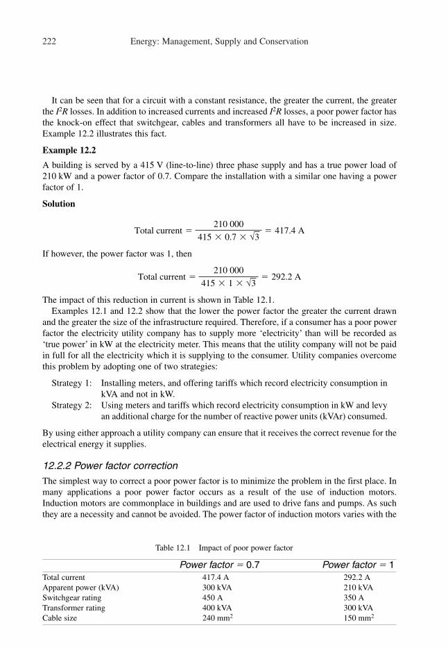
222 Energy: Management, Supply and Conservation
It can be seen that for a circuit with a constant resistance, the greater the current, the greater
the I2R losses. In addition to increased currents and increased I2R losses, a poor power factor has
the knock-on effect that switchgear, cables and transformers all have to be increased in size.
Example 12.2 illustrates this fact.
Example 12.2
A building is served by a 415 V (line-to-line) three phase supply and has a true power load of
210 kW and a power factor of 0.7. Compare the installation with a similar one having a power
factor of 1.
Solution
If however, the power factor was 1, then
The impact of this reduction in current is shown in Table 12.1.
Examples 12.1 and 12.2 show that the lower the power factor the greater the current drawn
and the greater the size of the infrastructure required. Therefore, if a consumer has a poor power
factor the electricity utility company has to supply more ‘electricity’ than will be recorded as
‘true power’ in kW at the electricity meter. This means that the utility company will not be paid
in full for all the electricity which it is supplying to the consumer. Utility companies overcome
this problem by adopting one of two strategies:
Strategy 1: Installing meters, and offering tariffs which record electricity consumption in
kVA and not in kW.
Strategy 2: Using meters and tariffs which record electricity consumption in kW and levy
an additional charge for the number of reactive power units (kVAr) consumed.
By using either approach a utility company can ensure that it receives the correct revenue for the
electrical energy it supplies.
12.2.2 Power factor correction
The simplest way to correct a poor power factor is to minimize the problem in the first place. In
many applications a poor power factor occurs as a result of the use of induction motors.
Induction motors are commonplace in buildings and are used to drive fans and pumps. As such
they are a necessity and cannot be avoided. The power factor of induction motors varies with the
Total current �210 000
415 � 1 � √3� 292.2 A
Total current �210 000
415 � 0.7 � √3� 417.4 A
Table 12.1 Impact of poor power factor
Power factor � 0.7 Power factor � 1Total current 417.4 A 292.2 A
Apparent power (kVA) 300 kVA 210 kVA
Switchgear rating 450 A 350 A
Transformer rating 400 kVA 300 kVA
Cable size 240 mm2 150 mm2
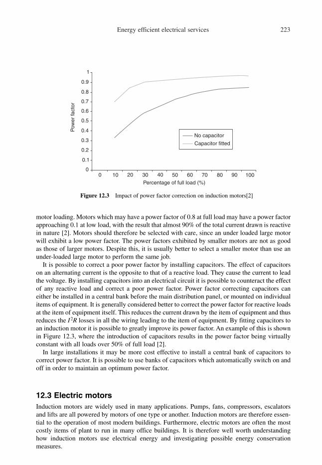
Energy efficient electrical services 223
motor loading. Motors which may have a power factor of 0.8 at full load may have a power factor
approaching 0.1 at low load, with the result that almost 90% of the total current drawn is reactive
in nature [2]. Motors should therefore be selected with care, since an under loaded large motor
will exhibit a low power factor. The power factors exhibited by smaller motors are not as good
as those of larger motors. Despite this, it is usually better to select a smaller motor than use an
under-loaded large motor to perform the same job.
It is possible to correct a poor power factor by installing capacitors. The effect of capacitors
on an alternating current is the opposite to that of a reactive load. They cause the current to lead
the voltage. By installing capacitors into an electrical circuit it is possible to counteract the effect
of any reactive load and correct a poor power factor. Power factor correcting capacitors can
either be installed in a central bank before the main distribution panel, or mounted on individual
items of equipment. It is generally considered better to correct the power factor for reactive loads
at the item of equipment itself. This reduces the current drawn by the item of equipment and thus
reduces the I2R losses in all the wiring leading to the item of equipment. By fitting capacitors to
an induction motor it is possible to greatly improve its power factor. An example of this is shown
in Figure 12.3, where the introduction of capacitors results in the power factor being virtually
constant with all loads over 50% of full load [2].
In large installations it may be more cost effective to install a central bank of capacitors to
correct power factor. It is possible to use banks of capacitors which automatically switch on and
off in order to maintain an optimum power factor.
12.3 Electric motors
Induction motors are widely used in many applications. Pumps, fans, compressors, escalators
and lifts are all powered by motors of one type or another. Induction motors are therefore essen-
tial to the operation of most modern buildings. Furthermore, electric motors are often the most
costly items of plant to run in many office buildings. It is therefore well worth understanding
how induction motors use electrical energy and investigating possible energy conservation
measures.
1
0.9
0.8
0.7
0.6
0.5
0.4
0.3
0.2
0.1
00
10 20 30 40 50 60 70 80 90 100
No capacitor
Capacitor fitted
Percentage of full load (%)
Pow
er
facto
r
Figure 12.3 Impact of power factor correction on induction motors[2]

224 Energy: Management, Supply and Conservation
All induction motors have inherent inefficiencies. These energy losses include [3]:
• Iron losses which are associated with the magnetic field created by the motor. They are voltage
related and therefore constant for any given motor and independent of load.
• Copper losses (or I2R losses) which are created by the resistance of the copper wires in the
motor. The greater the resistance of the coil, the more heat is generated and the greater the
power loss. These losses are proportional to the square of the load current.
• Friction losses which are constant for a given speed and independent of load.
These losses can be divided into those which vary with motor load and those which are constant
whatever the load. When a motor is running at full load, the split between the two is about 70%
and 30% respectively [3]. Under part load this split changes; at low load the current drawn is
small and the I2R losses are low. Consequently, the iron losses predominate and since they result
from the consumption of reactive current, the power factor is correspondingly low. Even at full
load, induction motors exhibit a relatively poor power factor, typically around 0.8 [3].
12.3.1 Motor sizing
Correct sizing of electric motors is critical to their efficient operation, since oversized motors
tend to exhibit poor power factors and lower efficiencies. Depending on size and speed, a typical
standard motor may have a full load efficiency between 55% and 95% [2]. Generally, the lower
the speed, the lower the efficiency, and the lower the power factor. Typically motors exhibit
efficiencies which are reasonably constant down to approximately 75% full load. Thereafter they
may lose approximately 5% down to 50% of full load, after which the efficiency rapidly falls (as
shown in Figure 12.4) [2].
It can be seen from the performance curve in Figure 12.4 that it is possible to oversize a motor
by up to 25% without seriously affecting its efficiency, provided that a motor is run at a relatively
constant load. If the load fluctuates and rarely achieves 75% full load, then both the efficiency
and the power factor of the motor will be adversely affected. In fact the power factor tends to fall
off more rapidly than the efficiency under part-load conditions. Therefore, if motors are
oversized, the need for power factor correction becomes greater. Oversizing of motors also
increases the capital cost of the switchgear and wiring which serves the motor.
0 10 20 30 40 50 60 70 80 90 100
100
90
80
70
60
50
40
30
20
10
0
Percentage of Full Load (%)
Effic
iency (
%)
Figure 12.4 Relationship between motor loading and efficiency[2]

Energy efficient electrical services 225
12.4 Variable speed drives (VSD)
Most induction motors used in buildings are fitted to fans or pumps. The traditional approach to
pipework and ductwork systems has been to oversize pumps and fans at the design stage, and
then to use commissioning valves and dampers to control the flow rate by increasing the system
resistance. While mechanical constrictions are able to control the flow rate delivered by fans and
pumps (see Figure 12.5), the constriction itself increases the system resistance and results in
increased energy loss. This situation is highly undesirable and is one of the main reasons why
the energy consumption associated with fans and pumps is so high in so many buildings [1]. An
alternative approach to the use of valves and dampers is to control the flow rate by reducing the
speed of the fan or pump motor. This strategy results in considerable energy savings, as
illustrated in Example 12.3.
Example 12.3
It is proposed to use a forward-curved centrifugal fan in a mechanical ventilation system. The
fan is required to deliver a volume flow rate of 1.8 m3/s and the estimated system resistance is
500 Pa. However, the proposed fan delivers 2.06 m3/s against a resistance of 500 Pa while
running at a speed of 1440 rpm. Determine the fan power input, if:
(a) A volume control damper is used to achieve a volume flow rate of 1.8 m3/s by increasing the
total system resistance to 750 Pa.
(b) The fan speed is reduced in order to deliver 1.8 m3/s.
Solution
(a) Fan air power input:
W � v.� Pt
where v.
is the air volume flow rate (m3/s), and Pt is the total system resistance (Pa).
Let W1 be the fan power when delivering 2.06 m3/s against a resistance of 500 Pa, and W2 be
the fan power when delivering 1.8 m3/s against a resistance of 750 Pa.
Volume flowrate (m /s)
3Desired increase involume flow rate
Resultant increasein system resistance
Resistance (Pa)
Figure 12.5 Impact of a volume control damper on system resistance

226 Energy: Management, Supply and Conservation
Therefore
W1 � 2.06 � 500 � 1030 W
and
W2 � 1.8 � 750 � 1350 W
Therefore
(b) The fan laws state that:
v.� N
and
W � N3
where v is the air volume flow rate (m3/s), N is the fan speed (rpm), and W is the fan air power
input (W).
Let N1 be the fan speed when delivering 2.06 m3/s against a resistance of 500 Pa, N3 be the fan
speed when delivering 1.8 m3/s, and W3 be the fan power when delivering 1.8 m3/s.
Therefore
Therefore
Reduction in power consumption (W3 compared with W1)
However
Reduction in power consumption (W3 compared with W2)
It can be seen from Example 12.3 that:
• The use of volume control dampers to regulate air flow significantly increases fan energy
consumption. The precise magnitude of this increase will depend on the characteristics of the
particular fan selected.
• Reducing the fan speed to regulate the air flow rate always results in fan energy savings.
The fan power savings which can be achieved through reducing fan speeds are considerable,
especially when compared with the fan power increase which results from using volume control
�1350 � 687.2
1350� 100 � 49.1%
�1030 � 687.2
1030� 100 � 33.3%
W3 � 1030 �1.83
2.063� 687.2 W.
N3 � 1440 �1.8
2.06� 1258.3 rpm,
Increase in power consumption �1350 � 1030
1030� 100 � 31.1%

Energy efficient electrical services 227
dampers. As a result there are great advantages to be gained, if fan and pump speeds can be
controlled.
The energy savings achieved in Example 12.3 are indicative of the type of savings which can
be achieved through the use of VSDs on fans and pumps. In most applications the potential for
saving energy through the use of VSDs on pumps, fans and compressors is considerable. Most
designers overestimate system resistances with the result that most pumps and fans are theoreti-
cally oversized before the actual fan or pump selection is undertaken. During the selection
process, the cautious designer is unlikely to find a fan, or pump, which matches the theoretical
‘calculated’ specification and thus a larger one is selected which is sure to perform the required
task. This strategy protects the system designer and ensures that he/she does not negligently
undersize the fans or pumps. Unfortunately, it also ensures that the system is greatly oversized
and that during the commissioning process, volume control dampers and dampers will have to
be used to reduce the volume flow rate. Consequently, both the capital and future operating costs
of the system are greatly increased. By using VSDs it is possible to ensure that even if fans and
pumps are oversized, energy consumption will not be greatly increased. This makes the installa-
tion of VSDs one of the most cost effective energy efficiency measures that can be taken. It has
been estimated that for VSDs payback periods of less than 2 years are the norm [2].
In addition to the energy savings gained through using VSDs on constant flow systems, even
greater savings can be made by employing VSDs on variable volume flow systems. When the
load profiles and duty cycles of heating, air conditioning and ventilation systems are examined
in detail, it is found that most regularly operate well below their intended design specification.
The main reason for this is that system designers are overcautious at the design stage. As a result,
over-large constant volume flow rate, variable temperature systems are designed. While this
approach works in practice, it means that pump and fan running costs are constant and high, no
matter what the operating load. An alternative approach is to keep the temperature constant and
vary the flow rate, so that pump and fan running costs reduce as the operating load reduces. The
classic system which adopts this approach is the VAV air conditioning system, for which VSDs
are ideally suited.
12.4.1 Principles of VSD operation
Modern electronic VSD systems adjust the mains alternating current to regulate motor speed.
Various electronic VSD systems are available. One of the most popular types is the variable
frequency drive, which achieves speed control by varying the voltage and frequency output. Such
drives regulate the voltage to the motor in proportion to the output frequency in order to ensure
that the ratio of voltage to frequency remains relatively constant. Changes in motor speed are
achieved by modulating the voltage and frequency to the motor. Figure l2.6 shows the basic
components in a variable frequency drive VSD system.
Variable frequency drive systems comprise two main components, a rectifier and an inverter.
The rectifier converts standard alternating current (ac) (e.g. 240 V and 50 Hz) to an adjustable
direct current (dc), which is then fed to the inverter. The inverter comprises electronic switches
which turn the dc power on and off to produce a pulsed ac power output. This can then be
controlled to produce the required frequency and voltage. The switching characteristics of the
inverter are modified by a regulator, so that the output frequency can be controlled.
The inverter is the critical part of a VSD system. One type of inverter currently in use is the
pulse width modulated (PWM) inverter, which receives a fixed dc voltage from the rectifier and
adjusts the output voltage and frequency. The PWM inverter produces a current waveform which
approximates to the pure sine wave of mains ac supply.

228 Energy: Management, Supply and Conservation
12.5 Lighting energy consumption
The energy consumed by electric lighting in most building types is considerable. Table 12.2
shows the proportion of overall energy consumed by lighting for a variety of building types in
the UK.
Although in many buildings the energy consumed by the heating system is often greater than
that consumed by lighting, the energy costs associated with lighting are often considerably greater
than those associated with the heating [1]. It is possible to achieve considerable energy cost sav-
ings through the careful design and maintenance of lighting schemes. On average, good practice
‘standard’ air conditioned office buildings in the UK experience an annual lighting cost is £1.48
per m2, which compares very favourably with the typical value of £2.97 per m2 of floor space [1].
12.5.1 Daylighting
Although the focus of this chapter is on electrical services, daylighting is relevant to the subject
of artificial lighting and so a short discussion is included here. The ability of daylighting to
reduce lighting energy costs should not be underestimated. Daylight can make a substantial
contribution to the lighting of buildings by reducing reliance on artificial lighting.
The major factors affecting the daylighting of an interior are the depth of the room, the size
and location of windows, the glazing system, and any external obstructions. These factors
usually depend on decisions made at the initial design stage. Through appropriate planning at an
early stage it is possible to produce a building which is energy efficient as well as having a
pleasing internal appearance. Glazing can, however, impose severe constraints on the form and
Rectifier
Regulator
Inverter Motor
Speed referencefrom load
Variable DCvoltage
Variablevoltage andfrequency ACpower
Mains AC supply
Figure 12.6 Components of a variable speed drive. Crown copyright is reproduced with the
permission of the Controller of Her Majesty’s Stationery Office and the Queen’s Printer for Scotland [4]
Table 12.2 Typical energy consumption on lighting for various applications in the UK [5]
Typical percentage of energyBuilding type consumed by lighting (%)Banks 19
Factories 15
Hotels 9
Offices 16–20
Schools 9–12
Supermarkets 11

Energy efficient electrical services 229
operation of a building. If poor design decisions are made concerning fenestration it is possible
to create a building in which the occupants are uncomfortable, and in which energy consumption
is high. Glazing should therefore be treated with care!
12.5.2 Lighting definitions
Before discussing the factors which influence the energy consumption of artificial lighting
schemes, it is important first to understand the terminology involved, and to appreciate how
lighting schemes are designed. A full discussion of the subject of lighting design is however
beyond the scope of this book.
When an incandescent lamp is switched on, it emits a luminous flux in all directions. The
fundamental SI unit of luminous flux is the lumen (lm). It should be noted that the lumen is
simply a measure of the quantity of luminous flux. It tells us nothing about the direction of the
light. When a lamp is placed in a luminaire fitting with an integral reflector, the luminous flux
from the lamp will be directed in one particular direction (e.g. downward in the case of a ceiling
mounted fitting). A certain number of lumens are therefore focused in a particular direction with
a certain luminous intensity. Luminous intensity, as the term suggests, is the intensity of
luminous flux in any given 3-dimentional angular direction and its SI unit is the candela (cd).
‘3-dimensional angular direction’ is a difficult concept to define; but it is usually referred to as
solid angle. It is the 3-dimensional equivalent of a 2-dimensional angle. The steradian is the SI
unit of solid angle and is the 3-dimensional equivalent of the radian. The candela can therefore
be defined as being a lumen per steradian. More precisely, one candela can be defined as the
luminous intensity from a source producing light at 540 000 000 MHz and at a specific intensity
of 1/683 W per steradian [6].
Lighting manufacturers use a system of polar diagrams to describe luminous intensity
distribution from luminaire fittings. Figure 12.7 shows a typical polar diagram for a transverse
section across a ceiling mounted luminaire fitting. It should be noted that luminous intensity
produced by the lamp is not the same in all directions. For example, while the intensity in
a vertical direction is 112 cd per klm of lamp flux, the intensity at 40° to the vertical is only
88 cd per klm. Lighting manufacturers usually specify intensity in terms of cd per klm of
installed lamp flux because it is often possible to use a variety of lamps in any particular
luminaire fitting.
From a purely functional point of view, it is not so much the intensity of light coming from
a light source (i.e. a luminaire fitting) that is important, but rather the amount of light that is
falling on a particular surface. For example, a room may be illuminated only by spotlights
which shine brightly on certain specific objects while leaving the rest of the room in relative
darkness. If a person tries to read a book in a region of the room which is not well lit, they will
experience difficulties. Although there may be a large luminous flux in the room, the problem
is that very little of it is falling on the pages of the book. The person then experiences difficul-
ties in reading. The amount of luminous flux falling on a surface is therefore of great
importance. It is referred to as illuminance and has the SI unit, the lux (lx). One lux is defined
as a luminous flux of 1 lumen falling on a surface having an area of 1 m2. Artificial lighting
schemes are usually specified as being capable of supplying a specified number of lux on
a horizontal working plane. Generally, the more demanding the work, the higher the level of
illuminance required.
Because light is a form of radiant energy, its ability to illuminate a surface (i.e. its illuminance)
varies inversely with the square of the distance between the source and the surface. In simple
terms, if the distance increases, the illuminance decreases by the square of the distance. This

230 Energy: Management, Supply and Conservation
relationship is known as the inverse square law. Also, if a horizontal surface is illuminated from
the side, so that the light hits the surface at an angle other than 90°, the available luminous flux
is shared out over a larger surface area so that illuminance decreases. The angle at which light
strikes a surface is therefore of importance. This fact can be combined with the inverse square
law to produce the cosine law of illuminance, which can be expressed as
� (12.5)
where � is the angle at which light strikes the horizontal surface (i.e. angle from the vertical)
(°), I� is the luminous intensity in direction � (cd), and d is the distance of plane from light
source (m).
Example 12.4 shows how the cosine law can be applied to the data contained in the polar
diagram shown in Figure 12.7.
Illuminance on a horizontal surface Eh �I�
d2� cos
cd/1
000lu
mens
150° 160° 170° 180° 170° 160° 150°
140°
130°
120°
110°
100°
90°
80°
70°
60°
50°
40°
140°
130°
120°
110°
100°
90°
80°
70°
60°
50°
40°
30° 20° 10° 0° 10° 20° 30°
20
40
60
80
100
120
140
160
180
200
Figure 12.7 Polar intensity diagram (from Smith, Phillips and Sweeney (1987) Environmental
Science © Longman Group Ltd, reprinted by permission of Pearson Education Ltd.)

Energy efficient electrical services 231
Example 12.4
Using the luminaire polar diagram shown in Figure 12.7, determine the illuminance on a hori-
zontal surface: (Assume that the luminaire fitting contains 2 fluorescent tubes each with a lumi-
nous flux of 3200 lm.)
(i) At a point (a) 3 m directly below the luminaire.
(ii) At a point (b) 2 m to the right of point (a).
Solution
(i) From Figure 12.7 it can be seen that the luminous intensity in the vertical direction is 112
cd per klm of lamp flux. Therefore
Luminous intensity in the vertical direction � 112 � (2 � 3.2)
� 716.8 cd.
Therefore:
(ii) Considering point (b)
Therefore
� � 33.69°
and
From Figure 12.7 it can be seen that the luminous intensity at 33.7° from in the vertical is
96 cd per klm of lamp flux. Therefore
Luminous intensity in the vertical direction � 96 � (2 � 3.2)
� 614.4 cd
Therefore
12.6 Artificial lighting design
The performance of an artificial lighting scheme is influenced by:
• The efficacy of the lamps (i.e. the light output per watt of electrical power consumed).
• The luminaire performance.
Illuminance on a horizontal surface at point (b) �614.4
3.6062� cos 33.69 � 39.3 lx
d � (22 � 32) � 3.606 m
tan� �2
3� 0.667
Illuminance on a horizontal surface at point (a) �716.8
32� cos� � 79.6 lx
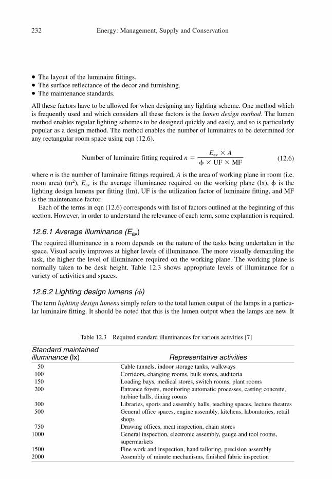
232 Energy: Management, Supply and Conservation
• The layout of the luminaire fittings.
• The surface reflectance of the decor and furnishing.
• The maintenance standards.
All these factors have to be allowed for when designing any lighting scheme. One method which
is frequently used and which considers all these factors is the lumen design method. The lumen
method enables regular lighting schemes to be designed quickly and easily, and so is particularly
popular as a design method. The method enables the number of luminaires to be determined for
any rectangular room space using eqn (12.6).
(12.6)
where n is the number of luminaire fittings required, A is the area of working plane in room (i.e.
room area) (m2), Eav is the average illuminance required on the working plane (lx), � is the
lighting design lumens per fitting (lm), UF is the utilization factor of luminaire fitting, and MF
is the maintenance factor.
Each of the terms in eqn (12.6) corresponds with list of factors outlined at the beginning of this
section. However, in order to understand the relevance of each term, some explanation is required.
12.6.1 Average illuminance (Eav)
The required illuminance in a room depends on the nature of the tasks being undertaken in the
space. Visual acuity improves at higher levels of illuminance. The more visually demanding the
task, the higher the level of illuminance required on the working plane. The working plane is
normally taken to be desk height. Table 12.3 shows appropriate levels of illuminance for a
variety of activities and spaces.
12.6.2 Lighting design lumens (�)
The term lighting design lumens simply refers to the total lumen output of the lamps in a particu-
lar luminaire fitting. It should be noted that this is the lumen output when the lamps are new. It
Number of luminaire fitting required n �Eav � A
� � UF � MF
Table 12.3 Required standard illuminances for various activities [7]
Standard maintained illuminance (lx) Representative activities
50 Cable tunnels, indoor storage tanks, walkways
100 Corridors, changing rooms, bulk stores, auditoria
150 Loading bays, medical stores, switch rooms, plant rooms
200 Entrance foyers, monitoring automatic processes, casting concrete,
turbine halls, dining rooms
300 Libraries, sports and assembly halls, teaching spaces, lecture theatres
500 General office spaces, engine assembly, kitchens, laboratories, retail
shops
750 Drawing offices, meat inspection, chain stores
1000 General inspection, electronic assembly, gauge and tool rooms,
supermarkets
1500 Fine work and inspection, hand tailoring, precision assembly
2000 Assembly of minute mechanisms, finished fabric inspection

Energy efficient electrical services 233
is also important to appreciate that lighting manufacturers produce luminaire fittings which
might accommodate a variety of lamps, each of which will emit a different luminous flux. The
type of lamp to be used in the luminaire should therefore be specified.
12.6.3 Utilization factor (UF)
The UF can be expressed as:
(12.7)
The UF takes into account both the direct luminous flux which reaches the working plane
straight from the luminaire and the flux which reaches the working plane having been reflected
from the walls and the ceiling. The UF is influenced by the nature of the luminaire used, the
room surface reflectance, and the room dimensions. Table 12.4 shows a typical set of UF data
produced by a manufacturer for a particular luminaire fitting.
It should be noted that both the room surface reflectance and the room geometry are allowed
for in Table 12.4. The room geometry is allowed for by the ‘room index’ which is expressed as:
(12.8)
where L is the length of room (m), W is the width of room (m), and Hm is the mounting height
(i.e. height above working plane) (m).
12.6.4 Maintenance factor (MF)
The effective light output from any luminaire decreases with time. This is because of a number
of factors:
• Lamp output decreases with time.
• Luminaire reflectors and diffusers become dirty with time.
• Room surfaces become dirty with time.
To compensate for this drop in luminaire output, a MF is introduced into the lumen design
method. The MF also allows for the fact that periodically individual lamps fail and remain
unattended for some period of time until they are replaced.
Both lamp survival and lamp output fall with time. Figure 12.8 shows output and survival
characteristic curves for fluorescent and tungsten filament lamps. It can be seen that two types
of lamps behave very differently. The lumen output of a fluorescent lamp falls by nearly 10%
during the first 500 hours of operation [7]. Thereafter, the output decreases less rapidly. With a
tungsten filament lamp the decrease in light output is much more gradual, although the lamp life
is much shorter than that of a fluorescent tube.
Room index �L � W
Hm � (L � W )
UF �Total flux reaching the working plane
Total lamp flux
Table 12.4 Luminaire utilization factor table
Room index
1.00 1.25 1.50 2.00 2.50 3.00
Room reflectance’s 50 [50] 0.50 0.54 0.57 0.61 0.63 0.65
ceiling (%) [wall %] 50 [30] 0.47 0.51 0.54 0.58 0.61 0.63
50 [10] 0.44 0.48 0.51 0.56 0.59 0.61

234 Energy: Management, Supply and Conservation
The extent to which luminaire fittings become dirty depends very much on the type of fitting.
For example, a ventilated luminaire, used in conjunction with an extract plenum, will cause dust
and dirt from the room space to collect on the luminaire reflector with the result that it may
quickly become dirty. Figure 12.9 shows how light output decreases with dirt deposition for a
variety of luminaire types.
100
80
60
40
20
0
100
80
60
40
20
0
100
80
60
40
20
0
100
80
60
40
20
0
400 800
4000 8000
Lamp survival
Lamp survival
Lumen output
Lumen output
Per
cent of surv
ivors
Tungsten filament lampsup to 100W
Per
cent of in
itia
llig
ht outp
ut
1200
Burning hours
Tubular fluorescent lamps
Per
cent of surv
ivors
Burning hours12 000
Figure 12.8 Lamp output and survival curves[7]
100
80
60
40
20
0 2 4 6 8 10 12
(a) Ventilated reflector
(b) Open-base diffuser
(c) Non-ventilated reflector
(d) Indirect cornice
Months of use
Per
cent of in
itia
l lig
ht outp
ut
a
b
c
d
Figure 12.9 Fall in light output due to dirt deposition [7]

Energy efficient electrical services 235
Table 12.5 Lamp lumen maintenance and survival factors
Operating hoursLamp type Factor 6000 10 000 12 000
Fluorescent (tri-phosphor) LLMF 0.87 0.85 0.84
LSF 0.99 0.85 0.75
Metal halide LLMF 0.72 0.66 0.63
LSF 0.91 0.83 0.77
Sodium (high-pressure) LLMF 0.91 0.88 0.87
LSF 0.96 0.92 0.89
From Pritchard (1995) Lighting © Longman Group UK Ltd, reprinted by permission of Pearson Education Ltd
Table 12.6 Luminaire maintenance factor (LMF)
6 months cleaning 12 months cleaning 18 months cleaning Luminaire interval interval interval
type Clean Normal Dirty Clean Normal Dirty Clean Normal Dirty
Batten 0.95 0.92 0.88 0.93 0.98 0.83 0.91 0.87 0.80
Enclosed IP2X 0.92 0.87 0.83 0.88 0.82 0.77 0.85 0.79 *
Up-lighter 0.92 0.89 0.85 0.86 0.81 * 0.81 * *
* Not recommended.
From Pritchard (1995) Lighting © Longman Group UK Ltd, reprinted by permission of Pearson Education Ltd
Table 12.7 Room surface maintenance factor (RSMF)
12 months cleaning 24 months cleaning Luminaire flux interval interval
Room index distribution Clean Normal Dirty Clean Normal Dirty
2.5–5.0 Direct 0.98 0.96 0.95 0.96 0.95 0.94
2.5–5.0 General 0.92 0.88 0.85 0.89 0.85 0.81
2.5–5.0 Indirect 0.88 0.82 0.77 0.84 0.77 0.70
From Pritchard (1995) Lighting © Longman Group UK Ltd, reprinted by permission of Pearson Education Ltd
Tables 12.5, 12.6 and 12.7 are attempts to quantify the various factors associated with
decreased luminaire output. Table 12.5 quantifies lamp performance over time in two ways, the
lumen maintenance factor (LLMF) is the proportion of initial lamp lumens ‘remaining’ after a
given time period, while the lamp survival factor (LSF) is the proportion of lamps surviving (i.e.
lamps that have not failed) after a given time [8].
The luminaire maintenance factor (LMF) referred to in Table 12.6 quantifies the impact of
various maintenance regimes on different luminaire types in a variety of environments.
The impact of various cleaning regimes on room surface reflectance is quantified in Table 12.7
by using a room surface maintenance factor (RSMF).
Example 12.5 shows how a realistic MF might be developed in practice.
Example 12.5
The lighting scheme in an office space comprises 60 batten type luminaire fittings with
fluorescent (tri-phosphor type) tubes. The lamps are changed in bulk every 6000 hours and
the luminaire fittings and room surfaces are cleaned every 12 months. The cleanliness
of the environment within the office space is normal and the luminous flux distribution

236 Energy: Management, Supply and Conservation
from the luminaries is ‘general’ in nature. Determine a suitable maintenance factor for
the installation.
Solution
From Table 12.5
LLMF � 0.87
LSF � 0.99
From Table 12.6
LMF � 0.98
From Table 12.7
RSMF � 0.88
Therefore
MF � 0.87 � 0.99 � 0.98 � 0.88 � 0.74
When designing a lighting scheme it is important to ensure that the illuminance on the working
plane is evenly distributed. If the luminaires are too far apart, gloomy patches will appear on
the working plane. This makes it important not to exceed the spacing to mounting height ratio
stated for the particular luminaire being used. The nominal spacing for luminaire fittings can
be determined using eqn (12.9).
(12.9)
The process involved in the lumen design method is illustrated in Example 12.6.
Example 12.6
A 15 � 9 � 3 m high office space is required to be illuminated to 500 lux. Given the following
data design a suitable artificial lighting layout for the space.
Data:
Height of working plane � 800 mm
Height of luminaire fittings above floor level � 3000 mm
Design lumens per fitting � 8000 lm
Maintenance factor � 75%
Ceiling reflectance factor � 50%
Wall reflectance factor � 50%
Maximum spacing to mounting height ratio � 1.2 : 1.0
Room index
1.00 1.25 1.50 2.00 2.50 3.00
Room reflectance’s 50 [50] 0.50 0.54 0.57 0.61 0.63 0.65
ceiling (%) [wall %] 50 [30] 0.47 0.51 0.54 0.58 0.61 0.63
50 [10] 0.44 0.48 0.51 0.56 0.59 0.61
Nominal spacing between fittings S � √A
n

Energy efficient electrical services 237
Solution
Mounting height � 3.0 � 0.8 � 2.2 m
Using eqn (12.6)
Since, the ceiling reflectance is 50%, the wall reflectance is 50% and the room index is 2.56.
Therefore
UF � 0.632
Using eqn (12.6)
Since it is impossible to have 0.8 of a luminaire fitting, the number of luminaires required (n)
must be 18.
Using eqn (12.9)
Therefore
Spacing:Mounting height � 2.739:2.2 � 1.245:1.0
However, this spacing to mounting height ratio exceeds the maximum permissible ratio of
1.2:1.0. Therefore, it is necessary to increase the number of fittings to, say 20.
Therefore
Therefore
Spacing:Mounting height � 2.598:2.2 � 1.181:1.0
This spacing to mounting height ratio is acceptable. Therefore
Number of luminaire fittings required � 20
and
Suggested design layout: 4 rows of 5 fittings
12.7 Energy efficient lighting
The main factors which influence the energy consumption of lighting schemes are:
(i) The light output per watt of electrical power consumed (i.e. lamp efficacy).
(ii) Luminaire performance.
(iii) The number of luminaires and their location.
(iv) The reflectance of internal room surfaces.
(v) Maintenance and procedure standards.
(vi) Duration of operation.
(vii) The switching and control techniques used.
Nominal spacing between fittings S � ˆ((15 � 9)� 20) � 2.598 m
Nominal spacing between fittings S � ˆ((15 � 9)�18) � 2.739 m
Number of luminaire fitting required n �500 � (15 � 9)
8000 � 0.632 � 0.75� 17.8
Room index �15 � 9
2.2 � (15 � 9)� 2.56
238 Energy: Management, Supply and Conservation
While points (i) to (iv) above are concerned with the fundamental efficiency of any installation,
points (v) to (vii) relate to the management and operation of the installation.
When considering the overall energy efficiency of luminaires it is helpful to look in isolation
at the individual components which together make-up the luminaire; namely the lamp, the
control gear and the fitting.
12.7.1 Lamps
There are a wide variety of lamps which can be used in artificial lighting schemes. Fluorescent,
tungsten filament, tungsten halogen, metal halide (MBI) and high pressure sodium vapour
(SON) are amongst the many lamp types in common use. Energy consumption varies greatly
with the type of lamp used. Figure 12.10 shows comparative lamp efficacies for a variety of lamp
types. Luminous efficacy is defined in lumens produced per watt of electricity consumed.
It can clearly be seen from Figure 12.10 that there is a wide variation in the luminous efficacy
between the various lamp types. For example, compact fluorescent lamps have an efficacy
of approximately 70 lm/W, while tungsten filament lamps exhibit an efficacy of approximately
10 lm/W. Clearly, the compact fluorescent lamp is a much more energy efficient option. It should
also be noted that the luminous efficacy of any lamp type increases as power input is increased.
While this increase may only be slight in some types of lamp (e.g. tungsten filament and tungsten
halogen lamps), in others, such as high and low pressure sodium lamps (SON and SOX), the
increase can be substantial.
When designing new artificial lighting installations, it is important to install lamps which
exhibit a high efficacy. In older installations, it may be worth considering refurbishing existing
luminaire fittings, so that they can incorporate newer more efficient lamp types. Refurbishment
of older installations using modern equipment can often result in substantial energy savings as
well as improved visual conditions. It is possible to improve older, less efficient, luminaires by
replacing existing diffusers with modern reflector systems at relatively low cost. However, some
changes can be considerably more expensive, such as replacement of the existing control gear to
facilitate the use of low energy lamps.
Tungsten filament lamps
Although the use of tungsten filament lamps is widespread, they are particularly inefficient
consumers of energy and should be avoided where possible. They have efficacies in the region
of 8 to 15 lm/W [9], with most of the electrical energy being converted to heat, which can lead
to space overheating problems. Lamp life is short, with most tungsten filaments burning out after
approximately 1000 hours of use [7].
Compact fluorescent lamps
Because standard tungsten filament lamps exhibit such poor efficacies, compact fluorescent
lamps were developed as a replacement. Where possible tungsten lamps should be replaced by
compact fluorescent lamps. These give comparable light output to tungsten lamps, but only
consume approximately 20% of the power required by tungsten lamps [8]. As the rated life of
the compact fluorescent lamps is in the region of 8000–12 000 hours, eight times longer than
tungsten lamps, maintenance costs are greatly reduced, albeit at a higher initial cost.
Compact fluorescent lamps can be divided into two distinct categories: those with integral
control gear and those which require separate gear. Since the life of control gear is generally
longer than that of a fluorescent lamp, it is often better to install lamps with separate control

Energy efficient electrical services 239
GLSMBFMBIFSONSOX
Tungsten filamentHigh pressure mercury discharge (fluorescent)High pressure mercury discharge (metal halide)High pressure sodium dischargeLow pressure sodium discharge
Key:
Initial lamp lumens
SO
X
SON
1000W
1000W
MBIF
MBF1000W
2000W
1000W
50 W
18 W
35 W
100W
250W
50 W
18 W
5 W
39W
Compact fluorescent
100WGLS
Tungsten halogen
Fluo
resc
ent
(tri p
hosp
hor)
Lum
inous e
ffic
acy (
lam
p lum
ens/lam
p w
atts)
15 W
20
40
60
80
100
120
110
160
180
200
0
SO
X-E
180W
131W
102
103
104
105
Figure 12.10 Efficacies of various lamps[9]

240 Energy: Management, Supply and Conservation
gear, as this is more cost effective. Lamps with integral control gear are more expensive, being
specifically designed as a direct replacement for existing tungsten filament lamps. As with
all discharge lamps, compact fluorescent lamps exhibit a poor factor, often as low as 0.5.
This however, can be corrected by using capacitors.
Fluorescent tubes
Fluorescent tubes are commonplace in most buildings and exhibit efficacies in the region of 80–100
lm/W [9]. Depending on the type of lamp and ballast used, they can last up to 18 times as long as
tungsten filament lamps. In recent years the 26 mm diameter fluorescent tube has replaced the 38 mm
diameter tubes as the standard for new installations. These slimmer lamps produce approximately the
same light output as the larger diameter lamps, but consume around 8% less electricity [10].
Metal halide lamps
MBI lamps have become popular for a wide variety of applications and are available in a wide
range of power ratings, 70–2000 W. They exhibit efficacies in the region of 70–100 lm/W,
depending on their power rating [9]. MBI lamps are particularly popular in industrial applications.
High pressure sodium lamps
SON lamps have proved particularly useful for lighting large high bay areas, such as factories
and warehouses, where their high efficacy (e.g. 70–120 lm/W) can produce a very energy effi-
cient lighting scheme. They are also useful for exterior lighting, car parks and floodlighting.
They are manufactured in a wide range of power ratings from 50 to 1000 W.
12.7.2 Control gear
Because of their nature, all discharge lamps, such as fluorescent lamps, require control gear to
operate, which comprises a starting device and ballast. A starting device is required to create the
high potential difference between the lamp electrodes, so that an electrical discharge is promoted.
Starters can be of a plug-in glow type, which should be replaced every second or third lamp change,
or else should be of an electronic type. Ballast is necessary to control the current drawn by the
lamp. If ballast were not installed, then the current would increase dramatically as the ionization
process takes place with the result that damage would be caused to wiring and the fitting itself.
In addition to the lamp load, ballast consumes electricity. The type of ballast used therefore has
an impact on overall energy consumption. Traditionally, ballast has come in the form of a wire-
wound choke, comprising a copper wire wrapped around a metal core. Current flowing through the
wire produces a magnetic field which dampens the growth of any further current, thus ‘choking’ the
current to the desired level. While conventional wire-wound chokes work very well, they result in
excess energy losses, typically in the region of 15–20% of total energy consumption. Recently new
high frequency electronic ballasts have been developed. These ballasts run at frequencies between
20 and 40 kHz [10], and can be fitted either with a rapid-start mechanism to facilitate instantaneous
starting, or a ‘soft-start’ which prolongs the lamp-life. High frequency ballasts consume up to 30%
less power than wire wound chokes and have the additional benefit of increasing lamp life [10].
12.7.3 Lighting controls
The appropriate use of lighting controls can result in substantial energy savings. These savings
arise principally from better utilization of available daylight and from switching off electric
lighting when a space is unoccupied. Therefore, when designing a lighting control strategy for

Energy efficient electrical services 241
any given application, it is important to understand the occupancy pattern in the space, since this
will heavily influence the potential for energy savings.
There are four basic methods by which lighting installations can be controlled:
• Time-based control;
• Daylight-linked control;
• Occupancy-linked control; and
• Localized switching.
Time signals may come from local solid-state switches or be derived from building management
systems. These signals switch the lights on and off at set times. It is important to include local
override so that lighting can be restored if the occupants need it.
Photoelectric cells can be used either simply to switch lighting on and off, or for dimming.
They may be mounted either externally or internally. It is however important to incorporate time
delays into the control system to avoid repeated rapid switching caused, for example, by fast
moving clouds. By using an internally mounted photoelectric dimming control system, it is pos-
sible to ensure that the sum of daylight and electric lighting always reaches the design level by
sensing the total light in the controlled area and adjusting the output of the electric lighting
accordingly. If daylight alone is able to meet the design requirements, then the electric lighting
can be turned off. The energy saving potential of dimming control is greater than a simple
photoelectric switching system. Dimming control is also more likely to be acceptable to room
occupants.
Occupancy-linked control can be achieved using infra-red, acoustic, ultrasonic or
microwave sensors, which detect either movement or noise in room spaces. These sensors
switch lighting on when occupancy is detected, and off again after a set time period, when no
occupancy movement is detected. They are designed to override manual switches and to pre-
vent a situation where lighting is left on in unoccupied spaces. With this type of system it is
important to incorporate a built-in time delay, since occupants often remain still or quiet for
short periods and do not appreciate being plunged into darkness if not constantly moving
around.
Localized switching should be used in applications which contain large spaces. Local switches
give individual occupants control over their visual environment and also facilitate energy savings.
By using localized switching it is possible to turn off artificial lighting in specific areas, while still
operating it in other areas where it is required, a situation which is impossible if the lighting for
an entire space is controlled from a single switch.
12.7.4 Maintenance
With the passage of time luminaires and room surfaces get dirty, and lamp output decreases.
Lamps also fail and need replacing. Consequently, the performance of all lighting installations
decreases with time. It is therefore necessary to carry out regular maintenance in order to
ensure that an installation is running efficiently. Simple cleaning of lamps and luminaires can
substantially improve lighting performance. Therefore, at the design stage maintenance
requirements should always be considered. Luminaires should be easily accessible for
cleaning and lamp replacement. Bulk replacement of lamps should be planned, so that they are
replaced at the end of their useful life, before light output deteriorates to an unacceptable level.
The cleaning of lamps and luminaires should be planned on a similar basis. In order to
minimize disruption to staff, planned cleaning and lamp replacement can take place during
holiday periods.

242 Energy: Management, Supply and Conservation
References
1. Energy use in offices (1998). Energy Consumption Guide 19, Department of the
Environment, Transport and the Regions.
2. Economic use of electricity in industry, Fuel Efficiency Booklet 9 (1994). Department of the
Environment.
3. Guidance notes for reducing energy consumption costs of electric motor and drive systems
(1995). Good Practice Guide 2. Department of the Environment.
4. Retrofitting AC variable speed drives (1994). Good Practice Guide 14. Department of the
Environment.
5. Energy audits and surveys (1991). CIBSE Applications Manual AM5.
6. Smith, B. J., Phillips, G. M. and Sweeney, M. (1987). Environmental Science (Chapter 8).
Longman Scientific and Technical.
7. CIBSE Code for interior lighting (1994).
8. Pritchard, D. C. (1995). Lighting (Chapter 7). Longman Scientific and technical, 5th edition.
9. Energy Management and Good Lighting Practices. Fuel Efficiency Booklet 12 (1993).
Department of the Environment.
10. Energy Efficient Lighting in Buildings. Thermie Programme, Directorate-General for
Energy. Commission of the European Communities.
Bibliography
Economic use of electricity in industry. Fuel Efficiency Booklet 9 (1994). Department of the
Environment.
Energy Efficient Lighting in Buildings. Thermie Programme, Directorate-General for Energy.
Commission of the European Communities.
Energy Management and Good Lighting Practices. Fuel Efficiency Booklet 12 (1993).
Department of the Environment.
Guidance notes for reducing energy consumption costs of electric motor and drive systems.
Good Practice Guide 2 (1995). Department of the Environment.
Pritchard, D. C. (1995). Lighting. Longman Scientific and technical, 5th edition.
Retrofitting AC variable speed drives. Good Practice Guide 14 (1994). Department of the
Environment.

13
Passive solar and low energybuilding design
This chapter deals with the use of passive techniques to control the environment within
buildings. Through the use of passive solar strategies it is possible to produce an architecture
which relies more on the building envelope, and less on the use of mechanical equipment as
the primary climate modifier. In particular, the impact of passive environmental control
strategies on the design and operation of buildings is discussed. Several active solar
technologies are also discussed.
13.1 Introduction
Strictly speaking the term passive solar refers to the harnessing of the sun’s energy to heat, cool,
ventilate and illuminate buildings without the use of mechanical equipment. As with so many
artificial classifications it has become somewhat corrupted and now is a generic term for a design
philosophy which seeks to produce low energy buildings which are sympathetic to the natural
environment. A better term might therefore be climate sympathetic architecture, since buildings
created by this design philosophy use their envelope as the primary climate modifier and relegate
any mechanical plant that is required to a supplementary role. This is in contrast to the twenti-
eth-century practice of erecting buildings with unsympathetic envelopes, thus creating a hostile
internal environment, which can only be rectified by the use of extensive mechanical services.
While the precise definition of the term passive solar architecture may be arguable, there is no
doubt that its central aim is to produce low energy buildings which utilize relatively simple tech-
nologies. In such buildings the emphasis is on the envelope, with the result that passive solar
buildings tend to have complex facades, which incorporate features such as external shading,
opening windows and light shelves.
While it may be possible in certain applications and in some locations to rely totally on the
sun’s energy to provide a comfortable internal environment, in most passive solar buildings some
mechanical plant is still required. This mechanical plant can be used either:
• to supplement the passive technologies as a secondary climate modifier; or
• as a facilitator, which enables the passive technologies to perform in an optimum manner.

Most passive solar buildings are therefore in reality hybrids in which passive technologies are
used in tandem with mechanical equipment to achieve a low energy solution. In recognition of
this fact, a new term mixed-mode has come into being. Mixed-mode buildings are so called
because they use a combination of natural ventilation and mechanical ventilation to achieve the
desired cooling effect [1]. Mixed-mode strategies tend to provide solutions which are more flex-
ible than those produced by pure passive strategies. They are therefore more suitable for use in
speculative buildings where the final use of the building may not be known at the design stage.
Because passive solar buildings contain fewer moving parts compared with their mechanical
counterparts, it is tempting to believe that passive buildings are simpler and easier to design. In
fact nothing could be further from the truth. To create a good passive building, the designer must
have a comprehensive knowledge and understanding of heat transfer and fluid mechanics. Unlike
mechanical buildings, which use known and easily quantifiable system drivers such as boilers and
fans, passive buildings use natural ‘variables’ as drivers, such as solar radiation and wind. This
means that considerable analysis must be undertaken at the design stage to ensure that a robust
design is produced (i.e. one which operates well under various meteorological conditions). If this is
not done, considerable problems can arise and costly mistakes can be made. For example, a build-
ing heated purely by solar energy may become uncomfortably cool on days when there is heavy
cloud. One major problem for designers is to predict, at the design stage, how passively controlled
buildings will behave in practice. Failure to predict performance at the design stage can be a recipe
for disaster. Therefore great care must be taken at the design stage. To assist in the design of passive
buildings, engineers often use complex and powerful tools such as computational fluid dynamics
(CFD) to predict accurately how such buildings will perform. However, the costs involved in using
CFD are high and expertize is scarce. Indeed, in some applications the high cost of CFD analysis
and the general lack of expertize in this field are major obstacles to the use of passive techniques.
13.2 Passive solar heating
Solar energy is the radiant heat source upon which all life ultimately depends. It is in plentiful
supply, even in relatively northerly latitudes. Consider for example, latitudes 45° north and 45°
south (i.e. the respective latitudes of Minneapolis in the USA and Dunedin in New Zealand). At
these latitudes the noontime solar intensity in mid-winter on south facing vertical glazing is 595
W/m2 [2]. Given that most of the Earth’s population lives between these latitudes, it becomes clear
that there is great worldwide potential for harnessing solar energy.
Passive solar heating techniques are particularly well suited to applications which experience
both low winter air temperatures and clear skies. Under these conditions the abundant solar
radiation available during the daytime can be collected and stored for use at nighttime when heat
is most required. Passive solar heating techniques have been successfully applied in North
America on many small- and medium-sized buildings [3]. The headquarters building of the
Rocky Mountain Institute in Colorado, USA uses solar energy to provide its heating and hot
water needs. Through the use of solar energy and a highly insulated envelope, the building man-
ages to maintain an acceptable internal environment with virtually no conventional heating,
despite experiencing outside air temperatures as low as �40 °C [4]. Passive solar heating tech-
niques have also been applied successfully in more northerly and cloudier climates. For exam-
ple, St George’s School in Wallasey, constructed in 1961, is an early example of one such
building in the UK [4]. However, it is true to say that it is more difficult to utilize solar energy
in the temperate and cloudy climates of northern Europe than it is in more southerly climates.
There are four basic approaches to passive solar heating: direct gain systems; indirect gain
systems; isolated gain systems; and thermosiphon systems [5, 6]. All four techniques aim to
244 Energy: Management, Supply and Conservation

Passive solar and low energy building design 245
store, in various ways, solar energy during the daytime for use at nighttime when outside air
temperatures are low. They all involve the use of high mass materials in the building fabric to
store heat. In the direct gain system, solar radiation enters room spaces directly through large
areas of south facing glazing. In the indirect gain system, the solar radiation is intercepted by
a high mass thermal storage element, which separates the room space from the south facing
glazing. The isolated gain system is a hybrid of the first two systems, which uses a separate sun
space, such as a conservatory or atrium, to capture the solar energy. Finally, thermosiphons can
be used to promote movement of warm air around buildings.
All solar heating systems rely on the use of large glazed areas to catch the sun’s radiation.
Glass transmits relatively short-wave solar radiation in the wavelength range 380–2500 nm, but
blocks radiation at wavelengths exceeding 2500 nm. Although glass permits solar radiation to
enter room spaces, it blocks much of the long-wave radiation which is emitted when the surfaces
in the room become hot. This phenomenon is known as the greenhouse effect (which should not
to be confused with the greenhouse effect associated with global warming) and it leads to heat
build-up within room spaces. Due to the greenhouse effect, the temperature within room spaces
rises until the heat losses by conduction and convection equal the heat gains by radiation.
As well as promoting the greenhouse effect within buildings, glazing also plays an important role
in the self-regulation of solar heat gains. Glass transmits much more solar radiation when the angle
of incidence is small, compared with when it is large. When the angle of incidence is large much of
the incident solar radiation is reflected. This quality can be used to great effect by building design-
ers. Consider the simple building shown in Figure 13.1. In winter, when solar heat gains are most
advantageous, the sun is low in the sky and the angle of incidence on the vertical glazing is small.
This maximizes the solar transmission through the glass so that the sun’s rays penetrate deep into
the room space. Conversely, in summer, when solar heat gains are undesirable, the sun is high in the
sky and the angle of incidence on the vertical glazing is large, with the result that much of the solar
radiation is reflected. In addition, because the sun’s angle of altitude is much higher in summer, ver-
tical windows present a much smaller ‘apparent’ area to solar radiation in summer compared with
winter (see Figure 13.2). As a result the solar intensity on vertical glazing is often much lower in
summer than in winter. It should be noted that if horizontal roof lights are used the situation is
reversed with the greatest solar heat gains being experienced during the summer months.
Most solar heating techniques rely on high mass materials to store heat. A variety of materials
can be used to store solar energy; concrete, masonry blocks, water tanks and even rocks have all
been used to fulfil this thermal storage role. Essentially, any material which has a high specific
heat capacity and is a good conductor of heat can be used in this role.
High angleof altitude
High levelof reflection
Summer
Low angleof altitude
Low levelof reflection
Winter
Figure 13.1 Solar reflection from glazing

13.2.1 Direct gain techniques
The utilization of direct solar gains is probably the simplest approach to passive solar heating.
It involves using the actual living space within a building as the solar collector (as shown in
Figure 13.3). To maximize the amount of solar radiation collected during the winter months,
rooms should have large areas of south facing glazing. Floors and walls of the rooms should be
constructed from dense materials with a high thermal storage capacity. During the daytime,
short-wave radiation is absorbed by the exposed high mass interior, while in the evening and at
nighttime heat is transferred from the warm room surfaces to the occupants and the air by radi-
ation and convection. As well as facilitating thermal storage, during the daytime the exposed
thermal mass absorbs heat and thus tempers the internal environment, so that over-heating is
prevented. In order to prevent conduction of the heat away from the high mass storage material,
insulation material should always be placed between the dense interior and the outside. Although
it is usual to use concrete or masonry blocks to achieve the thermal mass, it is possible to use
water containers inside the building to store heat. However, these tend to be difficult to integrate
into the overall building design.
246 Energy: Management, Supply and Conservation
High angleof altitude
Summer
Large apparentarea
Small apparentarea
Large apparentarea
Small apparentarea
Low angleof altitude
Winter
Figure 13.2 Solar angle and apparent area

13.2.2 Indirect gain techniques
In an indirect gain system, an element with high thermal mass is situated between the sun
and the room space. Any solar energy striking the thermal mass is absorbed so that it heats up
during the daytime. In the evening and at nighttime heat is transferred to the rooms from the
thermal mass by a combination of conduction, convection and radiation. Figure 13.4 illustrates
the operation of one such indirect system, the Trombe Wall, which comprises a masonry wall up
to 600 mm thick, located directly behind a south-facing glass façade. The outward facing surface
of the masonry wall is usually painted black to maximize its absorption of solar radiation. During
the daytime solar radiation is absorbed by the masonry wall with the result that the air between
Passive solar and low energy building design 247
Daytime Nighttime
Figure 13.3 Direct gain solar heating
Daytime
Vents open
Glazing
Nighttime
Vents closedGlazing
Figure 13.4 Trombe wall operation

the wall and the glass warms up. This causes the air to circulate through vents at the top and
bottom of the wall and into the room space, thus warming it. At night the vents in the wall are
sealed and the wall transfers heat energy by radiation and convection to the room space.
It is possible to increase the amount of solar radiation collected by a Trombe wall by placing
a reflective surface directly on the ground in front of the facade. This material reflects solar radi-
ation onto the thermal storage wall and thus increases its effectiveness.
Trombe walls work best in cold clear climates which experience large amounts of solar radia-
tion, such as those found at altitude in southern Europe. They are much less effective in north-
ern European climates where cloud cover is often extensive in winter.
Another indirect gain technique, which has been used in the USA, is the solar roof pond. As well
as providing passive heating in winter this system can also provide cooling in summer. It involves
constructing a pond on a flat roof. In winter during the daytime the pond absorbs solar energy. At
night the warm pond conducts heat through the roof structure and warms the rooms below by radia-
tion. It is necessary at night in winter to cover the pond with movable insulation material. In
summer, the pond can be used to provide passive cooling. Overnight the pond is cooled by expos-
ing it to the night air and once cooled, the water mass is used to draw heat from the space below.
13.2.3 Isolated gain techniques
Isolated gain solar heating is essentially a hybrid of the direct and indirect gain systems and
involves the construction of a separate sun room adjacent to a main living space. In the iso-
lated gain system, solar radiation entering the sun room is retained in the thermal mass of the
248 Energy: Management, Supply and Conservation
Daytime
Vents open
Nighttime
Vents closed
Figure 13.5 Operation of an isolated gain system

floor and the partition wall. Heat from the sun room then passes to the living space by con-
duction through the shared wall at the rear of the sun room and by convection through vents
or doors in the shared wall. One classic example of an isolated gain system is the use of a
south-facing glass conservatory on the side of a house. A typical isolated gain system is shown
in Figure 13.5.
13.2.4 Thermosiphon systems
If a flat solar collector containing water or air is placed below a heat exchanger, a ther-
mosiphon will be created. As the fluid heats up in the solar collector it becomes less dense and
more buoyant and thus rises to the heat exchanger. As the hot fluid travels through the heat
exchanger it cools down and so drops to the solar collector below, where the whole process
starts over again. It is possible to heat buildings passively by the use of a solar thermosiphon.
In such a system the south-facing solar collectors are placed at a level lower than the room
space. Warm air from the collectors is allowed to circulate around a floor void filled with
rocks. During the daytime the hot air produced by the solar collectors is used to heat up the
rocks and during nighttime the rocks give up their heat by convection to the room space
(as shown in Figure 13.6).
13.3 Active solar heating
While passive solar techniques can be used effectively to heat buildings they can place severe
constraints on the overall building form and are therefore generally unsuitable for larger more
complex building types. However, many of the limitations of passive systems can be overcome
by adopting an active system utilizing hot water pumps. Active solar heating systems can be cost
effective, provided that they are controlled properly and that pump or fan operating costs are kept
to a minimum.
Passive solar and low energy building design 249
Solar collectorRock bed
Figure 13.6 A thermosiphon system

The simplest form of active solar collector is probably the flat plate collector, which
comprises a ‘coiled’ metal pipe bonded to a metal plate and placed in a glass-fronted box. In
order to maximize the solar absorption the plate and pipe are usually painted matt black;
conduction losses are minimized by placing insulation material underneath the plate. The water
in such a collector heats up until an equilibrium temperature is reached where the losses by
conduction, convection and radiation to the ambient air equal the solar radiation gains. The heat
output from solar flat plate collectors can be determined using the Hottel–Whillier equation [7].
(13.1)
where Q is the rate of delivery of useful energy (W/m2), I is the intensity of solar radiation
(W/m2), � is the reflection coefficient, � is the absorption coefficient, U is the overall heat trans-
fer coefficient of plate to air (W/m2K), F is the solar collector efficiency factor, tw is the mean
water temperature (°C), and ta is the ambient air temperature (°C).
The efficiency of a solar collector is the ratio of the useful heat output over the solar heat input.
(13.2)
(13.3)
The efficiency of a solar collector is usually represented by plotting efficiency (�) against
((tw � ta)/I) on a graph (as shown in Figure 13.7).
Example 13.1
Experiments on a flat plate solar collector reveal that
and
Given this information and assuming that the collector is located in air at 12 °C and receives
400 W/m2 of solar radiation, determine the efficiency and output of the collector when:
FU � 7.0041
F(��) � 0.8188
� F�(��) �U(tw � ta)
I �
Efficiency � �Q
I
Q � F[(��)I � U(tw � ta)]
250 Energy: Management, Supply and Conservation
0
10
20
30
40
50
60
70
80
90
0 0.25 0.5 0.75 1(t –t )/Iw a
Effic
iency (
%)
Figure 13.7 Efficiency of solar water collector

(i) Delivering water at a mean temperature of 40 °C
(ii) Delivering water at a mean temperature of 50 °C
Solution
(i) At a mean water temperature of 40 °C
Therefore,
(ii) At a mean water temperature of 50 °C
Therefore,
Example 13.1 shows that the efficiency of the solar collector reduces dramatically as the mean
water temperature increases. This implies that the value of U is not constant and that it is depend-
ent on the water temperature. At higher water temperatures the value of U increases due to
increased radiant heat loss from the collector.
It is possible to greatly improve solar collection efficiency by using evacuated tube collectors
in which the collector surface is suspended in a vacuum tube. In this type of collector the inside
surface of the bottom half of the tube is silvered so that the solar radiation is focused on the
collector surface.
Higher water temperatures can be obtained by using solar collectors with silvered semi-
circular or parabolic reflectors, which focus the solar radiation of the collector surface. They
also reduce radiant heat losses from the collector. With this type of collector it is important
that the reflecting surfaces are clean, otherwise efficiency drops off. This can be a particular
problem in dry dusty environments, such as deserts.
13.4 Photovoltaics
It is possible to produce electricity from light by utilizing a photoelectric process. The term
photoelectric is used to describe any effect which produces electricity from light. There are
three main photoelectric processes: photoemissivity, photoconductivity, and the photovoltaic
effect. Photoemissivity occurs when materials emit electrons in the presence of light. The
Output Q � 400 � 0.1534 � 61.4 W/m2
�� 15.34%
�� 0.8188 �7.0041 � (50 � 12)
400� 0.1534
Output Q � 400 � 0.3285 � 131.4 W/m2
�� 32.85%
�� 0.8188 �7.0041 � (40 � 12)
400� 0.3285
�� F(��) �FU(tw � ta)
I
Passive solar and low energy building design 251

photoconductive effect refers to the phenomenon whereby an electric current flowing through
a substance is increased as a result of light falling on it. While both these photoelectric
processes are used in specialist applications, it is the photovoltaic effect which is most widely
used to produce electricity from sunlight. The photovoltaic effect occurs when light falls on
the boundary between two substances and causes electrons to be transferred from one side of
the boundary to the other. As a result of this transfer of electrons, one material acquires an
excess of electrons and becomes negatively charged, while the other loses electrons and
becomes positively charged. In this way a positive-negative (P-N) junction is formed. The
resulting imbalance in electrons across the P-N junction produces an electromotive force,
which when connected to a circuit causes a current to flow.
Photovoltaic cells were first developed in the 1950s in the space industry for use on satellites,
but interest in their terrestrial use emerged with the fuel crisis of the early 1970s. Since then,
there has been a steady growth in their terrestrial use, mainly limited to remote applications
where the provision of mains electricity is prohibitively expensive. In recent years reductions
in the cost of manufacture of solar cells has meant that the urban use of photovoltaics has
become more popular.
Photovoltaic cells comprise solid-state electronic cells, which are fabricated using crystalline
silicon wafers as a substrate onto which another metal is deposited using a screen-printing
process [8]. A photovoltaic cell with an area of 100 cm2 should produce approximately 3.5 A in
strong sunlight. Manufacturers encapsulate groups of photovoltaic cells under glass covers to
form modules. Within these modules, individual cells are interconnected in series and parallel to
produce desired voltages and currents. Similarly, photovoltaic modules can be grouped together
to form arrays to increase the power output.
Manufacturers subject their photovoltaic modules to a standard test condition of a solar
irradiance of 1000 W/m2 at an operating temperature of 25 °C, which is approximately
equivalent to the solar radiation which would be experienced by a horizontal surface, at
noon, in June in Saudi Arabia. It should be noted that the performance of photovoltaic mod-
ules drops off as the ambient air temperature increases above 25 °C. This is of particular
importance as photovoltaic modules are often used in environments which are much warmer
than 25 °C. It has been calculated that operating power reduces by about 0.5% for every
1 °C increase, thus a 100 W module (rated at 25 °C) when operating at 41 °C would
actually produce only 92 W.
13.5 Passive solar cooling
The term passive solar cooling is a very loose one, which can be used collectively to describe
a variety of passive cooling techniques, some of which directly utilize solar energy. However,
it is true to say that passive solar cooling has more to do with defending buildings against solar
energy than utilizing it. Many buildings, especially large commercial buildings, experience over-heating
problems during the summer months. These problems often arise because of poor building
envelope design. Rather than defending against solar gains, many buildings possess envelopes
which actively promote the greenhouse effect, necessitating the installation of large air con-
ditioning systems. There are instead a wide variety of passive techniques which can be employed
to prevent over-heating, such as the use of solar shading and stack ventilation. However, in many
buildings the use of these techniques alone is not enough to maintain a comfortable environment
and so it is necessary to employ supplementary mechanical plant, to provide a mixed-mode
solution. For example, while a naturally ventilated building may generally experience low levels
252 Energy: Management, Supply and Conservation

of heat gain, in specific areas the heat gains may be high and so air conditioning may be required.
It is therefore not uncommon to find ‘low energy’ buildings which exhibit both passive and
mechanical characteristics.
13.5.1 Shading techniques
By far the best way of preventing over-heating during the summer months, or indeed in any part
of the year, is to employ adequate solar shading. It is far better to prevent solar radiation from
entering a building than trying to deal with it once it has penetrated the building envelope.
Shading techniques can broadly be classified as external, internal or mid-pane. External and, to
a lesser extent, mid-pane shading techniques offer the best protection since they both prevent
solar radiation from penetrating the building envelope. The use of internal shading measures,
such as blinds, is much less effective, since although the blinds intercept the incoming solar
radiation, they heat up and in time convect and radiate heat to the room space.
External shading can be extremely effective at preventing solar heat gains. By using external
shades, such as fins, sails, balconies or even structural members, it is possible to achieve both a
‘horizontal’ and a ‘vertical’ shading effect (as shown in Figure 13.8). Vertical shading members,
in particular, can be very useful since the sun moves through the sky in an arc from east to west
and therefore for most of the time is not directly in front of any one window. However, external
shading does have its down side. External shades and fins are exposed to the elements and there-
fore can deteriorate rapidly if not properly maintained. In addition, in city centre locations they
can become colonized by pigeons.
Internal shading usually takes the form of horizontal, vertical or screen blinds which the
building occupants can control. Although they are good at reducing instantaneous solar gains,
they tend to warm up and emit heat into the room space. A compromise between external and
internal shading, is the use of blinds located in the air gap between the two panes of a double
window (as shown in Figure 13.9). As the blinds warm up, heat is trapped in the window cavity
and relatively little enters the room space. In some advanced windows designs, the warm air
produced in this cavity is vented either to outside or to the room space depending on whether
additional heating or cooling is required (see Figure 13.9).
Passive solar and low energy building design 253
Horizontal shading (vertical section) Vertical shading (plan)
Shaded region Shaded region
Shaded region
Figure 13.8 External horizontal and vertical shading

13.5.2 Solar control glazing
Figure 13.10 gives a breakdown of the component energy flows to and from a 6 mm clear
float glass pane. It can be seen that approximately 78% of the incident solar radiation is trans-
mitted directly through the glass, which explains why sunshine has such an instantaneous
effect on the occupants of buildings. Approximately 7% of the incident radiation is reflected
and the glass absorbs a further 15%. The heat which is absorbed warms up the glass and after
a period of time the warm glass emits heat, both inwards and outwards, by radiation and
convection.
It is possible to significantly reduce solar heat gains by using solar control glazing. This can
be divided into two broad categories, solar absorbing and solar reflecting glass. Solar absorb-
ing glass is body-tinted, typically bronze, grey, blue or green, using a variety of metal oxides.
It works in a similar way to conventional sunglasses by reducing the overall transmission of
solar radiation through the window. In doing so it also cuts down the transmission of light
through the window. Solar absorbing glass exhibits much higher absorption properties than
normal clear glass, with up to 70% absorption being achieved with bronze tinted glass [9].
However, it should be noted that although much of the incident solar energy is absorbed, it is
eventually re-emitted by the glass, with some of the re-emitted heat entering the interior of the
building. Solar reflecting glass is, as the name suggests, highly reflective. The high reflection
qualities of the glass are achieved by applying a thin layer of metal oxide to the external sur-
face. Solar reflecting glass can be manufactured in a variety of colours, including silver, bronze,
blue, green and grey. The mirrored surface of the glass reflects much of the solar radiation
which falls on it and is more effective at cutting down the transmission of solar radiation than
solar absorbing glass. It is important to note that this type of glass reflects large quantities of
solar radiation and that this can cause problems in surrounding buildings, which may overheat
if care is not taken at the design stage.
254 Energy: Management, Supply and Conservation
Winter Summer
Figure 13.9 Mid-pane shading

13.5.3 Advanced fenestration
One of the characteristics of many passive/mixed-mode buildings is the use of sophisticated
fenestration systems to minimize solar heat gains. Windows in such buildings are often required
to perform a number of different and sometimes conflicting tasks, including:
• Enabling daylight to enter the building
• Promoting natural ventilation
• Promoting solar heating
• Reducing solar heat gains
• Preventing the ingress of noise from outside
• Maintaining building security.
These tasks are usually achieved by installing complex window units, which incorporate some
or all of the following features:
• Solar control glazing (e.g. solar reflecting or absorbing glass)
• External shading
• Internal or mid-pane blinds
• Openable windows or vents.
In addition to the above features, many fenestration systems utilize light shelves to maximize
daylight and minimize energy consumption on artificial lighting. Figure 13.11 shows a typical
advanced fenestration system which might be found in a passive or mixed-mode building. Such
Passive solar and low energy building design 255
6mm float glass
78% Instantaneoustransmission
7% Reflection
15% Absorption
Absorbed heatreleased after aperiod of time
Figure 13.10 Radiation, reflection and absorption for 6 mm clear float glass

fenestration systems are complex and resemble a ‘Swiss army penknife’. It is important to appre-
ciate the crucial role played by such windows. In many advanced naturally ventilated buildings
the whole environmental control strategy is dependent on the successful operation of these com-
plex windows. If for any reason they cannot be easily operated, the whole ventilation strategy
becomes flawed and the internal environment may become uncomfortable.
13.5.4 Natural ventilation
One of the key components of any passive cooling strategy is the use of natural ventilation,
which can be divided into two basic strategies, cross-ventilation and buoyancy driven (or stack)
ventilation. Of the two strategies, stack ventilation is generally more predictable and more reli-
able than cross-ventilation. This is because, unlike cross-ventilation, stack ventilation is not
dependent on wind speed or wind direction, both of which can be extremely variable. The use of
stack ventilation is therefore more commonly found in passively controlled buildings than cross-
ventilation.
256 Energy: Management, Supply and Conservation
Soundattenuation
Top lightventilator
Lightshelf
Solarshading
Openingwindow
Internalblind
Figure 13.11 Typical advanced fenestration system

Cross-ventilation occurs when openings are placed on opposite sides of a building, so that
wind pressure pushes air through the room spaces. As air moves through a building it picks up
heat and pollutants, and its temperature rises. This limits the width of room space which can
effectively be cross-ventilated. It is recommended that plan width of a cross-ventilated space
should not exceed five times the floor to ceiling height [10], which usually results in a maximum
width of 14 or15 m. As a result of this, cross-ventilation tends to be restricted to buildings which
have narrow plan widths.
Although cross-ventilation is normally achieved by using opening windows, in hot desert
countries, wind-scoops are often used (as shown in Figure 13.12). Wind-scoops capture the wind
at high level and divert it through the occupied spaces in the building, thus cooling the interior.
Wind-scoops can be particularly effective in regions where there is a dominant prevailing wind
direction.
Stack ventilation relies on the fact that as air becomes warmer, its density decreases and it
becomes more buoyant. As the name suggests, stack ventilation involves the creation of stacks
or atria in buildings with vents at high level (as shown in Figure 13.13). As air becomes warmer
due to internal and solar heat gains, it becomes more buoyant and thus rises up the stacks where
it is exhausted at high level. In doing this a draught is created which draws in fresh air at low
level to replace the warm air which has been displaced. Stack ventilation has the beauty of being
self-regulating; when building heat gains are at their largest, the ventilation flow rate will be at
its largest, due to the large buoyancy forces.
The stack effect is driven by the pressure difference between air entering at low level and air
leaving at high level. This can be calculated using eqn (13.4).
(13.4)
where �P is the pressure difference between inlet and outlet (Pa), h is the height difference
between inlet and outlet (m), �i, �o is the density of air at inlet and outlet (kg/m3), and g is the
acceleration due to gravity (i.e. 9.81 m/s2).
Pressure difference �P � gh(�o � �i)
Passive solar and low energy building design 257
Figure 13.12 The use of a wind-scoop to produce cross-ventilation

The density of air at any temperature can be determined using eqn (13.5).
(13.5)
where, 1.191 kg/m3 is the density of air at 20 °C.
It can be seen from eqns (13.4) and (13.5) that the buoyancy force depends on the:
• Height difference between inlet and outlet vents; and the
• Temperature difference between the internal and external air.
The air volume flow rate drawn by the stack effect can be determined by:
(13.6)
where V is the volume flow rate of air (m3/s), Cd is the coefficient of discharge of openings, An
is the equivalent area of openings (m2), and �av is the average density of air (kg/m3).
The equivalent area of the openings (An) can be determined using eqn (13.7).
(13.7)
where �Ain is the combined free area of inlet vents (m2), and �Aout is the combined free area of
outlet vents (m2).
Example 13.2
A shopping mall is to be cooled using stack ventilation. The mall has vents at low level and in
the roof. Given the data below determine:
(i) The pressure difference driving the stack ventilation.
(ii) The ventilation air flow rate.
(iii) The cooling power produced by the stack ventilation.
1
(�An)2
�1
(� Ain)2
�1
(�Aout)2
V � CdAn√[(2gh.(�o � �t))��av]
Density of air at temperature t, �t � 1.191 �(273 � 20)
(273 � t)
258 Energy: Management, Supply and Conservation
Cooler
Warmer
Figure 13.13 Stack ventilation

Data:
Free area of top vents = 12 m2
Free area of lower vents = 6 m2
Height difference between vents = 35 m
Mean internal air temperature = 32 °C
External air temperature = 22 °C
Coefficient of discharge of openings is 0.61.
Solution
The equivalent area of openings is determined as follows:
Therefore,
The density of air at 22 °C:
The density of air at 32 °C:
(i) The pressure difference can be determined by using eqn (13.4).
(ii) The volume flow rate can be determined by using eqn (13.6).
(iii)
where is the mass flow rate of air (kg/s), Cp is the specific heat capacity of air (i.e. 1.025
kJ/kgK), and ti, to are the internal and external air temperatures (°C).
Therefore
When employing stack ventilation it is important to remember that the stack effect diminishes
the further up the building one goes, because the height difference reduces. The air inlet sizes
must therefore increase as one travels up a building in order to maintain the same volume flow
rate at each floor level. Because the stack effect diminishes towards the top of a building, it is
often worth considering an alternative method of ventilation on upper floors.
� 187.36 kW
Cooling power � 15.71 � [0.5 � (1.183 � 1.144)] � 1.025 � (32 � 22)
�m
Cooling power � �mCp(ti � to)
� 15.71 m3/s
Volume flow rate � 0.61 � 5.367 � ˆ[(2 � 13.4)�(0.5 � (1.183 � 1.144))]
Pressure difference � 9.81 � 35 � (1.183 � 1.144) � 13.4 Pa
�32 � 1.191 �(273 � 20)
(273 � 32)� 1.144 kg/mg3
�22 � 1.191 �(273 � 20)
(273 � 22)� 1.183 kg/m3
� An � 5.367 m2
1
(�An)2
�1
62�
1
122
Passive solar and low energy building design 259

13.5.5 Thermal mass
During the 1990s in Europe and the UK a new generation of low energy buildings were con-
structed, which made extensive use of thermally massive surfaces. Two of the finest examples of
these buildings are the Queen’s Building at De Montfort University, Leicester [10, 11] (see
Figure 13.14) and the Elizabeth Fry Building at the University of East Anglia [12] (see Figure
13.15). These buildings use thermal mass as an integral part of their environmental control strat-
egy to produce a thermally stable internal environment.
Thermal mass can be utilized in buildings to perform three separate, but interrelated, roles:
260 Energy: Management, Supply and Conservation
Figure 13.14 Queen’s Building at De Montfort University, Leicester[11]
Figure 13.15 Elizabeth Fry Building at the University of East Anglia[12]

• Mass can be added to the building envelope to create thermal inertia, which damps down the
extremes of the external environment.
• Exposed mass can be added internally to create a high admittance environment which is ther-
mally stable.
• Mass can be added either separately or to the building structure to create a thermal store which
can be used to cool buildings.
One unique feature of many ‘high mass/low energy’ buildings is their use of exposed mass to create
a high admittance internal environment. In most buildings the widespread use of suspended ceil-
ings and carpets effectively converts otherwise thermally heavyweight structures into thermally
lightweight ones, creating a low admittance environment which is poor at absorbing heat energy.
Surface temperatures tend to rise in such buildings, making it necessary to get rid of heat gains as
they occur. This is one of the main reasons why air conditioning has become a requirement in so
many office buildings. However, by exposing the mass of the building structure it is possible to
form a high admittance environment, which can successfully be utilized to combat over heating.
The creation of a high admittance environment has implications on the comfort of occupants.
It can be seen from the discussion in Sections 8.2 and 11.7 that it is the dry resultant tempera-
ture and not the air temperature which is critical to human comfort. Provided that room air velo-
cities are less than 0.1 m/s, dry resultant temperature can be expressed as:
(13.8)
Where tr is the mean radiant temperature (°C), and ta is the air temperature (°C).
By exposing the mass of the building structure it is possible to create a high admittance envi-
ronment and thus reduce the mean radiant temperature and the dry resultant temperature of the
internal space. Given that the dry resultant temperature is the average of the sum of the air tem-
perature and the mean radiant temperature, it is possible to allow the internal air temperature to
rise in summer without any noticeable discomfort to the occupants, provided that the mean radi-
ant temperature is maintained at a lower temperature than would be the case in a conventional
building with suspended ceilings.
In terms of thermal storage capacity, floors are by far the single most important element
within any building. A 50 mm deep ‘skin’ of exposed concrete can store in the region of
32 Wh/m2 °C, giving it considerable potential to provide cooling, if utilized correctly.
Buildings with a high mass envelope are extremely good at reducing peak solar heat gains,
because the mass increases the thermal inertia of the building. With heavy masonry walls the
time lag between the incident solar radiation occurring on the external face and the heat being
conducted to the interior is often in excess of 12 hours. The overall effect is therefore to dampen
down the internal diurnal temperature range, thus minimizing peak heat gains. This results in a
reduction in the required capacity of any air conditioning plant which may have to be installed.
13.5.6 Night venting
While the use of exposed concrete floor soffits may result in a high admittance environment,
problems can still arise if the structure is not periodically purged of heat. This is because the
mean radiant temperature will steadily rise as the floors absorb more and more heat, until con-
ditions become unacceptable. One effective low cost method by which heat can be purged from
a building structure is by night venting. In terms of heat removal capability, ventilation is at its
least effective during the daytime, when the difference in temperature between the interior of a
building and the external ambient is small. In heavyweight buildings night ventilation is much
more beneficial, since the temperature differentials are much greater than during the daytime.
Dry resultant temperature tres � 0.5 ta � 0.5 tr
Passive solar and low energy building design 261
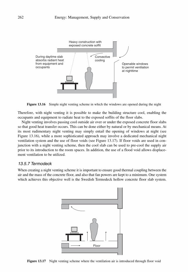
Therefore, with night venting it is possible to make the building structure cool, enabling the
occupants and equipment to radiate heat to the exposed soffits of the floor slabs.
Night venting involves passing cool outside air over or under the exposed concrete floor slabs
so that good heat transfer occurs. This can be done either by natural or by mechanical means. At
its most rudimentary night venting may simply entail the opening of windows at night (see
Figure 13.16), while a more sophisticated approach may involve a dedicated mechanical night
ventilation system and the use of floor voids (see Figure 13.17). If floor voids are used in con-
junction with a night venting scheme, then the cool slab can be used to pre-cool the supply air
prior to its introduction to the room spaces. In addition, the use of a flood void allows displace-
ment ventilation to be utilized.
13.5.7 Termodeck
When creating a night venting scheme it is important to ensure good thermal coupling between the
air and the mass of the concrete floor, and also that fan powers are kept to a minimum. One system
which achieves this objective well is the Swedish Termodeck hollow concrete floor slab system.
262 Energy: Management, Supply and Conservation
During daytime slababsorbs radiant heatfrom equipment andoccupants
Convectivecooling
Openable windowsto permit ventilationat nighttime
Heavy construction withexposed concrete soffit
Figure 13.16 Simple night venting scheme in which the windows are opened during the night
Floor
Figure 13.17 Night venting scheme where the ventilation air is introduced through floor void

The Termodeck system has been used successfully in many locations throughout northern Europe
and in the UK, notably in the Elizabeth Fry Building [12] and the Kimberlin Library Building at
De Montfort University [13]. The Termodeck system ensures good thermal coupling between the
air and the building mass by pushing ventilation air through the hollow cores in proprietary con-
crete floor slabs (as shown in Figure 13.18). By forming perpendicular coupling airways between
the hollow cores, it is possible to form a 3 or 5 pass circuit through which supply air may pass, thus
ensuring good heat transfer. During periods in which cooling is required, outside air at ambient
temperature is blown through the hollow core slabs for almost 24 hours of the day. Overnight the
slab is cooled to approximately 18–20 °C, so that during the daytime the incoming fresh air is pre-
cooled by the slab before entering the room space. By exposing the soffit of the slab it is also pos-
sible to absorb heat radiated from occupants and equipment within the space.
The Termodeck system is particularly worthy of note because it produces buildings which are
extremely thermally stable and comfortable without the need for any refrigeration. The example
of the Elizabeth Fry Building illustrates this fact very well. In a recent study of low energy build-
ings in the UK [14], the performance of the Elizabeth Fry Building was outstanding. This build-
ing achieved the highest comfort score, while at the same time being one of the lowest
consumers of energy; its electrical energy consumption in 1997 was only 61 kWh/m2 and the
normalized gas consumption for that year was 37 kWh/m2 [12], which compares very favourably
with the corresponding values of 128 kWh/m2 and 97 kWh/m2 set out in Energy Consumption
Guide 19 for good practice air conditioned office buildings in the UK [15].
13.6 Building form
The decision to utilize a passive environmental control strategy can put severe constraints on over-
all building form. For example, if natural ventilation is used to promote air movement, it will
inevitably lead to the creation of a narrow plan building, unless atria or central ventilation stacks
are used. This is because passive buildings are supposed to be climate responsive. Therefore
the further an internal space is from an external surface, the less chance there is of harnessing the
natural resources of the external environment. The use of a passive solar heating strategy also
results in a narrow plan building, but with large areas of south facing glazing. For this reason,
passive solar heating schemes tend to be restricted to small- and medium-sized buildings. It is
very difficult to use passive solar heating effectively on large deep plan buildings, not least
because such buildings tend to overheat for large parts of the year and thus primarily need to be
defended against solar heat gains.
Because larger commercial and public buildings generally experience over heating problems,
when a passive strategy is applied to the design of these buildings it is usually a cooling/natural
ventilation strategy rather than a solar heating one. This means that these so-called advanced
Passive solar and low energy building design 263
Hollow core concrete slab
Warm outside air Cool supply air
Figure 13.18 The Termodeck system

naturally ventilated buildings all tend to utilize the same generic design strategies and
technologies. Broadly speaking these generic technologies/strategies are as follows:
• The use of a heavily insulated outer envelope.
• The use of carefully designed and often complex fenestration, which minimizes solar gains
and building heat losses, whilst maximizing daylight penetration. It is also a requirement that
the windows can be opened.
• The use of stacks or atria to promote stack ventilation.
• The use of night ventilation to purge the building structure of the heat accumulated during the
daytime.
• The careful use of exposed building mass to dampen down swings in internal space tempera-
ture, and to promote radiant and convective cooling.
One of the characteristics of these advanced naturally ventilated buildings is that they often have
complex façades with openable windows, vents, blinds, external shades and even light shelves.
These façades incorporate advanced fenestration systems which have many moving parts and
which are often controlled by a building management system (BMS). Such complex façades are
necessary because the absence of internal mechanical services forces the external skin of the
building to become the primary climate modifier and to perform a wide variety of tasks (e.g. day-
lighting, defending against solar radiation, ventilation and preventing the ingress of external
noise). By creating a complex skin, the designers of such buildings are effectively distributing
‘complexity’ all around the building rather than concentrating it in a central plant room. This
degree of complexity in the skin can have a considerable impact on both the performance of the
occupants and the facilities management regime which must be adopted.
In contrast to advanced naturally ventilated buildings, the use of a mechanical ventilation sys-
tem offers considerably more flexibility and enables deeper plans to be utilized. In this respect
the Termodeck system appears to offer great potential, as it facilitates good thermal coupling
between the air and the building mass without the need for a particularly complex façade or an
open plan interior.
The use of the generic passive technologies/strategies described above puts constraints on
building design and dictates the building form. With larger buildings the use of natural ventila-
tion often results in buildings which have atria. These buildings comprise a narrow rectangular
plan wrapped around an atrium, which gives the appearance of a deep plan building. Vents in the
top of the atrium are used to promote buoyancy driven ventilation and air is drawn through vents
or windows in the façade. As a result, passively cooled and ventilated buildings tend to look
similar to each other, characterized by the use of atria or stacks and complex facades. Figures
13.19–13.22 show sections through four recently constructed passively cooled buildings in the
UK: the Learning Resource Centre at Anglia Polytechnic University, Chelmsford; the Ionica
Headquarters, Cambridge; the Inland Revenue Headquarters, Nottingham; and the School of
Engineering, De Montfort University, Leicester.
It can be seen from the illustrations above that all four buildings exhibit many similarities. In
the Anglia Polytechnic and Ionica buildings the designers have used atria to produce buoyancy
driven ventilation, whereas in the other two buildings purpose built stacks have been employed.
Table 13.1 summarizes the features of all four buildings.
It should be noted that although some of the above buildings, especially the De Montfort
building, do not appear to be narrow plan, from a ventilation point of view they are all narrow
plan buildings. The practical maximum width of space which can be naturally ventilated is
approximately 15 m. This dimension limits the form of the building to a narrow plan format.
Nevertheless, by constructing a narrow plan rectangular building around an atrium, which is
264 Energy: Management, Supply and Conservation

Passive solar and low energy building design 265
Fabric shading reflects daylightdown atrium and provides diffusedaylight to top floor (in lieu ofperimeter lightshelves)
700 mm deeplightshelves with10 pitch sidefixedto jambs
Atrium glazing,double glazed
Calicosail
Air passingthrough 50 mmgap via calicosails preventsheat build up
Light coloured perforated metalbalustrades and smoke reservoirsreflect daylight down atrium
Fabric lightshelvesprovide element ofreflected daylight
Figure 13.19 Learning Resource Centre at Anglia Polytechnic University, Chelmsford [10]
Table 13.1 Summary of characteristics of sample buildings [10]
Complex EnergyAtrium windows Exposed consumed
or with Night high mass Light per yearBuilding stacks shading venting soffits shelves KWh/m2/yearAnglia Atrium Yes Yes Yes Yes 82
Polytechnic
University
Ionica Atrium Yes Yes Yes No 64
Headquarters
Inland Revenue Stacks Yes Yes Yes Yes 89
Headquarters
De Montfort Stacks No Yes Yes Yes 120
University

essentially a glass covered courtyard, it is possible to achieve the appearance of a deep plan
building. In the case of the De Montfort building, the deeper plan is achieved by putting venti-
lation stacks in the middle of the building.
13.7 Building operation
The use of a passive environmental control strategy not only affects overall building form, it can also
have a considerable impact on the operation of buildings and the performance of their occupants,
especially if the building is large and naturally ventilated. By relying on a sophisticated envelope as
the primary climate modifier and taking a minimalist approach to the mechanical building services,
designers of such buildings need to be careful that they do not create an environment which hinders
the performance of the occupants. Although designers may feel that they have produced a comfort-
able low energy building, the reality may be that it is detracting from the occupier’s core business,
rather than adding to it. With this in mind, it should be remembered that any property which gets a
reputation for being uncomfortable, or unfit for its purpose, is unlikely to gain in value [16].
A recent study of prominent low energy buildings in the UK [14] found that higher levels of
occupant satisfaction were easier to achieve in buildings which exhibited:
• A narrow plan form.
• Cellularization of working spaces.
• A high thermal mass.
• Stable and thermally comfortable conditions.
266 Energy: Management, Supply and Conservation
Prevailing winds
By day mechanicalventilation operatesto maintain comfort
Windtower
Fixedlouvres
Hot air exhaustedto outside
Evaporative coolerand heat exchanger
Summer mode
Openingwindowsstillpossible
Nighttime ventilation ensures thatexposed structures can be pre-cooled
Mechanical air supplyto North and South zones
Atriumacts asexhaustplenum
Figure 13.20 Ionica Headquarters, Cambridge [10]

Passive solar and low energy building design 267
Fresh air drawnthrough underfloorducting and floorgrille (can be fanassisted)
Exhaust air atridge controlledby motorizeddampers
Tower roof movedup and downhydraulically tocontrol air flowrate
Fresh air risesas it is heatedby internal gains
Solar gainin towerincreasesbuoyancy
Doorsnormallyclosed tostop air intowerpassing intotop floor
Warm airdrawn uptower bystack effect
Doors totower heldopen
Corridor
Corridor
Office area
Office area
Figure 13.21 Inland Revenue Headquarters, Nottingham [10]
Centrallaboratory
Classroom Concourse
Auditorium
Lecture room
Drawing studio
Figure 13.22 School of Engineering, De Montfort University, Leicester [10]

• Control of air infiltration.
• Openable windows close to users.
• A view out.
• Effective and clear controls.
Conversely, occupant satisfaction was harder to achieve in buildings which exhibited:
• A deep plan form.
• Open work areas.
• The presence of complex and unfamiliar technology.
• Situations where occupants had little control over their environment.
• High and intrusive noise levels.
Inspection of the above lists reveals a fairly consistent picture; in short, people prefer to work
close to a window, which they can open, in a quiet cellular office space, which is thermally sta-
ble and comfortable. When these criteria are viewed in the context of passive buildings, a mixed
picture emerges. Clearly, in some respects passive buildings are very positive since they tend to
provide a high admittance environment which is thermally stable and comfortable. In other
respects they are not so beneficial. Many larger advanced naturally ventilated buildings have
large open plan internal spaces because central atria or vent stacks are used. In these buildings
many occupants are inevitably located some distance from the windows and therefore have little
control over their environment. In addition, the use of large spaces and acoustically hard
surfaces can lead to noise problems. Indeed, noise problems have been highlighted as a partic-
ular difficulty in advanced naturally ventilated buildings [14]. Given this, and the other reasons
mentioned above, it is not surprising that some advanced naturally ventilated buildings display
low levels of occupant comfort and productivity [14, 17].
The complex nature of the fenestration required in advanced naturally ventilated buildings can
be the cause of numerous problems and is therefore worthy of closer inspection. The issue of who
has control over the opening of windows is of particular importance. In large naturally ventilated
buildings, particularly those which require night ventilation, the function of the whole environ-
mental control strategy can be impaired if, for any reason, certain windows are not opened.
Consequently, BMS are often used to control the operation of windows, as the occupants cannot
be relied upon to open the windows when required. This automatically, brings the user into con-
flict with the BMS system, with the result that occupants sitting near windows may be unable to
shut the windows when they experience a draught, or conversely, open them when they feel too hot.
If a BMS system is not used, issues of conflict can still arise when, for example, the occupants next
to the windows may close them in situations where those requiring ventilation in the centre of the
building need them to be open. The use of complex fenestration systems, with many moving parts,
can also result in poor window sealing over a period of time, resulting in unwanted air infiltration.
From a maintenance point of view, complex fenestration can cause problems. The use of exter-
nal shading and the numerous protruding and moving parts in these fenestration systems means
that they are prone to mechanical damage, and are difficult to clean. The manufacturers of these
systems go to considerable effort to reduce potential cleaning difficulties, but it still remains true
that from a facilities management point of view these systems need considerably more attention
than conventional windows. A study by Kendrick and Martin has shown that the windows most
suited for night venting and BMS system control (i.e. high level top hung, and hopper windows)
are the most difficult to clean from inside [18]. These advanced fenestration systems have impor-
tant implications on the flexibility and day-to-day operation of the office space. They are required
to be opened by the occupants and are designed to be cleaned from inside. Any desks, bookcases
268 Energy: Management, Supply and Conservation

or benches against the external wall inhibit both the ability of the occupants to regulate their envir-
onment by opening windows, and the ability to clean and maintain the windows. Consequently,
some facilities managers faced with this problem have opted for a ‘furniture free’ zone next to the
windows, or else have installed movable furniture next to the windows. While making the clean-
ing of windows easy, such a policy can hardly be considered to be designed to increase the com-
fort and productivity of building occupants. In addition, forcing the occupants away from the
windows means that the potential daylighting zone is reduced and thus more people have to rely
on artificial lighting, which in energy efficiency terms is very counter productive.
Both developers and building tenants desire buildings which contain flexible space capable of
being adapted to meet the evolving needs of organizations. This need for flexibility/adaptability
has traditionally been resolved by designing deep open plan buildings. From a facilities man-
agement view point the use of an advanced natural ventilation strategy imposes severe con-
straints on the flexibility of the working space. In particular, it is extremely difficult to partition
off internal spaces in such buildings because:
• The insertion of full height partitions may restrict or prevent air movement through the space,
thus nullifying its environmental performance.
• It may be difficult to create an acceptable environment within any partitioned office spaces
that are created. In a conventional office space it is possible to ‘tap’ into the nearest mechani-
cal ventilation duct in the ceiling to serve a new space. In a naturally ventilated high mass
building there may well be no ceiling, and no mechanical ventilation services in the floor. This
makes it difficult to adequately ventilate partitioned spaces.
• The lack of a suspended ceiling can lead to flexibility problems when repositioning luminaires.
• In many advanced high mass buildings the exposed floor soffits are formed by deeply recessed
concrete floor beams. The geometry of these floor beams can create problems when erecting
partitions.
Even if full height partitions are not installed the environmental performance of a naturally ven-
tilated space may still be impaired by the insertion of high screens and furniture, which restrict
the air flow and thus create ‘dead’ spots.
From the discussion above it is tempting to conclude that all passive and mixed-mode buildings
result in operational difficulties. This however is not the case. The example of the Elizabeth Fry
Building, which utilizes the Termodeck system, clearly demonstrates that high mass mixed-mode
buildings can be very successful. Of all the buildings surveyed in the UK study [14], it was the
Elizabeth Fry Building which was outstanding. This building achieved the highest comfort score,
while at the same time being one of the lowest consumers of energy. Of particular note is the fact
that the building produced an extremely stable thermal environment and comfortable internal tem-
peratures during summer without the need for any refrigeration, clearly demonstrating the success
of the fabric thermal storage strategy. The reasons for its success are that the building:
• is thermally stable and comfortable;
• has cellular work spaces;
• has a relatively narrow plan;
• is well sealed and has tight control over air infiltration; and
• has windows which can be opened by the occupants.
These are all qualities which tend to promote user comfort and enhance productivity. When the
Elizabeth Fry Building is compared with less successful advanced naturally ventilated buildings,
it can be seen that its success lies in the fact that the Termodeck system is much more unobtrusive
and flexible than the more rigid requirements of the naturally ventilated buildings. For example,
Passive solar and low energy building design 269

the use of mechanical ventilation and hollow core slabs means that the façade of the building can
be relatively simple, which frees up the windows so that they can be opened at will by the occu-
pants without impairing the thermal performance of the building. The use of a mechanical venti-
lation system allows the internal space to be sub-divided into cellular rooms, something which it
is difficult to achieve in advanced naturally ventilated buildings. It also allows flexibility in the
shape and form of the building. Unlike the advanced naturally ventilated buildings where ‘com-
plexity’ is distributed around the skin of a building, the Termodeck system concentrates ‘com-
plexity’ in a central plant room where it can easily be controlled and maintained.
References
1. Bordass, W. T., Entwistle, M. J. and Willis, S. T. P. (1994). Naturally ventilated and mixed-
mode office buildings – opportunities and pitfalls. CIBSE National Conference, Brighton.
2. CIBSE Guide A2, Weather and solar data, 1982.
3. Hui, H. F., Fong, T. and Lai, K. W. (1996). Passive solar design in architecture. The Hong
Kong University.
4. Vale, B. and Vale, R. (1991). Green architecture – design for a sustainable future. Thames
and Hudson.
5. Mazria, E. (1979). The Passive Solar Energy Book. Rodale Press.
6. Lebens, R. M. (1980). Passive Solar Heating Design. Applied Science Publishers.
7. Francis, W. and Peters, M. C. (1980). Fuels and fuel technology. Pergamon Press.
8. Green, M. A. (1998). Photovoltaic solar energy conversion; an update. Australian Academy
of Technological Sciences and Engineering, ATSE Focus, No. 102, May/June.
9. Environmental control glasses, Pilkington.
10. Natural ventilation in non-domestic buildings (1997). CIBSE Application Manual AM10.
11. Bunn, R. (1993). Learning curve. Building Services Journal. October, pp. 20–5.
12. Standeven, M., Cohen, R., Bordass, B., and Leaman, A. (1998). PROBE 14: Elizabeth Fry
Building. Building Services Journal. April pp. 37–42.
13. Bunn, R. (1998). Cool desking. Building Services Journal. October, pp. 16–20.
14. Bordass, W., Leaman, A., Ruyssevelt, P. (1999). PROBE strategic review: Report 4 –
Strategic Conclusions. Department of the Environment, Transport and the Regions, August.
15. Energy use in offices (1997). Energy Consumption Guide 19, Department of the Environment,
Transport and the Regions.
16. Beggs, C. B. and Moodley, K. (1997). Facilities management of passively controlled build-
ings. Facilities, 15 (9/10), September/October, pp. 233–40.
17. Leaman, A. (1999). Comfort and joy. Building Services Journal. June, pp. 33–4.
18. Kendrick, C. and Martin, A. (1996) Refurbishment: The Natural Way. CIBSE Journal,
November, p. 29.
Bibliography
Bordass, W., Leaman, A. and Ruyssevelt, P. (1999). PROBE strategic review: Report 4 –
Strategic Conclusions. Department of the Environment, Transport and the Regions, August.
Hill, R., O’Keefe, P. and Snape, C. (1995). The future of energy use (Chapter 7), Earthscan.
Natural ventilation in non-domestic buildings (1997). CIBSE Application Manual AM10.
Vale, B. and Vale, R. (1991). Green architecture – Design for a sustainable future. Thames and
Hudson.
270 Energy: Management, Supply and Conservation

Passive solar and low energy building design 271

Appendix 1
Degree days
A1.1 Heating degree days
The concept of degree days was first developed about 100 years ago for use in horticulture [1].
Nowadays, however, degree days are generally used to predict heating energy consumption in
buildings. They provide building designers with a useful measure of the variation in outside
temperature, which enables energy consumption to be related to prevailing weather conditions.
It is not difficult to appreciate that in a cold month such as January, a given building will
consume more heating energy than in a warmer month such as March. This is because:
• the outside air temperature is likely to be colder during January than in March; and
• lower air temperatures are likely to persist for longer in January compared with March.
From this it can be seen that heat energy consumption relates both to the degree of coldness and
the duration of that coldness. The degree day method allows for both these factors by setting a
base outside air temperature, above which most domestic and commercial buildings do not
require any heating. In the UK this base temperature is generally taken to be 15.5 °C. If the
average outside air temperature on any given day is below the base temperature, then heating will
be required. However, the heat energy consumption in any given period is dependent not only on
the magnitude of the temperature differential but also on its duration. For example, if an outside
air temperature of 14.5 °C prevails for 24 hours, then a deficit of 1 °C will have been maintained
for 1 day and 1 degree day will have been accrued. If the outside temperature remains at 14.5 °C
for each day of a week, then a total of 7 degree days will be accumulated. Similarly, if an outside
air temperature of 10.5 °C is maintained for 1 week then 35 degree days will be accumulated.
By summating the daily temperature deficits over any given month it is possible to calculate
cumulative degree days for that particular month. Therefore, by monitoring daily outside air
temperature, it is possible to produce tables of monthly heating degree days for various locations,
which can be used by building designers and operators to estimate heating loads. For example, if
a particular building experiences 346 heating degree days in January and only 286 in March, it
is reasonable to assume that heating fuel consumption in January should be 1.21 times that for
March.
Monthly and annual degree day figures are published in many sources. Table A1.1 shows
20-year average heating degree day data for the various geographical regions of the UK.

Table A1.1 UK 20-year average heating degree day data to base 15.5 °C [2]
Region Jan Feb Mar April May June July Aug Sept Oct Nov Dec Average
Thames valley 346 322 286 205 120 51 22 25 54 130 242 312 2115
South eastern 368 344 312 233 150 74 39 44 82 160 267 334 2407
Southern 345 327 301 229 148 72 39 43 79 150 251 312 2296
South western 293 285 271 207 137 63 28 28 55 116 206 258 1947
Severn valley 321 305 280 201 128 56 24 27 61 138 237 300 2078
Midland 376 359 322 243 162 83 44 48 90 178 275 343 2523
West Pennines 361 340 312 230 144 75 38 39 78 157 267 328 2369
North western 375 345 323 245 167 90 50 56 96 171 284 341 2543
Borders 376 349 330 271 206 117 66 68 104 182 282 339 2690
North eastern 381 358 322 247 168 87 46 49 88 175 281 346 2548
East Pennines 372 352 313 232 154 78 42 44 81 165 272 341 2446
East Anglia 378 349 317 239 149 73 40 39 71 154 269 341 2419
West Scotland 383 352 328 246 170 94 58 64 111 188 299 352 2645
East Scotland 388 357 332 263 197 109 62 67 109 192 301 354 2731
North East Scotland 401 368 346 277 206 120 74 78 127 203 311 362 2873
Wales 330 320 307 240 170 92 49 45 77 145 235 294 2304
Northern Ireland 365 334 320 242 171 92 53 59 99 173 282 329 2519

A1.2 Changing the base temperature
In the UK, degree day data are generally produced for a base temperature of 15.5 °C. However,
other countries may use different base temperatures. Indeed, in the UK the National Health
Service uses an alternative base temperature of 18.5 °C. It may therefore be necessary to convert
data quoted at 15.5 °C to another base temperature. This can be done with relative accuracy by
using Hitchin’s formula [1] below:
where tb is the base temperature (°C), to is the mean air temperature in the month (°C), and k is
the constant.
The value of ‘k’ varies slightly with location and must be determined from 20-year weather
data. However, a general k value of 0.71 can be assumed for most locations in the UK [1].
A1.3 Cooling degree days
Heating degree days are of considerable use when estimating and monitoring the energy
consumption of non-air conditioned buildings. However, for air conditioned buildings they are
only of limited value. Consequently, the concept of the cooling degree day was developed.
Cooling degree days are defined as ‘the mean number of degrees by which the outside
temperature on a given day exceeds the base temperature, totalled for all the days in the period’ [1].
There is, however, no general consensus on the base temperature that should be used for
calculating cooling degree days and many users still use a 15.5 °C base [1].
References
1. Degree days. (1993). Fuel Efficiency Booklet 7, Department of the Environment.
2. Energy audits and surveys. (1991) CIBSE Applications Manual AM5.
Average degree days per day �(tb � to)
1 � e�k(tb� t0)
Appendix 1: Degree days 273
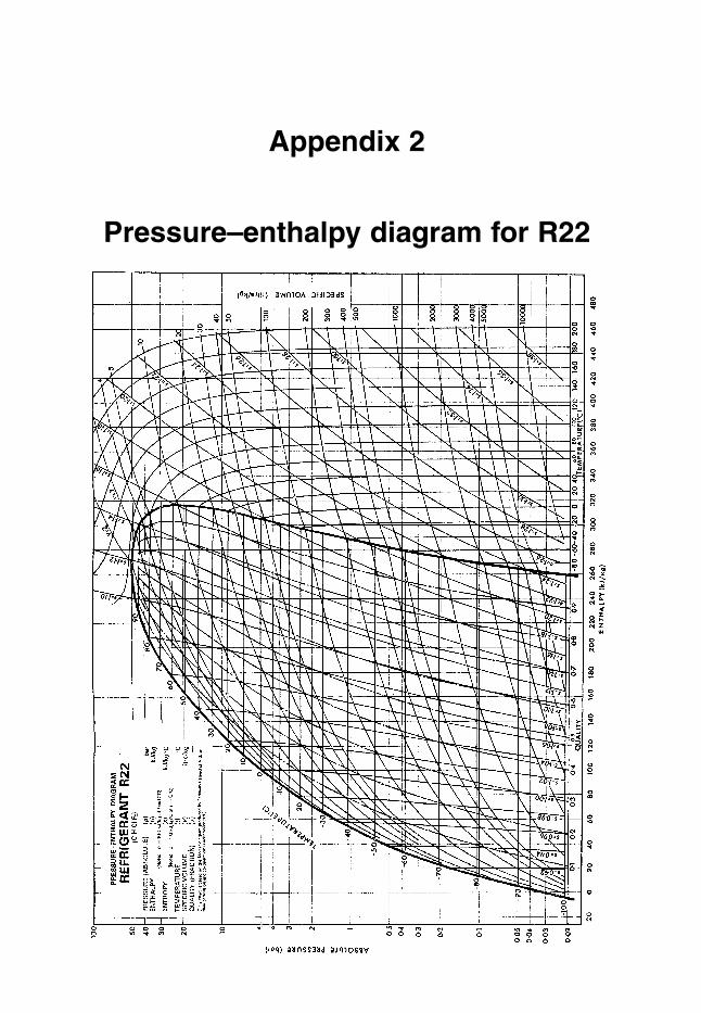
Appendix 2
Pressure–enthalpy diagram for R22

Ap
pen
dix
3
CIB
SE
Psych
rom
etric
Ch
art
BASED ON A BAROMETRICPRESSURE OF 101.325 kPa
00.10.2
0.3
0.4
0.5
0.6
0.7
0.80.91.00.90.8
0.7
0.6
0.5
0.4
0.3
0.20.1 0
20
25
30
35
40
45
50
55
60
65
70
75
80
85
90
95
100
105
110
115
SP
EC
IFIC
EN
TH
ALP
Y k
J/kg
SPECIFIC VOLUME m /kg3
SENSIBLE/TOTAL HEATRATIO FOR WATERADDED AT 30°C
–10
–5
0
5
10
15
0.75
–10
–10 0–5 5 10 15 20 25 30 35 40 45 50 55 60
–10 –5 0 5 10 15
20 25 3530 40
DRY - BULB TEMPERATURE °C
SPECIFIC ENTHALPY kJ/kg
45 50 55 60 65
0.000
0.001
0.002
0.003
0.004
0.005
0.006
0.007
0.008
0.009
0.010
0.011
0.012
0.013
0.014
0.015
0.016
0.017
0.018
0.019
0.020
0.021
0.022
0.023
0.024
0.025
0.026
0.027
0.028
0.029
0.03020304050
–5
0
5
10
15
20
25
0.85
30
0.90
90 80 70 60
120 125 130 135 140
PERCENTAGE SATURATIONCIBSEPSYCHROMETRIC
CHART
0.80
WET-
BULBTEM
PERAT
URE
°C(S
LIN
G)
70
75
80
85
90
95
100
105
110
115
120
125
130
135
140
MO
IST
UR
E C
ON
TE
NT
kg/k
g (D
RY
AIR
)
© CIBSE LONDON 1987.

This Page Intentionally Left Blank

Index
Advanced naturally ventilated buildings,
263–4, 268
AHU see Air handling unit
Air conditioning and ventilation, 186–218
see also Low energy buildings
air handling unit (AHU), 189–91, 215
chiller, 190–1, 193
conventional design weakness, 194–7
air system, 196–7
building design, 195
refrigeration system, 195–6
desiccant cooling, 214–17
combined air handling unit (AHU),
215–16, 217
psychrometric chart, 215–16
solar energy, 217
wheel system, 214–15
design for low energy use, 197–218
direct expansion refrigeration coil (DX),
189–90, 215
energy costs, 188
environmental impact, 186–9
evaporative cooling, 213–14
fabric thermal storage, 204–5
fan power, 197
ice thermal storage, 205–13
advantages, 205
chiller priority, 206–7, 209–10, 213
demand limited, 207–8
example of option calculations, 211–13
full storage, 206, 213
ice bank system, 208–9
ice harvester, 208, 210
sizing calculations, 209–11
store priority, 206–7
Legionella pneumophila hazard,
191, 199
refrigeration systems, 191–4, 198–201
coefficent of performance (COP), 193
compressors, 199–200
condensers, 198–9
evaporators, 198
expansion devices, 200–1
heat recovery, 201
vapour compression cycle, 191–4
splitting cooling and ventilation, 201–4
chilled ceilings, 202–3
ventilation, 203–4
systems, 189–91
split unit, 190, 192
through-the-wall, 190, 191
Air handling unit (AHU), 189–91, 215,
216, 217
Analysis of energy usage, 55–72
annual consumption, 55–7
cumulative sum deviation method
(CUSUM), 67–71
calculation, 70–1
standard performance equation,
67–8, 84
typical example of analysis
method, 68–71
linear regression analysis, 63–7
factors influencing energy
consumption, 64
multi-variable, 67
Pearson correlation coefficient,
65–6, 67
single independent variable, 63–5
typical calculations, 64–5, 66–7
variables compared, 63
normalized performance indicator (NPI),
56–61, 81, 82–3
space heating in buildings, 58–9

Analysis of energy usage (continued)
time dependent consumption, 61–3
typical calculation, 59–61
use of degree days, 62–3
yardsticks for buildings (kW/m2), 57, 60
Anglia Polytechnic University, 264, 265
Apparent power, 220–1
Audits of energy data, 73–91
audit costs, 75–6
the audit report, 91
comprehensive audits, 85
estimating usage, 86–7
example of a typical audit, 85–6
temporary sub-metering, 85–6
defined, 73–4
energy management opportunities, 74
energy surveys, 88–90
building fabric, 90
management, 88
objectives, 88
plant and equipment, 89–90
supply features, 89
financial energy audits, 75
preliminary audits, 77–83
data analysis, 80
electricity invoices, 78–9
example of a typical audit, 81–4
fuel oil, solid fuel and heat, 79–80
natural gas, 79
processes involved, 77–8
site records, 80
recommendations, 90
types of audit, 74–5
why energy is wasted, 76
Barrel, defined, 6
Black body radiation, 123–4
Block electricity tariff, 28–9
Boilers in heating systems, 143–7
British thermal unit (Btu), defined, 5
Building:
forms for low energy use, 263–6
heat losses, 120–31
management systems (BMS), 104, 268
operation, 266–70
California Power Exchange, 44–5
Calorie, defined, 6
Carbon credits and taxes, 15, 18
Carbon dioxide (CO2):
emission from power plants, 12–13
global emission rates, 13–14
as greenhouse gas, 11, 23, 187
Carbon intensity, 12–13
Carnot cycle, 165, 170–1
CCGT see Combined cycle gas turbine
CFC see Chlorofluorocarbons
CFD see Computational fluid dynamics
Chilled ceilings in air conditioning, 202–3
Chlorofluorocarbons (CFCs), 11, 12,
14, 15, 187
CHP see Combined heat and power
Climate change levy (UK), 15
Coal as fuel, 22–3
Coefficient of performance (COP):
defined, 164
for heat pump, 164–5
for refrigeration, 89, 194, 196, 198, 201
Cogeneration of heat and power, 171
Combined cycle gas turbine (CCGT), 12
Combined heat and power (CHP), 95, 170–85
advantages and disadvantages, 171–2
applications, 177–8
cogeneration, 171
concept of CHP, 170–2
district heating schemes, 176–7
economics, 180–4
comparisons with conventional
schemes, 180–4
examples of calculations, 180–4
main factors, 180
efficiency of system, 172–3
operating and capital costs, 178–9
size of plant, 178–9
systems, 173–6
gas turbines, 173–4
internal combustion engines, 173
micro-CHP, 175–6, 178
steam turbines, 173, 174–5
Competition in energy supply, 37–54
Californian electricity supply, 44–5
concepts, 38, 47–8
demand side management (DSM), 48–53
advantages, 49
costs, 53
defined, 49–50
278 Index

Index 279
expenditure by utilities, 50
UK experience, 51–3
US experience, 49–51
deregulation, 37, 45
electricity load management, 46–7
gas market, 45–6
UK electricity supply, 38–43
contract for differences, 42
evolution of the market, 43–4
horizontal integration, 40
pool prices, 42
typical daily variation in demand, 41–2
vertical integration, 39
Compressors in air conditioning
refrigeration systems, 199–200
Computational fluid dynamics (CFD), 244
Condensers in air conditioning refrigeration
systems, 198–9
Contract for differences, defined, 42
COP see Coefficient of performance
Cumulative sum deviation method
(CUSUM), 67–71, 110–12
De Montfort University, Leicester, 204, 260,
263, 264, 265
Degree days, 271–3
changing base temperature, 273
cooling degree days, 273
defined, 271
UK data, 272
Demand side management of energy supply
(DSM), 48–53
Department of the Environment, 108, 263
Desert coolers, 214
Desiccant cooling, 214–17
Design strategy for buildings, 264
Developing countries, 2, 8
Deviance chart, 110–11
DHW see Domestic hot water
Direct expansion refrigeration coil (DX)
in air conditioning, 189–90, 215
Discounted cash flow, 96–100
District heating schemes, 176–7
Domestic electricity tariff, 28
Domestic hot water (DHW), 176, 178
Dry resultant temperature, 120, 202–3, 204,
261
DSM see Demand side management
EAC see Energy account centre
East Midlands Electricity, 52
Economy 7 electricity tariff, 51–2
Effectiveness of heat exchange, 155
EIA see Energy Information Administration
Electric motors, 223–4
Electrical Power Research Institute (EPRI),
49–50
Electrical services, 219–42 see also
Electricity
cost of inefficiency, 219
electric motors, 223–4
inefficiencies, 224
sizing, 223–4
lighting, 228–41
daylight, 228–9
energy efficiency, 237–41
example of illuminance
calculation, 231
examples of lighting schemes, 235–7
fluorescent lamps, 238–9
high pressure sodium lamps, 240
illuminance (lux) defined, 229–30
lamp control gear, 240–1
lamp survival factor (LSF), 235
lighting design lumens, 232
lumen design method, 232
lumen maintenance factor
(LLMF), 235
luminaire maintenance factor
(LMF), 235
luminous efficacy of lamps, 238, 239
luminous flux (lumen) defined, 229
luminous intensity (candela)
defined, 229
maintenance, 241
maintenance factor (MF), 233–7
metal halide lamps, 240
polar intensity diagram, 229–30
room surface maintenance factor
(RSMF), 235
tungsten filament lamps, 238
utilization factor (UF), 233
power factor, 219–23
apparent power, 220–1
correction techniques, 222–3
defined, 221
effect of poor power factor, 221–2

Electrical services, power factor (continued)
reactive loads, 219–20
variable speed drives (VSD), 225–8
example of cost saving calculation,
225–7
fan power usage, 225–6
pulse width modulated inverter
(PWM), 227–8
variable frequency drive, 227–8
Electricity see also Electrical services
average price calculation, 31
charges involved in supply, 26–8
as fuel, 22–3
comparison with natural gas, 32
supply, 24–31
demand profiles, 27
network structure, 25–6
typical processes, 24–5
tariffs, 28–31
block, 28–9
domestic, 28
maximum demand, 29–30
seasonal time of day (STOD), 30
Elizabeth Fry Building, University of East
Anglia, 204, 260, 263, 269
Emissivity factor (E), 124
Energy see also Electricity; Heating
systems; Low energy buildings;
Monitoring and targeting energy
consumption; Waste heat recovery
audits of data, 73–91
competition in supply, 37–54
concepts, 4–7
definition and units, 4–5
efficiency in lighting, 237–41
environmental factors, 1–21
intensity, defined, 9
laws of thermodynamics, 6–7
primary and secondary forms, 23–4
reserves, 19–20
usage analysis, 55–72
Energy account centre (EAC), 103–4, 106,
115
Energy Consumption Guide (Dept of the
Environment), 263
Energy Information Administration (EIA), 19
Energy yardsticks for buildings (kW/m2),
57, 60
Environmental factors in energy usage, 1–21
developing countries, 2
energy use, 1–3
global warming, 2, 10–12
from air conditioning, 187
greenhouse gases, 11–12, 187
temperature change, 10
impact of air conditioning, 186–9
intergovernmental actions, 14–15
ozone layer depletion, 14, 187
politics, 3
EPRI see Electrical Power Research
Institute
Evaporative cooling, 213–14
Evaporators in air conditioning refrigeration
systems, 198
Expansion devices in air conditioning
refrigeration systems, 200–1
Fabric thermal storage, 204–5
Fan power estimates, 225–6
Flue gas heat losses, 89
Former Soviet Union (FSU), 9, 18
Gas turbines in CHP systems, 173–4
GDP see Gross domestic product
Global warming potential (GWP),
11–12, 189
GNP see gross national product
Greenhouse effect in buildings, 245
Greenhouse gases, 11–12, 187, 189
Gross domestic product (GDP), 1, 2, 3
energy consumption, 7–9
Gross national product (GNP), 8, 9
GWP see Global warming potential
HCFC see Hydrochlorofluorocarbons
Heat exchanger design for waste heat
recovery, 151–6
Heat recovery in air conditioning
refrigeration systems, 201
Heating systems, 117–47 see also
Combined heat and power; Low energy
buildings; Waste heat recovery
boilers, 143–7
blow-down, 145
causes of inefficiency, 144–5
condensing boilers, 145
280 Index

flue gas losses, 143–4
size and efficiency, 143
building heat loss, 120–31
black body radiation, 123–4
building heat loss calculation
examples, 126–31
comparison of heating systems, 131
emissivity factor (E), 124
fabric loss equation, 121
heat transfer calculation example,
125–6
Stefan–Boltzmann constant, 124
surface thermal resistance (Rs), 122–5
thermal conductivity, 123
thermal transmittance (U value), 121–6
ventilation loss equation, 121
causes of inefficient heating, 117–18
energy calculations, 131–5
examples of building heating cost
estimates, 133–5
seasonal heating plant efficiencies,
131–2
insulation of pipework, 138–43
economics, 141
estimating optimum costs of insulation,
141–3
example of heat loss estimate, 140–1
heat transfer equations, 139–40
insulation material properties, 138–9
intermittent heating, 135–6
low emissivity glazing, 137
radiant heating, 136–7
thermal comfort, 118–20
dry resultant temperature, 120, 202–3
effect of activity, 119–20
human heat balance, 119
mean radiant temperature, 120, 203
underfloor and wall heating, 137–8
Hitchen formula for degree days, 273
Hottel–Whillier equation for solar
radiation, 250
Hydrochlorofluorocarbons (HCFCs),
11, 12, 14, 15, 166, 187
Ice thermal storage, 205–13
Illuminance (lux) defined, 229
Inland Revenue Headquarters, Nottingham,
264, 265, 267
Insulation of pipework, 138–43
Intergovernmental Panel on Climate Change
(IPCC), 11, 12
Internal combustion engines in CHP
systems, 173
Internal rate of return, 99–100
Investment appraisal, 92–102
discounted cash flow, 96–100
discount factor (DF), 97
discount rate, 96
examples of evaluations, 98–9, 99–100
graph of net present value and
discount rate, 100
internal rate of return (IRR), 99–100
net present value (NPV), 96–9
profitability index, 100
effect of capital depreciation, 100–1
examples of appraisals, 93, 94, 95
fixed and variable costs, 93–4
interest charges, 94
payback period, 95
real value and inflation, 101–2
Ionica Headquarters, Cambridge, 264–6
IPCC see Intergovernmental Panel on
Climate Change (IPCC)
IRR see Internal rate of return
Kendrick, C, 268
Kilovoltamp-hour (kVAh) defined, 27–8
Kilowatt-hour (kWh), defined, 5
Kimberlin Library Building, De Montfort
University, Leicester, 263
Kyoto Protocol on global warming,
15, 18, 23
Learning Resource Centre, Anglia
Polytechnic University, Chelmsford,
264, 265
Legionella pneumophila hazard in air
conditioning, 191, 199
Lighting and energy efficiency,
228–41
LMTD see Log mean temperature
difference
Load factors in electricity supply, 47
Log mean temperature difference
(LMTD), 152
Low emissivity glazing, 137
Index 281

Low energy buildings, 243–69
active solar heating, 249–51
example of water heater, 249–51
flat plate collector, 250–1
building forms, 263–6
advanced naturally ventilated
buildings, 263–4, 268, 270
design strategy for buildings, 264
recent low energy buildings, 264–6
building operation, 266–70
cleaning problems, 268–9
occupant satisfaction, 266, 268, 269
reasons for success, 269–70
passive solar cooling, 252–63
advanced fenestration, 255–6
example of ventilation calculation,
258–60
natural ventilation, 256–60
night venting, 261–2
shading techniques, 253–4
solar control glazing, 254–5
stack ventilation, 257–8
thermal mass, 260–1
passive solar heating, 243–9
alternative systems, 244–5
current experience, 244
design requirements, 243–4
direct gain system, 246–7
indirect gain technique, 247–8
isolated gain technique, 248–9
Termodeck system, 262–3
thermosiphon system, 249
photovoltaics, 251–2
Low temperature hot water (LTHW),
175–6, 177
Luminous flux (lumen) defined, 229
Luminous intensity (candela) defined, 229
Maintenance factor (MF) in lighting, 233–7
Martin, A., 268
Maximum demand electricity tariff, 29–30
Mean radiant temperature, 120, 203,
204, 261
Medium temperature hot water
(MTHW), 175
Meteorological Office, UK, 12
Methane as greenhouse gas, 11
Micro-CHP systems, 175–6
Monitoring and targeting energy
consumption (M&T), 103–16
causes of wastage, 114
computer based data, 104
data collection, 105–6
diagnosing changes in usage, 111–13
energy targets, 106–7
key elements of monitoring
programme, 103–4
prioritizing efficiency measures, 115
reporting, 107–11
exception reports, 111
frequency, 107–8
graphical techniques, 110–11
league tables, 109–10, 115
waste avoidance, 113–14
Montreal Protocol on ozone depletion,
14, 187
M&T see Monitoring and targeting energy
consumption
MTHW see Medium temperature hot water
National Grid Company (NGC), 41, 43, 44
Natural gas as fuel, 22–3, 31–5
comparison with electricity, 32
composition, 32
peak demand, 33–4
production processes, 32–3
tariffs, 34
Net present value, 96–7
New Electricity Trading Arrangement
(NETA), 43, 44
NGC see National Grid Company
Norm chart, 110
NPV see Net present value
Number of transfer units (NTU) in heat
exchange, 155–6
Oil as fuel, 22–3, 35
Ontario Hydro (Canada), 48
Ozone layer depletion, 14, 187
Pacific Gas and Electric, 44, 45, 48
Passive solar cooling, 252–63
Pearson correlation coefficient in regression
analysis, 65–6, 67
Photovoltaics, 251–2
Polar intensity diagram for lighting, 229–30
282 Index

Politics and energy supply, 3
Pool purchase price for electricity (PPP), 42
Pool selling price for electricity (PSP), 42
Power factor, 219–23
PPP see Pool purchase price
PSP see Pool selling price
Psychrometric chart for desiccant cooling,
215–16
Public Utility Commissioners (USA), 48, 50
Pulse width modulated inverter (PWM) for
variable speed drive, 227–8
Queens Building, De Montfort University,
Leicester, 204, 260, 263
Reactive electrical load, 28, 219–20
Recuperatve heat exchangers, 149–51
Refrigerant HCFC 22, 166
Refrigerants as greenhouse gases, 187
Refrigeration systems in air conditioning,
191–4
Regenerative heat exchangers, 160–4
Rocky Mountain Institute, Colorado
USA, 244
Run-around coils for heat exchange, 157–60
School of Engineering, De Montfort
University, Leicester, 264, 265, 267
Seasonal time of day electricity tariff, 30
SMP see System marginal price
Solar energy, 243–62 see also low energy
buildings
desiccant cooling, 217
Southern California Edison, 44, 45
Soviet Union, 9, 18
�R thermal resistance (m2K/W), defined, 121
St George’s School, Wallasey Cheshire, 244
Standard performance equation for energy
usage, 67–8, 84, 103, 106, 112
Stark energy information systems, 108
Steam turbines in CHP systems, 174–5
Stefan–Boltzmann constant, 124
STOD see Seasonal time of day
electricity tariff
Sulphur dioxide (SO2), 23
Surface thermal resistance (Rs), 122–5
System marginal price for electricity
(SMP), 42
Termodeck floor system, 204–5, 262–3,
269, 270
Thermal conductivity of materials, 123
Thermal resistance �R (m2K/W),
defined, 121
Thermal transmittance (U value)
(W/m2K), 121–6
Thermal wheel regenerative heat
exchangers, 160–2
Therme, defined, 5
Thermodynamics, laws of, 6–7
Tonne of oil equivalent (toe), defined, 6
Trombe Wall, 247–8
U value see Thermal transmittance
UF see Utilization factor in lighting
Ultraviolet (UV) radiation, 14
Units of energy, 4–5
University of East Anglia, 204, 260, 263
Utility companies, 22–36 see also Electrical
services; Electricity
Utilization factor in lighting, 233
Value added tax (VAT), 30, 33
Variable speed drives (VSD), 225–8
Waste heat recovery, 148–69 see also
Heating systems; Monitoring and
targeting energy consumption
concepts, 148–9
heat exchanger design, 151–6
counter flow and parallel flow,
151–2, 153–4
effectiveness of heat exchange, 155
examples of calculations, 152–4, 156
log mean temperature difference
(LMTD), 152
number of transfer units (NTU),
155–6
heat pumps, 164–9
applied to swimming pools, 166
coefficient of performance (COP),
164–5
defined, 164
examples of calculations, 166–9
recuperative heat exchangers, 149–51
flat plate recuperator, 151, 166, 167
plate exchanger, 150–1
Index 283

Waste heat recovery, recuperative heat
exchangers (continued)
shell and tube design, 150
thermal resistance, 149
regenerative heat exchangers, 160–4
example of calculations, 162–4
heat transfer equations, 161–2
thermal wheel, 160–2
run-around coils, 157–60
examples of calculations,
158–60
heat transfer equations, 157–8
World Bank, 8
World energy consumption, 16–19
284 Index


![Energy Management in Microgrids with Renewable Energy … › record › 84387 › files › texto... · 2019-11-05 · demand and supply [2]. Renewable energy resources, distributed](https://img.pdfslide.net/doc/110x75/5f14eec895a58653f7207a10/energy-management-in-microgrids-with-renewable-energy-a-record-a-84387-a-files.jpg)