Embed Size (px)
Citation preview
.
Energy Partition on FractalsJEREMY STANLEY, ROBERT S. STRICHARTZ,
& ALEXANDER TEPLYAEV
ABSTRACT. The energy of a function defined on a post–criticallyfinite self–similar fractal can be written as a sum of directionalenergies. We show, under mild hypotheses, that each directionalenergy is a fixed multiple of the total energy, and we computethe multiple for a one–parameter family of energy forms on theSierpinski gasket. For the standard one, the result is an equiparti-tion of energy principle. Also we discuss the energy partition forgeneral p.c.f. fractals, and the relation of it to the uniqueness andstability of a self-similar Dirichlet form.
1. INTRODUCTION
The energy of a function u on an open set Ω in Rn, defined to be a multiple(taken to be 1 for simplicity) of the integral of |∇u|2, can be written as a sumof directional energies
∫Ω |∂u/∂xj|2dx. There are no required relations betweenthe directional energies in this case, as may be seen just taking u to be a linearfunction. But something quite different happens on fractals.
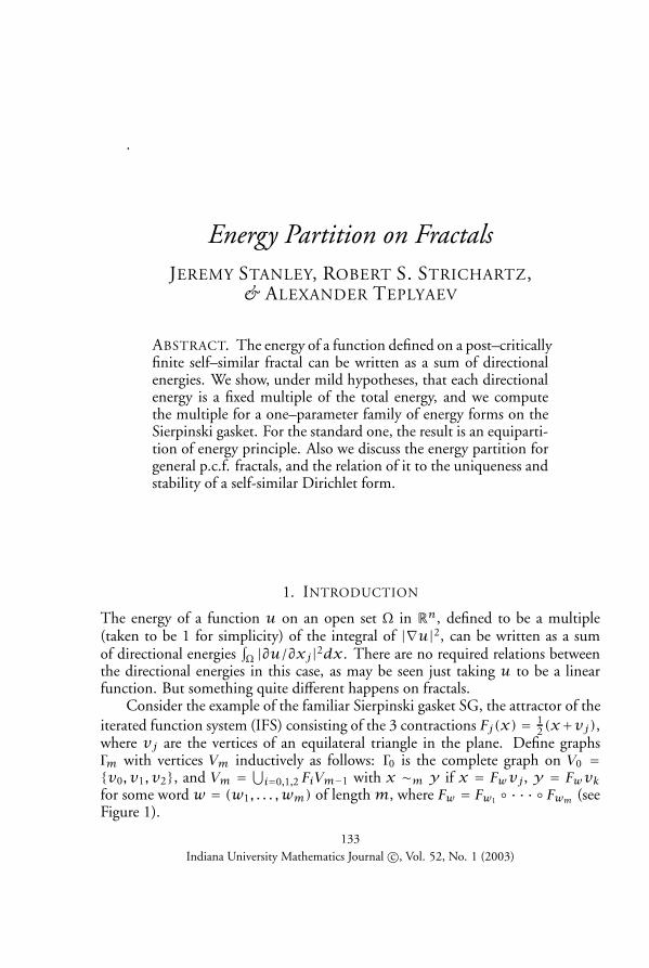
Consider the example of the familiar Sierpinski gasket SG, the attractor of theiterated function system (IFS) consisting of the 3 contractions Fj(x) = 1
2(x+vj),where vj are the vertices of an equilateral triangle in the plane. Define graphsΓm with vertices Vm inductively as follows: Γ0 is the complete graph on V0 =v0, v1, v2, and Vm = ⋃
i=0,1,2 FiVm−1 with x ∼m y if x = Fwvj, y = Fwvkfor some word w = (w1, . . . ,wm) of length m, where Fw = Fw1 · · · Fwm (seeFigure 1).
133Indiana University Mathematics Journal c©, Vol. 52, No. 1 (2003)
134 J. STANLEY, R. S. STRICHARTZ &A. TEPLYAEV
Γ0 :
v0
v1
v2t t
t
TT
TT
T Γ1 :
v0
v1
v2s s
ss s
s
s s
s
TTT
TTT
TTT
Γ2 :
v0
v1
v2s s
ss s
s
s s
s
s s
ss s
s
s s
s
s s
ss s
s
s s
s
TTTT
TT
TTTT
TT
TTTT
TT
FIGURE 1. The first 3 graphs Γ0, Γ1, and Γ2 approximating SG.
Then SG is the closure of⋃m Vm, and we may define the standard energy (or
Dirichlet form) as
(1.1) E(u,u) = limm→∞Em(u,u)
where
(1.2) Em(u,u) =(
53
)m ∑x∼my
(u(x)−u(y))2.
The sequence Em(u,u) is monotone increasing, and the domain of E, thespace of functions of finite energy, is defined to be the space of functions u forwhich the limit (1.1) is finite [Ki1,Ki2]. (It is important to observe that pointshave positive capacity for this Dirichlet form, so that functions in dom E mustbe continuous, and the pointwise values in (1.2) are well–defined.) We may alsowrite the approximate energy Em, using cyclic notation for subscripts of vi, as
(1.3) Em(u,u) =2∑i=0
E(i)m (u,u)
for
(1.4) E(i)m (u,u) =(
53
)m ∑|w|=m
(u(Fwvi+1)−u(Fwvi))2,
partitioning the sum along the 3 directions of the edges. These directional ap-proximate energies are no longer monotone increasing, and one might wonderwhether or not the limits
(1.5) E(i)(u,u) = limm→∞E
(i)m (u,u)
defining directional energies exist. In Section 2 we show that the limits exist forany function of finite energy, and indeed E(i)(u,u) = 1
3E(u,u), so we have
Energy Partition on Fractals 135
equipartition for this symmetric energy form. In fact, for harmonic functions wehave the more precise result
(1.6) E(i)m (u,u)−13E(u,u) =
(45
)m (E(i)0 (u,u)− 1
3E(u,u)
)(in this case E(u,u) = Em(u,u) for all m). Once we have equipartition forharmonic functions, it follows immediately for piecewise harmonic splines, andthen for all functions of finite energy because harmonic splines are dense in energynorm ([Ki2] Lemma 3.2.17). However, (1.6) does not hold for a wider class offunctions.
In Section 3 we consider analogous results for a one–parameter family of self–similar Dirichlet forms on SG, involving a more complicated analog of (1.2) forthe approximate energy. The approximate energy again splits via (1.3) into threedirectional energies via the analog of (1.4), with the limits (1.5) existing and yield-ing a partition of energy
(1.7) E(i)(u,u) = aiE(u,u)
where the coefficients ai are given by explicit algebraic functions of the parameter.One important observation arising from the details of this family of examples isthat there is apparently no simple recipe for finding the coefficients ai in (1.17).
In this case we do not have an exact equality like (1.6), but only an estimatethat implies exponential convergence. It should be noted already in (1.6) thatthe convergence ratio 4/5 is quite close to 1, so numerical values of the approxi-mate directional energies E(i)m (u,u)will not reveal the energy partition with muchaccuracy in the range of values of m for which computations are feasible. Never-theless, we must confess that the discovery of the phenomenon of energy partitionarose from the examination of the results of numerical experiments which revealed(1.6).
In Section 4 we show that the analogs of (1.5) and (1.7) hold for self–similarDirichlet forms on general post–critically finite (p.c.f.) self–similar fractals [Ki1,Ki2], under very mild assumptions. In the general case we do not have an explicitexpression for the coefficients in (1.7). Judging by the explicit expression for theexamples considered in Section 3, any explicit expression would have to be quitecomplicated.
The results in this paper are closely connected to works on self-similar Dirich-let forms by Metz [M1,M2], R. Peirone [P] and Sabot [Sa] (see also references inthese papers). The article [KK] deals with a probabilistic version of these ques-tions. If a self-similar Dirichlet form exists and a certain irreducibility conditionis satisfied, our results imply its uniqueness and stability under discrete approxi-mations (another way of dealing with this problem can be found in [P]). In com-parison to the previous results, our presentation, based on the standard Perron-Frobenius theory, is shorter and simpler, and also deals with some situations not
136 J. STANLEY, R. S. STRICHARTZ &A. TEPLYAEV
previously covered (see Remark 4.8 on “essential fixed points”). However oneshould note that the most important part of [M1,M2,Sa] concerns existence anduniqueness problem for self–similar Dirichlet forms, while in our paper the ex-istence is assumed. In particular, the main object of study in [M1,M2,Sa] is anonlinear renormalization map, whereas in our paper we significantly simplify thesituation by considering the linearization of this map, namely its derivative at afixed point.
The partition of energy by directions should be contrasted with the distribu-tion of energy by location. Indeed, there exist energy measures νu such that
(1.8) E(u,u) =∫Kdνu
where K denotes the whole fractal, and νu(A) represents the energy localized tothe set A. A straightforward consequence of our results is that we also have apartition of the energy measure, νu =
∑ν(i)u and ν(i)u = aiνu, where ν(i)u are
directional energy measures. But for most fractals νu is singular with respect tothe standard Hausdorff measure on K (see [Ku] or [BST]). We can paraphrase theresults as follows: energy distribution is geographically wild but directionally tame.
One consequence of the energy partition is the observation that the analogof elliptic pde in divergence form on these fractals resembles more the Sturm–Liouville ode’s on an interval. In other words, the operator
(1.9) Lu(x) =∑j
∑k
∂∂xj
(ajk(x)
∂u∂xk
)
in Rn is associated to the Dirichlet form
(1.10) E(u,u) =∑j
∑k
∫Ω ajk(x)
∂u∂xj
∂u∂xk
dx,
which seems to suggest that one consider
(1.11) limm→∞
(53
)m 2∑i=0
∑|w|=m
12(ai(Fwvi+1)+ ai(Fwvi−1))
× (u(Fwvi+1)−u(Fwvi−1))2
as the analogous non–self–similar Dirichlet form on SG, for a vector(a0(x), a1(x), a2(x)) of continuous functions. But this is just equal to
(1.12) limm→∞
(53
)m ∑x∼my
12(a(x)+ a(y))(u(x) −u(y))2
Energy Partition on Fractals 137
for a(x) = 13(a0(x)+ a1(x)+ a2(x)), which is the analog of
(1.13)∫ 1
0a(x)u′(x)2dx
on the interval, associated with the Sturm–Liouville operator (au′)′. For somepreliminary work on this see the web site http://www.mathlab.cornell.edu/∼jstanley/
2. EQUIPARTITION ON SG
We consider the standard self–similar Dirichlet form on SG defined by (1.1) and(1.2). A continuous function u on SG is called harmonic if it minimizes en-ergy for given boundary values u|V0 . Harmonic functions have the property thatEm(u,u) is independent of m. They are determined by their boundary values bya local linear extension algorithm
(2.1) u(FwFivi+1) = 25u(Fwvi)+ 2
5u(Fwvi+1)+ 1
5u(Fwvi−1).
We can also write this in matrix form
(2.2)
u(FwFiv0)u(FwFiv1)u(FwFiv2)
= Aiu(Fwv0)u(Fwv1)u(Fwv2)
where
(2.3) A0 =1 0 0
25
25
15
25
15
25
, A1 =
25
25
15
0 1 015
25
25
, A2 =
25
15
25
15
25
25
0 0 1
.The space of harmonic functions is only 3 dimensional, but by creating piecewiseharmonic splines we can approximate any function of finite energy, so most ques-tions about energy can be reduced to the corresponding questions for harmonicfunctions.
Lemma 2.1. For any harmonic function, (1.6) holds.
Proof. Denote by d(i)m the discrepancy
(2.4) E(i)m (u,u)−13Em(u,u).
It suffices to show
(2.5) d(i)m+1 =45d(i)m .
138 J. STANLEY, R. S. STRICHARTZ &A. TEPLYAEV
Consider the case m = 0. By a linear substitution and a rotation we may reduceto the case u(v0) = 0, u(v1) = x, u(v2) = 1 with 0 ≤ x ≤ 1. Then u(F0v1) =(2x + 1)/5, u(F1v2) = (2 + 2x)/5, u(F2v0) = (2 + x)/5 by (2.1). A routinecomputation yields (2.5). For example, E0 = E1 = 2x2−2x+2, E(2)0 = 1, E(2)1 =215x
2 − 215x + 14
15 , so that d(2)0 = 13(1+ 2x − 2x2) and d(2)1 = 4
15(1+ 2x − 2x2),and the other directions are similar.
The general case is essentially the same argument. Because of (1.4) the com-putation of d(i)m involves a sum over all wordsw of lengthm of a discrepancy overthe cell FwK where we use the m = 0 case for the harmonic function u Fw .
Theorem 2.2. Equipartition of energy, (1.7) with a0 = a1 = a2 = 1/3, holdsfor all functions of finite energy (in particular, the limit (1.5) exists).
Remark 1. The passage from Lemma 2.1 to Theorem 2.2 is generic, andapplies to the cases in the next sections.
Proof. This is obvious for harmonic functions from Lemma 2.1. Define aharmonic spline of order n to be a continuous function u such that u Fw is aharmonic function for all words w of length n. Note that Em(u,u) = E(u,u)for all m ≥ n for such functions, and from Lemma 2.1 it follows that (2.5) holdsfor all m ≥ n. So (1.7) holds for harmonic splines. By Lemma 3.2.17 of [Ki2],the interpolating harmonic splines un approximate a general function u of finiteenergy:
(2.6) limn→∞E(u−un,u−un) = 0.
Because all the terms in (1.3) are positive,
E(i)m (u−un,u−un) ≤ Em(u−un,u−un) ≤ E(u−un,u−un),
so (2.6) implies the existence of the limit (1.5) and
limn→∞E
(i)(u−un,u−un) = 0.
The equipartition of energy is then inherited from un to u.
Remarks.(1) The existence of the limit (1.5) for one value of i does not imply that the
function has finite energy, however. For example, a function of the formu(x,y) = g(y) would have horizontal energy equal to zero, but infiniteenergy for any nonconstant g.
(2) When u is harmonic we have a rate of convergence O((4
5
)m) for E(i)m (u,u)−13E(u,u), but the theorem does not guarantee a rate of convergence underthe hypothesis that u has finite energy. If we are willing to assume more
Energy Partition on Fractals 139
in the way of “smoothness” for u, then we can again obtain an exponentialrate of convergence O(γm) for some γ < 1 (however 4/5 is a lower boundfor γ). For example, suppose u is in the domain of the Laplacian associatedwith E and the standard normalized Hausdorff measure µ. This means uis in the domain of E and there exists a continuous function ∆u such thatE(u,v) = − ∫ (∆u)vdµ for all v in dom E vanishing on the boundary. ThenTheorem 4.8 in [SU] gives the estimate
E(u−un,u−un)1/2 ≤ c5−n/2
(under the slightly weaker hypothesis that ∆u ∈ L2). By routine estimatesthis yields
∣∣∣E(i)m (u,u)− 13E(u,u)
∣∣∣≤∣∣∣E(i)m (un,un)− 1
3E(un,un)
∣∣∣+ c|E(u,u)−E(un,un)|≤∣∣∣E(i)m (un,un)− 1
3E(un,un)
∣∣∣+ cE(u,u)1/25−n/2
and Lemma 2.1 implies
∣∣∣E(i)m (un,un)− 13E(un,un)
∣∣∣ ≤ c (45
)m−nfor m ≥ n. (Here we use c to denote a generic constant.) If we choosen = [βm] for 0 < β < 1 we obtain a rate of convergence O
(( 45
)(1−β)m) +O(( 1
5
)mβ/2). The optimal choice of β makes these two rates equal, so
β = log 5− log 432 log 5− log 4
≈ .2170947 and γ ≈ .8397087.
We could reduce γ further by assuming that u is in the domain of suitablepowers of ∆, getting down to .8+ ε for any ε > 0, but it seems hardly worththe effort.
The simple proof of the Lemma does not reveal clearly what is going on, sowe give a more elaborate explanation to set the stage for later examples. The keyidea is to introduce the operator T defined in (2.11) below. LetQ denote a generalquadratic form that annihilates constants over a 3 dimensional space that we willinterpret to be the boundary values [u] = (u(v0),u(v1),u(v2)) of a harmonicfunction. Q is represented by a 3× 3 symmetric matrix with row sums zero. The
140 J. STANLEY, R. S. STRICHARTZ &A. TEPLYAEV
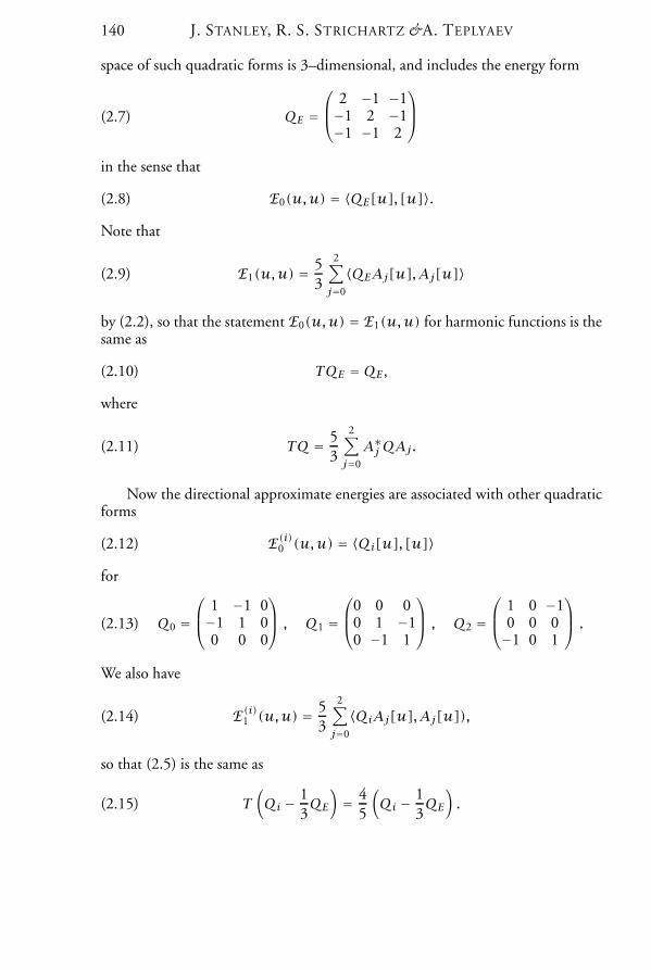
space of such quadratic forms is 3–dimensional, and includes the energy form
(2.7) QE = 2 −1 −1−1 2 −1−1 −1 2
in the sense that
(2.8) E0(u,u) = 〈QE[u], [u]〉.
Note that
(2.9) E1(u,u) = 53
2∑j=0
〈QEAj[u],Aj[u]〉
by (2.2), so that the statement E0(u,u) = E1(u,u) for harmonic functions is thesame as
(2.10) TQE = QE,
where
(2.11) TQ = 53
2∑j=0
A∗j QAj.
Now the directional approximate energies are associated with other quadraticforms
(2.12) E(i)0 (u,u) = 〈Qi[u], [u]〉
for
(2.13) Q0 = 1 −1 0−1 1 00 0 0
, Q1 =0 0 0
0 1 −10 −1 1
, Q2 = 1 0 −1
0 0 0−1 0 1
.We also have
(2.14) E(i)1 (u,u) = 53
2∑j=0
〈QiAj[u],Aj[u]),
so that (2.5) is the same as
(2.15) T(Qi − 1
3QE)= 4
5
(Qi − 1
3QE).
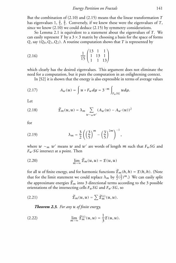
Energy Partition on Fractals 141
But the combination of (2.10) and (2.15) means that the linear transformation Thas eigenvalues 1, 4
5 , 45 . Conversely, if we knew these were the eigenvalues of T ,
since we know (2.10) we could deduce (2.15) by symmetry considerations.So Lemma 2.1 is equivalent to a statement about the eigenvalues of T . We
can easily represent T by a 3× 3 matrix by choosing a basis for the space of formsQ, say (Q0,Q1,Q2). A routine computation shows that T is represented by
(2.16)115
13 1 11 13 11 1 13
which clearly has the desired eigenvalues. This argument does not eliminate theneed for a computation, but it puts the computation in an enlightening context.
In [S2] it is shown that the energy is also expressible in terms of average values
(2.17) Aw(u) =∫u Fwdµ = 3−m
∫FwSG
udµ.
Let
(2.18) Em(u,u) = λm∑
w∼mw′(Aw(u)−Aw′(u))2
for
(2.19) λm = 32
((35
)m−(
35
)2m)−1
,
where w ∼m w′ means w and w′ are words of length m such that FwSG andFw′SG intersect at a point. Then
(2.20) limm→∞ Em(u,u) = E(u,u)
for all u of finite energy, and for harmonic functions Em(h,h) = E(h,h). (Notethat for the limit statement we could replace λm by 3
2(53)m.) We can easily split
the approximate energies Em into 3 directional terms according to the 3 possibleorientations of the intersecting cells FwSG and Fw′SG, so
(2.21) Em(u,u) =∑E(i)m (u,u).
Theorem 2.3. For any u of finite energy,
(2.22) limm→∞ E
(i)m (u,u) =
13E(u,u).
142 J. STANLEY, R. S. STRICHARTZ &A. TEPLYAEV
For harmonic functions, we have more precisely
(2.23) E(i)m (h,h)−13E(h,h) = 4m − 3m
5m − 3m· 2(E(i)1 (h,h)− 1
3E(h,h)).
Proof. As before it suffices to prove (2.23). Write
(2.24) E(i)m (h,h) =∑(Aw(h)−Aw′(h))2
where the sum extends over all pairs of adjacent cells in the i direction, so thatE(i)m (h,h) = λmE(i)m (h,h). The basic observation is that
(2.25) E(i)m (h,h) =2∑j=0
E(i)m−1(h Fj, h Fj)+ (A(i+1)im−1(h)−Ai(i+1)m−1(h))2
because all adjacent pairs belong to one FjSG except for the single pair contribut-ing the last term on the right in (2.25). Using the harmonic extension algorithmfor average values (2.12) in [S2] we find that the last term in (2.25) is just
(2.26)(
35
)2(m−1)E(i)1 (h,h).
This leads to the expectation that
(2.27) E(i)m (h,h) = bmE(i)1 (h,h)+ cm 425E(h,h)
for certain coefficients bm, cm to be determined, with b1 = 1, c1 = 0. Substi-tuting (2.27) into (2.25) and again using the harmonic extension algorithm foraverage values we find after some algebraic computations the recursion relations
bm = 1225bm−1 +
(35
)2(m−1),(2.28)
cm = 125bm−1 + 3
5cm−1 .(2.29)
The solution to these equations is
bm = 253
((1225
)m−(
35
)2m)
(2.30)
cm = 2518
((35
)m+(
35
)2m− 2
(1225
)m).(2.31)
Energy Partition on Fractals 143
Since E(i)m (h,h) = λmE(i)m (h,h), we find
(2.32) E(i)m (h,h)−13E(h,h) = 4m − 3m
5m − 3m
(252E(i)1 (h,h)− 2
3E(h,h)
)
by substituting (2.30) and (2.31) in (2.27) and simplifying. In particular
E(i)1 (h,h)− 13E(h,h) = 1
2
(252E(i)1 (h,h)− 2
3E(h,h)
)
when m = 1, so we obtain (2.23).
Note that the rate of convergence in (2.23) is asymptotically the same as in(1.6), as might be expected.
3. ENERGY FORMS ON SG WITH BILATERAL SYMMETRY
In this section we examine a family of examples depending on a parameter b in(0,∞). The underlying fractal is still SG, but the energy form varies. We want aself–similar identity
(3.1) E(u,u) =2∑j=0
1rjE(u Fj,u Fj)
but the weights rj are not all equal to 3/5. We will impose the bilateral symmetrycondition r1 = r2 to simplify the computations. The initial conductances definingE0 are also required to have this symmetry, so we may choose them as follows:
(3.2) E0(u,u) = (u(v0)−u(v1))2+ (u(v0)−u(v2))2+b(u(v1)−u(v2))2.
It is known ([Sa] or Exercise 3.1 of [Ki2]) that b > 0 determines r0 and r1 asfollows, where we introduce an additional parameter λ to simplify the expressions:
r0 = λr1 ,(3.3)
r1 = r2 = 1+ λ+ b1+ 2λ+ 2b
,(3.4)
3b2 + 2b = λ2 + 2λ2b + 2λb2 .(3.5)
These equations force the restriction
(3.6) 0 < λ < 3/2.
144 J. STANLEY, R. S. STRICHARTZ &A. TEPLYAEV
Notice that (3.5) is a quadratic equation in both b and λ, so we can solve in eitherdirection
λ = −b2 + √b(b + 1)(b2 + 5b + 2)1+ 2b
(3.7)
b = λ2 − 1+ √(λ2 − 1)2 + λ2(3− 2λ)3− 2λ
(3.8)
to eliminate one parameter.In view of (3.1) we define
(3.9) Em(u,u) =∑
|w|=mr−1w ((u(Fwv0)−u(Fwv1))2
+ (u(Fwv0)−u(Fwv2))2 + b(u(Fwv1)−u(Fwv2))2),
where rw = rw1 ·rw2 · · · rwm . A function that minimizes (3.9) for fixed boundaryvalues is called harmonic. The equations (3.3–5) imply that Em(u,u) is indepen-dent of m for harmonic functions, so Em(u,u) is monotone increasing for anyu, hence
(3.10) E(u,u) = limm→∞Em(u,u)
is well-defined, and (3.1) holds. Moreover, we have an extension algorithm of theform (2.2) for harmonic functions, where the matrices have the form
(3.11) A0 = 1 0 0B3 B5 B4B3 B4 B5
, A1 =B3 B5 B4
0 1 0B1 B2 B2
, A2 =B3 B4 B5B1 B2 B20 0 1
where
(3.12)
B1 = 11+ λ+ b + 2bλ
,
B2 = 12B1(λ+ b + 2bλ),
B3 = B1(1+ b), B4 = 12B1(λ+ 2bλ)− λ
2(2λ+ 1+ 2b),
B5 = 12B1(λ+ 2bλ)+ λ
2(2λ+ 1+ 2b).
It is natural to split the approximate energy directionally as follows:
(3.13)
E(0)m =∑
|w|=mr−1w (u(Fwv0)−u(Fwv1))2
E(1)m = b∑
|w|=mr−1w (u(Fwv1)−u(Fwv2))2
E(2)m =∑
|w|=mr−1w (u(Fwv0)−u(Fwv2))2
Energy Partition on Fractals 145
so that (1.3) still holds, and (1.5) will define directional energies if the limits exist.We will show this is the case, and (1.7) holds with a0 = a2 by symmetry. Todo this we follow the method outlined at the end of Section 2. Let T denote theoperator on quadratic forms
(3.14) TQ =2∑j=0
r−1j A∗j QAj.
We use the same basis (2.13) for the space of quadratic forms. Now
(3.15) QE = Q0 + bQ1 +Q2
and (2.10) continues to hold.
Lemma 3.1. The eigenvalues of T are 1, µ2, µ3 with
µ2 = 1+ 3b + 2b2 + 2λ+ 4λb1+ 4b + 4b2 + 2λ+ 4λb
(3.16)
µ3 = 1− b + 12
(1+ 2λ+ 2b)(1+ λ+ b) −(1+ 2λ+ 2b)(b + 1
2)(1+ λ+ b + 2λb)2(1+ λ+ b)(3.17)
with corresponding eigenvectors (1,1, b), (−1,1,0) and (1,1,−η) for
(3.18) η = 12+(b + 1
2
)(1+ λ+ b + 2λb
1+ 2λ+ 2b
)2
;
the notation here is that (x,y, z) represents the quadratic form
x(u(v0)−u(v1))2 +y(u(v0)−u(v2))2 + z(u(v1)−u(v2))2.
We have |µ2| < 1 and |µ3| < 1 (in fact 12 < µ2 < 1 and 0 < µ3 < 1).
Proof. We already know T(1,1, b) = (1,1, b). A direct calculation from(3.14) yields T(−1,1,0) = µ2(−1,1,0) with µ2 = r−1
0 (1 − B3)(B5 − B4)+r−1
1 (B3−B1(B5−B4)), and this simplifies to (3.16) using (3.3), (3.4), (3.5) and(3.12). Another direct calculation yields T(0,0,1) = r−1
1 (B21 , B
21 ,2B2(1 − B2) +
λ−1(B5 − B4)2). Thus the eigenvalue equation T(1,1,−η) = µ3(1,1,−η) can beexpressed as µ3(1,1,−η) = (1,1, b) − (b + η)T(0,0,1) and hence is equivalentto the system of equations
µ3 = 1− b + ηr1
B21(3.19)
−µ3η = b − b + ηr1(2B2(1− B2)+ λ−1(B5 − B4)2)(3.20)
146 J. STANLEY, R. S. STRICHARTZ &A. TEPLYAEV
for the unknowns η and µ3. We substitute (3.19) into (3.20) to eliminate µ3 andobtain a quadratic equation in η. But we know that η = −b is a solution, so wecancel the factor η+ b and obtain
η = B−21 (r1 − 2B2(1− B2)− λ−1(B5 − B4)2)
for the other solution, and this simplifies to (3.18). Substituting (3.18) in (3.19)yields (3.17).
It is obvious from (3.16) that 0 < µ2 < 1, and from (3.17) that µ3 < 1. Weobtain µ2 > 1
2 from (3.16) by writing
µ2 = 1− b + 2b2
1+ 4b + 4b2 + 2λ+ 4λb
and observing b + 2b2 < 12(1 + 4b + 4b2 + 2λ + 4λb). To show µ3 > 0 we
rearrange terms in (3.17) to reduce it to the inequality
(3.21)(b + 1
2
)[(1+ λ+ b + 2λb)2 + (1+ 2λ+ 2b)2]
< (1+ λ+ b)(1+ 2λ+ 2b)(1+ λ+ b + 2λb)2.
Now (3.21) is implied by
(b + 1
2
) [(1+ λ+ b + 2λb)2 + (1+ 2λ+ 2b)2]
< (1+ λ+ b)(2b + 1)(1+ λ+ b + 2λb)2
which is equivalent, after canceling the b + 12 factor, to
(1+ λ+ b + 2λb)2 + (1+ 2λ+ 2b)2 < (2+ 2λ+ 2b)(1+ λ+ b + 2λb)2
which is the same as
(1+ 2λ+ 2b)2 < (1+ 2λ+ 2b)(1+ λ+ b + 2λb)2
or
(1+ 2λ+ 2b) < (1+ λ+ b + 2λb)2,
which is obvious.There is another proof that µ3 > 0. Suppose for a moment µ3 ≤ 0. Let Q be
the eigenvector of T of the form (1,1,−η) and h be a symmetric harmonic func-tion with boundary values h(v1) = h(v2) = 0, h(v0) = 1. We will write Q(h)
Energy Partition on Fractals 147
for 〈Q[h], [h]〉). Then Q(h) = 2. By our assumption TQ(h) = µ3Q(h) ≤ 0.Clearly Q(h F0) > 0 and so Q(h F1) = Q(h F2) < 0. Then Q(h F1) < 0easily implies η > 1 since 0 = h F1(v1) < h F1(v2) < h F1(v0).
Let now h be a skew symmetric harmonic function with boundary valuesh(v1) = 1, h(v2) = −1, h(v0) = 0. Then Q(h) = 2 − 4η < 0 by the previousparagraph. By our assumption TQ(h) = µ3Q(h) ≥ 0. Clearly Q(hF0) < 0 andso Q(h F1) = Q(h F2) > 0. Let x = h F1(v0). We have 0 < x < 1 and soQ(h F1) = 1− 2x + 2x2 − η < 0. This is a contradiction and so µ3 > 0.
Note that µ2 → 1 as b → 0 (hence λ → 0) and µ3 → 1 as b → ∞ (henceλ → 3/2). This means that the rate of convergence of the directional energies totheir limits becomes extremely slow as we approach either extreme.
Theorem 3.2. For any function u of finite energy (3.10),
(3.22) limm→∞E
(j)m (u,u) = ajE(u,u)
for
(3.23)
a0 = b
η+ b =2b
2b + 1
(1+
(1+ λ+ b + 2λb
1+ 2λ+ 2b
)2)−1
,
a1 = a2 = η2(η+ b) .
Proof. We write (0,0, b) = a0(1,1, b) − a0(1,1,−η) for a0 = b/(η + b)hence Tm(0,0, b) → a0(1,1, b) as m → ∞. Similarly (1,0,0) = a1(1,1, b) +(a1b/η)(1,1,−η) − 1
2(−1,1,0) for a1 = η/2(η + b), hence Tm(1,0,0) →a1(1,1, b).
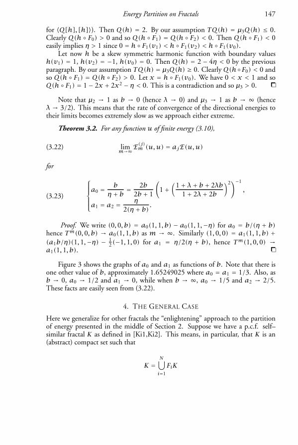
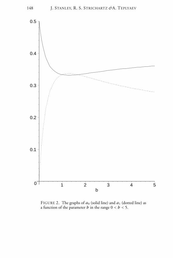
Figure 3 shows the graphs of a0 and a1 as functions of b. Note that there isone other value of b, approximately 1.65249025 where a0 = a1 = 1/3. Also, asb → 0, a0 → 1/2 and a1 → 0, while when b → ∞, a0 → 1/5 and a2 → 2/5.These facts are easily seen from (3.22).
4. THE GENERAL CASE
Here we generalize for other fractals the “enlightening” approach to the partitionof energy presented in the middle of Section 2. Suppose we have a p.c.f. self–similar fractal K as defined in [Ki1,Ki2]. This means, in particular, that K is an(abstract) compact set such that
K =N⋃i=1
FiK
148 J. STANLEY, R. S. STRICHARTZ &A. TEPLYAEV
0
0.1
0.2
0.3
0.4
0.5
1 2 3 4 5b
FIGURE 2. The graphs of a0 (solid line) and a1 (dotted line) asa function of the parameter b in the range 0 < b < 5.
Energy Partition on Fractals 149
where Fi are continuous injections, which are contractive in most examples, andthere is a finite subset ∂K = V0 = v1, . . . , vN0, called the boundary of K, suchthat
FwK ∩ Fw′K ⊆ FwV0 ∩ Fw′V0
for Fw and Fw′ distinct.Suppose also that we have a local regular self–similar Dirichlet form E on K.
This means, similarly to (1.1) and (1.2), that
(4.1) E(u,u) = limm→∞Em(u,u)
where
E0(u,u) =∑j≠k
cjk(u(vj)−u(vk))2(4.2)
Em(u,u) =∑
|w|=mr−1w E0(u Fw,u Fw)(4.3)
for a choice of rj ∈ (0,1) with the “decimation property” that Em(u,u) is inde-pendent of m for harmonic functions (energy minimizers given the N0 boundaryvalues on V0). The self–similar identity
E(u,u) =N∑j=1
r−1j E(u Fj,u Fj)
is then an immediate consequence of (4.1) and (4.3). We assume cjk ≥ 0 andE0(u,u) > 0 unless u is constant on V0.
It is still not known in general under what conditions such a Dirichlet form ex-ists, but there are sufficient conditions and numerous examples (see [Ki1, Ki2, M1,M2, Sa] and references therein). It should be noted that the choice of the conduc-tance coefficients cjk and the energy ratios rj is a very delicate matter.
Let A1, . . . , AN denote the harmonic extension matrices, so that
u∣∣FiV0
= Aiu∣∣V0
for any harmonic function u. These matrices are obtained by solving the systemof linear equations
N∑i=1
∑j≠k
r−1i cjk(u(Fivj)−u(Fivk)) = 0.
The constant vector is invariant under all the matrices Ai, and we need to factorout this trivial common eigenvector. Let W0 denote the space of functions on V0,
150 J. STANLEY, R. S. STRICHARTZ &A. TEPLYAEV
let W denote the quotient space of W0 modulo constants, and let Mi denote theinduced action of Ai on W . Note that W is a vector space of dimension N0 − 1,and we could represent Mi by a matrix of size (N0 − 1)× (N0 − 1) by choosing abasis for W . Let Mw = Mw1 Mw2 · · · Mwm .
Hypothesis 4.1. Assume the following span–irreducibility condition:
(4.4)For every nonzero x ∈ W there exists m ≥ 1 such thatthe span of Mwx|w|=m is all of W .
Note that routine compactness arguments show that we can find a single mfor all x. Also note that the span–irreducibility condition implies thatM1, . . . ,MNare irreducible (they do not have a proper common invariant subspace), but theconverse is not true in general.
Lemma 4.2. Condition (4.4) holds if there is no proper subspace ofW invariantunder all Mi, and there is at least one point v ∈ V0 which is fixed by one of the mapsFi.
Proof. Suppose Fi(v) = v. Consider the subspace of harmonic functionsthat vanish at v. This subspace is invariant under Ai, and all the entries of Airestricted to this subspace are nonnegative, with at least one positive. Note thatthis subspace can be naturally identified with W . Then, by the Perron–FrobeniusTheorem, there is a positive eigenvalue λ of Mi such that |λ′| < λ < 1 for anyother eigenvalue λ′ of Mi. Let Wλ be the eigenspace of Mi corresponding to λ(there is no nondiagonal Jordan block corresponding to λ).
If x ∈ Wλ, then the spacesWm = Span Mwx|w|=m are increasing and so wehave Wm = W for somem ≤ N0−1, since there are no proper common invariantsubspaces. So (4.4) holds with m = N0 − 1 for x ∈ Wλ.
For a general nonzero vector x ∈ W , let W ′ = Closure⋃m≥0Wm, where Wm
is as in the previous paragraph. Then Span W ′ = W since there are no properinvariant subspaces. Also if y ∈ W ′ then for all j we have
limm→∞
Mmj y
‖Mmj y‖
∈ W ′.
Then it is easy to see that W ′ ∩ Wλ ≠ 0. A simple continuity argument implies(4.4).
The energy form (4.2) can be regarded as a symmetric bilinear form on W0annihilating constants, as can its directional components
E(jk)0 (u,u) = cjk(u(vj)−u(vk))2.
We can reduce from W0 to W and express these as nonnegative quadratic formsQE and Qjk satisfying
QE =∑j≠k
Qjk.
Energy Partition on Fractals 151
We define approximate directional energies by
E(jk)m (u,u) =∑
|w|=mr−1w E(jk)0 (u Fw,u Fw)
and directional energies
(4.5) E(jk)(u,u) = limm→∞E
(jk)m (u,u)
if the limit exists (similarly to (1.5)). Then the analog of Theorem 2.2 is as follows.
Theorem 4.3. Under Hypothesis 4.1, the limits (4.5) exist and there exist positiveconstants αjk such that
E(jk)(u,u) = αjkE(u,u)
for all functions u of finite energy.
We define an operator T on quadratic forms on W by
(4.6) TQ =N∑j=1
r−1j M∗
j QMj.
Then the decimation property that Em(u,u) is independent for m when u isharmonic is equivalent to
(4.7) TQE = QE.
Theorem 4.3 follows from the next lemma by the same proof as Theorem 2.2.
Lemma 4.4. Under Hypothesis 4.1, there exist positive constants αjk such that
limm→∞T
mQjk = αjkQE.
Lemma 4.4 follows from Theorem 4.6, which is a special case of a kind ofPerron–Frobenius Theorem for operators of the form (4.6). We begin with asimple result of Kusuoka [Ku].
Proposition 4.5. If T is an operator of the form (4.6) for M1, . . . ,MN irre-ducible, then there is a unique non–negative definite eigenvector. Moreover the eigen-vector is positive definite and the eigenvalue is positive.
Without loss of generality we may assume the eigenvalue is 1, and we denotethe eigenvector by QE to conform to (4.7). The next theorem is not new and canbe deduced from different generalizations of the Perron–Frobenius Theorem. Wegive a concise proof here for the sake of completeness.
152 J. STANLEY, R. S. STRICHARTZ &A. TEPLYAEV
Theorem 4.6. IfM1, . . . ,MN satisfy the span–irreducibility condition (4.4), then1 is a simple eigenvalue of T and every other eigenvalue λ satisfies |λ| < 1. Moreover,for any nonzero Q that is nonnegative definite there exists a positive constant α(Q)such that
(4.8) limm→∞T
m(Q) = α(Q)QE.
Proof. We will writeA > B (A ≥ B) ifA−B is positive–definite (nonnegative–definite) matrix. Because QE > 0 by Proposition 4.5, for any real Q there existsa constant c such that Q ≤ cQE , hence TmQ ≤ cQE for any m. Thus T cannothave an eigenvalue λ with |λ| > 1, nor a nondiagonal Jordan block correspondingto an eigenvalue with |λ| = 1. This does not use (4.4).
Without loss of generality (pass to a power of T ) we may assume that m = 1in (4.4). We claim that for any nonzero symmetric Q satisfying Q ≥ 0 we haveTQ > 0. Indeed, for any x ≠ 0,
〈TQx,x〉 =N∑j=1
r−1j 〈QMjx,Mjx〉 > 0
because Mjx spans the whole space.Suppose TQλ = λQλ with |λ| = 1 and Qλ is not a multiple of QE . Denote
by Qλ the matrix whose entries are complex adjoint of the entries of Qλ. ThenQλ+Qλ is real and we can assume it is not nonpositive. SinceQE−α(Qλ+Qλ) ≥0 for α small enough, we may define ε so thatQE−ε(Qλ+Qλ) ≥ 0 and ε achievesthe maximum value subject to this condition.
Then T(QE − ε(Qλ +Qλ)) > 0 by the claim, hence we have
QE − ε(λQλ + λQλ) ≥ δQE
for some δ > 0, and more generally
QE − ε(λnQλ + λnQλ) ≥ δQE
for any n ≥ 1. By choosing n so that λn is sufficiently close to 1 we contradictthe maximality of |ε|.
Finally, if Q ≥ 0 is nonzero then there is δ > 0 such TnQ > δQE for alln ≥ 1. Thus we can write Q as a linear combination of eigenvectors and associ-ated eigenvectors of T where the coefficient α(Q) of QE is positive. This yields(4.8).
Theorem 4.7. For a given set of positive energy weights rj there exists at mostone, up to a constant multiple, local regular self–similar Dirichlet form provided thespan–irreducibility condition (4.4) is satisfied for at least one such form.
Energy Partition on Fractals 153
Proof. Let E and E′ be two such Dirichlet forms, and QE and Q′E be thecorresponding quadratic forms. Suppose that (4.4) is satisfied for E, and defineT in terms of E. Then Theorem 4.6 implies that limm→∞ Tm(Q′E) = αQE.Hence for any piecewise E–harmonic function f we have E′(f , f ) = αE(f , f ).Since piecewise harmonic functions are dense in C(K) (see [Ki1,Ki2]), we haveE′ = αE.
4.8. Remark. Results similar to Theorems 4.6 and 4.7 have appeared in theliterature several times, for example in [P]. These theorems give so called “exis-tence implies stability implies uniqueness” arguments provided some irreducibil-ity conditions hold. Our approach is somewhat simpler and more straightforward,although the absence of invariant subspaces may be difficult to verify in some sit-uations. We do not require that K ⊂ Rn with Fi linear contractions, but thisassumption may not be crucial anyway. Perhaps it is more important that we donot require that every point of V0 is a fixed point of some Fi (so called “essentialfixed points”). We will abbreviate this condition as the EFP condition. Below wegive a simple example where this condition is not satisfied, and there are manymore examples.
There is an important relation of our work to the existence and uniquenessresults by V. Metz [M1,M2] and C. Sabot [Sa] (see also references in these papers).Namely, the map T is the derivative atQE of a nonlinear renormalization operator,usually called Fr or Λ, for which QE is a fixed point (see [Ki1,Ki2,M1,M2,Sa]).It is shown in [M2] that the uniqueness holds if for any nonzero Q ≥ 0 we haveTnQ > 0 for large enough n. It is easy to see that this is equivalent to our span–irreducibility condition (4.4). However the condition TnQ > 0 is difficult toverify mainly because the cone of nonnegative operators is more difficult to char-acterize in the context of fractals than the cone of Dirichlet forms. So [M2] alsocontains a very useful uniqueness condition in terms of Dirichlet forms. However[M2] assumes the EFP condition, and it is not clear how crucial this condition isto the results there.
The span–irreducibility condition (4.4) is similar to the conditions studied in[KK] under the EFP condition. If Fi has a fixed point v in V0, then Ai has at leastone Perron–Frobenius eigenvector that vanishes at v, as described in the proofof Lemma 4.2. Denote the collection of these eigenvectors for all i by IPF . Byfactoring out constants, we may assume that IPF ⊂ W . The assumptions in [KK]included some symmetry assumptions and that Span IPF = W . The followinglemma is easy to prove similarly to Lemma 4.2.
Lemma 4.8. Suppose Span IPF = W . Condition (4.4) holds if, for any subsetI′PF of IPF , Span I′PF is not invariant under all Mi unless Span I′PF = W .
It is easy to see that in the well known example of the Vicsek set we haveSpan IPF = W but the span–irreducibility fails, as does the energy partition result.It is known from the works of V. Metz that the self–similar Dirichlet form is not
154 J. STANLEY, R. S. STRICHARTZ &A. TEPLYAEV
unique in this case. Below we gave an example (without the EPF condition) wherethe span–irreducibility, and hence the uniqueness and energy partition, hold.
v1 v2
v3
................................................................................................................................
................................................
....................................................................
............
................................................................................................ ....................................................................................
............
................................................................
................................................
....................................................................
............
................
................................................
................................................
................
................................................................................................................................
................................................
....................................................................
............
................................................................................................ ....................................................................................
............
................................................................
................................ ................................................................ ................................ ................................................................................................ ................................
................................................................................................................................
................................................
....................................................................
............
................................................................................................ ....................................................................................
............
................................................................
................................................
....................................................................
............
................
................................................
................................................
................
................................................................................................................................
................................................
....................................................................
............
................
................................................
................................................
................................................................................ ................
................................................
................................................
....................................................................
............
................
................................................
................................................
................
................................................................................................................................
................................................
....................................................................
............
................................................................................................ ....................................................................................
............
................................................................
................................................
....................................................................
............
................
................................................
................................................
................
................................................................................................................................
................................................
....................................................................
............
................................................................................................ ....................................................................................
............
................................................................
................................ ................................................................ ................................ ................................................................................................ ................................
................................................................................................................................
................................................
....................................................................
............
................................................................................................ ....................................................................................
............
................................................................
................................ ................................................................ ................................ ................................................................................................ ................................
................................ ................................................................................................................................ ................................
................................ ................................ ................................................................................................ ....................................................................................
............
................................................................
................................ ................................................................ ................................ ................................................................................................ ................................
................................................................................................................................
................................................
....................................................................
............
................................................................................................ ....................................................................................
............
................................................................
................................................
....................................................................
............
................
................................................
................................................
................
................................................................................................................................
................................................
....................................................................
............
................................................................................................ ....................................................................................
............
................................................................
................................ ................................................................ ................................ ................................................................................................ ................................
................................................................................................................................
................................................
....................................................................
............
................................................................................................ ....................................................................................
............
................................................................
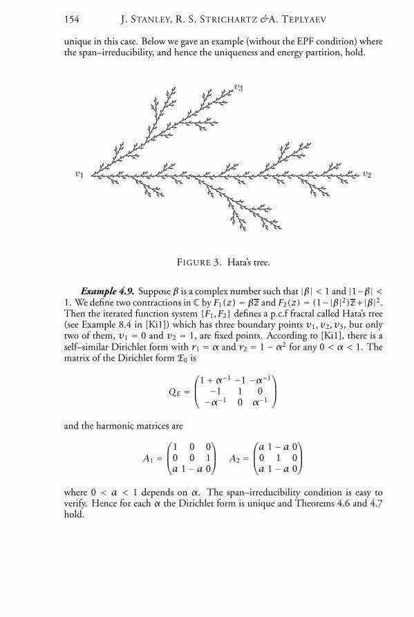
FIGURE 3. Hata’s tree.
Example 4.9. Suppose β is a complex number such that |β| < 1 and |1−β| <1. We define two contractions in C by F1(z) = βz and F2(z) = (1−|β|2)z+|β|2.Then the iterated function system F1, F2 defines a p.c.f fractal called Hata’s tree(see Example 8.4 in [Ki1]) which has three boundary points v1, v2, v3, but onlytwo of them, v1 = 0 and v2 = 1, are fixed points. According to [Ki1], there is aself–similar Dirichlet form with r1 = α and r2 = 1− α2 for any 0 < α < 1. Thematrix of the Dirichlet form E0 is
QE =1+α−1 −1 −α−1
−1 1 0−α−1 0 α−1
and the harmonic matrices are
A1 =1 0 0
0 0 1a 1− a 0
A2 =a 1− a 0
0 1 0a 1− a 0
where 0 < a < 1 depends on α. The span–irreducibility condition is easy toverify. Hence for each α the Dirichlet form is unique and Theorems 4.6 and 4.7hold.
Energy Partition on Fractals 155
Acknowledgements. We are grateful to the anonymous referee for several im-portant suggestions. We thank V. Metz for interesting and helpful discussionsduring the preparation of this article.
REFERENCES
[BST] O. BEN–BASSAT, R. STRICHARTZ, AND A. TEPLYAEV, What is not in the domain of theLaplacian on a Sierpinski gasket type fractal, J. Functional Anal. 166 (1999), 197–217.
[Ki1] J. KIGAMI, Harmonic calculus on p.c.f. self-similar sets, Trans. Amer. Math. Soc. 335 (1993),721–755.
[Ki2] J. KIGAMI, Analysis on Fractals, Cambridge Tracts in Mathematics, Vol. 143. CambridgeUniversity Press, Cambridge, 2001. .
[KK] T. KUMAGAI AND S. KUSUOKA, Homogenization on nested fractals, Probab. Theory RelatedFields 104 (1996), 375–398.
[Ku] S. KUSUOKA, Dirichlet forms on fractals and products of random matrices, Publ. Res. Inst.Math. Sci. 25 (1989), 659–680.
[M1] V. METZ, Renormalization contracts on nested fractals, J. Reine Angew. Math. 480 (1996),161–175.
[M2] V. METZ, The cone of diffusions on finitely ramified fractals, Preprint.[P] R. PEIRONE, Convergence and uniqueness problems for Dirichlet forms on fractals., Boll.
Unione Mat. Ital. Sez. B Artic. Ric. Mat. (8) 3 (2000), 431–460.[Sa] C. SABOT, Existence and uniqueness of diffusions on finitely ramified self–similar fractals, Ann.
Sci. Ecole Norm. Sup (4) 30 (1997), 605–673.[S1] R. S. STRICHARTZ, Analysis on fractals, Notices Amer. Math. Soc. 46 (1999), 1199–1208.[S2] R. S. STRICHARTZ, The Laplacian on the Sierpinski gasket via the method of averages, Pacific
J. Math. 201 (2001), 241–256.[SU] R. S. STRICHARTZ AND M. USHER, Splines on fractals, Math. Proc. Camb. Phil. Soc. 129
(2000), 331–360.
JEREMY STANLEY:Ernst & Young L.L.P.5 Times SquareNew York, NY 10036–6530
and
Mathematics DepartmentWichita State UniversityWichita, KS 67204, U.S.A.E-MAIL: [email protected]: Research supported by the National Science Foundation through the Re-search Experiences for Undergraduates program at Cornell University.
156 J. STANLEY, R. S. STRICHARTZ &A. TEPLYAEV
ROBERT S. STRICHARTZ:Mathematics DepartmentMalott HallCornell UniversityIthaca, NY 14853, U.S.A.E-MAIL: [email protected]: Research supported in part by the National Science Foundation, Grant DMS9970337.
ALEXANDER TEPLYAEV:Department of MathematicsUniversity of ConnecticutStorrs CT 06269, U.S.A.
and
Mathematics DepartmentUniversity of CaliforniaRiverside, CA 92521, U.S.A.E-MAIL: [email protected]: Reseach supported by the National Science Foundation through a Mathe-matical Sciences Postdoctoral Fellowship.
KEY WORDS AND PHRASES: fractals; Sierpinski gasket; energy partition; Dirichlet form.
2000 MATHEMATICS SUBJECT CLASSIFICATION: Primary 31C45, 28A80.Received : October 30th, 2000; revised: July 8th, 2002.