Energy Resource Recovery Account (ERRA) 2018 … ERRA Resource Recovery Account (ERRA) 2018 Forecast of Operations Table Of Contents (Continued) Section Page Witness ii E. SCE’s

Application No.: A.17-05-XXX

Exhibit No.: SCE-1 Witnesses: S. DiBernardo S. Liu E. Martinez T. Cameron E. Lavik R. Thomas D. Cox K. Seeto S. Lelewer M. Sheriff R. Hite D. Wong A. Wong

(U 338-E)

Energy Resource Recovery Account (ERRA)

2018 Forecast of Operations

Public Version

Before the

Public Utilities Commission of the State of California

Rosemead, California

May 1, 2017

SCE-1: ERRA Resource Recovery Account (ERRA) 2018 Forecast of Operations

Table Of Contents

Section Page Witness

-i-

I. INTRODUCTION .............................................................................................1 S. DiBernardo

II. 2018 ERRA FORECAST PROCEEDING REVIEW REQUIREMENT ...............................................................................................4

A. 2018 ERRA Forecast Proceeding Revenue Requirement ......................4

1. Functionalized ERRA-Related Revenue Requirement ..............5

a) ERRA-Related Generation Service Revenue Requirement ...................................................................6

III. SCE’S BUNDLED ENERGY FORECAST ......................................................8 E. Martinez

A. Retail Sales Forecast Summary .............................................................8

B. Methodology ..........................................................................................9

C. Historical Trends ..................................................................................10

D. Economic Outlook ...............................................................................12

E. Weather Assumptions ..........................................................................13

F. Other Factors Influencing the Forecast ................................................14

G. Total Retail Sales Forecast by Customer Class ...................................15

H. Customer Forecast ...............................................................................16

I. Annual and Monthly Bundled Energy .................................................17

IV. FORECAST ENERGY PRODUCTION AND COSTS FROM SCE’S PORTFOLIO OF RESOURCES .........................................................19 E. Lavik

A. Introduction ..........................................................................................19

B. Energy Production Forecast Methodology ..........................................19

C. Validation of SCE’s Energy Production Forecast ...............................21

D. 2018 Energy and Cost Forecast Summary ...........................................22


Table Of Contents (Continued)


ii

E. SCE’s Utility-Owned Generation and Purchased Power Contracts ..............................................................................................26

1. Hydro Facilities ........................................................................26

2. SCE Solar Photovoltaic Generation .........................................27

3. CHP and Renewables ...............................................................28

a) Energy Forecast ...........................................................28

b) Payment Forecast .........................................................29

c) Energy and Capacity Prices .........................................29

4. Utility-Owned Natural Gas Facilities ......................................30

a) SCE Peakers .................................................................30

(1) Background and Production .............................30

(2) Costs .................................................................30

b) Mountainview Generating Station ...............................30

5. Interutility Contracts Production ..............................................31 D. Cox

a) WAPA-Reclamation Agreement .................................32

b) Pasadena Corporation Grant Deed ...............................33

c) Interutility Contract Resource Costs ............................34

6. New System Generation CAM Contracts ................................34 E. Lavik

a) Production ....................................................................34

b) Costs .............................................................................34

7. 2013 Bilateral Contracts Production ........................................34

a) Production ....................................................................34

b) Costs .............................................................................35




iii

8. Generic and Bilateral RA Contracts ........................................35

a) Production ....................................................................35

9. Local Capacity Requirements (LCR) Contracts ......................35

a) Production ....................................................................36

b) Costs .............................................................................36

10. Preferred Resource Pilot (PRP) ...............................................36

a) Production ....................................................................36

b) Costs .............................................................................36

11. Green Tariff Shared Renewables (GTSR) Program ................37

F. Other SCE Resources and Programs....................................................38 S. Lelewer

1. Nuclear .....................................................................................38

a) Production ....................................................................38

b) Costs .............................................................................38

(1) Introduction ......................................................38

(2) Nuclear Fuel Management ...............................39

(3) SONGS Nuclear Fuel Expense ........................39

(a) Fuel Expense – Generation Related .................................................39

(i) Permanent Disposition of Used Fuel .............................39

(b) Other Costs – Non-Generation-Related .................................................40

(i) Interim Storage.........................40

(4) PVNGS Nuclear Fuel Expense ........................40




iv

(a) Fuel Expense – Generation Related .................................................40

(i) PVNGS Unit 1 .........................40

(ii) PVNGS Unit 2 .........................41

(iii) PVNGS Unit 3 .........................41

(iv) Permanent Disposition of Used Fuel .............................41

(b) Other Costs – Non-Generation-Related .................................................42

(i) Interim Storage.........................42

2. Catalina Fuel Costs ..................................................................42 R. Hite

3. Demand Response ...................................................................44 A. Wong

G. CAISO Costs and Short-Term Market Activity ..................................45 E. Lavik

1. CAISO Costs ............................................................................45

2. Short-Term Market Activity Costs ..........................................46

H. Gas Price Sensitivity ............................................................................46

I. Direct GHG Costs ................................................................................47

J. Gas Hedging Costs ..............................................................................47 S. Liu

1. Transaction Fees ......................................................................47

2. Option Premiums .....................................................................47

K. Gas Transportation and Storage ..........................................................47 D. Cox

1. Transportation ..........................................................................48

a) SoCalGas Transportation Agreement for Mountainview Generating Station ...............................48




v

b) SoCalGas Transportation Agreements for UCSB and CSUSB .......................................................48

c) SoCalGas Transportation Agreements for SCE Peakers .........................................................................48

V. FINANCING COSTS .....................................................................................50 T. Cameron

A. Commission Decisions Regarding Financing Costs and Collateral Costs ....................................................................................50

B. SCE’s Current Short-Term Financings ................................................50

1. Credit Facilities (Revolvers) ....................................................50

2. Collateral Requirements ...........................................................51

3. Fixed Rate Bonds Supporting Fuel Inventories .......................52

4. Commercial Paper ....................................................................52

5. Costs of Collateral Issuance .....................................................53

C. Additional Options Supporting Collateral ...........................................53

VI. CARRYING COSTS .......................................................................................54

A. Fuel Inventory Carrying Costs .............................................................54

B. GHG Compliance Carrying Costs .......................................................55

C. Collateral Carrying Costs .....................................................................55

VII. GHG FORECAST COSTS AND REVENUES AND RECONCILIATION .......................................................................................57 M. Sheriff

A. Overview ..............................................................................................57

B. 2018 Cap-and-Trade Costs and Reconciliation of Prior Period GHG Costs ..........................................................................................58 K. Seeto

1. Sources of GHG Costs .............................................................59

a) Direct Costs ..................................................................59




vi

(1) Compliance Costs ............................................59

(2) Procurement Contract Costs ............................60

b) Indirect Costs ...............................................................60

(1) QF Contract Costs ............................................60

(2) Market Purchase Costs .....................................61

2. GHG Emissions Volume Forecast Methodology ....................61

a) GHG Emissions Associated with Direct Costs ............61

(1) GHG Emissions Associated with Compliance Exposure ......................................62

(2) GHG Emissions Associated with Procurement Contracts .....................................63

b) GHG Emissions Associated with Indirect Costs .............................................................................63

(1) GHG Emissions Associated with QF Contracts ..........................................................63

(2) GHG Emissions Associated with In-State Market Purchases of Electricity ..............64

c) Forecast of 2018 GHG Emissions Volumes ................65

3. GHG Emissions Price Forecast Methodology .........................65

4. SCE’s Forecast 2018 GHG Costs ............................................66

5. Reconciliation of Prior Period GHG Costs ..............................66

C. 2018 Administrative and Customer Outreach Costs Forecast and Prior Period Reconciliation ...........................................................71 M. Sheriff

1. Reconciliation of Prior Period Administrative and Customer Outreach Costs ........................................................71

D. 2018 GHG Allowance Revenue Forecast ............................................72 K. Seeto




vii

1. Amortization and Reconciliation of Prior Period GHG Allowance Revenues ................................................................73

E. 2018 Proposed GHG Revenue Return .................................................74 M. Sheriff

1. Expected December 31, 2017 GHGRBA Balance and Prior Period Revenue Return True-Up ....................................76

2. 2018 GHG Cost and Revenue Distribution for EITE and Volumetric Returns ...........................................................78 R. Thomas

3. 2018 Residential California Climate Credit .............................80

4. GHG Costs and Revenues by Rate Schedule ...........................81

VIII. 2018 FORECAST REVENUE REQUIREMENT AND RATEMAKING PROPOSAL ........................................................................82 S. DiBernardo

A. Introduction ..........................................................................................82

B. Estimated 2018 ERRA-Related Generation Service Revenue Requirement .........................................................................................83

1. Estimated 2018 Fuel and Purchased Power Revenue Requirement .............................................................................83

a) Fuel Expense ................................................................85

b) Purchased Power Expense ...........................................85

2. Estimated December 31, 2017 ERRA Balance ........................86

3. Estimated Energy Settlement Refunds and Litigation Costs .........................................................................................87

C. Estimated 2018 ERRA-Related Delivery Service Revenue Requirement .........................................................................................87

1. Estimated New System Generation Net Capacity CAM-Related Cost...................................................................88

a) Introduction ..................................................................88

b) 2018 CAM Eligible Costs ............................................89




viii

2. Estimated December 31, 2017 NSGBA Balancing Account ....................................................................................90

3. Estimated 2018 Spent Nuclear Fuel Revenue Requirement .............................................................................91

IX. DIRECT ACCESS, DEPARTING LOAD AND COMMUNITY CHOICE AGGREGATION COST RESPONSIBILITY SURCHARGES ..............................................................................................92 D. Wong

A. Background ..........................................................................................93

B. Total Portfolio Costs ............................................................................94

C. 2018 Market Price Benchmark ............................................................95

X. PRESENT RATE REVENUE ........................................................................98 R. Thomas

Appendix A Estimated December 31, 2017 Balancing Account Balances

Appendix B Indifference Rate Calculation


List Of Tables

Table Page

-ix-

Table II-1 Estimated 2018 ERRA Forecast Revenue Requirement Changes ($000) ..................................4

Table II-2 2018 ERRA Forecast Proceeding Revenue Requirement Changes ($

thousands) ..............................................................................................................................................6

Table III-3 2018 Bundled Customer Load Forecast (GWh) ........................................................................9

Table III-4 Annual Retail Sales by Customer Class (GWh) ......................................................................16

Table III-5 Year-End Customers by Customer Class ................................................................................16

Table III-6 Bundled Energy at CAISO (GWh) ..........................................................................................18

Table IV-7 2018 Energy Forecast of the SCE Portfolio (GWh) Confidential ...........................................23

Table IV-8 2018 Forecast of Fuel and Purchased Power Costs ($000) Confidential ................................24

Table IV-9 2018 Forecast of SCE SPVP Production (GWh) ....................................................................27

Table IV-10 Annual Capacity Factors by Technology ..............................................................................29

Table IV-11 2018 Forecast of Posted Energy and Capacity Prices ...........................................................30

Table IV-12 Non-Coincident Contract Capacity Quantities and Expiration Dates for

SCE’s Major Interutility Contracts ......................................................................................................31

Table IV-13 SCE Entitlement to Hoover Dam Electrical Output for Year 2017 Source:

Bureau of Reclamation - CRSR 3/2016 Most Probable Inflow ...........................................................33

Table IV-14 Projected 2018 Forecast Period Nuclear Fuel Expense (Thousands of Dollars

– SCE’s Share) .....................................................................................................................................42

Table IV-15 Catalina Diesel Fuel 2018 Forecast Delivered Diesel Cost (2016-2017

Recorded) .............................................................................................................................................43

Table IV-16 2018 Forecast Delivered Propane Cost (MTs) (2016-2017 Recorded) .................................44

Table VI-17 Estimate of 2018 Carrying Costs ($000) ...............................................................................54

Table VI-18 Estimated 2018 Fuel Inventory Carrying Costs ($000) ........................................................55


List Of Tables (Continued)

Table Page

-x-

Table VI-19 Estimated 2018 GHG Compliance Carrying Costs ($000) ...................................................55

Table VI-20 Estimated 2018 Procurement Collateral Carrying Costs ($000) ...........................................56

Table VII-21 SCE’s Forecast of 2018 GHG Emissions Volumes (Metric Tons CO2e) ..........................65

Table VII-22 SCE’s Forecast of 2018 GHG Costs ($000) ........................................................................66

Table VII-23 Annual GHG Emissions and Associated Costs (Template D-2) ........................................67

Table VII-24 Weighted Average Cost of GHG Compliance Instruments Calculation

(Template C-1) .....................................................................................................................................70

Table VII-25 Detail of Outreach and Administrative Expenses (Template D-3) .....................................72

Table VII-26 SCE’s 2018 Forecast Consignment in ARB Auctions (Metric Tons CO2e .........................73

Table VII-27 SCE’s Forecast 2018 Allowance Revenue ($000) ..............................................................73

Table VII-28 SCE’s Recorded/Forecast 2017 Allowance Revenue ..........................................................74

Table VII-29 SCE’s 2018 Proposed GHG Revenue Returns ....................................................................76

Table VII-30 Annual Allowance Revenue Receipts and Customer Returns (Template D-

1) ..........................................................................................................................................................78

Table VII-31 GHG Allowance Revenue Allocation by Class ...................................................................80

Table VII-32 GHG Costs and Revenues by Rate Schedule (Template D-4) .............................................81

Table VII-33 History of GHG Revenues, Costs, and Emissions Intensity (Template D-5) ......................81

Table VIII-34 Estimated 2018 ERRA Forecast Proceeding Revenue Requirement ($000) ......................82

Table VIII-35 Estimated 2018 Fuel and Purchased Power Revenue Requirement ($000) .......................84

Table VIII-36 2018 Estimated Fuel Expense ($000) .................................................................................85

Table VIII-37 Estimated 2018 Purchased Power Expense ($000) ............................................................86

Table VIII-38 CAM Applicable Resources ...............................................................................................89

Table VIII-39 Estimated 2018 CAM-Related Revenue Requirement ($000) ...........................................90

Table VIII-40 Estimated 2018 Spent Nuclear Fuel Revenue Requirement ($000) ...................................91


List Of Tables (Continued)

Table Page

-xi-

Table IX-41 Comparison of MPBs Over Time..........................................................................................97

Table X-42 SCE 2018 ERRA Forecast Class Average Rates ....................................................................98

Table X-43 Average Generation Rates ......................................................................................................99


List Of Figures

Figure Page

-xii-

Figure III-1 Total Non-Farm Employment Growth in the Counties Served by SCE 2006

to 2016 .................................................................................................................................................11

Figure III-2 Residential Housing Starts in Counties Served by SCE ........................................................12

Figure III-3 Total Non-Farm Employment Growth in SCE Service Area Actual and

Forecast ................................................................................................................................................13

Figure III-4 Recorded and Forecast Cooling Degree Days .......................................................................14

Figure III-5 Average System Electricity Rates, Actual and Forecast ........................................................15

1

I. 1

INTRODUCTION 2

Southern California Edison Company (SCE or Company) files this annual Energy Resource 3

Recovery Account (ERRA) Forecast application to request the Commission to authorize SCE’s 2018 4

ERRA Forecast proceeding revenue requirement in the amount of $4.183 billion. The Commission has 5

established this process for the review and approval of SCE’s forecast of fuel and purchased power 6

expenses for the purpose of setting rates.1 The 2018 ERRA Proceeding revenue requirement forecast of 7

$4.183 billion is supported in the following chapters of this testimony, and is based on SCE’s best 8

estimate of such factors as kWh sales and load, natural gas and power prices, and an estimate of the 9

December 31, 2017 balancing account balances included in this revenue requirement.2 The forecast 10

adopted by the Commission in this proceeding does not determine which procurement-related costs are 11

ultimately eligible for cost recovery, as the actual fuel and purchased power costs must be reviewed by 12

the Commission and found eligible for recovery in a subsequent ERRA Review proceeding or Quarterly 13

Compliance Report (QCR) determination. Consistent with past ERRA Forecast applications, SCE will 14

update its 2018 ERRA Forecast proceeding revenue requirement forecast in November 2017, so that the 15

latest forecast assumptions can be incorporated into SCE’s 2018 rates. 16

As directed by the Commission’s Phase 2 Decision Adopting Standard Procedures for Electric 17

Utilities to File Greenhouse Gas (GHG) Forecast Revenue and Reconciliation (FR&R) Requests (D.14-18

10-033), issued in A.13-08-002 et al., dated October 16, 2014, the investor-owned utilities (IOUs) are to 19

include their Greenhouse Gas (GHG) revenue and reconciliation requests as an additional chapter or 20

section within the annual ERRA Forecast applications.3 In this Application, SCE proposes to return a 21

1 Decision (D.) 04-01-050 and D.04-01-048, and as modified by D.04-03-023.

2 Pursuant to SCE’s 2015 ERRA Forecast D.15-10-037, SCE is including only the ERRA Balancing Account, the Energy Settlements Memorandum Account (ESMA)/Litigation Costs Tracking Account (LCTA) and the New System Generation Balancing Account (NSGBA) forecast year-end 2017 balances in the 2018 ERRA Forecast revenue requirement.

3 D.14-10-033, Ordering Paragraph (OP) 10.

2

total of $373.3 million in GHG allowance revenues to eligible customers in 2018 based on the 1

Commission-adopted methodologies and utilizing GHG revenues and cap-and-trade costs, including 2

administrative and customer outreach costs, as proposed and supported in this testimony. Based on 3

SCE’s estimated GHG allowance revenues available for return to eligible customers in 2018, residential 4

customers can expect a semi-annual, on-bill California Climate Credit of $36.00 in 2018. 5

A discussion of SCE’s estimated 2018 ERRA Forecast proceeding revenue requirement and the 6

resulting rate change are presented in Chapter II, and the remaining chapters of this testimony address 7

the following: 8

• Chapter III, SCE’s Bundled Energy Forecast 9

• Chapter IV, Forecast Energy Production and Costs from SCE’s Portfolio of Resources 10

• Chapter V, Financing Costs 11

• Chapter VI, Carrying Costs 12

• Chapter VII, GHG Forecast Costs and Revenues and Reconciliation 13

• Chapter VIII, 2018 Forecast Revenue Requirement and Ratemaking Issues 14

• Chapter IX, Cost Responsibility Surcharges (Direct Access, Departing Load, and Community 15

Choice Aggregation) 16

• Appendix A, Estimated December 31, 2017 Balancing Account Balances 17

• Appendix B, Indifference Rate Calculation 18

D.16-01-017 approved an amendment to Rule 2.1(c) of the Commission’s Rules of Practice and 19

Procedure (Title 20, Division 1, of the California Code of Regulations) to require all applications to 20

identify all relevant safety considerations implicated by the application. One of SCE’s core values is to 21

assure public and employee safety. As such, the procurement of fuel and purchased power (whether for 22

SCE-owned units, contracted through Power Purchase Agreements, or purchased through CAISO or 23

other power exchanges), inherently assumes that all power providers are fully compliant with laws, 24

rules, regulations and internally-managed controls to assure that their generating facilities are operated 25

and maintained in a safe working condition. Likewise, SCE’s management of air emissions costs (i.e., 26

Greenhouse Gas Cap-and-Trade costs and other similar costs), and transmission capacity procurement 27

activities, also assume the counter-parties to these transactions are fully compliant with laws, rules, 28

3

regulations and internally-managed controls to assure that their facilities are operated and maintained in 1

a safe working condition. 2

The safety performance of the counter-parties involved (once contracted) is not directly related 3

to SCE’s activities at issue in this proceeding, which include the forecast for sales and purchases of 4

power, fuel, transmission capacity and air emissions credits and allowances. Nevertheless, these 5

activities do support public and employee safety, as these transactions are an inherent part of assuring a 6

reliable supply of electricity to SCE customers. Costs incurred by SCE to operate and maintain the SCE 7

office and public spaces, shops, warehouses, transmission and distribution facilities, and utility-owned 8

power plants in a safe condition are reviewed in SCE’s GRC Applications. In addition, per D.14-12-9

025, SCE filed a Safety Model Assessment Proceeding (SMAP) Application “to provide Commission 10

staff and other parties with the opportunity to analyze and understand the various models and 11

methodologies that the energy utilities will be using to prioritize safety in their GRC proceedings. This 12

prioritization of safety is to be achieved through the use of models and methodologies to assess the 13

energy utility’s risk, and the mitigation measures the energy utility plans to take to reduce and minimize 14

such risks.”4 15

4 D.14-12-025, p. 24.

4

II. 1

2018 ERRA FORECAST PROCEEDING REVIEW REQUIREMENT 2

A. 2018 ERRA Forecast Proceeding Revenue Requirement 3

As shown in Table II-1, SCE is forecasting a decrease of approximately $302 million in its 2018 4

ERRA Forecast proceeding revenue requirement 5 as compared to the revenue requirement used to set 5

the rates in effect today.6 6

Table II-1 Estimated 2018 ERRA Forecast Revenue Requirement Changes

($000)

5 In order to estimate the year-end ERRA, ESMA/LCTA and NSGBA balances, SCE has used recorded

amounts through March 31, 2017, plus a forecast of the activity SCE expects to be recorded from April through December 2017.

6 The rates in effect today are based on the revenue requirement approved by D.16-12-054.

Line Description

Estimated 2018 Revenue Requirement In Rates 1/

Rev. Req. Change

(a) (b) (c) (d) (e) = (c) - (d)

1. Fuel and Purchased Power 2/ 4,384,196$ 4,584,334$ (200,137)$ 2. ERRA Balancing Account (42,764)$ (94,007)$ 51,243$ 3. Energy Settlements Memorandum Account - Net Amount 3/ (7,115)$ -$ (7,115)$ 4. New System Generation Balancing Account (42,051)$ 8,896$ (50,947)$ 5. SUBTOTAL ERRA-RELATED 4,292,266$ 4,499,222$ (206,956)$

6. GHG Cap-and-Trade Costs 264,510$ 313,776$ (49,266)$ 7. GHG Allowance Revenues (373,300)$ (327,941)$ (45,359)$ 8. SUBTOTAL GHG-RELATED (108,790)$ (14,165)$ (94,625)$

9. TOTAL ERRA PROCEEDING REVENUE REQUIREMENT 4,183,476$ 4,485,057$ (301,581)$

1/ D.16-12-054 (2017 ERRA Rev Rqmt) implemented January 1, 2017 (Advice Letter 3515-E-A).2/ Amounts Include Spent Nuclear Fuel.3/ Amount reflects 2017 forecast ESMA refunds less forecast litigation-related costs in the Litigation Cost Tracking Account (LCTA).

5

As discussed in more detail below and in Chapter IV, the primary reasons for the decrease in the 1

estimated 2018 fuel and purchased power expenses from the amounts included in the 2017 Forecast 2

revenue requirement are summarized below: 3

1. SCE expects its sales to be lower than the levels included in current rates; 4

2. SCE expects lower fuel-related costs from its natural gas-fueled UOG and tolling resources 5

due to lower forecast natural gas prices; 6

3. SCE expects lower open market costs due to lower forecast SP-15 forward market power 7

prices; and 8

4. SCE expects lower Short-Run Avoided Cost (SRAC) payments due to lower forecast market 9

prices. 10

1. Functionalized ERRA-Related Revenue Requirement 11

SCE’s ERRA Forecast proceeding revenue requirement is functionalized between “generation 12

service” and “delivery service.” The generation service revenue requirement is recovered from only 13

SCE’s bundled service customers, while the delivery service revenue requirement is recovered from all 14

customers to whom SCE delivers electricity, which includes Direct Access (DA) and Community 15

Choice Aggregation (CCA) customers. SCE’s delivery service revenue requirement also includes the 16

purchased power costs the Commission has deemed to benefit all customers, and is therefore recovered 17

from all customers through a Cost Allocation Mechanism (CAM). The CAM is explained in more detail 18

beginning in Section C.1 of Chapter VIII. 19

As shown on Line No. 23 in Table II-2 and as discussed above, SCE is forecasting a decrease of 20

approximately $302 million in its 2018 ERRA Forecast proceeding revenue requirement from the 21

revenue requirement used to set rates in effect today. This sum includes a decrease of $140 million in its 22

generation service requirement from the rates in effect today, as shown on Line No. 6, and a decrease of 23

$162 million in its delivery service revenue requirement from the rates in effect today, as shown on Line 24

No. 22. The discussion below compares the forecast 2018 ERRA Forecast proceeding revenue 25

requirement with the 2017 authorized ERRA Forecast revenue requirement by function. 26

6

Table II-2 2018 ERRA Forecast Proceeding Revenue Requirement Changes

($ thousands)

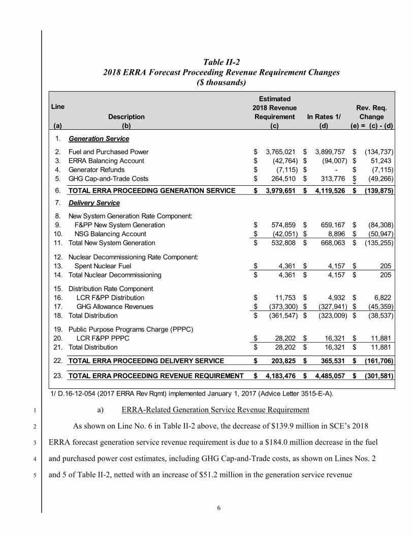
a) ERRA-Related Generation Service Revenue Requirement 1

As shown on Line No. 6 in Table II-2 above, the decrease of $139.9 million in SCE’s 2018 2

ERRA forecast generation service revenue requirement is due to a $184.0 million decrease in the fuel 3

and purchased power cost estimates, including GHG Cap-and-Trade costs, as shown on Lines Nos. 2 4

and 5 of Table II-2, netted with an increase of $51.2 million in the generation service revenue 5

Line

Description

Estimated 2018 Revenue Requirement In Rates 1/

Rev. Req. Change

(a) (b) (c) (d) (e) = (c) - (d)

1. Generation Service

2. Fuel and Purchased Power 3,765,021$ 3,899,757$ (134,737)$ 3. ERRA Balancing Account (42,764)$ (94,007)$ 51,243$ 4. Generator Refunds (7,115)$ -$ (7,115)$ 5. GHG Cap-and-Trade Costs 264,510$ 313,776$ (49,266)$ $ 6. TOTAL ERRA PROCEEDING GENERATION SERVICE 3,979,651$ 4,119,526$ (139,875)$

7. Delivery Service

8. New System Generation Rate Component:9. F&PP New System Generation 574,859$ 659,167$ (84,308)$ 10. NSG Balancing Account (42,051)$ 8,896$ (50,947)$ 11. Total New System Generation 532,808$ 668,063$ (135,255)$

12. Nuclear Decommissioning Rate Component:13. Spent Nuclear Fuel 4,361$ 4,157$ 205$ 14. Total Nuclear Decommissioning 4,361$ 4,157$ 205$

15. Distribution Rate Component16. LCR F&PP Distribution 11,753$ 4,932$ 6,822$ 17. GHG Allowance Revenues (373,300)$ (327,941)$ (45,359)$ 18. Total Distribution (361,547)$ (323,009)$ (38,537)$

19. Public Purpose Programs Charge (PPPC)20. LCR F&PP PPPC 28,202$ 16,321$ 11,881$ 21. Total Distribution 28,202$ 16,321$ 11,881$

22. TOTAL ERRA PROCEEDING DELIVERY SERVICE 203,825$ 365,531$ (161,706)$

23. TOTAL ERRA PROCEEDING REVENUE REQUIREMENT 4,183,476$ 4,485,057$ (301,581)$

1/ D.16-12-054 (2017 ERRA Rev Rqmt) implemented January 1, 2017 (Advice Letter 3515-E-A).

7

requirement as shown on Line No. 3 of Table II-2 associated with the estimated year-end 2017 ERRA 1

balance, and a decrease of approximately $7.1 million associated with net Generator refunds related to 2

the 2000-2001 California Energy Crisis settlements approved by the Federal Energy Regulatory 3

Commission (FERC). 4

In addition to the bundled service generation revenue requirement identified in Table II-2 above, 5

SCE’s estimated 2018 ERRA Forecast revenue requirement also includes delivery service amounts. As 6

shown on Line No. 22 in Table II-2 above, the decrease of $161.7 million in SCE’s 2018 ERRA forecast 7

delivery service revenue requirement is due to a decrease in the New System Generation (i.e., CAM-8

related) revenue requirement of $84.3 million, a decrease of $50.9 million associated with SCE’s year-9

end 2017 NSGBA balance, an increase of $0.2 million associated with spent nuclear fuel costs, an 10

increase of $18.7 million associated with Local Capacity Requirement (LCR) contracts and a decrease 11

of $45.4 million associated with GHG allowance revenues to be returned to eligible customers. SCE 12

discusses the background for recovering these costs through CAM in more detail in Chapter VIII. The 13

GHG allowance revenue forecast is discussed in Chapter VII.14

8

III. 1

SCE’S BUNDLED ENERGY FORECAST 2

This chapter presents a summary of SCE’s forecast of 2018 bundled service customer energy 3

load in its service area and a brief description of the methodology used to produce the forecast. A brief 4

discussion of the major factors and assumptions that influence the forecast is also presented. 5

A. Retail Sales Forecast Summary 6

SCE developed its bundled customer energy forecast for this ERRA filing based on a retail 7

customer sales forecast that was completed on December 4, 2016. The retail sales forecast consists of 8

forecast sales to bundled service, DA, and CCA customers measured at the customer meter. Total retail 9

electricity sales in the SCE service area totaled 85,448 GWh in 2016. For 2017 and 2018, SCE is 10

forecasting sales of 83,171 GWh and 83,227 GWh, respectively. The predicted decrease in sales 11

between 2016 and 2017 is about negative 2.7 percent. The primary drivers of the lower forecast are 12

weather and declining average residential usage as a result of energy efficiency savings. Temperatures 13

as measured by Cooling Degree Days were warmer than normal in 2016. Therefore, the transition from 14

an above-normal weather year to a normal weather year assumed in the forecast has a downward impact 15

on predicted sales in 2017 relative to recorded sales in 2016. 16

For the ERRA forecast proceeding, the forecast of retail sales is converted to a forecast of 17

bundled service customer sales, and then converted to a forecast of bundled customer energy at the 18

California Independent System Operator (CAISO) interface (i.e., distribution line losses are accounted 19

for). The difference between bundled sales and bundled energy is that bundled sales represents the 20

energy delivered to and measured at the customer meter as it is billed, while bundled energy consists of 21

the energy delivered to the customer meter plus distribution losses as measured during the hour it is 22

consumed. This definition of load is referred to as “measured at the CAISO interface.” The CAISO 23

interface is where all wholesale energy transactions and settlements take place. 24

Table III-3 summarizes the steps in converting retail sales to bundled customer energy at the 25

CAISO interface. Retail sales consist of two components: (1) bundled service customer sales and (2) 26

DA and CCA sales. Deducting the forecast of DA and CCA sales from total retail sales yields a forecast 27

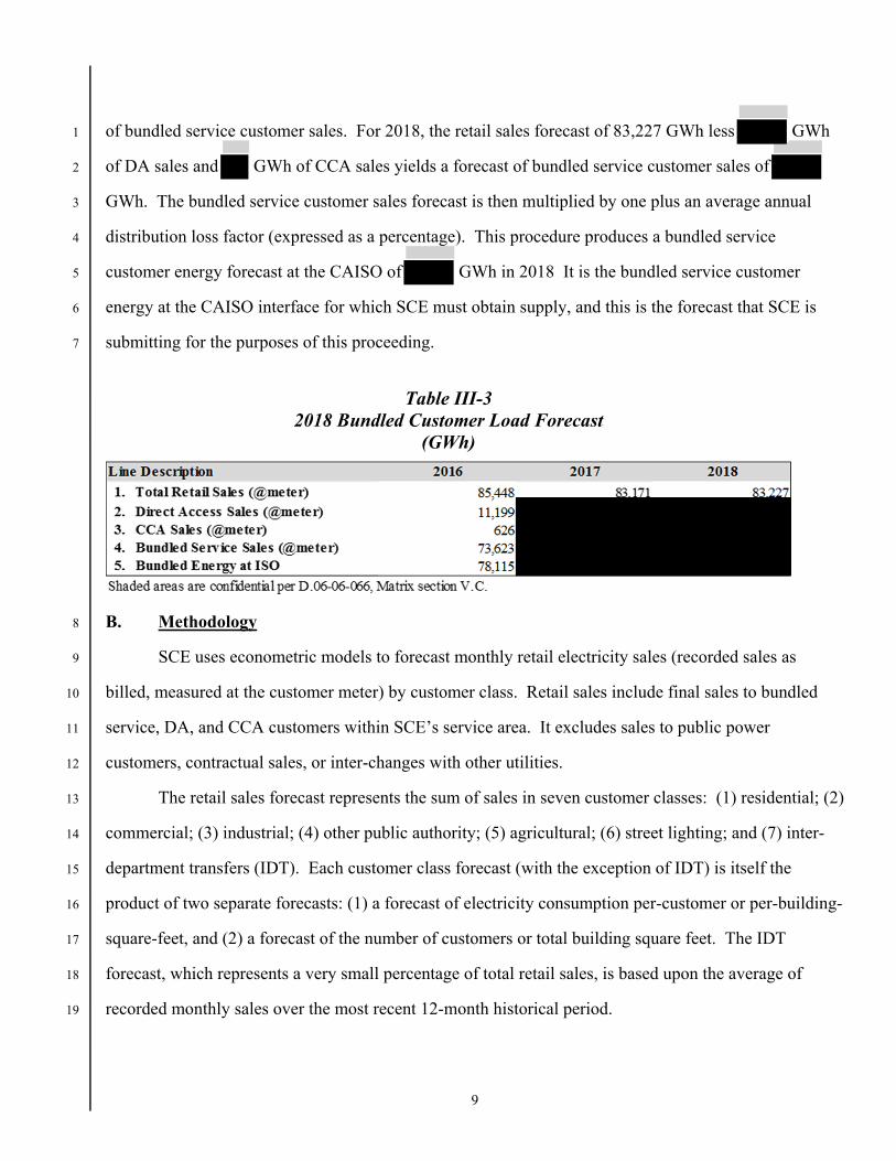
9

of bundled service customer sales. For 2018, the retail sales forecast of 83,227 GWh less GWh 1

of DA sales and GWh of CCA sales yields a forecast of bundled service customer sales of 2

GWh. The bundled service customer sales forecast is then multiplied by one plus an average annual 3

distribution loss factor (expressed as a percentage). This procedure produces a bundled service 4

customer energy forecast at the CAISO of GWh in 2018 It is the bundled service customer 5

energy at the CAISO interface for which SCE must obtain supply, and this is the forecast that SCE is 6

submitting for the purposes of this proceeding. 7

Table III-3 2018 Bundled Customer Load Forecast

(GWh)

B. Methodology 8

SCE uses econometric models to forecast monthly retail electricity sales (recorded sales as 9

billed, measured at the customer meter) by customer class. Retail sales include final sales to bundled 10

service, DA, and CCA customers within SCE’s service area. It excludes sales to public power 11

customers, contractual sales, or inter-changes with other utilities. 12

The retail sales forecast represents the sum of sales in seven customer classes: (1) residential; (2) 13

commercial; (3) industrial; (4) other public authority; (5) agricultural; (6) street lighting; and (7) inter-14

department transfers (IDT). Each customer class forecast (with the exception of IDT) is itself the 15

product of two separate forecasts: (1) a forecast of electricity consumption per-customer or per-building-16

square-feet, and (2) a forecast of the number of customers or total building square feet. The IDT 17

forecast, which represents a very small percentage of total retail sales, is based upon the average of 18

recorded monthly sales over the most recent 12-month historical period. 19

10

Econometric models employ statistical techniques to quantify the relationship between electricity 1

consumption and the various economic, demographic, and other factors that influence electricity 2

consumption. Examples of such variables are weather, electricity rates, billing days, energy efficiency 3

program savings, employment, personal income, and building floor stock. Historical data is used to 4

determine these relationships. The typical estimation procedure used to construct the models is ordinary 5

least squares (OLS). Model-generated forecasts may be modified based on current trends, judgment, 6

and events that are not specifically modeled in the econometric equations. 7

Once a satisfactory statistical relationship is established, SCE uses historical average values of 8

weather (cooling and heating degree days) and billing days to represent typical or normal conditions in 9

future periods. Forecasts of economic drivers such as employment, personal income, and building floor 10

stock, along with the typical weather and billing day variables, are then “plugged into” the models in 11

order to derive forecast values of electricity consumption per customer. Moody’s Analytics and Dodge 12

Data & Analytics are the principal sources of employment, personal income, and floor stock data, both 13

historical and forecast. 14

The forecasts of both residential and non-residential customers are based on econometric models 15

that relate changes in the number of customers to a change in economic activity. For example, in the 16

case of residential customers, population growth is used as the leading economic variable to forecast the 17

number of customers. Changes in the number of small commercial customers are assumed to be 18

influenced by changes in the number of residential customers, while changes in the number of industrial 19

customers are dependent upon changes in manufacturing employment. 20

C. Historical Trends 21

On a recorded basis, SCE’s total electricity sales increased at an average annual rate of negative 22

0.6 percent per year between 2009 and 2016. Sales growth has not been consistently negative during 23

this period. For example, annual sales growth surpassed 3 and 2 percent in 2012 and 2014, respectively. 24

However, increased sales in these two years were a result of above-average weather. Customer growth 25

has remained positive during the post-recession period of 2009 to 2016, averaging 0.5% annual growth. 26

11

In 2014 and 2015, annual customer growth reached 0.6%, the highest level since 2007, but still well 1

below the levels reached during the regional housing boom. 2

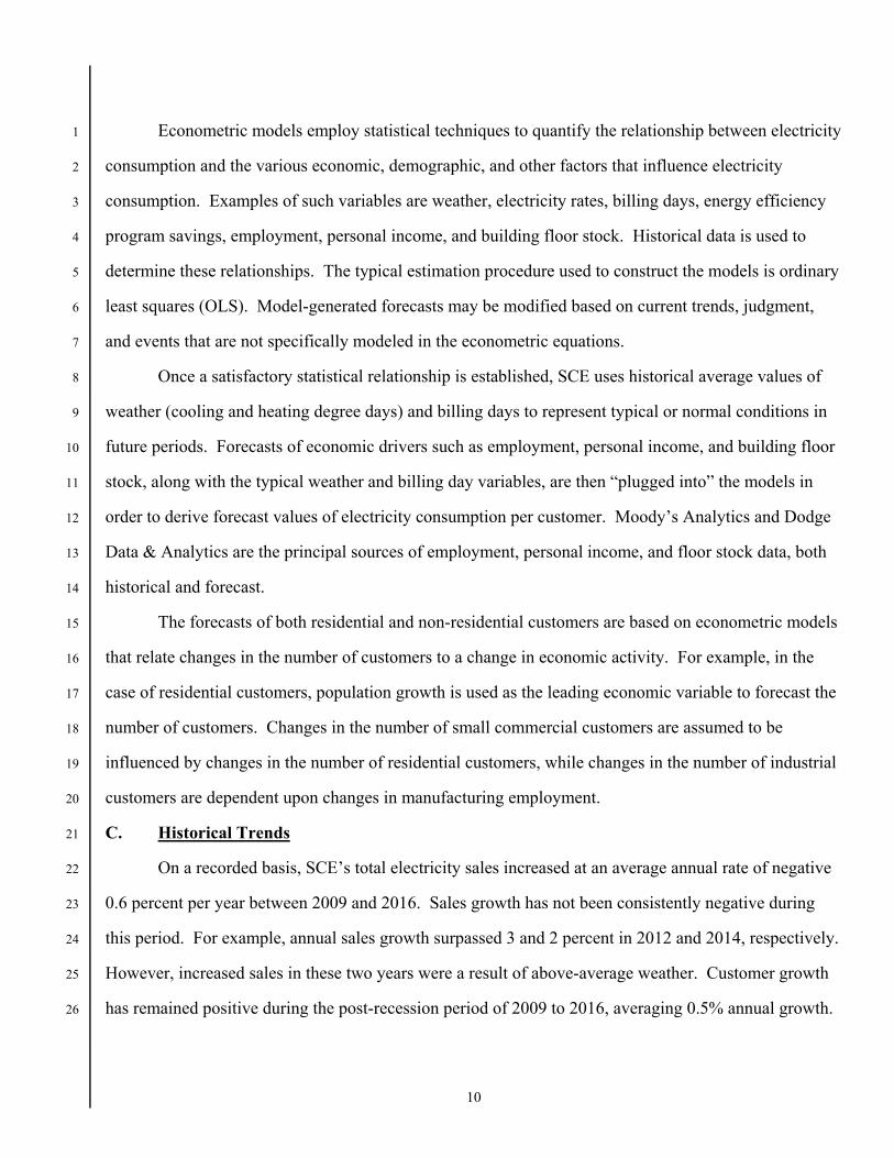
After the Great Recession and the weak initial recovery, the Southern California economy has 3

settled into a modest economic expansion as outlined in Figure III-1. The pace of job growth in SCE’s 4

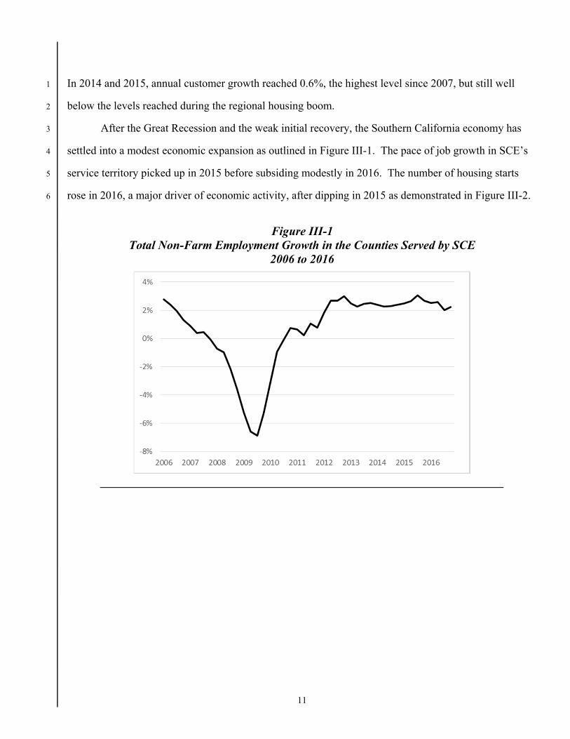
service territory picked up in 2015 before subsiding modestly in 2016. The number of housing starts 5

rose in 2016, a major driver of economic activity, after dipping in 2015 as demonstrated in Figure III-2. 6

Figure III-1 Total Non-Farm Employment Growth in the Counties Served by SCE

2006 to 2016

12

Figure III-2 Residential Housing Starts in Counties Served by SCE

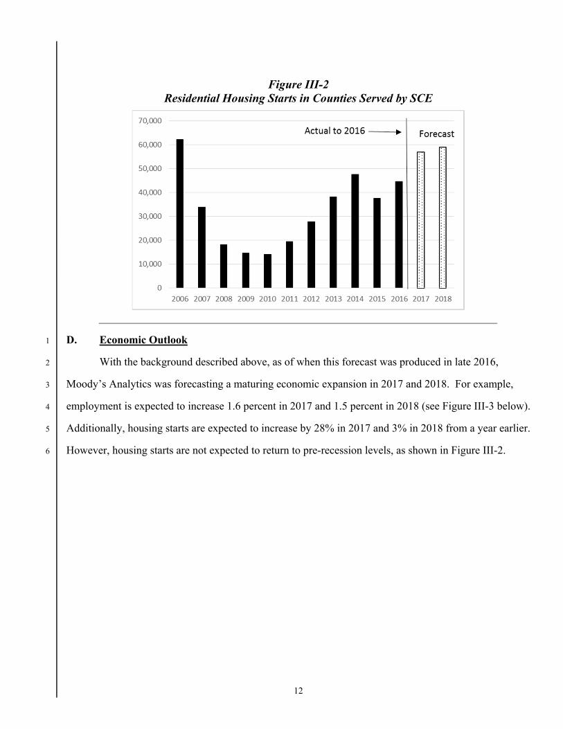
D. Economic Outlook 1

With the background described above, as of when this forecast was produced in late 2016, 2

Moody’s Analytics was forecasting a maturing economic expansion in 2017 and 2018. For example, 3

employment is expected to increase 1.6 percent in 2017 and 1.5 percent in 2018 (see Figure III-3 below). 4

Additionally, housing starts are expected to increase by 28% in 2017 and 3% in 2018 from a year earlier. 5

However, housing starts are not expected to return to pre-recession levels, as shown in Figure III-2. 6

13

Figure III-3 Total Non-Farm Employment Growth in SCE Service Area

Actual and Forecast

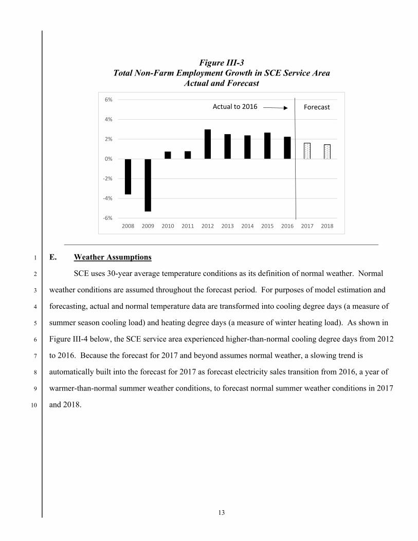
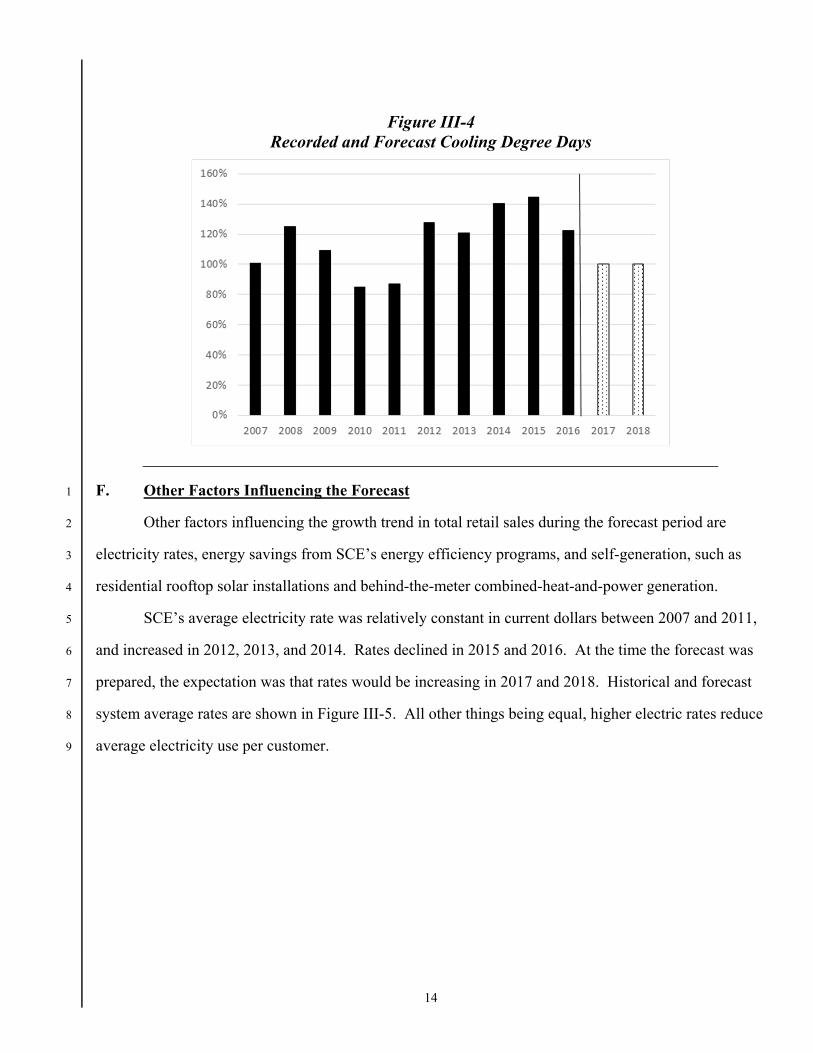
E. Weather Assumptions 1

SCE uses 30-year average temperature conditions as its definition of normal weather. Normal 2

weather conditions are assumed throughout the forecast period. For purposes of model estimation and 3

forecasting, actual and normal temperature data are transformed into cooling degree days (a measure of 4

summer season cooling load) and heating degree days (a measure of winter heating load). As shown in 5

Figure III-4 below, the SCE service area experienced higher-than-normal cooling degree days from 2012 6

to 2016. Because the forecast for 2017 and beyond assumes normal weather, a slowing trend is 7

automatically built into the forecast for 2017 as forecast electricity sales transition from 2016, a year of 8

warmer-than-normal summer weather conditions, to forecast normal summer weather conditions in 2017 9

and 2018. 10

-6%

-4%

-2%

0%

2%

4%

6%

2008 2009 2010 2011 2012 2013 2014 2015 2016 2017 2018

Actual to 2016 Forecast

14

Figure III-4 Recorded and Forecast Cooling Degree Days

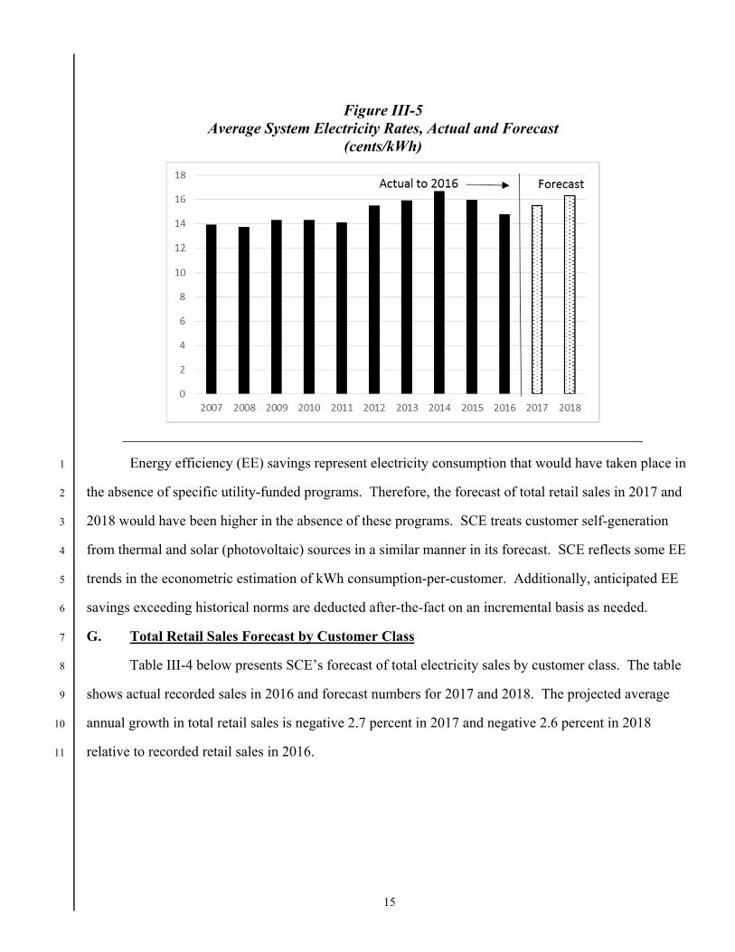
F. Other Factors Influencing the Forecast 1

Other factors influencing the growth trend in total retail sales during the forecast period are 2

electricity rates, energy savings from SCE’s energy efficiency programs, and self-generation, such as 3

residential rooftop solar installations and behind-the-meter combined-heat-and-power generation. 4

SCE’s average electricity rate was relatively constant in current dollars between 2007 and 2011, 5

and increased in 2012, 2013, and 2014. Rates declined in 2015 and 2016. At the time the forecast was 6

prepared, the expectation was that rates would be increasing in 2017 and 2018. Historical and forecast 7

system average rates are shown in Figure III-5. All other things being equal, higher electric rates reduce 8

average electricity use per customer. 9

15

Figure III-5 Average System Electricity Rates, Actual and Forecast

(cents/kWh)

Energy efficiency (EE) savings represent electricity consumption that would have taken place in 1

the absence of specific utility-funded programs. Therefore, the forecast of total retail sales in 2017 and 2

2018 would have been higher in the absence of these programs. SCE treats customer self-generation 3

from thermal and solar (photovoltaic) sources in a similar manner in its forecast. SCE reflects some EE 4

trends in the econometric estimation of kWh consumption-per-customer. Additionally, anticipated EE 5

savings exceeding historical norms are deducted after-the-fact on an incremental basis as needed. 6

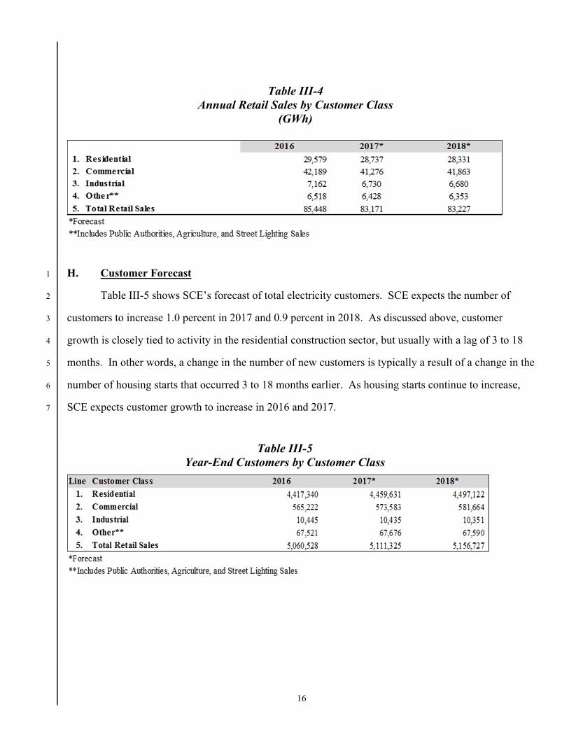
G. Total Retail Sales Forecast by Customer Class 7

Table III-4 below presents SCE’s forecast of total electricity sales by customer class. The table 8

shows actual recorded sales in 2016 and forecast numbers for 2017 and 2018. The projected average 9

annual growth in total retail sales is negative 2.7 percent in 2017 and negative 2.6 percent in 2018 10

relative to recorded retail sales in 2016. 11

16

Table III-4 Annual Retail Sales by Customer Class

(GWh)

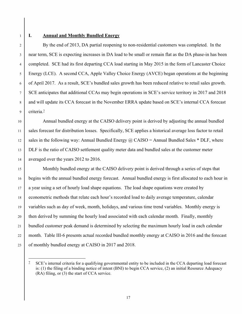
H. Customer Forecast 1

Table III-5 shows SCE’s forecast of total electricity customers. SCE expects the number of 2

customers to increase 1.0 percent in 2017 and 0.9 percent in 2018. As discussed above, customer 3

growth is closely tied to activity in the residential construction sector, but usually with a lag of 3 to 18 4

months. In other words, a change in the number of new customers is typically a result of a change in the 5

number of housing starts that occurred 3 to 18 months earlier. As housing starts continue to increase, 6

SCE expects customer growth to increase in 2016 and 2017. 7

Table III-5 Year-End Customers by Customer Class

17

I. Annual and Monthly Bundled Energy 1

By the end of 2013, DA partial reopening to non-residential customers was completed. In the 2

near term, SCE is expecting increases in DA load to be small or remain flat as the DA phase-in has been 3

completed. SCE had its first departing CCA load starting in May 2015 in the form of Lancaster Choice 4

Energy (LCE). A second CCA, Apple Valley Choice Energy (AVCE) began operations at the beginning 5

of April 2017. As a result, SCE’s bundled sales growth has been reduced relative to retail sales growth. 6

SCE anticipates that additional CCAs may begin operations in SCE’s service territory in 2017 and 2018 7

and will update its CCA forecast in the November ERRA update based on SCE’s internal CCA forecast 8

criteria.7 9

Annual bundled energy at the CAISO delivery point is derived by adjusting the annual bundled 10

sales forecast for distribution losses. Specifically, SCE applies a historical average loss factor to retail 11

sales in the following way: Annual Bundled Energy @ CAISO = Annual Bundled Sales * DLF, where 12

DLF is the ratio of CAISO settlement quality meter data and bundled sales at the customer meter 13

averaged over the years 2012 to 2016. 14

Monthly bundled energy at the CAISO delivery point is derived through a series of steps that 15

begins with the annual bundled energy forecast. Annual bundled energy is first allocated to each hour in 16

a year using a set of hourly load shape equations. The load shape equations were created by 17

econometric methods that relate each hour’s recorded load to daily average temperature, calendar 18

variables such as day of week, month, holidays, and various time trend variables. Monthly energy is 19

then derived by summing the hourly load associated with each calendar month. Finally, monthly 20

bundled customer peak demand is determined by selecting the maximum hourly load in each calendar 21

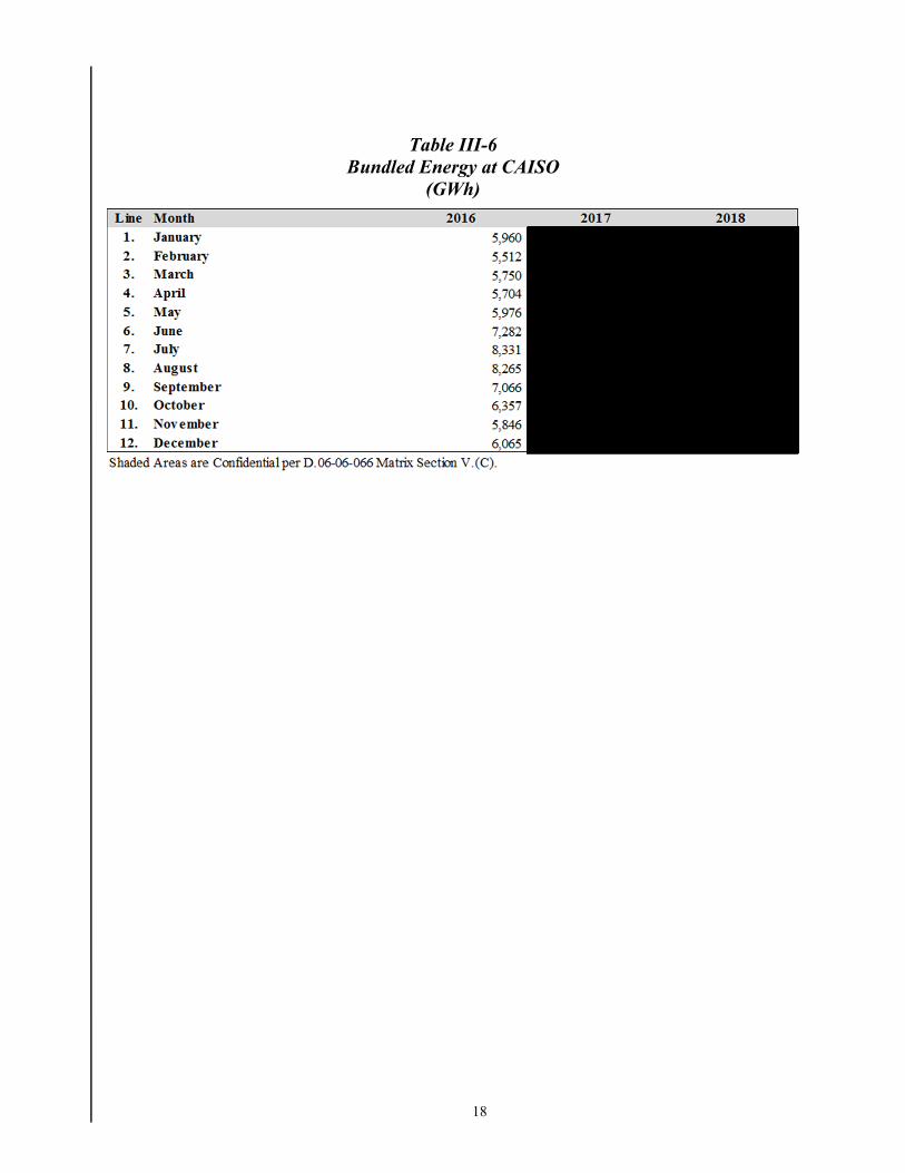
month. Table III-6 presents actual recorded bundled monthly energy at CAISO in 2016 and the forecast 22

of monthly bundled energy at CAISO in 2017 and 2018. 23

7 SCE’s internal criteria for a qualifying governmental entity to be included in the CCA departing load forecast

is: (1) the filing of a binding notice of intent (BNI) to begin CCA service, (2) an initial Resource Adequacy (RA) filing, or (3) the start of CCA service.

18

Table III-6 Bundled Energy at CAISO

(GWh)

19

IV. 1

FORECAST ENERGY PRODUCTION AND COSTS FROM SCE’S PORTFOLIO OF 2

RESOURCES 3

A. Introduction 4

This chapter describes SCE’s resource portfolio and the associated forecast costs that SCE 5

proposes to recover in its ERRA balancing account. SCE’s resource portfolio is comprised of its utility-6

owned generation (UOG), which includes nuclear, natural gas, hydroelectric, fuel cells, and renewable 7

generation resources; SCE’s purchased power resources, including CHP and renewable resources, 8

interutility contracts, and bilateral contracts; and proxy8 (i.e., generic) costs from anticipated future 9

solicitations and market purchases. SCE’s 2018 forecast also includes executed contracts from SCE’s 10

Local Capacity Requirements (LCR) solicitations for the Western Los Angeles (LA) Basin and 11

Moorpark regions, as approved in D.15-11-041 and proposed in A.14-11-016, respectively. 12

The decrease in SCE’s 2018 fuel and purchased power cost forecast can be generally attributed 13

to four major factors. First, SCE expects its sales to be lower than it did for the 2017 ERRA forecast. 14

Second, SCE expects lower fuel-related costs from its natural gas-fueled UOG and tolling resources due 15

to lower forecast natural gas prices. Third, SCE expects lower open market costs due to lower forecast 16

SP-15 forward market power prices. Fourth, SCE expects lower SRAC payments due to lower forecast 17

market prices. SCE used $58.27/kW-year as the proxy price to meet Generic Capacity need as outlined 18

in the 2015 “Estimated Cost of New Renewable and Fossil Generation in California Final Staff Report” 19

study issued by the CEC. 20

B. Energy Production Forecast Methodology 21

In this ERRA Forecast application, as in its past forecast applications, SCE forecasts energy 22

production from its portfolio primarily using the Ventyx Planning and Risk (PROSYM) software.9 The 23

8 The proxy capacity costs are further discussed in Section IV.E.

9 Ventyx is the current owner of the originally developed Henwood PROSYM tool. Ventyx’s Planning and Risk Software is primarily powered by the PROSYM engine.

20

Ventyx models are used to: (1) forecast the least-cost dispatch (LCD) of dispatchable resources in 1

SCE’s portfolio; (2) optimize hydro dispatch; and (3) perform Monte Carlo simulations of forced outage 2

rates of individual units. 3

The simulated dispatch is based on a forecast of power, gas, and GHG prices,10 physical 4

constraints of each generating unit, and contractual limitations. SCE’s forecast methodology 5

economically dispatches resources in a least-cost manner as directed by the Commission, rather than 6

force-dispatching resources to meet SCE’s forecast of bundled customer demand. Under the LCD 7

principle, a generating resource or contract is simulated to dispatch if its marginal operating cost is less 8

than the market price of power, while simultaneously observing all operating constraints.11 For a given 9

hour, the difference between the forecast bundled load and the total forecast economic dispatch of SCE’s 10

resource portfolio constitutes SCE’s projected open position for the hour. 11

SCE based its 2018 power price forecast on the forward power broker quotes for 2018 in effect 12

as of February 23, 2017. The 24-hour flat price as of February 23, 2017, was $28.59/MWh for 2018.12 13

SCE derived its hourly price forecast by applying on-peak and off-peak hourly price profiles to the 14

respective monthly on-peak and off-peak forward quotes for 2018 in effect as of February 23, 2017,13 15

such that the simple averages of the hourly on-peak and off-peak forecast prices for a particular month 16

match the forward on-peak and off-peak power prices for that month. SCE updated its existing MRTU-17

based statistical models to generate hourly price profiles for the SP-15 and NP-15 zones.14 18

10 The Ventyx models were not used to develop forecasts of competitive market power or GHG prices. These

prices were developed independently, as discussed in the following paragraphs. The GHG price forecast was incorporated as part of the resource dispatch cost similar to natural gas prices in order to reflect the additional GHG cost for the generation resources that have GHG emissions.

11 Energy- and use-limited hydroelectric and peaking resources are also dispatched pursuant to LCD; this analysis also incorporates opportunity cost principles regarding water and emissions limitations, respectively, to ensure that such units are dispatched during higher-priced hours, when it is most economic to do so.

12 SCE has contracts in NP-15. SCE used relevant prices to forecast the cost of those contracts.

13 SCE used forward prices from the same trading day for power, GHG, and natural gas price forecasts to maintain the consistency of the forward-market outlook.

14 The statistical models incorporated historical MRTU data from the CAISO’s Integrated Forward Market (IFM).

21

SCE used the Intercontinental Exchange’s (ICE) settlement price of a 2018-vintage GHG 1

allowance as the basis for its 2018 GHG price forecast. The ICE settlement price as of February 23, 2

2017, was $14.06/MT for 2018. This price is assumed to be constant for any GHG emissions produced 3

in 2018.15 Lastly, SCE based its daily natural gas price forecast on monthly NYMEX forward prices at 4

the SoCal Border in effect as of February 23, 2017, plus intrastate transportation charges from Southern 5

California Gas Company (SoCalGas), as applicable.16 The 12-month average NYMEX forward gas 6

price as of February 23, 2017 was $2.78/MMBtu for 2018. Within a given month, SCE assumed that the 7

daily gas price forecast is equal to the monthly forward price. 8

C. Validation of SCE’s Energy Production Forecast 9

SCE follows a consistent process to forecast its energy production and costs for the subsequent 10

calendar year, supported by a robust internal validation process. SCE’s forecast process is discussed 11

below. 12

The first stage of SCE’s forecast process involves developing all forecast inputs. These inputs 13

include, but are not limited to, SCE’s forecast of power, gas, and GHG prices; production from UOG 14

resources (nuclear, hydro, gas, fuel cells and renewable facilities); CHP and renewable energy 15

production and costs; gas hedging costs; CAISO costs, etc. These inputs are developed and vetted by 16

various business groups or divisions responsible for each input and then submitted to senior managers in 17

SCE’s Power Supply Organizational Unit for further review and approval. 18

Once approved, the forecast inputs are utilized in PROSYM, which is an industry-standard 19

production cost model capable of modeling various types of resources with differing constraints. SCE 20

uses PROSYM to forecast its LCD activities. Once the dispatch results are produced, SCE conducts a 21

15 In prior years, direct and indirect GHG costs were reviewed in a separate GHG Cost and Revenue Forecast

application. Pursuant to D.14-10-033, they will now be reviewed in this proceeding, and are discussed in further detail in Chapter VII.

16 Not all generating resources in SCE’s portfolio utilize transportation service from SoCalGas.

22

thorough validation of the dispatch outcomes by resource.17 If necessary, SCE will rerun the previous 1

forecast steps if it believes more accurate dispatch results can be realized. 2

Once dispatch results are validated, all energy and cost forecasts are input into SCE’s ERRA 3

forecasting tool, an internally-developed, automated software program that aggregates the hourly energy 4

production and cost forecast data. The ERRA forecasting tool produces the ERRA forecast tables 5

included in the following section(s). Prior to inclusion in SCE’s ERRA Forecast filing, the forecast 6

tables are reviewed and approved by SCE’s senior management. 7

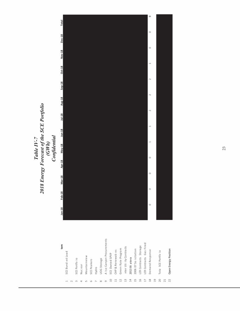
D. 2018 Energy and Cost Forecast Summary 8

Because this ERRA application is designed to forecast SCE’s energy-related costs that will 9

ultimately be used to establish retail generation rates in 2018, a single expected scenario forecast is 10

utilized. All production and residual open position forecasts provided in this section are reflected at the 11

CAISO system interface. To accomplish this, SCE reduced generation production forecasts by the 12

forecast transmission losses and grossed up the forecast retail load by the forecast distribution losses. 13

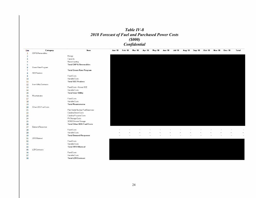
Table IV-7 summarizes the monthly forecast production from SCE’s portfolio and SCE’s open energy 14

positions. Table IV-8 summarizes the monthly forecast cost of SCE’s purchased power resources 15

accounted for in the ERRA balancing account. The remainder of this chapter provides detailed 16

descriptions of the resources and the underlying forecast assumptions.17

17 For example, SCE compares its dispatch results against prior ERRA forecasts and reviews any significant

discrepancies to ensure that its results are reasonably justified.

23

Tabl

e IV

-7

2018

Ene

rgy

For

ecas

t of t

he S

CE

Por

tfolio

(G

Wh)

C

onfid

entia

l te

mJa

n-18

Feb-

18M

ar-1

8Ap

r-18

May

-18

Jun-

18Ju

l-18

Aug-

18Se

p-18

Oct

-18

Nov

-18

Dec

-18

Tota

l

1SC

E Bu

nded

Loa

d

2 3SC

E Po

rtfo

io

4N

ucea

r

5M

ount

ainv

iew

6SC

E Pe

aker

s

7H

ydro

8U

OG

Sto

rage

9A

iso

Cany

on P

rocu

rem

ents

10SC

EO

wne

d SP

VP

11CH

P &

Ren

ewab

es

12G

reen

Rat

e Pr

ogra

m

13nt

erU

tiit

y Co

ntra

cts

1420

13 B

iat

era

1520

0607

So

icit

atio

n

16LC

R Co

ntra

cts

Sto

rage

17LC

R Co

ntra

cts

Gas

Fir

ed

18D

eman

d Re

spon

se0

00

01

12

22

10

09

19 20To

ta S

CE P

ortf

oio

21 22O

pen

Ener

gy P

ositi

on

24

Table IV-8 2018 Forecast of Fuel and Purchased Power Costs

($000) Confidential

25

Table IV-8 (Con’t) 2018 Forecast of Fuel and Purchased Power Costs

($000) Confidential

26

E. SCE’s Utility-Owned Generation and Purchased Power Contracts 1

1. Hydro Facilities 2

SCE’s hydro resources consist of 33 powerhouses in central and southern California, which 3

provide 1,176 MW of nameplate capacity. SCE’s hydro division is organized into two regions, Northern 4

and Eastern. The Northern Division hydro region, also known as the Big Creek Project, is located in 5

central California about 50 miles east of Fresno in the western Sierra Nevada Mountains. Big Creek’s 6

nine powerhouses provide 1,015 MW of nameplate capacity. The Eastern Division hydro region 7

consists of SCE’s powerhouses located in the eastern and southern Sierra Nevada Mountains, as well as 8

in the San Bernardino and San Gabriel Mountains of southern California. The Eastern Division hydro 9

region’s 24 powerhouses provide 161 MW of nameplate capacity. 10

The Big Creek hydro system is a flexible, dispatchable resource, except during the period of 11

spring run-off. During this period, in a normal water year, the generating units typically need to operate 12

near maximum capacity for 24 hours per day to ensure that spill is minimized. For ERRA forecast 13

purposes, SCE optimizes the Big Creek Project by operating at full capacity (when operationally 14

possible) during the highest economic value hours. When Big Creek does not operate at full capacity, it 15

can generally provide ancillary services to the CAISO market. 16

Eastwood powerhouse is a pump-storage unit providing 199.8 MW of nameplate generating 17

capacity, and is part of the Big Creek Project. The pumpback efficiency is approximately 75 percent, 18

meaning that approximately 1.33 MWh of pumping energy is required to pump enough water back into 19

the forebay to generate 1 MWh of energy at a later time. Pumpback duration generally varies from two 20

to six hours and consumes approximately 180 MWh per hour. Every three hours of pumpback stores 21

enough water to generate for approximately two hours at 199.8 MW. Pumpback and generation 22

dispatch for Eastwood are modeled on an hourly basis assuming economic dispatch. To maximize the 23

value of the resource, pumpback normally takes place during off-peak hours when energy prices are 24

lower, and dispatch normally takes place during peak hours when energy prices are higher. 25

27

SCE’s Eastern Division hydro facilities are predominantly run-of-the-river, non-dispatchable 1

resources and their actual MW output varies based on hydrological conditions. As a result, the forecast 2

energy production is largely deterministic. 3

For 2018, SCE’s forecast of its UOG Hydro production, inclusive of pumpback operations, is 4

shown in Table IV-7. This forecast assumes a slightly-above-normal hydrological year for 2018, and 5

also incorporates SCE’s best estimate of upcoming major planned outages of Big Creek and Eastern 6

Hydro units in 2018. 7

2. SCE Solar Photovoltaic Generation 8

SCE’s Solar Photovoltaic Program (SPVP) is a Commission-approved initiative to install, own, 9

and operate up to 91 MW Direct Current (DC) of utility-owned solar photovoltaic projects on 10

commercial rooftop space and ground-mounts in SCE’s service area.18 SCE estimates that in 2018 that 11

its UOG SPVP solar projects will provide a total of approximately 91 MW DC of capacity, primarily 12

(although not exclusively) located in San Bernardino County. These photovoltaic projects generally 13

provide energy during peak usage times. For 2018, SCE’s forecast of SPVP production, based on the 14

previous year’s project capacity factors, is shown in Table IV-9. 15

Table IV-9 2018 Forecast of SCE SPVP Production

(GWh)

18 The Commission originally approved a 500 MW SPVP program, with 250 MW of projects to be UOG and

250 MW to be owned by independent power producers. See D.09-06-049. SCE’s February 2011 Petition for Modification requested the program be modified to include, among other things, a reduction of both the UOG and the Independent Power Producer portions from 250 MW to 125 MW, and the petition was approved on February 16, 2012. On July 27, 2012, SCE filed a second Petition for Modification to further reduce the UOG portion of the SPVP from 125 MW to 91 MW, given that 18 MW of ground sites were at risk due to interconnection cost and schedule, and 16 MW of formerly-committed rooftops were no longer viable. SCE proposed that the 34 MW reduction from the UOG SPVP Program be transferred to the Renewable RAM Procurement Program. The Commission approved SCE’s petition in D.13-05-033, capping the UOG portion of SPVP at 91 MW. The independent power producer portion of the program maintains its 125 MW program goal.

28

3. CHP and Renewables 1

a) Energy Forecast 2

For the 2018 Forecast Period, SCE expects 19 of energy deliveries at the CAISO 3

interface as shown in Table IV-7 from CHP (combined heat and power) and renewable projects. The 4

energy deliveries from cogeneration and renewable projects are effectively “must take” energy. There 5

are some gas-fired contracts that are dispatched based on market prices. 6

Energy deliveries at the generators’ meters are forecast to be The 319 projects 7

delivering energy have approximately 9,789 MW of contract capacity allocated as follows: 8

• 1,319 MW of CHP capacity; 9

• 8,470 MW of renewable capacity.20 10

In addition and not included in the above capacity numbers, SCE has contracted an additional 11

174 MW of dispatchable capacity through the CHP Program Settlement requests for offers. 12

SCE uses the historical performance of each project to forecast monthly energy deliveries. From 13

March 2017 through December 2018, 31 projects are expected to begin delivering energy. Some of 14

these projects have been delivering energy and signed new contracts. Others are new projects under 15

development and are adjusted by their probability of successful development and commercial operation. 16

The total capacity for these projects is approximately 1,187 MW. The nineteen new projects (15 solar 17

and 4 wind) are expected to begin delivering energy during the period from March 2017 through 18

December 2018. Because there are no historical performance data for these new projects, forecast 19

energy deliveries are based on contractual expectations discounted by their expected probabilities of 20

successful development. 21

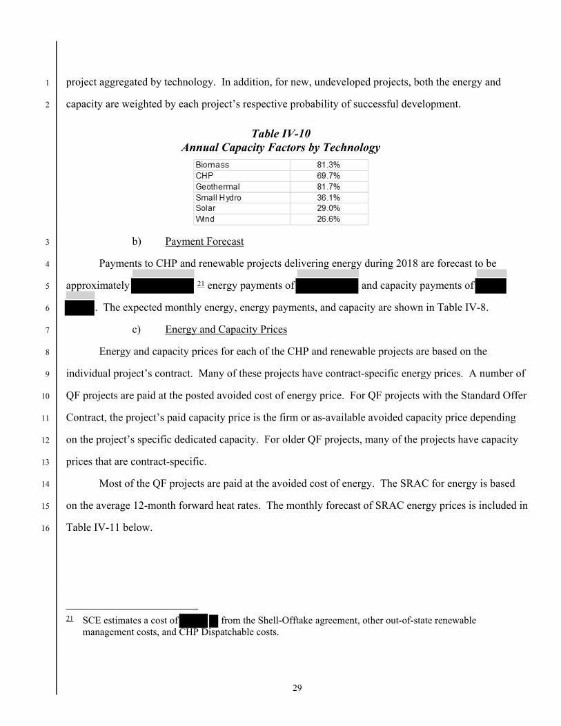
Table IV-10 lists the average annual capacity factors for each of the six technologies. These 22

average annual capacity factors are based on expected annual energy and contract capacity for each 23

19 includes generation loss and the Shell Offtake agreement, and excludes 11 GWh allocated to

serve Green Tariff customers as a part of the GTSR Program described in Section E.10.

20 The contract capacity for a project that is not developed is weighted by the project’s expected commercially-operable success rate.

29

project aggregated by technology. In addition, for new, undeveloped projects, both the energy and 1

capacity are weighted by each project’s respective probability of successful development. 2

Table IV-10 Annual Capacity Factors by Technology

b) Payment Forecast 3

Payments to CHP and renewable projects delivering energy during 2018 are forecast to be 4

approximately 21 energy payments of and capacity payments of 5

. The expected monthly energy, energy payments, and capacity are shown in Table IV-8. 6

c) Energy and Capacity Prices 7

Energy and capacity prices for each of the CHP and renewable projects are based on the 8

individual project’s contract. Many of these projects have contract-specific energy prices. A number of 9

QF projects are paid at the posted avoided cost of energy price. For QF projects with the Standard Offer 10

Contract, the project’s paid capacity price is the firm or as-available avoided capacity price depending 11

on the project’s specific dedicated capacity. For older QF projects, many of the projects have capacity 12

prices that are contract-specific. 13

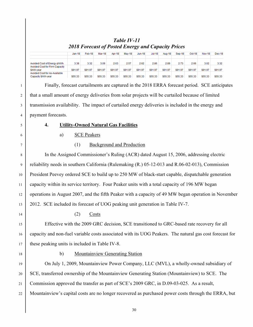
Most of the QF projects are paid at the avoided cost of energy. The SRAC for energy is based 14

on the average 12-month forward heat rates. The monthly forecast of SRAC energy prices is included in 15

Table IV-11 below. 16

21 SCE estimates a cost of from the Shell-Offtake agreement, other out-of-state renewable

management costs, and CHP Dispatchable costs.

30

Table IV-11 2018 Forecast of Posted Energy and Capacity Prices

Finally, forecast curtailments are captured in the 2018 ERRA forecast period. SCE anticipates 1

that a small amount of energy deliveries from solar projects will be curtailed because of limited 2

transmission availability. The impact of curtailed energy deliveries is included in the energy and 3

payment forecasts. 4

4. Utility-Owned Natural Gas Facilities 5

a) SCE Peakers 6

(1) Background and Production 7

In the Assigned Commissioner’s Ruling (ACR) dated August 15, 2006, addressing electric 8

reliability needs in southern California (Rulemaking (R.) 05-12-013 and R.06-02-013), Commission 9

President Peevey ordered SCE to build up to 250 MW of black-start capable, dispatchable generation 10

capacity within its service territory. Four Peaker units with a total capacity of 196 MW began 11

operations in August 2007, and the fifth Peaker with a capacity of 49 MW began operation in November 12

2012. SCE included its forecast of UOG peaking unit generation in Table IV-7. 13

(2) Costs 14

Effective with the 2009 GRC decision, SCE transitioned to GRC-based rate recovery for all 15

capacity and non-fuel variable costs associated with its UOG Peakers. The natural gas cost forecast for 16

these peaking units is included in Table IV-8. 17

b) Mountainview Generating Station 18

On July 1, 2009, Mountainview Power Company, LLC (MVL), a wholly-owned subsidiary of 19

SCE, transferred ownership of the Mountainview Generating Station (Mountainview) to SCE. The 20

Commission approved the transfer as part of SCE’s 2009 GRC, in D.09-03-025. As a result, 21

Mountainview’s capital costs are no longer recovered as purchased power costs through the ERRA, but 22

31

instead are recovered in SCE’s authorized base generation revenue requirement and through base rates. 1

However, Mountainview fuel costs and availability and heat rate incentive payments continue to be 2

recorded in the ERRA balancing account.22 SCE included its Mountainview generation forecast in 3

Table IV-7. The natural gas forecast for Mountainview is included in Table IV-8. 4

5. Interutility Contracts Production 5

SCE is a party to three23 major interutility contracts under which it is expected to purchase and/or 6

exchange capacity and associated energy for various periods through September 2017, except for the 7

City of Pasadena which has no expiration date. These interutility contracts were executed prior to 8

industry restructuring and contain complex terms and conditions that were designed to satisfy the unique 9

needs of SCE and each of the counterparties. The current contracts with 1) Western Area Power 10

Administration (WAPA) and the Bureau of Reclamation (Reclamation), and 2) the Metropolitan Water 11

District of Southern California (MWD) expire at the end of September 2017. SCE executed a new fifty-12

year agreement with WAPA and Reclamation with an initial service date of October 1, 2017. Table IV-13

12 summarizes these major interutility contracts. 14

Table IV-12 Non-Coincident Contract Capacity Quantities and

Expiration Dates for SCE’s Major Interutility Contracts

22 See SCE’s 2009 GRC Application, A.07-11-011, Exhibit SCE-02, Vol. 9, Ch. 1, dated November 2007, in

which SCE proposed to include the concepts of the PPA incentive mechanisms in the ERRA proceeding.

23 Excluded from this total are SCE’s so-called “Fringe Service” agreements, which provide for small amounts of energy exchanges among neighboring utilities. These include two contracts with the Department of Defense for the Air Force that SCE presented to the Commission in Advice Letters 2686-E and 1777-E and contracts associated with retail tariffs.

32

The process of forecasting the level of energy deliveries and receipts for interutility contracts 1

with dispatchability (i.e., with WAPA-Reclamation) is an inherently complex task. SCE is forecasting 2

net interutility contract purchases of 198 GWh in 2018. 3

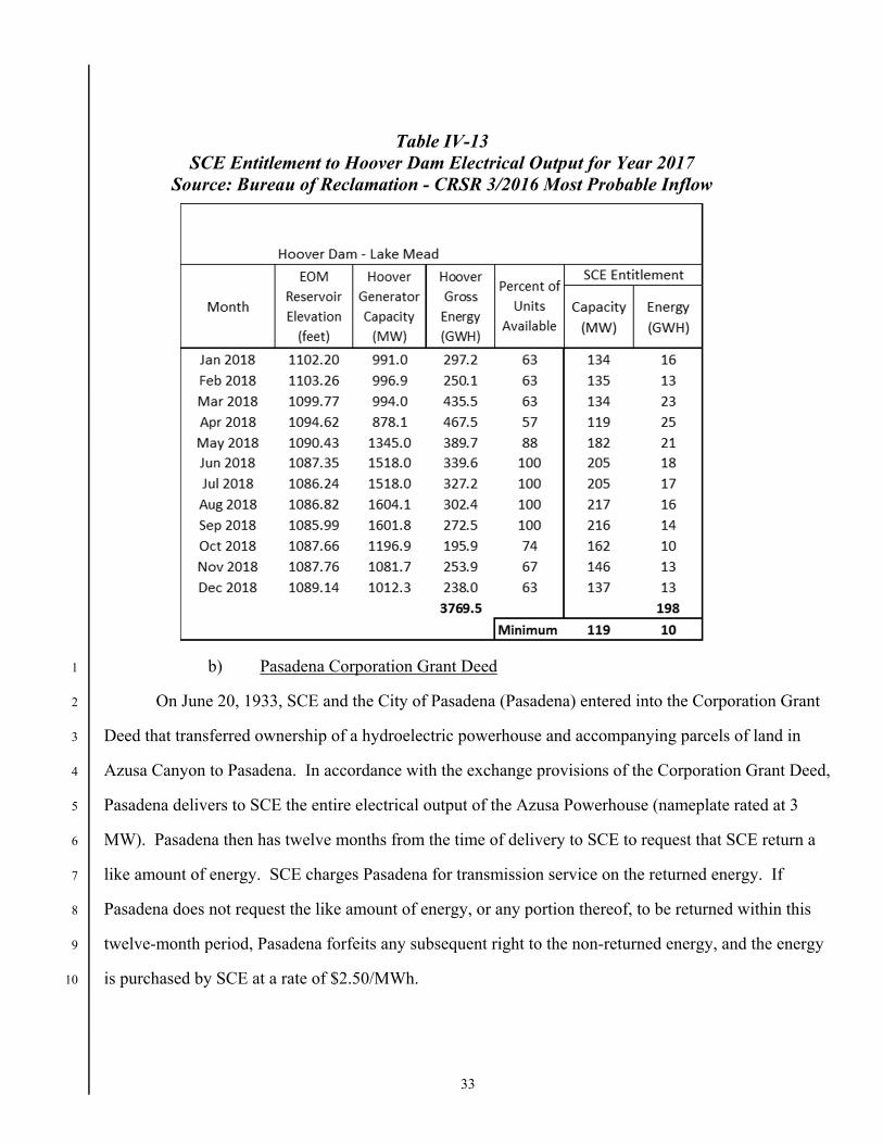
a) WAPA-Reclamation Agreement 4

For 2018, SCE has an entitlement of 280.245 MW of contingent capacity and 238 GWh of firm 5

energy24 from the Boulder Canyon Project (Hoover), marketed by WAPA. 6

Due to the lowering of the surface elevation of Lake Mead, which is the forebay to the Hoover 7

power plant, the amount of capacity and firm energy available to SCE will be reduced from the amounts 8

described in the previous paragraph. For the year 2018, the monthly capacity and firm energy available 9

to SCE could range as low as 119 MW and 10 GWh, respectively.25 The forecast amount of capacity 10

and energy available to SCE out of Hoover is shown in Table IV-13. 11

24 Firm energy is energy obligated from Hoover under the Hoover Power Plant Act. During periods when

Hoover is unable to provide energy in amounts equal to the firm energy, WAPA is obligated to provide any deficit, if requested by the purchaser, at a rate equal to WAPA’s cost to acquire.

25 The Bureau of Reclamation, the owner and operator of Hoover Dam, anticipates a low reservoir elevation through 2018 and beyond. The reason for the low elevation is due to low precipitation since 2000.

33

Table IV-13 SCE Entitlement to Hoover Dam Electrical Output for Year 2017

Source: Bureau of Reclamation - CRSR 3/2016 Most Probable Inflow

b) Pasadena Corporation Grant Deed 1

On June 20, 1933, SCE and the City of Pasadena (Pasadena) entered into the Corporation Grant 2

Deed that transferred ownership of a hydroelectric powerhouse and accompanying parcels of land in 3

Azusa Canyon to Pasadena. In accordance with the exchange provisions of the Corporation Grant Deed, 4

Pasadena delivers to SCE the entire electrical output of the Azusa Powerhouse (nameplate rated at 3 5

MW). Pasadena then has twelve months from the time of delivery to SCE to request that SCE return a 6

like amount of energy. SCE charges Pasadena for transmission service on the returned energy. If 7

Pasadena does not request the like amount of energy, or any portion thereof, to be returned within this 8

twelve-month period, Pasadena forfeits any subsequent right to the non-returned energy, and the energy 9

is purchased by SCE at a rate of $2.50/MWh. 10

34

c) Interutility Contract Resource Costs 1

During the 2018 Forecast Period, SCE will purchase or exchange capacity and associated energy 2

with WAPA-Reclamation and the City of Pasadena. Table IV-12 and Table IV-13 above summarize the 3

estimated amounts of energy attributable to SCE’s major interutility agreements. 4

6. New System Generation CAM Contracts 5

a) Production 6

Pursuant to D.07-09-044 and the Joint Party Proposal (JPP) adopted in that decision, SCE will 7

hold the dispatch rights for all New Gen contracts in 2018. SCE included its bundled service customer 8

share of energy in the portfolio position forecast. 9

b) Costs 10

Consistent with the New Generation cost allocation decisions,26 SCE accounted for the forecast 11

of total net capacity costs for all the New Generation contracts that are expected to operate in 2018. The 12

total forecasted New Generation CAM costs, found in Table IV-8, reflect the total of the capacity costs 13

net of estimated expected revenue and production cost. SCE’s bundled service customers are 14

responsible for their assessed load-share responsibility. 15

7. 2013 Bilateral Contracts Production 16

a) Production 17

In July 2012, SCE and JPMorgan, on behalf of BE CA LLC, began bilateral negotiations. On 18

February 15, 2013, SCE filed Advice Letter 2853-E to seek CPUC approval of this bilaterally-negotiated 19

capacity and tolling agreement between SCE and BE CA LLC. This agreement was approved by the 20

CPUC on May 9, 2013. The projected total production in 2018 from this contract is shown in Table IV-21

7. 22

26 In D.06-07-029, the Commission adopted a CAM that allows the benefits and costs of new generation to be

shared by all customers in an IOU’s service area. The decision also ordered the IOUs to develop energy auction implementation plans. Subsequently, D.07-09-044 adopted specific auction processes for the distribution of energy rights in new generation contracts, including specific products and cost and benefit sharing mechanisms.

35

b) Costs 1

The four general cost categories for SCE’s 2013 Bilateral Contracts are (1) natural gas fuel costs; 2

(2) GHG costs; (3) variable charges; and (4) capacity payments. Table IV-8 provides the forecast 3

monthly costs for these contracts. 4

8. Generic and Bilateral RA Contracts 5

a) Production 6

For 2018, SCE estimates a system capacity need and a local area capacity need that varies by 7

month. Within this calculation, SCE forecasts the RA requirement it will need to meet in 2018. This 8

requirement, less RA contracts already procured, then determines SCE’s forecast remaining 2018 RA 9

need. SCE further assumed that RA contracts will be procured at a forecast generic cost to meet this 10

projected RA need for 2018.27 Table IV-8 provides the forecasted monthly capacity costs for both the 11

generic and bilateral RA contracts. 12

9. Local Capacity Requirements (LCR) Contracts 13

On September 12, 2013, SCE launched its LCR RFO to procure specified amounts of Preferred 14

Resources28, Energy Storage, and Gas Fired Generation (GFG) in the Western LA Basin and Moorpark 15

local reliability areas to meet long-term local capacity requirements. SCE filed A.14-11-01229 and 16

A.14-11-01630 (LCR RFO Applications) for approval of all contracts entered into as a result of the 17

procurement. Pursuant to the Long Term Procurement Plan (LTPP) Track 1 and 4 decisions31 and as 18

27 SCE applied the capacity price of $58.26/kW-year, based on the CEC’s “Estimated Cost of New Renewable

and Fossil Generation in California Final Staff Report” study.

28 Preferred Resources defined as cost-effective energy efficiency, demand response, renewable resources, and distributed generation. See State Energy Action Plan II at page 2.

29 Application for Approval of the Results of its 2013 LCR RFO for the Western LA Basin Sub-Area was approved, in part, in D.15-11-041 on November 19, 2015.

30 Application for Approval of the Results of its 2013 LCR RFO for the Moorpark Sub-Area was approved, in part, in D.16-05-050 on May 26, 2016.

31 D.13-02-015 (Track 1 decision) OP 15 and D.14-03-004 OP 13.

36

proposed in the LCR RFO Applications, the net cost of the capacity32 is allocated to all benefitting 1

customers. 2

a) Production 3

The LCR contracts included in the forecast are behind-the-meter as well as in front-of-the-meter 4

resources. Table IV-8 provides the forecasted monthly energy from the in-front-of-the-meter LCR 5

resources. Behind-the-meter LCR resources reduce the overall bundled load requirement. 6

b) Costs 7

The capacity costs are forecasted in the LCR Costs line item in Table IV-8. 8

10. Preferred Resource Pilot (PRP) 9

On September 24, 2015 SCE launched its PRP RFO #2 to solicit electrical energy, capacity and 10

renewable attributes from eligible resources such as Demand Response, Renewable Distributed 11

Generation, Energy Storage, Renewable Distributed Generation paired with Energy Storage and 12

Permanent Load Shifting. On November 4, 2016, SCE submitted an application seeking approval for 13

the contracts executed during PRP solicitation. Some of the contracts that are executed as a result of this 14

solicitation are expected to operate during 2018. 15

a) Production 16

The PRP contracts that are expected to operate in 2018 are behind-the-meter energy storage 17

resources. Behind-the-meter resources reduce the overall bundled load requirement. 18

b) Costs 19

The capacity costs are forecasted in the PRP Costs line item in Table IV-8.33 20

32 The energy and capacity components of the newly-acquired generation are disaggregated. The net capacity

cost is calculated as the net of the total cost of the contract minus the energy revenues associated with the dispatch of the contract.

33 As described on pages 81-83 of SCE-01 in A.16-11-002, SCE proposes to recover the costs of the PRP behind-the-meter energy storage contracts from customers through the Public Purpose Programs Charge.

37

11. Green Tariff Shared Renewables (GTSR) Program 1

In D.15-01-051, the Commission approved with modifications SCE’s proposal to implement a 2

GTSR program to comply with Senate Bill 43. The GTSR program provides two options for customers: 3

a green tariff option (Green Tariff) that allows customers to allocate either 50% or 100% of their 4

electricity bill to renewable energy, and an enhanced community renewables (ECR) option that allows 5

customers to support renewable energy in their local community via agreements with third-party 6

renewable energy developers. In 2018, SCE has forecasted Green Tariff participation to be 10,296,441 7

kWh and 699,593 KWh of Community Renewables. SCE will update this forecast in the November 8

Update and incorporate it into the sales forecast discussed in Chapter 2.34 Because SCE anticipates that 9

new Green Tariff-specific projects will not have reached commercial operation by 2018, SCE will 10

initially use existing RPS resources that are eligible for the Green Tariff program (Interim GTSR Pool) 11

to serve Green Tariff customers.35 As described in D.15-01-051,36 SCE will use a cost-sharing 12

mechanism to allocate the costs from the Interim GTSR Pool to Green Tariff customers by estimating 13

the amount of energy required to serve participating Green Tariff customers and removing that “slice” of 14

the Interim GTSR Pool from the bundled portfolio.37 SCE’s RPS compliance requirements will be 15

described in SCE’s RPS Procurement Plan filed in R.15-02-020. 16

To account for this program in SCE’s 2018 energy and cost forecast, SCE has included Green 17

Tariff line items in Table IV-7 and Table IV-8, and adjusted the CHP and Renewables energy and cost 18

34 Decision 15-01-051 states that “[i]t is appropriate for an IOU to provide a summary and true-up of costs and

revenues against charges and credits applied to Green Tariff Shared Renewables (GTSR) customers on an annual basis, either through the IOU’s annual ERRA or in a separate application.” This decision also references the IOUs filing an annual Tier 2 advice letter “summarizing the true-up of costs and revenue against charges and credits applied to GTSR customer bills.” In accordance with this language, SCE filed Tier 2 Advice 3525-E on December 2, 2016 updating the GTSR program rate components for 2017. SCE anticipates filing a similar Tier 2 advice filing later this year to update the GTSR program rate components for 2018.

35 SCE will not begin serving ECR customers until ECR-specific projects reach commercial operation.

36 D.15-01-051 at page 40.

37 The remaining Interim GTSR Pool energy and costs will stay in the CHP and Renewables line items of Table IV-7 and Table IV-8.

38

forecast accordingly. The forecasted kWh required to serve Green Tariff customers are removed from 1

the CHP and Renewables energy and shown separately. Similarly, procurement costs for the Green 2

Tariff are estimated by multiplying the forecasted energy by the forecasted 2018 Green Rate Portfolio 3

Charge presented in Advice 3525-E,38 and are removed from the CHP and Renewables costs and 4

allocated directly to Green Tariff customers. 5

F. Other SCE Resources and Programs 6

1. Nuclear 7

a) Production 8

SCE has an ownership interest in two nuclear generation stations – San Onofre Nuclear 9

Generating Station (SONGS) and Palo Verde Nuclear Generating Station (PVNGS). On June 7, 2013, 10

SCE announced the permanent shut down and retirement of SONGS. Accordingly, there are no nuclear 11

fuel expenses or generation forecasted for SONGS during 2018, except for interim fuel storage costs. 12

For purposes of this filing, SCE assumes that PVNGS operates in a baseload manner. 13

SCE owns 15.8% of PVNGS Units 1, 2, and 3, which provide a maximum capacity to SCE of 14

207 MW per unit. Arizona Public Service (APS) is the operator of PVNGS. A refueling outage 15

is scheduled to commence at PVNGS Unit 3 on and a refueling outage is 16

scheduled to commence at PVNGS Unit 2 on . The total forecast 2018 production from 17

SCE’s share of PVNGS is shown in Table IV-7. 18

b) Costs 19

(1) Introduction 20

This section presents SCE’s forecast of its share of SONGS and PVNGS nuclear fuel expense for 21

the 2018 Forecast Period. This forecast includes the SONGS interim storage costs and PVNGS 22

generation-related fuel expense, Department of Energy (DOE) used fuel disposal charges, and interim 23

used fuel storage costs. The total 2018 forecast fuel expense is included in Table IV-8. 24

38 Advice 3525-E (which is currently pending), Attachment B.

39

(2) Nuclear Fuel Management 1

Nuclear fuel management consists of a sequence of activities involving the procurement and 2

scheduling of materials and services required to manufacture nuclear fuel assemblies for use in a nuclear 3

generating station, and the disposal of used fuel assemblies after their discharge from the reactor. These 4

activities encompass: (1) mining and milling natural uranium concentrates (U3O8); (2) conversion to 5

uranium hexafluoride (UF6); (3) enrichment; (4) design and fabrication of fuel assemblies; and (5) used 6

fuel transportation, interim storage, and permanent disposal. 7

SCE and APS, as PVNGS operating agent with SCE’s prior approval, have entered into contracts 8

with various suppliers for each of the activities required to manufacture nuclear fuel for PVNGS. 9

During each refueling and maintenance outage, a batch of new fuel assemblies is loaded into the 10

reactor core and one or more batches of fuel assemblies are removed. A “batch” is a group of nuclear 11

fuel assemblies loaded together into the core of a nuclear generating unit at the beginning of an 12

operating cycle and later removed together at the end of their operating life. The placement of the new 13

fuel assemblies and the fuel assemblies in the remaining batches within the reactor core is based on 14

various reactor core design analyses performed. A batch typically remains in the reactor core for at least 15

two fuel cycles. A fuel cycle begins with a unit’s return to operation following a refueling and 16

maintenance outage shutdown. 17

(3) SONGS Nuclear Fuel Expense 18

SCE projects SONGS nuclear fuel expense of $4.3 million during the Forecast Period. SCE 19

bases this expense on the interim used fuel storage costs of SONGS Unit 1 assemblies at a General 20

Electric (GE) facility in Morris, Illinois. 21

(a) Fuel Expense – Generation Related 22

(i) Permanent Disposition of Used Fuel 23

The DOE retains the ultimate responsibility for the permanent disposal of high-level radioactive 24

waste and used fuel under the authority of the 1982 Waste Policy Act. Under authority given to the 25

DOE by the 1982 Act, SONGS has entered into a contract with DOE for disposal of used fuel and/or 26

high-level radioactive waste for all units. The contract requires payment of a 1.0 mill/kWh fee based on 27

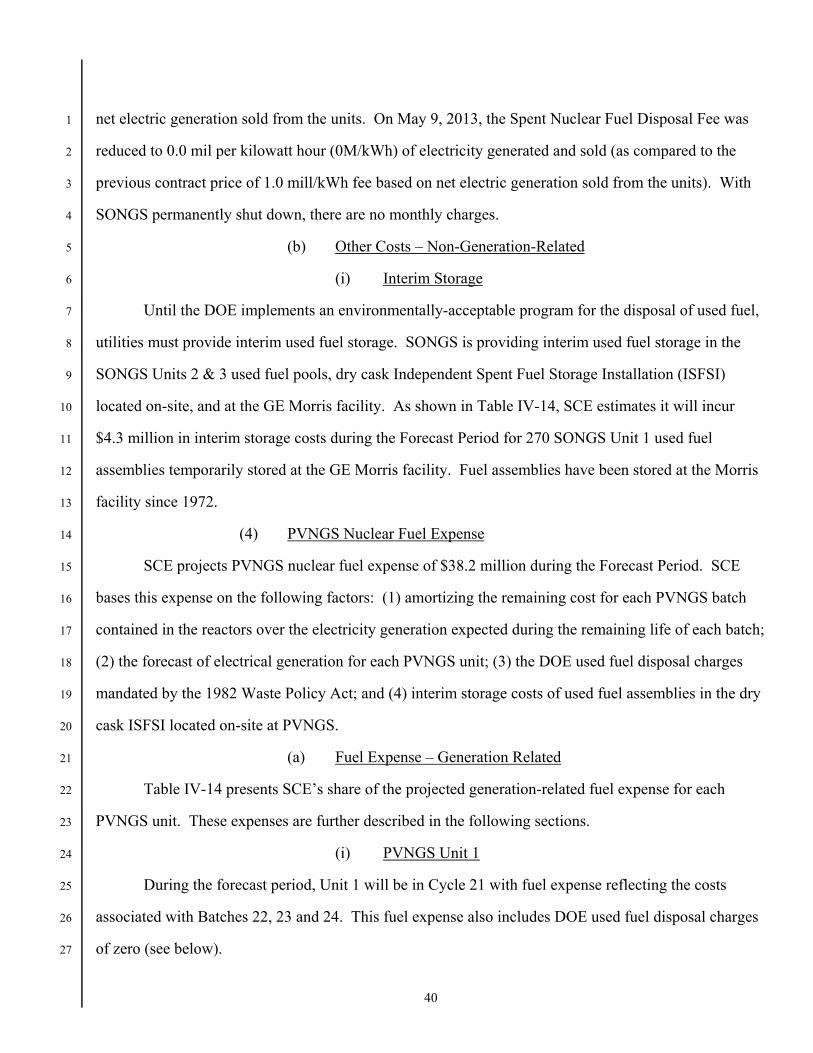
40

net electric generation sold from the units. On May 9, 2013, the Spent Nuclear Fuel Disposal Fee was 1

reduced to 0.0 mil per kilowatt hour (0M/kWh) of electricity generated and sold (as compared to the 2

previous contract price of 1.0 mill/kWh fee based on net electric generation sold from the units). With 3

SONGS permanently shut down, there are no monthly charges. 4

(b) Other Costs – Non-Generation-Related 5

(i) Interim Storage 6

Until the DOE implements an environmentally-acceptable program for the disposal of used fuel, 7

utilities must provide interim used fuel storage. SONGS is providing interim used fuel storage in the 8

SONGS Units 2 & 3 used fuel pools, dry cask Independent Spent Fuel Storage Installation (ISFSI) 9

located on-site, and at the GE Morris facility. As shown in Table IV-14, SCE estimates it will incur 10

$4.3 million in interim storage costs during the Forecast Period for 270 SONGS Unit 1 used fuel 11

assemblies temporarily stored at the GE Morris facility. Fuel assemblies have been stored at the Morris 12

facility since 1972. 13

(4) PVNGS Nuclear Fuel Expense 14

SCE projects PVNGS nuclear fuel expense of $38.2 million during the Forecast Period. SCE 15

bases this expense on the following factors: (1) amortizing the remaining cost for each PVNGS batch 16

contained in the reactors over the electricity generation expected during the remaining life of each batch; 17

(2) the forecast of electrical generation for each PVNGS unit; (3) the DOE used fuel disposal charges 18

mandated by the 1982 Waste Policy Act; and (4) interim storage costs of used fuel assemblies in the dry 19

cask ISFSI located on-site at PVNGS. 20

(a) Fuel Expense – Generation Related 21

Table IV-14 presents SCE’s share of the projected generation-related fuel expense for each 22

PVNGS unit. These expenses are further described in the following sections. 23

(i) PVNGS Unit 1 24

During the forecast period, Unit 1 will be in Cycle 21 with fuel expense reflecting the costs 25

associated with Batches 22, 23 and 24. This fuel expense also includes DOE used fuel disposal charges 26

of zero (see below). 27

41

(ii) PVNGS Unit 2 1

During the forecast period, Unit 2 is forecast to undergo and complete a refueling outage. It is 2

forecast to complete Cycle 21 and commence Cycle 22 with fuel expense reflecting the costs associated 3

with Batches 22, 23, 24 and 25. This fuel expense also includes DOE used fuel disposal charges of zero 4

(see below). 5

(iii) PVNGS Unit 3 6

During the forecast period, Unit 3 is forecast to undergo and complete a refueling outage. It is 7

forecast to complete Cycle 20 and commence Cycle 21 with fuel expense reflecting the costs associated 8

with Batches 21, 22, 23 and 24. This fuel expense also includes DOE used fuel disposal charges of zero 9

(see below). 10

(iv) Permanent Disposition of Used Fuel 11

During a reactor refueling, depleted fuel assemblies are removed from the reactor core and 12

replaced with new fuel assemblies. Since the depleted assemblies are highly radioactive, they must be 13

stored in a manner that isolates them from the environment. The DOE retains the ultimate responsibility 14

for the permanent disposal of high-level radioactive waste and used fuel under the authority of the 1982 15

Waste Policy Act. Under authority given to the DOE by the 1982 Act, PVNGS has entered into a 16

contract with DOE for disposal of used fuel and/or high-level radioactive waste for all units. On May 9, 17

2013, DOE notified APS that as of May 15, 2014, the Spent Nuclear Fuel Disposal Fee will be 0.0 mil 18

per kilowatt hour (0M/kWh) of electricity generated and sold (as compared to the previous contract 19

price of 1.0 mill/kWh fee based on net electric generation sold from the units). Accordingly, the 20

monthly generation-related fuel expense shown for each PVNGS unit in Table IV-14 does not include 21

any estimated monthly charges for these fees during the Forecast Period. SCE notes that if the contract-22

based fee is recalculated in the future, SCE will seek to recover these costs through ERRA as 23

appropriate. 24

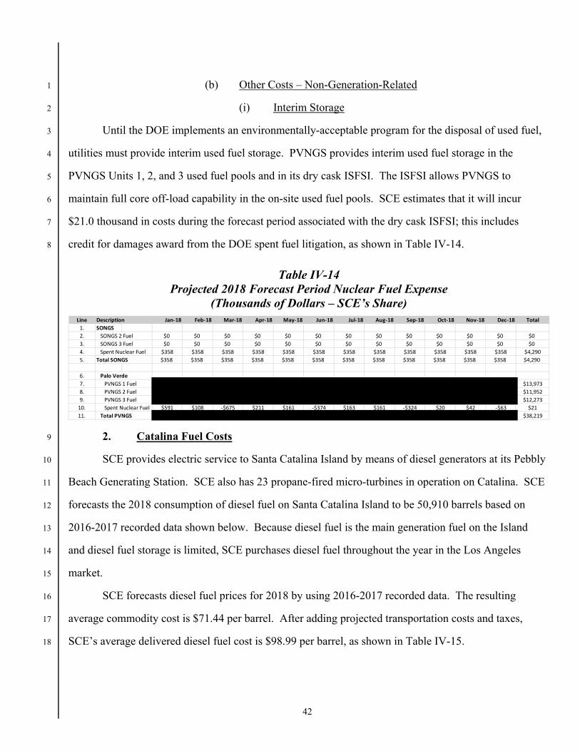
42

(b) Other Costs – Non-Generation-Related 1

(i) Interim Storage 2

Until the DOE implements an environmentally-acceptable program for the disposal of used fuel, 3

utilities must provide interim used fuel storage. PVNGS provides interim used fuel storage in the 4

PVNGS Units 1, 2, and 3 used fuel pools and in its dry cask ISFSI. The ISFSI allows PVNGS to 5

maintain full core off-load capability in the on-site used fuel pools. SCE estimates that it will incur 6

$21.0 thousand in costs during the forecast period associated with the dry cask ISFSI; this includes 7

credit for damages award from the DOE spent fuel litigation, as shown in Table IV-14. 8

Table IV-14 Projected 2018 Forecast Period Nuclear Fuel Expense

(Thousands of Dollars – SCE’s Share)

2. Catalina Fuel Costs 9

SCE provides electric service to Santa Catalina Island by means of diesel generators at its Pebbly 10

Beach Generating Station. SCE also has 23 propane-fired micro-turbines in operation on Catalina. SCE 11

forecasts the 2018 consumption of diesel fuel on Santa Catalina Island to be 50,910 barrels based on 12

2016-2017 recorded data shown below. Because diesel fuel is the main generation fuel on the Island 13

and diesel fuel storage is limited, SCE purchases diesel fuel throughout the year in the Los Angeles 14

market. 15

SCE forecasts diesel fuel prices for 2018 by using 2016-2017 recorded data. The resulting 16

average commodity cost is $71.44 per barrel. After adding projected transportation costs and taxes, 17

SCE’s average delivered diesel fuel cost is $98.99 per barrel, as shown in Table IV-15. 18

Line Description Jan-18 Feb-18 Mar-18 Apr-18 May-18 Jun-18 Jul-18 Aug-18 Sep-18 Oct-18 Nov-18 Dec-18 Total1. SONGS2. SONGS 2 Fuel $0 $0 $0 $0 $0 $0 $0 $0 $0 $0 $0 $0 $03. SONGS 3 Fuel $0 $0 $0 $0 $0 $0 $0 $0 $0 $0 $0 $0 $04. Spent Nuclear Fuel $358 $358 $358 $358 $358 $358 $358 $358 $358 $358 $358 $358 $4,2905. Total SONGS $358 $358 $358 $358 $358 $358 $358 $358 $358 $358 $358 $358 $4,290

6. Palo Verde7. PVNGS 1 Fuel $13,9738. PVNGS 2 Fuel $11,9529. PVNGS 3 Fuel $12,273

10. Spent Nuclear Fuel $591 $108 -$675 $211 $161 -$374 $163 $161 -$324 $20 $42 -$63 $2111. Total PVNGS $38,219

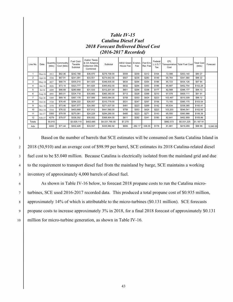
43

Table IV-15 Catalina Diesel Fuel

2018 Forecast Delivered Diesel Cost (2016-2017 Recorded)

Based on the number of barrels that SCE estimates will be consumed on Santa Catalina Island in 1

2018 (50,910) and an average cost of $98.99 per barrel, SCE estimates its 2018 Catalina-related diesel 2

fuel cost to be $5.040 million. Because Catalina is electrically isolated from the mainland grid and due 3

to the requirement to transport diesel fuel from the mainland by barge, SCE maintains a working 4

inventory of approximately 4,000 barrels of diesel fuel. 5

As shown in Table IV-16 below, to forecast 2018 propane costs to run the Catalina micro-6

turbines, SCE used 2016-2017 recorded data. This produced a total propane cost of $0.935 million, 7

approximately 14% of which is attributable to the micro-turbines ($0.131 million). SCE forecasts 8

propane costs to increase approximately 3% in 2018, for a final 2018 forecast of approximately $0.131 9

million for micro-turbine generation, as shown in Table IV-16. 10

Line No. Date Quantity

(bbls)Commodity Cost (bbls)

Fuel Cost-Taxable Subtotal

Avalon Taxes & CA Advance Collection DSL

Combined

SubtotalAB32 Green House Fee

Environ. Fee

Fed Env Rec Fee

Federal L.U.S.T

Tax

CFL Transportation

CostTotal Fuel Cost

Total Cost (bbls)

Forecast

1 Mar-16 3912 $62.06 $242,788 $36,970 $279,758.00 $559 $259 $312 $164 72,088 $353,140 $90 27

2 Apr-16 3550 $67.91 $241,091 $33,551 $274,642.00 $507 $235 $283 $149 65,764 $341,580 $96 22

3 May-16 4437 $68.74 $305,010 $41,925 $346,935.00 $634 $294 $354 $186 85,723 $434,126 $97 84

4 Jun-16 4426 $73.15 $323,777 $41,825 $365,602.00 $632 $294 $353 $186 85,687 $452,754 $102.29

5 Jul-16 4209 $66.68 $280,668 $31,533 $312,201.00 $601 $294 $336 $177 82,568 $396,177 $94.13

6 Aug-16 4995 $65.01 $324,718 $35,665 $360,383.00 $713 $329 $399 $210 97,078 $459,111 $91 91

7 Sep-16 5309 $69.16 $367,178 $37,906 $405,084.00 $758 $353 $424 $223 103,467 $510,309 $96.12

8 Oct-16 3720 $76.40 $284,222 $26,557 $310,779.00 $531 $247 $297 $156 73,165 $385,175 $103.54

9 Nov-16 3370 $73.46 $247,577 $24,060 $271,637.00 $481 $223 $269 $142 65,634 $338,385 $100.41

10 Dec-16 5310 $76.02 $403,668 $37,912 $441,580.00 $758 $353 $424 $223 103,203 $546,541 $102.93

11 Jan-17 3393 $79.59 $270,061 $24,229 $294,290.00 $485 $223 $271 $143 65,555 $360,966 $106.39

12 Feb-17 4279 $79.07 $338,352 $30,552 $368,904.00 $611 $282 $341 $180 82,641 $452,959 $105.86

Totals 50,910 $3,629,110 $402,685 $4,031,795.00 $7,270 $982,573 $5,031,225 $1,187 91

Adv 4243 $71.44 $302,426 $33,557 $335,982.92 $606 282.17 338.55 $178 81,881 $419,269 $98 99 5,040 00

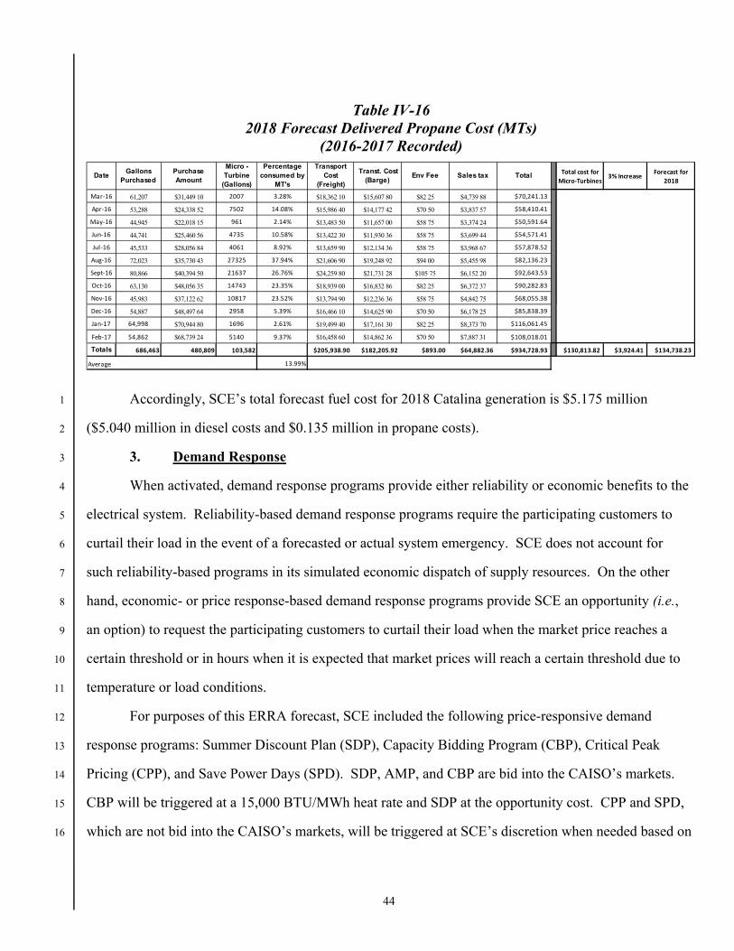
44

Table IV-16 2018 Forecast Delivered Propane Cost (MTs)

(2016-2017 Recorded)

Accordingly, SCE’s total forecast fuel cost for 2018 Catalina generation is $5.175 million 1

($5.040 million in diesel costs and $0.135 million in propane costs). 2

3. Demand Response 3

When activated, demand response programs provide either reliability or economic benefits to the 4

electrical system. Reliability-based demand response programs require the participating customers to 5

curtail their load in the event of a forecasted or actual system emergency. SCE does not account for 6

such reliability-based programs in its simulated economic dispatch of supply resources. On the other 7

hand, economic- or price response-based demand response programs provide SCE an opportunity (i.e., 8

an option) to request the participating customers to curtail their load when the market price reaches a 9

certain threshold or in hours when it is expected that market prices will reach a certain threshold due to 10

temperature or load conditions. 11

For purposes of this ERRA forecast, SCE included the following price-responsive demand 12

response programs: Summer Discount Plan (SDP), Capacity Bidding Program (CBP), Critical Peak 13

Pricing (CPP), and Save Power Days (SPD). SDP, AMP, and CBP are bid into the CAISO’s markets. 14

CBP will be triggered at a 15,000 BTU/MWh heat rate and SDP at the opportunity cost. CPP and SPD, 15

which are not bid into the CAISO’s markets, will be triggered at SCE’s discretion when needed based on 16

DateGallons

PurchasedPurchase Amount

Micro - Turbine

(Gallons)

Percentage consumed by

MT's

Transport Cost

(Freight)

Transt. Cost (Barge)

Env Fee Sales tax Total Total cost for Micro-Turbines

3% Increase Forecast for 2018

Mar-16 61,207 $31,449 10 2007 3.28% $18,362 10 $15,607 80 $82 25 $4,739 88 $70,241.13

Apr-16 53,288 $24,338 52 7502 14.08% $15,986 40 $14,177 42 $70 50 $3,837 57 $58,410.41

May-16 44,945 $22,018 15 961 2.14% $13,483 50 $11,657 00 $58 75 $3,374 24 $50,591.64

Jun-16 44,741 $25,460 56 4735 10.58% $13,422 30 $11,930 36 $58 75 $3,699 44 $54,571.41

Jul-16 45,533 $28,056 84 4061 8.92% $13,659 90 $12,134 36 $58 75 $3,968 67 $57,878.52

Aug-16 72,023 $35,730 43 27325 37.94% $21,606 90 $19,248 92 $94 00 $5,455 98 $82,136.23

Sept-16 80,866 $40,394 50 21637 26.76% $24,259 80 $21,731 28 $105 75 $6,152 20 $92,643.53

Oct-16 63,130 $48,056 35 14743 23.35% $18,939 00 $16,832 86 $82 25 $6,372 37 $90,282.83

Nov-16 45,983 $37,122 62 10817 23.52% $13,794 90 $12,236 36 $58 75 $4,842 75 $68,055.38

Dec-16 54,887 $48,497 64 2958 5.39% $16,466 10 $14,625 90 $70 50 $6,178 25 $85,838.39

Jan-17 64,998 $70,944 80 1696 2.61% $19,499 40 $17,161 30 $82 25 $8,373 70 $116,061.45

Feb-17 54,862 $68,739 24 5140 9.37% $16,458 60 $14,862 36 $70 50 $7,887 31 $108,018.01

Totals 686,463 480,809 103,582 $205,938.90 $182,205.92 $893.00 $64,882.36 $934,728.93 $130,813.82 $3,924.41 $134,738.23

Average 13.99%

45

factors such as: CAISO-issued alert or warning notice, day-ahead load and/or price forecast, and 1

extreme or unusual temperature conditions impacting system demand, etc. 2

SCE forecasts an estimated 9 GWh of energy reductions to be provided by its price-responsive 3

demand response programs in 2018. This forecast utilizes a combination of SCE’s Load Impact 4

Protocols39

and other factors such as annual available hours, expected event months, and number of 5

events per year. The load impact estimates are based on past customer performance and forecasted 6

enrollment rates for program participation. Since the programs are voluntary and enrollment can vary 7

month-to-month, these estimates provide a reasonable assessment of annual load reduction capability. 8

SCE’s cost recovery for its DR programs are recovered outside of ERRA, through the Purchase 9

Agreement Administrative Costs Balancing Account (PAACBA) and the distribution subaccount of the 10

Base Revenue Requirement Balancing Account (BRRBA). 11

G. CAISO Costs and Short-Term Market Activity 12

CAISO implemented a new market design, known as MRTU, on April 1, 2009. The new market 13

design includes elements such as the IFM, locational marginal pricing (LMP), and congestion revenue 14

rights (CRRs), and operates in a dramatically different manner than the previous zonal market. Due to 15

the complexity of the CAISO market, SCE separated the total costs from the CAISO market into (1) the 16

non-energy-related CAISO costs (CAISO costs); and (2) energy-related short-term market activity cost 17

(short-term market activity cost). SCE forecast the CAISO costs and the short-term market activity 18

costs separately, applying different forecasting methodologies as described below. 19

1. CAISO Costs 20

SCE’s 2018 ERRA forecast of CAISO costs is comprised of the net cost of: grid management 21

charges (GMC); FERC fees; CRR auction-related costs; ancillary services; CAISO uplift costs; Standard 22

Capacity Product (SCP) costs; and other non-energy-related CAISO costs. SCE considers these costs as 23

the non-energy-related CAISO costs as they are not sensitive to short-term energy market prices. 24

39 D.08-04-050, Attachment A, Load Impact Estimation for Demand Response: Protocols and Regulatory

Guidance, California Public Utilities Commission, Energy Division, April 2008 (the Load Impact Protocols).

46

Therefore, SCE assumed that its 2018 CAISO costs, described above, would be equal to its historical 1

costs for the most recent 12-month period (i.e., from January 2016 through December 2016). SCE’s 2

2018 forecast CAISO costs are presented in Table IV-7. 3

2. Short-Term Market Activity Costs 4

SCE estimates its hourly open energy positions by netting its projected production from its 5

supply portfolio against its forecasted bundled load for each hour. SCE covers a major portion of its 6

open positions through the IFM,40 with bilateral transactions comprising a smaller portion. SCE also 7

covers a very small portion of its open positions in the CAISO hour-ahead and real-time (RT) markets. 8

For the purpose of this ERRA forecast application, SCE separated the forecast energy costs associated 9

with covering its open positions from the forecast CAISO costs discussed in the preceding section. All 10

forecast short-term market activity costs are reported separately in Table IV-8. 11

H. Gas Price Sensitivity 12

Pursuant to an agreement with ORA reached in A.10-08-001, SCE agreed to perform a two-13

standard-deviation gas price sensitivity analysis for ORA in support of its future ERRA forecasts for up 14

to five years. SCE performed the subject gas price sensitivity analysis and included the results in its 15

2011 ERRA Application (A.11-08-002) for the 2012 forecast calendar year.41 SCE conducted a similar 16

sensitivity analysis for this 2018 ERRA forecast. 17

Using this sensitivity analysis, SCE’s forecasted 2018 ERRA costs are projected to increase or 18

decrease by similar amounts, approximately , with an approximate $0.10/MMBtu upward or 19

downward gas price movement from the base case forecast SoCal Border gas price of $2.78 /MMBtu for 20

the 2018 12-month strip. 21

As SCE has stated in previous ERRA forecast proceedings, the gas price sensitivity analysis can 22

only serve as a “rough check” on the updated ERRA forecasts and cannot be used to determine forecast 23

40 The short-term market activity cost includes the net costs associated with covering the open energy positions

inclusive of estimated CRR revenues SCE expects to benefit from future CRR holdings.

41 SCE provided the detailed description of the methodology SCE applied to its gas price sensitivity analysis in A.11-08-022.

47

accuracy. One cannot simply apply the gas price sensitivity analysis to assess the accuracy of ERRA 1

forecast updates due to the multiple changes of the major input drivers (e.g., SCE’s portfolio changes) 2

that occur. 3

I. Direct GHG Costs 4

Direct GHG costs are shown separately in Table IV-8. Indirect GHG costs are embedded in the 5

purchased power contracts and utility-owned generation forecasts, and are identified and discussed in 6

further detail in Chapter VII. 7

J. Gas Hedging Costs 8

The total forecast cost to hedge the natural gas price risk for SCE’s UOG, purchased power 9

contracts, and QF contracts in 2018 is . This amount includes mark-to-market (MTM) 10

gains/losses on existing hedges for gas risk, expected transaction fees for gas to be procured and hedged 11

for 2018, and costs for expected future option premiums related to 2018 gas risk. These costs are made 12

up of: (1) forecasted transaction fees of and (2) forecasted option premiums of 13

Each of these items is discussed further below. 14

15

1. Transaction Fees 16

Transaction fees consist of clearing and exchange fees charged by the NYMEX and 17

Intercontinental Exchange (ICE), as well as brokerage fees from over-the-counter brokered financial 18

transactions. 19

2. Option Premiums 20

The price of an option is reflected as a cost in addition to the forecast cost of gas. The option 21

premium is the cost of removing the risk of increased gas prices. 22

K. Gas Transportation and Storage 23

For 2018, SCE expects to maintain gas transportation agreements with an estimated fixed cost of 24

$1,200. This estimated cost is for reliable delivery of natural gas to both SCE-owned and -contracted 25

natural gas-fired resources. SCE does not expect to purchase storage on the SoCalGas system in 2018. 26

Due to operational problems at SoCalGas’ Aliso Canyon storage facility, SoCalGas does not have a 27

48

clear picture of how much injection, withdrawal, and inventory capacity it will be able to provide for 1

this next storage year. As a result, until further notice SoCalGas will not be offering sales of unbundled 2

storage services to noncore customers. 3

1. Transportation 4

SCE’s estimated fixed cost of natural gas transportation for 2018 is $1,200. This estimate is 5

based on a fixed monthly customer charge for the SCE UOG fuel cells located at UC Santa Barbara 6

(UCSB) and California State University, San Bernardino (CSUSB) under SoCalGas Schedule No. GT-7

NC (Intrastate Transportation Service). 8

In accordance with CPUC Decision D.16-07-008, SoCalGas provided a new Schedule A to the 9

SoCalGas Master Services Contract for natural gas transportation. Among the changes, there are no 10

longer firm or interruptible service priorities, and contract term durations were changed from two or 11

three years in length to month-to-month. 12

a) SoCalGas Transportation Agreement for Mountainview Generating Station 13

Effective February 1, 2017, SCE entered into a month-to-month contract with SoCalGas for 14

transportation capacity under Rate Schedule GT-TLS, under a volumetric rate. There is no fixed 15

component for the term of the contract. It is expected that this transportation contract will auto-renew 16

for each month during 2018. 17

b) SoCalGas Transportation Agreements for UCSB and CSUSB 18

Effective February 1, 2017, SCE entered into month-to-month contracts with SoCalGas for 19

transportation capacity under Rate Schedule GT-NC to the SCE fuel cells at UCSB and CSUSB. The 20

fixed component is a $50 monthly customer charge for each agreement. The total expected fixed cost 21

for both agreements in 2018 is $1,200. It is expected that these transportation contracts will auto-renew 22

for each month during 2018. 23

c) SoCalGas Transportation Agreements for SCE Peakers 24

Effective February 1, 2017, SCE entered into month-to-month contracts with SoCalGas for 25

transportation capacity under Rate Schedule GT-TLS, under a volumetric rate for the SCE Barre, 26

Center, Grapeland, McGrath, and Mira Loma Peakers. There is no fixed component associated with 27

49

these transportation contracts. It is expected that these transportation contracts will auto-renew for each 1

month during 2018. 2

50

V. 1

FINANCING COSTS 2

This chapter discusses financing costs that relate to SCE’s forecast power production and 3

procurement during 2018 that are recovered through the operation of the ERRA. 4

A. Commission Decisions Regarding Financing Costs and Collateral Costs 5

Existing Commission decisions authorize SCE to recover actual fuel inventory financing costs 6

and actual collateral costs. D.93-01-027 authorizes SCE to recover actual fuel inventory financing 7

costs.42 D.02-10-062, which established the ERRA, provides for recovery of fuel and credit costs, 8

including collateral costs.43 9

Provisions for the recovery of financing costs associated with ERRA balancing account 10

undercollections are specified in D.04-01-048. The decision states that once SCE is able to issue 11

commercial paper, the three-month commercial paper rate index will be applied to undercollected 12

balances.44 13

B. SCE’s Current Short-Term Financings 14

1. Credit Facilities (Revolvers) 15

SCE currently has a $2.5 billion multi-year revolving credit facility (also referred to as “facility” 16

or “revolver”) that supports its short-term borrowing requirements, including liquidity support for 17

commercial paper45 as well as letters of credit and cash collateral for procurement needs. Furthermore, 18

the credit facility carries only a marginal facility fee if no borrowings or other usage is required. 19

Because SCE has exhausted both its one-year extension options under the credit facility, SCE 20

plans to renegotiate the credit facility in 2018, in order to maintain a five-year term and add two one-21

42 D.93-01-027, Findings of Fact 23-26, 28, 30-32, Conclusion of Law 14, 47 CPUC 2d 682, 696-698.

43 D.02-10-062, Finding of Fact 23, mimeo, p. 71.

44 D.04-01-048, mimeo, p. 10, Ordering Paragraph 4, p. 23.

45 The SCE commercial paper program requires a backup credit facility so that SCE can redeem commercial paper when it comes due, in the event that SCE cannot issue replacement commercial paper.

51

year extension options. SCE expects the facility to have the following key features, similar to the 1

existing facility: 2

• $2.75 billion total amount 3

• July 2023 maturity 4

• Arrangement and up-front costs and fees of approximately $10.0 million 5

• Additional up-front costs and fees for exercising the two one-year extension options 6

• $20,000 annual administrative fee 7

• 10 basis point annual facility fee 8

• 90 basis point participation fee on any outstanding letters of credit 9

• 20 basis point issuer fees on any letters of credit 10

• LIBOR plus 90 basis points borrowing (loan) rate 11

Only a portion of the up-front costs and fees shown above is allocated to ERRA. 12

The total size of the revolver is based on projected collateral requirements, balancing account 13

undercollections, and short-term general purpose borrowing needs during the term of the revolver. 14

Therefore, a pro-rata share of the costs of the revolver, corresponding to the capacity required to support 15

potential collateral requirements and balancing account undercollections financed by the revolver, is 16

recovered through the ERRA. For 2018, SCE forecasts that of the five-year credit 17

facility will be dedicated to providing capacity for collateral and supporting balancing accounts. The 18

facility fees associated with this $ amount should therefore be recorded in the ERRA 19

balancing account. ERRA undercollections that are financed by the revolver should be charged the 20

appropriate interest rate on the undercollected balance pursuant to D.04-01-048. SCE intends to recover 21

the remaining facility and commitment fees that are associated with general corporate borrowing, along 22

with general purpose interest costs, through base rates. 23

2. Collateral Requirements 24

Collateral requirements vary with changes in power prices and must be provided to 25

counterparties within a few days of a collateral call. As a result, the capacity for the maximum collateral 26

draw must be maintained at all times. Up to of SCE’s current credit facility is dedicated 27

52

to supporting its collateral requirements and balancing account undercollections. The remaining 1

of SCE’s $2.75 billion credit facility is available capacity for general purpose working 2

capital needs. SCE’s collateral requirements will change if the Commission requires SCE to change its 3

planned procurement of reserves to meet resource adequacy requirements or requires SCE to sign 4

additional long-term contracts for other purposes. As a result, if SCE needs to increase its collateral 5

capacity in 2018, it should be allowed to recover any such increased costs through the ERRA balancing 6

account. 7

3. Fixed Rate Bonds Supporting Fuel Inventories 8

Currently, SCE has a $100 million fixed rate bond to support the minimum balance of all fuel 9

inventories projected through November 2017. The $100 million fixed rate bond matures in November 10

2017. SCE anticipates issuing a $125 million fixed rate 3-year fuel inventory bond in November 2017 11

to replace the expired fixed rate bond support the minimum balance of all fuel inventories projected 12

through November 2020. SCE estimates approximately $1,000,000 in issuance costs and expenses for 13

the new fixed rate bond, which will be recorded at the time of offering, in November 2017. 14

4. Commercial Paper 15

In January 2011, SCE expanded its commercial paper program to $2.0 billion. In 2018, SCE’s 16

$2.0 billion commercial paper program will finance fuel inventories in excess of the amount covered by 17

the fixed rate bond.46 SCE’s 2018 forecast assumes that the market for A2/P1 commercial paper will 18

continue to remain stable, and that SCE will be able to utilize the commercial paper program for its 19

short-term borrowing needs. 20

SCE’s commercial paper program has the following features: 21

• $2 billion capacity; 22

• A2/P1/F2 rating; and 23

• 5 basis point annualized dealer fee on each issue. 24

46 From time to time, SCE may use commercial paper or borrowings against its credit facility to fund cash

collateral requirements; however, SCE customarily provides collateral through letters of credit supported by the revolving credit agreement.

53

5. Costs of Collateral Issuance 1

For most counterparties, SCE will provide collateral in the form of letters of credit rather than 2

having to borrow cash. The participation fees and additional fees associated with the letters of credit 3

issued under the revolver will be charged to the ERRA. 4

C. Additional Options Supporting Collateral 5

As previously discussed, the revolvers may not be large enough to support all of SCE’s collateral 6

requirements. Therefore, SCE’s current credit facility includes an option to increase its credit facility 7

limit from . If additional collateral support is required, SCE may seek to 8

increase the limits of its credit facility up to 9

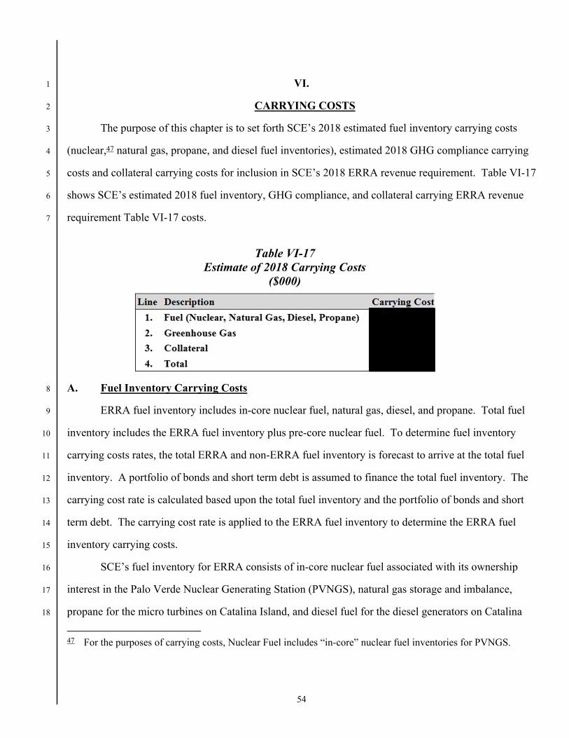
54

VI. 1

CARRYING COSTS 2

The purpose of this chapter is to set forth SCE’s 2018 estimated fuel inventory carrying costs 3

(nuclear,47 natural gas, propane, and diesel fuel inventories), estimated 2018 GHG compliance carrying 4

costs and collateral carrying costs for inclusion in SCE’s 2018 ERRA revenue requirement. Table VI-17 5

shows SCE’s estimated 2018 fuel inventory, GHG compliance, and collateral carrying ERRA revenue 6

requirement Table VI-17 costs. 7

Table VI-17 Estimate of 2018 Carrying Costs

($000)

A. Fuel Inventory Carrying Costs 8

ERRA fuel inventory includes in-core nuclear fuel, natural gas, diesel, and propane. Total fuel 9

inventory includes the ERRA fuel inventory plus pre-core nuclear fuel. To determine fuel inventory 10

carrying costs rates, the total ERRA and non-ERRA fuel inventory is forecast to arrive at the total fuel 11

inventory. A portfolio of bonds and short term debt is assumed to finance the total fuel inventory. The 12

carrying cost rate is calculated based upon the total fuel inventory and the portfolio of bonds and short 13

term debt. The carrying cost rate is applied to the ERRA fuel inventory to determine the ERRA fuel 14

inventory carrying costs. 15

SCE’s fuel inventory for ERRA consists of in-core nuclear fuel associated with its ownership 16

interest in the Palo Verde Nuclear Generating Station (PVNGS), natural gas storage and imbalance, 17

propane for the micro turbines on Catalina Island, and diesel fuel for the diesel generators on Catalina 18

47 For the purposes of carrying costs, Nuclear Fuel includes “in-core” nuclear fuel inventories for PVNGS.

55

Island. The calculation of ERRA fuel inventory carrying costs is based on forecast average monthly 1

ERRA inventory balances (PVNGS nuclear in-core, diesel, propane, and natural gas) and the carrying 2

cost rate. The total estimated 2018 ERRA fuel inventory balance and associated financing costs are 3

presented in Table VI-18. 4

Table VI-18 Estimated 2018 Fuel Inventory Carrying Costs

($000)

B. GHG Compliance Carrying Costs 5

This section discusses the forecast of GHG procurement compliance carrying costs in 2018. 6

SCE is authorized to recover the actual interest expense associated with the cash outlays to meet GHG 7

procurement compliance costs.48 To forecast carrying costs, SCE uses the ERRA balancing account 8

interest rates to finance GHG procurement compliance carrying costs. The forecast 2018 GHG 9

procurement compliance inventory and carrying costs are presented in the Table VI-19 below. 10

Table VI-19 Estimated 2018 GHG Compliance Carrying Costs

($000)

C. Collateral Carrying Costs 11

Table VI-20 sets forth the calculation of the carrying costs associated with SCE’s collateral 12

requirements necessary to procure power. This calculation is based on estimated average collateral 13

requirements and the projected terms of SCE’s revolvers, discussed in Chapter V.B. As SCE’s collateral 14

requirements change during 2018, SCE will use actual collateral requirements in determining its 15

carrying costs recorded in the ERRA. 16

48 See D.14-10-033, Attachment B, Section G - GHG Accounting Procedures for Ratesetting Purposes

Description Jan-18 Feb-18 Mar-18 Apr-18 May-18 Jun-18 Jul-18 Aug-18 Sep-18 Oct-18 Nov-18 Dec-18 Total

Average ERRA Fuel Inventory Value

Inventory Carrying Cost

Line Description Jan-18 Feb-18 Mar-18 Apr-18 May-18 Jun-18 Jul-18 Aug-18 Sep-18 Oct-18 Nov-18 Dec-18 Total

1. Average ERRA GHG Inventory Value

2. Inventory Carrying Cost

56

Table VI-20 Estimated 2018 Procurement Collateral Carrying Costs

($000) Line Description Jan-18 Feb-18 Mar-18 Apr-18 May-18 Jun-18 Jul-18 Aug-18 Sep-18 Oct-18 Nov-18 Dec-18 Total

1. Average Collateral Value2. Collateral Carrying Cost

57

VII. 1

GHG FORECAST COSTS AND REVENUES AND RECONCILIATION 2

A. Overview 3

Pursuant to the Commission’s Phase 2 Decision Adopting Standard Procedures for Electric 4

Utilities to File Greenhouse Gas Forecast Revenue and Reconciliation Requests (D.14-10-033 or Phase 5

2 Decision) issued in A.13-08-002 et al., dated October 16, 2014, the utilities are to include their GHG 6

revenue and reconciliation requests as an additional chapter or section within the annual ERRA Forecast 7

applications, commencing with the 2016 Forecast Period. 8

Therefore, this chapter presents SCE’s (1) forecast of 2018 GHG allowance revenue (allowance 9

revenue) and revenue returns to eligible customers, (2) reconciliation of prior period “computed” GHG 10

costs to true-up the GHG allowance revenue returns, (3) forecast of 2018 administrative and customer 11

outreach costs, and (4) reconciliation of the prior period activity to account for deviations between actual 12

revenues returned to customers, and actual revenues received from the consignment of allowances to the 13

auction, net of actual administrative and customer outreach costs. 14

In summary, SCE proposes to return a total of $373.300 million in net available GHG revenues 15

to eligible customers in 2018 based on the Commission-adopted methodologies and utilizing GHG 16

revenues and cap-and-trade costs, including administrative and customer outreach costs, as proposed and 17

supported in this Application. Based on SCE’s estimated GHG allowance revenues available for return 18

to eligible customers in 2018 as set forth in this testimony, and after accounting for administrative and 19

customer outreach costs, the AB693 set aside for Multi Family Affordable Housing Solar Roofs 20

Program49, Emissions-Intensive Trade-Exposed (EITE) revenue returns, and small business customer 21

49 Pursuant to Assembly Bill 693, which established the Multifamily Affordable Housing Solar Roofs Program,

on March 18, 2016 ALJ Simon issued a ruling in R.14-07-002 requiring utilities to set aside one hundred million dollars ($100,000,000) or ten percent of available funds, whichever is less, from the revenues described in subdivision (c) of Section 748.52 for the Multifamily Affordable Housing Solar Roofs Program. This item is further discussed in Section E. of this Chapter.

58

volumetric returns set to offset all or a portion of GHG costs in rates, residential customers can expect a 1

semi-annual, on-bill California Climate Credit of $36.00 in 2018.50 2

Upon Commission approval of this Application, SCE will file a Tier 1 advice letter to implement 3

changes to its tariffs as necessary to include the authorized cap-and-trade costs and GHG revenue 4

returns in rates. These changes will include revisions to SCE’s: (1) residential rate schedules, including 5

master-metered rate schedules, to include the authorized 2018 residential California Climate Credit 6

amounts; (2) small business rate schedules to include the volumetric $/kWh distribution rate credit to 7

offset all or a portion51 of the authorized amount of cap-and-trade costs in generation rates and to also 8

reflect the true-up amount associated with the reconciliation of prior period recorded GHG costs; and (3) 9

rate schedules to include recovery, in all bundled service customers’ generation $/kWh rates, of the cap-10

and-trade costs as authorized in this Application. 11

The Phase 2 Decision directed the utilities to provide tables that were contained in Attachment C 12

(Template C-1) and Attachment D (Templates D-1 through D-5) to the Phase 2 Decision when 13

submitting their GHG revenue showings.52 In this chapter, SCE provides the Attachment C and 14

Attachment D templates populated with recorded and forecast information as contained and supported 15

herein. 16

B. 2018 Cap-and-Trade Costs and Reconciliation of Prior Period GHG Costs 17

SCE forecasts $261.475 million of costs that SCE expects to incur as a result of the cap-and-18

trade program in 2018. Consistent with the Phase 2 Decision, the forecasted costs are calculated by 19

multiplying the forecasted GHG emissions volumes by SCE’s forecasted 2018 proxy price of 20

50 D.15-07-001 was issued in the Residential Rate OIR (R.12-06-013) on July 3, 2015. That decision

discontinues the residential volumetric offset beginning January 1, 2016, and allocates GHG revenues to the residential class solely through the semi-annual California Climate Credit.

51 Pursuant to Ordering Paragraph (OP) 2 in D.13-12-002, a 70% industry assistance factor is to be applied to the small business revenue returns in 2017. This reflects the delay in the decline of the industry assistance factors approved by the CARB on April 25, 2014 and approved by the Office of Administrative Law (OAL) on June 26, 2014, and made effective on July 1, 2014.

52 As modified in the Commission’s Order Correcting Error in Decision 14-10-055 and Correcting Error in Decision 14-10-033, dated January 20, 2015.

59

$14.06/MT.53 Discussed below are: (1) the different categories of GHG costs associated with procured 1

electricity, (2) the methodologies used to calculate the volume of GHG emissions associated with each 2

category, (3) the forecasted price associated with those GHG emissions, and (4) the combination of the 3

volume and price projections to calculate a total GHG cost forecast. 4

1. Sources of GHG Costs 5

SCE began incurring compliance-related costs associated with Assembly Bill 32 and the 6

California Air Resources Board’s (CARB) GHG cap-and-trade program on January 1, 2013. SCE will 7

continue to incur costs for the duration of the program associated with its dispatch and purchases of 8

electricity from fossil fuel-fired (or unspecified) resources. The total costs SCE expects to incur as a 9

result of the cap-and-trade program can be separated into “direct costs,” which include SCE’s 10

compliance costs and procurement contract costs, and “indirect costs,” including Qualifying Facility 11

(QF) contract payment costs and market purchase costs. Each category and subcategory of SCE’s GHG 12

costs are discussed below. 13

a) Direct Costs 14

Direct costs originate from GHG-emitting power generation sources for which SCE must pay the 15

cost of compliance instruments in order to satisfy its obligations. These obligations can take the form of 16

(1) compliance instrument surrender requirements under the Cap-and-Trade Regulation, which are 17

classified as compliance costs, or (2) physical or financial reimbursement for compliance instruments 18

that must be surrendered to the CARB by third-party generators under long-term contracts with SCE, 19

which are classified as procurement contract costs. 20

(1) Compliance Costs 21

Pursuant to the CARB Cap-and-Trade Regulation, SCE must physically surrender compliance 22

instruments to the CARB by annual and triennial deadlines to cover (1) GHG emissions measured from 23

SCE’s UOG facilities located in California with annual GHG emissions greater than 25,000 metric tons 24

53 The forecast proxy price for both direct and indirect GHG costs is based on the ICE allowance futures

contracts for the vintage year equal to the forecast year with delivery in December of the forecast year.

60

(MT), and (2) electricity that SCE imports into California as unspecified market power (assessed at a 1

default GHG emissions rate of 0.428 MT per MWh, non-zero specified source power (assessed at a 2

CARB-assigned GHG emissions rate specific to the generating facility), or Asset-Controlling Supplier 3

power (assessed at a CARB-assigned GHG emissions rate specific to the entity that supplies the power). 4

As the “First Deliverer” of electricity from these sources into the California market, SCE incurs a 5

compliance obligation to the CARB for these GHG emissions under the Cap-and-Trade Regulation. 6

(2) Procurement Contract Costs 7

Under most of SCE’s tolling agreements with in-state gas-fired power generators, SCE 8

contractually bears responsibility for reimbursing the generator for the GHG costs the generator incurs 9

associated with the cap-and-trade program. These costs are calculated based on the quantity of natural 10

gas burned by the generating facility during the settlement period and a contract-specific emission 11

factor, expressed as pounds of carbon dioxide equivalent (CO2e) per MMBtu. Depending on the 12

contract, SCE may be required to reimburse the tolling counterparty physically, with allowances and/or 13

offsets, or financially, based on the previous CARB auction clearing price. Other contracts give SCE 14

the optionality to reimburse the counterparty physically and/or financially in its discretion. 15

b) Indirect Costs 16

Indirect costs originate from sources of power generation for which SCE is not explicitly 17

obligated to pay for the generator’s GHG costs, but is nonetheless exposed to these costs through the 18

effect of GHG on power pricing. This indirect exposure to GHG costs can come from (1) power 19

purchase agreements in which the power price varies as a function of current market prices for GHG, 20

classified as QF contract costs; or (2) wholesale market purchases of electricity, in which the cost of 21

GHG compliance obligations is embedded in the market power price. 22

(1) QF Contract Costs 23

Unlike non-QF counterparties with procurement contracts, QFs are not reimbursed for the costs 24

associated with their cap-and-trade compliance obligations on a one-to-one basis. Instead, pursuant to 25

61

the Commission-approved QF CHP Settlement Agreement (Settlement Agreement),54 QFs are paid on a 1

monthly basis according to the avoided cost of energy, as discussed in further detail in Chapter IV, 2

Section E.3. Beginning in 2016, the QF resources are paid based on a forward market heat rate, which 3

contains an embedded premium to account for GHG costs incurred by power generators in the market. 4

(2) Market Purchase Costs 5

The final category of SCE’s GHG costs, purchases of electricity from the California wholesale 6

market, also includes an embedded GHG premium. This premium covers the additional costs incurred 7

by in-state generators for purchasing allowances or offsets to meet their cap-and-trade compliance 8

obligations. Like with SCE’s QF contracts, the GHG premium embedded in the price of wholesale 9

power purchases is a function of the prevailing market heat rate, which serves as a proxy indicator of the 10

fuel efficiency of the marginal generating unit dispatched in the market. 11

2. GHG Emissions Volume Forecast Methodology 12

The first input into the calculation of SCE’s forecasted GHG costs is the total equivalent volume 13

of GHG emissions for which SCE bears financial exposure and responsibility as a result of cap-and-14

trade regulatory, contractual, or market obligations.55 SCE’s methodology for calculating the emissions 15

volumes for which it has a financial exposure associated with its direct and indirect GHG costs is 16

discussed below. 17

a) GHG Emissions Associated with Direct Costs 18

For sources of SCE’s direct GHG costs, emissions are forecast as a simple function of the 19

volume of energy SCE expects to generate or purchase from each source and the emissions intensity of 20

54 The Commission approved the QF/CHP Settlement Agreement on December 16, 2010 in D.10-12-035. For a

description of the QF/CHP Settlement and associated “Legacy Amendments,” refer to SCE’s April 1, 2013 ERRA Review Filing A.13-04-001, Exhibit SCE-02, Chapter IX.

55 The total GHG emissions volumes do not necessarily reflect the physical volume of GHG emitted into the atmosphere by generating units. The actual emission total may differ from SCE’s financial exposure because of contractually agreed-upon emission factors, settlement formulas, and market determination of power prices that may or may not incorporate the full value of compliance instruments associated with the GHG emissions from the dispatched generators.

62

the energy produced. This section describes the methodologies for forecasting emissions from the 1

sources of SCE’s direct costs, including (1) sources for which SCE carries a compliance obligation 2

under the CARB Cap-and-Trade Regulation and (2) procurement contracts that assign contractual 3

liability for GHG costs to SCE. 4

(1) GHG Emissions Associated with Compliance Exposure 5

SCE’s compliance costs originate both from its fossil fuel-fired UOG resources that emit more 6

than 25,000 MT CO2e per year, and from electricity that SCE imports into the state of California. For 7

2017, SCE’s only UOG resource that is expected to have a compliance obligation under the cap-and-8

trade program is the Mountainview Generating Station (Mountainview).56 Mountainview’s forecasted 9

GHG emission volume for 2018 is calculated by multiplying its forecasted gas burn by its emission 10

factor. Since the CARB does not publish actual emission factors for specified resources until after 11

emissions data has been reported for the year, SCE estimates the 2018 emission factor for Mountainview 12

by dividing the average actual GHG emissions reported for Mountainview in 2015 by its average actual 13

gas burn as reported by the Southern California Gas Company. 14

SCE’s forecasted volume of imports of electricity into the state of California for 2018 is 15

determined based on SCE’s forecast of the monthly price differential between the intertie points at 16

which SCE can import electricity into the CAISO and the in-state CAISO market zone in which SCE 17

primarily trades and operates, which is known as the SP-15 market. SCE forecasts imports of electricity 18

to be economic anytime this price differential exceeds the added costs of importing electricity. The 19

added costs of importing electricity that go into this decision-making process include (1) the cost of 20

GHG allowances,57 (2) the cost of line losses between the intertie point and the first point of 21

interconnection into CAISO, and (3) a GMC imposed by CAISO. Because ancillary services are 22

56 The UOG Peakers in SCE’s portfolio are forecasted to emit less than 25,000 MT CO2e in 2018. As such, the

Peakers are not expected to have compliance obligations under the cap-and-trade program.

57 As the “First Jurisdictional Deliverer” under the cap-and-trade program (i.e., the first entity to bring energy into the CAISO zone), SCE is required to purchase and surrender cap-and-trade compliance instruments for each MWh of electricity it imports into the CAISO.

63

included in any firm electricity SCE imports, ancillary service charges are subtracted from the marginal 1

cost of importing electricity. The cost of line losses, GMC, and ancillary services are all forecast based 2

on average historical data collected by SCE. 3

If the spread between the forecast price of electricity at an intertie point and the price of 4

electricity in the SP-15 market is greater than the marginal cost of importing electricity, SCE assumes 5

that it will import electricity at that intertie equal to the volume of long-term CRRs it holds at that tie 6

point. Conversely, if the forecast price spread at an intertie is less than the total added cost of importing 7

electricity, SCE assumes it will import no electricity at that tie point. 8

To calculate the volume of GHG emissions associated with all of SCE’s forecast imports, the 9

forecast total volume of imports is multiplied by the CARB’s default emission factor for unspecified 10

power, equal to 0.428 MT CO2e/MWh. This calculation methodology assumes that SCE will import all 11

of its power as unspecified in 2018. 12

(2) GHG Emissions Associated with Procurement Contracts 13

To calculate the forecast GHG emission volumes for the procurement contracts under which 14

SCE has assumed the costs of cap-and-trade program compliance, the forecast gas burn at the contracted 15

facility is multiplied by the corresponding contract-specific emission factor. 16

b) GHG Emissions Associated with Indirect Costs 17

Unlike with sources of direct GHG costs, the volume of GHG emissions associated with SCE’s 18

indirect GHG costs cannot be precisely calculated as a function of energy produced and emissions 19

intensity. Since these GHG costs are embedded in market-based energy costs that vary according to 20

market conditions, SCE must estimate its indirect GHG costs and the emissions associated with them 21

using more complex methodologies that involve some simplifying assumptions. The methodologies for 22

estimating GHG emission volumes associated with (1) QF contracts and (2) in-state market power 23

purchases are discussed below. 24

(1) GHG Emissions Associated with QF Contracts 25

The volume of GHG emissions associated with SCE’s QF contracts is forecast according to the 26

Settlement Agreement option selected by each counterparty. The monthly contract prices paid to 27

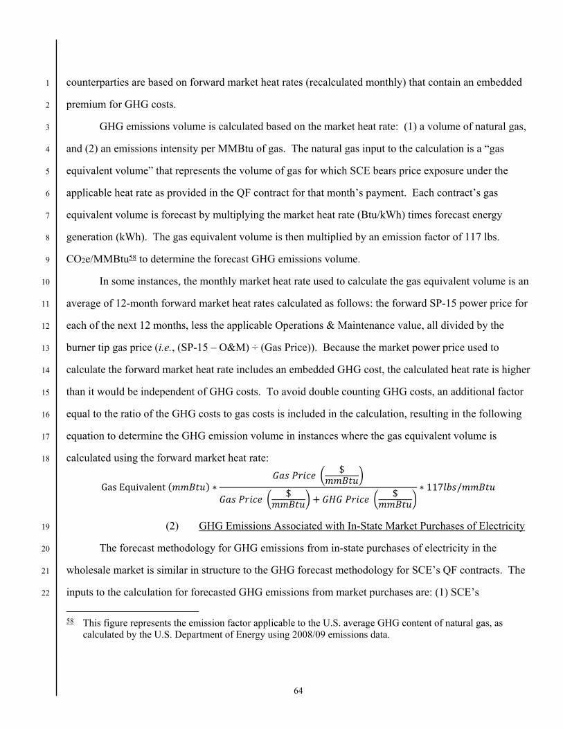
64

counterparties are based on forward market heat rates (recalculated monthly) that contain an embedded 1

premium for GHG costs. 2

GHG emissions volume is calculated based on the market heat rate: (1) a volume of natural gas, 3

and (2) an emissions intensity per MMBtu of gas. The natural gas input to the calculation is a “gas 4

equivalent volume” that represents the volume of gas for which SCE bears price exposure under the 5

applicable heat rate as provided in the QF contract for that month’s payment. Each contract’s gas 6

equivalent volume is forecast by multiplying the market heat rate (Btu/kWh) times forecast energy 7

generation (kWh). The gas equivalent volume is then multiplied by an emission factor of 117 lbs. 8

CO2e/MMBtu58 to determine the forecast GHG emissions volume. 9

In some instances, the monthly market heat rate used to calculate the gas equivalent volume is an 10

average of 12-month forward market heat rates calculated as follows: the forward SP-15 power price for 11

each of the next 12 months, less the applicable Operations & Maintenance value, all divided by the 12

burner tip gas price (i.e., (SP-15 – O&M) ÷ (Gas Price)). Because the market power price used to 13

calculate the forward market heat rate includes an embedded GHG cost, the calculated heat rate is higher 14

than it would be independent of GHG costs. To avoid double counting GHG costs, an additional factor 15

equal to the ratio of the GHG costs to gas costs is included in the calculation, resulting in the following 16

equation to determine the GHG emission volume in instances where the gas equivalent volume is 17

calculated using the forward market heat rate: 18

GasEquivalent( ) ∗ $ $ + $ ∗ 117 /

(2) GHG Emissions Associated with In-State Market Purchases of Electricity 19

The forecast methodology for GHG emissions from in-state purchases of electricity in the 20

wholesale market is similar in structure to the GHG forecast methodology for SCE’s QF contracts. The 21

inputs to the calculation for forecasted GHG emissions from market purchases are: (1) SCE’s 22

58 This figure represents the emission factor applicable to the U.S. average GHG content of natural gas, as

calculated by the U.S. Department of Energy using 2008/09 emissions data.

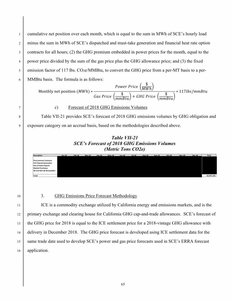
65

cumulative net position over each month, which is equal to the sum in MWh of SCE’s hourly load 1

minus the sum in MWh of SCE’s dispatched and must-take generation and financial heat rate option 2

contracts for all hours; (2) the GHG premium embedded in power prices for the month, equal to the 3

power price divided by the sum of the gas price plus the GHG allowance price; and (3) the fixed 4

emission factor of 117 lbs. CO2e/MMBtu, to convert the GHG price from a per-MT basis to a per-5

MMBtu basis. The formula is as follows: 6

Monthlynetposition( ℎ) ∗ $ ℎ $ + $ ∗ 117 /

c) Forecast of 2018 GHG Emissions Volumes 7

Table VII-21 provides SCE’s forecast of 2018 GHG emissions volumes by GHG obligation and 8

exposure category on an accrual basis, based on the methodologies described above. 9

Table VII-21 SCE’s Forecast of 2018 GHG Emissions Volumes

(Metric Tons CO2e)

3. GHG Emissions Price Forecast Methodology 10

ICE is a commodity exchange utilized by California energy and emissions markets, and is the 11

primary exchange and clearing house for California GHG cap-and-trade allowances. SCE’s forecast of 12

the GHG price for 2018 is equal to the ICE settlement price for a 2018-vintage GHG allowance with 13

delivery in December 2018. The GHG price forecast is developed using ICE settlement data for the 14

same trade date used to develop SCE’s power and gas price forecasts used in SCE’s ERRA forecast 15

application. 16

Description Jan-18 Feb-18 Mar-18 Apr-18 May-18 Jun-18 Jul-18 Aug-18 Sep-18 Oct-18 Nov-18 Dec-18 Total

Procurement ContractsSCE-Owned GenerationOut of State ImportsMarket PurchasesQF and Non QF Renewables

Total 18,597,102

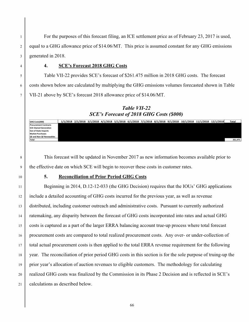
66

For the purposes of this forecast filing, an ICE settlement price as of February 23, 2017 is used, 1

equal to a GHG allowance price of $14.06/MT. This price is assumed constant for any GHG emissions 2

generated in 2018. 3

4. SCE’s Forecast 2018 GHG Costs 4

Table VII-22 provides SCE’s forecast of $261.475 million in 2018 GHG costs. The forecast 5

costs shown below are calculated by multiplying the GHG emissions volumes forecasted shown in Table 6

VII-21 above by SCE’s forecast 2018 allowance price of $14.06/MT. 7

Table VII-22 SCE’s Forecast of 2018 GHG Costs ($000)

This forecast will be updated in November 2017 as new information becomes available prior to 8

the effective date on which SCE will begin to recover these costs in customer rates. 9

5. Reconciliation of Prior Period GHG Costs 10

Beginning in 2014, D.12-12-033 (the GHG Decision) requires that the IOUs’ GHG applications 11

include a detailed accounting of GHG costs incurred for the previous year, as well as revenue 12

distributed, including customer outreach and administrative costs. Pursuant to currently authorized 13

ratemaking, any disparity between the forecast of GHG costs incorporated into rates and actual GHG 14

costs is captured as a part of the larger ERRA balancing account true-up process where total forecast 15

procurement costs are compared to total realized procurement costs. Any over- or under-collection of 16

total actual procurement costs is then applied to the total ERRA revenue requirement for the following 17

year. The reconciliation of prior period GHG costs in this section is for the sole purpose of truing-up the 18

prior year’s allocation of auction revenues to eligible customers. The methodology for calculating 19

realized GHG costs was finalized by the Commission in its Phase 2 Decision and is reflected in SCE’s 20

calculations as described below. 21

GHG Costs(000) 1/1/2018 2/1/2018 3/1/2018 4/1/2018 5/1/2018 6/1/2018 7/1/2018 8/1/2018 9/1/2018 10/1/2018 11/1/2018 12/1/2018 TotalProcurement ContractsSCE-Owned GenerationOut of State ImportsMarket PurchasesQF and Non QF RenewablesTotal 261,475

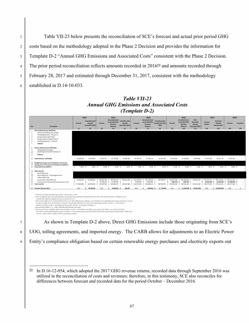
67

Table VII-23 below presents the reconciliation of SCE’s forecast and actual prior period GHG 1

costs based on the methodology adopted in the Phase 2 Decision and provides the information for 2

Template D-2 “Annual GHG Emissions and Associated Costs” consistent with the Phase 2 Decision. 3

The prior period reconciliation reflects amounts recorded in 201659 and amounts recorded through 4

February 28, 2017 and estimated through December 31, 2017, consistent with the methodology 5

established in D.14-10-033. 6

Table VII-23 Annual GHG Emissions and Associated Costs

(Template D-2)

As shown in Template D-2 above, Direct GHG Emissions include those originating from SCE’s 7

UOG, tolling agreements, and imported energy. The CARB allows for adjustments to an Electric Power 8

Entity’s compliance obligation based on certain renewable energy purchases and electricity exports out 9

59 In D.16-12-054, which adopted the 2017 GHG revenue returns, recorded data through September 2016 was

utilized in the reconciliation of costs and revenues; therefore, in this testimony, SCE also reconciles for differences between forecast and recorded data for the period October – December 2016.

Line Description

ForecastFinal (Recorded

through December 2013)

Forecast

Recorded (Used to Set 2015 GHG

Revenue Returns)

Final (Recorded through

December 2014)Forecast


Revenue Returns)

Final (Recorded through December

2015)Forecast


Revenue Returns)

Final(Recorded

through December 2016)

ForecastUpdate

Recorded Through

February 2017Forecast Recorded

(1) (2) (3) (4) (5) (6) (7) (8) (9) (10) (11) (12) (13) (14) (15)1 Direct GHG Emissions (MTCO2e)2 Utility Owned Generation (UOG) 3 Tolling Agreements - Physical 1/4 Energy Imports (Specified)5 Energy Imports (Unspecified) 2/6 Tolling Agreements - Financial 7 Subtotal

8 Indirect GHG Emissions (MTCO2e)9 CAISO Market Purchases10 Qualifying Facility (QF) Contracts 3/ 11 Subtotal

12 Total Emissions (MTCO2e) 18 540 635 24 754 614 22 787 127 24 720 902 24 609 528 24 704 713 25 142 6 0 24 541 264 26 250 022 27 148 085 26 406 680 23 515 963 20 641 87 8 597 102 -

13 Weighted Average Cost of Compliance Instrument 14 Average Price for Financial Toll Settlement ($/MT) 4/15 Proxy GHG Price ($/MT) 5/ 14.62$ 13.56$ 12.48$ 11.97$ 12.04$ 12.65$ 12.76$ 12.79$ 13.14$ 12.81$ 12.84$ 13.19$ 13.60$ 14.06$ -$

16 GHG Costs ($)17 Direct GHG Costs18 Direct GHG Costs - Tolling Agreements19 Indirect GHG Costs20 Current Year Total GHG Costs 271 064 082$ 313 850 285$ 284 383 339$ 293 032 374$ 293 315 968$ 312 514 619$ 311 749 078$ 304 588 374$ 344 925 289$ 343 583 069$ 335 041 510$ 310 175 547$ 280 719 041$ 261 475 248$ -$ 21 Previous Year's Forecast Reconciliation (Line 23) -$ -$ 42 786 203$ 42 786 203$ -$ 8 649 035$ 8 649 035$ -$ (481,947)$ (481,947)$ -$ (8,502,925)$ (8,502,925)$ (37,998,066)$ -$ 22 Total Costs ($) 271 064 082$ 313 850 285$ 327 169 542$ 335 818 577$ 293 315 968$ 321 163 654$ 320 398 113$ 304 588 374$ 344 443 342$ 343 101 122$ 335 041 510$ 301 672 623$ 272 216 116$ 223 477 182$ -$

23 Forecast Variance ($) 6/ N/A 42,786,203$ N/A 8,649,035$ 283,594$ N/A (765,541)$ (7, 60,705)$ N/A (1,342,220)$ (8,541,559)$ N/A (29,456,507)$ N/A 0

1/ Emissions for Tolling Agreement exposure that s settled using in entory.

2/ Electr city importers may cla m certain adjustments for renewable energy purchases and exported electric ty. These ad ustments may reduce a compliance ent ty's

cap-and-trade compl ance obligation and are accounted for in L ne 5.

3/ SCE considers GHG costs associated with QF Contracts as an indirect GHG emissions obligation since the GHG costs are embedded in the energy costs for these resources.

/ In order to calculate the costs associated w th Financial Toll Agreement Settlement cons stent w th the methodology described n Section 2.1 of the Phase II

Decision the utilit es use the A erage Settlement Price for these resources as calculated in Template C-1.

5/ Recorded Proxy GHG Pr ce = A erage CAISO Daily GHG Allowance Price Index

6/ The Forecast Var ance of ($8.502) m llion shown in Column 11 was pre ously reflected n the GHG cost true-up in the 2017 GHG re enue returns (D.16-12-05 ).

The Forecast Variance of ($37 998) mill on shown in Column 13 s the incremental true-up amount for 2016 associated with using actual year-end data of ($8 5 2) mill on plus

a forecast ariance of ($29. 57) mill on in 2017 (us ng February recorded).

201820162013 20152014 2017

68

of California. In order to capture these adjustments, Line 5 of Template D-2, Energy Imports 1

(Unspecified), is reduced accordingly. 2

To calculate the costs associated with Direct GHG Emissions, all physical exposures (that is, 3

emissions associated with UOG, tolling agreements that are/will be settled with compliance instruments, 4

and energy imports) less the adjustments described in the previous paragraph are multiplied by the 5

Weighted Average Cost of GHG Compliance Instruments in inventory (shown in Table VII-24, 6

Template C-1) for recorded years. Separately, the emissions associated with tolling agreements that 7

were settled financially are multiplied on a monthly basis by that month’s corresponding ICE GHG price 8

(also shown in Table VII-24, Template C-1). For forecast years, all Direct GHG Emissions are simply 9

multiplied by the GHG allowance proxy price. 10

Indirect GHG Emissions include those associated with CAISO Market Purchases and QF 11

contracts, where the GHG costs are embedded in energy costs. Pursuant to the Phase 2 Decision, to 12

calculate the Indirect GHG Costs for a recorded year, the Indirect GHG Emissions are multiplied by the 13

annual average CAISO-daily GHG Allowance Price Index. To calculate the Indirect GHG Costs for a 14

forecast year, the Indirect GHG Emissions are multiplied by the GHG allowance proxy price. 15

As shown in Template D-2, SCE’s forecast of 2018 GHG costs is $261.475 million. As 16

presented in Section E of this chapter, SCE will adjust the 2018 allowance revenue returns to eligible 17

small business customers that receive volumetric returns of allowance revenue to account for the 18

($37.998) million deviation between prior period forecasts and recorded costs (Line 21 in Template D-2) 19

for both the 2017 estimated overcollection of ($29.457) million and the 2016 final true-up overcollection 20

of ($8.542) million. 21

Table VII-24 below provides the information for Template C-1 “Weighted Average Cost of 22

Compliance Instruments Calculation” consistent with the Phase 2 Decision and provides the support for 23

69

the 2016 recorded weighted average cost of compliance instrument inventory $/MT and the average 1

price for financial toll settlement $/MT used in Template D-2 above.60 2

60 Pursuant to the Phase 2 Decision, beginning in 2014, SCE switched to the accrual method of accounting for

GHG direct costs in its ERRA balancing account (consistent with the methodology presented in Template C-1) and made a one-time adjustment for prior years.

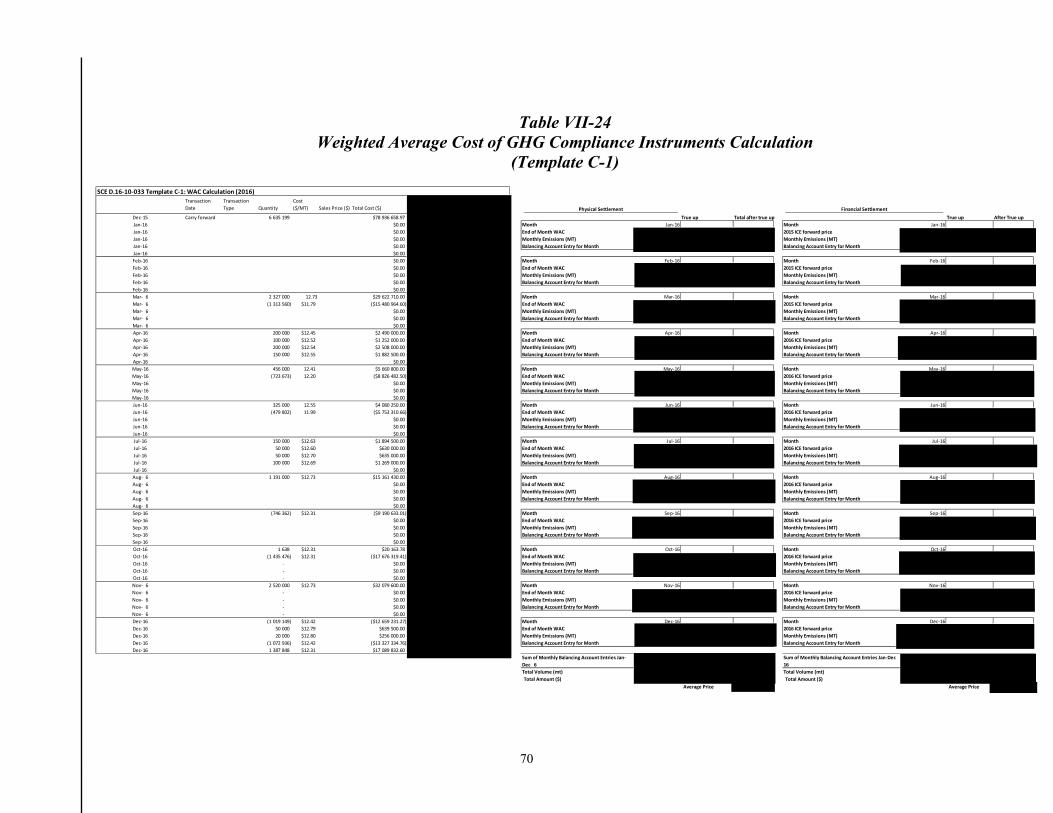
70

Table VII-24 Weighted Average Cost of GHG Compliance Instruments Calculation

(Template C-1)

SCE D.16-10-033 Template C-1: WAC Calculation (2016)

Transaction Date

Transaction Type Quantity

Cost ($/MT) Sales Price ($) Total Cost ($)

Dec-15 Carry forward 6 635 199 $78 936 658.97 True up Total after true up True up After True upJan-16 $0.00 Month Jan-16 Month Jan-16Jan-16 $0.00 End of Month WAC 2015 ICE forward priceJan-16 $0.00 Monthly Emissions (MT) Monthly Emissions (MT)Jan-16 $0.00 Balancing Account Entry for Month Balancing Account Entry for MonthJan-16 $0.00Feb-16 $0.00 Month Feb-16 Month Feb-16Feb-16 $0.00 End of Month WAC 2015 ICE forward priceFeb-16 $0.00 Monthly Emissions (MT) Monthly Emissions (MT)Feb-16 $0.00 Balancing Account Entry for Month Balancing Account Entry for MonthFeb-16 $0.00Mar- 6 2 327 000 12.73 $29 622 710.00 Month Mar-16 Month Mar-16Mar- 6 (1 313 560) $11.79 ($15 480 964.60) End of Month WAC 2015 ICE forward priceMar- 6 $0.00 Monthly Emissions (MT) Monthly Emissions (MT)Mar- 6 $0.00 Balancing Account Entry for Month Balancing Account Entry for MonthMar- 6 $0.00Apr-16 200 000 $12.45 $2 490 000.00 Month Apr-16 Month Apr-16Apr-16 100 000 $12.52 $1 252 000.00 End of Month WAC 2016 ICE forward priceApr-16 200 000 $12.54 $2 508 000.00 Monthly Emissions (MT) Monthly Emissions (MT)Apr-16 150 000 $12.55 $1 882 500.00 Balancing Account Entry for Month Balancing Account Entry for MonthApr-16 $0.00May-16 456 000 12.41 $5 660 800.00 Month May-16 Month May-16May-16 (723 673) 12.20 ($8 826 482.50) End of Month WAC 2016 ICE forward priceMay-16 $0.00 Monthly Emissions (MT) Monthly Emissions (MT)May-16 $0.00 Balancing Account Entry for Month Balancing Account Entry for MonthMay-16 $0.00Jun-16 325 000 12.55 $4 080 250.00 Month Jun-16 Month Jun-16Jun-16 (479 802) 11.99 ($5 753 310.66) End of Month WAC 2016 ICE forward priceJun-16 $0.00 Monthly Emissions (MT) Monthly Emissions (MT)Jun-16 $0.00 Balancing Account Entry for Month Balancing Account Entry for MonthJun-16 $0.00Jul-16 150 000 $12.63 $1 894 500.00 Month Jul-16 Month Jul-16Jul-16 50 000 $12.60 $630 000.00 End of Month WAC 2016 ICE forward priceJul-16 50 000 $12.70 $635 000.00 Monthly Emissions (MT) Monthly Emissions (MT)Jul-16 100 000 $12.69 $1 269 000.00 Balancing Account Entry for Month Balancing Account Entry for MonthJul-16 $0.00Aug- 6 1 191 000 $12.73 $15 161 430.00 Month Aug-16 Month Aug-16Aug- 6 $0.00 End of Month WAC 2016 ICE forward priceAug- 6 $0.00 Monthly Emissions (MT) Monthly Emissions (MT)Aug- 6 $0.00 Balancing Account Entry for Month Balancing Account Entry for MonthAug- 6 $0.00Sep-16 (746 362) $12.31 ($9 190 633.01) Month Sep-16 Month Sep-16Sep-16 $0.00 End of Month WAC 2016 ICE forward priceSep-16 $0.00 Monthly Emissions (MT) Monthly Emissions (MT)Sep-16 $0.00 Balancing Account Entry for Month Balancing Account Entry for MonthSep-16 $0.00Oct-16 1 638 $12.31 $20 163.78 Month Oct-16 Month Oct-16Oct-16 (1 435 476) $12.31 ($17 676 319.41) End of Month WAC 2016 ICE forward priceOct-16 - $0.00 Monthly Emissions (MT) Monthly Emissions (MT)Oct-16 - $0.00 Balancing Account Entry for Month Balancing Account Entry for MonthOct-16 - $0.00Nov- 6 2 520 000 $12.73 $32 079 600.00 Month Nov-16 Month Nov-16Nov- 6 - $0.00 End of Month WAC 2016 ICE forward priceNov- 6 - $0.00 Monthly Emissions (MT) Monthly Emissions (MT)Nov- 6 - $0.00 Balancing Account Entry for Month Balancing Account Entry for MonthNov- 6 - $0.00Dec-16 (1 019 149) $12.42 ($12 659 231.27) Month Dec-16 Month Dec-16Dec-16 50 000 $12.79 $639 500.00 End of Month WAC 2016 ICE forward priceDec-16 20 000 $12.80 $256 000.00 Monthly Emissions (MT) Monthly Emissions (MT)Dec-16 (1 072 936) $12.42 ($13 327 334.76) Balancing Account Entry for Month Balancing Account Entry for MonthDec-16 1 387 848 $12.31 $17 089 832.60

Sum of Monthly Balancing Account Entries Jan-Dec 6

Sum of Monthly Balancing Account Entries Jan-Dec 16

Total Volume (mt) Total Volume (mt)Total Amount ($) Total Amount ($)

Average Price Average Price

Physical Settlement Financial Settlement

71

C. 2018 Administrative and Customer Outreach Costs Forecast and Prior Period 1

Reconciliation 2

The utilities are authorized to track administrative costs and costs related to customer outreach 3

and education in a memorandum account, and to pay for such efforts with GHG allowance revenue.61 In 4

order to ensure that adequate funding is available, the GHG Decision directs the IOUs to set aside a 5

portion of the GHG allowance revenue to fund customer outreach and administrative activities before 6

distribution of any funds to EITE, small business, and residential customers.62 Beginning in 2014, the 7

GHG applications must also include a detailed accounting of actual GHG costs incurred for the previous 8

year as well as revenue distributed to eligible customer classes.63 In this chapter, SCE includes a 2018 9

forecast of administrative and customer outreach costs as well as an accounting of actual administrative 10

and customer outreach costs for the prior period. 11

As detailed in below, which provides the information for Template D-3 “Detail of Outreach and 12

Administrative Expenses” as ordered by the Phase 2 Decision, SCE is currently forecasting $250,000 in 13

internal customer outreach-related costs in 2018. These costs are accounted for in the GHG 14

Administrative Costs Memorandum Account (GHGACMA) primarily to be spent of marketing, with the 15

bulk of the costs associated with the April and October residential climate credit bill inserts. 16

1. Reconciliation of Prior Period Administrative and Customer Outreach Costs 17

D.16-12-054 found SCE’s 2017 total administrative costs forecast of $250,000 (includes SCE-18

outreach activities) reasonable for the purposes of calculating the 2017 residential California Climate 19

Credit. As detailed in Table VII-25 below, SCE recorded $212,439 in 2016 associated with 20

administrative and internal customer outreach-related costs. Of the total spent in 2016 on GHG-related 21

administration and outreach, $27,728 was related to IT system configuration work to allow SCE’s 22

billing system to process the EITE credit and $184,711 was spent on marketing, with the bulk associated 23

61 D. 12-12-033 at pp. 141-142, 149, CL 56-58, OP 16-17.

62 Id.

63 Id. at p. 148.

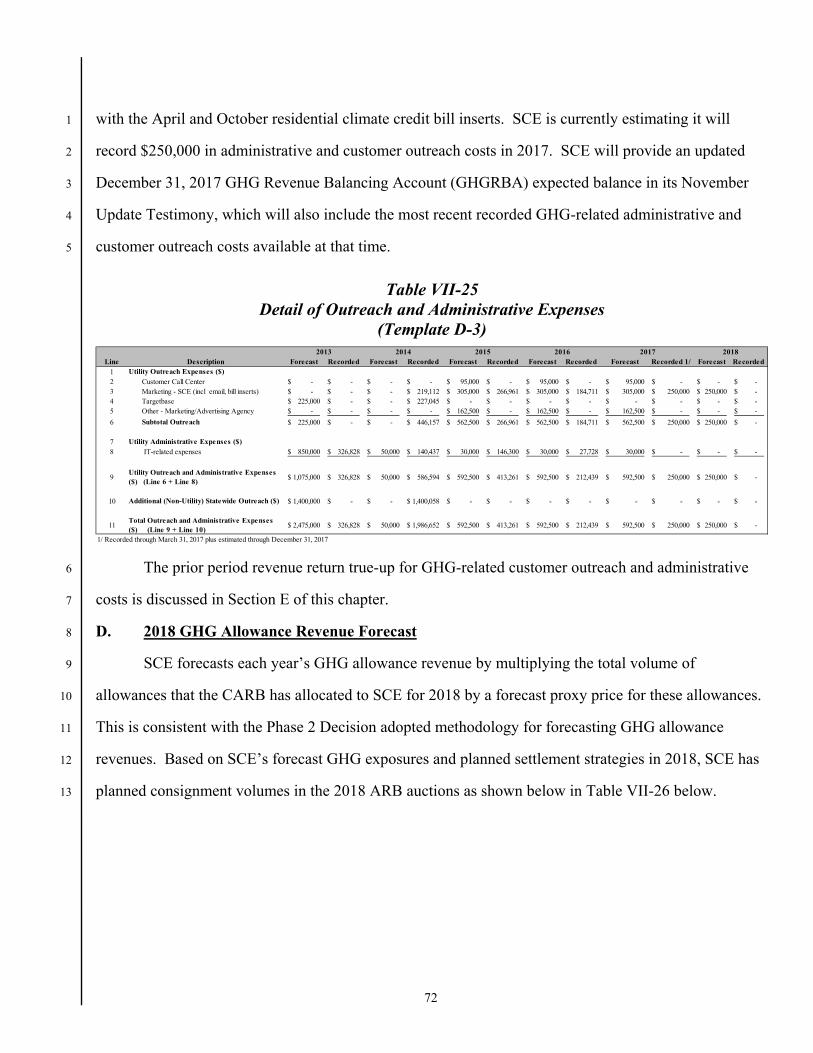
72

with the April and October residential climate credit bill inserts. SCE is currently estimating it will 1

record $250,000 in administrative and customer outreach costs in 2017. SCE will provide an updated 2

December 31, 2017 GHG Revenue Balancing Account (GHGRBA) expected balance in its November 3

Update Testimony, which will also include the most recent recorded GHG-related administrative and 4

customer outreach costs available at that time. 5

Table VII-25 Detail of Outreach and Administrative Expenses

(Template D-3)

The prior period revenue return true-up for GHG-related customer outreach and administrative 6

costs is discussed in Section E of this chapter. 7

D. 2018 GHG Allowance Revenue Forecast 8

SCE forecasts each year’s GHG allowance revenue by multiplying the total volume of 9

allowances that the CARB has allocated to SCE for 2018 by a forecast proxy price for these allowances. 10

This is consistent with the Phase 2 Decision adopted methodology for forecasting GHG allowance 11

revenues. Based on SCE’s forecast GHG exposures and planned settlement strategies in 2018, SCE has 12

planned consignment volumes in the 2018 ARB auctions as shown below in Table VII-26 below. 13

Line Description Forecast Recorded Forecast Recorded Forecast Recorded Forecast Recorded Forecast Recorded 1/ Forecast Recorded 1 Utility Outreach Expenses ($)2 Customer Call Center -$ -$ -$ -$ 95,000$ -$ 95,000$ -$ 95,000$ -$ -$ -$ 3 Marketing - SCE (incl email, bill inserts) -$ -$ -$ 219,112$ 305,000$ 266,961$ 305,000$ 184,711$ 305,000$ 250,000$ 250,000$ -$ 4 Targetbase 225,000$ -$ -$ 227,045$ -$ -$ -$ -$ -$ -$ -$ -$ 5 Other - Marketing/Advertising Agency -$ -$ -$ -$ 162,500$ -$ 162,500$ -$ 162,500$ -$ -$ -$

6 Subtotal Outreach 225,000$ -$ -$ 446,157$ 562,500$ 266,961$ 562,500$ 184,711$ 562,500$ 250,000$ 250,000$ -$

7 Utility Administrative Expenses ($)8 IT-related expenses 850,000$ 326,828$ 50,000$ 140,437$ 30,000$ 146,300$ 30,000$ 27,728$ 30,000$ -$ -$ -$

9Utility Outreach and Administrative Expenses ($) (Line 6 + Line 8)

1,075,000$ 326,828$ 50,000$ 586,594$ 592,500$ 413,261$ 592,500$ 212,439$ 592,500$ 250,000$ 250,000$ -$

10 Additional (Non-Utility) Statewide Outreach ($) 1,400,000$ -$ -$ 1,400,058$ -$ -$ -$ -$ -$ -$ -$ -$

11Total Outreach and Administrative Expenses ($) (Line 9 + Line 10)

2,475,000$ 326,828$ 50,000$ 1,986,652$ 592,500$ 413,261$ 592,500$ 212,439$ 592,500$ 250,000$ 250,000$ -$

1/ Recorded through March 31, 2017 plus estimated through December 31, 2017

201820172015 201620142013

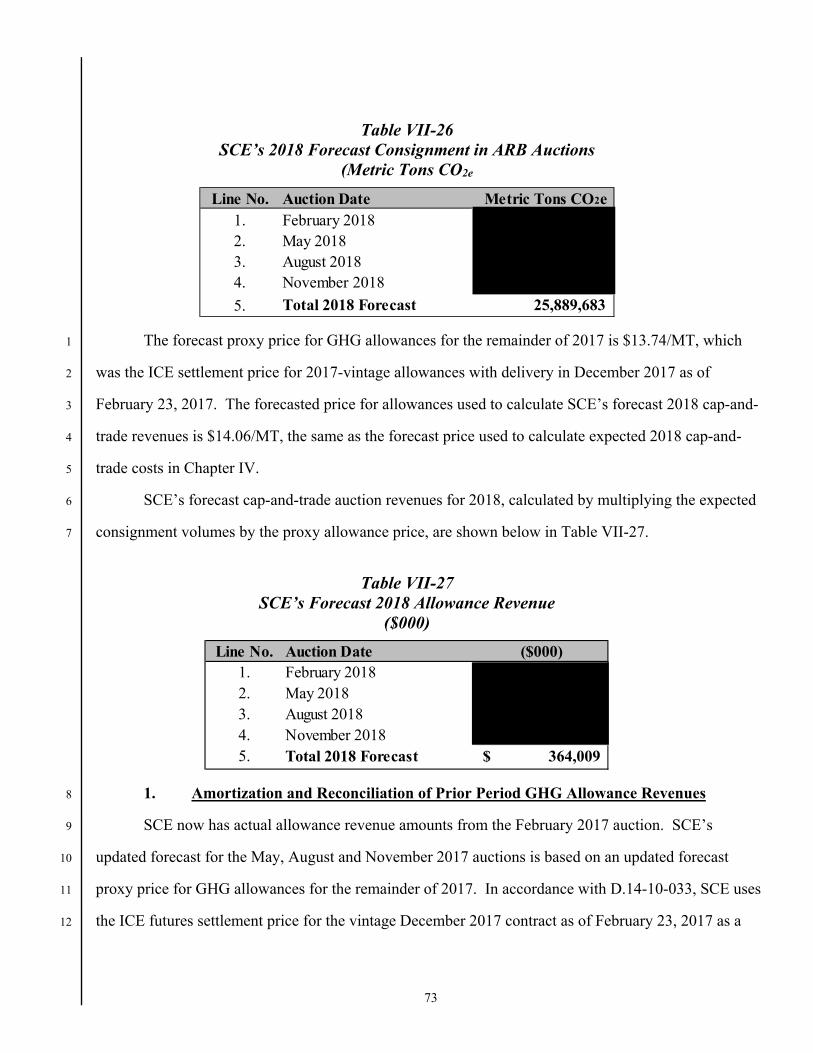
73

Table VII-26 SCE’s 2018 Forecast Consignment in ARB Auctions

(Metric Tons CO2e

The forecast proxy price for GHG allowances for the remainder of 2017 is $13.74/MT, which 1

was the ICE settlement price for 2017-vintage allowances with delivery in December 2017 as of 2

February 23, 2017. The forecasted price for allowances used to calculate SCE’s forecast 2018 cap-and-3

trade revenues is $14.06/MT, the same as the forecast price used to calculate expected 2018 cap-and-4

trade costs in Chapter IV. 5

SCE’s forecast cap-and-trade auction revenues for 2018, calculated by multiplying the expected 6

consignment volumes by the proxy allowance price, are shown below in Table VII-27. 7

Table VII-27 SCE’s Forecast 2018 Allowance Revenue

($000)

1. Amortization and Reconciliation of Prior Period GHG Allowance Revenues 8

SCE now has actual allowance revenue amounts from the February 2017 auction. SCE’s 9

updated forecast for the May, August and November 2017 auctions is based on an updated forecast 10

proxy price for GHG allowances for the remainder of 2017. In accordance with D.14-10-033, SCE uses 11

the ICE futures settlement price for the vintage December 2017 contract as of February 23, 2017 as a 12

Line No. Auction Date Metric Tons CO2e1. February 20182. May 20183. August 20184. November 2018

5. Total 2018 Forecast 25,889,683

Line No. Auction Date ($000)1. February 20182. May 20183. August 20184. November 20185. Total 2018 Forecast 364,009$

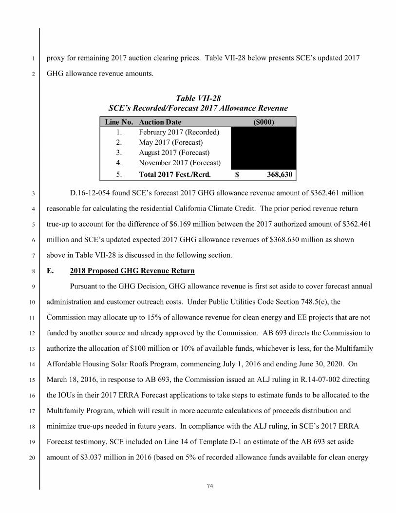
74

proxy for remaining 2017 auction clearing prices. Table VII-28 below presents SCE’s updated 2017 1

GHG allowance revenue amounts. 2

Table VII-28 SCE’s Recorded/Forecast 2017 Allowance Revenue

D.16-12-054 found SCE’s forecast 2017 GHG allowance revenue amount of $362.461 million 3

reasonable for calculating the residential California Climate Credit. The prior period revenue return 4

true-up to account for the difference of $6.169 million between the 2017 authorized amount of $362.461 5

million and SCE’s updated expected 2017 GHG allowance revenues of $368.630 million as shown 6

above in Table VII-28 is discussed in the following section. 7

E. 2018 Proposed GHG Revenue Return 8

Pursuant to the GHG Decision, GHG allowance revenue is first set aside to cover forecast annual 9

administration and customer outreach costs. Under Public Utilities Code Section 748.5(c), the 10

Commission may allocate up to 15% of allowance revenue for clean energy and EE projects that are not 11

funded by another source and already approved by the Commission. AB 693 directs the Commission to 12

authorize the allocation of $100 million or 10% of available funds, whichever is less, for the Multifamily 13

Affordable Housing Solar Roofs Program, commencing July 1, 2016 and ending June 30, 2020. On 14

March 18, 2016, in response to AB 693, the Commission issued an ALJ ruling in R.14-07-002 directing 15

the IOUs in their 2017 ERRA Forecast applications to take steps to estimate funds to be allocated to the 16

Multifamily Program, which will result in more accurate calculations of proceeds distribution and 17

minimize true-ups needed in future years. In compliance with the ALJ ruling, in SCE’s 2017 ERRA 18

Forecast testimony, SCE included on Line 14 of Template D-1 an estimate of the AB 693 set aside 19

amount of $3.037 million in 2016 (based on 5% of recorded allowance funds available for clean energy 20

Line No. Auction Date ($000)1. February 2017 (Recorded)2. May 2017 (Forecast)3. August 2017 (Forecast)4. November 2017 (Forecast)

5. Total 2017 Fcst./Rcrd. 368,630$

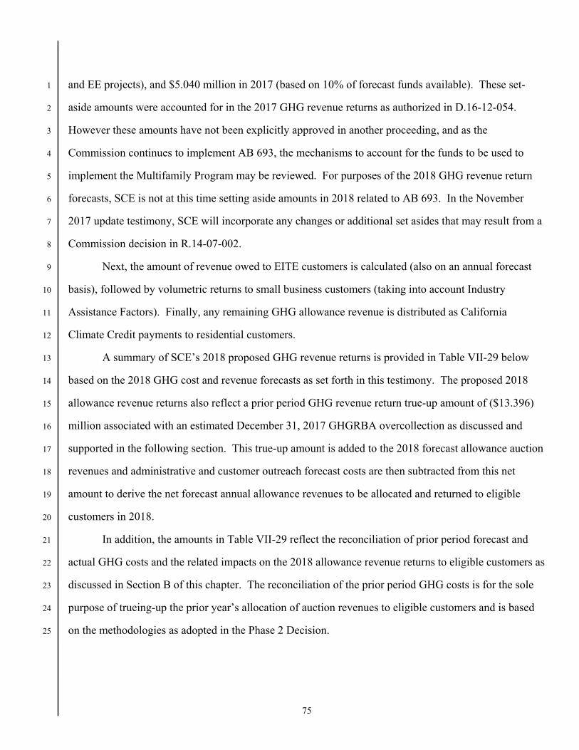
75

and EE projects), and $5.040 million in 2017 (based on 10% of forecast funds available). These set-1

aside amounts were accounted for in the 2017 GHG revenue returns as authorized in D.16-12-054. 2

However these amounts have not been explicitly approved in another proceeding, and as the 3

Commission continues to implement AB 693, the mechanisms to account for the funds to be used to 4

implement the Multifamily Program may be reviewed. For purposes of the 2018 GHG revenue return 5

forecasts, SCE is not at this time setting aside amounts in 2018 related to AB 693. In the November 6

2017 update testimony, SCE will incorporate any changes or additional set asides that may result from a 7

Commission decision in R.14-07-002. 8

Next, the amount of revenue owed to EITE customers is calculated (also on an annual forecast 9

basis), followed by volumetric returns to small business customers (taking into account Industry 10

Assistance Factors). Finally, any remaining GHG allowance revenue is distributed as California 11

Climate Credit payments to residential customers. 12

A summary of SCE’s 2018 proposed GHG revenue returns is provided in Table VII-29 below 13

based on the 2018 GHG cost and revenue forecasts as set forth in this testimony. The proposed 2018 14

allowance revenue returns also reflect a prior period GHG revenue return true-up amount of ($13.396) 15

million associated with an estimated December 31, 2017 GHGRBA overcollection as discussed and 16

supported in the following section. This true-up amount is added to the 2018 forecast allowance auction 17

revenues and administrative and customer outreach forecast costs are then subtracted from this net 18

amount to derive the net forecast annual allowance revenues to be allocated and returned to eligible 19

customers in 2018. 20

In addition, the amounts in Table VII-29 reflect the reconciliation of prior period forecast and 21

actual GHG costs and the related impacts on the 2018 allowance revenue returns to eligible customers as 22

discussed in Section B of this chapter. The reconciliation of the prior period GHG costs is for the sole 23

purpose of trueing-up the prior year’s allocation of auction revenues to eligible customers and is based 24

on the methodologies as adopted in the Phase 2 Decision. 25

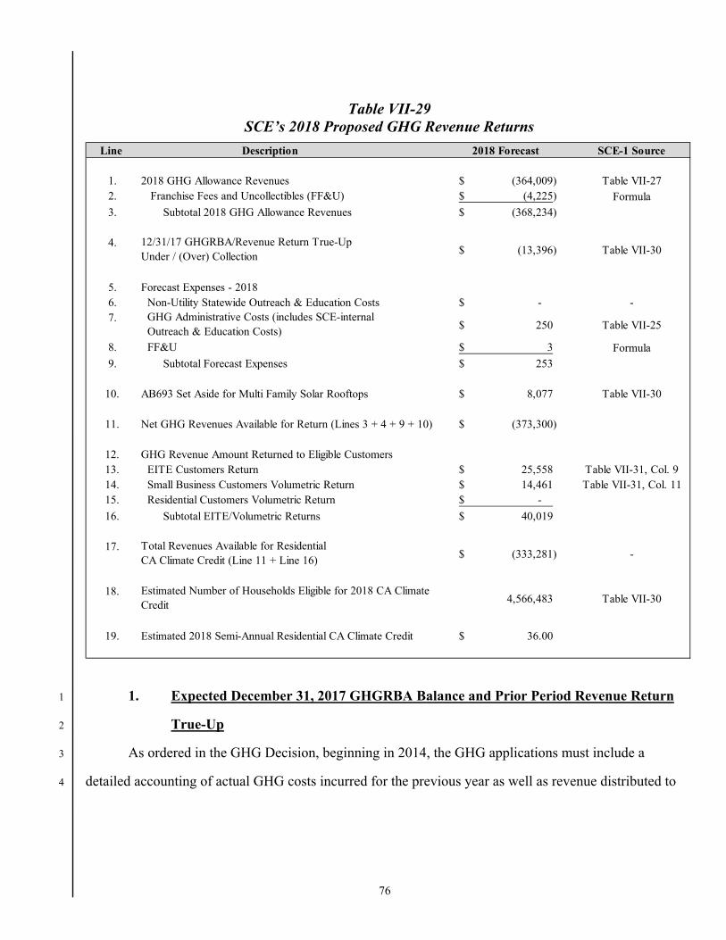
76

Table VII-29 SCE’s 2018 Proposed GHG Revenue Returns

1. Expected December 31, 2017 GHGRBA Balance and Prior Period Revenue Return 1

True-Up 2

As ordered in the GHG Decision, beginning in 2014, the GHG applications must include a 3

detailed accounting of actual GHG costs incurred for the previous year as well as revenue distributed to 4

Line Description 2018 Forecast SCE-1 Source

1. 2018 GHG Allowance Revenues (364,009)$ Table VII-272. Franchise Fees and Uncollectibles (FF&U) (4,225)$ Formula

3. Subtotal 2018 GHG Allowance Revenues (368,234)$

4. 12/31/17 GHGRBA/Revenue Return True-Up Under / (Over) Collection

(13,396)$ Table VII-30

5. Forecast Expenses - 20186. Non-Utility Statewide Outreach & Education Costs -$ -7. GHG Administrative Costs (includes SCE-internal

Outreach & Education Costs)250$ Table VII-25

8. FF&U 3$ Formula

9. Subtotal Forecast Expenses 253$

10. AB693 Set Aside for Multi Family Solar Rooftops 8,077$ Table VII-30

11. Net GHG Revenues Available for Return (Lines 3 + 4 + 9 + 10) (373,300)$

12. GHG Revenue Amount Returned to Eligible Customers13. EITE Customers Return 25,558$ Table VII-31, Col. 914. Small Business Customers Volumetric Return 14,461$ Table VII-31, Col. 1115. Residential Customers Volumetric Return -$

16. Subtotal EITE/Volumetric Returns 40,019$

17. Total Revenues Available for Residential CA Climate Credit (Line 11 + Line 16)

(333,281)$ -

18. Estimated Number of Households Eligible for 2018 CA Climate Credit 4,566,483 Table VII-30

19. Estimated 2018 Semi-Annual Residential CA Climate Credit 36.00$

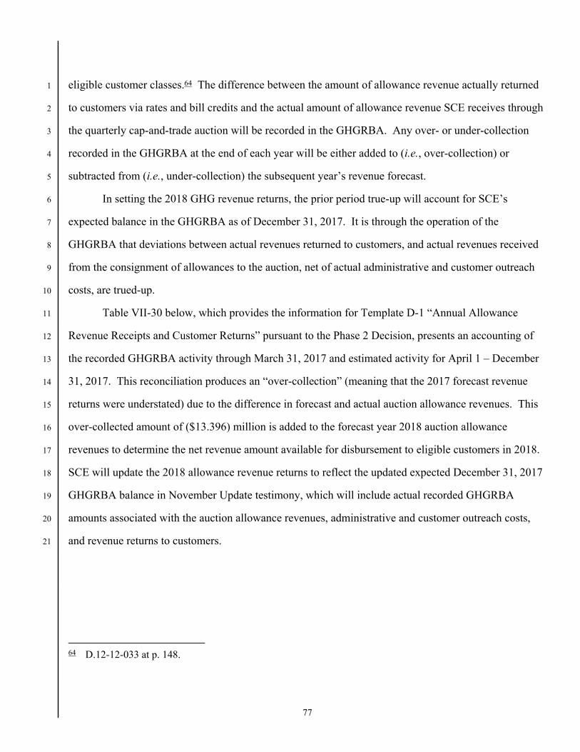
77

eligible customer classes.64 The difference between the amount of allowance revenue actually returned 1

to customers via rates and bill credits and the actual amount of allowance revenue SCE receives through 2

the quarterly cap-and-trade auction will be recorded in the GHGRBA. Any over- or under-collection 3

recorded in the GHGRBA at the end of each year will be either added to (i.e., over-collection) or 4

subtracted from (i.e., under-collection) the subsequent year’s revenue forecast. 5

In setting the 2018 GHG revenue returns, the prior period true-up will account for SCE’s 6

expected balance in the GHGRBA as of December 31, 2017. It is through the operation of the 7

GHGRBA that deviations between actual revenues returned to customers, and actual revenues received 8

from the consignment of allowances to the auction, net of actual administrative and customer outreach 9

costs, are trued-up. 10

Table VII-30 below, which provides the information for Template D-1 “Annual Allowance 11

Revenue Receipts and Customer Returns” pursuant to the Phase 2 Decision, presents an accounting of 12

the recorded GHGRBA activity through March 31, 2017 and estimated activity for April 1 – December 13

31, 2017. This reconciliation produces an “over-collection” (meaning that the 2017 forecast revenue 14

returns were understated) due to the difference in forecast and actual auction allowance revenues. This 15

over-collected amount of ($13.396) million is added to the forecast year 2018 auction allowance 16

revenues to determine the net revenue amount available for disbursement to eligible customers in 2018. 17

SCE will update the 2018 allowance revenue returns to reflect the updated expected December 31, 2017 18

GHGRBA balance in November Update testimony, which will include actual recorded GHGRBA 19

amounts associated with the auction allowance revenues, administrative and customer outreach costs, 20

and revenue returns to customers. 21

64 D.12-12-033 at p. 148.

78

Table VII-30 Annual Allowance Revenue Receipts and Customer Returns (Template D-1)

2. 2018 GHG Cost and Revenue Distribution for EITE and Volumetric Returns 1

Table VII-31 below sets forth the proposed 2018 amounts of GHG revenue allocated to EITE 2

customers and the amounts of GHG revenues allocated to small business customers (utilizing a 70% 3

small business assistance factor in 2017 per D.13-12-002) on a volumetric return basis necessary to 4

offset the amount of cap-and-trade costs in rates, based on the cap-and-trade costs described in Chapter 5

IV of this exhibit, and to also true-up for the deviation between the forecast authorized prior period 6

GHG costs (used to set the 2017 revenue returns) and actual prior period GHG costs as supported in 7

Section B of this chapter.65 8

D.14-12-037 requires the Commission’s Energy Division to perform the calculations necessary 9

to determine the specific amount of GHG allowance revenue that will be returned to individual EITE 10

65 D.15-07-001 was issued in the Residential Rate OIR (R.12-06-013) on July 3, 2015. That decision

discontinues the residential volumetric offset beginning January 1, 2016, and allocates GHG revenues to the residential class solely through the semi-annual California Climate Credit.

Line Description Forecast Recorded Forecast Recorded Forecast Recorded Forecast Recorded Forecast Recorded 1/ Forecast Recorded

1 Proxy GHG Price ($/MT) N/A N/A 12.48$ 12.04$ 12.65$ 12.79$ 13.14$ 12.84$ 13.50$ N/A 14.06$ N/A

2 Allocated Allowances (MT) 32 603 468 32 603 468 31 594 859 31 594 859 31 399 111 31 399 111 29 550 282 29 550 281 26 868 834 26 868 834 25 889 683 25 889 683

3 Revenues ($)4 Prior Balance N/A N/A (389 586 000)$ (384 888 000)$ (160 837 218)$ (167 118 600)$ (346 523)$ (22 378 563)$ 30 396 659$ 29 397 778$ (13 395 955)$ -$ 5 Allowance Revenue (389 232 000)$ (384 638 000)$ (394 304 000)$ (368 730 000)$ (397 199 000)$ (390 808 663)$ (388 290 705)$ (376 175 077)$ (362 460 584)$ (368 630 000)$ (364 009 000)$ -$ 6 Interest (354 000)$ (250 000)$ 177 000$ (299 600)$ -$ -$ -$ -$ -$ -$ -$ -$ 7 Franchise Fees and Uncollectibles -$ -$ (6 620 000)$ (7 641 000)$ (4 463 271)$ (5 606 232)$ (4 363 170)$ (4 227 028)$ (4 207 516)$ (4 279 132)$ (4 225 491)$ -$ 8 Subtotal Revenues (389 586 000)$ (384 888 000)$ (790 333 000)$ (761 558 600)$ (562 499 489)$ (563 533 494)$ (393 000 398)$ (402 780 668)$ (336 271 441)$ (343 511 355)$ (381 630 445)$ -$

9 Expenses ($)10 Outreach and Administrative Expenses (from Template D-3) 2 475 000$ -$ 50 000$ 2 313 000$ 592 500$ 413 261$ 592 500$ 212 439$ 250 000$ 250 000$ 250 000$ -$ 11 Franchise Fees and Uncollectibles -$ -$ -$ -$ 6 658 4 797 6 658 2 466 2 902 2 902$ 2 902$ -$ 12 Interest -$ -$ -$ -$ -$ -$ -$ -$ -$ -$ -$ -$ 13 Subtotal Expenses 2 475 000$ -$ 50 000$ 2 313 000$ 599 158$ 418 058$ 599 158$ 214 905$ 252 902$ 252 902$ 252 902$ -$

14 AB693 Set Aside for Multi Family Solar Rooftops (2017 funds) 5 040 278$ 5 040 278$ 5 040 278$ 15 Prior Year Set Aside (2016 funds) 3 036 945$ 3 036 945$ 3 036 945$ -$

16 Net GHG Revenues ($) (Line 8 Line 13 Line 14 Line 15) (387 111 000)$ (384 888 000)$ (790 283 000)$ (759 245 600)$ (561 900 331)$ (563 115 436)$ (392 401 240)$ (402 565 763)$ (327 941 316)$ (340 221 507)$ (373 300 320)$ -$ 17 GHG Revenues to be Distributed in Future Years ($) -$ -$ 194 616 000$ 192 319 000$ -$ -$ -$ -$ -$ -$ -$ -$

18Net GHG Revenues Available for Customers in Forecast Year ($) (Line 16 Line 17)

(387 111 000)$ (384 888 000)$ (595 667 000)$ (566 926 600)$ (561 900 331)$ (563 115 436)$ (392 401 240)$ (402 565 763)$ (327 941 316)$ (340 221 507)$ (373 300 320)$ -$

19 GHG Revenue Returned to Eligible Customers ($)20 EITE Customer Return -$ -$ 30 008 000$ 30 008 000$ 34 673 000$ 34 673 000$ 25 488 811$ 50 591 667$ 26 673 763$ 25 558 000$ 25 558 000$ -$ 21 Small Business Volumetric Return -$ -$ 30 550 000$ 40 961 000$ 39 496 000$ 52 964 531$ 24 446 633$ 32 179 018$ 21 725 095$ 21 725 095$ 14 460 991$ -$ 22 Residential Volumetric Return -$ -$ 178 425 000$ 169 887 000$ 225 679 000$ 194 522 279$ -$ 11 209 570$ -$ -$ -$ 23 Subtotal EITE Volumetric Returns -$ -$ 238 983 000$ 240 856 000$ 299 848 000$ 282 159 809$ 49 935 444$ 93 980 255$ 48 398 858$ 47 283 095$ 40 018 991$ -$

24 Number of Households Eligible for the California Climate Credit - - 4 447 615 4 380 118 4 487 449 4 427 938 4 493 380 4 434 566 4 522 905 4 522 905 4 566 483 - 25 Per-Household Semi-Annual Climate Credit N/A N/A 40$ 40$ 29$ 29$ 38$ 38$ 31$ 31$ 36$ -$

(0.5 x Line 18 Line 23) / Line 24)

26Revenue Distributed for the Climate Credit ($)(2 x Line 25 x Line 24)

-$ -$ 356 684 000$ 351 271 000$ 262 052 331$ 258 577 064$ 342 465 796$ 337 983 286$ 279 542 458$ 279 542 458$ 333 281 329$ -$

27 Revenue Balance ($) (in the GHGRBA) (Line 8 Line 13 Line 23 26) (387 111 000)$ (384 888 000)$ (194 616 000)$ (167 118 600)$ -$ (22 378 563)$ -$ 29 397 778$ (8 077 223)$ (13 395 955)$ (8 077 223)$ -$

1/ Recorded through March 31 2017 plus estimated through December 31 2017.

2013 201820162014 2015 2017

79

entities. In March 2017, the Energy Division provided the IOUs the amounts of EITE credits to 1

distribute in April 2017. As provided by the Energy Division, the amount of EITE credits for SCE to 2

distribute in 2017 is $25.265 million, or $25.558 million including FF&U. For the purpose of 3

forecasting the 2018 GHG allowance revenue returns, until SCE receives the 2018 EITE allowance 4

revenue distribution, SCE is assuming the same amount as the 2017 returns to EITE customers of 5

$25.265 million, or $25.558 million including FF&U. 6

In 2018, SCE is proposing recovery of 2018 forecast cap-and-trade costs of 261.475 million, or 7

$264.511 million including FF&U, through all bundled service customers’ generation rates. For the 8

purposes of setting the small business volumetric credits in 2018, this total 2018 GHG cost amount of 9

$264.511 million is decreased to account for the $37.998 million ($38.439 million including FF&U) 10

deviation between the forecast authorized prior period GHG costs and actual prior period GHG 11

computed costs as presented in Template D-2. This results in an amount of $226.071 million to be used 12

to set the 2018 allowance revenue returns (i.e., volumetric ¢/kWh credits) to eligible small business 13

customers as shown in Table VII-31 below. 14

80

Table VII-31 GHG Allowance Revenue Allocation by Class

3. 2018 Residential California Climate Credit 1

To calculate the amount of revenue included in each residential California Climate Credit 2

payment, SCE divides its annual forecasted California Climate Credit revenue (residually calculated in 3

Table VII-31 above) among all eligible residential households based on service accounts, including 4

master-meter subaccount, as follows: 5

1 2 ∗ + − 6

Based on the updated costs and revenues as set forth in this Application, SCE’s proposed 2018 7

California Climate Credit is $36.00 to be distributed twice (April and October) in 2018 on residential 8

customer bills as shown below.66 9

66 The semi-annual residential California Climate Credit is rounded to the nearest dollar for ease of messaging

and customer understanding. Any under- or over-return of GHG revenues resulting from this rounding will be subject to the subsequent year’s true-up process.

(1) (2) (3) (4) (5) (6) (7) (8) (9) (10) (11) (12)Rate Class GHG GHG 2018 Forecasted GHG GHG GHG EITE EITE Non-EITE Non-EITE Total

Line By Bndl Cost Bndl Cost Bundled Unit Cost Bndl Cost w/true up Unit Cost Credit Credit Credit Credit CreditNo. Customer Group Allocator ($000) MWh Rate ($000) w/true up System MWh ($000) System MWh ($000) ($000)

DomesticGroup Total 41.5% $0.00393 $0.00336 -$

Lighting-SM Med PowerGS-1 8.6% $0.00402 $0.00344 13,948$ GS-2 17.9% $0.00389 $0.00333 801$ TC-1 0.1% $0.00312 $0.00266TOU-GS-2 8.4% $0.00368 $0.00315 171$

Large PowerTOU-8-SEC 7.8% $0.00344 $0.00294 1,473$ TOU-8-PRI 4.5% $0.00333 $0.00285 2,918$ TOU-8-SUB 4.2% $0.00299 $0.00256 11,762$

Agricultural & PumpingTOU-PA-2 2.3% $0.00354 $0.00303 622$ TOU-PA-3 1.4% $0.00253 $0.00216 261$

Street & Area LightingLS-1 0.3% $0.00207 $0.00177 -$ LS-2 0.1% $0.00214 $0.00183LS-3 0.2% $0.00237 $0.00202DWL 0.0% $0.00213 $0.00182OL-1 0.0% $0.00216 $0.00185

StandbyTOU-8-SEC 0.2% $0.00337 $0.00288 72$ TOU-8-PRI 0.7% $0.00319 $0.00273 542$ TOU-8-SUB 1.9% $0.00280 $0.00239 7,452$

Total 100% 264,511$ 226,071$ 25,558$ 14,461$ 40,019$

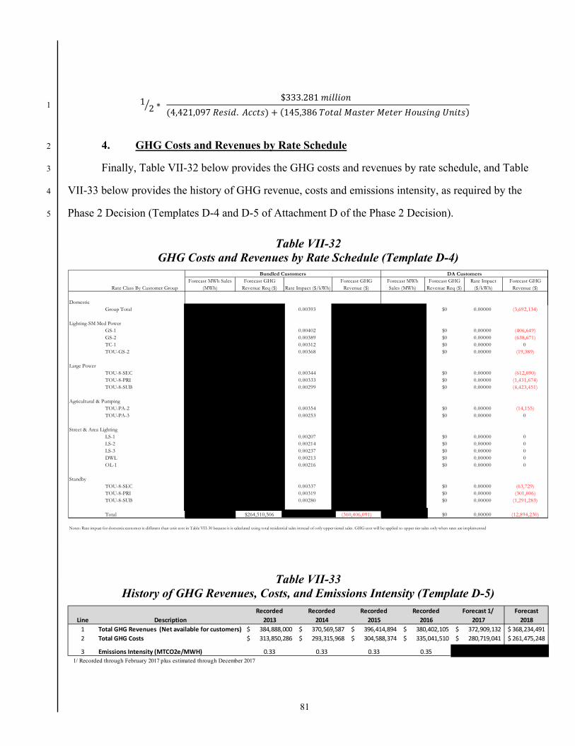
81

1 2 ∗ $333.281 (4,421,097 . ) + (145,386 ) 1

4. GHG Costs and Revenues by Rate Schedule 2

Finally, Table VII-32 below provides the GHG costs and revenues by rate schedule, and Table 3

VII-33 below provides the history of GHG revenue, costs and emissions intensity, as required by the 4

Phase 2 Decision (Templates D-4 and D-5 of Attachment D of the Phase 2 Decision). 5

Table VII-32 GHG Costs and Revenues by Rate Schedule (Template D-4)

Table VII-33 History of GHG Revenues, Costs, and Emissions Intensity (Template D-5)

Rate Class By Customer GroupForecast MWh Sales

(MWh)Forecast GHG

Revenue Req ($) Rate Impact ($/kWh)Forecast GHG

Revenue ($)Forecast MWh Sales (MWh)

Forecast GHG Revenue Req ($)

Rate Impact ($/kWh)

Forecast GHG Revenue ($)

DomesticGroup Total 0.00393 $0 0.00000 (3,692,134)

Lighting-SM Med PowerGS-1 0.00402 $0 0.00000 (406,649)GS-2 0.00389 $0 0.00000 (638,671)TC-1 0.00312 $0 0.00000 0TOU-GS-2 0.00368 $0 0.00000 (19,389)

Large PowerTOU-8-SEC 0.00344 $0 0.00000 (612,090)TOU-8-PRI 0.00333 $0 0.00000 (1,431,674)TOU-8-SUB 0.00299 $0 0.00000 (4,423,451)

Agricultural & PumpingTOU-PA-2 0.00354 $0 0.00000 (14,155)TOU-PA-3 0.00253 $0 0.00000 0

Street & Area LightingLS-1 0.00207 $0 0.00000 0LS-2 0.00214 $0 0.00000 0LS-3 0.00237 $0 0.00000 0DWL 0.00213 $0 0.00000 0OL-1 0.00216 $0 0.00000 0

StandbyTOU-8-SEC 0.00337 $0 0.00000 (63,729)TOU-8-PRI 0.00319 $0 0.00000 (301,006)TOU-8-SUB 0.00280 $0 0.00000 (1,291,283)

Total $264,510,506 (360,406,091) $0 0.00000 (12,894,230)

Notes: Rate impact for domestic customer is different than unit cost in Table VII-30 because it is calculated using total residential sales instead of only upper tiered sales. GHG cost will be applied to upper tier sales only when rates are implemented

Bundled Customers DA Customers

Recorded Recorded Recorded Recorded Forecast 1/ ForecastLine Description 2013 2014 2015 2016 2017 2018

1 Total GHG Revenues (Net available for customers) 384,888,000$ 370,569,587$ 396,414,894$ 380,402,105$ 372,909,132$ 368,234,491$ 2 Total GHG Costs 313,850,286$ 293,315,968$ 304,588,374$ 335,041,510$ 280,719,041$ 261,475,248$

3 Emissions Intensity (MTCO2e/MWH) 0.33 0.33 0.33 0.351/ Recorded through February 2017 plus estimated through December 2017

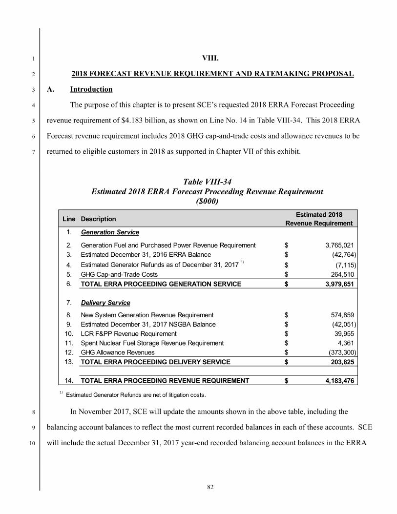
82

VIII. 1

2018 FORECAST REVENUE REQUIREMENT AND RATEMAKING PROPOSAL 2

A. Introduction 3

The purpose of this chapter is to present SCE’s requested 2018 ERRA Forecast Proceeding 4

revenue requirement of $4.183 billion, as shown on Line No. 14 in Table VIII-34. This 2018 ERRA 5

Forecast revenue requirement includes 2018 GHG cap-and-trade costs and allowance revenues to be 6

returned to eligible customers in 2018 as supported in Chapter VII of this exhibit. 7

In November 2017, SCE will update the amounts shown in the above table, including the 8

balancing account balances to reflect the most current recorded balances in each of these accounts. SCE 9

will include the actual December 31, 2017 year-end recorded balancing account balances in the ERRA 10

Table VIII-34 Estimated 2018 ERRA Forecast Proceeding Revenue Requirement

($000)

Line Description Estimated 2018

Revenue Requirement1. Generation Service

2. Generation Fuel and Purchased Power Revenue Requirement 3,765,021$

3. Estimated December 31, 2016 ERRA Balance (42,764)$

4. Estimated Generator Refunds as of December 31, 2017 1/(7,115)$

5. GHG Cap-and-Trade Costs 264,510$

6. TOTAL ERRA PROCEEDING GENERATION SERVICE 3,979,651$

7. Delivery Service

8. New System Generation Revenue Requirement 574,859$

9. Estimated December 31, 2017 NSGBA Balance (42,051)$

10. LCR F&PP Revenue Requirement 39,955$

11. Spent Nuclear Fuel Storage Revenue Requirement 4,361$

12. GHG Allowance Revenues (373,300)$

13. TOTAL ERRA PROCEEDING DELIVERY SERVICE 203,825$

14. TOTAL ERRA PROCEEDING REVENUE REQUIREMENT 4,183,476$

1/ Estimated Generator Refunds are net of litigation costs.

83

revenue requirement rate change and advice letter filed in compliance with a Commission decision in 1

this proceeding, if available. 2

B. Estimated 2018 ERRA-Related Generation Service Revenue Requirement 3

As shown above on Line No. 6 of Table VIII-34, SCE requests a 2018 ERRA generation service 4

revenue requirement of $3.980 billion. This revenue requirement is a consolidation of estimated fuel 5

and purchased power expenses, GHG cap-and-trade costs, the estimated December 31, 2017 balance in 6

the ERRA balancing account and estimated net67 generator refunds stemming from electricity 7

overcharges to SCE during the 2000-2001 California Energy Crisis. 8

1. Estimated 2018 Fuel and Purchased Power Revenue Requirement 9

As shown below on Line No. 35 in Table VIII-35, SCE’s requested 2018 fuel and purchased 10

power cost revenue requirement is $4.644 billion. This amount includes $57.110 million for franchise 11

fees and uncollectible (FF&U) expense and municipal surcharges.68 12

67 The forecast estimated net generator refunds are net of forecast associated litigation costs, which are recorded

in the LCTA.

68 The FF&U amount is determined using the current FF&U factor adopted by the Commission in D.15-11-021. The municipal surcharge amount as shown on Line 23 is the amount of the municipal surcharges (franchise fees) that SCE estimates it will pay associated with the DWR revenue requirement in 2018.

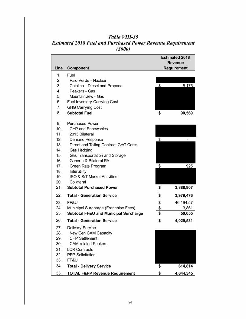
84

Table VIII-35 Estimated 2018 Fuel and Purchased Power Revenue Requirement

($000)

Line

Estimated 2018 Revenue

Requirement

1. Fuel2. Palo Verde - Nuclear3. Catalina - Diesel and Propane 5 175$ 4. Peakers - Gas5. Mountainview - Gas6. Fuel Inventory Carrying Cost7. GHG Carrying Cost8. Subtotal Fuel 90,569$

9. Purchased Power10. CHP and Renewables 11. 2013 Bilateral 12. Demand Response -$ 13. Direct and Tolling Contract GHG Costs14. Gas Hedging15. Gas Transportation and Storage16. Generic & Bilateral RA17. Green Rate Program 925$ 18. Interutility19. ISO & S/T Market Activities20. Collateral21. Subtotal Purchased Power 3,888,907$

22. Total - Generation Service 3,979,476$

23. FF&U 46,194.57$ 24. Municipal Surcharge (Franchise Fees) 3,861$ 25. Subtotal FF&U and Municipal Surcharge 50,055$

26. Total - Generation Service 4,029,531$

27. Delivery Service28. New Gen CAM Capacity 29. CHP Settlement30. CAM-related Peakers

31. LCR Contracts32. PRP Solicitation33. FF&U

34. Total - Delivery Service 614,814$

35. TOTAL F&PP Revenue Requirement 4,644,345$

Component

85

a) Fuel Expense 1

As shown below on Line No. 12 in Table VIII-36, SCE has estimated its total 2018 fuel costs to 2

be $90.569 million. 3

Table VIII-36 2018 Estimated Fuel Expense

($000)

The estimated 2018 PVNGS, Mountainview, Peakers, and Catalina fuel costs are supported in 4

Chapter IV. 5

The forecast of fuel inventory carrying costs associated with nuclear, natural gas, and diesel fuel 6

inventories are supported in Chapter VI. 7

b) Purchased Power Expense 8

As shown below on Line No. 25 in Table VIII-37, SCE has estimated its total 2018 purchased 9

power costs to be $4.497 billion as supported in Chapter IV. Collateral costs, as shown on Line No. 24, 10

are supported in Chapter VI. 11

Line Amount

1. Nuclear - Palo Verde

2. Gas3. Peakers4. Mountainview5. Gas Subtotal 44,840$

6. Catalina7. Diesel 5,040$ 8. Propane 135$ 9. Catalina Subtotal 5,175$

10. Fuel Inventory Carrying Cost11. GHG Carrying Cost

12. TOTAL 90,569$

Component

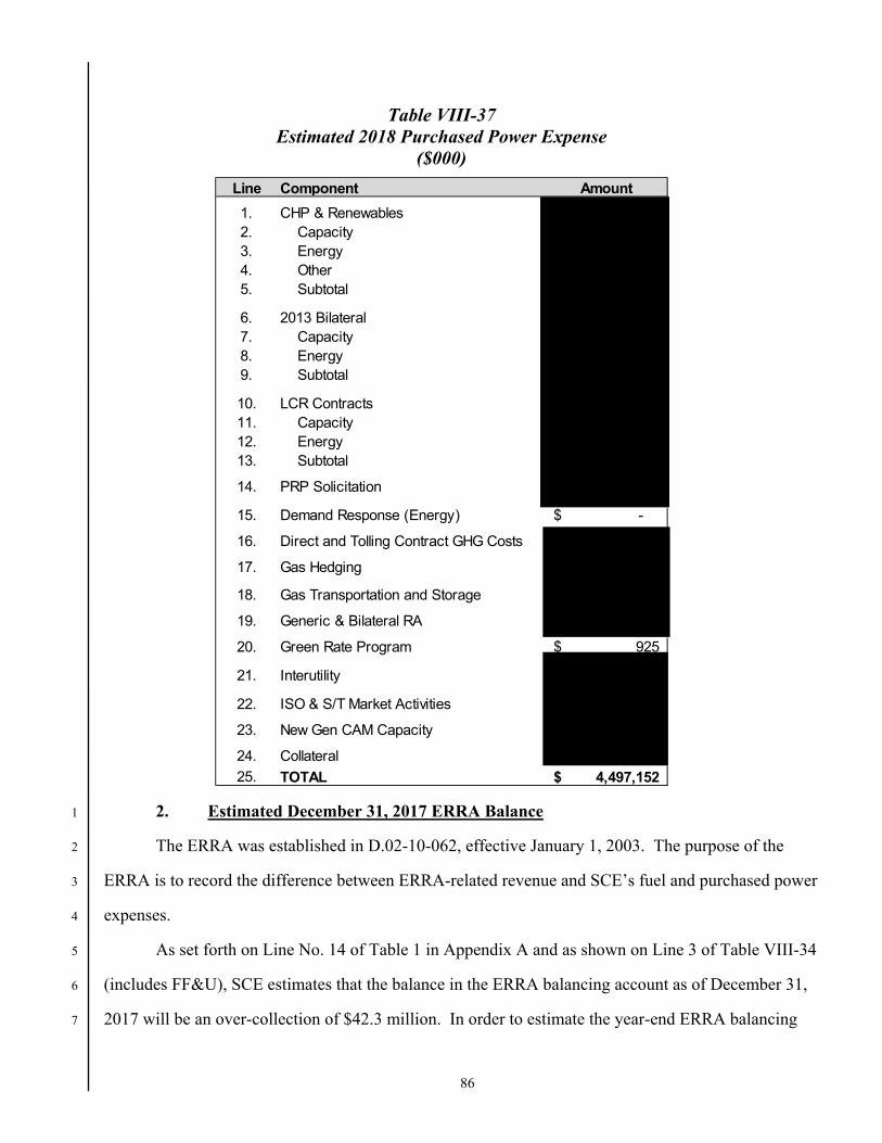
86

Table VIII-37 Estimated 2018 Purchased Power Expense

($000)

2. Estimated December 31, 2017 ERRA Balance 1

The ERRA was established in D.02-10-062, effective January 1, 2003. The purpose of the 2

ERRA is to record the difference between ERRA-related revenue and SCE’s fuel and purchased power 3

expenses. 4

As set forth on Line No. 14 of Table 1 in Appendix A and as shown on Line 3 of Table VIII-34 5

(includes FF&U), SCE estimates that the balance in the ERRA balancing account as of December 31, 6

2017 will be an over-collection of $42.3 million. In order to estimate the year-end ERRA balancing 7

Line Amount

1. CHP & Renewables2. Capacity3. Energy4. Other5. Subtotal

6. 2013 Bilateral7. Capacity8. Energy9. Subtotal

10. LCR Contracts11. Capacity12. Energy13. Subtotal

14. PRP Solicitation

15. Demand Response (Energy) -$

16. Direct and Tolling Contract GHG Costs

17. Gas Hedging

18. Gas Transportation and Storage

19. Generic & Bilateral RA

20. Green Rate Program 925$

21. Interutility

22. ISO & S/T Market Activities

23. New Gen CAM Capacity

24. Collateral

25. TOTAL 4,497,152$

Component

87

account balance, SCE has used recorded amounts through March 31, 2017, plus a forecast of the activity 1

SCE expects to be recorded in the ERRA during April through December 2017. Including FF&U of 2

$0.5 million, the total estimated ERRA year-end over-collection is $42.8 million. SCE will provide an 3

updated estimate of the year-end 2017 ERRA balance in its Update Testimony to be served in November 4

2017, which will reflect the latest recorded data and power and natural gas price assumptions. 5

3. Estimated Energy Settlement Refunds and Litigation Costs 6

SCE is pursuing refunds from generators who overcharged SCE (and the other California IOUs) 7

for electricity during the 2000-2001 California Energy Crisis. As shown on Line No. 13 of Table 3 in 8

Appendix A, SCE is estimating a December 31, 2017 over-collected balance of $10.4 million (including 9

FF&U) in the ESMA. SCE will update the amount of refunds included in the 2018 ERRA Forecast 10

revenue requirement in its November 2017 ERRA Update Testimony. In addition, SCE will include the 11

recorded operation of the ESMA for the 2017 Record Period in its April 1, 2018 ERRA Review 12

application. 13

Also included in Table 3 in Appendix A is the Litigation Costs Tracking Account (LCTA). In 14

accordance with Resolution E-3894, SCE shall maintain a LCTA within the ESMA to track: 1) 15

litigation costs that are “set-aside” in the FERC investigation settlement agreements; and 2) actual 16

litigation costs incurred by SCE. As shown on Line No. 30 of Table 3 in Appendix A, SCE is 17

estimating a December 31, 2017 under-collected balance of $3.3 million (including FF&U) in the 18

LCTA. SCE will include the recorded operation of the LCTA for the 2017 Record Period in its April 1, 19

2018 ERRA Review application. Combining the ESMA and LCTA estimated December 31, 2017 20

ending balances results in an overcollection of $7.1 million, as shown on Line 4 of Table VIII-34. 21

C. Estimated 2018 ERRA-Related Delivery Service Revenue Requirement 22

As shown on Line No. 13 of Table VIII-34 above, SCE requests a 2018 ERRA Forecast 23

Proceeding delivery service revenue requirement of $203.8 million. This amount is a consolidation of 24

New System Generation costs, the estimated December 31, 2017 balance in the NSGBA, the estimated 25

spent nuclear fuel storage revenue requirement, the estimated LCR contracts revenue requirement, and 26

88

estimated GHG allowance revenues to be returned to eligible customers in 2018. GHG allowance 1

revenue returns are discussed in Chapter VII. 2

1. Estimated New System Generation Net Capacity CAM-Related Cost 3

a) Introduction 4

The Commission in D.06-07-029 adopted a CAM to allocate the benefits and costs of new 5

generation to all benefiting customers in an IOU’s service territory for up to ten years. Under D.06-07-6

029, the Commission required utilities to make a selection at the time they seek contract approval 7

whether or not they intend that the CAM should apply to the contract.69 In addition, the Commission 8

either adopts or rejects the utility’s request in the decision approving or rejecting the new generation 9

contract. Consistent with D.06-07-029, SCE established the non-bypassable New System Generation 10

rate component and associated NSGBA to recover the net costs of the new generation resources from all 11

benefiting customers, including bundled service, DA, and CCA customers. 12

In addition, the Commission in D.10-12-035 adopted the QF and CHP Program Settlement 13

Agreement which, among other things, allows SCE to purchase CHP generation on behalf of DA 14

customers’ Energy Service Providers and CCAs. The Commission allowed the IOUs to recover “net 15

capacity costs” from all bundled service, DA and CCA customers through the CAM. 16

Subsequent to D.06-07-029 and D.10-12-035, Senate Bill (SB) 695 was enacted and expressly 17

requires the Commission “to ensure, under certain conditions, the net capacity costs of the specified 18

generation resources are allocated on a fully non-bypassable basis to bundled service customers, and DA 19

and CCA customers.” As a result of SB 695, the Commission issued D.11-05-005 modifying the new 20

generation and long-term contract CAM previously adopted in D.06-07-029. D.11-05-005 eliminates 21

the “election” process and changes the duration of CAM treatment from a 10-year period to match the 22

69 D.06-07-029, Conclusion of Law No. 6, p. 60.

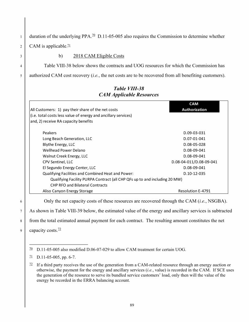
89

duration of the underlying PPA.70 D.11-05-005 also requires the Commission to determine whether 1

CAM is applicable.71 2

b) 2018 CAM Eligible Costs 3

Table VIII-38 below shows the contracts and UOG resources for which the Commission has 4

authorized CAM cost recovery (i.e., the net costs are to be recovered from all benefiting customers). 5

Table VIII-38 CAM Applicable Resources

Only the net capacity costs of these resources are recovered through the CAM (i.e., NSGBA). 6

As shown in Table VIII-39 below, the estimated value of the energy and ancillary services is subtracted 7

from the total estimated annual payment for each contract. The resulting amount constitutes the net 8

capacity costs.72 9

70 D.11-05-005 also modified D.06-07-029 to allow CAM treatment for certain UOG.

71 D.11-05-005, pp. 6-7.

72 If a third party receives the use of the generation from a CAM-related resource through an energy auction or otherwise, the payment for the energy and ancillary services (i.e., value) is recorded in the CAM. If SCE uses the generation of the resource to serve its bundled service customers’ load, only then will the value of the energy be recorded in the ERRA balancing account.

CAM All Customers: 1) pay their share of the net costs Authorization(i.e. total costs less value of energy and ancillary services)and, 2) receive RA capacity benefits

Peakers D.09-03-031Long Beach Generation, LLC D.07-01-041Blythe Energy, LLC D.08-05-028Wellhead Power Delano D.08-09-041Walnut Creek Energy, LLC D.08-09-041CPV Sentinel, LLC D.08-04-011/D.08-09-041El Segundo Energy Center, LLC D.08-09-041Qualifying Facilities and Combined Heat and Power: D.10-12-035

Qualifying Facility PURPA Contract (all CHP QFs up to and including 20 MW)CHP RFO and Bilateral Contracts

Aliso Canyon Energy Storage Resolution E-4791

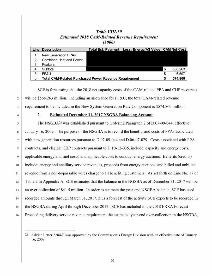
90

Table VIII-39 Estimated 2018 CAM-Related Revenue Requirement

($000)

SCE is forecasting that the 2018 net capacity costs of the CAM-related PPA and CHP resources 1

will be $568.263 million. Including an allowance for FF&U, the total CAM-related revenue 2

requirement to be included in the New System Generation Rate Component is $574.860 million. 3

2. Estimated December 31, 2017 NSGBA Balancing Account 4

The NSGBA73 was established pursuant to Ordering Paragraph 2 of D.07-09-044, effective 5

January 16, 2009. The purpose of the NSGBA is to record the benefits and costs of PPAs associated 6

with new generation resources pursuant to D.07-09-044 and D.06-07-029. Costs associated with PPA 7

contracts, and eligible CHP contracts pursuant to D.10-12-035, include: capacity and energy costs, 8

applicable energy and fuel costs, and applicable costs to conduct energy auctions. Benefits (credits) 9

include: energy and ancillary service revenues, proceeds from energy auctions, and billed and unbilled 10

revenue from a non-bypassable wires charge to all benefiting customers. As set forth on Line No. 17 of 11

Table 2 in Appendix A, SCE estimates that the balance in the NGSBA as of December 31, 2017 will be 12

an over-collection of $41.5 million. In order to estimate the year-end NSGBA balance, SCE has used 13

recorded amounts through March 31, 2017, plus a forecast of the activity SCE expects to be recorded in 14

the NSGBA during April through December 2017. SCE has included in the 2018 ERRA Forecast 15

Proceeding delivery service revenue requirement the estimated year-end over-collection in the NSGBA, 16

73 Advice Letter 2284-E was approved by the Commission’s Energy Division with an effective date of January

16, 2009.

Line Description Total Est. Payment Less: Energy/AS Value CAM Net Cost

1. New Generation PPAs2. Combined Heat and Power3. Peakers4. Subtotal 568,263$ 5. FF&U 6,597$ 6. Total CAM-Related Purchased Power Revenue Requirement 574,860$

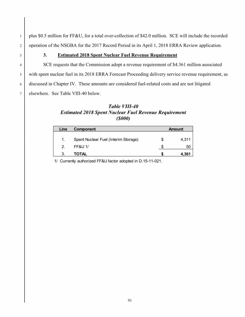
91

plus $0.5 million for FF&U, for a total over-collection of $42.0 million. SCE will include the recorded 1

operation of the NSGBA for the 2017 Record Period in its April 1, 2018 ERRA Review application. 2

3. Estimated 2018 Spent Nuclear Fuel Revenue Requirement 3

SCE requests that the Commission adopt a revenue requirement of $4.361 million associated 4

with spent nuclear fuel in its 2018 ERRA Forecast Proceeding delivery service revenue requirement, as 5

discussed in Chapter IV. These amounts are considered fuel-related costs and are not litigated 6

elsewhere. See Table VIII-40 below. 7

Table VIII-40 Estimated 2018 Spent Nuclear Fuel Revenue Requirement

($000)

Line Amount

1. Spent Nuclear Fuel (Interim Storage) 4,311$

2. FF&U 1/ 50$

3. TOTAL 4,361$

1/ Currently authorized FF&U factor adopted in D.15-11-021.

Component

92

IX. 1

DIRECT ACCESS, DEPARTING LOAD AND COMMUNITY CHOICE AGGREGATION 2

COST RESPONSIBILITY SURCHARGES 3

The purpose of this chapter is to describe the methodology used to determine the 2018 Cost 4

Responsibility Surcharge (CRS)74 for Direct Access (DA), Departing Load (DL), and Community 5

Choice Aggregation (CCA) customers, collectively CRS. In this initial application, SCE is only 6

providing a preliminary estimate of CRS as several key inputs, such as the Energy Market Price 7

Benchmark (MPB) and the Renewable MPB, will not be finalized until later this year as called for in 8

Resolution E-4475. SCE will provide an updated estimate of the 2018 CRS based on these updated 9

MPBs in its November update filing. Calculations for the estimated Competition Transition Charge 10

(CTC) and Power Charge Indifference Adjustment (PCIA), which together constitute the CRS 11

Indifference Charge, are included in Appendix B.75 12

As will be described in further detail below, the Indifference Charge is forecast to increase in 13

2018 due to four factors: 1) the expiration of various one-time adjustments and refunds that temporarily 14

decreased the Indifference Charge in 2016 and 2017, as can be seen by comparing the 2018 forecast 15

Indifference Charges in Appendix B to the “Unadjusted” (i.e. without adjustments and refunds) and 16

“Adjusted” 2017 Indifference Charges in Appendix B presented in the November Update to A.16-05-17

001 ; 2) the inadvertent addition of approximately 6,000 GWh of renewable energy in 2017 Indifference 18

74 The CRS also includes the Department of Water Resources (DWR) Bond Charge, which is determined in the

annual DWR Revenue Requirement proceeding. The DWR Bond Charge listed in the illustrative CRS rates in Appendix B is the 2017 DWR Bond Charge.

75 The format of Appendix B aligns directly with the common workpapers agreed to by participants in the PCIA Working Group. Formal Commission approval of this new format change is pending in the Joint Utilities’ and Community Choice Aggregators’ Joint Petition for Modification of D.06-07-030, filed on April 5, 2017. In addition, SCE (in conjunction with Pacific Gas & Electric Company and San Diego Gas & Electric Company) filed A.17-04-018 for Approval of the Portfolio Allocation Methodology For All Customers on April 25, 2017 (PAM). PAM is intended to prospectively replace the current indifference charge methodology.

93

Charge rates that served to artificially decrease those rates; 3) a forecast 10% decrease to the energy 1

MPB; and 4) a forecast 15% decrease to the Renewable MPB. 2

A. Background 3

The CRS Indifference Charge, as established in D.02-11-022 and modified by D.03-07-030, 4

D.06-07-030, D.08-09-012, D.11-12-018, and Resolution E-4475, is designed to maintain bundled 5

service customer indifference to departing load by ensuring that departing load customers remain 6

responsible for the stranded, or above-market, costs of generation resources procured on their behalf 7

prior to their departure from bundled service.76 To derive this “Indifference Amount,” SCE quantifies 8

the difference between the forecast annual cost of the generation portfolio procured by SCE (“Total 9

Portfolio Cost”), and the forecast market value of that portfolio (defined as the forecast output of the 10

resources in the generation portfolio multiplied by the total MPB). A positive Indifference Amount 11

indicates that the utility’s generation portfolio is “above-market” for that year, and similarly, a negative 12

Indifference Amount indicates that the utility’s generation portfolio is “below market” for that year. In 13

D.08-09-012, the Commission adopted the practice of vintaging the utility’s generation portfolio to 14

ensure that departing load customers be held responsible only for generation procured prior to the date 15

of their departure from bundled customer service. Accordingly, SCE has calculated Indifference 16

Amounts for each “vintage year” based on the generation resources that were committed in each 17

calendar year.77 18

The vintaged Indifference Amount is then used to set the Indifference Charge, which consists of 19

two separate rate components: the Ongoing CTC, which recovers the above-market costs of pre-20

restructuring resources such as eligible QF and is the same for all vintages; and the PCIA, which 21

recovers the above-market costs of all non-CTC-eligible resources (i.e., UOG and “New-World” 22

generation resources as authorized in D.04-12-048) and varies by vintage based on the generation 23

76 See generally Resolution E-4475 at p. 2.

77 Pursuant to D.08-09-012, customers are assigned a vintage based on the date of their departure. If they departed on or before June 30 of a given year, they are assigned to the prior year’s vintage. Alternatively, if they departed on or after July 1 of a given year, they are assigned that year’s vintage.

94

resources included in that vintage. As described in D.06-07-030, the CTC and PCIA are set such that 1

the sum of the two equals the Indifference Charge. 2

B. Total Portfolio Costs 3

The Portfolio Costs for each vintage are determined based on the forecast fixed and variable 4

costs, consistent with those outlined in Table IV-1, of generation resources forecast to be used to serve 5

bundled service customers in 2018. Specifically, these costs include the base generation capital revenue 6

requirement, as set in the most recent General Rate Case (GRC) Phase 1,78 fuel costs, and direct GHG 7

costs for all eligible UOG;79 RPS-eligible contract costs; qualifying facility and non-CAM-eligible CHP 8

contract costs; all bilateral and RFO contract costs, including fuel costs and direct GHG costs; and any 9

applicable one-time refunds or adjustments.80 The Portfolio does not include any costs associated with 10

CAM and LCR-eligible resources, ISO-load related costs, Residual Net Position spot market (i.e., 11

“short-term”) purchases, or balancing account balances. 12

As described in SCE’s 2016 and 2017 ERRA Forecast Applications, proceeds from the Nuclear 13

Decommissioning Trust and NEIL Litigation Settlement refunds received in 2015 and “carried over” 14

negative Indifference Amounts for the 2001-2008 vintages from the 2016 ERRA Forecast were applied 15

as downward adjustments to the otherwise applicable 2017 ERRA Forecast Indifference Amount.81 The 16

78 The GRC Phase 1 revenue requirements included in the Indifference Amount calculation reflect the

authorized 2017 revenue requirement, as approved in D.15-11-021. SCE’s 2018 GRC Phase 1 Application, A.16-09-001, is currently pending before the Commission. Pursuant to D.06-07-030, the Indifference Amount calculation should reflect the revenue requirement adopted in the “most recent base revenue requirement proceeding.”

79 Pursuant to D.03-07-032 and D.04-12-048, the ten-year presumptive limit on departing load cost recovery for SCE’s UOG Mountainview Generating Station has ended. As such, its costs, energy, and capacity have been removed from the Total Portfolio calculation for purposes of this Application.

80 Pursuant to D.15-10-037, the Total Portfolio Costs for all non-LCE vintages shall reflect an adjustment such that those customers receive 10.05% of the refunds and costs recorded in 2016 in the ESMA and LCTA, respectively. The 2014 vintage shall reflect an adjustment such that those customers receive their share of the refunds and costs recorded in 2016 in the ESMA and LCTA as though they were bundled service customers. SCE is currently forecasting to receive approximately $10M in Energy Crisis-related refunds and incur $3M in litigation costs.

81 Similarly, pursuant to D.06-07-030 and D.07-05-005, any negative Indifference Amounts in this 2017 ERRA Forecast will be tracked, by vintage, and will be applied to any future positive Indifference Amounts that may

(Continued)

95

inclusion of those one-time adjustments directly reduced the Indifference Amount, and resulted in 2017 1

Indifference Charges that were not representative of the above- or below-market costs of SCE’s 2017 2

ERRA generation portfolio. Those adjustments have expired and are not included in the 2018 3

Indifference Amount calculation. 4

C. 2018 Market Price Benchmark 5

The preliminary 2018 MPB shown in Appendix B was calculated based on the methodology 6

described in D.11-12-018 and Resolution E-4475. Due to the timing of SCE’s application filing, the 7

MPB is an initial estimate of the 2018 result using forecast inputs. Based on the forecast inputs, SCE 8

forecasts that the 2018 MPB will be approximately 15% lower than the 2017 MPB, and, all else being 9

held equal, will increase the Indifference Amount. 10

The Energy MPB used in Appendix B is based on April 2017 forward market data, rather than 11

October data as described in Resolution E-4475. This forward market price estimate of $31.06/MWh is 12

based on Platt’s on- and off-peak data accessed on April 20, 2017, and is weighted based on SCE’s 2015 13

recorded load. The Energy MPB will be updated using on- and off-peak forward price quotes from 14

October 1 through October 31, 2017, and will be weighted based on SCE’s 2016 recorded load. 15

Pursuant to Resolution E-4475, the Renewable MPB is determined using two sets of inputs: the 16

IOU Green Benchmark, which is based on the weighted average price of newly-delivering contracts for 17

all three California IOUs and weighted at 62%, and the DOE Green Adder, which is based on the 18

average price of voluntary renewable programs throughout the Western Electric Coordinating Council, 19

added to the energy MPB and weighted at 38%. Because the IOU Green Benchmark source data is 20

confidential and cannot be shared among IOUs, initial estimates of the Indifference Charge submitted in 21

the ERRA Forecast have typically utilized the prior year’s Renewable MPB as a proxy input until the 22

Continued from the previous page accrue in future years for those vintages, and the Indifference Charge for any vintages with a negative Indifference Amount will be set to zero.

96

final IOU Green Benchmark is determined by the Energy Division in October. Based on feedback 1

received at the PCIA Working Groups convened pursuant to D.16-09-044, SCE is providing a forecast 2

of the IOU Green Benchmark using trends observed in its own data, and forecasts that the contracts 3

expected to begin deliveries in 2017 and 2018 will have a weighted average price that is approximately 4

15% lower than the contracts that were used to set the 2017 IOU Green Benchmark. SCE has reduced 5

the 2017 IOU Green Benchmark by 15%, resulting in a forecast 2018 IOU Green Benchmark of 6

$62.83/MWh. Because the DOE Green Adder does not typically vary significantly from year to year, 7

SCE has used the 2017 DOE Green Adder as a proxy input. Based on these two sets of data, SCE 8

forecasts that the Renewable MPB will decrease to approximately $57.20/MWh, and has used that 9

forecast Renewable MPB to calculate the Indifference Charges shown in Appendix B. The Renewable 10

MPB will be updated using data from the utilities’ October 1 informational filings. 11

The Capacity MPB used in Appendix B is based on the going-forward costs of a combustion 12

turbine calculated in the California Energy Commission’s “Estimated Cost of New Renewable and 13

Fossil Generation in California Final Staff Report” released on March 9, 2015. Based on that data, 14

which is the same data used to set the 2017 Capacity MPB, SCE forecasts that the 2018 Capacity MPB 15

will be $58.26/kW-Year. 16

As shown below in Table IX-41, the MPB components in aggregate have steadily decreased 17

over the past five years.82 All other things being equal, decreases to the MPB will increase the 18

Indifference Charges. 19

82 SCE reserves all of its rights to challenge any or all of these MPBs to ensure customer indifference and

protection from impermissible cost-shifting. See, e.g., April 25, 2017, testimony served in support of A.17-04-018.

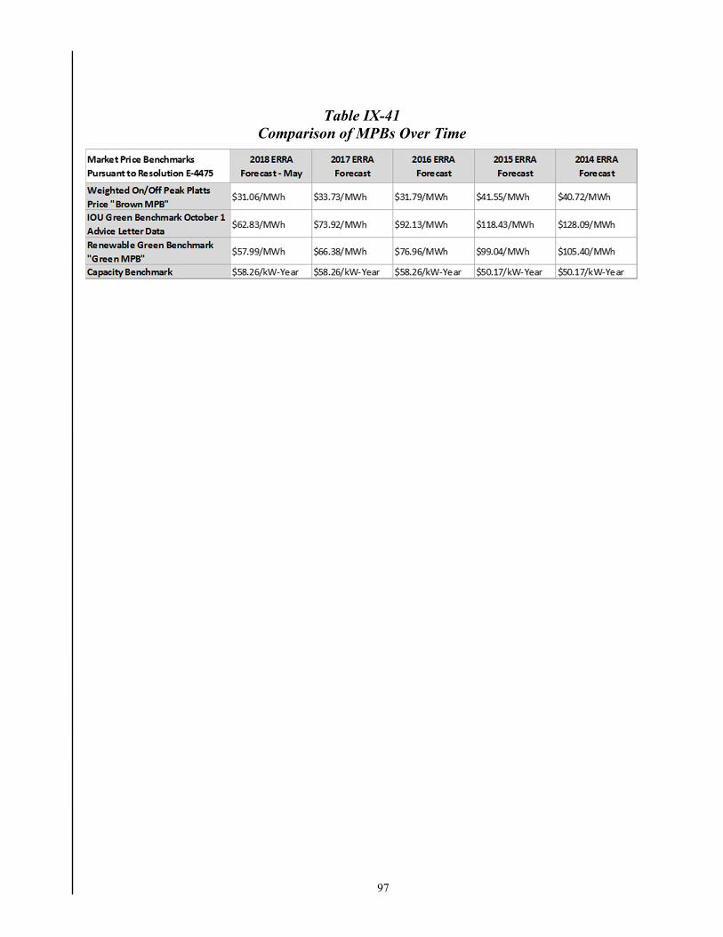
97

Table IX-41 Comparison of MPBs Over Time

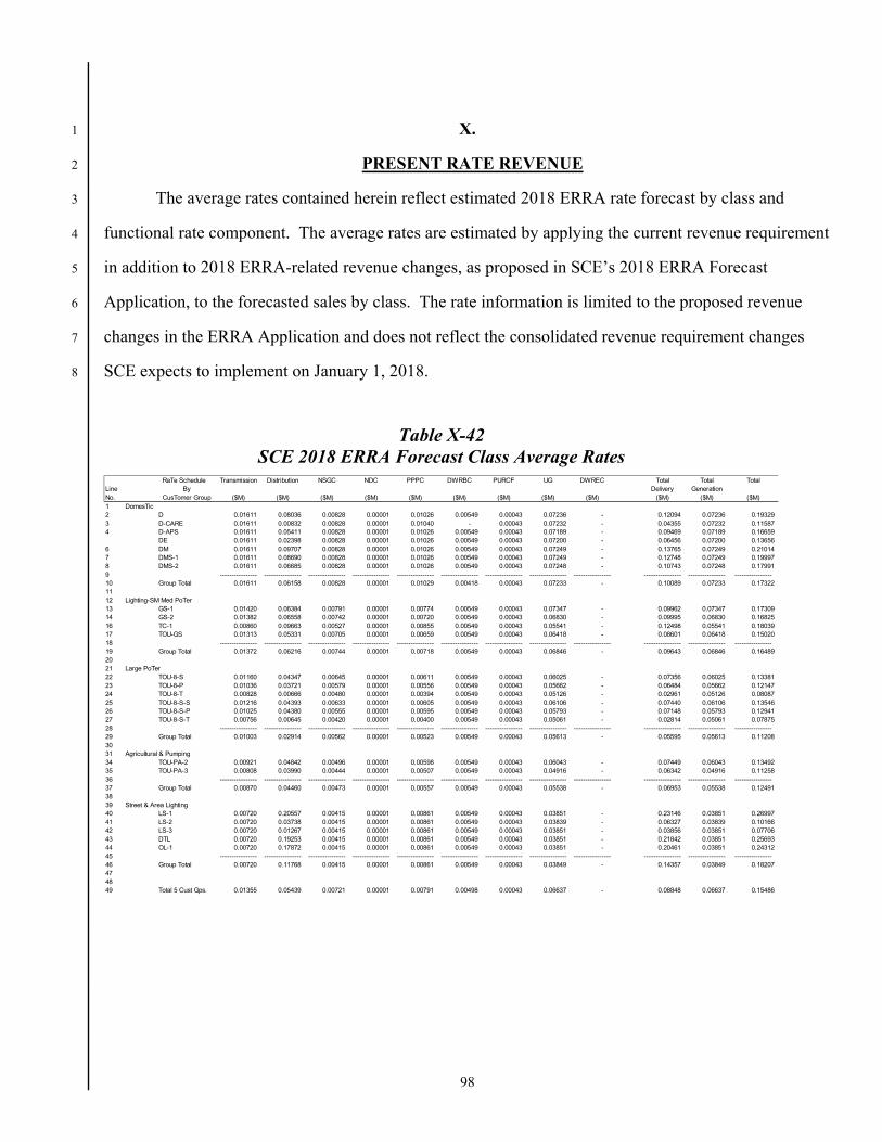
98

X. 1

PRESENT RATE REVENUE 2

The average rates contained herein reflect estimated 2018 ERRA rate forecast by class and 3

functional rate component. The average rates are estimated by applying the current revenue requirement 4

in addition to 2018 ERRA-related revenue changes, as proposed in SCE’s 2018 ERRA Forecast 5

Application, to the forecasted sales by class. The rate information is limited to the proposed revenue 6

changes in the ERRA Application and does not reflect the consolidated revenue requirement changes 7

SCE expects to implement on January 1, 2018. 8

Table X-42 SCE 2018 ERRA Forecast Class Average Rates

RaTe Schedule Transmission Distribution NSGC NDC PPPC DWRBC PURCF UG DWREC Total Total TotalLine By Delivery GenerationNo. CusTomer Group ($M) ($M) ($M) ($M) ($M) ($M) ($M) ($M) ($M) ($M) ($M) ($M)1 DomesTic2 D 0.01611 0.08036 0.00828 0.00001 0.01026 0.00549 0.00043 0.07236 - 0.12094 0.07236 0.19329 3 D-CARE 0.01611 0.00832 0.00828 0.00001 0.01040 - 0.00043 0.07232 - 0.04355 0.07232 0.11587 4 D-APS 0.01611 0.05411 0.00828 0.00001 0.01026 0.00549 0.00043 0.07189 - 0.09469 0.07189 0.16659

DE 0.01611 0.02398 0.00828 0.00001 0.01026 0.00549 0.00043 0.07200 - 0.06456 0.07200 0.13656 6 DM 0.01611 0.09707 0.00828 0.00001 0.01026 0.00549 0.00043 0.07249 - 0.13765 0.07249 0.21014 7 DMS-1 0.01611 0.08690 0.00828 0.00001 0.01026 0.00549 0.00043 0.07249 - 0.12748 0.07249 0.19997 8 DMS-2 0.01611 0.06685 0.00828 0.00001 0.01026 0.00549 0.00043 0.07248 - 0.10743 0.07248 0.17991 9 ---------------- ---------------- ---------------- ---------------- ---------------- ---------------- ---------------- ---------------- ---------------- ---------------- ---------------- ----------------10 Group Total 0.01611 0.06158 0.00828 0.00001 0.01029 0.00418 0.00043 0.07233 - 0.10089 0.07233 0.17322 1112 Lighting-SM Med PoTer13 GS-1 0.01420 0.06384 0.00791 0.00001 0.00774 0.00549 0.00043 0.07347 - 0.09962 0.07347 0.17309 14 GS-2 0.01382 0.06558 0.00742 0.00001 0.00720 0.00549 0.00043 0.06830 - 0.09995 0.06830 0.16825 16 TC-1 0.00860 0.09663 0.00527 0.00001 0.00855 0.00549 0.00043 0.05541 - 0.12498 0.05541 0.18039 17 TOU-GS 0.01313 0.05331 0.00705 0.00001 0.00659 0.00549 0.00043 0.06418 - 0.08601 0.06418 0.15020 18 ---------------- ---------------- ---------------- ---------------- ---------------- ---------------- ---------------- ---------------- ---------------- ---------------- ---------------- ----------------19 Group Total 0.01372 0.06216 0.00744 0.00001 0.00718 0.00549 0.00043 0.06846 - 0.09643 0.06846 0.16489 2021 Large PoTer22 TOU-8-S 0.01160 0.04347 0.00645 0.00001 0.00611 0.00549 0.00043 0.06025 - 0.07356 0.06025 0.13381 23 TOU-8-P 0.01036 0.03721 0.00579 0.00001 0.00556 0.00549 0.00043 0.05662 - 0.06484 0.05662 0.12147 24 TOU-8-T 0.00828 0.00666 0.00480 0.00001 0.00394 0.00549 0.00043 0.05126 - 0.02961 0.05126 0.08087 25 TOU-8-S-S 0.01216 0.04393 0.00633 0.00001 0.00605 0.00549 0.00043 0.06106 - 0.07440 0.06106 0.13546 26 TOU-8-S-P 0.01025 0.04380 0.00555 0.00001 0.00595 0.00549 0.00043 0.05793 - 0.07148 0.05793 0.12941 27 TOU-8-S-T 0.00756 0.00645 0.00420 0.00001 0.00400 0.00549 0.00043 0.05061 - 0.02814 0.05061 0.07875 28 ---------------- ---------------- ---------------- ---------------- ---------------- ---------------- ---------------- ---------------- ---------------- ---------------- ---------------- ----------------29 Group Total 0.01003 0.02914 0.00562 0.00001 0.00523 0.00549 0.00043 0.05613 - 0.05595 0.05613 0.11208 3031 Agricultural & Pumping34 TOU-PA-2 0.00921 0.04842 0.00496 0.00001 0.00598 0.00549 0.00043 0.06043 - 0.07449 0.06043 0.13492 35 TOU-PA-3 0.00808 0.03990 0.00444 0.00001 0.00507 0.00549 0.00043 0.04916 - 0.06342 0.04916 0.11258 36 ---------------- ---------------- ---------------- ---------------- ---------------- ---------------- ---------------- ---------------- ---------------- ---------------- ---------------- ----------------37 Group Total 0.00870 0.04460 0.00473 0.00001 0.00557 0.00549 0.00043 0.05538 - 0.06953 0.05538 0.12491 3839 Street & Area Lighting40 LS-1 0.00720 0.20557 0.00415 0.00001 0.00861 0.00549 0.00043 0.03851 - 0.23146 0.03851 0.26997 41 LS-2 0.00720 0.03738 0.00415 0.00001 0.00861 0.00549 0.00043 0.03839 - 0.06327 0.03839 0.10166 42 LS-3 0.00720 0.01267 0.00415 0.00001 0.00861 0.00549 0.00043 0.03851 - 0.03856 0.03851 0.07706 43 DTL 0.00720 0.19253 0.00415 0.00001 0.00861 0.00549 0.00043 0.03851 - 0.21842 0.03851 0.25693 44 OL-1 0.00720 0.17872 0.00415 0.00001 0.00861 0.00549 0.00043 0.03851 - 0.20461 0.03851 0.24312 45 ---------------- ---------------- ---------------- ---------------- ---------------- ---------------- ---------------- ---------------- ---------------- ---------------- ---------------- ----------------46 Group Total 0.00720 0.11768 0.00415 0.00001 0.00861 0.00549 0.00043 0.03849 - 0.14357 0.03849 0.18207 474849 Total 5 Cust Gps. 0.01355 0.05439 0.00721 0.00001 0.00791 0.00498 0.00043 0.06637 - 0.08848 0.06637 0.15486

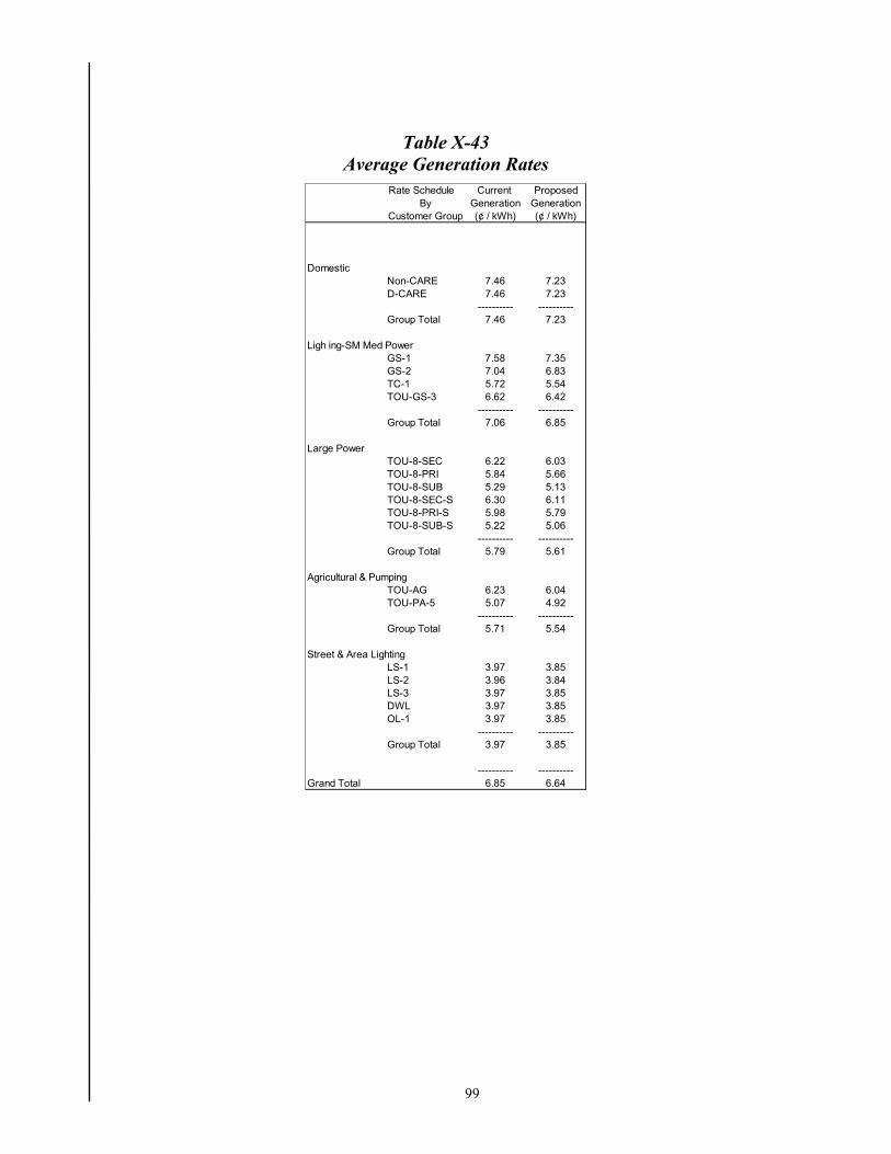
99

Table X-43 Average Generation Rates

Rate Schedule Current ProposedBy Generation Generation

Customer Group (¢ / kWh) (¢ / kWh)

DomesticNon-CARE 7.46 7.23D-CARE 7.46 7.23

---------- ----------Group Total 7.46 7.23

Ligh ing-SM Med PowerGS-1 7.58 7.35GS-2 7.04 6.83TC-1 5.72 5.54TOU-GS-3 6.62 6.42

---------- ----------Group Total 7.06 6.85

Large PowerTOU-8-SEC 6.22 6.03TOU-8-PRI 5.84 5.66TOU-8-SUB 5.29 5.13TOU-8-SEC-S 6.30 6.11TOU-8-PRI-S 5.98 5.79TOU-8-SUB-S 5.22 5.06

---------- ----------Group Total 5.79 5.61

Agricultural & PumpingTOU-AG 6.23 6.04TOU-PA-5 5.07 4.92

---------- ----------Group Total 5.71 5.54

Street & Area LightingLS-1 3.97 3.85LS-2 3.96 3.84LS-3 3.97 3.85DWL 3.97 3.85OL-1 3.97 3.85

---------- ----------Group Total 3.97 3.85

---------- ----------Grand Total 6.85 6.64

Appendix A

Estimated December 31, 2017 Balancing Account Balances

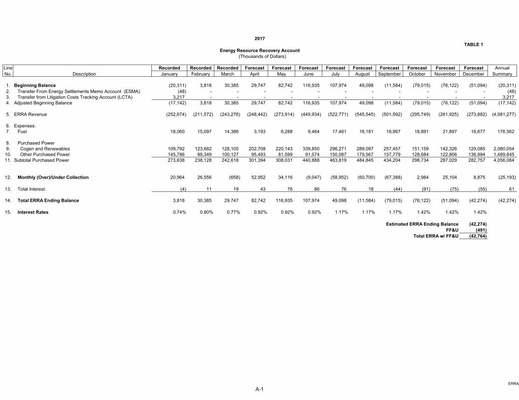
TABLE 1

Line Recorded Recorded Recorded Forecast Forecast Forecast Forecast Forecast Forecast Forecast Forecast Forecast AnnualNo. Description January February March April May June July August September October November December Summary

1. Beginning Balance (20,311) 3,818 30,385 29,747 82,742 116,935 107,974 49,098 (11,584) (79,015) (76,122) (51,094) (20,311) 2. Transfer From Energy Settlements Memo Account (ESMA) (48) - - - - - - - - - - - (48) 3. Transfer from Litigation Costs Tracking Account (LCTA) 3,217 - - - - - - - - - - - 3,217 4. Adjusted Beginning Balance (17,142) 3,818 30,385 29,747 82,742 116,935 107,974 49,098 (11,584) (79,015) (76,122) (51,094) (17,142)

5. ERRA Revenue (252,674) (211,572) (243,276) (248,442) (273,914) (449,934) (522,771) (545,545) (501,592) (295,749) (261,925) (273,882) (4,081,277)

6. Expenses:7. Fuel 18,060 15,097 14,386 3,193 6,288 9,464 17,461 16,181 18,967 18,891 21,897 16,677 176,562

8. Purchased Power9. Cogen and Renewables 109,792 123,682 128,105 202,708 220,143 339,850 296,271 289,097 257,457 151,159 142,326 129,085 2,080,054

10. Other Purchased Power 145,786 99,349 100,127 95,493 81,599 91,574 150,087 179,567 157,779 128,684 122,806 136,994 1,489,84511. Subtotal Purchased Power 273,638 238,128 242,618 301,394 308,031 440,888 463,819 484,845 434,204 298,734 287,029 282,757 4,056,084

12. Monthly (Over)/Under Collection 20,964 26,556 (658) 52,952 34,116 (9,047) (58,952) (60,700) (67,388) 2,984 25,104 8,875 (25,193)

13. Total Interest: (4) 11 19 43 76 86 76 18 (44) (91) (75) (55) 61

14. Total ERRA Ending Balance 3,818 30,385 29,747 82,742 116,935 107,974 49,098 (11,584) (79,015) (76,122) (51,094) (42,274) (42,274)

15. Interest Rates 0.74% 0.80% 0.77% 0.92% 0.92% 0.92% 1.17% 1.17% 1.17% 1.42% 1.42% 1.42%

Estimated ERRA Ending Balance (42,274) FF&U (491)

Total ERRA w/ FF&U (42,764)

2017

Energy Resource Recovery Account (Thousands of Dollars)

ERRA

A-1

TABLE 2


1. Beginning Balance (5,992) (31,829) (61,221) (96,574) (123,911) (141,274) (140,011) (83,609) (35,794) (2,971) (13,863) (30,759) (5,992) 2. Adjustment/Transfer - - - - - - - - - - - - - 3. Associated Interest - - - - - - - - - - - - - 4. Adjusted Beginning Balance (5,992) (31,829) (61,221) (96,574) (123,911) (141,274) (140,011) (83,609) (35,794) (2,971) (13,863) (30,759) (5,992)

5. Revenue:6. Billed (40,625) (49,959) (58,165) (40,294) (54,703) (61,605) (70,828) (75,749) (74,071) (65,793) (55,693) (59,236) (706,719)

7. Change in Unbilled8. Current Month Accrual (23,465) (20,711) (16,551) (29,807) (34,114) (33,819) (35,109) (34,538) (29,572) (24,649) (25,331) (25,013) (332,680) 9. Last Month Reversal 12,322 23,465 20,711 16,551 29,807 34,114 33,819 35,109 34,538 29,572 24,649 25,331 319,989

10. Change in Unbilled (11,143) 2,754 4,160 (13,256) (4,307) 295 (1,289) 571 4,966 4,923 (682) 318 (12,691)

11. Less: FF&U (Rate 0.988525) (594) (542) (620) (614) (677) (704) (828) (863) (793) (698) (647) (676) (8,255)

12. NSGBA Revenue (51,173) (46,663) (53,385) (52,935) (58,333) (60,607) (71,290) (74,315) (68,312) (60,172) (55,728) (58,242) (711,155)

13. Authorized Peaker Rev. Rqm't 4,610 4,168 4,437 4,140 4,207 4,627 5,107 5,392 5,386 4,939 4,342 4,520 55,876

14. Expenses 20,739 13,133 13,646 21,542 36,864 57,352 122,693 116,796 95,768 44,349 34,517 42,955 620,354

15. Monthly (Over)/Under Collection (25,825) (29,361) (35,302) (27,253) (17,262) 1,371 56,511 47,873 32,842 (10,883) (16,869) (10,767) (34,925)

16. Total Interest: (12) (31) (51) (84) (102) (108) (109) (58) (19) (10) (26) (43) (651)

17. Ending Balance (31,829) (61,221) (96,574) (123,911) (141,274) (140,011) (83,609) (35,794) (2,971) (13,863) (30,759) (41,569) (41,569)

18. Interest Rates 0.74% 0.80% 0.77% 0.92% 0.92% 0.92% 1.17% 1.17% 1.17% 1.42% 1.42% 1.42%

Estimated NSGBA Ending Balance (41,569) FF&U (483)

Total NSGBA w/ FF&U (42,051)

2017

New System Generation Balancing Account(Thousands of Dollars)

NSGBA

A-2

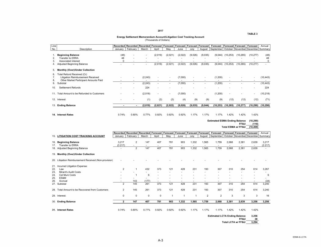
TABLE 3


1. Beginning Balance (48) - - (2,019) (2,021) (2,022) (9,026) (9,035) (9,044) (10,253) (10,265) (10,277) (48) 2. Transfer to ERRA 48 - - - - - - - - - - - 48 3. Associated interest 0 - - - - - - - - - - - 0 4. Adjusted Beginning Balance - - - (2,019) (2,021) (2,022) (9,026) (9,035) (9,044) (10,253) (10,265) (10,277) -

5. Monthly (Over)/Under Collection

6. Total Refund Received (Cr) 7. Litigation Reimbursement Received - - (2,243) - - (7,000) - - (1,200) - - - (10,443) 8. Other Market Participant Amounts Paid - - - - - - - - - - - - - 9. Subtotal - - (2,243) - - (7,000) - - (1,200) - - - (10,443)

10. Settlement Refunds - - 224 - - - - - - - - - 224

11. Total Amount to be Refunded to Customers - - (2,018) - - (7,000) - - (1,200) - - - (10,218)

12. Interest: - - (1) (2) (2) (4) (9) (9) (9) (12) (12) (12) (71)

13. Ending Balance - - (2,019) (2,021) (2,022) (9,026) (9,035) (9,044) (10,253) (10,265) (10,277) (10,290) (10,290)

14. Interest Rates 0.74% 0.80% 0.77% 0.92% 0.92% 0.92% 1.17% 1.17% 1.17% 1.42% 1.42% 1.42%

Estimated ESMA Ending Balance (10,290) FF&U (119)

Total ESMA w/ FF&U (10,409)

Recorded Recorded Recorded Forecast Forecast Forecast Forecast Forecast Forecast Forecast Forecast Forecast Annual15. LITIGATION COST TRACKING ACCOUNT January February March April May June July August September October November December Summary

16. Beginning Balance 3,217 2 147 407 781 903 1,332 1,565 1,759 2,068 2,381 2,639 3,217 17. Transfer to ERRA (3 217) - - - - - - - - - - - (3 217) 18. Adjusted Beginning Balance - 2 147 407 781 903 1,332 1,565 1,759 2,068 2,381 2,639 -

19. Monthly (Over)/Under Collection

20. Litigation Reimbursement Received (Non-provision) - - - - - - - - - - - - -

21. Incurred Litigation Expense:22. Law 2 1 432 373 121 428 231 193 307 310 254 614 3,267 23. Mirant's Audit Costs - - - - - - - - - - - - - 24. Cal Muni Costs - 1 6 - - - - - - - - - 6 25. ES&M - - - - - - - - - - - - - 26. Accrual - 143 (177) - - - - - - - - - (34) 27. Subtotal 2 145 261 373 121 428 231 193 307 310 254 614 3,240

28. Total Amount to be Recovered from Customers 2 145 261 373 121 428 231 193 307 310 254 614 3,240

29. Interest: 0 0 0 0 1 1 1 2 2 3 3 3 16

30. Ending Balance 2 147 407 781 903 1,332 1,565 1,759 2,068 2,381 2,639 3,256 3,256

31. Interest Rates 0.74% 0.80% 0.77% 0.92% 0.92% 0.92% 1.17% 1.17% 1.17% 1.42% 1.42% 1.42%

Estimated LCTA Ending Balance 3,256 FF&U 38

Total LCTA w/ FF&U 3,294

2017

Energy Settlement Memorandum Account/Litigation Cost Tracking Account (Thousands of Dollars)

ESMA & LCTA

A-3

Appendix B

Indifference Rate Calculation

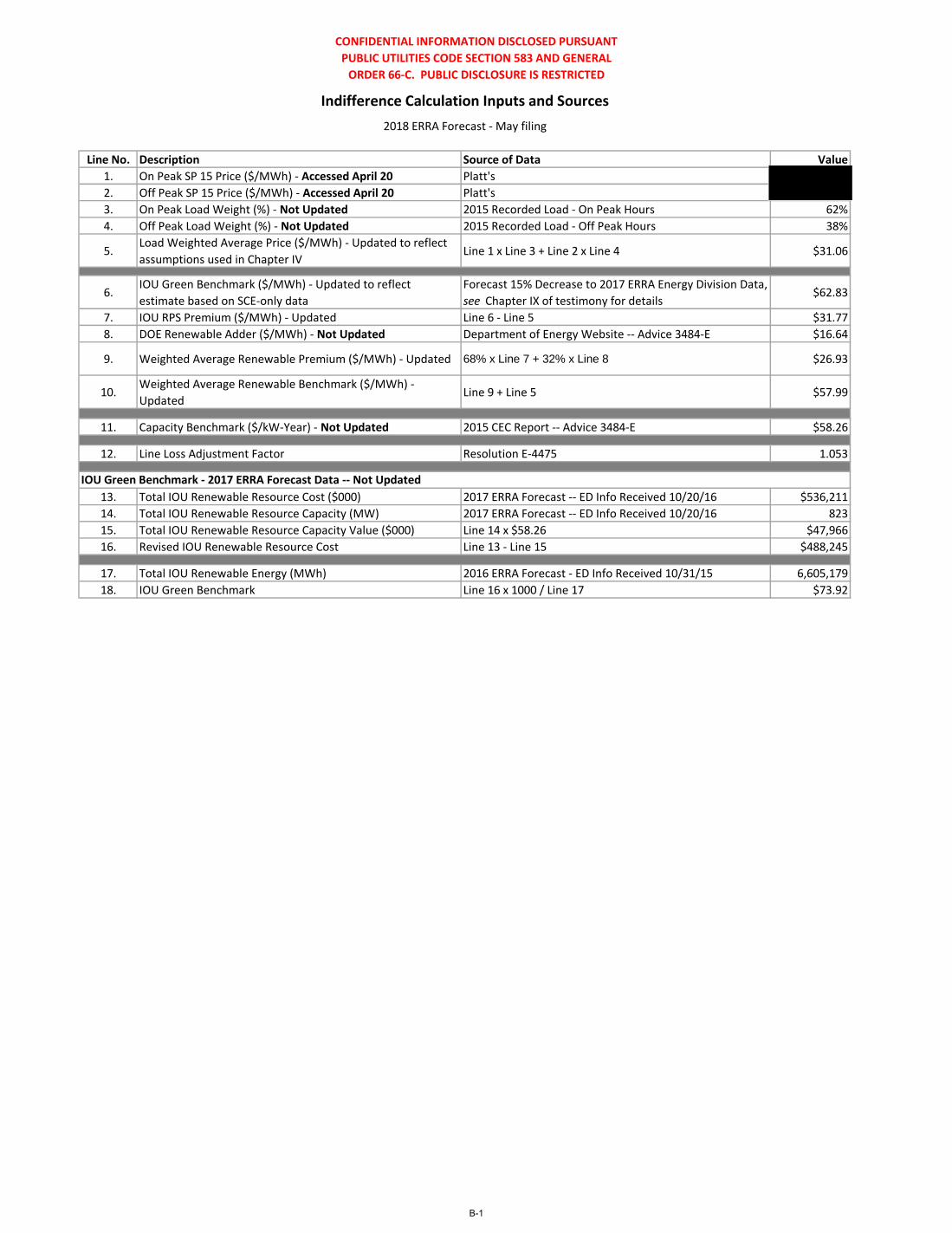
CONFIDENTIAL INFORMATION DISCLOSED PURSUANT

PUBLIC UTILITIES CODE SECTION 583 AND GENERAL

ORDER 66-C. PUBLIC DISCLOSURE IS RESTRICTED

Line No. Description Source of Data Value

1. On Peak SP 15 Price ($/MWh) - Accessed April 20 Platt's

2. Off Peak SP 15 Price ($/MWh) - Accessed April 20 Platt's

3. On Peak Load Weight (%) - Not Updated 2015 Recorded Load - On Peak Hours 62%

4. Off Peak Load Weight (%) - Not Updated 2015 Recorded Load - Off Peak Hours 38%

5.Load Weighted Average Price ($/MWh) - Updated to reflect

assumptions used in Chapter IVLine 1 x Line 3 + Line 2 x Line 4 $31.06

6.IOU Green Benchmark ($/MWh) - Updated to reflect

estimate based on SCE-only data

Forecast 15% Decrease to 2017 ERRA Energy Division Data,

see Chapter IX of testimony for details$62.83

7. IOU RPS Premium ($/MWh) - Updated Line 6 - Line 5 $31.77

8. DOE Renewable Adder ($/MWh) - Not Updated Department of Energy Website -- Advice 3484-E $16.64

9. Weighted Average Renewable Premium ($/MWh) - Updated 68% x Line 7 + 32% x Line 8 $26.93

10.Weighted Average Renewable Benchmark ($/MWh) -

UpdatedLine 9 + Line 5 $57.99

11. Capacity Benchmark ($/kW-Year) - Not Updated 2015 CEC Report -- Advice 3484-E $58.26

12. Line Loss Adjustment Factor Resolution E-4475 1.053

13. Total IOU Renewable Resource Cost ($000) 2017 ERRA Forecast -- ED Info Received 10/20/16 $536,211

14. Total IOU Renewable Resource Capacity (MW) 2017 ERRA Forecast -- ED Info Received 10/20/16 823

15. Total IOU Renewable Resource Capacity Value ($000) Line 14 x $58.26 $47,966

16. Revised IOU Renewable Resource Cost Line 13 - Line 15 $488,245

17. Total IOU Renewable Energy (MWh) 2016 ERRA Forecast - ED Info Received 10/31/15 6,605,179

18. IOU Green Benchmark Line 16 x 1000 / Line 17 $73.92

IOU Green Benchmark - 2017 ERRA Forecast Data -- Not Updated

Indifference Calculation Inputs and Sources

2018 ERRA Forecast - May filing

B-1

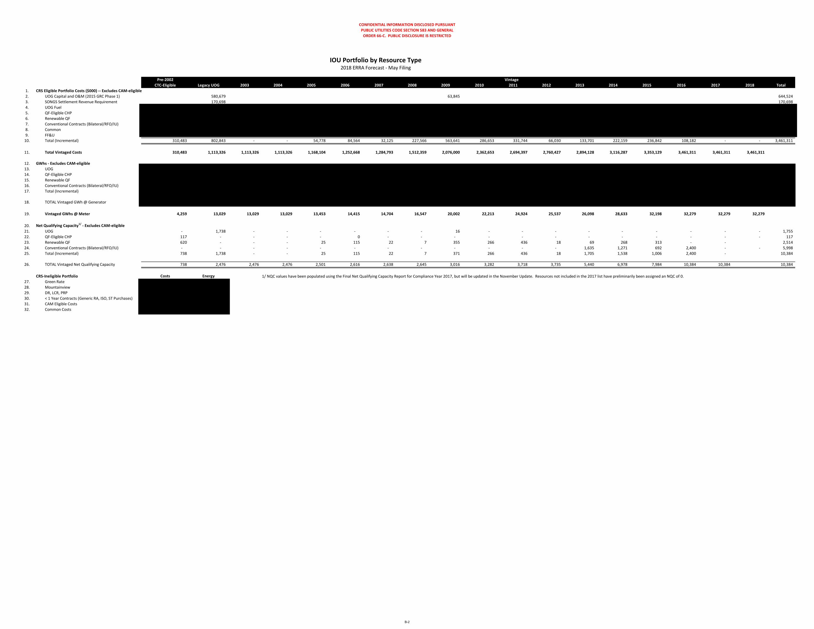
CONFIDENTIAL INFORMATION DISCLOSED PURSUANT

PUBLIC UTILITIES CODE SECTION 583 AND GENERAL

ORDER 66-C. PUBLIC DISCLOSURE IS RESTRICTED

Pre-2002

CTC-Eligible Legacy UOG 2003 2004 2005 2006 2007 2008 2009 2010 2011 2012 2013 2014 2015 2016 2017 2018 Total

1. CRS Eligible Portfolio Costs ($000) -- Excludes CAM-eligible

2. UOG Capital and O&M (2015 GRC Phase 1) 580,679 63,845 644,524

3. SONGS Settlement Revenue Requirement 170,698 170,698

4. UOG Fuel

5. QF-Eligible CHP

6. Renewable QF

7. Conventional Contracts (Bilateral/RFO/IU)

8. Common

9. FF&U

10. Total (Incremental) 310,483 802,843 - - 54,778 84,564 32,125 227,566 563,641 286,653 331,744 66,030 133,701 222,159 236,842 108,182 - - 3,461,311

11. Total Vintaged Costs 310,483 1,113,326 1,113,326 1,113,326 1,168,104 1,252,668 1,284,793 1,512,359 2,076,000 2,362,653 2,694,397 2,760,427 2,894,128 3,116,287 3,353,129 3,461,311 3,461,311 3,461,311

12. GWhs - Excludes CAM-eligible

13. UOG

14. QF-Eligible CHP

15. Renewable QF

16. Conventional Contracts (Bilateral/RFO/IU)

17. Total (Incremental)

18. TOTAL Vintaged GWh @ Generator

19. Vintaged GWhs @ Meter 4,259 13,029 13,029 13,029 13,453 14,415 14,704 16,547 20,002 22,213 24,924 25,537 26,098 28,633 32,198 32,279 32,279 32,279

20. Net Qualifying Capacity1/ - Excludes CAM-eligible

21. UOG - 1,738 - - - - - - 16 - - - - - - - - - 1,755

22. QF-Eligible CHP 117 - - - - 0 - - - - - - - - - - - - 117

23. Renewable QF 620 - - - 25 115 22 7 355 266 436 18 69 268 313 - - 2,514

24. Conventional Contracts (Bilateral/RFO/IU) - - - - - - - - - - - - 1,635 1,271 692 2,400 - - 5,998

25. Total (Incremental) 738 1,738 - - 25 115 22 7 371 266 436 18 1,705 1,538 1,006 2,400 - 10,384

26. TOTAL Vintaged Net Qualifying Capacity 738 2,476 2,476 2,476 2,501 2,616 2,638 2,645 3,016 3,282 3,718 3,735 5,440 6,978 7,984 10,384 10,384 10,384

CRS-Ineligible Portfolio Costs Energy 1/ NQC values have been populated using the Final Net Qualifying Capacity Report for Compliance Year 2017, but will be updated in the November Update. Resources not included in the 2017 list have preliminarily been assigned an NQC of 0.

27. Green Rate

28. Mountainview

29. DR, LCR, PRP

30. < 1 Year Contracts (Generic RA, ISO, ST Purchases)

31. CAM Eligible Costs

32. Common Costs

IOU Portfolio by Resource Type2018 ERRA Forecast - May Filing

Vintage

B-2

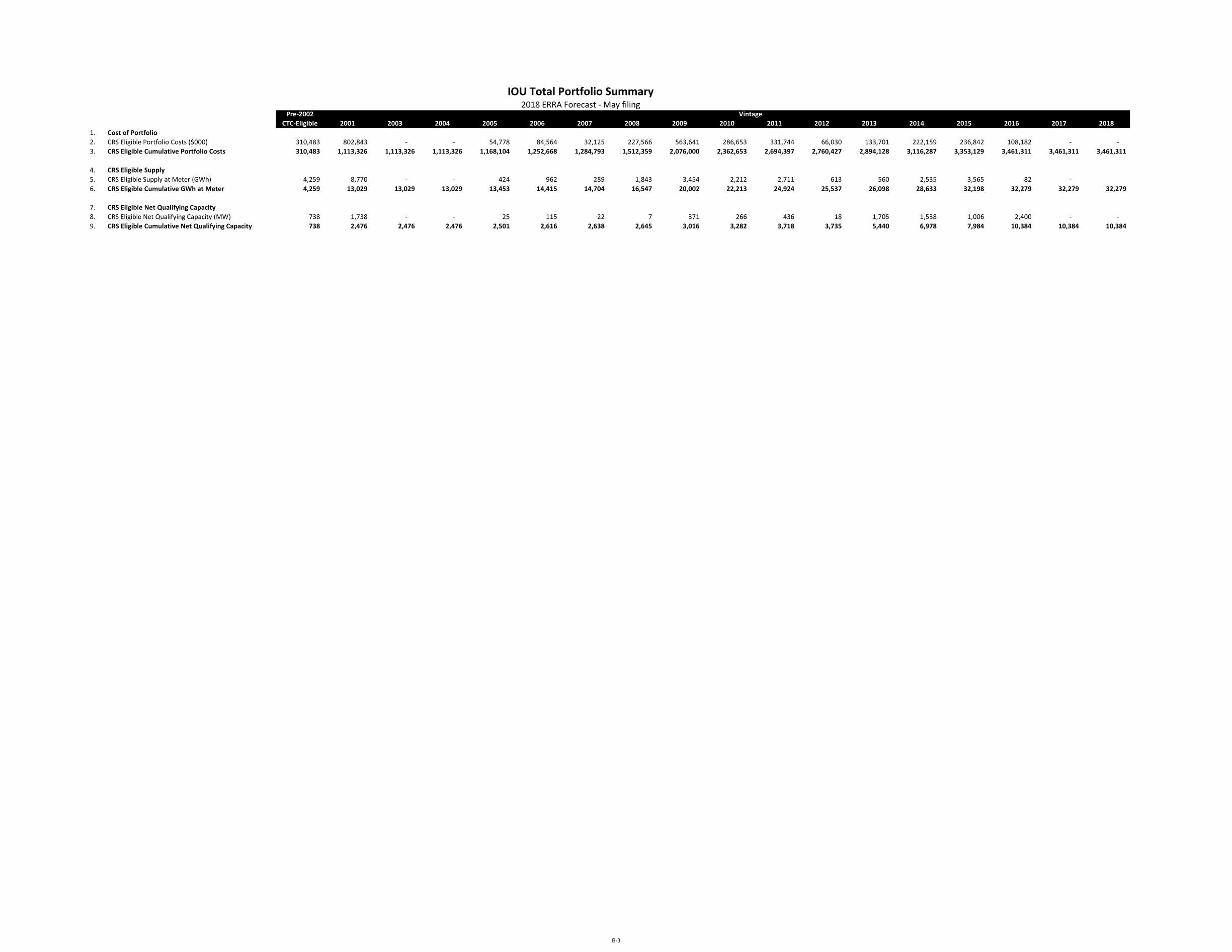
Pre-2002

CTC-Eligible 2003 2004 2005 2006 2007 2008 2009 2010 2011 2012 2013 2014 2015 2016 2017 2018

1. Cost of Portfolio

2. CRS Eligible Portfolio Costs ($000) 310,483 802,843 - - 54,778 84,564 32,125 227,566 563,641 286,653 331,744 66,030 133,701 222,159 236,842 108,182 - -

3. CRS Eligible Cumulative Portfolio Costs 310,483 1,113,326 1,113,326 1,113,326 1,168,104 1,252,668 1,284,793 1,512,359 2,076,000 2,362,653 2,694,397 2,760,427 2,894,128 3,116,287 3,353,129 3,461,311 3,461,311 3,461,311

4. CRS Eligible Supply

5. CRS Eligible Supply at Meter (GWh) 4,259 8,770 - - 424 962 289 1,843 3,454 2,212 2,711 613 560 2,535 3,565 82 -

6. CRS Eligible Cumulative GWh at Meter 4,259 13,029 13,029 13,029 13,453 14,415 14,704 16,547 20,002 22,213 24,924 25,537 26,098 28,633 32,198 32,279 32,279 32,279

7. CRS Eligible Net Qualifying Capacity

8. CRS Eligible Net Qualifying Capacity (MW) 738 1,738 - - 25 115 22 7 371 266 436 18 1,705 1,538 1,006 2,400 - -

9. CRS Eligible Cumulative Net Qualifying Capacity 738 2,476 2,476 2,476 2,501 2,616 2,638 2,645 3,016 3,282 3,718 3,735 5,440 6,978 7,984 10,384 10,384 10,384

IOU Total Portfolio Summary2018 ERRA Forecast - May filing

2001

Vintage

B-3

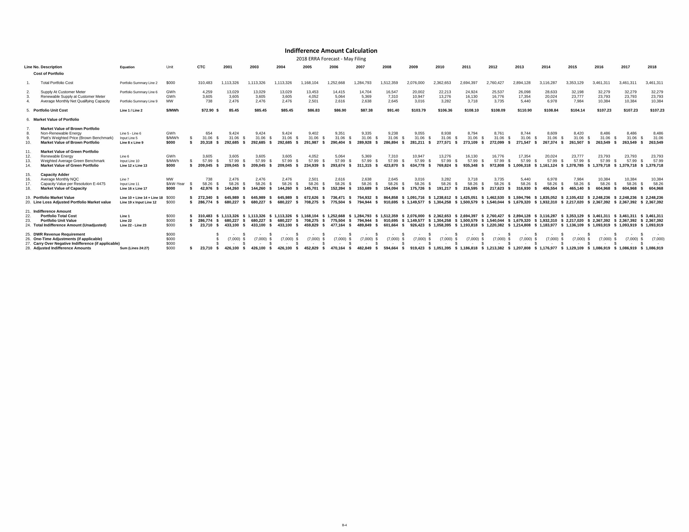
Line No. Description Equation Unit CTC 2001 2003 2004 2005 2006 2007 2008 2009 2010 2011 2012 2013 2014 2015 2016 2017 2018

Cost of Portfolio

1. Total Portfolio Cost Portfolio Summary Line 2 $000 310,483 1,113,326 1,113,326 1,113,326 1,168,104 1,252,668 1,284,793 1,512,359 2,076,000 2,362,653 2,694,397 2,760,427 2,894,128 3,116,287 3,353,129 3,461,311 3,461,311 3,461,311

2. Supply At Customer Meter Portfolio Summary Line 6 GWh 4,259 13,029 13,029 13,029 13,453 14,415 14,704 16,547 20,002 22,213 24,924 25,537 26,098 28,633 32,198 32,279 32,279 32,279

3. Renewable Supply at Customer Meter GWh 3,605 3,605 3,605 3,605 4,052 5,064 5,369 7,310 10,947 13,276 16,130 16,776 17,354 20,024 23,777 23,793 23,793 23,793

4. Average Monthly Net Qualifying Capacity Portfolio Summary Line 9 MW 738 2,476 2,476 2,476 2,501 2,616 2,638 2,645 3,016 3,282 3,718 3,735 5,440 6,978 7,984 10,384 10,384 10,384

5. Portfolio Unit Cost Line 1 / Line 2 $/MWh $72.90 85.45$ $85.45 $85.45 $86.83 $86.90 $87.38 $91.40 $103.79 $106.36 $108.10 $108.09 $110.90 $108.84 $104.14 $107.23 $107.23 $107.23

6. Market Value of Portfolio

7. Market Value of Brown Portfolio

8. Non-Renewable Energy Line 5 - Line 6 GWh 654 9,424 9,424 9,424 9,402 9,351 9,335 9,238 9,055 8,938 8,794 8,761 8,744 8,609 8,420 8,486 8,486 8,486

9. Platt's Weighted Price (Brown Benchmark) Input Line 5 $/MWh 31.06$ 31.06$ 31.06$ 31.06$ 31.06$ 31.06$ 31.06$ 31.06$ 31.06$ 31.06$ 31.06$ 31.06$ 31.06$ 31.06$ 31.06$ 31.06$ 31.06$ 31.06$

10. Market Value of Brown Portfolio Line 8 x Line 9 $000 20,318$ 292,685$ 292,685$ 292,685$ 291,987$ 290,404$ 289,928$ 286,894$ 281,211$ 277,571$ 273,109$ 272,099$ 271,547$ 267,374$ 261,507$ 263,549$ 263,549$ 263,549$

11. Market Value of Green Portfolio

12. Renewable Energy Line 6 GWh 3,605 3,605 3,605 3,605 4,052 5,064 5,369 7,310 10,947 13,276 16,130 16,776 17,354 20,024 23,777 23,793 23,793 23,793

13. Weighted Average Green Benchmark Input Line 10 $/MWh 57.99$ 57.99$ 57.99$ 57.99$ 57.99$ 57.99$ 57.99$ 57.99$ 57.99$ 57.99$ 57.99$ 57.99$ 57.99$ 57.99$ 57.99$ 57.99$ 57.99$ 57.99$

14. Market Value of Green Portfolio Line 12 x Line 13 $000 209,045$ 209,045$ 209,045$ 209,045$ 234,939$ 293,674$ 311,315$ 423,870$ 634,778$ 769,824$ 935,348$ 972,808$ 1,006,318$ 1,161,124$ 1,378,785$ 1,379,718$ 1,379,718$ 1,379,718$

15. Capacity Adder

16. Average Monthly NQC Line 7 MW 738 2,476 2,476 2,476 2,501 2,616 2,638 2,645 3,016 3,282 3,718 3,735 5,440 6,978 7,984 10,384 10,384 10,384

17. Capacity Value per Resolution E-4475 Input Line 11 $/kW-Year 58.26$ 58.26$ 58.26$ 58.26$ 58.26$ 58.26$ 58.26$ 58.26$ 58.26$ 58.26$ 58.26$ 58.26$ 58.26$ 58.26$ 58.26$ 58.26$ 58.26$ 58.26$

18. Market Value of Capacity Line 16 x Line 17 $000 42,976$ 144,260$ 144,260$ 144,260$ 145,701$ 152,394$ 153,689$ 154,094$ 175,726$ 191,217$ 216,595$ 217,623$ 316,930$ 406,554$ 465,140$ 604,968$ 604,968$ 604,968$

19. Portfolio Market Value Line 10 + Line 14 + Line 18 $000 272,340$ 645,989$ 645,989$ 645,989$ 672,626$ 736,471$ 754,932$ 864,858$ 1,091,716$ 1,238,612$ 1,425,051$ 1,462,530$ 1,594,796$ 1,835,052$ 2,105,432$ 2,248,236$ 2,248,236$ 2,248,236$

20. Line Loss Adjusted Portfolio Market value Line 19 x Input Line 12 $000 286,774$ 680,227$ 680,227$ 680,227$ 708,275$ 775,504$ 794,944$ 910,695$ 1,149,577$ 1,304,258$ 1,500,579$ 1,540,044$ 1,679,320$ 1,932,310$ 2,217,020$ 2,367,392$ 2,367,392$ 2,367,392$

21. Indifference Amount

22. Portfolio Total Cost Line 1 $000 310,483$ 1,113,326$ 1,113,326$ 1,113,326$ 1,168,104$ 1,252,668$ 1,284,793$ 1,512,359$ 2,076,000$ 2,362,653$ 2,694,397$ 2,760,427$ 2,894,128$ 3,116,287$ 3,353,129$ 3,461,311$ 3,461,311$ 3,461,311$

23. Portfolio Unit Value Line 22 $000 286,774$ 680,227$ 680,227$ 680,227$ 708,275$ 775,504$ 794,944$ 910,695$ 1,149,577$ 1,304,258$ 1,500,579$ 1,540,044$ 1,679,320$ 1,932,310$ 2,217,020$ 2,367,392$ 2,367,392$ 2,367,392$

24. Total Indifference Amount (Unadjusted) Line 22 - Line 23 $000 23,710$ 433,100$ 433,100$ 433,100$ 459,829$ 477,164$ 489,849$ 601,664$ 926,423$ 1,058,395$ 1,193,818$ 1,220,382$ 1,214,808$ 1,183,977$ 1,136,109$ 1,093,919$ 1,093,919$ 1,093,919$

25. DWR Revenue Requirement $000 -$ -$ -$ -$ -$ -$ -$ -$ -$ -$ -$ -$ -$ -$ -$ -$ -$

26. One-Time Adjustments (if applicable) $000 (7,000)$ (7,000)$ (7,000)$ (7,000)$ (7,000)$ (7,000)$ (7,000)$ (7,000)$ (7,000)$ (7,000)$ (7,000)$ (7,000)$ (7,000)$ (7,000)$ (7,000)$ (7,000)$ (7,000)$

27. Carry Over Negative Indifference (if applicable) $000 -$ -$ -$ -$ -$ -$ -$ -$ -$ -$ -$ -$ -$ -$ -$ -$ -$

28. Adjusted Indifference Amounts Sum (Lines 24:27) $000 23,710$ 426,100$ 426,100$ 426,100$ 452,829$ 470,164$ 482,849$ 594,664$ 919,423$ 1,051,395$ 1,186,818$ 1,213,382$ 1,207,808$ 1,176,977$ 1,129,109$ 1,086,919$ 1,086,919$ 1,086,919$

Indifference Amount Calculation2018 ERRA Forecast - May Filing

B-4

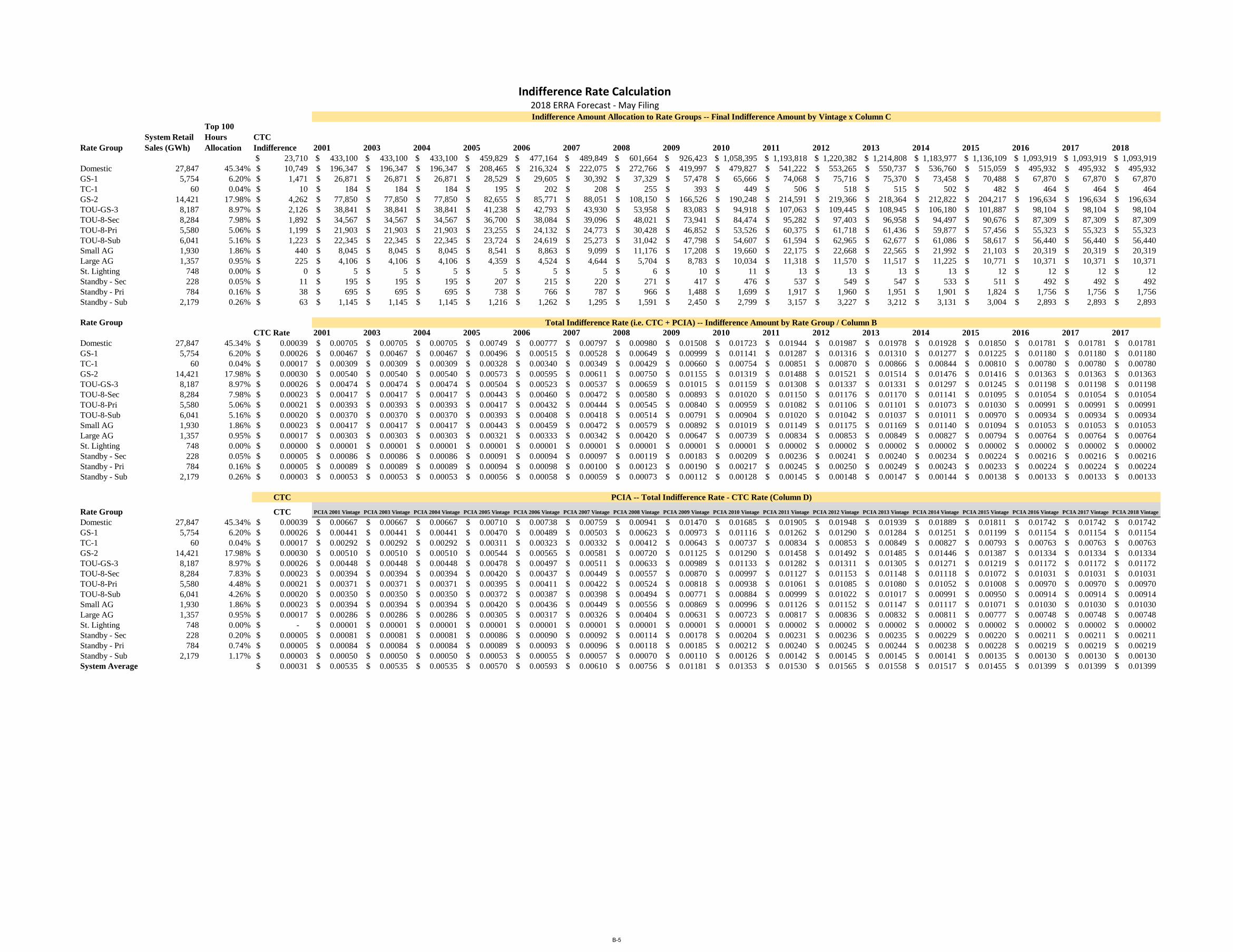
Rate Group

System Retail

Sales (GWh)

Top 100

Hours

Allocation

CTC

Indifference 2001 2003 2004 2005 2006 2007 2008 2009 2010 2011 2012 2013 2014 2015 2016 2017 2018

$ 23,710 $ 433,100 $ 433,100 $ 433,100 $ 459,829 $ 477,164 $ 489,849 $ 601,664 $ 926,423 $ 1,058,395 $ 1,193,818 $ 1,220,382 $ 1,214,808 $ 1,183,977 $ 1,136,109 $ 1,093,919 $ 1,093,919 $ 1,093,919

Domestic 27,847 45.34% 10,749$ 196,347$ 196,347$ 196,347$ 208,465$ 216,324$ 222,075$ 272,766$ 419,997$ 479,827$ 541,222$ 553,265$ 550,737$ 536,760$ 515,059$ 495,932$ 495,932$ 495,932$

GS-1 5,754 6.20% 1,471$ 26,871$ 26,871$ 26,871$ 28,529$ 29,605$ 30,392$ 37,329$ 57,478$ 65,666$ 74,068$ 75,716$ 75,370$ 73,458$ 70,488$ 67,870$ 67,870$ 67,870$

TC-1 60 0.04% 10$ 184$ 184$ 184$ 195$ 202$ 208$ 255$ 393$ 449$ 506$ 518$ 515$ 502$ 482$ 464$ 464$ 464$

GS-2 14,421 17.98% 4,262$ 77,850$ 77,850$ 77,850$ 82,655$ 85,771$ 88,051$ 108,150$ 166,526$ 190,248$ 214,591$ 219,366$ 218,364$ 212,822$ 204,217$ 196,634$ 196,634$ 196,634$

TOU-GS-3 8,187 8.97% 2,126$ 38,841$ 38,841$ 38,841$ 41,238$ 42,793$ 43,930$ 53,958$ 83,083$ 94,918$ 107,063$ 109,445$ 108,945$ 106,180$ 101,887$ 98,104$ 98,104$ 98,104$

TOU-8-Sec 8,284 7.98% 1,892$ 34,567$ 34,567$ 34,567$ 36,700$ 38,084$ 39,096$ 48,021$ 73,941$ 84,474$ 95,282$ 97,403$ 96,958$ 94,497$ 90,676$ 87,309$ 87,309$ 87,309$

TOU-8-Pri 5,580 5.06% 1,199$ 21,903$ 21,903$ 21,903$ 23,255$ 24,132$ 24,773$ 30,428$ 46,852$ 53,526$ 60,375$ 61,718$ 61,436$ 59,877$ 57,456$ 55,323$ 55,323$ 55,323$

TOU-8-Sub 6,041 5.16% 1,223$ 22,345$ 22,345$ 22,345$ 23,724$ 24,619$ 25,273$ 31,042$ 47,798$ 54,607$ 61,594$ 62,965$ 62,677$ 61,086$ 58,617$ 56,440$ 56,440$ 56,440$

Small AG 1,930 1.86% 440$ 8,045$ 8,045$ 8,045$ 8,541$ 8,863$ 9,099$ 11,176$ 17,208$ 19,660$ 22,175$ 22,668$ 22,565$ 21,992$ 21,103$ 20,319$ 20,319$ 20,319$

Large AG 1,357 0.95% 225$ 4,106$ 4,106$ 4,106$ 4,359$ 4,524$ 4,644$ 5,704$ 8,783$ 10,034$ 11,318$ 11,570$ 11,517$ 11,225$ 10,771$ 10,371$ 10,371$ 10,371$

St. Lighting 748 0.00% 0$ 5$ 5$ 5$ 5$ 5$ 5$ 6$ 10$ 11$ 13$ 13$ 13$ 13$ 12$ 12$ 12$ 12$

Standby - Sec 228 0.05% 11$ 195$ 195$ 195$ 207$ 215$ 220$ 271$ 417$ 476$ 537$ 549$ 547$ 533$ 511$ 492$ 492$ 492$

Standby - Pri 784 0.16% 38$ 695$ 695$ 695$ 738$ 766$ 787$ 966$ 1,488$ 1,699$ 1,917$ 1,960$ 1,951$ 1,901$ 1,824$ 1,756$ 1,756$ 1,756$

Standby - Sub 2,179 0.26% 63$ 1,145$ 1,145$ 1,145$ 1,216$ 1,262$ 1,295$ 1,591$ 2,450$ 2,799$ 3,157$ 3,227$ 3,212$ 3,131$ 3,004$ 2,893$ 2,893$ 2,893$

Rate Group

CTC Rate 2001 2003 2004 2005 2006 2007 2008 2009 2010 2011 2012 2013 2014 2015 2016 2017 2017

Domestic 27,847 45.34% 0.00039$ 0.00705$ 0.00705$ 0.00705$ 0.00749$ 0.00777$ 0.00797$ 0.00980$ 0.01508$ 0.01723$ 0.01944$ 0.01987$ 0.01978$ 0.01928$ 0.01850$ 0.01781$ 0.01781$ 0.01781$

GS-1 5,754 6.20% 0.00026$ 0.00467$ 0.00467$ 0.00467$ 0.00496$ 0.00515$ 0.00528$ 0.00649$ 0.00999$ 0.01141$ 0.01287$ 0.01316$ 0.01310$ 0.01277$ 0.01225$ 0.01180$ 0.01180$ 0.01180$

TC-1 60 0.04% 0.00017$ 0.00309$ 0.00309$ 0.00309$ 0.00328$ 0.00340$ 0.00349$ 0.00429$ 0.00660$ 0.00754$ 0.00851$ 0.00870$ 0.00866$ 0.00844$ 0.00810$ 0.00780$ 0.00780$ 0.00780$

GS-2 14,421 17.98% 0.00030$ 0.00540$ 0.00540$ 0.00540$ 0.00573$ 0.00595$ 0.00611$ 0.00750$ 0.01155$ 0.01319$ 0.01488$ 0.01521$ 0.01514$ 0.01476$ 0.01416$ 0.01363$ 0.01363$ 0.01363$

TOU-GS-3 8,187 8.97% 0.00026$ 0.00474$ 0.00474$ 0.00474$ 0.00504$ 0.00523$ 0.00537$ 0.00659$ 0.01015$ 0.01159$ 0.01308$ 0.01337$ 0.01331$ 0.01297$ 0.01245$ 0.01198$ 0.01198$ 0.01198$

TOU-8-Sec 8,284 7.98% 0.00023$ 0.00417$ 0.00417$ 0.00417$ 0.00443$ 0.00460$ 0.00472$ 0.00580$ 0.00893$ 0.01020$ 0.01150$ 0.01176$ 0.01170$ 0.01141$ 0.01095$ 0.01054$ 0.01054$ 0.01054$

TOU-8-Pri 5,580 5.06% 0.00021$ 0.00393$ 0.00393$ 0.00393$ 0.00417$ 0.00432$ 0.00444$ 0.00545$ 0.00840$ 0.00959$ 0.01082$ 0.01106$ 0.01101$ 0.01073$ 0.01030$ 0.00991$ 0.00991$ 0.00991$

TOU-8-Sub 6,041 5.16% 0.00020$ 0.00370$ 0.00370$ 0.00370$ 0.00393$ 0.00408$ 0.00418$ 0.00514$ 0.00791$ 0.00904$ 0.01020$ 0.01042$ 0.01037$ 0.01011$ 0.00970$ 0.00934$ 0.00934$ 0.00934$

Small AG 1,930 1.86% 0.00023$ 0.00417$ 0.00417$ 0.00417$ 0.00443$ 0.00459$ 0.00472$ 0.00579$ 0.00892$ 0.01019$ 0.01149$ 0.01175$ 0.01169$ 0.01140$ 0.01094$ 0.01053$ 0.01053$ 0.01053$

Large AG 1,357 0.95% 0.00017$ 0.00303$ 0.00303$ 0.00303$ 0.00321$ 0.00333$ 0.00342$ 0.00420$ 0.00647$ 0.00739$ 0.00834$ 0.00853$ 0.00849$ 0.00827$ 0.00794$ 0.00764$ 0.00764$ 0.00764$

St. Lighting 748 0.00% 0.00000$ 0.00001$ 0.00001$ 0.00001$ 0.00001$ 0.00001$ 0.00001$ 0.00001$ 0.00001$ 0.00001$ 0.00002$ 0.00002$ 0.00002$ 0.00002$ 0.00002$ 0.00002$ 0.00002$ 0.00002$

Standby - Sec 228 0.05% 0.00005$ 0.00086$ 0.00086$ 0.00086$ 0.00091$ 0.00094$ 0.00097$ 0.00119$ 0.00183$ 0.00209$ 0.00236$ 0.00241$ 0.00240$ 0.00234$ 0.00224$ 0.00216$ 0.00216$ 0.00216$

Standby - Pri 784 0.16% 0.00005$ 0.00089$ 0.00089$ 0.00089$ 0.00094$ 0.00098$ 0.00100$ 0.00123$ 0.00190$ 0.00217$ 0.00245$ 0.00250$ 0.00249$ 0.00243$ 0.00233$ 0.00224$ 0.00224$ 0.00224$

Standby - Sub 2,179 0.26% 0.00003$ 0.00053$ 0.00053$ 0.00053$ 0.00056$ 0.00058$ 0.00059$ 0.00073$ 0.00112$ 0.00128$ 0.00145$ 0.00148$ 0.00147$ 0.00144$ 0.00138$ 0.00133$ 0.00133$ 0.00133$

CTC

Rate Group CTC PCIA 2001 Vintage PCIA 2003 Vintage PCIA 2004 Vintage PCIA 2005 Vintage PCIA 2006 Vintage PCIA 2007 Vintage PCIA 2008 Vintage PCIA 2009 Vintage PCIA 2010 Vintage PCIA 2011 Vintage PCIA 2012 Vintage PCIA 2013 Vintage PCIA 2014 Vintage PCIA 2015 Vintage PCIA 2016 Vintage PCIA 2017 Vintage PCIA 2018 Vintage

Domestic 27,847 45.34% 0.00039$ 0.00667$ 0.00667$ 0.00667$ 0.00710$ 0.00738$ 0.00759$ 0.00941$ 0.01470$ 0.01685$ 0.01905$ 0.01948$ 0.01939$ 0.01889$ 0.01811$ 0.01742$ 0.01742$ 0.01742$

GS-1 5,754 6.20% 0.00026$ 0.00441$ 0.00441$ 0.00441$ 0.00470$ 0.00489$ 0.00503$ 0.00623$ 0.00973$ 0.01116$ 0.01262$ 0.01290$ 0.01284$ 0.01251$ 0.01199$ 0.01154$ 0.01154$ 0.01154$

TC-1 60 0.04% 0.00017$ 0.00292$ 0.00292$ 0.00292$ 0.00311$ 0.00323$ 0.00332$ 0.00412$ 0.00643$ 0.00737$ 0.00834$ 0.00853$ 0.00849$ 0.00827$ 0.00793$ 0.00763$ 0.00763$ 0.00763$

GS-2 14,421 17.98% 0.00030$ 0.00510$ 0.00510$ 0.00510$ 0.00544$ 0.00565$ 0.00581$ 0.00720$ 0.01125$ 0.01290$ 0.01458$ 0.01492$ 0.01485$ 0.01446$ 0.01387$ 0.01334$ 0.01334$ 0.01334$

TOU-GS-3 8,187 8.97% 0.00026$ 0.00448$ 0.00448$ 0.00448$ 0.00478$ 0.00497$ 0.00511$ 0.00633$ 0.00989$ 0.01133$ 0.01282$ 0.01311$ 0.01305$ 0.01271$ 0.01219$ 0.01172$ 0.01172$ 0.01172$

TOU-8-Sec 8,284 7.83% 0.00023$ 0.00394$ 0.00394$ 0.00394$ 0.00420$ 0.00437$ 0.00449$ 0.00557$ 0.00870$ 0.00997$ 0.01127$ 0.01153$ 0.01148$ 0.01118$ 0.01072$ 0.01031$ 0.01031$ 0.01031$

TOU-8-Pri 5,580 4.48% 0.00021$ 0.00371$ 0.00371$ 0.00371$ 0.00395$ 0.00411$ 0.00422$ 0.00524$ 0.00818$ 0.00938$ 0.01061$ 0.01085$ 0.01080$ 0.01052$ 0.01008$ 0.00970$ 0.00970$ 0.00970$

TOU-8-Sub 6,041 4.26% 0.00020$ 0.00350$ 0.00350$ 0.00350$ 0.00372$ 0.00387$ 0.00398$ 0.00494$ 0.00771$ 0.00884$ 0.00999$ 0.01022$ 0.01017$ 0.00991$ 0.00950$ 0.00914$ 0.00914$ 0.00914$

Small AG 1,930 1.86% 0.00023$ 0.00394$ 0.00394$ 0.00394$ 0.00420$ 0.00436$ 0.00449$ 0.00556$ 0.00869$ 0.00996$ 0.01126$ 0.01152$ 0.01147$ 0.01117$ 0.01071$ 0.01030$ 0.01030$ 0.01030$

Large AG 1,357 0.95% 0.00017$ 0.00286$ 0.00286$ 0.00286$ 0.00305$ 0.00317$ 0.00326$ 0.00404$ 0.00631$ 0.00723$ 0.00817$ 0.00836$ 0.00832$ 0.00811$ 0.00777$ 0.00748$ 0.00748$ 0.00748$

St. Lighting 748 0.00% -$ 0.00001$ 0.00001$ 0.00001$ 0.00001$ 0.00001$ 0.00001$ 0.00001$ 0.00001$ 0.00001$ 0.00002$ 0.00002$ 0.00002$ 0.00002$ 0.00002$ 0.00002$ 0.00002$ 0.00002$

Standby - Sec 228 0.20% 0.00005$ 0.00081$ 0.00081$ 0.00081$ 0.00086$ 0.00090$ 0.00092$ 0.00114$ 0.00178$ 0.00204$ 0.00231$ 0.00236$ 0.00235$ 0.00229$ 0.00220$ 0.00211$ 0.00211$ 0.00211$

Standby - Pri 784 0.74% 0.00005$ 0.00084$ 0.00084$ 0.00084$ 0.00089$ 0.00093$ 0.00096$ 0.00118$ 0.00185$ 0.00212$ 0.00240$ 0.00245$ 0.00244$ 0.00238$ 0.00228$ 0.00219$ 0.00219$ 0.00219$

Standby - Sub 2,179 1.17% 0.00003$ 0.00050$ 0.00050$ 0.00050$ 0.00053$ 0.00055$ 0.00057$ 0.00070$ 0.00110$ 0.00126$ 0.00142$ 0.00145$ 0.00145$ 0.00141$ 0.00135$ 0.00130$ 0.00130$ 0.00130$

System Average 0.00031$ 0.00535$ 0.00535$ 0.00535$ 0.00570$ 0.00593$ 0.00610$ 0.00756$ 0.01181$ 0.01353$ 0.01530$ 0.01565$ 0.01558$ 0.01517$ 0.01455$ 0.01399$ 0.01399$ 0.01399$

Indifference Rate Calculation2018 ERRA Forecast - May FilingIndifference Amount Allocation to Rate Groups -- Final Indifference Amount by Vintage x Column C

Total Indifference Rate (i.e. CTC + PCIA) -- Indifference Amount by Rate Group / Column B

PCIA -- Total Indifference Rate - CTC Rate (Column D)

B-5

Rate Group

DWRBC (All

Vintages)

CTC (For All

Vintages)

PCIA 2001

Vintage

PCIA 2004

Vintage

PCIA 2009

Vintage

PCIA 2010

Vintage

PCIA 2011

Vintage

PCIA 2012

Vintage

PCIA 2013

Vintage

PCIA 2014

Vintage

PCIA 2015

Vintage

PCIA 2016

Vintage

PCIA 2017

Vintage

PCIA 2018

Vintage

Proposed Class

Average Bundled

Generation

Domestic 0.00549 0.00039 0.00667 0.00667 0.01470 0.01685 0.01905 0.01948 0.01939 0.01889 0.01811 0.01742 0.01742 0.01742 0.07233

GS-1 0.00549 0.00026 0.00441 0.00441 0.00973 0.01116 0.01262 0.01290 0.01284 0.01251 0.01199 0.01154 0.01154 0.01154 0.07347

TC-1 0.00549 0.00017 0.00292 0.00292 0.00643 0.00737 0.00834 0.00853 0.00849 0.00827 0.00793 0.00763 0.00763 0.00763 0.05541

GS-2 0.00549 0.00030 0.00510 0.00510 0.01125 0.01290 0.01458 0.01492 0.01485 0.01446 0.01387 0.01334 0.01334 0.01334 0.06830

TOU-GS-3 0.00549 0.00026 0.00448 0.00448 0.00989 0.01133 0.01282 0.01311 0.01305 0.01271 0.01219 0.01172 0.01172 0.01172 0.06418

TOU-8-Sec 0.00549 0.00023 0.00394 0.00394 0.00870 0.00997 0.01127 0.01153 0.01148 0.01118 0.01072 0.01031 0.01031 0.01031 0.06025

TOU-8-Pri 0.00549 0.00021 0.00371 0.00371 0.00818 0.00938 0.01061 0.01085 0.01080 0.01052 0.01008 0.00970 0.00970 0.00970 0.05662

TOU-8-Sub 0.00549 0.00020 0.00350 0.00350 0.00771 0.00884 0.00999 0.01022 0.01017 0.00991 0.00950 0.00914 0.00914 0.00914 0.05126

Small AG 0.00549 0.00023 0.00394 0.00394 0.00869 0.00996 0.01126 0.01152 0.01147 0.01117 0.01071 0.01030 0.01030 0.01030 0.06043

Large AG 0.00549 0.00017 0.00286 0.00286 0.00631 0.00723 0.00817 0.00836 0.00832 0.00811 0.00777 0.00748 0.00748 0.00748 0.04916

St. Lighting 0.00549 - 0.00001 0.00001 0.00001 0.00001 0.00002 0.00002 0.00002 0.00002 0.00002 0.00002 0.00002 0.00002 0.03917

Standby - Sec 0.00549 0.00005 0.00081 0.00081 0.00178 0.00204 0.00231 0.00236 0.00235 0.00229 0.00220 0.00211 0.00211 0.00211 0.06106

Standby - Pri 0.00549 0.00005 0.00084 0.00084 0.00185 0.00212 0.00240 0.00245 0.00244 0.00238 0.00228 0.00219 0.00219 0.00219 0.05793

Standby - Sub 0.00549 0.00003 0.00050 0.00050 0.00110 0.00126 0.00142 0.00145 0.00145 0.00141 0.00135 0.00130 0.00130 0.00130 0.05061

ERRA CRS Rates2018 ERRA Forecast - May filing

B-6

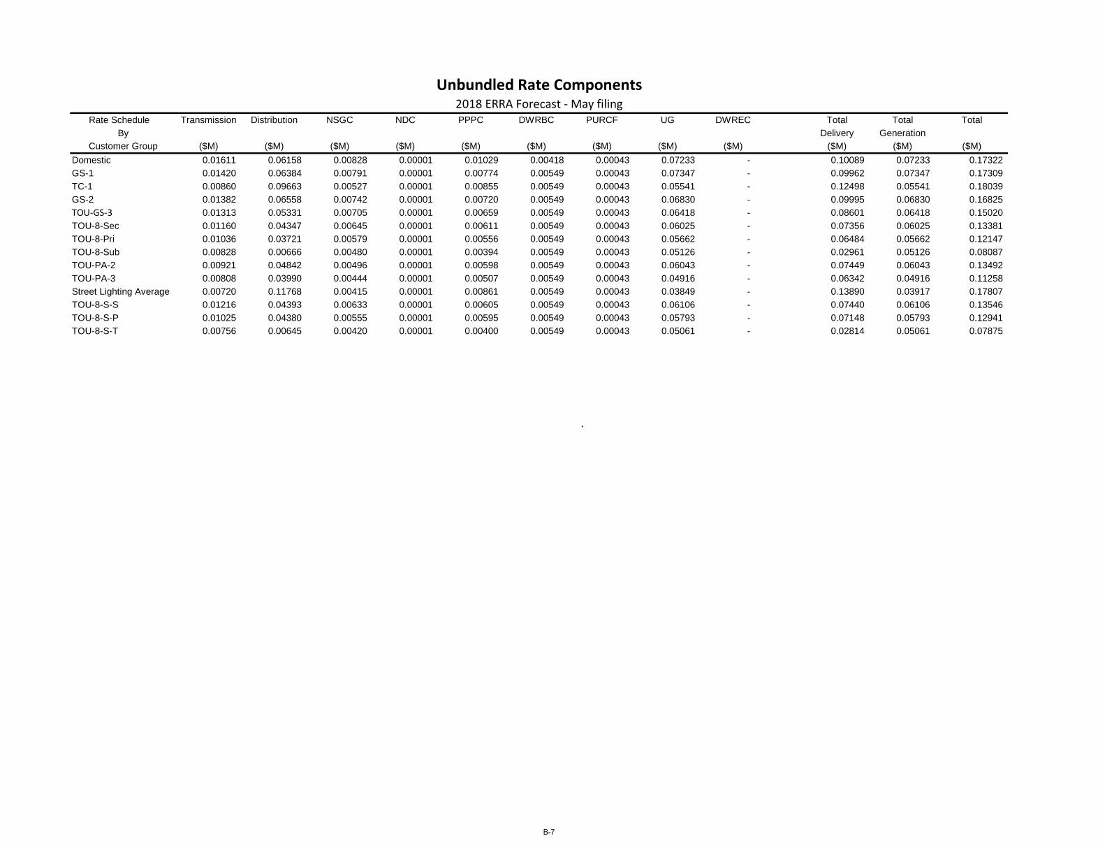
Rate Schedule Transmission Distribution NSGC NDC PPPC DWRBC PURCF UG DWREC Total Total Total

By Delivery Generation

Customer Group ($M) ($M) ($M) ($M) ($M) ($M) ($M) ($M) ($M) ($M) ($M) ($M)

Domestic 0.01611 0.06158 0.00828 0.00001 0.01029 0.00418 0.00043 0.07233 - 0.10089 0.07233 0.17322

GS-1 0.01420 0.06384 0.00791 0.00001 0.00774 0.00549 0.00043 0.07347 - 0.09962 0.07347 0.17309

TC-1 0.00860 0.09663 0.00527 0.00001 0.00855 0.00549 0.00043 0.05541 - 0.12498 0.05541 0.18039

GS-2 0.01382 0.06558 0.00742 0.00001 0.00720 0.00549 0.00043 0.06830 - 0.09995 0.06830 0.16825

TOU-GS-3 0.01313 0.05331 0.00705 0.00001 0.00659 0.00549 0.00043 0.06418 - 0.08601 0.06418 0.15020

TOU-8-Sec 0.01160 0.04347 0.00645 0.00001 0.00611 0.00549 0.00043 0.06025 - 0.07356 0.06025 0.13381

TOU-8-Pri 0.01036 0.03721 0.00579 0.00001 0.00556 0.00549 0.00043 0.05662 - 0.06484 0.05662 0.12147

TOU-8-Sub 0.00828 0.00666 0.00480 0.00001 0.00394 0.00549 0.00043 0.05126 - 0.02961 0.05126 0.08087

TOU-PA-2 0.00921 0.04842 0.00496 0.00001 0.00598 0.00549 0.00043 0.06043 - 0.07449 0.06043 0.13492

TOU-PA-3 0.00808 0.03990 0.00444 0.00001 0.00507 0.00549 0.00043 0.04916 - 0.06342 0.04916 0.11258

Street Lighting Average 0.00720 0.11768 0.00415 0.00001 0.00861 0.00549 0.00043 0.03849 - 0.13890 0.03917 0.17807

TOU-8-S-S 0.01216 0.04393 0.00633 0.00001 0.00605 0.00549 0.00043 0.06106 - 0.07440 0.06106 0.13546

TOU-8-S-P 0.01025 0.04380 0.00555 0.00001 0.00595 0.00549 0.00043 0.05793 - 0.07148 0.05793 0.12941

TOU-8-S-T 0.00756 0.00645 0.00420 0.00001 0.00400 0.00549 0.00043 0.05061 - 0.02814 0.05061 0.07875

Unbundled Rate Components2018 ERRA Forecast - May filing

B-7

Documents

Energy Resource Recovery Account (ERRA) 2018 … ERRA Resource Recovery Account (ERRA) 2018 Forecast of Operations Table Of Contents (Continued) Section Page Witness ii E. SCE’s