Engr.10

1

JKA & KY

Engr.10

Engineering Analysis

2

• Engineering analysis is a systematic process for analyzing problems that arise in the various fields of engineering.

• As part of the problem solving process, the data collected has to be processed, analyzed and sometimes displayed graphically by using many mathematical tools that are available.

• In many cases, once you have defined and set up the problem properly, numerical methods are required to solve the mathematical equations.

Microsoft’s Excel spreadsheet software has many numerical procedures built directly into its program structure.

Engr.10Material Strength

Ken YoussefiPDM I, SJSU 3

Standard Tensile TestStandard Specimen

Ductile Steel (low carbon)

Sy – yield strength

Su – fracture strength

σ (stress) = Load / Area

ε (strain) = (change in length) / (original length)

Engr.10

Spreadsheets’ Capabilities

4

• Store, process, and sorts data

• Graphically display data (Engineering application)

• Perform statistical analysis

• Fit equations to curves (Engineering application)

• Solve single and system of algebraic equations (Engr. Appl.)

• Solve optimization problems (Engineering application)

• Draw Flow Charts

Data Analysis Tools

Engr.10

5

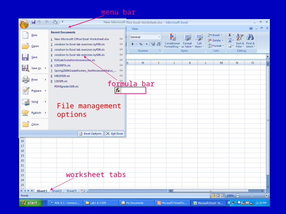
currently active cell (A1)

File management options

menu bar

formula bar

worksheet tabs

Engr.10

Entering Data into Cells (Cell Content)

6

Engr.10Copying Cells

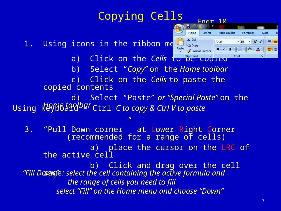
““Fill Down” : select the cell containing the active formula andFill Down” : select the cell containing the active formula and the range of cells you need to fillthe range of cells you need to fill

select “Fill” on the Home menu and choose “Down”select “Fill” on the Home menu and choose “Down”

7

1. Using icons in the ribbon menu

a) Click on the Cells to be copiedb) Select “Copy” Copy” on theon the Home toolbar Home toolbarc) Click on the c) Click on the Cells Cells to paste the copied contentsto paste the copied contentsd) d) Select “Paste” or “Special Paste” ” or “Special Paste” on theon the Home Home

toolbartoolbar

2.2. Using keyboard - Ctrl Using keyboard - Ctrl C to copy & Ctrl V to pasteC to copy & Ctrl V to paste

3.3. ““Pull Down corner” at Pull Down corner” at LLower ower RRight ight CCorner orner (recommended for a range of cells)(recommended for a range of cells) a) place the cursor on the a) place the cursor on the LRCLRC of the active cell of the active cell b) Click and drag over the cell rage b) Click and drag over the cell rage

Engr.10

Relative Addressing A B C D E

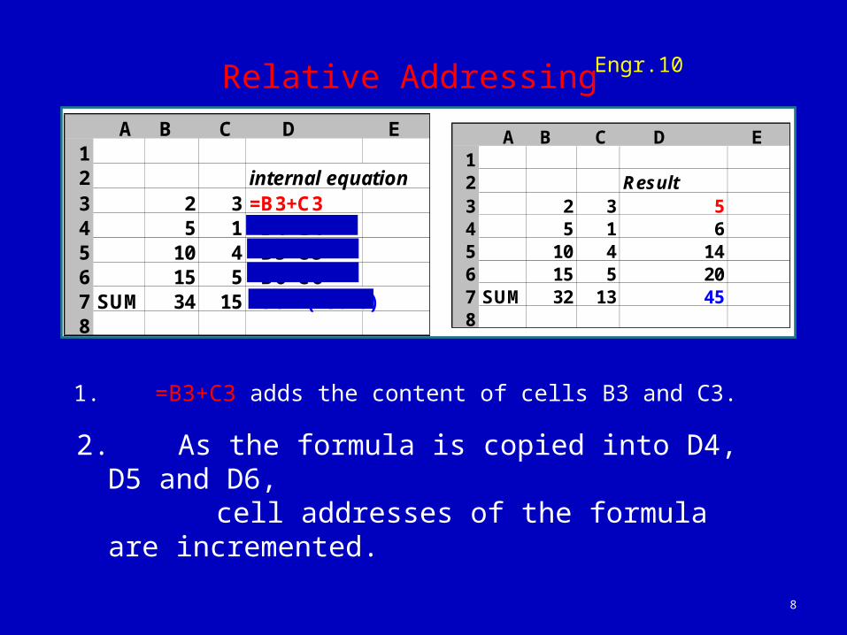
12 internal equation3 2 3 =B3+C34 5 1 =B4+C45 10 4 =B5+C56 15 5 =B6+C67 SUM: 34 15 =SUM(D3:D6)8

A B C D E12 Result3 2 3 54 5 1 65 10 4 146 15 5 207 SUM: 32 13 458

1. =B3+C3 adds the content of cells B3 and C3.

8

2. As the formula is copied into D4, D5 and D6, cell addresses of the formula are incremented.

Engr.10Absolute Addressing

A B C D E1 k= 0.52 internal equation3 2 3 =B3+C3+$B$14 5 1 =B4+C4+$B$15 10 4 =B5+C5+$B$16 15 5 =B6+C6+$B$17 SUM: 34 15 =SUM(D3:D6)8

A B C D E1 k= 0.52 Result3 2 3 5.54 5 1 6.55 10 4 14.56 15 5 20.57 SUM: 32 13 478

• Using the absolute cell address, $B$1, will keep the cell reference constant for all calculations.

9

Engr.10

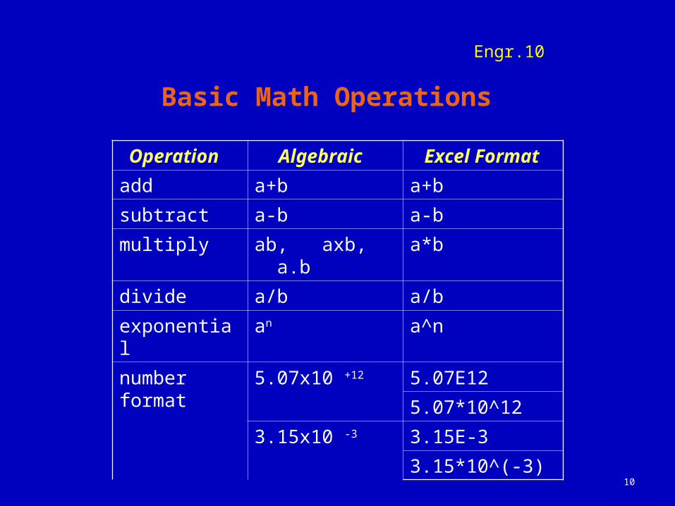
Basic Math Operations

10

Operation Algebraic Excel Format

add a+b a+b

subtract a-b a-b

multiply ab, axb, a.b a*b

divide a/b a/b

exponential an a^n

number format

5.07x10 +12 5.07E12

5.07*10^12

3.15x10 -3 3.15E-3

3.15*10^(-3)

Engr.10

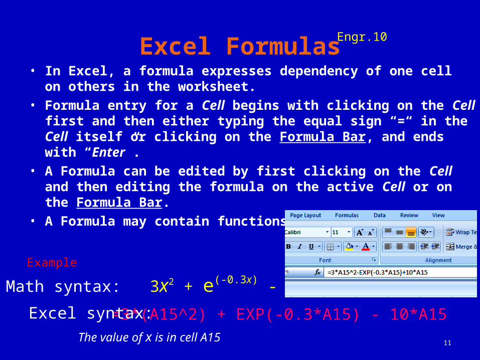
Excel Formulas• In Excel, a formula expresses dependency of one cell on

others in the worksheet.

• Formula entry for a Cell begins with clicking on the Cell first and then either typing the equal sign “=“ in the Cell itself or clicking on the Formula Bar, and ends with “Enter”.

• A Formula can be edited by first clicking on the Cell and then editing the formula on the active Cell or on the Formula Bar.

• A Formula may contain functions.

11The value of x is in cell A15

Example

Math syntax: 3x2 + e(-0.3x) - 10x

=3*(A15^2) + EXP(-0.3*A15) - 10*A15Excel syntax:

Engr.10

12

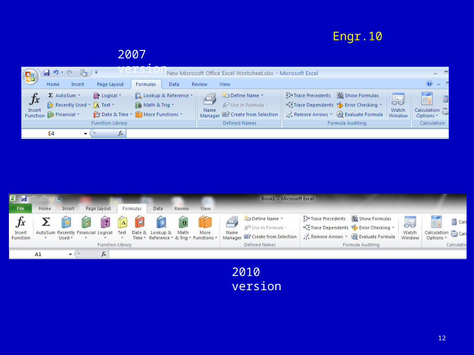
2007 version

2010 version

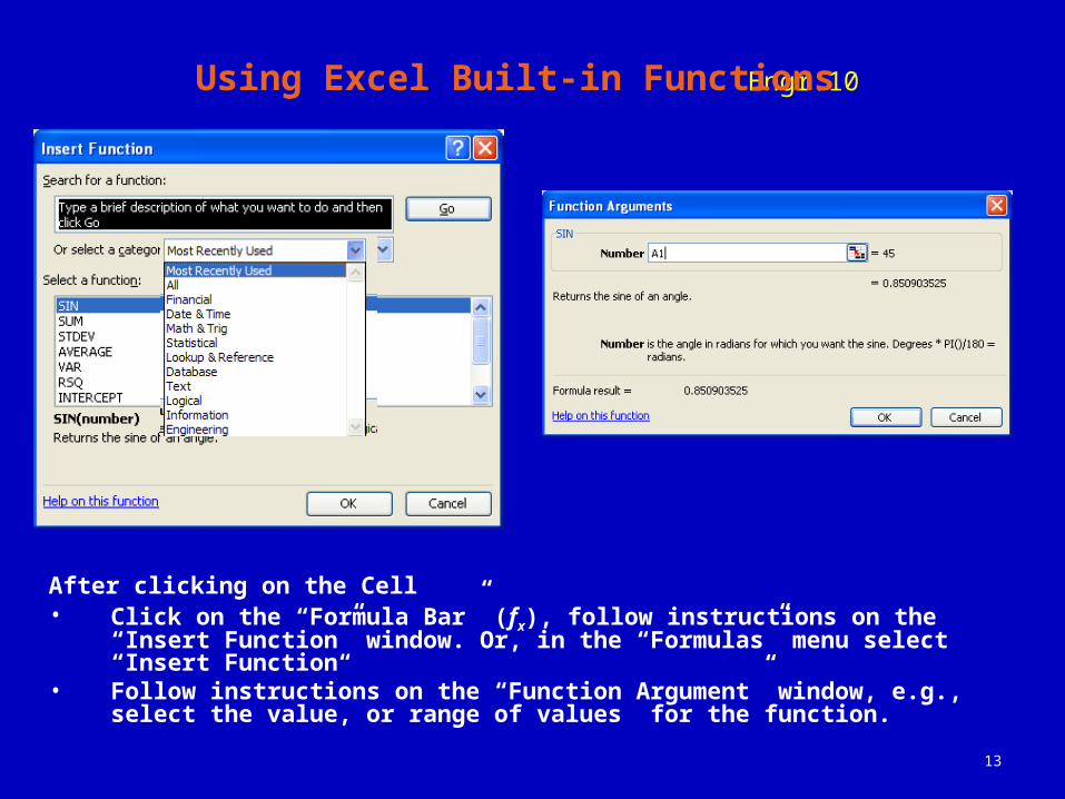
Engr.10Using Excel Built-in Functions

After clicking on the Cell• Click on the “Formula Bar” (fx), follow instructions on the “Insert Function”

window. Or, in the “Formulas” menu select “Insert Function“• Follow instructions on the “Function Argument” window, e.g., select the

value, or range of values for the function.

13

Engr.10

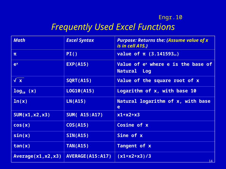
Frequently Used Excel FunctionsMath Excel Syntax Purpose: Returns the: (Assume value of x

is in cell A15.)

π PI() value of π (3.141593…)

ex EXP(A15) Value of ex where e is the base of

Natural Log

√ x SQRT(A15) Value of the square root of x

log10 (x) LOG10(A15) Logarithm of x, with base 10

ln(x) LN(A15) Natural logarithm of x, with base e

SUM(x1,x2,x3) SUM( A15:A17) x1+x2+x3

cos(x) COS(A15) Cosine of x

sin(x) SIN(A15) Sine of x

tan(x) TAN(A15) Tangent of x

Average(x1,x2,x3) AVERAGE(A15:A17) (x1+x2+x3)/3

14

Engr.10

Example: “My Expense Table”

15

Engr.10

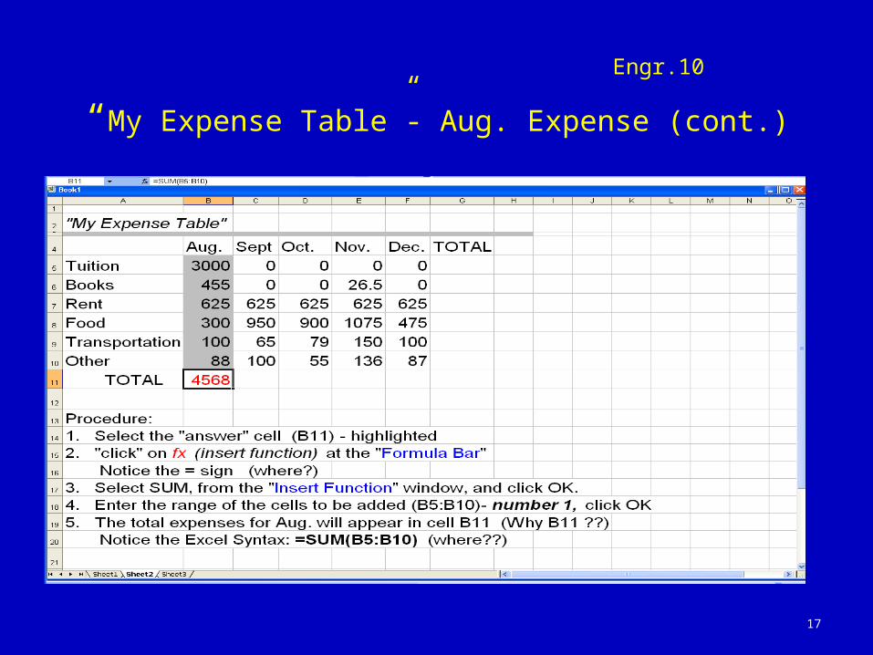
“My Expense Table”- Aug. Expense

16

=SUM(B5:B10)

Engr.10

“My Expense Table”- Aug. Expense (cont.)

17

Engr.10

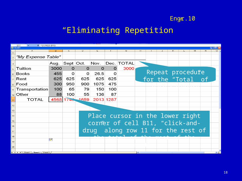
“Eliminating Repetition”

18

Place cursor in the lower right corner of cell B11, “click-and-drug” along row 11 for the rest

of the total of the rest of the months

Repeat procedure for the “Total” of each category

Engr.10

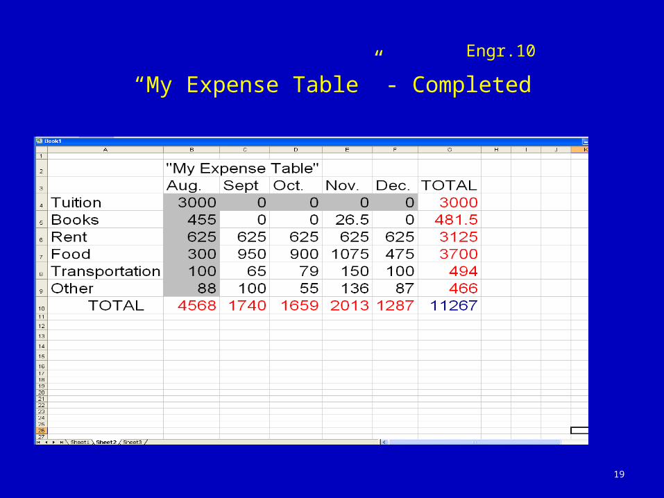
“My Expense Table” - Completed

19

Engr.10

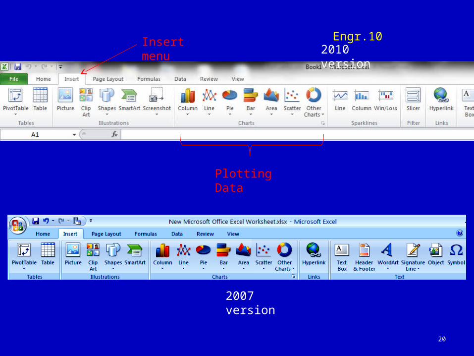
20

Insert menu

Plotting Data

2007 version

2010 version

Engr.10

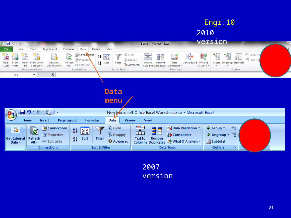
21

Data menu

2007 version

2010 version

Engr.10

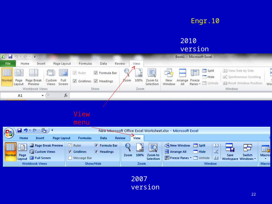
22

View menu

2007 version

2010 version

Engr.10

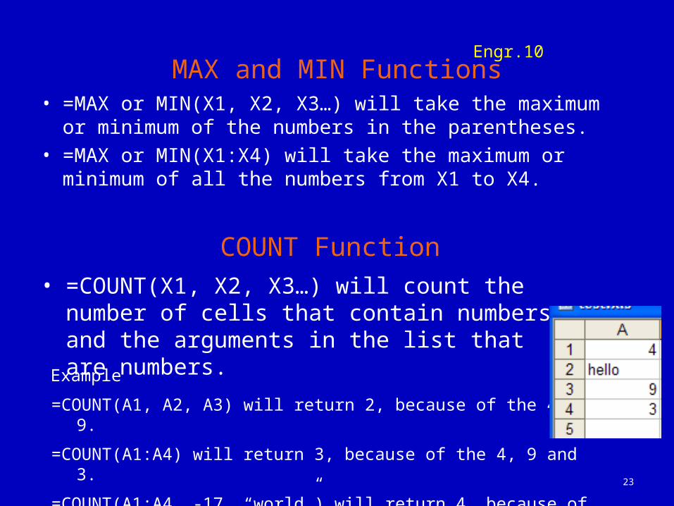
MAX and MIN Functions• =MAX or MIN(X1, X2, X3…) will take the maximum or

minimum of the numbers in the parentheses.• =MAX or MIN(X1:X4) will take the maximum or minimum

of all the numbers from X1 to X4.

23

COUNT Function• =COUNT(X1, X2, X3…) will count the number of

cells that contain numbers and the arguments in the list that are numbers.

=COUNT(A1, A2, A3) will return 2, because of the 4 and 9.

=COUNT(A1:A4) will return 3, because of the 4, 9 and 3.

=COUNT(A1:A4, -17, “world”) will return 4, because of the 4, 9, 3 and -17.

Example

Engr.10

COUNTIF Function

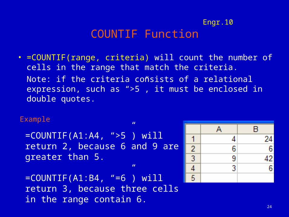
• =COUNTIF(range, criteria) will count the number of cells in the range that match the criteria.

Note: if the criteria consists of a relational expression, such as “>5”, it must be enclosed in double quotes.

24

=COUNTIF(A1:A4, “>5”) will return 2, because 6 and 9 are greater than 5.

=COUNTIF(A1:B4, “=6”) will return 3, because three cells in the range contain 6.

Example

Engr.10

IF Logical Function

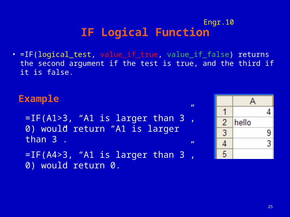
• =IF(logical_test, value_if_true, value_if_false) returns the second argument if the test is true, and the third if it is false.

25

=IF(A1>3, “A1 is larger than 3”, 0) would return “A1 is larger than 3”.

=IF(A4>3, “A1 is larger than 3”, 0) would return 0.

Example

Engr.10

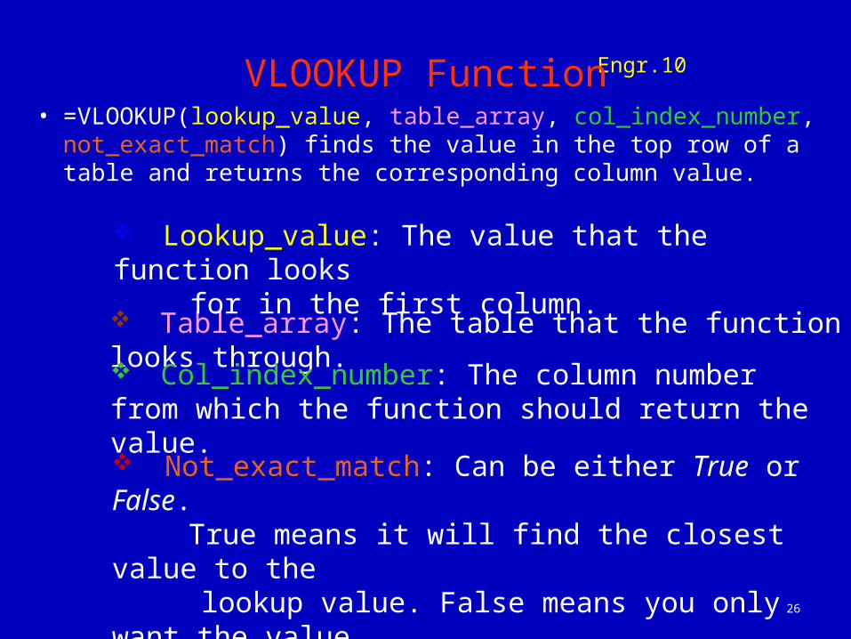
VLOOKUP Function• =VLOOKUP(lookup_value, table_array, col_index_number,

not_exact_match) finds the value in the top row of a table and returns the corresponding column value.

26

Not_exact_match: Can be either True or False. True means it will find the closest value to the lookup value. False means you only want the value returned if it is an exact match.

Table_array: The table that the function looks through.

Col_index_number: The column number from which the function should return the value.

Lookup_value: The value that the function looks for in the first column.

Engr.10

27

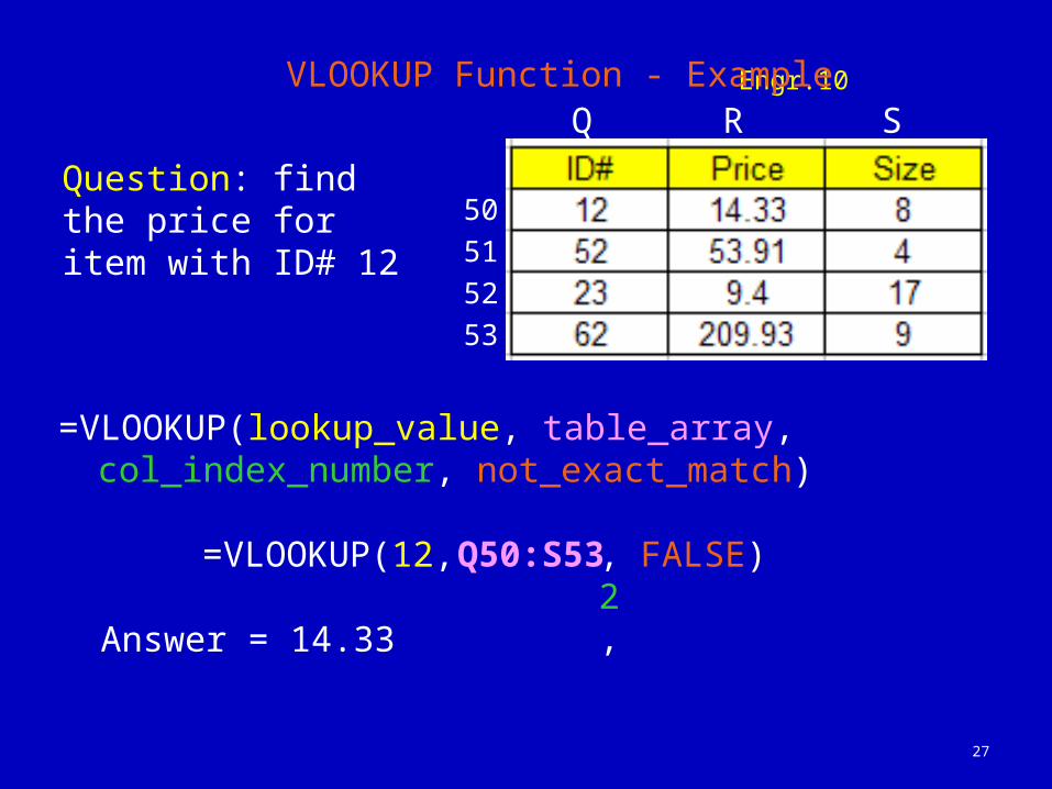
Question: find the price for item with ID# 12

VLOOKUP Function - Example

=VLOOKUP(12,Q50:S53,2,FALSE)

=VLOOKUP(lookup_value, table_array, col_index_number, not_exact_match)

Q SR

50

51

53

52

Answer = 14.33

Engr.10

28

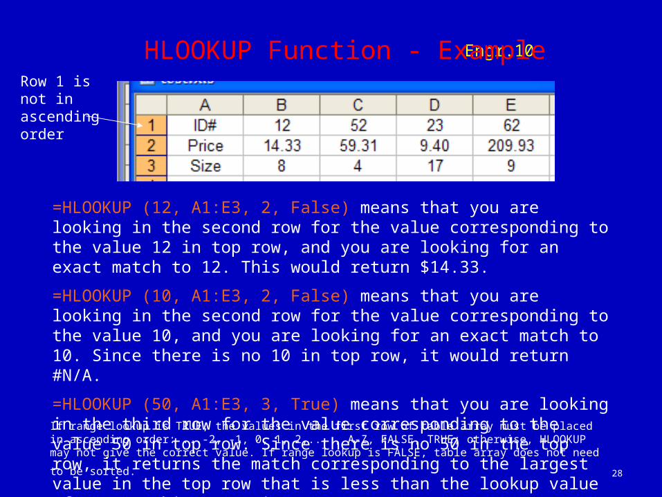
HLOOKUP Function - Example

=HLOOKUP (12, A1:E3, 2, False) means that you are looking in the second row for the value corresponding to the value 12 in top row, and you are looking for an exact match to 12. This would return $14.33.

=HLOOKUP (10, A1:E3, 2, False) means that you are looking in the second row for the value corresponding to the value 10, and you are looking for an exact match to 10. Since there is no 10 in top row, it would return #N/A.

=HLOOKUP (50, A1:E3, 3, True) means that you are looking in the third row for the value corresponding to the value 50 in top row. Since there is no 50 in the top row, it returns the match corresponding to the largest value in the top row that is less than the lookup value of 52. In this case, it returns 8.

If range lookup is TRUE, the values in the first row of table array must be placed in ascending order: ...-2, -1, 0, 1, 2,... , A-Z, FALSE, TRUE; otherwise, HLOOKUP may not give the correct value. If range lookup is FALSE, table

array does not need to be sorted.

Row 1 is not in ascending order