Enhanced enstrophy generation for turbulentconvection in low-Prandtl-number fluidsJörg Schumachera,1, Paul Götzfrieda, and Janet D. Scheelb

aDepartment of Mechanical Engineering, Technische Universität Ilmenau, D-98684 Ilmenau, Germany; and bDepartment of Physics, Occidental College,Los Angeles, CA 90041

Edited by Katepalli R. Sreenivasan, New York University, New York, NY, and approved June 23, 2015 (received for review March 13, 2015)

Turbulent convection is often present in liquids with a kinematicviscosity much smaller than the diffusivity of the temperature.Here we reveal why these convection flows obey a much strongerlevel of fluid turbulence than those in which kinematic viscosityand thermal diffusivity are the same; i.e., the Prandtl number Pr isunity. We compare turbulent convection in air at Pr= 0.7 and inliquid mercury at Pr=0.021. In this comparison the Prandtl numberat constant Grashof number Gr is varied, rather than at constantRayleigh number Ra as usually done. Our simulations demonstratethat the turbulent Kolmogorov-like cascade is extended both at thelarge- and small-scale ends with decreasing Pr. The kinetic energyinjection into the flow takes place over the whole cascade range. Incontrast to convection in air, the kinetic energy injection rate is par-ticularly enhanced for liquid mercury for all scales larger than thecharacteristic width of thermal plumes. As a consequence, meanvalues and fluctuations of the local strain rates are increased, whichin turn results in significantly enhanced enstrophy production byvortex stretching. The normalized distributions of enstrophy produc-tion in the bulk and the ratio of the principal strain rates are found toagree for both Prs. Despite the different energy injection mecha-nisms, the principal strain rates also agree with those in homoge-neous isotropic turbulence conducted at the same Reynolds numbersas for the convection flows. Our results have thus interesting impli-cations for small-scale turbulence modeling of liquid metal convec-tion in astrophysical and technological applications.

thermal convection | vorticity generation | direct numerical simulation |liquid metals

Turbulent convection depends strongly on the material prop-erties of the working fluid that are quantified by the Prandtl

number, the ratio of kinematic viscosity of the fluid to thermaldiffusivity of the temperature, Pr= ν=κ. Compared with the vastnumber of investigations at Pr≥ 1 (1, 2), the very-low-Pr regimeappears almost as a “terra incognita” despite many applications.Turbulent convection in the Sun is present at Prandtl numbersPr< 10−3 (3–5). The Prandtl number in the liquid metal core ofthe Earth is Pr∼ 10−2 (6). Convection in material processing (7),nuclear engineering (8), or liquid metal batteries (9) has Prandtlnumbers between 3× 10−2 and 10−3. Rayleigh–Bénard convec-tion (RBC), a fluid flow in a layer that is cooled from above andheated from below, is a paradigm for all of these examples. Onereason for significantly fewer low-Pr RBC studies is that labo-ratory measurements have to be conducted in opaque liquidmetals such as mercury or gallium at Pr= 0.021 (10–12). Thelowest value for a Prandtl number that can be obtained in op-tically transparent fluids is Pr= 0.2 for binary gas mixtures (13),i.e., an order of magnitude larger than in liquid metals. Directnumerical simulations (DNS) are currently the only way to gainaccess to the full 3D convective turbulent fields in low-Pr con-vection (14–18). These simulations turn out to become very de-manding if the small-scale structure of turbulence is to be studied,even for moderate Rayleigh number Ra, the parameter thatquantifies the thermal driving in turbulent convection (19, 20).Whereas heat transport is reduced in low-Pr convection, theproduction of vorticity and shear are enhanced significantly, which

amplifies the small-scale intermittency in these flows. An analysisof vorticity generation mechanisms in such flows and a compari-son with other turbulent flows, which requires the resolution ofspatial derivatives of the turbulent fields, is still missing. Thesedetails are, however, essential to improve parameterizations of thesmall-scale turbulence in low-Prandtl-number fluids such as al-gebraic heat flux and other subgrid-scale models (21, 22).In the present work, we investigate the reasons for this en-

hanced vorticity generation in low-Pr convection and compareand contrast the enstrophy production to turbulent convection atPr∼ 1. Our studies are based on high-resolution 3D DNS. Ratherthan studying the Pr dependence of convection at a fixed Rayleighnumber Ra, as is usually done, we compare two simulations atthe same Grashof number Gr, which is defined by

Gr=gαΔTH3

ν2=RaPr

. [1]

Here, g is the acceleration due to gravity, α is the thermal ex-pansion coefficient, and ΔT is the total temperature differenceacross the cell height H. In such a comparison, Ra and Pr arevaried now simultaneously and the corresponding dimensionlessmomentum equations (Eq. 4) remain unchanged. This impliesthat the strongly differing Prandtl numbers show up only in theadvection–diffusion equation [5] for temperature. We demon-strate this perspective for two simulations at one Grashof num-ber. We also mention that a similar discussion was emphasized in2D quasi-geostrophic DNS (20). Fig. 1 illustrates our point ofview. In Fig. 1 A and C, we show snapshots of temperature (Fig.1 A and C, Left) and velocity magnitude (Fig. 1 A and C, Right)for the two runs. Compared with convection in air (Fig. 1 A), thetemperature field in the liquid metal flow is much more diffusive,

Significance

Low-Prandtl-number thermal convection flows in liquid metals forwhich the temperature diffusivity is much larger than the fluidviscosity have been studied much less frequently than convectiveflows in air or water, despite many important applications reach-ing from astrophysics to energy conversion. Currently, the turbu-lence in low-Prandtl-number flows is fully accessible only by three-dimensional simulations. Our numerical studies reveal why thesmall-scale turbulence is much more vigorous compared withconvection in air. We also find that the generation of small-scalevorticity in the bulk of convection follows the same mechanismsand statistics as in idealized isotropic turbulence, especially for thelow-Prandtl-number flow. This opens new perspectives for nec-essary turbulence parameterizations in applications.

Author contributions: J.S. and J.D.S. designed research; J.S., P.G., and J.D.S. performedresearch; J.S., P.G., and J.D.S. analyzed data; and J.S. and J.D.S. wrote the paper.

The authors declare no conflict of interest.

This article is a PNAS Direct Submission.1To whom correspondence should be addressed. Email: joerg.schumacher@tu-ilmenau.de.

This article contains supporting information online at www.pnas.org/lookup/suppl/doi:10.1073/pnas.1505111112/-/DCSupplemental.

9530–9535 | PNAS | August 4, 2015 | vol. 112 | no. 31 www.pnas.org/cgi/doi/10.1073/pnas.1505111112

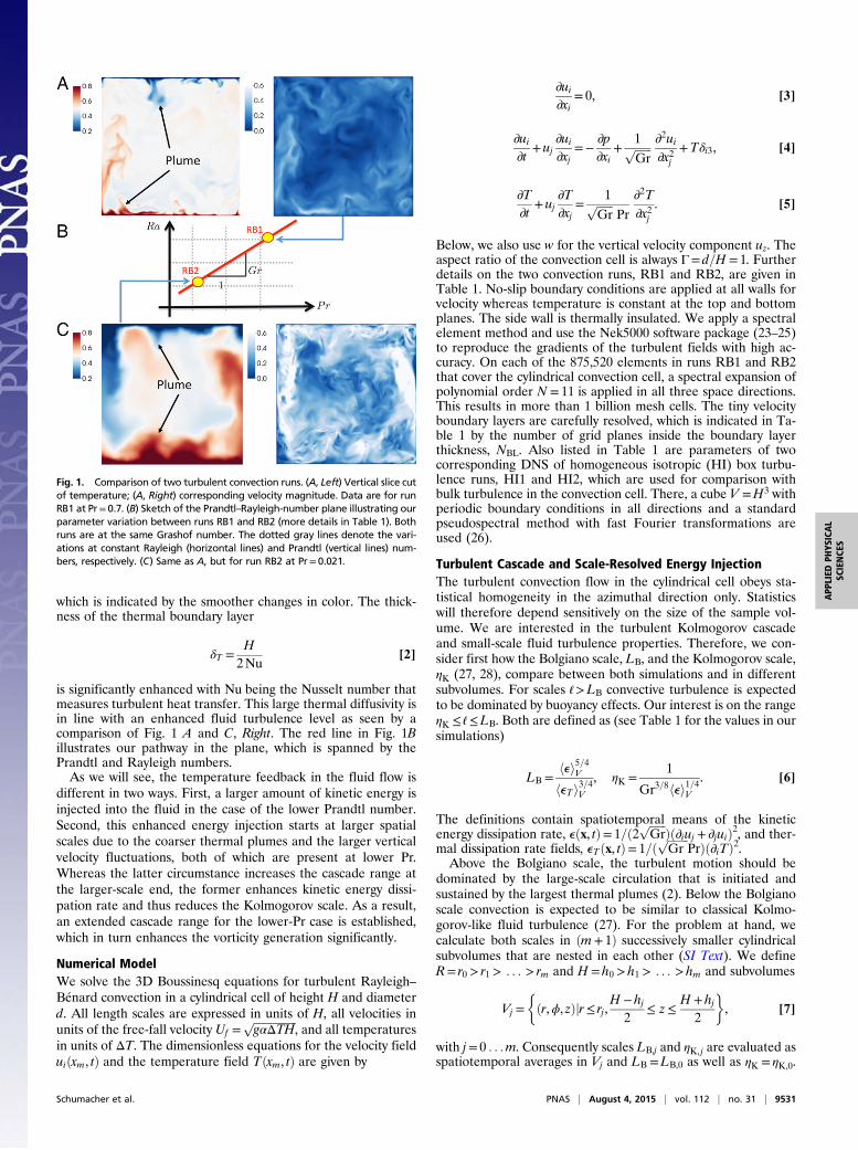
which is indicated by the smoother changes in color. The thick-ness of the thermal boundary layer

δT =H

2Nu[2]

is significantly enhanced with Nu being the Nusselt number thatmeasures turbulent heat transfer. This large thermal diffusivity isin line with an enhanced fluid turbulence level as seen by acomparison of Fig. 1 A and C, Right. The red line in Fig. 1Billustrates our pathway in the plane, which is spanned by thePrandtl and Rayleigh numbers.As we will see, the temperature feedback in the fluid flow is

different in two ways. First, a larger amount of kinetic energy isinjected into the fluid in the case of the lower Prandtl number.Second, this enhanced energy injection starts at larger spatialscales due to the coarser thermal plumes and the larger verticalvelocity fluctuations, both of which are present at lower Pr.Whereas the latter circumstance increases the cascade range atthe larger-scale end, the former enhances kinetic energy dissi-pation rate and thus reduces the Kolmogorov scale. As a result,an extended cascade range for the lower-Pr case is established,which in turn enhances the vorticity generation significantly.

Numerical ModelWe solve the 3D Boussinesq equations for turbulent Rayleigh–Bénard convection in a cylindrical cell of height H and diameterd. All length scales are expressed in units of H, all velocities inunits of the free-fall velocity Uf =

ffiffiffiffiffiffiffiffiffiffiffiffiffiffiffiffigαΔTH

p, and all temperatures

in units of ΔT. The dimensionless equations for the velocity fielduiðxm, tÞ and the temperature field Tðxm, tÞ are given by

∂ui∂xi

= 0, [3]

∂ui∂t

+ uj∂ui∂xj

=−∂p∂xi

+1ffiffiffiffiffiffiGr

p ∂2ui∂x2j

+Tδi3, [4]

∂T∂t

+ uj∂T∂xj

=1ffiffiffiffiffiffi

Grp

  Pr∂2T∂x2j

. [5]

Below, we also use w for the vertical velocity component uz. Theaspect ratio of the convection cell is always Γ= d=H = 1. Furtherdetails on the two convection runs, RB1 and RB2, are given inTable 1. No-slip boundary conditions are applied at all walls forvelocity whereas temperature is constant at the top and bottomplanes. The side wall is thermally insulated. We apply a spectralelement method and use the Nek5000 software package (23–25)to reproduce the gradients of the turbulent fields with high ac-curacy. On each of the 875,520 elements in runs RB1 and RB2that cover the cylindrical convection cell, a spectral expansion ofpolynomial order N = 11 is applied in all three space directions.This results in more than 1 billion mesh cells. The tiny velocityboundary layers are carefully resolved, which is indicated in Ta-ble 1 by the number of grid planes inside the boundary layerthickness, NBL. Also listed in Table 1 are parameters of twocorresponding DNS of homogeneous isotropic (HI) box turbu-lence runs, HI1 and HI2, which are used for comparison withbulk turbulence in the convection cell. There, a cube V =H3 withperiodic boundary conditions in all directions and a standardpseudospectral method with fast Fourier transformations areused (26).

Turbulent Cascade and Scale-Resolved Energy InjectionThe turbulent convection flow in the cylindrical cell obeys sta-tistical homogeneity in the azimuthal direction only. Statisticswill therefore depend sensitively on the size of the sample vol-ume. We are interested in the turbulent Kolmogorov cascadeand small-scale fluid turbulence properties. Therefore, we con-sider first how the Bolgiano scale, LB, and the Kolmogorov scale,ηK (27, 28), compare between both simulations and in differentsubvolumes. For scales ℓ>LB convective turbulence is expectedto be dominated by buoyancy effects. Our interest is on the rangeηK ≤ ℓ≤LB. Both are defined as (see Table 1 for the values in oursimulations)

LB =hei5=4V

heTi3=4V

, ηK =1

Gr3=8hei1=4V

. [6]

The definitions contain spatiotemporal means of the kineticenergy dissipation rate, eðx, tÞ= 1=ð2 ffiffiffiffiffiffi

Grp Þð∂iuj + ∂juiÞ2, and ther-

mal dissipation rate fields, eTðx, tÞ= 1=ð ffiffiffiffiffiffiffiffiGr 

pPrÞð∂iTÞ2.

Above the Bolgiano scale, the turbulent motion should bedominated by the large-scale circulation that is initiated andsustained by the largest thermal plumes (2). Below the Bolgianoscale convection is expected to be similar to classical Kolmo-gorov-like fluid turbulence (27). For the problem at hand, wecalculate both scales in ðm+ 1Þ successively smaller cylindricalsubvolumes that are nested in each other (SI Text). We defineR= r0 > r1 > . . . > rm and H = h0 > h1 > . . . > hm and subvolumes

Vj =�ðr,ϕ, zÞjr≤ rj,

H − hj2

≤ z≤H + hj

2

�, [7]

with j= 0 . . .m. Consequently scales LB,j and ηK, j are evaluated asspatiotemporal averages in Vj and LB =LB,0 as well as ηK = ηK,0.

Fig. 1. Comparison of two turbulent convection runs. (A, Left) Vertical slice cutof temperature; (A, Right) corresponding velocity magnitude. Data are for runRB1 at Pr= 0.7. (B) Sketch of the Prandtl–Rayleigh-number plane illustrating ourparameter variation between runs RB1 and RB2 (more details in Table 1). Bothruns are at the same Grashof number. The dotted gray lines denote the vari-ations at constant Rayleigh (horizontal lines) and Prandtl (vertical lines) num-bers, respectively. (C) Same as A, but for run RB2 at Pr= 0.021.

Schumacher et al. PNAS | August 4, 2015 | vol. 112 | no. 31 | 9531

APP

LIED

PHYS

ICAL

SCIENCE

S

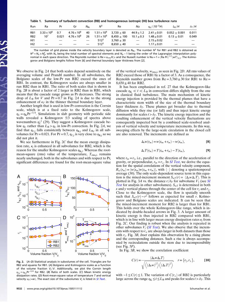
We observe in Fig. 2A that both scales depend sensitively on theaveraging volume and Prandtl number. In all subvolumes, theBolgiano scales of the low-Pr run RB2 exceed the ones ofRB1. In contrast, the Kolmogorov scales are always smaller inrun RB2 than in RB1. The ratio of both scales that is shown inFig. 2B is about a factor of 2 larger in RB2 than in RB1, whichmeans that the cascade range grows as Pr decreases. The strongdrop of LB for V and Pr= 0.7 in Fig. 2A is due to the strongenhancement of eT in the thinner thermal boundary layer.Another length that is used in low-Pr convection is the Corrsin

scale, which is at a fixed ratio to the Kolmogorov scale,ηC = ηKPr

−3=4. Simulations in slab geometry with periodic sidewalls revealed a Kolmogorov 5/3 scaling of spectra abovewavenumbers η−1C (29). They suggest a Kolmogorov cascade be-low ηC rather than LB > ηC in low-Pr convection. In Fig. 2A, wefind that ηC,j falls consistently between ηK,j and LB,j in all sub-volumes for Pr= 0.021. For Pr= 0.7, ηC,j is very close to ηK,j so wedid not plot it.We see furthermore in Fig. 2C that the mean energy dissipa-

tion rate, ej is enhanced in all subvolumes for RB2, which is thereason for the smaller Kolmogorov scales ηK,j. Whereas the root-mean-square (rms) value of the temperature, Trms,j, remainsnearly unchanged, both in the subvolumes and with respect to Pr,significant differences are found for the root-mean-square value

of the vertical velocity, wrms,j, as seen in Fig. 2D. All rms values ofRB2 exceed those of RB1 by a factor of 3. As a consequence, theReynolds number grows from Re= 3,760± 30 for RB1 to Re=8,650± 40 for RB2.It has been emphasized in ref. 27 that the Kolmogorov-like

cascade ηK � ℓ � LB in convection differs slightly from the onein classical fluid turbulence. The main mechanism of kineticenergy injection is provided by the thermal plumes that have acharacteristic stem width of the size of the thermal boundarylayer thickness δT. These plumes get broader due to thermaldiffusion while they rise (or fall) and thus inject kinetic energydominantly for scales ℓ> δT. The kinetic energy injection and theresulting enhancement of the vertical velocity fluctuations areconsequently inspected best by a combined scale-resolved anal-ysis of vertical velocity and temperature increments. In this way,sweeping effects by the large-scale circulation in the closed cellare also removed. The increments are defined as

ΔrwðrmÞ=wðxm + rmÞ−wðxmÞ, [8]

ΔrTðrmÞ=Tðxm + rmÞ−TðxmÞ, [9]

where rm = rk, i.e., parallel to the direction of the acceleration ofgravity, or perpendicular, rm = r⊥. In SI Text, we derive the equa-tion for the spatial correlations of the vertical velocity component,RzzðrmÞ= hwðxmÞwðxm + rmÞi, with h · i denoting a spatiotemporalaverage (30). The only scale-dependent source term in this equa-tion is the mixed-increment moment SwTðrÞ= hΔrwΔrTi. This isplotted in Fig. 3A vs. the distance r=δT for subvolume V1 (see SIText for analysis in other subvolumes). SwT is determined in bothx and y vertical planes through the center of the cell for rk and r⊥.Close to the Kolmogorov scale, the flow is spatially smoothsuch that SwTðrÞ∼ r2 follows as expected for small r. Kolmo-gorov and Bolgiano scales are indicated. It can be seen thatthe mixed-increment moment for RB2 is larger than for RB1.This holds over the whole Kolmogorov-like range, which is in-dicated by double-headed arrows in Fig. 3. A larger amount ofkinetic energy is thus injected in RB2 compared with RB1,which is in line with larger mean energy dissipation rates ej fromFig. 2C. Our finding is robust when the analysis is repeated inother subvolumes Vj (SI Text). We also observe that the increm-ents with respect to r⊥ are always larger in both datasets than thosewith rk. Fig. 3B, Inset explains this observation by a rising plumeand the corresponding distances. Such a rise is always accompa-nied by recirculations outside the stem due to incompressibility(see Fig. 5F).In Fig. 3B, we show the correlation coefficient

CðrÞ= hΔrwΔrTiffiffiffiffiffiffiffiffiffiffiffiffiffiffiffiffiffiffiffiffiffiffiffiffiffiffiffiffiffiffiffiffiffiffiffiffiffiffiffiffiDðΔrwÞ2

EDðΔrTÞ2

Er , r=�rk, r⊥

�, [10]

with −1≤CðrÞ≤ 1. The variation of Cðr⊥Þ of RB2 is particularlylarge across the range ηK ≤ ℓ≤LB and peaks for scales ℓ> δT. This

Table 1. Summary of turbulent convection (RB) and homogeneous isotropic (HI) box turbulence runs

Run Ra Pr Gr NBL N3 Re Nu ηK=ð10−3HÞ LB=H δT=H

RB1 3.33× 108 0.7 4.76× 108 40 1.51×109 3,720 ± 60 44.9±1.2 2.41±0.01 0.052 ± 0.001 0.011RB2 107 0.021 4.76× 108 26 1.51×109 8,450 ± 100 10.1±0.3 1.48±0.01 0.13 ± 0.01 0.049HI1 — — — — 5123 3,760 ± 30 — 2.15±0.02 — —

HI2 — — — — 5123 8,650 ± 40 — 1.17±0.01 — —

The number of grid planes inside the velocity boundary layer is denoted as NBL. The number N3 for RB1 and RB2 is obtained asN3 =Ne ×N3

p, with Ne being the total number of spectral elements and Np − 1 being the order of the Lagrangian interpolation poly-nomial in each space direction. The Reynolds number is Re=urmsH=ν and the Nusselt number is Nu= 1+ ðRa  PrÞ1=2hwTiV ,t. The Kolmo-gorov and Bolgiano lengths follow from [6] and thermal boundary layer thickness from [2].

0 0.5 110−3

10−2

10−1

L B,j, η

C,j a

nd η

K,j

LB,j

ηC,jηK,j

A

0 0.5 10

50

100

150

L B,j/η

K,j

B

0 0.5 110−4

10−3

10−2

10−1

Volume fraction Vj/V0

ε j

C

0 0.5 1

10−1

100

wrm

s,j a

nd T

rms,

j

Volume fraction Vj/V0

wrms

TrmsD

RB1RB2

Fig. 2. (A–D) Statistical analysis in subvolumes of the cell. Triangles are forRB2 and squares for RB1. (A) Bolgiano and Kolmogorov scales as a functionof the volume fraction Vj=V. Additionally, we plot the Corrsin lengthηC,j = ηK,jPr

−3=4 for RB2. (B) Ratio of both scales. (C) Mean kinetic energydissipation rates. (D) Root-mean-square value of temperature T and verticalvelocity uzð=wÞ. The exact size of the subvolumes Vj is listed in SI Text.

9532 | www.pnas.org/cgi/doi/10.1073/pnas.1505111112 Schumacher et al.

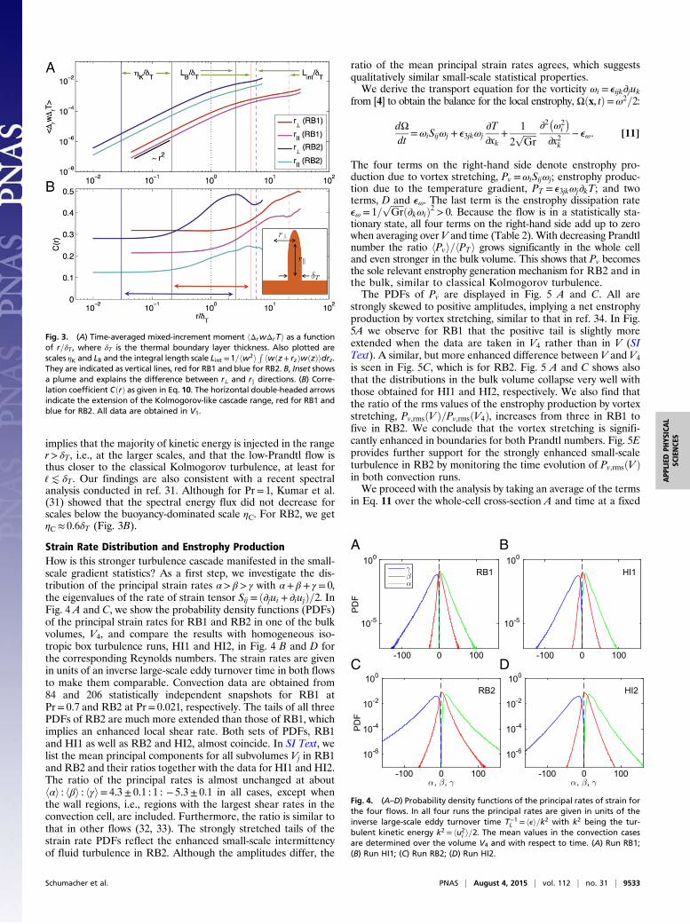
implies that the majority of kinetic energy is injected in the ranger> δT, i.e., at the larger scales, and that the low-Prandtl flow isthus closer to the classical Kolmogorov turbulence, at least forℓK δT. Our findings are also consistent with a recent spectralanalysis conducted in ref. 31. Although for Pr= 1, Kumar et al.(31) showed that the spectral energy flux did not decrease forscales below the buoyancy-dominated scale ηC. For RB2, we getηC ≈ 0.6δT (Fig. 3B).

Strain Rate Distribution and Enstrophy ProductionHow is this stronger turbulence cascade manifested in the small-scale gradient statistics? As a first step, we investigate the dis-tribution of the principal strain rates α> β> γ with α+ β+ γ = 0,the eigenvalues of the rate of strain tensor Sij = ð∂jui + ∂iujÞ=2. InFig. 4 A and C, we show the probability density functions (PDFs)of the principal strain rates for RB1 and RB2 in one of the bulkvolumes, V4, and compare the results with homogeneous iso-tropic box turbulence runs, HI1 and HI2, in Fig. 4 B and D forthe corresponding Reynolds numbers. The strain rates are givenin units of an inverse large-scale eddy turnover time in both flowsto make them comparable. Convection data are obtained from84 and 206 statistically independent snapshots for RB1 atPr= 0.7 and RB2 at Pr= 0.021, respectively. The tails of all threePDFs of RB2 are much more extended than those of RB1, whichimplies an enhanced local shear rate. Both sets of PDFs, RB1and HI1 as well as RB2 and HI2, almost coincide. In SI Text, welist the mean principal components for all subvolumes Vj in RB1and RB2 and their ratios together with the data for HI1 and HI2.The ratio of the principal rates is almost unchanged at abouthαi : hβi : hγi= 4.3± 0.1 : 1 : − 5.3± 0.1 in all cases, except whenthe wall regions, i.e., regions with the largest shear rates in theconvection cell, are included. Furthermore, the ratio is similar tothat in other flows (32, 33). The strongly stretched tails of thestrain rate PDFs reflect the enhanced small-scale intermittencyof fluid turbulence in RB2. Although the amplitudes differ, the

ratio of the mean principal strain rates agrees, which suggestsqualitatively similar small-scale statistical properties.We derive the transport equation for the vorticity ωi = eijk∂juk

from [4] to obtain the balance for the local enstrophy, Ωðx, tÞ=ω2=2:

dΩdt

=ωiSijωj + e3jkωj∂T∂xk

+1

2ffiffiffiffiffiffiGr

p ∂2�ω2i

�∂x2k

− eω. [11]

The four terms on the right-hand side denote enstrophy pro-duction due to vortex stretching, Pv =ωiSijωj; enstrophy produc-tion due to the temperature gradient, PT = e3jkωj∂kT; and twoterms, D and eω. The last term is the enstrophy dissipation rateeω = 1=

ffiffiffiffiffiffiGr

p ð∂kωiÞ2 > 0. Because the flow is in a statistically sta-tionary state, all four terms on the right-hand side add up to zerowhen averaging over V and time (Table 2). With decreasing Prandtlnumber the ratio hPvi=hPTi grows significantly in the whole celland even stronger in the bulk volume. This shows that Pv becomesthe sole relevant enstrophy generation mechanism for RB2 and inthe bulk, similar to classical Kolmogorov turbulence.The PDFs of Pv are displayed in Fig. 5 A and C. All are

strongly skewed to positive amplitudes, implying a net enstrophyproduction by vortex stretching, similar to that in ref. 34. In Fig.5A we observe for RB1 that the positive tail is slightly moreextended when the data are taken in V4 rather than in V (SIText). A similar, but more enhanced difference between V and V4is seen in Fig. 5C, which is for RB2. Fig. 5 A and C shows alsothat the distributions in the bulk volume collapse very well withthose obtained for HI1 and HI2, respectively. We also find thatthe ratio of the rms values of the enstrophy production by vortexstretching, Pv,rmsðV Þ=Pv,rmsðV4Þ, increases from three in RB1 tofive in RB2. We conclude that the vortex stretching is signifi-cantly enhanced in boundaries for both Prandtl numbers. Fig. 5Eprovides further support for the strongly enhanced small-scaleturbulence in RB2 by monitoring the time evolution of Pv,rmsðV Þin both convection runs.We proceed with the analysis by taking an average of the terms

in Eq. 11 over the whole-cell cross-section A and time at a fixed

Fig. 3. (A) Time-averaged mixed-increment moment hΔrwΔrTi as a functionof r=δT , where δT is the thermal boundary layer thickness. Also plotted arescales ηK and LB and the integral length scale Lint =1=hw2i R hwðz+ rzÞwðzÞidrz.They are indicated as vertical lines, red for RB1 and blue for RB2. B, Inset showsa plume and explains the difference between r⊥ and rk directions. (B) Corre-lation coefficient CðrÞ as given in Eq. 10. The horizontal double-headed arrowsindicate the extension of the Kolmogorov-like cascade range, red for RB1 andblue for RB2. All data are obtained in V1.

A B

C D

Fig. 4. (A–D) Probability density functions of the principal rates of strain forthe four flows. In all four runs the principal rates are given in units of theinverse large-scale eddy turnover time T−1

L = hei=k2 with k2 being the tur-bulent kinetic energy k2 = hu2

i i=2. The mean values in the convection casesare determined over the volume V4 and with respect to time. (A) Run RB1;(B) Run HI1; (C) Run RB2; (D) Run HI2.

Schumacher et al. PNAS | August 4, 2015 | vol. 112 | no. 31 | 9533

APP

LIED

PHYS

ICAL

SCIENCE

S

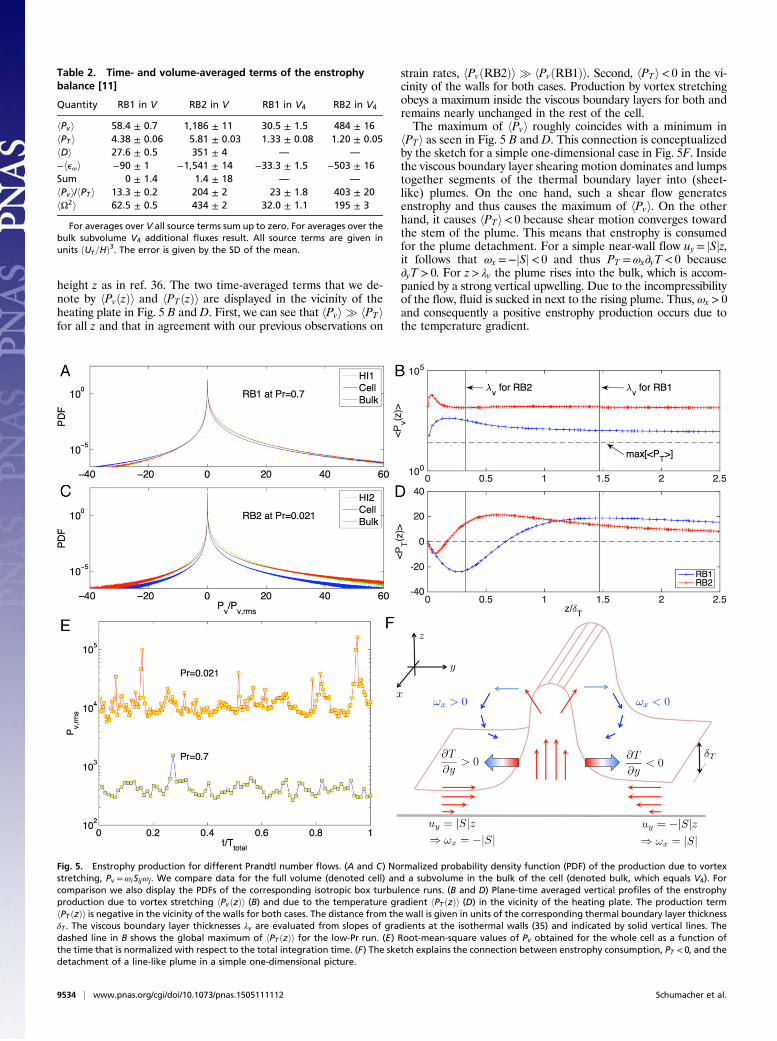
height z as in ref. 36. The two time-averaged terms that we de-note by hPvðzÞi and hPTðzÞi are displayed in the vicinity of theheating plate in Fig. 5 B and D. First, we can see that hPvi � hPTifor all z and that in agreement with our previous observations on

strain rates, hPvðRB2Þi � hPvðRB1Þi. Second, hPTi< 0 in the vi-cinity of the walls for both cases. Production by vortex stretchingobeys a maximum inside the viscous boundary layers for both andremains nearly unchanged in the rest of the cell.The maximum of hPvi roughly coincides with a minimum in

hPTi as seen in Fig. 5 B and D. This connection is conceptualizedby the sketch for a simple one-dimensional case in Fig. 5F. Insidethe viscous boundary layer shearing motion dominates and lumpstogether segments of the thermal boundary layer into (sheet-like) plumes. On the one hand, such a shear flow generatesenstrophy and thus causes the maximum of hPvi. On the otherhand, it causes hPTi< 0 because shear motion converges towardthe stem of the plume. This means that enstrophy is consumedfor the plume detachment. For a simple near-wall flow uy = jSjz,it follows that ωx =−jSj< 0 and thus PT =ωx∂yT < 0 because∂yT > 0. For z> λv the plume rises into the bulk, which is accom-panied by a strong vertical upwelling. Due to the incompressibilityof the flow, fluid is sucked in next to the rising plume. Thus, ωx > 0and consequently a positive enstrophy production occurs due tothe temperature gradient.

Table 2. Time- and volume-averaged terms of the enstrophybalance [11]

Quantity RB1 in V RB2 in V RB1 in V4 RB2 in V4

hPvi 58.4 ± 0.7 1,186 ± 11 30.5 ± 1.5 484 ± 16hPT i 4.38 ± 0.06 5.81 ± 0.03 1.33 ± 0.08 1.20 ± 0.05hDi 27.6 ± 0.5 351 ± 4 — —

−heωi −90 ± 1 −1,541 ± 14 −33.3 ± 1.5 −503 ± 16Sum 0 ± 1.4 1.4 ± 18 — —

hPvi/hPT i 13.3 ± 0.2 204 ± 2 23 ± 1.8 403 ± 20hΩ2i 62.5 ± 0.5 434 ± 2 32.0 ± 1.1 195 ± 3

For averages over V all source terms sum up to zero. For averages over thebulk subvolume V4 additional fluxes result. All source terms are given inunits ðUf=HÞ3. The error is given by the SD of the mean.

Fig. 5. Enstrophy production for different Prandtl number flows. (A and C) Normalized probability density function (PDF) of the production due to vortexstretching, Pv =ωiSijωj. We compare data for the full volume (denoted cell) and a subvolume in the bulk of the cell (denoted bulk, which equals V4). Forcomparison we also display the PDFs of the corresponding isotropic box turbulence runs. (B and D) Plane-time averaged vertical profiles of the enstrophyproduction due to vortex stretching hPvðzÞi (B) and due to the temperature gradient hPT ðzÞi (D) in the vicinity of the heating plate. The production termhPT ðzÞi is negative in the vicinity of the walls for both cases. The distance from the wall is given in units of the corresponding thermal boundary layer thicknessδT . The viscous boundary layer thicknesses λv are evaluated from slopes of gradients at the isothermal walls (35) and indicated by solid vertical lines. Thedashed line in B shows the global maximum of hPT ðzÞi for the low-Pr run. (E) Root-mean-square values of Pv obtained for the whole cell as a function ofthe time that is normalized with respect to the total integration time. (F) The sketch explains the connection between enstrophy consumption, PT < 0, and thedetachment of a line-like plume in a simple one-dimensional picture.

9534 | www.pnas.org/cgi/doi/10.1073/pnas.1505111112 Schumacher et al.

Summary and DiscussionWe have presented a high-resolution simulation study that re-veals the enhanced enstrophy generation mechanisms in turbu-lent convection at very low Prandtl numbers. Our high-resolutionDNS demonstrate that the Kolmogorov-like cascade range growsbecause the Bolgiano scale LB increases and the Kolmogrovscale ηK decreases as Pr gets smaller for the same Gr. In parallel,the flux of kinetic energy down to the smaller scales, which isgiven by the mean energy dissipation rate, is enhanced. By meansof the mixed temperature–velocity structure function, we showthat kinetic energy is injected into the convection flow on allscales ηk ≤ ℓ≤LB. The amount of injected energy is systematicallylarger for the low-Prandtl-number case and dominates startingfrom the thermal boundary layer thickness scale δT that is alsoequal to the average width of the thermal plumes. The resultingmore vigorous fluid turbulence is manifested by a larger-flowReynolds number that enhances the amplitudes of the localstrain and thus the enstrophy generation, dominantly due tovortex stretching. Despite the different driving of the fluid tur-bulence via the coupling to the temperature over a whole rangeof scales and the reduced number of statistically homogeneousdirections, the normalized PDFs of enstrophy production andthe ratio of the principal strain rates—two typical measures of

the small-scale velocity gradient statistics—are found to agreewith the idealized classical Kolmogorov turbulence.Our study provides thus further numerical evidence for the

universality of small-scale turbulence as, for example, discussedrecently in ref. 37. This opens interesting perspectives for themodeling of small-scale turbulent statistics that is necessary forseveral important applications of low-Prandtl-number convec-tion. Simulations at higher Rayleigh and/or lower Prandtl num-bers will obtain a sufficient scale separation to identify either theCorrsin or the Bolgiano scale as the large scale of a Kolmogorov-like cascade in low-Pr convection. A further point for future workis to study how this enhanced fluid turbulence couples back tothe boundary layer dynamics.

ACKNOWLEDGMENTS. Helpful discussions with J. Aurnou and G. Grötzbachare acknowledged. This work is supported by Research Unit 1182 and ResearchTraining Group 1567 of the Deutsche Forschungsgemeinschaft. We acknowl-edge supercomputing time at the Jülich Supercomputing Centre provided byGrants HIL07 and HIL08 of the John von Neumann Institute for Computing.Furthermore, we acknowledge an award of computer time provided bythe Innovative and Novel Computational Impact on Theory and Experiment(INCITE) program. This research used resources of the Argonne LeadershipComputing Facility at the Argonne National Laboratory, which is supportedby the US Department of Energy under Contract DE-AC02-06CH11357. J.S.thanks the Institute of Pure and AppliedMathematics at University of California,Los Angeles, and the US National Science Foundation for financial support.

1. Kadanoff LP (2001) Turbulent heat flow: Structures and scaling. Phys Today 54(8):34–39.

2. Chillà F, Schumacher J (2012) New perspectives in turbulent Rayleigh-Bénard con-vection. Eur J Phys E 35:58.

3. Christensen-Dalsgaard J, Gough DO, Thompson MJ (1991) The depth of the solarconvection zone. Astrophys J 378:413–437.

4. Sreenivasan KR, Donnelly RJ (2001) Role of cryogenic helium in classical fluid dy-namics: Basic research and model testing. Adv Appl Mech 37:239–276.

5. Hanasoge SM, Duvall TL, Jr, Sreenivasan KR (2012) Anomalously weak solar convec-tion. Proc Natl Acad Sci USA 109(30):11928–11932.

6. King EM, Aurnou JM (2013) Turbulent convection in liquid metal with and withoutrotation. Proc Natl Acad Sci USA 110(17):6688–6693.

7. Asai S (2012) Electromagnetic Processing of Materials: Materials Processing by UsingElectric and Magnetic Functions (Springer, Heidelberg).

8. Grötzbach G (2013) Challenges in low-Prandtl number heat transfer simulation andmodelling. Nucl Eng Des 264:41–55.

9. Kelley DH, Sadoway DR (2014) Mixing in a liquid metal electrode. Phys Fluids 26:057102.

10. Takeshita T, Segawa T, Glazier JA, Sano M (1996) Thermal turbulence in mercury. PhysRev Lett 76(9):1465–1468.

11. Cioni S, Ciliberto S, Sommeria J (1997) Strongly turbulent Rayleigh-Bénard convectionin mercury: Comparison with results at moderate Prandtl number. J Fluid Mech 335:111–140.

12. Büttner L, et al. (2013) Dual-plane ultrasound flow measurements in liquid metals.Meas Sci Technol 24:055302.

13. Liu L, Ahlers G (1997) Rayleigh-Bénard convection in binary gas mixtures: Thermo-physical properties and the onset of convection. Phys Rev E Stat Phys Plasmas FluidsRelat Interdiscip Topics 55:6950–6968.

14. Camussi R, Verzicco R (1998) Convective turbulence in mercury: Scaling laws andspectra. Phys Fluids 10:516–527.

15. Kerr RM, Herring JR (2000) Prandtl number dependence of Nusselt number in directnumerical simulations. J Fluid Mech 419:325–344.

16. Silano G, Verzicco R, Sreenivasan KR (2010) Numerical simulations of Rayleigh-Bénardconvection for Prandtl numbers between 10−1 and 104 and Rayleigh numbers be-tween 105 and 109. J Fluid Mech 662:409–446.

17. Verma MK, Mishra PK, Pandey A, Paul S (2012) Scalings of field correlations and heattransport in turbulent convection. Phys Rev E Stat Nonlin Soft Matter Phys 85(1 Pt 2):016310.

18. van der Poel EP, Stevens RAJM, Lohse D (2013) Comparison between two- and three-dimensional Rayleigh-Bénard convection. J Fluid Mech 736:177–194.

19. Breuer M, Wessling S, Schmalzl J, Hansen U (2004) Effect of inertia in Rayleigh-Bénardconvection. Phys Rev E Stat Nonlin Soft Matter Phys 69(2 Pt 2):026302.

20. Calkins MA, Aurnou JM, Eldredge JD, Julien K (2012) The influence of fluid propertieson the morphology of core turbulence and the geomagnetic field. Earth Planet SciLett 359–360:55–60.

21. Gizon L, Birch AC (2012) Helioseismology challenges models of solar convection. ProcNatl Acad Sci USA 109(30):11896–11897.

22. Shams A, Roelofs F, Baglietto E, Lardeau S, Kenjeres S (2014) Assessment and cali-bration of an algebraic turbulent heat flux model for low-Prandtl fluids. Int J HeatMass Transfer 79:589–601.

23. Fischer PF (1997) An overlapping Schwarz method for Spectral Element Solution ofthe incompressible Navier-Stokes equations. J Comput Phys 133:84–101.

24. Deville MO, Fischer PF, Mund EH (2002) High-Order Methods for Incompressible FluidFlow (Cambridge Univ Press, Cambridge, UK).

25. Scheel JD, Emran MS, Schumacher J (2013) Resolving the fine-scale structure in tur-bulent Rayleigh-Bénard convection. New J Phys 15:113063.

26. Schumacher J, Sreenivasan KR, Yakhot V (2007) Asymptotic exponents from low-Reynolds-number flows. New J Phys 9:89.

27. Lohse D, Xia K-Q (2010) Small-scale properties of turbulent Rayleigh-Bénard con-vection. Annu Rev Fluid Mech 42:335–364.

28. Kaczorowski M, Xia K-Q (2013) Turbulent flow in the bulk of Rayleigh-Bénard con-vection: Small-scale properties in a cubic cell. J Fluid Mech 722:596–617.

29. Mishra PK, Verma MK (2010) Energy spectra and fluxes for Rayleigh-Bénard convec-tion. Phys Rev E Stat Nonlin Soft Matter Phys 81(5 Pt 2):056316.

30. Yakhot V (1992) 4/5 Kolmogorov law for statistically stationary turbulence: Applica-tion to high-Rayleigh-number Bénard convection. Phys Rev Lett 69(5):769–771.

31. Kumar A, Chatterjee AG, Verma MK (2014) Energy spectrum of buoyancy-driventurbulence. Phys Rev E Stat Nonlin Soft Matter Phys 90(2):023016.

32. Ashurst WT, Kerstein AR, Kerr RM, Gibson CH (1987) Alignment of vorticity and scalargradient with strain rate in simulated Navier-Stokes turbulence. Phys Fluids 30:2343–2353.

33. Zeff BW, et al. (2003) Measuring intense rotation and dissipation in turbulent flows.Nature 421(6919):146–149.

34. Lüthi B, Tsinober A, Kinzelbach W (2005) Lagrangian measurement of vorticity dy-namics in turbulent flow. J Fluid Mech 528:87–118.

35. Scheel JD, Schumacher J (2014) Local boundary layer scales in turbulent Rayleigh-Bénard convection. J Fluid Mech 758:344–373.

36. Kerr RM (1996) Rayleigh number scaling in numerical convection. J Fluid Mech310:139–179.

37. Schumacher J, et al. (2014) Small-scale universality in fluid turbulence. Proc Natl AcadSci USA 111(30):10961–10965.

Schumacher et al. PNAS | August 4, 2015 | vol. 112 | no. 31 | 9535

APP

LIED

PHYS

ICAL

SCIENCE

S