NUMERICAL SIMULATION OF TURBULENT FORCED CONVECTION ... · Numerical Simulation of Turbulent Forced Convection Coupled to Heat Conduction in Square Ducts necessary condition for calculating

22nd International Congress of Mechanical Engineering (COBEM 2013) November 3-7, 2013, Ribeirão Preto, SP, Brazil

NUMERICAL SIMULATION OF TURBULENT FORCED CONVECTION

COUPLED TO HEAT CONDUCTION IN SQUARE DUCTS

Gustavo Adolfo Ronceros Rivas Universidade Federal da Integração Latino-Americana (UNILA) Engenharia de Energias Renováveis. Avenida Tancredo Neves, 6731 - Bloco 4, CEP: 85867-970, Foz do Iguaçu - Paraná - Brasil. [email protected] Ézio Castejon Garcia Instituto Tecnológico de Aeronáutica (ITA) Divisão de Engenharia Mecânica e Aeronáutica, Departamento de Energia. Praça Marechal do Ar Eduardo Gomes, 50 - Vila das acácias, CEP: 12.228-900, SJC - SP - Brasil. [email protected] Marcelo Assato Universidade Federal de Juiz de Fora (UFJF) Departamento de Engenharia Mecânica. Rua José Lourenço Kelmer, s/n - Campus Universitário, Bairro São Pedro - CEP: 36036-900, Juiz de fora, MG - Brasil. [email protected]

Abstract. In the present work, the numerical simulation was adopted to resolve the problem of the turbulent forced convection coupled to heat conduction in a duct of the square cross-section. The governing equations for turbulent con-vection are the continuity, momentum, and energy equations (Reynolds Averaged Navier Stokes, RANS). These equa-tions are coupled to heat conduction comings through of four plates situated around of the channel flow, the plates are coupled between itself with thermal resistance of ideal contact. Assumptions main in the flow, such as: condition of fully developed turbulent and incompressible flow had been assumed. The comparison way, had been used two turbulent models to resolve the equations of the momentum and one model to resolve the energy equation. That is, to determine the profiles of velocity, the models of turbulence, k-ε non linear (NLEVM) and Reynolds Stress Model (RSM), this last model simulated in a commercial code, they had been adopted and studied. The fluid temperature field will be deter-mined from of the model Simple Eddy Diffusivity (SED), based in the hypothesis of the Constant turbulent Prandtl num-ber; for the equation of the energy of the fluid had been dimensionless and developed in a code of programming FORTRAN. The models had been validated in base the experimental and numerical results of literature. Finally the results of this investigation allow evaluating the fluid temperature field for different square cross-sectional sections throughout of the direction of the main flow, which is influenced mainly by the temperature distribution in the wall.

Keywords: Numerical simulation,turbulent forced convection, square ducts, coupled solid fluid, thermal systems

1. INTRODUCTION

Square ducts are widely used in heat transfer devices. For example, in compact heat exchangers, gas turbine cooling

systems (secondary flows), cooling channels in combustion chambers, nuclear reactors. The forced turbulent heat convection in a square duct is one of the fundamental problems in the thermal science and fluid mechanics. Recently, Qin and Plecther (2006) showed that the Prandtl’s secondary flow of the second kind has a significant effect on the transport of heat and momentum as revealed by the recent large eddy simulation (LES). Several experimental and numerical studies have been conducted on turbulent flow though a non-circular duct, namely, (Nikuradse (1926); Gessner and Emery (1976); Gessner and Po (1976); Melling and Whitelaw (1976); Nakayama et al. (1983); Myon and Kobayashi (1991); Assato (2001) and others). Similarly important works in the turbulent heat convection were developed (Launder and Ying (1973); Emery et al. (1980); Hirota et al. (1997); Rokni (2000); Y. Hongxing (2009)) and others). The experimental work of Melling and Whitelaw (1973) shows detailed characteristics of turbulent flow in a rectangular duct where they used a laser-Doppler anemometer to report the axial development of the mean velocity, secondary mean velocity, etc. Nakayama et al. (1983), it shows the analysis the fully developed flow field in ducts of rectangular and trapezoidal cross-sections using a finite-difference method with the model of Launder and Ying (1973). On the other hand, Hirota et al. (1997) present an experimental work on the turbulent heat transfer in a square duct, shows detailed characteristics of turbulent flow and temperature field. Likewise, Rokni (1998), in the doctoral thesis achievement a comparison of four different turbulence models for predicting the turbulent Reynolds Stresses and three turbulent heat fluxes models for ducts square. In the turbulence model it is well known that Linear Eddy Viscosity Models (LEVM) can give rise to inaccurate predictions for the Reynolds normal stresses and so that not have the ability to predict secondary flows of the second kind. In spite of that, they are one of the most popular models in the engineering due to its simplicity, good numerical stability and it can be applied to a wide variety of flows. Thus, NLEVM represents a progress of the classical LEVM which permits inequality of the Reynolds normal stresses, a

ISSN 2176-5480

6815

G. Rivas, E. Garcia and M. Assato Numerical Simulation of Turbulent Forced Convection Coupled to Heat Conduction in Square Ducts

necessary condition for calculating turbulence-driven secondary flow in non-circular ducts within the relative cost of a two-equation formulation. The model RSM, also called the second order or second moment closure model is very accurate in the calculation of mean flow properties and all Reynolds stresses for many simple and more complex flows including wall jets, asymmetric channel and non-circular duct flows and curved flows, also present, disadvantages, just as, very large computing costs. The SED models for calculated turbulent heat flux have been adopted and studied. The bibliographical revision shows that the majority of the cited works had been previously developed for constant temperatures in the contour. However, in many applications the heat flux and surface temperature are non-uniform around the duct, becoming important the knowledge of the variation of the conductance around of the duct, Kays and Crawford (1980). According to developments performed by Garcia (1996), it is possible to carry out analysis with non-uniform wall temperature boundary conditions. In this case, it is necessary to define a value that represents the mean wall temperatures in a given cross section, “TWm”, in such away, in the present work intended to give a small contribution with respect to the influence the non-uniform wall temperature on the fluid temperature field considering internal flow with fluids air. 2. NOMENCLATURE

cp specific heat at constant pressure D duct height Dh hydraulic diameter, DLDLPAD eh ..2.4 dP/dz pressure gradient at z direction (longitudinal axis) f, Cf factor of Moody´s friction, and Fanning´s friction coefficient, respectively. kf fluid thermal conductivity L duct width Nu Nusselt number Pe perimeter Pk turbulence production term Re Reynolds number T temperature Tb internal flow bulk temperature TWm wall mean temperature T1, T2, T3 and T4 temperature distributions at duct wall (bottom, right side, top and left side) Ub internal flow bulk velocity U, V and W average velocity in the Cartesian plane in the direction x, y and z; respectively y+ dimensionless wall distance Greek Symbols α thermal diffusivity, α = kf / (ρ. cp) distance normal to the wall dimensionless temperature distribution μ dynamic viscosity μt turbulent viscosity density

t turbulent Prandtl number

3. Mathematical Formulation

3.1. Governing Equations

The Reynolds Averaged Navier Stokes (RANS) equation system is composed of: continuity equation (1), momentum equation (2), energy equation (3) and (4) heat conduction equation.

0)(

j

j

Ux

(1)

ISSN 2176-5480

6816


)(111)( ''ji

ji

j

j

i

jiji

j

uuxx

UxU

xxPUU

x

(2)

''

Pr1 tu

xT

xTU

x jj

f

jfj

j

(3)

0

i

ws

i xTk

x (4)

For analyses of fully developed turbulent flow and heat transfer, the following hypothesis has been adopted: steady

state, condition of non-slip on the wall and fluid with constant properties. The turbulent Reynolds stress )( ''jiuu and

the turbulent heat flux )( '' tu j were modeled and solved by algebraic and/or differential expressions.

3.2. Turbulence Models for Reynolds Stresses

3.2.1. Nonlinear Eddy Viscosity Model (NLEVM)

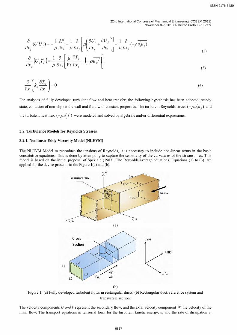
The NLEVM Model to reproduce the tensions of Reynolds, it is necessary to include non-linear terms in the basic constitutive equations. This is done by attempting to capture the sensitivity of the curvatures of the stream lines. This model is based on the initial proposal of Speziale (1987). The Reynolds average equations, Equations (1) to (3), are applied for the device presents in the Figure 1(a) and (b).

(a)

(b)

Figure 1: (a) Fully developed turbulent flows in rectangular ducts, (b) Rectangular duct: reference system and transversal section.

The velocity components U and V represent the secondary flow, and the axial velocity component W, the velocity of the main flow. The transport equations in tensorial form for the turbulent kinetic energy, κ, and the rate of dissipation ,

ISSN 2176-5480

6817


respectively, they are given by:

k

ik

t

iii P

xk

xxkU (5)

kfcP

kc

xxxU k

i

t

iii

2

221

(6)

The symbols kP and t , represent the rate of the turbulent kinetic energy production and the turbulent viscosity, respectively, and thus, we have:

j

iijk x

UP

,

2kfct (7)

In the present work for NLEVM, the formulations of Low Reynolds Number will be assumed for wall treatment. The damping functions 2f and f is observed in the Equations (6) and (7) and shown in the Table 1. These functions and

the constant 1C and 2C have been used together with the equations κ-ε, the subscribed letter P refers to the nodal point

near to the wall. Thus PU and Pk are the values of the velocity and kinetic energy in this point, respectively. The

constant c , 1c , 2c , k and they adopt the values of 0.09; 1.5; 1.9; 1.4 e 1.3; respectively. The new constitutive relation for the tensions of Reynolds in the model NLEVM, assumed in the thesis of Assato, 2001, is given by:

NL

jilklk31

jkkit1NLL

jitji SSSSkcS

(8)

This expression shows that the second term of the right side of the Equation (8), represents the nonlinear term added the original constitutive relation. This quadratic term represents the degree of anisotropy between the normal tensions of Reynolds, which makes it possible to predict the presence of the secondary flow in non circular ducts. The values of

NLc1 proposed by Speziale (1987) are equal to 1.68. Here, NLc1 will be analyzed and will adopt values for the formula-tion of Low Reynolds Numbers. The tensions of Reynolds, normal and shear, are presented in the Equations (9), (10) and (10), are expressed as:

22

1 32

31

yW

xWkc tNLxx

;

22

1 32

31

xW

yWkc tNLyy

(9)

yW

xWkc tNLxy

1 ;

xW

txz

;

yW

tyz

(10)

The following differences for the normal tensions of Reynolds are presented and have been observed for this type of flow.

22

1 xW

yWkc tNLxxyy

(11)

In such a way in Equation (7), including the derivatives above the tensions of Reynolds, the turbulence production term, is expressed as:

ISSN 2176-5480

6818


yW

xWP yzxzk

(12)

3.2.2. Reynolds Stress Model (RSM)

The most complex turbulence is the Reynolds Stress Model (RSM), also called of second order, it involves calculations

of the tensions of Reynolds in an individual form, ''jiuu , used for this differential equations of transport. The indi-

vidual Reynolds tensions are utilized to close the average Reynolds equations of the momentum. This model has shown superiority regarding the models of two equations in complex flows that involve swirl, rotation, etc. The exact equa-

tions of transport for the Reynolds tensions, ''jiuu , can be written as follows:

)()(2)(2)(

)()()(

)())(())((

''''''''

''''''''

'''''''''

jSiuuuuhxu

xug

xu

xup

fugugexuuu

xu

uuduuxx

cuupuuux

buuux

auut

jkmmiikmmjkk

j

k

i

i

j

j

i

ijjik

ikj

k

jkiji

kk

jikikjkjik

jikk

ji

(13)

Where the respective letters represent: (a) local derivative of the time;(b) ijC convection;(c) ijTD , Turbulent

diffusion;(d) ijLD , molecular diffusion;(e) ijP production Term of tensions;(f) ijG buoyancy production

Term;(g) ij Term of pressure-tension (redistribution);(h) ij Term of dissipation; (i) ijF Term production for the

rotation system;(j) jS Source term; The terms of the exact equations, presented previously, ijC , ijLD , , ijP and ijF

do not require modeling. However, the terms ijTD , , ijG , ij and ij need to be modeled to close the equations. For the present analysis, the model LRR (Launder, Reece e Rodi, 1975) is chosen, which assumes that the correlation velocity pressure is a linear function of the anisotropy tensor LRR in the phenomenology of the redistribution, ij . For the treatment of the wall, it is also assumed the Low Reynolds numbers and the periodic conditions, Rokni (1996). This model had been simulated in the commercial code Fluent 6.3. 3.3 Turbulence Models for Turbulent Heat Flux

3.3.1. Simple Eddy Diffusivity (SED)

This method is based on the Boussinesq viscosity model. The turbulent diffusivity for the energy equation can be ex-

pressed as: t

tt

, where the turbulent Prandtl number t needs to be given. The SED Model assumes that

the turbulent Prandtl number is constant in the entire region, for the air t it assumes values of 0.89, independent on the wall proximity effect.

j

f

T

tj x

Ttu

(14)

3.3.2. Generalized Gradient Diffusion Hypothesis (GGDH)

Daly and Harlow (1970) present the following formulation to the turbulent heat flux:

k

fkjtj x

TuukCtu

(15)

ISSN 2176-5480

6819


The constant tC , assuming the value of 0.3, is adopted. The main advantage of this model is that it considers the anisotropic behavior of the fluid heat transport in ducts.

3.3.3. Dimensionless Energy Equation for SED and GGDH Models

For a given cross section of area “A”, it is possible to define a mean velocity “Ub” and a bulk temperature “Tb”, express as:

dydxWA

Ub ..1 and

dydxTW

UAAU

dATWT f

bb

Af

b ....1

.

.. (16) and (17)

Kays and Crawford (1980) developed an applicable formulation to rectangular cross section ducts. They considered the boundary conditions with prescribed uniform wall temperatures at the cross section, and along the duct length. According to developments performed by Garcia (1996), it is possible to carry out analysis with non-uniform wall temperature boundary conditions. In this case, it is necessary to define a value that represents the mean wall temperatures in a given cross section, “TWm”, given as:

)(2

.,.1.,.1.0,.1.,0.10 0 430 20 1

DL

dxLxTD

dyyDTL

dxxTD

dyyTLT

L DDL

Wm

(18)

It is possible to develop a formula similar to Kays and Crawford (1980), the new expression for the turbulent energy equation, is presented as:

0

wt

zT

zvt

yT

yut

xT

xzT

Wy

TV

xT

U ffffff

(19)

The following considerations are applied to obtain the variables in dimensionless form:

hDxX ,

hDyY and

dzdT

DU

TT

bhb

fWm

..

.

2

(20), (21) and (22)

Replacing Equation (14), Equation (15), Equation (20) up to (22) in Equation (19), dimensionless energy equation for SED and GGDH becomes, respectively:

BBhtt U

WY

VX

UDYYXX

)(

(23)

XYC

YXC

UW

YV

XUD

YYXX

Yt

XtBB

heyex

)(

(24)

The fluid temperature field “Tf” can be replaced by “Tb” and the Equation (22) can be expressed as:

ISSN 2176-5480

6820


dzdT

DU

TT

bhb

bWmb

..

.2

, and b

bbhWmb dz

dTUDTT

..

.2

(25) and (26)

From Equation (21), the Equation (26) is obtained, and applying this in Equation (17), one gets Equation (28):

dz

dTDU

TT

bhb

Wmf

... 2

, and dydxWdz

dTA

DTT bh

Wmb ......

2

(27) and (28)

Replacing Equation (27) in Equation (24), and using also Equations (19) and (20), the dimensionless bulk temperature is obtained:

dYdXWUA

D

b

hb ....

.

2

(29)

It is possible to compute the heat transfer rate per unit length on the wall surface, “ q’ ”, Equation (30). It depends on values for “TWm”, “Tb”, and on the average heat convection coefficient, “ h ”. From fluid enthalpy derivative gradient [dhb = cp.dTb], the heat transfer rate per unit length in the fluid, “ q’f ”, can be expressed by Equation (31).

).(.,bWme TThPq , and

dzdT

cAUq bpbf .... (30) and (31)

When Equation (30) is made equal to (31), integrating two cross sections (inlet, namely z1, and outlet, namely z2), it is possible to develop the resulting expression, Equation (32).

.21

2

12

...2

zzNuUA

P

bWmWmbb

e

zzeTTTT

(32)

From Equation (32), the bulk temperature longitudinal (z-axis) variation “Tb” is obtained. It is done by “cutting” the duct into a lot of segments and applying the numerical method to find “Tb” at each finite cross section. For a given bulk temperature at the duct inlet section (Tb1), after solving the equation system, duct outlet bulk temperature (Tb2) is computed from that expression, Equation (32). The Dimensionless boundary conditions are given by the following equations:

dzdT

DU

TTY

bhb

Wm

..

.),0(

2

1 , and

dzdT

DU

TTX

bhb

Wm

..

.)0,(

2

2 (33)

dzdT

DU

TTY

bhb

WmD

Dh

..

.),(

2

3 , and

dzdT

DU

TTX

bhb

WmDL

h

..

.),(

2

4 (34)

When considering uniform wall temperature, Equation (33) and Equation (34) are equal to zero, and for these particular conditions, it is possible to notice that these boundary conditions are not functions of “ dzdTb ”. That simplification becomes equal to the one studied by Patankar (1991). Equations (25),(26) and (27) , as well as the boundary conditions from Equations (33) and (34), form a set of differential equations, in which “” and “dTb/dz” parameters are unknown. When that equation system is solved, it is possible to obtain “Tf”.

ISSN 2176-5480

6821


3.3.4. Additional Equations

Additional equations were utilized for the calculation of the factor of friction Moody, f ; coefficient of friction of

Fanning, fC ; Prandtl law; local Nusselt number for the Low Reynolds formulation (Rokni, 2000), xpNu and

Correlation of Gnielinsky, Nu , respectively; these equations are given by:

2

./2B

h

UDdzdPf

,

4fC f , 8.0Relog21

ff

, bw

Pwhxp TT

TTDNu

and

1Pr8/7.121

Pr1000Re8/3

22

1f

fNu (35),(36),(37),(38) and (39)

4. Numerical Implementation

After applying the method of finite differences to the algebraic equations, to obtain the temperature fields, the following five steps indicate the developed methodology in the numerical solution. (Garcia, 1996): Step 1: To define the function value of the non uniform temperatures in the walls of the duct

),(),,(),0,(),,0( 4321 LxTyDTxTyTfTWm , what that can be expressed by a Fourier expansion;

Step2: To obtain velocity field and estimated values for “ bU ”“TWm” and “dTb/dz”; Step 3: Equations for the boundary conditions are evaluated (Equations 33 and 34); Step 4: Dimensionless energy equation (Temperature field, “Ø”) at Equation (24) is solved and “Øb” is computed according to Equation (30), until convergence is obtained (Øb < tolerance). This is the end of the first iterative loop; Step 5: A value for “dTb/dz” is computed in accordance with Equation (25). Boundary conditions are updated (step 3) to obtain a solution for the new temperature field (step 4), until convergence is obtained (dTb/dz < tolerance). This is the end of the second iterative loop; For all steps, “tolerance of 10-7” is the value to be accomplished by the convergence criteria, which is applicable to “Øb” (dimensionless bulk temperature), “dTb /dz" and “Ø” (dimensionless temperature field). The above procedure is applied for contours of variable temperatures. 5. Results and Discussion

5.1 Fluid Flow and Heat Transfer Field

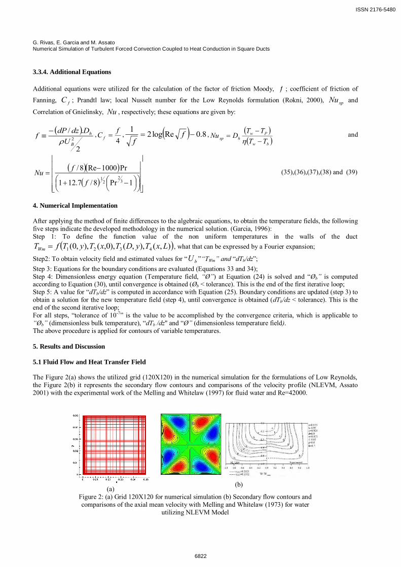
The Figure 2(a) shows the utilized grid (120X120) in the numerical simulation for the formulations of Low Reynolds, the Figure 2(b) it represents the secondary flow contours and comparisons of the velocity profile (NLEVM, Assato 2001) with the experimental work of the Melling and Whitelaw (1997) for fluid water and Re=42000.

(a)

(b)

Figure 2: (a) Grid 120X120 for numerical simulation (b) Secondary flow contours and comparisons of the axial mean velocity with Melling and Whitelaw (1973) for water

utilizing NLEVM Model

ISSN 2176-5480

6822


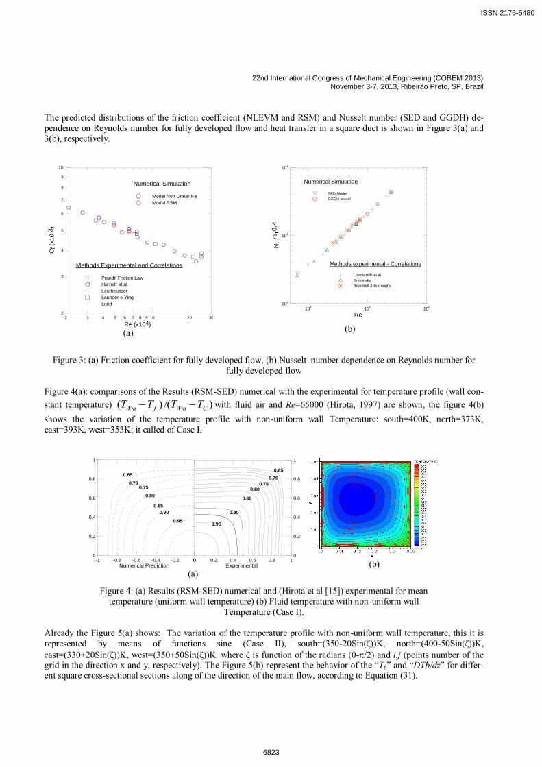
The predicted distributions of the friction coefficient (NLEVM and RSM) and Nusselt number (SED and GGDH) de-pendence on Reynolds number for fully developed flow and heat transfer in a square duct is shown in Figure 3(a) and 3(b), respectively.

102 3 4 5 6 7 8 9 20 30

Re (x104)

10

9

8

7

6

5

4

3

2

Cf (

x10-

3 )

Methods Experimental and Correlations

Prandtl Friction LawHarnett et al.LeutheusserLaunder e YingLund

Numerical Simulation

Model Non Linear k-eModel RSM

(a)

104 105 106

Re

101

102

103

Nu/

Pr0.4

Methods experimental - Correlations

Lowdermilk et al.GnielinskyBrundrett & Burroughs

Numerical Simulation

SED ModelGGDH Model

(b)

Figure 3: (a) Friction coefficient for fully developed flow, (b) Nusselt number dependence on Reynolds number for fully developed flow

Figure 4(a): comparisons of the Results (RSM-SED) numerical with the experimental for temperature profile (wall con-stant temperature) )/()( CWmfWm TTTT with fluid air and Re=65000 (Hirota, 1997) are shown, the figure 4(b) shows the variation of the temperature profile with non-uniform wall Temperature: south=400K, north=373K, east=393K, west=353K; it called of Case I.

0 0.2 0.4 0.6 0.8 1Experimental

0

0.2

0.4

0.6

0.8

1

0

0.2

0.4

0.6

0.8

1

-1 -0.8 -0.6 -0.4 -0.2 0Numerical Prediction

Mean Temperature

0.95

0.90

0.85

0.800.75

0.70

0.65

0.95

0.90

0.85

0.80

0.750.70

0.65

(a)

(b)

Figure 4: (a) Results (RSM-SED) numerical and (Hirota et al [15]) experimental for mean temperature (uniform wall temperature) (b) Fluid temperature with non-uniform wall

Temperature (Case I).

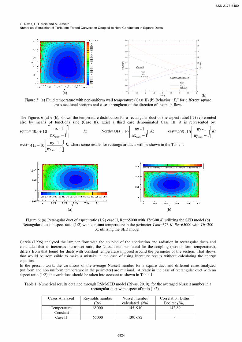
Already the Figure 5(a) shows: The variation of the temperature profile with non-uniform wall temperature, this it is represented by means of functions sine (Case II), south=(350-20Sin(ζ))K, north=(400-50Sin(ζ))K, east=(330+20Sin(ζ))K, west=(350+50Sin(ζ))K. where ζ is function of the radians (0-/2) and i,j (points number of the grid in the direction x and y, respectively). The Figure 5(b) represent the behavior of the “Tb” and “DTb/dz” for differ-ent square cross-sectional sections along of the direction of the main flow, according to Equation (31).

ISSN 2176-5480

6823


(a) 0 0.5 1 1.5 2 2.5 3 3.5 4

Z (m)

290

300

310

320

330

340

350

360

370

380

T Bu

lk (K

)

0

2

4

6

8

10

12

14

16

18

DTb

/dz

Case Constant Tw

TwmTb(Z)(DTb/dz)

Case II

TwmTb(Z)(DTb/dz)

(b) Figure 5: (a) Fluid temperature with non-uniform wall temperature (Case II) (b) Behavior “Tb” for different square

cross-sectional sections and cases throughout of the direction of the main flow.

The Figures 6 (a) e (b), shown the temperature distribution for a rectangular duct of the aspect ratio(1:2) represented also by means of functions sine (Case II). Exist a third case denominated Case III, it is represented by:

south=

1nx1-nx 10405

máx

K; North=

1nx1-nx 10395

máx

K; east=

1ny1-ny 10-054

máx

K;

west=

1ny1-ny 10154

máx

K, where some results for rectangular ducts will be shown in the Table I.

(a)

(b)

Figure 6: (a) Retangular duct of aspect ratio (1:2) case II, Re=65000 with Tb=300 K, utilizing the SED model (b) Retangular duct of aspect ratio (1:2) with constant temperature in the perimeter Twm=373 K, Re=65000 with Tb=300

K, utilizing the SED model.

Garcia (1996) analyzed the laminar flow with the coupled of the conduction and radiation in rectangular ducts and concluded that as increases the aspect ratio, the Nusselt number found for the coupling (non uniform temperature), differs from that found for ducts with constant temperature imposed around the perimeter of the section. That shows that would be admissible to make a mistake in the case of using literature results without calculating the energy equation. In the present work, the variations of the average Nusselt number for a square duct and different cases analyzed (uniform and non uniform temperature in the perimeter) are minimal. Already in the case of rectangular duct with an aspect ratio (1:2), the variations should be taken into account as shown in Table 1.

Table 1. Numerical results obtained through RSM-SED model (Rivas, 2010), for the averaged Nusselt number in a rectangular duct with aspect of ratio (1:2).

Cases Analyzed Reynolds number

(Re) Nusselt number calculated (Nu)

Correlation Dittus Boelter (Nu).

Temperature Constant

65000 145, 910 142,89

Case II 65000 139, 682 -

ISSN 2176-5480

6824


Case III 65000 145, 059 - Temperature

Constant 28853 79, 101 77,1

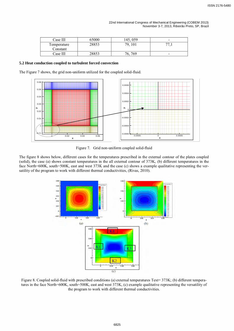
Case III 28853 76, 769 - 5.2 Heat conduction coupled to turbulent forced convection

The Figure 7 shows, the grid non-uniform utilized for the coupled solid-fluid.

x

y

0 0.02 0.04 0.06-0.01

0

0.01

0.02

0.03

0.04

0.05

0.06

Frame 001 09 Jun 2010 Modelo Acoplamento=

x

y

-0.0005 0 0.0005-0.0006

-0.0004

-0.0002

0

0.0002

0.0004

0.0006

Frame 001 09 Jun 2010 Modelo Acoplamento=

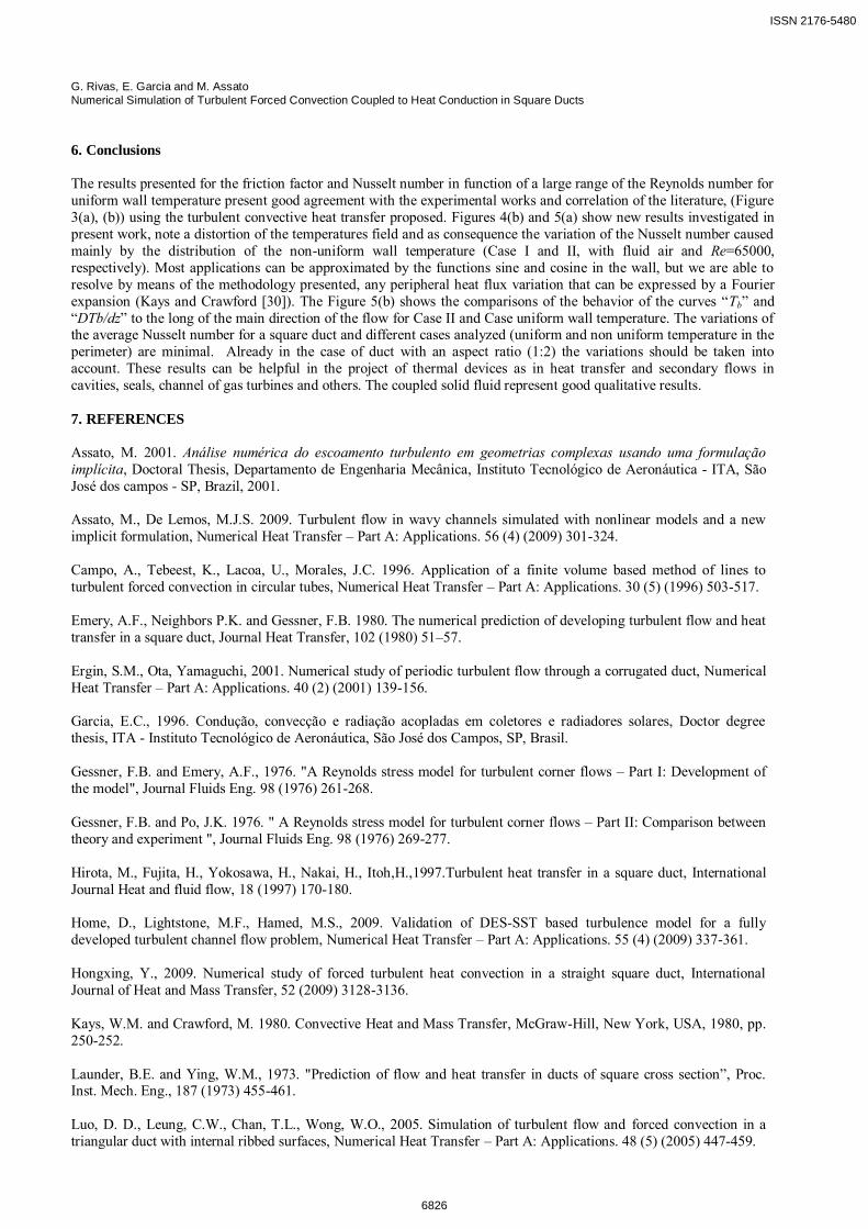
Figure 7. Grid non-uniform coupled solid-fluid The figure 8 shows below, different cases for the temperatures prescribed in the external contour of the plates coupled (solid), the case (a) shows constant temperatures in the all external contour of 373K, (b) different temperatures in the face North=600K, south=500K, east and west 373K and the case (c) shows a example qualitative representing the ver-satility of the program to work with different thermal conductivities, (Rivas, 2010).

Figure 8. Coupled solid-fluid with prescribed conditions (a) external temperatures Text= 373K; (b) different tempera-tures in the face North=600K, south=500K, east and west 373K, (c) example qualitative representing the versatility of

the program to work with different thermal conductivities.

ISSN 2176-5480

6825


6. Conclusions

The results presented for the friction factor and Nusselt number in function of a large range of the Reynolds number for uniform wall temperature present good agreement with the experimental works and correlation of the literature, (Figure 3(a), (b)) using the turbulent convective heat transfer proposed. Figures 4(b) and 5(a) show new results investigated in present work, note a distortion of the temperatures field and as consequence the variation of the Nusselt number caused mainly by the distribution of the non-uniform wall temperature (Case I and II, with fluid air and Re=65000, respectively). Most applications can be approximated by the functions sine and cosine in the wall, but we are able to resolve by means of the methodology presented, any peripheral heat flux variation that can be expressed by a Fourier expansion (Kays and Crawford [30]). The Figure 5(b) shows the comparisons of the behavior of the curves “Tb” and “DTb/dz” to the long of the main direction of the flow for Case II and Case uniform wall temperature. The variations of the average Nusselt number for a square duct and different cases analyzed (uniform and non uniform temperature in the perimeter) are minimal. Already in the case of duct with an aspect ratio (1:2) the variations should be taken into account. These results can be helpful in the project of thermal devices as in heat transfer and secondary flows in cavities, seals, channel of gas turbines and others. The coupled solid fluid represent good qualitative results. 7. REFERENCES

Assato, M. 2001. Análise numérica do escoamento turbulento em geometrias complexas usando uma formulação implícita, Doctoral Thesis, Departamento de Engenharia Mecânica, Instituto Tecnológico de Aeronáutica - ITA, São José dos campos - SP, Brazil, 2001. Assato, M., De Lemos, M.J.S. 2009. Turbulent flow in wavy channels simulated with nonlinear models and a new implicit formulation, Numerical Heat Transfer – Part A: Applications. 56 (4) (2009) 301-324.

Campo, A., Tebeest, K., Lacoa, U., Morales, J.C. 1996. Application of a finite volume based method of lines to turbulent forced convection in circular tubes, Numerical Heat Transfer – Part A: Applications. 30 (5) (1996) 503-517.

Emery, A.F., Neighbors P.K. and Gessner, F.B. 1980. The numerical prediction of developing turbulent flow and heat transfer in a square duct, Journal Heat Transfer, 102 (1980) 51–57.

Ergin, S.M., Ota, Yamaguchi, 2001. Numerical study of periodic turbulent flow through a corrugated duct, Numerical Heat Transfer – Part A: Applications. 40 (2) (2001) 139-156.

Garcia, E.C., 1996. Condução, convecção e radiação acopladas em coletores e radiadores solares, Doctor degree thesis, ITA - Instituto Tecnológico de Aeronáutica, São José dos Campos, SP, Brasil.

Gessner, F.B. and Emery, A.F., 1976. "A Reynolds stress model for turbulent corner flows – Part I: Development of the model", Journal Fluids Eng. 98 (1976) 261-268.

Gessner, F.B. and Po, J.K. 1976. " A Reynolds stress model for turbulent corner flows – Part II: Comparison between theory and experiment ", Journal Fluids Eng. 98 (1976) 269-277.

Hirota, M., Fujita, H., Yokosawa, H., Nakai, H., Itoh,H.,1997.Turbulent heat transfer in a square duct, International Journal Heat and fluid flow, 18 (1997) 170-180.

Home, D., Lightstone, M.F., Hamed, M.S., 2009. Validation of DES-SST based turbulence model for a fully developed turbulent channel flow problem, Numerical Heat Transfer – Part A: Applications. 55 (4) (2009) 337-361.

Hongxing, Y., 2009. Numerical study of forced turbulent heat convection in a straight square duct, International Journal of Heat and Mass Transfer, 52 (2009) 3128-3136.

Kays, W.M. and Crawford, M. 1980. Convective Heat and Mass Transfer, McGraw-Hill, New York, USA, 1980, pp. 250-252.

Launder, B.E. and Ying, W.M., 1973. "Prediction of flow and heat transfer in ducts of square cross section”, Proc. Inst. Mech. Eng., 187 (1973) 455-461.

Luo, D. D., Leung, C.W., Chan, T.L., Wong, W.O., 2005. Simulation of turbulent flow and forced convection in a triangular duct with internal ribbed surfaces, Numerical Heat Transfer – Part A: Applications. 48 (5) (2005) 447-459.

ISSN 2176-5480

6826


Melling, A. and Whitelaw, J.H. 1976. " Turbulent flow in a rectangular duct ", Journal Fluid Mechanical. 78 (1976) 289-315.

Moran, M. J. et al., Introdução à Engenharia de Sistemas Térmicos: Termodinâmica, Mecânica dos Fluidos e Transferência de Calor, LTC Ed., Rio de Janeiro-RJ, Brasil, 2005.

Myon, H.K. and Kobayashi, T. 1991. Numerical Simulation Of Three Dimensional Developing Turbulent Flow in a Square Duct with the Anisotropic κ-ε Model, Advances in Numerical Simulation of Turbulent Flows ASME, Fluids Engineering Conference, 1991. Vol.117, Portland, United States of America, pp. 17-23.

Nakayama, A., Chow, W.L. and Sharma, D. 1983. Calculation of fully development turbulent flows in ducts of arbi-trary cross-section, Journal Fluid Mechanical, 128 (1983) 199-217.

Nikuradse, J. 1926. "Untersuchung uber die Geschwindigkeitsverteilung in turbulenten Stromungen", Diss. Göttingen, VDI - forschungsheft 281.

Park, T.S. 2004. Numerical study of turbulent flow and heat transfer in a convex channel of a calorimetric rocket chamber, Numerical Heat Transfer – Part A: Applications. 45 (10) (2004) 1029-1047.

Patankar, S.V., Computation of Conduction and Duct Flow Heat Transfer, Innovative Research, Maple Grove, USA, 1991.

Qin, Z.H., Plecther, R.H. 2006. "Large eddy simulation of turbulent heat transfer in a rotating square duct", International Journal Heat Fluid Flow. 27 (2006) 371-390.

Rivas Ronceros, G.A., 2010. Simulação numérica da convecção forçada turbulenta acoplada à condução de calor em dutos retangulares, Doctor degree thesis, ITA - Instituto Tecnológico de Aeronáutica, São José dos Campos, SP, Brasil. Rokni, M. 1998. Numerical investigation of turbulent fluid flow and heat transfer in complex duct, Doctoral Thesis, Department of Heat and Power Engineering. Lund Institute of Technology, Sweden, 1998.

Rokni, M., 2000. A new low-Reynolds version of an explicit algebraic stress model for turbulent convective heat transfer in ducts, Numerical Heat Transfer – Part B: Fundamentals. 37 (3) (2000) 331-363.

Rokni, M., Sundén, B., 1996. Numerical investigation of turbulent forced convection in ducts with rectangular and trapezoidal cross section area by using different turbulence models, Numerical Heat Transfer – Part A: Applications. 30 (4) (1996) 321-346.

Saidi, A., Sundén, B., 2001. " Numerical simulation of turbulent convective heat transfer in square ribbed ducts", Numerical Heat Transfer – Part A: Applications. 38 (1) (2001) 67-88.

Sharatchandra, M.C., Rhode, D.L., 1997. Turbulent flow and heat transfer in staggered tube banks with displaced tube rows, Numerical Heat Transfer – Part A: Applications. 31 (6) (1997) 611-627.

Speziale, C.G., 1987. "on non linear k-l and k-e models of turbulence, Journal Fluid Mechanical"., v.178, p. 459-475, 1987.

Su, J., Da Silva Neto, A.J., 2001. Simultaneous estimation of inlet temperature and wall heat flux in turbulent circular pipe flow, Numerical Heat Transfer – Part A: Applications. 40 (7) (2001) 751-766. Valencia, A., 2000. Turbulent flow and heat transfer in a channel with a square bar detached from the wall, Numerical Heat Transfer – Part A: Applications. 37 (3) (2000) 289-306.

Yang, G., Ebadian, M.A.,1991. Effect of Reynolds and Prandtl numbers on turbulent convective heat transfer in a three-dimensional square duct, Numerical Heat Transfer – Part A: Applications. 20 (1) (1991) 111-122.

Yang, Y.T., Hwang, M.L. 2008. Numerical simulation of turbulent fluid flow and heat transfer characteristics in a rectangular porous channel with periodically spaced heated blocks, Numerical Heat Transfer – Part A: Applications.

ISSN 2176-5480

6827


54 (8) (2008) 819-836.

Zhang, J., Dong, L., Zhou, L., Nieh, S. 2003. Simulation of swirling turbulent flows and heat transfer in a annular duct, Numerical Heat Transfer – Part A: Applications. 44 (6) (2003) 591-609.

Zheng, B., Lin, C.X., Ebadian, M.A., 2003. Combined turbulent forced convection and thermal radiation in a curved pipe with uniform wall temperature, Numerical Heat Transfer – Part A: Applications. 44 (2) (2003) 149-167.

8. RESPONSIBILITY NOTICE

The author(s) is (are) the only responsible for the printed material included in this paper.

ISSN 2176-5480

6828

Documents

NUMERICAL SIMULATION OF TURBULENT FORCED CONVECTION ... · Numerical Simulation of Turbulent Forced Convection Coupled to Heat Conduction in Square Ducts necessary condition for calculating