Embed Size (px)
Citation preview
Ministry of Higher Education
& Scientific Research
University of Technology
Chemical Engineering Department
Enhancement of Reverse Osmosis Membranes
Performance with Air Sparging Technique
A Thesis
Submitted to the Chemical Engineering Department
Of The University of Technology
In Partial Fulfillment of the Requirements for
The Degree of Doctor of Philosophy in
Chemical Engineering.
By Talib Mohammad Naief
(M. Sc. Chem. Eng.2001)
May - 2009

الرحيم الرحمن هللا بسم
الماء نسوق أنا يروا أولم
فنخرج الجرز األرض إلى
مهم آع أن منه تأكل زرعا به
يبصرون أفال وأنفسهم
العظيم هللا صدق السجدة سورة
)27( االية
Certification
I certify that this thesis entitled (Enhancement of Reverse
Osmosis Membranes Performance with Air Sparging
Technique) was prepared under my linguistic supervision. It was
amended to meet the style of English Language.
Signature
Name: Asst. Prof. Dr. Ahmad AL-Beiruti.
Date: / / 2009
Certification of Supervisor We certify that the thesis entitled (Enhancement of Reverse
Osmosis Membranes Performance with Air Sparging
Technique) was prepared under our supervision as a partial
fulfillment of the requirements of the degree of Philosophy of
Doctorate in Chemical Engineering at the Chemical Engineering
Department, University of Technology.
Signature: Signature: Name: Prof. Dr. Mumtaz A. Yousif Name: Asst. prof. Dr. Qusay Fadhel Date: / / 2009 Date: / / 2009
In view of the available recommendations, I forward this
thesis for debate by the examination committee.
Signature
Asst.Prof. Dr. Kahlid A.Sukkar
Head of post graduate Committee
Department of Chemical Engineering.
Date: / / 2009

Dedication
Especially Dedicated To…. The memory of my Father To my mother with love My brothers and my sisters My Wife and Children Ibrahim and Masarra.
Talib
I
Acknowledgment
I would like to express my sincere thanks, gratitude and
appreciation to my supervisors Prof. Dr. Mumtaz A. Zabluk and
Asst. Prof. Dr. Qusay Fadhel Abdul Hameed for their kind
supervision, advice, reading and Criticizing the proofs of this
study.
First of all, I thanks god who offered me patience, power and
faith in a way that words cannot express.
My respectful regards to head of Chemical Engineering
Department at the University of Technology Prof. Dr. Mumtaz A.
Zabluk for his kind help in providing facilities.
My respectful regards to all staff of Physical Science Faculty
at the University of Complutense – Madrid - Spain. For their kind
help in providing facilities.
My grateful thanks to the staff of AL-Mansour Company for
their help in the experimental work.
My respectful regards to head of Material Engineering
Department at the University of Technology Prof. Dr. Ali H.Ataiwi
for his kind help in providing facilities.
My grateful thanks to Miss Nisreen, the chief of computer
laboratory.
My deepest gratitude and sincere appreciation goes to my
beloved family for their patience and encouragement that gave me
so much hopes and support that I feel short of thanks.
Talib
II
Abstract
In the present work, the central composite design (CCD) technique was
used to study the effects of various operating conditions such as: NaCl
concentration (15-45) gm/l, temperature (10-50) °C, flow rates (100-250) l/hr
and operating pressure (5-15) bar on the performance of the reverse osmosis
membrane (RO) type (Cellulose acetate, Sc-6200, spiral-wound model) were
studied by using the experimental design (Box Wilson) method. The objective
function (Response) was the flux of permeate and salt rejection. The coefficients
of the proposed model (second order polynomial model) were found, and then
the significant and non-significant parameters for the proposed model were
checked by the (F-test) method. In order to ensure a good model the (F-test) for
significance of the regression model was performed by applying the analysis of
variance (ANOVA). The maximum conditions for the proposed model by using
optimization program (Hook and Jeeves) were applied for the permeate flux and
salt rejection, where permeate flux was equal to (3.406 kg/m
2
An application of the gas-liquid two-phase flow for the permeate flux
enhancement during the (RO) membrane has been studied, through sparging air
in the system at different velocities by fixing the four variables at the maximum
conditions and then different velocities of liquid at fixed velocity of air. The
results of the experiments showed a positive effect of the constant gas-liquid
two-phase flow on the permeate flux and salt rejection, where the permeate flux
.hr) and salt
rejection was equal to (85%). In addition, it was found that the flux and the
rejection of NaCl solution throughout the reverse osmosis (RO) dependent on
feed concentration, feed temperature, feed flow rate and operating pressure in
the following sequence: feed concentration > operating pressure > feed
temperature > feed flow rate. A mathematical model was developed by (Jamal et
al, 2004) for prediction the permeate flux during reverse osmosis (RO)
membrane process has been applied and the results showed a good agreement
between the experimental data and the proposed model.
III
was increased from (3.406 kg/m2.hr) to (5.676 kg/m2
.hr) and salt rejection
increased from (85%) to (91%). It might be concluded from the analysis of the
experimental results based on the spiral wound filtration model that a two-phase
flow seemed to enhance the permeate flux and rejection with a slug flow pattern.
Thus allowing higher fluxes which led to an increase in permeate flux by a
factor (1.66).
IV
LLiisstt ooff CCoonntteennttss
Subject Page
Acknowledgments ........................................................... I
Abstract ............................................................................ II
List of Contents ......................................................... IV
Nomenclature ........................................................... VII
Chapter One – Introduction 1
1.1 Types of Membrane .............................................. 2
1.2 Membrane Modules .............................................. 3
1.3 Application of Membrane Filtration ....................... 4
1.4 Transport Phenomena in Membrane ....................... 5
1.5 Two - Phase Flow ................................................... 6
1.6 Aim of the Present Work ........................................ 8
Chapter Two - Theoretical Concepts and Literature Survey 9
2.1 Reverse Osmosis (RO) Process Description and
Terminology..................................................................
11
2.2 Theory ..................................................................... 13
2.3 Factors Affecting Flux ……………………………
2.3.1Operating Parameter ...............................
2.3.2 PH of Feed …………………….
17
17
18
2.4 Flux Decline in Membranes and Strategies to Reduce
Fouling ..........................................................................
19
2.5 Two - Phase Flow ................................................... 24
2.5.1 Flow Pattern .................................................. 24
2.5.2 Air Flow Rate ............................................... 27
2.6 Spiral Wound Modules ........................................... 28
2.7 Previous Studies for Sparging Air in Membrane. ... 28
V
Subject Page
Chapter Three – Mathematical Model 36
3.1 Mathematical Modeling of Reverse Osmosis ........ 37
3.1.1 Models for Solvent and Solute Transport in Reverse
Osmosis……………………………………………………
37
Chapter Four – Experimental work 46
4.1 The Experimental System ...................................... 47
4.1.1 Measuring Devices .............................................. 49
4.1.2. Experimental Procedures .................................... 50
4.2 Experimental Design ……………………………… 51
4.2.1 Fitting the Second Order Model…………………. 51
4.2.2 Central Composite Rotatable Design…………….. 52
4.3 Experimental Work for Injection Air Process……… 55
4.3.1 Equipment and Apparatus………………………… 56
Chapter Five - Results and Discussion 59
5.1 Analysis of Experimental Result ........................... 59
5.2 Postulating the polynomial Model .......................... 60
5.2.1 The second Order Curve Fitting .......................
5.2.2 Effect of Concern Variables ………………
62
64
5.3 Estimating the Maximum Condition ...................... 64
5.4 Examination of The Effective Variables (F-test) .... 64
5.5 The Analysis of Variance (ANOVA) ..................... 64
5.6 Effect of operating conditions on performance of reverse
osmosis membrane ........................................................
5.6.1Effect of Maximum Conditions on Reverse Osmosis
Membrane Permeate Flux ……………………………………
69
69
5.6.2 Effect of optimum conditions on Reverse Osmosis
Membrane Rejection flux ............................................
73
5.7 Simulation Results of Reverse Osmosis Membrane 76
VI
Subject Page
5.8 The Effect of Sparging Air on Reverse Osmosis
Membrane Performance ..............................................
77
5.8.1 Effect of Different Superficial Air Velocities on
Permeate Flux ............................................
77
5.8.2 Effect of Different Superficial Liquid Velocities on
Permeate Flux ............................................
81
5.8.3 Effect of Different Superficial Air Velocities on
Rejection .............................................
84
5.8.4 Effect of Different Superficial Liquid Velocities on
Rejection .............................................
85
Chapter Six – Conclusions and Recommendations For
Further Work
86
6.1 Conclusions ............................................................. 86
6.2 Recommandations .................................................. 87
References 88
Appendix
Appendix A: Optimization Program (Hook and Jeeves)
Appendix B: Examination of the Effective Variables
Appendix B-1: Table (F-1) Analysis of variances of variables
Appendix C: Solution steps of ANOVA analysis
Appendix D: Figures (D1) to (D24)
Appendix E: Computer Program
VII
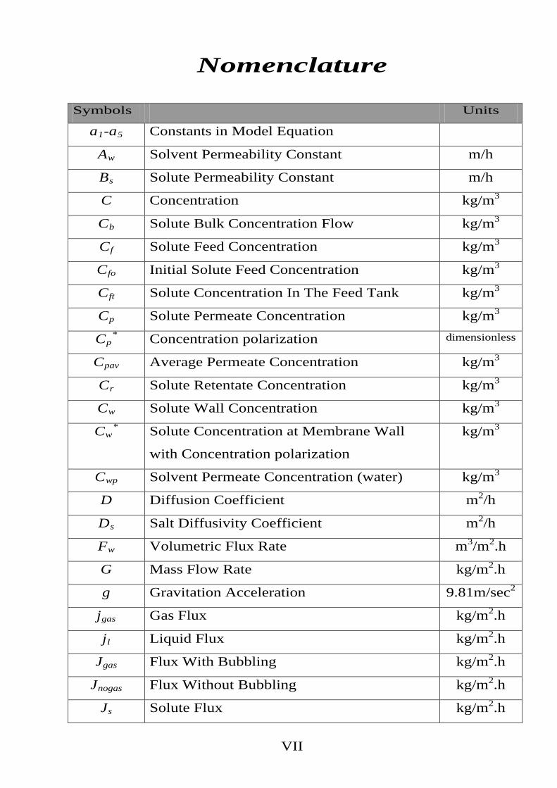
Nomenclature
Symbols Units
a1-a Constants in Model Equation 5
A Solvent Permeability Constant w m/h
B Solute Permeability Constant s m/h
C Concentration kg/m3
C Solute Bulk Concentration Flow b kg/m3
C Solute Feed Concentration f kg/m3
C Initial Solute Feed Concentration fo kg/m3
C Solute Concentration In The Feed Tank ft kg/m3
C Solute Permeate Concentration p kg/m3
Cp Concentration polarization * dimensionless
C Average Permeate Concentration pav kg/m3
C Solute Retentate Concentration r kg/m3
C Solute Wall Concentration w kg/m3
Cw Solute Concentration at Membrane Wall
with Concentration polarization
* kg/m3
C Solvent Permeate Concentration (water) wp kg/m3
D Diffusion Coefficient m2/h
D Salt Diffusivity Coefficient s m2/h
F Volumetric Flux Rate w m3/m2.h
G Mass Flow Rate kg/m2.h
g Gravitation Acceleration 9.81m/sec2
j Gas Flux gas kg/m2.h
j Liquid Flux l kg/m2.h
J Flux With Bubbling gas kg/m2.h
J Flux Without Bubbling nogas kg/m2.h
J Solute Flux s kg/m2.h
VIII
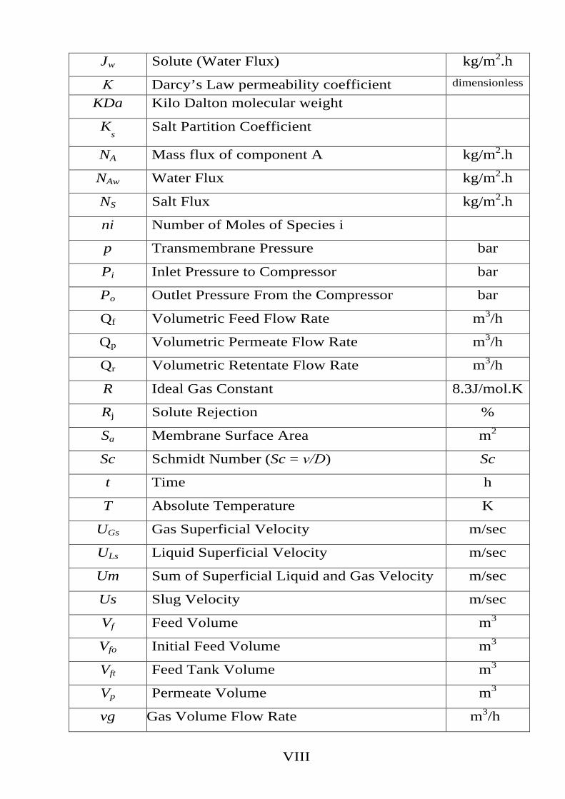
J Solute (Water Flux) w kg/m2.h
Κ Darcy’s Law permeability coefficient dimensionless
KDa Kilo Dalton molecular weight
Ks Salt Partition Coefficient
NA Mass flux of component A kg/m2.h
NAw Water Flux kg/m2.h
NS Salt Flux kg/m2.h
ni Number of Moles of Species i
p Transmembrane Pressure bar
Pi Inlet Pressure to Compressor bar
Po Outlet Pressure From the Compressor bar
Qf Volumetric Feed Flow Rate m3/h
Qp Volumetric Permeate Flow Rate m3/h
Qr Volumetric Retentate Flow Rate m3/h
R Ideal Gas Constant 8.3J/mol.K
Rj Solute Rejection %
Sa Membrane Surface Area m2
Sc Schmidt Number (Sc = ν/D) Sc
t Time h
T Absolute Temperature K
UGs Gas Superficial Velocity m/sec
ULs Liquid Superficial Velocity m/sec
Um Sum of Superficial Liquid and Gas Velocity m/sec
Us Slug Velocity m/sec
Vf Feed Volume m3
Vfo Initial Feed Volume m3
Vft Feed Tank Volume m3
Vp Permeate Volume m3
vg Gas Volume Flow Rate m3/h
IX
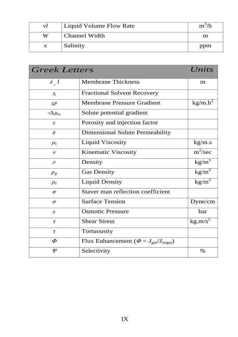
vl Liquid Volume Flow Rate m3/h
W Channel Width m
x Salinity ppm
Greek Letters Units δ , l Membrane Thickness m
∆ Fractional Solvent Recovery
P∆ Membrane Pressure Gradient kg/m.h2
-∆µw Solute potential gradient
ε Porosity and injection factor
θ Dimensional Solute Permeability
μl Liquid Viscosity kg/m.s
ν Kinematic Viscosity m2/sec
ρ Density kg/m3
ρg Gas Density kg/m3
ρl Liquid Density kg/m3
σ Staver man reflection coefficient
σ Surface Tension Dyne/cm
π Osmotic Pressure bar
τ Shear Stress kg.m/s2
τ Tortuousity
Φ Flux Enhancement (Φ = Jgas/Jnogas)
Ψ Selectivity %
X
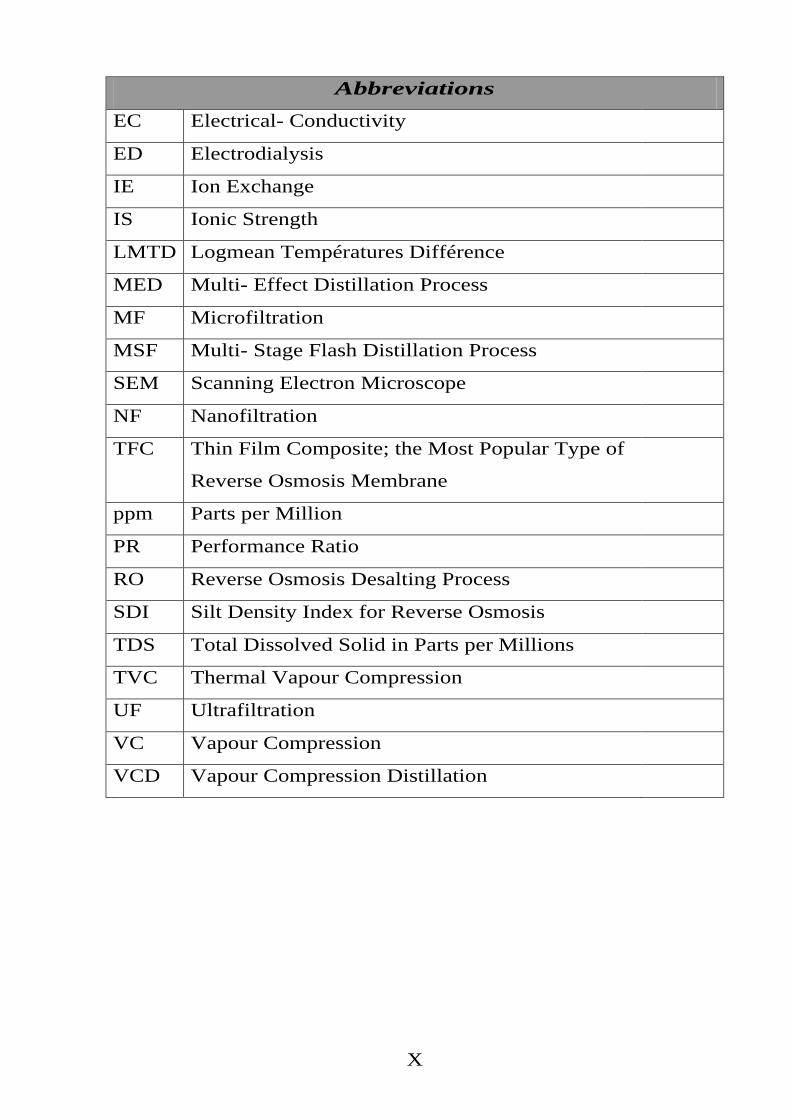
Abbreviations
EC Electrical- Conductivity
ED Electrodialysis
IE Ion Exchange
IS Ionic Strength
LMTD Logmean Températures Différence
MED Multi- Effect Distillation Process
MF Microfiltration
MSF Multi- Stage Flash Distillation Process
SEM Scanning Electron Microscope
NF Nanofiltration
TFC Thin Film Composite; the Most Popular Type of
Reverse Osmosis Membrane
ppm Parts per Million
PR Performance Ratio
RO Reverse Osmosis Desalting Process
SDI Silt Density Index for Reverse Osmosis
TDS Total Dissolved Solid in Parts per Millions
TVC Thermal Vapour Compression
UF Ultrafiltration
VC Vapour Compression
VCD Vapour Compression Distillation [
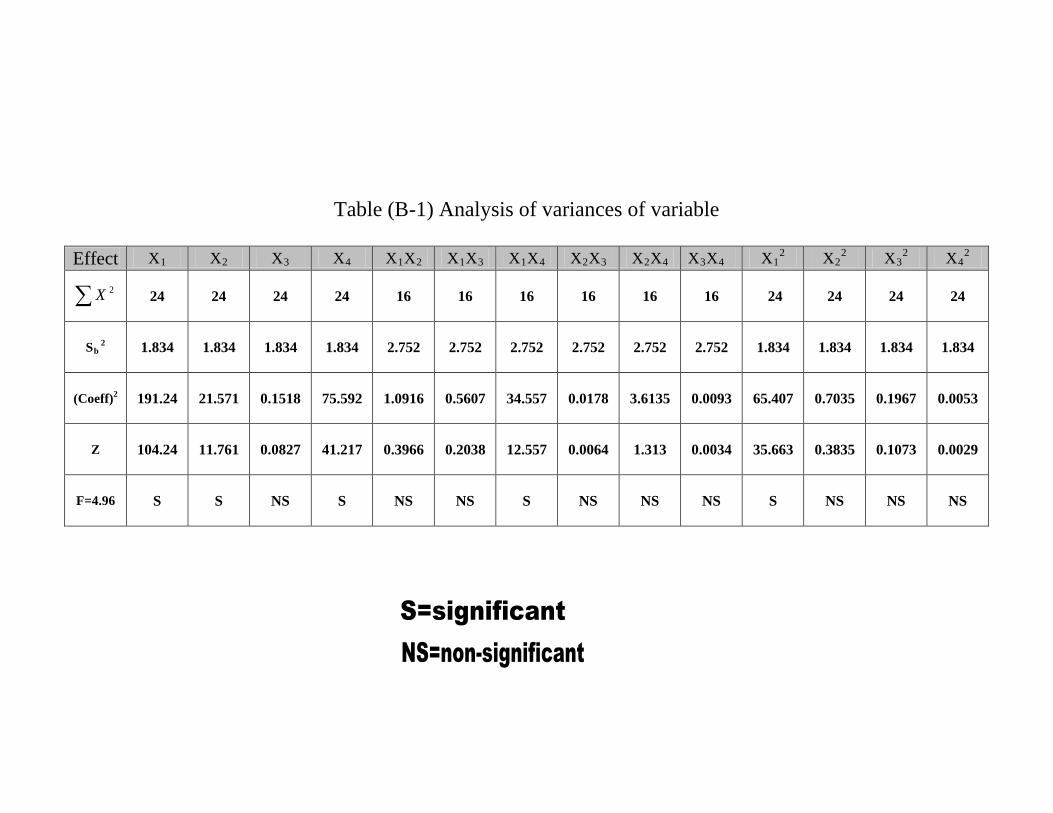
Table (B-1) Analysis of variances of variable
Effect X1 X2 X3 X4 X1X2 X1X3 X1X4 X2X3 X2X4 X3X4 X12
X22
X32
X42
∑ 2X
24
24 24 24 16 16 16 16 16
16
24
24
24
24
Sb
2 1.834
1.834 1.834 1.834 2.752 2.752 2.752 2.752 2.752 2.752 1.834 1.834 1.834 1.834
(Coeff)
2 191.24
21.571 0.1518 75.592 1.0916 0.5607 34.557 0.0178 3.6135
0.0093
65.407
0.7035
0.1967
0.0053
Z
104.24
11.761 0.0827 41.217 0.3966 0.2038 12.557 0.0064 1.313
0.0034
35.663
0.3835
0.1073
0.0029
F=4.96
S
S NS S NS NS S NS NS
NS
S
NS
NS
NS
Chapter One Introduction
1
Chapter One
Introduction
Desalination through the use of membranes was introduced in 1960s as an
alternative to distillation. A reverse osmosis membrane process is a physical
separation process, where salt is separated from seawater or brackish water to
produce drinking water.
Reverse osmosis (RO) is relatively new as compared to the distillation
processes. The first commercial unit was installed in Florida in 1971. The
reverse osmosis membrane separation process separates freshwater from
saltwater under high pressure where the freshwater passes through the
membrane layer while the salt content remains outside the membrane. The
amount of freshwater produced varies from 30 to 80% depending on the salt
content of the water, pressure and type of membranes used. Brackish water
membrane systems typically have higher recoveries and operate under lower
pressures, ranging from 225 psi to 375 psi. Seawater reverse osmosis systems
typically have lowers recoveries due to the higher salt content and their
operating range is typically 800 to 1200 psi (Beck, 2002).
Reverse osmosis is a process that transforms an unusable water supply
into a usable resource. It is capable of renovating a broad spectrum of feed
waters from municipal water supplies that need refinement for industrial
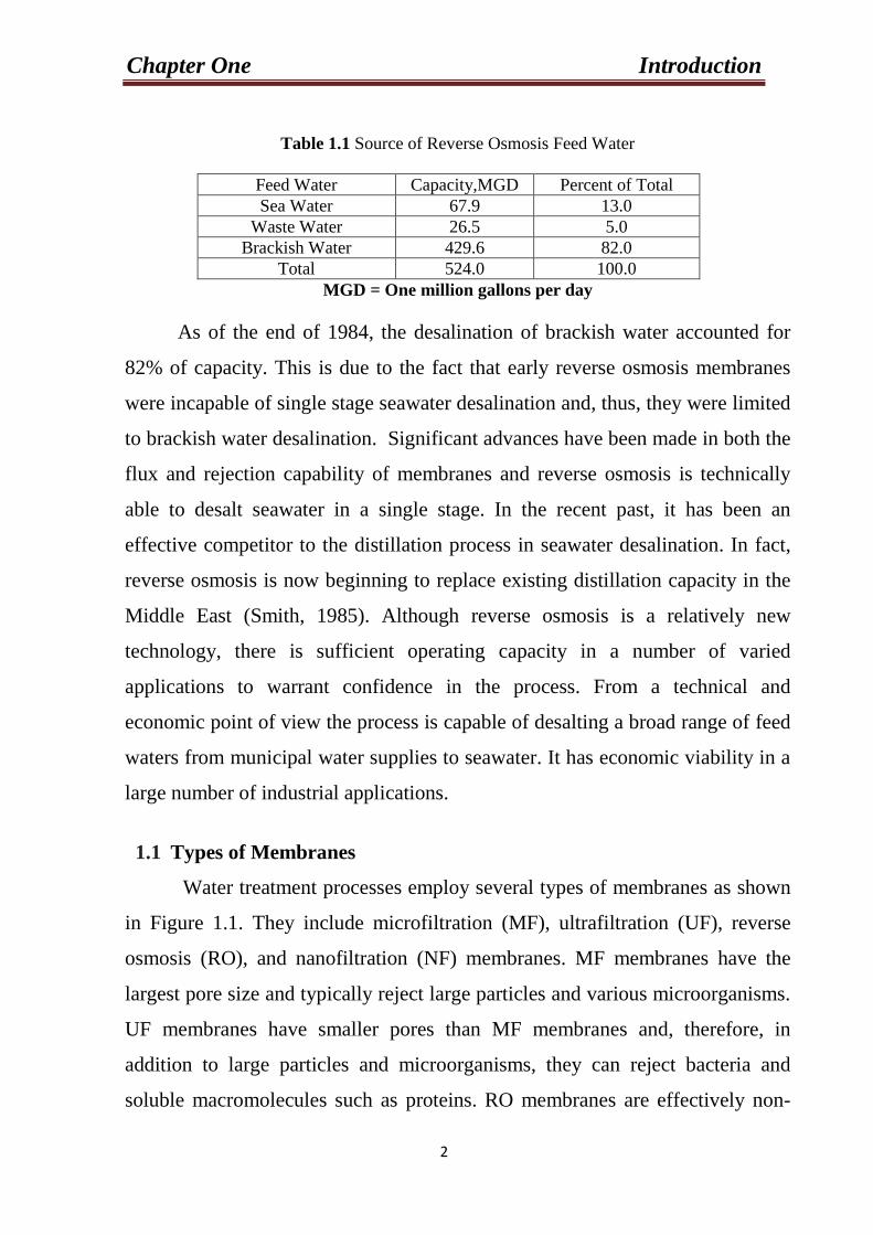
purposes to seawater that is refined into a potable water supply. Table 1.1 shows
the different types of feed water being processed by reverse osmosis units
(Mark, 1990). Seawater is considered to have nominal total dissolved solids
(TDS) content of 35,000 mg/l.
Chapter One Introduction
2
Table 1.1 Source of Reverse Osmosis Feed Water
Feed Water Capacity,MGD Percent of Total Sea Water 67.9 13.0
Waste Water 26.5 5.0 Brackish Water 429.6 82.0
Total 524.0 100.0 MGD = One million gallons per day
As of the end of 1984, the desalination of brackish water accounted for
82% of capacity. This is due to the fact that early reverse osmosis membranes
were incapable of single stage seawater desalination and, thus, they were limited
to brackish water desalination. Significant advances have been made in both the
flux and rejection capability of membranes and reverse osmosis is technically
able to desalt seawater in a single stage. In the recent past, it has been an
effective competitor to the distillation process in seawater desalination. In fact,
reverse osmosis is now beginning to replace existing distillation capacity in the
Middle East (Smith, 1985). Although reverse osmosis is a relatively new
technology, there is sufficient operating capacity in a number of varied
applications to warrant confidence in the process. From a technical and
economic point of view the process is capable of desalting a broad range of feed
waters from municipal water supplies to seawater. It has economic viability in a
large number of industrial applications.
1.1 Types of Membranes
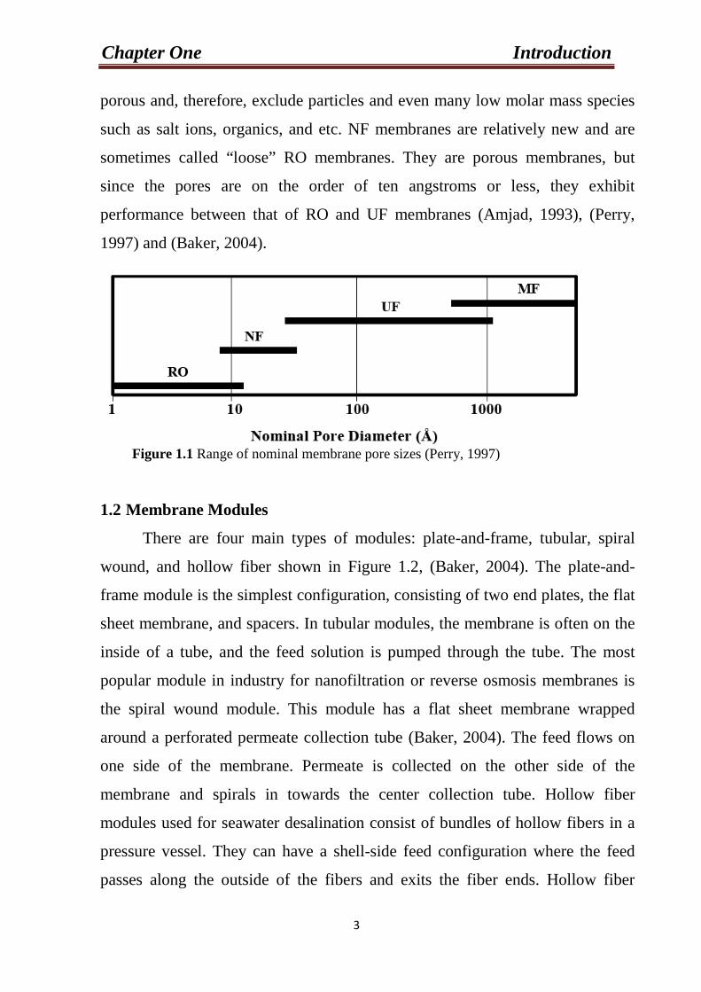
Water treatment processes employ several types of membranes as shown
in Figure 1.1. They include microfiltration (MF), ultrafiltration (UF), reverse
osmosis (RO), and nanofiltration (NF) membranes. MF membranes have the
largest pore size and typically reject large particles and various microorganisms.
UF membranes have smaller pores than MF membranes and, therefore, in
addition to large particles and microorganisms, they can reject bacteria and
soluble macromolecules such as proteins. RO membranes are effectively non-
Chapter One Introduction
3
porous and, therefore, exclude particles and even many low molar mass species
such as salt ions, organics, and etc. NF membranes are relatively new and are
sometimes called “loose” RO membranes. They are porous membranes, but
since the pores are on the order of ten angstroms or less, they exhibit
performance between that of RO and UF membranes (Amjad, 1993), (Perry,
1997) and (Baker, 2004).
Figure 1.1 Range of nominal membrane pore sizes (Perry, 1997) 1.2 Membrane Modules
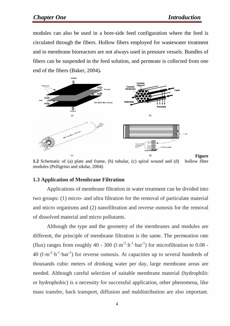
There are four main types of modules: plate-and-frame, tubular, spiral
wound, and hollow fiber shown in Figure 1.2, (Baker, 2004). The plate-and-
frame module is the simplest configuration, consisting of two end plates, the flat
sheet membrane, and spacers. In tubular modules, the membrane is often on the
inside of a tube, and the feed solution is pumped through the tube. The most
popular module in industry for nanofiltration or reverse osmosis membranes is
the spiral wound module. This module has a flat sheet membrane wrapped
around a perforated permeate collection tube (Baker, 2004). The feed flows on
one side of the membrane. Permeate is collected on the other side of the
membrane and spirals in towards the center collection tube. Hollow fiber
modules used for seawater desalination consist of bundles of hollow fibers in a
pressure vessel. They can have a shell-side feed configuration where the feed
passes along the outside of the fibers and exits the fiber ends. Hollow fiber
Chapter One Introduction
4
modules can also be used in a bore-side feed configuration where the feed is
circulated through the fibers. Hollow fibers employed for wastewater treatment
and in membrane bioreactors are not always used in pressure vessels. Bundles of
fibers can be suspended in the feed solution, and permeate is collected from one
end of the fibers (Baker, 2004).
Figure 1.2 Schematic of (a) plate and frame, (b) tubular, (c) spiral wound and (d) hollow fiber modules (Pelligrino and sikdar, 2004)
1.3 Application of Membrane Filtration
Applications of membrane filtration in water treatment can be divided into
two groups: (1) micro- and ultra filtration for the removal of particulate material
and micro organisms and (2) nanofiltration and reverse osmosis for the removal
of dissolved material and micro pollutants.
Although the type and the geometry of the membranes and modules are
different, the principle of membrane filtration is the same. The permeation rate
(flux) ranges from roughly 40 - 300 (l·mP
-2P·hP
-1P·barP
-1P) for microfiltration to 0.08 -
40 (l·mP
-2P·h P
-1P·barP
-1P) for reverse osmosis. At capacities up to several hundreds of
thousands cubic meters of drinking water per day, large membrane areas are
needed. Although careful selection of suitable membrane material (hydrophilic
or hydrophobic) is a necessity for successful application, other phenomena, like
mass transfer, back transport, diffusion and maldistribution are also important.
Chapter One Introduction
5
All these phenomena have a clear relation to the hydrodynamics in the
installation. In the design of membrane installations, these hydrodynamics play
an important role in the membrane (module design) and module arrangement
(plant design) to provide successful applications and limited energy
consumption and investment costs (Verberk, 2005).
1.4 Transport Phenomena in Membranes
The driving force for membrane filtration in water treatment is the
pressure gradient across the membrane. As a result of this driving force a
convective transport of material from the bulk to the membrane surface is
obtained. Solvent (water) permeates through the membrane and solutes
(dissolved and particulate material) are partly or completely retained by the
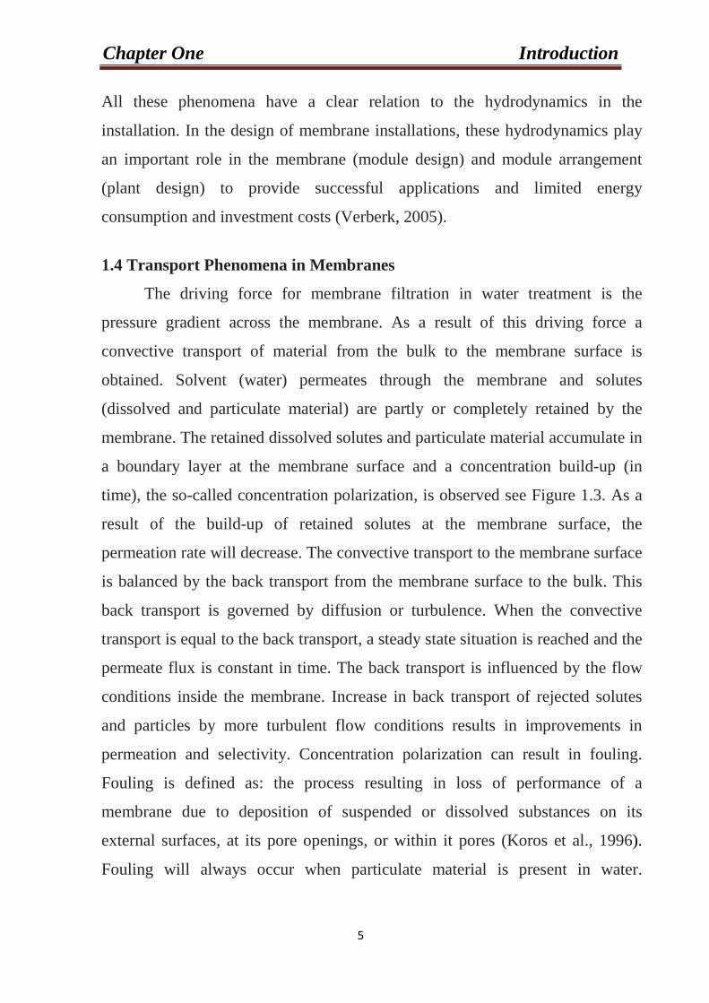
membrane. The retained dissolved solutes and particulate material accumulate in
a boundary layer at the membrane surface and a concentration build-up (in
time), the so-called concentration polarization, is observed see Figure 1.3. As a
result of the build-up of retained solutes at the membrane surface, the
permeation rate will decrease. The convective transport to the membrane surface
is balanced by the back transport from the membrane surface to the bulk. This
back transport is governed by diffusion or turbulence. When the convective
transport is equal to the back transport, a steady state situation is reached and the
permeate flux is constant in time. The back transport is influenced by the flow
conditions inside the membrane. Increase in back transport of rejected solutes
and particles by more turbulent flow conditions results in improvements in
permeation and selectivity. Concentration polarization can result in fouling.
Fouling is defined as: the process resulting in loss of performance of a
membrane due to deposition of suspended or dissolved substances on its
external surfaces, at its pore openings, or within it pores (Koros et al., 1996).
Fouling will always occur when particulate material is present in water.
Chapter One Introduction
6
Especially in micro- and ultra filtration the particulate fouling is a major point of
attention because rapid undesired flux decreases occur.
Figure 1.3 Concentration profiles of dissolved or particulate material and the main transport mechanisms in a membrane filtration process (Verberk, 2005)
1.5 Two-Phase Flow
Two-phase flow is the area of fluid mechanics that describes the flow of
mixtures consisting of two or more immiscible phases. Two-phase flow is the
simplest case of multi-phase flow. The different phases of multi-phase flow are
liquid, gas and solid. Two-phase flow is constantly met in our daily practice. For
example sandstorm, fog, snow and rain are natural examples of two-phase flow.
Two-phase flow is a well-known phenomenon in many industrial applications
(Wallis, 1969) and (Bachelor, 1989). Depending on the superficial velocities and
the pipe geometry different two-phase flow patterns occur, like bubble flow,
slug flow and annular flow. The segmented flow pattern slug flow is reported to
be very effective in small diameter tubes to increase heat and mass transfer rates
compared to single-phase flow. Slug flow was found to augment radial mass
transfer in reactors with catalytically active walls (Horvath, 1973). These results
suggest that slug flow could be a useful means to improve the efficiency of
Chapter One Introduction
7
many devices, which employ small diameter tubes and laminar flow by
enhancing radial mass transport or reducing axial dispersion. Such devices
include tubes with an absorbing wall for liquid chromatography or for selective
removal of solutes, reverse osmosis, or ultrafiltration systems having a semi-
permeable wall (Wallis, 1969). Water and air two-phase flow is already used in
water treatment processes. Well known examples are the water-air backwashing
of rapid sand filters and the water-air scouring of pipelines in the distribution
network.
From literature on heat and mass transfer, it is known that Taylor flow is a
specific two-phase flow pattern, results in an increased liquid-to-solid mass
transfer rate from bulk to wall compared to single phase liquid flow. This
increased mass transfer is caused by secondary rotating flows in the liquid slugs.
The increased mass transfer takes place at even lower pressure drops compared
to single phase flow (Kreutzer, 2003). In the automotive exhaust gas cleaning
Taylor flow is used to enhance mass transfer in monolith reactors. Monolith
reactors are ceramic structures of many parallel straight channels with a
diameter in the order of one millimeter. Based on structural configuration
membrane modules can be well compared with monoliths and the question
arises whether water-air two phase flow is also applicable in membrane filtration
processes to enhance the mass transfer. A major difference between monoliths
and membrane processes is the operational mode. In monoliths, the superficial
velocities are low compared to the velocities in membranes, so the extrapolation
of existing pressure loss equations, mass transfer relations and scale-up guide
lines are not directly possible.
Chapter One Introduction
8
1.6 Aim of the Present Work
This study focuses on investigating gas sparging as a technique to reduce
external fouling. In industrial membrane applications, membranes are typically
operated for several weeks before chemical cleaning. The main focus was on
monitoring the flux development with and without air sparging. Very rare work
was carried out in order to quantify the enhancement of permeates flux in
reverse osmosis membrane using sparging air. Slug flow is the most efficient
flow to enhance significantly the mass transfer in reverse osmosis membranes
when it is limited by particle deposit (Mercier et al; 1995). As a consequence,
this flow pattern has been chosen for the following study.
The aim of the present work can be summarized as follows:
1. Studying the effect of various operating conditions such as: concentration
(15-45) gm/l, temperature (10-50) °C, flow rates (100-250) l/hr and operating
pressure (5-15) bar ; on the performance of the reverse osmosis membrane ( type
(Sc-6200, spiral-wound model) by using NaCl as a feed solution. Flux of
permeate and salt rejection will be the main objective of this work.
2. Using experimental design (Box Wilson) methods in order to obtain the
proposed model (second order polynomial model) and its coefficient.
3. Obtaining maximum conditions for the proposed model by using optimization
program (Hook and Jeeves).
4. Sparging air in the system at different velocities of air after fixing the four
variables at the optimum conditions and different velocities of liquid at a fixed
velocity of air.
Chapter Two Theoretical Concepts and Literature Survey
9
Chapter Two
Theoretical Concepts and Literature Survey
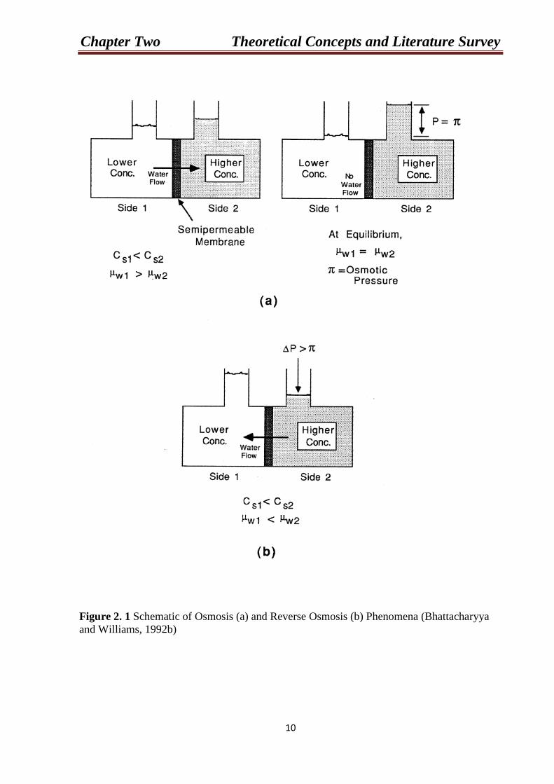
Osmosis is a natural phenomenon in which a solvent (usually water)
passes through a semi permeable barrier from the side with lower solute
concentration to the higher solute concentration side. As shown in Figure 2.1a,
water flow continues until chemical potential equilibrium of the solvent is
established. At equilibrium, the pressure difference between the two sides of the
membrane is equal to the osmotic pressure of the solution. To reverse the flow
of water (solvent), a pressure difference greater than the osmotic pressure
difference is applied see Figure 2.1b; as a result, separation of water from the
solution occurs as pure water flows from the high concentration side to the low
concentration side. This phenomenon is termed reverse osmosis (it has also been
referred to as hyper filtration). A reverse osmosis membrane acts as the semi
permeable barrier to flow in the RO process, allowing selective passage of a
particular species (solvent, usually water) while partially or completely retaining
other species (solutes). Chemical potential gradients across the membrane
provide the driving forces for solute and solvent transport across the membrane:
- Δ μ Rs R , the solute chemical potential gradient, is usually expressed in terms of
concentration; and - Δ μ RwR , the water (solvent) chemical potential gradient, is
usually expressed in terms of pressure difference across the membrane
(Bhattacharyya and Williams, 1992b).
Chapter Two Theoretical Concepts and Literature Survey
10
Figure 2. 1 Schematic of Osmosis (a) and Reverse Osmosis (b) Phenomena (Bhattacharyya and Williams, 1992b)
Chapter Two Theoretical Concepts and Literature Survey
11
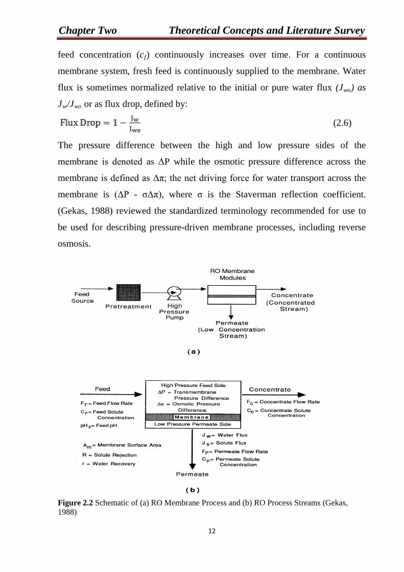
2.1 Reverse Osmosis Process Description and Terminology
The reverse osmosis process is relatively simple in design. It consists of a
feed water source, feed pretreatment, high pressure pump, reverse osmosis
membrane modules, and, in some cases, post treatment steps. A schematic of the
reverse osmosis process is shown in Figure 2.2a.
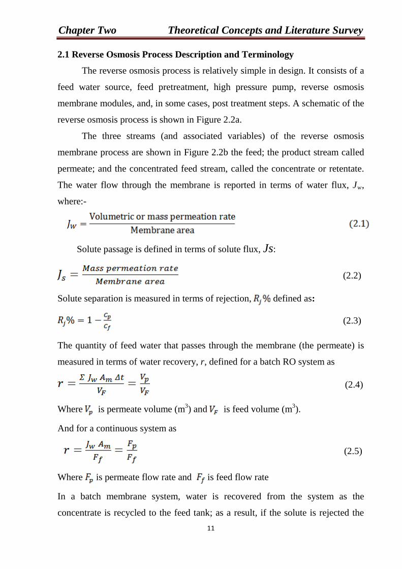
The three streams (and associated variables) of the reverse osmosis
membrane process are shown in Figure 2.2b the feed; the product stream called
permeate; and the concentrated feed stream, called the concentrate or retentate.
The water flow through the membrane is reported in terms of water flux, JRwR,
where:-
Solute passage is defined in terms of solute flux, Js:
(2.2)
Solute separation is measured in terms of rejection, defined as:
(2.3)
The quantity of feed water that passes through the membrane (the permeate) is
measured in terms of water recovery, r, defined for a batch RO system as
R R(2.4)
Where is permeate volume (mP
3P) and is feed volume (mP
3P).
And for a continuous system as
(2.5)
Where is permeate flow rate and is feed flow rate
In a batch membrane system, water is recovered from the system as the
concentrate is recycled to the feed tank; as a result, if the solute is rejected the
Chapter Two Theoretical Concepts and Literature Survey
12
feed concentration (cRfR) continuously increases over time. For a continuous
membrane system, fresh feed is continuously supplied to the membrane. Water
flux is sometimes normalized relative to the initial or pure water flux (JRwoR) as
JRwR/JRwoR or as flux drop, defined by:
(2.6)
The pressure difference between the high and low pressure sides of the
membrane is denoted as ΔP while the osmotic pressure difference across the
membrane is defined as Δπ; the net driving force for water transport across the
membrane is (ΔP - σΔπ), where σ is the Staverman reflection coefficient.
(Gekas, 1988) reviewed the standardized terminology recommended for use to
be used for describing pressure-driven membrane processes, including reverse
osmosis.
Figure 2.2 Schematic of (a) RO Membrane Process and (b) RO Process Streams (Gekas, 1988)
Chapter Two Theoretical Concepts and Literature Survey
13
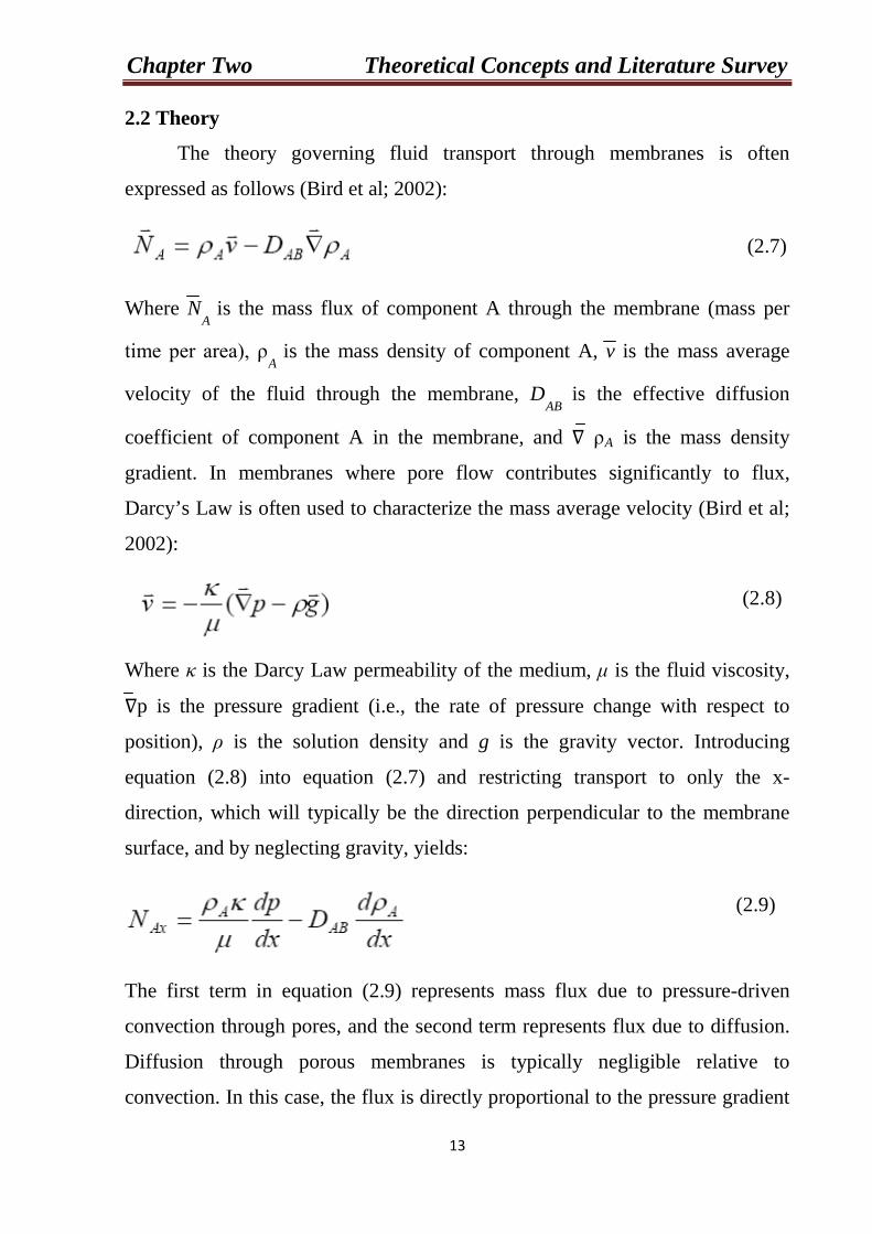
2.2 Theory
The theory governing fluid transport through membranes is often
expressed as follows (Bird et al; 2002):
Where NR
A R
is the mass flux of component A through the membrane (mass per
time per area), ρR
A R
is the mass density of component A, v is the mass average
velocity of the fluid through the membrane, DR
AB R
is the effective diffusion
coefficient of component A in the membrane, and ∇ ρRAR is the mass density
gradient. In membranes where pore flow contributes significantly to flux,
Darcy’s Law is often used to characterize the mass average velocity (Bird et al;
2002):
Where κ is the Darcy Law permeability of the medium, μ is the fluid viscosity,
∇p is the pressure gradient (i.e., the rate of pressure change with respect to
position), ρ is the solution density and g is the gravity vector. Introducing
equation (2.8) into equation (2.7) and restricting transport to only the x-
direction, which will typically be the direction perpendicular to the membrane
surface, and by neglecting gravity, yields:
The first term in equation (2.9) represents mass flux due to pressure-driven
convection through pores, and the second term represents flux due to diffusion.
Diffusion through porous membranes is typically negligible relative to
convection. In this case, the flux is directly proportional to the pressure gradient
(2.7)
(2.8)
(2.9)
Chapter Two Theoretical Concepts and Literature Survey
14
across the membrane. The applied pressure difference across the membrane
which often called the transmembrane pressure difference is the driving force
governing transport of liquid through a porous membrane.
In applying the convective term of equation (2.9) to transport through UF
and MF membranes, the permeability, κ, depends often in a complex way, on
factors such as the porosity and the tortuosity of the membrane. Tortuosity, τ, is
the ratio of the average length of the “tortuous” path that the fluid must travel to
pass through the membrane to the membrane thickness. For example, a
cylindrical pore perpendicular to the surface has a tortuousity of one. Most
phase inversion membranes have tortuousities from 1.5 to 2.5 (Baker, 2004).
Porosity, ε, is the void fraction of the membrane. UF and MF membrane
porosity typically ranges from 0.3 to 0.7 (Baker, 2004).
Since RO membranes are effectively non-porous, the transport of a
molecule across the membrane is diffusion controlled. This means that the
second term of equation (2.9) controls the flux across the membrane. Water
molecules desorb into the upstream face of the membrane, diffuse down the
chemical potential gradient across the membrane, and then desorbed from the
downstream face of the membrane. The second step, diffusion through the
membrane, is the rate-determining step in water transport across the membrane.
This mechanism of mass transport across membranes is commonly referred to as
the “solution- diffusion” modelP
P(Bird et al; 2002).
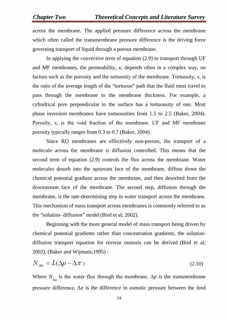
Beginning with the more general model of mass transport being driven by
chemical potential gradients rather than concentration gradients, the solution-
diffusion transport equation for reverse osmosis can be derived P
P(Bird et al;
2002), (Baker and Wijmans,1995) :
Where NR
Aw R
is the water flux through the membrane, Δp is the transmembrane
pressure difference, Δπ is the difference in osmotic pressure between the feed
(2.10)
Chapter Two Theoretical Concepts and Literature Survey
15
and the permeate, and L is a constant describing the physical characteristics of
the membrane itself. Within the context of the solution-diffusion model used to
describe transport in nonporous films, L is given byP
P(Baker and Wijmans, 1995):
Where D is the water diffusivity in the membrane, S is the water solubility in the
membrane, V is the molar volume of water, R is the ideal gas constant, T is the
ambient temperature, and l is the membrane thickness. A complete derivation
can be found in the Baker and Wijmans review of the solution-diffusion model
(Baker and Wijmans, 1995) and in Paul’s recent re-examination of the solution-
diffusion model for reverse osmosisP
P(Paul, 2004).
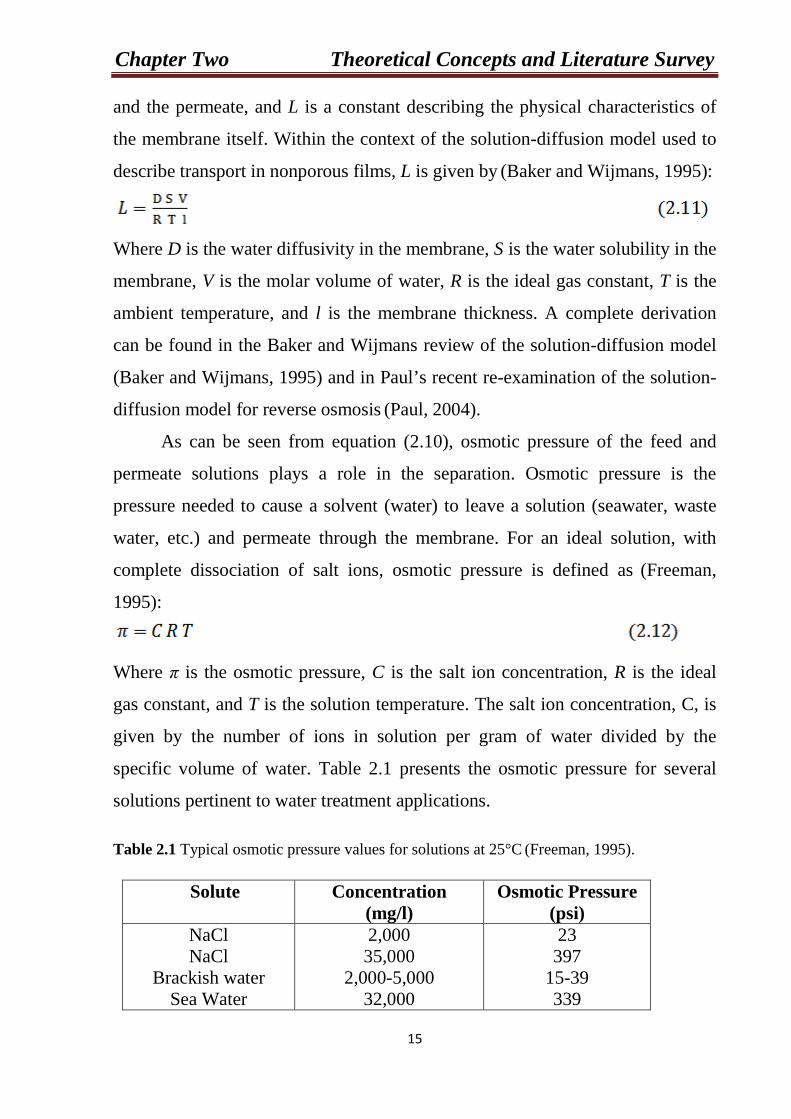
As can be seen from equation (2.10), osmotic pressure of the feed and
permeate solutions plays a role in the separation. Osmotic pressure is the
pressure needed to cause a solvent (water) to leave a solution (seawater, waste
water, etc.) and permeate through the membrane. For an ideal solution, with
complete dissociation of salt ions, osmotic pressure is defined as P
P(Freeman,
1995):
Where π is the osmotic pressure, C is the salt ion concentration, R is the ideal
gas constant, and T is the solution temperature. The salt ion concentration, C, is
given by the number of ions in solution per gram of water divided by the
specific volume of water. Table 2.1 presents the osmotic pressure for several
solutions pertinent to water treatment applications. Table 2.1 Typical osmotic pressure values for solutions at 25°CP
P(Freeman, 1995).
Solute Concentration
(mg/l) Osmotic Pressure
(psi) NaCl NaCl
Brackish water Sea Water
2,000 35,000
2,000-5,000 32,000
23 397
15-39 339
Chapter Two Theoretical Concepts and Literature Survey
16
In reverse osmosis, salt transport across a membrane is as important as
water transport. However, unlike water flux, which is driven by both applied
transmembrane pressure and osmotic pressure, the salt flux is only a function of
salt concentrationP
P(Baker and Wijmans, 1995):
Where NR
s R
is the salt flux through the membrane, B is the salt permeability
constant describing the physical characteristics of the membrane, R R
is the salt
concentration in the feed solution, and R R
is the salt concentration in the
permeate solution. Analogous to L in the solution-diffusion equation, B is given
byP
P(Baker and Wijmans, 1995):
Where DR
s R
is the salt diffusivity in the membrane, KR
s R
is the salt partition
coefficient, and l is the membrane thickness. However, instead of reporting salt
flux values, most membrane performance specifications provide salt rejection
values.
Furthermore, water flux and salt flux depend on each other. Equation (2.15)
relates the water flux, NR
AwR
, to the salt flux, NR
sRP
P(Riley et al; 1967):
Where CR
w R
is the water concentration in permeate and R R
is the salt concentration
in permeate. By substituting equation (2.10) and equation (2.13) into equation
(2.15) and rearranging terms, the following expression for rejection may be
derivedP
P(Riley et al; 1967):
Chapter Two Theoretical Concepts and Literature Survey
17
Equation (2.16) relates salt rejection to the physical properties of the
membrane (which influence L and B), the applied transmembrane pressure
difference, and the osmotic pressure difference between permeate and the feed.
Equation (2.16) allows one to predict the salt rejection of the membrane based
on the experimental conditions and the membrane properties.
2.3 Factors Affecting Flux
2.3.1 Operating Parameter
There are four major operating parameters that affect the flux: (1)
pressure, (2) feed concentration, (3) temperature, and (4) turbulence in the feed
channel (flow rate).
1. Pressure
The major parameter that directly influences the energy consumption of
the RO plant is the feed pressure. The higher feed pressure is the higher energy
consumption of the plant. The permeate production strongly depends on the feed
pressure. Whereas the feed pressure influences the two primary operating
parameters, productivity and product water conductivity. The pressure drop
affects the mechanical stability of the RO equipment. In a spiral-wound system,
the pressure drop translates into a force directly on the membrane element and
also on the product tube (Herold ., 2001).
2. Feed Concentration
The film theory model states that the flux will decrease exponentially with
increasing feed concentration. This relationship should hold true regardless of
the type of flow or degree of turbulence or the temperature (Munir, 1998).
3. Temperature
In General, higher temperatures will lead to higher flux in both the
pressure controlled region and in the mass transfer-controlled region, this
assumes there are no other unusual effects occurring simultaneously, such as
fouling of the membrane due to precipitation of insoluble salts at higher
Chapter Two Theoretical Concepts and Literature Survey
18
temperatures or denaturation of proteins or gelatinization of starch at higher
temperatures. In the pressure controlled region, the effect of temperature on flux
is due to its effect on fluid density and viscosity. Activation energies for both
flux and viscosity are similar in the region of 20-50°C, about 3400 kcal/mole. In
practical terms,it will take a temperature rise of 30-45°C to double the flux
(Munir, 1998).
4. Flow Rate and Turbulence
Turbulence, whether produced by stirring, pumping the fluid, or vibrating
the membrane, has a large effect on flux in the mass transfer-controlled region.
Agitation and mixing of the fluid near the membrane surface "sweep" away the
accumulated solute, reducing the hydraulic resistance of the "cake" and reducing
thickness of the boundary layer. There is also a belief that extremely high shear,
such as that obtained with thin - channel and rotary device, actually reduce the
thickness of the "gel" layer. In any case, this is one of the simplest and most
effective methods of controlling the effects of concentration polarization (Munir,
1998).
2.3.2 PH of Feed
The pH of the feed water must be measured and controlled in reverse
osmosis desalination of water for several reasons. The first is to prevent CaCOR3R
precipitation. The second reason is to maximize the life of membrane of the
cellulose acetate type. Cellulose acetate is an ester which reacts slowly with
water to form an alcohol and an acid. The rate of this reaction, which is called
hydrolysis, is dependent on both pH and temperature.
The minimum hydrolysis rate at a particular temperature occurs at a pH of
(4.5-5) as the hydrolysis continues, the passage through the membrane of both
water and salt increases. The salt passage increases the product water
conductivity. In the operation of cellulose acetate membrane, the pH is reduced
to pH 6 or less in order to slow the hydrolysis rate to a value which permits long
term operation (Mindler & Epstein, 1986).
Chapter Two Theoretical Concepts and Literature Survey
19
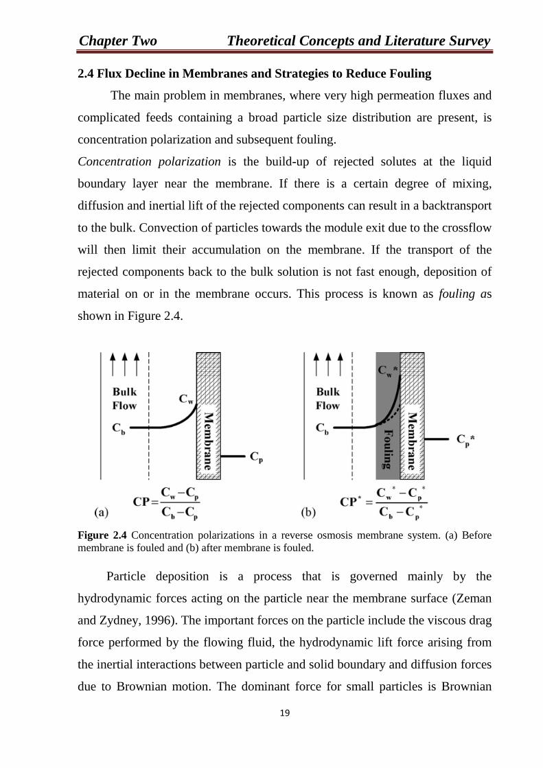
2.4 Flux Decline in Membranes and Strategies to Reduce Fouling
The main problem in membranes, where very high permeation fluxes and
complicated feeds containing a broad particle size distribution are present, is
concentration polarization and subsequent fouling.
Concentration polarization is the build-up of rejected solutes at the liquid
boundary layer near the membrane. If there is a certain degree of mixing,
diffusion and inertial lift of the rejected components can result in a backtransport
to the bulk. Convection of particles towards the module exit due to the crossflow
will then limit their accumulation on the membrane. If the transport of the
rejected components back to the bulk solution is not fast enough, deposition of
material on or in the membrane occurs. This process is known as fouling as
shown in Figure 2.4.
Figure 2.4 Concentration polarizations in a reverse osmosis membrane system. (a) Before membrane is fouled and (b) after membrane is fouled.
Particle deposition is a process that is governed mainly by the
hydrodynamic forces acting on the particle near the membrane surface (Zeman
and Zydney, 1996). The important forces on the particle include the viscous drag
force performed by the flowing fluid, the hydrodynamic lift force arising from
the inertial interactions between particle and solid boundary and diffusion forces
due to Brownian motion. The dominant force for small particles is Brownian
Chapter Two Theoretical Concepts and Literature Survey
20
motion, which is responsible for the equilibrium state in macrosolute-membrane
interactions. As the particle size increases, the importance of Brownian diffusion
decreases since it becomes too slow. Deposition of bigger particles will occur
when the forces towards the membrane surface are greater than the repulsive
interactions between particles, inertial lift forces and shear-induced diffusion.
The analysis of the flux decline due to particle deposition is of special
importance since it can provide some insight to the phenomena that take place
during microfiltration. Depending on the solute and the process conditions,
different blocking mechanisms that explain the flux decline during membrane
filtration has been developed (Hermia, 1982), (Bowen et al, 1995) and
(Wessling, 2001):
– Complete blocking (pore blocking)
– Standard blocking (pore narrowing)
– Intermediate blocking (long term deposition)
– Cake formation (gel/cake layer)
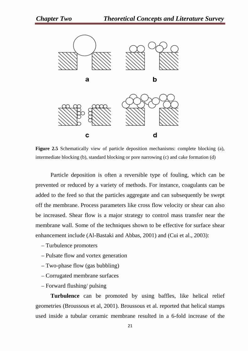
These mechanisms are schematically shown in Figure 2.5. Pore blocking (a) is
caused by rejected particles bigger than the membrane pores. This mechanism
assumes that each particle arriving at the membrane contributes in the complete
inactivation of one or more pores, causing a dramatic flux decline. Pore
narrowing (c) is mostly caused by smaller components that can adhere to the
internal pore wall, accumulate or bridge and finally clog the pore. Intermediate
blocking (b) is the stage preceding cake layer formation (d). A cake layer is
formed when each particle arriving to the surface accumulates on each other,
thus completely blocking the membrane surface. The flux decline due to
particles can be governed by one mechanism but it can also be a combination of
more than one. Although these mechanisms are developed for the filtration of
proteins, they are also valid for different types of solutes.
Chapter Two Theoretical Concepts and Literature Survey
21
Figure 2.5 Schematically view of particle deposition mechanisms: complete blocking (a),
intermediate blocking (b), standard blocking or pore narrowing (c) and cake formation (d)
Particle deposition is often a reversible type of fouling, which can be
prevented or reduced by a variety of methods. For instance, coagulants can be
added to the feed so that the particles aggregate and can subsequently be swept
off the membrane. Process parameters like cross flow velocity or shear can also
be increased. Shear flow is a major strategy to control mass transfer near the
membrane wall. Some of the techniques shown to be effective for surface shear
enhancement include (Al-Bastaki and Abbas, 2001) and (Cui et al., 2003):
– Turbulence promoters
– Pulsate flow and vortex generation
– Two-phase flow (gas bubbling)
– Corrugated membrane surfaces
– Forward flushing/ pulsing
Turbulence can be promoted by using baffles, like helical relief
geometries (Broussous et al, 2001). Broussous et al. reported that helical stamps
used inside a tubular ceramic membrane resulted in a 6-fold increase of the
Chapter Two Theoretical Concepts and Literature Survey
22
permeate flux compared to using smooth surfaces (Broussous et al, 1998). Dean
vortices, which are centrifugal instabilities produced in curved channels when
the critical Dean number is exceeded, have also been a mean to improve the flux
of dairy whey and Baker’s yeast (Winzeler and Belfort, 1993), (Luque et al,
1999).
The injection of air bubbles or gas sparging is a resource to enhance
mass transfer. The secondary flows and bubbles promote mixing and reduce the
thickness of the concentration polarization layer. When the bubble diameter
exceeds the channel diameter (from the module, in flat sheets, or from the
hollow fibers) slugs are formed, which can displace the boundary layer and
cause the local pressure to fluctuate. Another flow regime commonly observed
is bubble flow, which occurs when the gas bubbles are significantly smaller than
the fiber or channel size (Cui et al., 2003). Air sparging in combination with
hollow-fiber or flat-sheet UF membranes is very useful to enhance the flux of
dextrans and proteins ( Bellara et al.,1996) enzymes or microparticles ( Laborie
et al.,1998) or more specifically, to fractionate protein mixtures ( Li et al.,1998).
In microfiltration, the main uses are related to enhance yeast filtration (Sur and
Cui, 2001), (Mercier et al., 1998). Other applications include air sparging in
membrane bed reactors for wastewater treatment (Chang and Judd, 2002) and
nanofiltration (Ducom and Cabassud, 2002), (Ducom and Cabassud, 2003) the
enhancement of permeate flux by gas bubbling is clearly demonstrated in all
these studies.
Flow instabilities can also be induced by pulses, with approaches like
backflushing, forward flushing or backpulsing. These strategies are generally
considered as cleaning methods because they remove deposited matter from the
surface. Backflushing and backpulsing are based on temporary permeate flow
reversal; while crossflushing is the stoppage of permeate flow while crossflow is
maintained. The main difference between a backpulse and a backflush is the
force and time used to lift accumulated deposits off the membrane. Generally, in
Chapter Two Theoretical Concepts and Literature Survey
23
backflushing flow reversal occurs for a few seconds once every several minutes,
while backpulsing occurs at a higher frequency and the pulses are applied for a
short time (< 1s) (Sondhi and Bhave, 2001) , ( Kuberkar and Davis, 1998). The
efficiency of both techniques depends strongly on the frequency, pulse duration,
pressure, etc. (Levesley and Hoare, 1999) used high frequency backflushing (1s
pulse at 1 Hz frequency) for the microfiltration of yeast homogenate suspensions
using a ceramic tubular membrane. Backflushing resulted in a 5.4 times
increased solute flux compared to the non-backflushing situation. (Kuberkar
and Davis, 1998) used high-frequency short backpulses (0.1-1 s) to increase the
permeate flux of washed bacterial suspensions and bacterial fermentation broths.
Washed bacterial suspensions were easier to backpulse, in comparison to
bacterial fermentation broths, due to lower concentration of suspended
components. (Parnham and Davis, 1996) reported higher flux of proteins from
bacterial cell debris by applying high-frequency backpulsing. Beolchini and
coworkers also emphasized the importance of backpulsing with skimmed bovine
milk filtration using ceramic tubular membranes with a pore diameter around
1.4µm (Beolchini et al, 2004). Backpulsing was required in order to reduce
membrane fouling and achieve milk permeation.
For adherent foulants and irreversible fouling other approaches than the
ones discussed above are generally used. Irreversible fouling is triggered by
hydrophobic interactions, hydrogen bonding, van der Waals attractions and
other effects. Some of the methods to eliminate this kind of fouling are based on
modifying the membrane surface by moieties that repel certain components or
change the surface charge of the material. Physically coating the surface with
water-soluble polymers or surfactants for a temporary effect, or grafting
monomers by UV or electron beam irradiation are also frequently reported
techniques.
Chapter Two Theoretical Concepts and Literature Survey
24
2.5 Two - Phase Flow
Part of the definition of the flow regime is a description of the
morphological arrangement of the components, or flow pattern. The flow pattern
is often obvious from visual or photographic observations but is not adequate to
define the regime completely because of additional distinguishing criteria, such
as the difference between laminar and turbulent flow and the relative importance
of various forces. In order to keep the terminology manageable, the numerous
imaginative expressions which have been used throughout the literatures to
describe flow patterns will not be quoted. It is far simpler to restrict
classification to the morphological flow patterns (for example, bubbly, slug,
annular, and drop flow in gas-liquid system) and create further subdivision into
distinct regimes within each of these classifications. Hybrid flow patterns,
usually representing a region of transition from one pattern to another, are
denoted by hyphenated expression (thus, slug-annular and annular-drop flows).
Some synonyms (e.g., “fog” or “mist” instead of “drop”) may be used when
perfunctory repetition of a single word becomes monotonous (Wallis, 1969).
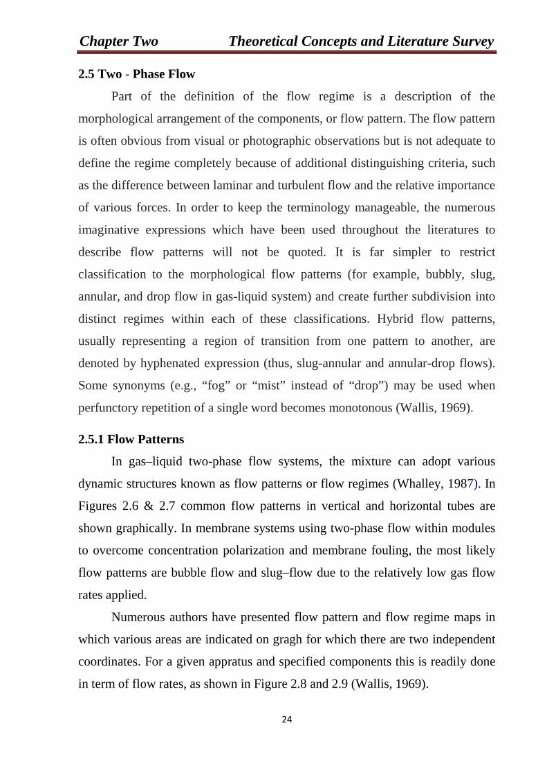
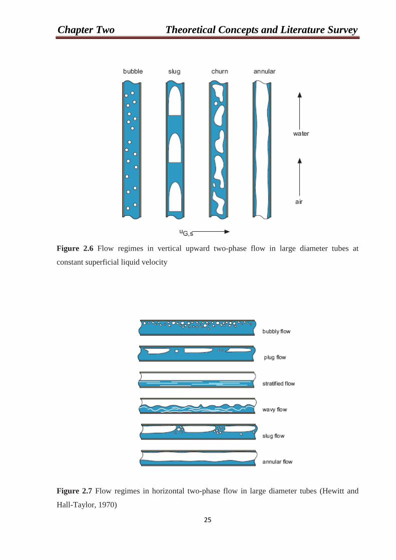
2.5.1 Flow Patterns
In gas–liquid two-phase flow systems, the mixture can adopt various
dynamic structures known as flow patterns or flow regimes (Whalley, 1987). In
Figures 2.6 & 2.7 common flow patterns in vertical and horizontal tubes are
shown graphically. In membrane systems using two-phase flow within modules
to overcome concentration polarization and membrane fouling, the most likely
flow patterns are bubble flow and slug–flow due to the relatively low gas flow
rates applied.
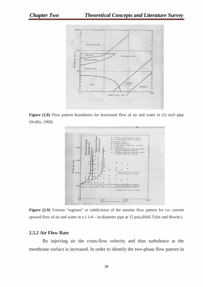
Numerous authors have presented flow pattern and flow regime maps in
which various areas are indicated on gragh for which there are two independent
coordinates. For a given appratus and specified components this is readily done
in term of flow rates, as shown in Figure 2.8 and 2.9 (Wallis, 1969).
Chapter Two Theoretical Concepts and Literature Survey
25
Figure 2.6 Flow regimes in vertical upward two-phase flow in large diameter tubes at
constant superficial liquid velocity
Figure 2.7 Flow regimes in horizontal two-phase flow in large diameter tubes (Hewitt and
Hall-Taylor, 1970)
Chapter Two Theoretical Concepts and Literature Survey
26
Figure (2.8) Flow pattern boundaries for horizontal flow of air and water in (1) inch pipe
(Wallis, 1969)
Figure (2.9) Various “regimes” or subdivision of the annular flow pattern for co- current
upward flow of air and water in a 1 1/4 – in-diameter pipe at 15 psia.(Hall-Tylor and Hewitt.)
2.5.2 Air Flow Rate
By injecting air the cross-flow velocity and thus turbulence at the
membrane surface is increased. In order to identify the two-phase flow pattern in
Chapter Two Theoretical Concepts and Literature Survey
27
the membranes the injection factor ε is sometimes used. This factor is defined
as:
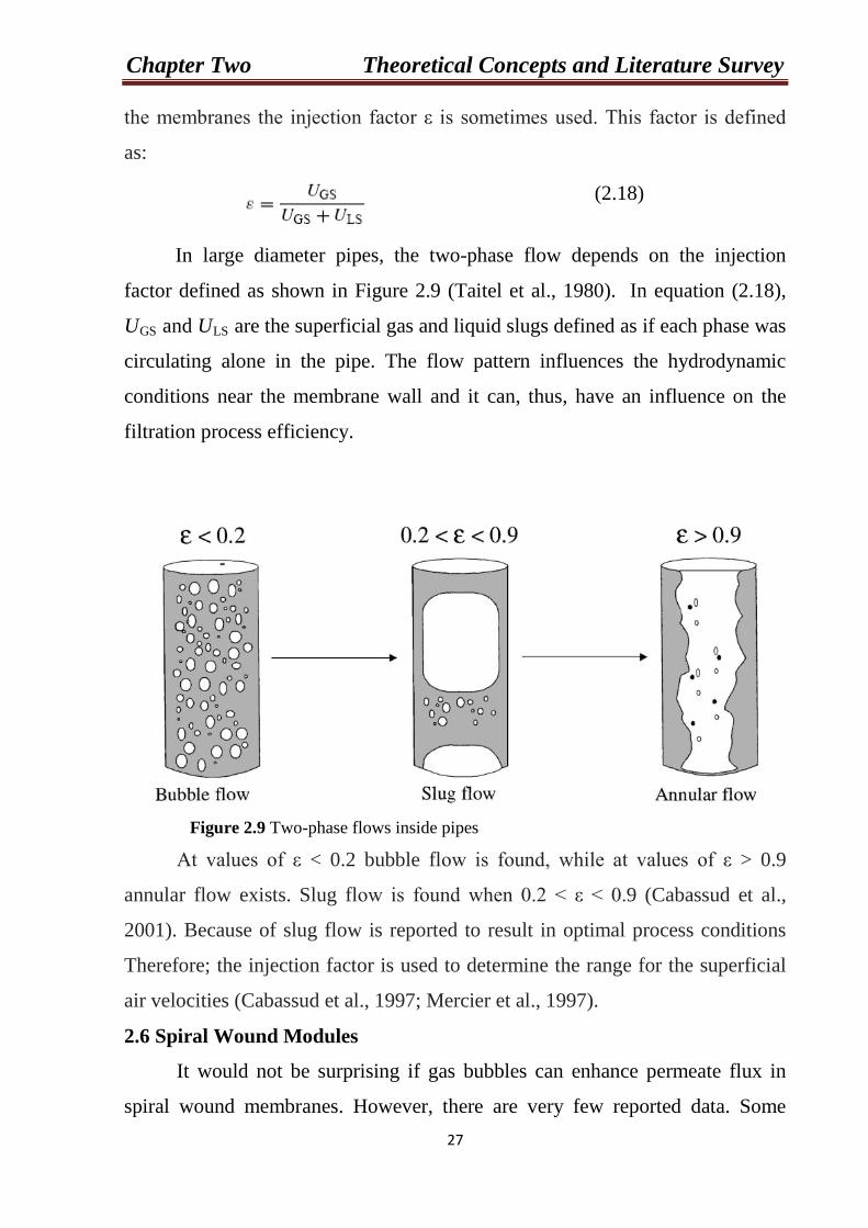
In large diameter pipes, the two-phase flow depends on the injection
factor defined as shown in Figure 2.9 (Taitel et al., 1980). In equation (2.18),
URGSR and URLSR are the superficial gas and liquid slugs defined as if each phase was
circulating alone in the pipe. The flow pattern influences the hydrodynamic
conditions near the membrane wall and it can, thus, have an influence on the
filtration process efficiency.
Figure 2.9 Two-phase flows inside pipes
At values of ε < 0.2 bubble flow is found, while at values of ε > 0.9
annular flow exists. Slug flow is found when 0.2 < ε < 0.9 (Cabassud et al.,
2001). Because of slug flow is reported to result in optimal process conditions
Therefore; the injection factor is used to determine the range for the superficial
air velocities (Cabassud et al., 1997; Mercier et al., 1997).
2.6 Spiral Wound Modules
It would not be surprising if gas bubbles can enhance permeate flux in
spiral wound membranes. However, there are very few reported data. Some
(2.18)
Chapter Two Theoretical Concepts and Literature Survey
28
preliminary data (Cui, 1993) were obtained using an l00 kDa spiral wound UF
membrane for solutions of dextrans of different molecular weights. Injecting
bubbles had a positive effect on permeate flux, particularly when concentration
polarization was severe, for the largest MW dextran. The flux enhancement
ranged up to about 25%. The results were obtained with a vertically aligned
spiral module to avoid trapping gas within the module, and with a relative low
flow rate gas injection. The need for vertical alignment, and distribution of
bubbles in the system could limit the use of bubbling in spiral wound systems
(Cui et al., 2003).
2.7 Previous Studies for Sparging Air in Membrane
Membranes are widely used in the chemical, pharmaceutical, food and
water industries. Practical difficulties arise in designing and operating the
process due to concentration polarization and membrane fouling. In membrane
processes, fouling remains the main drawback and the toughest challenge at
present and in the foreseeable future. Enhancement of membrane is highly
desirable to achieve a higher permeate flux at a fixed energy input, or a reduced
energy input whilst maintaining the level of permeate flux, or an improved
selectivity of the membrane. One effective, simple, and economic technique
used to enhance membrane is the use of gas bubbles, i.e. injecting gas into the
feed stream to create a gas– liquid two-phase cross-flow operation. In this
regard, in the last years some studies have pointed out the value of air sparging
to enhance the flux in ultrafiltration, microfiltration and nanofiltration for
different applications — drinking water production(Cui and Taha,2003).
A novel membrane filtration system was proposed by Takuo et al 1993
with the aim of saving energy. That is, a gas-liquid two-phase crossflow
filtration was combined in the anaerobic bioreactor. It was confirmed that the
membrane filtration not only offered very stable and large permeate flux, but
enhanced the processing efficiency by retaining the microorganisms in the
Chapter Two Theoretical Concepts and Literature Survey
29
bioreactor. Furthermore, the power consumption per unit permeates volume in
the membrane system.
Cui and Wright; 1994 proposed a method for reducing concentration
polarisation and membrane fouling by injecting air into the feed stream, creating
a gas-liquid two-phase flow across the membrane surface. The injected air
promotes turbulence, increasing the superficial cross-flow velocity of the
process fluid, suppressing the polarisation layer and enhancing the ultrafiltration
process. On the addition of air to the liquid stream, permeate flux was observed
to increase by up to 60% for dextran, 113% for dyed dextran and 91% for BSA.
Mercier et al; 1995 used an easy technique, consisting in injecting air into
the liquid stream, is proposed to enhance the permeate flux in cross flow
filtration of a model fluid (i.e. a bentonite suspension). The injected air promotes
turbulence and increases the superficial cross flow velocity that leads to a
regular disturbance of the boundary layer. A systematic study of different two-
phase configurations points up that the slug flow seems the most appropriate
regime. The resulting permeate rate is increased up to 140%, in comparison with
the usual filtration processes.
Gas-liquid two-phase crossflow ultrafiltration was studied in downwards
flow condition by Cui and Wright; 1996. Flux increases up to 320% were
achieved with gas sparging in the experimental study compared to single liquid
phase crossflow ultrafiltration.
Bellara et al; 1996 focused on the use of gas-liquid two-phase crossflow to
overcome concentration polarization in the ultrafiltration of macromolecular
solutions as applied to hollow fibre membrane systems. The results were
encouraging, with flux enhancements of 20-50% obtained for dextran and 10-
60% for albumin, when air was injected into the system over the range of
process variables examined.
The use of a gas-liquid two-phase flow by injecting air directly into the
feed stream was studied by Mercier et al; 1997. The experimental study was
Chapter Two Theoretical Concepts and Literature Survey
30
carried out by filtering suspensions (bentonite and yeast) through an
ultrafiltration to reduce tubular mineral membrane fouling. Results related to the
permeate flux showed an enhancement by a factor of 3, with a slug flow-
structure for the two kinds of suspension (200% of flux increase).
A new process is proposed to reduce particulate membrane fouling by
injecting air into the feed stream, creating a gas/liquid two-phase flow on the
membrane surface by Laborie et al; 1997. The air injection process led to an
increase in the permeate flux, depending on the liquid velocity and
transmembrane pressure, for all the various feed concentrations. For specific
conditions, the flux can be increased by 155% using a critical gas velocity.
Above this critical value, the flux is no longer enhanced.
The poor selectivity of membranes has been regarded as one of the critical
factors limiting the application of membrane systems to protein fractionation. Li
et al ; 1997 demonstrated that ultrafiltration enhanced by gas sparging, together
with proper adjustment of solution conditions, can dramatically improve the
selectivity of a commercially available tubular membrane, as well as
significantly increase permeate flux. Besides, gas sparged ultrafiltration
experiment are performed using a tubular module with solution of dextran and
human serum albumin (HAS) as the test media. It was found that the permeate
flux increases with the bubbling frequency in the examined range also by Li et
al; 1997. In additing gas sparged ultrafiltration has been applied to a flat sheet
membrane module and the enhancing effect from the injected bubbles was
examined experimentally by Li et al; 1998. Experimental results showed that gas
sparging can increase permeate flux and improve the efficiency of protein
fractionation.
Mercier et al; 1998 studied the use of an upward gas/liquid slug flow to
reduce tubular mineral membrane fouling. Experimental study was carried out
by filtering a biological suspension (yeast). Flux enhancements of a factor of
Chapter Two Theoretical Concepts and Literature Survey
31
three could be achieved with gas sparging compared with single liquid phase
crossflow filtration.
The effects of gas flow rate, liquid flow rate and feed concentration on the
selectivity of fractionation were examined by Ghosh and Cui; 1998. Gas
sparging enhances protein fractionation; under suitable solution conditions,
nearly complete separation of BSA and lysozyme was achieved with gas
sparged ultrafiltration. The permeate flux was also increased by gas sparing. The
mechanism of flux enhancement in ultrafiltration processes by gas sparging, in
the special case of upward slug flow in tubular membrane module was also
discussed by Ghosh et al ; 1999.The results suggested that gas sparging is more
effective at higher transmembrane pressure, and increasing the liquid flow rate
has opposite effects in single phase flow and gas-sparged ultrafiltration.
Based on air sparging inside hollow fibres throughout the filtering period
a process was proposed by Laborie et al; 1998. The generated gas/liquid two-
phase flow inside fibres showed a high efficiency to enhance the stabilised
permeates flux, by preventing particle deposition. The use of air in backwash of
hollow-fiber modules was investigated experimentally from bench to full scale
by Christophe et al; 1999. Results indicated that the cake layer is
instantaneously lifted off by the reversed permeate flux and is concentrated in
the free volume of the module.
Flux enhancements by gas slugs for dextran T500 solutions ultrafiltrated
in a ZrOR2R/carbon tubular membrane module were measured and discussed for
various resistances of the concentration boundary layer by Cheng et al;1998. It
was concluded that the same permeate flux obtained in single liquid-phase
ultrafiltration with a higher crossflow velocity can also be achieved with a lower
liquid velocity by introducing gas slugs of moderate velocity, and lead to
reduced energy consumption. The permeate fluxes of an inclined gas-slugs
ultrafiltration system were measured and discussed under various gas-liquid
flow ratios and inclination angles by Cheng et al; 1999. The enhancement in flux
Chapter Two Theoretical Concepts and Literature Survey
32
is due to the combination effects of natural convection and forced convection
induced by the slug flow in the inclined tubular membrane.
Vera et al; 2000, was observed the steady-state flux, for gas-sparged
microfiltration or ultrafiltration through inorganic composite membranes. Also
experimental study was carried out with a ferric hydroxide suspension and a
biologically treated wastewater, both of them filtered through a tubular
inorganic microfiltration membrane. The sparging led to an increase of the
permeate flux with a slug flow structure for the two kinds of suspension and
preventing the membrane fouling and enhancing the microfiltration mass
transfer.
Sheng and Fane; 2000, studied the effect of bubbling on particle deposition
on hollow fiber membranes. The results show that bubbling is effective in
enhancement of the filtration performance but the enhancement is not sensitive
to changes in two-phase flow mixture velocity when the operation is controlled
by the deposition in the falling film zone induce by slugs. Also proved that
injecting air into hollow fibers and tubular membranes to be effective in order to
control flux decline which caused by concentration polarization and particle
deposition. In addition, Sheng and Fane; 2001 examines the effect of fiber
diameter on filtration and flux distribution with inter-fiber two-phase flow for
conditions relevant to submerged bioreactors (SMBR). The experimental results
showed that the effect of the fiber diameter on filtration increased with the
increase in turbulence around the fibers. For filtration with two-phase flow, the
performance was sensitive to changes in fiber diameter and significantly lower
flux declines were obtained with smaller fibers.
The effect of membrane inclination on the flux of single-phase or gas–
liquid two-phase ultrafiltration in a tubular membrane has been investigated by
Cheng; 2002. Experimental result shows that membrane inclination has a
significant enhancement on the flux of two-phase ultrafiltration operated at slug
flow pattern.
Chapter Two Theoretical Concepts and Literature Survey
33
Petr MikulBSek et al; 2002 studied an application of the gas-liquid two-
phase flow for the flux enhancement during the tubular membrane
microfiltration of aqueous titanium dioxide. The results of experiments showed
a positive effect of the constant gas-liquid two-phase flow on the flux. A
mathematical model for the flux prediction during two-phase gas-liquid
microfiltration has been developed. The results showed a good agreement
between experimental data and model prediction.
Computational fluid dynamics (CFD) was employed to predict the flow
behaviour inside capillaries by Stanton et al; 2002. The CFD model and
experimental results compared well. The CFD model yielded detailed
information of the flow parameters and the flow patterns inside the capillaries
and this allowed for better understanding of the hydrodynamics of the capillary
tube slug-flow process.
Ducom et al ; 2002 studied the enhancement of the flux during
nanofiltration of droplet suspensions in water, using air sparging, which consists
of injecting air directly into the feed stream during filtration. It was first shown
that injecting air, even at high gas velocities, does not modify the permeability
to pure water. In both cases (for stabilised and non-stabilised oil-in-water
emulsions), a significant flux enhancement was observed with air sparging, due
to the ability of air bubbles for disrupting the oil layer over the membrane
surface.
Lev; 2003, studied the hydrodynamic and statistics of naturally occurring
continuous slug flow in pipes, as well as the results of experiments with
controlled injection of elongated bubbles are reviewed. It is demonstrated how
the information obtained in the controlled experiments can be applied to
improve the performance of slug flow and slug tracking models.
Cui and Taha; 2003, made an attempt to compare the effect of ‘bubbling’
on the ultrafiltration performance, using different membrane modules (in
particular, tubular and hollow fibre membrane modules). The difference in
Chapter Two Theoretical Concepts and Literature Survey
34
performance can be related to the feature of two-phase flow hydrodynamics and
its respective effect on mass transfer. Kaichang et al; 2003 tested a method for
enhancing the critical fluxes by injecting air into a shell-side feed organic
hollow fiber membrane module. It has been found that air sparging promoted
turbulence, resulting significant enhancements of critical flux.
Posp´ıšil et al; 2004, studied the influence of gas flow velocity on flux for
cross flow microfiltration. The results of experiments show positive effects of
constant gas–liquid two-phase flow on the flux.
Psoch and Schiewer; 2006, focused the study on permeate flux
enhancement by air sparging. The results showed that air sparging over several
weeks significantly increased permeate flux. Psoch and Schiewer; 2006,
combined anti-fouling strategies. In a membrane bioreactor (MBR) fed with
synthetic wastewater with mixed liquor suspended solids concentrations
between 3 and 10 g/l, the solid/liquid separation was achieved by a tubular
membrane in side stream. For longer sustainable flux, air sparging was supplied
to fight external fouling with the scouring effect of slug flow. Additional to that,
backflushing was provided as a technique against internal fouling. The
combination of both techniques showed very promising results and was superior
to the operation of only one flux enhancement technique, yielding about three
times higher fluxes compared to the non-enhanced application after continuous
filtration for 8 days. Backflushing accomplished significant flux increases with
minimal product loss.
The effect of air sparging to limit concentration polarization is also
investigated by Verberk and Dijk; 2006. As expected, air sparging decreases
concentration polarization, resulting in an increase in permeate flux and
retention. Computational fluid dynamics (CFD) modeling of gas–liquid two-
phase cross-flow ultrafiltraion in horizontal and inclined tubular membranes is
studied by Taha et al; 2006. Experiments showed that flux enhancement, as a
Chapter Two Theoretical Concepts and Literature Survey
35
consequence of gas sparging, is profoundly augmented. The wall shear rate and
flux are highest when the membrane was inclined at 45 P
°P from the horizontal.
Gas sparging and back-flushing treatments were compared as a means to
tackle the problem of fouling in yeast microfiltration by Fadaei et al; 2007. In
this condition gas sparging showed greater efficiency in flux enhancement. On
the other hand at lower feed concentration the relative importance of internal
fouling due to pore blockage, increased. In this case back-flushing was more
effective. The flux enhancement in cross-flow microfiltration of submicron
particles by sparged air-bubble is studied by Hwang and Wu; 2007. The results
show that the pseudo-steady filtration flux increases as the air-bubble velocity
and filtration pressure increase. The sparged air-bubble can significantly
improve filtration flux, but the flux enhancement is more remarkable in the
lower air-bubble velocity region. A gas–liquid two-phase flow model is adopted
for estimating the shear stress acting on the membrane surface under various
operating conditions.
B´erub´e et al; 2008, characterized the effect of operating a submerged air
sparged membrane system over a wide range of operating conditions (i.e. sub-
and super-critical flux conditions) on the extent and mechanisms of membrane
fouling during drinking water treatment. The overall fouling coefficient, as well
as the evolution of the trans-membrane pressure in a submerged air sparged
hollow fiber membrane system, could be effectively modeled for all operating
zones using a relatively simple semi-empirical relationship which considered the
back-transport of particles (i.e. foulants) from the membrane surface. It is
expected that this simple relationship can be used in parallel with pilot-scale
testing and reduce the extent of testing needed to identify the parameters that
minimize fouling.
Chapter Three Mathematical Model
36
Chapter Three
Mathematical Model
Membrane separation systems are gaining popularity in the food and
bioprocessing industries due to their less energy requirements, negligible
denaturation of food product and retention of aroma and flavours. This technique
has also got numerous applications in processing industries such as chemical,
nuclear, biotechnology, petroleum and petrochemical industries. Reverse osmosis is
the most popular technology for seawater desalination. During the last two decades
hundreds of reverse osmosis seawater desalination plants have been built
worldwide. Each year the plant sizes and cost-effectiveness have increased.
Recently the reverse osmosis has achieved growing acceptance as an economical
and viable alternative to multistage flash distillation (MSF) process for desalting
seawater (Al-Mudaiheem and Miyamura;1985), (Aly;1986) and (Brandt;1985).
A number of investigators carried out the work on different aspects of
reverse osmosis seawater desalination. Few models for solvent and solute fluxes
through membranes have been developed and analyzed neglecting the effect of
mass transfer inhibition. Concentration polarization and fouling of the membrane
are the two serious problems that would prevent the use of RO into many of the
processes. Concentration polarization may be defined as the presence of a higher
concentration of rejected species, at the surface of a membrane than in the bulk
solution, due to the convective transport of both solute and solvent (Ohya, 1976)
and (Jamal, 1996).
Chapter Three Mathematical Model
37
3.1 Mathematical Modeling of Reverse Osmosis
This model has been developed by (Jamal et al, 2004) and used
as a tool for calculation in the present work. The formulated model
deduced a non-linear differential equation representing the feed
concentration as a function of the operating time. The solution of the
differential equations was obtained by using fourth order Range-
Kutta method due to self starting and stability. The model was
verified using the data of the experimental work which was carried
out at University of Complutense Faculty of Physics, Department of
Applied Physics in Spain-Madrid.
3.1.1 Models for Solvent and Solute Transport in Reverse
Osmosis
The flow of solvent through the membrane is defined in terms of flux (Slater
et al., 1985) & (Jamal. 2004)
wpapw CSQJ )/(= .................................................................... (3.1)
The solvent flux of permeate depends on the hydraulic pressure applied across the
membrane, minus the difference in the osmotic pressure of the solutions of the feed
and permeate side of the membrane (Aly, 1986).
)( π∆−∆= PAJ ww ............................................................... (3.2)
While the solute flux depends on the concentration gradient CBJ ss ∆= ........................................................................ (3.3)
Pf CCC −=∆ ..................................................................... (3.4)
The membrane rejection is defined as the difference between the feed
concentrations and permeates concentration
[ ]fPfPf CCCCCRj /(1/)( −=−= ................................................ (3.5)
Chapter Three Mathematical Model
38
From the solvent and solute flux equations (3.2) and (3.3) it can be seen that
the rejection is the function of pressure and concentrations. Thus when combining
flux models and then relating it with rejection, one can seen that the permeate
concentration is equal to material balance around the membrane
)J/J(CC wswPP = .............................................................. (3.6)
So that the rejection R is given by
fWwps CJCJRj /1−= ............................................................. (3.7)
Substituting the expressions for the fluxes in the expression of rejection to get:
[ ] 1)(/)(1 −∆−∆+= πPACBRj wwpS .............................................. (3.8)
From this expression, it appears that if pressure drop is increased to large
value then rejection approaches towards unity. However this cannot be achieved
due to the limitation of membrane. Nevertheless one can reach almost up to the
desired level. The model presented above is the model for ideal mass transfer
which does not give the exact picture of the reverse osmosis system.
The simple process case of continuous mode of operation as shown in Figure
(3.1) is run most easily. Under this type of operation, feed characteristics remain
the same and the retentate or concentrate is collected separately, as is permeate.
If an initial feed volume is used, feed is run to exhaustion. In the absence of mass
transfer inhibition, rejection, flux and stream concentrations ideally remain the
same with time. The single pass recovery for this type of operation relates permeate
production to feed rate
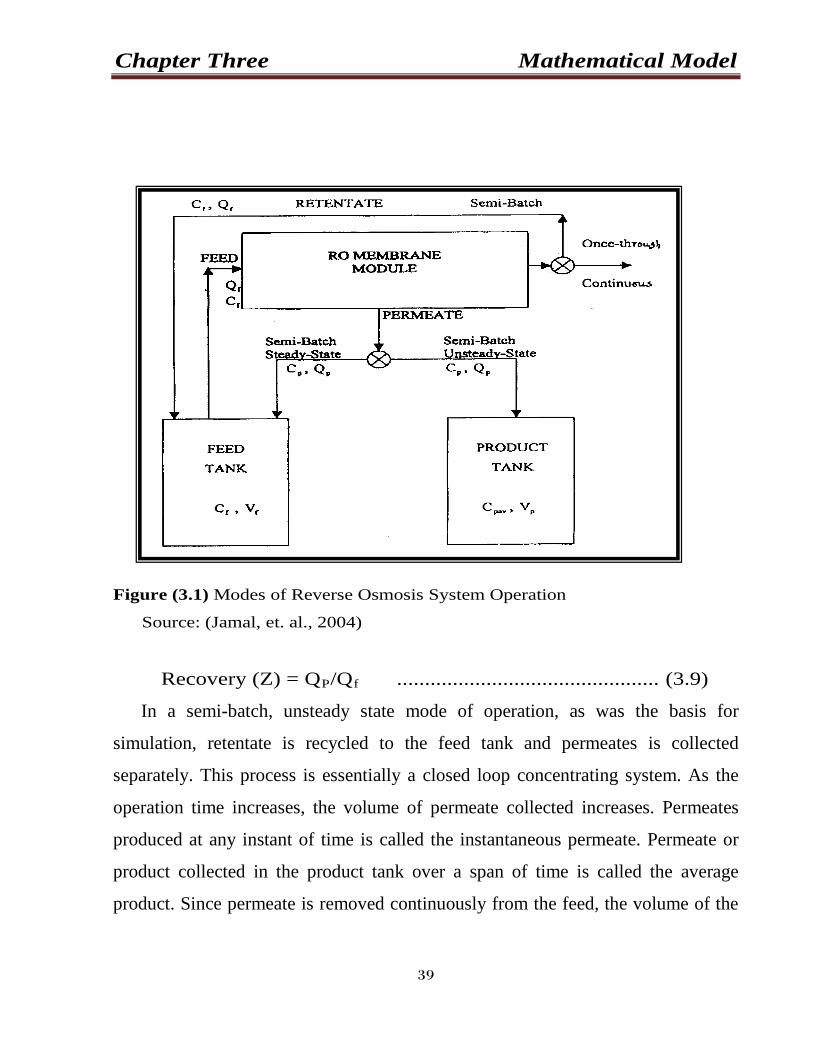
Chapter Three Mathematical Model
39
Figure (3.1) Modes of Reverse Osmosis System Operation
Source: (Jamal, et. al., 2004)
Recovery (Z) = QP/Qf
In a semi-batch, unsteady state mode of operation, as was the basis for
simulation, retentate is recycled to the feed tank and permeates is collected
separately. This process is essentially a closed loop concentrating system. As the
operation time increases, the volume of permeate collected increases. Permeates
produced at any instant of time is called the instantaneous permeate. Permeate or
product collected in the product tank over a span of time is called the average
product. Since permeate is removed continuously from the feed, the volume of the
............................................... (3.9)
Chapter Three Mathematical Model
40
feed decreases, the feed becomes more and more concentrated with time. The feed
in this type of process can also be referred to as the concentrate. As feed volume diminishes and concentration increases, the system will operate as
if it were running in sequential increments of increasing concentration, in a semi-
batch, steady state mode. Recovery is defined in terms of an overall system
recovery as the total quality of product generated up to a given time divided by the
initial feed volume:
fP V/V)X(Recovery = ............................................................ (3.10)
As in some point in the operation the system must be stopped as the feed
becomes so concentrated that the flux drops significantly, due to a large increase in
the osmotic pressure of the feed. If the permeate flows in a semi-batch, unsteady-
state system is returned to the feed tank, the mode of operation is termed “semi-
batch, steady state”.
The system material balances, together with these mass transfer models,
were used to simulate system operation. Correlation of flux, solute concentrations
and rejection with operating time and overall system recovery are functions of the
model. This model also predicts operational performance characteristics of the
system at various times and recoveries. The effects of pressure, feed concentration,
and volume and membrane characteristics on separation efficiency can also be
described.
A material balance made on the product tank yields to
dt/)CV(dCQ PavPpp = ............................................................ (3.11)
pPavPavppp V)dt/Cd(C)dt/dV(CQ += ....................................... (3.12)
Boundary conditions: at t PPavP CC,0V,0 ===
Chapter Three Mathematical Model
41
The change in the volume of permeate with time is the production rate of the
membrane.
PP Qdt/dV = ........................................................................ (3.13)
Substitution in equation (3.12) we get
PPavPavPPP VdtCdCQCQ )/(+=
or
PpavPPPav VCCQdtCd /)(/ −= .............................................. … (3.14)
The material balance around the membrane module is:
rrffPP CQCQCQ −= .............................................................. (3.15)
In this balance an assumption is made that in this system the concentration within
the membrane does not change greatly with spatial distribution. A mean permeate
concentration from the membrane module is used.
Similarly the balance around the feed tank becomes
dtCVdCQCQ ftftffrr /)(=− ....................................................... ..(3.16)
In the model it was assumed that the feed tank was well mixed. Therefore, at any
instant in time, t, Cft = Cf.
ftC
Combination of equations (3.15) and (3.16) with
substitution of as fC gives.
ftffftPP VdtdCCdtdVCQ )/()/( +=− .............................................. .. (3.17)
Pft QdtdV =− / ..................................................... …………... (3.18)
Integrating with boundary condition at t= 0, foft V V =
tQVV pfoft −= ........................................................................ .. (3.19)
Substituting this value into equation (3.17) we get
)/()( dtdCtQVCQCQ fpfofPPP −+−=− .................................... (3.20)
Chapter Three Mathematical Model
42
Rearranging of equation (4.20) gives. )tQV(/)CC(Qdt/dC pfoPfPf −−= ............................................ (3.21)
In order to get the solution of equation (3.21) the relationship between Qp and Cf,
with the expression for Cp in terms of Cf
RTvnQ )/(=π
is needed to achieve this we have to get
the relationship between osmotic pressure and feed concentration, expressed by
Van’t Hoff as:
...................................................................... (3.22)
Where π is the osmotic pressure, T temperature in Kelvin, R ideal gas constant,
)/( vn number of moles and Q is the number of species ions. For
convenience, this model assumed to be at constant temperature and incorporated
the other constant Ψ which simplifies osmotic pressure to solute concentration
coefficient. Cψπ =
C∆=∆ ψπ .......................................................................... (3.23)
The value of Ψ was assumed to be constant over the operating range of the solute
concentration. Incorporation of equation (3.23) into the expression for the solute
flux equation (3.2) yields: [ ])( PfWW CCPAJ −−∆= ψ .......................................................... (3.24)
)( PfSS CCBJ −= ................................................................... (3.3)
)/( WPPWS CCJJ = .................................................................... (3.6)
Combining the above equations to get:
PWWPS CJCJ =
[ ] pPfWWPPfS CCCPACCCB )()( −−∆=− ψ .................................. (3.25)
[ ]PWPSPwWPSPfwWPSPwf CCBCACBCCACBCPAC ++−∆= )/()/()/( 2ψψ
Chapter Three Mathematical Model
43
Approximating the equation through
PfSWSW CCandBABpA >>>>∆ // ψ For high rejection,
[ ]fWPSWWPSWPf CCBACBPACC )/()/(1 ψ−∆+= ........................... (3.26)
[ ] 1)/()/(1 −−∆+= fWPSWWPSWfP CCBACBPACC ψ ......................... (3.27)
By substituting the expression for CP in equation (3.24) to get the
expression for flux in terms of C [ ])(/)( 43 fffWW CaaCCPAJ −+−∆= ψψ
f
...................................... (4.28)
Substituting of equation (3.28) into equation (3.1)
( ) ( ) [ ]fffP CaaCaCaaQ 43221 / −+−=
Putting the expression for CP and QP
[ ] [ ]/)Caa/(C(C)Caa/()Ca()Ca(adt/dC f43fff43f2f21f −−−+−=
, Equations (3.27) and (3.28)
into the expression for the concentration change with time into
Equation (3.21), we get:
[ ])Caa/(tCatCataa f43f2f215 −−+− .................................. (3.30)
Where the model constants are
WPWa CPASa /)(1 ∆=
WPWa CASa /)(2 ψ=
)/(13 WPSW CBPAa ∆+=
)(/)(4 WPSW CBAa ψ=
foVa =5 Equation (3.30) is the non-linear differential equation, which can be solved
numerically. The solution of this equation gives the relationship between the
operating time and concentration of feed. Concentration of feed is a function of
operating time. In this mode of operation used, the system is essentially closed; that
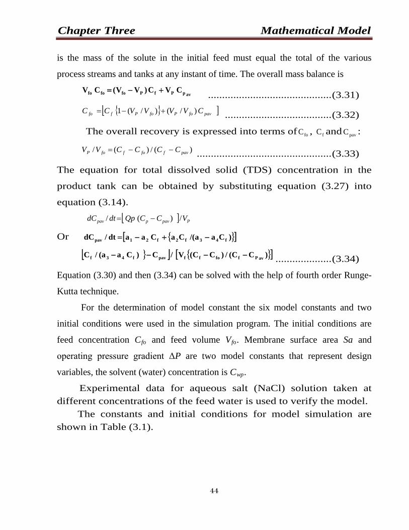
Chapter Three Mathematical Model
44
is the mass of the solute in the initial feed must equal the total of the various
process streams and tanks at any instant of time. The overall mass balance is
avpPfPfofofo CVC)VV(CV +−= ............................................ (3.31)
][ pavfoPfoPffo CVVVVCC )/()/(1 +−= ...................................... (3.32)
The overall recovery is expressed into terms of foC , fC and pavC :
)(/)(/ pavffoffoP CCCCVV −−= ................................................ (3.33)
The equation for total dissolved solid (TDS) concentration in the
product tank can be obtained by substituting equation (3.27) into
equation (3.14).
][ Ppavppav VCCQpdtdC /)(/ −=
Or [ ])Caa/(CaCaadt/dC f43f2f21pav −+−=
[ ] [ ])CC(/)CC(V/C)Caa(/C avPffoffpavf43f −−−− .................... (3.34)
Equation (3.30) and then (3.34) can be solved with the help of fourth order Runge-
Kutta technique.
For the determination of model constant the six model constants and two
initial conditions were used in the simulation program. The initial conditions are
feed concentration Cfo and feed volume Vfo. Membrane surface area Sa and
operating pressure gradient ΔP are two model constants that represent design
variables, the solvent (water) concentration is Cwp
Experimental data for aqueous salt (NaCl) solution taken at different concentrations of the feed water is used to verify the model.
.
The constants and initial conditions for model simulation are shown in Table (3.1).
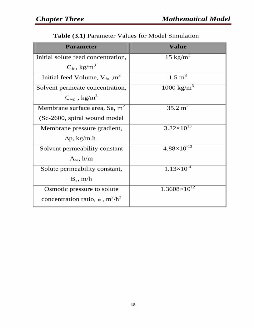
Chapter Three Mathematical Model
45
Table (3.1) Parameter Values for Model Simulation
Parameter Value
Initial solute feed concentration,
Cfo, kg/m
15 kg/m3
3
Initial feed Volume, Vfo ,m 1.5 m3 3
Solvent permeate concentration,
Cwp , kg/m
1000 kg/m3
3
Membrane surface area, Sa, m
(Sc-2600, spiral wound model
2 35.2 m2
Membrane pressure gradient, ∆p, kg/m.h
3.22×10 P
13
Solvent permeability constant ARwR, h/m
4.88×10 P
-13
Solute permeability constant,
BRsR, m/h
1.13×10 P
-4P
Osmotic pressure to solute
concentration ratio, ψ , m P
2P/h P
2
1.3608×10 P
12
Chapter Four Experimental Work
46
Chapter Four
Experimental work
The present study includes the achievement of experimental work through
central composite rotatable design method to create samples of different artificial
flux and rejection. The experimental work of desalination sample water was carried
out in two stages. The first stage treatment of salt water by laboratory scale of
reverse osmosis membrane was carried out in Spain - Madrid - University of
Complutense – Faculty of Physics, Department of Applied Physics. In this stage
the removing of TDS was within the allowable requirement range and the result
was analyzed theoretically.
The operating conditions using reverse osmosis membrane process were
commenced with the following ranges:
A. Concentration of Feed (15-45) g/l.
B. Temperature of Feed (10-50) °C.
C. Flow rate of Feed (100-250) l/hr.
D. Operating Pressure (5-15) bar.
The second stage includes injection air with salted water for enhancement
permeates flux and rejection after obtaining the maximum conditions from the first
stage. This stage was carried out by laboratory scale of reverse osmosis membrane
system which located at in AL-Mansuor Company - Ministry of Industry and
Minerals - Baghdad - Iraq.
This chapter explains and views in details the experimental part of this work.
It includes the description of the experimental rig in order to study the behavior of
the process and measuring the experimental data.
Chapter Four Experimental Work
47
4.1 The Experimental System
Figure (4.1) and Figure (4.2) show the schematic diagram and photograph of
the Reverse Osmosis membrane system used in this study. The Reverse Osmosis
membrane system consists of the following items:-
1. Electrical Pump
It’s a horizontal rotodynamic high pressure pump type (GE motors &
industrial system). The electrical pump is provided to aid up the makeup NaCl
solution into the reverse osmosis membrane module and maintain it at the required
level from the pressure and flow rate. The specifications of this type were (HP ½ ,
Hz 60/50 , V 100-120/200-240 , PH 1, RPM 11725/1425 , A 7.1-7.2/3.4-3.6 , gage
of pressure read 300 Psi as a maximum) assembled in Mexico.
2. Membrane Module
Type of membrane was osmonics (Cellous acetate, Sc-6200, spiral-wound
model, DESAL™ Membrane Products, made in USA) the surface area of membrane
1.12 m2
3. Feed Tank
. This reverse osmosis membrane module can be used to extract fresh water
from salt water but it requires a lot of pressure.
The feed solution was prepared by dissolving NaCl salt in distilled water
according the concentration of each experiment and poured in the feed tank which
was cylindrical glass vessel with total capacity 5 liter (made in Germany).
4. Thermostat
To maintain the temperature for each experiment constant, a rectangular
container of bathwater was filled with water and by circulating this water inside the
jacket of the feed tank while the temperature remains constant during the time of
the experiment.
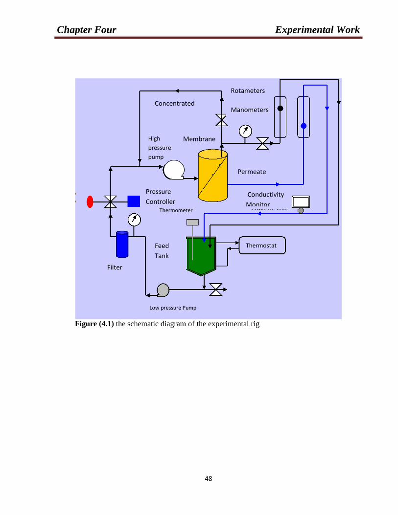
Chapter Four Experimental Work
48
Figure (4.1) the schematic diagram of the experimental rig
Rotameters
Concentrated Manometers
Permeate
Conductivity Monitor
Pressure Controller
Thermometer
Filter
Feed Tank
Thermostat
High pressure pump
Low pressure Pump
Membrane
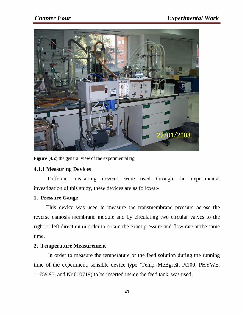
Chapter Four Experimental Work
49
Figure (4.2) the general view of the experimental rig
4.1.1 Measuring Devices
Different measuring devices were used through the experimental
investigation of this study, these devices are as follows:-
1. Pressure Gauge
This device was used to measure the transmembrane pressure across the
reverse osmosis membrane module and by circulating two circular valves to the
right or left direction in order to obtain the exact pressure and flow rate at the same
time.
2. Temperature Measurement
In order to measure the temperature of the feed solution during the running
time of the experiment, sensible device type (Temp.-MeBgreät Pt100, PHYWE.
11759.93, and Nr 000719) to be inserted inside the feed tank, was used.
Chapter Four Experimental Work
50
3. Conductivity Meter
Metrohm Ω 712 Digital conduct meter types 1.712.0010 and Nr.10191 was
used to measure the conductivity of feed solution and permeate water for each
sample (made in Switzerland).
4. Rota meter
Is an instrument used for measuring the flow rate of the feed solution.
5. Electronic Balance
Eventually, digital electronic balance from AD instrument LTD. Type GF-
1200-EC, max.1210g, e = 0.01, min.0.02g, d = 0.001g and has Ac adapter DC 12v
with digital means was employed to measure weight of permeate water during flux
calculation (made in Japan).
4.1.2 Experimental Procedures
1. Preparation of salt solution as a test media was achieved to the desired
concentration according to the number of experiments in a table of experimental
design and the checking of the desired concentration was performed by
conductivity meter. Hereinafter, the prepared solution is poured in the glass feed
tank.
2. The electrical current was switched on to operate the experimental rig and the
calibration for the pump was done to obtain the desired pressure and flow rate
while the temperature of salted solution was controlled by thermostat.
3. After adjusting the operating conditions, predetermined a condition that has
been already designed was applied according to the central composite rotatable
design of Box-Wilson. Accordingly, the flow rate measurement, water bath
temperature, concentration of the feed solution and eventually the pressure were
justified.
Chapter Four Experimental Work
51
4. Each experiment that was already carried out according to the previous pre
designed conditions, by measuring the volumetric flow rate of permeate water was
followed in order to calculate the flux and rejection. After measuring the
volumetric flow rate of permeates water, the samples were weighted by electronic
digital balance type GF-1200-EC.
4.2 Experimental Design
The experimental work of the present study involves the investigation of the
four variables such as; concentration, temperature, flow rate and pressure of feed
solution. Experimental planning was applied as recommended by Cochran
(Cochran, 1957) to reduce the number of experiments that would give sufficient
information in order to conclude the extent of the effect of each variable on the
membrane efficiency. The application of the experimental design for planning the
required experiment to examine the system, will extract the information from pre-
existing data by using a statistical method in order to interpret the results in a
regular form with the minimum number of observation. (Cochran and Cox, 1957).
The experimental design technique consists of two parts:-
1. Planning the experiments according to a specified plan, taking into account
the description of the variables value in the plan by a coded form.
2. Achieving the regression analysis for the specified set of runs in the plan,
also taking into account the coded form of the objective function regarding
each experiment in the set.
4.2.1 Fitting the Second Order Model
An experimental design for fitting the second-order model must have at least
five levels for each factor so that the model parameters can be estimated (i.e.
variables are usually called factor and the particular value of the variable is called
Chapter Four Experimental Work
52
the level). There are many techniques for the application of experimental planning,
such as factorial design, fractional design and box-Wilson. The proper technique
for planning a system of more than three variables "central composite rotatable
design" the total number of treatment combination is equal to (2K +2K +1), where
(K) is the number of variables, plus one additional further treatment that takes the
lack of fit and experimental error into account.
4.2.2 Central Composite Rotatable Design
This design consist of a 2K fractional (i.e. coded to the usual ± 1 notation) augmented by 2K axial points [i.e. (± ,0,0,…..,0),(0, ±, 0,…..,0), (0,0, ±,…..,0), …., (0,0,…., ±,) and center points (0,0,0,…..,0)].
A preliminary step is to set up the relationships between the coded levels and
the corresponding real variables, these relationships are as follows (Box and
George., 1978):
( )1.4][.min
−
=−
KXXXXX
center
centeractualCoded
The operating conditions of Reverse Osmosis membrane system are as follows:-
1. Concentration of Feed (15-45) g/l.
2. Temperature of Feed (10-50) °C.
3. Flow rate of Feed (100-250) l/hr.
4. Operating Pressure (5-15) bar.
The central composite rotatable design of four variables is used. The coded
levels are related to the real process values of these variables as follows:
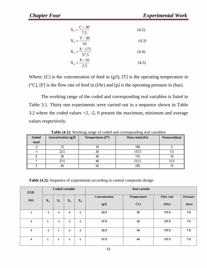
Chapter Four Experimental Work
53
(4.5)2.5
10PX
(4.4)37.5
175FX
(4.3)10
30TX
(4.2)7.5
30CX
4
3
2
1
−=
−=
−=
−=
Where: [C] is the concentration of feed in (g/l), [T] is the operating temperature in
(°C), [F] is the flow rate of feed in (l/hr) and [p] is the operating pressure in (bar).
The working range of the coded and corresponding real variables is listed in
Table 3.1. Thirty one experiments were carried out in a sequence shown in Table
3.2 where the coded values +2, -2, 0 present the maximum, minimum and average
values respectively.
Table (4.1): Working range of coded and corresponding real variables Coded level
Concentration (g/l) Temperature (C⁰) Flow rate(L/hr) Pressure(bar)
-2 15 10 100 5 -1 22.5 20 137.5 7.5 0 30 30 175 10 1 37.5 40 212.5 12.5 2 45 50 250 15
Table (4.2): Sequence of experiments according to central composite design
EXP.
NO.
Coded variable Real variable
X1 X2 X3 X4 Concentration
(g/l)
Temperature
(оC)
Flow rate
(l/hr)
Pressure
(bar)
1 - 1 -1 -1 -1 22.5 20 137.5 7.5
2 1 -1 -1 -1 37.5 20 137.5 7.5
3 - 1 1 -1 -1 22.5 40 137.5 7.5
4 1 1 -1 -1 37.5 40 137.5 7.5
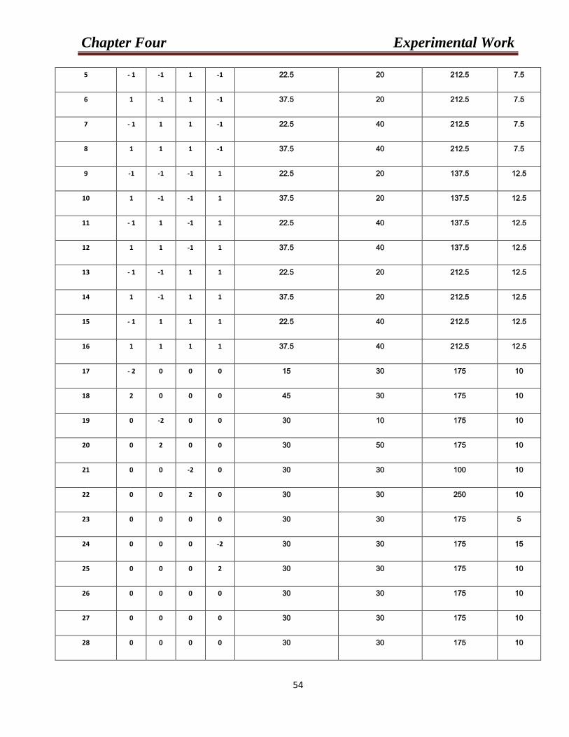
Chapter Four Experimental Work
54
5 - 1 -1 1 -1 22.5 20 212.5 7.5
6 1 -1 1 -1 37.5 20 212.5 7.5
7 - 1 1 1 -1 22.5 40 212.5 7.5
8 1 1 1 -1 37.5 40 212.5 7.5
9 -1 -1 -1 1 22.5 20 137.5 12.5
10 1 -1 -1 1 37.5 20 137.5 12.5
11 - 1 1 -1 1 22.5 40 137.5 12.5
12 1 1 -1 1 37.5 40 137.5 12.5
13 - 1 -1 1 1 22.5 20 212.5 12.5
14 1 -1 1 1 37.5 20 212.5 12.5
15 - 1 1 1 1 22.5 40 212.5 12.5
16 1 1 1 1 37.5 40 212.5 12.5
17 - 2 0 0 0 15 30 175 10
18 2 0 0 0 45 30 175 10
19 0 -2 0 0 30 10 175 10
20 0 2 0 0 30 50 175 10
21 0 0 -2 0 30 30 100 10
22 0 0 2 0 30 30 250 10
23 0 0 0 0 30 30 175 5
24 0 0 0 -2 30 30 175 15
25 0 0 0 2 30 30 175 10
26 0 0 0 0 30 30 175 10
27 0 0 0 0 30 30 175 10
28 0 0 0 0 30 30 175 10
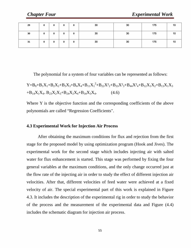
Chapter Four Experimental Work
55
29 0 0 0 0 30 30 175 10
30 0 0 0 0 30 30 175 10
31 0 0 0 0 30 30 175 10
The polynomial for a system of four variables can be represented as follows:
Y=B0+B1X1+B2X2+B3X3+B4X4+B11X12+B22X²2+B33X²3+B44X²4+B12X1X2+B13X1X3
+B14X1X4+ B23X2X3+B24X2X4+B34X3X4. (4.6)
Where Y is the objective function and the corresponding coefficients of the above
polynomials are called “Regression Coefficients".
4.3 Experimental Work for Injection Air Process
After obtaining the maximum conditions for flux and rejection from the first
stage for the proposed model by using optimization program (Hook and Jives). The
experimental work for the second stage which includes injecting air with salted
water for flux enhancement is started. This stage was performed by fixing the four
general variables at the maximum conditions, and the only change occurred just at
the flow rate of the injecting air in order to study the effect of different injection air
velocities. After that, different velocities of feed water were achieved at a fixed
velocity of air. The special experimental part of this work is explained in Figure
4.3. It includes the description of the experimental rig in order to study the behavior
of the process and the measurement of the experimental data and Figure (4.4)
includes the schematic diagram for injection air process.
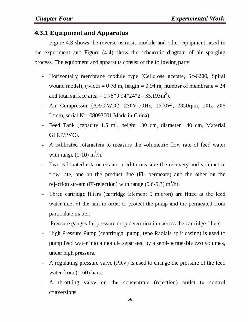
Chapter Four Experimental Work
56
4.3.1 Equipment and Apparatus
Figure 4.3 shows the reverse osmosis module and other equipment, used in
the experiment and Figure (4.4) show the schematic diagram of air sparging
process. The equipment and apparatus consist of the following parts:
- Horizontally membrane module type (Cellulose acetate, Sc-6200, Spiral
wound model), (width = 0.78 m, length = 0.94 m, number of membrane = 24
and total surface area = 0.78*0.94*24*2= 35.193m2).
- Air Compressor (AAC-WD2, 220V-50Hz, 1500W, 2850rpm, 50L, 208
L/min, serial No. 08093001 Made in China).
- Feed Tank (capacity 1.5 m3, height 100 cm, diameter 140 cm, Material
GFRP/PVC).
- A calibrated rotameters to measure the volumetric flow rate of feed water
with range (1-10) m3/h.
- Two calibrated rotameters are used to measure the recovery and volumetric
flow rate, one on the product line (FI- permeate) and the other on the
rejection stream (FI-rejection) with range (0.6-6.3) m3/hr.
- Three cartridge filters (cartridge Element 5 micron) are fitted at the feed
water inlet of the unit in order to protect the pump and the permeated from
particulate matter.
- Pressure gauges for pressure drop determination across the cartridge filters.
- High Pressure Pump (centrifugal pump, type Radials split casing) is used to
pump feed water into a module separated by a semi-permeable two volumes,
under high pressure.
- A regulating pressure valve (PRV) is used to change the pressure of the feed
water from (1-60) bars.
- A throttling valve on the concentrate (rejection) outlet to control
conversions.
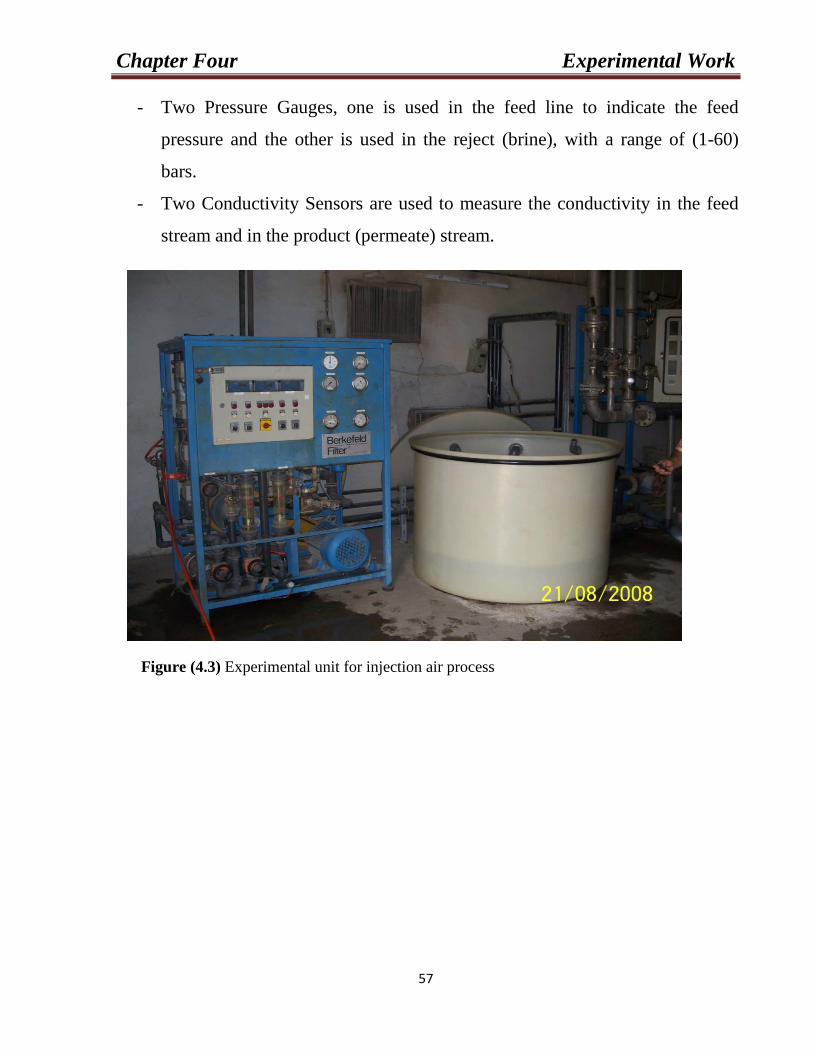
Chapter Four Experimental Work
57
- Two Pressure Gauges, one is used in the feed line to indicate the feed
pressure and the other is used in the reject (brine), with a range of (1-60)
bars.
- Two Conductivity Sensors are used to measure the conductivity in the feed
stream and in the product (permeate) stream.
Figure (4.3) Experimental unit for injection air process
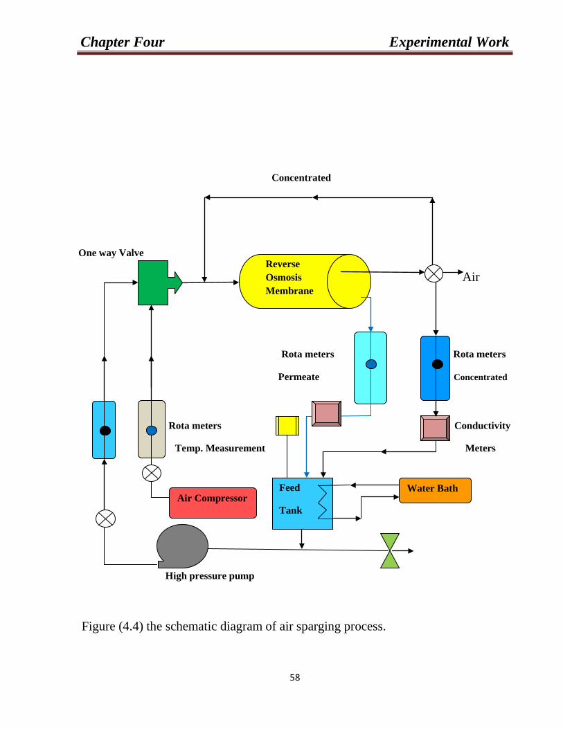
Chapter Four Experimental Work
58
Concentrated
One way Valve
ReRRr Air
Rota meters Rota meters
Permeate Concentrated
Rota meters Conductivity
Temp. Measurement Meters
High pressure pump
Figure (4.4) the schematic diagram of air sparging process.
Feed
Tank Air Compressor
Reverse Osmosis Membrane
Water Bath
Chapter Five Results and Discussion
59
Chapter Five
Results and Discussion
The experimental results of the effect of operating variables on the reverse
osmosis performance and the maximum operating conditions of the process were
studied.
A series of samples that conducting sodium chloride solution were prepared
to study the effect of the most affective variables (i.e. concentration, temperature,
flow rate and operating pressure for the system). These variables had been
correlated with the flux and rejection of the specimen by a second order polynomial
model after estimation of the coefficients would carry over according to one of the
methods of optimization. In addition, specimens at the predicted maximum values
of the concerned variables were further prepared to prepare a final study by
measuring the samples to calculate the flux and rejection.
Finally the mathematical model of reverse osmosis membrane system was
simulated in the present work to predict the theoretical transient response with aid
of computer program using FORTRAN program. The theoretical results were
compared with the experimental result of reverse osmosis membrane system.
5.1 Analysis of Experimental Result
The response of experiments conducted according to Box-Wilson method,
which represented by flux and rejection are fitted to a second order polynomial
model and the maximum conditions are calculated from this model. The effect of
each variable on the response is also determined by using F-test and ANOVA
analysis of variance.
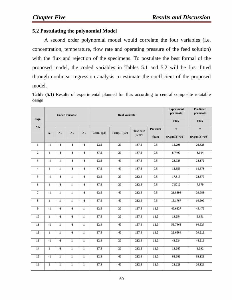
Chapter Five Results and Discussion
60
5.2 Postulating the polynomial Model
A second order polynomial model would correlate the four variables (i.e.
concentration, temperature, flow rate and operating pressure of the feed solution)
with the flux and rejection of the specimens. To postulate the best formal of the
proposed model, the coded variables in Tables 5.1 and 5.2 will be first fitted
through nonlinear regression analysis to estimate the coefficient of the proposed
model. Table (5.1) Results of experimental planned for flux according to central composite rotatable design
Exp.
No.
Coded variable Real variable
Experiment permeate
Flux
Predicted permeate
Flux
X1 X2 X3 X4 Conc. (g/l) Temp. (Cº) Flow rate (L/hr)
Pressure
(bar)
Y
(Kg/mP
2P.s)*10P
-5
Y
(Kg/mP
2P.s)*10P
-5
1 -1 -1 -1 -1 22.5 20 137.5 7.5 15.296 20.323
2 1 -1 -1 -1 37.5 20 137.5 7.5 6.7407 8.014
3 -1 1 -1 -1 22.5 40 137.5 7.5 23.023 28.172
4 1 1 -1 -1 37.5 40 137.5 7.5 12.659 11.678
5 -1 -1 1 -1 22.5 20 212.5 7.5 17.819 22.679
6 1 -1 1 -1 37.5 20 212.5 7.5 7.5712 7.370
7 -1 1 1 -1 22.5 40 212.5 7.5 21.8898 29.988
8 1 1 1 -1 37.5 40 212.5 7.5 13.1767 10.500
9 -1 -1 -1 1 22.5 20 137.5 12.5 40.6827 45.479
10 1 -1 -1 1 37.5 20 137.5 12.5 13.554 9.651
11 -1 1 -1 1 22.5 40 137.5 12.5 56.7963 60.927
12 1 1 -1 1 37.5 40 137.5 12.5 23.6584 20.919
13 -1 -1 1 1 22.5 20 212.5 12.5 43.224 48.216
14 1 -1 1 1 37.5 20 212.5 12.5 12.687 9.392
15 -1 1 1 1 22.5 40 212.5 12.5 62.282 63.129
16 1 1 1 1 37.5 40 212.5 12.5 21.229 20.126
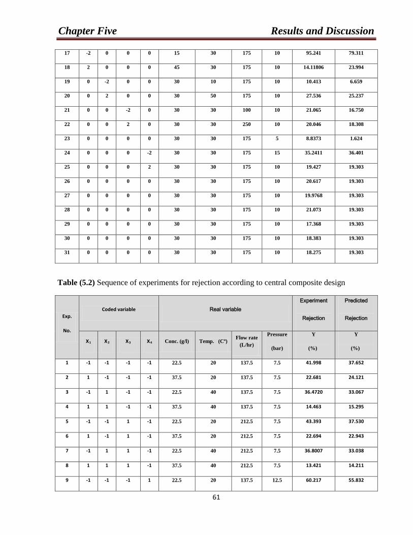
Chapter Five Results and Discussion
61
17 -2 0 0 0 15 30 175 10 95.241 79.311
18 2 0 0 0 45 30 175 10 14.11806 23.994
19 0 -2 0 0 30 10 175 10 10.413 6.659
20 0 2 0 0 30 50 175 10 27.536 25.237
21 0 0 -2 0 30 30 100 10 21.065 16.750
22 0 0 2 0 30 30 250 10 20.046 18.308
23 0 0 0 0 30 30 175 5 8.8373 1.624
24 0 0 0 -2 30 30 175 15 35.2411 36.401
25 0 0 0 2 30 30 175 10 19.427 19.303
26 0 0 0 0 30 30 175 10 20.617 19.303
27 0 0 0 0 30 30 175 10 19.9768 19.303
28 0 0 0 0 30 30 175 10 21.073 19.303
29 0 0 0 0 30 30 175 10 17.368 19.303
30 0 0 0 0 30 30 175 10 18.383 19.303
31 0 0 0 0 30 30 175 10 18.275 19.303
Table (5.2) Sequence of experiments for rejection according to central composite design
Exp.
No.
Coded variable Real variable Experiment
Rejection
Predicted
Rejection
XR1 XR2 XR3 XR4 Conc. (g/l) Temp. (Cº) Flow rate (L/hr)
Pressure
(bar)
Y
(%)
Y
(%)
1 -1 -1 -1 -1 22.5 20 137.5 7.5 41.998 37.652
2 1 -1 -1 -1 37.5 20 137.5 7.5 22.681 24.121
3 -1 1 -1 -1 22.5 40 137.5 7.5 36.4720 33.067
4 1 1 -1 -1 37.5 40 137.5 7.5 14.463 15.295
5 -1 -1 1 -1 22.5 20 212.5 7.5 43.393 37.530
6 1 -1 1 -1 37.5 20 212.5 7.5 22.694 22.943
7 -1 1 1 -1 22.5 40 212.5 7.5 36.8007 33.038
8 1 1 1 -1 37.5 40 212.5 7.5 13.421 14.211
9 -1 -1 -1 1 22.5 20 137.5 12.5 60.217 55.832
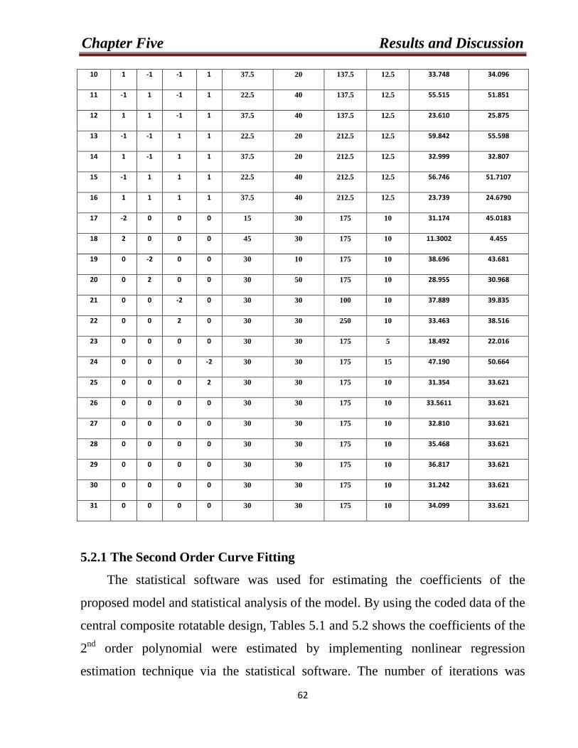
Chapter Five Results and Discussion
62
10 1 -1 -1 1 37.5 20 137.5 12.5 33.748 34.096
11 -1 1 -1 1 22.5 40 137.5 12.5 55.515 51.851
12 1 1 -1 1 37.5 40 137.5 12.5 23.610 25.875
13 -1 -1 1 1 22.5 20 212.5 12.5 59.842 55.598
14 1 -1 1 1 37.5 20 212.5 12.5 32.999 32.807
15 -1 1 1 1 22.5 40 212.5 12.5 56.746 51.7107
16 1 1 1 1 37.5 40 212.5 12.5 23.739 24.6790
17 -2 0 0 0 15 30 175 10 31.174 45.0183
18 2 0 0 0 45 30 175 10 11.3002 4.455
19 0 -2 0 0 30 10 175 10 38.696 43.681
20 0 2 0 0 30 50 175 10 28.955 30.968
21 0 0 -2 0 30 30 100 10 37.889 39.835
22 0 0 2 0 30 30 250 10 33.463 38.516
23 0 0 0 0 30 30 175 5 18.492 22.016
24 0 0 0 -2 30 30 175 15 47.190 50.664
25 0 0 0 2 30 30 175 10 31.354 33.621
26 0 0 0 0 30 30 175 10 33.5611 33.621
27 0 0 0 0 30 30 175 10 32.810 33.621
28 0 0 0 0 30 30 175 10 35.468 33.621
29 0 0 0 0 30 30 175 10 36.817 33.621
30 0 0 0 0 30 30 175 10 31.242 33.621
31 0 0 0 0 30 30 175 10 34.099 33.621
5.2.1 The Second Order Curve Fitting
The statistical software was used for estimating the coefficients of the
proposed model and statistical analysis of the model. By using the coded data of the
central composite rotatable design, Tables 5.1 and 5.2 shows the coefficients of the
2P
ndP order polynomial were estimated by implementing nonlinear regression
estimation technique via the statistical software. The number of iterations was
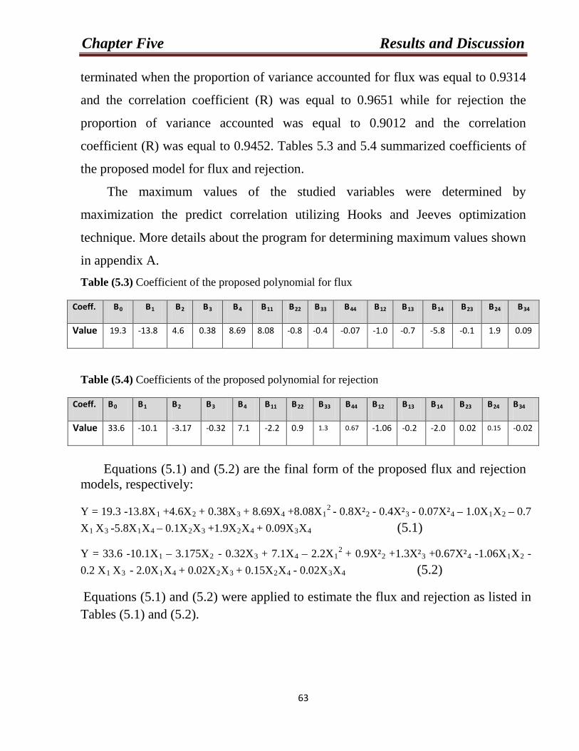
Chapter Five Results and Discussion
63
terminated when the proportion of variance accounted for flux was equal to 0.9314
and the correlation coefficient (R) was equal to 0.9651 while for rejection the
proportion of variance accounted was equal to 0.9012 and the correlation
coefficient (R) was equal to 0.9452. Tables 5.3 and 5.4 summarized coefficients of
the proposed model for flux and rejection.
The maximum values of the studied variables were determined by
maximization the predict correlation utilizing Hooks and Jeeves optimization
technique. More details about the program for determining maximum values shown
in appendix A. Table (5.3) Coefficient of the proposed polynomial for flux
Coeff. B0 B1 B2 B3 B4 B11 B22 B33 B44 B12 B13 B14 B23 B24 B34
Value 19.3 -13.8 4.6 0.38 8.69 8.08 -0.8 -0.4 -0.07 -1.0 -0.7 -5.8 -0.1 1.9 0.09
Table (5.4) Coefficients of the proposed polynomial for rejection
Coeff. B0 B1 B2 B3 B4 B11 B22 B33 B44 B12 B13 B14 B23 B24 B34
Value 33.6 -10.1 -3.17 -0.32 7.1 -2.2 0.9 1.3 0.67 -1.06 -0.2 -2.0 0.02 0.15 -0.02
Equations (5.1) and (5.2) are the final form of the proposed flux and rejection models, respectively:
Y = 19.3 -13.8X1 +4.6X2 + 0.38X3 + 8.69X4 +8.08X1
2 - 0.8X²2 - 0.4X²3 - 0.07X²4 – 1.0X1X2 – 0.7 X1 X3 -5.8X1X4 – 0.1X2X3 +1.9X2X4 + 0.09X3X4
Y = 33.6 -10.1X
(5.1)
1 – 3.175X2 - 0.32X3 + 7.1X4 – 2.2X12 + 0.9X²2 +1.3X²3 +0.67X²4 -1.06X1X2 -
0.2 X1 X3 - 2.0X1X4 + 0.02X2X3 + 0.15X2X4 - 0.02X3X4
Equations (5.1) and (5.2) were applied to estimate the flux and rejection as listed in Tables (5.1) and (5.2).
(5.2)
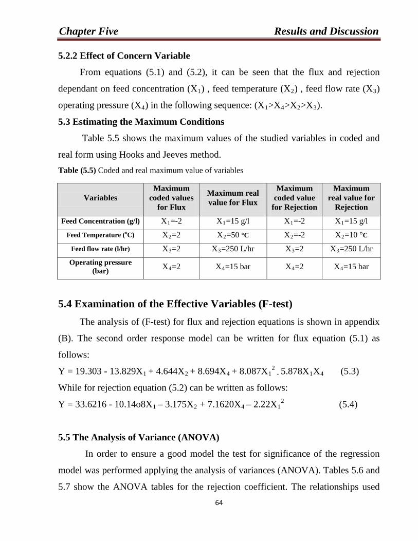
Chapter Five Results and Discussion
64
5.2.2 Effect of Concern Variable
From equations (5.1) and (5.2), it can be seen that the flux and rejection
dependant on feed concentration (X1) , feed temperature (X2) , feed flow rate (X3)
operating pressure (X4) in the following sequence: (X1>X4>X2>X3
5.3 Estimating the Maximum Conditions
).
Table 5.5 shows the maximum values of the studied variables in coded and
real form using Hooks and Jeeves method. Table (5.5) Coded and real maximum value of variables
Variables Maximum
coded values for Flux
Maximum real value for Flux
Maximum coded value
for Rejection
Maximum real value for
Rejection
Feed Concentration (g/l) X1 X=-2 1 X=15 g/l 1 X=-2 1=15 g/l
Feed Temperature (o XC) 2 X=2 2 X=50 °C 2 X=-2 2=10 °C
Feed flow rate (l/hr) X3 X=2 3 X=250 L/hr 3 X=2 3=250 L/hr
Operating pressure (bar) X4 X=2 4 X=15 bar 4 X=2 4=15 bar
5.4 Examination of the Effective Variables (F-test) The analysis of (F-test) for flux and rejection equations is shown in appendix
(B). The second order response model can be written for flux equation (5.1) as
follows:
Y = 19.303 - 13.829X1 + 4.644X2 + 8.694X4 + 8.087X12
- 5.878X1X4
While for rejection equation (5.2) can be written as follows:
(5.3)
Y = 33.6216 - 10.14o8X1 – 3.175X2 + 7.1620X4 – 2.22X12
(5.4)
5.5 The Analysis of Variance (ANOVA)
In order to ensure a good model the test for significance of the regression
model was performed applying the analysis of variances (ANOVA). Tables 5.6 and
5.7 show the ANOVA tables for the rejection coefficient. The relationships used
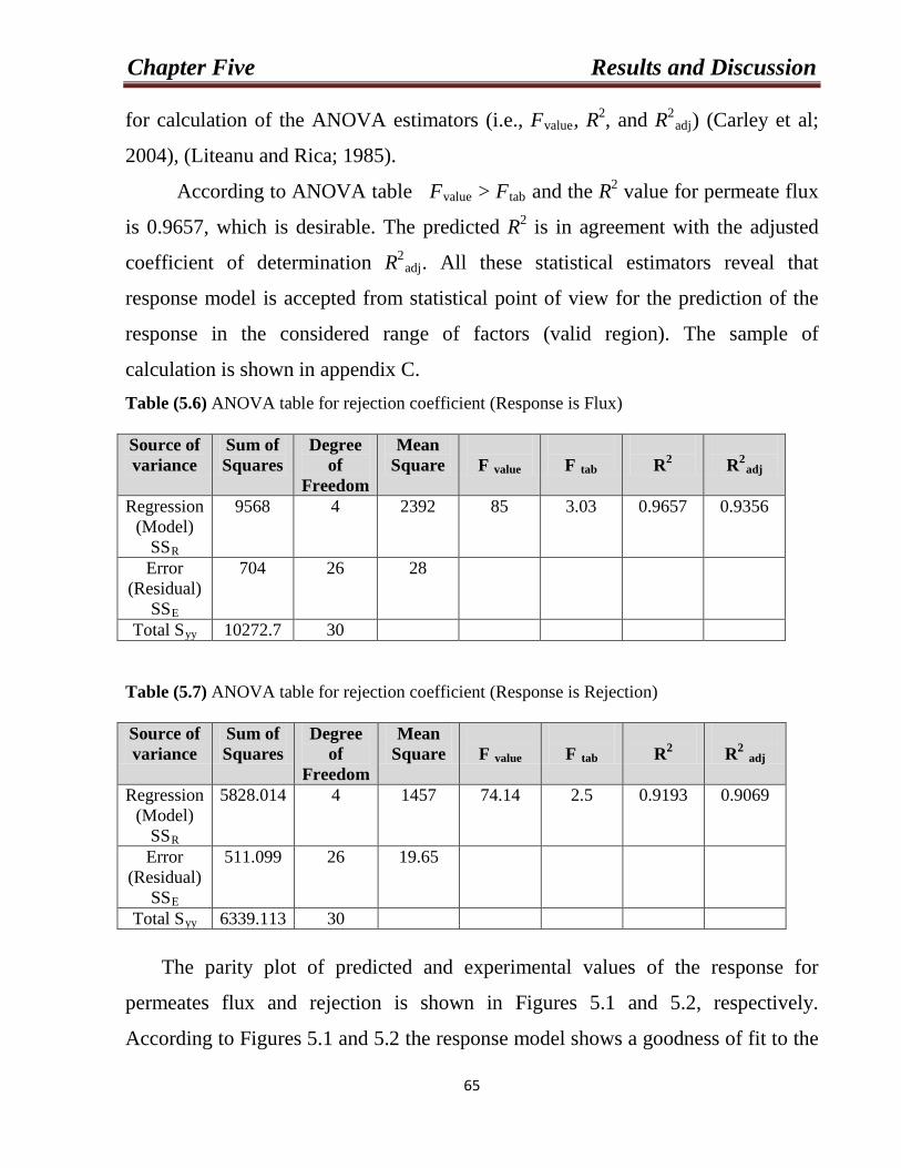
Chapter Five Results and Discussion
65
for calculation of the ANOVA estimators (i.e., Fvalue, R2, and R2adj
According to ANOVA table F
) (Carley et al;
2004), (Liteanu and Rica; 1985).
value > Ftab and the R2 value for permeate flux
is 0.9657, which is desirable. The predicted R2 is in agreement with the adjusted
coefficient of determination R2adj
Table (5.6) ANOVA table for rejection coefficient (Response is Flux)
. All these statistical estimators reveal that
response model is accepted from statistical point of view for the prediction of the
response in the considered range of factors (valid region). The sample of
calculation is shown in appendix C.
Source of variance
Sum of Squares
Degree of
Freedom
Mean Square
F value
F tab
R2
R2
adj
Regression (Model)
SS
9568
R
4 2392 85 3.03 0.9657 0.9356
Error (Residual)
SS
704
E
26 28
Total S 10272.7 yy 30 Table (5.7) ANOVA table for rejection coefficient (Response is Rejection) Source of variance
Sum of Squares
Degree of
Freedom
Mean Square
F value
F tab
R2
R2 adj
Regression (Model)
SS
5828.014
R
4 1457 74.14 2.5 0.9193 0.9069
Error (Residual)
SS
511.099
E
26 19.65
Total S 6339.113 yy 30
The parity plot of predicted and experimental values of the response for
permeates flux and rejection is shown in Figures 5.1 and 5.2, respectively.
According to Figures 5.1 and 5.2 the response model shows a goodness of fit to the
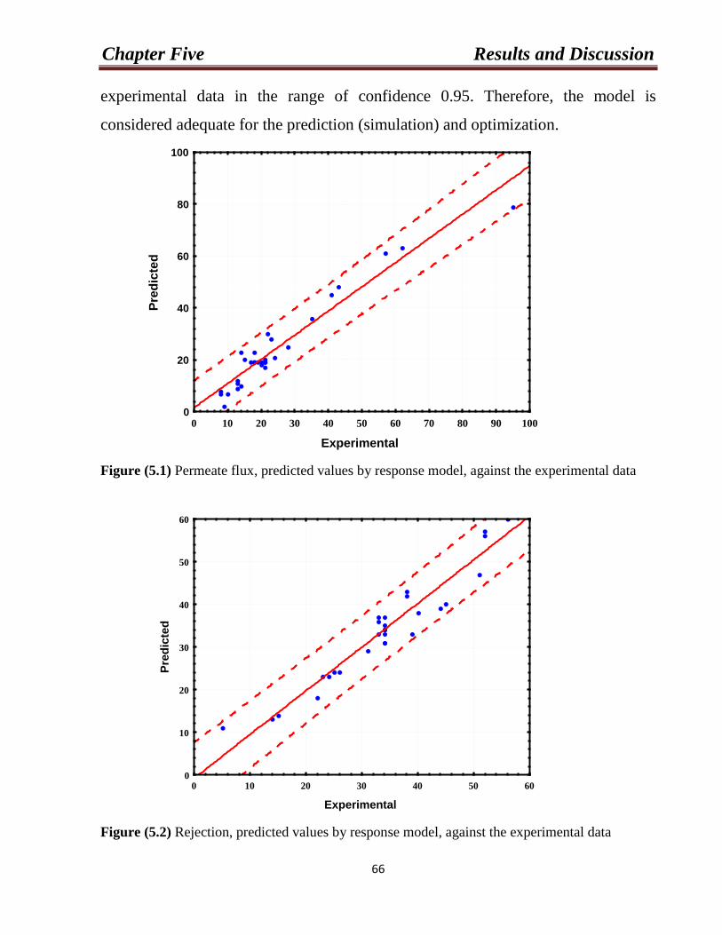
Chapter Five Results and Discussion
66
experimental data in the range of confidence 0.95. Therefore, the model is
considered adequate for the prediction (simulation) and optimization.
0 10 20 30 40 50 60 70 80 90 100
Experimental
0
20
40
60
80
100Pr
edic
ted
Figure (5.1) Permeate flux, predicted values by response model, against the experimental data
0 10 20 30 40 50 60
Experimental
0
10
20
30
40
50
60
Pred
icte
d
Figure (5.2) Rejection, predicted values by response model, against the experimental data
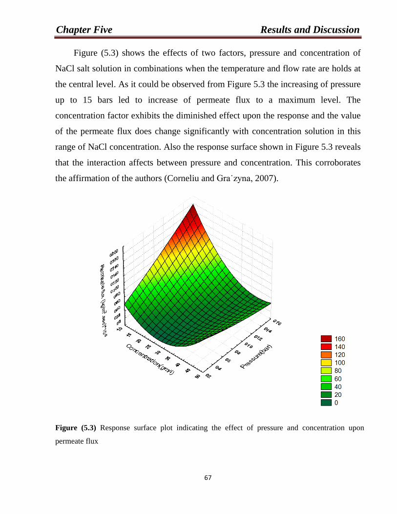
Chapter Five Results and Discussion
67
Figure (5.3) shows the effects of two factors, pressure and concentration of
NaCl salt solution in combinations when the temperature and flow rate are holds at
the central level. As it could be observed from Figure 5.3 the increasing of pressure
up to 15 bars led to increase of permeate flux to a maximum level. The
concentration factor exhibits the diminished effect upon the response and the value
of the permeate flux does change significantly with concentration solution in this
range of NaCl concentration. Also the response surface shown in Figure 5.3 reveals
that the interaction affects between pressure and concentration. This corroborates
the affirmation of the authors (Corneliu and Gra˙zyna, 2007).
Figure (5.3) Response surface plot indicating the effect of pressure and concentration upon
permeate flux
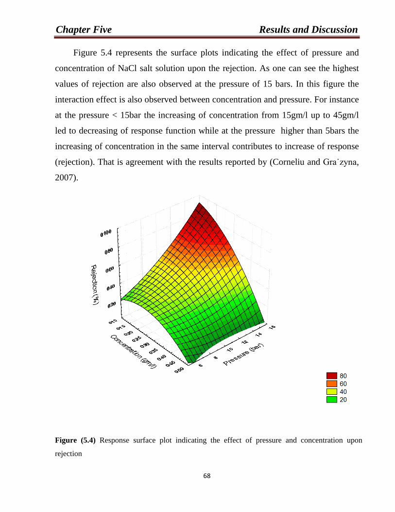
Chapter Five Results and Discussion
68
Figure 5.4 represents the surface plots indicating the effect of pressure and
concentration of NaCl salt solution upon the rejection. As one can see the highest
values of rejection are also observed at the pressure of 15 bars. In this figure the
interaction effect is also observed between concentration and pressure. For instance
at the pressure < 15bar the increasing of concentration from 15gm/l up to 45gm/l
led to decreasing of response function while at the pressure higher than 5bars the
increasing of concentration in the same interval contributes to increase of response
(rejection). That is agreement with the results reported by (Corneliu and Gra˙zyna,
2007).
Figure (5.4) Response surface plot indicating the effect of pressure and concentration upon
rejection
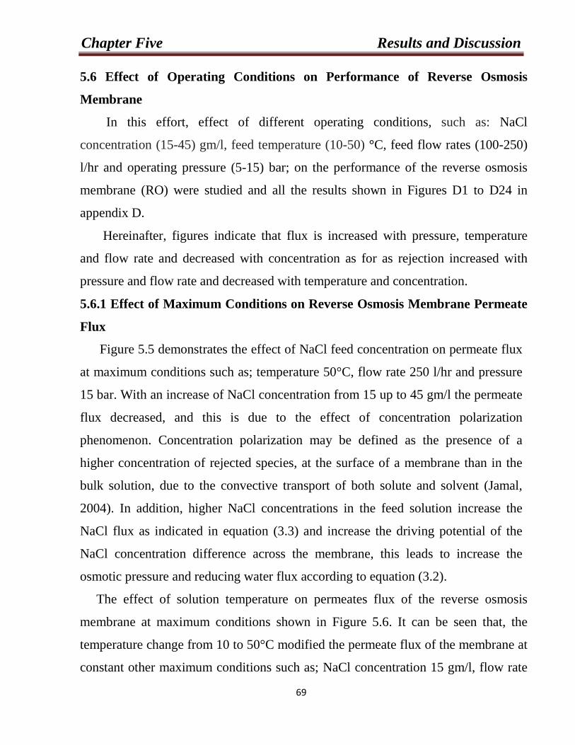
Chapter Five Results and Discussion
69
5.6 Effect of Operating Conditions on Performance of Reverse Osmosis
Membrane
In this effort, effect of different operating conditions, such as: NaCl
concentration (15-45) gm/l, feed temperature (10-50) °C, feed flow rates (100-250)
l/hr and operating pressure (5-15) bar; on the performance of the reverse osmosis
membrane (RO) were studied and all the results shown in Figures D1 to D24 in
appendix D.
Hereinafter, figures indicate that flux is increased with pressure, temperature
and flow rate and decreased with concentration as for as rejection increased with
pressure and flow rate and decreased with temperature and concentration.
5.6.1 Effect of Maximum Conditions on Reverse Osmosis Membrane Permeate
Flux
Figure 5.5 demonstrates the effect of NaCl feed concentration on permeate flux
at maximum conditions such as; temperature 50°C, flow rate 250 l/hr and pressure
15 bar. With an increase of NaCl concentration from 15 up to 45 gm/l the permeate
flux decreased, and this is due to the effect of concentration polarization
phenomenon. Concentration polarization may be defined as the presence of a
higher concentration of rejected species, at the surface of a membrane than in the
bulk solution, due to the convective transport of both solute and solvent (Jamal,
2004). In addition, higher NaCl concentrations in the feed solution increase the
NaCl flux as indicated in equation (3.3) and increase the driving potential of the
NaCl concentration difference across the membrane, this leads to increase the
osmotic pressure and reducing water flux according to equation (3.2).
The effect of solution temperature on permeates flux of the reverse osmosis
membrane at maximum conditions shown in Figure 5.6. It can be seen that, the
temperature change from 10 to 50°C modified the permeate flux of the membrane at
constant other maximum conditions such as; NaCl concentration 15 gm/l, flow rate
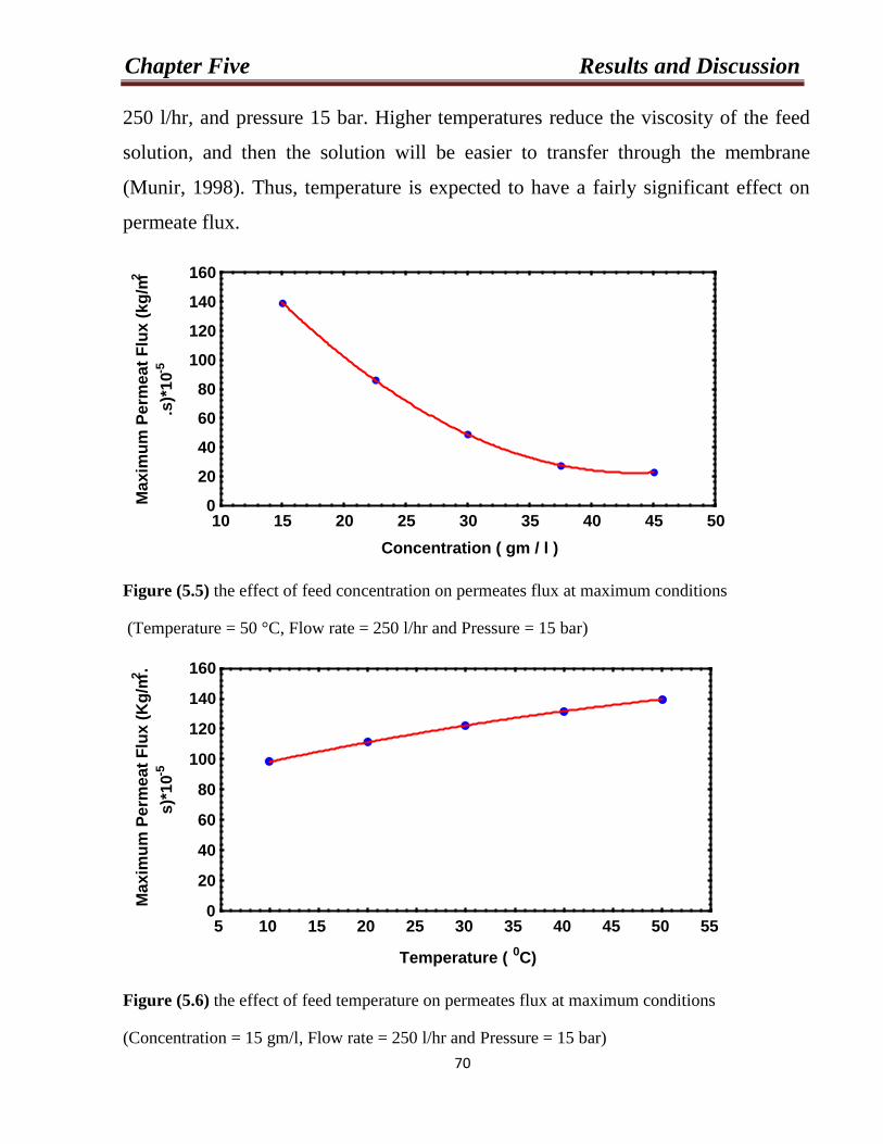
Chapter Five Results and Discussion
70
250 l/hr, and pressure 15 bar. Higher temperatures reduce the viscosity of the feed
solution, and then the solution will be easier to transfer through the membrane
(Munir, 1998). Thus, temperature is expected to have a fairly significant effect on
permeate flux.
10 15 20 25 30 35 40 45 50Concentration ( gm / l )
0
20
40
60
80
100
120
140
160
Max
imum
Per
mea
t Flu
x (k
g/m2
.s)*
10-5
Figure (5.5) the effect of feed concentration on permeates flux at maximum conditions
(Temperature = 50 °C, Flow rate = 250 l/hr and Pressure = 15 bar)
5 10 15 20 25 30 35 40 45 50 55
Temperature ( 0C)
0
20
40
60
80
100
120
140
160
Max
imum
Per
mea
t Flu
x (K
g/m2 .
s)*1
0-5
Figure (5.6) the effect of feed temperature on permeates flux at maximum conditions
(Concentration = 15 gm/l, Flow rate = 250 l/hr and Pressure = 15 bar)
Chapter Five Results and Discussion
71
Besides, the effect of feed flow rate on permeate flux of the reverse osmosis
is illustrated in Figure 5.7. With an increase of the feed flow rate the permeate flux
increased. Munir, 1998, reported that the flow rate or turbulence; whether produced
by stirring, pumping the fluid, or moving the membrane, has a noticeable effect on
permeate flux. In addition, agitation and mixing of the fluid near the membrane
surface “sweeps’’ away the accumulated solute, reducing the hydraulic resistance
of the “cake’’ and reducing thickness of the boundary layer. There is also a belief
that extremely high shear, such as that obtained with thin channel and rotary
devices, actually reduces the thickness of the “gel’’ layer. In any case, this is one of
the simplest methods of controlling the effect of concentration polarization.
Figure 5.8 illustrate the effect of operating pressure on permeate flux at
maximum conditions. Equation (3.2) shows that the water flux is directly
proportional to the pressure drop across the membrane. However, there is an indirect
effect of pressure on the product concentration. If the pressure is reduced, NaCl will
tend to accumulate on the feed side of the membrane; it increases the osmotic
pressure, reduces the driving potential )( π−P and hence, reduces the water flux
(Jamal et al, 2004).
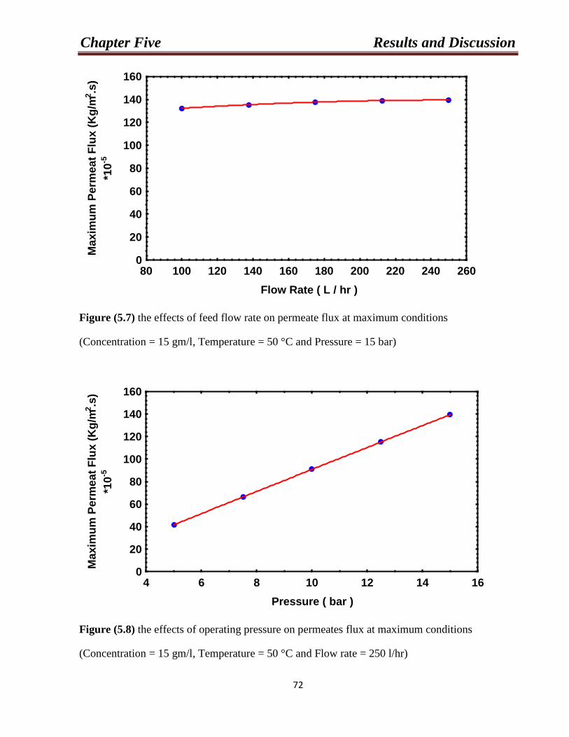
Chapter Five Results and Discussion
72
80 100 120 140 160 180 200 220 240 260 Flow Rate ( L / hr )
0
20
40
60
80
100
120
140
160M
axim
um P
erm
eat F
lux
(Kg/
m2 .s
)*1
0-5
Figure (5.7) the effects of feed flow rate on permeate flux at maximum conditions
(Concentration = 15 gm/l, Temperature = 50 °C and Pressure = 15 bar)
4 6 8 10 12 14 16Pressure ( bar )
0
20
40
60
80
100
120
140
160
Max
imum
Per
mea
t Flu
x (K
g/m
2 .s)
*10-5
Figure (5.8) the effects of operating pressure on permeates flux at maximum conditions
(Concentration = 15 gm/l, Temperature = 50 °C and Flow rate = 250 l/hr)
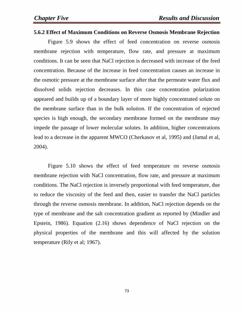
Chapter Five Results and Discussion
73
5.6.2 Effect of Maximum Conditions on Reverse Osmosis Membrane Rejection
Figure 5.9 shows the effect of feed concentration on reverse osmosis
membrane rejection with temperature, flow rate, and pressure at maximum
conditions. It can be seen that NaCl rejection is decreased with increase of the feed
concentration. Because of the increase in feed concentration causes an increase in
the osmotic pressure at the membrane surface after that the permeate water flux and
dissolved solids rejection decreases. In this case concentration polarization
appeared and builds up of a boundary layer of more highly concentrated solute on
the membrane surface than in the bulk solution. If the concentration of rejected
species is high enough, the secondary membrane formed on the membrane may
impede the passage of lower molecular solutes. In addition, higher concentrations
lead to a decrease in the apparent MWCO (Cherkasov et al, 1995) and (Jamal et al,
2004).
Figure 5.10 shows the effect of feed temperature on reverse osmosis
membrane rejection with NaCl concentration, flow rate, and pressure at maximum
conditions. The NaCl rejection is inversely proportional with feed temperature, due
to reduce the viscosity of the feed and then, easier to transfer the NaCl particles
through the reverse osmosis membrane. In addition, NaCl rejection depends on the
type of membrane and the salt concentration gradient as reported by (Mindler and
Epstein, 1986). Equation (2.16) shows dependence of NaCl rejection on the
physical properties of the membrane and this will affected by the solution
temperature (Rily et al; 1967).
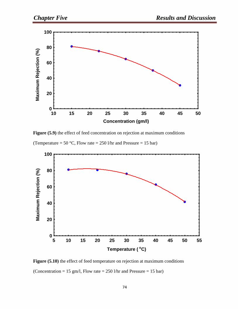
Chapter Five Results and Discussion
74
10 15 20 25 30 35 40 45 50Concentration (gm/l)
0
20
40
60
80
100M
axim
um R
ejec
tion
(%)
Figure (5.9) the effect of feed concentration on rejection at maximum conditions
(Temperature = 50 °C, Flow rate = 250 l/hr and Pressure = 15 bar)
5 10 15 20 25 30 35 40 45 50 55
Temperature ( oC)
0
20
40
60
80
100
Max
imum
Rej
ectio
n (%
)
Figure (5.10) the effect of feed temperature on rejection at maximum conditions
(Concentration = 15 gm/l, Flow rate = 250 l/hr and Pressure = 15 bar)
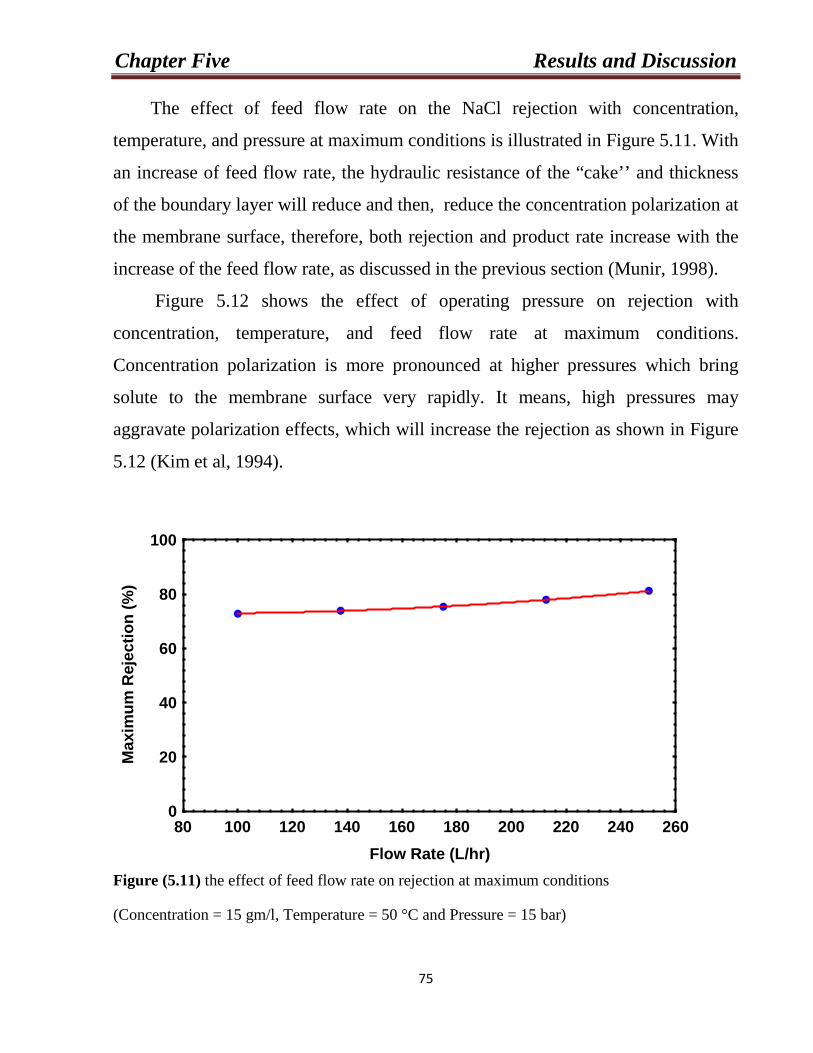
Chapter Five Results and Discussion
75
The effect of feed flow rate on the NaCl rejection with concentration,
temperature, and pressure at maximum conditions is illustrated in Figure 5.11. With
an increase of feed flow rate, the hydraulic resistance of the “cake’’ and thickness
of the boundary layer will reduce and then, reduce the concentration polarization at
the membrane surface, therefore, both rejection and product rate increase with the
increase of the feed flow rate, as discussed in the previous section (Munir, 1998).
Figure 5.12 shows the effect of operating pressure on rejection with
concentration, temperature, and feed flow rate at maximum conditions.
Concentration polarization is more pronounced at higher pressures which bring
solute to the membrane surface very rapidly. It means, high pressures may
aggravate polarization effects, which will increase the rejection as shown in Figure
5.12 (Kim et al, 1994).
80 100 120 140 160 180 200 220 240 260Flow Rate (L/hr)
0
20
40
60
80
100
Max
imum
Rej
ectio
n (%
)
Figure (5.11) the effect of feed flow rate on rejection at maximum conditions
(Concentration = 15 gm/l, Temperature = 50 °C and Pressure = 15 bar)
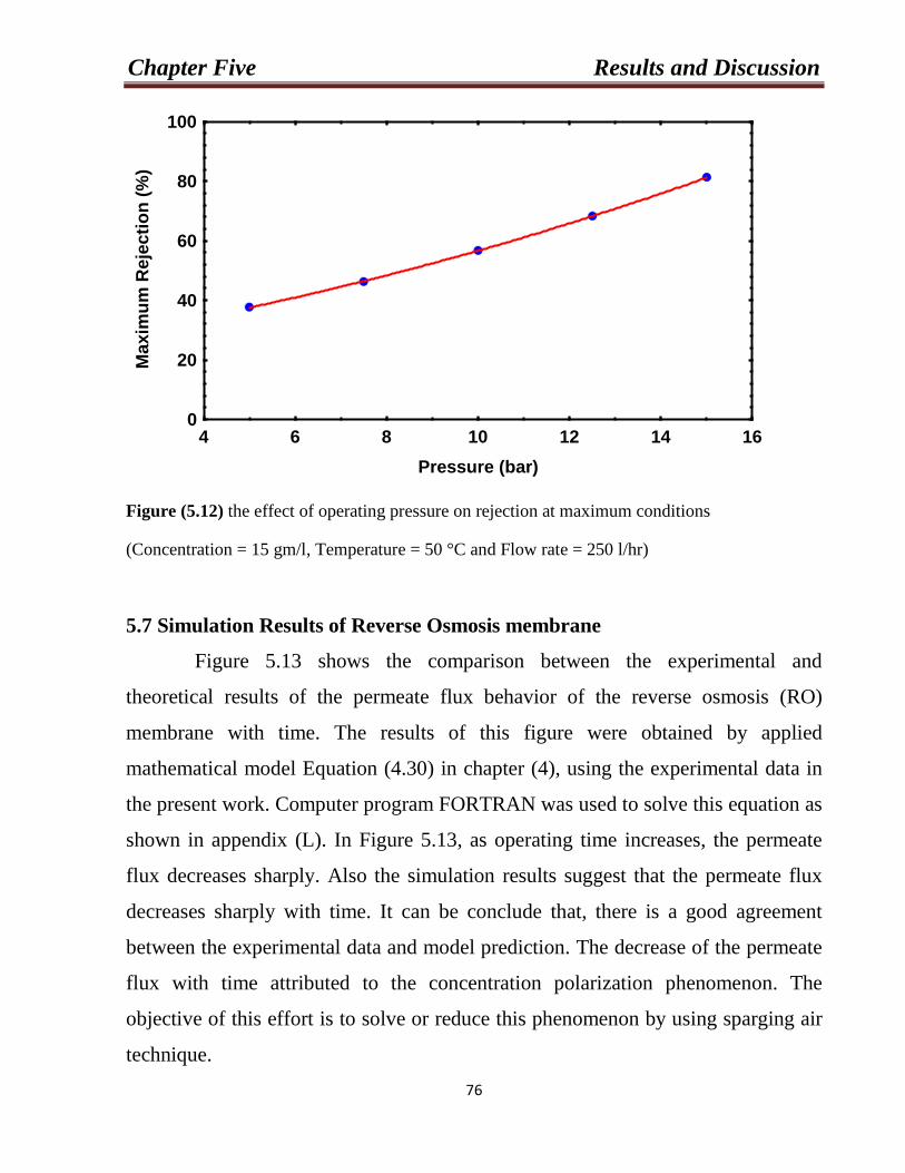
Chapter Five Results and Discussion
76
4 6 8 10 12 14 16Pressure (bar)
0
20
40
60
80
100M
axim
um R
ejec
tion
(%)
Figure (5.12) the effect of operating pressure on rejection at maximum conditions
(Concentration = 15 gm/l, Temperature = 50 °C and Flow rate = 250 l/hr)
5.7 Simulation Results of Reverse Osmosis membrane
Figure 5.13 shows the comparison between the experimental and
theoretical results of the permeate flux behavior of the reverse osmosis (RO)
membrane with time. The results of this figure were obtained by applied
mathematical model Equation (4.30) in chapter (4), using the experimental data in
the present work. Computer program FORTRAN was used to solve this equation as
shown in appendix (L). In Figure 5.13, as operating time increases, the permeate
flux decreases sharply. Also the simulation results suggest that the permeate flux
decreases sharply with time. It can be conclude that, there is a good agreement
between the experimental data and model prediction. The decrease of the permeate
flux with time attributed to the concentration polarization phenomenon. The
objective of this effort is to solve or reduce this phenomenon by using sparging air
technique.
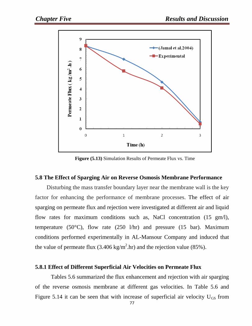
Chapter Five Results and Discussion
77
Figure (5.13) Simulation Results of Permeate Flux vs. Time
5.8 The Effect of Sparging Air on Reverse Osmosis Membrane Performance
Disturbing the mass transfer boundary layer near the membrane wall is the key
factor for enhancing the performance of membrane processes. The effect of air
sparging on permeate flux and rejection were investigated at different air and liquid
flow rates for maximum conditions such as, NaCl concentration (15 gm/l),
temperature (50°C), flow rate (250 l/hr) and pressure (15 bar). Maximum
conditions performed experimentally in AL-Mansour Company and induced that
the value of permeate flux (3.406 kg/m2
.hr) and the rejection value (85%).
5.8.1 Effect of Different Superficial Air Velocities on Permeate Flux
Tables 5.6 summarized the flux enhancement and rejection with air sparging
of the reverse osmosis membrane at different gas velocities. In Table 5.6 and
Figure 5.14 it can be seen that with increase of superficial air velocity UGS from
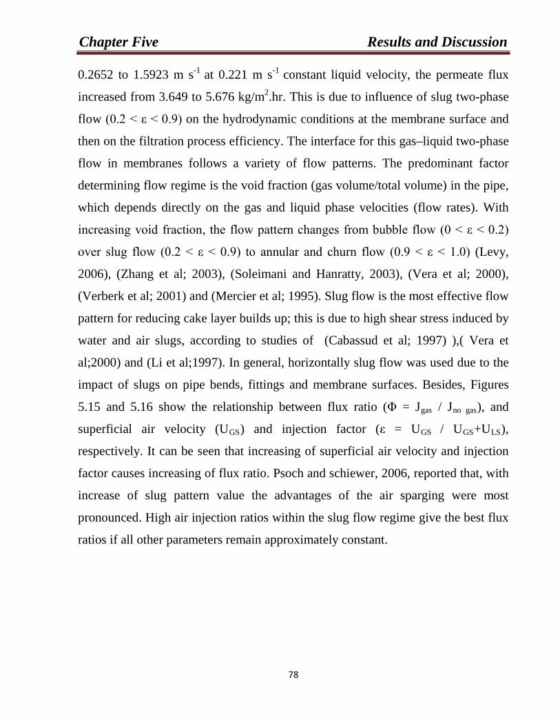
Chapter Five Results and Discussion
78
0.2652 to 1.5923 m s-1 at 0.221 m s-1 constant liquid velocity, the permeate flux
increased from 3.649 to 5.676 kg/m2.hr. This is due to influence of slug two-phase
flow (0.2 < ε < 0.9) on the hydrodynamic conditions at the membrane surface and
then on the filtration process efficiency. The interface for this gas–liquid two-phase
flow in membranes follows a variety of flow patterns. The predominant factor
determining flow regime is the void fraction (gas volume/total volume) in the pipe,
which depends directly on the gas and liquid phase velocities (flow rates). With
increasing void fraction, the flow pattern changes from bubble flow (0 < ε < 0.2)
over slug flow (0.2 < ε < 0.9) to annular and churn flow (0.9 < ε < 1.0) (Levy,
2006), (Zhang et al; 2003), (Soleimani and Hanratty, 2003), (Vera et al; 2000),
(Verberk et al; 2001) and (Mercier et al; 1995). Slug flow is the most effective flow
pattern for reducing cake layer builds up; this is due to high shear stress induced by
water and air slugs, according to studies of (Cabassud et al; 1997) ),( Vera et
al;2000) and (Li et al;1997). In general, horizontally slug flow was used due to the
impact of slugs on pipe bends, fittings and membrane surfaces. Besides, Figures
5.15 and 5.16 show the relationship between flux ratio (Φ = Jgas / Jno gas), and
superficial air velocity (UGS) and injection factor (ε = UGS / UGS+ULS
),
respectively. It can be seen that increasing of superficial air velocity and injection
factor causes increasing of flux ratio. Psoch and schiewer, 2006, reported that, with
increase of slug pattern value the advantages of the air sparging were most
pronounced. High air injection ratios within the slug flow regime give the best flux
ratios if all other parameters remain approximately constant.
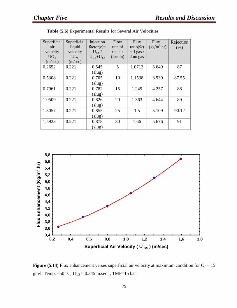
Chapter Five Results and Discussion
79
Table (5.6) Experimental Results for Several Air Velocities
Superficial air
velocity UGS
(m/sec)
Superficial liquid
velocity ULS
(m/sec)
Injection factor(ε)=
UGS / UGS+ULS
Flow rate of the air
(L/min)
Flux ratio(Ф) = J gas / J no gas
Flux (kg/m2.hr)
Rejection (%)
0.2652 0.221 0.545 (slug)
5 1.0713 3.649 87
0.5308 0.221 0.705 (slug)
10 1.1538 3.930 87.55
0.7961 0.221 0.782 (slug)
15 1.249 4.257 88
1.0509 0.221 0.826 (slug)
20 1.363 4.644 89
1.3057 0.221 0.855 (slug)
25 1.5 5.109 90.12
1.5923 0.221 0.878 (slug)
30 1.66 5.676 91
0,2 0,4 0,6 0,8 1,0 1,2 1,4 1,6 1,8
Superficial Air Velocity ( U GS ) (m/sec)
3,43,63,84,04,24,44,64,85,05,25,45,65,8
Flux
Enh
ance
men
t (K
g/m
2 .hr)
Figure (5.14) Flux enhancement verses superficial air velocity at maximum condition for Cf = 15
gm/l, Temp. =50 °C, ULS = 0.345 m.sec-1, TMP=15 bar
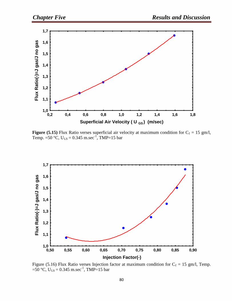
Chapter Five Results and Discussion
80
0,2 0,4 0,6 0,8 1,0 1,2 1,4 1,6 1,8
Superficial Air Velocity ( U GS ) (m/sec)
1,0
1,1
1,2
1,3
1,4
1,5
1,6
1,7Fl
ux R
atio
(-)=J
gas
/J n
o ga
s
Figure (5.15) Flux Ratio verses superficial air velocity at maximum condition for Cf = 15 gm/l, Temp. =50 °C, ULS = 0.345 m.sec-1
, TMP=15 bar
0,50 0,55 0,60 0,65 0,70 0,75 0,80 0,85 0,90
Injection Factor(-)
1,0
1,1
1,2
1,3
1,4
1,5
1,6
1,7
Flux
Rat
io(-)
=J g
as/J
no
gas
Figure (5.16) Flux Ratio verses Injection factor at maximum condition for Cf = 15 gm/l, Temp. =50 °C, ULS = 0.345 m.sec-1, TMP=15 bar
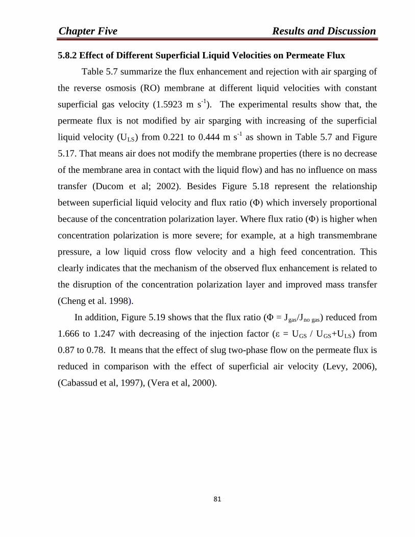
Chapter Five Results and Discussion
81
5.8.2 Effect of Different Superficial Liquid Velocities on Permeate Flux
Table 5.7 summarize the flux enhancement and rejection with air sparging of
the reverse osmosis (RO) membrane at different liquid velocities with constant
superficial gas velocity (1.5923 m s-1). The experimental results show that, the
permeate flux is not modified by air sparging with increasing of the superficial
liquid velocity (ULS) from 0.221 to 0.444 m s-1
In addition, Figure 5.19 shows that the flux ratio (Φ = J
as shown in Table 5.7 and Figure
5.17. That means air does not modify the membrane properties (there is no decrease
of the membrane area in contact with the liquid flow) and has no influence on mass
transfer (Ducom et al; 2002). Besides Figure 5.18 represent the relationship
between superficial liquid velocity and flux ratio (Φ) which inversely proportional
because of the concentration polarization layer. Where flux ratio (Φ) is higher when
concentration polarization is more severe; for example, at a high transmembrane
pressure, a low liquid cross flow velocity and a high feed concentration. This
clearly indicates that the mechanism of the observed flux enhancement is related to
the disruption of the concentration polarization layer and improved mass transfer
(Cheng et al. 1998).
gas/Jno gas) reduced from
1.666 to 1.247 with decreasing of the injection factor (ε = UGS / UGS+ULS
) from
0.87 to 0.78. It means that the effect of slug two-phase flow on the permeate flux is
reduced in comparison with the effect of superficial air velocity (Levy, 2006),
(Cabassud et al, 1997), (Vera et al, 2000).
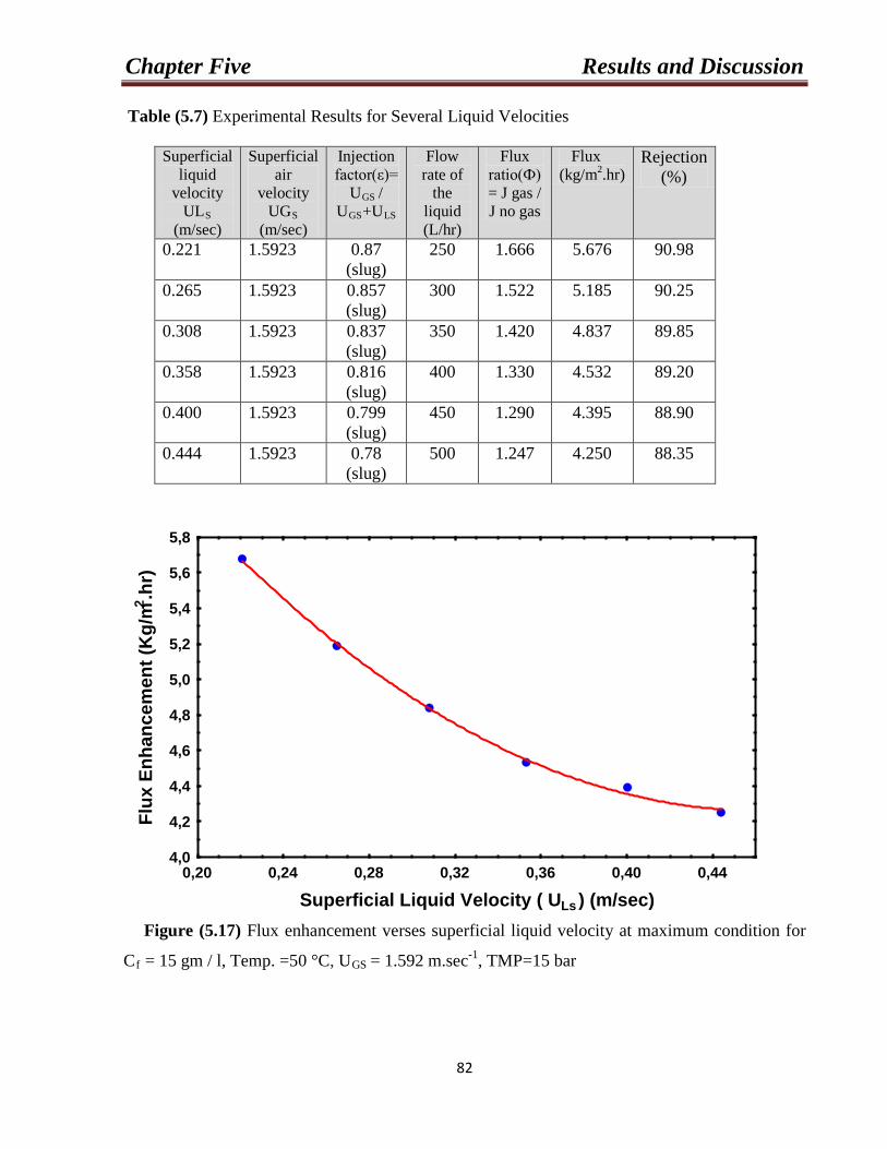
Chapter Five Results and Discussion
82
Table (5.7) Experimental Results for Several Liquid Velocities
Superficial liquid
velocity ULS
(m/sec)
Superficial air
velocity UGS
(m/sec)
Injection factor(ε)=
UGS / UGS+ULS
Flow rate of
the liquid (L/hr)
Flux ratio(Ф) = J gas / J no gas
Flux (kg/m2.hr)
Rejection (%)
0.221 1.5923 0.87 (slug)
250 1.666 5.676 90.98
0.265 1.5923 0.857 (slug)
300 1.522 5.185 90.25
0.308 1.5923 0.837 (slug)
350 1.420 4.837 89.85
0.358 1.5923 0.816 (slug)
400 1.330 4.532 89.20
0.400 1.5923 0.799 (slug)
450 1.290 4.395 88.90
0.444 1.5923 0.78 (slug)
500 1.247 4.250 88.35
0,20 0,24 0,28 0,32 0,36 0,40 0,44
Superficial Liquid Velocity ( U Ls ) (m/sec)
4,0
4,2
4,4
4,6
4,8
5,0
5,2
5,4
5,6
5,8
Flux
Enh
ance
men
t (K
g/m2 .h
r)
Figure (5.17) Flux enhancement verses superficial liquid velocity at maximum condition for
Cf = 15 gm / l, Temp. =50 °C, UGS = 1.592 m.sec-1
, TMP=15 bar
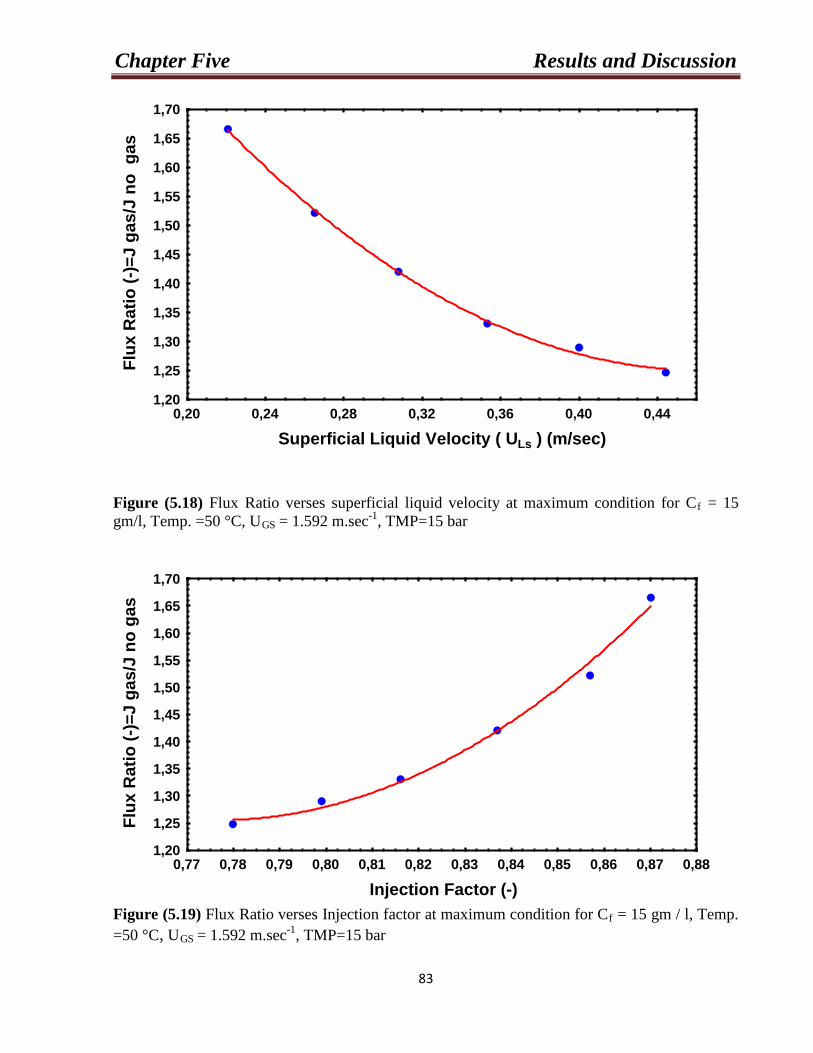
Chapter Five Results and Discussion
83
0,20 0,24 0,28 0,32 0,36 0,40 0,44
Superficial Liquid Velocity ( U Ls ) (m/sec)
1,20
1,25
1,30
1,35
1,40
1,45
1,50
1,55
1,60
1,65
1,70Fl
ux R
atio
(-)=
J ga
s/J
no g
as
Figure (5.18) Flux Ratio verses superficial liquid velocity at maximum condition for Cf = 15 gm/l, Temp. =50 °C, UGS = 1.592 m.sec-1
, TMP=15 bar
0,77 0,78 0,79 0,80 0,81 0,82 0,83 0,84 0,85 0,86 0,87 0,88
Injection Factor (-)
1,20
1,25
1,30
1,35
1,40
1,45
1,50
1,55
1,60
1,65
1,70
Flux
Rat
io (-
)=J
gas/
J no
gas
Figure (5.19) Flux Ratio verses Injection factor at maximum condition for Cf = 15 gm / l, Temp. =50 °C, UGS = 1.592 m.sec-1
, TMP=15 bar
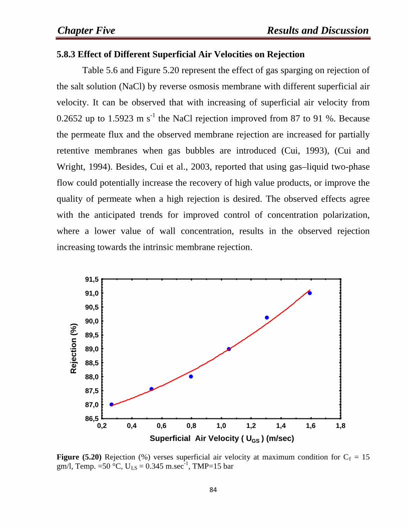
Chapter Five Results and Discussion
84
5.8.3 Effect of Different Superficial Air Velocities on Rejection
Table 5.6 and Figure 5.20 represent the effect of gas sparging on rejection of
the salt solution (NaCl) by reverse osmosis membrane with different superficial air
velocity. It can be observed that with increasing of superficial air velocity from
0.2652 up to 1.5923 m s-1
the NaCl rejection improved from 87 to 91 %. Because
the permeate flux and the observed membrane rejection are increased for partially
retentive membranes when gas bubbles are introduced (Cui, 1993), (Cui and
Wright, 1994). Besides, Cui et al., 2003, reported that using gas–liquid two-phase
flow could potentially increase the recovery of high value products, or improve the
quality of permeate when a high rejection is desired. The observed effects agree
with the anticipated trends for improved control of concentration polarization,
where a lower value of wall concentration, results in the observed rejection
increasing towards the intrinsic membrane rejection.
0,2 0,4 0,6 0,8 1,0 1,2 1,4 1,6 1,8
Superficial Air Velocity ( U GS ) (m/sec)
86,5
87,0
87,5
88,0
88,5
89,0
89,5
90,0
90,5
91,0
91,5
Rej
ectio
n (%
)
Figure (5.20) Rejection (%) verses superficial air velocity at maximum condition for Cf = 15 gm/l, Temp. =50 °C, ULS = 0.345 m.sec-1
, TMP=15 bar
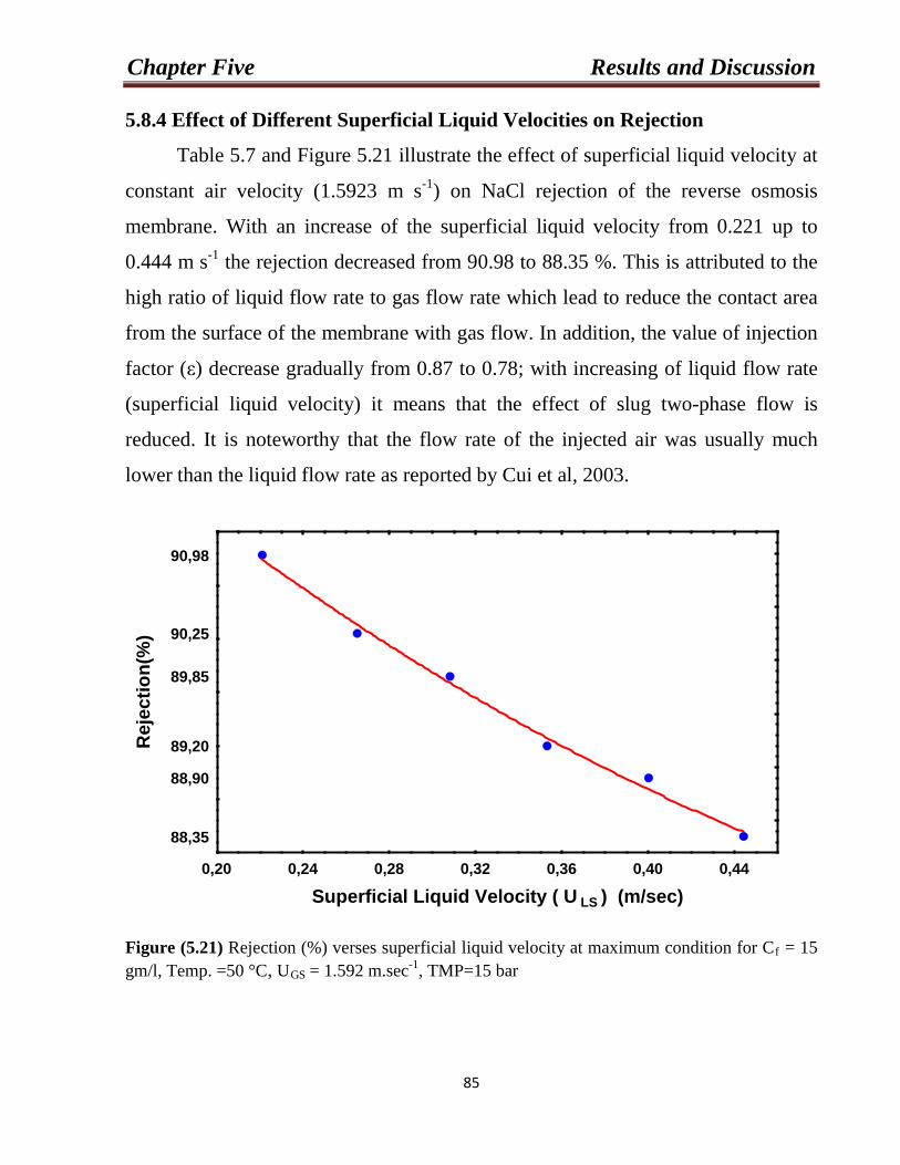
Chapter Five Results and Discussion
85
5.8.4 Effect of Different Superficial Liquid Velocities on Rejection
Table 5.7 and Figure 5.21 illustrate the effect of superficial liquid velocity at
constant air velocity (1.5923 m s-1) on NaCl rejection of the reverse osmosis
membrane. With an increase of the superficial liquid velocity from 0.221 up to
0.444 m s-1
the rejection decreased from 90.98 to 88.35 %. This is attributed to the
high ratio of liquid flow rate to gas flow rate which lead to reduce the contact area
from the surface of the membrane with gas flow. In addition, the value of injection
factor (ε) decrease gradually from 0.87 to 0.78; with increasing of liquid flow rate
(superficial liquid velocity) it means that the effect of slug two-phase flow is
reduced. It is noteworthy that the flow rate of the injected air was usually much
lower than the liquid flow rate as reported by Cui et al, 2003.
0,20 0,24 0,28 0,32 0,36 0,40 0,44
Superficial Liquid Velocity ( U LS ) (m/sec)
88,35
88,90
89,20
89,85
90,25
90,98
Rej
ectio
n(%
)
Figure (5.21) Rejection (%) verses superficial liquid velocity at maximum condition for Cf = 15 gm/l, Temp. =50 °C, UGS = 1.592 m.sec-1
, TMP=15 bar
Chapter Six Conclusions and Recommendations
86
Chapter Six
Conclusions and Recommendations
6.1 Conclusions
The concept of bubbling or gas sparging is to enhance surface mass transfer
can be very effectively applied to membrane processes, such as MF and UF, and
may be useful in NF and RO. The flux enhancement is most significant where the
non-sparged operation is most polarization layer controlled (or in another words
where high boundary layer resistance occurs), such as at low liquid flow rates,
higher solute/particle concentrations and low operating pressures. The following
conclusions are induced from the experimental work:
1. The permeate flux increases with increasing operating pressure, feed
temperature and feed flow rate.
2. The salt rejection of membrane and the quantity of product water increase
with increasing operating pressure and feed flow rate when feed solution was
equal to (15 g/l).
3. The model of reverse osmosis membrane developed by (Jamal et al, 2004)
without concentration polarization is effectively used for the prediction of
flux as a function of operating time.
4. The experiments showed that gas–liquid two-phase flow enhances reverse
osmosis membrane flux by a factor of (1.66) that means permeate flux
increases by (166%) and rejection is also increased up to (91%). This effect
is due to the high and transient wall shear stress induced by the sparging.
5. The hydrodynamic regime inducing the largest enhancement in filtration flux
is slug flow in the case of NaCl solution where a permeate flux plateau was
reached at the beginning of the slug flow regime.
Chapter Six Conclusions and Recommendations
87
6. In the experimental range explored, corresponding to slug flow, the most
significant effects occurred at a moderate liquid flow velocity (0.221 – 0.444
m s−1), gas velocity (0.256 – 1.592 m s−1
6.2 Recommendations
) and high proportion of injected gas
(ε > 0.2).
The following recommendations are presented for future studies:
1. Development of membranes can be studies in order to achieve better
performance at reduced permeation pressures with two- phase flow in
reverse osmosis (RO) membrane.
2. Developing an improved methodology in order to achieve optimal
hydrodynamic conditions of two-phase flow.
3. Using different hydrodynamic conditions, different geometry of modules and
different injection system process.
4. Improving the membrane salt rejection with two-phase flow in reverse
osmosis (RO) membrane.
5. In the continuation of the study, it will be possible to evaluate the effect of
air sparging on permeates flux for complex solution, such as emulsions.
6. Enhancement surface shear with the following technique which include :
a) Turbulence promoters.
b) Pulsate flow and vortex generation.
c) Corrugated membrane surfaces.
d) Forward flushing/ pulsing.
References
88
References
Al-Bastaki N., Abbas A., "Use of fluid instabilities to enhance membrane
performance": a review, Desalination 136 (2001) 255.
Al-Mudaiheem A. M. and Miyamura H., Construction and commissioning of Al
Jobail Phase II desalination plant. Desalination, 55 (1985) 1–11.
Aly S.E., Combined RO/VC desalination system, Desalination, 58 (1986) 85–97.
Amjad Z., Ed. Reverse Osmosis: Membrane Technology, Water Chemistry, and
Industrial Applications; Van Nostrand Reinhold: New York, 1993.
Bachelor G. K, A brief guide to two-phase flow, in: P. Germain, M. Piau, D.
Caillerie (Eds.), Theoretical and Applied Mechanics, Elsevier Science Publishers,
Amsterdam, 1989, pp. 27–40.
B´erub´e P.R. , HLin H., Watai Y. "Fouling in air sparged submerged hollow fiber
membranes at sub- and super-critical flux conditions", Journal of Membrane
Science 307 (2008) 169–180.
Baker R. W. Membrane Technology and Applications, 2nd ed.; John Wiley &
Sons, Ltd.: Chichester, 2004.
Baker R.W.; Wijmans J.G. "The solution-diffusion model: A review", Journal of
Membrane Science, 107 (1995) 1-21.
References
89
Beck R.W., “Demineralization Treatment Technologies for the Seawater
Demineralization Feasibility Investigation”. Inc. Special Publication SJ 2004SP7
(December 31, 2002).
Bellara S.R.,Cui Z.F. and Pepper D.S., "Gas sparging to enhance permeate flux in
ultrafiltration using hollow fibre membranes", Journal of Membrane Science 121
(1996) 175 – 184.
Beolchini F., Veglio F., Barba D., Microfiltration of bovine and ovine milk for the
reduction of microbial content in a tubular membrane: a preliminary investigation,
Desalination 161 (2004) 251.
Bhattacharyya D. and Williams M., "Introduction and Definitions - Reverse
Osmosis", in Membrane Handbook, W. Ho and K. Sirkar, eds., pp. 265-268, Van
Nostrand Reinhold, New York(1992b).
Broussous L. Schmitz P. Prouzet E. Becque L. Larbot A. New ceramic membranes
designed for crossflow filtration enhancement, Sep. Purif. Technol. 25 (2001) 333.
Broussous, L., Ruiz J.C., Larbot A. and Cot L., Stamped ceramic porous tubes for
tangential filtration, Sep. Purif. Technol. 14 (1998) 53. Bird R. B., Stewart W. E., Lightfoot E. N. "Transport Phenomena", 2nd ed.; John
Wiley & Sons, Inc.: New York, 2002.
Bowen W. R., Calvo. J.I., Hernndez. A., "Steps of membrane blocking in flux
decline during protein microfiltration", J. Membr. Sci. 101 (1995) 153.
References
90
Box and George E.P., “statistics experimenters”, New York (1978).
Brandt D.C., Seawater reverse osmosis: an economic alternative to distillation.
Desalination, 52 (1985) 177–186.
Cabassud C., Ducom G. and Laborie S. "Measurement and comparison of wall
shear stresses in a gas/ liquid two-phase flow for two module configurations",
Conf. proc. IMSTEC, Sydney, paper 163, 2003, 6 pp.
Cabassud C., Laborie S. and Laîné .J.M.," How slug flow can improve
ultrafiltration flux in organic hollow fibres", J. Membr. Sci. 128 (1997) 93–101.
Cabassud C., Laborie S., Durand-Bourlier L., Lainé J.M. , Air sparging in
ultrafiltration hollow fibers: relationship between flux enhancement, cake
characteristics and hydrodynamic parameters. Journal of Membrane Science 181
(2001) 57–69.
Carley K.M., Kamneva N.Y., Reminga. J.,"Response Surface, Methodology,
CASOS Technical Report", Carnegie Mellon University, CMU-ISRI-04- 136,
October 2004.
Chang I. and Judd I., "Air sparging of a submerged MBR for municipal
wastewater treatment", Process Biochemistry 37 (2002) 915.
Cheng T. W., Yeh H.M., and Gau C.T.," Enhancement of Permeate Flux by Gas
Slugs for Crossflow Ultrafiltration in Tubular Membrane Module", Separation and
Science Technology, 33(15), (1998) pp. 2295-2309.
References
91
Cheng T.W, "Influence of inclination on gas-sparged cross-flow ultrafiltration
through an inorganic tubular membrane", Journal of Membrane Science 196 (2002)
103–110.
Cheng T.W., Yeh H.M., and Wu J.H.,"Effects of gas slugs and inclination angle on
the ultrafiltration flux in tubular membrane module", Journal of Membrane Science
158 (1999) 223-234.
Cherkasov A.N, Tsareva S.V. and Polotsky A.E. Selictive properties of
ultrafiltration membranes from the standpoint of concentration polarization and
adsorption phenomena. J.Membrane Sci. Vol.104: (1995).157-164.
Christophe S., Durand-Bourlier L., Michael J. C., Philippe M., Jean-Christophe
R., Philippe A.," Use of air sparging to improve backwash efficiency in hollow-
fiber modules", Journal of Membrane Science 161 (1999) 95-113.
Cochran W. G.and Cox. G.M.,"experimental design", 2nd ed., john Wiley and sons
Inc, 1957.
Corneliu C. and Gra˙zyna Z., Response surface modeling and optimization of
copper removal from aqua solutions using polymer assisted ultrafiltration, Journal
of Membrane Science 298 (2007) 56–70.
Cui Z. F, Chang. S., Fane .A.G., the use of gas bubbles to enhance membrane
processes", J. Membr. Sci. 221 (2003) 1-35.
References
92
Cui Z.F, Wright K.I.T., "Gas-liquid two phase flow ultrafiltration of BSA and
dextran solutions", J. Membr. Sci. 90 (1994) 183–189.
Cui Z.F, Wright K.I.T.," Flux enhancements with gas sparging in downwards
crossflow ultrafiltration: performance and mechanism", Journal of Membrane
Science 117 (1996) 109-116.
Cui Z.F. , Chang S., Fane A.G.," The use of gas bubbling to enhance membrane
processes",Journal of Membrane Science 221 (2003) 1–35.
Cui Z.F. and Taha T., "Enhancement of ultrafiltration using gas sparging: a
comparison of different membrane Modules", Journal of Chemical Technology and
Biotechnology 78: (2003) 249–253.
Cui Z.F., Bellara S.R., Homewood P., "Airlift crossflow membrane filtration—a
feasibility study with dextran ultrafiltration", J. Membr. Sci. 128 (1997) 83–91.
Cui Z.F.," Experimental investigation on enhancement of cross flow ultra filtration
with air sparging, in: Effective Membrane Processes New Perspectives", Mech.
Eng. London, (1993) pp. 237–245.
Ducom G., Matamoros H., Cabassud C., "Air sparging for flux enhancement in
nanofiltration membranes: application to O/W stabilised and non-stabilised
emulsions", Journal of Membrane Science 204 (2002) 221–236.
Ducom.G and Cabassud C., "Possible effects of air sparging for nanofiltration of
salted solutions", Desalination, 156 (2003) 267–274.
References
93
Fadaei H, Tabaei S.R., Roostaazad R.," Comparative assessment of the
efficiencies of gas sparging and back-flushing to improve yeast microfiltration
using tubular ceramic membranes", Desalination 217 (2007) 93–99.
Feki M,M .Chaabouni H.F.Ayedi,J.C.Heughebaert,M.Vaillant,“Statistical analysis
of the removal of aluminum and magnesium impurities from wet process
phosphoric acid” ,The Canadian Journal of Chemical Engineering,vol.65.1987.
Freeman B. D. “Osmosis”, In Encyclopedia of Applied Polymer Physics, 1995;
Vol. 13, pp 59-71.
Gekas V., "Terminology for Pressure-Driven Membrane Operations", Desalination,
68, 77 (1988).
Ghosh R., Cui Z.F., "Mass transfer in gas-sparged ultrafiltration: upward slug flow
in tubular membranes", Journal of Membrane Science 162 (1999) 91-102.
Ghosh R., Li Q., and Cui Z.F. "Fractionation of BSA and Lysozyme Using
Ultrafiltration: Effect of Gas Sparging", AIChE Journal. Vol. 44, No. 1. (1998) 61-
67.
Hermia J.," Constant pressure blocking filtration laws – Application to power-law
non-Newtonian fluids", Trans. IChemE 60 (1982) 183.
Herold D.,''A small Pv-Driven Reverse Osmosis Desalination Plant''. Desalination,
137, 2001. pp (285-292).
References
94
Hewitt G.F., Hall-Taylor N.S., "Annular two-phase flow", Pergamon: Oxford
Press. (1970).
Horvath C, Solomon B. A., Engasser J. M.,Measurement of radial transport in slug
flow using enzyme tubes, Ind. Eng. Chem. Fund. 12 (1973) 431– 439.
Hwang K.J., Wu Y.J. "Flux enhancement and cake formation in air-sparged cross-
flow microfiltration", Chemical Engineering Journal (2007).5462; No. of Pages 8.
Jamal K., Khan M.A. and Kamil M. “Mathematical modeling of reverse osmosis
systems’’, Desalination 160 (2004) 29–42.
Jamal K. Modeling of reverse osmosis membrane system, M. Tech. dissertation,
AMU Aligarh, 1996.
Kaichang Y., Xianghua W., QingJie B. Huang X.,"Critical flux enhancements with
air sparging in axial hollow fibers cross-flow microfiltration of biologically treated
wastewater". Journal of Membrane Science 224 (2003) 69–79.
Kim k. J., Fane A. G., Ben Aim R., Liu M G., Jonsson G., Tessaro I. C., Broek A.
P. and Bargeman D., 1994, a comparative study of techniques used for porous
membrane characterization: pore chrectraization. Journal of Membrane science
Vol.87. (1994): 35-46.
Koros W.J., Ma Y.H., Shimizu T. Terminology for membrane processes - IUPAC
recommendations, Journal of Membrane Science, 120, (1996), 149-159.
Kreutzer M., Hydrodynamics of Taylor flow in capillaries and monolith reactors.
Delft: Ph.D. Thesis, Delft University of Technology (2003).
References
95
Kuberkar V., Davis R., Flux enhancement for membrane filtration of bacterial
suspensions using high frequency backpulsing, Biotechnol. Bioeng. 60 (1998) 77.
Laborie S., Cabassud C. , Durand-Bourli L., Laine J.M., "Fouling control by air
sparging inside hollow fibre membranes effects on energy consumption",
Desalination 118 (1998) 189-196.
Laborie S. and Cabassud C., Durand-Bourlier. L. and Laine J.M., Flux
Enhancement by a Continuous Tangential Gas Flow in Ultrafiltration Hollow
Fibres for Drinking Water Production: Effects of Slug Flow on Cake Structure,
Filtration and separation,(1997) Page 887-891.
Lee C.K, Chang W.G, Ju Y.H., "Air slugs entrapped cross flow filtration of
bacterial suspensions", Biotechnol. Bioeng. 41 (1993) 525–530.
Lev S., "Hydrodynamic and statistical parameters of slug flow", International
Journal of Heat and Fluid Flow 24 (2003) 334–344.
Levy S., "Two-Phase Flow in Complex Systems", Desalination 197 (2006) 9–22.
Li Q.Y., Cui Z.F., Pepper D.S., "Fractionation of HSA and IgG by gas sparged
ultrafiltration", Journal of Membrane Science 136 (1997) 181-190.
Li Q.Y., Cui Z.F., Pepper D.S.," Effect of bubble size and frequency on the
permeate flux of gas sparged ultrafiltration with tubular membrane", Chemical
Engineering Journal 67 (1997) 71–75.

References
96
Li Q.Y., Ghosh R., Bellara S.R, Cui Z.F. and Pepper D.S., Enhancement of
ultrafiltration by gas sparging with flat sheet membrane modules, Separation and
Purification Technology 14 (1998) 79–83.
Liteanu C., Rica I., "Optimization of Analytical Processes", Ed. Acad., Bucharest,
1985.
Luque S., Maluubhotla H., Gehlert G., Kuriyel R., Dzengeleski S., Pearl S., Belfort
G., A new coiled hollowfiber module design for enhanced microfiltration
performance in biotechnology, Biotechnol. Bioeng. 65 (1999) 247.
Levesley J.A., Hoare M., The effect of high frequency backflushing on the
microfiltration of yeast homogenate suspensions for the recovery of soluble
proteins, J. Membr. Sci. 158 (1999)169.
Majewska-Nowak. K., Kabsch-Korbutowicz M. and Winnicki T., The effect of
gas bubble flow on ultrafiltration efficiency, Desalination, 126 (1999) 187–192.
Mark C. Porter, "Handbook of Industrial membrane Technology", (1990), by
Noyes Publications,United States.
Mercier M., Fonade C., Lafforgue-Delorme C., "How slug flow can enhance the
ultrafiltration flux in mineral tubular membranes", Journal of Membrane Science
128 (1997) 103-113.
Mercier M, Fonade C., and Lafforgue-Delorme C.," Yeast suspension filtration:
enhancement using an upward gas/liquid slug flow-Application to continuous
alcoholic fermentation with cell recycles", Biotechnol. Bioeng. 58 (1998) 47.
References
97
Mercier M., Fonade C. and Lafforgue-Delorme C.," Influence of the flow regime
on the efficiency of a gas liquid two-phase medium filtration", Biotechnology
Techniques. Vol. 9 No.12 (Dec.1995) p.853-858.
Mindler A. B. and Epstein A.C., “Measurements And Control In Reverse Osmosis
Desalination”. Desalination, No. 59, New York, 1986. P (343-379).
Munir C., "Ultrafiltration and Microfiltration Handbook", Technomic Publishing
Copany, Inc.1998.
Ohya H. Reverse Osmosis Method, Ultrafiltration Method, I. Theory. Sachu
Publisher, Japan, 1976.
Paul D.R., "Reformulation of the solution-diffusion theory of reverse osmosis",
Journal of Membrane Science, 241 (2004) 371-386. Parnham C. S., Davis R. H., Protein recovery from bacterial cell debris using
crossflow microfiltration with backpulsing, J. Membr. Sci. 118 (1996) 259. Perry R. H.,Green D. W., Eds. Perry's Chemical Engineers' Handbook, 7th ed.;
McGraw-Hill: New York, 1997.
Pelligrino, J.; Sikdar S.K. Membrane Technology Fundamentals for
Bioremediation. http://www.membranes.nist.gov, (2004).
Petr MikulBSek, Petr PospiSil, Petr DoleCek, Jifi Cakl,"Gas-liquid two-phase flow
in microfiltration mineral tubular membranes: relationship between flux
enhancement and hydrodynamic parameters", Desalination 146 (2002) 103-109.
References
98
Posp´ıšil P., Wakeman R.J., Hodgsonb I.O.A, Mikulášek P. , "Shear stress-based
modelling of steady state permeate flux in microfiltration enhanced by two-phase
flows", Chemical Engineering Journal 97 (2004) 257–263.
Psoch C, Schiewer S.," Dimensionless numbers for the analysis of air sparging
aimed to reduce fouling in tubular membranes of a membrane bioreactor",
Desalination 197 (2006) 9–22.
Psoch C. and Schiewer S.," Anti-fouling application of air sparging and back
flushing for MBR", Journal of Membrane Science 283 (2006) 273–280.
Psoch C. and S. Schiewer, Anti-fouling application of air sparging and
backflushing for MBR, Journal of Membrane Science 283 (2006) 273–280.
Raymond H. M., Douglas. C. Montgomery “Response Surface Methodology".
1995 by John wiley & Sons.
Riley R. J., Lonsdale H. K., Lyons C. R., and Merten U., "Preparation of Ultrathin
Reverse Osmosis Membranes and the Attainment of Theoretical Salt Rejection",
Journal of Applied Polymer Science, 11 (1967) 2143-2158.
Sheng C., Fane A.G.,"The effect of fibre diameter on filtration and flux
distribution—relevance to submerged hollow fibre modules", Journal of Membrane
Science 184 (2001) 221–231.
References
99
Sheng C., Fane A.G., "Characteristics of microfiltration of suspensions with inter-
fiber two-phase flow", Journal of Chemical Technology and Biotechnology75:533-
540 (2000).
Sheng C., Fane A.G., "Filtration of biomass with axial inter-fibre upward slug
flow: performance and mechanisms", Journal of Membrane Science 180 (2000)
57–68.
Slater C. S., Zielinski J.M., Wendel. R.G. and Uchrin C.G.," Modeling of a small
scale reverse osmosis systems". Desalination, 52 (1985) 267–284.
Smith M. C., Ed., Water Desalination Report, Vol. XXI, No. 37 (September 19,
1985).
Soleimani A. and Hanratty T., "Critical liquid flows for the transition from the
pseudo-slug and stratified patterns to slug flow", Internl. J. Multiphase Flow, 29
(2003) 51–67.
Sondhi R., Bhave R., Role of backpulsing in fouling minimization in crossflow
filtration with ceramic membranes, J. Membr. Sci. 186 (2001) 41.
Stanton S., Taha T., Cui Z.F., "Enhancing hollow fibre ultrafiltration using slug-
flow - a hydrodynamic study", Desalination 146 (2002) 69-74.
Sur H. W., Cui .Z.F," Experimental study on the enhancement of yeast
microfiltration with gas sparging", J. Chem. Technol. Biotechnol. 76 (2001) 477.
References
100
Taha T., Cheong W.L., Field R.W., Cui Z.F.," Gas-sparged ultrafiltration using
horizontal and inclined tubular membranes—A CFD study", Journal of Membrane
Science 279 (2006) 487–494.
Taha T. And Cui Z., "CFD modeling of gas-sparged ultrafiltration in tubular
membranes", Journal of Membrane Science, 210 (2002) 13–27.
Taitel Y., Barnéa D., Duckler A.E., "Modeling flow pattern transitions for steady
upward gas–liquid flow in vertical tubes", AICHE J. 3 (1980) 345–354.
Takuo I., Hiroyuki S., Kohnosuke M., Tomoya F., and Nobuhiko K., Application
of gas –liquid two-phase cross-flow filtration to pilot-scale methane fermentation,
Drying technology, 11 (4), (1993) 769-785.
Vera L., Delgado S. and Elmaleh D.,"Gas sparged cross-flow microfiltration of
biologically treated wastewater", Wat. Sci. Technol., 41(10) (2000) 173–180.
Vera L., Delgado S., and Elmaleh S.," Dimensionless numbers for the steady-state
flux of cross-flow microfiltration and ultrafiltration with gas sparging". Chemical
Engineering Science 55 (2000) 3419-3428.
Vera L., Villarroel R., Delgado S. and Elmaleh S., "Enhancing microfiltration
through an inorganic tubular membrane by gas sparging", Journal of Membrane
Science, 165 (2000) 47–57.
References
101
Vera L., Villarroel R., Delgado S., Elmaleh S., “Enhancing microfiltration through
an inorganic tubular membrane by gas sparging". Journal of Membrane Science
165 (2000) 47–57.
Verberk J., Worm G., Futselaar H. and van Dijk J., combined air-water flush in
dead-end ultrafiltration, Wat. Sci. Technol., Wat. Supply, 1(5/6) (2001) 393–402.
Verberk J.Q., "Application of air in membrane filtration". Copyright
by J.Q.J.C.Verberk (2005).
Verberk J.Q., Van Dijk J.C., "Air sparging in capillary nanofiltration", Journal of
Membrane Science 284 (2006) 339–351.
Wallis G.B., One-dimensional two-phase flow. New York: McGraw-Hill. (1969).
Wessling M., Two-dimensional stochastic modeling of membrane fouling, Sep.
Purif. Technol. 24 (2001) 375.
Whalley P.B," Boiling Condensation and Gas–Liquid Flow", Clarendon Press,
Oxford, 1987.
Winzeler H. B., Belfort G., Enhanced performance for pressure-driven membrane
processes: The argument for fluid instabilities, J. Membr. Sci. 80 (1993) 35.
Xu J.H., Luo G.S., Chen G.G., Tan B., "Mass transfer performance and two-phase
flow characteristic in membrane dispersion mini-extractor", Journal of Membrane
Science 249 (2005) 75–81.
References
102
Zeman L.J., Zydney A.L.," Microfiltration and ultrafiltration: principles and
applications", Marcel Dekker, New York, 1996.
Zhang H.Q., Wang Q., Sarica C. and Brill J., "A unified mechanistic model for
slug liquid holdup and transition between slug and dispersed bubbleflows", Internl.
J. Multiphase Flow, 29 (2003) 97–107.
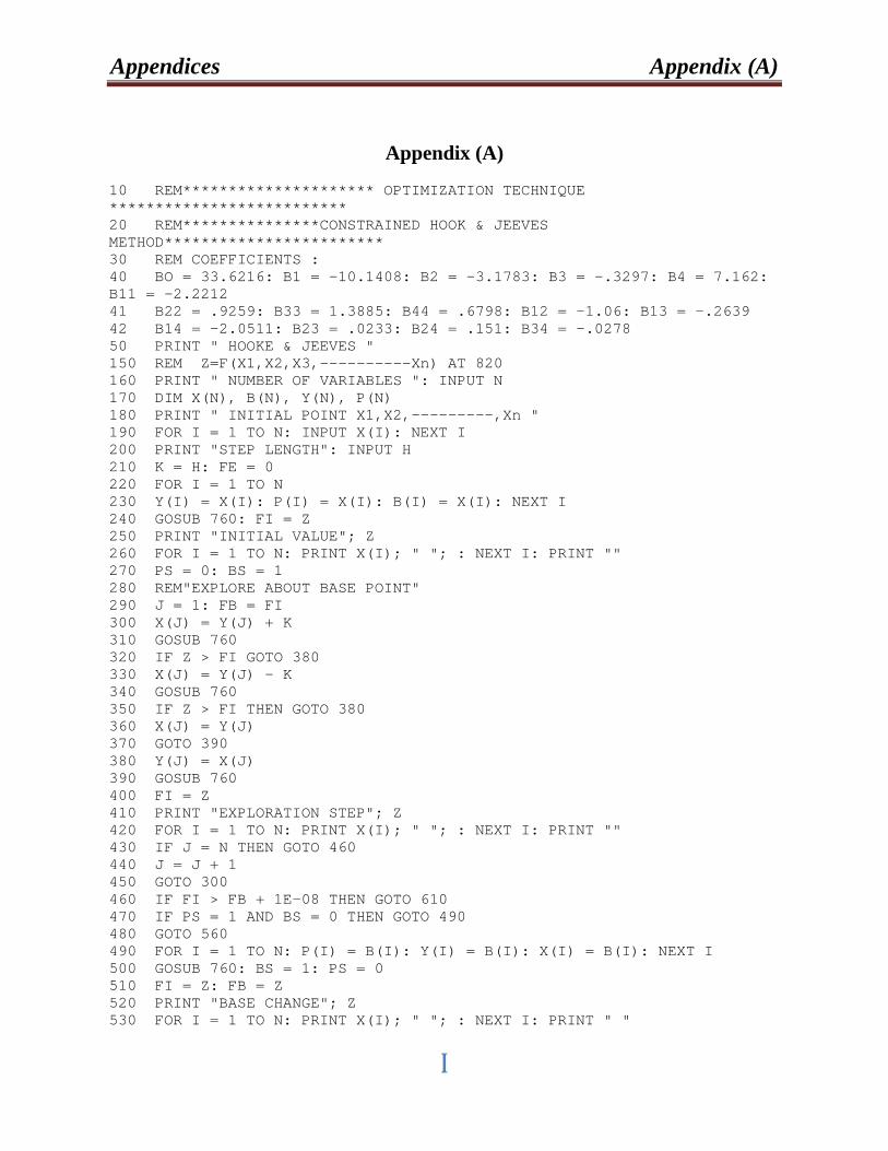
Appendices Appendix (A)
I
Appendix (A) 10 REM********************* OPTIMIZATION TECHNIQUE ************************** 20 REM***************CONSTRAINED HOOK & JEEVES METHOD************************ 30 REM COEFFICIENTS : 40 BO = 33.6216: B1 = -10.1408: B2 = -3.1783: B3 = -.3297: B4 = 7.162: B11 = -2.2212 41 B22 = .9259: B33 = 1.3885: B44 = .6798: B12 = -1.06: B13 = -.2639 42 B14 = -2.0511: B23 = .0233: B24 = .151: B34 = -.0278 50 PRINT " HOOKE & JEEVES " 150 REM Z=F(X1,X2,X3,----------Xn) AT 820 160 PRINT " NUMBER OF VARIABLES ": INPUT N 170 DIM X(N), B(N), Y(N), P(N) 180 PRINT " INITIAL POINT X1,X2,---------,Xn " 190 FOR I = 1 TO N: INPUT X(I): NEXT I 200 PRINT "STEP LENGTH": INPUT H 210 K = H: FE = 0 220 FOR I = 1 TO N 230 Y(I) = X(I): P(I) = X(I): B(I) = X(I): NEXT I 240 GOSUB 760: FI = Z 250 PRINT "INITIAL VALUE"; Z 260 FOR I = 1 TO N: PRINT X(I); " "; : NEXT I: PRINT "" 270 PS = 0: BS = 1 280 REM"EXPLORE ABOUT BASE POINT" 290 J = 1: FB = FI 300 X(J) = Y(J) + K 310 GOSUB 760 320 IF Z > FI GOTO 380 330 X(J) = Y(J) - K 340 GOSUB 760 350 IF Z > FI THEN GOTO 380 360 X(J) = Y(J) 370 GOTO 390 380 Y(J) = X(J) 390 GOSUB 760 400 FI = Z 410 PRINT "EXPLORATION STEP"; Z 420 FOR I = 1 TO N: PRINT X(I); " "; : NEXT I: PRINT "" 430 IF J = N THEN GOTO 460 440 J = J + 1 450 GOTO 300 460 IF FI > FB + 1E-08 THEN GOTO 610 470 IF PS = 1 AND BS = 0 THEN GOTO 490 480 GOTO 560 490 FOR I = 1 TO N: P(I) = B(I): Y(I) = B(I): X(I) = B(I): NEXT I 500 GOSUB 760: BS = 1: PS = 0 510 FI = Z: FB = Z 520 PRINT "BASE CHANGE"; Z 530 FOR I = 1 TO N: PRINT X(I); " "; : NEXT I: PRINT " "
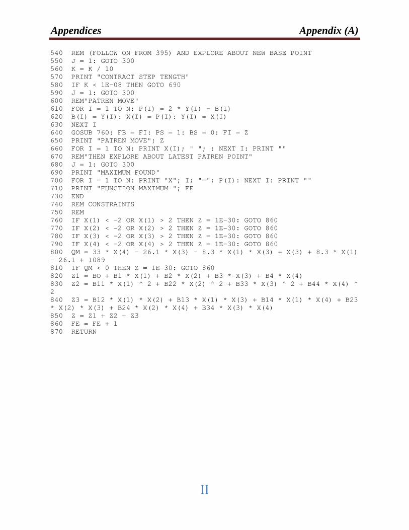
Appendices Appendix (A)
II
540 REM (FOLLOW ON FROM 395) AND EXPLORE ABOUT NEW BASE POINT 550 J = 1: GOTO 300 560 K = K / 10 570 PRINT "CONTRACT STEP TENGTH" 580 IF K < 1E-08 THEN GOTO 690 590 J = 1: GOTO 300 600 REM"PATREN MOVE" 610 FOR I = 1 TO N: P(I) = 2 * Y(I) - B(I) 620 B(I) = Y(I): X(I) = P(I): Y(I) = X(I) 630 NEXT I 640 GOSUB 760: FB = FI: PS = 1: BS = 0: FI = Z 650 PRINT "PATREN MOVE"; Z 660 FOR I = 1 TO N: PRINT X(I); " "; : NEXT I: PRINT "" 670 REM"THEN EXPLORE ABOUT LATEST PATREN POINT" 680 J = 1: GOTO 300 690 PRINT "MAXIMUM FOUND" 700 FOR I = 1 TO N: PRINT "X"; I; "="; P(I): NEXT I: PRINT "" 710 PRINT "FUNCTION MAXIMUM="; FE 730 END 740 REM CONSTRAINTS 750 REM 760 IF X(1) < -2 OR X(1) > 2 THEN Z = 1E-30: GOTO 860 770 IF X(2) < -2 OR X(2) > 2 THEN Z = 1E-30: GOTO 860 780 IF X(3) < -2 OR X(3) > 2 THEN Z = 1E-30: GOTO 860 790 IF X(4) < -2 OR X(4) > 2 THEN Z = 1E-30: GOTO 860 800 QM = 33 * X(4) - 26.1 * X(3) - 8.3 * X(1) * X(3) + X(3) + 8.3 * X(1) - 26.1 + 1089 810 IF QM < 0 THEN Z = 1E-30: GOTO 860 820 Z1 = BO + B1 * X(1) + B2 * X(2) + B3 * X(3) + B4 * X(4) 830 Z2 = B11 * X(1) ^ 2 + B22 * X(2) ^ 2 + B33 * X(3) ^ 2 + B44 * X(4) ^ 2 840 Z3 = B12 * X(1) * X(2) + B13 * X(1) * X(3) + B14 * X(1) * X(4) + B23 * X(2) * X(3) + B24 * X(2) * X(4) + B34 * X(3) * X(4) 850 Z = Z1 + Z2 + Z3 860 FE = FE + 1 870 RETURN
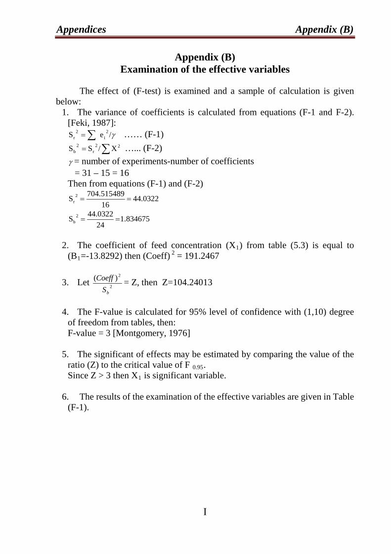
Appendices Appendix (B)
I
Appendix (B) Examination of the effective variables
The effect of (F-test) is examined and a sample of calculation is given below:
1. The variance of coefficients is calculated from equations (F-1 and F-2). [Feki, 1987]:
γ/eS 2i
2r ∑= …… (F-1)
∑= 22r
2b X/SS …... (F-2)
γ = number of experiments-number of coefficients = 31 – 15 = 16 Then from equations (F-1) and (F-2)
0322.4416515489.704S 2
r ==
834675.1240322.44S 2
b ==
2. The coefficient of feed concentration (X1) from table (5.3) is equal to
(B1=-13.8292) then (Coeff) 2
3. Let
= 191.2467
2
2)(
bSCoeff = Z, then Z=104.24013
4. The F-value is calculated for 95% level of confidence with (1,10) degree
of freedom from tables, then: F-value = 3 [Montgomery, 1976]
5. The significant of effects may be estimated by comparing the value of the ratio (Z) to the critical value of F 0.95. Since Z > 3 then X1
6. The results of the examination of the effective variables are given in Table (F-1).
is significant variable.
Appendices Appendix (B)
ΙΙ
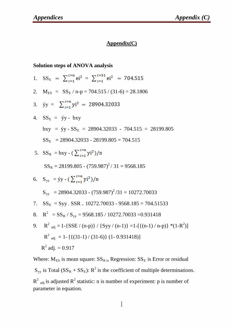
Appendices Appendix (C)
I
Appendix(C)
Solution steps of ANOVA analysis
1. SSRER =
2. MRES R = SSRER / n-p = 704.515 / (31-6) = 28.1806
3. ýy =
4. SSRER = ýy - bxy
bxy = ýy - SSRER = 28904.32033 - 704.515 = 28199.805
SSRER = 28904.32033 - 28199.805 = 704.515
5. SSRR R= bxy - (
SSRRR = 28199.805 - (759.987)P
2 P/ 31 = 9568.185
6. SRyy R= ýy - (
SRyy R = 28904.32033 - (759.987)P
2 P/31 = 10272.70033
7. SSRE R= SyyR -R SSRR =R 10272.70033 - 9568.185 = 704.51533
8. RP
2P = SSRRR / SRyyR = 9568.185 / 10272.70033 =0.931418
9. R P
2P RadjR =P
P1-SSE / (n-p) / Syy / (n-1) =1-[(n-1) / n-p) *(1-RP
2P)]
RP
2P Radj R= 1- [(31-1) / (31-6) (1- 0.931418)]
RP
2P adj. = 0.917
Where: MRESR is mean square: SSRR isR Regression: SSRER is Error or residual
SRyyR is Total (SSRRR + SSRER): RP
2P is the coefficient of multiple determinations.
RP
2P Radj Ris adjusted RP
2P statistic: n is number of experiment: p is number of
parameter in equation.
Appendices Appendix (C)
II
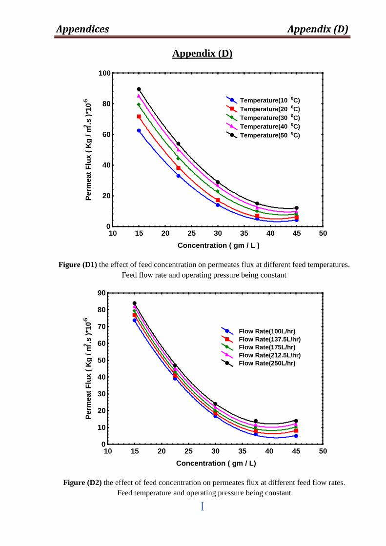
Appendices Appendix (D)
I
Appendix (D)
10 15 20 25 30 35 40 45 50Concentration ( gm / L )
0
20
40
60
80
100
Perm
eat F
lux
( Kg
/ m2 .s
)*10
-5 Temperature(10 0C) Temperature(20 0C) Temperature(30 0C) Temperature(40 0C) Temperature(50 0C)
Figure (D1) the effect of feed concentration on permeates flux at different feed temperatures. Feed flow rate and operating pressure being constant
10 15 20 25 30 35 40 45 50Concentration ( gm / L)
0
10
20
30
40
50
60
70
80
90
Perm
eat F
lux
( Kg
/ m2 .s
)*10
-5
Flow Rate(100L/hr) Flow Rate(137.5L/hr) Flow Rate(175L/hr) Flow Rate(212.5L/hr) Flow Rate(250L/hr)
Figure (D2) the effect of feed concentration on permeates flux at different feed flow rates. Feed temperature and operating pressure being constant
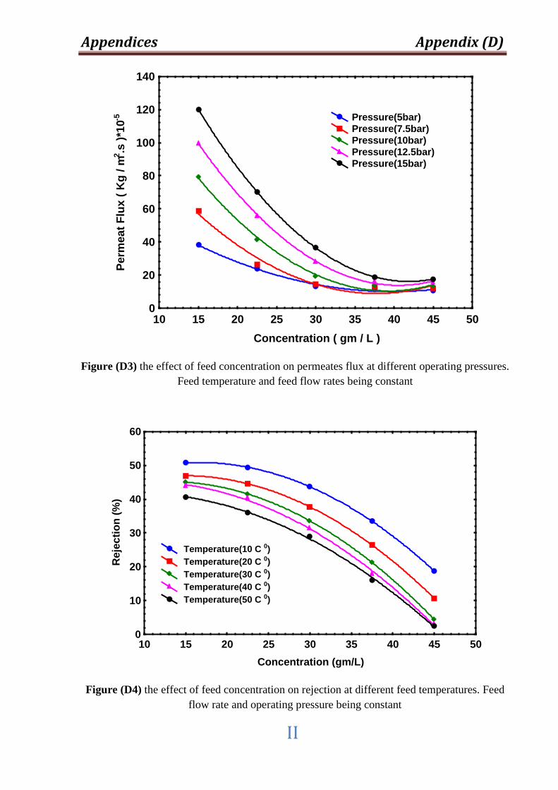
Appendices Appendix (D)
II
10 15 20 25 30 35 40 45 50Concentration ( gm / L )
0
20
40
60
80
100
120
140
Perm
eat F
lux
( Kg
/ m2 .s
)*10
-5 Pressure(5bar) Pressure(7.5bar) Pressure(10bar) Pressure(12.5bar) Pressure(15bar)
Figure (D3) the effect of feed concentration on permeates flux at different operating pressures. Feed temperature and feed flow rates being constant
10 15 20 25 30 35 40 45 50Concentration (gm/L)
0
10
20
30
40
50
60
Rej
ectio
n (%
)
Temperature(10 C 0) Temperature(20 C 0) Temperature(30 C 0) Temperature(40 C 0) Temperature(50 C 0)
Figure (D4) the effect of feed concentration on rejection at different feed temperatures. Feed flow rate and operating pressure being constant
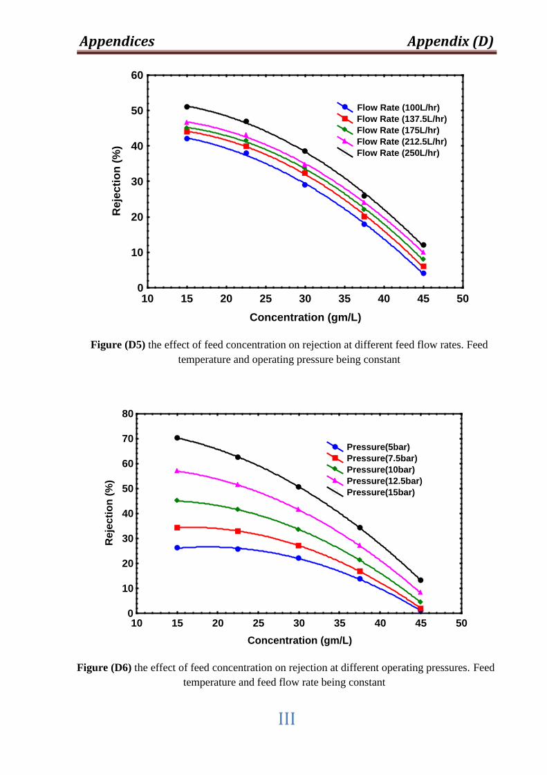
Appendices Appendix (D)
III
10 15 20 25 30 35 40 45 50Concentration (gm/L)
0
10
20
30
40
50
60
Rej
ectio
n (%
) Flow Rate (100L/hr) Flow Rate (137.5L/hr) Flow Rate (175L/hr) Flow Rate (212.5L/hr) Flow Rate (250L/hr)
Figure (D5) the effect of feed concentration on rejection at different feed flow rates. Feed temperature and operating pressure being constant
10 15 20 25 30 35 40 45 50Concentration (gm/L)
0
10
20
30
40
50
60
70
80
Rej
ectio
n (%
)
Pressure(5bar) Pressure(7.5bar) Pressure(10bar) Pressure(12.5bar) Pressure(15bar)
Figure (D6) the effect of feed concentration on rejection at different operating pressures. Feed temperature and feed flow rate being constant
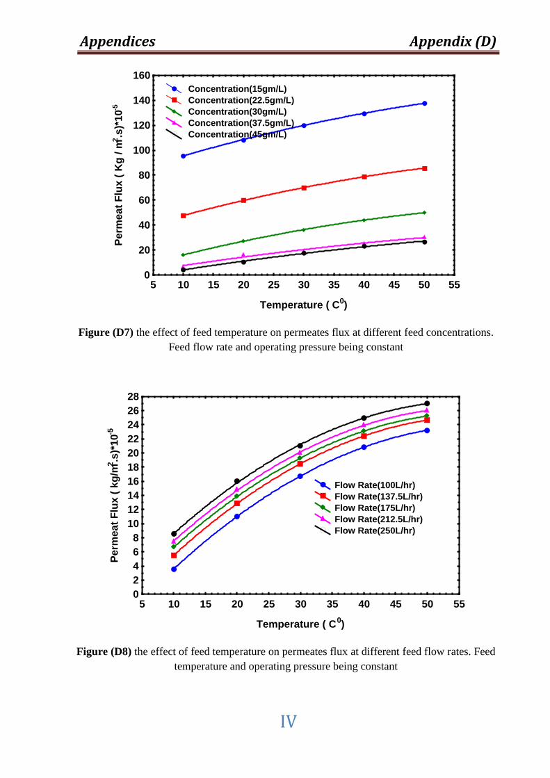
Appendices Appendix (D)
IV
5 10 15 20 25 30 35 40 45 50 55
Temperature ( C0)
0
20
40
60
80
100
120
140
160
Perm
eat F
lux
( Kg
/ m2 .s
)*10
-5
Concentration(15gm/L) Concentration(22.5gm/L) Concentration(30gm/L) Concentration(37.5gm/L) Concentration(45gm/L)
Figure (D7) the effect of feed temperature on permeates flux at different feed concentrations. Feed flow rate and operating pressure being constant
5 10 15 20 25 30 35 40 45 50 55
Temperature ( C0)
02468
10121416182022242628
Perm
eat F
lux
( kg/
m2 .s)*
10-5
Flow Rate(100L/hr) Flow Rate(137.5L/hr) Flow Rate(175L/hr) Flow Rate(212.5L/hr) Flow Rate(250L/hr)
Figure (D8) the effect of feed temperature on permeates flux at different feed flow rates. Feed temperature and operating pressure being constant
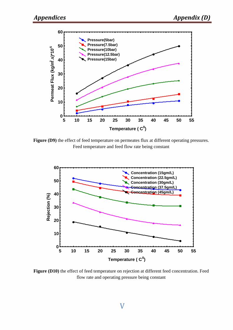
Appendices Appendix (D)
V
5 10 15 20 25 30 35 40 45 50 55
Temperature ( C0)
0
10
20
30
40
50
60
Perm
eat F
lux
(kg/
m2 .s)*
10-5
Pressure(5bar) Pressure(7.5bar) Pressure(10bar) Pressure(12.5bar) Pressure(15bar)
Figure (D9) the effect of feed temperature on permeates flux at different operating pressures. Feed temperature and feed flow rate being constant
5 10 15 20 25 30 35 40 45 50 55
Temperature ( C0)
0
10
20
30
40
50
60
Rej
ectio
n (%
)
Concentration (15gm/L) Concentration (22.5gm/L) Concentration (30gm/L) Concentration (37.5gm/L) Concentration (45gm/L)
Figure (D10) the effect of feed temperature on rejection at different feed concentration. Feed flow rate and operating pressure being constant
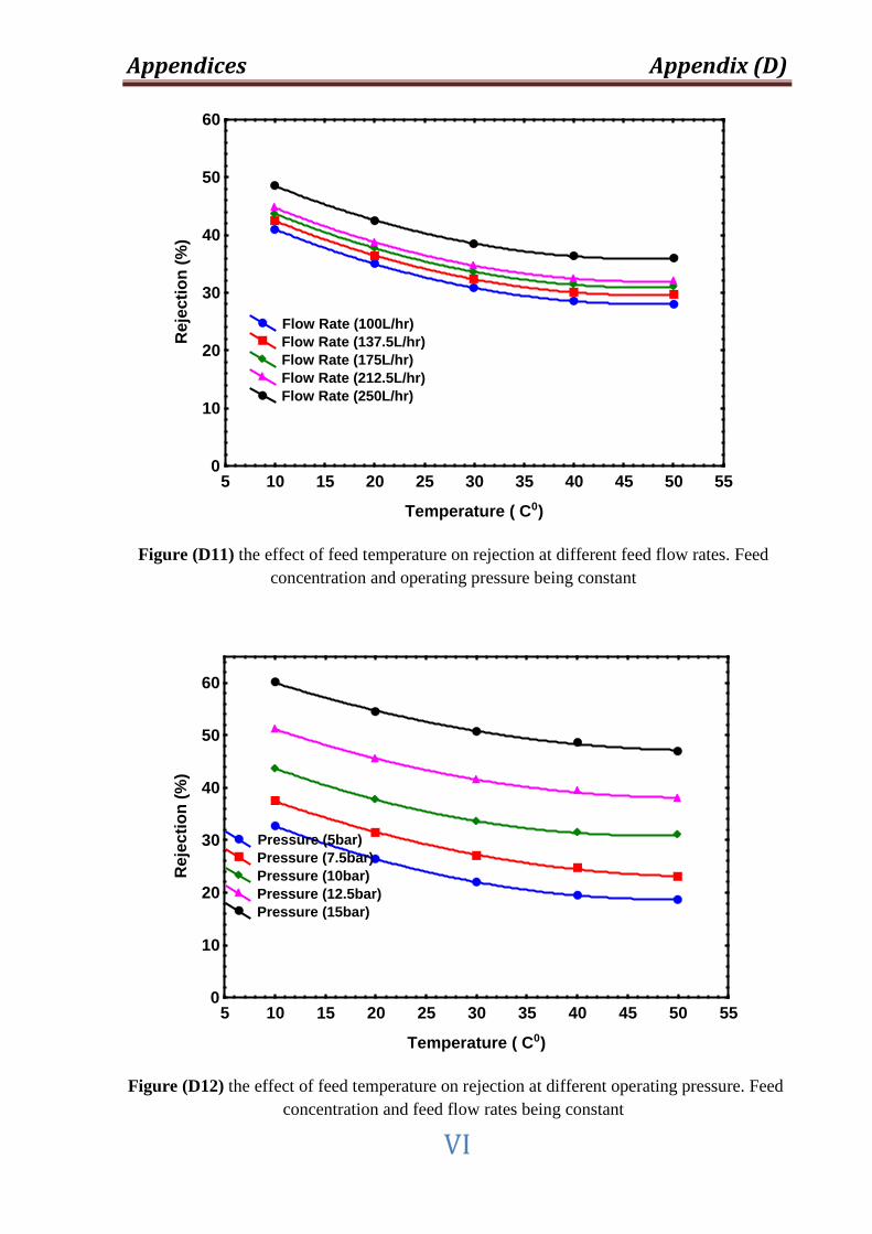
Appendices Appendix (D)
VI
5 10 15 20 25 30 35 40 45 50 55
Temperature ( C0)
0
10
20
30
40
50
60
Rej
ectio
n (%
)
Flow Rate (100L/hr) Flow Rate (137.5L/hr) Flow Rate (175L/hr) Flow Rate (212.5L/hr) Flow Rate (250L/hr)
Figure (D11) the effect of feed temperature on rejection at different feed flow rates. Feed concentration and operating pressure being constant
5 10 15 20 25 30 35 40 45 50 55
Temperature ( C0)
0
10
20
30
40
50
60
Rej
ectio
n (%
)
Pressure (5bar) Pressure (7.5bar) Pressure (10bar) Pressure (12.5bar) Pressure (15bar)
Figure (D12) the effect of feed temperature on rejection at different operating pressure. Feed concentration and feed flow rates being constant
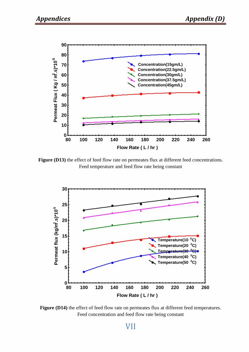
Appendices Appendix (D)
VII
80 100 120 140 160 180 200 220 240 260Flow Rate ( L / hr )
0
10
20
30
40
50
60
70
80
90
Perm
eat F
lux
( Kg
/ m2 .s
)*10
-5
Concentration(15gm/L) Concentration(22.5gm/L) Concentration(30gm/L) Concentration(37.5gm/L) Concentration(45gm/L)
Figure (D13) the effect of feed flow rate on permeates flux at different feed concentrations. Feed temperature and feed flow rate being constant
80 100 120 140 160 180 200 220 240 260Flow Rate ( L / hr )
0
5
10
15
20
25
30
Perm
eat f
lux
(kg/
m2 .s)*
10-5
Temperature(10 0C) Temperature(20 0C) Temperature(30 0C) Temperature(40 0C) Temperature(50 0C)
Figure (D14) the effect of feed flow rate on permeates flux at different feed temperatures. Feed concentration and feed flow rate being constant
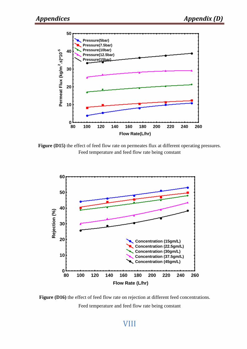
Appendices Appendix (D)
VIII
80 100 120 140 160 180 200 220 240 260Flow Rate(L/hr)
0
10
20
30
40
50
Perm
eat F
lux
(kg/
m2 .s
)*10
-5
Pressure(5bar) Pressure(7.5bar) Pressure(10bar) Pressure(12.5bar) Pressure(15bar)
Figure (D15) the effect of feed flow rate on permeates flux at different operating pressures. Feed temperature and feed flow rate being constant
80 100 120 140 160 180 200 220 240 260Flow Rate (L/hr)
0
10
20
30
40
50
60
Rej
ectio
n (%
)
Concentration (15gm/L) Concentration (22.5gm/L) Concentration (30gm/L) Concentration (37.5gm/L) Concentration (45gm/L)
Figure (D16) the effect of feed flow rate on rejection at different feed concentrations.
Feed temperature and feed flow rate being constant
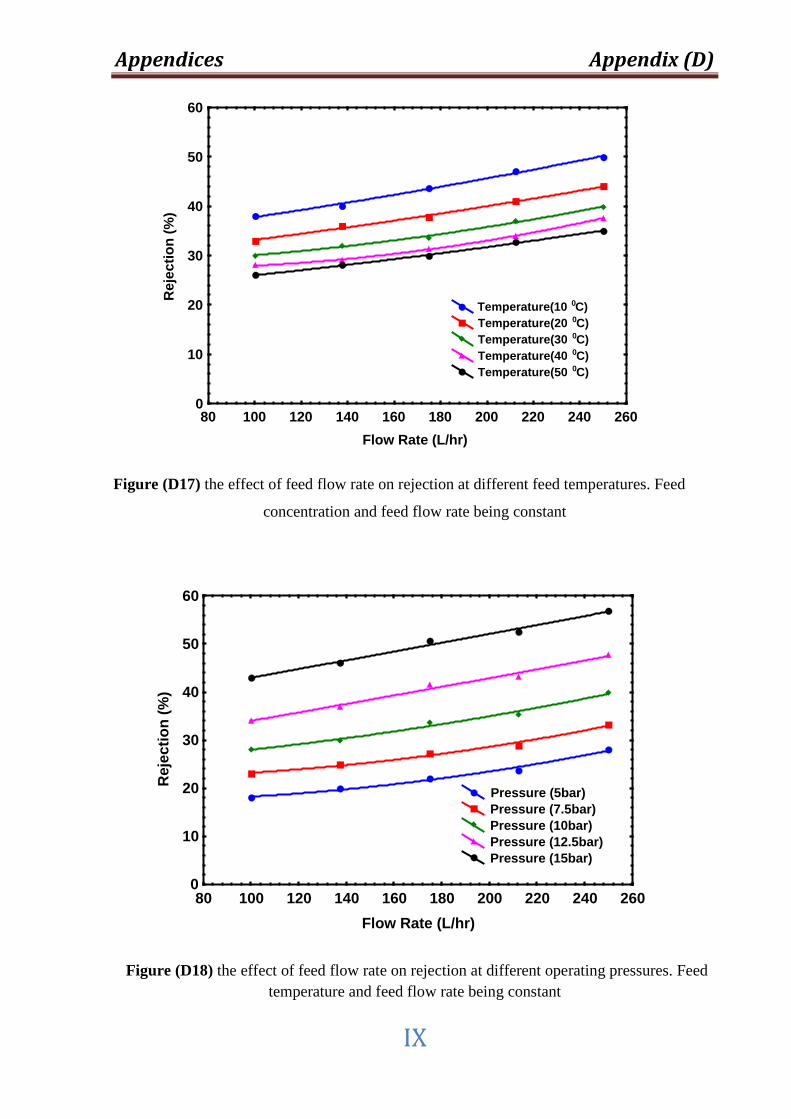
Appendices Appendix (D)
IX
80 100 120 140 160 180 200 220 240 260Flow Rate (L/hr)
0
10
20
30
40
50
60
Rej
ectio
n (%
)
Temperature(10 0C) Temperature(20 0C) Temperature(30 0C) Temperature(40 0C) Temperature(50 0C)
Figure (D17) the effect of feed flow rate on rejection at different feed temperatures. Feed
concentration and feed flow rate being constant
80 100 120 140 160 180 200 220 240 260Flow Rate (L/hr)
0
10
20
30
40
50
60
Rej
ectio
n (%
)
Pressure (5bar) Pressure (7.5bar) Pressure (10bar) Pressure (12.5bar) Pressure (15bar)
Figure (D18) the effect of feed flow rate on rejection at different operating pressures. Feed temperature and feed flow rate being constant
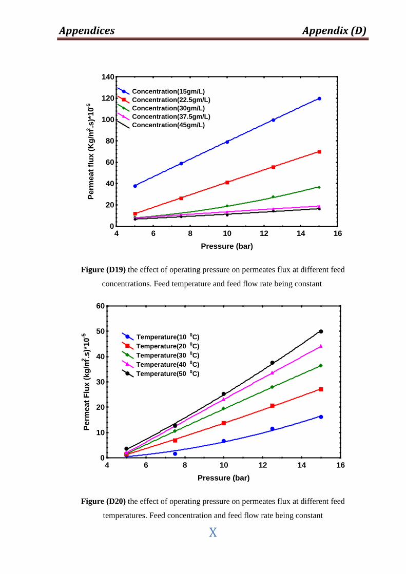
Appendices Appendix (D)
X
4 6 8 10 12 14 16Pressure (bar)
0
20
40
60
80
100
120
140Pe
rmea
t flu
x (K
g/m
2 .s)*
10-5
Concentration(15gm/L) Concentration(22.5gm/L) Concentration(30gm/L) Concentration(37.5gm/L) Concentration(45gm/L)
Figure (D19) the effect of operating pressure on permeates flux at different feed
concentrations. Feed temperature and feed flow rate being constant
4 6 8 10 12 14 16Pressure (bar)
0
10
20
30
40
50
60
Perm
eat F
lux
(kg/
m2 .s)*
10-5 Temperature(10 0C)
Temperature(20 0C) Temperature(30 0C) Temperature(40 0C) Temperature(50 0C)
Figure (D20) the effect of operating pressure on permeates flux at different feed
temperatures. Feed concentration and feed flow rate being constant
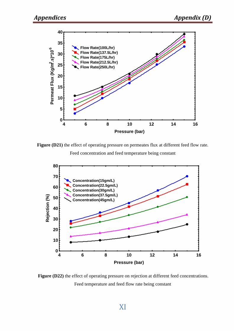
Appendices Appendix (D)
XI
4 6 8 10 12 14 16Pressure (bar)
0
5
10
15
20
25
30
35
40
Perm
eat F
lux
(Kg/
m2 .s
)*10
-5 Flow Rate(100L/hr) Flow Rate(137.5L/hr) Flow Rate(175L/hr) Flow Rate(212.5L/hr) Flow Rate(250L/hr)
Figure (D21) the effect of operating pressure on permeates flux at different feed flow rate.
Feed concentration and feed temperature being constant
4 6 8 10 12 14 16Pressure (bar)
0
10
20
30
40
50
60
70
80
Rej
ectio
n (%
)
Concentration(15gm/L) Concentration(22.5gm/L) Concentration(30gm/L) Concentration(37.5gm/L) Concentration(45gm/L)
Figure (D22) the effect of operating pressure on rejection at different feed concentrations.
Feed temperature and feed flow rate being constant
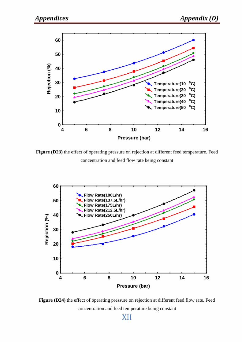
Appendices Appendix (D)
XII
4 6 8 10 12 14 16Pressure (bar)
0
10
20
30
40
50
60R
ejec
tion
(%)
Temperature(10 0C) Temperature(20 0C) Temperature(30 0C) Temperature(40 0C) Temperature(50 0C)
Figure (D23) the effect of operating pressure on rejection at different feed temperature. Feed
concentration and feed flow rate being constant
4 6 8 10 12 14 16Pressure (bar)
0
10
20
30
40
50
60
Rej
ectio
n (%
)
Flow Rate(100L/hr) Flow Rate(137.5L/hr) Flow Rate(175L/hr) Flow Rate(212.5L/hr) Flow Rate(250L/hr)
Figure (D24) the effect of operating pressure on rejection at different feed flow rate. Feed
concentration and feed temperature being constant
Appendices Appendix (E)
I
Appendix (E) !************************************* !*Fourth Order Runge-kutta method * !************************************* program Runge_kutta_method implicit none real,dimension(1:100)::t,Cf,Cpav,Cp,Jw integer::n,i real::fnf,fmf real::dt,k1,k2,k3,k4,L1,L2,L3,L4 real::init,endt,iniCf,iniCpav real::a1,a2,a3,a4,a5 real::Sa,Aw,dP,Cwp,IPSI,Bs,Vfo common/pro/a1,a2,a3,a4,a5 init=0.0 endt=3. iniCf=15. iniCpav=0.01 n=20 !n number of stage open(2,file='out.dat') Aw=4.2e-13;dP=4.02e13;Cwp=1.0e3 IPSI=1.02e12;Bs=1.12e-4;Vfo=1.5 Sa=35.2 !0.181 a1=Sa*Aw*dP/Cwp a2=Sa*Aw*IPSI/Cwp a3=1+(Aw*dP/(Bs*Cwp)) a4=(Aw*IPSI)/(Bs*Cwp) a5=Vfo print*,a1,a2,a3,a4,a5 dt=(endt-init)/real(n) t(1)=init;Cf(1)=iniCf;Cpav(1)=iniCpav Cp(1)=Cf(1)/(a3-a4*Cf(1)) Jw(1)=Aw*( dP-IPSI*Cf(1)+IPSI*Cf(1)/(a3-a4*Cf(1)) ) write(2,"(5f20.10)")t(1),Cf(1),Cpav(1),Cp(1),Jw(1) write(6,*)t(1),Cf(1),Cpav(1) do i=1,n k1=dt*fnf(t(i),Cf(i),Cpav(i)) L1=dt*fmf(t(i),Cf(i),Cpav(i))
Appendices Appendix (E)
II
k2=dt*fnf(t(i)+dt/2.,Cf(i)+k1/2.,Cpav(i)+L1/2.) L2=dt*fmf(t(i)+dt/2.,Cf(i)+k1/2.,Cpav(i)+L1/2.) k3=dt*fnf(t(i)+dt/2.,Cf(i)+k2/2.,Cpav(i)+L2/2.) L3=dt*fmf(t(i)+dt/2.,Cf(i)+k2/2.,Cpav(i)+L2/2.) k4=dt*fnf(t(i)+dt,Cf(i)+k3,Cpav(i)+L3) L4=dt*fmf(t(i)+dt,Cf(i)+k3,Cpav(i)+L3) Cf(i+1)=Cf(i)+(k1+ 2*k2 + 2*k3 +k4)/6. Cpav(i+1)=Cpav(i)+(L1+ 2*L2 + 2*L3 +L4)/6. t(i+1)=t(i)+dt !*i Cp(i+1)=Cf(i+1)/(a3-a4*Cf(i+1)) Jw(i+1)=Aw*( dP-IPSI*Cf(i+1)+IPSI*Cf(i+1)/(a3-a4*Cf(i+1)) ) write(2,"(5f20.10)")t(i+1),Cf(i+1),Cpav(i+1),Cp(i+1),Jw(i+1) write(6,*)t(i+1),Cf(i+1),Cpav(i+1) end do end program !--------------------------------- ! Functions !--------------------------------- function fnf(t,Cf,Cpav) implicit none real::a1,a2,a3,a4,a5 real::t,Cf,Cpav,fnf,Cft real::var1,var2,var3,var4,var5 common/pro/a1,a2,a3,a4,a5 Cft=Cf var1=a1-a2*Cf var2=a2*Cf/(a3-a4*Cf) var3=Cf-Cf/(a3-a4*Cf) var4=a5-a1*t+a2*Cft var5=a2*Cft/(a3-a4*Cf) fnf=(var1+var2)*var3/(var4-var5) return end !--------------------------------- function fmf(t,Cf,Cpav) implicit none real::a1,a2,a3,a4,a5 real::t,Cf,Cpav,fmf,Vfo,Cfo
Appendices Appendix (E)
III
real::var1,var2,var3,var4 common/pro/a1,a2,a3,a4,a5 Vfo=1.5;Cfo=2. var1=a1-a2*Cf var2=a2*Cf/(a3-a4*Cf) var3=Cf/(a3-a4*Cf)-Cpav var4=Vfo*(Cf-Cfo)/(Cf-Cpav) fmf=(var1+var2)*var3/var4 return end !----------------------------------
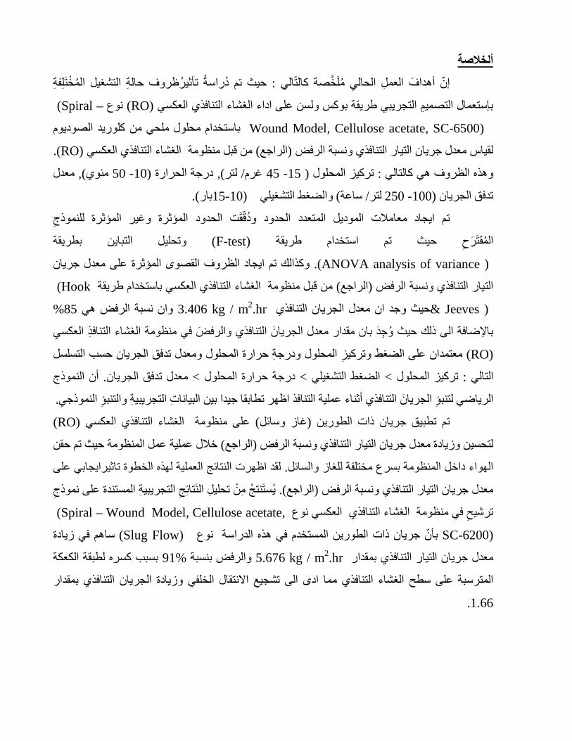
ألخالصة
حالة التشغيل المختلفة ظروفتأثير ة سادر حيث تم : إن أهداف العمل الحالي ملخصة كالتالي
– Spiral) نوع (RO)العكسي فذيالغشاء التنا اداء بإستعمال التصميم التجريبي طريقة بوكس ولسن على
Wound Model, Cellulose acetate, SC-6500) ام محلول ملحي من كلوريد الصوديومباستخد
. (RO)من قبل منظومة الغشاء التنافذي العكسي )الراجع( الرفضنسبة التنافذي و التيار جريان معدل لقياس
معدل , )مئوي 50 -10(درجة الحرارة , )لتر/ غرم 45 -15( تركيز المحلول : وهذه الظروف هي كالتالي
.)بار15-10( والضغط التشغيلي )ساعة/ لتر 250 -100(الجريان تدفق
ودققت الحدود المؤثرة وغير المؤثرة للنموذج تم ايجاد معامالت الموديل المتعدد الحدود
بطريقة لتباينليل اوتح (F-test) استخدام طريقةيث تم ح المقترح
(ANOVA analysis of variance ) .جريان على معدل المؤثرة قصوىوكذالك تم ايجاد الظروف ال
Hook) لعكسي باستخدام طريقة تنافذي امن قبل منظومة الغشاء ال) الراجع(التيار التنافذي ونسبة الرفض
& Jeeves ) 3.406 الجريان التنافذي معدل حيث وجد ان kg / mP
2P.hr 85نسبة الرفض هي وان%
التنافذ العكسي الغشاء منظومة رفض فيالو التنافذي الجريان مقدار معدل بانوجد ذلك حيث الى باإلضافة
)RO (تسلسلال حسب ومعدل تدفق الجريان المحلولودرجة حرارة لمحلولتركيز االضغط و على انمعتمد
ن النموذج أ. الجريانمعدل تدفق > المحلول درجة حرارة > الضغط التشغيلي > المحلول تركيز : التالي
.النموذجي بين البيانات التجريبية والتنبؤ جيدا اظهر تطابقا أثناء عملية التنافذ التنافذي الرياضي لتنبؤ الجريان
(RO) على منظومة الغشاء التنافذي العكسي) غاز وسائل(تم تطبيق جريان ذات الطورين
ة حيث تم حقن خالل عملية عمل المنظوم )الراجع(جريان التيار التنافذي ونسبة الرفض معدل لتحسين وزيادة
لقد اظهرت النتائج العملية لهذه الخطوة تاثيرايجابي على .الهواء داخل المنظومة بسرع مختلفة للغاز والسائل
ستندة على نموذج الميستنتج من تحليل النتائج التجريبية .)الراجع(جريان التيار التنافذي ونسبة الرفض معدل
,Spiral – Wound Model, Cellulose acetate) ع نافذي العكسي نوشاء التالغ في منظومة ترشيح
SC-6200) نوع المستخدم في هذه الدراسة جريان ذات الطورين بأن (Slug Flow) ساهم في زيادة
kg / mP 5.676 بمقدار التنافذي التيار جريانمعدل
2P.hr بسبب كسره لطبقة الكعكة %91 بنسبة والرفض
بمقدار الخلفي وزيادة الجريان التنافذيتشجيع االنتقال سطح الغشاء التنافذي مما ادى الىالمترسبة على
1.66.

وزارة التعليم العالي والبحث العلمي
ةالجامعة التكنولوجي قسم الهندسة الكيمياوية
حقن تقنية التناضح العكسي باستخدام أغشيةأداء تحسين الهواء
رسالة قسم الهندسة الكيمياوية إلىمقدمة
في الجامعة التكنولوجية وهي جزء من متطلبات نيل فلسفة شهادة دكتوراه
في الهندسة الكيمياوية
من قبل طالب محمد نايف البياتي
) 2001هندسة كيمياويةماجستير (
هـ1430 م 2009


![[PPT]Cell Membranes Osmosis and Diffusioniteachbio.com/Life Science/LifeFunctionsandTheCell... · Web viewCell Membranes Osmosis and Diffusion Visit For 100’s of free powerpoints](https://img.pdfslide.net/doc/110x75/5af231247f8b9abc788f6788/pptcell-membranes-osmosis-and-sciencelifefunctionsandthecellweb-viewcell-membranes.jpg)