Embed Size (px)
Citation preview

Entrepreneurship and Public
Health Insurance
Gareth Olds
Working Paper 16-144

Working Paper 16-144
Copyright © 2016 by Gareth Olds
Working papers are in draft form. This working paper is distributed for purposes of comment and discussion only. It may
not be reproduced without permission of the copyright holder. Copies of working papers are available from the author.
Entrepreneurship and Public Health
Insurance
Gareth Olds Harvard Business School

ENTREPRENEURSHIP AND
PUBLIC HEALTH INSURANCE
Gareth Olds⇤
This draft: May 2016
Abstract
I examine the relationship between public health insurance and firm formation.Developing a variant of regression discontinuity, I find the Child Health Insurance Pro-gram lowered the child uninsured rate by 40% and increased self-employment by15%. Monte-Carlo evidence suggests the technique significantly reduces bias andType-1 Error. SCHIP increased incorporated ownership by 36% and business shareof household income by 12%, implying higher-quality ventures. The mechanism isa reduction in risk rather than credit constraints, and I find no imbalance in observ-able characteristics between treatment and control groups. These findings stronglysuggest social safety nets have spillover benefits on the supply of firms.
⇤Harvard Business School. Email: [email protected]. This research was supported in part by the NationalScience Foundation’s IGERT Fellowship and the Hazeltine Fellowship for Research in Entrepreneurship.I am grateful to Ken Chay, Brian Knight and David Weil for their feedback and support. A special thanksto Ronnie Chatterji, Alex Eble, Josh Lerner, Bill Kerr, Dina Pomeranz, and various seminar participants atHarvard and Brown for useful suggestions.
1

Entrepreneurs occupy a central place in the economist’s imagination. Schumpetercalled the entrepreneur “certainly the most important person” in his theory of capital in-terest (Schumpeter, 1961), an observation that sparked a large literature on the role ofentrepreneurship in economic growth (Aghion and Howitt, 1997). Empirical evidence sug-gests young firms are outsize contributors to gross job creation, and firms that survivetheir early years are important sources of net new jobs (Decker et al., 2014). In recentdecades, parallel debates have emerged about the loss of business dynamism as en-trepreneurship rates fall and the optimal size of the welfare state. Despite widespreadconcern about both topics, little is known about how social insurance programs actuallyaffect new firm formation.
This paper provides evidence that public healthcare programs encourage entrepreneur-ship.1 I examine the State Child Health Insurance Program (SCHIP), a large-scale publichealthcare initiative similar to Medicaid but aimed at children in moderate-income fami-lies. Using data from the Current Population Survey (CPS), I show that SCHIP reducedthe number of households with uninsured children by 40%, consistent with earlier esti-mates (Sasso and Buchmueller, 2004; Bansak and Raphael, 2005a). I also show thatSCHIP increased the self-employment rate among parents by 15%. These businessesare disproportionately more likely to be high-quality ventures: SCHIP increased the num-ber of incorporated businesses by 36% and the share of household income derived fromthe business by 12%. This is driven by a 12% increase in firm birth rates and a 26%increase in the rate of incorporated firm formation, and I document only small and in-significant gains in firm survival. I also observe a large increase in labor supply as aresult of the program, both on the extensive margin (significantly more wage earners inaffected households) and the intensive margin (longer work-years as measured by weeksand hours employed).
To identify the causal effect of the policy, I explore a quasi-experimental research de-sign that enhances regression discontinuity (RD) by incorporating pre-policy data into theestimator. This method, a “difference-in-regression discontinuity” (DRD), identifies thetreatment effect using differences in threshold breaks over time.2 I provide Monte Carlo
1I use the terms “self-employment” and “entrepreneurship” interchangeably to signify a household’sownership of a business, which is standard practice in the literature (Parker, 2009). However, since en-trepreneurship is frequently associated with risk-taking innovators who incorporate their ventures (Levineand Rubinstein, 2013) I also show that the results are consistent for incorporated business ownership.
2Note that this not the same as the first-difference RD estimator (Lemieux and Milligan, 2008) or fixed-effects RD (Pettersson-Lidbom, 2012)—both of which require panel data—since I use cross-sectional in-formation to construct the RD in the post- and pre-policy periods. Like difference-in-differences, this differ-encing procedure for RD can be implemented on either cross-sectional or panel data, and can be used inconjunction with fixed effects (see the robustness section). Grembi et al. (2012) independently develop asimilar estimator, but there are some important differences in identifying assumptions and implementation
2

evidence that the estimator dramatically reduces bias and Type 1 Error compared to tra-ditional RD and difference-in-differences (DID) estimators, particularly when treatmenteffects are small or when bandwidths are large. This strategy improves on earlier studiesof SCHIP by providing a plausible counterfactual: I find no evidence that treatment andcontrol groups differ in observable characteristics. The core findings are also robust tomore traditional quasi-experimental methods, such as propensity score matching.
There are two channels through which the safety net can affect entrepreneurship.Social programs provide insurance against consumption shocks in the case of businessfailure (the risk channel) and free up resources for use as collateral or to fund start-upcosts (the credit channel). I find the strongest evidence for the risk channel: eligibilityfor public insurance reduces the risks of entering self-employment, since children can ob-tain care if the family loses private coverage, which protects the household from payingfor potentially expensive procedures out-of-pocket. This is consistent with results in thedevelopment literature that uninsured risk, rather than access to credit, is the binding con-straint for low-income firms (Karlan et al., 2012; Bianchi and Bobba, 2013). There is alsosome limited evidence that SCHIP relaxes credit constraints by reducing medical expen-ditures, allowing households to build up savings and enter self-employment. However, thecentral mechanism appears to be a reduction in the overall risk of starting a business.
Finally, I examine the affect of the policy on non-parent firm formation as a falsifi-cation check. The difference-in-RD estimator can be extended to include a “placebo”population in much the same way that DID models can accommodate a triple-differenceestimator. Using both triple-difference and the extended difference-in-RD estimators, Ishow significant gains in self-employment among parents net of any underlying changesin non-parent entrepreneurship. The extended difference-in-RD method also balancescovariates along both the treated/untreated dimension and with respect to parenthoodbetter than the triple-difference estimator, implying a more appropriate treatment-controlgrouping.
Economists and policymakers both stress the importance of entrepreneurship for eco-nomic growth and job creation, but self-employment rates in the US have been steadilydeclining for five decades. Social insurance programs can promote entrepreneurship byreducing the risks of business ownership and relaxing credit constraints. This paper pro-vides evidence that a large-scale public healthcare program significantly increased thenumber of entrepreneurs. The findings suggest there may be welfare losses from an in-efficiently weak social safety, as public programs have important spillover benefits on thesupply of firms.
(see the identification section).
3

1 Background
Previous literature.
Very few studies have examined the link between entrepreneurship and health insurance.Fairlie et al. (2011) use differences in healthcare demand between people whose spouseshave health insurance and those who do not to identify the relationship between health-care and self-employment. They also improve upon previous studies by implementing aregression-discontinuity strategy using the change in Medicare eligibility at age 65, moti-vated by concerns that spousal coverage is not exogenous when couples make employ-ment decisions jointly. Using matched, monthly CPS data from 1996-2006, they find thatbusiness ownership increases significantly among men just after they turn 65, increas-ing by 3.4 percentage points (a 14% increase from the relatively high baseline of 24.6%),suggesting that employer-based healthcare induces some form of “entrepreneurship lock”analogous to a long literature on traditional job lock. However, these results are difficultto generalize for non-elderly populations since new retirees are often at their maximumwealth level and are the least likely to be credit-constrained, as evidenced by their self-employment rate being two times the national average.
However, there is a large literature on the role of public policy more generally in fos-tering business ownership. Economists have organized their focus along two broad path-ways: bankruptcy reform and the tax code. Business ownership is risky, and governmentsmay try to reduce these risks by providing stronger bankruptcy protection to debtors (Fanand White, 2003; Berkowitz and White, 2004; Meh and Terajima, 2008). Tax policy canaffect entrepreneurship through marginal tax rates, which change the returns to businesssuccess (Gentry and Hubbard, 2000b; Meh, 2005; Bruce and Mohsin, 2006), and wealthtaxation, which affects capital accumulation (Cagetti and Nardi, 2009).
One strand of this literature has centered on government interventions into credit mar-kets to reduce rationing—the inability of some borrowers to receive a loan at any interestrate, or restrictions on the maximum loan size a borrower can secure. Credit rationingshould generate a positive relationship between entry into entrepreneurship and assets,since banks use collateral as a screening mechanism. Evans and Jovanovic (1989) finda positive and significant effect of assets on entrepreneurship, arguing that 94% of peo-ple who are likely to start a business have faced credit rationing, and that 1.3% of theUS population has been prevented from starting a business as a result. Holtz-Eakin etal. (1994a), Holtz-Eakin et al. (1994b), and Blanchflower and Oswald (1998) all find astrong link between inherited funds and entrepreneurship, consistent with credit marketimperfections that prevent potential entrepreneurs from borrowing against future income.
4

In the development literature, Bianchi and Bobba (2013) examine a large-scale random-ized cash grant program in Mexico and find an 11% increase in the self-employment rateamong recipients, though this is driven primarily by a reduction in risk rather than an al-leviation of credit constraints. Karlan et al., 2012 also point to the primacy of uninsuredrisk as a barrier to business formation and expansion by running an insurance and creditintervention among Ghanaian farmers. Finally, governments can guarantee loans or lenddirectly to alleviate credit rationing, but despite widespread use of loan guarantee pro-grams, there is disagreement about their effectiveness (Parker, 2009).
In addition to influencing lender risk, governments sometimes reduce borrower risk bystrengthening bankruptcy protection. There is substantial heterogeneity among states inthe amount of assets that are protected under bankruptcy law, and large asset exemptionsfor personal bankruptcy proceedings—which cover unincorporated businesses—have siz-able and significantly positive effects on the number of entrepreneurs (Fan and White,2003), though this effect may not be linear (Georgellis and Wall, 2006). However, thereduction in risk from entrepreneurs raises the risks faced by lenders, since they can-not recoup some of their losses. These exemptions increase bank rejection rates fornew loans, reduce the average value of small business loans, and push up interest rates(Berkowitz and White, 2004). This means government interventions in credit markets toreduce risks for borrowers are at odds with their efforts to reduce lender risk and may infact increase credit rationing and harm new business formation. Recent evidence sug-gests that the offsetting effect of increased credit rationing may outweigh the reduction inentrepreneurial risk, so that stronger bankruptcy protection lowers the overall supply ofentrepreneurs (Meh and Terajima, 2008).
In some cases governments have enacted social programs to encourage entrepreneur-ship directly. For example, the United Kingdom ran the Enterprise Allowance Schemeduring the 1980’s, which provided income support and cash grants to the unemployed forstarting businesses. At it’s peak in 1987, the program has over 100,000 members andaccounted for 30% of the country’s new business starts (Parker, 2009). The program wasconsidered cost-effective because it replaced unemployment benefits that the governmentwas already obligated to pay, but the effect on unemployment was small. While the UShas not attempted a similar policy, other European countries have established analogousprograms with mixed success.
Taxation is the other key channel through which governments influence entrepreneur-ship. High marginal tax rates may discourage business ownership by reducing the payoffto successful ventures. Some studies have found that both marginal rates and the taxcode’s overall progressivity negatively impact entry (Gentry and Hubbard, 2000b; Meh,
5

2005) and innovation (Gentry and Hubbard, 2005), but the effect may be small (Bruceand Mohsin, 2006) or non-monotonic (Georgellis and Wall, 2006). The average rate ispositively associated with self-employment rates (Schuetze, 2000), though this is oftentaken as evidence of tax evasion (Robson and Wren, 1999).
Taxes may also play a part in capital accumulation. Wealth and saving rates are highamong the self-employed (Quadrini, 2000), which may in part be driven by the inabilityof entrepreneurs to finance new businesses with outside funds (Gentry and Hubbard,2000a). Taxes on wealth can restrict entry into entrepreneurship if entrepreneurs mustpost collateral for loans or pay a portion of start-up costs out-of-pocket (Cagetti and Nardi,2006). The effect of tax policy on capital accumulation may be particularly important ifcredit market imperfections are holding back business formation (King and Levine, 1993).However, more recent work has found a negligible effect of wealth taxes (Cagetti andNardi, 2009).
Finally, this paper hews closely to extensive work by labor economists on “job lock,”the idea that employer-sponsored health insurance discourages workers from switchingjobs. Estimates of whether health insurance non-portability creates labor market rigiditieshave been mixed: some find no effect on job mobility (Holtz-Eakin, 1994; Berger et al.,2004; Fairlie et al., 2012) whereas others find sizable effects (Gruber and Madrian, 1993;Madrian, 1994; Gilleskie and Lutz, 1999; Hamersma and Kim, 2009; Gruber and Madrian,2002; Bansak and Raphael, 2005b).3 Recent work by Garthwaite et al. (2013) examinesa massive disenrollment in Tennessee’s public health insurance program, finding a largeincrease labor supply. With regard to entrepreneurship, Holtz-Eakin et al. (1996) find thathealth insurance portability does not affect entry into self-employment, whereas Gumusand Regan (2013) find that tax deductibility for health insurance premiums increased self-employment.
SCHIP.
In order to investigate the effect of social insurance programs on entrepreneurship, I ex-amine the State Child Health Insurance Program (now just called the Child Health Insur-ance Program), which was passed by Congress in July of 1997. The program’s originalgoal was to insure 5 million children using a public health insurance plan modeled in parton an existing plan in Massachusetts. The program was aimed at children whose fam-ily income made them ineligible for Medicaid benefits but who nevertheless did not havehealth insurance. This was motivated by large numbers of uninsured lower- and middle-
3See Gruber and Madrian, 2002 for an excellent review of this literature.
6

class children: in 1998, nearly one in seven families with children had no health insurancecoverage for their kids.
SCHIP is structured similarly to Medicaid, with state administration based on federalguidelines and cost-sharing between governments. The law allowed states to administerthe program in several ways: they could create their own, separate child health insuranceprogram; they could expand their Medicaid program to cover higher-income children; orthey could do a combination of both. Twenty-six states chose a combination of the two,with 17 opting for a separate program and the remainder expanding their Medicaid cover-age.
The implementation of SCHIP was relatively swift. The program was originally con-ceived by Senator Ted Kennedy after Massachusetts passed a similar child health insur-ance program in July of 1996. President Clinton called for a nationwide program in hisJanuary 1997 State of the Union address, and the bill was ratified by the House in Juneof that year. Forty-one states had SCHIP programs in place by the end of 1998, andthere were 1 million enrolled children by the beginning of 1999. The program now cov-ers 7 million children, with about 13% of households reporting a child covered by SCHIP.Eligibility differs by state, but children are usually eligible for coverage up until age 18 iftheir net family income is below the state income threshold, generally subject to yearlyreauthorization. States were also allowed to set these thresholds independently, so thereis a wide array of cut-offs with respect to the Federal Poverty Line, ranging from 100%(Arkansas, Tennessee and Texas) to 350% (New Jersey).
For SCHIP to have an effect on employment choices, it is important that the benefitshave a significant impact on household budget constraints. While it is less costly to insurea child than an adult, spending on children is still sizable: yearly healthcare expendituresaveraged $4,000 for children under 3 and $2,000 for all children, and even high-deductibleinsurance plans with minimal benefits rarely drop below $1,000.4 However, the distributionof medical costs has a large upper tail, so parents may be particularly concerned aboutlow-probability events with large price tags. For example, in 2010 the average inpatientprocedure for a child cost $12,000, and the average surgical procedure was $35,000.If households place an outsize weight on the upper tail of the cost distribution, publicinsurance may have a strong impact on labor market decisions even when the immediateshift in the budget constraint is more modest. Further, when households are unable toobtain insurance at any price because of pre-existing conditions they may be reluctant toleave wage employment or reduce hours to start a side-project for fear of losing current
4According to the Health Care Cost Institute’s Child Health Care Spending Report, 2007-2010 (availableat www.healthcostinstitute.org) and the author’s calculations.
7

coverage. Eligibility for SCHIP provides a stop-gap source of insurance for this population,independent of health insurance costs.
Data.
I use data from the Current Population Survey (CPS) and the Survey of Income andProgram Participation (SIPP) to identify the impact of SCHIP on health insurance statusand entrepreneurship. Data come from the 1992-2013 CPS March supplement files, ag-gregated to the household level since eligibility is determined based on total householdincome. Samples from both datasets are restricted to non-farm households with at leastone child under 18. The main variables of interest are the presence of a child who hashealth insurance and the presence of a self-employed member. I also make use of a vec-tor of demographic and economics variables in order to test covariate balance; variabledescriptions and summary statistics can be found in the appendix.
Eligibility for SCHIP is determined by total household income and the threshold rel-evant to a family. This income cut-off comes from the state’s policy and is based onthe Federal Poverty Line; because federal guidelines on poverty vary by household size,there is within-state variation in income thresholds. I use a household’s total income fromthe previous calendar year to determine whether households are eligible at a given date,since families are required to show tax records or pay stubs when applying for SCHIPbenefits and when reapplying to maintain coverage in future years.
Finally, data on the state threshold levels and the timing of policy implementationcomes from Rosenbach et al. (2001), Mathematica Policy Research’s first annual reportto the US Department of Health and Human Services on SCHIP implementation.5 Forthe 17 states that adopted both a Medicaid expansion and a separate state health insur-ance program, I use the threshold levels and enrollment dates from the separate program,since the Medicaid expansions tended to have much stricter requirements for child age orbirth year.
2 Empirical Strategy
In order to estimate the causal impact of SCHIP eligibility on self-employment, I imple-ment a variant of regression discontinuity that uses pre-policy data about the populationto incorporate a falsification test directly into the estimator. The intuition for this is straight-forward: since eligibility is based on a continuous forcing variable—income—which is col-
5The report is available at http://www.mathematica-mpr.com/PDFs/schip1.pdf.
8

lected both before and after policy implementation, households just above the thresholdcan be compared both to those just below and to those above and below in the pre-policyregime. Under certain conditions, described below, this procedure eliminates bias thatmight arise in a traditional RD estimator when the conditional expectation of the outcomevariables with respect to the forcing variable are highly non-linear.
Essentially this “difference-in-RD” strategy amounts to first estimating an RD in thepost-policy and pre-policy periods and then identifying the differences in the thresholdbreaks. Because this approach controls for some pre-existing changes in the dependentvariable at the threshold in the pre-policy period, this method incorporates a falsificationtest directly into the estimator in one step. One advantage to this approach is that it doesnot require that unobserved characteristics of the treated and untreated groups remaincomove over time—a variant of the parallel trends assumption from DID. Instead, thisonly needs to be true for people close to the discontinuity. However, this strategy hasthe same drawback as all RD designs: it only identifies treatment effects that are localto the threshold, meaning some external validity is sacrificed in order to sharpen theidentification. I formalize this procedure below using the potential outcomes notation inImbens and Lemieux (2008). I will focus on the “sharp” version of RD here, but the resultsare easily extended to the “fuzzy” case by scaling up the marginal effects along the linesof intent-to-treat models.
Identification.
Let Xi
be the forcing variable with threshold c, and let Yi,P
(1) be the outcome for individuali in period P if they are treated and Y
i,P
(0) be the outcome for the same person if theywere untreated, where P 2 {0, 1} indicates whether t � PolicyY ear
s
.We typically would like to know the population average treatment effect
⌧ATE
= E[Y (1)� Y (0)|X]
since we never observe Yi
(1) and Yi
(0) for the same person. Regression discontinuityinstead identifies the treatment effect at the discontinuity,
⌧ATE|X=c
= E[YP
(1)� YP
(0)|X = c, P = 1].
To estimate this value, RD designs that the potential outcomes for the treated and un-treated are continuous in expectation, meaning lim
x"c E[Y1(0)|X] = limx#c E[Y1(0)|X] and
9

limx"c E[Y1(1)|X] = lim
x#c E[Y1(1)|X].6 Under this assumption, E[Y1(0)|X] = limx#c E[Y1(0)|X] =
limx#c E[Y1|X], where the first equality is due to continuity and the second to the uncon-
foundedness assumption that Yi
(0), Yi
(1) ?? Treati
|Xi
; in the same vein, E[Y1(1)|X] =
limx"c E[Y1|X]. The treatment effect at the discontinuity is just
⌧ATE|X=c
⌘ E[Y1(1)� Y1(0)|X = c] = E[Y1(1)|X = c]� E[Y1(0)|X = c]
= limx"c
E[Y1|X]� limx#c
E[Y1|X] ⌘ ⌧RD
using the definitions above.What happens if the continuity assumption isn’t satisfied? For example, other policies
could have nearby thresholds that cause a jump in the outcome variable.7 We can useinformation from before the policy was enacted to get information about the counterfactualfor the treatment group. Define
limx"c
E[YP
(0)|X,P = 0]� limx#c
E[YP
(0)|X,P = 0] ⌘ 0,0 6= 0
limx"c
E[YP
(1)|X,P = 0]� limx#c
E[YP
(1)|X,P = 0] ⌘ 1,0 6= 0
and define 0,1 and 1,1 analogously for P = 1. Now consider the following assumption:
Assumption 1. 1,1 � 1,0 = 0,1 � 0,0.
Assumption 1 means that any differences in the expectations of the potential outcomevariable for the treated and untreated are the same. Note that this is closely related to theparallel trends assumption, except that instead of the changes in the outcome variablesbeing the same, this assumption requires that the breaks at the discontinuity not changefor both groups. Because this version of the parallel trends is local only to the discontinuity,it does not require that potential outcomes for the treated and untreated groups far fromthe discontinuity grow at the same rates.
Assumption 2. 0,1 � 0,0 = 0.
This stronger assumption says that in the absence of treatment, the pre-existing breakin the untreated group would remain the same.8
6For example, this is a restatement of Assumption 2.1 in Imbens and Lemieux (2008).7This could occur even when there is no discontinuity in the actual expectations; there only needs to be a
jump in the estimated expectation E[Y (·)|Xi
, P = 1] for the problem to arise. Since regression discontinuitydesigns are typically estimated using a parametric relationship as an approximation to a non-parametric one(to avoid the slow convergence of non-parametric estimators), this assumption of distributional continuitycould be true in theory but violated in practice.
8Assumption (2) is the same as the first assumption in Grembi et al. (2012). However, their model
10

Notice that Assumptions 1 and 2 also imply continuity in the differences of the potentialoutcome functions, even when the expectations themselves are not continuous:
0,1 � 0,0 = 0 , limx"c
E[Y1(0)� Y0(0)]|X] = limx#c
E[Y1(0)� Y0(0)]|X]
1,1 � 1,0 = 0 , limx"c
E[Y1(1)� Y0(1)]|X] = limx#c
E[Y1(1)� Y0(1)]|X]
Using this continuity result and Assumption 1, define the differenced RD estimator as
⌧DRD
= limx"c
E[Y1 � Y0|X]� limx#c
E[Y1 � Y0|X]
= E[Y1(1)� Y0(1)|X = c]� E[Y1(0)� Y0(0)]|X = c]
= E[Y1(1)� Y1(0)� [Y0(1)� Y0(0)]|X = c]
= E[Y1(1)� Y1(0)|X = c]
= ⌧ATE|X=c
where the first equality comes from the continuity in the time difference in potential out-comes, the second from properties of expectations, the third from the fact that policiescannot affect outcomes before they are enacted—meaning E[Y0(1) � Y0(0)|X] = 0—andthe last using the definition of ⌧
ATE|X=c
.To see more clearly how this RD estimator is the one-step equivalent to running re-
gression discontinuity designs in the pre- and post-policy periods, rewrite it as:
⌧DRD
= limx"c
E[Y1|X]� limx#c
E[Y1|X]�✓limx"c
E[Y0|X]� limx#c
E[Y0|X]
◆
This is almost the same thing as using the treated group in the pre-period (since the policydid not yet exist, these really are the “would-have-been-treated”) as counterfactuals forthe (truly) treated group in the post period. The important difference is that the outcomevariable for the pre-policy treatment group is shifted to reflect changes in the untreated
also assumes that the jumps in the conditional expectation are the same in the post period for the treatedand untreated groups; using the notation of this paper, the assumption is equivalent to 1,1 = 0,1. Thisassumption may not be plausible for contexts in which the underlying characteristics of the treatment groupare substantively different than those for the untreated. Assumptions (1) and (2) imply that 1,1 = 1,0,meaning the underlying jump in the conditional expectation is the same for the treatment group before andafter the policy. Here the relationship to the parallel trends assumption becomes more clear: treated anduntreated groups need not have the same jumps, only consistent differences over time. In some sense thisis weaker than the assumptions in Grembi et al. (2012) because it still guarantees the continuity neededfor identification without imposing cross-group restrictions (only within-group ones); however, neither setof assumptions implies the other. The implementation of the estimator (below) also differs, since I do notassume the functional form of the expectation differs in the pre- and post-policy periods.
11

group over time. Basically, the counterfactual for the treated group in the post-policyperiod is constructed using two pieces of information: the “treated” pre-period individualsand the trends in the untreated.
Intuition and implementation.
Figure 1 gives some intuition for what this estimator is picking up. The upper panel plotsa local polynomial fit for the difference in child health insurance coverage—post-policy mi-nus pre-policy—against the forcing variable—difference between previous year’s incomeand the threshold-–net of state and year fixed effects and state-specific linear trends.These differences are calculated by sorting the assignment rule distribution into equally-sized bins and taking the within-bin time differences in healthcare outcomes, which arethen used to fit the lines in Figure 1. The plot also includes average values in $10,000intervals, though it is important to note that the fitted lines are based on the localizedwithin-bin differences and not these aggregate values. After the policy was enacted,households just below the cutoff were differentially more likely to have an insured childthan those just above the cutoff relative to households in the same area of the distributionbefore the policy. The lower panel repeats the procedure for self-employment, and the re-sults are similar. While poorer families in general had larger increases in self-employmentthan their richer counterparts, those just to the left of the threshold were significantly morelikely to have a business after the policy, even when accounting for this relationship.
Difference-in-differences essentially takes the average difference in conditional expec-tations to the left of the break and subtracts the same difference to the right; difference-in-RD, on the other hand, uses only individuals close to the discontinuity while controlling forthe slope of the difference in conditional expectations. While the parallel trends assump-tion in DID makes restrictions on the changes to the whole population below and abovethe cut-off, the analogous assumption in difference-in-RD only requires that the differencein the expectations below and above the threshold would have remained the same in thepost period in the absence of treatment (though the expectations themselves could beshifted).
The estimator can be implemented in the same way as a typical RD. I will focus onthe same two methods from the RD literature as before: high-order polynomials and locallinear regression. The first is to allow a flexible function f(·) to capture the relationshipbetween the outcome variable and the assignment rule. When households are just be-low the threshold they are “treated” (i.e. marginally more likely be enrolled, making thisa “fuzzy” RD), so an indicator for this captures the marginal increase in the probability of
12

Figure 1: Regression Discontinuity (Differenced)
−.0
4−
.02
0.0
2.0
4D
iffe
ren
ce in
ch
ild h
ea
lth in
sura
nce
ra
te
−40000 −20000 0 20000 40000 60000Income difference from cut−off ($)
Child Health Insurance−
.03
−.0
2−
.01
0.0
1D
iffe
ren
ce in
se
lf−e
mp
loym
en
t ra
te
−40000 −20000 0 20000 40000 60000Income difference from cut−off ($)
Self−Employment
13

enrollment. If f(·) accurately captures the conditional expectation of the outcome variablewith respect to the assignment rule, the treatment indicator picks only only differences thatarise from being just below the threshold. The second method allows the conditional ex-pectation to vary non-parametrically by using a linear function of the assignment rule andrestricting the sample to data within an arbitrarily narrow bandwidth around the threshold.In the context of difference-in-RD, this means estimating for individual i in state s at timet:
Yist
= �1 + �DRDpoly
· Treatit
Postst
+ �2 · Treatit + �3 · Postst
+ f(Ruleit
)
+ ⌫s
+ ⌘t
+ � · t⌫s
+ "ist
(1)
for the polynomial regression and
Yist
= �1 + �DRDlin
· Treatit
Postst
+ �2 · Treatit + �3 · Postst
+ �4 ·Ruleit
+ ⌫s
+ ⌘t
+ � · t⌫s
+ "ist
if abs(Ruleit
) W (2)
for the local linear specification, where Ruleit
= Incit�1 � Thresh
ist
is the forcing vari-able, f(·) is a high-order function, and Y
ist
is either child health insurance status or self-employment. The variable Treat
it
= 1[Incit�1 Thresh
ist
] is an indicator for whetherthe household is “treated” (i.e. has income below the relevant policy threshold), the termPost
st
= 1[t > PolicyY ears
] is an indicator for being observed in the post-policy period,and Treat
it
Postst
is their interaction. The parameters ⌫s
and ⌘t
are state and year fixedeffects, and � ·t⌫
s
is a state-specific linear time trend.9 A positive and significant coefficienton �
DRD
in the health insurance regression would mean SCHIP increased the number ofinsured children; if the same result holds with self-employment on the left-hand side, itsuggests SCHIP eligibility positively affected business ownership.
Results.
Table 1 shows the parametric estimates using these two methods, with child health in-surance coverage as the outcome variable in Panel A and presence of a self-employedindividual as the measure in Panel B.10 The results in column (1) of Panel A suggeststhat SCHIP increased the proportion of households with an insured child by 4.68 percent-
9The assumption of a linear trend is not important here; state-by-year fixed effects produce similar re-sults.
10Density plots of the assignment rule in the pre- and post-policy periods appear in the appendix. Thefunctions are smooth near the discontinuity in both periods, meaning there is no evidence that peoplemanipulated the assignment rule in order to select into (or out of) treatment.
14

age points, which represents a 34% drop in the rate of uninsured children; the inclusionof demographic covariates increasing this number somewhat to 5.5 percentage points.Though the results are all significant statistically and in policy terms, they is markedlylower than the 9 percentage point drop reported in Sasso and Buchmueller (2004) andBansak and Raphael (2005a). The local linear method, shown in columns (2)-(6), fur-ther reduces this amount; restricting the sample to households with income less than$5,000 away from the cutoff drops the treatment effect to a 1.9 percentage points dropin the number of uninsured households, translating to a local average treatment effect of11%. In treatment-on-the-treated terms, where the pre-policy “treated” are those belowthe threshold, the drop in the uninsured is closer to 10%. The decrease in the effect sizeis due to the fact that lower-income households are less likely to be insured in the firstplace, so fixed percentage-point gains in insurance rates have a proportionally smallereffect on the ranks of the uninsured.
The self-employment are reported in Panel B, and show business ownership increas-ing by more than 4 percentage points using the polynomial method—column (1)—andnearly 2 percentage points using data close to the cutoff—column (2). These treatmenteffects imply an increase in self-employment rates of 23% using the polynomial methodand 14% using the local linear method. The results are on the same order of magni-tude to those in Fairlie et al. (2011), who find a 14% increase in the self-employmentrate as a result of Medicare coverage. However, in treatment-on-the-treated terms, theincrease in self-employment is between 15% (local linear) and 30% (polynomial), sincelower-income households are less likely to own a business. About 11% of the targetpopulation had a self-employed member before the policy took effect, in keeping withnationally-representative statistics of business ownership.
3 Model Extensions and Evaluation
So far the analysis has focused only on households that have children living at home at thetime the family is surveyed. A simple extension of the empirical strategy is to incorporatehouseholds that do not have children: if the estimators are truly picking up the causaleffect of the policy, the findings should hold after netting out any concurrent changesin the self-employment rate of childless households. These changes might representunderlying bias in the estimator, movement of households who anticipate soon becomingparents into self-employment as a result of the policy, or both. In the first case the inclusionof childless households will simply remove a nuisance parameter, whereas in the secondcase the estimator excises more indirect effects of the policy to focus on the direct effects
15

Table 1: Difference-in-Regression Discontinuity Results
Polynomial Method Local Linear Method(1) (2) (3) (4) (5) (6)
Panel A: Child Health Insurance
Treat · Post 0.0468** 0.0550** 0.0415** 0.0346** 0.0193* 0.0192*(0.00546) (0.00470) (0.00467) (0.00529) (0.00796) (0.00743)
Pre-policy avg. 0.861 0.861 0.829 0.826 0.827 0.827LATE (%) 5.438 6.390 5.003 4.197 2.334 2.323Treated avg. 0.783 0.783 0.783 0.793 0.810 0.810TOT (%) 5.980 7.027 5.297 4.366 2.383 2.372
Bandwidth — — ±$20,000 ±$10,000 ±$5,000 ±$5,000Covariates No Yes No No No YesObservations 475,546 456,756 203,411 106,034 53,566 50,942R-squared 0.047 0.113 0.035 0.032 0.032 0.091
Panel B: Self-Employment
Treat · Post 0.0323** 0.0211** 0.0142** 0.0104* 0.0180** 0.0185**(0.00402) (0.00347) (0.00303) (0.00390) (0.00578) (0.00542)
Pre-policy avg. 0.140 0.140 0.120 0.125 0.127 0.127LATE (%) 23.10 15.12 11.88 8.307 14.19 14.55Treated avg. 0.102 0.102 0.105 0.116 0.117 0.117TOT (%) 31.52 20.63 13.58 8.967 15.35 15.75
Bandwidth — — ±$20,000 ±$10,000 ±$5,000 ±$5,000Covariates No Yes No No No YesObservations 481,678 462,760 206,155 107,487 54,295 51,648R-squared 0.023 0.049 0.009 0.008 0.008 0.054
OLS. Dep. var. is presence of insured child (Panel A) or presence of self-employed member (Panel B).Polynomial fits 6th-order function using entire distribution, local linear uses data within bandwidth.Includes time/state FE and state trends. See appendix for covariate list. Data: CPS 1992-2013.** 0.01, * 0.05, + 0.1. Robust standard errors clustered at the state level in parentheses.
16

of eligibility (as opposed to anticipated future eligibility). In either case the basic resultsshould maintain if the difference-in-RD estimator signifies a causal relationship.
I use the standard triple-difference estimator as a benchmark:
Yist
= �1 + �DDD
· Treatit
Postst
HasKidsit
+ �2 · TreatitHasKidsit
+ �3 · Postst
HasKidsit
+ �4 · TreatitPostst
+ �5 · Treatit + �6 · Postst
+ �7 ·HasKidsit
+ ⌫s
+ ⌘t
+ � · t⌫s
+ "ist
(3)
where HasKidsit
is a binary indicator of whether household i has at least one child livingat home in time t, Treat
it
is an indicator for the household income being below the thresh-old level, and all other variables defined as before. The triple-difference (DDD) estimator�1 will identify the effect SCHIP eligibility on the outcome variable relative both to ineligiblehouseholds, households in the pre-policy regime, and households that do not have chil-dren. The difference-in-RD estimator can be analogously extended to include childlesshouseholds by interacting HasKids
it
with all Treatit
and Postst
variables in equations1 and 2; the result looks identical to equation 3 except with Rule
it
terms and applica-ble bandwidth restrictions. This double-difference-in-RD (DDRD) estimator identifies themarginal effect of being just below the income cut-off relative to households just above thecutoff, households around the threshold in the pre-policy period, and smiler householdsthat have no children.
Table 2 shows the results when childless households are included, using self-employmentas the outcome variable.11 Columns (1) and (2) show the DDD results with and withoutcovariates, which indicate a 0.8 percentage point increase in the self-employment rateas a result of SCHIP eligibility (though this is smaller and insignificant once covariatesare introduced). The DDRD estimators, however, report a 0.6 to 1.5 percentage point in-crease; using the local linear method and including covariates, self-employment increasedby 11.3% relative to the pre-policy baseline, or about 15% among the treated population.These are smaller though on the same order of magnitude as the estimates in Table 1,suggesting the difference-in-RD estimator is not being driven by underlying changes inthe general population that are unrelated to having a child in the household.
Since the difference-in-RD model includes elements of both DID and RD, one natu-ral way to evaluate the estimator is to compare it to the two more traditional methods.
11Child health insurance coverage obviously cannot be used in this case, since the variable is undefinedfor childless households.
17

Tabl
e2:
Trip
le-D
iffer
ence
and
Dou
ble-
Diff
eren
ce-in
-RD
Res
ults
DD
DD
DR
D,P
olyn
omia
lD
DR
D,L
ocal
Line
ar(1
)(2
)(3
)(4
)(5
)(6
)D
ep.v
aria
ble:
Sel
f-em
ploy
men
t
Treat·P
ost
0.00
858*
*0.
0050
30.
0127
**0.
0069
2*0.
0128
+0.
0148
*·H
asK
ids
(0.0
0300
)(0
.003
07)
(0.0
0296
)(0
.003
01)
(0.0
0654
)(0
.006
28)
Pre
-pol
icy
avg.
0.13
10.
131
0.13
10.
131
0.13
10.
131
LATE
(%)
6.54
93.
839
9.70
75.
277
9.73
511
.30
Trea
ted
avg.
0.09
730.
0973
0.09
730.
0973
0.09
730.
0973
TOT
(%)
8.82
65.
174
13.0
87.
112
13.1
215
.23
Ban
dwid
th—
——
—±
$5,0
00±
$5,0
00C
ovar
iate
sN
oYe
sN
oYe
sN
oYe
sO
bser
vatio
ns1,
039,
514
999,
363
1,03
9,51
299
9,36
112
6,92
612
0,87
4R
-squ
ared
0.01
00.
039
0.02
40.
046
0.00
90.
044
OLS
.Dep
ende
ntva
riabl
eis
pres
ence
ofse
lf-em
ploy
edm
embe
r.Po
lyno
mia
lmet
hod
fits
a6t
h-or
derf
unct
ion
usin
gth
een
tire
data
set,
loca
llin
earu
ses
data
with
inth
eba
ndw
idth
.Ti
me/
stat
eFE
and
stat
etre
nds
incl
uded
inal
lspe
cific
atio
ns.S
eeap
pend
ixfo
rcov
aria
telis
t.D
ata:
CP
S19
92-2
013.
**0.
01,*
0.05
,+0.
1.R
obus
tsta
ndar
der
rors
clus
tere
dat
the
stat
ele
veli
npa
rent
hese
s.
18

Consider the standard DID estimator �DID
identified from:
Yist
= �1 + �DID
· Treatit
Postst
+ �2 · Treatit + �3 · Postst
+ ⌫s
+ ⌘t
+ � · t⌫s
+ "ist
(4)
and the standard RD estimator �RD
identified from:
Yist
= �1 + �RDpoly
· Treatit
+ f(Ruleit
) + ⌫s
+ ⌘t
+ � · t⌫s
+ "ist
if Postst
= 1 (5)
for the polynomial method, and
Yist
= �1 + �RDlin
· Treatit
+ �2 ·Ruleit
+ ⌫s
+ ⌘t
+ � · t⌫s
+ "ist
if Postst
= 1 and abs(Ruleit
) W (6)
for the local linear method. As an evaluation metric, consider demographic covariatesthat should be unaffected by the policy: in an experimental setting, differences betweentreatment and control groups along these lines is evidence of poor randomization or self-selection into treatment. Similarly, an estimator is less convincing as having isolated thecausal effect of an intervention if it also picks up underlying differences in the population,since the synthetic “control” group differs significantly from those affected by the policy.In order to test whether covariates are balanced, I apply the estimators in equations 1, 2and 3 to a range of demographic variables, and compare the results to the more traditionalmethods captured in equations 4, 5 and 6.
The results are shown in Table 3. Difference-in-differences estimation, reported in col-umn (1), suggests that SCHIP induced a 3.4 percentage point increase health insurancecoverage and a 1.2 percentage point increase in the self-employment rate. However, re-peating the specification using each of the covariates as an outcome variables revealsthat nine out of 16 of these variables—about 56%—vary in a statistically significant wayat the 5% level along the same dimension supposedly being explained by the policy. Eventriple-differencing, which should control for any underlying changes in the population solong as they are parallel between childless and non-childless households, shows a sig-nificant imbalance between covariates. This may not be surprising as there are severalwell-known problems with difference-in-difference strategies. Besides issues with over-rejection in the presence of serial correlation (Bertrand et al., 2004), the logic of DID canbe misleading: comparing changes in one group against changes in another suggestsall else being equal, the changes are good counterfactuals for one another. Put anotherway, any underlying unobservable characteristics between the two groups should not bechanging in different ways (this is the parallel trends assumption).
19

Note that controlling for these covariates in the DID specification does not solve theproblem of non-orthogonality of covariates reported in Table 3: unconditional orthogonal-ity of assignment to the treatment group with respect to observables and unobservables isa stricter requirement than conditional orthogonality (with respect to unobservables) oncecontrols are included. While both rely on assumptions about unobservables, the first canbe partially tested by using observables as outcomes; the second requires making anassumption about observables containing sufficient information such that unobservablesare as good as random.
Another metric useful for evaluating an estimator is its sensitivity to parameter choicesthat are within the control of the econometrician. In an RD setting, the researcher typicallyspecifies a bandwidth either using an optimal rule based on the data’s density or presentsa range of treatment effects for different bandwidth choices. Difference-in-RD eliminatesmuch of the heterogeneity in the treatment effect by bandwidth choice since any bias in-duced by an inappropriately large window will be cancelled out so long as that bias alsoexists when estimating the model in the pre-policy regime. In the context of SCHIP, Fig-ure A1.2 in the Appendix presents the estimated treatment effect and 95% confidenceintervals for a wide range of bandwidth choices, both for child health insurance coverageand self-employment. The results are generally stable across the entire range, thoughlosing in precision as the window narrows and more data is excluded from the regres-sion. This same finding is not true when the model is estimated using a traditional RDframework (not shown). I present some Monte Carlo evidence in support of this relativebandwidth-invariance later on in the discussion.
Business source and quality.
Where is this business growth coming from? Table 4 breaks down the self-employmentresults by previous businesses status, using the falsification procedure described above.The effect for people who already have businesses 1.3 percentage points, suggestingSCHIP caused an insignificant 1.7% increase in the pre-policy yearly firm survival rate of74%.12 The effect on non-business-owning households is 0.6 percentage points, a 12%increase in the yearly firm birth rate of 4.7%. The marginal effects are actually highest forthe incorporated firm birth rate, which increased by 0.27 percentage points (26% higherthan the baseline). This was entirely driven by new firms rather than newly-incorporatedexisting firms, whose numbers actually fell as a result of the policy. The growth also
12These numbers should be interpreted with caution since the sample sizes are much smaller, bothbecause of restrictions based on previous employment status and because the sample of households ob-served at two time periods is smaller.
20

Tabl
e3:
Cov
aria
teB
alan
ceA
cros
sM
odel
s
Est
imat
or:
Poly
nom
ialM
etho
dLo
calL
inea
rMet
hod
DID
DD
DR
DD
RD
DD
RD
RD
DR
DD
DR
DD
ep.v
aria
ble
(1)
(2)
(3)
(4)
(5)
(6)
(7)
(8)
Chi
ldH
ealth
Ins.
0.03
38**
—-0
.035
2**
0.04
68**
—0.
0056
60.
0193
*—
Sel
f-Em
ploy
men
t0.
0120
**0.
0085
8**
-0.0
0022
60.
0323
**0.
0127
**0.
0017
50.
0180
**0.
0128
+
Age
ofA
dults
-0.2
80**
1.12
2**
-0.3
77**
0.47
3**
1.23
2**
0.08
310.
132
0.39
2B
ache
lor’s
Deg
.-0
.037
6**
-0.0
196*
*-0
.050
0**
0.03
96**
-0.0
0507
-0.0
224*
*0.
0020
6-0
.000
907
Bla
ck-0
.008
21-0
.024
8**
0.04
27**
-0.0
256*
*-0
.028
4**
0.02
86**
0.00
420
-0.0
0313
Chi
ldre
n-0
.051
8**
-0.0
513*
*-0
.142
**-0
.158
**-0
.068
4**
0.04
08*
-0.0
131
-0.0
132
Dis
able
d0.
0019
9**
0.00
464*
*0.
0029
7**
0.00
171*
0.00
450*
*-0
.001
83-0
.000
957
0.00
269
Gra
duat
eD
eg.
-0.0
203*
*-0
.007
70**
0.00
536*
0.01
86**
-0.0
0056
2-0
.000
970
-0.0
0058
80.
0053
9H
igh
Sch
ool
0.01
31*
-0.0
130+
-0.0
632*
*0.
0455
**-0
.006
46-0
.021
5**
0.00
459
-0.0
116
His
pani
c0.
0119
0.02
06*
0.06
06**
-0.0
123
0.01
66+
0.02
53**
-0.0
0271
0.00
0689
Hou
seho
ldS
ize
-0.0
451*
*-0
.047
4**
-0.3
17**
-0.1
19**
-0.0
538*
*0.
0635
*-0
.008
73-0
.041
1+M
arrie
d0.
0043
60.
0163
+-0
.103
**0.
0526
**0.
0282
**0.
0113
0.00
591
0.00
0496
Med
icai
d-0
.041
7**
-0.0
755*
*0.
111*
*-0
.075
4**
-0.0
816*
*0.
0305
**0.
0049
9-0
.000
400
Mov
ed-0
.010
3+-0
.018
2**
0.05
54**
-0.0
205*
*-0
.020
5**
0.04
39**
0.00
996
0.01
08R
ente
r0.
0014
8-0
.030
3**
0.16
5**
-0.0
565*
*-0
.042
8**
0.04
61**
0.00
310
0.00
395
Une
mpl
oym
ent
0.00
488
0.00
235
0.01
46**
-0.0
0147
0.00
164
0.01
85*
-0.0
0002
2-0
.000
842
Urb
an0.
0033
5-0
.016
7**
-0.0
0263
0.02
06**
-0.0
138*
0.01
08-0
.001
64-0
.014
1+Ve
tera
n-0
.002
44**
0.00
709*
*-0
.001
05-0
.001
120.
0073
6**
0.00
222
-0.0
0073
90.
0006
74
Ban
dwid
th—
——
——
±$5
,000
±$5
,000
±$5
,000
Unb
alan
ced
vars
.↵=
5%56
%81
%88
%81
%69
%63
%0%
0%↵=
10%
63%
94%
88%
81%
75%
63%
0%13
%
OLS
.Coe
ffici
ents
repo
rted
are
treat
men
teffe
cts
fort
heap
plic
able
mod
el,w
ithro
was
depe
nden
tvar
iabl
e.Po
lyno
mia
lmet
hod
fits
a6t
h-or
derf
unct
ion
usin
gth
een
tire
data
set,
loca
llin
earu
ses
data
with
inth
eba
ndw
idth
.Ti
me/
stat
efix
edef
fect
san
dst
ate
trend
sin
clud
ed.D
ata:
CP
S19
92-2
013.
**0.
01,*
0.05
,+0.
1R
obus
tsta
ndar
der
rors
clus
tere
dat
the
stat
ele
vela
reom
itted
forb
revi
ty.
21

Tabl
e4:
Bus
ines
sS
ourc
e(D
iffer
ence
-in-R
D)
Bus
ines
sw
aspr
evio
usly
...H
ouse
hold
was
...E
xist
ent
Non
-exi
sten
tU
ninc
orp.
Em
ploy
edU
nem
p.D
epen
dent
(1)
(2)
(3)
(4)
(5)
(6)
varia
ble:
Sel
f-Em
p.S
elf-E
mp.
Inco
rp.
Inco
rp.
Sel
f-Em
p.S
elf-E
mp.
Treat·P
ost
0.01
260.
0057
90.
0027
2+-0
.015
9+0.
0223
**0.
0070
9(0
.018
0)(0
.003
79)
(0.0
0162
)(0
.009
12)
(0.0
0588
)(0
.016
8)
Pre
-pol
icy
avg.
0.74
20.
0466
0.01
060.
0106
0.15
80.
0237
LATE
1.69
712
.42
25.8
2-1
50.9
14.1
029
.85
Trea
ted
avg.
0.65
90.
0441
0.00
451
0.00
451
0.12
90.
0160
TOT
1.90
913
.14
60.3
7-3
52.8
17.3
044
.20
Obs
erva
tions
18,8
1711
1,30
111
1,30
112
,232
122,
708
7,41
0R
-squ
ared
0.03
30.
008
0.01
60.
048
0.02
20.
047
DR
Dm
etho
dus
ing
a6t
h-or
derp
olyn
omia
l.D
ata:
CP
S19
92-2
013.
Incl
udes
time/
stat
eFE
and
stat
etre
nds.
**0.
01,*
0.05
,+0.
1.R
obus
tsta
ndar
der
rors
clus
tere
dat
the
stat
ele
veli
npa
rent
hese
s.
22

Table 5: Business Quality (Difference-in-RD)
Dependent % HH inc. Wagevariable: Incorp. from bus. Workers earners Weeks Hours
(1) (2) (3) (4) (5) (6)
Treat · Post 0.0148** 0.0419** 0.191** 0.175** 2.175** 0.623**(0.00150) (0.0102) (0.0185) (0.0181) (0.154) (0.0887)
Pre-policy avg. 0.0408 0.362 1.727 1.656 45.89 39.93LATE 36.20 11.56 11.08 10.55 4.739 1.561Treated avg. 0.0138 0.417 1.286 1.227 41.86 37.78TOT 107.2 10.03 14.88 14.25 5.194 1.650
Observations 481,678 57,290 481,678 481,678 452,090 452,090R-squared 0.040 0.048 0.189 0.175 0.094 0.053
DRD using 6th-order polynomial. CPS 1992-2013. Includes time/state FE and state trends.** 0.01, * 0.05, + 0.1. Robust standard errors clustered at the state level in parentheses.
seem to be coming from households with previously employed members rather than theunemployed, though the marginal effects for the unemployed are higher if statisticallyinsignificant.
Another important concern is the quality of these new businesses: are they high-quality ventures that contribute to job growth and innovation, or household side-projectsthat supplement income but do not hire employees? Without more detailed data on pay-roll, receipts or long-term survival rates it is difficult to answer this question, but Table 5 inthe appendix provides some suggestive evidence. Researchers often use incorporationas a measure of entrepreneur “seriousness” or quality (Levine and Rubinstein, 2013), soTable 5 repeats the specifications above using a household’s ownership of an incorpo-rated business as the outcome variables. The effects on incorporation are large: SCHIPcaused a 1.5 percentage point increase in incorporation ownership, a 36% increase fromthe pre-policy baseline (4.1% of households had an incorporated firm before the policy).Since the overall increase in self-employment was only 15%, SCHIP disproportionatelyencouraged people to open incorporated businesses, shifting the overall composition offirms toward more “serious” ventures.
Table 5 also looks at the percentage of income that self-employed households derivefrom their businesses as another gauge for seriousness. The business share of incomerose by 4.2 percentage points as a result of SCHIP, a 12% increase from the baseline.Table 5 also shows the change in a household’s extensive and intensive labor supply mar-
23

gins. More than one in ten households added a working adult or wage earner; combinedwith the fact that household size was unchanged, this suggests SCHIP induced someindividuals who were previously out of the labor market to enter employment. Householdsalso spent more time working because of the policy: the average employed memberworked more than two additional weeks out of the year. Taken as a whole, the findingssupport the interpretation that SCHIP induced entry of high-quality entrepreneurs whodevote a significant amount of their time to running a business.
Finally, risk-taking is closely related to the quality and innovative nature of businesses.Are these new businesses high-risk ventures? While this question cannot be answeredat the individual level without a longer panel on business income, aggregate relation-ships provide some interesting results. Figure 2 plots the coefficient of variation—thestandard deviation divided by mean—for self-employment income by the number of yearssince SCHIP was enacted, separately for households with and without children. Using thismeasure of risk, the two groups track very closely before the policy; for five years followingthe child health insurance program, however, households with children had more varia-tion in business income relative to childless households. This is consistent with SCHIPenabling households to take on high-risk entrepreneurial ventures they would otherwisehave avoided, which suggests these new firms are engaged in more innovative projects.
Mechanisms.
How does public health insurance eligibility influence entrepreneurship? To answer thisquestion, I focus on two theoretical mechanisms: the risk channel and the credit channel.Public programs like SCHIP may operate through risk channel by reducing the uncer-tainty associated with entering self-employment and losing employer-sponsored healthinsurance, since public insurance protects the family from medical debts (Baicker et al.,2013) and the resulting consumption shocks. These programs may also work through acredit channel by freeing up income for credit-constrained households, which can be usedto post as collateral for business loans or fund start-up costs.
In order to isolate the risk channel, I look at differences between households who werepreviously insured and those who were not. Households with health insurance experiencea change in their exposure to risk—they now have a fall-back source of insurance shouldthey lose private coverage—but no change in their budget constraint since they do notimmediately receive benefits. Table 6 estimates the treatment effects separately basedon whether a household’s children were insured in the previous year. Columns (1) and (2)estimate the treatment effect on the subset of the population that previously reported hav-
24

Figure 2: Business Risk
Households with children
Households without children
1.4
1.6
1.8
2C
oeff
icie
nt
of
variatio
n,
self−
em
p.
inco
me
−6 −5 −4 −3 −2 −1 0 1 2 3 4 5 6Years from policy implementation
ing health insurance for at least some of their children; columns (3) and (4) do the samefor fully uninsured households. The results indicate that both previously insured and unin-sured children benefited from the program, but that unsurprisingly it was the uninsuredwho enjoyed the biggest gains in next-year coverage. However, the self-employment in-crease is largely driven by entrepreneurship among previously insured households, whoface no immediate changes to their budget constraints but are now eligible for publiclysubsidized coverage should they lose their current plan. This is an important piece ofevidence in support of the risk channel: the increase in self-employment cannot be ex-plained solely by changes to the budget constraint, because many families move intobusiness ownership even when they do not benefit directly from SCHIP. This is consistentwith the risk channel, in which eligibility for public benefits lowers a household’s exposureto risk whether or not they avail themselves of the program’s benefits. The results sug-gest the risk channel plays an important role in the effect of health insurance on businessformation.
Isolating the credit channel is more difficult without detailed information on the con-straints that households face. However, higher-income households are less likely to facecredit constraints than poorer ones, so heterogeneity in the treatment effect along income
25

Tabl
e6:
Mec
hani
sms
(Diff
eren
ce-in
-RD
)
Chi
ldre
nw
ere
prev
ious
ly:
Uni
nsur
edIn
sure
d(1
)(2
)(3
)(4
)(5
)(6
)(7
)D
epen
dent
varia
ble:
Hea
lthin
s.S
elf-e
mp.
Hea
lthin
s.S
elf-e
mp
Sel
f-em
p.S
elf-e
mp.
Sel
f-em
p.
Treat·P
ost
0.05
16*
0.01
610.
0314
**0.
0305
**0.
0305
**0.
0151
+0.
0234
**(0
.023
7)(0
.014
6)(0
.007
03)
(0.0
0549
)(0
.005
49)
(0.0
0879
)(0
.004
98)
Treat·P
ost·I
ncome/10k
-0.0
0489
+(0
.002
68)
Treat·P
ost·C
hildren
0.00
505+
(0.0
0253
)
Treat·P
ost·R
isk
-0.0
415*
(0.0
186)
Pre
-pol
icy
avg.
0.57
20.
179
0.92
40.
150
——
—LA
TE9.
021
9.01
03.
398
20.4
2—
——
Trea
ted
avg.
0.52
10.
146
0.86
10.
107
——
—TO
T9.
903
11.0
23.
645
28.4
2—
——
Obs
erva
tions
11,1
8511
,279
104,
905
105,
297
130,
118
481,
678
481,
678
R-s
quar
ed0.
046
0.03
10.
031
0.02
50.
030
0.02
50.
023
DR
Dm
etho
dus
ing
a6t
h-or
derp
olyn
omia
l.D
ata:
CP
S19
92-2
013.
Incl
udes
time/
stat
eFE
and
stat
etre
nds.
**0.
01,*
0.05
,+0.
1.R
obus
tsta
ndar
der
rors
clus
tere
dat
the
stat
ele
veli
npa
rent
hese
s.
26

lines may hint at the role of credit. Column (5) interacts Treatit
Postst
with the household’stotal income in the previous year (in tens of thousands of dollars); the negative coeffi-cient means poorer households had larger increases in the self-employment rate as aresult of SCHIP, which is consistent with the program alleviating credit constraints. Thesemi-elasticity of income on the treatment effect is relatively large: an increase in house-hold income by one standard deviation—about $6,800—decreases the marginal effect ofSCHIP eligibility on self-employment by 1.09 percentage points, more than one-third ofthe baseline effect. However the coefficient is only marginally significant, and the resultis also consistent with a model in which risk aversion is decreasing in income, so that thetreatment effects are largest in the most risk averse (and poorest) households.
Column (6) interacts each of the variables with the number of children in the house-hold. Larger households may be more credit-constrained than smaller ones, though theeffective value of SCHIP coverage is larger for big families, so the comparisons aren’texact. The results suggest larger families benefited more from the policy than smallerones, and the effects are large (an increase in household size by one choice—close tothe standard deviation—raises the treatment effect by one-third) though only marginallysignificant. This could be the result of either canceling effects from the simultaneouslymore binding credit constraint and bigger benefit pay-out, or from insurance and self-employment decisions that are driven by high-cost, low-risk events—which are relativelyinvariant to household size—rather than routine care.
Finally, column (7) interacts Treatit
Postst
with a measure of self-employment risk: thecoefficient of variation in self-employment income before the policy was enacted, calcu-lated at the state level. The negative estimate means treatment effects were largest instates with low levels of self-employment income volatility. This might be the result ofmore risk averse people to entering entrepreneurship as a result of SCHIP, so long aspeople of similar risk aversion tend to reside in the same states. Alternatively, it couldbe the case that the reduction in risk was insufficient to induce large changes in self-employment in high-risk states—perhaps because there is a threshold level of risk abovewhich little entrepreneurship takes place—whereas the reduction in lower-risk states wasmore effective. Overall, Table 6 finds the strongest evidence for the risk channel, withsome suggestive evidence that the credit channel matters as well.
4 Monte Carlo Analysis and Robustness
Does difference-in-RD generally perform better than traditional RD and DID designs, or isthis a quirk of the data and policy? Covariate balance is a useful indicator of randomization
27

quality but provides no information about bias or whether hypothesis testing providescorrect inference. In this section I use Monte Carlo analysis to directly control the data-generating process and identify whether the estimator is unbiased in finite samples and iftest statistics are correctly sized in a more general setting.
I use the following Monte Carlo procedure:
1. First I draw 10,000 observations of the forcing variable X ⇠ F (✓), where F (·) is aprobability distribution with parameter vector ✓; in practice I use the empirical incomedistribution from the 2010 and 2011 CPS, but results for the uniform and standardnormal distributions are very similar.
2. Next, I assign post-policy status randomly, so that half of the observations fall in the“post” period (with the empirical income distribution I call 2010 the pre-policy yearand draw 5,000 observations from each year).13
3. I then construct an outcome variable Y = g(X|⇠) + " using the mapping g(·|⇠) withparameter vector ⇠; for the results below I run a non-stochastic version (" ⌘ 0) withpolynomials of order k = [1, ..., 7], where the coefficients ⇠
k
⇠ N(0, 1); the naturallogarithm; and a sinusoidal function with a period equal to one-fifth of the domain ofX.
4. The next step is to randomly assign treatment status, which I do by randomly choos-ing an observation i and assigning treatment to all individuals j such that x
j
xi
—this is equivalent to choosing a threshold x ⇠ F (✓)—and then subtract xi
fromX.
5. I then add a treatment effect ⌘ so that Y = g(X|⇠)+⌘ ·1[xj
xi
]+ "; when modelingType 1 Error, ⌘ = 0, and for Type 2 Error I use a range of ⌘ 2 [.01, 1] where the unitsare standard deviations of Y .
6. Finally, I use several different estimators T (·)—DID, RD and differenced RD—and arange of bandwidths to generate predictions Y .
Each draw m of the M total draws produces an estimate Ym
, which generate the followingstatistics:
13Since RD uses only post-policy data, this procedure might unfairly stack the deck against RD since it willuse half as many observations. I develop two remedies for this. First, I double the number of observationssampled for RD, so that each estimator uses a sample size of 10,000 on average; these are the resultsshown below. Second, I use an algorithm to identify the differenced RD bandwidth size whose number ofobservations would match the observations for a given RD bandwidth (usually around half, depending onthe density of X). The results, which apply only to the local linear method and are not shown here, are verysimilar.
28

• Bias: E[(Y � Y )/�y
], which has the sample analogue 1M
PM
m=1(Ym
� Y )/�y
;
• Root-mean-squared error (RMSE):
s
E⇣
Y�Y
�y
⌘2�, which is calculated as
r1M
PM
m=1
⇣Ym�Y
�y
⌘2
;
• Type 1 Error: ph⇣
Y |xi
xj
⌘6=
⇣Y |x
i
> xj
⌘|T (·),↵, ⌘ = 0
i, which has the sample
analogue1
M
MX
m=1
1h⇣
Ym
|xi
xj
⌘6=
⇣Ym
|xi
> xj
⌘|T (·),↵, ⌘ = 0
i;
• Statistical Power: ph⇣
Y |xi
xj
⌘=
⇣Y |x
i
> xj
⌘|T (·),↵, ⌘ 6= 0
i, which is calculated
as1
M
MX
m=1
1h⇣
Ym
|xi
xj
⌘=
⇣Ym
|xi
> xj
⌘|T (·),↵, ⌘ 6= 0
i.
If the hypothesis testing procedure is correct, the estimated Type 1 Error should be equalto the size of the test, ↵ (I use a 5% level of significance below). Table ?? shows theresults of this procedure when there is no treatment effect (⌘ = 0), using the polynomialversions of RD and differenced RD and the empirical income distribution for X.
Panel A pretends as though the econometrician knows the exact functional form of theconditional expectation, meaning when g(·) is quadratic, the estimators include x and x2
terms; when g(·) is logarithmic, the regression includes ln(x); and so on. This providesa “best case scenario” in which error arises only from the research design itself ratherthan functional form misspecification. Since this is unrealistic in most settings, Panel Bimposes a cubic approximation of g(·), which is one of the more common strategies usedby researchers deploying RD. Finally, Panel C presents the results using difference-in-differences as an additional benchmark. The stars denote statistically-significant differ-ences from theoretical values (0.05 in the case of Type 1 Error and zero in the case ofbias).
Regression discontinuity dramatically over-rejects the null hypothesis in these simu-lations, with Type 1 Error rates ranging from 30% to 99% depending on the degree ofnon-linearity in the conditional expectation. This is true even when the econometricianmodels the exact functional form; for example, a random quadratic relationship betweenY and X will find a “treatment” effect significant at the 5% level 43% of the time. Theinaccuracy of the test statistic seems to be increasing with the non-linearity of g(·), andwhen Y has a periodic relationship to X—such as the sine function—regression discon-tinuity nearly always finds a significant effect. Hypothesis testing under the differencedRD estimator, by contrast, produces a nearly correctly-sized test, with Type 1 Error rates
29

Tabl
e7:
Mon
teC
arlo
,No
Trea
tmen
tEffe
ct(P
olyn
omia
lMet
hod)
g(x|⇠)
Poly
nom
ialo
ford
erk=
...Pa
nelA
:Exa
ctg(·)
know
n1
23
57
Log
Sin
Type
1E
rror
:R
D0.
29**
0.43
**0.
47**
0.46
**0.
33**
0.69
**0.
99**
Diff
eren
ced
0.06
0.07
*0.
10**
0.10
**0.
060.
81**
0.19
**B
ias,
sd(y):
RD
-0.0
00.
000.
000.
00-0
.00
0.00
0.92
**D
iffer
ence
d0.
00*
0.00
0.00
-0.0
00.
000.
00-0
.01*
*R
MS
E:
RD
0.00
0.00
0.00
0.00
0.00
0.00
1.07
Diff
eren
ced
0.00
0.00
0.00
0.00
0.00
0.00
0.14
Pane
lB:C
ubic
appr
oxim
atio
nto
g(·)
Type
1E
rror
:R
D0.
30**
0.40
**0.
47**
0.97
**0.
98**
0.96
**0.
98**
Diff
eren
ced
0.06
0.09
**0.
10**
0.32
**0.
11**
0.19
**0.
24**
Bia
s,sd(y):
RD
-0.0
0-0
.00
-0.0
00.
08**
0.03
+-0
.17*
*-0
.41*
*D
iffer
ence
d0.
000.
000.
000.
02**
-0.0
00.
01**
0.01
RM
SE
:R
D0.
000.
000.
000.
400.
600.
641.
91D
iffer
ence
d0.
000.
000.
000.
110.
090.
070.
19
Pane
lC:D
iffer
ence
-in-D
iffer
ence
s
Type
1E
rror
:0.
08**
0.08
**0.
13**
0.23
**0.
58**
0.10
**0.
21**
Bia
s,sd(y):
-0.0
1-0
.15*
*-0
.19*
*-0
.31*
*-0
.11*
*-0
.00*
-0.0
1*R
MS
E:
0.33
1.00
1.14
1.36
0.33
0.05
0.15
**0.
01,*
0.05
,+0.
1.R
obus
tsta
ndar
der
rors
calc
ulat
edus
ing
the
num
bero
fsim
ulat
ions
(om
itted
forb
revi
ty).
Test
sar
efo
rdiff
eren
cefro
m↵
(forT
ype
1E
rror
)orz
ero
(forb
ias)
.X
⇠em
piric
alin
com
edi
strib
utio
n(2
010-
2011
CP
S).
Eac
hce
llre
pres
ents
1,00
0dr
aws
of10
,000
obse
rvat
ions
.
30

generally much lower than their RD counterparts and often not significantly different from5%.
Incorrectly-sized tests may be relatively unimportant if the estimator is unbiased: re-searchers will find significant policy effects but conclude the point estimates are so smallas to be indistinguishable from zero. To address these concerns, Table ?? also presentsthe average bias from the Monte Carlo simulations in units of �
y
. In Panel A, RD is gener-ally unbiased except in the case of the sine function, where regression discontinuity findsa spurious effect of nearly one standard deviation almost every draw. This is particularlyrelevant to contexts with regular fluctuations—for example, a time series subject to a busi-ness cycle—where the researcher runs a discontinuity design based on the timing of apolicy. This over-rejection and bias is present even when the regression directly controlsfor the functional form of the conditional expectation.
More realistically, however, the researcher does not know the exact nature of the rela-tionship g(·) and approximates this function with a cubic polynomial in X. Panel B repeatsthe Monte Carlo simulations using this estimation strategy. First notice that the Type 1Error rates are almost uniformly larger using this method, especially when the g(·) has ahigher degree of non-linearity than is controlled for in the regression. However, while theerror rates also increase for differenced version of RD, the rise is much smaller than fortraditional RD, with reductions in error of around 75% on average.
Second, RD begins exhibiting statistically significant amounts of bias for conditionalexpectations of order higher than three. Even a fairly un-exotic quintic function nearlyalways finds a “treatment” effect of around 8% of a standard deviation, which would bea notable result in the education or labor economics literature. A logarithmic relationshipbetween Y and X causes RD to identify a 0.17 standard deviation decrease in the out-come variable for the “treated” group, an underlying bias that would mask even extremelylarge policy effects. The falsification check version of RD, on the other hand, completelyeliminates this bias, with coefficient estimates rarely different than zero and never morethan 3% of a standard deviation. The difference-in-difference estimates in Panel C arebiased even at low levels of non-linearity, and while Type 1 Error rates are lower than forRD they are generally higher than the differenced version.
Finally, Table ?? also presents the root-mean-squared error (RMSE) from the simu-lations. While comparing efficiency of the estimators is difficult when one is not unbi-ased, the uniformly lower RMSE of differenced RD relative to traditional RD suggests themethod carries some improvements in precision.
Using only the polynomial method is somewhat misleading, since most researcherssupplement this method with local linear estimation. This conforms more closely to the
31

Tabl
e8:
Mon
teC
arlo
,No
Trea
tmen
tEffe
ct(L
ocal
Line
arM
etho
d)
Ban
dwid
th(in
term
sof
�x
)Pa
nelA
:Qua
drat
icg(·)
10.
50.
250.
10.
050.
01
Type
1E
rror
:R
D0.
98**
0.96
**0.
84**
0.54
**0.
48**
0.48
**D
iffer
ence
d0.
08**
0.07
*0.
060.
07**
0.09
**0.
11**
Bia
s,sd(y):
RD
-0.0
05**
-0.0
02**
-.000
2**
-0.0
00**
-0.0
00**
-0.0
00**
Diff
eren
ced
0.00
00.
000
0.00
00.
000
0.00
00.
000
RM
SE
:R
D0.
038
0.00
80.
002
0.00
00.
000
0.00
0D
iffer
ence
d0.
005
0.00
20.
000
0.00
00.
000
0.00
0
Pane
lB:L
ogar
ithm
icg(·)
Type
1E
rror
:R
D0.
98**
0.98
**0.
92**
0.55
**0.
47**
0.50
**D
iffer
ence
d0.
07*
0.06
+0.
07*
0.07
*0.
08**
0.10
**B
ias,
sd(y):
RD
-0.0
71**
-0.0
30**
-0.0
07**
-0.0
01**
-0.0
000.
000*
*D
iffer
ence
d0.
001
0.00
2**
0.00
1+-0
.000
-0.0
000.
000
RM
SE
:R
D0.
349
0.15
80.
057
0.00
90.
002
0.00
0D
iffer
ence
d0.
023
0.02
00.
017
0.00
20.
001
0.00
0
Pane
lC:S
inus
oida
lg(·)
Type
1E
rror
:R
D0.
97**
0.96
**0.
80**
0.56
**0.
49**
0.49
**D
iffer
ence
d0.
08**
0.08
**0.
07*
0.07
*0.
08**
0.10
**B
ias,
sd(y):
RD
-0.0
67**
0.01
4**
0.00
4**
0.00
0**
0.00
0**
0.00
0**
Diff
eren
ced
-0.0
05*
0.00
00.
000
0.00
00.
000*
*0.
000*
*R
MS
E:
RD
0.76
00.
149
0.02
30.
003
0.00
10.
000
Diff
eren
ced
0.07
80.
026
0.00
70.
002
0.00
00.
000
Obs
.(ap
prox
.)7,
130
4,48
82,
492
1,04
652
711
0
**0.
01,*
0.05
,+0.
1.R
obus
ts.e
.cal
cula
ted
usin
gnu
mbe
rofs
imul
atio
ns(o
mitt
edfo
rbre
vity
).Te
sts
are
diffe
renc
efro
m↵
(Typ
e1
Err
or)o
rzer
o(b
ias)
.X⇠
empi
rical
inco
me
dist
.201
0-20
11C
PS.
“Obs
.(ap
prox
.)”is
obse
rvat
ions
used
inre
gres
sion
s,av
erag
edov
ersi
mul
atio
nsan
dg(·)
func
tions
.E
ach
cell
repr
esen
ts1,
000
draw
sof
10,0
00ob
serv
atio
ns.
32

underlying logic of RD, which is that the estimator is unbiased as the bandwidth asymp-totically approaches zero. Does this mean that test statistics are correctly sized as thebandwidth narrows? Table ?? shows the Monte Carlo results for a local linear estimator ofvarying bandwidths for several functional forms of g(·), where bandwidths are measuredin standard deviations of X. While the bias of RD tends to zero as the bandwidth de-creases, Type 1 Error is significantly different than zero and actually begins to increaseas the sample size becomes very small. Difference-in-RD, in contrast, rejects the null hy-pothesis correctly nearly every time while retaining the unbiasedness of RD. In particular,while RD is significantly biased for large bandwidths, differenced RD remains unbiasedeven when the econometrician chooses an inappropriately large sample for local linearestimation. In this sense, this method is “researcher-proof”, meaning the econometriciancannot selectively present bandwidth levels with rejection rates and coefficient estimatesthat confirm his or her prior.
This bandwidth-choice invariance is a striking feature of Figure 3, which shows theType 1 Error rates for the estimators using each of the functions g(·) from Table ??. Thehorizontal axis for each graph is the bandwidth in terms of standard deviations of X,starting at 0.1 (less than 1% of the data) and ending at 0.25 (about 15% of the totalobservations). While the rates decline monotonically for RD as the bandwidth closes, thelevels are always significantly different from 5%—represented by a horizontal line—andbegin to rise close to zero. Adding a falsification check directly in to RD, however, uniformlyreduces Type 1 Error rates in a way that is generally orthogonal to the bandwidth choice,with estimates that are generally not significantly different than ↵.
Testing the estimator’s performance when the treatment effect is non-zero is slightlymore difficult, since it requires taking into account two dimensions: treatment effect size⌘ (measured in �
y
) and bandwidth size (measured in �x
). A helpful visualization of thismapping is a heat-map, which varies in color depending on the underlying value at agiven coordinate. Panel (a) of Figure 4 shows the bias as a fraction of the treatment effect⌘ of the basic and difference-corrected RD, for a wide range of bandwidths and treat-ment effects, using a 4th-order polynomial as the g(·) function (other relationships lookvery similar). Regression discontinuity produces biased estimates even in relatively smallbandwidths, and the problem is particularly severe when treatment effects are small. Forexample, a true treatment effect of 0.02 �
y
estimated with a bandwidth of 0.15 �x
, whichuses about 15% of the observations, would be overstated by 50%. Even a more com-monly sized policy effect for labor or education—something on the order of 0.1 �
y
—wouldbe biased upwards by 10%.
The difference-corrected RD estimator, shown in the right panel, reduces much of this
33

Figure 3: Monte Carlo, Type 1 Error
0.2
.4.6
.8
0 .05 .1 .15 .2 .25Bandwidth, sd(x)
10
.2.4
.6.8
0 .05 .1 .15 .2 .25Bandwidth, sd(x)
2
0.2
.4.6
.8
0 .05 .1 .15 .2 .25Bandwidth, sd(x)
3
0.2
.4.6
.8
0 .05 .1 .15 .2 .25Bandwidth, sd(x)
4
0.2
.4.6
.8
0 .05 .1 .15 .2 .25Bandwidth, sd(x)
5
0.2
.4.6
.8
0 .05 .1 .15 .2 .25Bandwidth, sd(x)
6
0.2
.4.6
.8
0 .05 .1 .15 .2 .25Bandwidth, sd(x)
7
0.2
.4.6
.8
0 .05 .1 .15 .2 .25Bandwidth, sd(x)
log
0.2
.4.6
.8
0 .05 .1 .15 .2 .25Bandwidth, sd(x)
sin
Note: Titles refer to functional form of g(·). Top (red) line is RD; bottom (blue) line has the differencecorrection; dashed (grey) reference line is at 5%.
34

Figure 4: Monte Carlo, Positive Treatment Effect (4th Order g(·), Local Linear Method)
(a) Bias
.01
.25
Effect
, sd
(y)
.01 .25Bandwith, sd(x)
0
.5
1
RD
.01
.25
Effect
, sd
(y)
.01 .25Bandwith, sd(x)
Differenced
(b) Power
.01
.25
Effect
, sd
(y)
.01 .25Bandwith, sd(x)
.75
.8
.85
.9
.95
1
RD
.01
.25
Effect
, sd
(y)
.01 .25Bandwith, sd(x)
Differenced
(c) RMSE
.01
.25
Effect
, sd
(y)
.01 .25Bandwith, sd(x)
0
10
20
30
40
RD
.01
.25
Effect
, sd
(y)
.01 .25Bandwith, sd(x)
Differenced
35

bias. The range of bias values drops by 45%, and much of the distortion is confined toextremely small effects and large bandwidths. And while 9% of the bias values in the RDgraph are significantly different from zero at the 5% level (generally on the small bandwidthend of the plane) none of the bias values on the righthand side are significant.
Panel (b) of Figure 4 shows the statistical power (the counterpart to Type 2 Error) ofbasic and corrected RD for a range of effect sizes and bandwidths, over several differentg(·) functions. Not surprisingly, RD is underpowered when the effect size is very small,and this problem is exacerbated when bandwidths are large. Differenced RD has slightlylower power for large bandwidths, but the effects are minimal and the estimator has similarType 2 Error rates to RD.
Finally, panel (c) of Figure 4 plots the root-mean-squared error of the two estimators,again using a 4th order polynomial for g(·) and a range of bandwidths and treatmenteffects. Regression discontinuity estimates are very imprecise out when policy effectsare small, irrespective of the bandwidth. The root-mean-squared error of RD with thedifference correction is much lower, with the range of values decreasing by more than25%. While efficiency comparisons aren’t useful when both estimators are not unbiased,Figure 4 suggests some gains in precision from including a falsification test into RD.
Additional falsification and robustness tests.
An important question when evaluating a policy is whether the research design picks upshifts in the underlying populations that would have occurred without the program. TheRD framework provides a natural falsification test: if treatment status is assigned usingdifferent points in the forcing variable’s domain, the largest jump occur at the true policythreshold. Treatment effects estimated at non-policy levels should pick up only small andinsignificant differences.
Incorporating a falsification check into RD adds another dimension of potential testing,since the date the policy was enacted is also a variable of interest. Assigning post-policystatus using fake dates should produce insignificant results. However, if the interactionterm is significant only when the true policy date is used, the results are more plau-sibly uncontaminated by violations of the parallel trends assumption. Because the dif-ferenced version of RD has two dimensions of falsification—threshold levels and policyyears—every combination of these points forms a falsification test. A region of large t-statistics only in the neighborhood of the true policy’s date and threshold would supportthe claim that the estimator isn’t picking up spurious changes in the population (see Chayand Munshi, 2013 for a similar method).
36
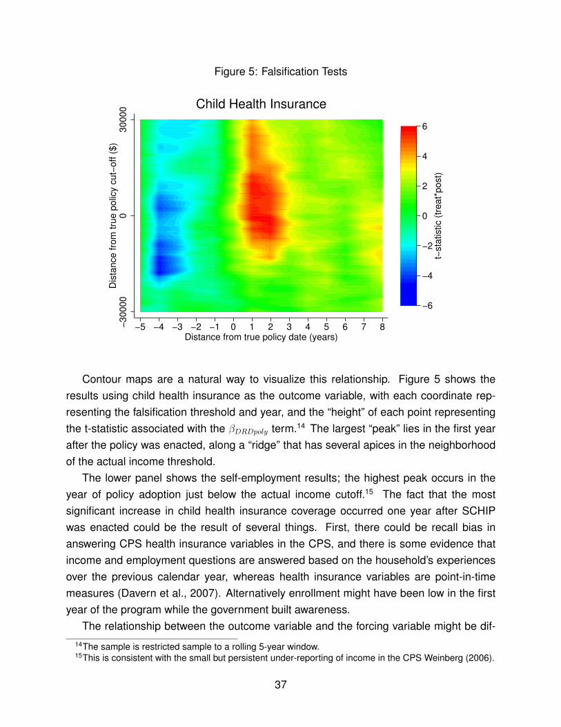
Figure 5: Falsification Tests
−3
000
00
30
00
0D
ista
nce
fro
m t
rue
po
licy
cut−
off
($
)
−5 −4 −3 −2 −1 0 1 2 3 4 5 6 7 8Distance from true policy date (years)
−6
−4
−2
0
2
4
6
t−st
atis
tic (
tre
at*
post
)
Child Health Insurance
Contour maps are a natural way to visualize this relationship. Figure 5 shows theresults using child health insurance as the outcome variable, with each coordinate rep-resenting the falsification threshold and year, and the “height” of each point representingthe t-statistic associated with the �
DRDpoly
term.14 The largest “peak” lies in the first yearafter the policy was enacted, along a “ridge” that has several apices in the neighborhoodof the actual income threshold.
The lower panel shows the self-employment results; the highest peak occurs in theyear of policy adoption just below the actual income cutoff.15 The fact that the mostsignificant increase in child health insurance coverage occurred one year after SCHIPwas enacted could be the result of several things. First, there could be recall bias inanswering CPS health insurance variables in the CPS, and there is some evidence thatincome and employment questions are answered based on the household’s experiencesover the previous calendar year, whereas health insurance variables are point-in-timemeasures (Davern et al., 2007). Alternatively enrollment might have been low in the firstyear of the program while the government built awareness.
The relationship between the outcome variable and the forcing variable might be dif-14The sample is restricted sample to a rolling 5-year window.15This is consistent with the small but persistent under-reporting of income in the CPS Weinberg (2006).
37

ferent for the treated, perhaps because treatment induces changes in economic behaviorunrelated to health insurance. This means the conditional expectation changes slopeacross the treatment threshold; including Treat
it
· g(Ruleit
) or Treatit
Ruleit
terms into thespecifications from Table 1 allows for this flexibility. Table A1.2 in the appendix showsthe sensitivity to allowing this difference, and the treatment effects are all robust to thischange. A popular method for dealing with selection on observables is propensity scorematching, which explicitly balances observables to generate matched groups with thesame propensity to be treated. Table A1.3 in the appendix shows the result of includinga propensity score (using Treat
it
as the treatment variable and the covariates discussedearlier as the predictors) in the regressions. The findings are all robust to including apropensity score, which is strongly and negatively correlated with the outcomes of inter-est.
5 Discussion
The social safety net is a crucial source of support for millions of Americans, yet little atten-tion has been paid to its effect on business ownership. This paper tests whether the StateChild Health Insurance program impacted firm formation. I develop a quasi-experimentalresearch design to identify the causal effect of the policy and find that SCHIP reducedthe number of households with uninsured children by nearly 40%. The program alsoincreased the self-employment rate by 15%, the number of incorporated firms by 36%,and the share of household income derived from self-employment by 12%, indicating thatthese are relatively high-quality ventures. The increase is driven largely by a 12% rise infirm birth rates and a 26% increase in the birth rate of incorporated firms. I also documenta large increase in labor supply, both on the extensive margin (more wage-earners inaffected households) and the intensive margin (treated households worked an additionaltwo weeks out of the year). There is no evidence that observable characteristics differbetween treatment and control groups, and the results survive a number of falsificationand robustness tests. Monte Carlo analysis strongly suggest the difference-in-RD estima-tor outperforms more traditional estimators in terms of bias and Type 1 Error, particularlywhen bandwidths are large and treatment effects are small.
Public health insurance may encourage self-employment by protecting householdsfrom the risk of catastrophic medical debt if they start a business and lose coverage(the risk channel) and by freeing up assets for use as loan collateral or start-up funds (thecredit channel). I find the strongest evidence for the risk channel: households who did notenroll in SCHIP but were otherwise eligible saw significant increases in self-employment,
38

even though their budget constraint had not shifted. The importance of uninsured riskin constraining firm formation and expansion is consistent with work in the developmentliterature on barriers faced by low-income firms (Bianchi and Bobba, 2013; Karlan et al.,2012).
The link between public health insurance and entrepreneurship is particularly salientin light of recent healthcare reform and the Affordable Care Act, but the theoretical mech-anisms apply to a more general class of programs. To the extent that entrepreneurscontribute to innovation, job creation or economic growth, these findings strongly suggestsocial insurance programs provide spillover benefits by affecting the supply of firms.
39

References
Aghion, Philippe and Peter Howitt, Endogenous Growth Theory, Vol. 1 of MIT PressBooks, The MIT Press, July 1997.
Baicker, Katherine, Sarah L. Taubman, Heidi L. Allen, Mira Bernstein, Jonathan H.Gruber, Joseph P. Newhouse, Eric C. Schneider, Bill J. Wright, Alan M. Zaslavsky,and Amy N. Finkelstein, “The Oregon Experiment: Effects of Medicaid on ClinicalOutcomes,” New England Journal of Medicine, 2013, 368 (18), 1713–1722. PMID:23635051.
Bansak, Cynthia and Steven Raphael, “The Effects of State Policy Design Featureson Take Up and Crowd Out Rates for the State Children’s Health Insurance Program,”Working Papers 0002, San Diego State University, Department of Economics Mar 2005.
and , “The State Health Insurance Program and Job Mobility: Identifying Job Lockamong Working Parents in Near-Poor Households,” Institute for Research on Labor andEmployment, Working Paper Series, Institute of Industrial Relations, UC Berkeley May2005.
Berger, Mark C., Dan A. Black, and Frank A. Scott, “Is There Job Lock? Evidence fromthe Pre-HIPAA Era,” Southern Economic Journal, 2004, 70 (4), pp. 953–976.
Berkowitz, Jeremy and Michelle J. White, “Bankruptcy and Small Firms’ Access toCredit,” RAND Journal of Economics, Spring 2004, 35 (1), 69–84.
Bertrand, Marianne, Esther Duflo, and Sendhil Mullainathan, “How Much ShouldWe Trust Differences-in-Differences Estimates?,” The Quarterly Journal of Economics,February 2004, 119 (1), 249–275.
Bianchi, Milo and Matteo Bobba, “Liquidity, Risk, and Occupational Choices,” Review ofEconomic Studies, 2013, 80 (2), 491–511.
Blanchflower, David G and Andrew J Oswald, “What Makes an Entrepreneur?,” Journalof Labor Economics, January 1998, 16 (1), 26–60.
Bruce, Donald and Mohammed Mohsin, “Tax Policy and Entrepreneurship: New TimeSeries Evidence,” Small Business Economics, 2006, 26 (5), pp. 409–425.
Cagetti, Marco and Mariacristina De Nardi, “Entrepreneurship, Frictions, and Wealth,”Journal of Political Economy, October 2006, 114 (5), 835–870.
and , “Estate Taxation, Entrepreneurship, and Wealth,” American Economic Review,March 2009, 99 (1), 85–111.
Chay, Kenneth and Kaivan Munshi, “Black Networks After Emancipation: Evidencefrom Reconstruction and the Great Migration,” Mimeo, 2013.
40

Davern, Michael, Gestur Davidson, Jeanette Ziegenfuss, Stephanie Jarosek, BrianLee, Tzy-Chyi Yu, and Lynn Blewett, A comparison of the health insurance coverageestimates from four national surveys and six state surveys: a discussion of measure-ment issues and policy implications, University of Minnesota School of Public Health,State Health Access Data Assistance Center, 2007.
Decker, Ryan, John Haltiwanger, Ron Jarmin, and Javier Miranda, “The Role of En-trepreneurship in US Job Creation and Economic Dynamism,” Journal of EconomicPerspectives, 2014, 28 (3), 3–24.
Evans, David S and Boyan Jovanovic, “An Estimated Model of Entrepreneurial Choiceunder Liquidity Constraints,” Journal of Political Economy, August 1989, 97 (4), 808–27.
Fairlie, Robert W., Kanika Kapur, and Susan Gates, “Is employer-based health insur-ance a barrier to entrepreneurship?,” Journal of Health Economics, 2011, 30 (1), 146 –162.
Fairlie, Robert W, Kanika Kapur, and Susan Gates, “Job Lock: Evidence from a Re-gression Discontinuity Design,” Working Papers 201215, School Of Economics, Univer-sity College Dublin Apr 2012.
Fan, Wei and Michelle J White, “Personal Bankruptcy and the Level of EntrepreneurialActivity,” Journal of Law and Economics, October 2003, 46 (2), 543–67.
Garthwaite, Craig, Tal Gross, and Matthew J. Notowidigdo, “Public Health Insurance,Labor Supply, and Employment Lock,” NBER Working Papers 19220, National Bureauof Economic Research, Inc July 2013.
Gentry, William M. and R. Glenn Hubbard, “Entrepreneurship and Household Saving,”NBER Working Papers 7894, National Bureau of Economic Research, Inc September2000.
and , “Tax Policy and Entrepreneurial Entry,” The American Economic Review, 2000,90 (2), pp. 283–287.
and , “"Success Taxes," Entrepreneurial Entry, and Innovation,” in “Innovation Policyand the Economy, Volume 5” NBER Chapters, National Bureau of Economic Research,Inc, August 2005, pp. 87–108.
Georgellis, Yannis and Howard J. Wall, “Entrepreneurship and the policy environment,”Review, 2006, (Mar), 95–112.
Gilleskie, Donna B. and Byron F. Lutz, “The Impact of Employer-Provided Health Insur-ance on Dynamic Employment Transitions,” Working Paper 7307, National Bureau ofEconomic Research August 1999.
Grembi, Veronica, Tommaso Nannicini, and Ugo Troiano, “Policy Responses to Fis-cal Restraints: A Difference-in-Discontinuities Design,” IZA Discussion Papers 6952,Institute for the Study of Labor (IZA) October 2012.
41

Gruber, Jonathan and Brigitte C. Madrian, “Limited Insurance Portability and Job Mo-bility: The Effects of Public Policy on Job-Lock,” NBER Working Papers 4479, NationalBureau of Economic Research, Inc Sep 1993.
and , “Health Insurance, Labor Supply, and Job Mobility: A Critical Review of theLiterature,” NBER Working Papers 8817, National Bureau of Economic Research, IncFebruary 2002.
Gumus, Gulcin and Tracy Regan, “Self-Employment and the Role of Health Insurance,”Discussion Paper 3952, IZA 2013.
Hamersma, Sarah and Matthew Kim, “The effect of parental Medicaid expansions onjob mobility,” Journal of Health Economics, July 2009, 28 (4), 761–770.
Holtz-Eakin, Douglas, “Health Insurance Provision and Labor Market Efficiency in theUnited States and Germany,” in “Social Protection versus Economic Flexibility: Is Therea Trade-Off?” NBER Chapters, National Bureau of Economic Research, Inc, April 1994,pp. 157–188.
, David Joulfaian, and Harvey S. Rosen, “Entrepreneurial Decisions and LiquidityConstraints,” NBER Working Papers 4526, National Bureau of Economic Research, IncJune 1994.
, , and , “Sticking It Out: Entrepreneurial Survival and Liquidity Constraints,” Journalof Political Economy, February 1994, 102 (1), 53–75.
, John R. Penrod, and Harvey S. Rosen, “Health insurance and the supply of en-trepreneurs,” Journal of Public Economics, October 1996, 62 (1-2), 209–235.
Imbens, Guido W. and Thomas Lemieux, “Regression discontinuity designs: A guide topractice,” Journal of Econometrics, February 2008, 142 (2), 615–635.
Karlan, Dean, Robert Osei, Isaac Osei-Akoto, and Chris Udry, “Agricultural Decisionsafter Relaxing Credit and Risk Constraints,” Working paper 2012.
King, Robert G and Ross Levine, “Finance and Growth: Schumpeter Might Be Right,”The Quarterly Journal of Economics, August 1993, 108 (3), 717–37.
Lemieux, Thomas and Kevin Milligan, “Incentive effects of social assistance: A re-gression discontinuity approach,” Journal of Econometrics, February 2008, 142 (2),807–828.
Levine, Ross and Yona Rubinstein, “Smart and Illicit: Who Becomes an Entrepreneurand Does it Pay?,” Working Paper 19276, National Bureau of Economic Research Au-gust 2013.
Madrian, Brigitte C, “Employment-Based Health Insurance and Job Mobility: Is ThereEvidence of Job-Lock?,” The Quarterly Journal of Economics, February 1994, 109 (1),27–54.
42

Meh, Cesaire, “Entrepreneurship, Wealth Inequality, and Taxation,” Review of EconomicDynamics, July 2005, 8 (3), 688–719.
Meh, Cesaire A. and Yaz Terajima, “Unsecured Debt, Consumer Bankruptcy, and SmallBusiness,” Technical Report 2008.
Parker, S.C., The Economics of Entrepreneurship The Economics of Entrepreneurship,Cambridge University Press, 2009.
Pettersson-Lidbom, Per, “Does the size of the legislature affect the size of government?Evidence from two natural experiments,” Journal of Public Economics, 2012, 96 (3),269–278.
Quadrini, Vincenzo, “Entrepreneurship, Saving and Social Mobility,” Review of EconomicDynamics, January 2000, 3 (1), 1–40.
Robson, Martin T. and Colin Wren, “Marginal and Average Tax Rates and the Incentivefor Self-Employment,” Southern Economic Journal, 1999, 65 (4), pp. 757–773.
Rosenbach, Margo, Marilyn Ellwood, John Czajka, Carol Irvin, Wendy Coupe, andBrian Quinn, “Implementation of the State Children’s Health Insurance Program: Mo-mentum is increasing after a modest start,” Prepared for the Centers for Medicare andMedicaid Services, Mathematica Policy Research, 2001.
Sasso, Anthony T. Lo and Thomas C. Buchmueller, “The effect of the state children’shealth insurance program on health insurance coverage,” Journal of Health Economics,2004, 23 (5), 1059–1082.
Schuetze, Herb J, “Taxes, economic conditions and recent trends in male self-employment: a Canada-US comparison,” Labour Economics, 2000, 7 (5), 507 – 544.
Schumpeter, J.A., The Theory of Economic Development: An Inquiry Into Profits, Cap-ital, Credit, Interest, and the Business Cycle A galaxy book. GB 55, Oxford UniversityPress, 1961.
Weinberg, Daniel H, “Income data quality issues in the CPS,” Monthly Lab. Rev., 2006,129, 38.
43

Appendix (for online publication)
Figure A1.1: Density
Pre−policy
Post−policy
05.0
00
e−
06
.00
00
1.0
00
01
5D
en
sity
−40000 −20000 0 20000 40000 60000 80000Income difference from cut−off ($)
44

Tabl
eA
1.1:
CP
SS
umm
ary
Sta
tistic
s
Varia
ble
Des
crip
tion
Obs
.M
ean
Std
.Dev
.
Chi
ldH
ealth
Insu
ranc
eH
asch
ildco
vere
dby
heal
thin
sura
nce
4945
510.
8585
747
0.34
846
Sel
f-Em
ploy
men
tH
asse
lf-em
ploy
edm
embe
r10
3951
40.
1268
891
0.33
2848
9In
com
eTo
talh
ouse
hold
inco
me
($)
1039
514
6309
4.25
6460
7.19
Bla
ckH
asbl
ack
fam
ilym
embe
r10
3951
40.
1277
164
0.33
3773
9H
ispa
nic
Has
His
pani
cfa
mily
mem
ber
1039
514
0.14
6994
70.
3541
008
Hou
seho
ldS
ize
Hou
seho
ldsi
ze10
3951
42.
8929
611.
5059
89C
hild
ren
Num
bero
fchi
ldre
n10
3951
40.
8808
222
1.16
8134
Age
ofA
dults
Hou
seho
ldav
erag
ead
ulta
ge10
3951
441
.978
9911
.673
93M
arrie
dH
asm
arrie
dm
embe
rs10
3951
40.
5757
142
0.49
4234
3H
asK
ids
Has
child
ren
livin
gat
hom
e10
3951
40.
4633
685
0.49
8656
6M
oved
Mov
edin
the
last
year
1039
514
0.17
4142
0.37
9231
7U
rban
Live
sin
urba
nar
ea10
3159
80.
7871
341
0.40
9333
8R
ente
rR
ents
dom
icile
1039
514
0.34
3127
70.
4747
539
Hig
hS
choo
lH
asm
embe
rwith
high
scho
olde
gree
1039
514
0.88
0241
90.
2902
053
Bac
helo
r’sD
egre
eH
asm
embe
rwith
Bac
helo
r’sde
gree
1006
809
0.36
1690
80.
4289
68G
radu
ate
Deg
ree
Has
mem
berw
ithgr
adua
tede
gree
1006
809
0.08
9928
20.
2490
771
Une
mpl
oym
ent
Rec
eive
sun
empl
oym
enti
nsur
ance
1039
514
0.07
9896
0.27
1132
2D
isab
led
Rec
eive
sdi
sabi
lity
bene
fits
1039
514
0.01
5994
0.12
5452
1Ve
tera
nR
ecei
ves
vete
rans
bene
fits
1039
514
0.01
9901
60.
1396
623
Med
icai
dR
ecei
ves
Med
icai
dbe
nefit
s10
3951
40.
1130
461
0.31
6649
3E
mpl
oyed
Has
empl
oyed
mem
ber
1039
514
0.89
2315
10.
3099
822
Ris
kC
oeff.
ofva
riatio
nin
SE
(sta
te-le
vel)
1039
514
1.66
7465
0.17
9969
6S
elf-e
mp.
inco
me
Perc
ento
finc
ome
from
busi
ness
1152
5628
769.
9550
912.
09W
orke
rsN
umbe
rofw
orki
ngad
ults
1039
514
1.56
1936
0.92
6290
5W
age
earn
ers
Num
bero
fwag
eea
rner
sin
the
hous
ehol
d10
3951
41.
4904
590.
9376
618
Wee
ksW
eeks
wor
ked
durin
gth
eye
ar93
1307
46.9
4887
9.69
3488
Hou
rsH
ours
wor
ked
inty
pica
lwee
k93
1307
40.0
9455
9.49
2656
Inco
rpor
ated
Has
anin
corp
orat
edbu
sine
ss10
3951
40.
0421
986
0.20
1042
Year
Ref
eren
ceye
arfo
rhou
seho
ld10
3951
420
02.2
396.
3197
57Po
licy
Year
Year
polic
yw
asen
acte
d10
3951
419
98.2
210.
6387
923
Thre
shol
dPo
licy
thre
shol
d(%
ofFP
L)10
3951
420
7.98
4545
.460
71R
ule
Last
year
’sIn
com
em
inus
Thre
shol
d10
3951
431
251.
6662
774.
42Tr
eat
Trea
tmen
tsta
tus
(rul
e
0)10
3951
40.
2908
205
0.45
4141
1Po
stPo
st-p
olic
y(y
ear�
post
year
)10
3951
40.
7210
504
0.44
8482
9
45

Tabl
eA
1.2:
Sep
arat
ePo
lyno
mia
lsac
ross
Thre
shol
d(D
iffer
ence
-in-R
D)
Chi
ldH
ealth
Insu
ranc
eS
elf-E
mpl
oym
ent
(1)
(2)
(3)
(4)
(5)
(6)
Treat·P
ost
0.04
62**
0.03
47**
0.01
93*
0.03
07**
0.01
01*
0.01
80**
(0.0
0558
)(0
.005
31)
(0.0
0803
)(0
.003
95)
(0.0
0390
)(0
.005
76)
Pre
-pol
icy
avg.
0.86
10.
826
0.82
70.
140
0.12
50.
127
LATE
5.36
94.
207
2.33
121
.93
8.11
814
.18
Trea
ted
avg.
0.78
30.
793
0.81
00.
102
0.11
60.
117
TOT
5.90
44.
377
2.38
129
.93
8.76
215
.34
Ban
dwid
th:
Poly
nom
ial
±$1
0,00
0±
$5,0
00Po
lyno
mia
l±
$10,
000
±$5
,000
Obs
erva
tions
475,
546
106,
034
53,5
6648
1,67
810
7,48
754
,295
R-s
quar
ed0.
048
0.03
20.
032
0.02
30.
008
0.00
8
Tim
e/st
ate
FEan
dst
ate
trend
sin
clud
ed.D
ata:
CP
S19
92-2
013.
**0.
01,*
0.05
,+0.
1.Po
lyno
mia
lmet
hod
fits
a6t
h-or
derf
unct
ion
usin
gth
een
tire
data
set,
loca
llin
earu
ses
data
with
inth
eba
ndw
idth
.Po
lyno
mia
lspe
cific
atio
nsin
clud
eTreat·g
(Rule)
and
loca
llin
ears
peci
ficat
ions
incl
udeTreat·R
ule
.R
obus
tsta
ndar
der
rors
clus
tere
dat
the
stat
ele
veli
npa
rent
hese
s.
46

Tabl
eA
1.3:
Pro
pens
ityS
core
Chi
ldH
ealth
Insu
ranc
eS
elf-E
mpl
oym
ent
DID
RD
(Diff
eren
ced)
DID
RD
(Diff
eren
ced)
(1)
(2)
(3)
(4)
(5)
(6)
Treat·P
ost
0.03
32**
0.05
12**
0.01
98*
0.00
983*
*0.
0199
**0.
0186
**(0
.005
32)
(0.0
0539
)(0
.008
17)
(0.0
0344
)(0
.003
51)
(0.0
0558
)
Prop.score
0.03
23**
0.07
97**
0.02
34*
-0.1
97**
-0.1
79**
-0.2
14**
(0.0
0843
)(0
.008
71)
(0.0
105)
(0.0
0444
)(0
.004
82)
(0.0
0811
)
Pre
-pol
icy
avg.
0.86
10.
861
0.82
70.
140
0.14
00.
127
LATE
3.85
85.
948
2.39
77.
029
14.2
614
.65
Trea
ted
avg.
0.78
30.
783
0.81
00.
102
0.10
20.
117
TOT
4.24
26.
541
2.44
89.
593
19.4
715
.85
Ban
dwid
th:
—Po
lyno
mia
l±
$5,0
00—
Poly
nom
ial
±$5
,000
Obs
erva
tions
456,
756
456,
756
50,9
4246
2,76
046
2,76
051
,648
R-s
quar
ed0.
043
0.04
90.
033
0.02
50.
033
0.02
9
OLS
.Tim
e/st
ate
FEan
dst
ate
trend
sin
clud
ed.D
ata:
CP
S19
92-2
013.
Poly
nom
ialm
etho
dfit
sa
6th-
orde
rfun
ctio
nus
ing
the
entir
eda
tase
t,lo
call
inea
ruse
sda
taw
ithin
the
band
wid
th.
**0.
01,*
0.05
,+0.
1.R
obus
tsta
ndar
der
rors
clus
tere
dat
the
stat
ele
veli
npa
rent
hese
s.
47

Figure A1.2: Treatment Effects by Bandwidth, RD (Differenced)
0.0
2.0
4.0
6T
reatm
ent effect
5000 10000 15000 20000 25000 30000Bandwidth ($ from threshold)
Child Health Insurance
0.0
1.0
2.0
3T
reatm
ent effect
5000 10000 15000 20000 25000 30000Bandwidth ($ from threshold)
Self−Employment
48

Figure A1.3: Monte Carlo, Positive Treatment Effect (6th Order g(·), Local Linear Method)
(a) Bias
.01
.25
Effect
, sd
(y)
.01 .25Bandwith, sd(x)
−.5
0
.5
1
1.5
RD
.01
.25
Effect
, sd
(y)
.01 .25Bandwith, sd(x)
Differenced
(b) Power
.01
.25
Effect
, sd
(y)
.01 .25Bandwith, sd(x)
.8
.85
.9
.95
1
RD
.01
.25
Effect
, sd
(y)
.01 .25Bandwith, sd(x)
Differenced
(c) RMSE
.01
.25
Effect
, sd
(y)
.01 .25Bandwith, sd(x)
0
10
20
30
40
50
RD
.01
.25
Effect
, sd
(y)
.01 .25Bandwith, sd(x)
Differenced
49

Figure A1.4: Monte Carlo, Positive Treatment Effect (Sinusoidal g(·), Local Linear Method)
(a) Bias
.01
.25
Effect
, sd
(y)
.01 .25Bandwith, sd(x)
−1.5
−1
−.5
0
RD
.01
.25
Effect
, sd
(y)
.01 .25Bandwith, sd(x)
Differenced
(b) Power
.01
.25
Effect
, sd
(y)
.01 .25Bandwith, sd(x)
.5
.6
.7
.8
.9
1
RD
.01
.25
Effect
, sd
(y)
.01 .25Bandwith, sd(x)
Differenced
(c) RMSE
.01
.25
Effect
, sd
(y)
.01 .25Bandwith, sd(x)
0
10
20
30
40
RD
.01
.25
Effect
, sd
(y)
.01 .25Bandwith, sd(x)
Differenced
50