Entropy and Counting∗

Jaikumar RadhakrishnanSchool of Technology and Computer Science

Tata Institute of Fundamental ResearchHomi Bhabha Road, Mumbai 400 005

email: jaikumar@tcs.tifr.res.in

Abstract

We illustrate the role of information theoretic ideas in combinatorial problems,some of them arising in computer science. We also consider the problem of coveringgraphs using other graphs, and show how information theoretic ideas are appliedto this setting. Our treatment of graph covering problems naturally motivates two(already known) definitions of Korner’s graph entropy.

Keywords: Shannon entropy, counting problems, covering problems, graph entropy.

Contents:

IntroductionSortingOrganization of the article

EntropyCounting problems

Bregman’s thoeremShearer’s lemma

Covering problemsHansel’s theoremThe Fredman-Komlos boundContent of a graph

Korner’s graph entropyTwo definitions of graph entropyProperties of graph entropy

Remarks

∗This paper appeared in the IIT Kharagpur, Golden Jubilee Volume, on Computational Mathematics,Modelling and Algorithms (Ed. JC Mishra), Narosa Publishers, New Delhi, 2001.

1

CreditsAcknowledgements

References

1 Introduction

Information theoretic ideas underlie several combinatorial arguments. This is not sur-prising, because in these arguments, one typically establishes a correspondence betweenelements a of a set A, whose size one wishes to determine, and elements b of another set B,whose size is known in advance. In other words, one shows how one can encode elementsof one set using elements of another. This is an information theoretic argument: one canuniquely determine the element a from its encoding b. Let us consider an example.

1.1 Sorting

Suppose we are given a sequence 〈a1, a2, . . . , an〉 of distinct natural numbers. We wishto compare these numbers, two at a time, and reorder them as 〈a′1, a′2, . . . , a′n〉 such thata′1 < a′2 < · · · < a′n.

The sorting problem: How many comparisons must we make in the worst case?

The combinatorial argument: Fix a strategy for sorting. Suppose it makes t compar-isons in the worst case. We wish to obtain a lower bound for t. Each comparison has twopossible outcomes, which we encode as 0 and 1. Thus, with each of the n! permutationswe can associated a unique string of 0’s and 1’s of lenght t. (If the algorithm stops beforemaking t comparisons, just let the remaining bits of the string to be 0’s.) The crucialobservation for us is this: once the outcomes of all the comparisons are known, the finalpermutation is uniquely determined. Thus, a strategy for sorting using at most t compar-isons implicitly gives us a procedure for uniquely encoding the n! permutations using 0-1strings of length t. For this to be feasible, we must have 2t ≥ n!, that is, t ≥ log n!. (Alllogarithms in this paper have base 2.)

This is just a counting argument. Let us try to make explicit the information theoreticreasoning underlying it. The informal arguments is as follows. Since there are n! permu-tations, one needs at least log n! bits of information to describe a permutation. On theother hand, each comparison gives us at most one bit of information. The results of thesecomparisons together allow us to identify the permutation uniquely. So, to collect log n!bits of information we make log n! comparisons.

The counting argument above is straight forward, whereas the information theoreticargument is rather vague. This vagueness can be removed by formalising the argumentusing the notion of entropy. In the next section, we will discuss this notion briefly. We willthen return to the problem of sorting and give a formal information theoretic proof. Thisformalisation will be rather contrived, containing hardly any new insight beyond what is

2

there in the counting argument above. However, in later examples entropy will play a morecrucial role. For example, consider the following puzzle.

Suppose n distinct points in R3 have n1 distinct projections on the XY-plane,n2 distinct projections on the XZ-plane and n3 distinct projections on the YZ-plane. Then, n2 ≤ n1n2n3.

We will see later how the notion of entropy provides a rather simple and natural solution.

Organisation of this article

In the next section, we recall Shannon’s definition of entropy and describe some its prop-erties. In Section 1.1, we give examples of some counting problems (including the puzzleabove) where entropy can be applied fruitfully. In Section 3.2, we study entropy in thecontext of graph covering problems. A useful tool in this study is graph entropy discov-ered by Korner [18]. In fact, there are several equivalent definitions of graph entropy. Wewill see that two of these definitions can be derived naturally from our combinatorial andinformation theoretic analysis of graph covering problems.

We assume that the reader is familiar with elementary probability: random variables,conditioning, expectations, Jensen’s inequality. Many of our applications are for graphs.We assume that the reader is familiar with the definitions of graphs: vertices, edges, degree,independent sets, chromatic number.

2 Entropy

The entropy of a random variable X with finite range is

H[X]def= −

∑x∈range[X]

Pr[X = x] log2 Pr[X = x].

H[X] measures the amount of uncertainty in X, or the amount of information obtainedwhen X is revealed. This formula is due to Shannon, who arrived at it while studyinginformation transmission; one can also derive this formula from axioms that a measure ofinformation is supposed to satisfy (see Khinchin [16]). Renyi [30] compares the pragmaticand axiomatic approaches to entropy, and discusses other ways of measuring the informa-tion in a random variable. To learn more about entropy and information theory see thetexts by Csiszar and Korner [7], and Cover and Thomas [6]. For our purposes, it will beenough to keep the following intuitive picture in mind. There are two parties A and B.At some later point in time, A and B will be separated by a large distance. The valueof the random variable X, will be revealed to A, who must then describe it to B. Tominimise the cost of communication, A and B fix a encoding (using 0-1 strings) of thepossible values that X can take. Roughly speaking, H[X] is the average number of bits Amust communicate to convey to B the value of X, under the best encoding.

3

The conditional entropy of X given Y , measures the average uncertainty in X, afterthe value of Y has been revealed; it is given by

H[X | Y ]def= E

Y[H[XY ]],

where for y ∈ range[Y ], Xy is a random variable taking values in range(X), such that

Pr[Xy = x] = Pr[X = x | Y = y].

Facts about entropy: The following equalities follow immediately from the definitions.

H[XY ] = H[X] +H[Y | X];

H[XY | Z] = H[X | Z] +H[Y | XZ].

We will also need the following facts, which follow from Jensen’s inequality: for a concavefunction f , E[f(X)] ≤ f(E[X]), and if f is strictly concave, equality holds if and only if Xis constant.

H[X] ≥ H[X | f(Y )] ≥ H[X | Y ] ≥ 0 for any function f ;

H[X] ≤ log2 | range[X]| (with equality iff X is uniformly distributed).

Notation: From now on, when we write log we mean log2. Also, [n] stands for the set{1, 2, . . . , n}, and for a set U ,

(Ur

)is the set of all subsets of U of size r.

3 Counting problems

Let us now state the lower bound for sorting using the notation of entropy. Let X be arandom permutation of [n] chosen with uniform distribution. Then,

H[X] = lg n.

Let Y1, Y2, . . . , Yt be the outcome of the t comparisons performed when the actual or-dering of the input is given by X. Thus, Y1, Y2, . . . , Yt are random variables dependenton X. On the other hand, since we can recover X from Y1, Y2, . . . , Yt, it follows thatX = f(Y1, Y2, . . . , Yt), for some f . Thus,

lg n! ≤ H[f(Y1, Y2, . . . , Yt)]

≤ H[Y1, Y2, . . . , Yt]

≤t∑i=1

H[Yi]

≤ t.

4

3.1 Bregman’s theorem

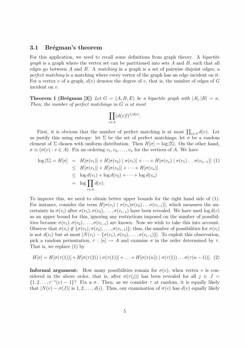
For this application, we need to recall some definitions from graph theory. A bipartitegraph is a graph where the vertex set can be partitioned into sets A and B, such that alledges go between A and B. A matching in a graph is a set of pairwise disjoint edges; aperfect matching is a matching where every vertex of the graph has an edge incident on it.For a vertex v of a graph, d(v) denotes the degree of v, that is, the number of edges of Gincident on v.

Theorem 1 (Bregman [3]) Let G = (A,B,E) be a bipartite graph with |A|, |B| = n.Then, the number of perfect matchings in G is at most∏

v∈A

(d(v)!)1/d(v).

First, it is obvious that the number of perfect matching is at most∏

v∈A d(v). Letus justify this using entropy: let Σ be the set of perfect matchings; let σ be a randomelement of Σ chosen with uniform distribution. Then H[σ] = log |Σ|. On the other hand,σ ≡ (σ(v) : v ∈ A). Fix an ordering v1, v2, . . . , vn for the vertices of A. We have

log |Σ| = H[σ] = H[σ(v1)] +H[σ(v2) | σ(v1)] + · · ·+H[σ(vn) | σ(v1) . . . σ(vn−1)] (1)

≤ H[σ(v1)] +H[σ(v2)] + · · ·+H[σ(vn)]

≤ log d(v1) + log d(v2) + · · ·+ log d(vn)

= log∏v∈A

d(v).

To improve this, we need to obtain better upper bounds for the right hand side of (1).For instance, consider the term H[σ(vi) | σ(v1)σ(v2) . . . σ(vi−1)], which measures the un-certainty in σ(vi) after σ(v1), σ(v2), . . . , σ(vi−1) have been revealed. We have used log d(v)as an upper bound for this, ignoring any restrictions imposed on the number of possibil-ities because σ(v1), σ(v2), . . . , σ(vi−1) are known. Now we wish to take this into account.Observe that σ(vi) 6∈ {σ(v1), σ(v2), . . . , σ(vi−1)}; thus, the number of possibilities for σ(vi)is not d(vi) but at most |N(vi)− {σ(v1), σ(v2), . . . , σ(vi−1)}|. To exploit this observation,pick a random permutation, τ : [n] → A and examine σ in the order determined by τ .That is, we replace (1) by

H[σ] = H[σ(τ(1))] +H[σ(τ(2)) | σ(τ(1))] + . . .+H[σ(τ(n)) | σ(τ(1)) . . . σ(τ(n− 1))]. (2)

Informal argument: How many possibilities remain for σ(v), when vertex v is con-sidered in the above order, that is, after σ(τ(j)) has been revealed for all j ∈ J ={1, 2 . . . , τ−1(v) − 1}? Fix a σ. Then, as we consider τ at random, it is equally likelythat |N(v)− σ(J)| is 1, 2, . . . , d(i). Thus, our examination of σ(v) has d(v) equally likely

5

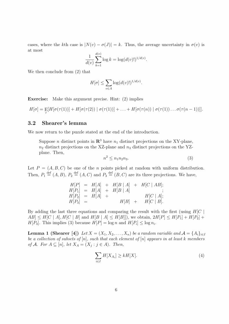
cases, where the kth case is |N(v) − σ(J)| = k. Thus, the average uncertainty in σ(v) isat most

1

d(v)

d(v)∑k=1

log k = log(d(v)!)1/d(v).

We then conclude from (2) that

H[σ] ≤∑v∈A

log(d(v)!)1/d(v).

Exercise: Make this argument precise. Hint: (2) implies

H[σ] = Eτ[H[σ(τ(1))] +H[σ(τ(2)) | σ(τ(1))] + . . .+H[σ(τ(n)) | σ(τ(1)) . . . σ(τ(n− 1))]].

3.2 Shearer’s lemma

We now return to the puzzle stated at the end of the introduction.

Suppose n distinct points in R3 have n1 distinct projections on the XY-plane,n2 distinct projections on the XZ-plane and n3 distinct projections on the YZ-plane. Then,

n2 ≤ n1n2n3. (3)

Let P = (A,B,C) be one of the n points picked at random with uniform distribution.

Then, P1def= (A,B), P2

def= (A,C) and P3

def= (B,C) are its three projections. We have,

H[P ] = H[A] + H[B | A] + H[C | AB];H[P1] = H[A] + H[B | A] ;H[P2] = H[A] + H[C | A];H[P3] = H[B] + H[C | B].

By adding the last three equations and comparing the result with the first (using H[C |AB] ≤ H[C | A], H[C | B] and H[B | A] ≤ H[B]]), we obtain, 2H[P ] ≤ H[P1] +H[P2] +H[P3]. This implies (3) because H[P ] = log n and H[Pi] ≤ log ni.

Lemma 1 (Shearer [4]) Let X = (X1, X2, . . . , Xn) be a random variable and A = {Ai}i∈Ibe a collection of subsets of [n], such that each element of [n] appears in at least k membersof A. For A ⊆ [n], let XA = (Xj : j ∈ A). Then,∑

i∈I

H[XAi] ≥ kH[X]. (4)

6

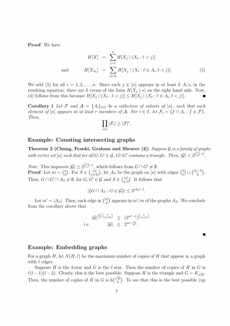
Proof: We have

H[X] =n∑j=1

H[Xj | (X` : ` < j)]

and H[XAi] =

∑j∈Ai

H[Xj | (X` : ` ∈ Ai, ` < j)]. (5)

We add (5) for all i = 1, 2, . . . , n. Since each j ∈ [n] appears in at least k Ai’s, in theresulting equation, there are k terms of the form H[Xj | ∗] on the right hand side. Now,(4) follows from this because H[Xj | (X` : ` < j)] ≤ H[Xj | (X` : ` ∈ Ai, ` < j)].

Corollary 1 Let F and A = {Ai}i∈I be a collection of subsets of [n], such that eachelement of [n] appears in at least r members of A. For i ∈ I, let Fi = {f ∩ Ai : f ∈ F}.Then, ∏

i∈I

|Fi| ≥ |F|r.

Example: Counting intersecting graphs

Theorem 2 (Chung, Frankl, Graham and Shearer [4]) Suppose G is a family of graphs

with vertex set [n] such that for all G,G′ ∈ G, G∩G′ contains a triangle. Then, |G| < 2(n2)−2.

Note: This improves |G| ≤ 2(n2)−1, which follows from G ∩G′ 6= ∅.

Proof: Let m =(n2

). For S ∈

([n]

bn/2c

), let AS be the graph on [n] with edges

(S2

)∪

([n]−S

2

).

Then, G ∩G′ ∩ AS 6= ∅, for G,G′ ∈ G and S ∈(

[n]n/2

). It follows that

|{G ∩ AS : G ∈ G}| ≤ 2|AS |−1.

Let m′ = |AS|. Then, each edge in([n]2

)appears in m′/m of the graphs AS. We conclude

from the corollary above that

|G|m′m ( n

bn/2c) ≤ (2m′−1)(

nbn/2c)

i.e. |G| ≤ 2m− mm′ .

Example: Embedding graphs

For a graph H, let N(H, `) be the maximum number of copies of H that appear in a graphwith ` edges.

Suppose H is the 3-star and G is the `-star. Then the number of copies of H in G is`(`− 1)(`− 2). Clearly, this is the best possible. Suppose H is the triangle and G = K√

2`.

Then, the number of copies of H in G is 6(√

2`3

). To see that this is the best possible (up

7

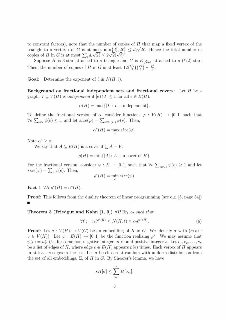
to constant factors), note that the number of copies of H that map a fixed vertex of thetriangle to a vertex i of G is at most min{d2

i , 2`} ≤ di√

2`. Hence the total number ofcopies of H in G is at most

∑i di√

2` ≤ 2√

2(√`)3.

Suppose H is 3-star attached to a triangle and G is K√`+1 attached to a (`/2)-star.

Then, the number of copies of H in G is at least 12(`/23

)(√`

2

)∼ `4

4.

Goal: Determine the exponent of ` in N(H, `).

Background on fractional independent sets and fractional covers: Let H be agraph. I ⊆ V (H) is independent if |e ∩ I| ≤ 1 for all e ∈ E(H).

α(H) = max{|I| : I is independent}.

To define the fractional version of α, consider functions ϕ : V (H) → [0, 1] such that∀e

∑v∈e φ(v) ≤ 1, and let size(ϕ) =

∑v∈V (H) ϕ(v). Then,

α∗(H) = maxϕ

size(ϕ).

Note α∗ ≥ α.We say that A ⊆ E(H) is a cover if

⋃A = V .

ρ(H) = min{|A| : A is a cover of H}.

For the fractional version, consider ψ : E → [0, 1] such that ∀v∑

e:v∈e ψ(e) ≥ 1 and letsize(ψ) =

∑e ψ(e). Then,

ρ∗(H) = minψ

size(ψ).

Fact 1 ∀H ρ∗(H) = α∗(H).

Proof: This follows from the duality theorem of linear programming (see e.g. [5, page 54])

Theorem 3 (Friedgut and Kahn [1, 9]) ∀H ∃c1, c2 such that

∀` : c1`ρ∗(H) ≤ N(H, `) ≤ c2`

ρ∗(H). (6)

Proof: Let σ : V (H) → V (G) be an embedding of H in G. We identify σ with (σ(v) :v ∈ V (H)). Let ψ : E(H) → [0, 1] be the function realizing ρ∗. We may assume thatψ(e) = n(e)/s, for some non-negative integers n(e) and positive integer s. Let e1, e2, . . . , ekbe a list of edges of H, where edge e ∈ E(H) appears n(e) times. Each vertex of H appearsin at least s edges in the list. Let σ be chosen at random with uniform distribution fromthe set of all embeddings, Σ, of H in G. By Shearer’s lemma, we have

sH[σ] ≤k∑i=1

H[σei].

8

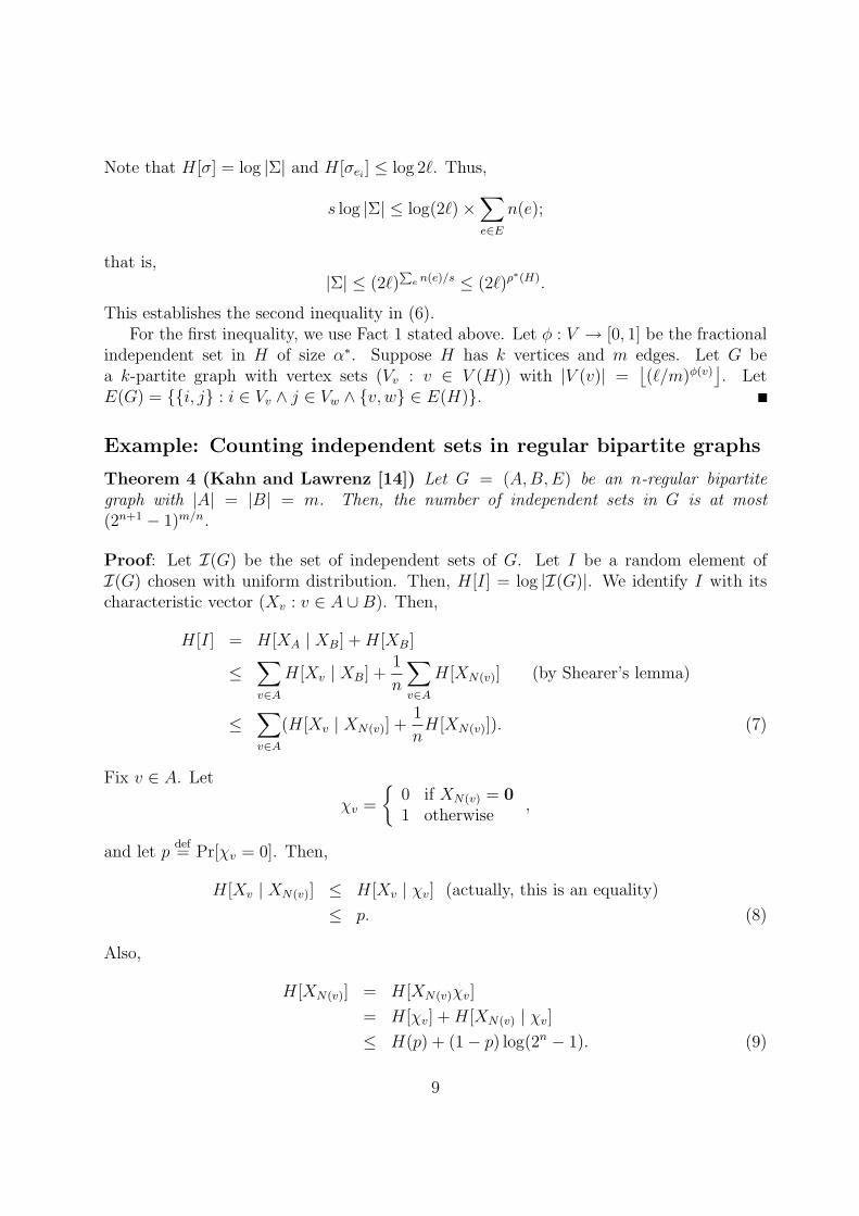
Note that H[σ] = log |Σ| and H[σei] ≤ log 2`. Thus,

s log |Σ| ≤ log(2`)×∑e∈E

n(e);

that is,|Σ| ≤ (2`)

Pe n(e)/s ≤ (2`)ρ

∗(H).

This establishes the second inequality in (6).For the first inequality, we use Fact 1 stated above. Let φ : V → [0, 1] be the fractional

independent set in H of size α∗. Suppose H has k vertices and m edges. Let G bea k-partite graph with vertex sets (Vv : v ∈ V (H)) with |V (v)| =

⌊(`/m)φ(v)

⌋. Let

E(G) = {{i, j} : i ∈ Vv ∧ j ∈ Vw ∧ {v, w} ∈ E(H)}.

Example: Counting independent sets in regular bipartite graphs

Theorem 4 (Kahn and Lawrenz [14]) Let G = (A,B,E) be an n-regular bipartitegraph with |A| = |B| = m. Then, the number of independent sets in G is at most(2n+1 − 1)m/n.

Proof: Let I(G) be the set of independent sets of G. Let I be a random element ofI(G) chosen with uniform distribution. Then, H[I] = log |I(G)|. We identify I with itscharacteristic vector (Xv : v ∈ A ∪B). Then,

H[I] = H[XA | XB] +H[XB]

≤∑v∈A

H[Xv | XB] +1

n

∑v∈A

H[XN(v)] (by Shearer’s lemma)

≤∑v∈A

(H[Xv | XN(v)] +1

nH[XN(v)]). (7)

Fix v ∈ A. Let

χv =

{0 if XN(v) = 01 otherwise

,

and let pdef= Pr[χv = 0]. Then,

H[Xv | XN(v)] ≤ H[Xv | χv] (actually, this is an equality)

≤ p. (8)

Also,

H[XN(v)] = H[XN(v)χv]

= H[χv] +H[XN(v) | χv]≤ H(p) + (1− p) log(2n − 1). (9)

9

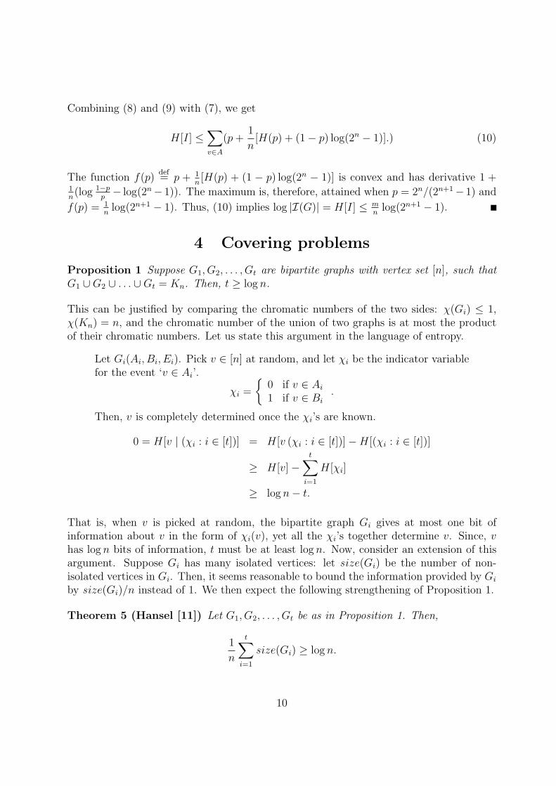
Combining (8) and (9) with (7), we get

H[I] ≤∑v∈A

(p+1

n[H(p) + (1− p) log(2n − 1)].) (10)

The function f(p)def= p + 1

n[H(p) + (1 − p) log(2n − 1)] is convex and has derivative 1 +

1n(log 1−p

p− log(2n− 1)). The maximum is, therefore, attained when p = 2n/(2n+1− 1) and

f(p) = 1n

log(2n+1 − 1). Thus, (10) implies log |I(G)| = H[I] ≤ mn

log(2n+1 − 1).

4 Covering problems

Proposition 1 Suppose G1, G2, . . . , Gt are bipartite graphs with vertex set [n], such thatG1 ∪G2 ∪ . . . ∪Gt = Kn. Then, t ≥ log n.

This can be justified by comparing the chromatic numbers of the two sides: χ(Gi) ≤ 1,χ(Kn) = n, and the chromatic number of the union of two graphs is at most the productof their chromatic numbers. Let us state this argument in the language of entropy.

Let Gi(Ai, Bi, Ei). Pick v ∈ [n] at random, and let χi be the indicator variablefor the event ‘v ∈ Ai’.

χi =

{0 if v ∈ Ai1 if v ∈ Bi

.

Then, v is completely determined once the χi’s are known.

0 = H[v | (χi : i ∈ [t])] = H[v (χi : i ∈ [t])]−H[(χi : i ∈ [t])]

≥ H[v]−t∑i=1

H[χi]

≥ log n− t.

That is, when v is picked at random, the bipartite graph Gi gives at most one bit ofinformation about v in the form of χi(v), yet all the χi’s together determine v. Since, vhas log n bits of information, t must be at least log n. Now, consider an extension of thisargument. Suppose Gi has many isolated vertices: let size(Gi) be the number of non-isolated vertices in Gi. Then, it seems reasonable to bound the information provided by Gi

by size(Gi)/n instead of 1. We then expect the following strengthening of Proposition 1.

Theorem 5 (Hansel [11]) Let G1, G2, . . . , Gt be as in Proposition 1. Then,

1

n

t∑i=1

size(Gi) ≥ log n.

10

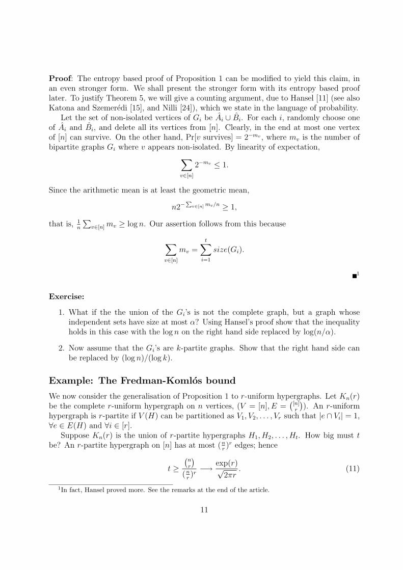
Proof: The entropy based proof of Proposition 1 can be modified to yield this claim, inan even stronger form. We shall present the stronger form with its entropy based prooflater. To justify Theorem 5, we will give a counting argument, due to Hansel [11] (see alsoKatona and Szemeredi [15], and Nilli [24]), which we state in the language of probability.

Let the set of non-isolated vertices of Gi be Ai ∪ Bi. For each i, randomly choose oneof Ai and Bi, and delete all its vertices from [n]. Clearly, in the end at most one vertexof [n] can survive. On the other hand, Pr[v survives] = 2−mv , where mv is the number ofbipartite graphs Gi where v appears non-isolated. By linearity of expectation,∑

v∈[n]

2−mv ≤ 1.

Since the arithmetic mean is at least the geometric mean,

n2−P

v∈[n]mv/n ≥ 1,

that is, 1n

∑v∈[n]mv ≥ log n. Our assertion follows from this because

∑v∈[n]

mv =t∑i=1

size(Gi).

1

Exercise:

1. What if the the union of the Gi’s is not the complete graph, but a graph whoseindependent sets have size at most α? Using Hansel’s proof show that the inequalityholds in this case with the log n on the right hand side replaced by log(n/α).

2. Now assume that the Gi’s are k-partite graphs. Show that the right hand side canbe replaced by (log n)/(log k).

Example: The Fredman-Komlos bound

We now consider the generalisation of Proposition 1 to r-uniform hypergraphs. Let Kn(r)be the complete r-uniform hypergraph on n vertices, (V = [n], E =

([n]r

)). An r-uniform

hypergraph is r-partite if V (H) can be partitioned as V1, V2, . . . , Vr such that |e ∩ Vi| = 1,∀e ∈ E(H) and ∀i ∈ [r].

Suppose Kn(r) is the union of r-partite hypergraphs H1, H2, . . . , Ht. How big must tbe? An r-partite hypergraph on [n] has at most (n

r)r edges; hence

t ≥(nr

)(nr)r−→ exp(r)√

2πr. (11)

1In fact, Hansel proved more. See the remarks at the end of the article.

11

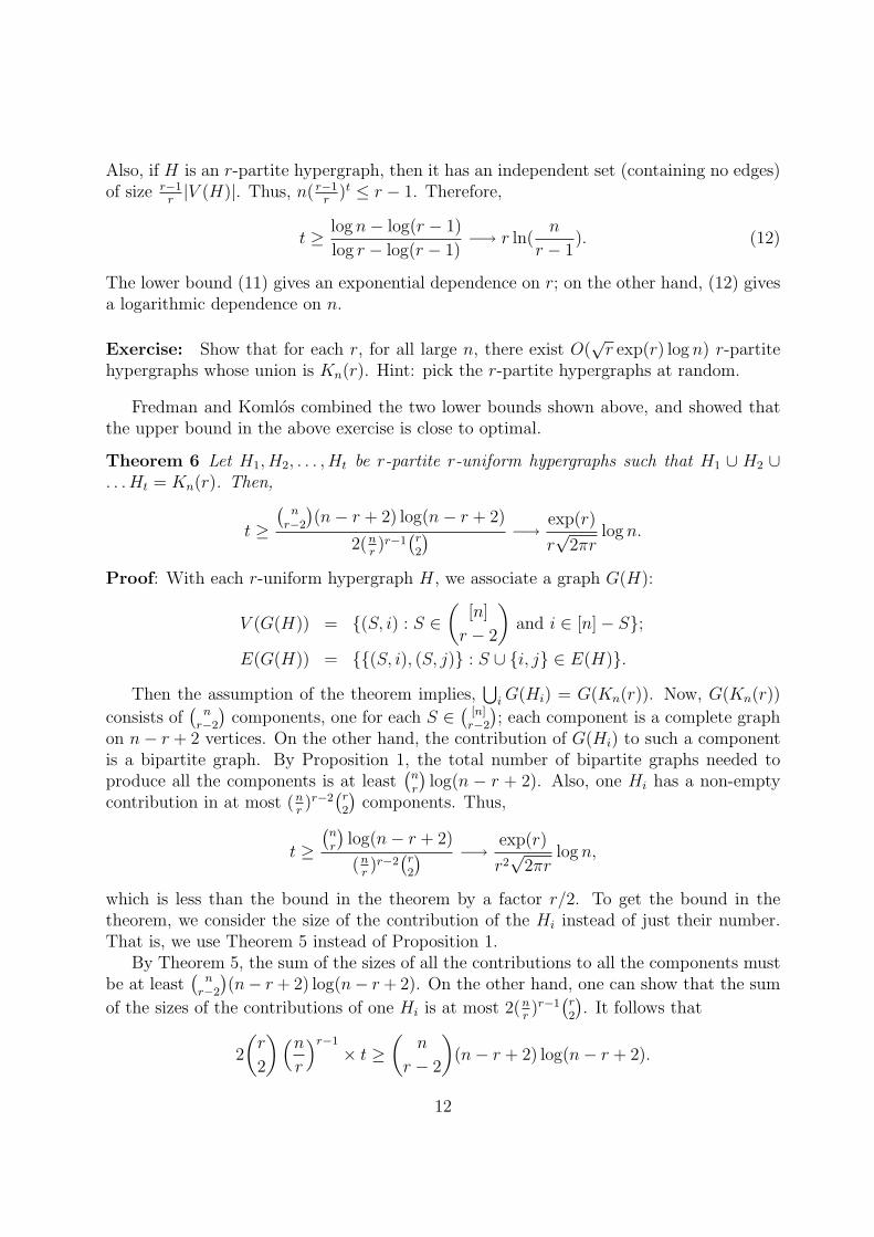
Also, if H is an r-partite hypergraph, then it has an independent set (containing no edges)of size r−1

r|V (H)|. Thus, n( r−1

r)t ≤ r − 1. Therefore,

t ≥ log n− log(r − 1)

log r − log(r − 1)−→ r ln(

n

r − 1). (12)

The lower bound (11) gives an exponential dependence on r; on the other hand, (12) givesa logarithmic dependence on n.

Exercise: Show that for each r, for all large n, there exist O(√r exp(r) log n) r-partite

hypergraphs whose union is Kn(r). Hint: pick the r-partite hypergraphs at random.

Fredman and Komlos combined the two lower bounds shown above, and showed thatthe upper bound in the above exercise is close to optimal.

Theorem 6 Let H1, H2, . . . , Ht be r-partite r-uniform hypergraphs such that H1 ∪ H2 ∪. . . Ht = Kn(r). Then,

t ≥(nr−2

)(n− r + 2) log(n− r + 2)

2(nr)r−1

(r2

) −→ exp(r)

r√

2πrlog n.

Proof: With each r-uniform hypergraph H, we associate a graph G(H):

V (G(H)) = {(S, i) : S ∈(

[n]

r − 2

)and i ∈ [n]− S};

E(G(H)) = {{(S, i), (S, j)} : S ∪ {i, j} ∈ E(H)}.

Then the assumption of the theorem implies,⋃iG(Hi) = G(Kn(r)). Now, G(Kn(r))

consists of(nr−2

)components, one for each S ∈

([n]r−2

); each component is a complete graph

on n− r + 2 vertices. On the other hand, the contribution of G(Hi) to such a componentis a bipartite graph. By Proposition 1, the total number of bipartite graphs needed toproduce all the components is at least

(nr

)log(n − r + 2). Also, one Hi has a non-empty

contribution in at most (nr)r−2

(r2

)components. Thus,

t ≥(nr

)log(n− r + 2)

(nr)r−2

(r2

) −→ exp(r)

r2√

2πrlog n,

which is less than the bound in the theorem by a factor r/2. To get the bound in thetheorem, we consider the size of the contribution of the Hi instead of just their number.That is, we use Theorem 5 instead of Proposition 1.

By Theorem 5, the sum of the sizes of all the contributions to all the components mustbe at least

(nr−2

)(n− r+ 2) log(n− r+ 2). On the other hand, one can show that the sum

of the sizes of the contributions of one Hi is at most 2(nr)r−1

(r2

). It follows that

2

(r

2

) (nr

)r−1

× t ≥(

n

r − 2

)(n− r + 2) log(n− r + 2).

12

This theorem has its roots in computer science; it arises in the study of hashing, amethod widely used to store efficiently.

Let U = [n] and let f : U → [k]. We say that a subset S of U is perfectlyhashed by f if f is one-to-one on S (that is, there are no collisions). We saythat a family F of functions from U to [k] is a (k, r)-family of perfect hashfunctions if for every subset S of U of size r, there is a fucntions f in F thatperfectly hashes S. Such a family provides a means for storing subsets of size rin tables with k cells. We wish to determine the minimum size of a (k, r)-familyof perfect hash functions for a universe of size n.

The following exercise is just a translation of this problem in the language of hypergraphs.This is a slight generalization of Theorem 6, and one can apply the same method.

Exercise: Let H1, H2, . . . , Ht be k-partite r-uniform hypergraphs such that H1 ∪ H2 ∪. . . Ht = Kn(r). Then,

t ≥(nr−2

)(n− r + 2) log(n− r + 2)

(k − r + 2)(nk)r−1

(kr−2

)log(k − r + 2)

. (13)

Fredman and Komlos, however, proved (13) without appealing to Theorem 5. Instead,they used a functional on graphs, which they called its content, and proved an inequalityon the content of a union of graphs. Their notion of content and their inequality (inequality(18) below) can, in fact, be derived by refining Hansel’s proof. It can also be obtained froman information theoretic proof of Hansel’s theorem due to Pippenger [25]. To illustratePippenger’s method, we will use it to derive the inequality of Fredman and Komlos.

Let G1, G2, . . . , Gt be graphs with vertex set [n], such that

G1 ∪G2 ∪ . . . ∪Gt = Kn.

Let χi be a colouring of Gi. The argument we are about to present resembles the entropybased proof of Proposition 1. Let X be a random element of [n]. For i = 1, 2, . . . , t, defineYi as follows:

Yidef=

{χi(X) if X is non-isolated in Gi

χ(Zi) if X is isolated in Gi.,

where Zi is a random (uniformly chosen, independent of X and other Zi’s) non-isolatedvertex of Gi. We then have

0 = H[X | Y1Y2 . . . Yt] (14)

= H[XY1 . . . Yt]−H[Y1 . . . Yt]

= H[X] +H[Y1 . . . Yt | X]−H[Y1 . . . Yt] (15)

≥ log n+H[Y1 . . . Yt | X]−t∑i=1

H[Yi] (16)

13

Now, Y1, Y2, . . . , Yt are independent when conditioned on X (e.g. Pr[Y1 = y1 ∧ Y2 = y2 |X = x] = Pr[Y1 = y1 | X = x] × Pr[Y2 = y2 | X = x].) Hence, H[Y1Y2 . . . Yt | X] =∑t

i=1H[Yi | X]. Thus, (16) implies

t∑i=1

H[Yi]−H[Yi | X] ≥ log n.

Furthermore, it follows from the definition of conditional entropy, that

H[Yi | X] =

(1− size(Gi)

n

)H[Yi].

Hence, we havet∑i=1

H[Yi]size(Gi)

n≥ log n. (17)

Definition 1 For a graph G on [n], let χ be the colouring of the non-isolated vertices ofG such that H[χ(Z)] is minimum, where Z is a randomly chosen non-isolated vertex of G.Then,

content(G)def=

size(G)

nH[χ(Z)].

Inequality (17) can now be restated using content.

Theorem 7 If G1, G2, . . . , Gt are graphs on vertex set [n] such that G1∪G2∪. . .∪Gt = Kn,then

t∑i=1

content(Gi) ≥ log n.

Exercise: Strengthen the above theorem to the following: if G1∪G2∪ . . .∪Gt = G, then

t∑i=1

content(Gi) ≥ log

(n

α(G)

). (18)

Example: Scrambling permutations

Theorem 8 [10] Let S be a set of permutations of [n] such that for each triple (i, j, k) ofdistinct elements of [n], there is a permutation π ∈ S such that either π(i) < π(j) < π(k)or π(k) < π(j) < π(i). Then,

|S| ≥ (2

log e) log n.

14

Proof: With each permutation π ∈ S, we associate a graph G(π):

V (G(π)) = {(i, j) : i, j ∈ [n], i 6= j};E(G(π)) = {{(i, j), (k, j)} : π(i) < π(j) < π(k) or π(k) < π(j) < π(k)}.

The graph G∗ =⋃π∈S G(π) consists of n components, each a clique on n− 1 vertices. One

G(π), on the other hand, contributes n−2 complete bipartite graphs to these cliques. Thesum of the contents of these bipartite graphs is precisely

n−2∑i=1

H

(i

n− 1

)≤ (n− 1)

∫ 1

0

H(p)dp =

(log e

2

)(n− 1).

[Exercise: Verify the first inequality.] Thus, the sum of the contents of all the bipartitegraphs contributed by the G(π)’s, π ∈ S, put together is at most |S| · ( log e

2)(n − 1). By

Theorem 7, this quantity must be at least n log(n−1). Hence, |S| ≥ ( 2log e

)( nn−1

) log(n−1) ≥( 2

log e) log n.

5 Korner’s graph entropy

The arguments above are based on the inequalities relating the content of graphs tosome property of their union. We can extract even more from the proof of these inequalities.This will lead us to a notion of entropy of a graph G, denoted by H(G), where we can willbe able to write

t∑i=1

H(Gi) ≥ H(t⋃i=1

Gi).

The inequalities derived earlier will then become special cases of this new inequality. In fact,we will arrive at two competing definitions for H(G), one from the proof of Theorem 7 andanother from the proof the combinatorial proof of Theorem 5. These seemingly differentdefinitions will turn out to be equivalent!The first definition of graph entropy (H(G)): Why was (14) in the proof of The-orem 7 justified? Because, two different vertices cannot be independent in all Gi’s. Themain point, therefore, is that Yi represents an independent set of Gi containing X; that Yiarose from a colouring of Gi is not significant. Let us, then restate Pippenger’s argumentkeeping only what is needed.

For each v ∈ V and each i, let Di,v be a distribution on independent sets ofGi containing the vertex v. Now, pick X at random and let Yi be a randomindependent set chosen according to Di,X . Inequality (17) now becomes

t∑i=1

H[Yi]−H[Yi | Xi] ≥ log n;

i.e.t∑i=1

I[X, Yi] ≥ log n.

15

[For random variables (X,Y ) with some joint distribution, I[X, Y ] stands formutual information of X and Y :

I[X, Y ]def= H[X] +H[Y ]−H[XY ].

]

This motivates the following definition.

Definition 2 H(G) = min I(X, Y ), where (X, Y ) range over pairs of randomvariables (with some joint distribution) such that

1. X takes values in V (G) with uniform distribution;

2. Y takes values in the set of independent sets of G;

3. Pr[X ∈ Y ] = 1.

Proposition 2 1.t⋃i=1

Gi = G⇒t∑i=1

H[Gi] ≥ log

(n

α(G)

).

2. H(G) ≤ content(G).

3. H(G) ≥ log

(n

α(G)

).

The second definition of graph entropy (H(G)): We arrived at the definition ofH(G) by refining Pippenger’s proof of Theorem 7; the key idea was that we allowed in-dependent sets associated with a vertex of a graph to be chosen without recourse to anunderlying colouring of the graph. We will now use this idea and refine Hansel’s proof ofTheorem 5.

For i = 1, 2, . . . , t, let Yi (independent for each i) be a random variable takingvalues as independent sets in Gi. For i = 1, 2, . . . , t, delete all vertices outsideYi from [n]. As before,

1 ≥∑v∈[n]

Pr[v ∈t⋂i=1

Yi]

=∑v∈[n]

t∏i=1

Pr[v ∈ Yi]

≥ n∏v∈n

t∏i=1

Pr[v ∈ Yi]1/n.

That is,t∑i=1

−∑v∈[n]

1

nlog Pr[v ∈ Yi] ≥ log n.

This motivates the following definition.

16

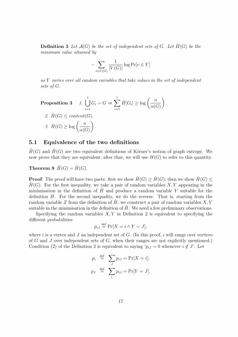
Definition 3 Let A(G) be the set of independent sets of G. Let H(G) be theminimum value attained by

−∑

v∈V (G)

1

|V (G)|log Pr[v ∈ Y ]

as Y varies over all random variables that take values in the set of independentsets of G.

Proposition 3 1.t⋃i=1

Gi = G⇒t∑i=1

H[Gi] ≥ log

(n

α(G)

).

2. H(G) ≤ content(G).

3. H(G) ≥ log

(n

α(G)

).

5.1 Equivalence of the two definitions

H(G) and H(G) are two equivalent definitions of Korner’s notion of graph entropy. Wenow prove that they are equivalent; after that, we will use H(G) to refer to this quantity.

Theorem 9 H(G) = H(G).

Proof: The proof will have two parts: first we show H(G) ≥ H(G); then we show H(G) ≤H(G). For the first inequality, we take a pair of random variables X, Y appearing in theminimisation in the definition of H and produce a random variable Y suitable for thedefinition H. For the second inequality, we do the reverse. That is, starting from therandom variable Z from the definition of H, we construct a pair of random variables X, Ysuitable in the minimisation in the definition of H. We need a few preliminary observations.

Specifying the random variables X, Y in Definition 2 is equivalent to specifying thedifferent probabilities

piJdef= Pr[X = i ∧ Y = J ],

where i is a vertex and J an independent set of G. (In this proof, i will range over verticesof G and J over independent sets of G, when their ranges are not explicitly mentioned.)Condition (2) of the Definition 2 is equivalent to saying ‘piJ = 0 whenever i 6∈ J ’. Let

pidef=

∑J

piJ = Pr[X = i];

pJdef=

∑i

piJ = Pr[Y = J ].

17

By condition (1) of Definition 2, pi = 1n. Now,

H[X] = −∑i

pi log pi = −∑iJ

piJ log pi;

H[X | Y ] = −∑i

pi∑J

piJpi

logpiJpi

;

hence, I[X,Y ] = −∑

i,J :piJ>0

piJ logpipJpiJ

.

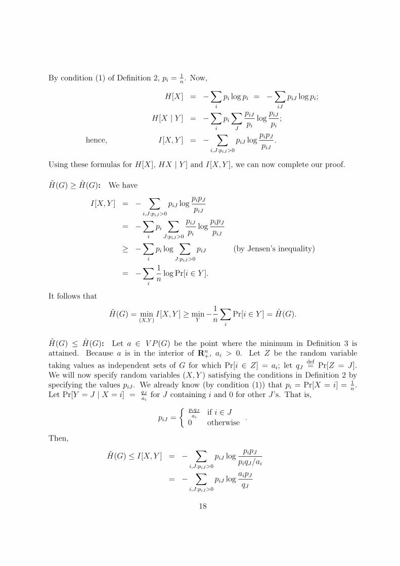
Using these formulas for H[X], HX | Y ] and I[X, Y ], we can now complete our proof.

H(G) ≥ H(G): We have

I[X,Y ] = −∑

i,J :piJ>0

piJ logpipJpiJ

= −∑i

pi∑

J :piJ>0

piJpi

logpipJpiJ

≥ −∑i

pi log∑

J :piJ>0

piJ (by Jensen’s inequality)

= −∑i

1

nlog Pr[i ∈ Y ].

It follows that

H(G) = min(X,Y )

I[X, Y ] ≥ minY− 1

n

∑i

Pr[i ∈ Y ] = H(G).

H(G) ≤ H(G): Let a ∈ VP (G) be the point where the minimum in Definition 3 isattained. Because a is in the interior of Rn

+, ai > 0. Let Z be the random variable

taking values as independent sets of G for which Pr[i ∈ Z] = ai; let qJdef= Pr[Z = J ].

We will now specify random variables (X, Y ) satisfying the conditions in Definition 2 byspecifying the values piJ . We already know (by condition (1)) that pi = Pr[X = i] = 1

n.

Let Pr[Y = J | X = i] = qJai

for J containing i and 0 for other J ’s. That is,

piJ =

{ piqJai

if i ∈ J0 otherwise

.

Then,

H(G) ≤ I[X, Y ] = −∑

i,J :piJ>0

piJ logpipJpiqJ/ai

= −∑

i,J :piJ>0

piJ logaipJqJ

18

= −∑iJ

piJ log ai −∑

i,J :piJ>0

piJ logpJqJ

= − 1

n

∑i

log ai +∑

J :piJ>0

pJ logqJpJ

≤ − 1

n

∑i

log ai + log∑J :pJ>0

qJ

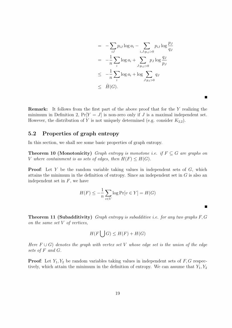
≤ H(G).

Remark: It follows from the first part of the above proof that for the Y realizing theminimum in Definition 2, Pr[Y = J ] is non-zero only if J is a maximal independent set.However, the distribution of Y is not uniquely determined (e.g. consider K2,2).

5.2 Properties of graph entropy

In this section, we shall see some basic properties of graph entropy.

Theorem 10 (Monotonicity) Graph entropy is monotone i.e. if F ⊆ G are graphs onV where containment is as sets of edges, then H(F ) ≤ H(G).

Proof: Let Y be the random variable taking values in independent sets of G, whichattains the minimum in the definition of entropy. Since an independent set in G is also anindependent set in F , we have

H(F ) ≤ −1

n

∑v∈V

log Pr[v ∈ Y ] = H(G)

Theorem 11 (Subadditivity) Graph entropy is subadditive i.e. for any two graphs F,Gon the same set V of vertices,

H(F⋃

G) ≤ H(F ) +H(G)

Here F ∪ G) denotes the graph with vertex set V whose edge set is the union of the edgesets of F and G.

Proof: Let Y1, Y2 be random variables taking values in independent sets of F,G respec-tively, which attain the minimum in the definition of entropy. We can assume that Y1, Y2

19

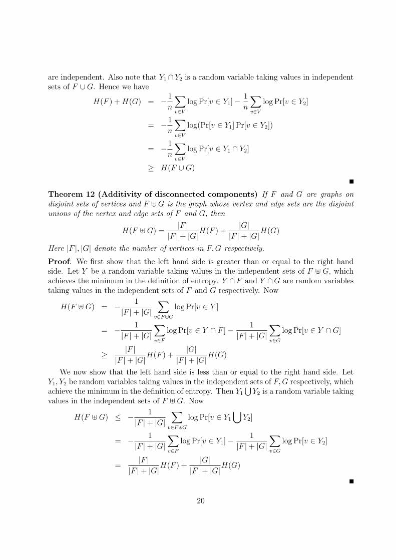
are independent. Also note that Y1 ∩ Y2 is a random variable taking values in independentsets of F ∪G. Hence we have

H(F ) +H(G) = − 1

n

∑v∈V

log Pr[v ∈ Y1]−1

n

∑v∈V

log Pr[v ∈ Y2]

= − 1

n

∑v∈V

log(Pr[v ∈ Y1] Pr[v ∈ Y2])

= − 1

n

∑v∈V

log Pr[v ∈ Y1 ∩ Y2]

≥ H(F ∪G)

Theorem 12 (Additivity of disconnected components) If F and G are graphs ondisjoint sets of vertices and F ]G is the graph whose vertex and edge sets are the disjointunions of the vertex and edge sets of F and G, then

H(F ]G) =|F |

|F |+ |G|H(F ) +

|G||F |+ |G|

H(G)

Here |F |, |G| denote the number of vertices in F,G respectively.

Proof: We first show that the left hand side is greater than or equal to the right handside. Let Y be a random variable taking values in the independent sets of F ] G, whichachieves the minimum in the definition of entropy. Y ∩F and Y ∩G are random variablestaking values in the independent sets of F and G respectively. Now

H(F ]G) = − 1

|F |+ |G|∑

v∈F]G

log Pr[v ∈ Y ]

= − 1

|F |+ |G|∑v∈F

log Pr[v ∈ Y ∩ F ]− 1

|F |+ |G|∑v∈G

log Pr[v ∈ Y ∩G]

≥ |F ||F |+ |G|

H(F ) +|G|

|F |+ |G|H(G)

We now show that the left hand side is less than or equal to the right hand side. LetY1, Y2 be random variables taking values in the independent sets of F,G respectively, whichachieve the minimum in the definition of entropy. Then Y1

⋃Y2 is a random variable taking

values in the independent sets of F ]G. Now

H(F ]G) ≤ − 1

|F |+ |G|∑

v∈F]G

log Pr[v ∈ Y1

⋃Y2]

= − 1

|F |+ |G|∑v∈F

log Pr[v ∈ Y1]−1

|F |+ |G|∑v∈G

log Pr[v ∈ Y2]

=|F |

|F |+ |G|H(F ) +

|G||F |+ |G|

H(G)

20

Exercise: Show that the entropy of the empty graph is zero. Also show that if G is notempty, then H(G) > 0. (Hint: Use monotonicity and additivity).

Exercise: Show that the entropy of the complete graph is log n.

Exercise: Show that the entropy of a bipartite graph is at most 1.

6 Remarks

Counting problems: A short proof for Bregman’s Theorem (Minc’s conjecture) wasfound by Schrijver [31]. Spencer [34] (see also Alon and Spencer [2]) described Schrijver’sargument using a randomised algorithm; Radhakrishnan [29] stated this argument in thelanguage of entropy.

Usually, Corollary 1 is called Shearer’s Lemma. The version above (Lemma 1) wasstated explicitly by Kahn [12], with the remark that the original entropy based proofactually implies this stronger form. The proof given above is due to Llewellyn and Rad-hakrishnan [22].

Theorem 3 was proved by Alon [1] using a different method. The proof given above,due to Friedgut and Kahn [9], works for hypergraphs as well, although we have stated itonly for graphs. In fact, for the special case of graphs, Kahn and Friedgut give anotherproof using harmonic analysis.

Kahn [12] generalises Theorem 4, using essentially the same ideas, to graded posets.This gives a simple proof of the following theorem of Klietman and Markowsky [17]: thenumber of antichains in the poset of subsets of an n-element set is

2(1+O((logm)/√m))( m

bm/2c).

Covering problems: Hansel’s elegant argument appeared in the context of computingBoolean functions [11].

A monotone contact network is an undirected graph with two distinguishedvertices s and t. Each edge is labelled by a Boolean variable xi, i = 1, 2, . . . , n.What is the minimum number of edges in a monotone contact network suchthat there is an (s, t)-path of all 1s iff at least two variables are set to 1? Takea random (s, t)-cut in this graph. Then, clearly, the number of variables ‘goingacross’ the cut is at least n − 1. If variable xi appears ni times, then theprobability that it goes across the cut is at most 1 − 2−ni . By linearity ofexpectation

n∑i=1

(1− 2−ni) ≥ n− 1.

It follows that∑n

i=1 ni ≥ n log n; hence, the contact network has at least n log nedges.

21

A similar result in the context of Boolean formulas was proved by Krichevskii [21].The Fredman-Komlos bound was proved for a family of perfect hash functions. They

considered the following question: What is the smallest family of hash function from [n] to[k] so that every set r sized subset of [n] is perfectly hashed by some hash function in thefamily. They showed that the right hand side of (13) is a lower bound on the size of such afamily. Subsequently, their bounds were rederived using graph entropy by Korner [19] andimproved by Korner and Marton [20]. Nilli [24] derives the bound of Korner and Martonusing elementary arguments (similar to those used in the proof of Theorem 5 above).

The original proof (see [10]) of Furedi’s theorem on scrambling permutations used en-tropy directly without appealing to the Fredman-Komlos inequality. Furedi also considereda generalisation of the problem.

Call a family F of an n-element underlying set P completely k-scrambling if forevery sequence 〈p1, p2, . . . , pk〉 of k distinct elements of P there is a permutationπ ∈ F with

π(p1) < π(p2) < · · · < π(pk).

Determine N∗(n, k), the size of the smallest completely k-scrambling family.

It is known that

1

2(k − 1)! log n < N∗(n, k) <

k

log(k!/(k!− 1))log n.

(The first inequality was shown by Furedi, the second by Hajnal and Spencer [33].) Notethat N∗(n, k) ≥ k!, so Furedi’s lower bound is interesting only when k is much smallerthan log n. Using the Fredman-Komlos inequality, one can improve Furedi’s lower boundto (

2

log e

) (n

2n− k + 1

)(k − 1)! log(n− k + 2).

(See [26] for details.)

Graph entropy: Graph entropy was defined by Korner [18] in 1973, in connection with aproblem in coding theory, where he showed that his definition was equivalent to the defini-tion of H(G) above. Our second definition, H(G) and the proof that it is equivalent to theearlier definitions are taken from Csiszar, Korner, Lovaasz, Marton and Simonyi [8]. How-ever, it does not seem to have been observed before that these definitions arise naturallyfrom previous works on graph covering. Graph entropy has been applied to several prob-lems: lower bounds on the size of families of perfect hash functions [19, 20], lower boundsfor Boolean formula size [23, 27, 28], algorithms for sorting partially ordered sets [13] andcharacterising perfect graphs [8]. Simonyi [32] gives a survey of graph entropy and itsvarious application.

22

Acknowledgements

This article is based on material used in a series of lectures, that Pranab Sen and I gaveat the Institute of Mathematical Sciences, Chennai, and at the Indian Institute of Science,Bangalore, in 2000. I am grateful to these institutions for their hospitality while thismaterial was being put together.

References

[1] Alon, N. On the number of subgraphs of prescribed type of graphs with a givennumber of edges. Israel Journal of Mathematics 38 (1981), 116–130.

[2] Alon, N., and Spencer, J. The Probabilistic Method. Wiley-Interscience, NewYork, 1992.

[3] Bregman, L. Some properties of nonnegative matrices and their permanents. SovietMathematics Doklady 14 (1973), 945–949.

[4] Chung, F., Frank, P., Graham, R., and Shearer, J. Some intersection the-orems for ordered sets and graphs. Journal of Combinatorial Theory (A) 43 (1986),23–37.

[5] Chvatal, V. Linear programming. W. H. Freeman and Company, 1980.

[6] Cover, T., and Thomas, J. Elements of information theory. John Wiley, NewYork, 1991.

[7] Csiszar, I., and Korner, J. Information Theory: Coding Theorem for discretememoryless systems. Academic Press, New York, 1981.

[8] Csiszar, I., Korner, J., Lovasz, L., Marton, K., and Simonyi, G. Entropysplitting for antiblocking corners and perfect graphs. Combinatorica 10 (1990), 27–40.

[9] Friedgut, E., and Kahn, J. On the number of copies of one hypergraph in another.Israel Journal of Mathematics 105 (1998), 251–256.

[10] Furedi, Z. Scrambling permutations and entropy of hypergraphs. Random Structuresand Algorithms 8, 2 (1996), 97–104.

[11] Hansel, G. Nombre minimal de contacts de fermature necessaires pour realiser unefonction booleenne symetrique de n variables. C. R. Acad. Sci. Paris (1964), 6037–6040.

[12] Kahn, J. Entropy, independent sets and antichains: A new approach to Dedekind’sproblem. Proc. Amer. Math. Soc. 130 (2002), 371–378.

23

[13] Kahn, J., and Kim, J. H. Entropy and sorting. Journal of Computer and SystemSciences 51 (1995), 390–399.

[14] Kahn, J., and Lawrenz, A. Generalized rank functions and an entropy argument.Journal of Combinatorial Theory (A) 87 (1999), 398–403.

[15] Katona, G., and Szemeredi, E. On a problem of graph theory. Studia Sci. Math.Hungarica 2 (1967), 23–28.

[16] Khinchin, A. Mathematical foundations of information theory. Dover Publications,1957.

[17] Kleitman, D., and Markowsky, G. On Dedekind’s problem: the number ofisotone boolean functions ii. Transactions of the American Mathematical Society 213(1975), 373–390.

[18] Korner, J. Coding of an information source having ambiguous alphabet and entropyof graphs. In Proc. 6th Prague Conference on Information Theory (1973), pp. 411–425.

[19] Korner, J. Fredman-Komlos bound and information theory. SIAM J. Alg. Disc.Meth. 7 (1986), 560–570.

[20] Korner, J., and Marton, K. New bounds for perfect hashing via informationtheory. European Journal of Combinatorics 9 (1988), 523–530.

[21] Krichevskii, R. E. Complexity of contact circuits realizing a function of logicalalgebra. Sov. Phys. Dokl. 8 (1964), 770–772.

[22] Llewellyn, J., and Radhakrishnan, J. On Shearer’s lemma. Manuscript.

[23] Newman, I., and Wigderson, A. Lower bounds on formula size of boolean func-tions using hypergraph-entropy. SIAM J. of Discrete Math. 8, 4 (1995), 536–542.

[24] Nilli, A. Perfect hashing and probability. Combinatorics, Probability and Computing3 (1994), 407–409.

[25] Pippenger, N. An information-theoretic method in combinatorial theory. Journalof Combinatorial Theory 23 (1977), 99–104.

[26] Radhakrishnan, J. A note on completely scrambling permutations.http://www.tcs.tifr.res.in/ jaikumar.

[27] Radhakrishnan, J. ΣΠΣ threshold formaulas. Combinatorica 14, 3 (1994), 345–374.

[28] Radhakrishnan, J. Better lower bounds for monotone threshold formulas. Journalof Computer and System Sciences 54, 2 (1997), 221–226.

24

[29] Radhakrishnan, J. An entropy proof of Bregman’s theorem. Journal of Combina-torial Theory (A) 77, 1 (1997), 161–164.

[30] Renyi, A. On the foundations of information theory. Review of the InternationalStatistical Institute 33, 1 (1965), 1–14.

[31] Schrijver, A. A short proof of Minc’s conjecture. Journal of Combinatorial Theory(A) 25 (1978), 80–83.

[32] Simonyi, G. Graph entropy. In Combinatorial Optimization, L. L. W. Cook andP. Seymour, Eds., vol. 20 of DIMACS Series on Discrete Math and Computer Science.1995, pp. 391–441.

[33] Spencer, J. Minimal scrambling sets of simple orders. Acta Mathematica Hungarica22 (1972), 349–353.

[34] Spencer, J. The probabilistic lens: Sperner, Turan, Bregman revisited. In A tributeto Paul Erdos, A. Baker, B. Bollobas, and A. Hajnal, Eds. Cambridge UniversityPress, 1990, pp. 391–396.

25