Entropy and Optimization of Portfolios

Krzysztof Urbanowicz∗

Quant Technology Sp z o.o.Modlinska 175A

PL–03-186 Warsaw, Poland(Dated: September 25, 2014)

We briefly review the approach to optimization of portfolios according to the theory of Markowitzand propose a further modification that can improve the outcome of the optimization process. Themodification takes account of the entropic contribution from the time series used to compute theparameters in the Markowitz method.

PACS numbers: 89.65.Gh, 05.10.-a

I. BACKGROUND

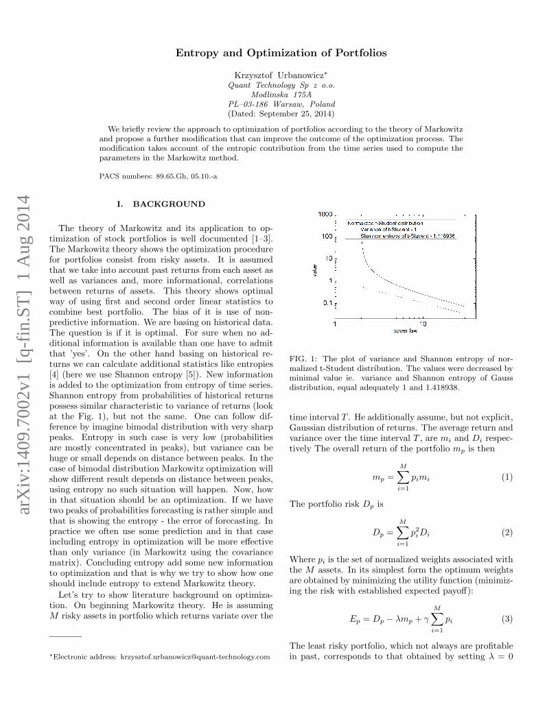
The theory of Markowitz and its application to op-timization of stock portfolios is well documented [1–3].The Markowitz theory shows the optimization procedurefor portfolios consist from risky assets. It is assumedthat we take into account past returns from each asset aswell as variances and, more informational, correlationsbetween returns of assets. This theory shows optimalway of using first and second order linear statistics tocombine best portfolio. The bias of it is use of non-predictive information. We are basing on historical data.The question is if it is optimal. For sure when no ad-ditional information is available than one have to admitthat ’yes’. On the other hand basing on historical re-turns we can calculate additional statistics like entropies[4] (here we use Shannon entropy [5]). New informationis added to the optimization from entropy of time series.Shannon entropy from probabilities of historical returnspossess similar characteristic to variance of returns (lookat the Fig. 1), but not the same. One can follow dif-ference by imagine bimodal distribution with very sharppeaks. Entropy in such case is very low (probabilitiesare mostly concentrated in peaks), but variance can behuge or small depends on distance between peaks. In thecase of bimodal distribution Markowitz optimization willshow different result depends on distance between peaks,using entropy no such situation will happen. Now, howin that situation should be an optimization. If we havetwo peaks of probabilities forecasting is rather simple andthat is showing the entropy - the error of forecasting. Inpractice we often use some prediction and in that caseincluding entropy in optimization will be more effectivethan only variance (in Markowitz using the covariancematrix). Concluding entropy add some new informationto optimization and that is why we try to show how oneshould include entropy to extend Markowitz theory.

Let’s try to show literature background on optimiza-tion. On beginning Markowitz theory. He is assumingM risky assets in portfolio which returns variate over the

∗Electronic address: krzysztof.urbanowicz@quant-technology.com

FIG. 1: The plot of variance and Shannon entropy of nor-malized t-Student distribution. The values were decreased byminimal value ie. variance and Shannon entropy of Gaussdistribution, equal adequately 1 and 1.418938.

time interval T . He additionally assume, but not explicit,Gaussian distribution of returns. The average return andvariance over the time interval T , are mi and Di respec-tively The overall return of the portfolio mp is then

mp =

M∑i=1

pimi (1)

The portfolio risk Dp is

Dp =

M∑i=1

p2iDi (2)

Where pi is the set of normalized weights associated withthe M assets. In its simplest form the optimum weightsare obtained by minimizing the utility function (minimiz-ing the risk with established expected payoff):

Ep = Dp − λmp + γ

M∑i=1

pi (3)

The least risky portfolio, which not always are profitablein past, corresponds to that obtained by setting λ = 0

arX

iv:1

409.

7002

v1 [

q-fi

n.ST

] 1

Aug

201

4

2

leading to the optimum weights:

p∗i =1

ZDiwhere Z =

M∑j=1

1

Dj(4)

A later version of the theory takes account of correlationsbetween assets via the symmetric correlation matrix, Cij .The risk is now defined to be:

Dp =

M∑i=1

pipjCij (5)

Minimizing the risk given by definition (5) and again set-ting λ = 0 yields the optimum weights p∗i . The least riskyportfolio have no constrains on expected payoff. This issimplification of full formula:

p∗i =1

Z

M∑j=1

C−1ij where Z =

M∑i,j=1

C−1ij (6)

As Bouchaud and Potters have pointed out, the mainlesson of the theory of Markowitz’ theory is the needto diversify portfolios effectively [6]. Bouchaud, Pottersand Aguilar [7] have noted that one problem associatedwith the approach is that the resulting portfolio can beconcentrated on only a few assets. To overcome this, theyproposed including an additional constraint, the entropyof weights of assets:

Yq =

M∑i=1

(p∗i )q

(7)

The parameter q was chosen to be equal to 2 when itis seen that the term also represents the average weightof an asset in the portfolio. In general the term is, touse the language of physics, an entropic contribution tothe minimization process. Indeed as Bouchaud and Pot-ter point out, the equation (7) is linearly related to theTsallis [8, 9] entropy function and the entire process ofobtaining the weights, pi is equivalent to minimizing afree - utility function:

Fq = E − ν Yq − 1

q − 1(8)

Important hint we should mention. In this paper we aremanaging with including entropy of returns from eachassets. In the paper [7] authors are refering to entropyof weights of assets in portfolio. This is two different en-tropies. Even that results are similar, we are approachingto the problem from different directions. Bouchaud, Pot-ters and Aguilar are adding new constrain to Markowitzformula artificially, to increase diversification in practise,when errors of covariance matrix and average returns arein practical calculations with large errors. We, on theother hand, are adding entropy of time series to increaseused information in optimization and it is rather naturalway of such addition.

Bouchaud has noted another issue linked to the use ofcorrelation matrices. This is linked to the use of finitetime series when computing the M(M − 1)/2 individualelements of the correlation matrix. If the number of as-sets in the portfolio becomes large it is possible that thenumber of data points used to compute the elements ofthe correlation matrix is of the same order of magnitudeas the number of entries. As an example, for portfolios ofthe size of the S&P500 where the correlation matrix con-tains 500x499/2 = 124, 750 different entries. Using timeseries extending over two years of daily data the num-ber of data points is 500x500 = 250, 000 which is only afactor of two larger that the number of correlation coef-ficients. So the statistical precision on these coefficientsis subject to a large degree of measurement noise. Herewe consider smaller portfolios of the order of 27 stockswhere this issue does not arise.

We discuss in this note another issue that can be re-solved by a further modification of the theory and thatleads to novel route to measure risk and further improve-ments in the optimization process.

II. APPROACH

The above discussion leads directly to the following’free-utility’ function [7]:

F =

M∑i,j=1

pipjCij+α

M∑i=1

(pi)2+β

M∑i=1

pimi+γ

M∑i=1

pi (9)

Where α, β and γ are Lagrange multipliers. We now rec-ognize that the entropy is in fact similar to the variancein that it is a measure of the level of variability in thetime series and propose that it serve as an estimator ofrisk (this concept was noted in the first section). Theentropy can be replaced by the variance only in the caseof Gaussian distributions. The ’fat’ tailed distributionsare not fully described by a variance (see Fig. 1) and insuch a case we need more parameters. Risk related to’fat’ tailed distributions is larger than the variance so forrisk evaluation we introduce a second risk factor that de-scribes the level of possible realizations of the system inthe case of a fully random process, which is measured byentropy.

The parameter that balances the impact of varianceand entropy in physics is the temperature. Here it is theLagrange multiplier corresponding to the entropy.

On the basis of this reasoning, we now propose a newfunctional of the weights, pi:

F =

M∑i,j=1

pipjCij + α

M∑i=1

Si (pi)2

+ β

M∑i=1

pimi + γ

M∑i=1

pi

(10)Similar to the previous equation (9) it contains an essen-tial difference in the entropy factors Si. These coefficientsare computed directly from the time series data for each

3

of the M assets in the portfolio. Thus for each i we com-pute the Shannon (Boltzmann) entropy associated withthe time series:

Si = −∫Pi (x) lnPi (x) dx (11)

Pi(x) is the distribution function (PDF) associated withthe returns of the time series associated with the i-thasset. The use of additive entropies is a somewhat sim-plified assumption. Strictly speaking we should use con-ditional entropies that include dependencies among theassets. However our approach has the merit that it yieldsformulas that can be solved analytically. We also believethat the dependencies are, as for the correlation matrix,much smaller than the diagonal elements.

One can easy derive the solutions for weights fromequation (10). Reverting to vector notation, we obtain:

pc = (C + αSI)−1

(γ1− βm) (12)

I is a identity matrix, 1 is the identity vector and:

β = mc·1T C−11−mT C−11mT C−11·1T C−1m−mT C−1m·1T C−11

C = C + αSI (13)

γ = 1+β·1T C−1m

1T C−11

We have introduced mc for the level of expected profit(payoff) of the portfolio. If it is not stated differently,the expected return mc is set to 20% per annum. TheLagrange multiplier, α, should be calculated from someother formula with constrain, such as setting constant ex-pected profit of market portfolio (we will show the resultof this solution below).

In a previous paper [10], we have developed the con-cept of the objective function that is proportional to theShannon entropy and the covariance matrix C as the co-variance of ’objective values’ for the returns, CObV . Theobjective values, w(x) is defined in terms of the station-ary probability distribution for returns, P (x), viz:

P (x) =1

Ze−

w(x)d (14)

where Z is a normalization factor. Such functions arefamiliar to physicists and may be derived by minimizinga ’free energy’ functional, F (w(x)), subject to constraintson the mean value of the objective function, viz:

F =

∫dxP (x)

[lnP (x) +

w (x)

d− δ]

(15)

Here δ is a normalization parameter to P(x). Normal-ized covariance matrix CObV and mean values

{mObVi

}are due to the normalization procedure which in simplewords makes all 〈wi (x)〉 equal. Here the notation i showsthe dependence of objective value on different asset i.

We use these ideas in this paper noting that in addi-tion we now need also to change average values for the

returns {mi} to the set{mObVi

}. The reader should read

reference [10] for the details of the method.Within this approach, the risk is computed as follows:

R =

N∑i,j=1

CObVij pipj + α

N∑i=1

Sip2i (16)

We now propose a further new quantity that measuresthe ’quality ratio’ (similar to Sharp ratio [11], but stan-dard deviation is replaced by variance) of the portfolio:

QR =profit

risk=

β∑Mi=1m

ObVi∑N

i,j=1 CObVij pipj + α

∑Ni=1 Sip

2i

(17)

To complete these calculations requires of course knowingthe value of the Lagrange multipliers, α and β.

A route to compute α is by standardizing QR ratioto a market portfolio, QRm. Market weights pm are as-sociated with the market portfolio (weights comes fromcapitalizations) and balanced by investors with all avail-able information. One can assume that QRm takes themaximum value, ie.

QRm =βpTmm

ObV

pTmCObV pm + αpTmSpm

(18)

Putting QRm = 1 we can solve equation (18)

α =βpTmm

ObV − pTmCObV pmpTmSpm

(19)

Note that the parameter β depends on α itself (seeEq. 13). A self consistent solution is then required.

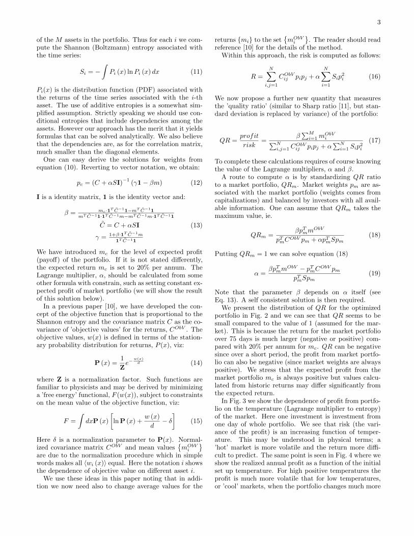
We present the distribution of QR for the optimizedportfolio in Fig. 2 and we can see that QR seems to besmall compared to the value of 1 (assumed for the mar-ket). This is because the return for the market portfolioover 75 days is much larger (negative or positive) com-pared with 20% per annum for mc. QR can be negativesince over a short period, the profit from market portfo-lio can also be negative (since market weights are alwayspositive). We stress that the expected profit from themarket portfolio mc is always positive but values calcu-lated from historic returns may differ significantly fromthe expected return.

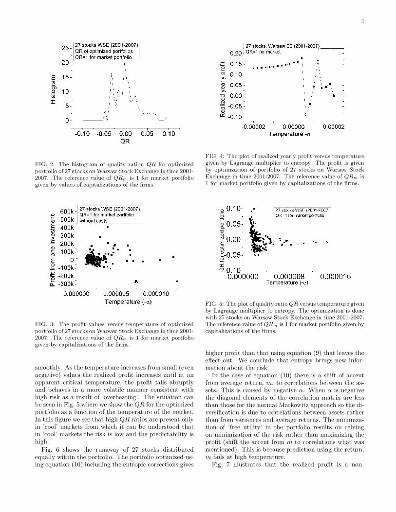
In Fig. 3 we show the dependence of profit from portfo-lio on the temperature (Lagrange multiplier to entropy)of the market. Here one investment is investment fromone day of whole portfolio. We see that risk (the vari-ance of the profit) is an increasing function of temper-ature. This may be understood in physical terms; a’hot’ market is more volatile and the return more diffi-cult to predict. The same point is seen in Fig. 4 where weshow the realized annual profit as a function of the initialset up temperature. For high positive temperatures theprofit is much more volatile that for low temperatures,or ’cool’ markets, when the portfolio changes much more

4

FIG. 2: The histogram of quality ration QR for optimizedportfolio of 27 stocks on Warsaw Stock Exchange in time 2001-2007. The reference value of QRm is 1 for market portfoliogiven by values of capitalizations of the firms.

FIG. 3: The profit values versus temperature of optimizedportfolio of 27 stocks on Warsaw Stock Exchange in time 2001-2007. The reference value of QRm is 1 for market portfoliogiven by capitalizations of the firms.

smoothly. As the temperature increases from small (evennegative) values the realized profit increases until at anapparent critical temperature, the profit falls abruptlyand behaves in a more volatile manner consistent withhigh risk as a result of ’overheating’. The situation canbe seen in Fig. 5 where we show the QR for the optimizedportfolio as a function of the temperature of the market.In this figure we see that high QR ratios are present onlyin ’cool’ markets from which it can be understood thatin ’cool’ markets the risk is low and the predictability ishigh.

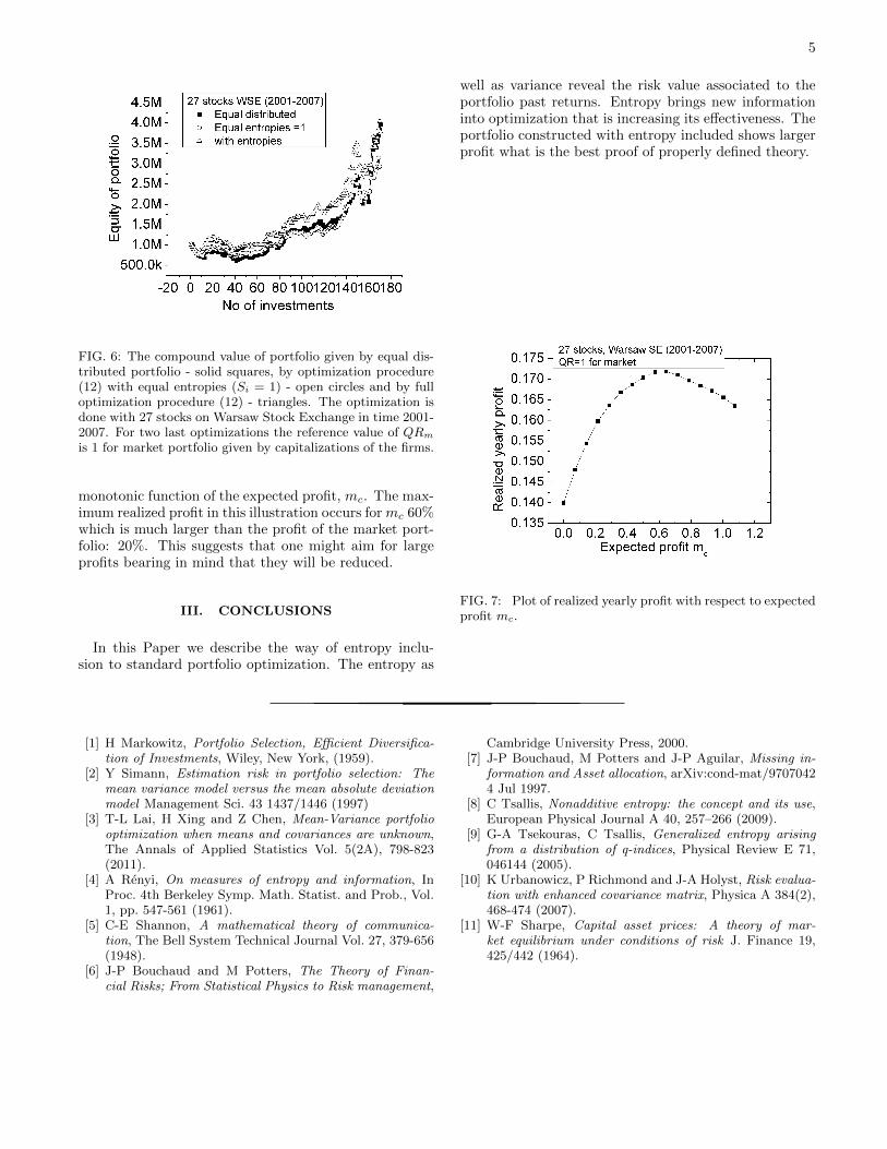
Fig. 6 shows the runaway of 27 stocks distributedequally within the portfolio. The portfolio optimized us-ing equation (10) including the entropic corrections gives

FIG. 4: The plot of realized yearly profit versus temperaturegiven by Lagrange multiplier to entropy. The profit is givenby optimization of portfolio of 27 stocks on Warsaw StockExchange in time 2001-2007. The reference value of QRm is1 for market portfolio given by capitalizations of the firms.

FIG. 5: The plot of quality ratio QR versus temperature givenby Lagrange multiplier to entropy. The optimization is donewith 27 stocks on Warsaw Stock Exchange in time 2001-2007.The reference value of QRm is 1 for market portfolio given bycapitalizations of the firms.

higher profit than that using equation (9) that leaves theeffect out. We conclude that entropy brings new infor-mation about the risk.

In the case of equation (10) there is a shift of accentfrom average return, m, to correlations between the as-sets. This is caused by negative α. When α is negativethe diagonal elements of the correlation matrix are lessthan those for the normal Markowitz approach so the di-versification is due to correlations between assets ratherthan from variances and average returns. The minimiza-tion of ’free utility’ in the portfolio results on relyingon minimization of the risk rather than maximizing theprofit (shift the accent from m to correlations what wasmentioned). This is because prediction using the return,m fails at high temperature.

Fig. 7 illustrates that the realized profit is a non-

5

FIG. 6: The compound value of portfolio given by equal dis-tributed portfolio - solid squares, by optimization procedure(12) with equal entropies (Si = 1) - open circles and by fulloptimization procedure (12) - triangles. The optimization isdone with 27 stocks on Warsaw Stock Exchange in time 2001-2007. For two last optimizations the reference value of QRm

is 1 for market portfolio given by capitalizations of the firms.

monotonic function of the expected profit, mc. The max-imum realized profit in this illustration occurs formc 60%which is much larger than the profit of the market port-folio: 20%. This suggests that one might aim for largeprofits bearing in mind that they will be reduced.

III. CONCLUSIONS

In this Paper we describe the way of entropy inclu-sion to standard portfolio optimization. The entropy as

well as variance reveal the risk value associated to theportfolio past returns. Entropy brings new informationinto optimization that is increasing its effectiveness. Theportfolio constructed with entropy included shows largerprofit what is the best proof of properly defined theory.

FIG. 7: Plot of realized yearly profit with respect to expectedprofit mc.

[1] H Markowitz, Portfolio Selection, Efficient Diversifica-tion of Investments, Wiley, New York, (1959).

[2] Y Simann, Estimation risk in portfolio selection: Themean variance model versus the mean absolute deviationmodel Management Sci. 43 1437/1446 (1997)

[3] T-L Lai, H Xing and Z Chen, Mean-Variance portfoliooptimization when means and covariances are unknown,The Annals of Applied Statistics Vol. 5(2A), 798-823(2011).

[4] A Renyi, On measures of entropy and information, InProc. 4th Berkeley Symp. Math. Statist. and Prob., Vol.1, pp. 547-561 (1961).

[5] C-E Shannon, A mathematical theory of communica-tion, The Bell System Technical Journal Vol. 27, 379-656(1948).

[6] J-P Bouchaud and M Potters, The Theory of Finan-cial Risks; From Statistical Physics to Risk management,

Cambridge University Press, 2000.[7] J-P Bouchaud, M Potters and J-P Aguilar, Missing in-

formation and Asset allocation, arXiv:cond-mat/97070424 Jul 1997.

[8] C Tsallis, Nonadditive entropy: the concept and its use,European Physical Journal A 40, 257–266 (2009).

[9] G-A Tsekouras, C Tsallis, Generalized entropy arisingfrom a distribution of q-indices, Physical Review E 71,046144 (2005).

[10] K Urbanowicz, P Richmond and J-A Holyst, Risk evalua-tion with enhanced covariance matrix, Physica A 384(2),468-474 (2007).

[11] W-F Sharpe, Capital asset prices: A theory of mar-ket equilibrium under conditions of risk J. Finance 19,425/442 (1964).