Environmental Data Analysis with MatLab Lecture 19: Smoothing, Correlation and Spectra

Environmental Data Analysis with MatLab

Lecture 19:

Smoothing, Correlation and Spectra

Lecture 01 Using MatLabLecture 02 Looking At DataLecture 03 Probability and Measurement Error Lecture 04 Multivariate DistributionsLecture 05 Linear ModelsLecture 06 The Principle of Least SquaresLecture 07 Prior InformationLecture 08 Solving Generalized Least Squares ProblemsLecture 09 Fourier SeriesLecture 10 Complex Fourier SeriesLecture 11 Lessons Learned from the Fourier TransformLecture 12 Power Spectral DensityLecture 13 Filter Theory Lecture 14 Applications of Filters Lecture 15 Factor Analysis Lecture 16 Orthogonal functions Lecture 17 Covariance and AutocorrelationLecture 18 Cross-correlationLecture 19 Smoothing, Correlation and SpectraLecture 20 Coherence; Tapering and Spectral Analysis Lecture 21 InterpolationLecture 22 Hypothesis testing Lecture 23 Hypothesis Testing continued; F-TestsLecture 24 Confidence Limits of Spectra, Bootstraps

SYLLABUS

purpose of the lecture

examine interrelationships between

smoothing, correlation and power spectral density

review

Autocorrelationand

Cross-correlation

AutocorrelationMeasure of correlation in time series

at different lags

tu(t)


at different lags

t

t

lag, t

a(t)

0

lag, multiply and sum areano lag


at different lags

t

t

lag, t

a(t)

0

lag, multiply and sum areasmall lag


at different lags

t

t

lag, t

a(t)

0

lag, multiply and sum arealarge lag


at different lags

t

t

lag, t

a(t)

0

lag, multiply and sum area


at different lags

t

t

lag, t

a(t)

0

lag, multiply and sum area

a(t)=u(t)⋆u(t)

crooss-correlationMeasure of correlation between two time series

at different lags

t

t

u(t)

v(t)

crooss-correlationMeasure of correlation between two time series

at different lags

t

t

u(t)

v(t)

c(t)=u(t)⋆v(t)

important relationships

c(t) = u(t)⋆v(t) = u(-t)*v(t)

c(ω) = u*(ω) v(ω)

a(ω)= |u(ω)|2

rough time series

frequency, ω0

tu(t)

lag, t

a(t)

0

sharp autocorrelation

wide spectrum

|u(ω)|2

smooth time series

frequency, ω0

tu(t)

lag, t

a(t)

0

wide autocorrelation

narrow spectrum

|u(ω)|2

lag, t

a(t)

0

rough timeseries

lag, t

a(t)

0

tv(t)

tv(t)

lag, t

a(t)

0

Part 1Smoothing a Time Series

smoothing as filtering(example of 3-point smoothing)

non-causal

smoothing as filtering(example of 3-point smoothing)

fix-upallow for a delay

fix-upallow for a delay

dsmoothed and delayed = s * dobscausal filter, s

triangular smoothing filters

si

siindex, iindex, i

3 points

21 points

50 100 150 200 250 300 350 400 450 5000

1

2

x 104

time, days

d-ob

s

50 100 150 200 250 300 350 400 450 5000

1

2

x 104

time, days

3-po

int

50 100 150 200 250 300 350 400 450 5000

1

2

x 104

time, days

21-p

oint

smoothing if Neuse River Hydrograph

question

how does smoothing effect the

the autocorrelation of d

answer

the autocorrelation of s

acts as a smoothing filter on


effect of smoothing on autocorrelation


autocorrelation of smoothed time series



everything written as convolution



everything written as convolution

regrouped


autocorrelation of smoothing filter

autocorrelation of time seriesconvolved

with*

answer

the autocorrelation of s

acts as a smoothing filter on


Part 2What Makes a Good Smoothing Filter?

then by the convolution theorem

dsmoothed(t) = s(t) * dobs(t)

then by the convolution theorem

dsmoothed(t) = s(t) * dobs(t)

so what’s this look like?

example of auniform or “boxcar” smoothing filters(t)

time, tT01/T

take Fourier Transform

wheresinc(x) = sin(πx) / (πx)

0 5 10 15 20 25 30 35 40 45 500

0.5

1

frequency, Hz

|s| fo

r L=

3

0 5 10 15 20 25 30 35 40 45 500

0.5

1

frequency, Hz

|s| fo

r L=

21

A) T=3

B) T=21

0 5 10 15 20 25 30 35 40 45 500

0.5

1

frequency, Hz

|s| fo

r L=

3

0 5 10 15 20 25 30 35 40 45 500

0.5

1

frequency, Hz

|s| fo

r L=

21

B) T=21

falls off with frequency (good)

0 5 10 15 20 25 30 35 40 45 500

0.5

1

frequency, Hz

|s| fo

r L=

3

0 5 10 15 20 25 30 35 40 45 500

0.5

1

frequency, Hz

|s| fo

r L=

21

B) T=21

bumpy side lobes (bad)

a box car filter does not suppress high frequencies evenly

the challenge

find a filter that suppresses high frequencies evenly

Normal Function

Fourier Transform of a Normal Function

is a

Normal Function

(which has no side lobes)

A) L=3

0 5 10 15 20 25 30 35 40 45 500

0.5

1

frequency, Hz

|s| fo

r L=

3

0 5 10 15 20 25 30 35 40 45 500

0.5

1

frequency, Hz

|s| fo

r L=

21

B) T=21

B) T=3

but a Normal Function

is non-causal

(unless you truncate it, in which case it is not exactly a Normal Function)

Normal Function

Box Car

Triangle

simplicity

sidelobes

Part 3Designing a Filter that Suppresses

Specific Frequencies

General form of the IIR Filter, f

z-transform of the IIR filter

General form of the IIR Filter

z-transform

General form of the IIR Filter

z-transform ratio of polynomials

z-transform v(z) as a product of its

factors

u(z) as a product of its

factorsroots of u(z)

roots of v(z)

z-transform of the IIR filter

ratio of polynomials

so designing a filteris equivalent to

specifying the roots

of the two polynomailsu(z) and v(z)

at this point we need to explore the relationship between the

Fourier Transformand the

z-transform

Answer

the Fourier Transform

is the

z-transform

evaluated at a specific set of z’s

Relationship between Fourier Transform and Z-transform

since


since

Fourier Transform


since

Fourier Transformdiscrete times and

frequencies


since


frequencies

z-transform


since


frequencies

z-transform specific choice of z’s

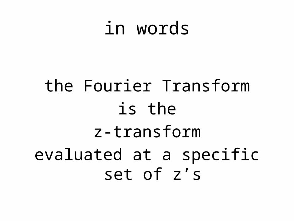
in words

the Fourier Transform

is the

z-transform

evaluated at a specific set of z’s

there are N specific z’s

zkor

with θ

real zq

imag z

unit circle, |z|2=1

they plot as equally-spaced points around a “unit circle” in the complex z-plane

zero frequency

Nyquist frequency

Back to the IIR Filter roots of u(z)

roots of v(z)

Back to the IIR Filter

(z-zju) is zero at z=zjuproduces a low amplitude

region near z=zjucalled a “zero”

Back to the IIR Filter

1/(z-zkv) is infinite at z=zkuproduces a high amplitude

region near z=zkvcalled a “pole”

so build a filter by

placing the poles and zeros at

strategic points in the complex z-plane

Rules

zeros suppress frequencies

poles amplify frequencies

all poles must be outside the unit circle(so vinv converges)

all poles, zeros must be in complex conjugate pairs

(so filter is real)

A)

B)

-2 -1 0 1 2

-2

-1.5

-1

-0.5

0

0.5

1

1.5

2

real z

imag

z

|S|2

0 0.1 0.2 0.3 0.4 0.50

0.5

1

1.5

2

2.5

3

3.5

4

frequency, Hz

|S|2

-2 -1 0 1 2

-2

-1.5

-1

-0.5

0

0.5

1

1.5

2

real z

imag

z

|S|2

0 0.1 0.2 0.3 0.4 0.50

0.5

1

1.5

2

2.5

3

3.5

4

frequency, Hz

|S|2

A)

B)

-2 -1 0 1 2

-2

-1.5

-1

-0.5

0

0.5

1

1.5

2

real z

imag

z

|S|2

0 0.1 0.2 0.3 0.4 0.50

0.5

1

1.5

2

2.5

3

3.5

4

frequency, Hz

|S|2

-2 -1 0 1 2

-2

-1.5

-1

-0.5

0

0.5

1

1.5

2

real z

imag

z

|S|2

0 0.1 0.2 0.3 0.4 0.50

0.5

1

1.5

2

2.5

3

3.5

4

frequency, Hz

|S|2

zero near zero frequency suppresses low frequencies“high pass filter”zero near the Nyquist frequency suppresses high frequencies“low pass filter”

A)

B)

-2 -1 0 1 2

-2

-1

0

1

2

real z

imag

z

|S|2

0 0.1 0.2 0.3 0.4 0.50

5

10

15

20

25

30

35

frequency, Hz

|S|2

-2 -1 0 1 2

-2

-1

0

1

2

real z

imag

z

|S|2

0 0.1 0.2 0.3 0.4 0.50

0.2

0.4

0.6

0.8

1

1.2

frequency, Hz

|S|2

A)

B)

-2 -1 0 1 2

-2

-1

0

1

2

real z

imag

z

|S|2

0 0.1 0.2 0.3 0.4 0.50

5

10

15

20

25

30

35

frequency, Hz

|S|2

-2 -1 0 1 2

-2

-1

0

1

2

real z

imag

z

|S|2

0 0.1 0.2 0.3 0.4 0.50

0.2

0.4

0.6

0.8

1

1.2

frequency, Hz

|S|2

poles near ± a given frequency amplify that frequency“band pass filter”poles and zeros near ± a given frequency attenuate that frequency“notch filter”

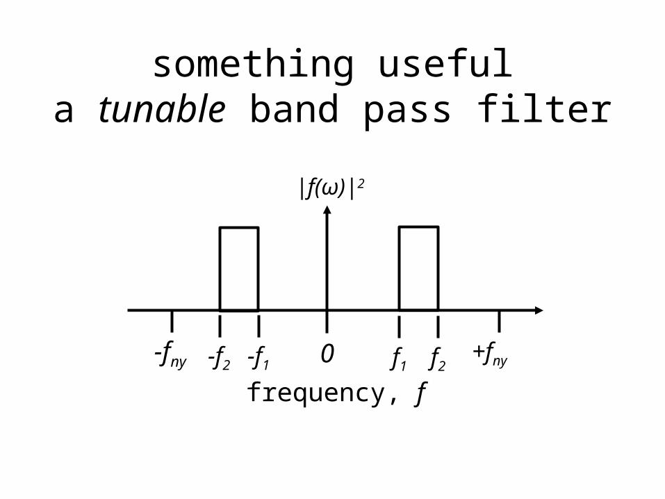
something usefula tunable band pass filter

frequency, f-fny +fny0

|f(ω)|2

f1 f2-f2 -f1

-2 -1.5 -1 -0.5 0 0.5 1 1.5 2

-2

-1.5

-1

-0.5

0

0.5

1

1.5

2

real z

imag z

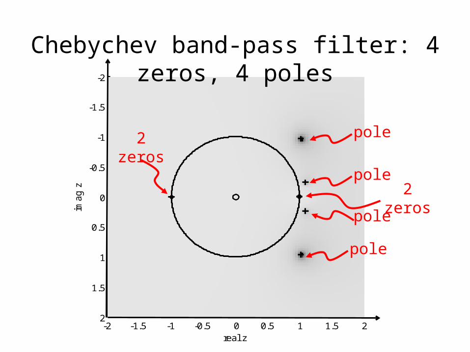
Chebychev band-pass filter: 4 zeros, 4 poles

-2 -1.5 -1 -0.5 0 0.5 1 1.5 2

-2

-1.5

-1

-0.5

0

0.5

1

1.5

2

real z

imag z

Chebychev band-pass filter: 4 zeros, 4 poles

2 zeros 2 zerospolepolepolepole

0.8 0.9 1 1.1 1.2-1

-0.5

0

0.5

1

time, s

inpu

t

0 10 20 30 40 500

0.5

1

frequency, Hz

inpu

t sp

ectr

um

0.8 0.9 1 1.1 1.2-1

-0.5

0

0.5

1

time, s

outp

ut

0 10 20 30 40 500

0.5

1

frequency, Hz

outp

ut s

pect

rum

0.8 0.9 1 1.1 1.2-1

-0.5

0

0.5

1

time, s

inpu

t

0 10 20 30 40 500

0.5

1

frequency, Hz

inpu

t sp

ectr

um

0.8 0.9 1 1.1 1.2-1

-0.5

0

0.5

1

time, s

outp

ut

0 10 20 30 40 500

0.5

1

frequency, Hz

outp

ut s

pect

rum

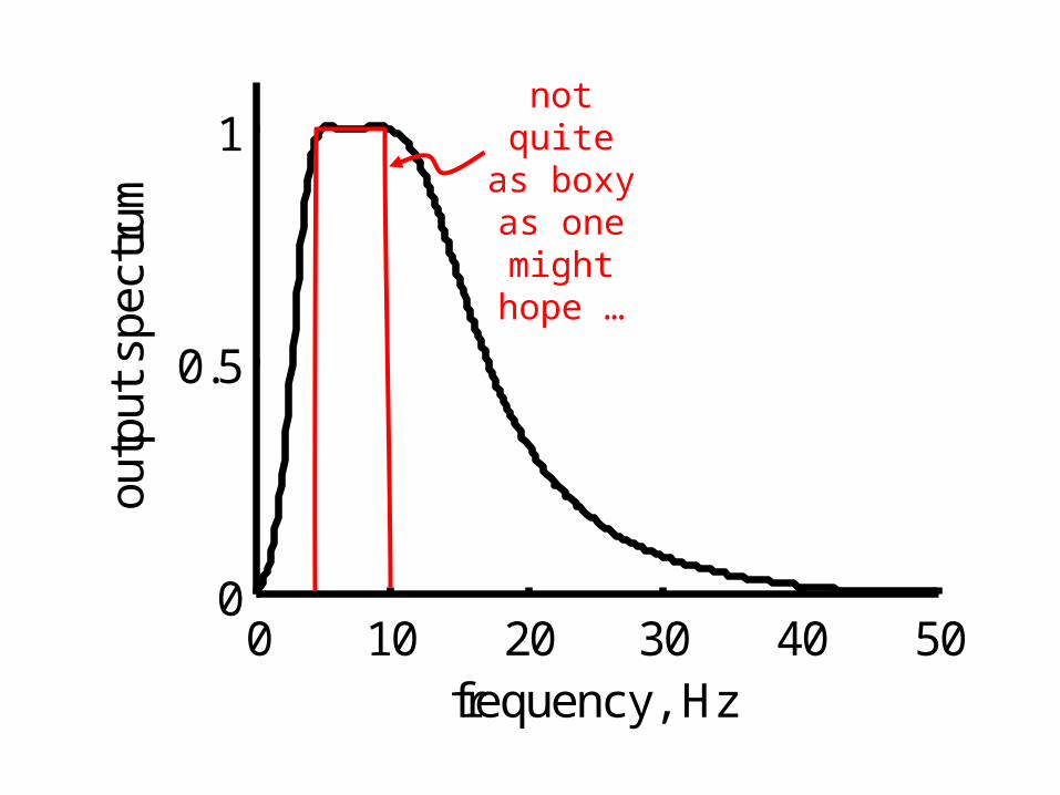
not quite as boxy as one might hope …

0.8 0.9 1 1.1 1.2-1

-0.5

0

0.5

1

time, s

inpu

t0 10 20 30 40 50

0

0.5

1

frequency, Hz

inpu

t sp

ectr

um

0.8 0.9 1 1.1 1.2-1

-0.5

0

0.5

1

time, s

outp

ut

0 10 20 30 40 500

0.5

1

frequency, Hz

outp

ut s

pect

rum

In MatLab

Ground velocity at Palisades NY


Low pass filter


high pass filter

Documents

Environmental Data Analysis with MatLab Lecture 19: Smoothing, Correlation and Spectra