EPANET by Example { A How-to-Manual for Network Modelingtheodores-pro.ttu.edu/ncimm/training-modules/epa-net-1440/epanet... · CE 3372 Water Systems Design FALL 2015 EPANET by Example

CE 3372 Water Systems Design FALL 2015

EPANET by Example – A How-to-Manual for Network Modeling

by

Theodore G. Cleveland, Ph.D., P.E., Cristal C. Tay, EIT, and Caroline Neale, EIT

Suggested CitationCleveland, T.G., Tay, C.C., and Neale, C.N. 2015. EPANET by Example. Department ofCivil and Environmental Engineering, Texas Tech University.

Page 1 of 24


Contents

1 Hydraulic Modeling with EPA-NET – Introduction 31.1 About . . . . . . . . . . . . . . . . . . . . . . . . . . . . . . . . . . . . . . . 31.2 Installing EPA-NET . . . . . . . . . . . . . . . . . . . . . . . . . . . . . . . 31.3 EPA-NET Modeling by Example: . . . . . . . . . . . . . . . . . . . . . . . . 3

1.3.1 Defaults . . . . . . . . . . . . . . . . . . . . . . . . . . . . . . . . . . 31.4 Example 1: Flow in a Single Pipe . . . . . . . . . . . . . . . . . . . . . . . . 41.5 Example 2: Flow Between Two Reservoirs . . . . . . . . . . . . . . . . . . . 121.6 Example 3: Three-Reservoir-Problem . . . . . . . . . . . . . . . . . . . . . . 131.7 Example 4: A Simple Network . . . . . . . . . . . . . . . . . . . . . . . . . . 161.8 Example 5: Pumping Water Uphill . . . . . . . . . . . . . . . . . . . . . . . 17

Page 2 of 24


1 Hydraulic Modeling with EPA-NET – Introduction

1.1 About

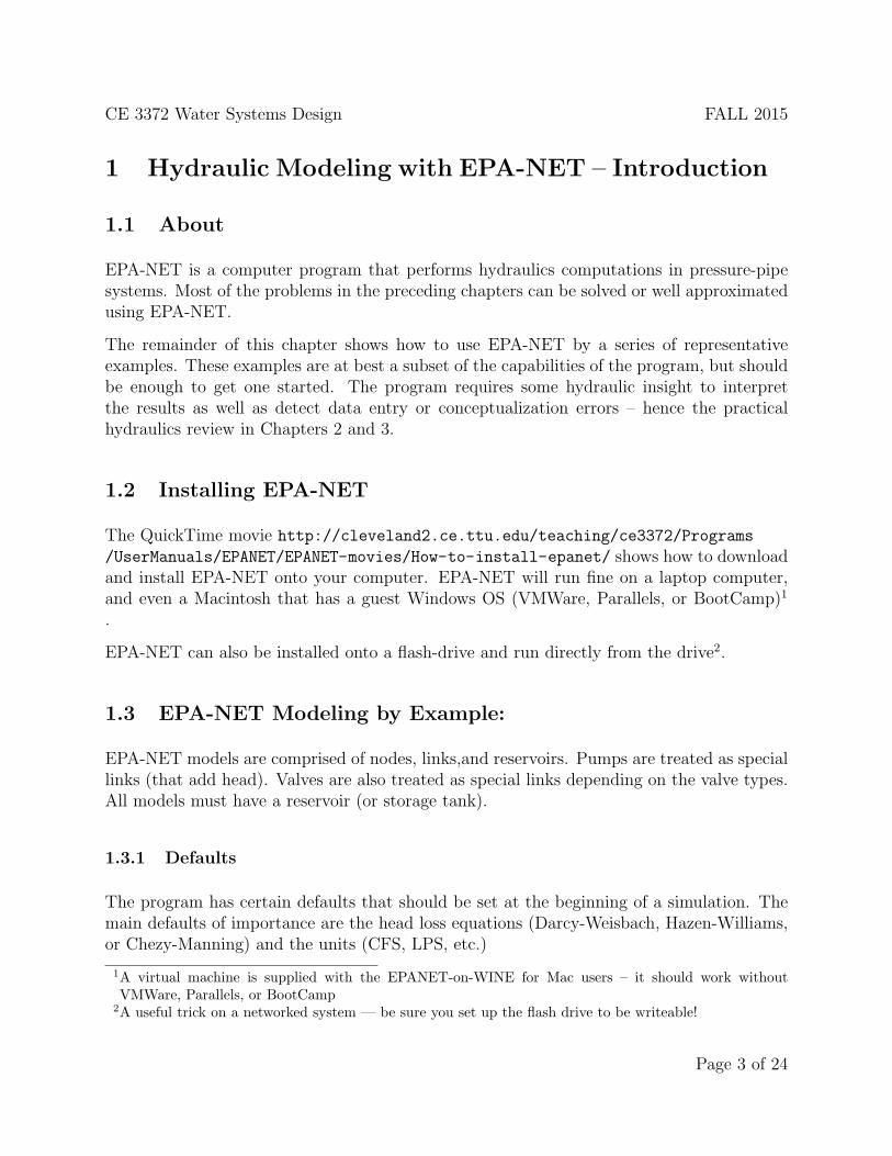
EPA-NET is a computer program that performs hydraulics computations in pressure-pipesystems. Most of the problems in the preceding chapters can be solved or well approximatedusing EPA-NET.

The remainder of this chapter shows how to use EPA-NET by a series of representativeexamples. These examples are at best a subset of the capabilities of the program, but shouldbe enough to get one started. The program requires some hydraulic insight to interpretthe results as well as detect data entry or conceptualization errors – hence the practicalhydraulics review in Chapters 2 and 3.

1.2 Installing EPA-NET

The QuickTime movie http://cleveland2.ce.ttu.edu/teaching/ce3372/Programs

/UserManuals/EPANET/EPANET-movies/How-to-install-epanet/ shows how to downloadand install EPA-NET onto your computer. EPA-NET will run fine on a laptop computer,and even a Macintosh that has a guest Windows OS (VMWare, Parallels, or BootCamp)1

.

EPA-NET can also be installed onto a flash-drive and run directly from the drive2.

1.3 EPA-NET Modeling by Example:

EPA-NET models are comprised of nodes, links,and reservoirs. Pumps are treated as speciallinks (that add head). Valves are also treated as special links depending on the valve types.All models must have a reservoir (or storage tank).

1.3.1 Defaults

The program has certain defaults that should be set at the beginning of a simulation. Themain defaults of importance are the head loss equations (Darcy-Weisbach, Hazen-Williams,or Chezy-Manning) and the units (CFS, LPS, etc.)

1A virtual machine is supplied with the EPANET-on-WINE for Mac users – it should work withoutVMWare, Parallels, or BootCamp

2A useful trick on a networked system — be sure you set up the flash drive to be writeable!

Page 3 of 24


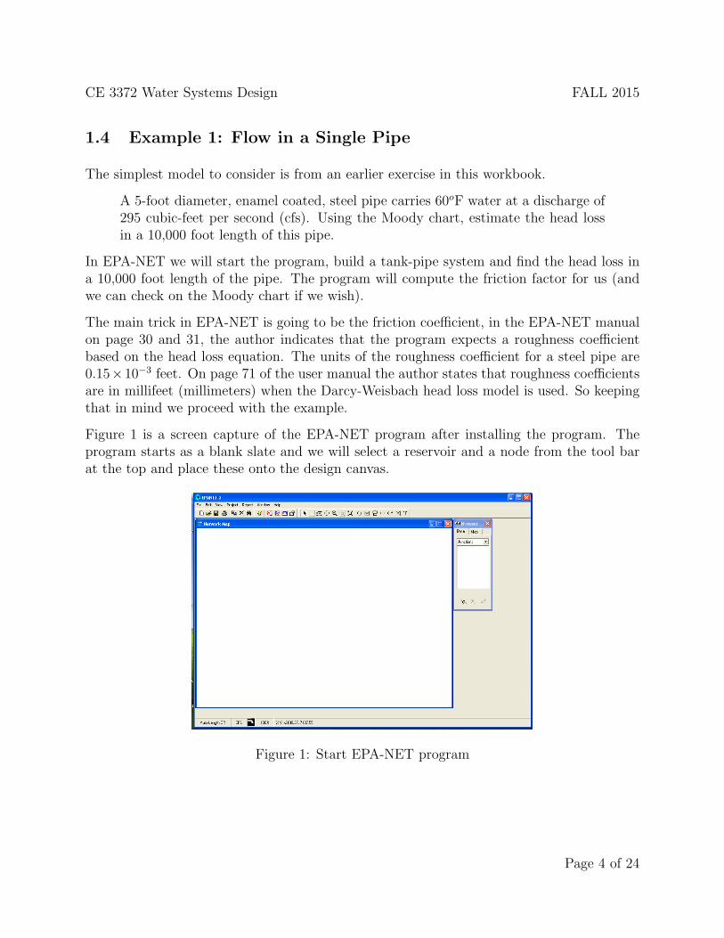
1.4 Example 1: Flow in a Single Pipe

The simplest model to consider is from an earlier exercise in this workbook.

A 5-foot diameter, enamel coated, steel pipe carries 60oF water at a discharge of295 cubic-feet per second (cfs). Using the Moody chart, estimate the head lossin a 10,000 foot length of this pipe.

In EPA-NET we will start the program, build a tank-pipe system and find the head loss ina 10,000 foot length of the pipe. The program will compute the friction factor for us (andwe can check on the Moody chart if we wish).

The main trick in EPA-NET is going to be the friction coefficient, in the EPA-NET manualon page 30 and 31, the author indicates that the program expects a roughness coefficientbased on the head loss equation. The units of the roughness coefficient for a steel pipe are0.15×10−3 feet. On page 71 of the user manual the author states that roughness coefficientsare in millifeet (millimeters) when the Darcy-Weisbach head loss model is used. So keepingthat in mind we proceed with the example.

Figure 1 is a screen capture of the EPA-NET program after installing the program. Theprogram starts as a blank slate and we will select a reservoir and a node from the tool barat the top and place these onto the design canvas.

Figure 1: Start EPA-NET program

Page 4 of 24


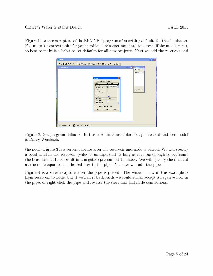
Figure 1 is a screen capture of the EPA-NET program after setting defaults for the simulation.Failure to set correct units for your problem are sometimes hard to detect (if the model runs),so best to make it a habit to set defaults for all new projects. Next we add the reservoir and

Figure 2: Set program defaults. In this case units are cubic-feet-per-second and loss modelis Darcy-Weisbach.

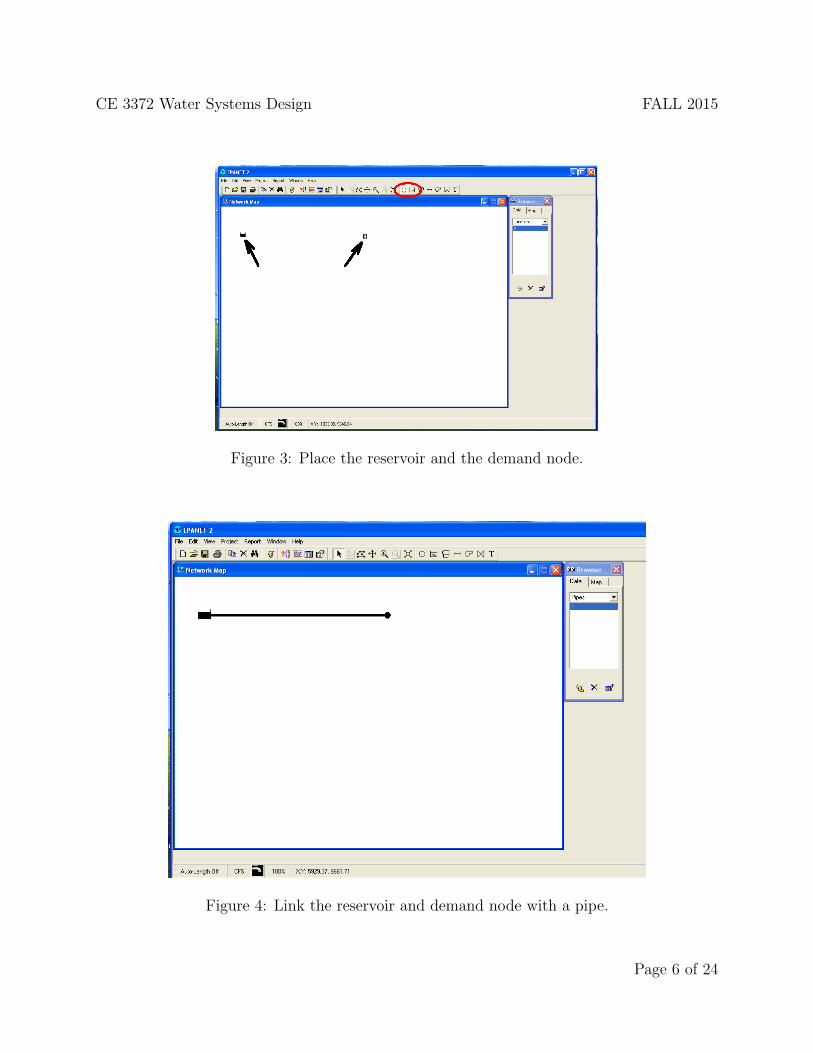
the node. Figure 3 is a screen capture after the reservoir and node is placed. We will specifya total head at the reservoir (value is unimportant as long as it is big enough to overcomethe head loss and not result in a negative pressure at the node. We will specify the demandat the node equal to the desired flow in the pipe. Next we will add the pipe.

Figure 4 is a screen capture after the pipe is placed. The sense of flow in this example isfrom reservoir to node, but if we had it backwards we could either accept a negative flow inthe pipe, or right-click the pipe and reverse the start and end node connections.

Page 5 of 24


Figure 3: Place the reservoir and the demand node.

Figure 4: Link the reservoir and demand node with a pipe.

Page 6 of 24


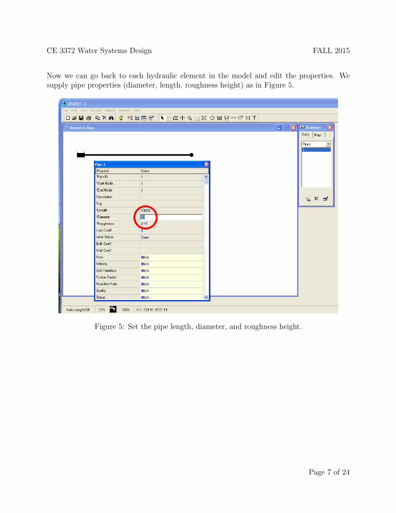
Now we can go back to each hydraulic element in the model and edit the properties. Wesupply pipe properties (diameter, length, roughness height) as in Figure 5.

Figure 5: Set the pipe length, diameter, and roughness height.

Page 7 of 24


We supply the reservoir total head as in Figure 6.

Figure 6: Set the reservoir total head, 100 feet should be enough in this example.

Page 8 of 24


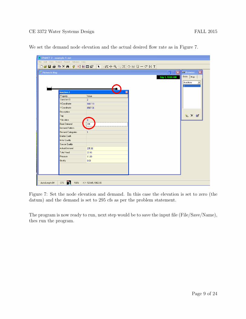
We set the demand node elevation and the actual desired flow rate as in Figure 7.

Figure 7: Set the node elevation and demand. In this case the elevation is set to zero (thedatum) and the demand is set to 295 cfs as per the problem statement.

The program is now ready to run, next step would be to save the input file (File/Save/Name),thes run the program.

Page 9 of 24


Run the program by selecting the lighting bolt looking thing (kind of channeling Zeus here)and the program will start. If the nodal connectivity is OK and there are no computednegative pressures the program will run. Figure 8 is the appearance of the program afterthe run is complete (the annotations are mine!). A successful run means the program found

Figure 8: Running the program

an answer to the problem you provided – whether it is the correct answer to your problemrequires the engineer to interpret results and decide if they make sense. The more commonconceptualization errors are incorrect units and head loss equation for the supplied roughnessvalues, missed connections, and forgetting demand somewhere. With practice these kind oferrors are straightforward to detect. In the present example we select the pipe and thesolution values are reported at the bottom of a dialog box.

Page 10 of 24


Figure 9: Solution dialog box for the pipe.

Figure 9 is the result of turning on the computed head values at the node (and reservoir)and the flow value for the pipe. The dialog box reports about 7.2 feet of head loss per 1000feet of pipe for a total of 72 feet of head loss in the system. The total head at the demnadnode is about 28 feet, so the head loss plus remaining head at the node is equal to the 100feet of head at the reservoir, the anticipated result.

The computed friction factor is 0.010, which we could check against the Moody chart if wewished to adjust the model to agree with some other known friction factor.

Page 11 of 24


1.5 Example 2: Flow Between Two Reservoirs

This example represents the situation where the total head is known at two points on apipeline, and one wishes to determine the flow rate (or specify a flow rate and solve for apipe diameter). Like the prior example it is contrived, but follows the same general modelingprocess.

As in the prior example, we will use EPA-NET to solve a problem we have already solvedby hand.

Using the Moody chart, and the energy equation, estimate the diameter of a cast-iron pipe needed to carry 60oF water at a discharge of 10 cubic-feet per second(cfs) between two reservoirs 2 miles apart. The elevation difference between thewater surfaces in the two reservoirs is 20 feet.

As in the prior example, we will need to specify the pipe roughness terms, then solve by trial-and-error for the diameter required to carry the water at the desired flowrate. Page 31 ofthe EPA-NET manual suggests that the roughness height for cast iron is 0.85 millifeet.

As before the steps to model the situation are:

1. Start EPA-NET

2. Set defaults

3. Select the reservoir tool. Put two reservoirs on the map.

4. Select the node tool, put a node on the map. EPA NET needs one node!

5. Select the link (pipe) tool, connect the two reservoirs to the node. One link is the 2mile pipe, the other is a short large diameter pipe (negligible head loss).

6. Set the total head each reservoir.

7. Set the pipe length and roughness height in the 2 mile pipe.

8. Guess a diameter.

9. Save the input file.

10. Run the program. Query the pipe and find the computed flow. If the flow is too largereduce the pipe diameter, if too small increase the pipe diameter. Stop when withina few percent of the desired flow rate. Use commercially available diameters in thetrial-and-error process, so exact match is not anticipated.

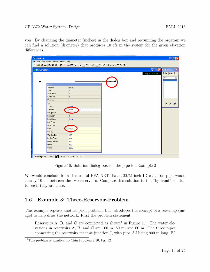
Figure 10 is a screen capture after the model is built and some trial-and-error diameterselection. Of importance is the node and the “short pipe” that connects the second reser-

Page 12 of 24


voir. By changing the diameter (inches) in the dialog box and re-running the program wecan find a solution (diameter) that produces 10 cfs in the system for the given elevationdifferences.

Figure 10: Solution dialog box for the pipe for Example 2

We would conclude from this use of EPA-NET that a 22.75 inch ID cast iron pipe wouldconvey 10 cfs between the two reservoirs. Compare this solution to the “by-hand” solutonto see if they are close.

1.6 Example 3: Three-Reservoir-Problem

This example repeats another prior problem, but introduces the concept of a basemap (im-age) to help draw the network. First the problem statement

Reservoirs A, B, and C are connected as shown3 in Figure 11. The water ele-vations in reservoirs A, B, and C are 100 m, 80 m, and 60 m. The three pipesconnecting the reservoirs meet at junction J, with pipe AJ being 900 m long, BJ

3This problem is identical to Chin Problem 2.30, Pg. 92

Page 13 of 24


being 800 m long, and CJ being 700 m long. The diameters of all the pipes are850 mm. If all the pipes are ductile iron, and the water temperature is 293oK,find the direction and magnitude of flow in each pipe.

Figure 11: Three-Reservoir System Schematic

Here we will first convert the image into a bitmap (.bmp) file so EPA-NET can import thebackground image and we can use it to help draw the network. The remainder of the problemis reasonably simple and is an extension of the previous problem.

The steps to model the situation are:

1. Convert the image into a bitmap, place the bitmap into a directory where the modelinput file will be stored.

2. Start EPA-NET

3. Set defaults

4. Import the background.

5. Select the reservoir tool. Put three reservoirs on the map.

6. Select the node tool, put the node on the map.

7. Select the link (pipe) tool, connect the three reservoirs to the node.


Page 14 of 24


9. Set the pipe length, roughness height, and diameter in each pipe.


11. Run the program.

Figure 12 is the result of the above steps. In this case the default units were changed to LPS(liters per second). The roughness height is about 0.26 millimeters (if converted from the0.85 millifeet unit).

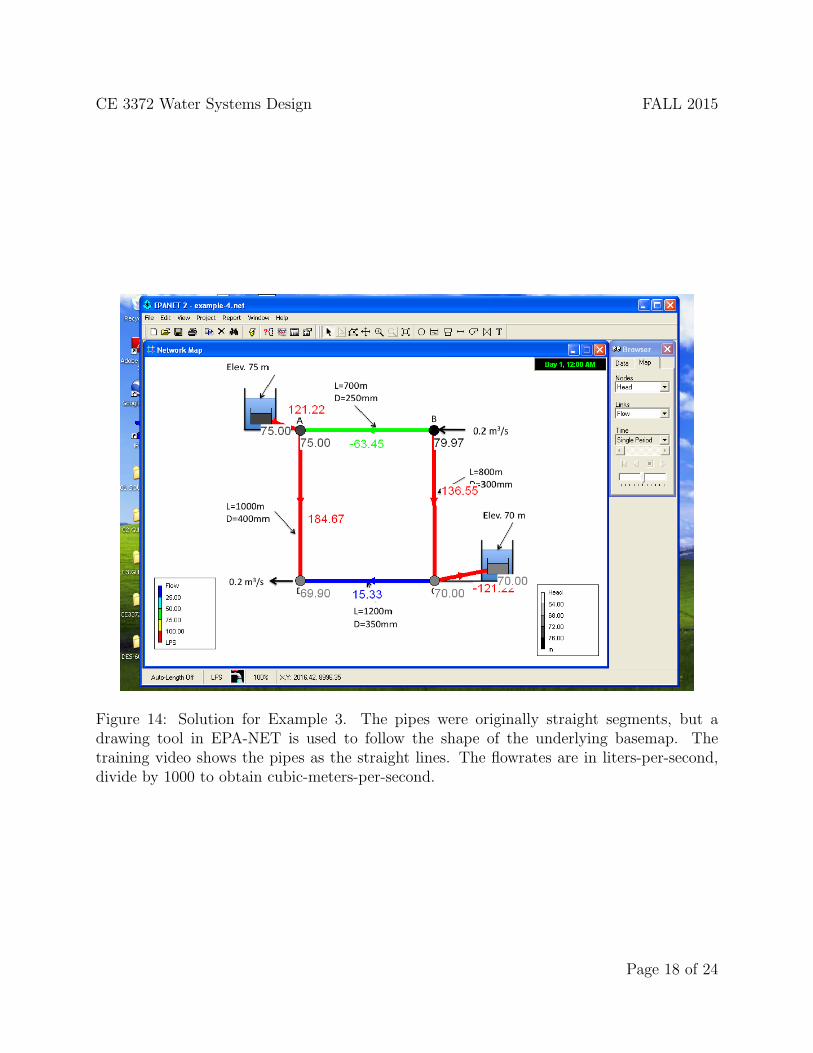
Figure 12: Solution for Example 3. The pipes were originally straight segments, but adrawing tool in EPA-NET is used to follow the shape of the underlying basemap. Thetraining video shows the pipes as the straight lines. The flowrates are in liters-per-second,divide by 1000 to obtain cubic-meters-per-second.

Page 15 of 24


1.7 Example 4: A Simple Network

Expanding the examples, we will next consider a looped network. As before we will use aprior exercise as the motivating example.

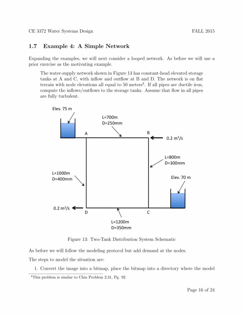
The water-supply network shown in Figure 13 has constant-head elevated storagetanks at A and C, with inflow and outflow at B and D. The network is on flatterrain with node elevations all equal to 50 meters4. If all pipes are ductile iron,compute the inflows/outflows to the storage tanks. Assume that flow in all pipesare fully turbulent.

Figure 13: Two-Tank Distribution System Schematic

As before we will follow the modeling protocol but add demand at the nodes.

The steps to model the situation are:

1. Convert the image into a bitmap, place the bitmap into a directory where the model

4This problem is similar to Chin Problem 2.31, Pg. 92

Page 16 of 24


input file will be stored.

2. Start EPA-NET

3. Set defaults



6. Select the node tool, put 4 nodes on the map.

7. Select the link (pipe) tool, connect the reservoirs to their nearest nodes. Connect thenodes to each other.


9. Set the pipe length, roughness height, and diameter in each pipe. The pipes thatconnect to the reservoirs should be set as short and large diameter, we want negligiblehead loss in these pipes so that the reservoir head represents the node heads at theselocations.



In this case the key issues are the units (liters per second) and roughness height (0.26millimeters). Figure 14 is a screen capture of a completed model.

1.8 Example 5: Pumping Water Uphill

The next example illustrates how to model a pump in EPA-NET. A pump is a special “link”in EPA-NET. This link causes a negative head loss (adds head) according to a pump curve.In additon to a pump curve there are three other ways to model added head — these arediscussed in th eunser manual and are left for the reader to explore on their own.

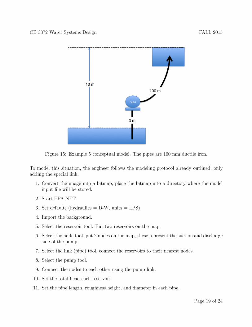
Figure 15 is a conceptual model of a pump lifting water through a 100 mm diameter, 100meter long, ductile iron pipe from a lower to an upper reservoir. The suction side of thepump is a 100 mm diameter, 4-meter long ductile iron pipe. The difference in reservoirfree-surface elevations is 10 meters. The pump performance curve is given as

hp = 15 − 0.1Q2 (1)

where the added head is in meters and the flow rate is in liters per second (Lps). The analysisgoal is to estimate the flow rate in the system.

Page 17 of 24


Figure 14: Solution for Example 3. The pipes were originally straight segments, but adrawing tool in EPA-NET is used to follow the shape of the underlying basemap. Thetraining video shows the pipes as the straight lines. The flowrates are in liters-per-second,divide by 1000 to obtain cubic-meters-per-second.

Page 18 of 24


Figure 15: Example 5 conceptual model. The pipes are 100 mm ductile iron.

To model this situation, the engineer follows the modeling protocol already outlined, onlyadding the special link.

1. Convert the image into a bitmap, place the bitmap into a directory where the modelinput file will be stored.

2. Start EPA-NET

3. Set defaults (hydraulics = D-W, units = LPS)



6. Select the node tool, put 2 nodes on the map, these represent the suction and dischargeside of the pump.

7. Select the link (pipe) tool, connect the reservoirs to their nearest nodes.

8. Select the pump tool.

9. Connect the nodes to each other using the pump link.


11. Set the pipe length, roughness height, and diameter in each pipe.

Page 19 of 24


12. On the Data menu, select Curves. Here is where we create the pump curve. Thisproblem gives the curve as an equation, we will need three points to define the curve.Shutoff (Q = 0), and simple to compute points make the most sense.



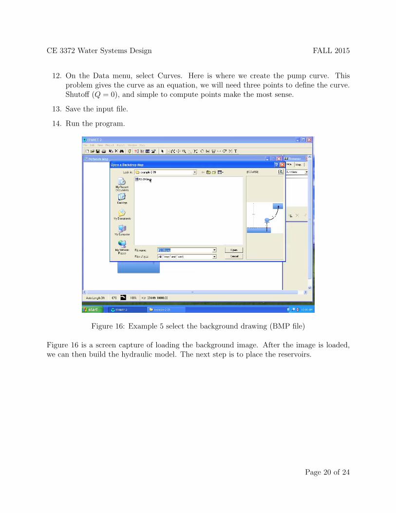
Figure 16: Example 5 select the background drawing (BMP file)

Figure 16 is a screen capture of loading the background image. After the image is loaded,we can then build the hydraulic model. The next step is to place the reservoirs.

Page 20 of 24


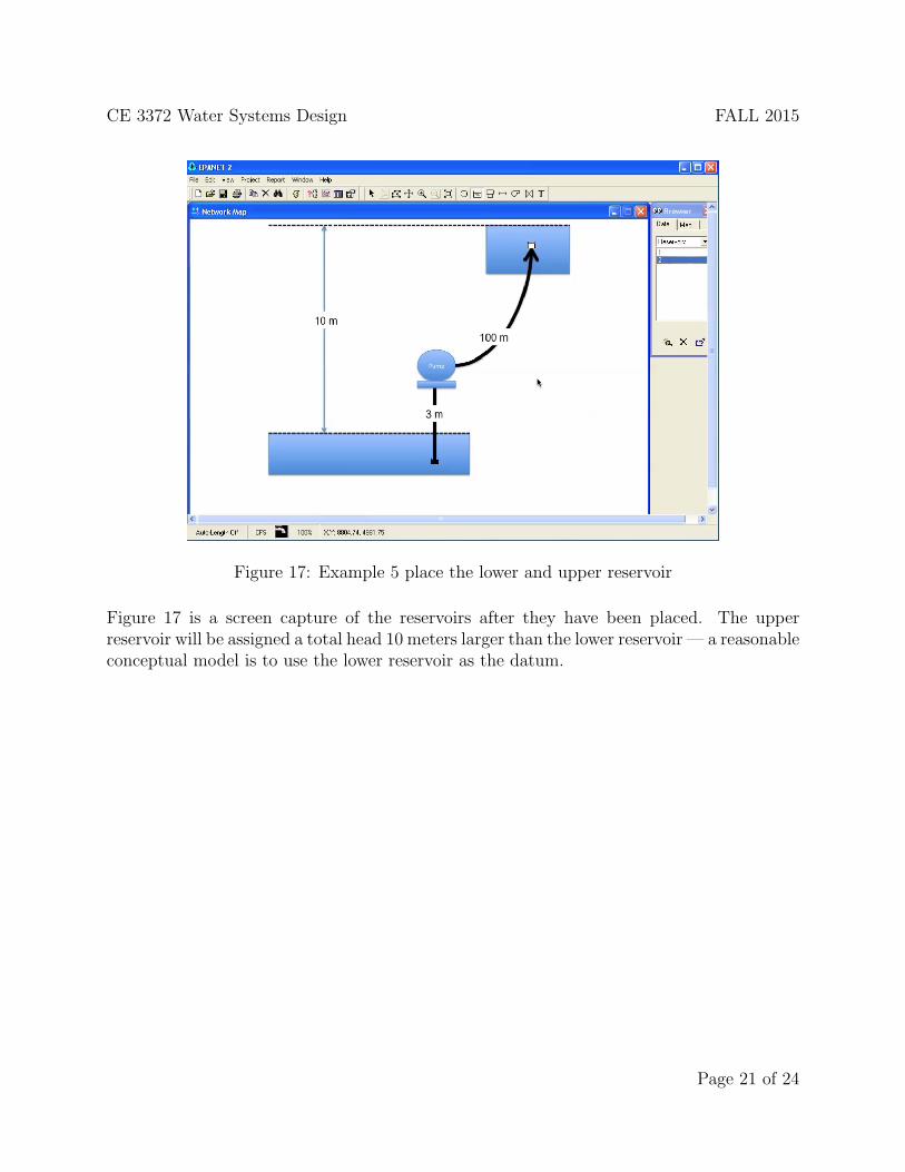
Figure 17: Example 5 place the lower and upper reservoir

Figure 17 is a screen capture of the reservoirs after they have been placed. The upperreservoir will be assigned a total head 10 meters larger than the lower reservoir — a reasonableconceptual model is to use the lower reservoir as the datum.

Page 21 of 24


Figure 18: Example 5 place the nodes, pipes, and the pump link.

Figure 18 is a screen capture of model just after the pump is added. The next steps areto set the pipe lengths (not shown) and the reservoir elevations (not shown). Finally, theengineer must specify the pump curve.

Page 22 of 24


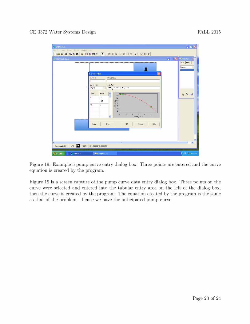
Figure 19: Example 5 pump curve entry dialog box. Three points are entered and the curveequation is created by the program.

Figure 19 is a screen capture of the pump curve data entry dialog box. Three points on thecurve were selected and entered into the tabular entry area on the left of the dialog box,then the curve is created by the program. The equation created by the program is the sameas that of the problem – hence we have the anticipated pump curve.

Page 23 of 24


Next the engineer associates the pump curve with the pump as shown in Figure 20.

Figure 20: Setting the pump curve.

Upon completion of this step, the program is run to estimate the flow rate in the system.

References

Rossman, L. (2000). EPANET 2 users manual. Technical Report EPA/600/R-00/057,U.S. Environmental Protection Agency, National Risk Management Research LaboratoryCincinnati, OH 45268.

Page 24 of 24

Documents

EPANET by Example { A How-to-Manual for Network Modelingtheodores-pro.ttu.edu/ncimm/training-modules/epa-net-1440/epanet... · CE 3372 Water Systems Design FALL 2015 EPANET by Example