Equation for the Landauer resitivity in the case of multichannel scattering

Equation for the Landauer Resitivity in the Case of Multichannel Scattering

D. M. Sedrakiana and L. R. Sedrakianb

aYerevan State University, Yerevan, Armenia bRussian–Armenian (Slavonic) State University, Yerevan, Armenia

Received March 21, 2010

Abstract⎯Generalization of the Landauer resistivity LNρ is given for the case of multichannel

scattering of a particle by the system of nonoverlapped N random potentials, depending on ix x− and y, which are localized near the points ix (i = 1,2,…N). It is shown that in this case a new resistivity

SNρ appears, which is a power function of N. A recurrent equation is obtained for definition of the

Landauer resistivity .LNρ

DOI: 10.3103/S1068337210050026 Key words: multichannel scattering, random potentials, Landauer resistivity

1. INTRODUCTION One of the main consequences of the presence of disorder in a system is the appearance of

macroscopically large number of localized states in it. Consideration of all possible realizations of the random field leads to the fact that the expected fraction of nonlocalized states generally is negligible small. In particular, the presence of any small one-dimensional disorder results in the situation when the probability of realization of delocalized states in the system is equal to zero, i.e., a total localization of all states of the single-particle spectrum takes place [1]. This leads to the absence of the electrical conductivity in a one-dimensional disordered system at the zero temperature. Disorder necessarily leads to the fact that the resistance of a one-dimensional sample of a length L at the zero temperature in the limit L →∞ becomes infinitely large. Therefore in the presence of any small disorder in the system a conductor necessarily transforms into a dielectric [2, 3].

Effects of localization are extremely sensitive to various external conditions which may both reduce and increase the localization of states. Of special interest is the elucidation of the dependence of localization effects on the size of a system, in particular, on the motion of a particle along two directions. In this case a random field depends on two variables: ( ), ,U x y and if we restrict our consideration to localized motion of the particle along y and its scattering by the potential ( ),U x y along the x-direction, then this scattering will be multichannel. Such a scattering results in the variation of localization of single-particle states of the particle. In order to study these changes, it is necessary to formulate the problem of determination of the nature of single-particle states and, correspondingly, of calculation of the localization radius, which is reduced to determination of the mean resistance of the system. It is necessary to prove that, as in the case of a one-dimensional problem, the asymptotical dependence of the mean resistance of the system on its length L at the zero temperature has the form

1 exp ,2

L⎧ ⎫ρ = ⎨ ⎬ξ⎩ ⎭

where angular brackets mean the averaging over all possible realizations of the random fields. Here ξ is the localization radius of single-particle states depending on the particle energy and the kind of the random filed.

As will be shown below, the mean resistivity for the system of N random potentials, introduced by Landauer for a one-dimensional motion [4], is generalized and consists of a sum of two resistivities: the Landauer resistivity L

Nρ and SNρ introduced by us. The last term in this sum appears in view of allowance

for a multichannel character of the scattering at the quasi-one-dimensional motion of the particle. In works [5] it was shown that in multichannel scattering by a chain of potentials

ISSN 1068–3372, Journal of Contemporary Physics (Armenian Academy of Sciences), 2010, Vol. 45, No. 5, pp. 203–208. © Allerton Press, Inc., 2010. Original Russian Text © D.M. Sedrakian, L.R. Sedrakian, 2010, published in Izvestiya NAN Armenii, Fizika, 2010, Vol. 45, No. 5, pp. 314–321.

203

D.M.SEDRAKIAN, L.R.SEDRAKIAN

204

JOURNAL OF CONTEMPORARY PHYSICS (ARMENIAN Ac. Sci.) Vol. 45 No. 5 2010

( ) ( )1

, , ,N

i ii

U x y U x x y=

= −∑ (1)

where N is the number of scatterers in the chain, ( ),i iU x x y− are nonoverlapped functions localized near the points ix ( 1,2, ),i N= … the transfer-matrix has the form

( ) ( ) ( )( ) ( ) ( )

( ) ( ) ( )( )

1 1 11

1 1 1

, , 0,

, , , 0 0

, , 0, 0 ,

nN

n

nN n n nn

n

D N D N M NTD N D N M N

T D N D N M N

D N

∗ ∗ ∗

∗ ∗ ∗

− −⎛ ⎞⎜ ⎟ − −⎜ ⎟⎜ ⎟ =⎜ ⎟

− −⎜ ⎟⎜ ⎟⎝ ⎠ −

…

…

…

( ) ( )

1

1

. 0

, , 0

N

nNn nn

R

RD N M N

⎛ ⎞⎛ ⎞⎜ ⎟⎜ ⎟⎜ ⎟⎜ ⎟⎜ ⎟⎜ ⎟⎜ ⎟⎜ ⎟⎜ ⎟⎜ ⎟⎜ ⎟⎜ ⎟⎜ ⎟⎝ ⎠−⎝ ⎠…

(2)

Here mNT and mNR are the scattering amplitudes of a chain from N potentials along the channel m which is characterized by the scattering momentum mk ( )1,2 ,m n= … while ( )mD N , ( )mD N and ( )imM N are the elements of this transfer-matrix. They are connected with the scattering amplitudes by the formulas

( ) ( ) ( )2 2 2

11 , , ,mn N mn mn mnm m im

mn mn mn

T R T R TD N D N M NT T T T T T

= = = (3)

where 2 2

1.

n

N mnm

T T=

=∑

The conservation law for the density of the probability flow is written in the following form:

( ) ( ) ( )22 2

1 21.

n n

m m mim i

D N D N M N= =

⎛ ⎞− − =⎜ ⎟⎝ ⎠

∑ ∑ (4)

The desired functions ( )mD N , ( )mD N , ( )miM N are defined from the formula derived in [5]:

( )( )

( )( )

( )( )

( )( )1 1 11

,m m mi m

i

D N D N M N ND N M N ND N

α= = =

α (5)

where

( )( )

2 2

1 11

1 1 1

1, .m N mN N

mN N N N

N T T TN T T T T

α= α =

α (6)

The functions ( )1D N , ( )1D N , and ( )1iM N are determined from the following recurrent equations [5]:

( ) ( ) ( ) ( ) ( ) ( )( ) ( ) ( ) ( ) ( ) ( )

( ) ( ) ( )

1 1 1 1 1 1

1 1 1 1 1 1

1 1 1

1 1 ,

1 1 ,

1 ,i i

D N N D N N r N D N

D N N D N N r N D N

M N N M N

∗ ∗ ∗

= α − +α −

= α − +α −

= α −

(7)

where

( ) ( ) ( ) , 11 1 1

2 1 1, 1

1 , 1.N

mN m N

m N N

R Tr N R N R N N

R T−

= −

⎡ ⎤= π = + ≥⎢ ⎥

⎢ ⎥⎣ ⎦∑ (8)

The initial conditions for the system of equations (7) are given as

( ) ( ) ( ) ( )( )

1 1

1

0 1, 0 0 0 0, 1,

0 , 1. m m

i i

D D D D m

M R i

= = = = ≥

= ≥

The goal of this work is, using the difference equations for elements of the transfer-matrix for a chain of potentials consisting of a finite number of scattering centers [5], to derive an equation defining the Landauer resistivity as well as the connections between the functions ,mD mD and ,mT mR obtained in [6], for the case of multichannel scattering. In Section 2 a concept of the Landauer resistivity is generalized with the introduction of a new resistivity S

Nρ which appears in view of the multichannel character of scattering. In section 3 we derive an equation for defining the Landauer resistivity .L

Nρ In

EQUATION FOR THE LANDAUER RESISTIVITY

205


Conclusion the obtained results are listed and it is shown that in the case of one-dimensional motion or one-dimensional scattering the equation for L

Nρ passes into the equation derived in [2].

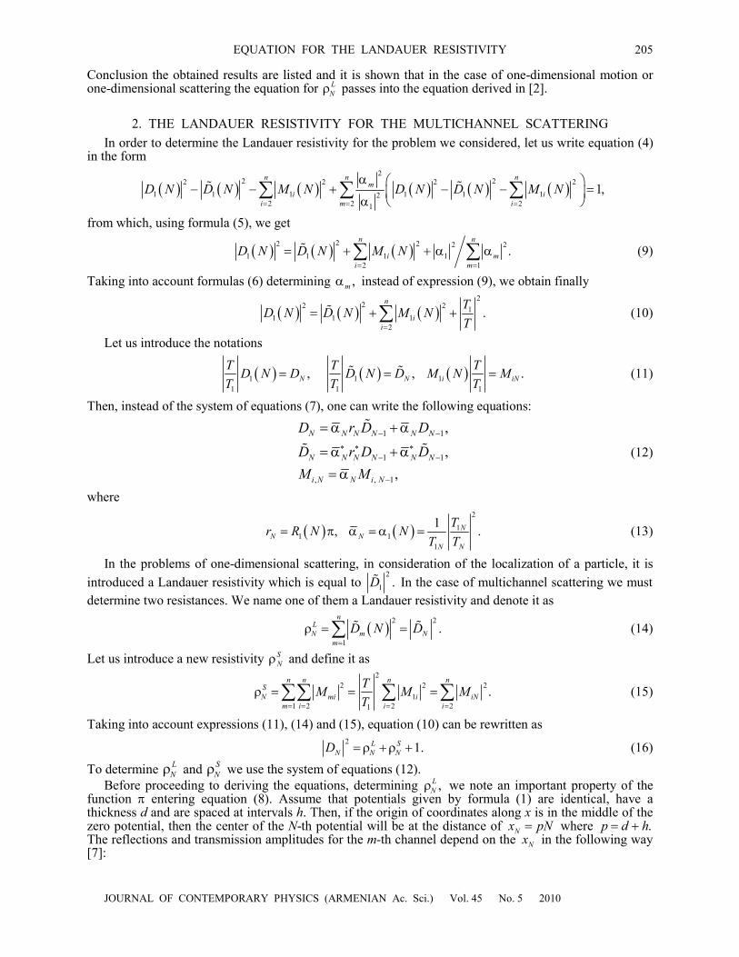
2. THE LANDAUER RESISTIVITY FOR THE MULTICHANNEL SCATTERING In order to determine the Landauer resistivity for the problem we considered, let us write equation (4)

in the form

( ) ( ) ( ) ( ) ( ) ( )2

2 22 2 2 21 1 1 1 1 12

2 2 21

1,n n n

mi i

i m iD N D N M N D N D N M N

= = =

α ⎛ ⎞− − + − − =⎜ ⎟

α ⎝ ⎠∑ ∑ ∑

from which, using formula (5), we get

( ) ( ) ( )22 2 2 2

1 1 1 12 1

.n n

i mi m

D N D N M N= =

= + + α α∑ ∑ (9)

Taking into account formulas (6) determining ,mα instead of expression (9), we obtain finally

( ) ( ) ( )2

22 2 11 1 1

2.

n

ii

TD N D N M NT=

= + +∑ (10)

Let us introduce the notations

( ) ( ) ( )1 1 11 1 1

, , .N N i iNT T TD N D D N D M N MT T T

= = = (11)

Then, instead of the system of equations (7), one can write the following equations:

1 1

1 1

, , 1

,

,,

N N N N N N

N N N N N N

i N N i N

D r D D

D r D DM M

− −

∗ ∗ ∗− −

−

= α +α

= α +α= α

(12)

where

( ) ( )2

11 1

1

1, .NN N

N N

Tr R N NT T

= π α = α = (13)

In the problems of one-dimensional scattering, in consideration of the localization of a particle, it is introduced a Landauer resistivity which is equal to

2

1 .D In the case of multichannel scattering we must determine two resistances. We name one of them a Landauer resistivity and denote it as

( )2 2

1.

nLN m N

mD N D

=

ρ = =∑ (14)

Let us introduce a new resistivity SNρ and define it as

2

2 2 21

1 2 2 21

.n n n n

SN mi i iN

m i i i

TM M MT= = = =

ρ = = =∑∑ ∑ ∑ (15)

Taking into account expressions (11), (14) and (15), equation (10) can be rewritten as

2 1.L SN N ND = ρ + ρ + (16)

To determine LNρ and S

Nρ we use the system of equations (12). Before proceeding to deriving the equations, determining ,L

Nρ we note an important property of the function π entering equation (8). Assume that potentials given by formula (1) are identical, have a thickness d and are spaced at intervals h. Then, if the origin of coordinates along x is in the middle of the zero potential, then the center of the N-th potential will be at the distance of Nx pN= where .p d h= + The reflections and transmission amplitudes for the m-th channel depend on the Nx in the following way [7]:


206


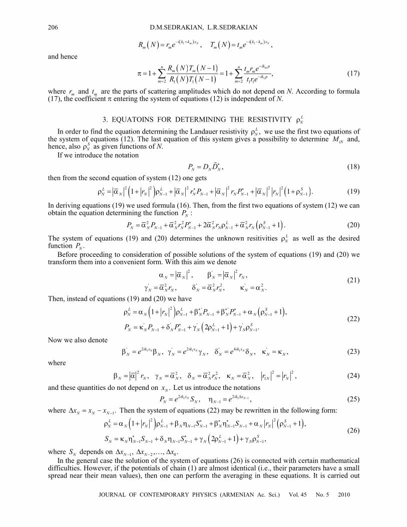
( ) ( ) ( ) ( )1 1, ,m N m Ni k k x i k k xm m m mR N r e T N t e− + − −= =

and hence

( ) ( )( ) ( ) 1

2 21 1 1 1

11 1 ,

1

mik pn nm m m m

ik pm m

R N T N t r eR N T N t re

−

−= =

−π = + = +

−∑ ∑ (17)

where mr and mt are the parts of scattering amplitudes which do not depend on N. According to formula (17), the coefficient π entering the system of equations (12) is independent of N.

3. EQUATOINS FOR DETERMINING THE RESISTIVITY LNρ

In order to find the equation determining the Landauer resistivity ,LNρ we use the first two equations of

the system of equations (12). The last equation of this system gives a possibility to determine iNM and, hence, also S

Nρ as given functions of N. If we introduce the notation

,N N NP D D∗= (18) then from the second equation of system (12) one gets

( ) ( )2 2 2 2 2 21 1 1 11 1 .L L S

N N N N N N N N N N N N Nr r P r P r∗ ∗− − − −ρ = α + ρ + α + α + α + ρ (19)

In deriving equations (19) we used formula (16). Then, from the first two equations of system (12) we can obtain the equation determining the function :NP

( )2 2 2 2 21 1 1 12 1L S

N N N N N N N N N N N NP P r P r r∗− − − −= α + α + α ρ +α ρ + . (20)

The system of equations (19) and (20) determines the unknown resitivities LNρ as well as the desired

function .NP Before proceeding to consideration of possible solutions of the system of equations (19) and (20) we

transform them into a convenient form. With this aim we denote

2 2'

' 2 ' 2 2 ' 2

, ,

, , .N N N N N

N N N N N N N N

r

r r

α = α β = α

γ = α δ = α κ = α

(21)

Then, instead of equations (19) and (20) we have

( ) ( )

( )

2 ' '1 1 1 1

' ' ' '1 1 1 1

1 1 ,

2 1 .

L L SN N N N N N N N N N

L SN N N N N N N N N

r P P

P P P

∗ ∗ ∗− − − −

∗− − − −

ρ = α + ρ +β +β +α ρ +

= κ + δ + γ ρ + + γ ρ (22)

Now we also denote 1 1 12 2 4' ' ' ', , , ,N N Nik x ik x ik x

N N N N N N N Ne e eβ = β γ = γ δ = δ κ = κ (23) where

2 2 22 2 2 21, , , , ,N N N N N N N N N N Nr r r rβ = α γ = α δ = α κ = α = (24)

and these quantities do not depend on .Nx Let us introduce the notations 1 1 12 2

1, ,N Nik x ik xN N NP e S e −Δ

−= η = (25) where 1.N N Nx x x −Δ = − Then the system of equations (22) may be rewritten in the following form:

( ) ( )

( )

2 21 1 1 1 1 1

1 1 1 1 1 1

1 1 ,

2 1 ,

L L SN N N N N N N N N N N N N

L SN N N N N N N N N N N

r S S r

S S S

∗ ∗ ∗− − − − − −

∗ ∗− − − − − −

ρ = α + ρ +β η +β η +α ρ +

= κ η + δ η + γ ρ + + γ ρ (26)

where NS depends on 1 2 0, , , .N Nx x x− −Δ Δ Δ… In the general case the solution of the system of equations (26) is connected with certain mathematical

difficulties. However, if the potentials of chain (1) are almost identical (i.e., their parameters have a small spread near their mean values), then one can perform the averaging in these equations. It is carried out

EQUATION FOR THE LANDAUER RESISTIVITY

207


over a given distribution of these deviations from their mean values. Indeed, for instance, a mean value of the function 1N−η equal to η will be depend on the mean distance between the potentials because it depends on the distance between the potentials N and 1.N − The terms entering the system of equations (26) have such a form which allows a factorization, i.e., for instance, in averaging of the term 1 1N N NS ∗

− −β η one can write

1 1 1 1N N N N N NS S∗ ∗− − − −β η = β η .

If mean values entering averaged equations (26) are denoted by the same letters, then instead of equations (26) we get

( ) ( )

( )

2 21 1 1 1

1 1 1 1

1 1 ,

2 1 ,

L L SN N N N N

L SN N N N N

r S S r

S S S

∗ ∗ ∗− − − −

∗ ∗− − − −

< ρ >= α + < ρ > +βη < > +β η < > +α < ρ > +

< >= κη < > +δη < > + γ < ρ > + + γ < ρ > (27)

where α, β, γ, δ and η are independent of N. Here we take into account that 2 2Nr r= does not depend on

the index N. The first equation of system (27) is a recurrent equation for determining the Landauer resistivity .L

N< ρ > However, there are the unknown functions 1NS −< > and 1 ,NS ∗−< > which should be

expressed in terms of the functions LN< ρ > and S

N< ρ > in order to obtain an equation for determining .L

N< ρ > For this purpose we write the first equation of system (27) for the functions 1 ,LN−< ρ > 2

LN−< ρ >

and the second equation for the functions 1 ,NS −< > 1 ,NS ∗−< > 2 ,NS −< > and 2 .NS ∗

−< > Them we get the following system of equations:

( ) ( )( ) ( )

( )( )

2 21 2 2 2 2

2 22 3 3 3 3

1 2 2 2 2

1 2 2 2

1 1 ,

1 1 ,

2 1 ,

2 1

L L SN N N N N

L L SN N N N N

L SN N N N N

LN N N N

r S S r

r S S r

S S S

S S S

∗ ∗ ∗− − − − −

∗ ∗ ∗− − − − −

∗ ∗− − − − −

∗ ∗ ∗ ∗ ∗ ∗− − − −

< ρ >= α + < ρ > +ηβ < > +β η < > +α < ρ > +

< ρ >= α + < ρ > +ηβ < > +β η < > +α < ρ > +

< >= κη < > + δη < > + γ < ρ > + + γ < ρ >

< >= κ η < > +δ η < > + γ < ρ > +

( )( )

2

2 3 3 3 3

2 3 3 3 3

,

2 1 ,

2 1 .

SN

L SN N N N N

L SN N N N N

S S S

S S S

∗−

∗ ∗− − − − −

∗ ∗ ∗ ∗ ∗ ∗ ∗− − − − −

+ γ < ρ >

< >= κη < > +δη < > + γ < ρ > + + γ < ρ >

< >= κ η < > +δ η < > + γ < ρ > + + γ < ρ >

(28)

As a result we have six equations for six unknown functions: 1 ,NS −< > 1 ,NS ∗−< > 2 ,NS −< > 2 ,NS ∗

−< > 3NS −< > and 3 .NS ∗

−< > After solving this system of linear algebraic equations the desired functions 1NS −< > and 1NS ∗

−< > , entering the first equation of system (27), are expressed via the functions 1 ,L

N−< ρ > 2LN−< ρ > and 3

LN−< ρ > . The functions 1 ,S

N−< ρ > 2SN−< ρ > and 3

SN−< ρ > , which are the known

functions of N also enter these equations. Substituting the functions 1NS −< > and 1NS ∗

−< > derived by solving the system of equations (28), into the first equation of system (27), we obtain the following recurrent equation for determining the Landauer resistivity :L

N< ρ > 1 2 3 0,L L L L

N N N N NA B C D− − −< ρ > − < ρ > − < ρ > − < ρ > − = (29) where

( ) ( ) ( )

( ) ( ) ( )

2 2 2

2 2 2 21 2 3

1 2 , 2 1 2 , 1 2 ,

1 2 2 ,S S SN N N N

A r B r C r u

D r u r r r u− − −

= α + + θ = φ − −α + θ = α + −

= α − θ + + φ − +α < ρ > + φ − θα < ρ > + α − < ρ >

v v

v v (30)

with the notations

( )

( )

2 2 2, , ,

Re 1 , .

u∗ ∗ ∗ ∗ ∗ ∗

∗ ∗∗ ∗ ∗

∗

φ = β η γ +βηγ = η Γ γ + ηΓγ = η κ − δ

⎡ ⎤⎛ ⎞ ⎛ ⎞Γ βΓθ = η κ − δ − Γ = η κβ − δβ⎢ ⎥⎜ ⎟ ⎜ ⎟Γ β Γ⎝ ⎠ ⎝ ⎠⎣ ⎦

v (31)

Equation (29) determines the Landauer resistivity for the system of N random two-dimensional potentials of type (1).


208


4. CONCLUSION A main result of this work is deriving the recurrent equation for finding the Landauer resistivity L

Nρ in the case of particle scattering by the system of N random potentials of type (1). The parameters, describing these potentials in average, are identical but they have compositional and structural disorder. The latter leads to localization of the particle motion along x, and the localization radius may be determined from the solution of equation (29).

The obtained equation (29) keeps its form in the case of one-dimensional motion or in one-channel scattering. Only the constants entering this equation [2] are changed:

( )

( ) ( )( ) 2

2 1 2 , 2 2 1 2 , 12 1 2 , 1 1 2 , .

A B

C u D ut

= α − + θ = φ − − α − θ

= α − − = α − − θ + + φ − α =

v

v v (32)

The method of solving the equation (29), when a free term ( ND ) does not depend on N, is given in works [2]. By generalizing this method one can derive the solutions of equation (29) when the free term ND depends on N. This problem will be considered in the next publication.

REFERENCES 1. Madelung, O., Introduction to Solid-State Theory, Berlin, Heidelberg: Springer, 1996. 2. Sedrakian, D.M., Badalian, D.A., and Khachatrian, A.Zh., FTT, 1999, vol. 41, p. 1687; 1999, vol. 41, p. 1851;

2000, vol. 42, p. 747. 3. Khachatrian, A.Zh., Robke, G., Badalian, D.H., and Sedrakian, D.M., Phys. Rev. B, 2000, vol. 62, p. 13501. 4. Landauer, R., Phil. Mag., 1970, vol. 21, p. 863. 5. Sedrakian, D.M., J. Contemp. Phys. (Armenian Ac. Sci.), 2010, vol. 45, p. 25; 2010, vol. 45, p. 118. 6. Sedrakian, L.R., Doklady NAN Armeniii, 2009, vol. 109, p. 214. 7. Sedrakian, D.M., Kazaryan, E.M., and Sedrakian, L.R., J. Contemp. Phys. (Armenian Ac. Sci.), 2009, vol. 44,

p. 257.

Documents

Equation for the Landauer resitivity in the case of multichannel scattering