Equation of State Dependence of Nonlinear Mode-tide

Equation of State Dependence of Nonlinear Mode-tide Coupling in Coalescing BinaryNeutron Stars

Yixiao Zhou1 and Fan Zhang2,31 Research School of Astronomy and Astrophysics, Australian National University, Canberra, ACT 2611, Australia

2 Gravitational Wave and Cosmology Laboratory, Department of Astronomy, Beijing Normal University, Beijing 100875, China3 Department of Physics and Astronomy, West Virginia University, P.O. Box 6315, Morgantown, WV 26506, USAReceived 2016 January 10; revised 2017 September 25; accepted 2017 September 30; published 2017 November 7

Abstract

Recently, an instability due to the nonlinear coupling of p-modes to g-modes in tidally deformed neutron stars incoalescing binaries has been studied in some detail. The result is significant because it could influence the inspiraland leave an imprint on the gravitational wave signal that depends on the neutron star equation of state (EOS).Because of its potential importance, the details of the instability should be further elucidated and its sensitivity tothe EOS should be investigated. To this end, we carry out a numerical analysis with six representative EOSs forboth static and non-static tides. We confirm that the absence of the p-g instability under static tides, as well as itsreturn under non-static tides, is generic across EOSs, and further reveal a new contribution to it that becomesimportant for moderately high-order p-g pairs (previous studies concentrated on very high order modes), whoseassociated coupling strength can vary by factors of ∼10–100 depending on the EOS. We find that, for stars withstiffer EOSs and smaller buoyancy frequencies, the instability onsets earlier in the inspiral and the unstable modesgrow faster. These results suggest that the instability’s impact on the gravitational wave signal might be sensitive tothe neutron star EOS. To fully assess this prospect, future studies will need to investigate its saturation as a functionof the EOS and the binary parameters.

Key words: binaries: close – stars: neutron – stars: oscillations

1. Introduction

Soon after the commissioning of the second generationgravitational wave (GW) detectors, which include theAdvanced LIGO (Harry 2010) and Advanced Virgo (TheVirgo Collaboration 2012), GWs from binary black holes weresuccessfully detected (Abbott et al. 2016a, 2016b). The nextwave of excitement will likely come from neutron starcoalescences (see Abbott et al. 2016c for an upper limit onevent rates given the absence of detection from LIGO’s firstobserving run), which would provide us with a new channel forprobing the neutron star equation of state (EOS). Such apossibility has been examined in various studies. In particular,Flanagan & Hinderer (2008), Hinderer et al. (2010), Damouret al. (2012), Hotokezaka et al. (2013), and Read et al. (2013)have developed schemes concentrating on the effects of theneutron stars’ EOS-dependent tidal deformations on thegravitational waveform. A particularly interesting issue relatedto this line of investigation is whether tidally driven instabilitiescan develop within the neutron stars, which would grow bydraining energy from the orbital motion, keeping some asmodal energy and dissipating the rest as heat. Such instabilities,if they exist (1) and are sensitively dependent on the EOS (2),would impart signatures of the EOS onto the orbital and thusthe gravitational waveform’s phases, enhancing the GWdetectors’ ability to characterize the EOS.

The question (1) regarding the existence of said instabilitieshas been examined by Weinberg et al. (2013) (WAB),Venumadhav et al. (2014) (VZH), and Weinberg (2016)(W2016). Previous study by Wu & Goldreich (2001)demonstrated that three-mode coupling coefficients canbecome large when wave numbers of the two daughter modesbecome comparable. By considering such three-mode non-linear couplings, and setting the daughter modes to be p-g pairs

with similar wavelengths, WAB discovered a new non-resonant instability, with which a tidal force can quickly drivehigh-order p- and g-modes to large amplitudes. Assuming astatic tide, VZH then extended the calculation to include fourmode couplings, by employing a novel volume-preservingtransformation that greatly simplifies the computation. Whatthey found is that a near-exact cancellation occurs between thethree- and four-mode couplings, which reduced the growth rateand implied that the instability cannot affect the inspiralsignificantly. W2016 then further relaxed simplifying assump-tions, allowing for volume-altering non-static tides (the starsbecome compressible under the influence of linear tides).The result is that the near-exact cancellation is undone, and theinstability becomes important once again. In this paper, weconfirm that these conclusions for both the static and non-staticcases are valid across EOSs, and also demonstrate the presenceof an additional contributing factor to the instability. Weemphasize that our results differ from previous literature onlyin that we look at alternative additional terms that becomeimportant under different circumstances. Under the circum-stances that are relevant to those works, the instabilities theyfound would still be the dominant contribution. We wish todemonstrate here that strong EOS dependence is present for atleast some of the cases, so using the instabilities to study EOSwould be a promising avenue, but a comprehensive dictionaryof the instabilities for all possible mode pairs is far beyond thescope of the paper (and would be useful only when saturations,etc. are also thoroughly considered).In terms of observational consequences, the aforementioned

studies (see also Essick et al. 2016) were mostly concernedwith the detectability of GWs using matched-filtering techni-ques, supposing that the template waveforms do not correctlyaccount for the tidally induced phase shifts. Therefore, theemphasis was on computing whether the growth rate of the

The Astrophysical Journal, 849:114 (21pp), 2017 November 10 https://doi.org/10.3847/1538-4357/aa906e© 2017. The American Astronomical Society. All rights reserved.

1

https://orcid.org/0000-0002-8438-7155

https://orcid.org/0000-0002-8438-7155

https://orcid.org/0000-0002-8438-7155

https://doi.org/10.3847/1538-4357/aa906e

http://crossmark.crossref.org/dialog/?doi=10.3847/1538-4357/aa906e&domain=pdf&date_stamp=2017-11-07

http://crossmark.crossref.org/dialog/?doi=10.3847/1538-4357/aa906e&domain=pdf&date_stamp=2017-11-07

instabilities generally is large enough to make a significantalteration to templates necessary, and only a single fiducialEOS (SLy4) was invoked to provide concrete examplenumbers. Here, we will instead concentrate on the flip side ofthe story, and try to see if the timing for the onset of theinstabilities (as calibrated to the orbital frequency), and thus theappearance of its alteration to the tidally induced phase shift,can be put to use and narrow down EOS possibilities. Ourexpectation that such a pursuit may be useful is born out of theobservation that, due to the very nature of instabilities, anysmall EOS-dependent variations in the related parameterswould necessarily become amplified into “diverging” quanti-tative differences, even if broad qualitative features, such aswhether an instability appears, are not sensitive to the EOS. Wetherefore focus on answering question (2): whether thenonlinear instability is sensitive to the EOSs. To this end, wenumerically implement the computational procedure developedby VZH and Weinberg et al. (2012) and compute the explicitp- and g-mode coupling strengths to the tide for sixrepresentative EOSs, in terms of their impacts on the g-modefrequencies. Our results show that they can easily differ by anorder of magnitude, likely leading to observable effects.Physically, this result is not entirely surprising. Previousnumerical study by Stergioulas et al. (2011) has suggested asensitive dependence on the EOSs for nonlinear modeinteractions in the post-merger hypermassive neutron stars(we concentrate instead on the pre-merger stage in this work).We caution however, that nonlinear instabilities are typicallysubjected to many complications that are beyond the scope ofthis paper. This omission is particularly acute when theunstable modes grow to large amplitudes. Therefore, anaccurate determination of the instability window and aquantitative description of the dissipation and mode-saturationeffects are vitally important before we can achieve a reliableEOS reading from GW signals using this type of instability.

The remainder of the paper is organized as follows. Section 2is devoted to an introduction and comparison of the six typicalEOSs. We demonstrate their properties by numerically solvingthe Tolman-Oppenheimer-Volkoff (TOV) equations. The maintopic of Section 3 is the computation and comparison (acrossEOSs) of the mode-tide coupling strengths in the presence of astatic tide. We then turn to non-static tides in Section 4, to re-evaluate the coupling constant and analyze the emerginginstability. Finally, we conclude in Section 5.

2. Equations of State

In this section, we briefly enumerate and compare the sixEOSs included in our computations, providing their analyticalforms where available and pointing to references for tabulateddata. Due to the complicated and extensive nature of the field ofstudy on neutron star EOSs, our introduction is necessarilycursory, and we refer the readers to review articles such asLattimer (2012) and Heiselberg & Hjorth-Jensen (2000) formore detailed discussions.

2.1. The Six Choices

2.1.1. SLy4

The first EOS we include in our computations is the SLy4(Chabanat et al. 1997, 1998), which is also adopted by WABand W2016 as their fiducial example. This EOS is developedout of a refined Skyrme-like effective potential (Skyrme 1959),

originating from the shell-model description of the nuclei.SLy4 is simple enough that analytical expressions for the EOSare readily available, aside from some parameters to bedetermined by fitting to experimental data. One starts withthe total energy density

n n n n m c n m c

n E n Y n

, ,

, , 1p n e p p n n

b b p e

tot2 2

bind

= ++ +

( )( ) ( ) ( )

where n n n, ,p n e are proton, neutron, and electron numberdensities, respectively, n n nb p nº + is the baryon numberdensity, and Yp is the proton fraction defined asY Z A n np p bº = . After imposing charge neutrality np=ne,Equation (1) simplifies into

n Y n mc n E n Y n, , , 2b p b b b p ptot2

bind = + +( ) ¯ ( ) ( ) ( )

where m n m n m np p n n b= +¯ ( ) denotes the mean value of thenucleon mass. The term Ebind is the average binding energy perparticle, whose density functional is given in Chabanat et al.(1997) Equation (3.18). Parameters in this analytical expressionare found in Table1 of Chabanat et al. (1998) for SLy4. For theelectron energy density ne ( ), we note that the electrondistribution is approximated by an ideal degenerate Fermi gas(Shapiro & Teukolsky 1983), hence

n Y n mc n E n Yc

n, ,4

3 ,

3

b p b b b p ptot2

bind 22 4 3

pp= + +( ) ¯ ( ) ( )

( )

where mc 938.91897 MeV2 =¯ and c 197.32705 MeV = ·fm are adopted from Chabanat et al. (1997). At a given baryonnumber density nb, the equilibrium (called β-equilibrium inreference to the inverse β-decay) proton fraction Yp is the onethat minimizes tot . That is to say, equilibrium states depend onlyon nb. For concreteness, we take nb from 0.01 to 1.0 fm 3- insteps of 0.01, and plot the corresponding equilibrium protonfraction values in Figure 1 (c.f. Figure12 in Chabanatet al. 1997). Subsequently, pressure P and mass density ρ can

Figure 1. The equilibrium relationship between the mass density ρ and theproton fraction Yp for the SLy4 EOS, as computed by minimizing tot inEquation (3).

2

The Astrophysical Journal, 849:114 (21pp), 2017 November 10 Zhou & Zhang

be obtained with the formula

P n Y nd n

dn

n Yc

, ,

, . 4

b p bb

b

b p

2 tot

tot2

r

=

=

( ) ( )

( ) ( )

Substituting nb and the corresponding Yp into Equation (4) thengives the P r- relation, i.e., the equation of state.

The SLy4 EOS is applicable in the high-density regime(10 4 10 g cm13 15 3- ´ - ), and for below-neutron-drip densi-ties, we supplement it with the Baym–Pethick–Sutherland(BPS) EOS (Baym et al. 1971b). Moreover, for the connectingintermediate densities 4 10 10 g cm11 13 3´ - -( ), we adopt theBaym-Bethe-Pethick (BBP) EOS (Baym et al. 1971a). Thedetailed tabulated data for both the BBP and the BPS EOSs arecollected from Canuto (1974), and we plot all three aforemen-tioned EOSs together in Figure 2. We see that the transitionbetween them is relatively smooth, without jumps at the seamsthat would signal potential inconsistencies.

2.1.2. Shen EOS

The Shen EOS (Shen et al. 1998a, 1998b) is derived with arelativistic mean field (RMF) description of the nuclear matter,taking ingredients from quantum fields and the Hartree analysisfor many-particle systems. It is a more sophisticated model thanits non-relativistic counterparts, such as those based on theSkyrme force, because not only does it take into account thespecial relativistic effects, it also treats both nucleons andmesons. For a more comprehensive discussion regarding theRMF, please consult Gambhir et al. (1990).

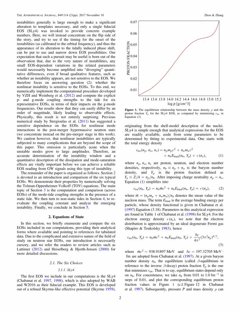
In addition to being comparatively more thorough, ShenEOS also covers broad density and temperature ranges(10 10 g cm5 15.5 3r< < - ; T0 100< < MeV). For these rea-sons, it is widely adopted in supernova simulations and neutronstar calculations. For example, Duez et al. (2010) andStergioulas et al. (2011) included the Shen EOS when studyingblack hole-neutron star mergers and the excitation of non-axisymmetric modes in the post-merger remnant, respectively.We will not go into any details about the derivation ofthis EOS, only pointing to its tabulated values on Shen’shome page: http://phy.nankai.edu.cn/grzy/shenhong/EOS/index.html. We will use these data in the context of T=0 andnote that, although they contain both ρ and P, only baryoncontributions are accounted for. To add the influence of leptonsand obtain a more complete EOS, we return to Equation (3),use the tabulated data to fill in bind at a given ρ, and thenminimize tot to extract the proton fraction Yp at β-equilibrium,which is plotted in Figure 3. The first row of Equation (4) thenprovides us with the full pressure, including the leptoncontributions. Repeating this procedure for various ρ choicesthen results in the final EOS, which is depicted in Figure 2.

2.1.3. Four APR Equations of State

APR is the abbreviation of a series of four realistic EOSsdeveloped by Akmal, Pandharipande, and Ravenhall (Akmalet al. 1998). All of them originate from nuclear physics andprovide good fits to the two-nucleon scattering data. Forconvenience, we name them APRs 1 through 4. APR1 is the“primary version” of the APR EOSs, which is constructed fromthe Argonne v18 potential that describes the interaction betweentwo nucleons. On the basis of APR1, APR2 further considersrelativistic boost effects while APR3 incorporates the Urbanamodel IX (UIX) describing interaction among three nucleons.Finally, APR4, the “complete version” of this series, includesboth the relativistic corrections and the three nucleoninteraction potential UIX. The APR EOSs, especially APR4,is commonly used in neutron star simulations, for it appears to

Figure 2. The SLy4, BBP, BPS, and Shen EOSs. The SLy4 governs only thehigh-density regime, while the segment with density below that of neutron drip( 4 10 g cmdrip

11 3r » ´ - ) is described by the BPS EOS. They are bridged bythe BBP EOS. It turns out that neutron star properties (which will be computedlater) do not depend sensitively on the BPS or the BBP EOS, and we willsimply refer to the SLy4 + BBP + BPS combination as the SLy4 EOS in thefollowing sections.

Figure 3. The equilibrium relationship between the mass density ρ and Yp forthe Shen EOS (i.e., the β-equilibrium curve; cf. Shen et al. 1998a Figure 5).

3


http://phy.nankai.edu.cn/grzy/shenhong/EOS/index.html

http://phy.nankai.edu.cn/grzy/shenhong/EOS/index.html

be compatible with astronomical observations (consult, forexample, Figure8 in Hebeler et al. 2013). Therefore, the APREOSs are often referred to as being among the “classi-cal” EOSs.

The four APR EOSs are depicted in Figure 4 (analyticexpressions of the effective Hamiltonians and the corresp-onding parameters for the four EOSs can be found inAppendix A of Akmal et al. 1998). It is apparent that for anygiven mass density, APR1 has the lowest pressure whileAPR3 has the highest. This property is referred to as the“softness” (or “stiffness”) of an EOS, describing theweakness (or strength) of the interaction between nuclearmatter. Therefore, APR1 can be classified as a (relatively)soft EOS, whereas APR3 can be called stiff. Also noticeableis the discontinuity appearing in Figure 4 for APR3 andAPR4. This discontinuity represents a phase transition fromnormal neutron fluid to a phase with pion condensation.4

Such transitions will not occur unless we consider the three-nucleon interactions, and are therefore not seen in APR1 andAPR2. Finally, it is worth pointing out that APR EOSs coveronly the high-density regime above 0.1 fm 3- (approximatelythe crust-core transition density). In our computation, weapply the FPS EOS (Pethick et al. 1995) slightly below 0.1fm 3- and continue it with the BBP EOS until the neutron dripdensity is reached. The BPS EOS is once again adopted atdensities below neutron drip. We note that our choice ofEOSs is consistent with Akmal et al. (1998) (cf. Section IV inthat paper and Lorenz et al. 1993).

2.2. Comparing the Six Equations of State

Although not large in number, our choice of the six typical(commonly invoked in literature) EOSs are extensive in the

sense that they are derived with different techniques: non-relativistic effective potential for SLy4, relativistic mean fieldfor Shen, and variational calculation (also known asvariational chain summation method or ab initio calculationfor many body system) for APR. Our typical six thus cover amajority of the approaches to modeling nuclear matter. Wecaution, however, that other models exist, including moreexotic ones, such as strange-quark (see Witten 1984, thoughit appears that quark stars predicted with this theory are notconsistent with the observation of a M1.97 neutron star, themost massive one to date (Demorest et al. 2010; Hebeleret al. 2013)).The six also cover a broad range of physical properties for

their respective predicted neutron stars. In the sphericallysymmetric case, such properties can be computed by solvingthe TOV equations:

dm

dr

r

M

dP

dr

GM

c

m

rP

r P

m M

GM

c

m

r

d

dr

GM

c

m

r

r P

m M

GM

c

m

r

4,

14

12

,

14

12

, 5

2

12 2 1

31

2

1

12 2

31

2

1

*

**

*

**

*

p r

rp

p

=

=- + +

´ -

F= + -

-

-

⎜ ⎟

⎜ ⎟

⎛⎝⎜

⎞⎠⎟

⎛⎝

⎞⎠

⎛⎝⎜

⎞⎠⎟

⎛⎝

⎞⎠

( )

( )

where m M M* = is the dimensionless mass parameter,P P c1

2= has the same dimension as ρ (g cm 3- ), andc1

2F = F is the modified gravitational potential of a testparticle with unit mass.For our concrete numerical calculations, we fix the neutron

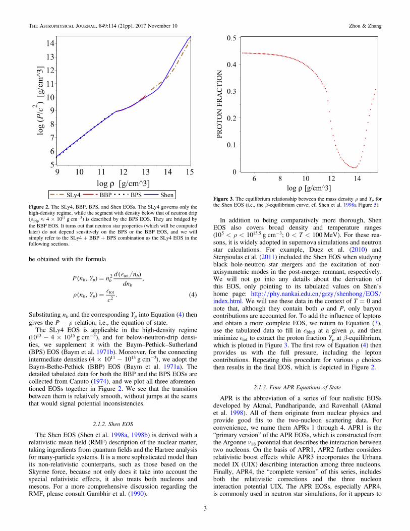
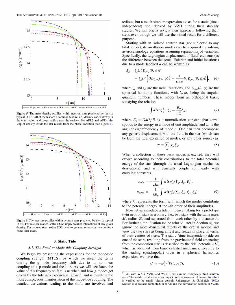
star mass at the typical value of M M1.4» . To obtain theneutron star properties, we first specify an arbitrary centraldensity cr before integrating the TOV equations until thesurface of the star (P 01 = ) is reached, at which stage we wouldhave a value for the total mass m*. Adjusting the cr value thenallows us to drive m* toward 1.4. The radii and centraldensities thus obtained for different EOSs are tabulated inTable 1. It is clear that a softer EOS has a denser core andsmaller size.Figures 5 and 6 further depict the detailed distributions of

density and pressure inside the star. Because the same overallmass is shared across all EOSs, we immediately see that softerEOSs with more matter concentrated in the core predict morecompact stars. From these figures, we can also assess thestiffness of the SLy4 and Shen EOSs. The six EOSs, orderedfrom stiff to soft, are Shen, APR3, SLy4, APR4, APR2, andAPR1, forming a rather evenly spaced sequence with no onebeing redundant.

Figure 4. Four APR EOSs. Note that the discontinuity of pressure in APR3 andAPR4 (highlighted with cyan circles) represents a phase transition from normalneutron fluid to a phase with pion condensation, which occurs when takingthree-nucleon interactions into consideration.

Table 1The Radii and Central Densities of Neutron Stars with Mass M1.4 ,

According to Different EOSs

EOS SLy4 Shen APR1 APR2 APR3 APR4

(km) 11.663 14.921 9.205 10.051 12.132 11.461log g cmc

3r -( ) 14.995 14.677 15.300 15.193 14.913 15.000

4 Transition from hadronic to quark matter is also discussed in Akmal et al.(1998). Nevertheless, as stated in the same paper, this phenomena is notexpected to happen inside a M1.4 neutron star, as is assumed for our study.

4


3. Static Tide

3.1. The Road to Mode-tide Coupling Strength

We begin by presenting the expressions for the mode-tidecoupling strength (MTCS), by which we mean the termsdriving the g-mode frequency shift due to its nonlinearcoupling to a p-mode and the tide. As we will see later, thevalue of this frequency shift tells us when and how g-modes getdriven by the tide into exponential growth, and is therefore themost conspicuous manifestation of the mode-tide coupling. Thedetailed derivations leading to the shifts are involved and

tedious, but a much simpler expression exists for a static (time-independent) tide, derived by VZH during their stabilitystudies. We will briefly review their approach, following theirsteps even though we will use their final result for a differentpurpose.Starting with an isolated neutron star (not subjected to any

tidal forces), its oscillation modes can be acquired by solvingasteroseismology equations assuming separability of variables.Specifically, the Lagrangian displacement of fluid5 elements (asthe difference between the actual Eulerian and initial locations)due to a mode labelled a can be written as

r Y r

r Y Y

,

,1

sin, , 6

a r l m

h l m l m

a a

a a a a

x x q f

x q f qq

q f f

=

+ ¶ + ¶q f⎜ ⎟⎛⎝

⎞⎠

( ) ( ) ˆ

( ) ( ) ˆ ( ) ˆ ( )

where rx and hx are the radial functions, and Y ,l ma aq f( ) are the

spherical harmonic functions, with l m,a a being the angularquantum numbers. These modes form an orthogonal basis,satisfying the relation

xdE

, 7a ba

ab3 0

2*ò x xr

wd=· ( )

where E GM02 º is a normalization constant that corre-

sponds to the energy in a mode of unit amplitude, and aw is theangular eigenfrequency of mode a. One can then decomposeany generic displacement g to the fluid in the star (which canbe from the tide, excitation of modes, or any other source) as

. 8a

a aåg xc= ( )

When a collection of these basis modes is excited, they willevolve according to their contributions to the total potentialenergy of the star (through the usual Lagrangian mechanicsderivations), and will generally couple nonlinearly withcoupling constants

x

x

Ed f

Ed f

1

2, , ,

1

6, , , , 9

abc a b c

abcd a b c d

0

33

0

34

ò

ò

x x x

x x x x

k r

k r

=-

=-

( )

( ) ( )

where fn represents the form with which the modes contributeto the potential energy at the nth order of their amplitudes.Now let us introduce a tidal influence, taking for a prototype

twin neutron stars in a binary, i.e., two stars with the same massM , radius , and separated from each other by a distance A.For further simplification (to be relaxed later in Section 4), weignore the more dynamical effects of the orbital motion andview the two stars as being at rest and frozen in place, in termsof their centers of mass. The static (time-independent) tide onone of the stars, resulting from the gravitational field emanatingfrom the companion star, is described by the tidal potential U ,which is obtained from basic celestial mechanics. Keeping tothe leading (quadrupolar) order in a spherical harmonicsexpansion, we have that

U r P cos , 1002 2

2w q» - ( ) ( )

Figure 5. The mass density profiles within neutron stars predicted by the sixtypical EOSs. All of them share a common feature, i.e., density varies slowly inthe core region and drops swiftly near the surface. For APR3 and APR4, theleap of density inside the star results from the phase transition (see Figure 4).

Figure 6. The pressure profiles within neutron stars predicted by the six typicalEOSs. For nuclear matter, softer EOSs imply weaker interactions at any givendensity. For neutron stars, softer EOSs lead to greater pressure in the core for afixed total mass.

5 As with WAB, VZH, and W2016, we assume completely fluid neutronstars. The solid crust does have an impact on core g-modes. However, its effectis verified to be small (please consult Reisenegger & Goldreich (1992)Section5.2; see also footnote 6 in WAB and the introduction section in VZH).

5


with P cos2 q( ) being the l=2 Legendre polynomial,

A3 3 º being the tidal strength, and GM03w º the

characteristic dynamical frequency. This U enters into thepotential energy and changes the equations of motion forthe fluid elements, thus causing a change to the modes; namely,the original modes of the isolated neutron star are perturbed in atidally deformed star. Applying the usual perturbation theory(similar to the familiar one from quantum mechanics), weexpect that the modal frequencies will be shifted. Indeed,detailed calculation in VZH shows that

U

U

1 2

2 3

2 ,

11

ggg

aagg a

a bagg a abgg a b

p

p gpg

aapg a

2

21

2

,

2 1 1

22

2 21

23

å

å

å

ww

k c

k c k c c

w

w wk c

= - +

- +

--

+ +

-⎛⎝⎜

⎞⎠⎟

( )

( )

( )

¯ ¯( )

¯( )

¯( ) ( )

¯ ¯( )

where w- is the perturbed g-mode frequency (the potentialinstability lies in the perturbed high-order g-modes that havesmall initial g

2w to start with (VZH), so such modes are thefocus here) when a pair of daughter p- and g-modes nonlinearlycouple to the tide. The symbol a indexes the complexconjugation of the basis vector of mode a, and the realitycondition demands that the coefficient to ax is related to itscomplex conjugate counterpart through a parity factor 1 ma-( ) .

The quantities aic( ) and Uab are defined by

xUE

d U

,

1, 12

aa a a

ab a b

1 2 2

0

3

ò

åc x

x x

c c

r

= +

=-

( )

· ( · ) ( )

( ) ( )

where the tidal deformation c is the static response of theneutron star to the tide. Worth noting are the appearances ofthree- and four-mode coupling constants in Equation (11).They are obviously there to account for the coupling betweenthe neutron star eigenmodes and the tidal deformation (as theprimary perturbation), as their contribution vanishes when

0 = . Although we have decomposed c into modal basis, andthus the overall coupling to tide into modal pieces, we candefine a “vector potential”

UE

d x U1

, 13a a0

3 *ò xr= - · ( )

and carry out resummations such as Uc ggc ckå to reassemblequantities into forms that are more directly identifiable asbeing “tidal” and more economical in notation (see, e.g., theleft-hand side of Equation (19), below). With regard tostability, previous investigations (WAB, VZH) have proventhat a apg a p g

1k c w wå ~( ) , which implies that such couplingscan be large for higher-order p-g pairs (i.e., a high-frequencyp-mode and low-frequency g-mode), and thus drive the left-hand-side of Equation (11) negative (barring any cancella-tions). This is the non-resonant p-mode g-mode instabilitydiscovered by WAB.

Before proceeding further, we note that a judicious choicefor the definition of the displacements would likely simplifycomputations. Instead of defining them as the differencebetween the Eulerian coordinates and the initial coordinatesin the isolated neutron star, the alternative of using an initialcoordinate system more suited to the tidally deformed starappears to make sense. Such an approach is adopted by VZH,who developed a novel technique called the volume preservingtransformation (VPT, briefly reviewed in Appendix B). Thistransformation maps a tidally deformed star into a radiallystretched spherical star of equal volume. By comparing thepotential energy in two coordinate systems, they arrive at thetransformation rules

U J J2 , 14abc

abc c ab ba1 1 1å k c+ = - +( ) ( )¯ ¯

( )¯( )

¯( )

and

J J J J V V

2 3

2 , 15

c dabc c abcd c d

cca cb ab ba abc c ab

,

2 1 1

1 1 2 2

å

å

k c k c c

k

+

= - + + - -

( )

( ) ( )

¯( )

¯( ) ( )

¯( ) ( )

¯( )

¯( )

¯ ¯

where the definitions of Va and Vab are formally the same asthose of Ua and Uab, but with the derivatives taken against thenew coordinates (so Va is purely radial), and Jab

i( ) is the ith order(in ò) Jacobian of the VPT.Given the rules (14) and (15), and the fact that p g

2 2w w forhigh-order p- and g-mode, the expression for the perturbedg-mode frequency becomes

J J J J J

J J J J V V

J V

J J J J J

1 2

2

1 2 2

2 2 ,

16

ggg pg gp pg gp

c p gcg cg gg gg ggc c gg

gg gg gg

gg gp pg gp gg

2

21 2 1 1 1 1

2

,

1 1 2 2

1 2

2 1 2 1 2 1 1 2

å

ww

k

k

» + - + +

+ + + - -

» - +

+ - - +

s

-

=

( )( )

( )

{ ( )

[( ) ( ) ]}( )

¯( )

¯( )

¯( ) ( ) ( )

{ }¯

( ) ( )¯( )

¯( )

¯ ¯

( )

( ) ( ) ( ) ( ) ( )

where Vab c abc ck kº ås . The sign in the third line ofEquation (16) is determined by mp and mg. A plus signcorresponds to even mp and mg,

6 while odd mp and mg give theminus sign. The right-hand side of Equation (16) represents theimpact of the tide on the g-mode that is coupled to it.Comparing Equation (16) with Equation (11), we see that, afterthe VPT, the explicit four-mode coupling term drops out,greatly simplifying the derivation. We also note that the lastline in Equation (16) is in fact much smaller than the rest of theterms on the right-hand side (an explanation is provided inAppendix A), so we can drop it to obtain

J V1 2 2 . 17g

gg gg gg

2

21 2 w

wk» - +s

- [ ( )] ( )( )

Because only mp g, choices that lead to potential instabilities areof interest to us, we specialize to the cases where the minussign is taken above. The remaining Jacobian contribution to

6 The p-g pair must share the same parity in order to satisfy the selection rule.

6


Equation (17) is given by (VZH Equation (89))

JE

I , 18ggg

gg1

2

0

1 w

= - c ( )( ) ( )

and the integral Igg 1c( ) is given by Equation (50) (VZH Equation(81)). With static tide, this Jacobian term appears at ( ) and isnon-negligible when the two neutron stars are far apart.However, it makes a much smaller contribution (see Table 2below) in the more interesting late-inspiral regime. Therefore,although we compute its values (the details are provided inAppendix A) for completeness, we will exclude it from thedefinition of the MTCS. Instead, we will refer to the absolutevalue of V2 gg gg

2 k +s( ) as the MTCS—and note that itsdetailed expression is provided by VZH Equation (99), whichwe reproduce here:

g

g

g

g

V

Edr r P

r P r gd

dr r

r rg g Pd

dr r

rd

drr

dV

dr

rg gd

d r

MTCS 2

11

ln

4

2 2

2ln

ln, 19

gg gg

s

r

r r rr

g g h r rr

r

r r r

2

0

21 1

1

2

12 3 2

2

2

2 2 2 21

2 2

2

òs

k

r

s rs

w rs

rs

r

r

º +

=- G G + +¶G¶

´

- G -

- L + G

+ - +

´ +

s

⎜ ⎟

⎜ ⎟

⎪

⎪

⎧⎨⎩

⎡⎣⎢⎢

⎛⎝⎜

⎞⎠⎟

⎤⎦⎥⎥

⎛⎝

⎞⎠

⎛⎝

⎞⎠

⎡⎣⎢

⎛⎝⎜

⎞⎠⎟

⎤⎦⎥

⎡⎣⎢

⎤⎦⎥

⎫⎬⎭

∣ ∣

( )

( · )( · )

( · )

[ ( · ) ]

( · ) ( )

g

gg

where l l 1g g g2L º +( ). We will discuss the quantities appearing

in Equation (19) in more details below, but mention that thederivation of this equation has invoked the Cowling approximation,i.e., it neglects the Eulerian perturbation to the gravitationalpotential (denoted F¢). The Cowling approximation is reasonablefor high-order modes because, when the radial and angularquantum numbers n and l are large,F¢ is very small as compared tothe Eulerian perturbations to the density ρ and the pressure P (seeChristensen-Dalsgaard 2014 Ch. 5.2).

3.2. The Ingredients of the MTCS

As Equation (19) is central to our analysis, we devote thissection to explaining the quantities appearing in it anddemonstrating how to compute them.

3.2.1. g and 1G

The symbol g refers to the local gravitational acceleration.Following VZH, we define d drº Fg rather than the usual= -Fg . Here, Pln ln s1 rG º ¶ ¶( ) is the adiabatic index,

which is in principal not the same as the polytropic exponentd P dln ln rG º in the equilibrium state. The appearance of 1G

in Equation (19) implies that only adiabatic oscillation isdiscussed in this paper. That is, we assume that the system isthermally isolated and the entropy does not change ( s 0D = )throughout our discussion. We can obtain g straightforwardlyby solving the TOV Equation (5), while 1G must be derivedfrom the EOS itself.

3.2.2. gr and gh

The functions gr and gh are the radial and horizontalcomponents of the g-mode eigenfunction (see Equation (6)).They are governed by the equations of oscillation (Unnoet al. 1989 Equations (13.1)–(13.3))

r

d

drr g

cg

l l c

r

P

c

l l

r

dP

dr cP N g

d

dr

r

d

drr

d

dr

l l

rG

P

c

Ng

11

1

1,

1,

1 14 .

20

rs

rg g s

g s

g g

g

sg r

g g

sr

22

2

2

2 2 2

2 2

22 2

22

2 2

2

w r

w

r rw

p rr

- + -+ ¢

=+

F¢

¢+ ¢ + - = -

F¢

F¢-

+F¢ =

¢+⎜ ⎟

⎛⎝⎜⎜

⎞⎠⎟⎟

⎛⎝

⎞⎠

⎛⎝⎜

⎞⎠⎟

( )( )

( )

( )

( )

( )

g

g

g

gr

P1, 21h

g2w r

=¢+ F¢

⎛⎝⎜

⎞⎠⎟ ( )

where c Ps 1 rº G is the adiabatic sound speed, with a valueof c c0.1s ~ in the neutron star center, and must not exceed thespeed of light c anywhere by causality. In this equation, P¢ andF¢ are the Eulerian perturbations to the pressure and thegravitational potential due to the g-mode, respectively, and N iscalled the buoyancy frequency (also called the Brunt–Väisäläfrequency; please see further discussions in Section 3.2.3).Equation (20) is the standard equation system describing thenon-radial oscillations of the star, originating from the continuityequations, the hydrostatic equations for fluids, and the Poissonequation; it is simplified to this form under the assumption ofadiabatic oscillation. We solve Equations (20) and (21) for g g,r hand the eigenfrequency gw numerically, using the Aarhusadiabatic oscillation package (ADIPLS; please consult Christen-sen-Dalsgaard 2008 for a thorough introduction to the ADIPLS

Table 2The MTCS and the Jacobian Contributions to the Frequency Shift, under a

Static Tide and for lg=4, n=32 g-modes

EOS A 100 km= A 2=MTCS Jgg

1 ( ) MTCS Jgg1 ( )

SLy4 1.30×10−3 −1.08×10−4 8.04 −8.51×10−3

Shen 1.18×10−4 −2.31×10−4 0.167 −8.70×10−3

APR1 3.34×10−5 −5.36×10−5 0.857 −8.59×10−3

APR2 2.20×10−5 −6.05×10−5 0.333 −7.44×10−3

APR3 4.11×10−5 −1.18×10−4 0.201 −8.26×10−3

APR4 2.91×10−5 −9.46×10−5 0.201 −7.85×10−3

Note. The neutron star radius corresponding to each EOS is displayed inTable 1.

7


and its usage) with the boundary conditions of

g l g

d

dr

l

r

,

, 22

r g h

g

=

F¢= F¢ ( )

at the center (r= 0) and

Pd

dr

l

r

0,1

, 23g

d =F¢

=-+

F¢ ( )

on the surface ( Pd represents the Lagrangian perturbation topressure).

An example lg=4, n=32 g-mode under the SLy4 model isdemonstrated in Figure 7. It is obvious that fluid elementsoscillate severely in the deep interior of the star; in contrast, theoscillations become relatively subdued near the surface. This istypical of g-modes (see, e.g., Figure5.10 in Christensen-Dalsgaard 2014). Additionally, we clarify that, in order to beconsistent with WAB, VZH, and W2016, the normalizationrule for gr and gh (equivalently, the definition of thenormalization constant E0) in this paper is given byEquation (7), rather than Equation(36) in Christensen-Dalsgaard (2008).

Another associated constituent appearing in Equation (19) isg r( · ) , the radial component of the divergence of the g-mode

displacement vector. Its expression is given by

gP

g rg , 24r r g h1

2rw =

G- + F¢( · ) ( ) ( )g

which is actually equivalent to the first equation in (20).7 Interms of numerical computations, it is safe to ignore the lasttwo terms in Equation (24) because neither of them iscomparable with the first one throughout the entire neutronstar. For our neutron star models, F¢ is a mere one-thousandth

in magnitude, as compared to grg , and the second term is evensmaller than F¢ for low-frequency g-modes.

3.2.3. N

The buoyancy frequency N, although not present explicitlyin Equation (19), does have an indirect influence on the MTCSthrough its strong impacts on gr and gh (Equation (20)). Thus,we devote this subsection to the computation of N. The fulldefinition for the buoyancy frequency is

Nc c

1 1, 25

e s

2 22 2

º -⎛⎝⎜

⎞⎠⎟ ( )g

where c dP de rº is called the equilibrium sound speed.However, Equation (25) is not suitable for numerical evalua-tion, because the difference between c1 e

2 and c1 s2 is tiny so

the subtraction operation may not be accurate. Instead, we plugLai (1994) Equation (4.7) into Equation (25) to get

Nc c

P

Y

dY

d. 26

e s p

p22

2 2 r= -

¶¶

r

⎛⎝⎜

⎞⎠⎟

⎛⎝⎜

⎞⎠⎟ ( )g

Because the discrepancy between ce2 and cs

2 is small, it isadequate to make the following approximation

Nc

P

Y

dY

d. 27

e p

p22

4 r» -

¶¶

r

⎛⎝⎜

⎞⎠⎟

⎛⎝⎜

⎞⎠⎟ ( )g

This equation is what we use to numerically calculatebuoyancy frequency. The expression P Yp¶ ¶ at fixed ρ anddY dp r can be computed from the EOS.

Even though Equation (25) is a universal definition for N, wedo not use it in every part of the star. As stated in Section 3.1(and will be once again emphasized in Section 3.3), we assumecompletely fluid neutron stars and confine our discussions tocore g-modes. This assumption leads to the restriction thatN=0 throughout the crust, which signifies the vanishing ofcrust g-mode.What is more, under this assumption, it is necessary to

determine the exact critical density at which the crust-coretransition occurs (in other words, the position where N is cutoff) for each EOS. For SLy4, because it is combined with theBBP EOS in the crust-core transition region, we adoptthe critical density determined by Baym et al. (1971a), withthe exact value of 2.4 10cut

14r = ´ g cm 3- (Baym et al. 1971aSection10). For the APR EOSs, the crust-core transition isexpected to occur at nb=0.1 fm−3 (corresponds to

1.67 10cut14r = ´ g cm 3- , see Akmal et al. 1998 and Pethick

et al. 1995 Table 1). However, for Shen, the crust-coreboundary is not specified, so we determine it by choosing theposition where Yp hits its minimum. This is also the criterionadopted in Lai (1994) to distinguish the core g-modes fromtheir crust counterparts (cf. Section 4.1 in that paper).To conclude, we use Equation (27) to compute N in the core

and set N=0 throughout the crust, the crust-core boundary isspecified for each EOS individually. The numerical results weobtain are presented in Figure 8.

3.2.4. V

The external potential V (in the next-to-last line ofEquation (19)) is derived through the VPT. It represents, but

Figure 7. The scaled radial function for a lg=4, n=32 g-mode withfrequency f 2.7 Hzg » . gr, as well as fg, are computed with the ADIPLS

package within the SLy4 model.

7 To find the connection between Equations (20) and (24), one couldsubstitute the definition of divergence (VZH Equation (96)) and Equation (21)into Equation (24).

8


is not exactly equivalent to, the tidal potential; its expression is(see Equation (48) of VZH)

V rn r

10

6. 280

4 3w= -

-( ) ( ) ( )g

The quantity n is defined as d d rln lng , and has the value ofn 1» in the neutron star core, so we can regard it simply as aconstant.

3.2.5. s and rs

The vector s is the displacement from unperturbed star toradially stretched spherical star (after the VPT), and rs is theradial component of s after separation of variables (hereafter,we will refer to it as the radial displacement).

To solve the radial displacement rs , we use the VZHEquation (96) (the definition of divergence) and 98 (the radialequation of motion), which in our case are

d

dr rd

drP

r

d

dr

d

dr

2,

2. 29

rr

r

r r1tide

s

s

ss

rs r

= +

G =- - +F¢⎜ ⎟⎛

⎝⎞⎠

( · )

[ ( · ) ] ( )g g

The validity of these equations is subtle, as the radial “mode” isnot a normal mode of the star. We refer readers to thediscussion in VZH for more details, but note that only tidalperturbation to the potential tideF¢ is present in Equation (29),and is given by the external potential in Equation (28),

V r . 30tide2F¢ = ( ) ( )

The absence of F¢ (perturbation by g-modes) is a result of theCowling approximation.8 Combining the two equations in (29),we obtain

d

drP r

dX

drX r

d

drX

n n

A

GM

c

r

3 2

3 6

10, 31

1 1 11

6 2

2 2

1

r

r

G + = - +

-- -

⎜ ⎟

⎜ ⎟

⎡⎣⎢

⎛⎝

⎞⎠

⎤⎦⎥

⎛⎝⎜

⎞⎠⎟

⎡⎣⎢

⎛⎝

⎞⎠

⎤⎦⎥

( )( ) ( )

gg

g

with the dimensionless radial displacement X rrsº ,P P c1

2º , and c12ºg g . We numerically solve this ordinary

differential equation (ODE), with the neutron star EOSs listedin Section 2.2, and the initial conditions of

X X0 0, 0 0. 32= ¢ =( ) ( ) ( )

The condition X 0 0=( ) is a consequence of there being noradial displacements at r=0, while X 0 0¢ =( ) is demanded bythe ODE itself after setting X 0 0=( ) . For demonstration, theresulting X is displayed in Figure 9, assuming a binaryseparation of A 100 km= . We also note that, to a goodapproximation, X r Ar

6sº µ - . Therefore, the X valuescorresponding to other A choices not shown in the figure canbe estimated by a simple rescaling.Notice that the radial displacement rs is negative, indicating

that the static tidal force actually compresses the star. FromFigure 9, one additionally notices that the star governed by asoft EOS has a comparatively small radial displacement, i.e.,less deformed by the tidal force. The fact that a “soft” star ismore rigid than a “stiff” one can be explained by Figures 5 and6: “softer” stars are denser and have higher inner pressures; inother words, they are more tightly bound.

Figure 8. The distribution of buoyancy frequency in the neutron star core.Here, Rboundary is the radius where crust-core transition takes place. Thediscontinuities of N2 in APR3 and APR4 are due to a phase transition (seeSection 2.1.3). Note that the buoyancy frequency for SLy4 model isextraordinarily small as compared to others, which has a profound effect onthe MTCS that will be explained below.

Figure 9. The radial displacement measure X rrs= in the neutron starinterior, as computed by solving Equation (31). Notice that the star obeying theShen EOS has the largest displacement, which implies a comparatively severetidal deformation. This feature was also observed in numerical simulations (see,e.g., Stergioulas et al. 2011).

8 In order to be self-consistent, the computation of the radial displacement rsmust be confined to be under the Cowling approximation, as rs is directlyrelated to the VPT that is based on that approximation.

9


3.3. The Results

Now that we have discussed the quantities appearing in theMTCS, the natural subsequent step is to turn to its evaluation.However, before proceeding further, we shall rewriteEquation (19) into a different form that is more amenable tonumerical evaluation. With the simplification discussed in theend of Section 3.2.2, Equation (28), and the first equation of(29), we have that Equation (19) finally turns into

V

Edr g c

rdX

drX

r

cX

r

c

r rc

g

g

dX

drr

d X

dr

rdX

drr X r X

d

dr

n n r

A

GM

c

r

c

d

d r

MTCS 2

11

ln

ln

3 4

2 2

6 3

10

2 ln

ln, 33

gg gg

rs

s s

gg h

r

s

2

0

2 21

1

212

12

212

12

2 22

2

2

2 1 13

2

2

21 1

2 1

3

61

2

2

1

12

ò

k

rr

w

r

º +

»- G + +¶ G¶

´ + -

- L + -

´ - - +

-- -

´ +

s

⎜ ⎟

⎜ ⎟

⎪

⎪

⎪

⎪

⎧⎨⎩

⎡⎣⎢⎢

⎛⎝⎜

⎞⎠⎟

⎤⎦⎥⎥

⎛⎝

⎞⎠

⎛⎝⎜⎜

⎞⎠⎟⎟

⎡⎣⎢

⎛⎝

⎞⎠

⎤⎦⎥

⎛⎝⎜

⎞⎠⎟

⎫⎬⎭

∣ ∣

( )( )

( )

g g

g g

g gg

g

g

where c c cs s1 = .Now we are ready to perform the MTCS calculations for the

static tide, using formula (33). We impose the neutron starproperties of Section 2 and gr, gh, and X as computedrespectively in Sections 3.2.2 and 3.2.5. The choice of binaryseparation is somewhat arbitrary because the MTCS, as awhole, is approximately proportional to A 6- . Furthermore, wenote that the radial function gr and the dimensionless radialdisplacement X (as well as its derivatives) are present in almostevery term of Equation (33), so they do, in fact, exertsignificant influences on the magnitude of the MTCS.

We tabulate the MTCS results for the six EOSs in Table 2,and display their “cumulative distribution” within the neutronstar in Figure 10, in which the horizontal axis represents theupper limit of the integral in Equation (33) (i.e., we stop theintegration prematurely at some radius before , to show howmuch different parts of the neutron star contribute to theMTCS). In WAB, it was proven that the three-mode coupling isstrong in the core region (WAB Section 3.2). However, we seefrom Figure 10, after taking the four-mode interaction intoconsideration, that MTCS becomes nearly zero for all EOSs,suggesting that the cancellation between the three- and four-mode couplings, as revealed by VZH, is near-exact in the core.In contrast, in the outer half of the star, the near-exactcancellation begins to collapse, and MTCS grows rapidly nearthe crust-core interface. To explain this phenomenon, we notethat a hint is provided by Figure 9; namely, both the (absolute)value and the slope of X, the frequently appearing variable inEquation (33), inflate significantly as r approaches the crust-core interface.

Meanwhile, it should be emphasized that our treatments donot apply in the crust (a solid stratification with a densitybetween 10 g cm6 3- and the crust-core transition density cutr

(Shapiro & Teukolsky 1983 Ch. 9.3)) because the neutron starmatter is assumed to be of a fluid nature everywhere, which isnot a valid description of solid regions. Therefore, we terminatethe integration in Equation (33) at cutr r= (geographically,r Rboundary= ). However, as shown by Reisenegger & Goldreich(1992), the crust and the surface do not sustain core g-modes(cf. Figure 3 in that paper) so that errors induced by halting theintegration before reaching are unlikely to be large if we, aswith the previous studies on the topic of g-mode stability,confine our discussion to core g-modes.Now that we have had a glimpse of the general

characteristics of the MTCS, we turn to its EOS dependence.Because the MTCS is composed of many variables, and each ofthem, to a greater or lesser extent, depends on the specificchoice of the EOS, it is difficult to determine at first glancewhich EOS will predict a stronger MTCS and which leads to aweaker one. However, if we omit the result of APR1 and theabnormally large MTCS of SLy4 for now, and focus on theother four, we shall discover that the ranking of MTCSs for thefour EOSs is in line with the ranking of their stiffness(cf. Section 2.2). Consequently, one may speculate that thecoupling to tide tends to be stronger in stars with stiffer EOSs.Indeed, as discussed in Section 3.2.5 and depicted in Figure 9,stars predicted by softer EOSs are less severely deformed bythe tidal force, i.e., they have smaller X. To be more specific,we can use APR2 (a soft EOS) and APR3 (a relatively stiffEOS) for comparison (from the same family, thus giving acleaner comparison). Our numerical result shows that, in mostparts of the core, the dimensionless radial displacement (as wellas its first and second derivatives) for stars governed by APR3is roughly twice that given by the APR2 EOS, which isconsistent with the value of MTCS for the APR3 model beingapproximately twice that of its APR2 counterpart.Besides greater X, a stiff EOS also leads to larger

inhomogeneous terms that contain the external potential V.

Figure 10. The MTCS under static tide. The horizontal axis is the upper limitof the integration in Equation (33). The binary separation is set at A 100 km= ,and all g-modes share the same degree (lg=4) and radial order (n = 32) forthis figure.

10


Specifically, the inhomogeneous term in Equation (33) is

n n

A

GM

c

r6 3

10. 34

6 2

2 3

11

1-- -

µ -⎜ ⎟⎛⎝

⎞⎠

( )( ) ( )g

g

Applying the TOV Equation (5), we further obtain thatM m r P41

31* pµ +g . Because the star mass is fixed in our

computation, the equation above then tells us that a softer EOSwith a higher interior pressure (see Figure 6) corresponds to asmaller inhomogeneous term (as expected, because thegravitational acceleration is stronger in more compact starspredicted by softer EOSs).

So far, the picture is that stiffer EOSs predict less compactand larger neutron stars (Figure 5 and Table 1), which are moreeasily deformed by tidal forces (Figure 9) and possess largerinhomogeneous terms, leading to stronger mode-tide couplings.However, our analysis is not complete yet, as we havedeliberately overlooked the results for APR1 and SLy4. Forthese two EOSs, there is no apparent correspondence betweenstiffness and the MTCS. Especially striking is the MTCS forSLy4; regarding stiffness, SLy4 is only an intermediate EOS,yet it predicts extremely strong coupling that is far in excess ofthe other five. Hence, there must exist other (at times moredominant) factors to account for the conspicuously large MTCSfor SLy4.

A careful scrutiny of Equation (33) reveals that gr, the radialcomponent of the g-mode eigenfunction, also plays animportant role in determining the mode-tide coupling. This isphysically reasonable, as larger intrinsic modal deformationsshould enable greater overlaps with tidal deformations. Thequestion that arises then is: when the degree (lg) and the radialorder (n) of the g-mode is fixed, what kind of EOSs will give alarger g-mode amplitude? To answer this question, we employthe Wentzel–Kramers–Brillouin (WKB) method to provideanalytic forms for the g-mode eigenfunction. The WKBmethod (for a detailed introduction to the method and itsapplications to stellar oscillations, please refer to standardtextbooks such as Christensen-Dalsgaard 2014) is a satisfactoryapproximation for high-frequency p-modes and low-frequencyg-modes (we will only use it for explanatory illustrations here,so the results in this paper are not bound by the applicability ofthe WKB). Under the Cowling and the WKB approximations,the solution of Equation (20) is

gA

Nk r

E

r

k r

N

gA

k rE

r

k r

sinsin

,

coscos

, 35

rg

gg g

hg

g gg

g g

g g

0

2

0

2

ar

wa

r w

=

L=

L

( )( )

( )( )

( )

where (WAB Section 3.2)

N

rNd rln

0.4, 36g

1

òa º »-( ) ( )

and kg is the g-mode wave number given by k N rg g gwL ( ).From Equations (35) and (36), we see that the factor g Er

20r in

Equation (33), as a whole, is roughly in inverse proportion toN2. That is, when other variables are controlled, EOSs withsmaller buoyancy frequency through the neutron star core areexpected to sustain larger g-mode amplitudes, resulting instronger couplings. We are now able to provide an explanationfor the case of SLy4. Figure 8 shows that the N2 calculated with

SLy4 is two orders of magnitude smaller than with the otherEOSs across nearly the entire core region. Accordingly, theinverse proportion relation then gives much greater g Er

20r as

compared to the other models, and subsequently a large MTCS.To sum up the relationship between static MTCSs and the

EOSs: two dominant ingredients, the stiffness of the EOS andthe buoyancy frequency predicted by the EOS, affect theMTCS simultaneously. In other words, the mode-tide couplingdepends on the description of high-density nuclear matter in arather sophisticated way; both the property of nuclear matter inβ-equilibrium (i.e., the stiffness of EOS) and away fromequilibrium (represented by the buoyancy frequency) wouldhave an impact on the coupling strength.Now that the properties of the MTCS have been discussed,

we briefly turn to the Jacobian term Jgg1 ( ). According to

Table 2, at A 100 km= , Jgg1 ( ) is approximately one tenth of the

MTCS in the SLy4 model, comparable with the MTCS forShen, but several times the size of the MTCS for the APREOSs. However, because J Agg

1 3 µ -( ) (see Equation (53)) whileAMTCS 6µ - , the MTCS gradually gains dominance as the

binary winds tighter. As for the EOS dependence, like MTCS,the exact values of Jgg

1 ( ) also vary from one EOS to another: thestiffer the EOS we choose, the larger the Jgg

1 ( ) we get.Aside from examining the MTCS’s (as well as the

Jacobian’s) dependence on the EOSs, we also confirm VZH’sresult directly, i.e., that the non-resonant instability does notoccur in the case of static tide during early inspiral stage (VZHSection 4.2). Over and above that, VZH’s assertion can beextended to the entire evolution process of neutron starbinaries. To achieve this, we compute the MTCSs as well asthe Jacobians in the extreme situation of A 2= , when thetwo stars are well into the merger phase. Nevertheless, fromTable 2, we see that both MTCS and Jgg

1 ( ) are less than 1 forShen and APR1-4 EOSs (with SLy4 the only exception), and

J V1 2 2 0 37g

gg gg gg

2

21 2 w

wk» - + + >s

- ∣ ∣ ∣∣ ( )( )

representing stable g-modes. In other words, for most EOSs,the onset of instability due to the static tide is avoided all theway up to merger, not just during the early inspiral period whentwo stars are far apart. It should, of course, be pointed out herethat our formalism actually breaks down at A 2= . At such aclose distance, higher-order tidal potentials should be included.For example, the l=3 (octupole) term is no longer negligible.However, higher-order terms are always smaller than theleading order (in the case of A 2= , the octupole term is lessthan half of the quadrupole one). We therefore expect thequalitative, although not the quantitative, conclusion to remainvalid, even with a more thorough treatment of the mergerphase.In this section, we have demonstrated that nonlinear mode

couplings to the static tide depend on neutron star EOS—rathersensitively, in fact. However, the baseline MTCS value is verylow, so the nonlinear effect is likely too small to be detectablein the static tide scenario. Interestingly, however, more recentresults by W2016 suggest that the situation appears to bedifferent when one considers the non-static tide (through theinclusion of the m 2= harmonics). We turn to this casebelow, and show that the sensitive EOS dependence ispreserved (as is to be expected because the qualitative

11


consequences of the differences in EOSs invoked so far do notrely on the tide being static).

4. Non-static Tide

We turn now to the non-static tide, and show that thetemporal variation introduces highly nontrivial effects, and sothe behavior of the resulting MTCS changes significantly.Above all, we emphasize the compressible nature of the non-static tide in Section 4.1, demonstrating that it does notpreserve the volume of the star at leading order and maytherefore already result in the resurrection of the instability atthis order. We then move on to evaluate the first order MTCSin Section 4.2 to verify that this is indeed the case. It turns outthat it is not straightforward, at least not in an airtight, rigorousmanner, to adapt the VPT method to the time-dependent case,so we evaluate the MTCS using its non-VPT-treated originalexpression instead. With the results thus obtained, we discussin Section 4.3 the general features of the MTCS and thesensitive EOS dependence it exhibits, before interpreting theobservational consequences of these findings in Section 4.4.

4.1. The Compressible Nature of Non-static Tide

Non-static tides are more realistic for inspiraling binaries. Inthis context, the tidal force comes from a companion star that isin circular motion rather than standing still. The sphericalharmonic expansion of the full tidal potential Ufull is (Lai 1994Equation (2.2))

U GM Wr

AY e, . 38

l mlm

l

l lmim t

full,

1 å q f= -

+- W( ) ( )

Like W2016, we keep the leading quadrupole term (W2016Equation (3)) to get

U r W Y e, , 39m

m mim t

full 02 2

2

2

2 2åw q f» -=-

- W( ) ( )

where the coefficients Wlm depend on (l, m), particularly withW 520 p= - , W 02, 1 = , and W 3 102, 2 p= . The m=0term in Equation (39) is the previously discussed static tide,while the m 2= harmonics refer to the non-static tide, ascharacterized by the presence of the orbital angular frequencyΩ. Although the differences between static and non-static tidescome only through the e im t- W factor, the latter is neverthelessaccompanied by important new effects. For example, the non-static tide is now able to (a) excite g-modes in compact binariesby the resonant excitation mechanism (Lai 1994; Fuller & Lai2011) and (b) change the volume of the star at leading order(W2016). Although observation (a) has an impact on thenonlinear mode coupling (see W2016 Figure 9; it accounts forthe fluctuation in the MTCS with binary separation), it is (b)that spoils the near-exact cancellation and raises the MTCSorders of magnitude larger. Here, we go into some details andprovide a brief description for the consequences of (b).

Beginning with the basic hydrodynamic equations and thenon-static tidal potential, W2016 gave the expression for thefirst-order (in ò, similarly hereinafter) tidal displacement 1c( )

and showed that (W2016 Equation (62))

m

N c

d

d r

1

2

ln

ln, 40

sr

12

2 ,st1c r

cW ⎜ ⎟⎛

⎝⎞⎠· ( )( ) ( )g

where r,st1c( ) is the radial component of the first-order tidal

displacement we had with static tides. With Equation (40), it isobvious that 01c =· ( ) in a static tide ( 0W = ), so we had aninvariant volume at leading order. In other words, after VPT,the new spherical star is exactly the same as the unperturbedone (at leading order), meaning there is no first-order radialdisplacement (i.e., 0r

1s =( ) ). Consequently, the first-orderexternal potential V 1( ) vanishes (see Equation (30); the tidalpotential enters at the second order). On the other hand, 0W ¹leads to a nonvanishing divergence for 1c( ) (termed the “finitefrequency correction to linear tide” in W2016) and subse-quently nonvanishing r

1s( ) and V 1( ) (elaborated in Appendix B)that significantly alters the situation. Namely, as noted inSection 3.3, the radial displacement and the inhomogeneousterm are two crucial constituents in the expression of MTCSand make non-negligible contributions to the coupling strength,so one should thus expect the MTCS to become roughly 1 times larger in a non-static setting.To investigate the EOS dependence, explicit computations of

the MTCS are needed. In principle, both the first- and second-order contributions to the frequency shift in Equation (11)should be evaluated. The second-order frequency shift, whichcontains the four-mode coupling constant and the second-ordertidal displacements, has already been carefully scrutinized byW2016, and its effects are embodied by the three- and four-mode residual term Rgg in that paper. However, we further notethat because 01c ¹· ( ) , 0r

1s ¹( ) andV 01 ¹( ) , the first-ordercontribution also ceases to be an insignificant piece in the caseof non-static tide. To quantify this leading-order effect (thoughnot always greater in value than higher-order terms, as we willelaborate below), we compute the first-order MTCS using theformalism developed by Weinberg et al. (2012) (WAQB). Thismore direct—but also more computationally intensive—method is needed due to the difficulties in generalizing theVPT to the time-dependent case (see Appendix B for details).

4.2. The First-order Mode-tide Coupling Strengths

Because a rotating tidal force does not preserve the volumeof a star even at the linear order in ò, we neglect all higher-ordercontributions in the rest of this chapter, and concentrate onexpounding how the first-order MTCS is computed.To begin with, we note that the g-mode frequency shift

resulting from tidal perturbations, kept to leading order, isgiven by (Equation (11))

U1 2 . 41g

gg gg

2

221 w

wk= - + +c

- ∣ ∣ ( ) ( )( )

Just as in Section 3.1, the absolute value of the first-orderMTCS (hereinafter simply referred as the MTCS) is takenbecause we are only concerned with the frequency shift thatmay lead to instabilities. Meanwhile, as mentioned in WAQBand VZH, the g-mode, g-mode, tide coupling constant gg1kc( )

can be separated into a homogeneous part in which the tidaldisplacement is treated using normal modes, and an

12


inhomogeneous part that accounts for the tidal perturbation tothe gravitational potential, specifically

U1 2 2 . 42g

gg gg I gg H

2

2 , ,21 1 w

wk k= - + + +c c

- ∣ ∣ ( ) ( )( ) ( )

The homogeneous three-mode coupling constant gg H,1kc( ) wasoriginally derived in WAQB Appendix A, while the rest of theMTCS is given by WAQB Equation A71. Here, we rearrangeand simplify them under the Cowling approximation, into

g

g

g

g

U

Edr T r c

T rc g g

Td

d rr

d

drg

T r rd

drg

g

MTCS 2 2

11

ln

ln

2 4

4

ln

ln4

4

2 43

gg gg I gg H

s

sr

s r h g r

r h r

r r

r

r r r

, ,

0

2 21

1 1 2

2 1 2

2 1 2 1

1 2

1 2

1

1 1

ò

c

c

c

k k

r

r

r

c c

rr

c

r

c

º + +

» G +

+¶ G¶

+ L -

+ L -

+ +

+ +

+

c c

c

⎜ ⎟

⎜ ⎟

⎛⎝⎜

⎞⎠⎟

⎤⎦⎥⎥

⎛⎝

⎞⎠

⎛⎝

⎞⎠

∣ ∣

{ [

· ( · )

[ · ( · ) ( )

( · ) ( )]

[ ·

( · ) ] ( )

( )

( )

( ) ( )

( )

( )

( )

( ) ( )

gg

gg

r g g G G G

r g g F F F

r g g F F F

r g g F F F

r g g F F T

r g g F F T

r g g F F T

3 3 2

3 3 2

3 3 2

6

6

6

44

h h h g g g g

r h h g g g g g g

h r h g g g g g

h r h g g g g g

h r r g g g g

r r h g g g

r r h g g g

1 2 2 2

1 2 2 2 2 2

1 2 2 2 2 2

1 2 2 2 2 2

1 2 2 2

1 2 2 2

1 2 2 2

r c w w w

r c w w w w w

r c w w w w w

r c w w w w w

r c w w w

r c w w w

r c w w w

- + +

- - - - +

- - - - +

- - - - +

+ + -

+ + -

+ + -

c c

c c

c c c

c c c

c

c c

c c

( )

[( ) ( )]

[( ) ( )]

[( ) ( )]

( )

( )

( )}( )

( )

( )

( )

( )

( )

( )

( )

gWT l

Mdr r

rg rg

2 ln

ln2 , 45lm l

lr r r2

ò rr

-+ ¶

¶+

⎡⎣⎢

⎤⎦⎥

( ) ( · ) ( )

where mw º Wc , and the subscript “χ” denotes those entitiesrelevant to the tide. The quantities T, Fa, and Ga, on the otherhand, are angular integrals defined via Equation (52). Theexpression above is applicable to both static and non-statictides. In the former case, we have zero orbital frequency( 0W = ) and 01c =· ( ) , while r

1c( ), h1c( ) are given analyti-

cally in Equation (51). Using these constrains to furthersimplify Equations (43)–(45), one will find that lines (43) and(45) cancel out and the MTCS reduces into lines (44) (with

0w =c ), which is comparable to the first-order Jacobian Jgg1 ( )

in magnitude. Therefore, under static tide, no instability willoccur at leading order (nor in second order, as concluded inSection 3). In contrast, under the circumstance of a non-statictide, although the definitions of c and g remain similar to thestatic case, they pick up an additional exponential factor e im t- W .Carrying out the separation of variables in the same way as in

W2016 Equation (50), we obtain

g

r r r r Y e

g r r rg r Y e

,

. 46r h h lm

im t

r h h lmim t

c c cº +

º +

- W

- W

[ ( ) ˆ ( ) ][ ( ) ˆ ( ) ] ( )

This innocuous-looking alteration to c induces deep-reachingchanges in the magnitude of MTCS. Specifically, it spoils theexact cancellation between lines (43) and line (45), therebyraising the MTCS orders of magnitudes larger. The finiteorbital frequency also makes analytic solutions for the lineartide difficult to acquire, so instead, the radial and horizontalcomponents of the linear tide, i.e., r

1c( ) and h1c( ), are now

obtained numerically by solving the forced oscillation equation(similar to the free oscillation Equation (20), but contain tidalforcing terms; cf. Equation (73) in Appendix C) at a fixedbinary separation A, using the shooting technique (alsointroduced in Appendix C). The result for r

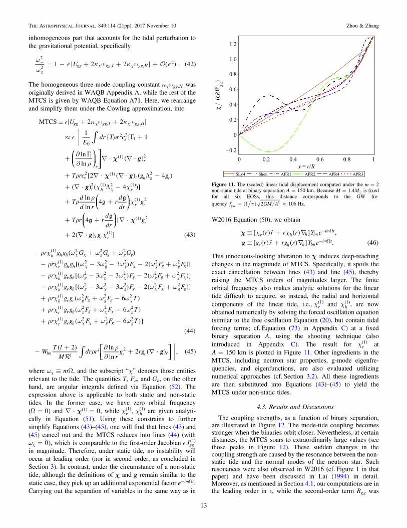
1c( ) atA 150 km= is plotted in Figure 11. Other ingredients in theMTCS, including neutron star properties, g-mode eigenfre-quencies, and eigenfunctions, are also evaluated utilizingnumerical approaches (cf. Section 3.2). All these ingredientsare then substituted into Equations (43)–(45) to yield theMTCS under non-static tides.

4.3. Results and Discussions

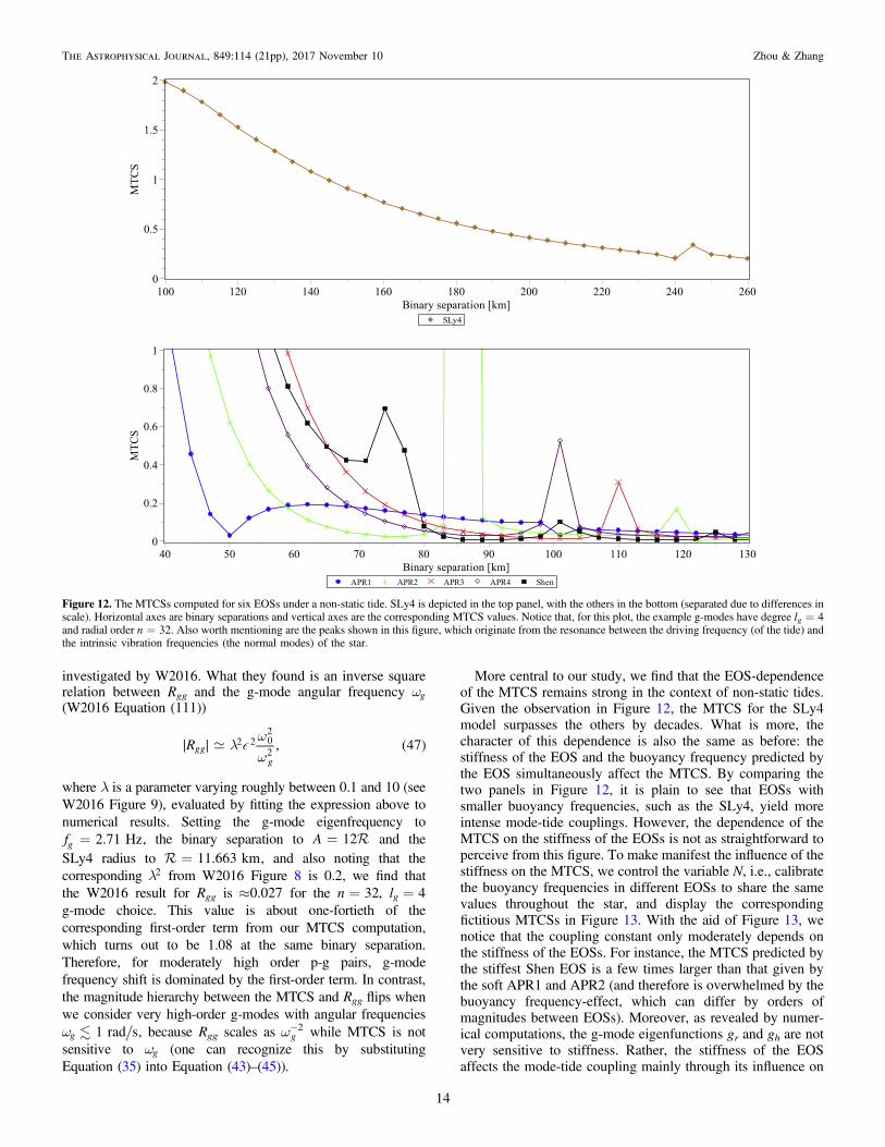
The coupling strengths, as a function of binary separation,are illustrated in Figure 12. The mode-tide coupling becomesstronger when the binaries orbit closer. Nevertheless, at certaindistances, the MTCS soars to extraordinarily large values (seethose peaks in Figure 12). These sudden changes in thecoupling strength are caused by the resonance between the non-static tide and the normal modes of the neutron star. Suchresonances were also observed in W2016 (cf. Figure 1 in thatpaper) and have been discussed in Lai (1994) in detail.Moreover, as mentioned in Section 4.1, our computations are inthe leading order in ò, while the second-order term Rgg was

Figure 11. The (scaled) linear tidal displacement computed under the m=2non-static tide at binary separation A 150 km= . Because M M1.4= is fixedfor all six EOSs, this distance corresponds to the GW fre-quency f GM A1 2 106 Hzgw

3p= »( ) .

13


investigated by W2016. What they found is an inverse squarerelation between Rgg and the g-mode angular frequency gw(W2016 Equation (111))

R , 47ggg

2 2 02

2l

ww

∣ ∣ ( )

where λ is a parameter varying roughly between 0.1 and 10 (seeW2016 Figure 9), evaluated by fitting the expression above tonumerical results. Setting the g-mode eigenfrequency tof 2.71 Hzg = , the binary separation to A 12= and theSLy4 radius to 11.663 km = , and also noting that thecorresponding 2l from W2016 Figure 8 is 0.2, we find thatthe W2016 result for Rgg is 0.027» for the n=32, lg=4g-mode choice. This value is about one-fortieth of thecorresponding first-order term from our MTCS computation,which turns out to be 1.08 at the same binary separation.Therefore, for moderately high order p-g pairs, g-modefrequency shift is dominated by the first-order term. In contrast,the magnitude hierarchy between the MTCS and Rgg flips whenwe consider very high-order g-modes with angular frequencies

1 rad sg w , because Rgg scales as g2w- while MTCS is not

sensitive to gw (one can recognize this by substitutingEquation (35) into Equation (43)–(45)).

More central to our study, we find that the EOS-dependenceof the MTCS remains strong in the context of non-static tides.Given the observation in Figure 12, the MTCS for the SLy4model surpasses the others by decades. What is more, thecharacter of this dependence is also the same as before: thestiffness of the EOS and the buoyancy frequency predicted bythe EOS simultaneously affect the MTCS. By comparing thetwo panels in Figure 12, it is plain to see that EOSs withsmaller buoyancy frequencies, such as the SLy4, yield moreintense mode-tide couplings. However, the dependence of theMTCS on the stiffness of the EOSs is not as straightforward toperceive from this figure. To make manifest the influence of thestiffness on the MTCS, we control the variable N, i.e., calibratethe buoyancy frequencies in different EOSs to share the samevalues throughout the star, and display the correspondingfictitious MTCSs in Figure 13. With the aid of Figure 13, wenotice that the coupling constant only moderately depends onthe stiffness of the EOSs. For instance, the MTCS predicted bythe stiffest Shen EOS is a few times larger than that given bythe soft APR1 and APR2 (and therefore is overwhelmed by thebuoyancy frequency-effect, which can differ by orders ofmagnitudes between EOSs). Moreover, as revealed by numer-ical computations, the g-mode eigenfunctions gr and gh are notvery sensitive to stiffness. Rather, the stiffness of the EOSaffects the mode-tide coupling mainly through its influence on

Figure 12. The MTCSs computed for six EOSs under a non-static tide. SLy4 is depicted in the top panel, with the others in the bottom (separated due to differences inscale). Horizontal axes are binary separations and vertical axes are the corresponding MTCS values. Notice that, for this plot, the example g-modes have degree lg=4and radial order n=32. Also worth mentioning are the peaks shown in this figure, which originate from the resonance between the driving frequency (of the tide) andthe intrinsic vibration frequencies (the normal modes) of the star.

14


tidal deformation. This feature has also seen during previousinvestigations. For example, with dynamical tide, Maselli et al.(2012) discovered that the tidal Love number k2,

9 whichquantitatively measures the extent of deformation of a star dueto the external tidal field, is larger for a stiffer EOS during lateinspiral (cf. Figure1 in Maselli et al. 2012). Similar conclu-sions were also made when a static tidal field is assumed(consult, e.g., the pioneering work by Hinderer et al. 2010regarding this issue).

In short, the MTCS turns out to be quite sensitive to theneutron star EOS, particularly in that MTCSs predicted bydifferent EOSs can vary by over a decade. This observation,and the related possible instability (detailed below), offer anintriguing opportunity to distinguish EOSs by examining thenonlinear couplings’ effects on binary coalescences.

4.4. The Instability

For concreteness, the discussion in this section specializes toa specific lg=4 example g-mode. The eigenfrequency of thisexample g-mode and the MTCS values for six EOS choices aretabulated in Table 3. We see from Table 3 that, with mostEOSs, the MTCS value is roughly on the order of 10−2, ascompared to the typical size of 10 5~ - (Table 2, and alsoTable 3) under a static tide. This makes the onset of instabilitiespossible in a binary coalescence scenario. Namely, someperturbed g-mode frequencies 2w- could become negative wellbefore merger. To directly illustrate this effect, we estimate the

instability threshold, the growth rate, and the growth windowfor the example mode. Aside from our MTCS results with thisexample mode, however, we additionally note that in the caseof very high-order g-modes with even lower eigenfrequencies(e.g., 1 rad sg w ), the three- and four-mode residual Rgg canrise to overwhelmingly large values (W2016, Section 4.3),which would further enhance instabilities, bringing its onsetforward to an even earlier instant during inspiral.Instability begins when the square of the perturbed g-mode

frequency crosses zero. The threshold separation when thisoccurs is listed in Table 3 for each EOS, which is estimatedusing linear interpolation between discrete MTCS data points.When the MTCS exceeds 1, the perturbed frequency can beapproximated by

i MTCS 1 , 48gw w» -- ( )

and so the shifted modal frequency w- becomes imaginary andexponentially drives the mode to large amplitudes with growthrate MTCS 1gw - by appropriating energy from orbitalmotion. It is worth mentioning that the energy injection ratedE dtinj from the tidal potential into the unstable g-mode is acrucial quantity, and its balance with factors such as thedamping effects is vital for determining the instabilitywindow.10 Unfortunately, a lack of detailed knowledgeregarding the driving process prevents an a priori determinationof dE dtinj within the scope of this paper.

Figure 13. The MTCSs calculated by controlling all six EOSs to possess exactly the same buoyancy frequency N throughout the star. Note that the MTCS valuesappearing in this figure are fictitious, constructed to isolate the effects of the EOSs stiffness, and will not arise in real astronomical settings.

Table 3The MTCS Evaluated with the lg=4, n=32 Example G-modes at A=95 km (No Resonance Occurs at this Binary Separation), together with the Instability

Threshold and the Duration of the Instability Growth Window

EOS fg (Hz)MTCS (A = 95 km) Instability

Static Tide Non-static Tide Threshold (km) tmg (ms)

SLy4 2.71 1.75×10−3 2.01 144 1583Shen 27.7 1.60×10−4 1.23×10−2 57.0 35.4APR1 23.3 4.53×10−5 9.71×10−2 41.2 10.1APR2 23.7 2.99×10−5 5.27×10−2 46.8 16.9APR3 15.9 5.58×10−5 1.91×10−2 58.9 42.8APR4 18.8 3.95×10−5 4.10×10−2 54.4 30.7

9 The tidal Love number k2 is defined via k Q C3 2ij ij25= -( ) ( ), where Qij

is the quadrupole moment tensor of the star and Cij is the tidal field tensor.

10 See, e.g.,Pnigouras & Kokkotas (2015) for derivations and illustrations ofthe instability window for the fundamental mode (f-mode, radial order n = 0)in spinning neutron stars.

15


This diverging growth is not likely to be interrupted by the“collapse instability” (proposed by Wilson & Mathews 1995,suggesting that coalescing neutron stars may collapse intoblack holes before merger) prior to merger because of the tidalstabilization effect (Lai 1996; Shibata et al. 1998). It wouldeither be terminated by dissipative effects and so the modessaturate, or simply continues until merger happens (or possiblytear the neutron star apart before merger). A description of thesaturation configuration is beyond the scope of this paper (butrefer to Essick et al. 2016 for a first attempt on this topic), sowe will begin by ignoring it and computing the maximum finalmodal amplitude potentially achievable before merger for eachEOS. This quantity is limited by both the instability growth rateand the growth window. The tmg in Table 3 denotes theapproximate maximum growth window, defined as thetemporal interval between the onset of instability and merger.11

These windows are quite narrow in general, but much widerfor the SLy4 EOS (the inspiral duration depends on the initial“onset separation” rather nonlinearly, a fact that can potentiallymagnify any observable signal’s sensitivity on EOS differ-ences). The exponential growth in modal amplitudes thenfurther acts as a highly effective amplifier, with the finalamplitude of unstable modes differing by more than 10 orders

of magnitude between the SLy4 and the APR1 EOS (seeFigure 14).Such massive differences can potentially lead to observable

consequences, and a subsequent constraining of the EOS. Forour discussion, we concentrate on the GWs given off by thebinary system as opposed to the electromagnetic signature.This is because, first of all, the GWs reveal the celestialmechanics of the neutron stars more cleanly, withoutcontamination/blockage due to processes occurring withinthe magnetosphere or in the interstellar medium. Second, GWdetectors are “all-sky” (i.e., have broad antenna patterns), andas such have a good chance of observing the late inspiral stage(without needing to be alerted by dramatic triggers such as themerger itself). Indeed, studies by, e.g., Andersson & Kokkotas(1998) have identified unstable modes as promising candi-dates to be studied with GW asteroseismology, as they maygrow to such large amplitudes that they emit GWs detectableon Earth (Andersson 2011). Moreover, even when the wavefrom the modes themselves are too weak, indirect modaleffects imprinted onto the more prominent orbital-motion-generated waves should be observable. In the most optimisticscenario, unmissable qualitative distinctions—such as neutronstars with SLy4 EOS being torn apart pre-merger while thoseEOSs with larger buoyancy frequencies remain intact—willimprint EOS information onto the amplitude of the gravita-tional waveform. On the other hand, in the conservativescenario that the modes simply saturate, at similar finalamplitudes for different EOSs, the modes would still impartphase modifications onto the orbital motion, and thus thecumulative phase of the gravitational waveform. As someEOSs would reach saturation significantly earlier than others,the accumulated phase corrections may still provide usefulinformation. More specifically, the accumulated phase errorscales as the the −3rd power of the initial orbital frequency atwhich instability appears (WAB). Using Kepler’s law for avery crude estimate, the total accumulated phase error scaleswith threshold separation as its 4.5th order. Taking data fromTable 3, this translates into approximately a 102 times greatertotal phase error for the least stable EOS than the most stableone. Finally, we have only considered inviscid fluids in thisstudy, while linear dampings may further enhance theinstability (W2016)—and if they are also EOS-dependent,that would make it easier to determine the actual EOS.

5. Conclusion

In this paper, we have examined the EOS-dependence of thegrowth of neutron star g-modes driven by tidal interactions. Arepresentative collection of six EOSs at zero-temperature areconsidered. The twin neutron stars are assumed to consist ofnormal fluid, each with mass M M1.4» and non-spinning.The cases of both static and non-static tides are examined,using the volume-preserving transformation of VZH and theoriginal formalism describing nonlinear mode interactions byWAQB, respectively. With static tide, our results show that,while the mode-tide coupling is stronger in stars that are largerin size and with smaller buoyancy frequencies, the near-exactcancellation between the three- and four- mode couplings asrevealed by VZH provides a sufficient level of suppression thatthe g-modes remain stable with all the EOSs considered. Inother words, the qualitative conclusion reached by VZHregarding the stability is explicitly shown to be EOS-independent. On the other hand, a return of the instability

Figure 14. The relationship between the binary separation and the energye-folding number, with ξ denoting the modal oscillation amplitude and ix itsinitial value at the instability threshold. Positions marked by asterisks indicatethe distance at which the binary merges. Our results should be compared withsimilar energy e-folding diagrams presented in W2016; see, for example, theirFigure 13 for results assuming very high-order n 1000( ) g-modes within theSLy4 EOS.

11 For the estimation of tmg, we adopt Lai (1994) Equation (2.12), which givesthe orbital decay rate due to the emission of GWs from a point-mass binary.However, we caution that this formula suffers from complications during thelate inspiral stage, partly from the so-called dynamical instability considered byLai et al. (1994). The dynamical instability indicates that circular orbits willbecome unstable when A 3 (the exact value depends on the EOS). Withsuch close separations, tidal effects would accelerate the orbital decay rate, andthus narrow the growth window of the unstable modes. Nevertheless, thediscrepancy between the tmg as given by Lai (1994) Equation (2.12) and frommore advanced formalisms is tolerable (see the middle panel of Lai et al. 1994Figure 4).

16


under non-static tides is unambiguously seen from ournumerical results, even for moderately high-order p-g pairs.The combination of a longer growth window (the instabilitydoes not rely on any resonance condition being met, so once itappears, it continues to be present as the neutron stars inspiral)and a larger growth rate enables g-modes in stars with smallerbuoyancy frequencies to either (1) grow to much larger (orderof 1012~ from its initial value, for the extreme case of SLy4)amplitudes if mode saturation (or star disruption) does notoccur or occurs only at very large amplitudes, (2) reach low-amplitude saturation states much earlier. When these results forthe pre-merger inspiral stage are viewed in conjunction withother studies mentioned in the introduction, and the strong EOSdependence seen for the post-merger remnant by Stergioulaset al. (2011), there is reason for optimism that strategies forconstraining the EOS using GW observations should be viable,utilizing features in the amplitude and phase of the waveformsto cater to the two scenarios above, respectively or incombination.

Nevertheless, there is still a long and winding road that weneed to traverse from our highly stylized derivations to realisticpredictions for observational signatures. Many uncertaintiesthat may affect the mode-tide coupling and the p-g instabilityremain untouched. First of all, neutron star’s structural details,such as whether it is spinning or non-spinning, or if it has zeroor finite temperature, should all influence the mode-tidecoupling strength. Moreover, hydrodynamical effect wouldalso influence the magnitude of the coupling constants. Forinstance, taking the same EOS but assuming either normal fluidor superfluid for the neutron star matter will result in differentbuoyancy frequencies (Yu & Weinberg 2017 Figure 2), andthereby lead to different MTCS values (Section 3.3). Evenmore urgently needed, for the purpose of predicting theinstability’s impact on GW waveforms, is an understanding ofthe complications arising when the unstable modes grow tolarge amplitudes. As discussed in Section 4.4, this includes, butis not limited to the determination of the instability window, aquantitative analysis of (both the linear and the nonlinear)damping and the saturation of the unstable g-modes.

On the other hand, the MTCS’s sensitivity to the buoyancyfrequency also reveals limitations of the tabulated Pr - EOSdata that are currently available in literature, and the demandfor a more thorough description of nuclear matter with ultra-high densities, including its composition and properties awayfrom β-equilibrium. Further analytical investigations wouldlikely be very involved, as more complications arise whenmodes grow to large amplitudes. For example, the four-modeinteractions included in the computations here and the previousliterature include only two daughter eigenmodes interactingwith two copies of the tidal field, but interactions involvingthree or more eigenmodes would have to be considered if thesemodes grow to large amplitudes. An important step in terms offurther characterization of the instability issue would thuspossibly be the development of numerical simulations begin-ning sufficiently early in the inspiral for there to be enoughtime for the modes to grow (WAB, W2016), which explore avariety of EOSs (see, e.g., Suh et al. 2017 for numerical effortsin this direction). If more precise data are needed in the future,however, more sophisticated analytical treatments should bepossible on this front.

We thank Nevin Weinberg for kindly and patientlyanswering many questions regarding the computation of thelinear tide and the usage of the ADIPLS package; his valuablecomments on this manuscript are also greatly appreciated. F.Z.is supported by NSFC Grants 11443008 and 11503003,Fundamental Research Funds for the Central UniversitiesGrant No.2015KJJCB06, and a Returned Overseas ChineseScholars Foundation grant.

Appendix AThe Jacobians

The full expression for the perturbed g-mode frequency inthe initial coordinate system is given by Equation (11) (VZHEquation (56)). After the VPT, the equivalent expressionconsists of Jacobians and the MTCS, and is given byEquation (16). Within static tides, our attention is focused onthe MTCS, but Jgg

1 ( ) is nevertheless non-negligible in certaincircumstances. Therefore, this appendix is devoted to thecalculation of Jgg

1 ( ), and to give the reason why the last term ofEquation (16) can be ignored.We begin with the expression for the first-order Jacobians as

given in VZH Equation (89),

JE

I , 49aba

ab1

2

0

1w

= - c ( )( ) ( )

where the integral Iab 1c( ) is given by VZH Equation (81):

I dr r Ta bd

dr

Fa b

rF b a

d

dra b

rG F , 50

ab r rr

ar h

r h b r hh

h hh r

21

1 11

1 1

1

1 1

ò rc

c cc

c c

=

+ - +

+ +

c

c c

⎡⎣⎢⎢

⎤⎦⎥

( )

( ) ( )

( )

( ) ( )( )

( ) ( )

( )

( ) ( )

where ar and ah are the radial and horizontal components of theeigenfunction for mode a, and

r

r l l

d r

dr

,

1

1, 51

r

hr

1 02 2

12 1

cw

cc

=

=+( )

( )( )

( )

( )( )

g

being the radial and horizontal components of the tidaldeformation induced by a static tide, respectively. The angularintegrals T, Fa, and Ga are defined as (WAQB Equation A20–A22, VZH Equation D1–D3)

T Y Y Y d d

FT

GT

sin ,

2,

4. 52

l m l m lm

a b a

a a b

0

2

0

2 2 2

4 2 2 2

a a b b

1

1

ò ò q q f=

= L + L - L

= L - L - L

p p

c

c

( )

[ ( ) ] ( )

( )

( )

17


The expression for Jgg1 ( ) can be deduced from Equations (49)

and (50), which turns out to be

JA E

dr r Tgd

dr

Fg g

rF g g

d

dr

g

rG F . 53

ggg

rr

gr h

r h g r hh

hh r

13

3

2

0 0

2 21

1 11

21 1

1 1

òw

rc

c cc

c c

=-

+ - +

+ +c c

⎡⎣⎢⎢

⎤⎦⎥⎥

( )

( ) ( )

( )( )

( ) ( )( )

( ) ( )( ) ( )

After substituting in the values for gr and gh calculated inSection 3.2.2, and inserting the expressions for r

1c( ) and h1c( )

from Equation (51), we are ready to evaluate Equation (53) andobtain an estimate of the size of the Jacobians. To be inaccordance with the main text, we use the six EOSs introducedin Section 2.2 and set lg=4, l=2. From Equation (52), wethen obtain T 10 5 77 p= ( ) ( ), F T3g = , F T171 =c( ) , andG T91 =c( ) , and ultimately arrive at the numerical resultsshown in Table 2.

Now we can also compare Jgg2 1 2 ( )( ) with the MTCS. When

A 100 km= , J 10gg2 1 2 8 ~ -( )( ) with the six EOSs, at least 103

times smaller than the MTCS (see Table 2); thus, it isreasonable to ignore the former. Moreover, because all first-order Jacobians are governed by Equation (49), one canconfirm that J J2 pg gp

2 1 1 ( ) ( ) and Jgp2 1 2 ( )( ) are also much smaller

than the MTCS, by repeating the same computationalprocedures for other modes. In addition, as stated in VZHSection4.2, the second-order Jacobians are of the samemagnitude as the first-order ones. Therefore, J2 gg

2 2 ( ) is also asmall quantity. All in all, it is safe to ignore all Jacobian termsat 2( ).

Appendix BReview of the Volume Preserving Transformation

The VPT developed by Venumadhav, Zimmerman, andHirata (VZH) plays an important role in our analysis.Therefore, in this appendix, we review it in the context ofstatic tide first, and then partially extend the transformation tonon-static tide. Our introduction is only cursory and a thoroughdiscussion can be found in VZH Section3.1.

In the initial coordinate system r, ,q f( ), the star is deformedby the tidal force to an irregular shape, hence the tidaldisplacement depends on r, θ, and f. Fortunately, there(always) exists another coordinate system R, ,Q F( ), in whichthe deformed star regains its spherical symmetry. Thiscoordinate system, once found, will greatly simplify thecomputation of the mode-tide coupling, which is the aim ofthe VPT. Representing this transformation with an infinitesimaldisplacement vector z , the physical constraint it must satisfy isthat the volume must be conserved, or

0. 54z =· ( )

That z is divergence-free and that the physical quantitiesshould not be affected by the choice of coordinate systems arethe two crucial conditions for the VPT program. The first one isthe only constraint on displacement vector z , while the secondcan be applied to the (tidally perturbed) gravitational potential,

whose expression in the static tide scenario is

r U r r W Y , 550 st 0 02 2

20 20 w qY = Y + = Y -( ) ( ) ( ) ( )

where r0Y ( ) is the potential of the unperturbed star, and Ust isthe static tidal potential (m= 0 term in Equation (39)).Equation (55) implicitly suggests that the Cowling approx-imation is employed, i.e., the perturbation from the star itself isignored in the expression of Ψ. The VPT is effective by theinfinitesimal displacement operator , via

X x x x x

x X X X X

,

, 56

z zz z

= ñ = + ñ= - ñ = - ñ

( ( ))∣ ∣ ( )( ( ))∣ ∣ ( ) ( )

where x and X stand for the coordinate systems before andafter the VPT, respectively. In Equation (56), we have followedthe notations from quantum mechanics, where xd( ) simplyrepresents the infinitesimal displacement operator that bringsstate xñ∣ to state x xd+ ñ∣ . Applying Equation (56) to R, Q( ) atleading order, we find that

r R R,

, 57

1

1

z

zq

= -

=Q - Q

· ˆ

· ˆ ( )

( )

( )

where R and Q are the unit basis vectors in the R and Θ

directions, and 1z ( ) is the first-order infinitesimal displacement(we limit our discussion to the leading order, while thederivation of 2z ( ) is available in VZH Section3.1). Recallingthat the choice of coordinate systems would not affect the valueof the scalar field Ψ, we can substitute Equation (57) intoEquation (55), obtaining

R R R W Y . 5801

02 2

20 202 z wY = Y - + Q +( ) [ · ˆ ( )] ( ) ( )( )g

Equation (58) is similar to VZH Equation (38), with thegravitational acceleration given by d dR0º Fg , while R1z · ˆ( )

is derived under the divergence-free constraint on z that wementioned earlier. The specific steps toward R1z · ˆ( ) areexpounded below.We begin with the spherical harmonic expansion of an

arbitrary vector E:

E YE r E r E r , 59l m l

l

lm lm lm lm lm lm0

1 2 3å å Y F= + +=

¥

=-

( ( ) ( ) ( ) ) ( )

with Y Y rlm lm= ˆ, r Ylm lmY = , and r YlmF = ´ . Thedivergence of this vector is

EdE

dr rE

l l

rE Y

2 1.

60l m l

llm

lm lm lm0

11 2å å = + -

+

=

¥

=-

⎜ ⎟⎛⎝

⎞⎠· ( )

( )

Combining Equations (54) and (60), l" , and m l l, ,= - , wefind that

d R

dR RR

l l

RR

2 10. 61lm

lm lm1

1 2z

z z+ -+

=( )

( ) ( ) ( ) ( )

Once we define

u

Ru , 62lm

lmR lm2z º + ¶ ( )

18


where ulm is a coefficient that depends only on R, thedivergence-free condition (61) then implies

CR l

l l

Ru l

0 ,

10 . 63lm lm

1002

1

z

z

= =

=+

¹

- ( )( ) ( ) ( )

Here, we note that the static tidal potential is axi-symmetric,i.e., independent of the azimuth angle. Therefore, thedisplacement vector z should also respect rotational symmetry.Substituting ulm into the spherical harmonic expansion of z(Equation (59)) and setting m=0, we get

YR R R Y

CR Y Rl l

Ru Y R

u

Ru Y

1

, 64

ll l l l

ll l

lR l l

01 0 0 2 0 0

200

10 0

00 0

å

å

z z z= +

= ++

Q

+ + ¶ ¶ Q Q

=

¥

-

=

¥

Q⎜ ⎟

⎡⎣⎢

⎛⎝

⎞⎠

⎤⎦⎥

( ( ) ( ) )

ˆ ( ) ( ) ˆ

( ( )) ˆ ( )

which is always divergence-free. Now that we have the radialcomponent of z from Equation (64), Equation (58) then turnsout to be

R CR Yl l

Ru Y

R W Y

1

. 65

ll l0

200

10 0

02 2

20 202

å

w

Y = Y - ++

Q

+ Q +

-

=

¥⎡⎣⎢⎢

⎛⎝⎜

⎞⎠⎟( ) ( ) ( )

( )] ( ) ( )

g

The gravitational potential being finite at R=0 requires thatC=0. We (as VZH did) then insist that Ψ in the newcoordinate system depends only on R (all terms that contain thespherical harmonic function must be eliminated), yielding(VZH Equation (45))

uR W

6. 66l l0

1 02 3

202

wd= - ( )( )

g

Finally, placing ul01( ) back into Equation (65), we immediately

confirm that the first-order external potential vanishes (as doesthe first-order radial displacement).

Now we move on to non-static tide. The only differencebetween static and non-static tides lies in the form of the tidalpotential, with the latter characterized by an exponential factore im t- W ; hence, it depends on both space and time. This time-dependence in the potential term leads to a profound physicaleffect and will influence the VPT at a fundamental level. To bemore specific, when conducting the transformation, one shouldnot only consider an infinitesimal (and volume-preserving)displacement of fluid elements, but also take the infinitesimaltime evolution into account. Otherwise, if time is frozen, theexponential factor shall reduce to a constant and there will beno difference between the static and non-static tidal potentials.Actually, for inspiraling binary systems with quasi-circularorbits, the effect of infinitesimal time evolution on the subjectstar is equivalent to a rotation of an infinitesimal angle tWD fora small fluid parcel at position x r, ,q f( ) on that star ( tDsymbolizes the finite time interval). In other words, the wholetransformation is now

r r R, , , , , , . 67displacement

infinitesimal

rotation

time evolutionq f q f¢ ¢ ¢ Q F( ) ⟶ ( ) ⟶ ( ) ( )

( )

In the form of operators and the bracket notation (analogous toEquation (56)),

X x x x x

x x x

x X X X X X

t t

t

,

,68

z zz dz z d

= D ñ = WD ñ= + + ñ= - -WD ñ = - - ñ

( ) ( ( ))∣ ( ) ( ( ))∣∣ ( ) ( )

( ( )) ( )∣ ∣ ( ) ( )( )

where d denotes the displacement induced by rotation. Relation(68) represents the displacement operator and the temporalevolution operator (equivalently, the rotation operator 12)acting on a small fluid parcel with state xñ∣ . Apply thetransformation above to R (we do not explicitly write outsimilar relations for the Θ- and Φ-components because they arenot needed in the ensuing derivations), we obtain to leadingorder that

r R R R t1

2sin . 691 2 2z= - + Q WD· ˆ ( )( ) ( )( )

The next step is to express the gravitational potential in the newcoordinate system. Because the procedure is nearly identical tothe static case, we skip the derivation details and write down

R t, , ,Y Q F( ) directly:

R t R R

R t

R W Y e

R R R t

RY t

R W Y e

, , ,1

2sin

,1

32

3 5

, . 70

i t

i t

01

2 2

02 2

22 222

01 2

202

02 2

22 222

z

z

w

p

w

Y Q F = Y -

+ Q WD

- Q F

= Y - + WD

- Q WD

- Q F

- W

- W

( ) ( ) · ˆ

( )( )

( )

( ) · ˆ ( )

( )( )

( ) ( )

( )

( )

g

g

g g

g

Comparing Equations (58) and (70), it is manifest that newphysics within the non-static tide context lie in the orbitalangular frequency Ω. This observation echoes the one madethrough Equation (40), but is made from the perspective of theVPT. In order to eliminate the angular dependence of Ψ in thenew coordinate system, the expression of R1z · ˆ( ) should be

Rt

RY

R WY e

2

3 5

, . 71i t

12

20

2 222

222

z p

wf

=WD

Q

- Q - W

· ˆ ( ) ( )

( ) ( )

( )

g

Plugging the expression above into Equation (70), we finallyobtain

R R t1

3, 720

2Y = Y + WD( ) ( ) ( )g

12 The origin of our chosen coordinate system is the center of the subject star,with the orbital plane being the x−y plane. Thus, the precise effect of

t WD( ) is to rotate states around the z-axis by an angle tWD .

19


with R t 32WD( )g being the external potential. It is clear that,due to the appearance of a nonvanishing orbital frequency, thenon-static tidal potential dose not preserve the volume of a star,even in leading order.

Up to now, we have seen the VPT with both static and non-static tidal potentials, and have explained the emergence of thefinite orbital frequency correction to the gravitational potential(the main assertion in W2016) at an illustrative level. However,note that both R1z · ˆ( ) and the external potential depend on thevalue of the finite time interval tD , which can be of anyarbitrary value. Hence, neither the external potential nor theexpression for R1z · ˆ( ) derived above can be utilized in ournumerical evaluations. To this end, we adopt the direct methoddeveloped by WAQB in the main text of the paper, whichallows us to compute the MTCS explicitly.

Appendix CNumerical Method for the Non-static Linear Tide

The linear tidal displacement 1c( ) represents the response ofa fluid star to the external non-static tidal field, which, as shownin Section 3.1, couples nonlinearly to the normal modes ofneutron star and result in the frequency shift. It is outlined inSection 4.2 that the (non-static) linear tide is solvednumerically by means of the so-called shooting technique.This appendix, as a supplementary section to Section 4.2,serves as a detailed description of our numerical approach.

Here, 1c( ) is governed by the forced oscillation equations,with the m 2= tidal potential being the driving term. Thestandard form of this ODE system can be expressed as (Pfahlet al. 2008 Equations (A1)–(A4), WAQB Equations (A9)–(A11))

r

d

drr

c

l l c

r m

P

c

l l

r m

l l W

mdP

dr cP N m

d

drrW

r

d

drr

d

dr

l l

r

GP

c

N

11

1

1 1,

1

2 ,

1 1

4 0, 73

rs

rs

s

sr

sr

22 1

21

2

2 2 2

2 202

222

22 2 1

02

22

22

2

2

21

c cr

w

r rc

w

p rr

c

- + -+

W¢

-+W

F¢ = -+

W¢+ ¢ + - W

+F¢

=

F¢-

+F¢

-¢+ =

⎜ ⎟

⎛⎝⎜

⎞⎠⎟

⎛⎝

⎞⎠

⎛⎝⎜

⎞⎠⎟

( ) ( )( )

( )( )

( )( )

( ( ) )

( )

( )

( ) ( )

( )

( )

g

g

g

where F¢ is the Eulerian perturbation to the gravitationalpotential of the star itself, Ω being the orbital angular frequencyand l=2, m 2= for the non-static tide. The inner andsurface boundary conditions for (73) are the same as for freeoscillation (i.e., conditions (22) and (23)).

Now that we have presented the boundary value problem,the next step is to reduce the standard oscillation Equation (73)to a dimensionless formulation, which is more suitable fornumerical computation. Following the conventions in

Christensen-Dalsgaard (2008), we set

y x

y x xP l l

m r

y x xr

y x xd

dx

y

x

,

1,

,

, 74

r1

1

2 2 2

3

42 3

c

r

=

=¢+ F¢

+W

=-F¢

= ⎜ ⎟

⎛⎝⎜

⎞⎠⎟

⎛⎝

⎞⎠

( )

( ) ( )( )

( )

( ) ( )

( )

g

in which we have introduced the (dimensionless) radiusfraction x r º . Substituting the dimensionless quantitiesy y1 4¼ into (73), the original fourth-order ODE turns into

xdy

dx

r

cy

m r

l l cy

r

cy

l l W x

xdy

dxl l

N

my

N ry

l l N

my

l l W x

xdy

dxy y

xdy

dx

G r Ny

G r m

l l cy

l lG r N r r

cy

G ry

21

1

1,

1 1 1

1 2 1,

0,

4 4

1

14

2

24

1 0, 75

s s

s

s

s

12 1

2 2

2 2

2 322

2

22

2 1

2

2

2

2 322

2

33 4

42 2

2 1

3 2

2 2

2

2 3

4

v

v

p r p r

p r

p r

+ - +W+

-

+ = -+

+ +W

- + -

-+W

=+

- - =

+ +W

+

- + + - +

+ - =

⎛⎝⎜

⎞⎠⎟

⎡⎣⎢

⎤⎦⎥

⎡⎣⎢

⎤⎦⎥

⎛⎝⎜

⎞⎠⎟

⎡⎣⎢⎢

⎛⎝⎜

⎞⎠⎟

⎤⎦⎥⎥

⎛⎝⎜

⎞⎠⎟

( )( )

( )

( )( )

( )( )

( )

( )( )

( )

( )

g

g

g

g g

g g

g

g

accompanied by the boundary conditions

y l y

y

yl l

y y

y ly

0 1 0 ,

0 0,

11

1 1 ,

1 1 , 76

2 1

4

2 2 1 3

4 3

v

= +=

=+

-

=-

( ) ( ) ( )( )

( ) ( ) ( ( ) ( ))

( ) ( ) ( )

where ϖ, defined via m 0v wº W , is called the dimensionlessfrequency ratio.Equations (75) and (76) comprise a (purely mathematical)

two-point boundary value problem that is solved by theshooting method, because it is considerably more stable thanother algorithms if one boundary is a singular or near-singularpoint (or if both are). The essential concept of the shootingtechnique (a comprehensive introduction to the shootingmethod is available in Press et al. 1992) is to convert theboundary value problem into two initial value problems. Onethen specifies all initial conditions and then starts to integrate(shoot) Equation (75) from the center and the surface,respectively, to an intermediate fitting point. The mismatchbetween the two asymptotes at the fitting point can be graduallyreduced with Newton-Raphson iterations until a tolerable error

20


is reached. The radial component of the linear tide (scaled) thuscalculated is displayed in Figure 11.

ORCID iDs

Fan Zhang https://orcid.org/0000-0002-8438-7155

References

Abbott, B. P., Abbott, R., Abbott, T. D., et al. 2016a, PhRvL, 116, 241103Abbott, B. P., Abbott, R., Abbott, T. D., et al. 2016b, PhRvL, 116, 061102Abbott, B. P., Abbott, R., Abbott, T. D., et al. 2016c, ApJL, 832, L21Akmal, A., Pandharipande, V. R., & Ravenhall, D. G. 1998, PhRvC, 58, 1804Andersson, N. 2011, PrPNP, 66, 239Andersson, N., & Kokkotas, K. D. 1998, MNRAS, 299, 1059Baym, G., Bethe, H. A., & Pethick, C. J. 1971a, NuPhA, 175, 225Baym, G., Pethick, C., & Sutherland, P. 1971b, ApJ, 170, 299Canuto, V. 1974, ARA&A, 12, 167Chabanat, E., Bonche, P., Haensel, P., Meyer, J., & Schaeffer, R. 1997,

NuPhA, 627, 710Chabanat, E., Bonche, P., Haensel, P., Meyer, J., & Schaeffer, R. 1998,

NuPhA, 635, 231Christensen-Dalsgaard, J. 2008, Ap&SS, 316, 113Christensen-Dalsgaard, J. 2014, Lecture Notes on Stellar Oscillations, http://

astro.phys.au.dk/∼jcd/oscilnotes/Damour, T., Nagar, A., & Villain, L. 2012, PhRvD, 85, 123007Demorest, P. B., Pennucci, T., Ransom, S. M., Roberts, M. S. E., &

Hessels, J. W. T. 2010, Natur, 467, 1081Duez, M. D., Foucart, F., Kidder, L. E., Ott, C. D., & Teukolsky, S. A. 2010,

CQGra, 27, 114106Essick, R., Vitale, S., & Weinberg, N. N. 2016, PhRvD, 94, 103012Fuller, J., & Lai, D. 2011, MNRAS, 412, 1331Flanagan, É. É., & Hinderer, T. 2008, PhRvD, 77, 021502Gambhir, Y. K., Ring, P., & Thimet, A. 1990, AnPhy, 198, 132Harry, G. M. 2010, CQGra, 27, 084006Hebeler, K., Lattimer, J. M., Pethick, C. J., & Schwenk, A. 2013, ApJ, 773, 11Heiselberg, H., & Hjorth-Jensen, M. 2000, PhR, 328, 237Hinderer, T., Lackey, B. D., Lang, R. N., & Read, J. S. 2010, PhRvD, 81, 123016

Hotokezaka, K., Kyutoku, K., & Shibata, M. 2013, PhRvD, 87, 044001Lai, D. 1994, MNRAS, 270, 611Lai, D. 1996, PhRvL, 76, 4878Lai, D., Rasio, F. A., & Shapiro, S. L. 1994, ApJ, 420, 811Lattimer, J. M. 2012, ARNPS, 62, 485Lorenz, C. P., Ravenhall, D. G., & Pethick, C. J. 1993, PhRvL, 70, 379Maselli, A., Gualtieri, L., Pannarale, F., & Ferrari, V. 2012, PhRvD, 86,

044032Pethick, C. J., Ravenhall, D. G., & Lorenz, C. P. 1995, NuPhA, 584, 675Pfahl, E., Arras, P., & Paxton, B. 2008, ApJ, 679, 783Pnigouras, P., & Kokkotas, K. D. 2015, PhRvD, 92, 084018Press, W. H., Teukolsky, S. A., Vetterling, W. T., & Flannery, B. P. 1992,

Numerical Recipes in FORTRAN. The Art of Scientific Computing (2nded.; Cambridge: Cambridge Univ. Press)

Read, J. S., Baiotti, L., Creighton, J. D. E., et al. 2013, PhRvD, 88, 044042Reisenegger, A., & Goldreich, P. 1992, ApJ, 395, 240Shapiro, S. L., & Teukolsky, S. A. 1983, Black Holes, White Dwarfs, and

Neutron stars: The Physics of Compact Objects (New York: Wiley)Shen, H., Toki, H., Oyamatsu, K., & Sumiyoshi, K. 1998a, NuPhA, 637, 435Shen, H., Toki, H., Oyamatsu, K., & Sumiyoshi, K. 1998b, PThPh, 100, 1013Shibata, M., Baumgarte, T. W., & Shapiro, S. L. 1998, PhRvD, 58, 023002Skyrme, T. 1959, NuPhA, 9, 615Stergioulas, N., Bauswein, A., Zagkouris, K., & Janka, H.-T. 2011, MNRAS,

418, 427Suh, I.-S., Mathews, G. J., Haywood, J. R., & Lan, N. Q. 2017, AdAst, 2017,

612703The Virgo Collaboration 2012, Advanced Virgo Technical Design Report,[VIR-

0128A-12], https://workarea.ego-gw.it/ego2/virgo/advanced-virgo/isc/TDR_ISC_v1r1.pdf

Unno, W., Osaki, Y., Ando, H., Saio, H., & Shibahashi, H. 1989, NonradialOscillations of Stars (2nd ed.; Tokyo: Univ. of Tokyo Press)

Venumadhav, T., Zimmerman, A., & Hirata, C. M. 2014, ApJ, 781, 23Weinberg, N. N. 2016, ApJ, 819, 109Weinberg, N. N., Arras, P., & Burkart, J. 2013, ApJ, 769, 121Weinberg, N. N., Arras, P., Quataert, E., & Burkart, J. 2012, ApJ, 751, 136Wilson, J. R., & Mathews, G. J. 1995, PhRvL, 75, 4161Witten, E. 1984, PhRvD, 30, 272Wu, Y., & Goldreich, P. 2001, ApJ, 546, 469Yu, H., & Weinberg, N. N. 2017, MNRAS, 464, 2622

21


https://orcid.org/0000-0002-8438-7155

https://orcid.org/0000-0002-8438-7155

https://orcid.org/0000-0002-8438-7155

https://orcid.org/0000-0002-8438-7155

https://orcid.org/0000-0002-8438-7155

https://orcid.org/0000-0002-8438-7155

https://orcid.org/0000-0002-8438-7155

https://orcid.org/0000-0002-8438-7155

https://doi.org/10.1103/PhysRevLett.116.241103

http://adsabs.harvard.edu/abs/2016PhRvL.116x1103A


http://adsabs.harvard.edu/abs/2016PhRvL.116f1102A

https://doi.org/10.3847/2041-8205/832/2/L21

http://adsabs.harvard.edu/abs/2016ApJ...832L..21A

https://doi.org/10.1103/PhysRevC.58.1804

http://adsabs.harvard.edu/abs/1998PhRvC..58.1804A

https://doi.org/10.1016/j.ppnp.2011.01.013

http://adsabs.harvard.edu/abs/2011PrPNP..66..239A

https://doi.org/10.1046/j.1365-8711.1998.01840.x

http://adsabs.harvard.edu/abs/1998MNRAS.299.1059A

https://doi.org/10.1016/0375-9474(71)90281-8

http://adsabs.harvard.edu/abs/1971NuPhA.175..225B

https://doi.org/10.1086/151216

http://adsabs.harvard.edu/abs/1971ApJ...170..299B

https://doi.org/10.1146/annurev.aa.12.090174.001123

http://adsabs.harvard.edu/abs/1974ARA&A..12..167C

https://doi.org/10.1016/S0375-9474(97)00596-4

http://adsabs.harvard.edu/abs/1997NuPhA.627..710C

https://doi.org/10.1016/S0375-9474(98)00180-8

http://adsabs.harvard.edu/abs/1998NuPhA.635..231C

https://doi.org/10.1007/s10509-007-9689-z

http://adsabs.harvard.edu/abs/2008Ap&SS.316..113C

http://astro.phys.au.dk/~jcd/oscilnotes/

http://astro.phys.au.dk/~jcd/oscilnotes/

https://doi.org/10.1103/PhysRevD.85.123007

http://adsabs.harvard.edu/abs/2012PhRvD..85l3007D

https://doi.org/10.1038/nature09466

http://adsabs.harvard.edu/abs/2010Natur.467.1081D

https://doi.org/10.1088/0264-9381/27/11/114106

http://adsabs.harvard.edu/abs/2010CQGra..27k4106D


http://adsabs.harvard.edu/abs/2016PhRvD..94j3012E

https://doi.org/10.1111/j.1365-2966.2010.18017.x

http://adsabs.harvard.edu/abs/2011MNRAS.412.1331F


http://adsabs.harvard.edu/abs/2008PhRvD..77b1502F

https://doi.org/10.1016/0003-4916(90)90330-Q

http://adsabs.harvard.edu/abs/1990AnPhy.198..132G

https://doi.org/10.1088/0264-9381/27/8/084006

http://adsabs.harvard.edu/abs/2010CQGra..27h4006H

https://doi.org/10.1088/0004-637X/773/1/11

http://adsabs.harvard.edu/abs/2013ApJ...773...11H

https://doi.org/10.1016/S0370-1573(99)00110-6

http://adsabs.harvard.edu/abs/2000PhR...328..237H


http://adsabs.harvard.edu/abs/2010PhRvD..81l3016H


http://adsabs.harvard.edu/abs/2013PhRvD..87d4001H

https://doi.org/10.1093/mnras/270.3.611

http://adsabs.harvard.edu/abs/1994MNRAS.270..611L


http://adsabs.harvard.edu/abs/1996PhRvL..76.4878L

https://doi.org/10.1086/173606

http://adsabs.harvard.edu/abs/1994ApJ...420..811L

https://doi.org/10.1146/annurev-nucl-102711-095018

http://adsabs.harvard.edu/abs/2012ARNPS..62..485L


http://adsabs.harvard.edu/abs/1993PhRvL..70..379L


http://adsabs.harvard.edu/abs/2012PhRvD..86d4032M

http://adsabs.harvard.edu/abs/2012PhRvD..86d4032M

https://doi.org/10.1016/0375-9474(94)00506-I

http://adsabs.harvard.edu/abs/1995NuPhA.584..675P

https://doi.org/10.1086/586878

http://adsabs.harvard.edu/abs/2008ApJ...679..783P


http://adsabs.harvard.edu/abs/2015PhRvD..92h4018P


http://adsabs.harvard.edu/abs/2013PhRvD..88d4042R

https://doi.org/10.1086/171645

http://adsabs.harvard.edu/abs/1992ApJ...395..240R

https://doi.org/10.1016/S0375-9474(98)00236-X

http://adsabs.harvard.edu/abs/1998NuPhA.637..435S

https://doi.org/10.1143/PTP.100.1013

http://adsabs.harvard.edu/abs/1998PThPh.100.1013S


http://adsabs.harvard.edu/abs/1998PhRvD..58b3002S

https://doi.org/10.1016/0029-5582(58)90345-6

https://doi.org/10.1111/j.1365-2966.2011.19493.x

http://adsabs.harvard.edu/abs/2011MNRAS.418..427S

http://adsabs.harvard.edu/abs/2011MNRAS.418..427S

https://doi.org/10.1155/2017/6127031

https://workarea.ego-gw.it/ego2/virgo/advanced-virgo/isc/TDR_ISC_v1r1.pdf

https://workarea.ego-gw.it/ego2/virgo/advanced-virgo/isc/TDR_ISC_v1r1.pdf

https://doi.org/10.1088/0004-637X/781/1/23

http://adsabs.harvard.edu/abs/2014ApJ...781...23V

https://doi.org/10.3847/0004-637X/819/2/109

http://adsabs.harvard.edu/abs/2016ApJ...819..109W

https://doi.org/10.1088/0004-637X/769/2/121


https://doi.org/10.1088/0004-637X/751/2/136



http://adsabs.harvard.edu/abs/1995PhRvL..75.4161W


http://adsabs.harvard.edu/abs/1984PhRvD..30..272W

https://doi.org/10.1086/318234


https://doi.org/10.1093/mnras/stw2552

http://adsabs.harvard.edu/abs/2017MNRAS.464.2622Y

Documents

Equation of State Dependence of Nonlinear Mode-tide