Embed Size (px)
Citation preview
Equazioni lineari matriciali
proprieta, metodi numerici ed applicazioni
V. Simoncini
Dipartimento di Matematica, Universita di Bologna (Italy)
1
Some matrix equations
• Sylvester matrix equation
AX+XB +D = 0
Eigenvalue problems, Control, Model Order Reduction, Assignment problems,
Riccati equation
Lyapunov matrix equation
AX+XA⊤ +D = 0, D = D⊤
Stability analysis in Control and Dynamical systems, Signal processing,
eigenvalue computations
2
Some matrix equations
• Sylvester matrix equation
AX+XB +D = 0
Eigenvalue problems, Control, Model Order Reduction, Assignment problems,
Riccati equation
• Lyapunov matrix equation
AX+XA⊤ +D = 0, D = D⊤
Stability analysis in Control and Dynamical systems, Signal processing,
eigenvalue computations
3
Some matrix equations
• Algebraic Riccati equation
AX+XA⊤ −XBB⊤X+D = 0, D = D⊤
Lancaster-Rodman ’95, Konstantinov-Gu-Mehrmann-Petkov, ’02,
Bini-Iannazzo-Meini ’12
Multiterm matrix equation
A1XB1 +A2XB2 + . . .+AℓXBℓ = C
Elliptic PDEs, PDEs with stochastic inputs, bilinear dynamical systems, etc.
Focus: All or some of the matrices are large (and possibly sparse)
4
Some matrix equations
• Algebraic Riccati equation
AX+XA⊤ −XBB⊤X+D = 0, D = D⊤
Lancaster-Rodman ’95, Konstantinov-Gu-Mehrmann-Petkov, ’02,
Bini-Iannazzo-Meini ’12
• Multiterm linear matrix equation
A1XB1 +A2XB2 + . . .+AℓXBℓ = C
Elliptic PDEs, PDEs with stochastic inputs, bilinear dynamical systems, etc.
Focus: All or some of the matrices are large (and possibly sparse)
5
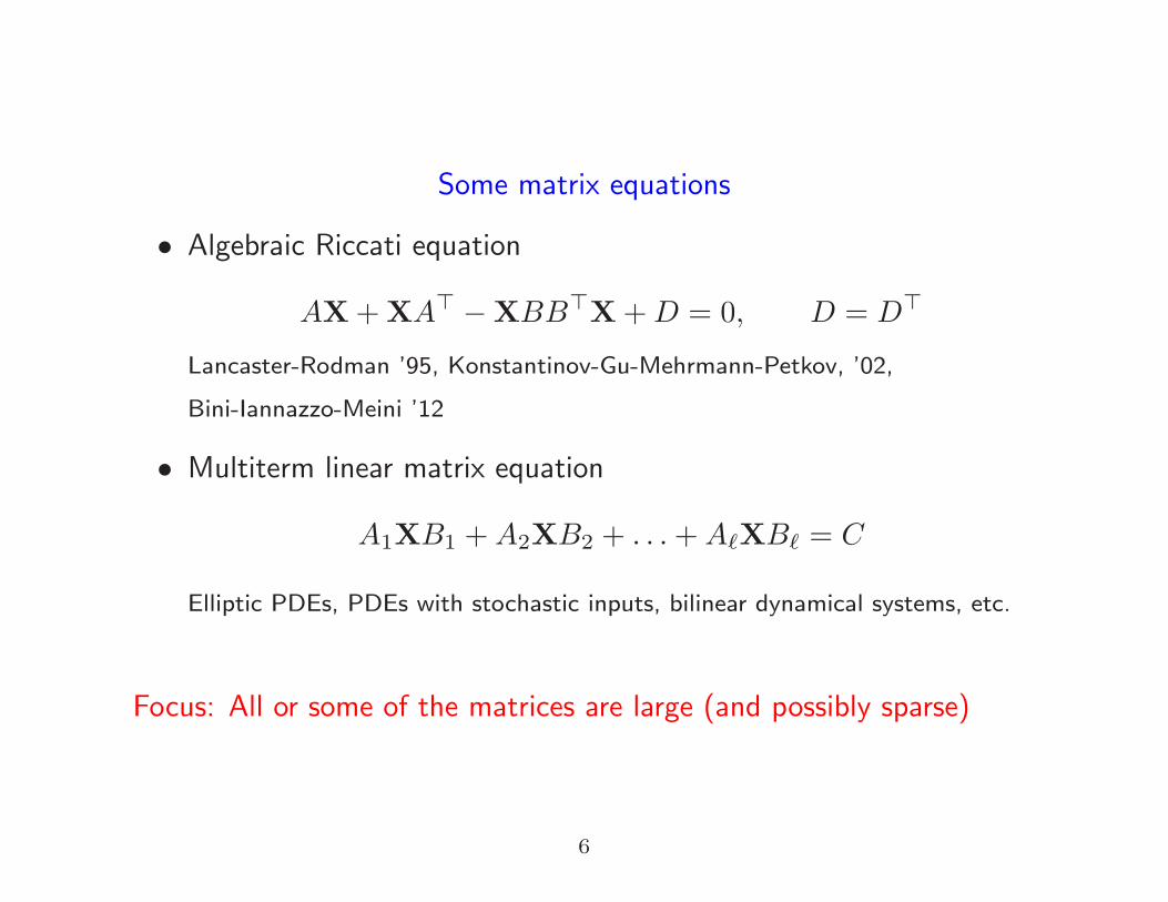
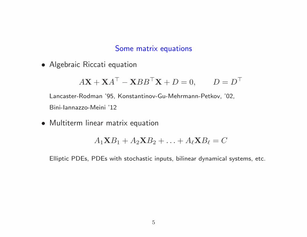
Some matrix equations
• Algebraic Riccati equation
AX+XA⊤ −XBB⊤X+D = 0, D = D⊤
Lancaster-Rodman ’95, Konstantinov-Gu-Mehrmann-Petkov, ’02,
Bini-Iannazzo-Meini ’12
• Multiterm linear matrix equation
A1XB1 +A2XB2 + . . .+AℓXBℓ = C
Elliptic PDEs, PDEs with stochastic inputs, bilinear dynamical systems, etc.
Focus: All or some of the matrices are large (and possibly sparse)
6
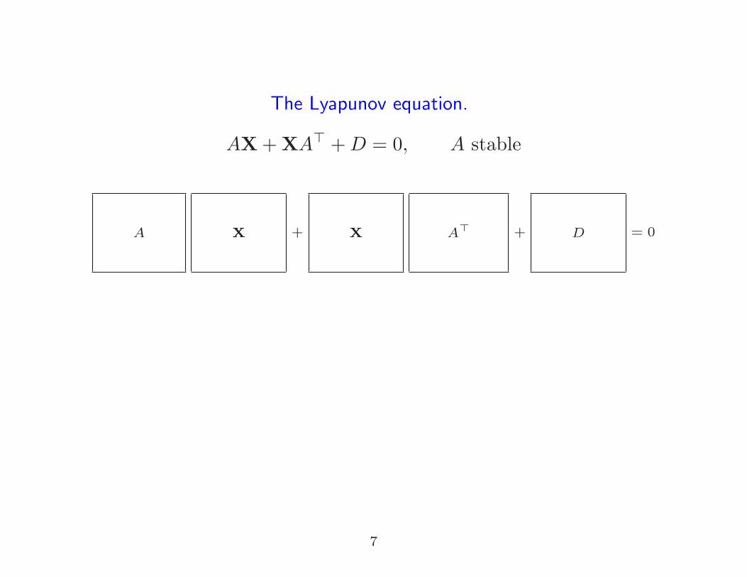
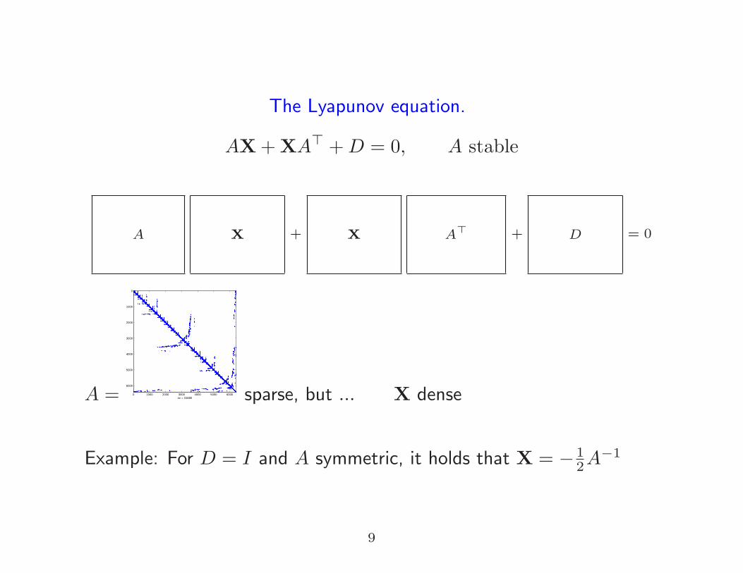
The Lyapunov equation.
AX+XA⊤ +D = 0, A stable
A X + X A⊤ + D = 0
A = sparse, but ... X dense
Example: For D = I and A symmetric, it holds that X = − 12A
−1
7
The Lyapunov equation.
AX+XA⊤ +D = 0, A stable
A X + X A⊤ + D = 0
A = 0 1000 2000 3000 4000 5000 6000
0
1000
2000
3000
4000
5000
6000
nz = 31680 sparse, but ... X dense
Example: For D = I and A symmetric, it holds that X = − 12A
−1
8
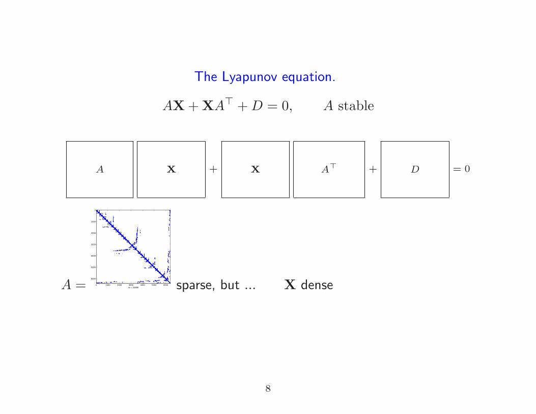
The Lyapunov equation.
AX+XA⊤ +D = 0, A stable
A X + X A⊤ + D = 0
A = 0 1000 2000 3000 4000 5000 6000
0
1000
2000
3000
4000
5000
6000
nz = 31680 sparse, but ... X dense
Example: For D = I and A symmetric, it holds that X = − 12A
−1
9
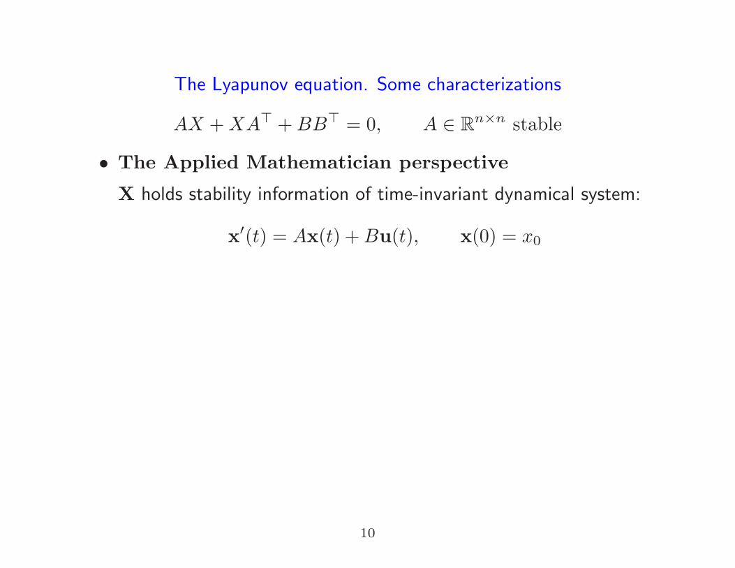
The Lyapunov equation. Some characterizations
AX +XA⊤ +BB⊤ = 0, A ∈ Rn×n stable
• The Applied Mathematician perspective
X holds stability information of time-invariant dynamical system:
x′(t) = Ax(t) +Bu(t), x(0) = x0
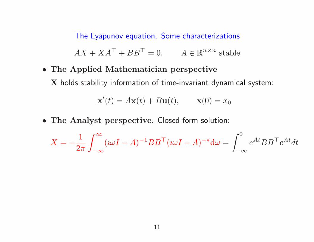
• The Analyst perspective. Closed form solution:
X = − 1
2π
∫ ∞
−∞
(ıωI −A)−1BB⊤(ıωI −A)−∗dω =
∫ 0
−∞
eAtBB⊤eAtdt
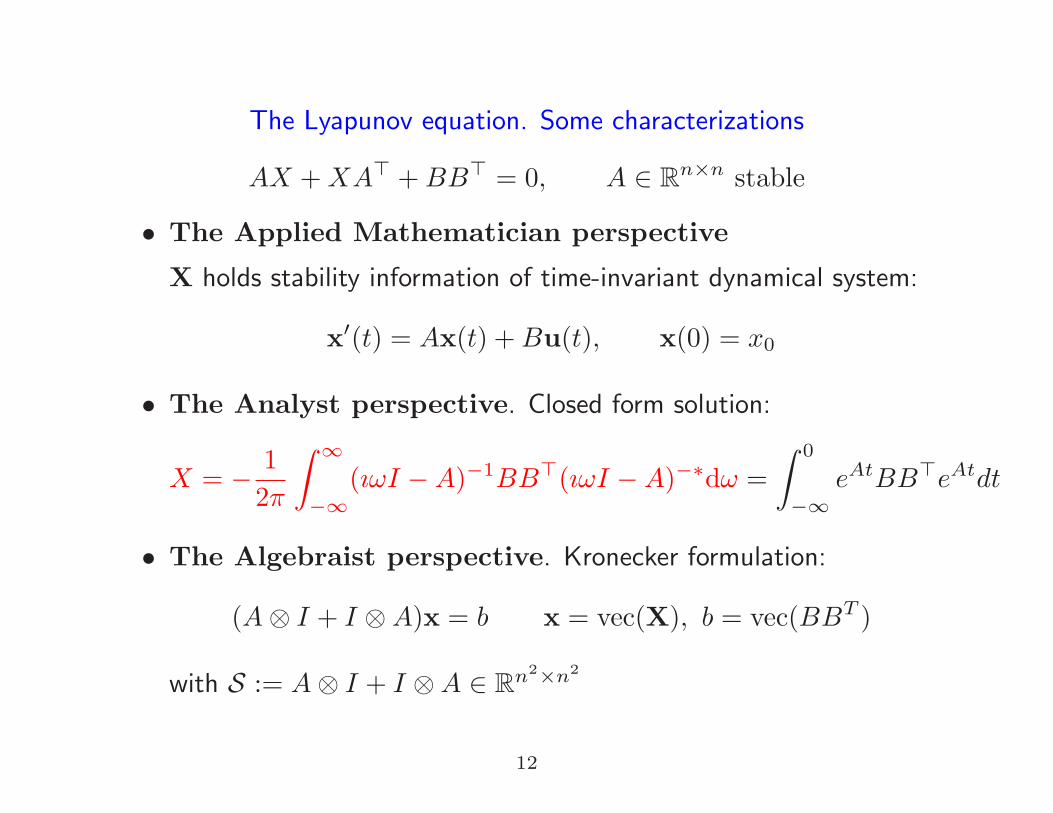
• The Algebraist perspective. Kronecker formulation:
(A⊗ I + I ⊗A)x = b x = vec(X), b = vec(BBT )
with S := A⊗ I + I ⊗A ∈ Rn2×n2
10
The Lyapunov equation. Some characterizations
AX +XA⊤ +BB⊤ = 0, A ∈ Rn×n stable
• The Applied Mathematician perspective
X holds stability information of time-invariant dynamical system:
x′(t) = Ax(t) +Bu(t), x(0) = x0
• The Analyst perspective. Closed form solution:
X = − 1
2π
∫ ∞
−∞
(ıωI −A)−1BB⊤(ıωI −A)−∗dω =
∫ 0
−∞
eAtBB⊤eAtdt
• The Algebraist perspective. Kronecker formulation:
(A⊗ I + I ⊗A)x = b x = vec(X), b = vec(BBT )
with S := A⊗ I + I ⊗A ∈ Rn2×n2
11
The Lyapunov equation. Some characterizations
AX +XA⊤ +BB⊤ = 0, A ∈ Rn×n stable
• The Applied Mathematician perspective
X holds stability information of time-invariant dynamical system:
x′(t) = Ax(t) +Bu(t), x(0) = x0
• The Analyst perspective. Closed form solution:
X = − 1
2π
∫ ∞
−∞
(ıωI −A)−1BB⊤(ıωI −A)−∗dω =
∫ 0
−∞
eAtBB⊤eAtdt
• The Algebraist perspective. Kronecker formulation:
(A⊗ I + I ⊗A)x = b x = vec(X), b = vec(BBT )
with S := A⊗ I + I ⊗A ∈ Rn2×n2
12
Linear systems vs linear matrix equations
Large linear systems:
Sx = b,
• Krylov subspace methods (CG, MINRES, GMRES, BiCGSTAB, etc.)
• Preconditioners: find P such that
SP−1x = b x = P−1x
is easier and fast to solve
Large linear matrix equation:
AX +XA⊤ +BB⊤ = 0
No preconditioning to preserve symmetry
X is a large, dense matrix ⇒ low rank approximation
X ≈ X = ZZ⊤, Z tall
13
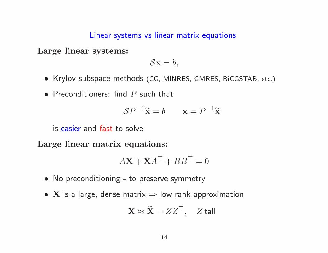
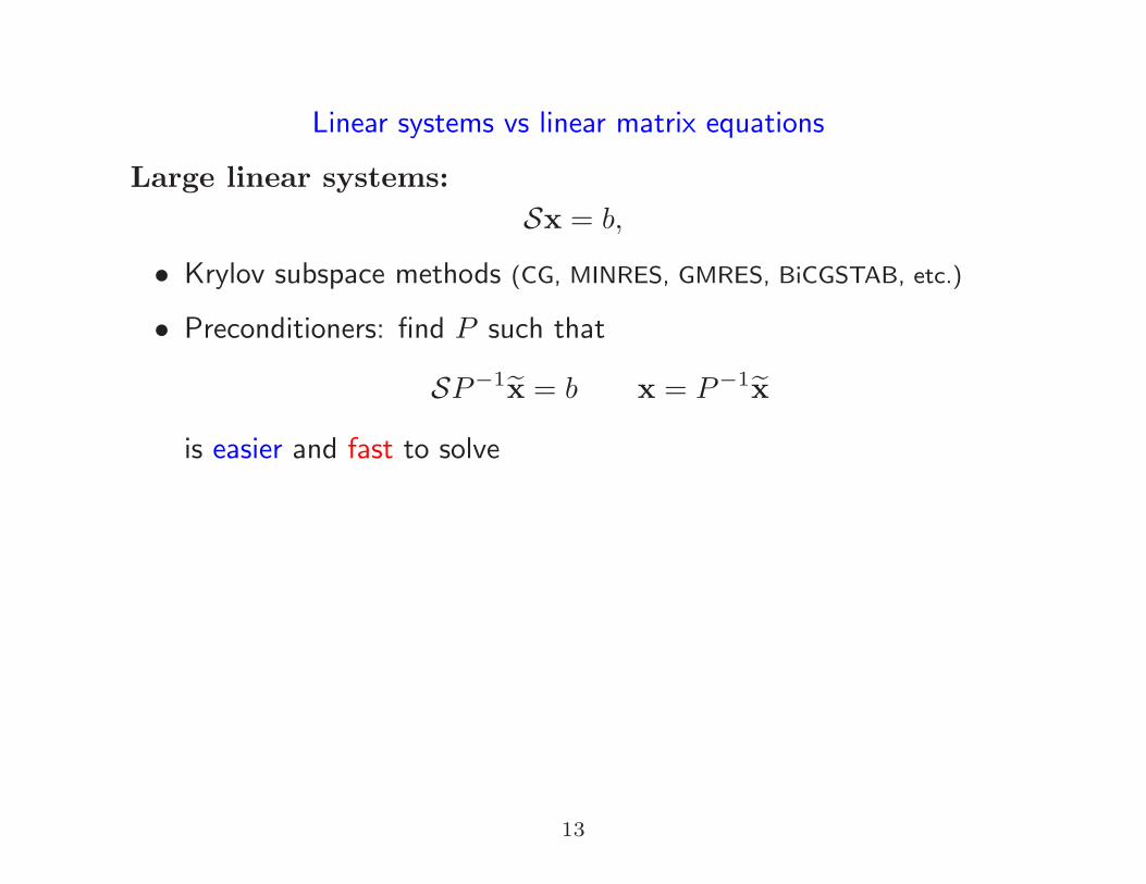
Linear systems vs linear matrix equations
Large linear systems:
Sx = b,
• Krylov subspace methods (CG, MINRES, GMRES, BiCGSTAB, etc.)
• Preconditioners: find P such that
SP−1x = b x = P−1x
is easier and fast to solve
Large linear matrix equations:
AX+XA⊤ +BB⊤ = 0
• No preconditioning - to preserve symmetry
• X is a large, dense matrix ⇒ low rank approximation
X ≈ X = ZZ⊤, Z tall
14
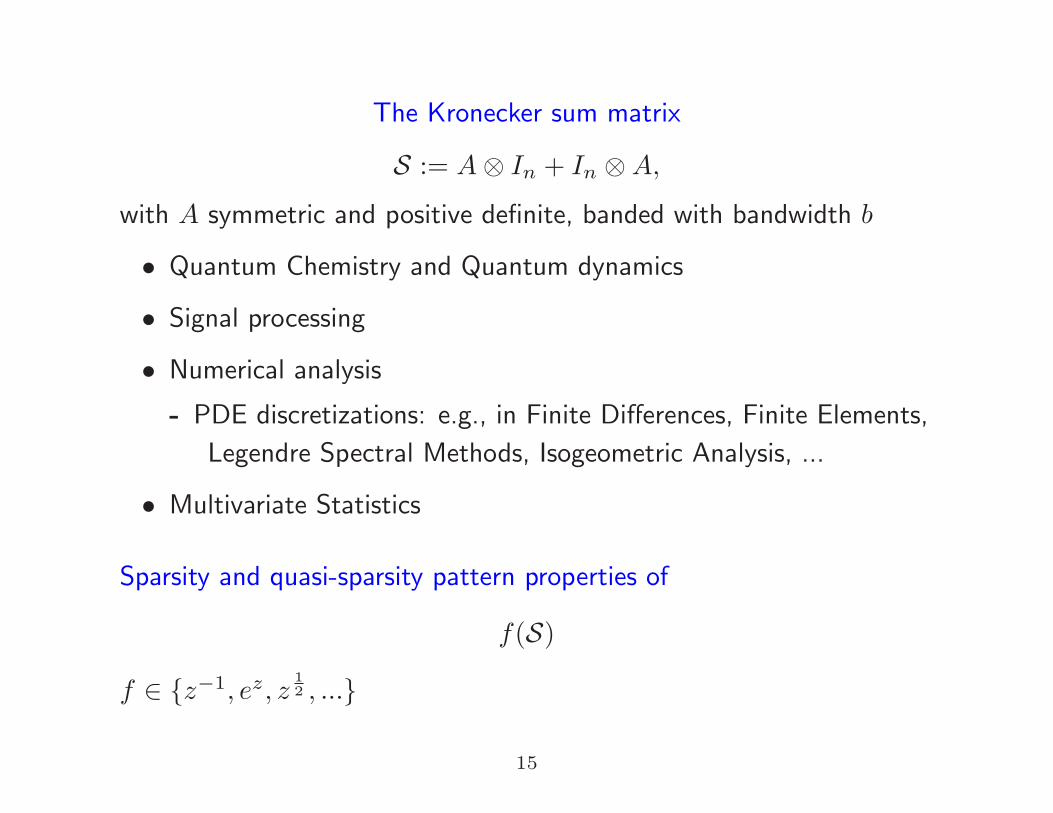
The Kronecker sum matrix
S := A⊗ In + In ⊗A,
with A symmetric and positive definite, banded with bandwidth b
• Quantum Chemistry and Quantum dynamics
• Signal processing
• Numerical analysis
- PDE discretizations: e.g., in Finite Differences, Finite Elements,
Legendre Spectral Methods, Isogeometric Analysis, ...
• Multivariate Statistics
Sparsity and quasi-sparsity pattern properties of
f(S)
f ∈ z−1, ez, z1
2 , ...
15
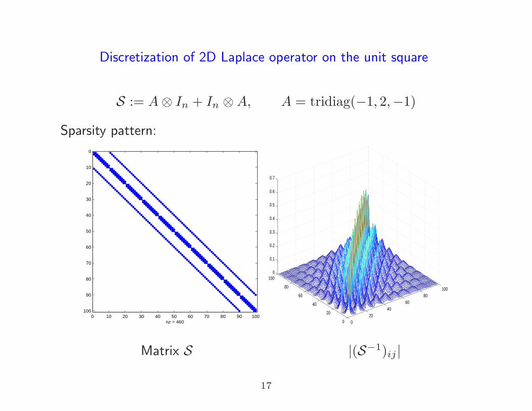
Discretization of 2D Laplace operator on the unit square
S := A⊗ In + In ⊗A, A = tridiag(−1, 2,−1)
Sparsity pattern:
0 10 20 30 40 50 60 70 80 90 100
0
10
20
30
40
50
60
70
80
90
100
nz = 4600 10 20 30 40 50 60 70 80 90 100
0
10
20
30
40
50
60
70
80
90
100
nz = 9380
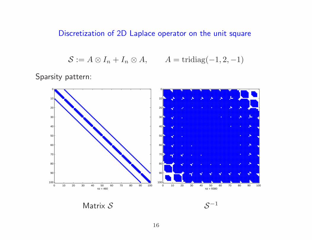
Matrix S S−1
16
Discretization of 2D Laplace operator on the unit square
S := A⊗ In + In ⊗A, A = tridiag(−1, 2,−1)
Sparsity pattern:
0 10 20 30 40 50 60 70 80 90 100
0
10
20
30
40
50
60
70
80
90
100
nz = 460 020
4060
80100
0
20
40
60
80
1000
0.1
0.2
0.3
0.4
0.5
0.6
0.7
Matrix S |(S−1)ij |
17
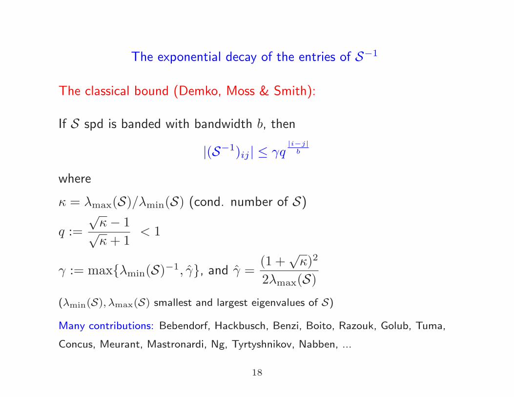
The exponential decay of the entries of S−1
The classical bound (Demko, Moss & Smith):
If S spd is banded with bandwidth b, then
|(S−1)ij | ≤ γq|i−j|
b
where
κ = λmax(S)/λmin(S) (cond. number of S)
q :=
√κ− 1√κ+ 1
< 1
γ := maxλmin(S)−1, γ, and γ =(1 +
√κ)2
2λmax(S)(λmin(S), λmax(S) smallest and largest eigenvalues of S)
Many contributions: Bebendorf, Hackbusch, Benzi, Boito, Razouk, Golub, Tuma,
Concus, Meurant, Mastronardi, Ng, Tyrtyshnikov, Nabben, ...
18
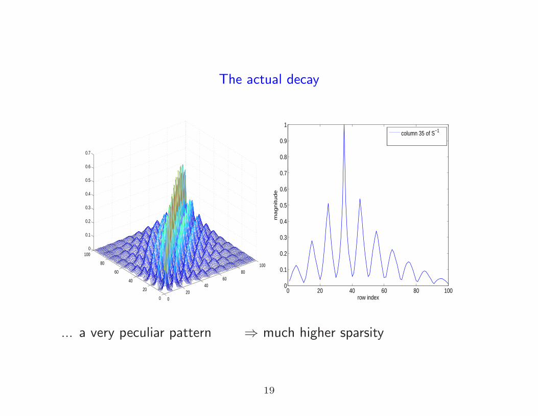
The actual decay
020
4060
80100
0
20
40
60
80
1000
0.1
0.2
0.3
0.4
0.5
0.6
0.7
0 20 40 60 80 1000
0.1
0.2
0.3
0.4
0.5
0.6
0.7
0.8
0.9
1
row index
ma
gn
itu
de
column 35 of S−1
... a very peculiar pattern ⇒ much higher sparsity
19
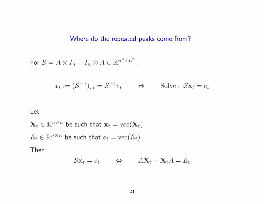
Where do the repeated peaks come from?
For S = A⊗ In + In ⊗A ∈ Rn2×n2
:
xt := (S−1):,t = S−1et ⇔ Solve : Sxt = et
Let
Xt ∈ Rn×n be such that xt = vec(Xt)
Et ∈ Rn×n be such that et = vec(Et)
Then
Sxt = et ⇔ AXt +XtA = Et
20
Where do the repeated peaks come from?
For S = A⊗ In + In ⊗A ∈ Rn2×n2
:
xt := (S−1):,t = S−1et ⇔ Solve : Sxt = et
Let
Xt ∈ Rn×n be such that xt = vec(Xt)
Et ∈ Rn×n be such that et = vec(Et)
Then
Sxt = et ⇔ AXt +XtA = Et
21
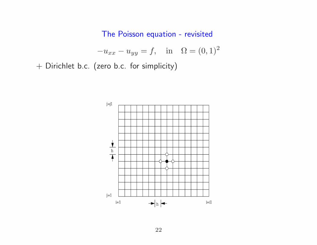
The Poisson equation - revisited
−uxx − uyy = f, in Ω = (0, 1)2
+ Dirichlet b.c. (zero b.c. for simplicity)
22
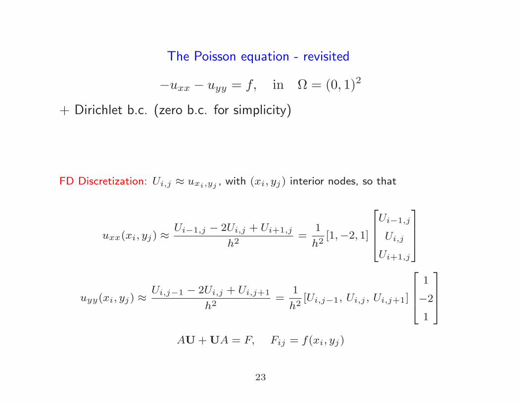
The Poisson equation - revisited
−uxx − uyy = f, in Ω = (0, 1)2
+ Dirichlet b.c. (zero b.c. for simplicity)
FD Discretization: Ui,j ≈ uxi,yj , with (xi, yj) interior nodes, so that
uxx(xi, yj) ≈Ui−1,j − 2Ui,j + Ui+1,j
h2=
1
h2[1,−2, 1]
Ui−1,j
Ui,j
Ui+1,j
uyy(xi, yj) ≈Ui,j−1 − 2Ui,j + Ui,j+1
h2=
1
h2[Ui,j−1, Ui,j , Ui,j+1]
1
−2
1
AU+UA = F, Fij = f(xi, yj)
23
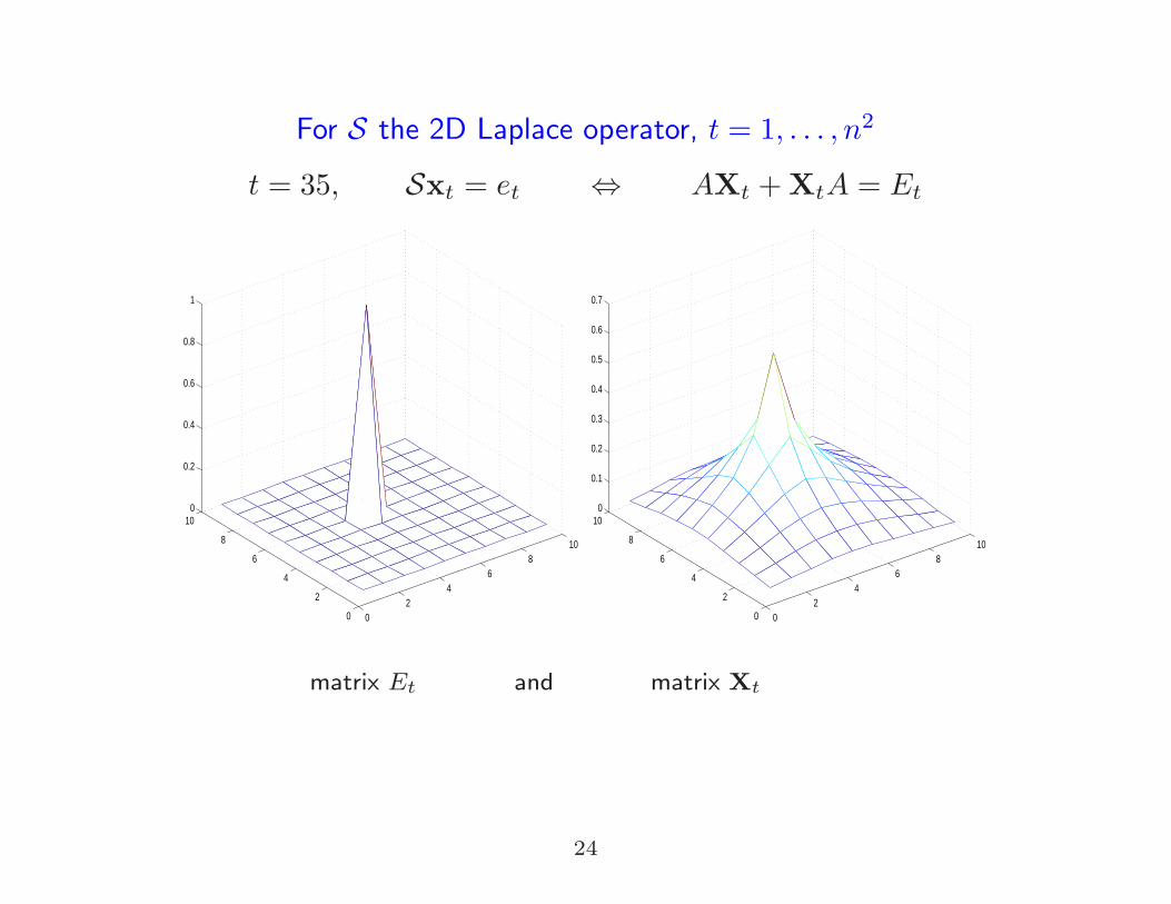
For S the 2D Laplace operator, t = 1, . . . , n2
t = 35, Sxt = et ⇔ AXt +XtA = Et
02
46
810
0
2
4
6
8
100
0.2
0.4
0.6
0.8
1
02
46
810
0
2
4
6
8
100
0.1
0.2
0.3
0.4
0.5
0.6
0.7
matrix Et and matrix Xt
Et has only one nonzero element
Lexicographic order: (Et)ij , j = ⌊(t− 1)/n⌋+ 1, i = tn⌊(t− 1)/n⌋
24
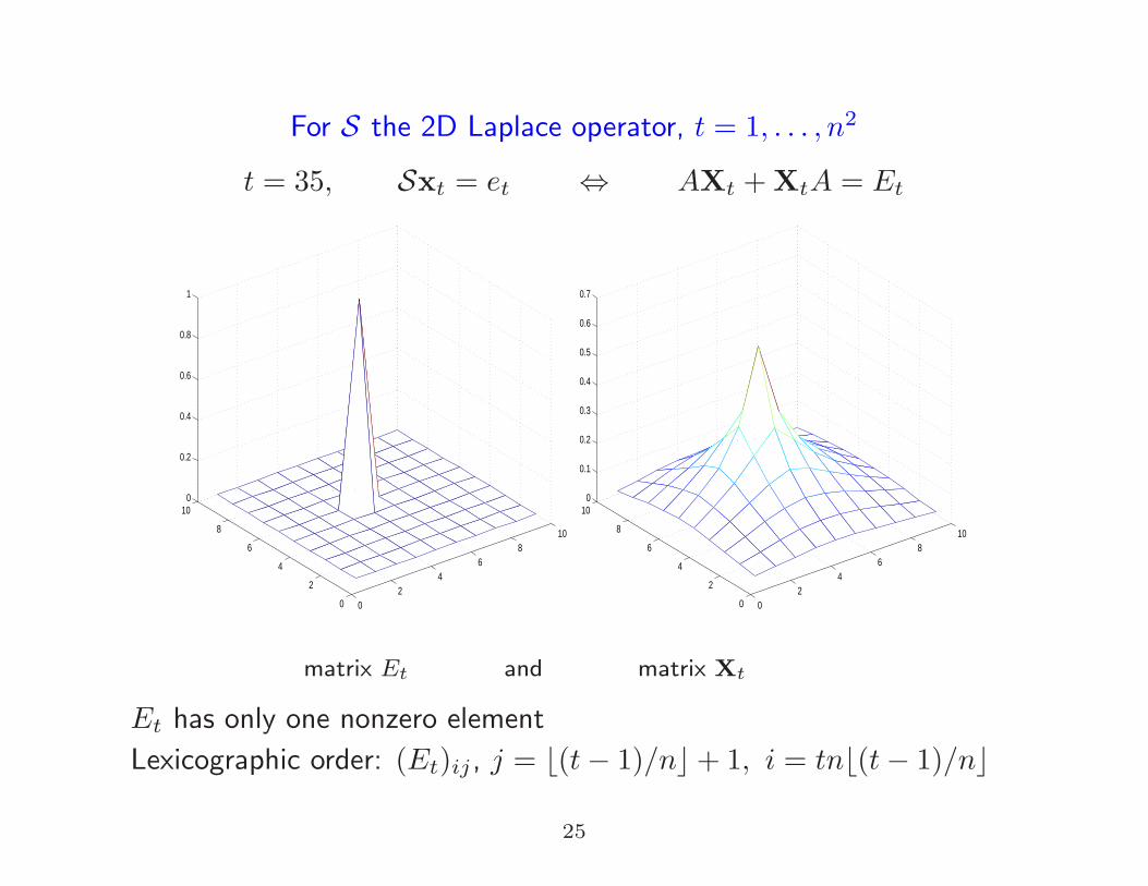
For S the 2D Laplace operator, t = 1, . . . , n2
t = 35, Sxt = et ⇔ AXt +XtA = Et
02
46
810
0
2
4
6
8
100
0.2
0.4
0.6
0.8
1
02
46
810
0
2
4
6
8
100
0.1
0.2
0.3
0.4
0.5
0.6
0.7
matrix Et and matrix Xt
Et has only one nonzero element
Lexicographic order: (Et)ij , j = ⌊(t− 1)/n⌋+ 1, i = tn⌊(t− 1)/n⌋
25

0 10 20 30 40 50 60 70 80 90 1000
0.1
0.2
0.3
0.4
0.5
0.6
0.7
component0
24
68
10
0
2
4
6
8
100
0.1
0.2
0.3
0.4
0.5
0.6
0.7
ij
Left: Row of S−1 Right: same row on the grid
26
0 10 20 30 40 50 60 70 80 90 1000
0.1
0.2
0.3
0.4
0.5
0.6
0.7
component0
24
68
10
0
2
4
6
8
100
0.1
0.2
0.3
0.4
0.5
0.6
0.7
ij
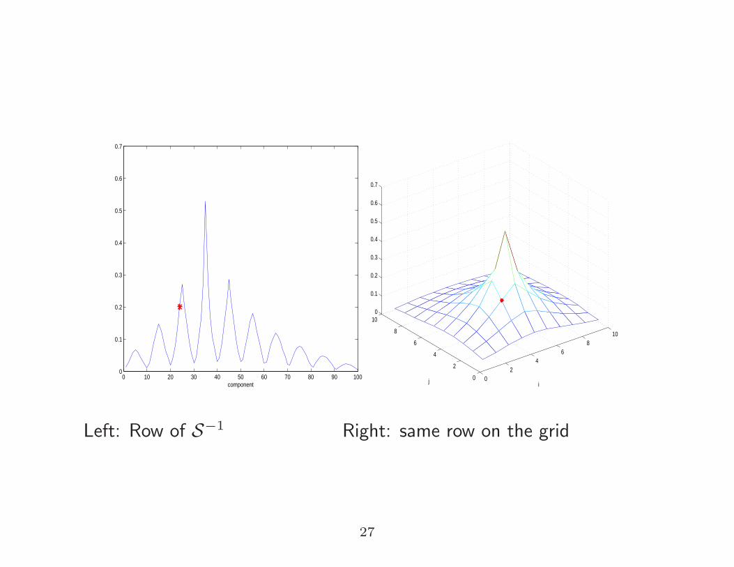
Left: Row of S−1 Right: same row on the grid
27

0 10 20 30 40 50 60 70 80 90 1000
0.1
0.2
0.3
0.4
0.5
0.6
0.7
component0
24
68
10
0
2
4
6
8
100
0.1
0.2
0.3
0.4
0.5
0.6
0.7
ij
Left: Row of S−1 Right: same row on the grid
28

0 10 20 30 40 50 60 70 80 90 1000
0.1
0.2
0.3
0.4
0.5
0.6
0.7
component0
24
68
10
0
2
4
6
8
100
0.1
0.2
0.3
0.4
0.5
0.6
0.7
ij
Left: Row of S−1 Right: same row on the grid
29
0 10 20 30 40 50 60 70 80 90 1000
0.1
0.2
0.3
0.4
0.5
0.6
0.7
component0
24
68
10
0
2
4
6
8
100
0.1
0.2
0.3
0.4
0.5
0.6
0.7
ij
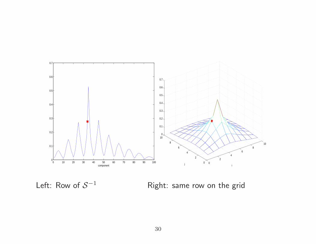
Left: Row of S−1 Right: same row on the grid
30

0 10 20 30 40 50 60 70 80 90 1000
0.1
0.2
0.3
0.4
0.5
0.6
0.7
component0
24
68
10
0
2
4
6
8
100
0.1
0.2
0.3
0.4
0.5
0.6
0.7
ij
Left: Row of S−1 Right: same row on the grid
31
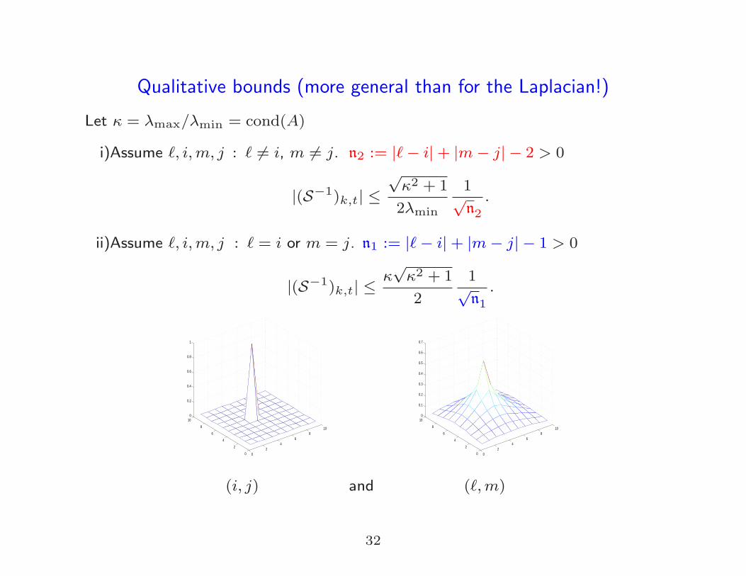
Qualitative bounds (more general than for the Laplacian!)
Let κ = λmax/λmin = cond(A)
i)Assume ℓ, i,m, j : ℓ 6= i, m 6= j. n2 := |ℓ− i|+ |m− j| − 2 > 0
|(S−1)k,t| ≤√κ2 + 1
2λmin
1√n2
.
ii)Assume ℓ, i,m, j : ℓ = i or m = j. n1 := |ℓ− i|+ |m− j| − 1 > 0
|(S−1)k,t| ≤κ√κ2 + 1
2
1√n1
.
02
46
810
0
2
4
6
8
100
0.2
0.4
0.6
0.8
1
02
46
810
0
2
4
6
8
100
0.1
0.2
0.3
0.4
0.5
0.6
0.7
(i, j) and (ℓ,m)
32
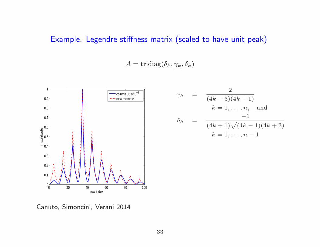
Example. Legendre stiffness matrix (scaled to have unit peak)
A = tridiag(δk, γk, δk)
0 20 40 60 80 1000
0.1
0.2
0.3
0.4
0.5
0.6
0.7
0.8
0.9
1
row index
ma
gn
itu
de
column 35 of S−1
new estimate γk =
2
(4k − 3)(4k + 1)
k = 1, . . . , n, and
δk =−1
(4k + 1)√
(4k − 1)(4k + 3)
k = 1, . . . , n − 1
Canuto, Simoncini, Verani 2014
33
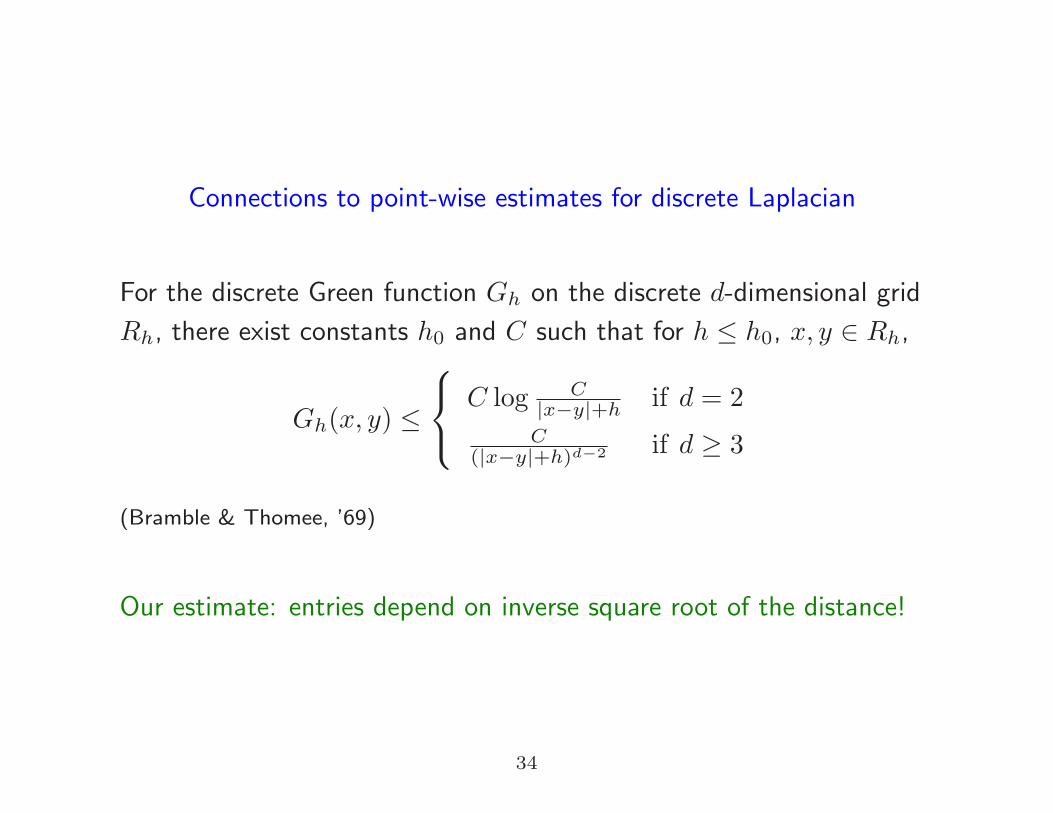
Connections to point-wise estimates for discrete Laplacian
For the discrete Green function Gh on the discrete d-dimensional grid
Rh, there exist constants h0 and C such that for h ≤ h0, x, y ∈ Rh,
Gh(x, y) ≤
C log C|x−y|+h
if d = 2
C(|x−y|+h)d−2 if d ≥ 3
(Bramble & Thomee, ’69)
Our estimate: entries depend on inverse square root of the distance!
34
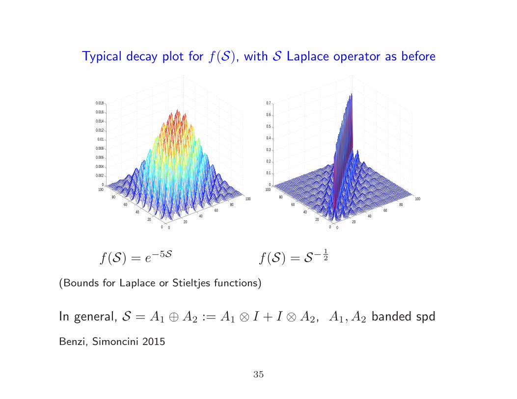
Typical decay plot for f(S), with S Laplace operator as before
020
4060
80100
0
20
40
60
80
1000
0.002
0.004
0.006
0.008
0.01
0.012
0.014
0.016
0.018
020
4060
80100
0
20
40
60
80
1000
0.1
0.2
0.3
0.4
0.5
0.6
0.7
f(S) = e−5S f(S) = S− 1
2
(Bounds for Laplace or Stieltjes functions)
In general, S = A1 ⊕A2 := A1 ⊗ I + I ⊗A2, A1, A2 banded spd
Benzi, Simoncini 2015
35
Generalizations
• Three-dimensional case
• (banded) Non-symmetric matrices
• “Quasi” Kronecker structure
• Numerical solution of PDEs on structured grids
36
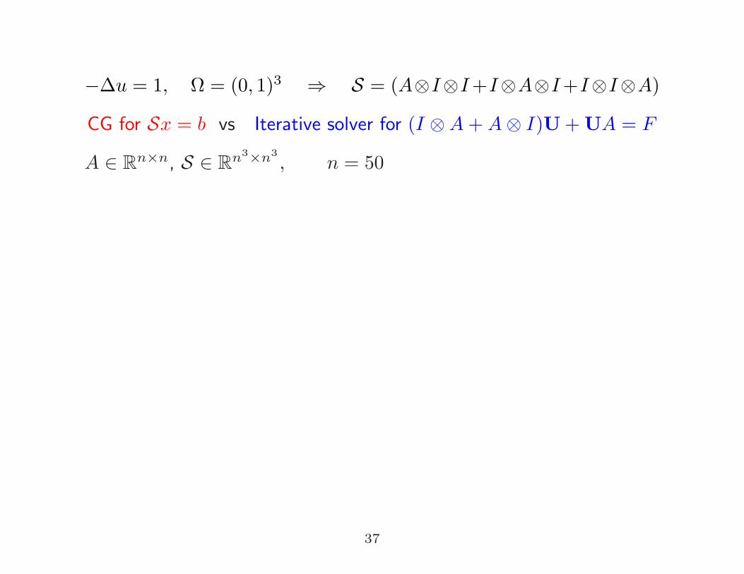
−∆u = 1, Ω = (0, 1)3 ⇒ S = (A⊗I⊗I+I⊗A⊗I+I⊗I⊗A)
CG for Sx = b vs Iterative solver for (I ⊗A+A⊗ I)U+UA = F
A ∈ Rn×n, S ∈ R
n3×n3
, n = 50
CG PCG Matrix Eqn solver
Comput. Time 2.91 0.56 0.08
37
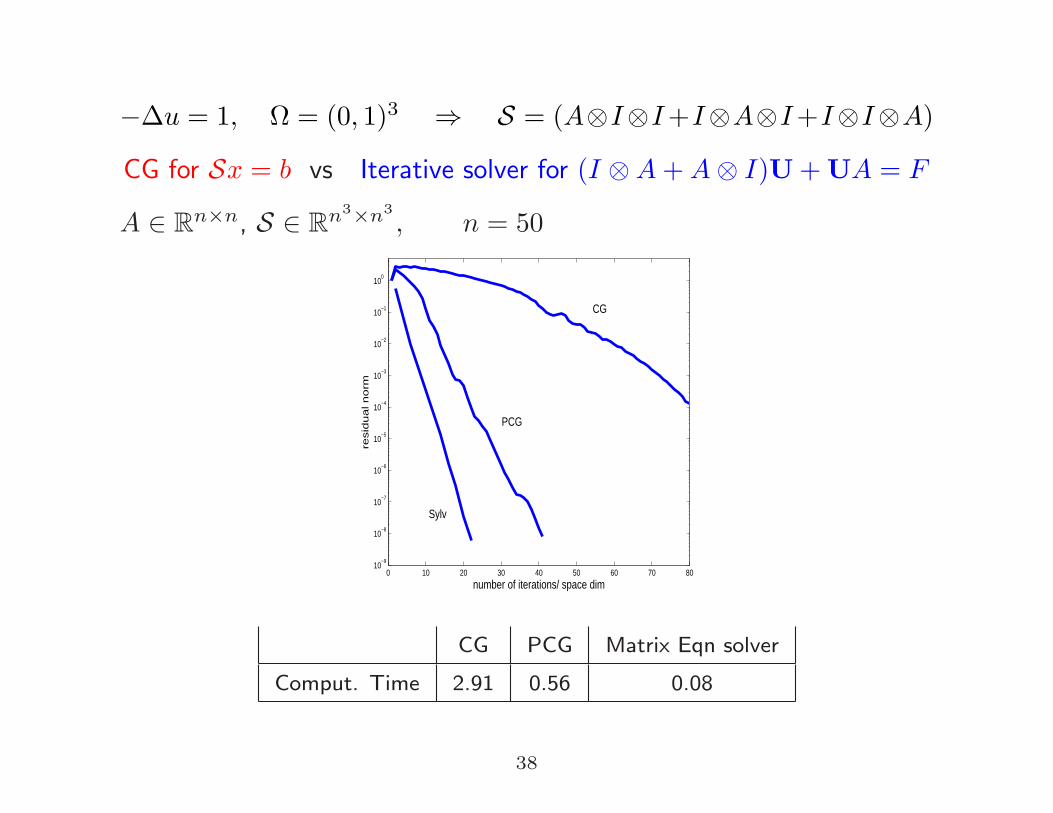
−∆u = 1, Ω = (0, 1)3 ⇒ S = (A⊗I⊗I+I⊗A⊗I+I⊗I⊗A)
CG for Sx = b vs Iterative solver for (I ⊗A+A⊗ I)U+UA = F
A ∈ Rn×n, S ∈ R
n3×n3
, n = 50
0 10 20 30 40 50 60 70 8010
−9
10−8
10−7
10−6
10−5
10−4
10−3
10−2
10−1
100
number of iterations/ space dim
resid
ua
l n
orm
CG
PCG
Sylv
CG PCG Matrix Eqn solver
Comput. Time 2.91 0.56 0.08
38
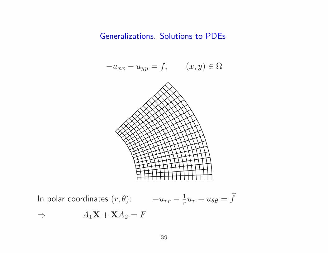
Generalizations. Solutions to PDEs
−uxx − uyy = f, (x, y) ∈ Ω
In polar coordinates (r, θ): −urr − 1rur − uθθ = f
⇒ A1X+XA2 = F
39
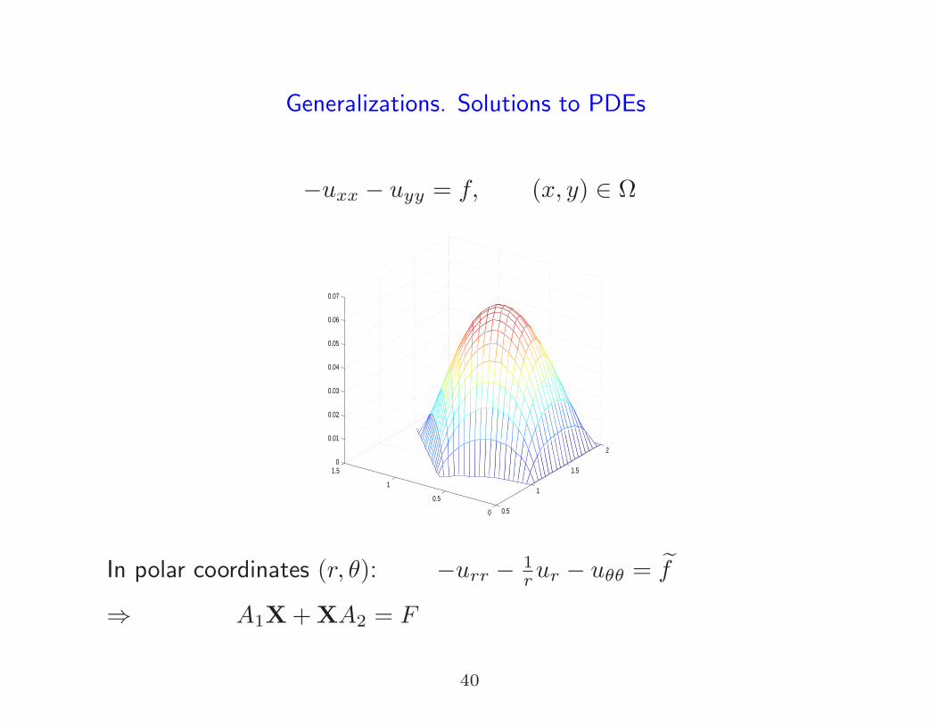
Generalizations. Solutions to PDEs
−uxx − uyy = f, (x, y) ∈ Ω
0.5
1
1.5
2
0
0.5
1
1.50
0.01
0.02
0.03
0.04
0.05
0.06
0.07
In polar coordinates (r, θ): −urr − 1rur − uθθ = f
⇒ A1X+XA2 = F
40
Structured grids
Applications
• Computational Aero- and Fluid-Dynamics
• Seminconductor devices
• Object modelling
• Parallel computation
• ...
Classical strategies (building blocks)
• Conformal mappings (Boundary-fitted curvilinear coord.)
• Algebraic grid generators (Transfinite interpolation)
• Elliptic, hyperbolic grids with controls
• Variational methods
• ...
41
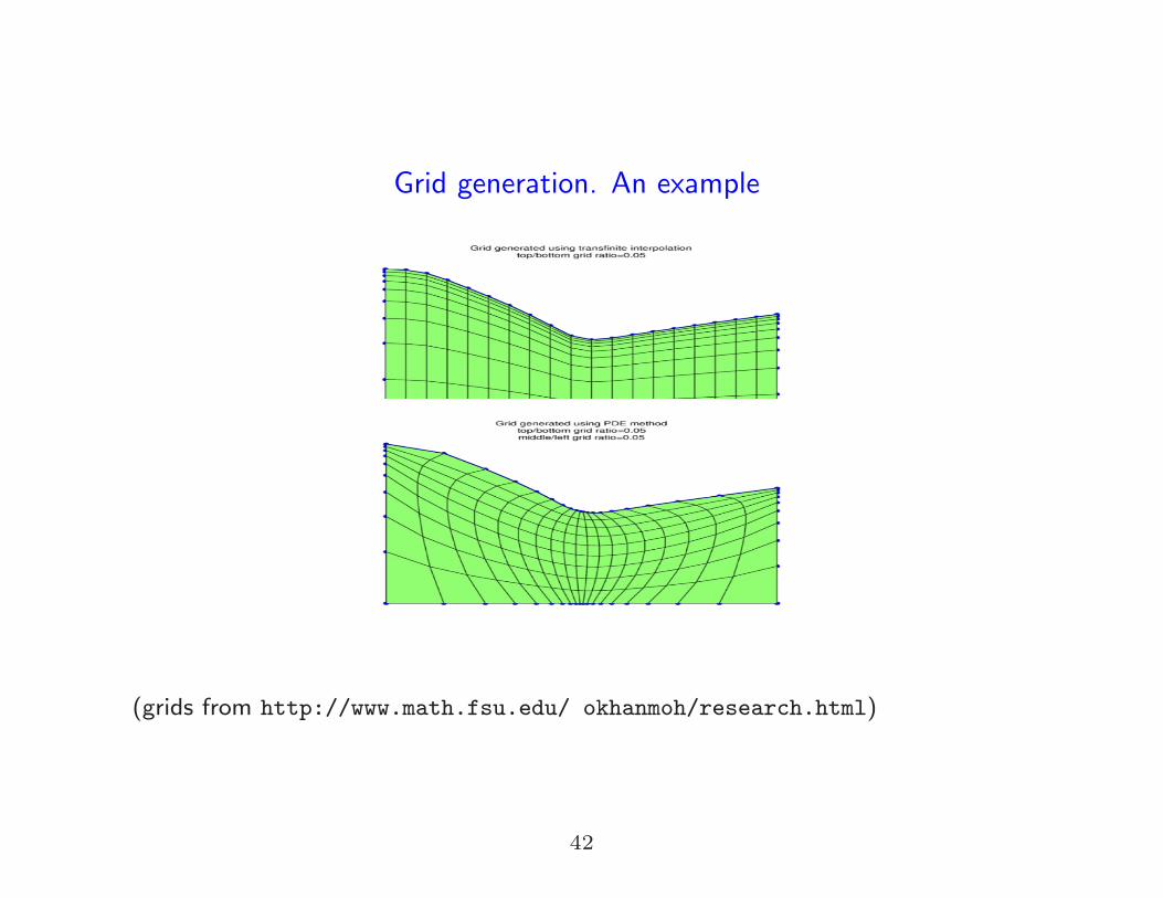
Grid generation. An example
(grids from http://www.math.fsu.edu/ okhanmoh/research.html)
42
Conclusions
• Matrix equations have very broad applicability
(structure recurrent in many application problems...)
• Recent appropriate computational devices
• Important tool for matrix sparsity analysis
references:
M. Benzi, V. Simoncini, SIMAX, v.36, 2015.
C. Canuto, V. Simoncini and M. Verani, LAA, v.452, 2014.
V. Simoncini, Survey on computational methods for matrix equations, to appear in
SIAM Review
43