Equidistribution and counting under equilibrium states innegative curvature and trees. Applications tonon-Archimedean Diophantine approximation

Anne Broise-Alamichel Jouni Parkkonen Frédéric Paulin

February 15, 2019

arX

iv:1

612.

0671

7v2

[m

ath.

DS]

14

Feb

2019

2 15/02/2019

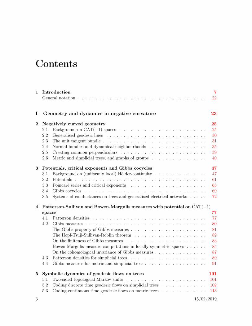
Contents

1 Introduction 7General notation . . . . . . . . . . . . . . . . . . . . . . . . . . . . . . . . . . . . . 22

I Geometry and dynamics in negative curvature 23

2 Negatively curved geometry 252.1 Background on CATp´1q spaces . . . . . . . . . . . . . . . . . . . . . . . . . 252.2 Generalised geodesic lines . . . . . . . . . . . . . . . . . . . . . . . . . . . . . 302.3 The unit tangent bundle . . . . . . . . . . . . . . . . . . . . . . . . . . . . . . 312.4 Normal bundles and dynamical neighbourhoods . . . . . . . . . . . . . . . . . 352.5 Creating common perpendiculars . . . . . . . . . . . . . . . . . . . . . . . . . 392.6 Metric and simplicial trees, and graphs of groups . . . . . . . . . . . . . . . . 40

3 Potentials, critical exponents and Gibbs cocycles 473.1 Background on (uniformly local) Hölder-continuity . . . . . . . . . . . . . . . 473.2 Potentials . . . . . . . . . . . . . . . . . . . . . . . . . . . . . . . . . . . . . . 613.3 Poincaré series and critical exponents . . . . . . . . . . . . . . . . . . . . . . . 653.4 Gibbs cocycles . . . . . . . . . . . . . . . . . . . . . . . . . . . . . . . . . . . 693.5 Systems of conductances on trees and generalised electrical networks . . . . . 72

4 Patterson-Sullivan and Bowen-Margulis measures with potential on CATp´1qspaces 774.1 Patterson densities . . . . . . . . . . . . . . . . . . . . . . . . . . . . . . . . . 774.2 Gibbs measures . . . . . . . . . . . . . . . . . . . . . . . . . . . . . . . . . . . 80

The Gibbs property of Gibbs measures . . . . . . . . . . . . . . . . . . . . . . 81The Hopf-Tsuji-Sullivan-Roblin theorem . . . . . . . . . . . . . . . . . . . . . 82On the finiteness of Gibbs measures . . . . . . . . . . . . . . . . . . . . . . . 83Bowen-Margulis measure computations in locally symmetric spaces . . . . . . 85On the cohomological invariance of Gibbs measures . . . . . . . . . . . . . . . 87

4.3 Patterson densities for simplicial trees . . . . . . . . . . . . . . . . . . . . . . 894.4 Gibbs measures for metric and simplicial trees . . . . . . . . . . . . . . . . . . 91

5 Symbolic dynamics of geodesic flows on trees 1015.1 Two-sided topological Markov shifts . . . . . . . . . . . . . . . . . . . . . . . 1015.2 Coding discrete time geodesic flows on simplicial trees . . . . . . . . . . . . . 1025.3 Coding continuous time geodesic flows on metric trees . . . . . . . . . . . . . 113

3 15/02/2019

5.4 The variational principle for metric and simplicial trees . . . . . . . . . . . . . 118

6 Random walks on weighted graphs of groups 1276.1 Laplacian operators on weighted graphs of groups . . . . . . . . . . . . . . . . 1276.2 Patterson densities as harmonic measures for simplicial

trees . . . . . . . . . . . . . . . . . . . . . . . . . . . . . . . . . . . . . . . . . 132

7 Skinning measures with potential on CATp´1q spaces 1397.1 Skinning measures . . . . . . . . . . . . . . . . . . . . . . . . . . . . . . . . . 1397.2 Equivariant families of convex subsets and their skinning measures . . . . . . 148

8 Explicit measure computations for simplicial trees and graphs of groups 1518.1 Computations of Bowen-Margulis measures for simplicial trees . . . . . . . . . 1528.2 Computations of skinning measures for simplicial trees . . . . . . . . . . . . . 156

9 Rate of mixing for the geodesic flow 1639.1 Rate of mixing for Riemannian manifolds . . . . . . . . . . . . . . . . . . . . 1639.2 Rate of mixing for simplicial trees . . . . . . . . . . . . . . . . . . . . . . . . . 1649.3 Rate of mixing for metric trees . . . . . . . . . . . . . . . . . . . . . . . . . . 174

II Geometric equidistribution and counting 183

10 Equidistribution of equidistant level sets to Gibbs measures 18510.1 A general equidistribution result . . . . . . . . . . . . . . . . . . . . . . . . . 18510.2 Rate of equidistribution of equidistant level sets for manifolds . . . . . . . . . 19010.3 Equidistribution of equidistant level sets on simplicial

graphs and random walks on graphs of groups . . . . . . . . . . . . . . . . . . 19210.4 Rate of equidistribution for metric and simplicial trees . . . . . . . . . . . . . 196

11 Equidistribution of common perpendicular arcs 20111.1 Part I of the proof of Theorem 11.1: the common part . . . . . . . . . . . . . 20311.2 Part II of the proof of Theorem 11.1: the metric tree case . . . . . . . . . . . 20511.3 Part III of the proof of Theorem 11.1: the manifold case . . . . . . . . . . . . 20911.4 Equidistribution of common perpendiculars in simplicial trees . . . . . . . . . 215

12 Equidistribution and counting of common perpendiculars in quotient spaces22512.1 Multiplicities and counting functions in Riemannian orbifolds . . . . . . . . . 22512.2 Common perpendiculars in Riemannian orbifolds . . . . . . . . . . . . . . . . 22812.3 Error terms for equidistribution and counting for Riemannian orbifolds . . . . 23112.4 Equidistribution and counting for quotient simplicial and metric trees . . . . 23412.5 Counting for simplicial graphs of groups . . . . . . . . . . . . . . . . . . . . . 24112.6 Error terms for equidistribution and counting for metric and simplicial graphs

of groups . . . . . . . . . . . . . . . . . . . . . . . . . . . . . . . . . . . . . . 246

13 Geometric applications 25513.1 Orbit counting in conjugacy classes for groups acting on trees . . . . . . . . . 25513.2 Equidistribution and counting of closed orbits on metric and simplicial graphs

(of groups) . . . . . . . . . . . . . . . . . . . . . . . . . . . . . . . . . . . . . 259

4 15/02/2019

III Arithmetic applications 263

14 Fields with discrete valuations 26514.1 Local fields and valuations . . . . . . . . . . . . . . . . . . . . . . . . . . . . . 26514.2 Global function fields . . . . . . . . . . . . . . . . . . . . . . . . . . . . . . . . 267

15 Bruhat-Tits trees and modular groups 27115.1 Bruhat-Tits trees . . . . . . . . . . . . . . . . . . . . . . . . . . . . . . . . . . 27115.2 Modular graphs of groups . . . . . . . . . . . . . . . . . . . . . . . . . . . . . 27515.3 Computations of measures for Bruhat-Tits trees . . . . . . . . . . . . . . . . . 27615.4 Exponential decay of correlation and error terms for arithmetic quotients of

Bruhat-Tits trees . . . . . . . . . . . . . . . . . . . . . . . . . . . . . . . . . . 28115.5 Geometrically finite lattices with infinite Bowen-Margulis measure . . . . . . 287

16 Equidistribution and counting of rational points in completed function fields29116.1 Counting and equidistribution of non-Archimedian Farey fractions . . . . . . 29116.2 Mertens’s formula in function fields . . . . . . . . . . . . . . . . . . . . . . . . 299

17 Equidistribution and counting of quadratic irrational points innon-Archimedean local fields 30117.1 Counting and equidistribution of loxodromic fixed points . . . . . . . . . . . . 30117.2 Counting and equidistribution of quadratic irrationals in positive characteristic 30517.3 Counting and equidistribution of quadratic irrationals in Qp . . . . . . . . . . 312

18 Equidistribution and counting of crossratios 31918.1 Counting and equidistribution of crossratios of loxodromic fixed points . . . . 31918.2 Counting and equidistribution of crossratios of quadratic irrationals . . . . . . 324

19 Equidistribution and counting of integral representations by quadratic normforms 327

Appendix 331

A A weak Gibbs measure is the unique equilibrium, by J. Buzzi 333A.1 Introduction . . . . . . . . . . . . . . . . . . . . . . . . . . . . . . . . . . . . . 333A.2 Proof of the main result Theorem A.4 . . . . . . . . . . . . . . . . . . . . . . 336

List of Symbols 343

Index 349

Bibliography 355

5 15/02/2019

6 15/02/2019

Chapter 1

Introduction

In this book, we study equidistribution and counting problems concerning locally geodesic arcsin negatively curved spaces endowed with potentials, and we deduce, from the special case oftree quotients, various arithmetic applications to equidistribution and counting problems innon-Archimedean local fields.

For several decades, tools in ergodic theory and dynamical systems have been used to ob-tain geometric equidistribution and counting results on manifolds, both inspired by and withapplications to arithmetic and number theoretic problems, in particular in Diophantine ap-proximation. Especially pioneered by Margulis, this field has produced a huge corpus of works,by Bowen, Cosentino, Clozel, Dani, Einseidler, Eskin, Gorodnik, Ghosh, Guivarc’h, Kim,Kleinbock, Kontorovich, Lindenstraus, Margulis, McMullen, Michel, Mohammadi, Mozes,Nevo, Oh, Pollicott, Roblin, Shah, Sharp, Sullivan, Ullmo, Weiss and the last two authors,just to mention a few contributors. We refer for now to the surveys [Bab2, Oh, PaP16, PaP17c]and we will explain in more details in this introduction the relation of our work with previousworks.

In this text, we consider geometric equidistribution and counting problems weighted witha potential function in quotient spaces of CATp´1q spaces by discrete groups of isometries.The CATp´1q spaces form a huge class of metric spaces that contains (but is not restricted to)metric trees, hyperbolic buildings and simply connected complete Riemannian manifolds withsectional curvature bounded above by ´1. In Chapter 2, we review some basic properties ofthese spaces and we refer to [BridH] for more details. Although some of the equidistributionand counting results with potentials on negatively curved manifolds are known,1 as well assome of such results on CATp´1q spaces without potential,2 bringing together these twoaspects and producing new results and applications is one of the goals of this book.

We extend the theory of Patterson-Sullivan, Bowen-Margulis and skinning measures toCATp´1q spaces with potentials, with a special emphasis on trees endowed with a system ofconductances. We prove that under natural nondegeneracy, mixing and finiteness assump-tions, the pushforward under the geodesic flow of the skinning measure of properly immersedlocally convex closed subsets of locally CATp´1q spaces equidistributes to the Gibbs measure,generalising the main result of [PaP14a].

We also prove that the (appropriate generalisations of) the initial and terminal tangentvectors of the common perpendiculars to any two properly immersed locally convex closed

1See for instance [PauPS].2See for instance [Rob2]

7 15/02/2019

subsets jointly equidistribute to the skinning measures when the lengths of the common per-pendiculars tend to `8. This result is then used to prove asymptotic results on weightedcounting functions of common perpendiculars whose lengths tend to `8. Common perpendic-ulars have been studied, in various particular cases, sometimes not explicitly, by Basmajian,Bridgeman, Bridgeman-Kahn, Eskin-McMullen, Herrmann, Huber, Kontorovich-Oh, Mar-gulis, Martin-McKee-Wambach, Meyerhoff, Mirzakhani, Oh-Shah, Pollicott, Roblin, Shah,the last two authors and many others. See the comments after Theorem 1.5 below, and thesurvey [PaP16] for references.

In Part III of this book, we apply the geometric results obtained for trees to deduce arith-metic applications in non-Archimedean local fields. In particular, we prove equidistributionand counting results for rationals and quadratic irrationals in any completion of any functionfield over a finite field.

Let us now describe more precisely the content of this book, restricted to special cases forthe sake of the exposition.

Geometric and dynamical tools

Let Y be a geodesically complete connected proper locally CATp´1q space (or good orbispace),which is nonelementary, that is, whose fundamental group is not virtually nilpotent. In thisintroduction, we will mainly concentrate on the cases where Y is either a metric graph (orgraph of finite groups in the sense of Bass and Serre, see [Ser3]) or a Riemannian manifold (orgood orbifold) of dimension at least 2 with sectional curvature at most ´1. Let GY be thespace of locally geodesic lines of Y , on which the geodesic flow pgtqtPR acts by real translationson the source. When Y is a simplicial3 graph (of finite groups), we consider the discrete timegeodesic flow pgtqtPZ, see Section 2.6. If Y is a Riemannian manifold, then GY is naturallyidentified with the unit tangent bundle T 1Y by the map that associates to a locally geodesicline its tangent vector at time 0. In general, we define T 1Y as the space of germs of locallygeodesic lines in Y , and GY maps onto T 1Y with possibly uncountable fibers.

Let F : T 1Y Ñ R be a continuous map, called a potential, which plays the same rolein the construction of Gibbs measures/equilibrium states as the energy function in Bowen’streatment of the thermodynamic formalism of symbolic dynamical systems in [Bowe2, Sect. 1].We define in Section 3.3 the critical exponent δF associated with F , which describes thelogarithmic growth of an orbit of the fundamental group on the universal cover of Y weightedby the (lifted) potential F , and which coincides with the classical critical exponent whenF “ 0. When Y is a metric graph, we associate in Section 3.5 a potential Fc to a systemof conductances c (that is, a map from the set of edges of Y to R), in such a way that thecorrespondence c ÞÑ Fc is bijective at the level of cohomology classes, and we denote δFc byδc.

In this introduction, we assume that F is bounded and that δF is finite and positive inorder to simplify the statements.

We say that the pair pY, F q satisfies the HC-property if the integral of F on compact locallygeodesic segments of Y varies in a Hölder-continuous way on its extremities (see Definition3.13). The pairs which have the HC-property include complete Riemannian manifolds with

3that is, if its edges all have lengths 1

8 15/02/2019

pinched sectional curvature at most ´1 and Hölder-continuous potentials, and metric graphswith any potential. This HC-property is the new technical idea compared to [PauPS] whichallows the extensions to our very general framework. See also [ConLT], under the very strongassumption that Y is compact.

In Chapter 4, building on the works of [Rob2]4 when F “ 0 and of [PauPS]5 when Y is aRiemannian manifold, we generalise, to locally CATp´1q spaces Y endowed with a potentialF satisfying the HC-property, the construction and basic properties of the Patterson densitiesat infinity of the universal cover of Y associated with F and the Gibbs measure mF on GYassociated with F .

Using the Patterson-Sullivan-Bowen-Margulis approach, the Patterson densities are limitsof renormalised measures on the orbit points of the fundamental group on the universalcover of Y , weighted by the potential, and the Gibbs measures on GY are local products ofPatterson densities on the endpoints of the geodesic line, with the Lebesgue measure on thetime parameter, weighted by the Gibbs cocycle defined by the potential.

Generalising a result of [CoP2], we prove in Section 6.2 that when Y is a regular simpli-cial graph and c is an antireversible system of conductances, then the Patterson measures,normalised to be probability measures, are harmonic measures (or hitting measures) on theboundary at infinity of the universal cover of Y for a transient random walk on the vertices,whose transition probabilities are constructed using the total mass of the Patterson measures.

Gibbs measures were first introduced in statistical mechanics, and are naturally associatedvia the thermodynamic formalism6 with symbolic dynamics. We prove in Section 4.2 that ourGibbs measures satisfy a Gibbs property analogous to the one in symbolic dynamics. If F “ 0,the Gibbs measure mF is the Bowen-Margulis measure mBM. If Y is a compact Riemannianmanifold and F is the strong unstable Jacobian v ÞÑ ´ d

dt |t“0ln Jac

`

gt|W´pvq

˘

pvq, then mF isthe Liouville measure and δF “ 0 (see [PauPS, Chap. 7] for more general assumptions on Y ).Thus, one interesting aspect of Gibbs measure is that they form a natural family of measuresinvariant under the geodesic flow that interpolates between the Liouville measure and theBowen-Margulis measure (which in variable curvature are in general not in the same measureclass). Another interesting point is that such measures are plentiful: a recent result of Belarif[Bel] proves that when Y is a geometrically finite Riemannian manifold with pinched nega-tive curvature and topologically mixing geodesic flow, the finite and mixing Gibbs measuresassociated with bounded Hölder-continuous potentials are, once normalised, dense (for theweak-star topology) in the whole space of probability measures invariant under the geodesicflow.

The Gibbs measures are remarkable measures for CATp´1q spaces endowed with poten-tials due to their unique ergodic-theoretic properties. Let pZ, pφtqtPRq be a topological spaceendowed with a continuous one-parameter group of homeomorphisms and let ψ : Z Ñ R bea bounded continuous map. Let M be the set of Borel probability measures on Z invariantunder the flow pφtqtPR. Let hmpφ1q be the (metric) entropy of the geodesic flow with respect tom P M . The metric pressure for ψ of a measure m P M and the pressure of ψ are respectively

Pψpmq “ hmpφ1q `

ż

Zψ dm and Pψ “ sup

mPMPψpmq .

An element m P M is an equilibrium state for ψ if the least upper bound defining Pψ is4itself building on the works of Patterson, Sullivan, Coornaert, Burger-Mozes, ...5itself building on the works of Ledrappier [Led], Hamenstädt, Coudène, Mohsen6See for instance [Rue3, Kel, Zin].

9 15/02/2019

attained on m.Let F 7 : GY Ñ R be the composition of the canonical map GY Ñ T 1Y with F , and note

that F 7 “ F if Y is a Riemannian manifold. When F “ 0 and Y is a Riemannian manifold,whose sectional curvatures and their first derivatives are bounded, by [OtaP, Theo. 2], thepressure PF coincides with the entropy of the geodesic flow, it is equal to the critical exponentof the fundamental group of Y , and the Bowen-Margulis measure mF “ mBM, normalisedto be a probability measure, is the measure of maximal entropy. When Y is a Riemannianmanifold whose sectional curvatures and their first derivatives are bounded and F is Hölder-continuous, by [PauPS, Theo. 6.1], we have PF “ δF . If furthermore the Gibbs measure mF

is finite and normalised to be a probability measure, then mF is an equilibrium state for F .In Section 5.4, we prove an analog of these results for the potential F 7 when Y is a metric

graph of groups. The case when Y is a finite simplicial graph7 is classical by the work of Bowen[Bowe2], as it reduces to arguments of subshifts of finite type (see for instance [CoP1]). WhenY is a compact8 locally CATp´1q-space,9 a complete statement about existence, uniquenessand Gibbs property of equilibrium states for any Hölder-continuous potential is given in[ConLT].

Theorem 1.1 (The variational principle for metric graphs of groups). Assume that Y is ametric graph of finite groups, with a positive lower bound and finite upper bound on the lengthsof edges. If the critical exponent δF is finite, if the Gibbs measure mF is finite, then PF 7 “ δFand the Gibbs measure normalised to be a probability measure is the unique equilibrium statefor F 7.

The main tool is a natural coding of the discrete time geodesic flow by a topological Markovshift (see Section 5.1). This coding is delicate when the vertex stabilisers are nontrivial, inparticular as it does not satisfy in general the Markovian property of dependence only onthe immediate past (see Section 5.2). We then apply results of Buzzi and Sarig in symbolicdynamics over a countable alphabet (see Appendix A written by J. Buzzi), and suspensiontechniques introduced in Section 5.3. See also [Kemp].

Let Y be any geodesically complete connected proper locally CATp´1q space, and let Dbe any connected proper nonempty properly immersed10 closed locally convex subset of Y .In Chapter 7, we generalise for nonconstant potentials on Y the construction of the skinningmeasures σ`D and σ´D on the outer and inner unit normal bundles ofD in Y . We refer to Section2.4 for the appropriate definition of the outer and inner unit normal bundles of D when theboundary of D is not smooth. We construct these measures σ`D and σ´D as pushforwards ofthe Patterson densities associated with the potential F to the outer and inner unit normalbundles of the lift of D in the universal cover of Y . This construction generalises the one in[PaP14a] when F “ 0, which itself generalises the one in [OhS1, OhS2] when M has constantcurvature and D is a ball, a horoball or a totally geodesic submanifold.

In Section 10.1, we prove the following result on the equidistribution of equidistant hyper-surfaces in CATp´1q spaces. This result is a generalisation of [PaP14a, Theo. 1] (valid in Rie-mannian manifolds with zero potential) which itself generalised the ones in [Mar2, EM, PaP12]

7that is, a finite graph of trivial groups with edge lengths 18a very strong assumption that we do not want to make in this text9not in the orbifold sense, hence this excludes for instance the case of graphs of groups with some nontrivial

vertex stabiliser10By definition, D is the image in Y , by the universal covering map, of a proper nonempty closed convex

subset of the universal cover of Y , whose family of images under the universal covering group is locally finite.

10 15/02/2019

when Y has constant curvature, F “ 0 and D is a ball, a horoball or a totally geodesic sub-manifold. See also [Rob2] when Y is a CATp´1q space, F “ 0 and D is a ball or a horoball.

Theorem 1.2. Let Y,D be as above, and let F be a potential of Y satisfying the HC-property.Assume that the Gibbs measure mF on GY is finite and mixing for the geodesic flow pgtqtPR,and that the skinning measure σ`D is finite and nonzero. Then, as t tends to `8, the pushfor-wards pgtq˚σ`D of the skinning measure of D by the geodesic flow weak-star converge towardsthe Gibbs measure mF (after normalisation as probability measures).

We prove in Theorem 10.4 an analog of Theorem 1.2 for the discrete time geodesic flowon simplicial graphs and, more generally, simplicial graphs of groups. As a special case,we recover known results on nonbacktracking simple random walks on regular graphs. Theequidistribution of the pushforward of the skinning measure of a subgraph is a weighted versionof the following classical result, see for instance [AloBLS], which under further assumptionson the spectral properties on the graph gives precise rates of convergence.

Corollary 1.3. Let Y be a finite regular graph which is not bipartite. Let Y1 be a nonemptyconnected subgraph. Then the n-th vertex of the nonbacktracking simple random walk on Ystarting transversally to Y1 converges in distribution to the uniform distribution as nÑ `8.

See Chapter 10 for more details and for the extensions to nonzero potential and to graphsof groups, as well as Section 10.4 for error terms.

The distribution of common perpendiculars

Let D´ and D` be connected proper nonempty properly immersed locally convex closedsubsets of Y . A common perpendicular from D´ to D` is a locally geodesic path in Y startingperpendicularly from D´ and arriving perpendicularly to D`.11 We denote the length of acommon perpendicular α from D´ to D` by λpαq, and its initial and terminal unit tangentvectors by v´α and v`α . In the general CATp´1q case, v˘α are two different parametrisations(by ¯r0, λpαqs) of α, considered as elements of the space

p

GY of generalised locally geodesiclines in Y , see [BartL] or Section 2.2. For all t ą 0, we denote by PerppD´, D`, tq the set ofcommon perpendiculars from D´ to D` with length at most t (considered with multiplicities),and we define the counting function with weights by

ND´, D`, F ptq “ÿ

αPPerppD´, D`, tq

eş

α F ,

whereş

α F “şλpαq0 F pgtv´α q dt. We refer to Section 12.1 for the definition of the multiplicities

in the manifold case, which are equal to 1 if D´ and D` are embedded and disjoint. Highermultiplicities for common perpendiculars α can occur for instance when D´ is a nonsimpleclosed geodesic and the initial point of α is a multiple point of D´.

Let PerppD´, D`q be the set of all common perpendiculars from D´ to D` (consideredwith multiplicities). The family pλpαqqαPPerppD´, D`q is called the marked ortholength spec-trum from D´ to D`. The set of lengths (with multiplicities) of elements of PerppD´, D`qis called the ortholength spectrum of D´, D`. This second set has been introduced by Bas-majian [Basm] (under the name “full orthogonal spectrum”) when M has constant curvature,

11See Section 2.5 for explanations when the boundary of D´ or D` is not smooth.

11 15/02/2019

and D´ and D` are disjoint or equal embedded totally geodesic hypersurfaces or embeddedhorospherical cusp neighbourhoods or embedded balls. We refer to the paper [BridK] whichproves that the ortholength spectrum with D´ “ D` “ BM determines the volume of acompact hyperbolic manifoldM with totally geodesic boundary (see also [Cal] and [MasaM]).

We prove in Chapter 12 that the critical exponent δF of F is the exponential growth rateof ND´, D`, F ptq, and we give an asymptotic formula of the form ND´, D`, F ptq „ c eδF t astÑ `8, with error term estimates in appropriate situations. The constants c that will appearin such asymptotic formulas will be explicit, in terms of the measures naturally associatedwith the (normalised) potential F : the Gibbs measure mF and the skinning measures of D´

and D`.When F “ 0 and Y is a Riemannian manifold with pinched sectional curvature and finite

and mixing Bowen-Margulis measure, the asymptotics of the counting function ND´, D`, 0ptqare described in [PaP17b, Theo. 1]. The only restriction on the two convex sets D˘ is thattheir skinning measures are finite. Here, we generalise that result by allowing for nonzeropotential and more general CATp´1q spaces than just manifolds.

The counting function ND´, D`, 0ptq has been studied in negatively curved manifolds sincethe 1950’s and in a number of more recent works, sometimes in a different guise. A numberof special cases (all with F “ 0 and covered by the results of [PaP17b]) were known:• D´ and D` are reduced to points, by for instance [Hub2], [Mar1] and [Rob2],• D´ and D` are horoballs, by [BeHP], [HeP3], [Cos] and [Rob2] without an explicit form

of the constant in the asymptotic expression,• D´ is a point and D` is a totally geodesic submanifold, by [Herr], [EM] and [OhS3] in

constant curvature,• D´ is a point and D` is a horoball, by [Kon] and [KonO] in constant curvature, and [Kim]

in rank one symmetric spaces,• D´ is a horoball and D` is a totally geodesic submanifold, by [OhS1] and [PaP12] in

constant curvature, and• D´ and D` are (properly immersed) locally geodesic lines in constant curvature and

dimension 3, by [Pol2].We refer to the survey [PaP16] for more details on the manifold case.

When X is a compact metric or simplicial graph and D˘ are points, the asymptotics ofND´, D`, 0ptq as t Ñ `8 is treated in [Gui], as well as [Rob2]. Under the same setting, seealso the work of Kiro-Smilansky-Smilansky announced in [KiSS] for a counting result of paths(not assumed to be locally geodesic) in finite metric graphs with rationally independent edgelengths and vanishing potential.

The proofs of the asymptotic results on the counting function ND´, D`, F are based onthe following simultaneous equidistribution result that shows that the initial and terminaltangent vectors of the common perpendiculars equidistribute to the skinning measures of D´

and D`. We denote the unit Dirac mass at a point z by ∆z and the total mass of any measurem by m.

Theorem 1.4. Assume that Y is a nonelementary Riemannian manifold with pinched sec-tional curvature at most ´1 or a metric graph. Let F : T 1Y Ñ R be a potential, with finiteand positive critical exponent δF , which is bounded and Hölder-continuous when Y is a man-ifold. Let D˘ be as above. Assume that the Gibbs measure mF is finite and mixing for the

12 15/02/2019

geodesic flow. For the weak-star convergence of measures onp

GY ˆ

p

GY , we have

limtÑ`8

δF mF e´δF t

ÿ

αPPerppD´, D`, tq

eş

α F ∆v´αb∆v`α

“ σ`D´b σ´

D`.

There is a similar statement for nonbipartite simplicial graphs and for more general graphsof groups on which the discrete time geodesic flow is mixing for the Gibbs measure, see theend of Chapter 11 and Section 12.4. Again, the results can then be interpreted in terms ofnonbacktracking random walks.

In Section 12.2, we deduce our counting results for common perpendiculars between thesubsets D´ and D` from the above simultaneous equidistribution theorem.

Theorem 1.5. (1) Let Y, F,D˘ be as in Theorem 1.4. Assume that the Gibbs measure mF

is finite and mixing for the continuous time geodesic flow and that the skinning measures σ`D´

and σ´D`

are finite and nonzero. Then, as sÑ `8,

ND´, D`, F psq „σ`D´ σ´

D`

mF

eδF s

δF.

(2) If Y is a finite nonbipartite simplicial graph, then

ND´, D`,F pnq „eδF σ`

D´ σ´

D`

peδF ´ 1q mF eδF n .

The above Assertion (1) is valid when Y is a good orbifold instead of a manifold ora metric graph of finite groups instead of a metric graph (for the appropriate notion ofmultiplicities), and when D´ and D` are replaced by locally finite families. See Section 12.4for generalisations of Assertion (2) to (possibly infinite) simplicial graphs of finite groups andSections 12.3 and 12.6 for error terms.

We avoid any compactness assumption on Y , we only assume that the Gibbs measure mF

of F is finite and that it is mixing for the geodesic flow. By Babillot’s theorem [Bab1], ifthe length spectrum of Y is not contained in a discrete subgroup of R, then mF is mixing iffinite. If Y is a Riemannian manifold, this condition is satisfied for instance if the limit setof a fundamental group of Y is not totally disconnected, see for instance [Dal1, Dal2]. WhenY is a metric graph, Babillot’s mixing condition is in particular satisfied if the lengths of theedges of Y are rationally independent.

As in [PaP17b], we have very weak finiteness and curvature assumptions on the spaceand the convex subsets we consider. Furthermore, the space Y is no longer required to be amanifold and we extend the theory to nonconstant weights using equilibrium states. Such aweighted counting has only been used in the orbit-counting problem in manifolds with pinchednegative curvature in [PauPS]. The approach is based on ideas from Margulis’s thesis to usethe mixing of the geodesic flow. Our skinning measures are much more general than thePatterson measures appearing in earlier works. As in [PaP17b], we push simultaneously theunit normal vectors to the two convex sets D´ and D` in opposite directions.

Classically, an important characterisation of the Bowen-Margulis measure on closed neg-atively curved Riemannian manifolds (F “ 0) is that it coincides with the weak-star limitof properly normalised sums of Lebesgue measures supported on periodic orbits. The resultwas extended to CATp´1q spaces with zero potential in [Rob2] and to Gibbs measures in

13 15/02/2019

the manifold case in [PauPS, Theo. 9.11]. As a corollary of the simultaneous equidistributionresult Theorem 1.4, we obtain a weighted version for simplicial and metric graphs of groups.The following is a simplified version of such a result for Gibbs measures of metric graphs.

Let Per1ptq be the set of prime periodic orbits of the geodesic flow on Y . Let λpgq denotethe length of a closed orbit g. Let Lg be the Lebesgue measure along g and let LgpF q be theperiod of g for the potential F .

Theorem 1.6. Assume that Y is a finite metric graph, that the critical exponent δF is positiveand that the Gibbs measure mF is mixing for the continuous time geodesic flow. As tÑ `8,the measures

δF eδF t

ÿ

gPPer1ptq

eLgpF qLg

andδF t e

δF tÿ

gPPer1ptq

eLgpF q Lg

λpgq

converge to mFmF

for the weak-star convergence of measures.

See Section 13.2 for the proof of the full result and for a similar statement for (possiblyinfinite) simplicial graphs of finite groups. As a corollary, we obtain counting results of simpleloops in metric and simplicial graphs, generalising results of [ParP], [Gui].

Corollary 1.7. Assume that Y is a finite metric graph whose vertices have degrees at least3, such that the critical exponent δF is positive.

(1) If the Gibbs measure is mixing for the continuous time geodesic flow, then

ÿ

gPPer1ptq

eLgpF q „eδF t

δF t

as tÑ `8.

(2) If Y is simplicial and if the Gibbs measure is mixing for the discrete time geodesic flow,then

ÿ

gPPer1ptq

eLgpF q „eδF

eδF ´ 1

eδF t

t

as tÑ `8.

In the cases when error bounds are known for the mixing property of the continuous time ordiscrete time geodesic flow on GY , we obtain corresponding error terms in the equidistributionresult of Theorem 1.2 generalising [PaP14a, Theo. 20] (where F “ 0) and in the approximationof the counting function ND´, D`, 0 by the expression introduced in Theorem 1.5. In themanifold case, see [KM1], [Clo], [Dol1], [Sto], [Live], [GLP], and Section 12.3 for definitionsand precise references. Here is an example of such a result in the manifold case.

Theorem 1.8. Assume that Y is a compact Riemannian manifold and mF is exponentiallymixing under the geodesic flow for the Hölder regularity, or that Y is a locally symmetricspace, the boundary of D˘ is smooth, mF is finite, smooth, and exponentially mixing underthe geodesic flow for the Sobolev regularity. Assume that the strong stable/unstable ball massesby the conditionals of mF are Hölder-continuous in their radius.

14 15/02/2019

(1) As t tends to `8, the pushforwards pgtq˚σ`D´ of the skinning measure of D´ by thegeodesic flow equidistribute towards the Gibbs measure mF with exponential speed.

(2) If the skinning measures σ`D´

and σ´D`

are finite and nonzero, there exists κ ą 0 suchthat, as tÑ `8,

ND´, D`, F ptq “σ`D´ σ´

D`

δF mF eδF t

`

1`Ope´κtq˘

.

See Section 12.3 for a discussion of the assumptions and the dependence of Op¨q on thedata. Similar (sometimes more precise) error estimates were known earlier for the countingfunction in special cases of D˘ in constant curvature geometrically finite manifolds (often insmall dimension) through the work of Huber, Selberg, Patterson, Lax and Phillips [LaxP],Cosentino [Cos], Kontorovich and Oh [KonO], Lee and Oh [LeO].

When Y is a finite volume hyperbolic manifold and the potential F is constant 0, the Gibbsmeasure is proportional to the Liouville measure and the skinning measures of totally geodesicsubmanifolds, balls and horoballs are proportional to the induced Riemannian measures ofthe unit normal bundles of their boundaries. In this situation, there are very explicit formsof the counting results in finite-volume hyperbolic manifolds, see [PaP17b, Cor.21], [PaP16].These results are extended to complex hyperbolic space in [PaP17a].

As an example of this result, if D´ and D` are closed geodesics of Y of lengths `´ and``, respectively, then the number N psq “ ND´, D`, 0psq of common perpendiculars (countedwith multiplicity) from D´ to D` of length at most s satisfies, as sÑ `8,

N psq „πn2´1Γpn´1

2 q2

2n´2pn´ 1qΓpn2 q

`´``VolpY q

epn´1qs . (1.1)

Counting in weighted graphs of groups

From now on in this introduction, we only consider metric or simplicial graphs or graphs ofgroups.

Let Y be a connected finite graph with set of vertices V Y and set of edges EY (see [Ser3]for the conventions). We assume that the degree of the graph at each vertex is at least 3. Letλ : EY Ñ s0,`8r with λpeq “ λpeq for every e P EY be an edge length map, let Y “ |Y|λbe the geometric realisation of Y where the geometric realisation of every edge e P EY haslength λpeq, and let c : EY Ñ R be a map, called a (logarithmic) system of conductances inthe analogy between graphs and electrical networks, see for instance [Zem].

Let Y˘ be proper nonempty subgraphs of Y. For every t ě 0, we denote by PerppY´,Y`, tqthe set of edge paths α “ pe1, . . . , ekq in Y without backtracking, of length λpαq “

řki“1 λpeiq

at most t, of conductance cpαq “řki“1 cpeiq, starting from a vertex of Y´ but not by an edge

of Y´, ending at a vertex of Y` but not by an edge of Y`. Let

NY´,Y`ptq “ÿ

αPPerppY´,Y`, tq

ecpαq

be the number of paths without backtracking from Y´ to Y` of length at most t, countedwith weights defined by the system of conductances.

15 15/02/2019

Recall that a real number x is Diophantine if it is badly approximable by rational numbers,that is, if there exist α, β ą 0 such that |x´ p

q | ě α q´β for all p, q P Z with q ą 0. We obtainthe following result, which is a very simplified version of our results for the sake of thisintroduction.

Theorem 1.9. (1) If Y has two cycles whose ratio of lengths is Diophantine, then there existsC ą 0 such that for every k P N´ t0u, as tÑ `8,

NY´,Y`ptq “ C eδc t`

1`Opt´kq˘

.

(2) If λ ” 1, then there exist C 1, κ ą 0 such that, as n P N tends to `8,

NY´,Y`pnq “ C 1 eδc n`

1`Ope´κnq˘

.

Note that the Diophantine assumption on Y in Theorem 1.9 (1) is standard in the theoryof quantum graphs (see for instance [BerK]).

The constants C “ CY˘, c, λ ą 0 and C 1 “ C 1Y˘, c ą 0 in the above asymptotic formulasare explicit. When c ” 0 and λ ” 1, the constants can often be determined concretely, asindicated in the two examples below.12 Among the ingredients in these computations arethe explicit expressions of the total mass of many Bowen-Margulis measures and skinningmeasures obtained in Chapter 8.

See Sections 12.4, 12.5 and 12.6 for generalisations of Theorem 1.9 when the graphs Y˘are not embedded in Y, and for versions in (possibly infinite) metric graphs of finite groups.In particular, Assertion (2) remains valid if Y is the quotient of a uniform simplicial tree by ageometrically finite lattice in the sense of [Pau4], such as an arithmetic lattice in PGL2 over anon-Archimedian local field, see [Lub1]. Recall that a locally finite metric tree X is uniformif it admits a discrete and cocompact group of isometries, and that a lattice Γ of X is alattice in the locally compact group of isometries of X preserving without edge inversions thesimplicial structure. We refer for instance to [BasK, BasL] for uncountably many examplesof tree lattices.

Example 1.10. (1) When Y is a pq ` 1q-regular finite graph with constant edge length mapλ ” 1 and vanishing system of conductances c ” 0, then δc “ ln q, and if furthermore Y` andY´ are vertices, then (see Equation (12.11))

C 1 “q ` 1

pq ´ 1qCardpV Yq.

(2) When Y is biregular of degrees p` 1 and q` 1 with p, q ě 2, when λ ” 1 and c ” 0, thenδc “ ln

?pq , and if furthermore the subgraphs Y˘ are simple cycles of lengths L˘, then (see

Equation (12.12)) the number of common perpendiculars of even length at most 2N from Y´to Y` as N Ñ `8 is asymptotic to

pp` qq L´ L`

2 ppq ´ 1q CardpEYqppqqN`1

The main tool in order to obtain the error terms in Theorem 1.9 and its more generalversions is to study the error terms in the mixing property of the geodesic flow. Using the

12See Section 12.4 for more examples.

16 15/02/2019

already mentioned coding (given in Section 5.2) of the discrete time geodesic flow by a two-sided topological Markov shift, classical reduction to one-sided topological Markov shift, andresults of Young [You1] on the decay of correlations for Young towers with exponentiallysmall tails, we in particular obtain the following simple criteria for the exponential decay ofcorrelation of the discrete time geodesic flow, where we only assume Y to be locally finite(and maybe not finite). See Theorem 9.1 for the complete result.

Theorem 1.11. Assume that the Gibbs measure mF is finite and mixing for the discrete timegeodesic flow on Y. Assume moreover that there exist a finite subset E of V Y and C 1, κ1 ą 0such that for all n P N, we have

mF

`

t` P GY : `p0q P E and @ k P t1, . . . , nu, `pkq R Eu˘

ď C 1 e´κ1n .

Then the discrete time geodesic flow has exponential decay of Hölder correlations for mF .

The assumption of having exponentially small mass of geodesic lines which have a bigreturn time to a given finite subset of V Y is in particular satisfied (see Section 9.2) if Yis the quotient of a uniform simplicial tree by a geometrically finite lattice,13 such as anarithmetic lattice in PGL2 over a non-Archimedian local field, see [Lub1], but also by manyother examples of Y. This statement corrects the mistake in [Kwo], as indicated in its erratum.

These results allow to prove in Section 9.3, under Diophantine assumptions, the rapidmixing property for the continuous time geodesic flow, that leads to Assertion (1) of Theorem1.9, see Section 12.6. The proof uses suspension techniques due to Dolgopyat [Dol2] when Yis a compact metric tree, and to Melbourne [Mel1] otherwise.

As a corollary of the general version of the counting result Theorem 1.5, we have thefollowing asymptotic for the orbital counting function in conjugacy classes for groups actingon trees. Given x0 P X and a nontrivial conjugacy class K in a discrete group Γ of isometriesof X, we consider the counting function

NK, x0ptq “ Cardtγ P K : dpx0, γx0q ď tu ,

introduced by Huber [Hub1] when X is replaced by the real hyperbolic plane and Γ is alattice. We refer to [PaP15] for many results on the asymptotic growth of such orbital countingfunctions in conjugacy classes, when X is replaced by a finitely generated group with a wordmetric, or a complete simply connected pinched negatively curved Riemannian manifold. Seealso [ChaP, ArCT, Pol3].

Theorem 1.12. Let X be a uniform metric tree with vertices of degree ě 3, let δ be theHausdorff dimension of its space of ends, let Γ be a discrete group of isometries of X, let x0

be a vertex of X with trivial stabiliser in Γ, and let K be a loxodromic conjugacy class in Γ.(1) If the metric graph ΓzX is compact and has two cycles whose ratio of lengths is Diophan-tine, then there exists C ą 0 such that for every k P N´ t0u, as tÑ `8,

NK, x0ptq “ C eδ2t`

1`Opt´kq˘

.

(2) If X is simplicial and Γ is a geometrically finite lattice of X, then there exist C 1, κ ą 0such that, as n P N tends to `8,

NK, x0pnq “ C 1 eδ tpn´λpγqq2u`

1`Ope´κnq˘

.13See for instance [Pau4].

17 15/02/2019

We refer to Theorem 13.1 for a more general version, including a version with a systemof conductances in the counting function, and when K is elliptic. When ΓzX is compactand Γ is torsion free,14 Assertion (1) of this result is due to Kenison and Sharp [KeS], whoproved it using transfer operator techniques for suspensions of subshifts of finite type. Upto strengthening the Diophantine assumption, using work of Melbourne [Mel1] on the decayof correlations of suspensions of Young towers, we are able to extend Assertion (1) to allgeometrically finite lattices Γ of X in Section 13.1.

The constants C “ CK,x0 and C 1 “ C 1K,x0are explicit. For instance in Assertion (2), if X

is the geometric realisation of a regular simplicial tree X of degree q ` 1, if x0 is a vertex ofX, if K is the conjugacy class of γ0 with translation length λpγ0q on X, if

VolpΓzzXq “ÿ

rxsPΓzV X

1

|Γx|

is the volume15 of the quotient graph of groups ΓzzX , then

C 1 “λpγ0q

rZΓpγ0q : γZ0 s VolpΓzzXq,

where ZΓpγ0q is the centraliser of γ0 in Γ. When furthermore Γ is torsion free, γ0 is not aproper power and ΓzX is finite, as δ “ ln q, we get that there exists κ ą 0 such that

NK, x0pnq “λpγ0q

CardpΓzXqqtpn´λpγ0qq2u `Opqp1´κ

1qn2q

as n P N tends to `8, thus recovering the result of [Dou] who used the spectral theory of thediscrete Laplacian.

Selected arithmetic applications

We end this introduction by giving a sample of our arithmetic applications (see Part III of thisbook) of the ergodic and dynamical results on the discrete time geodesic flow on simplicialtrees described in Part II of this book, as summarized above. Our equidistribution andcounting results of common perpendiculars between subtrees indeed produce equidistributionand counting results of rationals and quadratic irrationals in non-Archimedean local fields.We refer to [BrPP] for an announcement of the results of Part III, with a presentation differentfrom the one in this introduction.

To motivate what follows, consider R “ Z the ring of integers, K “ Q its field of fractions,pK “ R the completion of Q for the usual Archimedean absolute value | ¨ |, and Haar

pKthe

Lebesgue measure of R (which is the Haar measure of the additive group R normalised sothat Haar

pKpr0, 1sq “ 1).

The following equidistribution result of rationals, due to Neville [Nev], is a quantitativestatement on the density of K in pK: For the weak-star convergence of measures on pK, assÑ `8, we have

limsÑ`8

π

6s´2

ÿ

p,qPR : pR`qR“R, |q|ďs

∆ pq“ Haar

pK.

14In particular, Γ then has the very restricted structure of a free group.15See for instance [BasK, BasL].

18 15/02/2019

Furthermore, there exists ` P N such that for every smooth function ψ : pK Ñ C withcompact support, there is an error term in the above equidistribution claim evaluated onψ, of the form Opspln sqψ`q where ψ` is the Sobolev norm of ψ. The following countingresult due to Mertens on the asymptotic behaviour of the average of Euler’s totient functionϕ : k ÞÑ CardpRkRqˆ, follows from the above equidistribution one:

nÿ

k“1

ϕpkq “3

πn2 `Opn lnnq .

See [PaP14b] for an approach using methods similar to the ones in this text, and for instance[HaW, Theo. 330] for a more traditional proof, as well as [Walf] for a better error term.

Let us now switch to a non-Archimedean setting, restricting to positive characteristic inthis introduction. See Part III for analogous applications in characteristic zero.

Let Fq be a finite field of order q. Let R “ FqrY s be the ring of polynomials in onevariable Y with coefficients in Fq. Let K “ FqpY q be the field of rational fractions in Y withcoefficients in Fq, which is the field of fractions of R. Let pK “ FqppY ´1qq be the field of formalLaurent series in the variable Y ´1 with coefficients in Fq, which is the completion of K forthe (ultrametric) absolute value |PQ | “ qdegP´degQ. Let O “ FqrrY ´1ss be the ring of formalpower series in Y ´1 with coefficients in Fq, which is the ball of centre 0 and radius 1 in pK forthis absolute value.

Note that pK is locally compact, and we endow the additive group pK with the Haar measureHaar

pKnormalised so that Haar

pKpOq “ 1. The following results extend (with appropriate

constants) when K is replaced by any function field of a nonsingular projective curve over Fqand pK any completion of K, see Part III.

The following equidistribution result16 of elements of K in pK gives an analog of Neville’sequidistribution result for function fields. Note that when G “ GL2pRq, we have pP,Qq PGp1, 0q if and only if xP,Qy “ R. We denote by Hx the stabiliser of any element x of any setendowed with any action of any group H.

Theorem 1.13. Let G be any finite index subgroup of GL2pRq. For the weak-star convergenceof measures on pK, we have

limtÑ`8

pq ` 1q rGL2pRq : Gs

pq ´ 1q q2 rGL2pRqp1,0q : Gp1,0qsq´2 t

ÿ

pP,QqPGp1,0q, degQďt

∆PQ“ Haar

pK.

We emphazise the fact that we are not assumingG to be a congruence subgroup of GL2pRq.This is made possible by our geometric and ergodic methods.

The following variation of this result is more interesting when the class number of thefunction field K is larger than 1 (see Corollary 16.7 in Chapter 16).

Theorem 1.14. Let m be a nonzero fractional ideal of R with norm Npmq. For the weak-starconvergence of measures on pK, we have

limtÑ`8

q ` 1

pq ´ 1q q2s´2

ÿ

px,yqPmˆmNpmq´1 Npyqďs, Rx`Ry“m

∆xy“ Haar

pK.

If α P pK is quadratic irrational over K,17 let ασ be the Galois conjugate of α,18 let16See Theorem 16.4 in Chapter 16 for a more general version.17that is, α does not belong to K and satisfies a quadratic equation with coefficients in K18that is, the other root in pK of the irreducible quadratic polynomial over K defining α

19 15/02/2019

trpαq “ α` ασ and npαq “ αασ, and let

hpαq “1

|α´ ασ|.

This is an appropriate complexity for quadratic irrationals in a given orbit by homographiesunder PGL2pRq. See Section 17.2 and for instance [HeP4, §6] for motivations and results.Note that although there are only finitely many orbits by homographies of PGL2pRq on K(and exactly one in the particular case of this introduction), there are infinitely many orbitsof PGL2pRq in the set of quadratic irrationals in pK over K. The following result gives inparticular that any orbit of quadratic irrationals under PGL2pRq equidistributes in pK, whenthe complexity tends to infinity. See Theorem 17.6 in Section 17.2 for a more general version.We denote by ¨ the action by homographies of GL2p pKq on P1p pKq “ pK Y t8 “ r1 : 0su.

Theorem 1.15. Let G be a finite index subgroup of GL2pRq. Let α0 P pK be a quadraticirrational over K. For the weak-star convergence of measures on pK, we have

limsÑ`8

pln qq pq ` 1q m0 rGL2pRq : Gs

2 q2 pq ´ 1q3ˇ

ˇ ln | tr g0|ˇ

ˇ

s´1ÿ

αPG¨α0, hpαqďs

∆α “ HaarpK.

where g0 P G fixes α0 with | tr g0| ą 1, and m0 is the index of gZ0 in Gα0.

Another equidistribution result of an orbit of quadratic irrationals under PGL2pRq isobtained by taking another complexity, constructed using crossratios with a fixed quadraticirrational. We denote by ra, b, c, ds “ pc´aqpd´bq

pc´bqpd´aq the crossratio of four pairwise distinct elements

in pK. If α, β P pK are two quadratic irrationals over K such that α R tβ, βσu,19 let

hβpαq “ maxt|rα, β, βσ, ασs|, |rασ, β, βσ, αs|u ,

which is also an appropriate complexity when α varies in a given orbit of quadratic irra-tionals by homographies under PGL2pRq. See Section 18.1 and for instance [PaP14b, §4] formotivations and results in the Archimedean case.

Theorem 1.16. Let G be a finite index subgroup of GL2pRq. Let α0, β P pK be two quadraticirrationals over K. For the weak-star convergence of measures on pK ´tβ, βσu, we have, withg0 and m0 as in the statement of Theorem 1.15,

limsÑ`8

pln qq pq ` 1q m0 rGL2pRq : Gs

2 q2 pq ´ 1q3 |β ´ βσ|ˇ

ˇ ln | tr g0|ˇ

ˇ

s´1ÿ

αPG¨α0, hβpαqďs

∆α

“dHaar

pKpzq

|z ´ β| |z ´ βσ|.

The fact that the measure towards which we have an equidistribution is only absolutelycontinuous with respect to the Haar measure is explained by the invariance of α ÞÑ hβpαqunder the (infinite) stabiliser of β in PGL2pRq. See Theorem 18.4 in Section 18.1 for a moregeneral version.

19See Section 18.1 when this condition is not satisfied.

20 15/02/2019

The last statement of this introduction is an equidistribution result for the integral repre-sentations of quadratic norm forms

px, yq ÞÑ npx´ yαq

on K ˆ K, where α P pK is a quadratic irrational over K. See Theorem 19.1 in Section 19for a more general version, and for instance [PaP14b, §5.3] for motivations and results in theArchimedean case.

There is an extensive bibliography on the integral representation of norm forms and moregenerally decomposable forms over function fields, see for instance [Sch1, Maso1, Gyo, Maso2].These references mostly consider higher degrees, with an algebraically closed ground field ofcharacteristic 0, instead of Fq.

Theorem 1.17. Let G be a finite index subgroup of GL2pRq and let β P pK be a quadraticirrational over K. For the weak-star convergence of measures on pK ´ tβ, βσu, we have

limsÑ`8

pq ` 1q rGL2pRvq : Gs

q2 pq ´ 1q3 rGL2pRvqp1,0q : Gp1,0qss´1

ÿ

px,yqPGp1,0q,|x2´xy trpβq`y2 npβq|ďs

∆xy

“dHaar

pKpzq

|z ´ β| |z ´ βσ|.

Furthermore, we have error estimates in the arithmetic applications: There exists κ ą 0such that for every locally constant function with compact support ψ : pK Ñ C in Theorems1.13, 1.14 and 1.15, or ψ : pK ´ tβ, βσu Ñ C in Theorems 1.16 and 1.17, there are error termsin the above equidistribution claims evaluated on ψ, of the form Ops´κq where s “ qt inTheorem 1.13, with for each result an explicit control on the test function ψ involving onlysome norm of ψ, see in particular Section 15.4.

The link between the geometry described in the first part of this introduction and theabove arithmetic statements is provided by the Bruhat-Tits tree of pPGL2, pKq, see [Ser3] andSection 15.1 for background. We refer to Part III for more general arithmetic applications.

Acknowledgements: This work was partially supported by the NSF grants no 093207800 and DMS-1440140, while the third author was in residence at the MSRI, Berkeley CA, during the Spring 2015and Fall 2016 semesters. The second author thanks Université Paris-Sud, Forschungsinstitut fürMathematik of ETH Zürich, and Vilho, Yrjö ja Kalle Väisälän rahasto for their support during thepreparation of this work. This research was supported by the CNRS PICS n0 6950 “Equidistributionet comptage en courbure négative et applications arithmétiques”. We thank, for interesting discussionson this text, Y. Benoist, J. Buzzi (for his help in Sections 5.2 and 9.2, and for kindly agreeing to insertAppendix A used in Section 5.4), N. Curien, S. Mozes, M. Pollicott (for his help in Section 9.3),R. Sharp and J.-B. Bost (for his help in Sections 14.2 and 16.1). We especially thank O. Sarig for hishelp in Section 9.2: In a long email, he explained to us how to prove Theorem 9.2.

21 15/02/2019

General notation

In this preamble, we introduce some general notation that will be used throughout the book.We recommend the use of the List of symbols (mostly in alphabetical order by the first letter)and of the Index for easy references to the definitions in the text.

Let A be a subset of a set E. We denote by 1A : E Ñ t0, 1u the characteristic (or indicator)function of A: 1Apxq “ 1 if x P A, and 1Apxq “ 0 otherwise. We denote by cA “ E ´ A thecomplementary subset of A in E.We denote by txu “ suptn P N : n ď xu the lower integral part of any x P R and byrxs “ inftn P N : x ď nu its upper integral part.We denote by ln the natural logarithm (with lnpeq “ 1).We denote by CardpEq or by |E| the order of a finite set E.We denote by µ the total mass of a finite positive measure µ.If pX,A q and pY,Bq are measurable spaces, f : X Ñ Y a measurable map, and µ a measureon X, we denote by f˚µ the image measure of µ by f , with f˚µpBq “ µpf´1pBqq for everyB P B.If pX, dq is a metric space, then Bpx, rq is the closed ball with centre x P X and radius r ą 0.For every subset A of a metric space and for every ε ą 0, we denote by NεA the closedε-neighbourhood of A, and by convention N0A “ A. We denote by N´εA the set of points ofA at distance at least ε from the complement of A.Given a topological space Z, we denote by CcpZq the vector space of continuous maps fromZ to R with compact support.Given a locally compact topological space Z, we denote by ˚

á the weak-star convergence of(Borel, positive) measures on Z: We have µn

˚á µ if and only if limnÑ`8 µnpfq “ µpfq for

every f P CcpZq.The negative part of a real-valued map f is f´ “ maxt0,´fu.We denote by ∆x the unit Dirac mass at a point x in any measurable space.

Finally, the symbol l right at the end of a statement indicates that this statement will notbe given a proof, either since a reference is given or since it is an immediate consequence ofprevious statements.

22 15/02/2019

Part I

Geometry and dynamics in negativecurvature

23 15/02/2019

Chapter 2

Negatively curved geometry

2.1 Background on CATp´1q spaces

LetX be a geodesically complete proper CATp´1q space, let x0 P X be an arbitrary basepoint,and let Γ be a nonelementary discrete group of isometries of X.

We refer for example to [BridH] for the relevant terminology, proofs and complementson these notions. In this Section, we recall some definitions and notation for the sake ofcompleteness.

A metric space is proper if its closed balls are compact. A geodesic in a metric space X 1

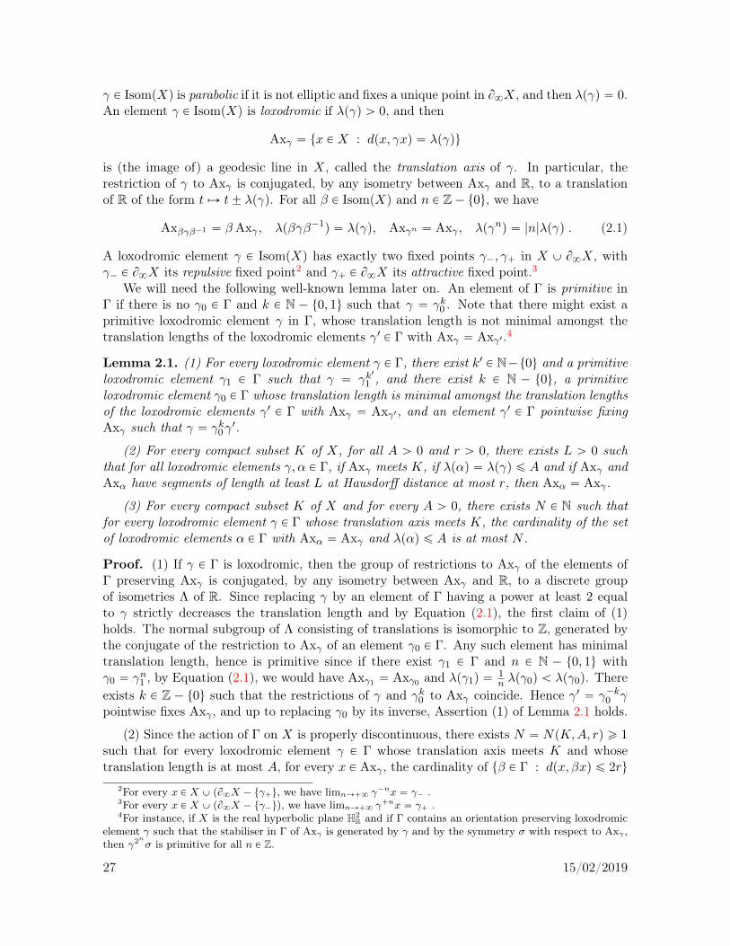
is an isometric map c from an interval I of R into X 1.1 A metric space X 1 is geodesic if forall x, y P X 1, there exists a geodesic segment c : ra, bs Ñ X 1 from x “ cpaq to y “ cpbq. Ageodesic metric space X 1 is geodesically complete (or has extendible geodesics) if any isometricmap from an interval in R to X 1 extends to at least one isometric map from R to X 1. Acomparison triangle of a triple of points px, y, zq in a metric space X 1 is a (unique up toisometry) triple of points px, y, zq in the real hyperbolic plane H2

R such that dpx, yq “ dpx, yq,dpy, zq “ dpy, zq and dpz, xq “ dpz, xq.

X

x

p

q

H2R

y

zz

x

y

p

q

A metric space X 1 is CATp´1q if it is geodesic and if for every triple of points px, y, zqin X 1, for all geodesic segments a, b respectively from x to y and from x to z, and for allpoints p, q in the image of a, b respectively, if px, y, zq is a comparison triangle of px, y, zq,if p (resp. q) is the point on the geodesic segment from x to y (resp. z) at distance dpx, pq(resp. dpx, qq) from x, then dpp, qq ď dpp, qq.

We will put a special emphasis on the case when X is a (proper, geodesically complete)R-tree, that is, a uniquely arcwise connected geodesic metric space. In the Introduction, we

1We say that c is a geodesic segment if I is compact, a geodesic ray if I is a half-infinite interval, and ageodesic line if I “ R.

25 15/02/2019

have denoted by Y the geodesically complete proper locally CATp´1q good orbispace ΓzX,see for instance [GH, Ch. 11] for the terminology.

Two geodesic rays ρ, ρ1 : r0,`8r Ñ X are asymptotic if their images are at finite Hausdorffdistance, or equivalently if there exists a P R such that limtÑ`8 dpρptq, ρ

1pt ` aqq “ 0. Wedenote by B8X the space at infinity of X, which consists of the asymptotic classes of geodesicrays in X, and we endow it with the quotient topology of the compact-open topology. Itcoincides with the space of (Freudenthal’s) ends of X when X is an R-tree.

Let x, y P X and ξ, ξ1 P B8X. We denote by rx, ys “ rx, ys the unique image of a geodesicsegment from x to y. We denote by rx, ξr the image of the unique geodesic ray ρ : r0,`8rÑ Xin the asymptotic class ξ with ρp0q “ x, and we say that ρ starts from x and ends at ξ. Wedenote by sξ, ξ1r “ sξ1, ξr the unique image of a geodesic line ` : R Ñ X with t ÞÑ `ptq andt ÞÑ `p´tq in the asymptotic classes ξ and ξ1 respectively, and we say that ` starts from ξ1 andends at ξ.

We endow the disjoint union X Y B8X with the unique metrisable compact topology(independent of x0) inducing the above topologies on X and B8X, such that a sequencepyiqiPN in X converges to ξ P B8X if and only if limiÑ`8 dpx0, yiq “ `8 and, with ci :r0, dpx0, yiqs Ñ X the geodesic segment from x0 to yi and ρ : r0,`8rÑ X the geodesic rayfrom x0 to ξ, we have limiÑ`8 dpciptq, ρptqq “ 0 for every t ě 0.

We denote by IsompXq the isometry group of X, and we endow it with the compact-opentopology. Its action on X uniquely extends to a continuous action on X YB8X. We say thata discrete subgroup Γ1 of IsompXq is nonelementary if it does not fix a point or an unorderedpair of points inXYB8X. We denote by ΛΓ the limit set of Γ, which is the set of accumulationpoints in B8X of any orbit of Γ in X. It is the smallest closed nonempty Γ-invariant subsetof B8X.

A subset D of X Y B8X is convex if for all u, v P D, the image of the unique geodesicsegment, ray or line from u to v is contained in D. We denote by C ΛΓ the convex hull in X ofΛΓ, which is the intersection of the closed convex subsets of X Y B8X containing ΛΓ. WhenX is an R-tree, then a subset D of X is convex if and only if it is connected, and we will callit a subtree. In particular, if X is an R-tree, then C ΛΓ is equal to the union of the geodesiclines between pairs of distinct points in ΛΓ, since this union is connected and contained inC ΛΓ.

A point ξ P B8X is called a conical limit point of Γ if there exists a sequence of orbitpoints of x0 under Γ converging to ξ while staying at bounded distance from a geodesic rayending at ξ. The set of conical limit points of Γ is the conical limit set ΛcΓ of Γ.

A point p P ΛΓ is a bounded parabolic limit point of Γ if its stabiliser Γp in Γ acts properlydiscontinuously with compact quotient on ΛΓ ´ tpu. The discrete nonelementary group ofisometries Γ of X is said to be geometrically finite if every element of ΛΓ is either a conicallimit point or a bounded parabolic limit point of Γ. See for instance [Bowd], as well as [Pau4]when X is an R-tree, and [DaSU] for a very interesting study of equivalent conditions in aneven greater generality.

For all x P X YB8X and A Ă X, the shadow of A seen from x is the subset OxA of B8Xconsisting of the endpoints towards `8 of the geodesic rays starting at x and meeting A ifx P X, and of the geodesic lines starting at x and meeting A if x P B8X.

The translation length of an isometry γ P IsompXq is

λpγq “ infxPX

dpx, γxq .

An element γ P IsompXq is elliptic if it fixes a point in X, and then λpγq “ 0. An element

26 15/02/2019

γ P IsompXq is parabolic if it is not elliptic and fixes a unique point in B8X, and then λpγq “ 0.An element γ P IsompXq is loxodromic if λpγq ą 0, and then

Axγ “ tx P X : dpx, γxq “ λpγqu

is (the image of) a geodesic line in X, called the translation axis of γ. In particular, therestriction of γ to Axγ is conjugated, by any isometry between Axγ and R, to a translationof R of the form t ÞÑ t˘ λpγq. For all β P IsompXq and n P Z´ t0u, we have

Axβγβ´1 “ βAxγ , λpβγβ´1q “ λpγq, Axγn “ Axγ , λpγnq “ |n|λpγq . (2.1)

A loxodromic element γ P IsompXq has exactly two fixed points γ´, γ` in X Y B8X, withγ´ P B8X its repulsive fixed point2 and γ` P B8X its attractive fixed point.3

We will need the following well-known lemma later on. An element of Γ is primitive inΓ if there is no γ0 P Γ and k P N ´ t0, 1u such that γ “ γk0 . Note that there might exist aprimitive loxodromic element γ in Γ, whose translation length is not minimal amongst thetranslation lengths of the loxodromic elements γ1 P Γ with Axγ “ Axγ1 .4

Lemma 2.1. (1) For every loxodromic element γ P Γ, there exist k1 P N´t0u and a primitiveloxodromic element γ1 P Γ such that γ “ γk

1

1 , and there exist k P N ´ t0u, a primitiveloxodromic element γ0 P Γ whose translation length is minimal amongst the translation lengthsof the loxodromic elements γ1 P Γ with Axγ “ Axγ1 , and an element γ1 P Γ pointwise fixingAxγ such that γ “ γk0γ

1.

(2) For every compact subset K of X, for all A ą 0 and r ą 0, there exists L ą 0 suchthat for all loxodromic elements γ, α P Γ, if Axγ meets K, if λpαq “ λpγq ď A and if Axγ andAxα have segments of length at least L at Hausdorff distance at most r, then Axα “ Axγ.

(3) For every compact subset K of X and for every A ą 0, there exists N P N such thatfor every loxodromic element γ P Γ whose translation axis meets K, the cardinality of the setof loxodromic elements α P Γ with Axα “ Axγ and λpαq ď A is at most N .

Proof. (1) If γ P Γ is loxodromic, then the group of restrictions to Axγ of the elements ofΓ preserving Axγ is conjugated, by any isometry between Axγ and R, to a discrete groupof isometries Λ of R. Since replacing γ by an element of Γ having a power at least 2 equalto γ strictly decreases the translation length and by Equation (2.1), the first claim of (1)holds. The normal subgroup of Λ consisting of translations is isomorphic to Z, generated bythe conjugate of the restriction to Axγ of an element γ0 P Γ. Any such element has minimaltranslation length, hence is primitive since if there exist γ1 P Γ and n P N ´ t0, 1u withγ0 “ γn1 , by Equation (2.1), we would have Axγ1 “ Axγ0 and λpγ1q “

1n λpγ0q ă λpγ0q. There

exists k P Z ´ t0u such that the restrictions of γ and γk0 to Axγ coincide. Hence γ1 “ γ´k0 γpointwise fixes Axγ , and up to replacing γ0 by its inverse, Assertion (1) of Lemma 2.1 holds.

(2) Since the action of Γ on X is properly discontinuous, there exists N “ NpK,A, rq ě 1such that for every loxodromic element γ P Γ whose translation axis meets K and whosetranslation length is at most A, for every x P Axγ , the cardinality of tβ P Γ : dpx, βxq ď 2ru

2For every x P X Y pB8X ´ tγ`u, we have limnÑ`8 γ´nx “ γ´ .

3For every x P X Y pB8X ´ tγ´uq, we have limnÑ`8 γ`nx “ γ` .

4For instance, if X is the real hyperbolic plane H2R and if Γ contains an orientation preserving loxodromic

element γ such that the stabiliser in Γ of Axγ is generated by γ and by the symmetry σ with respect to Axγ ,then γ2nσ is primitive for all n P Z.

27 15/02/2019

is at most N . Let L “ AN . For every loxodromic element α P Γ with λpαq “ λpγq ď A,assume that rx, ys and rx1, y1s are segments in Axγ and Axα respectively, with length exactlyL such that dpx, x1q, dpy, y1q ď r. We may assume, up to replacing γ and α by their inverses,that γ translates from x towards y and α translates from x1 towards y1. In particular fork “ 0, . . . , N , we have dpα´kγkx, xq ď dpγkx, αkx1q ` dpx1, xq ď 2r since γkx and αkx1 arerespectively the points at distance kλpγq ď kA ď L from x and x1 on the segments rx, ysand rx1, y1s. Hence by the definition of N , there exists k ‰ k1 such that α´kγk “ α´k

1

γk1 .

Therefore γk´k1 “ αk´k1 , which implies by Equation (2.1) that Axγ “ Axα.

(3) Since the action of Γ on X is properly discontinuous, there exists N 1 P N such thatthe cardinality of the stabiliser in Γ of a point of K is at most N 1, and there exists η ą 0such that λpγq ě η for every loxodromic element γ P Γ whose translation axis meets K. Letus fix such an element γ P Γ. We may assume that its translation length is minimal amongstthe translation lengths of the loxodromic elements γ1 P Γ with Axγ “ Axγ1 . Then as seen inthe proof of Assertion (1), for every loxodromic element α P Γ with Axα “ Axγ , there existk P N ´ t0u and α1 P Γ pointwise fixing Axγ such that α “ γkα1. Thus if λpαq ď A, then|k| “ λpαq

λpγq ďAη , and there are at most N “ N 1p2rAη s` 1q such elements α. l

For every x P X, recall that the Gromov-Bourdon visual distance dx on B8X seen from x(see [Bou]) is defined by

dxpξ, ηq “ limtÑ`8

e12pdpξt, ηtq´dpx, ξtq´dpx, ηtqq , (2.2)

where ξ, η P B8X and t ÞÑ ξt, ηt are any geodesic rays ending at ξ, η respectively. If X is anR-tree, if ξ, η P B8X are distinct, if p P X is such that rx, ps “ rx, ξr X rx, ηr, then

dxpξ, ηq “ e´dpx, pq . (2.3)

For all x P X, ξ, η P B8X and γ P IsompXq, we have

dγxpγξ, γηq “ dxpξ, ηq .

By the triangle inequality, for all x, y P X and ξ, η P B8X, we have

e´dpx, yq ďdxpξ, ηq

dypξ, ηqď edpx, yq . (2.4)

In particular, the identity map from pB8X, dxq to pB8X, dyq is a bilipschitz homeomorphism.Under our assumptions, pB8X, dx0q is hence a compact metric space, on which IsompXq actsby bilipschitz homeomorphisms. The following well-known result compares shadows of ballsto balls for the visual distance.

Lemma 2.2. For every geodesic ray ρ in X, starting from x P X and ending at ξ P B8X, forall R ě 0 and t P sR,`8r , we have

Bdxpξ,R e´tq Ă OxBpρptq, Rq Ă Bdxpξ, e

R e´tq .

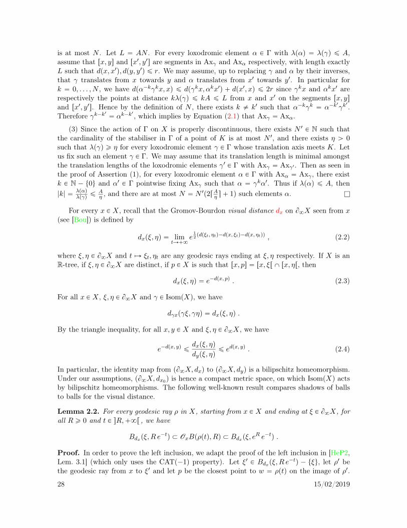
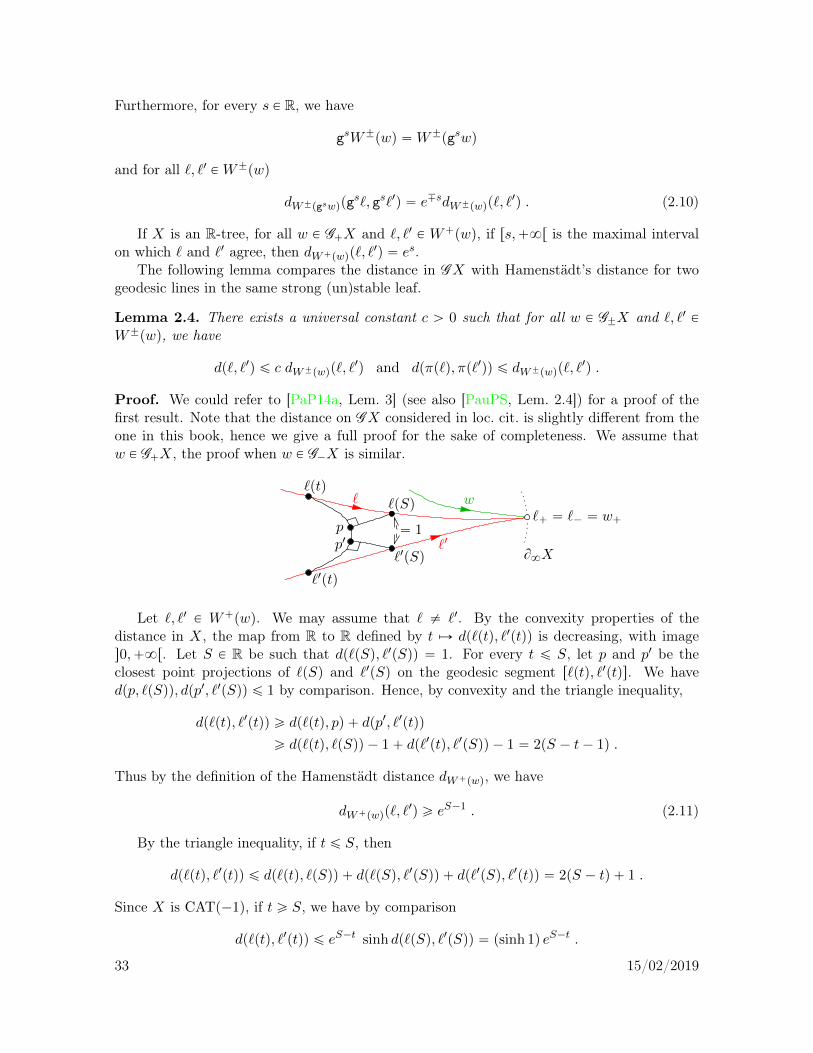
Proof. In order to prove the left inclusion, we adapt the proof of the left inclusion in [HeP2,Lem. 3.1] (which only uses the CATp´1q property). Let ξ1 P Bdxpξ,R e´tq ´ tξu, let ρ1 bethe geodesic ray from x to ξ1 and let p be the closest point to w “ ρptq on the image of ρ1.

28 15/02/2019

For every s ą t, let y “ ρpsq and z “ ρ1psq. Let px, y, zq be a comparison triangle in H2R of

px, y, zq, and let θ P r0, πs be its angle at x. Let w be the point on rx, ys at distance t from x,and let p be its orthogonal projection on rx, zs. By the CATp´1q property, we have

dpw, pq ď dpw, pq .

x

H2R

θ

p

w “ ρptq

z “ ρ1psq

y “ ρpsq

By the hyperbolic sine rule for right angled triangles in H2R, we have

sin θ “sinh dpw, pq

sinh tand sin

θ

2“

sinh 12 dpy, zq

sinh dpx, yq“

sinh 12 dpy, zq

sinh s.

Hence

dpw, pq ď dpw, pq ďedpx,wq

2 sinh dpx,wqsinh dpw, pq “

1

2et sin θ ď et sin

θ

2.

Since

limsÑ`8

sinθ

2“ lim

sÑ`8e

12dpy,zq´s “ dxpξ, ξ

1q ď Re´t ,

we hence have dpw, pq ď R, so that ξ1 P OxBpw,Rq, as wanted.

In order to prove the right inclusion in Lemma 2.2, let ξ1 P OxBpρptq, Rq and let ρ1 be thegeodesic ray from x to ξ1. The closest point p to ρptq on the image of ρ1 satisfies dpp, ρptqq ď R,hence dpx, pq ě t´R. Therefore, for t1 large enough, dpρ1pt1q, pq ď t1 ´ pt´Rq, and

dxpξ1, ξq ď lim sup

t1Ñ`8e

12

`

dpρpt1q, ρptqq`dpρptq, pq`dpp, ρ1pt1qq˘

´t1

ď limt1Ñ`8

e12

`

pt1´tq`R`pt1´t`Rq˘

´t1“ eRe´t .

Therefore ξ1 P Bdxpξ, eR e´tq, as wanted. l

The Busemann cocycle of X is the map β : B8X ˆX ˆX Ñ R defined by

pξ, x, yq ÞÑ βξpx, yq “ limtÑ`8

dpξt, xq ´ dpξt, yq ,

where t ÞÑ ξt is any geodesic ray ending at ξ. If X is an R-tree, if p P X is such thatrx, ξr X ry, ξr “ rp, ξr , then

βξpx, yq “ dpx, pq ´ dpy, pq . (2.5)

The triangle inequality gives immediately the upper bound

|βξpx, yq | ď dpx, yq . (2.6)

The horosphere with centre ξ P B8X through x P X is ty P X : βξpx, yq “ 0u, andty P X : βξpx, yq ď 0u is the (closed) horoball centred at ξ bounded by this horosphere.Horoballs are nonempty proper closed (strictly) convex subsets of X. Given a horoball Hand t ě 0, we denote by H rts “ tx P H : dpx, BH q ě tu the horoball contained in H(hence centred at the same point at infinity as H ) whose boundary is at distance t from theboundary of H .

29 15/02/2019

2.2 Generalised geodesic lines

Letp

GX be the space of 1-Lipschitz maps w : RÑ X which are isometric on a closed intervaland locally constant outside it.5 This space has been introduced by Bartels and Lück in[BartL], to which we refer for the following basic properties. The elements of

p

GX are calledthe generalised geodesic lines of X. Any geodesic segment or ray of X will be considered asan element of

p

GX, by extending it continuously to R as locally constant outside its domainof definition.

We endowp

GX with the distance d “ dp

GXdefined by

@ w,w1 P

p

GX, dpw,w1q “

ż `8

´8

dpwptq, w1ptqq e´2|t| dt . (2.7)

The group IsompXq acts isometrically onp

GX by postcomposition. The distance d inducesthe topology of uniform convergence on compact subsets on

p

GX, andp

GX is a proper metricspace.

The geodesic flow pgtqtPR onp

GX is the one-parameter group of homeomorphisms of thespace

p

GX defined by gtw : s ÞÑ wps ` tq for all w Pp

GX and t P R. It commutes with theaction of IsompXq. If w is isometric exactly on the interval I, then g´tw is isometric exactlyon the interval t` I.

The footpoint projection is the IsompXq-equivariant 12 -Hölder-continuous

6 map π :

p

GX Ñ

X defined by πpwq “ wp0q for all w P

p

GX. The antipodal map ofp

GX is the IsompXq-equivariant isometric map ι :

p

GX Ñ

p

GX defined by ιw : s ÞÑ wp´sq for all w Pp

GX, whichsatisfies ι ˝ gt “ g´t ˝ ι for every t P R and π ˝ ι “ π.

The positive and negative endpoint maps are the continuous maps fromp

GX to X Y B8Xdefined by

w ÞÑ w˘ “ limtÑ˘8

wptq .

The space GX of geodesic lines in X is the IsompXq-invariant closed metric subspace ofp

GX consisting of the elements ` Pp

GX with `˘ P B8X. Note that the distances on GXconsidered in [BartL] and [PauPS] are topologically equivalent to, although slightly differentfrom, the restriction to GX of the distance defined in Equation (2.7). The factor e´2|t| in thisequation, sufficient in order to deal with Hölder-continuity issues, is replaced by e´t2

?π in

[PauPS] and by e´|t|2 in [BartL].Note that for all w P

p

GX and s P R, we have

dpw, gswq ď |s| , (2.8)

with equality if w P GX.We will also consider the IsompXq-invariant closed subspaces

G˘X “ tw P

p

GX : w˘ P B8Xu ,

5that is, constant on each complementary component6See Section 3.1 for the definition of the (locally uniform) Hölder-continuity used in this book, and Propo-

sition 3.2 for a proof of this claim.

30 15/02/2019

and their IsompXq-invariant closed subspaces G˘, 0X consisting of the elements ρ P G˘Xwhich are isometric exactly on ˘r0,`8r.

The subspaces GX and G˘X satisfy G´X XG`X “ GX and they are invariant under thegeodesic flow. The antipodal map ι preserves GX, and maps G˘X to G¯X as well as G˘, 0X

to G¯, 0X. We denote again by ι : Γz

p

GX Ñ Γz

p

GX and by pgtqtPR with gt : Γz

p

GX Ñ Γz

p

GXthe quotient maps of ι and gt, for every t P R.

Let w P

p

GX be isometric exactly on an interval I of R. If I is compact then w is a(generalised) geodesic segment, and if I “ s´8, as or I “ ra,`8r for some a P R, then wis a (generalised) (negative or positive) geodesic ray in X. Any geodesic line pw P GX suchthat pw|I “ w|I is an extension of w. Note that pw is an extension of w if and only if γ pw is anextension of γw for any γ P IsompXq, if and only if ι pw is an extension of ιw, and if and onlyif gs pw is an extension of gsw for any s P R. For any subset Ω1 of

p

GX and any subset A of R,let

Ω1|A “ tw|A : w P Ω1u .

Remark 2.3. Let p`iqiPN be a sequence of generalised geodesic lines such that rt´i , t`i s is

the maximal segment on which `i is isometric. Let psiqiPN be a sequence in R such thatt˘i ´ si Ñ ˘8 as i Ñ `8 and `ipsiq stays in a compact subset of X, then dp`i,GXq Ñ 0as i Ñ `8. Furthermore if psiqiPN is bounded, then up to extracting a subsequence, p`iqiPNconverges to an element in GX.

This conceptually important observation explains how it is conceivable that long commonperpendicular segments may equidistribute towards measures supported on geodesic lines. SeeChapter 11 for further developments of these ideas.

2.3 The unit tangent bundle

In this book, we define the unit tangent bundle T 1X of X as the space of germs at 0 of thegeodesic lines in X. It is the quotient space

T 1X “ GX „

where ` „ `1 if and only if there exists ε ą 0 such that `|r´ε,εs “ `1|r´ε,εs. The canonicalprojection from GX to T 1X will be denoted by ` ÞÑ v`. When X is a Riemannian manifold,the spaces GX and T 1X canonically identify with the usual unit tangent bundle of X, but ingeneral, the map ` ÞÑ v` has infinite fibers.

We endow T 1X with the quotient distance d “ dT 1X of the distance of GX, defined by:

@ v, v1 P T 1X, dT 1Xpv, v1q “ inf

`, `1PGX : v“v`, v1“v`1dp`, `1q . (2.9)

It is easy to check that this distance is indeed Hausdorff, hence that T 1X is locally compact,and that it induces on T 1X the quotient topology of the compact-open topology of GX. Themap ` ÞÑ v` is 1-Lipschitz.

The action of IsompXq on GX induces an isometric action of IsompXq on T 1X. Theantipodal map and the footpoint projection restricted to GX respectively induce an IsompXq-equivariant isometric map ι : T 1X Ñ T 1X and an IsompXq-equivariant 1

2 -Hölder-continuousmap π : T 1X Ñ X called the antipodal map and footpoint projection of T 1X. The canonical

31 15/02/2019

projection from GX to T 1X is IsompXq-equivariant and commutes with the antipodal map:For all γ P IsompXq and ` P GX, we have γv` “ vγ`, ιv` “ vι` and πpv`q “ πp`q. We denoteagain by ι : ΓzT 1X Ñ ΓzT 1X the quotient map of ι.

Let B28X be the subset of B8XˆB8X which consists of pairs of distinct points at infinity of

X. Hopf’s parametrisation of GX is the homeomorphism which identifies GX with B28XˆR,

by the map ` ÞÑ p`´, ``, tq, where t is the signed distance from the closest point to thebasepoint x0 on the geodesic line ` to `p0q.7 We have gsp`´, ``, tq “ p`´, ``, t ` sq for alls P R, and for all γ P Γ, we have γp`´, ``, tq “ pγ`´, γ``, t ` tγ, `´, ``q where tγ, `´, `` P Rdepends only on γ, `´ and ``. In Hopf’s parametrisation, the restriction of the antipodalmap to GX is the map p`´, ``, tq ÞÑ p``, `´,´tq.

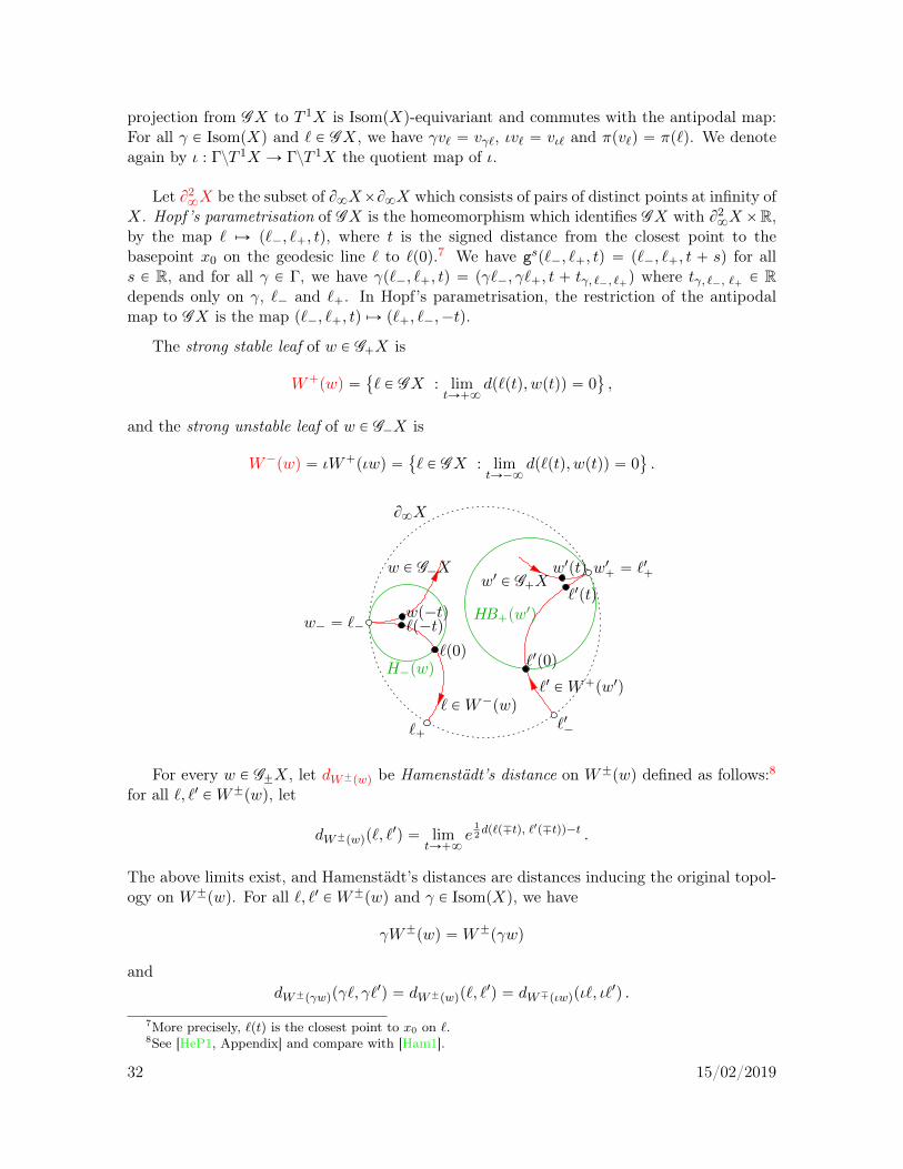
The strong stable leaf of w P G`X is

W`pwq “

` P GX : limtÑ`8

dp`ptq, wptqq “ 0(

,

and the strong unstable leaf of w P G´X is

W´pwq “ ιW`pιwq “

` P GX : limtÑ´8

dp`ptq, wptqq “ 0(

.

B8X

`1 PW`pw1q

wp´tq

H´pwq

` PW´pwq

`1p0q

`p´tqw´ “ `´

w P G´X

`p0q

w1` “ `1`

`1´

w1 P G`Xw1ptq

`1ptq

``

HB`pw1q

For every w P G˘X, let dW˘pwq be Hamenstädt’s distance on W˘pwq defined as follows:8

for all `, `1 PW˘pwq, let

dW˘pwqp`, `1q “ lim

tÑ`8e

12dp`p¯tq, `1p¯tqq´t .

The above limits exist, and Hamenstädt’s distances are distances inducing the original topol-ogy on W˘pwq. For all `, `1 PW˘pwq and γ P IsompXq, we have

γW˘pwq “W˘pγwq

anddW˘pγwqpγ`, γ`

1q “ dW˘pwqp`, `1q “ dW¯pιwqpι`, ι`

1q .

7More precisely, `ptq is the closest point to x0 on `.8See [HeP1, Appendix] and compare with [Ham1].

32 15/02/2019

Furthermore, for every s P R, we have

gsW˘pwq “W˘pgswq

and for all `, `1 PW˘pwq

dW˘pgswqpgs`, gs`1q “ e¯sdW˘pwqp`, `

1q . (2.10)

If X is an R-tree, for all w P G`X and `, `1 P W`pwq, if rs,`8r is the maximal intervalon which ` and `1 agree, then dW`pwqp`, `

1q “ es.The following lemma compares the distance in GX with Hamenstädt’s distance for two

geodesic lines in the same strong (un)stable leaf.

Lemma 2.4. There exists a universal constant c ą 0 such that for all w P G˘X and `, `1 PW˘pwq, we have

dp`, `1q ď c dW˘pwqp`, `1q and dpπp`q, πp`1qq ď dW˘pwqp`, `

1q .

Proof. We could refer to [PaP14a, Lem. 3] (see also [PauPS, Lem. 2.4]) for a proof of thefirst result. Note that the distance on GX considered in loc. cit. is slightly different from theone in this book, hence we give a full proof for the sake of completeness. We assume thatw P G`X, the proof when w P G´X is similar.

B8X

`pSq

`1ptq

p1p

`1pSq

`ptq

`1“ 1

``` “ `´ “ w`

w

Let `, `1 P W`pwq. We may assume that ` ‰ `1. By the convexity properties of thedistance in X, the map from R to R defined by t ÞÑ dp`ptq, `1ptqq is decreasing, with images0,`8r. Let S P R be such that dp`pSq, `1pSqq “ 1. For every t ď S, let p and p1 be theclosest point projections of `pSq and `1pSq on the geodesic segment r`ptq, `1ptqs. We havedpp, `pSqq, dpp1, `1pSqq ď 1 by comparison. Hence, by convexity and the triangle inequality,

dp`ptq, `1ptqq ě dp`ptq, pq ` dpp1, `1ptqq

ě dp`ptq, `pSqq ´ 1` dp`1ptq, `1pSqq ´ 1 “ 2pS ´ t´ 1q .

Thus by the definition of the Hamenstädt distance dW`pwq, we have

dW`pwqp`, `1q ě eS´1 . (2.11)

By the triangle inequality, if t ď S, then

dp`ptq, `1ptqq ď dp`ptq, `pSqq ` dp`pSq, `1pSqq ` dp`1pSq, `1ptqq “ 2pS ´ tq ` 1 .

Since X is CATp´1q, if t ě S, we have by comparison

dp`ptq, `1ptqq ď eS´t sinh dp`pSq, `1pSqq “ psinh 1q eS´t .

33 15/02/2019

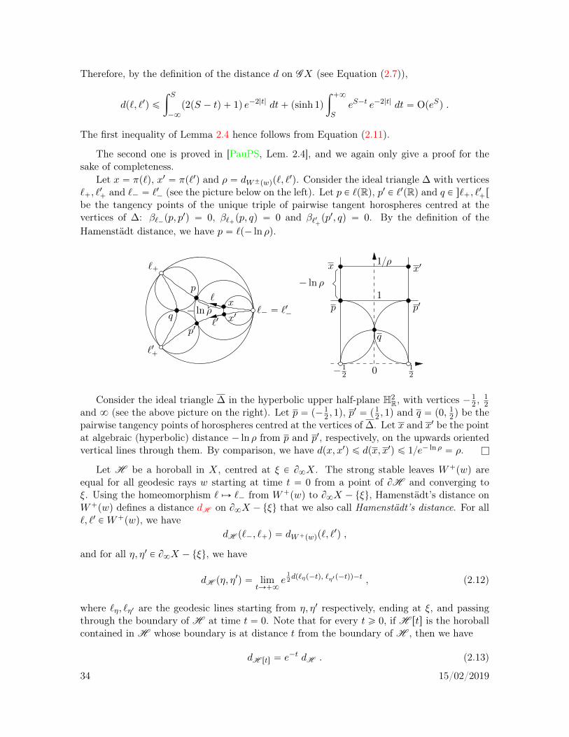
Therefore, by the definition of the distance d on GX (see Equation (2.7)),

dp`, `1q ď

ż S

´8

p2pS ´ tq ` 1q e´2|t| dt` psinh 1q

ż `8

SeS´t e´2|t| dt “ OpeSq .

The first inequality of Lemma 2.4 hence follows from Equation (2.11).

The second one is proved in [PauPS, Lem. 2.4], and we again only give a proof for thesake of completeness.

Let x “ πp`q, x1 “ πp`1q and ρ “ dW˘pwqp`, `1q. Consider the ideal triangle ∆ with vertices

``, `1` and `´ “ `1´ (see the picture below on the left). Let p P `pRq, p1 P `1pRq and q P s``, `1`r

be the tangency points of the unique triple of pairwise tangent horospheres centred at thevertices of ∆: β`´pp, p

1q “ 0, β``pp, qq “ 0 and β`1`pp1, qq “ 0. By the definition of the

Hamenstädt distance, we have p “ `p´ ln ρq.

p

x1

0

q

1ρ

p1

x

1

´12

12

´ ln ρp

p1q

´ ln ρx1x

``

`

`1`´ “ `1´

`1`

Consider the ideal triangle ∆ in the hyperbolic upper half-plane H2R, with vertices ´1

2 ,12

and 8 (see the above picture on the right). Let p “ p´12 , 1q, p

1 “ p12 , 1q and q “ p0,

12q be the

pairwise tangency points of horospheres centred at the vertices of ∆. Let x and x1 be the pointat algebraic (hyperbolic) distance ´ ln ρ from p and p1, respectively, on the upwards orientedvertical lines through them. By comparison, we have dpx, x1q ď dpx, x1q ď 1e´ ln ρ “ ρ. l

Let H be a horoball in X, centred at ξ P B8X. The strong stable leaves W`pwq areequal for all geodesic rays w starting at time t “ 0 from a point of BH and converging toξ. Using the homeomorphism ` ÞÑ `´ from W`pwq to B8X ´ tξu, Hamenstädt’s distance onW`pwq defines a distance dH on B8X ´ tξu that we also call Hamenstädt’s distance. For all`, `1 PW`pwq, we have

dH p`´, ``q “ dW`pwqp`, `1q ,

and for all η, η1 P B8X ´ tξu, we have

dH pη, η1q “ lim

tÑ`8e

12dp`ηp´tq, `η1 p´tqq´t , (2.12)

where `η, `η1 are the geodesic lines starting from η, η1 respectively, ending at ξ, and passingthrough the boundary of H at time t “ 0. Note that for every t ě 0, if H rts is the horoballcontained in H whose boundary is at distance t from the boundary of H , then we have

dH rts “ e´t dH . (2.13)

34 15/02/2019

Let w P G˘X and η1 ą 0. We define B˘pw, η1q as the set of ` P W˘pwq such that thereexists an extension pw P GX of w with dW˘pwqp`, pwq ă η1. In particular, B˘pw, η1q containsall the extensions of w, and is the union of the open balls centred at the extensions of w, ofradius η1, for Hamenstädt’s distance on W˘pwq.

B8X

πpB`pw, η1qq

πpV `w, η, η1q

pwpηq

pwp0q

pwp´ηq

w

`1´

`1 P V `w,η,η1 ` P B`pw, ηq

`´

`` “ w`

The union over t P R of the images under gt of the strong stable leaf of w P G`X is thestable leaf

W 0`pwq “ď

tPRgtW`pwq

of w, which consists of the elements ` P GX with `` “ w`. Similarly, the unstable leaf ofw P G´X

W 0´pwq “ď

tPRgtW´pwq ,

consists of the elements ` P GX with `´ “ w´. Note that the (strong) (un)stable leavesare subsets of the space of geodesic lines GX. The (un)stable leaves are invariant under thegeodesic flow, and for all w P G˘X and γ P IsompXq, we have

ιW 0˘pwq “W 0¯pι wq and γW 0˘pwq “W 0˘pγwq .

The unstable horosphere H´pwq of w P G´X is the horosphere in X centred at w´ andpassing through pwp0q for any extension pw P GX of w (see the picture above the definition ofHamenstädt’s distance). The stable horosphere H`pwq of w P G`X is the horosphere in Xcentred at w` and passing through pwp0q for any extension pw P GX of w. These horospheresH˘pwq do not depend on the chosen extensions pw of w P G˘X. The unstable horoball HB´pwqof w P G´X and stable horoball HB`pwq of w P G`X are the horoballs bounded by thesehorospheres. Note that

πpW˘pwqq “ H˘pwq (2.14)

for every w P G˘X, and that wp0q belongs to H˘pwq if and only if w is isometric at least on˘r0,`8r.

2.4 Normal bundles and dynamical neighbourhoods

In this Section, adapting [PaP17b, §2.2] to the present context, we define spaces of geodesicrays that generalise the unit normal bundles of submanifolds of negatively curved Riemannianmanifolds. When X is a manifold, these normal bundles are submanifolds of the unit tangent

35 15/02/2019

bundle of X, which identifies with GX. In general and in particular in trees, it is essential touse geodesic rays to define normal bundles, and not geodesic lines.

Let D be a nonempty proper9 closed convex subset in X. We denote by BD its boundaryin X and by B8D its set of points at infinity. Let

PD : X Y pB8X ´ B8Dq Ñ D

be the (continuous) closest point map to D, defined on ξ P B8X ´ B8D by setting PDpξq tobe the unique point in D that minimises the function y ÞÑ βξpy, x0q from D to R. The outerunit normal bundle B1

`D of (the boundary of) D is

B1`D “ tρ P G`, 0X : PDpρ`q “ ρp0qu .

The inner unit normal bundle B1´D of (the boundary of) D is

B1´D “ ιB1

`D “ tρ P G´, 0X : PDpρ´q “ ρp0qu.

Note that B1`D and B1

´D are spaces of geodesic rays. If X is a smooth manifold, then thesespaces have a natural identification with subsets of GX because every geodesic ray is therestriction of a unique geodesic line. But this does not hold in general.

B8X

ρp0q “ PDpρ´q ρ1p0q “ PDpρ1`q

D

ρ1`ρ´

ρ1 “ P`D pρ1`q P B

1`D

ρ “ P´D pρ´q P B1´D

Remark 2.5. As X is assumed to be proper with extendible geodesics, we have

πpB1˘Dq “ BD .

To see this, let x P BD and let pxkqkPN be a sequence of points in the complement of Dconverging to x. For all k P N, let ρk P B1

`D be a geodesic ray with ρkp0q “ PDpxkq and suchthat the image of ρk contains xk. As the closest point map does not increase distances, thesequence pPDpxkqqkPN converges to x. Since X is proper, the space B8X is compact and thesequence ppρkq`qkPN has a subsequence that converges to a point ξ P B8X. The claim followsfrom the continuity of the closest point map.

The possible failure of this equality when X is not proper is easy to see. For example, letX be the R-tree constructed by starting with the Euclidean line D “ R and attaching a copyof the halfline r0,`8r at each x P D such that x ą 0. Then 0 P BD ´ πpB1

˘Dq.

9that is, different from X

36 15/02/2019

The restriction of the endpoint map ρ ÞÑ ρ˘ to B1˘D is a homeomorphism to its image

B8X ´ B8D. We denote its inverse map by P˘D (see the above picture): for every ρ P B1˘D,

we haveρ “ P˘D pρ˘q .

Note that PD “ π ˝P˘D . For every isometry γ of X, we have B1˘pγDq “ γ B1

˘D and P˘γD ˝ γ “γ ˝ P˘D . In particular, B1

˘D is invariant under the isometries of X that preserve D.For every w P G˘X, we have a canonical homeomorphism

N˘w : W˘pwq Ñ B1¯HB˘pwq ,

that associates to each geodesic line ` PW˘pwq the unique geodesic ray ρ P B1¯HB˘pwq such

that `¯ “ ρ¯, or, equivalently, such that `ptq “ ρptq for every t P R with ¯t ą 0. It is easy tocheck that N˘γw ˝ γ “ γ ˝N˘w for every γ P IsompXq.

We defineU ˘D “ t` P GX : `˘ R B8Du . (2.15)

Note that U ˘D is an open subset of GX, invariant under the geodesic flow. We have U ˘

γD “

γU ˘D for every isometry γ of X and, in particular, U ˘

D is invariant under the isometries of Xpreserving D. Define

f˘D : U ˘D Ñ B1

˘D

as the composition of the continuous endpoint map ` ÞÑ `˘ from U ˘D onto B8X ´ B8D and

the homeomorphism P˘D from B8X ´ B8D to B1˘D (see the picture below). The continuous

map f˘D takes ` P U ˘D to the unique element ρ P B1

˘D such that ρ˘ “ `˘. The fiber ofρ P B1

`D for f`D is exactly the stable leaf W 0`pρq, and the fiber of ρ P B1´D for f´D is the

unstable leaf W 0´pρq. For all γ P IsompXq and t P R, we have

f˘γD ˝ γ “ γ ˝ f˘D and f˘D ˝ gt “ f˘D . (2.16)

ρp0q “ PDp``q

B8XD

`´ `

`` “ ρ`

ρ “ f`D p`q “ P`D p``q P B1`D

Let w P G˘X and η, η1 ą 0. We define (see the picture after Equation (2.13)) the dynamicalpη, η1q-neighbourhood of w by

V ˘w, η, η1 “ď

sPs´η, η r

gsB˘pw, η1q . (2.17)

37 15/02/2019

Example 2.6. If X is an R-tree, w P G`X and η ă ln η1, then V `w, η, η1 , which is the setof gs` where s P s´η, ηr and ` P GX is such that there exists an extension pw of w withinftt P R : `ptq “ pwptqu ď ln η1, is as in the following picture.

πpV `w, η, η1q

w

πpB`pw, η1qq

pwp0qpwp´ηq

pwpln η1q

pwpηqw` “ pw`

Clearly, B˘pw, η1q “ ιB¯pιw, η1q, and hence we have V ˘w, η, η1 “ ιV ¯ιw, η, η1 . Furthermore, forevery s P R,

gsB˘pw, η1q “ B˘pgsw, e¯sη1q , hence gsV ˘w, η, η1 “ V ˘gsw, η, e¯sη1

. (2.18)

For every γ P IsompXq, we have γB˘pw, η1q “ B˘pγw, η1q and γV ˘w, η, η1 “ V ˘γw, η, η1 . The mapfrom s´η, ηr ˆB˘pw, η1q to V ˘w, η, η1 defined by ps, `1q ÞÑ gs`1 is a homeomorphism.

For all subsets Ω´ of G`X and Ω` of G´X, let

V ˘η, η1pΩ

¯q “ď

wPΩ¯

V ˘w, η, η1 , (2.19)

that we call the dynamical neighbourhoods of Ω¯. Note that they are subsets of GX, not ofG˘X. The families pV ˘

η, η1pΩ¯qqη,η1ą0 are nondecreasing in η and in η1. For every γ P IsompXq,

we have γV ˘η, η1pΩ

¯q “ V ˘η, η1pγΩ¯q and for every t ě 0, we have

g˘tV ˘η, η1pΩ

¯q “ V ˘

η, e´tη1pg˘tΩ¯q . (2.20)

Note thatď

η , η1ą0

V ˘η, η1pB

1˘Dq “ U ˘

D ,

and thatŞ

η, η1ą0 V ˘η, η1pB

1˘Dq is the set of all extensions in GX of the elements of B1

˘D. Assumethat Ω¯ is a subset of B1

˘D. The restriction of f˘D to V ˘η, η1pΩ

¯q is a continuous map onto Ω¯,with fiber over w P Ω¯ the open subset V ˘w, η, η1 of W

0˘pwq.

We will need the following elementary lemma in Section 10.4.

Lemma 2.7. There exists a universal constant c1 ą 0 such that for every w P G`X which isisometric on rsw,`8r and every ` P V `w, η, η1 , we have

dp`, wq ď c1pη ` η1 ` eswq .

38 15/02/2019

Proof. By Equation (2.17) and by the definition of B`pw, η1q in Section 2.2, there exists P s´η,`ηr and an extension pw P GX of w such that gs` P W`pwq and dW`pwqpg

s`, pwq ďη1. By Equation (2.8), we have dp`, gs`q ď |s| ď η. By Lemma 2.4, we have dpgs`, pwq ďc dW`pwqpg

s`, pwq ď c η1. By the definition of the distance onp

GX (see Equation (2.7)), wehave

dp pw,wq ď

ż sw

´8

|sw ´ t| e´2|t| dt “ Opeswq .

Therefore the result follows from the triangle inequality

dp`, wq ď dp`, gs`q ` dpgs`, pwq ` dp pw,wq . l

2.5 Creating common perpendiculars

Let D´ and D` be two nonempty proper closed convex subsets of X, where X is as inthe beginning of Section 2.1. A geodesic arc α : r0, T s Ñ X, where T ą 0, is a commonperpendicular of length T from D´ to D` if there exists w¯ P B1

˘D¯ such that w´|r0, T s “

g´Tw`|r0, T s “ α. Since X is CATp´1q, this geodesic arc α is the unique shortest geodesicsegment from a point of D´ to a point of D`. There exists a common perpendicular fromD´ to D` if and only if the closures of D´ and D` in X Y B8X are disjoint. When X is anR-tree, then two closed subtrees of X have a common perpendicular if and only if they arenonempty and disjoint.

One of the aims of this book is to count orbits of common perpendiculars between twoequivariant families of closed convex subsets of X. The crucial remark is that two nonemptyproper closed convex subsets D´ and D` of X have a common perpendicular α of lengtha given T ą 0 if and only if the subsets gT 2B1

`D´ˇ

ˇ

r´T2, T

2sand g´T 2B1

´D`ˇ

ˇ

r´T2,T

2sof

p

GX

intersect. This intersection then consists of the common perpendicular from D´ to D`

reparametrised by r´T2 ,

T2 s. As a controlled perturbation of this remark, we now give an

effective creation result of common perpendiculars in R-trees. It has a version satisfied for Xin the generality of Section 2.1, see the end of this Section.

Lemma 2.8. Assume that X is an R-tree. For all R ą 1, η P s0, 1s and t ě 2 lnR ` 4,for all nonempty closed connected subsets D´, D` in X, and for every geodesic line ` Pgt2V `

η,RpB1`D

´q X g´t2V ´η,RpB

1´D

`q, there exist s P s´2η, 2ηr and a common perpendicular rcfrom D´ to D` such that• the length of rc is t` s,• the endpoint of rc in D¯ is w¯p0q where w¯ “ f˘

D¯p`q,

• the footpoint `p0q of ` lies on rc, and

max!

dpw´` t

2

˘

, `p0qq, dpw``

´t

2

˘

, `p0qq)

ď η .

`p0q

w´p t2q w`p´ t2q

ď logR ď logR

x´ x`

D´

w`p0q

D`

`p t2 ` s`q

w´p0q

`p´ t2 ´ s

´q

39 15/02/2019

Proof. Let R, η, t,D˘, ` be as in the statement. By the definition of the sets V ¯η,RpB

1¯D

˘q,there exist geodesic rays w˘ P B1

¯D˘, geodesic lines pw˘ P GX extending w˘, and s˘ P

s´η,`ηr, such that `˘ “ pw¯q˘ and

dW˘pw¯qpg¯ t

2¯s¯`, pw¯q ď R .

Let x˘ be the closest point to w˘p0q on `. By the definition of Hamenstädt’s distances, wehave

dpw˘p0q, x˘q “ dp`p˘t

2˘ s˘q, x˘q ď lnR ,

and in particular x˘ “ w˘p0q if and only if `p˘ t2 ˘ s˘q “ w˘p0q. As t ě 2 lnR ` 4 and

|s˘| ď 2η ď 2, the points `p´ t2 ´ s´q, x´, `p0q, x`, `p t2 ` s`q are in this order on `. In

particular, the segment rw´p0q, x´s Y rx´, x`s Y rx`, w`p0qs is a nontrivial geodesic segmentfrom a point of D´ to a point of D` that meets D¯ only at an endpoint. Hence, D´ and D`

are disjoint, and rw´p0q, w`p0qs is the image of the common perpendicular from D´ to D`.Let s “ s´ ` s`. The length of rc is p t2 ` s

`q ´ p´ t2 ´ s

´q “ t` s. The point `p0q lies onrc, we have w¯ “ f˘

D¯p`q and the endpoints of rc are w˘p0q. Furthermore,

dpw¯p˘t

2q, `p0qq “

ˇ

ˇ dpw¯p˘t

2q, w¯p0qq ´ dp`p0q, `p¯

t

2¯ s¯qq

ˇ

ˇ “ |s¯| ď η . l

When X is as in the beginning of Section 2.1, the statement and the proof of the followinganalog of Lemma 2.8 is slightly more technical. We refer to [PaP17b, Lem. 7] for a proof inthe Riemannian case, and we leave the extension to the reader, since we will not need it inthis book.

Lemma 2.9. Let X be as in the beginning of Section 2.1. For every R ą 0, there existt0, c0 ą 0 such that for all η P s0, 1s and all t P rt0,`8r , for all nonempty closed convexsubsets D´, D` in X, and for all w P gt2V `

η,RpB1`D

´q X g´t2V ´η,RpB

1´D

`q, there exist s Ps ´ 2η, 2ηr and a common perpendicular rc from D´ to D` such that• the length of rc is contained in rt` s´ c0 e

´ t2 , t` s` c0 e

´ t2 s,

• if w¯ “ f˘D¯pwq and if p˘ is the endpoint of rc in D˘, then dpπpw˘q, p˘q ď c0 e

´ t2 ,

• the basepoint πpwq of w is at distance at most c0 e´ t

2 from a point of rc, and

maxt dpπpgt2w´q, πpwqq, dpπpg´

t2w`q, πpwqq u ď η ` c0 e

´ t2 . l

2.6 Metric and simplicial trees, and graphs of groups

Metric and simplicial trees and graphs of groups are important examples throughout thisbook. In this Section, we recall the definitions and basic properties of these objects.

Using Serre’s definitions in [Ser3, §2.1], a graph X is the data consisting of two sets V X andEX, called the set of vertices and the set of edges of X, of two maps o, t : EXÑ V X and of afixed point free involution e ÞÑ e of EX, such that tpeq “ opeq for every e P EX. The elementsopeq, tpeq and e are called the initial vertex, the terminal vertex and the opposite edge of anedge e P EX. The quotient of EX by the involution e ÞÑ e is called the set of nonorientededges of X. Recall that a connected graph is bipartite if it is endowed with a partition of itsset of vertices into two nonempty subsets such that any two elements of either subset are notrelated by an edge.

40 15/02/2019

The degree of a vertex x P V X is the cardinality of the set te P EX : opeq “ xu. For allj, k P N, a graph X is k-regular if the degree of each vertex x P V X is k, and it is pj, kq-biregularif it is bipartite with the elements of the partition of its vertices into two subsets having degreej and k respectively.

A metric graph pX, λq is a pair consisting of a graph X and a map λ : EXÑ s0,`8r witha positive lower bound10 such that λpeq “ λpeq, called its edge length map. A simplicial graphX is a metric graph whose edge length map is constant equal to 1.

The topological realisation of a graph X is the topological space obtained from the familypIeqePEX of closed unit intervals Ie for every e P EX by the finest equivalence relation thatidentifies intervals corresponding to an edge and its opposite edge by the map t ÞÑ 1 ´ tand identifies the origins of the intervals Ie1 and Ie2 if and only if ope1q “ ope2q, see [Ser3,Sect. 2.1].

The geometric realisation of a metric tree pX, λq is the topological realisation of X endowedwith the maximal geodesic metric that gives length λpeq to the topological realisation of eachedge e P EX, and we denote it by X “ |X|λ. We identify V X with its image in X. The metricspace X determines pX, λq up to subdivisions of edges, hence we will often not make a strictdistinction between X and pX, λq. In particular, we will refer to convex subsets of pX, λq asconvex subsets of X, etc.

If X is a tree, the metric space X is an R-tree, hence it is a CATp´1q space. Since λ isbounded from below by a positive constant, the R-tree X is geodesically complete if and onlyif X is not reduced to one vertex and has no terminal vertex (that is, no vertex of degree 1).

We will denote by AutpX, λq, and AutX in the simplicial case, the group of edge-preservingisometries of X that have no inversions.11 Since the edge length map has a positive lowerbound, the metric space X is proper if and only if X is locally finite. In this case, thenonelementary discrete subgroups Γ of isometries of X we will consider will always be edge-preserving and without inversion. If Γ is a subgroup of AutpX, λq, we will again denote byλ : ΓzEXÑ s0,`8r the map induced by λ : EXÑ s0,`8r.

A locally finite metric tree pX1, λq is uniform if there exists some discrete subgroup Γ1 ofAutpX1, λq such that Γ1zX1 is a finite graph. See [BasK, BasL] for characterisations of thisproperty in the case of simplicial trees.

Discrete time geodesic flow on trees Let X be a locally finite simplicial tree. The spaceof generalised discrete geodesic lines of X is the locally compact space

p

GX of 1-Lipschitzmappings w from R to the geometric realisation X “ |X|1 which are isometric on a closedinterval with endpoints in ZYt´8,`8u and locally constant outside it, such that wp0q P V X(or equivalently wpZq Ă V X). Note that

p

GX is hence a proper subset ofp

GX, unless X isreduced to one vertex.

By restriction top

GX, or intersection withp

GX, of the objects defined in Sections 2.2 and2.4 for

p

GX, we define the distance d onp

GX, the subspaces G˘X, GX, G˘,0X, the strongstable/unstable leaves W˘pwq of w P G˘X and their Hamenstädt distances dW˘pwq, thestable/unstable leaves W 0˘pwq of w P G˘X, the outer and inner unit normal bundles B1

˘D10This assumption, though not necessary at this stage, will be used repeatedly in this book, hence we prefer

to add it to the definition.11An automorphism g of a graph has an inversion if there exists an edge e of the graph such that ge “ e.

The assumption that the elements of AutpXq have no inversion ensures that, for every subgroup Γ1 of AutpXq,the quotient map Γ1zEX Ñ Γ1zEX of e ÞÑ e is still a fixed point free involution, so that with the quotientmaps Γ1zEXÑ Γ1zV X defined by o and t, we do have a quotient graph structure Γ1zX.

41 15/02/2019

of a nonempty proper simplicial subtree D of X, the dynamical neighbourhoods V ˘η, η1pΩ

¯q ofsubsets Ω¯ of B1

˘D as well as the fibrations

f˘D : U ˘D “ t` P GX : `˘ R B8|D|1u Ñ B1

˘D ,

whose fiber over ρ P B1˘D is W 0˘pρq. Note that some definitions actually simplify when

considering generalised discrete geodesic lines. For instance, for all w P G˘X, η1 ą 0 and η Ps0, 1r , the dynamical neighbourhood V ˘w, η, η1 is equal to B

˘pw, η1q, and is hence independentof η P s0, 1r .

Besides the map π : GX Ñ V X defined as in the continuous case by ` ÞÑ `p0q, we haveanother natural map Tπ : GX Ñ EX, which associates to ` the edge e with opeq “ `p0q andtpeq “ `p1q. This map is equivariant under the group of automorphisms (without inversions)AutpXq of X, and we also denote by Tπ : ΓzGXÑ ΓzEX its quotient map, for every subgroupΓ of AutpXq.

If X has no terminal vertex, for every e P EX, let

BeX “ t`` : ` P GX, Tπp`q “ eu

be the set of points at infinity of the geodesic rays whose initial (oriented) edge is e.Given x0 P V X, the discrete Hopf parametrisation now identifies GX with B2

8XˆZ by themap ` ÞÑ p`´, ``, tq where t P Z is the signed distance from the closest vertex to the basepointx0 on the geodesic line ` to the vertex `p0q.

The discrete time geodesic flow pgtqtPZ onp

GX is the one-(discrete-)parameter group ofhomeomorphisms of

p

GX consisting of (the restriction top

GX of) the integral time maps of thecontinuous time geodesic flow of the geometric realisation of X: we have gtw : s ÞÑ wps ` tq

for all w Pp

GX and t P Z.

Crossratios of ends of trees Let X be a locally finite simplicial tree, with geometricrealisation X “ |X|1. Recall12 that if pξ1, ξ2, ξ3, ξ4q is an ordered quadruple of pairwisedistinct points in B8X, then their (logarithmic) crossratio is

vξ1, ξ2, ξ3, ξ4w “ limxiÑξi, xiPV X

1

2

`

dpx1, x4q ´ dpx4, x3q ` dpx3, x2q ´ dpx2, x1q˘

. (2.21)

A similar definition is valid for general CATp´1q-spaces, but we will only need the case ofsimplicial trees in this book.

If x and y are the closest points on the geodesic line sξ1, ξ3r to ξ2 and ξ4 respectively, then

vξ1, ξ2, ξ3, ξ4w “ dpx, yq

if ξ1, x, y, ξ3 are in this order on sξ1, ξ3r and

vξ1, ξ2, ξ3, ξ4w “ ´dpx, yq

otherwise. In particular, vξ1, ξ2, ξ3, ξ4w “ 0 if the geodesic lines sξ1, ξ3r and sξ2, ξ4r are disjoint.

12See [Pau2], as well as [Ota] in the case of Riemannian manifolds, and note that the convention on theorder varies in the literature.

42 15/02/2019

`

` ´

´

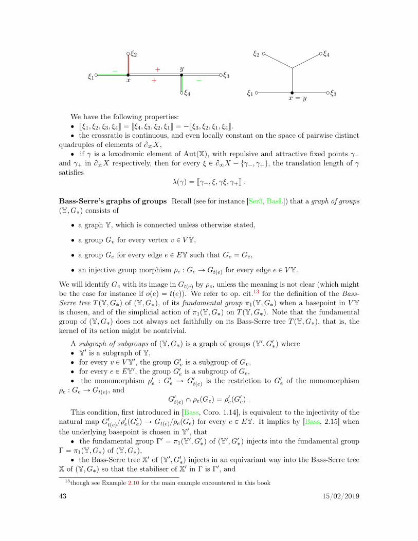
x

x “ yξ1

ξ2

y

ξ2

ξ3

ξ4

ξ4

ξ3

ξ1

We have the following properties:‚ vξ1, ξ2, ξ3, ξ4w “ vξ4, ξ3, ξ2, ξ1w “ ´vξ3, ξ2, ξ1, ξ4w.‚ the crossratio is continuous, and even locally constant on the space of pairwise distinct

quadruples of elements of B8X,‚ if γ is a loxodromic element of AutpXq, with repulsive and attractive fixed points γ´

and γ` in B8X respectively, then for every ξ P B8X ´ tγ´, γ`u, the translation length of γsatisfies

λpγq “ vγ´, ξ, γξ, γ`w .

Bass-Serre’s graphs of groups Recall (see for instance [Ser3, BasL]) that a graph of groupspY, G˚q consists of

‚ a graph Y, which is connected unless otherwise stated,

‚ a group Gv for every vertex v P V Y,

‚ a group Ge for every edge e P EY such that Ge “ Ge,

‚ an injective group morphism ρe : Ge Ñ Gtpeq for every edge e P V Y.

We will identify Ge with its image in Gtpeq by ρe, unless the meaning is not clear (which mightbe the case for instance if opeq “ tpeq). We refer to op. cit.13 for the definition of the Bass-Serre tree T pY, G˚q of pY, G˚q, of its fundamental group π1pY, G˚q when a basepoint in V Yis chosen, and of the simplicial action of π1pY, G˚q on T pY, G˚q. Note that the fundamentalgroup of pY, G˚q does not always act faithfully on its Bass-Serre tree T pY, G˚q, that is, thekernel of its action might be nontrivial.

A subgraph of subgroups of pY, G˚q is a graph of groups pY1, G1˚q where‚ Y1 is a subgraph of Y,‚ for every v P V Y1, the group G1v is a subgroup of Gv,‚ for every e P EY1, the group G1e is a subgroup of Ge,‚ the monomorphism ρ1e : G1e Ñ G1tpeq is the restriction to G1e of the monomorphism

ρe : Ge Ñ Gtpeq, andG1tpeq X ρepGeq “ ρ1epG

1eq .

This condition, first introduced in [Bass, Coro. 1.14], is equivalent to the injectivity of thenatural map G1tpeqρ

1epG

1eq Ñ GtpeqρepGeq for every e P EY. It implies by [Bass, 2.15] when

the underlying basepoint is chosen in Y1, that‚ the fundamental group Γ1 “ π1pY1, G1˚q of pY1, G1˚q injects into the fundamental group

Γ “ π1pY, G˚q of pY, G˚q,‚ the Bass-Serre tree X1 of pY1, G1˚q injects in an equivariant way into the Bass-Serre tree

X of pY, G˚q so that the stabiliser of X1 in Γ is Γ1, and13though see Example 2.10 for the main example encountered in this book

43 15/02/2019

‚ the map pΓ1zX1q Ñ pΓzXq induced by the inclusion map X1 Ñ X by taking quotient isinjective:

@ γ P Γ, @ z P V X1 Y EX1, if γz P V X1 Y EX1, then D γ1 P Γ1, γ1z “ γz . (2.22)

The edge-indexed graph pY, iq of the graph of groups pY, G˚q is the graph Y endowed withthe map i : EYÑ N´ t0u defined by ipeq “ rGopeq : Ges (see for instance [BasK, BasL]).

In Section 12.4, we will consider metric graphs of groups pY, G˚, λq which are graphs ofgroups endowed with an edge length function λ : EY Ñ s0,`8r (with λpeq “ λpeq for everye P EY).

Example 2.10. The main examples of graphs of groups that we will consider in this bookare the following ones. Let X be a simplicial tree and let Γ be a subgroup of AutpXq. Thequotient graph of groups ΓzzX is the following graph of groups pY, G˚q. Its underlying graph Yis the quotient graph ΓzX. Fix a lift rz P V XYEX for every z P V YYEY. For every e P EY,assume that re “ re, and fix an element ge P Γ such that ge Ątpeq “ tpreq. For every y P V YYEY,take as Gy the stabiliser Γ

ry in Γ of the fixed lift ry. Take as monomorphism ρe : Ge Ñ Gtpeqthe restriction to Γ

re of the conjugation γ ÞÑ g´1e γge by g´1

e . Note that ΓzzX has finite vertexgroups if X is locally finite and Γ is discrete. For every choice of basepoint in V Y, there exista group isomorphism θ : π1pY, G˚q Ñ Γ and a θ-equivariant simplicial isomorphism from theBass-Serre tree T pY, G˚q to X (see for instance [Ser3, BasL]).

The volume form of a graph of finite groups pY, G˚q is the measure volpY, G˚q on the discreteset V Y, such that for every y P V Y,

volpY, G˚qptyuq “1

|Gy|,

where |Gy| is the order of the finite group Gy. Its total mass, called the volume of pY, G˚q, is

VolpY, G˚q “ volpY, G˚q “ÿ

yPV Y

1

|Gy|.

We denote by L2pY, G˚q “ L2pV Y, volpY,G˚qq the complex Hilbert space of square integrablemaps V YÑ C for this measure volpY,G˚q, and by f ÞÑ f2 and pf, gq ÞÑ xf, gy2 its norm and(antilinear on the right) scalar product. Let

L20pY, G˚q “

f P L2pY, G˚q :

ż

f d volpY, G˚q “ 0(

.

When VolpY, G˚q is finite, L20pY, G˚q is the orthogonal subspace to the constant functions.

We also consider a (edge-)volume form TvolpY, G˚q on the discrete set EY such that forevery e P EY,

TvolpY, G˚qpteuq “1

|Ge|,

with total massTVolpY, G˚q “ TvolpY, G˚q “

ÿ

ePEY

1

|Ge|.

44 15/02/2019

The (edge-)volume form of a metric graph of groups pY, G˚, λq is given by

TvolpY, G˚,λq “ds

|Ge|

on each edge e of Y parameterised by its arclength s, so that its total mass is

TVolpY, G˚, λq “ TvolpY, G˚,λq “ÿ

ePEY

λpeq

|Ge|.

For λ ” 1, this total mass agrees with that of the discrete definition above.

Remark 2.11. Note that TVolpY, G˚q “ CardpEYq when the edge groups are trivial. Wehave

TVolpY, G˚q “ÿ

ePEY

1

|Ge|“

ÿ

yPV Y

1

|Gy|

ÿ

ePEY, opeq“y

|Gy|

|Ge|“

ÿ

yPV Y

degpryq

|Gy|,

where ry is any lift of y in the Bass-Serre tree of pY, G˚q. In particular, if X is a uniformsimplicial tree and Γ is discrete subgroup of AutX, then the finiteness of VolpΓzzXq and ofTVolpΓzzXq are equivalent. Defining the volume form on V Y by tyu ÞÑ degpryq

|Gy |sometimes makes

formulas simpler, but we will follow the convention which occurs in the classical references(see for instance [BasL]).

If the Bass-Serre tree of pY, G˚q is pq ` 1q-regular, then

π˚TvolY, G˚ “ pq ` 1q volY, G˚ and TVolpY, G˚q “ pq ` 1qVolpY, G˚q . (2.23)

We say that a discrete group of (inversion-free) automorphisms Γ of a locally finite metricor simplicial tree pX, λq is a (tree) lattice of pX, λq if the quotient graph of groups ΓzzX hasfinite volume:

VolpΓzzXq ă `8 .

This implies by [BasK, Prop. 4.5]14 that Γ is a lattice15 in the locally compact group AutpX, λq(hence that AutpX, λq is unimodular, see for instance [Rag, Chap. I, Rem. 1.9]), the conversebeing true for instance if pX, λq is uniform. If Γ is a uniform lattice of pX, λq, that is, if Γ isa discrete subgroup of AutpX, λq and if the quotient graph ΓzX is finite, then Γ is clearly a(tree) lattice of pX, λq.

A graph of finite groups pY, G˚q is a cuspidal ray if Y is a simplicial ray such that thehomomorphisms Gen Ñ Gopenq are surjective for its sequence of consecutive edges peiqiPNoriented towards the unique end of Y. By [Pau3], a discrete group Γ1 of AutpXq (hence ofIsomp|X|1q) is geometrically finite if and only if it is nonelementary and if the quotient graph ofgroups by Γ1 of its minimal nonempty invariant subtree is the union of a finite graph of groupsand a finite number of cuspidal rays attached to the finite graph at their finite endpoints.

Remark 2.12. If X is a locally finite simplicial tree and if Γ1 is a geometrically finite discretegroup of AutpXq such that the convex hull of its limit set C ΛΓ1 is (the geometric realisationof) a uniform tree, then Γ1 is a lattice of the simplicial tree C ΛΓ1.

14using the fact that AutpX, λq is a closed subgroup of AutpXq15Recall that a lattice in a locally compact group G is a discrete subgroup Γ1 of G such that the left quotient

space Γ1zG admits a probability measure invariant under translations on the right by G.

45 15/02/2019

Proof. Since C ΛΓ1 is uniform, there is a uniform upper bound on the length of an edgepath in C ΛΓ1 which injects in Γ1zC ΛΓ1 and such that the stabiliser of each edge of this edgepath is equal to the stabilisers of both endpoints of this edge. It is hence easy to see that thevolume of each of the (finitely many) cuspidal rays in Γ1zzC ΛΓ1 is finite, by a geometric seriesargument. Hence the volume of Γ1zzC ΛΓ1 is finite. l

Note that contrarily to the case of Riemannian manifolds, there are many more (tree)lattices than there are geometrically finite (tree) lattices, even in regular trees, see for instance[BasL].

In Part III of this book, we will consider simplicial graphs of groups that arise from thearithmetic of non-Archimedean local fields. We say that a discrete group Γ of (inversion-free)automorphisms of a simplicial tree X is algebraic if there exist a non-Archimedean local fieldpK (a finite extension of Qp for some prime p or the field of formal Laurent series over afinite field) and a connected semi-simple algebraic group G with finite centre defined overpK, of pK-rank one, such that X identifies with the Bruhat-Tits tree of G in such a way thatΓ identifies with a lattice of the locally compact group Gp pKq. If Γ is algebraic, then Γ isgeometrically finite by [Lub1]. Note that X is then bipartite, see Section 2 of op. cit. for adiscussion and references. See Sections 14 and 15.1 for more details, and their subsequentSections for arithmetic applications arising from algebraic lattices.

46 15/02/2019

Chapter 3

Potentials, critical exponents andGibbs cocycles

LetX be a geodesically complete proper CATp´1q space, let x0 P X be an arbitrary basepoint,and let Γ be a nonelementary discrete group of isometries of X.

In this Chapter, we define potentials on T 1X, which are new data on X in addition toits geometry. We introduce the fundamental tools associated with potentials, and we givesome of their basic properties. The development follows [PauPS] with modifications to fit thepresent more general context.

In Section 3.5, given a simplicial or metric tree pX, λq, with geometric realisation X,we introduce a natural method to associate a (Γ-invariant) potential rFc : T 1X Ñ R to aΓ-invariant function rc : EX Ñ R defined on the set of edges of X, that we call a systemof conductances on X. This construction gives a nonsymmetric generalisation of electricnetworks.

3.1 Background on (uniformly local) Hölder-continuity

In this preliminary Section, we recall the notion of Hölder-continuity we will use in thisbook, which needs to be defined appropriately in order to deal with noncompactness issues.The Hölder-continuity will be used on the one hand for potentials when X is a Riemannianmanifold in Section 3.2, and on the other hand for error term estimates in Chapters 9, 10 and11.

As in [PauPS], we will use the following uniformly local definition of Hölder-continuousmaps. Let E and E1 be two metric spaces, and let α P s0, 1s. A map f : E Ñ E1 is• α-Hölder-continuous if there exist c, ε ą 0 such that for all x, y P E with dpx, yq ď ε, we

havedpfpxq, fpyqq ď c dpx, yqα .

• locally α-Hölder-continuous if for every x P E, there exists a neighbourhood U of x suchthat the restriction of f to U is α-Hölder-continuous;

• Hölder-continuous (respectively locally Hölder-continuous) if there exists α P s0, 1s suchthat f is α-Hölder-continuous (respectively locally α-Hölder-continuous);

• Lipschitz if it is 1-Hölder-continuous and locally Lipschitz if it is locally 1-Hölder-continuous.

47 15/02/2019

Let E be a set. Two distances d and d1 on E are (uniformly locally) Hölder-equivalentif the identity map from pE, dq to pE, d1q and the identity map from pE, d1q to pE, dq areHölder-continuous. This is an equivalence relation on the set of distances on E, and a Hölderstructure on E is the choice of such an equivalence class. For a map between two metricspaces, to be Hölder-continuous depends only on the Hölder structures on the source andtarget spaces.

Let E and E1 be two metric spaces. We say that a map f : E Ñ E1 has• at most linear growth if there exist a, b ě 0 such that dpfpxq, fpyqq ď a dpx, yq ` b for allx, y P E,

• subexponential growth if for every a ą 0, there exists b ě 0 such that dpfpxq, fpyqq ďb ea dpx, yq for all x, y P E.

Remark 3.1. When E is a geodesic space, a consequence of the (uniformly local) Hölder-continuous property of f : E Ñ E1 is that f then has at most linear growth: the definitionimplies that

dpfpxq, fpyqq ď c εα´1 dpx, yq ` c εα

for all x, y in X, by subdividing the geodesic segment in E from x to y intoPdpx,yq

ε

T

segmentsof equal lengths at most ε and using the triangle inequality in E1.

The following result (due to Bartels-Lück [BartL] with a different distance onp

GX) provesin particular that the footpoint projection π :

p

GX Ñ X is 12 -Hölder-continuous, as claimed

in Section 2.2. Recall thatp

GX is endowed with the distance d defined by Equation (2.7).

Proposition 3.2. For every t P R, the map fromp

GX to X defined by ` ÞÑ `ptq is 12 -Hölder-

continuous.

Proof. Let `, `1 Pp

GX be such that dp`, `1q ď 1. Assume that t ě 0, otherwise the argumentis similar, replacing

şt`εt by

ştt´ε. For every ε ą 0, we have by the triangle inequality

dp`, `1q ě

ż t`ε

tdp`psq, `1psqq e´2s ds ě

`

dp`ptq, `1ptqq ´ 2ε˘

ε e´2t´2ε .

If dp`ptq, `1ptqq ě 4, let ε “ 1, so that dp`, `1q ě e´2t´2

2 dp`ptq, `1ptqq, hence

dp`ptq, `1ptqq ď 2 e2t`2 dp`, `1q12 .

If dp`ptq, `1ptqq ď 4, let ε “ 14 dp`ptq, `

1ptqq ď 1. Hence dp`, `1q ě 18 dp`ptq, `

1ptqq2 e´2t´2, so that

dp`ptq, `1ptqq ď 2?

2 et`1 dp`, `1q12 . l

When X is an R-tree, the regularity property of the footpoint projection π : GX Ñ X isstronger than the one given by Proposition 3.2 (see Lemma 3.4 (2)). The results below, thatwill be needed in Sections 10.4 and 12.6, say that not only the evaluation maps ` ÞÑ `ptq are12 -Hölder-continuous, but so are the endpoint maps ` ÞÑ `˘. As we will only need these factsin the tree case, we prove them only when X is an R-tree, and we start by a simplicial versionof it.

48 15/02/2019

Lemma 3.3. Let X be a simplicial tree. There are universal constants ε0 ą 0, c0 ě 1 suchthat for all ε P s0, ε0r and ` P GX, the ball Bdp`, εq is contained in

t`1 P GX : `1p0q “ `p0q, `1˘ P Bd`p0qp`˘, c0

?ε qu

and contains t`1 P GX : `1p0q “ `p0q, `1˘ P Bd`p0qp`˘,1c0

?ε qu.

In particular, the endpoint maps ` ÞÑ `˘ from GX to B8X are 12 -Hölder-continuous.

Proof. If `, `1 P GX have distinct footpoints, then dp`p0q, `1p0qq ě 1, so that dp`ptq, `1ptqq ě 12

if |t| ď 14 , so that dp`, `1q ě

ş

14

´ 14

12 e

´2|t| “ ε0 ą 0.

Conversely, assume that `, `1 P GX have equal footpoints, so that they coincide on r´N,N 1sfor some N,N 1 P N. By the definition of the visual distances (see Equation (2.3)), we have

d`p0qp``, `1`q “ e´N

1

and similarly d`p0qp`´, `1´q “ e´N . By the definition of the distance onp

GX (see Equation(2.7)), we have, by an easy change of variables,

dp`, `1q “

ż `8

N 12 |t´N 1| e´2t dt`

ż ´N

´8

2 | ´N ´ t| e2t dt

“ pe´2N 1 ` e´2N q

ż `8

02u e´2u du “

1

2pe´2N 1 ` e´2N q .

The result follows. l

Let us now give a (more technical) version of this lemma for R-trees, also proving thatthe footpoint projection is Lipschitz. If a and b are positive functions of some parameters, wewrite a — b if there exists a universal constant C ą 0 such that 1

C b ď a ď C b.

Lemma 3.4. Assume that X is an R-tree.

(1) There exists a universal constant c1 ą 0 such that for all `, `1 P GX, if dp`, `1q ď c1,then `1p0q P `pRq, the intersection `pRqX`1pRq is not reduced to a point, the orientationsof ` and `1 coincide on this intersection, and

dp`, `1q — d`p0qp`´, `1´q

2 ` d`p0qp``, `1`q

2 ` dp`p0q, `1p0qq .

(2) The footpoint map π : GX Ñ X defined by ` ÞÑ `p0q is (uniformly locally) Lipschitz.

(3) There are universal constants ε0 ą 0, c0 ě 1 such that for all ε P s0, ε0r and ` P GX,the ball Bdp`, εq in GX is contained in

t`1 P GX : `1p0q P `pRq, dp`1p0q, `p0qq ď c0 ε, `1˘ P Bd`p0qp`˘, c0

?ε qu

and contains

t`1 P GX : `1p0q P `pRq, dp`1p0q, `p0qq ď1

c0ε, `1˘ P Bd`p0qp`˘,

1

c0

?ε qu .

(4) The endpoint maps ` ÞÑ `˘ from GX to B8X are 12 -Hölder-continuous.

49 15/02/2019

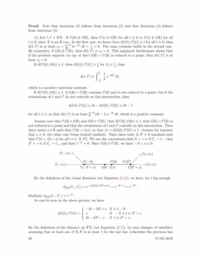
Proof. Note that Assertion (2) follows from Assertion (1) and that Assertion (4) followsfrom Assertion (3).

(1) Let `, `1 P GX. If `1p0q R `pRq, then `1ptq R `pRq for all t ě 0 or `1ptq R `pRq for allt ď 0, since X is an R-tree. In the first case, we hence have dp`ptq, `1ptqq ě t for all t ě 0, thusdp`, `1q is at least c2 “

ş`8

0 te´2 t dt “ 14 ą 0. The same estimate holds in the second case.

By symmetry, if `p0q R `1pRq, then dp`, `1q ě c2 ą 0. This argument furthermore shows thatif the geodesic segment (or ray or line) `pRq X `1pRq is reduced to a point, then dp`, `1q is atleast c2 ą 0.

If dp`1p0q, `p0qq ě 1, then dp`ptq, `1ptqq ě 12 for |t| ď 1

4 , thus

dp`, `1q ě

ż 14

´ 14

1

2e´2|t| dt ,

which is a positive universal constant.If dp`1p0q, `p0qq ď 1, if `pRq X `1pRq contains `1p0q and is not reduced to a point, but if the

orientations of ` and `1 do not coincide on this intersection, then

dp`ptq, `1ptqq ě 2t´ dp`p0q, `1p0qq ě 2t´ 1

for all t ě 1, so that dp`, `1q is at leastş`8

1 p2t´ 1q e´2t dt, which is a positive constant.

Assume now that `1p0q P `pRq and `p0q P `1pRq, that dp`1p0q, `p0qq ď 1, that `pRqX `1pRq isnot reduced to a point and that the orientations of ` and `1 coincide on this intersection. Thenthere exists s P R such that `1p0q “ `psq, so that |s| “ dp`p0q, `1p0qq ď 1. Assume for instancethat s ě 0, the other case being treated similarly. Then there exist S, S1 ě 0 maximal suchthat `1ptq “ `pt` sq for all t P r´S, S1s. We use the conventions that S “ `8 if `1´ “ `´, thatS1 “ `8 if `1` “ ``, and that e´8 “ 0. Since `p0q P `1pRq, we have ´S ` s ď 0.

`p0q `pS1 ` sq`psq`p´S ` sq`p´8q `p`8q

`1p´8q `1p`8q

`1p´Sq `1p0q `1pS1q

By the definition of the visual distances (see Equation (2.3)), we have, for t big enough,

d`p0qp``, `1`q “ e´dp`p0q, `pS

1`sqq “ e´S1´s — e´S

1

.

Similarly d`p0qp`´, `1´q — e´S .As can be seen in the above picture, we have

dp`ptq, `1ptqq “

$

&

%

´2t´ 2S ` s if t ď ´Ss if ´ S ď t ď S1 ` s2t´ 2S1 ´ s if t ě S1 ` s .

By the definition of the distance onp

GX (see Equation (2.7)), by easy changes of variables,assuming that at least one of S, S1 is at least 1 for the last line (otherwise the previous line

50 15/02/2019

shows that dp`, `1q is larger than a positive constant), we have

dp`, `1q “

ż ´S

´8

p´2t´ 2S ` sq e´2|t| dt`

ż S1`s

´Ss e´2|t| dt`

ż `8

S1`sp2t´ 2S1 ´ sq e´2t dt

“1

2e´2S`s

ż `8

su e´u du` s

ż S1`s

´Se´2|t| dt`

1

2e´2S1´s

ż `8

su e´u du

— e´2S ` e´2S1 ` s .

Assertion (1) of Lemma 3.4 follows.

(3) The first inclusion in Assertion (3) follows easily from Assertion (1). The secondinclusion follows from the argument of its proof, and the fact that if d`p0qp``, `1`q, d`p0qp`´, `´qand dp`p0q, `1p0qq are at most some small positive constant, then `pRq X `1pRq contains `1p0qand is not reduced to a point. l

When X is a Riemannian manifold with pinched sectional curvature, the following resultsays that the Hölder structure defined by the distance d given in Equation (2.7) on the unittangent bundle of X, identified with GX and T 1X as explained previously, is the usual one.

Recall that Sasaki’s metric on T 1X is the Riemannian metric induced on the submanifoldT 1X by the canonical Riemannian metric on the tangent bundle TX, such that for everyv P TX, if TvTX “ Vv ‘ Hv is the direct sum decomposition defined by the Levi-Civitaconnection of the Riemannian manifold X, then

‚ the direct sum Vv ‘Hv is orthogonal for Sasaki’s metric,

‚ the canonical isomorphism Vv » TπpvqX is an isometry, when Vv is endowed with Sasaki’sscalar product,

‚ the restriction of the tangent map of the footpoint projection Tπ : Hv Ñ TπpvqX is anisometry, when Hv is endowed with Sasaki’s scalar product.

Proposition 3.5. When X is a Riemannian manifold with pinched sectional curvature, thefollowing distances on T 1X are Hölder-equivalent:

(1) the Riemannian distance on T 1X defined by Sasaki’s metric,

(2) the distance δ1 on T 1X defined, for all `, `1 P T 1X, by

δ1p`, `1q “ expp´ suptt ě 0 : sup

sPr´t,tsdp`psq, `1psqq ď 1uq ,

with the convention δ1p`, `1q “ 1 if dp`p0q, `1p0qq ą 1 and δ1p`, `

1q “ 0 if ` “ `1,

(3) the distance δ2 on T 1X defined, for all `, `1 P T 1X, by

δ2p`, `1q “ sup

sPr0,1sdp`psq, `1psqq ,

(4) the distance d defined by Equation (2.7).

51 15/02/2019

Note that we could replace the interval r0, 1s in the definition of δ2 by any interval ra, bswith a ă b.

Proof. The fact that the first three distances on T 1X are Hölder-equivalent is already known,see for instance [Bal, p. 70].

Let us hence prove that d and δ2 are Hölder-equivalent. By the convexity of the distancefunction between two geodesic segments in a CATp´1q-space, we have

δ2p`, `1q “ maxtdp`p0q, `1p0qq, dp`p1q, `1p1qqu .

Hence by Proposition 3.2 applied twice (with t “ 0 and t “ 1), there exists c ą 0 such that ifdp`, `1q ď 1, then δ2p`, `

1q ď c dp`, `1q12 . Therefore the identity map from pT 1X, dq to pT 1X, δ2q

is Hölder-continuous.

Let us now prove conversely that there exist two constants c11 ě 1 and c12 P s0, 1s such thatfor all `, `1 P GX, if δ2p`, `

1q ď 12 , then

dp`, `1q ď c11 δ2p`, `1qc12 . (3.1)

Let x “ `p0q, y “ `1p0q, z “ `p1q, z1 “ `1p1q. Note that dpy, zq ě 12 by the triangle

inequality, since dpx, yq ď δ2p`, `1q ď 1

2 and dpx, zq “ 1. Let `2 be the geodesic line throughy and z, oriented from y to z with `2p0q “ y. Let us prove that dp`, `2q ď c11

2 dpx, yqc12 for

appropriate constants c11 and c12. A similar argument proves that dp`2, `1q ď c112 dpz, z1qc

12 , and

the triangle inequality for the distance d gives Equation (3.1).

`z

s y1

x

y`1

`2

z1

If dpy, zq ď dpx, zq, let x1 P rx, zs be such dpx1, zq “ dpy, zq ě 12 . We have s “ dpx, x1q “

dpx, zq ´ dpx1, zq “ dpx, zq ´ dpy, zq ď dpx, yq by the triangle inequality, and dpx1, yq ď dpx, yqby convexity. By Equation (2.8), we have

dp`, `2q ď dp`, gs`q ` dpgs`, `2q ď s` dpgs`, `2q ď dpx, yq ` dpgs`, `2q .

If dpy, zq ě dpx, zq, let y1 P ry, zs be such dpy1, zq “ dpx, zq “ 1 ě 12 (see the above picture).

We similarly have dpx, y1q ď dpx, yq and dp`, `2q ď dpx, yq ` dpgs`2, `2q if s “ dpy, y1q.We hence only have to prove that for all x, y, z P X with 0 ă dpx, yq ď 1

2 and dpx, zq “dpy, zq ě 1

2 , if u and v are the unit tangent vectors at x and y respectively pointing to z, thendpu, vq ď c21 dpx, yq

c22 for appropriate constants c21 and c22. This follows from the followinglemma with t “ 0, since 1

2 ě12

a

dpx, yq. We will need its more general version in the proofof Lemma 3.15.

Lemma 3.6. There exist two constants c8 ě 1 and c3 P s0, 1s such that for all x, y, z P Xwith 0 ă dpx, yq ď 1 and ρ “ dpx, zq “ dpy, zq ě 1

2

a

dpx, yq, for every t P r0, ρs, if u and vare the unit tangent vectors at x and y respectively pointing to z, then

dpgtu, gtvq ď c8 dpx, yqc3pe´t ` e2t´2ρq . (3.2)

52 15/02/2019

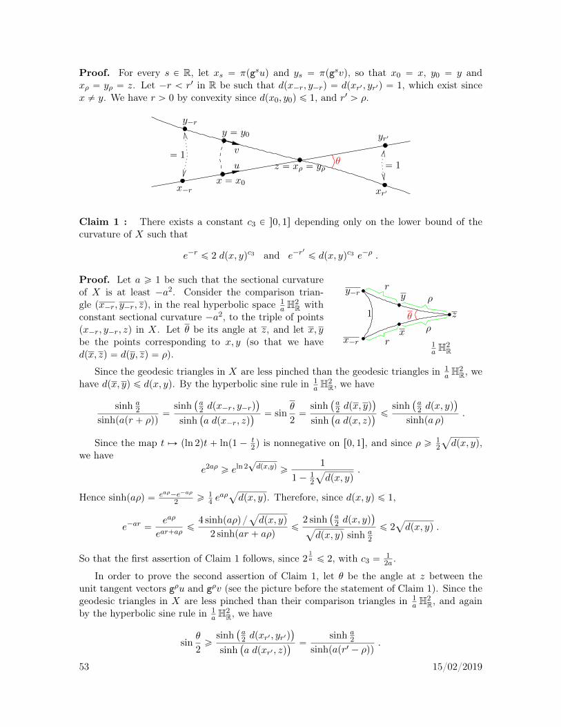
Proof. For every s P R, let xs “ πpgsuq and ys “ πpgsvq, so that x0 “ x, y0 “ y andxρ “ yρ “ z. Let ´r ă r1 in R be such that dpx´r, y´rq “ dpxr1 , yr1q “ 1, which exist sincex ‰ y. We have r ą 0 by convexity since dpx0, y0q ď 1, and r1 ą ρ.

x´r xr1

θ

y´r

yr1

“ 1“ 1

x “ x0

v

u z “ xρ “ yρ

y “ y0

Claim 1 : There exists a constant c3 P s0, 1s depending only on the lower bound of thecurvature of X such that

e´r ď 2 dpx, yqc3 and e´r1

ď dpx, yqc3 e´ρ .

Proof. Let a ě 1 be such that the sectional curvatureof X is at least ´a2. Consider the comparison trian-gle px´r, y´r, zq, in the real hyperbolic space 1

a H2R with

constant sectional curvature ´a2, to the triple of pointspx´r, y´r, zq in X. Let θ be its angle at z, and let x, ybe the points corresponding to x, y (so that we havedpx, zq “ dpy, zq “ ρ).

ρ

r

rρ

1 θ

x´r

y´r

x

y

1a H

2R

z

Since the geodesic triangles in X are less pinched than the geodesic triangles in 1a H

2R, we

have dpx, yq ď dpx, yq. By the hyperbolic sine rule in 1a H

2R, we have

sinh a2

sinhpapr ` ρqq“

sinh`

a2 dpx´r, y´rq

˘

sinh`

a dpx´r, zq˘ “ sin

θ

2“

sinh`

a2 dpx, yq

˘

sinh`

a dpx, zq˘ ď

sinh`

a2 dpx, yq

˘

sinhpa ρq.

Since the map t ÞÑ pln 2qt ` lnp1 ´ t2q is nonnegative on r0, 1s, and since ρ ě 1

2

a

dpx, yq,we have

e2aρ ě eln 2?dpx,yq ě

1

1´ 12

a

dpx, yq.

Hence sinhpaρq “ eaρ´e´aρ

2 ě 14 e

aρa

dpx, yq. Therefore, since dpx, yq ď 1,

e´ar “eaρ

ear`aρď

4 sinhpaρq a

dpx, yq

2 sinhpar ` aρqď

2 sinh`

a2 dpx, yq

˘

a

dpx, yq sinh a2

ď 2a

dpx, yq .

So that the first assertion of Claim 1 follows, since 21a ď 2, with c3 “

12a .

In order to prove the second assertion of Claim 1, let θ be the angle at z between theunit tangent vectors gρu and gρv (see the picture before the statement of Claim 1). Since thegeodesic triangles in X are less pinched than their comparison triangles in 1

a H2R, and again

by the hyperbolic sine rule in 1a H

2R, we have

sinθ

2ě

sinh`

a2 dpxr1 , yr1q

˘

sinh`

a dpxr1 , zq˘ “

sinh a2

sinhpapr1 ´ ρqq.

53 15/02/2019

Since the geodesic triangles in X are more pinched than their comparison triangles in H2R,

since dpx, yq ď 1 and since sinh ρ ě ρ ě 12

a

dpx, yq, we have

sinθ

2ď

sinh`

12 dpx, yq

˘

sinh dpx, zqďpsinh 1

2qdpx, yq

sinh ρď 2 psinh

1

2qa

dpx, yq .

Let c4 “

´

sinh 12

sinh a2

¯1a , which is positive and strictly less than 1 since a ą 1. Then

e´ar1

“e´aρ

ear1´aρď

e´aρ

2 sinhpapr1 ´ ρqqď e´aρ

sinh 12

2 sinh a2

dpx, yq

sinh ρ

ď e´aρ c4aa

dpx, yq . (3.3)

So that the second assertion of Claim 1 follows, since c4 ď 1, again with c3 “12a . l

Let us remark that since dpx, yq ď 1, Equation (3.3) also gives that

r1 ´ ρ ě ´ ln c4 ą 0 .

Since θ is also the angle between the unit tangent vectors ´gρu and ´gρv, a similar argumentgives that

sinh 12

sinhpr1 ´ ρq“

sinh`

12 dpxr1 , yr1q

˘

sinh dpxr1 , zqě sin

θ

2ě

sinh`

a2 dpx, yq

˘

sinh`

a dpx, zq˘ ě

a dpx, yq

2 sinhpa ρq.

Let c5 “2 sinh 1

2

ap1´c24qą 0. Since the map t ÞÑ sinhptq

et is nondecreasing on R, we hence have

er1´ρ ď

e´ ln c4

sinhp´ ln c4qsinhpr1 ´ ρq ď

2

1´ c24

2 sinh 12

a dpx, yqsinhpa ρq ď

c5

dpx, yqeaρ .

Therefore1` r1 ď pa` 1qρ` p1` ln c5q ´ ln dpx, yq , (3.4)

a formula which be useful later on.

Let t P r0, ρs. By the definition of the distance d on GX (see Equation (2.7)), we have

dpgtu, gtvq “

ż `8

´8

dpπpgsgtuq, πpgsgtvqq e´2|s| ds “

ż `8

´8

dpxs, ysq e´2|s´t| ds . (3.5)

We subdivide the integralş`8

´8as

ş´r´8`ş0´r `

şρ0 `

şr1

ρ `ş`8

r1 .

Claim 2 : We have

I1 “

ż ´r

´8

dpxs, ysq e´2|s´t| ds ď 2 e´2t dpx, yqc3 .

Proof. By the triangle inequality, for every s P rr,`8r, we have

dpx´s, y´sq ď dpx´s, x´rq ` dpx´r, y´rq ` dpy´r, y´sq ď 2s` 1 .

54 15/02/2019

Hence

I1 “

ż `8

rdpx´s, y´sq e

´2ps`tq ds ď e´2t

ż `8

rp2s` 1q e´2s ds ď e´2te´r ,

and the result follows from the first assertion of Claim 1. l

Claim 3 : We have

I2 “

ż 0

´rdpxs, ysq e

´2|s´t| ds ď 2 psinh 1q e´2t dpx, yqc3 .

Proof. Recall that since X is CATp´1q and by an easy exercise in hyperbolic geometry (seefor instance [PauPS, Lem. 2.5 (i)]), for all x1, y1, z1 in X such that dpx1, z1q “ dpy1, z1q, forevery t1 P r0, dpx1, z1qs, if x1t (respectively y1t) is the point on rx1, z1s (respectively ry1, z1s) atdistance t1 from x1 (respectively y1), then

dpx1t, y1tq ď e´t

1

sinh dpx1, y1q . (3.6)

Hence for all s P r0, rs, we have dpx´s, y´sq ď e´pr´sq sinh dpx´r, y´rq “ e´r`s sinh 1. Thus

I2 “

ż r

0dpx´s, y´sq e

´2ps`tq ds

ď psinh 1q e´2t

ż `8

0e´r`s e´2s ds “ psinh 1q e´2t e´r ,

and the result also follows from the first assertion of Claim 1. l

Claim 4 : There exists a universal constant c6 ą 0 such that

I3 “

ż ρ

0dpxs, ysq e

´2|s´t| ds ď c6 e´t dpx, yq .

Proof. By Equation (3.6) and since dpx, yq ď 1, for every s P r0, ρs, we have

dpxs, ysq ď e´s sinh dpx, yq ď psinh 1q e´s dpx, yq .

Therefore

I3 “

ż t

0dpxs, ysq e

´2pt´sqq ds`

ż ρ

tdpxs, ysq e

´2ps´tqq ds

ď psinh 1q dpx, yq´

e´2t

ż t

0es ds` e2t

ż `8

te´3s ds

¯

ď4 sinh 1

3dpx, yq e´t . l

Claim 5 : We have

I4 “

ż r1

ρdpxs, ysq e

´2|s´t| ds ď psinh 1q e2t´2ρ dpx, yqc3 .

Proof. By Equation (3.6), for every s P rρ, r1s, we have

dpxs, ysq ď e´pr1´sq sinh dpxr1 , yr1q “ psinh 1q e´r

1`s .

55 15/02/2019

Hence

I4 “

ż r1

ρdpxs, ysq e

´2ps´tqq ds ď psinh 1q e2t e´r1

ż r1

ρe´s ds ď psinh 1q e2t´ρ e´r

1

.

The result follows from the second assertion of Claim 1. l

Claim 6 : There exists a constant c7 ą 0 depending only on the lower bound of the curvatureof X such that

I5 “

ż `8

r1dpxs, ysq e

´2|s´t| ds ď c7 e2t´2ρ dpx, yqc3 .

Proof. By the triangle inequality, for every s P rr1,`8r, we have

dpxs, ysq ď dpxs, xr1q ` dpxr1 , yr1q ` dpyr1 , ysq ď 2s` 1 .

Hence, using the second assertion of Claim 1, we have

I5 “

ż `8

r1dpxs, ysq e

´2ps´tq ds ď e2t

ż `8

r1p2s` 1q e´2s ds “ e2tp1` r1qe´2r1 .

By Equation (3.3), since sinh ρ ě ρ ě 12

a

dpx, yq and c3 “12a , we have

e´2r1 ď e´2ρ c24

´ dpx, yq

2 sinh ρ

¯2aď e´2ρ dpx, yq2c3 .

Since c ď ec for every c ě 0 and dpx, yq ď 1, we have ´ ln dpx, yq ď 1c3dpx, yq´c3 . Hence by

Equation (3.4), we have

I5 ď e2t´2ρ´

pa` 1qc24 dpx, yq

2a ρ

p2 sinh ρq2a` p1` ln c5q dpx, yq

2c3 `1

c3dpx, yqc3

¯

.

Assuming, as we may, that a ě 2, the map ρ1 ÞÑ ρ1

psinh ρ1q2ais bounded on r0,`8r. Since

c3 “12a ď

2a , this proves Claim 6. l

Since dpx, yq ď 1, it follows from Equation (3.5) and from Claims 2 to 6 that there existsa constant c8 ą 0 depending only on the lower bound of the curvature of X such that

dpgtu, gtvq “ I1 ` I2 ` I3 ` I4 ` I5 ď c8 dpx, yqc3pe´t ` e2t´2ρq .

This proves Lemma 3.6, hence concludes the proof of Proposition 3.5. l l

Let D be a nonempty proper closed convex subset of X. The regularity property in theRiemannian manifold case of the fibrations f˘D : U ˘

D Ñ B1˘D defined in Section 2.4, that will

be needed in Section 12.3, is the Hölder-continuity one, as proved in the following lemma (seealso [PaP17b, Lem. 6]).

Lemma 3.7. Assume that X is a Riemannian manifold with pinched negative curvature. Themaps f˘D are Hölder-continuous on any set of elements ` P U ˘

D such that dpπp`q, πpf˘D p`qqq isbounded.

Proof. We prove the result for f`D , the one for f´D follows similarly. We will use the Hölder-equivalent distances δ1 and δ2, defined in the statement of Proposition 3.5, on the unit tangentbundle of X, identified with GX as explained previously.

56 15/02/2019

D x1

xT

y1

y

w1

w

v

v1v` “ w`

v1` “ w1`

Let v, v1 P T 1X be such that dpvp0q, v1p0qq ď 1, let w “ f`D pvq and w1 “ f`D pv1q. Let

T “ suptt ě 0 : supsPr0,ts dpvpsq, v1psqq ď 1u, so that δ1pv, v

1q ě e´T . We may assume thatT is finite, otherwise v` “ v1`, hence w “ w1. Let x “ vpT q and x1 “ v1pT q, which satisfydpx, x1q ď 1. Let y (respectively y1) be the closest point to x (respectively x1) on the geodesicray defined by w (respectively w1). By convexity, since dpvp0q, wp0qq and dpv1p0q, w1p0qq arebounded by a constant c ą 0 and since v` “ w`, v

1` “ w1`, we have dpx, yq ď c and

dpx1, y1q ď c. By the triangle inequality, we have dpy, y1q ď 2c`1, dpy, wp1qq ě T ´2c´1 anddpy1, w1p1qq ě T ´ 2c´ 1. By convexity, and since closest point maps exponentially decreasethe distances, there exists a constant c1 ą 0 such that

δ2pw,w1q “ dpwp1q, w1p1qq ď c1 dpy, y1q e´pT´2c´1q ď c1 p2c` 1q e2c`1 δ1pv, v

1q .

The result follows. l

When X is an R-tree, we have a stronger version of Lemma 3.7, that will be needed inSection 12.6.

Lemma 3.8. Assume that X is an R-tree. Let η,R ą 0 be such that η ď 1 ď lnR, and let Dbe a nonempty closed convex subset of X. Then the restriction to the dynamical neighborhoodV ˘η,RpB

1˘Dq of the fibration f˘D is (uniformly locally) Lipschitz, with constants independent of

η.

Proof. We assume for instance that ˘ “ `. Let `, `1 P V `η,RpB

1`Dq and let w “ f`D p`q, w

1 “

f`D p`1q.

Since the fiber over ρ P B1`D of the restriction to V `

η,RpB1`Dq of f

`D is V `ρ, η,R,

1 there exists, s1 P s ´ η, ηr such that gs` P B`pw,Rq and gs

1

`1 P B`pw1, Rq, so that gs`ptq “ wptq andgs1

`1ptq “ w1ptq for all t ě lnR by the definition of the Hamenstädt balls. Up to permuting `and `1, we assume that s1 ě s.

wď lnR

`1p0q

s1 ď η

`

`

w1

`p0q

`1

`1

1See the end of Section 2.4.

57 15/02/2019

By (the proof of) Lemma 3.4 (1), there exists a constant cR ą 0 depending only on R suchthat if dp`, `1q ď cR and s2 “ dp`p0q, `1p0qq, then s2 “ s1 ´ s and the geodesic lines gs` andgs1

`1 coincide at least on r´ lnR´ 1, lnR` 1s . In particular, we have, since |s|, |s1| ď η ď 1,

wplnRq “ `ps` lnRq “ `1ps1 ` lnRq “ w1plnRq .

Since the origin of w is the closest point on D to any point of wpr0,`8rq, we hence have thatwptq “ w1ptq for all t P r0, lnRs. Therefore (using Equation (2.8) for the last inequality),

dpw,w1q “

ż `8

lnRdpwptq, w1ptqq e´2 t dt “

ż `8

lnRdpgs`ptq, gs

1

`1ptqq e´2 t dt

“ e2s

ż `8

lnR`sdp`puq, gs

2

`1puqq e´2u du ď e2s dp`, gs2

`1q

ď e2s`

dp`, `1q ` dp`1, gs2

`1q˘

ď e2s pdp`, `1q ` s2q

“ e2s`

dp`, `1q ` dp`p0q, `1p0qq˘

,

so that the result follows from Lemma 3.4 (2).

Note that when X is (the geometric realisation of) a simplicial tree, we have s “ s1 “s2 “ 0 and the above computations simplify to give dpw,w1q ď dp`, `1q. l

For any metric space Z and α P s0, 1s, the Hölder norm of a bounded α-Hölder-continuousfunction f : Z Ñ R is

fα “ f8 ` f1α ,

wheref1α “ sup

x, y PZ0ădpx, yqď1

|fpxq ´ fpyq|

dpx, yqα.

When the diameter of Z is bounded by 1,2 this coincides with the usual definition. Note thateven if the constant ε in the definition of a α-Hölder-continuous map is less than 1, this normis finite, since

supx, yPZ

εďdpx,yqď1

|fpxq ´ fpyq|

dpx, yqαď 2 ε´α f8 .

Note that for all bounded α-Hölder-continuous maps f, g : Z Ñ R, we have

fgα ď fα g8 ` f8 gα . (3.7)

We denote by C αc pZq (respectively C α

b pZq) the space of α-Hölder-continuous real-valuedfunctions with compact support (respectively which are bounded) on Z, endowed with thisnorm. Note that C α

b pZq is a real Banach space.3

The next two lemmas will be needed only in Part III of this book. The first one is ametric estimate on the extension of geodesic segments to geodesic rays, with its functionalcounterpart.

2This is in particular the case for the sequence spaces of symbolic dynamical systems, see Sections 5.2 and9.2.

3The standard proof using Arzela-Ascoli’s theorem applies with our slightly different definition of the Höldernorms.

58 15/02/2019

Lemma 3.9. Let X be a geodesically complete proper CATp´1q space, let T ě 1, and let α Pp

GX be a generalised geodesic line which is isometric exactly on r0, T s. For every generalisedgeodesic line ρ P

p

GX which is isometric exactly on r0,`8r , such that ρ|r0,T s “ α|r0,T s, wehave

dpα, ρq “e´2T

4ă 1 ,

and hence for all β P s0, 1s and rψ P C βb p

p

GXq,

| rψpαq ´ rψpρq| ďe´2β T

4β rψ β .

Proof. By Equation (2.7) defining the distance onp

GX, we have, since dpαptq, ρptqq “ 0 forall t P s ´8, T s and dpαptq, ρptqq “ t´ T otherwise,

dpα, ρq “

ż `8

Tpt´ T q e´2t dt “ e´2T

ż `8

0u e´2u du “

e´2T

4.

The result follows. l

The second lemma gives a metric estimate, with its functional counterpart, on the mapwhich associates to a geodesic ray in an outer normal unit bundle its point at infinity, em-phasising the 1

2 -Hölder-continuity of endpoints maps (see Lemma 3.4 (4)). We start by givingsome definitions.

Let X be a geodesically complete proper CATp´1q space, and let D be a nonempty properclosed convex subset of X. The distance-like map

dD :`

B8X ´ B8D˘2Ñ r0,`8r

associated with D is defined in [HeP4, §2.2] as follows. For ξ, ξ1 P B8X ´ B8D, let ξt, ξ1t :r0,`8r Ñ X be the geodesic rays starting at the closest points PDpξq, PDpξ1q to ξ, ξ1 on Dand converging to ξ, ξ1 as tÑ8. Let

dDpξ, ξ1q “ lim

tÑ`8e

12dpξt, ξ1tq´t . (3.8)

The distance-like map dD is invariant by the diagonal action of the isometries of X preservingD. If D consists of a single point x, then dD is the visual distance4 dx on B8X based at x. IfD is a horoball with point at infinity ξ0, then dD is Hamenstädt’s distance5 on B8X ´ tξ0u.As seen in [HeP4, §2.2, Ex. (4)], if X is a metric tree, then

dDpξ, ξ1q “

$

’

&

’

%

e12dpPDpξq, PDpξ

1qq ą 1 if PDpξq ‰ PDpξ1q

dxpξ, ξ1q “ e´dpx, yq ď 1 if PDpξq “ PDpξ

1q “ x

and rx, ξr X rx, ξ1r “ rx, ys .

In particular, although in general it is not an actual distance on its whole domain B8X´B8D,the map dD is locally a distance, and we can define with the standard formula the β-Hölder-continuity of maps with values in pB8X ´ B8D, dDq and the β-Hölder-norm of a functiondefined on pB8X´B8D, dDq. In the next result, we endow B8X´B8D with the distance-likemap dD.

4See Equation (2.2).5See Equation (2.12).

59 15/02/2019

Proposition 3.10. Let X be a locally finite simplicial tree without terminal vertices, and letD be a proper nonempty simplicial subtree of X. Let X “ |X|1 and D “ |D|1 be their geometricrealisations. The homeomorphism B` : B1

`DÑ pB8X ´B8Dq defined by ρ ÞÑ ρ` is 12 -Hölder-

continuous, and for all β P s0, 1s and ψ P C βb pB8X ´ B8Dq, the map ψ ˝ B` : B1

`D Ñ R isbounded and β

2 -Hölder-continuous, with

ψ ˝ B`β2ď p1` 2

β2`1q ψβ .

Proof. Let us prove that for every ρ, ρ1 P B1`D, if dpρ, ρ1q ď 1, then ρp0q “ ρ1p0q, and

dDpρ`, ρ1`q “

?2 dpρ, ρ1q

12 . (3.9)

This proves that the map B` is 12 -Hölder-continuous. We may assume that ρ ‰ ρ1.

Let ρ, ρ1 P B1`D. If ρp0q ‰ ρ1p0q, then the images of ρ and ρ1 are disjoint and their

connecting segment in the tree X joins ρp0q and ρ1p0q; hence for every t P r0,`8r , we have

dpρptq, ρ1ptqq “ dpρp0q, ρ1p0qq ` dpρptq, ρp0qq ` dpρ1ptq, ρ1p0qq ě 1` 2 t .

Thus

dpρ, ρ1q “

ż 0

´8

dpρp0q, ρ1p0qq e2 t dt`

ż `8

0dpρptq, ρ1ptqq e´2 t dt

ě

ż 0

´8

e2 t dt`

ż `8

0p1` 2tq e´2 t dt ą 2

ż `8

0e´2 t dt “ 1 .

Assume that x “ ρp0q “ ρ1p0q and let n be the length of the intersection of ρ and ρ1. Then

dDpρ`, ρ1`q “ dxpρ`, ρ

1`q “ lim

tÑ`8e

12dpρptq, ρ1ptqq´t “ e´n .

Furthermore, since ρptq “ ρ1ptq for t ď n and dpρptq, ρ1ptqq “ 2pt ´ nq otherwise, we have,using the change of variables u “ 2pt´ nq,

dpρ, ρ1q “

ż `8

n2 pt´ nq e´2 t dt “ e´2n

ż `8

0u e´u

du

2“e´2n

2.

This proves Equation (3.9).Let β P s0, 1s and ψ P C β

b pB8X ´ B8Dq. We have ψ ˝ B`8 “ ψ8 since B` is ahomeomorphism, and, by Equation (3.9),

ψ ˝ B`1β2

“ supρ, ρ1PB1

`D, 0ădpρ, ρ1qď1

|ψ ˝ B`pρq ´ ψ ˝ B`pρ1q|

dpρ, ρ1qβ2

ď supρ, ρ1PB1

`D, 0ădpρ, ρ1qď 12

|ψ ˝ B`pρq ´ ψ ˝ B`pρ1q|

dpρ, ρ1qβ2

`2 ψ ˝ B`8

2´β2

ď supξ, ξ1PB8X´B8D0ădDpξ, ξ

1qď1

|ψpξq ´ ψpξ1q|

2´β2 dDpξ, ξ1qβ

` 2β2`1 ψ8

ď 2β2`1 ψβ .

60 15/02/2019

Since ψ ˝ B`β2“ ψ ˝ B`8 ` ψ ˝ B

`1β2

, this proves the last claim of Proposition 3.10. l

A stronger assumption than the Hölder regularity is the locally constant regularity, thatwe now define. Alhough it is only useful for totally disconnected metric spaces, several errorterms estimates in the literature use this stronger regularity (see for instance [AtGP, KemaPS]and Part III of this book).

Let ε ą 0. For every metric space E and every set E1, we say that a map f : E Ñ E1 isε-locally constant if f is constant on every closed ball of radius ε (or equivalently of radius atmost ε) in E. We say that f : E Ñ E1 is locally constant if there exists ε ą 0 such that f isε-locally constant.

Note that if E is a geodesic metric space and f : E Ñ E1 is locally constant, then f isconstant. But when E is for instance an ultrametric space, since two distinct closed ballsof the same radius are disjoint, the above definition turns out to be very interesting (andmuch used in representation theory in positive characteristic, for instance). For example, thecharacteristic function 1A of a subset A of E is ε-locally constant if and only if for everyx P A, the closed ball Bpx, εq is contained in A. In particular, the characteristic function of aclosed ball of radius ε in an ultrametric space is ε-locally constant.

Remark 3.11. Let E and E1 be two metric spaces. If a map f : E Ñ E1 is ε-locally constant,then it is α-Hölder-continuous for every α P s0, 1s. Indeed, for all x, y P E, if dpx, yq ď ε thendpfpxq, fpyqq “ 0 ď c dpx, yqα for all c ą 0. If furthermore E1 “ R and f is bounded, then

supx,yPE, x‰y

|fpxq ´ fpyq|

dpx, yqα“ sup

x,yPE, dpx, yqąε

|fpxq ´ fpyq|

dpx, yqαď

2

εαf8 .

For all ε P s0, 1s and β ą 0, we denote by C ε lc, βb pEq the real vector space6 of ε-locally

constant functions f : E Ñ R endowed with the ε lc-norm of exponent β defined by

fε lc, β “ ε´β f8 .

The above remark proves that if β P s0, 1s, then fβ ď 3fε lc, β , so that the inclusion mapfrom C ε lc, β

b pEq into C βb pEq is continuous.

3.2 Potentials

In this book, a potential for Γ is a continuous Γ-invariant function rF : T 1X Ñ R. Thequotient function F : ΓzT 1X Ñ R of rF is called a potential on ΓzT 1X. Precomposing by thecanonical projection GX Ñ T 1X, the function rF defines a continuous Γ-invariant functionfrom GX to R, also denoted by rF , by rF p`q “ rF pv`q for every ` P GX.

For all x, y P X, and any geodesic line ` P GX such that `p0q “ x and `pdpx, yqq “ y, letż y

x

rF “

ż dpx,yq

0

rF pvgt`q dt .

Note that for all t P s0, dpx, yqr, the germ vgt` is independent on the choice of such a line `,hence

şyxrF does not depend on the extension ` of the geodesic segment rx, ys. The following

6Note that a linear combination of ε-locally constant functions is again a ε-locally constant function.

61 15/02/2019

properties are easy to check using the Γ-invariance of rF and the basic properties of integrals:For all γ P Γ

ż γy

γx

rF “

ż y

x

rF , (3.10)

for the antipodal map ιż x

y

rF “

ż y

x

rF ˝ ι , (3.11)

and, for any z P rx, ys,ż y

x

rF “

ż z

x

rF `

ż y

z

rF . (3.12)

The period of a loxodromic isometry γ of X for the potential rF is

PerF pγq “

ż γx

x

rF

for any x in the translation axis of γ. Note that, for all α P Γ and n P N´ t0u, we have

PerF pαγα´1q “ PerF pγq, PerF pγ

nq “ n PerF pγq and PerF pγ´1q “ PerF˝ιpγq . (3.13)

In trees, we have the following Lipschitz-type control on the integrals of the potentialsalong segments.

Lemma 3.12. When rF is constant or when X is an R-tree, for all x, x1, y, y1 P X, we have

ˇ

ˇ

ˇ

ż y

x

rF ´

ż y1

x1

rFˇ

ˇ ď dpx, x1q supπ´1prx, x1sq

| rF | ` dpy, y1q supπ´1pry, y1sq

| rF | .

Proof. When rF is constant, the result follows from the triangle inequality.Assume that X is an R-tree. Consider the case x “ x1. Let z P X be such that rx, zs “

rx, ys X rx, y1s. Using Equation (3.12) and the fact that dpy, zq ` dpz, y1q “ dpy, y1q, the claimfollows. The general case follows by combining this case x “ x1 and a similar estimate for thecase y “ y1. l

Some form of uniform Hölder-type control of the potential, analogous to the Lipschitz-type one in the previous lemma, will be crucial throughout the present work. The followingDefinition 3.13 formalises this (weaker) assumption.

Definition 3.13. The triple pX,Γ, rF q satisfies the HC-property (Hölder-type control) if rFhas subexponential growth when X is not an R-tree and if there exist κ1 ě 0 and κ2 P s0, 1ssuch that for all x, y, x1, y1 P X with dpx, x1q, dpy, y1q ď 1, we have

ˇ

ˇ

ˇ

ż y

x

rF ´

ż y1

x1

rFˇ

ˇ

ˇ(HC)

ď`

κ1 ` 2 maxπ´1pBpx, 1qYBpx1, 1qq

| rF |˘

dpx, x1qκ2 ``

κ1 ` 2 maxπ´1pBpy, 1qYBpy1, 1qq

| rF |˘

dpy, y1qκ2 .

62 15/02/2019

By Equation (3.11), pX,Γ, rF ˝ ιq satisfies the HC-property if and only if pX,Γ, rF q does.By the triangle inequality | dpx, yq ´ dpx1, y1q | ď dpx, x1q ` dpy, y1q, for every κ P R, the triplepX,Γ, rF`κq satisfies the HC-property (up to changing the constant κ1) if and only if pX,Γ, rF qdoes.

WhenX is assumed to be a Riemannian manifold with pinched sectional curvature, requir-ing the potentials to be Hölder-continuous as in [PauPS] is sufficient to have the HC-property,as we will see below.

Proposition 3.14. The triple pX,Γ, rF q satisfies the HC-property if one of the followingconditions is satisfied:• rF is constant,• X is an R-tree,• X is a Riemannian manifold with pinched sectional curvature and rF is Hölder-continuous.

Proof. The first two cases are treated in Lemma 3.12, and we may take for them κ1 “ 0 andκ2 “ 1 in the definition of the HC-property.

The claim for Riemannian manifolds follows from the property of at most linear growthof the Hölder-continuous maps (see Remark 3.1) and from the following lemma, so that theconstants κ1 ą 0 and κ2 P s0, 1s of the HC-property depend only on the Hölder-continuityconstants of rF and on the bounds on the sectional curvature of X.

Lemma 3.15. If X is a Riemannian manifold with pinched sectional curvature and rF isHölder-continuous, there exist two constants c1 ą 0 and c2 P s0, 1s such that, for all x, y, z inX with dpx, yq ď 1, we have

ˇ

ˇ

ˇ

ż z

x

rF ´

ż z

y

rFˇ

ˇ

ˇď c1 dpx, yq

c2 ` 2 dpx, yq12 maxπ´1pBpx, 1qYBpy, 1qq

| rF | .

The constants c1 and c2 depend only on the Hölder-continuity constants of rF and the boundson the sectional curvature of X.

This lemma is similar to the second claim in [PauPS, Lem. 3.2], but the proof of this claim(and more precisely the proof of [PauPS, Lem. 2.3] used in the proof of [PauPS, Lem. 3.2]),which involves a different distance d on GX, does not extend with the present definition of d.

Proof. By symmetry, we may assume that dpx, zq ě dpy, zq. The result is true if x “ y,hence we assume that x ‰ y. Let x1 be the point on rx, zs at distance dpy, zq from z.

x x1 z

y

p

The closest point p of y on rx, zs lies in rx1, zs by convexity. Hence

dpx, x1q ď dpx, pq ď dpx, yq ďa

dpx, yq ď 1 ,

since closest point maps do not increase distances and dpx, yq ď 1. Therefore

ˇ

ˇ

ˇ

ż x1

x

rFˇ

ˇ

ˇď dpx, x1q max

π´1prx, x1sq| rF | ď

a

dpx, yq maxπ´1pBpx, 1qq

| rF | , (3.14)

63 15/02/2019

SinceşzxrF “

şx1

xrF `

şzx1

rF (see Equation (3.12)), we have

ˇ

ˇ

ˇ

ż z

x

rF ´

ż z

y

rFˇ

ˇ

ˇď

ˇ

ˇ

ˇ

ż z

x1

rF ´

ż z

y

rFˇ

ˇ

ˇ`

ˇ

ˇ

ˇ

ż x1

x

rFˇ

ˇ

ˇ. (3.15)

Assume first that dpy, zq “ dpx1, zq ď 12

a

dpx, yq. We have

ˇ

ˇ

ˇ

ż z

x

rF ´

ż z

y

rFˇ

ˇ

ˇď

ˇ

ˇ

ˇ

ż z

x1

rFˇ

ˇ

ˇ`

ˇ

ˇ

ˇ

ż z

y

rFˇ

ˇ

ˇ`

ˇ

ˇ

ˇ

ż x1

x

rFˇ

ˇ

ˇ

ď dpx1, zq maxπ´1prx1, zsq

| rF | ` dpy, zq maxπ´1pry, zsq

| rF | `a

dpx, yq maxπ´1pBpx, 1qq

| rF |

ď 2a

dpx, yq maxπ´1pBpx, 1qYBpy, 1qq

| rF | ,

and Lemma 3.15 follows, for any c1 ą 0 and c2 P s0, 1s.

Now assume that that dpy, zq ě 12

a

dpx, yq. Since the distance function from a given pointto a point varying on a geodesic line is convex, we have dpx1, yq ď dpx, yq. By Equations (3.14)and (3.15), we may therefore assume that x “ x1 and prove that

ˇ

ˇ

ˇ

ż z

x

rF ´

ż z

y

rFˇ

ˇ

ˇď c1 dpx, yq

c2

for appropriate constants c1, c2.Since X is a Riemannian manifold, we identify GX and T 1X with the usual unit tangent

bundle of X as explained previously. Let u (respectively v) be the unit tangent vector at x(respectively y) pointing towards z. Let ρ “ dpx, zq “ dpy, zq ě 1

2

a

dpx, yq, and t P r0, ρs. Weapply Lemma 3.6, whose hypotheses are indeed satisfied.

Since t P r0, ρs and dpx, yq ď 1, the term on the right hand side of Equation (3.2) isbounded by 2 c8. Since rF is Hölder-continuous, let c ą 0 and α P s0, 1s be the Hölder-continuity constants such that | rF pu1q ´ rF pv1q| ď c dpu1, v1qα for all u1, v1 P T 1X such thatdpu1, v1q ď 2 c8. Then, by Lemma 3.6,

ˇ

ˇ

ˇ

ż z

x

rF ´

ż z

y

rFˇ

ˇ

ˇ“

ˇ

ˇ

ˇ

ż ρ

0

`

rF pgtuq ´ rF pgtvq˘

dtˇ

ˇ

ˇď

ż ρ

0c dpgtu, gtvqα dt

ď c c8α dpx, yqαc3

´

ż `8

0e´αt dt`

ż ρ

´8

e2αt´2αρ dt¯

“3c

2αc8α dpx, yqαc3 .

This concludes the proof of Lemma 3.15 with c2 “ αc3 and c1 “3c2α c

α8 , hence completes the

proof of Proposition 3.14 in the Riemannian manifold case. l l

Remark 3.16. (1) If X “ ĂM is a Riemannian manifold, then T 1X is naturally identifiedwith the usual Riemannian unit tangent bundle of ĂM . If the potential rF : T 1

ĂM Ñ R isHölder-continuous for Sasaki’s Riemannian metric on T 1

ĂM , it is a potential as in [Rue1] and[PauPS]. Furthermore, the definition of

şyxrF coincides with the one in these references.

(2) The quotient function F is Hölder-continuous when rF is Hölder-continuous.

64 15/02/2019

Let rF , rF ˚ : T 1X Ñ R be potentials for Γ. We say that rF ˚ is cohomologous to rF (see forinstance [Livš]) if there exists a continuous Γ-invariant function rG : T 1X Ñ R, such that, forevery ` P GX, the map t ÞÑ rGpvgt`q is differentiable and

rF ˚pv`q ´ rF pv`q “d

dt |t“0

rGpvgt`q . (3.16)

When working with Hölder-continuous potentials, the regularity requirement is for rG toalso be Hölder-continuous. Note that the right-hand side of Equation (3.16) does not dependon the choice of the representative ` of its germ v`. In particular, PerF pγq “ PerF˚pγq for anyloxodromic isometry γ if rF and rF ˚ are cohomologous potentials.

A potential rF is said to be reversible if rF and rF ˝ ι are cohomologous.

3.3 Poincaré series and critical exponents

Let us fix a potential rF : T 1X Ñ R for Γ, and x, y P X.The critical exponent of pΓ, F q is the element δ “ δΓ, F of the extended real line r´8,`8s

defined by

δ “ lim supnÑ`8

1

nln

ÿ

γPΓ, n´1ădpx,γyqďn

eşγyx

rF .

The Poincaré series of pΓ, F q is the map Q “ QΓ, F, x, y : RÑ r0,`8s defined by

Q : s ÞÑÿ

γPΓ

eşγyx p

rF´sq .

If δ ă `8, we say that pΓ, F q is of divergence type if the series QΓ, F, x, ypδq diverges, and ofconvergence type otherwise.

When F “ 0, the critical exponent δΓ, 0 is the usual critical exponent δΓ P s0,`8s of Γ,the Poincaré series QΓ, 0, x, y is the usual Poincaré series of Γ, and we recover the usual notionof divergence or convergence type of Γ, see for instance [Rob2].

The Poincaré series of pΓ, F q and its critical exponent make sense even if Γ is elementary(see for instance Lemma 3.17 (10)). The following result collects some of the basic propertiesof the critical exponent.

Lemma 3.17. Assume that pX,Γ, rF q satisfies the HC-property. Then

(1) the critical exponent δΓ, F and the divergence or convergence of QΓ, F, x, ypsq are inde-pendent of the points x, y P X; they depend only on the cohomology class of rF ;

(2) QΓ, F˝ι, x, y “ QΓ, F, y, x and δΓ, F˝ι “ δΓ, F ; in particular, pΓ, F q is of divergence type ifand only if pΓ, F ˝ ιq is of divergence type ;

(3) the Poincaré series Qpsq diverges if s ă δΓ, F and converges if s ą δΓ, F ;

(4) δΓ, F`κ “ δΓ, F`κ for any κ P R, and pΓ, F q is of divergence type if and only if pΓ, F`κqis of divergence type ;

(5) if Γ1 is a nonelementary subgroup of Γ, denoting by F 1 : Γ1zT 1X Ñ R the map inducedby rF , then δΓ1, F 1 ď δΓ, F ;

65 15/02/2019

(6) if δΓ ă `8, then δΓ ` infπ´1pC ΛΓq

rF ď δΓ, F ď δΓ ` supπ´1pC ΛΓq

rF ;

(7) δΓ, F ą ´8 ;

(8) the map rF ÞÑ δΓ, F is convex, sub-additive, and 1-Lipschitz for the uniform norm on thevector space of real continuous maps on π´1pC ΛΓq ;7

(9) if Γ2 is a discrete cocompact group of isometries of X such that rF is Γ2-invariant,denoting by F 2 : Γ2zT 1X Ñ R the map induced by rF , then

δΓ, F ď δΓ2, F 2 ;

(10) if Γ is infinite cyclic, generated by a loxodromic isometry γ of X, then pΓ, F q is ofdivergence type and

δΓ, F “ max!PerF pγq

λpγq,PerF˝ιpγq

λpγq

)

.

Proof. We give details of the proofs of the statements (1)–(7) and (10) which are the ones usedin this book, only for the sake of completeness. The proofs from [PauPS, Lem. 3.3] generaliseto the current setting, replacing the use of [PauPS, Lem. 3.2] by the following consequence ofthe HC-property: there exist κ1 ě 0 and κ2 P s0, 1s such that for every N P N ´ t0u, for allx, y, x1, y1 P X with dpx, x1q, dpy, y1q ď N , we have

ˇ

ˇ

ˇ

ż y

x

rF ´

ż y1

x1

rFˇ

ˇ

ˇď 2N

`

κ1 ` 2 maxπ´1pBpx,NqYBpx1, NqYBpy,NqYBpy1, Nqq

| rF |˘

. (3.17)

This is obtained from Equation (HC) by subdividing the segments rx, x1s and ry, y1s into Nsubintervals of equal lengths at most 1, and by using the triangle inequality.

(1) For x1, y1 P X, if N “ maxtrdpx, x1qs, rdpy, y1qsu, by Equation (3.17) and by the Γ-invariance of rF , we have, for every γ P Γ,

ˇ

ˇ

ˇ

ż γy

x

rF ´

ż γy1

x1

rFˇ

ˇ

ˇď c “ 2N

`

κ1 ` 2 maxπ´1pBpx,NqYBpx1,NqYBpy,NqYBpy1,Nqq

| rF |˘

,

which is finite since the continuous map rF is bounded on compact subsets of T 1X. Hence bythe triangle inequality, we have, for every s P R,

e´c´s dpx, x1q´s dpy, y1q QΓ, F, x, ypsq ď QΓ, F, x1, y1psq ď ec`s dpx, x

1q`s dpy, y1q QΓ, F, x, ypsq .

The first claim of Assertion (1) follows.

Let rF ˚ : T 1X Ñ R be a potential for Γ which is cohomologous to rF . Let rG : T 1X Ñ R bea continuous Γ-invariant function satisfying Equation (3.16). Let κx “ maxπ´1pxq |

rG|, which

7That is, if rF , ĂF˚ : T 1X Ñ R are potentials for Γ satisfying the HC-property, inducing F, F˚ : ΓzT 1X Ñ R,and if δΓ, F , δΓ, F˚ ă `8, then δΓ, tF`p1´tqF˚ ď t δΓ, F ` p1´ tq δΓ, F˚ for every t P r0, 1s,

δΓ, F`F˚ ď δΓ, F ` δΓ, F˚ ,

| δΓ, F˚ ´ δΓ, F | ď supvPπ´1pCΛΓq

| ĂF˚pvq ´ rF pvq | .

66 15/02/2019

is finite by continuity. By Γ-invariance, for every γ P Γ, we have κγy “ κy. For every γ P Γ,with ` P GX any geodesic line such that `p0q “ x and `pdpx, γyqq “ γy, we have

ˇ

ˇ

ˇ

ż γy

x

rF ˚ ´

ż γy

x

rFˇ

ˇ

ˇ“

ˇ

ˇ

ˇ

ż dpx,γyq

0

d

dt |t“0

rGpvgtgs`q dsˇ

ˇ

ˇ“

ˇ

ˇ

ˇ

ż dpx,γyq

0

d

dsrGpvgs`q ds

ˇ

ˇ

ˇ

“ˇ

ˇ rGpv`q ´ rGpvgdpx,γyq`qˇ

ˇ ď κx ` κy .

Hence by the triangle inequality, we have, for every s P R,

e´κx´κy QΓ, F, x, ypsq ď QΓ, F˚, x, ypsq ď eκx`κy QΓ, F, x, ypsq .

The second claim of Assertion (1) follows.

(2) This assertion follows from Equations (3.11) and (3.10), by the change of variableγ ÞÑ γ´1 in the summation of the Poincaré series.

(3) This assertion is a standard argument of Poincaré series. For every s ‰ δΓ, F , letε “ 1

2 |δΓ, F ´ s| ą 0. First assume that s ą δΓ, F . By the definition of the critical exponentδΓ, F , there exists N P N such that for every integer n ě N ,

ÿ

γPΓ, n´1ădpx,γyqďn

eşγyx

rF ď enpδΓ, F`εq .

Hence there exists c ą 0 such that

Qpsq ď c`ÿ

nPNenpδΓ, F`εq´s n`|s| “ c` e|s|

ÿ

nPNe´εn ă `8 .

Now assume that s ă δΓ, F . By the definition of δΓ, F , there exists an increasing sequencepnkqkPN in N such that for every k P N, we have

ÿ

γPΓ, nk´1ădpx,γyqďnk

eşγyx

rF ě enkpδΓ, F´εq .

HenceQpsq ě

ÿ

kPNenkpδΓ, F´εq´s nk´|s|q “ e´|s|

ÿ

kPNeε nk “ `8 .

This proves Assertion (3).

Assertions (4) and (5) are immediate by Assertion (3), since with κ and Γ1, F 1 as in theseassertions, for every s P R, we have

QΓ, F`κ, x, ypsq “ QΓ, F, x, yps´ κq and QΓ1, F 1, x, ypsq ď QΓ, F, x, ypsq .

(6) If x is a point in the convex hull C ΛΓ of the limit set of Γ, then, for every γ P Γ, thegeodesic segment between x and γx is contained in C ΛΓ. Hence

dpx, γxq´

infπ´1pC ΛΓq

rF ´ s¯

ď

ż γx

xp rF ´ sq ď dpx, γxq

´

supπ´1pC ΛΓq

rF ´ s¯

.

This proves Assertion (6) by taking the exponential, summing over γ P Γ with n ´ 1 ădpx, γyq ď n, taking the logarithm, dividing by n and taking the upper limit as n tends to`8.

67 15/02/2019

(7) Let Γ1 be a nonelementary convex-cocompact subgroup of Γ (for instance a Schottkysubgroup of Γ, which exists since Γ is nonelementary). Denote by F 1 : Γ1zT 1X Ñ R the mapinduced by rF . Since | rF | is Γ-invariant and bounded on compact subsets of T 1X, by Assertion(6), we have δΓ1, F 1 ą ´8 as δΓ ě 0. Assertion (7) then follows from Assertion (5).

(10) For every s P R, if x belongs to the translation axis of γ, we have by Equation (3.13)

ÿ

αPΓ

eşαxx p rF´sq “

ÿ

nPNeşγnxx p rF´sq `

ÿ

nPN´t0ueşγ´nxx p rF´sq

“ÿ

nPNenpPerF pγq´s `pγqq `

ÿ

nPN´t0uenpPerF˝ιpγq´s `pγqq .

Hence QΓ, F, x, xpsq converges if and only if PerF pγq ´ s `pγq ă 0 and PerF˝ιpγq ´ s `pγq ă 0.Let δ “ max

PerF pγqλpγq , PerF˝ιpγq

λpγq

(

. By Assertion (3), letting s tend to δΓ, F on the right givesthat δΓ, F ě δ, and letting s tend to δ on the left gives the reverse inequality. The abovecomputation also gives that QΓ, F, x, xp δ q diverges, which proves Assertion (10) and concludesthe proof of Lemma 3.17. l

Examples 3.18. (1) If δΓ is finite and rF is bounded, then the critical exponent δ is finite byLemma 3.17 (6).

(2) If X is a Riemannian manifold with pinched negative curvature or when X has a compactquotient, then δΓ is finite. See for instance [Bou].

(3) There are examples of pX,Γq with δΓ “ `8 (and hence δ “ `8 if rF is constant), forinstance when X is the complete ideal hyperbolic triangle complex with 3 ideal triangles alongeach edge, see [GaP], and Γ its isometry group. Hence the finiteness assumption of the criticalexponent is nonempty in general. For the type of results treated in this book, it is howevernatural and essential.

We may replace upper limits by limits in the definition of the critical exponents, as follows.

Theorem 3.19. Assume that pX,Γ, rF q satisfies the HC-property. If c ą 0 is large enough,then

δ “ limnÑ`8

1

nln

ÿ

γPΓ, n´cădpx,γyqďn

eşγyx

rF .

If δ ą 0, then

δ “ limnÑ`8

1

nln

ÿ

γPΓ, dpx,γyqďn

eşγyx

rF .

Proof. The proofs of [PauPS, Theo. 4.2 and Theo. 4.3], either using the original argumentsof [Rob1] valid when rF is constant, or the super-multiplicativity arguments of [DaPS], extend,using the HC-property (see Definition 3.13) instead of [PauPS, Lem. 3.2]. l

In what follows, we fix a potential rF for Γ such that pX,Γ, rF q satisfies the HC-property.We define rF` “ rF and rF´ “ rF ˝ ι, we denote by F˘ : ΓzT 1X Ñ R their induced maps, andwe assume that δ “ δΓ, F` “ δΓ, F´ is finite.

68 15/02/2019

3.4 Gibbs cocycles

The (normalised) Gibbs cocycle associated with the group Γ and the potential rF˘ is the mapC˘ “ C˘

Γ,F˘: B8X ˆX ˆX Ñ R defined by

pξ, x, yq ÞÑ C˘ξ px, yq “ limtÑ`8

ż ξt

yp rF˘ ´ δq ´

ż ξt

xp rF˘ ´ δq ,

where t ÞÑ ξt is any geodesic ray with endpoint ξ P B8X.We will prove in Proposition 3.20 below that this map is well defined, that is, the above

limits exist for all pξ, x, yq P B8X ˆ X ˆ X and they are independent of the choice of thegeodesic rays t ÞÑ ξt. If rF˘ “ 0, then C´ “ C` “ δΓβ, where β is the Busemann cocycle. IfX is an R-tree, then

C˘ξ px, yq “

ż p

yp rF˘ ´ δq ´

ż p

xp rF˘ ´ δq , (3.18)

where p P X is the point for which r p, ξr “ rx, ξr X ry, ξr ; in particular, the map ξ ÞÑ C˘ξ px, yqis locally constant on the totally discontinuous space B8X.

The Gibbs cocycles satisfy the following equivariance and cocycle properties: For all ξ PB8X and x, y, z P X, and for every isometry γ of X, we have

C˘γξpγx, γyq “ C˘ξ px, yq and C˘ξ px, zq ` C˘ξ pz, yq “ C˘ξ px, yq . (3.19)

For every ` P GX, for all x and y on the image of the geodesic line `, if `´, x, y, `` are in thisorder on `, we have

C´`´px, yq “ C```py, xq “ ´C```px, yq “

ż y

xp rF` ´ δq . (3.20)

Proposition 3.20. Assume that pX,Γ, rF q satisfies the HC-property and that δ ă `8.

(1) The maps C˘ : B8X ˆX ˆX Ñ R are well-defined.

(2) With the constants κ1, κ2 of the HC-property, for all x, y P X and ξ P B8X, if weassume that dpx, yq ď 1, then

|C˘ξ px, yq | ď pκ1 ` 2 |δ| ` 2 maxπ´1pBpx, 1qYBpy, 1qq

| rF |q dpx, yqκ2 ,

and, in general, if N “ rdpx, yqs, then

|C˘ξ px, yq | ď N pκ1 ` 2 |δ| ` 2 maxπ´1pBpx,NqYBpy,Nqq

| rF |q .

If X is an R-tree, then for all x, y P X and ξ P B8X, we have

|C˘ξ px, yq | ď dpx, yq maxπ´1prx, ysq

| rF˘ ´ δ| .

(3) The maps C˘ : B8X ˆX ˆX Ñ R are locally Hölder-continuous (and locally Lipschitzwhen X is an R-tree). In particular, they are continuous.

69 15/02/2019

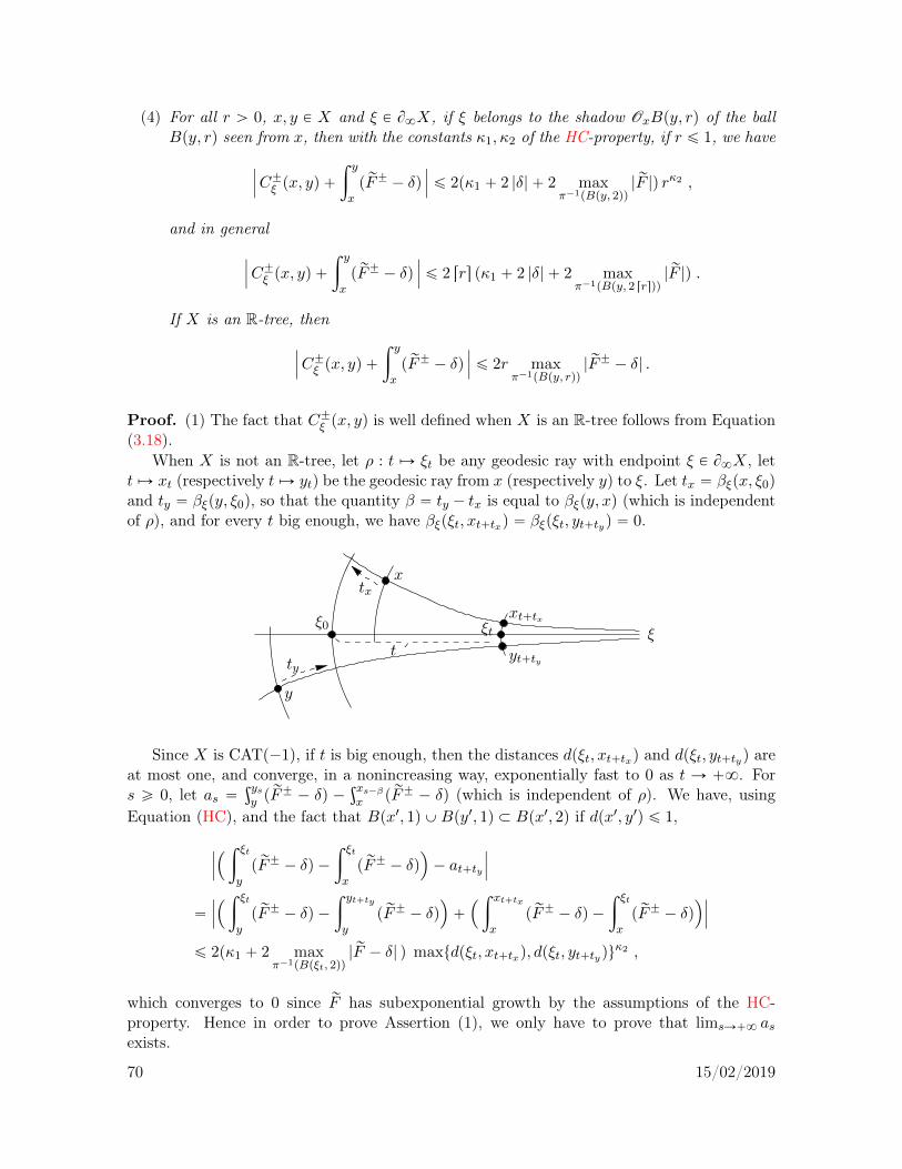
(4) For all r ą 0, x, y P X and ξ P B8X, if ξ belongs to the shadow OxBpy, rq of the ballBpy, rq seen from x, then with the constants κ1, κ2 of the HC-property, if r ď 1, we have

ˇ

ˇ

ˇC˘ξ px, yq `

ż y

xp rF˘ ´ δq

ˇ

ˇ

ˇď 2pκ1 ` 2 |δ| ` 2 max

π´1pBpy, 2qq| rF |q rκ2 ,

and in general

ˇ

ˇ

ˇC˘ξ px, yq `

ż y

xp rF˘ ´ δq

ˇ

ˇ

ˇď 2 rrs pκ1 ` 2 |δ| ` 2 max

π´1pBpy, 2 rrsqq| rF |q .

If X is an R-tree, thenˇ

ˇ

ˇC˘ξ px, yq `

ż y

xp rF˘ ´ δq

ˇ

ˇ

ˇď 2r max

π´1pBpy, rqq| rF˘ ´ δ| .

Proof. (1) The fact that C˘ξ px, yq is well defined when X is an R-tree follows from Equation(3.18).

When X is not an R-tree, let ρ : t ÞÑ ξt be any geodesic ray with endpoint ξ P B8X, lett ÞÑ xt (respectively t ÞÑ yt) be the geodesic ray from x (respectively y) to ξ. Let tx “ βξpx, ξ0q

and ty “ βξpy, ξ0q, so that the quantity β “ ty ´ tx is equal to βξpy, xq (which is independentof ρ), and for every t big enough, we have βξpξt, xt`txq “ βξpξt, yt`tyq “ 0.

ξξ0

y

tx

xt`tx

yt`ty

x

ξtt

ty

Since X is CATp´1q, if t is big enough, then the distances dpξt, xt`txq and dpξt, yt`tyq areat most one, and converge, in a nonincreasing way, exponentially fast to 0 as t Ñ `8. Fors ě 0, let as “

şysy p

rF˘ ´ δq ´şxs´βx p rF˘ ´ δq (which is independent of ρ). We have, using

Equation (HC), and the fact that Bpx1, 1q YBpy1, 1q Ă Bpx1, 2q if dpx1, y1q ď 1,

ˇ

ˇ

ˇ

´

ż ξt

yp rF˘ ´ δq ´

ż ξt

xp rF˘ ´ δq

¯

´ at`ty

ˇ

ˇ

ˇ

“

ˇ

ˇ

ˇ

´

ż ξt

yp rF˘ ´ δq ´

ż yt`ty

yp rF˘ ´ δq

¯

`

´

ż xt`tx

xp rF˘ ´ δq ´

ż ξt

xp rF˘ ´ δq

¯ˇ

ˇ

ˇ

ď 2pκ1 ` 2 maxπ´1pBpξt, 2qq

| rF ´ δ| q maxtdpξt, xt`txq, dpξt, yt`tyquκ2 ,

which converges to 0 since rF has subexponential growth by the assumptions of the HC-property. Hence in order to prove Assertion (1), we only have to prove that limsÑ`8 asexists.

70 15/02/2019

For all s ě t ě |β|, we have, by the additivity of the integral along geodesics (see Equation(3.12)) and by using again Equation (HC),

|at ´ as| “ˇ

ˇ

ˇ

ż ys

yt

p rF˘ ´ δq ´

ż xs´β

xt´β

p rF˘ ´ δqˇ

ˇ

ˇ

ď pκ1 ` 2 maxπ´1pBpxt´β , 2qq

| rF ´ δ|q dpyt, xt´βqκ2 ` pκ1 ` 2 max

π´1pBpys, 2qq| rF ´ δ| q dpys, xs`βq

κ2 .

Again by the subexponential growth of rF , the above expression converges (exponentially fast,for future use) to 0 as t Ñ `8 uniformly in s, hence limsÑ`8 as exists by a Cauchy typeargument.

(2) Let pξ, x, yq P B8X ˆ X ˆ X. Assertion (2) of Proposition 3.20 follows from Equation(3.18) when X is an R-tree, since rx, ys “ rx, ps Y rp, ys where p is the closest point to y onrx, ξr. When X is not an R-tree, the first claim of Assertion (2) follows immediately from theHC-property of pX,Γ, rF˘ ´ δq, and the second claim from this HC-property and the samesubdivision argument of the geodesic segment rx, ys into rdpx, yqs subintervals of equal lengths(at most 1), as in the proof of Equation (3.17).

(3) Let pξ, x, yq, pξ1, x1, y1q P B8X ˆX ˆX. By the cocycle property (3.19), we have

|C˘ξ px, yq ´ C˘ξ1 px

1, y1q| ď |C˘ξ px, yq ´ C˘ξ1 px, yq| ` |C

˘ξ1 px, x

1q| ` |C˘ξ1 py, y1q| . (3.21)

First assume that X is an R-tree. Let K be a compact subset of X, and let

εK “ infx,yPK

e´dpx, x0q´dpx, yq ą 0 .

x

ξ1

ξp q

y

Let p, q be the points in X such that rx, ξr X ry, ξr “ rp, ξr and rx, ξr X rx, ξ1r “ rx, qs. Ifdx0pξ, ξ

1q ď εK , then by the definition of the visual distance (see Equation (2.3)) and byEquation (2.4), we have

e´dpx, qq “ dxpξ, ξ1q ď edpx, x0q dx0pξ, ξ

1q ď e´dpx, yq ď e´dpx, pq .

In particular q P rp, ξr, so that rx, ξ1r X ry, ξ1r “ rp, ξ1r. Thus by Equation (3.18), we have

|C˘ξ px, yq ´ C˘ξ1 px, yq | “ 0 .

Therefore, by Equation (3.21) and by the R-tree case of Assertion (2), if dx0pξ, ξ1q ď εK , if

x, y P K and dpx, x1q, dpy, y1q ď 1, then

|C˘ξ px, yq ´ C˘ξ1 px

1, y1q| ď dpx, x1q maxπ´1prx, x1sq

| rF˘ ´ δ| ` dpy, y1q maxπ´1pry, y1sq

| rF˘ ´ δ| .

Since rF is bounded on compact subsets of T 1X, this proves that C˘ is locally Lipschitz.

Let us now consider the case when X is general. For all distinct ξ, ξ1 P B8X, let t ÞÑ ξtand t ÞÑ ξ1t be the geodesic rays from x0 to ξ and ξ1 respectively. By the end of the proof

71 15/02/2019

of Assertion (1), for every compact subset K of X, there exist a1, a2 ą 0 such that for everyx, y P K, we have for all η P tξ, ξ1u and t ě 0,

ˇ

ˇ

ˇC˘η px, yq ´

´

ż ηt

yp rF˘ ´ δq ´

ż ηt

xp rF˘ ´ δq

¯ˇ

ˇ

ˇď a1 e

´a2t .

Let T “ ´12 ln dx0pξ, ξ

1q. If T ě 0, by the properties of CATp´1q-spaces (see Equation (3.6)for the second inequality), there exist two constants a3, a4 ą 0 such that dpξ2T , ξ

12T q ď a3 and

dpξT , ξ1T q ď a4 e

´T . Hence if dx0pξ, ξ1q ď min

1a2

4, 1(

(so that T ě 0 and dpξT , ξ1T q ď 1), wehave, using Equation (HC) for the last inequality,

|C˘ξ px, yq ´ C˘ξ1 px, yq |

ď

ˇ

ˇ

ˇ

ż ξT

yp rF˘ ´ δq ´

ż ξ1T

yp rF˘ ´ δq

ˇ

ˇ

ˇ`

ˇ

ˇ

ˇ

ż ξT

xp rF˘ ´ δq ´

ż ξ1T

xp rF˘ ´ δq

ˇ

ˇ

ˇ` 2 a1 e

´a2T

ď2 pκ1 ` 2 maxπ´1pBpξT , 2qq

| rF˘ ´ δ|q dpξT , ξ1T qκ2 ` 2 a1 e

´a2T .

By the subexponential growth of rF , there exists a5 ą 0 such that

|C˘ξ px, yq ´ C˘ξ1 px, yq | ď a5 e

´κ22T ` 2 a1 e

´a2T ď pa5 ` 2 a1q dx0pξ, ξ1qmint

κ24,a22u .

We now conclude from Equation (3.21) and Assertion (2) as in the end of the above tree casethat C˘ is locally Hölder-continuous.

(4) Let r ą 0, x, y P X and ξ P B8X be such that ξ P OxBpy, rq. Let p be the closest pointto y on rx, ξr , so that dpp, yq ď r. By Equations (3.20) and (3.19), we have

ˇ

ˇ

ˇC˘ξ px, yq `

ż y

xp rF˘ ´ δq

ˇ

ˇ

ˇ“

ˇ

ˇ

ˇC˘ξ px, yq ´ C

˘ξ px, pq ´

ż p

xp rF˘ ´ δq `

ż y

xp rF˘ ´ δq

ˇ

ˇ

ˇ

ď |C˘ξ pp, yq| `ˇ

ˇ

ˇ

ż p

xp rF˘ ´ δq ´

ż y

xp rF˘ ´ δq

ˇ

ˇ

ˇ. (3.22)

First assume that X is an R-tree. Then by Assertion (2) and by Lemma 3.12, we deducefrom Equation (3.22) that

ˇ

ˇ

ˇC˘ξ px, yq `

ż y

xp rF˘ ´ δq

ˇ

ˇ

ˇď 2 dpy, pq max

π´1pry,psq| rF˘ ´ δ| ď 2r max

π´1pBpy, rqq| rF˘ ´ δ| .

In the general case, the result then follows similarly from Equation (3.22) by using Asser-tion (2) and the HC-property if r ď 1 of Equation (3.17) in general. l

3.5 Systems of conductances on trees and generalised electricalnetworks

Let pX, λq be a locally finite metric tree without terminal vertices, letX “ |X|λ be its geometricrealisation, and let Γ be a nonelementary discrete subgroup of IsompX, λq.

Let rc : EX Ñ R be a Γ-invariant function, called a system of (logarithmic) conductancesfor Γ. We denote by c : ΓzEXÑ R the function induced by rc, which we also call a system ofconductances on ΓzX.

72 15/02/2019

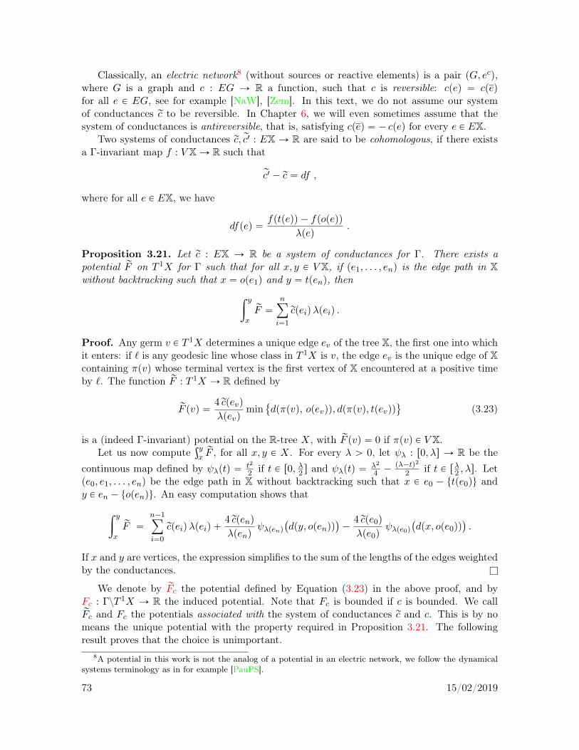
Classically, an electric network8 (without sources or reactive elements) is a pair pG, ecq,where G is a graph and c : EG Ñ R a function, such that c is reversible: cpeq “ cpeqfor all e P EG, see for example [NaW], [Zem]. In this text, we do not assume our systemof conductances rc to be reversible. In Chapter 6, we will even sometimes assume that thesystem of conductances is antireversible, that is, satisfying cpeq “ ´ cpeq for every e P EX.

Two systems of conductances rc, rc1 : EX Ñ R are said to be cohomologous, if there existsa Γ-invariant map f : V XÑ R such that

rc1 ´ rc “ df ,

where for all e P EX, we have

dfpeq “fptpeqq ´ fpopeqq

λpeq.

Proposition 3.21. Let rc : EX Ñ R be a system of conductances for Γ. There exists apotential rF on T 1X for Γ such that for all x, y P V X, if pe1, . . . , enq is the edge path in Xwithout backtracking such that x “ ope1q and y “ tpenq, then

ż y

x

rF “nÿ

i“1

rcpeiqλpeiq .

Proof. Any germ v P T 1X determines a unique edge ev of the tree X, the first one into whichit enters: if ` is any geodesic line whose class in T 1X is v, the edge ev is the unique edge of Xcontaining πpvq whose terminal vertex is the first vertex of X encountered at a positive timeby `. The function rF : T 1X Ñ R defined by

rF pvq “4rcpevq

λpevqmin

dpπpvq, opevqq, dpπpvq, tpevqq(

(3.23)

is a (indeed Γ-invariant) potential on the R-tree X, with rF pvq “ 0 if πpvq P V X.Let us now compute

şyxrF , for all x, y P X. For every λ ą 0, let ψλ : r0, λs Ñ R be the

continuous map defined by ψλptq “ t2

2 if t P r0, λ2 s and ψλptq “λ2

4 ´pλ´tq2

2 if t P rλ2 , λs. Letpe0, e1, . . . , enq be the edge path in X without backtracking such that x P e0 ´ ttpe0qu andy P en ´ topenqu. An easy computation shows that

ż y

x

rF “

n´1ÿ

i“0

rcpeiqλpeiq `4rcpenq

λpenqψλpenq

`

dpy, openqq˘

´4rcpe0q

λpe0qψλpe0q

`

dpx, ope0qq˘

.

If x and y are vertices, the expression simplifies to the sum of the lengths of the edges weightedby the conductances. l

We denote by rFc the potential defined by Equation (3.23) in the above proof, and byFc : ΓzT 1X Ñ R the induced potential. Note that Fc is bounded if c is bounded. We callrFc and Fc the potentials associated with the system of conductances rc and c. This is by nomeans the unique potential with the property required in Proposition 3.21. The followingresult proves that the choice is unimportant.

8A potential in this work is not the analog of a potential in an electric network, we follow the dynamicalsystems terminology as in for example [PauPS].

73 15/02/2019

Given a potential rF : T 1X Ñ R for Γ, let us define a map rcF : EXÑ R by

rcF : e ÞÑ rcF peq “1

λpeq

ż tpeq

opeq

rF . (3.24)

Note that rcF is Γ-invariant, hence it is a system of conductances for Γ. We denote bycF : ΓzEX Ñ R the function induced by rcF : EX Ñ R. Note that rcF`κ “ rcF ` κ for everyconstant κ P R, that rcF is bounded if rF is bounded, and that cFc “ c by the above proposition.

Proposition 3.22.

(1) Every potential (resp. bounded potential) for Γ is cohomologous to a potential (resp. boundedpotential) associated with a system of conductances for Γ.

(2) If two systems of conductances rc1 and rc are cohomologous, then their associated poten-tials rFc1 and rFc are cohomologous.

(3) If X has no vertex of degree 2, if two potentials rF ˚ and rF for Γ are cohomologous, thenthe systems of conductances rcF˚ and rcF for Γ are cohomologous.

Hence if X has no vertex of degree 2, the map rF s ÞÑ rcF s from the set of cohomologyclasses of potentials for Γ to the set of cohomology classes of systems of conductances for Γis bijective, with inverse rcs ÞÑ rFcs.

Proof. (1) Let rF be a potential for Γ, and let rF ˚ “ rFcF be the potential associated withthe system of conductances rcF . Note that if rF is bounded, so is rcF by Equation (3.24), hencerF ˚ is bounded by Equation (3.23). For all e P EX and t P s0, λpeqr , let ve, t P T 1X be thegerm of any geodesic line passing at time 0 through the point of e at distance t from opeq.Let rG : T 1X Ñ R be the map defined by rGpvq “ 0 if πpvq P V X and such that for all e P EXand t P s0, λpeqr ,

rGpve, tq “

ż t

0p rF ˚pve, sq ´ rF pve, sqq ds .

Sinceştpeqopeq

rF “ λpeq rcF peq by the construction of rcF and λpeq rcF peq “ştpeqopeq

rF ˚ by Proposition

3.21, the map rG : T 1X Ñ R is continuous. Let ` be a geodesic line. The map t ÞÑ rGpvgt`q

is obviously differentiable at time t “ 0 if πp`q R V X, with derivative rF ˚pv`q ´ rF pv`q. Byconsidering right and left derivatives of this map at t “ 0, by using the fact that

ştpeqopeqp

rF´ rF ˚q “

0 for every e P EX, and by the continuity of rF and rF ˚ at such a point, this is still true ifπp`q P V X. Hence rF ˚ and rF are cohomologous, and this proves the first claim.

(2) Assume that rc1 and rc are cohomologous systems of conductances for Γ, and let f : V XÑ Rbe a Γ-invariant function such that rc1 ´ rc “ df . Define rGpvq “ fpπpvqq if πpvq P V X. For alle P EX and t P s0, λpeqr , define

rGpve, tq “

ż t

0p rFc1pve, sq ´ rFcpve, sqq ds` fpopeqq ,

which is Γ-invariant. Its limit as t Ñ 0 is fpopeqq (independent of the edge e with givenorigin), and its limit as tÑ λpeq is, by the construction of rFc and rFc1 ,

λpeq`

rc1peq ´ rcpeq˘

` fpopeqq “ λpeq dfpeq ` fpopeqq “ fptpeqq

74 15/02/2019

(independent of the edge e with given extremity). This proves that rG is continuous. Onechecks as in Assertion (1) that rFc1 and rFc are cohomologous.

(3) In order to prove the third claim, assume that rF ˚ and rF are two cohomologous potentialsfor Γ, and let rG : T 1X Ñ R be as in the definition of cohomologous potentials, see Equation(3.16). By the continuity of rG, for all elements v and v1 in T 1X such that πpvq “ πpv1q P V X,we have rGpvq “ rGpv1q, since (by the assumption on the degrees of vertices) the two edges(possibly equal) into which v and v1 enter can be extended to geodesic lines with a commonnegative subray. Hence for every x P V X, the value fpxq “ rGpvxq for every vx P T 1X suchthat πpvxq “ x does not depend on the choice of vx. The map f : V X Ñ R thus definedis Γ-invariant. With the above notation and by Equation (3.24), we hence have, for everye P EX,

rcF˚peq ´ rcF peq “1

λpeq

ż λpeq

0

`

rF ˚pve, tq ´ rF pve, tq˘

dt “1

λpeq

ż λpeq

0

d

dtrGpve, tq dt

“1

λpeq

`

rGpvtpeqq ´ rGpvopeqq˘

“fptpeqq ´ fpopeqq

λpeq“ dfpeq .

Hence rcF˚ and rcF are cohomologous. l

Given a metric tree pX, λq, we define the critical exponent of a Γ-invariant system ofconductances rc : EX Ñ R (or of the induced system of conductances c : ΓzEX Ñ R) as thecritical exponent of pΓ, rFcq where rFc is the potential for Γ associated with rc :

δc “ δΓ, Fc .

By Proposition 3.22 (2) and Lemma 3.17 (1), this does not depend on the choice of a potentialrFc satisfying Proposition 3.21.

75 15/02/2019

76 15/02/2019

Chapter 4

Patterson-Sullivan andBowen-Margulis measures withpotential on CATp´1q spaces

Let X,x0,Γ be as in the beginning of Section 2.1,1 and let rF be a potential for Γ. From nowon, we assume that the triple pX,Γ, rF q satisfies the HC-property of Definition 3.13 and thatthe critical exponent δ “ δΓ, F˘ is finite.

In this chapter, we discuss geometrically and dynamically relevant measures on the bound-ary at infinity of X and on the space of geodesic lines GX. We extend the theory of Gibbsmeasures from the case of manifolds with pinched negative sectional curvature treated in[PauPS] 2 to CATp´1q spaces with the HC-property.

4.1 Patterson densities

A family pµ˘x qxPX of finite nonzero (positive Borel) measures on B8X, whose support is ΛΓ,is a (normalised) Patterson density for the pair pΓ, rF˘q if

γ˚µ˘x “ µ˘γx (4.1)

for all γ P Γ and x P X, and if the following Radon-Nikodym derivatives exist for all x, y P Xand satisfy for (almost) all ξ P B8X

dµ˘xdµ˘y

pξq “ e´C˘ξ px, yq . (4.2)

In particular, the measures µ˘x are in the same measure class for all x P X, and, by Proposition3.20, they depend continuously on x for the weak-star convergence of measures. Note thata Patterson density for pΓ, F˘q is also a Patterson density for pΓ, F˘ ` sq for every s P R,since the definition involves only the normalised potential rF˘´ δ. If F “ 0, we get the usualnotion of a Patterson-Sullivan density (of dimension δΓ) for the group Γ, see for instance[Pat2, Sul2, Nic, Coo, Bou, Rob2].

1That is, X is a geodesically complete proper CATp´1q space, x0 P X is a basepoint, and Γ is a nonele-mentary discrete group of isometries of X.

2See also the previous works [Led, Ham2, Cou, Moh].

77 15/02/2019

Proposition 4.1. There exists at least one Patterson density for the pair pΓ, rF˘q.

Proof. The Patterson construction (see [Pat1], [Coo]) modified as in [Led] (with a multiplica-tive rather than additive parameter s), [Moh] and [PauPS, Section 3.6] (all in the Riemannianmanifold case) gives the result, and we give a proof only for the sake of completeness.

We start by an independent lemma, generalizing [Pat2, Lem. 3.1] with a similar proof.

Lemma 4.2. Let δ1 P R. Let panqnPN and pbnqnPN be sequences of positive real numbers suchthat limnÑ`8 an “ `8 and the generalised Dirichlet series

ř

nPN bn a´sn converges if s ą δ1

and diverges if s ă δ1. Then there exists a positive nondecreasing map h on s0,`8r such that‚ for every ε ą 0, there exists r1ε ą 0 such that hpt1r1q ď t1 ε hpr1q for all t1 ą 1 and r1 ě r1ε;‚ the series

ř

nPN bn a´sn hpanq converges if and only if s ą δ1.

Proof. Let t0 “ 0, t1 “ 1 and h1 : s0, 1s Ñ r1,`8r the constant map 1. Let us define byinduction on n P N ´ t0u a positive real number tn and a continous map hn : stn´1, tns Ñr1,`8r . If tn and hn are constructed, let tn`1 P R be such that

hnptnq

t1nn

ÿ

kPN : tnăakďtn`1

bk a´δ1`1nk ě 1 ,

which exists since the generalised Dirichlet series diverges at s “ δ1 ´ 1n. For every t P

stn, tn`1s, let hn`1ptq “ hnptnq`

ttn

˘1n.Note that the sequence ptnqnPN is increasing. Let h : s0,`8r Ñ r1,`8r be the map equal

to hn on stn´1, tns for every n P N´t0u. The map h is positive, continuous and nondecreasing.For every ε ą 0, let n “ r1

ε s. Since lnhptq is continuous and piecewise affine in ln t with slopesat most 1

n on rtn,`8r, we have lnphpt1r1qq ´ lnhpr1q ď 1n ln t1 ď ε ln t1 if t1 ą 1 and r1 ě tn,

which proves the first claim on h.We have

ÿ

nPNbn a

´δ1

n hpanq “ÿ

nPN

ÿ

kPNtnăakďtn`1

bk a´δ1

k hptnq`aktn

˘1ně

ÿ

nPN1 “ `8 .

If s ą δ1, let ε “ s´δ1

2 ą 0. Since by construction hptq “ Optεq as t Ñ `8, there existsa constant C ą 0 such that hpanq ď C aεn for every n P N, and the convergence of theseries

ř

nPN bn a´sn hpanq follows from the convergence of the generalised Dirichlet seriesř

nPN bn a´δ´εn , thus proving the second claim on h. l

Now, for every z P X, recall that ∆z denotes the unit Dirac mass at z. Let h˘ : r0,`8r Ñs0,`8r be a nondecreasing map such that‚ for every ε ą 0, there exists rε ě 0 such that h˘pt ` rq ď eε th˘prq for all t ě 0 and

r ě rε;‚ if Qxpsq “

ř

γPΓ eşγx0x p rF˘´sq h˘pdpx, γx0qq, then Qxpsq diverges if and only if the

inequality s ď δ holds.If pΓ, F˘q is of divergence type, we may take h˘ “ 1 constant. Otherwise, the existence ofh˘ follows from Lemma 4.2.3 For all s ą δ and x P X, define the measure

µ˘x, s “1

Qx0psq

ÿ

γPΓ

eşγx0x p rF˘´sq h˘pdpx, γx0qq ∆γx0

3Let pγnqnPN be an enumeration of the elements of Γ, take an “ edpx,γnx0q and bn “ eşγnx0x

rF˘ , and thentake h˘ “ h ˝ exp for h the map given by Lemma 4.2.

78 15/02/2019

on X. By compactness for the weak-star topology of the space of probability measures onthe compact space X Y B8X, there exists a sequence pskqkPN in sδ,`8r converging to δ suchthat the sequence of probability measures pµx0, skqkPN weak-star converges to a probabilitymeasure µx0 on X Y B8X. Since Qx0

pδq “ `8 and since the support of µx0, s in X Y B8Xis equal to Γx0 “ Γx0 Y ΛΓ, the support of µx0 is contained in ΛΓ, hence equal to ΛΓ byminimality. The Radom-Nikodym derivative dµ˘x, s

dµ˘x0, sis the map with support Γx0 defined by

dµ˘x, s

dµ˘x0, spγx0q “ e

şγx0x p rF˘´sq´

şγx0x0

p rF˘´sq h˘pdpx, γx0qq

h˘pdpx0, γx0qq. (4.3)

For every k P N, if dpx0, γx0q is large enough, then

h˘pdpx, γx0qq ď h˘pdpx, x0q ` dpx0, γx0qq ď epsk´δqdpx, x0q h˘pdpx0, γx0qq .

By the HC-property, as k Ñ `8, the right hand side of Equation (4.3) with s “ sk convergesto e´C

˘ξ px, x0q uniformly in ξ P ΛΓ as γx0 tends to ξ. Therefore, as k Ñ `8, the measures µ˘x, sk

converge to a (finite nonzero) measure µ˘x with support ΛΓ such that dµ˘xdµ˘x0

pξq “ e´C˘ξ px, x0q.

Let γ P Γ. Since γ˚∆z “ ∆γ z for every z P X, a change of variable in the summation definingµ˘x, s gives that γ˚µ˘x, s “ µ˘γx, s. By the continuity of pushforwards of measures, we haveγ˚µ

˘x “ µ˘γx. By the cocycle properties of the Radom-Nikodym derivatives and of the Gibbs

cocycles, the family pµ˘x qxPX is a (normalised) Patterson density for pΓ, rF˘q. l

We refer to Theorem 4.6 for the uniqueness up to scalar multiple of the Patterson densitywhen pΓ, F˘q is of divergence type and to [DaSU, Coro. 17.1.8] for a characterisation of theuniqueness when F “ 0.

The Patterson densities satisfy the following extension of the classical Sullivan shadowlemma (which gives the claim when rF is constant, see [Rob2]), and its corollaries.

If µ is a positive Borel measure on a metric space pX, dq, the triple pX, d, µq is called ametric measure space. A metric measure space pX, d, µq is doubling if there exists c ě 1 suchthat, for all x P X and r ą 0,

µpBpx, 2 rqq ď c µpBpx, rqq .

Note that, up to changing c, the number 2 may be replaced by any constant larger than1. See for instance [Hei] for more details on doubling metric measure spaces. We refer forinstance to [DaSU, Ex. 17.4.12] for examples of nondoubling Patterson(-Sullivan) measures,and to [DaSU, Prop. 17.4.4] for a characterisation of the doubling property of the Pattersonmeasures when Γ is geometrically finite and F “ 0.

A family ppX,µi, diqqiPI of positive Borel measures µi and distances di on a common setX is called uniformly doubling if there exists c ě 1 such that, for all i P I, x P X and r ą 0,

µipBdipx, 2 rqq ď c µipBdipx, rqq .

Lemma 4.3. Let pµ˘x qxPX be a Patterson density for the pair pΓ, F˘q, and let K be a compactsubset of X.

(1) [Mohsen’s shadow lemma] If R is large enough, there exists C ą 0 such that for allγ P Γ and x, y P K,

1

Ceşγyx p

rF˘´δq ď µ˘x`

OxBpγy,Rq˘

ď C eşγyx p

rF˘´δq .

79 15/02/2019

(2) For all x, y P X, there exists c ą 0 such that for every n P Nÿ

γPΓ : n´1ădpx, γyqďn

eşγyx p

rF˘´δq ď c .

(3) For every R ą 0 large enough, there exists C “ CpRq ą 0 such that for all γ P Γ andall x, y P K

µ˘x pOxBpγy, 5Rqq ď C µ˘x pOxBpγy,Rqq .

(4) If Γ is convex-cocompact, then the metric measure space pΛΓ, dx, µ˘x q is doubling for

every x inX, and the family of metric measure spaces ppΛΓ, dx, µ˘x qqxPCΛΓ is uniformly

doubling.

Proof. For the first assertion, the proof of [PauPS, Lem. 3.10] (see also [Cou, Lem. 4] with themultiplicative rather than additive convention, as well as [Moh]) extends, using Proposition3.20 (2), (4) instead of [PauPS, Lem. 3.4 (i), (ii)]. The second assertion is similar to the one of[PauPS, Lem. 3.11 (i)], and the proof of the last two assertions is similar to the one of [PauPS,Prop. 3.12], using Lemma 2.2 instead of [HeP4, Lem. 2.1]. The uniformity in the last assertionfollows from the compactness of ΓzCΛΓ and the invariance and continuity properties of thePatterson densities. l

4.2 Gibbs measures

We fix from now on two Patterson densities pµ˘x qxPX for the pairs pΓ, F˘q.The Gibbs measure rmF on GX (associated with this ordered pair of Patterson densities)

is the measure rmF on GX given by the density

drmF p`q “ eC´`´

px0, `p0qq`C```px0, `p0qq

dµ´x0p`´q dµ

`x0p``q dt (4.4)

in Hopf’s parametrisation with respect to the basepoint x0. The Gibbs measure rmF is in-dependent of x0 by Equations (4.2) and (3.19). Hence it is invariant under the action of Γby Equations (4.1) and (3.19). It is invariant under the geodesic flow by construction (andthe invariance of Lebesgue’s measure under translation). Thus,4 it defines a measure mF onΓzGX which is invariant under the quotient geodesic flow, called the Gibbs measure on ΓzGX(associated with the above ordered pair of Patterson densities). If F “ 0 and the Pattersondensities pµ`x qxPX and pµ´x qxPX coincide, the Gibbs measure mF coincides with the Bowen-Margulis measure mBM on ΓzGX (associated with this Patterson density), see for instance[Rob2].

Remark 4.4. (i) The (positive Borel) measure given by the density

dλpξ, ηq “ eC´ξ px0, pq`C

`η px0, pq dµ´x0

pξq dµ`x0pηq (4.5)

on B28X is (by the same arguments as above) independent of p P sξ, ηr , locally finite and

invariant under the diagonal action of Γ on B28X. It is a geodesic current for the action of

4See for instance [PauPS, §2.6] for the precautions in order to push locally forward an invariant measureby an orbifold covering, since the group Γ does not necessarily act freely on GX.

80 15/02/2019

Γ on the Gromov-hyperbolic proper metric space X in the sense of Ruelle-Sullivan-Bonahon,see for instance [Bon] and references therein.

(ii) Another parametrisation of GX also depending on the choice of the basepoint x0 inX, is the map from GX to B2

8X ˆ R sending ` to p`´, ``, sq where now s “ β`´pπp`q, x0q

(one may also use the different time parameter s “ β``px0, πp`qq). For every pη, ξq in B28X,

let pη, ξ be the closest point to x0 on the geodesic line between η and ξ.

x0s

`p0q

tp`´, ```´ ``

For every ` P GX, with p`´, ``, tq the original Hopf parametrisation, since

s´ t “ β`´p`p0q, x0q ´ β`´p`p0q, p`´,``q “ β`´pp`´,`` , x0q

depends only on `´ and ``, the measures dµ´x0p`´q dµ

`x0p``q dt and dµ´x0

p`´q dµ`x0p``q ds are

equal. Hence using the above variant of Hopf’s parametrisation does not change the Gibbsmeasures rmF and mF .

(iii) Since the time reversal map ι is p`´, ``, tq ÞÑ p``, `´,´tq in Hopf’s coordinates, themeasure ι˚ rmF is the Gibbs measure on GX associated with the switched pair of Pattersondensities

`

pµ`x qxPX , pµ´x qxPX

˘

(and similarly on ΓzGX).

The Gibbs property of Gibbs measures Let us now indicate why the terminology ofGibbs measures is indeed appropriate. This explanation will be the aim of Proposition 4.5,but we need to give some definitions first.

For all ` P GX and r ą 0, T, T 1 ě 0, the dynamical (or Bowen) ball around ` is

Bp`;T, T 1, rq “

`1 P GX : suptPr´T 1,T s

dp`ptq, `1ptqq ă r(

.

Bowen balls have the following invariance properties: for all s P r´T 1, T s and γ P Γ,

gsBp`;T, T 1, rq “ Bpgs`;T ´ s, T 1 ` s, rq and γBp`;T, T 1, rq “ Bpγ`;T, T 1, rq .

The following inclusion properties of the dynamical balls are immediate: If r ď s, T ě S,T 1 ě S1, then Bp`;T, T 1, rq is contained in Bp`;S, S1, sq. The dynamical balls are almostindependent on r : For all r1 ě r ą 0, there exists Tr, r1 ě 0 such that for all ` P GX andT, T 1 ě 0, the dynamical ball Bp`;T ` Tr, r1 , T 1 ` Tr, r1 , r1q is contained in Bp`;T, T 1, rq. Thisfollows from the properties of long geodesic segments with endpoints at bounded distance ina CATp´1q-space.

For every ` P ΓzGX, let us define Bp`;T, T 1, r1q as the image by the canonical projectionGX Ñ ΓzGX of Bpr`;T, T 1, r1q, for any preimage r` of ` in GX.

A pgtqtPR-invariant measure m1 on ΓzGX satisfies the Gibbs property for the potential Fwith constant cpF q P R if for every compact subset K of ΓzGX, there exist r ą 0 and cK, r ě 1such that for all large enough T, T 1 ě 0, for every ` P ΓzGX with g´T

1

`, gT ` P K, we have

1

cK, rď

m1pBp`;T, T 1, rqq

eşT´T 1 pF pvgt`q´cpF qq dt

ď cK, r .

81 15/02/2019

We refer to [PauPS, Sect. 3.8] for equivalent variations on the definition of the Gibbsproperty mF . The following result shows that the Gibbs measures indeed satisfy the Gibbsproperty on the dynamical balls of the geodesic flow, thereby justifying the name. We refer forinstance to [PauPS, Sect. 3.8] for the explanations of the connection with symbolic dynamicsmentioned in the introduction. See also Proposition 4.14 for a discussion of the case when Xis a simplicial tree – here the correspondence with symbolic dynamics is particularly clear.

Proposition 4.5. Let mF be the Gibbs measure on ΓzGX associated with a pair of Pattersondensities pµ˘x qxPX for pΓ, rF˘q. Then mF satisfies the Gibbs property for the potential F , withconstant cpF q “ δ.

Proof. The proof is similar to the one of [PauPS, Prop. 3.16] (in which the key Lemma 3.17uses only CATp´1q arguments), up to replacing [PauPS, Lem. 3.4 (1)] by Proposition 3.20(2). l

The Hopf-Tsuji-Sullivan-Roblin theorem The basic ergodic properties of the Gibbsmeasures are summarised in the following result. The case when rF is constant is due to[Rob2], see also [BuM, §6].

Theorem 4.6 (Hopf-Tsuji-Sullivan-Roblin). The following conditions are equivalent

(i) The pair pΓ, F q is of divergence type.

(ii)´ The conical limit set of Γ has positive measure with respect to µ´x for some (equivalentlyevery) x P X.

(ii)` The conical limit set of Γ has positive measure with respect to µ`x for some (equivalentlyevery) x P X.

(iii) The dynamical system pB28X,Γ, pµ

´x bµ

`x q|B2

8Xq is ergodic for some (equivalently every)

x P X.

(iv) The dynamical system pB28X,Γ, pµ

´x b µ`x q|B2

8Xq is conservative for some (equivalently

every) x P X.

(v) The dynamical system pΓzGX, pgtqtPR,mF q is ergodic.

(vi) The dynamical system pΓzGX, pgtqtPR,mF q is conservative.

If one of the above conditions is satisfied, then

(1) the measures µ˘x have no atoms for any x P X,

(2) the diagonal of B8X ˆ B8X has measure 0 for µ´x b µ`x ,

(3) the Patterson densities pµ˘x qxPX are unique up to a scalar multiple, and

(4) for all x, y P X, as nÑ `8,

maxγPΓ, n´1ădpx,γyqďn

eşγyx

rF˘ “ opeδ nq .

82 15/02/2019

Proof. The proof5 of the equivalence claim is similar to the one of [PauPS, Theo. 5.4], using‚ Proposition 3.20 (2), (4) instead of [PauPS, Lem. 3.4],‚ the HC-property instead of [PauPS, Lem. 3.2],‚ Lemma 3.17 (2) instead of [PauPS, Lem. 3.3 (ii)],‚ Lemma 4.3 (2) instead of [PauPS, Coro. 3.11 (i)],‚ Lemma 4.3 (3) instead of [PauPS, Coro. 3.12 (i)],‚ Remark 4.4 (ii) instead of [PauPS, Rem. (ii), §3.7],‚ Lemma 4.3 (1) instead of [PauPS, Lem. 3.10].

Claims (1) and (4) are proved as in [PauPS, Prop. 5.13], Claim (2) is proved as in [PauPS,Prop. 5.5 (c)], and Claim (3) is proved as in [PauPS, Coro. 5.12]. l

The following corollary follows immediately from Poincaré’s recurrence theorem and theHopf-Tsuji-Sullivan-Roblin theorem, see [PauPS, Coro. 5.15, Theo. 5.4 (ii’)-(iii’)] for the ar-guments written for the manifold case, which extend.

Corollary 4.7. If mF is finite, then

(1) the pair pΓ, F˘q is of divergence type,

(2) the Patterson densities pµ˘x qxPX are unique up to a multiplicative constant and the Gibbsmeasure mF is uniquely defined up to a multiplicative constant.

(3) the Gibbs measure mF gives full measure to the image Ωc of

rΩc “ t` P GX : `˘ P ΛcΓu

in ΓzGX, and

(4) the geodesic flow is ergodic for mF . l

On the finiteness of Gibbs measures As the finiteness of the Gibbs measures will be astanding hypothesis in many of the following results, we now give criteria for Gibbs measures tobe finite. Recall6 that the discrete nonelementary group of isometries Γ of X is geometricallyfinite if every element of ΛΓ is either a conical limit point or a bounded parabolic limit pointof Γ.

Theorem 4.8. Assume that Γ is a geometrically finite discrete group of isometries of X.

(1) If pΓ, F˘q is of divergence type, then the Gibbs measure mF is finite if and only if forevery bounded parabolic limit point p of Γ, the series

ÿ

αPΓp

dpx, αyq eşαyx p rF˘´δq

converges, where Γp is the stabiliser of p in Γ.

(2) If we have δΓp, F˘pă δ, for every bounded parabolic limit point p of Γ with stabiliser Γp

in Γ and with F˘p : ΓpzX Ñ R the map induced by rF˘, then pΓ, F q is of divergencetype. In particular, mF is finite.

5The proof occupies about 16 pages in [PauPS], hence we cannot reproduce it in this book.6See Section 2.1.

83 15/02/2019

When X is a manifold, this result is due to [DaOP, Theo. B] for the case F “ 0, and to[Cou] and [PauPS, Theo. 8.3, 8.4] for the general case of Hölder-continuous potentials. WhenF “ 0 but on much more general assumptions on X with optimal generality, this result is dueto [DaSU, Theo. 17.1.2].

Proof. The proof is similar to the manifold case in [PauPS], which follows closely the proofof [DaOP]. Note that the convergence or divergence of the above series does not depend onthe choice of the sign ˘.

Let ParΓ be the set of bounded parabolic limit points of Γ. By [Rob2, Lem. 1.9]7, thereexists a Γ-equivariant family pHpqpPParΓ

of pairwise disjoint closed horoballs, with Hp centredat p, such that the quotient

M0 “ Γz`

C ΛΓ´ď

pPParΓ

Hp

˘

is compact. Using Proposition 3.20, Theorem 4.6 and Equation (3.17) instead of respectively[PauPS, Lem. 3.4, Coro. 5.10,Lem. 3.2], the HC-property, the proofs of [PauPS, Theo. 8.3,8.4] then extend to our situation. l

Recall that the length spectrum of Γ on X is the additive subgroup of R generated by thetranslation lengths in X of the elements of Γ.

Recall that a continuous-time one-parameter group phtqtPR of homeomorphisms of a topo-logical space Z is topologically mixing if for all nonempty open subsets U, V of Z, there existst0 P R such that for every t ě t0, we have U X htV ‰ H.

We have the following result, due to [Bab1, Theo. 1] in the manifold case, with develop-ments by [Rob2] when rF “ 0, and by [PauPS, Theo. 8.1] for manifolds with pinched negativecurvature.

Theorem 4.9. If the Gibbs measure is finite, then the following assertions are equivalent :

(1) the geodesic flow of ΓzX is mixing for the Gibbs measure,

(2) the geodesic flow of ΓzX is topologically mixing on its nonwandering set, which is thequotient under Γ of the space of geodesic lines in X both of whose endpoints belong toΛΓ.

(3) the length spectrum of Γ on X is not contained in a discrete subgroup of R. l

In the manifold case, the third assertion of Theorem 4.9 is satisfied, for example, if Γ hasa parabolic element, if ΛΓ is not totally disconnected (hence if ΓzX is compact), or if X is asurface or a (rank-one) symmetric space, see for instance [Dal1, Dal2].

Error terms for the mixing property will be described in Chapter 9. The above resultholds for the continuous time geodesic flow when X is a metric tree. See Theorem 4.17 for aversion of this theorem for the discrete time geodesic flow on simplicial trees. At least whenX is an R-tree and Γ is a uniform lattice (so that ΓzX is a finite metric graph), we have astronger result under additional regularity assumptions, see Section 9.2.

7See also [Pau4] for the case of simplicial trees and [DaSU, Theo. 12.4.5] for a greater generality on X.

84 15/02/2019

Bowen-Margulis measure computations in locally symmetric spaces Assume in thissubsection that the potential rF is zero. The next result, Proposition 4.10, gathers compu-tations done in [PaP16, PaP17a] of the Bowen-Margulis measures mBM when X is a real orcomplex hyperbolic space, and Γ is a lattice. We start by giving the notation necessary inorder to state Proposition 4.10.

When X is a complete simply connected Riemannian manifold with dimension m ě 2and sectional curvature at most ´1, we endow the usual unit tangent bundle T 1X withSasaki’s Riemannian metric.8 Its Riemannian measure d volT 1X , called Liouville’s measure,disintegrates (equivariantly with respect to Γ) under the fibration π : T 1X Ñ X over theRiemannian measure d volX of X, as

d volT 1X “

ż

xPXd volT 1

xXd volXpxq ,

where d volT 1xX

is the spherical measure on the fiber T 1xX of π above x P X. In particular,

VolpT 1pΓzXqq “ VolpSm´1qVolpΓzXq .

Assume furthermore that X is a symmetric space, and that Γ is a lattice in IsompXq. Inparticular, Γ is geometrically finite and the critical exponent of the stabiliser in Γ of everybounded parabolic fixed point of Γ is strictly less than the critical exponent of Γ, see forinstance [Dal1, Dal2]. Then the Patterson density is independent of Γ and uniquely definedup to a multiplicative constant by Theorem 4.8 (2) and Lemma 4.7 (2). We take µ´x “ µ`xfor every x P Hn

C and we will denote this measure simply by µx. By homogeneity reasons, theBowen-Margulis measure of Γ on X is proportional to the Liouville measure volT 1X , and themain point of Proposition 4.10 is to compute the proportionality constant.

Let n ě 2. We endow Rn´1 with its usual Euclidean norm ¨ and its usual Lebesguemeasure λn´1. We use the upper halfspace model for the real hyperbolic spaceHn

R of dimensionn, that is, Hn

R “ tpx1, ¨ ¨ ¨ , xnq P Rn : xn ą 0u endowed with the Riemannian metric

ds2HnR“

1

x2n

pdx21 ` ¨ ¨ ¨ ` dx

2nq .

We identify Rn´1 with Rn´1 ˆ t0u in Rn, and again denote by ¨ the usual Euclidean normon Rn. The boundary at infinity of Hn

R is B8HnR “ Rn´1 Y t8u. Assuming that Γ is a lattice

in IsompHnRq, we normalise its Patterson density so that in the ball model of Hn

R with center0, the measure µ0 is the spherical measure on the space at infinity Sn´1.

Let n ě 2. We refer to [Gol] and [PaP17a, §3] for background on the complex hyperbolicn-space Hn

C. We denote by ζ ¨ ζ 1 “řn´1i“1 ζi ζ

1i the standard Hermitian product and by dζ

the standard Lebesgue measure on Cn´1. We denote by Heis2n´1 the Heisenberg group ofdimension 2n´ 1, which is the real Lie group structure on Cn´1 ˆ R with law

pζ, uqpζ 1, u1q “ pζ ` ζ 1, u` u1 ` 2 Im ζ ¨ ζ 1q .

We endow Heis2n´1 with the usual left-invariant Haar measure dλ2n´1pζ, uq “ dζ du andwith the Cygan distance9 dCyg which is the unique left-invariant distance on Heis2n´1 withdCygppζ, uq, p0, 0qq “ p|ζ|

4 ` u2q14 .

8See Section 3.1.9See [Gol, page 160]. It is called the Korányi distance by many people working in sub-Riemannian geometry,

though Korányi [Kor] does attribute it to Cygan [Cyg].

85 15/02/2019

We use the Siegel domain model of the complex hyperbolic space HnC of dimension n, nor-

malised to have maximum constant sectional curvature ´1, hence to be CATp´1q. This is themanifold Heis2n´1ˆs0,`8r endowed with the Riemannian metric given, in the horosphericalcoordinates pζ, u, tq P Cn´1 ˆ Rˆs0,`8r, by

ds2HnC“

1

4 t2`

dt2 ` pdu` 2 Im dζ ¨ ζ q2 ` 4 t dζ ¨ dζ˘

,

so that its volume form is

d volHnC pζ, u, tq “1

4 tn`1dζ du dt .

Note that the action of Heis2n´1 on HnC “ Heis2n´1ˆs0,`8r by left translations on the

first factor, preserving the second one, is isometric. We identify Heis2n´1 with Heis2n´1ˆt0uand we endow Heis2n´1ˆr0,`8r with the distance dCyg extending the Cygan distance onHeis2n´1, defined by

dCygppζ, u, tq, pζ1, u1, t1qq “

ˇ

ˇ

ˇ|ζ ´ ζ 1|2 ` |t´ t1| ` ipu´ u1 ` 2 Im ζ ¨ ζ 1q

ˇ

ˇ

ˇ

12.

The space at infinity B8HnC of Hn

C is the Alexandrov compactification Heis2n´1Yt8u, so thatthe extension at infinity of the isometric action of Heis2n´1 on Hn

C fixes 8 and is the lefttranslation on Heis2n´1. We denote by H8 “ Heis2n´1ˆr1,`8r the horoball of Hn

C centeredat 8 whose boundary contains the point p0, 0, 1q.

Assuming that Γ is a lattice in IsompHnCq, we normalise its Patterson density pµxqxPHnC as

follows. If µH8is the measure defined in Proposition 7.2 associated with the horoball H8,

thendµH8

pζ, uq “ dλ2n´1pζ, uq “ dζ du .

This is possible since µH8is invariant under the isometric action of Heis2n´1 on Hn

C, whichpreserves H8, hence is a left-invariant Haar measure on B8Hn

C ´ t8u “ Heis2n´1.As the arguments of the following result are purely computational and rather long, we

do not copy them in this book, but we refer respectively to the proofs of [PaP16, Eq. (19),Eq. (21), Prop. 10] and [PaP17a, Lem. 12 (i), (ii), (iii)]. Analogous computations can be donewhen X is the quaternionic hyperbolic n-space Hn

H.

Proposition 4.10. (1) Let Γ be a lattice in IsompHnRq, with Patterson density pµxqxPHnR

normalised as above. For all x “ px0, ¨ ¨ ¨ , xnq in HnR, ξ P B8Hn

R ´ t8u and v P T 1HnR such

that v˘ ‰ 8, we have

(i) dµxpξq “`

2xnx´ξ2

˘n´1dλn´1pξq,

(ii) using a Hopf parametrisation v ÞÑ pv´, v`, sq,

drmBMpvq “22pn´1qdλn´1pv´q dλn´1pv`q dt

v` ´ v´2pn´1q,

(iii)rmBM “ 2n´1 VolT 1HnR ,

and in particular,mBM “ 2n´1 VolpSn´1qVolpΓzHn

Rq .

86 15/02/2019

(2) Let Γ be a lattice in IsompHnCq, with Patterson density pµxqxPHnC normalised as above.

For all x “ pζ, u, tq in HnC, pξ, rq P B8Hn

C ´ t8u and v P T1Hn

C such that v˘ ‰ 8, we have

(i) dµxpξ, rq “tn

dCygpx, pξ, rqq4ndξ dr ;

(ii) using a Hopf parametrisation v ÞÑ pv´, v`, sq,

drmBMpvq “dλ2n´1pv´q dλ2n´1pv`q ds

dCygpv´, v`q4n;

(iii)

rmBM “1

22n´2volT 1HnC ,

and in particular

mBM “πn

22n´3 pn´ 1q!VolpΓzHn

Cq . l

On the cohomological invariance of Gibbs measures We end this Section by an ele-mentary remark on the independence of Gibbs measures upon replacement of the potential Fby a cohomologous one.

Remark 4.11. Let rF ˚ : T 1X Ñ R be a potential for Γ cohomologous to rF and satisfyingthe HC-property. As usual, let rF ˚` “ rF ˚ and rF ˚´ “ rF ˚ ˝ ι, and let F ˚ : ΓzT 1X Ñ Rbe the induced map. Let rG : T 1X Ñ R be a continuous Γ-invariant function such that, forevery ` P GX, the map t ÞÑ rGpvgt`q is differentiable and rF ˚pv`q ´ rF pv`q “

ddt |t“0

rGpvgt`q.Furthermore assume that X is an R-tree or that G is uniformly continuous (for instanceHölder-continuous).

For all x P X and ξ P B8X, let `x, ξ be any geodesic line with footpoint `x, ξp0q “ xand positive endpoint p`x, ξq` “ ξ, and let `ξ, x be any geodesic line with `ξ, xp0q “ x andorigin p`ξ, xq´ “ ξ. Note that the value rGpv`x, ξq is independent of the choice of `x, ξ, by thecontinuity of rG, and similarly for rGpv`ξ, xq. In particular, for all γ P Γ, by the Γ-invariance ofrG, we have

rGpv`x, γ´1ξq “ rGpv`γx, ξq and rG ˝ ι pv`x, ξq “

rGpv`ξ, xq . (4.6)

Note that rF ˚´ “ rF ˚ ˝ ι and rF´ “ rF ˝ ι are cohomologous, since if rG˚ “ ´ rG ˝ ι, for every` P GX, we have

rF ˚ ˝ ιpv`q ´ rF ˝ ιpv`q “ rF ˚pvι`q ´ rF pvι`q “d

dt |t“0

rGpvgtι`q

“d

dt |t“0

rGpιvg´t`q “d

dt |t“0

rG˚pvgt`q .

As already seen in Lemma 3.17 (1) and (2), the critical exponent δΓ, F˚˘ is equal to thecritical exponent δΓ, F˘ , and independent of the choice of ˘, and we denote by δ the commonvalue in the definition of the Gibbs cocycle.

Let us prove that if C˚˘ “ C˘Γ, F˚˘

is the Gibbs cocycle associated with pΓ, F ˚˘q, thenC˚˘ and C˘ are cohomologous:

C˚`ξ px, yq ´ C`ξ px, yq “rGpv`x, ξq ´

rGpv`y, ξq , (4.7)

87 15/02/2019

and similarlyC˚´ξ px, yq ´ C´ξ px, yq “

rG˚pv`x, ξq ´rG˚pv`y, ξq . (4.8)

We only prove the first equality, the second one follows similarly, noting that rG˚ is uniformlycontinuous if rG is, since ι is isometric. For all x, y in X and ξ P B8X, let t ÞÑ ξt be a geodesicray with point at infinity ξ, let at “ dpx, ξtq, let bt “ dpy, ξtq, and for z “ x, y, let `z, ξt be anygeodesic line with footpoint z passing through ξt. Then

´

ż ξt

yp rF ˚` ´ δq ´

ż ξt

xp rF ˚` ´ δq

¯

´

´

ż ξt

yp rF` ´ δq ´

ż ξt

xp rF` ´ δq

¯

“

ż ξt

yp rF ˚` ´ rF`q ´

ż ξt

xp rF ˚` ´ rF`q

“

ż bt

0

d

dtrGpvgs`y, ξt q ds´

ż at

0

d

dtrGpvgs`x, ξt q ds

“ rGpv`x, ξt q ´rGpv`y, ξt q `

`

rGpvgbt`y, ξtq ´ rGpvgat`x, ξt q

˘

.

When t goes to `8, the first term of this series of equalities converges to C˚`ξ px, yq´C`ξ px, yq

by the definition of the Gibbs cocycle (see Section 3.4). By continuity, rGpv`y, ξt q andrGpv`x, ξt q

converge to rGpv`y, ξq and rGpv`x, ξq respectively. If X is an R-tree, then if t is large enough, wehave vgbt`y, ξt “ vgat`x, ξt , hence Equation (4.7) follows. Otherwise, by the uniform continuity

of rG, since vgbt`y, ξt and vgat`x, ξt are uniformly arbitrarily close as t tends to 0 by the CATp´1qproperty, the result also follows.

Let pµ˘x qxPX be a Patterson density for pΓ, F˘q. In order to simplify the notation, letrG` “ rG and rG´ “ rG˚. The family of measures pµ˚˘x qxPX defined by setting, for all x P Xand ξ P B8X,

dµ˚˘x pξq “ e´ rG˘pv`x, ξ q dµ˘x pξq , (4.9)

is also a Patterson density for pΓ, F ˚˘q. Indeed, the equivariance property (4.1) for pµ˚˘x qxPXfollows from the one for pµ˘x qxPX and from Equation (4.6). The absolutely continuous property(4.2) for pµ˚˘x qxPX follows from the one for pµ˘x qxPX and Equations (4.7) and (4.8).

Assume that the Patterson density for pΓ, F ˚˘q defined by Equation (4.9) is chosen inorder to construct the Gibbs measure rmF˚ for pΓ, F ˚q on GX. Then using‚ Hopf’s parametrisation with respect to the base point x0 and Equation (4.4) with F

replaced by F ˚ for the first equality,‚ Equations (4.7), (4.8), (4.9) and cancellations for the second equality,‚ the definition of rG˚ “ ´ rG ˝ ι and again Equation (4.4) for the third equality,‚ Equation (4.6) and the fact that we may choose ``´, `p0q “ ` and ``p0q, `` “ ` for the last

equality,we have

drmF˚p`q “ eC˚´`´

px0, `p0qq`C˚```px0, `p0qq

dµ˚´x0p`´q dµ

˚`x0p``q dt

“ eC´`´

px0, `p0qq´ rG˚pv``p0q, `´q´C```

px0, `p0qq` rGpv``p0q, ``qdµ´x0

p`´q dµ`x0p``q dt

“ erG˝ιpv``p0q, `´

q´ rGpv``p0q, `´qdrmF p`q

“ erGpv`q´ rGpv`q drmF p`q ,

88 15/02/2019

hence rmF˚ “ rmF .In particular, since the Gibbs measure, when finite, is independent up to a multiplicative

constant on the choice of the Patterson densities by Corollary 4.7, we have that mF is finiteif and only if mF˚ is finite, and then

mF˚

mF˚“

mF

mF . (4.10)

4.3 Patterson densities for simplicial trees

In this Section and the following one, we specialise and modify the general framework of theprevious sections to treat simplicial trees. Recall10 that a simplicial tree X is a metric treewhose edge length map is constant equal to 1. The time 1 map of the geodesic flow pgtqtPRon the space

p

GX of all generalised geodesic lines of the geometric realisation X “ |X|1 of Xpreserves for instance its subset of generalised geodesic lines whose footpoints are at distanceat most 14 from vertices. Since both this subset and its complement have nonempty interiorin

p

GX, the geodesic flow onp

GX has no mixing or ergodic measure with full support. This iswhy we considered the discrete time geodesic flow pgtqtPZ on

p

GX in Section 2.6.

Let X be a locally finite simplicial tree without terminal vertices, and let X “ |X|1be its geometric realisation. Let Γ be a nonelementary discrete subgroup of AutpXq. LetrF : T 1X Ñ R be a potential for Γ, and let rF` “ rF , rF´ “ rF ˝ ι. Let δ “ δΓ,F˘ be the criticalexponent of pΓ, F˘q. Let C˘ : B8X ˆ X ˆ X Ñ R be the associated (normalised) Gibbscocycles. Let pµ˘x qxPX be two Patterson densities on B8X for the pairs pΓ, F˘q.

Note that only the restrictions of the cocycles C˘ to B8X ˆ V X ˆ V X are useful andthat it is often convenient and always sufficient to replace the cocycles by finite sums involv-ing a system of conductances (as defined in Section 3.5), see below. Furthermore, only therestriction pµ˘x qxPV X of the family of Patterson densities to the set of vertices of X is useful.

Example 4.12. Let X be a simplicial tree with geometric realisation X and let rc : EXÑ Rbe a system of conductances on X. For all x, y in V X and ξ P B8X, with the usual conventionon the empty sums, let

c`ξ px, yq “mÿ

i“1

rcpeiq ´nÿ

j“1

rcpfjq

and

c´ξ px, yq “mÿ

i“1

rcpeiq ´nÿ

j“1

rcpfjq ,

where, if p P V X is such that rp, ξr “ rx, ξr X ry, ξr , then pe1, e2, . . . , emq is the geodesic edgepath in X from x “ ope1q to p “ tpemq and pf1, f2, . . . , fnq is the geodesic edge path in X fromv “ opf1q to p “ tpfnq.

f1

fnξ

px e1

em

y f2

10See Section 2.6.

89 15/02/2019

With δc defined in the end of Section 3.5 and with C˘ the Gibbs cocycles for pΓ, rFcq, byEquation (3.18) and by Proposition 3.21, we have, for all ξ P B8X and x, y P V X,

C˘ξ px, yq “ ´ c˘ξ px, yq ` δc βξpx, yq ,

and Equation (4.2) gives

dµ˘x pξq “ ec˘ξ px, yq´δc βξpx, yq dµ˘y pξq .

Using the particular structure of trees, we can prove a version of the Shadow Lemma 4.3where one can take the radius R to be 0. When F “ 0, this result is due to Coornaert [Coo].

Lemma 4.13 (Mohsen’s shadow lemma for trees). Let K be a finite subset of V X. Thereexists C ą 0 such that for all γ P Γ and x, y P K with y P C ΛΓ, we have

1

Ceşγyx p

rF˘´δq ď µ˘x`

Oxtγyu˘

ď C eşγyx p

rF˘´δq .

Proof. The structure of the proof is the same one as for Lemma 4.3 (1) (that is, the oneof [PauPS, Lem. 3.10]) with differences towards the end of the argument. Let us prove thatthere exists C “ CK ą 0 such that for all γ P Γ and x, y P K with γy P C ΛΓ, we have

1

Cď µ˘γy

`

Oxtγyu˘

ď C . (4.11)

Assuming this, let us prove Lemma 4.13. By Equation (4.2), we have

µ˘x`

Oxtγyu˘

“

ż

ξPOxtγyue´C

˘ξ px, γyq dµ˘γypξq .

Note that C˘ξ px, γyq `şγyx p

rF˘ ´ δq “ 0 if ξ P Oxtγyu (that is, if γy P rx, ξr ), by Equation(3.20). Hence

µ˘x pOxtγyuq “ eşγyx p

rF˘´δq µ˘γypOxtγyuq ,

and Lemma 4.13 follows from Equation (4.11).

Let us now prove the upper bound in Equation (4.11). Fix z0 P K, and let

C 1 “ supx, yPK, ξPB8X

|C˘ξ px, yq| ,

which is finite by Proposition 3.20 (2), since K is compact and rF˘ continuous. Then, usingEquation (4.1) for the equality and Equation (4.2) for the last inequality, we have

µ˘γypOxtγyuq ď µ˘γy “ µ

˘y ď eC

1

µ˘z0 ,

and the upper bound holds if C ě eC1

µ˘z0.

Finally, in order to prove the lower bound in Equation (4.11), we assume for a contradictionthat there exist sequences pxiqiPN, pyiqiPN in K with yi P C ΛΓ and pγiqiPN in Γ such thatµ˘γiyipOxitγiyiuq converges to 0 as i Ñ `8. Up to extracting a subsequence, since K isfinite, we may assume that the sequences pxiqiPN and pyiqiPN are constant, say with value xand y respectively. Since y P C ΛΓ, as every point in C ΛΓ belongs to at least one geodesic

90 15/02/2019

line between two limit points of Γ, the geodesic segment from x to γiy may be extended to ageodesic ray from x to a limit point of Γ. Since the support of µ˘z is equal to ΛΓ for any z P X,we have µ˘γiypOxtγiyuq ą 0 for all i P N. Thus, up to taking a subsequence, we can assumethat γ´1

i x converges to ξ P ΛΓ (otherwise by discreteness, we may extract a subsequence sothat pγiqiPN is constant, and µ˘γiypOxtγiyuq cannot converge to 0).

Since X is a tree, there exists a positive integer N such that Oγ´1i xtyu “ Oγ´1

N xtyu “ Oξtyu

for all i ě N . As above, Oξtyu meets ΛΓ since y P C ΛΓ, thus µ˘y pOξtyuq ą 0. But for everyi ě N ,

µ˘y`

Oξtyu˘

“ pγ´1i q˚µ

˘γiy

`

Oγ´1i xtyu

˘

“ µ˘γiy`

Oxtγiyu˘

tends to 0 as iÑ `8, a contradiction. l

Let rφµ˘ : V XÑ r0,`8r be the total mass functions of the Patterson densities :

rφµ˘pxq “ µ˘x

for every x P V X. These maps are Γ-invariant by Equation (4.1), hence they induce mapsφµ˘ : ΓzV X Ñ r0,`8r. In the case of real hyperbolic manifolds and vanishing potentials,the total mass functions have important links to the spectrum of the hyperbolic Laplacian(see [Sul1]). See also [CoP3, CoP5] for the case of simplicial trees and the discrete Laplacian,Section 6.1 for a generalisation of the result of Coornaert and Papadopoulos, and for instance[BerK] for developments in the field of quantum graphs.

4.4 Gibbs measures for metric and simplicial trees

Let pX, λq be a locally finite metric tree without terminal vertices, letX “ |X|λ be its geometricrealisation, and let x0 P V X be a basepoint. Let Γ be a nonelementary discrete subgroup ofAutpX, λq. Let rF : T 1X Ñ R be a potential for Γ, and let rF` “ rF , rF´ “ rF ˝ι. Let δ “ δΓ,F˘

be the critical exponent of pΓ, F˘q, assumed to be finite. Let pµ˘x qxPV X be two (normalised)Patterson densities on B8X for the pairs pΓ, F˘q.

The Gibbs measure rmF on the space of discrete geodesic lines GX of X, invariant underΓ and under the discrete time geodesic flow pgtqtPZ of

p

GX, is defined analogously with thecontinuous time case, using the discrete Hopf parametrisation for any basepoint x0 P V X, by

drmF p`q “ eC´`´

px0, `p0qq`C```px0, `p0qq

dµ´x0p`´q dµ

`x0p``q dt , (4.12)

where now dt is the counting measure on Z. We again denote by mF the measure that rmF

induces on ΓzGX.In this Section, we prove that the Gibbs measures in the case of trees satisfy a Gibbs

property even closer to the one in symbolic dynamics, we give an analytic finiteness criterionof the Gibbs measures for metric trees, and we recall the ergodic properties of tree lattices.

As recalled in the introduction, Gibbs measures were first introduced in statistical me-chanics and consequently in symbolic dynamics, see for example [Bowe2], [ParP], [PauPS].In order to motivate the terminology used in this book, we recall the definition of a Gibbsmeasure for the full two-sided shift on a finite alphabet:11 Let Σn “ t1, 2, . . . , nuZ be theproduct space of sequences x “ pxnqnPZ indexed by Z in the finite discrete set t1, 2, . . . , nu,

11See Section 5.1 for the appropriate definition when the alphabet is countable.

91 15/02/2019

and let σ : Σn Ñ Σn be the shift map defined by σppxnqnPZq “ pxn`1qnPZ. A shift-invariantprobability measure µ on Σn satisfies the Gibbs property for an energy function φ : Σn Ñ R if

1

Cďµpra´m´ , a´m´`1, . . . , am`´1, am`sq

e´P pm´`m``1q`

řm`k“´m´

φpσkxqď C

for some constants C ě 1 and P P R (called the pressure) and for all m˘ in N with m´ ď m`and x in the cylinder ra´m´ , a´m´`1, . . . , am`´1, am`s that consists of those x P Σn for whichxk “ ak for all k P r´m´,m`s.

Let x´, x` P V X and let x0 P V XX rx´, x`s. Let us define the tree cylinder of the triplepx´, x0, x`q by

rx´, x0, x`s “ t` P GX : `˘ P Ox0tx˘u, `p0q “ x0u .

These cylinders are close to the dynamical balls that have been introduced in Section 4.2, andthe parallel with the symbolic case is obvious, as this cylinder is the set of geodesic lines whichcoincides on r´m´,m`s, where m˘ “ dpx0, x˘q, with a given geodesic line passing throughx˘ and through x0 at time t “ 0. The Gibbs measure rmF on the space of discrete geodesiclines GX satisfies a variant of the Gibbs property which is even closer to the one in symbolicdynamics than the general case described in Proposition 4.5.

Proposition 4.14 (Gibbs property). Let K be a finite subset of V X X C ΛΓ. There existsC 1 ą 1 such that for all x˘ P ΓK and x0 P V XX rx´, x`s,

1

C 1ď

rmF prx´, x0, x`sq

e´δ dpx´, x`q`

şx`x´

rFď C 1 .

Proof. The result is immediate if dpx´, x`q is bounded, since the above denominator andnumerator take only finitely many values by the finiteness of K and by Γ-invariance, and thenumerator is nonzero since x˘ P C ΛΓ, hence the tree cylinder rx´, x0, x`s meets the supportof rmF . We may hence assume that dpx´, x`q ě 2. Using the invariance of rmF under thediscrete time geodesic flow, we may thus assume that x0 ‰ x´, x`. By Γ-invariance, we mayassume that x´ varies in the finite set K, and that x0 is at distance 1 from x´, hence alsovaries in a finite set.

Using the discrete Hopf parametrisation with respect to the vertex x0, we have, by Lemma4.13, for some C ą 0,

rmF prx´, x0, x`sq “ µ´x0pOx0tx´uqµ

`x0pOx0tx`uq

ď C2 eşx´x0p rF˝ι´δq

eşx`x0p rF´δq

“ C2eşx`x´p rF´δq

.

This proves the upper bound in Proposition 4.14 with C 1 “ C2 and the lower bound followssimilarly. l

Next, we give a finiteness criterion of the Gibbs measure for metric trees in terms of thetotal mass functions of the Patterson densities, extending the case when Γ is torsion free andrF “ 0, due to [CoP4, Theo. 1.1].

Proposition 4.15. Let pX, λ,Γ, rF q be as in the beginning of this Section.

(1) If pX, λq is simplicial and ¨ 2 is the Hilbert norm of L2pΓzV X, volΓzzXq, we have12

mF ď φµ`2 φµ´2 .12The maps φµ˘ are defined at the end of Section 4.3.

92 15/02/2019

(2) In general, with ¨ 2 the Hilbert norm of L2pΓzEX,TvolpΓzzX,λqq, we have13

mF ď φµ` ˝ o2 φµ´ ˝ o2 .

Proof. (1) The simplicial assumption on pX, λq means that all edges have length 1. Thespace ΓzGX is the disjoint union of the subsets t` P ΓzGX : πp`q “ `p0q “ rxsu as theorbit rxs “ Γx of x P V X ranges over ΓzV X. By Equation (4.12), using the discrete Hopfdecomposition with respect to the basepoint x, we have

dprmF qˇ

ˇ

t`PGX : `p0q“xup`q “ dµ´x p`´q dµ

`x p``q .

Let ∆rxs be the unit Dirac mass at rxs. By ramified covering arguments, we hence have thefollowing equality of measures on the discrete set ΓzV X:

π˚mF “ÿ

rxsPΓzV X

1

|Γx|

`

µ´x ˆ µ`x

˘`

tp`´, ``q P B28X : x P s`´, ``ru

˘

∆rxs . (4.13)

Thus, using the Cauchy-Schwarz inequality and by the definition of the measure volΓzzX,

mF “ π˚mF ďÿ

rxsPΓzV X

1

|Γx|µ´x ˆ µ

`x “ xφµ´ , φµ`y2

ď φµ´2φµ`2 .

This proves Assertion (1) of Proposition 4.15.

(2) The argument is similar to the previous one. Since the singletons in R have zero Lebesguemeasure, the space ΓzGX is, up to a measure zero subset for mF , the disjoint union forres P ΓzEX of the sets Ares consisting of the elements ` P ΓzGX such that `p0q belongs to theinterior of the edge res and the orientations of ` and e coincide on e. We fix a representativee of each res P ΓzEX. For every t P r0, λpeqs, let et be the point of e at distance t from opeq.By Equation (4.4), using Hopf’s decomposition with respect to the basepoint opeq in Ares, wehave as above

mF “ÿ

resPΓzEX

1

|Γe|

ż

`´PBeX

ż

``PBeX

ż λpeq

0

eC´`´

popeq, etq`C```popeq, etq

dµ´opeqp`´q dµ`

opeqp``q dt .

Since `´, opeq, et, `` are in this order on the geodesic line ` with `´ P BeX and `` P BeX, wehave C´`´popeq, etq ` C```popeq, etq “ 0 by Equation (3.20). Hence, by the definition of themeasure TvolpΓzzX,λq,14

mF “ÿ

resPΓzEX

λpeq

|Γe|µ´opeqpBeXq µ

`

opeqpBeXq

ďÿ

resPΓzEX

λpeq

|Γe|µ´opeq µ

`

opeq “ xφµ´ ˝ o, φµ` ˝ oy2

ď φµ´ ˝ o2 φµ` ˝ o2 ,

13Recall that o : ΓzEXÑ ΓzV X is the initial vertex map, see Section 2.6.14See Section 2.6.

93 15/02/2019

which finishes the proof. l

Let us give some corollaries of this proposition in the case of simplicial trees. It followsfrom Assertion (1) of Proposition 4.15 that if the L2-norms of the total mass of the Pattersondensities are finite, then the Gibbs measure mF is finite. Taking rF “ 0 and pµ`x qxPV X “

pµ´x qxPV X, so that the Gibbs measure mF is the Bowen-Margulis measure mBM, it followsfrom this proposition that

mBM ď φµ˘22ď VolpΓzzXq sup

xPV Xµ˘x

2 . (4.14)

In particular, if Γ is a (tree) lattice15 of X and if the total mass of the Patterson density isbounded, then the Bowen-Margulis measure mBM is finite.

The following statement summarises the basic ergodic properties of the lattices of pX, λqwhen F “ 0.

Proposition 4.16. Let pX, λq be a metric or simplicial tree, with geometric realisation X.Assume that pX, λq is uniform and that Γ is a lattice in AutpX, λq. Then

(1) Γ is of divergence type, and its critical exponent δΓ is the Hausdorff dimension of anyvisual distance dx on B8X “ ΛΓ;

(2) the Patterson density pµxqxPX coincides, up to a scalar multiple, with the family ofHausdorff measures pµHaus

x qxPX of dimension δΓ of the visual distances pB8X, dxq; inparticular, it is AutpX, λq-equivariant: for all γ P AutpX, λq and x P X, we have γ˚µx “µγx;

(3) the Bowen-Margulis measure rmBM of Γ on GX is AutpX, λq-invariant, and the Bowen-Margulis measure mBM of Γ on ΓzGX is finite.

Proof. Let Γ1 be any uniform lattice of pX, λq, which exists since the metric tree pX, λq isuniform. It is well-known (see for instance [Bou]) that the critical exponent δΓ1 of Γ1 is finiteand equal to the Hausdorff dimension of any visual distance pB8X, dxq, and that the familypµHausx qxPV X of Hausdorff measures of the visual distances pB8X, dxq is a Patterson density

for any discrete nonelementary subgroup of AutpX, λq with critical exponent equal to δΓ1 .By [BuM, Coro. 6.5(2)], the lattice Γ in AutpX, λq is of divergence type and δΓ “ δΓ1 . By

the uniqueness property of the Patterson densities when Γ is of divergence type (see Theorem4.6 (3)), the family pµxqxPV X coincides, up to a scalar multiple, with pµHaus

x qxPV X .As the graph Γ1zX is compact, the total mass function of the Hausdorff measures of the

visual distances is bounded, hence so is pµxqxPV X . By Proposition 4.15, since Γ is a treelattice of pX, λq, hence of X, this implies that the Bowen-Margulis measure mBM of Γ is finite.l

Note that as in [DaOP], when pX, λq (or its minimal nonempty Γ-invariant subtree) is notassumed to be uniform, there are examples of Γ that are lattices (or are geometrically finite)whose Bowen-Margulis measure mBM is infinite, see Section 15.5 for more details.

Assume till the end of this Section that pX, λq is simplicial, that is, that λ ” 1. Let usnow discuss the mixing properties of the discrete time geodesic flow on ΓzGX for the Gibbsmeasure mF .

15See Section 2.6.

94 15/02/2019

Let LΓ be the length spectrum of Γ, which is, in the present simplicial case, the subgroupof Z generated by the translation lengths in X of the elements of Γ.

Recall that x0 P V X is a fixed basepoint. Let VevenX “ tx P V X : dpx, x0q “ 0 mod 2u bethe set of vertices of X at an even distance from the basepoint x0, and let VoddX “ V X´VevenX.Let GevenX (respectively

p

Geven X) be the subset of GX (respectivelyp

GX) that consists of thegeodesic lines (respectively generalised geodesic lines) in X whose origin is in VevenX.

Recall16 that a discrete time one-parameter group phnqnPZ of homeomorphisms of a topo-logical space Z is topologically mixing if for all nonempty open subsets U, V of Z, there existsn0 P N such that for all n ě n0, we have U X hnpV q ‰ H.

Recall that given a measured space pZ,mq, with m nonzero and finite, endowed with a dis-crete time one-parameter group phnqnPZ of measure-preserving transformations, the measurem is mixing under phnqnPZ if for all f, g P L2pZ,mq, we have

limnÑ`8

ż

Zf g ˝ hn dm “

1

m

ż

Zf dm

ż

Zg dm ,

or equivalently if for every g P L2pZ,mq, the functions g ˝ hn weakly converge in the Hilbertspace L2pZ,mq to the constant function 1

m

ş

Z g dm as nÑ `8.

Theorem 4.17. Assume that the smallest nonempty Γ-invariant simplicial subtree of X isuniform, without vertices of degree 2, and that mF is finite. Then the following assertions areequivalent:• the length spectrum of Γ satisfies LΓ “ Z;• the discrete time geodesic flow on ΓzGX is topologically mixing on its nonwandering set;• the quotient graph ΓzX is not bipartite;• the Gibbs measure mF is mixing under the discrete time geodesic flow pgtqtPZ on ΓzGX.Otherwise LΓ “ 2Z, and the square of the discrete time geodesic flow pg2tqtPZ is topologicallymixing on the nonwandering subset of ΓzGevenX and the restriction of the Gibbs measure mF

to ΓzGevenX is mixing under pg2tqtPZ.

Proof. The nonwandering set of pgtqtPZ on ΓzGX is Γzt` P GX : `˘ P ΛΓu, and thenonwandering set of pg2tqtPZ on ΓzGevenX is

Ωeven “ Γzt` P GevenX : `˘ P ΛΓu .

Since the translation axis of any loxodromic element of Γ is contained in the convex hull ofthe limit set, we may hence assume that the geometric realisation of X is equal to C ΛΓ.

Lemma 4.18. If X is a locally finite tree without vertices of degree 2, if Γ is a nonelemen-tary discrete sugbroup of AutpXq such that X is tree-minimal (that is, does not contain aΓ-invariant proper nonempty subtree), then the length spectrum LΓ of Γ is equal either to Zor to 2Z, and equal to 2Z if and only if the quotient graph ΓzX is bipartite.

Proof. This lemma is essentially due to [GaL]. By for instance [Pau1, Lem. 4.3], sinceX is tree-minimal, every geodesic segment (and in particular any two consecutive edges) iscontained in the translation axis of a loxodromic element of Γ. Hence if x and y are thetwo endpoints of any edge e of X, since they have degree at least 3, there exist at least twoloxodromic elements α and β of Γ such that the translation axes Axα and Axβ contain x and

16See above Theorem 4.9 for the continuous-time version

95 15/02/2019

y respectively, but do not meet the interior of the edge e, so that dpx, yq “ dpAxα,Axβq. Inparticular Axα and Axβ are disjoint, which implies by for instance [Pau1, Prop. 1.6] that thetranslation lengths of α, β and αβ satisfy

λpαβq “ λpαq ` λpβq ` 2 dpAxα,Axβq .

Hence 2 “ 2 dpx, yq “ λpαβq ´ λpαq ´ λpβq P LΓ. Therefore 2Z Ă LΓ Ă Z, and either LΓ “ Zor LΓ “ 2Z.

Note that for all vertices x, y, z in a simplicial tree, if dpx, yq and dpy, zq are both even orboth odd, then

dpx, zq “ dpx, yq ` dpy, zq ´ 2 dpy, rx, zsq “ 0 mod 2 . (4.15)

Note that for all x P V X and γ P Γ, we have

dpx, γxq “ λpγq mod 2 . (4.16)

Indeed, if γ is loxodromic, then dpx, γxq “ λpγq ` 2 dpx,Axγq and otherwise, dpx, γxq “2 dpx,Fixpγqq where Fixpγq is the set of fixed points of the elliptic element γ. For future use,this proves that the following assertions are equivalent :

p1q LΓ Ă 2Zp2q @ x P X, @ γ P Γ, dpx, γxq P 2Z . (4.17)

Assume that LΓ “ 2Z. Then VevenX (hence VoddX) is Γ-invariant, since for all x P VevenX,the distance dpx, γxq is even by Equation (4.16), and dpγx, γx0q “ dpx, x0q is even, so thatdpγx, x0q is even by Equation (4.15). Since no edge of X has both endpoints in VevenX, thisproves that ΓzX is bipartite, with partition of its set of vertices pΓzVevenXq \ pΓzVoddXq.

Assume conversely that ΓzX is bipartite. The set VevenX, which is the lift of one of thetwo elements of the partition of its vertices by the canonical projection V X Ñ ΓzV X, isΓ-invariant. By Equation (4.16), this proves that LΓ Ă 2Z, hence that LΓ “ 2Z. l

The equivalence of the first, second and fourth claims in the statement of Theorem 4.17follows from a discrete time version with potential of [Rob2, Theo. 3.1] or a discrete timeversion of [Bab1, Theo. 1] (which can be extended to CATp´1q spaces by the remark in[Bab1, page 70]). It can also be recovered from the following arguments when LΓ “ 2Z, andwe prefer to concentrate on this case, since it requires a lot of modifications and is stated withalmost no proof in [BrP2, Prop. 3.3], and only when rF “ 0.

Assume from now on that LΓ “ 2Z. Since VevenX is Γ-invariant as seen above, and sincedp`p0q, g2s`p0qq “ 2|s| is even for all ` P GX and s P Z, it follows from the definition ofGevenX “ t` P GX : πp`q P VevenXu and from Equation (4.15) that GevenX is invariantunder the even discrete time geodesic flow pg2sqsPZ and under Γ. Note that the discrete Hopfparametrisation of GX gives a homeomorphism from GevenX to

pξ, η, tq P B28Xˆ Z : t “ dpx0, sξ, ηr q mod 2

(

.

The restriction of the Gibbs measure rmF to GevenX, that we will again denote by rmF , disin-tegrates by the projection on the first factor B2

8X ˆ Z Ñ B28X over the geodesic current pmF

where, for every pξ, ηq P B28X and (any) x P sξ, ηr,

dpmF pξ, ηq “ eC´ξ px0, xq`C

`η px0, xqdµ´x0

pξq dµ`x0pηq , (4.18)

96 15/02/2019

with conditional measure on the fiber over pξ, ηq the counting measure on the discrete settt P Z : t “ dpx0, sξ, ηr q mod 2u. Since mF is finite and invariant under the discretetime geodesic flow, it is conservative by Poincaré’s recurrence theorem. Hence the measurequasi-preserving action of Γ on the measured space pB2

8X, pmF q is ergodic by (the discrete timeversion of) Theorem 4.6.

Since the distance between two points in a horosphere of a simplicial tree is even, and againby Equation (4.15), every horosphere of X is either entirely contained in VevenX or entirelycontained in VoddX. For every ` P GevenX, its strong stable/unstable leaf

W˘p`q “ t`1 P GX : limtÑ˘8

dp`ptq, `1ptqq “ 0u

is contained in GevenX, since the image by the footpoint projection of a strong stable/instableleaf is a horosphere (see Equation (2.14)). Thus GevenX is saturated by the partition intostrong stable/instable leaves of GX.

We now follow rather closely the arguments of [Bab1, Theo. 1] in order to prove the lastclaims of Theorem 4.17, the main point being that the geodesic current pmF is a quasi-productmeasure.

The following lemmas are particular cases of respectively Lemma 1 and Fact page 64of [Bab1], valid for general finite measure preserving dynamical systems, applied, with thenotation of loc. cit, to pTtqtPA “ pg2tqtPZ.

Lemma 4.19. Let f P L2pΓzGevenX,mF q be such thatş

f dmF “ 0. If there exists an increas-ing sequence ptnqnPN in Z such that f ˝ g2tn does not converge to 0 for the weak topology onL2pΓzGevenX,mF q, then there exist an increasing sequence psnqnPN in Z and a nonconstant17

element f˚ P L2pΓzGevenX,mF q such that f ˝ g2sn and f ˝ g´2sn both converge to f˚ for theweak topology on L2pΓzGevenX,mF q. l

Lemma 4.20. If pfnqnPN is a sequence in L2pΓzGevenX,mF q weakly converging to f˚ inL2pΓzGevenX,mF q, then there exists a subsequence pfnkqkPN such that the Cesàro averages

1N2

řN2´1k“0 fnk converge pointwise almost everywhere to f˚ as N Ñ `8. l

Recall that the support of mF is the nonwandering set Ωeven. Assume for a contradictionthat the restriction ofmF to ΓzGevenX is not mixing under the even discrete time geodesic flow.Then there exists a continuous function f with compact support on Ωeven such that

ş

f dmF “

0 and pf ˝ g2nqnPN does not weakly converge to 0 in L2pΓzGevenX,mF q. By Lemmas 4.19 and4.20, there exist a nonconstant element f˚ P L2pΓzGevenX,mF q and increasing sequencespn˘k qkPN in N such that 1

N2

řN2´1k“0 f ˝ g˘2n˘k pointwise almost everywhere converges to f˚ as

N Ñ `8.Let rf˚ “ f˚ ˝ peven, where peven : GevenX Ñ ΓzGevenX is the canonical projection, be the

lift of f˚ to GevenX. Since the conditional measures for the disintegration of rmF over pmF arecounting measures on countable sets, there exists a full pmF -measure subset E0 of B2

8X suchthat, for every ` P GevenX with p`´, ``q P E0, the above convergences hold after lifting toGevenX at the points g2n` for all n P Z.

For every ` P GevenX, the subgroup A` of 2Z given by the periods of the map 2n ÞÑ rf˚pg2n`qonly depends on p`´, ``q. Thus, we have a measurable map from E0 into the (discrete) set

17Recall that an element of L2pZ,mq is nonconstant if any representative function is not almost everywhere

constant.

97 15/02/2019

of subgroups of 2Z, which is Γ-invariant, hence is constant pmF -almost everywhere by theergodicity of pmF under Γ.

Assume for a contradiction that this almost everywhere constant subgroup is 2Z, that is,that the values of rf˚ almost everywhere do not depend on the time parameter in the discreteHopf parametrisation of GevenX. Then rf˚ defines a Γ-invariant measurable function on B2

8X.Again by ergodicity, this function is almost everywhere constant, contradicting the fact thatf˚ is not almost everywhere constant.

Hence there exist a full pmF -measure subset E1 of E0 and κ P N´t0, 1u such that A` “ 2κZfor every ` P GevenX with p`´, ``q P E1. Let us finally prove that LΓ is contained in 2κZ,which contradicts the original assumption that LΓ “ 2Z.

Let rf˘ “ lim supNÑ`81N2

řN2

k“0 f ˝ g˘2n˘k ˝ peven, so that the set

E “ tpξ, ηq P E1 : @ ` P GevenX, if `´ “ ξ and `` “ η, then rf`p`q “ rf´p`q “ rf˚p`qu

has full pmF -measure. By the hyperbolicity of the geodesic flow (see Equation (2.10)) and theuniform continuity of f , the map rf` is constant along any strong stable leaf of GevenX andrf´ is constant along any strong unstable leaf. Let

E´ “ tξ P ΛΓ : pξ, η1q P E for µ`x0-almost every η1 P ΛΓu

andE` “ tη P ΛΓ : pξ1, ηq P E for µ´x0

-almost every ξ1 P ΛΓu .

Since pmF is in the same measure class as the product measure µ´x0b µ`x0

(see Equation(4.18)), and by Fubini’s theorem, we have µ´x0

p cE´q “ 0 and µ`x0p cE`q “ 0, and the set

E´ ˆ E` has full pmF -measure.Let γ be a loxodromic element of Γ, and let x be any vertex of X on the translation axis of

γ. Since dpx, γxq is even (see Equation (4.17)), the midpoint y of the geodesic segment rx, γxsis a vertex of X. Since x and y have degree at least 3, there exist ξx and ξy in B8X whoseclosest points on the translation axis of γ are respectively x and y. Note that ξx, ξy P ΛΓ asX “ C ΛΓ. Since y and x are the closest points to γ` and γ´ on the geodesic line sξx, ξyr, wehave18 vξx, γ`, ξy, γ´w “ dpx, yq.

x

y

γx

γ´ ξx

η

η1

γ`ξ1

ξ

`1p0q

ξy`2p0q

`3p0q

`4p0q`0p0q

Since EXpE´ˆE`q has full pmF -measure, there exists pξ, ηq P EXpE´ˆE`q arbitrarilyclose to pγ´, ξxq. Since the set

tpξ1, η1q P B28Γ : pξ, η1q, pξ1, ηq, pξ1, η1q P Eu

18See Section 2.6 for the definition of the crossratio of an ordered quadruple of pairwise distinct points inB8X.

98 15/02/2019

has full pmF -measure, there exists such a pξ1, η1q arbitrarily close to pγ`, ξyq. Let `0 P GevenXbe such that `0´ “ ξ and `0` “ η. Let `1 P W`p`0q be such that `1´ “ ξ1. Let `2 P W´p`1q besuch that `2` “ η1. Let `3 P W`p`2q be such that `3´ “ ξ. Finally, let `4 P W´p`3q be suchthat `4` “ η. Then `4 “ g2s`0 for some s P Z with 2|s| “ dp`0p0q, `4p0qq.

By the definition of E and since rf` (resp. rf´) is constant along the strong stable (resp. un-stable) leaves, we have

rf˚p`0q “ rf`p`0q “ rf`p`1q “ rf´p`1q “ rf´p`2q “ rf`p`2q “ rf`p`3q

“ rf´p`3q “ rf´p`4q “ rf˚p`4q “ rf˚pg2 s`0q .

Hence 2 |s| is a period in A`0 , thus is contained in 2κZ.If t ą 0 is large enough, we have

`0ptq “ `1ptq, `1p´tq “ `2p´tq, `2ptq “ `3ptq, `3p´tq “ `4p´tq ,

which respectively tend to η, ξ1, η1, ξ as tÑ `8. Since the crossratio is locally constant andby its properties, in particular its definition in Equation (2.21), we have

`pγq “ dpx, γxq “ 2 dpx, yq “ 2 vξx, γ`, ξy, γ´w “ 2 vη, ξ1, η1, ξw

“ limtÑ`8

dp`0ptq, `3p´tqq ´ dp`3p´tq, `2ptqq ` dp`2ptq, `1p´tqq ´ dp`1p´tq, `0ptqq

“ limtÑ`8

dp`0ptq, `3p´tqq ´ dp`1p´tq, `1ptqq “ limtÑ`8

dp`0ptq, `4p´tqq ´ 2 t

“ dp`0p0q, `4p0qq “ 2 |s| P 2κZ .

Thus LΓ Ă 2κZ, which contradicts the fact that LΓ “ 2Z. l

By Proposition 4.16, the general assumptions of Theorem 4.17 are satisfied if X is uniform,without vertices of degree 2, Γ is a lattice of X and rF “ 0. Thus, if we assume furthermorethat ΓzX is not bipartite, then the Bowen-Margulis measure mBM of Γ is mixing under thediscrete time geodesic flow on ΓzGX.

99 15/02/2019

100 15/02/2019

Chapter 5

Symbolic dynamics of geodesic flowson trees

In this Chapter, we give a coding of the discrete time geodesic flow on the nonwandering setsof quotients of locally finite simplicial trees X without terminal vertices by nonelementarydiscrete subgroups of AutpXq by a subshift of finite type on a countable alphabet. Similarlywe give a coding of the continuous time geodesic flow on the nonwandering sets of quotients oflocally finite metric trees pX, λq without terminal vertices by nonelementary discrete subgroupsof AutpX, λq by suspensions of such subshifts. These codings are used in Section 5.4 to provethe variational principle in both contexts, and in Sections 9.2 and 9.3 to obtain rates of mixingof the flows.

5.1 Two-sided topological Markov shifts

In this short and independent Section, that will be used in Sections 5.2, 5.3, 5.4, 9.2 and 9.3,we recall some definitions concerning symbolic dynamics on countable alphabets.1

A (two-sided) topological Markov shift2 is a topological dynamical system pΣ, σq con-structed from a countable discrete alphabet A and a transition matrix A “ pAi, jqi, jPA P

t0, 1uAˆA , where Σ is the closed subset of the topological product space A Z defined by

Σ “

x “ pxnqnPZ P A Z : @ n P Z, Axn,xn`1 “ 1u ,

and σ : Σ Ñ Σ is the (two-sided) shift defined by

pσpxqqn “ xn`1

for all x P Σ and n P Z. Note that to be given pA , Aq is equivalent to be given an orientedgraph with countable set of vertices A (and set of oriented edges a subset of A ˆ A ) andwith incidence matrix A such that Ai, j “ 1 if there is an oriented edge from the vertex i tothe vertex j and Ai, j “ 0 otherwise.

1See for instance [Kit, Sar2].2Note that the terminology could be misleading, a topological Markov shift comes a prori without a measure,

and many probability measures invariant under the shift do not satisfy the Markov chain property that theprobability to pass from one state to another depends only on the previous state, not of all past states.

101 15/02/2019

For all p ď q in Z, a finite sequence panqpďnďq P A tp,...,qu is admissible (or A-admissiblewhen we need to make A precise) if Aan, an`1 “ 1 for all n P tp, . . . , q ´ 1u. A topologicalMarkov shift is transitive if for all x, y P A , there exists an admissible finite sequence panqpďnďqwith ap “ x and aq “ y. This is equivalent to requiring the dynamical system pΣ, σq to betopologically transitive: for all nonempty open subsets U, V in Σ, there exists n P Z such thatU X σnpV q ‰ H.

Note that the product space A Z is not locally compact when A is infinite. When thematrix A has only finitely many nonzero entries on each line and each colum, then pΣ, σq isalso called a subshift of finite type (on a countable alphabet). The topological space Σ is thenlocally compact: By diagonal extraction, for all p ď q in Z and ap, ap`1, . . . , aq´1, aq in A ,every cylinder

rap, ap`1, . . . , aq´1, aqs “

pxnqnPZ P Σ : @ n P tp, . . . , qu, xn “ an(

is a compact open subset of Σ.Given a continuous map Fsymb : Σ Ñ R and a constant cFsymb

P R, we say that a measureP on Σ, invariant under the shift σ, satisfies the Gibbs property3 with Gibbs constant cFsymb

for the potential Fsymb if for every finite subset E of the alphabet A , there exists CE ě 1such that for all p ď q in Z and for every x “ pxnqnPZ P Σ such that xp, xq P E, we have

1

CEď

Pprxp, xp`1, . . . , xq´1, xqsq

e´cFsymb

pq´p`1q`řqn“p Fsymbpσnxq

ď CE . (5.1)

Two continuous maps Fsymb, F1symb : Σ Ñ R are cohomologous if there exists a continuous

map G : Σ Ñ R such thatF 1symb ´ Fsymb “ G ˝ σ ´G .

5.2 Coding discrete time geodesic flows on simplicial trees

Let X be a locally finite simplicial tree without terminal vertices, with X “ |X|1 its geometricrealisation. Let Γ be a nonelementary discrete subgroup of AutpXq, and let rF : T 1X Ñ R bea potential for Γ.

In this Section, we give a coding of the discrete time geodesic flow pgtqtPZ on the nonwan-dering subset of ΓzGX by a locally compact transitive (two-sided) topological Markov shift.This explicit construction will be useful later on in order to study the variational principle(see Section 5.4) and rates of mixing (see Section 9.2).

The main technical aspect of this construction, building on [BrP2, §6], is to allow the casewhen Γ has torsion. When Γ is torsion free and ΓX is finite, the construction is well-known,we refer for instance to [CoP6] for a more general setting when the potential is 0. In orderto consider for instance nonuniform tree lattices, it is important to allow torsion in Γ. Ourdirect approach also avoids the assumption that the discrete subgroup Γ is full, that is, equalto the subgroup consisting of the elements g P AutpXq such that p ˝ g “ p where p : XÑ ΓzXis the canonical projection, as in [Kwo] (building on [BuM, 7.3]).

Let X1 be the minimal nonempty Γ-invariant simplicial subtree of X, whose geometricrealisation is C ΛΓ. Since we are only interested in the support of the Gibbs measures,

3Note that some references have a stronger notion of Gibbs measure (see for instance [Sar1]), with theconstant C independent of E.

102 15/02/2019

we will only code the geodesic flow on the nonwandering subset ΓzX1 of ΓzGX. The sameconstruction works with the full space ΓzGX, but the resulting Markov shift is then notnecessarily transitive.

Let pY, G˚q “ ΓzzX1 be the quotient graph of groups of X1 by Γ (see for instance Example2.10), and let p : X1 Ñ Y “ ΓzX1 be the canonical projection. We denote by r1s “ H thetrivial double coset in any double coset set HzGH of a group G by a subgroup H.

We consider the alphabet A consisting of the triples pe´, h, e`q where‚ e˘ P EY satisfy tpe´q “ ope`q and‚ h P ρe´pGe´qzGope`qρ e`pGe`q satisfy h ‰ r1s if e

` “ e´.

This set is countable (and finite if and only if the quotient graph ΓzX1 is finite), we endowit with the discrete topology. We consider the (two-sided) topological Markov shift withalphabet A and transition matrix Ape´, h, e`q, pe1´, h1, e1`q “ 1 if e` “ e1´ and 0 otherwise.Note that this matrix A “ pAi,jqi,jPA has only finitely many nonzero entries on each line andeach column, since X1 is locally finite and Γ has finite vertex stabilisers in X1. We considerthe subspace

Σ “

pe´i , hi, e`i qiPZ P A Z : @ i P Z, e`i´1 “ e´i

(

of the product space A Z, and the shift σ : Σ Ñ Σ defined by pσpxqqi “ xi`1 for all pxiqiPZ inΣ and i in Z. As seen above, Σ is locally compact.

Let us now construct a natural coding map Θ from ΓzGX1 to Σ, by slightly modifying theconstruction of [BrP2, §6].

Ąei`1

geiĆtpeiq

rei

γi`1 p ei

fi fi`1

γi

g ei`1

ei`1

`

in X1in pY, G˚q “ ΓzzX1

hi`1p`q P Gtpeiq

For every discrete geodesic line ` P GX1, for every i P Z, let fi “ fip`q be the edge ofX1 whose geometric realisation is `pri, i ` 1sq with origin fpiq and endpoint fpi ` 1q, and letei “ ppfiq, which is an edge in Y. Let us use the notation of Example 2.10: we fix lifts reand rv of every edge e and vertex v of Y in X1 such that re “ re, and elements ge P Γ suchthat ge Ątpeq “ tpreq. Since ppreiq “ ei “ ppfiq, there exists γi “ γip`q P Γ, well defined up tomultiplication on the left by an element of Gei “ Γ

rei , such that γifi “ rei for all i P Z.We define e´i`1p`q “ ei, e`i`1p`q “ ei`1, and

hi`1p`q “ g ´1e´i`1p`q

γip`q γi`1p`q´1 g

e`i`1p`q. (5.2)

Since for every edge e of Y the structural monomorphism

ρe : Ge “ Γre ÝÑ Gtpeq “ Γ

Ątpeq

103 15/02/2019

is the map g ÞÑ g´1e gge, the double coset of hip`q in ρe´i p`q

pGe´i p`qqzGope`i p`qq

ρe`i p`q

pGe`i p`qq

does not depend on the choice of the γi’s, and we again denote it by hip`q.

The next result shows that, assuming only that Γ is discrete and nonelementary, the time-one discrete geodesic flow g1 on its nonwandering subset of ΓzGX is topologically conjugateto a locally compact transitive (two-sided) topological Markov shift.

Theorem 5.1. With X1 “ C ΛΓ, the map Θ : ΓzGX1 Ñ Σ defined by

Γ` ÞÑ pe´i p`q, hip`q, e`i p`qqiPZ

is a homeomorphism which conjugates the time-one discrete geodesic flow g1 and the shift σ,that is, the following diagram commutes

ΓzGX1 g1

ÝÝÝÝÑ ΓzGX1

Θ

§

§

đ

§

§

đΘ

Σσ

ÝÝÝÝÑ Σ ,

and the topological Markov shift pΣ, σq is locally compact and transitive.Furthermore, if we endow ΓzGX1 with the quotient distance of

dp`, `1q “ e´ sup

nPN : `|r´n,ns “ `1|r´n,ns

(

on GX1 and Σ with the distance

dpx, x1q “ e´ sup

nPN : @ i P t´n,...,nu, xi “ x1i

(

,

then Θ is a bilipschitz homeomorphism.Finally, if X1 is a uniform tree without vertices of degree at most 2, if the Gibbs measure

mF of Γ is finite, and if the length spectrum LΓ of Γ is equal to Z, then the topological Markovshift pΣ, σq is topologically mixing.

Note that when Y is finite (or equivalently when Γ is cocompact), the alphabet A is finite(hence pΣ, σq is a standard subshift of finite type). When furthermore the vertex groups ofpY, G˚q are trivial (or equivalently when Γ acts freely, and in particular is a finitely generatedfree group), this result is well-known, but it is new if the vertex groups are not trivial. Comparewith the construction of [CoP6], whose techniques might be applied since Γ is word-hyperbolicif Y is finite, up to replacing Gromov’s (continuous time) geodesic flow of Γ by the (discretetime) geodesic flow on GX1, thus avoiding the suspension part (see also the end of op. cit. whenΓ is a free group).

Proof. For all ` P GX1 and γ P Γ, we can take γipγ`q “ γip`qγ´1, and since ppγfiq “ ppfiq, we

have e˘i pγ`q “ e˘i p`q and hipγ`q “ hip`q, hence the map Θ is well defined. By construction,the map Θ is equivariant for the actions of g1 on ΓzGX1 and σ.

With the distances indicated in the statement of Theorem 5.1, if `, `1 P GX1 satisfy`|r´n, ns “ `1

|r´n, ns for some n P N, then we have e˘i p`q “ e˘i p`1q for ´n ď i ď n ´ 1,

and we may take γip`q “ γip`1q for ´n ď i ď n´ 1, so that hip`q “ hip`

1q for ´n ď i ď n´ 1.Therefore, we have

dpΘpΓ`q,ΘpΓ`1q q ď e dpΓ`,Γ`1q ,

104 15/02/2019

and Θ is Lipschitz (hence continuous).

Let us construct an inverse Ψ : Σ Ñ ΓzGX1 of Θ, by a more general construction that willbe useful later on. Let I be a nonempty interval of consecutive integers in Z, either finite orequal to Z (the definition of the inverse of Θ only requires the second case I “ Z). For alle´, e` P EY such that tpe´q “ ope`q, we fix once and for all a representative of every doublecoset in ρe´pGe´qzGope`qρ e`pGe`q, and we will denote this double coset by its representative.

Let w “ pe´i , hi, e`i qiPI be a sequence indexed by I in the alphabet A such that for all

i P I such that i ´ 1 P I, we have e`i´1 “ e´i (when I is finite, this means that w is an A-admissible sequence in A , and when I “ Z, this means that w P Σ). In particular, the elementhi P Gope`i q

“ ΓČope`i q

is the chosen representative of its double coset ρe´i pGe´i q hi ρ e`ipGe`i

q.

For every i P I, note that

ophi g´1

e`i

Ăe`i q “ op g ´1

e`i

Ăe`i q “Čope`i q “

Ćtpe´i q “ tp g ´1e´i

Ăe´i q .

But hi g ´1

e`i

Ăe`i is not the opposite edge of the edge g ´1e´i

Ăe´i , since the double coset of hi is

not the trivial one r1s when e`i “ e´i , hence hi does not fix g´1e´i

Ăe´i . Therefore the length 2

edge path (see the picture below)

p g ´1e´i

Ăe´i , hi g´1

e`i

Ăe`i q

is geodesic.

e´i “ e`i´1 e`i`1e`i “ e´i`1

g ´1e´i

Ăe´i

hi

hi`1

Čope`i q

Y

X

fi´1 fi

αi´1

αi

fi`1

p

g ´1

e`i

Ăe`i

g ´1e`i

Ăe`i

g ´1

e`ige`i

Let us construct by induction a geodesic segment rw in X1 (which will be a discrete geodesicline if I “ Z), well defined up to the action of Γ, as follows.

We fix i0 P I (for instance i0 “ 0 if I “ Z or i0 “ min I if I is finite), and αi0 P Γ. Let usdefine

fi0 “ fi0pwq “ αi0 g´1e`i0

Ăe`i0 .

Let us then define

αi0´1 “ αi0´1pwq “ αi0 g´1

e`i0ge`i0

h ´1i0

and fi0´1 “ fi0´1pwq “ αi0´1 g´1

e´i0

Ăe´i0 .

105 15/02/2019

We have αi0´1 hi0 g´1

e`i0

Ăe`i0 “ fi0 and pfi0´1, fi0q is a geodesic edge path of length 2 (as the

image by αi0´1 of such a path).Let i ´ 1, i1 P I be such that i1 ď i0 ď i ´ 1. Assume by increasing induction on i and

decreasing induction on i1 that a geodesic edge path pfi1´1 “ fi1´1pwq, . . . , fi´1 “ fi´1pwqq inX1 and a sequence pαi1´1 “ αi1´1pwq, . . . , αi´1 “ αi´1pwqq in Γ have been constructed suchthat

fj “ αj g´1

e`j

Ăe`j and αj “ αj´1 hj g´1

e`jge`j

for every j P N such that i1 ´ 1 ď j ď i´ 1, with besides j ě i1 for the equality on the right.If i does not belong to I, we stop the construction on the right hand side at i ´ 1. If on

the contrary i P I, let us define (see the above picture)

αi “ αi´1 hi g´1

e`ige`i

and fi “ fipwq “ αi g´1

e`i

Ăe`i .

Thenpfi´1, fiq “

`

αi´1 g´1

e´i

Ăe´i , αi´1 hi g´1

e`i

Ăe`i˘

,

is a geodesic edge path of length 2 (as the image by αi´1 of such a path). As an edge pathis geodesic if and only if it has no back-and-forth, pfi1 , . . . , fiq is a geodesic edge path in X1.Thus the construction holds at rank i on the right.

If i1´ 1 does not belong to I, we stop the construction on the left side at i1. Otherwise weproceed as for the construction of αi0´1 and fi0´1 in order to construct αi1´2 and fi1´2 withthe required properties.

If I “ rp, qs X Z with p ď q in Z, let I 1 “ rp ´ 1, qs X Z. If I “ Z, let I 1 “ Z. We havethus constructed a geodesic edge path

pfiqiPI 1 “ pfipwqqiPI 1 (5.3)

in X1. We denote by rw its parametrisation by R if I “ Z and by rp´ 1, q` 1s if I “ rp, qsXZ,in such a way that rwpiq “ opfiq for all i P I. In particular, fi “ rwpri, i ` 1sq for all i P I 1.When I “ rp, qs X Z, we consider rw as a generalised discrete geodesic line, by extending it toa constant on s ´ 8, p´ 1s and on rq ` 1,`8r .

The orbit Γ rw of rw does not depend on the choice of αi0 , since replacing αi0 by α1i0 replacesfi by α1i0α

´1i0fi for all i P I 1, hence replaces rw by α1i0α

´1i0

rw. This also implies that Γ rw doesnot depend on the choice of i0 P I.

Assume from now on that I “ Z, and define Ψ : Σ Ñ ΓzGX1 by

Ψpwq “ Γ rw .

Let w “ pe´i , hi, e`i qiPZ and w1 “ pe1i

´, h1i, e1i`qiPI in Σ satisfy e˘i “ e1i

˘ and hi “ h1i for alli P t´n, . . . , nu for some n P N. Then we may take the same i0 “ 0 and αi0 in the constructionof rw and Ăw1. We thus have αipwq “ αipw

1q and fipwq “ fipw1q for ´n ď i ď n. Therefore,

with the distances indicated in the statement of Theorem 5.1, we have

dpΨpwq,Ψpw1q q ď dpw,w1q ,

and Ψ is Lipschitz.

106 15/02/2019

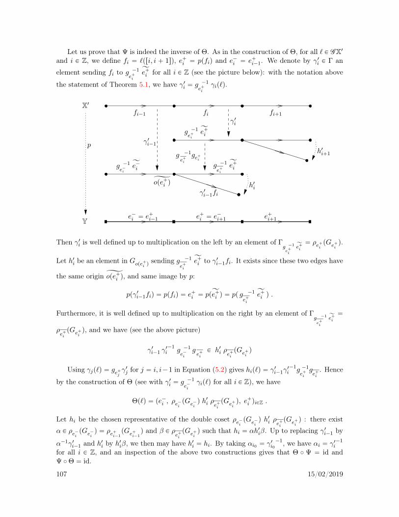
Let us prove that Ψ is indeed the inverse of Θ. As in the construction of Θ, for all ` P GX1and i P Z, we define fi “ `pri, i ` 1sq, e`i “ ppfiq and e´i “ e`i´1. We denote by γ1i P Γ an

element sending fi to g ´1e`i

Ăe`i for all i P Z (see the picture below): with the notation above

the statement of Theorem 5.1, we have γ1i “ g ´1e`i

γip`q.

e´i “ e`i´1 e`i`1e`i “ e´i`1Y

fi´1 fi fi`1

g ´1e`i

Ăe`i

g ´1e´i

Ăe´i

h1i

h1i`1

γ1i

X1

γ1i´1

Čope`i q

γ1i´1fi

p

g ´1

e`i

Ăe`i

g ´1

e`ige`i

Then γ1i is well defined up to multiplication on the left by an element of Γg ´1

e`i

Ăe`i“ ρe`i

pGe`iq.

Let h1i be an element in Gope`i q sending g´1

e`i

Ăe`i to γ1i´1fi. It exists since these two edges have

the same origin Čope`i q, and same image by p:

ppγ1i´1fiq “ ppfiq “ e`i “ ppĂe`i q “ pp g ´1

e`i

Ăe`i q .

Furthermore, it is well defined up to multiplication on the right by an element of Γg ´1

e`i

Ăe`i“

ρe`ipGe`i

q, and we have (see the above picture)

γ1i´1 γ1i´1

g ´1e´i

ge`iP h1i ρe`i

pGe`iq

Using γjp`q “ ge`jγ1j for j “ i, i´1 in Equation (5.2) gives hip`q “ γ1i´1γ

1i´1g ´1

e`ige`i. Hence

by the construction of Θ (see with γ1i “ g ´1e´i

γip`q for all i P Z), we have

Θp`q “ pe´i , ρe´ipGe´i

q h1i ρe`ipGe`i

q, e`i qiPZ .

Let hi be the chosen representative of the double coset ρe´i pGe´i q h1i ρe`i

pGe`iq : there exist

α P ρe´ipGe´i

q “ ρe`i´1pGe`i´1

q and β P ρe`ipGe`i

q such that hi “ αh1iβ. Up to replacing γ1i´1 by

α´1γ1i´1 and h1i by h1iβ, we then may have h1i “ hi. By taking αi0 “ γ1i0

´1, we have αi “ γ1i´1

for all i P Z, and an inspection of the above two constructions gives that Θ ˝ Ψ “ id andΨ ˝Θ “ id.

107 15/02/2019

Since the discrete time geodesic flow is topologically transitive on its nonwandering subsetand by conjugation, the topological Markov shift pΣ, σq is topologically transitive.

If X1 is a uniform tree without vertices of degree at most 2, if the length spectrum of Γ isequal to Z and if the Gibbs measuremF for Γ is finite, then by Theorem 4.17, the discrete timegeodesic flow on ΓzGX1 is topologically mixing, hence by conjugation by Θ, the topologicalMarkov shift pΣ, σq is topologically mixing. This concludes the proof of Theorem 5.1. l

When the length spectrum LΓ of Γ is different from Z, the topological Markov shift pΣ, σqconstructed above is not always topologically mixing. We now modify the above constructionin order to take care of this problem.

Recall that X1 “ C ΛΓ and that GevenX1 is the space of geodesic lines ` P GX1 whose origin`p0q is at even distance from the basepoint x0 (we assume that x0 P X1), which is invariantunder the time-two discrete geodesic flow g2 and, when LΓ “ 2Z, under Γ, as seen in theproof of Theorem 4.17.

Consider Aeven the alphabet consisting of the quintuples pf´, h´, f0, h`, f`q where thetriples pf´, h´, f0q and pf0, h`, f`q belong to A and opf0q is at even distance from theimage in Y “ ΓzX1 of the basepoint x0. Let Aeven “ pAeven, i,jqi,jPAeven be the transitionmatrix with line and column indices in Aeven such that for all i “ pf´, h´, f0, h`, f`q andj “ pf´˚ , h

´˚ , f

0˚ , h

`˚ , f

`˚ q, we have Aeven, i,j “ 1 if and only if f` “ f´˚ . We denote by

pΣeven, σevenq the associated topological Markov shift. We endow Σeven with the slightlymodified distance

devenpx, x1q “ e´2 sup

nPN : @ k P t´n, ..., nu, xk “ x1k

(

,

where x “ pxkqkPZ and x1 “ px1kqkPZ are in Σeven.We have a canonical injection inj : Σeven Ñ Σ sending the sequence pf´n , h´n , f0

n, h`n , f

`n qnPZ

to pe´n , hn, e`n qnPZ with, for every n P Z,

e´2n “ f´n , h2n “ h´n , e`2n “ f0

n, e´2n`1 “ f0

n, h2n`1 “ h`n , e`2n`1 “ f`n , .

By construction, inj is clearly a homeomorphism onto its image, and

ΘpΓzGevenX1q “ injpΣevenq .

If two sequences in Σeven coincide between ´n and n, then their images by inj coincidebetween ´2n and 2n. Conversely, if the images by inj of two sequences in Σeven coincidebetween ´2n´ 1 and 2n` 1, then these sequences coincide between ´n and n. Hence inj isbilipschitz, for the above distances.

Let us define Θeven “ inj´1 ˝Θ|ΓzGevenX1 : ΓzGevenX1 Ñ Σeven. The following diagram hencecommutes

ΓzGevenX1ΘevenÝÝÝÝÑ Σeven

§

§

đ

§

§

đ

inj

ΓzGX1 ΘÝÝÝÝÑ Σ ,

where the vertical map on the left hand side is the inclusion map.

Theorem 5.2. Assume that X1 “ C ΛΓ is a uniform tree without vertices of degree at most 2,that the Gibbs measure mF of Γ is finite, and that the length spectrum LΓ of Γ is equal to 2Z.Then the map Θeven : ΓzGevenX1 Ñ Σeven is a bilipschitz homeomorphism which conjugatesthe time-two discrete geodesic flow g2 and the shift σeven, and the topological Markov shiftpΣeven, σevenq is locally compact and topologically mixing.

108 15/02/2019

Proof. The only claims that remains to be proven is the last one, which follows from Theorem4.17, by conjugation. l

Let us now study the properties of the image by the coding map Θ of finite Gibbs measureson ΓzGX.

Let δ “ δΓ,F˘ be the critical exponent of pΓ, F˘q. Let pµ˘x qxPV X be two (normalised)Patterson densities on B8X for the pairs pΓ, F˘q, where as previously rF` “ rF , rF´ “ rF ˝ ι.Assume that the associated Gibbs measure mF on ΓzGX (using the convention for discretetime of Section 4.3) is finite.

Let us defineP “

1

mF Θ˚mF (5.4)

as the image of the Gibbs measure mF (whose support is ΓzGX1) by the homeomorphism Θ,normalised to be a probability measure. It is a probability measure on Σ, invariant under theshift σ.

Let pZnqnPZ be the random process classically associated with the full shift σ on Σ: it isthe random process on the Borel space Σ indexed by Z with values in the discrete alphabetA , where Zn : Σ Ñ A is the (continuous hence measurable) n-th projection pxkqkPN ÞÑ xnfor all n P Z.

The following Proposition 5.5 summarises the properties of the probability measure P. Westart by recalling and giving some notation used in this proposition.

For every admissible finite sequence w “ pap, . . . , aqq in A , where p ď q in Z, we denote‚ by rws “ rap, . . . , aqs “ tpxnqnPZ P Σ : @ n P tp, . . . , qu, xn “ an

(

the associatedcylinder in Σ,‚ by pw the associated geodesic edge path in X1 with length q ´ p` 2 constructed in the

proof of Theorem 5.1 (see Equation (5.3)), with origin pw´ and endpoint pw`.

For every geodesic edge path α “ pfp´1, . . . , fqq in X1, we define (See Section 2.6 for thenotation, and the picture below)

B`αX1 “ BfqX1 and B´αX1 “ B fp´1X1 ,

andGαX “ t` P GX : `pp´ 1q “ opfp´1q and `pq ` 1q “ tpfqqu .

fqfp´1B`αX1B´αX1

α

We define a map Fsymb : Σ Ñ R by

Fsymbpxq “

ż tpe`0 q

ope`0 qF (5.5)

if x “ pxiqiPZ with x0 “ pe´0 , h0, e

`0 q. Note that for all pxnqnPZ, pynqnPZ P Σ, if x0 “ y0, then

Fsymbpxq “ Fsymbpyq, so that Fsymb is locally constant (constant on each cylinder of length 1at time 0), hence continuous.

109 15/02/2019

For instance, if F “ Fc is the potential associated with a system of conductances c :ΓzEX1 Ñ R (see Section 3.5), then

Fsymbpxq “ cpe`0 q .

Note that if c, c1 : ΓzEX1 Ñ R are cohomologous systems of conductances on ΓzEX1, then thecorresponding maps Fsymb, F

1symb : Σ Ñ R are cohomologous. Indeed if f : ΓzV X Ñ R is a

map such that c1peq ´ cpeq “ fptpeqq ´ fpopeqq for every e P ΓzEX, with G : Σ Ñ R the mapdefined by Gpxq “ fpope`0 qq if x “ pxiqiPZ with x0 “ pe

´0 , h0, e

`0 q, then G is locally constant,

hence continuous, and since tpe`0 q “ ope`1 q, we have, for every x P Σ,

F 1symbpxq ´ Fsymbpxq “ Gpσxq ´Gpxq .

Definition 5.3. Let X2 be a locally finite simplicial tree. A nonelementary discrete sub-group Γ1 of AutpX2q is Markov-good if for every n P N ´ t0u and every geodesic edge pathpe0, . . . , en`1q in C ΛΓ1, we have

|Γ1e0 X ¨ ¨ ¨ X Γ1en | |Γ1en´1

X Γ1en X Γ1en`1| “ |Γ1e0 X ¨ ¨ ¨ X Γ1en`1

| |Γ1en´1X Γ1en | . (5.6)

Remark 5.4. (1) Note that Equation (5.6) is automatically satisfied if n “ 1 and that Γ1 isMarkov-good if Γ1 acts freely on X2.

(2) A group action on a simplicial tree is 2-acylindrical 4 if the stabiliser of any geodesic edgepath of length 2 is trivial. If Γ1 is 2-acylindrical on X, then Γ1 is Markov-good, since all groupsappearing in Equation (5.6) are trivial.

(3) If X2 has degrees at least 3 and if Γ1 is a noncocompact geometrically finite lattice of X2with abelian edge stabilisers, then Γ1 is not Markov-good.

Proof. (3) Since the quotient graph Γ1zX2 is infinite, the graph of groups Γ1zzX2 contains atleast one cuspidal ray. Consider a geodesic ray in X2 with consecutive edges pfnqnPN mappinginjectively onto this cuspiday ray, pointing towards its end. The stabilisers of the edges fn inΓ1 are hence nondecreasing in n: we have Γ1fn Ă Γ1fn`1

for all n P N. By the finiteness of thevolume, there exists n ě 3 such that Γ1fn´2

is strictly contained in Γ1fn´1. Since X2 has degrees

at least 3, there exists γ P Γ1 fixing tpfn´1q but not fixing fn´1. Let e0 “ f0, . . . , en´1 “ fn´1,en “ γ fn´1 and en`1 “ γ fn´2. Since the stabilisers of fn´1 and en are conjugated byγ within the abelian stabiliser of fn, they are equal. Then pe0, . . . , en`1q is a geodesic edgepath in the simpliciak tree X2 (whose geometric realisation is equal to C ΛΓ1 since Γ1 is alattice). Since Γ1e0 X ¨ ¨ ¨ X Γ1en “ Γ1f0

, Γ1en´1X Γ1en X Γ1en`1

“ Γ1fn´2, Γ1e0 X ¨ ¨ ¨ X Γ1en`1

“ Γ1f0,

Γ1en´1X Γ1en “ Γ1fn´1

and |Γ1fn´2| ‰ |Γ1fn´1

|, the subgroup Γ1 is not Markov-good. l

Recall that a random process pZ 1nqnPZ on pΣ,Pq is a Markov chain if and only if for allp ď q in Z and ap, . . . , aq, aq`1 in A , we have, when defined,

PpZ 1q`1 “ aq`1 |Z1q “ aq, . . . , Z

1p “ apq “ PpZ 1q`1 “ aq`1 |Z

1q “ aqq . (5.7)

Proposition 5.5. (1) For every admissible finite sequence w in A , we have

Pprwsq “µ´pw´pB´pwX

1q µ`pw`pB`pwX

1q eş

pw`pw´p rF´δq

|Γpw| mF

.

4See for instance [Sel, GuL], which require other minor hypotheses that are not relevant here.

110 15/02/2019

(2) The random process pZnqnPZ on pΣ,Pq is a Markov chain if and only if Γ is Markov-good.

(3) The measure P on the topological Markov shift Σ satisfies the Gibbs property with Gibbsconstant δ for the potential Fsymb.

It follows from the above Assertion (2) and from Remark 5.4 that when X has degrees atleast 3 and Γ is a noncocompact geometrically finite lattice of X with abelian edge stabilisers(and more generally, this is not a necessary assumption), then pZnqnPZ is not a Markov chain.The fact that codings of discrete time geodesic flows on trees might not satisfy the Markovchain property had been noticed by Burger and Mozes around the time the paper [BuM] waspublished.5 When proving the variational principle in Section 5.4 and the exponential decayof correlations in Section 9.2, we will hence have to use tools that are not using the Markovchain property.

Proof. (1) Let w “ pap, . . . , aqq, with p ď q in Z, be an admissible finite sequence in A .Recall that rws “ tx P Σ : @ i P tp, . . . , qu, xi “ aiu. By the construction of Θ, the preimageΘ´1prwsq is equal to the image ΓG

pwX1 of GpwX1 in ΓzGX1. Hence, since Γ

pw is the stabiliser ofGpwX1 in Γ,

Pprwsq “1

mF mF pΓG

pwX1q “1

|Γpw| mF

rmF pGpwX1q .

In the expression of rmF given by Equation (4.12), let us use as basepoint the origin pw´ ofthe edge path pw, and note that all elements of G

pwX1 pass through pw´ at time t “ p ´ 1, sothat by the invariance of rmF under the discrete time geodesic flow, we have

rmF pGpwX1q “

ż

`PGpwX1

drmF pg1´p`q “

ż

`´PB´pwX1

ż

``PB`pwX1dµ´

pw´p`´qdµ

`pw´p``q

“ µ´pw´pB´pwX

1q µ`pw´pB`pwX

1q “ µ´pw´pB´pwX

1q µ`pw`pB`pwX

1q eş

pw`pw´p rF´δq

,

where this last equality follows by Equations (4.2) and (3.20) with x “ pw´ and y “ pw`, sincefor every `` P B`

pwX1, we have pw` P r pw`, ``r .

(2) Let us fix p ď q in Z and ap, . . . , aq, aq`1 in A , and let us try to verify Equation (5.7) forpZ 1nqnPN “ pZnqnPN. Let α˚ “ pap, . . . , aqq, which is an admissible sequence, since we assumedthe conditional probability PpZq`1 “ aq`1 |Zq “ aq, . . . , Zp “ apq to be well defined. Wemay assume that α “ pap, . . . , aq, aq`1q is an admissible sequence, otherwise both sides ofEquation (5.7) are 0. Let us consider

Qα “PpZq`1 “ aq`1 |Zq “ aq, . . . , Zp “ apq

PpZq`1 “ aq`1 |Zq “ aqq“

Pprap, . . . , aq`1sq PpraqsqPprap, . . . , aqsq Ppraq, aq`1sq

.

Let us replace each one of the four terms in this ratio by its value given by Assertion (1).Since B´

pαX1 “ B

´

xα˚X1, B`

pαX1 “ B

`

aq ,aq`1X1, B`

xα˚X1 “ B`

xaqX1 and B´

xaqX1 “ B´

aq ,aq`1X1, all Patterson

measure terms cancel. Denoting by y1 the common origin of pα and xα˚, by y2 the commonorigin of paq and aq, aq`1, by y3 the common terminal point of paq and xα˚, and by y4 thecommon terminal point of aq, aq`1 and pα, we thus have by Assertion (1)

Qα “|Γ

xα˚ | |Γ aq ,aq`1|

|Γpα| |Γxaq |

eşy4y1p rF´δq

eşy3y2p rF´δq

eşy3y1p rF´δq

eşy4y2p rF´δq

.

5Personal communication.

111 15/02/2019

Since y1, y2, y3, y4 are in this order on ry1, y4s, we have

Qα “|Γ

xα˚ | |Γ aq ,aq`1|

|Γpα| |Γxaq |

.

Since every geodesic edge path of length n ` 1 at least 3 in X1 defines an admissiblesequence of length n at least 2 in A , by Equation (5.6), we have Qα “ 1 for every admissiblesequence α in A if and only if Γ is Markov-good.

(3) Let E be a finite subset of the alphabet A , and let w “ pap, . . . , aqq with p ď q in Z bean admissible sequence in A such that ap, aq P E. By Assertion (1), we have

Pprwsq “µ´pw´pB´pwX

1q µ`pw`pB`pwX

1q eş

pw`pw´p rF´δq

|Γpw| mF

.

Since ap, aq are varying in the finite subset E of A , the first and last edges of pw vary amongstthe images under elements of Γ of finitely many edges of X1. Since w is admissible, thesets B˘

pwX1 are nonempty open subsets of ΛΓ, hence they have positive Patterson measures.

Furthermore, the quantities µ˘pw˘pB˘pwX

1q are invariant under the action of Γ on the first/lastedge of pw. Hence there exists c1 ě 1 depending only on E such that 1 ď |Γ

pw| ď |Γ pw´ | ď c1

and 1c1ď µ˘

pw˘pB˘pwX

1q ď c1.Note that the length of pw is equal to q ´ p` 2. Therefore

e´δ

c31 mF

e´δpq´p`1q`

ş

pw`pw´

rFď Pprwsq ď

e´δ c21

mF e´δpq´p`1q`

ş

pw`pw´

rF.

If pw “ pfp´1, fp, . . . , fqq and x P rws, we have by the definition of Fsymb

ż

pw`

pw´

rF “

qÿ

i“p´1

ż tpfiq

opfiq

rF “

ż tpfp´1q

opfp´1q

rF `

qÿ

i“p

Fsymbpσipxqq .

Since rF is continuous and Γ-invariant, and since opfp´1q remains in the image under Γ

of a finite subset of V X1, there exists c2 ą 0 depending only on E such that | rF pvq| ď c2 forevery v P T 1X with πpvq P ropfp´1q, tpfp´1qs. Hence |

ştpfp´1q

opfp´1qrF | ď c2, and Assertion (3) of

Proposition 5.5 follows (see Equation (5.1) for the definition of the Gibbs property). l

Again in order to consider the case when the length spectrum LΓ of Γ is 2Z, we define

Peven “1

pmF q| ΓzGevenX1pΘevenq˚

`

pmF q| ΓzGevenX1˘

,

and pZeven, nqnPZ the random process associated with the full shift σeven on Σeven, with Zeven, n :Σeven Ñ Aeven the n-th projection for every n P Z.

By a proof similar to the one of Proposition 5.5, we have the following result. We definea map Fsymb, even : Σeven Ñ R by

Fsymb, evenpxq “

ż tpf`0 q

opf00 q

F (5.8)

if x “ pxiqiPZ with x0 “ pf´0 , h

´0 , f

00 , h

`0 , f

`0 q. As previously, Fsymb, even is locally constant,

hence continuous.

112 15/02/2019

Proposition 5.6. The measure Peven on the topological Markov shift Σeven satisfies the Gibbsproperty with Gibbs constant δ for the potential Fsymb, even. l

Again, if Γ is a noncocompact geometrically finite lattice of X with abelian edge stabilisersand X1 has degrees at least 3, then pZeven, nqnPZ is not a Markov chain.

5.3 Coding continuous time geodesic flows on metric trees

Let pX, λq be a locally finite metric tree without terminal vertices, with X “ |X|λ its geometricrealisation. Let Γ be a nonelementary discrete subgroup of AutpX, λq, and let rF : T 1X Ñ R bea potential for Γ. Let X 1 “ C ΛΓ, which is the geometric realisation |X1|λ of a metric subtreepX1, λq. Let δ “ δΓ,F˘ be the critical exponent of pΓ, F˘q. Let pµ˘x qxPV X be the (normalised)Patterson densities on B8X for the pairs pΓ, F˘q, and assume that the associated Gibbsmeasure mF is finite. We also assume in this Section that the lengths of the edges of pX1, λqhave a finite upper bound (which is in particular the case if pX1, λq is uniform). They have apositive lower bound by definition (see Section 2.6).

In this Section, we prove that the continuous time geodesic flow on ΓzGX 1 is isomorphic toa suspension of a transitive (two-sided) topological Markov shift on a countable alphabet, byan explicit construction that will be useful later on in order to study the variational principle(see Section 5.4) and rates of mixing (see Section 9.3). Since we are only interested in thesupport of the Gibbs measures, we will only give such a description for the geodesic flow onthe nonwandering subset ΓzGX 1 of ΓzGX. The same construction works with the full spaceΓzGX, but the resulting Markov shift is then not necessarily transitive.

We start by recalling (see for instance [BrinS, §1.11]) the definitions of the suspension ofan invertible discrete time dynamical system and of the first return map on a cross-section ofa continuous time dynamical system, which allow to pass from transformations to flows andback, respectively.

Let pZ, µ, T q be a metric space Z endowed with a homeomorphism T and a T -invariant(positive Borel) measure µ. Let r : Z Ñ s0,`8r be a continuous map, such that for allz P Z, the subset trpTnzq : n P Nu Y t´ rpT´pn`1qzq : n P Nu is discrete in R. Then thesuspension (or also special flow) over pZ, µ, T q with roof function r is the following continuoustime dynamical system pZr, µr, pT

trqtPRq :

‚ The space Zr is the quotient topological space pZ ˆ Rq„ where „ is the equivalencerelation on Z ˆ R generated by pz, s ` rpzqq „ pTz, sq for all pz, sq P Z ˆ R. We denote byrz, ss the equivalence class of pz, sq. Note that

F “ tpz, sq : z P Z, 0 ď s ă rpzqu

is a measurable strict fundamental domain for this equivalence relation. We endow Zr withthe Bowen-Walters distance, see [BowW] and particularly the appendix in [BarS].

‚ For every t P R, the map T tr : Zr Ñ Zr is the map rz, ss ÞÑ rz, s ` ts. Equivalently,when pz, sq P F and t ě 0, then T trprz, ssq “ rTnz, s1s where n P N and s1 P R are such that

t` s “n´1ÿ

i“0

rpT izq ` s1 and 0 ď s1 ă rpTnzq .

113 15/02/2019

‚ Denoting by ds the Lebesgue measure on R, the measure µr is the pushforward ofthe restriction to F of the product measure dµ ds by the restriction to F of the canonicalprojection pZ ˆ Rq Ñ Zr.

Note that pT trqtPR is indeed a continuous one-parameter group of homeomorphisms of Zr,preserving the measure µr. The measure µr is finite if and only if

ş

Z r dµ is finite, since

µr “

ż

Fdµds “

ż

Zr dµ .

We will denote by pZ, µ, T qr the continuous time dynamical system pZr, µr, pTtrqtPRq thus

constructed.

Conversely, let pZ, µ, pφtqtPRq be a metric space Z endowed with a continuous one-parametergroup of homeomorphisms pφtqtPR, preserving a (positive Borel) measure µ. Let Y be across-section of pφtqtPR, that is a closed subspace of Z such that for every z P Z, the settt P R : φtpzq P Y u is infinite and discrete. Let τ : Y Ñ s0,`8r be the (continuous) firstreturn time on the cross-section Y : for every y P Y ,

τpyq “ mintt ą 0 : φtpyq P Y u .

Let φY : Y Ñ Y be the (homeomorphic) first return map to (or Poincaré map of) the cross-section Y , defined by

φY : y ÞÑ φτpyqpyq .

By the invariance of µ under the flow pφtqtPR, the restriction of µ to

tφtpyq : y P Y, 0 ď t ă τpyqu

disintegrates6 by the (well-defined) map φtpyq ÞÑ y over a measure µY on Y , which is invariantunder the first return map φY :

dµpφtpyqq “ dt dµY pyq .

Note that if τ has a positive lower bound and if µ is finite, then µY is finite, since

µ ě µY inf τ ,

and pY, µY , φY q is a discrete time dynamical system.

Recall that an isomorphism from a continuous time dynamical system pZ, µ, pφtqtPRq toanother one pZ 1, µ1, pφ1tqtPRq is a homeomorphism between the underlying spaces preservingthe underlying measures and commuting with the underlying flows.

Example 5.7. If pZ, µ, T q and pZ 1, µ1, T 1q are (invertible) discrete time dynamical systems,endowed with roof functions r : Z Ñ s0,`8r and r1 : Z 1 Ñ s0,`8r respectively, if θ : Z Ñ Z 1

is a measure preserving homeomorphism commuting with the transformations T and T 1 (thatis, θ˚µ “ µ1, θ ˝ T “ T 1 ˝ θ) and such that

r1 ˝ θ “ r ,

then the mapp

θ : Zr Ñ Z 1r1 defined by rz, ss ÞÑ rθpzq, ss is an isomorphim between thesuspensions pZ, µ, T qr and pZ 1, µ1, T 1qr1 .

6with conditional measure on the fiber tφtpyq : 0 ď t ă τpyqu over y P Y the image of the Lebesguemeasure on r0, τpyqr by t ÞÑ φtpyq

114 15/02/2019

It is well known (see for instance [BrinS, §1.11]) that the above two constructions areinverses one to another, up to isomorphism. In particular, we have the following result.

Proposition 5.8. With the general notation above Example 5.7, the suspension pY, µY , φY qτover pY, µY , φY q with roof function τ is isomorphic to pZ, µ, pφtqtPRq by the map fY : ry, ss ÞÑφsy. l

In order to describe the continuous time dynamical system`

ΓzGX 1, mFmF

, pgtqtPR˘

as asuspension over a topological Markov shift, we will start by describing it as a suspensionof the discrete time geodesic flow on ΓzGX1. Note that the Patterson densities and Gibbsmeasures depend not only on the potential, but also on the lengths of the edges.7 We henceneed to relate precisely the continuous time and discrete time situations, and we will use inthis Section the left exponent 7 to indicate a discrete time object whenever needed.

For instance, we set8 7X 1 “ |X1|1 and we denote by p7gtqtPZ the discrete time geodesicflow on ΓzGX1. Note that X 1 and 7X 1 are equal as topological spaces (but not as metricspaces). The boundaries at infinity of X 1 and 7X 1, which coincide with their spaces of endsas topological spaces (by the assumption on the lengths of the edges), are hence equal anddenoted by B8X.

We may assume by Section 3.5 that the potential rF : T 1X Ñ R is the potential rFcassociated with a system of conductances rc on the metric tree pX, λq for Γ. Let δc “ δFc . Wedenote by 7rc : EXÑ R the Γ-invariant system of conductances

7rc : e ÞÑ prcpeq ´ δcqλpeq (5.9)

on the simplicial tree X for Γ, by rF7c : T 1p 7Xq Ñ R its associated potential, and by 7c :ΓzEXÑ R and F7c : ΓzT 1p 7Xq Ñ R their quotient maps.

Note that the inclusion morphism AutpX, λq Ñ AutpXq is a homeomorphism onto itsimage (for the compact-open topologies), by the assumption of a positive lower bound on thelengths of the edges, hence that Γ is also a nonelementary discrete subgroup of AutpXq.

Now, let pΣ, σ,Pq be the (two-sided) topological Markov shift conjugated to the discretetime geodesic flow

`

ΓzGX1, 7g1,mF7cmF7c

˘

by the bilipschitz homeomorphism Θ : ΓzGX1 Ñ Σ of

Theorem 5.1 (where the potential F is replaced by F7c). Let r : Σ Ñ s0,`8r be the map

r : x ÞÑ λpe`0 q (5.10)

if x “ pxnqnPZ P Σ and x0 “ pe´0 , h0, e

`0 q P A . This map is locally constant, hence continuous

on Σ, and has a positive lower bound, since the lengths of the edges of pX1, λq have a positivelower bound.

7The fact that the Patterson densities could be singular one with respect to another when the metric variesis a well known phenomenon, even when the potential vanishes. For instance, let Σ “ ΓzH2

R and Σ1 “ Γ1zH2R be

two closed connected hyperbolic surfaces, uniformised by the real hyperbolic plane pH2R, ds

2hypq endowed with

torsion free cocompact Fuchsian groups Γ and Γ1. Let φ : Σ Ñ Σ1 be a diffeomorphism, with lift rφ : H2R Ñ H2

R.Then Γ is a discrete group of isometries for the two CATp´1q-metrics ds2

hyp and rφ˚ds2hyp. Kuusalo’s theorem

[Kuu] says that the corresponding two Patterson densities of Γ are absolutely continuous one with respect tothe other if and only if φ is isotopic to the identity. See an extension of this result in [HeP1]. See also theresult of [KaN] which parametrises the Culler-Vogtmann space using Patterson densities for cocompact andfree actions of free groups on metric trees.

8See Section 2.6 for the definition of the geometric realisation |Y|1 of a simplicial tree Y.

115 15/02/2019

Theorem 5.9. Assume that the lengths of the edges of pX1, λq have a finite upper bound,and that the Gibbs measure mF is finite. Then there exists a ą 0 such that the continuoustime dynamical system

`

ΓzGX 1, mFmF

, pgtqtPR˘

is isomorphic to the suspension pΣ, σ, aPqr overpΣ, σ, aPq with roof function r, by a bilipschitz homeomorphism Θr : ΓzGX 1 Ñ Σr.

Proof. LetY “ t` P ΓzGX 1 : `p0q P ΓzV Xu .

Then the (closed) subset Y of ΓzGX 1 is a cross-section of the continuous time geodesicflow pgtqtPR, since every orbit meets Y infinitely many times in a discrete set of times andsince the lengths of the edges of pX1, λq have a positive lower bound. Let τ : Y Ñ s0,`8r bethe first return time, let µY be the measure on Y (obtained by disintegrating mF

mF ), and let

gY : Y Ñ Y be the first return map associated with this cross-section Y .We have a natural reparametrisation map R : Y Ñ ΓzGX1, defined by ` ÞÑ 7`, where

7`pnq “ pgnY `qp0q is the n-th passage of ` in V X, for every n P Z. Since there exist m,M ą 0such that λpEXq Ă rm,M s, the map R is a bilipschitz homeomorphism. It conjugates thefirst return map gY and the discrete time geodesic flow on ΓzGX1:

R ˝ gY “7g1 ˝R .

The main point of this proof is the following result relating the measures µY and mF7c.

Lemma 5.10.

(1) The family pµ˘x qxPV X is a Patterson density for pΓ, F7cq on the boundary at infinity ofthe simplicial tree X1, and the critical exponent δ7c of 7c is equal to 0.

(2) We have R˚ µYµY

“mF7cmF7c

.

Proof. (1) By the definition of the potential associated with a system of conductances,9 forevery x, y P V X1, if pe1, . . . , enq is the edge path in X with ope1q “ x and tpenq “ y, then(noting that the integrals along paths depend on the lengths of the edges, the first one belowbeing in X 1, the second one in 7X 1)

ż y

xpĂFc ´ δcq “

nÿ

i“1

prcpeiqλpeiq ´ δcλpeiqq “

ż y

x

ĂF7c . (5.11)

Let us denote10 by7Qpsq “ QΓ, F7c, x, y

psq “ÿ

γPΓ

eşγyx p

rF7c´sq

andQpsq “ QΓ, Fc´δc, x, ypsq “

ÿ

γPΓ

eşγyx p

rFc´δc´sq

the Poincaré series for the simplicial tree with potential rF7c and for the metric tree withnormalised potential rFc ´ δc, respectively. With M an upper bound on the lengths of theedges of pX, λq, the distances d7X 1 on 7X 1 and dX 1 on X 1 satisfy d7X 1 ě

1M dX 1 on the pairs

9See Section 3.5.10See Section 3.3.

116 15/02/2019

of vertices of X1. We hence have 7Qpsq ď Qp sM q ă `8 if s ą 0 and 7Qpsq ě Qp sM q “ `8 ifs ă 0. Thus the critical exponent δ7c of pΓ, F7cq for the simplicial tree X1 is equal to 0, henceF7c is a normalised potential.

By the definition11 of the Gibbs cocycles (which uses the normalised potential), Equation(5.11) also implies that the Gibbs cocycles C˘ and 7C˘ for pΓ, Fcq and pΓ, F7cq respectivelycoincide on B8X ˆ V X ˆ V X. Thus by Equations (4.1) and (4.2), the family pµ˘x qxPV X isindeed a Patterson density for pΓ, F7cq: for all γ P Γ and x, y P V X, and for (almost) allξ P B8X,

γ˚µ˘x “ µ˘γx and

dµ˘xdµ˘y

pξq “ e´7C˘ξ px, yq .

(2) We may hence choose these families pµ˘x qxPV X in order to define the Gibbs measure mF7cassociated with the potential F7c on ΓzGX. Note that since we will prove that mF7c

is finite,

the normalised measuremF7cmF7c

is independent of this choice (see Corollary 4.7).

Let rY “ t` P GX 1 : `p0q P V X1u be the (Γ-invariant) lift of the cross-section Y to GX 1,let rR : rY Ñ GX1 be the lift of R, mapping a geodesic line ` P rY to a discrete geodesic line 7`with same footpoint obtained by reparametrisation, and let õY be the measure on rY whoseinduced measure on Y “ ΓzrY is µY . We have a partition of rY into the closed-open subsetsrYx “ t` P GX 1 : `p0q “ xu as x varies in V X1.

Let us fix x P V X. By the definition of µY as a disintegration of mFcmFc

with respect to thecontinuous time, by lifting to GX 1, by using Hopf’s parametrisation with respect to x andEquation (4.4) with x0 “ x , we have for every ` P rYx,

dõY p`q “1

mFcdµ´x p`´q dµ

`x p``q .

Note that `p0q “ 7`p0q, `´ “ 7`´, `` “ 7`` since the reparametrisation does not change theorigin or the two points at infinity. Hence by Assertion (1), we have

rR˚põY q “1

mFcrmF7c

.

As µY is a finite measure since τ has a positive lower bound, this implies that mF7cis finite.

By renormalizing as probability measures, this proves Assertion (2). l

Let a “ µY ą 0, so that by Lemma 5.10 (2) we have R˚µY “a mF7cmF7c

. Let

p

r : ΓzGX1 Ñ

s0,`8s be the mapp

r : Γ` ÞÑ λ`

`pr0, 1sq˘

given by the length for λ of the first edge followed by a discrete geodesic line ` P GX1. Notethat

p

r is locally constant, hence continuous, and thatp

r is a roof function for the discrete timedynamical system pΓzGX1, 7g1q. Also note that

p

r ˝R “ τ and r ˝Θ “

p

r

by the definitions of τ and r.11See Section 3.4.

117 15/02/2019

Let us finally define Θr : ΓzGX 1 Ñ Σr as the compositions of the following three maps

pΓzGX 1,mF

mF , pgtqtPRq

f ´1YÝÑ pY, µY , gY qτ

p

RÝÑ pΓzGX1,

a mF7c

mF7c, 7g1q

p

r

p

ΘÝÑ pΣ, aP, σqr , (5.12)

where the first one is the inverse of the tautological isomorphism given by Proposition 5.8and the last two ones, given by Example 5.7, are the isomorphisms

p

R andp

Θ of continuoustime dynamical systems obtained by suspensions of the isomorphisms R and Θ of discretetime dynamical systems. It is easy to check that Θr is a bilipschitz homeomorphism, usingthe following description of the Bowen-Walters distance, see for instance [BarS, Appendix].

Proposition 5.11. Let pZ, µ, T qr be the suspension over an invertible dynamical system suchthat T is a bilipschitz homeomorphism, with roof function r having a positive lower boundand a finite upper bound. Let dBW : Zr ˆ Zr Ñ R be the map12 defined (using the canonicalrepresentatives) by

dBWprx, ss, rx1, s1sq “

mintdpx, x1q ` |s´ s1|, dpTx, x1q ` rpxq ´ s` s1, dpx, Tx1q ` rpx1q ` s´ s1u

Then there exists a constant CBW ą 0 such that the Bowen-Walters distance d on Σr satisfies

1

CBWdBW ď d ď CBW dBW . l

This concludes the proof of Theorem 5.9. l

5.4 The variational principle for metric and simplicial trees

In this Section, we assume that X is the geometric realisation of a locally finite metric treewithout terminal vertices pX, λq (respectively of a locally finite simplicial tree X withoutterminal vertices). Let Γ be a nonelementary discrete subgroup of AutpX, λq (respectivelyAutpXq).

We relate in this Section the Gibbs measures13 to the equilibrium states14 for the contin-uous time geodesic flow on ΓzGX (respectively for the discrete time geodesic flow on ΓzGX).

When X is a Riemannian manifold with pinched negative curvature such that the deriva-tives of the sectional curvature are uniformly bounded, and when the potential is Hölder-continuous, the analogs of the results of this Section are due to [PauPS, Theo. 6.1]. Theirproofs generalise the proofs of Theorems 1 and 2 of [OtaP], with ideas and techniques goingback to [LedS]. When Y is a compact locally CATp´1q-space, a complete statement aboutexistence, uniqueness and Gibbs property of equilibrium states for any Hölder-continuouspotential is given in [ConLT].

The proof of the metric tree case will rely strongly (via the suspension process describedin Section 5.3) upon the proof of the simplicial tree case, hence we start by the latter.

12The map dBW is actually not a distance, but this proposition says that it may replace the Bowen-Walterstrue distance when working up to multiplicative constants or bilipschitz homeomorphisms.

13See the definition in Sections 4.2 and 4.3.14See the definitions below.

118 15/02/2019

The simplicial tree case.

Let X be a locally finite simplicial tree without terminal vertices, with geometric realisationX “ |X|1. Let Γ be a nonelementary discrete subgroup of AutpXq. Let rc : EX Ñ R be asystem of conductances for Γ on X and c : ΓzEX Ñ R its quotient map. Let rFc : T 1X Ñ Rbe its associated potential, with quotient map Fc : ΓzT 1X Ñ R, and let δc be the criticalexponent of c.

We define a map rFc : GXÑ R by

rFcp`q “ rc pe`0 p`qq “

ż tpe`0 p`qq

ope`0 p`qq

rFc

for all ` P GX, where e`0 p`q is the edge of X in which ` enters at time t “ 0. This map islocally constant, hence continuous, and it is Γ-invariant, hence it induces a continuous mapFc : ΓzGXÑ R which is also called a potential.15

The following result proves that the Gibbs measure of pΓ, Fcq for the discrete time geodesicflow on ΓzGX is an equilibrium state for the potential Fc. We start by recalling the definitionof an equilibrium state,16 see also [Bowe2, Rue3].

Let Z be a locally compact topological space, let T : Z Ñ Z be a homeomorphism, andlet φ : Z Ñ R be a continuous map. Let Mφ be the set of Borel probability measures m onZ, invariant under the transformation T , such that the negative part φ´ “ maxt0,´φu of φis m-integrable. Let hmpT q be the (metric) entropy of the transformation T with respect tom P Mφ (see for instance [BrinS]). The metric pressure for the potential φ of a measure m inMφ is

Pφpmq “ hmpT q `

ż

Zφdm .

The fact that the negative part of φ is m-integrable, which is in particular satisfied if φ isbounded, implies that Pφpmq is well defined in RY t`8u. The pressure of the potential φ isthe element of RY t`8u defined by

Pφ “ supmPMφ

Pφpmq .

A measure m0 in Mφ is an equilibrium state for the potential φ if Pφpm0q “ Pφ.

Theorem 5.12 (The variational principle for simplicial trees). Let X,Γ,rc be as above. Assumethat δc ă `8 and that there exists a finite Gibbs measure mc for Fc such that the negativepart of the potential Fc is mc-integrable. Then mc

mcis the unique equilibrium state for the

potential Fc under the discrete time geodesic flow on ΓzGX, and the pressure of Fc coincideswith the critical exponent δc of c :

PFc “ δc .

In order to prove this result, using the coding of the discrete time geodesic flow given inSection 5.2, the main tool is the following result of J. Buzzi in symbolic dynamics, buildingon works of Sarig and Buzzi-Sarig, whose proof is given in Appendix A.

15See after the proof of Theorem 5.12 for a comment on cohomology classes.16This definition is given for transformations and not for flows, and for possibly unbounded potentials,

contrarily to the one the Introduction.

119 15/02/2019

Let σ : Σ Ñ Σ be a two-sided topological Markov shift17 with (countable) alphabet Aand transition matrix A, and let φ : Σ Ñ R be a continuous map.

For every n P N, we denote18 by

varn φ “ supx, y PΣ

@ i P t´n, ..., nu, xi“yi

|φpxq ´ φpyq|

the n-variation of φ. For instance, if φpxq depends only on x0 where x “ pxiqiPZ, thenvarn φ “ 0 for every n P N (and hence

ř

nPN pn` 1q varn φ “ 0 converges).A weak Gibbs measure for φ with Gibbs constant Cpmq P R is a σ-invariant (positive Borel)

measure m on Σ such that for every a P A , there exists ca ě 1 such that for all n P N´ t0uand x P ras such that σnpxq “ x, we have

1

caď

mprx0, . . . , xn´1sq

e´Cpmqn eřn´1i“0 φpσixq

ď ca . (5.13)

Theorem 5.13 (J. Buzzi, see Corollary A.5). Let pΣ, σq be a two-sided transitive topologicalMarkov shift on a countable alphabet and let φ : Σ Ñ R be a continuous map such thatř

nPN pn`1q varn φ converges. Let m be a weak Gibbs measure for φ on Σ with Gibbs constantCpmq, such that

ş

φ´ dm ă `8. Then the pressure of φ is finite, equal to Cpmq, and m isthe unique equilibrium state. l

Proof of Theorem 5.12. In Section 5.2, we constructed a transitive topological Markovshift pΣ, σq on a countable alphabet A and a homeomorphism Θ : ΓzGX1 Ñ Σ which conju-gates the time-one discrete geodesic flow g1 on the nonwandering subset ΓzGX1 of ΓzGX andthe shift σ on Σ (see Theorem 5.1). Let us define a potential Fc, symb : Σ Ñ R by

Fc, symbpxq “ cpe`0 q (5.14)

if x “ pxiqiPZ P Σ with x0 “ pe´0 , h0, e

`0 q. Note that this potential is the one denoted by Fsymb

in Equation (5.5), when the potential F on T 1X is replaced by Fc. By the construction of Θand the definition of Fc, we have

Fc, symb ˝Θ “ Fc . (5.15)

Note that all probability measures on ΓzGX invariant under the discrete time geodesic floware supported on the nonwandering set ΓzGX1. The pushforward of measures Θ˚ hence givesa bijection from the space MFc of g1-invariant probability measures on ΓzGX for which thenegative part of Fc is integrable to the space MFc, symb

of σ-invariant probability measureson Σ for which the negative part of Fc, symb is integrable. This bijection induces a bijectionbetween the subsets of equilibrium states.

Note that Fc, symbpxq depends only on x0 for every x “ pxiqiPZ P Σ. Hence as seen above,the series

ř

nPN pn` 1q varn Fc, symb converges.By definition,19 the measure P is the pushforward of mc

mcby Θ. Hence, P is a σ-invariant

probability measure on Σ for which the negative part of Fc, symb is integrable, by the assump-tion of Theorem 5.12. By Proposition 5.5 (3), the measure P on Σ satisfies the Gibbs property

17See Section 5.1 for definitions.18with a shift of indices compared with the notation of Appendix A19See Equation (5.4).

120 15/02/2019

with Gibbs constant δc for the potential Fc, symb, hence20 satisfies the weak Gibbs propertywith Gibbs constant δc. Theorem 5.12 then follows from Theorem 5.13. l

Remark. It follows from Equation (5.15), from the remark above Definition 5.3 and from thefact that Θ ˝ g1 “ σ ˝Θ, that if c, c1 : ΓzEX1 Ñ R are cohomologous systems of conductanceson ΓzEX1, then the corresponding maps Fc,Fc1 : ΓzGX1 Ñ R are cohomologous: there existsa continuous map G : ΓzGX1 Ñ R such that for every ` P ΓzGX1,

Fc1p`q ´ Fcp`q “ Gpg1`q ´Gp`q .

Note that given two bounded cohomologous continuous potentials on a topological dy-namical system pZ, T q as above, one has finite pressure (resp. admits an equilibrium state) ifand only if the other one does, and they have the same pressure and same set of equilibriumstates.

The metric tree case.

Let pX, λq be a locally finite metric tree without terminal vertices with geometric realisationX “ |X|λ, let Γ be a nonelementary discrete subgroup of AutpX, λq and let rc : EXÑ R be asystem of conductances for Γ on X. Let rFc : T 1X Ñ R be its associated potential (see Section3.5), and let δc “ δFc be the critical exponent of c.

Recall21 that we have a canonical projection GX Ñ T 1X which associates to a geodesicline ` its germ v` at its footpoint `p0q. Let rF6c : GX Ñ R be the Γ-invariant map obtained byprecomposing the potential rFc : T 1X Ñ R with this canonical projection:

rF6c : ` ÞÑ rFcpv`q .

Let F6c : ΓzGX Ñ R be its quotient map, which is continuous as a composition of continuousmaps.

The following result proves that the Gibbs measure of pΓ, Fcq for the continuous timegeodesic flow on ΓzGX, once renormalised to be a probability measure, is an equilibriumstate for the potential F6c. We start by recalling the definition of an equilibrium state for apossibly unbounded potential under a flow.22

Given pZ, pφtqtPRq a topological space endowed with a continuous one-parameter group ofhomeomorphisms and ψ : Z Ñ R a continuous map (called a potential), let Mψ be the set ofBorel probability measures m on Z invariant under the flow pφtqtPR, such that the negativepart ψ´ “ maxt0,´ψu of ψ is m-integrable. Let hmpφ1q be the (metric) entropy of thegeodesic flow with respect to m P Mψ (see for instance [BrinS]). The metric pressure for ψof a measure m P Mψ is

Pψpmq “ hmpφ1q `

ż

Zψ dm .

The fact that the negative part of ψ is m-integrable, which is in particular satisfied if ψ isbounded, implies that Pψpmq is well defined in RY t`8u. The pressure of the potential ψ isthe element of RY t`8u defined by

Pψ “ supmPMψ

Pψpmq .

20For every a P A , for the constant ca required by the definition of the weak Gibbs property in Equation(5.13), take the constant CE given by the definition (see Equation (5.1)) of the Gibbs property with E “ tau.

21See Section 2.3.22This requires only minor modifications to the definition given in the Introduction for bounded potentials.

121 15/02/2019

Note that Pψ`c “ Pψ ` c for every constant c P R. An element m P Mψ is an equilibriumstate for ψ if the least upper bound defining Pψ is attained on m.

Note that if ψ1 is another potential cohomologous to ψ, that is, if there exists a continuousmap G : Z Ñ R, differentiable along every orbit of the flow, such that ψ1pxq ´ ψpxq “ddt |t“0

Gpφtpxqq, if ψ and ψ1 are bounded (so that Mψ1 “ Mψ), then, for every m P Mψ, wehave Pψ1pmq “ Pψpmq, Pψ1 “ Pψ and the equilibrium states for ψ1 are exactly the equilibriumstates for ψ.

Theorem 5.14 (The variational principle for metric trees). Let pX, λq,Γ,rc be as above. As-sume that the lengths of the edges of pX, λq have a finite upper bound.23 Assume that δc ă `8and that there exists a finite Gibbs measure mc for Fc such that the negative part of the poten-tial F6c is mc-integrable. Then mc

mcis the unique equilibrium state for the potential F6c under

the continuous time geodesic flow on ΓzGX, and the pressure of F6c coincides with the criticalexponent δc of c :

PF6c“ δc .

Using the description of the continuous time dynamical system`

ΓzGX 1, mcmc

, pgtqtPR˘

asa suspension over a topological Markov shift (see Theorem 5.9), this statement reduces towell-known techniques in the thermodynamic formalism of suspension flows, see for instance[IJT], as well as [BarI, Kemp, IJ, JKL]. Our situation is greatly simplified by the fact thatour roof function has a positive lower bound and a finite upper bound, and that our symbolicpotential is constant on the 1-cylinders tx “ pxiqiPZ P Σ : x0 “ au for a in the alphabet.

Proof. Since finite measures invariant under the geodesic flow on ΓzGX are supported onits nonwandering set, up to replacing X by X 1 “ C ΛΓ, we assume that X “ X 1.

Since equilibrium states are unchanged up to adding a constant to the potential, underthe assumptions of Theorem 5.14, let us prove that mc

mcis the unique equilibrium state for

the potential F6c´δc under the continuous time geodesic flow on ΓzGX, and that the pressureof F6c ´ δc vanishes. The last claim of Theorem 5.14 follows, since

PF6c´ δc “ PF6c´δc

.

We refer to the paragraphs before the statement of Theorem 5.9 for the definitions of‚ the system of conductances 7rc for Γ on the simplicial tree X,‚ the (two-sided) topological Markov shift pΣ, σ,Pq on the alphabet A , conjugated to the

discrete time geodesic flow`

ΓzGX, 7g1,mF7cmF7c

˘

by the homeomorphism Θ : ΓzGXÑ Σ,

‚ the roof function r : Σ Ñ s0,`8r, and‚ the suspension pΣ, σ, aPqr “ pΣr, pσ

trqtPR, aPrq over pΣ, σ, aPq with roof function r,

conjugated to the continuous time geodesic flow`

ΓzGX, mcmc

, pgtqtPR˘

by the homeomorphismΘr : ΓzGX Ñ Σr defined at the end of the proof of Theorem 5.9. We will always (uniquely)represent the elements of Σr as rx, ss with x P Σ and 0 ď s ă rpxq.

We denote by F6c, symb : Σr Ñ R the potential defined by

F6c, symb “ F6c ˝Θ´1r , (5.16)

which is continuous as a composition of continuous maps. The key technical observation inthis proof is the following one.

23They have a positive lower bound by definition, see Section 2.6.

122 15/02/2019

Lemma 5.15. For every x P Σ, we have F7c, symbpxq “şrpxq0 pF6c, symb ´ δcqprx, ssq ds. For

every x P Σ, the sign of F6c, symbprx, ssq is constant on s P r0, rpxqr.

Proof. Let x “ pxnqnPZ P Σ and x0 “ pe´0 , h0, e

`0 q P A . By the definition of the first return

time r in Equation (5.10), we have in particular

rpxq “ λpe`0 q .

By Equation (5.14) and by the definition of 7rc in Equation (5.9), we have

F7c, symbpxq “7cpe`0 q “ pcpe

`0 q ´ δcqλpe

`0 q .

Using in the following sequence of equalities respectively‚ the two definitions of the potential F6c, symb in Equation (5.16) and of the suspension

flow pσtrqtPR,‚ the fact that the suspension flow pσtrqtPR is conjugated to the continuous time geodesic

flow by Θr,‚ the definition of Θr using the reparametrisation map24 R of continuous time geodesic

lines with origin on vertices to discrete time geodesic lines,25

‚ the definition of the potential F6c,‚ the fact that e`0 is the first edge followed by the discrete time geodesic line Θ´1x, hence

by the continuous time geodesic line R´1Θ´1x, and the relation between c and the potentialFc associated with c (see Proposition 3.21),we have

ż rpxq

0F6c, symbprx, ssq ds “

ż rpxq

0F6c`

Θ´1r σsrrx, 0s

˘

ds “

ż rpxq

0F6c`

gsΘ´1r rx, 0s

˘

ds

“

ż rpxq

0F6c`

gsR´1Θ´1x˘

ds “

ż λpe`0 q

0Fc`

vgsR´1Θ´1x

˘

ds

“ cpe`0 qλpe`0 q .

Sinceşrpxq0 δc ds “ δc λpe

`0 q, the first claim of Lemma 5.15 follows. The second claim

follows by the definition of the potential Fc associated with c, see Equation (3.23). l

By Equation (5.16), the pushforwards of measures by the homeomorphism Θr, whichconjugates the flows pgtqtPR and pσtrqtPR, is a bijection from MF6c

to MF6c, symb, such that

PF6c, symbppΘrq˚mq “ PF6c

pmq

for every m P MF6c. In particular, we only have to prove that pΘrq˚

mcmc

“ aPr is the unique

equilibrium state for the potential F6c, symb ´ δc under the suspension flow pσtrqtPR, and thatthe pressure of F6c, symb ´ δc vanishes.

The uniqueness follows for instance from [IJT, Theo. 3.5],26 since the roof function r islocally constant and the potential g “ F6c, symb is such that the map27 from Σ to R defined by

24See its definition above Lemma 5.10.25See Equation (5.12), with the notation of Example (5.7) and Proposition 5.8.26Note that a topological Markov shift which is (incorrectly) called topologically mixing in [IJT, page 551]

is actually (topologically) transitive with the definition in this book, Section 5.1.27denoted by ∆g in loc. cit.

123 15/02/2019

x ÞÑşrpxq0 gprx, ssq ds is locally Hölder-continuous by Lemma 5.15 and since F7c, symb is locally

constant.

Let us now relate the σ-invariant measures on Σ with the pσtrqtPR-invariant measures onΣr. Recall that we denote the Lebesgue measure on R by ds and the points in Σr by rx, sswith x P Σ and 0 ď s ă rpxq.

Lemma 5.16. The map S : MF7c, symbÑ MF6c, symb

, which associates to any measure m inMF7c, symb

on Σ the measure

dSpmqprx, ssq “1

ş

Σ r dmdµpxq ds

on Σr, is a bijection, such that, for every m P MF7c, symb,

PF6c, symb´δcpSpmqq “

PF7c, symbpmq

ş

Σ r dm.

Proof. Note thatş

Σ r dm is the total mass of the measure dµrprx, ssq “ dµpxq ds on Σr. Inparticular, Spmq is indeed a probability measure on Σr.

Since r has a positive lower bound and a finite upper bound, it is well known since [AmK],see also [IJT, §2.4], that the map S defined above28 is a bijection from the set of σ-invariantprobability measures m on Σ to the set of pσtrqtPR-invariant probability measures on Σr.

Furthermore, for every σ-invariant probability measure m on Σ, we have the followingKac formula, by the definition of the probability measure Spmq and by Lemma 5.15,

ż

Σr

F6c, symb dSpmq ´ δc “

ż

Σr

pF6c, symb ´ δcq dSpmq

“1

ş

Σ r dm

ż

xPΣ

ż rpxq

0pF6c, symb ´ δcqprx, ssq dmpxq ds

“1

ş

Σ r dm

ż

ΣF7c, symb dm . (5.17)

By the comment on the signs at the end of Lemma 5.15, this computation also proves thatthe negative part of F6c, symb is integrable for Spmq if and only if the negative part of F7c, symb

is integrable for m. Hence S is indeed a bijection from MF7c, symbto MF6c, symb

.

By Abramov’s formula [Abr], see also [IJT, Prop. 2.14], we have

hSpmqpσ1r q “

hmpσqş

Σ r dm. (5.18)

The last claim of Lemma 5.16 follows by summation from Equations (5.17) and (5.18). l

By the proof of Theorem 5.12 (replacing the potential c by 7c), the pressure of the potentialF7c, symb is equal to the critical exponent δ7c of the potential 7c, and by Lemma 5.10 (1), wehave δ7c “ 0. Hence for every m P MF7c, symb

, we have

PF6c, symb´δcpSpmqq “

PF7c, symbpmq

ş

Σ r dmďPF7c, symbş

Σ r dm“

δ7cş

Σ r dm“ 0 .

28and denoted by R in [IJT, §2.4]

124 15/02/2019

In particular, the pressure of the potential F6c, symb´ δc is at most 0, since S is a bijection. Bythe proof of Theorem 5.12 (replacing the potential c by 7c), we know that P is an equilibriumstate for the potential F7c, symb. Hence

PF6c, symb´δcpSpPqq “

PF7c, symbpPq

ş

Σ r dP“ 0 .

Therefore, SpPq is an equilibrium state of the potential F6c, symb´δc, with pressure 0. But aPr,which is equal to Pr

Pr since aPr is a probability measure, is by construction equal to SpPq.The result follows. l

With slightly different notation, this result implies Theorem 1.1 in the Introduction.

Proof of Theorem 1.1. Any bounded potential rF for Γ on T 1X is cohomologous to abounded potential rFc associated with a system of conductances (see Proposition 3.22). If twopotentials rF and rF 1 for Γ on T 1X are cohomologous29 then the potentials ` ÞÑ rF pv`q and` ÞÑ rF 1pv`q for Γ on GX are cohomologous for the definition given before the statement ofTheorem 5.14. Since the existence and uniqueness of an equilibrium state depends only onthe cohomology class of the bounded30 potentials on GX, the result follows. l

29See the definition at the end of Section 3.2.30hence with integrable negative part for any probability measure

125 15/02/2019

126 15/02/2019

Chapter 6

Random walks on weighted graphs ofgroups

Let X be a locally finite simplicial tree without terminal vertices, and let X “ |X|1 be itsgeometric realisation. Let Γ be a nonelementary discrete subgroup of AutpXq.

In Section 6.1, given a (logarithmic) system of conductances c : ΓzEXÑ R, we define anoperator ∆c on the functions defined on the set of vertices of the quotient graph of groupsΓzzX. This operator is the infinitesimal generator1 of the random walk on ΓzzX associatedwith the (normalised) exponential of this system of conductances. When Γ is torsion free andthe system of conductances vanishes, the construction recovers the standard Laplace operatoron the graph ΓzX.

Under appropriate antireversibility assumptions on the system of conductances c, usingtechniques of Sullivan and Coornaert-Papadopoulos, we prove that the total mass of thePatterson densities is a positive eigenvector for the operator ∆c associated with c.

In Section 6.2, we study the nonsymmetric nearest neighbour random walks on V X asso-ciated with antireversible systems of conductivities, and we show that the Patterson densitiesare the harmonic measures of these random walks.

6.1 Laplacian operators on weighted graphs of groups

Let X be a locally finite simplicial tree without terminal vertices, and let X “ |X|1 be itsgeometric realisation. Let Γ be a nonelementary discrete subgroup of AutpXq. Let rc : EXÑ Rbe a (Γ-invariant) system of conductances for Γ.

We define rc` “ rc and rc´ : e ÞÑ rcpeq, which is another system of conductances for Γ. Recall(see Section 3.5) that rc is reversible (respectively antireversible) if rc´ “ rc` (respectivelyrc´ “ ´rc`). For every x P V X, we define

degrc˘pxq “

ÿ

ePEX, opeq“xerc˘peq .

The quotient graph of groups ΓzzX is endowed with the quotient maps c˘ : ΓzEXÑ R of rc˘.1More precisely, it is the infinitesimal generator of the continuous time random process on the graph ΓzX

whose co-called “discrete skeleton” or “jump chain” is the aforementioned random walk. The process waits anexponentially distributed time with parameter 1 at a vertex x, then instantaneously jumps along an edge estarting from x with probability ipeqecpeqdegcpxq. See for instance [AlF, §2.1.2].

127 15/02/2019

Also note that the quantity degrc˘pxq is constant on the Γ-orbit of x. Hence, it defines a map

degc˘ : ΓzV XÑ s0,`8r .On the vector space CV X of maps from V X to C, we consider the operator ∆

rc˘ , calledthe (weighted) Laplace operator of pX, c˘q,2 defined by setting, for all f P CV X and x P V X,

∆rc˘fpxq “

1

degrc˘pxq

ÿ

ePEX, opeq“xerc˘peq

`

fpxq ´ fptpeqq˘

. (6.1)

This is the standard Laplace operator3 of a weighted graph for the weight function e ÞÑ erc˘peq,

except that usually one requires that rcpeq “ rcpeq. Note that p˘peq “ erc˘peq

degrc˘ popeqq

is a Markovtransition kernel on the tree X, see the following Section 6.2.

The weighted Laplace operator ∆rc˘ is invariant under Γ: for all f P CV X and γ P Γ, we

have∆

rc˘pf ˝ γq “ p∆rc˘fq ˝ γ .

In particular, this operator induces an operator on functions defined on the quotient graphΓzX, as follows.

Let pY, G˚q be a graph of finite groups. We denote4 by L2pV Y, volpY,G˚qq the Hilbertspace of maps f : V YÑ C with finite norm fvol for the following scalar product:

xf, gyvol “ÿ

xPV Y

1

|Gx|fpxq gpxq .

We denote5 by L2pEY,TvolpY,G˚qq the Hilbert space of maps φ : EY Ñ C with finite normφTvol for the following scalar product:

xφ, ψyTvol “1

2

ÿ

ePEY

1

|Ge|φpeq ψpeq .

Let i : EYÑ N´t0u be the index map ipeq “ rGopeq : Ges. For every function c : EYÑ R,let degc : V YÑ R be the positive function defined by

degcpxq “ÿ

ePEY, opeq“xipeq ecpeq .

The Laplace operator6 of pY, G˚, cq is the operator ∆c “ ∆Y,G˚,c on L2pV Y, volY,G˚q definedby

∆cf : x ÞÑ1

degcpxq

ÿ

ePEY, opeq“xipeq ecpeq

`

fpxq ´ fptpeqq˘

.

Remark 6.1. (1) Let pY, G˚q “ ΓzzX be a graph of finite groups with p : V XÑ V Y “ ΓzV Xthe canonical projection. Let rc : EX Ñ R be a potential for Γ and let c : EY “ ΓzEX Ñ Rbe the map induced by rc. An easy computation shows that for all f P CV Y and x P V Y, wehave

∆cfpxq “ ∆crfprxq

2or on X associated with the system of conductances rc˘3See for example [Car] with the opposite choice of the sign, or [ChGY].4See Section 2.6 for the definition of the measure volpY,G˚q on the discrete set V Y.5See Section 2.6 for the definition of the measure TvolpY,G˚q on the discrete set EY.6See for instance [Mor] when c “ 0.

128 15/02/2019

if rf “ f ˝ p : V XÑ C and rx P V X satisfies pprxq “ x.

(2) For every x P V Y, letipxq “

ÿ

ePEY, opeq“xipeq .

Then ipxq is the degree of any vertex of any universal cover of pY, G˚q above x. In particular,the map i : V Y Ñ R is bounded if and only if the universal cover of pY, G˚q has uniformlybounded degrees. When c “ 0, we denote the Laplace operator by ∆ “ ∆Y, G˚ and for everyx P V Y, we have

∆fpxq “1

ipxq

ÿ

ePEY, opeq“xipeq

`

fpxq ´ fptpeqq˘

.

We thus recover the Laplace operator of [Mor] on the edge-indexed graph pY, iq.

Proposition 6.2. Let pY, G˚q be a graph of finite groups, whose map i : V YÑ R is bounded.Let c : EYÑ R be a system of conductances on Y, and let

ppeq “ecpeq

degcpopeqq

for every e P EY. The following properties hold.

(1) The Laplace operator ∆c : L2pV Y, volpY,G˚qq Ñ L2pV Y, volpY,G˚qq is linear and bounded.

(2) The map dc : L2pV Y, volpY,G˚qq Ñ L2pEY,TvolpY,G˚qq defined by

dcpfq : e ÞÑa

ppeq`

fptpeqq ´ fpopeqq˘

is linear and bounded, and its dual operator

d˚c : L2pEY,TvolpY,G˚qq Ñ L2pV Y, volpY,G˚qq

is given by

d˚c pφq : x ÞÑÿ

ePEY, opeq“x

ipeq

2

´

a

ppeq φpeq ´a

ppeq φpeq¯

.

(3) Assume that c is reversible and that the map degc : V YÑ R is constant. Then

∆c “ d˚cdc .

In particular, ∆c is self-adjoint and nonnegative.

Proof. By the assumptions, there exists M P N such that ipxq ď M for every x P V Y, andhence ipeq ďM for every e P EY. Note that ipeq “ |Gopeq|

|Ge|, that Ge “ Ge and that ppeq ď 1 .

(1) For every f P L2pV Y, volpY,G˚qq, using in the following computations‚ the Cauchy-Schwarz inequality for the first inequality,‚ the fact that for every x P V Y, we have

ÿ

ePEY, opeq“xipeq2 ppeq2 ďM2

ÿ

ePEY, opeq“xppeq ďM2

ÿ

ePEY, opeq“xipeqppeq “M2

129 15/02/2019

for the second inequality,‚ the fact that |Gopeq| ě |Ge| for every e P EY for the third inequality, and‚ the change of variable e ÞÑ e in

ř

ePEY1|Ge||fptpeqq|2 (since Ge “ Ge) for the first equality

on the fifth line of the computations,we have

∆cf2vol “

ÿ

xPV Y

1

|Gx|

ˇ

ˇ

ˇ

ÿ

ePEY, opeq“xipeq ppeq

`

fpxq ´ fptpeqq˘

ˇ

ˇ

ˇ

2

ďÿ

xPV Y

1

|Gx|

´

ÿ

ePEY, opeq“xipeq2 ppeq2

¯´

ÿ

ePEY, opeq“x

ˇ

ˇfpxq ´ fptpeqqˇ

ˇ

2¯

ď 2M2ÿ

xPV Y

1

|Gx|

´

ÿ

ePEY, opeq“x

`ˇ

ˇfpxqˇ

ˇ

2`ˇ

ˇfptpeqqˇ

ˇ

2˘¯

ď 2M2ÿ

ePEY

1

|Ge|

´

ˇ

ˇfpopeqqˇ

ˇ

2`ˇ

ˇfptpeqqˇ

ˇ

2¯

“ 4M2ÿ

ePEY

1

|Ge|

ˇ

ˇfpopeqqˇ

ˇ

2“ 4M2

ÿ

xPV Y

1

|Gx|

ÿ

ePEY, opeq“xipeq |fpxq|2

“ 4M2ÿ

xPV Y

ipxq

|Gx||fpxq|2 ď 4M3

ÿ

xPV Y

1

|Gx||fpxq|2 “ 4M3 f2vol .

Hence the linear operator ∆c is bounded.

(2) For every f P L2pV Y, volpY,G˚qq, we have

dcf2Tvol “

1

2

ÿ

ePEY

ppeq

|Ge|

ˇ

ˇfptpeqq ´ fpopeqqˇ

ˇ

2

ďÿ

ePEY

1

|Ge|

´

ˇ

ˇfptpeqqˇ

ˇ

2`ˇ

ˇfpopeqqˇ

ˇ

2¯

“ 2ÿ

ePEY

1

|Ge|

ˇ

ˇfpopeqqˇ

ˇ

2

“ 2ÿ

ePEY

ipeq

|Gopeq|

ˇ

ˇfpopeqqˇ

ˇ

2“ 2

ÿ

xPV Y

ipxq

|Gx||fpxq|2 ď 2Mf2vol .

Hence the linear operator dc is bounded.For all f P L2pV Y, volpY,G˚qq and φ P L2pEY,TvolpY,G˚qq, using again the change of

variable e ÞÑ e, we have

xφ, dcfyTvol “1

2

ÿ

ePEY

1

|Ge|

a

ppeq φpeq`

fptpeqq ´ fpopeq˘

“1

2

ˆ

ÿ

ePEY

a

ppeq

|Ge|φpeq fpopeqq ´

ÿ

ePEY

a

ppeq

|Ge|φpeq fpopeqq

˙

“ÿ

xPV Y

1

|Gx|

ÿ

ePEY, opeq“x

ipeq

2

´

a

ppeq φpeq ´a

ppeq φpeq¯

fpxq .

This gives the formula for d˚c .

(3) Let f, g P L2pV Y, volpY,G˚qq. Note that ppeq “ ppeq7 by the reversibility of c and the factthat degc is constant. Hence, by developping the products in the first line and by making the

7This is the usual reversibility requirement for the corresponding Markov chain.

130 15/02/2019

change of variable e ÞÑ e in half the values, we have

xdcf, dcgyTvol “1

2

ÿ

ePEY

1

|Ge|ppeq

`

fptpeqq ´ fpopeqq˘`

gptpeqq ´ gpopeqq˘

“ÿ

ePEY

ipeq

|Gopeq|ppeq

`

fpopeqq gpopeqq ´ fptpeqq gpopeqq˘

“ÿ

xPV Y

1

|Gx|

ÿ

ePEY, opeq“xipeq ppeq

`

fpxq ´ fptpeqq˘

gpxq

“ x∆cf, gyvol .

This proves the last claim in Proposition 6.2. l

The following result is an extension to antireversible systems of conductances of [CoP2,Prop. 3.3] (who treated the case of zero conductances), which is a discrete version of Sullivan’sanalogous result for hyperbolic manifolds (see [Sul1]). Let rFc : T 1X Ñ R be the potential forΓ associated with rc,8 so that p rFcq˘ “ rFc˘ , and let δc be their common critical exponent. LetC˘ : B8XˆV XˆV XÑ R be the associated Gibbs cocycles. Let pµ˘x qxPV X be two Pattersondensities on B8X for the pairs pΓ, Fc˘q.

Proposition 6.3. Assume that X is pq ` 1q-regular, that the system of conductances rc isantireversible and that the map deg

rc˘ : V X Ñ R is constant with value κ˘. Then the totalmass φµ˘ : x ÞÑ µ˘x of the Patterson density is a positive eigenvector associated with theeigenvalue

1´eδc ` qe´δc

κ˘.

for the Laplace operator ∆rc˘ on CV X.

Proof. Note that the function rc˘ : EX Ñ R is bounded, since erc˘peq ď degrc˘popeqq “ κ˘

for every e P EX. Hence p rFcq˘ “ rFc˘ is bounded by its definition in Section 3.5. Since X ispq ` 1q-regular, the critical exponent δΓ is finite and hence the critical exponent δc “ δΓ, Fc˘

is finite by Lemma 3.17 (6). Since

φµ˘pxq “

ż

B8Xdµ˘x “

ż

B8Xe´C

˘ξ px, x0q dµ˘x0

,

by Equation (4.2) and by linearity, we only have to prove that for every fixed ξ P B8X themap

f : x ÞÑ e´C˘ξ px, x0q

is an eigenvector with eigenvalue 1´ eδc`qe´δc

κ˘for ∆

rc˘ .For every e P EX, recall9 that BeX is the set of points at infinity of the geodesic rays

in X whose initial edge is e. By Equation (3.20) and by the definition of the potentialassociated with a system of conductances10, for all e P EX and η P BeX, since tpeq P ropeq, ηr(independently of the choice of sign ˘), we have

C˘η ptpeq, opeqq “

ż tpeq

opeqp rFc˘ ´ δcq “ rc˘peq ´ δc .

8See Section 3.5.9See Section 2.6.

10See Proposition 3.21 with the edge length map λ constant equal to 1.

131 15/02/2019

Thus if ξ P BeX, we have

fptpeqq “ e´C˘ξ ptpeq, opeqq´C

˘ξ popeq, x0q “ e´rc

˘peq`δc fpopeqq ,

and otherwisefptpeqq “ eC

˘ξ ptpeq, opeqq´C

˘ξ popeq, x0q “ erc

˘peq´δc fpopeqq .

For every x P V X, let eξ be the unique edge of X with origin x such that ξ P BeξX. Then,

∆rc˘fpxq “ fpxq ´

1

degrc˘pxq

ÿ

opeq“x

erc˘peqfptpeqq

“ fpxq ´1

κ˘erc˘peξqfptpeξqq ´

1

κ˘

ÿ

e‰eξ, opeq“x

erc˘

fptpeqq

“

´

1´eδc

κ˘´q e´δc

κ˘

¯

fpxq .

This proves the result. l

Note that the antireversibility of the potential is used in an essential way in order to getthe last equation in the proof of Proposition 6.3.

6.2 Patterson densities as harmonic measures for simplicialtrees

In this Section, we define and study a Markov chain on the set of vertices of a simplicialtree endowed with a discrete group of automorphisms and with an appropriate system ofconductances, such that the associated (nonsymmetric, nearest neighbour) random walk con-verges almost surely to points in the boundary of the tree, and we prove that the Pattersondensities, once normalised, are the corresponding harmonic measures. We thereby gener-alise the zero potential case treated in [CoP2], which is also a special case of [CoM] whenX is a tree under the additional restriction that the discrete group is cocompact. For otherconnections between harmonic measures and Patterson measures, we refer for instance to[CoM, BlHM, Tan, GouMM] and their references.

Let X be a pq ` 1q-regular simplicial tree, with q ě 2. Let Γ be a nonelementary discretesubgroup of AutpXq. Let rc : EXÑ R be an antireversible system of conductances for Γ, suchthat the associated map deg

rc : V X Ñ R on the vertices of X is constant. Let pµxqxPV X bea Patterson density for pΓ, Fcq, where Fc is the potential associated with c. We denote byφµ : x ÞÑ µx the associated total mass function on V X.

We start this Section by recalling a few facts about discrete Markov chains, for which werefer for instance to [Rev, Woe1]. A state space is a discrete and countable set I. A transitionkernel on I is a map p : I ˆ I Ñ r0, 1s (considered as a square matrix with coefficients inr0, 1s, and with row and column indices in I) such that for every x P I,

ÿ

yPI

ppx, yq “ 1 .

Let λ be a probability measure on I. A (discrete) Markov chain on a state space I with initialdistribution λ and transition kernel p is a sequence pZnqnPN of random variables with valuesin I such that for all n P N and x0, . . . , xn`1 P I, the probability of events P satisfies

132 15/02/2019

(1) PrZ0 “ x0s “ λptx0uq,

(2) PrZn`1 “ xn`1 | Z0 “ x0, Z1 “ x1, . . . , Zn “ xns “PrZn`1 “ xn`1 | Zn “ xns “ ppxn, xn`1q.

The associated random walk consists in choosing a point x0 in I with law λ, and by induction,once xn is constructed, in choosing xn`1 in I with probability ppxn, xn`1q. Note that

PrZ0 “ x0, Z1 “ x1, . . . , Zn “ xns “ λptx0uq ppx0, x1q . . . ppxn´1, xnq .

When the initial distribution λ is the unit Dirac mass ∆x at x P I, the Markov chain is thenuniquely determined by its transition kernel p and by x, and is denoted by pZxnqnPN.

For every n P N, we denote by ppnq the iterated matrix product of the transition kernelp: we define pp0qpx, yq to be the Kronecker symbol δx,y for all x, y P I, and by inductionppn`1q “ p ppnq, that is, for all x, z P I,

ppn`1qpx, zq “ÿ

yPI

ppx, yqppnqpy, zq .

Note thatppnqpx, yq “ PrZxn “ ys

is the probability for the random walk starting at time 0 from x of being at time n at thepoint y. The Green kernel of p is the map Gp from I ˆ I to r0,`8s defined by

px, yq ÞÑ Gppx, yq “ÿ

nPNppnqpx, yq ,

and its Green function is the following power series in the complex variable z :

Gppx, y | zq “ÿ

nPNppnqpx, yq zn .

Recall that if Gppx, yq ‰ 0 for all x, y P I, then the random walk is recurrent11 if Gppx, yq “ 8for any (hence all) px, yq P I ˆ I, and transient otherwise. Note that, using again matrixproducts of I ˆ I matrices,

Gp “ Id`p Gp . (6.2)

We will from now on consider as state space the set V X of vertices of X. If a Markov chainpZxnqnPN starting at time 0 from x converges almost surely in V XYB8X to a random variableZx8, the law of Zx8 is called the harmonic measure (or hitting measure on the boundary)associated with this Markov chain, and is denoted by

νx “ pZx8q˚pPq .

Note that νx is a probability measure on B8X.For instance, the transition kernel of the simple nearest neighbour random walk on X is

defined by taking as transition kernel the map p where

ppx, yq “1

q ` 1Apx, yq

11that is, Cardtn P N : Zxn “ yu “ 8 for every y P I (or equivalently, there exists y P I such thatCardtn P N : Zxn “ yu “ 8)

133 15/02/2019

for all x, y P V X, with A : V Xˆ V XÑ t0, 1u the adjacency matrix of the tree X, defined byApx, yq “ 1 for any two vertices x, y of X that are joined by an edge in X and Apx, yq “ 0otherwise. We denote by

Gpx, y | zq “ÿ

kPNppnqpx, yq zn .

the Green function of p, whose radius of convergence is r “ q`12?q and which diverges at z “ r,

see for example [Woe1], [Woe2, Ex. 9.82], [LyP2, §6.3].

The antireversible system of conductances rc : EX Ñ R defines a cocycle on the set ofvertices of X, as follows. For all u, v P V X, let cpu, vq “ 0 if u “ v and otherwise let

cpx, yq “nÿ

i“1

rcpeiq ,

where pe1, e2, . . . , emq is the geodesic edge path in X from u “ ope1q to v “ tpenq.

Lemma 6.4.

(1) For every edge path pe11, e12, . . . , e

1n1q from u to v, we have

cpu, vq “n1ÿ

i“1

rcpe1iq .

(2) The map c : V Xˆ V XÑ R has the following cocycle property: for all u, v, w P V X,

cpu, vq ` cpv, wq “ cpu,wq and hence cpv, uq “ ´cpu, vq .

(3) We have cpu, vq “şvurFc.

(4) For all ξ P B8X and u, v P V X, if Cc¨ p¨, ¨q is the Gibbs cocycle associated with rFc, wehave

Ccξpu, vq “ cpv, uq ` δcβξpu, vq .

Proof. (1) Since X is a simplicial tree, any nongeodesic edge path from u to v has a back-and-forth on some edge, which contributes to 0 in the sum defining cpx, yq by the antireversibilityassumption on the system of conductances. Therefore, by induction, the sum in Assertion (1)indeed does not depend on the choice of the edge path from u to v.

Assertion (2) is immediate from Assertion (1). Assertion (3) follows from the definition ofcp¨, ¨q by Proposition 3.21.

(4) For every ξ P B8X, if p P V X is such that ru, ξr X rv, ξr “ rp, ξr , then using Equation(3.18) and Assertions (3) and (2), we have

Ccξpu, vq “

ż p

vp rFc ´ δcq ´

ż p

up rFc ´ δcq “ cpv, pq ´ cpu, pq ` δc βξpu, vq

“ cpv, uq ` δc βξpu, vq . l

Letκc “

q ` 1

eδc ` q e´δc,

134 15/02/2019

which belongs to s0, q`12?q s , with κc “

q`12?q if and only if eδc “ ?q. Note that this constant κc

is less than the radius of convergence r “ q`12?q of the Green function Gpx, y | zq if and only

if δc ‰ 12 ln q. The computation (due to Kesten) of the Green function of p is well known,

and gives the following formula, see for instance [CoP2, Prop. 3.1]: If δc ‰ 12 ln q, then there

exists α ą 0 such that12 for all x, y P V X

Gpx, y | κcq “ α e´δc dpx, yq . (6.3)

We now define the transition kernel pc associated with13 the (logarithmic) system of con-ductances c by, for all x, y P V X,

pcpx, yq “ κcφµpyq

φµpxqecpx, yq ppx, yq .

From now on, we denote by pZxnqnPN the Markov chain with initial distribution ∆x andtransition kernel pc.

Lemma 6.5.

(1) The map pc is a transition kernel on V X.

(2) The Green kernel Gc “ Gpc of pc is

Gcpx, yq “ ecpx, yqφµpyq

φµpxqGpx, y | κcq . (6.4)

In particular, the Green kernel of pc is finite if δc ‰ 12 ln q.

(3) Assume that δc ‰ 12 ln q. For all x, y, z P V X, we have

φµpyq Gcpy, zq

φµpxq Gcpx, zq“ ecpy, xq`δcpdpx, zq´dpy, zqq .

If furthermore z R rx, yr , then, for every ξ P Oxpzq,14

φµpyq Gcpy, zq

φµpxq Gcpx, zq“ eC

cξpx, yq .

Proof. (1) By the proof of Proposition 6.3, the positive function φµ is an eigenvector witheigenvalue eδc ` q e´δc for the operator

f ÞÑ tx ÞÑÿ

ePEX, opeq“xercpeq fptpeqqu .

12We actually have α “ q`1

eδc`pq´1q e´δc.

13The transition kernel also depends on the choice of the Patterson density if Γ is not of divergence type.14Recall that given x, z P V X, the shadow Oxpzq of z seen from x is the set of points at infinity of the

geodesic rays from x through z.

135 15/02/2019

Since ppopeq, tpeqq “ 1q`1 for every e P EX, we hence have

ÿ

yPV Xpcpx, yq “

ÿ

ePEX, opeq“xpcpx, tpeqq

“1` q

peδc ` q e´δcq φµpxq

ÿ

ePEX, opeq“xercpeq φµptpeqq ppx, tpeqq “ 1 .

(2) Let us first prove that for all x, y P V X and n P N, we have

ppnqc px, yq “ pκcqn φµpyq

φµpxqecpx, yq ppnqpx, yq . (6.5)

Indeed, by the cocycle property of cp¨, ¨q and by a telescopic cancellation argument, we have

ppnqc px, yq

“ÿ

x1,..., xn´1PV Xpcpx, x1q pcpx1, x2q . . . pcpxn´2, xn´1q pcpxn´1, yq

“ pκcqn φµpyq

φµpxqecpx, yq

ÿ

x1,..., xn´1PV Xppx, x1q ppx1, x2q . . . ppxn´2, xn´1q ppxn´1, yq

“ pκcqn φµpyq

φµpxqecpx, yq ppnqpx, yq .

Equation (6.4) follows from Equation (6.5) by summation on n. As we have already seen,κc ă r if and only if δc ‰ 1

2 ln q. The last claim of Assertion (2) follows.

(3) Let x, y, z P V X. Using (twice) Assertion (2), the cocycle property of c and (twice)Equation (6.3), we have

Gcpy, zq

Gcpx, zq“ecpy, zq φµpzq φµpxq Gpy, z | κcq

ecpx, zq φµpyq φµpzq Gpx, z | κcq“ ecpy, xq

φµpxq

φµpyq

α e´δc dpy, zq

α e´δc dpx, zq

“φµpxq

φµpyqecpy, xq`δcpdpx, zq´dpy, zqq .

This proves the first claim of Assertion (3). Under the additional assumptions on x, y, z, ξ,we have

βξpx, yq “ dpx, zq ´ dpy, zq .

The last claim of Assertion (3) hence follows from Lemma 6.4 (4). l

Using the criterion that the random walk starting from a given vertex of X with transitionprobabilities pc is transient if and only if the Green kernel Gcpx, yq of pc is finite (for any,hence for all, x, y P V X), Lemma 6.5 (2) implies that if δc ‰ 1

2 ln q, then pZxnqnPN almostsurely leaves every finite subset of V X. The following result strengthens this remark.

Proposition 6.6. If δc ‰ 12 ln q, then for every x P V X, the Markov chain pZxnqnPN (with

initial distribution ∆x and transition kernel pc) converges almost surely in V X Y B8X to arandom variable with values in B8X. In particular the harmonic measure νx of pZxnqnPN iswell defined if δc ‰ 1

2 ln q.

136 15/02/2019

Proof. Since X is a tree, if pxnqnPN is a sequence in V X such that dpxn, xn`1q “ 1 for everyn P N and which does not converge to a point in B8X, then there exists a point y such thatthis sequence passes infinitely often through y, that is, tn P N : xn “ yu is infinite. Theresult then follows from the fact that the Markov chain pZxnqnPN is transient since δc ‰ 1

2 ln q.l

The following result, generalising [CoP2, Theo. 4.5] when rc “ 0, says that the Pattersonmeasures associated with the system of conductances rc, once renormalised to probabilitymeasures, are exactly the harmonic measures for the random walk with transition probabilitiespc.

Theorem 6.7. Let pX,Γ,rc, pµxqxPV Xq be as in the beginning of Section 6.2. If δc ‰ 12 ln q,

then for every x P V X, the harmonic measure of the Markov chain pZxnqnPN is

νx “µxµx

.

Proof. We fix x P V X. For every n P N, we denote by Spx, nq and Bpx, nq the sphere and(closed) ball of centre x and radius n in V X, and we define two maps f1, f2 : V X Ñ R withfinite support by

f1pzq “µxpOxpzqq

µx Gcpx, zqand f2pzq “

νxpOxpzqq

Gcpx, zq

if z P Spx, nq, and f1pzq “ f2pzq “ 0 otherwise. Let us prove that f1 “ f2 for every n P N.Since tOxpzq : z P V Xu generates the Borel σ-algebra of B8X, this proves that the Borelmeasures νx and µx

µxcoincide.

We will use the following criterion. For all maps G : V X ˆ V X Ñ R and f : V X Ñ Rsuch that f has finite support, let us again denote by G f : V X Ñ R the matrix product ofthe square matrix G and the column matrix f , defined by, for every y P V X,

G fpyq “ÿ

zPV XGpy, zqfpzq .

Lemma 6.8. For all f, f 1 : V XÑ R with finite support, if Gc f “ Gc f1, then f “ f 1.

Proof. By Equation (6.2), we have

f 1 “ Gc f1 ´ pc Gc f

1 “ Gc f ´ pcGc f “ f . l

Let us hence fix n P N and prove that Gc f1 “ Gc f2. Theorem 6.7 then follows.

Step 1: For every y P Bpx, nq, since tOxpzq : z P Spx, nqu is a Borel partition of B8X,by Equation (4.2), since z R rx, yr if z P Spx, nq and y P Bpx, nq, and by the second claim ofLemma 6.5 (3), we have

1 “1

φµpyq

ż

B8Xdµy “

1

φµpyq

ÿ

zPSpx,nq

ż

Oxpzqe´C

cξpy, xq dµxpξq

“1

φµpyq

ÿ

zPSpx,nq

ż

Oxpzq

φµpyq Gcpy, zq

φµpxq Gcpx, zqdµxpξq

“ÿ

zPSpx,nq

Gcpy, zqµxpOxpzqq

µx Gcpx, zq“ pGc f1qpyq . (6.6)

137 15/02/2019

Step 2: For all y, z P V X such that z R rx, yr , any random walk starting at time 0 from yand converging to a point in Oxpzq goes through z. Let us denote by Cxpzq the set of verticesdifferent from z on the geodesic rays from z to the points in Oxpzq. Partioning by the lasttime the random walk passes through z, using the Markov property saying that what happensbefore the random walk arrives at z and after it leaves z are independent, we have

νypOxpzqq “ PrZy8 P Oxpzqs “ Gcpy, zq Pr@n ą 0, Zzn P Cxpzqs ,

so thatνypOxpzqq

νxpOxpzqq“

Gcpy, zq

Gcpx, zq. (6.7)

Step 3: For every y P Bpx, nq, again since tOxpzq : z P Spx, nqu is a Borel partition ofB8X, and by Equation (6.7), we have

1 “ νy “ÿ

zPSpx,nq

νypOxpzqq “ÿ

zPSpx,nq

Gcpy, zqνxpOxpzqq

Gcpx, zq“ pGc f2qpyq . (6.8)

Step 4: By Steps 1 and 3, we have pGc f1qpyq “ pGc f2qpyq for every y P Bpx, nq. Let nowy P V X´Bpx, nq. Define y1 P Spx, nq as the point at distance n from x on the geodesic segmentrx, ys. For every z P Spx, nq, we have dpy1, zq ´ dpy, zq “ ´dpy, y1q, which is independent of z.

y

z

y1x

n

Since y1 P Bpx, nq, we have, as just said, pGc f1qpy1q “ pGc f2qpy

1q. Hence by the first claimof Lemma 6.5 (3), we have

pGc f1qpyq “ÿ

zPSpx,nq

Gcpy, zq f1pzq

“ÿ

zPSpx,nq

ecpy, y1q`δcpdpy1, zq´dpy, zqq φµpy

1q

φµpyqGcpy

1, zq f1pzq

“ ecpy, y1q´δcdpy, y1q φµpy

1q

φµpyqpGc f1qpy

1q

“ ecpy, y1q´δcdpy, y1q φµpy

1q

φµpyqpGc f2qpy

1q “ pGc f2qpyq .

This proves that Gc f1 “ Gc f2, thereby concluding the proof of Theorem 6.7. l

138 15/02/2019

Chapter 7

Skinning measures with potential onCATp´1q spaces

In this Chapter, we introduce skinning measures as weighted pushforwards of the Patterson-Sullivan densities associated with a potential to the unit normal bundles of convex subsets ofa CATp´1q space. The development follows [PaP14a] with modifications to fit the presentcontext.

Let X,x0,Γ, rF be as in the beginning of Chapter 4, and rF˘, F˘, δ “ δΓ, F˘ ă `8 theassociated notation. Let pµ˘x qxPX be (normalised) Patterson densities on B8X for the pairspΓ, F˘q.1

7.1 Skinning measures

Let D be a nonempty proper closed convex subset of X. The outer skinning measure rσ`D onthe outer normal bundle B1

`D of D and the inner skinning measure rσ´D on the inner normalbundle B1

´D ofD associated with the Patterson densities pµ˘x qxPX for pΓ, rF˘q are the measuresrσ˘D “ rσ˘

D,F˘on B1

˘D defined by

drσ˘Dpρq “ eC˘ρ˘px0, ρp0qq dµ˘x0

pρ˘q , (7.1)

where ρ P B1˘D, using the endpoint homeomorphisms ρ ÞÑ ρ˘ from B1

˘D to B8X ´ B8D, andnoting that ρp0q “ PDpρ˘q depends continuously on ρ˘.

When rF “ 0, the skinning measure has been defined by Oh and Shah [OhS2] for theouter unit normal bundles of spheres, horospheres and totally geodesic subspaces in real hy-perbolic spaces. The definition was generalised in [PaP14a] to the outer unit normal bundlesof nonempty proper closed convex sets in Riemannian manifolds with variable negative cur-vature.

Note that the Gibbs measure is defined on the space GX of geodesic lines, the potentialis defined on the space T 1X of germs at time t “ 0 of geodesic lines, and since B1

˘D iscontained in G˘, 0X (see Section 2.4), the skinning measures are defined on the spaces G˘, 0Xof (generalised) geodesic rays. In the manifold case, all the above spaces are canonicallyidentified with the standard unit tangent bundle, but in general, the natural restriction mapsGX Ñ T 1X and GX Ñ G˘, 0X have infinite (though compact) fibers.

1See Section 4.1.

139 15/02/2019

Remark 7.1. (1) If D “ txu is a singleton, then

drσ˘Dpρq “ dµ˘x pρ˘q (7.2)

where ρ is a geodesic ray starting (at time t “ 0) from x.

(2) When the potential rF is equal to rF ˝ ι (in particular when F “ 0), we have C´ “ C`,and we may (and we will) take µ´x “ µ`x for all x P X, hence ι˚ rmF “ rmF and

rσ´D “ ι˚rσ`D .

More generally, if rF is reversible, let rG : T 1X Ñ R be a continuous Γ-invariant functionsuch that, for every ` P GX, the map t ÞÑ rGpvgt`q is differentiable and rF ˚pv`q ´ rF pv`q “ddt |t“0

rGpvgt`q. Furthermore assume that X is an R-tree or that G is uniformly continuous(for instance Hölder-continuous). Then we have, for every ρ P B1

`D, denoting by pρ P GX anyextension of ρ to a geodesic line in X,

dι˚rσ´Dpρq “ e´

rGpvpρq drσ`Dpρq .

Indeed, for all x, y P X and ξ P B8X, let `x, ξ be any geodesic line with footpoint `x, ξp0q “ xand positive endpoint p`x, ξq` “ ξ. Then by Remark 4.11, we have

C´ξ px, yq ´ C`ξ px, yq “

rGpv`x, ξq ´rGpv`y, ξq ,

and we may (and we will) take

dµ´x pξq “ e´ rGpv`x, ξ q dµ`x pξq .

Hence for every ρ P B1`D, we have

drσ´Dpιρq “ eC´pιρq´

px0, pιρqp0qqdµ´x0

ppιρq´q “ eC´ρ`px0, ρp0qq dµ´x0

pρ`q

“ eC`ρ` px0, ρp0qq´ rGpv``p0q, ρ`

qdµ`x0

pρ`q “ e´ rGpv`ρp0q, ρ`

qdrσ`Dpρq .

(3) The (normalised) Gibbs cocycle being unchanged when the potential F is replaced by thepotential F `σ for any constant σ, we may (and will) take the Patterson densities, hence theGibbs measure and the skinning measures, to be unchanged by such a replacement.

When D is a horoball in X, let us now relate the skinning measures of D with previouslyknown measures on B8X, constructed using techniques due to Hamenstädt.

Let H be a horoball centred at a point ξ P B8X. Recall that PH : B8X ´ tξu Ñ BH isthe closest point map on H , mapping η ‰ ξ to the intersection with the boundary of H ofthe geodesic line from η to ξ. The following result is proved in [HeP3, §2.3] when F “ 0.

Proposition 7.2. Let ρ : r0,`8rÑ X be the geodesic ray starting from any point of theboundary of H and converging to ξ. The following weak-star limit of measures on B8X´tξu

dµ˘H pηq “ limtÑ`8

e´şPH pηq

ρptqp rF˘´δq

dµ˘ρptqpηq

exists, and it does not depend on the choice of ρ. The measure µ˘H is invariant under theelements of Γ preserving H , and it satisfies, for every x P X and (almost) every η P B8X ´tξu,

dµ˘Hdµ˘x

pηq “ e´C˘η pPH pηq, xq .

140 15/02/2019

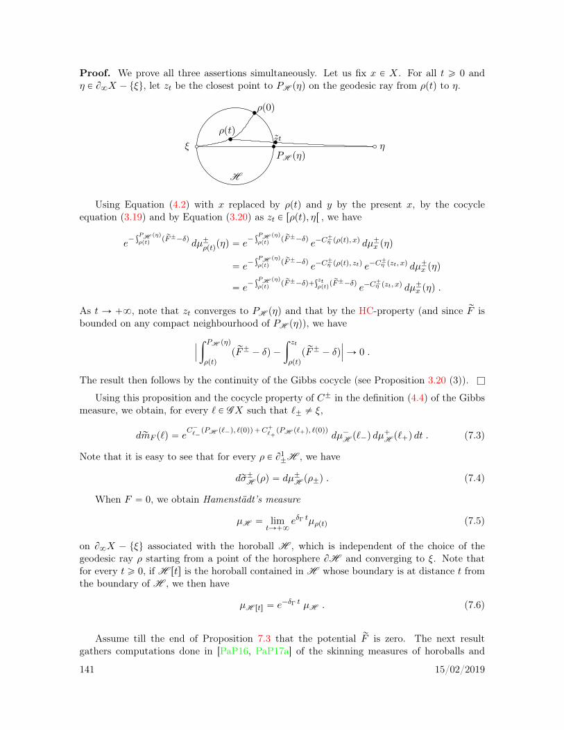
Proof. We prove all three assertions simultaneously. Let us fix x P X. For all t ě 0 andη P B8X ´ tξu, let zt be the closest point to PH pηq on the geodesic ray from ρptq to η.

H

ηξ

ρp0q

PH pηq

ztρptq

Using Equation (4.2) with x replaced by ρptq and y by the present x, by the cocycleequation (3.19) and by Equation (3.20) as zt P rρptq, ηr , we have

e´şPH pηq

ρptqp rF˘´δq

dµ˘ρptqpηq “ e´şPH pηq

ρptqp rF˘´δq

e´C˘η pρptq, xq dµ˘x pηq

“ e´şPH pηq

ρptqp rF˘´δq

e´C˘η pρptq, ztq e´C

˘η pzt, xq dµ˘x pηq

“ e´şPH pηq

ρptqp rF˘´δq`

şztρptqp rF˘´δq

e´C˘η pzt, xq dµ˘x pηq .

As t Ñ `8, note that zt converges to PH pηq and that by the HC-property (and since rF isbounded on any compact neighbourhood of PH pηq), we have

ˇ

ˇ

ˇ

ż PH pηq

ρptqp rF˘ ´ δq ´

ż zt

ρptqp rF˘ ´ δq

ˇ

ˇ

ˇÑ 0 .

The result then follows by the continuity of the Gibbs cocycle (see Proposition 3.20 (3)). l

Using this proposition and the cocycle property of C˘ in the definition (4.4) of the Gibbsmeasure, we obtain, for every ` P GX such that `˘ ‰ ξ,

drmF p`q “ eC´`´

pPH p`´q, `p0qq`C```pPH p``q, `p0qq

dµ´H p`´q dµ`H p``q dt . (7.3)

Note that it is easy to see that for every ρ P B1˘H , we have

drσ˘H pρq “ dµ˘H pρ˘q . (7.4)

When F “ 0, we obtain Hamenstädt’s measure

µH “ limtÑ`8

eδΓ tµρptq (7.5)

on B8X ´ tξu associated with the horoball H , which is independent of the choice of thegeodesic ray ρ starting from a point of the horosphere BH and converging to ξ. Note thatfor every t ě 0, if H rts is the horoball contained in H whose boundary is at distance t fromthe boundary of H , we then have

µH rts “ e´δΓ t µH . (7.6)

Assume till the end of Proposition 7.3 that the potential rF is zero. The next resultgathers computations done in [PaP16, PaP17a] of the skinning measures of horoballs and

141 15/02/2019

some totally geodesic subspaces, when X is a real or complex hyperbolic space and Γ is alattice. We consider the notation Hn

R, HnC, H8, Heis2n´1, λ2n´1 introduced in Section 4.2,

and we again endow T 1HnR and T 1Hn

C with their Sasaki’s Riemannian metric. Recall that acomplex hyperbolic line in Hn

C is a totally geodesic plane with constant sectional curvature ´4.As the arguments of the following result are purely computational and rather long, we do

not copy them in this book, but we refer respectively to the proofs of [PaP16, Prop. 11 (1),(2)] and [PaP17a, Lem. 12 (iv), (v), (vi)]. Analogous computations can be done when X isthe quaternionic hyperbolic n-space Hn

H.

Proposition 7.3. (1) Let Γ be a lattice in IsompHnRq, with Patterson density pµxqxPHnR nor-

malised as in Section 4.2.(i) If D is a horoball in Hn

R, if volB1˘D

is the Riemannian measure of the submanifold B1˘D in

T 1HnR, then

rσ˘D “ 2n´1 volB1˘D

.

If the point at infinity of D is a parabolic fixed point of Γ, with stabiliser ΓD in Γ, then2

σ˘D “ 2n´1 VolpΓDzB1˘Dq “ 2n´1 VolpΓDzBDq “ 2n´1pn´ 1qVolpΓDzDq .

(ii) If D is a totally geodesic hyperbolic subspace of dimension k P t1, . . . , n ´ 1u in HnR, if

volB1˘D

is the Riemannian measure of the submanifold B1˘D in T 1Hn

R, then

rσ˘D “ volB1˘D

.

With ΓD the stabiliser of D in Γ and m the order of the pointwise stabiliser of D in Γ, ifΓDzD has finite volume, then

σ˘D “VolpSn´k´1q

mVolpΓDzDq .

(2) Let Γ be a lattice in IsompHnCq, with Patterson density pµxqxPHnC normalised as in

Section 4.2.

(i) Using the homeomorphism v ÞÑ v˘ from B1˘H8 to B8Hn

C ´ t8u “ Heis2n´1, we have

drσ˘H8pvq “ dλ2n´1pv˘q .

For every horoball D in HnC, if volBD is the Riemannian measure of the hypersurface BD in

HnC, then

π˚rσ˘D “ 2 volBD .

If the point at infinity of D is a parabolic fixed point of Γ, with stabiliser ΓD in Γ, then

σ˘D “ 4n VolpΓDzDq .

(ii) For every geodesic line D in HnC, if volB1

˘Dis the Riemannian measure of the submanifold

B1˘D in T 1Hn

C, we havedπ˚rσ

˘D “

n

4n´1 p2n´ 1qdπ˚ volB1

˘D.

2See for instance [Hers, p. 473] for the last equality.

142 15/02/2019

With ΓD the stabiliser of D in Γ and m the order of the pointwise stabiliser of D in Γ, ifΓDzD has finite length, then

σ˘D “2πn´1 n!

m p2n´ 1q!VolpΓDzDq .

(iii) For every complex geodesic line D in HnC, if volB1

`Dis the Riemannian measure of the

submanifold B1`D in T 1Hn

C, we have

dπ˚rσ`D “

1

22n´3dπ˚ volB1

`D.

With ΓD the stabiliser of D in Γ and m the order of the pointwise stabiliser of D in Γ, ifΓDzD has finite area, then

σ`D “πn´1

m 4n´2 pn´ 2q!VolpΓDzDq . l

The following results give the basic properties of the skinning measures analogous to thosein [PaP14a, Sect. 3] when the potential is zero.

Proposition 7.4. Let D be a nonempty proper closed convex subset of X, and let rσ˘D be theskinning measures on B1

˘D for the potential rF .(i) The skinning measures rσ˘D are independent of x0.(ii) For all γ P Γ, we have γ˚rσ˘D “ rσ˘γD. In particular, the measures rσ˘D are invariant underthe stabiliser of D in Γ.(iii) For all s ě 0 and w P B1

˘D, we have3

d rσ˘NsDppg˘swq

ˇ

ˇ

˘r0,`8rq “ eC

˘w˘pπpwq, πpg˘swqq drσ˘Dpwq

“ e´şπpg˘swqπpwq

p rF˘´δqdrσ˘Dpwq .

(iv) The support of rσ˘D is

tv P B1˘D : v˘ P ΛΓu “ P˘D pΛΓ´ pΛΓX B8Dqq .

In particular, rσ˘D is the zero measure if and only if ΛΓ is contained in B8D.

For future use, the version4 of Assertion (iii) when F “ 0 is

dpg˘sq˚rσ˘D

d rσ˘NsD

pg˘swq “ e´δΓ s , (7.7)

where w P B1˘D and we again denote by g˘s the map from B1

˘D to B1˘N1D defined by

w ÞÑ pg˘swqˇ

ˇ

˘r0,`8r.

As another particular case of Assertion (iii) for future use, consider the case whenX “ |X|λis the geometric realisation of a metric tree pX, λq and when rF “ rFc is the potential associated

3denoting by pg˘swq|˘r0,`8r the element of G˘, 0 which coincides with g˘sw on ˘r0,`8r4contained in [PaP14a, Prop. 4]

143 15/02/2019

with a system of conductances rc on X for a subgroup Γ of AutpXq (see Equation (3.23) andProposition 3.22). Then for all w P B1

`D (respectively w P B1´D), if ew is the first (respectively

the last) edge followed by w, with length λpewq, then

ż πpg˘λpewqwq

πpwq

rF˘ “ rcpewq λpewq

by Proposition 3.21, so that

d rσ˘NsDppg˘λpewqwq|˘r0,`8rq “ e´prcpewq`δqλpewq drσ˘Dpwq . (7.8)

Proof. The proofs of the claims are straightforward modifications of those for zero potentialin [PaP14a, Prop. 4]. We give details of the proofs for the measure rσ`D, the case of rσ´D beingsimilar.(i) The claim follows from Equation (4.2) and the cocycle property (3.19).(ii) The claim follows from Equation (4.1), the first part of Equation (3.19) and Claim (i).(iii) Since

`

pgswq|r0,`8r˘

`“ w` and since w P B1

`D if and only if pgswq|r0,`8r P B1`NsD, we

have, using the definition (7.1) of the skinning measure and the cocycle property (3.19), forall s ě 0,

d rσ`NsDppgswq|r0,`8rq “ eC

`w`px0, πpgswqq dµ`x0

pw`q “ eC`w`pπpwq, πpgswqq d rσ`Dpwq .

This proves Claim (iii) for rσ`D, using Equation (3.20).(iv) The claims follow from the fact that the support of any Patterson measure is ΛΓ, seeSubsection 4.1. l

Given two nonempty closed convex subsets D and D1 of X, let

AD,D1 “ B8X ´ pB8D Y B8D1q

and let h˘D,D1 : P˘D pAD,D1q Ñ P˘D1pAD,D1q be the restriction of P˘D1 ˝ pP˘D q´1 to P˘D pAD,D1q. It

is a homeomorphism between open subsets of B1˘D and B1

˘D1, associating to the element w

in the domain the unique element w1 in the range with w1˘ “ w˘.

Proposition 7.5. Let D and D1 be nonempty closed convex subsets of X and let h˘ “ h˘D,D1 .The measures ph˘q˚ rσ˘D and rσ˘D1 on P

˘D1pAD,D1q are absolutely continuous one with respect to

the other, withdph˘q˚ rσ

˘D

drσ˘D1pw1q “ e´C

˘w˘pπpwq, πpw1qq,

for (almost) all w P P˘D pAD,D1q and w1 “ h˘pwq.

Proof. As w1˘ “ w˘, we have

drσ˘D1pw1q “ e

C˘w1˘

px0, πpw1qqdµ˘x0

pw1˘q “ eC˘w1˘

px0, πpwqqeC˘w1˘

pπpwq, πpw1qqdµ˘x0

pw1˘q

“ eC˘w˘pπpwq, πpw1qq drσ˘Dpwq

using the definition (7.1) of the skinning measure and the cocycle property (3.19). l

144 15/02/2019

Let w P G˘X. With N˘w : W˘pwq Ñ B1¯HB˘pwq the canonical homeomorphism defined in

Section 2.4, we define the skinning measures µW˘pwq on the strong stable or strong unstableleaves W˘pwq by

µW˘pwq “ ppN˘w q´1q˚rσ

¯

HB˘pwq,

so that

dµW˘pwqp`q “ eC¯`¯

px0, `p0qqdµ¯x0

p`¯q (7.9)

for every ` P W˘pwq. By Proposition 7.4 (ii) and the naturality of N˘w , for every γ P Γ, wehave

γ˚µW˘pwq “ µW˘pγwq . (7.10)

By Proposition 7.4 (iv), the support of µW˘pwq is t` PW˘pwq : `¯ P ΛΓu. For all t P R and` PW˘pwq, we have, using Equations (7.9), (3.19) and (3.20), and since `˘ “ w˘,

dpg´tq˚µW˘pwq

dµW˘pgtwqpgt`q “ e

C¯`¯p`ptq, `p0qq

“ eC˘w˘p`p0q, `ptqq . (7.11)

Let w P G˘X. The homeomorphisms W˘pwq ˆ RÑW 0˘pwq, defined by

p`, sq ÞÑ `1 “ gs` ,

conjugate the actions of R by translation on the second factor of the domain and by thegeodesic flow on the range, and the actions of Γ (trivial on the second factor of the domain).Let us consider the measures ν¯w on W 0˘pwq given, using the above homeomorphism, by

dν¯w p`1q “ eC

˘w˘pwp0q, `p0qq dµW˘pwqp`q ds . (7.12)

They satisfy pgtq˚ν˘w “ ν˘w for all t P R (since if `1 “ gs`, then g´t`1 “ gs´t`, and byinvariance under translations of the Lebesgue measure on R). Furthermore, γ˚ν˘w “ ν˘γw forall γ P Γ. In general, they depend on w, not only on W˘pwq. Furthermore, the support ofν˘w is t`1 P W 0˘pwq : `1¯ P ΛΓu. These properties follow easily from the properties of theskinning measures on the strong stable or strong unstable leaves.

Lemma 7.6. (i) For every nonempty proper closed convex subset D1 in X, there exists R0 ą 0such that for all R ě R0, η ą 0, and w P B1

˘D1, we have ν¯w pV

˘w, η,Rq ą 0.5

(ii) For all w P G˘X and t P R, the measures ν¯gtw and ν¯w are proportional:

ν¯gtw “ eC

˘w˘pwptq, wp0qq ν¯w .

Proof. (i) Let us show, as in [PaP14a, Lem. 7], that there exists R0 ą 0 (depending only onD1 and on the Patterson densities) such that for all R ě R0, w P B1

`D1 and w1 P B1

´D1, we

have µW`pwqpB`pw,Rqq ą 0 and µW´pw1qpB

´pw1, Rqq ą 0. The result follows from this bythe definitions of ν¯w and V ˘w, η,R.

5See Section 2.4 for the definition of V ˘w, η,R.

145 15/02/2019

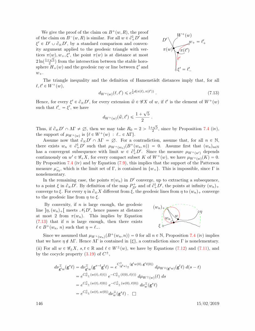
We give the proof of the claim on B`pw,Rq, the proofof the claim on B´pw,Rq is similar. For all w P B1

`D1 and

ξ1 P D1 Y B8D1, by a standard comparison and convex-

ity argument applied to the geodesic triangle with ver-tices πpwq, w`, ξ1, the point πpwq is at distance at most2 lnp1`

?5

2 q from the intersection between the stable horo-sphere H`pwq and the geodesic ray or line between ξ1 andw`.

ξ1 “ `1´

`1

πpwq

W`pwq

w` “ `1`

πp`1q

D1

The triangle inequality and the definition of Hamenstädt distances imply that, for all`, `1 PW`pwq,

dW`pwqp`, `1q ď e

12dpπp`q, πp`1qq . (7.13)

Hence, for every ξ1 P B8D1, for every extension pw P GX of w, if `1 is the element of W`pwqsuch that `1´ “ ξ1, we have

dW`pwqp pw, `1q ď

1`?

5

2.

Thus, if B8D1 X ΛΓ ‰ H, then we may take R0 “ 2 ą 1`?

52 , since by Proposition 7.4 (iv),

the support of µW`pwq is t` PW`pwq : `´ P ΛΓu.Assume now that B8D1 X ΛΓ “ H. For a contradiction, assume that, for all n P N,

there exists wn P B1`D

1 such that µW`pwnqpB`pwn, nqq “ 0. Assume first that pwnqnPN

has a convergent subsequence with limit w P B1`D

1. Since the measure µW`pw1q dependscontinuously on w1 P G`X, for every compact subset K of W`pwq, we have µW`pwqpKq “ 0.By Proposition 7.4 (iv) and by Equation (7.9), this implies that the support of the Pattersonmeasure µ´x0

, which is the limit set of Γ, is contained in tw`u. This is impossible, since Γ isnonelementary.

In the remaining case, the points πpwnq in D1 converge, up to extracting a subsequence,to a point ξ in B8D1. By definition of the map P`D1 and of B1

`D1, the points at infinity pwnq`

converge to ξ. For every η in B8X different from ξ, the geodesic lines from η to pwnq` convergeto the geodesic line from η to ξ.

By convexity, if n is large enough, the geodesicline sη, pwnq`r meets N1D

1, hence passes at distanceat most 2 from πpwnq. This implies by Equation(7.13) that if n is large enough, then there exists` P B`pwn, nq such that η “ `´.

pwnq`

wwn

η

ξ

Since we assumed that µW`pwnqpB`pwn, nqq “ 0 for all n P N, Proposition 7.4 (iv) implies

that we have η R ΛΓ. Hence ΛΓ is contained in tξu, a contradiction since Γ is nonelementary.

(ii) For all w P G˘X, s, t P R and ` P W˘pwq, we have by Equations (7.12) and (7.11), andby the cocycle property (3.19) of C˘,

dν¯gtwpg

s`q “ dν¯gtwpg

s´tgt`q “ eC˘pgtwq˘

pgtwp0q, gt`p0qqdµW˘pgtwqpg

t`q dps´ tq

“ eC˘w˘pwptq, `ptqq e´C

˘w˘p`p0q, `ptqq dµW˘pwqp`q ds

“ eC˘w˘pwptq, `p0qq e´C

˘w˘pwp0q, `p0qq dν¯w pg

s`q

“ eC˘w˘pwptq, wp0qqdν¯w pg

s`q . l

146 15/02/2019

The following disintegration result of the Gibbs measure over the skinning measures ofany closed convex subset is a crucial tool for our equidistribution and counting results. Recallthe definition in Equation (2.15) of the flow-invariant open sets U ˘

D and the definition of thefibrations f˘D : U ˘

D Ñ B1˘D from Section 2.4.

Proposition 7.7. Let D be a nonempty proper closed convex subset of X. The restriction toU ˘D of the Gibbs measure rmF disintegrates by the fibration f˘D : U ˘

D Ñ B1˘D over the skinning

measure rσ˘D of D, with conditional measure ν¯ρ on the fiber pf˘D q´1pρq “W 0˘pρq of ρ P B1

˘D:when ` ranges over U ˘

D , we have

drmF |U ˘Dp`q “

ż

ρPB1˘D

dν¯ρ p`q drσ˘Dpρq .

Proof. In order to prove the claim for the fibration f`D , let φ P CcpU`D q. Using in the various

steps below:• Hopf’s parametrisation with time parameter t and the definitions of rmF (see Equation

(4.4)) and of U `D (see Equation (2.15)),

• the positive endpoint homeomorphism w ÞÑ w` from B1`D to B8X´B8D, and the negative

endpoint homeomorphism `1 ÞÑ `1´ from W`pwq to B8X ´ tw`u, with s P R the realparameter such that `1 “ g´s` P W`pwq where ` P W 0`pwq, noting that t ´ s dependsonly on `` “ w` and `´ “ `1´,

• the definitions Equation (7.9) and (7.1) of the measures µW`pwq and rσ`D, and the cocycleproperty (3.19) of C˘,

• Equation (3.20) and the cocycle property (3.19) of C`,we have

ż

`PU `D

φp`q drmF p`q

“

ż

``PB8X´B8D

ż

`´PB8X´t``u

ż

tPRφp`q e

C´`´px0, πp`qq`C

```px0, πp`qq

dt dµ´x0p`´q dµ

`x0p``q

“

ż

wPB1`D

ż

`1PW`pwq

ż

sPRφpgs`1q e

C´`1´

px0, πpgs`1qq`C`w`

px0, πpgs`1qq

ds dµ´x0p`1´q dµ

`x0pw`q

“

ż

wPB1`D

ż

`1PW`pwq

ż

sPRφpgs`1q e

C´`1´

pπp`1q, πpgs`1qq`C`w`pπpwq, πpgs`1qq

ds dµW`pwqp`1q drσ`Dpwq

“

ż

wPB1`D

ż

`1PW`pwq

ż

sPRφpgs`1q e

C`w`pπpwq, πp`1qq

ds dµW`pwqp`1q drσ`Dpwq ,

which implies the claim for the fibration f`D , by the definition (7.12) of the measure ν´w . Theproof for the fibration f´D is similar. l

For every u P G´X, if D “ HB´puq, we have B1`D “ N´u pW

´puqq and

U `D “ GX ´W 0`pιuq “

ď

wPW´puq

W 0`pwq .

Applying the above proposition and a change of variable, the restriction to GX ´W 0`pιuq ofthe Gibbs measure rmF disintegrates over the strong unstable measure µW´puq “ ppN

´u q´1q˚rσ

`D,

147 15/02/2019

with conditional measure on the fiber W 0`pwq of w P W´puq the measure ν´w “ ν´N´u pwq

: for

every φ P CcpGX ´W 0`pιuqq, we haveż

`PGX´W 0`pιuqφp`q drmF p`q “

ż

wPW´puq

ż

`1PW`pwq

ż

sPRφpgs`1q eC

`w`pπpwq, πp`1qq ds dµW`pwqp`

1q dµW´puqpwq . (7.14)

Note that if the Patterson densities have no atoms, then the stable and unstable leaves havemeasure zero for the associated Gibbs measure. This happens for instance if the Gibbs measuremF is finite, see Corollary 4.7 and Theorem 4.6.

7.2 Equivariant families of convex subsets and their skinningmeasures

Let I be an index set endowed with a left action of Γ. A family D “ pDiqiPI of subsets of Xor of

p

GX indexed by I is Γ-equivariant if γDi “ Dγi for all γ P Γ and i P I. We will denoteby

„ “ „D

the equivalence relation on I defined by i „ j if and only if Di “ Dj and there exists γ P Γsuch that j “ γi. This equivalence relation is Γ-equivariant: for all i, j P I and γ P Γ, wehave γi „ γj if and only if i „ j. We say that D is locally finite if for every compact subsetK in X or in

p

GX, the quotient set ti P I : Di XK ‰ Hu„ is finite.

Examples. (1) Fixing a nonempty proper closed convex subset D of X, taking I “ Γ withthe left action by translations pγ, iq ÞÑ γi, and setting Di “ iD for every i P Γ gives aΓ-equivariant family D “ pDiqiPI . In this case, we have i „ j if and only if i´1j belongs tothe stabiliser ΓD of D in Γ, and I„ “ ΓΓD. Note that γD depends only on the class rγs of γin ΓΓD. We could also take I 1 “ ΓΓD with the left action by translations pγ, rγ1sq ÞÑ rγγ1s,and D 1 “ pγDqrγsPI 1 , so that for all i, j P I 1, we have i „D 1 j if and only if i “ j, and besides,D 1 is locally finite if and only if D is locally finite. The following choices of D yield equivariantfamilies with different characteristics:

(a) Let γ0 P Γ be a loxodromic element with translation axisD “ Axγ0 . The family pγDqγPΓis locally finite and Γ-equivariant. Indeed, by Lemma 2.1, only finitely many elementsof the family pγDqγPΓΓD meet any given bounded subset of X.

(b) Let ` P GX be a geodesic line whose image under the canonical map GX Ñ ΓzGX hasa dense orbit in ΓzGX under the geodesic flow, and let D “ `pRq be its image. Thenthe Γ-equivariant family pγDqγPΓ is not locally finite.

(c) More generally, let D be a convex subset such that ΓDzD is compact. Then the familypγDqγPΓ is a locally finite Γ-equivariant family.

(d) Let ξ P B8X be a bounded parabolic limit point of Γ, and let H be any horoball in Xcentred at ξ. Then the family pγH qγPΓ is a locally finite Γ-equivariant family.

148 15/02/2019

(2) More generally, let pDαqαPA be a finite family of nonempty proper closed convex subsetsof X, and for every α P A, let Fα be a finite set. Define I “

Ť

αPA Γ ˆ tαu ˆ Fα with theaction of Γ by left translation on the first factor, and for every i “ pγ, α, xq P I, let Di “ γDα.Then I„ “

Ť

αPA ΓΓDα ˆ tαu ˆ Fα and the Γ-equivariant family D “ pDiqiPI is locallyfinite if and only if the family pγDαqγPΓ is locally finite for every α P A. The cardinalities ofFα for α P A contribute to the multiplicities (see Section 12.2).

Let D “ pDiqiPI be a locally finite Γ-equivariant family of nonempty proper closed convexsubsets of X. Let Ω “ pΩiqiPI be a Γ-equivariant family of subsets of

p

GX, where Ωi is ameasurable subset of B1

˘Di for all i P I (the sign ˘ being constant), such that Ωi “ Ωj ifi „D j. Then

rσ˘Ω “ÿ

iPI„

rσ˘Di |Ωi ,

is a well-defined Γ-invariant locally finite measure onp

GX, whose support is contained inG˘, 0X. Hence, the measure rσ˘Ω induces6 a locally finite measure on Γz

p

GX, denoted by σ˘Ω .When Ω “ B1

˘D “ pB1˘DiqiPI , the measure rσ˘Ω is denoted by

rσ˘D “ÿ

iPI„

rσ˘Di .

The measures rσ`D and rσ´D are respectively called the outer and inner skinning measures of D

onp

GX, and their induced measures σ`D and σ´D on Γz

p

GX are the outer and inner skinningmeasures of D on Γz

p

GX.

Example. Consider the Γ-equivariant family D “ pγDqγPΓΓx with D “ txu a singleton inX. With π˘ “ pP˘D q

´1 : B1˘D Ñ B8X the homeomorphism ρ ÞÑ ρ˘, we have pπ˘q˚rσ˘D “ µ˘x

by Remark 7.1 (1), and7

σ˘D “µ˘x

|Γx|. (7.15)

6See for instance [PauPS, §2.6] and the beginning of Chapter 12 for details on the definition of the inducedmeasure when Γ may have torsion, hence does not necessarily acts freely on

p

GX.7See also the beginning of Chapter 12.

149 15/02/2019

150 15/02/2019

Chapter 8

Explicit measure computations forsimplicial trees and graphs of groups

In this Chapter, we compute skinning measures and Bowen-Margulis measures for some highlysymmetric simplicial trees X endowed with a nonelementary discrete subgroup Γ of AutpXq.These computations are parallel to the ones given in Section 4.2 when X is a rank onesymmetric space. The potentials F are supposed to be 0 in this Chapter, and we assumethat the Patterson densities pµ`x qxPV X and pµ´x qxPV X of Γ are equal, denoted by pµxqxPV X. Asthe study of geometrically finite discrete subgroups of AutpXq mostly reduces to the study ofparticular (tree) lattices (see Remark 2.12), we will assume that Γ is a lattice in this Chapter.

The results of these computations will be useful when we state special cases of the equidis-tribution and counting results in regular and biregular trees and, in particular, in the arith-metic applications in Part III. The reader only interested in the continuous time case mayskip directly to Chapter 9.

A rooted simplicial tree pX, x0q is spherically symmetric if X is not reduced to x0 and hasno terminal vertex, and if the stabiliser of x0 in AutpXq acts transitively on each sphere ofcentre x0. The set of isomorphism classes of spherically symmetric rooted simplicial treespX, x0q is in bijection with the set of sequences ppnqnPN in N´t0u, where pn` 1 is the degreeof any vertex of X at distance n from x0.

x0

p0 ` 1 p2p1 p3 . . .

If pX, x0q is spherically symmetric, it is easy to check that the simplicial tree X is uniform1

if and only if the sequence ppnqnPN is periodic with palindromic period in the sense that there1See Section 2.6 for the terminology concerning simplicial trees.

151 15/02/2019

exists N P N´ t0u such that pn`N “ pn for every n P N and pN´n “ pn for every n P N suchthat n ď N . If N “ 1, then X “ Xp0 is the regular tree of degree p0 ` 1, and if N “ 2, thenX “ Xp0, p1 is the biregular tree of degrees p0 ` 1 and p1 ` 1.

We denote by X “ |X|1 the geometric realisation of X. The Hausdorff dimension hX ofB8X for any visual distance is then

hX “1

Nlnpp0 . . . pN´1q , (8.1)

see for example [Lyo, p. 935].

8.1 Computations of Bowen-Margulis measures for simplicialtrees

The next result gives examples of computations of the total mass of Bowen-Margulis measuresfor lattices of simplicial trees having some regularity properties.

Analogous computations can be performed for Riemannian manifolds having appropriateregularity properties. We refer for instance to [PaP16, Prop. 10] and [PaP17b, Prop. 20(1)] for computations of Bowen-Margulis measures for lattices in the isometry group of thereal hyperbolic spaces, and to [PaP17a, Lem. 12 (iii)] for the computation in the complexhyperbolic case. In both cases, the main point is the computation of the proportionalityconstant between the Bowen-Margulis measure and Sasaki’s Riemannian volume of the unittangent bundle. When dealing now with simplicial trees, similar consequences of homogeneityproperties will appear below.

We refer to Section 2.6 for the definitions of vol, Vol, Tπ, Tvol, TVol appearing in thefollowing result.

Proposition 8.1. Let pX, x0q be a spherically symmetric rooted simplicial tree, with associatedsequence ppnqnPN, such that X is uniform, and let Γ be a lattice of X.(1) For every x P V X, let rx “ dpx,AutpXqx0q, and let

cx “pprx ´ 1qe2 rx hX

pp0 ` 1q2p21 . . . p

2rx´1prx

`2p0

pp0 ` 1q2

if rx ‰ 0 and cx “ p0

p0`1 if rx “ 0. Then

mBM “ÿ

rxsPΓzV X

1

|Γx|

`

µx2 ´

ÿ

ePEX : opeq“x

µxpBeXq2˘

“ µx02

ÿ

rxsPΓzV X

cx|Γx|

. (8.2)

(2) If X “ Xp, q is the biregular tree of degrees p ` 1 and q ` 1, with V X “ VpX \ VqX thecorresponding partition of the set of vertices of X, if the Patterson density pµxqxPV X of Γ isnormalised so that µx “ p`1

?p for all x P VpX, then

pTπq˚mBM “ TvolΓzzX

152 15/02/2019

andmBM “ TVolpΓzzXq “

ÿ

rxsPΓzVpX

p` 1

|Γx|`

ÿ

rxsPΓzVqX

q ` 1

|Γx|. (8.3)

(3) If X “ Xq is the regular tree of degree q ` 1, if the Patterson density pµxqxPV X of Γ isnormalised to be a family of probability measures, then

π˚mBM “q

q ` 1volΓzzX

and in particularmBM “

q

q ` 1VolpΓzzXq . (8.4)

Proof. We start by proving the first equality of Assertion (1). For every x P V X, we maypartition the set of geodesic lines ` P GX with `p0q “ x according to the two edges startingfrom x contained in the image of `. The only restriction for the edges is that they are requiredto be distinct.

For every e P EX, recall from Section 2.6 that BeX is the set of points at infinity of thegeodesic rays whose initial edge is e. For all e P EX and x P V X, say that e points away fromx if opeq P rx, tpeqs, and that e points towards x otherwise. In particular, all edges with originx point away from x. Hence by Equation (4.13), and since µx “ µ´x “ µ`x , we have

π˚mBM “ÿ

rxsPΓzV X

1

|Γx|

ÿ

e, e1PEX : opeq“ope1q“x, e‰e1

µ´x pBeXq µ`x pBe1Xq ∆rxs (8.5)

“ÿ

rxsPΓzV X

1

|Γx|

´

`

ÿ

ePEX : opeq“x

µxpBeXq˘2´

ÿ

ePEX : opeq“x

µxpBeXq2¯

∆rxs . (8.6)

This gives the first equality of Assertion (1).

Let us prove the second equality of Assertion (1). By homogeneity, we assume thatµx0 “ 1 and we will prove that

mBM “ÿ

rxsPΓzV X

cx|Γx|

.

Let N P N ´ t0u be such that pn`N “ pn for every n P N and pN´n “ pn for everyn P t0, . . . , Nu, which exists since X is assumed to be uniform. Then the automorphismgroup AutpXq of the simplicial tree X acts transitively on the set of vertices at distance amultiple of N from x0. Hence for every x P V X, the distance rx “ dpx,AutpXqx0q belongs to

0, 1, . . . , tN2 u(

, and there exist γx, γ1x P AutpXq such that

dpx, γxx0q “ rx, x P rγxx0, γ1xx0s and dpγxx0, γ

1xx0q “ N .

The map x ÞÑ rx is constant on the orbits of Γ in V X,2 hence so is the map x ÞÑ cx, and thusthe right hand side of Equation (8.2) is well defined.

Since the family pµHausx qxPV X of Hausdorff measures of the visual distances pB8X, dxq is

invariant under any element of AutpXq, since Γ is a lattice and by Proposition 4.16, we haveδΓ “ hX and γ˚µx “ µγx for all x P V X and γ P AutpXq.

2In fact, it is constant on the orbits of AutpXq.

153 15/02/2019

Since pX, x0q is spherically symmetric, and since µx0 is a probability measure, we have byinduction, for every e P EX pointing away from x0 with dpx0, opeqq “ n,

µx0pBeXq “1

pp0 ` 1q p1 . . . pn(8.7)

if n ‰ 0, and µx0pBeXq “ 1p0`1 otherwise.

For every fixed x P V X, let us now compute µxpBeXq for every edge e of X with origin x.Let γ “ γx, γ

1 “ γ1x P AutpXq be as above. By the spherical transitivity, we may assume thate or e belongs to the edge path from γx0 to γ1x0.

rx

γx0

ex γ1x0

N ´ rx

There are two cases to consider.

Case 1: Assume first that e points away from γx0. There are p0 ` 1 such edges startingfrom x if rx “ 0, and prx otherwise. By Equation (8.7) and by invariance under AutpXq ofpµHausx qxPV X, we have

µγx0pBeXq “1

pp0 ` 1q p1 . . . prx,

with the convention that the denominator is p0 ` 1 if rx “ 0. Since the map ξ ÞÑ βξpx, γx0q

is constant with value ´rx on BeX, and by the quasi-invariance property of the Pattersondensity (see Equation (4.2)), we have

µxpBeXq “ e´δΓp´rxqµγx0pBeXq “erxhX

pp0 ` 1q p1 . . . prx,

with the same convention as above.

Case 2: Assume now that e points towards γx0. This implies that rx ě 1, and there is oneand only one such edge starting from x. Then as above we have

µγ1x0pBeXq “1

ppN ` 1q pN´1 . . . prx,

and

µxpBeXq “ e´δΓp´pN´rxqqµγ1x0pBeXq “epN´rxqhX

ppN ` 1q pN´1 . . . prx.

For every x P V X, let

Cx “´

ÿ

ePEX : opeq“x

µxpBeXq¯2´

ÿ

ePEX : opeq“x

µxpBeXq2 . (8.8)

154 15/02/2019

If rx ‰ 0, since the stabiliser of γx0 in AutpXq acts transitively on the prx edges with originx pointing away from γx0, since eNhX “ p0p1 . . . pN´1 and pN “ p0, we have

Cx “´

prxerxhX

pp0 ` 1q p1 . . . prx`

epN´rxqhX

ppN ` 1q pN´1 . . . prx

¯2

´

´

prx` erxhX

pp0 ` 1q p1 . . . prx

˘2`` epN´rxqhX

ppN ` 1q pN´1 . . . prx

˘2¯

“pprx

2´ prxq e

2 rxhX

pp0 ` 1q2 p12 . . . prx

2`

2 prxeN hX

pp0 ` 1q p1 . . . prxprx . . . pN´1ppN ` 1q

“pprx ´ 1q e2 rxhX

pp0 ` 1q2 p12 . . . prx´1

2prx`

2 p0

pp0 ` 1q2“ cx .

If rx “ 0, we have

Cx “´

pp0 ` 1q1

p0 ` 1

¯2´ pp0 ` 1q

´ 1

p0 ` 1

¯2“

p0

p0 ` 1“ cx .

Assertion (1) now follows from Equation (8.6).

Let us prove Assertion (2). Note that X “ Xp, q is spherically symmetric with respect toany vertex of X, and that, by Equation (8.1),

hX “1

2lnppqq .

Let e be an edge of X, with x “ opeq P VpX and y “ tpeq P VqX. For every z P V X, we defineCz as in Equation (8.8).

Note that by homogeneity, we have Cz “ Cx and µz “ µx for all z P VpX, as well asCz “ Cy and µz “ µy for all z P VqX. Hence the normalisation of the Patterson densityas in the statement of Assertion (2) is possible. By the spherical symmetry at x, and thenormalisation of the measure, we have µxpBeXq “ 1?

p and µxpBeXq “?p. Therefore

µy “ µypBeXq ` µypBeXq “ ehXµxpBeXq ` e´hXµxpBeXq

“?pq

1?p`

1?pq

?p “

q ` 1?q

.

This symmetry in the values of µy and µx explains the choice of our normalisation of thePatterson density. We have

Cx “ µx2 ´ pp` 1q

´

µx

p` 1

¯2“

p

p` 1µx

2 “ p` 1

and similarly Cy “ qq`1µy

2 “ q ` 1. This proves the second equality in Equation (8.3), bythe first equation of Assertion (1).

In order to prove that pTπq˚mBM “ TvolΓzzX, we now partition ΓzGX as

ď

resPΓzEXΓz

` P GX : `p0q “ πpopeqq, `p1q “ πptpeqq(

.

155 15/02/2019

Using on every element of this partition Hopf’s decomposition with respect to the basepointopeq, we have, by a ramified covering argument already used in the proof of the second partof Proposition 4.15,

pTπq˚mBM “ÿ

resPΓzEX

1

|Γe|µopeqpB8X ´ BeXq µopeqpBeXq ∆res .

Since µopeqpBeXq “ e´hXµtpeqpBeXq and by homogeneity, we have

pTπq˚mBM “ÿ

resPΓzEX

1

|Γe|

deg opeq ´ 1

deg opeqµopeq

deg tpeq ´ 1

deg tpeqµtpeq e

´hX ∆res

“ÿ

resPΓzEX

1

|Γe|

µopeq µtpeq?pq

pp` 1qpq ` 1q∆res “ TvolΓzzX .

The first equality of Equation (8.3) follows, since pushforwards of measures preserve the totalmass.

Finally, the last claim of Assertion (3) of Proposition 8.1 follows from Equation (8.2), sincecx “

qq`1 for every x P V Xq (or by taking q “ p in Equation (8.3) and by renormalising). The

first claim of Assertion (3) follows from the first claim of Assertion (2), by using Equation(2.23) and renormalising. l

Remark 8.2. (1) In particular, if X “ Xq is regular, if the Patterson density is normalisedto be a family of probability measures and if Γ is torsion free, then π˚mBM is q

q`1 times thecounting measure on ΓzV X. In this case, Equation (8.4) is given by [CoP4, Rem. 2].(2) If X “ Xp, q is biregular with p ‰ q, then π˚mBM is not proportional to volΓzzX. Inparticular, if Γ is torsion free and if the Patterson density is normalised to be a family ofprobability measures, then π˚mBM is the sum of p

p`1 times the counting measure on ΓzVpXand q

q`1 times the counting measure on ΓzVqX.This statement is coherent with the well-known fact that in pinched but variable cur-

vature, the Bowen-Margulis measure is generally not absolutely continuous with respect toSasaki’s Riemannian measure on the unit tangent bundle (they would then be proportionalby ergodicity of the geodesic flow in the lattice case).

8.2 Computations of skinning measures for simplicial trees

We now give examples of computations of the total mass of skinning measures (for zeropotentials), after introducing some notation. Let X be a locally finite simplicial tree withoutterminal vertices, and let Γ be a discrete subgroup of AutpXq.

For every simplicial subtree D of X, we define the boundary BV D of V D in X as

BV D “ tx P V D : D e P EX, opeq “ x, tpeq R V Du .

The boundary BD of D is the maximal subgraph (which might be non connected) of X withset of vertices BV D. It is contained in D. The stabiliser ΓD of D in Γ acts discretely on BD.

For every x P V X, we define the codegree of x in D as codegDpxq “ 0 if x R D and otherwise

codegDpxq “ degXpxq ´ degDpxq .

156 15/02/2019

Note that codegDpxq “ 0 if x R BV D, and that the codegree codegN1Dpxq of x P V X in the1-neighbourhood N1D of D is equal to 0 unless x lies in the boundary of N1D, in which caseit is equal to degXpxq ´ 1.

Let D “ pDiqiPI be a locally finite Γ-equivariant family of simplicial subtrees of X, and letx P V X. We define the multiplicity3 of x in (the boundary of) D as (see Section 7.2 for thedefinition of „D)

mDpxq “Cardti P I„D : x P BV Diu

|Γx|.

The numerator and the denominator are finite by the local finiteness of the family D andthe discreteness of Γ, and they depend only on the orbit of x under Γ. Note that if D is asimplicial subtree of X which is precisely invariant under Γ (that is, whenever γ P Γ is suchthat DX γD is nonempty, then γ belongs to the stabiliser ΓD of D in Γ), if D “ pγDqγPΓΓD ,and if x P BV D, then

mDpxq “1

|Γx|.

In particular, if furthermore Γ is torsion free, then mDpxq “ 1 if x P BV D, and mDpxq “ 0otherwise.

Example 8.3. Let G be a connected graph without vertices of degree ď 2 and let X be itsuniversal cover, with covering group Γ. If C is a cycle in G “ ΓzX and if D is the family ofgeodesic lines in X lifting C, then mDpxq “ 1 for all x P V X whose image in G “ ΓzX belongsto C if C is a simple cycle (that is, if C passes through no vertex twice).

We define the codegree of x in D as

codegDpxq “ÿ

iPI„D

codegDipxq ,

which is well defined as codegDipxq depends only on the class of i P I modulo „D . Note that

codegDpxq “ pdegX x´ kq |Γx|mDpxq (8.9)

if degDipxq “ k for every x P BV Di and i P I. If every vertex of X has degree at least 3, this isin particular the case with k “ 2 if Di is a line for all i P I and with k “ 1 if Di is a horoballfor all i P I.

We will say that a simplicial subtree D of X, with stabiliser ΓD in Γ, is almost preciselyinvariant if there exists N P N such that for every x P V D, the number of γ P ΓΓD such thatx P γV D is at most N . It follows from this property that if D “ pγDqγPΓ, then D is locallyfinite and codegDpxq ď N codegDpxq for every x P V X.

Proposition 8.4. Assume that X is a regular or biregular simplicial tree with degrees at least3, and that Γ is a lattice of X.(1) For every simplicial subtree D of X, we have

π˚rσ˘D “

ÿ

xPV X

µx codegDpxq

degXpxq∆x .

3See Section 12.2 for explanations on the terminology.

157 15/02/2019

(2) If D “ pDiqiPI is a locally finite Γ-equivariant family of simplicial subtrees of X, then

π˚σ˘D “

ÿ

rxsPΓzV X

µx codegDpxq

|Γx| degXpxq∆rxs .

(3) Let k P N and let D be a simplicial subtree of X such that degDpxq “ k for every x P BV Dand the Γ-equivariant family D “ pγDqΓΓD is locally finite. Then

π˚σ˘D “

ÿ

ΓDy PΓDzBV D

µy pdegXpyq ´ kq

|pΓDqy| degXpyq∆Γy .

(4) If D is a simplicial subtree of X such that the Γ-equivariant family D “ pγDqγPΓ is locallyfinite, then the skinning measure σ˘D is finite if and only if the graph of groups ΓDzzBD hasfinite volume.

Before proving Proposition 8.4, let us give some immediate consequences of its Assertion(3). If X “ Xp, q is biregular of degrees p ` 1 and q ` 1, let V X “ VpX \ VqX be thecorresponding partition of the set of vertices of X and, for r P tp, qu, let BrD be the edgelessgraph with set of vertices BV DX VrX.

Corollary 8.5. Assume that pX,Γq is as in Proposition 8.4. Let D be a simplicial subtree ofX such that the Γ-equivariant family D “ pγDqγPΓΓD is locally finite.

(1) If X “ Xp, q is biregular of degrees p` 1 and q ` 1 and if the Patterson density pµxqxPV X

of Γ is normalised so that µx “degXpxq?degXpxq´1

for all x P V X, then

‚ if D is a horoball,

σ˘D “?p VolpΓDzzBpDq `

?q VolpΓDzzBqDq ,

‚ if D is a line,

σ˘D “p´ 1?p

VolpΓDzzBpDq `q ´ 1?q

VolpΓDzzBqDq . (8.10)

(2) If X “ Xq is the regular tree of degree q ` 1 and if the Patterson measures pµxqxPV X arenormalised to be probability measures, then

‚ if D is a horoball,σ˘D “

q

q ` 1VolpΓDzzBDq (8.11)

‚ if D is a line,

σ˘D “q ´ 1

q ` 1VolpΓDzzDq . l (8.12)

Proof of Proposition 8.4. (1) We may partition the outer/inner unit normal bundleB1˘D of D according to the first/last edge of the elements in B1

˘D. On each of the elementsof this partition, for the computation of the skinning measures using its definition and itsindependence of the basepoint (see Section 7.1), we take as basepoint the initial/terminal

158 15/02/2019

point of the corresponding edge. Since D is a simplicial tree, note that for every e P EX suchthat opeq P V D, we have e P ED if and only if tpeq P V D. Thus, we have

π˚rσ`D “

ÿ

ePEX : opeqPV D, tpeqRV DµopeqpBeXq ∆opeq

“ÿ

xPBV D

´

ÿ

ePEX : opeq“x, tpeqRV DµxpBeXq

¯

∆x .

and similarly

π˚rσ´D “

ÿ

ePEX : tpeqPV D, opeqRV DµtpeqpBeXq ∆tpeq

“ÿ

xPBV D

´

ÿ

ePEX : opeq“x, tpeqRV DµxpBeXq

¯

∆x .

As in the proof of Proposition 8.1 (2), since X is spherically homogeneous around each pointand since Γ is a lattice (so that the Patterson density is AutpXq-equivariant, see Proposition4.16), we have µxpBeXq “ µx

degXpxqfor all x P V X and e P EX with opeq “ x. Assertion (1)

follows, sinceř

ePEX : opeq“x, tpeqRV D 1 “ codegDpxq if x P BV D and codegDpxq “ 0 otherwise.

(2) By the definition4 of the skinning measures associated with Γ-equivariant families, wehave rσ˘D “

ř

iPI„rσ`Di , where „ “ „D . Hence by Assertion (1)

π˚rσ˘D “

ÿ

iPI„

rπ˚σ`Di “

ÿ

iPI„

ÿ

xPV X

µx codegDipxq

degXpxq∆x

“ÿ

xPV X

´

ÿ

iPI„

codegDipxq¯

µx

degXpxq∆x “

ÿ

xPV X

µx codegDpxq

degXpxq∆x .

By the definition of the measure induced in ΓzV X when Γ may have torsion (see for instance[PauPS, §2.6] and the beginning of Chapter 12), Assertion (2) follows.

(3) It follows from Assertion (2) and from Equation (8.9) that

π˚σ˘D “

ÿ

rxsPΓzV X

degXpxq ´ k

degXpxqµx mDpxq ∆rxs .

For every x P V X, by the definition of mDpxq, we have, by partitioning BV D into its orbitsunder ΓD,

mDpxq “1

|Γx|Cardtγ P ΓDzΓ : γx P BV Du

“1

|Γx|

ÿ

ΓDy PΓDzBV DCardtγ P ΓDzΓ : ΓDγx “ ΓDyu

“1

|Γx|

ÿ

ΓDy PΓDzBV D, Γx“Γy

Cardtγ P ΓDzΓ : ΓDγy “ ΓDyu

“1

|Γx|

ÿ

ΓDy PΓDzBV D, Γx“Γy

rΓy : pΓDqys “ÿ

ΓDy PΓDzBV D, Γx“Γy

1

|pΓDqy|.

4See Section 7.2.

159 15/02/2019

This proves Assertion (3), sinceř

rxsPΓzV X, Γx“Γy ∆rxs “ ∆Γy.

(4) It follows from Assertion (2) that

σ˘D “ÿ

rxsPΓzV X

µx codegDpxq

|Γx| degXpxq.

Note that for every x P BV D, we have

|Γx|mDpxq ď codegDpxq ď degXpxq |Γx|mDpxq .

Let m “ minxPV X µx and M “ maxxPV X µx, which are positive and finite, as the totalmass of the Patterson measures takes at most two values, since Γ is a lattice and X is biregular.By arguments similar to those in the proof of Assertion (3), we hence have

m

minxPV X degXpxqVolpΓDzzBDq ď σ˘D ďM VolpΓDzzBDq

The result follows. l

We now give a formula for the skinning measure (with zero potential) of a geodesic linein the simplicial tree X, using5 Hamenstädt’s distance dH and measure µH associated witha fixed horoball H in X. This expression for the skinning measure will be useful in Part III.

Lemma 8.6. Let H be a horoball in X centred at a point ξ P B8X. Let L be a geodesic linein X with endpoints L˘ P B8X ´ tξu. Then for all ρ P B1

`L such that ρ` ‰ ξ,

drσ`L pρq “dH pL`, L´q

δΓ

dH pρ`, L´qδΓ dH pρ`, L`qδΓdµH pρ`q .

Proof. By Equations (2.13) and (7.6), the power dHδΓ of the distance and the measure µH

scale by the same factor when the horoball is replaced by another one centred at the samepoint. Thus, we can assume in the proof that L does not intersect the interior of H .

Fix ρ P B1`L such that ρ` ‰ ξ. Let y be the closest point to ξ on L, let x0 be the closest

point to L on H , and let z be the closest point to ξ on ρpr0,`8rq. Let t ÞÑ xt be the geodesicray starting from x0 at time t “ 0 and converging to ξ. When t is large enough, the pointsρ`, z, xt and ξ are in this order on the geodesic line sρ`, ξr.

We have, by the definition in Equation (7.1) of the skinning measure, the cocycle propertyof the Busemann function, Equation (3.20) and the definition of z,

drσ`L pρq “ eδΓ βρ` pxt, ρp0qqdµxtpρ`q “ eδΓ βρ` pxt, zq`δΓ βρ` pz, ρp0qqdµxtpρ`q

“ e´δΓ βξpxt, zq´δΓ dpz, ρp0qqdµxtpρ`q

“ eδΓ t´δΓ βξpx0, zq´δΓ dpz, ρp0qqdµxtpρ`q ,

and, by the definition of Hamenstädt’s measure µH (see Equation (7.5)),

dµH pρ`q “ eδΓ tdµxtpρ`q .

5See the definitions of Hamenstädt’s distance and measure in Sections 2.2 and 7.1 respectively.

160 15/02/2019

ρ`

yL´

x0

L`

xt

z “ ρp0q

BH

ξ

L´ L`

xtBH

ξ

ρ`

y “ ρp0q

x0 “ z

Case 1: Assume first that ρp0q ‰ y. We may assume that ρp0q P ry, L`r. Then z “ ρp0q andz is the closest point to H on the geodesic line sL`, ρ`r. Thus dH pL´, L`q “ dH pL´, ρ`qand dH pL`, ρ`q “ e´dpz, x0q “ eβξpx0, zq, and the claim follows.

Case 2: Assume now that y “ ρp0q. Then ry, zs “ ry, ξr X ry, ρ`r, and we may assume thatx0 “ z up to adjusting the horoball H while keeping its point at infinity. Thus dH pL´, L`q “e´dpy, x0q “ e´dpz, ρp0qq and dH pL´, ρ`q “ dH pL`, ρ`q “ 1, and the claim follows. l

161 15/02/2019

162 15/02/2019

Chapter 9

Rate of mixing for the geodesic flow

Let X, x0, Γ, rF , pµ˘x qxPX be as in the beginning of Chapter 7, and rF˘, F˘, δ “ δΓ, F˘ ă 8,rmF , mF the associated notation. In this Chapter, we start by collecting in Section 9.1 knownresults on the rate of mixing of the geodesic flow for manifolds. The main part of the Chapterthen consists in proving analogous bounds for the discrete time and continuous time geodesicflow for quotient spaces of simplicial and metric trees respectively.

We define mF “mFmF

when the Gibbs measure is finite. Recall that this measure isnonzero since Γ is nonelementary.

Let α P s0, 1s.1 We will say that the (continuous time) geodesic flow on ΓzGX is ex-ponentially mixing for the α-Hölder regularity or that it has exponential decay of α-Höldercorrelations for the potential F if there exist C, κ ą 0 such that for all φ, ψ P C α

b pΓzGXq andt P R, we have

ˇ

ˇ

ˇ

ż

ΓzGXφ ˝ g´t ψ dmF ´

ż

ΓzGXφ dmF

ż

ΓzGXψ dmF

ˇ

ˇ

ˇď C e´κ|t| φα ψα , (9.1)

and that it is polynomially mixing for the α-Hölder regularity or has polynomial decay of α-Hölder correlations if there exist C ą 0 and n P N ´ t0u such that for all φ, ψ P C α

b pΓzGXqand t P R, we have

ˇ

ˇ

ˇ

ż

ΓzGXφ ˝ g´t ψ dmF ´

ż

ΓzGXφ dmF

ż

ΓzGXψ dmF

ˇ

ˇ

ˇď C p1` |t|q´n φα ψα .

9.1 Rate of mixing for Riemannian manifolds

When X “ ĂM is a complete simply connected Riemannian manifold with pinched negativesectional curvature with bounded derivatives, then the boundary at infinity of ĂM , the strongunstable, unstable, stable, and strong stable foliations of T 1

ĂM are Hölder-smooth and onlyHölder-smooth in general.2 Hence the assumption of Hölder regularity on functions on T 1

ĂMis appropriate for these manifolds.

The geodesic flow is known to have exponential decay of Hölder correlations for compactmanifolds M “ ΓzĂM when

1We refer to Section 3.1 for the definition of the Banach space C αb pZq of bounded α-Hölder-continuous

functions on a metric space Z.2See for instance [Brin] when ĂM has a compact quotient (a result first proved by Anosov), and [PauPS,

Theo. 7.3].

163 15/02/2019

• M is two-dimensional and F is any Hölder-continous potential by [Dol1],• M is 19-pinched and F “ 0 by [GLP, Coro. 2.7],• mF is the Liouville measure by [Live], see also [Tsu], [NZ, Coro. 5] who give more precise

estimates,• M is locally symmetric and F is any Hölder-continuous potential by [Sto], see also [MO].

When ĂM is a symmetric space, then the boundary at infinity of ĂM , the strong unstable,unstable, stable, and strong stable foliations of T 1

ĂM are smooth. Hence talking about leafwiseC `-smooth functions on T 1

ĂM makes sense. For every ` P N, we will denote by C `c pT

1Mq thevector space of real-valued C `-smooth functions on the orbifold T 1M “ ΓzT 1

ĂM with compactsupport in T 1M , and by ψ` the SobolevW `,2-norm of any ψ P C `

c pT1Mq. This space consists

of functions induced on T 1M by C `-smooth Γ-invariant functions with compact support onT 1

ĂM .Given ` P N, we will say that the geodesic flow on T 1M is exponentially mixing for the `-

Sobolev regularity (or that it has exponential decay of `-Sobolev correlations) for the potentialF if there exist c, κ ą 0 such that for all φ, ψ P C `

c pT1Mq and all t P R, we have

ˇ

ˇ

ˇ

ż

T 1Mφ ˝ g´t ψ dmF ´

ż

T 1Mφ dmF

ż

T 1Mψ dmF

ˇ

ˇ

ˇď c e´κ|t| ψ` φ` .

When F “ 0 and Γ is an arithmetic lattice in the isometry group of ĂM (the Gibbs measurethen coincides, up to a multiplicative constant, with the Liouville measure), this property, forsome ` P N, follows from [KM1, Theorem 2.4.5], with the help of [Clo, Theorem 3.1] to checkits spectral gap property, and of [KM2, Lemma 3.1] to deal with finite cover problems.

9.2 Rate of mixing for simplicial trees

Let X be a locally finite simplicial tree without terminal vertices, with geometric realisationX “ |X|1, and x0 P V X. Let Γ be a nonelementary discrete subgroup of AutpXq and letrc : EX Ñ R be a system of conductances for Γ on X. Let rFc : T 1X Ñ R be the associatedpotential of rc, and c : ΓzEX Ñ R, Fc : ΓzT 1X Ñ R the quotient functions. Let δc “ δΓ, Fc

be the critical exponent of c, assumed to be finite.3 Let pµ˘x qxPV X be (normalised) Pattersondensities on B8X for the pairs pΓ, F˘c q, and let rmc “ rmFc and mc “ mFc be the associatedGibbs measures on GX and ΓzGX.

In this Section, building on the end of Section 4.4 concerning the mixing properties them-selves,4 we now study the rate of mixing of the discrete time geodesic flow on ΓzGX for theGibbs measure mc “ mFc , when it is mixing.

Let pZ,m, T q be a dynamical system with pZ,mq a probability space and T : Z Ñ Z a(not necessarily invertible) measure preserving map. For all n P N and φ, ψ P L2pmq, the(well-defined) n-th correlation coefficient of φ, ψ is

covm,npφ, ψq “

ż

Zφ ˝ Tn ψ dm´

ż

Zφ dm

ż

Zψ dm .

Let α P s0, 1s and assume that Z is a metric space (endowed with its Borel σ-algebra).Similarly as for the case of flows in the beginning of Chapter 9, we will say that the dynamical

3That is, to be ă `8, since The critical exponentas it is ą ´8 by Lemma 3.17 (7).4See Theorem 4.17.

164 15/02/2019

system pZ,m, T q is exponentially mixing for the α-Hölder regularity or that it has exponentialdecay of α-Hölder correlations if there exist C, κ ą 0 such that for all φ, ψ P C α

b pZq and n P N,we have

| covm,npφ, ψq| ď C e´κn φα ψα .

Note that this property is invariant under measure preserving conjugations of dynamicalsystems by bilipschitz homeomorphisms.

The main result of this Section is a simple criterion for the exponential decay of correlationof the discrete time geodesic flow on ΓzGX.

We define mc “mcmc

when the Gibbs measure mc on ΓzGX is finite, and we use thedynamical system pΓzGX, mc, g

1q in the definition of the correlation coefficients.Given a finite subset E of ΓzV X, we denote by τE : ΓzGXÑ NY t`8u the first return5

time to E of the discrete time geodesic flow:

τEp`q “ inftn P N´ t0u : gn`p0q P Eu ,

with the usual convention that infH “ `8.

Theorem 9.1. Let X,Γ,rc be as above, with δc finite. Assume that the Gibbs measure mc isfinite and mixing for the discrete time geodesic flow on ΓzGX. Assume moreover that thereexist a finite subset E of ΓzV X and C 1, κ1 ą 0 such that for all n P N, we have

mc

`

t` P ΓzGX : `p0q P E and τEp`q ě nu˘

ď C 1 e´κ1n . (9.2)

Then the discrete time geodesic flow on ΓzGX has exponential decay of α-Hölder correlationsfor the system of conductances c.

A similar statement holds for the square of the discrete time geodesic flow on ΓzGevenXwhen mc is finite, C ΛΓ is a uniform simplicial tree with degrees at least 3 and LΓ “ 2Z.

Note that the crucial Hypothesis (9.2) of Theorem 9.1 is in particular satisfied if ΓzX isfinite, by taking E “ ΓzV X. In this case, the result is quite well-known: when Γ is torsionfree, it follows from Bowen’s result [Bowe2, 1.26] that a mixing subshift of finite type isexponentially mixing.

Proof. Let X1 “ C ΛΓ. Using the coding introduced in Section 5.2, we first reduce thisstatement to a statement in symbolic dynamics.

Step 1 : Reduction to two-sided symbolic dynamics. Let pΣ, σq be the (two-sided)topological Markov shift with alphabet A and transition matrix A constructed in Section 5.2,which is conjugated to pΓzGX1, g1q by the homeomorphism Θ : ΓzGX1 Ñ Σ (see Theorem5.1). Let P “ Θ˚

mcmc

, which is a mixing σ-invariant probability measure on Σ with fullsupport, since ΓzGX1 is the support of mc. Let

E “ tpe´, h, e`q P A : tpe´q “ ope`q P Eu .

The set E is finite since the degrees and the vertex stabilisers of X are finite. For all x P Σand k P Z, we denote by xk the k-th component of x “ pxnqnPZ. Let

τE pxq “ inftn P N´ t0u : xn P E u

5Actually, a more precise terminology is “first positive passage time”, but we use the shorter one. If ` P ΓzGXis such that `p0q P E, then “return” is appropriate.

165 15/02/2019

be the first return6 time to E of x under iteration of the shift σ.Let π` : Σ Ñ A N be the natural extension7 pxnqnPZ ÞÑ pxnqnPN. Theorem 9.1 will follow

from the following two-sided symbolic dynamics result.8

Theorem 9.2. Let pΣ, σq be a locally compact transitive two-sided topological Markov shiftwith alphabet A and transition matrix A, and let P be a mixing σ-invariant probability measurewith full support on Σ. Assume that

(1) for every A-admissible finite sequence w “ pw0, . . . , wnq in A , the Jacobian of the mapfw from tpxkqkPN P π`pΣq : x0 “ wnu to tpykqkPN P π`pΣq : y0 “ w0, . . . , yn “ wnudefined by px0, x1, x2, . . . q ÞÑ pw0, . . . , wn, x1, x2, . . . q, with respect to the restrictions ofthe pushforward measure pπ`q˚P, is constant;

(2) there exist a finite subset E of A and C 1, κ1 ą 0 such that for all n P N, we have

P`

tx P Σ : x0 P E and τE pxq ě nu˘

ď C 1 e´κ1n . (9.3)

Then pΣ,P, σq has exponential decay of α-Hölder correlations.

Proof that Theorem 9.2 implies Theorem 9.1. Since rmc is supported on GX1, up toreplacing X by X1, we may assume that B8X “ ΛΓ.

By the construction of Θ just before the statement of Theorem 5.1, for every ` “ Γr` PΓzGX, we have pΘ`q0 “ pe´0 pr` q, h0pr` q, e

`0 p

r` qq with e`0 pr` q “ ppr`pr0, 1sqq where p : X Ñ ΓzXis the canonical projection, so that o

`

e`0 pr` qq

˘

“ `p0q. Since Θ conjugates g1 to σ, for everyn P N, we have

pΘ`qn “ pσnpΘ`qq0 “ pΘpg

n`qq0 .

Thus pΘ`qn P E if and only if gn`p0q P E, and

τE pΘ`q “ τEp`q .

Therefore Theorem 9.1 will follow from Theorem 9.2 by conjugation since Θ is bilipschitz,once we have proved that Hypothesis (1) of Theorem 9.2 is satisfied for the two-sided topo-logical Markov shift pΣ, σq conjugated by Θ to pΓzGX, g1q, which is the main point in thisproof.

We hence fix an A-admissible finite sequence w “ pw0, . . . , wnq in A . We consider the(one-sided) cylinders

rwns “ tpxkqkPN P π`pΣq : x0 “ wnu ,

rws “ tpykqkPN P π`pΣq : y0 “ w0, . . . , yn “ wnu

and the map fw : rwns Ñ rws with px0, x1, x2, . . . q ÞÑ pw0, . . . , wn, x1, x2, . . . q that appear inHypothesis (1). We denote by rw and Ăwn the discrete generalised geodesic lines in X associatedwith w and wn (see the proof of Theorem 5.1 just after Equation (5.3)). Since w ends withwn, by the construction of Θ, there exists γ P Γ sending the two consecutive edges of rwn tothe last two consecutive edges of w. We denote by x “ rwp0q and y “ Ăwnp0q the footpoints ofrw and Ăwn respectively.

6See the previous footnote.7The authors are not responsible for this questionable terminology, rather standard in symbolic dynamics.8Assumption (1) of Theorem 9.2 is far from being optimal, but will be sufficient for our purpose.

166 15/02/2019

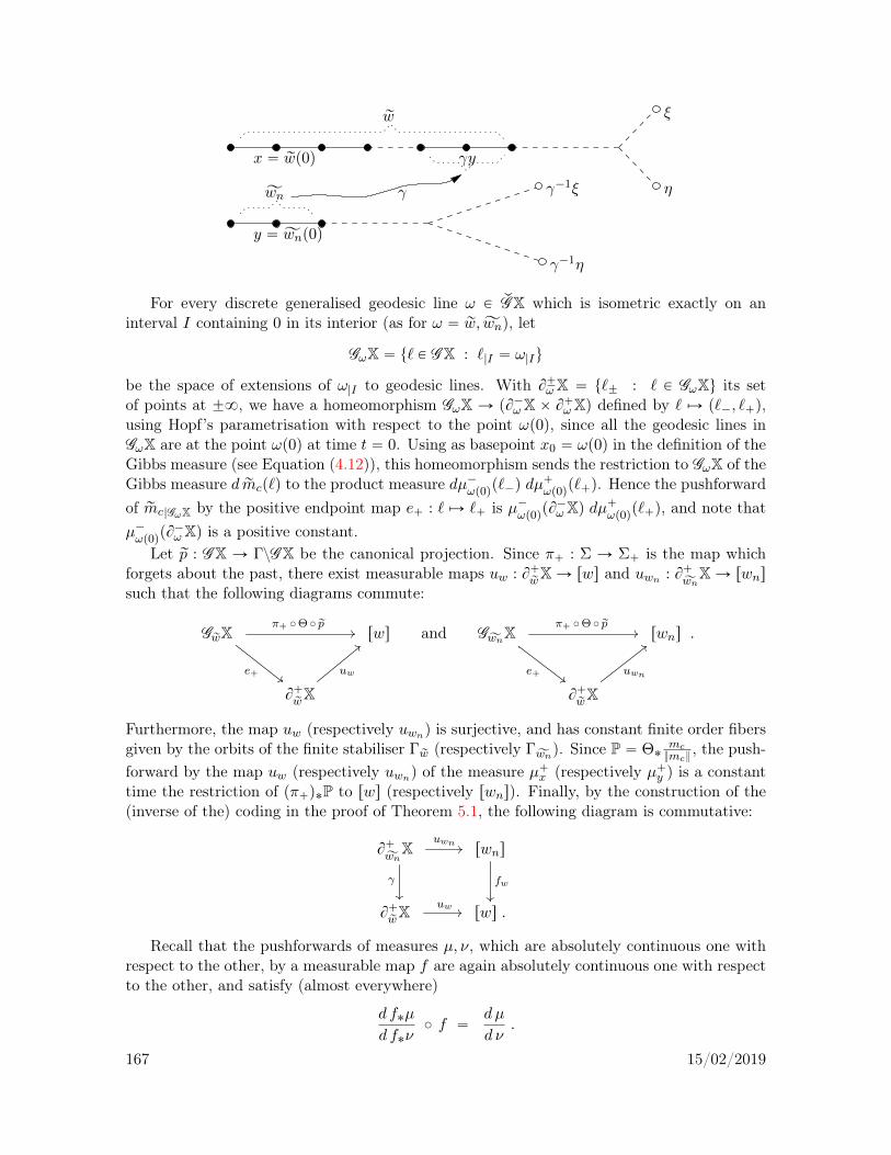
rw

Ăwn

γyx “ rwp0q

y “ Ăwnp0q

η

ξ

γ´1ξ

γ´1η

γ

For every discrete generalised geodesic line ω P

p

GX which is isometric exactly on aninterval I containing 0 in its interior (as for ω “ rw,Ăwn), let

GωX “ t` P GX : `|I “ ω|Iu

be the space of extensions of ω|I to geodesic lines. With B˘ωX “ t`˘ : ` P GωXu its setof points at ˘8, we have a homeomorphism GωX Ñ pB´ωX ˆ B`ωXq defined by ` ÞÑ p`´, ``q,using Hopf’s parametrisation with respect to the point ωp0q, since all the geodesic lines inGωX are at the point ωp0q at time t “ 0. Using as basepoint x0 “ ωp0q in the definition of theGibbs measure (see Equation (4.12)), this homeomorphism sends the restriction to GωX of theGibbs measure d rmcp`q to the product measure dµ´ωp0qp`´q dµ

`

ωp0qp``q. Hence the pushforwardof rmc|GωX by the positive endpoint map e` : ` ÞÑ `` is µ´ωp0qpB

´ωXq dµ`ωp0qp``q, and note that

µ´ωp0qpB´ωXq is a positive constant.

Let rp : GX Ñ ΓzGX be the canonical projection. Since π` : Σ Ñ Σ` is the map whichforgets about the past, there exist measurable maps uw : B`

rwXÑ rws and uwn : B`ĂwnXÑ rwns

such that the following diagrams commute:

GrwX

π` ˝Θ ˝ rp//

e`##

rws

B`rwX

uw

<<and G

ĂwnXπ` ˝Θ ˝ rp

//

e`##

rwns

B`rwX

uwn

<<.

Furthermore, the map uw (respectively uwn) is surjective, and has constant finite order fibersgiven by the orbits of the finite stabiliser Γ

rw (respectively ΓĂwn). Since P “ Θ˚

mcmc

, the push-forward by the map uw (respectively uwn) of the measure µ`x (respectively µ`y ) is a constanttime the restriction of pπ`q˚P to rws (respectively rwns). Finally, by the construction of the(inverse of the) coding in the proof of Theorem 5.1, the following diagram is commutative:

B`

ĂwnX

uwn //

γ

rwns

fw

B`rwX

uw // rws .

Recall that the pushforwards of measures µ, ν, which are absolutely continuous one withrespect to the other, by a measurable map f are again absolutely continuous one with respectto the other, and satisfy (almost everywhere)

d f˚µ

d f˚ν˝ f “

dµ

d ν.

167 15/02/2019

Hence in order to prove that Hypothesis (1) in the statement of Theorem 9.2 is satisfied, weonly have to prove that the map γ : B`

ĂwnX Ñ B

`rwX has a constant Jacobian for the measures

µ`y on B`ĂwnX and µ`x on B`

rwX respectively.For all ξ, η P B`

rwX, by the properties of the Patterson densities (see Equations (4.1) and(4.2)), since γy belongs to the geodesic ray from x to ξ and η (see the above picture), and byEquation (3.20), we have

d γ˚µ`y

dµ`xpξq

d γ˚µ`y

dµ`xpηq

“

dµ`γydµ`x

pξq

dµ`γydµ`x

pηq“e´C

`ξ pγy, xq

e´C`η pγy, xq

“e´

şγyx p

rF`c ´δcq

e´şγyx p

rF`c ´δcq“ 1 .

This proves that Hypothesis (1) in Theorem 9.2 is satisfied, and concludes the proof ofTheorem 9.1. l

We now indicate how to pass from a one-sided version of Theorem 9.2 to the two-sidedone, as was communicated to us by J. Buzzi.

Step 2 : Reduction to one-sided symbolic dynamics. Let pΣ`, σ`q be the one-sidedtopological Markov shift with alphabet A and transition matrix A, that is, Σ` is the closedsubset of the topological product space A N defined by

Σ` “

x “ pxnqnPN P A N : @ n P N, Axn,xn`1 “ 1u ,

and σ` : Σ` Ñ Σ` is the (one-sided) shift9 defined by

pσ`pxqqn “ xn`1

for all x P Σ` and n P N. We endow Σ` with the distance

dpx, x1q “ e´max

nPN : @ i P t0,...,nu, xi “ x1i

(

.

Note that the distances on Σ and Σ` are bounded by 1.The natural extension π` : pxnqnPZ ÞÑ pxnqnPN maps Σ to Σ`. It satisfies π` ˝σ “ σ` ˝π`

and is 1-Lipschitz. Note that Σ is transitive (respectively locally compact) if and only if Σ`is transitive (respectively locally compact).

In the one-sided case, we always assume that the cylinders start at time t “ 0: Given anadmissible sequence w “ pw0, w1, . . . , wn´1q, we will say that the cylinder

rws “ rw0, . . . , wn´1s “ tpxnqnPN P Σ` : @ i P t0, . . . , n´ 1u, xi “ wiu

defined by w has length |w| “ n.

We first explain how to relate the decay of correlations for the two-sided and one-sidedsystems. This is well-known since the works of Sinai [Sin, §3] and Bowen [Bowe2, Lem. 1.6], seefor instance [You1, §4], and the following proof has been communicated to us by J. Buzzi. We

9Although it is standard to denote the one-sided shift by σ in the same way as the two-sided shift, we useσ` for readability.

168 15/02/2019

fix α P s0, 1s. For all metric spaces Z and bounded α-Hölder-continuous functions f : Z Ñ R,recall10 that

f1α “ supx, y PZ

0ădpx, yqď1

|fpxq ´ fpyq|

dpx, yqαand fα “ f8 ` f

1α .

For every a P A , let us fix za P Σ such that pzaq0 “ a.

Lemma 9.3. Let φ : Σ Ñ R be a bounded α-Hölder-continuous map and N P N. Forall x P Σ`, let ypNqpxq “ pyiqiPN P Σ, where yi “ xi`N if i ě ´N and yi “ pzx0qi`N

otherwise. Define φpNq : Σ` Ñ R by φpNqpxq “ φpypNqpxqq. Then φpNq is bounded andα-Hölder-continuous on Σ`, with

|φ ˝ σN ´ φpNq ˝ π`| ď φ1α e

´αN .

Moreover,φpNq1α ď eαN φ1α and φpNq8 ď φ8 .

Proof. For every x “ pxnqnPZ P Σ, if y “ ypNqpπ`pxqq, we have pσN pxq˘

n“ xn`N “ yn if

|n| ď N . Hence,

|φ ˝ σN pxq ´ φpNqpπ`pxqq| “ |φpσN pxqq ´ φpyq|

ď φ1α dpσN pxq, yqα ď φ1α e

´αN .

Moreover, for all x “ pxnqnPN, x1 “ px1nqnPN in Σ`, if y “ ypNqpxq and y1 “ ypNqpx1q, thendpy, y1q “ eN dpx, x1q if dpx, x1q ă e´N and otherwise dpy, y1q ď 1 ď eNdpx, x1q, so that

|φpNqpxq ´ φpNqpx1q| “ |φpyq ´ φpy1q| ď φ1α dpy, y1qα ď φ1α e

αN dpx, x1qα . l

Proposition 9.4. Let µ be a σ-invariant probability measure on Σ. Assume that the dynam-ical system pΣ`, σ`, pπ`q˚µq has exponential decay of α-Hölder correlations. Then pΣ, σ, µqhas exponential decay of α-Hölder correlations.

Proof. Let C, κ ą 0 be such that for all bounded α-Hölder-continuous maps φ1, ψ1 : Σ` Ñ Rand n P N, we have

| covpπ`q˚µ, npφ1, ψ1q| ď C φ1α ψ

1α e´κn .

Let φ, ψ : Σ Ñ R be bounded α-Hölder-continuous maps and n P N. Denoting by ˘ t anyvalue in r´t, ts for every t ě 0, we have, by the first part of Lemma 9.3 and for every N P N,11

ż

Σφ ˝ σn ψ dµ “

ż

Σφ ˝ σn`N ψ ˝ σN dµ

“

ż

ΣpφpNq ˝ π` ˘ φ

1α e

´αN q ˝ σn pψpNq ˝ π` ˘ ψ1α e

´αN q dµ

“

ż

Σ`

φpNq ˝ σn` ψpNq dpπ`q˚µ ˘ φα ψα e´αN .

10See Section 3.1 for the definition of the Hölder norm ¨ α.11to be chosen appropriately below

169 15/02/2019

A similar estimate holds for the second term in the definition of the correlation coefficients.Hence, by the second part of Lemma 9.3,

| covµ, npφ, ψq|

ď | covpπ`q˚µ, npφpNq, ψpNqq| ` 2 φα ψα e

´αN

ď C pφ8 ` φ1α e

αN q pψ8 ` ψ1α e

αN q e´κn ` 2 φα ψα e´αN

ď φα ψαpC e2αN´κn ` 2 e´αN q .

Taking N “ tκn4α u, C 1 “ C ` 2 eα and κ1 “ κ4 , we have

| covµ, npφ, ψq| ď C 1 φα ψα e´κ1n ,

and the result follows. l

In order to conclude Step 2, we now state the one-sided version of Theorem 9.2 and provehow it implies Theorem 9.2.12 For every finite subset E of A , let

τξpxq “ inftn P N´ t0u : xn P E u

be the first return time13 of x P Σ` under iteration of the one-sided shift.

Theorem 9.5. Let pΣ`, σ`q be a locally compact transitive one-sided topological Markov shiftwith alphabet A and transition matrix A, and let P` be a mixing σ`-invariant probabilitymeasure with full support on Σ`. Assume that

(1) for every A-admissible finite sequence w “ pw0, . . . , wnq in A , the Jacobian of the mapfrom rwns to rws defined by pwn, x1, x2, . . . q ÞÑ pw0, . . . , wn, x1, x2, . . . q with respect tothe restrictions of the measure P` is constant;

(2) there exist a finite subset E of A and C 1, κ1 ą 0 such that for all n P N, we have

P``

tx P Σ` : x0 P E and τE pxq ě nu˘

ď C 1 e´κ1n . (9.4)

Then pΣ`,P`, σ`q has exponential decay of α-Hölder correlations.

Proof that Theorem 9.5 implies Theorem 9.2. Let pΣ, σ,P,E q be as in the statementof Theorem 9.2. Let P` “ pπ`q˚P, which is a mixing σ`-invariant probability measure onΣ` with full support. Note that Hypothesis (1) in Theorem 9.5 follows from Hypothesis (1)of Theorem 9.2. Similarly, Equation (9.4) follows from Equation (9.3). Hence Theorem 9.2follows from Theorem 9.5 and Proposition 9.4. l

Let us now consider Theorem 9.5. The scheme of its proof, using inducing and Youngtower arguments, was communicated to us by O. Sarig.

12Assumption (1) of Theorem 9.5 is far from being optimal, but will be sufficient for our purpose.13or rather the first positive passage time

170 15/02/2019

Step 3 : Proof of Theorem 9.5. In this final Step, using inducing of the dynamical systempΣ`, σ`q on the subspace tx P Σ` : x0 P E u “

Ť

aPE ras (a finite union of 1-cylinders), wepresent pΣ`, σ`q as a Young tower to which we will apply the results of [You2].

Note that since σ` is mixing and P` has full support, there exists a σ`-invariant mea-surable subset of full measure ∆ of Σ` such that the orbit under σ` of every element of ∆passes infinitely many times inside the nonempty open subset

Ť

aPE ras. We again denote byτE : ∆ Ñ N´ t0u the restriction to ∆ of the first return time in

Ť

aPE ras, so that if

∆0 “ tx P ∆ : x0 P E u “ď

aPE

∆X ras ,

then τE pxq “ mintn P N ´ t0u : σn`pxq P ∆0u for all x P ∆. We denote by F : ∆ Ñ ∆0 thefirst return map to ∆0 under iteration of the one-sided shift, that is

F : x ÞÑ στE pxq` pxq .

Let W be the set of admissible sequences w of length |w| at least 2 such that if w “

pw0, . . . , wnq with n “ |w| ´ 1 then

w0, wn P E and w1, . . . , wn´1 R E .

We have the following properties:‚ the sets ∆a “ ∆X ras for a P E form a finite measurable partition of ∆0 and for every

a P E , the sets ∆w “ ∆X rws for w P W and w0 “ a form a countable measurable partitionof ∆a;‚ for every w P W , the first return time τE is constant (equal to |w| ´ 1) on ∆w, and if

w|w|´1 “ b, then the first return map F is a bijection from ∆w to ∆b;‚ for all w PW and x, y P ∆w, since x, y have the same |w| first components, we have

dpF pxq, F pyqq “ dpσ|w|´1` x, σ

|w|´1` yq “ e|w|´1 dpx, yq ě e dpx, yq ;

‚ for all w PW , n P t0, . . . , |w| ´ 2u and x, y P ∆w, we have

dpσn`x, σn`yq “ en dpx, yq ď e|w|´2 dpx, yq ă dpF pxq, F pyqq ;

‚ for every w P W , the Jacobian of the first return map F : ∆w Ñ ∆w|w|´1for the

restrictions to ∆w and ∆w|w|´1of P` is constant.14

By an easy adaptation of [You2, Theo. 3] (see also [Mel1, §2.1]) which considers the casewhen E is a singleton, we have the following noneffective15 exponential decay of correlation:there exists κ ą 0 such that for every φ, ψ P C α

b pΣ`q, there exists a constant Cφ,ψ ą 0 suchthat

| covP`, npφ, ψq| ď Cφ,ψ e´κn

By an elegant argument using the Principle of Uniform Boundedness, it is proved in [ChCS,Appendix B] that this implies that there exist C, κ ą 0 such that for every φ, ψ P C α

b pΣ`q,we have

| covP`, npφ, ψq| ď C φα ψα e´κn .

14Actually, only a much weaker assumption is required, such as a Hölder-continuity property of this Jacobian,see [You2].

15Actually, there is in [You2] (see also [CyS]) a control on the constant in terms of some norms of the testfunctions, but these norms are not the ones we are interested in.

171 15/02/2019

This concludes the proof of Theorem 9.5, hence the proof of Theorem 9.1. l l

The next result gives examples of applications of Theorem 9.1 when ΓzX is infinite. Itstrengthens [AtGP, Theo. 2.1] that applies only to arithmetic lattices and only for the locallyconstant regularity (see Section 15.4), see also [BekL] for an approach using spectral gaps. Itwas claimed in [Kwo], but was retracted by the author.

Corollary 9.6. Let X be a locally finite simplicial tree without terminal vertices. Let Γ be ageometrically finite subgroup of AutpXq such that the smallest nonempty Γ-invariant subtreeof X is uniform without vertices of degree 2. Let α P s0, 1s.

(1) If LΓ “ Z, then the discrete time geodesic flow on ΓzGX has exponential decay ofα-Hölder correlations for the zero system of conductances.

(2) If LΓ “ 2Z, then the square of the discrete time geodesic flow on ΓzGevenX has expo-nential decay of α-Hölder correlations for the zero system of conductances, that is, there existC, κ ą 0 such that for all φ, ψ P C α

b pΓzGevenXq and n P Z, we have

ˇ

ˇ

ˇ

ż

ΓzGevenXφ ˝ g´2n ψ dmBM ´

1

mBMpΓzGevenXq

ż

ΓzGevenXφ dmBM

ż

ΓzGevenXψ dmBM

ˇ

ˇ

ˇ

ď C e´κ|n| φα ψα .

The main point in order to obtain this corollary is to prove the exponential decay of vol-umes of geodesic lines going high in the cuspidal rays of ΓzX, stated as Assumption (9.2) inTheorem 9.1. There is a long history of similar results, starting from the exponential decayof volumes of small cusp neighbourhoods in noncompact finite volume hyperbolic manifolds(based on the description of their ends) used by Sullivan to deduce Diophantine approxima-tion results (see [Sul3, §9]).16 These results were extended to the case of locally symmetricRiemannian manifolds by Kleinbock-Margulis [KM2] (based on the description of their endsusing Siegel sets). Note that the geometrically finite lattice assumption on Γ is here in orderto obtain similar descriptions of the ends of ΓzX.

Proof. Up to replacing X by C ΛΓ, we assume that X is a uniform simplicial tree withdegrees at least 3 and that Γ is a geometrically finite lattice of X. We use the zero system ofconductances.

(1) By [Pau4],17 the graph ΓzX is the union of a finite graph Y and finitely many cuspidalrays Ri for i P t1, . . . , ku. If pxi, nqnPN is the sequence of vertices in increasing order alongRi for i “ 1, . . . , k, then the vertex group Gxi, n of xi, n in the quotient graph of groups ΓzzXsatisfies Gxi, n Ă Gxi, n`1 for every n P N, and the edge group of the edge ei,n with origin xi,nand endpoint xi, n`1 is equal to Gxi, n .18 Note that since the degrees of the vertices of X areat least 3, we have rGxi, n`1 : Gxi,ns ě 2 and |Gxi, 0 | ě 1, so that, for every n P N,

|Gxi, n | ě 2n . (9.5)

Let E be the (finite) set of vertices V Y of Y. Note that for all n P N´t0u and ` P ΓzGX, if`p0q P E and τEp`q ě 2n, then ` leaves Y after time 0 and it travels (geodesically) inside some

16and by probabilists in order to study the statistics of cusp excursions (see for instance [EF])17See also Section 2.6.18identifying the edge group of an edge e with its image by the structural map Ge Ñ Gopeq

172 15/02/2019

cuspidal ray for a time at least n, so that there exists i P t1, . . . , ku such that `pnq “ xi, n.Hence for all n P N, using‚ the invariance of mBM under the discrete time geodesic flow in order to get the third

term,‚ Equation (8.5) where rxi, n is a fixed lift of xi, n in V X for the fifth term, and‚ Equation (9.5) since |Γ

rxi, n | “ |Gxi, n |, and the facts that the degrees of the uniformsimplicial tree X are uniformly bounded and that the total mass of the Patterson measuresof the lattice Γ are uniformly bounded (see Proposition 4.16) for the last term,we have

mBM

`

t` P ΓzGX : `p0q P E and τEp`q ě 2nu˘

ď

kÿ

i“1

mBM

`

t` P ΓzGX : `pnq “ xi,nu˘

“

kÿ

i“1

mBM

`

t` P ΓzGX : `p0q “ xi,nu˘

“

kÿ

i“1

π˚mBMptxi,nuq

“

kÿ

i“1

1

|Γrxi, n |

ÿ

e, e1PEX : opeq“ope1q“ rxi, n, e‰e1

µrxi, npBeXq µrxi, npBe1Xq

ď k1

2nmaxxPV X

degpxq2 maxxPV X

µx2 .

The result then follows from Theorem 9.1 using the above finite set E which satisfiesAssumption (9.2) as we just proved, and using Proposition 4.16 and Theorem 4.17 in orderto check that under the assumption that LΓ “ Z, the Bowen-Margulis measure mBM of Γ isfinite and mixing under the discrete time geodesic flow on ΓzGX.

(2) The proof of Assertion (2) is similar to the one of Assertion (1). l

Remark. The techniques introduced in the above proof in order to check the main hypothesisof Theorem 9.1 may be applied to numerous other examples. For instance, let X be a locallyfinite simplicial tree without terminal vertices. Let Γ be a nonelementary discrete subgroup ofAutpXq such that the smallest nonempty Γ-invariant subtree of X is uniform without verticesof degree 2, and such that LΓ “ Z. Let α P s0, 1s. Assume that ΓzX is the union of a finitegraph A and finitely many trees T1, . . . ,Tk meeting A in one and exactly one vertex ˚1, . . . , ˚nsuch that for every edge e in Ti pointing away from the root ˚i of Ti, the canonical morphismGe Ñ Gopeq between edge and vertex groups of the quotient graph of groups ΓzzX “ pΓzX, G˚qis an isomorphism. Assume that there exist C, κ ą 0 such that for all n P N,

ÿ

i“1,...,k, xPV Ti : dpx,˚iq“n

1

|Gx|ď Ce´κn .

Then the discrete time geodesic flow on ΓzGX has exponential decay of α-Hölder correlationsfor the zero system of conductances.

This is in particular the case for every k, q P N such that k ě 2, q ą 2k ` 1 and q ´ k isodd, when the quotient graph of groups ΓzzX has underlying edge-indexed graph19 a loop-edgewith both indices equal to q´k`1

2 glued to the root of a regular k-ary rooted tree, with indices19See definition in Section 2.6.

173 15/02/2019

1 for the edges pointing towards the root and q ´ k ` 1 for the edges pointing away from theroot (see the picture below with k “ 2). Note that X is then the pq ` 1q-regular tree, andthat the loop edge is here in order to ensure that LΓ “ Z. For instance, the vertex group ofa point at distance n from the root may be chosen to be Zp q´k`1

2 qZˆ`

Zpq ´ k ` 1qZ˘n.

q ´ 111

q ´ 1 q ´ 111

q ´ 1q ´ 111

q ´ 1q ´ 111

q ´ 1

q ´ 1q ´ 1

1

1

q´12

1

q ´ 1

1

q ´ 1

1

q ´ 1 q ´ 1

1

q´12

9.3 Rate of mixing for metric trees

Let pX, λq, X, Γ, rF , rF˘, δ “ δΓ, F˘ ă `8 and pµ˘x qxPV X be as in the beginning of Section 4.4.Let rmF and mF be the associated Gibbs measures on GX and ΓzGX. The aim of this Sectionis to study the problem of finding conditions on these data under which the (continuous time)geodesic flow on ΓzGX is polynomially mixing for the Gibbs measure mF .

We will actually prove a stronger property, though it applies only to observables which aresmooth enough along the flow. Let us fix α P s0, 1s. Let pZ, µ, pφtqtPRq be a topological spaceZ endowed with a continuous one-parameter group pφtqtPR of homeomorphisms preservinga (Borel) probability measure µ on Z. For all k P N, let C k, α

b pZq be the real vector spaceof maps f : Z Ñ R such that for all z P Z, the map t ÞÑ fpφtzq is C k-smooth, and suchthat the maps Bitf : Z Ñ R defined by z ÞÑ di

dti

ˇ

ˇ

t“0fpφtzq for 0 ď i ď k are bounded and

α-Hölder-continuous. It is a Banach space when endowed with the norm

fk, α “kÿ

i“0

Bitfα ,

and it is contained in L2pZ, µq by the finiteness of µ. We denote by C k, αc pZq the vector

subspace of elements of C k, αb pZq with compact support.

For all ψ,ψ1 P L2pZ, µq and t P R, let

covµ, tpψ,ψ1q “

ż

Zψ ˝ φt ψ

1 dµ´

ż

Zψ dµ

ż

Zψ1 dµ

be the (well-defined) correlation coefficient of the observables ψ,ψ1 at time t under theflow pφtqtPR for the measure µ. We say20 that the (continuous time) dynamical system

20See [Dol2], and more precisely [Mel1, Def. 2.2] whose definition is slightly different but implies the onegiven in this paper by the Principle of Uniform Boundedness argument of [ChCS, Appendix B] already usedin Section 9.2.

174 15/02/2019

pZ, µ, pφtqtPRq has superpolynomial decay of α-Hölder correlations if for every n P N thereexist C “ Cn ą 0 and k “ kn P N such that for all ψ,ψ1 P C k, α

b pZq and t P R, we have

| covµ, tpψ,ψ1q| ď C p1` |t|q´n ψk, α ψ

1k, α .

Following Dolgopyat, we say that the dynamical system pZ, µ, pφtqtPRq is rapidly mixing if thereexists α ą 0 such that pZ, µ, pφtqtPRq has superpolynomial decay of α-Hölder correlations

We will use the following two assumptions on our data, introduced respectively in [Dol2]and [Mel1]. Recall that the Gibbs measure mF , when finite, is mixing if and only the lengthspectrum LΓ is dense in R (see Theorem 4.9). The rapidly mixing property will requirestronger assumptions on LΓ.

We say that the length spectrum LΓ of Γ is 2-Diophantine if there exists a ratio of twotranslation lengths of elements of Γ which is Diophantine. Recall that a real number x isDiophantine if there exist α, β ą 0 such that

ˇ

ˇx´p

q

ˇ

ˇ ě α q´β

for all p, q P Z with q ą 0.Let E be a finite subset of vertices of ΓzX, and let rE be the set of vertices of X mapping to

E. We denote by TE the set of triples pλpγq, dpγq, qpγ, pqq where γ P Γ has translation lengthλpγq ą 0, has dpγq vertices on its translation axis Axpγq modulo γZ and if the first return timeof a vertex p in rE X Axpγq under the discrete time geodesic flow along the translation axishas period qpγ, pq. We say that the length spectrum LΓ of Γ is 4-Diophantine with respect toE if for all sequences pbkqkPN in r1 ` 8r converging to `8 and pωkqkPN, pϕkqkPN in r0, 2πr ,there exists N P N such that for all a ě N and C, β ě 1, there exist k ě 1 and pτ, d, qq P TEsuch that

d`

pbkτ ` ωkdqtβ ln bku` qϕk, 2πZq ě C q b´ak .

We define the first return time after time ε on a finite subset E of vertices of ΓzX as themap τąεE : ΓzGX Ñ r0,`8s defined by τąεE p`q “ inftt ą ε : `ptq P Eu.

Theorem 9.7. Assume that the Gibbs measure mF is finite and mixing for the (continuoustime) geodesic flow, and that the lengths of the edges of pX, λq have a finite upper bound.21

Furthermore assume that

(a) either ΓzX is compact and the length spectrum of Γ is 2-Diophantine,

(b) or there exists a finite subset E of vertices of ΓzX satisfying the following properties:

(1) there exist C, κ ą 0 and ε P s0,minλr such that for all t ě 0,

mF pt` P ΓzGX : dp`p0q, Eq ď ε and τąεE p`q ě tuq ď C e´κ t ,

(2) the length spectrum of Γ is 4-Diophantine with respect to E.

Then the (continuous time) geodesic flow on ΓzGX has superpolynomial decay of α-Höldercorrelations for the normalised Gibbs measure mF

mF .

21They have a positive lower bound by definition, see Section 2.6.

175 15/02/2019

Note that the existence of E satisfying the exponentially small tail Hypothesis (1) is inparticular satisfied if Γ is geometrically finite with E the set of vertices of a finite subgraph ofΓzX whose complement in ΓzX is the underlying graph of a union of cuspidal rays in ΓzzX :see the proof of Corollary 9.6 and use the hypothesis on the lengths of edges.

Note that the exponentially small tail Hypothesis (1) might be weakened to a superpoly-nomially small tail hypothesis while keeping the same conclusion, see [Mel2]. Since the formeris easier to check than the latter, we prefer to state Theorem 9.7 as it is.

We will follow a scheme of proof analogous to the one in Section 9.2 for simplicial trees,by reducing the study to a problem of suspensions of Young towers, and then apply results of[Dol2] and [Mel1] for the rapid mixing property of suspensions of hyperbolic and nonuniformlyhyperbolic dynamical systems.

Proof. Since the Gibbs measure normalised to be a probability measure depends only on thecohomology class of the potential (see Equation (4.10)), we may assume by Proposition 3.22that F “ Fc is the potential on ΓzT 1X associated with a system of conductances rc : EXÑ Rfor Γ. We denote by δc the critical exponent of pΓ, Fcq, and by mc the Gibbs measure mFc .Up to replacing X by its minimal nonempty Γ-invariant subtree, we assume that X “ C ΛΓ.

Step 1 : Reduction to a suspension of a two-sided symbolic dynamics. We refer tothe paragraphs before the statement of Theorem 5.9 and at the beginning of Section 5.3 forthe definitions of‚ the system of conductances 7c for Γ on the simplicial tree X,‚ the (two-sided) topological Markov shift pΣ, σ,Pq on the alphabet A , conjugated to the

discrete time geodesic flow`

ΓzGX, 7g1,m7cm7c

˘

by the homeomorphism Θ : ΓzGXÑ Σ,

‚ the roof function r : Σ Ñ s0,`8r ,‚ the suspension pΣ, σ, aPqr “ pΣr, pσ

trqtPR, aPrq over pΣ, σ, aPq with roof function r,

where a “ 1Pr .

The suspension pΣ, σ, aPqr is conjugated to the geodesic flow`

ΓzGX, mcmc

, pgtqtPR˘

by thebilipschitz homeomorphism Θr : ΓzGX Ñ Σr defined at the end of the proof of Theorem 5.9.We will always (uniquely) represent the elements of Σr as rx, ss with x P Σ and 0 ď s ă rpxq.

Note that since Θ´1r conjugates pσtrqtPR and pgtqtPR, we have for all f : ΓzGX Ñ R and

x P Σr, when defined,

Bitpf ˝Θ´1r qpxq “

di

dtiˇ

ˇ

t“0f ˝Θ´1

r pσtrxq “

di

dtiˇ

ˇ

t“0fpgtΘ´1

r pxqq “ pBitfq ˝Θ´1

r pxq .

Hence if f : ΓzGX Ñ R is Ck-smooth along the orbits of pgtqtPR, then f ˝Θ´1r is Ck-smooth

along the orbits of pσtrqtPR. Furthermore, since Θr is bilipschitz, the precomposition map byΘ´1r is a continuous linear isomorphism from C k, α

b pΓzGXq to C k, αb pΣrq.

Note that since Θr conjugates pgtqtPR and pσtrqtPR, and sends mcmc

to PrPr , we have, for all

ψ,ψ1 P L2pΓzGXq and t P R,

cov mcmc

, tpψ,ψ1q “ cov Pr

Pr, tpψ ˝Θ´1

r , ψ1 ˝Θ´1r q .

Therefore we only have to prove that the suspension pΣr, pσtrqtPR,

PrPrq is rapidly mixing under

one of the assumptions (a) and (b).

176 15/02/2019

Step 2 : Reduction to a suspension of a one-sided symbolic dynamics. In this Step,we explain the rather standard reduction concerning mixing rates from suspensions of two-sided topological Markov shifts to suspensions of one-sided topological Markov shifts. Weuse the obvious modifications of the notation and constructions concerning the suspensionof a noninvertible transformation to a semiflow, given for invertible transformations at thebeginning of Section 5.3.

We consider the one-sided topological Markov shift pΣ`, σ`,P`q over the alphabet Aconstructed at the beginning of Step 2 of the proof of Theorem 9.1, where the system ofconductances c is now replaced by 7c, so that P “ Θ˚pm7cm7cq. Let π` : Σ Ñ Σ` be thenatural extension so that P` “ pπ`q˚P and π` ˝ σ “ σ` ˝ π`.

We are going to construct in Step 2, as the suspension of pΣ`, σ`,P`q with an appro-priate roof function r`, a semiflow ppΣ`qr` ,

`

pσ`qtr`

˘

tě0, pP`qr`q, and prove that the flow

`

Σr, pσtrqtPR,

PrPr

˘

is rapidly mixing if the semiflow ppΣ`qr` ,`

pσ`qtr`

˘

tě0,pP`qr`pP`qr`

q is rapidlymixing.

Let r` : Σ` Ñ s0,`8r be the map defined by

r` : x ÞÑ λpe`0 q , (9.6)

where if x “ pxnqnPN, the edge e`0 is such that x0 “ pe´0 , h0, e`0 q. Note that this map has

a positive lower bound, and a finite upper bound, and that it is locally constant (and evenconstant on the 1-cylinders of Σ`). By Equation (5.10), we have

r` ˝ π` “ r . (9.7)

We denote by ppΣ`qr` ,`

pσ`qtr`

˘

tě0, pP`qr`q the suspension semiflow over pΣ`, σ`,P`q with

roof function r`. We (uniquely) represent the points of the suspension space pΣ`qr` as rx, ssfor x P Σ` and 0 ď s ă r`pxq. For all t ě 0, we have pσ`qtr`prx, ssq “ rσ

n`x, s

1s where n P Nand s1 P R are such that t` s “

řn´1i“0 r`pσ

i`xq ` s

1 and 0 ď s1 ă r`pσn`xq.

We define the suspended natural extension as the map π r` : Σr Ñ pΣ`qr` by

π r` : rx, ss ÞÑ rπ`pxq, ss ,

which is well defined by Equation (9.7). Note that π r` is 1-Lipschitz for the Bowen-Walters

distances on Σr and pΣ`qr` (see Proposition 5.11).22

For all ψ : Σr Ñ R and T ě 0, let us construct a function ψpT q : pΣ`qr` Ñ R as follows.For every rx, ss P pΣ`qr` , let N P N and s1 ě 0 be such that pσ`qTr`rx, ss “ rσ

N` x, s

1s, with

0 ď s1 ă r`pσN` xq and s` T “

N´1ÿ

i“0

r`pσi`xq ` s

1 .

LetψpT qprx, ssq “ ψpry, s1sq

where y “ pynqnPZ is such that yi “ xi`N if i ě ´N and yi “ pzx0qi`N otherwise. Note thaty0 “ xN , hence rpyq “ r`pσ

N` pxqq and 0 ď s1 ă rpyq, so that the above map is well defined.

22Note that Proposition 5.11 is stated for suspensions of invertible maps, but the roof function is constanton 1-cylinders, and the branches of the inverse of σ` on these 1-cylinders are uniformely Lipschitz, hence theproof of [BarS, Appendix] extends.

177 15/02/2019

Finally, for every ψ P C k, αb pΣrq or ψ P C k, α

b ppΣ`qr`q, let

ψk,8 “kÿ

i“0

Bitψ8 and ψ1k, α “kÿ

i“0

Bitψ1α ,

so thatψk, α “ ψk,8 ` ψ

1k, α .

Lemma 9.8. Let T ě 0 and ψ P C k, αb pΣrq.

(1) For all t ě 0, we have pσ`qtr` ˝ πr` “ π r

` ˝ σtr.

(2) With α1 “ αsupλ , there exists a constant C1 ě 1 (independent of k, T and ψ) such that

|ψ ˝ σTr ´ ψpT q ˝ π r

`| ď C1 ψ1α e

´α1 T .

(3) We have ψpT q P C k, αb ppΣ`qr`q and ψpT qk,8 ď ψk,8. With α2 “ α

inf λ , there exists aconstant C2 ě 1 (independent of k, T and ψ) such that

ψpT q1k, α ď C2 eα2 T ψ1k, α . (9.8)

Proof. (1) For all t ě 0 and rx, ss P Σr, let n P N and s1 ě 0 be such that

t` s “n´1ÿ

i“0

r`pσi`π`pxqq ` s

1 and 0 ď s1 ă r`pσn`π`pxqq .

Since r` ˝ σi` ˝ π` “ r ˝ σi for every i P N, these two conditions are equivalent to

t` s “n´1ÿ

i“0

rpσixq ` s1 and 0 ď s1 ă rpσnxq .

Hencepσ`q

tr` ˝ π

r`prx, ssq “ pσ`q

tr`prπ`pxq, ssq “ rσ

n`π`pxq, s

1s

andπ r` ˝ σ

trprx, ssq “ π r

`prσnx, s1sq “ rπ`pσ

nxq, s1s .

This proves Assertion (1) since π` ˝ σ “ σ` ˝ π`.

(2) By Proposition 5.11, we may assume that, in the formula of the Hölder norms, the Bowen-Walters distance is replaced by the function dBW, as this will only change C1 by CαBW C1.

For every rx, ss P Σr, with ry, s1s and N associated with π r`prx, ssq “ rπ`pxq, ss as in the

definition of ψpT qprπ`pxq, ssq, we have

dBWpσTr rx, ss, ry, s

1sq “ dBWprσNx, s1s, ry, s1sq ď dpσNx, yq ď e´N .

Since the positive roof function r is bounded from above by the least upper bound supλ ofthe lengths of the edges, we have

N ě

N´1ÿ

i“0

rpσixq

supλ“

1

supλps` T ´ s1q ě

T

supλ´ 1 .

178 15/02/2019

Hence

|ψ ˝ σTr prx, ssq ´ ψpT qpπ r

`pxqq| “ |ψpσTr rx, ssq ´ ψpry, s

1sq|

ď ψ1α dBWpσTr rx, ss, ry, s

1sqα ď ψ1α e´ α

supλT`α

.

(3) Let us prove that ψpT q is C k along semiflow lines. Fix rx, ss P pΣ`qr` . With ry, s1s and Nas in the construction of ψpT qprx, ssq, let us consider ε ą 0 small enough, so that ε ă r`pxq´sand ε ă r`pσ

N` pxqq ´ s

1 “ rpyq ´ s1. Then

ψpT q ˝ pσ`qεr`prx, ssq “ ψpT qprx, s` εsq “ ψpry, s1 ` εsq “ ψ ˝ σεrpry, s

1sq .

Therefore by taking derivatives with respect to ε in this formula, ψpT q is indeed C k alongsemiflow lines, and, for i “ 0, . . . , k, we have

Bit

`

ψpT q˘

“`

Bitψ˘pT q

. (9.9)

The inequality ψpT q8 ď ψ8 is immediate by construction. Using the above centredequation, we have ψpT qk,8 ď ψk,8.

Let us prove that there exists a constant C2 ě 1 (independent of T and ψ) such that

ψpT q1α ď C2 eα2 T ψ1α . (9.10)

Let rx, ss P pΣ`qr` , take ry, s1s and N as in the definition of ψpT qprx, ssq. Let rx, s s PpΣ`qr` , take ry, s1s and N as in the definition of ψpT qprx, s sq. Up to exchanging rx, ss andrx, s s, we assume that N ě N .

By Proposition 5.11,23 we may assume that, in the Hölder norms formulas, the Bowen-Walters distance is replaced by the function dBW, as this will only change C2 by C2α

BW C2.Let

C3 “ minte´1, inf λu .

We haveˇ

ˇψpT qprx, ssq ´ ψpT qprx, s sqˇ

ˇ “ˇ

ˇψpry, s1sq ´ ψpry, s1sqˇ

ˇ ď ψ1α dBWpry, s1s, ry, s1sqα . (9.11)

Note that the map dBW on Σr ˆ Σr is bounded from above by 1 ` supλ, since the dis-tance on Σ is at most 1 and since the roof function r is bounded from above by supλ. IfdBWprx, ss, rx, s sq ě C3 e

´ Tinf λ , then

dBWpry, s1s, ry, s1sq ď 1` supλ ď

1` supλ

C3e

Tinf λ dBWprx, ss, rx, s sq .

Therefore Equation (9.10) follows from Equation (9.11) whenever C2 ěp1`supλqα

Cα3.

Conversely, suppose that dBWprx, ss, rx, s sq ă C3 e´ T

inf λ . Assume that

dBWprx, ss, rx, s sq “ dpx, xq ` |s´ s| ,

the other possibilities are treated similarly. Since

s` T “N´1ÿ

i“0

r`pσi`xq ` s

1

23See the previous footnote.

179 15/02/2019

and since the roof function r` is bounded from below by inf λ, we have T ě N inf λ ´ inf λ,or equivalently N ď T

inf λ ` 1. Hence dpx, xq ă C3 e´ T

inf λ ď e´N by the definition of C3. Inparticular the sequences x and x indexed by N have the same N ` 1 first coefficients. Sincer`pzq depends only on z0 for all z P Σ`, we thus have r`pσi`xq “ r`pσ

i` xq for i “ 0, . . . , N .

Note that we have

s` T “

N´1ÿ

i“0

r`pσi` xq ` s

1 .

If N “ N , then by taking the difference of the last two centred equations, we haves ´ s “ s1 ´ s1, and by construction, the sequences y and y indexed by Z satisfy yi “ pyqi ifi ď 0 and if 0 ď i ď ´ ln dpx, xq ´N . Therefore dpy, yq ď eN dpx, xq and

dBWpry, s1s, ry, s1sq ď dpy, yq ` |s1 ´ s1| ď eN dpx, xq ` |s´ s|

ď eN dBWprx, ss, rx, s sq ď eT

inf λ`1 dBWprx, ss, rx, s sq .

Therefore Equation (9.10) follows from Equation (9.11) whenever C2 ě eα.If N ą N , then again by difference

s´ s “

N´1ÿ

i“N`1

r`pσi` xq ` r`pσ

N` xq ´ s

1 ` s1.

Note that s1 ě 0, that r`pσN` xq´s1 ě 0, and that |s´s| ă C3 e´ T

inf λ ď inf λ by the definitionof C3. Hence we have N “ N`1 and s´s “ r`pσ

N` xq´s

1`s1. By construction, the sequencesσy and y indexed by Z satisfy pσyqi “ pyqi if i ď 0 and if 0 ď i ď ´ ln dpx, xq ´N ´ 1. Henceby the definition of dBW and since rpyq “ r`pσ

N` xq, we have

dBWpry, s1s, ry, s1sq ď dpσy, yq ` rpyq ´ s1 ` s1 ď eN`1 dpx, xq ` |s´ s|

ď eN`1 dBWprx, ss, rx, s sq ď eT

inf λ`2 dBWprx, ss, rx, s sq .

Therefore Equation (9.10) follows from Equation (9.11) whenever C2 ě e2α. This ends theproof of Equation (9.10).

Now note that Equations (9.9) and (9.10) imply Equation (9.8) by summation (using theindependence of C2 on ψ), thus concluding the proof of Lemma 9.8. l

Proposition 9.9. Let µ be a pσtrqtPR-invariant probability measure on Σr. Assume that thedynamical system

`

pΣ`qr` , ppσ`qtr`qtPR, pπ

r`q˚µ

˘

has superpolynomial decay of α-Hölder cor-relations. Then pΣr, pσ

trqtPR, µq has superpolynomial decay of α-Hölder correlations.

Proof. We fix n P N. Let N “ 1` 2rsupλinf λ s. Let k P N and C4 ą 0 (depending on n) be such

that for all ψ,ψ1 P C k, αb ppΣ`qr`q, we have for all t ě 1

ˇ

ˇ covpπ r`q˚µ, tpψ,ψ1qˇ

ˇ ď C4 ψk, α ψ1k, α t

N n . (9.12)

Now let ψ,ψ1 P C k, αb pΣrq. We again denote by ˘ a any value in r´a, as for every a ě 0.

By invariance of µ under pσtrqtPR, by Lemma 9.8 (2) and by Lemma 9.8 (1), we have, for every

180 15/02/2019

T ě 0 (to be chosen appropriately later on),

ż

Σr

ψ ˝ σtr ψ1 dµ “

ż

Σr

ψ ˝ σT`tr ψ1 ˝ σTr dµ

“

ż

Σr

pψpT q ˝ π r` ˘ C1 ψ

1α e

´α1 T q ˝ σtr pψ1pT q ˝ π r

` ˘ C1 ψ11α e

´α1 T q dµ

“

ż

pΣ`qr`

ψpT q ˝ pσ`qtr` ψ1

pT qdpπ r

`q˚µ ˘ C21 ψα ψ

1α e´α1 T .

A similar estimate holds for the second term in the definition of the correlation coefficients.Hence, applying Equation (9.12) to the observables ψpT q and ψ1pT q, by Lemma 9.8 (3), wehave since C2 e

α2 T ě 1,

| covµ, tpψ,ψ1q| ď | covpπ r`q˚µ, tpψ

pT q, ψ1pT qq| ` 2 C2

1 ψα ψ1α e

´α1 T

ď C4 pψk,8 ` C2 ψ1k, α e

α2 T q pψ1k,8 ` C2 ψ11k, α e

α2 T q t´N n

` 2 C21 ψα ψ

1α e´α1 T

ď ψk, α ψ1k, α pC4 C

22 e

2α2T t´N n ` 2 C21 e

´α1 T q .

Take T “ nα1 ln t ě 0. Since N “ 1 ` 2rα

2

α1 s, we have 2α2 nα1 ´ N n ď ´n. Hence with

C5 “ C4 C22 ` 2 C2

1 , we have for all t ě 1

| covµ, tpψ,ψ1q| ď C5 ψk, α ψ

1k, α t´n .

This concludes the proof of Proposition 9.9. l

Step 3 : Conclusion of the proof of Theorem 9.7. In this Step, we prove that the semi-flow

`

pΣ`qr` ,`

pσ`qtr`

˘

tě0,pP`qr`pP`qr`

˘

is rapidly mixing, which concludes the proof of Theorem

9.7, using Proposition 9.9 with µ “ PrPr .

Recall24 that Y “ t` P ΓzGX : `p0q P V Xu is a cross-section of the geodesic flow onΓzGX, and that if R : Y Ñ ΓzGX is the reparametrisation map of ` P Y to a discrete geodesicline 7` P ΓzGX with the same origin, then the measure µY , induced by the Gibbs measure mc

on the cross-section Y by disintegration along the flow, maps by R˚ to a constant multipleof m7c “ mF7c

(see Lemma 5.10 (2)). Hence for all n P N ´ t0u and ε P s0, 12 inf λr , by

24See the proof of Theorem 5.9.

181 15/02/2019

Assumption (b) (1) in the statement of Theorem 9.7, we have

m7c

´!

7` P ΓzGX :7`p0q P E

@ k P t1, . . . , n´ 1u, 7`pkq R E

)¯

ďm7c

µY µY

´!

R´1p7`q P Y :R´1p7`qp0q P E

@ t P s0, n inf λr , R´1p7`qptq R E

)¯

ďm7c

ε µY mc

´!

gsR´1p7`q P ΓzGX :0 ď s ď ε, dpgsR´1p7`qp0q, Eq ď ε@ t P sε, n inf λ´ εr , gsR´1p7`qptq R E

)¯

ďm7c

ε µY C e´κ pinf λqn`κ ε .

Therefore Equation (9.2) (where c is replaced by 7c) is satisfied, with C 1 “m7cC e

κ ε

ε µY and

κ1 “ κ inf λ. As seen in the proof of Theorem 9.1, this implies that there exists a finite subsetE of the alphabet A such that Equation (9.4) is satisfied.

We now apply [Mel1, Theo. 2.3] with the dynamical system pX,m0, T q “ pΣ`,P`, σ`q(using the system of conductances 7c) and the roof function h “ r`. This dynamical systemis presented as a Young tower in Step 3 of the proof of Theorem 9.1. Equation (9.4) forthe first return map τE and the 4-Diophantine hypothesis are exactly the hypothesis neededin order to apply [Mel1, Theo. 2.3]. Thus the semiflow ppΣ`qr` ,

`

pσ`qtr`

˘

tě0,pP`qr`pP`qr`

q hassuperpolynomial decay of α-Hölder correlations.

When ΓzX is compact, the alphabet A is finite and pΣ`, σ`,P`q is a (one-sided) subshiftof finite type, hence we do not need the exponentially small tail assumption, but only the2-Diophantine hypothesis, and we may apply [Dol2]. l

Corollary 9.10. Assume that the Gibbs measure mF is finite and mixing for the (continuoustime) geodesic flow, that the lengths of the edges of pX, λq have a finite upper bound, andthat Γ is geometrically finite. There exists a full measure subset A of R4 (for the Lebesguemeasure) such that if Γ has a quadruple of translation lengths in A, or if the length spectrum is4-Diophantine, then the (continuous time) geodesic flow on ΓzGX has superpolynomial decayof α-Hölder correlations for the Bowen-Margulis measure mBM.

Proof. The exponentially small tail Assumption (b) (1) is checked as in the proof of Corollary9.6. The deduction of Corollary 9.10 from Theorem 9.7 then proceeds, by an argument goingback in part to Dolgopyat, as for the deduction of Corollary 2.4 from Theorem 2.3 in [Mel1].l

Note that under the general assumptions of Theorem 4.9, the geodesic flow on ΓzGXmight not be exponentially mixing, see for instance [Pol1, page 162] or [Rue2] for analogousbehaviour.

182 15/02/2019

Part II

Geometric equidistribution andcounting

183 15/02/2019

Chapter 10

Equidistribution of equidistant levelsets to Gibbs measures

Let X be a geodesically complete proper CATp´1q space, let Γ be a nonelementary discretegroup of isometries of X, let rF be a continuous Γ-invariant map on T 1X such that δ “ δΓ, F˘

is finite and positive and that the triple pX,Γ, rF q satisfies the HC-property,1 and let pµ˘x qxPXbe Patterson densities for the pairs pΓ, F˘q.

In this Chapter, we prove that the skinning measure on (any nontrivial piece of) the outerunit normal bundle of any properly immersed nonempty proper closed convex subset of X,pushed a long time by the geodesic flow, equidistributes towards the Gibbs measure, underfiniteness and mixing assumptions. This result gives four important extensions of [PaP14a,Theo. 1], one for general CATp´1q spaces with constant potentials, one for Riemannianmanifolds with pinched negative curvature and Hölder-continuous potentials, one for R-treeswith general potentials, and one for simplicial trees.

10.1 A general equidistribution result

Before stating this equidistribution result, we start by a technical construction which will alsobe useful in the following Chapter 11. We refer to Section 2.4 for the notation concerning thedynamical neighbourhoods (including V ¯w, η1, R) and to Chapter 7 for the notation concerningthe skinning measures (including ν˘w ).

Technical construction of bump functions. Let D˘ be nonempty proper closed convexsubsets of X, and let R ą 0 be such that ν˘w pV

¯w, η2, Rq ą 0 for all η2 ą 0 and w P B1

¯D˘. Let

η ą 0 and let Ω˘ be measurable subsets of B1¯D

˘. We now construct functions

φ¯η,R,Ω˘

: GX Ñ r0,`8r

whose supports are contained in dynamical neigbourhoods of Ω˘. If X “ ĂM is a Riemanianmanifold and rF “ 0, we recover the same bump functions as in [PaP14a] after the standardidentifications.

1See Definition 3.13.

185 15/02/2019

For all η1 ą 0, let h˘η, η1 : G¯X Ñ r0,`8r be the Γ-invariant measurable maps defined by

h˘η, η1pwq “1

ν˘w pV¯w, η, η1q

(10.1)

if ν˘w pV¯w, η, η1q ą 0 (which is for instance satisfied if w˘ P ΛΓ and for every w P B1

¯D˘ if η1 “ R

by the choice of R) and h˘η, η1pwq “ 0 otherwise.These functions h˘η, η1 have the following behaviour under precomposition by the geodesic

flow. By Lemma 7.6 (2), by Equation (2.18), and by the invariance of ν˘w under the geodesicflow, we have, for all t P R and w P G˘X,

h¯η, η1pg¯twq “ eC

˘w˘pwp0q, wp¯tqq h¯

η, e´tη1pwq . (10.2)

Let us also describe the behaviour of h˘η, η1 when η1 is small. Let w P G˘X be such that w

is isometric at least on ˘r0,`8r, which is for instance the case if w P B1˘D

¯. For all η1 ą 0and ` P B˘pw, η1q, let pw be an extension of w such that dW˘pwqp`, pwq ă η1. Then pwp0q “ wp0qby the assumption on w, and using Lemma 2.4, we have

dp`p0q, wp0qq “ dp`p0q, pwp0qq ď dW˘pwqp`, pwq ă η1 .

Hence, with κ1 and κ2 the constants in Definition 3.13, if η1 ď 1 and

c1 “ κ1 ` 2 δ ` 2 supπ´1pBpwp0q, 2qq

| rF | ,

we have, by Proposition 3.20 (2),

| C¯w¯pwp0q, `p0qq | ď c1 pη1qκ2 .

Using the defining Equation (7.12) of ν¯w , for all s P R, η1 P s0, 1s and ` P B˘pw, η1q, we have

e´c1pη1qκ2

ds dµW˘pwqp`q ď dν¯w pgs`q ď ec1pη

1qκ2ds dµW˘pwqp`q .

It follows that for all η1 P s0, 1s and w P B1˘D

¯ such that w˘ P ΛΓ, we have the followingcontrol of h¯η, η1pwq:

e´c1pη1qκ2

2η µW˘pwqpB˘pw, η1qq

ď h¯η, η1pwq ďec1pη

1qκ2

2η µW˘pwqpB˘pw, η1qq

. (10.3)

Note that when X is an R-tree, we may take κ2 “ 1 and c1 “ supπ´1pBpwp0q,1qq |rF ´ δ| in this

equation, as said in the last claim of Proposition 3.20 (2). Note that c1 is bounded when wranges over any compact subset of G˘X, and is uniformly bounded when rF is bounded.

Recall that 1A denotes the characteristic function of a subset A. We now define the testfunctions φ¯

η,R,Ω˘: GX Ñ r0,`8r with support in a dynamical neighbourhood of Ω¯ by

φ¯η,R,Ω¯

“ h¯η,R ˝ f˘

D¯1V ˘η,RpΩ

¯q, (10.4)

where V ˘η,RpΩ

¯q and f˘D¯

are as in Section 2.4. Note that if ` P V ˘η,RpΩ

¯q, then `˘ R B8D¯

by convexity. Thus, ` belongs to the domain of definition U ˘

D¯of f˘

D¯. Hence φ¯

η,R,Ω¯p`q “

h¯η,R ˝ f˘

D¯p`q is well defined. By convention, φ¯

η,R,Ω¯p`q “ 0 if ` R V ˘

η,RpΩ¯q.

186 15/02/2019

We now globalise these test functions in order to apply them to equivariant families ofsupports.

Let η ą 0. Let D “ pDiqiPI be a locally finite Γ-equivariant family of nonempty properclosed convex subsets ofX with ΓzI finite, and „“„D . Let R ą 0 be such that ν˘w pV

¯w, η2, Rq ą

0 for all η2 ą 0, i P I and w P B1˘Di. Let Ω “ pΩiqiPI be a locally finite Γ-equivariant family

of measurable subsets ofp

GX, with Ωi Ă B1˘Di for all i P I and Ωi “ Ωj if i „ j. We define

the global test functions rΦ¯η : GX Ñ r0,`8r by

rΦ¯η “ÿ

iPI„

φ¯η,R,Ωi “ÿ

iPI„

h¯η,R ˝ f˘

D¯1V ˘η,RpΩ

¯q. (10.5)

A subset ∆Γ ofp

GX is a fundamental domain for the action of Γ if the interiors of itstranslates are disjoint and any compact subset of

p

GX meets only finitely many translates of∆Γ: If mF is finite, a fundamental domain with boundary of zero measure exists by [Rob2,p. 13], using the fact that rmF has no atoms according to Corollary 4.7 (1) and to Theorem4.6.

The following properties of the bump functions are proved as in [PaP14a, Prop. 18].

Lemma 10.1. (1) For every η ą 0, the functions φ¯η,R,Ω˘

are measurable, nonnegative andsatisfy

ż

GXφ¯η,R,Ω˘

drmF “ rσ˘D¯pΩ¯q .

(2) For every η ą 0, the function rΦ¯η is well defined, measurable and Γ-invariant. It defines,by passing to the quotient, a measurable function Φ¯η : ΓzGX Ñ r0,`8r such that

ż

ΓzGXΦ¯η dmF “ σ

˘Ω . (10.6)

Proof. (1) Recall that the fiber of the restriction of f˘D¯

to V ˘η,RpΩ

¯q over w P Ω¯ is the opensubset V ˘w, η, η1 of W

0˘pwq. By the disintegration result of Proposition 7.7, by the definitionof h¯η,R and by the choice of R, we have

ż

GXφ¯η,R,Ω˘

drmF “

ż

`PV ˘η,RpΩ¯q

h¯η,R ˝ f˘

D¯p`q drmF p`q

“

ż

wPΩ¯h¯η,Rpwq

ż

`PV ˘w, η,R

dν¯w p`q drσ˘

D¯pwq “ rσ˘

D¯pΩ¯q .

(2) The function rΦ¯η is well defined, since Ωi “ Ωj and thus V ˘η,RpΩiq “ V ˘

η,RpΩjq if i „ j,since h¯η,R ˝ f

˘Dip`q is finite if ` P V ˘

η,RpΩiq (by the definition of R), and since the sum definingrΦ¯η has only finitely many nonzero terms, by the local finiteness of the family Ω (given ` P GX,the summation over I„ giving rΦ¯η p`q may be replaced by a summation over the finite setti P I : ` P V ˘

η,RpΩiqu„).The function rΦ¯η is Γ-invariant since

1V ˘η,RpΩiq˝ γ “ 1γ´1V ˘η,RpΩiq

“ 1V ˘η,RpΩγ´1iq

187 15/02/2019

and2

h¯η,R ˝ f˘Di˝ γ “ h¯η,R ˝ γ ˝ f

˘

γ´1Di“ h¯η,R ˝ f

˘Dγ´1i

and by a change of index in Equation (10.5). If ∆Γ is a fundamental domain for the actionof Γ, we have by Assertion (1)

ż

ΓzGXΦ¯η dmF “

ż

∆Γ

rΦ¯η drmF “ÿ

iPI„

ż

GXφ¯η,R,ΩiX∆Γ

drmF

“ÿ

iPI„

rσ˘Dip∆Γ X Ωiq “ rσ˘Ω p∆Γq “ σ˘Ω . l

We now state and prove the aforementioned equidistribution result. Note that as the ele-ments of the outer unit normal bundles are only geodesic rays on r0,`8r, their pushforwardsby the geodesic flow at time t are geodesic rays on r´t,`8r and the convergence towardsgeodesic lines (defined on s´8,`8r ) does take place in the full space of generalised geodesiclines

p

GX. This explains why it is important not to forget to consider the negative times inorder for the skinning measures, supported on geodesic rays, when pushed by the geodesicflow, to have a chance to weak-star converge to Gibbs measures, supported on geodesic lines,up to renormalisation.

The proof of the following result has similarities with that of [PaP14a, Theo. 1], but thecomputations do not apply in the present context because the proof in loc. cit. does not keeptrack of the past: here we can no longer reduce our study to the outer unit normal bundle ofthe t-neighbourhood of the elements of D .

Theorem 10.2. Let pX,Γ, rF q be as in the beginning of Chapter 10. Assume that the Gibbsmeasure mF on ΓzGX is finite and mixing for the geodesic flow. Let D “ pDiqiPI be a locallyfinite Γ-equivariant family of nonempty proper closed convex subsets of X. Let Ω “ pΩiqiPI

be a locally finite Γ-equivariant family of measurable subsets ofp

GX, with Ωi Ă B1˘Di for all

i P I and Ωi “ Ωj if i „D j. Assume that σ˘Ω is finite and nonzero. Then, as t Ñ `8, forthe weak-star convergence of measures on Γz

p

GX,

1

pg˘tq˚σ˘Ωpg˘tq˚σ

˘Ω

˚á

1

mF mF .

Proof. We only give the proof when ˘ “ `, the other case is treated similarly. Given threenumbers a, b, c (depending on some parameters), we write a “ b˘ c if |a´ b| ď c.

Let η P s0, 1s. We may assume that ΓzI is finite, since for every ε ą 0, there exists aΓ-invariant partition I “ I 1 Y I2 with ΓzI 1 finite such that if Ω1 “ pΩiqiPI 1 and Ω2 “ pΩiqiPI2 ,then σ`Ω “ σ`Ω1 ` σ

`Ω2 with pg´tq˚σ`Ω2 “ σ

`Ω2 ă ε. Hence, using Lemma 7.6 (i), we may fix

R ą 0 such that ν´w pV`w, η,Rq ą 0 for all i P I and w P B1

`Di.

Fix ψ P CcpΓz

p

GXq, a continuous function with compact support on Γz

p

GX. Let us provethat

limtÑ`8

1

pgtq˚σ`Ω

ż

ΓzGXψ dpgtq˚σ

`Ω “

1

mF

ż

ΓzGXψ dmF .

Let ∆Γ be a fundamental domain for the action of Γ onp

GX, such that the boundary of ∆Γ

has zero measure. By a standard argument of finite partition of unity and up to modifying2See Equation (2.16).

188 15/02/2019

∆Γ, we may assume that there exists a function rψ :

p

GX Ñ R whose support has a smallneighbourhood contained in ∆Γ such that rψ “ ψ ˝ p on this neighbourhood, where p :

p

GX Ñ

Γz

p

GX is the canonical projection (which is Lipschitz). Fix ε ą 0. Since rψ is uniformlycontinuous, for every η ą 0 small enough and for every t ě 0 large enough, for all w P G`Xisometric on r´t,`8r and ` P V `

w, η, e´tR, we have

rψp`q “ rψpwq ˘ε

2. (10.7)

If t is large enough and η small enough, we have, using respectively• the definition of the global test function rΦη “ rΦ´η , since the support of rψ is contained in

∆Γ and the support of φ´η,R,Ωi is contained in U `Di, for the second equality,

• the disintegration property of f`Di in Proposition 7.7 for the third equality,• the fact that if ` is in the support of ν´ρ , then f

`Dipg´t`q “ f`Dip`q “ ρ and the change of

variables by the geodesic flow w “ gtρ for the fourth equality,• the fact that the support of ν´

g´twis contained in W 0`pg´twq, and that

W 0`pg´twq X gtV `η,RpΩiq “ gt`

W 0`pg´twq X V `η,RpΩiqq “ gtV `g´tw, η,R

for the fifth equality,• Equation (10.7) for the sixth equality, and• the definition of h´, the invariance of the measure ν´

g´twand the Gibbs measure rmF under

the geodesic flow, and the definition of the measure σ`Ω for the last two equalities:ż

ΓzGXψ Φη ˝ g

´t dmF “

ż

∆ΓXGX

rψ rΦη ˝ g´t drmF

“ÿ

iPI„

ż

`PU `Di

rψp`q φ´η,R,Ωipg´t`q drmF p`q

“ÿ

iPI„

ż

ρPB1`Di

ż

`PU `Di

rψp`q h´η,Rpf`Dipg´t`qq1V `η,RpΩiq

pg´t`q dν´ρ p`q drσ`Dipρq

“ÿ

iPI„

ż

wPgtB1`Di

ż

`PgtV `η,RpΩiq

rψp`q h´η,Rpg´twqq dν´

g´twp`q dpgtq˚rσ

`Dipwq

“ÿ

iPI„

ż

wPgtB1`Di

ż

`PgtV `g´tw, η, R

rψp`q h´η,Rpg´twq dν´

g´twp`q dpgtq˚rσ

`Dipwq

“ÿ

iPI„

ż

wPgtB1`Di

rψpwq h´η,Rpg´twq ν´

g´twpgtV `

g´tw, η,Rq dpgtq˚rσ

`Dipwq

˘ε

2

ż

∆ΓXGX

rΦη ˝ g´t drmF

“ÿ

iPI„

ż

p

GX

rψ dpgtq˚rσ`Di˘ε

2

ż

ΓzGXΦη ˝ g

´t dmF

“

ż

Γz

p

GXψ dpgtq˚σ

`Ω ˘

ε

2

ż

ΓzGXΦη dmF . (10.8)

We then conclude as in the end of the proof of [PaP14a, Theo. 19]. By Equation (10.6), wehave pgtq˚σ`Ω “ σ`Ω “

ş

ΓzGX Φη dmF . By the mixing property of the geodesic flow on

189 15/02/2019

ΓzGX for the Gibbs measure mF , for t ě 0 large enough (while η is small but fixed), wehence have

ş

Γz

p

GXψ dpgtq˚σ

`Ω

pgtq˚σ`Ω

“

ş

ΓzGX Φη ˝ g´t ψ dmF

ş

ΓzGX Φη dmF˘ε

2“

ş

ΓzGX ψ dmF

mF ˘ ε .

This proves the result. l

Recall that by Proposition 3.14, Theorem 10.2 applies to Riemannian manifolds withpinched negative curvature and for R-trees for which the geodesic flow is mixing and whichsatisfy the finiteness requirements of the Theorem.

Since pushforwards of measures are weak-star continuous and preserve total mass, wehave, under the assumptions of Theorem 10.2, the following equidistribution result in X ofthe immersed t-neighbourhood of a properly immersed nonempty proper closed convex subsetof X: as tÑ `8,

1

σ`Ωπ˚pg

tq˚σ`Ω

˚á

1

mF π˚mF . (10.9)

10.2 Rate of equidistribution of equidistant level sets for man-ifolds

If X “ ĂM is a Riemannian manifold and if the geodesic flow of ΓzĂM is mixing with exponen-tially decaying correlations, we get a version of Theorem 10.2 with error bounds. See Section9.1 for conditions on Γ and rF that imply the exponential mixing.

Theorem 10.3. Let ĂM be a complete simply connected Riemannian manifold with negativesectional curvature. Let Γ be a nonelementary discrete group of isometries of ĂM . Let rF :T 1

ĂM Ñ R be a bounded Γ-invariant Hölder-continuous function with critical exponent δ “δΓ, F . Let D “ pDiqiPI be a locally finite Γ-equivariant family of nonempty proper closed convexsubsets of ĂM , with finite nonzero skinning measure σD . Let M “ ΓzĂM and let F : T 1M Ñ Rbe the potential induced by rF .(i) If M is compact and if the geodesic flow on T 1M is mixing with exponential speed for theHölder regularity for the potential F , then there exist α P s0, 1s and κ2 ą 0 such that for allψ P C α

c pT1Mq, we have, as tÑ `8,

1

σD

ż

ψ dpgtq˚σD “1

mF

ż

ψ dmF `Ope´κ2t ψαq .

(ii) If ĂM is a symmetric space, if Di has smooth boundary for every i P I, if mF is finiteand smooth, and if the geodesic flow on T 1M is mixing with exponential speed for the Sobolevregularity for the potential F , then there exist ` P N and κ2 ą 0 such that for all ψ P C `

c pT1Mq,

we have, as tÑ `8,

1

σD

ż

ψ dpgtq˚σD “1

mF

ż

ψ dmF `Ope´κ2t ψ`q .

Note that if ĂM is a symmetric space and M has finite volume, then M is geometricallyfinite. Theorem 4.8 implies that mF is finite if F is small enough. The maps Op¨q depend onĂM,Γ, F,D , and the speeds of mixing.

190 15/02/2019

Proof. Up to rescaling, we may assume under the assumptions of Claim (i) or (ii) that thesectional curvature is bounded from above by ´1. The critical exponent δ and the Gibbsmeasure mF are finite under the assumptions of the theorem.

Let us consider Claim (i). Under its assumptions, there exists α P s0, 1r such that thegeodesic flow on T 1M is exponentially mixing for the Hölder regularity α and such that thestrong stable foliation of T 1

ĂM is α-Hölder.3

First assume that ΓzI is finite. Fix R ą 0 large enough and, for every η ą 0, let usconsider the test function Φη as in the proof of Theorem 10.2. Up to replacing Di by N1Di,we may assume that the boundary of Di is C 1,1-smooth, for every i P I, see for instance[Walt].

Fix ψ P C αc pT

1Mq. We may assume as in the proof of Theorem 10.2 that there exists alift rψ : T 1

ĂM Ñ R of ψ whose support is contained in a given fundamental domain ∆Γ for theaction of Γ on T 1

ĂM . There exist η0 ą 0 and t0 ě 0 such that for every η P s0, η0s, and forevery t P rt0,`8r, for every w P T 1

ĂM and v P V `w, η, e´tR

, we have

rψpvq “ rψpwq `O`

pη ` e´tqαψα˘

, (10.10)

since dpv, wq “ Opη ` e´tq by Equation (2.8) and Lemma 2.4.Let mF “

mFmF

be the normalisation of the Gibbs measure mF to a probability measure.As in the proof of Theorem 10.2 using Equation (10.10) instead of Equation (10.7), we have

ş

T 1M ψ dpgtq˚σ`Ω

pgtq˚σ`Ω

“

ş

T 1M Φη ψ ˝ gt dmF

ş

T 1M Φη dmF`O

`

pη ` e´tqαψα˘

.

As M is compact, the Patterson densities and the Bowen-Margulis measure are doublingmeasures by Lemma 4.3 (4).4 Using discrete convolution approximation,5 there exist κ1 ą 0and, for every η ą 0, a nonnegative function RΦη P Cα

c pT1Mq such that

‚ş

T 1M RΦη dmF “ş

T 1M Φη dmF ,

‚ş

T 1M | RΦη ´ Φη| dmF “ Opηş

T 1M Φη dmF q,

‚ RΦηα “ Opη´κ1 ş

T 1M Φη dmF q.

Hence, applying the exponential mixing of the geodesic flow, with κ ą 0 as in its definition(9.1), we have, for η P s0, η0s and t P rt0,`8r,

ş

T 1M ψ dpgtq˚σ`Ω

pgtq˚σ`Ω

“

“

ş

T 1M RΦη ψ ˝ gt dmF

ş

T 1M Φη dmF`O

`

η ψ8 ` pη ` e´tqαψα

˘

“

ş

T 1M RΦη dmFş

T 1M Φη dmF

ż

T 1Mψ dmF `O

`

e´κt RΦηαψα ` η ψ8 ` pη ` e´tqαψα

˘

“

ż

T 1Mψ dmF `O

`

pe´κtη´κ1

` η ` pη ` e´tqαqψα˘

.

3See Section 9.1.4See also [PauPS, Prop. 3.12].5See for instance [Sem, p. 290-292] or [KinKST].

191 15/02/2019

Taking η “ e´tλ for λ small enough (for instance λ “ κp2κ1q), the result follows (for instancewith κ2 “ mintκ2, κp2κ1q, αmint1, κp2κ1quu), when ΓzI is finite. As the implied constantsdo not depend on the family D , the result holds in general.

For Claim (ii), the required smoothness of mF (that is, the fact that mF is absolutelycontinuous with respect to the Lebesgue measure with smooth Radon-Nikodym derivative)allows to use the standard convolution approximation described for instance in [Zie, §1.6],instead of the operator R as above, and the proof proceeds similarly. l

10.3 Equidistribution of equidistant level sets on simplicialgraphs and random walks on graphs of groups

Let X, X, Γ, rc, c, rFc, Fc, δc ă `8, pµ˘x qxPV X, rmc “ rmFc , mc “ mFc be as in the beginningof Section 9.2.

In this Section, we state an equidistribution result analogous to Theorem 10.2, which nowholds in the space of generalised discrete geodesic lines Γz

p

GX, but whose proof is completelyanalogous.

Theorem 10.4. Let X,Γ,rc, pµ˘x qxPV X be as above. Assume that the Gibbs measure mc onΓzGX is finite and mixing for the discrete time geodesic flow. Let D “ pDiqiPI be a locallyfinite Γ-equivariant family of nonempty proper simplicial subtrees of X, and Di “ |Di|1. LetΩ “ pΩiqiPI be a locally finite Γ-equivariant family of measurable subsets of

p

GX, with Ωi Ă

B1`Di for all i P I and Ωi “ Ωj if i „D j. Assume that σ`Ω is finite and nonzero. Then, asnÑ `8, for the weak-star convergence of measures on Γz

p

GX,

1

pgnq˚σ`Ωpgnq˚σ

`Ω

˚á

1

mF mF . l

We leave to the reader the analog of this result when the restriction to ΓzGevenX of theGibbs measure is finite and mixing for the square of the discrete time geodesic flow.

Using Proposition 4.16 and Theorem 4.17 in order to check that the Bowen-Margulismeasure mBM on ΓzGX is finite and mixing, we have the following consequence of Theorem10.4, using the system of conductances rc “ 0.

Corollary 10.5. Let X be a uniform simplicial tree. Let Γ be a lattice of X such that thegraph ΓzX is not bipartite. Let D “ pDiqiPI be a locally finite Γ-equivariant family of nonemptyproper simplicial subtrees of X and Di “ |Di|1. Let Ω “ pΩiqiPI be a locally finite Γ-equivariantfamily of measurable subsets of

p

GX, with Ωi Ă B1`Di for all i P I and Ωi “ Ωj if i „D j.

Assume that the skinning measure σ`Ω (with vanishing potential) is finite and nonzero. Then,as nÑ `8, for the weak-star convergence of measures on Γz

p

GX,

1

pgnq˚σ`Ωpgnq˚σ

`Ω

˚á

1

mBMmBM . l

When furthermore X is regular, we have the following corollary, using Proposition 8.1 (3).

Corollary 10.6. Let X be a regular simplicial tree of degree at least 3. Let Γ be a lattice ofX such that the graph ΓzX is not bipartite. Let D “ pDiqiPI be a locally finite Γ-equivariantfamily of nonempty proper simplicial subtrees of X and Di “ |Di|1. Let Ω “ pΩiqiPI be a

192 15/02/2019

locally finite Γ-equivariant family of measurable subsets ofp

GX, with Ωi Ă B1`Di for all i P I

and Ωi “ Ωj if i „D j. Assume that the skinning measure σ`Ω (with vanishing potential) isfinite and nonzero. Then, as nÑ `8, for the weak-star convergence of measures on ΓzV X,

1

pgnq˚σ`Ω

π˚pgnq˚σ

`Ω

˚á

1

VolpΓzzXqvolΓzzX . l

Let us give an application of Corollary 10.6 in terms of random walks on graphs of groups,which might also be deduced from general result on random walks, as indicated to the thirdauthor by M. Burger and S. Mozes.

Let pY, G˚q be a graph of finite groups with finite volume, and let pY1, G1˚q be a connectedsubgraph of subgroups.6 Note that pY1, G1˚q also has finite volume, less than or equal to thevolume of pY, G˚q. We say that pY, G˚q is locally homogeneous if

ř

ePEY, opeq“x|Gx||Ge|

is constantat least 3 for all x P V Y. We say that a graph of groups is 2-acylindrical if the action of itsfundamental group on its Bass-Serre tree is 2-acylindrical (see Remark 5.4). In particular,this action is faithful if the graph has at least two edges.

The non-backtracking simple random walk on pY, G˚q starting transversally to pY1, G1˚qis the following Markovian random process pXn “ pfn, γnqqnPN where fn P EY and γn is adouble coset or right coset of Gopfnq for all n P N. Choose at random a vertex y0 of Y1 forthe probability measure 1

VolpY1,G1˚qvolY1,G1˚ (we will call y0 the origin of the random path).

Then choose uniformly at random X0 “ pf0, γ0q where f0 P EY is such that opf0q “ y0

and γ0 is a double coset in G1y0zGy0ρ f0

pGf0q such that if f0 P EY1 then γ0 R G1y0ρ f0pGf0q.7

Assuming Xn “ pfn, γnq constructed, choose uniformly at random Xn`1 “ pfn`1, γn`1q wherefn`1 P EY is such that opfn`1q “ tpfnq and γn`1 P Gopfn`1qρ fn`1

pGfn`1q is such that iffn`1 “ fn then γn`1 R ρ fn`1

pGfn`1q. The n-th vertex of pXn “ pfn, γnqqnPN is opfnq.

Corollary 10.7. Let pY, G˚q be a locally homogeneous 2-acylindrical nonbipartite graph offinite groups with finite volume, and let pY1, G1˚q be a locally homogeneous nonempty properconnected subgraph of subgroups. Then the n-th vertex of the non-backtracking simple randomwalk on pY, G˚q starting transversally to pY1, G1˚q converges in distribution to 1

VolpY,G˚q volY,G˚as nÑ `8.

Proof. Let Γ be the fundamental group of pY, G˚q (with respect to a choice of basepoint inV Y1), which is a lattice of the Bass-Serre tree X of pY, G˚q, since Γ acts faithfully on X andpY, G˚q has finite volume. Note that X is regular since pY, G˚q is locally homogeneous. Letp : XÑ Y “ ΓzX be the canonical projection.

Let Γ1 be the fundamental group of pY1, G1˚q (with respect to the same choice of basepoint).As seen in Section 2.6, there exists a simplicial subtree X1 whose stabiliser in Γ is Γ1, such thatthe quotient graph of groups Γ1zzX1 identifies with pY1, G1˚q and the map pΓ1zX1q Ñ pΓzXq isinjective. Similarly, X1 is regular since pY1, G1˚q is locally homogeneous. Let D “ pγX1qγPΓ,which is a locally finite Γ-equivariant family of nonempty proper simplicial subtrees of X.

Using the notation of Example 2.10 for the graph of groups ΓzzX (which identifies withpY, G˚q), we fix lifts rf and ry in X by p of every edge f and vertex y of Y such that rf “ rf ,and elements gf P Γ such that gf Ątpfq “ tp rf q. We may assume that rf P EX1 if f P EY1, thatry P V X1 if y P V Y1, and that gf P Γ1 if f P EY1, which is possible by Equation (2.22).

6See Section 2.6 for definitions and background.7This last condition says that γ0 is not the double coset of the trivial element.

193 15/02/2019

Let pΩ,Pq be the (canonically constructed) probability space of the random walk pXn “

pfn, γnqqnPN. For all n P N, let yn “ opfnq be the random variable (with values in the discretespace Y “ ΓzX) of the n-th vertex of the random walk pXnqnPN.

Let us define a measurable map Ψ : Ω Ñ Γz

p

GX, with image contained in the image ofB1`X1 by the canonical projection

p

GX Ñ Γz

p

GX, such that Ψ˚P is the normalised skinning

measure σ`Dσ`D

and that the following diagram commutes for all n P N :

ΩΨ //

yn

Γz

p

GX

π˝gn

Y .

(10.11)

Assuming that we have such a map, we have

pynq˚P “ pπ˚ ˝ pgnq˚ ˝Ψ˚qP “ π˚pg

nq˚σ`Dσ`D

“1

pgnq˚σ`D

π˚pgnq˚σ

`D

so that the convergence of the law of yn to 1VolpY,G˚q volY,G˚ follows from Corollary 10.6

applied to Ω “ pB1`DiqiPI .

Y

X

p

fn fn`1yn`1yn yn`2

αn

Ăynγn

αn`1

Ćyn`1

en en`1

g ´1fn

Ăfn

g ´1fn

Ăfn

γn`1g ´1fn`1

Ćfn`1

g ´1fn

g fn

y0 f0

ry0

rf0

g f0

e0

g ´1f0

rf0 γ0

Let pXn “ pfn, γnqqnPN be a random path with origin y0 P Y1, corresponding to ω P Ω.Fix a representative of γn in its right class for every n ě 1, and a representative of γ0 in itsdouble class, that we still denote by γn and γ0 respectively. Using ideas introduced for thecoding in Section 5.2, let us construct by induction an infinite geodesic edge path penqnPNwith origin ope0q “ ry0 and a sequence pαnqnPN in Γ such that

en “ αnγng´1

fnĂfn . (10.12)

Let α0 “ id and e0 “ γ0 g´1

f0

rf0. Since op rf0q “ g f0

Ćopf0q “ g f0ry0 by the construction

of the lifts and since γ0 P Gy0 “ ΓĂy0, we have ope0q “ ry0. Since the stabiliser of g ´1

f0

rf0 is

194 15/02/2019

ρ f0pGf0q, the edge e0 does not depend on the choice of the representative γ0 modulo ρ f0

pGf0q

on the right, but depends on the choice of the representative γ0 modulo G1y0“ Γ1

Ăy0on the left.

The hypothesis that if f0 P EY1 then γ0 R G1y0ρ f0pGf0q ensures that the edge e0 does not

belong to EX1. Indeed, assume otherwise that e0 belongs to EX1. Then f0 “ ppe0q P EY1,and by the assumptions on the choice of lifts, the edges g ´1

f0

rf0 and e0 both belong to EX1.Since they are both mapped to f0 by the map X1 Ñ Y1 “ Γ1zX1, and by Equation (2.22),they are mapped one to the other by an element of Γ1

Ăy0“ G1y0

. Let γ10 P Γ1Ăy0

be such thatγ10 e0 “ g ´1

f0

rf0. Then γ10´1γ0 belongs to the stabiliser in Γ of the edge g ´1

f0

rf0, which is

equal to g ´1f0

ΓĂf0g f0

“ ρ f0pGf0q. Therefore γ0 P G

1y0ρ f0pGf0q, a contradiction.

Assume by induction that en and αn are constructed. Define

αn`1 “ αn γn g´1

fngfn

anden`1 “ αn`1 γn`1 g

´1fn`1

Ćfn`1 ,

so that the induction formula (10.12) at rank n ` 1 is satisfied. By the construction of thelifts, since yn`1 “ tpfnq “ opfn`1q, we have

Ćyn`1 “ g ´1fn

tpĂfnq “ g ´1fn`1

opĆfn`1q .

Hence, since γn`1 P Gyn`1 “ ΓĆyn`1

fixes Ćyn`1, using the induction formula (10.12) at rank nfor the last equality,

open`1q “ αn`1 γn`1 g´1

fn`1opĆfn`1q “ αn`1 γn`1 Ćyn`1 “ αn`1 Ćyn`1

“ αn`1 g´1fn

tpĂfnq “ αn γn g´1

fntpĂfnq “ tpenq .

In particular, the sequence penqnPN is an edge path in X.Since the stabiliser of g ´1

fn`1

Ćfn`1 is

g ´1fn`1

ΓĆfn`1

g fn`1“ ρ fn`1

pGfn`1q ,

the edge γn`1 g´1

fn`1

Ćfn`1 does not depend on the choice of the representative of the right

coset γn`1. Let us prove that the length 2 edge path pg ´1fn

Ăfn, γn`1 g´1

fn`1

Ćfn`1q is geodesic.

Otherwise, the two edges of this path are opposite one to another, hence fn`1 “ fn by usingthe projection p : X Ñ Y, therefore g fn`1

“ gfn . Thus γn`1 maps g ´1fn

Ăfn to g ´1fn

Ăfn, hencebelongs to ρfnpGfnq “ ρ fn`1

pGfn`1q, a contradiction by the assumptions on the random walk.By construction, the element αn`1 of Γ sends the above length 2 geodesic edge path

pg ´1fn

Ăfn, γn`1 g´1

fn`1

Ćfn`1q to pen, en`1q. This implies on the one hand that the edge pathpen, en`1q is geodesic, and on the other hand that αn`1 is uniquely defined, since the actionof Γ on X is 2-acylindrical.

In particular, penqnPN is the sequence of edges followed by a (discrete) geodesic ray in X,starting from a point of X1 but not by an edge of X1, that is, an element of B1

`X1. Furthermore,this ray is well defined up to the action of Γ1

Ăy0, hence its image, that we denote by Ψpωq, is

195 15/02/2019

well defined in Γz

p

GX. Since ppopenqq “ ppĂynq “ yn for all n P N, the commutativity of thediagram (10.11) is immediate.

For every x P V X1, let B1`X1pxq be the subset of B1

`X1 consisting of the elements w withwp0q “ x. By construction, the above map from the subset of random paths in Ω startingfrom y0 to Γ1

Ăy0zB1`X1p ry0q, which associates to pXnqnPN the Γ1

Ăy0-orbit of the geodesic ray with

consecutive edges penqnPN, is clearly a bijection. This bijection maps the measure P to the

normalised skinning measure σ`Dσ`D

, since by homogeneity, the restriction to B1`X1p ry0q of rσ`X1

to B1`X1p ry0q, normalised to be a probability measure, is the restriction to B1

`X1p ry0q of theAutpXqx-homogeneous probability measure on the space of geodesic rays with origin x in theregular tree X. This proves the result. l

When Y is finite, all the groups Gy for y P V Y are trivial and Y1 is reduced to a vertex,8 theabove random walk is the non-backtracking simple random walk on the nonbipartite regularfinite graph Y, and 1

VolpY,G˚q volY,G˚ is the uniform distribution on V Y. Hence this result(stated as Corollary 1.3 in the Introduction) is classical. See for instance [OW, Theo. 1.2] and[AloBLS], which under further assumptions on the spectral properties of Y gives precise ratesof convergence, and also the book [LyP2], including its Section 6.3 and its references.

10.4 Rate of equidistribution for metric and simplicial trees

In this Section, we give error terms for the equidistribution results stated in Theorem 10.2 formetric trees, and in Theorem 10.4 for simplicial trees, under additional assumptions requiredin order to get the error terms for the mixing property discussed in Chapter 9.

We first consider the simplicial case, for the discrete time geodesic flow. Let X, X, Γ, rc,c, rFc, Fc, δc ă `8, pµ˘x qxPV X, rmc, mc be as in the beginning of Section 9.2.

Theorem 10.8. Assume that δc is finite and that the Gibbs measure mc on ΓzGX is finite.Assume furthermore that

(1) the families pΛΓ, µ´x , dxqxPV C ΛΓ and pΛΓ, µ`x , dxqxPV C ΛΓ of metric measure spaces areuniformly doubling,9

(2) there exists α P s0, 1s such that the discrete time geodesic flow on pΓzGX,mcq is expo-nentially mixing for the α-Hölder regularity.

Let D “ pDiqiPI be a locally finite Γ-equivariant family of nonempty proper simplicial subtreesof X with ΓzI finite. Let Ω “ pΩiqiPI be a locally finite Γ-equivariant family of measurablesubsets of

p

GX, with Ωi Ă B1˘Di for all i P I and Ωi “ Ωj if i „D j. Assume that σ˘Ω is finite

and positive. Then there exists κ1 ą 0 such that for all ψ P C αc pΓz

p

GXq, we have, as nÑ `8,

1

pg˘nq˚σ˘Ω

ż

ψ dπ˚pg˘nq˚σ

˘Ω “

1

mc

ż

ψ dmc `Opψα e´κ1 nq .

Remarks. (1) If rc “ 0, if the simplicial subtree X1 of X satisfying |X1|1 “ C ΛΓ is uniform,if LΓ “ Z and if Γ is a lattice of X1, then we claim that δc “ δΓ is finite, mc “ mBM is finiteand mixing, and pΛΓ, µx “ µ˘x , dxqxPV C ΛΓ is uniformly doubling.

8The result for general Y1 follows by averaging.9See Section 4.1 for definitions.

196 15/02/2019

Indeed, the above finiteness and mixing properties follow from the results of Section 4.4.Since X1 is uniform, it has a cocompact discrete group of isometries Γ1 whose Patterson density(for the vanishing potential) is uniformly doubling on ΛΓ1 “ ΛΓ, by Lemma 4.3 (4). Sincerc “ 0 and Γ is a lattice, the Patterson densities of Γ and of Γ1 coincide (up a scalar multiple)by Proposition 4.16 (2).

(2) Assume that rc “ 0, that the simplicial subtree X1 of X satisfying |X1|1 “ C ΛΓ is uniformwithout vertices of degree 2, that LΓ “ Z and that Γ is a geometrically finite lattice of X.Then all assumptions of Theorem 10.8 are satisfied by the first remark and by Corollary 9.6.Therefore we have an exponentially small error term in the equidistribution of the equidistantlevels sets.

Proof. We only give the proof when ˘ “ `, the other case is treated similarly. We followthe proof of Theorem 10.2, concentrating on the new features. We now have ΓzI finite byassumption. Let η P s0, 1s and ψ P C α

c pΓz

p

GXq. We consider the constant R ą 0, the testfunction Φη, the fundamental domain ∆Γ and the lift rψ of ψ as in the proof of Theorem 10.2.

For all n P N, all w P G`X isometric on r´n,`8r and all ` P V `w, η, e´nR

“ B`pw, e´nRq,10

by Lemma 2.7 where we can take η “ 0, we have dp`, wq “ Ope´nq. Since p is Lipschitz, themap rψ is α-Hölder-continuous with α-Hölder norm at most ψα. Hence for all n P N, allw P G`X isometric on r´n,`8r and all ` P V `

w, η, e´nR, we have

rψp`q “ rψpwq `Ope´nα ψαq . (10.13)

As in the proof of Theorem 10.2 with t replaced by n, using Equation (10.13) instead ofEquation (10.7) in the series of equations (10.8), since the symbols w that appear in them areindeed generalised geodesic lines isometric on r´n,`8r , we have

ş

Γz

p

GX ψ dpgnq˚σ`Ω

pgnq˚σ`Ω

“

ş

ΓzGX ψ Φη ˝ g´n dmc

ş

ΓzGX Φη dmc`Ope´nα ψαq . (10.14)

Let us now apply the assumption on the decay of correlations. In order to do that, weneed to regularise our test functions Φη .

By the definition of the Gibbs measures,11 Lemma 3.3 implies that, for all ε ą 0 smallenough and ` P GX,

µ´`p0q`

Bd`p0qp`p´8q,1

c0

?ε q˘

µ``p0q`

Bd`p0qp`p`8q,1

c0

?ε q˘

ď rmcpBdp`, εqq

ď µ´`p0q`

Bd`p0qp`p´8q, c0

?ε q˘

µ``p0q`

Bd`p0qp`p`8q, c0

?ε q˘

.

Since the Patterson densities are uniformly doubling for basepoints in C ΛΓ, since the foot-points of the geodesic lines in the support of rmc belong to C ΛΓ, the Gibbs measure mc ishence doubling on its support. Letmc “

mcmc

. As in the proof of Theorem 10.3, using discreteconvolution approximation, there exists κ2 ą 0 and, for every η ą 0, a nonnegative functionRΦη P Cα

c pΓzGXq such that10As said in Section 2.6, the subsets V `w, η, s and B`pw, sq of the space of discrete geodesic lines GX are equal

for every s ą 0 since X is simplicial and η ă 1.11See Equation (4.4), using x0 “ `p0q as the basepoint for the Hopf parametrisation, and the fact that if

ε ą 0 is small enough and `1 P Bdp`, εq, then `1p0q “ `p0q as seen in the proof of Lemma 3.3.

197 15/02/2019

(1)ş

ΓzGX RΦη dmc “ş

ΓzGX Φη dmc,

(2)ş

ΓzGX | RΦη ´ Φη| dmc “ O`

ηş

ΓzGX Φη dmc

˘

,

(3) RΦηα “ O`

η´κ2 ş

ΓzGX Φη dmc

˘

.

By Equation (10.6), the integralş

ΓzGX Φη dmc “ σ`Ω is constant (in particular indepen-

dent of η). All integrals below besides the first one being over ΓzGX, and using

‚ Equation (10.14) and the above property (2) of the regularised map RΦη for the firstequality,

‚ the assumption of exponential decay of correlations for the second one, involving someconstant κ ą 0, for the second equality,

‚ the above properties (1) and (3) of the regularised map RΦη for the last equality,

we hence haveş

Γz

p

GX ψ dpgnq˚σ`Ω

pgnq˚σ`Ω

“

ş

ψ RΦη ˝ g´n dmc

ş

Φη dmc`Ope´nα ψα ` η ψ8q

“

ş

RΦη dmc

ş

ψ dmcş

Φη dmc`Ope´nα ψα ` η ψ8`

1ş

Φη dmce´κn RΦηαψαq

“

ż

ψ dmc `O`

pe´nα ` η ` e´κn η´κ2

qψα˘

.

Taking η “ e´λn with λ “ κ2κ2 , the result follows with κ1 “ mintα, κ

2κ2 ,κ2 u. l

Let us now consider the metric tree case, for the continuous time geodesic flow, where themain change is to assume a superpolynomial decay of correlations and hence get a superpoly-nomial error term, for observables which are smooth enough along the flow lines. Let pX, λq,X, Γ, rF , δ “ δΓ, F˘ ă 8, pµ˘x qxPX , rmF and mF be as in the beginning of Section 9.3.

Theorem 10.9. Assume that the Gibbs measure mF on ΓzGX is finite. Assume furthermorethat

(1) the families pΛΓ, µ´x , dxqxPC ΛΓ and pΛΓ, µ`x , dxqxPC ΛΓ of metric measure spaces are uni-formly doubling,12 and rF is bounded on T 1C ΛΓ,

(2) there exists α P s0, 1s such that the (continuous time) geodesic flow on pΓzGX,mF q hassuperpolynomial decay of α-Hölder correlations.

Let D “ pDiqiPI be a locally finite Γ-equivariant family of nonempty proper closed convexsubsets of X with ΓzI finite. Let Ω “ pΩiqiPI be a locally finite Γ-equivariant family ofmeasurable subsets of

p

GX, with Ωi Ă B1˘Di for all i P I and Ωi “ Ωj if i „D j. Assume

that σ˘Ω is finite and nonzero. Then for every n P N, there exists k P N such that for allψ P C k, α

c pΓz

p

GXq, we have, as tÑ `8,

1

pg˘tq˚σ˘Ω

ż

ψ dπ˚pg˘tq˚σ

˘Ω “

1

mF

ż

ψ dmF `Opψk, α t´nq .

12See Section 4.1 for definitions.

198 15/02/2019

Remarks. (1) If F “ 0, if the metric subtree X 1 “ C ΛΓ of X is uniform, if the lengthspectrum of Γ on X is not contained in a discrete subgroup of R and if Γ is a lattice of X 1, thenwe claim that δ “ δΓ is finite, mF “ mBM is finite and mixing, and pΛΓ, µx “ µ˘x , dxqxPX 1 isuniformly doubling.

Indeed, the above finiteness and mixing properties follow from Proposition 4.16 and The-orem 4.9. Since X 1 is uniform, it has a cocompact discrete sugbroup of isometries Γ1 whosePatterson density (for the vanishing potential) is uniformly doubling on ΛΓ1 “ ΛΓ, by Lemma4.3 (4). Since F “ 0 and Γ is a lattice, the Patterson densities of Γ and of Γ1 coincide (up toa scalar multiple) by Proposition 4.16.

(2) Assume that F “ 0, that the metric subtree X 1 “ C ΛΓ of X is uniform, that the lengthspectrum of Γ onX is 4-Diophantine and that Γ is a geometrically finite lattice ofX 1. Then allassumptions of Theorem 10.9 are satisfied by the first remark and by Corollary 9.10. Thereforewe have a superpolynomially small error term in the equidistribution of the equidistant levelssets.

Proof. The proof is similar to the one of Theorem 10.8, except for the doubling propertyof the Gibbs measure on its support and the conclusion of the proof. Let X 1 “ C ΛΓ. Themodification of Lemma 3.3 used in the previous proof is now the third assertion of Lemma3.4.

If the footpoints of `, `1 P GX 1 are at distance bounded by c0 ε0, then by Proposition 3.20(2), since | rF | is bounded on T 1X 1 by assumption, the quantities |C˘ξ p`p0q, `

1p0qq| for ξ P ΛΓ

are bounded by the constant c10 “ c0 ε0 pmaxT 1X 1 |rF ´ δ|q. By the definition of the Gibbs

measures (see Equation (4.4)), Assertion (3) of Lemma 3.4 hence implies that if ε ď ε0 thenfor every ` P GX,

e´2c10 ε µ´`p0q`

Bd`p0qp`p´8q,1

c0

?ε q˘

µ``p0q`

Bd`p0qp`p`8q,1

c0

?ε q˘

ď rmcpBdp`, εqq

ď e2c10 ε µ´`p0q`

Bd`p0qp`p´8q, c0

?ε q˘

µ``p0q`

Bd`p0qp`p`8q, c0

?ε q˘

.

As in the simplicial case, since the Patterson densities are uniformly doubling for basepointsin X 1, the Gibbs measure mc is hence doubling on its support.

Fix n P N. As in the end of the proof of Theorem 10.8, using the assumption of superpoly-nomial decay of correlations, involving some degree of regularity k in order to have polynomialdecay in t´Nn where N “ rκ2s` 1, instead of the exponential one, we have, for all t ě 1 andψ P C k,α

c pΓz

p

GXq,ş

Γz

p

GX ψ dpgtq˚σ`Ω

pgtq˚σ`Ω

“

ż

ψ dmc `O`

pe´t α ` η ` t´Nn η´κ2

qψk, α˘

.

Taking η “ t´n, by the definition of N , we hence haveş

Γz

p

GX ψ dpgtq˚σ`Ω

pgtq˚σ`Ω

“

ż

ψ dmc `O`

t´n ψk, α˘

.

This proves Theorem 10.9. l

199 15/02/2019

200 15/02/2019

Chapter 11

Equidistribution of commonperpendicular arcs

In this Chapter, we prove the equidistribution of the initial and terminal vectors of com-mon perpendiculars of convex subsets, at the universal covering space level, for Riemannianmanifolds and for metric and simplicial trees. The results generalise [PaP17b, Theo. 8].

From now untill the end of Section 11.3, we consider the continuous time situation whereX is a proper CATp´1q-space which is either an R-tree without terminal point or a completeRiemannian manifold with pinched negative curvature at most ´1. In Section 11.4, X will bethe geometric realisation of a simplicial tree X, and we will consider the discrete time geodesicflow.

Let Γ be a nonelementary discrete group of isometries of X. Let x0 be any basepoint inX. Let rF be a continuous Γ-invariant potential on T 1X, which is Hölder-continuous if X isa manifold. Assume that δ “ δΓ, F˘ is finite and positive and let pµ˘x qxPX be (normalised)Patterson densities for the pairs pΓ, F˘q, with associated Gibbs measure mF . Let D´ “

pD´i qiPI´ and D` “ pD`j qjPI` be locally finite Γ-equivariant families of nonempty properclosed convex subsets of X.

For every pi, jq in I´ˆ I` such that the closures D´i and D`j of D´i and D`j in X YB8Xhave empty intersection, let λi,j “ dpD´i , D

`j q be the length of the common perpendicular

from D´i to D`j , and let α´i, j Pp

GX be its parametrisation: it is the unique map from R to Xsuch that‚ α´i, jptq “ α´i, jp0q P D

´i if t ď 0,

‚ α´i, jptq “ α´i, jpλi, jq P D`j if t ě λi, j , and

‚ α´i,j |r0, λi,js “ αi, j is the shortest geodesic arc starting from a point of D´i and endingat a point of D`j .

Let α`i,j “ gλi,jα´i,j . In particular, we have gλi,j

2 α´i,j “ g´λi,j

2 α`i,j .

We now state our main equidistribution result of common perpendiculars between convexsubsets in the continuous time and upstairs settings. We will give the discrete time versionin Section 11.4, and the downstairs version in Chapter 12.

Theorem 11.1. Let X be either a proper R-tree without terminal points or a complete simplyconnected Riemannian manifold with pinched negative curvature at most ´1. Let Γ be anonelementary discrete group of isometries of X and let rF be a bounded Γ-invariant potential

201 15/02/2019

on X which is Hölder-continuous if X is a manifold. Let D˘ “ pD˘k qkPI˘ be locally finite Γ-equivariant families of nonempty proper closed convex subsets of X. Assume that the criticalexponent δ is positive,1 and that the Gibbs measure mF is finite and mixing for the geodesicflow on ΓzGX. Then

limtÑ`8

δ mF e´δ t

ÿ

iPI´„, jPI`„, γPΓ

D´

i XD`

γj“H, λi, γjďt

eş

αi,γjrF

∆α´i, γjb∆α`

γ´1i, j

“ rσ`D´ b rσ´D`

for the weak-star convergence of measures on the locally compact spacep

GX ˆ

p

GX.

The proof of Theorem 11.1 follows that of [PaP17b, Theo. 8], which proves this resultwhen X is a manifold and F “ 0. The first two and a half steps work for both trees andmanifolds and are given in Section 11.1. The differences begin in Step 3T. After this, thesteps for trees are called 3T and 4T and are given in Section 11.2 and the corresponding stepsfor manifolds are 3M and 4M , given in Section 11.3.

In the special case of D´ “ pγxqγPΓ and D` “ pγyqγPΓ for some x, y P X, this statement,2

with Equation (7.2), gives the following version with potentials of Roblin’s double equidistri-bution theorem [Rob2, Theo. 4.1.1] when F “ 0, see [PauPS, Theo. 9.1] for general F whenX is a Riemannian manifold with pinched sectional curvature at most ´1.

Corollary 11.2. Let X, Γ, rF , δ, mF be as in Theorem 11.1, and let x, y P X. We have

limtÑ`8

δ mF e´δ t

ÿ

γPΓ : dpx,γyqďt

eşγyx

rF ∆γy b∆γ´1x “ µ`x b µ´y

for the weak-star convergence of measures on the compact space pX YB8Xq ˆ pX YB8Xq. l

Let us give a version of Theorem 11.1 without the assumption δ ą 0.

Theorem 11.3. Let X, Γ, rF , δ, mF be as in Theorem 11.1, except that the critical exponentδ is not assumed to be positive. Then for every τ ą 0, we have

limtÑ`8

δ mF

1´ e´τ δe´δ t

ÿ

iPI´„, jPI`„, γPΓ

D´

i XD`

γj“H, t´τăλi, γjďt

eş

αi,γjrF

∆α´i, γjb∆α`

γ´1i, j

“ rσ`D´ b rσ´D`

for the weak-star convergence of measures on the locally compact spacep

GX ˆ

p

GX.

Proof. The key ingredient in order to deduce Theorem 11.3 from Theorem 11.1 is thefollowing classical lemma (see [PauPS, Lem. 9.5] for a proof).

Lemma 11.4. Let I be a discrete set and let f, g : I Ñ r0,`8r be maps with f proper. Ifδ ` κ ą 0 and, as tÑ `8,

ÿ

iPI, fpiqďt

eκ fpiqgpiq „epδ`κqt

δ ` κ,

1It is finite since rF is bounded, see Lemma 3.17 (6).2or rather the following Equation (11.1)

202 15/02/2019

then for every c ą 0, as tÑ `8,

ÿ

iPI, t´căfpiqďt

gpiq „1´ e´c δ

δeδt . l

Let κ ą 0 be such that δΓ, F`κ “ δΓ, F ` κ ą 0. As the definition of the Gibbs measureonly involves the normalised potential, we have mF`κ “ mF . Thus, the statement ofTheorem 11.1 for the potential F ` κ is equivalent to the claim that, as tÑ `8,

ÿ

iPI´„, jPI`„, γPΓ

D´

i XD`

γj“H, λi, γjďt

eκλi, γjeş

αi,γjrFψpα´i, γj , α

`

γ´1i, jq „

epδ`κq t

pδ ` κq mF

ż

ψ dprσ`D´ b rσ´D`q

for all positive functions ψ P Ccp

p

GX ˆ

p

GXq. Since the function pi, j, γq ÞÑ λi,γj is proper bythe local finiteness of the families D´ and D`, Lemma 11.4 implies that for every τ ą 0, astÑ `8,

ÿ

iPI´„, jPI`„, γPΓ

D´

i XD`

γj“H, t´τăλi, γjďt

eş

αi,γjrFψpα´i, γj , α

`

γ´1i, jq „ eδ t

1´ eτ δ

δ mF

ż

ψ dprσ`D´ b rσ´D`q ,

which yields Theorem 11.3. l

11.1 Part I of the proof of Theorem 11.1: the common part

Step 1: Reduction. By additivity, by the local finiteness of the families D˘, and by thedefinition of rσ˘D¯ “

ř

kPI¯„rσ˘D¯k

, we only have to prove, for all fixed i P I´ and j P I`, that

limtÑ`8

δ mF e´δ t

ÿ

γPΓ : 0ăλi, γjďt

eş

αi,γjrF

∆α´i, γjb∆α`

γ´1i, j

“ rσ`D´ib rσ´

D`j(11.1)

for the weak-star convergence of measures onp

GX ˆ

p

GX.Let Ω´ be a Borel subset of B1

`D´i and let Ω` be a Borel subset of B1

´D`j . In order to

simplify the notation, let

D´ “ D´i , D` “ D`j , αγ “ αi,γj , α´γ “ α´i, γj , α`γ “ α`γ´1i, j

,

λγ “ λi, γj , rσ˘ “ rσ˘D¯

. (11.2)

Assume that Ω´ and Ω` have positive finite skinning measures and that their boundaries inB1`D

´ and B1´D

` have zero skinning measures (for rσ` and rσ´ respectively). Let

IΩ´,Ω`ptq “ δ mF e´δ t

ÿ

γPΓ : 0ăλγďt

α´γ |s0,λγ sPΩ´|s0,λγ s, α

`γ |s´λγ,0sPΩ

`|s´λγ,0s

eş

αγrF. (11.3)

We will prove the stronger statement, implying Equation (11.1) by restricting to Ω˘ compact,and useful in this generality for Chapter 12, that, for every such Ω˘, we have

limtÑ`8

IΩ´,Ω`ptq “ rσ`pΩ´q rσ´pΩ`q . (11.4)

203 15/02/2019

Step 2: First upper and lower bounds. Using Lemma 7.6 (1), we may fix R ą e2 suchthat ν˘w pV

¯w, η,Rq ą 0 for all η P s0, 1s and w P B1

¯D˘. Let φ¯η “ φ¯

η,R,Ω˘be the test functions

defined in Equation (10.4).For all t ě 0, let

aηptq “ÿ

γPΓ

ż

`PGXφ´η pg

´t2`q φ`η pgt2γ´1`q drmF p`q . (11.5)

As in [PaP17b], the heart of the proof is to give two pairs of upper and lower bounds, asT ě 0 is large enough and η P s0, 1s is small enough, of the (Cesàro-type) quantity

iηpT q “

ż T

0eδ t aηptq dt . (11.6)

By passing to the universal cover, the mixing property of the geodesic flow on ΓzGX forthe Gibbs measure mF gives that, for every ε ą 0, there exists Tε “ Tε,η ě 0 such that for allt ě Tε, we have

e´ε

mF

ż

GXφ´η drmF

ż

GXφ`η drmF ď aηptq ď

eε

mF

ż

GXφ´η drmF

ż

GXφ`η drmF .

Hence by Lemma 10.1 (1), for all ε ą 0 and η P s0, 1s, there exists cε “ cε,η ą 0 such that forevery T ě 0, we have

e´εeδ T

δ mF rσ`pΩ´q rσ´pΩ`q ´ cε ď iηpT q ď eε

eδ T

δ mF rσ`pΩ´q rσ´pΩ`q ` cε . (11.7)

Step 3: Second upper and lower bounds. Let T ě 0 and η P s0, 1s. By Fubini’stheorem for nonnegative measurable maps, the definition3 of the test functions φ˘η and theflow-invariance4 of the fibrations f˘

D¯, we have

iηpT q “ÿ

γPΓ

ż T

0eδ t

ż

`PGXh´η,R ˝ f

`

D´p`q h`η,R ˝ f

´

D`pγ´1`q

1gt2V `η,RpΩ´qp`q 1g´t2V ´η,RpγΩ`qp`q drmF dt . (11.8)

We start the computations by rewriting the product term involving the functions h˘η,R. Forall γ P Γ and ` P U `

D´XU ´

γD`, define (using Equation (2.16))

w´ “ f`D´p`q P G`, 0X and w` “ f´

γD`p`q “ γf´

D`pγ´1`q P G´, 0X . (11.9)

This notation is ambiguous (w´ depends on `, and w` depends on ` and γ), but it makes thecomputations less heavy. By Equations (10.2) and (3.20), we have, for every t ě 0,

h´η,Rpw´q “ h´η,R ˝ g

´t2pgt2w´q “ eşw´pt2q

w´p0qp rF´δq

h´η, e´t2R

pgt2w´q .

3See Equation (10.4).4See Equation (2.16).

204 15/02/2019

Similarly,

h`η,Rpγ´1w`q “ e

şw`p0q

w`p´t2qp rF´δq

h`η, e´t2R

pg´t2w`q .

Hence,

h´η,R ˝ f`

D´p`q h`η,R ˝ f

´

D`pγ´1`q

“ e´δ t eşw´pt2q

w´p0qrF`

şw`p0q

w`p´t2qrFh´η, e´t2R

pgt2w´qh`η, e´t2R

pg´t2w`q . (11.10)

11.2 Part II of the proof of Theorem 11.1: the metric tree case

In this Section, we assume that X is an R-tree and we will consider the manifold case sepa-rately in Section 11.3.

Step 3T. Consider the product term in Equation (11.8) involving the characteristic func-tions. By Lemma 2.8 (applied by replacing D` by γD`), there exists t0 ě 2 lnR ` 4 suchthat for all η P s0, 1s, t ě t0, γ P Γ and ` P GX, if 1gt2V `η,RpΩ

´qp`q 1g´t2V ´η,RpγΩ`qp`q ‰ 0, or

equivalently by Equation (2.20) if

` P V `

η, e´t2Rpgt2Ω´q X V ´

η, e´t2Rpγg´t2Ω`q ,

then the following facts hold.

(i) By the convexity of D˘, we have ` P U `

D´XU ´

γD`.

(ii) By the definition5 of w˘, we have w´ P Ω´ and w` P γΩ`. The notation pw´, w`qhere coincides with the notation pw´, w`q in Lemma 2.8.

(iii) There exists a common perpendicular αγ from D´ to γD`, whose length λγ satisfies

| λγ ´ t | ď 2η , (11.11)

whose origin is α´γ p0q “ w´p0q, whose endpoint is γ α`γ p0q “ w`p0q, such that thepoints w´p t2q and w

`p´ t2q are at distance at most η from `p0q P αγ .

See the picture following Lemma 2.8 (replacing D` by γD`). Hence, by Lemma 3.12 andsince rF is bounded,

e´2η F 8 eş

αγrFď e

şw´pt2q

w´p0qrF`

şw`p0q

w`p´t2qrFď e2η F 8 e

ş

αγrF. (11.12)

For all η P s0, 1s, γ P Γ and T ě t0, let

Aη,γpT q “

pt, `q P rt0, T s ˆ GX : ` P V `

η, e´t2Rpgt2Ω´q X V ´

η, e´t2Rpγg´t2Ω`q

(

andjη, γpT q “

ij

pt, `qPAη,γpT q

h´η, e´t2R

pgt2w´q h`η, e´t2R

pg´t2w`q dt drmF p`q .

5See Equation (11.9).

205 15/02/2019

By the above, since the integral of a function is equal to the integral on any Borel set containingits support, and since the integral of a nonnegative function is nondecreasing in the integrationdomain, there hence exists c4 ą 0 such that for all T ě 0 and η P s0, 1s, we have

iηpT q ě ´ c4 ` e´2ηF 8

ÿ

γPΓ : t0`2ďλγďT´2η

α´γ |r0, λγ sPΩ´|r0, λγ s, α

`γ |r´λγ, 0sPΩ

`|r´λγ, 0s

eş

αγrFjη, γpT q ,

and similarly, for every T 1 ě T (later on, we will take T 1 to be T ` 4η),

iηpT q ď c4 ` e2η F 8

ÿ

γPΓ : t0`2ďλγďT`2η

α´γ |r0, λγ sPΩ´|r0, λγ s, α

`γ |r´λγ, 0sPΩ

`|r´λγ, 0s

eş

αγrFjη, γpT

1q .

Step 4T: Conclusion. Let ε ą 0. Let γ P Γ be such that D´ and γD` do not intersectand the length of their common perpendicular satisfies λγ ě t0 ` 2. Let us prove that if η issmall enough and λγ is large enough,6 then for every T ě λγ ` 2η, we have

1´ ε ď jη, γpT q ď 1` ε . (11.13)

This estimate proves the claim (11.4), as follows. For every ε ą 0, if η ą 0 is small enough,we have

iηpT ` 2ηq ě ´c4 ` e´2ηF 8p1´ εq

´ IΩ´,Ω`pT q

δ mF e´δ T´

IΩ´,Ω`pt0 ` 2q

δ mF e´δpt0`2q

¯

and by Equation (11.7)

iηpT ` 2ηq ď cε `eε rσ`pΩ´q rσ´pΩ`q

δ mF e´δpT`2ηq.

Thus, for η small enough,

rσ`pΩ´q rσ´pΩ`q ě1´ ε

eεIΩ´,Ω`pT q ` op1q

as T Ñ `8, which gives

lim supTÑ`8

IΩ´,Ω`pT q ď rσ`pΩ´q rσ´pΩ`q.

The similar estimate for the lower limit proves the claim (11.4).In order to prove the claim (11.13), let η P s0, 1s and T ě λγ ` 2η. In order to simplify

the notation, letrt “ e´t2R, w´t “ gt2w´ and w`t “ g´t2w` .

By the definition of jη, γ , using the inequalities (10.3) where the constant c1 is uniform since rFis bounded (with the comment following them) and the fact that rt “ Ope´λγ2q by Equation

6with the enough’s independent of γ

206 15/02/2019

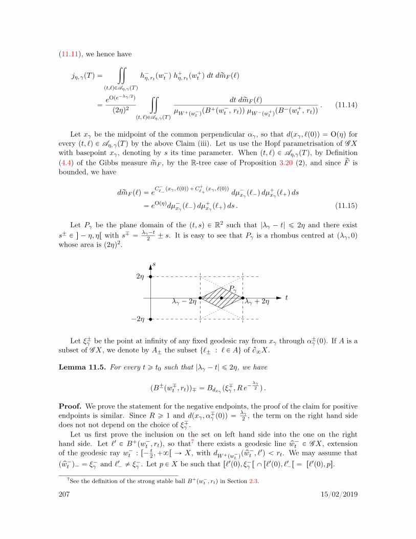
(11.11), we hence have

jη, γpT q “

ij

pt,`qPAη,γpT q

h´η, rtpw´t q h

`η, rtpw

`t q dt drmF p`q

“eOpe´λγ 2q

p2ηq2

ij

pt, `qPAη,γpT q

dt drmF p`q

µW`pw´t qpB`pw´t , rtqq µW´pw`t q

pB´pw`t , rtqq. (11.14)

Let xγ be the midpoint of the common perpendicular αγ , so that dpxγ , `p0qq “ Opηq forevery pt, `q P Aη, γpT q by the above Claim (iii). Let us use the Hopf parametrisation of GXwith basepoint xγ , denoting by s its time parameter. When pt, `q P Aη,γpT q, by Definition(4.4) of the Gibbs measure rmF , by the R-tree case of Proposition 3.20 (2), and since rF isbounded, we have

drmF p`q “ eC´`´

pxγ , `p0qq`C```pxγ , `p0qq

dµ´xγ p`´q dµ`xγ p``q ds

“ eOpηqdµ´xγ p`´q dµ`xγ p``q ds . (11.15)

Let Pγ be the plane domain of the pt, sq P R2 such that |λγ ´ t| ď 2η and there exists˘ P s ´ η, ηr with s¯ “ λγ´t

2 ˘ s. It is easy to see that Pγ is a rhombus centred at pλγ , 0qwhose area is p2ηq2.

´2η

λγ ` 2η t

s

2η

λγ ´ 2η

Pγ

Let ξ˘γ be the point at infinity of any fixed geodesic ray from xγ through α˘γ p0q. If A is asubset of GX, we denote by A˘ the subset t`˘ : ` P Au of B8X.

Lemma 11.5. For every t ě t0 such that |λγ ´ t| ď 2η, we have

pB˘pw¯t , rtqq¯ “ Bdxγ pξ¯γ , R e

´λγ2 q .

Proof. We prove the statement for the negative endpoints, the proof of the claim for positiveendpoints is similar. Since R ě 1 and dpxγ , α

¯γ p0qq “

λγ2 , the term on the right hand side

does not not depend on the choice of ξ¯γ .Let us first prove the inclusion on the set on left hand side into the one on the right

hand side. Let `1 P B`pw´t , rtq, so that7 there exists a geodesic line pw´t P GX, extensionof the geodesic ray w´t : r´ t

2 ,`8r Ñ X, with dW`pw´t qp pw´t , `

1q ă rt. We may assume thatp pw´t q´ “ ξ´γ and `1´ ‰ ξ´γ . Let p P X be such that r`1p0q, ξ´γ r X r`1p0q, `1´r “ r`1p0q, ps.

7See the definition of the strong stable ball B`pw´t , rtq in Section 2.3.

207 15/02/2019

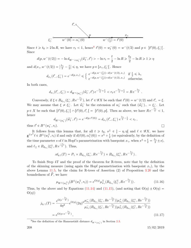
p

ξ´γ w´p0q “ α´γ p0q

`1´

xγ

w´p t2q “ `1p0q

Since t ě t0 ą 2 lnR, we have rt ă 1, hence8 `1p0q “ w´t p0q “ w´pt2q and p P s`1p0q, ξ´γ r .Since

dpp, w´pt2qq “ ´ ln dW´`w´t qp pw´t , `

1q ą ´ ln rt “t

2´ lnR ě

t02´ lnR ě 1 ě η

and dpxγ , w´pt2qq “ˇ

ˇ

λγ2 ´

t2

ˇ

ˇ ď η, we have p P rxγ , ξ´γ r . Hence

dxγ p`1´, ξ

´γ q “ e´dpp, xγq ď

! e´dpp, w´p t

2qq´dpw´pt2q, xγq if t

2 ď λγ

e´dpp, w´p t

2qq`dpw´pt2q, xγq otherwise.

In both cases,

dxγ p`1´, ξ

´γ q “ dW`pw´t q

p pw´t , `1q e´

λγ2` t

2 ă rt e´λγ2` t

2 “ Re´λγ2 .

Conversely, if ξ P Bdxγ pξ´γ , R e

´λγ2 q, let `1 P GX be such that `1p0q “ w´pt2q and `1´ “ ξ.

We may assume that ξ ‰ ξ´γ . Let pw´t be the extension of w´t such that p pw´t q´ “ ξ´γ . Let

p P X be such that r`1p0q, ξ´γ r X r`1p0q, `1´r “ r`1p0q, ps. Then as above, we have Re´λγ2 ă 1,

hencedW`pw´t q

p pw´t , `1q “ e´dpp, `

1p0qq “ dxγ p`1´, ξ

´γ q e

λγ2´ t

2 ă rt ,

thus `1 P B`pw´t , rtq. l

It follows from this lemma that, for all t ě t0, s˘ P s ´ η, ηr and ` P GX, we haveg¯s

¯

` P B˘pw¯t , rtq if and only if dp`p0q, α˘γ p0qq “ s˘` t2 (or equivalently, by the definition of

the time parameter s of ` in Hopf’s parametrisation with basepoint xγ , when s˘` t2 “

λγ2 ˘s),

and `˘ P Bdxγ pξ˘γ , R e

´λγ2 q. Thus,

Aη,γpT q “ Pγ ˆBdxγ pξ´γ , R e

´λγ2 q ˆBdxγ pξ

`γ , R e

´λγ2 q .

To finish Step 4T and the proof of the theorem for R-trees, note that by the definitionof the skinning measure (using again the Hopf parametrisation with basepoint xγ), by theabove Lemma 11.5, by the claim for R-trees of Assertion (2) of Proposition 3.20 and theboundedness of rF , we have

µW˘pw¯t qpB˘pw¯t , rtqq “ eOpηqµ¯xγ pBdxγ pξ

¯γ , R e

´λγ2 qq . (11.16)

Thus, by the above and by Equations (11.14) and (11.15), (and noting that Opηq ˘ Opηq “Opηq)

jη, γpT q “eOpe´

λγ2 q

4η2eOpηqp2ηq2

µ´xγ pBdxγ pξ´γ , Re

´λγ2 qqµ`xγ pBdxγ pξ

`γ , Re

´λγ2 qq

µ´xγ pBdxγ pξ´γ , Re

´λγ2 qqµ`xγ pBdxγ pξ

`γ , Re

´λγ2 qq

“ eOpη`e´λγ2 q , (11.17)

8See the definition of the Hamenstädt distance dW`pw´t q

in Section 2.3.

208 15/02/2019

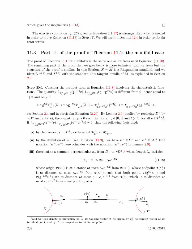
which gives the inequalities (11.13). l

The effective control on jη, γpT q given by Equation (11.17) is stronger than what is neededin order to prove Equation (11.13) in Step 4T. We will use it in Section 12.6 in order to obtainerror terms.

11.3 Part III of the proof of Theorem 11.1: the manifold case

The proof of Theorem 11.1 for manifolds is the same one as for trees until Equation (11.10).The remaining part of the proof that we give below is more technical than for trees but thestructure of the proof is similar. In this Section, X “ ĂM is a Riemannian manifold, and weidentify GX and T 1X with the standard unit tangent bundle of ĂM , as explained in Section2.3.

Step 3M. Consider the product term in Equation (11.8) involving the characteristic func-tions. The quantity 1V `η,RpΩ

´qpg´t2vq 1V ´η,RpΩ

`qpγ´1gt2vq is different from 0 (hence equal to

1) if and only if

v P gt2V `η,RpΩ

´q X γg´t2V ´η,RpΩ

`q “ V `

η, e´t2Rpgt2Ω´q X V ´

η, e´t2Rpγg´t2Ω`q ,

see Section 2.4 and in particular Equation (2.20). By Lemma 2.9 (applied by replacing D` byγD` and w by v), there exist t0, c0 ą 0 such that for all η P s0, 1s and t ě t0, for all v P T 1

ĂM ,if 1V `η,RpΩ

´qpg´t2vq 1V ´η,RpΩ

`qpγ´1gt2vq ‰ 0, then the following facts hold:

(i) by the convexity of D˘, we have v P U `

D´XU ´

γD`,

(ii) by the definition of w˘ (see Equation (11.9)), we have w´ P Ω´ and w` P γΩ` (thenotation pw´, w`q here coincides with the notation pw´, w`q in Lemma 2.9),

(iii) there exists a common perpendicular αγ from D´ to γD`,9 whose length λγ satisfies

| λγ ´ t | ď 2η ` c0 e´t2 , (11.18)

whose origin πpv´γ q is at distance at most c0 e´t2 from πpw´q, whose endpoint πpv`γ q

is at distance at most c0 e´t2 from πpw`q, such that both points πpgt2w´q and

πpg´t2w`q are at distance at most η ` c0 e´t2 from πpvq, which is at distance at

most c0 e´t2 from some point pv of αγ .

pv

vπpvq

αγ

v´γ v0γ

xγπpv´γ q v`γ

πpv`γ q

D´γD`

9and we then denote as previously by v´γ its tangent vector at its origin, by v`γ its tangent vector at itsterminal point, and by v0

γ its tangent vector at its midpoint

209 15/02/2019

Using (iii) and the (HC)-property10 which introduces a constant κ2 P s0, 1s, and since rF isbounded, for all η P s0, 1s, t ě t0 and v P T 1

ĂM for which 1V `η,RpΩ´qpg´t2vq 1V ´η,RpΩ

`qpγ´1gt2vq ‰

0, we have

e

şπpgt2w´q

πpw´qrF`

şπpw`q

πpg´t2w`qrF“ e

şpv

πpv´γ qrF`

şπpv`γ qpv

rF`Oppη`e´t2qκ2 q

“ eş

αγrFeOppη`e´λγ 2qκ2 q . (11.19)

For all η P s0, 1s, γ P Γ and T ě t0, define

Aη,γpT q “

pt, vq P rt0, T s ˆ T1ĂM : v P V `

η, e´t2Rpgt2Ω´q X V ´

η, e´t2Rpγg´t2Ω`q

(

,

andjη, γpT q “

ij

pt, vqPAη,γpT q

h´η, e´t2R

pgt2w´q h`η, e´t2R

pg´t2w`q dt drmF pvq .

By the above, since the integral of a function is equal to the integral on any Borel set containingits support, and since the integral of a nonnegative function is nondecreasing in the integrationdomain, there hence exists c4 ą 0 such that for all T ě 0 and η P s0, 1s, we have

iηpT q ě ´ c4 `ÿ

γPΓ : t0`2`c0ďλγďT´Opη`e´λγ 2q

v´γ PN´Opη`e´λγ 2q

Ω´, v`γ P γN´Opη`e´λγ 2q

Ω`

eş

αγrFjη, γpT q e

´Oppη`e´λγ 2qκ2 q ,

and similarly, for every T 1 ě T ,

iηpT q ď c4 `ÿ

γPΓ : t0`2`c0ďλγďT`Opη`e´λγ 2q

v´γ PNOpη`e´λγ 2q

Ω´, v`γ P γNOpη`e´λγ 2q

Ω`

eş

αγrFjη, γpT

1q eOppη`e´λγ 2qκ2 q .

We will take T 1 to be of the form T `Opη` e´λγ2q, for a bigger Op¨q than the one appearingin the index of the above summation.

Step 4M: Conclusion. Let γ P Γ be such that D´ and γD` have a common perpendicularwith length λγ ě t0 ` 2 ` c0. Let us prove that for all ε ą 0, if η is small enough and λγ islarge enough, then for every T ě λγ`Opη`e´λγ2q (with the enough’s and Op¨q independentof γ), we have

1´ ε ď jη, γpT q ď 1` ε . (11.20)

Note that rσ˘pNεpΩ¯qq and rσ˘pN´εpΩ

¯qq tend to rσ˘pΩ¯q as ε Ñ 0 (since rσ˘pBΩ¯q “ 0 asrequired in Step 1). Using Steps 2, 3M and 4M, this will prove Equation (11.4), hence willcomplete the proof of Theorem 11.1.

We say that pĂM,Γ, rF q has radius-continuous strong stable/unstable ball masses if for everyε ą 0, if r ą 1 is close enough to 1, then for every v P T 1

ĂM , if B´pv, 1q meets the support ofµ`W´pvq

, thenµ`W´pvq

pB´pv, rqq ď eεµ`W´pvq

pB´pv, 1qq

10See Definition 3.13.

210 15/02/2019

and if B`pv, 1q meets the support of µ´W`pvq

, then

µ´W`pvq

pB`pv, rqq ď eεµ´W`pvq

pB`pv, 1qq .

We say that pĂM,Γ, rF q has radius-Hölder-continuous strong stable/unstable ball masses if thereexist c P s0, 1s and c1 ą 0 such that for every ε P s0, 1s, if r ą 1 is close enough to 1, then forevery v P T 1

ĂM , if B´pv, 1q meets the support of µ`W´pvq

, then

µ`W´pvq

pB´pv, rqq ď ec1εcµ`

W´pvqpB´pv, 1qq

and if B`pv, 1q meets the support of µ´W`pvq

, then

µ´W`pvq

pB`pv, rqq ď ec1εcµ´

W`pvqpB`pv, 1qq .

Note that when F “ 0 andM is locally symmetric with finite volume, the conditional measureson the strong stable/unstable leaves are homogeneous. Hence pĂM,Γ, rF q has radius-Hölder-continuous strong stable/unstable ball masses.

When the sectional curvature of ĂM has bounded derivatives and when pĂM,Γ, rF q hasradius-Hölder-continuous strong stable/unstable ball masses, we will prove a stronger state-ment: With a constant c7 ą 0 and functions Op¨q independent of γ, for all η P s0, 1s andT ě λγ `Opη ` e´λγ2q, we have

jη, γpT q “´

1`O´e´λγ2

2η

¯¯2eOppη`e´λγ 2qc7 q . (11.21)

This stronger version will be needed for the error term estimate in Section 12.3. In order toobtain Theorem 11.1, only the fact that jη, γpT q tends to 1 as firstly λγ tends to `8, secondlyη tends to 0 is needed. A reader not interested in the error term may skip many technicaldetails below.

Given a, b ą 0 and a point x in a metric space X (with a, b, x depending on parameters),we will denote by Bpx, a eOpbqq any subset Y of X such that there exists a constant c ą 0(independent of the parameters) with

Bpx, a e´c bq Ă Y Ă Bpx, a ec bq . (11.22)

Let η P s0, 1s and T ě λγ `Opη ` e´λγ2q. In order to simplify the notation, let

rt “ e´t2R, w´t “ gt2w´ and w`t “ g´t2w` .

By the definition of jη, γ , using the inequalities (10.3) where the constant c1 is uniform sincerF is bounded, and the fact that rt “ Ope´λγ2q by Equation (11.18), we hence have

jη, γpT q “

ij

pt,vqPAη,γpT q

h´η, rtpw´t q h

`η, rtpw

`t q dt drmF pvq

“eOpe´κ2λγ 2q

p2ηq2

ij

pt,vqPAη,γpT q

dt drmF pvq

µW`pw´t q

pB`pw´t , rtqq µW´pw`t qpB´pw`t , rtqq

. (11.23)

We start the proof of Equation (11.20) by defining parameters s`, s´, s, v1, v2 associatedwith pt, vq P Aη,γpT q.

211 15/02/2019

v0γ

v2v1

v

gt2w´g´t2w`s

s´ ´s`

W´pg´t2w`qW`pgt2w´qW`pv1qW

´pv2q

W`pv0γqW´pv0

γq

xγ

We have pt, vq P Aη,γpT q if and only if there exist s˘ P s ´ η, ηr such that

g¯s¯

v P B˘pg˘t2w¯, e´t2Rq .

In order to define the parameters s, v1, v2, we use the well known local product structure ofthe unit tangent bundle in negative curvature. If v P T 1M is close enough to v0

γ (in particular,v´ ‰ pv0

γq` and v` ‰ pv0γq´), then let v1 “ f`

HB´pv0γqpvq be the unique element of W´pv0

γq

such that v1` “ v`, let v2 “ f´HB`pv0

γqpvq be the unique element of W`pv0

γq such that v2´ “ v´,and let s be the unique element of R such that g´sv P W`pv1q. The map v ÞÑ ps, v1, v2q isa homeomorphism from a neighbourhood of v0

γ in T 1ĂM to a neighbourhood of p0, v0

γ , v0γq in

RˆW´pv0γq ˆW

`pv0γq. Note that if v “ grv0

γ for some r P R close to 0, then

w´ “ v´γ , w` “ v`γ , s “ r, v1 “ v2 “ v0

γ ,

s´ “λγ ´ t

2` s, s` “

λγ ´ t

2´ s .

Up to increasing t0 (which does not change Step 3M, up to increasing c4), we may assume thatfor every pt, vq P Aη,γpT q, the vector v belongs to the domain of this local product structureof T 1

ĂM at v0γ .

The vectors v, v1, v2 are close to v0γ if t is large and η small, as the following result shows.

We denote (also) by d the Riemannian distance induced by Sasaki’s metric on T 1ĂM .

Lemma 11.6. For every pt, vq P Aη,γpT q, we have dpv, v0γq, dpv

1, v0γq, dpv

2, v0γq “ Opη` e´t2q.

Proof. Consider the distance d1 on T 1ĂM , defined by

@ v1, v2 P T1ĂM, d1pv1, v2q “ max

rPr´1,0sd`

πpgrv1q, πpgrv2q

˘

.

As seen in Claim (iii) of Step 3M, we have dpπpw˘q, πpv˘γ qq, dpπpvq, αγq “ Ope´t2q, andfurthermore, dpπpg˘t2w¯q, πpvqq, λγ2 ´

t2 “ Opη`e´t2q. Hence dpπpvq, πpv0

γqq “ Opη`e´t2q.By Lemma 2.4, we have

dpπpg´t2´s´vq, πpv´γ qq ď dpπpg´

t2´s´vq, πpw´qq ` dpπpw´q, πpv´γ qq ď R` c0 e

´t2 .

By an exponential pinching argument, we hence have d1pv, v0γq “ Opη ` e´λγ2q. Since d and

d1 are equivalent by Proposition 3.5,11 we therefore have dpv, v0γq “ Opη ` e´λγ2q.

11In fact, Proposition 3.5 considers the distance δ2pv, v1q “ suprPr0,1s dpπpgrvq, πpgrv1qq instead of d1, but

the argument is similar.

212 15/02/2019

For all w P T 1ĂM and V P TwT

1ĂM , we may uniquely write V “ V ´ ` V 0 ` V ` with

V ´ P TwW´pwq, V 0 P R d

dt

ˇ

ˇ

t0gtw and V ` P TwW

`pwq. By [PauPS, Lem. 7.4],12 Sasaki’smetric (with norm ¨ ) is equivalent to the Riemannian metric with (product) norm

V 1 “a

V ´ 2 ` V 0 2 ` V ` 2 .

By the dynamical local product structure of T 1ĂM in the neighbourhood of v0

γ and by thedefinition of v1, v2, the result follows, since the exponential map of T 1

ĂM at v0γ is almost

isometric close to 0 and the projection to a factor of a product norm is Lipschitz. l

We now use the local product structure of the Gibbs measure to prove the following result.

Lemma 11.7. For every pt, vq P Aη,γpT q, we have

dt drmF pvq “ eOppη`e´λγ 2qκ2 q dt ds dµW´pv0γqpv1q dµW`pv0

γqpv2q .

Proof. By the definition of the measures (see Equations (4.4) and (7.9)), since the aboveparameter s differs, when v´, v` are fixed, only up to a constant from the time parameter inHopf’s parametrisation with respect to the basepoint xγ “ πpv0

γq, we have

drmF pvq “ eC´v´pxγ , πpvqq`C

`v`pxγ , πpvqq dµ´xγ pv´q dµ

`xγ pv`q ds

dµW´pv0γqpv1q “ e

C`v1`

pxγ , πpv1qqdµ`xγ pv

1`q ,

dµW`pv0γqpv2q “ e

C´v2´

pxγ , πpv2qqdµ´xγ pv

2´q .

By Proposition 3.20 (2) since F is bounded, we have |C˘ξ pz, z1q | “ Opdpz, z1qκ2q for all

ξ P B8ĂM and z, z1 P ĂM with dpz, z1q bounded. Since the map π : T 1ĂM Ñ ĂM is Lipschitz, and

since v` “ v1` and v´ “ v2´, the result follows from Lemma 11.6. l

When λγ is large, the submanifold gλγ2Ω´ has a second order contact at v0γ with W´pv0

γq

and similarly, g´λγ2Ω` has a second order contact at v0γ with W`pv0

γq. Let Pγ be the planedomain of pt, sq P R2 such that |λγ ´ t| ď 2η ` c0e

´t2 and there exist s˘ P s ´ η, ηr withs¯ “

λγ´t2 ˘ s`Ope´λγ2q. Note that its area is p2η `Ope´λγ2qq2. By the above, we have13

Aη,γpT q “ Pγ ˆB´pv0

γ , rλγ eOpη`e´λγ 2qq ˆB`pv0

γ , rλγ eOpη`e´λγ 2qq .

By Lemma 11.7, we hence haveż

Aη,γpT qdt drmF pvq “ eOppη`e´λγ 2qκ2 q p2η `Ope´λγ2qq2 ˆ

µW´pv0γqpB´pv0

γ , rλγ eOpη`e´λγ 2qqq µW`pv0

γqpB`pv0

γ , rλγ eOpη`e´λγ 2qqq .

(11.24)

The last ingredient of the proof of Step 4M is the following continuity property of themasses of balls in the strong stable and strong unstable manifolds as their centre varies. Thisresult generalises [PaP17b, Lem. 11]. The precise control for the error term is used in Section12.3.

12building on [Brin] whose compactness assumption onM and torsion free assumption on Γ are not necessaryfor this, the pinched negative curvature assumption is sufficient

13with the obvious meaning of a double inclusion by Equation (11.22)

213 15/02/2019

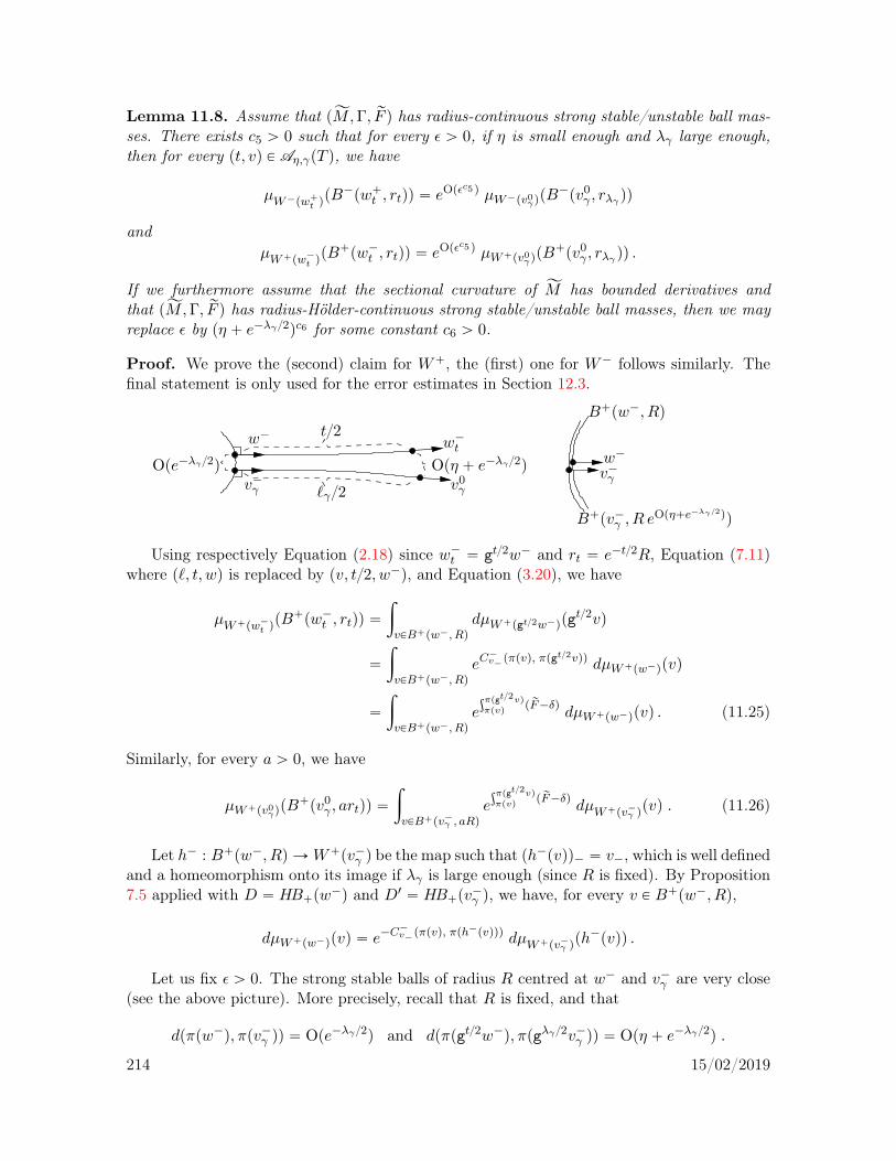
Lemma 11.8. Assume that pĂM,Γ, rF q has radius-continuous strong stable/unstable ball mas-ses. There exists c5 ą 0 such that for every ε ą 0, if η is small enough and λγ large enough,then for every pt, vq P Aη,γpT q, we have

µW´pw`t qpB´pw`t , rtqq “ eOpεc5 q µW´pv0

γqpB´pv0

γ , rλγ qq

andµW`pw´t q

pB`pw´t , rtqq “ eOpεc5 q µW`pv0γqpB`pv0

γ , rλγ qq .

If we furthermore assume that the sectional curvature of ĂM has bounded derivatives andthat pĂM,Γ, rF q has radius-Hölder-continuous strong stable/unstable ball masses, then we mayreplace ε by pη ` e´λγ2qc6 for some constant c6 ą 0.

Proof. We prove the (second) claim for W`, the (first) one for W´ follows similarly. Thefinal statement is only used for the error estimates in Section 12.3.

v´γ

w´ t2

`γ2v0γ

w´t

v´γw´

B`pw´, Rq

Ope´λγ2q Opη ` e´λγ2q

B`pv´γ , R eOpη`e´λγ 2qq

Using respectively Equation (2.18) since w´t “ gt2w´ and rt “ e´t2R, Equation (7.11)where p`, t, wq is replaced by pv, t2, w´q, and Equation (3.20), we have

µW`pw´t qpB`pw´t , rtqq “

ż

vPB`pw´, RqdµW`pgt2w´qpg

t2vq

“

ż

vPB`pw´, RqeC

´v´pπpvq, πpgt2vqq dµW`pw´qpvq

“

ż

vPB`pw´, Rqeşπpgt2vqπpvq

p rF´δqdµW`pw´qpvq . (11.25)

Similarly, for every a ą 0, we have

µW`pv0γqpB`pv0

γ , artqq “

ż

vPB`pv´γ , aRqeşπpgt2vqπpvq

p rF´δqdµW`pv´γ q

pvq . (11.26)

Let h´ : B`pw´, Rq ÑW`pv´γ q be the map such that ph´pvqq´ “ v´, which is well definedand a homeomorphism onto its image if λγ is large enough (since R is fixed). By Proposition7.5 applied with D “ HB`pw

´q and D1 “ HB`pv´γ q, we have, for every v P B`pw´, Rq,

dµW`pw´qpvq “ e´C´v´pπpvq, πph´pvqqq dµW`pv´γ q

ph´pvqq .

Let us fix ε ą 0. The strong stable balls of radius R centred at w´ and v´γ are very close(see the above picture). More precisely, recall that R is fixed, and that

dpπpw´q, πpv´γ qq “ Ope´λγ2q and dpπpgt2w´q, πpgλγ2v´γ qq “ Opη ` e´λγ2q .

214 15/02/2019

Therefore we have dpπpvq, πph´pvqqq ď ε for every v P B`pw´, Rq if η is small enough andλγ is large enough. If we furthermore assume that the sectional curvature has boundedderivatives, then by Anosov’s arguments, the strong stable foliation is Hölder-continuous, seefor instance [PauPS, Theo. 7.3]. Hence we have dpπpvq, πph´pvqqq “ Oppη ` e´λγ2qc6q forevery v P B`pw´, Rq, for some constant c6 ą 0, under the additional regularity assumptionon the curvature. We also have h´pB`pw´, Rqq “ B`pv´γ , R e

Opεqq and, under the additionalhypothesis on the curvature, h´pB`pw´, Rqq “ B`pv´γ , R e

Oppη`e´λγ 2qc6 qq.In what follows, we assume that ε “ pη ` e´λγ2qc6 under the additional assumption

on the curvature. By Proposition 3.20 (2) since rF is bounded, we hence have, for everyv P B`pw´, Rq,

dµW`pw´qpvq “ eOpεκ2 q dµW`pv´γ qph´pvqq

and, using the (HC)-property and the boundedness of rF ,

ż πpgt2vq

πpvqp rF ´ δq ´

ż πpgt2h´pvqq

πph´pvqqp rF ´ δq “ Opεκ2q .

The result follows, by Equation (11.25) and (11.26) and the continuity properties in the radiusof the strong stable/unstable ball masses. l

Now Lemma 11.8 (with ε as in its statement, and when its hypotheses are satisfied) impliesthat

ij

pt,vqPAη,γpT q

dt drmF pvq

µ´W`pw´t q

pB`pw´t , rtqq µ`

W´pw`t qpB´pw`t , rtqq

“eOpεc5 q

ť

pt,vqPAη,γpT qdt drmF pvq

µ´W`pv0

γqpB`pv0

γ , rtqq µ`

W´pv0γqpB´pv0

γ , rtqq.

By Equation (11.23) and Equation (11.24), we hence have

jη, γpT q “ eOppη`e´λγ 2qκ2 q eOpεc5 q p2η `Ope´λγ2qq2

p2ηq2

under the technical assumptions of Lemma 11.8. The assumption on radius-continuity ofstrong stable/unstable ball masses can be bypassed using bump functions, as explained in[Rob2, page 81]. This completes the proof of Equation (11.20), hence the proof of Theorem11.1. l

11.4 Equidistribution of common perpendiculars in simplicialtrees

In this Section, we prove a version of Theorem 11.1 for the discrete time geodesic flow onsimplicial trees (and we leave to the reader the version without the assumption that thecritical exponent of the system of conductances is positive).

Let X, X, x0, Γ, rc, c, rFc, Fc, δc ă `8, pµ˘x qxPV X, rmc, mc be as in the beginning ofSection 9.2. Let D´ “ pD´i qiPI´ and D` “ pD`j qjPI` be locally finite Γ-equivariant families

215 15/02/2019

of nonempty proper simplicial subtrees of X. We denote by D˘k “ |D˘k |1 the geometricrealisation of D˘k for k P I˘.

For every edge path α “ pe1, . . . , enq in X, we set

rcpαq “nÿ

i“1

rcpeiq .

Theorem 11.9. Assume that the critical exponent δc of rc is positive and that the Gibbsmeasure mc is finite and mixing for the discrete time geodesic flow on ΓzGX. Then

limtÑ`8

eδc ´ 1

eδcmc e

´δc tÿ

iPI´„, jPI`„, γPΓ

D´i XD`γj“H, λi, γjďt

ercpαi,γjq ∆α´i, γjb∆α`

γ´1i, j

“ rσ`D´ b rσ´D`

for the weak-star convergence of measures on the locally compact spacep

GXˆp

GX.

Proof. The proof is a modification of the continuous time proof for metric trees in Sections11.1 and 11.2. Here, we indicate the changes to adapt the proof to the discrete time. We usethe conventions for the discrete time geodesic flow described in Section 2.6.

Note that for all i P I´, j P I`, γ P Γ, the common perpendicular αi,γj is now an edgepath from D´i to D`γj , and that by Proposition 3.21, we have

ż

αi,γj

rFc “ rcpαi,γjq .

In the definition of the bump functions in Section 10.1, we assume (as we may) that η ă 1,so that for all η1 P s0, 1r and w P B1

¯D˘ such that w¯ P ΛΓ, we have

V ˘w,η,η1 “ B˘pw, η1q ,

see Equation (2.17) and recall that we are only considering discrete geodesic lines. As `p0q “wp0q for every ` P B˘pw, η1q since η1 ă 1, and as the time is now discrete, Equations (10.1)and (7.12) give

h¯η, η1pwq “1

µW˘pwqpB˘pw, η1qq

. (11.27)

This is a considerable simplification compared with the inequalities of Equation (10.3).In the whole proof, we restrict to t “ n P N, T “ N P N. We keep the notation of

Equation (11.2), as well as the only assumptions on the Borel sets Ω˘ Ă B1¯D

˘ to have finitepositive skinning measure, with boundary of zero skinning measure. In Steps 1 and 2, wedefine instead of Equation (11.3)

IΩ´,Ω`pNq “ peδc ´ 1q mc e´δcpN`1q

ÿ

γPΓ : 0ăλγďN

α´γ |s0,λγ sPΩ´|s0,λγ s, α

`γ |s´λγ,0sPΩ

`|s´λγ,0s

eş

αγrFc ,

and instead of Equation (11.5)

aηpnq “ÿ

γPΓ

ż

`PGXφ´η pg

´tn2u`q φ`η pgrn2sγ´1`q drmcp`q .

216 15/02/2019

Equation (11.6) is replaced by

iηpNq “Nÿ

n“0

eδc n aηpnq ,

so that by a geometric sum argument, the pair of inequalities (11.7) becomes

e´εeδc pN`1q

rσ`pΩ´q rσ´pΩ`q

peδc ´ 1q mc´ cε ď iηpNq ď eε

eδc pN`1qrσ`pΩ´q rσ´pΩ`q

peδc ´ 1q mc` cε .

Step 3 is unchanged up to replacingşT0 by

řNn“0, rF by rFc, δ by δc and t2 by either tn2u

or rn2s, so that Equation (11.10) becomes, since tn2u` rn2s “ n,

h´η,R˝f`

D´p`q h`η,R ˝ f

´

D`pγ´1`q

“ e´δc n eşw´ptn2uq

w´p0qrFc`

şw`p0q

w`p´rn2sqrFch´η, e´tn2uR

pgtn2uw´qh`η, e´rn2sR

pg´rn2sw`q .

The proof then follows in the same way as in Section 11.2, with the simplifications in thepoint (iii) that, taking η ă 12, we have λγ equal to t “ n, and the points w´ptn2 uq, w`p´rn2 sq

and `p0q are equal. In particular, Equation (11.12) simplifies as

e

şw´pt t2 uq

w´p0qrFc`

şw`p0q

w`p´r t2 sq

rFc“ e

ş

αγrFc ,

thus avoiding the assumption that Fc (or equivalently c, see Section 3.2) is bounded. We nowdefine

Aη,γpNq “

pn, `q P rt0, N s ˆ GX : ` P V `

η, e´tn2 uRpgtn

2uΩ´q X V ´

η, e´rn2 sRpγg´rn

2sΩ`q

(

.

The end of Step 3T simplifies as

´ c4 ď iηpNq ´ÿ

γPΓ : t0`2ďλγďN

α´γ |r0, λγ sPΩ´|r0, λγ s, α

`γ |r´λγ, 0sPΩ

`|r´λγ, 0s

eş

αγrFc jη, γpNq ď c4 .

The statement of Step 4T now simplifies as

jη,γpNq “ 1 ,

if η ă 12 , and if γ P Γ is such that D´ and γD` do not intersect and λγ is large enough. We

introduce in its proof the slightly modified notation

r´n “ e´tn2

uR, r`n “ e´rn2

sR, w´n “ gtn2

uw´ and w`n “ g´rn2

sw` .

and we now take as xγ the point at distance tn2 u from its origin on the common perpendicularαγ . Equation (11.14) becomes (using Equation (11.27) instead of Equation (10.3))

jη, γpNq “

ij

pn, `qPAη,γpNq

dn drmcp`q

µW`pw´n qpB`pw´n , r

´n qq µW´pw`n q

pB´pw`n , r`n qq

.

217 15/02/2019

Since `p0q “ xγ if pn, `q P Aη, γpNq, Equation (11.15) simplifies as

drmcp`q “ dµ´xγ p`´q dµ`xγ p``q ds ,

with ds the counting measure on the Hopf parameter s P Z of ` (with basepoint xγ). If η ă 12 ,

replacing Pγ with its intersection with Z2 reduces it to one point pλγ , 0q, and now s “ s˘ “ 0.Lemma 11.5 becomes

pB`pw´n , r´n qq´ “ Bdxγ pξ

´γ , R e

´tλγ2

uq, pB´pw`n , r`n qq` “ Bdxγ pξ

`γ , R e

´rλγ2

sq ,

so thatAη,γpNq “ tpλγ , 0qu ˆBdxγ pξ

´γ , R e

´tλγ2

uq ˆBdxγ pξ`γ , R e

´rλγ2

sq .

Finally, since `p0q “ xγ if pn, `q P Aη, γpNq, Equation (11.16) becomes

µW`pw´n qpB`pw´n , r

´n qq “ µ´xγ pBdxγ pξ

´γ , R e

´tλγ2

uqq,

µW´pw`t qpB´pw`n , r

`n qq “ µ`xγ pBdxγ pξ

`γ , R e

´rλγ2

sqq .

The last centred equation in Step 4T now reduces to jη, γpT q “ 1. l

For lattices in regular trees, we get more explicit expressions.

Corollary 11.10. Let X be a pq`1q-regular simplicial tree (with q ě 2) and let Γ be a latticeof X such that ΓzX is not bipartite. Assume that the Patterson density is normalised to bea family of probability measures. Let D˘ be nonempty proper simplicial subtrees of X withstabilisers ΓD˘ in Γ, such that D˘ “ pγD˘qγPΓΓD˘

is locally finite. Let σ¯D˘ be their skinningmeasures for the sero system of conductances. Then

limtÑ`8

q ´ 1

q ` 1VolpΓzzXq q´t

ÿ

pα, β, γqPΓΓD´ˆΓΓD`ˆΓ

0ădpαD´, γβD`qďt

∆α´α, γβb∆α`

γ´1α, β

“ rσ`D´ b rσ´D` ,

for the weak-star convergence of measures on the locally compact spacep

GXˆp

GX.If the measure σ´D` is nonzero and finite, then

limtÑ`8

q ´ 1

q ` 1

VolpΓzzXqσ´D`

q´tÿ

γPΓΓD` , 0ădpD´, γD`qďt

∆α´e, γ“ rσ`D´ ,

for the weak-star convergence of measures on the locally compact spacep

GX.

Proof. In order to prove the first claim, we apply Theorem 11.9 with rc ” 0, so that byProposition 4.16, Theorem 4.17, and Proposition 8.1 (3), we have δc “ ln q ą 0, mc “ mBM

is finite and mixing, and mBM “qq`1 VolpΓzzXq.

The second claim follows by restricting to α “ β “ e and integrating on an appropriatefundamental domain (note that Equation (11.4) does not require Ω` to be relatively compact,just to have finite measure for rσ´). l

The mixing assumption in Theorem 11.9 implies that the length spectrum LΓ of Γ isequal to Z. The next result considers the other case, when only the square of the geodesicflow is mixing, while appropriately restricted. Note that the smallest nonempty Γ-invariantsimplicial subtree of X is uniform, without vertices of degree 2, for instance in the case whenX is pp` 1, q ` 1q-biregular with p, q ě 2 and Γ is a lattice of X.

218 15/02/2019

Theorem 11.11. Assume that the smallest nonempty Γ-invariant simplicial subtree of X isuniform, without vertices of degree 2, and that the length spectrum LΓ of Γ is 2Z. Assumethat the critical exponent δc of rc is positive, that the Gibbs measure mc is finite and that itsrestriction to ΓzGevenX is mixing for the square of the discrete time geodesic flow on ΓzGevenX.Then

limtÑ`8

e2 δc ´ 1

2 e2 δcmc e

´δc tÿ

iPI´„, jPI`„, γPΓ

D´i XD`γj“H, λi, γjďt

ercpαi,γjq ∆α´i, γjb∆α`

γ´1i, j

“ rσ`D´ b rσ´D`

for the weak-star convergence of measures on the locally compact spacep

GXˆp

GX.

Proof. We denote by rσ˘D¯, eventhe restriction of rσ˘D¯ to

p

Geven X, and by rσ˘D¯, oddthe restriction

of rσ˘D¯ top

Godd X “p

GX ´p

Geven X. We denote by VevenX the subset of V X consisting of thevertices at even distance from x0, and by VoddX “ V X´ VevenX its complement. The subsetsVevenX and VoddX are Γ-invariant if LΓ “ 2Z by Equation (4.17).

Let us first prove that

limtÑ`8

e2 δc ´ 1

2 e2 δcmc e

´δc tÿ

iPI´„, jPI`„, γPΓ

πpα´i,γjq, πpα`

γ´1i,jq PVevenX

D´i XD`γj“H, λi, γjďt

ercpαi,γjq ∆α´i, γjb∆α`

γ´1i, j

“ rσ`D´, evenb rσ´D`, even

(11.28)

for the weak-star convergence of measures on the locally compact spacep

Geven Xˆp

Geven X.

The proof of this Equation (11.28) is a modification of the proof of the previous Theorem11.9. We now restrict to t “ 2n P N, T “ 2N P N, and we replace rmc by prmcq

ˇ

ˇ

GevenX andpgtqtPZ by pg2tqtPZ. Note that since rmc is invariant under the time 1 of the geodesic flow,which maps ΓzGevenX to ΓzGX´ ΓzGevenX, we have

›

›pmcqˇ

ˇ

ΓzGevenX

›

› “1

2mc . (11.29)

Note that for all i P I´, j P I` and γ P Γ, if πpα´i,γjq and πpα`γ´1i,j

q belong to VevenX,then the distance between D´i and γD`j is even.14

In Steps 1 and 2, we now consider Ω˘ two Borel subsets of B1¯D

˘X

p

Geven X, and we defineinstead of Equation (11.3)

IΩ´,Ω`p2Nq “ pe2 δc ´ 1q

mc

2e´2 δcpN`1q ˆ

ÿ

γPΓ : 0ăλγď2N, πpα´γ q, πpα`γ q PVevenX

α´γ |s0,λγ sPΩ´|s0,λγ s, α

`γ |s´λγ,0sPΩ

`|s´λγ,0s

eş

αγrFc ,

14Indeed, for all x, y, z in a simplicial tree, if p is the closest point to x on ry, zs, then dpy, zq “ dpy, xq `dpx, zq ´ 2 dpx, pq.

219 15/02/2019

and instead of Equation (11.5)

aηp2nq “ÿ

γPΓ

ż

`PGevenXφ´η pg

´2tn2u`q φ`η pg2rn2sγ´1`q drmcp`q .

Equation (11.6) is replaced by

iηp2Nq “Nÿ

n“0

eδc 2n aηp2nq .

The mixing property of the square of the geodesic flow on ΓzGevenX for the restriction of theGibbs measure mc gives that, for every ε ą 0, there exists Tε “ Tε,η ě 0 such that for alln ě Tε, we have

e´εş

GevenX φ´η drmc

ş

GevenX φ`η drmc

pmcqˇ

ˇ

ΓzGevenX

ď aηp2nq ďeε

ş

GevenX φ´η drmc

ş

GevenX φ`η drmc

pmcqˇ

ˇ

ΓzGevenX.

Note that GevenX is saturated by the strong stable and strong unstable leaves, since two pointsx, y on a given horosphere of centre ξ P B8X are at even distance one from another (equalto 2dpx, pq where rx, ξr X ry, ξr “ rp, ξr ). By the disintegration statement in Proposition 7.7,when ` ranges over U ˘

D X GevenX, we have

drmc|U ˘D XGevenXp`q “

ż

ρPB1˘DX

p

Geven Xdν¯ρ p`q drσ

˘Dpρq .

Hence the proof of Lemma 10.1 extends to giveż

GevenXφ¯η drmc “ rσ˘evenpΩ

¯q , (11.30)

where in order to simplify notation rσ˘even “ rσ˘D¯, even

.Therefore, by Equations (11.29) and (11.30), and by a geometric sum argument, the pair

of inequalities (11.7) becomes

2 e´εe2δc pN`1qrσ`evenpΩ

´q rσ´evenpΩ`q

pe2δc ´ 1q mc´ cε

ď iηp2Nq ď2 eεe2δc pN`1q

rσ`evenpΩ´q rσ´evenpΩ

`q

pe2δc ´ 1q mc` cε .

Up to replacing the summations from n “ 0 to N to summations on even numbers between0 to 2N , and replacing tn2u by 2tn2u as well as rn2s by 2rn2s, the remaining part of theproof applies and gives the result, noting that in Claim (iii) of Step 3T, we furthermore havethat the origin and endpoint of the constructed common perpendicular αγ are in VevenX. Thisconcludes the proof of Equation (11.28).

The remainder of the proof of Theorem 11.11 consists in proving versions of the equidis-tribution result Equation (11.28) in

p

Godd X ˆp

Godd X,p

Geven X ˆp

Godd X,p

Godd X ˆp

Geven X re-spectively , and in summing these four contributions.

220 15/02/2019

By applying Equation (11.28) by replacing x0 by a vertex x10 in VoddX, which exchangesVevenX and VoddX,

p

Geven X andp

Godd X, as well as rσ˘D¯, evenand rσ˘D¯, odd

, we have

limtÑ`8

e2 δc ´ 1

2 e2 δcmc e

´δc tÿ

iPI´„, jPI`„, γPΓ

πpα´i,γjq, πpα`

γ´1i,jq PVoddX

D´i XD`γj“H, λi, γjďt

erc pαi,γjq ∆α´i, γjb∆α`

γ´1i, j

“ rσ`D´, oddb rσ´D`, odd

(11.31)

for the weak-star convergence of measures on the locally compact spacep

Godd Xˆp

Godd X.

Let us now apply Equation (11.28) by replacing D´ “ pD´i qiPI´ by N1D´ “ pN1D´i qiPI´ .

Let us consider the map ϕ` :

p

GX Ñ

p

GX, which maps a generalised geodesic line ` to thegeneralised geodesic line which coincides with g`1` on r0,`8r and is constant (with value`p1q) on s ´ 8, 0r. Note that this map is continuous and Γ-equivariant, and that it mapsp

Geven X inp

Godd X andp

Godd X inp

Geven X.Furthermore, by convexity, ϕ` induces for every i P I´ a homeomorphism from B1

`D´i to

B1`N1D

´i , which sends B1

`D´i X

p

Godd X to B1`N1D

´i X

p

Geven X, such that, by Equation (7.8),for all w P B1

`D´i X

p

Godd X, if ew is the first edge followed by w

drσ`D´i , odd

pwq “ erc pewq´δc drσ`N1D

´i , even

pϕ`pwqq .

Note that for all ` ą 0, there is a one-to-one correspondence between the set of commonperpendiculars of length `, with origin and endpoint both in Veven, between N1D

´i and γD`j

for all i P I´, j P I` and γ P Γ, and the set of common perpendiculars of length ` ` 1, withorigin in Vodd and endpoint in Veven, between D´i and γD`j for all i P I´, j P I` and γ P Γ.In particular, ϕ`pα´i,γjq is the common perpendicular between N1D

´i and γD`j , starting at

time t “ 0 from N1D´i .

Therefore Equation (11.28) applied by replacing D´ “ pD´i qiPI´ by N1D´ “ pN1D´i qiPI´

gives

limtÑ`8

e2 δc ´ 1

2 e2 δcmc e

´δc t

ÿ

iPI´„, jPI`„, γPΓ

πpα´i,γjq PVoddX, πpα`γ´1i,jq PVevenX

D´i XD`γj“H, λi, γjďt`1

erc pe

α´i, γj

q`rc pϕ`pα´i,γjqq

∆α´i, γjb∆α`

γ´1i, j

“ eδc rσ`D´, oddb rσ´D`, even

for the weak-star convergence of measures on the locally compact spacep

Godd X ˆp

Geven X.

221 15/02/2019

Since rcpeα´i, γj q ` rcpϕ`pα´i,γjqq “ rcpα´i,γjq, replacing t by t´ 1 and simplifying by eδc , we get

limtÑ`8

e2 δc ´ 1

2 e2 δcmc e

´δc t

ÿ

iPI´„, jPI`„, γPΓ

πpα´i,γjq PVoddX, πpα`γ´1i,jq PVevenX

D´i XD`γj“H, λi, γjďt

ercpα´i,γjq ∆α´i, γj

b∆α`γ´1i, j

“ rσ`D´, oddb rσ´D`, even

(11.32)

for the weak-star convergence of measures on the locally compact spacep

Godd Xˆp

Geven X.Now Theorem 11.11 follows by summing Equation (11.28), Equation (11.31), Equation

(11.32) and the formula, proven similarly, obtained from Equation (11.28) by replacing D` “

pD`j qjPI` by pN1D`j qjPI` . l

The following result for bipartite graphs (of groups) is used in the arithmetic applicationsin Part III (see Section 15.4).

Corollary 11.12. Let X be a pp`1, q`1q-biregular simplicial tree (with p, q ě 2, possibly withp “ q), with corresponding partition V X “ VpX\ VqX. Let Γ be a lattice of X such that thispartition is Γ-invariant. Assume that the Patterson density is normalised so that µx “ p`1

?p

for every x P VpX. Let D˘ be nonempty proper simplicial subtrees of X with stabilisers ΓD˘in Γ, such that the families D˘ “ pγD˘qγPΓΓD˘

are locally finite. Let σ¯D˘ be their skinningmeasures for the sero system of conductances. Then

limtÑ`8

pq ´ 1

2TVolpΓzzXq

?pq´t´2

ÿ

pα, β, γqPΓΓD´ˆΓΓD`ˆΓ

0ădpαD´, γβD`qďt

∆α´α, γβb∆α`

γ´1α, β

“ rσ`D´ b rσ´D`

for the weak-star convergence of measures on the locally compact spacep

GXˆp

GX.If the measure σ´D` is nonzero and finite, then

limtÑ`8

pq ´ 1

2

TVolpΓzzXqσ´D`

?pq´t´2

ÿ

γPΓΓD`0ădpD´, γD`qďt

∆α´e, γ“ rσ`D´ ,

for the weak-star convergence of measures on the locally compact spacep

GX.

Proof. In order to prove the first result, we apply Theorem 11.11 with rc ” 0, so thatby Equation (8.1), Proposition 4.16, Theorem 4.17, and Proposition 8.1 (2), we have δc “12 lnppqq ą 0, mc “ mBM is finite and its restriction to ΓzGevenX is mixing under the squareof the geodesic flow, and mBM “ TVolpΓzzXq.

The second claim follows as in the proof of Corollary 11.10. l

Remark. In some special occasions, the measures involved in the statements of Theo-rem 11.11 and Corollary 11.12 (whether skinning measures or Dirac masses) are actuallyall supported on

p

Geven X (up to choosing appropriately x0). This is in particular the caseif D˘ “ pγD˘qγPΓΓD˘

with D´,D` horoballs at even signed distance (see below), as thefollowing lemma shows.

222 15/02/2019

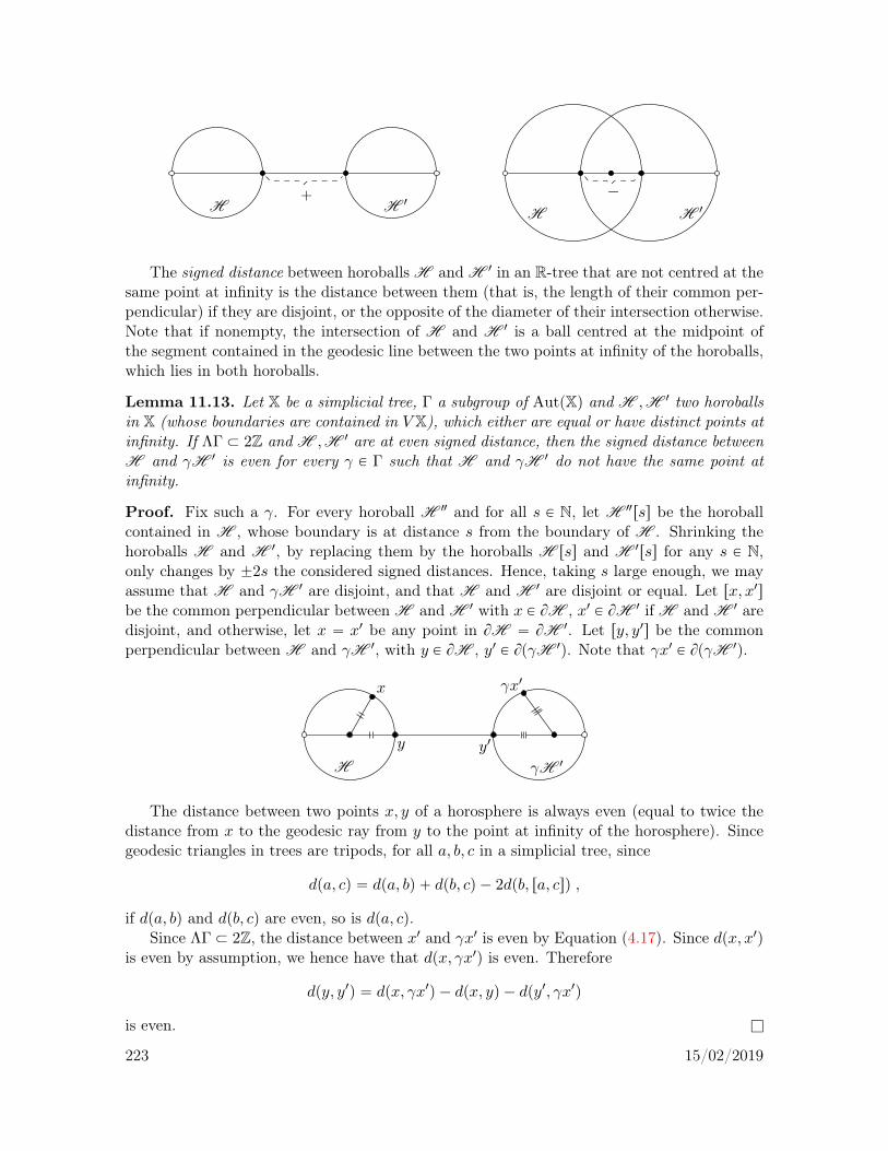
` ´H H 1

H H 1

The signed distance between horoballs H and H 1 in an R-tree that are not centred at thesame point at infinity is the distance between them (that is, the length of their common per-pendicular) if they are disjoint, or the opposite of the diameter of their intersection otherwise.Note that if nonempty, the intersection of H and H 1 is a ball centred at the midpoint ofthe segment contained in the geodesic line between the two points at infinity of the horoballs,which lies in both horoballs.

Lemma 11.13. Let X be a simplicial tree, Γ a subgroup of AutpXq and H ,H 1 two horoballsin X (whose boundaries are contained in V X), which either are equal or have distinct points atinfinity. If ΛΓ Ă 2Z and H ,H 1 are at even signed distance, then the signed distance betweenH and γH 1 is even for every γ P Γ such that H and γH 1 do not have the same point atinfinity.

Proof. Fix such a γ. For every horoball H 2 and for all s P N, let H 2rss be the horoballcontained in H , whose boundary is at distance s from the boundary of H . Shrinking thehoroballs H and H 1, by replacing them by the horoballs H rss and H 1rss for any s P N,only changes by ˘2s the considered signed distances. Hence, taking s large enough, we mayassume that H and γH 1 are disjoint, and that H and H 1 are disjoint or equal. Let rx, x1sbe the common perpendicular between H and H 1 with x P BH , x1 P BH 1 if H and H 1 aredisjoint, and otherwise, let x “ x1 be any point in BH “ BH 1. Let ry, y1s be the commonperpendicular between H and γH 1, with y P BH , y1 P BpγH 1q. Note that γx1 P BpγH 1q.

x

H

y1y

γx1

γH 1

The distance between two points x, y of a horosphere is always even (equal to twice thedistance from x to the geodesic ray from y to the point at infinity of the horosphere). Sincegeodesic triangles in trees are tripods, for all a, b, c in a simplicial tree, since

dpa, cq “ dpa, bq ` dpb, cq ´ 2dpb, ra, csq ,

if dpa, bq and dpb, cq are even, so is dpa, cq.Since ΛΓ Ă 2Z, the distance between x1 and γx1 is even by Equation (4.17). Since dpx, x1q

is even by assumption, we hence have that dpx, γx1q is even. Therefore

dpy, y1q “ dpx, γx1q ´ dpx, yq ´ dpy1, γx1q

is even. l

223 15/02/2019

224 15/02/2019

Chapter 12

Equidistribution and counting ofcommon perpendiculars in quotientspaces

In this Chapter, we use the results of Chapter 11 to prove equidistribution and countingresults in Riemannian manifolds (or good orbifolds) and in metric and simplicial graphs (ofgroups).

Let X, x0, Γ and rF be as in the beginning of Chapter 11. We will need the following twonotions in this chapter.

Recall that the narrow topology1 on the set MfpY q of finite measures on a Polish spaceY is the smallest topology such that the map from MfpY q to R defined by µ ÞÑ µpgq iscontinuous for every bounded continuous function g : Y Ñ R. Since continous functionswith compact support are bounded, the narrow convergence of finite measures implies theirweak-star convergence.

Recall that given a discrete group G acting properly (but not necessarily freely) on alocally compact space Z, the induced measure2 on GzZ of a (positive, Radon) measure µ onZ is a measure µ which depends linearly and continuously for the weak-star topology on µ,and satisfies ∆z “

1|Gz |

∆Gz for every z P Z. The following observation on the behaviour ofinduced measures under quotients by properly discontinuous group actions will be used in theproofs of Corollary 12.3 and its analogues in Section 12.4. Let G be a discrete group thatacts properly on a Polish space rY and let Y “ GzrY . Let rµk for k P N and rµ be G-invariantlocally finite measures on rY , with finite induced measures µk for k P N and µ on Y . If forevery Borel subset B of rY with rµpBq finite and rµpBBq “ 0 we have limkÑ8 rµkpBq “ rµpBq,then the sequence pµkqkPN narrowly converges to µ.

12.1 Multiplicities and counting functions in Riemannian orb-ifolds

In this Section, we assume that X “ ĂM is a Riemannian manifold. We denote its quotientRiemannian orbifold under Γ by M “ ΓzĂM , and the quotient Riemannian orbifold under Γ

1also called weak topology see for instance [DM, p. 71-III] or [Bil, Part]2See for instance [PauPS, §2.6] for details.

225 15/02/2019

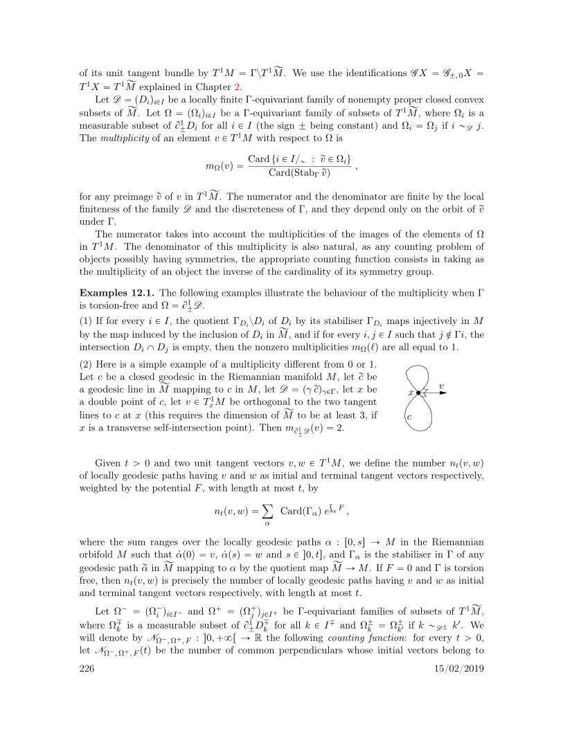
of its unit tangent bundle by T 1M “ ΓzT 1ĂM . We use the identifications GX “ G˘, 0X “

T 1X “ T 1ĂM explained in Chapter 2.

Let D “ pDiqiPI be a locally finite Γ-equivariant family of nonempty proper closed convexsubsets of ĂM . Let Ω “ pΩiqiPI be a Γ-equivariant family of subsets of T 1

ĂM , where Ωi is ameasurable subset of B1

˘Di for all i P I (the sign ˘ being constant) and Ωi “ Ωj if i „D j.The multiplicity of an element v P T 1M with respect to Ω is

mΩpvq “Card ti P I„ : rv P Ωiu

CardpStabΓ rvq,

for any preimage rv of v in T 1ĂM . The numerator and the denominator are finite by the local

finiteness of the family D and the discreteness of Γ, and they depend only on the orbit of rvunder Γ.

The numerator takes into account the multiplicities of the images of the elements of Ωin T 1M . The denominator of this multiplicity is also natural, as any counting problem ofobjects possibly having symmetries, the appropriate counting function consists in taking asthe multiplicity of an object the inverse of the cardinality of its symmetry group.

Examples 12.1. The following examples illustrate the behaviour of the multiplicity when Γis torsion-free and Ω “ B1

˘D .(1) If for every i P I, the quotient ΓDizDi of Di by its stabiliser ΓDi maps injectively in Mby the map induced by the inclusion of Di in ĂM , and if for every i, j P I such that j R Γi, theintersection Di XDj is empty, then the nonzero multiplicities mΩp`q are all equal to 1.

(2) Here is a simple example of a multiplicity different from 0 or 1.Let c be a closed geodesic in the Riemannian manifold M , let rc bea geodesic line in ĂM mapping to c in M , let D “ pγ rcqγPΓ, let x bea double point of c, let v P T 1

xM be orthogonal to the two tangentlines to c at x (this requires the dimension of ĂM to be at least 3, ifx is a transverse self-intersection point). Then mB1

˘Dpvq “ 2.

xv

c

Given t ą 0 and two unit tangent vectors v, w P T 1M , we define the number ntpv, wqof locally geodesic paths having v and w as initial and terminal tangent vectors respectively,weighted by the potential F , with length at most t, by

ntpv, wq “ÿ

α

CardpΓαq eş

α F ,

where the sum ranges over the locally geodesic paths α : r0, ss Ñ M in the Riemannianorbifold M such that 9αp0q “ v, 9αpsq “ w and s P s0, ts, and Γα is the stabiliser in Γ of anygeodesic path rα in ĂM mapping to α by the quotient map ĂM ÑM . If F “ 0 and Γ is torsionfree, then ntpv, wq is precisely the number of locally geodesic paths having v and w as initialand terminal tangent vectors respectively, with length at most t.

Let Ω´ “ pΩ´i qiPI´ and Ω` “ pΩ`j qjPI` be Γ-equivariant families of subsets of T 1ĂM ,

where Ω¯k is a measurable subset of B1˘D

¯k for all k P I¯ and Ω˘k “ Ω˘k1 if k „D˘ k1. We

will denote by NΩ´,Ω`, F : s0,`8r Ñ R the following counting function: for every t ą 0,let NΩ´,Ω`, F ptq be the number of common perpendiculars whose initial vectors belong to

226 15/02/2019

the images in T 1M of the elements of Ω´ and terminal vectors to the images in T 1M of theelements of Ω`, counted with multiplicities and weighted by the potential F , that is:

NΩ´,Ω`, F ptq “ÿ

v, w PT 1M

mΩ´pvq mΩ`pwq ntpv, wq .

When Ω˘ “ B1¯D˘, we denote NΩ´,Ω`, F by ND´,D`, F .

Remark 12.2. Let Y be a negatively curved complete connected Riemannian manifold andlet rY Ñ Y be its Riemannian universal cover. Let D˘ be a locally convex3 geodesic metricspace endowed with a continuous map f˘ : D˘ Ñ Y such that if rD˘ Ñ D˘ is a locallyisometric universal cover and if rf˘ : rD˘ Ñ rY is a lift of f˘, then rf˘ is on each connectedcomponent of rD˘ an isometric embedding whose image is a proper nonempty closed locallyconvex subset of rY , and the family of images under the covering group of rY Ñ Y of theimages by rf˘ of the connected components of rD˘ is locally finite. Then D˘ (or the pairpD˘, f˘q) is a proper nonempty properly immersed closed locally convex subset of Y .

If Γ is a discrete subgroup without torsion of isometries of a CAT(´1) Riemannian mani-foldX, if D˘ “ pγ rD˘qγPΓ where rD˘ is a nonempty proper closed convex subset ofX such thatthe family D˘ is locally finite, and if D˘ is the image of rD˘ by the covering map X Ñ ΓzX,then D˘ is a proper nonempty properly immersed closed convex subset of ΓzX. Under theseassumptions, ND´,D`, F is the counting function ND´, D`, F given in the introduction.

Let us continue fixing the notation used in Sections 12.2 and 12.3. For every pi, jq inI´ˆI` such that D´i and D`j have a common perpendicular4, we denote by αi, j this commonperpendicular, by λi, j its length, by v´i, j P B

1`D

´i its initial tangent vector and by v`i, j P B

1´D

`i

its terminal tangent vector. Note that if i1 „ i, j1 „ j and γ P Γ, then

γ αi1, j1 “ αγi, γj , λi1, j1 “ λγi, γj and γ v˘i1, j1 “ v˘γi, γj . (12.1)

When Γ has no torsion, we have, for the diagonal action of Γ on I´ ˆ I`,

ND´,D`, F ptq “ÿ

pi, jqPΓzppI´„qˆpI`„qq : D´i XD`j “H, λi, jďt

eş

αi, jrF.

When the potential F is zero and Γ has no torsion, ND´,D`, F ptq is the number of commonperpendiculars of length at most t, and the counting function t ÞÑ ND´,D`, 0ptq has beenstudied in various special cases of negatively curved manifolds since the 1950’s and in anumber of recent works, see the Introduction. The asymptotics of ND´,D`, 0ptq as t Ñ `8

in the case when X is a Riemannian manifold with pinched negative curvature are describedin general in [PaP17b, Theo. 1], where it is shown that if the skinning measures σ`D´ and σ´D`are finite and nonzero, then as sÑ `8,

ND´,D`, 0psq „σ`D´ σ

´

D`

mBM

eδΓ s

δΓ. (12.2)

3not necessarily connected4that is, whose closures D´i and D`j in X Y B8X have empty intersection

227 15/02/2019

12.2 Common perpendiculars in Riemannian orbifolds

Corollary 12.3 below is the main result of this text on the counting with weights of commonperpendiculars and on the equidistribution of their initial and terminal tangent vectors innegatively curved Riemannian manifolds endowed with a Hölder-continuous potential. Weuse the notation of Section 12.1.

Corollary 12.3. Let ĂM be a complete simply connected Riemannian manifold with pinchednegative sectional curvature at most ´1. Let Γ be a nonelementary discrete group of isometriesof ĂM . Let rF : T 1

ĂM Ñ R be a bounded Γ-invariant Hölder-continuous function with positivecritical exponent δ. Let D´ “ pD´i qiPI´ and D` “ pD`j qjPI` be locally finite Γ-equivariantfamilies of nonempty proper closed convex subsets of ĂM . Assume that the Gibbs measure mF

is finite and mixing for the geodesic flow on T 1M . Then,

limtÑ`8

δ mF e´δ t

ÿ

v, wPT 1M

mB1`D´pvq mB1

´D`pwq ntpv, wq ∆v b∆w

“ σ`D´ b σ´

D` (12.3)

for the weak-star convergence of measures on the locally compact space T 1M ˆ T 1M . If σ`D´and σ´D` are finite, the result also holds for the narrow convergence.

Furthermore, for all Γ-equivariant families Ω˘ “ pΩ˘k qkPI˘ of subsets of T 1ĂM with Ω˘k a

Borel subset of B1¯D

˘k for all k P I˘ and Ω˘k “ Ω˘k1 if k „D˘ k

1, with nonzero finite skinningmeasure and with boundary in B1

˘D¯k of zero skinning measure, we have, as tÑ `8,

NΩ´,Ω`, F ptq „σ`

Ω´ σ´

Ω`

δ mF eδ t .

Proof. Note that the sum in Equation (12.3) is locally finite, hence it defines a locally finitemeasure on T 1M ˆ T 1M . We are going to rewrite the sum in the statement of Theorem 11.1in a way which makes it easier to push it down from T 1

ĂM ˆ T 1ĂM to T 1M ˆ T 1M .

For every rv P T 1ĂM , let

m¯prvq “ Card tk P I¯„ : rv P B1˘D

¯k u ,

so that for every v P T 1M , the multiplicity of v with respect to the family B1˘D¯ is5

mB1˘D¯pvq “

m¯prvq

CardpStabΓ rvq,

for any preimage rv of v in T 1ĂM .

For all γ P Γ and rv, rw P T 1ĂM , there exists pi, jq P pI´„q ˆ pI`„q such that rv “ v´i,γj

and rw “ v`γ´1i,j

“ γ´1v`i,γj if and only if γ rw P gR rv, there exists i1 P I´„ such that rv P B1`D

´i1

and there exists j1 P I`„ such that γ rw P B1´D

`j1 . Then the choice of such elements pi, jq, as

5See Section 12.1.

228 15/02/2019

well as i1 and j1, is free. We hence have

ÿ

iPI´„, jPI`„, γPΓ

0ăλi, γjďt , v´i, γj“rv , v

`

γ´1i, j“ rw

eş

αi, γjrF

∆v´i, γjb∆v`

γ´1i, j

“ÿ

γPΓ, 0ăsďtγ rw“gsrv

eşγπp rwqπprvq

rFCard

pi, jq P pI´„q ˆ pI`„q : v´i, γj “ rv , v`

γ´1i, j“ rw

(

∆rv b∆

rw

“ÿ

γPΓ, 0ăsďtγ rw“gsrv

eşγπp rwqπprvq

rFm´prvq m`pγ rwq ∆

rv b∆rw .

Thereforeÿ

iPI´„, jPI`„, γPΓ0ăλi, γjďt

eş

αi, γjrF

∆v´i, γjb∆v`

γ´1i, j

“ÿ

rv, rw PT 1ĂM

´

ÿ

γPΓ, 0ăsďtγ rw“gsrv

eşγπp rwqπprvq

rF¯

m´prvq m`p rwq ∆rv b∆ rw .

By definition, σ˘D¯ is the measure on T 1M induced by the Γ-invariant measure rσ˘D¯ .Thus Corollary 12.3 follows from Theorem 11.1 after a similar reduction6 as in Section 11.1.The narrow convergence is obtained when the skinning measures σ˘D¯ are finite, using thecontinuity properties of the induced measures recalled at the beginning of Chapter 12, sinceno compactness assumptions were made in Equation (11.4) on Ω˘.

The counting statement follows from the equidistribution result by integration. l

In particular, if the skinning measures σ`D´ and σ´D` are positive and finite, Corollary 12.3gives, as tÑ `8,

ND´,D`, F ptq „σ`D´ σ

´

D`

δ mF eδ t .

Remark 12.4. Under the assumptions of Corollary 12.3 with the exception that δ may nowbe nonpositive, we have the following asymptotic result as t Ñ `8 for the growth of theweighted number of common perpendiculars with lengths in st´ τ, ts for every fixed τ ą 0:

ND´,D`, F ptq ´ND´,D`, F pt´ τq „p1´ e´δ τ q σ`D´ σ

´

D`

δ mF eδ t .

This result follows by considering a large enough constant σ such that δΓ, F`σ “ δ ` σ ą 0,by applying Corollary 12.3 with the potential F ` σ (see Remark 7.1 (2)) as in the proof ofTheorem 11.3.

Using the continuity of the pushforwards of measures for the weak-star and the narrowtopologies, applied to the basepoint maps π ˆ π from T 1

ĂM ˆ T 1ĂM to ĂM ˆ ĂM , and from

6See Step 1 of the proof of Theorem 11.1.

229 15/02/2019

T 1M ˆ T 1M to M ˆM , we have the following result of equidistribution of the ordered pairsof endpoints of common perpendiculars between two equivariant families of convex sets inĂM or two families of locally convex sets in M . When M has constant curvature and finitevolume, F “ 0 and D´ is the Γ-orbit of a point and D` is the Γ-orbit of a totally geodesiccocompact submanifold, this result is due to Herrmann [Herr]. When D˘ are Γ-orbits ofpoints and F is a Hölder-continuous potential, see [PauPS, Theo. 9.1, 9.3], and we refer forinstance to [BoyM] for an application of this particular case.

Corollary 12.5. Let ĂM,Γ, rF ,D´,D` be as in Corollary 12.3. Then

limtÑ`8

δ mF e´δ t

ÿ

iPI´„, jPI`„, γPΓ0ăλi, γjďt

eş

αi, γjrF

∆πpv´i, γjqb∆πpv`

γ´1i, jq

“ π˚rσ`

D´ b π˚rσ´

D` ,

for the weak-star convergence of measures on the locally compact space ĂM ˆ ĂM , and

limtÑ`8

δ mF e´δ t

ÿ

v, wPT 1M

mB1`D´pvq mB1

´D`pwq ntpv, wq ∆πpvq b∆πpwq

“ π˚σ`

D´ b π˚σ´

D` ,

for the weak-star convergence of measures on M ˆM . If the measures σ˘D¯ are finite, thenthe above claim holds for the narrow convergence of measures on M ˆM . l

We will now prove Theorems 1.4 and 1.5 (1) in the Introduction for Riemannian manifolds.Recall from Remark 12.2 the definition of proper nonempty properly immersed closed locallyconvex subsets D˘ in a pinched negatively curved complete connected Riemannian manifoldY and the associated maps rf˘ : rD˘ Ñ rY .

Proof of Theorems 1.4 and 1.5 (1) for Riemannian manifolds. Let Y, F,D˘ be as inthese statements and assume that Y is a Riemannian manifold. Let Γ be the covering groupof a universal Riemannian cover rY Ñ Y . Let I˘ “ Γˆ π0p rD

˘q with the action of Γ definedby γ ¨ pα, cq “ pγα, cq for all γ, α P Γ and every connected component c of rD˘. Considerthe families D˘ “ pD˘k qkPI˘ where D˘k “ α rf˘pcq if k “ pα, cq. Then D˘ are Γ-equivariantfamilies of nonempty proper closed convex subsets of rY , which are locally finite since D˘ areproperly immersed in Y . The conclusions in Theorems 1.4 and 1.5 (1) when Y is a manifoldthen follow from Corollary 12.3, applied with ĂM “ rY and with rF the lift of F to T 1

ĂM . l

Corollary 12.6. Let ĂM,Γ, rF ,D´,D` be as in Corollary 12.3. Assume that σ˘D¯ are finiteand nonzero. Let

nt,D`pvq “ÿ

wPT 1M

mB1´D`pwq ntpv, wq

be the number (counted with multiplicities) of locally geodesic paths in M of length at most t,with initial vector v, arriving perpendicularly to D`. Then

limsÑ`8

limtÑ`8

δ mF 2 e´δt

σ`D´σ´

D`

ÿ

vPT 1M

mB1`D´pvq nt,D`pvq ∆gsv “ mF ,

for the narrow convergence on ΓzG ĂM .

230 15/02/2019

Proof. For every s P R, by Corollary 12.3, using the continuity of the pushforwards ofmeasures by the first projection pv, wq ÞÑ v from T 1M ˆ T 1M to T 1M , and by the geodesicflow on T 1M at time s, since pgsq˚∆v “ ∆gsv, we have

limtÑ`8

δ mF e´δt

ÿ

vPT 1M

mB1`D´pvq nt,D`pvq ∆gsv “ pgsq˚σ

`

D´σ´

D` .

The result then follows from Theorem 10.2 with Ω “ B1`D´. l

12.3 Error terms for equidistribution and counting for Rieman-nian orbifolds

In Section 9.1, we discussed various results on the rate of mixing of the geodesic flow forRiemannian manifolds. In this Section, we apply these results to give error bounds to thestatements of equidistribution and counting of common perpendicular arcs given in Section12.2. We use again the notation of Section 12.1.

Theorem 12.7. Let ĂM be a complete simply connected Riemannian manifold with pinchednegative sectional curvature at most ´1. Let Γ be a nonelementary discrete group of isome-tries of ĂM . Let rF : T 1

ĂM Ñ R be a bounded Γ-invariant Hölder-continuous function withpositive critical exponent δ. Assume that pĂM,Γ, rF q has radius-Hölder-continuous strong sta-ble/unstable ball masses. Let D´ “ pD´i qiPI´ and D` “ pD`j qjPI` be locally finite Γ-equivariant families of nonempty proper closed convex subsets of ĂM such that ΓzI˘ are finite,with finite nonzero skinning measure σD´ and σD`. Let M “ ΓzĂM and let F : T 1M Ñ R bethe potential induced by rF .(1) Assume that M is compact and that the geodesic flow on T 1M is mixing with exponentialspeed for the Hölder regularity for the potential F . Then there exist α P s0, 1s and κ1 ą 0 suchthat for all nonnegative ψ˘ P C α

c pT1Mq, we have, as tÑ `8,

δ mF

eδ t

ÿ

v, wPT 1M

mB1`D´pvq mB1

´D`pwq ntpv, wq ψ´pvqψ`pwq

“

ż

T 1Mψ´dσ`D´

ż

T 1Mψ`dσ´D` `Ope´κ

1tψ´α ψ`αq .

(2) Assume that ĂM is a symmetric space, that D˘k has smooth boundary for every k P I˘,that mF is finite and smooth,7 and that the geodesic flow on T 1M is mixing with exponentialspeed for the Sobolev regularity for the potential F . Then there exist ` P N and κ1 ą 0 suchthat for all nonnegative maps ψ˘ P C `

c pT1Mq, we have, as tÑ `8,

δ mF

eδ t

ÿ

v, wPT 1M

mB1`D´pvq mB1

´D`pwq ntpv, wq ψ´pvqψ`pwq

“

ż

T 1Mψ´dσ`D´

ż

T 1Mψ`dσ´D` `Ope´κ

1tψ´` ψ``q .

7Recall that a measure on a smooth manifold N is smooth if any local chart, it is absolutely continuouswith respect to the Lebesgue measure, with smooth Radon-Nikodym derivative.

231 15/02/2019

Furthermore, if D´ and D` respectively have nonzero finite outer and inner skinningmeasures, and if pĂM,Γ, rF q satisfies the conditions of (1) or of (2) above, then there existsκ2 ą 0 such that, as tÑ `8,

ND´,D`, F ptq “σ`D´ σ

´

D`

δ mF eδ t

`

1`Ope´κ2tq

˘

.

The maps Op¨q depend on ĂM,Γ, F,D , and the speeds of mixing. The proof is a generali-sation to nonzero potential of [PaP17b, Theo. 15].

Proof. We will follow the proofs of Theorem 11.1 and Corollary 12.3 to prove generalisationsof the assertions (1) and (2) by adding to these proofs a regularisation process of the testfunctions rφ˘η as for the deduction of Theorem 10.3 from Theorem 10.2. We will then deducethe last statement from these generalisations, again using this regularisation process.

Let β be either α P s0, 1s small enough in the Hölder regularity case or ` P N large enoughin the Sobolev regularity case. We fix i P I´, j P I`, and we use the notation D˘, αγ , λγand rσ˘ of Equation (11.2). Let v˘γ P B1

¯D˘ be the initial and terminal tangent vectors to

αγ and γ´1αγ respectively. Let rψ˘ P C βc pB

1¯D

˘q. Under the assumptions of Assertion (1) orof Assertion (2), we first prove the following avatar of Equation (11.4), indicating only therequired changes in its proof: there exists κ0 ą 0 (independent of rψ˘) such that, as T Ñ `8,

δ mF e´δ T

ÿ

γPΓ, 0ăλγďT

eş

αγrFrψ´pv´γ q

rψ`pv`γ q

“

ż

B1`D

´

rψ´ drσ`ż

B1´D

`

rψ` drσ´ `Ope´κ0T rψ´β rψ`βq . (12.4)

By Lemma 3.7 and the Hölder regularity of the strong stable and unstable foliations underthe assumptions of Assertion (1), or by the smoothness of the boundary of D˘ under theassumptions of Assertion (2), the maps f˘

D¯: V ˘

η,RpB1˘D

¯q Ñ B1˘D

¯ are respectively Hölder-continuous or smooth fibrations, whose fiber over w P B1

˘D¯ is exactly V ˘w, η,R. By applying

leafwise the regularisation process described in the proof of Theorem 10.3 to characteristicfunctions, there exist a constant κ11 ą 0 and χ˘η,R P C βpT 1

ĂMq such that‚ χ˘η,Rβ “ Opη´κ

11q,

‚ 1V ¯η e´Opηq, R e´Opηq

pB1¯D

˘qď χ˘η,R ď 1V ¯η,RpB

1¯D

˘q,

‚ for every w P B1¯D

˘, we haveż

V ¯w, η,R

χ˘η,R dν˘w “ ν˘w pV

¯w, η,Rq e

´Opηq “ ν˘w pV¯

w, η e´Opηq, R e´Opηqq eOpηq .

We now define the new test functions (compare with Section 10.1). For every w P B1¯D

˘,let

H˘η,Rpwq “1

ş

V ¯w, η,Rχ˘η,R dν

˘w.

Let Φ˘η : T 1ĂM Ñ R be the map defined by

Φ˘η “ pH˘η,R

rψ˘q ˝ f¯D˘

χ˘η,R .

232 15/02/2019

The support of this map is contained in V ¯η,RpB

1¯D

˘q. Since M is compact in Assertion (1)and by homogeneity in Assertion (2), if R is large enough, by the definitions of the measuresν˘w , the denominator of H˘η,Rpwq is at least c η where c ą 0. The map H˘η,R is hence Hölder-continuous under the assumptions of Assertion (1), and it is smooth under the assumptionsof Assertion (2). Therefore Φ˘η P C βpT 1

ĂMq and there exists a constant κ12 ą 0 such that

Φ˘η β “ Opη´κ12 rψ˘βq .

As in Lemma 10.1, the functions Φ˘η are measurable, nonnegative and satisfyż

T 1ĂM

Φ˘η drmF “

ż

B1¯D

˘

rψ˘ drσ¯ .

As in the proof of Theorem 11.1, we will estimate in two ways the quantity

IηpT q “

ż T

0eδ t

ÿ

γPΓ

ż

T 1ĂMpΦ´η ˝ g

´t2q pΦ`η ˝ gt2 ˝ γ´1q drmF dt . (12.5)

We first apply the mixing property, now with exponential decay of correlations, as in Step2 of the proof of Theorem 11.1. For all t ě 0, let

Aηptq “ÿ

γPΓ

ż

vPT 1ĂM

Φ´η pg´t2vq Φ`η pg

t2γ´1vq drmF pvq .

Then with κ ą 0 as in the definitions of the exponential mixing for the Hölder or Sobolevregularity, we have

Aηptq “1

mF

ż

T 1ĂM

Φ´η drmF

ż

T 1ĂM

Φ`η drmF ` O`

e´κ tΦ´η βΦ`η β

˘

“1

mF

ż

B1`D

´

rψ´ drσ`ż

B1´D

`

rψ` drσ´ ` O`

e´κ tη´2κ12 rψ´β rψ`β

˘

.

Hence by integrating,

IηpT q “eδ T

δ mF

´

ż

B1`D

´

rψ´ drσ`ż

B1´D

`

rψ` drσ´ ` O`

e´κT η´2κ12 rψ´β rψ`β

˘

¯

. (12.6)

Now, as in Step 3 of the proof of Theorem 11.1, we exchange the integral over t and thesummation over γ in the definition of IηpT q, and we estimate the integral term independentlyof γ:

IηpT q “ÿ

γPΓ

ż T

0eδ t

ż

T 1ĂMpΦ´η ˝ g

´t2q pΦ`η ˝ gt2 ˝ γ´1q drmF dt .

Let pΦ˘η “ H˘η,R ˝ f¯

D˘χ˘η,R, so that Φ˘η “

rψ˘ ˝ f¯D˘

pΦ˘η . By the last two properties of theregularised maps χ˘η,R, we have, with φ˘

η1, η2,Ω˘defined as in Equation (10.4),

φ˘η e´Opηq, R e´Opηq, B1

¯D˘ e

´Opηq ď pΦ˘η ď φ˘η eOpηq . (12.7)

If v P T 1ĂM belongs to the support of pΦ´η ˝ g´t2q pΦ`η ˝ gt2 ˝ γ´1q, then we have v P

gt2V `η,RpB

1`D

´q X g´t2V ´η,RpγB

1´D

`q. Hence the properties (i), (ii) and (iii) of Step 3M of

233 15/02/2019

the proof of Theorem 11.1 still hold (with Ω´ “ B1`D

´ and Ω` “ B1´pγD

`q). In particular,if w´ “ f`

D´pvq and w` “ f´

γD`pvq, we have, by Assertion (iii) in Step 3M of the proof of

Theorem 11.1,8 thatdpw˘, v˘γ q “ Opη ` e´λγ2q .

Hence, with κ13 “ α in the Hölder case and κ13 “ 1 in the Sobolev case (we may assume that` ě 1), we have

| rψ˘pw˘q ´ rψ˘pv˘γ q | “ Oppη ` e´λγ2qκ13 rψ˘βq .

Therefore there exists a constant κ14 ą 0 such that

IηpT q “ÿ

γPΓ

`

rψ´pv´γ qrψ`pv`γ q `Oppη ` e´λγ2qκ

14 rψ´β rψ

`βq˘

ˆ

ż T

0eδ t

ż

vPT 1ĂM

pΦ´η pg´t2vq pΦ`η pγ

´1gt2vq drmF pvq dt .

Now, using the inequalities (12.7), Equation (12.4) follows as in Steps 3M and 4M of theproof of Theorem 11.1, by taking η “ e´κ

15T for some κ15 ą 0 and using the effective control

given by Equation (11.21) in Step 4M.

In order to prove Assertions (1) and (2) of Theorem 12.7, we may assume that the supportsof ψ˘ are small enough, say contained in Bpx˘, εq for some x˘ P T 1M and ε small enough. Letrx˘ be lifts of x˘ and let rψ˘ P C β

c pT 1ĂMq with support in Bp rx˘, εq be such that rψ˘ “ ψ˘ ˝Tp

on Bp rx˘, εq where p : ĂM Ñ M is the universal Riemanian orbifold cover. By a finitesummation argument since ΓzI˘ are finite, and by Equation (12.4), we have

δ mF e´δ T

ÿ

iPI´„, jPI`„, γPΓ0ăλi, γjďT

eş

αγrFrψ´pv´γ q

rψ`pv`γ q

“

ż

B1`D

´

rψ´ drσ`ż

B1´D

`

rψ` drσ´ `Ope´κ0T rψ´β rψ`βq . (12.8)

Assertions (1) and (2) are deduced from this equation in the same way that Corollary 12.3is deduced from Theorem 11.1. Taking the functions ψ˘k to be the constant functions 1 inAssertion (1) gives the last statement of Theorem 12.7 under the assumptions of Assertion(1). An approximation argument gives the result under the assumptions of Assertion (2). l

12.4 Equidistribution and counting for quotient simplicial andmetric trees

In this Section, we assume that X is the geometric realisation of a locally finite metrictree without terminal vertices pX, λq, and that Γ is a (nonelementary discrete) subgroupof AutpX, λq. Let rc : EX Ñ R be a system of conductances for Γ, and let c : ΓzEX Ñ Rbe its quotient function. We assume in this Section that the potential rF is the potential rFcassociated9 with c. Let δc “ δΓ, Fc be the critical exponent of pΓ, Fcq and let rmc “ rmFc and

8See also the picture at the beginning of the proof of Lemma 11.8.9See Section 3.5.

234 15/02/2019

mc “ mFc be the Gibbs measures of Fc for the continuous time geodesic flow on respectivelyGX and ΓzGX, as well as for the discrete time geodesic flow on respectively GX and ΓzGXwhen pX, λq is simplicial, that is, if λ is constant with value 1.

Let D˘ be simplicial subtrees of X, with the edge length map induced by λ, and D˘ “|D˘|λ its geometric realisation, such that the Γ-equivariant families D˘ “ pγD˘qγPΓΓD˘

arelocally finite in X.10

For all γ, γ1 in Γ such that γD´ and γ1D` are disjoint, we denote by αγ, γ1 the com-mon perpendicular from γD´ to γ1D` (which is an edge path in X), with length λγ, γ1 “

dpγD´, γ1D`q P N, and by α˘γ, γ1 Pp

G X its parametrisations as in the beginning of Chapter11: it is the unique map from R to X such that α´γ, γ1ptq P γV D´ is the origin opαγ, γ1q ofthe edge path αγ, γ1 if t ď 0, α´γ, γ1ptq P γ

1V D` is the endpoint tpαγ, γ1q of the edge path αγ, γ1if t ě λγ, γ1 , and α´γ, γ1 |r0, λγ, γ1 s is the shortest geodesic arc starting from a point of γD´ andending at a point of γ1D`.

For all γ, γ1 in Γ such that γD´ and γ1D` are disjoint, we define the multiplicity of thecommon perpendicular αγ, γ1 from γD´ to γ1D` as

mγ, γ1 “1

CardpγΓD´γ´1 X γ1ΓD`γ

1´1q. (12.9)

Note that mγ, γ1 “ 1 for all γ, γ1 P Γ when Γ acts freely on EX (for instance when Γ istorsion-free). Generalising the definition for simplicial trees in Section 11.4, we set

rcpαq “kÿ

i“1

rc peiqλpeiq ,

for any edge path α “ pe1, . . . , ekq in X.For n P N´ t0u, let

ND´,D`pnq “ÿ

rγsPΓD´zΓΓD`0ădpD´,γD`qďn

me, γ erc pαe, γq , (12.10)

where d is the the distance on X “ |X|λ. When Γ is torsion-free, ND´,D`pnq is the numberof edge paths in the graph ΓzX of length at most n, starting by an outgoing edge from theimage of D´ and ending by the opposite of an outgoing edge from the image of D`, withmultiplicities coming from the fact that ΓD˘zD˘ is not assumed to be embedded in ΓzX, andwith weights coming from the conductances.

In the next results, we distinguish the continuous time case (Theorem 12.8) from thediscrete time case (Theorem 12.9). We leave to the reader the versions without the assumptionδc ą 0, giving for every τ P N´ t0u an asymptotic on

ND´,D`, τ pnq “ÿ

rγsPΓD´zΓΓD`n´τădpD´,γD`qďn

me, γ erc pαe, γq .

When ΓzX is compact, c “ 0 and D˘ are reduced to points, the counting results inTheorems 12.8 and 12.9 are proved in [Gui]. When D˘ are singletons, Theorem 12.8 is dueto [Rob2] if c “ 0. Otherwise, the result seems to be new.

10We leave to the reader the extension to more general locally finite families of subtrees, as for instancefinite unions of those above.

235 15/02/2019

Theorem 12.8. Let pX, λq, Γ, D˘ and c be as in the beginning of this Section. Assume thatthe critical exponent δc is finite and positive, that the skinning measures σ˘D¯ are finite andnonzero, and that the Gibbs measure mc is finite and mixing for the continuous time geodesicflow. Then as tÑ `8, the measures

δc mc e´δc t

ÿ

rγs PΓD´zΓΓD`0ădpD´,γ D`qďt

me, γ erc pαe, γq ∆Γα´e,γ

b∆Γα`γ´1,e

narrow converge to σ`D´ b σ´

D` in Γz

p

GX ˆ Γz

p

GX, and

ND´,D`ptq „σ`D´ σ

´

D`

δc mceδc t .

Proof. By Theorem 11.1, we have

limtÑ`8

δc mc e´δc t

ÿ

pa,b,γqPΓΓD´ˆΓΓD`ˆΓ

0ădpaD´, γbD`qďt

e

ş

αa,γbrFc

∆α´a,γbb∆α`

γ´1a,b

“ rσ`D´ b rσ´D` ,

for the weak-star convergence onp

G Xˆp

G X.The group Γˆ Γ acts on ΓΓD´ ˆ ΓΓD` ˆ Γ by

pa1, b1q ¨ pa, b, γq “ pa1a, b1b, a1γpb1q´1q .

and the map from the discrete set ΓΓD´ ˆ ΓΓD` ˆ Γ top

G Xˆp

G X which sends pa, b, γq topα´a,γb , α

`

γ´1a,bq is pΓˆΓq-equivariant. In particular, the pushforward of measures by this map

sends the unit Dirac mass at pa, b, γq to ∆α´a,γbb∆α`

γ´1a,b

.

Every orbit of ΓˆΓ on ΓΓD´ˆΓΓD`ˆΓ has a representative of the form pΓD´ ,ΓD` , γq forsome γ P Γ, since pa, bq¨pΓD´ ,ΓD` , a

´1γ bq “ paΓD´ , bΓD´ , γq. Furthermore the double class inΓD´zΓΓD` of such a γ is uniquely defined, and the stabiliser of pΓD´ ,ΓD` , γq has cardinality|ΓD´ X γΓD`γ

´1|, since pa, bq ¨ pΓD´ ,ΓD` , γq “ pΓD´ ,ΓD` , γ1q if and only if a P ΓD´ , b P ΓD`

and aγ b´1 “ γ1. When γ1 “ γ, this happens if and only if b “ γ´1aγ and a P ΓD´XγΓD`γ´1.

By using the properties recalled at the beginning of Chapter 12 on the narrow convergenceof induced measures, and since no compactness assumptions were made in Equation (11.4)on Ω˘, the measures

δc mc e´δc t

ÿ

rγs PΓD´zΓΓD`0ădpD´,γ D`qďt

1

|ΓD´ X γΓD`γ´1|

eş

Γαe,γFc ∆Γα´e,γ

b∆Γα`γ´1,e

hence narrow converge as t Ñ `8 to σ`D´ b σ´D` in Γz

p

G X ˆ Γz

p

G X. By applying thisconvergence to the constant function 1, and by the finiteness and nonvanishing of σ`D´ andσ´D` , the result follows using the defining property of the potential Fc, see Proposition 3.21.l

In the remainder of this Section, we consider simplicial trees with the discrete time geodesicflow.

236 15/02/2019

Theorem 12.9. Let pX, λq, Γ, rc and D˘ be as in the beginning of this Section, with λ constantwith value 1. Assume that the critical exponent δc is finite and positive. If the Gibbs measuremc on the space ΓzGX of discrete geodesic lines modulo Γ is finite and mixing for the discretetime geodesic flow, and if the skinning measures σ˘D¯ are finite and nonzero, then as nÑ `8,the measures

eδc ´ 1

eδcmc e

´δc nÿ

rγs PΓD´zΓΓD`0ădpD´,γ D`qďn

me, γ erc pαe, γq ∆Γα´e,γ

b∆Γα`γ´1,e

narrow converge to σ`D´ b σ´

D` in Γz

p

G Xˆ Γz

p

G X and

ND´,D`pnq „eδc σ`D´ σ

´

D`

peδc ´ 1q mceδc n .

Proof. The claims follow as in Theorem 12.8, replacing Theorem 11.1 by Theorem 11.9. l

Remark 12.10. A common perpendicular in a simplicial tree is, in the language of graphtheory, a non-backtracking walk. Among other applications,11 Theorem 12.9 gives a completeasymptotic solution to the problem of counting non-backtracking walks from a given vertexto a given vertex of a (finite) nonbipartite graph. See Theorem 12.12 for the correspondingresult in bipartite graphs, and for example [AloBLS, Th. 1.1], [AnFH, p. 4290,4302], [Fri2,L. 2.3], [Sod, Prop. 6.4] for related results. Anticipating on the error terms that we will givein Section 12.6, note that the paper [AloBLS, Th. 1.1] for instance gives a precise speed usingspectral properties, more precise than the ones we obtain.

Examples 12.11. (1) Let X,Γ,rc be as in Theorem 12.9, and let D´ “ txu and D` “ tyu forsome x, y P V X. If the Gibbs measure mc is finite and mixing for the discrete time geodesicflow on ΓzGX, then we have a discrete time version of Roblin’s simultaneous equidistributiontheorem with potential,12 and the number Nx, ypnq of nonbacktracking edge paths of lengthat most n from the image of x to the image of y (counted with weights and multiplicities)satisfies, by Equation (7.15),

Nx, ypnq „eδc µ`x µ

´y

peδc ´ 1q mc |Γx| |Γy|eδc n .

(2) If Y is a finite connected nonbipartite pq ` 1q-regular graph (with q ě 2) and Y˘ arepoints, then the number of nonbacktracking edge paths from Y´ to Y` of length at most nis equivalent as nÑ `8 to

q ` 1

q ´ 1

qn

|V Y|`Oprnq (12.11)

for some r ă q. Indeed, by Theorem 12.9 with X the universal cover of Y, Γ its covering groupand c “ 0, we have δc “ ln q and mc is the Bowen-Margulis measure, so that normalising thePatterson measures to be probability measures, we have mc “

qq`1 |V Y| by Equation (8.4).

We refer to Section 12.6 (see Remark (i) following the proof of Theorem 12.16) for the errorterm.

11when restricting to groups Γ acting freely, which is never the case if Γ is a nonuniform lattice in the treeX, that is, when the quotient graph of groups ΓzX is infinite but has finite volume

12See Corollary 11.2 for the continuous time version.

237 15/02/2019

Let Y be the figure 8-graph with a single vertex and four directed edges, and let Y˘ bethe singleton consisting of its vertex. In this simple example, it is easy to count by handthat the number of loops of length exactly n without backtracking in Y is 4 3n´1. Thus thenumber N pnq of common perpendiculars of the vertex to itself of length at most n is by asimple geometric sum 2p3n ´ 1q. This agrees with Equation (12.11) that gives N pnq „ 2 3n

as nÑ `8.(3) Let Y be a finite connected nonbipartite pq ` 1q-regular graph (with q ě 2). Let Y˘ beregular connected subgraphs of degrees q˘ ě 0, with q˘ ă q ` 1. Then the number N pnqof nonbacktracking edge paths of length at most n starting transversally to Y´ and endingtransversally to Y` satisfies

N pnq “pq ` 1´ q´qpq ` 1´ q`q |V Y´| |V Y`|

pq2 ´ 1q |V Y|qn `Oprnq

for some r ă q. This is a direct consequence of Theorem 12.9, using Proposition 8.1 (3) andProposition 8.4 (3), again refering to Section 12.6 for the error term.

We refer for instance to Chapters 15 and 16 for examples of counting results in graphs ofgroups where the underlying graph is infinite.

In some applications (see the examples at the end of this Section), we encounter bipartitesimplicial graphs and, consequently, their discrete time geodesic flow is not mixing. Thefollowing result applies in this context.

Until the end of this section, we assume that the simplicial tree X has a Γ-invariantstructure of a bipartite graph, and we denote by V X “ V1X\V2X the corresponding partitionof its set of vertices. For every i P t1, 2u, we denote by

p

GiX the space of generalised discretegeodesic lines ` P

p

G X such that `p0q P ViX, so that we have a partitionp

G X “p

G1 X \p

G2 X.Note that if the basepoint x0 lies in ViX, then GevenX is equal to

p

GiX X GX. Let σ˘D¯, i “σ˘D¯ |Γz

p

Gi X. For all i, j P t1, 2u, we define

ND´,D`, i, jpnq “ÿ

rγsPΓD´zΓΓD`0ădpD´,γD`qďn

opαe,γqPViX, tpαe,γqPVjX

me, γ erc pαe, γq .

Theorem 12.12. Let pX, λq, Γ and c be as in the beginning of this Section, with λ constantwith value 1. Assume that the critical exponent δc is finite and positive. Assume that X hasa Γ-invariant structure of a bipartite graph as above, and that the restriction to ΓzGevenX ofthe Gibbs measure mc is finite and mixing for the square of the discrete time geodesic flow.Then for all i, j P t1, 2u such that the measures σ´D´, i and σ

`

D`, j are finite and nonzero, as ntends to `8 with n ” i´ j mod 2, the measures

e2 δc ´ 1

2 e2 δcmc e

´δc nÿ

rγs PΓD´zΓΓD`0ădpD´,γ D`qďn

opαe,γqPViX, tpαe,γqPVjX

me, γ erc pαe, γq ∆Γα´e,γ

b∆Γα`γ´1,e

narrow converge to σ`D´, i b σ´

D`, j in Γz

p

G Xˆ Γz

p

G X and

ND´,D`, i, jpnq „2 e2 δc σ`D´, i σ

´

D`, j

pe2 δc ´ 1q mceδc n .

238 15/02/2019

Proof. This Theorem is proved in the same way as the above Theorem 12.9 using Theorem11.11. Note that we have a pΓˆ Γq-invariant partition

p

G Xˆp

G X “ğ

pi, jqPt1, 2u2

p

GiXˆp

Gj X ,

that α´e, γ Pp

GiX if and only if opαe, γq P ViX, and that α`γ´1, e

P

p

Gj X if and only if tpαe, γq P VjX,since α`

γ´1, ep0q “ γ´1α`e, γp0q “ γ´1tpαe, γq. l

Examples 12.13. (1) Let X,Γ, c be as in Theorem 12.12, and let D´ “ txu and D` “ tyufor some vertices x, y in the same ViX for i P t1, 2u. If the restriction to ΓzGevenX of the Gibbsmeasure mc is finite and mixing for the square of the discrete time geodesic flow, then as n iseven and tends to `8 ,

ND´,D`pnq „2 e2 δc

e2 δc ´ 1

µ`x µ´y

mc |Γx| |Γy|eδc n .

Indeed, we have ND´,D`pnq “ ND´,D`, i, ipnq and σ˘D˘, i “ σ˘D˘ , and we conclude as inExample 12.11 (1).

(2) Let Y be the complete biregular graph with q`1 vertices of degree p`1 and p`1 verticesof degree q ` 1. Let Y˘ “ tyu be a fixed vertex of degree p` 1. Note that Y being bipartite,all common perpendiculars from y to y have even length (the shortest one having length 4).Then as n is even and tends to `8, we have

NY´,Y`pnq „qpp` 1q

pq ` 1qppq ´ 1qppqqn2 .

Indeed, the biregular tree Xp,q of degrees pp` 1, q` 1q is a universal cover of Y with coveringgroup Γ acting freely and cocompactly, so that with c “ 0 we have δc “ ln

?pq and the Gibbs

measure mc is the Bowen-Margulis measure mBM. If we normalise the Patterson density suchthat µy “ p`1

?p , then by Proposition 8.1 (2), we have mBM “ 2pp ` 1qpq ` 1q. Thus the

result follows from the above Example (1). Note that if p “ q, then

NY´,Y`pnq „q

q2 ´ 1qn ,

and the constant in front of qn is indeed different from that in the nonbipartite case.

(3) Let Y be a finite biregular graph with vertices of degrees p` 1 and q ` 1, where p, q ě 2,and let V Y “ VpY\ VqY be the corresponding partition. If Y´ “ tvu where v P VpY and Y`is a cycle of length L ě 2, then as N Ñ `8, the number of common perpendiculars of evenlength at most 2N from Y´ to Y` is equivalent to

L q pp´ 1q

2 ppq ´ 1q |VpY|ppqqN ,

and the number of common perpendiculars of odd length at most 2N ´ 1 from v to Y` isequivalent to

L pq ´ 1q

2 ppq ´ 1q |VpY|ppqqN .

239 15/02/2019

Proof. The cycle Y` has even length L and has L2 vertices in both VpY and VqY. A common

perpendicular from Y´ to Y` has even length if and only if it ends at a vertex in VpY.Let XÑ Y be a universal cover of Y, whose covering group Γ acts freely and cocompactly

on X. Let D´ “ trvu where rv P VpX is a lift of v, and let D´ be a geodesic line in X mapping toY`. We use Theorem 12.12 with V1X the (full) preimage of VpY in X, with V2X the preimageof VqY in X and with c “ 0, so that δc “ ln

?pq and mc “ mBM. Let us normalise the

Patterson density of Γ as in Proposition 8.1 (2), so that

σ`D´, 1 “ µ rv “p` 1?p

.

By the proof of Equation (8.10), the mass for the skinning measure of the part of the innerunit normal bundle of Y` with basepoint in VpY is p´1

?pL2 and its complement has mass Lpq´1q

2?q .

Recall also that, by Proposition 8.1 (2) and Remark 2.11, considering the graph Y as a graphof groups with trivial groups,

mBM “ TVolpYq “ |EY| “ 2pp` 1q|VpY| “ 2pq ` 1q|VqY| .

The claim about the common perpendiculars of even length at most 2N follows fromTheorem 12.12 with i “ j “ 1, since

2 e2 δc σ`D´, i σ´

D`, j

pe2 δc ´ 1q mc“

2 pq p`1?p

Lpp´1q2?p

ppq ´ 1q 2 pp` 1q |VpY|“

L q pp´ 1q

2 ppq ´ 1q |VpY|.

The claim about the common perpendiculars of odd length at most 2N´1 follows similarlyfrom Theorem 12.12 with i “ 1 and j “ 2. l

(4) Let Y be a finite biregular graph with vertices of degrees p` 1 and q ` 1, where p, q ě 2,and let V Y “ VpY \ VqY be the corresponding partition. If Y´ and Y` are cycles of lengthL´ ě 2 and L` ě 2 respectively, then as N Ñ `8, the number of common perpendicularsof even length at most 2N from Y´ to Y` is equal to

pp` qq L´ L`

2 ppq ´ 1q |EY|ppqqN`1 `OprN q (12.12)

for some r ă ?pq.

Proof. As in the above proof of Example (3), let X Ñ Y be a universal cover of Y, withcovering group Γ and let D˘ be a geodesic line in X mapping to Y˘. Let V1X be the preimageof VpY and V2X be one of VqY. We normalise the Patterson density pµxqxPV X of Γ so thatµx “

degXpxq?degXpxq´1

. By Proposition 8.4 (3) with k “ 1 and trivial vertex stabilisers, and since

a (simple) cycle of length λ in a biregular graph of different degrees p`1 and q`1 has exactlyλ2 vertices of degree either p` 1 or q ` 1, we have

σ˘D¯,1 “ÿ

ΓxPVpY¯

µx pdegXpxq ´ kq

degXpxq“

ÿ

yPVpY¯

?p “

L¯?p

2.

Similarly, σ˘D¯,2 ““L¯?q

2 . The result without the error term then follows from Theorem12.12, using Proposition 8.1 (2) and Remark 2.11, since the number we are looking for isND´,D`,1,1p2Nq ` ND´,D`,2,2p2Nq. We refer to Section 12.6 (see Remark (ii) following theproof of Theorem 12.16) for the error term. l

240 15/02/2019

12.5 Counting for simplicial graphs of groups

In this Section, we give an intrinsic translation “a la Bass-Serre” of the counting result inTheorem 12.9 using graphs of groups (see [Ser3] and Section 2.6 for background information).

Let pY, G˚q be a locally finite, connected graph of finite groups, and let pY˘, G˘˚ q beconnected subgraphs of subgroups.13 Let c : EYÑ R be a system of conductances on Y.

Let X be the Bass-Serre tree of the graph of groups pY, G˚q (with geometric realisationX “ |X|1) and Γ its fundamental group (for an indifferent choice of basepoint). Assume thatΓ is nonelementary. We denote by G pY, G˚q “ ΓzGX and

`

gt : G pY, G˚q Ñ G pY, G˚q˘

tPZ thequotient of the (discrete time) geodesic flow on GX, by rc : X Ñ R the (Γ-invariant) lift ofc, with δc its critical exponent and rFc : T 1X Ñ R its associated potential, by mc the Gibbsmeasure on G pY, G˚q associated with a choice of Patterson densities pµ˘x qxPX for the pairspΓ, F˘c q, by D˘ two subtrees in X such that the quotient graphs of groups ΓD˘zzD˘ identifywith pY˘, G˘˚ q (see below for precisions), and by σ˘

pY¯,G¯˚ qthe associated skinning measures.

The fundamental groupoid πpY, G˚q of pY, G˚q14 is the quotient of the free product of thegroups Gv for v P V Y and of the free group on EY by the normal subgroup generated by theelements e e and e ρepgq e ρ epgq´1 for all e P EY and g P Ge. We identify each Gx for x P V Ywith its image in πpY, G˚q.

Let n P N ´ t0u. A (locally) geodesic path of length n in the graph of groups pY, G˚q isthe image α in πpY, G˚q of a word, called reduced in [Bass, 1.7],

h0 e1 h1 e2 . . . hn´1 en hn

with

‚ ei P EY and tpeiq “ opei`1q for 1 ď i ď n ´ 1 (so that pe1, . . . , enq is an edge path inthe graph Y);

‚ h0 P Gope1q and hi P Gtpeiq for 1 ď i ď n;

‚ if ei`1 “ ei then hi does not belong to ρeipGeiq, for 1 ď i ď n´ 1.

Its origin is opαq “ ope1q and its endpoint is tpαq “ tpenq. They do not depend on the chosenwords with image α in πpY, G˚q.

A common perpendicular of length n from pY´, G´˚ q to pY`, G`˚ q in the graph of groupspY, G˚q is the double coset

rαs “ G´opαq α G`

tpαq

of a geodesic path α of length n as above, such that:‚ α starts transversally from pY´, G´˚ q, that is, its origin opαq “ ope1q belongs to V Y´

and h0 R G´

ope1qρ e1pGe1q if e1 P EY´,

‚ α ends transversally in pY`, G`˚ q, that is, its endpoint tpαq “ tpenq belongs to Y` andhn R ρenpGenqG

`

tpenqif en P EY`.

Note that these two notions do not depend on the representative of the double cosetG´opαq α G

`

tpαq, and we also say that the double coset rαs starts transversally from pY´, G´˚ q orends transversally in pY´, G´˚ q.

13See Section 2.6 for definitions and background.14denoted by F pY, G˚q in [Ser3, §5.1], called the path group in [Bass, 1.5], see also [Hig]

241 15/02/2019

We denote by PerpppY˘, G˘˚ q, nq the set of common perpendiculars in pY, G˚q of lengthat most n from pY´, G´˚ q to pY`, G`˚ q. We denote by

cpαq “nÿ

i“1

cpeiq

the conductance of a geodesic path α as above, which depends only on the double class rαs.We define the multiplicity mα of a geodesic path α as above by

mα “1

CardpG´opαq X αG`

tpαq α´1q

.

It depends only on the double class rαs of α. We define the counting function of the commonperpendiculars in pY, G˚q of length at most n from pY´, G´˚ q to pY`, G`˚ q (counted withmultiplicities and with weights given by the system of conductances c) as

NpY´,G´˚ q, pY`,G

`˚ qpnq “

ÿ

rαsPPerpppY˘,G˘˚ q,nq

mα ecpαq .

Theorem 12.14. Let pY, G˚q, pY˘, G˘˚ q and c be as in the beginning of this Section. Assumethat the critical exponent δc of c is finite and positive and that the Gibbs measure mc onG pY, G˚q is finite and mixing for the discrete time geodesic flow. Assume that the skinningmeasures σ˘

pY¯,G¯˚ qare finite and nonzero. Then as n P N tends to 8

NpY´,G´˚ q, pY`,G

`˚ qpnq „

eδc σ`pY´,G´˚ q

σ´pY`,G`˚ q

peδc ´ 1q mceδc n .

Proof. Let X be the Bass-Serre tree of pY, G˚q and Γ its fundamental group (for an indifferentchoice of basepoint). As seen in Section 2.6, the Bass-Serre trees D˘ of pY˘, G˘˚ q, withfundamental groups Γ˘, identify with simplicial subtrees D˘ of X, such that Γ˘ are thestabilisers ΓD˘ of D˘ in Γ, and that the maps pΓD˘zD˘q Ñ pΓzXq induced by the inclusionmaps D˘ Ñ X by taking quotient, are injective.

As in Definition 2.10, for all z P V Y Y EY and e P EY, we fix a lift rz P V X Y EX of zand ge P Γ, such that re “ re, ge Ątpeq “ tpreq, Gz “ Γ

rz, and the monomorphism ρe : Ge Ñ Gtpeqis γ ÞÑ g´1

e γge. We assume, as we may, that rz P V D˘ Y ED˘ if z P V Y˘ Y EY˘. Weassume, as we may using Equation (2.22), that if e P EY˘, then ge P ΓD˘ . We denote byp : XÑ Y “ ΓzX the canonical projection.

242 15/02/2019

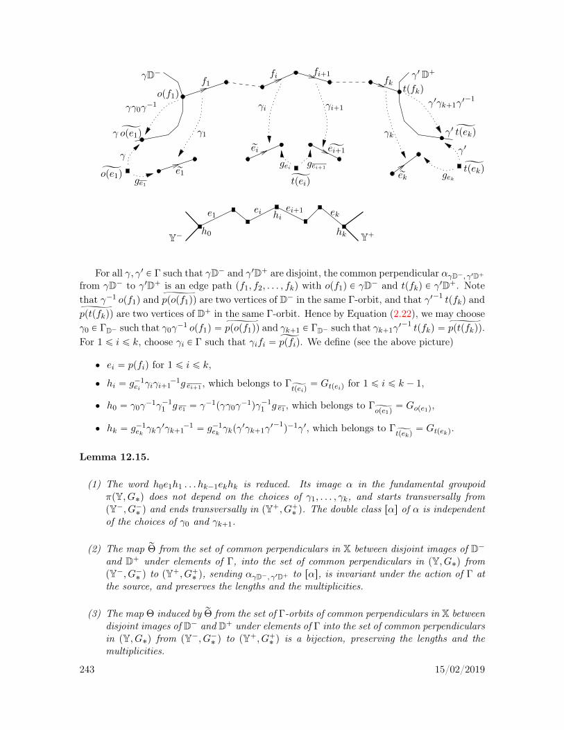
fk

γk

f1

re1

γ1

Ąei`1

gei

Y´

e1ei

Ćtpeiq

fi fi`1

γi`1

gei`1

rei

γi

Y`

ek

γ1γk`1γ1´1

γD´

γγ0γ´1

γ Ćope1q γ1 Ćtpekq

γ1D`

tpfkqopf1q

rek

γ1

gekĆtpekq

γ

ge1Ćope1q

ei`1

hk

hi

h0

For all γ, γ1 P Γ such that γD´ and γ1D` are disjoint, the common perpendicular αγD´, γ1D`from γD´ to γ1D` is an edge path pf1, f2, . . . , fkq with opf1q P γD´ and tpfkq P γ1D`. Notethat γ´1 opf1q and ppopf1qq„

are two vertices of D´ in the same Γ-orbit, and that γ1´1 tpfkq andpptpfkqq„

are two vertices of D` in the same Γ-orbit. Hence by Equation (2.22), we may chooseγ0 P ΓD´ such that γ0γ

´1 opf1q “ ppopf1qq„

and γk`1 P ΓD´ such that γk`1γ1´1 tpfkq “ pptpfkqq„

.For 1 ď i ď k, choose γi P Γ such that γifi “ Ćppfiq. We define (see the above picture)

‚ ei “ ppfiq for 1 ď i ď k,

‚ hi “ g´1ei γiγi`1

´1g ei`1 , which belongs to ΓĆtpeiq

“ Gtpeiq for 1 ď i ď k ´ 1,

‚ h0 “ γ0γ´1γ´1

1 g e1 “ γ´1pγγ0γ´1qγ´1

1 g e1 , which belongs to ΓČope1q

“ Gope1q,

‚ hk “ g´1ekγkγ

1γk`1´1 “ g´1

ekγkpγ

1γk`1γ1´1q´1γ1, which belongs to Γ

Ćtpekq“ Gtpekq.

Lemma 12.15.

(1) The word h0e1h1 . . . hk´1ekhk is reduced. Its image α in the fundamental groupoidπpY, G˚q does not depend on the choices of γ1, . . . , γk, and starts transversally frompY´, G´˚ q and ends transversally in pY`, G`˚ q. The double class rαs of α is independentof the choices of γ0 and γk`1.

(2) The map rΘ from the set of common perpendiculars in X between disjoint images of D´and D` under elements of Γ, into the set of common perpendiculars in pY, G˚q frompY´, G´˚ q to pY`, G`˚ q, sending αγD´, γ1D` to rαs, is invariant under the action of Γ atthe source, and preserves the lengths and the multiplicities.

(3) The map Θ induced by rΘ from the set of Γ-orbits of common perpendiculars in X betweendisjoint images of D´ and D` under elements of Γ into the set of common perpendicularsin pY, G˚q from pY´, G´˚ q to pY`, G`˚ q is a bijection, preserving the lengths and themultiplicities.

243 15/02/2019

Proof. (1) If ei`1 “ ei, then by the definition of hi, we have

hi P ρeipGeiq “ g´1ei Γ

reigei ðñ gei hi g´1ei rei “ rei

ðñ gei g´1ei γiγi`1

´1g ei`1 g´1ei rei “ rei

ðñ γiγi`1´1

Ąei`1 “ rei

ðñ γi`1´1

Ąei`1 “ γ´1i rei ðñ fi`1 “ fi .

Hence the word h0e1h1 . . . hk´1ekhk is reduced.The element γi for i P t1, . . . , ku is uniquely determined up to multiplication on the left

by an element of Γrei “ Gei . If we fix15 i P t1, . . . , ku and if we replace γi by γ1i “ αγi for some

α P Gei , then only the elements hi´1 and hi change, replaced by elements that we denote byh1i´1 and h1i respectively. We have (if 2 ď i ď k´ 1, but otherwise the argument is similar bythe definitions of h0 and hk)

h1i´1 ei h1i “ g´1

ei´1γi´1 γi

´1α´1g ei ei g´1ei αγi γi`1

´1g ei`1

“ g´1ei´1

γi´1 γi´1g ei ρ eipαq

´1 ei ρeipαq g´1ei γi γi`1

´1g ei`1 .

Since ρ eipαq´1 ei ρeipαq is equal to ei ´1 “ ei in the fundamental groupoid, the words h1i´1 ei h1i

and hi´1 ei hi have the same image in πpY, G˚q. Therefore α is does not depend on the choicesof γ1, . . . , γk.

We have opαq “ ope1q P V Y´ and tpαq “ tpekq P V Y`, hence α starts from Y´ and endsin Y`.

Assume that e1 P EY´. Let us prove that h0 P G´

ope1qρ e1pGe1q if and only if f1 P γ ED´.

γ´1f1

Ćope1q

γ0g e1

opγ´1f1q

re1 D´

By the definition of ρ e1 , we have h0 P G´ope1q ρ e1pGe1q if and only if there exists α P

ΓČope1q

XΓD´ such that α´1 h0 P g´1e1

ΓĂe1 g e1 . By the definition of h0 and since γ1 maps f1 to

re1, we have

α´1 h0 P g´1e1

ΓĂe1 g e1 ðñ g e1 α

´1`

γ0γ´1γ´1

1 g e1˘

g ´1e1

re1 “ re1

ðñ f1 “ γ γ´10 α g ´1

e1re1 .

Since re1 P ED´ and γ0, α, g e1 all belong to ΓD´ , this last condition implies that f1 P γ ED´.Conversely (for future use), if f1 P γ ED´, then (see the above picture) γ0 γ

´1f1 is an edgeof D´ with origin Ćope1q, in the same Γ-orbit than the edge g ´1

e1re1 of D´, which also has

origin Ćope1q. By Equation (2.22), this implies that there exists α P ΓČope1q

X ΓD´ such that

f1 “ γ γ´10 α g ´1

e1re1. By the above equivalences, we hence have that h0 P G

´

ope1qρ e1pGe1q.

15We leave to the reader the verification that the changes induced by various i’s do not overlap.

244 15/02/2019

Similarly, one proves that if ek P EY`, then hk P ρekpGekqG`

tpekqif and only if fk P γ1ED`.

Since pf1, . . . , fnq is the common perpendicular edge path from γ D´ to γ1D`, this proves thatα starts transversally from Y´ and ends transversally in Y´.

Note that the element γ0 P ΓD´ is uniquely defined up to multiplication on the left byan element of Γ

Čope1qX ΓD´ “ G´ope1q, and appears only as the first letter in the expression of

h0. Note that the element γk`1 P ΓD` is uniquely defined up to multiplication on the left byan element of Γ

ĆtpekqX ΓD` “ G`tpekq, hence γ

´1k`1 is uniquely defined up to multiplication on

the right by an element of G`tpekq, and appears only as the last letter in the expression of hk.Therefore α is uniquely defined in the fundamental groupoid πpY, G˚q up to multiplicationon the left by an element of G´ope1q and multiplication on the right by an element of G`tpekq,that is, the double class rαs Ă πpY, G˚q is uniquely defined.

(2) Let β be an element in Γ and let x “ αγD´, γ1D` be a common perpendicular in Xbetween disjoint images of D´ and D` under elements of Γ. Let us prove that rΘpβ xq “ rΘpxq.

Since β x “ αβ γD´, β γ1D` , in the construction of rΘpβ xq, we may take, instead of theelements γ0, γ1, . . . , γk, γk`1 used to construct rΘpxq, the elements

γ70 “ γ0, γ71 “ γ1 β´1, . . . , γ7k “ γk β

´1, γ7k`1 “ γk`1.

And instead of γ and γ1, we now may use γ7 “ β γ and γ17 “ β γ1.The only terms involving γ, γ1, γ1, . . . , γk in the construction of rΘpxq come under the form

γ´1γ´11 in h0, γi γi`1

´1 in hi for 1 ď i ď k´ 1, and γkγ1 in hk. Since pγ7q´1pγ71q´1 “ γ´1γ´1

1 ,pγ7i qpγ

7

i`1q´1 “ γi γi`1

´1 for 1 ď i ď k ´ 1, and pγ7kqpγ17q “ γkγ

1, this proves that rΘpβ xq “rΘpxq, as wanted.

It is immediate that if the length of αγD´, γ1D` is k, then the length of rαs is k.Let us prove that the multiplicity, given in Equation (12.9),

mγ, γ1 “1

CardpγΓD´γ´1 X γ1ΓD`γ

1´1q

of the common perpendicular αγD´, γ1D` in X between γ D´ and γ1D` is equal to the multi-plicity

mα “1

CardpG´opαq X αG`

tpαq α´1q

of the common perpendicular α in pY, G˚q from pY´, G´˚ q to pY`, G`˚ q.Since the multiplicity mγ, γ1 is invariant under the diagonal action by left translations of

γ´10 γ´1 P Γ on pγ, γ1q, we may assume that γ “ γ0 “ id. Since the multiplicity mγ, γ1 is

invariant under right translation by γk`1´1, which stabilises D`, on the element γ1, we may

assume that γk`1 “ id. In particular, we have

opf1q “Ćope1q and tpfkq “ γ1 Ćtpekq .

We use the basepoint x0 “ ope1q in the construction of the fundamental group and theBass-Serre tree of pY, G˚q, so that (see in particular [Bass, Eq. (1.3)])

V X “ž

βPπpY, G˚q : opβq“x0

β Gtpβq

245 15/02/2019

andΓ “ π1pY, G˚q “ tβ P πpY, G˚q : opβq “ tpβq “ x0u .

Since an element in Γ which preserves D´ and γ1D` fixes pointwise its (unique) commonperpendicular in X, we have

ΓD´ X γ1ΓD`γ1´1

“ ΓD´ X Γγ1 D` “ pΓopf1q X ΓD´q X pΓtpfkq X Γγ1 D`q

“ pΓČope1q

X ΓD´q X pΓγ1 Ćtpekq

X Γγ1 D`q .

Note that ΓČope1q

X ΓD´ “ G´ope1q. By the construction of the edges in the Bass-Serre tree of a

graph of groups (see [Bass, page 11]), the vertex α Gtpekq is exactly the vertex tpfkq “ γ1 Ćtpekq.By [Bass, Eq. (1.4)], we hence have

αGtpekq α´1 “ Stabπ1pY,G˚qpαGtpekqq “ Γ

γ1 Ćtpekq.

Therefore mγ, γ1 “ mα.

(3) Let rαs “ Gopαq αGtpαq be a common perpendicular in pY, G˚q from pY´, G´˚ q topY`, G`˚ q, with representative α P πpY, G˚q, and let h0 e1 h1 . . . ek hk be a reduced wordwhose image in πpY, G˚q is α.

We define

‚ γ1 “ g e1 h´10 ,

‚ f1 “ γ´11 re1 ,

‚ assuming that γi and fi for some 1 ď i ď k ´ 1 are constructed, let

γi`1 “ g ei`1 h´1i g´1

ei γi and fi`1 “ γi`1´1

Ąei`1 ,

‚ with γk and fk constructed by induction, finally let γ1 “ γ´1k gek hk.

It is easy to check, using the equivalences in the proof of Lemma 12.15 (1) with γ “ γ0 “

γk`1 “ id, that the sequence pf1, . . . , fkq is the edge path of a common perpendicular in Xfrom D´ to γ1D` with origin Ćope1q and endpoint γ1 Ćtpekq.

If h0 is replaced by αh0 with α P G´ope1q, then by induction, f1, f2 . . . , fk are replaced byαf1, αf2, . . . , αfk and γ1 is replaced by αγ1. Note that pαf1, αf2, . . . , αfkq is then the commonperpendicular edge path from D´ “ αD´ to αγ1D`. If hk is replaced by hk α with α P G`tpekq,then f1, f2 . . . , fk are unchanged, and γ1 is replaced by γ1 α. Note that γ1 αD` “ γ1D`.

Hence the map which associates to rαs the Γ-orbit of the common perpendicular in X fromD´ to γ1D` with edge path pf1, . . . , fkq is well defined. It is easy to see by construction thatthis map is the inverse of Θ. l

Theorem 12.14 now follows from Theorem 12.9. l

12.6 Error terms for equidistribution and counting for metricand simplicial graphs of groups

In this Section, we give error terms to the equidistribution and counting results of Section12.4, given by Theorem 12.8 for metric trees (and their continuous time geodesic flows) and by

246 15/02/2019

Theorem 12.9 for simplicial trees (and their discrete time geodesic flows), under appropriateassumptions on bounded geometry and the rate of mixing.

Let pX, λq, X, Γ, rc, c, rFc, Fc, δc, D˘, D˘, D˘, λγ,γ1 , αγ,γ1 , α˘γ,γ1 , mγ,γ1 be as in Section12.4. We first consider the simplicial case (when λ “ 1), for the discrete time geodesic flow.

Theorem 12.16. Let X be a locally finite simplicial tree without terminal vertices, let Γ bea nonelementary discrete subgroup of AutpXq, let rc be a system of conductances on X for Γand let D˘ be nonempty proper simplicial subtrees of X. Assume that the critical exponent δcis finite and positive, that the Gibbs measure mc (for the discrete time geodesic flow) is finiteand that the skinning measures σ˘D¯ are finite and nonzero. Assume furthermore that

(1) at least one of the following holds :

‚ ΓD˘zBD˘ is compact

‚ C ΛΓ is uniform and Γ is a lattice of C ΛΓ,

(2) there exists β P s0, 1s such that the discrete time geodesic flow on pΓzGX,mcq is expo-nentially mixing for the β-Hölder regularity.

Then there exists κ1 ą 0 such that for all ψ˘ P C βc pΓz

p

GXq, we have, as nÑ `8,

eδc ´ 1

eδcmc e

´δc nÿ

rγs PΓD´zΓΓD`0ădpD´,γ D`qďn

me, γ erc pαe, γq ψ´pΓα´e,γq ψ

`pΓα`γ´1,e

q

“

ż

ψ´ dσ`D´

ż

ψ` dσ´D` `O`

e´κ1 n ψ´β ψ

`β˘

and if ΓD˘zBD˘ is compact, then

ND´,D`pnq “eδc σ`D´ σ

´

D`

peδc ´ 1q mceδc n `O

`

epδc´κ1qn˘

.

Proof. We follow the scheme of proof of Theorem 12.7, replacing aspects of Riemannianmanifolds by aspects of simplicial trees as in the proof of Theorem 11.9. Let rψ˘ P C β

c p

p

GXq.In order to simplify the notation, let λγ “ λe,γ , αγ “ αe,γ , α´γ “ α´e,γ , α`γ “ α`

γ´1,eand

rσ˘ “ rσ˘D¯ .Let us first prove the following avatar of Equation (12.4), indicating only the required

changes in its proof: there exists κ0 ą 0 (independent of rψ˘) such that, as nÑ `8,

eδc ´ 1

eδcmc e

´δc nÿ

γPΓ, 0ăλγďn

erc pαγq rψ´pα´γ qrψ`pα`γ q

“

ż

B1`D

´

rψ´ drσ`ż

B1´D

`

rψ` drσ´ `Ope´κ0n rψ´β rψ`βq . (12.13)

Most of the new work to be done in order to prove this formula concerns regularity propertiesof the test functions that will be introduced later on.

247 15/02/2019

We fix R ą e2 large enough. Let 0 ă η ă 1. We introduce the following modification ofthe test functions φ˘η :16

Φ˘η “ ph˘η,R

rψ˘q ˝ f¯D˘

1V ¯η,RpB1¯D

˘q.

As in Lemma 10.1, the functions Φ˘η are measurable and satisfyż

GXΦ˘η drmc “

ż

B1¯D˘

rψ˘ drσ¯ . (12.14)

Lemma 12.17. The maps Φ˘η are β-Hölder-continuous with

Φ˘η β “ Op rψ˘βq . (12.15)

Proof. Since X is a simplicial tree and η ă 1, we have V ˘w, η,R “ B˘pw,Rq for everyw P B1

˘D¯. By the proof of Lemma 3.3,17 there exists cR ą 0 depending only on R such that

if `1 P GX satisfy dp`, `1q ď cR, then `1 coincides with ` on ˘r0, lnR ` 1s. Therefore, if ` PB˘pw,Rq for some w P B1

˘D¯ and dp`, `1q ď cR, then `1 coincides with w on ˘rlnR, lnR` 1s,

thus `1 P B˘pw1, Rq where w1 P B1˘D

¯ is the geodesic ray with w1p0q “ wp0q and w1˘ “ `1˘.Hence (see Section 3.1) the characteristic function 1V ˘η,RpB

1˘D

¯qis cR-locally constant, thus

β-Hölder-continuous by Remark 3.11.By Assumption (1) in the statement of Theorem 12.16, the denominator of

h¯η,Rpwq “1

µW˘pwqpB˘pw,Rqq

is at least a positive constant depending only on R, hence h¯η,R is bounded by a constantdepending only on R. Since the map 1B˘pw,Rq is cR-locally constant, so is the map h¯η,R. Theresult then follows from Lemma 3.8 and Equation (3.7). l

In order to prove Equation (12.13), as in the proofs of Theorems 12.7 and 11.9, for allN P N, we estimate in two ways the quantity

IηpNq “Nÿ

n“0

eδc nÿ

γPΓ

ż

`PGXΦ´η pg

´tn2u`q Φ`η pgrn2sγ´1`q drmcp`q . (12.16)

On the one hand, as in order to obtain Equation (12.6), using now Assumption (2) in thestatement of Theorem 12.16 on the exponential mixing for the discrete time geodesic flow, ageometric sum argument and Equations (12.14) and (12.15), we have

IηpNq “eδcpN`1q

peδc ´ 1q mc

´

ż

B1`D´

rψ´ drσ`ż

B1´D`

rψ` drσ´ `

Ope´κN rψ´β rψ`βq

¯

. (12.17)

16See Equation (10.4) for the definition of φ˘η and Equation (10.1) for the definition of h˘η,R, that simplifiesas h¯η,Rpwq “ pµW˘pwqpB

˘pw,Rqqq´1 since X is simplicial, as seen in Equation (11.27).

17See also the proof of Lemmas 3.4 and 3.8.

248 15/02/2019

On the other hand, exchanging the summations over γ and n in the definition of IηpNq,we have

IηpNq “ÿ

γPΓ

Nÿ

n“0

eδc nż

GXΦ´η pg

´tn2u`q Φ`η pgrn2sγ´1`q drmcp`q .

With the simplifications in Step 3T of the proof of Theorem 11.1 given by the proof of Theorem11.9, if η ă 1

2 , if ` P GX belongs to the support of Φ´η ˝ g´tn2u Φ`η ˝ g

rn2s ˝ γ´1, settingw´ “ f`

D´p`q and w` “ f´

γD`p`q, we then have λγ “ n, w´p0q “ α´γ p0q, w`p0q “ γα`γ p0q and

w´ptn2uq “ w`p´rn2sq “ `p0q “ α´γ ptn2uq “ γα`γ p´rn2sq .

Hence by the triangle inequality

dpw´, α´γ q “

ż `8

tn2u

dpw´psq, α´γ psqq e´2s ds ď e´2tn2u

ż `8

02s1 e´2s1 ds1

“ Ope´λγ q .

Similarly, dpw`, γα`γ q “ Ope´λγ q. Therefore, since rψ˘ is β-Hölder-continuous,

| rψ´pw´q ´ rψ´pv´γ q |, |rψ`pγ´1w`q ´ rψ`pv˘γ q | “ Ope´βλγ rψ˘βq .

Note that now Φ˘η “rψ˘ ˝ f¯

D˘φ˘η , so that

IηpNq “ÿ

γPΓ

`

rψ´pα´γ qrψ`pα`γ q `Ope´2βλγ rψ´β rψ

`βq˘

ˆ

Nÿ

n“0

eδc nż

GXφ´η pg

´tn2u`q φ`η pgrn2sγ´1`q drmcp`q .

Now if η ă 12 , Equation (12.13) with κ0 “ mint2β, κu follows as in Steps 3T and 4T of

the proof of Theorem 11.1 with the simplifications given by the proof of Theorem 11.9.The end of the proof of the equidistribution claim of Theorem 12.16 follows from Equation

(12.13) as the one of Theorem 12.7 from Equation (12.4).The counting claim follows from the equidistribution one by taking ψ˘ “ 1ΓVη,RpB1

¯D˘q,

which has compact support since ΓD˘zBD˘ is assumed to be compact, and is β-Hölder-continuous by previous arguments. l

Remarks. (i) Assume that rc “ 0, that the simplicial tree X1 with |X1|1 “ C ΛΓ is uniformwithout vertices of degree 2, that LΓ “ Z and that Γ is a geometrically finite lattice of X1. Thenall assumptions of Theorem 12.16 are satisfied by the results of Section 4.4 and by Corollary9.6. Therefore we have an exponentially small error term in the (joint) equidistribution of thecommon perpendiculars, and in their counting if ΓD˘zBD˘ is compact, see Examples 12.11(2) and 12.13 (4).

(ii) Assume in this remark that Assumption (2) of the above theorem is replaced by theassumptions that C ΛΓ is uniform without vertices of degree 2, that LΓ “ 2Z, and that thereexists β P s0, 1s such that the square of the discrete time geodesic flow on pΓzGevenX,mcq

is exponentially mixing for the β-Hölder regularity, for instance by Corollary 9.6 (2) if Γis geometrically finite. Then a similar proof (replacing the references to Theorem 11.9 by

249 15/02/2019

references to Theorem 11.11) shows that there exists κ1 ą 0 such that for all ψ˘ P C βc pΓz

p

GXq,we have, as nÑ `8,

e2δc ´ 1

2 e2δcmc e

´δc nÿ

rγs PΓD´zΓΓD`0ădpD´,γ D`qďn

me, γ erc pαe, γq ψ´pΓα´e,γq ψ

`pΓα`γ´1,e

q

“

ż

ψ´ dσ`D´

ż

ψ` dσ´D` `O`

e´κ1 n ψ´β ψ

`β˘

and if ΓD˘zBD˘ is compact, then

ND´,D`pnq “2 e2δc σ`D´ σ

´

D`

pe2δc ´ 1q mceδc n `O

`

epδc´κ1qn˘

.

Let us now consider the metric tree case, for the continuous time geodesic flow, where themain change is to assume a superpolynomial decay of correlations and hence get a superpoly-nomial error term. We refer to the beginning of Section 9.3 for the definitions of the functionspace C k, β

c pΓz

p

GXq and the superpolynomial mixing.

Theorem 12.18. Let pX, λq, Γ, rc and D˘ be as in the beginning of this Section, and letD˘ “ |D˘|λ. Assume that the critical exponent δc is finite and positive, that the Gibbsmeasure mc (for the continuous time geodesic flow) is finite and that the skinning measuresσ˘D¯ are finite and nonzero. Assume furthermore that

(1) at least one of the following holds :

‚ ΓD˘zBD˘ is compact

‚ the metric subtree C ΛΓ is uniform and Γ is a lattice of C ΛΓ,

(2) there exists β P s0, 1s such that the continous time geodesic flow on pΓzGX,mcq hassuperpolynomial decay of β-Hölder correlations.

Then for every n P N there exists k P N such that for all ψ˘ P C k, βc pΓz

p

GXq, we have, asT Ñ `8,

δc mc e´δc T

ÿ

rγs PΓD´zΓΓD`0ădpD´,γ D`qďT

me, γ erc pαe, γq ψ´pΓα´e,γq ψ

`pΓα`γ´1,e

q

“

ż

Γz

p

GXψ´ dσ`D´

ż

Γz

p

GXψ` dσ´D` `O

`

T´n ψ´k, β ψ`k, β

˘

and if ΓD˘zBD˘ is compact, then for every n P N

ND´, D`pT q “σ`D´ σ

´

D`

δc mceδc T `O

`

eδc TT´n˘

.

Remark. Assume that rc “ 0, that the metric tree C ΛΓ is uniform, either that ΓzX isfinite and the length spectrum LΓ of Γ is 2-Diophantine, or that Γ is a geometrically finitelattice of C ΛΓ and LΓ is 4-Diophantine. Then all assumptions of Theorem 12.18 are satisfiedby the results of Section 4.4 and by Corollary 9.10. Therefore we have a superpolynomially

250 15/02/2019

small error term in the (joint) equidistribution of the common perpendiculars (and in theircounting if ΓD˘zBD

˘ is compact).

Proof. The proof is similar to the one of Theorem 12.16, except that since the time isnow continuous, we need to regularise our test functions also in the time direction in orderto obtain the regularity required for the application of the assumption on the mixing rate.We again use the simplifying notation λγ “ λe,γ , αγ “ αe,γ , α´γ “ α´e,γ , α`γ “ α`

γ´1,eand

rσ˘ “ rσ˘D¯

.We fix n P N ´ t0u. Using the rapidly mixing property, there exists a regularity k such

that for all ψ,ψ1 P C k, βb pΓzGXq we have as tÑ `8

covmc, t pψ,ψ1q “ Opt´N n ψk, β ψ

1k, βq , (12.18)

where N P N´ t0u is a constant which will be made precise later on.Let us first prove that for all rψ˘ P C k, β

c p

p

GXq, we have, as T Ñ `8,

δc mc e´δc T

ÿ

γPΓ, 0ăλγďT

erc pαγq rψ´pα´γ qrψ`pα`γ q

“

ż

B1`D

´

rψ´ drσ`ż

B1´D

`

rψ` drσ´ `OpT´n rψ´k, β rψ`k, βq . (12.19)

In order to prove this formula, we introduce modified test functions with bounded Hölder-continuous derivatives up to order k (by a standard construction) in the time direction (thestable leaf and unstable leaf directions remain discrete). We fix R ą 0 large enough.

For every η P s0, 1r , there exists a map x1η : R Ñ r0, 1s which has bounded β-Hölder-continuous derivatives up to order k, which is equal to 0 if t R r´η, ηs and to 1 if t Pr´η e´η, η e´ηs (when k “ 0, just take x1η to be continuous and affine on each remainingsegment r´η,´η e´ηs and rη e´η, ηs), such that, for some constant κ11 ą 0,

x1ηk, β “ Opη´κ11q .

Using leafwise this regularisation process, there exists χ˘η,R P C k, βb pGXq such that

‚ χ˘η,Rk, β “ Opη´κ11q,

‚ 1V ¯η e´η,R

pB1¯D

˘qď χ˘η,R ď 1V ¯η,RpB

1¯D

˘q,

‚ for every w P B1¯D

˘, we haveż

V ¯w, η,R

χ˘η,R dν˘w “ ν˘w pV

¯w, η,Rq e

´Opηq “ ν˘w pV¯

w, η e´η , Rq eOpηq .

As in the proof of Theorem 12.7 in the manifold case, the new test functions are defined, with

H˘η,R : w P B1¯D

˘ ÞÑ1

ş

V ¯w, η,Rχ˘η,R dν

˘w,

byΦ˘η “ pH

˘η,R

rψ˘q ˝ f¯D˘

χ˘η,R : GX Ñ R .

Let pΦ˘η “ H˘η,R ˝ f¯

D˘χ˘η,R, so that Φ˘η “

rψ˘ ˝ f¯D˘

pΦ˘η . By the last two properties of theregularised maps χ˘η,R, we have, with φ¯η defined as in Equation (10.4),

φ˘η e´η

e´Opηq ď pΦ˘η ď φ˘η eOpηq . (12.20)

251 15/02/2019

By Assumption (1), if R is large enough, by the definitions of the measures ν˘w , thedenominator of H˘η,Rpwq is at least c η where c ą 0. As in the proof of Theorem 12.7,

ż

GXΦ˘η drmc “

ż

B1¯D

˘

rψ˘ drσ¯

and there exists κ2 ą 0 such that

Φ˘η k, β “ Opη´κ2

rψ˘k, βq .

We again estimate in two ways as T Ñ `8 the quantity

IηpT q “

ż T

0eδc t

ÿ

γPΓ

ż

`PGXΦ´η pg

´t2`q Φ`η pgt2γ´1`q drmcp`q dt . (12.21)

Note that as T Ñ `8,

e´δc Tż T

1eδc t t´N n dt “ e´δc T

ż T 2

1eδc t t´N n dt` e´δc T

ż T

T 2eδc t t´N n dt

“ Ope´δc T 2q `OpT´N n`1q “ OpT´pN´1qnq .

Using Equation (12.18), an integration argument and the above two properties of the testfunctions, we hence have

IηpT q “eδc T

δc mc

´

ż

B1`D

´

rψ´ drσ`ż

B1´D

`

rψ` drσ´ `

OpT´pN´1qnη´2κ2 rψ´k, β rψ`k, βq

¯

. (12.22)

As in Step 3T of the proof of Theorem 11.1, for all γ P Γ and t ą 0 large enough, if ` P GXbelongs to the support of Φ´η ˝ g

´t2 Φ`η ˝ gt2 ˝ γ´1 (which is contained in the support of

φ´η ˝ g´t2 φ`η ˝ g

t2 ˝ γ´1 ), then we may define w´ “ f`D´p`q and w` “ f´

γD`p`q.

By the property (iii) in Step 3T of the proof of Theorem 11.1, the generalised geodesiclines w´ and α´γ coincide, besides on s ´ 8, 0s, at least on r0, t2 ´ ηs, and similarly, w` andγα`γ coincide, besides on r0,`8r , at least on r´ t

2 ` η, 0s. Therefore, by an easy change ofvariable and since | t2 ´

λγ2 | ď η,

dpw´, α´γ q ď

ż `8

t2´ηdpw´psq, α´γ psqq e

´2s ds ď e´2p t2´ηq

ż `8

02s e´2s ds

“ Ope´tq “ Ope´λγ q .

Similarly, dpw`, γα`γ q “ Ope´λγ q. Hence since rψ˘ is β-Hölder-continuous, we have

| rψ´pw´q ´ rψ´pα´γ q |, |rψ`pγ´1w`q ´ rψ`pα`γ q | “ Ope´βλγ rψ˘βq .

Therefore, as in the proof of Theorem 12.16, we have

IηpT q “ÿ

γPΓ

`

rψ´pα´γ qrψ`pα`γ q `Ope´2βλγ rψ´β rψ

`βq˘

ˆ

ż T

0eδ t

ż

`PGX

pΦ´η pg´t2`q pΦ`η pγ

´1gt2`q drmcp`q dt .

252 15/02/2019

Finally, Equation (12.19) follows as in the end of the proof of Equation (12.4), usingEquations (12.20) and (11.17) instead of Equations (12.7) and (11.21), by taking η “ T´n

and N “ 2prκ2s` 1q.The end of the proof of the equidistribution claim of Theorem 12.18 follows from Equation

(12.19) as the one of Theorem 12.7 from Equation (12.4).The counting claim follows from the equidistribution one by taking ψ˘ to be β-Hölder-

continuous plateau functions around ΓVη,RpB1¯D˘q. l

We are now in a position to prove one of the counting results in the introduction.

Proof of Theorem 1.9. Let X be the universal cover of Y, with fundamental group Γ foran indifferent choice of basepoint, and let D˘ be connected components of the preimagesof Y˘ in X. Assertion (1) of Theorem 1.9 follows from Theorem 12.18 and its subsequentRemark. Assertion (2) of Theorem 1.9 follows from Theorem 12.16 and its Remarks (ii) and(i) following its proof, respectively, if Y is bipartite or not. l

253 15/02/2019

254 15/02/2019

Chapter 13

Geometric applications

In this final Chapter of Part II, we apply the equidistribution and counting results obtainedin the previous Chapters in order to study geometric equidistribution and counting problemsfor metric and simplicial trees concerning conjugacy classes in discrete isometry groups andclosed orbits of the geodesic flows.

13.1 Orbit counting in conjugacy classes for groups acting ontrees

In this Section, we study the orbital counting problem for groups acting on metric or simplicialtrees when we consider only the images by elements in a given conjugacy class. We refer tothe Introduction for motivations and previously known results for manifolds (see [Hub1] and[PaP15]) and graphs (see [Dou] and [KeS]). The main tools we use are Theorem 12.8 for themetric tree case and Theorem 12.16 for the simplicial tree case, as well as their error terms.In particular, we obtain a much more general version of Theorem 1.12 in the Introduction.

Let pX, λq be a locally finite metric tree without terminal vertices, let X “ |X|λ be its geo-metric realisation, let x0 P V X and let Γ be a nonelementary discrete subgroup of AutpX, λq.1Let rc : EX Ñ R be a Γ-invariant system of conductances, let rFc and Fc be its associatedpotentials on T 1X and ΓzT 1X respectively, and let δc “ δΓ, F˘c

be its critical exponent.2 Letpµ˘x qxPX (respectively pµ˘x qxPV X) be (normalised) Patterson densities for the pairs pΓ, F˘c q,and let rmc “ rmFc and mc “ mFc be the associated Gibbs measures on GX and ΓzGX(respectively GX and ΓzGX) for the continuous time geodesic flow (respectively the discretetime geodesic flow, when λ ” 1).3

Recall that the virtual centre ZvirtpΓq of Γ is the finite (normal) subgroup of Γ consistingof the elements γ P Γ acting by the identity on the limit set ΛΓ of Γ in B8X, see for instance[Cha, §5.1]. If ΛΓ “ B8X (for instance if Γ is a lattice), then ZvirtpΓq “ tidu.

For any nontrivial element γ in Γ with translation length λpγq in X, let Cγ be

‚ the translation axis of γ if γ is loxodromic on X,

‚ the fixed point set of γ if γ is elliptic on X,

1See Section 2.6 for definitions and notation.2See Section 3.5 for definitions and notation.3See Sections 4.3 and 4.4 for definitions and notation.

255 15/02/2019

and let ΓCγ be the stabiliser of Cγ in Γ. In the simplicial case (that is, when λ ” 1), Cγ is asimplicial subtree of X. Note that λpγq “ λpγ1γpγ1q´1q and γ1Cγ “ Cγ1γpγ1q´1 for all γ1 P Γ,and that for any x0 P X

dpx0, Cγq “dpx0, γx0q ´ λpγq

2. (13.1)

Let D “ pγ1Cγqγ1PΓΓCγ , which is a locally finite Γ-invariant family of nonempty proper(since γ ‰ id) closed convex subsets of X.4 By the equivariance properties of the skinningmeasures, the total mass of the skinning measure5 σ´D depends only on the conjugacy classK of γ in Γ, and will be denoted by σ´K . This quantity, called the skinning measure of K,is positive unless B8Cγ “ ΛΓ, which is equivalent to γ P ZvirtpΓq (and implies in particularthat γ is elliptic). Furthermore, σ´K is finite if γ is loxodromic, and it is finite if γ is ellipticand ΓCγzpCγ X C ΛΓq is compact. This last condition is in particular satisfied if Cγ X C ΛΓitself is compact, and this is the case for instance if, for some k ě 0, the action of Γ on Xis k-acylindrical (see for instance [Sel, GuL]), that is, if any element of Γ fixing a segment oflength k in C ΛΓ is the identity.

For every γ P Γ´ teu, we define

mγ “1

CardpΓx0 X ΓCγ q,

which is a natural multiplicity of γ, and equals 1 if the stabiliser of x0 in Γ is trivial (forinstance if Γ is torsion-free). Note that for every β P Γ, the real number mβγβ´1 depends onlyon the double coset of β in Γx0zΓΓCγ .

The centraliser ZΓpγq of γ in Γ is contained in the stabiliser of Cγ in Γ. The index

iK “ rΓCγ : ZΓpγqs

depends only on the conjugacy class K of γ; it will be called the index of K. The index iK isfinite if γ is loxodromic (the stabiliser of its translation axis Cγ is then virtually cyclic), andalso finite if Cγ is compact (as for instance if the action of Γ on X is k-acylindrical for somek ě 0).

We define

cγ “kÿ

i“1

rc peiqλpeiq ,

where pe1, . . . , ekq is the shortest edge path from x0 to Cγ .

We finally define the orbital counting function in conjugacy classes, counting with multi-plicities and weights coming from the system of conductances, as

NK, x0ptq “ÿ

αPK, dpx0, αx0qďt

mα ecα .

for t P r0,`8r (simply t P N in the simplicial case). When the stabiliser of x0 in Γ is trivialand when the system of conductances c vanishes, we recover the definition of the Introduction(above Theorem 1.12).

4See Section 7.2 for definitions and notations.5See the previous footnote.

256 15/02/2019

Theorem 13.1. Let K be the conjugacy class of a nontrivial element γ0 of Γ, with finite indexiK, and with positive and finite skinning measure σ´K . Assume that δc is finite and positive.

(1) Assume that mc is finite and mixing for the continuous time geodesic flow on ΓzX. Then,as tÑ `8,

NK, x0ptq „iK µ

`x0 σ´K e

´λpγ0q

2

δc mceδc2t .

If ΓCγzpCγ X C ΛΓq is compact when γ P K is elliptic and if there exists β P s0, 1s suchthat the continous time geodesic flow on pΓzGX,mcq has superpolynomial decay of β-Höldercorrelations, then the error term is O

`

t´n eδc2t˘

for every n P N.

(2) Assume that λ ” 1 and that mc is finite and mixing for the discrete time geodesic flow onΓzGX. Then, as nÑ `8,

NK, x0pnq „eδc iK µ

`x0 σ´K

peδc ´ 1q mceδct

n´λpγ0q2

u .

If ΓCγzpCγXC ΛΓq is compact when γ P K is elliptic and if there exists β P s0, 1s such that thediscrete time geodesic flow on pΓzGX,mcq is exponentially mixing for the β-Hölder regularity,then the error term is O

`

epδc´κqn2˘

for some κ ą 0.

One can also formulate a version of the above result for groups acting on bipartite simplicialtrees based on Theorem 12.12 and Remark (ii) following the proof of Theorem 12.16.

The error term in Assertion (1) holds for instance if rc “ 0, X is uniform, and either ΓzXis compact and the length spectrum LΓ is 2-Diophantine or Γ is a geometrically finite latticeof X whose length spectrum LΓ is 4-Diophantine, by the Remark following Theorem 12.18.When ΓzX is compact and Γ has no torsion (in particular, Γ has then a very restricted groupstructure, as it is then a free group), we thus recover a result of [KeS].

The error term in Assertion (2) holds for instance if rc “ 0, X is uniform with vertices ofdegrees at least 3, Γ is a geometrically finite lattice of X with length spectrum equal to Z, byRemark (i) following the proof of Theorem 12.16.

Theorem 1.12 in the introduction follows from this theorem, using Proposition 4.16 (3)and Theorem 4.17.

Proof. We only give a full proof of Assertion (1) of this theorem, Assertion (2) followssimilarly using Theorems 12.9 and 12.16 instead of Theorems 12.8 and 12.18.

The proof is similar to the proof of [PaP15, Theo. 8]. Let D´ “ tx0u and D` “ Cγ0 . LetD´ “ pγD´qγ1PΓΓD´ and D` “ pγD`qγPΓΓD` . By Equation (7.15), we have

σ`D´ “µ`x0

|Γx0 |.

By Equation (13.1), by the definition6 of the counting function ND´, D` and by the last claim

6See Equation (12.10) in Section 12.4.

257 15/02/2019

of Theorem 12.8, we have, as tÑ `8,ÿ

αPK, 0ădpx0, αx0qďt

mα ecα “

ÿ

αPK, 0ădpx0, Cαqďt´λpγ0q

2

mα ecα

“ÿ

γPΓZΓpγ0q, 0ădpx0, γCγ0 qďt´λpγ0q

2

mγγ0γ´1 ecγγ0γ

´1

“ |Γx0 | iKÿ

γPΓx0zΓΓCγ0, 0ădpx0, γCγ0 qď

t´λpγ0q2

mγγ0γ´1 ecγγ0γ

´1

“ |Γx0 | iK ND´, D`` t´ λpγ0q

2

˘

„ |Γx0 | iKσ`D´ σ

´

D`

δc mceδc

t´λpγ0q2 .

Assertion (1) without the error term follows, and the error term statement follows similarlyfrom Theorem 12.18. l

Theorem 13.1 (1) without an explicit form of the multiplicative constant in the asymptoticis due to [KeS] under the strong restriction that Γ is a free group acting freely on X and ΓzXis a finite graph. The following result is due to [Dou, Theo. 1] in the special case when X isa regular tree and the group Γ has no torsion and finite quotient ΓzX.

Corollary 13.2. Let X be a regular simplicial tree with vertices of degree q ` 1 ě 3, letx0 P V X, let Γ be a lattice of X such that ΓzX is nonbipartite, and let K be the conjugacy classof a loxodromic element γ0 P Γ. Then, as nÑ `8,

ÿ

αPK, dpx0, αx0qďn

mα „λpγ0q

rZΓpγ0q : γZ0 s VolpΓzzXqqtn´λpγ0q

2u .

If we assume furthermore that Γ has no torsion and that γ0 is primitive, then we have asnÑ `8,

Cardtα P K : dpx0, αx0q ď nu „λpγ0q

|ΓzV X|qtn´λpγ0q

2u .

Proof. Under these assumptions, taking c ” 0 in Theorem 13.1 so that the Gibbs measureis the Bowen-Margulis measure, the discrete time geodesic flow on ΓzGX is finite and mixingby Proposition 4.16 (3) and Theorem 4.17. We also have δc “ ln q. Using the normalisationof the Patterson density pµ˘x qxPV X to probability measures, Proposition 8.1 (3) and Equation(8.12), the result follows, since when γ is loxodromic,

VolpΓCγzzCγq “VolpγZzzCγq

rΓCγ : γZs“

λpγq

rΓCγ : ZΓpγqs rZΓpγq : γZs. . l

The value of C 1 given below Theorem 1.12 in the Introduction follows from this corollary.

We leave to the reader an extension with nonzero potential F of the results for manifoldsin [PaP15], along the lines of the above proofs.

258 15/02/2019

13.2 Equidistribution and counting of closed orbits on metricand simplicial graphs (of groups)

Classically, an important characterisation of the Bowen-Margulis measure on compact nega-tively curved Riemannian manifolds is that it coincides with the weak-star limit of properlynormalised sums of Lebesgue measures supported on periodic orbits, see [Bowe1]. Under muchweaker assumptions than compactness, this result was extended to CATp´1q spaces with zeropotential in [Rob2] and to Gibbs measures in the manifold case in [PauPS, Theo. 9.11]. Asa corollary of the simultaneous equidistribution results from Chapter 11, we prove in thisSection the equidistribution towards the Gibbs measure of weighted closed orbits in quotientsof metric and simplicial graphs of groups and as a corollary of this result, in the standardmanner, we obtain asymptotic counting results for weighted (primitive) closed orbits.

Let pX, λq be a locally finite metric tree without terminal vertices, and let X “ |X|λ beits geometric realisation. Let Γ be a nonelementary discrete subgroup of AutpX, λq. Letrc : EXÑ R be a Γ-invariant system of conductances, and c : ΓzEXÑ R its induced function.

Given a periodic orbit g of the geodesic flow on ΓzGX, if pe1, . . . , ekq is the sequence ofedges followed by g, we denote by Lg the Lebesgue measure along g, by λpgq the length of gand by cpgq its period for the system of conductances c:

λpgq “kÿ

i“1

λpeiq and cpgq “kÿ

i“1

λpeiq cpeiq .

Let Perptq be the set of periodic orbits of the continuous time geodesic flow on ΓzGX withlength at most t and let Per1ptq be the subset of primitive ones.

Theorem 13.3. Assume that the critical exponent δc of c is finite and positive and that theGibbs measure mc of c is finite and mixing for the continuous time geodesic flow. As tÑ `8,the measures

δc e´δc t

ÿ

gPPer1ptq

ecpgqLg

andδc t e

´δc tÿ

gPPer1ptq

ecpgqLg

λpgq

converge to mcmc

for the weak-star convergence of measures. If Γ is geometrically finite, theconvergence holds for the narrow convergence.

We conjecture that if Γ is geometrically finite and if its length spectrum is 4-Diophantine7,then for all n P N and β P s0, 1s, there exist k P N and an error term of the form Optn ψk, βq

for these equidistribution claims evaluated on any ψ P C k, βc pΓzGXq. But since we will not

need this result and since the proof is likely to be very long, we do not address the problemhere.

Proof. Let rFc and Fc be the potentials on T 1X and ΓzT 1X respectively associated8 with c,and note that the period of a periodic orbit g for the geodesic flow on ΓzGX satisfies9

cpgq “ LgpF7c q “ PerFcpγq ,

7See the definition in Section 9.3.8See Section 3.5.9See Proposition 3.21 and Section 3.2.

259 15/02/2019

where F 7c is the composition of the canonical map ΓzGX Ñ ΓzT 1X with Fc : ΓzT 1X Ñ R,and γ P Γ is the loxodromic element of Γ whose conjugacy class corresponds to g.

Let HΓ,t be the subset of Γ that consists in the loxodromic elements whose translationlength is at most t, and let H 1

Γ,t be the subset of HΓ,t that consists in the primitive ones. Forevery γ P HΓ,t, we denote by gγ its corresponding periodic orbit in ΓzGX. The first claim isequivalent to the following assertion: we have

δc e´δc t

ÿ

γPH 1Γ,t

ePerFc pγqLgγ˚á

mc

mc(13.2)

as t Ñ `8. We proceed with the proof of the convergence claimed in Equation (13.2) as in[PauPS, Theo. 9.11]. We first prove that

ν2t “ δc mc e´δc t

ÿ

γPHΓ,t

ePerFc pγqLgγ˚á mc . (13.3)

We then refer to Step 2 of the proof of [PauPS, Theo. 9.11] for the fact that the contributionof the non primitive elements is negligible, so that Equation (13.3) implies Equation (13.2).Although the proof of this deduction in loc. cit. is written for manifolds, the arguments aredirectly applicable for any CATp´1q space X and potential F satisfying the HC-property.10

In particular, the use of Proposition 5.13 (i) and (ii) of op. cit. in the proof of Step 2 inloc. cit. is replaced now by the use of Theorem 4.6 (1) and (4) respectively.

Let us fix x P X. Let

V pxq “

pξ, ηq P pX Y B8Xq2 : ξ ‰ η, x P sξ, ηr

(

,

which is an open subset of X Y B8X. Note that the family pV pyqqyPX covers the set of pairsof distinct points of B8X. For every t ą 0, let νt be the measure on pX Y B8Xq2 defined by

νt “ δc mc e´δct

ÿ

γPΓ : dpx,γxqďt

eşγxx

rFc∆γ´1x b∆γx .

The measures νt weak-star converge to µ´x b µ`x as t Ñ `8 by Corollary 11.2 (taking in itsstatement y “ x).

Let γ˘ be the attracting and repelling fixed points of any loxodromic element γ P Γ. Let

ν3t “ δc mc e´δc t

ÿ

γPHΓ, t

ePerFc pγq∆γ´ b∆γ` .

Since X is an R-tree, every element γ P Γ such that x P sγ´1x, γxr is loxodromic, and for suchx and γ we have

dpx, γxq “ λpγq and

ż γx

x

rFc “ PerFcpγq .

If furthermore dpx, γxq is large, then γ´1x and γx are respectively close to γ´ and γ` inX Y B8X.

Hence, for every continuous map ψ : pX Y B8Xq2 Ñ r0,`8r with compact support

contained in V pxq, and for every ε ą 0, if t is large enough, we have

e´ενtpψq ď ν3t pψq ď eενtpψq .

10See Definition 3.13.

260 15/02/2019

Using Hopf’s parametrisation with basepoint x, and by Equation (3.20), the measures rmc andµ´x b µ

`x b ds are equal on V pxq ˆ R. Hence the measures νt b ds weak-star converge to rmc

on V pxqˆR as tÑ `8. For every continuous ψ1 : GX Ñ R which is a product of continuousfunctions in each variable with compact support in V pxq ˆR and for every ε ą 0, if t is largeenough, we hence have

e´ε rmcpψ1q ď ν3t b dspψ

1q ď eε rmcpψ1q .

Note that the support of any continuous function with compact support on GX may becovered by finitely many open sets V pxq ˆ R where x P X. The induced measure11 of theΓ-invariant measure ν3t b ds on GX is the measure ν2t on ΓzGX. Since mc is the inducedmesasure of rmc, this proves Equation (13.3), hence gives the first claim of Theorem 13.3.

The second claim follows from the first one in the same way as in [PauPS, Theo. 9.11]:Consider the measures

m1t “ δce´δct

ÿ

gPPer1ptq

eLgpF q Lg and m2t “ δcte´δct

ÿ

gPPer1ptq

eLgpF q Lg

λpgq

on ΓzGX. Fix a continuous map ψ : ΓzGX Ñ r0,`8r with compact support. For everyε ą 0, for every t ą 0, we have, since λpgq ě e´εt for all g in the second sum below,

m2t pψq ě m1tpψq ě δce´δct

ÿ

gPPer1ptq´Per1pe´εtq

eLgpF q Lgpψq

ě e´εδcte´δct

ÿ

gPPer1ptq´Per1pe´εtq

eLgpF q Lgpψq

λpgq

“ e´εm2t pψq ´ e´εδct e

´δctÿ

gPPer1pe´εtq

eLgpF q Lgpψq

λpgq.

By the local finiteness of X, the closed orbits meeting the support of ψ have a positive lowerbound on their lengths. Thus, by the first claim of Theorem 13.3, there exists a constantC ą 0 such that the second term of the above difference is at most C t e´δcteδc e´εt, whichtends to 0 as t tends to `8. Hence by applying twice the first claim of Theorem 13.3, wehave

mcpψq

mc“ lim

tÑ`8m1tpψq ď lim inf

tÑ`8m2t pψq ď lim sup

tÑ`8m2t pψq ď lim

tÑ`8eεm1tpψq “ eε

mcpψq

mc,

and the result follows by letting ε go to 0. (and writing any continuous map ψ : T 1M Ñ Rwith compact support into the sum of its positive and negative parts).

In order to prove the last claim of Theorem 13.3, assume that Γ is geometrically finite. Thenarrow convergence follows as in [PauPS, Theo. 9.16], using the fact that there exists a com-pact subset of ΓzGX meeting every periodic orbit of the geodesic flow, and replacing Lemma3.10, Lemma 3.2, Equation (112), Theorem 8.3 and Corollary 5.15 of op. cit. by respectivelyLemma 4.3 (1), the (HC)-property, Proposition 3.20 (4), Theorem 4.8 and Corollary 4.7 (1).l

11See the beginning of Chapter 12.

261 15/02/2019

In a similar way, replacing in the above proof Corollary 11.2 of Theorem 11.1 by the similarcorollary of Theorem 11.9 with D´ “ pγxqγPΓ and D´ “ pγyqγPΓ for any x, y P V X, we getthe following analogous result for simplicial trees. For every n P N, let now Perpnq be the setof periodic orbits of the discrete time geodesic flow on ΓzGX with length at most n and letPer1pnq be the subset of primitive ones.

Theorem 13.4. Let X be a locally finite simplicial tree without terminal vertices, let Γ bea nonelementary discrete subgroup of AutpXq and let rc : EX Ñ R be a Γ-invariant systemof conductances. Assume that the critical exponent δc of c is finite and positive and that theGibbs measure mc is finite and mixing for the discrete time geodesic flow. As n Ñ `8, themeasures

eδc ´ 1

eδce´δcn

ÿ

gPPer1pnq

ecpgqLg

andeδc ´ 1

eδcn e´δcn

ÿ

gPPer1pnq

ecpgqLg

λpgq

converge to mcmc

for the weak-star convergence of measures. If Γ is geometrically finite, theconvergence holds for the narrow convergence. l

In the special case when ΓzX is a compact graph and F “ 0, the following immediatecorollary of Theorem 13.3 is proved in [Gui], and it follows from the results of [ParP].12 Thereare also some works on non-backtracking random walks with related results. For example,for regular finite graphs, [LuPS1] and [Fri1] (see [Fri2, Lem. 2.3]) give an expression of theirreducible trace which is the number of closed walks of a given length.

Corollary 13.5. Let pX, λq be a locally finite metric tree without terminal vertices. Let Γ bea geometrically finite discrete subgroup of AutpX, λq. Let c : EXÑ R be a Γ-invariant systemof conductances, with finite and positive critical exponent δc.(1) If the Gibbs measure mc is finite and mixing for the continuous time geodesic flow, then

ÿ

gPPer1ptq

ecpgq „eδc t

δc t

as tÑ `8.(2) If λ “ 1 and if the Gibbs measure mc is finite and mixing for the discrete time geodesicflow, then

ÿ

gPPer1pnq

ecpgq „eδc

eδc ´ 1

eδc n

n

as nÑ `8. l

12See the introduction of [Sha] for comments.

262 15/02/2019

Part III

Arithmetic applications

263 15/02/2019

Chapter 14

Fields with discrete valuations

Let pK be a non-Archimedean local field. Basic examples of such fields are the field of formalLaurent series over a finite field, and the field of p-adic numbers (see Examples 14.1 and14.2). In Part III of this book, we apply the geometric equidistribution and counting resultsfor simplicial trees given in Part II, in order to prove arithmetic equidistribution and countingresults in such fields pK. The link between the geometry and the algebra is provided by theBruhat-Tits tree of pPGL2, pKq, the construction of which is recalled in Section 15.1. We willonly use the system of conductances equal to 0 in this Part III.

In the present Chapter, before embarking on our arithmetic applications, we recall basicfacts on local fields for the convenience of the geometer reader. For more details, we refer forinstance to [Ser2, Gos]. We refer to [BrPP] for an announcement of the results of Part III,with a presentation different from the one in the Introduction.

We will only give results for the algebraic group G “ PGL2 over pK and special discretesubgroups Γ of PGL2p pKq, even though the same methods give equidistribution and countingresults when G is any semisimple connected linear algebraic group over pK of pK-rank 1 and Γany lattice in G “ Gp pKq.

14.1 Local fields and valuations

Let F be a field and let Fˆ “ pF ´ t0u,ˆq be its multiplicative group. A surjective groupmorphism v : Fˆ Ñ Z to the additive group Z, that satisfies

vpa` bq ě mintvpaq, vpbqu

for all a, b P Fˆ, is a (normalised discrete) valuation v on F . We make the usual conventionand extend the definition of v to F by setting vp0q “ `8. Note that vpa`bq “ mintvpaq, vpbquif vpaq ‰ vpbq. When F is an extension of a finite field k, the valuation v vanishes on kˆ.

The subringOv “ tx P F : vpxq ě 0u

is the valuation ring (or local ring) of v (or of F is v is implicit).The maximal ideal

mv “ tx P F : vpxq ą 0u

of Ov is principal and it is generated as an ideal of Ov by any element πv P F with

vpπvq “ 1

265 15/02/2019

which is called a uniformiser of F .The residual field of the valuation v is

kv “ Ovmv .

When kv is finite, the valuation v defines a (normalised, non-Archimedean) absolute value | ¨ |von F by

|x|v “ |kv|´vpxq ,

with the convention that |kv|´8 “ 0. This absolute value induces an ultrametric distance onF by

px, yq ÞÑ |x´ y|v .

Let Fv be the completion of F with respect to this distance. The valuation v of F uniquelyextends to a (normalised discrete) valuation on Fv, again denoted by v.

Example 14.1. Let K “ FqpY q be the field of rational functions in one variable Y withcoefficients in a finite field Fq of order a positive power q of a positive prime p in Z, let FqrY sbe the ring of polynomials in one variable Y with coefficients in Fq, and let v8 : Kˆ Ñ Z bethe valuation at infinity of K, defined on every P Q P K with P P FqrY s and Q P FqrY s´t0uby

v8pP Qq “ degQ´ degP .

The absolute value associated with v8 is

|P Q|8 “ qdegP´degQ .

The completion of K for v8 is the field Kv8 “ FqppY ´1qq of formal Laurent series in onevariable Y ´1 with coefficients in Fq. The elements x in FqppY ´1qq are of the form

x “ÿ

iPZxi Y

´i

where xi P Fq for every i P Z, and xi “ 0 for i small enough. The valuation at infinity ofFqppY ´1qq extending the valuation at infinity of FqpY q is

v8pxq “ supti P Z : @ j ă i, xj “ 0u ,

that is,

v8`

8ÿ

i“i0

xiY´i˘

“ i0

if xi0 ‰ 0. The valuation ring of v8 is the ring Ov8 “ FqrrY ´1ss of formal power series in onevariable Y ´1 with coefficients in Fq. The element

πv8 “ Y ´1

is a uniformiser of v8, the residual field Ov8πv8Ov8 of v8 is kv8 “ Fq.

266 15/02/2019

Example 14.2. Given a positive prime p P Z, the field of p-adic numbers Qp is the completionof Q with respect to the absolute value | ¨ |p of the p-adic valuation vp defined by setting

vp`

pna

b

˘

“ n ,

when n P Z, a, b P Z ´ t0u are not divisible by p. Then the valuation ring Ovp , denoted byZp, of Qp is the closure of Z for the absolute value | ¨ |p, the element πvp “ p is a uniformiser,and the residual field is kvp “ ZppZp “ Fp, a finite field of order p.

A field endowed with a valuation is a non-Archimedean local field if it is complete withrespect to its absolute value and if its residual field is finite.1 Its valuation ring is then acompact open additive subgroup. Any non-Archimedean local field is isomorphic to a finiteextension of the p-adic field Qp for some prime p, or to the field FqppY ´1qq of formal Laurentseries in one variable Y ´1 over Fq for some positive power q of a prime p.

These formal Laurent series fields may occur as completions of numerous (global) fonctionsfields, that we now define. The basic case is described in Example 14.1 above, and the generalcase is detailed in Section 14.2 below. The geometer reader may skip Section 14.2 and useonly Example 14.1 in the remainder of Part III (using g “ 0 when the constant g occurs).

14.2 Global function fields

In this Section, we fix a finite field Fq with q elements, where q is a positive power of a positiveprime p P Z, and we recall the definitions and basic properties of a function field K over Fq,its genus g, its valuations v, its completion Kv for the associated absolute value | ¨ |v and theassociated affine function ring Rv. See for instance [Gos, Ros] for the content of this Section.

Let K be a (global) function field over Fq, which can be defined in two equivalent ways as

(1) the field of rational functions on a geometrically irreducible smooth projective curve Cover Fq, or

(2) an extension of Fq of transcendence degree 1, in which Fq is algebraically closed.

There is a bijection between the set of closed points of C and the set of (normalised discrete)valuations of its function field K, the valuation of a given element f P K being the order ofthe zero or the opposite of the order of the pole of f at the given closed point. We fix suchan element v from now on. We denote by g the genus of the curve C.

In the basic Example 14.1, C is the projective line P1 over Fq, which is a curve of genusg “ 0, and the closed point associated with the valuation at infinity v8 is the point at infinityr1 : 0s.

We denote by Kv the completion of K for v, and by

Ov “ tx P Kv : vpxq ě 0u

the valuation ring of (the unique extension to Kv) of v. We choose a uniformiser πv P K ofv. We denote by kv “ OvπvOv the residual field of v, which is a finite field of order

qv “ |kv| .

1There are also two Archimedean local fields C and R, see for example [Cas].

267 15/02/2019

The field kv is from now on identified with a fixed lift in Ov (see for instance [Col, Théo. 1.3]),and is an extension of the field of constants Fq. The degree of this extension is denoted bydeg v, so that

qv “ qdeg v .

We denote by | ¨ |v the (normalised) absolute value associated with v : for every x P Kv, wehave

|x|v “ pqvq´vpxq “ q´vpxq deg v .

Every element x P Kv is2 a (converging) Laurent series x “ř

iPZ xi pπvqi in the variable πv

over kv, where xi P kv is zero for i P Z small enough. We then have

|x|v “ pqvq´ suptjPZ : @ iăj, xi“0u , (14.1)

and Ov consists of the (converging) power series x “ř

iPN xi pπvqi (where xi P kv) in the

variable πv over kv.

We denote by Rv the affine algebra of the affine curve C´ tvu, consisting of the elementsof K whose only poles are at the closed point v of C. Its field of fractions is equal to K, hencewe will often write elements of K as xy with x, y P Rv and y ‰ 0. In the basic Example 14.1,we have Rv8 “ FqrY s. Note that

Rv X Ov “ Fq , (14.2)

since the only rational functions on C whose only poles are at v and whose valuation at v isnonnegative are the constant ones. We have (see for instance [Ser3, II.2 Notation], [Gos, page63])

pRvqˆ “ pFqqˆ . (14.3)

The following result is immediate when C “ P1, since then Rv ` Ov “ Kv.

Lemma 14.3. The dimension of the quotient vector space KvpRv ` Ovq over Fq is equal tothe genus g of C.

Proof. (indicated by J.-B. Bost) We refer for instance to [Ser1] for background on sheafcohomology. We denote in the same way the valuation v and the corresponding closed pointon C.

Let O “ K X Ov be the discrete valuation ring of v restricted to K. Since K is dense inKv and Ov is open and contains 0, we have Kv “ K ` Ov. Therefore the canonical map

KpRv ` Oq Ñ KvpRv ` Ovq

is a linear isomorphism over Fq. Let us hence prove that dimFq KpRv ` Oq “ g.In what follows, V ranges over the affine Zariski-open neighbourhoods of v in C, ordered

by inclusion. Let OC be the structural sheaf of C. Note that by the definition of Rv, since thezeros of elements of Kˆ are isolated and by the relation between valuations of K and closedpoints of C,

Rv “ H0pC´ tvu,OCq, K “ limÝÑV

H0pV ´ tvu,OCq and O “ limÝÑV

H0pV ,OCq .

2See for instance [Col, Coro. 1.6].

268 15/02/2019

Since V and C´ tvu are affine curves, we have H1pC´ tvu,OCq “ H1pV ,OCq “ 0. By theMayer-Vietoris exact sequence for the covering tC ´ tvu,V u of C, we hence have an exactsequence

H0pC,OCq Ñ H0pC´ tvu,OCq ˆH0pV ,OCq Ñ H0pV ´ tvu,OCq Ñ H1pC,OCq .

Therefore

KpRv ` Oq “ limÝÑV

H0pV ´ tvu,OCq`

H0pC´ tvu,OCq `H0pV ,OCq

˘

» H1pC,OCq .

Since dimFq H1pC,OCq “ g by one definition of the genus of C, the result follows. l

Recall that Rv is a Dedekind ring.3 In particular, every nonzero ideal (respectively frac-tional ideal) I of Rv may be written uniquely as I “

ś

p pvppIq where p ranges over the prime

ideals in Rv and vppIq P N (respectively vppIq P Z), with only finitely many of them nonzero.By convention I “ Rv if vppIq “ 0 for all p. For all x, y P Rv (respectively x, y P K), wedenote by

xx, yy “ xRv ` y Rv

the ideal (respectively fractional ideal) of Rv generated by x, y. If I, J are nonzero fractionalideals of Rv, we have

I X J “ź

p

pmaxtvppIq, vppJqu and I ` J “ź

p

pmintvppIq, vppJqu . (14.4)

The (absolute) norm of a nonzero ideal I “ś

p pvppIq of Rv is

NpIq “ rRv : Is “ |RvI| “ź

p

qvppIq deg p ,

where deg p is the degree of the field Rvp over Fq, so that NpRvq “ 1. By conventionNp0q “ 0. This norm is multiplicative:

NpIJq “ NpIqNpJq ,

and the norm of a nonzero fractional ideal I “ś

p pvppIq of Rv is defined by the same formula

NpIq “ś

p qvppIq deg p. Note that if paq is the principal fractional ideal in Rv generated by a

nonzero element a P K, we define Npaq “ N`

paq˘

. We have (see for instance [Gos, page 63])

Npaq “ |a|v . (14.5)

Dedekind’s zeta function of K is (see for instance [Gos, §7.8] or [Ros, §5])

ζKpsq “ÿ

I

1

NpIqs

3See for instance [Ser3, II.2 Notation]. We refer for instance to [Nar, §1.1] for background on Dedekindrings.

269 15/02/2019

if Re s ą 1, where the summation is over the nonzero ideals I of Rv. By for instance [Ros, §5],it has an analytic continuation on C´ t0, 1u with simple poles at s “ 0, s “ 1. It is actuallya rational function of q´s. In particular, if K “ FqpY q, then (see [Ros, Theo. 5.9])

ζFqpY qp´1q “1

pq ´ 1qpq2 ´ 1q. (14.6)

We denote by HaarKv the Haar measure of the (abelian) locally compact topologicalgroup pKv,`q, normalised so that HaarKvpOνq “ 1.4 The Haar measure scales as followsunder multiplication: for all λ, x P Kv, we have

dHaarKvpλxq “ |λ|v dHaarKvpxq . (14.7)

Note that any nonzero fractional ideal I of Rv is a discrete subgroup of pKv,`q, and wewill again denote by HaarKv the Haar measure on the compact group KvI which is inducedby the above normalised Haar measure of Kv.

Lemma 14.4. For every nonzero fractional ideal I of Rv, we have

HaarKvpKvIq “ q g´1 NpIq .

Proof. By the scaling properties of the Haar measure, we may assume that I is an idealin Rv. By Lemma 14.3, we have Card KvpRv ` Ovq “ qg. By Equation (14.2) and by thenormalisation of the Haar measure, we have

HaarKvpRv ` OvqRv “ HaarKv OvpRv X Ovq “ HaarKv OvFq “1

q.

HenceHaarKvpKvRvq “ Card

`

KvpRv ` Ovq˘

HaarKvpRv ` OvqRv “ qg´1 .

Since HaarKvpKvIq “ NpIq HaarKvpKvRvq, the result follows. l

4Other normalisations are useful when considering Fourier transforms, see for instance Tate’s thesis [Tat].

270 15/02/2019

Chapter 15

Bruhat-Tits trees and modular groups

In this Chapter, we give background information and preliminary results on the main linkbetween the geometry and the algebra used for our arithmetic applications: the (discrete time)geodesic flow on quotients of Bruhat-Tits trees by arithmetic lattices. We refer to Section 2.6for the basic notation and terminology for trees and graphs (of groups).

We denote the image in PGL2 of an elementˆ

a bc d

˙

P GL2 by„

a bc d

P PGL2.

15.1 Bruhat-Tits trees

Let Kv be a non-Archimedean local field, with valuation v, valuation ring Ov, choice ofuniformiser πv, and residual field kv of order qv (see Section 14.1 for definitions).

In this Section, we recall the construction and basic properties of the Bruhat-Tits tree Xvof pPGL2,Kvq, see for instance [Tit]. We use its description given in [Ser3], to which we referfor proofs and further information.

An Ov-lattice Λ in the Kv-vector space KvˆKv is a rank 2 free Ov-submodule of KvˆKv,generating Kv ˆKv as a vector space. The Bruhat-Tits tree Xv of pPGL2,Kvq is the graphwhose set of vertices V Xv is the set of homothety classes (under pKvq

ˆ) rΛs of Ov-latticesΛ in Kv ˆKv, and whose nonoriented edges are the pairs tx, x1u of vertices such that thereexist representatives Λ of x and Λ1 of x1 for which Λ Ă Λ1 and Λ1Λ is isomorphic to OvπvOv.We again denote by Xv the geometric realisation of Xv.1 Two (oriented) edges are naturallyassociated with each nonoriented edge. If K is any field endowed with a valuation v whosecompletion is Kv, then the similarly defined Bruhat-Tits tree of pPGL2,Kq coincides withXv, see [Ser3, p. 71].

The graph Xv is a regular tree of degree |P1pkvq| “ qv ` 1. In particular, the Bruhat-Titstree of pPGL2,Qpq is regular of degree p ` 1, and if Kv “ FqppY ´1qq and v “ v8, then theBruhat-Tits tree Xv of pPGL2,Kvq is regular of degree q ` 1. More generally, if Kv is thecompletion of a function field over Fq endowed with a valuation v as in Section 14.2, then theBruhat-Tits tree of pPGL2,Kvq is regular of degree qv ` 1 “ qdeg v ` 1.

The standard base point ˚v of X is the homothety class rOvˆOvs of the Ov-lattice OvˆOv,generated by the canonical basis of Kv ˆKv. In particular, we have

dp˚v, rOv ˆ xOvsq “ |vpxq| (15.1)1giving length 1 to (the geometric realisation of) each nonoriented edge, see Section 2.6.

271 15/02/2019

for every x P pKvqˆ. The link

lkp˚vq “ ty P V Xv : dpy, ˚vq “ 1u

of ˚v in Xv identifies with the projective line P1pkvq.The left linear action of GL2pKvq onKvˆKv induces a faithful, vertex-transitive left action

by automorphisms of PGL2pKvq on the Bruhat-Tits tree Xv. The stabiliser in PGL2pKvq of˚v is PGL2pOvq, acting projectively on lkp˚vq “ P1pkvq by reduction modulo πvOv of the coef-ficients. We will hence identify PGL2pKvqPGL2pOvq with V Xv by the map g PGL2pOvq ÞÑ

g ˚v.We identify the projective line P1pKvq with Kv Y t8u using the map Kvpx, yq ÞÑ

xy , so

that8 “ r1 : 0s .

The projective action of GL2pKvq or PGL2pKvq on P1pKvq is the action by homographies2

on Kv Y t8u, given by pg, zq ÞÑ g ¨ z “ a z`bc z`d if g “

ˆ

a bc d

˙

P GL2pKvq, or g “„

a bc d

P

PGL2pKvq. As usual we define 8 ÞÑ ac and ´d

c ÞÑ 8.There exists a unique homeomorphism between the boundary at infinity B8Xv of Xv and

P1pKvq such that the (continuous) extension to B8Xv of the isometric action of PGL2pKvq onXv corresponds to the projective action of PGL2pKvq on P1pKvq. From now on, we identifyB8Xv and P1pKvq by this homeomorphism. Under this identification, Ov consists of thepositive endpoints `` of the geodesic lines ` of Xv with negative endpoint `´ “ 8 that passthrough the vertex ˚v (see the picture below).

8

B8Xv

0

Ov

0 0˚v

x0

x2

0

x1

xi0

x P Kv

H8

Let H8 be the horoball centred at 8 P B8Xv whose associated horosphere passes through˚v. There is a unique labeling of the edges of Xv by elements of P1pkvq “ kv Y t8u such that(see the above picture)• the label of any edge of Xv pointing towards 8 P B8Xv is 8,• for any x “

ř

iPZ xi pπvqi P Kv, the sequence pxiqiPZ is the sequence of the labels of the

(directed) edges that make up the geodesic line s8, xr oriented from 8 towards x,• x0 is the label of the edge of s8, xr exiting the horoball H8.

2or linear fractional transformations

272 15/02/2019

We refer to [Pau3, Sect. 5] for a detailed treatment of the case Kv “ FqppY ´1qq and v “ v8.

For all η, η1 P Kv “ B8Xv ´ t8u, we have

|η ´ η1|v “ dH8pη, η1qln qv (15.2)

by the definitions of the absolute value |¨|v and of Hamenstädt’s distance, see Equation (14.1),the above geometric interpretation, and Equation (2.12). Note that in [Pau3], Hamenstädt’sdistance in a regular tree is defined in a different way: In that reference, the distance |η´ η1|vequals Hamenstädt’s distance between η and η1.

In particular, the Hölder norms3 ψβ, | ¨ ´ ¨ |v and ψβ1, dH8of a function ψ : Kv Ñ R,

respectively for the distances px, yq ÞÑ |x ´ y|v and dH8on Kv, are related by the following

formula:@ β P

‰

0,1

ln qv

‰

, ψβ, | ¨ ´ ¨ |v “ ψβ ln qv , dH8. (15.3)

The group PGL2pKvq acts simply transitively on the set of ordered triples of distinctpoints in B8Xv “ P1pKvq. In particular, it acts transitively on the space GXv of (discrete)geodesic lines in Xv. The stabiliser under this action of the geodesic line (from 8 “ r1 : 0s to0 “ r0 : 1s)

`˚ : n ÞÑ rOv ˆ pπvq´nOvs

is the maximal compact-open subgroup

ApOvq “

#

„

a 00 d

: a, d P pOvqˆ

+

of the diagonal group

ApKvq “

#

„

a 00 d

: a, d P pKvqˆ

+

.

We will hence identify PGL2pKvqApOvq with GXv by the mapping rΞ : gApOvq ÞÑ g `˚. Define

av “

„

1 00 π´1

v

,

which belongs to ApKvq and centralises ApOvq. The homeomorphism rΞ is equivariant for theactions on the left of PGL2pKvq on PGL2pKvqApOvq and GXv. It is also equivariant for theactions on PGL2pKvqApOvq under translations on the right by pavqZ and on GXv under thediscrete geodesic flow pgnqnPZ: for all n P Z and x P PGL2pKvqApOvq, we have

rΞ px avnq “ gn rΞ pxq . (15.4)

Furthermore, the stabiliser in PGL2pKvq of the ordered pair of endpoints p`˚´ “ 8, `˚` “ 0qof `˚ in B8Xv “ P1pKvq is ApKvq. Therefore any element γ P PGL2pKvq which is loxodromicon Xv is diagonalisable over Kv. By [Ser3, page 108], the translation length on Xv of γ0 “„

a 00 d

is

λpγ0q “ |vpaq ´ vpdq| . (15.5)3See the definition in Section 3.1.

273 15/02/2019

Note that if rγ0 “

ˆ

a 00 d

˙

P GL2pKvq is a representative of γ0 such that det rγ0 P pOvqˆ,

then 0 “ vpdet rγ0q “ vpadq “ vpaq ` vpdq, so that vpdq “ ´vpaq and λpγ0q “ 2|vpaq|. Sincevpaq ‰ vpdq if λpγ0q ‰ 0, we have vptr rγ0q “ vpa` dq “ mintvpaq, vpdqu “ ´|vpaq|. Thus,

λpγ0q “ 2|vptr rγ0q| . (15.6)

By conjugation, this formula is valid if γ0 P PGL2pKvq is loxodromic on Xv and representedby rγ0 P GL2pKvq such that det rγ0 P pOvq

ˆ.

Let H be a horoball in Xv whose boundary is contained in V Xv and whose point atinfinity ξ is different from 8. With β8 : V Xv ˆ V Xv Ñ Z the Busemann function at 8 (seeEquation (2.5)), the height of H is

ht8pH q “ maxtβ8px, ˚vq : x P BH u P Z ,

which is the signed distance between H8 and H .4 It is attained at the intersection pointwith BH of the geodesic line from 8 to ξ, which is then called the highest point of H . Notethat the height of H is invariant under the action of the stabiliser of H8 in PGL2pKvq onthe set of such horoballs H .

The following lemma is a generalisation of [Pau3, Prop. 6.1] that only covered the partic-ular case of K “ FqpY q and v “ v8.

Lemma 15.1. Assume that Kv is the completion of a function field K over Fq endowed with

a valuation v, with associated affine function ring Rv. For every γ “„

a bc d

P PGL2pKq

with a, b, c, d P K such that ad´ bc P pOvqˆ and c ‰ 0, the image of H8 by γ is the horoball

centred at ac P K Ă Kv “ B8Xv ´ t8u with height

ht8pγH8q “ ´2 vpcq .

Proof. It is immediate that γ8 “ ac under the projective action. Up to multiplying γ on

the left by„

1 ´ac

0 1

P PGL2pKq, which does not change c nor the height of γH8, we may

assume that a “ 0 and that b has the form c´1u with u “ bc ´ ad P pOvqˆ. Multiplying γ

on the right by„

1 ´dc

0 1

P PGL2pKq preserves γH8 and does not change a “ 0, b “ c´1u or

c. Hence we may assume that d “ 0. Since γ then exchanges the points 8 and 0 in B8Xv,the highest point of γH8 is γ˚v. Assuming first that 0, γ˚v, ˚v,8 are in this order on thegeodesic line from 0 to 8, we have by Equation (15.1)

ht8pγH8q “ dp˚v, γ˚vq “ dprOv ˆ Ovs, rc´1uOv ˆ cOvsq

“ dprOv ˆ Ovs, rOv ˆ c2Ovsq “ ´vpc

2q “ ´2 vpcq .

If 0, γ˚v, ˚v,8 are in the opposite order, then the same computation holds, up to replacingthe distance d by its opposite ´d. l

4See the definition of the signed distance just above Lemma 11.13.

274 15/02/2019

15.2 Modular graphs of groups

Let K be a function field over Fq, let v be a (normalised discrete) valuation of K, let Kv bethe completion of K associated with v, and let Rv be the affine function ring associated withv (see Section 14.2 for definitions).

The group Γv “ PGL2pRvq is a lattice in the locally compact group PGL2pKvq, and alattice5 of the Bruhat-Tits tree Xv of pPGL2,Kvq, called the modular group at v of K. Thequotient graph ΓvzXv is called the modular graph at v of K, and the quotient graph of groups6

ΓvzzXv is called the modular graph of groups at v of K. We refer to [Ser3] for backgroundinformation on these objects, and for instance to [Pau3] for a geometric treatment whenK “ FqpY q and v “ v8.

By for instance [Ser3], the set of cusps ΓvzP1pKq is finite, and ΓvzXv is the disjointunion of a finite connected subgraph containing Γv ˚v and of maximal open geodesic rayshzp s0,`8rq, for z “ Γvrz P ΓvzP1pKq, where hz (called a cuspidal ray, see Section 2.6) isthe injective mage by the canonical projection Xv Ñ ΓvzXv of a geodesic ray whose point atinfinity in P1pKq Ă B8Xv is equal to rz. Conversely, any geodesic ray whose point at infinitylies in P1pKq Ă B8Xv contains a subray that maps injectively by the canonical projectionXv Ñ ΓvzXv.

The group Γv “ PGL2pRvq is a geometrically finite lattice7 by for instance [Pau4]. Theset of bounded parabolic fixed points of Γv is exactly P1pKq Ă B8Xv, and the set of conicallimit points of Γv is P1pKvq ´ P1pKq.

Let us denote by ΓvzXv “ pΓvzXvq \ Ev Freudenthal’s compactification of ΓvzXv by itsfinite set of ends Ev, see [Fre]. This set of ends is indeed finite, in bijection with ΓvzP1pKqby the map which associates to z P ΓvzP1pKq the end towards which the cuspidal ray hzconverges. See for instance [Ser3] for a geometric interpretation of Ev in terms of the curveC.

Let Iv be the set of classes of fractional ideals of Rv. The map which associates to anelement rx : ys P P1pKq the class of the fractional ideal xRv ` yRv generated by x, y inducesa bijection from the set of cusps ΓzP1pKq to Iv.

The volume8 of the modular graph of groups ΓvzzXv can be computed using Equation(14.3) and Exercice 2 b) in [Ser3, II.2.3]:

VolpPGL2pRvqzzXvq “ pq ´ 1qVolpGL2pRvqzzXvq “ 2 ζKp´1q . (15.7)

If K “ FqpY q is the rational function field over Fq and if we consider the valuation atinfinity v “ v8 of K, then the Nagao lattice9 Γv “ PGL2pFqrY sq acts transitively on P1pKq.Its quotient graph of groups ΓvzzXv is the following modular ray (with associated edge-indexedgraph)

5See Section 2.6 for a definition.6See Section 2.6 for a definition.7See Section 2.6 for a definition and for instance [BasL] for a profusion of geometrically infinite lattices in

simplicial trees.8See Section 2.6 for a definition.9This lattice was studied by Nagao in [Nag], see also [Moz, BasL]. It is called the modular group in [Wei2].

275 15/02/2019

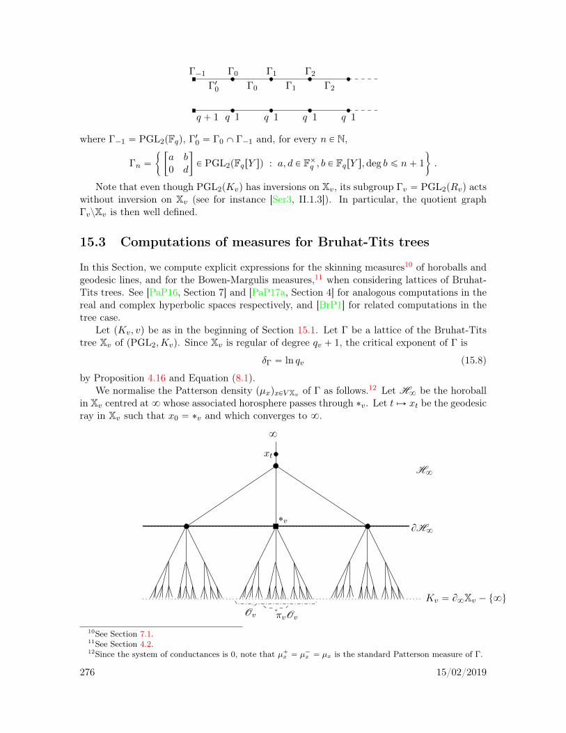
Γ´1 Γ0 Γ1 Γ2

Γ10 Γ0 Γ1 Γ2

q ` 1 q 1 q 1 1 q 1q

where Γ´1 “ PGL2pFqq, Γ10 “ Γ0 X Γ´1 and, for every n P N,

Γn “

"„

a b0 d

P PGL2pFqrY sq : a, d P Fˆq , b P FqrY s,deg b ď n` 1

*

.

Note that even though PGL2pKvq has inversions on Xv, its subgroup Γv “ PGL2pRvq actswithout inversion on Xv (see for instance [Ser3, II.1.3]). In particular, the quotient graphΓvzXv is then well defined.

15.3 Computations of measures for Bruhat-Tits trees

In this Section, we compute explicit expressions for the skinning measures10 of horoballs andgeodesic lines, and for the Bowen-Margulis measures,11 when considering lattices of Bruhat-Tits trees. See [PaP16, Section 7] and [PaP17a, Section 4] for analogous computations in thereal and complex hyperbolic spaces respectively, and [BrP1] for related computations in thetree case.

Let pKv, vq be as in the beginning of Section 15.1. Let Γ be a lattice of the Bruhat-Titstree Xv of pPGL2,Kvq. Since Xv is regular of degree qv ` 1, the critical exponent of Γ is

δΓ “ ln qv (15.8)

by Proposition 4.16 and Equation (8.1).We normalise the Patterson density pµxqxPV Xv of Γ as follows.12 Let H8 be the horoball

in Xv centred at8 whose associated horosphere passes through ˚v. Let t ÞÑ xt be the geodesicray in Xv such that x0 “ ˚v and which converges to 8.

8

˚vBH8

Kv “ B8Xv ´ t8uπvOv

H8

xt

Ov

10See Section 7.1.11See Section 4.2.12Since the system of conductances is 0, note that µ`x “ µ´x “ µx is the standard Patterson measure of Γ.

276 15/02/2019

Hamenstädt’s measure13 associated with H8

µH8“ lim

tÑ`8eδΓtµxt “ lim

tÑ`8qvtµxt

is a Radon measure on B8Xv ´ t8u “ Kv, invariant under all isometries of Xv preservingH8, since Γ is a lattice. Hence it is invariant under the translations by the elements of Kv.By the uniqueness property of Haar measures, µH8

is a constant multiple of the chosen Haarmeasure14 of Kv, and we normalise the Patterson density pµxqxPV Xv so that

µH8“ HaarKv . (15.9)

We summarise the various measure computations in the following result.

Proposition 15.2. Let Γ be a lattice of the Bruhat-Tits tree Xv of pPGL2,Kvq, with Pattersondensity normalised as above.

(1) The outer/inner skinning measures of the singleton t˚vu are given by

d rσ˘t˚vu

pρq “ dµ˚vpρ˘q “`

maxt1, |ρ˘|vu˘´2

dHaarKvpρ˘q

on the set of ρ P B1˘t˚vu such that ρ˘ ‰ 8.

(2) The total mass of the Patterson density is

µx “qv ` 1

qv

for all x P V Xv.

(3) The skinning measure of the horoball H8 is the projection of the Haar measure of Kv:For all ρ P B1

˘H8, we have

drσ˘H8pρq “ dµH8

pρ˘q “ dHaarKvpρ˘q .

(4) If 8 is a bounded parabolic fixed point of Γ, with Γ8 its stabiliser in Γ, if D “

pγH8qγPΓΓ8, we have

σ˘D “ HaarKvpΓ8zKvq “ VolpΓ8zzBH8q .

(5) Let L be a geodesic line in Xv with endpoints L˘ P Kv “ B8Xv ´ t8u. Then on the setof ρ P B1

`L such that ρ` P Kv “ B8Xv ´t8u and ρ` ‰ L˘, the outer skinning measureof L is

d rσ`L pρq “|L` ´ L´|v

|ρ` ´ L´|v |ρ` ´ L`|vdHaarKvpρ`q .

(6) Let L be a geodesic line in Xv, let ΓL be the stabiliser in Γ of L, and assume that ΓLzLhas finite length. Then with D “ pγLqγPΓΓL, we have

σ˘D “qv ´ 1

qvVolpΓLzzLq .

13See Equation (7.5).14Recall that we normalise the Haar measure of pKv,`q such that HaarKv pOvq “ 1.

277 15/02/2019

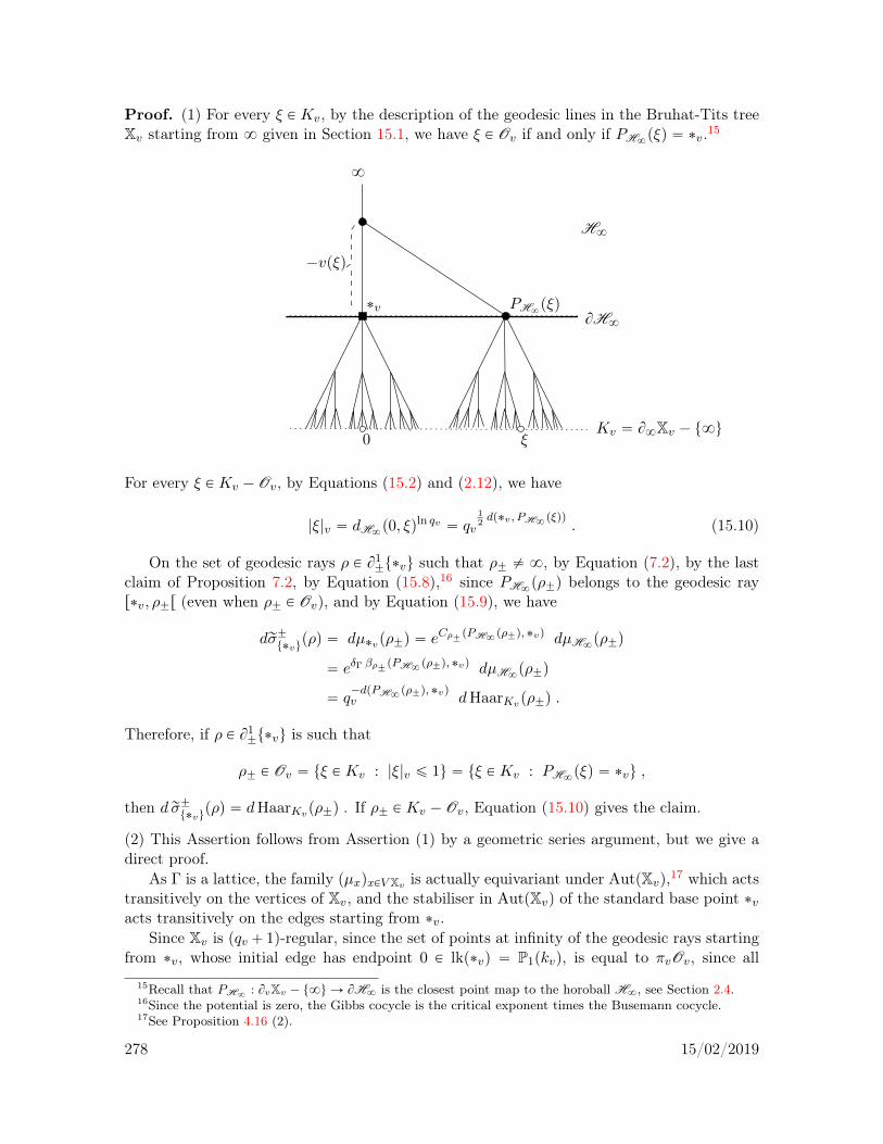
Proof. (1) For every ξ P Kv, by the description of the geodesic lines in the Bruhat-Tits treeXv starting from 8 given in Section 15.1, we have ξ P Ov if and only if PH8

pξq “ ˚v.15

8

˚v

Kv “ B8Xv ´ t8u

H8

ξ

PH8pξq

BH8

0

´vpξq

For every ξ P Kv ´ Ov, by Equations (15.2) and (2.12), we have

|ξ|v “ dH8p0, ξqln qv “ q

12dp˚v , PH8 pξqq

v . (15.10)

On the set of geodesic rays ρ P B1˘t˚vu such that ρ˘ ‰ 8, by Equation (7.2), by the last

claim of Proposition 7.2, by Equation (15.8),16 since PH8pρ˘q belongs to the geodesic ray

r˚v, ρ˘r (even when ρ˘ P Ov), and by Equation (15.9), we have

drσ˘t˚vu

pρq “ dµ˚vpρ˘q “ eCρ˘ pPH8 pρ˘q,˚vq dµH8pρ˘q

“ eδΓ βρ˘ pPH8 pρ˘q,˚vq dµH8pρ˘q

“ q´dpPH8 pρ˘q,˚vqv dHaarKvpρ˘q .

Therefore, if ρ P B1˘t˚vu is such that

ρ˘ P Ov “ tξ P Kv : |ξ|v ď 1u “ tξ P Kv : PH8pξq “ ˚vu ,

then d rσ˘t˚vu

pρq “ dHaarKvpρ˘q . If ρ˘ P Kv ´ Ov, Equation (15.10) gives the claim.

(2) This Assertion follows from Assertion (1) by a geometric series argument, but we give adirect proof.

As Γ is a lattice, the family pµxqxPV Xv is actually equivariant under AutpXvq,17 which actstransitively on the vertices of Xv, and the stabiliser in AutpXvq of the standard base point ˚vacts transitively on the edges starting from ˚v.

Since Xv is pqv ` 1q-regular, since the set of points at infinity of the geodesic rays startingfrom ˚v, whose initial edge has endpoint 0 P lkp˚vq “ P1pkvq, is equal to πvOv, since all

15Recall that PH8 : BvXv ´ t8u Ñ BH8 is the closest point map to the horoball H8, see Section 2.4.16Since the potential is zero, the Gibbs cocycle is the critical exponent times the Busemann cocycle.17See Proposition 4.16 (2).

278 15/02/2019

geodesic lines from 8 P B8Xv to points of πvOv Ă B8Xv pass through ˚v, and by thenormalisation of the Patterson density and of the Haar measure, we have

µ˚v “ pqv ` 1q µ˚vpπvOvq “ pqv ` 1q µH8pπvOvq “ pqv ` 1qHaarKvpπvOvq

“qv ` 1

qvHaarKvpOvq “

qv ` 1

qv.

(3) This follows from Equation (7.4), and from the normalisation µH8“ HaarKv of the

Patterson density.

(4) This follows from Assertion (3) and from Equation (8.11) (where the normalisation of thePatterson density was different than the one given by Assertion (2)).

(5) Let L,L`, L´ be as in the statement of Assertion (5), see the picture below. The resultfollows from Lemma 8.6 applied with H “ H8, from Equations (15.9), (15.8) and (15.2).

ρp`8q

˚v

ρp0q

B8X

L`L´

(6) This follows from Equation (8.12) (where the normalisation of the Patterson density wasdifferent), since Xv is pqv ` 1q-regular, and from Assertion (2):

σ˘D “ µ˚vqv ´ 1

qv ` 1VolpΓLzzLq “

qv ´ 1

qvVolpΓLzzLq . l

We now turn to measure computations for arithmetic lattices Γ in Xv in the function fieldcase. We still assume that the Patterson density of Γ is normalised so that µH8

pOvq “ 1, andwe denote by mBM the Bowen-Margulis measure of Γ associated with this choice of Pattersondensity.

Proposition 15.3. Let K be a function field over Fq of genus g and let v be a valuation ofK. Let Γ be a finite index subgroup of Γv “ PGL2pRvq, with Patterson density normalisedsuch that µH8

“ HaarKv .

(1) We have

mBM “pqv ` 1q rΓv : Γs

qvVolpΓvzzXvq “

2 pqv ` 1q ζKp´1q rΓv : Γs

qv,

279 15/02/2019

and if K “ FqpY q and v “ v8 is the valuation at infinity of C “ P1, then

mBM “2 rPGL2pFqrY sq : Γs

q pq ´ 1q2.

(2) Let Γ8 be the stabiliser in Γ of 8 P B8Xv, and let D “ pγH8qγPΓΓ8. We have

σ˘D “q g´1 rpΓvq8 : Γ8s

q ´ 1.

Proof. (1) Recall that Γv “ PGL2pRvq acts without inversion on Xv. By Equation (8.4)(which uses a different normalisation of the Patterson density of Γ), and by Proposition 15.2(2), we have

mBM “ µ˚v2 qvqv ` 1

VolpΓzzXvq “pqv ` 1q rΓv : Γs

qvVolpΓvzzXvq .

The first claim of Assertion (1) hence follows from Equation (15.7).If K “ FqpY q and v “ v8, then the second claim of Assertion (1) follows either from the

first claim where the value of ζKp´1q is given by Equation (14.6), or from the fact that qv “ qand that the covolume VolpPGL2pFqrY sqzzXv8q of the Nagao lattice PGL2pFqrY sq is

VolpPGL2pFqrY sqzzXv8q “2

pq ´ 1qpq2 ´ 1q, (15.11)

as an easy geometric series computation shows using the description of the modular ray inSection 15.2 (see also [BasL, Sect. 10.2]).

(2) Let us prove that

HaarKvppΓvq8zKvq “q g´1

q ´ 1. (15.12)

The result then follows by Proposition 15.2 (4) since

σ˘D “ HaarKvpΓ8zKvq “ rpΓvq8 : Γ8s HaarKvppΓvq8zKvq .

The stabiliser of 8 “ r1 : 0s in Γv acts on Kv exactly by the set of transformationsz ÞÑ az ` b with a P pRvqˆ and b P Rv. Since18 pRvq

ˆ “ pFqqˆ acts freely by multiplicationon the left on pKv ´RvqRv, and by Lemma 14.4, we have

HaarKvppΓvq8zKvq “1

q ´ 1HaarKvpKvRvq “

q g´1

q ´ 1.

This proves Equation (15.12). l

18See Equation (14.3).

280 15/02/2019

15.4 Exponential decay of correlation and error terms for arith-metic quotients of Bruhat-Tits trees

As in the beginning of Section 15.1, let Kv be a non-Archimedean local field, with valuationv, valuation ring Ov, choice of uniformiser πv, and residual field kv of order qv. Let Γ be alattice of the Bruhat-Tits tree Xv of pPGL2,Kvq. In this Section, we discuss the error termsestimates that we will use in Part III.

Partly in order to simplify the references, we start by summarizing in the next statementthe only results from the geometric Part II of this book, on geometric equidistribution andcounting problems, that we will use in this algebraic Part III. We state it with the normali-sation introduced in Section 15.3 which will be useful in what follows.

Theorem 15.4. Let Γ be a lattice of Xv whose length spectrum LΓ is equal to 2Z. Assumethat the Patterson density of Γ is normalised so that µx “ qv`1

qvfor every x P V Xv. Let D˘

be nonempty proper simplicial subtrees of Xv with stabilisers ΓD˘ in Γ, such that the familiesD˘ “ pγD˘qγPΓΓD˘

are locally finite in Xv. For every γ P Γ such that D´ and γD` aredisjoint, let α´e, γ be the generalised geodesic line, isometric exactly on r0, dpD´, γD`qs, whoseimage is the common perpendicular between D´ and γD`. If the measure σ´D` is nonzero andfinite, then

limnÑ`8

pqv2 ´ 1qpqv ` 1q

2 qv3

VolpΓzzXvqσ´D`

q´nv

ÿ

γPΓΓD`0ădpD´, γD`qďn

∆α´e, γ“ rσ`D´ ,

for the weak-star convergence of measures on the locally compact spacep

GXv.Furthermore, if Γ is geometrically finite, then for every β P s0, 1s, there exists an error

term for this equidistribution claim when evaluated on rψ P C βc p

p

GXq of the form Op rψ β e´κnq

for some κ ą 0.

As recalled at the end of Section 2.6, lattices in PGL2pKvq are geometrically finite, see[Lub1]. We will hence be able to use the error term in Theorem 15.4 in particular when‚ Kv is the completion of a function fieldK over Fq with respect to a (normalised discrete)

valuation v of K and Γ is a finite index subgroup of PGL2pRvq with Rv the affine functionring associated with v,19 as in Chapters 16 and 19, and in Sections 17.2 and 18.2;‚ when Kv “ Qp and Γ is an arithmetic lattice in PGL2pKvq derived from a quaternion

algebra, see Sections 17.3 and 18.2.

Proof. In order to prove the first claim, we apply Corollary 11.12 with X “ Xv and p “ q “ qv.Since LΓ “ 2Z, the lattice Γ leaves invariant the partition of V Xv into vertices at even distancefrom a basepoint x0 P V Xv and vertices at odd distance from x0. Since the Patterson densityis now normalised so that µx0 “

qv`1qv

(instead of µx0 “qv`1?qv

in Corollary 11.12), theskinning measures rσ¯D˘ are now 1?

qvtimes the ones in the statement of Corollary 11.12.

Hence the second assertion of Corollary 11.12 gives

limnÑ`8

qv2 ´ 1

2 qv2

TVolpΓzzXvq?qv σ

´

D`qv´n

ÿ

γPΓΓD`0ădpD´, γD`qďn

∆α´e, γ“?qv rσ`D´ .

19See Section 14.2 for definitions.

281 15/02/2019

By Equation (2.23), we have

TVolpΓzzXvq “ pqv ` 1q VolpΓzzXvq .

The first claim follows.

The last claim concerning error terms follows from Remark (ii) following the proof ofTheorem 12.16. l

In the last four Chapters 16, 17, 18 and 19 of this book, we will need to push to infinitythe measures appearing in the statement of Theorem 15.4. We regroup in the following tworemarks the necessary control tools for such a pushing.

Remark 15.5. With the notation of Theorem 15.4, we will use Lemma 3.9 when X “ |Xv|1is the geometric realisation of the simplicial tree Xv, α “ α´e, γ is20 the common perpendicularbetween D´ and γD` for γ P Γ (when it exists), and ρ “ ργ is any extension of α to ageodesic ray, or rather to a generalised geodesic line isometric exactly on r0,`8r . Under theassumptions of Theorem 15.4, we have by Lemma 3.9

pqv2 ´ 1qpqv ` 1q

2 qv3

VolpΓzzXvqσ´D`

q´nv

ÿ

γPΓΓD`0ădpD´, γD`qďn

∆ργ˚á rσ`D´ , (15.13)

with, if Γ is geometrically finite, an error term when evaluated on rψ P C βc p

p

GXvq of the formOpe´κn rψ βq for some κ ą 0 small enough (depending in particular on β P s0, 1s).

From now on in this book, for every subtree D of Xv with geometric realisation D “

|D|1, we endow B8Xv ´ B8D with the distance-like map dD defined in Equation (3.8). Weuse this map dD in order to define both the β-Hölder-continuity of maps with values inpB8Xv ´ B8D, dDq and the β-Hölder-norm of a function defined on pB8Xv ´ B8D, dDq.

Remark 15.6. With the notation of Theorem 15.4, we will use Proposition 3.10 when X “ Xvand D “ D´. Under the assumptions of Theorem 15.4, with ργ any extension to a geodesicray of the common perpendicular α´e, γ between D´ and γD` for γ P Γ, since pushing forwardmeasures on B1

`D´ by the homeomorphism B` : ρ ÞÑ ρ` introduced in Proposition 3.10 iscontinuous, we have by Equation (15.13)

pqv2 ´ 1qpqv ` 1q

2 qv3

VolpΓzzXvqσ´D`

q´nv

ÿ

γPΓΓD`0ădpD´, γD`qďn

∆pργq`˚á pB`q˚rσ

`

D´ . (15.14)

If Γ is geometrically finite, for all β P s0, 1s and ψ P C βc pB8Xv ´ B8D´q, using the error

term in Equation (15.13) with regularity β2 when evaluated on rψ “ ψ ˝ B`, which belongs to

Cβ2c p

p

GXvq by the first claim of Proposition 3.10, we have by the last claim of Proposition 3.10an error term in Equation (15.14) evaluated on ψ of the form Ope´κn ψ βq for some κ ą 0small enough.

20the generalised geodesic line isometric exactly on r0, dpD´, γD`qs parametrising

282 15/02/2019

A stronger assumption than the Hölder regularity is the locally constant regularity, thathas been defined at the end of Section 3.1, and is applicable here since the involved spacesare totally disconnected. Several error terms estimates in the literature use this strongerregularity (see for instance [AtGP, KemaPS]). The following result of decay of correlationsunder locally constant regularity follows from Corollary 9.6 by Remark 3.11 and since21 anylattice of PGL2pKvq is geometrically finite.22

Proposition 15.7. Assume that Γ is a lattice of PGL2pKvq, and let β P s0, 1s.(1) If LΓ “ Z, there exist C, κ ą 0 such that for every ε P s0, 1s, for all ε-locally constant

maps φ, ψ : ΓzGXv Ñ R and n P Z, we haveˇ

ˇ

ˇ

ż

ΓzGXvφ ˝ g´n ψ dmBM´

1

mBM

ż

ΓzGXvφ dmBM

ż

ΓzGXvψ dmBM

ˇ

ˇ

ˇ

ď C e´κ|n| φε lc, β ψε lc, β .

(2) If LΓ “ 2Z, then there exist C, κ ą 0 such that for every ε P s0, 1s, for all ε-locallyconstant maps φ, ψ : ΓzGevenXv Ñ R and n P Z, we have

ˇ

ˇ

ˇ

ż

ΓzGevenXφ ˝ g´2n ψ dmBM´

1

mBMpΓzGevenXq

ż

ΓzGevenXφ dmBM

ż

ΓzGevenXψ dmBM

ˇ

ˇ

ˇ

ď C e´κ|n| φε lc, β ψε lc, β . l

We will not use the following result in this book, but its Assertion (2) is used in theannouncement [BrPP] which only considers the locally constant regularity.

Theorem 15.8. Assume that Γ is a lattice of PGL2pKvq, and let β P s0, 1s.(1) If LΓ “ Z, there exists κ ą 0 such that for every ε P s0, 1s and every ε-locally constant

map rψ :

p

GXv Ñ R, we have, as nÑ `8,

pqv ´ 1q

pqv ` 1q qv

VolpΓzzXvqσ´D`

q´nv

ÿ

γPΓΓD`0ădpD´, γD`qďn

rψpα´e, γq

“

ż

p

GXv

rψ drσ`D´ `O`

e´κn rψ ε lc, β

˘

.

(2) If LΓ “ 2Z, there exists κ ą 0 such that for every ε P s0, 1s and every ε-locally constantmap rψ :

p

GXv Ñ R, we have, as nÑ `8,

pqv2 ´ 1qpqv ` 1q

2 qv3

VolpΓzzXvqσ´D`

q´nv

ÿ

γPΓΓD`0ădpD´, γD`qďn

rψpα´e, γq

“

ż

p

GXv

rψ drσ`D´ `O`

e´κn rψ ε lc, β

˘

.

Proof. This result follows by replacing in the proof of Theorem 12.16 (or rather Remark(ii) following its proof) the use of the exponential decay of β-Hölder correlations given byCorollary 9.6 by the use of Proposition 15.7.

21See the end of Section 2.6.22Note that being a lattice of PGL2pKvq is much stronger than been a lattice in AutpXvq.

283 15/02/2019

We conclude this Section by giving an algebraic second proof of Theorem 15.8, in thefollowing situation. Let Kv be the completion of a function field K over Fq with respect to avaluation v of K and let Γ be a nonuniform23 lattice of Gv “ PGL2pKvq. We only obtain aversion using an exponent β ě ln qv for the locally constant norm. For simplicity, we consideronly Assertion (1) of Theorem 15.8, though Assertion (2) xould be treated similarly.

The group Gv acts (on the left) on the complex vector space of maps ψ from ΓzGv to R,by right translation on the source: For every g P Gv, we have gψ : x ÞÑ ψpxgq. A functionψ : ΓzGv Ñ R is algebraically locally constant if there exists a compact-open subgroup U ofPGL2pOvq which leaves ψ invariant:

@ g P U, gψ “ ψ ,

or equivalently, if ψ is constant on each orbit of U under the right action of Gv on ΓzGv. Notethat ψ is then continuous, since the orbits of U are compact-open subsets. We define

dψ “ dim`

VectRpPGL2pOvqψq˘

as the dimension of the complex vector space generated by the images of ψ under the elementsof PGL2pOvq, which is finite, and even satisfies

dψ ď rPGL2pOvq : U s .

We define the alc-norm of every bounded algebraically locally constant map ψ : ΓzGv Ñ Rby

ψalc “a

dψ ψ8 .

Though the alc-norm does not satisfy the triangle inequality, we have λψalc “ |λ| ψalc

for every λ P R. We denote by alcpΓzGvq the vector space of bounded algebraically locallyconstant maps ψ from ΓzGv to R.

For every n P N, let Un be the compact-open subgroup of PGL2pOvq which is the kernelof the morphism PGL2pOvq Ñ PGL2pOvπv

nOvq of reduction modulo πvn. Note that anycompact-open subgroup U of PGL2pOvq contains Un for some n P N. Hence ψ : ΓzGv Ñ R isalgebraically locally constant if and only if there exists n P N such that ψ is constant on eachright orbit of Un. For every n P N, since the order of PGL2pOvπv

nOvq is at most the orderof pOvπv

nOvq4, which is qv4n, if ψ : ΓzGv Ñ R is constant on each right orbit of Un, then

ψalc ď qv2n ψ8 . (15.15)

Recall24 that we have a natural homeomorphism Ξ : ΓgApOvq ÞÑ Γg `˚ between the doublecoset space ΓzGvApOvq and ΓzGXv. We denote by pG : ΓzGv Ñ ΓzGXv the compositionmap of the canonical projection

`

ΓzGv˘

Ñ`

ΓzGvApOvq˘

and of Ξ. By Equation (15.4), forall x P ΓzGv and n P N, we have

pG px avnq “ gn pG pxq . (15.16)

Lemma 15.9. For every ε P s0, 1s, for every ε-locally constant function ψ : ΓzGXv Ñ R, ifn “ r´1

2 ln εs, then the map ψ ˝ pG : ΓzGv Ñ R is Un-invariant and

ψ ˝ pG alc ď qv2 ψε lc, ln qv . (15.17)

23This assumption is introduced in order to apply the following Theorem 15.10. Note that the existence ofa nonuniform lattice in Gv “ PGL2pKvq forces the characteristic to be positive, see for instance [Lub1].

24See Section 15.1.

284 15/02/2019

Proof. Let ε, ψ, n be as in the statement. Let us first prove that if `, `1 P GXv satisfy`r´n,`ns “ `1

r´n,`ns, then dp`, `1q ď ε.

If `r´n,`ns “ `1r´n,`ns, then dp`ptq, `

1ptqq “ 0 for t P r´n, ns and by the triangle inequalitydp`ptq, `1ptqq ď 2p|t| ´ nq if |t| ě n, hence

dp`, `1q ď 2

ż `8

n2 pt´ nq e´2 t dt “ 2 e´2n

ż `8

0u e´u

du

2“ e´2n

ď e´2p´ 12

ln εq “ ε ,

as wanted.

In order to prove that ψ ˝ pG : ΓzGv Ñ R is Un-invariant, let x, x1 P ΓzGv be such thatx1 P xUn. Since Un acts by the identity map on the ball of radius n in the Bruhat-Tits tree Xv,the geodesic lines pG pxq and pG px

1q in ΓzGXv coincide (at least) on r´n, ns. Hence, as we sawin the beginning of the proof, we have dppG pxq, pG px

1qq ď ε. Therefore ψppG pxqq “ ψppG px1qq

since ψ is ε-locally constant.Now, using Equation (15.15), we have

ψ ˝ pG alc ď qv2n ψ ˝ pG 8

ď qv2p1´ 1

2ln εq ψ8 “ qv

2 ε´ ln qv ψ8 “ qv2 ψε lc, ln qv . l

Now, we will use an algebraic result of exponential decay of correlations, Theorem 15.10(see for instance [AtGP]). We first recall some definitions and notation, useful for its state-ment.

Recall that the left action of the locally compact unimodular group Gv on the locallycompact space GXv is continuous and transitive, and that its stabilisers are compact henceunimodular. Since Γ is a lattice, the (Borel, positive, regular) Bowen-Margulis measurermBM on GXv is Gv-invariant (see Proposition 4.16 (2)). Hence by [Wei1] (see also [GoP,Lem. 5]), there exists a unique Haar measure on Gv, which disintegrates by the evaluation mapĂpG : Gv Ñ GXv defined by g ÞÑ g`˚, with conditional measure on the fiber over ` “ g`˚ P GXvthe probability Haar measure on the stabiliser gApOvqg

´1 of ` under Gv. Hence, taking thequotient under Γ and normalising in order to have probability measures, if µv is the rightGv-invariant probability measure on ΓzGv, we have

ppG q˚µv “mBM

mBM. (15.18)

For every g P Gv, we denote by Rg : ΓzGv Ñ ΓzGv the right action of g, and for allbounded continuous functions rψ, rψ1 on ΓzGv, we define

covµv , gprψ, rψ1q “

ż

ΓzGv

rψ ˝Rg rψ1 dµv ´

ż

ΓzGv

rψ dµv

ż

ΓzGv

rψ1 dµv .

Note that by Equations (15.18) and (15.16), for all bounded continuous functions ψ,ψ1 :ΓzGXv Ñ R and n P Z, we have25

cov mBMmBM

, npψ,ψ1q “ covµv , avnpψ ˝ pG , ψ

1 ˝ pG q . (15.19)

25See Section 9.2 for a definition of covµ, n.

285 15/02/2019

Recall that the adjoint representation of Gv “ PGL2pKvq is the continuous morphismGv Ñ GLpM2pKvqq defined by rhs ÞÑ tx ÞÑ hxh´1u, which is independent of the choice ofthe representative h P GL2pKvq of rhs P PGL2pKvq. For every g P Gv, we denote by |g|v the

operator norm of the adjoint representation of g. For instance, recalling that av “„

1 00 π´1

v

,

we have, for all n P Z,|av

n|v “ qv|n| . (15.20)

We refer for instance to [AtGP] for the following result of exponential decay of correlations.

Theorem 15.10. Let Γ be a nonuniform lattice of Gv. There exist C 1, κ1 ą 0 such that, forall bounded locally constant functions rψ, rψ1 : ΓzGv Ñ R and g P Gv,

ˇ

ˇ covµv , gprψ, rψ1q

ˇ

ˇ ď C 1 rψalc rψ1alc |g|v

´κ1 . l (15.21)

Proposition 15.7 (1) and therefore Theorem 15.8 (1) with β ě ln qv follows from this resultapplied to rψ “ ψ ˝ pG , rψ1 “ ψ1 ˝ pG and g “ av

n by using Equations (15.19), (15.17) and(15.20) and by taking C “ C 1q4

v and κ “ κ1 ln qv. l

Remark. There is a similar relationship between locally constant functions on Kv in analgebraic sense and the ones in the metric sense.

The additive group pKv,`q acts on the complex vector space of functions from Kv to R,by translations on the source: for all y P Kv and ψ : Kv Ñ R, the function y ¨ ψ is equal tox ÞÑ ψpx ` yq. A function ψ : Kv Ñ R is algebraically locally constant if there exists k P Nsuch that ψ is invariant under the action of the compact-open subgroup pπvqkOv of Kv, thatis, if for all x P Kv and y P pπvqkOv, we have ψpx` yq “ ψpxq. Note that a locally constantfunction from Kv to R is continuous.

For any locally constant function ψ : Kv Ñ R, the complex vector space VectRpOv ¨ ψqgenerated by the images of ψ under the elements of Ov is finite dimensional. Its dimensiondψ satisfies, with k as above,

dψ ď rOv : pπvqkOvs “ qv

k .

We define the alc-norm of every bounded algebraically locally constant function ψ : Kv Ñ Rby

ψalc “a

dψ ψ8 .

Though the alc-norm does not satisfy the triangle inequality, we have λψalc “ |λ| ψalc forevery λ P R, and the set of bounded algebraically locally constant maps from Kv to R is areal vector space.

Actually, a function ψ : Kv Ñ R is algebraically locally constant if and only if it is locallyconstant. More precisely, for every ε P s0, 1s, since the closed balls of radius q´kv in Kv arethe orbits by translations under pπvqkOv, every ε-locally constant function ψ : Kv Ñ R isconstant under the additive action of pπvqkOv for k “ r´ ln ε

ln qvs, hence

ψalc ď ψε lc, 12.

286 15/02/2019

15.5 Geometrically finite lattices with infinite Bowen-Margulismeasure

This Section is a digression from the theme of arithmetic applications, in which we use theNagao lattice defined in Section 15.2 in order to construct a geometrically finite discretegroup of automorphisms of a simplicial tree which has infinite Bowen-Margulis measure. Thisexample was promised after Proposition 4.16, where we saw that such examples do not existfor uniform trees.

We will equivariantly change the lengths of the edges of a simplicial tree X endowed witha geometrically finite (nonuniform) lattice Γ in order to turn X into a metric tree in which thegroup Γ remains a geometrically finite lattice, but now has a geometrically finite subgroupwith infinite Bowen-Margulis measure. This example is an adaptation of the negatively curvedmanifold example of [DaOP, §4]. The simplicial example is obtained as a modification of themetric tree example.

Theorem 15.11. There exists a geometrically finite discrete group of automorphisms of ametric tree with constant degrees, whose Bowen-Margulis measure is infinite.

There exists a geometrically finite discrete group of automorphisms of a simplicial treewith uniformly bounded degrees whose Bowen-Margulis measure is infinite.

Proof. Let v “ v8 be the valuation at infinity of K “ FqpY q, Kv “ FqppY ´1qq, Ov “

FqrrY ´1ss and Rv “ FqrY s. Let Xv be the Bruhat-Tits tree of pPGL2,Kvq with base point˚v “ rOv ˆ Ovs. Let Γv “ PGL2pRvq, which is a lattice of Xv, with quotient graph of groupsthe modular ray ΓvzzXv described in Section 15.2. We denote by pyiqi“´1,0,... the orderedvertices along ΓvzzXv with vertex stabilisers pΓiqi“´1,0,..., and by peiqiPN the ordered edgesalong ΓvzzXv (pointing away from the origin of the modular ray).

The subgroup

P “ď

iě0

Γi “

"„

a Q0 d

: Q P FqrY s, a, d P Fˆq*

is the stabiliser in Γ of 8 P B8Xv. Let P0 be the finite index subgroup of P consisting of the

elements„

1 Q0 1

with Qp0q “ 0. Observing that dpγ˚v, ˚vq “ 2pi ` 1q for any γ P Γi ´ Γi´1

and that the cardinality of pΓi ´ Γi´1q X P0 is pq ´ 1qqi`1, it is easy to see that the Poincaréseries

QP0, 0,˚v ,˚vpsq “ÿ

γPP0

e´s dp˚v ,γ˚vq

of the discrete (though elementary) subgroup P0 of IsompXvq is (up to a multiplicative con-stant) equal to

ř8i“0 q

ie´2si, which gives δP0 “ln q2 for the critical exponent of P0 on Xv.

Let h be an element of Γv which is loxodromic on Xv and whose fixed points belong tothe open subset Y ´1Ov of Kv “ B8Xv ´ t8u. Hence the horoball H8 centred at 8 P B8Xv,whose horosphere contains ˚v, is disjoint from the translation axis Axh of h. Note that thestabiliser of H8 in Γv is P and that P0 acts freely on the edges exiting H8. Let x0 P V Xv bethe closest point on Axh to H8, let e˚ be the edge with origin ˚v pointing towards x0, andlet e´, e` be the two edges with origin x0 on Axh.

287 15/02/2019

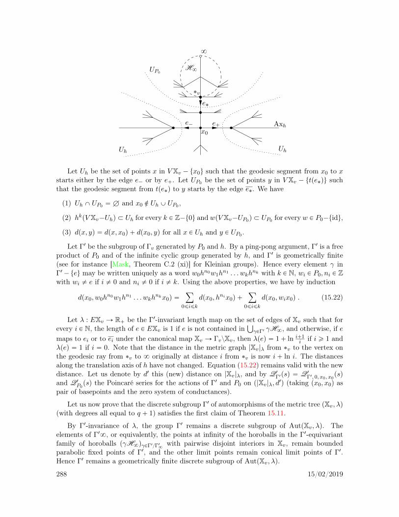
Uh

Axh

Uh

e`e´

e˚

UP0

8

˚v

H8

x0

Let Uh be the set of points x in V Xv ´ tx0u such that the geodesic segment from x0 to xstarts either by the edge e´ or by e`. Let UP0 be the set of points y in V Xv ´ ttpe˚qu suchthat the geodesic segment from tpe˚q to y starts by the edge e˚. We have

(1) Uh X UP0 “ H and x0 R Uh Y UP0 ,

(2) hkpV Xv´Uhq Ă Uh for every k P Z´t0u and wpV Xv´UP0q Ă UP0 for every w P P0´tidu,

(3) dpx, yq “ dpx, x0q ` dpx0, yq for all x P Uh and y P UP0 .

Let Γ1 be the subgroup of Γv generated by P0 and h. By a ping-pong argument, Γ1 is a freeproduct of P0 and of the infinite cyclic group generated by h, and Γ1 is geometrically finite(see for instance [Mask, Theorem C.2 (xi)] for Kleinian groups). Hence every element γ inΓ1´teu may be written uniquely as a word w0h

n0w1hn1 . . . wkh

nk with k P N, wi P P0, ni P Zwith wi ‰ e if i ‰ 0 and ni ‰ 0 if i ‰ k. Using the above properties, we have by induction

dpx0, w0hn0w1h

n1 . . . wkhnkx0q “

ÿ

0ďiďk

dpx0, hnix0q `

ÿ

0ďiďk

dpx0, wix0q . (15.22)

Let λ : EXv Ñ R` be the Γ1-invariant length map on the set of edges of Xv such that forevery i P N, the length of e P EXv is 1 if e is not contained in

Ť

γPΓ1 γH8, and otherwise, if emaps to ei or to ei under the canonical map Xv Ñ ΓvzXv, then λpeq “ 1` ln i`1

i if i ě 1 andλpeq “ 1 if i “ 0. Note that the distance in the metric graph |Xv|λ from ˚v to the vertex onthe geodesic ray from ˚v to 8 originally at distance i from ˚v is now i` ln i. The distancesalong the translation axis of h have not changed. Equation (15.22) remains valid with the newdistance. Let us denote by d1 this (new) distance on |Xv|λ, and by Q1

Γ1psq “ Q1Γ1, 0, x0, x0

psqand Q1

P0psq the Poincaré series for the actions of Γ1 and P0 on p|Xv|λ, d1q (taking px0, x0q as

pair of basepoints and the zero system of conductances).

Let us now prove that the discrete subgroup Γ1 of automorphisms of the metric tree pXv, λq(with degrees all equal to q ` 1) satisfies the first claim of Theorem 15.11.

By Γ1-invariance of λ, the group Γ1 remains a discrete subgroup of AutpXv, λq. Theelements of Γ18, or equivalently, the points at infinity of the horoballs in the Γ1-equivariantfamily of horoballs pγH8qγPΓ1Γ18 with pairwise disjoint interiors in Xv, remain boundedparabolic fixed points of Γ1, and the other limit points remain conical limit points of Γ1.Hence Γ1 remains a geometrically finite discrete subgroup of AutpXv, λq.

288 15/02/2019

The Poincaré series Q1P0

is (up to a multiplicative and additive constant)ř8i“1 q

i e´2si i´2s,which has the same critical exponent δP0 “

ln q2 as previously, but it is easy to see that the

discrete group P0 is now of convergence type if q ě 3.Let λphq be the (old and new) translation length of h. Using Equation (15.22) and

partitionning the above words by the number of nonzero powers of h they contain, we have,for every s ě 0,

Q1Γ1psq “

ÿ

γPΓ1

e´s d1px0,γx0q

ď

´

1``8ÿ

k“1

´

ÿ

iPZ´t0ue´s |i|λphq

ÿ

wPP0

e´s d1px0,wx0q

¯k¯ ÿ

wPP0

e´s d1px0,wx0q .

At s “ δP0 , the above sums over i P Z´t0u and over w P P0 converge, and by replacing h by ahigh enough power if necessary, we may assume that

ř

iPZ´t0u e´s |i|λphq

ř

wPP0e´s d

1px0,wx0q ă 1

if s “ δP0 , which makes the Poincaré series of Γ1 converge at s “ δP0 . Since P0 is a subgroupof Γ1 with critical exponent δP , we have that Q1

Γ1psq ě Q1P0psq “ `8 if s ă δP0 . We conclude

that the critical exponent of Γ1 is equal to δP0 and that Γ1 is of convergence type. By Corollary4.7 (1), the Bowen-Margulis measure of Γ1 is infinite.

In order to prove the second claim of Theorem 15.11, we first define a new length mapλ : EXv Ñ R` which coincides with the previous one on every edge e of Xv, unless e maps toei or to ei for any i P N under the canonical map Xv Ñ ΓzXv, in which case we set

λpeq “ 1` tlnpi` 1qu´ tln iu

if i ě 1 and λpeq “ 1 if i “ 0 (where t¨u is the largest previous integer map). This map λnow has values in t1, 2u, and we subdivide each edge of length 2 into two edges of length 1.The tree Y thus obtained has uniformly bounded degrees (although it is no longer a uniformtree), and the group Γ1 defines a geometrically finite discrete subgroup of AutpYq with infiniteBowen-Margulis measure. To see that P0 is again of convergence type, observe that eachdistance in the simplicial case appearing in the Poincaré series differs by at most 1 from thecorresponding distance in the metric tree case. The remainder of the argument is the sameas in the metric tree case. l

289 15/02/2019

290 15/02/2019

Chapter 16

Equidistribution and counting ofrational points in completed functionfields

Let K be a (global) function field over Fq of genus g, let v be a (normalised discrete) valuationofK, letKv be the associated completion ofK and let Rv be the affine function ring associatedwith v.1 In this Chapter, we prove analogues of the classical results on the counting andequidistribution towards the Lebesgue measure on R of the Farey fractions p

q with pp, qq PZˆpZ´t0uq relatively prime.2 In particular, we prove various equidistribution results of locallyfinite families of elements of K towards the Haar measure on Kv, using the geometrical workon equidistribution of common perpendiculars done in Section 11.4 and recalled in Section15.4.

16.1 Counting and equidistribution of non-Archimedian Fareyfractions

The first result of this Section is an analog in function fields of the equidistribution of Fareyfractions to the Lebesgue measure in R, see the Introduction, and for example [PaP14b, p. 978]for the precise statement and a geometric proof. For every px0, y0q P Rv ˆRv ´ tp0, 0qu, let

mv, x0, y0 “ Cardta P pRvqˆ : D b P x0Rv X y0Rv, pa´ 1qx0y0 ´ bx0 P y

20Rvu .

For future use, note that by Equation (14.3)

mv, 1, 0 “ q ´ 1 . (16.1)

For every pa, bq P Rv ˆ Rv and every subgroup H of GL2pRvq, let Hpa,bq be the stabiliser ofpa, bq for the linear action of H on Rv ˆRv.

Theorem 16.1. Let G be a finite index subgroup of GL2pRvq, and let px0, y0q P Rv ˆ Rv ´tp0, 0qu. Let

c “pqv

2 ´ 1q pqv ` 1q ζKp´1q mv, x0, y0 pNxx0, y0yq2 rGL2pRvq : Gs

pq ´ 1q q g´1 q3v rGL2pRvqpx0,y0q : Gpx0,y0qs

.

1See Section 14.2 for definitions and background.2See for instance [Nev], as well as [PaP14b] for an approach using methods similar to the ones in this text.

291 15/02/2019

Then, as sÑ `8,c s´2

ÿ

px, yqPGpx0, y0q, |y|vďs

∆xy

˚á HaarKv .

For every β P s0, 1ln qv

s, there exists κ ą 0 such that for every β-Hölder-continuous functionψ : Kv Ñ R with compact support,3 as for instance if ψ : Kv Ñ R is locally constant withcompact support (see Remark 3.11), there is an error term in the equidistribution claim ofTheorem 16.1 evaluated on ψ, of the form Ops´κψβq.

It is remarkable that due to the general nature of our geometrical tools, we are able to workwith any finite index subgroup G of GL2pRvq, and not only with its congruence subgroups. Inthis generality, the usual techniques (for instance involving analysis of Eisenstein series) arenot likely to apply. Also note that the Hölder regularity for the error term is a much weakerassumption than the locally constant one that is usually obtained by analytic number theorymethods.

Theorem 1.13 in the Introduction follows from this result, by taking K “ FqpY q (so thatg “ 0), v “ v8, qv “ q, px0, y0q “ p1, 0q and s “ qt, and by using Equations (14.6) and (16.1)in order to simplify the constant.

Before proving Theorem 16.1, let us give a counting result which follows from this equidis-tribution result.

The additive group Rv acts on Rv ˆRv by the horizontal shears (transvections):

@ z P Rv, @ px, yq P Rv ˆRv, z ¨ px, yq “ px` zy, yq ,

and this action preserves the absolute value |y|v of the vertical coordinate y. Let G be afinite index subgroup of GL2pRvq, and let x0, y0 P Rv. Let Rv,G be the finite index additive

subgroup of Rv consisting of the elements x P Rv such thatˆ

1 x0 1

˙

P G, acting by horizontal

shears on Gpx0, y0q. Note that Rv,G “ Rv if G “ GL2pRvq. We may then define a countingfunction ΨG, x0,y0 of the elements of K in an orbit by homographies under G, as

ΨG, x0, y0psq “ Card Rv,G z

px, yq P Gpx0, y0q, |y|v ď su .

Corollary 16.2. Let G be a finite index subgroup of GL2pRvq, and let px0, y0q P Rv ˆ Rv ´tp0, 0qu. Then there exists κ ą 0 such that, as sÑ `8,

ΨG, x0,y0psq

“pq ´ 1q q 2g´2 q3

v rGL2pRvqpx0,y0q : Gpx0,y0qs rRv : Rv,Gs

pqv2 ´ 1q pqv ` 1q ζKp´1q mv, x0, y0 pNxx0, y0yq2 rGL2pRvq : Gs

s2 `Ops2´κq .

Proof. This follows from Theorem 16.1, by considering the locally constant characteristicfunction of a closed and open fundamental domain of Kv modulo the action by translationsof Rv,G, and by using Lemma 14.4 with I “ Rv. l

Let us fix some notation for this Section. For every subgroup H of GL2pRvq, we denoteby H its image in Γv “ PGL2pRvq. Let Xv be the Bruhat-Tits tree4 of pPGL2,Kvq, which isregular of degree qv ` 1. Let

r “x0

y0P K Y t8u .

3where Kv is endowed with the distance px, yq ÞÑ |x´ y|v4See Section 15.1.

292 15/02/2019

If y0 “ 0, let gr “ id P GL2pKq, and if y0 ‰ 0, let

gr “

ˆ

r 11 0

˙

P GL2pKq .

Proof of Theorem 16.1. We apply Theorem 15.4 with Γ “ G, D´ “ H8 and D` “ grH8.Recall that H8 is the horoball in Xv centred at 8 whose boundary contains ˚v (see Section15.1).

Note that Γ has finite index in Γv and, in particular, it is a lattice of Xv. By [Ser3, II.1.2,Coro.], for all x P V Xv and γ P GL2pRvq, the distance dpx, γxq is even since vpdet γq “ 0.Hence by the equivalence in Equation (4.17), the length spectrum LΓv of Γv is 2Z. The lengthspectrum of Γ is also 2Z, since it is contained in LΓv .

Note that D` is a horoball in Xv centred at r “ x0y0P B8Xv, by Lemma 15.1. The stabiliser

ΓD´ of D´ (respectively ΓD` of D`) coincides with the stabiliser Γ8 of8 P B8Xv (respectivelythe stabiliser Γr of r) in Γ. Note that the families D˘ “ pγD˘qγPΓΓD˘

are locally finite, sinceΓv, and hence its finite index subgroup Γ, is geometrically finite,5 and since 8 and r P K arebounded parabolic limit points of Γv, hence of its finite index subgroup Γ.

For every γ P ΓΓr such that D´ and γD` are disjoint, let α´e, γ be the generalised geodesicline, isometric exactly on r0, dpD´, γD`qs, whose image is the common perpendicular betweenD´ and γD`, and let ργ be the geodesic ray starting (at time t “ 0) from α´e, γp0q and endingat the point at infinity γ ¨ r of γD`. Note that ργ and α´e, γ coincide on r0, dpD´, γD`qs.

Since the Patterson densities of lattices of Xv have total mass qv`1qv

by Proposition 15.2(2), they are normalised as in Theorem 15.4. Then by Equation (15.14), we have

limnÑ`8

pqv2 ´ 1qpqv ` 1q

2 q3v

VolpΓzzXvqσ´D`

qv´n

ÿ

γPΓΓr0ădpD´, γD`qďn

∆pργq` “ pB`q˚rσ`

D´ . (16.2)

Furthermore, for every β P s0, 1ln qv

s, by the comment following Equation (15.14), we have anerror term of the form Ope´κn ψβ ln qvq for some κ ą 0 in the above formula when evaluatedon ψ P C β ln qv

c pB8Xv ´ t8uq, where B8Xv ´ t8u is endowed with Hamenstädt’s distance6

dH8. Hence we have an error term Ope´κn ψβq for some κ ą 0 in the above formula

when evaluated on ψ P C βc pKvq, where Kv “ B8Xv ´ t8u is endowed with the distance

px, yq ÞÑ |x´ y|v, see Equation (15.3).By Proposition 15.2 (3), we have

pB`q˚rσ`

D´ “ HaarKv .

Hence Equation (16.2) gives, with the appropriate error term,

limnÑ`8

pqv2 ´ 1qpqv ` 1q

2 q3v

VolpΓzzXvqσ´D`

qv´n

ÿ

γPΓΓr0ădpD´, γD`qďn

∆γ¨r “ HaarKv . (16.3)

5See Section 15.2.6See Equation (2.12), and note that withD “ H8, Hamenstädt’s distance dH8 coincides with the distance-

like function dD introduced in Equation (3.8) and used in Remark 15.6, since D is a horoball.

293 15/02/2019

Let g P GL2pKq be such that g8 ‰ 8. This condition is equivalent to asking thatthe p2, 1q-entry c “ cpgq of g is nonzero. By Lemma 15.1, the signed distance between thehorospheres H8 and gH8 is

dpH8, gH8q “ ´2 vpcq “ 2ln |c|vln qv

. (16.4)

If y0 ‰ 0, then px, yq “ gpx0, y0q if and only if p xy0, yy0q “ ggrp1, 0q, and the p2, 1q-entry of ggr

is yy0. If y0 “ 0 (which implies that gr “ id and x0 ‰ 0), then px, yq “ gpx0, y0q if and only if

p xx0, yx0q “ gp1, 0q, and the p2, 1q-entry of g “ ggr is y

x0. Let

z0 “

"

y0 if y0 ‰ 0x0 otherwise.

By Equation (16.4), the signed distance between D´ “ H8 and gD` “ g grH8 is

dpD´, gD`q “2

ln qvlnˇ

ˇ

ˇ

y

z0

ˇ

ˇ

ˇ

v.

By discreteness, there are only finitely many double classes rgs P Gp1,0qzGGpx0,y0q suchthat D´ “ H8 and gD` “ g grH8 are not disjoint. Let ZpGq be the centre of G, whichis finite. Since ZpGq acts trivially on P1pKvq, the map GGpx0,y0q Ñ ΓΓr induced by thecanonical map GL2pRvq Ñ PGL2pRvq is |ZpGq|-to-1. Using the change of variable

s “ |z0|v qvn2 ,

so that qv´n “ |z0|v2 s´2, Equation (16.3) gives, with the appropriate error term,

limsÑ`8

pqv2 ´ 1q pqv ` 1q |z0|v

2

2 qv3 |ZpGq|

VolpΓzzXvqσ´D`

s´2ÿ

px, yqPGpx0, y0q, |y|vďs

∆xy

“ HaarKv . (16.5)

The order of the centre ZpGL2pRvqq “ pRvqˆ id is q ´ 1 by Equation (14.3). The map

GL2pRvqGÑ ΓvΓ induced by the canonical map GL2pRvq Ñ PGL2pRvq is hence q´1|ZpGq| -to-1.

By Equation (15.7), we hence have

VolpΓzzXvq “ rΓv : ΓsVolpΓvzzXvq “ 2 ζKp´1q rΓv : Γs

“2

q ´ 1ζKp´1q |ZpGq| rGL2pRvq : Gs . (16.6)

Theorem 16.1 follows from Equations (16.5) and (16.6) and from Lemma 16.3 below. l

Lemma 16.3. We have

σ´D` “q g´1 |z0|v

2rGL2pRvqpx0,y0q : Gpx0,y0qs

mv, x0, y0 pNxx0, y0yq2

.

294 15/02/2019

Proof. Let γr be the image of gr in PGL2pKq. Let us define Γ1 “ γr´1Γγr, which is a finite

index subgroup in Γ1v “ γr´1Γvγr and a lattice of Xv. Since γr maps 8 to r, the point 8 is a

bounded parabolic limit point of Γ1, and we have pΓ1q8 “ γr´1Γrγr. Since the canonical map

GL2pRvq Ñ PGL2pRvq is injective on the stabiliser GL2pRvqpx0,y0q, we have

rpΓ1vq8 : pΓ1q8s “ rpΓvqr : Γrs “ rGL2pRvqpx0,y0q : Gpx0,y0qs .

Since the Patterson density of a lattice does not depend on the lattice (see Proposition4.16 (1)), the skinning measures rσ˘H of a given horoball H do not depend on the lattice.Thus

γ˚ rσ˘H “ rσ˘γH

for every γ P AutpXvq. Let D`1 “ pγ1H8qγ1PΓ1Γ18 , which is a locally finite Γ1-equivariant

family of horoballs. We hence have, using Proposition 15.2 (4) for the third equality,

σ´D` “ σ´

γrD`1

“ σ´D`1 “ HaarKvppΓ

1q8zKvq

“ rpΓ1vq8 : pΓ1q8s HaarKvppΓ1vq8zKvq

“ rGL2pRvqpx0,y0q : Gpx0,y0qs HaarKvppΓ1vq8zKvq . (16.7)

Every element in the stabiliser of 8 in PGL2pKvq can be uniquely written in the form

α “

„

a b0 1

with pa, bq P pKvqˆ ˆKv. Note that

ˆ

r 11 0

˙ˆ

a b0 1

˙ˆ

0 11 ´r

˙

“

ˆ

br ` 1 ar ´ br2 ´ rb a´ br

˙

.

When x0 “ 0 or y0 “ 0, we have α P Γ1v if and only if

b P Rv and a P pRvqˆ .

When x0, y0 ‰ 0, we have α P Γ1v if and only if γrαγr´1 P Γv, hence if and only if

b P Rv X1

rRv, a P pRvq

ˆ, ar ´ br2 ´ r P Rv .

Let U 18 be the kernel of the group morphism from pΓ1vq8 to pKvqˆ sending

„

a b0 1

to a,

and let mv be its index in pΓ1vq8. If x0 “ 0 or y0 “ 0, then mv is equal to |pRvqˆ|, so that,by Equation (14.3),

mv “ |pRvqˆ| “ |pFqqˆ| “ q ´ 1 .

If x0, y0 ‰ 0, we have

mv “ Card ta P pRvqˆ : D b P Rv X

1

rRv, ar ´ br2 ´ r P Rvu .

Note that the notation mv coincides with the constant mv, x0, y0 defined before the statementof Theorem 16.1 in both cases.

If Ipx0,y0q is the nonzero fractional ideal

Ipx0,y0q “

#

Rv if x0 “ 0 or y0 “ 0 ,

Rv X1rRv X

1r2Rv otherwise,

295 15/02/2019

then

U 18 “

"„

1 b0 1

: b P Ipx0,y0q

*

.

Therefore by Lemma 14.4,

HaarKvppΓ1vq8zKvq “

HaarKvpIpx0,y0qzKvq

rpΓ1vq8 : U 18s“q g´1 NpIpx0,y0qq

mv. (16.8)

Let px0q “ś

p pνppx0q and py0q “

ś

p pνppy0q be the prime decompositions of the principal

ideals px0q and py0q. By the formulas of the prime decompositions of intersections, sums andproducts of ideals in Dedekind rings (see for instance [Nar, §1.1] and Equation (14.4)), wehave

px20q X px0y0q X py

20q “ px

20q X py

20q “

ź

p

p2 maxtνppx0q, νppy0qu

andxx0, y0y “

ź

p

pmintνppx0q, νppy0qu .

By the definition of the ideal Ipx0,y0q, by the multiplicativity of the norm, and by Equation(14.5), we hence have if x0 ‰ 0 and y0 ‰ 0

NpIpx0,y0qq pNxx0, y0yq2

|y0|v2 “ N

´

`

px20q X px0y0q X py

20q˘

xx0, y0y2px0q

´2py0q´2¯

“ 1 . (16.9)

If x0 “ 0 or y0 “ 0, thenNpIpx0,y0qq “ NpRvq “ 1 . (16.10)

Lemma 16.3 follows from Equations (16.7), (16.8) and (16.9) if x0 ‰ 0 and y0 ‰ 0 or(16.10) if x0 “ 0 or y0 “ 0. l

Let us state one particular case of Theorem 16.1 in an arithmetic setting, using a congru-ence sugbroup.

Theorem 16.4. Let I be a nonzero ideal of Rv. Then as tÑ `8, we have

pq 2v ´ 1q pqv ` 1q ζKp´1q NpIq

ś

p|Ip1`1

Nppqq

q g´1 q 3v

pqvq´2t

ÿ

px,yqPRvˆIxx, yy“Rv , vpyqě´t

∆xy

˚á HaarKv ,

where the product ranges over the prime factors p of the ideal I. Furthermore, if

Ψptq “ Card Rv z

px, yq P Rv ˆ I : xx, yy “ Rv, vpyq ě ´t(

,

then there exists κ ą 0 such that, as tÑ `8,

Ψptq “q 2g´2 q 3

v

pqv2 ´ 1q pqv ` 1q ζKp´1q NpIqś

p|Ip1`1

Nppqqqv

2t `Opqvp2´κqtq .

296 15/02/2019

For every β P s0, 1ln qv

s, there exists κ ą 0 such that for every ψ P C βc pKvq there is an error

term in the above equidistribution claim evaluated on ψ, of the form Opq ´κ tv ψβq.

Proof. The counting claim is deduced from the equidistribution claim in the same way thatCorollary 16.2 is deduced from Theorem 16.1, noting that the action of Rv by horizontalshears preserves Rv ˆ I.

In order to prove the equidistribution claim, we apply Theorem 16.1 with px0, y0q “ p1, 0qand with G the Hecke congruence subgroup

GI “

"ˆ

a bc d

˙

P GL2pRvq : c P I

*

, (16.11)

which is the preimage of the upper triangular subgroup of GL2pRvIq by reduction moduloI. In this case, the constant mv,x0,y0 appearing in the statement of Theorem 16.1 is equal toq ´ 1 by Equation (16.1). The group GI has finite index in GL2pRvq. The following result iswell-known to arithmetic readers (see for instance [Shi, page 24] when Rv is replaced by Z),we only give a sketch of proof (indicated to us by J.-B. Bost) for the sake of the geometerreaders.

Lemma 16.5. We have

rGL2pRvq : GIs “ NpIqź

p|I

p1`1

Nppqq ,

where the product ranges over the prime factors p of the ideal I.

Proof. Recall that we denote by |E| the cardinality of a finite set E. For every commutativering A with finite group of invertible elements Aˆ, we have a disjoint union

GL2pAq “ď

aPAˆ

ˆ

a 00 1

˙

SL2pAq .

Hence rGL2pAq : SL2pAqs “ |Aˆ|. Since

ˆ

a 00 1

˙

belongs to GI for all a P pRvqˆ, we have

GI “ď

aPpRvqˆ

ˆ

a 00 1

˙

GI X SL2pRvq ,

so that rGL2pRvq : GIs “ rSL2pRvq : GI X SL2pRvqs.The group morphism of reduction modulo I from SL2pRvq to SL2pRvIq is onto, by an

argument of further reduction to the various prime power factors of I and of lifting elementarymatrices. The order of the upper triangular subgroup of SL2pRvIq is |pRvIqˆ| |RI|, wherepRvIq

ˆ is the group of invertible elements of the ring RvI (that we will see again below).Hence

rGL2pRvq : GIs “ rSL2pRvq : GI X SL2pRvqs “| SL2pRvIq|

|pRvIqˆ| |RI|

“|GL2pRvIq|

|pRvIqˆ|2|RI|. (16.12)

297 15/02/2019

By the multiplicativity of the norm and by the Chinese remainder theorem,7 one reduces theresult to the case when I “ pn is the n-th power of a fixed prime ideal p with norm Nppq “ N ,where n P N. Note that since Rvp is a field, we have

|GL1pRvpq| “ |pRvpqˆ| “ |Rvp| ´ 1 “ N ´ 1

and|GL2pRvpq| “ p|Rvp|

2 ´ 1qp|Rvp|2 ´ |Rvp|q “ N2pN ´ 1q2

`

1`1

N

˘

.

For k “ 1 or k “ 2, the kernel of the morphism of reduction modulo p from GLkpRvIq “GLkpRvp

nq to GLkpRvpq has order Nk2pn´1q. Hence

|GL2pRvIq| “ N4pn´1qN2pN ´ 1q2`

1`1

N

˘

,

and|pRvIq

ˆ| “ Nn´1pN ´ 1q .

Therefore, by Equation (16.12), we have

rGL2pRvq : GIs “N4pn´1qN2pN ´ 1q2

`

1` 1N

˘

N2pn´1qpN ´ 1q2Nn“ Nn

`

1`1

N

˘

.

This proves the result. l

We can now conclude the proof of Theorem 16.4. Note that GL2pRvqp1,0q “ pGIqp1,0q. Theresult then follows from Theorem 16.1 and its Corollary 16.2, using the change of variabless “ pqvq

t, sinceGIp1, 0q “ tpx, yq P Rv ˆ I : xx, yy “ Rvu . l

The following result is a particular case of Theorem 16.4.

Corollary 16.6. Let P0 be a nonzero element of the polynomial ring R “ FqrY s over Fq, andlet P0 “ a0

śki“1pPiq

ni be the prime decomposition of P0. Then as tÑ `8,

pq ` 1qśki“1 q

ni degPip1` q´degPiq

pq ´ 1q q2q´2t

ÿ

pP,QqPRˆpP0RqPR`QR“R, degQďt

∆PQ

˚á HaarFqppY ´1qq .

For every β P s0, 1ln qv

s, there exists κ ą 0 such that for every ψ P C βc

`

FqppY ´1qq˘

there isan error term in the above equidistribution claim evaluated on ψ, of the form Opq ´κ t ψβq.

Proof. In this statement, we use the standard convention that k “ 0 if P0 is constant,a0 P pFqqˆ and Pi P R is monic.

We apply the first claim of Theorem 16.4 with K “ FqpT q and v “ v8 so that g “ 0,qv “ q and Rv “ R, and with I “ P0R, so that NpIq “

śki“1 q

ni degPi . The result followsfrom Equation (14.6). l

7saying that the rings RvI andś

pRvpvppIq are isomorphic, see for instance [Nar, page 11]

298 15/02/2019

16.2 Mertens’s formula in function fields

In this Section, we recover the function field analogue of Mertens’s classical formula on the av-erage order of the Euler function. We begin with a more general counting and equidistributionresult.

Let m be a (nonzero) fractional ideal of Rv, with norm Npmq. Note that the action ofthe additive group Rv on Kv ˆKv by the horizontal shears z ¨ px, yq “ px ` zy, yq preservesmˆm. We consider the counting function ψm : r0,`8r Ñ N defined by

ψmpsq “ Card`

Rv z

px, yq P mˆm : 0 ă Npmq´1Npyq ď s, xx, yy “ m(˘

.

Note that ψm depends only on the ideal class of m and thus we can assume in the computationsthat m is integral, that is, contained in Rv.

Corollary 16.7. There exists κ ą 0 such that, as sÑ `8,

ψmpsq “pq ´ 1q q 2g´2 qv

3

pqv2 ´ 1q pqv ` 1q ζKp´1q mv, x0, y0

s2 `Ops2´κq ,

where m “ xx0, y0y. Furthermore, as sÑ `8,

pqv2 ´ 1q pqv ` 1q ζKp´1q mv, x0, y0

pq ´ 1q q g´1 qv3s´2

ÿ

px,yqPmˆmNpmq´1Npyqďs, xx,yy“m

∆xy

˚á HaarKv .

For every β P s0, 1ln qv

s, there exists κ ą 0 such that for every ψ P C βc

`

Kvq˘

there is anerror term in the above equidistribution claim evaluated on ψ, of the form Ops´κ ψβq.

Theorem 1.14 in the Introduction follows from this result, by taking K “ FqpY q (so thatg “ 0) and v “ v8 (so that qv “ q). In order to simplify the constant, we use Equation(14.6) and the fact that the ideal class number of K, that equals the number of orbits ofPGL2pFqrY sq on P1pFqpY qq, is 1. Thus, if m “ xx0, y0y then the constant mv, x0, y0 is equal tomv, 1, 0, which is q ´ 1 by Equation (16.1).

Proof. Every nonzero ideal I in Rv is of the form I “ xRv`yRv for some px, yq P RvˆRv´tp0, 0qu, see for instance [Nar, Coro. 5, page 11]. For all px, yq and pz, wq in Rv ˆRv, we havexRv ` y Rv “ z Rv ` wRv if and only if pz, wq P GL2pRvqpx, yq. The ideal class group of Kcorresponds bijectively to the set PGL2pRvqzP1pKq of cusps of the quotient graph of groupsPGL2pRvqzzXv,8 by the map induced by I “ xRv ` y Rv ÞÑ rx : ys P P1pKq.

Given a fixed ideal m in Rv, we apply Theorem 16.1 with G “ GL2pRvq and px0, y0q P

Rv ˆ Rv ´ tp0, 0qu a fixed pair such that x0Rv ` y0Rv “ m, so that Gpx0, y0q “ m ˆ m.Using therein the change of variable s ÞÑ Npmqs and Equation (14.5), the result follows fromTheorem 16.1 and its Corollary 16.2. l

As already encountered in the proof of Lemma 16.5, the Euler function ϕRv of Rv isdefined on the set of (nonzero, integral) ideals I of Rv by setting9

ϕRvpIq “ CardppRvIqˆq ,

8where Xv is the Bruhat-Tits tree of pPGL2,Kvq9See for example [Ros, §1].

299 15/02/2019

and we denote ϕRvpyq “ ϕRvpy Rvq for every y P Rv. Thus, by the definition of the action ofRv on Rv ˆRv by horizontal shears, we have

ψRvpsq “ÿ

yPRv , 0ăNpyqďs

Cardtx P RvyRv : xx, yy “ Rvu

“ÿ

yPRv , 0ăNpyqďs

ϕRvpyq . (16.13)

As a particular application of Corollary 16.7, we get a well-known asymptotic result onthe number of relatively prime polynomials in FqrY s. The Euler function of the ring ofpolynomials R “ FqrY s is then the map φq : R´ t0u Ñ N defined by

φqpQq “ˇ

ˇ

`

RQR˘ˆˇ

ˇ “ Card

P P R : xP,Qy “ R, degP ă degQ(

.

Note that φqpλQq “ φqpQq for every λ P pFqqˆ.

Corollary 16.8 (Mertens’s formula for polynomials). We have

limnÑ`8

1

q2n

ÿ

QPFqrXs, degQďn

φqpQq “q pq ´ 1q

q ` 1.

Proof. We apply the first claim of Corollary 16.7, in the special case when K “ FqpT q andv “ v8 so that g “ 0, qv “ q and Rv “ R, and with m “ Rv, so that mv, x0, y0 “ q ´ 1, inorder to obtain the asymptotic value of ψRvpsq with the change of variable s “ qn. The resultfollows from Equations (16.13) and (14.6). l

The above result is an analog of Mertens’s formula when K is replaced by Q and Rv by Z,see [HaW, Theo. 330]. See also [Grot, Satz 2], [Cos, §4.3], as well as [PaP14b] and [PaP17a,§5] for further developments.

A much more precise result than Corollary 16.8 can be obtained by purely number theo-retical means as follows. The average value of φq is computed in [Ros, Prop. 2.7]: For n ě 1,

ÿ

deg f“n, f monic

φqpfq “ q2np1´1

qq .

This givesř

deg f“n φqpfq “ q2n pq´1q2

q , so that

ÿ

0ădeg fďn

φqpfq “nÿ

k“1

q2k pq ´ 1q2

q“ qpq ´ 1q2

q2n ´ 1

q2 ´ 1“qpq ´ 1qpq2n ´ 1q

pq ` 1q,

from which Corollary 16.8 easily follows.

300 15/02/2019

Chapter 17

Equidistribution and counting ofquadratic irrational points innon-Archimedean local fields

Let Kv be a non-Archimedean local field, with valuation v, valuation ring Ov, choice ofuniformiser πv, and residual field kv of order qv; let Xv be the Bruhat-Tits tree of pPGL2,Kvq.1

In this Chapter, we give counting and equidistribution results in Kv “ B8Xv´t8u of an orbitunder a lattice of PGL2pKvq of a fixed point of a loxodromic element of this lattice. We usethese results to deduce equidistribution and counting results of quadratic irrational elementsin non-Archimedean local fields.

When Xv is replaced by a real hyperbolic space, or by a more general simply connectedcomplete Riemannian manifold with negative sectional curvature, there are numerous quan-titative results on the density of such an orbit, see the works of Patterson, Sullivan, Hill,Velani, Stratmann, Hersonsky-Paulin, Parkkonen-Paulin. See for instance [PaP16] for ref-erences. The arithmetic applications when Xv is replaced by the upper halfspace model ofthe real hyperbolic space of dimension 2, 3 or 5 are counting and equidistribution resultsof quadratic irrational elements in R, C and the Hamiltonian quaternions. See for instance[PaP12, Coro. 3.10] and [PaP14b].

17.1 Counting and equidistribution of loxodromic fixed points

An element γ P PGL2pKvq is said to be loxodromic if it is loxodromic2 on the (geometricrealisation of the) simplicial tree Xv. Its translation length is

λpγq “ minxPV Xv

dpx, γxq ą 0 ,

and the subsetAxγ “ tx P V Xv : dpx, γxq “ λpγqu

is the image of a (discrete) geodesic line in Xv, which we call the (discrete) translation axis ofγ. The points at infinity of Axγ are denoted by γ´ and γ`, chosen so that γ translates away

1See Sections 14.1 and 15.1.2See Section 2.1.

301 15/02/2019

from γ´ and towards γ` on Axγ . Note that for every γ1 P PGL2pKvq, we have

γ1Axγ “ Axγ1γ pγ1q´1 and γ1 γ˘ “ pγ1γ pγ1q´1q˘ .

If Γ is a discrete subgroup of PGL2pKvq and if α is one of the two fixed points of aloxodromic element of Γ, we denote the other fixed point of this element by ασ. Since Γ isdiscrete, the translation axes of two loxodromic elements of Γ coincide if they have a commonpoint at infinity. Hence ασ is uniquely defined. For every γ P Γ, we hence have

pγ ¨ αqσ “ γ ¨ pασq . (17.1)

We define the complexity hpαq of the loxodromic fixed point α by

hpαq “1

|α´ ασ|v(17.2)

if α, ασ ‰ 8, and by hpαq “ 0 if α or ασ is equal to 8. We define ια P t1, 2u by ια “ 2 ifthere exists an element γ P Γ such that γ ¨ α “ ασ, and ια “ 1 otherwise.3

Following [Ser3, II.1.2], we denote by PGL2pKvq` the kernel of the group morphism

PGL2pKvq Ñ Z2Z defined by γ “ rgs ÞÑ vpdet gq mod 2. The definition does not dependon the choice of a representative g P GL2pKvq of an element γ P PGL2pKvq, since

v`

det

ˆ

λ 00 λ

˙

˘

“ 2 vpλq

is even for every λ P pKvqˆ. Note that when Kv is the completion of a function field over Fq

endowed with a valuation v, with associated affine function ring Rv, the group Γv “ PGL2pRvqis contained in PGL2pKvq

`: For every g P GL2pRvq, since det g P pRvqˆ “ pFqqˆ,4 we have

vpdet gq “ 0.

The following result proves the equidistribution in Kv of the loxodromic fixed pointswith complexity at most s in a given orbit by homographies under a lattice in PGL2pKvq ass Ñ `8, and its associated counting result. If ξ P B8Xv “ P1pKvq and Γ is a subgroup ofPGL2pKvq, we denote by Γξ the stabiliser in Γ of ξ.

Theorem 17.1. Let Γ be a lattice in PGL2pKvq`, and let γ0 P Γ be a loxodromic element of

Γ. Then as sÑ `8,

pqv ` 1q2 VolpΓzzXvq2 q2

v VolpΓγ´0zzAxγ0q

s´1ÿ

α PΓ¨γ´0 , hpαqďs

∆α˚á HaarKv

and there exists κ “ κΓ ą 0 such that

Cardtα P pΓ ¨ γ´0 q X Ov : hpαq ď su “2 q2

v VolpΓγ´0zzAxγ0q

pqv ` 1q2 VolpΓzzXvqs`Ops1´κq .

3Recall that the groups GL2pKvq and PGL2pKvq act on P1pKvq “ Kv Y t8u by homographies, and that

these actions are denoted by ¨ , see Section 15.1.4See Equation (14.3).

302 15/02/2019

For every β P s0, 1ln qv

s, there is an error term of the form Ops´κψβq for some κ ą 0 inthe equidistribution claim evaluated on any β-Hölder-continuous function ψ : Ov Ñ C.

Proof. The second result follows from the first one by integrating on the characteristicfunction of the compact-open subset Ov, whose Haar measure is 1.

In order to prove the equidistribution result, we apply Theorem 15.4 with D´ “ t˚vu

and D` “ Axγ0 . The families D˘ “ pγD˘qγPΓΓD˘are locally finite, since Γ is discrete and

the stabiliser ΓD` of D` acts cocompactly on D`. Furthermore, σ´D` is finite and nonzeroby Equation (8.12). Since Γ is contained in PGL2pKvq

`, the length spectrum LΓ of Γ iscontained in 2Z by [Ser3, II.1.2, Coro.]. Hence, it is equal to 2Z by the equivalence given byEquation (4.17).

For every γ P Γ such that dpD´, γD`q ą 0,5 let α´e, γ be the generalised geodesic line,isometric exactly on r0, dpD´, γD`qs, whose image is the common perpendicular between D´and γD`, and let ργ be the geodesic ray starting at time 0 from the origin of α´e, γ (which is˚v) with point at infinity γ ¨ γ´0 . Since Xv is a tree and γ ¨ γ´0 is one of the two endpointsof γD`, the geodesic segment α´e, γ |r0,dpD´,γD`qs is an initial subsegment of ργ .6 Therefore, byEquation (15.14), for the weak-star convergence of measures on B1

`D´, we have

limnÑ`8

pqv2 ´ 1qpqv ` 1q

2 q3v

VolpΓzzXvqσ´D`

qv´n

ÿ

γPΓΓD`0ădpD´, γD`qďn

∆γ¨γ´0“ pB`q˚rσ

`

D´ . (17.3)

Furthermore, for every β P s0, 1ln qv

s, by the comment following Equation (15.14) and sinceΓ, being a lattice in PGL2pKvq, is geometrically finite,7 we have an error term of the formOpe´κn ψβ ln qvq for some κ ą 0 in the above formula when evaluated on ψ P C β ln qv

c pB8Xvq,where B8Xv is endowed with the visual distance d˚v .8 Note that on Ov, the visual distanced˚v and the distance px, yq ÞÑ |x´ y|v are related by

|x´ y|v “ dH8px, yqln qv “ d˚vpx, yq

ln qv ,

using Equation (15.2) for the first equality. Hence we have an error term Ope´κn ψβq forsome κ ą 0 in the above formula when evaluated on ψ P C β

c pOvq, where Ov is endowed withthe distance px, yq ÞÑ |x´ y|v.

5that is, such that ˚v R γD`6It connects ˚v to its closest point PγD`p˚vq on γD`, with P ¨ p¨q defined in Section 2.4.7See the end of Section 2.6.8Note that when D “ txu is a singleton, the distance-like map dD used in Remark 15.6 coincides with the

visual distance dx, as said after Equation (3.8).

303 15/02/2019

8

˚v

H8

Kv “ B8Xv ´ t8u

kk

BH8

Ov π´kv ` Ov

pH8pπ´kv q

γ ¨ γ´0γ ¨ γ`0

γD`

Let us fix for the moment k P N. For every ξ P π´kv ` Ov, we have |ξ|v “ q´vpξqv “ qkv if

k ě 1 and |ξ|v ď 1 if k “ 0. By restricting the measures to the compact-open subset π´kv `Ov

and by Proposition 15.2 (1), we have, with the appropriate error term when k “ 0,

limnÑ`8

pqv2 ´ 1qpqv ` 1q

2 q3v

VolpΓzzXvqσ´D`

qv´n

ÿ

γPΓΓD`

γ¨γ´0 Pπ´kv `Ov

0ădpD´, γD`qďn

∆γ¨γ´0

“ q´2 kv HaarKv

ˇ

ˇ

pπvq´k`Ov. (17.4)

If β P Γ is loxodromic and satisfies β´ P π´kv `Ov and β` R π´kv `Ov, then the translationaxis of β passes at distance at most 2k from ˚v, since it passes through PH8

pπ´kv q which isthe closest point on H8 to π´kv . If β P Γ is loxodromic and satisfies β´, β` P π´kv `Ov, then

dp˚v,Axβq “ 2k ` dpH8,Axβq .

Furthermore, we have, by Equations (15.2) and (2.12)

|β´ ´ β`|v “ dH8pβ´, β`qln qv “ q

´dpH8,Axβqv .

Therefore by the definition of the complexity in Equation (17.2), we have for these elements

hpβ´q “1

|β´ ´ β`|v“ q

dpH8,Axβqv “ q

dp˚v ,Axβq´2kv . (17.5)

Since the family D` “ pγD`qγPΓΓD`is locally finite, there are only finitely many elements

γ P ΓΓD` such that γD` “ Axγγ0γ´1 is at distance at most 2k from ˚v. Hence for all butfinitely many γ P ΓΓD` such that γ ¨ γ´0 “ pγγ0γ

´1q´ P π´kv ` Ov, we have γ ¨ γ`0 “

pγγ0γ´1q` P π´kv ` Ov and, using Equation (17.5) with β “ γγ0γ

´1,

hpγ ¨ γ´0 q “ q dpD´,γD`q´2k

v .

304 15/02/2019

Therefore, using the change of variable s “ q n´2kv , Equation (17.4) becomes

limsÑ`8

pqv2 ´ 1qpqv ` 1q

2 q3v

VolpΓzzXvqσ´D`

s´1ÿ

γPΓΓD`

γ¨γ´0 Pπ´kv `Ov

0ăhpγ¨γ´0 qďs

∆γ¨γ´0“ HaarKv |pπvq´k`Ov

. (17.6)

Note that the stabiliser Γγ´0of γ´0 in Γ has index ιγ´0 in ΓD` by the definition of ιγ´0 and

that ΓΓγ´0identifies with Γ ¨ γ´0 by the map γΓγ´0

ÞÑ γ ¨ γ´0 . Since`

pπvq´k ` Ov

˘

kPN is acountable family of pairwise disjoint compact-open subsets covering Kv, and since the supportof any continuous function with compact support is contained in finitely many elements ofthis family, we have

limsÑ`8

pqv2 ´ 1qpqv ` 1q

2 q3v ιγ´0

VolpΓzzXvqσ´D`

s´1ÿ

αPΓ¨γ´00ăhpαqďs

∆α “ HaarKv , (17.7)

with the appropriate error term.Recall that by Equation (8.12), if the Patterson measures are normalised to be probability

measures, then

σ´D` “qv ´ 1

qv ` 1VolpΓD`zzD`q .

Hence if instead the Patterson densities are normalised to have total mass qv`1qv

as in Propo-sition 15.2 (2), then

σ´D` “qv ´ 1

qvVolpΓD`zzD`q .

Note that, since ιγ´0 “ rΓAxγ0: Γγ´0

s,

VolpΓγ´0zzAxγ0q “ ιγ´0

VolpΓAxγ0zzAxγ0q .

Equation (17.7) thus gives the equidistribution result in Theorem 17.1. l

In the following two Sections, we use Theorem 17.1 to deduce counting and equidistri-bution results of elements of non-Archimedean local fields that are quadratic irrational overappropriate subfields, when an appropriate algebraic complexity tends to infinity.

17.2 Counting and equidistribution of quadratic irrationals inpositive characteristic

Let K be a (global) function field over Fq, let v be a (normalised discrete) valuation of K, letKv be the associated completion of K and let Rv be the affine function ring associated withv.9

An element β P Kv is quadratic irrational over K if β R K and β is a root of a quadraticpolynomial aβ2 ` bβ ` c for some a, b, c P K with a ‰ 0. The Galois conjugate βσ of β is theother root of the same polynomial. Let

trpβq “ β ` βσ and npβq “ ββσ

9See Section 14.2.

305 15/02/2019

be the relative trace and relative norm of β. It is easy to check that βσ ‰ β, as the followinglemma shows.

Recall that for every field F , a polynomial P P F rY s is separable if its roots in any algebraicclosure of F are simple, and inseparable otherwise. It is well known (see for instance [Lan,§V.6]) that, with p the characteristic of F , any irreducible quadratic polynomial P over F isseparable when p ‰ 2, and is inseparable when p “ 2 if and only if P “ apY 2´bq with a P Fˆ

and b P F which is not a square in F .

Lemma 17.2. An irreducible quadratic polynomial P over K which splits over Kv is separable.

Proof. The result is immediate if q is odd. Otherwise, assume for a contradiction that Pis inseparable, so that P “ apX2 ´ bq with a P Fˆ and b P K not a square in K. Since Psplits over Kv, the element b is a square in Kv. Since Kv is isomorphic to the field Fqvppπvqqof formal Laurent series over Fqv with variable the uniformiser πv, which may be assumed tobelong to K, there exist m P Z and a sequence panqnPN in Fqv such that, by the properties ofthe Frobenius automorphism x ÞÑ x2,

b “`

ÿ

nPNanπ

m`kv

˘2“ π2m

v

`

ÿ

nPNa2nπ

2kv

˘

.

Since b P K, this implies that a2n “ 0 for n large enough, hence that an “ 0 for n large enough,

so that b is a square in K, a contradiction. l

The next proposition gives a characterisation of quadratic irrationals over K.

Proposition 17.3. Let β P Kv. The following assertions are equivalent:

(1) β is quadratic irrational over K,

(2) β is a fixed point of a loxodromic element of PGL2pRvq.

Proof. The fact that (2) implies (1) is immediate since PGL2pRvq acts by homographies.The converse is classical once we know that β ‰ βσ, see for instance [PaP11b, Lem. 6.2] inthe Archimedean case and [BerN] above its Section 5 when K “ FqpY q and v “ v8. l

If β P Kv is quadratic irrational over K, its Galois conjugate βσ is the other fixed pointof any loxodromic element of PGL2pRvq fixing β, hence the notations βσ in this Section andin Section 17.1 coincide.

The actions by homographies of the groups GL2pRvq and PGL2pRvq on KvYt8u preservethe set of quadratic irrationals over K. Contrary to the case of rational points, both groupsact with infinitely many orbits.

The complexity of a quadratic irrational α P Kv over K is

hpαq “1

|α´ ασ|v,

see for instance [HeP4, §6] for motivations and results when K “ FqpY q and v “ v8. Notethat this complexity is invariant under the action of the stabiliser GL2pRvq8 of8 in GL2pRvq,which is its upper triangular subgroup. In particular, it is invariant under the action of Rv bytranslations.10 In [PaP12], where K and | ¨ |v are replaced by Q and its Archimedean absolute

10This is a particular case of Proposition 17.4 (2) below.

306 15/02/2019

value, there was, for convenience, an extra factor 2 in the numerator of the complexity, whichis not needed here. We refer for instance to [PaP11b, Rem. 3, p. 136] for the connection of thiscomplexity to the standard height, and to [PaP12, §4.2, 4.4] and [PaP11b, §6.1] for studiesusing this complexity.

The complexity hp¨q satisfies the following elementary properties, giving in particular itsbehaviour under the action of PGL2pRvq by homographies on the quadratic irrationals in Kv

over K. We also give the well-known computation of the Jacobian of the Haar measure forthe change of variables given by homographies, and prove the invariance of a measure whichwill be useful in Section 18.1.

For all g “ˆ

a bc d

˙

P GL2pKvq and z P Kv such that g ¨ z ‰ 8, let

jgpzq “|det g|v|c z ` d| 2

v

.

Proposition 17.4. Let α P Kv be a quadratic irrational over K.

(1) We have hpαq “1

a

| trpαq2 ´ 4 npαq|v.

(2) For every g “ˆ

a bc d

˙

P GL2pKq with | det g|v “ 1, we have

hpg ¨ αq “ | npd` c αq|v hpαq .

(3) If Qα : RvˆRv Ñ r0,`8r is the map px, yq ÞÑ | npx´y αq|v, then for every g P GL2pRvq,we have

Qg¨α “hpαq

hpg ¨ αqQα ˝ g

´1 .

In particular, if g P GL2pRvq fixes α, then

Qα ˝ g “ Qα .

(4) For all x, y, z P Kv and g P GL2pKvq such that g ¨ x, g ¨ y, g ¨ z ‰ 8, we have

|g ¨ x´ g ¨ y| 2v “ |x´ y| 2

v jgpxq jgpyq

and

jgpzq “dpg´1q˚HaarKv

dHaarKvpzq .

(5) The measure

dµpzq “dHaarKvpzq

|z ´ α|v |z ´ ασ|v

on Kv ´ tα, ασu is invariant under the stabiliser of α in PGL2pRvq

Proof. (1) This follows from the formula pα´ ασq2 “ pα` ασq2 ´ 4αασ.

307 15/02/2019

(2) Since g has rational coefficients (that is, coefficients in K), we have

g ¨ α´ pg ¨ αqσ “ g ¨ α´ g ¨ ασ “aα` b

cα` d´aασ ` b

cασ ` d

“pad´ bcqpα´ ασq

pcα` dqpcασ ` dq“pdet gqpα´ ασq

npd` cαq.

Taking absolute values and inverses, this gives Assertion (2).

(3) Let g “ˆ

a bc d

˙

P GL2pRvq. Note that g´1 ¨ α “ dα´ba´cα . For all x, y P Rv, we hence have

n`

pax` byq ´ pcx` dyqα˘

“ n`

xpa´ cαq ´ ypdα´ bq˘

“ n`

xpa´ cαq ´ ypa´ cαq g´1 ¨ α˘

“ npa´ cαq npx´ y g´1 ¨ αq .

Taking absolute values and using Assertion (2), we have

Qα ˝ g “hpg´1 ¨ αq

hpαqQg´1¨α .

Assertion (3) follows by replacing g by its inverse.

(4) Let g “ˆ

a bc d

˙

P GL2pKvq. As seen in the proof of Assertion (2), we have

g ¨ x´ g ¨ y “pdet gqpx´ yq

pc x` dqpc y ` dq.

Taking absolute values and squares, this gives the first claim of Assertion (4).Recall that a homography z ÞÑ a z`b

c z`d is holomorphic11 on Kv ´ t´dc u, with derivative

z ÞÑ ad´bcpcz`dq2

. Hence infinitesimally close to z, the homography acts (up to translations whichleave the Haar measure invariant) by a homothety of ratio ad´bc

pcz`dq2. By Equation (14.7), this

proves that

dHaarKvpg ¨ zq “| det g|v|c z ` d| 2

v

dHaarKvpzq ,

as wanted.

(5) Let g “ˆ

a bc d

˙

P GL2pRvq fixing α. Note that an element of GL2pRvq which fixes α also

fixes ασ. By Assertion (4), we have

dµpg ¨ zq “dHaarKvpg ¨ zq

|g ¨ z ´ α|v |g ¨ z ´ ασ|v“

dHaarKvpg ¨ zq

|g ¨ z ´ g ¨ α|v |g ¨ z ´ g ¨ ασ|v

“jgpzq dHaarKvpzq

|z ´ α|va

jgpzq jgpαq |z ´ ασ|va

jgpzq jgpασq

“1

a

jgpαq jgpασqdµpzq .

11We refer for instance to [Ser4] for background on holomorphic functions on non-Archimedean local fields.

308 15/02/2019

By Assertion (4) applied with x “ α and y “ ασ, we have

a

jgpαq jgpασq “|g ¨ α´ g ¨ ασ|v|α´ ασ|v

“ 1 .

The result follows. l

Let G be a finite index subgroup of GL2pRvq. We say that a quadratic irrational β P Kv

over K is G-reciprocal (simply reciprocal if G “ GL2pRvq) if some element of G maps β to βσ.We define the G-reciprocity index ιGpβq as 2 if β is G-reciprocal and 1 otherwise. Similarly,we say that a loxodromic element γ of G is G-reciprocal (simply reciprocal if G “ GL2pRvq)if there exists an element in G that switches the two fixed points of γ.

Proposition 17.5. Let G be a finite index subgroup of GL2pRvq, and let γ be a loxodromicelement of G. The following assertions are equivalent:

(1) γ is conjugate in G to γ1γ´1 for some γ1 P G pointwise fixing Axγ,

(2) the loxodromic element γ is G-reciprocal,

(3) the quadratic irrational γ´ is G-reciprocal.

When G “ GL2pRvq, Assertions (1), (2) and (3) are also equivalent to

(4) the image of γ2γ in PGL2pRvq, for some γ2 P G pointwise fixing Axγ, is conjugate tothe image in PGL2pRvq of tγ.

Proof. Most of the proofs are similar to the ones when Rv, K and | ¨ |v are replaced by Z,Q and its Archimedean absolute value, see for instance [PaP12]. We only give hints for thesake of completeness. Let α “ γ´.

If α is G-reciprocal, then let β P G be such that β ¨ α “ ασ. Since Rv Ă K, we haveβ ¨ ασ “ α. Hence βγβ´1 is a loxodromic element of G fixing α and ασ, having the sametranslation length as γ, but translating in the opposite direction on Axγ . Hence γ1 “ βγβ´1γfixes pointwise Axγ . Therefore (3) implies (1).

If β P G conjugates γ to γ1γ´1 for some γ1 P G pointwise fixing Axγ , then β preserves theset tα, ασu. Hence, it preserves the translation axis of γ but it switches α and ασ since γ andγ1γ´1 translate in opposite directions on Axγ . Therefore (1) implies (2).

The fact that (2) implies (3) is immediate, since ασ “ γ`.

The equivalence between (1) and (4) when G “ GL2pRvq follows from the fact that thestabiliser of Axγ normalises the pointwise stabiliser of Axγ , and from the formula

t

ˆ

a bc d

˙´1

“1

ad´ bc

ˆ

0 1´1 0

˙ˆ

a bc d

˙ˆ

0 1´1 0

˙´1

which is valid over any field. l

The following result says that any orbit of a given quadratic irrational in Kv over K, byhomographies under a given finite index subgroup of the modular group PGL2pRvq, equidis-tributes to the Haar measure on Kv. Again, note that we are not assuming the finite indexsubgroup to be a congruence subgroup.

309 15/02/2019

Theorem 17.6. Let G be a finite index subgroup of GL2pRvq. Let α0 P Kv be a quadraticirrational over K. Then, as sÑ `8,

pqv ` 1q2 ζKp´1q m0 rGL2pRvq : Gs

2 q2v pq ´ 1q |vptr g0q|

s´1ÿ

αPG¨α0 : hpαqďs

∆α˚á HaarKv ,

where g0 P G fixes α0 with vptr g0q ‰ 0, and where m0 is the index of gZ0 in the stabiliser ofα0 in G. Furthermore, there exists κ ą 0 such that, as sÑ `8,

Cardtα P pG ¨ α0q X Ov : hpαq ď su “2 q2

v pq ´ 1q |vptr g0q|

pqv ` 1q2 ζKp´1q m0 rGL2pRvq : Gss`Ops1´κq .

For every β P s0, 1ln qv

s, there exists κ ą 0 such that for every ψ P C βc pKvq there is an error

term in the above equidistribution claim evaluated on ψ, of the form Ops´κψβq.

Proof. We apply Theorem 17.1 with Γ the image of G in Γv “ PGL2pRvq and with γ0 theimage in Γv of the element g0 introduced in the statement. Note that Γ, which is containedin Γv, is indeed contained in PGL2pKvq

`.By Equation (15.6), for every g P GL2pRvq, the translation length of g in Xv is 2 |vptr gq|,

and g is loxodromic if and only if vptr gq ‰ 0. This implies that g0 exists, since G hasfinite index in GL2pRvq, and such an element exists in GL2pRvq by Proposition 17.3. Up toreplacing g0 by its inverse, which changes neither |vptr g0q| nor m0, we assume that γ´0 “ α0.Furthermore

λpγ0q “ 2 |vptr g0q| .

Since the centre of GL2pKvq acts trivially by homographies, we have

G ¨ α0 “ Γ ¨ α0 .

For every α P G ¨ α0, the complexities hpαq, when α is considered as a quadratic irrational orwhen α is considered as a loxodromic fixed point, coincide.

Since the centre ZpGq of G acts trivially by homographies, by the definition of m0 in thestatement, we have

rΓγ´0: γZ0 s “

rGα0 : gZ0 s

|ZpGq|“

m0

|ZpGq|.

Therefore,

VolpΓγ´0zzAxγ0q “

1

rΓγ´0: γZ0 s

VolpγZ0 zzAxγ0q “λpγ0q

rΓγ´0: γZ0 s

“2 |vptr g0q| |ZpGq|

m0. (17.8)

Theorem 17.6 now follows from Theorem 17.1 using Equations (16.6) and (17.8). l

Example 17.7. (1) Theorem 1.15 in the Introduction follows from this result, by takingK “ FqpY q and v “ v8, and by using Equation (14.6) in order to simplify the constant.

(2) Let GI be the Hecke congruence subgroup associated with a nonzero ideal I of Rv, seeEquation (16.11). By Lemma 16.5, we have, as sÑ `8,

pqv ` 1q2 ζKp´1q m0 NpIqś

p|Ip1`1

Nppqq

2 q2v pq ´ 1q |vptr g0q|

s´1ÿ

αPGI ¨α0 : hpαqďs

∆α˚á HaarKv .

310 15/02/2019

We conclude this Section by a characterisation of quadratic irrationals and reciprocalquadratic irrationals in the field of formal Laurent series FqppY ´1qq in terms of continuedfractions. When FqrY s, FqpY q and v8 are replaced by Z, Q and its Archimedean absolutevalue, we refer for instance to [Sarn] and [PaP12, Prop. 4.3] for characterisations of reciprocalquadratic irrationals.

Recall that Artin’s continued fraction expansion of f P FqppY ´1qq´FqpY q is the sequencepai “ aipfqqiPN in FqrY s with deg ai ą 0 if i ą 0 such that

f “ a0 `1

a1 `1

a2 `1

a3 `1

. . .

.

See for instance the surveys [Las, Sch2], as well as [Pau3] for a geometric interpretation. Wesay that the continued fraction expansion of f is eventually periodic if there exist n P N andN P N´ t0u such that an`i “ an`N`i for every i P N, and we write

f “ ra0, . . . , an´1, an, . . . , an`N´1s .

Such a sequence an, . . . , an`N´1 is called a period of f , and if of minimal length, it is welldefined up to cyclic permutation.

Two elements β, β1 P FqppY ´1qq are in the same PGL2pFqrY sq-orbit if and only if theircontinued fraction expansions have equal tails up to an invertible element of FqrY s by [Sch2,Theo. 1] or [BerN, Theo. 1] (and even before that by [deM, Sect. IV.3]). More precisely,β, β1 P Kv are in the same PGL2pFqrY sq-orbit if and only if there exist m,n P N and x P Fˆqsuch that for every k P N, we have an`kpβ1q “ xp´1qk am`kpβq.

Proposition 17.8. Assume that K “ FqpY q and v “ v8.

(1) An element α P Kv ´ K is quadratic irrational over K if and only if its continuedfraction expansion of β is eventually periodic, and if and only if it is a fixed point of aloxodromic element of PGL2pFqrY sq.

(2) A quadratic irrational α P Kv is reciprocal if and only if the period a0, . . . , aN´1 of thecontinued fraction expansion of α is palindromic up to cyclic permutation and invertibleelements, in the sense that there exist x P Fˆq and p P N such that for k “ 0, . . . , N ´ 1,we have ak`p “ xp´1qkaN´k´1 (with indices modulo N).

Proof. (1) The equivalence of being quadratic irrational and having an eventually periodiccontinued fraction expansion is well-known, see for instance the survey [Las, Theo. 3.1]. Thesecond part of the claim follows from Proposition 17.3.

(2) The proof is similar to the Archimedean case in [Per, §23].12 For every quadratic irrationalf P FqppY ´1qq, up to the action of GL2pFqrY sq, we may assume that f, pfσq´1 P Y ´1FqrrY ´1ss

12See also [BerN, Coro. 1] by relating, using twice the period, what the authors call the ´ continued fractionexpansion to the standard expansion.

311 15/02/2019

and f “ r0, a1, a2, . . . , ans. Then we may define by induction quadratic irrationals f2, . . . , fn PFqppY ´1qq over FqpY q such that

1

f“ a1 ` f2,

1

f2“ a2 ` f3, . . . ,

1

fn`1“ an`1 ` fn,

1

fn“ an ` f .

Passing to the Galois conjugates, we have

1

fσ“ a1 ` f

σ2 ,

1

fσ2“ a2 ` f

σ3 , . . . ,

1

fσn“ an ` f

σ .

Taking these equations in the reverse order, we have

1

´ 1fσ“ an ´

1

fσn,

1

´ 1fσn

“ an´1 ´1

fσn´1

, . . . ,1

´ 1fσ2

“ a1 ´1

fσ,

so that, since ´ 1fσ P Y

´1FqrrY ´1ss, we have

´1

fσ“ r0, an, . . . , a2, a1s .

Therefore fσ “ r´an, . . . ,´a2,´a1s. Thus, if f and fσ are in the same orbit, the periodsare palindromic up to cyclic permutation and invertible elements by [Sch2, Theo. 1], [BerN,Theo. 1]. l

17.3 Counting and equidistribution of quadratic irrationals inQp

There are interesting arithmetic (uniform) lattices of PGL2pQpq constructed using quaternionalgebras. In this Section, we study equidistribution properties of loxodromic fixed points ele-ments of these lattices. See for instance [LedP] for an equidistribution result of the eigenvaluesof the loxodromic elements. We use [Vig] as our standard reference on quaternion algebras.

Let F be a field and let a, b P Fˆ. Let D “`

a,bF

˘

be the quaternion algebra over Fwith basis 1, i, j, k as a F -vector space such that i2 “ a, j2 “ b and ij “ ji “ ´k. Ifx “ x0 ` x1i` x2j ` x3k P D, then its conjugate is

x “ x0 ´ x1i´ x2j ´ x3k ,

its (reduced) norm is

Npxq “ xx “ xx “ x20 ´ a x

21 ´ b x

22 ` ab x

23

and its (reduced) trace isTrpxq “ x` x “ 2x0 .

Let us fix two negative rational integers a, b and let D “`

a,bQ˘

. For every field extensionE of Q, we denote by DE the quaternion algebra DbQE over E, and we say that D splits overE if the E-algebra D bQ E is isomorphic to M2pEq. The assumption that a, b are negativeimplies that D does not split over R. Furthermore, when p P N is an odd prime, D splits overQp if and only if the equation a x2 ` b y2 “ 1 has a solution in Qp, see [Vig, page 32].

312 15/02/2019

The reduced discriminant of D is

DiscD “ź

qPRampDq

q .

where RampDq is the finite set of primes p such that D does not split over Qp.For instance, the quaternion algebra D “

`

´1,´1Q

˘

splits over Qp if and only if p ‰ 2, henceit has reduced discriminant 2.

Assume from now on that p P N is a positive rational prime such that D splits over Qp

and, for simplicity, that Qp contains square roots?a and

?b of a and b. For example, if

a “ b “ ´1, this is satisfied if p ” 1 mod 4. We then have an isomorphism of Qp-algebrasθ “ θa, b : DQp ÑM2pQpq defined by

θpx0 ` x1i` x2j ` x3kq “

˜

x0 ` x1?a

?b px2 `

?a x3q

?b px2 ´

?a x3q x0 ´ x1

?a

¸

, (17.9)

so thatdetpθpxqq “ Npxq and trpθpxqq “ Trpxq .

If the assumption on the existence of the square roots in Qp is not satisfied, we can replaceQp by an appropriate finite extension, and prove equidistribution results in this extension.

Let O be a Z“

1p

‰

-order in DQp , that is, a finitely generated Z“

1p

‰

-submodule of DQp gener-ating DQp as a Qp-vector space, which is a subring of DQp . Let O1 be the group of elements ofnorm 1 in O. Then the image Γ1

O of θpO1q in PGL2pQpq is a cocompact lattice, see for instance[Vig, Sect. IV.1]. In fact, this lattice is contained in PSL2pQpq, hence in PGL2pQpq

`. In thisSection 17.3, we denote by Xp the Bruhat-Tits tree of pPSL2,Qpq, which is pp` 1q-regular.

The next result computes the covolume of this lattice.13

Proposition 17.9. Let D be a quaternion algebra over Q which splits over Qp and does notsplit over R, and let O be a Z

“

1p

‰

-order in DQp . If Omax is a maximal Z“

1p

‰

-order in DQpcontaining O, then

VolpΓ1OzzXpq “ rO

1max : O1s

p

12

ź

qDiscD

pq ´ 1q .

Proof. We refer to [Vig, page 53] for the (common) definition of the discriminant DiscpQpq

of the local field Qp and DiscpDQpq of the quaternion algebra DQp over the local field Qp. Wewill only use the facts that DiscpQpq “ 1 as it easily follows from the definition, and that

DiscpDQpq “ DiscpQpq4`

NppZpq˘2“ p2 (17.10)

which follows by [Vig, Lem. 4.7, page 53] and [Vig, Cor. 1.7, page 35] for the first equalityand NppZpq “ CardpZppZpq “ CardpZpZq “ p for the second one.

We refer to [Vig, Sect. II.4] for the definition of the Tamagawa measure µT on Xˆ whenX “ DQp or X “ Qp. It is a Haar measure of the multiplicative locally compact group Xˆ,and understanding its explicit normalisation is the main point of this proposition. By [Vig,

13The index q ranges over the primes dividing DiscD, that is, over the elements of RampDq .

313 15/02/2019

Lem. 4.6, page 52],14 with dx the Haar measure on the additive group X,15 with x themodule of the left multiplication by x P Xˆ on the additive group X,16 we have

dµTpxq “1

a

DiscpXq xdx .

By [Vig, proof of Lem. 4.3, page 50], identifying DQp toM2pQpq by θ, the measure of GL2pZpqfor the measure 1

p1´p´1q xdx is 1´ p´2. Hence, by scaling and by Equation (17.10), we have

µTpGL2pZpqq “p1´ p´2qp1´ p´1q

a

DiscpDQpq“pp2 ´ 1qpp´ 1q

p4.

By [Vig, Lem. 4.3, page 49], the mass of Zˆp for the measure 1p1´p´1q x

dx on Qˆp is 1, henceby scaling

µTpZˆp q “1´ p´1

a

DiscpQpq“p´ 1

p.

By [Vig, pages 53–54], since we have an exact sequence

1 ÝÑ SL2pQpq ÝÑ GL2pQpqdetÝÑ Qˆp ÝÑ 1 ,

the Tamagawa measure of GL2pQpq disintegrates by the determinant over the Tamagawameasure of Qˆp with conditional measures the translates of a measure on SL2pQpq, called theTamagawa measure of SL2pQpq and again denoted by µT. Thus,

µTpSL2pZpqq “µTpGL2pZpqqµTpZˆp q

“p2 ´ 1

p3

By Example 3 on page 108 of [Vig], since the Z“

1p

‰

-order Omax is maximal, we have, withG “ θpO1

maxq,

µTpGzSL2pQpqq “1

24p1´ p´2q

ź

qDiscD

pq ´ 1q .

Since GL2pQpq acts transitively on V Xp with stabiliser of the base point ˚ “ rZpˆZps themaximal compact subgroup GL2pZpq,17 and by the centred equation mid-page 116 of [Ser3],we have

VolpGzzXpq “ÿ

rxsPGzV Xp

1

|Gx|“µTpGzGL2pQpqq

µTpGL2pZpqq“µTpGzSL2pQpqq

µTpSL2pZpqq

“p

24

ź

q|DiscD

pq ´ 1q .

The natural homomorphism G “ θpO1maxq Ñ Γ1

Omaxis 2-to-1, so that

VolpΓ1Omax

zzXpq “ 2 VolpGzzXpq .14See more precisely the top of page 55 in op. cit.15with a normalisation that does not need to be made precise16so that pMxq˚dx “ x dx where Mx : y ÞÑ xy is the left multiplication by x on X17See Section 15.1.

314 15/02/2019

Since rΓ1Omax

: Γ1O s “ rO

1max : O1s, Proposition 17.9 follows. l

Note that the fixed points z for the action on P1pQpq “ QpYt8u by homographies of theelements in the image of θpDq are quadratic over Qp

?a,?bq. More precisely, z?

bis quadratic

over Qp?aq. An immediate application of Theorem 17.1, using Proposition 17.9, gives the

following result of equidistribution of quadratic elements in Qp over Qp?a,?bq.

Theorem 17.10. Let Γ be a finite index subgroup of Γ1O , and let γ0 P Γ be a loxodromic

element of Γ. Then as sÑ `8,

pp` 1q2ś

q|DiscDpq ´ 1q rO1

max : O1s rΓ1O : Γs

24 p VolpΓγ´0zzAxγ0q

s´1ÿ

α PΓ¨γ´0 , hpαqďs

∆α

˚á HaarQp ,

where Omax is a maximal Z“

1p

‰

-order in DQp containing O, and there exists κ ą 0 such thatas sÑ `8

Cardtα P pΓ ¨ γ´0 q X Zp : hpαq ď su

“24 p VolpΓγ´0

zzAxγ0q

pp` 1q2ś

q|DiscDpq ´ 1q rO1

max : O1s rΓ1O : Γs

s`Ops1´κq . l

Assume furthermore that the positive rational prime p P N is such that p ” 1 mod 4

and that the integer p2´14 is not of the form 4ap8b ` 7q for a, b P N (for instance p “ 5). By

Legendre’s three squares theorem (see for instance [Gros]), there exist x11, x12, x13 P Z such thatp2´1

4 “ x112` x12

2` x13

2. Hence there are x1, x2, x3 P 2Z such that p2 ´ 1 “ x12 ` x2

2 ` x32.

A standard consequence of Hensel’s theorem says that when p is odd, a number n P Zhas a square root in Zp if n is relatively prime to p and has a square root modulo p, see forinstance [Kna, page 351]. Thus, 1´ p2 has a square root in Zp, that we denote by

a

1´ p2.As noticed above, since p ” 1 mod 4, the element ´1 has a square root in Qp, that we denoteby ε. The element

α0 “ε x1 `

a

1´ p2

x3 ` ε x2

is a quadratic irrational in Qp over Qpεq.The following result is a counting and equidistribution result of quadratic irrationals over

Qpεq in Qp. We denote by ασ the Galois conjugate of a quadratic irrational α in Qp overQpεq, and by

hpαq “1

|α´ ασ|p

the complexity of α.

Theorem 17.11. Let D “`

´1,´1Q

˘

be Hamilton’s quaternion algebra over Q. Let p P N bea positive rational prime with p ” 1 mod 4 such that p2 ´ 1 “ x1

2 ` x22 ` x3

2 for somex1, x2, x3 P 2Z, and let O be the Z

“

1p

‰

-order18

O “

y P Z“

1p

‰

` Z“

1p

‰

i` Z“

1p

‰

j ` Z“

1p

‰

k : y ” 1 mod 2(

18This order plays an important role in the construction of Ramanujan graphs by Lubotzky, Phillips andSarnak [LuPS1, LuPS2] (see also [Lub2, §7.4]), and in the explicit construction of free subgroups of SOp3qin order to construct Hausdorff-Banach-Tarsky paradoxical decompositions of the 2-sphere, see for instance[Lub2, page 11].

315 15/02/2019

in DQp . Let Γ be a finite index subgroup of Γ1O . Then as sÑ `8,

pp` 1q2 rΓ1O : Γs

2 p2 kΓs´1

ÿ

α PΓ¨α0, hpαqďs

∆α˚á HaarQp ,

where kΓ is the smallest positive integer such that„

1` ε x1 ´x3 ` ε x2

x3 ` ε x2 1´ ε x1

kΓ

P Γ. Further-

more, there exists κ ą 0 such that as sÑ `8

Cardtα P pΓ ¨ α0q X Zp : hpαq ď su “2 p2 kΓ

pp` 1q2 rΓ1O : Γs

s`Ops1´κq .

Proof. The group Oˆ of invertible elements of O is

Oˆ “

x P O : Npxq P pZ(

.

The centre of Oˆ is ZpOˆq “ t˘pn : n P Zu and the centre of O1 is ZpO1q “ t˘1u. Weidentify O1ZpO1q with its image in OˆZpOˆq. The quotient group OˆZpOˆq is a freegroup on s “ p`1

2 generators γ1, γ2, . . . , γs, which are the images modulo ZpOˆq of someelements of O of norm p, see for instance [Lub2, Coro. 2.1.11].19

Since Nppq “ p2, any reduced word of even length in S “ tγ˘1 , γ˘2 , . . . , γ

˘s u belongs to

O1ZpO1q. Two distinct elements in S differ by a reduced word of length 2, and γ1 does notbelong to O1ZpO1q. Hence t1, γ1u is a system of left coset representatives of O1ZpO1q inOˆZpOˆq, and the index of O1ZpO1q in OˆZpOˆq is

rOˆZpOˆq : O1ZpO1qs “ 2 . (17.11)

Let

g0 “

˜

1`ε x1p

´x3`ε x2p

x3`ε x2p

1´ε x1p

¸

.

By the definition of the isomorphism θ in Equation (17.9) (with?a “

?b “ ε) and of the

integers x1, x2, x3, the element g0 belongs to θpOq since x1, x2, x3 are even (and p is odd), anddet g0 “ 1. Hence g0 P θpO1q. Its fixed points for its action by homography on P1pQpq are,by an easy computation,

ε x1 ˘a

1´ p2

x3 ` ε x2.

In particular, α0 is one of these two fixed points. Note that tr g0 “2p , hence |vpptr g0q| “ 1,

and the image rg0s of g0 in PGL2pQpq is a primitive loxodromic element of Γ1O .

Let us defineγ0 “ rg0s

u kΓ

where u P t˘1u is chosen so that γ´0 “ α0 and where kΓ is defined in the statement of Theorem17.11. Since Γ has finite index in Γ1

O , some power of rg0s does belong to Γ, hence kΓ exists(and note that kΓ “ 1 if Γ “ Γ1

O). By the minimality of kΓ, the element γ0 is a primitiveloxodromic element of Γ. We will apply Theorem 17.1 to this γ0.

19The group OˆZpOˆq is denoted by Λp2q in [Lub2, page 11].

316 15/02/2019

The algebra isomorphism θ induces a group isomorphism from OˆZpOˆq onto its imagein PGL2pQpq, that we denote by ΓˆO .

20 By [Lub2, Lem. 7.4.1], the group ΓˆO acts simplytransitively on the vertices of the Bruhat-Tits tree Xp.

In particular, Γ1O acts freely on Xp, and by Equation (17.11), we have

VolpΓ1OzzXpq “ rΓ

ˆO : Γ1

O s VolpΓˆOzzXpq“ rOˆZpOˆq : O1ZpO1qs Card

`

ΓˆOzV Xp˘

“ 2 . (17.12)

Again since Γ1O (hence Γ) acts freely on Xp, since γ0 is primitive loxodromic in Γ, and by

Equation (15.6), we have

VolpΓγ´0zzAxγ0q “ Card

`

Γγ´0zVAxγ0

˘

“ λpγ0q

“ kΓ λprg0sq “ 2 kΓ |vpptr g0q| “ 2 kΓ . (17.13)

Using Equations (17.12) and (17.13), the result now follows from Theorem 17.1. l

20This group is denoted by Γp2q in [Lub2, page 95].

317 15/02/2019

318 15/02/2019

Chapter 18

Equidistribution and counting ofcrossratios

We use the same notation as in Chapter 17: Kv is a non-Archimedean local field, withvaluation v, valuation ring Ov, choice of uniformiser πv, residual field kv of order qv, and Xvis the Bruhat-Tits tree of pPGL2,Kvq. Let Γ be a lattice in PGL2pKvq.

In this Chapter, we give counting and equidistribution results in Kv “ B8Xv ´ t8u oforbit points under Γ, using a complexity defined using crossratios, which is different from theone in Chapter 17. We refer to [PaP14b] for the development when Kv is R or C with itsstandard absolute value.

Recall that the crossratio of four pairwise distinct points a, b, c, d in P1pKvq “ Kv Y t8u

is

ra, b, c, ds “pc´ aq pd´ bq

pc´ bq pd´ aqP pKvq

ˆ ,

with the standard conventions when one of the points is8. Adopting Ahlfors’s terminology inthe complex case, the absolute crossratio of four pairwise distinct points a, b, c, d P P1pKvq “

Kv Y t8u is

|a, b, c, d|v “ |ra, b, c, ds|v “|c´ a|v |d´ b|v|c´ b|v |d´ a|v

,

with conventions analogous to the previous ones when one of the points is 8. As in theclassical case, the crossratio and the absolute crossratio are invariant under the diagonalprojective action of GL2pKvq on the set of quadruples of pairwise distinct points in P1pKvq.1

18.1 Counting and equidistribution of crossratios of loxodromicfixed points

Let α, β P Kv be loxodromic fixed points of Γ. Recall that ασ, βσ is the other fixed point ofa loxodromic element of Γ fixing α, β, respectively. The relative height of β with respect to α

1The logarithm in base qv of this absolute crossratio is up to the order equal to the (logarithmic) crossratiov¨, ¨, ¨, ¨w introduced in Section 2.6: More precisely, if ξ1, ξ2, ξ3, ξ4 are pairwise distinct points in the boundaryof Xv, then

vξ1, ξ2, ξ3, ξ4w “ logqv |ξ1, ξ4, ξ3, ξ2|v .

We will not use this relationship in this book.

319 15/02/2019

is2

hαpβq “1

|α´ ασ|v |β ´ βσ|vmax

|β ´ α|v |βσ ´ ασ|v, |β ´ α

σ|v |βσ ´ α|v

(

.

When β R tα, ασu, we have

hαpβq “ maxt|α, β, βσ, ασ|v, |α, βσ, β, ασ|vu “

1

mint|α, β, ασ, βσ|v, |α, βσ, ασ, β|vu. (18.1)

We will use the relative height as a complexity when β varies in a given orbit of Γ (and α isfixed).

The following properties of relative heights are easy to check using the definitions, theinvariance properties of the crossratio and Equation (17.1).

Lemma 18.1. Let α, β P Kv be loxodromic fixed points of Γ. Then(1) hαρpβτ q “ hαpβq for all ρ, τ P tid, σu.(2) If β P tα, ασu, then hαpβq “ 1.(3) hγ¨αpγ ¨ βq “ hαpβq for every γ P Γ.(4) hαpγ ¨ βq “ hαpβq for every γ P StabΓptα, α

σuq. l

The following result relates the relative height of two loxodromic fixed points with thedistance between the two translation axes.

Proposition 18.2. Let α, β P Kv be loxodromic fixed points of Γ such that β R tα, ασu. Then

hαpβq “ q dpsα,ασr , sβ,βσrq

v .

In particular, we have hαpβq ą 1 if and only if the geodesic lines sα, ασr and sβ, βσr in Xvare disjoint, and hαpβq “ 1 otherwise (using Lemma 18.1 (2) when β P tα, ασu).

Proof. Up to replacing α, β, ασ, βσ by their images under a large enough power γ of aloxodromic element in Γ with attracting fixed point in Ov, we may assume that these fourpoints belong to Ov. Note that γ exists since ΛΓ “ B8Xv, and it preserves the relative heightby Lemma 18.1 (3) as well as the distances between translation axes.

Let A “ sα, ασr and B “ sβ, βσr. Let u be the closest point to ˚v on A, so that

vpα´ ασq “ dpu, ˚vq .

We will consider five configurations.

α ασ β βσ

˚v

β βσα ασ

˚v

a “ u b

u1

b

u

a

2The factor |α´ ασ|v in the denominator, that did not appear in [PaP14b] in the analogous definition forthe case when Kv is R or C, is there in order to simplify the statements below.

320 15/02/2019

Case 1. First assume that A and B are disjoint. Let ra, bs be the common perpendicularfrom A to B, with a P A, so that, by the geometric interpretation of elements in Ov given inSection 15.1, we have

dpA,Bq “ dpa, bq .

First assume that u ‰ a. Up to exchanging α, ασ (which does not change dpA,Bq or hαpβqby Lemma 18.1 (1)), we may assume that a P ru, αr . Then (see the picture on the left above),

vpβ ´ βσq “ dpb, ˚vq, vpα´ βq “ vpα´ βσq “ dpa, ˚vq

andvpασ ´ βq “ vpασ ´ βσq “ dpu, ˚vq .

Therefore

|α, β, ασ, βσ|v “ |α, βσ, ασ, β|v “ q vpα´βq`vpα

σ´βσq´vpα´ασq´vpβ´βσqv

“ qdpa,˚vq´dpb,˚vqv “ q´dpa,bqv “ q´dpA,Bqv ,

which proves the result by Equation (18.1).

Assume on the contrary that u “ a. Let u1 P V Xv be such that ra, ˚vs X ra, bs “ ra, u1s.Note that u1 P r˚v, bs since β, βσ P Ov. Then (see the picture on the right above),

vpβ ´ βσq “ dpb, ˚vq, vpα´ βq “ vpα´ βσq “ vpασ ´ βq “ vpασ ´ βσq “ dpu1, ˚vq .

Therefore

|α, β, ασ, βσ|v “ |α, βσ, ασ, β|v “ q vpα´βq`vpα

σ´βσq´vpα´ασq´vpβ´βσqv

“ q2dpu1,˚vq´dpa,˚vq´dpb,˚vqv “ q´dpa, bqv “ q´dpA,Bqv ,

which proves the result by Equation (18.1).

βσ ασα β

˚v

α

˚v

β βσασα

˚v

β ασβσ

b

u

a a

u1

u “ bba

u

Case 2. Now assume that A and B are not disjoint, so that

dpA,Bq “ 0 .

Since β R tα, ασu, the intersection AXB is a compact segment ra, bs (possibly with a “ b) inXv. Up to exchanging a and b, α and ασ, as well as β and βσ (which does not change dpA,Bqor hαpβq by Lemma 18.1 (1)), we may assume that α, a, b, ασ and β, a, b, βσ are in this orderon A and B respectively, and that a P ru, αr .

Assume first that b P su, αr . Then (see the picture on the left above),

vpα´ βq “ dpa, ˚vq, vpα´ βσq “ vpβ ´ βσq “ dpb, ˚vq

321 15/02/2019

andvpβ ´ ασq “ vpβσ ´ ασq “ dpu, ˚vq .

Therefore

|α, βσ, ασ, β|v “ q vpα´βq`vpασ´βσq´vpα´ασq´vpβ´βσq

v “ qdpa,˚vq´dpb,˚vqv “ qdpa,bqv ě 1 ,

and|α, β, ασ, βσ|v “ q vpα´β

σq`vpασ´βq´vpα´ασq´vpβ´βσqv “ q0

v “ 1 “ q´dpA,Bqv ,

which proves the result by Equation (18.1).

Assume that b P su, ασr . Then (see the picture in the middle above),

vpα´ βq “ dpa, ˚vq, vpασ ´ βσq “ dpb, ˚vq

andvpα´ βσq “ vpβ ´ ασq “ vpβ ´ βσq “ dpu, ˚vq .

Therefore

|α, βσ, ασ, β|v “ q vpα´βq`vpασ´βσq´vpα´ασq´vpβ´βσq

v

“ qdpa,˚vq`dpb,˚vq´2dpu,˚vqv “ qdpa,bqv ě 1 ,

and|α, β, ασ, βσ|v “ q vpα´β

σq`vpασ´βq´vpα´ασq´vpβ´βσqv “ q0

v “ 1 “ q´dpA,Bqv ,

which proves the result by Equation (18.1).

Assume at last that b “ u. Let u1 P V Xv be such that rb, ˚vs X rb, βσr “ rb, u1s. Then (seethe picture on the right above),

vpα´ βq “ dpa, ˚vq, vpασ ´ βq “ dpu, ˚vq

andvpα´ βσq “ vpβ ´ βσq “ vpασ ´ βσq “ dpu1, ˚vq .

Therefore

|α, βσ, ασ, β|v “ q vpα´βq`vpασ´βσq´vpα´ασq´vpβ´βσq

v

“ qdpa,˚vq´dpu,˚vqv “ qdpa,bqv ě 1 ,

and|α, β, ασ, βσ|v “ q vpα´β

σq`vpασ´βq´vpα´ασq´vpβ´βσqv “ q0

v “ 1 “ q´dpA,Bqv ,

which proves the result by Equation (18.1). l

The next result says that the relative height is an appropriate complexity on a given orbitunder Γ of a loxodromic fixed point, and that the counting function we will study is welldefined. We denote by Γξ the stabiliser in Γ of a point ξ P B8Xv “ P1pKvq.

Lemma 18.3. Let α, β P Kv be loxodromic fixed points of Γ. Then for every s ą 1, the set

Es “ tβ1 P ΓαzΓ ¨ β : 1 ă hαpβ

1q ď su

is finite.

322 15/02/2019

Proof. The set Es is well defined by Lemma 18.1 (4). Recall that a loxodromic fixed point isone of the two points at infinity of a unique translation axis. By local finiteness, there are, upto the action of the stabiliser of a fixed translation axis A, only finitely many images underΓ of another translation axis B at distance at most ln s

ln qvfrom A. Since the stabiliser of A

contains the stabiliser of either of its points at infinity with index at most 2, the result thenfollows from Proposition 18.2. l

We now state our main counting and equidistribution result of orbits of loxodromic fixedpoints, when the complexity is the relative height with respect to a fixed loxodromic fixedpoint.

Theorem 18.4. Let Γ be a lattice in PGL2pKvq`. Let α0, β0 P Kv be loxodromic fixed points

of Γ. Then for the weak-star convergence of measures on Kv ´ tα0, ασ0u, as sÑ `8,

pqv ` 1q2 VolpΓzzXvq2 q2

v |α0 ´ ασ0 |v VolpΓβ0zz sβ0, βσ0 rqs´1

ÿ

βPΓ¨β0 : hα0 pβqďs

∆β˚á

dHaarKvpzq

|z ´ α0|v |z ´ ασ0 |v.

Furthermore, there exists κ ą 0 such that, as sÑ `8,

Card Γα0ztβ P Γ ¨ β0 : hα0pβq ď su

“2 qv pqv ´ 1q VolpΓα0zz sα0, α

σ0 rq VolpΓβ0zz sβ0, β

σ0 rq

pqv ` 1q2 VolpΓzzXvqs`Ops1´κq .

For every β1 P s0, 1s, there exists κ ą 0 such that for every ψ P C β1c pKv ´tα0, α

σ0uq, where

Kv ´ tα0, ασ0u is endowed with the distance-like map dsα0, ασ0 r

,3 there is an error term in theequidistribution claim of Theorem 18.4 when evaluated on ψ, of the form Ops´κψβ1q. Thisresult applies for instance if ψ : Kv ´tα0, α

σ0u Ñ R is locally constant with compact support,

see Remark 3.11.

Proof. The proof of the equidistribution claim is similar to the one of Theorem 17.1. Wenow apply Theorem 15.4 with D´ :“ sα0, α

σ0 r and D` :“ sβ0, β

σ0 r . Since Γ is contained in

PGL2pKvq`, the length spectrum LΓ of Γ is equal to 2Z. The families D˘ “ pγD˘qγPΓΓD˘

are locally finite, and σ´D` is finite and nonzero.Arguing as in the proof of Theorem 17.1,4 we have

limnÑ`8

pqv2 ´ 1qpqv ` 1q

2 qv3

VolpΓzzXvqσ´D`

qv´n

ÿ

γPΓΓD`0ădpD´, γD`qďn

∆γ¨β0 “ pB`q˚rσ`

D´ (18.2)

for the weak-star convergence of measures on B8Xv´B8D´. Futhermore, for every β1 P s0, 1s,there exists κ ą 0 such that for every β-Hölder-continuous function ψ P C β1

c pB8Xv ´ B8D´q,where B8Xv´B8D´ is endowed with the distance-like map dD´ , there is an error term in theequidistribution statement of Equation (18.2) when evaluated on ψ, of the form Ops´κψβ1q.

By Proposition 18.2, we have

hα0pγ ¨ β0q “ q dpD´, γD`q

v .

3See Equation (3.8).4See Equation (17.3).

323 15/02/2019

By Proposition 15.2 (5), we have

pB`q˚rσ`

D´pzq “|α0 ´ α

σ0 |v

|z ´ α0|v |z ´ ασ0 |vdHaarKvpzq

for z in the full measure subset Kv ´ tα0, ασ0u of B8Xv. Hence, using the change of variable

s “ q nv , we have, with the appropriate error term,

limsÑ`8

pqv2 ´ 1qpqv ` 1q

2 q3v

VolpΓzzXvq|α0 ´ ασ0 |v σ

´

D`s´1

ÿ

γPΓΓD`1ăhα0 pγ¨β0qďs

∆γ¨β0 “dHaarKvpzq

|z ´ α0|v |z ´ ασ0 |v.

We again denote by ια0 the index

ια0 “ rΓtα0, ασ0 u: Γα0s ,

and similarly for β0. Since the stabiliser Γβ0 of β0 in Γ has index ιβ0 in ΓD` and ΓΓβ0

identifies with Γ ¨ β0 by the map γ ÞÑ γ ¨ β0, we have, with the appropriate error term,

limsÑ`8

pqv2 ´ 1qpqv ` 1q

2 q3v

VolpΓzzXvq|α0 ´ ασ0 |v σ

´

D` ιβ0

s´1ÿ

βPΓ¨β0

1ăhα0 pβqďs

∆β “dHaarKvpzq

|z ´ α0|v |z ´ ασ0 |v.

As in the end of the proof of Theorem 17.1, we have

σ´D` “qv ´ 1

qv ιβ0

VolpΓβ0zz sβ0, βσ0 rq .

This proves the equidistribution claim, and its error term.In order to obtain the counting claim, we note that since rσ`D´ is invariant under the

stabiliser in Γ of D´, hence under Γα0 , the measures on both sides of the equidistributionclaim in Theorem 18.4 are invariant under Γα0 , see Proposition 17.4 (5) for the invariance ofthe right hand side. By Proposition 15.2 (5) and (6), and by the definition of ια0 , we have

ż

Γα0zpKv´tα0, ασ0 uq

dHaarKvpzq

|z ´ α0|v |z ´ ασ0 |v“

ια0

|α0 ´ ασ0 |v

ż

ΓD´zB1`D´

drσ`D´

“pqv ´ 1q ια0 VolpΓD´zzD´q

qv |α0 ´ ασ0 |v

“pqv ´ 1q VolpΓα0zz sα0, α

σ0 rq

qv |α0 ´ ασ0 |v. (18.3)

The counting claim follows by evaluating the equidistribution claim on the characteristicfunction ψ of a compact-open fundamental domain for the action of Γα0 on Kv ´ tα0, α

σ0u.

This characteristic function is locally constant, hence β1-Hölder-continuous for the distance-like function dD´ , as seen end of Section 3.1. l

18.2 Counting and equidistribution of crossratios of quadraticirrationals

In this Section, we give two arithmetic applications of Theorem 18.4.

324 15/02/2019

Let us first consider an application in positive characteristic. Let K be a (global) functionfield over Fq, let v be a (normalised discrete) valuation of K, let Kv be the associated com-pletion of K and let Rv be the affine function ring associated with v.5 Given two quadraticirrationals α, β P Kv overK, with Galois conjugates ασ, βσ respectively, such that β R tα, ασu,we define the relative height of β with respect to α by

hαpβq “1

mint|α, β, ασ, βσ|v, |α, βσ, ασ, β|vu. (18.4)

The following result says that the orbit of any quadratic irrational in Kv over K, by homo-graphies under a given finite index subgroup of the modular group PGL2pRvq, equidistributes,when its complexity is given by the relative height with respect to another fixed quadraticirrational α0. The limit measure is absolutely continuous with respect to the Haar measureon Kv and it is invariant under the stabiliser of α0 in PGL2pRvq by Proposition 17.4 (5).

Theorem 18.5. Let G be a finite index subgroup of GL2pRvq. Let α0, β0 P Kv be quadraticirrationals over K. Let g0, h0 be elements in G fixing α0, β0 with vptr g0q, vptrh0q ‰ 0, and letm0, n0 be the index of gZ0 , h

Z0 in the stabiliser of α0, β0 in G respectively. Then, as sÑ `8,

pqv ` 1q2 ζKp´1q n0 rGL2pRvq : Gs

2 q2v pq ´ 1q |α0 ´ ασ0 |v |vptrh0q|

s´1ÿ

βPG¨β0 : hα0 pβqďs

∆β

˚á

dHaarKvpzq

|z ´ α0|v |z ´ ασ0 |v,

and there exists κ ą 0 such that, as sÑ `8,

Card Γα0ztβ P G ¨ β0 : hα0pβq ď su

“4 qv pqv ´ 1q pq ´ 1q |vptr g0q| |vptrh0q| |ZpGq|

pqv ` 1q2 ζKp´1q m0 n0 rGL2pRvq : Gss`Ops1´κq .

Proof. This follows, as in the proof of Theorem 17.6, from Theorem 18.4 using Equations(16.6) and (17.8), as well as Equation (18.3) for the counting claim. l

Example 18.6. (1) Theorem 1.16 in the Introduction follows from this result, by takingK “ FqpY q and v “ v8 (so that qv “ q), and by using Equation (14.6) in order to simplifythe constant.

(2) If GI is the Hecke congruence subgroup associated with a nonzero ideal I of Rv (seeEquation (16.11)), using Lemma 16.5, we have, as sÑ `8,

pqv ` 1q2 ζKp´1q n0 NpIqś

p|Ip1`1

Nppqq

2 q2v pq ´ 1q |α0 ´ ασ0 |v |vptrh0q|

s´1ÿ

βPGI ¨β0 : hα0 pβqďs

∆β˚á

dHaarKvpzq

|z ´ α0|v |z ´ ασ0 |v.

The second arithmetic application of Theorem 18.4 is in Qp. We use the notation ofSection 17.3.

5See Section 14.2.

325 15/02/2019

Let p P N be a positive rational prime with p ” 1 mod 4 such that p2´14 is not of the

form 4ap8b ` 7q for a, b P N (for instance p “ 5). Let ε be a square root of ´1 in Qp. Letx1, x2, x3 P 2Z be such that p2 ´ 1 “ x1

2 ` x22 ` x3

2. We again consider

α0 “ε x1 `

a

1´ p2

x3 ` ε x2,

which is a quadratic irrational in Qp over Qpεq. We denote by ασ the Galois conjugate of aquadratic irrational α in Qp over Qpεq, and by

hαpβq “1

mint|α, β, ασ, βσ|p, |α, βσ, ασ, β|pu(18.5)

the relative height of a quadratic irrational β in Qp over Qpεq with respect to α, assumingthat β R tα, ασu. We again consider Hamilton’s quaternion algebra D “ p

´1,´1Q q over Q and

its Z“

1p

‰

-order

O “

y P Z“

1p

‰

` Z“

1p

‰

i` Z“

1p

‰

j ` Z“

1p

‰

k : y ” 1 mod 2(

.

The following result says that the orbit of α0 in Qp by homographies under a given finiteindex subgroup of the arithmetic group Γ1

O (defined in Section 17.3) equidistributes, whenits complexity is given by the relative height with respect to α0, to a measure absolutelycontinuous with respect to the Haar measure on Qp.

Theorem 18.7. With the above notation, let Γ be a finite index subgroup of Γ1O . Then, as

sÑ `8,

pp` 1q2 rΓ1O : Γs

2 p2 kΓ |α0 ´ ασ0 |ps´1

ÿ

αPΓ¨α0 : hα0 pαqďs

∆α˚á

dHaarQppzq

|z ´ α0|p |z ´ ασ0 |p,

where kΓ is the smallest positive integer such that„

1` ε x1 ´x3 ` ε x2

x3 ` ε x2 1´ ε x1

kΓ

P Γ. Further-

more, there exists κ ą 0 such that, as sÑ `8,

Card Γα0ztα P Γ ¨ α0 : hα0pαq ď su “4 p pp´ 1q pkΓq

2

pp` 1q2 rΓ1O : Γs

s`Ops1´κq .

Proof. This follows, as in the proof of Theorem 17.11, from Theorem 18.4 using Equations(17.12) and (17.13), as well as Equation (18.3) and again Equation (17.13) for the countingclaim. l

326 15/02/2019

Chapter 19

Equidistribution and counting ofintegral representations by quadraticnorm forms

In the final Chapter of this book, we give another arithmetic equidistribution and countingresult of rational elements in non-Archimedean local fields of positive characteristic, againusing our geometric equidistribution and counting results of common perpendiculars in treessummarised in Section 15.4. We use here a complexity defined using the norm forms associatedwith fixed quadratic irrationals. In particular, the complexity in this Chapter is different fromthat used in the Mertens type of results in Section 16.1. We refer for instance to [PaP14b, §5.3]for motivations and results in the Archimedean case, and also to [GoP] for higher dimensionalnorm forms.

Let K be a (global) function field over Fq of genus g, let v be a (normalised discrete)valuation of K, let Kv be the associated completion of K and let Rv be the affine functionring associated with v.1 Let α P Kv be a quadratic irrational over K. The norm form nαassociated with α is the quadratic form K ˆK Ñ K defined by

px, yq ÞÑ npx´ yαq “ px´ yαqpx´ yασq “ x2 ´ xy trpαq ` y2 npαq .

See Proposition 17.4 (3) for elementary transformation properties under elements of GL2pRvqof this norm form.

A pair px, yq P Rv ˆRv is an integral representation of an element z P K by the quadraticnorm form nα if nαpx, yq “ z. The following result describes the projective equidistributionas s Ñ `8 of the integral representations by nα of elements with absolute value at most s.For every px0, y0q P Rv ˆ Rv, let Hpx0,y0q be the stabiliser of px0, y0q for the linear action ofany subgroup H of GL2pRvq on Rv ˆ Rv. We use the notation Nxx0, y0y for the norm ofthe ideal xx0, y0y generated by x0, y0 (see Section 14.2) and the notation mv, x0, y0 introducedabove Theorem 16.1.

Theorem 19.1. Let G be a finite index subgroup of GL2pRvq, let α P Kv be a quadraticirrational over K, and let px0, y0q P Rv ˆRv ´ tp0, 0qu. Let

c1 “pqv ´ 1q pqv ` 1q2 ζKp´1q mv, x0, y0 pNxx0, y0yq

2 rGL2pRvq : Gs

q3v pq ´ 1q qg´1 rGL2pRvqpx0, y0q : Gpx0, y0qs

.

1See Section 14.2.

327 15/02/2019

Then for the weak-star convergence of measures on Kv ´ tα, ασu, we have

limsÑ`8

c1 s´1ÿ

px, yqPGpx0, y0q, | npx´yαq|vďs

∆xy“

dHaarKvpzq

|z ´ α|v |z ´ ασ|v.

For every β P s0, 1s, there exists κ ą 0 such that for every ψ P C βc pKv ´ tα, α

σuq, whereKv ´ tα, α

σu is endowed with the distance-like map dsα, ασr,2 there is an error term in theequidistribution claim of Theorem 19.1 when evaluated on ψ, of the form Ops´κψβq. Thisholds for instance if ψ : Kv ´ tα, α

σu Ñ R is locally constant with compact support (seeRemark 3.11).

Examples 19.2. (1) Let px0, y0q “ p1, 0q, K “ FqpY q and v “ v8 (so that g “ 0 andqv “ q). Theorem 1.17 in the Introduction follows from Theorem 19.1, using Equations (14.6)and (16.1) to simplify the constant c1.(2) Let px0, y0q “ p1, 0q and let G “ GI be the Hecke congruence subgroup of GL2pRvq definedin Equation (16.11). The index in rGL2pRvq : GIs is given by Lemma 16.5 and GI satisfiespGIqp1,0q “ GL2pRvqp1,0q. For every nonzero ideal I of Rv, for the weak-star convergence ofmeasures on Kv ´ tα, α

σu, we have

limsÑ`8

cI s´1

ÿ

px, yqPRvˆI, xx, yy“Rv , | npx´yαq|vďs

∆xy“

dHaarKvpzq

|z ´ α|v |z ´ ασ|v,

where

cI “pqv ´ 1q pqv ` 1q2 ζKp´1q NpIq

ś

p|Ip1`1

Nppqq

q3v q

g´1.

(3) This third example is only interesting when the ideal class number is larger than 1. Givenany fractional ideal m of Rv, taking px0, y0q P Rv ˆRv such that the fractional ideals xx0, y0y

and m have the same ideal class and G “ GL2pRvq, using the change of variables s ÞÑ sNpmq2

in the statement of Theorem 19.1, for the weak-star convergence of measures on Kv´tα, ασu,

with the same error term as for Theorem 19.1, we have

limsÑ`8

cm s´1

ÿ

px, yqPmˆm, xx, yy“m, Npmq´2| npx´yαq|vďs

∆xy“

dHaarKvpzq

|z ´ α|v |z ´ ασ|v,

where

cm “pqv ´ 1q pqv ` 1q2 ζKp´1q mv, x0, y0

q3v pq ´ 1q qg´1

.

Before proving Theorem 19.1, let us give a counting result which follows from it. Anysubgroup of G acts on the left on any orbit of G. Furthermore, the stabiliser Gα of α inG preserves the map px, yq ÞÑ | npx ´ yαq|v, by Proposition 17.4 (3). We may then define acounting function Ψ1psq “ Ψ1G,α, x0,y0

psq of elements of RvˆRv in a linear orbit under a finiteindex subgroup G of GL2pRvq on which the absolute value of the norm form associated withα is at most s, as

Ψ1psq “ Card Gα z

px, yq P Gpx0, y0q, | npx´ yαq|v ď su .

2See Equation (3.8).

328 15/02/2019

Corollary 19.3. Let G be a finite index subgroup of GL2pRvq, let α P Kv be a quadraticirrational over K, and let px0, y0q P Rv ˆRv ´ tp0, 0qu. Let g0 P Gα with vptr g0q ‰ 0 and letm0 be the index of gZ0 in Gα. Let

c2 “2 q2

v pq ´ 1q qg´1 |ZpGq| |vptr g0q| rGL2pRvqpx0, y0q : Gpx0, y0qs

pqv ` 1q2 ζKp´1q |α´ ασ|v m0 mv, x0, y0 pNxx0, y0yq2 rGL2pRvq : Gs

.

Then there exists κ ą 0 such that, as sÑ `8,

Ψ1psq “ c2 s`Ops1´κq .

Proof. Using Equation (18.3) (with Γ the image of G in PGL2pRvq) and Equation (17.8),we have

ż

GαzpKv´tα, ασuq

dHaarKvpzq

|z ´ α|v |z ´ ασ|v“

2 pqv ´ 1q |ZpGq| |vptr g0q|

qv |α´ ασ|v m0.

The corollary then follows by applying the equidistribution claim in Theorem 19.1 to thecharacteristic function of a compact-open fundamental domain of Kv ´ tα, α

σu modulo theaction by homographies of Gα. l

Example 19.4. Let px0, y0q “ p1, 0q, K “ FqpY q, v “ v8 (so that g “ 0 and qv “ q)and G “ GL2pFqrY sq. Using Equations (14.6) and (16.1), Proposition 17.4 (1), the changeof variable s “ qt and the fact that |ZpGq| “ q ´ 1 in order to simplify the constant c2 ofCorollary 19.3, and recalling the expression of the absolute value at 8 in terms of the degreefrom Section 14.2, we get the following counting result: For every integral quadratic irrationalα P FqppY ´1qq over FqpY q, there exists κ ą 0 such that, as tÑ `8,

Card GL2pFqrY sqα

I

"

px, yq P FqrY s ˆ FqrY s :xx, yy “ FqrY s,degpx2 ´ xy trpαq ` y2 npαqq ď t

*

“2 q pq ´ 1q3

m0 pq ` 1qdegptr g0q q

´ 12

degptrpαq2´4 npαqq qt `Opqt´κq ,

where g0 P GL2pFqrY sq fixes α with degptr g0q ‰ 0 and m0 is the index of gZ0 in the stabiliserGL2pFqrY sqα of α in GL2pFqrY sq.

Proof of Theorem 19.1. The proof is similar to that of Theorem 16.1. Let r “ x0y0P

K Y t8u. If y0 “ 0, let gr “ id P GL2pKq, and if y0 ‰ 0, let

gr “

ˆ

r 11 0

˙

P GL2pKq .

We apply Theorem 15.4 with Γ “ G the image of G in PGL2pRvq, D´ “ sα, ασr the (imageof any) geodesic line in Xv with points at infinity α and ασ, and D` “ γrH8, where γr is theimage of gr in PGL2pRvq.

We have LΓv “ 2Z and the family D` “ pγD`qγPΓΓD`is locally finite, as seen in the

beginning of the proof of Theorem 16.1. The family D´ “ pγD´qγPΓΓD´is locally finite as

seen in the beginning of the proof of Theorem 17.1.By Proposition 15.2 (5), we have (on the full measure subset Kv ´ tα, α

σu of B8Xv)

pB`q˚rσ`

D´ “|α´ ασ|v

|z ´ α|v |z ´ ασ|vdHaarKvpzq .

329 15/02/2019

As in order to obtain Equation (16.3), since the point at infinity of γD` is γ ¨ r, we have,with an error term for every β P s0, 1s of the form Ops´κψβq for some κ ą 0 when evaluatedon ψ P C β

c pB8Xv ´ B8D´q,

limnÑ`8

pqv2 ´ 1qpqv ` 1q

2 q3v

VolpΓzzXvqσ´D`

qv´n

ÿ

γPΓΓr0ădpD´, γD`qďn

∆γ¨r

“|α´ ασ|v

|z ´ α|v |z ´ ασ|vdHaarKvpzq . (19.1)

We use the following result in order to switch from counting over elements γ P ΓΓr forwhich 0 ă dpD´, γD`q ď t to counting over integral representations with bounded valueof the norm form. See [PaP11a, page 1054] for the analogous result for the real hyperbolic3-space and indefinite binary Hermitian forms.

Lemma 19.5. Let g P GL2pRvq and let γ be the image of g in PGL2pKq. Let z0 “ y0 ify0 ‰ 0 and z0 “ x0 otherwise. Let px, yq “ gpx0, y0q. If dpD´, γD`q ą 0, then

dpD´, γD`q “1

ln qvln´

| npx´ yαq|vhpαq

|z0|2v

¯

.

Proof. We start by showing that

g grp1, 0q “´ x

z0,y

z0

¯

.

Indeed, if y0 ‰ 0, we have

g grp1, 0q “ gpr, 1q “1

y0gpx0, y0q

and otherwiseg grp1, 0q “ gp1, 0q “

1

x0gpx0, 0q “

1

x0gpx0, y0q .

In particular,

pg grq´1 “

ˆ

˚ ˚

´yz0

xz0

˙

.

Note that g gr P GL2pKq and |detpg grq|v “ |det g|v | det gr|v “ 1 since g P GL2pRvq. ByProposition 17.4 (2), we hence have

hppg grq´1 ¨ αq “

ˇ

ˇ

ˇn´ x

z0´y

z0α¯ˇ

ˇ

ˇ

vhpαq “ | npx´ y αq|v

hpαq

|z0|2v

. (19.2)

With β ¨ p¨, ¨q the Busemann function defined in Equation (2.5), we use the signed distancedpL,Hq “ minxPL βξpx, xHq between a geodesic line L and a horoball H centred at ξ ‰ L˘,where xH is any point of the boundary of H. Now, by Equations (15.2) and (2.12), we have

dpD´, γD`q “ dpsα, ασr , γγrH8q “ d`

spg grq´1 ¨ α, pg grq

´1 ¨ ασr ,H8

˘

“ v`

pg grq´1 ¨ α´ pg grq

´1 ¨ ασ˘

“´ ln

ˇ

ˇpg grq´1 ¨ α´ pg grq

´1 ¨ ασˇ

ˇ

v

ln qv“

lnhppg grq´1 ¨ αq

ln qv. (19.3)

330 15/02/2019

Combining Equations (19.2) and (19.3) gives the result. l

By discreteness, there are only finitely many double classes rgs P GαzGGpx0,y0q such thatD´ “ sα, ασr and gD` “ g grH8 are not disjoint. Let ZpGq be the centre of G, which is finite.Since ZpGq acts trivially on P1pKvq, the map GGpx0,y0q Ñ ΓΓr induced by the canonicalmap GL2pRvq Ñ PGL2pRvq is |ZpGq|-to-1. Using the change of variable

s “|z0|v

2

hpαqqvn ,

and Lemma 19.5 since γ ¨ r “ xy with the notation of this lemma, Equation (19.1) gives

limsÑ`8

pqv2 ´ 1q pqv ` 1q |z0|v

2

2 qv3 |ZpGq|

VolpΓzzXvqσ´D`

s´1ÿ

px, yqPGpx0, y0q, | npx´yαq|vďs

∆xy

“dHaarKvpzq

|z ´ α|v |z ´ ασ|v,

with the appropriate error term. Replacing VolpΓzzXvq and σ´D` by their values respectivelygiven by Equation (16.6) and Lemma 16.3, the claim of Theorem 19.1 follows. l

331 15/02/2019

332 15/02/2019

Appendix A

A weak Gibbs measure is the uniqueequilibrium, by J. Buzzi

In this Appendix, for a transitive topological Markov shift endowed with a Hölder-continuouspotential, we prove that a weak Gibbs measure is the unique equilibrium measure.

A.1 Introduction

Let σ : Σ Ñ Σ be a topological Markov shift (possibly one- or two-sided), see for instanceSection 5.1. More precisely, we consider the one-sided and two-sided vertex-shifts defined bya countable oriented graph G with set of vertices VG and set of arrows AG Ă VG ˆ VG. Weassume that Σ is transitive, that is, that G is connected (as an oriented graph).

We denote by PpΣq the set of σ-invariant probability measures on Σ and by PergpΣq thesubset of ergodic ones. Recall that, for all n P N, the n-cylinders are the following subsets ofΣ, where x varies in Σ:

Cnpxq “ rx0, . . . , xn´1s “ ty P Σ : @ k P t0, . . . , n´ 1u, yk “ xku ,

so that the 1-cylinders are rvs “ ty P Σ : y0 “ vu for all v P VG. The points of Σ admittingn P N as period under the shift σ form the set

FixnpΣq “ tx P Σ : σnx “ xu .

We fix a potential on Σ, that is, a continuous function φ : Σ Ñ R. We do not assume that φis bounded. We define φ´ “ maxt´φ, 0u and, for all n P N´ t0u,

varnpφq “ supx,yPΣ : @ kPt0,...,n´1u, xk“yk

|φpyq ´ φpxq|

if pΣ, σq is one-sided and otherwise

varnpφq “ supx,yPΣ : @ kPt´n`1,...,n´1u, xk“yk

|φpyq ´ φpxq| .

We say that φ has summable variations ifř

ně1 varnpφq ă 8. This is in particular the case ifφ is Hölder-continuous. Let Snφ “

řn´1i“0 φ ˝ σ

i for all n P N.

333 15/02/2019

Definition A.1. A weak Gibbs measure for the potential φ is a σ-invariant Borel probabilitymeasure m on Σ such that there exists a number cpmq P R such that for every v P VG, thereexists C ě 1 with

@ n ě 1, @x P FixnpΣq X rvs, C´1 ďmpCnpxqq

exp pSnφpxq ´ cpmqnqď C . (A.1)

Note that cpmq is then unique; it is called the Gibbs constant of m. Let us stress that wedo not assume the so-called Big Image Property [Sar1] and hence using the above weakenedGibbs property (that is, allowing C to depend on v) is necessary.

Note that if Σ is locally compact, that is, if every vertex of G has finite degree (the numberof arrows arriving or leaving from the given vertex), then the above condition is equivalent tothe fact that for any nonempty compact subset K in Σ, there exists C ě 1 with

@ n ě 1, @ x P FixnpΣq XK, C´1 ďmpCnpxqq

exp pSnφpxq ´ cpmqnqď C .

The pressure P pφ, νq of an element ν P PpΣq such thatş

φ´ dν ă `8 is

P pφ, νq “ hνpσq `

ż

φdν .

An equilibrium measure µeq for pΣ, φq is an element µeq P PpΣq such thatş

φ´ dµeq ă `8

andP pφ, µeqq “ suptP pφ, νq : ν P PpΣq and

ż

φ´ dν ă `8u .

The Gurevič pressure is

PGpφq “ lim supnÑ8

1

nlog

ÿ

xPFixnpΣqXrvs

eSnφpxq

for any vertex v P VG. Note that the Gurevič pressure does not depend on v. Let us recall afew results on the above notions.

Theorem A.2 (Iommi-Jordan [IJ, Theorem 2.2]). If φ has summable variations, the followingvariational principle holds:

PGpφq “ suptP pφ, νq : ν P PpΣq andż

φ´ dν ă `8u . l

Theorem A.3 (Buzzi-Sarig [BuS, Theorem 1.1]). Assume that φ has summable variations.If PGpφq ă 8, then there exists at most one equilibrium measure.If there exists an equilibrium measure µ, then dµ “ h dν where h : Σ Ñ R is a continuous,

positive function and ν is a positive measure with full support on Σ such that

‚ Lφ h “ ePGpφqh, and L˚φ ν “ ePGpφqν where Lφ is the transfer operator defined byLφ u pxq “

ř

yPσ´1x eφpyq upyq.

‚ ν is finite on each cylinder. l

We note that [BuS] assumed supφ ă 8, but this was only used to justify the variationalprinciple and so this condition can be removed by using Theorem A.2.

We now state the main result of this appendix.

334 15/02/2019

Theorem A.4. Let pΣ, σq be a one-sided transitive topological Markov shift and let φ : Σ Ñ Rbe a potential with summable variations. Let m be a σ-invariant probability measure on Σ suchthat

ş

φ´dm ă `8.Then m is a weak Gibbs measure if and only if it is an equilibrium measure. In this

case, the Gibbs constant cpmq is equal to the Gurevič pressure and the equilibrium measure isunique.

By a classical argument that follows, this result extends to two-sided topological Markovshifts (up to a slight strengthening of the regularity assumption on φ, still satisfied if φ isHölder-continuous).

Corollary A.5. Let pΣ, σq be a two-sided transitive topological Markov shift and let φ : Σ Ñ Rbe a potential with

ř

ně1 n varnpφq ă 8. Let m be a σ-invariant probability measure on Σsuch that

ş

φ´dm ă `8.Then m is a weak Gibbs measure if and only if it is an equilibrium measure. In this

case, the Gibbs constant cpmq is equal to the Gurevič pressure and the equilibrium measure isunique.

Remark. The case of the full shift NZ has been treated in [PeSZ, Sec. 3]. More generally,assuming the Big Image Property, the above result follows from [Sar1] and [BuS] along thelines of [PeSZ].

Proof of Corollary A.5. Let pΣ, σq, φ, and m be as in the statement of this Corollary. Letπ : Σ Ñ Σ` with pxnqnPZ ÞÑ pxnqnPN be the obvious factor map onto the one-sided topologicalMarkov shift pΣ`, σ`q defined by the same graph G as for pΣ, σq, called the natural extension.

First, we replace φ by a potential φ depending only on future coordinates. The proof of[Bowe2, Lemma 1.6] applies to our non-compact setting without changes. To be more precise,for each vertex a P VG, choose za P Σ with za0 “ a. Define r : Σ Ñ Σ by rpxq “ y withyn “ xn for n ě 0 and yn “ zx0

n for n ď 0. For every x P Σ, let

upxq “ÿ

kě0

pφ ˝ σk ´ φ ˝ σk ˝ rqpxq .

This defines a bounded real function on Σ since |φ ˝ σk ´ φ ˝ σk ˝ r| ď vark`1pφq and φ hassummable variations. Moreover, u itself has summable variations since, given x, y P Σ withxk “ yk for |k| ă n, we have

|upxq ´ upyq| ďÿ

0ďkătn2u

´

|φpσkxq ´ φpσkyq| ` |φpσkprxqq ´ φpσkpryqq|¯

`ÿ

kětn2u

´

|φ ˝ σkpxq ´ φ ˝ σkprxq| ` |φ ˝ σkpyq ´ φ ˝ σkpryq|¯

ď 4ÿ

kětn2u

vark`1pφq ,

so thatÿ

ně1

varnpuq ď 8ÿ

kě1

k varkpφq ă 8 .

Now define φ : Σ Ñ R byφ “ φ` u ˝ σ ´ u .

335 15/02/2019

The function φ is continuous with summable variations. Following [Bowe2], let us prove thatφ “ φ ˝ r. We have

φ “ φ`ÿ

kě0

pφ ˝ σk`1 ´ φ ˝ σk ˝ r ˝ σq ´ÿ

kě0

pφ ˝ σk ´ φ ˝ σk ˝ rq

“ φ´ φ´ÿ

kě0

´

φ ˝ σk ˝ r ˝ σ ´ φ ˝ σk ˝ r¯

“ÿ

kě0

´

φ ˝ σk ˝ r ´ φ ˝ σk ˝ r ˝ σ¯

.

Now, r2 “ r and r ˝ σ ˝ r “ r ˝ σ. Hence φ ˝ r “ φ as claimed. Thus, φ induces on theone-sided shift a function rφ : Σ` Ñ R defined by

φ : pxnqnPN ÞÑ φp. . . zx0´2z

x0´1x0x1 . . . q ,

satisfying φ “ rφ ˝ π.To conclude, observe that Snφpxq´Snφpxq “ Snpu˝σ´uqpxq “ 0 if x P Fixnpσq, and that

cylinders defined by the same finite words have the same measure for an invariant probabilitymeasurem on the two-sided shift pΣ, σq and for its image π˚m on the one-sided shift pΣ`, σ`q.Therefore m is a weak Gibbs measure for φ if and only if π˚m is a weak Gibbs measure forrφ, and their Gibbs constant are then equal.

By construction π˚mprφq “ mpφq “ mpφq since m is invariant. As it is well-known, thenatural extension π preserves the entropy. Thus, the measure m is an equilibrium measurewith respect to φ if and only if π˚m is an equilibrium measure with respect to rφ.

The reduction to one-sided topological Markov shifts is thus complete. l

A.2 Proof of the main result Theorem A.4

The uniqueness of the equilibrium state is given by Theorem A.3. We need to prove thatweak Gibbs measures and equilibrium measures coincide under the integrability assumptionon φ´ and that the number cpmq is equal to the Gurevič pressure.

Step 1. If m is an equilibrium measure, then it is a weak Gibbs measure.

This is a routine consequence of Theorem A.3. Our definition of an equilibrium measurem enforces

ş

φ´ dm ă `8 (hences excludes the concomitance of hmpσq “ `8 andş

φdm “

´8).Recall from Theorem A.3 that dm “ h dν with h and ν as mentionned. For v P VG and

x P FixnpΣq X rvs, we have

mpCnpxqq “

ż

h1Cnpxq dν “ e´nPGpφqż

h1Cnpxq dppL˚φqnνq

“ e´nPGpφqż

Lnφph1Cnpxqq dν .

By definition,

Lnφph1Cnpxqqpzq “ exppSnφpx0 . . . xn´1zqq hpx0 . . . xn´1zq

336 15/02/2019

for all z P σnpCnpxqq “ σprvsq (and Lnφph1Cnpxqqpzq “ 0 otherwise). Hence1

mpCnpxqq “ e´nPGpφq exp´

Snφpxq ˘nÿ

k“1

varkpφq¯

ż

σprvsqh dν .

As 0 ăş

σprvsq h dν ă `8 andř`8k“1 varkpφq ă `8, the measure m is a weak Gibbs measure

for φ with Gibbs constant cpmq “ PGpφq.

We now turn to the converse implication. Let m be a weak Gibbs measure for φ such thatş

φ´ dm ă `8.

The weak Gibbs condition only controls the cylinders that start and end with the samesymbol. Passing to an induced system (that is, considering a first return map on a 1-cylinder)will remove this restriction. More precisely, let a P VG be a vertex of G and let µ be aninvariant probability measure on pΣ, σq with µprasq ą 0. The induced system on the 1-cylinder ras “ tx P Σ : x0 “ au is the map σ : ras Ñ ras (almost everywhere) defined asfollows:

‚ let τpxq “ inftn ě 1 : σnx P rasu be the first-return time in ras, that we also denoteby τraspxq when we want to emphasize ras;

‚ let σpxq “ στpxqpxq if τpxq ă 8;

‚ let µpBq “ µpB X rasqµprasq for every Borel subset B of Σ be the restriction of µ toras normalized to be a probability measure.

We also define τ0pxq “ 0 and by induction τn`1pxq “ τpxq ` τnpσxq for every n P N. Notethat σ can only be iterated on the subset

tx P ras : @ n ě 1, τnpxq ă 8u .

By Poincaré’s recurrence theorem, this is a full measure subset of ras, hence the distinctionwill be irrelevant for our purposes.

The induced partition is

β “ tra, ξ1, . . . , ξn´1, as ‰ H : n ě 1, ξi ‰ au .

We note that σ : ras Ñ ras is topologically Bernoulli with respect to the partition β (that is,σ : bÑ ras is a homeomorphism for each b P β). For every integer N ě 1, we define the N -thiterated partition βN of β by

βN “ tb0 X σ´1b1 X ¨ ¨ ¨ X σ

´N`1bN´1 ‰ H : b0, . . . , bN´1 P βu

and we write βN pxq for the element of the partition βN that contains x.

Step 2. The topological Markov shift may be assumed to be topologically mixing.

This follows from the spectral decomposition for topological Markov shifts, see for instance[BuS, Lem. 2.2].

1We use, for all u, v, d ě 0 and c ą 0, the notation u “ c˘dv if 1cdv ď u ď cdv.

337 15/02/2019

Step 3. The Gibbs property implies full support and ergodicity.

Let A be a σ-invariant (σ´1pAq “ A) measurable subset of Σ with mpAq ą 0 and let usprove that mpAq “ 1.

Observe that the Gibbs property, together with the transitivity of Σ, implies that anycylinder has positive measure for m, hence that m has full support. Let a P VG be such thatmpAX rasq ą 0.

As mprasq ą 0, we may consider the induced system on ras. Let N ě 1. When f isa homeomorphism between topological spaces, let f˚ denote the pushforwards of measuresby f´1. First note that, for almost every x P ras and every N P N ´ t0u, since σN is anhomeomorphism from βN pxq onto ras, we have

mpAX rasq

mprasq“mpσN pAX βN pxqqq

mpσN pβN pxqqq“

ş

βN pxqXAdpσN q˚m

dm dmş

βN pxqdpσN q˚m

dm dm.

Now, observe that for m-almost every y P βN pxq:

dpσN q˚m

dmpyq “ lim

nÑ8

mpστN pyqry0, . . . , ynsq

mpry0, . . . , ynsq“ C˘2e

´SτN pyq

φpyq`τN pyq cpmq.

Hence, since τN is constant on βN pxq,

mpAX rasq

mprasq“ C˘4 e˘

ř

kě1 varkpφqmpAX βN pxqq

mpβN pxqq.

By Doob’s increasing martingale convergence theorem (see for instance [Pet]), for m-almostevery x P ras ´ A, the ratio on the right hand side converges to 0 as N Ñ 8. Thus ras iscontained in A modulo m. Therefore A “

Ť

aPW ras modulo m for some subset W of VG.Since Σ is topologically mixing, for any vertex b, the intersection ras X σ´irbs X σ´jras

is not empty for some integers 0 ă i ă j. Pick some point x in that set. By invariance,mprbsq ě mpσipCjpxqqq ě mpCjpxqq. But this last number is positive by the weak Gibbsproperty. Thus rbs is contained in A modulo m. Hence mpAq “ 1, proving the ergodicity ofm.

Step 4. The Gurevič pressure PGpφq is equal to cpmq, hence is finite. Furthermore hmpσq ă 8and φ P L1pmq.

Fix v P VG and let K “ rvs. Note that mpKq ą 0. The ergodicity of m gives a Cesaroconvergence: as nÑ8, we have

1

n

n´1ÿ

k“0

mpK X σ´kKq ÝÑ mpKq2 ą 0 .

The Gibbs property implies that, for all n ě 1,

mpK X σ´nKq “ C˘1ÿ

xPFixnpΣqXK

eSnφpxq´cpmqn

“ C˘1´

ÿ

xPFixnpΣqXK

eSnφpxq¯

e´cpmqn . (A.2)

338 15/02/2019

If we write Zn for the term between the parenthesis, we have by the definition of the Gurevičpressure:

PGpφq “ lim supnÑ8

1

nlogZn .

As the value of the left hand side of Equation (A.2) is less than one, we see that cpmq ě PGpφq.If this was a strict inequality, then the left hand side of Equation (A.2) would converge tozero, contradicting its Cesaro convergence to mpKq2 ą 0. Therefore PGpφq “ cpmq.

Since cpmq is finite, so is PGpφq. Hence Theorem A.2 implies that, for any ν P PpΣq withş

φ´ dν ă `8, we have hνpσq ă 8 and φ is ν-integrable. In particular, this holds for ν “ m,which finishes the proof of Step 4.

Step 5. If the mean entropy Hµpβq “ ´ř

bPβ µpbq logµpbq is finite, then

hµpσq “ ´

ż

logdµ

dσ˚µdµ ,

where σ˚µ is the measure on Σ defined by B ÞÑř

bPβ µpσpB X bqq, with respect to which µ isabsolutely continuous: µ Î σ˚µ.

This is a classical formula, sometimes called the Rokhlin formula (see for instance [BuS]),which follows from the computation of the entropy in terms of the information function whenthe mean entropy is finite

hµpσq “ ´

ż

ÿ

bPβ

1bpxq limnÑ8

logEµp1b | σ´1β _ ¨ ¨ ¨ _ σ´nβqpxq dµpxq

and from the identity, for x P b,

Eµp1b | σ´1β _ ¨ ¨ ¨ _ σ´nβqpxq “µpβn`1pxqq

µpβnpσxqq“

µpβn`1pxqq

σ˚µpβn`1pxqq.

The absolute continuity follows from a direct computation and ensures that the integral aboveis well-defined.

Step 6. For all a P VG, N ě 1 and µ P PergpΣq withş

φ´ dµ ă `8, we have

hµpσq “ ´µprasq

ż

ras

1

Nlog

dµ

dppσN q˚ µqdµ (A.3)

We use arguments from the proof of [BuS, Theorem 1.1]: the key is to see that theinduced partition β of ras has finite mean entropy for the induced measure µ using a Bernoulliapproximation.

Let us consider the Bernoulli measure µB for pras, σq defined by

µB`

n´1č

i“0

σ´iBi˘

“

n´1ź

i“0

µpBiq

for all Bi P β. We construct from it an invariant measure µB on pΣ, σq: For every Borelsubset A, let

µBpAq “ µprasq

ż

ras

τras´1ÿ

i“0

1A ˝ σi dµB .

339 15/02/2019

Note that µB is ergodic, since µB is ergodic andŤ

iě1 σ´iprasq has full measure. Define

φ “řτras´1

i“0 φ ˝ σi. Let C 1 “ supkě1 varkpφq, which is finite since φ has summable variations.Since every b P β is a cylinder of length τraspxq`1 for every x P b, the conditional expectation

Eµpφ |βq “ÿ

bPβ

1b1

µpbq

ż

bφdµ

satisfies φ´ Eµpφ |βq8 ď C 1. Henceż

φdµB “ µprasq

ż

rasφ dµB ě µprasq

ż

ras

`

Eµpφ |βq ´ C 1˘

dµB

ě µprasq

ż

rasφ dµ´ C 1 “

ż

φdµ´ C 1 ą ´8 .

Therefore, the last paragraph of the proof of Step 4 applies to ν “ µB and hµB pσq ă `8.Since µB is ergodic, Abramov’s formula yields

hµB pσq “ µprasqhµB pσq .

Since µB is Bernoulli, the right hand side of this equality is equal to

µprasqHµB pβq “ µprasqHµpβq ,

so that Hµpβq is proven to be finite. Thus, Step 5 applies:

hµpσq “ ´

ż

raslog

dµ

dpσ˚µqdµ .

This formula extends to hµpσN q for all integers N ě 1. Using Abramov’s formula this timefor µ and µ (since µ is ergodic), we have

hµpσq “ µprasqhµpσq “µprasq

Nhµpσ

N q “ ´µprasq

ż

ras

1

Nlog

dµ

dppσN q˚µqdµ ,

as claimed.

Step 7. The entropy of m is equal to cpmq ´ş

φdm.

In order to prove this, we apply Step 6 with µ “ m (which is possible, since m has beenproven to be ergodic in Step 3). As in the proof of Step 3, the Radon-Nikodym derivative isalmost everywhere

dm

dppσN q˚mqpxq “ lim

nÑ8

mpβnpxqq

mpσN pβnpxqqq“ C˘2 exp

`

SτN pxqφpxq ´ cpmqτN pxq

˘

.

Therefore, using Step 6 and the fact that m|ras “ mprasqm, we have

hmpσq “ limNÑ8

1

N

´

ż

ras

`

cpmq τN pxq ´ SτN pxqφpxq˘

dm˘ 2 logC¯

. (A.4)

340 15/02/2019

Note that τN pxq can be seen as a Birkhoff sum for the induced system on ras and the functionτ and that, by Kac’s theorem (see for instance [Pet, Sect. 2.4]),

ż

rasτ dm “ mprasq´1 .

Therefore, Birkhoff’s ergodic theorem yields, with convergence in L1pmq,

limNÑ8

cpmq τN pxq

N“

cpmq

mprasq.

In order to analyze the second term in Equation (A.4), let φpxq “řτpxq´1k“0 φpσkxq and observe

that, by a variation of the proof of Kac’s theorem, φ P L1pmq with mpφq “ mprasq´1mpφq.Indeed, passing to the natural extension, one can assume the system to be invertible and usethe partition modulo m given by

ď

ně1, 0ďkăn

σkptx P ras : τpxq “ nuq .

Since SτN pxqφpxq coincides with the Birkhoff sum SN φpxq for the induced system, Birkhoff’sergodic theorem yields, with convergence in L1pmq,

limNÑ8

1

NSτN pxqφpxq “ lim

NÑ8

1

NSN φpxq “ mprasq´1mpφq .

The claim follows.

Step 8. Conclusion: any weak Gibbs measure is an equilibrium measure and cpmq “ PGpφq.

Steps 4 and 7 prove that hmpσq `ş

φdm is well-defined and equal to cpmq, which by Step4 is equal to PGpφq, which is equal to suptP pφ, νq : ν P PpΣq and

ş

φ´ dν ă `8u by TheoremA.2, so that m is an equilibrium measure. This completes the proof of Theorem A.4. l

341 15/02/2019

342 15/02/2019

List of Symbols

8 standard point at infinity r1 : 0s of a projective line 272˚á weak-star convergence of measures on locally compact spaces 221A characteristic function of a subset A 22„ “ „D equivalence relation on index set of an equivariant family D 148fα α-Hölder norm of f P C α

c pZq 58ψ` Sobolev W `,2-norm of ψ P C `

c pNq 164| ¨ |v (normalised) absolute value associated with a valuation v 268|w| length of the cylinder rws associated with an admissible sequence w 168˚v base point ˚v “ rOv ˆ Ovs of the Bruhat-Tits tree Xv 271

ApOvq maximal compact-open diagonal subgroup of PGL2pKvq 273AutpX, λq automorphism group (edge-preserving, without inversion) of a metric

tree pX, λq41

AutX automorphism group (without inversion) of a simplicial tree X 41

Bpx, rq closed ball of center x and radius r in a metric space 22B˘pw, η1q Hamenstädt’s ball of radius η1 ą 0 with center any geodesic line

extension of w P G˘X35

Bp`;T, T 1, rq dynamical ball in the space of geodesic lines GX 81

C geometrically connected smooth projective curve over Fq 267cA complementary set of a subset A 22rcF system of conductances on X associated with a potential rF 74cF system of conductances on ΓzX associated with a potential F 74cpgq period for a system of conductances c of a closed orbit g for the

geodesic flow259

CcpZq space of real-valued continuous maps with compact support on Z 22C α

b pZq space of bounded α-Hölder-continuous real-valued functions on Z 58C k, α

b pZq space of real-valued functions on Z with bounded α-Hölder-continuousderivatives of order at most k along the flow

174

C αc pZq space of α-Hölder-continuous real-valued functions with compact

support on Z58

343 15/02/2019

C k, αc pZq space of real-valued functions on Z with bounded α-Hölder-continuous

derivatives of order at most k along the flow and compact support174

C `c pT

1Mq space of real-valued C `-smooth functions with compact support on T 1M 164CATp´1q metric space satisfying the Alexandrov-Topogonov comparison property

with the real hyperbolic space of constant curvature ´125

C˘Γ,F˘

(normalised) Gibbs cocycle associated with the group Γ and thepotential rF˘

69

codegDpxq codegree of a vertex x with respect to a subtree D 156codegDpxq codegree of a vertex x with respect to a family of subtrees D 157covm,npφ, ψq n-th correlation coefficient of two observables φ, ψ for the measure m

under a transformation164

covµ, tpψ,ψ1q correlation coefficient at time t of ψ,ψ1 for the measure µ under a flow 174

covµv , g correlation coefficient for g P Gv and a measure µv on ΓzGv 285C ΛΓ convex hull in X of the limit set ΛΓ of Γ 26x conjugate of a quaternion x 312ra, b, c, ds crossratio of pairwise distinct points a, b, c, d in Kv 319|a, b, c, d|v absolute crossratio of pairwise distinct points a, b, c, d for a valuation v 319vξ1, ξ2, ξ3, ξ4w (logarithmic) crossratio of pairwise distinct points ξ1, ξ2, ξ3, ξ4 in B8X 42

B8X space at infinity of X 26B28X space of distinct ordered pairs of points at infinity of X 32BeX set of points at infinity of the geodesic rays whose initial (oriented) edge

is e42

BV D boundary of set of vertices of a simplicial subtree D 156BD maximal subgraph with set of vertices BV D 156B1´D inner unit normal bundle of a closed convex subset D 36B1`D outer unit normal bundle of a closed convex subset D 36

deg v degree of valuation v, equal to dimFq kv 268δ “ δΓ, F critical exponent of pΓ, F q 65∆

rc˘ Laplacian operator associated with a system of conductances rc˘ on asimplicial tree

128

∆c Laplacian operator associated with a system of conductances c on agraph of groups

128

∆x unit Dirac mass at a point x 22DiscD reduced discriminant of a quaternion algebra D over Q 313dD distance-like map on B8X ´ B8D associated with a closed convex

subset D59

d “ dp

GXdistance on the space of generalised geodesic lines 30

d “ dT 1X distance on the space of germs of geodesic lines 31dH Hamenstädt’s distance at infinity associated with an horoball H 34dx visual distance on B8X seen from x P X 28dW˘pwq Hamenstädt’s distance on the strong stable/unstable ball of w P G˘X 32

344 15/02/2019

EX set of edges of a graph X 40ϕRv Euler function of function ring Rv 299

f´ negative part of a real-valued map f 22f˘D fibration over B1

˘D with fibers the stable/unstable leaves 37rF potential on T 1X 61F potential on ΓzT 1X 61rFc potential on T 1X associated with a system of conductances rc 73Fc potential on ΓzT 1X associated with a system of conductances c 73Fq finite field of order a prime power q 267

Γv modular group at a valuation v of a function field 275g genus of the smooth projective curve C 267GX space of geodesic lines in X 30p

GX space of generalised geodesic lines in X 30p

GX space of generalised discrete geodesic lines in a simplicial tree X 41p

Geven X space of generalised discrete geodesic lines ` in X with dp`p0q, x0q even 95GevenX space of discrete geodesic lines ` in X with `p0q at even distance from x0 95G˘X space of generalised positive/negative geodesic rays in X 30G˘, 0X space of generalised geodesic lines in X isometric exactly on ˘r0,`8r 31pgtqtPR (continuous time) geodesic flow on space of generalised geodesics

p

GX 30pgtqtPR (continuous time) geodesic flow on the quotient space of generalised

geodesics Γz

p

GX

31

pgtqtPZ (discrete time) geodesic flow on space of generalised geodesicsp

GX, aswell as on Γz

p

GX42

hmpT q metric entropy of a transformation T with respect to a probabilitymeasure m

119

hmpφ1q metric entropy of a flow pφtqtPR with respect to a probability measure m 121hpαq complexity of a loxodromic fixed point α 302hpαq complexity of a quadratic irrational α in Kv 306hpαq complexity of a quadratic irrational α in Qp 315hαpβq relative height of a loxodromic fixed point β with respect to α 320hαpβq relative height of a quadratic irrational β with respect to α 325HaarKv normalised Haar measure of pKv,`q 270ht8 height of a horoball in the Bruhat-Tits tree Xv 274Heis2n´1 Heisenberg group of dimension 2n´ 1 85H rts horoball contained in H whose boundary is at distance t from the

boundary of H29

HB`pwq stable horoball of w P G`X 35

345 15/02/2019

HB´pwq unstable horoball of w P G´X 35H`pwq stable horosphere of w P G`X 35H´pwq unstable horosphere of w P G´X 35Hn

C complex hyperbolic space of dimension n 86

ι antipodal map w ÞÑ tt ÞÑ wp´tqu onp

GX, as well as on T 1X 30ι antipodal map Γw ÞÑ tt ÞÑ Γwp´tqu on Γz

p

GX, as well as on ΓzT 1X 31ια reciprocity index of a loxodromic fixed point α 302ιGpβq G-reciprocity index of a quadratic irrational β 309IsompXq isometry group of X 26Iv set of classes of fractional ideals of Rv 275

K global function field over Fq 267Kv completion of function field K for the valuation v 267kv residual field of the valuation v on K 267

λpγq translation length of an isometry γ of X 26λpgq length of a periodic orbit g 259ΛΓ limit set of a discrete group of isometries Γ of X 26ΛcΓ conical limit set of a discrete group of isometries Γ of X 26L2pY, G˚q Hilbert space of square integrable maps on V Y for the measure volpY,G˚q 44Lg Lebesgue measure along a periodic orbit g 259lk links of vertices in simplicial trees 272LΓ length spectrum of action of Γ on X 95ln natural logarithm (with lnpeq “ 1) 22`˘ positive/negative endpoint of geodesic line ` 30`˚ standard basepoint in space of geodesic lines GXv 273

mDpxq multiplicity of a vertex x with respect to an equivariant family D 157rmF Gibbs measure on the space of geodesic lines GX 80mF Gibbs measure on the quotient space of geodesic lines ΓzGX 80rmF Gibbs measure on the space of discrete geodesic lines GX 91mF Gibbs measure on the quotient space of discrete geodesic lines ΓzGX 91mF renormalised Gibbs measure mF ||mF || on ΓzGX 163mc renormalised Gibbs measure mc||mc|| on ΓzGX 165pµ˘x qxPX (normalised) Patterson density for the pair pΓ, rF˘q 77µW˘pwq skinning measures on the strong stable or strong unstable leaf W˘pwq 145pµHausx qxPX Hausdorff measures of the visual distances dx on ΛΓ 94

NpIq (absolute) norm of a nonzero ideal I in a Dedekind ring 269NεA closed ε-neighbourhood of a subset A of a metric space 22

346 15/02/2019

N´εA set of points of A at distance at least ε from the complement of A 22N˘w homeomorphism between stable/unstable leaves and inner/outer normal

bundles of horoballs37

npβq relative norm of quadratic irrational β 305Npxq reduced norm of a quaternion x 312ν¯w conditional measure on the (weak) stable/unstable leaf W 0˘pwq of

w P G˘X145

o initial vertex map EXÑ V X in a graph X 40OxA shadow of a subset A of X seen from x P X Y B8X 26Ov valuation ring of v in Kv 267Ωc two-sided recurrent set for the geodesic flow in ΓzGX 83

π footpoint projection w ÞÑ wp0q of (generalised) geodesic lines, and oftheir germs at 0

30

π` natural extension from one-sided to two-sided shifts 166πv uniformiser of a field endowed with a valuation v 265πv uniformiser of a valuation v of a function field K over Fq 267πpY, G˚q fundamental groupoid of a graph of groups pY, G˚q 241PD closest point map to a convex subset D 36P˘D closest point map homeomorphism from B8X ´ B8D to outer/inner

normal bundle of D37

rφµ˘ total mass function of Patterson density pµ˘x qxPX 91PGL2pKvq

` kernel of morphism rgs ÞÑ vpdet gq mod 2 from PGL2pKvq to Z2Z 302Pφ pressure of a potential φ under a transformation 119Pψ pressure of a potential ψ under a flow 9, 121Pφpmq metric pressure for a potential φ of a probability measure m invariant

under a transformation119

Pψpmq metric pressure for a potential ψ of a flow-invariant probability measurem

9, 121

Q “ QΓ, F, x, y Poincaré series of pΓ, F q 65qv order of residual field kv 267

Rv affine algebra of the affine curve C´ tvu 268

σ` one-sided shift in symbolic dynamics 168ασ Other fixed point than α of a loxodromic element 302βσ Galois conjugate of a quadratic irrational β in Kv 305ασ Galois conjugate of a quadratic irrational α in Qp 315rσ˘D skinning measure on outer/inner normal bundle of convex subset D 139σ´D inner skinning measure on Γz

p

GX of a family of closed convex subsets D 149

347 15/02/2019

σ`D outer skinning measure on Γz

p

GX of a family of closed convex subsets D 149rσ˘D outer/inner skinning measure on

p

GX of a family of closed convexsubsets D

149

rσ˘Ω outer/inner skinning measure of a family Ω “ pΩiqiPI of subsets ofpB1˘DiqiPI

149

t terminal vertex map EXÑ V X in a graph X 40Tπ first edge map of a discrete time geodesic line 42T 1X space of germs at t “ 0 of geodesic lines in X 31trpβq relative trace of quadratic irrational β 305Trpxq reduced trace of a quaternion x 312TvolpY, G˚q volume form on the set of edges of a graph of finite groups pY, G˚q 44TvolpY, G˚,λq volume form of the set of edges of a metric graph of finite groups

pY, G˚, λq45

TVolpY, G˚q total volume of the set of edges of a graph of finite groups pY, G˚q 44TVolpY, G˚, λq total volume of the set of edges of a metric graph of finite groups

pY, G˚, λq45

U ˘D domain of the fibration f˘D 37

V ˘w, η, η1 dynamical neighbourhoods of a point w P G˘X 37V ˘η, η1pΩ

¯q dynamical neighbourhood of a subset Ω¯ of G˘X 38v8 valuation at infinity of FqpY q 266v` germ at t “ 0 of a geodesic line ` 31volpY, G˚q volume form on the set of vertices of a graph of finite groups pY, G˚q 44VolpY, G˚q volume of a graph of finite groups pY, G˚q 44V X set of vertices of a graph X 40VevenX set of vertices of a pointed graph pX, x0q at even distances from x0 95VoddX set of vertices of a pointed graph pX, x0q at odd distances from x0 95

w˘ positive/negative endpoint of generalised geodesic line w 30W`pwq strong stable leaf of w P G`X 32W 0`pwq stable leaf of w P G`X 35W´pwq strong unstable leaf of w P G´X 32W 0´pwq unstable leaf of w P G´X 35

|X|λ geometric realisation of a metric tree pX, λq 41Xv Bruhat-Tits tree of pPGL2,Kvq 271

ζKpsq Dedekind’s zeta function of a function field K 269

348 15/02/2019

Index

absolutecrossratio, 319value, 266

acylindrical, 110, 193, 256adjacency matrix, 134admissible, 102alc-norm, 284, 286algebraic lattice, 46algebraically locally constant, 284, 286almost precisely invariant, 157antipodal map, 30, 31antireversible, 73attractive, 27

bipartite, 40biregular, 41boundary, 156bounded parabolic limit point, 26Bowen ball, 81Bowen-Margulis measure, 80Bowen-Walters distance, 113Busemann cocycle, 29

closest point map, 36cocycle

Busemann, 29cohomologous, 87Gibbs, 69

codegree, 156, 157cohomologous, 65, 73, 87, 102, 122common perpendicular, 39, 241

ending transversally, 241endpoint, 241multiplicity, 235origin, 241starting transversally, 241

comparison triangle, 25complex geodesic line, 142

complexity, 302, 306, 315conductance, 72, 242

reversible, 73conical limit

point, 26set, 26

conjugate, 312continued fraction, 311

eventually periodic, 311convergence

narrow, 225weak, 225

convergence type, 65convex, 26convex hull, 26correlation coefficient, 164, 174counting function, 226, 242, 292, 328critical exponent, 65, 75cross-section, 114crossratio, 42, 319

absolute, 319cusp, 275cuspidal ray, 45Cygan distance, 85cylinder, 102, 166

tree, 92

decay of correlationsexponential, 163polynomial, 163superpolynomial, 175

Dedekind’s zeta function, 269degree, 41Diophantine, 16, 1752-Diophantine, 1754-Diophantine, 175discriminant, 313

reduced, 313

349 15/02/2019

distanceBowen-Walters, 113Cygan , 85Hamenstädt’s, 32, 34signed, 223visual, 28

distance-like map, 59divergence type, 65doubling measure, 79

uniformly, 79dynamical

ball, 81neighbourhood, 38of a point, 37

edgelength map, 41nonoriented, 40opposite, 40

edge-indexed graph, 44ε lc-norm, 61elliptic, 26ending transversally, 241endpoint, 241

negative, 30positive, 30

equilibrium measure, 334equilibrium state, 9, 119, 122equivariant family, 148

locally finite, 148Euler function, 299exponential decay

Hölder, 163, 165Sobolev, 164

exponentially mixingHölder, 163, 165Sobolev, 164

extendible geodesics, 25extension, 31

first returnmap, 114time, 114

footpoint projection, 30, 31full, 102function field, 267fundamental groupoid, 241

Galois conjugate, 305generalised geodesic

line, 30discrete, 41

ray, 31segment, 31

geodesic, 25current, 81flow, 30discrete time, 42

line, 25generalised, 30generalised discrete, 41

path, 241ray, 25asymptotic, 26

segment, 25geodesically complete, 25geometric realisation, 41geometrically finite, 26Gibbs

cocycle, 69constant, 102, 334measure, 80, 91weak, 120, 334

property, 82, 92, 102graph, 40

bipartite, 40edge-indexed, 44of groups, 43metric, 44quotient, 44

Greenfunction, 133kernel, 133

growthlinear, 48subexponential, 48

Gurevič pressure, 334

Hamenstädt’sdistance, 32, 34measure, 141

harmonic measure, 133heigth, 274Heisenberg group, 85highest point, 274

350 15/02/2019

Hölder-continuity, 47local, 47

Hölder-equivalent, 48Hölder norm, 58homogeneous

locally, 193homography, 272Hopf parametrisation, 32

discrete, 42Hopf-Tsuji-Sullivan-Roblin theorem, 82horoball, 29

stable, 35unstable, 35

horosphere, 29stable, 35unstable, 35

horospherical coordinates, 86

index, 256induced

partition, 337system, 337

inner unit normal bundle, 36inseparable, 306inversion, 41isomorphism, 114iterated partition, 337

Kac formula, 124

Laplacian, 128lattice, 45

(tree), 45algebraic, 46uniform, 45

Ov-lattice, 271leaf

stable, 35strong stable, 32strong unstable, 32unstable, 35

lengthof common perpendicular, 39spectrum, 84, 95

limit pointbounded parabolic, 26conical, 26

limit set, 26

linear growth, 48link, 272Liouville’s measure, 85Lipschitz, 47local field

non-Archimedean, 267locally

constant, 61finite, 148Hölder-continuous, 47Lipschitz, 47

loxodromic, 27, 301reciprocal, 309

Markovchain, 110, 132shiftone-sided, 168transitive, 102two-sided, 101

Markov-good, 110measure

Bowen-Margulis, 80doubling, 79Gibbs, 80Hamenstädt’s, 141induced, 225Liouville, 85Patterson, 77satisfying the Gibbs property, 82, 92, 102skinning, 139, 145smooth, 231Tamagawa, 313, 314

measured metric space, 79metric

graph of groups, 44pressure, 9, 119, 121tree, 41

mixing, 95modular

graph, 275graph of groups, 275group, 275ray, 275

multiplicity, 157, 226, 235, 242

Nagao lattice, 275narrow topology, 225

351 15/02/2019

natural extension, 166, 335suspended, 177

negativeendpoint, 30part, 22

non-Archimedean local field, 267non-backtracking, 193nonelementary, 26norm, 269

ε lc, 61alc, 284, 286form, 327Hölder, 58of a quaternion, 312of quadratic irrational, 306

opposite edge, 40order, 313origin, 193, 241ortholength spectrum, 11

marked, 11outer unit normal bundle, 36

parabolic, 27Patterson density, 77period, 62, 259, 311Poincaré

map, 114series, 65

pointingaway, 153towards, 153

polynomially mixing, 163positive endpoint, 30potential, 61, 121

associated with, 73cohomologous, 65reversible, 65

precisely invariant, 157almost, 157

pressure, 9, 92, 119, 121, 334Gurevič, 334metric, 9, 119, 121

primitive, 27proper, 25, 36proper nonempty properly immersed closed

locally convex subset, 227properly immersed, 10

property HC, 8, 62

quadratic irrational, 305complexity, 306reciprocal, 309

radius-continuous ball masses, 210radius-Hölder-continuous ball masses, 211random walk, 133

non-backtracking, 193rapid mixing, 175ray

cuspidal, 45generalised geodesic, 31

reciprocal, 309reciprocity index, 309recurrent, 133reduced, 241regular, 41relative height, 319, 325, 326repulsive, 27residual field, 266reversible, 65Rokhlin formula, 339roof function, 113

Sasaki’s metric, 51separable, 306shadow, 26

lemma, 79for trees, 90

shift, 92, 101, 168Siegel domain, 86signed distance, 223simple, 157simplicial tree, 41skinning measure, 139, 145, 256

inner, 149outer, 149

space at infinity, 26special flow, 113spherically symmetric, 151splitting over, 312stable

horoball, 35horosphere, 35leaf, 35

standard base point, 271

352 15/02/2019

starting transversally, 241state space, 132strong

stable leaf, 32unstable leaf, 32

subexponential growth, 48subgraph of subgroups, 43subshift of finite type, 102subtree, 26suspension, 113system of conductances, 8, 72

antireversible, 73cohomologous, 73reversible, 73

Tamagawa measure, 313, 314terminal vertex, 41Theorem

of Hopf-Tsuji-Sullivan-Roblin, 82thermodynamic formalism, 9topological Markov shift

one-sided, 168transitive, 102two-sided, 101

topologicallymixing, 84, 95transitive, 102

topologynarrow, 225weak, 225

traceof a quaternion, 312of quadratic irrational, 306

transient, 133transition kernel, 132transitive, 102translation

axis, 27, 301length, 26

treebiregular, 41metric, 41uniform, 41

regular, 41simplicial, 41

R-tree, 25tree cylinder, 92

uniform tree, 41uniformiser, 266uniformly doubling, 79unit

normal bundleinner, 36outer, 36

tangent bundle, 31unstable

horoball, 35horosphere, 35leaf, 35

valuation, 265p-adic, 267at infinity, 266ring, 265

n-variation, 120vertex

initial, 40terminal, 40

n-th vertex of a random walk, 193virtual centre, 255visual distance, 28volume

formof a graph of groups, 44of a graph of groups (edge-), 44of a metric graph of groups, 45

of a graph of groups, 44

weak Gibbs measure, 120weak topology, 225

zeta function, 269

353 15/02/2019

354 15/02/2019

Bibliography

[Abr] L. M. Abramov. On the entropy of a flow. Doklady Akad. Nauk. SSSR 128 (1959) 873–875.

[AlF] D. Aldous and J. A. Fill. Reversible Markov Chains and Random Walks on Graphs. Unfin-ished monograph 2002, recompiled 2014, available at http://www.stat.berkeley.edu/$\sim$aldous/RWG/book.html.

[AloBLS] N. Alon, I. Benjamini, E. Lubetzky, and S. Sodin. Non-backtracking random walks mixfaster. Commun. Contemp. Math. 9 (2007) 585–603.

[AloL] N. Alon and E. Lubetzky. Poisson approximation for non-backtracking random walks. IsraelJ. Math. 174 (2009) 227–252.

[AmK] W. Ambrose and S. Kakutani. Structure and continuity of measurable flows. Duke Math. J.9 (1942) 25–42.

[AnFH] O. Angel, J. Friedman, and S. Hoory. The non-backtracking spectrum of the universal coverof a graph. Trans. Amer. Math. Soc. 367 (2015) 4287–4318.

[ArCT] G. Arzhantseva, C. Cashen, and J. Tao. Growth tight actions. Pacific J. Math. 278 (2015)1–49.

[AtGP] J. Athreya, A. Ghosh, and A. Prasad. Ultrametric logarithm laws, II. Monat. Math. 167(2012) 333–356.

[Bab1] M. Babillot. On the mixing property for hyperbolic systems. Israel J. Math. 129 (2002) 61–76.

[Bab2] M. Babillot. Points entiers et groupes discrets : de l’analyse aux systèmes dynamiques. In"Rigidité, groupe fondamental et dynamique", P. Foulon ed., Panor. Synthèses 13, 1–119,Soc. Math. France, 2002.

[Bal] W. Ballmann. Lectures on spaces of nonpositive curvature. DMW Seminar 25, Birkhäuser,1995.

[BarI] L. Barreira and G. Iommi. Suspension flows over countable Markov shifts. J. Stat. Phys. 124(2006) 207–230.

[BarS] L. Barreira and B. Saussol. Multifractal analysis of hyperbolic flows. Comm. Math. Phys.214 (2000) 339–371.

[BartL] A. Bartels and W. Lück. Geodesic flow for CAT(0)-groups. Geom. & Topol. 16 (2012)1345–1391.

[Basm] A. Basmajian. The orthogonal spectrum of a hyperbolic manifold. Amer. Math. J. 115 (1993)1139–1159.

[Bass] H. Bass. Covering theory for graphs of groups. J. Pure Appl. Math. 89 (1993) 3–47.

[BasK] H. Bass and R. Kulkarni. Uniform tree lattices. J. Amer. Math. Soc 3 (1990) 843–902.

[BasL] H. Bass and A. Lubotzky. Tree lattices. Prog. in Math. 176, Birkhäuser, 2001.

355 15/02/2019

[BekL] B. Bekka and A. Lubotzky. Lattices with and lattices without spectral gap. Groups Geom.Dyn. 5 (2011) 251–264.

[BeHP] K. Belabas, S. Hersonsky, and F. Paulin. Counting horoballs and rational geodesics. Bull.Lond. Math. Soc. 33 (2001), 606–612.

[Bel] K. Belarif. Genericity of weak-mixing measures on geometrically finite manifolds. Preprint[arXiv:1610.03641].

[BerK] G. Berkolaiko and P. Kuchment. Introduction to quantum graphs. Math. Surv. Mono. 86,Amer. Math. Soc. 2013.

[BerN] V. Berthé and H. Nakada. On continued fraction expansions in positive characteristic: equiv-alence relations and some metric properties. Expo. Math. 18 (2000) 257–284.

[Bil] P. Billingsley. Convergence of probability measures. Wiley, 1968.

[BlHM] S. Blachère, P. Haïssinsky, and P. Mathieu. Harmonic measures versus quasi-conformalmeasures for hyperbolic groups. Ann. Sci. Éc. Norm. Supér. 44 (2011) 683–721.

[Bon] F. Bonahon. Geodesic currents on negatively curved groups. In “Arboreal group theory”, R.Alperin ed., pp. 143–168, Pub. M.S.R.I. 19, Springer Verlag 1991.

[Bou] M. Bourdon. Structure conforme au bord et flot géodésique d’un CATp´1q espace. L’Ens.Math. 41 (1995) 63–102.

[Bowd] B. Bowditch. Geometrical finiteness with variable negative curvature. Duke Math. J. 77(1995) 229–274.

[Bowe1] R. Bowen. Periodic orbits for hyperbolic flows. Amer. J. Math. 94 (1972), 1–30.

[Bowe2] R. Bowen. Equilibrium states and the ergodic theory of Anosov diffeomorphisms. Lect. NotesMath. 470, Springer Verlag, 1975.

[BowW] R. Bowen and P. Walters. Expansive one-parameter flows. J. Diff. Eq. 12 (1972) 180–193.

[BoyM] A. Boyer and D. Mayeda. Equidistribution, ergodicity and irreducibility associated with Gibbsmeasures. Comment. Math. Helv. 92 (2017) 349–387.

[BridH] M. R. Bridson and A. Haefliger. Metric spaces of non-positive curvature. Grund. math. Wiss.319, Springer Verlag, 1999.

[BridK] M. Bridgeman and J. Kahn. Hyperbolic volume of manifolds with geodesic boundary andorthospectra. Geom. Funct. Anal. 20 (2010) 1210–1230.

[Brin] M. Brin. Ergodicity of the geodesic flow. Appendix in W. Ballmann, Lectures on spaces ofnonpositive curvature, DMV Seminar 25, Birkhäuser, 1995, 81–95.

[BrinS] M. Brin and G. Stuck. Introduction to dynamical systems. Cambridge Univ. Press, 2002.

[BrP1] A. Broise-Alamichel and F. Paulin. Dynamique sur le rayon modulaire et fractions continuesen caractéristique p. J. London Math. Soc. 76 (2007) 399–418.

[BrP2] A. Broise-Alamichel and F. Paulin. Sur le codage du flot géodésique dans un arbre. Ann. Fac.Sci. Toulouse 16 (2007) 477–527.

[BrPP] A. Broise-Alamichel, J. Parkkonen, and F. Paulin. Equidistribution non archimédienne etactions de groupes sur les arbres. C. R. Acad. Scien. Paris, Ser I 354 (2016) 971-975.

[BuM] M. Burger and S. Mozes. CAT(´1) spaces, divergence groups and their commensurators. J.Amer. Math. Soc. 9 (1996) 57–94.

[BuS] J. Buzzi and O. Sarig. Uniqueness of equilibrium measures for countable Markov shifts andmultidimensional piecewise expanding maps. Erg. Theo. Dyn. Sys. 23 (2003) 1383–1400.

356 15/02/2019

[Cal] D. Calegari. Bridgeman’s orthospectrum identity. Topology Proc. 38 (2011) 173–179.

[Car] P. Cartier. Fonctions harmoniques sur un arbre. In "Symposia Mathematica" Vol. IX (Con-vegno di Calcolo delle Probabilità, INDAM, Rome, 1971), pp 203–270, Academic Press, 1972.

[Cas] J. W. S. Cassels. Local fields. London Math. Soc. Stud. Texts 3, Cambridge Univ. Press,1986.

[Cha] C. Champetier. L’espace des groupes de type fini. Topology 39 (2000) 657–680.

[ChaP] D. Chatzakos and Y. Petridis. The hyperbolic lattice point problem in conjugacy classes.Forum Math. 28 (2016) 981–1003.

[ChCS] J.-R. Chazottes and P. Collet and B. Schmitt. Statistical consequences of the Devroye in-equality for processes. Applications to a class of non-uniformly hyperbolic dynamical systems.Nonlinearity 18 (2005) 2341–2364.

[ChGY] F. Chung, A. Grigor’yan, and S.-T. Yau. Higher eigenvalues and isoperimetric inequalitieson Riemannian manifolds and graphs. Comm. Anal. Geom., 8 (2000) 969–1026.

[Clo] L. Clozel. Démonstration de la conjecture τ . Invent. Math. 151 (2003) 297–328.

[Col] P. Colmez. Corps locaux. Master lecture notes, Université Pierre et Marie Curie, https://webusers.imj-prg.fr/~pierre.colmez/CL.pdf.

[CoM] C. Connell and R. Muchnik. Harmonicity of quasiconformal measures and Poisson bound-aries of hyperbolic spaces. Geom. Funct. Anal. 17 (2007) 707–769.

[ConLT] D. Constantine and J.-F. Lafont and D. Thompson. The weak specification property forgeodesic flows on CATp´1q spaces. Preprint [arXiv:1606.06253], to appear in Groups,Geometry, and Dynamics.

[Coo] M. Coornaert. Mesures de Patterson-Sullivan sur le bord d’un espace hyperbolique au sensde Gromov. Pacific J. Math. 159 (1993) 241–270.

[CoP1] M. Coornaert and A. Papadopoulos. Symbolic dynamics and hyperbolic groups. Lect. NotesMath. 1539, Springer Verlag, 1993.

[CoP2] M. Coornaert and A. Papadopoulos. Récurrence de marches aléatoires et ergodicité du flotgéodésique sur les graphes réguliers. Math. Scand. 79 (1996) 130–152.

[CoP3] M. Coornaert and A. Papadopoulos. Positive eigenfunctions of the Laplacian and conformaldensities on homogeneous trees. J. London Math. Soc. 55 (1997) 609–624.

[CoP4] M. Coornaert and A. Papadopoulos. Upper and lower bounds for the mass of the geodesicflow on graphs. Math. Proc. Cambridge Philos. Soc. 121 (1997) 479–493.

[CoP5] M. Coornaert and A. Papadopoulos. Spherical functions and conformal densities on spheri-cally symmetric CATp´1q-spaces. Trans. Amer. Math. Soc. 351 (1999) 2745–2762.

[CoP6] M. Coornaert and A. Papadopoulos. Symbolic coding for the geodesic flow associated to aword hyperbolic group. Manuscripta Math. 109 (2002) 465–492.

[Cos] S. Cosentino. Equidistribution of parabolic fixed points in the limit set of Kleinian groups.Erg. Theo. Dyn. Syst. 19 (1999) 1437–1484.

[Cou] Y. Coudène. Gibbs measures on negatively curved manifolds. J. Dynam. Control Syst. 9(2003) 89–101.

[Cyg] J. Cygan. Wiener’s test for Brownian motion on the Heisenberg group. Coll. Math. 39 (1978)367–373.

[CyS] V. Cyr and O. Sarig. Spectral gap and transience for Ruelle operators on countable Markovshifts. Comm. Math. Phys. 292 (2009) 637–666.

357 15/02/2019

[Dal1] F. Dal’Bo. Remarques sur le spectre des longueurs d’une surface et comptage. Bol. Soc. Bras.Math. 30 (1999) 199–221.

[Dal2] F. Dal’Bo. Topologie du feuilletage fortement stable. Ann. Inst. Fourier 50 (2000) 981–993.

[DaOP] F. Dal’Bo, J.-P. Otal, and M. Peigné. Séries de Poincaré des groupes géométriquement finis.Israel J. Math. 118 (2000) 109–124.

[DaPS] F. Dal’Bo, M. Peigné, and A. Sambusetti. On the horoboundary and the geometry of rays ofnegatively curved manifolds. Pacific J. Math. 259 (2012) 55–100.

[DaSU] T. Das, D. Simmons, and M. Urbański. Geometry and dynamics in Gromov hyperbolic metricspaces, with an emphasis on non-proper settings. Math. Surv. Monographs 218, Amer. Math.Soc. 2017.

[deM] B. de Mathan. Approximations diophantiennes dans un corps local. Mémoire Soc. Math.France 21, 1970.

[DM] C. Dellacherie and P.-A. Meyer. Probabilities and Potential. North-Holland Math. Stud. 29,North-Holland, 1978.

[Dol1] D. Dolgopyat. On decay of correlation in Anosov flows. Ann. of Math. 147 (1998) 357–390.

[Dol2] D. Dolgopyat. Prevalence of rapid mixing in hyperbolic flows. Erg. Th. Dyn. Sys. 18 (1998)1097–1114.

[Dou] F. Douma. A lattice point problem on the regular tree. Discrete Math. 311 (2011) 276–281.

[EF] N. Enriquez and J. Franchi. Masse des pointes, temps de retour et enroulements en courburenégative. Bull. Soc. Math. France 130 (2002) 349–386.

[EM] A. Eskin and C. McMullen. Mixing, counting, and equidistribution in Lie groups. DukeMath. J. 71 (1993) 181–209.

[Fre] H. Freudenthal. Über die Enden topologischer Räume und Gruppen. Math. Z. 33 (1931)692–713.

[Fri1] J. Friedman. On the second eigenvalue and random walks in random d-regular graphs. Com-binatorica 11 (1991) 331–362.

[Fri2] J. Friedman. A proof of Alon’s second eigenvalue conjecture and related problems. Mem.Amer. Math. Soc. 195, 2008.

[GaL] D. Gaboriau and G. Levitt. The rank of actions on R-trees. Ann. Scien. Ec. Norm. Sup. (4)28 (1995) 549–570.

[GaP] D. Gaboriau and F. Paulin. Sur les immeubles hyperboliques. Geom. Dedicata 88 (2001)153–197.

[GH] E. Ghys and P. de la Harpe. Sur les groupes hyperboliques d’après Mikhael Gromov. Prog.in Math. 83, Birkhäuser 1990.

[GLP] P. Giulietti, C. Liverani, and M. Pollicott. Anosov flows and dynamical zeta functions. Ann.of Math. 178 (2013) 687–773.

[Gol] W. Goldman. Complex hyperbolic geometry. Oxford Univ. Press, 1999.

[GoP] A. Gorodnik and F. Paulin. Counting orbits of integral points in families of affine homoge-neous varieties and diagonal flows. J. Modern Dynamics 8 (2014) 25–59.

[Gos] D. Goss. Basic structures of function field arithmetic. Erg. Math. Grenz. 35, Springer Verlag1996.

[GouMM] S. Gouëzel, F. Mathéus, and F. Maucourant. Entropy and drift in word hyperbolic groups.Invent. Math. 211 (2018) 1201–1255.

358 15/02/2019

[Gros] E. Grosswald. Representations of integers as sums of squares. Springer Verlag, 1985.

[Grot] W. Grotz. Mittelwert der Eulerschen ϕ-Funktion und des Quadrates der Dirichletschen Teil-erfunktion in algebraischen Zahlkörpern. Monatsh. Math. 88 (1979) 219–228.

[Gui] L. Guillopé. Entropies et spectres. Osaka J. Math. 31 (1994) 247–289.

[GuL] V. Guirardel and G. Levitt. Trees of cylinders and canonical splittings. Geom. Topol. 15(2011) 977–1012.

[Gyo] K. Győry. Bounds for the solutions of norm form, discriminant form and index form equationsin finitely generated integral domains. Acta Math. Hungarica 42 (1983) 45-80.

[Ham1] U. Hamenstädt. A new description of the Bowen-Margulis measure. Erg. Theo. Dyn. Sys. 9(1989) 455–464.

[Ham2] U. Hamenstädt. Cocycles, Hausdorff measures and cross ratios. Erg. Theo. Dyn. Sys. 17(1997) 1061–1081.

[HaW] G. H. Hardy and E. M. Wright. An introduction to the theory of numbers. Oxford Univ.Press, sixth ed., 2008.

[Hei] J. Heinonen. Lectures on analysis on metric spaces. Universitext, Springer Verlag, 2001.

[Herr] O. Herrmann. Über die Verteilung der Längen geodätischer Lote in hyperbolischen Raumfor-men. Math. Z. 79 (1962) 323–343.

[Hers] S. Hersonsky. Covolume estimates for discrete groups of hyperbolic isometries having parabolicelements. Michigan Math. J. 40 (1993) 467–475.

[HeP1] S. Hersonsky and F. Paulin. On the rigidity of discrete isometry groups of negatively curvedspaces. Comm. Math. Helv. 72 (1997) 349–388.

[HeP2] S. Hersonsky and F. Paulin. Hausdorff dimension of diophantine geodesics in negativelycurved manifolds. J. reine angew. Math. 539 (2001) 29–43.

[HeP3] S. Hersonsky and F. Paulin. Counting orbit points in coverings of negatively curved manifoldsand Hausdorff dimension of cusp excursions. Erg. Theo. Dyn. Sys. 24 (2004) 803–824.

[HeP4] S. Hersonsky and F. Paulin. On the almost sure spiraling of geodesics in negatively curvedmanifolds. J. Diff. Geom. 85 (2010) 271–314.

[Hig] P. J. Higgins. The fundamental groupoid of a graph of groups. J. London Math. Soc. 13(1976) 145–149.

[Hub1] H. Huber. Über eine neue Klasse automorpher Funktionen und ein Gitterpunktproblem inder hyperbolischen Ebene. I. Comment. Math. Helv. 30 (1956) 20–62.

[Hub2] H. Huber. Zur analytischen Theorie hyperbolischen Raumformen und Bewegungsgruppen.Math. Ann. 138 (1959) 1–26.

[IJ] G. Iommi and T. Jordan. Phase transitions for suspension flows. Comm. Math. Phys. 320(2013) 475–498.

[IJT] G. Iommi and T. Jordan and M. Todd. Recurrence and transience for suspension flows. Isr.J. Math. 209 (2015) 209–547.

[JKL] J. Jaerisch and M. Kesseböhmer and S. Lamei. Induced topological pressure for countablestate Markov shifts. Stoch. Dyn. 14 (2014), no. 2.

[KaN] I. Kapovich and T. Nagnibeda. The Patterson-Sullivan embedding and minimal volumeentropy for outer space. Geom. Funct. Anal. 17 (2007) 1201–1236.

[Kel] G. Keller. Equilibrium states in ergodic theory. London Math. Soc. Stud. Texts 42, CambridgeUniv. Press, 1998.

359 15/02/2019

[KemaPS] A. Kemarsky and F. Paulin and U. Shapira. Escape of mass in homogeneous dynamics inpositive characteristic. J. Modern Dyn. 11 (2017) 369–407.

[Kemp] T. Kempton. Thermodynamic formalism for suspension flows over countable Markov shifts.Nonlinearity 24 (2011) 2763–2775.

[KeS] G. Kenison and R. Sharp. Orbit counting in conjugacy classes for free groups acting on trees.J. Topol. Anal. 9 (2017) 631—647.

[Kim] I. Kim. Counting, mixing and equidistribution of horospheres in geometrically finite rank onelocally symmetric manifolds. J. reine angew. Math. 704 (2015) 85–133.

[KinKST] J. Kinnunen, R. Korte, N. Shanmugalingam and H. Tuominen. A characterization ofNewtonian functions with zero boundary values. Calc. Var. Part. Diff. Eq. 43 (2012) 507–528.

[KiSS] A. Kiro, Y. Smilansky, and U. Smilansky. The distribution of path lengths on directed weightedgraphs. Preprint [arXiv:1608.00150], to appear in “Analysis as a Tool in MathematicalPhysics: in Memory of Boris Pavlov”, edited by P. Kurasov, A. Laptev, S. Naboko andB. Simon, Birkhäuser.

[Kit] B. P. Kitchens. Symbolic Dynamics: One-sided, Two-sided and Countable State MarkovShifts. Universitext, Springer Verlag, 1998.

[KM1] D. Kleinbock and G. Margulis. Bounded orbits of nonquasiunipotent flows on homogeneousspaces. Sinai’s Moscow Seminar on Dynamical Systems, 141–172, Amer. Math. Soc. Transl.Ser. 171, Amer. Math. Soc. 1996.

[KM2] D. Kleinbock and G. Margulis. Logarithm laws for flows on homogeneous spaces. Invent.Math. 138 (1999) 451–494.

[Kna] A. W. Knapp. Advanced algebra. Birkhäuser, 2007.

[Kon] A. Kontorovich. The hyperbolic lattice point count in infinite volume with applications tosieves. Duke Math. J. 149 (2009) 1–36.

[KonO] A. Kontorovich and H. Oh. Apollonian circle packings and closed horospheres on hyperbolic3-manifolds. J. Amer. Math. Soc. 24 (2011) 603–648.

[Kor] A. Korányi. Geometric properties of Heisenberg-type groups. Adv. Math. 56 (1985) 28–38.

[Kuu] T. Kuusalo. Boundary mappings of geometric isomorphisms of Fuchsian groups. Ann. Acad.Sci. Fenn. 545 (1973) 1–7.

[Kwo] S. Kwon. Effective mixing and counting in Bruhat-Tits trees. Erg. Theo. Dyn. Sys. 38 (2018)257–283. Erratum 38 (2018) 284.

[Lan] S. Lang. Algebra. 3rd rev. ed. Springer Verlag, 2002.

[Las] A. Lasjaunias. A survey of Diophantine approximation in fields of power series. Monat.Math. 130 (2000) 211–229.

[LaxP] P. D. Lax and R. S. Phillips. The asymptotic distribution of lattice points in Euclidean andnon-Euclidean spaces. J. Funct. Anal. 46 (1982) 280–350.

[Led] F. Ledrappier. A renewal theorem for the distance in negative curvature. In “StochasticAnalysis” (Ithaca, 1993), p. 351–360, Proc. Symp. Pure Math. 57 (1995), Amer. Math. Soc.

[LedP] F. Ledrappier and M. Pollicott. Distribution results for lattices in SLp2,Qpq. Bull. Braz.Math. Soc. 36 (2005) 143–176.

[LedS] F. Ledrappier and J.-M. Strelcyn. A proof of the estimation from below in Pesin’s entropyformula. Erg. Theo. Dyn. Sys. 2 (1982) 203–219.

360 15/02/2019

[LeO] M. Lee and H. Oh. Effective circle count for Apollonian packings and closed horospheres.Geom. Funct. Anal. 23 (2013) 580–621.

[Live] C. Liverani. On contact Anosov flows. Ann. of Math. 159 (2004) 1275–1312.

[Livš] A. Livšic. Cohomology of dynamical systems. Math. USSR-Izv. 6 (1972) 1278–1301.

[Lub1] A. Lubotzky. Lattices in rank one Lie groups over local fields. GAFA 1 (1991) 405–431.

[Lub2] A. Lubotzky. Discrete groups, expanding graphs and invariant measures. Prog. Math. 125,Birkhäuser, 1994.

[LuPS1] A. Lubotzky, R. Phillips, and P. Sarnak. Ramanujan conjectures and explicit constructionof expanders. Proc. Symp. Theo. Comput. Scien (STOC) 86 (1986) 240–246.

[LuPS2] A. Lubotzky, R. Phillips, and P. Sarnak. Ramanujan graphs. Combinatorica 8 (1988) 261-246.

[Lyo] R. Lyons. Random walks and percolation on trees. Ann. of Prob. 18 (1990) 931–958.

[LyP2] R. Lyons and Y. Peres. Probability on trees and networks. Cambridge Univ. Press, 2016.Available at http://pages.iu.edu/~rdlyons/.

[MacR] C. Maclachlan and A. Reid. The arithmetic of hyperbolic 3-manifolds. Grad. Texts in Math.219, Springer Verlag, 2003.

[Mar1] G. Margulis. Applications of ergodic theory for the investigation of manifolds of negativecurvature. Funct. Anal. Applic. 3 (1969) 335–336.

[Mar2] G. Margulis. On some aspects of the theory of Anosov systems. Mono. Math., SpringerVerlag, 2004.

[MasaM] H. Masai and G. McShane. Equidecomposability, volume formulae and orthospectra. Alg. &Geom. Topo. 13 (2013) 3135–3152.

[Mask] B. Maskit. Kleinian groups. Grund. math. Wiss. 287, Springer Verlag, 1988.

[Maso1] R. Mason. On Thue’s equation over function fields. J. London Math. Soc. 24 (1981) 414–426.

[Maso2] R. Mason. Norm form equations I. J. Numb. Theo. 24 (1986) 190–207.

[Mel1] I. Melbourne. Rapid decay of correlations for nonuniformly hyperbolic flows. Trans. Amer.Math. Soc. 359 (2007) 2421–2441.

[Mel2] I. Melbourne. Decay of correlations for slowly mixing flows. Proc. London Math. Soc. 98(2009) 163–190.

[MO] A. Mohammadi and H. Oh. Matrix coefficients, counting and primes for orbits of geometri-cally finite groups. J. Euro. Math. Soc. 17 (2015) 837–897.

[Moh] O. Mohsen. Le bas du spectre d’une variété hyperbolique est un point selle. Ann. Sci. ÉcoleNorm. Sup. 40 (2007) 191–207.

[Mor] M. Morgenstern. Ramanujan diagrams. SIAM J. Discrete Math. 7 (1994) 560–570.

[Moz] S. Mozes. Trees, lattices and commensurators. In "Algebra, K-theory, groups, and education"(New York, 1997), pp. 145–151, Contemp. Math. 243, Amer. Math. Soc. 1999.

[Nag] H. Nagao. On GLp2,Krxsq. J. Inst. Polytech. Osaka City Univ. Ser. A 10 (1959) 117–121.

[Nar] W. Narkiewicz. Elementary and analytic theory of algebraic numbers. 3rd Ed., SpringerVerlag, 2004.

[NaW] C. Nash-Williams. Random walk and electric currents in networks. Proc. Camb. Phil. Soc.55 (1959) 181–194.

361 15/02/2019

[Nev] E. Neville. The structure of Farey series. Proc. London Math. Soc. 51 (1949) 132–144.

[Nic] P. Nicholls. The ergodic theory of discrete groups. London Math. Soc. Lect. Not. Ser. 143,Cambridge Univ. Press, 1989.

[NZ] S. Nonnenmacher and M. Zworski. Decay of correlations for normally hyperbolic trapping.Invent. Math. 200 (2015) 345–438.

[Oh] H. Oh. Orbital counting via mixing and unipotent flows. In "Homogeneous flows, modulispaces and arithmetic", M. Einsiedler et al eds., Clay Math. Proc. 10, Amer. Math. Soc.2010, 339–375.

[OhS1] H. Oh and N. Shah. The asymptotic distribution of circles in the orbits of Kleinian groups.Invent. Math. 187 (2012) 1–35.

[OhS2] H. Oh and N. Shah. Equidistribution and counting for orbits of geometrically finite hyperbolicgroups. J. Amer. Math. Soc. 26 (2013) 511–562.

[OhS3] H. Oh and N. Shah. Counting visible circles on the sphere and Kleinian groups. In "Geometry,Topology and Dynamics in Negative Curvature" (ICM 2010 satellite conference, Bangalore),C. S. Aravinda, T. Farrell, J.-F. Lafont eds, London Math. Soc. Lect. Notes 425, CambridgeUniv. Press, 2016.

[Ota] J.-P. Otal. Sur la géometrie symplectique de l’espace des géodésiques d’une variété à courburenégative. Rev. Mat. Ibero. 8 (1992) 441–456.

[OtaP] J.-P. Otal and M. Peigné. Principe variationnel et groupes kleiniens. Duke Math. J. 125(2004) 15–44.

[OW] R. Ortner and W. Woess. Non-backtracking random walks and cogrowth of graphs. Canad.J. Math. 59 (2007) 828–844.

[PaP11a] J. Parkkonen and F. Paulin. On the representations of integers by indefinite binary Hermi-tian forms. Bull. London Math. Soc. 43 (2011) 1048–1058.

[PaP11b] J. Parkkonen and F. Paulin. Spiraling spectra of geodesic lines in negatively curved mani-folds. Math. Z. 268 (2011) 101–142, Erratum: Math. Z. 276 (2014) 1215–1216.

[PaP12] J. Parkkonen and F. Paulin. Équidistribution, comptage et approximation par irrationnelsquadratiques. J. Mod. Dyn. 6 (2012) 1–40.

[PaP14a] J. Parkkonen and F. Paulin. Skinning measure in negative curvature and equidistributionof equidistant submanifolds. Erg. Theo. Dyn. Sys. 34 (2014) 1310–1342.

[PaP14b] J. Parkkonen and F. Paulin. On the arithmetic of crossratios and generalised Mertens’ for-mulas. Numéro Spécial ”Aux croisements de la géométrie hyperbolique et de l’arithmétique”,F. Dal’Bo, C. Lecuire eds, Ann. Fac. Scien. Toulouse 23 (2014) 967–1022.

[PaP15] J. Parkkonen and F. Paulin. On the hyperbolic orbital counting problem in conjugacy classes.Math. Z. 279 (2015) 1175–1196.

[PaP16] J. Parkkonen and F. Paulin. Counting arcs in negative curvature. In "Geometry, Topologyand Dynamics in Negative Curvature" (ICM 2010 satellite conference, Bangalore), C. S. Ar-avinda, T. Farrell, J.-F. Lafont eds, London Math. Soc. Lect. Notes 425, Cambridge Univ.Press, 2016.

[PaP17a] J. Parkkonen and F. Paulin. Counting and equidistribution in Heisenberg groups. Math.Annalen 367 (2017) 81–119.

[PaP17b] J. Parkkonen and F. Paulin. Counting common perpendicular arcs in negative curvature.Erg. Theo. Dyn. Sys. 37 (2017) 900–938.

362 15/02/2019

[PaP17c] J. Parkkonen and F. Paulin. A survey of some arithmetic applications of ergodic theory innegative curvature. In "Ergodic theory and negative curvature" CIRM Jean Morley Chairsubseries, B. Hasselblatt ed, Lect. Notes Math. 2164, pp. 293–326, Springer Verlag, 2017.

[ParP] W. Parry and M. Pollicott. Zeta functions and the periodic orbit structure of hyperbolicdynamics. Astérisque 187–188, Soc. Math. France, 1990.

[Part] K. R. Parthasarathy. Probability measures on metric spaces. Academic Press, 1967.

[Pat1] S. J. Patterson. A lattice-point problem in hyperbolic space. Mathematika 22 (1975) 81–88.

[Pat2] S. J. Patterson. The limit set of a Fuchsian group. Acta. Math. 136 (1976) 241–273.

[Pau1] F. Paulin. The Gromov topology on R-trees. Topology Appl. 32 (1989) 197–221.

[Pau2] F. Paulin. Un groupe hyperbolique est déterminé par son bord. J. London Math. Soc. 54(1996) 50–74.

[Pau3] F. Paulin. Groupe modulaire, fractions continues et approximation diophantienne en carac-téristique p. Geom. Dedi. 95 (2002) 65–85.

[Pau4] F. Paulin. Groupes géométriquement finis d’automorphismes d’arbres et approximation dio-phantienne dans les arbres. Manuscripta Math. 113 (2004) 1–23.

[PauPS] F. Paulin, M. Pollicott, and B. Schapira. Equilibrium states in negative curvature. Astérisque373, Soc. Math. France, 2015.

[Per] O. Perron. Die Lehre von den Kettenbrüchen. B. G. Teubner, 1913.

[PeSZ] Y. Pesin and S. Senti and K. Zhang. Thermodynamics of towers of hyperbolic type. Trans.Amer. Math. Soc. 368 (2016) 8519–8552.

[Pet] K. Petersen. Ergodic theory. Cambridge Stud. Adv. Math. 2, Corr. ed, Cambridge Univ.Press, 1989.

[Pol1] M. Pollicott. Meromorphic extensions of generalised zeta functions. Invent. Math. 85 (1986)147–164.

[Pol2] M. Pollicott. The Schottky-Klein prime function and counting functions for Fenchel doublecrosses. Preprint 2011.

[Pol3] M. Pollicott. Counting geodesic arcs in a fixed conjugacy class on negatively curved surfaceswith boundary. Preprint 2015.

[Rag] M. Raghunathan. Discrete subgroups of Lie groups. Springer Verlag, 1972.

[Rev] D. Revuz. Markov chains. North-Holland Math. Lib. 11, 2nd ed., Elsevier, 1984.

[Rob1] T. Roblin. Sur la fonction orbitale des groupes discrets en courbure négative. Ann. Inst.Fourier 52 (2002) 145–151.

[Rob2] T. Roblin. Ergodicité et équidistribution en courbure négative. Mémoire Soc. Math. France,95 (2003).

[Ros] M. Rosen. Number theory in function fields. Grad. Texts Math. 210, Springer Verlag, 2002.

[Rue1] D. Ruelle. The pressure of the geodesic flow on a negatively curved manifold. Bol. Soc. Bras.Mat. 12 (1981) 95–100.

[Rue2] D. Ruelle. Flows which do not exponentially mix. C. R. Math. Acad. Sci. Paris 296 (1983)191–194.

[Rue3] D. Ruelle. Thermodynamic formalism: The mathematical structure of equilibrium statisticalmechanics. 2nd ed., Cambridge Math. Lib. Cambridge Univ. Press, 2004.

363 15/02/2019

[Sar1] O. Sarig. Existence of Gibbs measures for countable Markov shifts. Proc. Amer. Math. Soc.131 (2003) 1751–1758.

[Sar2] O. Sarig. Thermodynamic formalism for countable Markov shifts. Proc. Symp. Pure Math.89 (2015) 81–117, Amer. Math. Soc.

[Sarn] P. Sarnak. Reciprocal geodesics. Clay Math. Proc. 7 (2007) 217–237.

[Sch1] W. M. Schmidt. Thue’s equation over function fields. J. Austral. Math. Soc. 25 (1978)385–422.

[Sch2] W. M. Schmidt. On continued fractions and Diophantine approximation in power seriesfields. Acta Arith. XCV (2000) 139–166.

[Sel] Z. Sela. Acylindrical accessibility for groups. Invent. Math. 129 (1997) 527–565.

[Sem] S. Semmes. Finding curves on general spaces through quantitative topology, with applicationsto Sobolev and Poincaré inequalities. Selecta Math. 2 (1996) 155–295.

[Ser1] J.-P. Serre. Faisceaux algébriques cohérents. Ann. of Math. 61 (1955) 197–278.

[Ser2] J.-P. Serre. Corps locaux. Pub. Inst. Math. Univ. Nancago VIII, Actualités Sci. Indust. 1296,Hermann, 1962. English version: Local Fields, Springer Verlag, 1979.

[Ser3] J.-P. Serre. Arbres, amalgames, SL2. 3ème éd. corr., Astérisque 46, Soc. Math. France, 1983.

[Ser4] J.-P. Serre. Lie algebras and Lie groups. Lect. Notes Math. 1500, Springer Verlag 1992.

[Sha] R. Sharp. Degeneracy in the length spectrum for metric graphs. Geom. Dedicata 149 (2010)177–188.

[Shi] G. Shimura. Introduction to the arithmetic theory of automorphic functions. Princeton Univ.Press, 1971.

[Sin] Y. G. Sinai. Gibbs measures in ergodic theory. Russian Math. Surv. 27 (1972) 21–70.

[Sod] S. Sodin. Random matrices, nonbacktracking walks, and orthogonal polynomials. J. Math.Phys. 48 123503 (2007).

[Sto] L. Stoyanov. Spectra of Ruelle transfer operators for axiom A flows. Nonlinearity 24 (2011)1089–1120.

[Sul1] D. Sullivan. Related aspects of positivity in Riemannian manifolds. J. Diff. Geom. 25 (1987)327–351.

[Sul2] D. Sullivan. The density at infinity of a discrete group of hyperbolic motions. Publ. Math.IHÉS 50 (1979) 172–202.

[Sul3] D. Sullivan. Disjoint spheres, approximation by imaginary quadratic numbers, and the loga-rithm law for geodesics. Acta Math. 149 (1982) 215–237.

[Tan] R. Tanaka. Hausdorff spectrum of harmonic measure. Erg. Theo. Dyn. Sys. 37 (2017) 277–307.

[Tat] J. Tate. Fourier analysis in number fields, and Hecke’s zeta-functions. In "Algebraic NumberTheory" (Proc. Instructional Conf., Brighton, 1965) pp. 305–347, Thompson.

[Tit] J. Tits. Reductive groups over local fields. In "Automorphic forms, representations and L-functions" (Corvallis, 1977), Part 1, pp. 29–69, Proc. Symp. Pure Math. XXXIII, Amer.Math. Soc., 1979.

[Tsu] M. Tsujii. Quasi-compactness of transfer operators for contact Anosov flows. Nonlinearity23 (2010) 1495–1545.

364 15/02/2019

[Vig] M. F. Vignéras. Arithmétique des algèbres de quaternions. Lect. Notes in Math. 800, SpringerVerlag, 1980.

[Walf] A. Walfisz. Weylsche Exponentialsummen in der neueren Zahlentheorie. VEB DeutscherVerlag der Wissenschaften, 1963.

[Walt] R. Walter. Some analytical properties of geodesically convex sets. Abh. Math. Sem. Univ.Hamburg 45 (1976) 263–282.

[Wei1] A. Weil. L’intégration dans les groupes topologiques et ses applications. Hermann, 1965.

[Wei2] A. Weil. On the analogue of the modular group in characteristic p. In "Functional Analysisand Related Fields" (Chicago, 1968), pp. 211–223, Springer Verlag, 1970.

[Woe1] W. Woess. Random walks on infinite graphs and groups - a survey on selected topics. Bull.London Math. Soc. 26 (1994) 1–60.

[Woe2] W. Woess. Denumerable Markov chains. EMS Textbooks in Math, Europ. Math. Soc. 2009.

[You1] L.-S. Young. Statistical properties of dynamical systems with some hyperbolicity. Ann. ofMath. 147 (1998) 585–650.

[You2] L.-S. Young. Recurrence times and rates of mixing. Israel J. Math. 110 (1999) 153–188.

[Zem] A. Zemanian. Infinite electrical networks. Cambridge Tracts Math. 101, Cambridge Univ.Press, 1991.

[Zie] W. P. Ziemer. Weakly differentiable function. Grad. Texts Math. 120, Springer Verlag, 1989.

[Zin] M. Zinsmeister. Formalisme thermodynamique et systèmes dynamiques holomorphes. Pano.Synth. 4, Soc. Math. France, 1996.

Laboratoire de mathématique d’Orsay, UMR 8628 Université Paris-Sud et CNRSUniversité Paris-Saclay, 91405 ORSAY Cedex, FRANCEe-mail: anne.broise@math.u-psud.fr

Department of Mathematics and Statistics, P.O. Box 3540014 University of Jyväskylä, FINLAND.e-mail: jouni.t.parkkonen@jyu.fi

Laboratoire de mathématique d’Orsay, UMR 8628 Université Paris-Sud et CNRSUniversité Paris-Saclay, 91405 ORSAY Cedex, FRANCEe-mail: frederic.paulin@math.u-psud.fr

365 15/02/2019