Equilibrium Equity and Variance Risk Premiums in A Cost ...€¦ · Equilibrium Equity and Variance Risk Premiums in A Cost-free Production Economy Abstract This paper provides a

Equilibrium Equity and Variance Risk Premiums in

A Cost-free Production Economy0

Xinfeng RuanDepartment of Accountancy and Finance

Otago Business School, University of OtagoDunedin 9054, New ZealandEmail: [email protected]

Jin E. ZhangDepartment of Accountancy and Finance

Otago Business School, University of OtagoDunedin 9054, New Zealand

Email: [email protected]

First Draft: 10 June 2016This Draft: 01 November 2016

0Xinfeng Ruan thanks the research support from the University of Otago Doctoral Scholarship. JinE. Zhang has been supported by an establishment grant from the University of Otago. Sent correspon-dence to Xinfeng Ruan, Department of Accountancy and Finance, Otago Business School, Universityof Otago, Dunedin 9054, New Zealand; telephone +64 204 0472005. Email: [email protected]. Wedeclare that we have no relevant or material financial interests that relate to the research describedin this paper.

1

Equilibrium Equity and Variance Risk Premiums in

A Cost-free Production Economy

Abstract

This paper provides a production-based equilibrium model with a recursive-preferences

investor, which successfully explains the equity premium puzzle and the large negative

variance risk premium with a low risk aversion setting, and theoretically generates the

negative sign of the diffusive volatility risk premium. The empirical results show that

the stochastic volatility with contemporaneous jumps (SVCJ) model built in our cost-

free production economy can well capture the equity premium, the realized variance

and the implied variance, so that the model can successfully explain both the large

equity and variance risk premiums.

Keywords: Equity risk premium; variance risk premium; cost-free production econ-

omy; SVCJ model

JEL Classifications:: G12; G13.

1

1. Introduction

In this paper, we construct an equilibrium model in a cost-free production economy with

a representative investor who has recursive preferences. To be simplified, we assume

the process of the stock price follows a stochastic volatility with contemporaneous

jumps (SVCJ) model.1 After solving the equilibrium, we conclude that the SVCJ

model built in our cost-free production economy can well capture the high equity risk

premium (ERP) and the large negative variance risk premium (VRP). The explanation

performance of our simpler production-based equilibrium model is similar to Drechsler

(2013) who uses a more complicated consumption-based equilibrium model with a

representative investor who model uncertainty that varies in intensity over time. To our

knowledge, our model is the first production-based equilibrium model to successfully

explain the equity premium puzzle and the large negative VRP.

To explain the high negative VRP, defined as the realized variance (RV) minus the

implied variance (IV), is a very important topic.2 In practically, the VRP is practition-

ers’ cost to get a protection against high realized variance via buying variance swaps.

How much they need to pay, of course, is the very curial issue that practitioners care

about.3 In empirically, Carr and Wu (2009) use the difference between the RV and

this synthetic variance swap rate to quantify the VRP and find that there exists the

large and negative mean of the VRP on five stock indexes and 35 individual stocks by

using a large options data set. Todorov (2010); Bollerslev and Todorov (2011); Boller-

slev et al. (2015) use the rare events to account for the large average VRP. Recently,

Gonzalez-Urteaga and Rubio (2016) discuss and test the volatility risk premium at

the individual and portfolio level.4 Barras and Malkhozov (2016) formally compare

1The SVCJ is one of most widely-used affine jump-diffusion (AJD) models (see Duffie et al. (2000)).2The large negative VRP means the large average negative VRP. Our definition follows Carr and

Wu (2009). Some papers propose the positive VRP as they defined the VRP as the implied varianceminus the realized variance.

3Mixon and Onur (2015) report that gross vega notional outstanding for variance swaps, in 2014,is over USD 2 billion, with USD 1.5 billion in S&P 500 products and USD 3 billion in the CBOE VIXfutures. The volatility market has become particularly popular over last decade.

4The difference between the variance risk premium and the volatility risk premium is whether we

2

the market VRP inferred from equity and option markets and find that the average

difference between the two VRPs is essentially zero. Ait-Sahalia et al. (2015); Li and

Zinna (2016) examine the term structures of the VRP by using variance swap rates

data. In theoretically, Bollerslev et al. (2009); Drechsler and Yaron (2011); Bollerslev

et al. (2012); Drechsler (2013); Jin (2015) adopt the long-run risks model (first pro-

posed by Bansal and Yaron (2004)) to successfully explain the large average VRP. In

addition, Buraschi et al. (2014) use a two-tree Lucas (1978) economy with two hetero-

geneous investors to well explain the volatility risk premium. All previous models in

the literature are built in a consumption economy. In this paper, we construct a simple

production-based equilibrium model and successfully explain the large ERP and VRP

with a much lower the level of the relative risk aversion (RRA) of 1.1. However, the

existing literature, Drechsler and Yaron (2011) choose a value of 9.5 to explain the

VRP and Drechsler (2013) set it as 5.

The production-based equilibrium model adopted in this paper is developed from

the neoclassical growth model in Constantinides (1990), which is first studied by Cox

et al. (1985a) and followed by Bates (1991, 1996); Vasicek (2005); Zhang et al. (2012);

Fu and Yang (2012); Ruan et al. (2016).5 The main difference between our production-

based equilibrium model and the classic consumption-based equilibrium model (e.g.,

Lucas (1978); Mehra and Prescott (1985); Bansal and Yaron (2004); Drechsler and

Yaron (2011); Wachter (2013)) is that we construct our model starting from the index

level (e.g., S&P 500), while the consumption-based model is based on the fundamentals

(i.e., consumptions and dividends). This difference does affect a lot. For example, in

terms of the equity premium puzzle, based on a consumption-based equilibrium model,

Mehra and Prescott (1985) obtain that the equity premium (6.18%) is the product of

the coefficient of the RRA and the variance of the growth rate of consumption (3.57%2),

take a square root of the variance.5The cost-free production economy is taken from Constantinides (1990). However, Constantinides

(1990) only solves a investment problem instead of an equilibrium problem. Thus, we adopt the equi-librium conditions in Cox et al. (1985a) and others to extend the investment model in Constantinides(1990) into a cost-free production-based equilibrium model.

3

which leads to the very large coefficient of RRA, 48.7, based on the sample of the U.S.

economy from 1889 to 1978. On the other hand, with same sample, the production-

based model (see the second term in Equation (3.1) in Zhang et al. (2012)) implies the

very small coefficient of the RRA, only 2.2! This is because the ERP in Zhang et al.

(2012) is the product of the coefficient of the RRA and the variance of the real return

on S&P 500 (16.54%2). As the production-based equilibrium model works so well in

explaining in the equity premium puzzle, in this paper, we extend it into explaining

the VRP.

The reason why we call our model as the cost-free production-based equilibrium

model, partially, is that it can be regarded as a special case of AK production model,

that is developed from the neoclassical investment model ( see Hayashi (1982)) and

recently well extended by Bolton et al. (2011); DeMarzo et al. (2012); Wang et al.

(2012); Bolton et al. (2013); Pindyck and Wang (2013) and others, in which there is

no cost of installing capital (i.e., new investments) and the firm’s productivity (i.e.,

“A”) and the Tobin’ q equals one, so that the value of the capital stock (i.e., stock

price) is same to the capital stock (i.e., “K”). For example, if we assume the cost

of installing capital is zero in Pindyck and Wang (2013), we will get the one-valued

Tobin’ q and solve that the stock price is the capital stock. In order to emphasize the

important of our model, we name this specialized model as the cost-free production-

based equilibrium model.

Should the diffusive volatility risk premium (DVRP), which is defined as the mean-

reverting speed of the volatility in the risk-neutral measure minus that in the physical

probability measure,6 be theoretically positive or negative? As a detailed overview

provided in Broadie et al. (2007), there exist the conflicting estimates of the DVRP

for a long time in the literature. For example, the simple stochastic volatility model

(SV), Jones (2003) estimate a positive DVRP, while, Pan (2002); Eraker et al. (2003)

observe a negative DVRP. Thus, regarding the sign of the DVRP, Broadie et al. (2007)

6The first concept is proposed by Cox et al. (1985b).

4

argue that there is no theory providing a guidance. Actually, there are a few studies on

that. Cox et al. (1985b); Bates (1991, 1996, 2000) show that the DVRP is negative as

the volatility is negatively correlated to the S&P 500 index. Recently, Eraker and Wu

(2014) propose a consumption-based equilibrium model and document that the DVRP

is negative for any positive risk aversion coefficients. In order to qualify Broadie et al.’s

(2007) argument, we use an equilibrium model to provide a guidance on the sign of

the DVRP based on SVCJ model. Consistent to Cox et al. (1985b); Bates (1991, 1996,

2000); Eraker and Wu (2014), our production-based model documents again that the

sign of the DVRP should be negative.

Finally, our model constructed in this paper involves the recursive preferences,

which are well studied by Weil (1989); Epstein and Zin (1989, 1991). Later on, Duffie

and Epstein (1992b,a) develop it into the continuous-time version. Now the recursive

preferences are popularly used in asset pricing models (e.g., Bansal and Yaron (2004);

Benzoni et al. (2011); Wachter (2013)). The main advantage of the recursive preferences

is separating the RRA and the elasticity of intertemporal substitution (EIS). In spite of

it increasing the complexity, we provide analytical expressions for all solutions, which

are linked to the impact of the RRA and the EIS. Similar to the DVRP, there exist

the conflicting estimates of the EIS in the literature. For example, Bansal and Yaron

(2004) estimate EIS of 1.5 and Bansal et al. (2007) estimate the EIS of 2, while Hall

(1988); Epstein and Zin (1991) and others estimate that EIS is below 1. Summarizing

the estimates in the previous literature, we find that the large EIS (> 1) is accompanied

by large RRA and the small EIS (< 1) is estimated with small RRA. In the paper,

based on the equilibrium model, we discuss the two combinations, and find that the

both are two possible candidates used to explain the large ERP and VRP. However, the

former works better in our cost-free production-based equilibrium model. The reason

is that the ERP is defined on the the variance of the real return on S&P 500 instead

of the growth rate of consumption, as we mentioned above. We need the lower RRA

to fit the ERP data.

5

There are at least two contributions in the paper: (i) We develop a cost-free

production-based equilibrium model as the first production-based equilibrium model

to successfully explain the equity premium puzzle and the large negative VRP. (ii) We

provide a guidance on the sign of the DVRP based on SVCJ model.

The remainder of our article is organized as follows. Section 2 presents the definition

of the ERP and VRP. Section 3 presents and solves the equilibrium model. Section 3

discusses the calibration and simulation. Section 4 concludes. Appendix A collects all

proofs and Appendix B gives a comparison of estimates.

2. Equity and Variance Risk Premiums

2.1 Model-implied Equity and Variance Risk Premiums

The affine jump-diffusion models are well studied by Duffie et al. (2000). In this paper,

we adopt the following SVCJ model (e.g., Eraker et al. (2003); Eraker (2004); Broadie

et al. (2007)) to describe the joint dynamics of the stock price.7 More general model

is discussed in Duffie et al. (2000).

Under the physical probability measure P, at time t, the stock price St follows, dStSt

= µdt+√VtdB

St + (ex − 1)dNt − λmdt,

dVt = κ(θ − Vt)dt+ σV√VtdB

Vt + ydNt,

(1)

where BSt and BV

t are a pair of correlated Brownian motions with correlation coefficient

ρ on a probability space (Ω,F ,P) ; N(t) is a Poisson process with the intensity λ; the

jump size of the volatility has an exponential distribution y ∼ exp(1/µV ) with mean µV

and the jump size of the stock price is x ∼ N(µS, σ2S); the growth rate µ = r+φt where

ERPt = 100×φt = ηSVt+(mλ−mQλQ

)is the equity risk premium (ERP) contributed

7The SVCJ is the most popular AJD models used for option and other derivatives pricing (e.g.,Eraker et al. (2003); Eraker (2004); Broadie et al. (2007); Zhu and Lian (2012); Zheng and Kwok(2014); Neumann et al. (2016) and others). They empirically document that the SVCJ works quitewell to fit the S&P 500 Index.

6

by the diffusive risk premium ηSVt and the price jump risk premium(mλ−mQλQ

)scaled 100 (see Broadie et al. (2007));8 κ, θ and σV are constant and m = eµS+ 1

2σ2S −1.9

The SVCJ model can be degenerated into two other model specifications often employed

in the literature, namely the stochastic volatility model with jumps in prices (SVJ)

(µV = 0) and the simple stochastic volatility model (SV) (µV = µS = σS = λ = 0).

We specify the transition between the risk-neutral measure Q and the physical

probability measure P by using the similar transformations to those applied in Eraker

(2004); Broadie et al. (2007).10 Then, the price process in a risk-neutral probability Q

becomes dStSt

= rdt+√VtdB

St (Q) + (ex − 1)dNt (Q)−mQλQdt,

dVt =(κθ − κQVt

)dt+ σV

√VtdB

Vt (Q) + ydNt (Q) ,

(2)

where mQ = eµQS+ 1

2σ2S − 1, x ∼ N(µQ

S , σ2S) and y ∼ exp(1/µQ

V ).11 In addition, ρ, κθ,

σV , σS are the same across both measures (the detailed transformations are shown in

Section 3). Hence the variance risk premium can be defined as follows.

Definition 1 (Model-implied Equity and Variance Risk Premiums). Having es-

timated the P and Q parameters, we can define the ERP as

ERPt100

=1

τEP[∫ t+τ

t

d lnSt

]− 1

τEQ[∫ t+τ

t

d lnSt

]= µ− r = ηSVt +

(mλ−mQλQ

),

(3)

where ηS is a constant and can be determined by the equilibrium, and define the VRP

8The constant ηS can be estimated, for example, see Neumann et al. (2016).9The independence of jump sizes is consistent with the results of previous studies. For example,

Eraker et al. (2003); Eraker (2004) report statistically insignificant correlations between the two jumpsizes. In addition, this correlation primarily affects the conditional skewness of returns, µV and thecorrelation between the two jump sizes play a very similar role. Broadie et al. (2007) show that it isdifficult to estimate this parameter precisely. Following Broadie et al. (2007), we assume two jumpsize are independent.

10In Broadie et al. (2007), they assume λ = λQ. We set λ 6= λQ which is corresponding to theequilibrium models in Bates (2000); Liu et al. (2005); Zhang et al. (2012); Ruan et al. (2016). Insection 3, we will confirm our setting.

11Following Broadie et al. (2007), a correlation between jumps in prices and volatility would bedifficult to identify under Q because µQ

V plays the same role in the conditional distribution of returns.In order to clearly define the volatility jump risk premium, it is necessary to assume the correlationbetween jumps should be zero.

7

as, based on SVCJ model,12

V RPt1002

=1

τEP[∫ t+τ

t

(d lnSt)2

]︸︷︷︸

RVt

− 1

τEQ[∫ t+τ

t

(d lnSt)2

]︸︷︷︸

IVt

=1

τEP[∫ t+τ

t

Vsds

]− 1

τEQ[∫ t+τ

t

Vsds

]+ λEP [x2

]− λQEQ [x2

]=(A− AQ) · Vt +

(B −BQ) (4)

where

A =1− e−κτ

κτ, B =

(θ +

λµVκ

)(1− A) + λ

(σ2S + µ2

S

), (5)

and

AQ =1− e−κQτ

κQτ, BQ =

(κθ

κQ+λQµQ

V

κQ

)(1− AQ) + λQ

(σ2S + µQ2

S

). (6)

As we are interested in one month (21 business days) horizon variance risk premium,

we set τ = 21 days.

Based on the above definition, the model-implied equity risk premium can be decom-

posed into two components: the ERP contributed by the stochastic volatility (ERP SV ),

the ERP contributed by the volatility jump (ERP PJ),

ERPt = ERP SVt + ERP PJ

t , (7)

whereERP SV

t

100= ηSVt,

ERP PJt

100= mλ−mQλQ. (8)

Similarly, the model-implied variance risk premium can be decomposed into three com-

ponents: the VRP contributed by the stochastic volatility (V RP SV ), the VRP mainly

12In SVCJ mdoel, according to Duan and Yeh (2010), V IX2 = 1τE

Q[∫ t+τt

Vsds]

+

2λQEQ [ex − x− 1], while, IVt = 1τE

Q[∫ t+τt

Vsds]

+ λQEQ [x2]. As ex = 1 + x + 12x

2 + O(x3),

we have V IX2 = IVt + O(x3). So, we find that the difference between IVt and V IX2 is very smalland then V IX2 can be regarded as a good proxy of the IVt.

8

contributed by the volatility jump (V RP V J) and the VRP contributed by the price

jump (V RP PJ).

V RPt = V RP SVt + V RP V J

t + V RP PJt , (9)

where

V RP SVt

1002=(A− AQ) · Vt + θ(1− A)−

(κθ

κQ

)(1− AQ), (10)

V RP V Jt

1002=λµVκ

(1− A)− λQµQV

κQ(1− AQ), (11)

V RP PJt

1002=λ(σ2S + µ2

S

)− λQ

(σ2S + µQ2

S

). (12)

From the expression (10), the V RP SV is mainly from the contribution of the DVRP

(i.e., κQ − κ). The jump intensity risk premium, λ − λQ, influences both V RP V J

and V RP PJ in (11)-(12). In Broadie et al. (2007), they conclude that the DVRP is

insignificant in all SV, SVJ and SVCJ models because of the flat implied volatility term

structure. In addition, they argue that even for the more efficient estimation procedure,

they still can not confront the fact that the term structure is flat, which still implies the

problem that DVRP is insignificant. In Section 3, we will give a economic explanation

that the DVRP is large and negative in the reality, that suggests researchers need to

choose more efficient data (e.g., Zhu and Lian (2012)), in order to get the significant

and negative DVRP.

2.2 Equity and Variance Risk Premiums

According to Bollerslev et al. (2009); Drechsler and Yaron (2011); Bollerslev et al.

(2012); Drechsler (2013); Jin (2015), we purposely rely on the readily available squared

VIX index as our measure for the risk-neutral expected variance.13 In addition, follow-

ing Buraschi et al. (2014); Gonzalez-Urteaga and Rubio (2016), we use daily returns of

13We download VIX from Yahoo Finance, see http://finance.yahoo.com/quote/%5EVIX/history.

9

S&P 500 to calculate the realized variance over 21-day windows.14 The daily ERP is

simply defined as the daily log returns of S&P 500 subtract the three-month Treasury

bill which is obtained from Thomson Reuters Datastream (see Figure 1).15

[Insert Figure 1]

Definition 2 (Equity and Variance Risk Premium). We defined the (annualized)

ERP as16

ERPt = (Rt − rt/252)︸︷︷︸Daily ERP

×252, (13)

where Rt = (lnSt − lnSt−1)× 100 is the daily percentage returns of S&P 500 and rt is

the daily three-month Treasury bill rate. In addition, we defined the VRP as17

V RPt = RVt − V IX2t . (14)

where RVt calculated by the daily percentage returns of S&P 500 over 21-day windows

at day t; V IX2t is daily squared VIX index divided by 12 as one-month horizon at time

t.

[Insert Table 1]

Table 1 shows that the mean of the daily equity risk premium is 0.01501 ( or the

mean of the annualized ERP is 3.7825) and the mean of variance risk premium in the

sample period is −10.8647, which is significant negative. However, some days have the

14We download S&P 500 Index from Yahoo Finance, seehttp://finance.yahoo.com/quote/%5EGSPC/history.

15The three-month Treasury bill data is percentage annual risk-free rate.16Throughout the paper, without added ”daily”, the ERP means annualized ERP.17As V IX2

t 6= EQ[RVt] = IVt based on Footnote 9, if there exist jumps in the return, we canrewrite the definition V RPt = RVt − SWVt + SWVt − V IX2 where swap variance SWVt is the sumof the difference between simple return and log return over 21-day windows and V IX2

t = EQ[SWVt].More details see Jiang and Yao (2013). We compute the average RVt − SWVt is 0.01373 and 0.02228during the period 02 January 1990 to 20 May 2016 and the subperiod 24 November 2010 to 20 May2016, respectively, which are very small compared with the average V RP . Thus, we use V IX2 as agood proxy of IVt here.

10

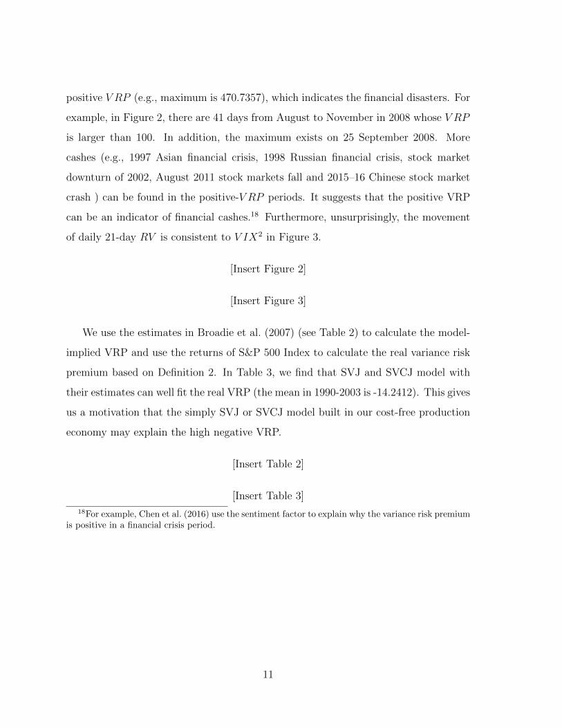
positive V RP (e.g., maximum is 470.7357), which indicates the financial disasters. For

example, in Figure 2, there are 41 days from August to November in 2008 whose V RP

is larger than 100. In addition, the maximum exists on 25 September 2008. More

cashes (e.g., 1997 Asian financial crisis, 1998 Russian financial crisis, stock market

downturn of 2002, August 2011 stock markets fall and 2015–16 Chinese stock market

crash ) can be found in the positive-V RP periods. It suggests that the positive VRP

can be an indicator of financial cashes.18 Furthermore, unsurprisingly, the movement

of daily 21-day RV is consistent to V IX2 in Figure 3.

[Insert Figure 2]

[Insert Figure 3]

We use the estimates in Broadie et al. (2007) (see Table 2) to calculate the model-

implied VRP and use the returns of S&P 500 Index to calculate the real variance risk

premium based on Definition 2. In Table 3, we find that SVJ and SVCJ model with

their estimates can well fit the real VRP (the mean in 1990-2003 is -14.2412). This gives

us a motivation that the simply SVJ or SVCJ model built in our cost-free production

economy may explain the high negative VRP.

[Insert Table 2]

[Insert Table 3]

18For example, Chen et al. (2016) use the sentiment factor to explain why the variance risk premiumis positive in a financial crisis period.

11

3. A Cost-free Production-based Equilibrium Model

3.1 Model Setup

Our cost-free production economy follows Constantinides (1990).19 There exists only

one production good, which is also the consumption. There are two technologies for the

good to consume or invest. There is no any cost for investments, so that we can call the

two production technologies as the cost-free technologies and the economy as the cost-

free production economy. The risky technology has stochastic return over the period

[t, t+dt], µdt+√VtdB

St +(ex−1)dNt−λmdt where dVt = κ(θ−Vt)dt+σV

√VtdB

Vt +ydNt.

The riskless technology has constant returns rdt.

We suppose that there is a representative investor whose portfolio is (ut, 1 − ut),

which represents the fraction of wealth invested in the risky and riskless technology,

respectively. The consumption rate of the investor is ct. Then the investor’s capital

process Wt with the initial capital W0 > 0 satisfies a stochastic differential equation as

follows, dWt

Wt= [r + (µ− r − λm)ut − ct

Wt]dt+ ut

√VtdB

St + ut(e

x − 1)dNt,


Vt + ydNt.

(15)

In addition, the representative consumer has recursive preferences (see Duffie and Ep-

stein (1992b,a)) given by

Jt = Et

[∫ ∞t

f(cs, Js)ds

], (16)

with

f(c, J) =β(1− γ)J

1− ψ−1

[c1−ψ−1

((1− γ)J)ω− 1

]=

β

1− ψ−1

c1−ψ−1 − ((1− γ)J)ω

((1− γ)J)ω−1 , (17)

19Similar assumptions for the representative-consumer production economy can be found in Coxet al. (1985a); Bates (1991, 1996); Vasicek (2005); Zhang et al. (2012); Fu and Yang (2012); Ruanet al. (2016).

12

where the subjective time discount factor is denoted by β; ψ is the EIS and γ is the

coefficient of RRA. In addition, we denote ω = (1 − ψ−1)/(1 − γ). Recursive utility

allows to separate the effects of RRA and EIS. The special case of power utility results

by setting the EIS equal to the inverse of the RRA coefficient. In this case, only

innovations to consumption are priced. In the general case γ 6= 1/ψ, state variables

carry a risk premium, too. We assume throughout that β > 0 and γ > 0. Most of the

discussion focuses on that case γ > 1.

By choosing the investment ut in the stock and the consumption rate ct, the repre-

sentative investor maximizes his/her expected objective function (16). Based on Cox

et al. (1985a); Bates (1991, 1996); Vasicek (2005); Zhang et al. (2012); Fu and Yang

(2012); Ruan et al. (2016), we define the market equilibrium in a production economy

as follows.

Definition 3 (Market equilibrium). Equilibrium in our cost-free production econ-

omy is defined in a standard way: equilibrium consumption-portfolio pairs (ut, ct) are

such that the representative investor maximizes his/her expected objective function in

(16), and markets clear, ut = 1.

3.2 Solutions

After solving the equilibrium defined in Definition 3, we get the following proposition.

Proposition 1. The value function is

J(W,V ) = eaV+bW1−γ

1− γ, (18)

and the optimal consumption rate is

c∗ =(e−ψω(aV+b)βψ

)W, (19)

13

where constant a and b satisfy,20

0 = −β(1−γ)

1−ψ−1 +[(

11−ψ−1 − 1

)(1− γ)

] ((1 + ψωaV

)e−ψω(aV+b)βψ

)+r (1− γ) + κθa+ λE

[eay+(1−γ)x − 1

]− (1− γ)λE [eay−γx(ex − 1)] ,

0 = −ae−ψω(aV+b)βψ + γ (1− γ) 12− κa+ 1

2σ2V a

2,

(20)

with V = κθ+λµVκ

.

The equity risk premium is solved as

ERPt100

= (γ − σV ρa)V + λE[(1− e−γx+ay)(ex − 1)

]= (γ − σV ρa)V + λm− λQmQ.

(21)

The state-price density is given by

dπtπt

= −rdt−γ√VtdB

St +aσV

√VtdB

Vt +(e−γx+ay − 1

)dNt−λE

(e−γx+ay − 1

)dt. (22)

The explicit transition between the risk-neutral measure Q and the physical probability

measure P is given by

κQ = κ+ (ργ − aσV )σV , µQS = µS − γσ2

S, µQV =

1

1− aµVµV , λQ =

λe12σ2Sγ

2−µSγ

1− aµV.

(23)

Following Constantinides (1990), if a firm has capital Kt at time t and it can be

freely invested in two production technologies, we assume the firm invest δ1Kt capital in

the risky technology and (1−δ1)Kt in riskless one where δ1 is constant. In addition, the

firm is financed with the equity (stock) St and risk-free bond Mt where dMt/Mt = rdt.

We assume the leverage δ2 = St/(St + Mt) which is a constant. Then we have the

equality between the investment in two production technologies and the value of the

20Note here we choose 0 < a < 1/µV and γ > 1.

14

firm. dSt +Mtrdt = δ1Kt(µdt+√VtdB

St + (ex − 1)dNt − λmdt) + (1− δ1)Ktrdt,


Vt + ydNt,

(24)

which can be rewritten as dStSt

= δ1δ2

(µ− rdt+

√VtdB

St + (ex − 1)dNt

)− λmdt+ rdt,


Vt + ydNt,

(25)

In order to be consistent with our stock price process in Equation (1), following Con-

stantinides (1990), we set δ1δ2

= 1. Thus, the process of the stock price (with dividends

included) in (25) is same to (1).

Remark 1. Our production-based model can be regarded as an extension of the model

in Cox et al. (1985a); Bates (1991, 1996, 2000); Vasicek (2005); Zhang et al. (2012); Fu

and Yang (2012); Ruan et al. (2016), which only consider that the representative con-

sumer has a constant relative risk aversion (CRRA) utility function. The production-

based equilibrium model studied in previous literature is widely used in derivative

pricing, especially in option pricing. It is reasonable to employ the production-based

model to explain the VRP, because VIX index can be regarded as the variance swaps

rates.

Remark 2. In Broadie et al. (2007), they suggest that ERPt100

= ηSVt +(mλ−mQλQ

)which is contributed by the diffusive risk premium ηSVt and the price jump risk pre-

mium(mλ−mQλQ

). The solution of the ERP in (21) supports their assumption.

In addition, ηS can be solved as γ − σV ρa, which is constant, and λm − λQmQ =

λE [(1− e−γx+ay)(ex − 1)], which can be verified by using the transition in (23). If the

volatility is a constant, σ, the ERP will become ERP100

= γσ2 + λE [(1− e−γx)(ex − 1)]

which has been studied in Zhang et al. (2012).

15

Remark 3. In the equilibrium model, we find out a stochastic density factor (i.e.,

state-price density) in (22), which provides a transition for parameters between the

risk-neutral measure Q and the physical probability measure P. The stochastic density

factor in (22) captures all risks, that are two Brownian motion risks (BSt and BV

t ) and

one jump risk (Nt). In the transition (23), it shows that the jump intensity in two

measures are not equal, i.e., λ 6= λQ, which is consistent to Bates (1991, 1996, 2000);

Liu et al. (2005); Zhang et al. (2012); Ruan et al. (2016). It suggests that we have to

estimate λQ as an independent risk-neutral parameter. In addition, as µS < 0, γ > 1

and 0 < a < 1/µV , we have λ < λQ. In other words, the jump intensity should be

larger in risk-neutral probability measure than in the physical probability measure.

Remark 4. The transition in (23) documents that κQ − κ = (ργ − aσV )σV < 0 for

ρ < 0, γ > 1, 0 < a < 1/µV and σV > 0. In other words, the equilibrium model can

generate the negative DVRP. It is not surprising. Actually, in the same production-

based framework, Cox et al. (1985b); Bates (1991, 1996, 2000) argue that DVRP is

negative because of the negative correlation between the volatility and the S&P 500

index. Recently, Eraker and Wu (2014) propose a consumption-based equilibrium

model and get the similar result that κQ − κ < 0 for any γ > 0.

Remark 5. For any a > 0 and γ > 0, we have µQS < µS < 0 and µQ

V > µV > 0.

It is corresponding to the empirical results, e.g., Eraker (2004); Broadie et al. (2007);

Neumann et al. (2016). It means that the jumps in the price and the volatility are

larger in risk-neutral probability measure than in the physical probability measure.

3.3 Equilibrium Model-implied ERP and VRP

Plugging the explicit transition between the risk-neutral measure Q and the physical

probability measure P given in (23) into Definition 1, we will get the model-implied

VRP based on our cost-free production-based equilibrium model.

16

Definition 4 (Equilibrium model-implied Equity and Variance Risk Premiums).

Having estimated the P parameters and the recursive preferences parameters of the rep-

resentative investor, based on SVCJ model, we define the equilibrium model-implied

ERP as

ERPt =[(γ − σV ρa)V + λE

((1− e−γx+ay)(ex − 1)

)]× 100, (26)

and the equilibrium model-implied VRP is defined as,

V RPt = (A∆ · Vt +B∆)× 1002, (27)

where

A∆ =1− e−κτ

κτ− 1− e−(κ+(ργ−aσV )σV )τ

(κ+ (ργ − aσV )σV ) τ,

and

B∆ =

(θ +

λµVκ

)(1− 1− e−κτ

κτ) + λ

(σ2S + µ2

S

)− 1

κ+ (ργ − aσV )σV

(κθ − λµV e

12σ2Sγ

2−µSγ

(1− aµV )2

)[1− 1− e−(κ+(ργ−aσV )σV )τ

(κ+ (ργ − aσV )σV ) τ

]+λe

12σ2Sγ

2−µSγ

1− aµV

(σ2S +

(µS − γσ2

S

)2).

Equation (27) shows that V RP is a function of the physical measure parameters (κ,

θ, σV , ρ, λ, µS, σS and µV ) and the preferences parameters (β, γ and ψ).21

We set the baseline model parameters as κ = 15, θ = 0.02, σV = 0.5, ρ = −0.9, λ =

2, µS = −0.01, σS = 0.02, µV = 0.06, r = 0.008, β = 0.001, γ = 2.5, ψ = 2 and E[V ] =

0.02.22 Then, the baseline average ERP = 5.2023, V RP = −15.3317 and a = 6.9101.

we will analyse how those preferences parameters affect the ERP and VRP.

[Insert Figure 4]

21The parameter a is determined by β, γ and ψ in Equation (20).22The value of parameters is according to our estimates in Table 9. The assumption, RRA = 2.5 > 2

and EIS = 2 > 1, is based on the parameter settings in Drechsler and Yaron (2011); Drechsler (2013).

17

[Insert Figure 5]

[Insert Figure 6]

From Figure 4, we find that, except θ, the higher κ, σV and the correlation ρ lead to

the higher equity risk premiums. In terms of the VRP, we find that the larger σV and

ρ produce the larger negative VRP but ρ less affects on the VRP. In addition, on the

one hand, the VRP increases with κ ≤ 20 and decreases with κ > 20. On the another

hand, the VRP decreases with θ ≤ 0.1 and increases with θ > 0.1. Empirically, the

estimates of κ are less than 20 and the estimates of θ are less than 0.1 (e.g., Bakshi

et al. (1997); Bates (2000); Eraker et al. (2003); Bates (2012); Neumann et al. (2016)).

Thus, normally, we can say that the VRP increases with κ and decreases with θ.

In Figure 5, the larger value of jump parameters, i.e., λ, µS, σS and µV , leads to the

larger ERP and VRP. It is consistent to (i) that the jump is the key factor to explain

the equity premium puzzle (e.g., Rietz (1988); Barro (2006); Wachter (2013); Branger

et al. (2016)); and (ii) the conclusion in Bakshi and Madan (2006) that the volatility

spreads are positive (the VRP is negative) when the distribution of the index is nega-

tively skewed and leptokurtic physical, which is denominated by the jump parameters.

Furthermore, they have different sensitivities to the ERP and VRP. For example, with

λ increasing from 2 to 20, the ERP goes up from 5.2023 to 13.9994 and the VRP goes

up from −8.4328 to −12.6136 in Figure 5-(a), while, with µS decreasing from −0.01 to

−0.1, the ERP jumps to 61.5961 and the VRP jumps to −31.3595 in Figure 5-(b).

Figure 6-(a) shows the ERP and VRP are a linear function of β, while, the ERP

and VRP are a convex function of the RRA (e.g., γ) in 6-(b). In our numerical

results, ERP = 10.1944 and V RP = −21.7746 when γ = 2.2 and then it sharply

decreases, for example, ERP = 3.5658 and V RP = −5.0358 when γ = 3. The ERP

reaches the minimal (2.7331) around γ = 5 and VRP reaches the minimal (−3.16)

around γ = 6. After that, the ERP and VRP increase with the RRA. For example,

ERP = 39.0374 and V RP = −36.2261 at γ = 50. The effects of the EIS on the

18

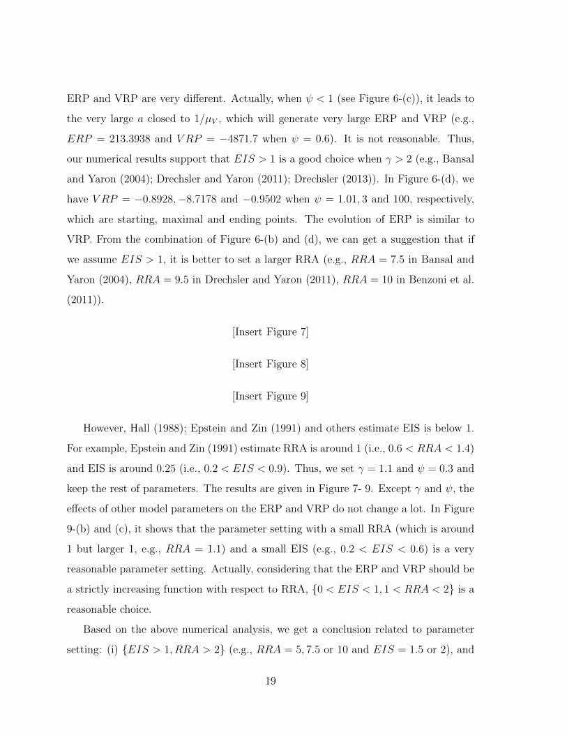
ERP and VRP are very different. Actually, when ψ < 1 (see Figure 6-(c)), it leads to

the very large a closed to 1/µV , which will generate very large ERP and VRP (e.g.,

ERP = 213.3938 and V RP = −4871.7 when ψ = 0.6). It is not reasonable. Thus,

our numerical results support that EIS > 1 is a good choice when γ > 2 (e.g., Bansal

and Yaron (2004); Drechsler and Yaron (2011); Drechsler (2013)). In Figure 6-(d), we

have V RP = −0.8928,−8.7178 and −0.9502 when ψ = 1.01, 3 and 100, respectively,

which are starting, maximal and ending points. The evolution of ERP is similar to

VRP. From the combination of Figure 6-(b) and (d), we can get a suggestion that if

we assume EIS > 1, it is better to set a larger RRA (e.g., RRA = 7.5 in Bansal and

Yaron (2004), RRA = 9.5 in Drechsler and Yaron (2011), RRA = 10 in Benzoni et al.

(2011)).

[Insert Figure 7]

[Insert Figure 8]

[Insert Figure 9]

However, Hall (1988); Epstein and Zin (1991) and others estimate EIS is below 1.

For example, Epstein and Zin (1991) estimate RRA is around 1 (i.e., 0.6 < RRA < 1.4)

and EIS is around 0.25 (i.e., 0.2 < EIS < 0.9). Thus, we set γ = 1.1 and ψ = 0.3 and

keep the rest of parameters. The results are given in Figure 7- 9. Except γ and ψ, the

effects of other model parameters on the ERP and VRP do not change a lot. In Figure

9-(b) and (c), it shows that the parameter setting with a small RRA (which is around

1 but larger 1, e.g., RRA = 1.1) and a small EIS (e.g., 0.2 < EIS < 0.6) is a very

reasonable parameter setting. Actually, considering that the ERP and VRP should be

a strictly increasing function with respect to RRA, 0 < EIS < 1, 1 < RRA < 2 is a

reasonable choice.

Based on the above numerical analysis, we get a conclusion related to parameter

setting: (i) EIS > 1, RRA > 2 (e.g., RRA = 5, 7.5 or 10 and EIS = 1.5 or 2), and

19

(ii) 0 < EIS < 1, 1 < RRA < 2 (e.g., RRA = 1.1 or 1.2 and EIS = 0.3, 0.4, 0.5

or 0.6) are two possible combinations to successfully capture the high VRP and ERP.

However, based on our cost-free production-based equilibrium model, in the empirical

analysis, the former is better to fit the data of the ERP and VRP. The reason is that

the ERP is defined on the the variance of the real return on S&P 500 instead of the

growth rate of consumption so that we need the lower RRA to fit the ERP data. Thus,

all the following empirical results are obtained by using the former parameter setting.23

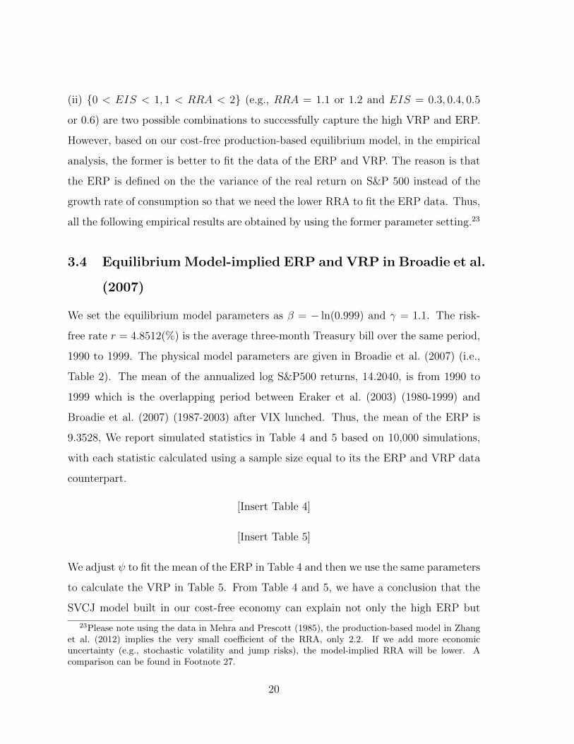
3.4 Equilibrium Model-implied ERP and VRP in Broadie et al.

(2007)

We set the equilibrium model parameters as β = − ln(0.999) and γ = 1.1. The risk-

free rate r = 4.8512(%) is the average three-month Treasury bill over the same period,

1990 to 1999. The physical model parameters are given in Broadie et al. (2007) (i.e.,

Table 2). The mean of the annualized log S&P500 returns, 14.2040, is from 1990 to

1999 which is the overlapping period between Eraker et al. (2003) (1980-1999) and

Broadie et al. (2007) (1987-2003) after VIX lunched. Thus, the mean of the ERP is

9.3528, We report simulated statistics in Table 4 and 5 based on 10,000 simulations,

with each statistic calculated using a sample size equal to its the ERP and VRP data

counterpart.

[Insert Table 4]

[Insert Table 5]

We adjust ψ to fit the mean of the ERP in Table 4 and then we use the same parameters

to calculate the VRP in Table 5. From Table 4 and 5, we have a conclusion that the

SVCJ model built in our cost-free economy can explain not only the high ERP but

23Please note using the data in Mehra and Prescott (1985), the production-based model in Zhanget al. (2012) implies the very small coefficient of the RRA, only 2.2. If we add more economicuncertainty (e.g., stochastic volatility and jump risks), the model-implied RRA will be lower. Acomparison can be found in Footnote 27.

20

also the large VRP (explanation rate is 56.91%). With the sensitivity analysis of model

parameter above, we can choose the high EIS to produce the more negative VRP but

the ERP will be slightly higher at same time. As a similar analysis will be studied in

Section 4.3, we do not show the details here.

3.5 VRP Return Predictability

We calculate the conditional equity premium as

Et

[ERPt+1

100

]= (γ − σV ρa)Et[Vt+1] + λE

[(1− e−γx+ay)(ex − 1)

]= (γ − σV ρa)

[e−κVt +

(θ +

λµVκ

)(1− e−κ)

]+ λE

[(1− e−γx+ay)(ex − 1)

]= (γ − σV ρa) e−κVt + (γ − σV ρa)

(θ +

λµVκ

)(1− e−κ)

+ λE[(1− e−γx+ay)(ex − 1)

]. (28)

Equation (27) implies that Vt =V RPt1002 −B∆

A∆. Combining with Equation (28), we can get

the predictive regression for the equity premium (excess market return),

ERPt+1

100= βpred

V RPt1002

+ αpred + εt+1, (29)

where

βpred =γ − σV ρa

A∆

e−κ, (30)

and

αpred = (γ − σV ρa) e−κ−B∆

A∆

+(γ − σV ρa)

(θ +

λµVκ

)(1−e−κ)+λE

[(1− e−γx+ay)(ex − 1)

].

(31)

As (ργ − aσV )σV < 0 which leads to A∆ < 0, we have βpred < 0. Therefore, the

predictive coefficient is negative (with respect to the V RPt1002 in Equation (4)). It is

corresponding to empirical results in Bollerslev et al. (2009); Drechsler and Yaron

21

(2011); Jin (2015) and others. We report our empirical results from the daily predictive

regressions of monthly equity premiums on variance risk premiums in Table 6. We will

find βpred is significantly negative with very large t-statistics. The predictive power

from the fact that the volatility Vt determines the expected excess return in Equation

(28) and the VRP in Equation (27). Thus, through the information of the volatility,

the variance risk premium is able to predict the excess market return.

[Insert Table 6]

4. Empirical Analysis

Even though, we have shown that the SVCJ model can well explain the ERP and VRP

based on the parameters in Broadie et al. (2007), in this section, we will use more

recent data to robustly examine whether the SVCJ model built in a cost-free economy

can explain the large ERP and VRP.

4.1 Estimates of Physical Measure Parameters

The first step is using S&P 500 returns data to estimate the physical measure param-

eters by using a Markov chain Monte Carlo (MCMC) sampler. Eraker et al. (2003);

Eraker (2004); Amengual (2009); Zhu and Lian (2012); Kaeck and Alexander (2012)

show that (i) MCMC yields very accurate estimates for jump-diffusion models; (ii)

MCMC provides estimates of the latent volatility; (iii) MCMC outperforms the gen-

eralized method of moments (GMM), the quantile maximum likelihood estimation

(QMLE) and the efficient method of moments (EMM); (iv) MCMC can utilize priors

to disentangle jumps from diffusions in an intuitive manner. Hence, we use MCMC ap-

proach to estimate our affine jump-diffusion models. We present a time-discretization

22

of Equation (1) by using the discrete scheme, Rt = α +√Vtε

St + JSt qt,

Vt = Vt−1 + κ(θ − Vt−1) + σV√Vt−1ε

Vt + JVt qt,

(32)

where α = r − 12Vt + ηSVt − λm; εSt and εVt are samples from two dependent standard

normal distributions with correlation ρ; Rt = (lnSt − lnSt−1) × 100, y ∼ exp(1/µV ),

x ∼ N(µS, σ2S) and qt ∼ Ber(λ). The parameters to be estimated are α, κ, θ, σV , ρ, λ,

µS, σS, µV .

[Insert Table 7 ]

Following Eraker et al. (2003), we run the MCMC algorithm for 110,000 itera-

tions, discarding the first 10,000 as a burn-in-period to achieve the convergence of the

chain. For each parameter to be estimated, we use the same priors as in Eraker et al.

(2003) and the sample period is from 24 November 2010 to 20 May 2016 (see Table 7).

Estimates are shown in Table 8.

[Insert Table 8 ]

These reported parameters are quite informative. Table 8 shows that the values

of the daily variance θ are 0.9298, 0.928 and 0.6983, respectively, for the SV, SVJ

and SVCJ models, which are a little lower than the unconditionally sampled standard

deviation of S&P500 return data, 0.97252. In the annualized view, the sampled stan-

dard deviation of data is 15.4380,24 while, estimated√

252θ are 15.3017, 15.3924 and

13.2654, respectively, for the SV, SVJ and SVCJ models. If we calculate the mean of

the annualized standard deviation of the SVCJ model,√

252(κθ + λµV )/κ, is 15.4564

which is almost same to the sampled value, 15.4380. Corresponding to S&P500 pa-

rameter estimates in Table III in Eraker et al. (2003), adding more jumps in the model

leads to the lower estimated values of θ, σV , but higher value of ρ. During our sample

2415.4380 = 0.9725√

252.

23

period (2010-2016), we have higher correlation ρ. It is not supervising. For example,

in Duan and Yeh (2010), they report that ρ is -0.5268 in 1990-1995 and -0.7389 in

2001-2007. It seems that the current data has much high ρ.

4.2 Model-implied Risk-neutral Parameters and ERP

In order to get the risk-neutral parameters implied in our equilibrium model, we convert

the daily percentage estimates into annualized values in Table 9.25 Then set β =

− ln(0.999) which is same to Drechsler and Yaron (2011); Drechsler (2013). Here we

set γ = 1.1 which is much lower than existing literature (e.g., 9.5 in Drechsler and

Yaron (2011); 5 in Drechsler (2013)). The risk-free rate r = 0.0730(%) which is the

average three-month Treasury bill over the same period, 24 November 2010 to 20 May

2016. In order to fit the mean of ERP in Table 10, we set ψ = 0.42, 0.42 and 0.37 for

SV, SVJ and SVCJ models, respectively, and then we get the annualized risk-neutral

parameters implied in our equilibrium model in Table 11 and convert them into daily

percentage value in Table 12.

[Insert Table 9 ]

[Insert Table 10 ]

[Insert Table 11 ]

[Insert Table 12 ]

In order to consider the estimate error for the MCMC spot variance, we also present

the results by using the 10,0000 simulations in Table 10.26 Comparing Panel A and

B in Table 10, we find that there is very little distinguish between the two sets. This

demonstrates that our main findings are robust to the MCMC spot variance. After

25A detailed guide for the conversion of parameters can be found in Appendix C of Branger andHansis (2015).

26Neumann et al. (2016) do a comparison analysis for the MCMC spot variance and the spotvariance estimated by the options data. They find that there is very little difference.

24

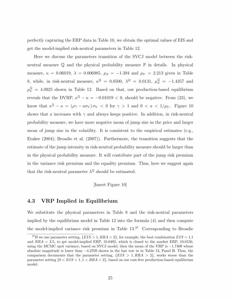
perfectly capturing the ERP data in Table 10, we obtain the optimal values of EIS and

get the model-implied risk-neutral parameters in Table 12.

Here we discuss the parameters transition of the SVCJ model between the risk-

neutral measure Q and the physical probability measure P in details. In physical

measure, κ = 0.06019, λ = 0.006985, µS = −1.394 and µV = 2.213 given in Table

8, while, in risk-neutral measure, κQ = 0.0500, λQ = 0.0131, µQS = −1.4357 and

µQV = 4.0925 shown in Table 12. Based on that, our production-based equilibrium

reveals that the DVRP, κQ − κ = −0.01019 < 0, should be negative. From (23), we

know that κQ − κ = (ργ − aσV )σV < 0 for γ > 1 and 0 < a < 1/µV . Figure 10

shows that a increases with γ and always keeps positive. In addition, in risk-neutral

probability measure, we have more negative mean of jump size in the price and larger

mean of jump size in the volatility. It is consistent to the empirical estimates (e.g.,

Eraker (2004); Broadie et al. (2007)). Furthermore, the transition suggests that the

estimate of the jump intensity in risk-neutral probability measure should be larger than

in the physical probability measure. It will contribute part of the jump risk premium

in the variance risk premium and the equality premium. Thus, here we suggest again

that the risk-neutral parameter λQ should be estimated.

[Insert Figure 10]

4.3 VRP Implied in Equilibrium

We substitute the physical parameters in Table 8 and the risk-neutral parameters

implied by the equilibrium model in Table 12 into the formula (4) and then compute

the model-implied variance risk premium in Table 13.27 Corresponding to Broadie

27If we use parameter setting, EIS > 1, RRA > 2, for example, the best combination EIS = 1.1and RRA = 3.5, to get model-implied ERP, 10.0492, which is closed to the market ERP, 10.0150,using the MCMC spot variance, based on SVCJ model, then the mean of the VRP is −1.7409 whoseabsolute magnitude is lower than −4.2709 shown in the last row in in Table 13, Panel B. Thus, thecomparison documents that the parameter setting, EIS > 1, RRA > 2, works worse than theparameter setting 0 < EIS < 1, 1 < RRA < 2, based on our cost-free production-based equilibriummodel.

25

et al. (2007) (See Table 3), the SVCJ model can explain more than 50% VRP. Table

14 provides statistics in details for the realized variance, the implied variance and the

variance risk premium, all at the monthly horizon. It demonstrates that the model

well fits the data of the realized variance and document that our estimates are very

accurate. So far, we will find the SVCJ model can well explain the large VRP built in

our cost-free production economy, after perfectly fitting the ERP data.

[Insert Table 13 ]

[Insert Table 14 ]

If we allow the model to generate a little bit higher ERP, the model-implied VRP

will be higher. For example, we follow the fitting level of ERP in Drechsler (2013), i.e.,

Table 15, and then we get the corresponding results in Table 16. Comparing Table

15 and 16, our model can explain the VRP of 74%, which is same to the Drechsler’s

(2013) (in Table 16). In other words, our simpler production-based equilibrium has

same power of explaining the equity and variance risk premiums, compared to the more

complex consumption model with the model uncertainty in Drechsler (2013). Panel B

in Table 16 examines the fraction of the VRP explained by the three components. We

find that the jump VRP (especially, the volatility jump VRP) explains around 80% of

the total VRP. It is consistent to Li and Zinna (2016) who calculate the fraction at

around 79%.

[Insert Table 15 ]

[Insert Table 16 ]

In addition, according to numerical analysis in Table 7, we can continue to rise the

value of EIS in order to fully capture the VRP data. In Table 17, with EIS = 0.61, the

SVCJ model can perfectly fit the mean of VRP. In the Panel A of Table 17, the model

generates slightly higher mean of the ERP which is around 14, compared to the real

26

mean of the ERP that is around 10. But it is still acceptable. We give the statistics in

details for the realized variance, the implied variance and the variance risk premium in

Table 18. It shows that, with EIS = 0.61, our model well fits the data of the realized

variance, implied variance and the variance risk premiums.

[Insert Table 17 ]

[Insert Table 18 ]

To summarize, the SVCJ model built in a cost-free production-based equilibrium

model can well explain the equity premium puzzle and the high negative VRP with

much low RRA and EIS coefficients.

5. Conclusions

The paper discusses the equity and variance risk premiums in a cost-free production-

based economy with one representative investor who has a recursive preference. After

solving the equilibrium, we provide an explicit transition for model parameters between

the risk-neutral measure and the physical probability measure. This transition docu-

ments that the diffusive volatility risk premium should be negative. In addition, using

the model-implied risk-neutral parameters, we calculate and analyse the model-implied

equity and variance risk premiums. From the numerical analysis, we suggest that lower

RRA and EIS setting is a good choice. Compared to the market data, we find that

the SVCJ model built in our cost-free production economy can well explain the equity

premium puzzle and the large negative VRP.

In contrast to Bollerslev et al. (2009); Drechsler and Yaron (2011); Drechsler (2013)

who use a long-run risks model, and Buraschi et al. (2014) who use a two-tree Lu-

cas (1978) economy with two heterogeneous investors, we employ a simpler cost-free

production-based equilibrium model and successfully explain the large equity and vari-

ance risk premiums. Our analysis in this paper can be extended to study the skewness

risk premium (e.g., Neuberger (2012); Kozhan et al. (2013)).

27

Appendix A: Proof of Proposition 1

The value function satisfies the following HJB equation,

0 = maxc,u

f(c, J) + [r + (φ− λm)u− c

W]WJW +

1

2u2W 2V JWW + κ(θ − V )JV

+1

2σ2V V JV V + σV ρuWV JWV + λE [J(W + uW (ex − 1), V + y)− J ]

. (33)

This leads to the two first-order conditions (FOCs),

fc(c, J)− JW = 0, (34)

(φ− λm)WJW + uW 2V JWW + σV ρWV JWV ,

+ λE [JW (W (1 + (ex − 1)u), V + y)W (ex − 1)] = 0. (35)

Applying the market clearing condition u = 1 to (35), we can solve the equity premium

as,

φ = λm− 1

JW(WV JWW + σV ρV JWV + λE [JW (Wex, V + y)(ex − 1)]) . (36)

In addition, from (34), we can solve the optimal consumption rate

c∗t =(JW [(1− γ)J ]ω−1 β−1

)−ψ. (37)

Plugging (36) into (33) and using u = 1, we get the following partial differential

equation (PDE),

0 =β(1− γ)J

1− ψ−1

[c∗1−ψ

−1

((1− γ)J)ω− 1

]− c∗JW + rWJW −

1

2W 2V JWW + κ(θ − V )JV

+1

2σ2V V JV V + λE [J(Wex, V + y)− J ]− λE [WJW (Wex, V + y)(ex − 1)] . (38)

28

We conjecture the value function has the following form,

J(W,V ) = eaV+bW1−γ

1− γ, (39)

where a > 0 and γ > 1 (similar assumptions see Wachter (2013)).

Substituting the conjectured value function in (39) into (37) and the PDE (38), the

optimal consumption rate (37) can be rewritten as

c∗t =(e−ψω(aV+b)βψ

)W, (40)

and the PDE (38) becomes

0 =β(1− γ)

1− ψ−1

[e−ψω(aV+b)βψ−1 − 1

]− (1− γ)

(e−ψω(aV+b)βψ

)+ r (1− γ) + γ (1− γ)

1

2V

+ κ(θ − V )a+1

2σ2V V a

2 + λE[eay+(1−γ)x − 1

]− (1− γ)λE

[eay−γx(ex − 1)

].

Using the affine approximation method (e.g., see Benzoni et al. (2011)), we expand

the exponential term in V near their long term mean level V = κθ+λE[y]κ

, e−ψω(aV+b) ≈

e−ψω(aV+b) − ψωae−ψω(aV+b)(V − V ) =(1 + ψωaV

)e−ψω(aV+b) − ψωae−ψω(aV+b)V and

collect the terms with the same power of V . Then a and b can be solved in the following

equation.0 = −β(1−γ)

1−ψ−1 +[(

11−ψ−1 − 1

)(1− γ)

] ((1 + ψωaV

)e−ψω(aV+b)βψ

)+r (1− γ) + κθa+ λE

[eay+(1−γ)x − 1

]− (1− γ)λE [eay−γx(ex − 1)] ,

0 = −ae−ψω(aV+b)βψ + γ (1− γ) 12− κa+ 1

2σ2V a

2.

(41)

Plugging (39) into (36), we get the equity premium as

φt = (γ − σV ρa)Vt + λE[(1− e−γx+ay)(ex − 1)

], (42)

29

and substituting (40) into (15), we obtain the optimal wealth process as follows, dWt

Wt= [(µ− λm)−

(e−ψω(aV+b)βψ

)]dt+

√VtdB

St + (ex − 1)dNt,


Vt + ydNt.

(43)

Finally, we define the SDF as

πt = exp

∫ t

0

fJ(c, J)ds

fc(c, J), (44)

ordπtπt

= fJ(c, J)dt+dfc(c, J)

fc(c, J), (45)

where

fc(c, J) = JW = eaV+bW−γ, (46)

and

fJ(c, J) =β(1− γ)

1− ψ−1

[c1−ψ−1

(1− ω)

((1− γ)J)ω− 1

]=β(1− γ)

1− ψ−1

[e−ψω(aV+b)βψ−1(1− ω)− 1

].

(47)

Implying Ito’s Lemma to (46), we have,

dfc(c, J)

fc(c, J)= −Γtdt−γ

√VtdB

St +aσV

√VtdB

Vt +(e−γx+ay − 1

)dNt−λE

(e−γx+ay − 1

)dt,

(48)

where

Γt =γ(µ− λm− e−ψω(aV+b)βψ

)− 1

2γ(γ + 1)V − aκ(θ − V )

− 1

2σ2V a

2V + γaρσV V − λE(e−γx+ay − 1

).

30

Finally, we plug (47) and (48) into (45) and then we get

dπtπt

= −rtdt− γ√VtdB

St + aσV

√VtdB

Vt +

(e−γx+ay − 1

)dNt − λE

(e−γx+ay − 1

)dt,

(49)

where28

rt = Γt −β(1− γ)

1− ψ−1

[e−ψω(aV+b)βψ−1(1− ω)− 1

]. (50)

As BSt and BV

t are a pair of correlated Brownian motions with correlation coefficient ρ,

according to Girsanovs theorem (see, e.g., Theorem 1.32 and Theorem 1.34, Øksendal

and Sulem (2007)), we present the transition between the risk-neutral measure Q and

the physical probability measure P,

dBSt (Q) =dBS

t + (γ − aρσV )√Vt,

dBVt (Q) =dBV

t + ρ (γ − aρσV )√Vt − (1− ρ2)aσV

√Vt = dBV

t + (ργ − aσV )√Vt,

µQS =µS − γσ2

S,

µQV =

1

1− aµVµV ,

λQ =λE[e−γx+ay] = λe12σ2Sγ

2−µSγ 1

1− aµV.

As Equation (41) can yield multiple solutions to a and b, we select a with the restriction,

a < 1/µV , to get make sure λQ > 0. According to the empirical results in Eraker (2004);

Broadie et al. (2007); Neumann et al. (2016), µQV > µV , it suggests the restriction a > 0

as µV > 0.

28Even though, the risk-free rate is determined by the equilibrium, we still assume it is exogenouslygiven. Based on that, the equity premium and the growth rate of the stock are both endogenous.

31

Appendix B: A Comparison of Our Codes

In order to verify the accuracy of our MCMC codes, we present the replicated estimates

by using the same sample in Eraker et al. (2003) and Yun (2011) with our MCMC

codes based on OpenBUGS,29 which are used in Section 4. We discard the first 10,000

runs as “burn-in”period and use the last 100,000 iterations in MCMC simulations to

estimate model parameters. Specifically, we take the mean of the posterior distribution

as parameter estimate and the standard deviation of the posterior as standard error in

parentheses.

As the jumps of the SVCJ model in Eraker et al. (2003) are correlated, we only

present the estimates of the SV and SVJ models. As a complementary comparison,

we compare our estimates of the SV, SVJ and SVCJ models with Yun’s (2011) which

are estimated by using WinBUGS. From Table 19 and 20, we can confirm that our

MCMC codes based on OpenBUGS can estimate similar model parameters with very

small difference to Eraker et al. (2003) and Yun (2011).

[Insert Table 19 ]

[Insert Table 20 ]

29The reason we choose OpenBUGS instead of WinBUGS is that OpenBUGS run-ning is faster and more functional. Changes between WinBUGS and OpenBUGS, seehttp://www.openbugs.net/w/OpenVsWin.

32

References

Ait-Sahalia, Yacine, Mustafa Karaman, and Loriano Mancini, 2015, The term structure

of variance swaps and risk premia, Available at SSRN 2136820 .

Amengual, Dante, 2009, The term structure of variance risk premia, Princeton Uni-

versity .

Bakshi, Gurdip, Charles Cao, and Zhiwu Chen, 1997, Empirical performance of alter-

native option pricing models, The Journal of Finance 52, 2003–2049.

Bakshi, Gurdip, and Dilip Madan, 2006, A theory of volatility spreads, Management

Science 52, 1945–1956.

Bansal, Ravi, A Ronald Gallant, and George Tauchen, 2007, Rational pessimism, ra-

tional exuberance, and asset pricing models, The Review of Economic Studies 74,

1005–1033.

Bansal, Ravi, and Amir Yaron, 2004, Risks for the long run: A potential resolution of

asset pricing puzzles, The Journal of Finance 59, 1481–1509.

Barras, Laurent, and Aytek Malkhozov, 2016, Does variance risk have two prices?

evidence from the equity and option markets, Journal of Financial Economics 121,

79–92.

Barro, Robert J, 2006, Rare disasters and asset markets in the twentieth century, The

Quarterly Journal of Economics 823–866.

Bates, David S, 1991, The crash of’87: Was it expected? the evidence from options

markets, The Journal of Finance 46, 1009–1044.

Bates, David S, 1996, Jumps and stochastic volatility: Exchange rate processes implicit

in deutsche mark options, Review of Financial Studies 9, 69–107.

33

Bates, David S, 2000, Post-’87 crash fears in the s&p 500 futures option market, Journal

of Econometrics 94, 181–238.

Bates, David S, 2012, Us stock market crash risk, 1926–2010, Journal of Financial

Economics 105, 229–259.

Benzoni, Luca, Pierre Collin-Dufresne, and Robert S Goldstein, 2011, Explaining asset

pricing puzzles associated with the 1987 market crash, Journal of Financial Eco-

nomics 101, 552–573.

Bollerslev, Tim, Natalia Sizova, and George Tauchen, 2012, Volatility in equilibrium:

Asymmetries and dynamic dependencies, Review of Finance 16, 31–80.

Bollerslev, Tim, George Tauchen, and Hao Zhou, 2009, Expected stock returns and

variance risk premia, Review of Financial Studies 22, 4463–4492.

Bollerslev, Tim, and Viktor Todorov, 2011, Tails, fears, and risk premia, The Journal

of Finance 66, 2165–2211.

Bollerslev, Tim, Viktor Todorov, and Lai Xu, 2015, Tail risk premia and return pre-

dictability, Journal of Financial Economics 118, 113–134.

Bolton, Patrick, Hui Chen, and Neng Wang, 2011, A unified theory of tobin’s q, cor-

porate investment, financing, and risk management, The Journal of Finance 66,

1545–1578.

Bolton, Patrick, Hui Chen, and Neng Wang, 2013, Market timing, investment, and risk

management, Journal of Financial Economics 109, 40–62.

Branger, Nicole, and Alexandra Hansis, 2015, Earning the right premium on the right

factor in portfolio planning, Journal of Banking & Finance 59, 367–383.

Branger, Nicole, Holger Kraft, and Christoph Meinerding, 2016, The dynamics of crises

and the equity premium, Review of Financial Studies 29, 232–270.

34

Broadie, Mark, Mikhail Chernov, and Michael Johannes, 2007, Model specification and

risk premia: Evidence from futures options, The Journal of Finance 62, 1453–1490.

Buraschi, Andrea, Fabio Trojani, and Andrea Vedolin, 2014, When uncertainty blows

in the orchard: Comovement and equilibrium volatility risk premia, The Journal of

Finance 69, 101–137.

Carr, Peter, and Liuren Wu, 2009, Variance risk premiums, Review of Financial Studies

22, 1311–1341.

Chen, Yankun, Jinghong Shu, and Jin E Zhang, 2016, Investor sentiment, variance risk

premium and delta-hedged gains, Applied Economics 48, 2952–2964.

Constantinides, George M, 1990, Habit formation: A resolution of the equity premium

puzzle, Journal of Political Economy 519–543.

Cox, John C, Jonathan E Ingersoll, and Stephen A Ross, 1985a, An intertemporal

general equilibrium model of asset prices, Econometrica 53, 363–384.

Cox, John C, Jonathan E Ingersoll Jr, and Stephen A Ross, 1985b, A theory of the

term structure of interest rates, Econometrica 385–407.

DeMarzo, Peter M, Michael J Fishman, Zhiguo He, and Neng Wang, 2012, Dynamic

agency and the q theory of investment, The Journal of Finance 67, 2295–2340.

Drechsler, Itamar, 2013, Uncertainty, time-varying fear, and asset prices, The Journal

of Finance 68, 1843–1889.

Drechsler, Itamar, and Amir Yaron, 2011, What’s vol got to do with it, Review of

Financial Studies 24, 1–45.

Duan, Jin-Chuan, and Chung-Ying Yeh, 2010, Jump and volatility risk premiums

implied by vix, Journal of Economic Dynamics and Control 34, 2232–2244.

35

Duffie, Darrell, and Larry G Epstein, 1992a, Asset pricing with stochastic differential

utility, Review of Financial Studies 5, 411–436.

Duffie, Darrell, and Larry G Epstein, 1992b, Stochastic differential utility, Economet-

rica: Journal of the Econometric Society 353–394.

Duffie, Darrell, Jun Pan, and Kenneth Singleton, 2000, Transform analysis and asset

pricing for affine jump-diffusions, Econometrica 68, 1343–1376.

Epstein, Larry G, and Stanley E Zin, 1989, Substitution, risk aversion, and the tem-

poral behavior of consumption and asset returns: A theoretical framework, Econo-

metrica 937–969.

Epstein, Larry G, and Stanley E Zin, 1991, Substitution, risk aversion, and the tem-

poral behavior of consumption and asset returns: An empirical analysis, Journal of

Political Economy 263–286.

Eraker, Bjørn, 2004, Do stock prices and volatility jump? reconciling evidence from

spot and option prices, The Journal of Finance 59, 1367–1404.

Eraker, Bjørn, Michael Johannes, and Nicholas Polson, 2003, The impact of jumps in

volatility and returns, The Journal of Finance 58, 1269–1300.

Eraker, Bjorn, and Yue Wu, 2014, Explaining the negative returns to vix futures and

etns: An equilibrium approach, Available at SSRN 2340070 .

Fu, Jun, and Hailiang Yang, 2012, Equilibruim approach of asset pricing under levy

process, European Journal of Operational Research 223, 701–708.

Gonzalez-Urteaga, Ana, and Gonzalo Rubio, 2016, The cross-sectional variation of

volatility risk premia, Journal of Financial Economics 119, 353–370.

Hall, Robert E, 1988, Intertemporal substitution in consumption, Journal of Political

Economy 96, 339–357.

36

Hayashi, Fumio, 1982, Tobin’s marginal q and average q: A neoclassical interpretation,

Econometrica: Journal of the Econometric Society 213–224.

Jiang, George J, and Tong Yao, 2013, Stock price jumps and cross-sectional return

predictability, Journal of Financial and Quantitative Analysis 48, 1519–1544.

Jin, Jianjian, 2015, Jump-diffusion long-run risks models, variance risk premium, and

volatility dynamics, Review of Finance 19, 1223–1279.

Jones, Christopher S, 2003, The dynamics of stochastic volatility: evidence from un-

derlying and options markets, Journal of econometrics 116, 181–224.

Kaeck, Andreas, and Carol Alexander, 2012, Volatility dynamics for the s&p 500:

Further evidence from non-affine, multi-factor jump diffusions, Journal of Banking

& Finance 36, 3110–3121.

Kozhan, Roman, Anthony Neuberger, and Paul Schneider, 2013, The skew risk pre-

mium in the equity index market, Review of Financial Studies 26, 2174–2203.

Li, Junye, and Gabriele Zinna, 2016, The variance risk premium: Components, term

structures and stock return predictability, Journal of Business & Economic Statistics

1–44.

Liu, Jun, Jun Pan, and Tan Wang, 2005, An equilibrium model of rare-event premia

and its implication for option smirks, Review of Financial Studies 18, 131–164.

Lucas, Robert E, 1978, Asset prices in an exchange economy, Econometrica 46, 1429–

1445.

Mehra, Rajnish, and Edward C Prescott, 1985, The equity premium: A puzzle, Journal

of Monetary Economics 15, 145–161.

Mixon, Scott, and Esen Onur, 2015, Volatility derivatives in practice: activity and

impact, Available at SSRN 2554745 .

37

Neuberger, Anthony, 2012, Realized skewness, Review of Financial Studies 25, 3423–

3455.

Neumann, Maximilian, Marcel Prokopczuk, and Chardin Wese Simen, 2016, Jump and

variance risk premia in the s&p 500, Journal of Banking & Finance 69, 72–83.

Øksendal, Bernt Karsten, and Agnaes Sulem, 2007, Applied Stochastic Control of Jump

Diffusions (Springer).

Pan, Jun, 2002, The jump-risk premia implicit in options: Evidence from an integrated

time-series study, Journal of Financial Economics 63, 3–50.

Pindyck, Robert S, and Neng Wang, 2013, The economic and policy consequences of

catastrophes, American Economic Journal: Economic Policy 5, 306–339.

Rietz, Thomas A, 1988, The equity risk premium a solution, Journal of monetary

Economics 22, 117–131.

Ruan, Xinfeng, Wenli Zhu, Jiexiang Huang, and Jin E Zhang, 2016, Equilibrium asset

pricing under the levy process with stochastic volatility and moment risk premiums,

Economic Modelling 54, 326–338.

Todorov, Viktor, 2010, Variance risk-premium dynamics: The role of jumps, Review of

Financial Studies 23, 345–383.

Vasicek, Oldrich Alfons, 2005, The economics of interest rates, Journal of Financial

Economics 76, 293–307.

Wachter, Jessica A, 2013, Can time-varying risk of rare disasters explain aggregate

stock market volatility?, The Journal of Finance 68, 987–1035.

Wang, Chong, Neng Wang, and Jinqiang Yang, 2012, A unified model of entrepreneur-

ship dynamics, Journal of Financial Economics 106, 1–23.

38

Weil, Philippe, 1989, The equity premium puzzle and the risk-free rate puzzle, Journal

of Monetary Economics 24, 401–421.

Yun, Jaeho, 2011, The role of time-varying jump risk premia in pricing stock index

options, Journal of Empirical Finance 18, 833–846.

Zhang, Jin E, Huimin Zhao, and Eric C Chang, 2012, Equilibrium asset and option

pricing under jump diffusion, Mathematical Finance 22, 538–568.

Zheng, Wendong, and Yue Kuen Kwok, 2014, Closed form pricing formulas for dis-

cretely sampled generalized variance swaps, Mathematical Finance 24, 855–881.

Zhu, Song-Ping, and Guang-Hua Lian, 2012, An analytical formula for vix futures and

its applications, Journal of Futures Markets 32, 166–190.

39

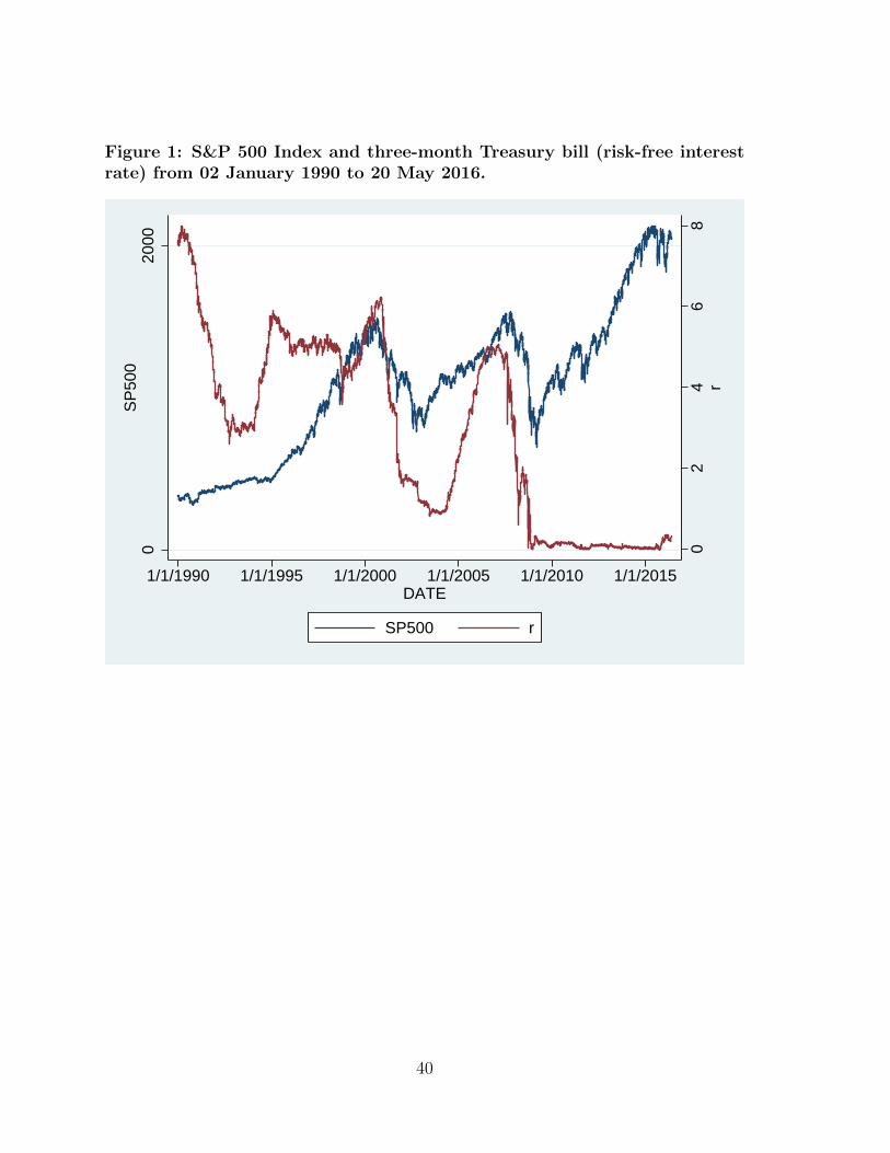
Figure 1: S&P 500 Index and three-month Treasury bill (risk-free interestrate) from 02 January 1990 to 20 May 2016.

02

46

8r

020

00S

P50

0

1/1/1990 1/1/1995 1/1/2000 1/1/2005 1/1/2010 1/1/2015DATE

SP500 r

40

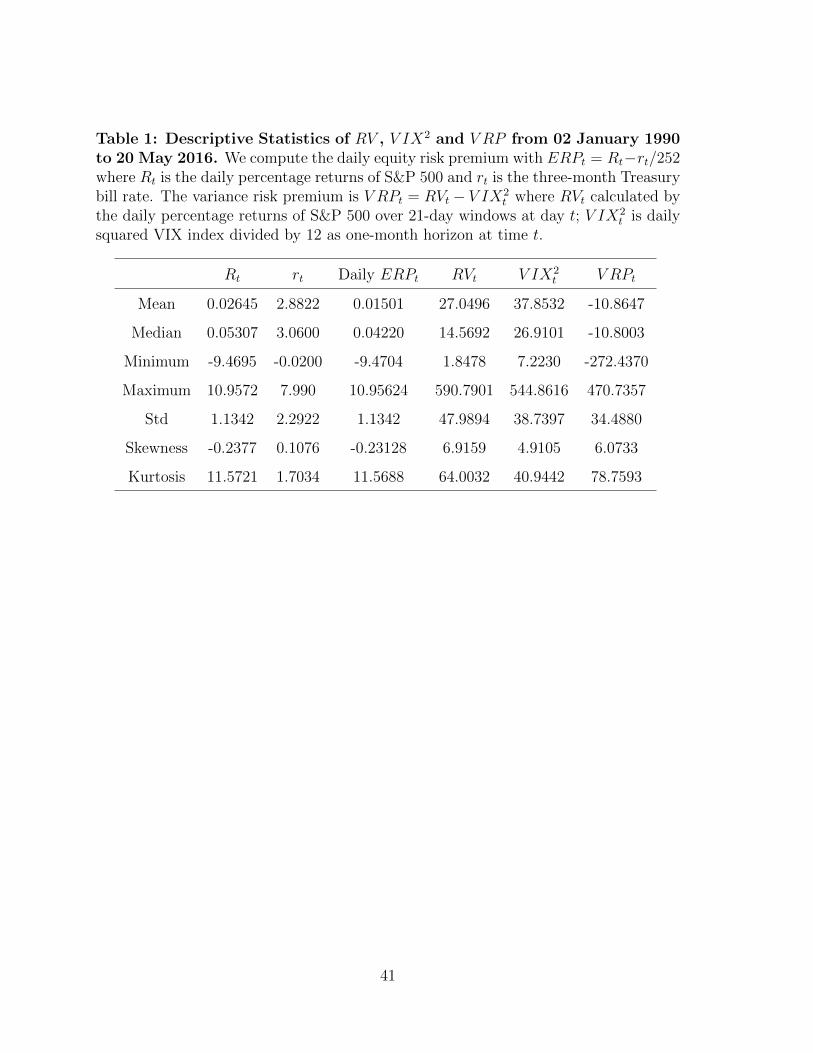
Table 1: Descriptive Statistics of RV , V IX2 and V RP from 02 January 1990to 20 May 2016. We compute the daily equity risk premium with ERPt = Rt−rt/252where Rt is the daily percentage returns of S&P 500 and rt is the three-month Treasurybill rate. The variance risk premium is V RPt = RVt − V IX2

t where RVt calculated bythe daily percentage returns of S&P 500 over 21-day windows at day t; V IX2

t is dailysquared VIX index divided by 12 as one-month horizon at time t.

Rt rt Daily ERPt RVt V IX2t V RPt

Mean 0.02645 2.8822 0.01501 27.0496 37.8532 -10.8647

Median 0.05307 3.0600 0.04220 14.5692 26.9101 -10.8003

Minimum -9.4695 -0.0200 -9.4704 1.8478 7.2230 -272.4370

Maximum 10.9572 7.990 10.95624 590.7901 544.8616 470.7357

Std 1.1342 2.2922 1.1342 47.9894 38.7397 34.4880

Skewness -0.2377 0.1076 -0.23128 6.9159 4.9105 6.0733

Kurtosis 11.5721 1.7034 11.5688 64.0032 40.9442 78.7593

41

Figure 2: V RP from 02 January 1990 to 20 May 2016. We defined the variancerisk premium as V RPt = RVt − V IX2

t where RVt calculated by the daily percentagereturns of S&P 500 over 21-day windows at day t; V IX2

t is daily squared VIX indexdivided by 12 as one-month horizon at time t.

−20

00

200

400

600

VR

P

1/1/1990 1/1/1995 1/1/2000 1/1/2005 1/1/2010 1/1/2015Date

42

Figure 3: RV and V IX2 from 02 January 1990 to 20 May 2016. We calculateRVt by using the daily percentage returns of S&P 500 over 21-day windows at day t;V IX2

t is daily squared VIX index divided by 12 as one-month horizon at time t.

020

040

060

0

1/1/1990 1/1/1995 1/1/2000 1/1/2005 1/1/2010 1/1/2015Date

RV VIX2

43

Table 2: Estimates in Broadie et al. (2007). The physical measure parametersestimated by Eraker et al. (2003) with sample (1980 to 1999). The risk-neutral pa-rameters estimated by options on S&P 500 futures with sample (1987 to 2003). Theparameter values correspond to daily percentage returns.

Model κ θ σV ρ λ µS σS µV κQ µQS

µQV

SV 0.023 0.90 0.14 -0.40 0.028

SVJ 0.013 0.81 0.10 -0.47 0.006 -2.59 4.07 0.023 -9.97

SVCJ 0.026 0.54 0.08 -0.48 0.006 -2.63 2.89 1.48 0.056 -6.58 10.81

Table 3: Model-implied Variance Risk Premium in Broadie et al. (2007). Wereport simulated statistics based on 10,000 simulations, with each statistic calculatedusing a sample size equal to its VRP data counterpart. We report the mean of theVRP from 1990 to 1999 which is the overlapping period between Eraker et al. (2003)and Broadie et al. (2007) after VIX lunched.

Model E[V RPSV ] V RPPJ V RPV J Model-based E[V RP ] E[V RP ] Explanation rate

SV 0.8241 0 0 0.8241 -14.5495 5.66%

SVJ 1.5341 -11.6793 0 -10.1452 -14.5495 69.83%

SVCJ 3.8162 -4.5838 -8.3754 -9.1430 -14.5495 62.84%

44

Figure 4: The effects of the volatility parameters (I). We set the baselinemodel parameters as κ = 15, θ = 0.02, σV = 0.5, ρ = −0.9, λ = 2, µS = −0.01, σS =0.02, µV = 0.06, r = 0.008, β = 0.001, γ = 2.5, ψ = 2 and E[V ] = 0.02. The baselineaverage ERP = 5.2023, V RP = −15.3317 and. The effects of a parameter on thesolutions of a and the VRP are only against the corresponding parameter and otherparameters keep the baseline value. (−) means the real value is negative but we presentit’s absolute value.

(a) The effects of κ

0 50 1002

3

4

5

6

7

8

9Panel A. Solutions of a

κ

0 50 1003

4

5

6

7

8

9Panel B. VRP (−)

κ

0 50 1001

2

3

4

5

6

7

8Panel B. ERP

κ

(b) The effects of θ

0 0.2 0.4 0.6 0.80

2

4

6

8

10


θ0 0.2 0.4 0.6 0.8

0

5

10

15

20

25

30

35Panel B. VRP (−)

θ0 0.2 0.4 0.6 0.8

0

2

4

6

8

10

12

14Panel B. ERP

θ

(c) The effects of σV

0 0.2 0.4 0.6 0.86.8

6.85

6.9

6.95

7

7.05

7.1

7.15Panel A. Solutions of a

σV

0 0.2 0.4 0.6 0.86

8

10

12


σV

0 0.2 0.4 0.6 0.84.6

4.8

5

5.2

5.4

5.6

5.8

6Panel B. ERP

σV

(d) The effects of ρ

0.2 0.4 0.6 0.85.5

6

6.5

7

7.5


ρ(−)0.2 0.4 0.6 0.8

7.5

8

8.5Panel B. VRP (−)

ρ(−)0.2 0.4 0.6 0.8

4.9

5

5.1

5.2

5.3Panel B. ERP

ρ(−)

45

Figure 5: The effects of the jump parameters (I). We set the baseline model pa-rameters as κ = 15, θ = 0.02, σV = 0.5, ρ = −0.9, λ = 2, µS = −0.01, σS = 0.02, µV =0.06, r = 0.008, β = 0.001, γ = 2.5, ψ = 2 and E[V ] = 0.02. The baseline averageERP = 5.2023, V RP = −8.4532 and a = 6.9193. The effects of a parameter on thesolutions of a and the VRP are only against the corresponding parameter and otherparameters keep the baseline value. (−) means the real value is negative but we presentit’s absolute value.

(a) The effects of λ

0 10 20 300

2

4

6

8


λ

0 10 20 302

4

6

8

10

12


λ0 10 20 30

0

5

10

15

20Panel B. ERP

λ

(b) The effects of µS

0 0.1 0.2 0.3 0.4

6.4

6.5

6.6

6.7

6.8

6.9

7


µS(−)0 0.1 0.2 0.3 0.4

0

200

400

600

800


µS(−)0 0.1 0.2 0.3 0.4

0

100

200

300

400

500

600

700Panel B. ERP

µS(−)

(c) The effects of σS

0 0.1 0.2 0.36.5

6.6

6.7

6.8

6.9


σS

0 0.1 0.2 0.30

200

400

600

800


σS

0 0.1 0.2 0.30

100

200

300

400

500Panel B. ERP

σS

(d) The effects of µV

0 0.05 0.16

6.5

7

7.5

8

8.5

9


µV

0 0.05 0.10

5

10

15

20

25

30


µV

0 0.05 0.10

2

4

6

8

10

12Panel B. ERP

µV

46

Figure 6: The effects of the preferences parameters (I). We set the baselinemodel parameters as κ = 15, θ = 0.02, σV = 0.5, ρ = −0.9, λ = 2, µS = −0.01, σS =0.02, µV = 0.06, r = 0.008, β = 0.001, γ = 2.5, ψ = 2 and E[V ] = 0.02. The baselineaverage ERP = 5.2023, V RP = −8.4532 and a = 6.9193. The effects of a parameteron the solutions of a and the VRP are only against the corresponding parameter andother parameters keep the baseline value. (−) means the real value is negative but wepresent it’s absolute value.

(a) The effects of β

0 0.5 16.8

7

7.2

7.4

7.6

7.8


β0 0.5 1

8

8.5

9

9.5

10

10.5

11


β0 0.5 1

5.5

6

6.5

Panel B. ERP

β

(b) The effects of γ > 2

0 20 40 600

2

4

6

8

10


γ0 20 40 60

0

5

10

15

20

25

30

35


γ0 20 40 60

0

5

10

15

20

25

30

35

40Panel B. ERP

γ

(c) The effects of ψ < 1

0 0.2 0.4 0.614.5

15

15.5

16


ψ < 10 0.2 0.4 0.6

0

1000

2000

3000

4000


ψ < 10 0.2 0.4 0.6

0

50

100

150

200

250Panel B. ERP

ψ < 1

(d) The effects of ψ > 1

0 50 1000

1

2

3

4

5

6

7


ψ > 10 50 100

0

2

4

6

8


ψ > 10 50 100

0

1

2

3

4

5

6Panel B. ERP

ψ > 1

47

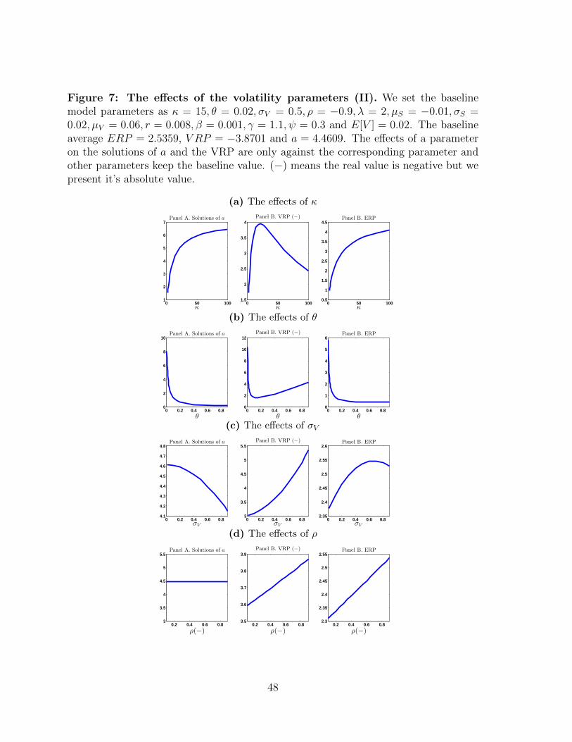
Figure 7: The effects of the volatility parameters (II). We set the baselinemodel parameters as κ = 15, θ = 0.02, σV = 0.5, ρ = −0.9, λ = 2, µS = −0.01, σS =0.02, µV = 0.06, r = 0.008, β = 0.001, γ = 1.1, ψ = 0.3 and E[V ] = 0.02. The baselineaverage ERP = 2.5359, V RP = −3.8701 and a = 4.4609. The effects of a parameteron the solutions of a and the VRP are only against the corresponding parameter andother parameters keep the baseline value. (−) means the real value is negative but wepresent it’s absolute value.

(a) The effects of κ

0 50 1001

2

3

4

5

6


κ

0 50 1001.5

2

2.5

3

3.5

4Panel B. VRP (−)

κ

0 50 1000.5

1

1.5

2

2.5

3

3.5

4

4.5Panel B. ERP

κ

(b) The effects of θ

0 0.2 0.4 0.6 0.80

2

4

6

8


θ0 0.2 0.4 0.6 0.8

0

2

4

6

8

10


θ0 0.2 0.4 0.6 0.8

0

1

2

3

4

5

6Panel B. ERP

θ

(c) The effects of σV

0 0.2 0.4 0.6 0.84.1

4.2

4.3

4.4

4.5

4.6

4.7


σV

0 0.2 0.4 0.6 0.83

3.5

4

4.5

5


σV

0 0.2 0.4 0.6 0.82.35

2.4

2.45

2.5

2.55

2.6Panel B. ERP

σV

(d) The effects of ρ

0.2 0.4 0.6 0.83

3.5

4

4.5

5


ρ(−)0.2 0.4 0.6 0.8

3.5

3.6

3.7

3.8


ρ(−)0.2 0.4 0.6 0.8

2.3

2.35

2.4

2.45

2.5

2.55Panel B. ERP

ρ(−)

48

Figure 8: The effects of the jump parameters (II). We set the baseline model pa-rameters as κ = 15, θ = 0.02, σV = 0.5, ρ = −0.9, λ = 2, µS = −0.01, σS = 0.02, µV =0.06, r = 0.008, β = 0.001, γ = 1.1, ψ = 0.3 and E[V ] = 0.02. The baseline averageERP = 2.5359, V RP = −3.8701 and a = 4.4609. The effects of a parameter on thesolutions of a and the VRP are only against the corresponding parameter and otherparameters keep the baseline value. (−) means the real value is negative but we presentit’s absolute value.

(a) The effects of λ

0 10 20 300

1

2

3

4

5

6


λ

0 10 20 301

2

3

4

5

6

7

8

9Panel B. VRP (−)

λ

0 10 20 300

2

4

6

8

10Panel B. ERP

λ

(b) The effects of µS

0 0.1 0.2 0.3 0.44.46

4.47

4.48

4.49

4.5

4.51


µS(−)0 0.1 0.2 0.3 0.4

0

50

100

150

200

250

300


µS(−)0 0.1 0.2 0.3 0.4

0

50

100

150

200

250Panel B. ERP

µS(−)

(c) The effects of σS

0 0.1 0.2 0.34.46

4.47

4.48

4.49

4.5


σS

0 0.1 0.2 0.30

50

100

150


σS

0 0.1 0.2 0.30

20

40

60

80

100

120Panel B. ERP

σS

(d) The effects of µV

0 0.05 0.13

3.5

4

4.5

5

5.5

6

6.5


µV

0 0.05 0.11

2

3

4

5

6

7

8Panel B. VRP (−)

µV

0 0.05 0.10.5

1

1.5

2

2.5

3

3.5Panel B. ERP

µV

49

Figure 9: The effects of the preferences parameters (II). We set the baselinemodel parameters as κ = 15, θ = 0.02, σV = 0.5, ρ = −0.9, λ = 2, µS = −0.01, σS =0.02, µV = 0.06, r = 0.008, β = 0.001, γ = 1.1, ψ = 0.3 and E[V ] = 0.02. The baselineaverage ERP = 2.5359, V RP = −3.8701 and a = 4.4609. The effects of a parameteron the solutions of a and the VRP are only against the corresponding parameter andother parameters keep the baseline value. (−) means the real value is negative but wepresent it’s absolute value.

(a) The effects of β

0 0.5 14.46

4.48

4.5

4.52

4.54


β0 0.5 1

3.86

3.88

3.9

3.92

3.94

3.96

3.98

4Panel B. VRP (−)

β0 0.5 1

2.54

2.55

2.56

2.57

2.58

2.59

2.6Panel B. ERP

β

(b) The effects of γ < 2

1 1.5 20

5

10


γ < 21 1.5 2

0

50

100

150

200

250


γ < 21 1.5 2

0

10

20

30

40

50Panel B. ERP

γ < 2

(c) The effects of ψ < 1

0.2 0.4 0.6 0.82

4

6

8

10

12

14


ψ0.2 0.4 0.6 0.8

0

50

100

150


ψ0.2 0.4 0.6 0.8

0

10

20

30

40Panel B. ERP

ψ

50

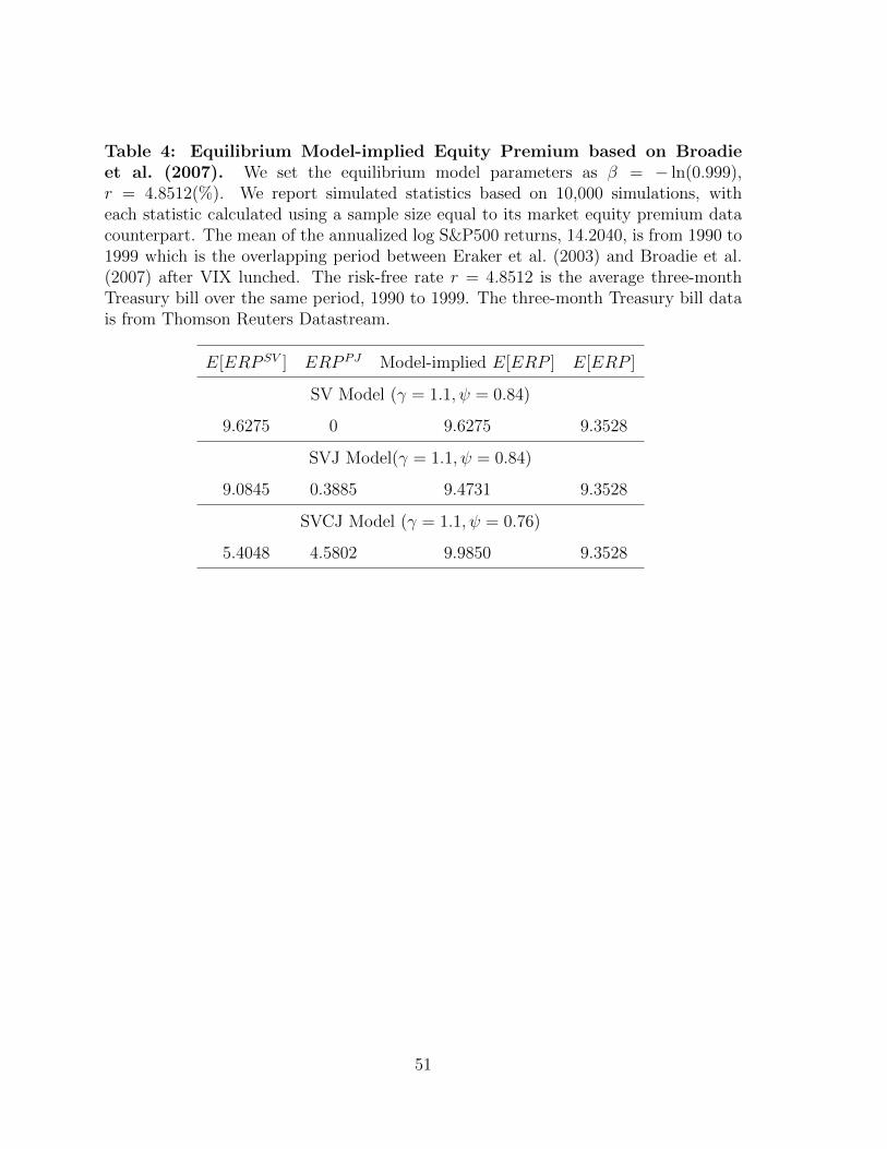
Table 4: Equilibrium Model-implied Equity Premium based on Broadieet al. (2007). We set the equilibrium model parameters as β = − ln(0.999),r = 4.8512(%). We report simulated statistics based on 10,000 simulations, witheach statistic calculated using a sample size equal to its market equity premium datacounterpart. The mean of the annualized log S&P500 returns, 14.2040, is from 1990 to1999 which is the overlapping period between Eraker et al. (2003) and Broadie et al.(2007) after VIX lunched. The risk-free rate r = 4.8512 is the average three-monthTreasury bill over the same period, 1990 to 1999. The three-month Treasury bill datais from Thomson Reuters Datastream.

E[ERP SV ] ERP PJ Model-implied E[ERP ] E[ERP ]

SV Model (γ = 1.1, ψ = 0.84)

9.6275 0 9.6275 9.3528

SVJ Model(γ = 1.1, ψ = 0.84)

9.0845 0.3885 9.4731 9.3528

SVCJ Model (γ = 1.1, ψ = 0.76)

5.4048 4.5802 9.9850 9.3528

51

Table 5: Equilibrium Model-implied Variance Risk Premium based onBroadie et al. (2007). We set the equilibrium model parameters as β = − ln(0.999).We report simulated statistics based on 10,000 simulations, with each statistic calcu-lated using a sample size equal to its VRP data counterpart. We report the mean of theVRP from 1990 to 1999 which is the overlapping period between Eraker et al. (2003)and Broadie et al. (2007) after VIX lunched. The risk-free rate r = 4.8512 is the av-erage three-month Treasury bill over the same period, 1990 to 1999. The three-monthTreasury bill data is from Thomson Reuters Datastream.

V RP SVt V RP PJ

t V RP V Jt Model-based V RPt V RPt Explanation rate

SV Model (γ = 1.1, ψ = 0.84)

-2.1308 0 0 -2.1308 -14.5495 14.65%

SVJ Model (γ = 1.1, ψ = 0.84)

-1.3123 -0.2146 0 -1.5269 -14.5495 10.49%

SVCJ Model (γ = 1.1, ψ = 0.76)

-0.4107 -2.2695 -5.6005 -8.2807 -14.5495 56.91%

Table 6: Return predictability. This table reports empirical results from the dailypredictive regressions of the equity premiums (S&P 500 log returns subtract the risk-free rate) on variance risk premiums (i.e., regression (29)). We defined the monthlyERP as (Rt−rt/252)×21 where Rt is the daily percentage returns of S&P 500 and rt isthe three-month Treasury bill rate. The variance risk premium is V RPt = RVt−V IX2

t

where RVt calculated by the daily percentage returns of S&P 500 over 21-day windowsat day t; V IX2

t is daily squared VIX index divided by 12 as one-month horizon at timet.

Periods02 January 1990 - 20 May 2016 24 November 2010 - 20 May 2016

βpred t-statistic adj. R2 (%) βpred t-statistic adj. R2 (%)

-13.5463 -16.26 3.82 -20.8929 -8.79 5.31

52

Table 7: Descriptive Statistics of Rt, RV , V IX2 and V RP from 24 November2010 to 20 May 2016. We compute the daily equity risk premium with ERPt =Rt−rt/252 where Rt is the daily percentage returns of S&P 500 and rt is the daily three-month Treasury bill rate. We defined the variance risk premium as V RPt = RVt−V IX2

t

where RVt calculated by the daily percentage returns of S&P 500 over 21-day windowsat day t; V IX2

t is daily squared VIX index divided by 12 as one-month horizon at timet.

Rt rt Daily ERP RVt V IX2t V RPt

Obs. 1381 1381 1381 1360 1360 1360

Mean 0.0400 0.07301 0.03974 19.9787 28.3325 -8.3538

Median 0.0549 0.0500 0.0546 12.4189 21.2934 -8.9812

Minimum -6.8958 -0.0200 -6.8960 2.1505 8.8752 -99.1070

Maximum 4.6317 0.3500 4.6316 195.5504 192 155.0615

Std 0.9725 .07027 0.9725 25.2038 22.6837 22.7515

Skewness -0.4732 1.8761 -0.4731 3.9569 3.0577 3.3699

Kurtosis 7.5650 6.4181 7.5649 22.4983 14.1150 24.6868

53

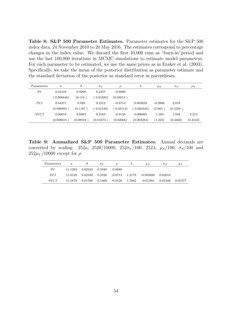
Table 8: S&P 500 Parameter Estimates. Parameter estimates for the S&P 500index data, 24 November 2010 to 20 May 2016. The estimates correspond to percentagechanges in the index value. We discard the first 10,000 runs as “burn-in”period anduse the last 100,000 iterations in MCMC simulations to estimate model parameters.For each parameter to be estimated, we use the same priors as in Eraker et al. (2003).Specifically, we take the mean of the posterior distribution as parameter estimate andthe standard deviation of the posterior as standard error in parentheses.

Parameters κ θ σV ρ λ µS σS µV

SV 0.04416 0.9298 0.2357 -0.8686

( 0.006846) (0.116 ) ( 0.01692) (0.03013 )

SVJ 0.04371 0.928 0.2312 -0.8714 0.004833 -0.3886 2.018

(0.006993 ) (0.1187 ) ( 0.01549) ( 0.03114) ( 0.004345) (2.665 ) (0.5229 )

SVCJ 0.06019 0.6983 0.2169 -0.9128 0.006985 -1.394 1.948 2.213

(0.008618 ) (0.08918 ) (0.01673 ) (0.02666) (0.003284) (1.222) (0.4666) (0.4543)

Table 9: Annualized S&P 500 Parameter Estimates. Annual decimals areconverted by scaling: 252κ, 252θ/10000, 252σV /100, 252λ, µS/100, σS/100 and252µV /10000 except for ρ.

Parameters κ θ σV ρ λ µS σS µV

SV 11.1283 0.02343 0.5940 -0.8686

SVJ 11.0149 0.02339 0.5826 -0.8714 1.2179 -0.003886 0.02018

SVCJ 15.1679 0.01760 0.5469 -0.9128 1.7602 -0.01394 0.01948 0.05577

54

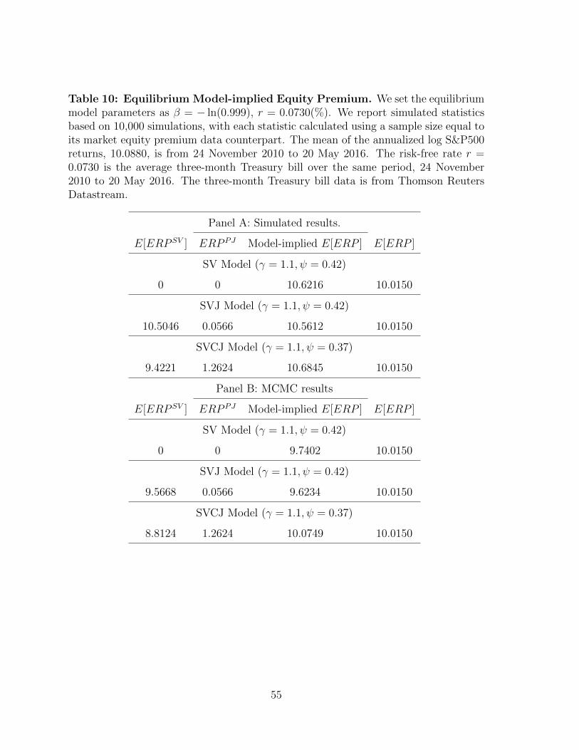
Table 10: Equilibrium Model-implied Equity Premium. We set the equilibriummodel parameters as β = − ln(0.999), r = 0.0730(%). We report simulated statisticsbased on 10,000 simulations, with each statistic calculated using a sample size equal toits market equity premium data counterpart. The mean of the annualized log S&P500returns, 10.0880, is from 24 November 2010 to 20 May 2016. The risk-free rate r =0.0730 is the average three-month Treasury bill over the same period, 24 November2010 to 20 May 2016. The three-month Treasury bill data is from Thomson ReutersDatastream.

Panel A: Simulated results.


SV Model (γ = 1.1, ψ = 0.42)

0 0 10.6216 10.0150

SVJ Model (γ = 1.1, ψ = 0.42)

10.5046 0.0566 10.5612 10.0150

SVCJ Model (γ = 1.1, ψ = 0.37)

9.4221 1.2624 10.6845 10.0150

Panel B: MCMC results


SV Model (γ = 1.1, ψ = 0.42)

0 0 9.7402 10.0150

SVJ Model (γ = 1.1, ψ = 0.42)

9.5668 0.0566 9.6234 10.0150

SVCJ Model (γ = 1.1, ψ = 0.37)

8.8124 1.2624 10.0749 10.0150

55

Table 11: Annualized model-implied risk-neutral parameters. We set theequilibrium model parameters as β = − ln(0.999) and r = 0.0730(%) which is theaverage three-month Treasury bill over the same period, 24 November 2010 to 20 May2016. The three-month Treasury bill data is from Thomson Reuters Datastream.

Model β γ ψ a κQ λQ µQS µQV

SV -ln(0.999) 1.1 0.42 6.6251 8.2160

SVJ -ln(0.999) 1.1 0.42 6.6542 8.1977 1.2234 -0.0043

SVCJ -ln(0.999) 1.1 0.37 13.3679 11.9858 2.6061 -0.014 0.0813

Table 12: Model-implied risk-neutral parameters. The estimates correspond todaily percentage changes in the index value.

Model κQ λQ µQS µQV

SV 0.0326

SVJ 0.0325 0.0049 -0.4334

SVCJ 0.0500 0.0131 -1.4357 4.0925

56

Figure 10: The solution of a against γ based on SVCJ. This figure shows thesolution of a against γ. The SVCJ model parameters are given in Table 9 and 11.

1.1 1.2 1.3 1.4 1.50

5

10

15

a

γ

57

Table 13: Model-implied Variance Risk Premium. We set the equilibrium modelparameters as β = − ln(0.999), r = 0.0730(%). We report simulated statistics basedon 10,000 simulations, with each statistic calculated using a sample size equal to itsmarket equity premium data counterpart. The MCMC results use the latent varianceVt from the MCMC estimation of the physical parameters. The mean of the annualizedlog S&P500 returns, 10.0880, is from 24 November 2010 to 20 May 2016. The risk-freerate r = 0.0730 is the average three-month Treasury bill over the same period, 24November 2010 to 20 May 2016. The three-month Treasury bill data is from ThomsonReuters Datastream.

Panel A: Simulated results.

E[V RP SV ] V RP PJ V RP V J Model-based E[V RP ] E[V RP ] Explanation rate

SV Model (γ = 1.1, ψ = 0.42)

-1.9146 0 0 -1.9146 -8.3538 22.92%

SVJ Model (γ = 1.1, ψ = 0.42)

-1.8489 -0.0057 0 -1.8546 -8.3538 20.20%

SVCJ Model (γ = 1.1, ψ = 0.37)

-0.9757 -0.4301 -2.9110 -4.3169 -8.3538 51.68%

Panel B: MCMC results.

E[V RP SV ] V RP PJ V RP V J Model-based E[V RP ] E[V RP ] Explanation rate

SV Model (γ = 1.1, ψ = 0.42)

-1.7970 0 0 -1.7970 -8.3538 21.51%

SVJ Model (γ = 1.1, ψ = 0.42)

-1.7264 -0.0057 0 -1.7321 -8.3538 20.73%

SVCJ Model (γ = 1.1, ψ = 0.37)

-0.9297 -0.4301 -2.9110 -4.2709 -8.3538 51.13%

58

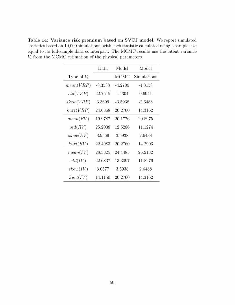
Table 14: Variance risk premium based on SVCJ model. We report simulatedstatistics based on 10,000 simulations, with each statistic calculated using a sample sizeequal to its full-sample data counterpart. The MCMC results use the latent varianceVt from the MCMC estimation of the physical parameters.

Data Model Model

Type of Vt MCMC Simulations

mean(V RP ) -8.3538 -4.2709 -4.3158

std(V RP ) 22.7515 1.4304 0.6941

skew(V RP ) 3.3699 -3.5938 -2.6488

kurt(V RP ) 24.6868 20.2760 14.3162

mean(RV ) 19.9787 20.1776 20.8975

std(RV ) 25.2038 12.5286 11.1274

skew(RV ) 3.9569 3.5938 2.6438

kurt(RV ) 22.4983 20.2760 14.2903

mean(IV ) 28.3325 24.4485 25.2132

std(IV ) 22.6837 13.3097 11.8276

skew(IV ) 3.0577 3.5938 2.6488

kurt(IV ) 14.1150 20.2760 14.3162

59

Table 15: Model-implied Equity and Variance Risk Premiums in Drechsler(2013). Data estimates are reported for samples starting in 1930 and ending in 2009.

Model-implied E[ERP ] Data E[ERP ] Explanation rate

6.29 4.93 127.59%

Model-based E[V RP ] Data E[V RP ] Explanation rate

-8.17 -10.55 77.44%

Table 16: Model-implied Equity and Variance Risk Premiums based onSVCJ model (γ = 1.1, ψ = 0.52). We set the equilibrium model parameters asβ = − ln(0.999), r = 0.0730(%). We report simulated statistics based on 10,000simulations, with each statistic calculated using a sample size equal to its marketequity premium data counterpart. The MCMC results use the latent variance Vt fromthe MCMC estimation of the physical parameters. The mean of the annualized logS&P500 returns, 10.0880%, is from 24 November 2010 to 20 May 2016. The risk-freerate r = 0.0730% is the average three-month Treasury bill over the same period, 24November 2010 to 20 May 2016. The three-month Treasury bill data is from ThomsonReuters Datastream.

Panel A: ERP with SVCJ Model (γ = 1.1, ψ = 0.52).

E[ERPSV ] ERPPJ Model-implied E[ERP ] E[ERP ] Explanation rate

(a) Simulated results.

11.0897 1.7310 12.8207 10.0150 128.01%

(b): MCMC results

10.3804 1.7310 12.1114 10.0150 120.93%

Panel B: VRP with SVCJ Model (γ = 1.1, ψ = 0.52).

E[V RPSV ] V RPPJ V RPV J Model-based E[V RP ] E[V RP ] Explanation rate


-1.2126 -0.5927 -4.4013 -6.2066 -8.3538 74.30%

(b) MCMC results.

-1.1561 -0.5927 -4.4013 -6.1501 -8.3538 73.62%

60

Table 17: Model-implied Equity and Variance Risk Premiums based onSVCJ model (γ = 1.1, ψ = 0.61). We set the equilibrium model parameters asβ = − ln(0.999), r = 0.0730(%). We report simulated statistics based on 10,000simulations, with each statistic calculated using a sample size equal to its marketequity premium data counterpart. The MCMC results use the latent variance Vt fromthe MCMC estimation of the physical parameters. The mean of the annualized logS&P500 returns, 10.0880%, is from 24 November 2010 to 20 May 2016. The risk-freerate r = 0.0730% is the average three-month Treasury bill over the same period, 24November 2010 to 20 May 2016. The three-month Treasury bill data is from ThomsonReuters Datastream.

Panel A: ERP with SVCJ Model (γ = 1.1, ψ = 0.61).

E[ERPSV ] ERPPJ Model-implied E[ERP ] E[ERP ]


12.5428 2.2474 14.7902 10.0150

(b): MCMC results

11.7424 2.2474 13.9898 10.0150

Panel B: VRP with SVCJ Model (γ = 1.1, ψ = 0.61).

E[V RPSV ] V RPPJ V RPV J Model-based E[V RP ] E[V RP ]


-1.4225 -0.7718 -6.2600 -8.4543 -8.3538

(b) MCMC results.

-1.3563 -0.7718 -6.2600 -8.3881 -8.3538

61

Table 18: Variance risk premium based on SVCJ model (γ = 1.1, ψ = 0.61).We report simulated statistics based on 10,000 simulations, with each statistic calcu-lated using a sample size equal to its full-sample data counterpart. The MCMC resultsuse the latent variance Vt from the MCMC estimation of the physical parameters.

Data Model Model

Type of Vt MCMC Simulations

mean(V RP ) -8.3538 -8.3881 -8.4543

std(V RP ) 22.7515 1.1411 1.0154

skew(V RP ) 3.3699 -3.5938 -2.6496

kurt(V RP ) 24.6868 20.2760 14.3113

mean(RV ) 19.9787 20.1776 20.9044

std(RV ) 25.2038 12.5286 11.1483

skew(RV ) 3.9569 3.5938 2.6496

kurt(RV ) 22.4983 20.2760 14.3113

mean(IV ) 28.3325 28.5656 29.3587

std(IV ) 22.6837 13.6698 12.1637

skew(IV ) 3.0577 3.5938 2.6496

kurt(IV ) 14.1150 20.2760 14.3113

62

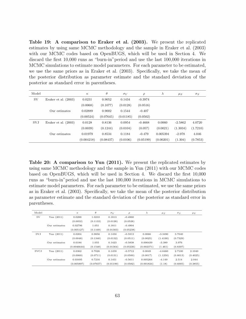
Table 19: A comparison to Eraker et al. (2003). We present the replicatedestimates by using same MCMC methodology and the sample in Eraker et al. (2003)with our MCMC codes based on OpenBUGS, which will be used in Section 4. Wediscard the first 10,000 runs as “burn-in”period and use the last 100,000 iterations inMCMC simulations to estimate model parameters. For each parameter to be estimated,we use the same priors as in Eraker et al. (2003). Specifically, we take the mean ofthe posterior distribution as parameter estimate and the standard deviation of theposterior as standard error in parentheses.

Model κ θ σV ρ λ µS σS

SV Eraker et al. (2003) 0.0231 0.9052 0.1434 -0.3974

(0.0068) (0.1077) (0.0128) (0.0516)

Our estimates 0.02889 0.9002 0.1544 -0.407

(0.00524) (0.07645) (0.01185) (0.0502)

SVJ Eraker et al. (2003) 0.0128 0.8136 0.0954 -0.4668 0.0060 -2.5862 4.0720

(0.0039) (0.1244) (0.0104) (0.057) (0.0021) (1.3034) (1.7210)

Our estimates 0.01979 0.8534 0.1184 -0.479 0.005394 -2.978 4.046

(0.004218) (0.08437) (0.0106) (0.05199) (0.00201) (1.304) (0.7853)

Table 20: A comparison to Yun (2011). We present the replicated estimates byusing same MCMC methodology and the sample in Yun (2011) with our MCMC codesbased on OpenBUGS, which will be used in Section 4. We discard the first 10,000runs as “burn-in”period and use the last 100,000 iterations in MCMC simulations toestimate model parameters. For each parameter to be estimated, we use the same priorsas in Eraker et al. (2003). Specifically, we take the mean of the posterior distributionas parameter estimate and the standard deviation of the posterior as standard error inparentheses.

Model κ θ σV ρ λ µS σS µV

SV Yun (2011) 0.0288 1.0210 0.1813 -0.4960

(0.0052) (0.1133) (0.0128) (0.0528)

Our estimates 0.02796 1.051 0.1811 -0.4904

(0.005127) (0.1168) (0.01303) (0.05238)

SVJ Yun (2011) 0.0204 0.9856 0.1450 -0.5912 0.0066 -3.3490 3.7040

(0.0048) (0.1340) (0.0132) (0.0511) (0.0025) (1.4190) (0.7329)

Our estimates 0.0184 1.055 0.1423 -0.5838 0.006439 -3.389 3.976

(0.0046644) (0.1548) (0.01364) (0.05226) (0.002371) (1.461) (0.8397)

SVCJ Yun (2011) 0.0362 0.7026 0.1459 -0.5712 0.0049 -4.6460 2.7100 2.1040

(0.0060) (0.0711) (0.0131) (0.0500) (0.0017) (1.1250) (0.8013) (0.4025)

Our estimates 0.03495 0.7216 0.1451 -0.5611 0.005264 -4.149 2.514 2.044

(0.005897) (0.07657) (0.01199) (0.0582) (0.001824) (1.18) (0.6005) (0.3855)

63

Documents

Equilibrium Equity and Variance Risk Premiums in A Cost ...€¦ · Equilibrium Equity and Variance Risk Premiums in A Cost-free Production Economy Abstract This paper provides a