Equilibrium Interpretations of Employment and Real … Interpretations of Employment and Real Wage Fluctuations The question of the influence on real wages of periods of boom and depression

This PDF is a selection from an out-of-print volume from the NationalBureau of Economic Research

Volume Title: NBER Macroeconomics Annual 1988, Volume 3

Volume Author/Editor: Stanley Fischer, editor

Volume Publisher: MIT Press

Volume ISBN: 0-262-06119-8

Volume URL: http://www.nber.org/books/fisc88-1

Publication Date: 1988

Chapter Title: Equilibrium Interpretations of Employment and Real WageFluctuations

Chapter Author: John Kennan

Chapter URL: http://www.nber.org/chapters/c10954

Chapter pages in book: (p. 157 - 216)

John Kennan THE UNIVERSITY OF IOWA, HOOVER INSTITUTION

Equilibrium Interpretations of Employment and Real Wage Fluctuations

The question of the influence on real wages of periods of boom and depression has a long history. J.M. Keynes (1939).

Observed real wages are not constant over the cycle, but neither do they exhibit consistent

pro- or countercyclical tendencies. This suggests that any attempt to assign systematic real

wage movements a central role in an explanation of business cycles is doomed to failure. Accordingly, I will proceed as though the real wage were fixed . . . Robert Lucas (1977, p. 226).

This change implies a substitution effect, which favors today's consumption and deters

today's leisure. Therefore, . . . it becomes possible to generate the typical pattern of business cycles, which features positive co-movements of current output, work effort, investment, and consumption. But notice that the real wage rate, which equals the

marginal product of labor, must rise along with the increases in output and work effort. In other words, a procyclical pattern for the real wage rate is central to our theoretical

analysis. Robert Barro and Robert King (1984, p. 833).

The problem with the simple competitive model is that it interprets the observed

employment-wage combinations as points on a simple, static labor supply curve. A glance at the data for the United States and many other economies shows large movements of employment occurring at the same time that the real wage remains unchanged. There are two possible explanations within the simple model. First, the labor supply schedule may be highly wage elastic. But a large literature on labor supply contradicts that view. Static labor supply is only slightly wage elastic, and then only for workers with major non-work alternatives. The second potential explanation is that shifts of the labor supply schedule may be a principal driving force in the economy, so that the observed wage-employment combinations are on an elastic labor demand schedule. In the second view, the typical recession occurs because people have decided not to work as hard as usual. That view has

158 KENNAN

no important support in the literature, to our knowledge. David Lilien and Robert Hall (1986, p. 1012-1013).

1. Introduction

This paper is primarily an attempt to document the facts about cyclical fluctuations in employment and real wages, using postwar monthly data from manufacturing industries in six countries. The main question is whether or not the data could have been generated by equilibrium models of the labor market. This question cannot be answered by representing employment as an optimal dynamic response to an exogenous stochastic

process for real wages; one must also explain how the wage process is

generated. The data are first summarized in terms of relative variability and correlation, and patterns of serial correlation. A competitive equilibrium model is then used to provide a framework in which these statistics can be

interpreted. A variation on this model is also presented, in which a central labor union acts as a monopoly seller of labor. The competitive and

monopoly equilibria are closely related, and either could, in principle, explain the data.

As the above quote from Lilien and Hall makes clear, it is difficult for a static equilibrium model of the labor market, which is driven mainly by shocks on the demand side, to reconcile an inelastic labor supply curve with aggregate employment and real wage fluctuations. The difficulty is two-fold: if the data lie close to an inelastic supply curve, then the real wage should vary more than employment, and the real wage should be strongly procyclical. It is unusual to find either of these features in the data. It is also difficult for an equilibrium model to explain the serial correlation found in the bivariate process for employment and real wages. As will be shown below, this process has two roots close to the unit circle, and a third root which is much smaller in magnitude, and generally negative.

When a dynamic model is used to interpret serial correlation, the

prediction of a procyclical real wage can be made to disappear. This is one of the most surprising results in the paper. For example, it will be shown (in Table 6) that UK employment and real wage data accept a null

hypothesis in which labor supply is relatively inelastic, less than 26 percent of the variance in employment is due to labor supply shocks, and yet the correlation coefficient between the innovations in employment and real

wages is only .1. It is important to note from this example that there is a big difference between a model that is driven exclusively by labor demand shocks, and a model that admits small labor supply shocks. On the other hand, the dynamic model does not succeed in explaining the U.S. data,

Employment and Real Wages * 159

primarily because in these data employment is much more variable than the real wage.

This paper focuses on some basic issues concerning the construction of structural models of the labor market. There is a large body of empirical literature that has been written recently on the general subject of employment fluctuations. The motivating force behind this literature is a desire to

explain, and help remedy, the dramatic rise in unemployment rates

experienced by many developed countries over the last fifteen years. For

example, Layard and Nickell (1986) presented a comprehensive attempt to

explain British unemployment, and Burda and Sachs (1987) analyzed unemployment increases in Germany. The main explanation offered by Layard and Nickell (1986) was that the demand curve for labor shifted. Demand was represented by the "cyclically adjusted" government budget deficit, the deviation of world trade from a polynomial trend of fifth order, and (perhaps) the terms of trade. All three of these variables moved

strongly in the wrong direction, especially after 1979. The Burda and Sachs

explanation was that wages were too high to clear the labor market in

Germany. In both Germany and the U.S. the manufacturing wage is

supposedly rigid because of unions, so that when a demand shock (due to oil prices or "productivity slowdown") hits the manufacturing sector

employment is reduced. This spills over into the service sector. In the U.S. the service sector has flexible wages, so when the wage falls full employment is restored. In Germany wages are rigid across the board, so

unemployment rises.1 Newell and Symons (1987) blamed OPEC for the rise in unemployment. Higher oil prices meant that lower real wages were needed to sustain employment, but workers were stubborn. Meanwhile, higher oil prices also caused inflation, and governments induced recessions to combat this inflation.2

The connection between employment and real wages has also been

extensively studied at the micro level, using U.S. data. First, there are labor

supply studies, which measure the response of individual workers to wage variations along a given age-earnings profile, and to shifts in the profile (see Pencavel (1986), and Killingsworth and Heckman (1986)). Second, Stock- man (1983), Bils (1985), Moffitt, Keane, and Runkle (1987), and Blank (1987) have used micro data to study wage changes for individuals in relation to

changes in aggregate hours worked. These studies concluded that the real

wage is mildly procyclical in the U.S.-although it seems difficult to obtain

1. Estimates of the NAIRU for Germany suggest strong secular increases. But the estimation procedure probably does little more than reflect the upward trend in the measured rate.

2. No attempt was made to measure the effect of higher oil prices on the equilibrium marginal product of labor, in order to compare this with real-wage movements.

160 KENNAN

reliable estimates of cyclical effects, given that the panel data contain less than 15 annual observations over the same time period for each individual. The finding of procyclical real wages in U.S. data is also clear in Neftci's

(1978) analysis of aggregate monthly data, and it appears in Sargent's (1981) quarterly results. It does not seem to show up for other countries, however, and it is sensitive to the choice of deflator, as was shown in Geary and Kennan (1982). In any case, as was mentioned above, dynamic equilibrium models of the labor market do not make strong predictions about the

cyclicality of real wages.

2. Data Analysis If employment and real wages are generated mainly by the impact of labor demand shocks on a competitive labor market, then the data should lie close to a dynamic labor supply function. If this supply function is inelastic, the variation in real wages should be larger than the variability in employment. Since the shocks are predominantly on the demand side, the variations in real wages and in employment should be closely related (because they are driven by a common force), and the relationship should be procyclical. The prevailing view is that the data do not support this

story, so that an intertemporal substitution model of the business cycle, driven by productivity shocks, is implausible.

As it stands, this description of the data is imprecise. For example, given that some shocks hit the supply side of the labor market, how small are these shocks supposed to be, relative to the demand shocks? Assume that the supply and demand shocks are uncorrelated, so that the variation in

employment can be decomposed into two uncorrelated components, one driven by supply, and the other by demand. A useful summary of the data can then be made by assuming that the standard deviation of the supply component is small, relative to the standard deviation of the demand

component. Write the supply and demand curves for labor as

w(t) = gsn(t) + vs(t) (2.1)

and

w(t) = gdn(t) + vd(t) (2.2)

where vs(t) and vd(t) are the supply and demand shocks, with variances c2

and c2. For the moment I will take w(t) and n(t) to be first differences of the logs of real wages and employment, so that gs and gd are the reciprocals of


the supply and demand elasticities. The equilibrium values of n(t) and w(t) are

d(t) d(t) - vs(t) gsvd(t) - gdvs(t) (2 n*(t) Wt) = (2.3)

gs - gd gs - gd

The variance of employment is

ar2 + a- Var[n*(t)] = (2.4)

(gs - gd)2

Thus, the relative importance of supply and demand shocks in explaining employment fluctuations can be measured by the parameter 8 = oa lau. When a value is assigned to 6, the supply and demand elasticities can be identified from the variance matrix of employment and real wages (as is shown in Appendix A). The estimates in Table 1 below assume 8 = .2, meaning that the standard deviation of the demand-induced component of

employment is five times the standard deviation of the supply-induced component.3 Of course, there might be an argument about whether this overstates the relative importance of labor supply shocks; and the point of the exercise is to allow the data to get in on this argument.

Table 1 shows the variance matrix of the changes in employment and real

wages, each measured in logs, for various countries and sample periods. Since the use of seasonally adjusted or time-averaged (quarterly or annual) data may cloud the measurement of serial correlation, I have chosen to use

unadjusted monthly data.4 This has the disadvantage that only 5 or 6 data sets are available, even for manufacturing. The hours variable is the product of average hours per worker times the number of workers employed; the latter variable is also analyzed as an alternative to total hours. The wage variable generally represents wage rates, rather than

earnings (further details of the data may be found in Appendix B, along

3. The point of this exercise is to assume that most of the variation in employment comes from demand shocks, not that the demand shocks are more variable than the supply shocks in some absolute sense. John Taylor pointed out that the supply and demand functions could be renormalized as n = h5w + u5 and n = hdW + Ud, and one could then assume that the ratio of the standard deviations of us and Ud is .2. This would give different (and apparently meaningless) results. The procedure discussed in the text, however, is invariant under renormalization, since the variance of employment, and its decomposition into supply and demand components, are invariant.

4. All regressions included seasonal dummy variables, and the levels regressions also included a linear trend.

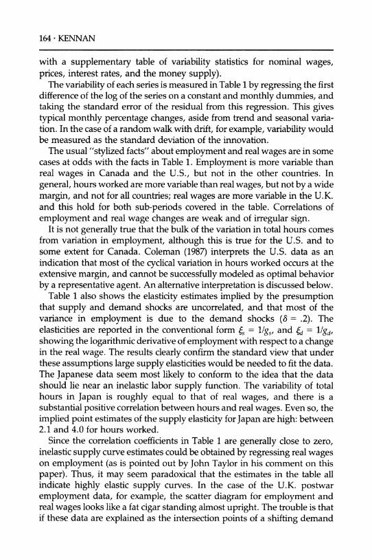
Table 1 RELATIVE VARIABILITY OF MANUFACTURING EMPLOYMENT AND REAL WAGES

CPI deflator WPI deflator Std Deviations Correlation Elasticities Std Dev Correlation Elasticities

,7, a-w C,,w ~s ed W,, C,, dnw

Postwar

Employment Austria 1965-83 0.614 1.785 Canada 1947-86 0.802 0.645 Japan 1952-85 0.543 1.332 UK 1953-83 0.387 1.375 U.S. 1947-86 0.949 0.501

Hours Canada 1947-86 1.554 0.645 Japan 1952-85 2.034 1.332 UK 1963-83 1.224 1.572 U.S. 1947-86 1.370 0.501

Employment Canada 1947-69 0.689 0.579 Japan 1952-69 0.529 1.154 UK 1953-69 0.246 0.774 U.S. 1947-69 1.006 0.521

Hours Canada 1947-69 1.407 0.579 Japan 1952-69 1.716 1.154 UK 1963-69 0.379 0.685 U.S. 1947-69 1.356 0.521

0.126 0.055 0.056

-0.018 0.196

-0.107 0.189

-0.007 0.057

0.037 -0.005 0.037 0.220

-0.010 0.184

-0.283 0.121

1.062 -0.071 1.755 4.879 -0.252 0.796 1.598 -0.083 1.318 1.546 -0.056 1.301 4.836 -0.403 0.619

26.165 -0.475 0.796 3.965 -0.323 1.318 4.036 -0.156 1.518

10.673 -0.554 0.619

Pre-1970

5.016 -0.240 0.785 2.353 -0.092 1.013 1.343 -0.064 0.641 4.652 -0.414 0.552

12.786 -0.485 0.785 3.909 -0.315 1.013

-6.055 -0.109 0.604 8.140 -0.537 0.552

-0.049 0.003

-0.028 -0.045 -0.005

-0.115 0.235

-0.046 -0.063

-0.068 -0.172

0.011 -0.013

-0.115 0.239

-0.340 -0.081

2.325 -0.069 4.960 -0.202 2.395 -0.082 1.918 -0.059 7.879 -0.306

23.219 -0.384 3.590 -0.334 5.259 -0.16

16.24 -0.438

6.653 -0.173 20.782 -0.102

1.824 -0.077 9.743 -0.364

21.423 -0.353 3.910 -0.367

-4.136 -0.124 20.780 -0.485

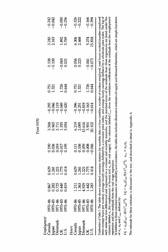
Post-1970

Employment Canada 1970-86 0.867 0.629 Japan 1970-85 0.282 1.241 Denmark 1971-86 0.725 1.221 UK 1970-83 0.440 1.775 U.S. 1970-86 0.819 0.414

Hours Canada 1970-86 1.211 0.629 Japan 1970-85 1.363 1.241 Denmark 1971-86 4.929 1.221 UK 1970-83 1.442 1.775 U.S. 1970-86 1.283 0.414

0.190 0.036 0.019

-0.017 0.195

3.568 -0.292 0.751 0.965 -0.046 1.321 2.711 -0.119 1.355 -0.049 1.726 5.054 -0.420 0.644

0.111 6.219 -0.396 0.751 0.336 2.095 -0.251 1.321 0.059 15.616 -0.819 0.008 3.901 -0.163 1.726

-0.046 20.102 -0.614 0.644

0.158 -0.100

-0.065 0.021

0.056 0.223

-0.041 -0.073

3.245 -0.242 2.163 -0.042

1.892 -0.050 5.769 -0.256

6.306 -0.326 2.468 -0.222

5.274 -0.166 15.818 -0.394

Explanation of Table 1: The table shows standard summary statistics for monthly data on four variables: number of workers employed, total hours worked (number employed times average hours per worker), average hourly earnings deflated by a consumer price index, and average hourly earnings deflated by a wholesale price index. The log of each series was first differenced and regressed on a constant and monthly dummies, and the standard errors of the residuals from these regressions are listed under the columns labeled a, (for employment or hours) and crw (for real wages). The columns labeled C,,,, show the correlation coefficients of the residuals from the employment regression and the residuals from the real wage regression. In addition to these standard measures of variability and correlation, the table also includes illustrative estimates of supply and demand elasticities, which are simple functions of o,,, oa and C,,, defined by:

1/6 = aw,[C,w+.2(1-C2,w)l2], 1/5 a = aw,[C1,,.-5(1-C2,,.)"12], a,,,,, = ajcr,,

The rationale for these estimates is discussed in the text, and described in detail in Appendix A.

164 KENNAN

with a supplementary table of variability statistics for nominal wages, prices, interest rates, and the money supply).

The variability of each series is measured in Table 1 by regressing the first difference of the log of the series on a constant and monthly dummies, and taking the standard error of the residual from this regression. This gives typical monthly percentage changes, aside from trend and seasonal variation. In the case of a random walk with drift, for example, variability would be measured as the standard deviation of the innovation.

The usual "stylized facts" about employment and real wages are in some cases at odds with the facts in Table 1. Employment is more variable than real wages in Canada and the U.S., but not in the other countries. In general, hours worked are more variable than real wages, but not by a wide margin, and not for all countries; real wages are more variable in the U.K. and this hold for both sub-periods covered in the table. Correlations of employment and real wage changes are weak and of irregular sign.

It is not generally true that the bulk of the variation in total hours comes from variation in employment, although this is true for the U.S. and to some extent for Canada. Coleman (1987) interprets the U.S. data as an indication that most of the cyclical variation in hours worked occurs at the extensive margin, and cannot be successfully modeled as optimal behavior by a representative agent. An alternative interpretation is discussed below.

Table 1 also shows the elasticity estimates implied by the presumption that supply and demand shocks are uncorrelated, and that most of the variance in employment is due to the demand shocks (8 = .2). The elasticities are reported in the conventional form s = 1/gs, and (d = 1/gd, showing the logarithmic derivative of employment with respect to a change in the real wage. The results clearly confirm the standard view that under these assumptions large supply elasticities would be needed to fit the data. The Japanese data seem most likely to conform to the idea that the data should lie near an inelastic labor supply function. The variability of total hours in Japan is roughly equal to that of real wages, and there is a substantial positive correlation between hours and real wages. Even so, the implied point estimates of the supply elasticity for Japan are high: between 2.1 and 4.0 for hours worked.

Since the correlation coefficients in Table 1 are generally close to zero, inelastic supply curve estimates could be obtained by regressing real wages on employment (as is pointed out by John Taylor in his comment on this paper). Thus, it may seem paradoxical that the estimates in the table all indicate highly elastic supply curves. In the case of the U.K. postwar employment data, for example, the scatter diagram for employment and real wages looks like a fat cigar standing almost upright. The trouble is that if these data are explained as the intersection points of a shifting demand


curve along a steep supply curve, most of the variation in employment must be explained by shifts in the supply curve. In the extreme case of a vertical supply curve, employment would not change at all if there were no labor supply shocks.5

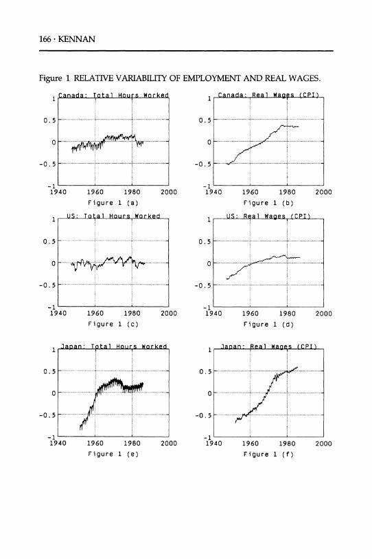
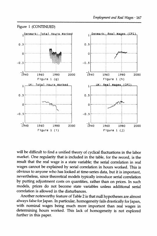
Relative variability of employment and real wages is displayed in a different way in Figure 1, which plots the two series in logs (after subtracting the sample means, but without adjusting for trends or seasonals). The plots are all drawn on the same grid to avoid optical illusions. The

plots confirm that U.S. employment is generally more variable than real

wages, but the real wage series is highly variable from 1970-1980. After 1970, there is a drop in manufacturing employment in all countries,6 and the upward trend in real wages is broken (except in Japan, where it is

merely bent). There are some unusually large real wage movements from 1970-1980, particularly in the U.K.7 There are big differences in seasonal

patterns of hours across countries, with Denmark showing the most dramatic differences.

2.1 CAUSALITY TESTS

Table 2 shows the results of tests for Granger-causality from real wages to hours worked, and vice versa, using alternative deflators and sample periods. Several tests of homogeneity are also shown, including tests

designed to indicate whether nominal wages help forecast employment, given that real wages are already included in the regression. Aside from the innovation correlations shown at the bottom of the table, the numbers are all p-values of F-statistics, giving the level of significance at which the null

hypothesis would just be rejected. The most important feature of Table 2 is that the results show no

regularity across countries and data periods. Each causality hypothesis is tested along a row of the table; it is sometimes strongly rejected (i.e. the

p-value is near zero), and sometimes easily accepted. This suggests that it

5. This point is well-known (although easily forgotten-by me). For example, Hall (1980) estimated that government military expenditures generate movements along an aggregate supply curve with an elasticity of around one-half. In response, Barro (1980) pointed out that this does not validate the intertemporal substitution model of employment fluctuations unless it can also be shown that movements in the relevant real-wage variable explain most of the movements in employment.

6. The plot of manufacturing employment in the U.K. looks like a mirror image of the unemployment plot for Britain in Layard and Nickell (1986, page S122).

7. Drobny and Gausden (1986) discuss the effects of incomes policies on real wages in the U.K. over the period 1976-1978. They argue that the data for these years (when included) dominate estimated employment/real-wage relationships. Although their data are quarterly, the monthly data used here are even more striking. In particular, the average nominal wage in manufacturing rose by 16 percent in a single month in April 1978, and by 10 percent in November 1979, due mainly to delayed wage increases for engineering workers.

166 KENNAN

Figure 1 RELATIVE VARIABILITY OF EMPLOYMENT AND REAL WAGES.

OnnrA .- T,tlr , I n l.sr, W nr rnLHl Cnar .a pail Wnne /(rPT\ 1

0.5

1

0.5 -

0 -" 0

-0.5

) 1960 1980

Figure 1 (a)

IS? Tn-tl1 Hniire WnrLaer

-1

2000 1940

1

1960 1980

Figure 1 (b)

II- Roa P1 Wne( /PrDT\

2000

0

-0.5 -

1960 1980

Figure 1 (c)

2000 -1 1940 1960 1980

Figure 1 (d)

2000

Japan: Real Wages (CPI)

1960 1980

Figure 1 (e)

2000 -1 1940 1960 1980

Figure 1 (f)

-0.5 -

-1 194C

1

0.5 -....

O -- 0 .....

-0.5 -.....

-1 1940

1

0.5

0

-1 1940

-0.5-

2000

r- I - r-r -

U I.O. I I,U I -

VI r, , uuiiuuu I/E~1- 1 . * . -, - i

I 1 I I

I. . ,

. . . . I .I

. 5

I. . . .. . . .. . ; . .. . . .. . . . .. . ... . . . .. . . .. . . .

?' . ". .

,. .,8 ? ,,,w , ,, W.,.k'"''Y

. . ........... .............,............

.............. :.......

I

. . . . . . . . . . . . . . . . . I . . - ; . . . . .

. . . . . . . .. . . . .. . . .. . .., . . . .

: : . .

_ , g

fl

: J : : I' :

S _ [v

* r : i :

J .

: r : ,

: #t : ,>

: _ z

r. .

: : . .

: : . .

i i

.......................................

.. ...

.. . . . . . . . . . . . .. . . . . ... ..,. . :.. . . . -.?,n.-: r-.---- :-

:

:??------ ?


Figure 1 (CONTINUED)

Total Hours Worked 1

0.5

0

Denmark: Real Wages (CPI)

-0.5 --.

1960 1980 2000

Figure 1 (g)

IV- Tn - 1 U-n,re W

-1 1940

1

0.5

0

1960 1980

Figure 1 (h)

II.K Da g1 Wna ,e /rPDT

1960 1980

Figure 1 (i)

2000 -1 1940 1960 1980

Figure 1 (j)

will be difficult to find a unified theory of cyclical fluctuations in the labor market. One regularity that is included in the table, for the record, is the result that the real wage is a state variable; the serial correlation in real wages cannot be explained by serial correlation in hours worked. This is obvious to anyone who has looked at time-series data, but it is important, nevertheless, since theoretical models typically introduce serial correlation by putting adjustment costs on quantities, rather than on prices. In such models, prices do not become state variables unless additional serial correlation is allowed in the disturbances.

Another noteworthy feature of Table 2 is that null hypotheses are almost always false for Japan. In particular, homogeneity fails drastically for Japan, with nominal wages being much more important than real wages in determining hours worked. This lack of homogeneity is not explored further in this paper.

0.5--

0

-0.5 -

40

L

-1 19,

1

0.5-

0-

2000

-1 1940 2000

1 T 'll ? ra?? . - rr X?-~ *vr_wwz . ll l I I .

~~~~~~~~~~~~~~...... . .........

.................. ............ ;_... .... .. ....... ..

: : . .

: : . ,

: :

: . . . .

.................... ............. ; ... ............ ....... .... . k

: : . .

: : . .

: : . .

: :

..... . ...... ... ,] ............ ...........

: e :

: r : v

: s : r :

. .

: :

. ................................... . ............................................. ................................... :

. .

: : . .

: . .

: : . .

: . .

I [

Pir, I ua, u ' i u Wl aI , l rsC - u - 1V- - -vl .

l\l~f I * %,W I \.:' L

. I

: : . .

: . . . .

: : :

- - - --- ^ - ^ - -r --*-- -- fi--?**- -------t - --

: : . .

: : . i

- ------- -- - - 9h

'. I 1h : :1 . .}

:k

* \

: : . .

_ : '

. .

: : . .

: : . .

: : . .

: : . .

t I

: : . .

: : . .

_ ; ; _

: : . .

: : . .

: :

w _ , ;] ; _

: ,_r :

: :

. r .

: : . .

. .

: : . .

_ _

. .

: :

a

: : . .

: :

:

-0. 5- -0.5

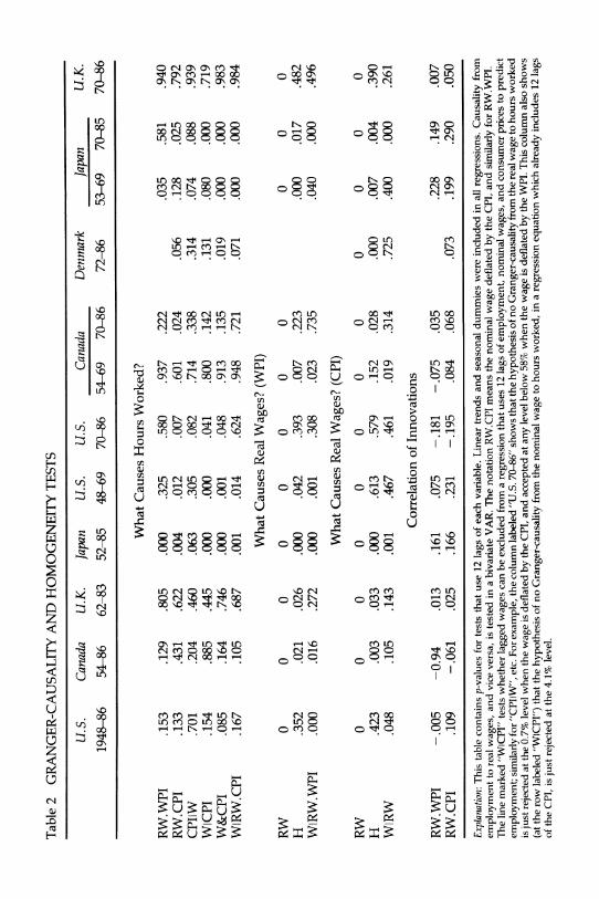
Table 2 GRANGER-CAUSALITY AND HOMOGENEITY TESTS

U.S. Canada U.K. Japan U.S. U.S. Canada Denmark Japan U.K.

1948-86 54-86 62-83 52-85 48-69 70-86 54-69 70-86 72-86 53-69 70-85 70-86

RW.WPI RW.CPI CPIIW WICPI W&CPI WIRW.CPI

.153

.133

.701

.154

.085

.167

RW 0 H .352 WIRW.WPI .000

RW H WIRW

0 .423 .048

What Causes Hours Worked?

.129 .805 .000 .325 .580 .937 .222

.431 .622 .004 .012 .007 .601 .024

.204 .460 .063 .305 .082 .714 .338

.885 .445 .000 .000 .041 .800 .142

.164 .746 .000 .001 .048 .913 .135

.105 .687 .001 .014 .624 .948 .721

What Causes Real Wages? (WPI)

0 0 0 0 0 0 0 .021 .026 .000 .042 .393 .007 .223 .016 .272 .000 .001 .308 .023 .735

What Causes Real Wages? (CPI)

0 0 0 0 0 0 0 .003 .033 .000 .613 .579 .152 .028 .105 .143 .001 .467 .461 .019 .314

Correlation of Innovations

.056

.314

.131

.019

.071

.035 .581 .940

.128 .025 .792

.074 .088 .939

.080 .000 .719

.000 .000 .983

.000 .000 .984

0 0 0 .000 .017 .482 .040 .000 .496

0 0 0 0 .000 .007 .004 .390 .725 .400 .000 .261

-.005 -0.94 .013 .161 .075 -.181 -.075 .035 .109 -.061 .025 .166 .231 -.195 .084 .068

.228 .149 .007 .073 .199 .290 .050

Explanation: This table contains p-values for tests that use 12 lags of each variable. Linear trends and seasonal dummies were included in all regressions. Causality from

employment to real wages, and vice versa, is tested in a bivariate VAR. The notation RW.CPI means the nominal wage deflated by the CPI, and similarly for RW.WPI. The line marked "WICPI" tests whether lagged wages can be excluded from a regression that uses 12 lags of employment, nominal wages, and consumer prices to predict employment; similarly for "CPIIW", etc. For example, the column labeled "U.S. 70-86" shows that the hypothesis of no Granger-causality from the real wage to hours worked is just rejected at the 0.7% level when the wage is deflated by the CPI, and accepted at any level below 58% when the wage is deflated by the WPI. This column also shows

(at the row labeled "WICPI") that the hypothesis of no Granger-causality from the nominal wage to hours worked, in a regression equation which already includes 12 lags of the CPI, is just rejected at the 4.1% level.

RW.WPI RW.CPI


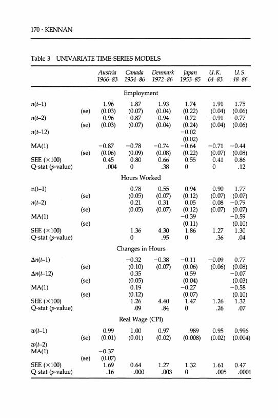
2.2 TIME-SERIES MODELS OF EMPLOYMENT, HOURS WORKED AND REAL WAGES

In order to document the serial correlation found in employment and real wages, simple ARIMA models were fit to the data for each country. The results, shown in Table 3, extend the Ashenfelter and Card (1982) discussion of the time-series properties of U.S. quarterly data. Each model included a linear trend and seasonal dummies. The first thing to be said is that any model that ignores serial correlation obviously has no chance of

fitting these data. The overall success of the ARIMA models in accounting for serial correlation may be judged by the p-value of the Box-Pierce Q-statistic which checks for serial correlation in the residuals. The cleanest result is that U.K. hours worked can be well described by a simple AR(1) model. An AR(2) fits the Danish hours data, and an ARMA(2,1) model is almost adequate for the U.S., but no satisfactory model was found for hours worked in Canada or Japan. The real wage can be described to a first

approximation by a random walk, but this approximation leaves considerable serial correlation unaccounted for, and no simple real wage model was found which would pass the Box-Pierce test, except for Austria. One

important reason for failure of these simple ARIMA models was that the

pattern of seasonal variation was too complicated to be explained by simply including monthly dummies.8

3. An Econometric Model of Competitive Equilibrium in the Labor Market In the following sections of the paper, I will analyze fully-specified models of labor market equilibrium, which are potentially capable of explaining the weak empirical association between employment and real wages, while

accounting for the strong serial correlation patterns described in Section 2. The models are built around a framework suggested by Sargent (1979), in which representative workers and employers take real wages as given, and choose employment according to dynamic labor supply and demand functions. In Section 4 a modified version of this model will be used to represent optimal dynamic wage-setting by a monopoly union which faces a dynamic labor demand curve. The empirical implications of these models are examined in Section 5 below.

This paper does not give a complete account of the various possible equilibrium interpretations of labor market fluctuations. Two alternatives must be described briefly, in order to put things in perspective. First,

8. Experiments with seasonal adjustment in the frequency domain were not successful either.

170 KENNAN

Table 3 UNIVARIATE TIME-SERIES MODELS

Austria Canada Denmark Japan U.K. U.S. 1966-83 1954-86 1972-86 1953-85 64-83 48-86

Employment

n(t-1)

n(t-2)

n(t-12)

MA(1)

SEE (xlOO0) Q-stat (p-value)

1.96 1.87 1.93 (se) (0.03) (0.07) (0.04)

-0.96 -0.87 -0.94 (se) (0.03) (0.07) (0.04)

-0.87 -0.78 -0.74 (se) (0.06) (0.09) (0.08)

0.45 0.80 0.66 .004 0 .38

Hours Worked

1.74 (0.22?)

-0.72 (0.24)

-0.02 (0.02)

-0.64 (0.22) 0.55 0

1.91 1.75 (0.04) (0.06)

-0.91 -0.77 (0.04) (0.06)

-0.71 -0.44 (0.07) (0.08) 0.41 0.86 0 .12

n(t-1)

n(t-2)

MA(1)


(se)

(se)

(se)

0.78 0.55 0.94 (0.05) (0.07) (0.12) 0.21 0.31 0.05

(0.05) (0.07) (0.12) -0.39 (0.I1)

1.36 4.30 1.86 0 .95 0

Changes in Hours

An(t-1)

An(t-12)

MA(1)


w(t-1)

w(t-2) MA(1)


(se)

(se)

(se)

-0.32 (0. 10) 0.35

(0.05) 0.19

(0.12) 1.26 .09

-0.38 -0.11 (0.07) (0.06)

0.59 (0.04)

-0.27 (0.07)

4.40 1.47 .84 0

Re;al Wage (CPI)

0.99 1.00 0.97

(se) (0.01) (0.01) (0.02)

-0.37 (se) (0.07)

1.69 0.64 1.27 .16 .000 .003

-0.09 0.77 (0.06) (0.08)

-0.07 (0.03)

-0.58 (0. 10)

1.26 1.32 .26 .07

.989 0.95 0.996 (0.008) (0.02) (0.004)

1.32 1.61 0.47 0 .005 .0001

0.90 1.77 (0.07) (0.07) 0.08 -0.79

(0.07) (0.07) -0.59 (0. 10)

1.27 1.30 .36 .04


competitive equilibrium can be decentralized in various ways. For example, labor contracts might set the employment level efficiently, while specifying a real wage that is a smooth version of the equilibrium spot market wage process. (See, for example, Abowd and Card, 1987). A different class of models regards the data as the outcome of a noncompetitive game, in which the wage is determined through bargaining between workers and

employers, and employment is determined by a labor demand curve, or, equivalently, by an Euler equation. For example, Fisher (1977) and Taylor (1980) proposed models in which nominal wages are fixed by labor contracts, and Ashenfelter and Card (1982) developed the time-series

implications of Taylor's model. Another possibility is a monopoly union model, in which the wage is set to maximize the utility of the current group of union members. Such models have recently been proposed by Blanch- ard and Summers (1986), and by Pencavel (1987). A version of the Blanchard-Summers model will be estimated in Section 5 below.

The other important aspect of labor market equilibrium which is not

analyzed here concerns the distinction between the extensive and the intensive margin of labor supply. As was shown in Table 1 above, the

variability in total hours worked in U.S. manufacturing comes mostly from

variability in the number of workers employed, rather than from average hours per worker. This has led to some spirited criticism of representative worker models by Coleman (1987), Heckman (1984), Heckman and Ma-

Curdy (1988), and MaCurdy (1987). As MaCurdy (1987) explains, for example, the wage offers rejected by unemployed workers are not observed, and yet variability of these wage offers is a potentially important part of the explanation of observed variations in employment.

In defense of the representative worker model that is used in this paper, there is reason to doubt the empirical relevance of the extensive margin in

regard to cyclical labor supply movements. First, as was mentioned above, Table 1 shows the variability of hours and employment for five countries, and in three of these the variability of total hours is far greater than the variability of employment. Second, the distinction between the intensive and the extensive margin of labor supply depends crucially on whether leisure is perfectly substitutable across periods. Decomposing the standard deviation of total hours worked into employment and average hours pieces is not a good way to tell whether the typical worker is at the interior solution of a utility maximization problem. If a change of 20 percent in annual hours is common at the individual level, as is argued by Card (1987), it must surely be common for workers to be without a job at certain times, and working 55 hour weeks at other times. Workers might well be indifferent to the choice of working 5 weeks at 40 hours per week, or 4 weeks at 50 hours, with a week off, or of working a 5-day week for 6 weeks,

172 ? KENNAN

as opposed to a 6-day week for 5 weeks, with a week off. In this light, large variations in the number of workers employed do not invalidate the

representative agent model of aggregate labor supply. At any given time some workers will be without a job, but this does not mean that their utility maximization problem has to be given special treatment.9

In what follows I will assume that the supply of labor can be approximated by a representative worker model, while acknowledging that the

empirical adequacy of this approximation is an open question.

3.1 PREFERENCES

Workers maximize an expected lifetime utility function of the form

00

U = E I RtUt[c(t), n(t), n(t - 1)] (3.1) t=l

where R is a time preference factor, c(t) and n(t) denote consumption and hours worked in period t, and the function Ut is defined by

Ut[J] = c(t) - 1/2{gs + (l+R)Ks}n(t)2 + Ksn(t)n(t-l) - v,(t)n(t)

gs + (I+R)K > 0 (3.2)

Here gs and Ks are parameters and vs(t) represents a random disturbance in the marginal rate of substitution between consumption and leisure. I assume that vs(t) has zero mean, with the understanding that all variables will be measured as deviations from trend.

Utility is linear in consumption, so if leisure is held fixed, workers will care only about the expected present value of lifetime consumption, without regard to the distribution of consumption over time. In addition, the MRS between consumption and leisure depends only on leisure, so

real-wage changes have no income effects on labor supply. This feature is attractive from a technical point of view because it allows a closed-form solution for the model. On the other hand, a backward-bending labor

supply curve is ruled out. The expected marginal utility of leisure in period t (which is also the MRS

between consumption and leisure) is given by

MU, = g,n(t) + K, {An(t) - REtn(t + 1)} + v,(t). (3.3)

9. As in the analysis of Hall and Lilien (1979), if workers have flat indifference curves for these alternatives, and if the real shocks impinge mainly on the demand side of the labor market, then it is efficient to give employers the right to vary work schedules at fixed wages.


where An(t) means n(t) - n(t - 1). Thus MUe is an increasing function of current employment, and an increasing function of steady-state employment if g, is positive. If K, is negative, as was assumed by Sargent (1979), then MUe also increases with n(t - 1) and Etn(t + 1), so that current leisure and leisure in adjacent periods are substitutes. A positive value of K, is also

plausible.

3.2 TECHNOLOGY

The production function is quadratic, with adjustment costs on employment:

q(t) = vd(t)n(t) - (llk) 1/2[(-gd)n (t)2 + Kd{n(t) - n(t - 1)}2] (3.4)

Here q and k denote output and capital, -gd and Kd are positive parameters, and vd(t) represents a zero-mean random disturbance in the marginal product of labor. The technology has constant returns to scale: if n(t), n(t - 1) and k are all doubled, then output also doubles.

3.3 COMPETITIVE EQUILIBRIUM

The competitive equilibrium for the labor market can be found by solving a planning problem in which the representative worker's utility is maximized, given the constraints imposed by the technology. Since the tech-

nology has constant returns, the planner need consider only the aggregate production function, without regard to the organization of firms. The units of capital are chosen so that there is one unit of capital for each worker in the economy. The representative worker's consumption is

c(t) = vd(t)n(t) + /2gdn(t)2 - 1/2K{n(t) - n(t - 1)}2- 0(t) (3.5)

where o0(t) units of output are allocated to the owners of capital. When this

equation is substituted in the utility function, the planning problem can be written as

00

max 9P = E , Rt2t[n(t), n(t - 1)] (3.6) n(t) t=l

where

t['] [vd(t) - vs(t)]n (t) - Y2[g, - gd + (1 + R)(K, + Kd)]n(t)2

+ [K, + Kd]n(t)n(t - 1) (3.7)

To ensure that this maximization problem is well-defined, it is necessary to assume (for reasons discussed in Kennan, 1988)

174 KENNAN

00

E Rt[vd(t) - V(t)]2 < , t=l

and

gs - gd + (1 + R)(K, + Kd) > 2 VR|K, + Kdl (3.8)

The Euler equation for the planning problem is

Vd(t) + gdn(t) - KdAn(t) + KdREtAn(t + 1) = vs(t) + gsn(t) + KsAn(t)

- KsREtAn(t + 1) (3.9)

The left side of this equation is the marginal product of labor, and the

right side is the MRS between consumption and leisure. The equilibrium stochastic process for employment makes these equal, and their common value defines a stochastic real-wage process w(t), which can be used to decentralize the solution of the planning problem. That is,10

w(t) = Vd(t) + gdn(t) - Kdn(t) + KdREtAn(t + 1) (3.10)

w(t) = Vs(t) + gsn(t) + KsAn(t) - K,REtAn(t + 1) (3.11)

3.4 SOLUTION OF THE SOCIAL PLANNING PROBLEM

Define w*(t) and n*(t) as the long-run static equilibrium price and quantity of labor which would emerge if the disturbances remained fixed at their current values. Then, as in Section 2 above,

Vd(t) Vt) gsvd(t) - gdV,(t) n*( t) = w*(t) = d() ) (3.12)

gs - gd gs - gd

The planning problem can be solved as follows. First, consider the canonical problem

10. On the assumption that the real wage is exogenous, the firm's Euler equation (3.10) can be used to estimate the dynamic demand function for labor, replacing Etn(t + 1) by n(t + 1) and using lagged values of n(t) as instruments. This method was used by Pindyck and Rotemberg (1983). Alternatively, the worker's Euler equation (3.11) can be used to estimate the dynamic supply function, using exactly the same procedure. This method was used by Mankiw, Rotemberg, and Summers (1985). It is clear from the symmetry of the Euler equations that these two "alternatives" are in fact identical, and that Euler equation estimates cannot generally identify either the supply or demand parameters.


min C [y(t)2 - 2yy(t)y(t - 1) - 2a(t)y(t)], y t=i

0 y<1/2 (3.13)

where y(O) is given. Define A as the unique number in [0,1) which satisfies

x y = (3.14)

(1 + X2)

Then, as in Kennan (1988), the solution of the canonical problem is

y(t) = Ay(t- 1) + a(t), t = 1, 2, 3... (3.15)

where

a(t) = (1 + X2) E i'a(t + i), i=O

t = 1, 2, 3 . . . (3.16)

The planning problem can be written as

min E Rt[12[gs - gd + (1 + R)(K + Kd)n(t)2 n(t) t=l

- [Ks + Kd]n(t)n(t - 1) - al(t)n(t)] (3.17)

where al(t) = vd(t) - v,(t) = (gs - gd)n*(t). This can be reduced to the canonical form as follows. First, the discount factor can be hidden and the

sign of Ks + Kd can be controlled by defining

o = viK + Kd y(t) = ctn(t) and c 2(t)= wtal(t). (3.18) |KS + Kd|

This transformation converts the planning problem to

min E [/2{gs - gd + (1 + R)(KS + Kd)}y(t)2 y(t) t=1

- V/RIK + Kdly(t)Y(t - 1) - a2(t)y(t)] (3.19)

176- KENNAN

Now divide by 1/2{g - gd + (1 + R)(K, + Kd)} to obtain the canonical

problem, where

IKS + Kdl ' =V'R ,and

gs - gd + (1 + R)(KS + Kd)

a2(t) a(t) = 2(t) (3.20)

gs - gd + (1 + R)(Ks + Kd)

The solution, using a simple certainty-equivalence argument from Kennan (1988), is given by

n(t) = In(t - 1) + (1 - i)n?(t), t = 1, 2, 3... (3.21)

where / = A/w is an optimal adjustment coefficient, and nO(t) is an "ideal" current employment level, which is defined by

n?(t) = (1 - /R) E iL'RiEtn*(t + i) (3.22) i=O

The equilibrium real wage can be found by substituting the equilibrium employment path into the Euler equation, to obtain

w(t) = gn(t) + w*(t) - gn*(t) (3.23)

where

g = Xgd + (1 - X)gs, X = Ks/(Kd + K,) (3.24)

3.5 DYNAMIC SUPPLY AND DEMAND FUNCTIONS

The competitive equilibrium decentralizes the planner's Pareto optimum by having workers and firms maximize expected discounted utility and

profits, using the discount factor R, and taking the real-wage w(t) as

given.1l Both the worker's and firm's problems can be represented by

11. The solution of the planner's problem is unique, so the equilibrium value of the marginal product of labor, wl(t), is unique. The decentralizing wage is not unique, in the sense that workers could be paid a random bonus in arrears, but the difference w(t) - w1(t) must be white noise, orthogonal to w1(t). This means that the variance of w(t) must be larger than the variance of wl(t). It may be, however, that the serial correlation properties of w(t) are different from those of w1(t): for example, if w1(t) is AR(1), then w(t) would be ARMA(1,1).

Employment and Real Wages ? 177

quadratic partial adjustment models with stochastic targets driven by w(t). The profit maximization problem for each firm is

00

max E E Rt[q(t) - w(t)n(t)] (3.25) n(t) t=1

where

q(t) = vd(t)n(t) + 1/2gdn (t)2 - 2Kd {n(t) - n (t - 1)}2 (3.26)

This can be written as

00

min E > Rt[4d{n(t) - n5d(t)}2 + ld{n(t) - n(t - 1)}2] (3.27) n(t) t=1

where

w(t) = gdnd*(t) + Vd(t) (3.28)

cPd = (1 - d)(l - R d), WPd /l,d = -gdlKd 0 < lud < 1. (3.29)

This is a version of Sargent's (1981) labor demand model. Equation (3.28) is a static labor demand curve which would hold in the absence of adjustment costs. The dynamic demand function is a partial adjustment rule

nd(t) = Ldnd(t - 1) + (1 - /Xd)(1 - IUdR) E p~Ri'Ednd(t + i) (3.30) i=l

The worker's problem can be written as

Still, the persistence of w(t) must be less than the persistence of w1(t), in the sense that the spectrum is flatter, since the spectrum of w is an average of two pieces, one being perfectly flat, and the other being wl(t).

178 * KENNAN

min E E Rt [s {n(t) - n* (t)}2 + /s {n(t) - n(t - 1)}2] (3.31) n(t) t=1

where

w(t) = gsn* (t) + vs (t) (3.32)

Os = (1 - ,s)(1 - RpXs), ksl,/s = gs!Ks, I\VR /s < 1. (3.33)

The coefficient sL is negative if Ks is negative, but 0s is always positive. If the

utility function is temporally separable (Ks = 0) then labor supply is

governed by the static supply curve (3.32). If /L is negative, the actual

supply of labor will be more variable than is indicated by equation (3.32). The dynamic labor supply function is a partial adjustment rule

ns(t) = -sns (t - 1) + (1 - pxs)(l - ps5R) usR'Etns(t + i) (3.34) i=O

The structural model is summarized by the symmetric pair of partial adjustment rules (3.30) and (3.34). The basic parameters are the adjustment coefficients /us and /d, and the slope coefficients g, and gd. The reduced form is given by equation (3.23) and the partial adjustment rule (3.21).

4. A Monopoly Union with Precommitment The structural interpretation of employment and real-wage movements

presented above involves a standard dynamic labor demand function, derived from a model of profit maximization with adjustment costs on

employment, and a less familiar labor supply function, which interacts with the demand function to determine a market-clearing equilibrium. In this section I will analyze a model in which a powerful national union is assumed to commit to a sequence of contingent plans for future wages, while firms choose employment according to the same dynamic demand function used in the previous section. Although realized wages will

depend on future disturbances, they must do so according to a functional

relationship which is announced in advance.12

12. There are two reasons for assuming precommitment, rather than assuming that the union's policy must be time-consistent. The first reason, which is not decisive, is that precommitment makes the union more powerful, and thus provides a sharper contrast to the competitive model. The second reason is that I have not yet solved the time-consistent model.


Suppose that the union can precommit to a sequence of contingent plans for employment at all future dates, where n(t) can depend on the realiza- tions of the preference shocks vs(r) and the technology shocks Vd(r), for T < t. The plan for period t can be varied independently of the plans for the other periods. The firm must be induced to go along with these plans, by establishing the right stochastic process for wages. This can be done by consulting the firm's Euler equation:

w(t) = vd(t) + gdn(t) - KdAn(t) + KdREtAn(t + 1) (4.1)

The optimal choice for the union can be found by substituting w(t)n(t) for

c(t) in the utility function, using the value of w(t) given by the firm's Euler

equation. The full effect of changing n(t) is shown by multiplying equation (4.1) by n(t) and lagging and leading one period:

c(t - 1) = Vd(t - 1)n(t - 1) + gdn(t - 1)2 - Kdn(t - 1)an(t - 1)

+ KdRn(t - 1)Et_,An(t) (4.2)

c(t) = vd(t)n(t) + gdn(t) - Kdn(t)An(t) + KdRn(t)EtAn(t + 1) (4.3)

c(t + 1) = vd(t + 1)n(t + 1) + gdn(t + 1)2 - Kdn(t + 1)An(t + 1)

+ KdRn(t + 1)Et+iAn(t + 2) (4.4)

Equation (4.2) shows that the employment level chosen in period t influences the wage in the previous period. The essential feature of the

precommitment model is that the union can exploit this link between the

present and the past.13 The time-inconsistent monopoly union's maximization problem can be

obtained by using equation (4.2) to substitute for c(t) in the utility function. It is convenient to shift the last term in equations (4.2) to (4.4) forward by one period. The problem can then be stated as

max A = E E Rt{t[n(t),n(t - 1)] (4.5) n(t) t=1

13. By making an analogy to a similar model by Hansen, Epple, and Roberds (1985), I guess that the time-consistent monopoly problem can be analyzed by assuming that the union ignores the link between n(t) and c(t - 1) shown in equation (4.2), while exploiting the links between n(t) and c(t) and c(t + 1) shown in equations (4.3) and (4.4). This introduces an asymmetry that makes the solution of the union's problem much more difficult.

180 ? KENNAN

where

Att ] = [vd(t) - v,(t)] n(t) - V2[g, - 2gd + (1 + R)(K, + 2Kd In (t)2

+ [K, + 2K d]n (t)n(t - 1) (4.6)

To ensure that this problem is well-defined, it is necessary to assume

gs - 2gd + (1 + R)(Ks + 2Kd) > 2VR IK, + 2Kdl

Define w*(t) and n *(t) as the long-run static equilibrium price and

quantity of labor that would emerge if the trend and disturbance variables remained fixed at their current values. Then

n d(t) - v s(t ) wV) (gs - gd)vd(t) - gdvs(t) n*(t) = w*(t) (4.7)

gs - 2gd gs - 2gd

The monopoly problem is essentially the same as the social planning problem, with a redefinition of parameters. Thus, the monopoly union can find out how to set employment by asking the social planner what he would do if the parameter g, were replaced by gs - gd and if Ks were

replaced by Ks + Kd. The answer is that he would use n*(t) instead of n*(t) as the static employment target, and also that he would change the speed of adjustment.

The Euler equation for the union's problem is

vd(t) + 2gdn(t) - 2KdAn(t) + 2KdREtAn(t + 1) = v,(t) + gsn(t) + Ks,n(t)

- K,REtAn(t + 1) (4.8)

The left side of this equation is the marginal revenue curve derived from the labor demand function, and the right side is the MRS between

consumption and leisure. To compare the speed of adjustment in the competitive and monopoly

models, first note that the value of y in the monopoly model is

Ks + 2KdI 3'm = M'R (4.9)

gs - 2gd + (1 + R)(Ks + 2Kd)

If Ks = 0, then y, is larger than y, and this implies that the adjustment coefficient Am must be closer to unity in the monopoly case. In other words,


when the union runs the market there is more persistence in employment than when the social planner runs it. This is true even though the

membership effects emphasized by Blanchard-Summers have been sup- pressed here.

These results must hold over some range of Ks close to zero. At the other extreme, if Kd is zero, then ym is smaller than y, so ]Lm must be closer to zero than ,u.

4.1 THE MONOPOLY WAGE

Given the employment path chosen by the union, the wage path can be inferred from the firm's Euler equation, which is

w(t) = vd(t) + gdn(t) + Kd[n(t - 1) - (1 + R)n(t) + REtn(t + 1)] (4.10)

Compare this with the union's Euler equation:

0 = [Vd(t) - v,(t)] + (2gd - g)n(t)

+ (2Kd + K,)[n(t - 1) - (1 + R)n(t) + REtn(t + 1)] (4.11)

Now use these two equations to eliminate [n(t - 1) + REtn(t + 1)], leaving an expression which determines w(t) from the union's policy for n(t).

(2Kd + K,)W(t) = (2Kd + K,)Vd(t) + (2Kd + K,)gdn(t)

+ (2Kd + Ks)Kd[n(t - 1) - (1 + R)n(t)

+ REtn(t + 1)] (4.12)

0 = Kd[Vd(t) - v(t)] + Kd(2gd - gs)n(t)

+ (2Kd + KS)Kd[n(t - 1) - (1 + R)n(t) + REtn(t + 1)] (4.13)

(2Kd + K,)W(t) = (Kd + K,)Vd(t) + Kdvs(t) + (Ksgd + Kdgs)n(t) (4.14)

This can be written as

w(t) = gmn(t) + w*(t) - gmn*(t) (4.15)

where

K, + Kd gm = Xmgd + (1 - Xm)(gs

- gd), Xm K (4.16)

2Kd + K,

So the monopolist sets both wages and employment as a social planner would if the supply slope were gs - gd, and the adjustment cost parameter

182 * KENNAN

were K, + Kd. Thus, the monopoly and competitive outcomes appear to be

equivalent, and can be distinguished only by asking which interpretation of the parameter estimates is more plausible. Since the monopoly model says that the true supply curve is flatter than that inferred from the competitive model, and since the competitive model is in trouble largely because it makes the supply curve too flat, things do not look good for the monopoly interpretation.14

5. Empirical Implementation of the Equilibrium Models To implement the competitive and monopoly models it is necessary to make specific assumptions about the supply and demand disturbances. The theoretical discussion in Section 3 referred to v,(t) and vd(t) as shocks to

preferences and technology. The empirical version of the model, however, must allow v,(t) and vd(t) to stand for the list of unmeasured variables that influence labor supply and demand. In the case of the empirical work reported below, this is necessarily a long list (since its complement is empty). In defense of this work, it seems that there is little chance of

building realistic equilibrium models of the labor market unless the interactions of dynamic labor supply and demand functions can first be sorted out in a highly simplified context.

Suppose first that the disturbances vs and vd are white noise. Then n*, w* and no are also white noise, and the equilibrium for employment and real wages is a restricted VAR(1), given by

n(t) = ,i n(t - 1) + 4 n*(t) (5.1)

w(t) = glu n(t - 1) + (g4 - 1) n*(t) + w*(t) (5.2)

In this case serial correlation in real wages is fully explained by serial correlation in employment: the real wage is not a state variable. As was shown in Table 2 above, this has no chance of fitting the data.

Suppose then that the supply and demand shocks are AR(1) processes:

vs(t) = pVs(t - 1) + 77(t), -1 < Ps < 1 (5.3)

Vd(t) = Pdvd(t - 1) + 7d(t), -1 < Pd < 1 (5.4)

14. Robert Hall pointed out to me that the results are very sensitive to the linearity of the supply and demand curves. For example, suppose that the marginal utility of leisure is a loglinear function of hours worked, and the marginal product of labor is also loglinear. Then in the static version of the monopoly model, vertical shifts in the demand curve trace out a curve parallel to the supply curve.

Employment and Real Wages'- 183

where qj(t) [rlq(t) rqd(t)]' is an innovation vector such that

E qj(t) r1(t)' = I, E q(t) 7q(T)' = 0, t f T. (5.5)

Then from equations (3.21) and (3.23)

n(t) = At n(t - 1) + vs(t) + Vt(t) (5.6) Ks + Kd 1 - Rups 1 - R Ap,

1 w(t) = g n(t) + [Kd v,(t) + Ks Vd(t)I (5.7)

K5 + Kd

These equations can be written in matrix form as

F y(t) = Jy(t - 1) + Tv(t) (5.8)

where y(t) is the vector [n(t) w(t)]', v(t) is [v,(t) vd(t)], and

1 0 ts td 0- F (Ks + Kd)T d (59)

g -1 Kd - Ks 0 0

tR td - (5.10) 1 - RAps 1 - R I?Pd

The VAR for employment and real wages is derived as

FT(I - CL) T 1(F - JL) y(t) = FT(I - CL) v(t) = FT q(t) e(t), (5.11)

where L is the lag operator, C diag(p,,pd), and FE = I. That is,

y(t) = A y(t - 1) + B y(t - 2) + 8(t), (5.12)

where

A = FTCT 1F + FJ and B -FTCT-1J. (5.13)

The second column of B is zero (since the second column of J is zero), so w(t - 2) does not enter either equation of the VAR.

184 KENNAN

The VAR has three nonzero roots,15 which match the serial correlation

parameters p, and Pd, and the market adjustment coefficient ,/, but one cannot tell which root is ps, which is Pd and which is /u. On the assumption that the three roots are distinct, the VAR coefficients in A and B can be used, as in Kennan (1988), to identify the three supply parameters is5, hs, ps, and the three demand parameters Pd, hd, pd. This gives estimates with large standard errors, and further analysis of the likelihood function is needed to determine whether there is a set of structural parameters, which is

plausible a priori, and which could have generated the data. This issue will be discussed further after the VAR estimates have been presented.

5.1 VAR ESTIMATES

Table 4 shows VAR estimates for hours worked and real wages (CPI- deflated), with both variables measured in logs, and with linear trends and deterministic seasonals included in each equation. There is no uniformity of results. At one extreme, the VAR(2) model gives a good approximation to the U.K. data, relative to a VAR(12), while at the other extreme the VAR(2) model fits the Japanese data very badly, and in fact even twelve

lags are not enough to dispose of the serial correlation in the hours equation for Japan. Given the VAR(2) approximation, w(t - 2) can always be excluded from the real-wage equation, but it is sometimes significant in the

employment equation. The VAR(2) model clearly does not allow a general explanation of the

dynamics of employment and real wages. It may be that more complicated models, which allow employment decisions to interact with inventory and

capital accumulation decisions, would capture some of the omitted dynamics. Yet, even though the simple VAR(2) model is not generally sufficient, it is also true that a more complicated model is not always necessary. In

particular, the U.K. hours variable seems to follow a simple univariate AR(1) process, which is close to a random walk.

In what follows, I will treat the VAR(2) model as an admittedly rough approximation, and use it to explore possible structural explanations for the second moments of the data, including the auto- and cross-covariances of

employment and real wages. Since the structural model discussed above refers to the levels of employment and real wages, rather than the logs of these variables, the following estimates are based on data expressed in index form (each series was divided by its sample mean, without taking logs). Table 5 shows detailed VAR(2) results, which are similar to the logarithmic results in Table 4. The exclusion restriction on w(t - 2) is tested

15. The fourth root of the VAR is zero because of the restriction that the second column of B is zero.


Table 4 VAR(2) AND VAR(12) MODELS

Denmark Canada Japan U.K. U.S.

1972-86 1954-86 1953-85 1963-83 1948-86

Hours

.774 (.051) .213

(.051) -0.014

(.113) .017

(.114) 1.38%

98.10% .00%

1.35% 4.68%

43.08% .00%

RWcpi

.022 (.023)

-0.009 (.023) .959

(.052) .035

(.052) .63%

3.85% .66%

.62% 3.65%

.32% 12.93%

.608 (.049) .380

(.048) .150

(.073) -0.176

(.073) 1.86%

.86%

.00%

1.46% .00% .39% .01%

-0.051 (.035) .057

(.034) 1.050 (.052)

-0.062 (.052) 1.33% 5.53%

.00%

1.20% .00% .00%

20. 78%

.890 (.066) .083

(.066) .023

(.052) -0.007

(.052) 1.24%

71.24% 12.08%

1.23% 38.05% 62.17% 63.66%

.034 (.084) .012

(.085) .876

(.066) .055

(.066) 1.58%

11.55% .21%

1.54% 4.00% 3.26%

13.98%

1.242 (.045)

-0.271 (.045) .180

(.140) -0.163

(.139) 1.34%

12.89% 1.29%

1.21% .82%

13.31% 35.27%

.014 (.015)

-0.017 (.015) 1.005 (.047)

-0.011 (.047) .45%

45.05% .60%

.45% 56.17% 42.77%

. 10%

Innovation Correlations

-0.068 .170 .003 .090 0.061 .166 .025 .109

VAR(2) n(t-1) (se) n(t-2) (se) w(t-1) (se) w(t-2) (se) SEE w :>n Q-stat VAR(12) SEE Lags 3-12 w - >n Q-stat

VAR(2) n(t-1) (se) n(t-2) (se) w(t-1) (se) w(t-2) (se) SEE n =>w Q-stat VAR(12) SEE Lags 3-12 n =>w Q-stat

.492 (.074) .271

(.075) .492

(.274) -0.663

(.267) 4.28%

98.00%

4.19% 17.32% 5.58%

93.97%

.002 (.021)

-0.037 (.021) .835

(.078) .096

(.076) 1.22% 5.22%

.08%

1.08% .00% .01%

63.29%

VAR(2) VAR(12)

.095

.073 -0.068 -0.061

.170

.166 .003 .025

.090

.109

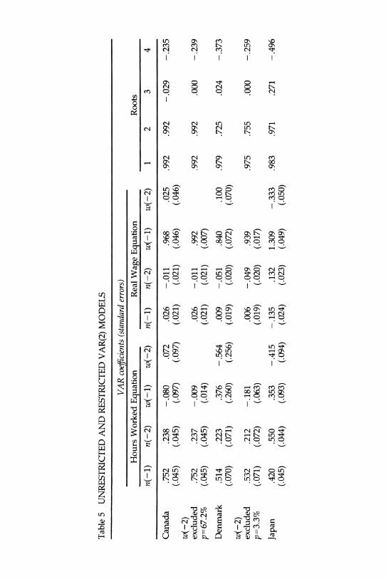
Table 5 UNRESTRICTED AND RESTRICTED VAR(2) MODELS

VAR coefficients (standard errors)

Hours Worked Equation Real Wage Equation Roots

n(-1) n(-2) w(-1) w(-2) n(-1) n(-2) w(-1) w(-2) 1 2 3 4

.752 .238 -.080 .072 .026 -.011 .968 .025 .992 .992 -.029 -.235 (.045) (.045) (.097) (.097) (.021) (.021) (.046) (.046)

w(-2) excluded .752 .237 -.009 .026 -.011 .992 .992 .992 p=67.2% (.045) (.045) (.014) (.021) (.021) (.007)

Denmark .514 .223 .376 -.564 .009 -.051 .840 .100 .979 .725 (.070) (.071) (.260) (.256) (.019) (.020) (.072) (.070)

w(-2) excluded .532 .212 -.181 .006 -.049 .939 .975 .755 p=3.3% (.071) (.072) (.063) (.019) (.020) (.017)

Japan .420 .550 .353 -.415 -.135 .132 1.309 -.333 .983 .971 (.045) (.044) (.093) (.094) (.024) (.023) (.049) (.050)

.000 -.239

.024 -.373

.000 -.259

.271 -.496

Canada

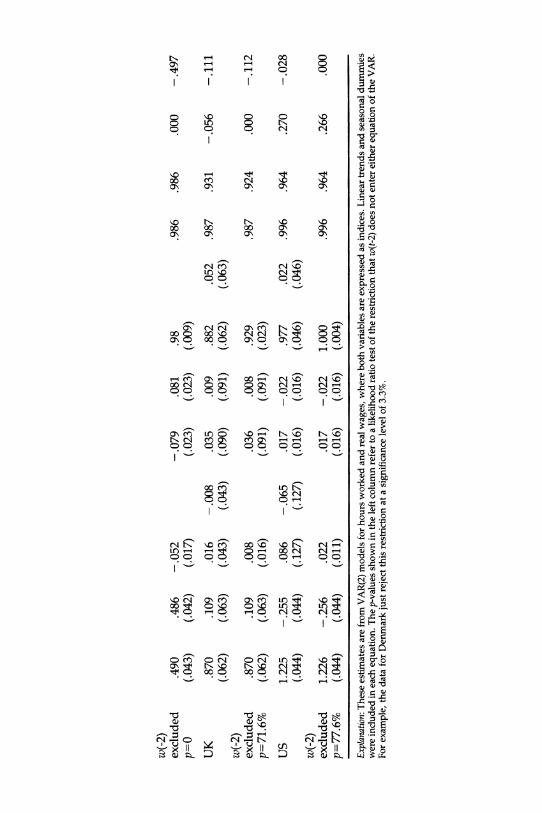
w(-2) excluded .490 .486 -.052 p=0 (.043) (.042) (.017)

-.079 .081 .98 (.023) (.023) (.009)

.986 .986 .000 -.497

.870 .109 .016 -.008 .035 .009 .882 .052 .987 .931 -.056 -.111 (.062) (.063) (.043) (.043) (.090) (.091) (.062) (.063)

w(-2) excluded .870 .109 .008 p=71.6% (.062) (.063) (.016)

.036 .008 .929 (.091) (.091) (.023)

.987 .924

1.225 -.255 .086 -.065 .017 -.022 .977 .022 .996 .964 (.044) (.044) (.127) (.127) (.016) (.016) (.046) (.046)

w(-2) excluded 1.226 -.256 .022 p=77.6% (.044) (.044) (.011)

.017 -.022 1.000 (.016) (.016) (.004)

.996 .964

.000 -.112

.270 -.028

.266 .000

Explanation: These estimates are from VAR(2) models for hours worked and real wages, where both variables are expressed as indices. Linear trends and seasonal dummies were included in each equation. The p-values shown in the left column refer to a likelihood ratio test of the restriction that w(t-2) does not enter either equation of the VAR. For example, the data for Denmark just reject this restriction at a significance level of 3.3%.

UK

US

188 KENNAN

and easily accepted for three of the five countries, but strongly rejected for

Japan (the p-values of a 2 test are shown in the table). Table 5 also shows the characteristic roots of the unrestricted and

restricted VAR(2) models for each country. In all cases two roots were found near the unit circle,16 and the next root was generally small in

magnitude, and negative in sign. This pattern is not easily explained by the model discussed above. One possibility is to account for the two big roots

by assuming that the shocks v,(t) and vd(t) follow the same autoregression, so that Ps = Pd = p. In this case A = C + FJ and B = -CFJ, and the VAR can be written as

n(t) - pn(t - 1)= -[n(t - 1) - pn(t - 2)] + en(t) (5.14)

w(t) - pw(t - 1) = gu[n(t - 1) - pn(t - 2)] + Ew(t) (5.15)

where the parameters ,/ and g may come from either the competitive or the

monopoly union model. This gives an implausible interpretation of the data, however, since the adjustment coefficient Au (which is the third root of the VAR) will generally be negative.

An alternative interpretation, which gives promising results for the U.K. data, is shown in Table 6. The two big roots are assigned to ,I and ps, meaning that preference shocks are very persistent, the market is slow to

adjust employment, and there is not much persistence in the demand shocks. The supply shock is small relative to the demand shock, and there is negative correlation between the innovations rls(t) and rlq(t). The adjustment costs on the demand side are high, so the employers' adjustment coefficient Id is about .95 (per month). The implications of this configuration will be illustrated by applying the dynamic model to the data on hours worked and real wages earned for the U.S. and the U.K.

Table 6 shows restricted maximum likelihood estimates corresponding to various assumptions about the structural parameters. The main question is whether or not plausible supply and demand elasticities can be found that fit the data, without violating the assumption that most of the variation in

employment comes from the demand shocks. For the U.S., the answer is

clearly no, as one would have expected. For the U.K., however, a

remarkably good fit is obtained with a relatively inelastic supply curve, a unit-elastic demand curve, and supply shocks which explain at most 26

16. Where two equal roots are shown, they represent a complex pair. The imaginary parts of these roots were of trivial magnitude in each instance, so the numbers shown represent both the real parts and the moduli, to three digits.

Table 6 STRUCTURAL INTERPRETATIONS OF U.S. AND UK HOURS AND REAL WAGES


Hours Worked Eq" Real Wage Eq" Innovations

n(-l) n(-2) w(-1) n(-l) n(-2) w(-) se(n) se(w) corr x (3)

U.S. 1948-71 Unconstrained

-=4 4=3.5 4-=3 s=2 &=1 s=.5

U.S. 1948-86 Unconstrained

s=6

e=5

rs=4 ~=3 UK1953-83 Unconstrained

1.278 -0.311 -0.052 0.003 -0.007 0.970 .0126 .0044 .256

se (0.056) (0.056) (0.037) (0.020) (0.020) (0.013) 1.240 -0.271 -0.021 0.021 -0.026 0.973 .0125 .0046 .288 3.24 1.215 -0.247 -0.022 0.034 -0.039 0.973 .0124 .0047 .309 8.27 1.184 -0.217 -0.023 0.050 -0.056 0.973 .0122 .0049 .332 18.27 1.108 -0.146 -0.027 0.103 -0.111 0.971 .0118 .0057 .376 77.35 1.028 -0.081 -0.040 0.252 -0.277 0.953 .0113 .0090 .380 297.25 1.040 -0.118 -0.063 0.562 -0.639 0.893 .0112 .0156 .306 601.05

1.228 -0.258 0.021 0.016 -0.020 1.000 .0130 .0050 .056 se (0.044) (0.044) (0.011) (0.017) (0.017) (0.004)

1.241 -0.257 -0.008 0.016 -0.019 0.998 .0130 .0049 .041 6.91 1.237 -0.252 -0.008 0.020 -0.024 0.998 .0130 .0049 .050 6.95 1.202 -0.217 -0.007 0.041 -0.045 0.998 .0128 .0050 .094 12.10 1.154 -0.169 -0.007 0.074 -0.078 0.997 .0125 .0053 .156 36.10

0.886 0.088 0.005 0.042 0.001 0.931 .0115 .0163 .010 se (0.062) (0.062) (0.016) (0.091) (0.091) (0.023)

-0.121 0.940 .0112 .0171 .098 6.36 =-.75 0.836 0.137 -0.006 0.165

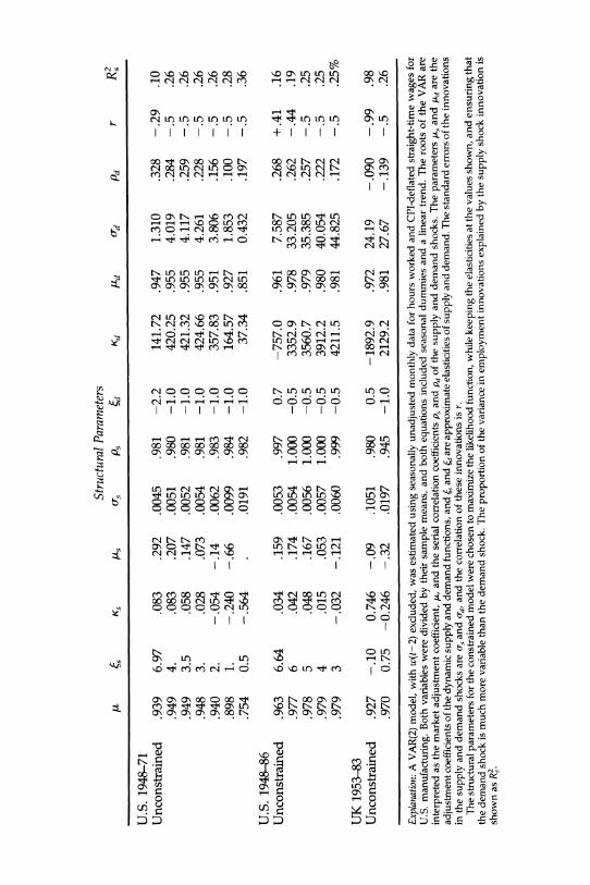
Structural Parameters . fs Ks s Uas Ps (d

U.S. 1948-71 Unconstrained .939 6.97 .083 .292 .0045 .981 -2.2

.949 4. .083 .207 .0051 .980 -1.0

.949 3.5 .058 .147 .0052 .981 -1.0

.948 3. .028 .073 .0054 .981 -1.0

.940 2. -.054 -.14 .0062 .983 -1.0

.898 1. -.240 -.66 .0099 .984 -1.0

.754 0.5 -.564 .0191 .982 -1.0

Kd tld o0d Pd r R

141.72 .947 1.310 .328 -.29 .10 420.25 .955 4.019 .284 -.5 .26 421.32 .955 4.117 .259 -.5 .26 424.66 .955 4.261 .228 -.5 .26 357.83 .951 3.806 .156 -.5 .26 164.57 .927 1.853 .100 -.5 .28 37.34 .851 0.432 .197 -.5 .36

U.S. 1948-86 Unconstrained .963 6.64 .034 .159 .0053 .997 0.7 -757.0 .961 7.587 .268 +.41 .16

.977 6 .042 .174 .0054 1.000 -0.5 3352.9 .978 33.205 .262 -.44 .19

.978 5 .048 .167 .0056 1.000 -0.5 3560.7 .979 35.385 .257 -.5 .25

.979 4 .015 .053 .0057 1.000 -0.5 3912.2 .980 40.054 .222 -.5 .25

.979 3 -.032 -.121 .0060 .999 -0.5 4211.5 .981 44.825 .172 -.5 .25%

UK 1953-83 Unconstrained .927 -.10 0.746 -.09 .1051 .980 0.5 -1892.9 .972 24.19 -.090 -.99 .98

.970 0.75 -0.246 -.32 .0197 .945 -1.0 2129.2 .981 27.67 -.139 -.5 .26

Explanation: A VAR(2) model, with w(t-2) excluded, was estimated using seasonally unadjusted monthly data for hours worked and CPI-deflated straight-time wages for U.S. manufacturing. Both variables were divided by their sample means, and both equations included seasonal dummies and a linear trend. The roots of the VAR are

interpreted as the market adjustment coefficient, A, and the serial correlation coefficients p, and p, of the supply and demand shocks. The parameters w, and Ad are the

adjustment coefficients of the dynamic supply and demand functions, and s, and d are approximate elasticities of supply and demand. The standard errors of the innovations in the supply and demand shocks are os and crd, and the correlation of these innovations is r.

The structural parameters for the constrained model were chosen to maximize the likelihood function, while keeping the elasticities at the values shown, and ensuring that the demand shock is much more variable than the demand shock. The proportion of the variance in employment innovations explained by the supply shock innovation is shown as R2.

Employment and Real Wages ? 191

percent of the variation in employment. The genesis of these results will be

briefly discussed. The estimates in Table 6 are based on the VAR(2) model with w(t - 2)

excluded, which is the reduced form of the structural model discussed above. If the innovation vector r(t) is assumed to be Gaussian, maximum likelihood estimates of the VAR(2) coefficients can be computed by least

squares regression. These unrestricted estimates are shown at the head of each panel in Table 6, along with the associated standard deviations and correlation coefficient for the estimated innovations in employment and real wages. Next, the likelihood is explored as a function of the supply elasticity 5s, while maintaining a fixed demand elasticity (either -1 or -0.5), and restricting the influence of the labor supply shock on employment. The latter restriction is accomplished by holding the correlation coefficient of -s(t) and 77d(t) above -.5, and the proportion of the variance in employment innovations explained by the supply shock innovation is shown in Table 6 as R2. Given these three restrictions, the likelihood function is maximized with respect to the six remaining structural parameters (Ks, ps, Kd, Pd, as, cd), and the likelihood ratio test of the three restrictions is shown in the column labeled 2(3).

Two sets of estimates are shown in Table 6 for the U.S. data: one for the full sample period, and one for the period 1948-1971, for purposes of

comparison with the results in Neftci (1978), Sargent (1981) and Kennan (1988). In each case, an implausibly large supply elasticity (at least 4) is needed in order to pass the likelihood ratio test.

The U.K. data, on the other hand, pass the likelihood ratio test with a

range of plausible values for the supply elasticity. The lower limit of this

range is roughly .75, and the estimates for this value are shown in Table 6. The observed serial correlation in employment and real wages is attributed to persistent (though small) labor supply shocks, and to large adjustment costs on the demand side of the labor market. There is not much serial correlation in the labor demand shocks, and the adjustment coefficient on the supply side is negative, indicating that leisure this month is a substitute for leisure next month.

The big surprise in Table 6 is that cyclical variation in the real wage is

unimportant. It is widely believed that alternative theoretical models of the business cycle can be tested against the "stylized fact" that the real wage is neither strongly procyclical nor strongly countercyclical.17 The estimates in Tables 1, 2 and 4 above confirm that the stylized fact is generally true

suggesting in particular that an equilibrium model driven by labor demand shocks cannot be expected to fit the data. Indeed, if the model is driven

17. See, for example, the Barro-King quote at the start of this paper.

192 * KENNAN

exclusively by labor demand shocks, then the predicted correlation between the employment and real wage innovations is + 1. But the estimates in Table 6 show that this prediction is not robust when small labor supply shocks are admitted. There is some ambiguity here since the innovations m7 and 'q in the labor supply and demand shocks are negatively correlated, so that even though ro- (the standard deviation of mr) is tiny relative to da, the influence of r, is not negligible. But even under the conservative assumption that all of the covariation between mr and d1 is included under the

heading of labor supply shocks, the influence of labor supply shocks on

employment is still small. In other words, the employment innovation En is a linear combination of r7, and 7d, and when En is regressed on 7sq, the R2 is .26, meaning that about 74 percent of the variation in employment is

unambiguously due to demand shocks.18

Although the dynamic model can easily accommodate acyclical real

wages, it cannot explain the other major "stylized fact": employment varies more than real wages. This can be seen in the results for the U.S. data. With a supply elasticity of .5, for example, the restricted ML estimate for the 1948-71 period leaves more variance in the real wage residual than in the

employment residual, even though the employment residual has much more variance in the unrestricted ML estimate. On the other hand, this

"stylized fact" is not true for the U.K., and so the U.K. data can be

interpreted as being largely generated by movements along a dynamic labor supply function, in response to shocks in the dynamic labor demand function.

In summary, both the competitive and the monopoly union models can in principle explain various patterns of serial correlation and cross-correlation in employment and real-wage data. In practice, it is difficult to fit the data with a structural parameter set that would include plausible supply and demand elasticities, relatively large demand shocks, and a reasonable

interpretation of the roots of the VAR. Analysis of the likelihood function for the U.K. data did, however, yield a reasonable structural interpretation. A novel feature of these results is that even though supply is inelastic, and the model is driven almost entirely by demand shocks, it is not the case that there are strong procyclical fluctuations in the real wage.

18. The sensitivity of the correlation between employment and real-wage innovations to small labor supply shocks is analyzed further in Appendix A. The correlation is small when there are large adjustment costs on the demand side, and not on the supply side, and when the supply shock is persistent and the demand shock is not.

Employment and Real Wages 193

5.2 THE BLANCHARD-SUMMERS MODEL

In a simple version of the hysteresis model presented in this space by Blanchard and Summers (1986), the union sets wages so that expected employment is a weighted average of a long-run target, r, and n(t - 1). Thus, according to their equation (3.2),

nu(t) = (1 - a)r + anu(t - 1) + vu(t) (5.16)

where vu(t) represents a random shock in the unions' objective, or a "tremble" in implementing its policy.19 When the parameter a is close to 1 there is hysteresis in employment, meaning that employment will look like an integrated process (as it does in Table 3 above). This is combined with the dynamic labor demand function (3.30) to obtain equilibrium employment and real wages.

If the shocks vu(t) and vd(t) are AR(1) processes, the Blanchard-Summers model implies a restricted VAR(2) for employment and real wages, in which the real wage does not Granger-cause employment, and w(t - 2) is excluded from the real-wage equation. This result is derived as follows. Write the firm's Euler equation written as

w(t) = v(t) + [g, - (1 + R)Kd]n(t) + Kdn(t - 1) + KdREtn(t + 1) (5.17)

Use the union's employment rule (5.16) to substitute for Etn(t + 1), so that

w(t) = vd(t) + KdRpuVu(t) + [gd + RKda - (1 + R)Kd]n(t) + Kdn(t - 1) (5.18)

where p, is the serial correlation coefficient of vu(t). Write equations (5.16) and (5.18) as

Fuy(t) = Juy(t - 1) + Tuv(t) (5.19)

1 0 1 0 a 0 Fu = Td = . (5.20)

f -1 -KdRpu - Kd 0

19. In Pencavel and Holmlund's (1987) model the union's objective function depends on n(t) and w(t), and also on w(t - 1), because the union's "aspirations" with regard to the wage may depend on previously established levels of the wage. An implication of this setup is that the real wage becomes a state variable, even when the disturbances are white noise. This is not true in the Blanchard-Summers model, although the two models are otherwise similar.

194 KENNAN

where v(t) is [v~(t) vd(t)]', and f = gd + RKda - (1 + R)Kd. The VAR for employment and real wages is then

y(t) = Auy(t - 1) + Buy(t - 2) + e(t), (5.21)

where

A = Fu,TCT-IF, + FJ, and B, =-F,,TuCT1J,. (5.22)

Pu +a 0

(f + KdRpu)(Pu - Pd) + af + Kd Pd

-- apu B= (5.23)

-apu[f + KdR(pu - Pd)] - KdPd 0

As in the competitive model, the second column of Bu is zero (since the second column of Ju is zero), so w(t - 2) does not enter either equation of the VAR. In addition, all of the matrices in equation (5.22) are lower

triangular, so w(t - 1) is excluded from the employment equation, and the real wage does not Granger-cause employment. The three nonzero roots are p,, Pd and the "hysteresis" parameter a, where p, and a appear in the

employment equation, and Pd is the coefficient of w(t - 1) in the real wage equation.

After subjecting equation (5.23) to some algebraic torture, estimates can be extracted of all of the structural parameters of the Blanchard-Summers model. Table 7 shows results for hours worked and real (CPI-deflated) wages.20 The roots of the VAR do not involve any demand-side parameters except for the serial correlation parameter of the demand shock. This means that there is not much room for adjustment costs as an explanation of the serial correlation in employment and real wages. In fact the estimates of the demand parameters Kd and (d (= l/g) are very weak, since they come

mainly from wobbly estimates of the off-diagonal coefficients in the VAR. The point estimate of ( generally has the wrong sign, and the estimated

adjustment cost is negative for the U.S. It is possible, however, that

plausible structural parameter values could be found that would give a reasonable fit to the data.

20. Using employment data in place of hours worked might be more in the spirit of the insider-outsider model, but the empirical results are equally discouraging when employment data are used.

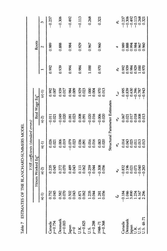
Table 7 ESTIMATES OF THE BLANCHARD-SUMMERS MODEL


Hours Worked Eq" Real Wage Eq" Roots

n(-1) n(-2) n(-1) n(-2) w(-1) 1 2 3

Canada p=0.754 Denmark p=0.003 Japan p=0 U.K. p=0.825 U.S. p=0.288 1948-71 p=0.368

0.752 0.045

0.582 0.070

0.502 0.043

0.871 0.062

1.235 0.044

1.281 0.056

0.235 0.045

0.272 0.070

0.489 0.043 0.111 0.062

-0.259 0.044

-0.308 0.056

0.026 0.021

0.006 0.019

-0.079 0.023

0.036 0.091

0.016 0.016

0.003 0.020

-0.011 0.021

-0.049 0.020

0.081 0.023

0.008 0.091

-0.020 0.016

-0.006 0.020

0.992 0.007

0.939 0.017

0.984 0.009

0.929 0.023

1.000 0.004

0.970 0.013

0.992

0.939

0.994

0.984

1.000

0.970

0.989

0.888

0.984

0.929

0.967

0.960

-0.237

-0.306

-0.492

-0.113

0.268

0.321

Structural Parameter Estimates

Canada Denmark Japan U.K. U.S. U.S. 48-71

-0.184 1.046 3.890 1.234 6.167 2.296

Kd

-0.832 0.196 0.021 0.071

-0.040 -0.283

au

0.014 0.043 0.025 0.011 0.013 0.013

0.067 0.021 0.017 0.018 0.008 0.013

rud

0.995 -0.839

0.630 -0.396 -0.787 -0.943

Pd

0.992 0.939 0.984 0.929 1.000 0.970

a

0.989 0.888 0.994 0.984 0.967 0.960

PS

-0.237 -0.306 -0.492 -0.113

0.268 0.321

196 * KENNAN

Both the competitive model and the Blanchard-Summers model attribute two roots of the VAR to serial correlation in the disturbances. The other root is explained by adjustment costs in the competitive model, and by the union's policy of protecting insiders in the Blanchard-Summers model. Thus the observed inertia in employment is explained by saying either that

employers find it expensive to make rapid changes, or that unions do not allow rapid changes. In either case the inertia in real wages is attributed to a shock that is close to a random walk. The Blanchard-Summers model calls this the technology shock, while the version of the competitive model

displayed in Table 6 calls it the preference shock. The remaining serial correlation is mopped up by mildly persistent shocks in the union's

preferences, or in technology.

6. Conclusion The empirical findings in this paper are consistent with the view that an

equilibrium model driven mostly by labor demand shocks requires a large short-run labor supply elasticity in order to explain why employment varies more than the real wage. Whether a large elasticity is implausible depends on one's view of the estimates extracted from panel data on individuals (see, for example, Ashenfelter (1984), and the discussion by Heckman (1984)).

As Card (1987) points out, low supply elasticities estimated from the micro data do not arise because individuals are reluctant to vary hours worked. In fact, the standard deviation of year-to-year changes in hours worked at the individual level is on the order of 20 percent in U.S. data, while in a typical cyclical downturn the change in aggregate hours is less than 3 percent. Thus, the individual variations are an order of magnitude larger than is needed to explain cyclical fluctuations. The trouble is that the source of the individual variations is not pinned down in the microdata, and in particular, variations in hours are not associated with variations in

wages.21 The level of time aggregation seems crucial in matching the micro data

and the aggregate data. The micro elasticity estimates are based on

life-cycle models that were not designed to measure short-run elasticities. In fact, these models assume that leisure in February 1989 is a perfect substitute for leisure in October 1989. The life-cycle model produces estimates like .1 for the elasticity that governs the redistribution of leisure

21. Note that there are also large variations in wages at the individual level, as was shown by Altonji and Ashenfelter (1980), although the transitory variations emphasized in the intertemporal substitution model are much smaller than the whole.


over the life-cycle in response to movements along the age-earnings profile. This is consistent with short-run behavior in which workers care only about total consumption and total leisure time, averaged over several months or a year, provided that the work schedule is not too extreme (e.g. 18-hour days or 84-hour weeks). Indeed, a short-run elasticity of .1 is not credible: a 30 percent wage increase is not needed to call forth a 3 percent increase in hours worked (this would mean that in order to get someone to stay 15 minutes longer on the job today, he would have to be paid 30 percent more for the whole day).22 In the standard econometric version of the life-cycle model, a business cycle consisting of regular oscillations within a period of six months would generate no real-wage response. What is needed is an

analysis of the response to irregular oscillations with a period of several

years, in the context of a life-cycle model with a period length of days or weeks.

This paper has also emphasized the importance of accounting for the serial correlation in employment and real wages within an equilibrium model. For example, a particular reading of serial correlation was crucial in

obtaining a plausible structural interpretation of the U.K. data. A better

understanding of serial correlation might be gained by interpreting real

wages as the shadow price of labor services in a stochastic growth model. For example, Hansen and Sargent (1987) have recently used such a model to analyze the equilibrium premium for overtime, although they do not

develop the implied time-series properties of real wages. Finally, this paper has dealt only with the basic building-blocks of

dynamic equilibrium models of the labor market. The empirical work has concentrated on cataloging the facts to be explained, and assessing whether

equilibrium explanations are worth pursuing. I think they are. But the

paper has ignored obviously relevant information in order to concentrate on basic structural explanations of the variability, covariability, and serial correlation found in employment and real-wage data. As Mark Bils points out in his comment below, the "unobservable" supply and demand shocks in the models discussed above correspond substantially to observable movements in output, capital, taxes, incomes policies, and so forth. Indeed, many one-sided models of aggregate labor supply or demand include a rich collection of explanatory variables, but these models do not

explain how the equilibrium real wage is determined. The next step is to

22. Introspection gives imprecise estimates of the elasticity of supply. If I say that your wage rate is going up temporarily by 10 percent and ask how much extra you want to work in response, the answer may be essentially nil. If, instead, I say that you are being asked to work 10 percent more, and ask how much your wage rate has to be raised to get you to agree to this, the answer is perhaps that the usual wage is good enough. One of these estimates gives a zero elasticity, and the other gives an infinite elasticity.

198 * KENNAN

bring such variables into the equilibrium model, through modifications in the assumptions about preferences and technology.

Appendix A: Derivations

THE ELASTICITIES IN TABLE 1

Write the variance matrix of the shocks as

s2 Urd 82 8r Var[n(t)] =

s = (A.1) OCsd Cd 8r 1

where r is the correlation coefficient of q7 and qd. Then the variance matrix of employment and real wages in the static model is

n(t) 1 Cov =

w(t) (g - gd)2

r2 + O - 20asd o-sgd + Or'gs - (gs + gd)sd (A.

CTsgd + 0igs - (gs + gd)(sd sgd + LST - 2gsgdUsd

Define the variance ratio a2 = Var(w)/Var(n), and the correlation coefficient Cnw = Cov(n,w)/[Var(n)Var(w)]1/2. Then

g[1 + 82a2 + 2a8r]

a2 1 2 (A.3) awn 1 + 82 - 2r (A3)

1 - 82a + (a - 1)8r C,w (A.4)

[(1 + 82 - 28r)(1 + 82a2 + 2a8r)]1/2 (

where a = -gd/gs. Let b,w = Cnw an denote the regression coefficient of w on n, and note that the Cauchy-Schwartz inequality means (bwn)2 - a2 The estimates in Table 1 assume that the supply and demand shocks are uncorrelated (r = 0). Then

a2= + (1 - )gs (A.5)

and

bwn = gd + (1 - )gs (A.6)


where

o2 2

2 + r = 1 2 (A.7) 2cr + ( 1+ 4 2

When a value is assigned to 8, equations (A.5) and (A.6) can be solved to obtain the supply and demand elasticities. Rearrange and square equation (A.6) to get

(bn)2 -

2tugdbWn + tI2g5 = (1- I_ )2g2 (A.8)

(bwn)2 - 2gdbwn + /2g% = (1 - q,)a2 n - 4(1 - _ )g3 (A.9)

l(bwn)2 - 2fgdbwn + ,g = (1 - q)[a2n - (bwn)2] (A.10)

So23

gd = bwn - (1/)[a2n - (bw)2]1/2 = awn[Cnw - (1/8)(1 - C2w)1/2] (A.11)

and

gs = bwn + 8 [awn - (bn)2]1/2 = a,n[Cnw + (1 - C,2)1/2] (A.12)

VARIABILITY AND CORRELATION IN THE DYNAMIC EQUILIBRIUM MODEL

From equations (5.6) and (5.7) the innovations en(t) and Ew(t) in employment and real wages can be written as

p, -1 1 ?n(t) = r (t) + 1

d(t) (A.13) Ks + Kd 1 - RAtps 1 - Rd,pd

1 W(t) = g En(t) + [Kd nrs(t) + KS '7d(t)] (A.14)

KS + Kd

Thus

n(t) = d(t) - v(t) (A.15)

23. There are two solutions. In a diagram with /1 - /,g on the horizontal and V/gd on the vertical axes, equation (A.5) is a circle around the origin, and equation (A.6) is a straight line with negative slope. I pick the southeast solution, which practically ensures that the demand elasticity is negative.

200 * KENNAN

ew(t) = avd(t) - adv(t) (A.16)

where

/~ 1 1 d 1 v(t) = rs(t); Vd(t)= r d(t) (A. 17)

Ks + Kd 1 - Rtzps Ks + Kd 1 - RALzpd

and

Ks(l - Rtpd) Kd(l - Rtps) as = g + ; ad = g - (A.18)

The variance matrix of the innovations then has a form similar to that shown in equation (A.2) above for the static model:

/I2 Var[E(t)] =

(Ks + Kd)2

tr + Tr - 2rsd rTas + rad - (as + ad)rsd

rta, + 7Tad - (as + ad)7Td rT2a + 7ra 2 - 2asadTsd

where

Ors O'd O'sd r7s = ; r = ; Ted = (A.20)

1 - R=tps 1 - RPd (1 - R Lpd)(1 - Rpps)(l RP (d)

The correlation between the employment and real-wage innovations is

1 - S2ao + (ao - 1)S,r Corr[e,(t), ew(t)] = (A 21)

[(1 + 82 2&6r)(1 + 8, a + 2ao87r)]/2

where aO = -ad/as, and , = r/Td. Evidently, if 86 is zero then the innovations are perfectly correlated. Also, if 86 is small then the correlation is well approximated by

1 - a2ao + (ao - 1) ,r Corr[E,(t), Ew(t)] = + (A.22)

(1 + a + 2ao8Tr)

Note that if Ps is close to unity, while Pd is close to zero (as is true in Table 6), 8, will be much larger than 8, and this reduces the correlation of the

Employment and Real Wages - 201

innovations. Also, if a0 is large in magnitude, the correlation may be far from unity, even when 8, is small. This means that even if the supply shocks are small in terms of their influence on the employment innovations, they may nevertheless be enough to explain why the correlation between the employment and real-wage innovations is small. This possibility is governed by the magnitude of a0, which is determined by

-ad Kd(l - Rtp,,) - gRp (A Cao = = (A.23)

as Ks(1 - RgApd) + gAx

In Table 6 the estimates of Ks are near zero, while Kd is very large, so that aO is large. This configuration allows the dynamic model to explain small correlations between the employment and real wage innovations.

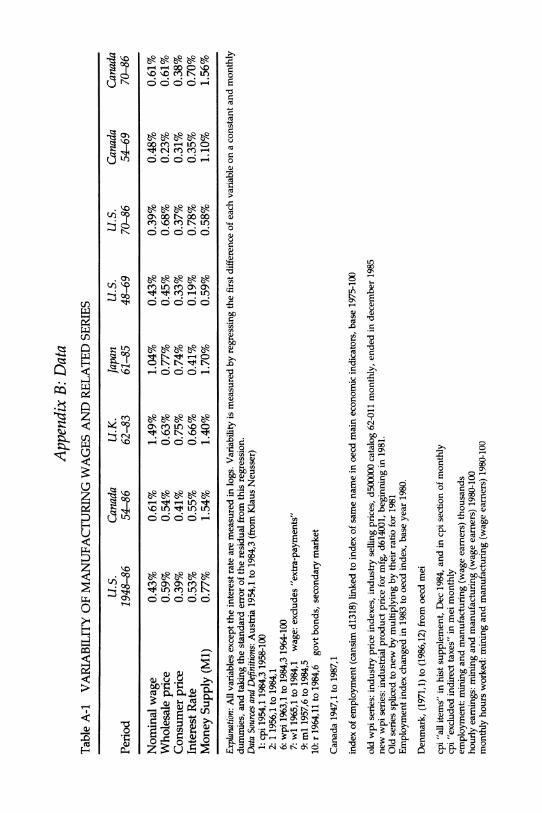
Appendix B: Data Table A-1 VARIABILITY OF MANUFACTURING WAGES AND RELATED SERIES

U.S. Canada U.K. Japan U.S. U.S. Canada Canada Period 1948-86 54-86 62-83 61-85 48-69 70-86 54-69 70-86

Nominal wage 0.43% 0.61% 1.49% 1.04% 0.43% 0.39% 0.48% 0.61% Wholesale price 0.59% 0.54% 0.63% 0.77% 0.45% 0.68% 0.23% 0.61% Consumer price 0.39% 0.41% 0.75% 0.74% 0.33% 0.37% 0.31% 0.38% Interest Rate 0.53% 0.55% 0.66% 0.41% 0.19% 0.78% 0.35% 0.70% Money Supply (M1) 0.77% 1.54% 1.40% 1.70% 0.59% 0.58% 1.10% 1.56%

Explanation: All variables except the interest rate are measured in logs. Variability is measured by regressing the first difference of each variable on a constant and monthly dummies, and taking the standard error of the residual from this regression. Data Sources and Definitions: Austria 1954,1 to 1984,3 (from Klaus Neusser)

1: cpi 1954,1 1984,3 1958-100 2: 1 1956,1 to 1984,1 6: wpi 1963,1 to 1984,3 1964-100 7: wl 1965,1 to 1984,1 wage: excludes "extra-payments" 9: ml 1957,6 to 1984,5

10: r 1964,11 to 1984,6 govt bonds, secondary market

Canada 1947,1 to 1987,1

index of employment (cansim d1318) linked to index of same name in oecd main economic indicators, base 1975-100

old wpi series: industry price indexes, industry selling prices, d500000 catalog 62-011 monthly, ended in december 1985 new wpi series: industrial product price for mfg, d614001, beginning in 1981. Old series spliced to new by multiplying by their ratio for 1981 Employment index changed in 1983 to oecd index, base year 1980.

Denmark, (1971,1) to (1986,12) from oecd mei

cpi "all items" in hist supplement, Dec 1984, and in cpi section of monthly cpi "excluded indirect taxes" in mei monthly employment: mining and manufacturing (wage earners) thousands hourly earnings: mining and manufacturing (wage earners) 1980-100 monthly hours worked: mining and manufacturing (wage earners) 1980-100

japan 1952,1 to 1985,12 arbci-annual report on business cycle indicators, economic planning agency, japanese government ha39.j3k4

See also year book of labour statistics, 331.0652 j35 Monthly statistics of japan 315.2 j352ms

1. Index of regular workers employed, mfg, arbci #179, (not oecd) 2. Index of hours worked per mo. Regular workers, mfg, arbci #181

Hours worked exclude rest periods, paid or unpaid. 3. Index of regular wages and salaries, reg. Workers, mfg. 1980-100

this series is called "contractual cash earnings" in year book not published in monthly statistics of japan, or in oecd

4. Index of wholesale prices, mfg ind. Products, arbci #203 5. Consumer price index, all commodities, all japan, arbci #208 data for 1952-1959 from monthly statistics of japan 9. M1 money supply, oecd

10. Interest rate on call money, oecd

UK (1953,1) to (1986,12)

h is an index of average weekly hours worked per operative in manufacturing base 1962-100. Historical abstract table 148; yearbook table 79 Dept of Employment Gazette, Aug 1962 pp 305-307, and Oct 63, page 404 "In February 1972 and again in January, February and March 1974, the volume of overtime and short-time was affected by the energy crisis." Year Book 1974, page 198, note. Hours fell by about 6.5% in Feb 1972, and by about 10% in Jan and Feb 1974. w is basic hourly rates of wages in manufacturing (index) base July 1972 These are rates negotiated in national collective agreements, and do not reflect local variations. r: 91-day t-bills ("average rate of allotment on last issue of month") mei

U.S. (1947,1) to (1987,3)

LPWM6 production workers on mfg payrolls nsa citibase PZR cpi revised wage earners, nsa, citibase LEXMO ahe excluding ot mfg, production workers, nsa, citibase total production worker payroll divided by (total production worker hours + 1/2 total overtime hours). PWM producer price index manufactured goods, citibase, nsa LPHRM6 awh production workers on mfg payrolls, nsa, citibase Hours means hours paid for during the pay period including the 12th of the month. Paid vacation and sick leave is included.

fygm3 3-month t-bill rates secondary market citibase fzml old ml 1947-1979,1 citibase fzml new ml 1959-1981,12 citibase Employment data adjusted to March 1986 benchmark

The data are available on diskette.

204 KENNAN

I thank Mark Bils, Tom MaCurdy, Tom Mroz, John Pencavel, John Taylor, and the participants in seminars at Berkeley and the Hoover Institution for helpful comments. The paper was completed while I was a National Fellow at the Hoover Institution. The research was supported by an honorarium from NBER, and was funded in part by the National Science Foundation, under grant SES-8607771.

REFERENCES

Altonji, J. and 0. Ashenfelter. 1980. Wage movements and the labor market equilibrium hypothesis. Economica 47: 217-245.

Abowd, J. M., and D. E. Card. 1987. Intertemporal labor supply and long-term employment contracts. American Economic Review 77(March): 50-68.

Ashenfelter, O. Macroeconomic analyses and microeconomic analyses of labor supply. Carnegie-Rochester Series on Public Policy 21(1984): 117-156.

Ashenfelter, 0., and D. Card. 1982. Time-series representations of economic variables and alternative models of the labour market. Review of Economic Studies 49: 761-782.

Barro, R. J. Discussion of Robert E. Hall's 'Labor supply and aggregate fluctuations'. In On The State of Macroeconomics, ed. K. Brunner and A. Meltzer. Carnegie- Rochester Series on Public Policy 12(1980): 35-38.

Barro, R. J., and R. G. King. 1984. Time-separable preferences and intertemporal- substitution models of business cycles. Quarterly Journal of Economics (November): 817-839.

Bils, M. 1985. Real wages over the business cycle: Evidence from panel data. Journal of Political Economy 93: 666-689.

Blanchard, O. J., and L. H. Summers. 1986. Hysteresis and the European unemployment problem. In NBER Macroeconomics Annual, ed. Stanley Fischer. Cam- bridge: MIT Press.

Blank, R. M. 1987. Why are wages cyclical in the 1970's? Working Paper #224, Industrial Relations Section. Princeton University (uly).

Burda, M. C., and J. D. Sachs. 1987. Institutional aspects of high unemployment in the Federal Republic of Germany. NBER Working Paper No. 2241 (May).

Card, D. 1987. Supply and demand in the labor market. Working Paper #228, Industrial Relations Section. Princeton University (November).

Coleman, T. S. 1987. Employment and hours in the U.S. Research Paper No. 298, SUNY Stony Brook (July).

Drobny, A., and R. Gausden. 1986. Granger-causality, real factor prices and employment: A re-appraisal with U.K. data. Unpublished draft (December).

Fischer, S. 1977. Long-term contracts, rational expectations and the optimal money supply rule. Journal of Political Economy 85: 191-205.

Geary, P. T., and J. Kennan. 1982. The employment-real wage relationship: An international study. Journal of Political Economy 90 No. 4(August): 854-871.

Hall, R. E. 1980. Labor supply and aggregate fluctuations. In On The State of Macroeconomics, ed. K. Brunner and Allan Meltzer. Carnegie-Rochester Series on Public Policy 12: 7-33.

Hall, R. E., and D. M. Lilien. 1979. Efficient wage bargains under uncertain supply and demand. American Economic Review 69 (5) (December): 868-879.

Hansen, G. D., and T. J. Sargent. 1987. Straight time and overtime in equilibrium. Unpublished, (September).

Hansen, L., D. Epple and W. Roberds. 1985. Linear-quadratic duopoly models of resource depletion. In Energy, Foresight and Strategy, ed. Thomas J. Sargent. Washington D.C.: Resources for the Future.


Heckman, J. 1984. Comments on the Ashenfelter and Kydland papers. Carnegie- Rochester Series on Public Policy 21: 209-224.

Heckman, J., and T. MaCurdy. 1988. Empirical tests of labor market equilibrium: An evaluation. Carnegie-Rochester Series on Public Policy. Forthcoming.

Kennan, J. 1979. The estimation of partial adjustment models with rational expectations. Econometrica 47(November): 1441-1456.

Kennan, J. 1988. An econometric analysis of fluctuations in aggregate labor supply and demand. Econometrica 56 (March): 317-333.

Keynes, J. M. 1939. Relative movements of real wages and output. Economic Journal 69(March): 34-51.

Killingsworth, M. R., and J. J. Heckman. 1986. Female labor supply: A survey. In Handbook of Labor Economics, ed. Orley Ashenfelter and Richard Layard. Amster- dam: North-Holland.

Layard, R., and S. Nickell. 1986. Unemployment in Britain. Economica 53: S121- S169.

Lilien, D. M., and R. E. Hall. 1986. Cyclical fluctuations in the labor market. In Handbook of Labor Economics, ed. Orley Ashenfelter and Richard Layard. Amster- dam: North-Holland.

Lucas, R. E., Jr. 1977. Understanding business cycles. Reprinted in Studies in Business Cycle Theory.

MaCurdy, T. 1987. Problems with testing the intertemporal substitution hypothesis. Unpublished draft. Stanford University (September).

Mankiw, N. G., J. J. Rotemberg, and L. H. Summers. 1985. Intertemporal substitution in macroeconomics. Quarterly Journal of Economics 100(February): 225-251.

Moffitt, R., M. Keane, and D. Runkle. 1987. Real wages over the business cycle: Estimating the impact of heterogeneity with micro data. Working Paper (March).

Neftci, S. N. 1978. A time-series analysis of the real wages-employment relationship. Journal of Political Economy 86 (2) (April): 281-291.

Newell, A., and J. Symons. 1987. Mid-1980's unemployment. Discussion Paper No. 283, Centre for Labour Economics, LSE (une).

Nickell, S. 1984. An investigation of the determinants of manufacturing employment in the United Kingdom. Review of Economic Studies 51(4) (October): 529-557.

Pencavel, J. 1986. Labor supply of men: A survey. In Handbook of Labor Economics, ed. O. Ashenfelter and R. Layard. Amsterdam: North-Holland.

Pencavel, J., and B. Holmlund. 1987. The determination of wages, employment, and work hours in an economy with centralized wage-setting: Sweden, 1950-83. Unpublished manuscript. Stanford University (October).

Pencavel, J. 1987. The classical unemployment hypothesis and international com- parisons of labor market behavior. Unpublished manuscript. Stanford University (September).

Pindyck, R. S., and J. J. Rotemberg. 1983. Dynamic factor demands and the effects of energy price shocks. American Economic Review 73(5) (December): 1066-1079.

Sargent, T. J. 1979. Macroeconomic Theory. New York: Academic Press. Sargent, T. J. 1981. Estimation of dynamic labor demand schedules under rational

expectations. In Rational Expectations and Econometric Practice, ed. Lucas, R. E. Jr. and T. J. Sargent. Minneapolis: The University of Minnesota Press.

Stockman, A. C. 1983. Aggregation bias and the cyclical behavior of real wages. First Annual NBER Macro Conference, Cambridge.

Taylor, J. B. 1980. Aggregate dynamics and staggered contracts. Journal of Political Economy 88: 1-23.

206 * BILS

Comments MARK BILS University of Rochester, Visiting the NBER

John Kennan examines implications of a market-clearing view of the behavior of employment and wage rates. Employing data for a half dozen countries, Kennan goes far beyond the narrow question of whether there is a "procyclical real-wage puzzle" or "countercyclical real-wage puzzle" to ask what restrictions on labor supply and demand are implied by the relative variability of wages and employment and the autocorrelations of the two series, as well as their correlation. This is a very useful exercise. I think it can be viewed as augmenting the empirical real business cycle literature (e.g., Prescott, 1986) which typically has ignored matching model

predictions to actual behavior of wage rates. Under an assumption that disturbances to labor demand predominate,

one conclusion Kennan draws is that for the actual fluctuations to be consistent with market clearing fluctuations a relatively flat labor supply curve (high elasticity of labor supply) is required. Of course, this is not a novel or surprising result, and is not marketed as such. A further result, which I think is an insight of the exercise, is that the data require two

separate theoretical sources for strong autocorrelation. This is because the

orthogonal components of wage and employment series each show great persistence. Kennan suggests this might be consistent with high adjustment costs to the firm of adjusting labor input, together with very persistent disturbances driving the labor demand process; but this further

requires that innovations to the labor supply process be white noise or even

negatively serially correlated. Finally, a single framework does not appear applicable across the different countries. Either supply and demand elasticities or the relative variability of demand and supply must vary across countries.

One major criticism of Kennan's exercise is that the model he examines-

employment and wages continuously varying to equate supply and demand-is very much a strawman. In the aftermath of implicit-contracting theory, one reasonably popular view of the labor market is that while compensation payments are smoothed for insurance, tax, or convenience reasons, firms and workers may exploit other mechanisms to arrive at choices for employment that approximately equate supply and demand. Recently Rhee and Espinosa (1987) have shown that in a repeated game, labor outcomes arbitrarily close to equating supply and demand are

Comments 207

possible even if the wage rate is not close to the market clearing value. Their results support Hall's (1980) contention that long-term attachments between firms and workers may provide a setting for achieving efficient labor choices despite rigidly set wages. In such a setting the wage series has a life of its own; and thus Kennan's approach of describing restrictions generated on wage series from market clearing will not be appropriate. That is, concluding that the wage and employment series together are not generated from the intersection of supply and demand does not tell you that the

employment series is not so generated; and presumably it is the behavior of employment that is of primary interest. Of course, the view of wage payments as pure installment payments is an equally extreme view. It may require a level of cooperation between firms and workers that one might argue we do not observe. Furthermore, the empirical success of this literature to date consists of having sufficiently weak empirical predictions that it is difficult to refute.

Kennan asks whether an equilibrium model is consistent with the data, given reasonable values for such factors as the importance of supply versus demand disturbances, the elasticities of labor supply and demand, persistence of supply and demand disturbances, and the importance of past employment in supply and demand decisions. A major problem with this

approach, however, is that we really have only weak notions for what constitutes reasonable values for each of these factors.

For example, in much of the paper Kennan assumes that demand disturbances are of principal importance. But this completely depends on what macro disturbances are affecting the economy. If we assume market

clearing in the goods market as well as in labor, then disturbances to the demand for goods, such as changes in government spending or temporary changes in firms' investment rates (for example, due to a temporary change in tax rates) will affect aggregate employment principally by shifting aggregate labor supply. The prediction of countercyclical real wages is not a Keynesian proposition, but rather dates at least to Marshall; it presumably followed from a view that cycles are generated by disturbances whose

impact is primarily through the demand for goods. I think it is much more difficult to propose plausible disturbances that shift the demand for labor. Disturbances that clearly do have this effect are shifts in production functions, such as those stressed by empirical real business models.

An alternative to assuming the relative importance of demand and

supply disturbances is to incorporate additional information that provides conditional estimates of whether a disturbance is from labor demand or supply. For example, conditional on government spending increases, our guess should be that an increase in employment reflects a disturbance to labor supply. Similarly, conditional on productivity increases, we should

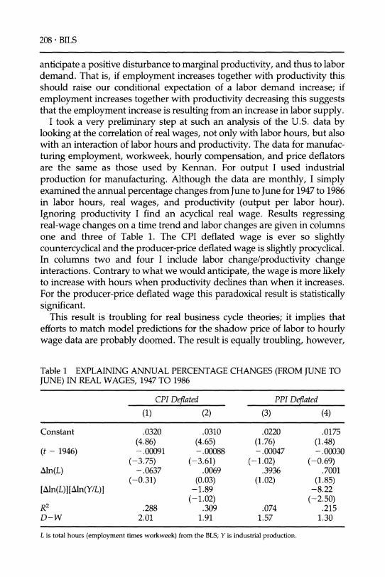
208 BILS

anticipate a positive disturbance to marginal productivity, and thus to labor demand. That is, if employment increases together with productivity this should raise our conditional expectation of a labor demand increase; if

employment increases together with productivity decreasing this suggests that the employment increase is resulting from an increase in labor supply.

I took a very preliminary step at such an analysis of the U.S. data by looking at the correlation of real wages, not only with labor hours, but also with an interaction of labor hours and productivity. The data for manufac-

turing employment, workweek, hourly compensation, and price deflators are the same as those used by Kennan. For output I used industrial

production for manufacturing. Although the data are monthly, I simply examined the annual percentage changes from June to June for 1947 to 1986 in labor hours, real wages, and productivity (output per labor hour). Ignoring productivity I find an acyclical real wage. Results regressing real-wage changes on a time trend and labor changes are given in columns one and three of Table 1. The CPI deflated wage is ever so slightly countercyclical and the producer-price deflated wage is slightly procyclical. In columns two and four I include labor change/productivity change interactions. Contrary to what we would anticipate, the wage is more likely to increase with hours when productivity declines than when it increases. For the producer-price deflated wage this paradoxical result is statistically significant.

This result is troubling for real business cycle theories; it implies that efforts to match model predictions for the shadow price of labor to hourly wage data are probably doomed. The result is equally troubling, however,

Table 1 EXPLAINING ANNUAL PERCENTAGE CHANGES (FROM JUNE TO JUNE) IN REAL WAGES, 1947 TO 1986

CPI Deflated PPI Deflated

(1) (2) (3) (4)

Constant .0320 .0310 .0220 .0175 (4.86) (4.65) (1.76) (1.48)

(t - 1946) -.00091 -.00088 -.00047 -.00030 (-3.75) (-3.61) (-1.02) (-0.69)

Aln(L) -.0637 .0069 .3936 .7001 (-0.31) (0.03) (1.02) (1.85)

[Aln(L)][Aln(Y/L)] -1.89 -8.22 (-1.02) (-2.50)

R2 .288 .309 .074 .215 D-W 2.01 1.91 1.57 1.30

L is total hours (employment times workweek) from the BLS; Y is industrial production.

Comments 209

for many other business cycle theories. For example, it has been suggested that procyclical real wages, particularly for the past twenty years, might be

explained by augmenting traditional Keynesian models with occasional

supply disturbances. But the wage behavior presented in Table 1 is at odds with that solution.

Elasticity of labor supply is also a parameter on which estimates and views greatly differ. Given Kennan's assumption that labor demand disturbances predominate, the data require an elastic labor supply to fit an

equilibrium model. Kennan suggests that in the short-run, with which he is concerned, we might expect high supply elasticity, even if workers very much dislike working long hours for extended periods. Although this is a valid point, it is also true that what we view as cyclical phases generally are fairly extended periods.

Work by Rogerson (1984) and others suggests that allowing labor to increase both along extensive (bodies) and intensive (hours per body) margins can imply a much larger labor supply elasticity than the intensive

margin alone. Much of the micro evidence upon which our priors are partly based, however, already includes adjustment along the extensive margin; and in sum these studies suggest much smaller aggregate elasticities than the 2.0 to 2.5 that Kennan suggests are needed (see Hall, 1980b).

Furthermore, movements in workweeks are not without importance. Some of Rogerson's work and the application by Hansen (1985) employ models where all persons are identical. When individuals are identical the best way to expand aggregate labor is to add workers with no change in hours per worker; workers can be added at constant cost, whereas longer hours per worker incurs increasing cost due to rising marginal utility of leisure. Jang-Ok Cho (1987) has extended such a model to include

heterogeneity among workers. As the workforce expands it is necessary to

bring in persons who are increasingly at a comparative disadvantage in the

workplace. This implies that an expansion is optimally achieved partly through additional persons working and partly through existing workers

working longer hours. Cho finds that achieving movements in workweeks of the magnitude observed in U.S. data would require sufficient heterogeneity that it greatly reduces the response of employment, and total labor to an increase in productivity. Looking at the numbers in Kennan's Table 1, we see that the changes in workweeks are of far less relative importance in the U.S. than the other countries. Thus Cho's analysis would be seen far more striking if conducted for these other countries. In both Japan and the U.K. the standard deviation of employment is only slightly greater than one-fourth the standard deviation of total hours. It is not possible to explain high labor supply elasticities in these countries by means of elastic extensive margins.

210 TAYLOR

Finally, we certainly have weak priors on how to attribute causes of serial

persistence. For instance, I would have guessed a different pattern than Kennan suggests for allocating the two large roots and one zero or negative root that he finds. I have no qualms with assuming considerable persistence in labor supply disturbances; movements in labor supply should

largely reflect movements in permanent income, which should obviously be persistent, or movements in real interest rates, which also appear to exhibit considerable persistence. By contrast, I would anticipate little

persistence caused by the dependence of employment demand and supply on past employment. For production workers the evidence suggests small costs of adjustment for labor demand (e.g., Shapiro, 1986). We might anticipate a negative dependence of labor supply on past employment. Leisure today may be a substitute for leisure tomorrow (as modeled in the

paper). Similarly, expiration of unemployment benefits could create a

negative dependence. Katz (1986) has documented the strong tendency of U.S. firms to recall workers as the time benefits expire.

REFERENCES

Cho, J. 1987. Heterogeneous agents and the business cycle. University of Roches- ter. Manuscript.

Hall, R. E. 1980a. Employment fluctuations and wage rigidity. Brookings Papers on Economic Activity 1: 91-123.

.1980b. Labor supply and aggregate fluctuations. Carnegie-Rochester Series on Public Policy 12: 7-33.

Hansen, G. D. 1985. Indivisible labor and the business cycle. Journal of Monetary Economics 16: 309-27.

Katz, L. F. 1986. Layoffs, recall, and the duration of unemployment. NBER Working Paper No. 1825.

Prescott, E. C. 1986. Theory ahead of business cycle measurement. Carnegie- Rochester Series on Public Policy 25: 11-44.

Rhee, C., and M. Espinosa. 1987. Efficient wage bargaining as a repeated game. Harvard University. Manuscript.

Rogerson, R. 1988. Indivisible labor, lotteries, and equilibrium. RCER Working Paper No. 11, University of Rochester.

Shapiro, M. D. 1986. The dynamic demand for capital and labor. Quarterly Journal of Economics 101: 513-42.

Comment JOHN B. TAYLOR Stanford University

210 TAYLOR

Finally, we certainly have weak priors on how to attribute causes of serial

persistence. For instance, I would have guessed a different pattern than Kennan suggests for allocating the two large roots and one zero or negative root that he finds. I have no qualms with assuming considerable persistence in labor supply disturbances; movements in labor supply should

largely reflect movements in permanent income, which should obviously be persistent, or movements in real interest rates, which also appear to exhibit considerable persistence. By contrast, I would anticipate little

persistence caused by the dependence of employment demand and supply on past employment. For production workers the evidence suggests small costs of adjustment for labor demand (e.g., Shapiro, 1986). We might anticipate a negative dependence of labor supply on past employment. Leisure today may be a substitute for leisure tomorrow (as modeled in the

paper). Similarly, expiration of unemployment benefits could create a

negative dependence. Katz (1986) has documented the strong tendency of U.S. firms to recall workers as the time benefits expire.

REFERENCES

Cho, J. 1987. Heterogeneous agents and the business cycle. University of Roches- ter. Manuscript.

Hall, R. E. 1980a. Employment fluctuations and wage rigidity. Brookings Papers on Economic Activity 1: 91-123.

.1980b. Labor supply and aggregate fluctuations. Carnegie-Rochester Series on Public Policy 12: 7-33.

Hansen, G. D. 1985. Indivisible labor and the business cycle. Journal of Monetary Economics 16: 309-27.

Katz, L. F. 1986. Layoffs, recall, and the duration of unemployment. NBER Working Paper No. 1825.

Prescott, E. C. 1986. Theory ahead of business cycle measurement. Carnegie- Rochester Series on Public Policy 25: 11-44.

Rhee, C., and M. Espinosa. 1987. Efficient wage bargaining as a repeated game. Harvard University. Manuscript.

Rogerson, R. 1988. Indivisible labor, lotteries, and equilibrium. RCER Working Paper No. 11, University of Rochester.

Shapiro, M. D. 1986. The dynamic demand for capital and labor. Quarterly Journal of Economics 101: 513-42.

Comment JOHN B. TAYLOR Stanford University

The main question raised by John Kennan is: can the employment and real wage fluctuations in 6 countries-the U.S., the U.K., Canada, Japan,

The main question raised by John Kennan is: can the employment and real wage fluctuations in 6 countries-the U.S., the U.K., Canada, Japan,

Comment 211

Denmark, and Austria-be explained by an equilibrium model of the labor market? Kennan addresses the question in two ways: first, by estimating a

simple static two-equation equilibrium model of the labor market in each

country, and second by estimating a more complex dynamic equilibrium model with explicit taste, technology, and adjustment cost parameters. To

help assess the adequacy of the dynamic model, he also estimates alternative "non-equilibrium" models of the labor market.

Estimating dynamic equilibrium models is a difficult task, but it is clear that the estimated parameters and the goodness of fit measures that

emerge from this study provide valuable information about the usefulness of these types of models. The novel data set on monthly employment, hours and real wages (unadjusted for seasonal variation) that Kennan has assembled for six countries also provides useful information. In comment-

ing on the data and the estimates I will focus first on the static supply- demand model, second on the dynamic model, and third on the class of alternative models that Kennan considers.

1. Contemporaneous Correlations and Labor Supply Elasticities

John Kennan's data convincingly reveal the strong empirical regularity that there is essentially no contemporaneous correlation between real wages and employment (or hours) over the business cycle. In his Table 1, for

example, the correlation between real wages and hours in the U.S. is only .057 (after a stochastic trend and seasonal factors are removed). In the U.K. it is -.007. Of course, this regularity is not a newly discovered one, as the 1977 quote from Robert Lucas at the start of Kennan's paper suggests, and it has been a starting point for many macroeconomic models, including the

misperception model of Lucas, staggered contracts models, and disequili- brium models.

Kennan gives a structural interpretation to these contemporaneous correlations by estimating aggregate labor supply elasticities with respect to the real wage. All the elasticities Kennan finds are very high-some are over 10. I found this structural interpretation to be unconvincing, given the observations. The high supply elasticities that Kennan finds are very sensitive to his identifying restrictions and his interpretation of the shocks. In some countries-most strikingly in the U.K., Canada, and Japan-the labor supply elasticities could just as plausibly be very low.

Kennan identifies the structural parameters by making apriori assumptions about the covariance matrix of the shocks-in particular by assuming

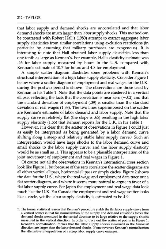
212 * TAYLOR

that labor supply and demand shocks are uncorrelated and that labor demand shocks are much larger than labor supply shocks. This method can be contrasted with Robert Hall's (1980) attempt to extract aggregate labor

supply elasticities from similar correlations using exclusion restrictions (in particular by assuming that military purchases are exogenous). It is

interesting to note that Hall obtained labor supply elasticities less than one-tenth as large as Kennan's. For example, Hall's elasticity estimate was .46 for labor supply measured by hours in the U.S. compared with Kennan's estimate of 10.7 for hours and 4.8 for employment.

A simple scatter diagram illustrates some problems with Kennan's structural interpretation of a high labor supply elasticity. Consider Figure 1 below where a scatter diagram of employment and real wages for the U.K.

during the postwar period is shown. The observations are those used by Kennan in his Table 1. Note that the data points are clustered in a vertical

ellipse, reflecting the facts that the correlation is near zero (-.02) and that the standard deviation of employment (.39) is smaller than the standard deviation of real wages (1.38). The two lines superimposed on the scatter are Kennan's estimates of labor demand and labor supply. Note that the

supply curve is relatively flat (the slope is .65) resulting in the high labor

supply elasticity (1.55) that Kennan reports for the U.K. in his Table 1. However, it is clear that the scatter of observations in Figure 1 could just

as easily be interpreted as being generated by a labor demand curve

shifting along a steep and relatively stable labor supply curve.1 Such an

interpretation would have large shocks to the labor demand curve and small shocks to the labor supply curve, and the labor supply elasticity would be as small as .1. This appears to be a plausible interpretation of the

joint movement of employment and real wages in Figure 1. Of course not all the observations in Kennan's international cross section

look like Figure 1, but because of the zero correlation the scatter diagrams are all either vertical ellipses, horizontal ellipses or simply circles. Figure 2 shows the data for the U.S., where the real-wage and employment data trace out a flat scatter diagram, and where it seems more natural to argue in favor of a flat labor supply curve. For Japan the employment and real-wage data look much like the U.K. For Canada the employment and real-wage scatter looks like a circle, yet the labor supply elasticity is estimated to be 4.9.

1. The formal statistical reason that Kennan's procedure yields the flat labor supply curve from a vertical scatter is that his normalization of the supply and demand equations forces the demand shocks measured in the vertical direction to be large relative to the supply shocks measured in the vertical direction. In order to trace out the scatter of points in Figure 1, Kennan's normalization implies that the labor supply shocks measured in the horizontal direction are larger than the labor demand shocks. If one reverses Kennan's normalization the alternative interpretation of a steep labor supply curve emerges.

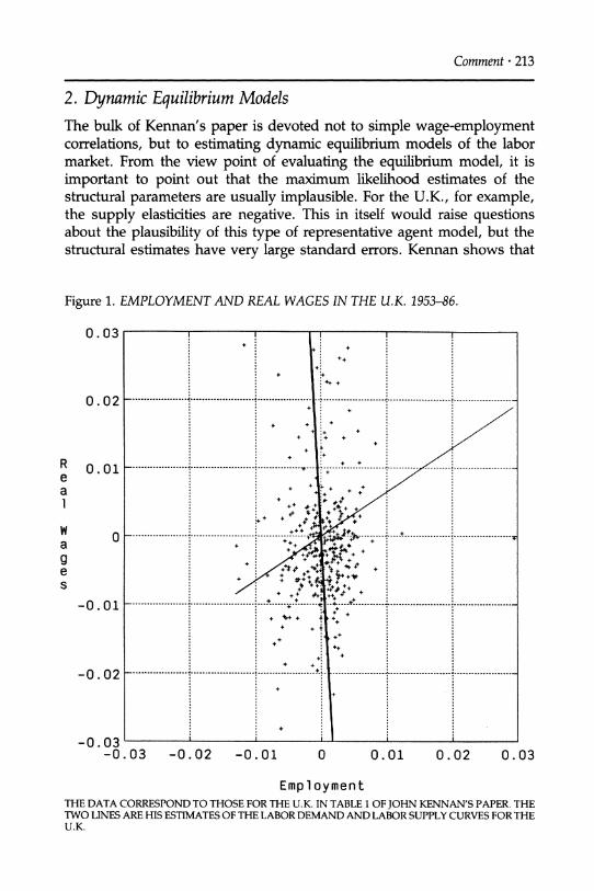
Comment * 213

2. Dynamic Equilibrium Models The bulk of Kennan's paper is devoted not to simple wage-employment correlations, but to estimating dynamic equilibrium models of the labor market. From the view point of evaluating the equilibrium model, it is

important to point out that the maximum likelihood estimates of the structural parameters are usually implausible. For the U.K., for example, the supply elasticities are negative. This in itself would raise questions about the plausibility of this type of representative agent model, but the structural estimates have very large standard errors. Kennan shows that

Figure 1. EMPLOYMENT AND REAL WAGES IN THE U.K. 1953-86.

0.03 I

++

++ +

,** +> I

: : 1:+ + :

,

--:--- -- --.

+ + I + '

:+ + + ,

e 0 .0 1 . .. . ... ............. .. .. ......................

i + '*** ^+ t

.............. ...................... .................. ......................

-0 ,02 . ......0,.1, ., ,, : + : I-++ + :

-0.03

-0. 0 -0.2 -001 0 0.01 0.02 0.03

+ : ,

' : . ' .+ + / . . -0O.02 ......... . . ...... '?' . .................. ...?.. .. . ....... ...............

-0.03 l , l l , -0.03 -0.02 -0 .01 0 0.01 0.02 0.03

Employment THE DATA CORRESPOND TO THOSE FOR THE U.K. IN TABLE 1 OF JOHN KENNAN'S PAPER. THE TWO LINES ARE HIS ESTIMATES OF THE LABOR DEMAND AND LABOR SUPPLY CURVES FOR THE U.K.

I

I II

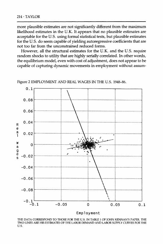
214 * TAYLOR

more plausible estimates are not significantly different from the maximum likelihood estimates in the U.K. It appears that no plausible estimates are

acceptable for the U.S. using formal statistical tests, but plausible estimates for the U.S. do seem capable of yielding autoregressive coefficients that are not too far from the unconstrained reduced forms.

However, all the structural estimates for the U.K. and the U.S. require random shocks to utility that are highly serially correlated. In other words, the equilibrium model, even with cost of adjustment, does not appear to be

capable of capturing dynamic movements in employment without assum-

Figure 2 EMPLOYMENT AND REAL WAGES IN THE U.S. 1948-86.

0.1

0.08

0.06

R 0.04 e a 0.02 1

a ? g e _-0.02

-0.04

-0.06

-0.08

-0.1 -0.1 -0.05 0 0.05 0.1

Employment THE DATA CORRESPOND TO THOSE FOR THE U.S. IN TABLE 1 OF JOHN KENNAN'S PAPER. THE TWO LINES ARE HIS ESTIMATES OF THE LABOR DEMAND AND LABOR SUPPLY CURVES FOR THE U.S.

Comment * 215

ing that these movements are significantly due to serially correlated taste shocks. If one views, as I do, the essential goal of business cycle theory as

explaining the dynamics of employment, as well as the co-movements with other variables, then the equilibrium model falls well short of this goal, according to Kennan's preliminary analysis. The movements in the data are

explained by exogenous serial correlation of shocks to tastes.

3. Alternative Models For comparison purposes, Kennan also estimates some alternative models of the labor market, in particular the Blanchard-Summers (1986) model with a powerful national union. As with the equilibrium model Kennan finds that the maximum likelihood estimates of the Blanchard-Summers model are implausible. For example, the demand elasticities are positive. Relatively speaking, therefore, the equilibrium models do not appear to

perform any worse than available alternatives. It should be emphasized that the model chosen by Kennan is only one of

several alternatives with which he could have compared the equilibrium model, and it is probably not the best alternative in terms of the statistical criteria that Kennan is using to evaluate models. As Kennan indicates, Ashenfelter and Card (1982) consider sticky wage models as an alternative to equilibrium models. Recent work by Benabou and Bismut (1988) indicates that such sticky wage models perform well for the U.S. in the sense that the maximum likelihood estimates are plausible and cannot be rejected against unconstrained autoregressions. By these criteria they seem to

perform better than the equilibrium model that Kennan considers in his

paper.

REFERENCES

Benabou, R., and C. Bismut. 1987. Wage bargaining and staggered contracts: Theory and estimation. Unpublished paper, CEPREMAP, Paris, France.

Hall, R. E. 1980. Labor supply and aggregate fluctuations. Carnegie Rochester Conference Series on Public Policy, ed. K. Brunner and A. H. Meltzer. Vol. 12 (Spring).

Discussion

The floor discussion began with some comments on the paper's treatment of labor supply. Martin Eichenbaum pointed out that using real wages to make inferences about labor supply is only valid in contract-free competitive economics. Hence the conclusion about labor supply elasticities need

Comment * 215

ing that these movements are significantly due to serially correlated taste shocks. If one views, as I do, the essential goal of business cycle theory as

explaining the dynamics of employment, as well as the co-movements with other variables, then the equilibrium model falls well short of this goal, according to Kennan's preliminary analysis. The movements in the data are

explained by exogenous serial correlation of shocks to tastes.

3. Alternative Models For comparison purposes, Kennan also estimates some alternative models of the labor market, in particular the Blanchard-Summers (1986) model with a powerful national union. As with the equilibrium model Kennan finds that the maximum likelihood estimates of the Blanchard-Summers model are implausible. For example, the demand elasticities are positive. Relatively speaking, therefore, the equilibrium models do not appear to

perform any worse than available alternatives. It should be emphasized that the model chosen by Kennan is only one of

several alternatives with which he could have compared the equilibrium model, and it is probably not the best alternative in terms of the statistical criteria that Kennan is using to evaluate models. As Kennan indicates, Ashenfelter and Card (1982) consider sticky wage models as an alternative to equilibrium models. Recent work by Benabou and Bismut (1988) indicates that such sticky wage models perform well for the U.S. in the sense that the maximum likelihood estimates are plausible and cannot be rejected against unconstrained autoregressions. By these criteria they seem to

perform better than the equilibrium model that Kennan considers in his

paper.

REFERENCES

Benabou, R., and C. Bismut. 1987. Wage bargaining and staggered contracts: Theory and estimation. Unpublished paper, CEPREMAP, Paris, France.

Hall, R. E. 1980. Labor supply and aggregate fluctuations. Carnegie Rochester Conference Series on Public Policy, ed. K. Brunner and A. H. Meltzer. Vol. 12 (Spring).

Discussion

The floor discussion began with some comments on the paper's treatment of labor supply. Martin Eichenbaum pointed out that using real wages to make inferences about labor supply is only valid in contract-free competitive economics. Hence the conclusion about labor supply elasticities need

216 * DISCUSSION

to be viewed cautiously. He felt a bigger puzzle was the co-movement of

average productivity and employment. Empirically the correlation is negative, while the theory suggests it should be positive. Ben Bemanke

suggested that heterogeneity might also be important to consider in

interpreting the reported labor supply elasticities. For instance, heterogeneity may arise from differences in individuals reservation wages.

Several comments addressed the adequacy of the dynamic specification of the model. James Stock felt the Granger causality tests should have been carried out in rates of growth instead of in levels. He also reported that

using a more general VAR (with 6 lags) he had found significantly different

dynamics. Matthew Shapiro also pointed out that it may be worth consid-

ering different types of labor and differences in adjustment costs. In this case the dynamic equation for total labor is likely to be more complicated than Kennan's specification. Lawrence Christiano noted that taste shocks and cost of adjustment dynamics may be hard to separately identify. Kennan agreed that all these considerations were important but that

analytical as well as data limitations would make them very difficult to

implement. Robert Gordon questioned whether the effects of the productivity slowdown has been properly handled in the estimation. He also felt that the cyclical fluctuations of real wages has changed since 1970 and that this should have been discussed in the paper.

Finally, Ben Bemanke and Robert Hall worried that the omission of movements of interest rates could be important, especially in the light of real business cycles models. Kennan argued that empirically the interest rate effects were dominated by real wage movements.

Documents

Equilibrium Interpretations of Employment and Real … Interpretations of Employment and Real Wage Fluctuations The question of the influence on real wages of periods of boom and depression