Equity and bond market signals as leading indicators of bank fragility

��

��

��

��

�� !��!

� � � � � � � � � � � � � � � � � �

��

��

��

��

��

�� !��!

� �� !��"#$��%"&��"'��(��"��#�%��"&�� )��"&�� *��" �%��&��" �� %�� " �� %%�� +�� !�� ,��" �� +�� -��.%��%��+��.��/��%%��!��0�

� � � � � � � � � � � � � � � � � �

��

� ��

��

�� !��

"�� #

$�� $��%&��

�� !��

"�� #

'� ��&�� ()��))�

*�� &��+,,---.�%/.��

��0 ()��))��

'� �0 )��))�%/�

��

��

��

��

��

��

��

��

��

�� !"�� #��$ %�� & ��

�� !�� '��(��) ��$ '�� *��& !+�� #��, %�� #

�- ,��.�� /0

- !�� /�-�� !�� /�-�$ 1�2�� //-�& 3�4�� /�

-�� 5��+�� /�

-�� &�� /#

1��

6��7��

�� /

!��&��$��8��2��%��

��

Abstract

We analyse the ability of the distance-to-default and bond spreads to signal bank fragility. We show thatboth indicators are complete and unbiased and that spreads are non-linear in the probability of bankdefault. We empirically test these properties in a sample of EU banks. We find leading properties for bothindicators. The distance-to-default exhibits lead times of 6 to 18 months. Spreads have signal value closeto default only, in line with the theory. We also find that implicit safety nets weaken the predictive powerof spreads. Further, the results suggest complementarity between both indicators, reducing type I errors.We also examine the interaction of the indicators with other bank information.

JEL codes: G21, G12

Key words: Banking, Bank fragility, Market Indicators

��

Non-technical summary

This paper examines whether forward-looking indicators of bank soundness could beconstructed using financial market data on the securities issued by banks. There isconsiderable interest on the issue, since market data are available on a high frequency,compared with profit and loss accounts and balance sheets. So far, all empirical evidence hasfocused on banks’ subordinated bond spreads. In this paper, we also examine the properties ofan equity market-based indicator, the distance-to-default, and compare its properties to thoseof the spread. The main contributions of the paper are (i) a theoretical examination of thepredictive properties of the two indicators, (ii) the estimation of a proportional hazard modelto test these properties, making efficient use of the information contained in the prevalence ofan indicator over time, and (iii) an explicit test for the role of the public safety net in theinformation content of market indicators.

Using a standard option pricing framework, we show that the equity-based distance-to-default and the subordinated bond spread have two highly desirable properties to be leadingindicators of bank fragility. They are complete in the sense that they reflect the three majordeterminants of default risk (earnings expectations, leverage and asset risk) and unbiased inthe sense that they reflect these risks correctly. However, the theory also suggests that the twoindictors exhibit important differences in their predictive ability. In particular, we show thatthe response of the spreads to an increase in default probability is non-linear, with littleresponse relatively far away from default and a strong reaction close to default. This alsoimplies that the distance-to-default should deliver an earlier signal of fragility than the spread.

In our empirical implementation, we calculate distances-to-default and subordinate debtspreads for European banks for which suitable data is available for the period 1991-2001. Forspreads, we focus on secondary market spreads on adequately large bond issues in order toabstract from noise due to limited liquidity. We use two different econometric models: a logitmodel, which we estimate for different time horizons (3-24 months ahead of default) and aproportional hazard model. The proportional hazard model permits conditional predictions offailure. The conditional predictions are based on having “survived” to a certain point in time,with a certain value of the market indicators in the previous period. Hence, the hazard modelallows analysing the importance of the persistence of the market signals. We also test theadditional information contained in market indicators compared with bank accountinginformation and ratings, as well as the impact of the expectation of public support on thesignal value obtainable from the market data. In the empirical implementation we were facedwith the problem that in Europe, very few banks – formally – declare bankruptcy. However,we circumvented this problem by using the downgrading of a bank to below C in theFitch/IBCA individual rating (a rating that excludes the safety net) and which is intended tosignal a material weakening in the stability of the bank. When examining the subsequentperformance of the bank, we found that in virtually all cases, either public intervention ormajor restructuring took place six to twelve months after the downgrade.

Our empirical results support the theory. Both indicators are found to have predictivepower for bank fragility. Further, the spread typically only reacts quite close (3 to 6 months)to default, whereas for the distance to default, we find predictive power as far from default as24 months. We also find strong support for the notion that the information content of spreadsis significantly diminished in the case of banks, which markets expect to be bailed out in caseof difficulties. The equity-based distance-to-default does not appear to suffer from thisshortcoming.

As regards the relationship of the two market indicators with several other sources ofbank specific information, we find, one, that the market indicators contain additionalinformation versus the initial ratings, especially in the case of long leads before the events ofbank fragility. Second, our results suggest complementarity between market information andbanks’ accounting information. And third, we find evidence that the two indicators (distance-to-default and spread) complement each other and lead to a reduction in Type I errors. Weshow that this is a reflection of the different properties of the two indicators.

��

I. Introduction

From a supervisory perspective the securities issued by banks are interesting for two reasons: First,

market prices of debt and equity may increase banks’ funding cost and, therefore, induce market

discipline, which may complement traditional supervisory practices (such as capital requirements and on-

site inspections) in ensuring the safety and soundness of banks. The market may play a particularly useful

role in disciplining the risks of large, complex and internationalised banking organisations. Second,

supervisors are considering the use of market data to complement traditional balance sheet data for

assessing bank fragility. Market prices may efficiently summarise information, beyond and above that

contained in other sources. Moreover, market information is available at a very high frequency.

Supervisors could use these signals as screening devices or inputs into supervisors’ early warning models

geared at identifying banks, which should be more closely scrutinised.2 Recently, it has also been

suggested to use subordinated debt spreads as triggers for supervisors’ disciplining action (Evanoff and

Wall 2000a, Flannery 2000).

A number of studies have analysed whether the market prices of the securities issued by banks

signal the risks incurred by them. If the prices reflect banks’ risks this is taken as evidence that markets

can indeed exert effective discipline on banks.3 Studies using U.S. data have found that banks’

subordinated debenture spreads in the secondary market do reflect banks’ (or bank holding companies’)

risks measured through balance-sheet and other indicators (Flannery and Sorescu 1996, Jagtiani et. al.

2000, Flannery 1998, and 2000). Morgan and Stiroh (2001) find the same to hold for the debenture

spreads at issue. Sironi (2000) is the only study that we are aware of, which provides evidence for

European banks. He also concludes that banks’ debenture spreads at issue tend to reflect cross-sectional

differences in risk.

There is also some evidence that market signals could usefully complement supervisors’ traditional

information. Evanoff and Wall (2000b) find that subordinated debt spreads have some leading properties

over supervisory CAMEL ratings. Conversely, DeYoung et. al. (2000) observe that on-site examinations

produce information that affects the spreads. However, they find that spread changes more often reflect

anticipated supervisory responses than new information. For example, bond investors in troubled banks

react positively to increased supervisory oversight, hence substituting the market’s own discipline.

2 Supervisory early warning models combine a set of bank-level financial indicators (balance sheet, income statement andmarket indicators), as well as sometimes also other variables (e.g. macroeconomic conditions), to make a prediction about thefuture state of a bank. A growing number of supervisory agencies have been experimenting with this kind of models (see Gilbertet.al. 1999).3 A much less researched question is whether a higher cost of funds actually discourages banks’ risk-taking. Bliss and Flannery(2000) identify some beneficial market influences, but do not find strong evidence that equity and especially bond investorsregularly influence managerial action.

�� *

Finally, Berger et. al. (2000) conclude that supervisory assessments are generally less predictive of future

changes in performance than equity and bond market indicators.

Finally, others have analysed the complementary role of the information contained in market

prices vis-à-vis the information contained in rating agencies’ assessments. Rating agencies are typically

argued to be conservative and to respond mainly to risks, which have already materialised (Altman and

Saunders 2000). Hand et al. (1992) find that only unanticipated rating changes produce reaction in the US

bond or equity markets (see also Goh and Ederington 1993). Using European data, Gropp and Richards

(2001) find that banks’ bond spreads do not react to rating announcements, while the equity prices do.

In general, research has focussed on bond rather than equity market signals. This has been the

case in part because mandatory subordinated debt issuance by banks has been prominently recommended

as a new tool to discipline banks (e.g. Calomiris 1997, and Kwast et. al. 1999). The argument relies on the

conjecture that subordinated debt-holders have particularly strong incentives to monitor banks’ risks,

because they are uninsured and have junior status. In addition, signals based on equity prices are

considered to be biased, because equity-holders benefit from the upside gains that accrue from increased

risk-taking (e.g. Hancock and Kwast 2000, and Berger et. al. 2000). The relative importance of this moral

hazard problem becomes the more pronounced the closer the bank to insolvency, or the lower its charter

value (e.g. Keeley 1990, Demsetz et al. 1996, and Gropp and Vesala 2001).

However, as we will argue in this paper, there are several aspects, which suggest that equity market

signals may be attractive as monitoring devices. First, we show that unbiased equity-based fragility

indicators can be derived. Second, there is broad consensus that the equity markets are efficient in

processing available information. Empirical evidence strongly supports that equity-holders respond

rationally to news concerning: banks’ asset quality (Docking et. al 1997), risks in LDC loans (e.g.

Smirlock and Kaufold 1987, and Musumeci and Sinkey 1990), other banks’ problems (e.g. Aharoney and

Swary 1996), or rating changes (op. cit.). Third, while bond spreads are conceptually simple, their

implementation is difficult. For example, different bonds issued by the same bank may yield different

estimates of the spread (Hancock and Kwast 2000). Moreover, monitoring must concentrate on

sufficiently liquid bonds in order to eliminate liquidity premia. In the European context, the construction

of appropriate risk-free yield-curves, which is a necessary ingredient to the calculation of spreads, may

also be difficult especially for smaller countries, as further explained below.

In this paper, we first examine the properties of the market indicators in terms of their capability of

capturing the major elements affecting default probability (completeness), and their alignment with

supervisors’ interests (unbiasedness). We show that a distance-to-default measure, derived using option-

pricing theory from the equity market data, is both complete and unbiased, as are uninsured bond yield-

spreads, provided that banks’ asset value is still sufficiently high. Thus, these indicators are preferred over

��

biased direct equity price-based measures and could represent useful leading indicators of bank fragility.

The theory also suggests, however, that spreads may react only relatively late to a deterioration in the

quality of a bank.

We then empirically test banks’ distances-to-default and subordinated bond spreads in relation to

their capability of anticipating a material weakening in banks’ financial condition. We use two different

econometric models: a logit-model and a proportional hazard model. We find support in favour of using

both indicators as leading indicators of bank fragility, regardless of our econometric specification.

However, while we find robust predictive performance of the distance-to-default indicator between 6 to

18 months in advance, its predictive properties are quite poor closer to default. In contrast, subordinated

debt spreads are found to have signal value, but only close to default. This is consistent with the

predictions of theory. Our results also indicate that the subordinated debt-based signals are powerful

predictors only for smaller banks, which are generally not implicitly insured against default. In contrast

and as expected, the public safety net does not appear to affect the predictive power of the distance-to-

default. We also find evidence that the indicators provide marginally additional information relative to

balance sheet data alone in the case of distance to default and no extra information in the case of spreads.

Finally, we find support for our theoretical prediction that the two indicators together have more

discriminatory power in predicting defaults than each alone.

A key issue for this as any similar study such as this one is the definition of events of banks’ major

financial problems, as formal bank bankruptcies have been extremely rare events in Europe. The study

uses as such events down-gradings of FitchIBCA individual rating to category C or below indicating a

severe concern. This is a sensible approach, because individual ratings exclude the effect of possible

public support and focus on the true condition of the bank and, moreover, the majority of banks in our

sample received public support or experienced a major restructuring after such a downgrading. Hence,

the problems were severe enough to warrant major remedial action, even though there was no formal

bankruptcy. The robustness of this definition and its possible implications are discussed later on at length.

If anything, our approach should bias our findings against finding predictive power for the indicators.

The remainder of the paper is organised as follows: Section II examines the basic properties of the

equity and bond market indicators and frames our empirical propositions. Section III defines our sample

and the variables used in the empirical study. Section IV contains descriptive analyses of the behaviour of

the market indicators. Section V reports our econometric specifications and results. Section VI presents

some extensions and robustness checks. Finally, Section VII concludes.

II. Properties of market indicators

In order to structure the analysis of the market indicators, we introduce two basic definitions:

�� #

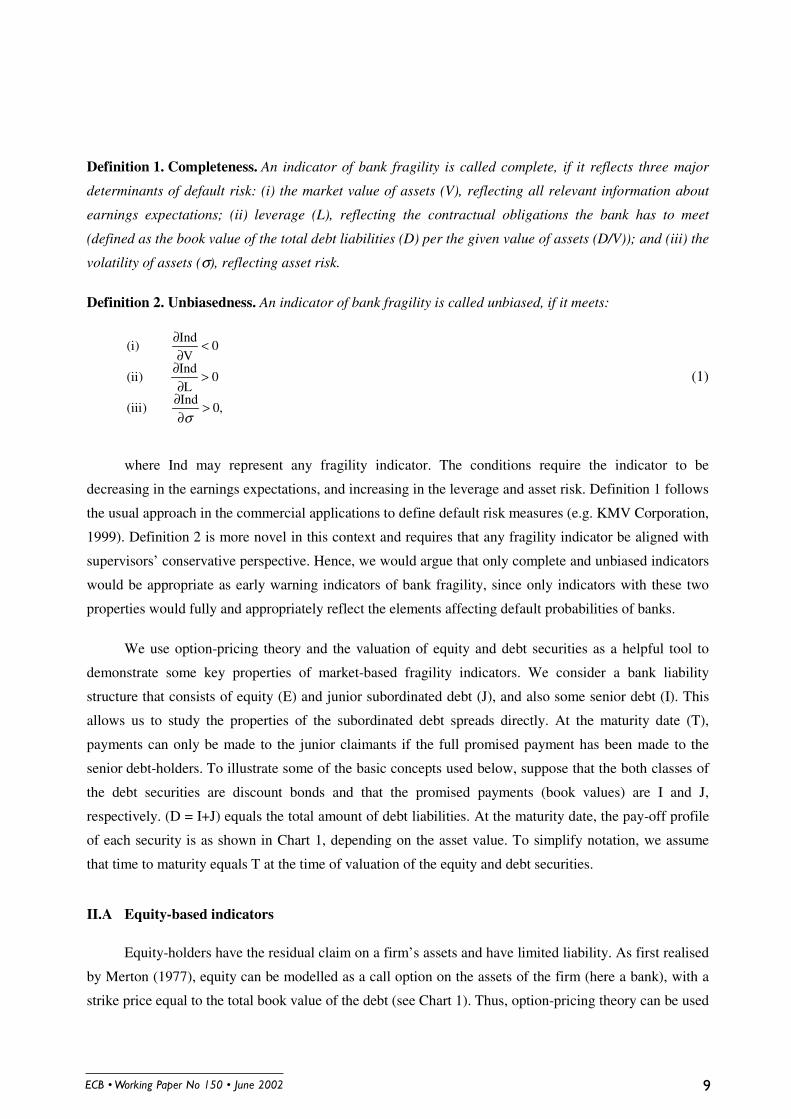
Definition 1. Completeness. An indicator of bank fragility is called complete, if it reflects three major

determinants of default risk: (i) the market value of assets (V), reflecting all relevant information about

earnings expectations; (ii) leverage (L), reflecting the contractual obligations the bank has to meet

(defined as the book value of the total debt liabilities (D) per the given value of assets (D/V)); and (iii) the

volatility of assets (σ), reflecting asset risk.

Definition 2. Unbiasedness. An indicator of bank fragility is called unbiased, if it meets:

,0Ind

)iii(

0L

Ind)ii(

0V

Ind)i(

>∂∂

>∂∂

<∂∂

σ

(1)

where Ind may represent any fragility indicator. The conditions require the indicator to be

decreasing in the earnings expectations, and increasing in the leverage and asset risk. Definition 1 follows

the usual approach in the commercial applications to define default risk measures (e.g. KMV Corporation,

1999). Definition 2 is more novel in this context and requires that any fragility indicator be aligned with

supervisors’ conservative perspective. Hence, we would argue that only complete and unbiased indicators

would be appropriate as early warning indicators of bank fragility, since only indicators with these two

properties would fully and appropriately reflect the elements affecting default probabilities of banks.

We use option-pricing theory and the valuation of equity and debt securities as a helpful tool to

demonstrate some key properties of market-based fragility indicators. We consider a bank liability

structure that consists of equity (E) and junior subordinated debt (J), and also some senior debt (I). This

allows us to study the properties of the subordinated debt spreads directly. At the maturity date (T),

payments can only be made to the junior claimants if the full promised payment has been made to the

senior debt-holders. To illustrate some of the basic concepts used below, suppose that the both classes of

the debt securities are discount bonds and that the promised payments (book values) are I and J,

respectively. (D = I+J) equals the total amount of debt liabilities. At the maturity date, the pay-off profile

of each security is as shown in Chart 1, depending on the asset value. To simplify notation, we assume

that time to maturity equals T at the time of valuation of the equity and debt securities.

II.A Equity-based indicators

Equity-holders have the residual claim on a firm’s assets and have limited liability. As first realised

by Merton (1977), equity can be modelled as a call option on the assets of the firm (here a bank), with a

strike price equal to the total book value of the debt (see Chart 1). Thus, option-pricing theory can be used

�� 0

to derive the market value and volatility of assets from the observable equity value (VE) and volatility

(σE), and D. Consider the basic Black and Scholes (1972) formula, valuing equity as:

,T1d2d

T

T2

rD

Vln

1d

,)1d(NVV

)2d(NeD)1d(VNV

2

EE

rTE

σσ

σ

σσ

−≡

++

≡

=

−= −

(2)

where N represents the cumulative normal distribution, r the risk-free, interest rate, and T the time

to the maturity of the debt liabilities.

We can see from (2) that VE is complete, since market prices reflect the relevant information for

capturing default risk (V, D and σ). However, VE is increasing in σ, which violates condition (iii) in (1).

Therefore, an increase in the share price may not be consistent with a reduction in default risk.

However, as an alternative consider the negative of the distance-to-default (-DD),4 which we derive

from the Black-Scholes model in Appendix I:

T

T2

rL

1ln

T

T2

rD

Vln

)DD(

22

σ

σ

σ

σ

−+

−=

−+

−=− . (3)

V and σ are solved from the non-linear two equation system (2). DD indicates the number of

standard deviations (σ) from the default point at maturity (V = D). From (3) we can obtain a first result:

Result 1. (-DD) is a complete and unbiased indicator of bank fragility for V>V’ (given D). V’ is

defined as T)r22/1(De +− σ .

Proof. (-DD) reflects V, L and σ; hence it is complete.

Clearly,V

)DD(

∂−∂

< 0 and L

)DD(

∂−∂

>0.

+

+=

∂−∂ −− rT

D

VlnTT

2

1)DD( 2/12σσ

> 0, when T)r22/1(DeV +−> σ . (–

DD) meets all the conditions in (1) when V is sufficiently large (given the amount of debt); hence, it is unbiased for V>V’.

4 A similar measure is the basic conceptual ingredient in the KMV Corporation’s model for estimating default risk (see KMVCorporation 1999).

��

(-DD) is unbiased for all positive values of DD, i.e. always when above the default point, since

DD>0 when T)r22/1(DeV −> σ .5 Hence, (-DD) is a complete and unbiased early warning indicator for all

banks, which are still solvent.

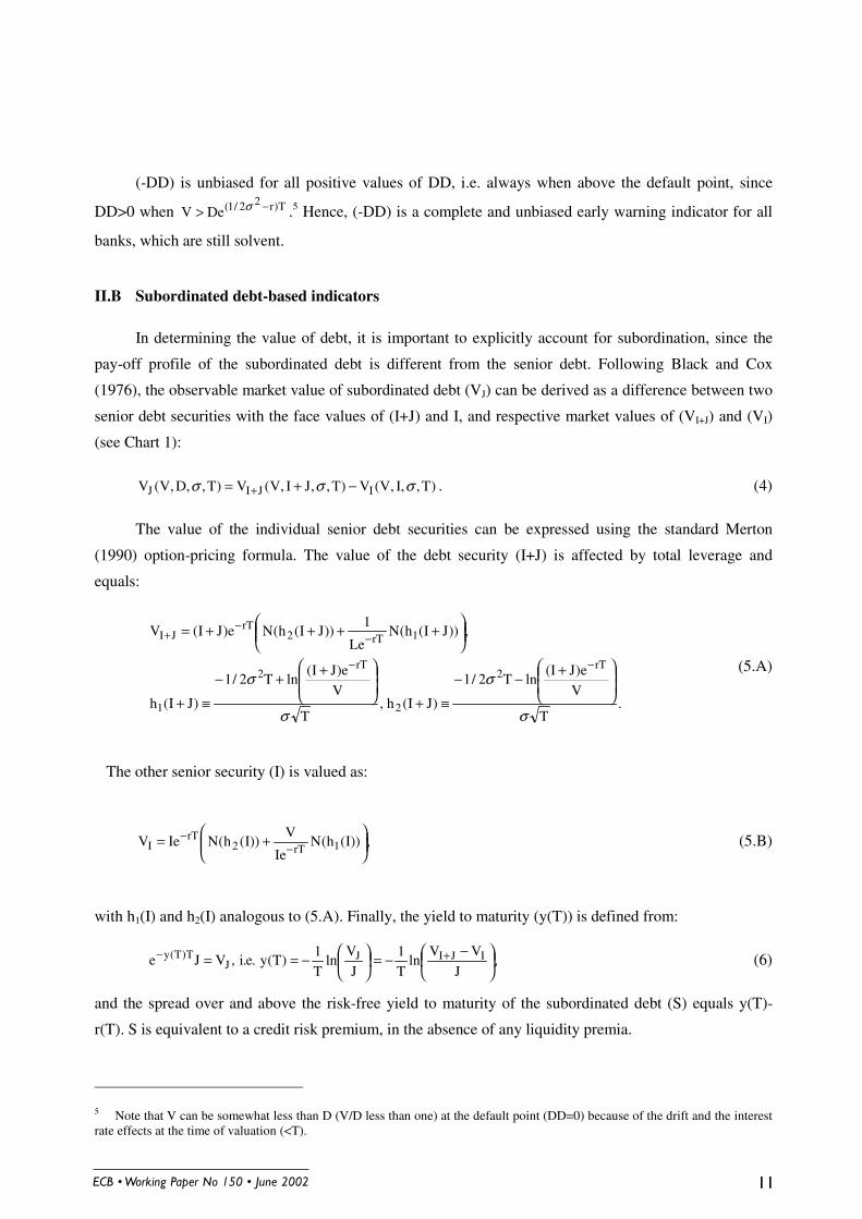
II.B Subordinated debt-based indicators

In determining the value of debt, it is important to explicitly account for subordination, since the

pay-off profile of the subordinated debt is different from the senior debt. Following Black and Cox

(1976), the observable market value of subordinated debt (VJ) can be derived as a difference between two

senior debt securities with the face values of (I+J) and I, and respective market values of (VI+J) and (VI)

(see Chart 1):

)T,,I,V(V)T,,JI,V(V)T,,D,V(V IJIJ σσσ −+= + . (4)

The value of the individual senior debt securities can be expressed using the standard Merton

(1990) option-pricing formula. The value of the debt security (I+J) is affected by total leverage and

equals:

.T

V

e)JI(lnT2/1

)JI(h,T

V

e)JI(lnT2/1

)JI(h

,))JI(h(NLe

1))JI(h(Ne)JI(V

rT2

2

rT2

1

1rT2rT

JI

σ

σ

σ

σ

+−−

≡+

++−

≡+

++++=

−−

−−

+

(5.A)

The other senior security (I) is valued as:

,))I(h(NIe

V))I(h(NIeV 1rT2

rTI

+= −

− (5.B)

with h1(I) and h2(I) analogous to (5.A). Finally, the yield to maturity (y(T)) is defined from:

,J

VVln

T1

J

Vln

T1

)T(y.e.i,VJe IJIJJ

T)T(y

−−=

−== +− (6)

and the spread over and above the risk-free yield to maturity of the subordinated debt (S) equals y(T)-

r(T). S is equivalent to a credit risk premium, in the absence of any liquidity premia.

5 Note that V can be somewhat less than D (V/D less than one) at the default point (DD=0) because of the drift and the interestrate effects at the time of valuation (<T).

�� /

Based on (5) and (6) we can state a second result:

Result 2. S is a complete and unbiased indicator of bank fragility for V>V* (given D=I+J). V* is defined

as [ ] T)r22/1(2/1 e)JI(I +−+ σ .

Proof. By (5) and (6), S reflects V, L and σ; hence, it is complete.

Unbiasedness:

.VV

V

V

TVJ

V)T(y

VS IJI

J

∂∂−

∂∂−=

∂∂=

∂∂ + Following Merton (1990), the value of a senior debt security is an increasing function

in the value of assets, and it turns out that )),JI(h(NV

V1

JI +=∂∂ + and ))I(h(N

V

V1

I =∂∂

. Thus,

[ ]))I(h(N))JI(h(NTV

J

V

S11

J−+−=

∂∂

. The expression in the square brackets is always positive, because h1 is increasing in

the face value of debt. Since J and VJ are always positive, 0V

S <∂∂

always.

Second,

∂∂−=

∂∂ +

L

V

TVJ

LS JI

J. Since 0L))JI(h(N

L

V 21

JI <+−=∂∂ −+ , 0

L

S >∂∂

always.

Third,

∂∂−=

∂∂

σσJ

J

V

TVJS

. Thus, the sign of σ∂∂S

is the opposite of the sign of σ∂∂ JV

. According to Black and Cox (1977)

(p.360), VJ is a decreasing (increasing) function of σ for V greater than (less than) the point of inflection, V*. Thus, for V>V*,

.0S >∂∂σ

Hence, S is unbiased for V>V* as it meets all the conditions in (1), and biased for V<V* by condition (iii).

V* is a geometric average of (I+J) and I (“adjusted” for time to maturity, drift and interest rate

effects), falling between the two face values (see Chart 1).6 When the value of bank assets is high enough

to cover both senior and junior debt, the interests of the senior and junior debt-holders are aligned with

each other and with the interests of the supervisor. Hence, when the bank is economically solvent (and

equity has some value), the subordinated debt spread is an unbiased indicator of bank fragility. Since

banks would likely to be monitored while being still sound enough to cover all debt, the spread can

constitute a useful early indicator of deterioration in financial condition.

However, one should note that when the value of assets is lower than the threshold value V*

(which is to some extent below the total value of debt, depending on the amount of junior debt) the two

groups of debt-holders have conflicting interests. The junior claimants have interests similar to those of

6 Note that V*<V’ as long as there is some junior debt outstanding.

��

the equity-holders to take on more asset risk, while the senior claimants’ expected pay-off is always

decreasing in risk.7

The above investigation of the properties of the market signals is made in the context of a specific

model: normal asset value diffusion and European option type (call for equity and put for debt). Namely,

the market value of a debt instrument can also be expressed on the basis of the discounted value assuming

no default risk and the value of a put option on the firm’s assets (see Merton 1977, and Ron and Verma

1986). The widespread use of the Merton model, also to generate quantitative probability of default

estimates, speaks in favour of it. But unfortunately, the literature has not established general conditions,

under which the unbiasedness property could be established and verified for specific asset-liability

structures (e.g. for banks). Thus, the performance of the market signals is ultimately an empirical issue.

Notwithstanding this general point, the crucial feature that, say, the call option value is

(monotonically) increasing in V and decreasing in L seems to be a much more general result than the

monotonic and increasing relationship between the option value and σ in the Merton model, which

produces the often-cited equity price-bias. This result may not obtain for certain ranges of V under

different (and possibly more plausible) distributional assumptions, e.g. based on bounded returns (Bliss

2000), more complex liability structures, or under different option types, e.g. barrier options (Bergman et.

al. 1996).8 Hence, alternative modelling assumptions would tend to question the universal biasedness of

the simple equity price-based indicators, rather than the unbiasedness of the DD or S-measures.9

The main concern of this paper is indeed an empirical one whether complete and unbiased market

indicators (as derived from a specific model) are capable of signalling an increase in the default risk in a

timely fashion.10 Traditional accounting measures, such as leverage ratios or earnings indicators are

generally incomplete and therefore less useful as indicators of bank fragility. Thus, the key proposition,

whose validity we test is as follows:

7 This effect has an impact on the role of subordinated debt-holders in disciplining banks’ risk taking: the contribution can beactually negative once the bank has entered the zone of de facto insolvency. In this zone, the sole right to approve businesspolicies should lie with the senior debt holders (or supervisors) in order to avoid moral hazard. Levonian (2001) also makes thispoint that the incentives of the subordinated debt-holders do not always side with those of the supervisors.8 There does not seem to be consensus about how to model the distribution of bank asset returns. Ritchken et. al. (1993) findsome consistency between the behaviour of bank equity and the outcomes from a barrier option framework.9 The analysis also relies on the idea that asset risk can be measured by asset variance, which seems to be relativelyuncontested, while alternative approaches has also been proposed (foremost Harrison and Kreps 1979).10 Empirical evidence has suggested that the actual spreads are higher than suggested by Merton’s model. Franks and Torous(1989) and Longstaff and Schwartz (1995) argue that an additional element in the spread is the expectation that equity-holdersand other junior claimants receive in the bankruptcy settlement more than what is consistent with absolute priority. In addition,Anderson and Sundaresan (1996) suggest that debt-holders are forced to accept concessions to pay less than originally agreedprior to formal bankruptcy proceedings. Mella-Barral and Perraudin (1997) incorporate this strategic debt service into an option-pricing-based model and show that the spread-widening impact can be significant.

��

Proposition 1. The equity market-based (-DD) and the bond market-based S constitute early indicators of

a weakening in a bank’s condition.

Finally, it is of interest to study how the subordinated debt spread behaves as a function of the asset

value (or the distance-to-default) to see how the spread would be predicted to react to a deterioration in

financial condition. According to Black and Cox (1976), the subordinated debt value is an increasing and

concave function of V for V>V*, like senior debt. Hence, the spread is a convex and decreasing function

of V for V>V*. This means that the spread would remain stable and close to zero for large intervals of

changes in V and only react significantly relatively close to the default point.11 This can be illustrated by

plotting the spread as a function of the distance-to-default (varying V, holding I,J constant), under

specific assumptions for the other parameters (see Chart 2). While the subordinated debt spread reacts

earlier and more than the senior debt spread, it moves up significantly only when DD is relatively low.

Hence, the equity-based distance-to-default measure can be expected to provide an indication of a

weakening financial condition earlier than the subordinated debt spread. This is a direct consequence of

the different pay-off structures of the equity and subordinated debt holders (for V>V*). Debt-holders care

only of the left tail of the distribution of returns, while equity-holders are interested in the whole

distribution of returns. In a nutshell, the theory predicts that the two indictors have qualitatively different

predicted properties, because the response of the spreads to an increase in default probability is non-

linear. Therefore, the distance-to-default measure would be predicted to deliver an earlier signal of

fragility than the spread. In the empirical analysis, we examine the performance of (-DD) and S with

respect to different time leads under the proposition that:

Proposition 2. The equity market-based (-DD) constitutes an earlier indicator of weakening in a bank’s

condition than S. S would react significantly only relatively close to the default point.

II.C Impact of the safety net

Following Merton 1977, the value of subordinated debt can be expressed in terms of two “no-

default-risk” values for the senior debt securities (I+J) and I and two put option values (strike prices

equalling the book values of debt as before). 12 A put option represents the value of the limited liability,

i.e. equity-holders’ right of walking away from their debts in exchange for handing over the firm’s assets

to the creditors. In case of fully insured debt (like insured deposits), the put option component disappears,

11 Bruche (2001) shows that the “hockey-stick” shape of the spread as a function of V can become more pronounced when oneintroduces into the basic pricing model asymmetric information and investors’ co-ordination failure.

12 For instance, ))I(1h(VN))I(2h(NeVeVVVeVV T)T(rI

T)T(rIPO,I

RFI

T)T(yII −+−−=−== −−− , where

T)T(rRFI IeV −= denotes the “no-default-risk” value and VPO the value of the put option.

��

and the market value of the debt equals the “no-default-risk” value (and S is zero). There is no signal of

fragility obtainable from the pricing of this debt. Hence, any market discipline requires that deposit

insurance is explicitly restricted, leaving out some creditors with their money at stake (e.g. Gropp and

Vesala 2001).13

The literature (e.g. Dewatripont and Tirole 1993) has also examined the problem related to the

credibility of the restricted safety net. Losses from a failure of a significant bank might affect the banking

system as a whole and, hence, imply systemic risk. In this case, it might be expected that the “systemic”

banks would never be liquidated, or that the exposures of the systemically relevant debt-holders (such as

other banks) would always be covered, regardless of the features of the explicit safety net arrangements

(“too-big-to-fail”). If the implicit safety net is perceived to be unrestricted, the value of the put option is

zero, since the debt-holders would not face the risk of having to take over the assets of the bank. Thus, the

market value of debt would again be equal to the “no-default-risk” value also in this case and all

uninsured debt-based fragility indicators would be incomplete and fail to capture increased default risk.

The perceived probability of bailout will generally be less than one, since there is typically no

certainty of public support under an explicitly restricted deposit insurance system. Authorities frequently

follow a policy of constructive ambiguity in this regard. Under these circumstances debt based indicators

would have predictive power, but much less compared to a hypothetical completely uninsured case. In

this context we take the existence of positive spreads on banks’ uninsured debt issues as evidence that the

perceived probability might be indeed less than one. However, the history of bank bailouts by the

government (significant banks have not failed in Europe in recent history) suggests that spreads might

nevertheless be substantially weakened in their power to lead banking problems as compared with the

case where the absence of bailouts is fully credible. Gropp and Vesala (2001) find empirical support for

this point. Their results suggest that banks’ risk taking in Europe was reduced in response to the

introduction of explicit and restricted deposit insurance schemes. They also find evidence in favour of

that a number of banks are “too-big-to-fail”. In addition, Gropp and Richards (2001)find that banks’ bond

spreads do not appear to react to ratings announcements. Their findings could be interpreted as evidence

in favour of widespread safety nets. After an extensive sensitivity analysis, they cannot exclude the

possibility that bondholders expect to be insured against default risk in Europe.

As a rule, equity-holders are not covered even in broad-based explicit safety nets. In addition, the

existence of an implicit safety net would induce banks to take on increased leverage and asset risk, and

these risk taking incentives (moral hazard) would be the greater the more extensive the perceived safety

13 The put option value also represents the value of the deposit insurance guarantee, since by guaranteeing the debt theguarantor has in fact issued the put option on the assets (see Merton 1977). Hence, the deposit insurance value (VPO) could alsobe used as an unbiased bank fragility indicator (see Bongini et. al. 2001) with the same characteristics as the market value ofdebt-based indicators.

��

net (see Gropp and Vesala 2001, section 2). While bond market indicators would not reflect this

additional effect under a broad safety net, correctly specified equity indicators, such as (-DD) would.

Hence, we can formulate an additional proposition:

Proposition 3. If a bank were covered by an implicit or explicit partial guarantee, the bond spread, S,

would be a weaker leading indicator of bank fragility than the negative distance to default, (-DD).

Whether equity and bond markets are able to effectively process the available information and send

early signals, which are informative of banks’ default risk, is investigated below in a sample of European

banks. We evaluate the usefulness of the preferred (complete and unbiased) market indicators (-DD and

S) for this purpose (Proposition 1). We also test whether the spread reacts later than (-DD) (Proposition

2), and whether a perception of the safety net dilutes the predictive power of the bond market signals, but

leaves the equity market signals intact (Proposition 3).

III. Empirical implementation

Our data set consists of monthly observations from January 1991 to March 2001. The relatively

high frequency of the data highlights one fundamental advantage of market-based indicators relative to

balance sheet indicators. We decided to use monthly data, rather than an even higher frequency, in order

to eliminate some of the noise in daily equity and bond prices. The data set consists of those EU banks,

for which the necessary rating, equity and bond market information is available. In the sample selection

process we started from roughly 100 EU banks, which had obtained a “financial strength” rating from

Fitch/IBCA.14 The sample size was then largely determined by the availability of market data. The two

sub-samples used in evaluating the equity and bond market signals consist of 84 and 59 banks,

respectively (see Table 1). The samples contain banks from 14 (equity sample) and 12 (bond sample) EU

countries.

III.A Measurement of bank “failures”

We were faced with the problem that no European banks formally declared bankruptcy during our

sample period. In the absence of formal bank defaults, we considered a downgrade in the Fitch/IBCA

“financial strength” to C or below as an event of materially weakened financial condition.15 There are 25

such downgrades in the equity and 19 in the bond sub-sample, 32 in total (Table 2). We defend our

definition of bank “failure” on two grounds: First, the “financial strength rating” is designed to exclude

14 For an explanation of a “financial strength” rating see below.15 See Appendix 2 for the exact definitions of the Fitch/IBCA rating grades.

�� *

the safety net and, hence, should indicate the bank’s true financial condition. A downgrade to the level of

C or below signifies that there are significant concerns regarding profitability and asset quality,

management and earnings prospects. In particular when the rating falls to the D/E category very serious

problems are indicated, which either require or are likely to require external support. Second, in many

cases after the downgrade to C or below, public support was eventually granted or a major restructuring

was carried out to solve the problem. As detailed in Table 2, 11 banks received public support, and 8

banks underwent a major restructuring after the downgrading. The support or restructuring operations

also generally took place relatively soon after these events (6-12 months). In the remaining cases, no

public support or substantial restructuring took place. In part this is a reflection of sample truncation in

March of 2001, as 6 of the remaining 13 downgrades took place in late 2000 or early 2001 and an

eventual intervention cannot be excluded. Given that the downgrades precede the actions aimed at

resolving the problem by quite some time, we would argue that our proxy for bank failures is quite

sensible and generally should bias our results against finding predictive power of the indicators.

Our study is similar to the US studies investigating the relationship between market information

and supervisory ratings (for example Evanoff and Wall 2000b, DeYoung et. al. 2000, and Berger et. al.

2000), while we use the “individual” ratings as signals of banking problems. While we are concerned

about our relatively small sample sizes (at least in terms of number of banks, not in terms of data points;

see below) Evanoff and Wall (2000b), for example, consider 13 downgrades in supervisory CAMEL

ratings in a sample of 557 US banks, constituting the default events. Hence, compared to the previous

literature our sample appears reasonably large and fairly balanced. Further, rather than use the

Fitch/IBCA ratings, it could be argued that we should use supervisory ratings (such as CAMEL ratings)

instead. Unfortunately, we did not have access to historical supervisory information on individual banks

and, in some European countries, comparable ratings by supervisors do not exist. Clearly, the supervisory

ratings may be based on more detailed information relative to ratings by a ratings agency, including

confidential information obtained at on-site inspections, but they may also be subject to forbearance.

III.B Market indicators

We calculated the negative of the distance-to-default (-DD) for each bank in the sample and for

each time period (t) (i.e. month) using that period’s equity market data. The system of equations in (2)

was solved by using the generalised reduced gradient method to yield the values for VA and σA, entering

into the calculation of (-DD). Variable definitions are given in Table 3 and descriptive statistics in Table

4.

As to the inputs to the calculation of (-DD), we used monthly averages of the equity market

capitalisation (VE) from Datastream. The equity volatility (σE) was estimated as the standard deviation of

the daily absolute equity returns and we took the 6-month moving average (backwards) to reduce noise

��

(as e.g. in Marcus and Shaked 1984). The presumption is that the market participants do not use the very

volatile short-term estimates, but more smoothed volatility measures. This is not an efficient procedure as

it imposes the volatility to be constant (it is stochastic in Merton’s original model). However, equity

volatility is accurately estimated for a specific time interval, as long as leverage does not change

substantially over that period (see for example Bongini et. al. 2001). The total debt liabilities (VL) are

obtained from published accounts and are interpolated (using a cubic spline) to yield monthly

observations. The time to the maturing of the debt (T) was set to one year, which is the common

benchmark assumption without particular information about the maturity structure. Finally, we used the

government bond rates as the risk-free rates (r).16 The values solved for V and σ were not sensitive to

changes in the starting values.

We largely followed convention when calculating the monthly averages of the secondary market

subordinated debt spreads (S). We used secondary market spreads, rather than those from the primary

market, as we would argue that secondary market spreads are more useful for the ongoing monitoring of

bank fragility. In the absence of mandatory issuance requirements, such as those proposed by Calomiris

(e.g. 1997), banks’ new issuance could be too infrequent, or limited to periods when pricing is relatively

advantageous. As we were concerned about too thin or illiquid bank bond markets in Europe, we only

selected bonds with an issue size of more than euro 150 million. This figure seemed the best compromise

between maintaining sample size and obtaining meaningful monthly price series from Bloomberg and

Datastream, which were our main data sources. In addition, in order to minimise noise in the data series,

we attempted to use fixed rate, straight, subordinated debt issues only. We were largely able to obtain

such bonds, but in some cases we had to permit floating rate bonds into the sample. We used the standard

Newton iterative method to calculate the bond yields to maturity.

For the larger countries, we were able to find bank bonds issued in the domestic currency, which

met our liquidity requirement. In case of smaller countries, banks more frequently issued foreign than

domestic currency-denominated bonds prior to the introduction of the euro. Hence, we largely resorted to

foreign currency issues (DM, euro, USD and in two cases, yen) and matched them to government bonds

issued in the same currency. We were able to construct risk-free yield-curves for Germany, France and

the UK and calculated spreads for banks in those countries relative to the corresponding point on those

curves. For the other smaller countries, we were unable to obtain sufficient data to construct full risk-free

yield-curves. We therefore instead matched the remaining term to maturity and the coupon of the bank

bond to a government bond issued by the government of the country of the bank’s incorporation in the

same currency.

16 Our (-DD) measure is subject to the Black-Scholes’ assumption of a cumulative normal distribution (N) for the underlyingasset values. Aspointed out by Bliss (2000), this assumption may not hold in practice. He argues that the normal distribution doesnot take into account that closer to the default point adjustment in debt liabilities will likely take place. Hence, empirically betterformulas could be found, while delivering fragility indicators with similar qualitative characteristics as the standard (-DD).

�� #

III.C Expectation of public support

We use the “support rating” issued by Fitch/IBCA to indicate the likelihood of public support. We

regard as cases of more likely public support the rating-grades 1 or 2 (see Appendix 2). The former grade

indicates existence of an assured legal guarantee, and the latter a bank, for which in Fitch/IBCA’s opinion

state support would be forthcoming. This could be, for example, because of the bank’s importance for the

economy. Hence, the likelihood of support could depend on the size of the institution (“too-big-to-fail”),

but a bank could be possibly “systemically” important also for other reasons. The weaker “support

ratings” (from 3 to 5) depend on the likelihood of private support from the parent organisation or owners,

rather than from public sources. The share of banks with a “support rating” of 1 or 2 is quite high (around

65% in the equity sample and 80% in the bond sample). This is not surprising, since we are considering

banks with a material securities market presence as an issuer. These banks tend to be significantly larger,

again as expected, than those with a rating of 3 to 5. Their average amount of total debt liabilities is

roughly 10 times higher.

III.D Sample Selection

Before we present the results, it may be worthwhile to examine the sample in a little more detail, in

particular with respect to sample selection issues. The first question that arises relates to the relevant

universe of banks. For the bond sample, the universe is determined by those banks in the EU that were

rated by Fitch/IBCA during the ten-year period under investigation.17 Out of this total, those banks

remained in the sample, for which we were able to calculate bond spreads, i.e. for which sufficiently

liquid and sizeable bonds were outstanding and the data were available in Bloomberg. Hence, relative to

the universe of 103 rated banks, we were able to obtain meaningful bond price data for 59 banks. Sample

selection issues may be a problem, if the banks in sample differ in their likelihood of failure relative to

those in the universe of banks. In particular, we were concerned that we had tended to over-sample

failures. It turns out that this is not the case. The probability of failure during the sample period is around

33 percent both in the universe and in the sample. Nevertheless, the banks in the sample may differ in

other important criteria from those in the universe. For example, given our requirement that the bank must

have substantial subordinated debt outstanding, the banks in the sample may be larger than those in the

universe. This is the case, although the difference is not statistically significant. Finally, a bias may arise

due to differences in data availability of the banks in the sample. If banks that eventually fail remain in

the sample only a relatively short period of time prior to failure, the proportional hazard model may

overstate the predictive power of indicators. There could be a number of reasons for this problem. One,

17 Clearly, this universe is substantially different from the notion of all EU banks. For small, non-traded banks,such as savings banks or co-operative banks, the idea of the importance of market indicators is clearly not relevant. Inany event, we would argue that market indicators are precisely of most use in case of large, complex financialinstitutions, because for these, balance sheet information may be more difficult to interpret.

�� /0

given that we chose a fixed starting point for our sample (1991) and given that naturally all failed banks

drop out after failure, the time period that non-failed banks remain in the sample is longer. This by itself

should not constitute a problem for the estimation. However, if failures occur disproportionately at the

beginning of the sample period, i.e. in 1991-1994, this could result in overstating the predictive power of

our indicators in the proportional hazard model. However, the average time period in the sample for

banks, which eventually failed, is 34 months. This should give us ample data to obtain unbiased

estimates.18

In case of the stock price sample, we would argue that the relevant universe is somewhat smaller.

Again taking those banks, which had obtained a rating from Fitch/IBCA as the starting point, the universe

of banks is further reduced by banks, which are not listed at a major European stock exchange. It turns out

that this concerns 11 banks. Of the remaining 92 banks, our sample contains 83 banks. The difference of

nine banks is due to the unavailability of a stock price series in Datastream. The probability of failure in

the sample is identical to that in the universe at one third. Again, we were concerned whether we observe

the failing banks long enough to make meaningful inferences from the proportional hazard model. The

average time of banks, which eventually fail, in the stock price sample is one month longer than those in

the bond price sample, namely 35 months (non-failing banks: 73 months). Again, we feel that this should

give us sufficient data to estimate the model.

IV. Descriptive statistics

We constructed the sample for the empirical analysis as follows. For each month (t) of a

downgrading (“default”) event, we took all non-downgraded banks as a control sub-sample, and

calculated all variables for both sub-samples with specified leads of x months.

As a first cut at the data, we conducted simple mean comparison tests to assess whether (-DD) and

S are able to distinguish weaker banks within our data set. We also examined whether the indicators could

lead the downgrading events by performing the mean comparison tests for various time leads (lead times

of 3, 6, 12, 18 and 24 months). The results reported in Table 5 indicate that the banks that were

downgraded had a significantly higher mean value of (-DD) than the non-downgraded banks up to and

including 24 months prior to the downgrading events. We also find in the second panel that the banks that

were downgraded had higher prior spreads (S) and that the spreads of the “defaulted” banks clearly

increase as the “default” event is approached. However, the difference between “defaulted” and “non-

defaulted” banks is never statistically significant when the full sample is considered. This suggests that S

is a weaker leading indicator of bank fragility than (-DD).

18 The average period in the sample of non-failing banks is, of course, longer with 76 months. Notice thatthe maximum number of observations per bank is limited by our sampling period to 131 months.

�� /�

The “default” indicators reflect two factors: One, the bank’s ability to repay out of its own

resources, and, second, the government’s perceived willingness to absorb default losses on behalf of

private creditors (e.g. Flannery and Sorescu 1996). Hence, in the third panel of Table 5 we limit the

sample to those banks with a support rating of 3 or higher. We only present the t-tests up to x equal 12

months in order to maintain some sample size. Nevertheless, the figures given here should be interpreted

with care, as even so sample sizes are small. The results offer further evidence that a safety net

expectation can dilute the power of the spreads to reflect bank fragility, while there is no apparent impact

on the distances-to-default. In this limited sample, there is now a significant difference in the mean values

of S between “defaulted” and “non-defaulted” banks. Also in absolute terms, the difference in the average

spreads is now higher.

V. Empirical estimation

V.A Estimation methods

We used two different econometric models to investigate the signalling properties of the market-

based indicators of bank fragility. The first is a standard logit-model of the form:

)DI*DSUPPDI(]1STATUSPr[ xtxt2xt10t −−− ++== αααψ (7)

where ψ( ) represents the cumulative logistic distribution, DIt-x the fragility indicator at time t-x, and

=otherwise0

ttimeatbeloworCtodowngradedwasbankif1STATUSt .

We estimate the model for different horizons separately, i.e. we investigate the predictive power of

our two indicators 3, 6, 12, 18 and 24 months before the downgrading event. Generally, we would expect

the predictive power to diminish as we move further away from the event. Significant and positive

coefficients of the lagged market indicators (indicating a higher unconditional likelihood of problems

when the fragility indicators have a high value) would support the use of (-DD) or S as early indicators of

bank fragility (Proposition 1).

We created a dummy variable (DSUPP), equalling one when the Fitch/IBCA “support rating” is 1

or 2 in order to control for the government’s perceived willingness to absorb default losses and to test for

whether this dilutes the power of the market indicators. To this end, we interacted this variable with the

market indicators. A significant and negative coefficient of (DSUPP*S) and insignificant coefficient of

(DSUPP*(-DD)) would support Proposition 3. Since we use several observations for the same bank in

case the bank does not “default” during our sample period, our observations are not independent within

�� //

banks, while they are independent across banks. Therefore, we adjusted the standard errors using the

generalised method based on Huber (1967).

Our second model is a Cox proportional hazard model of the form:

X2DI10 e)t(h)X,DI,t(h Β+= β , (8)

where h(t,DI,X) represents the proportional hazard function, h0(t) the baseline hazard, and X some

control variables (see below). Again, we calculated robust standard errors, as we had multiple

observations per bank and used Lin and Wei’s (1989) adjustment to allow for correlation of the residuals

within banks. The model parameters were estimated by maximising the partial log-likelihood function

( )∑

∑ Β+−∑ Β+=

= ∈∈

D

1j jRii2i1j

jDrr2r1 )XDIexp(lndXDILln ββ , (9)

where j indexes the ordered failure times t(j) (j=1,2,…D). Dj is the set of dj observations that

“default” at t(j) and Rj is the set of observations that are at risk at time t(j). The model allows for

censoring in the sense that, clearly, not all banks “default” during the sample period.19

The two models provide a robustness check whether equity and bond market indicators have

signalling property as regards bank “defaults”. In addition, they also provide insights into two distinct

questions: The logit-model permits a test of the unconditional predictive power of the indicators with

different lead-times, whereas the proportional hazard model yields estimates of the impact of the market

indicators on the conditional probability of “defaulting”. The latter means that we obtain “default”

probabilities, conditional on surviving to a certain point in time and facing a certain (-DD) or S in the

previous period.

V.B Logit-estimation results

Table 6.A reports the results from estimating logit-models with different time-leads. An increased

(-DD) value tends to predict a greater likelihood of financial trouble. The respective coefficient is

significant at the 10%-level for the 6, 12 and 18-month leads. Hence, we find support for Proposition 1:

(-DD) appears to have predictive properties of an increased (unconditional) likelihood of bank problems

up to 18 months in advance. The coefficient ceases to be significant more than 18 months ahead of the

event. However, we found the insignificance of the coefficient of the 3-month lead somewhat puzzling.

We suspect that the reason is increased noise in the -DD measure closer to the default, as evidenced by

19 For more details on estimating hazard models see Kalbfleisch and Prentice (1980).

�� /�

the higher standard error for the 3 than the 6-month leads. It may be the case that many eventually

downgraded banks exhibit a lowering in the equity volatility just before the downgrading, which causes

the derived asset volatility measure to decrease as well, reducing the (-DD) value.

Turning back to Table 6.A., we find that the coefficient of DSUPP*(-DDt-x), measuring the impact

of the safety net, is never statistically significant. Moreover, the hypothesis that the coefficient of (-DDt-x)

is zero for the banks with a strong expectation of government support is rejected for all lead times, except

for x=24. The safety net does not appear to be important for the predictive power of the distance to

default as an indicator of bank fragility.

The results for the bond spreads, S, strongly support Proposition 1 as well (see Table 6.B). The

coefficients for lead times of up to 18 months are significant at least at the five percent level. The results

also highlight that it is important to control for the expectation of public support in case of spreads. The

coefficient of the interacted term (DSUPP*St-x) is significant and negative, and, a joint hypothesis test

reveals that the coefficient on the spread is zero for the banks with a high (a rating of 1 or 2) expectation

of public support. This finding is in contrast to the results using -DD as an indicator of bank fragility.

A convenient way to summarise the results of the logit models just described is given in Chart 3.

The chart presents the coefficients from Tables 6.A and 6.B, normalised, such that the maximum effect is

equal to one. It reveals that the maximal predictive power of spreads occurs quite shortly before default,

around 6 to 12 months before. In contrast, DD has relatively little predictive power close to the event, but

instead reaches its maximum no less than 18 months ahead of the default. These patterns correspond

closely to the theoretical predictions of the option pricing framework discussed in section II.

The results of discrete choice models may be quite sensitive to the underlying distributional

assumptions, in particular in cases where the distribution of the dependent variable is as skewed as in this

sample. Only four percent of the bond sample and three percent of the stock sample were “defaulting”

observations. As a simple robustness check, we estimated the corresponding Probit-models and found

essentially unchanged results, both in terms of magnitude and significance.20

V.C Hazard-estimation results

Tables 7 and 8 give the hazard ratios and corresponding P-values for a model without additional

control variables for both (-DD) and S. Only (-DD) is significant (at the 5% level); both indicators have

the expected positive signs. The hazard ratios, indicating a greater conditional likelihood of “default”, are

increasing in the values of the fragility indicators, which is consistent with the logit-results.

20 The results are available from the authors upon request.

�� /

The tables also show the results for a test of the proportional hazard assumption (i.e. the zero-slope

test), which amounts to testing, whether the null hypothesis of a constant log hazard-function over time

holds for the individual covariates as well as globally. For (-DD), this assumption is violated. Hence, we

present in Table 9 results from an alternative model specification, in which we use a dummy variable of

the following form

−>−

=otherwise0

2.3)DD(if1ddind , (10)

where –3.2 represents 25th percentile of the distribution of (-DD). Hence, in this specification, we

investigate whether banks with “short” distances to default are more likely to fail compared to all other

banks. We find that the indicator significantly (at the 1%-level) increases the hazard of a bank

“defaulting”, as before, and the model is no longer rejected due to the violation of the proportional hazard

assumption.

We also examined the weaker performance of S than -DD in the baseline specification (as given in

Tables 7 and 8). In the logit-model, we found that two factors significantly affect the predictive power of

the spread: the presence of a safety net and whether or not the bank resides in the UK. Table 10 shows

that the coefficient of the spread significantly improves when controlling for the UK by means of a

dummy variable. S now is significant at the 1%-level. In addition, the dummy for the UK is significant at

the 5%-level: higher spreads in the UK are associated with a significantly lower hazard ratio, i.e. a

significantly lower likelihood of failure. For -DD the inclusion of the safety net dummy or the UK

dummy do not materially affect the results, as in the logit-specification, and are not reported here.

Further, the logit results suggested that for banks, which are likely to benefit from public support in case

of trouble, the predictive power of bond spreads is reduced to zero. This finding is confirmed in Table 11.

The most convenient way to interpret the results is to consider the Nelson-Aalen survivor functions,

which are depicted in Chart 4. The cumulative hazard functions display the probability of survival, given

that the bank survived to period t and had a fragility indicator of a certain level. For convenience of

presentation, we split the sample in those banks that have a default indicator in the top 25th percentile and

all other banks. We can then test whether the survivor functions are significantly different and read the

difference in the “default” probability at each point in time, given that the bank survived to that point.

Using a log-rank test for both the distance-to-default and the spread, we can reject the equality of the

survivor functions for the two groups at the 5%-level. Excluding UK banks (the second part of the lower

panel in Chart 4), we can reject equality at any significance level. Note that comparing the survivor

functions with and without UK banks, excluding the UK banks results in a downward shift of both curves.

Hence, excluding UK banks, all banks with a high spread (greater than 98 basis points) fail during the

sample period. Only UK banks survive the entire sample period with a high spread. In this paper we will

�� /�

not explore this issue further. We only conclude that a UK spread puzzle remains, which we cannot

explain.21

Even more interesting, we can immediately read off the difference in the survivor probability,

given that a bank has remained in one or the other group. For (-DD), we find no difference in the hazard

even after 2 years (24 months). Differences only arise subsequently: after 36 months, a bank which had a

(-DD) > -3.2 for that period of time has a failure probability that is 20 percentage points higher relative to

a bank that was consistently in the control group. This is consistent with the findings in the logit-model: (-

DD) is found to be an indicator, which has better leading properties for events further in the future. In

contrast, spreads react only relatively shortly before default. Given survival, spreads essentially lose all

their discriminating power after one year. The results also highlight that the prevalence of indicators

matters, which suggests that the use of hazard-models add new insights relative to standard logit-models.

Logit-models are unable to yield predictions, which are conditional on default indicators having prevailed

for periods of time.

Hence, in line with Proposition 2, the spread reacts more closely to the “default” point than (-DD).

Put differently, banks may “survive” substantially longer with a short distance-to-default, but the

likelihood of quite immediate problems is very high, if they exhibit a high spread (in our definition of 100

basis points or above). As we show in the earlier part of this paper, the strong reaction of the spreads only

close to the default point is explained by the non-linear pay-off profile of subordinated debt-holders.

Finally we present log-rank tests of the equality of survivor functions for those banks with an

implicit safety net (“support rating” of 1 or 2) in Table 12. We find that the distance to default has more

predictive power for banks, which are likely to benefit from governmental support, and little predictive

power for those that do not.22 More importantly, Table 12 shows the importance of UK banks, as well as

the safety net for the predictive qualities of bond spreads. With UK banks included, we find only weak

discriminating power of spreads even for banks, which are not likely to receive public support in case of

problems. Without UK banks, however, we find that spreads perform significantly better in case of banks

with little or no public support, confirming our earlier results and Proposition 3.

21 Gropp and Olters [2001] attempt an explanation using a political economy model. They argue that as the UK has a marketbased financial system as opposed to continental Europe, which is bank based, a political majority to bail out banks is moredifficult to obtain in the UK. Investors, therefore, want to be compensated for this additional default risk and require higherspreads.22 This somewhat puzzling finding, which we would not want to over-sell, may in fact have to do with sample composition.

�� /�

VI. Robustness and extensions

As an extension, it is interesting to examine whether the market indicators contain information,

which is not already summarised in ratings. To this end, we controlled for the “individual rating” at the

time the market indicators were observed. The results given in Table 13.A for the (-DD) measure are

fairly similar to those reported in Table 7.A, albeit the significance of the (-DD) indicator is somewhat

reduced. Overall, they suggest that the (-DD) indicator adds to the information obtainable from

(Fitch/IBCA) ratings and the more the longer the time leads. The results are even stronger for the spreads

(see Table 13.B). We conclude that both of the indicators analysed in this paper appear to contain

additional information from ratings, at least in terms of their ability to predict bank “failures”.

This also addresses the specific issue raised by our definition of “failures”. Namely, there is the

possibility that we would be using market indicators to predict rating down-gradings, which could be

based on the same set of information of the probability of default. However, as we find that the market

indicators contain additional information compared to prevailing ratings, this concern does not seem to be

warranted. However, even if the ratings would contain completely similar information as our market

indicators, we would find support in our standard logit and hazard models to using market indicators:

high-frequency market data has leading properties over discrete bank problem events reflected in their

individual ratings.

We also checked whether the distance-to-default measure performs better in terms of its

(unconditional) predictive property than simpler equity-based indicators. First, we estimated the logit-

models using the equity volatility as the fragility indicator. It, however, turned out to be a significantly

weaker predictor of “default”. The coefficients of σE,t-x were never statistically significant. The composite

nature of the (-DD) apparently improves predictive performance and reduces noise. We found similar

results for a simple leverage measure (VE/ VL).23

Next, we wanted to explore whether our market indicators add information to that already available

from banks’ balance sheet. Conceptually, this is obvious: Market based indicators should fully reflect past

balance sheet information as well as forward looking expectations about the prospect of the bank. First

note that we were unable to estimate the hazard model with balance sheet variables, as they fail to be

available at a monthly frequency. Hence, we estimated logit models only.24 Clearly, the choice of which

balance sheet variables to use is arbitrary. We followed the previous literature (see e.g. Sironi (2000),

Flannery and Sorescu (1996)) and considered a set of balance sheet indicators emulating the categories of

23 The results are available from the authors upon request.24 Even for the logit-models we were faced with a significant reduction in sample size. Since balance sheet data are availableonly on an annual basis, we used only end-year market indicators, rather than utilising all available monthly observations with thesame horizon as in the earlier specifications.

�� /*

CAMEL ratings (Capital adequacy, Asset quality, Management, Earnings, Liquidity).25 Then, we

calculated a composite score based on the bank’s position in each year’s distribution for every indicator.26

In this way, we were able to consider the correlation between the different indicators, i.e. whether a bank

is “strong” or “weak” by more than one indicator. In order to ensure comparability, we re-estimated the

model containing only the market indicators, in order to ensure comparability given the reduced sample

size. Second we estimated a model only with balance sheet indicators and third a model combining

market and balance sheet indicators. Here, we only report results for the 12 months time lead.

Results for the distance-to-default indicator (Table 14.A), show that it adds some information to

that already available from balance sheet data. In the model combining the distance-to-default and the

balance sheet indicators, the distance-to-default indicator is significant (at 5% level), and the model fit, as

measured by the pseudo-R2 increases from 0.20 to 0.24 over the one containing only balance sheet

variables.27 In addition, the significance of distance to the default indicator improves in the combined

model, when compared with the model with only the distance-to-default indicator. This suggests that the

distance-to-default indicator provides additional information to that of balance sheet variables, but it does

not replace the balance sheet indicators. In other words, the distance-to-default and the balance sheet

indicators are both useful for the monitoring of banks and play a complementary role.

Empirical estimates from the same exercise for the spreads indicator are presented in table 14.B.

They suggest that spreads also add some information to that already available from balance sheet data,

although the evidence is weaker. As before, the model combining the spreads and the balance sheet

indicators has a slightly better fit (in terms of pseudo-R2) over the one containing only balance sheet

variables. However, by itself spreads are not significant, even for the banks that are not expected to be

supported. Our interpretation is that spreads are highly correlated with the balance sheet information and,

hence, to some extent simply appear to reflect backward looking information, rather than information

about the future performance of the bank.

Clearly, tests of the sort presented here have the drawback that they can always be criticised on the

basis of omitted variable bias, i.e. that some other balance sheet indicator may be more relevant. In order

25 In order to maintain a sufficient sample size in the set of failed banks, we had to consider only four out of five indicators.Hence, the liquidity indicator was taken out from the analysis.26 The composite score is calculated in the following way:

• We considered the percentile ranking of the bank in each year distribution for every indicator;

• We divided the ranking distributions in four quartiles, and assigned a score varying from 0 (best) to 3 (worst) to the positionof the bank in the rankings;

• We obtained the composite score simply summing up the scores for each indicator, yielding a variable ranging from zero (abank in good condition with all indicators) to 15 (a bank in bad condition with all indicators).

The FDIC uses a broadly similar approach for its CAMEL model (see FDIC (1994)).27 The likelihood-ratio test rejects the hypothesis of no significance of the distance-to-default indicator.

�� /

to alleviate this criticism, we have taken care to use variables in line with the previous literature and have

also tried to emulate a CAMEL approach, which is used by many regulators. The most important result

based on this exercise may be that we find some complementarity between market and balance sheet

indicators.

Finally, we wondered whether the two market indicators might not provide complementary

information to each other. In particular, in the previous section, we demonstrated that the two indicators

have very different predictive properties through time. Spreads react late, but lose predictive power

further away from the event. The distance to default is not a very strong indicator close to default, but has

strong leading properties around two years out.28 Table 15 gives the results from a model with both

indicators included simultaneously. We find that both variables are significant at least at the 5 percent

level.

Based on this finding, we can ask two further questions. One, which combination of spread and

distance to default gives us the most discriminatory power? And, second, is this an improvement over

using one or the other indicator alone? In Chart 5 we attempt to shed some light on both questions. In the

top panel we have given the survivor functions for banks, which are above the median in at least one of

the indicators and are in the top 75th percentile in the other versus all other banks. We find that the

survivor functions are not significantly different from one another. In the bottom panel, we have plotted

the survivor functions for banks that are above the median in both indicators versus all other banks. Now

the survivor functions are statistically significantly different at the 5 percent level. It turns out that the

“above median in both indicators” criterion gives us maximal discriminatory power.

Further, comparing the lower panel of Chart 5 to Chart 4, we find that the combination of both

indicators provides us with better discriminatory power than either indicator alone. In comparison to the

distance to default (top panel of Chart 4), we have significantly more discriminatory power closer to the

default, which we would attribute to the addition of information contained in spreads. Looking at the

lower panel of Chart 4, we find that the addition of information contained in the distance to default to

spreads, reduces type one error dramatically. We are missing significantly fewer defaults, when using a

combination of both indicators, which is evident from the much flatter curvature of the top line in Chart 5

compared to Chart 4 (lower panel). Overall, we conclude that the market indicators appear to provide

useful information not only relative to balance sheet information and ratings, but also to each other.

28 The simple correlation coefficient between the spread and the distance to default is -0.034, in itself suggesting that the twoindicators measure different things. Note also that the sample sizes in Table 15 are reduced somewhat relative to earlier models,as they contain only those observations with both bond and stock market data during the same period.

�� /#

VII. Conclusion

In this paper, we present evidence in favour of using market price based measures as early

indicators of bank fragility. We first argue that sensible indicators of bank fragility should be both

complete, in that they should reflect all potential sources of default risk, and unbiased, in that they should

reflect these risks correctly. We then demonstrated that it is possible to derive indicators satisfying both

qualities from equity and as well as from debt prices. We find that the negative distance to default is a

preferred indicator over other equity price-based indicators, since it is unbiased in the sense that it will

correctly flag an increase in asset volatility. The standard bond spread also satisfies our conditions. We

show that both indicators perform quite well as leading indicators for bank fragility in a sample of EU

banks. Due to the absence of banks declaring formal bankruptcy, we measured a bank “failure” as a

downgrading in the Fitch/IBCA “financial strength rating” to C or below. We argue that this measure of

bank fragility may be sensible as in virtually all cases there was government support or a major

restructuring in the wake of the event.

Specifically, we estimate both a logit and a proportional hazard model. The logit-model estimates

suggest that both bond spreads and distance-to-defaults have predictive power up to 18 months in advance

of the event. This was corroborated by the estimates obtained using the hazard model. The results,

however, also point towards significant differences between the two indicators. One, the negative distance

to default exhibits poor predictive power close to the event. Similarly, our results show that banks might

“survive” relatively long periods of time with short distances-to-default. In contrast, bond spreads have a

tendency to only react close to the default, i.e. they only react when the situation of the bank has already

become quite desperate. This implies that banks tend to survive only relatively short periods of time with

high spreads. These findings are consistent with the theoretical properties of the respective indicators,

which we analyse in an option pricing framework. Second, we present some evidence that bond spreads

predict financial difficulties only in the case of (smaller) banks, which do not enjoy from a stronger

expectation of a public bailout. We measured this expectation in terms of the “support rating”, indicating

the likelihood of public intervention. The equity-based distance-to-default measure was not found

sensitive to the expectation of an implicit safety net, which is in line with our priors. Finally, we

demonstrate that, given the different properties of the bond and equity based indicators, they also provide

complimentary information to each other, in particular with respect to reducing type I errors.

We interpret our findings in a way to suggest that supervisors (and possibly the literature) may

want to devote more attention to the equity market when considering the use of the information embedded

in the market prices of the securities issued by banks. Equity market data could provide supervisors with

useful complementary information. The information may be complimentary both with respect to balance

sheet data, as well as with respect to bond based market indicators.

�� 0

As an important caveat, it is important to stress that there might be considerable practical

difficulties in using either of the indicators proposed in this paper. For example, the distance-to-default

measure, apart from its relative computational complexity, may be sensitive to shifts in derived asset

volatility. This, in turn, may be due to irregularities in the equity trading in the period closer to default.

Further, the measure is quite sensitive to the measure of equity volatility used and distributional

assumptions about equity returns. Similarly, the calculation of bond spreads may be difficult in practice,

because of relatively illiquid bond markets, resulting in noisy price data for bank bonds and the lack of

reliable risk-free benchmarks (especially in smaller countries).

��

Literature

Altman, E. and A. Saunders (2000) “An Analysis and Critique of the BIS Proposal on Capital Adequacyand Ratings”, mimeo New York University Stern School of Business (January).

Aharoney, J. and I. Swary (1996) “Contagion Effects of Bank Failures: Evidence from Capital Markets”,Journal of Business 56, pp. 305-322.

Anderson, R. and S. Sundaresan (1996) “Design and Valuation of Debt Contracts”, Review of FinancialStudies 9, pp. 37-68.

Berger, A., S. Davies and M. Flannery (2000) “Comparing Market and Supervisory Assessments of BankPerformance: Who Knows What When?”, Journal of Money Credit and Banking 32.

Bergman, Z. Yaacov, B. Grundy and Z. Weiner (1996) “General Properties of Option Prices”, Journal ofFinance, 51, 5, 1573-1610.

Black, F. and M. Scholes (1973) “The Pricing of Options and Corporate Liabilities”, Journal of PoliticalEconomy 3, pp. 637-654.

Black, F. and J. Cox (1976) “Valuing Corporate Securities: Some Effects of Bond Indenture Provisions”,Journal of Finance 2, pp. 351-367.

Bliss, R. (2000) “The Pitfalls in Inferring Risk from Financial Market Data”, mimeo Federal ReserveBank of Chicago (December).

Bliss, R. and M. Flannery (2000) “Market Discipline in the Governance of US Bank HoldingCompanies”, Federal Reserve Bank of Chicago Working Paper 03.

Board of the Governors of the Federal Reserve System (1999) “Using Subordinated Debt as anInstrument of Market Discipline”, Report of a study group, Board of the Governors of the FederalReserve System, Washington D.C. (December).

Bongini, P., L. Laeven and G. Majnoni (2001) “How Good is the Market at Assessing Bank Fragility? AHorse Race between Different Indicators”, mimeo World Bank (January).

Bruche, M. (2001) “Bond Pricing with Co-ordination Failure: Implications for the Use of Spreads as anIndicator of Financial Health”, mimeo European Central Bank.

Calomiris, C. (1997) The Post-modern Bank Safety Net: Lessons from Developed and DevelopingCountries. Washington D.C. American Enterprise Institute.

Demsetz, R., M. Saidenberg and P. Strahan (1996) “Banks with Something to Lose: The DisciplinaryRole of Franchise Value”, Federal Reserve Bank of New York Economic Policy Review 2, pp. 1-14.

Dewatripont M. and J. Tirole (1993) The Prudential Regulation of Banks, Editions Payot, Lausanne.

DeYoung, R., M. Flannery, W. Lang and S. Sorescu (2000) “The Information Content of Bank ExamRatings and Subordinated Debt Prices”, Journal of Money Credit and Banking.

Evanoff, D. and L. Wall (2000a) “Subordinated Debt as Bank Capital: A Proposal for RegulatoryReform”, mimeo Federal Reserve Bank of Chicago.

Evanoff, D. and L. Wall (2000b) “Sub-Debt Yields as Bank Risk Measures”, mimeo Federal ReserveBank of Chicago (November).

Federal Deposit Insurance Corporation (1994) “EMS/CAEL User Manual”, FDIC Division ofSupervision Analysis and Monitoring Section, Washington D.C. (February).

Flannery, M. and S. Sorescu (1996) “Evidence of Bank Market Discipline in Subordinated DebentureYields: 1983-1991”, Journal of Finance 4, pp. 1347-1377.

�� /

Flannery, M. (1998) “Using Market Information in Prudential Banking Supervision” A Review of USEvidence”, Journal of Money Credit and Banking 3, pp. 273-305.

Flannery, M. (2000) “The Faces of Market Discipline”, mimeo University of Florida (October).

Franks, J. and W. Torous (1989) “An Empirical Investigation of US Firms in Renegotiation”, Journal ofFinance 44, pp. 747-769.

Gilbert R. A., Meyer A. P., and Vaughan M. D. (1999) “The Role of Supervisory Screens andEconometric Models in Off-site Surveillance”, Federal Reserve Bank of St. Louis Review, pp. 31-56.

Goh, J. and L. Ederington (1993) “Is a Bond Rating Downgrade Bad News, Good News, or No News forStockholders?” Journal of Finance 48, pp. 2001-2008.

Gropp, R. and J.-P. Olters (2001) “The Political Economy of Bank Bail-Outs” Mimeo European CentralBank, June.

Gropp, R. and A. Richards (2001) “Rating Agency Actions and the Pricing of Debt and Equity ofEuropean Banks: What Can We Infer About Private Sector Monitoring of Bank Soundness?” EconomicNotes 30(3).

Gropp, R. and J. Vesala (2001) “Deposit Insurance and Moral Hazard: Does the Counterfactual Matter?”,European Central Bank Working Paper 47.

Hanckock, D. and M. Kwast (2000) “Using Subordinated Debt to Monitor Bank Holding Companies: Is ItFeasible?”, mimeo Board of the Governors of the Federal Reserve System.

Hand, J., R. Holthausen and R. Leftwich (1992) “The Effect of Bond Rating Agency Announcements onBond and Stock Prices”, Journal of Finance 57, pp. 733-752.

Harrison, J. and D. Kreps (1979) “Call Options and the Risk of Underlying Securities”, Journal ofFinancial Economics 13, 425-434.

Huber, P. (1967) “The Behaviour of Maximum Likelihood Estimates under Non-Standard Conditions”, inProceedings of the Fifth Berkeley Symposium on Mathematical Statistics and Probability Berkeley, CA,University of California Press, pp. 221-233.

Jagtiani, J., G. Kaufman and C. Lemieux (2000) “Do Markets Discipline Banks and Bank HoldingCompanies? Evidence from Debt Pricing”, Federal Reserve Bank of Chicago Emerging Issues Series 3R.

Kalbfleisch, J. and R. Prentice (1980) The Statistical Analysis of Failure Time Data Wiley Series inProbability and Mathematical Statistics, John Wiley and Sons New York.

Keeley, M. (1990) “Deposit Insurance, Risk, and Market Power in Banking”, American EconomicReview 80, pp. 1183-1200.

KMV Corporation (1999) Modelling Default Risk, KMV Corporation, San Francisco.

Levonian, M. (2001) “Subordinated Debt and the Quality of Market Discipline in Banking”, mimeoFederal Reserve Bank of San Francisco (May).

Lin, D. and Wei, L. (1989) “The Robust Inference for the Cox Proportional Hazard Model”, Journal ofthe American Statistical Association 84, pp. 1074-1078.

Longstaff, F. and E. Schwartz (1995) “A Simple Approach to Valuing Risky and Floating Rate Debt”,Journal of Finance 50, pp. 789-819.

Marcus, A. and I. Shaked (1984) “The Valuation of FDIC Deposit Insurance Using Option-PricingEstimates”, Journal of Money Credit and Banking 16, 446-460.

Mella-Barral, P. and W. Perraudin (1997) “Strategic Debt Service”, Journal of Finance 2, pp. 531-556.

Merton, R. (1990) Continuous Time Finance, Blackwell Oxford and Malden.

��

Merton, R. (1977) “An Analytic Derivation of the Cost of Deposit Insurance and Loan Guarantees”,Journal of Banking and Finance 1, pp. 3-11.

Morgan, D. and K. Stiroh (2001) “Bond Market Discipline of Bank: Is the Market Tough Enough?”,Federal Reserve Bank of New York Working Paper.

Musumeci, J. and J. Sinkey (1990) “The International debt Crisis, Investor Contagion, and Bank SecurityReturns in 1987: The Brazilian Experience”, Journal of Money Credit and Banking 22, pp. 209-220.

Ritchken, P, J. Thomson, R. DeGennari annd A. Li (1993) “On Flexibility, Capital Structure andInvestment Decisions for the Insured Bank”, Journal of Banking and Finance, 17, 1133-1146.

Ron, E. and A. Verma (1986) “Risk-Based Capital Adequacy Standards for a Sample of 43 MajorBanks”, Journal of Banking and Finance 13, pp. 21-29.

Sironi, A. (2000) “Testing for Market Discipline in the European Banking Industry: Evidence fromSubordinated Debt Spreads”, Board of Governors of the Federal Reserve System, Finance andEconomics Discussion Series, No. 2000-40 (July).

Smirlock, M. and H. Kaufold (1987) “Bank Foreign Lending, Mandatory Disclosure Rules, and theReaction of Bank Stock Prices to the Mexican Debt Crisis”, Journal of Business 60, pp. 347-364.

��

Table 1.

Composition of the banks by country and availability of equity and bond data

Equity Bond Equity Bond

Belgium 4 1 Italy 20 7

Denmark 2 Netherlands 3 4

Germany 10 16 Austria 3 2

Greece 3 Portugal 4 1

Spain 7 2 Finland 1 2

France 8 9 Sweden 3 3

Ireland 4 2 United Kingdom 11 10

Total 84 59

��

Table 2.

Downgrading events (to a “individual rating” C or below) in the sample

Bank Downgrading Support / restructuring /other

Timing

A. Cases of public support

Banco Espanol de Credito** June 93 Public financial support Dec. 93

Banco di Napoli** Jan. 95 Public capital injection Early-96

Banca Nazionale del Lavoro June 97 Public capital support in the form ofa transfer of Artigiancassa

During 96

Bankgesellschaft Berlin June 99 Re-capitalisation (partlygovernment owned bank)

During 01

CPR Nov. 98 Support from the parent group (CA) End-98

Credit Lyonnais* June 94 Public financial support Spring 95

Credit Foncier de France First rating (D) April 00 Public financial support April 96

Erste Bank der OesterreichischenSparkassen

Feb. 00 Capital injection (from the savingsbanks’ system)

Oct. 00

Okobank Oct. 94 Public capital injection Oct.93-end. 95

Skandinaviska Enskilda Banken July 92 Government guarantee Dec. 92

Svenska Handelsbanken Dec. 92 Government guarantee Dec. 92

B. Cases of substantialrestructuring

Banca Popolare di Novara** Oct. 95 Major restructuring, e.g. newmanagement

During 96

Bank Austria June 96 Absorbed by West-Deutsche LB May 97

Banque Natexis Nov. 96 Merger (Credit National andBanque Federal de BP)

Jan. 97

Banque Worms Nov. 99 Sold to Deutsche Bank Oct. 00

CIC Group Aug. 95 Fully privatised During 96

Commercial Bank of Greece Dec. 98 Sale of significant parts ofoperations (Ionian and PopularBank)

Early-99

Entenial March 99 Merger with Banque La Hénin-Epargne Crédit (BLH).

Creditanstalt Jan. 97 Take-over by Bank Austria Jan. 97

��

C. Other cases

Banca Commerciale Italiana June 00 Weak performance and asset quality

Banca di Roma Nov. 96 Depressed profitability and assetquality e.g. due to severalacquisitions

Banca Popolare di Intra** Feb. 01 Weak performance and asset quality

Banca Popolare di Lodi June 00 Weak performance and asset quality

Banca Popolare di Milano** Nov. 95 Weak performance and asset quality

Banca Popolare di Sondrio** March 00 Weak performance and asset quality

Banco Zaragozano** March 95 Weak performance and asset quality

Bayerische Landesbank* Dec. 99 Weak capital adequacy and assetquality

Credito Valtellinese Feb. 01 Weak performance and asset quality

Deutsche Genossenschaftsbank* Nov. 00 Weak performance and asset quality

HSBC Bank* May 91 Weak performance and asset quality

Standard Chartered* June 90 Weak performance and asset quality

Westdeutsche Landesbank* Nov 98 Exposures to Russia, weakcapitalisation

Source: Fitch/IBCA. * Only in the bond sample. ** Only in the equity sample.

Table 3.

Definition of variables

Variable Definition

Market value of equity (VE) Monthly average equity market capitalisation (millions of euro)

(TXLW\�YRODWLOLW\�� E) 6-month moving average (backwards) of daily absolute equity returns (%)

Book value of debt liabilities (D) Total debt liabilities (interpolated monthly observations) (millions of euro)

Market value of assets (V) Derived (equations (2)) monthly average of the total asset value (millions ofeuro)

9RODWLOLW\�RI�DVVHWV�� ) Derived (equations (2)) monthly estimate of the asset value volatility (%)

Negative of the distance-to-default (-DD) Monthly average (-DD) calculated from VA�� A, and VL(equation (3))

Spread (S) Calculated monthly average subordinated debt spread of the yield to maturityover the risk-free yield to maturity

Dummy indicating expected public support (DSUPP) Dummy variable equalling one if Fitch/IBCA support rating 1 or 2 (zerootherwise)

Status variable (STATUS) Binary variable equalling one if a bank experiences a downgrading inFitch/IBCA “individual rating” to C or below (zero otherwise)

�� *

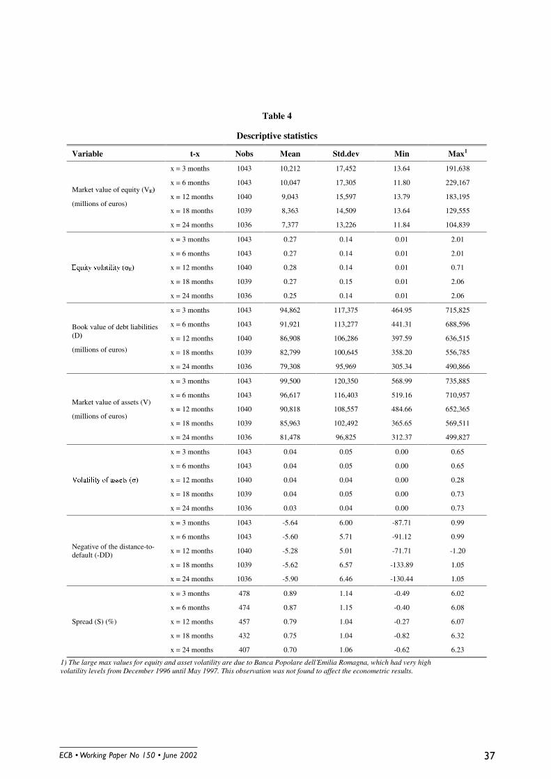
Table 4

Descriptive statistics

Variable t-x Nobs Mean Std.dev Min Max1

x = 3 months 1043 10,212 17,452 13.64 191,638

x = 6 months 1043 10,047 17,305 11.80 229,167

x = 12 months 1040 9,043 15,597 13.79 183,195

x = 18 months 1039 8,363 14,509 13.64 129,555

Market value of equity (VE)

(millions of euros)

x = 24 months 1036 7,377 13,226 11.84 104,839

x = 3 months 1043 0.27 0.14 0.01 2.01

x = 6 months 1043 0.27 0.14 0.01 2.01

x = 12 months 1040 0.28 0.14 0.01 0.71

x = 18 months 1039 0.27 0.15 0.01 2.06

(TXLW\�YRODWLOLW\�� E)

x = 24 months 1036 0.25 0.14 0.01 2.06

x = 3 months 1043 94,862 117,375 464.95 715,825

x = 6 months 1043 91,921 113,277 441.31 688,596

x = 12 months 1040 86,908 106,286 397.59 636,515

x = 18 months 1039 82,799 100,645 358.20 556,785

Book value of debt liabilities(D)

(millions of euros)

x = 24 months 1036 79,308 95,969 305.34 490,866

x = 3 months 1043 99,500 120,350 568.99 735,885

x = 6 months 1043 96,617 116,403 519.16 710,957

x = 12 months 1040 90,818 108,557 484.66 652,365

x = 18 months 1039 85,963 102,492 365.65 569,511

Market value of assets (V)

(millions of euros)

x = 24 months 1036 81,478 96,825 312.37 499,827

x = 3 months 1043 0.04 0.05 0.00 0.65

x = 6 months 1043 0.04 0.05 0.00 0.65

x = 12 months 1040 0.04 0.04 0.00 0.28

x = 18 months 1039 0.04 0.05 0.00 0.73

9RODWLOLW\�RI�DVVHWV�� )

x = 24 months 1036 0.03 0.04 0.00 0.73

x = 3 months 1043 -5.64 6.00 -87.71 0.99

x = 6 months 1043 -5.60 5.71 -91.12 0.99

x = 12 months 1040 -5.28 5.01 -71.71 -1.20

x = 18 months 1039 -5.62 6.57 -133.89 1.05

Negative of the distance-to-default (-DD)

x = 24 months 1036 -5.90 6.46 -130.44 1.05

x = 3 months 478 0.89 1.14 -0.49 6.02

x = 6 months 474 0.87 1.15 -0.40 6.08

x = 12 months 457 0.79 1.04 -0.27 6.07

x = 18 months 432 0.75 1.04 -0.82 6.32

Spread (S) (%)

x = 24 months 407 0.70 1.06 -0.62 6.23

1) The large max values for equity and asset volatility are due to Banca Popolare dell’Emilia Romagna, which had very highvolatility levels from December 1996 until May 1997. This observation was not found to affect the econometric results.

��

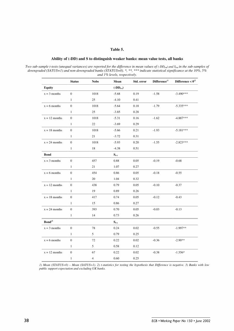
Table 5.

Ability of (-DD) and S to distinguish weaker banks: mean value tests, all banks

Two sub-sample t-tests (unequal variances) are reported for the difference in mean values of (-DDt-x) and St-x in the sub-samples ofdowngraded (SATUS=1) and non-downgraded banks (STATUS=0). *, **, *** indicate statistical significance at the 10%, 5%

and 1% levels, respectively.

Status Nobs Mean Std. error Difference(1 Difference < 0(2

Equity (-DDt-x)

x = 3 months 0 1018 -5.68 0.19 -1.58 -3.490***

1 25 -4.10 0.41

x = 6 months 0 1018 -5.64 0.18 -1.79 -5.335***

1 25 -3.85 0.28

x = 12 months 0 1018 -5.31 0.16 -1.62 -4.887***

1 22 -3.69 0.29

x = 18 months 0 1018 -5.66 0.21 -1.93 -5.181***

1 21 -3.72 0.31

x = 24 months 0 1018 -5.93 0.20 -1.55 -2.823***

1 18 -4.38 0.51

Bond St-x

x = 3 months 0 457 0.88 0.05 -0.19 -0.68

1 21 1.07 0.27

x = 6 months 0 454 0.86 0.05 -0.18 -0.55

1 20 1.04 0.32

x = 12 months 0 438 0.79 0.05 -0.10 -0.37

1 19 0.89 0.26

x = 18 months 0 417 0.74 0.05 -0.12 -0.43

1 15 0.86 0.27

x = 24 months 0 393 0.70 0.05 -0.03 -0.13

1 14 0.73 0.26

Bond(3 St-x

x = 3 months 0 78 0.24 0.02 -0.55 -1.997**

1 5 0.79 0.25

x = 6 months 0 72 0.22 0.02 -0.36 -2.90**

1 5 0.58 0.12

x = 12 months 0 67 0.22 0.02 -0.38 -1.556*

1 4 0.60 0.25

1) Mean (STATUS=0) – Mean (SATUS=1). 2) t-statistics for testing the hypothesis that Difference is negative. 3) Banks with lowpublic support expectation and excluding UK banks.

�� #

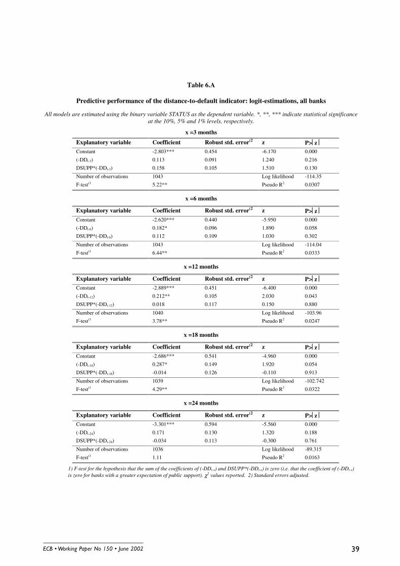
Table 6.A

Predictive performance of the distance-to-default indicator: logit-estimations, all banks

All models are estimated using the binary variable STATUS as the dependent variable. *, **, *** indicate statistical significanceat the 10%, 5% and 1% levels, respectively.

x =3 months

Explanatory variable Coefficient Robust std. error(2 z P>z Constant -2.803*** 0.454 -6.170 0.000

(-DDt-3) 0.113 0.091 1.240 0.216

DSUPP*(-DDt-3) 0.158 0.105 1.510 0.130

Number of observations 1043 Log likelihood -114.35

F-test(1 5.22** Pseudo R2 0.0307

x =6 months


(-DDt-6) 0.182* 0.096 1.890 0.058

DSUPP*(-DDt-6) 0.112 0.109 1.030 0.302


F-test(1 6.44** Pseudo R2 0.0333

x =12 months


(-DDt-12) 0.212** 0.105 2.030 0.043

DSUPP*(-DDt-12) 0.018 0.117 0.150 0.880


F-test(1 3.78** Pseudo R2 0.0247

x =18 months


(-DDt-18) 0.287* 0.149 1.920 0.054

DSUPP*(-DDt-18) -0.014 0.126 -0.110 0.913


F-test(1 4.29** Pseudo R2 0.0322

x =24 months


(-DDt-24) 0.171 0.130 1.320 0.188

DSUPP*(-DDt-24) -0.034 0.113 -0.300 0.761


F-test(1 1.11 Pseudo R2 0.0163

1) F-test for the hypothesis that the sum of the coefficients of (-DDt-x) and DSUPP*(-DDt-x) is zero (i.e. that the coefficient of (-DDt-x)is zero for banks with a greater expectation of public support). χ2 values reported. 2) Standard errors adjusted.

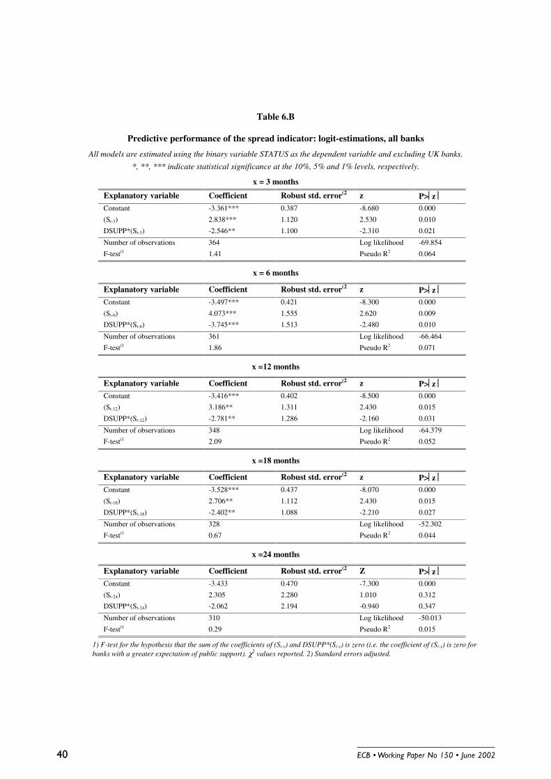
�� 0

Table 6.B

Predictive performance of the spread indicator: logit-estimations, all banks

All models are estimated using the binary variable STATUS as the dependent variable and excluding UK banks.

*, **, *** indicate statistical significance at the 10%, 5% and 1% levels, respectively.

x = 3 months


(St-3) 2.838*** 1.120 2.530 0.010

DSUPP*(St-3) -2.546** 1.100 -2.310 0.021



x = 6 months


(St-6) 4.073*** 1.555 2.620 0.009

DSUPP*(St-6) -3.745*** 1.513 -2.480 0.010



x =12 months


(St-12) 3.186** 1.311 2.430 0.015

DSUPP*(St-12) -2.781** 1.286 -2.160 0.031



x =18 months


(St-18) 2.706** 1.112 2.430 0.015

DSUPP*(St-18) -2.402** 1.088 -2.210 0.027



x =24 months

Explanatory variable Coefficient Robust std. error(2 Z P>z Constant -3.433 0.470 -7.300 0.000

(St-24) 2.305 2.280 1.010 0.312

DSUPP*(St-24) -2.062 2.194 -0.940 0.347



1) F-test for the hypothesis that the sum of the coefficients of (St-x) and DSUPP*(St-x) is zero (i.e. the coefficient of (St-x) is zero forbanks with a greater expectation of public support). χ2 values reported. 2) Standard errors adjusted.

��

Table 7.

Performance of the distance-to-default indicator: proportional hazard estimation, all banksEstimated using Cox regression. Log-likelihood given in the text. Standard errors are corrected for clustering using Wei and

Lin’s (1989) method *, **, *** indicate statistical significance at the 10%, 5% and 1% levels.

Explanatory variable Hazard ratio Robust std. error z P>z (-DD) 0.728** 0.115 2.02 0.04

Number of subjects 84 Time at risk 5365

Number of failures 25 Starting log likelihood -100.49

Number of observations 5365 Final log likelihood -96.71

Wald χ2 4.08** Zero-slope test 7.66***

Table 8.

Performance of the bond spread: proportional hazard estimation, all banksEstimated using Cox regression. Log-likelihood given in the text. Standard errors are corrected for clustering using Wei and

Lin’s (1989) method. *,**, *** indicate statistical significance at the 10%, 5% and 1% levels.

Explanatory variable Hazard ratio Robust std. error z P>z S 1.00 0.002 0.75 0.455




Wald χ2 0.56 Zero-slope test 0.40

Table 9.

Performance of the distance-to-default indicator: proportional hazard estimation using a dummy variable, allbanks

Estimated using Cox regression. Log-likelihood given in the text. Standard errors are corrected for clustering using Wei andLin’s (1989) method. *,**, *** indicate statistical significance at the 10%, 5% and 1% levels.

Explanatory variable Hazard ratio Robust std. error z P>z Dummy for (-DD) >-3.2 2.69*** 1.034 2.57 0.01




Wald χ2 6.62*** Zero-slope test 1.52

�� /

Table 10.

Performance of the bond spread: proportional hazard estimation controlling for the UK, all banksEstimated using Cox regression. Log-likelihood given in the text. Standard errors are corrected for clustering using Wei and

Lin’s (1989) method. *,**, *** indicate statistical significance at the 10%, 5% and 1% levels.

Explanatory variable Hazard ratio Robust std. error z P>z S 1.01*** 0.002 2.74 0.006

Dummy for UK -0.065** 0.080 -2.25 0.025




Wald χ2 8.76*** Zero-slope test (global test) 1.86

Table 11.

Performance of the bond spread: proportional hazard estimation controlling the level of support, UK banksexcluded


Explanatory variable Hazard ratio Robust std. error z P>z S 1.02*** 0.005 3.79 0.000

Dummy “high support”*S -0.99*** 0.005 -2.71 0.007





Table 12.

The role of the safety net and the UK location: Log-rank tests for equality of survivor functions, all banksEstimated using the Cox regression in tables 9 and 11. *,**, *** indicate statistical significance at the 10%, 5% and 1% levels.

χ2 P > χ2

(-DD)

Dummy “high support” equal to 1 4.94** 0.03

Dummy “high support” equal to 0 0.90 0.34

S

Dummy “high support” equal to 1 1.95 0.16

Dummy “high support” equal to 0 3.30* 0.07

S; excluding UK banks

Dummy “high support” equal to 1 7.81*** 0.005

Dummy “high support” equal to 0 30.19*** 0.000

��

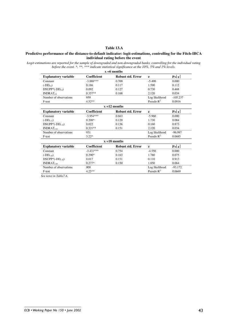
Table 13.A

Predictive performance of the distance-to-default indicator: logit-estimations, controlling for the Fitch-IBCAindividual rating before the event

Logit-estimations are reported for the sample of downgraded and non-downgraded banks, controlling for the individual ratingbefore the event. *, **, *** indicate statistical significance at the 10%, 5% and 1% levels.

x =6 months

Explanatory variable Coefficient Robust std. Error z P>z Constant -3.888*** 0.709 -5.490 0.000(-DDt-6) 0.186 0.117 1.590 0.112DSUPP*(-DDt-6) 0.092 0.127 0.730 0.468INDRATt-6 0.357** 0.168 2.120 0.034Number of observations 959 Log likelihood -105.237F-test 4.52** Pseudo R2 0.0916

x =12 months

Explanatory variable Coefficient Robust std. Error z P>z Constant -3.954*** 0.663 -5.960 0.000(-DDt-12) 0.208* 0.120 1.730 0.084DSUPP*(-DDt-12) 0.022 0.136 0.160 0.873INDRATt-12 0.321** 0.151 2.120 0.034Number of observations 931 Log likelihood -96.997F-test 3.22* Pseudo R2 0.0685

x =18 months

Explanatory variable Coefficient Robust std. Error z P>z Constant -3.431*** 0.754 -4.550 0.000(-DDt-18) 0.290* 0.163 1.780 0.075DSUPP*(-DDt-18) 0.017 0.151 0.110 0.913INDRATt-18 0.277* 0.150 1.850 0.064Number of observations 909 Log likelihood -93.172F-test 4.25** Pseudo R2 0.0669

See notes in Table7.A.

��

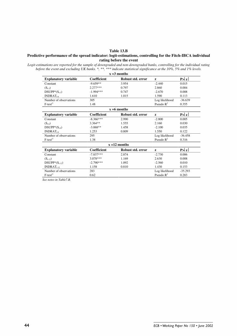
Table 13.BPredictive performance of the spread indicator: logit-estimations, controlling for the Fitch-IBCA individual

rating before the eventLogit-estimations are reported for the sample of downgraded and non-downgraded banks, controlling for the individual rating

before the event and excluding UK banks. *, **, *** indicate statistical significance at the 10%, 5% and 1% levels.x =3 months

Explanatory variable Coefficient Robust std. error z P>z Constant -9.659** 3.954 -2.440 0.015(St-3) 2.277*** 0.797 2.860 0.004DSUPP*(St-3) -1.994*** 0.747 -2.670 0.008INDRATt-6 1.610 1.015 1.590 0.113Number of observations 305 Log likelihood -36.639F-test(1 1.48 Pseudo R2 0.355

x =6 months

Explanatory variable Coefficient Robust std. error z P>z Constant -8.366*** 2.990 -2.800 0.005(St-6) 3.364** 1.555 2.160 0.030DSUPP*(St-6) -3.068** 1.458 -2.100 0.035INDRATt-6 1.253 0.809 1.550 0.122Number of observations 295 Log likelihood -36.458F-test(1 1.38 Pseudo R2 0.316

x =12 months

Explanatory variable Coefficient Robust std. error z P>z Constant -7.837*** 2.874 -2.730 0.006(St-12) 3.078*** 1.169 2.630 0.008DSUPP*(St-12) -2.790*** 1.092 -2.560 0.010INDRATt-12 1.158 0.810 1.430 0.153Number of observations 283 Log likelihood -35.293F-test(1 0.62 Pseudo R2 0.283

See notes in Table7.B.

��

Table 14.A

Information content of the distance-to-default indicator: logit-estimations, all banks

All models are estimated using the binary variable STATUS as the dependent variable. *, **, *** indicate statisticalsignificance at the 10%, 5% and 1% levels, respectively. SCORE is a synthetic variable summarising the ranking of thebank with regard to four indicators representing respectively capital adequacy, asset quality, efficiency, and profitability.

Model with only the distance-to-default indicatorx =12 months

Explanatory variable Coefficient Robust std. error(2 Z P>z Constant -1.790*** 0.492 -3.640 0.000

(DDt-x) 0.249** 0.121 2.070 0.039

DSUPP*(DDt-x) 0.005 0.119 0.040 0.970


F-test(1 3.97** Pseudo R2 0.035

Model with only balance-sheet indicatorsx =12 months


SCORE 0.574*** 0.121 4.740 0.000


Pseudo R2 0.199

Model with the distance-to-default indicator and balance-sheet indicatorsx =12 months


(DDt-x) 0.242** 0.110 2.200 0.028

DSUPP*(DDt-x) -0.044 0.127 -0.340 0.732

SCORE 0.585*** 0.125 4.670 0.000


F-test(1 3.03* Pseudo R2 0.238


��

Table 14.B

Information content of the spreads indicator: logit-estimations, all banks

All models are estimated using the binary variable STATUS as the dependent variable. *, **, *** indicate statisticalsignificance at the 10%, 5% and 1% levels, respectively. SCORE is a synthetic variable summarising the ranking of the

bank with regard to four indicators representing respectively capital adequacy, asset quality, efficiency, and profitability.The models exclude UK banks.

Model with only the spreads indicatorx =12 months


(St-x) 2.999** 1.353 2.220 0.027

DSUPP*(St-x) -2.575* 1.328 -1.940 0.053


F-test(1 2.00 Pseudo-R2 0.055

Model with only balance-sheet indicatorsx =12 months


SCORE 0.548*** 0.142 3.850 0.000


Pseudo-R2 0.230

Model with the spreads indicator and balance-sheet indicatorsx =12 months


(St-x) 2.079 1.627 1.280 0.201

DSUPP*(St-x) -1.662 1.600 -1.040 0.299

SCORE 0.514*** 0.138 3.730 0.000


Pseudo-R2 0.251


�� *

Table 15.

Performance of the distance to default and the bond spread: proportional hazard estimation, UK banksexcluded


Explanatory variable Hazard ratio Robust std. error z P>z Dummy for (-DD) >-3.2 4.01** 2.55 2.19 0.029

S 1.01*** 0.004 2.77 0.006

Dummy “high support”*S -0.99** 0.005 -2.41 0.016





��

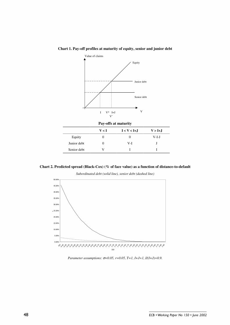
Chart 1. Pay-off profiles at maturity of equity, senior and junior debt

Value of claims

VI I+J

Senior debt

Junior debt

Equity

V*V’

Pay-offs at maturity

V < I I < V < I+J V > I+J

Equity 0 0 V-I-J

Junior debt 0 V-I J

Senior debt V I I

Chart 2. Predicted spread (Black-Cox) (% of face value) as a function of distance-to-default

Subordinated debt (solid line), senior debt (dashed line)

Parameter assumptions: σ=0.05, r=0.05, T=1, I+J=1, I/(I+J)=0.9.

0.00%

5.00%

10.00%

15.00%

20.00%

25.00%

30.00%

35.00%

40.00%

45.00%

50.00%

DD-0

.45-0

.35-0

.25-0

.15-0

.05 0.05

0.15

0.25

0.35

0.45

0.55

0.65

0.75

0.85

0.95

1.05

1.15

1.25

1.35

1.45

1.55

1.65

1.75

1.85

1.95

2.05

2.15

2.25

2.35

2.45

2.55

2.65

2.75

2.85

2.95

DD

s

�� #

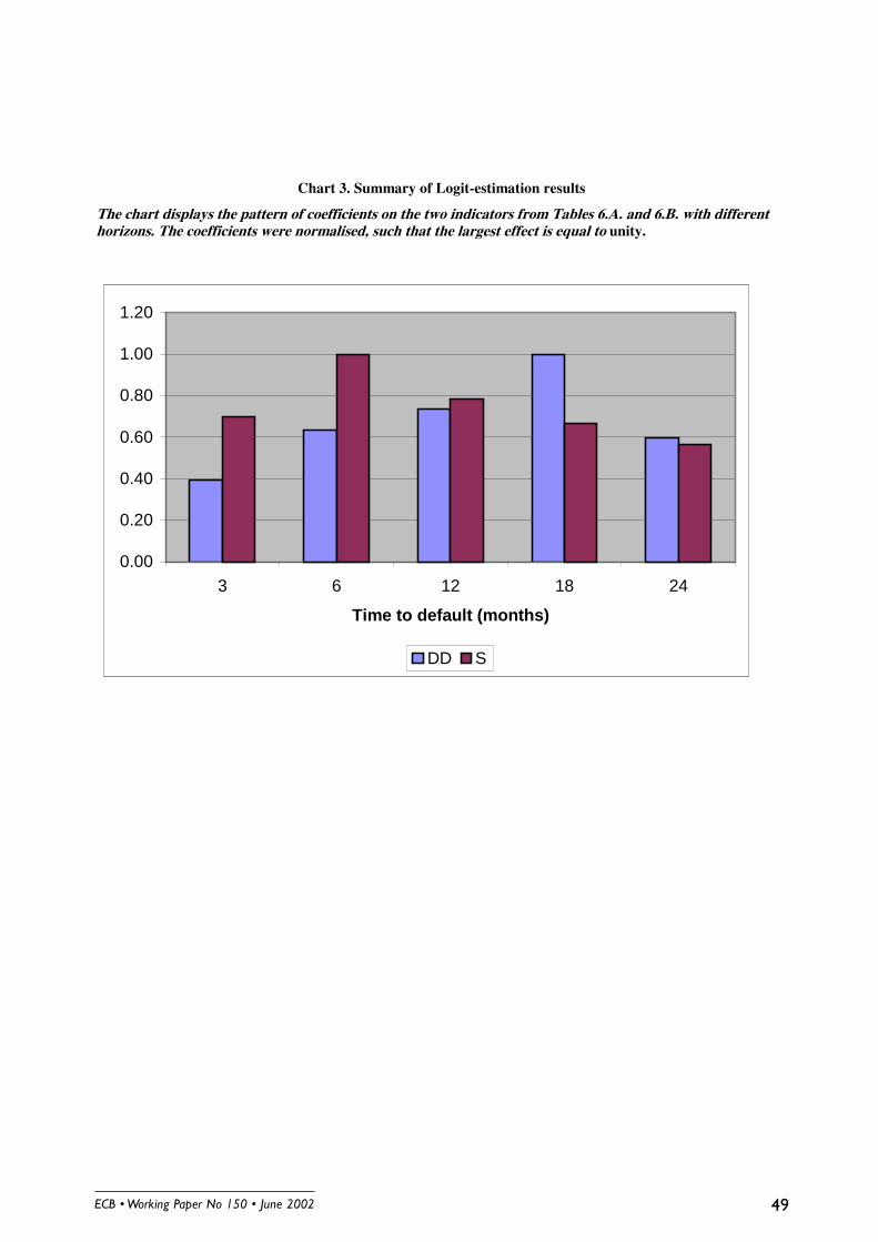
Chart 3. Summary of Logit-estimation results

The chart displays the pattern of coefficients on the two indicators from Tables 6.A. and 6.B. with differenthorizons. The coefficients were normalised, such that the largest effect is equal to unity.

0.00

0.20

0.40

0.60

0.80

1.00

1.20

3 6 12 18 24

Time to default (months)

DD S

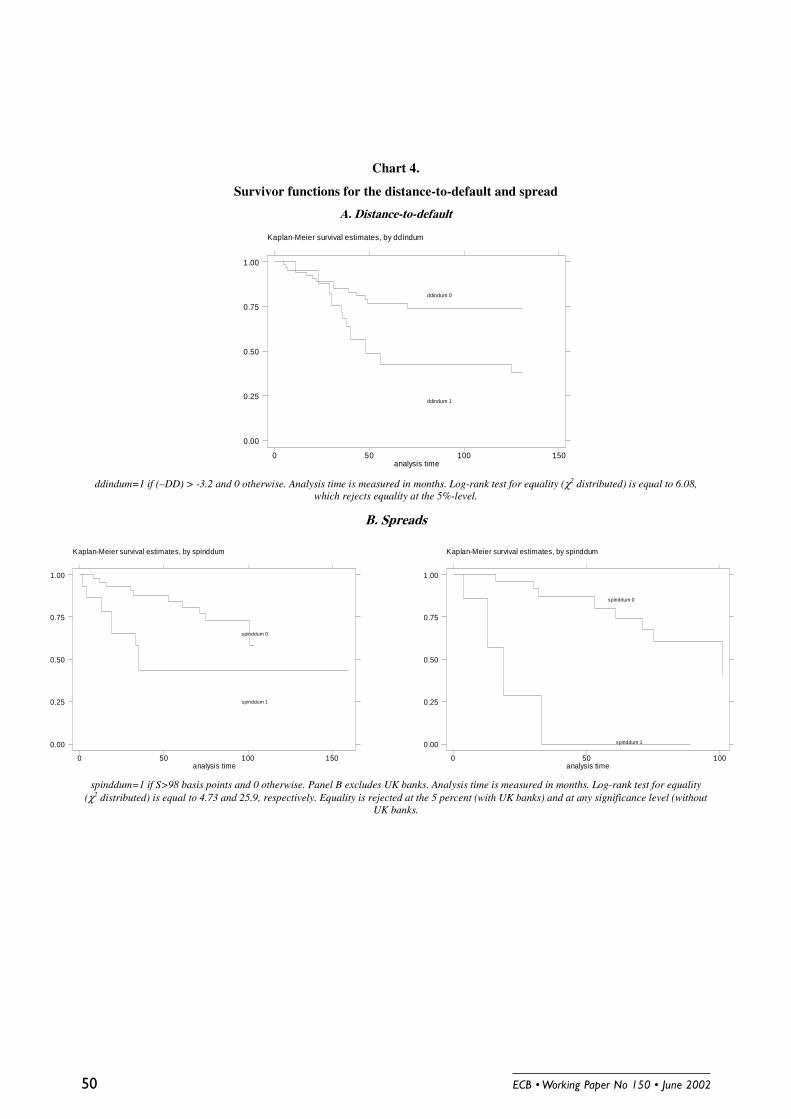
�� 0

Chart 4.

Survivor functions for the distance-to-default and spread

A. Distance-to-default

ddindum=1 if (–DD) > -3.2 and 0 otherwise. Analysis time is measured in months. Log-rank test for equality (χ2 distributed) is equal to 6.08,which rejects equality at the 5%-level.

B. Spreads

spinddum=1 if S>98 basis points and 0 otherwise. Panel B excludes UK banks. Analysis time is measured in months. Log-rank test for equality(χ2 distributed) is equal to 4.73 and 25.9, respectively. Equality is rejected at the 5 percent (with UK banks) and at any significance level (without

UK banks.

Kaplan-Meier survival estimates, by ddindum

analysis time0 50 100 150

0.00

0.25

0.50

0.75

1.00

ddindum 0

ddindum 1

Kaplan-Meier survival estimates, by spinddum

analysis time0 50 100 150

0.00

0.25

0.50

0.75

1.00

spinddum 0

spinddum 1

Kaplan-Meier survival estimates, by spinddum

analysis time0 50 100

0.00

0.25

0.50

0.75

1.00

spinddum 0

spinddum 1

��

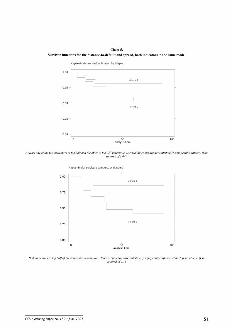
Chart 5.

Survivor functions for the distance-to-default and spread, both indicators in the same model

At least one of the two indicators in top half and the other in top 75th percentile. Survival functions are not statistically significantly different (Chisquared of 1.04).

Both indicators in top half of the respective distributions. Survival functions are statistically significantly different at the 5 percent level (Chisquared of 4.1).

Kaplan-Meier survival estimates, by ddspind


0.00

0.25

0.50

0.75

1.00

ddspind 0

ddspind 1

Kaplan-Meier survival estimates, by ddspind


0.00

0.25

0.50

0.75

1.00ddspind 0

ddspind 1

�� /

Appendix 1.

Distance-to-default according to the Black and Scholes formula29

In the BS model the time path of the market value of assets follows a stochastic process:

,TT2

rVlnVln A

2A

ATA εσ

σ+

−+=

which gives the asset value at time T (i.e. maturity of debt), given its current value (VA�� is the random componentof the firm’s return on assets, which the BS model assumes normally distributed, with zero mean and unit variance,N(0,1).

Hence, the current distance d from the default point (where DlnVln = ) can be expressed as:

.T

T2

rD

Vln

T

d

DlnTT)2

r(VlnDlnVlnd

2

2d

εσ

σ

σ

εσσ

+

−+

=

<=>−+−+=−=

That is, the distance-to-default (DD)

T

T2

rD

Vln

T

dDD

2

σ

σ

εσ

−+

=−≡

�� A) that the firm is from the default point.

The implied probability of default (IPD) can be defined as the probability that the asset value is less or equal to thebook value of debt liabilities when the debt matures:

[ ]

[ ].)DD(PrT

T2

rD

Vln

PrIPD

.e.i,DlnTT2

rVlnPrDlnVlnPrIPD

2

2T

εεσ

σ

εσσ

≤−=

≤

−+

−=

≤+

−+<=>≤≡

�� N(-DD).

29 See KMV Corporation (1999) for a similar derivation and more ample discussions.

��

Appendix 2.

Ratings definitions used by Fitch-IBCA

Fitch-IBCA’s Individual Ratings attempt to assess how a bank would be viewed if it were entirelyindependent, and could not rely on external support. These ratings are designed to assess a bank’s exposure to,appetite for, and management of risk, and thus represent the view on the likelihood that it would run into significantdifficulties. The principal factors analysed to evaluate the bank and determine these ratings include profitability andbalance sheet integrity, franchise, management, operating environment, and prospects.

Fitch-IBCA distinguishes among the following categories:

A. A very strong bank. Characteristics may include outstanding profitability and balance sheet integrity,franchise, management, operating environment, or prospects.

B. A strong bank. There are no major concerns regarding the bank. Characteristics may include strongprofitability and balance sheet integrity, franchise, management, operating environment or prospects.

C. An adequate bank which, however, possesses one or more troublesome aspects. There may besome concerns regarding its profitability and balance sheet integrity, franchise, management, operatingenvironment or prospects.

D. A bank which has weaknesses of internal and/or external origin. There are concerns regarding itsprofitability and balance sheet integrity, franchise, management, operating environment or prospects.

E. A bank with very serious problems which either requires or is likely to require external support.

Note that, in addition, there are gradations among these five rating categories, i.e. A/B, B/C, C/D, and D/E.

The Support Ratings do not assess the quality of a bank. Rather, they are Fitch-IBCA’s assessment ofwhether the bank would receive support should this be necessary.

1. A bank for which there is a clear legal guarantee on the part of the State, or a bank of such importanceboth internationally and domestically that, in Fitch-IBCA’s opinion, support from the State would beforthcoming, if necessary. The State in question must clearly be prepared and able to support itsprincipal banks.

2. A bank for which, in our opinion, state support would be forthcoming, even in the absence of a legalguarantee. This could be, for example, because of the bank’s importance to the economy or its historicrelationship with the authorities.

3. A bank or bank holding company which has institutional owners of sufficient reputation and possessingsuch resources that, in our opinion, support would be forthcoming, if necessary.

4. A bank for which support is likely but not certain.

A bank, or bank holding company, for which support, although possible, cannot be relied upon.

��

��

�� !��"��#��$%%"""&��&��'&

() *+��,�� -��.&�/� ��0&�� 1&��&�� 1� ��2334&

(5 *+�� -��0&�6��6&��7,8��1&�9�� 1� ��2334&

�3 *�� :��$�8� �� -��;&�� 1� ��2334&

�4 *.�� -��&�<��9&�9��&�6&��0��1� ��2334&

�2 *�� -��9&�� =&�6��1� ��2334&

�� *>�� ?�� 6��-��@&��.&��1� ��2334&

�A *>��-��B&��C��&�<� ��.��2334&

�D *0 �� -��9&�@�� =&��&�� .��2334&

�(��*=��:��$��"�� E-��=&�6��.&�1&�=��.��2334&

��*�� F�� $�.�� -��&�� &��,+��6&� �� &�<��G��7��6&�/��@&�@��9&�@�� @&�+�F� ��9��2334&

�)��*>� �� -��&�@�F��&�9��&�0�� 9��2334&

�5��*�� :��E�� -��/&�9��H��2334&

)3��*+��-��&�<��@&�@��.&�@�7��H��2334&

)4��*�� E-��1&�@��.&�@��H��2334&

)2��*��$�� -��&�<��@&�� H��2334&

��

)��*��,�:�� I��-��J&��&�� K� ��2334&

)A��*�� -��6&��.&�/� ��0&�� K� ��2334&

)D��*�� C��$��=%��=��-��&�@��,��7��&�H��&�9��7��K� ��2334&

)(��*=�� C�� $��"��C��-��@&��9&�6&�< ��9&��&�<��K� ��2334&

)��*�� -��&��K� ��2334&

)) *�� " ��C��E-��/&�J� ��@&��&�+� ��K� ��2334&

)5 *@�� -��0&��&��K� ��2334&

53 *�� "��-��9&�/��&�@�� 1&,�&�0�� K� ��2334&

54 *+��$�� 0.=� ��-��6&��&�9��2334&

52 *.�0.=�� -��&�@�F��6&��2334&

5� *+��,�� $�� -��&�@�.��1&�@��2334&

5A *@�� $�"�� E-��&� �� .&�/��1&�@��1&,�&�0� �� 2334&

5D *9�� -��.&,@&�.��&�@�F��2334&

5( *+�� 6��-��.&��2334&

5� *.�� &�.��4553�-��9&�J��2334&

5) *+�� K�� $�� -��/&��<��2334&

55 *>�� 9��E-��>&�<��1&�@�L��7,��M��2334&

��

433 *+�� $�� -��1&�+��1&�0� ��2334&

434 *@�� $��E-��&�/��&�9 ��&�9� ��2334&

432 *+�� $��-��/&��&�=�� @:��2334&

43� *��,�� $��>� �-��/&�6��2334&

43A *>�� 6��E�� -��9&�K&��K&��&�J�� 6&�+&�9��2334&

43D *�� -��@&��/&�6��1&�@�L��7,��M��&�9� ��.&��2334&

43( *>� �� $�� -��1&,�&�� .&�+��2334&

43� *+�� $�� "��, � � ��-��&��7��&��&�0�� 2334&

43) *�� .��$��,��-��@&�0 ��2334&

435 *@��6��$��"�� -��;&� ��J ��2334&

443 *�� E�.� �� >� ��-��&�6��.&�6�� 2334&

444 *@��$�� /�C�� -��&�/N��+&�@��O��2334&

442 *�� -��1&,�&�� .&�6�� >&�<��;&� ��J ��&��0�� 2334&

44� *�� $�� -��&��1&�/��J&�K�� 1��2332&

44A *@��$�"��"��E-��>&�.�� .&�J��&�@�F��&�+� �77��1��2332&

44D *@�� $�� "��-��.&�H��2334&

44( *=��6��45)D��455)-��1&�<��&�J�7&�1��2332&

�� *

44� *<��"��$��"�� -��H&�� &�0� � ��1��2332&

44) *�� C��:� ��$�� >� ��45)),455)-��6&�@&�+��1��2332&

445 *@�� -��K&�� &�@��1��2332&

423 */�� "��-��9&�<��F��J&�@��1��2332&

424 *K�� -��.&��=&��&�.&��2332&

422 *K�"�� "��-��&�0�F�� =&�. ��2332&

42� *.� �� -��&�+��.&�0��2332&

42A *@�� C��-��6&��&�� 9&�<��F��2332&

42D *�� -��9&�@�� 2332&

42( *H�� -��&�@��&�8��2332&

42� *�� "�� -��9&�<��F��J&�@��2332&

42) *H��C��,�� -��&�9��=&��2332&

425 *K��,�� "��:�� -��.&� ,K�"��/&�9��@��2332&

4�3 *<��7��C��$�� -��&��"��@��2332&

4�4 *@��<>��$�"��"��"��"��"��"E-��@&�.&��&�=��L��7,� ��7�� @��2332&

4�2 *>�� $��*��"�J��-�� -��H&�.�� &�=��L��7,� ��7�� &�+��@��2332&

4�� *�� 6��"��E-��.&�@��@&�=��@��2332&

��

�� !��"��#��$$��

��% ��&��&�'� ��'��&��(&��&��)��"��)��*��+��$$��

��, �-��.��(/�0��1��(��2��+��$$��

��3 �45(��(&��/��(��&6��&��.��7��+��$$��

��8 ��1��1��&(&�(��0�1��4#7��/�(�9��)��*��#�/��+��$$��

�� :��(��/��#��)��;��+��$$��

��$ �*��/�� #��<��#��$$��

�� +�� )��4��=��>�(.��#��$$��

�� #��/��.��(��'�� 5(��&��/�&�� 4(��<��.��+��<��2��<�&��#��;��+��?��)��#��$$��

�� +��&��&�� (��/��1�/��@��<��1 ��#��$$��

�� +� ��(��&��(��&�� 0��(�� &��&��'��&��(��/��#��>��>��?��#��$$��

��% ��1��1��1��/��&� � ��#��)��;��#��(��#��$$��

��, �<&��A�1��(��.��/9��4��<��*��?��&��#��$$��

��3 ��&��(��.��.��1�/��&�;��/�&��&��#��<��#��$$��

��8 �� (�� &� ��(��!��(��(��#��$$��

�� >��.� ��4><��&(��(��&��+��4��+��B��&��#��$$��

�%$ �45(��&��.��/��/�� .� ��/��-��2�� !��2��!(�� (��$$��

Documents

Equity and bond market signals as leading indicators of bank fragility