Equivalent Plate Analysis of Aircraft Wing with Discrete

American Institute of Aeronautics and Astronautics

This material is declared a work of the U.S. Government and is not subject to copyright protection in the United States.

Equivalent Plate Analysis of Aircraft Wing with Discrete Source Damage

T. Krishnamurthy* and Brian H. Mason† NASA Langley Research Center, Hampton, VA 23681, U.S.A.

Abstract

An equivalent plate procedure is developed to provide a computationally efficient means of matching the stiffness and frequencies of flight vehicle wing structures for prescribed loading conditions. First, the equivalent plate is used to match the stiffness of a stiffened panel without damage and the stiffness of a stiffened panel with damage. For both stiffened panels, the equivalent plate models reproduce the deformation of a corresponding detailed model exactly for the given loading conditions. Once the stiffness was matched, the equivalent plate models were then used to predict the frequencies of the panels. Two analytical procedures using the lumped-mass matrix were used to match the first five frequencies of the corresponding detailed model. In both the procedures, the lumped-mass matrix for the equivalent plate is constructed by multiplying the diagonal terms of the consistent-mass matrix by a proportionality constant. In the first procedure, the proportionality constant is selected such that the total mass of the equivalent plate is equal to that of the detailed model. In the second method, the proportionality constant is selected to minimize the sum of the squares of the errors in a set of pre-selected frequencies between the equivalent plate model and the detailed model. The equivalent plate models reproduced the fundamental first frequency accurately in both the methods. It is observed that changing only the mass distribution in the equivalent plate model did not provide enough flexibility to match all of the frequencies.

Introduction Understanding the effects of discrete source damage (e.g, uncontained rotor burst) on the response of aircraft structures is necessary to improve the survivability of future aircraft to adverse damage events. Rapid modeling and analysis methods are among the key requirements for real-time evaluation of damage effects that are needed for integrated vehicle health management. One such analysis method is equivalent plate analysis. Equivalent plate analysis has been used to replace the computationally expensive finite element analysis in initial design stages or in conceptual design of aircraft wing structures [1]. In equivalent plate modeling, the model characteristics are represented with polynomials, which require only a small fraction of the input data that would be required by a corresponding finite element model. An equivalent plate analysis procedure based on the Ritz method was proposed

* Aerospace Engineer, Computational Structures and Materials Branch, Senior Member, AIAA. † Aerospace Engineer, Computational Structures and Materials Branch, Senior Member, AIAA.


2

at NASA Langley Research Center as early as 1986 [2]. In the Ritz method-based equivalent plate theory, the aircraft wing structure is modeled with several trapezoidal segments. Several modifications and improvements to the initial theory proposed in reference 2 resulted in development of a structural analysis code ELAPS (Equivalent Laminated Plate Solution) [3, 4]. The ELAPS code solutions predict the displacement, stress, and mode shape calculations within five to ten percent of a comparable finite element solution [5]. However, the Ritz method-based equivalent plate theory in the ELAPS code is not easily amenable for implementation in general-purpose commercial structural finite element analysis codes. Hence, there is a need to develop an equivalent plate analysis which can be used in these general-purpose codes. Moreover, equivalent plate theory formulations with the ability to consider aircraft wing structures containing discrete source damage are not available in the literature. A method to analyze wing structures with discrete source damage is essential in health monitoring, in design of wing structures to consider moderate to heavy damage in flight and in design of wind tunnel models to study the effect of damage on the performance of the flight vehicle. The equivalent plate model can also be used to design a wind tunnel model to match the stiffness characteristics of the wing box of a full-scale flight vehicle model while satisfying strength-based requirements [6] In this paper, we develop an equivalent plate analysis for the aircraft wing structures that can:

a. be used with general purpose commercial finite element structural analysis codes; b. predict the static and dynamic characteristics of full-scale flight vehicles with and without

discrete source damage; c. accurately predict internal load change as a result of discrete source damage; and d. perform analysis with minimum computational effort during real-time simulations.

Equivalent Plate Theory Development

The approach adapted in the present study is to generate an equivalent plate model of a flight vehicle wing structure by matching the stiffness of the equivalent plate and the flight vehicle. The equivalent plate stiffness is assumed to be same as that of the flight vehicle if the deformation of the equivalent plate and the flight vehicle are identical for a given set of loading and boundary conditions. The deformation of the equivalent plate is matched with the flight vehicle primarily by changing the thickness distribution in the equivalent plate. The procedure to create the equivalent plate model is described as follows:

1. Obtain the displacement field of the flight vehicle by performing full scale finite element linear static analysis for the given loading and boundary conditions.

2. Fix the dimensions of the equivalent plate plan-form. 3. Construct the finite element model of the equivalent plate. 4. If the nodal locations of the equivalent plate model are different from that of the full-

scale fight vehicle finite element nodes, interpolate displacements at the equivalent plate nodal locations. In the present study, the interpolated displacements at the equivalent plate nodal locations are denoted as the flight vehicle reference displacements.

5. Find the displacement distribution of the equivalent plate by performing linear static analysis for a given thickness distribution of the plate and determine the optimum thickness distribution of the equivalent plate by minimizing the sum of the differences between the flight vehicle reference displacements and the equivalent plate model displacements at all nodal locations.


3

In the equivalent plate procedure described above, if the plan-form of the equivalent plate is different from the flight vehicle (e.g., in a wind tunnel model) appropriate scaling of the flight vehicle displacements and loading is performed consistent with the physics of the problem. Minimizing the difference in displacements between the full-scale flight vehicle and the equivalent plate in Step 5 is achieved by solving an optimization problem. The objective function Φ for the optimization problem can be stated as

( )∑ −=Φ=

N

i

Fi

Ei ww

1

2 (1)

The objective function Φ in Equation (1) is minimized in the optimization to obtain the thickness distribution of the equivalent plate. The thickness distribution in the equivalent plate is assumed as a polynomial in the plan-form dimension. The unknown coefficients in the assumed polynomial are determined in the optimization problem. If displacement based loading is applied, the optimization problem in Equation (1) is modified to include the constraint

FE PPG −= (2)

The constraint in Equation (2) is necessary to enforce the condition that the applied load in the equivalent plate and in the flight vehicle is the same.

Where, N is the number of finite element nodes in the equivalent plate model;

Eiw is the displacement at the thi node of the equivalent plate; and

Fiw is the interpolated displacement of the flight vehicle at the location

of the thi node of the equivalent plate.

Where G is the constraint to be satisfied in the optimization problem;

EP is the total load applied in the Equivalent plate model; and

FP is the total load applied in the Full scale flight vehicle model.


4

The general purpose finite element code ABAQUS [7] is used for the finite element analysis. The optimization code DOT [8] is used in step 5 to minimize the difference in displacements in Equation 1. This procedure is further explained in the context of the following two numerical examples.

Numerical Examples The equivalent plate procedure is demonstrated on a set of simple structures that simulate a cantilevered wing. In the first example, a stiffened panel with two blade stiffeners without damage is considered. In the second example, the stiffened panel is modified to include discrete source damage in the form of a circular hole in the center of the panel.

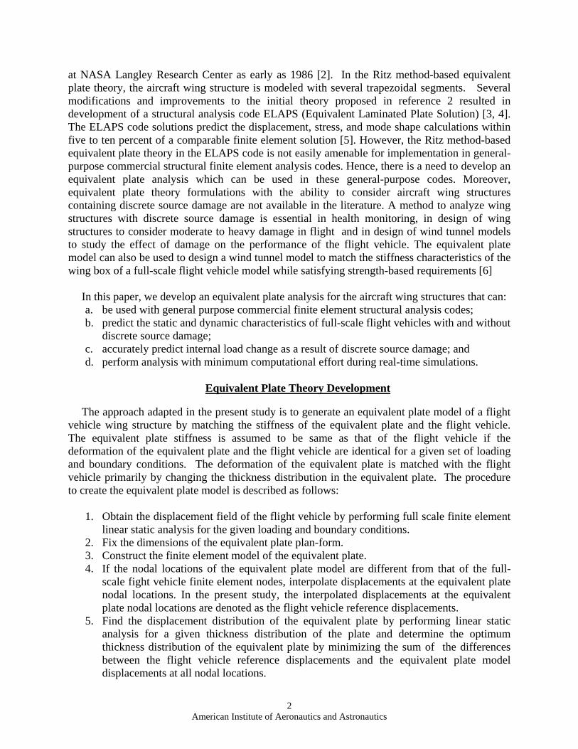
Example 1: Stiffened-Panel without Damage: The two-blade stiffened panel used to generate the equivalent plate model is shown in Figure 1. The dimensions, material properties and the loading used in the analysis are also shown in the figure. Figure 1. Geometry of the stiffened panel used in the equivalent plate generation The plate is completely fixed (cantilevered) at the edge CD. Two types of loading are applied simultaneously at the free edge AB. The first is a uniform vertical displacement Bw− that is applied at the free end from A to B to simulate a bending loading. The second is a torsional loading that is simulated by linearly varying the vertical displacement from Tw+ at the point A to Tw− at the point B. The finite element model of the stiffened panel and its equivalent plate model are shown in Figures 2 and 3, respectively. The nodes in the equivalent plate exactly match the nodes in the stiffened panel, thus eliminating the need for displacement interpolation in step 4 of the optimization procedure. Since the bending and torsional loads are simulated by applying

Thickness of the blade,

Material:

/ 0975.0

3.0 '08 1.0 '

3inlbm Density

RatiosPoissonpsiEModulussYoung

=

==

Loading and Boundary conditions:

A B x

z

AB x

z

a)

b)

c) Side CD fixed in all directions

Bw−

Tw−

Tw+

. 1.02 int =

Thickness of the plate, . 25.01 int =

Height of the blade stiffener. 5.1 inh =

Section On AA-AA

40 in.

5 in. 5 in.10 in.

AA AA

A B

C D

x

y

z


Material:

/ 0975.0

3.0 '08 1.0 '

3inlbm Density


=

==


A B x

z

AB x

z

a)

b)


Bw−

Tw−

Tw+

Material:

/ 0975.0

3.0 '08 1.0 '

3inlbm Density


=

==

Material:

/ 0975.0

3.0 '08 1.0 '

3inlbm Density


=

==


A B x

z

AB x

z

a)

b)


Bw−

Tw−

Tw+


A B x

z

A B x

z

AB x

z

a)

b)


Bw−

Tw−

Tw+

. 1.02 int =



Section On AA-AA

40 in.

5 in. 5 in.10 in.

AA AA

A B

C D

x

y

z

. 1.02 int =



Section On AA-AA

. 1.02 int =

Thickness of the plate, . 25.01 int =Thickness of the plate, . 25.01 int =



Section On AA-AA

40 in.

5 in. 5 in.10 in.

AA AA

A B

C D

x

y

z

40 in.

5 in. 5 in.10 in.

AA AA

A B

C D

x

y

z


5

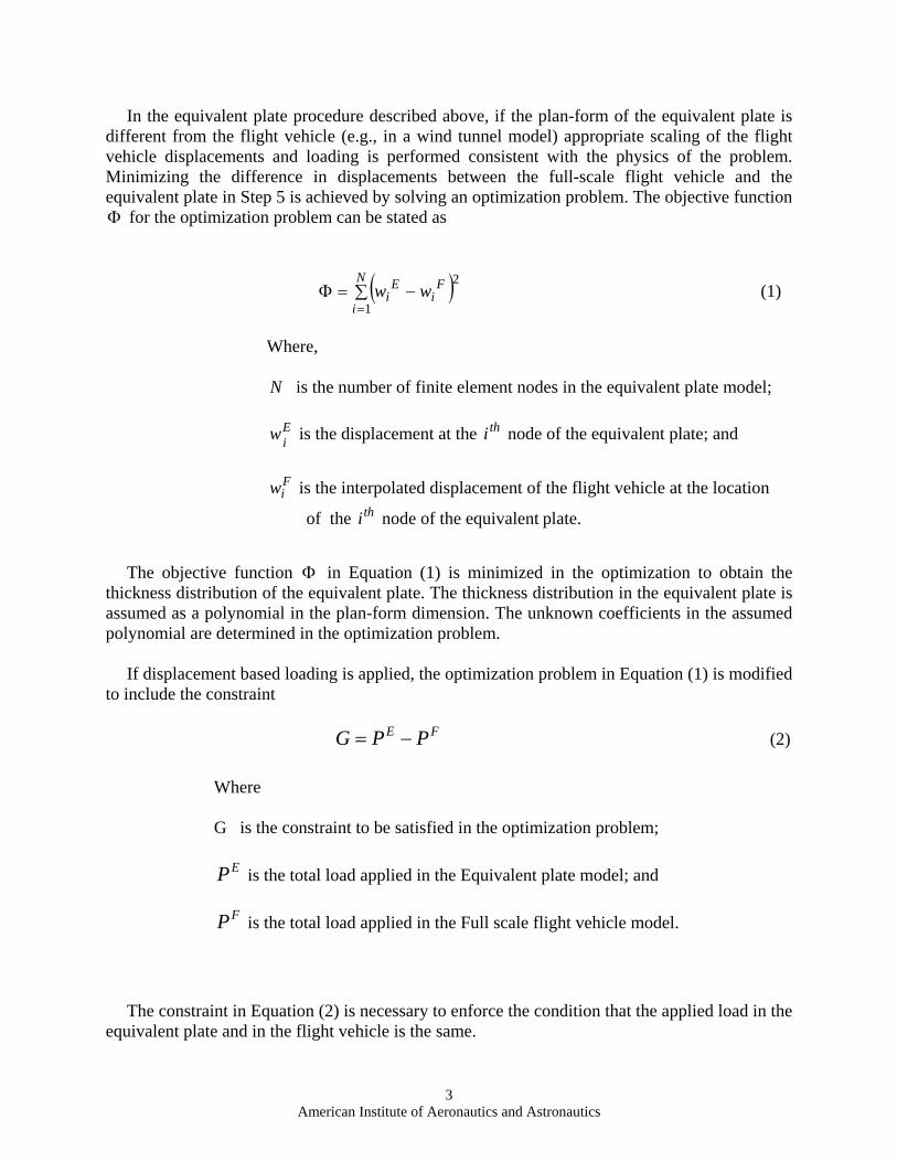
displacement boundary conditions at the free edge, the total load applied is obtained by summing the reactions at the fixed edge in each of the models.

Figure 2. Finite element model of the stiffened panel

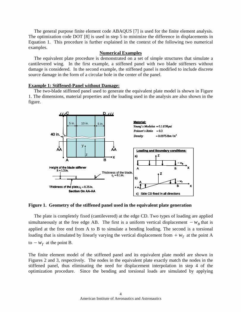
Figure 3. Plan-form and finite element model of the equivalent plate The thickness distribution of the plate is assumed to be constant along the width of the plate and assumed to be linearly varying along the length of the plate. Referring to Figure 1, the thickness t at any point in the plate is calculated using


6

Where

CDt is the thickness of the plate along the edge CD in Figure 1;

ABt is the thickness of the plate along the edge AB in Figure 1; and y is the coordinate of the plate in the y-direction (refer to Figure 1).

ytttt ABCDAB 40

)( −+= (3)

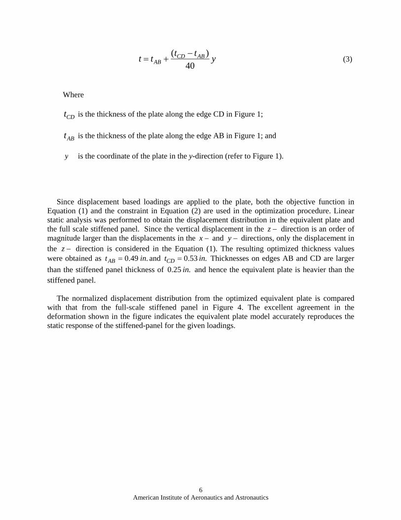
Since displacement based loadings are applied to the plate, both the objective function in Equation (1) and the constraint in Equation (2) are used in the optimization procedure. Linear static analysis was performed to obtain the displacement distribution in the equivalent plate and the full scale stiffened panel. Since the vertical displacement in the −z direction is an order of magnitude larger than the displacements in the −x and −y directions, only the displacement in the −z direction is considered in the Equation (1). The resulting optimized thickness values were obtained as .49.0 intAB = and .53.0 intCD = Thicknesses on edges AB and CD are larger than the stiffened panel thickness of .25.0 in and hence the equivalent plate is heavier than the stiffened panel. The normalized displacement distribution from the optimized equivalent plate is compared with that from the full-scale stiffened panel in Figure 4. The excellent agreement in the deformation shown in the figure indicates the equivalent plate model accurately reproduces the static response of the stiffened-panel for the given loadings.


7

Figure 4. Normalized displacement distribution: comparison between stiffened-panel and the equivalent plate.

Full Scale Stiffened Panel

Equivalent Plate Model




8

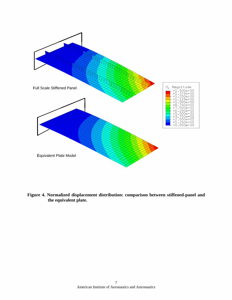
Example 2: Stiffened-Panel with Circular Damage: In this example, the stiffened panel from example 1 is modified by introducing damage in the form of a .5.2 in circular cut-out at the center. The stiffeners are cut at locations in the middle as shown schematically in Figure 5. The damage size in the stiffened-panel and the equivalent plate are kept the same. The bending and torsional loading applied at the free edge of panel is described schematically in the Figure.

Figure 5. Geometry of the stiffened panel with circular damage used in the equivalent plate

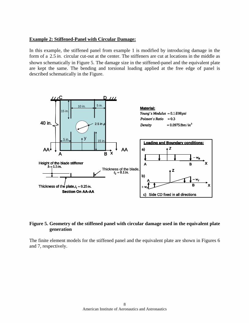
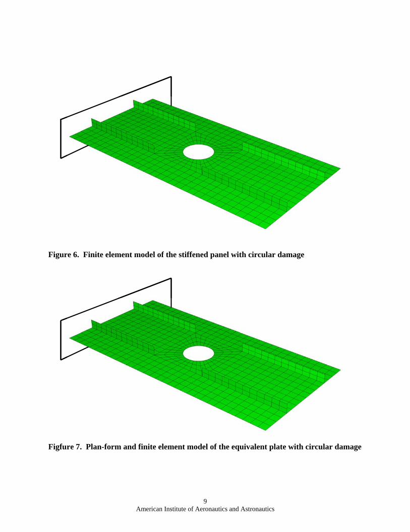
generation The finite element models for the stiffened panel and the equivalent plate are shown in Figures 6 and 7, respectively.


Material:

/ 0975.0

3.0 '08 1.0 '

3inlbm Density


=

==


A B x

z

AB x

z

a)

b)


Bw−

Tw−

Tw+

. 1.02 int =



Section On AA-AA

40 in.

AA AAA B

C D

x

yz

y5 in.

5 in.10 in.

15 in.

15 in.

2.5 in φ


Material:

/ 0975.0

3.0 '08 1.0 '

3inlbm Density


=

==


A B x

z

AB x

z

a)

b)


Bw−

Tw−

Tw+

Material:

/ 0975.0

3.0 '08 1.0 '

3inlbm Density


=

==

Material:

/ 0975.0

3.0 '08 1.0 '

3inlbm Density


=

==


A B x

z

AB x

z

a)

b)


Bw−

Tw−

Tw+


A B x

z

A B x

z

AB x

z

a)

b)


Bw−

Tw−

Tw+

. 1.02 int =



Section On AA-AA

40 in.

AA AAA B

C D

x

yz

y5 in.

5 in.10 in.

15 in.

15 in.

. 1.02 int =



Section On AA-AA

. 1.02 int =

Thickness of the plate, . 25.01 int =Thickness of the plate, . 25.01 int =



Section On AA-AA

40 in.

AA AAA B

C D

x

yz

y5 in.

5 in.10 in.

15 in.

15 in.

40 in.

AA AAA B

C D

x

yz

y5 in.

5 in.10 in.

15 in.

15 in.

2.5 in φ2.5 in φ


9

Figure 6. Finite element model of the stiffened panel with circular damage

Figfure 7. Plan-form and finite element model of the equivalent plate with circular damage


10

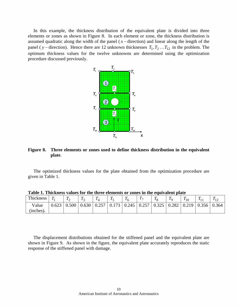
In this example, the thickness distribution of the equivalent plate is divided into three elements or zones as shown in Figure 8. In each element or zone, the thickness distribution is assumed quadratic along the width of the panel ( −x direction) and linear along the length of the panel ( −y direction). Hence there are 12 unknown thicknesses 1221, TTT K in the problem. The optimum thickness values for the twelve unknowns are determined using the optimization procedure discussed previously. Figure 8. Three elements or zones used to define thickness distribution in the equivalent

plate. The optimized thickness values for the plate obtained from the optimization procedure are given in Table 1. Table 1. Thickness values for the three elements or zones in the equivalent plate Thickness 1T 2T 3T 4T 5T 6T 7T 8T 9T 10T 11T 12T

Value (inches).

0.623 0.500 0.630 0.257 0.173 0.245 0.257 0.325 0.282 0.219 0.356 0.364

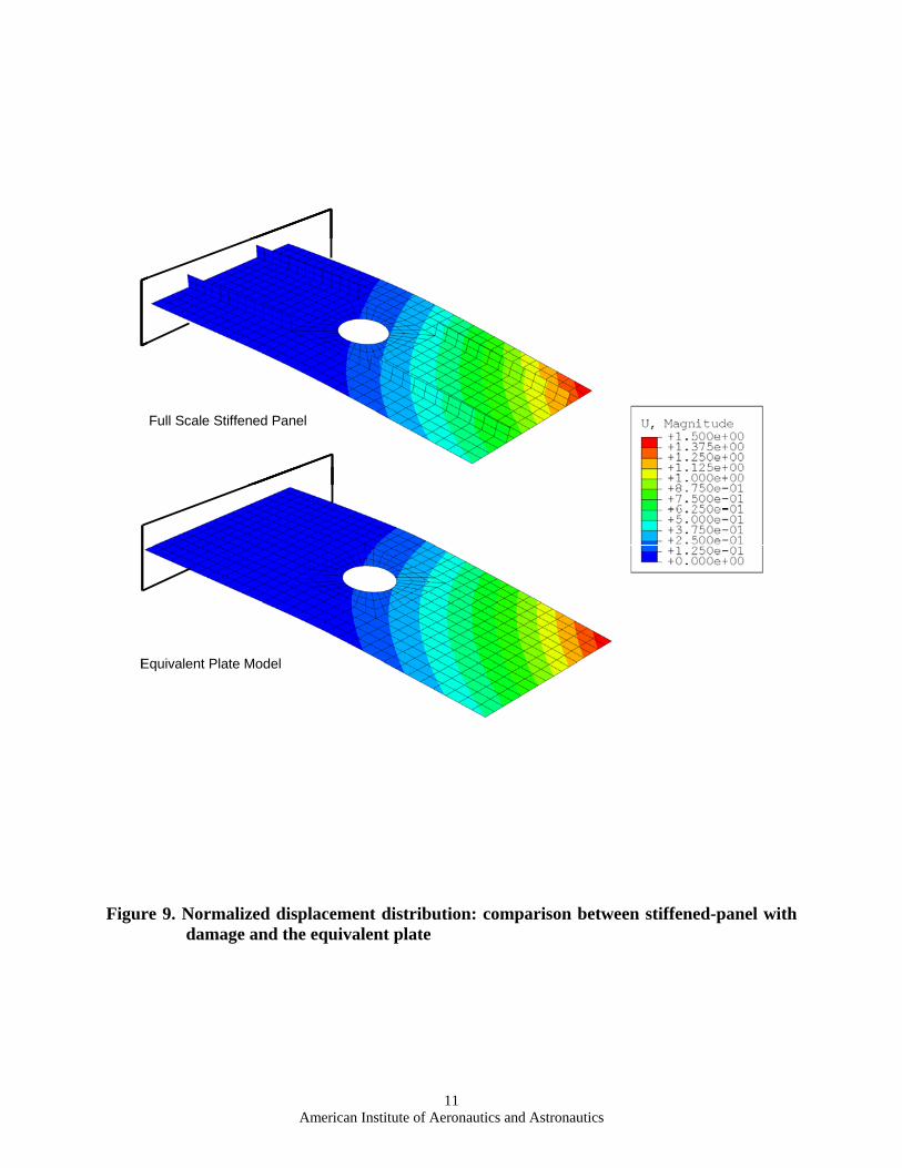
The displacement distributions obtained for the stiffened panel and the equivalent plate are shown in Figure 9. As shown in the figure, the equivalent plate accurately reproduces the static response of the stiffened panel with damage.

1T 2T3T

4T 6T

7T9T

10T 12T

5T

8T

11T

1

3

2

x

y

1T 2T3T

4T 6T

7T9T

10T 12T

5T

8T

11T

1

3

2

x

y


11

Figure 9. Normalized displacement distribution: comparison between stiffened-panel with

damage and the equivalent plate






12

Frequency Estimation Using An Equivalent Plate:

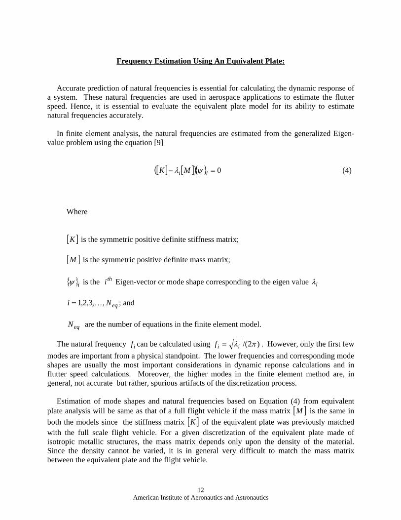
Accurate prediction of natural frequencies is essential for calculating the dynamic response of a system. These natural frequencies are used in aerospace applications to estimate the flutter speed. Hence, it is essential to evaluate the equivalent plate model for its ability to estimate natural frequencies accurately. In finite element analysis, the natural frequencies are estimated from the generalized Eigen-value problem using the equation [9]

[ ] [ ]( ){ } 0=− ii MK ψλ (4)

The natural frequency if can be calculated using )2/( πλiif = . However, only the first few modes are important from a physical standpoint. The lower frequencies and corresponding mode shapes are usually the most important considerations in dynamic reponse calculations and in flutter speed calculations. Moreover, the higher modes in the finite element method are, in general, not accurate but rather, spurious artifacts of the discretization process. Estimation of mode shapes and natural frequencies based on Equation (4) from equivalent plate analysis will be same as that of a full flight vehicle if the mass matrix [ ]M is the same in both the models since the stiffness matrix [ ]K of the equivalent plate was previously matched with the full scale flight vehicle. For a given discretization of the equivalent plate made of isotropic metallic structures, the mass matrix depends only upon the density of the material. Since the density cannot be varied, it is in general very difficult to match the mass matrix between the equivalent plate and the flight vehicle.

Where [ ]K is the symmetric positive definite stiffness matrix; [ ]M is the symmetric positive definite mass matrix; { }iψ is the thi Eigen-vector or mode shape corresponding to the eigen value iλ

eqNi ,,3,2,1 K= ; and

eqN are the number of equations in the finite element model.


13

In the present study, two analytical procedures are described to match the numerical values of the natural frequencies between the equivalent plate model and the flight vehicle. However, no attempt is made to match the actual modes shapes. The two analytical procedures require a lumped-mass matrix for their implementation. Hence, the construction of lumped mass matrix is summarized before the two analytical methods are described. Lumped Mass Matrix: In Galerkin-based finite element methods, the mass matrix [ ]M in Equation (4) is usually referred to as a variationally “consistent-mass” matrix. The consistent-mass matrix establishes a uniform convergence property to the analysis as the mesh is refined [9]. However, in many applications a diagonal or “lumped-mass” matrix is used due to its computational efficiency. Since the lumped-mass matrix is a diagonal matrix, it is used in explicit finite element methods for time-integration schemes. There are several methods available to form the lumped-mass matrix [9]. In the present study, the method developed by Hinton et al. [10] is used. In this method, the diagonal terms in the lumped-mass matrix are set proportional to the diagonal terms of the consistent-mass matrix. A constant of proportionality β is selected to conserve the total mass and is obtained using the diagonal terms of the assembled consistent-mass matrix as

∑=

=

N

jjj

T

m

M

1

β (5)

Once the proportionality constant β is obtained, the diagonal terms jjm of the lumped-mass matrix can be calculated using the corresponding diagonal terms jjm of the consistent-mass matrix as

Ntojmm jjjj 1for == β (6)

Where

jjm are the diagonal terms in the consistent-mass matrix in each direction ( ),, directionzoryx −−− ;

N are the number of nodes in the model; and

TM is the total mass of the structure.


14

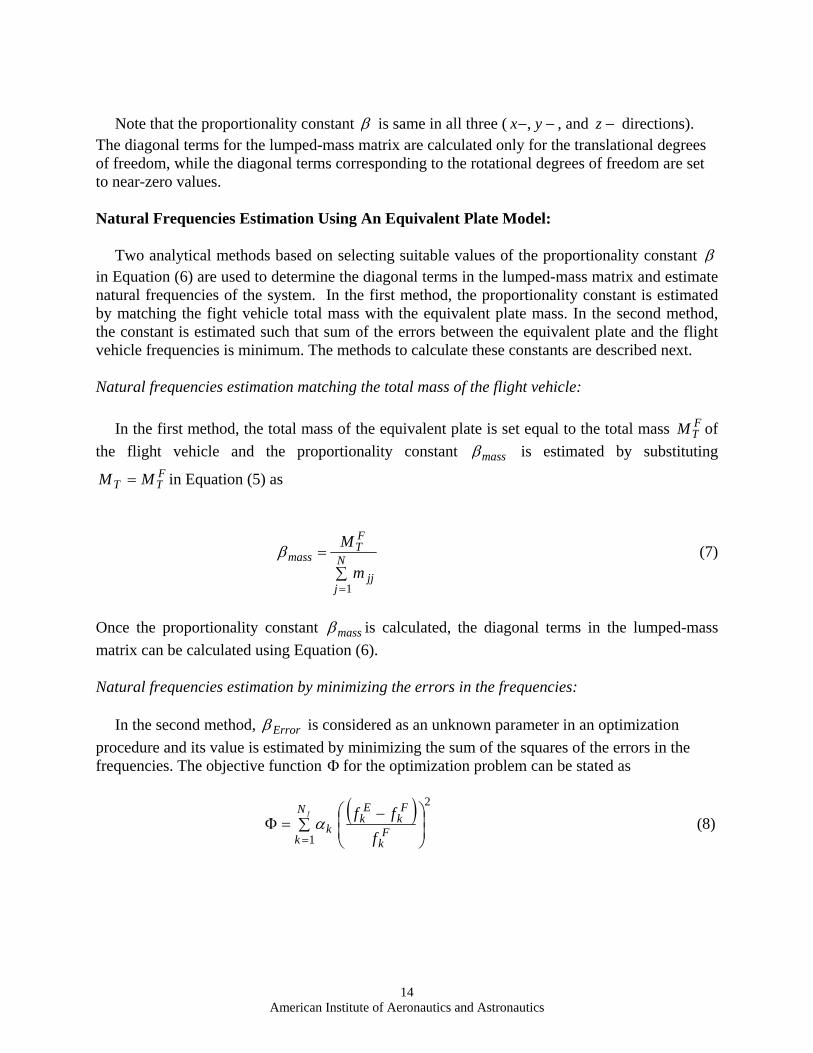
Note that the proportionality constant β is same in all three ( −− yx , , and −z directions). The diagonal terms for the lumped-mass matrix are calculated only for the translational degrees of freedom, while the diagonal terms corresponding to the rotational degrees of freedom are set to near-zero values. Natural Frequencies Estimation Using An Equivalent Plate Model: Two analytical methods based on selecting suitable values of the proportionality constant β in Equation (6) are used to determine the diagonal terms in the lumped-mass matrix and estimate natural frequencies of the system. In the first method, the proportionality constant is estimated by matching the fight vehicle total mass with the equivalent plate mass. In the second method, the constant is estimated such that sum of the errors between the equivalent plate and the flight vehicle frequencies is minimum. The methods to calculate these constants are described next. Natural frequencies estimation matching the total mass of the flight vehicle: In the first method, the total mass of the equivalent plate is set equal to the total mass F

TM of the flight vehicle and the proportionality constant massβ is estimated by substituting

FTT MM = in Equation (5) as

∑=

=

N

jjj

FT

massm

M

1

β (7)

Once the proportionality constant massβ is calculated, the diagonal terms in the lumped-mass matrix can be calculated using Equation (6). Natural frequencies estimation by minimizing the errors in the frequencies: In the second method, Errorβ is considered as an unknown parameter in an optimization procedure and its value is estimated by minimizing the sum of the squares of the errors in the frequencies. The objective function Φ for the optimization problem can be stated as

( ) 2

1∑ ⎟

⎟⎠

⎞⎜⎜⎝

⎛ −=Φ

=

fN

k Fk

Fk

Ek

kf

ffα (8)


15

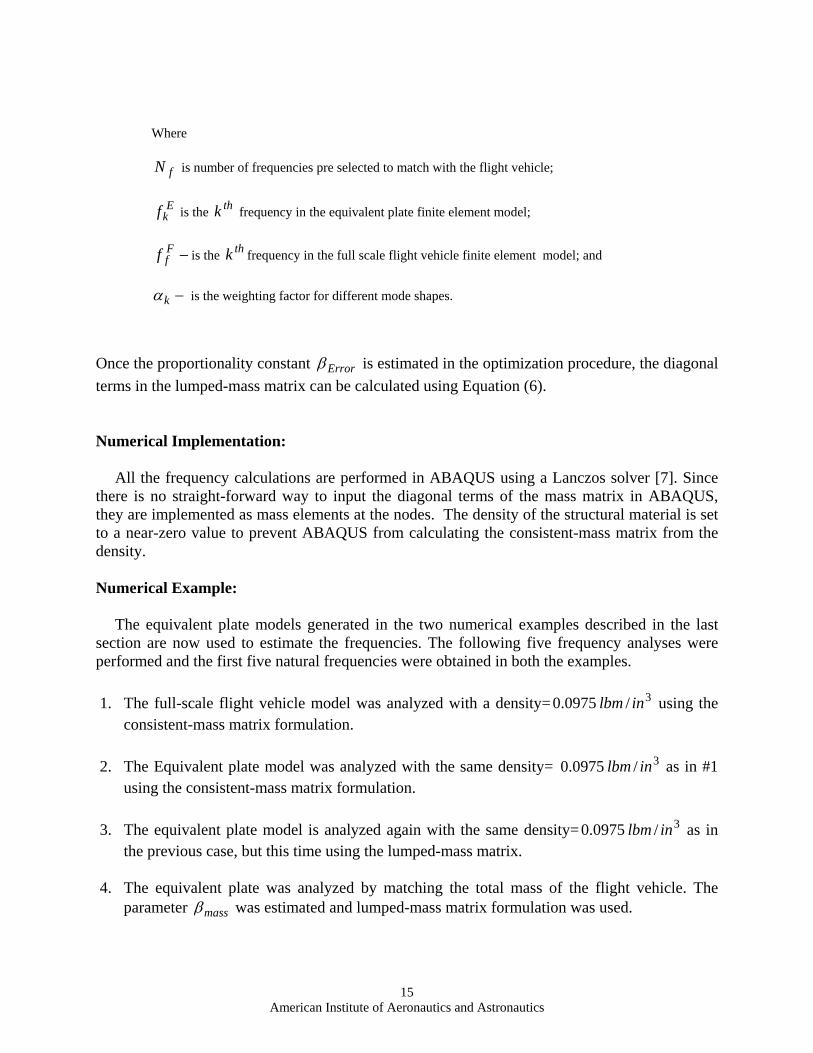
Once the proportionality constant Errorβ is estimated in the optimization procedure, the diagonal terms in the lumped-mass matrix can be calculated using Equation (6). Numerical Implementation: All the frequency calculations are performed in ABAQUS using a Lanczos solver [7]. Since there is no straight-forward way to input the diagonal terms of the mass matrix in ABAQUS, they are implemented as mass elements at the nodes. The density of the structural material is set to a near-zero value to prevent ABAQUS from calculating the consistent-mass matrix from the density. Numerical Example:

The equivalent plate models generated in the two numerical examples described in the last section are now used to estimate the frequencies. The following five frequency analyses were performed and the first five natural frequencies were obtained in both the examples. 1. The full-scale flight vehicle model was analyzed with a density= 3/0975.0 inlbm using the

consistent-mass matrix formulation. 2. The Equivalent plate model was analyzed with the same density= 3/0975.0 inlbm as in #1

using the consistent-mass matrix formulation. 3. The equivalent plate model is analyzed again with the same density= 3/0975.0 inlbm as in

the previous case, but this time using the lumped-mass matrix. 4. The equivalent plate was analyzed by matching the total mass of the flight vehicle. The

parameter massβ was estimated and lumped-mass matrix formulation was used.

Where

fN is number of frequencies pre selected to match with the flight vehicle;

Ekf is the thk frequency in the equivalent plate finite element model;

−Fff is the thk frequency in the full scale flight vehicle finite element model; and

−kα is the weighting factor for different mode shapes.


16

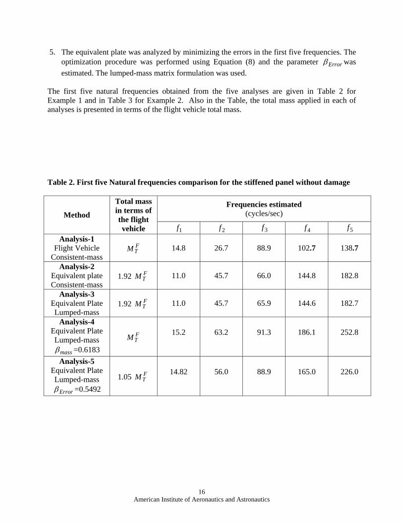
5. The equivalent plate was analyzed by minimizing the errors in the first five frequencies. The optimization procedure was performed using Equation (8) and the parameter Errorβ was estimated. The lumped-mass matrix formulation was used.

The first five natural frequencies obtained from the five analyses are given in Table 2 for Example 1 and in Table 3 for Example 2. Also in the Table, the total mass applied in each of analyses is presented in terms of the flight vehicle total mass. Table 2. First five Natural frequencies comparison for the stiffened panel without damage

Frequencies estimated (cycles/sec) Method

Total mass in terms of the flight vehicle 1f 2f 3f 4f 5f

Analysis-1 Flight Vehicle

Consistent-mass FTM 14.8 26.7 88.9 102.7 138.7

Analysis-2 Equivalent plate Consistent-mass

1.92 FTM 11.0 45.7 66.0 144.8 182.8

Analysis-3 Equivalent Plate Lumped-mass

1.92 FTM 11.0 45.7 65.9 144.6 182.7


massβ =0.6183

FTM 15.2

63.2

91.3

186.1

252.8


Errorβ =0.5492 1.05 F

TM 14.82

56.0

88.9

165.0

226.0


17

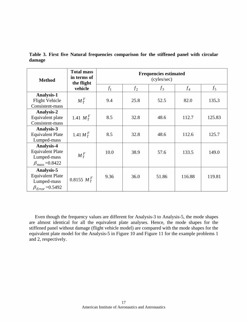
Table 3. First five Natural frequencies comparison for the stiffened panel with circular damage

Frequencies estimated (cyles/sec) Method

Total mass in terms of the flight vehicle 1f 2f 3f 4f 5f

Analysis-1 Flight Vehicle

Consistent-mass FTM 9.4 25.8 52.5 82.0 135.3

Analysis-2 Equivalent plate Consistent-mass

1.41 FTM 8.5 32.8 48.6 112.7 125.83


1.41 FTM 8.5 32.8 48.6 112.6 125.7


massβ =0.8422

FTM 10.0

38.9

57.6

133.5

149.0


Errorβ =0.5492 0.8155 F

TM 9.36

36.0

51.86

116.88

119.81

Even though the frequency values are different for Analysis-3 to Analysis-5, the mode shapes are almost identical for all the equivalent plate analyses. Hence, the mode shapes for the stiffened panel without damage (flight vehicle model) are compared with the mode shapes for the equivalent plate model for the Analysis-5 in Figure 10 and Figure 11 for the example problems 1 and 2, respectively.


18

Figure 10. Mode shapes comparison: stiffened-panel and equivalent plate model

Stiffened Panel Without DamageEquivalent Plate Model Without Damage

Mode-1

Mode-5

Mode-4

Mode-3

Mode-2

Stiffened Panel Without DamageEquivalent Plate Model Without Damage

Mode-1

Mode-5

Mode-4

Mode-3

Mode-2


19

Figure 11. Mode shapes comparison: stiffened-panel with circular damage and

equivalent plate model

Stiffened PanelWith Circular Damage

Equivalent Plate Model With Circular Damage

Mode-1

Mode-5

Mode-4

Mode-3

Mode-2

Stiffened PanelWith Circular Damage

Equivalent Plate Model With Circular Damage

Mode-1

Mode-5

Mode-4

Mode-3

Mode-2


20

Referring to Table 2 and Table 3 along with the mode shape comparisons in Figure 11 and Figure 12, the following observations can be made:

1. From the Analysis-2 and Analysis-3, the lumped-mass matrix and the consistent-mass matrix procedures give identical modes. This result validates the lumped-mass procedure described in the paper.

2. Natural frequencies estimated by matching the total mass of the flight vehicle

(Analysis-4) and natural frequencies estimated by minimizing the errors in the frequencies (Analysis-5) produced almost identical frequencies. Both the methods estimate the first natural frequency accurately.

3. All the equivalent plate analysis methods produced identical mode shapes. This implies

that the mode shape is determined by the stiffness or elastic forces. Changing the mass distribution changes the values of the frequencies, but not the mode shapes.

4. Only the first four modes of the equivalent plate are similar to the flight vehicle model,

whereas the fifth mode shape is entirely different.

5. The two analytical methods (Analysis-4 and Analysis-5) can only be used to match the first few frequencies.

6. It is not possible to match the frequencies and mode shapes by only changing the mass

distribution. Hence, composite materials may be considered for use in an equivalent plate model to provide enough flexibility to change the stiffness and mass distribution simultaneously to match the frequencies.

Concluding Remarks:

An equivalent plate procedure is developed to provide a computationally efficient means of matching the stiffness and frequencies of flight vehicle wing structures for prescribed loading conditions. First, the equivalent plate is used to match the stiffness of a stiffened panel without damage and the stiffness of a stiffened panel with damage. For both stiffened panels, the equivalent plate models reproduce the deformation of a correponding detailed model exactly for the given loading conditions. Once the stiffness was matched, the equivalent plate models were then used to predict the frequencies of the panels. Two analytical procedures using the lumped-mass matrix were used to match the first five frequencies of the corresponding detailed model. In both the procedures, the lumped-mass matrix for the equivalent plate is constructed by multiplying the diagonal terms of the consistent-mass matrix by a proportionality constant. In the first procedure, the proportionality constant is selected such that the total mass of the equivalent plate is equal to that of the detailed model. In the second method, the proportionality constant is selected to minimize the sum of the squares of the errors in a set of pre-selected frequencies between the equivalent plate model and the detailed model. The equivalent plate models reproduced the fundamental first frequency accurately in both the methods. It is observed that changing only the mass distribution in the equivalent plate model did not provide enough flexibility to match all of the frequencies.


21

References 1. Gary L. Giles, “Equivalent Plate Modeling for Conceptual Design of Aircraft Wing

Structures,” AIAA-1995-3945, Presented at 1st AIAA Aircraft Engineering, Technology and Operations Congress, Los Angeles, CA, Sept. 19-21, 1995.

2. Gary L. Giles, “Equivalent Plate Analysis of Aircraft Wing Box Structures with General

Planform Geometry,” Journal of Aircraft, Vol. 23. No. 11, pp. 858-864, 1986.

3. Gary L. Giles, “Further Generalization of Equivalent Plate Representation for Aircraft Structural Analysis,” Journal of Aircraft, Vol. 26. No. 1, pp. 67-74, 1989.

4. Steven C. Stone, Joseph L. Henderson, Mark M. Nazari, William N. Boyd, Bradley T.

Becker, Kumar G. Bhatia, Gary L. Giles, and Gregory A. Wrenn, “Evaluation of Equivalent Plate Solution (ELAPS) in HSST Sizing,” AIAA-2000-1452, Presented at 41st AIAA/ASME/ASCE/AHS/ASC Structures, Structural Dynamics, and Materials Conference and Exhibit, 41st, Atlanta, GA, Apr. 3-6, 2000.

5. Dimitri N. Mavris and William T. Hayden, “Probabilistic Analysis of an HSCT Modeled

with an Equivalent Laminated Plate Wing,” AIAA-1997-5571, Presented at AIAA and SAE, 1997 World Aviation Congress, Anaheim, CA, Oct. 13-16, 1997.

6. B. Mason, W. Stroud, T. Krishnamurthy, and C. Spain and A. Naser, “Probabilistic

Design of a Wind Tunnel Model to Match the Response of a Full-Scale Aircraft,” AIAA-2005-2185, Presented at 46th AIAA/ASME/ASCE/AHS/ASC Structures, Structural Dynamics and Materials Conference 13th AIAA/ASME/AHS Adaptive Structures Conference, Austin, Texas, Apr. 18-21, 2005.

7. Anonymous, Getting Started with ABAQUS, Version 6.5, ABAQUS, Inc., Providence, RI

02909.

8. Anonymous, DOT, Design Optimization Tools, User’s Manual, Version 5.0, Vanderplaats Research & Development, Inc., Colorado Springs, CO, 80906.

9. Thomas Huges, J.R., The Finite Element Method. Linear Static and Dynamic Finite

Element Analysis, Dover Publications, Inc., Mineloe, New York, 2000.

10. E. Hinton, T. Rock, and O. C. Zienkiewicz,” A Note On Mass Lumping And Related Process In The Finite Element Method,” Earthquake Engineering and Structural Dynamics, Vol. 4, pp. 245-249, 1976.

Documents

Equivalent Plate Analysis of Aircraft Wing with Discrete