Embed Size (px)
Citation preview
IntroductionBoundary condition changing operators
Erler-Maccaferri solutionsChan-Paton factors
Background Gauge Fields
.
.Erler-Maccaferri解について
高橋 智彦
奈良女子大学研究院自然科学系
2016年 2月 22日弦の場の理論16
(筑波大学東京キャンパス文京校舎)
1 / 48
IntroductionBoundary condition changing operators
Erler-Maccaferri solutionsChan-Paton factors
Background Gauge Fields
This talk is based on the work in collaboration with
石橋 延幸 (Tsukuba University)
岸本 功 (Niigata University)
in preparation (arXiv:16**.****)
2 / 48
IntroductionBoundary condition changing operators
Erler-Maccaferri solutionsChan-Paton factors
Background Gauge Fields
Introduction
Open string field theory has the possibility of revealingnon-perturbative aspects of string theory.
Recently, Erler and Maccaferri have proposed a method toconstruct classical solutions, which are expected to describe anyopen string background (2014).
Erler-Maccaferri’s solutions provide correct vacuum energy andgauge invariant observables.
3 / 48

IntroductionBoundary condition changing operators
Erler-Maccaferri solutionsChan-Paton factors
Background Gauge Fields
.. .1 Introduction.
. .2 Boundary condition changing operatorsboundary condition changing operatorstwo point functionsfour point functionsOPE of bcc
.. .3 Erler-Maccaferri solutions
modified bcc operatorsErler-Maccaferri解
.. .4 Chan-Paton factors
Erler-Maccaferri’s solution for N D-branesProjectorsBackground described by the solution
.. .5 Background Gauge Fields
background gauge fieldsbcc operators
4 / 48
IntroductionBoundary condition changing operators
Erler-Maccaferri solutionsChan-Paton factors
Background Gauge Fields
boundary condition changing operatorstwo point functionsfour point functionsOPE of bcc
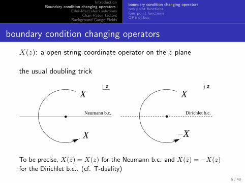
boundary condition changing operators
X(z): a open string coordinate operator on the z plane
the usual doubling trick
z
Neumann b.c.
X
X
z
X
X
Dirichlet b.c.
To be precise, X(z) = X(z) for the Neumann b.c. and X(z) = −X(z)
for the Dirichlet b.c.. (cf. T-duality)
5 / 48
IntroductionBoundary condition changing operators
Erler-Maccaferri solutionsChan-Paton factors
Background Gauge Fields
boundary condition changing operatorstwo point functionsfour point functionsOPE of bcc
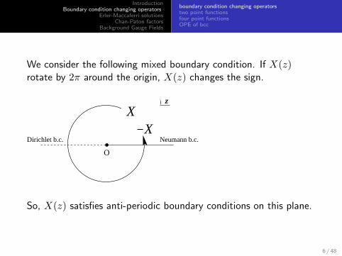
We consider the following mixed boundary condition. If X(z)rotate by 2π around the origin, X(z) changes the sign.
z
O
XX
Neumann b.c.Dirichlet b.c.
So, X(z) satisfies anti-periodic boundary conditions on this plane.
6 / 48
IntroductionBoundary condition changing operators
Erler-Maccaferri solutionsChan-Paton factors
Background Gauge Fields
boundary condition changing operatorstwo point functionsfour point functionsOPE of bcc
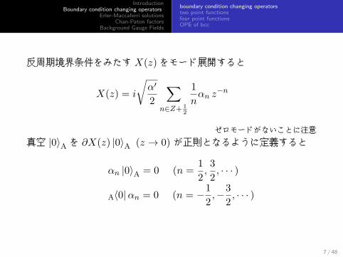
反周期境界条件をみたす X(z)をモード展開すると
X(z) = i
√α′
2
∑n∈Z+ 1
2
1
nαn z
−n
ゼロモードがないことに注意
真空 |0⟩A を ∂X(z) |0⟩A (z → 0) が正則となるように定義すると
αn |0⟩A = 0 (n =1
2,3
2, · · · )
A⟨0|αn = 0 (n = −1
2,−3
2, · · · )
7 / 48
IntroductionBoundary condition changing operators
Erler-Maccaferri solutionsChan-Paton factors
Background Gauge Fields
boundary condition changing operatorstwo point functionsfour point functionsOPE of bcc
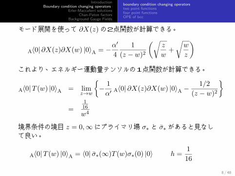
モード展開を使って ∂X(z)の2点関数が計算できる。
A⟨0| ∂X(z)∂X(w) |0⟩A = −α′
4
1
(z − w)2
(√z
w+
√w
z
)これより、エネルギー運動量テンソルの1点関数が計算できる。
A⟨0|T (w) |0⟩A = limz→w
{− 1
α′ A⟨0| ∂X(z)∂X(w) |0⟩A −1/2
(z − w)2
}=
116
w4
境界条件の境目 z = 0,∞にプライマリ場 σ∗ と σ∗ があると見なして良い。
A⟨0|T (w) |0⟩A = ⟨0| σ∗(∞)T (w)σ∗(0) |0⟩ h =1
16
8 / 48
IntroductionBoundary condition changing operators
Erler-Maccaferri solutionsChan-Paton factors
Background Gauge Fields
boundary condition changing operatorstwo point functionsfour point functionsOPE of bcc
two point functions
h = 1/16より ⟨σ∗(z)σ∗(w)
⟩=
C
(z − w)1/8
SL(2, R)変換によって z と wは自由に動かせる。⟨σ∗(z)σ∗(w)
⟩=⟨σ∗(z
′)σ∗(w′)⟩
z =az + b
cz + d(ad− bc = 1)
9 / 48
IntroductionBoundary condition changing operators
Erler-Maccaferri solutionsChan-Paton factors
Background Gauge Fields
boundary condition changing operatorstwo point functionsfour point functionsOPE of bcc
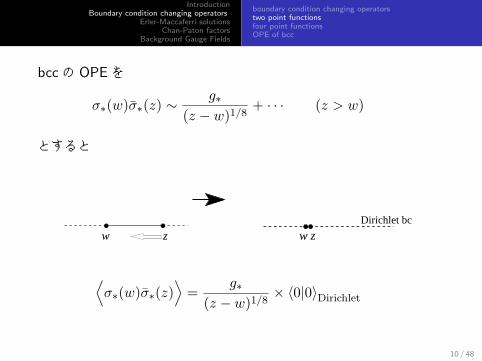
bccの OPEを
σ∗(w)σ∗(z) ∼g∗
(z − w)1/8+ · · · (z > w)
とすると
w zDirichlet bc
w z
⟨σ∗(w)σ∗(z)
⟩=
g∗
(z − w)1/8× ⟨0|0⟩Dirichlet
10 / 48
IntroductionBoundary condition changing operators
Erler-Maccaferri solutionsChan-Paton factors
Background Gauge Fields
boundary condition changing operatorstwo point functionsfour point functionsOPE of bcc
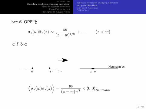
bccの OPEを
σ∗(w)σ∗(z) ∼g0
(z − w)1/8+ · · · (z < w)
とすると
w zNeumann bc
z w
⟨σ∗(w)σ∗(z)
⟩=
g0
(z − w)1/8× ⟨0|0⟩Neumann
11 / 48
IntroductionBoundary condition changing operators
Erler-Maccaferri solutionsChan-Paton factors
Background Gauge Fields
boundary condition changing operatorstwo point functionsfour point functionsOPE of bcc
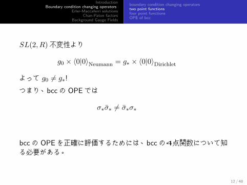
SL(2, R)不変性より
g0 × ⟨0|0⟩Neumann = g∗ × ⟨0|0⟩Dirichlet
よって g0 = g∗!
つまり、bccの OPEでは
σ∗σ∗ = σ∗σ∗
bccの OPEを正確に評価するためには、bccの4点関数について知る必要がある。
12 / 48
IntroductionBoundary condition changing operators
Erler-Maccaferri solutionsChan-Paton factors
Background Gauge Fields
boundary condition changing operatorstwo point functionsfour point functionsOPE of bcc
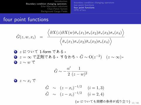
four point functions
G(z, w, xi) =
⟨∂X(z)∂X(w)σ∗(x1)σ∗(x2)σ∗(x3)σ∗(x4)
⟩⟨σ∗(x1)σ∗(x2)σ∗(x3)σ∗(x4)
⟩...1 z について 1-formである。...2 z =∞で正則である。すなわち、G ∼ O(z−2) (z ∼ ∞)。...3 z ∼ wで
G ∼ −α′
2
1
(z − w)2...4 z ∼ xi で
G ∼ (z − xi)−1/2 (i = 1, 3)
G ∼ (z − xi)−1/2 (i = 2, 4)
(w についても同様の条件が成り立つ) 13 / 48
IntroductionBoundary condition changing operators
Erler-Maccaferri solutionsChan-Paton factors
Background Gauge Fields
boundary condition changing operatorstwo point functionsfour point functionsOPE of bcc
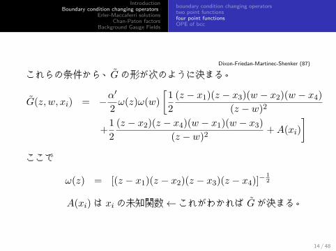
Dixon-Friedan-Martinec-Shenker (87)
これらの条件から、Gの形が次のように決まる。
G(z, w, xi) = −α′
2ω(z)ω(w)
[1
2
(z − x1)(z − x3)(w − x2)(w − x4)(z − w)2
+1
2
(z − x2)(z − x4)(w − x1)(w − x3)(z − w)2
+A(xi)
]ここで
ω(z) = [(z − x1)(z − x2)(z − x3)(z − x4)]−12
A(xi)は xi の未知関数←これがわかれば Gが決まる。
14 / 48
IntroductionBoundary condition changing operators
Erler-Maccaferri solutionsChan-Paton factors
Background Gauge Fields
boundary condition changing operatorstwo point functionsfour point functionsOPE of bcc
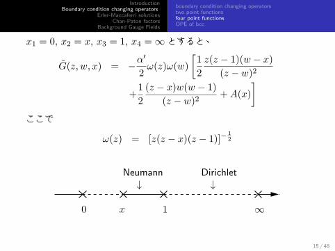
x1 = 0, x2 = x, x3 = 1, x4 =∞とすると、
G(z, w, x) = −α′
2ω(z)ω(w)
[1
2
z(z − 1)(w − x)(z − w)2
+1
2
(z − x)w(w − 1)
(z − w)2+A(x)
]ここで
ω(z) = [z(z − x)(z − 1)]−12
0 x 1 ∞
Neumann↓
Dirichlet↓
15 / 48
IntroductionBoundary condition changing operators
Erler-Maccaferri solutionsChan-Paton factors
Background Gauge Fields
boundary condition changing operatorstwo point functionsfour point functionsOPE of bcc
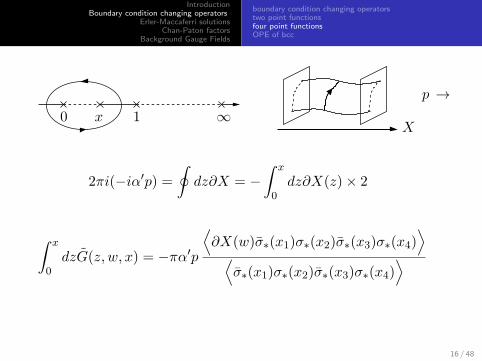
0 x 1 ∞p →
X
2πi(−iα′p) =
∮dz∂X = −
∫ x
0dz∂X(z)× 2
∫ x
0dzG(z, w, x) = −πα′p
⟨∂X(w)σ∗(x1)σ∗(x2)σ∗(x3)σ∗(x4)
⟩⟨σ∗(x1)σ∗(x2)σ∗(x3)σ∗(x4)
⟩
16 / 48

IntroductionBoundary condition changing operators
Erler-Maccaferri solutionsChan-Paton factors
Background Gauge Fields
boundary condition changing operatorstwo point functionsfour point functionsOPE of bcc
右辺は wについての特異性を調べると ω(w)に比例するから、⟨∂X(w)σ∗(0)σ∗(x)σ∗(1)σ∗(∞)
⟩⟨σ∗(0)σ∗(x)σ∗(1)σ∗(∞)
⟩ =−πα′p∫ x0 dzω(z)
× ω(w)
∴∫ x
0dzG(z, w, x) = −πα′p× (−πα′p)
ω(w)∫ x0 dzω(z)
17 / 48
IntroductionBoundary condition changing operators
Erler-Maccaferri solutionsChan-Paton factors
Background Gauge Fields
boundary condition changing operatorstwo point functionsfour point functionsOPE of bcc
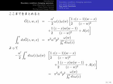
ここまでをまとめると
G(z, w, x) = −α′
2ω(z)ω(w)
[1
2
z(z − 1)(w − x)(z − w)2
+1
2
(z − x)w(w − 1)
(z − w)2+A(x)
]∫ x
0dzG(z, w, x) = π2α′2p2
ω(w)∫ x0 dzω(z)
よって
−α′
2
∫ x
0dzω(z)ω(w)
[1
2
z(z − 1)(w − x)(z − w)2
+1
2
(z − x)w(w − 1)
(z − w)2+A(x)
]= π2α′2p2
ω(w)∫ x0 dzω(z)
18 / 48
IntroductionBoundary condition changing operators
Erler-Maccaferri solutionsChan-Paton factors
Background Gauge Fields
boundary condition changing operatorstwo point functionsfour point functionsOPE of bcc
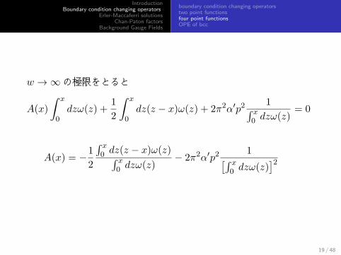
w →∞の極限をとると
A(x)
∫ x
0dzω(z) +
1
2
∫ x
0dz(z − x)ω(z) + 2π2α′p2
1∫ x0 dzω(z)
= 0
A(x) = −1
2
∫ x0 dz(z − x)ω(z)∫ x
0 dzω(z)− 2π2α′p2
1[∫ x0 dzω(z)
]2
19 / 48
IntroductionBoundary condition changing operators
Erler-Maccaferri solutionsChan-Paton factors
Background Gauge Fields
boundary condition changing operatorstwo point functionsfour point functionsOPE of bcc
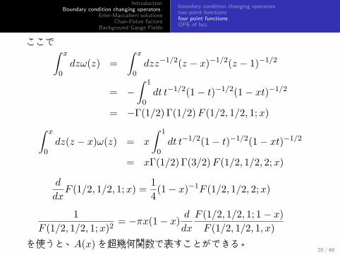
ここで∫ x
0dzω(z) =
∫ x
0dzz−1/2(z − x)−1/2(z − 1)−1/2
= −∫ 1
0dt t−1/2(1− t)−1/2(1− xt)−1/2
= −Γ(1/2) Γ(1/2)F (1/2, 1/2, 1;x)∫ x
0dz(z − x)ω(z) = x
∫ 1
0dt t−1/2(1− t)−1/2(1− xt)−1/2
= xΓ(1/2) Γ(3/2)F (1/2, 1/2, 2;x)
d
dxF (1/2, 1/2, 1;x) =
1
4(1− x)−1F (1/2, 1/2, 2;x)
1
F (1/2, 1/2, 1;x)2= −πx(1− x) d
dx
F (1/2, 1/2, 1; 1− x)F (1/2, 1/2, 1, x)
を使うと、A(x)を超幾何関数で表すことができる。20 / 48
IntroductionBoundary condition changing operators
Erler-Maccaferri solutionsChan-Paton factors
Background Gauge Fields
boundary condition changing operatorstwo point functionsfour point functionsOPE of bcc
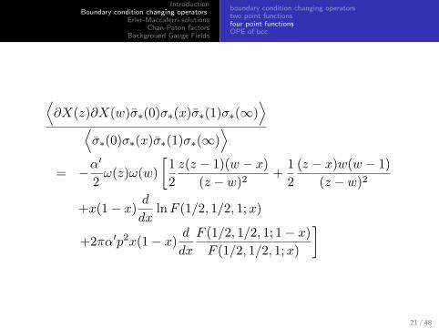
⟨∂X(z)∂X(w)σ∗(0)σ∗(x)σ∗(1)σ∗(∞)
⟩⟨σ∗(0)σ∗(x)σ∗(1)σ∗(∞)
⟩= −α
′
2ω(z)ω(w)
[1
2
z(z − 1)(w − x)(z − w)2
+1
2
(z − x)w(w − 1)
(z − w)2
+x(1− x) ddx
lnF (1/2, 1/2, 1;x)
+2πα′p2x(1− x) ddx
F (1/2, 1/2, 1; 1− x)F (1/2, 1/2, 1;x)
]
21 / 48
IntroductionBoundary condition changing operators
Erler-Maccaferri solutionsChan-Paton factors
Background Gauge Fields
boundary condition changing operatorstwo point functionsfour point functionsOPE of bcc
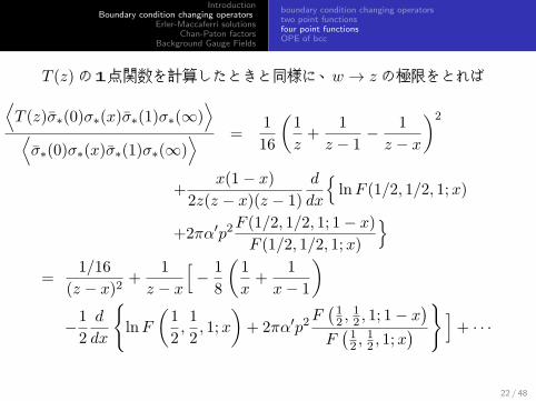
T (z)の1点関数を計算したときと同様に、w → z の極限をとれば⟨T (z)σ∗(0)σ∗(x)σ∗(1)σ∗(∞)
⟩⟨σ∗(0)σ∗(x)σ∗(1)σ∗(∞)
⟩ =1
16
(1
z+
1
z − 1− 1
z − x
)2
+x(1− x)
2z(z − x)(z − 1)
d
dx
{lnF (1/2, 1/2, 1;x)
+2πα′p2F (1/2, 1/2, 1; 1− x)F (1/2, 1/2, 1;x)
}=
1/16
(z − x)2+
1
z − x
[− 1
8
(1
x+
1
x− 1
)−1
2
d
dx
{lnF
(1
2,1
2, 1;x
)+ 2πα′p2
F(12 ,
12 , 1; 1− x
)F(12 ,
12 , 1;x
) } ]+ · · ·
22 / 48
IntroductionBoundary condition changing operators
Erler-Maccaferri solutionsChan-Paton factors
Background Gauge Fields
boundary condition changing operatorstwo point functionsfour point functionsOPE of bcc
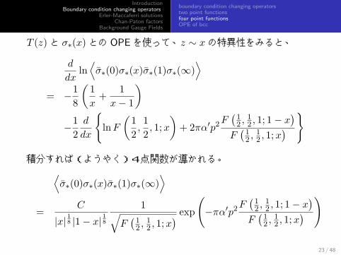
T (z)と σ∗(x)との OPEを使って、z ∼ xの特異性をみると、
d
dxln⟨σ∗(0)σ∗(x)σ∗(1)σ∗(∞)
⟩= −1
8
(1
x+
1
x− 1
)−1
2
d
dx
{lnF
(1
2,1
2, 1;x
)+ 2πα′p2
F(12 ,
12 , 1; 1− x
)F(12 ,
12 , 1;x
) }
積分すれば(ようやく)4点関数が導かれる。⟨σ∗(0)σ∗(x)σ∗(1)σ∗(∞)
⟩=
C
|x|18 |1− x|
18
1√F(12 ,
12 , 1;x
) exp(−πα′p2
F(12 ,
12 , 1; 1− x
)F(12 ,
12 , 1;x
) )
23 / 48
IntroductionBoundary condition changing operators
Erler-Maccaferri solutionsChan-Paton factors
Background Gauge Fields
boundary condition changing operatorstwo point functionsfour point functionsOPE of bcc
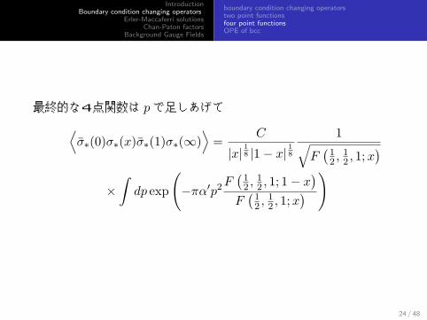
最終的な4点関数は pで足しあげて⟨σ∗(0)σ∗(x)σ∗(1)σ∗(∞)
⟩=
C
|x|18 |1− x|
18
1√F(12 ,
12 , 1;x
)×∫dp exp
(−πα′p2
F(12 ,
12 , 1; 1− x
)F(12 ,
12 , 1;x
) )
24 / 48
IntroductionBoundary condition changing operators
Erler-Maccaferri solutionsChan-Paton factors
Background Gauge Fields
boundary condition changing operatorstwo point functionsfour point functionsOPE of bcc
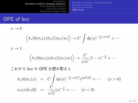
OPE of bcc
x→ 0 ⟨σ∗(0)σ∗(x)σ∗(1)σ∗(∞)
⟩→ C
∫dp |x|−
18+α′p2 + · · ·
x→ 1 ⟨σ∗(0)σ∗(x)σ∗(1)σ∗(∞)
⟩→ C√
α′|1− x|−
18 + · · ·
これから bccの OPEを読み取ると
σ∗(0)σ∗(x) = C
∫dp |x|−
18+α′p2eipX(0) + · · · (x > 0)
σ∗(x)σ∗(0) =C√α′|x|−
18 + · · · (x < 0)
25 / 48
IntroductionBoundary condition changing operators
Erler-Maccaferri solutionsChan-Paton factors
Background Gauge Fields
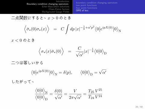
boundary condition changing operatorstwo point functionsfour point functionsOPE of bcc
二点関数にすると、x > 0のとき⟨σ∗(0)σ∗(x)
⟩= C
∫dp |x|−
18+α′p2
⟨0∣∣eipX(0)
∣∣0⟩N
x < 0のとき ⟨σ∗(x)σ∗(0)
⟩=
C√α′|x|−
18⟨0∣∣0⟩
D
二つは等しいから⟨0∣∣eipX(0)
∣∣0⟩N= δ(p),
⟨0∣∣0⟩
D=√α′
したがって、⟨0∣∣0⟩
N⟨0∣∣0⟩
D
=δ(0)√α′
=V
2π√α′
=T25 V
25
T24 V 24
26 / 48
IntroductionBoundary condition changing operators
Erler-Maccaferri solutionsChan-Paton factors
Background Gauge Fields
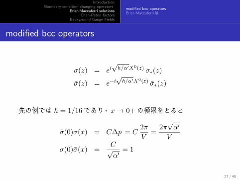
modified bcc operatorsErler-Maccaferri解
modified bcc operators
σ(z) = ei√
h/α′X0(z) σ∗(z)
σ(z) = e−i√
h/α′X0(z) σ∗(z)
先の例では h = 1/16であり、x→ 0+の極限をとると
σ(0)σ(x) = C∆p = C2π
V=
2π√α′
V
σ(0)σ(x) =C√α′
= 1
27 / 48
IntroductionBoundary condition changing operators
Erler-Maccaferri solutionsChan-Paton factors
Background Gauge Fields
modified bcc operatorsErler-Maccaferri解
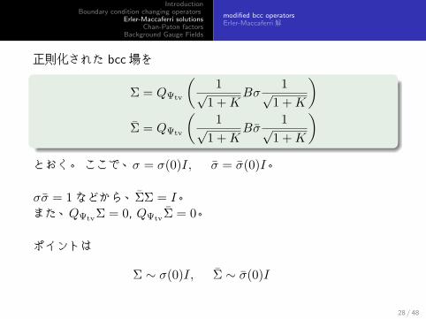
正則化された bcc場を.
.
. ..
.
.
Σ = QΨtv
(1√
1 +KBσ
1√1 +K
)Σ = QΨtv
(1√
1 +KBσ
1√1 +K
)とおく。 ここで、σ = σ(0)I, σ = σ(0)I。
σσ = 1などから、ΣΣ = I。また、QΨtvΣ = 0, QΨtvΣ = 0。
ポイントは
Σ ∼ σ(0)I, Σ ∼ σ(0)I
28 / 48
IntroductionBoundary condition changing operators
Erler-Maccaferri solutionsChan-Paton factors
Background Gauge Fields
modified bcc operatorsErler-Maccaferri解
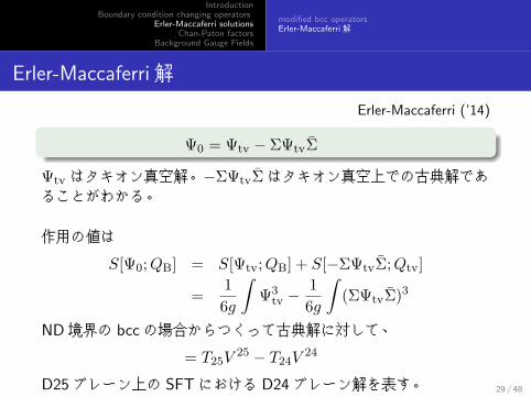
Erler-Maccaferri解
Erler-Maccaferri (’14).
.
. ...
.Ψ0 = Ψtv − ΣΨtvΣ
Ψtv はタキオン真空解。−ΣΨtvΣはタキオン真空上での古典解であることがわかる。
作用の値は
S[Ψ0;QB] = S[Ψtv;QB] + S[−ΣΨtvΣ;Qtv]
=1
6g
∫Ψ3
tv −1
6g
∫(ΣΨtvΣ)
3
ND境界の bccの場合からつくって古典解に対して、
= T25V25 − T24V 24
D25ブレーン上の SFTにおける D24ブレーン解を表す。 29 / 48
IntroductionBoundary condition changing operators
Erler-Maccaferri solutionsChan-Paton factors
Background Gauge Fields
modified bcc operatorsErler-Maccaferri解
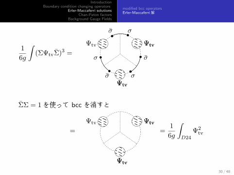
1
6g
∫(ΣΨtvΣ)
3 =
Ψtv Ψtv
Ψtv
σ
σ σ
σ
σ σ
Ψtv
Ψtv
ΣΣ = 1を使って bcc を消すと
=
Ψtv Ψtv
Ψtv
Ψtv
Ψtv
=1
6g
∫D24
Ψ2tv
30 / 48
IntroductionBoundary condition changing operators
Erler-Maccaferri solutionsChan-Paton factors
Background Gauge Fields
modified bcc operatorsErler-Maccaferri解
Erler-Maccaferri解 (’14).
.
. ...
.Ψ0 = Ψtv − ΣΨtvΣ
一般の bccを使って、任意の BCFTをつなぐ古典解が構成できると主張
energyと closed string tadpole(overlap)は正しく再現される
EM解で展開した cohomologyについて議論しているが不十分か? (Bonora-Tolla (’14))
tachyon lump解を構成し、解の成分場 (tachyon profile)を計算している。
多重ブレーン解を構成し、Chan-Paton因子が生じる可能性を述べている。
31 / 48
IntroductionBoundary condition changing operators
Erler-Maccaferri solutionsChan-Paton factors
Background Gauge Fields
Erler-Maccaferri’s solution for N D-branesProjectorsBackground described by the solution
There is one question related to the degree of freedom of stringfields in the background.
We have one string field in the theory on a single D-brane.
However, in the case that the multi-brane solution provides thebackground of the N D-branes, the number of string fieldsincreases to N2 around the solution.
Here, it is natural to ask how to generate N2 string fields orChan-Paton factors from one string field.
32 / 48
IntroductionBoundary condition changing operators
Erler-Maccaferri solutionsChan-Paton factors
Background Gauge Fields
Erler-Maccaferri’s solution for N D-branesProjectorsBackground described by the solution
On the other hand, it is well-known that matrix theories are able todescribe various D-branes (BFSS 1996, IKKT 1996).
In matrix theories, D-branes are created by classical solutions asblock diagonal matrices. After expanding a matrix around thesolution, block matrices can be understood as representing openstrings connecting each D-brane.
Here, it should be noted that there are similarities between thematrix and the open string field: the matrix is deeply tied to theopen string degree of freedom, and an open string field isinterpreted as a matrix in which the left and right indicescorrespond to the left and right half-strings(Witten 1985).
Then, it seems plausible that N2 string fields on N D-branes areembedded like block matrices in a string field on a D-brane.
33 / 48
IntroductionBoundary condition changing operators
Erler-Maccaferri solutionsChan-Paton factors
Background Gauge Fields
Erler-Maccaferri’s solution for N D-branesProjectorsBackground described by the solution
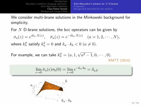
We consider multi-brane solutions in the Minkowski background forsimplicity.
For N D-brane solutions, the bcc operators can be given by
σa(z) = eika·X(z), σa(z) = e−ika·X(z) (a = 1, 2, · · · , N),
where kµa satisfy k2a = 0 and ka · kb < 0 (a = b).
For example, we can take kµa = (a, 1,√a2 − 1, 0, · · · , 0).
KMTT (2014).
.
. ..
.
.
limϵ→0
σa(ϵ)σb(0) = limϵ→0
ϵ−ka·kb = δa,b
ka · kb
ab
34 / 48
IntroductionBoundary condition changing operators
Erler-Maccaferri solutionsChan-Paton factors
Background Gauge Fields
Erler-Maccaferri’s solution for N D-branesProjectorsBackground described by the solution
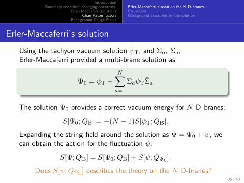
Erler-Maccaferri’s solution
Using the tachyon vacuum solution ψT, and Σa, Σa,Erler-Maccaferri provided a multi-brane solution as.
.
. ..
.
.
Ψ0 = ψT −N∑a=1
ΣaψTΣa
The solution Ψ0 provides a correct vacuum energy for N D-branes:
S[Ψ0;QB] = −(N − 1)S[ψT;QB].
Expanding the string field around the solution as Ψ = Ψ0 + ψ, wecan obtain the action for the fluctuation ψ:
S[Ψ;QB] = S[Ψ0;QB] + S[ψ;QΨ0 ].
Does S[ψ;QΨ0 ] describes the theory on the N D-branes?35 / 48
IntroductionBoundary condition changing operators
Erler-Maccaferri solutionsChan-Paton factors
Background Gauge Fields
Erler-Maccaferri’s solution for N D-branesProjectorsBackground described by the solution
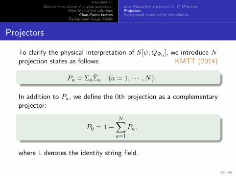
Projectors
To clarify the physical interpretation of S[ψ;QΨ0 ], we introduce Nprojection states as follows: KMTT (2014).
.
. ...
.
Pa = ΣaΣa (a = 1, · · · , N).
In addition to Pa, we define the 0th projection as a complementaryprojector:.
.
. ..
.
.
P0 = 1−N∑a=1
Pa,
where 1 denotes the identity string field.
36 / 48
IntroductionBoundary condition changing operators
Erler-Maccaferri solutionsChan-Paton factors
Background Gauge Fields
Erler-Maccaferri’s solution for N D-branesProjectorsBackground described by the solution
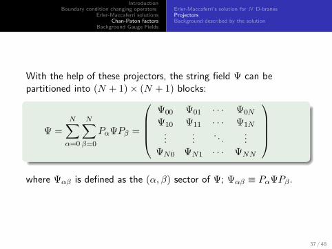
With the help of these projectors, the string field Ψ can bepartitioned into (N + 1)× (N + 1) blocks:.
.
. ..
.
.
Ψ =
N∑α=0
N∑β=0
PαΨPβ =
Ψ00 Ψ01 · · · Ψ0N
Ψ10 Ψ11 · · · Ψ1N...
.... . .
...ΨN0 ΨN1 · · · ΨNN
where Ψαβ is defined as the (α, β) sector of Ψ; Ψαβ ≡ PαΨPβ .
37 / 48
IntroductionBoundary condition changing operators
Erler-Maccaferri solutionsChan-Paton factors
Background Gauge Fields
Erler-Maccaferri’s solution for N D-branesProjectorsBackground described by the solution
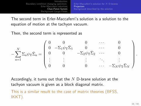
The second term in Erler-Maccaferri’s solution is a solution to theequation of motion at the tachyon vacuum.
Then, the second term is represented as
−N∑a=1
ΣaψTΣa =
0 0 0 · · · 00 −Σ1ψTΣ1 0 · · · 00 0 −Σ2ψTΣ2 · · · 0...
......
. . ....
0 0 0 · · · −ΣNψTΣN
.
Accordingly, it turns out that the N D-brane solution at thetachyon vacuum is given as a block diagonal matrix.
This is a similar result to the case of matrix theories (BFSS,IKKT).
38 / 48

IntroductionBoundary condition changing operators
Erler-Maccaferri solutionsChan-Paton factors
Background Gauge Fields
Erler-Maccaferri’s solution for N D-branesProjectorsBackground described by the solution
Background described by the solution
Now, we consider the fluctuation ψ around the N D-branesolution.
Using the projectors, ψ can be written by matrix representation:
ψ =N∑
α=0
N∑β=0
ϕαβ.
Here, we consider change of variables of ϕαβ .
ϕab can be rewritten as
ϕab = PaϕabPb = Σa(ΣaϕabΣb)Σb.
So, we can change the variables from ϕab to ϕab = ΣaϕabΣb.39 / 48

IntroductionBoundary condition changing operators
Erler-Maccaferri solutionsChan-Paton factors
Background Gauge Fields
Erler-Maccaferri’s solution for N D-branesProjectorsBackground described by the solution
Similarly, writing ϕ0a = χaΣa, ϕa0 = Σaχa, the fluctuation ψ isrepresented as.
.
. ..
.
.
ψ = χ+
N∑a=1
χaΣa +
N∑a=1
Σaχa +
N∑a=1
N∑b=1
ΣaϕabΣb
=
χ χbΣb
Σaχa ΣaϕabΣb
,
where we rewrite ϕ00 as χ.
40 / 48
IntroductionBoundary condition changing operators
Erler-Maccaferri solutionsChan-Paton factors
Background Gauge Fields
Erler-Maccaferri’s solution for N D-branesProjectorsBackground described by the solution
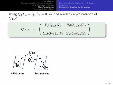
Using QTΣα = QTΣα = 0, we find a matrix representation ofQΨ0ψ:.
.
. ..
.
.
QΨ0ψ =
P0(QTχ)P0 P0(QT0χb)Σb
Σa(Q0Tχa)P0 Σa(QBϕab)Σb
.
41 / 48
IntroductionBoundary condition changing operators
Erler-Maccaferri solutionsChan-Paton factors
Background Gauge Fields
Erler-Maccaferri’s solution for N D-branesProjectorsBackground described by the solution
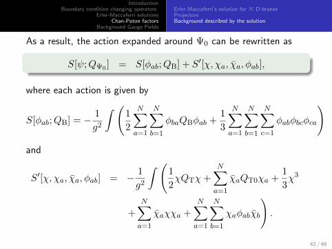
As a result, the action expanded around Ψ0 can be rewritten as.
.
. ..
.
.
S[ψ;QΨ0 ] = S[ϕab;QB] + S′[χ, χa, χa, ϕab],
where each action is given by
S[ϕab;QB] = −1
g2
∫ (1
2
N∑a=1
N∑b=1
ϕbaQBϕab +1
3
N∑a=1
N∑b=1
N∑c=1
ϕabϕbcϕca
)
and
S′[χ, χa, χa, ϕab] = − 1
g2
∫ (1
2χQTχ+
N∑a=1
χaQT0χa +1
3χ3
+
N∑a=1
χaχχa +
N∑a=1
N∑b=1
χaϕabχb
).
42 / 48
IntroductionBoundary condition changing operators
Erler-Maccaferri solutionsChan-Paton factors
Background Gauge Fields
background gauge fieldsbcc operators
background gauge fields
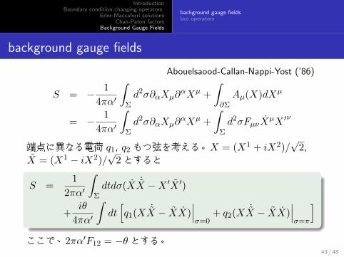
Abouelsaood-Callan-Nappi-Yost (’86)
S = − 1
4πα′
∫Σd2σ∂αXµ∂
αXµ +
∫∂ΣAµ(X)dXµ
= − 1
4πα′
∫Σd2σ∂αXµ∂
αXµ +
∫Σd2σFµνX
µX ′ν
端点に異なる電荷 q1, q2 もつ弦を考える。X = (X1 + iX2)/√2,
X = (X1 − iX2)/√2とすると
.
.
. ..
.
.
S =1
2πα′
∫Σdtdσ(X ˙X −X ′X ′)
+iθ
4πα′
∫dt[q1(X
˙X − XX)∣∣∣σ=0
+ q2(X˙X − XX)
∣∣∣σ=π
]ここで、2πα′F12 = −θ とする。
43 / 48
IntroductionBoundary condition changing operators
Erler-Maccaferri solutionsChan-Paton factors
Background Gauge Fields
background gauge fieldsbcc operators
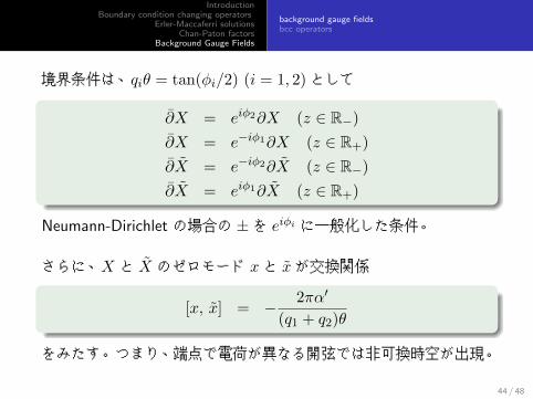
境界条件は、qiθ = tan(ϕi/2) (i = 1, 2)として.
.
. ..
.
.
∂X = eiϕ2∂X (z ∈ R−)
∂X = e−iϕ1∂X (z ∈ R+)
∂X = e−iϕ2∂X (z ∈ R−)
∂X = eiϕ1∂X (z ∈ R+)
Neumann-Dirichlet の場合の ±を eiϕi に一般化した条件。
さらに、X と X のゼロモード xと xが交換関係.
.
. ..
.
.
[x, x] = − 2πα′
(q1 + q2)θ
をみたす。つまり、端点で電荷が異なる開弦では非可換時空が出現。
44 / 48
IntroductionBoundary condition changing operators
Erler-Maccaferri solutionsChan-Paton factors
Background Gauge Fields
background gauge fieldsbcc operators
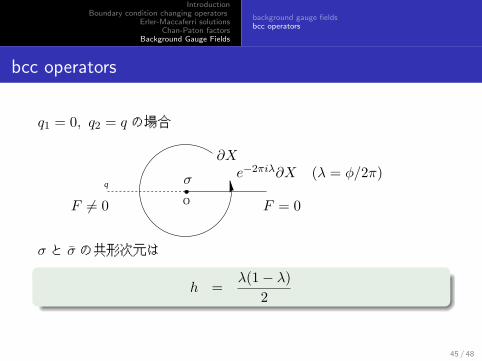
bcc operators
q1 = 0, q2 = q の場合
O
q
∂Xe−2πiλ∂X (λ = ϕ/2π)σ
F = 0F = 0
σ と σ の共形次元は.
.
. ..
.
.
h =λ(1− λ)
2
45 / 48
IntroductionBoundary condition changing operators
Erler-Maccaferri solutionsChan-Paton factors
Background Gauge Fields
background gauge fieldsbcc operators
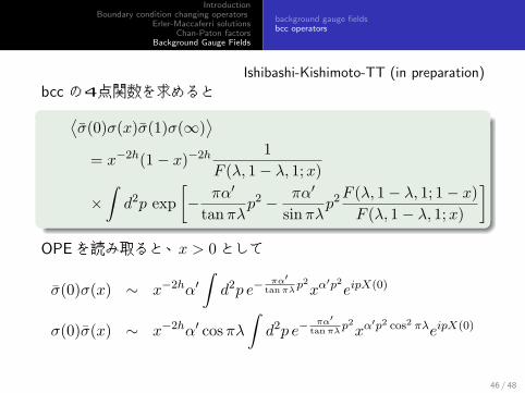
Ishibashi-Kishimoto-TT (in preparation)
bcc の4点関数を求めると.
.
. ..
.
.
⟨σ(0)σ(x)σ(1)σ(∞)
⟩= x−2h(1− x)−2h 1
F (λ, 1− λ, 1;x)
×∫d2p exp
[− πα′
tanπλp2 − πα′
sinπλp2F (λ, 1− λ, 1; 1− x)F (λ, 1− λ, 1;x)
]OPEを読み取ると、x > 0として
σ(0)σ(x) ∼ x−2hα′∫d2p e−
πα′tanπλ
p2xα′p2eipX(0)
σ(0)σ(x) ∼ x−2hα′ cosπλ
∫d2p e−
πα′tanπλ
p2xα′p2 cos2 πλeipX(0)
46 / 48
IntroductionBoundary condition changing operators
Erler-Maccaferri solutionsChan-Paton factors
Background Gauge Fields
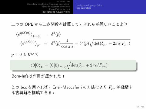
background gauge fieldsbcc operators
二つの OPEから二点関数を計算して、それらが等しいことより⟨eipX(0)
⟩F=0
= δ2(p)⟨eipX(0)
⟩F
= δ2(p)1
cosπλ= δ2(p)
√det(δµν + 2πα′Fµν)
p = 0とおいて.
.
. ..
.
.
⟨0∣∣0⟩
F=⟨0∣∣0⟩
F=0
√det(δµν + 2πα′Fµν)
Born-Infeld作用が導かれた!
この bccを用いれば、Erler-Maccaferriの方法により Fµν が凝縮する古典解を構成できる。
47 / 48
IntroductionBoundary condition changing operators
Erler-Maccaferri solutionsChan-Paton factors
Background Gauge Fields
background gauge fieldsbcc operators
まとめ
boundary condition changing operatorsについて。
Erler-Maccaferriは、bccを使えばあらゆる(BCFTを変化させる)古典解が構成できると主張した。
しかし、X0 を特別扱いしているので、「あらゆる」は言い過ぎ。EMの方法では D instantonはつくれない。
多重ブレーン解から Chan-Paton因子を導く方法が提唱されている。(KMTT)
Fµν が凝縮する古典解を構成した。(IKT)
コンパクト化した場合の解は非可換トーラスと関連。
Fµν の凝縮は Bµν の凝縮とも関係しているので、非可換時空や閉弦の凝縮について考察できればさらに面白くなるはず。
48 / 48