Embed Size (px)
Citation preview

Introduction & motivation Limit solutions Commutative case Noncommutative case Concluding remarks & References
Limit solutions for control systems
M. Soledad Aronna
Escola de Matemática Aplicada, FGV-Rio
Oktobermat XV, 19 e 20 de Outubro de 2017, PUC-Rio

Introduction & motivation Limit solutions Commutative case Noncommutative case Concluding remarks & References
1 Introduction & motivation
2 Limit solutions
3 Commutative case
4 Noncommutative case
5 Concluding remarks & References
Introduction & motivation Limit solutions Commutative case Noncommutative case Concluding remarks & References
Optimal Control, example 1: Fishing problem
[Clark, 1976]
State variable: x is the size of the fish population
Control variable: u is the fishing effort
Cost: net revenue in a fixed time interval
max
∫ T
0
(Eu(t)− c
x(t)u(t)
)dt,
x(t) = r x(t) (1− x(t)/k) − u(t),
0 ≤ u(t) ≤ Umax, a.e. on [0, T ],
x(t) ≥ 0 on [0, T ],
x(0) = x0, x(T ) free.
E : selling cost, c/x(t) : fishing cost, r : reproduction rater/k : mortality due to space competition

Introduction & motivation Limit solutions Commutative case Noncommutative case Concluding remarks & References
Optimal Control, example 2: the Goddard problem in 1D(vertical motion of a rocket)
[Goddard, 1919] [Seywald & Cliff, 1993]
State variables: (h, v,m) are the position, speed and mass.Control variable: u is the normalized thrust (proportion of Tmax)Cost: final mass of the rocket (or minimize fuel consumption)
max m(T ),
s.t. h(t) = v(t),
v(t) = −1/h(t)2 + 1/m(t)(Tmax u(t)−D(h(t), v(t))
),
m(t) = −b Tmax u(t),
0 ≤ u(t) ≤ 1, a.e. on [0, T ],
h(0) = 0, v(0) = 0, m(0) = 1, h(T ) = 1,
T : free final time, b : fuel consumption coefficient,Tmax is the maximal thrust, D(h, v) is the drag
Introduction & motivation Limit solutions Commutative case Noncommutative case Concluding remarks & References
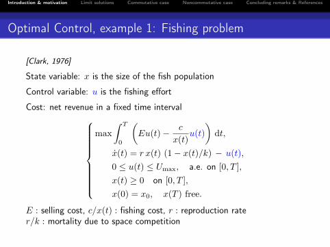
Standard Optimal control problem
A standard optimal control problem is generally written as
max
∫ T
0
L(t, x(t), u(t))dt+ φ(T, x(T )), [cost]
x(t) = f(t, x(t), u(t)), p.c.t. t ∈ [0, T ], [dynamics]x(0) = x0, [initial condition]
(T, x(T )) ∈ S ⊆ IRn+1, [final constraints]u(t) ∈ U ⊆ IRm. [control constraint]
(OCP)
In general, u ∈ L1([0, T ];U) and x ∈W 1,1([0, T ]; IRn).
Introduction & motivation Limit solutions Commutative case Noncommutative case Concluding remarks & References
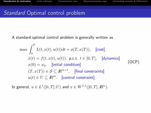
Example 3: Impulsive Control System
[Bressan & Piccoli, 2007]Boy riding swing: changes the radius of oscillationθ(t) : angle, r(t) : radius of oscillationKinetic and potential energies:
T (r, θ, r, θ) =m
2
(r2 + r2θ2), V (r, θ) = mgr cos θ.
Set L := T − V for the Lagrangian, then equation of motion for θ(t) :
d
dt
∂L
∂θ=∂L
∂θ
Introduction & motivation Limit solutions Commutative case Noncommutative case Concluding remarks & References
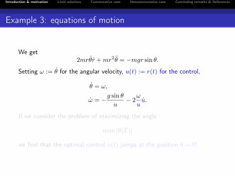
Example 3: equations of motion
We get2mrθr +mr2θ = −mgr sin θ.
Setting ω := θ for the angular velocity, u(t) := r(t) for the control,
θ = ω,
ω = −g sin θ
u− 2
ω
uu.
If we consider the problem of maximizing the angle
max |θ(T )|
we find that the optimal control u(t) jumps at the position θ = 0!
Introduction & motivation Limit solutions Commutative case Noncommutative case Concluding remarks & References
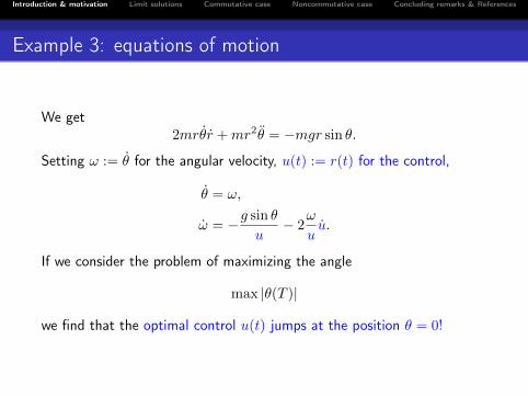
Example 3: equations of motion
We get2mrθr +mr2θ = −mgr sin θ.
Setting ω := θ for the angular velocity, u(t) := r(t) for the control,
θ = ω,
ω = −g sin θ
u− 2
ω
uu.
If we consider the problem of maximizing the angle
max |θ(T )|
we find that the optimal control u(t) jumps at the position θ = 0!

Introduction & motivation Limit solutions Commutative case Noncommutative case Concluding remarks & References
AIM
We aim at giving an appropriate interpretation of these impulsive controlequations, for control functions u that may jump or even have
unbounded variation!

Introduction & motivation Limit solutions Commutative case Noncommutative case Concluding remarks & References
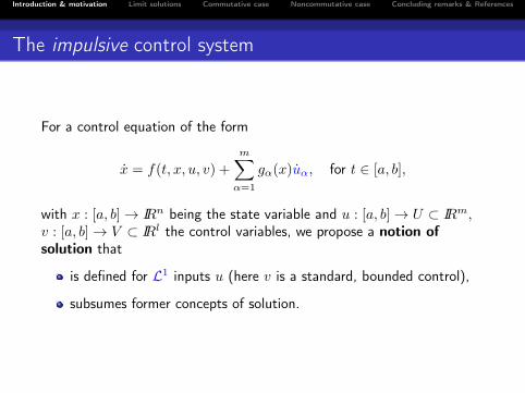
The impulsive control system
For a control equation of the form
x = f(t, x, u, v) +
m∑α=1
gα(x)uα, for t ∈ [a, b],
with x : [a, b]→ IRn being the state variable and u : [a, b]→ U ⊂ IRm,v : [a, b]→ V ⊂ IRl the control variables, we propose a notion ofsolution that
is defined for L1 inputs u (here v is a standard, bounded control),
subsumes former concepts of solution.
Introduction & motivation Limit solutions Commutative case Noncommutative case Concluding remarks & References
The impulsive control system
For a control equation of the form
x = f(t, x, u, v) +
m∑α=1
gα(x)uα, for t ∈ [a, b],
with x : [a, b]→ IRn being the state variable and u : [a, b]→ U ⊂ IRm,v : [a, b]→ V ⊂ IRl the control variables, we propose a notion ofsolution that
is defined for L1 inputs u (here v is a standard, bounded control),
subsumes former concepts of solution.

Introduction & motivation Limit solutions Commutative case Noncommutative case Concluding remarks & References
Some remarks
When u ∈ AC([a, b]; IRm), the system is standard and the solutionis interpreted in the sense of Carathéodory.Some reasons for looking at discontinuous trajectories:1) lack of coercivity in the cost,2) large change of value in a very short amount of time
[Azimov & Bishop, New trends in astrodynamics and applications:Optimal trajectories for space guidance. Annals of the NY Academy ofSciences, 2005][Catllá et al., On Spiking models for synaptic activity and impulsivedifferential equations, SIAM Review, 2005][Gajardo, Ramirez & Rapaport, Minimal time sequential batch reactorswith bounded and impulse controls, SIAM J. Control Opt., 2007]
Introduction & motivation Limit solutions Commutative case Noncommutative case Concluding remarks & References
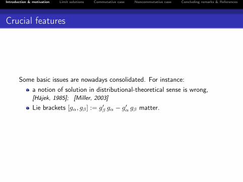
Crucial features
Some basic issues are nowadays consolidated. For instance:a notion of solution in distributional-theoretical sense is wrong,[Hájek, 1985]; [Miller, 2003]
Lie brackets [gα, gβ ] := g′β gα − g′α gβ matter.

Introduction & motivation Limit solutions Commutative case Noncommutative case Concluding remarks & References
“Good” notions of solution already existed in two cases.
CASE I: The commutative case
[gα, gβ ] ≡ 0.
One defines the solution via density of AC in L1
(we adopt this definition here).
It exploits the commutativity via the Flow-box theorem.
References:
[A. Bressan & F. Rampazzo, 1991]
[A.V. Sarychev, 1991]
Introduction & motivation Limit solutions Commutative case Noncommutative case Concluding remarks & References
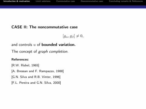
CASE II: The noncommutative case
[gα, gβ ] 6= 0,
and controls u of bounded variation.
The concept of graph completion.
References:
[R.W. Rishel, 1965]
[A. Bressan and F. Rampazzo, 1988]
[G.N. Silva and R.B. Vinter, 1996]
[F.L. Pereira and G.N. Silva, 2000]

Introduction & motivation Limit solutions Commutative case Noncommutative case Concluding remarks & References
1 Introduction & motivation
2 Limit solutions
3 Commutative case
4 Noncommutative case
5 Concluding remarks & References
Introduction & motivation Limit solutions Commutative case Noncommutative case Concluding remarks & References
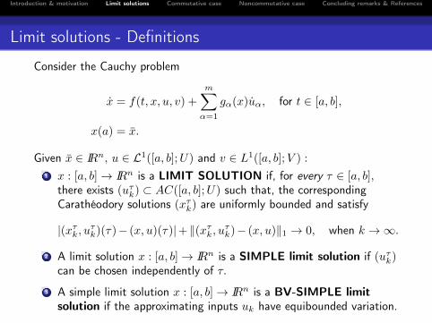
Limit solutions - Definitions
Consider the Cauchy problem
x = f(t, x, u, v) +
m∑α=1
gα(x)uα, for t ∈ [a, b],
x(a) = x.
Given x ∈ IRn, u ∈ L1([a, b];U) and v ∈ L1([a, b];V ) :
1 x : [a, b]→ IRn is a LIMIT SOLUTION if, for every τ ∈ [a, b],there exists (uτk) ⊂ AC([a, b];U) such that, the correspondingCarathéodory solutions (xτk) are uniformly bounded and satisfy
|(xτk, uτk)(τ)− (x, u)(τ)|+‖(xτk, uτk)− (x, u)‖1 → 0, when k →∞.
2 A limit solution x : [a, b]→ IRn is a SIMPLE limit solution if (uτk)can be chosen independently of τ.
3 A simple limit solution x : [a, b]→ IRn is a BV-SIMPLE limitsolution if the approximating inputs uk have equibounded variation.
Introduction & motivation Limit solutions Commutative case Noncommutative case Concluding remarks & References
Outline of the results
Consistency with standard (Carathéodory) solutions
Some existence results
Uniqueness in the commutative case
Comparison with “graph completion” solutions

Introduction & motivation Limit solutions Commutative case Noncommutative case Concluding remarks & References
Example 1[H.J. Sussmann & W. Liu, 1991]
g1(x) := (1, 0, x2)>, g2(x) := (0, 1,−x1)>, [g1, g2] = (0, 0,−2)>,
x = g1(x)u1 + g2(x)u2, t ∈ [0, 1], x(0) = (0, 0, 0)>.
For u ≡ (0, 0)>, the Carathéodory solution is xC ≡ (0, 0, 0)>.Approximating u by
uk(t) = (k−1/2(cos kt− 1), k−1/2 sin kt)>,
one gets
xk(t) = (k−1/2(cos kt− 1), k−1/2 sin kt,−t+ k−1 sin kt)>,
uk → (0, 0)>, xk → x(t) := (0, 0,−t)>, uniformly on [0, 1].
u ∈ AC, and x ∈ AC is a simple limit solution (but not BV simple!)Lack of uniqueness: the solution depends on (uk)
(we’ll see this holds in general whenever [gα, gβ ] 6= 0)

Introduction & motivation Limit solutions Commutative case Noncommutative case Concluding remarks & References
Example 2
x = xu, x(0) = 1, t ∈ [0, 1].
For every bounded u ∈ L1([0, 1]; IR), the map
x(t) = eu(t)−u(a)
is a limit solution.Actually, since m = 1, we will prove that x is the unique limit solution.Yet, x is not a simple limit solution in general, since for instance, if
u := 1Q∩[0,1]
is the Dirichlet function, there is no way of pointwise approximating uwith one sequence of absolutely continuous uk.

Introduction & motivation Limit solutions Commutative case Noncommutative case Concluding remarks & References
1 Introduction & motivation
2 Limit solutions
3 Commutative case
4 Noncommutative case
5 Concluding remarks & References
Introduction & motivation Limit solutions Commutative case Noncommutative case Concluding remarks & References
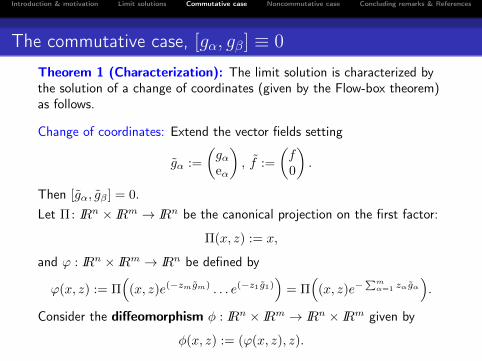
The commutative case, [gα, gβ] ≡ 0
Theorem 1 (Characterization): The limit solution is characterized bythe solution of a change of coordinates (given by the Flow-box theorem)as follows.
Change of coordinates: Extend the vector fields setting
gα :=
(gαeα
), f :=
(f0
).
Then [gα, gβ ] = 0.
Let Π: IRn × IRm → IRn be the canonical projection on the first factor:
Π(x, z) := x,
and ϕ : IRn × IRm → IRn be defined by
ϕ(x, z) := Π(
(x, z)e(−zmgm) . . . e(−z1g1))
= Π(
(x, z)e−∑mα=1 zαgα
).
Consider the diffeomorphism φ : IRn × IRm → IRn × IRm given by
φ(x, z) := (ϕ(x, z), z).
Introduction & motivation Limit solutions Commutative case Noncommutative case Concluding remarks & References
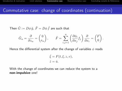
Commutative case: change of coordinates (continuation)
Then G := Dφ g, F = Dφ f are such that
Gα =∂
∂zα=
(0eα
), F =
n∑i,j=1
(∂φi∂xj
fj
)∂
∂xi=
(F0
).
Hence the differential system after the change of variables φ reads
ξ = F (t, ξ, z, v),
z = u.
With the change of coordinates we can reduce the system to anon-impulsive one!
Introduction & motivation Limit solutions Commutative case Noncommutative case Concluding remarks & References
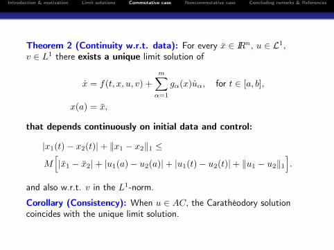
Theorem 2 (Continuity w.r.t. data): For every x ∈ IRn, u ∈ L1,v ∈ L1 there exists a unique limit solution of
x = f(t, x, u, v) +
m∑α=1
gα(x)uα, for t ∈ [a, b],
x(a) = x,
that depends continuously on initial data and control:
|x1(t)− x2(t)|+ ‖x1 − x2‖1 ≤
M[|x1 − x2|+ |u1(a)− u2(a)|+ |u1(t)− u2(t)|+ ‖u1 − u2‖1
].
and also w.r.t. v in the L1-norm.
Corollary (Consistency): When u ∈ AC, the Carathéodory solutioncoincides with the unique limit solution.
Introduction & motivation Limit solutions Commutative case Noncommutative case Concluding remarks & References
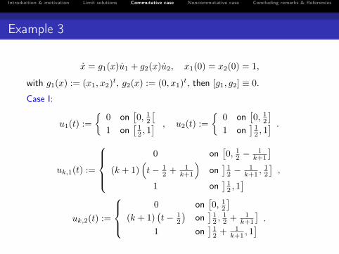
Example 3
x = g1(x)u1 + g2(x)u2, x1(0) = x2(0) = 1,
with g1(x) := (x1, x2)t, g2(x) := (0, x1)t, then [g1, g2] ≡ 0.
Case I:
u1(t) :=
{0 on
[0, 12[
1 on[12 , 1] , u2(t) :=
{0 on
[0, 12]
1 on]12 , 1] .
uk,1(t) :=
0 on
[0, 12 −
1k+1
](k + 1)
(t− 1
2 + 1k+1
)on]12 −
1k+1 ,
12
]1 on
]12 , 1] ,
uk,2(t) :=
0 on
[0, 12]
(k + 1)(t− 1
2
)on]12 ,
12 + 1
k+1
]1 on
]12 + 1
k+1 , 1] .

Introduction & motivation Limit solutions Commutative case Noncommutative case Concluding remarks & References
Example 3 - continuation
x1(t) :=
{1 on
[0, 12[
e on[12 , 1] , x2(t) :=
1 on
[0, 12[
e on t = 12
2e on]12 , 1]
Case II: We invert the controls, u1 := u2, u2 := u1,
(u1, u2) = (u1, u2) on [0, 1]\{1/2} uk,1 := uk,2, uk,2 := uk,1,
x1(t) :=
{1 on
[0, 12]
e on]12 , 1] , x2(t) :=
1 on
[0, 12[
2 on t = 12
2e on]12 , 1] .
Introduction & motivation Limit solutions Commutative case Noncommutative case Concluding remarks & References
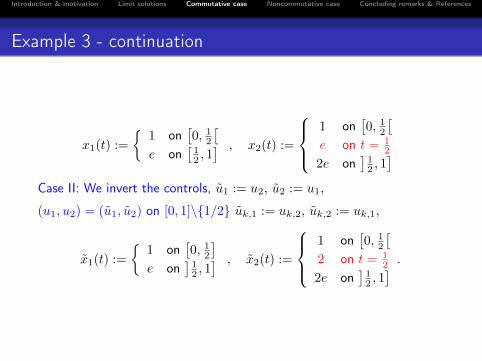
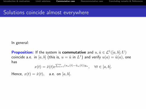
Solutions coincide almost everywhere
In general:
Proposition: If the system is commutative and u, u ∈ L1([a, b];U)coincide a.e. in [a, b] (this is, u = u in L1) and verify u(a) = u(a), onehas
x(t) = x(t)e∑mα=1(uα(t)−uα(t))gα , ∀t ∈ [a, b].
Hence, x(t) = x(t), a.e. on [a, b].
Introduction & motivation Limit solutions Commutative case Noncommutative case Concluding remarks & References
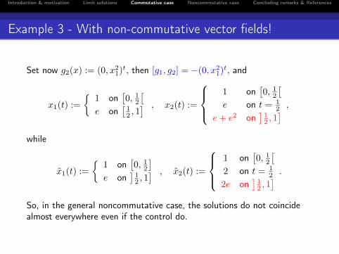
Example 3 - With non-commutative vector fields!
Set now g2(x) := (0, x21)t, then [g1, g2] = −(0, x21)t, and
x1(t) :=
{1 on
[0, 12[
e on[12 , 1] , x2(t) :=
1 on
[0, 12[
e on t = 12
e+ e2 on]12 , 1] ,
while
x1(t) :=
{1 on
[0, 12]
e on]12 , 1] , x2(t) :=
1 on
[0, 12[
2 on t = 12
2e on]12 , 1] .
So, in the general noncommutative case, the solutions do not coincidealmost everywhere even if the control do.

Introduction & motivation Limit solutions Commutative case Noncommutative case Concluding remarks & References
1 Introduction & motivation
2 Limit solutions
3 Commutative case
4 Noncommutative case
5 Concluding remarks & References

Introduction & motivation Limit solutions Commutative case Noncommutative case Concluding remarks & References
The noncommutative case, u ∈ BV - Space-time system
The existing notion of solution in the noncommutative case:
• For regular (absolutely continuous) controls u ∈ AC([a, b];U), onecan consider
s : [a, b]→ [0, 1], s(t) :=t+ Var[a,t](u)
b− a+ Var[a,b](u),
and reparametrize time ϕ0(·) := s−1(·) with ϕ0 : [0, 1]→ [a, b], and setϕ(s) := u ◦ ϕ0(s), y := x ◦ ϕ0.
• (ϕ0, ϕ, y) is solution of the space-times systemy′0(s) = ϕ′0(s),
y′(s) = f(y0(s), y(s), ϕ(s), ψ(s))ϕ′0(s) +
m∑α=1
gα(y(s))ϕα′(s),
(y0, y)(0) = (a, x) ,
s ∈ [0, 1].
Introduction & motivation Limit solutions Commutative case Noncommutative case Concluding remarks & References
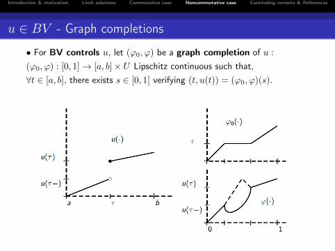
u ∈ BV - Graph completions
• For BV controls u, let (ϕ0, ϕ) be a graph completion of u :
(ϕ0, ϕ) : [0, 1]→ [a, b]× U Lipschitz continuous such that,∀t ∈ [a, b], there exists s ∈ [0, 1] verifying (t, u(t)) = (ϕ0, ϕ)(s).

Introduction & motivation Limit solutions Commutative case Noncommutative case Concluding remarks & References
Graph completion solutions
Given u ∈ BV ([a, b];U) and (ϕ0, ϕ) : [0, 1]→ [a, b]× U a graphcompletion of u, we let y be the solution ofy′0(s) = ϕ′0(s),
y′(s) = f(y0(s), y(s), ϕ(s), ψ(s))ϕ′0(s) +
m∑α=1
gα(y(s))ϕα′(s),
(y0, y)(0) = (a, x) ,
s ∈ [0, 1].
Graph completion solution: (possibly) set-valued map x : [a, b] ⇒ IRn,
t Z=⇒ x(t) := y ◦ ϕ−10 (t).
Single-valued graph completion solution:x : [a, b]→ IRn, σ : [a, b]→ [0, 1] a right-inverse of ϕ0 such that
(t, u(t)) = (ϕ0, ϕ) ◦ σ(t), x(t) = y ◦ σ(t), for all t ∈ [a, b].
Introduction & motivation Limit solutions Commutative case Noncommutative case Concluding remarks & References
Representation of BV simple limit solutions
Theorem 3 (Equivalence BV simple limit solution andsingle-valued graph completion solution): Given x ∈ IRn, u ∈ BV,v ∈ L1 : x is a BV simple limit solution if and only if x is a single-valuedgraph completion solution.
Ingredients of the proof:“if”: one has (t, u(t), x(t)) = (ϕ0, ϕ, y) ◦ σ(t), with σ ∈ BVincreasing. We prove pointwise approximation of σ with ACfunctions of uniform BV.
“only if”: compactness (Ascoli-Arzelà theorem)
Introduction & motivation Limit solutions Commutative case Noncommutative case Concluding remarks & References
Existence of limit solutions for u ∈ BV
An arcwise connected set U has the Whitney property isd(x, y) ≤M |x− y|, for some M > 0, where d is the geodesic distance.
Theorem 4 (Existence of limit solution): If U has the Whitneyproperty then, for any x ∈ IRn, u ∈ BV, v ∈ L1, there exists a BV simplelimit solution.
Introduction & motivation Limit solutions Commutative case Noncommutative case Concluding remarks & References
Consistency with Carathéodory solutions
Theorem 5 (Consistency): If x ∈ IRn, u ∈ AC, v ∈ L1, and x ∈ AC isa BV simple limit solution, then x is the Carathéodory solution.
Recall Example 1!

Introduction & motivation Limit solutions Commutative case Noncommutative case Concluding remarks & References
1 Introduction & motivation
2 Limit solutions
3 Commutative case
4 Noncommutative case
5 Concluding remarks & References
Introduction & motivation Limit solutions Commutative case Noncommutative case Concluding remarks & References
Concluding remarks
The same concept of solution is used both for the commutative andnoncommutative cases.
In the commutative case, the limit solutions are represented via achange of coordinates.
In the noncommutative case, there is a representation of the BVsimple limit solutions via the graph completion.
When u ∈ BV : “it is equivalent to approximate by AC functionswith uniform BV, than to complete the graph.”
Introduction & motivation Limit solutions Commutative case Noncommutative case Concluding remarks & References
References
H.J. Sussmann. Ann. Probability, 1978.A. Bressan and F. Rampazzo. Boll. Un. Mat. Ital., 1988.A. Bressan and F. Rampazzo. J. Optim. Theory Appl., 1991.A.V. Sarychev. In Nonlinear synthesis (Sopron, 1989), volume 9 ofProgr. Systems Control Theory, Birkhäuser Boston, Boston, MA,1991.M.S. Aronna and F. Rampazzo. A note on systems with ordinaryand impulsive controls. IMA J. Math. Control Inform., 2016M.S. Aronna and F. Rampazzo. L1 limit solutions for controlsystems. J. Differential Equations, 2015M.S. Aronna, M. Motta and F. Rampazzo. Necessary conditionsinvolving Lie brackets for impulsive optimal control problems, arXiv& in progress

Introduction & motivation Limit solutions Commutative case Noncommutative case Concluding remarks & References
OBRIGADA!