Estimating Degradation of Lithium Ion - NASA · Estimating Degradation of Lithium‐Ion Battery under Storage and Arbitrary Cycling ‐ Some Examples JayaJaya tnt SaSa as a ,rlashkar,

Estimating Degradation of Lithium‐Ion Battery under Storage and Arbitrary Cycling ‐Battery under Storage and Arbitrary Cycling Some Examples

Jayant Sarlashkar, PhDJaya t Sa as a ,[email protected], +1‐210‐522‐5506

Bapiraju Surampudi, PhDb i j di@ i 1 210 522 [email protected], +1‐210‐522‐3278

Southwest Research Institute, San Antonio, TX, USAWork funded by Southwest Research Institute (SwRI) Internal

©Copyright Southwest Research Institute ® 2014

y ( )R&D Project 03‐R8467. Investigators thank SwRI’s EssEs

Consortium for making available certain data sets.1

Outline• Company Background• Introduction Objective and Results• Introduction, Objective, and Results• Technical Approach

– Exploratory Data Analysis – Storage and Cycle– Assessing Quality of Model Fit– Handling Arbitrary Cycles

• Model Validation


• Conclusions and Future Work2

Southwest Research InstituteCompany Backgroundp y g

• Founded in 1947; 501 (c)(3) nonprofit corporation; contract R&D; independent and unbiased; based in San Antonio TXR&D; independent and unbiased; based in San Antonio TX

• Mission: Benefiting government, industry and the public through innovative science and technologythrough innovative science and technology

• Nine technical Divisions: From space to geosciences including automotive, chemistry, and materials, y,– Several pre‐competitive joint industry programs including one on energy

storage systems (EssEs.swri.org)


• FY2014: Revenue $549M; $7M Internal R&D3

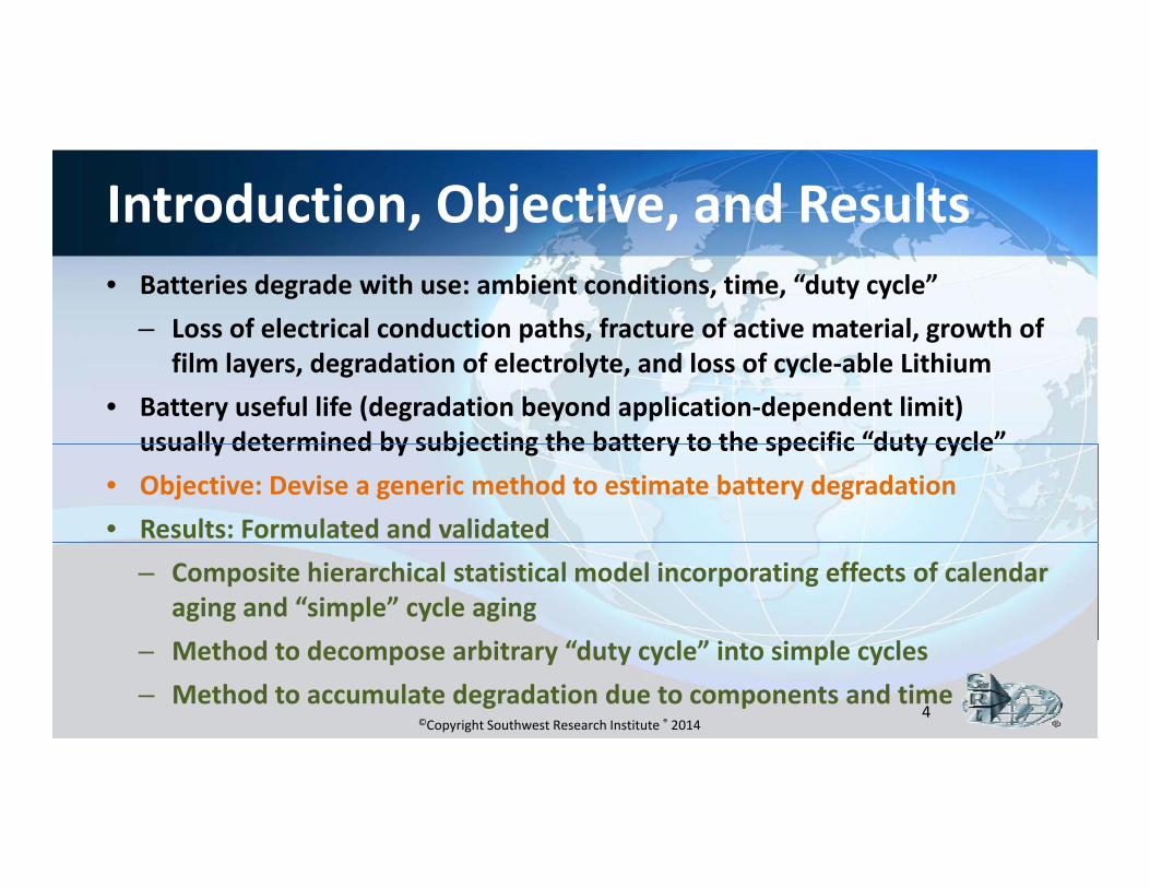
Introduction, Objective, and Results• Batteries degrade with use: ambient conditions, time, “duty cycle”

– Loss of electrical conduction paths, fracture of active material, growth of film layers, degradation of electrolyte, and loss of cycle‐able Lithium

• Battery useful life (degradation beyond application‐dependent limit) usually determined by subjecting the battery to the specific “duty cycle”usually determined by subjecting the battery to the specific duty cycle

• Objective: Devise a generic method to estimate battery degradation• Results: Formulated and validated

– Composite hierarchical statistical model incorporating effects of calendar aging and “simple” cycle aging

h d d b “d l ” l l


– Method to decompose arbitrary “duty cycle” into simple cycles– Method to accumulate degradation due to components and time

4

Technical Approach

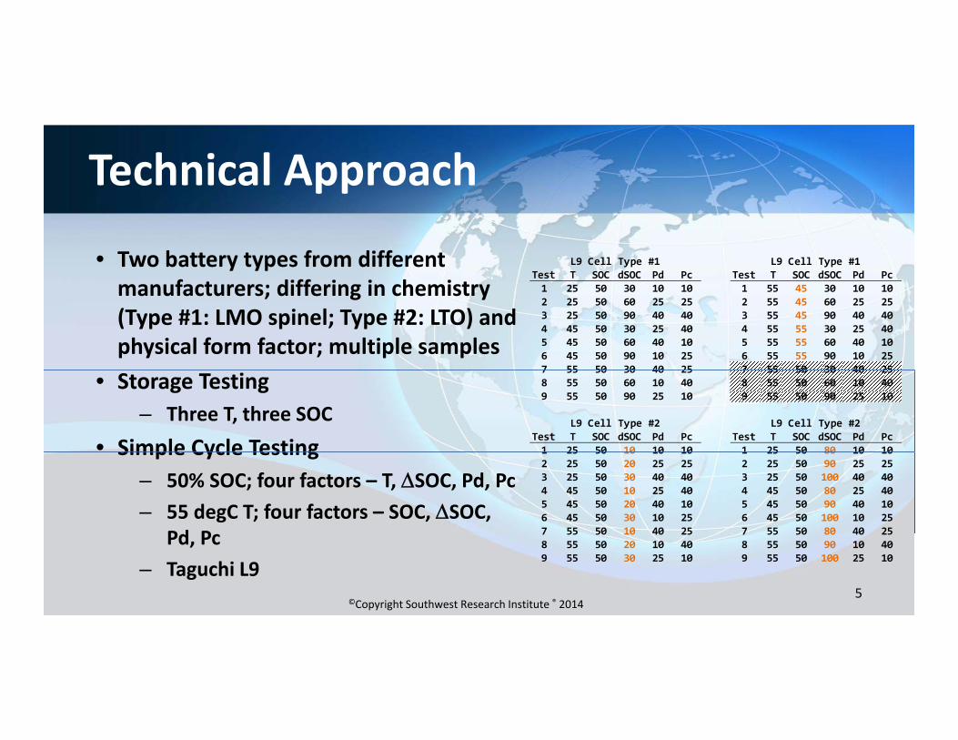
• Two battery types from different manufacturers; differing in chemistry

L9 Cell Type #1 L9 Cell Type #1Test T SOC dSOC Pd Pc Test T SOC dSOC Pd Pc1 25 50 30 10 10 1 55 45 30 10 10manufacturers; differing in chemistry

(Type #1: LMO spinel; Type #2: LTO) and physical form factor; multiple samples

1 25 50 30 10 10 1 55 45 30 10 102 25 50 60 25 25 2 55 45 60 25 253 25 50 90 40 40 3 55 45 90 40 404 45 50 30 25 40 4 55 55 30 25 405 45 50 60 40 10 5 55 55 60 40 106 45 50 90 10 25 6 55 55 90 10 257 55 50 30 40 25 7 55 50 30 40 25• Storage Testing

– Three T, three SOC

• Simple Cycle Testing

7 55 50 30 40 25 7 55 50 30 40 258 55 50 60 10 40 8 55 50 60 10 409 55 50 90 25 10 9 55 50 90 25 10

L9 Cell Type #2 L9 Cell Type #2Test T SOC dSOC Pd Pc Test T SOC dSOC Pd Pc1 25 50 10 10 10 1 25 50 80 10 10Simple Cycle Testing

– 50% SOC; four factors – T, SOC, Pd, Pc– 55 degC T; four factors – SOC, SOC,

Pd P

1 25 50 10 10 10 1 25 50 80 10 102 25 50 20 25 25 2 25 50 90 25 253 25 50 30 40 40 3 25 50 100 40 404 45 50 10 25 40 4 45 50 80 25 405 45 50 20 40 10 5 45 50 90 40 106 45 50 30 10 25 6 45 50 100 10 257 55 50 10 40 25 7 55 50 80 40 25


Pd, Pc– Taguchi L9

7 55 50 10 40 25 7 55 50 80 40 258 55 50 20 10 40 8 55 50 90 10 409 55 50 30 25 10 9 55 50 100 25 10

5

Exploratory Data Analysis

• Storage and cycle data visualized for patterns and choose model forms

Cell Type #1 calendar data

1.00

patterns and choose model forms• Conditional plots; projections

– Or else – a confusing mess -]

0.95

• Conditional plots help formulate hierarchical modelsDiff ll d diff i

norm

sta

t cap

[-

0.85

0.90

• Different cells need different metric– Type #1: Normalized static capacity

(and loss)

0.80


– Tyep #2: Normalized discharge pulse power capability (and loss) at 50% SOC

cumulative time [day]

0.75

0 50 100 150 200 250 300

6

Exploratory Data Analysis – Storage Cell Type #1 ypCell Type #1 calendar data conditioned on SOC and T

50 70 9025 45 55

0 50 100150200250300

50 70 9025 45 55

50 70 9025 45 55 • Each panel a univariate graph of

l i i f i i h ll

25 45 55 25 45 55 25 45 550.750.800.850.900.951.00 a multivariate function with all

but one variable fixed/shingled• Plot conditioning

orm

sta

t cap

[-] 50 70 90 50 70 90

0.800.850.900.951.00

50 70 90 • Plot conditioning– Left‐right: first variable (SOC)– Down‐up: second variable (T)no

0.850.900.951.00

50 70 9025 45 55

50 70 9025 45 55

50 70 9025 45 55

0.75 Down up: second variable (T)

• Consider shape and rate of decline of metric as a function

©Copyright Southwest Research Institute ® 2014cumulative time [day]

0.750.80

0 50 100150200250300 0 50 100150200250300of conditioning variables

7

Exploratory Data Analysis – CycleCell Type #1 yp

Cell Type #1 cycle data conditioned on dSOC and T at SOC = 50

0 530 60 9025 45 55

0 1000 2000 3000

30 60 9025 45 55

30 60 9025 45 55

Cell Type #1 cycle data conditioned on dSOC and SOC at T = 55

30 60 9045 50 55

0 500 1000 1500

30 60 9045 50 55

30 60 9045 50 55

25 45 55 25 45 55 25 45 550.00.10.20.30.40.5

45 50 55 45 50 55 45 50 550.00.10.20.30.40.5

m s

tat c

ap lo

ss [-

]

30 60 90 30 60 90

0 00.10.20.30.40.5

30 60 90

m s

tat c

ap lo

ss [-

]

30 60 90 30 60 90

0 00.10.20.30.40.5

30 60 90

norm

0.20.30.40.5

30 60 9025 45 55

30 60 9025 45 55

30 60 9025 45 55

0.0

norm

0.20.30.40.5

30 60 9045 50 55

30 60 9045 50 55

30 60 9045 50 55

0.0

©Copyright Southwest Research Institute ® 2014cycle count [-]

0.00.1

0 1000 2000 3000 0 1000 2000 3000

cycle count [-]

0.00.1

0 500 1000 1500 0 500 1000 1500

8

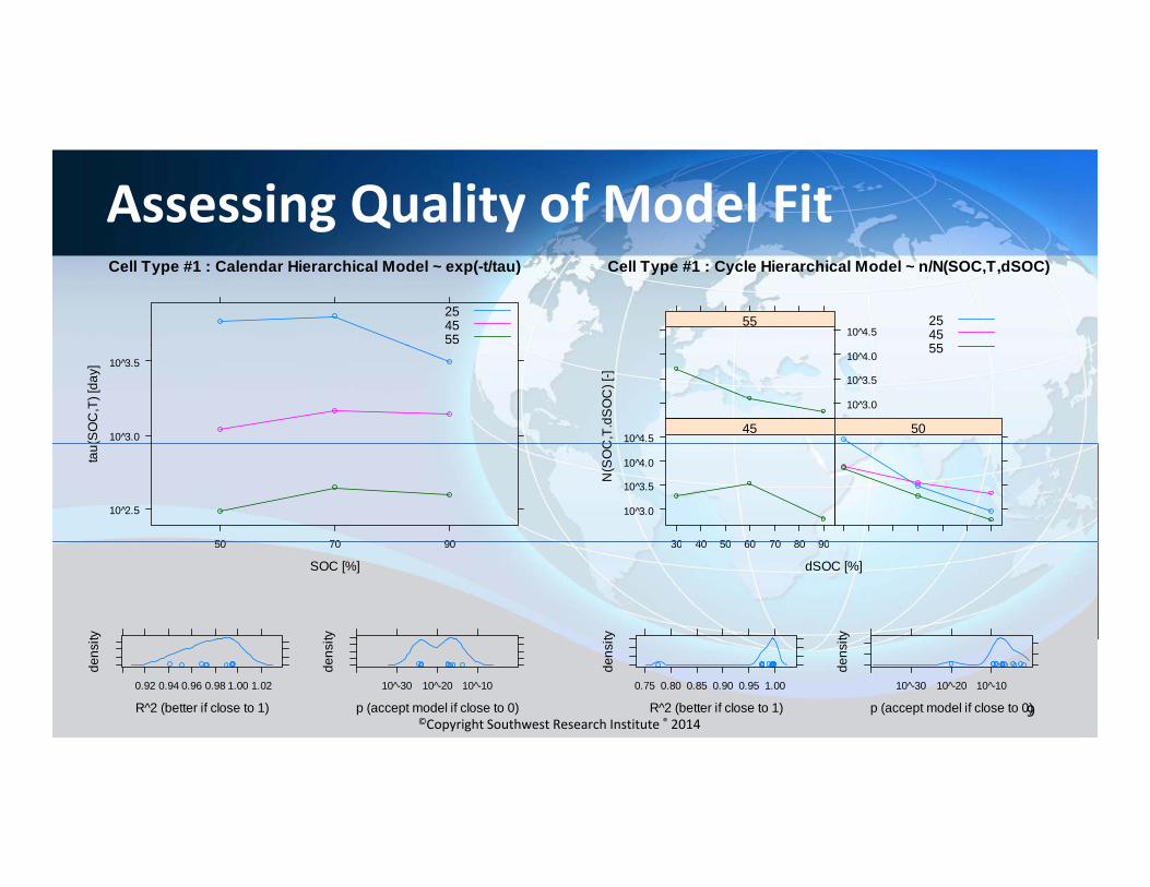
Assessing Quality of Model FitCell Type #1 : Cycle Hierarchical Model ~ n/N(SOC,T,dSOC)

10^4.555 25

4555

Cell Type #1 : Calendar Hierarchical Model ~ exp(-t/tau)

254555

C,T

.dS

OC

) [-]

10 4̂.545 50

10^3.0

10^3.5

10^4.055

(SO

C,T

) [da

y]

10 3̂.0

10 3̂.5

N(S

OC

10 3̂.0

10 3̂.5

10 4̂.0

30 40 50 60 70 80 90

tau

10 2̂.5

50 70 90

dSOC [%]

30 40 50 60 70 80 90

ty ty

SOC [%]

50 70 90

ty ty

©Copyright Southwest Research Institute ® 2014R^2 (better if close to 1)

dens

it

0.75 0.80 0.85 0.90 0.95 1.00

p (accept model if close to 0)

dens

it

10 -̂30 10 -̂20 10 -̂10

R^2 (better if close to 1)

dens

it

0.92 0.94 0.96 0.98 1.00 1.02

p (accept model if close to 0)

dens

it

10 -̂30 10 -̂20 10 -̂10

9

Exploratory Data Analysis ‐ Cycle and StorageCell Type #2yp

Cell Type #2 cycle data conditioned on dSOC and T at SOC = 50

102030809010025 45 55

0 5000

102030809010025 45 55

102030809010025 45 55

0 5000

102030809010025 45 55

102030809010025 45 55

0 5000

102030809010025 45 55

Cell Type #2 calendar data conditioned on SOC and T

30 50 7025 45 55

0 50 100150200250

30 50 7025 45 55

30 50 7025 45 55

e at

50%

SO

C [-

]

25 45 55 25 45 55 25 45 55 25 45 55 25 45 55 25 45 550.0

0.1

0.2

0.3

at 5

0% S

OC

[-]

25 45 55 25 45 55 25 45 550.750.800.850.900.951.00

ap lo

ss; d

isch

arge 10203080901001020308090100102030809010010203080901001020308090100

0 0

0.1

0.2

0.3

1020308090100

r cap

; dis

char

ge a 30 50 70 30 50 70

0.800.850.900.951.00

30 50 70

rm p

ulse

pow

er c

a

0 1

0.2

0.3

102030809010025 45 55

102030809010025 45 55

102030809010025 45 55

102030809010025 45 55

102030809010025 45 55

102030809010025 45 55

0.0

norm

pul

se p

ower

0.850.900.951.00

30 50 7025 45 55

30 50 7025 45 55

30 50 7025 45 55

0.75

©Copyright Southwest Research Institute ® 2014cycle count [-]

nor

0.0

0.1

0 5000 0 5000 0 5000

cumulative time [day]

n

0.750.800.85

0 50 100150200250 0 50 100150200250

10

Handling Arbitrary Cycles – Method

• Hierarchical models– Exponential‐form calendar model;

Cell Type #1 cd cycle

A]

100

Cell Type #1 fr cycle

A] 20

40

Exponential‐form calendar model; parameter depends on SOC and T

– Proprietary‐form cycle model; parameters depend on T, and

curre

nt [A

-50

0

50

curre

nt [A

-40

-20

0

20

p pnumber, range, bias, period of cycle

• Arbitrary charge‐discharge profile decomposed into “simple” cycles

time [hr]

51.0 51.1 51.2 51.3 51.4 51.5

time [hr]

40 45 50 55

Cell Type #2 cc cycle Cell Type #2 fr cycle

using proprietary method– Degradation due to each simple

cycle computed from the model and curre

nt [A

]0

50

100

curre

nt [A

]

-50

0

50

100


accumulated

time [hr]

-50

11.0 11.5 12.0 12.5 13.0

time [hr]

-100

20 25 30 35

11

Handling Arbitrary Cycles – DecompositionSimple cycles in blue; decomposition as heat mapp y ; p p

8010

0

Cell Type #1 cd cycle

8010

0

Cell Type #1 fr cycle Cell Type #1

c [-] cd

0.7 0.8 0.9 1.0

fr

2040

60

cycl

e am

pl [

%]

2040

60

cycl

e am

pl [

%]

mea

sure

d m

etric

0.7

0.8

0.9

1.0

30 40 50 60 70 80 90 100

0

cy cle bias [%]

30 40 50 60 70 80 90 100

0

cy cle bias [%]

100

Cell Type #2 cc cycle

100

Cell Type #2 fr cycle

estimated metric [-]

0.7 0.8 0.9 1.0

Cell Type #2

0 7 0 8 0 9 1 0

4060

80

cycl

e am

pl [

%]

4060

80

cycl

e am

pl [

%]

ured

met

ric [-

]0.8

0.9

1.0

cc

0.7 0.8 0.9 1.0

fr


30 40 50 60 70 80 90 100

020

cy cle bias [%]

30 40 50 60 70 80 90 100

020

cy cle bias [%] estimated metric [-]

mea

su

0.7

0.7 0.8 0.9 1.0

12

Conclusions and Future Work• “… all models are wrong but some are useful” – George Box• Degradation of battery estimated by decomposing arbitrary charge‐eg adat o o batte y est ated by deco pos g a b t a y c a ge

discharge pattern into “simple” cycles and accumulating degradation– Composite hierarchical statistical model for cycle and calendar effects

d b b d d d d d h l d– Good agreement between observed and estimated degradation when applied to batteries of different chemistries under various duty cycles

• Expected applications include– Optimizing a battery pack for a given duty cycle subject to constraints on life

expectancy, weight, volume, and costEstimation of warranty costs using uncertainty bounds on model parameters


– Estimation of warranty costs using uncertainty bounds on model parameters– Real‐time estimation of degradation

13

Documents

Estimating Degradation of Lithium Ion - NASA · Estimating Degradation of Lithium‐Ion Battery under Storage and Arbitrary Cycling ‐ Some Examples JayaJaya tnt SaSa as a ,rlashkar,