Loughborough UniversityInstitutional Repository

Estimating future biddingperformance of competitorbidders in capped tenders

This item was submitted to Loughborough University's Institutional Repositoryby the/an author.

Citation: BALLESTEROS-PEREZ, P. ... et al., 2014. Estimating futurebidding performance of competitor bidders in capped tenders. Journal of CivilEngineering and Management, 20(5), pp. 702-713.

Additional Information:

• This is an Accepted Manuscript of an article published by Taylor & Fran-cis in Journal of Civil Engineering and Management on 04 Jul 2014, avail-able online: https://doi.org/10.3846/13923730.2014.914096.

Metadata Record: https://dspace.lboro.ac.uk/2134/32769

Version: Accepted for publication

Publisher: c© Vilnius Gediminas Technical University (VGTU) Press. Pub-lished by Taylor and Francis

Rights: This work is made available according to the conditions of the Cre-ative Commons Attribution-NonCommercial-NoDerivatives 4.0 International(CC BY-NC-ND 4.0) licence. Full details of this licence are available at:https://creativecommons.org/licenses/by-nc-nd/4.0/

Please cite the published version.

THANKS FOR DOWNLOADING THIS PAPER.

This is a post-refereeing version of a manuscript published by Taylor and Francis.

Please, in order to cite this paper properly:

Ballesteros-Pérez, P., González-Cruz, M.C., Fernández-Diego, M., Pellicer, E. (2014)

“Estimating future bidding performance of competitor bidders in capped tenders.” Journal

of Civil Engineering and Management. In press. 1–12.

http://dx.doi.org/10.3846/13923730.2014.914096

The authors recommend going to the publisher’s website in order to access the full paper.

If this paper helped you somehow in your research, feel free to cite it.

This author’s version of the manuscript was downloaded totally free from:

https://www.researchgate.net/publication/263733991_Estimating_future_bidding_performance_of_

competitor_bidders_in_capped_tenders

ESTIMATING FUTURE BIDDING PERFORMANCE OF COMPETITOR BIDDERS IN

CAPPED TENDERS

Pablo BALLESTEROS-PÉREZa, M. Carmen GONZÁLEZ-CRUZb, Marta FERNÁNDEZ-DIEGOc, Eugenio PELLICERd*

aDepartment of Construction Engineering and Management, Universidad de Talca, Curicó, Chile bDepartment of Project Engineering, Universitat Politècnica de València, Valencia, Spain

cDepartment of Business Administration, Universitat Politècnica de València, Valencia, Spain dSchool of Civil Engineering, Universitat Politècnica de València, Valencia, Spain

*Corresponding author: E-mail: pellicer@upv.es

Received 20 Jun 2013; accepted 30 Jul 2013

Abstract. Research in Bid Tender Forecasting Models (BTFM) has been in progress since the 1950s. None of the developed models were easy-to-use tools for effective use by bidding practitioners because the advanced mathematical apparatus and massive data inputs required. This scenario began to change in 2012 with the development of the Smartbid BTFM, a quite simple model that presents a series of graphs that enables any project manager to study competitors using a relatively short historical tender dataset. However, despite the advantages of this new model, so far, it is still necessary to study all the auction participants as an indivisible group; that is, the original BTFM was not devised for analyzing the behavior of a single bidding competitor or a subgroup of them. The present paper tries to solve that flaw and presents a stand-alone methodology useful for estimating future competitors’ bidding behaviors separately. Keywords: bid, tender, auction, construction, score, forecast.

Reference to this paper should be made as follows: Ballesteros-Pérez, P.; González-Cruz, M. C.; Fernández-Diego, M.; Pellicer, E. 2014. Estimating future bidding performance of competitor bidders in capped tenders, Journal of Civil Engineering and Management

Introduction

The volume of economic transactions conducted by competitive bidding emphasizes the importance of the study of auctions as a part of basic research in economics and management science (Stark, Rothkopf 1979), and the assistance that bidding practitioners can derive from advances in auction theory (Rothkopf, Harstad 1994). Competitive bidding is a transparent procurement method in which bids from competing contractors, suppliers, or vendors are invited by openly advertising the scope, specifications, and terms and conditions of a proposed contract; as well as the criteria by which bids will be evaluated. Competitive bidding aims to procure goods and services at the lowest price by stimulating competition and preventing favoritism (OECD 2007; OECD 2009).

Research in the area of competitive bidding strategy models has been in progress since the 1950s (Rothkopf 1969; Näykki 1976; Engelbrecht-Wiggans 1980, 1989; Naoum 1994; Rothkopf, Harstad 1994; Deltas, Engelbrecht-Wiggans 2005; Dikmen et al. 2007; Lo et al. 2007; Harstad, SašaPekec 2008; Ye et al. 2008). Numerous competitive bidding strategy models have been developed that predict the probability of a bidder

winning an auction (Näykki 1976; Engelbrecht-Wiggans 1980), or being awarded a project (Vergara 1977; Ravanshadnia et al. 2010). Most of these models are based on games theory, decision analysis, and operational research concepts whose application to real-world business is difficult given the complex mathematical formulations required by the models and/or because the models do not suit the actual practices (Engelbrecht-Wiggans 1980; Rothkopf, Harstad 1994; Harstad, SašaPekec 2008).

Because of the multiple technical and financial criteria involved in public tendering (Näykki 1976; Engelbrecht-Wiggans 1980; Rothkopf, Harstad 1994; Fayek 1998; Skitmore et al. 2001; Skitmore 2002, 2004; Harstad, SašaPekec 2008) there is still a need for new tools to help decision makers and improve the selection process for bidders (Watt et al. 2009).

A completely new Bid Tender Forecasting Model (BTFM) was devised by Ballesteros-Pérez (2010) and extended by Ballesteros-Pérez et al. (2012a, b, 2013a) as a practical tool to help bidders improve their competitive bidding strategies and increase their chances of winning a contract. This tool, informally referred by its authors as the Smartbid model (Ballesteros-Pérez et al. 2013b) (used hereinafter for the sake of simplicity) enables bidders to place their bids using statistical procedures based on

previous bidding experiences that share the same Economic Scoring Formula (ESF).

The economic criterion is usually one of the most important evaluation criteria and Economic Scoring Formulae are used to rate different proposals. The variables of these formulae are termed Scoring Parameters (SP) (Ballesteros-Pérez et al. 2012b).

Taking into account that predicting a company’s closest rivals’ future behaviors is always highly advisable, the present work builds a methodology for studying one competitor or a subgroup of competitors bidding patterns, complementing the Smartbid model, but running independently. The methodology described in this paper has been derived from capped tenders. Capped tender contract value is upper-limited by the contracting authority and this limitation is clearly stated in the tender specifications. Bidders must underbid that estimation. Nevertheless, the model is not restricted to capped tenders. The proposed model can be extended to any other type of tender by simply reformulating some expressions and adding new hypotheses.

1. Literature background

A great body of knowledge exists on the theory of auctions and competitive bidding that is relevant for construction contract tendering. Most of this work, however, contains assumptions – such as perfect information – that are unlikely to be met in practice (Skitmore 2008). Bidding theory and strategy models (see Stark, Rothkopf 1969, for an early bibliography) frequently make use of so-called ‘statistical hypotheses’ because auction bids are assumed to contain statistical properties such as fixed parameters and randomness (Skitmore 2002).

Initial studies (e.g. Friedman 1956) assumed that each bidder drew bids from a probability distribution unique to that bidder, with low-frequency bidders being pooled as a special case. Pim (1974) analyzed a number of projects awarded to four American construction companies. His study pointed out that the average number of projects awarded is proportional to the reciprocal of the average number of bidders competing – the proportion that would be expected to be won by pure ‘chance’ alone. This observation suggested an extremely simple ‘equal probability’ model in which the expected probability of entering the lowest bid in a k-size auction, that is, an auction in which k bidders enter bids, is the reciprocal of k.

McCaffer and Pettitt (1976) and Mitchell (1977) assumed non-unique and homogeneous probability distributions, enabling a suitable distribution shape to be empirically fitted (uniform, in the case of McCaffer, Pettitt 1976) and the derivation of other statistics based on an assumed (Normal) density function.

Since then, most of the bidding literature has been concerned with setting a mark-up, m, so that the probability, Pr(m), of entering the winning bid reaches a desired level (Skitmore et al. 2007). Friedman (1956) assumed either interdependence or perfect estimation. Gates (1967), used a Weibul probability distribution

function. Carr (1982) assumed homogeneous variances. Skitmore (1991) used a lognormal probability distribution function.

All these models are based on the same statistical model but differ in their detailed assumptions of its specification. Nevertheless, previous work in auction bidding has been carried out to a large extent without any real supporting data. In fact, in the context of construction contract auction bidding, it has been considered as doubtful that sufficient data could be gathered for each bidder for any effective predictions to be made (Skitmore 2002). Moreover, Skitmore (1991) showed that the homogeneity assumption was untenable for real datasets of construction contract auctions, at least insofar as its superiority in predicting the probability of lowest bidders is concerned (Runeson, Skitmore 1999; Skitmore 2002).

No other remarkable BTFMs were developed from 1991 onwards until Ballesteros-Pérez et al. (2012a, b, 2013a) devised the Smartbid model for bidding practitioners and professionals. This model basically consists of three types of graphs: the iso-Score Curve Graph (iSCG), the Scoring Probability Graphs (SPG) and the Position Probability Graph (PPG); and solves the main limitations encountered in previous Bid Tender Forecasting models (Skitmore, Runeson 2006) as it enabled: (1) studying bidding behaviors with a significantly smaller databases than previous works; (2) forecasting the probability of obtaining a particular score and/or position among competitors; (3) analyzing time variations between tenders; and (4) measuring tender forecast performance.

However, the major flaw of the BTFM above is that it needs to study the whole competition as an indivisible group, which is not devised for analyzing the behavior of a single bidding competitor or a particular subgroup of bidders. Hence, the methodology proposed right after tackles that current limitation.

Some recent conceptual models have also been developed for use by contractors as part of a more reliable approach for identifying key competitors and as a basis for formulating bidding strategies (Oo et al. 2008a, 2010). Competitiveness between bids is examined using linear mixed models that employ variables such as project type and size; work sector; nature of the work; market conditions; as well as the number of bidders (Drew, Skitmore 1997; Oo et al. 2008a, 2008b, 2010). Some of these variables can also be considered as useful indicators (project type and size; work sector; work nature; and market conditions) but they are normally difficult to quantify.

2. Basic definitions

Contracting authorities in different countries use different terms to refer to the same tender concepts. Spanish tendering terminology is mainly used because this study was carried out in Spain, although some new terms are included. Therefore, for clarity we will define some of the terms used in this work.

‘Economic Scoring Formula’ (ESF) refers to the mathematical expressions used to assign numerical scores

to each bidder from the bid price expressed on a monetary-unit basis. ESF comprises the mathematical operations that provide the score and the mathematical expression that determines which bids are abnormal or risky (Abnormally Low Bids Criteria -ALBC). ALBC has received much less attention in the literature than the analysis of bidding behaviors (Kayhan et al. 2002; Chao, Liou 2007).

‘Bidder’s Drop’ (Di) is the discount or bid reduction on the initial price of a contract (A) submitted by a contractor i for a particular capped tender. It is mathematically expressed in Equation (1).

, (1)

where: Di is the Drop (expressed in per-unit values) of bidder ‘i’; Bi is the bid (expressed in monetary values) of bidder ‘i’; and A is the initial Amount of money (in monetary value) of the tender (generally set by the contracting authority in many countries) in capped tenders (tenders whose price is upper-limited).

In Spanish tendering practice, when referring to bid amounts, it is usual to use a ‘discount’ on the contract value A. This ‘discount’ is called ‘baja’ in Spanish, meaning literally drop or decrease. This term has been translated merely as ‘Drop’ because no other similar concept has been found in the international bibliography. However, the Spanish bidding background will not change any of the principles underlying the methodology proposed later, since both the Score’s and Position’s performance of one or several bidders will be calculated by means of a relative scale (specific score or position achieved compared to the best score or position possible), no matter the original Bid was calculated in Drops or monetary-based values, allowing the following method to be applied in any other bidding scenario.

Therefore, the ESF scores are obtained by either using the bidders’ bids (Bi) in monetary values or converting bids into drops (Di) in per-unit values.

‘Scoring Parameter’ (SP) is the variable used in ESFs and it is calculated from the distribution of the bids in a tender. The main SPs in capped tendering are: mean Drop (Dm), maximum Drop (Dmax); minimum Drop (Dmin); Drops’ standard deviation (σ); and abnormal Drop (Dabn). In uncapped tendering, equivalent but monetary-based values are used instead: mean Bid (Bm); maximum Bid (Bmax); minimum Bid (Bmin); Bidders’ standard deviation (S); and abnormal Bid (Babn).

3. Review of tendering specifications

To obtain a number of representative capped tenders with different combinations of Scoring Parameters (SPs) and therefore different Economic Scoring Formulas (ESFs), 120 tender specifications documents gathered from Ballesteros-Pérez (2010) and coming from Spanish public administrations and private companies were reviewed.

The dataset collected and analyzed is representative and comprises of: tender contests and auctions; all types of public administrations (city councils, regional governments, semi-public entities, universities,

ministries, and so on), private contracting authorities; a great variety of civil engineering works and services; representation from various geographical regions (including the islands), and a wide range of tender amounts.

Although the sample only contains Spanish tender documents, the ESF and SP analyzed are similar to those used in any country where the administration sets an initial tender amount (A) against which candidates underbid (capped tendering or upper-limited-price tendering).

The specification of an initial tender amount (A) enables the use of bid Drops as the Drop indicates a discount or reduction in the price relative to an initial amount A. The tool presented in this paper works well with both tender amounts directly and bid Drops, although the examples presented here have been calculated using bid Drops expressed in per-unit values.

Although the methodology explained below was validated through its application to nearly all 120 contracting authorities, one contracting authority was selected to illustrate the proposed methodology using a numerical example. The selected public administration is the ‘Agencia Catalana del Agua’ (Catalan Water Agency), ACA hereinafter, a semi-public contracting authority that manages most of the waste water treatment system in the Catalan region of Spain. ACA managed 51 construction tenders in approximately one year (from May 2007 to June 2008) and used the same ESF in its tender specifications.

4. Assessing the Scoring and Position performance of a single bidder.

This section describes how to measure the bidding performance of one bidder, regarding the score levels reached (Si) out of the maximum possible score (Smax), as well as its positions occupied (j) out of the total number of bidders (N) in each previous encounter. Therefore, both absolute variables: score (Si) and positions (j), are expressed as relative variables Si* and j*, respectively, with values ranging from 0 to 1 (which is more convenient when comparing many values).

However, as a necessary previous step to establishing bidding performance through variables Si* and j*, the previous tendering registers in which the studied bidder participated must be collected. Once the historical tender dataset has been analyzed, standard beta distributions (also ranging from 0 to 1) can be fitted to both relative variables (Si* and j*).

The following sub-section shows how to combine the performance assessments of several bidders in order to study subgroups of bidders.

4.1. Gathering previous tenders

As a general first step, an historical dataset is necessary for a performance assessment of the bidder. In this case, a tender dataset of previous tenders in which the bidder under assessment took part must be composed. The bidder’s proposed bids (Di) plus past scorings (Si) and positions occupied (j) (out of a maximum possible score

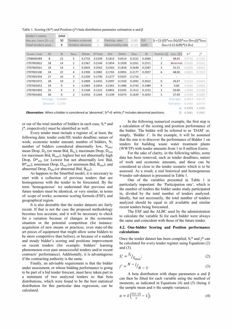
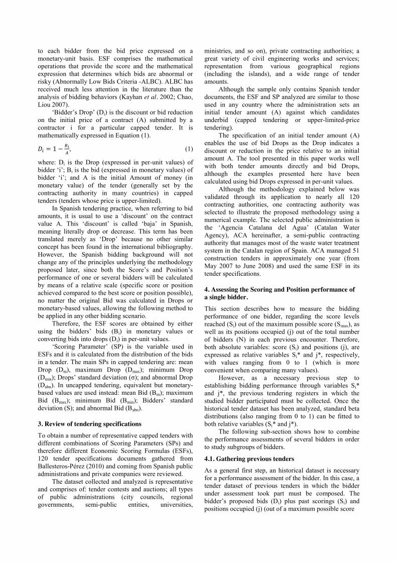
Table 1. Scoring (Si*) and Position (j*) beta distribution parameter estimation α and β

or out of the total number of bidders in each case, Si* and j*, respectively) must be identified as well.

Every tender must include a register of, at least, the following data: tender code/ID; tender deadline; nature of work; economic tender amount; number of bidders, N; number of bidders considered abnormally low, Nabn; mean Drop, Dm (or mean Bid, Bm,); maximum Drop, Dmax (or maximum Bid, Bmax); highest but not abnormally high Drop, D*max (or Lowest but not abnormally low Bid, B*min); minimum Drop, Dmin (or minimum Bid, Bmin); and abnormal Drop, Dabn (or abnormal Bid, Babn).

As happens to the Smartbid model, it is necessary to start with a collection of previous tenders that are homogeneous with the tender to be forecasted. By the term ‘homogeneous’ we understand that previous and future tenders must be identical, or very similar, in terms of: scope of works; economic scoring formula (ESF); and geographical region.

It is also desirable that the tender datasets are fairly recent. If that is not the case the proposed methodology becomes less accurate, and it will be necessary to check for a variation because of changes in the economic situation or the potential competition (for instance: acquisition of new means or practices, even state-of-the art pieces of equipment that might allow some bidders to be more competitive than before), or because of a sudden and steady bidder’s scoring and positions improvement on recent tenders (for example: bidders’ learning phenomenon over past unsuccessful tenders and/or recent contracts’ performance). Additionally, it is advantageous if the contracting authority is the same.

Finally, an advisable requirement is that the bidder under assessment, or whose bidding performance is going to be part of a bid tender forecast, must have taken part in a minimum of two analyzed tenders so that beta distributions, which were found to be the best statistical distribution for this particular data regression, can be calculated.

In the following numerical example, the first step is a calculation of the scoring and position performance of the bidder. The bidder will be referred to as ‘DAM’ or, simply, ‘Bidder 1’. In the example, it will be assumed that the aim is to discover the performance of Bidder 1 on tenders for building waste water treatment plants (WWTP) with tender amounts from 1 to 8 million Euros.

For the sake of clarity, in the following tables, some data has been removed, such as tender deadlines, nature of work and economic amounts, and these can be considered as close to the tender scenario which is to be assessed. As a result, a real historical and homogeneous 9-tender sub-dataset is presented in Table 1.

One of the variables presented in Table 1 is particularly important: the ‘Participation rate’, which is the number of tenders the bidder under study participated in, divided by the total number of tenders analyzed. Ideally, but not necessarily, the total number of tenders analyzed should be equal to all available and similar recent tenders being forecasted.

The ESF and the ALBC used by the administration to calculate the variable Si for each bidder were always the same and coincident with those of the future tender.

4.2. One-bidder Scoring and Position performance calculations

Once the tender dataset has been compiled, Si* and j* can be calculated for every tender register using Equations (2) and (3).

⁄ ; (2)

⁄ . (3)

A beta distribution with shape parameters α and β can then be fitted for each variable using the method of moments, as indicated in Equations (4) and (5) (being the sample mean and the sample variance).

( ( )

); (4)

Bidder's name: DAMMax pos. Score (Smax): 50 Tenders entered: 8 Particip. rate: 0.889 ESF: Si = [1-((D*max-Di)/(D*max-Dmin))]*Smax

Total tenders anal.: 9 Tenders abnorm.: 1 Abnormality rate: 0.125 ALBC: Dabn=1-(1-0,05)*(1-Dm)

Tender Code ID N Nabn Dmax D*max Dm Dmin Dabn Di Position (j) Scor. (Si) Si* j*CT08000389 8 22 5 0.2732 0.2109 0.1813 0.0514 0.2222 0.2066 7 48.65 0.9730 0.7143CT07002822 18 14 2 0.2367 0.2146 0.1854 0.1028 0.2261 0.2311 2 Abnormal 0.0000 0.9231CT07002921 19 14 1 0.2833 0.2562 0.2262 0.1818 0.2648 0.2287 3 31.51 0.6302 0.8462CT07002108 24 22 4 0.2390 0.2082 0.1765 0.0955 0.2177 0.2037 6 48.00 0.9601 0.7619CT07001934 27 16 3 0.2200 0.1700 0.1277 0.0325 0.1714 - - - - -CT07001972 28 10 2 0.2800 0.2435 0.2097 0.1550 0.2492 0.2022 6 26.67 0.5333 0.4444CT07002052 29 9 3 0.2985 0.2654 0.2361 0.1489 0.2743 0.1489 9 0.00 0.0000 0.0000CT07001903 33 9 2 0.1500 0.1222 0.0855 0.0105 0.1312 0.1222 3 50.00 1.0000 0.7500CT07001602 36 9 2 0.2450 0.1564 0.1199 0.0374 0.1639 0.1033 5 27.69 0.5538 0.5000

Average : 13.8889 Average : 0.5813 0.6175Desvest: 5.2784 Variance : 0.1442 0.0773

α: 0.3999 1.2690Observation: When a bidder is considered as 'abnormal', Si*=0 while j* includes abnormal positions. β: 0.2881 0.7861

( ) ( ( )

). (5)

With a beta distribution adjusted for variables Si* and j* both beta distribution curves and Y-axis values can be calculated (Table 2) and represented (Fig. 1).

Table 2. Scoring (Si*) and Position (j*) beta distribution representations

In Table 2, quadratic correlation coefficients (R2) have been calculated to establish if the beta regression curves fit the tender dataset well enough. According to other experiments, the R2 coefficients corresponding to j* values are usually above 0.90 and the Si*’s R2 values are almost always above 0.75. Nevertheless, unlike variable j*, variable Si* depends on the particular ESF that the tender dataset is using for producing the scores (if linear, Si*’s R2 values will be as high as j*’s R2 values).

Fig. 1. Single bidder Scoring (Si*) and Position (j*)

performance representation In addition to R2 calculations, Table 2 shows the

averages of the second and third columns (estimated Si* and j* values), although those values could also be obtained with the data of the last two columns.

These figures coincide with the bidder’s Scoring and Position performance (Bidder 1). Scoring performance is equal to 0.56 and Position performance is

equal to 0.61. Both performance indicators can range from 0 to 1, with 1 meaning a perfect performance, (i.e. a bidder that has always scored 100% and occupies the first positions). Such a perfect performance would be, of course, a rare exception.

Again, whereas Si* performance assessment is highly tied to the particular ESF and ALBC (because there are more or less lenient or tight-fisted ESFs and ALBCs) which produce higher or lower scores for all bidders according to their respective Di values); j* performance assessment is a good indicator of how well a particular bidder is performing. A coefficient of 0.50 means that, on average, that particular bidder is obtaining positions expected to be occupied by pure chance alone, and as long as its performance j* indicator is above 0.50, the bidder can be considered as bidding more wisely than the competition.

4.3. Complementing the Smartbid bid tender forecasting model

Once the single bidder’s Scoring performance beta distribution is known, the X-axis (see Table 2 or Fig. 1) reveals the equivalent different score levels represented by score curves in the Smartbid’s scoring probability graph (for instance, some common values in type-a SPGs are 1.0, 0.9, 0.8, …, 0.1, 0.0). In a tender forecast, the probability that the studied single bidder surpasses all the score levels in the SPG curve will then be known.

However, the problem becomes more complicated when studying likely future positions because to determine the probable positions that each competitor will occupy, it is necessary to delimit the number of potential bidders who will probably bid in the tender. Indeed, an extensive literature has focused on the study of the potential number of bidders (Banki et al. 2008; Carr 2005; Ngai et al. 2002); nonetheless, no variable has yet been proven to be reliable enough to forecast the number of bidders that will take part in a future tender.

Therefore, the present methodology considers the variable ‘number of bidders’ (N) as a random variable following a Normal distribution, which is a valid approach as proven when homogeneous tenders are analyzed (Ballesteros-Pérez et al. 2013a). Hence, variable N can be delimited through the average (Nm) and standard deviation (Nσ) of the N-values dataset from previous similar tenders.

The following paragraphs explain a series of successive calculations aimed at obtaining Figure 3, that is, the calculations of the probabilities of surpassing every possible position in a future tender. This graph implicitly includes calculations about the likely possible number of bidders N (from 1 to infinite, in theory), and the likelihood of occupying any possible position by the bidder under study, whose j* beta distribution is already known.

Extended calculations are shown in Table 3, although intermediate columns and rows have been removed because of the large number. In this particular case, the top number of bidders studied is N = Nm + 3Nσ =

X-axis Si* j* Si* j* Cum Si* Cum j*0.00 1.0000 1.0000 2 1 0.7500 0.87500.05 0.8550 0.9830 0 0 0.7500 0.87500.10 0.8066 0.9587 0 0 0.7500 0.87500.15 0.7699 0.9304 0 0 0.7500 0.87500.20 0.7388 0.8991 0 0 0.7500 0.87500.25 0.7109 0.8651 0 0 0.7500 0.87500.30 0.6849 0.8287 0 0 0.7500 0.87500.35 0.6602 0.7901 0 0 0.7500 0.87500.40 0.6362 0.7492 0 0 0.7500 0.87500.45 0.6126 0.7062 0 1 0.7500 0.75000.50 0.5891 0.6611 0 1 0.7500 0.62500.55 0.5653 0.6136 1 0 0.6250 0.62500.60 0.5409 0.5639 1 0 0.5000 0.62500.65 0.5155 0.5116 1 0 0.3750 0.62500.70 0.4887 0.4566 0 0 0.3750 0.62500.75 0.4598 0.3984 0 2 0.3750 0.37500.80 0.4276 0.3366 0 1 0.3750 0.25000.85 0.3906 0.2703 0 1 0.3750 0.12500.90 0.3449 0.1978 0 0 0.3750 0.12500.95 0.2805 0.1154 0 1 0.3750 0.00001.00 0.0000 0.0000 3 0 0.0000 0.0000

Average : 0.58 0.61 R^2 : 0.7973 0.9236R : 0.8929 0.9610

Estimated values Actual values

Table 3. Analysis of a single bidder’s Position (j*) performance for an upcoming tender

13.889 + 3·5.278 ≈ 30 bidders. Each column then displays the scenario with 1, 2, 3,… up to N = 30 bidders.

The first four rows (which constitute the first block at the top of Table 3) calculate the probability that each scenario with N bidders takes place. The average and standard deviation values of the Normal distribution of N bidders are known. However, a final correction is sometimes needed as shown in the fourth row (Weight N).

Initially, ‘Prob N’ and ‘Weight N’ rows are quite similar but they differ in the fact that ‘Weight N’-values have been calculated out of the area (probability) of the normal distribution that is effectively possible (values below N = 1 – 0.5 = 0.5 bidders and above N = 30 + 0.5 = 30.5 bidders are left out) and so ‘Weight N’-values are re-calculated by dividing ‘Prob N’-values by 0.9992 – 0.0056 = 0.9936. This correction might be especially important when N = Nm – 3Nσ < 0, although this is not the case here.

N Average (Nm): 13.889 Desvest (Nσ): 5.278 j* α: 1.269 β: 0.786

N 1 2 3 4 5 … 25 26 27 28 29 30Prob N-0.5 0.0056 0.0095 0.0155 0.0245 0.0376 … 0.9778 0.9861 0.9916 0.9950 0.9972 0.9984Prob N+0.5 0.0095 0.0155 0.0245 0.0376 0.0560 … 0.9861 0.9916 0.9950 0.9972 0.9984 0.9992

Prob N 0.0039 0.0060 0.0090 0.0131 0.0184 … 0.0083 0.0055 0.0035 0.0021 0.0013 0.0007Weight N 0.0039 0.0061 0.0091 0.0132 0.0185 … 0.0083 0.0055 0.0035 0.0022 0.0013 0.0007

j Pj = (N-j)/N N+3σ1 0.0000 0.5000 0.6667 0.7500 0.8000 … 0.9600 0.9615 0.9630 0.9643 0.9655 0.96672 0.0000 0.0000 0.3333 0.5000 0.6000 … 0.9200 0.9231 0.9259 0.9286 0.9310 0.93333 0.0000 0.0000 0.0000 0.2500 0.4000 … 0.8800 0.8846 0.8889 0.8929 0.8966 0.90004 0.0000 0.0000 0.0000 0.0000 0.2000 … 0.8400 0.8462 0.8519 0.8571 0.8621 0.86675 0.0000 0.0000 0.0000 0.0000 0.0000 … 0.8000 0.8077 0.8148 0.8214 0.8276 0.8333… … … … … … … … … … … … …25 0.0000 0.0000 0.0000 0.0000 0.0000 … 0.0000 0.0385 0.0741 0.1071 0.1379 0.166726 0.0000 0.0000 0.0000 0.0000 0.0000 … 0.0000 0.0000 0.0370 0.0714 0.1034 0.133327 0.0000 0.0000 0.0000 0.0000 0.0000 … 0.0000 0.0000 0.0000 0.0357 0.0690 0.100028 0.0000 0.0000 0.0000 0.0000 0.0000 … 0.0000 0.0000 0.0000 0.0000 0.0345 0.066729 0.0000 0.0000 0.0000 0.0000 0.0000 … 0.0000 0.0000 0.0000 0.0000 0.0000 0.033330 0.0000 0.0000 0.0000 0.0000 0.0000 … 0.0000 0.0000 0.0000 0.0000 0.0000 0.0000j Prob j* > Pj1 1.0000 0.6611 0.4936 0.3984 0.3366 … 0.0969 0.0940 0.0913 0.0887 0.0863 0.08412 1.0000 1.0000 0.8032 0.6611 0.5639 … 0.1664 0.1614 0.1567 0.1523 0.1482 0.14443 1.0000 1.0000 1.0000 0.8651 0.7492 … 0.2277 0.2209 0.2145 0.2086 0.2030 0.19784 1.0000 1.0000 1.0000 1.0000 0.8991 … 0.2840 0.2756 0.2677 0.2603 0.2534 0.24695 1.0000 1.0000 1.0000 1.0000 1.0000 … 0.3366 0.3267 0.3175 0.3088 0.3007 0.2930… … … … … … … … … … … … …25 1.0000 1.0000 1.0000 1.0000 1.0000 … 1.0000 0.9878 0.9719 0.9549 0.9376 0.920326 1.0000 1.0000 1.0000 1.0000 1.0000 … 1.0000 1.0000 0.9884 0.9731 0.9569 0.940227 1.0000 1.0000 1.0000 1.0000 1.0000 … 1.0000 1.0000 1.0000 0.9889 0.9743 0.958728 1.0000 1.0000 1.0000 1.0000 1.0000 … 1.0000 1.0000 1.0000 1.0000 0.9894 0.975429 1.0000 1.0000 1.0000 1.0000 1.0000 … 1.0000 1.0000 1.0000 1.0000 1.0000 0.989830 1.0000 1.0000 1.0000 1.0000 1.0000 … 1.0000 1.0000 1.0000 1.0000 1.0000 1.0000j (Prob j* > Pj)*Weight N1 0.0039 0.0040 0.0045 0.0053 0.0062 … 0.0008 0.0005 0.0003 0.0002 0.0001 0.00012 0.0039 0.0061 0.0073 0.0087 0.0104 … 0.0014 0.0009 0.0005 0.0003 0.0002 0.00013 0.0039 0.0061 0.0091 0.0114 0.0138 … 0.0019 0.0012 0.0008 0.0004 0.0003 0.00014 0.0039 0.0061 0.0091 0.0132 0.0166 … 0.0024 0.0015 0.0009 0.0006 0.0003 0.00025 0.0039 0.0061 0.0091 0.0132 0.0185 … 0.0028 0.0018 0.0011 0.0007 0.0004 0.0002… … … … … … … … … … … … …25 0.0039 0.0061 0.0091 0.0132 0.0185 … 0.0083 0.0054 0.0034 0.0021 0.0012 0.000726 0.0039 0.0061 0.0091 0.0132 0.0185 … 0.0083 0.0055 0.0035 0.0021 0.0012 0.000727 0.0039 0.0061 0.0091 0.0132 0.0185 … 0.0083 0.0055 0.0035 0.0021 0.0012 0.000728 0.0039 0.0061 0.0091 0.0132 0.0185 … 0.0083 0.0055 0.0035 0.0022 0.0013 0.000729 0.0039 0.0061 0.0091 0.0132 0.0185 … 0.0083 0.0055 0.0035 0.0022 0.0013 0.000730 0.0039 0.0061 0.0091 0.0132 0.0185 … 0.0083 0.0055 0.0035 0.0022 0.0013 0.0007j Cumulative by rows (Prob j* > Pj)*Weight N1 0.0039 0.0079 0.0124 0.0176 0.0239 … 0.1749 0.1754 0.1758 0.1759 0.1761 0.17612 0.0039 0.0099 0.0173 0.0260 0.0364 … 0.2940 0.2949 0.2954 0.2958 0.2959 0.29603 0.0039 0.0099 0.0190 0.0305 0.0443 … 0.3944 0.3956 0.3963 0.3968 0.3971 0.39724 0.0039 0.0099 0.0190 0.0323 0.0489 … 0.4821 0.4836 0.4846 0.4851 0.4855 0.48565 0.0039 0.0099 0.0190 0.0323 0.0507 … 0.5597 0.5615 0.5627 0.5633 0.5637 0.5639… … … … … … … … … … … … …25 0.0039 0.0099 0.0190 0.0323 0.0507 … 0.9868 0.9923 0.9957 0.9977 0.9989 0.999626 0.0039 0.0099 0.0190 0.0323 0.0507 … 0.9868 0.9923 0.9958 0.9979 0.9991 0.999827 0.0039 0.0099 0.0190 0.0323 0.0507 … 0.9868 0.9923 0.9958 0.9980 0.9992 0.999928 0.0039 0.0099 0.0190 0.0323 0.0507 … 0.9868 0.9923 0.9958 0.9980 0.9993 1.000029 0.0039 0.0099 0.0190 0.0323 0.0507 … 0.9868 0.9923 0.9958 0.9980 0.9993 1.000030 0.0039 0.0099 0.0190 0.0323 0.0507 … 0.9868 0.9923 0.9958 0.9980 0.9993 1.0000

Observation: Generally, it is enough to calculate from N=0 to N=Nm+3Nσ

The next four lower blocks of Table 3, separated by a gray heading with ‘j’ written on the top row, show sequential calculations of the probabilities of occupying each of the first 30 possible positions (usually the maximum positions studied should not go beyond N = Nm + 3Nσ, since further positional probabilities equal nearly 1 from that number upwards).

In every case, the mathematical expression used in each block is shown in the respective top gray row, on the left of the ‘j’ column.

Briefly, the first block calculates the probabilities of surpassing each possible position (by rows) according to the number of the bidders considered in each column. The second block introduces the actual previous bidder’s position performance (j*) by means of its Y-axis beta distribution values (found, for example, by finding their respective values from the upper block in Table 3 in Fig. 1’s X-axis).

Finally, there are another two blocks at the bottom of Table 3 that include the ‘Weight N’ row from the upper block (every value from the respective upper block is multiplied by the mentioned row in the last but one block); and, in the last block (at the bottom) of Table 3 where cumulative values from the block immediately above are shown.

If values from this lowest block are represented by rows (every curve represents a possible position: 1st, 2nd, 3rd,… , 25th without representing the last five positions), then Figure 2 is obtained.

Fig. 2. Single bidder’s position performance calculation accuracy

Figure 2 represents the stability (or accuracy) of position calculations in Figure 3. Whenever curves represented in Figure 2 reach horizontal gradients (in our case, this happens, of course, in N = 30 bidders; and, generally, in Nm + 3Nσ bidders) the calculations can be considered as good enough.

Figure 3 is easily obtained by representing in a different graph the values from the Figure 2 X-axis when N = 30 bidders, that is, values from j = 1 to 25 when N = 30 (lowest right-hand corner of Table 3).

Figure 3 shows the probability of occupying a particular (or higher) position, despite the fact that the number of bidders is not yet known. This is the kind of graph that greatly complements the information provided in the Smartbid position probability graphs, whose data was completely impersonal until now.

Fig. 3. Position performance for a single bidder

5. Assessing the Scoring and Position performance of a group of bidders

A numerical case has been developed, firstly to assess Scoring and Position performance for similar previous tenders; and, secondly, to adapt those results to provide a useful complement to the Smartbid BTFM.

Calculations have been applied to a single bidder (Bidder 1). In this section, calculations for a group of bidders are explained. Indeed, this is usually a necessary piece of information for bidding, since a company that is trying to forecast an auction often knows who are its strongest competitors and may wish to focus on those participants.

5.1. Scoring group performance

To analyze the performance of a group of known bidders, it is always necessary to have studied each independently beforehand (i.e., calculations shown in subsection 4.2. are a pre-requisite for each bidder). However, there is an advantage, with respect to the gathering of previous tendering registers: once the tender dataset is relatively complete, there is no need to continue gathering a different tender dataset for each bidder, that is, tendering data is shared among bidders, and so it will only be necessary to calculate the Scorings (Si*) and Positions (j*) for each bidder.

Once Si* and j* values are known, a beta distribution is fitted for the two parameters as shown in Table 1 in the lower right-hand corner. As a result, for every bidder that is analyzed as a part of the group, two beta distributions (represented by shape parameters α and β) are obtained.

Now that every scoring performance of every bidder to be jointly studied is known, there is one point that must be borne in mind: when a single bidder’s performance was previously studied, it was not taken into account that the bidder might not be interested in participating in the forecasted tender. This concept is quantified by means of the ‘Participation rate’ coefficient, that is, the percentage of similar tenders on average that every bidder enters.

When studying a single bidder’s behavior it is not always advisable to take into account the coefficient of participation since a company usually has enough

information to know whether a particular competitor is interested in winning a contract. However, when studying bidders as a group it is advisable to include the ‘participation rate’ coefficient since some of the group may not finally enter a tender and the forecasted probabilities may then become too conservative.

With all this information, Table 4 is obtained by analyzing the group Scoring performance of three bidders (n = 3) (the first bidder coincides with the bidder that was previously calculated, and the other two bidders are given as new examples). Each column represents a single bidder with its past Scoring performance – but without having multiplied the beta distribution values by the respective ‘Participation rate’ coefficients.

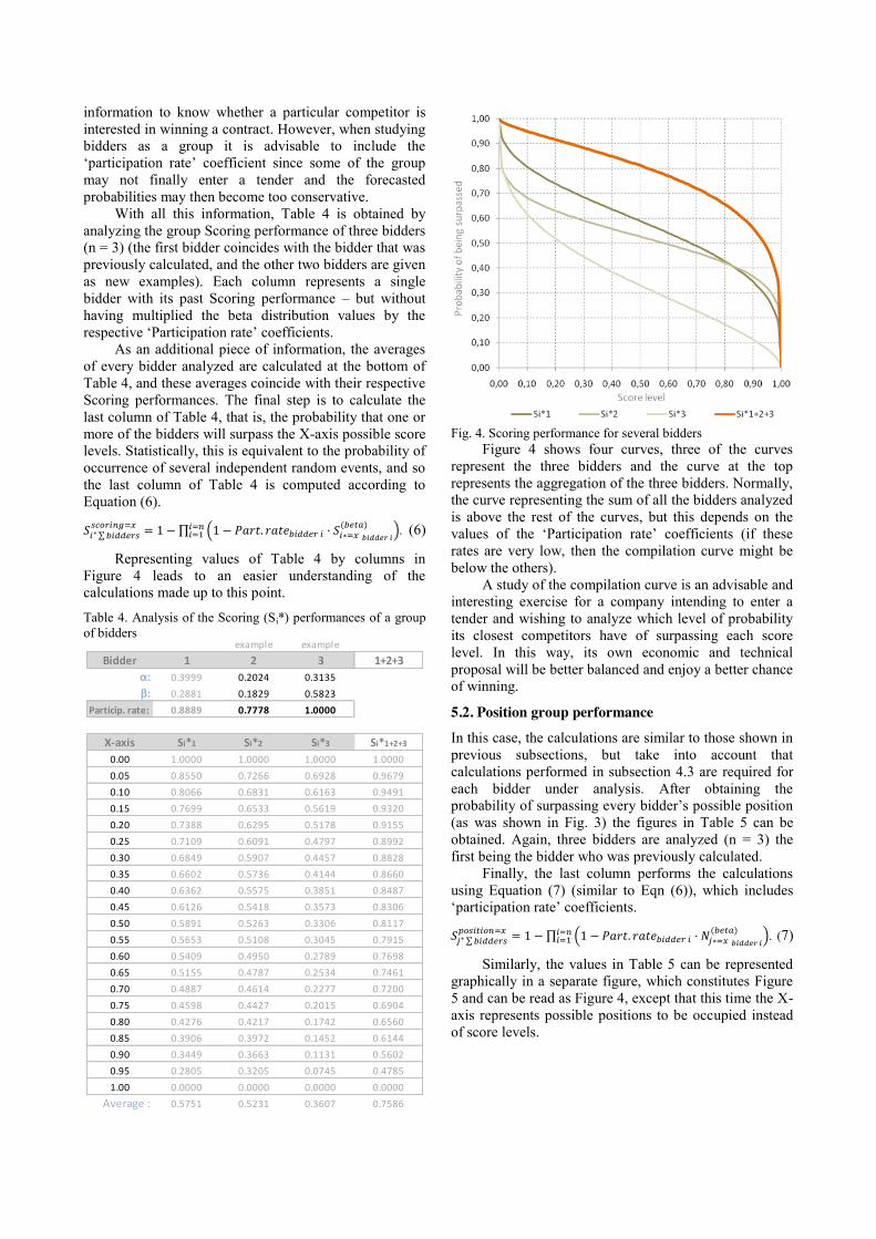
As an additional piece of information, the averages of every bidder analyzed are calculated at the bottom of Table 4, and these averages coincide with their respective Scoring performances. The final step is to calculate the last column of Table 4, that is, the probability that one or more of the bidders will surpass the X-axis possible score levels. Statistically, this is equivalent to the probability of occurrence of several independent random events, and so the last column of Table 4 is computed according to Equation (6).

∑ ∏ (

( ) ) . (6)

Representing values of Table 4 by columns in Figure 4 leads to an easier understanding of the calculations made up to this point.

Table 4. Analysis of the Scoring (Si*) performances of a group of bidders

Fig. 4. Scoring performance for several bidders

Figure 4 shows four curves, three of the curves represent the three bidders and the curve at the top represents the aggregation of the three bidders. Normally, the curve representing the sum of all the bidders analyzed is above the rest of the curves, but this depends on the values of the ‘Participation rate’ coefficients (if these rates are very low, then the compilation curve might be below the others).

A study of the compilation curve is an advisable and interesting exercise for a company intending to enter a tender and wishing to analyze which level of probability its closest competitors have of surpassing each score level. In this way, its own economic and technical proposal will be better balanced and enjoy a better chance of winning.

5.2. Position group performance

In this case, the calculations are similar to those shown in previous subsections, but take into account that calculations performed in subsection 4.3 are required for each bidder under analysis. After obtaining the probability of surpassing every bidder’s possible position (as was shown in Fig. 3) the figures in Table 5 can be obtained. Again, three bidders are analyzed (n = 3) the first being the bidder who was previously calculated.

Finally, the last column performs the calculations using Equation (7) (similar to Eqn (6)), which includes ‘participation rate’ coefficients.

∑ ∏ (

( ) ) . (7)

Similarly, the values in Table 5 can be represented graphically in a separate figure, which constitutes Figure 5 and can be read as Figure 4, except that this time the X-axis represents possible positions to be occupied instead of score levels.

example exampleBidder 1 2 3 1+2+3

α: 0.3999 0.2024 0.3135β: 0.2881 0.1829 0.5823

Particip. rate: 0.8889 0.7778 1.0000

X-axis Si*1 Si*2 Si*3 Si*1+2+3

0.00 1.0000 1.0000 1.0000 1.00000.05 0.8550 0.7266 0.6928 0.96790.10 0.8066 0.6831 0.6163 0.94910.15 0.7699 0.6533 0.5619 0.93200.20 0.7388 0.6295 0.5178 0.91550.25 0.7109 0.6091 0.4797 0.89920.30 0.6849 0.5907 0.4457 0.88280.35 0.6602 0.5736 0.4144 0.86600.40 0.6362 0.5575 0.3851 0.84870.45 0.6126 0.5418 0.3573 0.83060.50 0.5891 0.5263 0.3306 0.81170.55 0.5653 0.5108 0.3045 0.79150.60 0.5409 0.4950 0.2789 0.76980.65 0.5155 0.4787 0.2534 0.74610.70 0.4887 0.4614 0.2277 0.72000.75 0.4598 0.4427 0.2015 0.69040.80 0.4276 0.4217 0.1742 0.65600.85 0.3906 0.3972 0.1452 0.61440.90 0.3449 0.3663 0.1131 0.56020.95 0.2805 0.3205 0.0745 0.47851.00 0.0000 0.0000 0.0000 0.0000

Average : 0.5751 0.5231 0.3607 0.7586

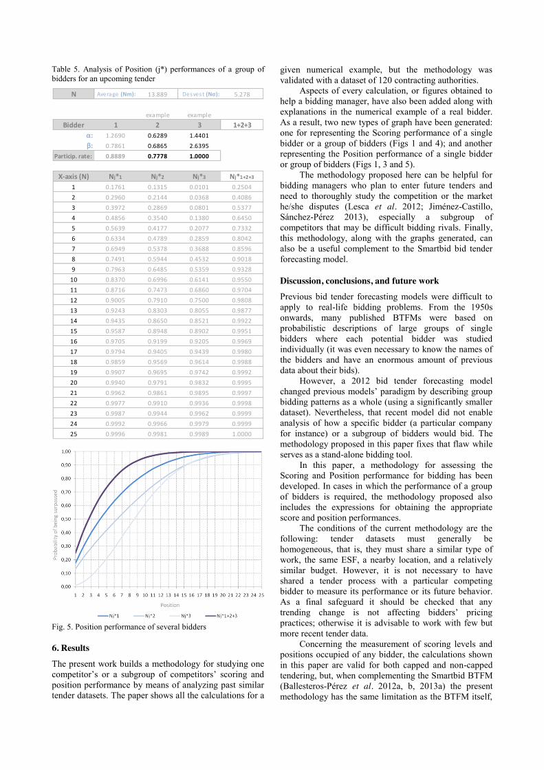
Table 5. Analysis of Position (j*) performances of a group of bidders for an upcoming tender

Fig. 5. Position performance of several bidders

6. Results

The present work builds a methodology for studying one competitor’s or a subgroup of competitors’ scoring and position performance by means of analyzing past similar tender datasets. The paper shows all the calculations for a

given numerical example, but the methodology was validated with a dataset of 120 contracting authorities.

Aspects of every calculation, or figures obtained to help a bidding manager, have also been added along with explanations in the numerical example of a real bidder. As a result, two new types of graph have been generated: one for representing the Scoring performance of a single bidder or a group of bidders (Figs 1 and 4); and another representing the Position performance of a single bidder or group of bidders (Figs 1, 3 and 5).

The methodology proposed here can be helpful for bidding managers who plan to enter future tenders and need to thoroughly study the competition or the market he/she disputes (Lesca et al. 2012; Jiménez-Castillo, Sánchez-Pérez 2013), especially a subgroup of competitors that may be difficult bidding rivals. Finally, this methodology, along with the graphs generated, can also be a useful complement to the Smartbid bid tender forecasting model.

Discussion, conclusions, and future work

Previous bid tender forecasting models were difficult to apply to real-life bidding problems. From the 1950s onwards, many published BTFMs were based on probabilistic descriptions of large groups of single bidders where each potential bidder was studied individually (it was even necessary to know the names of the bidders and have an enormous amount of previous data about their bids).

However, a 2012 bid tender forecasting model changed previous models’ paradigm by describing group bidding patterns as a whole (using a significantly smaller dataset). Nevertheless, that recent model did not enable analysis of how a specific bidder (a particular company for instance) or a subgroup of bidders would bid. The methodology proposed in this paper fixes that flaw while serves as a stand-alone bidding tool.

In this paper, a methodology for assessing the Scoring and Position performance for bidding has been developed. In cases in which the performance of a group of bidders is required, the methodology proposed also includes the expressions for obtaining the appropriate score and position performances.

The conditions of the current methodology are the following: tender datasets must generally be homogeneous, that is, they must share a similar type of work, the same ESF, a nearby location, and a relatively similar budget. However, it is not necessary to have shared a tender process with a particular competing bidder to measure its performance or its future behavior. As a final safeguard it should be checked that any trending change is not affecting bidders’ pricing practices; otherwise it is advisable to work with few but more recent tender data.

Concerning the measurement of scoring levels and positions occupied of any bidder, the calculations shown in this paper are valid for both capped and non-capped tendering, but, when complementing the Smartbid BTFM (Ballesteros-Pérez et al. 2012a, b, 2013a) the present methodology has the same limitation as the BTFM itself,

N Average (Nm): 13.889 Desvest (Nσ): 5.278

example exampleBidder 1 2 3 1+2+3

α: 1.2690 0.6289 1.4401β: 0.7861 0.6865 2.6395

Particip. rate: 0.8889 0.7778 1.0000

X-axis (N) Nj*1 Nj*2 Nj*3 Nj*1+2+3

1 0.1761 0.1315 0.0101 0.25042 0.2960 0.2144 0.0368 0.40863 0.3972 0.2869 0.0801 0.53774 0.4856 0.3540 0.1380 0.64505 0.5639 0.4177 0.2077 0.73326 0.6334 0.4789 0.2859 0.80427 0.6949 0.5378 0.3688 0.85968 0.7491 0.5944 0.4532 0.90189 0.7963 0.6485 0.5359 0.9328

10 0.8370 0.6996 0.6141 0.955011 0.8716 0.7473 0.6860 0.970412 0.9005 0.7910 0.7500 0.980813 0.9243 0.8303 0.8055 0.987714 0.9435 0.8650 0.8521 0.992215 0.9587 0.8948 0.8902 0.995116 0.9705 0.9199 0.9205 0.996917 0.9794 0.9405 0.9439 0.998018 0.9859 0.9569 0.9614 0.998819 0.9907 0.9695 0.9742 0.999220 0.9940 0.9791 0.9832 0.999521 0.9962 0.9861 0.9895 0.999722 0.9977 0.9910 0.9936 0.999823 0.9987 0.9944 0.9962 0.999924 0.9992 0.9966 0.9979 0.999925 0.9996 0.9981 0.9989 1.0000

since the Smartbid model has only been applied to capped tendering.

Therefore, further adaptations of the Smartbid model are still necessary. Some of these changes will involve studying new mathematical relationships between Scoring Parameters and current model uses – and transforming them as a function of monetary values instead of drop values (which is indispensable in non-capped tendering). However, the methodology proposed here will remain being exactly the same.

Acknowledgments

This research study has been funded in Chile by CONICYT under the Program Initiation into research 2013 (project number 11130666). The language revision of this paper was funded by the Universitat Politècnica de València.

References Ballesteros-Pérez, P. 2010. Propuesta de un nuevo modelo para

la predicción de bajas en licitaciones de Construcción: Doctoral Thesis [online], [21 January 2010 cited]. Universitat Politècnica de València. Departamento de Proyectos de Ingeniería – Departament de Projectes d’Enginyeria, Spain. Available from Internet: http://hdl.handle.net/10251/7025

Ballesteros-Pérez, P.; González-Cruz, M. C.; Pastor-Ferrando, J. P.; Fernández-Diego, M. 2012a. The iso-Score Curve Graph. A new tool for competitive bidding, Automation in Construction 22(1): 481–490. http://dx.doi.org/10.1016/j.autcon.2011.11.007

Ballesteros-Pérez, P.; González-Cruz, M. C.; Cañavate-Grimal, A. 2012b. Mathematical relationships between scoring parameters in capped tendering, International Journal of Project Management 30(7): 850–862. http://dx.doi.org/10.1016/j.ijproman.2012.01.008

Ballesteros-Pérez, P.; González-Cruz, M. C.; Cañavate-Grimal, A. 2013a. On competitive bidding: scoring and position probability graphs, International Journal of Project Management 31(3): 434–448. http://dx.doi.org/10.1016/j.ijproman.2012.09.012

Ballesteros-Pérez, P.; González-Cruz, M. C.; Cañavate-Grimal, A.; Pellicer, E. 2013b. Detecting abnormal and collusive bids in capped tendering, Automation in Construction 31(3): 215–229. http://dx.doi.org/10.1016/j.autcon.2012.11.036

Banki, M. T.; Esmaeeli, B.; Ravanshadnia, M. 2008. The assessment of bidding strategy of Iranian construction firms, International Journal of Management Science and Engineering Management 4(2): 153–160.

Carr, P. G. 2005. Investigation of Bid price competition measured through pre-bid project estimates, actual bid prices and Number of bidders, Journal of Construction Engineering and Management 131(11): 1165–1172. http://dx.doi.org/10.1016/j.autcon.2012.11.036

Carr, R. I. 1982. General bidding model, Journal of the Construction Division 108(CO4): 639–650.

Chao, L.; Liou, C. 2007. Risk-minimizing approach to bid-cutting limit determination, Construction Management and Economics 25(8): 835–843. http://dx.doi.org/10.1080/01446190701393018

Deltas, G.; Engelbrecht-Wiggans, R. 2005. Naive bidding, Management Science 51(3): 328–338. http://dx.doi.org/10.1287/mnsc.1040.0330

Dikmen, I.; Talat, M.; Kemal, A. 2007. A case-based decision support tool for bid mark-up estimation of international construction projects, Automation in Construction 17(1): 30–44. http://dx.doi.org/10.1016/j.autcon.2007.02.009

Drew, D.; Skitmore, R. M. 1997. The effect of contract type and size on competitiveness in bidding, Construction Management and Economics 15: 469–489. http://dx.doi.org/10.1080/014461997372836

Engelbrecht-Wiggans, R. 1980. State of the art – auctions and bidding models: a survey, Management Science 26(2): 119–142. http://dx.doi.org/10.1287/mnsc.26.2.119

Engelbrecht-Wiggans, R. 1989.The effect of regret on optimal bidding in auctions. Management Science 35(6): 685–692. http://dx.doi.org/10.1287/mnsc.35.6.685

Fayek, A. 1998. Competitive bidding strategy model and software system for bid preparation, Journal of Construction Engineering and Management 124(1): 1–10. http://dx.doi.org/10.1061/(ASCE)0733-9364(1998)124:1(1)

Friedman, L. 1956. A competitive bidding strategy, Operations Research 1(4): 104–12. http://dx.doi.org/10.1287/opre.4.1.104

Gates, M. 1967. Bidding strategies and probabilities, Journal of the Construction Division 93(CO1): 75–107.

Harstad, R. M.; SašaPekec, A. 2008. Relevance to practice and auction theory: a memorial essay for Michael Rothkopf, Interfaces 38(5): 367–380. http://dx.doi.org/10.1287/inte.1080.0396

Jiménez-Castillo, D.; Sánchez-Pérez, M. 2013. Nurturing employee market knowledge absorptive capacity through unified internal communication and integrated information technology, Information & Management 50(2–3): 76–86.

Kayhan, V. O.; McCart, J. A.; Bhattacherjee, A. 2002. Cross-bidding in simultaneous online auctions: antecedents and consequences, Information & Management 47(7–8): 325–332.

Lesca, N.; Caron-Fasan, M. L.; Falcy, S. 2012. How managers interpret scanning information, Information & Management 49(2): 126–134. http://dx.doi.org/10.1016/j.im.2012.01.004

Lo, W.; Lin, C. L.; Yan, M. R. 2007. Contractor’s opportunistic bidding behavior and equilibrium price level in the construction market, Journal of Construction Engineering and Management 133(6): 409–416. http://dx.doi.org/10.1061/(ASCE)0733-9364(2007)133:6(409)

McCaffer, R.; Pettitt, A. N. 1976. Distribution of bids for buildings and road contracts, Operational Research Quarterly 27(4): 835–843. http://dx.doi.org/10.2307/3009167

Mitchell, M. S. 1977. The probability of being the lowest bidder, Journal of the Royal Statistical Society: Series C (Applied Statistics) 26(2): 191–194.

Naoum, S. G. 1994. Critical analysis of time and cost of management and traditional contracts, Journal of Construction Engineering and Management 120(4): 687–705. http://dx.doi.org/10.1061/(ASCE)0733-9364(1994)120:4(687)

Näykki, P. 1976. On optimal bidding strategies, Management Science 23(2): 198–203. http://dx.doi.org/10.1287/mnsc.23.2.198

Ngai, S. C.; Derek, S.; Drew, H. P.; Skitmore, R. M. 2002. A theoretical framework for determining the minimum

number of bidders in construction bidding competitions, Construction Management and Economics 20(6): 473–482. http://dx.doi.org/10.1080/01446190210151041

OECD (Organisation for Economic Co-operation and Development) 2007. Bribery in procurement, methods, actors and counter-measures, Paris.

OECD (Organisation for Economic Co-operation and Development) 2009. Guidelines for fighting bid rigging in public procurement, Paris.

Oo, B. L.; Drew, D. S.; Runeson, G. 2010. Competitor analysis in construction bidding, Construction Management and Economics 28(12): 1321–1329. http://dx.doi.org/10.1080/01446193.2010.520721

Oo, B. L.; Drew, D. S.; Lo, H. P. 2008a. A comparison of contractors’ decision to bid behaviour according to different market environments, International Journal of Project Management 26(4): 439–447. http://dx.doi.org/10.1016/j.ijproman.2007.06.001

Oo, B. L.; Drew, D. S.; Lo, H. P. 2008b. Heterogeneous approach to modeling contractors’ decision-to-bid strategies, Journal of Construction Engineering and Management 134(10): 766–776. http://dx.doi.org/10.1061/(ASCE)0733-9364(2008)134:10(766)

Pim, J. C. 1974. Competitive tendering and bidding strategy, National Builder 55(11): 541–545.

Ravanshadnia, M.; Rajaie, H.; Abbasian, H. R. 2010. Hybrid fuzzy MADM project-selection model for diversified construction companies, Canadian Journal of Civil Engineering 37(8): 1082–1093. http://dx.doi.org/10.1139/L10-048

Rothkopf, M. H.; Harstad, R. M. 1994. Modeling competitive bidding: a critical essay, Management Science 40(3): 364–384. http://dx.doi.org/10.1287/mnsc.40.3.364

Rothkopf, M. H. 1969. A model of rational competitive bidding, Management Science 15(7): 362–373. http://dx.doi.org/10.1287/mnsc.15.7.362

Runeson, K. G.; Skitmore, R. M. 1999. Tendering theory revisited, Construction Management and Economics 17(3): 285–296. http://dx.doi.org/10.1080/014461999371493

Skitmore, R. M.; Runeson, G. 2006. Bidding models: testing the stationary assumption, Construction Management and

Economics 24(8): 791–803. http://dx.doi.org/10.1080/01446190600680432

Skitmore, R. M. 1991. The contract bidder homogeneity assumption: an empirical analysis, Construction Management and Economics 9(5): 403–429. http://dx.doi.org/10.1080/01446199100000032

Skitmore, R. M. 2002. The probability of tendering the lowest bid in sealed auctions: an empirical analysis of construction data, Journal of the Operational Research Society 53(1): 47–56. http://dx.doi.org/10.1057/palgrave/jors/2601236

Skitmore, R. M. 2004. Predicting the probability of winning sealed bid auctions: the effects of outliers on bidding models, Construction Management and Economics 22(1): 101–109. http://dx.doi.org/10.1080/0144619042000186103

Skitmore, R. M. 2008. First and second price independent values sealed bid procurement auctions: some scalar equilibrium results, Construction Management and Economics 26(8): 787–803. http://dx.doi.org/10.1080/01446190802175678

Skitmore, R. M.; Drew, D. S.; Ngai, S. 2001. Bid-spread, Journal of Construction Engineering and Management 127(2): 149–153. http://dx.doi.org/10.1061/(ASCE)0733-9364(2001)127:2(149)

Skitmore, R. M.; Pettitt, A. N.; McVinish, R. 2007. Gates’ bidding model, Journal of Construction Engineering and Management 133(11): 855–863. http://dx.doi.org/10.1061/(ASCE)0733-9364(2007)133:11(855)

Stark, R. M.; Rothkopf, M. H. 1979. Competitive bidding: a comprehensive bibliography, Journal of the Operational Research 27(2): 364–390.

Vergara, A. J. 1977. Probabilistic estimating and applications of portfolio theory in construction: PhD Thesis. Department of Civil Engineering, University of Illinois at Urbana-Champaign, Urbana, IL.

Watt, D. J.; Kayis, B.; Willey, K. 2009. Identifying key factors in the evaluation of tenders for projects and services, International Journal of Project Management 27(3): 250–260. http://dx.doi.org/10.1016/j.ijproman.2008.03.002

Ye, K.; Jiang, W.; Shen, L. 2008. Project competition intensity (PCI) in the construction market: a case study in China, Construction Management and Economics 26(5): 463–470. http://dx.doi.org/10.1080/01446190802036136

Pablo BALLESTEROS-PÉREZ holds a PhD in Engineering Projects and Innovation and a Msc in Project Management, both at Universitat Politècnica de València, Spain. After graduating in Civil Engineering and Geological Engineering he has been working as Construction Tendering Manager for ten years in an international private company devoted to DBO of Waste Water Treatment Plants. He is an IPMA certified Project Manager (level C) and currently is Assistant Professor at the Construction Engineering Project Management at Universidad de Talca, Chile. His areas of interest are project management in general and quantitative bidding in particular. M. Carmen GONZÁLEZ-CRUZ holds a PhD in Industrial Engineering from the Universitat Politècnica de València, Spain. After working in several engineering companies, she works as an Associate Professor/Senior Lecturer in Project Engineering (undergraduate), and Project Management (graduate). She is currently the Head of the Department of Project Engineering and she is also in charge of the MSc in Project Management at Universitat Politècnica de València, Spain. She has conducted research on the use of design methodology in industry, creativity and innovation management, and currently, she works in analysis and development of forecasting and bid models on procurement. Marta FERNÁNDEZ-DIEGO holds a European PhD in Electronic and Telecommunications Engineering from Lille University of Science and Technology, France. After some research and development contracts in universities and multinational companies from France, Great Britain and Spain, she is currently a lecturer in the Department of Business Administration at Universitat Politècnica de València, Spain, where she teaches project risk management, among other subjects. Eugenio PELLICER received his MSc degree from Stanford University, USA, and his PhD degree from the Universitat Politècnica de València, Spain, where he works as an Associate Professor/Senior Lecturer in Project Management, being also in charge of the MSc in Planning and Management in Civil Engineering. He is currently a Visiting Professor at the University of Colorado at Boulder. He is involved in several international projects with other European and Latin-American universities. His research interests include innovation in the construction process and project delivery strategies in construction.

View publication statsView publication stats