Estimating Hydrodynamic Coefficients with Various Trim and

Journal of the Korean Society of Marine Environment & Safety Research Paper

Vol. 23, No. 7, pp. 933-940, December 31, 2017, ISSN 1229-3431(Print) / ISSN 2287-3341(Online) https://doi.org/10.7837/kosomes.2017.23.7.933

11. Introduction

With the development of information technology, ship

modelling technology is required to satisfy all ships and

navigational conditions. Various loading conditions of a vessel,

which also affects draught and trim conditions, is one of the

major constraints to determine manoeuvrability. For example,

Corresponding Author : [email protected]

fully loaded vessel requires greater turning circle than the one in

ballast condition and trimmed by stern condition has larger circle

than even keel condition (Kijima et al., 1990; Oltmann, 2003).

The most reliable way to examine ship’s manoeuvrability

considering with loading conditions is to conduct the model tests,

such as planar motion mechanism, rotating arm and towing tank,

or real ship trial for every loading condition. However, it

requires expensive time and cost for the experiment (Yoon et al.,

2016). IMO standards for ship manoeuvrability consider that and

Estimating Hydrodynamic Coefficients with Various Trim and Draught

Conditions

Daewon Kim* Knud Benedict** Mathias Paschen***

* Graduate school, Faculty of Mechanical Engineering and Marine Technology, University of Rostock, Albert-Einstein-Strasse 2, 18059 Rostock, Germany

** ISSIMS Institute, Hochschule Wismar, University of Applied Sciences, Technology, Business and Design, Richard-Wagner-Str. 31,

18119 Rostock, Germany

*** Faculty of Mechanical Engineering and Marine Technology, University of Rostock, Albert-Einstein-Strasse 2, 18059 Rostock, Germany

흘수 트림 변화 고려한 체력 미계수 정에 한 연

김대원* Knud Benedict** Mathias Paschen***

로스 크 학 학원 비스마 학 * , ** ISSIMS Institute, 로스 크 학 조 해양공학***

Abstract : Draught and trim conditions are highly related to the loading condition of a vessel and are important factors in predicting ship

manoeuverability. This paper estimates hydrodynamic coefficients from sea trial measurements with three different trim and draught conditions. A

mathematical optimization method for system identification was applied to estimate the forces and moment acting on the hull. Also, fast time

simulation software based on the Rheinmetall Defense model was applied to the whole estimation process, and a 4,500 Twenty-foot Equivalent Unit

(TEU) class container carrier was chosen to collect sets of measurement data. Simulation results using both optimized coefficients and

newly-calculated coefficients for validation agreed well with benchmark data. The results show mathematical optimization using sea measurement

data enables hydrodynamic coefficients to be estimated more simply.

Key Words : Ship manoeuvrability, System identification method, Hydrodynamic coefficients, Sea trial, Mathematical optimization

요 약 : 다양한 흘수 트림 조건 조종 능 정 한 한 하나 다 본 논문에 는 종 흘수 트림 .

조건에 해상 시운전 료 탕 로 하여 체 체력 미계수 정하 다 시스 식별 하나 수학적 . (system identification)

적화 사 운동 적 한 시뮬레 프트웨어 하여 시운(mathematical optimization method) Rheinmetall Defense fast time

전 항적 련 시뮬레 료 하여 체 체력 미계수 정하 다 적화 계수 적 한 시뮬레 결과는 기존 .

계수 정식 사 한 시뮬레 결과 비하여 해상 시운전 계측 결과 사함 보여주었 가로 진행 차 검 결과에 도 2

상 적 로 높 사함 확 하 다.

핵심용어 : 조종 능 시스 식별 체력 미계수 해상 시운전 수학적 적화 , , , ,

Daewon Kim Knud Benedict Mathias Paschen

require only for full load condition of the vessel, also it is hard

to get such data for all ships (Im et al., 2005).

International Towing Tank Conference (ITTC) summarized

multiple ways to estimate and to approximate hydrodynamic

coefficients for the ship manoeuvrability (ITTC, 2008).

Computational methods, such as Computational Fluid Dynamics

(CFD) method and system identification method are also an

alternative for the model test.

As a preliminary study for estimation of all loading

conditions, this paper estimates hydrodynamic coefficients with

sets of sea measurement data by mathematical optimization,

which is a kind of the system identification method. Based on

the authors’ previous researches, coefficients are optimized

through the Interior point algorithm and these are validated

through comparison with the measurement data from sea trial

(Kim et al., 2016; Kim et al., 2017).

2. Modelling ship and benchmark data

2.1 Mathematical model

This study applied the 3-Degrees-of-Freedom (DOF) ship-fixed

and earth-fixed coordinate systems. Fig. 1 illustrates basic

information of the coordinate systems. The Ship-fixed-coordinate

plane and the Earth-fixed-coordinate plane are

placed on the undisturbed free surface, with the axis pointing

in the direction of the original heading of the ship. The axis

and the axis point downwards vertically. The angle between

the directions of the axis and the axis is defined as the

heading angle, .

Fig. 1. Coordinate system of the vessel.

where,

: Center of gravity

: Heading

: Drift angle

: Rudder angle

: Ship’s speed

: yaw rate

A fast time simulation tool SIMOPT with a mathematical

model of a Ship Handling Simulator (SHS) systems ANS5000,

developed by Rheinmetall Defence Electronics is used for the

optimization process (ISSIMS GmbH, 2013). In the mathematical

model of the tool, a ship is considered as a massive and rigid

body and forces and moment are acting on the hull can be

described as equation (1), according to the Newtonian law of

motion (Rheinmetall Defence Electronic, 2008).

(1)

The model applies modular structure to each force and

moment as equation (2): hull, propeller, rudder and other external

forces and moments.

(2)

The hydrodynamic forces and moment acting on the hull are

composed as Equation (3) and the empirical regression formulas

of Norrbin and Clarke are applied to calculate the initial

hydrodynamic coefficients (Norrbin, 1971; Clarke et al., 1983).

Each hydrodynamic coefficients can be expressed the function of

ship’s main dimension as equation (4): length, beam, draught and

displacement of the ship. and are non-linear

components of sway force and yaw moment. These non-linear

components vary according to the position of the ship’s turning

point.

′

′ ′

′ ′

′

′

′ ′

′ ′

′

′

′ ′

′ ′

′

(3)

′

′ ′

′ ′

′ ∆ (4)

Estimating Hydrodynamic Coefficients with Various Trim and Draught Conditions

2.2 Benchmark data

A set of benchmark data is acquired from sea trials using a

4,500 TEU class container carrier. Details of the vessel are given

in Table 1.

Five zig-zag manoeuvres under three different loading

conditions were carried out for this study. Table 2 shows

detailed conditions for each manoeuvre.

Type of ship 4,500 TEU Class container carrier

Length overall 294.12 m

Length between perpendicular 283.20 m

Beam 32.20 m

Design draught 12.00 m

Scantling draught 13.00 m

Maximum speed 23.70 knots

Type of main engine MAN B&W 9K90MC-C

Power 55,890 HP (41,040 KW)

Table 1. Particulars of benchmark vessel

Data1 Data2 Data3 Data4 Data5

Manoeuvre ZZ10P ZZ10S ZZ10S ZZ10P ZZ20S

Latitude 32.8N 32.0N 10.7N 9.7N 9.7N

Longitude 119.9W 117.3W 67.2W 79.6W 79.6W

Heading(°) 110 110 260 250 250

RPM ( ) 843 620 676 422 422

Draught fore(m) 12.75 12.75 10.00 9.10 9.10

Draught mid(m) 12.55 12.55 10.00 - -

Draught aft(m) 13.00 13.00 10.00 9.60 9.60

Wind direction(°) 270 310 20 50 50

Wind speed(kts) 12 15 5 15 15

Current direction(°) 160.47 251.56 169.50 23.62 23.62

Current speed(kts) 1.37 0.88 0.28 1.25 1.55

Water depth(m) >1000 >1000 >1000 >1000 >1000

Table 2. Maneouvre conditions of each trial

3. Estimation of hydrodynamic coefficients

3.1 Mathematical optimization

The mathematical optimization is a process to minimize or

maximize an objective function value, subject to several

constraints on its variables (Nocedal and Wright, 2006). This can

be written as equation (5):

∈ min , subject to (5)

∈

≥ ∈

where,

- is the variable, which has to be optimized ;

- is the objective function, a function which returns scalar

and it contains the information of minimization or

maximization;

- are constraints, which sets equations and inequality

condition those the variable must satisfy during the whole

optimization process. The constraints are optional in the

optimization process.

Fig. 2 shows the whole process of the mathematical optimization

to get tuned hydrodynamic coefficients. The optimization process

in the process is carried out by the Optimization Toolbox of

MATLAB.

Fig. 2. Concept flow of the coefficient optimization.

The solver requires an objective function, which calculates a

minimum or a maximum value of the function. Constraints also

can increase the reliability of the optimization results. In this

study, lower and upper bound are applied as constraints of the

optimization process.

3.2 Sensitivity analysis

A lot of target variables for the optimization process requires

expensive resources for the calculation. Therefore this study

conducted a sensitivity analysis of each coefficient with the

corresponding manoeuvre, prior to the main optimization process.


The procedures of the sensitivity analysis are as follows:

1) Split coefficients into two groups according to the

manoeuvre tests: the constant speed with straight motion

and zigzag manoeuvre.

2) Conduct manoeuvring simulations with regard to certain

changes of a specific coefficient.

3) Get derivative of each data set and conduct min-max

normalization for all hydrodynamic coefficients to figure

out their own sensitivity in the group.

Fig. 3 and Fig. 4 show the results of sensitivity analysis and

Table 3 shows the list of coefficients for the optimization of this

study. Stepwise optimization is carried out based on the results

of the sensitivity analysis. Two coefficients for the force acting

on X-axis is optimized with straight motion with constant speed.

Also four linear coefficients for the force acting on Y- and Z-

axis is optimized with various zig-zag manoeuvres.

Fig. 3. Result of sensitivity analysis (1): for straight

motion.

Fig. 4. Result of sensitivity analysis (2): for zig-zag

manoeuvre.

Optimization Step Coefficients Remarks

Step 1 Xuu Xu4 Straight motion

Step 2 Yuv Yur Nuv Nur Zig-zag manoeuvre

Table 3. Detailed conditions of optimization

3.3 Optimization conditions

Table 4 shows an example of optimization conditions, a

condition for measurement data 3. The initial values of the

optimization are calculated by the Clarke estimation and lower

and upper bounds are set by values close to 0 for each sign or

10 times the initial values. The object function calculates

differences of X and Y coordinates between the benchmark data

and the optimized coefficients at each iteration.

Optimizations are carried out only for three data sets,

measurement data 2 to 4, which have different trim and draught

conditions. Data 1 and data 5 are used for validation of

optimization results with corresponding trim and draught.

Step 1 Step 2

Solver fmincon

Algorithm interior-point

Initial values

Xuu -0.0373 Yuv -1.3811

Xu4 -0.4534 Yur 0.3820

Nuv -0.4401

Nur -0.2348

Lower bounds

Xuu -0.3700 Yuv -13.811

Xu4 -4.5000 Yur 0.0001

Nuv -4.4019

Nur -2.3480

Upper bounds

Xuu -0.0001 Yuv -0.0001

Xu4 -0.0001 Yur 3.8201

Nuv -0.0001

Nur -0.0001

Objective function

Track difference

straight motionzigzag

10 degrees

Linear/NonlinearConstraints none none

Table 4. Detailed conditions of optimization for data 3

4. Validation of optimization results

4.1 Validation with corresponding benchmarks

Table 5 and Table 6 presents optimization results, coefficients


and corresponding manoeuvre characteristics, respectively.

Simulation results using Clarke estimation coefficients have a

relatively big difference to the benchmark data compared with

the simulations results using the optimized coefficients.

Xuu Xu4 Yuv Yur Nuv Nur

Data 2

C -0.0280 -0.3405 -1.5857 0.4281 -0.5625 -0.2675

S1 -0.0250 -0.2865

S2 -1.9472 0.3426 -1.2354 -0.2783

Data 3

C -0.0373 -0.4534 -1.3811 0.3820 -0.4401 -0.2348

S1 -0.0515 -0.5873

S2 -2.2214 0.4827 -3.4181 -0.6116

Data 4

C -0.0407 -0.4948 -1.3947 0.3934 -0.3965 -0.2339

S1 -0.0665 -0.4536

S2 -2.2611 0.3919 -0.9541 -0.2335

RemarksC: Clarke estimationS1: Step 1 (Straight motion)S2: Step 2 (Zigzag manoeuvre)

Table 5. Optimization results: hydrodynamic coefficients

Way/Lpp Init. Yaw Ovst1 Ovst2

Data 2

Clarke 3.33 82 266 1.87 2.73

Step1 3.52 79 319 1.99 2.55

Step2 3.52 69 378 5.31 9.66

Bench 3.53 58 370 6.70 11.80

Data 3

Clarke 5.58 57 272 1.87 2.51

Step1 5.22 64 286 1.68 2.42

Step2 5.22 38 265 3.63 7.13

Bench 5.22 47 279 4.80 7.40D

ata 4

Clarke 3.89 89 414 1.71 1.79

Step1 3.50 93 438 1.53 1.72

Step2 3.51 87 423 2.98 3.90

Bench 3.52 78 398 3.20 4.60

Remarks

Bench: Benchmark data (Measured data)Way/Lpp: Distance from start point / LppInit. : Initial turning time (s)Yaw : Yaw checking time (s)Ovst1 : First overshoot angle ( )˚Ovst2 : Second overshoot angle ( )˚

Table 6. Optimization results: manoeuvre characteristics

As seen in Fig. 937 to Fig. 10, Simulation with optimized

coefficients made similar heading values to the reference data

and this also enables similar trajectory compared to the

simulation using Clarke estimation coefficients.

Fig. 5. Trajectory comparisons for Data 2.

Fig. 6. Heading comparisons for Data 2.






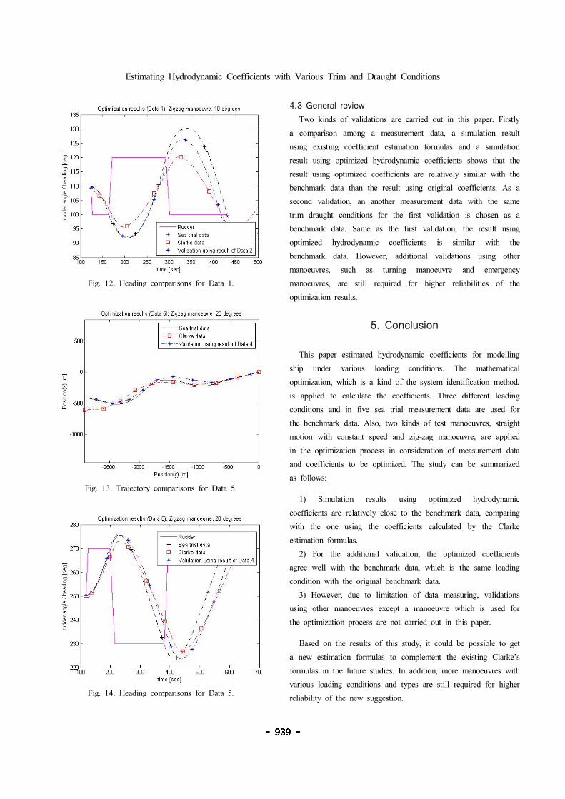
4.2 Validation with other manoeuvre data

An additional validation is carried out with rest manoeuvre

measurements. Trajectory and heading records for Data 1 and

Data 5 are compared simulation results using coefficients from

optimization of Data 2 and Data 4, respectively. Table 7 and

Fig. 11 to Fig. 14 presents a comparison between benchmark and

simulation results. For Data 1, the second overshoot angle and

Way/Lpp are still differed from the benchmark values and these

are related to the difference of trajectory between them. Whereas

the simulation result for Data 5 is almost similar with the

benchmark data even it uses the coefficients optimized from Data

4, which are based on same zig-zag manoeuvre, but different

rudder angles.

Way/Lpp Init. Yaw Ovst1 Ovst2

Data 1

Clarke 4.7 76 267 2.34 2.26

Val. 4.8 51 278 6.27 8.28

Bench 4.42 46 293 6.00 12.30

Data 5

Clarke 2.15 93 441 3.21 3.25

Val. 1.93 84 436 5.59 6.26

Bench 1.96 81 405 5.60 6.10

Remarks

Val.: Validation using optimization results of Data 2 and Data 4, respectively

Bench: Benchmark data (Measured data)Way/Lpp: Distance from start point / LppInit. : Initial turning time (s)Yaw : Yaw checking time (s)Ovst1 : First overshoot angle ( )˚Ovst2 : Second overshoot angle ( )˚

Table 7. Validation using additional manoeuvres






4.3 General review

Two kinds of validations are carried out in this paper. Firstly

a comparison among a measurement data, a simulation result

using existing coefficient estimation formulas and a simulation

result using optimized hydrodynamic coefficients shows that the

result using optimized coefficients are relatively similar with the

benchmark data than the result using original coefficients. As a

second validation, an another measurement data with the same

trim draught conditions for the first validation is chosen as a

benchmark data. Same as the first validation, the result using

optimized hydrodynamic coefficients is similar with the

benchmark data. However, additional validations using other

manoeuvres, such as turning manoeuvre and emergency

manoeuvres, are still required for higher reliabilities of the

optimization results.

5. Conclusion

This paper estimated hydrodynamic coefficients for modelling

ship under various loading conditions. The mathematical

optimization, which is a kind of the system identification method,

is applied to calculate the coefficients. Three different loading

conditions and in five sea trial measurement data are used for

the benchmark data. Also, two kinds of test manoeuvres, straight

motion with constant speed and zig-zag manoeuvre, are applied

in the optimization process in consideration of measurement data

and coefficients to be optimized. The study can be summarized

as follows:

1) Simulation results using optimized hydrodynamic

coefficients are relatively close to the benchmark data, comparing

with the one using the coefficients calculated by the Clarke

estimation formulas.

2) For the additional validation, the optimized coefficients

agree well with the benchmark data, which is the same loading

condition with the original benchmark data.

3) However, due to limitation of data measuring, validations

using other manoeuvres except a manoeuvre which is used for

the optimization process are not carried out in this paper.

Based on the results of this study, it could be possible to get

a new estimation formulas to complement the existing Clarke’s

formulas in the future studies. In addition, more manoeuvres with

various loading conditions and types are still required for higher

reliability of the new suggestion.


References

[1] Clarke, D., P. Gedling and G. Hine(1983), The Application

of Manoeuvring Criteria in Hull Design Using Linear

Theory, Transactions of the RINA, London, pp. 45-68.

[2] Im, N., S. Kweon and S. Kim(2005), The Study on the

Effect of Loading Condition on Ship Manoeuvrability,

Journal of the Society of Naval Architects of Korea, Vol.

42, No. 2, pp. 105-112.

[3] ITTC(2008), The Manoeuvring Committee Final Report

and Recommendations to the 25th ITTC, Proceedings of

25th ITTC, Vol. 1, pp. 145-152.

[4] Kijima, K., T. Katsuno, Y. Nakiri, Y. Furukawa(1990), On

the Manoeuvring Performance of a Ship with the Parameter

of Loading condition, Journal of the Society of Naval

Architects of Japan, Vol. 1990, No. 168, pp. 141-148.

[5] Kim, D. W., M. Paschen and K. Benedict(2016), A Study

on Hydrodynamic Coefficients Estimation of Modelling Ship

using System Identification Method, Journal of the Korean

Society of Marine Engineering, Vol. 40, No. 10, pp.

935-941.

[6] Kim, D. W., K. Benedict and M. Paschen(2017), Estimation

of Hydrodynamic Coefficients from Sea Trials Using a

System Identification Method, Journal of the Korean Society

of Marine Environment & Safety, Vol. 23, No. 3, pp.

258-265.

[7] Kirchhoff, M.(2013), Simulation to Optimize Simulator Ship

Models and Manoeuvres (SIMOPT), Software Manual,

ISSIMS GmbH, pp. 3-4, Rostock.

[8] Nocecdal, J. and S. J. Wright(2006), Numerical Optimization

- second edition, Springer.

[9] Norrbin, N. H.(1971), Theory and Observations on the Use

of a Mathematical Model for Ship Manoeuvring in Deep

and Confined Waters, SSPA Publication, No. 68, Gothenburg.

[10] Oltmann, P.(2003), Identification of Hydrodynamic Damping

Derivatives - a Progmatic Approach, International Conference

on Marine Simulation and Ship Manoeuvrability, Vol. 3,

Paper 3, pp. 1-9.

[11] Rheinmetall Defence Electronic(2008), Advanced Nautical

Simulator 5000 (ANS 5000) - Software Requirement

Specification (SRS), Company Publication, Bremen.

[12] Yoon, S., D. Kim and S. Kim(2016), A Study on the

Maneuvering Hydrodynamic Derivatives Estimation Applied

the Stern Shape of a Vessel, Journal of the Society of

Naval Architecture of Korea, Vol. 53, No. 1, pp. 76-83.

Received : 2017. 10. 24.

Revised : 2017. 12. 03.

Accepted : 2017. 12. 28.

Documents

Estimating Hydrodynamic Coefficients with Various Trim and