Estimating parameters in a land-surface model by applying

Estimating parameters in a land-surface model byapplying nonlinear inversion to eddy covariance fluxmeasurements from eight FLUXNET sites

Y I N G P I N G WA N G *, D E N N I S B A L D O C C H I w , R AY L E U N I N G z, E VA FA L G E § and

T I M O V E S A L A }*CSIRO Marine and Atmospheric Research, Private Bag #1, Aspendale, Vic. 3195, Australia, wDepartment of Environmental

Sciences, Policy and Management, Ecosystem Science Division, 151 Hilgard Hall, University of California, Berkeley,

CA 94720-3110, USA, zCSIRO Marine and Atmospheric Research, FC Pye Lab, GPO Box 1666, Canberra, ACT 2601, Australia,

§Plant Ecology, University of Bayreuth, 95440 Bayreuth, Germany, }Department of Physical Sciences, University of Helsinki,

FIN-00014, PO Box 64, Finland

Abstract

Flux measurements from eight global FLUXNET sites were used to estimate parameters

in a process-based, land-surface model (CSIRO Biosphere Model (CBM), using nonlinear

parameter estimation techniques. The parameters examined were the maximum photo-

synthetic carboxylation rate (vcmax; 25) the potential photosynthetic electron transport rate

(jmax, 25) of the leaf at the top of the canopy, and basal soil respiration (rs, 25), all at a

reference temperature of 25 1C. Eddy covariance measurements used in the analysis were

from four evergreen forests, three deciduous forests and an oak-grass savanna. Optimal

estimates of model parameters were obtained by minimizing the weighted differences

between the observed and predicted flux densities of latent heat, sensible heat and net

ecosystem CO2 exchange for each year. Values of maximum carboxylation rates obtained

from the flux measurements were in good agreement with independent estimates from

leaf gas exchange measurements at all evergreen forest sites. A seasonally varying vcmax; 25

and jmax, 25 in CBM yielded better predictions of net ecosystem CO2 exchange than a

constant vcmax; 25 and jmax, 25 for all three deciduous forests and one savanna site.

Differences in the seasonal variation of vcmax; 25 and jmax, 25 among the three deciduous

forests are related to leaf phenology. At the tree-grass savanna site, seasonal variation of

vcmax; 25 and jmax, 25 was affected by interactions between soil water and temperature,

resulting in vcmax; 25 and jmax, 25 reaching maximal values before the onset of summer

drought at canopy scale. Optimizing the photosynthetic parameters in the model allowed

CBM to predict quite well the fluxes of water vapor and CO2 but sensible heat fluxes

were systematically underestimated by up to 75 W m�2.

Keywords: CBM, FLUXNET, inversion, latent, parameter, photosynthesis, sensible heat flux

Received 20 December 2005; revised version received 12 May 2006 and accepted 12 May 2006

Introduction

For several decades now, measurements at leaf, plant

and canopy scale have been used to develop, test and

parameterize process-based land-surface models used

to study climate–biosphere interactions (Dickinson,

1983; Sellers et al., 1996). In those models, global vegeta-

tion is typically classified into different biome types,

and look-up tables are used to provide estimates of

model parameters for each biome (e.g. Sellers et al.,

1996). The parameters have generally been derived

from small numbers of measurements at the plant or

field scale or from expert judgment. However, problems

can arise when parameters derived at one scale are used

to estimate fluxes at a larger scale due to nonlinear

relationships between model parameters and the fluxes

and stores in land-surface scheme. In this case, para-

meters obtained at the leaf or plant scale will not be

applicable at larger scales and it is then necessary to

simplify and linearize the models, develop aggregationCorrespondence: Yingping Wang, tel. 1 61 3 9239 4577,

e-mail: [email protected]

Global Change Biology (2007) 13, 652–670, doi: 10.1111/j.1365-2486.2006.01225.x

r 2007 The Authors652 Journal compilation r 2007 Blackwell Publishing Ltd

rules from one scale to another, or to estimate para-

meters at the scale at which projections are required.

Because of the complexities which arise in scaling from

leaf to a canopy (Field et al., 1995; Leuning et al., 1995;

Wang & Leuning, 1998), it may be better to estimate

model parameters using ecosystem-scale measurements

for regional or global applications, rather than using

leaf-level parameters. Some parameters may vary sea-

sonally (Wilson et al., 2001; Xu & Baldocchi, 2003), so

intermittent field measurements such as leaf gas ex-

change, may not correctly capture their seasonal varia-

tions. In contrast, continuous eddy covariance flux

measurements provide a unique opportunity to exam-

ine the magnitude and dynamics of seasonal change in

some key parameters in land-surface models, and the

global FLUXNET database allows examination of para-

meter variation across diverse biomes and climates.

Sellers et al. (1996) identified nine key physiological

parameters as being strongly biome dependent in their

land-surface model. They found that maximum photo-

synthetic carboxylation rate and minimum stomatal

conductance were the most variable among biomes,

which suggests that these parameters need to be well

defined for a range of biomes globally. Photosynthetic

capacity is also a key parameter in the two leaf, CSIRO

Biosphere Model (CBM) through the close coupling of

photosynthesis and stomatal conductance, which af-

fects energy partitioning, transpiration and CO2 ex-

change (Leuning et al., 1995). Wang et al. (2001) found

that bulk estimates of the photosynthetic carboxylation

rate and the electron transport rate at the reference

temperature of 25 1C (vcmax; 25, and jmax, 25, respectively),

can be used to calculate accurately canopy photosynth-

esis and energy fluxes. They also showed that these

fluxes can be accurately predicted by the two-leaf

model for a mixture of two different vegetation types

if the vcmax and jmax values for each type are weighted

using their respective canopy leaf area index (LAI).

Process-based models usually require a large number

of parameters, only some of which can be estimated

from eddy flux data. The exact number of parameters

that can be extracted using nonlinear optimization

depends on the model used in the optimization and

quality of the measurements. If too many parameters

are estimated, the optimization will either not converge

or it will converge to a local minimum because of strong

correlations between different parameters. If too few

parameters are chosen, some information in the mea-

surements will not be extracted by the optimization,

and the estimates of the optimized parameters may be

sensitive to the values of the fixed parameters. This

problem can be partially resolved by constraining some

of the parameters using relatively small prior uncer-

tainties rather than fixing them, or selecting parameters

that are well constrained by measurements. Wang et al.

(2001) examined the constraints provided by eddy flux

data on parameters in CBM and concluded that only

three to five parameters can be estimated independently

using eddy flux measurements of sensible heat, water

vapor and CO2 because of the close coupling of canopy

photosynthesis and latent heat fluxes. On the other

hand, measurements of energy fluxes helped to distin-

guish between limitations of canopy photosynthesis

caused by stomatal conductance (the supply function)

and photosynthetic capacity (demand function), be-

cause canopy latent heat flux can be limited by stomatal

conductance but only indirectly by photosynthetic ca-

pacity.

Braswell et al. (2005) applied nonlinear inversion to

the eddy covariance flux measurements from Harvard

forest using a simplified model of photosynthesis and

evapotranspiration, and concluded that the multiple-

year eddy covariance flux measurements provide tight

constraints on photosynthetic parameters, but rather

poor constraints on parameters relating to soil decom-

position that varies at considerably longer time scale

than canopy photosynthesis and transpiration. Willaims

et al. (2005) also concluded that long-term measure-

ments of carbon pool sizes are required to estimate

the parameters relating to decomposition of soil organic

matter. Aalto et al. (2004) estimated two-key parameters

in their global biosphere model by applying nonlinear

inversion to eddy flux measurements and satellite mea-

surements of NDVI for 13 FLUXNET sites in Europe,

even though the actual number of parameters needed

by the model for each biome is far greater than two.

Over 250 flux towers are now installed worldwide to

monitor the fluxes of radiation, heat, water vapor and

CO2 (FLUXNET, Baldocchi et al., 2001). The global net-

work of long-term eddy flux stations continues the

pioneering work of Wofsy et al. (1993) who established

the first continuous measurements of surface fluxes in

the Harvard forest. Data collected from flux towers

have been used to study the diurnal and seasonal

variations of surface fluxes and energy partitioning

within different forest types (e.g. Black et al., 1996;

Goulden et al., 1996; Valentini et al., 1996; Falge et al.,

2001; Wilson et al., 2002, 2003; Leuning et al., 2005). We

have learnt a great deal about how plant functional

types respond to weather and soil conditions at canopy

scale (e.g. Baldocchi et al., 2004), and which factors

control seasonal and interannual variations of ex-

changes of carbon, water and heat between land surface

and lower atmosphere (Valentini et al., 2000; Baldocchi

et al., 2001). This study builds on previous experience

and understanding of using eddy flux data to develop a

framework for nonlinear parameter estimation and to

use the framework to estimate key model parameters in

ESTIMATING PARAMETERS IN A LAND-SURFACE MODEL FROM EIGHT FLUXNET SITES 653

r 2007 The AuthorsJournal compilation r 2007 Blackwell Publishing Ltd, Global Change Biology, 13, 652–670

CBM using data from eight FLUXNET sites. The results

are used to examine seasonal variation in the para-

meters and to identify systematic errors in the model.

Methodology

Optimization

The relationship between the parameters (P) in CBM

and the predicted surface fluxes (Y) is

Y ¼ fðP;MÞ; ð1Þ

where M represents the meteorological forcing, and f

represents CBM. The parameters were estimated by

minimizing the cost function (f) that was constructed

as

f ¼ 1

2ðY�OÞTC�1

0 ðY�OÞ þ 1

2ððx�xprior=CÞ

xÞ2; ð2Þ

where O is the vector of observed surface fluxes, x is the

estimate of the ratio jmax; 25=vcmax; 25 during the optimiza-

tion, xprior is the prior estimate of x, C0 is the covariance

of observed surface fluxes and Cx is the variance of the

prior estimate of x. In this study, we used the Mar-

quardt–Levenberg method as implemented in the non-

linear parameter estimation program PEST (Doherty,

2002) to find the minimum value of f. The covariance of

the estimates of parameter P, denoted Cp, is calculated as

C�1p ¼ J0C�1

0 JT0 þ JxC�1

x JT;x ð3Þ

where J0 is the first derivative of an observation (O) with

respect to P, and Jx is the first derivative of x with respect

to parameters P.

Sensitivities of observations to model parameters (J0)

and x to P (Jx) are calculated using the central difference

method (Doherty, 2002), and both are model dependent.

The quality of the measurements and prior knowledge

of x is quantified by the observation covariance (C0) and

uncertainty of xprior (Cx). Equation (3) shows that the

uncertainty of the parameter estimates increases

with C0 and Cx, and decreases with the first derivatives

(J0 and Jx). Therefore, only those parameters that are

sufficiently sensitive to observations can be reliably

determined by the optimization.

The second term on the right-hand side of Eqn (2)

represents the prior information used in the optimiza-

tion. Wullschleger (1993) found a strong correlation

between two photosynthetic parameters, the maximum

carboxylation rate (vcmax; 25) and maximum potential

electron transport rate (jmax, 25). Analysis by Leuning

(2002) suggested that the ratio xð ¼ jmax; 25=vmax; 25Þ at

leaf scale is about 2.7, a finding that is supported by

physiological arguments (Medlyn, 1996). We studied

the sensitivity of the unexplained residuals (the first

term on the right-hand side of Eqn (2)) to values of Cx

varying from 0.01 to 10.0. As the weighting factor, 1/Cx,

increases, the contribution of prior information to x

decreases, and estimates of x can differ significantly

from xprior 5 2.7, which is inconsistent with many field

and laboratory studies. We found that Cx 5 0.1 gives

estimates of x between 2 and 4 for the eight sites

studied.

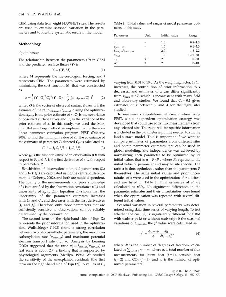
To maximize computational efficiency when using

PEST, a site-independent optimization strategy was

developed that could use eddy flux measurements from

any selected site. The required site-specific information

is included in the parameter input file needed to run the

land-surface model. This is important if we want to

compare estimates of parameters from different sites

and obtain parameter estimates that can be used in

global modeling. Site independence was achieved by

normalizing each parameter to be optimized by its

initial value, that is a 5 P/P0, where P0 represents the

initial value of parameter and may be site specific. The

ratio a is thus optimized, rather than the parameters P

themselves. The same initial values and prior uncer-

tainties of a were used in the optimizations for all sites,

and are listed in Table 1. Final estimates of P are

calculated as aTP0. No significant differences in the

parameter estimates and their uncertainties were found

when the optimization was repeated with several dif-

ferent initial values.

Seasonal variation in several parameters was deter-

mined using data time series of varying length. To test

whether the cost, f, is significantly different for CBM

with (subscript k) or without (subscript l) the seasonal

variations of vcmax; 25, the w2 value were calculated as

w2 ¼ fk � fl

fl

dfl

dfk � dfl; ð4Þ

where df is the number of degrees of freedom, calcu-

lated asP

j¼1; 2; 3 nj �m, where nj is total number of flux

measurements, for latent heat (j 5 1), sensible heat

(j 5 2) and CO2 (j 5 3), and m is the number of opti-

mized parameters.

Table 1 Initial values and ranges of model parameters opti-

mized in this study

Parameter Unit Initial value Range

aL – 1.0 0.8–1.0

ajmax, 25 – 1.0 0.1–5.0

jmax, 25/vcmax, 25 – 2.0 1.8–2.2

ars,25 – 1.0 0.01–50

To 1C 20 0–50

DT 1C 20 0–100

654 Y. P. WA N G et al.


An agreement index, d, developed by Willmott (1984)

is used to describe the agreement between model pre-

diction using the optimal estimates of parameters and

observations. Values of 0 or 1 represent no or perfect

agreement, respectively.

CBM and its parameterization for each FLUXNET site

CBM simulates the fluxes of latent and sensible heat

and net ecosystem CO2 exchange. It consists of sub-

models of (1) canopy radiation transfer using a simpli-

fied two-stream approximation (Spitters, 1986; Wang &

Leuning, 1998; Wang, 2003), (2) atmospheric transport

using the simplified localized near-field turbulence

theory of Raupach et al. (1997), (3) a two-leaf (sun-

shade) model that fully couples photosynthesis,

stomatal conductance, transpiration, and leaf energy

balances (Leuning et al., 1995; Wang & Leuning, 1998)

and (4) a module that simulates water and heat transfer

within soil and snow (Kowalczyk et al., 1994). CBM is

the land-surface scheme in the CSIRO global climate

model, and an international comparisons of various

such schemes found that CBM provided excellent

simulations of the fluxes of heat, water vapor and CO2

(Pitman et al., 1999).

The measured net exchanges of latent heat, Fe,

and sensible heat, Fh, are given by the sum of

fluxes from the canopy (subscript c) and the soil

(subscript s)

Fe ¼ Fec þ Fes; ð5Þ

Fh ¼ Fhc þ Fhs: ð6Þ

Net ecosystem CO2 exchange, Fc, is calculated as

the sum of three component fluxes: canopy net photo-

synthesis, An, nonleaf respiration, Rp, and soil respira-

tion, Rs:

Fc ¼ An þ Rp þ Rs; ð7Þ

where Fc is negative for CO2 uptake by the terrestrial

biosphere. The two-leaf canopy model described by

Wang & Leuning (1998) fully couples photosynthesis,

stomatal conductance, transpiration and leaf energy

balances (Leuning et al., 1995). This recognizes that

stomata provide the primary passage for the transport

of water vapor and CO2 between the leaf and ambient

air (Cowan & Farquhar, 1977), thereby controlling the

partitioning of energy between Fec and Fhc. Key para-

meters in the photosynthesis model include the max-

imum carboxylation rate of the enzyme Rubisco,

vcmax; 25, and maximum potential electron transport rate,

jmax, 25, at a leaf temperature of 25 1C. The stomatal

model has two empirical parameters, a and D0, which

describe the sensitivity of stomatal conductance to the

net photosynthesis rate and the humidity deficit of the

atmosphere. Following Leuning et al. (1995), the rela-

tionship between An and stomatal conductance, Gc, is

given by

Gc ¼ Gc0 þaAn

ðCs � GÞð1þDs=D0Þ; ð8Þ

where Cs is CO2 concentration at the leaf surface

(mmol mol�1), G is the CO2 compensation point of

photosynthesis (mmol mol�1), Ds is water vapor pres-

sure deficit at the leaf surface (Pa), and Gc0 is conduc-

tance of the leaves (mmol m�2 s�1) when An 5 0.

Equation (8) is applied to sunlit and shaded leaves

separately.

Respiration from woody tissue and roots (Rp) is

modeled as

Rp ¼ 0:7rp; 25QðTp�20Þ=10

10 ; ð9Þ

where rp, 25 is the basal respiration rate at 25 1C,

coefficient 0.7 represents the ratio of Rp at 20 and

25 1C, and Q10 decreases with an increase in plant tissue

temperature in 1C (Tp) according to Tjoelker et al.

(2001):

Q10 ¼ 3:22� 0:046Tp: ð10Þ

As Rp does not include leaf respiration that is in-

cluded in calculating An, respiration from roots will

contribute to most of Rp. Studies have shown that Q10

formulation is quite adequate for modeling the re-

sponse of Rp to temperature (Reichstein et al., 2005).

To calculate Rp it is assumed that Tp, is equal to ambient

air temperature (Ta) in this study.

Soil respiration or heterotrophic respiration, Rs, is

modeled as a function of soil temperature and moisture

using

Rs ¼ rs; 25f1ðTsÞf2ðvsÞ; ð11Þ

where rs, 25 is the soil respiration rate at soil temperature

(�Ts) of 25 1C with no water stress (f2 5 1), and where

functions f1 and f2 describe the dependence of soil

respiration on Ts, the mean soil temperature ( 1C) and

on vs, the mean fraction of water-filled pore space,

weighted by root mass fraction in all six soil layers.

The functions used are

f1ðTsÞ ¼ 2:43 exp3:36ðTs � 40Þ

Ts þ 31:79

� �; ð12Þ

f2ð�vsÞ ¼ 3:63�vs � 3:20�v2s � 0:12�v3

s : ð13Þ

Equations (12) and (13) are taken from Kirschbaum

(1995) and from Kelly et al. (2000), respectively.



Submodels for seasonal variation of maximumcarboxylation rate

Maximum carboxylation rate (vcmax) and maximum

potential electron transport rate (jmax) of the leaves at

the top of the canopy are calculated as

vcmax ¼ vcmax; 25fT; vfdfw ¼ vx; 25fT; v; ð14Þ

jmax ¼ jmax; 25fT; jfdfw ¼ jx; 25fT; j; ð15Þ

where vcmax; 25 and jmax, 25 are the corresponding values

at a leaf temperature of 25 1C. The functions fT, v and fT, j

for the temperature dependences of vcmax; 25 and jmax,

respectively, were taken from Leuning (2002).

Function fd accounts for canopy development and fwthe effect of water stress on the photosynthesis para-

meters. The water stress factor fw was calculated as

fw ¼ bX

n

Wr;nðyn � ywiltÞyfc � ywilt

; ð16Þ

where Wr, n is the root mass fraction in soil layer n

(n 5 1–6), yn is volumetric soil water content of soil

layer n, and ywilt and yfc are volumetric soil water

content at wilting point and field capacity, respectively.

Function fd is used to describe the influence of canopy

development on vcmax and jmax and two models for fdare considered, viz.

Model I:

fd ¼ 1: ð17Þ

Model II:

fd ¼ 1� Ts; 0:5 � T0

DT

� �2

; 0 � fd � 1; ð18Þ

where Ts, 0.5 is the temperature at 0.5 m depth, T0 and DT

( 1C) are parameters of the canopy-development model.

Both vcmax and jmax are leaf-scale photosynthetic

parameters and they are assumed to decrease exponen-

tially with the cumulated canopy LAI from the canopy

top in a canopy. Total canopy vcmax and Jmax (expressed

per ground area basis) are given by

vcmax ¼ vcmax; 25fT; vfdfwð1� expð�knLÞÞ=kn; ð19Þ

Jmax ¼ jmax; 25fT; jfdfwð1� expð�knLÞÞ=kn; ð20Þ

where L is canopy LAI, and kn is an empirical constant.

To compare estimates of the photosynthesis parameters

derived from flux measurements at the canopy scale

with those from leaf-level gas exchange measurements,

we use vx, 25 5 fdfw vcmax; 25 and jx, 25 5 fdfwjmax, 25, rather

than vcmax and jmax, because effects of leaf development

and soil water stress on vcmax; 25 or jmax are usually not

quantified in reports of leaf-level measurements. Fol-

lowing the notation of Wang & Leuning (1998), we use

Vcmax; 25 and Jmax for the total canopy and vcmax and jmax

for the leaf within the canopy.

For given values of canopy Vcmax or Jmax, the corre-

sponding leaf vcmax; 25 or jmax, 25 at the canopy top vary

with kn. The following equation can be used to calculate

leaf vcmax; 25 or jmax, 25 for different kn. That is

v1 ¼v2kn; 1ð1� expð�kn; 2LÞÞkn; 2ð1� expð�kn; 1LÞÞ ; ð21Þ

where v1 and v2 are the value of vcmax; 25 or jmax, 25 for

kn 5 kn, 1 and kn 5 kn, 2, respectively.

The FLUXNET dataset

The goal of this study is to test a parameter optimization

technique for a wide range of vegetation types growing

in different climates, using measurements of heat, water

vapor and CO2 fluxes and associated meteorological

variables in the gap-filled FLUXNET dataset compiled

by Falge et al. (2001) (http://www.fluxnet.ornl.gov/

fluxnet/gapzips.cfm). From the 36 sites where gap-

filled data are available, eight were selected, consisting

of three needle-leaved evergreen forests at high lati-

tude, three temperate deciduous broadleaf forests, one

temperate savanna, all in the northern hemisphere, and

one evergreen broad-leaf forest in Australia. Informa-

tion about the eight sites is given in Table 2 and the

listed references.

To predict surface fluxes, Fe, Fh and Fc, CBM requires

the inputs of meteorological forcing (incoming short-

wave and long-wave radiation, air temperature, relative

humidity, rainfall and wind speed) and four kinds of

parameters: morphological parameters: such as canopy

height, leaf size, rooting depth and vertical distribution

of root mass at different soil layers, leaf angle distribution

and LAI; optical properties: transmittance and reflectance

of all phyto-elements and the ground in the visible, near

infrared and long-wave wavebands; plant physiological

parameters: vcmax; 25, jmax, 25, the stomatal parameters

(a and D0), sensitivity of vcmax; 25 or jmax, 25 to soil water

(b), basal rate of nonleaf respiration rate at 25 1C (rp, 25);

and soil parameters: basal rate of soil respiration at 25 1C

(rs, 25), volumetric water content at wilting point and field

capacity and other soil physical properties.

The most important plant morphological parameters

are LAI, rooting depth and vertical distribution of roots

in soil. The latter were determined for the eight selected

sites using data compiled by Jackson et al. (1996) for

boreal forests, temperate coniferous forests, temperate

deciduous forests and savannas. Estimates of LAI and

its seasonal variations were either derived from the

literature, from MODIS products (http://public.ornl.

gov/fluxnet/modis.cfm), or from site-specific websites.

Canopy height and leaf size were obtained from the



published literature, internet websites or personal com-

munication with the primary investigators. These data

sources were also used for soil texture classification to

estimate soil physical properties through relationships

developed by Clapp & Hornberger (1978).

Estimates of optical properties for different phyto-

elements were taken from Wang & Leuning (1998). Leaf

angle distribution is assumed to be spherical for all

sites, as different leaf angle distributions were found to

have relatively little influences on the modeled canopy

fluxes (Fec, Fhc and Fcc) and spherical leaf distribution is

a good approximation for most forest canopies (see

Wang & Jarvis, 1990; Baldocchi & Meyers, 1998). Effects

of snow cover and snow age on surface optical proper-

ties are modeled according to Kowalczyk et al. (1994).

Initial soil temperature was set to annual mean tem-

perature and initial soil moisture was set to the mean of

soil moisture content at wilting point and field capacity

for each layer. The model was then spun up for 5 years

by reusing the same years of meteorological forcing.

Soil moisture and temperature of all six layers at the

end of the 5-year run were used as the initial values for

the sixth year of simulations that was used for para-

meter estimation. Optimization results did not differ

significantly from those obtained with a spin-up of 410

years.

Choosing the parameters to be optimized

Variations of vcmax; 25 and jmax, 25 are the largest for

different biomes (Sellers et al., 1996) and these para-

meters were estimated using PEST, with prior estimates

taken from the default values in CBM for each vegeta-

tion type or from the published literature. To limit the

number of parameters to be optimized, parameters for

the stomatal model (Eqn (8)) were set to a 5 9 and

D0 5 1.5 kPa (Leuning, 1995; Wang et al., 2001). The

nitrogen distribution coefficient was set to kn 5 0.7

(Eqns (19) and (20)) for all ecosystems.

Parameter b describes the sensitivity of vcmax; 25 or

jmax, 25 to soil water stress (Eqn (16)). Federer (1982)

discussed a similar parameter and its dependence on

soil and vegetation characteristics and found that his

parameter had higher values for crops and grass than

for forests, because trees have deeper roots. A value of 1

was used by Colello et al. (1998) for their global climate

simulation. The optimization did not always converge

in the present study when b was allowed to vary and branged from 0.7 to 1.3 when the optimization did

converge. We, therefore, chose b5 1 in this study.

Of the soil parameters, only basal soil respiration rate

at 25 1C and optimal water condition, rs, 25, was esti-

mated using optimization. Values of all soil physical

parameters were taken from the look-up table for each

soil type as used in CBM for global modeling studies

(Kowalczyk et al., 1994).

Results

In all, six parameters are optimized in this study. They

are canopy LAI (L), maximum carboxylation rate

(vcmax; 25) at 25 1C of leaves at the top of the canopy,

maximum potential electron transport rate at 25 1C of

leaves at the top of the canopy (jmax, 25), soil respiration

rate at 25 1C (rs, 25) and two additional parameters, T0

and DT that are used to describe the seasonal depen-

dence of vcmax or jmax on soil temperature at 0.5 m depth

(see Eqn (17)). The prescribed canopy leaf index varies

seasonally for deciduous forests and savanna, and was

assumed constant for all evergreen forests. In this study,

we optimized a constant multiplier of the prescribed

canopy LAI, xL. We also included the ratio

jmax; 25=vcmax; 25 ¼ 2:7 that Wullschleger (1993) and Leun-

ing (2002) found for a wide range of plant species as

prior information in the optimization. Because CO2

fluxes for plants and soil were not measured separately,

we cannot obtain independent estimates of basal rates

of nonleaf plant and soil respiration (rp, 25 and rs, 25). The

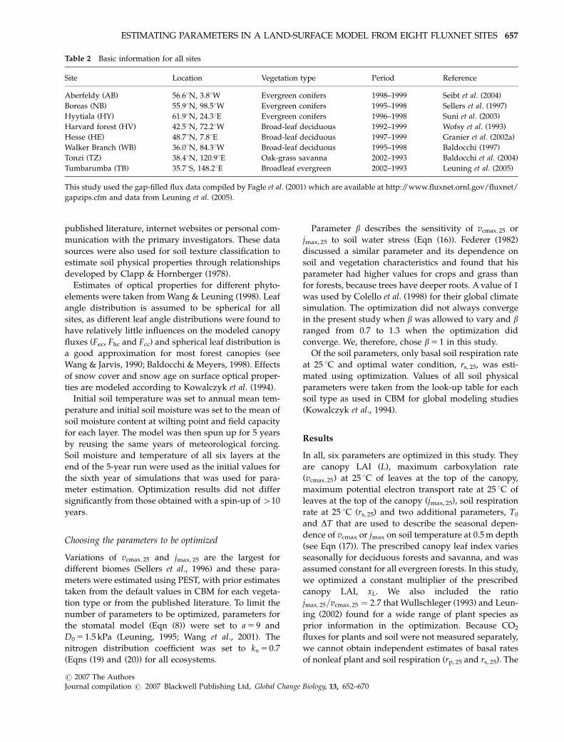
Table 2 Basic information for all sites

Site Location Vegetation type Period Reference

Aberfeldy (AB) 56.61N, 3.81W Evergreen conifers 1998–1999 Seibt et al. (2004)

Boreas (NB) 55.91N, 98.51W Evergreen conifers 1995–1998 Sellers et al. (1997)

Hyytiala (HY) 61.91N, 24.31E Evergreen conifers 1996–1998 Suni et al. (2003)

Harvard forest (HV) 42.51N, 72.21W Broad-leaf deciduous 1992–1999 Wofsy et al. (1993)

Hesse (HE) 48.71N, 7.81E Broad-leaf deciduous 1997–1999 Granier et al. (2002a)

Walker Branch (WB) 36.01N, 84.31W Broad-leaf deciduous 1995–1998 Baldocchi (1997)

Tonzi (TZ) 38.41N, 120.91E Oak-grass savanna 2002–1993 Baldocchi et al. (2004)

Tumbarumba (TB) 35.71S, 148.21E Broadleaf evergreen 2002–1993 Leuning et al. (2005)

This study used the gap-filled flux data compiled by Fagle et al. (2001) which are available at http://www.fluxnet.ornl.gov/fluxnet/

gapzips.cfm and data from Leuning et al. (2005).



soil respiration parameter was thus calculated using

rs, 25 5 re, 25–rp, 25, where re, 25 is total ecosystem respira-

tion at 25 1C and rp, 25 is a fixed common prior estimate

of basal plant respiration for all sites.

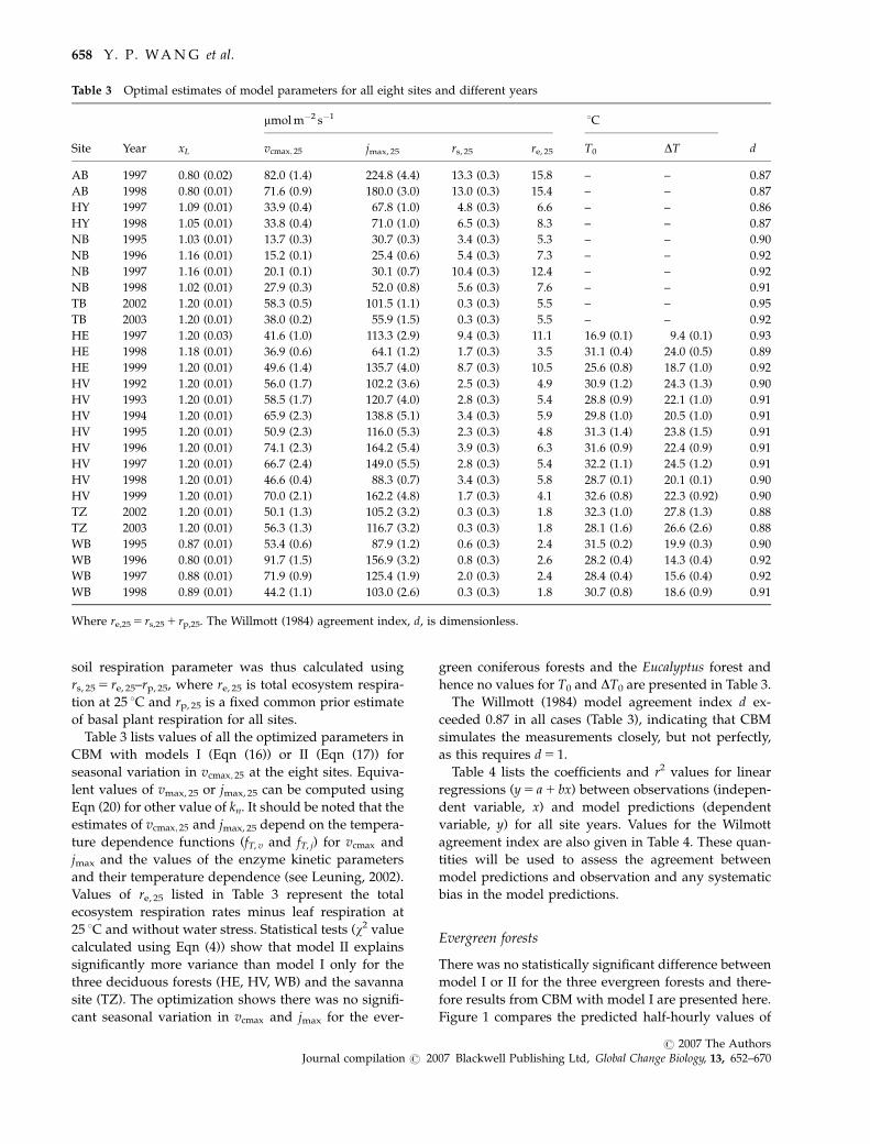
Table 3 lists values of all the optimized parameters in

CBM with models I (Eqn (16)) or II (Eqn (17)) for

seasonal variation in vcmax; 25 at the eight sites. Equiva-

lent values of vmax, 25 or jmax, 25 can be computed using

Eqn (20) for other value of kn. It should be noted that the

estimates of vcmax; 25 and jmax, 25 depend on the tempera-

ture dependence functions (fT, v and fT, j) for vcmax and

jmax and the values of the enzyme kinetic parameters

and their temperature dependence (see Leuning, 2002).

Values of re, 25 listed in Table 3 represent the total

ecosystem respiration rates minus leaf respiration at

25 1C and without water stress. Statistical tests (w2 value

calculated using Eqn (4)) show that model II explains

significantly more variance than model I only for the

three deciduous forests (HE, HV, WB) and the savanna

site (TZ). The optimization shows there was no signifi-

cant seasonal variation in vcmax and jmax for the ever-

green coniferous forests and the Eucalyptus forest and

hence no values for T0 and DT0 are presented in Table 3.

The Willmott (1984) model agreement index d ex-

ceeded 0.87 in all cases (Table 3), indicating that CBM

simulates the measurements closely, but not perfectly,

as this requires d 5 1.

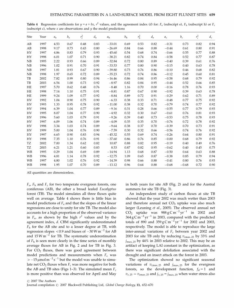
Table 4 lists the coefficients and r2 values for linear

regressions (y 5 a 1 bx) between observations (indepen-

dent variable, x) and model predictions (dependent

variable, y) for all site years. Values for the Wilmott

agreement index are also given in Table 4. These quan-

tities will be used to assess the agreement between

model predictions and observation and any systematic

bias in the model predictions.

Evergreen forests

There was no statistically significant difference between

model I or II for the three evergreen forests and there-

fore results from CBM with model I are presented here.

Figure 1 compares the predicted half-hourly values of

Table 3 Optimal estimates of model parameters for all eight sites and different years

Site Year xL

mmol m�2 s�11C

dvcmax; 25 jmax, 25 rs, 25 re, 25 T0 DT

AB 1997 0.80 (0.02) 82.0 (1.4) 224.8 (4.4) 13.3 (0.3) 15.8 – – 0.87

AB 1998 0.80 (0.01) 71.6 (0.9) 180.0 (3.0) 13.0 (0.3) 15.4 – – 0.87

HY 1997 1.09 (0.01) 33.9 (0.4) 67.8 (1.0) 4.8 (0.3) 6.6 – – 0.86

HY 1998 1.05 (0.01) 33.8 (0.4) 71.0 (1.0) 6.5 (0.3) 8.3 – – 0.87

NB 1995 1.03 (0.01) 13.7 (0.3) 30.7 (0.3) 3.4 (0.3) 5.3 – – 0.90

NB 1996 1.16 (0.01) 15.2 (0.1) 25.4 (0.6) 5.4 (0.3) 7.3 – – 0.92

NB 1997 1.16 (0.01) 20.1 (0.1) 30.1 (0.7) 10.4 (0.3) 12.4 – – 0.92

NB 1998 1.02 (0.01) 27.9 (0.3) 52.0 (0.8) 5.6 (0.3) 7.6 – – 0.91

TB 2002 1.20 (0.01) 58.3 (0.5) 101.5 (1.1) 0.3 (0.3) 5.5 – – 0.95

TB 2003 1.20 (0.01) 38.0 (0.2) 55.9 (1.5) 0.3 (0.3) 5.5 – – 0.92

HE 1997 1.20 (0.03) 41.6 (1.0) 113.3 (2.9) 9.4 (0.3) 11.1 16.9 (0.1) 9.4 (0.1) 0.93

HE 1998 1.18 (0.01) 36.9 (0.6) 64.1 (1.2) 1.7 (0.3) 3.5 31.1 (0.4) 24.0 (0.5) 0.89

HE 1999 1.20 (0.01) 49.6 (1.4) 135.7 (4.0) 8.7 (0.3) 10.5 25.6 (0.8) 18.7 (1.0) 0.92

HV 1992 1.20 (0.01) 56.0 (1.7) 102.2 (3.6) 2.5 (0.3) 4.9 30.9 (1.2) 24.3 (1.3) 0.90

HV 1993 1.20 (0.01) 58.5 (1.7) 120.7 (4.0) 2.8 (0.3) 5.4 28.8 (0.9) 22.1 (1.0) 0.91

HV 1994 1.20 (0.01) 65.9 (2.3) 138.8 (5.1) 3.4 (0.3) 5.9 29.8 (1.0) 20.5 (1.0) 0.91

HV 1995 1.20 (0.01) 50.9 (2.3) 116.0 (5.3) 2.3 (0.3) 4.8 31.3 (1.4) 23.8 (1.5) 0.91

HV 1996 1.20 (0.01) 74.1 (2.3) 164.2 (5.4) 3.9 (0.3) 6.3 31.6 (0.9) 22.4 (0.9) 0.91

HV 1997 1.20 (0.01) 66.7 (2.4) 149.0 (5.5) 2.8 (0.3) 5.4 32.2 (1.1) 24.5 (1.2) 0.91

HV 1998 1.20 (0.01) 46.6 (0.4) 88.3 (0.7) 3.4 (0.3) 5.8 28.7 (0.1) 20.1 (0.1) 0.90

HV 1999 1.20 (0.01) 70.0 (2.1) 162.2 (4.8) 1.7 (0.3) 4.1 32.6 (0.8) 22.3 (0.92) 0.90

TZ 2002 1.20 (0.01) 50.1 (1.3) 105.2 (3.2) 0.3 (0.3) 1.8 32.3 (1.0) 27.8 (1.3) 0.88

TZ 2003 1.20 (0.01) 56.3 (1.3) 116.7 (3.2) 0.3 (0.3) 1.8 28.1 (1.6) 26.6 (2.6) 0.88

WB 1995 0.87 (0.01) 53.4 (0.6) 87.9 (1.2) 0.6 (0.3) 2.4 31.5 (0.2) 19.9 (0.3) 0.90

WB 1996 0.80 (0.01) 91.7 (1.5) 156.9 (3.2) 0.8 (0.3) 2.6 28.2 (0.4) 14.3 (0.4) 0.92

WB 1997 0.88 (0.01) 71.9 (0.9) 125.4 (1.9) 2.0 (0.3) 2.4 28.4 (0.4) 15.6 (0.4) 0.92

WB 1998 0.89 (0.01) 44.2 (1.1) 103.0 (2.6) 0.3 (0.3) 1.8 30.7 (0.8) 18.6 (0.9) 0.91

Where re,25 5 rs,25 1 rp,25. The Willmott (1984) agreement index, d, is dimensionless.



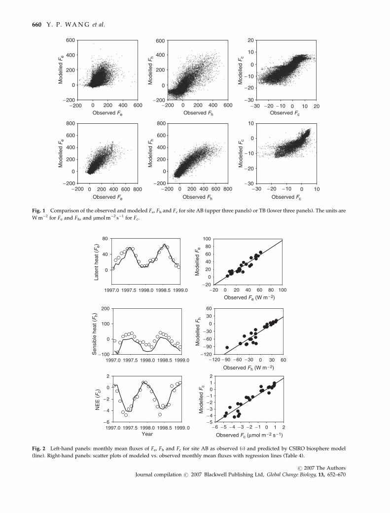
Fe, Fh and Fc for two temperate evergreen forests, one

coniferous (AB), the other a broad leafed Eucalyptus

forest (TB). The model simulates all three fluxes quite

well on average. Table 4 shows there is little bias in

model predictions of Fe and that the slopes of the linear

regressions are close to unity for site TB. The model also

accounts for a high proportion of the observed variance

in Fe, as shown by the high r2 values and by the

agreement index, d. CBM significantly underestimated

Fh for the AB site and to a lesser degree at TB, with

regression slopes o0.9 and biases of �30 W m�2 for AB

and 15 W m�2 for TB. The systematic underestimation

of Fh is seen more clearly in the time series of monthly

average fluxes for AB in Fig. 2 and for TB in Fig. 3.

For CO2 fluxes, there was good agreement between

model predictions and measurements when Fc was

4�15mmol m�2 s�1 but the model was unable to simu-

late net CO2 fluxes when Fc was more negative for both

the AB and TB sites (Figs 1–3). The simulated mean Fc

is more positive than was observed for April and May

in both years for site AB (Fig. 2) and for the Austral

summers for site TB (Fig. 3).

An independent study of carbon fluxes at site TB

showed that the year 2002 was much wetter than 2003

and therefore annual net CO2 uptake was also much

larger (Leuning et al., 2005). The observed annual net

CO2 uptake was 988 g C m�2 yr�1 in 2002 and

364 g C m�2 yr�1 in 2003, compared with the predicted

totals of 890 and 359 g C m�2 yr�1 for 2002 and 2003,

respectively. The model is able to reproduce the large

inter-annual variations of Fc between year 2002 and

2003 for site TB only by reducing vcmax; 25 by 33% and

jmax, 25 by 44% in 2003 relative to 2002. This may be an

artifact of keeping LAI constant in the optimization, as

there was significant defoliation associated with the

drought and an insect attack on the forest in 2003.

The optimization showed no significant seasonal

variations of vcmax; 25 and jmax, 25 for the evergreen

forests, so the development function, fd 5 1 and

vx; 25 ¼ vcmax; 25 and jx, 25 5 jmax, 25 when water stress also

Table 4 Regression coefficients for y 5 a 1 bx, r2 values, and the agreement index (d) for: Fe (subscript e), Fh (subscript h) or Fc

(subscript c), where x are observations and y the model predictions

Site Year ae be r2e de ah bh r2

h de ac bc r2c dc

AB 1997 4.53 0.67 0.48 0.83 �33.01 0.69 0.53 0.82 �0.31 0.73 0.82 0.94

AB 1998 9.17 0.73 0.43 0.80 �26.69 0.84 0.66 0.88 �0.44 0.61 0.80 0.91

HY 1997 4.86 0.83 0.79 0.93 �45.60 0.54 0.68 0.74 �0.66 0.55 0.77 0.88

HY 1998 6.01 1.07 0.71 0.90 �38.21 0.82 0.74 0.84 �0.58 0.52 0.77 0.87

NB 1995 2.22 0.93 0.66 0.89 �32.84 0.72 0.80 0.89 �0.40 0.39 0.61 0.76

NB 1996 1.02 0.91 0.70 0.91 �33.53 0.77 0.80 0.90 �0.15 0.40 0.63 0.78

NB 1997 1.81 0.93 0.67 0.90 �39.80 0.73 0.76 0.86 �0.10 0.46 0.68 0.82

NB 1998 1.97 0.65 0.72 0.89 �35.23 0.72 0.74 0.86 �0.12 0.45 0.60 0.81

TB 2002 7.82 0.99 0.80 0.94 �16.46 0.86 0.84 0.95 �0.58 0.68 0.79 0.92

TB 2003 6.54 1.00 0.73 0.92 �8.97 0.82 0.84 0.95 �0.44 0.52 0.66 0.85

HE 1997 5.70 0.62 0.48 0.76 �8.48 1.16 0.70 0.00 �0.16 0.78 0.76 0.93

HE 1998 7.14 1.10 0.75 0.91 �8.81 0.87 0.67 0.90 �0.92 0.39 0.63 0.78

HE 1999 9.24 1.09 0.77 0.92 �8.84 0.89 0.72 0.91 �0.29 0.62 0.71 0.89

HV 1992 1.04 0.90 0.75 0.90 �6.33 0.38 0.33 0.71 �0.48 0.77 0.75 0.92

HV 1993 1.33 0.95 0.78 0.92 �11.00 0.38 0.32 0.70 �0.79 0.74 0.77 0.92

HV 1994 6.39 1.04 0.77 0.89 �9.16 0.31 0.28 0.66 �0.55 0.77 0.79 0.93

HV 1995 8.07 1.04 0.77 0.90 �4.92 0.32 0.30 0.67 �0.61 0.76 0.81 0.93

HV 1996 5.60 1.03 0.79 0.91 �9.26 0.39 0.40 0.73 �0.53 0.75 0.78 0.93

HV 1997 6.09 1.06 0.74 0.89 �4.09 0.35 0.35 0.70 �0.76 0.72 0.78 0.92

HV 1998 3.34 1.03 0.74 0.89 �9.64 0.38 0.37 0.70 �0.39 0.70 0.73 0.91

HV 1999 5.00 1.04 0.76 0.90 �7.59 0.30 0.32 0.66 �0.56 0.74 0.76 0.92

HY 1997 6.65 0.90 0.83 0.94 �45.32 0.55 0.69 0.74 �0.26 0.64 0.80 0.91

HY 1998 7.35 1.10 0.76 0.91 �37.60 0.86 0.76 0.85 �0.00 0.68 0.79 0.92

TZ 2002 7.00 1.34 0.62 0.82 10.87 0.88 0.82 0.95 �0.19 0.40 0.49 0.76

TZ 2003 6.21 1.21 0.60 0.83 8.53 0.87 0.82 0.95 �0.62 0.40 0.45 0.75

WB 1995 0.29 1.04 0.69 0.89 �14.94 1.13 0.68 0.87 �0.50 0.64 0.63 0.88

WB 1996 4.81 1.14 0.78 0.92 �12.75 1.09 0.65 0.87 �0.38 0.85 0.79 0.94

WB 1997 4.80 1.02 0.76 0.92 �14.39 0.98 0.66 0.88 �0.41 0.80 0.76 0.93

WB 1998 1.95 1.07 0.70 0.89 �13.12 0.96 0.64 0.88 �0.68 �0.68 0.72 0.90

All quantities are dimensionless.



−200

−200−200−200 −200

0 200 400 600 800−200

00

200

400

600

800

−200 0 200 400 600 800−200

200

400

600

800

Observed FcObserved Fh

Observed FhObserved Fe

−30−30

−20

−20

−10

−10

0 10

Observed Fc

−30−30

−20

−20

−10

−10

0 10 20

Mod

elle

d F

cM

odel

led F

c

Observed Fe

Mod

elle

d F

eM

odel

led F

e

Mod

elle

d F

hM

odel

led F

h

0

10

0 200 400 600

0

200

400

600

0 200 400 600

0

200

400

600

0

10

20

Fig. 1 Comparison of the observed and modeled Fe, Fh and Fc for site AB (upper three panels) or TB (lower three panels). The units are

W m�2 for Fe and Fh, and mmol m�2 s�1 for Fc.

1997.0 1997.5 1998.0 1998.5 1999.0

0

40

80

1997.0 1997.5 1998.0 1998.5 1999.0

Sen

sibl

e he

at (F

h)La

tent

hea

t (F

e)

−100

0

100

200

Year1997.0 1997.5 1998.0 1998.5 1999.0

NE

E (F

c)

−6

−4

−2

0

2

−20 0 20 40 60 80 100−20

0

20

40

60

80

100

Observed Fh (W m−2)

Observed Fe (W m−2)

−120 −90 −60 −30 0 30 60−120

−90

−60

−30

0

30

60

Observed Fc (µmol m−2 s−1)

−6 −5 −4 −3 −2 −1 0 1 2

Mod

elle

d F

cM

odel

led F

hM

odel

led F

e

−5−4−3−2−1

012

Fig. 2 Left-hand panels: monthly mean fluxes of Fe, Fh and Fc for site AB as observed (�) and predicted by CSIRO biosphere model

(line). Right-hand panels: scatter plots of modeled vs. observed monthly mean fluxes with regression lines (Table 4).



is absent (Eqns (19) and (20)). Using leaf-gas exchange

measurements, Meir et al. (2002) estimated that vcmax; 25

varied from 40 to 20 mmol m�2 s�1 from the top to the

bottom of a Sitka Spruce forest near the AB site. Their

results agree well with our estimates if kn 5 0.35 (assum-

ing a canopy LAI of 7 and applying Eqn (20)). Max-

imum canopy photosynthesis occurs when the vertical

distribution of photosynthetic capacity in the canopy in

proportional to average radiation absorption at each

height (Field, 1983; de Pury & Farquhar, 1997; Wang &

Leuning, 1998). The low value of kn is thus possible, as

Wang & Jarvis (1993) estimated that the effective ex-

tinction coefficient of diffuse visible radiation within a

dense Sitka spruce canopy is about 0.4 because of

needle clumping. For the TB site in 2002, leaf gas

exchange measurements on leaves in the middle part

of the forest canopy gave a mean value for vcmax; 25

of 84 mmol m�2 s�1 (B. E. Medlyn, unpublished data),

which is about twice our estimates for kn 5 0.7. It is

unlikely that the estimate of kn will exceed 0.7 for site

TB, as the canopy is quite open with a maximal canopy

LAI of 2.5 (Leuning et al., 2005) and hence the reason

for the discrepancy is as yet unclear.

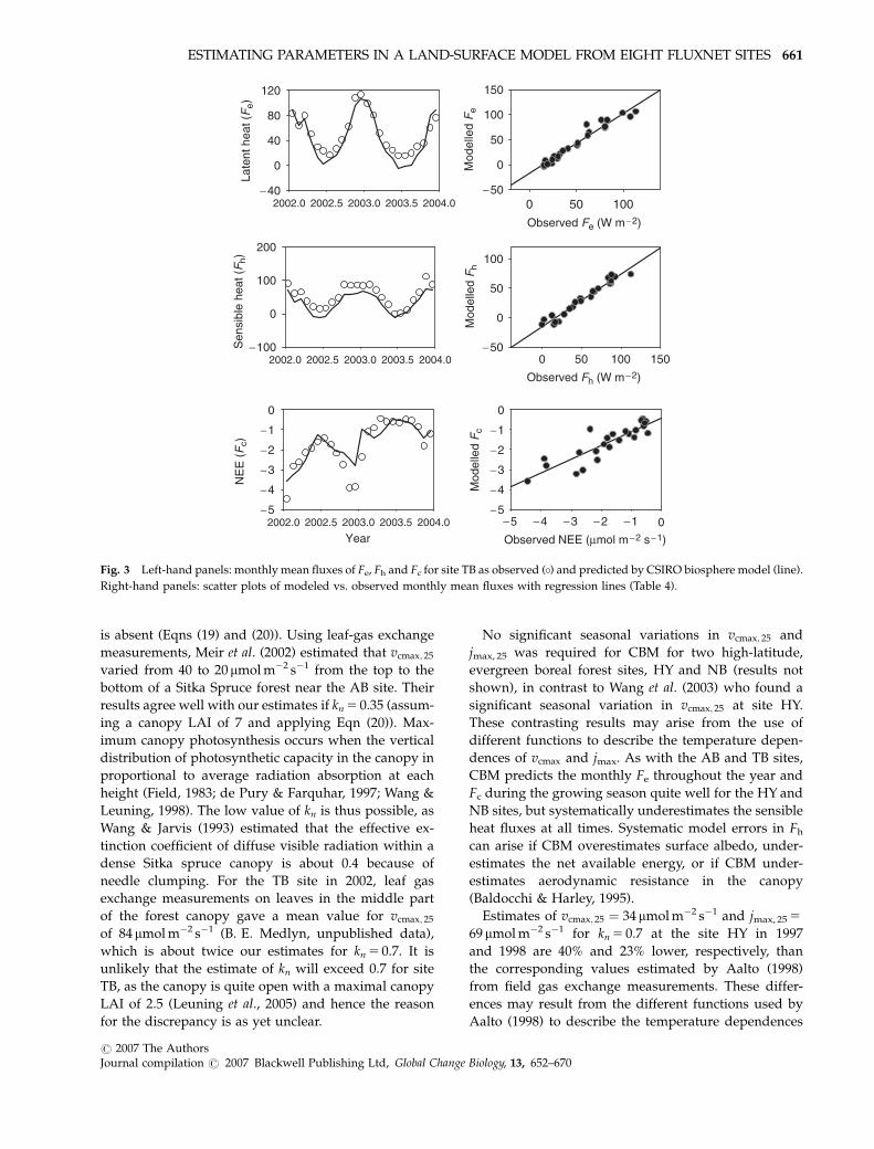
No significant seasonal variations in vcmax; 25 and

jmax, 25 was required for CBM for two high-latitude,

evergreen boreal forest sites, HY and NB (results not

shown), in contrast to Wang et al. (2003) who found a

significant seasonal variation in vcmax; 25 at site HY.

These contrasting results may arise from the use of

different functions to describe the temperature depen-

dences of vcmax and jmax. As with the AB and TB sites,

CBM predicts the monthly Fe throughout the year and

Fc during the growing season quite well for the HY and

NB sites, but systematically underestimates the sensible

heat fluxes at all times. Systematic model errors in Fh

can arise if CBM overestimates surface albedo, under-

estimates the net available energy, or if CBM under-

estimates aerodynamic resistance in the canopy

(Baldocchi & Harley, 1995).

Estimates of vcmax; 25 ¼ 34 mmol m�2 s�1 and jmax, 25 5

69 mmol m�2 s�1 for kn 5 0.7 at the site HY in 1997

and 1998 are 40% and 23% lower, respectively, than

the corresponding values estimated by Aalto (1998)

from field gas exchange measurements. These differ-

ences may result from the different functions used by

Aalto (1998) to describe the temperature dependences

2002.0 2002.5 2003.0 2003.5 2004.0−40

0

40

80

120

2002.0 2002.5 2003.0 2003.5 2004.0−100

0

100

200

Year2002.0 2002.5 2003.0 2003.5 2004.0

NE

E (F

c)

0 50 100−50

0

50

100

150

0 50 100 150−50

0

50

100

−5 −4 −3 −2 −1 0−5

−4

−3

−2

−1

0

−5

−4

−3

−2

−1

0

Observed NEE (µmol m−2 s−1)

Mod

elle

d F

c

Sen

sibl

e he

at (F

h)La

tent

hea

t (F

e)

Mod

elle

d F

hM

odel

led F

e



Fig. 3 Left-hand panels: monthly mean fluxes of Fe, Fh and Fc for site TB as observed (�) and predicted by CSIRO biosphere model (line).

Right-hand panels: scatter plots of modeled vs. observed monthly mean fluxes with regression lines (Table 4).



of vcmax and jmax, and the possible invalidity of the

assumption that both vcmax and jmax decline exponen-

tially with the cumulative canopy LAI from the canopy

top.

Values of vcmax; 25 at site NB obtained from CBM with

kn 5 0.7 agreed well with those for needles in the upper

canopy in July obtained by Rayment et al. (2002) from

field gas exchange measurements and by Dang et al.

(1998). The optimization suggests that there are no

strong seasonal trends in vcmax; 25 and jmax, 25 at NB,

which is consistent with Dang et al. (1998), but contrary

to the findings of Rayment et al. (2002). Because winter

temperature at NB can be as low as �30 1C, vcmax and

jmax would be close to 0 during winter time, our results

suggest that temperature adaptation of photosynthetic

machinery is rather weak at NB during the growing

season.

Deciduous forests

Photosynthetic capacity changes during leaf develop-

ment and senescence (Wilson et al., 2001; Tanaka et al.,

2002; Xu & Baldocchi, 2003) and this physiological

change is more evident in deciduous than in evergreen

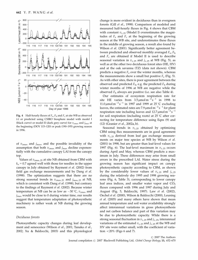
forests (Gill et al., 1998). Comparison of modeled and

measured half-hourly fluxes in Fig. 4 shows that CBM

with constant vx, 25 (Model I) overestimates the magni-

tudes of Fe and Fc at the beginning of the growing

season at the WB site, and underestimates these fluxes

in the middle of growing season, a result also found by

Wilson et al. (2001). Significantly better agreement be-

tween predicted and observed monthly averaged Fe, Fh

and Fc are obtained if Model II is used to describe

seasonal variation in vx, 25 and jx, 25 at WB (Fig. 5), as

well as at the other two deciduous forest sites (HE, HV)

and at the oak savanna (TZ) (data not shown). CBM

predicts a negative Fe over the winter months, whereas

the measurements show a small but positive Fe (Fig. 5).

As with other sites, there is poor agreement between the

observed and predicted Fh, e.g. the predicted Fh during

winter months of 1996 at WB are negative while the

observed Fh always are positive (i.e. see also Table 4).

Our estimates of ecosystem respiration rate for

site HE varies from 3.5mmol m�2 s�1 in 1998 to

11.0mmol m�2 s�1 in 1997 and 1999 at 25 1C excluding

leaves, the estimated rates are 7.9mmol m�2 s�1 for plant

respiration rate including leaves and 12.7mmol m�2 s�1

for soil respiration (including roots) at 25 1C after cor-

recting for temperature difference using Eqns (9) and

(12) (Granier et al., 2002a, b).

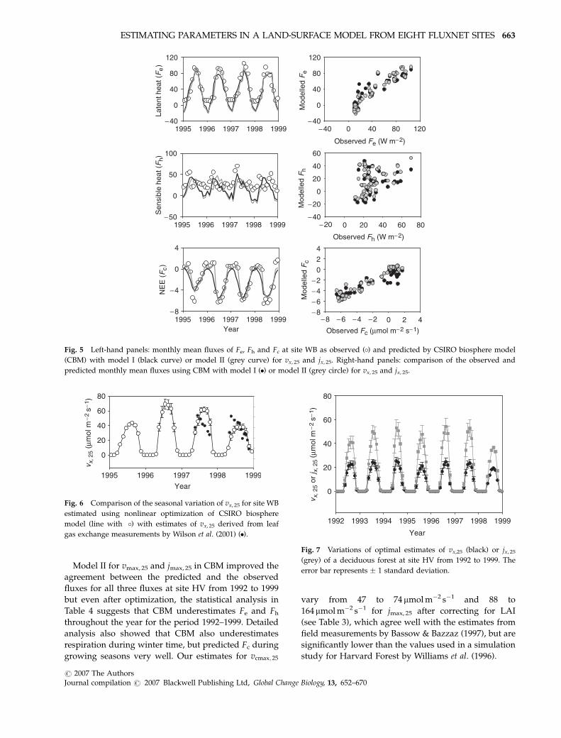
Seasonal trends in vx, 25 obtained by optimizing

CBM using flux measurements are in good agreement

with vx, 25 derived from leaf gas exchange measure-

ments on major tree species at WB by Wilson et al.

(2001) in 1998, but are greater than leaf-level values for

1997 (Fig. 6). The leaf-level maximum in vx, 25 occurs

during April and May, whereas CBM predicts a max-

imum in July. These differences may arise from small

errors in the prescribed LAI. Water stress during the

growing season has significant impact on canopy

photosynthetic capacity according to CBM, as shown

by the considerably lower values of vx, 25 and jx, 25

during the relatively dry 1995 and 1998 growing sea-

sons (Fig. 6, Table 3), corresponding to lower canopy

leaf area indices, and smaller water vapor and CO2

fluxes compared with 1996 and 1997 during July and

August (Fig. 5, Baldocchi, 1997). Law et al. (2002),

Oechel et al. (2000), Wilson & Baldocchi (2000), Leuning

et al. (2005) and many others have shown that mean

annual temperature and soil water availability strongly

affect interannual variations in gross photosynthesis

and net carbon balance and part of this variation may

be due to photosynthetic capacity. While there is a

strong seasonal fluctuation in vx, 25 and jx, 25, interannual

variations of the estimated vx, 25 and jx, 25 at the WB and

HV site were rather small, with the coefficient of varia-

tion o20% (Figs 6 and 7).

115 116 117 118 119 120190 191 192 193 194 195−200

0

200

400

600

800

115 116 117 118 119 120190 191 192 193 194 195

Sen

sibl

e he

at (

W m

−2)

Late

nt h

eat (

W m

−2)

−200

0

200

400

600

Day of year 1996115 116 117 118 119 120190 191 192 193 194 195

NE

E (

µmol

m−2

s−1

)

−40

−20

0

20

Fig. 4 Half-hourly fluxes of Fe, Fh and Fc at site WB as observed

(�) or predicted using CSIRO biosphere model with model I

(black curve) or model II (dark grey curve) for vcmax and jmax at

the beginning (DOY 115–120) or peak (190–195) growing season

in 1996.



Model II for vmax, 25 and jmax, 25 in CBM improved the

agreement between the predicted and the observed

fluxes for all three fluxes at site HV from 1992 to 1999

but even after optimization, the statistical analysis in

Table 4 suggests that CBM underestimates Fe and Fh

throughout the year for the period 1992–1999. Detailed

analysis also showed that CBM also underestimates

respiration during winter time, but predicted Fc during

growing seasons very well. Our estimates for vcmax; 25

vary from 47 to 74 mmol m�2 s�1 and 88 to

164 mmol m�2 s�1 for jmax, 25 after correcting for LAI

(see Table 3), which agree well with the estimates from

field measurements by Bassow & Bazzaz (1997), but are

significantly lower than the values used in a simulation

study for Harvard Forest by Williams et al. (1996).

1995 1996 1997 1998 1999

1995 1996 1997 1998 1999−50

0

50

100

1995 1996 1997 1998 1999−8

−4

0

4

−40 0 40 80 120−40

0

40

80

120

−40

0

40

80

120

−20 0 20 40 60 80−40

−20

0

20

40

60

−8 −6 −4 −2 0 2 4−8

−6

−4

−20

24

Sen

sibl

e he

at (F

h)La

tent

hea

t (F

e)

NE

E (F

c)

Mod

elle

d F

cM

odel

led F

hM

odel

led F

e

Year




Fig. 5 Left-hand panels: monthly mean fluxes of Fe, Fh and Fc at site WB as observed (�) and predicted by CSIRO biosphere model

(CBM) with model I (black curve) or model II (grey curve) for vx, 25 and jx, 25. Right-hand panels: comparison of the observed and

predicted monthly mean fluxes using CBM with model I (�) or model II (grey circle) for vx, 25 and jx, 25.

Year

1995 1996 1997 1998 1999

v x, 2

5 (µ

mol

m−2

s−1

)

0

20

40

60

80

Fig. 6 Comparison of the seasonal variation of vx, 25 for site WB

estimated using nonlinear optimization of CSIRO biosphere

model (line with �) with estimates of vx, 25 derived from leaf

gas exchange measurements by Wilson et al. (2001) (�). Year

1992 1993 1994 1995 1996 1997 1998 1999

0

20

40

60

80

v x, 2

5 or

j x, 2

5 (µ

mol

m−2

s−1

)

Fig. 7 Variations of optimal estimates of vx,25 (black) or jx, 25

(grey) of a deciduous forest at site HV from 1992 to 1999. The

error bar represents � 1 standard deviation.



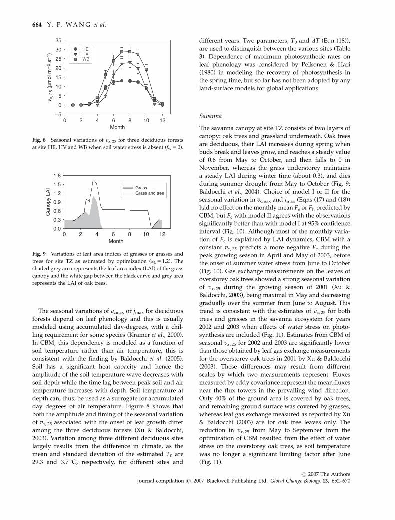
The seasonal variations of vcmax or jmax for deciduous

forests depend on leaf phenology and this is usually

modeled using accumulated day-degrees, with a chil-

ling requirement for some species (Kramer et al., 2000).

In CBM, this dependency is modeled as a function of

soil temperature rather than air temperature, this is

consistent with the finding by Baldocchi et al. (2005).

Soil has a significant heat capacity and hence the

amplitude of the soil temperature wave decreases with

soil depth while the time lag between peak soil and air

temperature increases with depth. Soil temperature at

depth can, thus, be used as a surrogate for accumulated

day degrees of air temperature. Figure 8 shows that

both the amplitude and timing of the seasonal variation

of vx, 25 associated with the onset of leaf growth differ

among the three deciduous forests (Xu & Baldocchi,

2003). Variation among three different deciduous sites

largely results from the difference in climate, as the

mean and standard deviation of the estimated T0 are

29.3 and 3.7 1C, respectively, for different sites and

different years. Two parameters, T0 and DT (Eqn (18)),

are used to distinguish between the various sites (Table

3). Dependence of maximum photosynthetic rates on

leaf phenology was considered by Pelkonen & Hari

(1980) in modeling the recovery of photosynthesis in

the spring time, but so far has not been adopted by any

land-surface models for global applications.

Savanna

The savanna canopy at site TZ consists of two layers of

canopy: oak trees and grassland underneath. Oak trees

are deciduous, their LAI increases during spring when

buds break and leaves grow, and reaches a steady value

of 0.6 from May to October, and then falls to 0 in

November, whereas the grass understorey maintains

a steady LAI during winter time (about 0.3), and dies

during summer drought from May to October (Fig. 9;

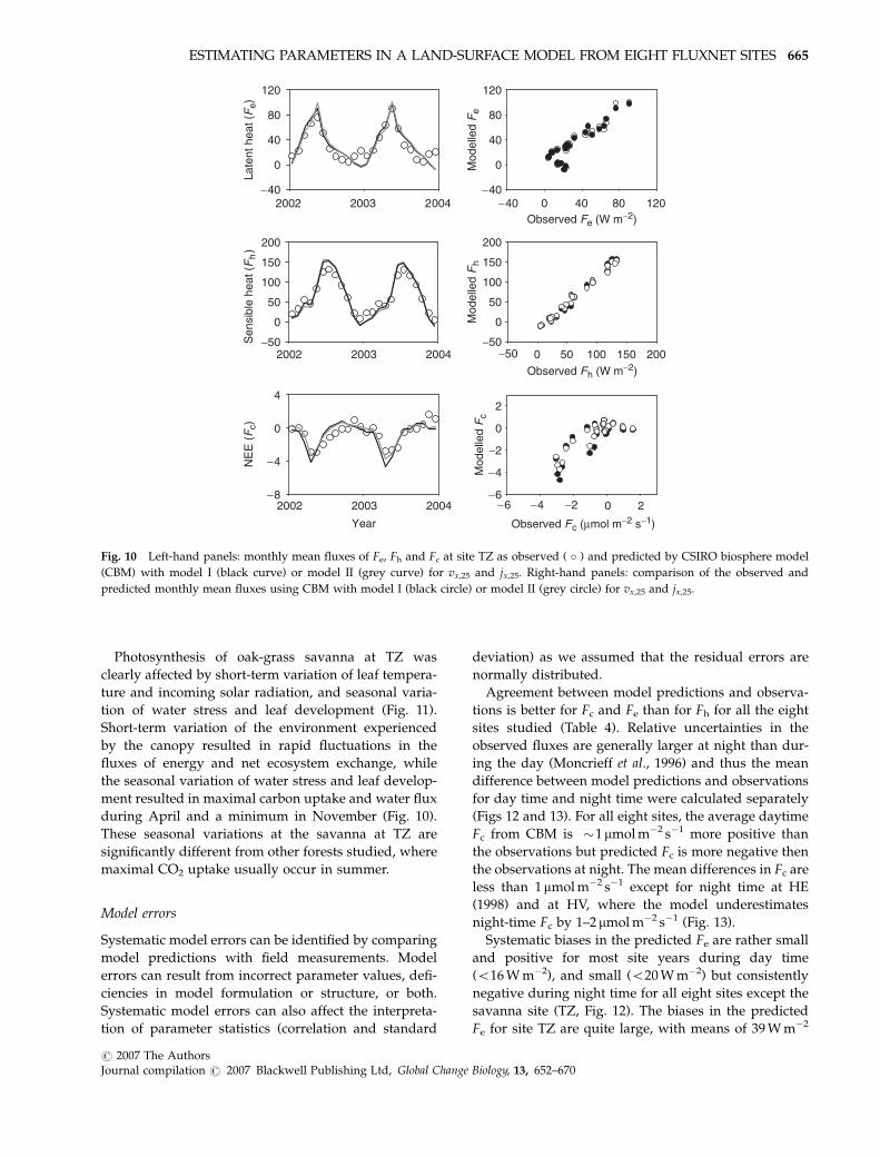
Baldocchi et al., 2004). Choice of model I or II for the

seasonal variation in vcmax and jmax (Eqns (17) and (18))

had no effect on the monthly mean Fe or Fh predicted by

CBM, but Fc with model II agrees with the observations

significantly better than with model I at 95% confidence

interval (Fig. 10). Although most of the monthly varia-

tion of Fc is explained by LAI dynamics, CBM with a

constant vx, 25 predicts a more negative Fc during the

peak growing season in April and May of 2003, before

the onset of summer water stress from June to October

(Fig. 10). Gas exchange measurements on the leaves of

overstorey oak trees showed a strong seasonal variation

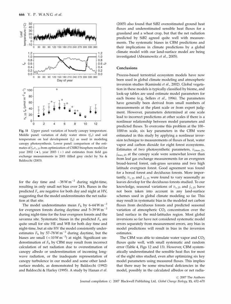
of vx, 25 during the growing season of 2001 (Xu &

Baldocchi, 2003), being maximal in May and decreasing

gradually over the summer from June to August. This

trend is consistent with the estimates of vx, 25 for both

trees and grasses in the savanna ecosystem for years

2002 and 2003 when effects of water stress on photo-

synthesis are included (Fig. 11). Estimates from CBM of

seasonal vx, 25 for 2002 and 2003 are significantly lower

than those obtained by leaf gas exchange measurements

for the overstorey oak trees in 2001 by Xu & Baldocchi

(2003). These differences may result from different

scales by which two measurements represent. Fluxes

measured by eddy covariance represent the mean fluxes

near the flux towers in the prevailing wind direction.

Only 40% of the ground area is covered by oak trees,

and remaining ground surface was covered by grasses,

whereas leaf gas exchange measured as reported by Xu

& Baldocchi (2003) are for oak tree leaves only. The

reduction in vx, 25 from May to September from the

optimization of CBM resulted from the effect of water

stress on the overstorey oak trees, as soil temperature

was no longer a significant limiting factor after June

(Fig. 11).

Month1086420 12

−5

0

5

10

15

20

25

30

35

HEHVWB

v x, 2

5 (µ

mol

m−2

s−1

)

Fig. 8 Seasonal variations of vx, 25 for three deciduous forests

at site HE, HV and WB when soil water stress is absent (fw 5 0).

Month1086420 12

Can

opy

LAI

0.0

0.3

0.6

0.9

1.2

1.5

1.8

GrassGrass and tree

Fig. 9 Variations of leaf area indices of grasses or grasses and

trees for site TZ as estimated by optimization (aL 5 1.2). The

shaded grey area represents the leaf area index (LAI) of the grass

canopy and the white gap between the black curve and grey area

represents the LAI of oak trees.



Photosynthesis of oak-grass savanna at TZ was

clearly affected by short-term variation of leaf tempera-

ture and incoming solar radiation, and seasonal varia-

tion of water stress and leaf development (Fig. 11).

Short-term variation of the environment experienced

by the canopy resulted in rapid fluctuations in the

fluxes of energy and net ecosystem exchange, while

the seasonal variation of water stress and leaf develop-

ment resulted in maximal carbon uptake and water flux

during April and a minimum in November (Fig. 10).

These seasonal variations at the savanna at TZ are

significantly different from other forests studied, where

maximal CO2 uptake usually occur in summer.

Model errors

Systematic model errors can be identified by comparing

model predictions with field measurements. Model

errors can result from incorrect parameter values, defi-

ciencies in model formulation or structure, or both.

Systematic model errors can also affect the interpreta-

tion of parameter statistics (correlation and standard

deviation) as we assumed that the residual errors are

normally distributed.

Agreement between model predictions and observa-

tions is better for Fc and Fe than for Fh for all the eight

sites studied (Table 4). Relative uncertainties in the

observed fluxes are generally larger at night than dur-

ing the day (Moncrieff et al., 1996) and thus the mean

difference between model predictions and observations

for day time and night time were calculated separately

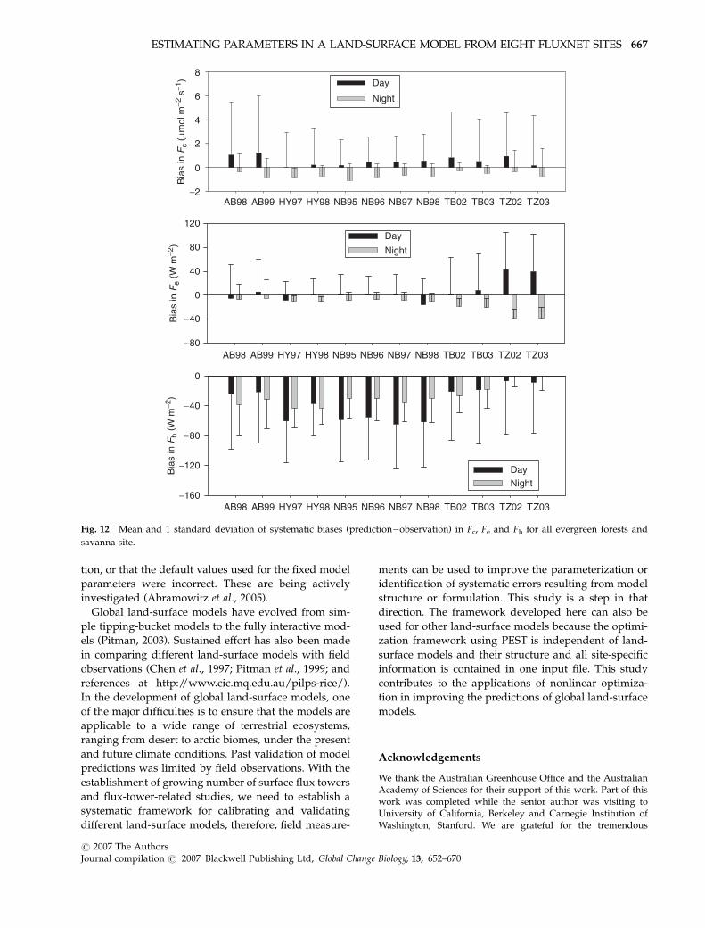
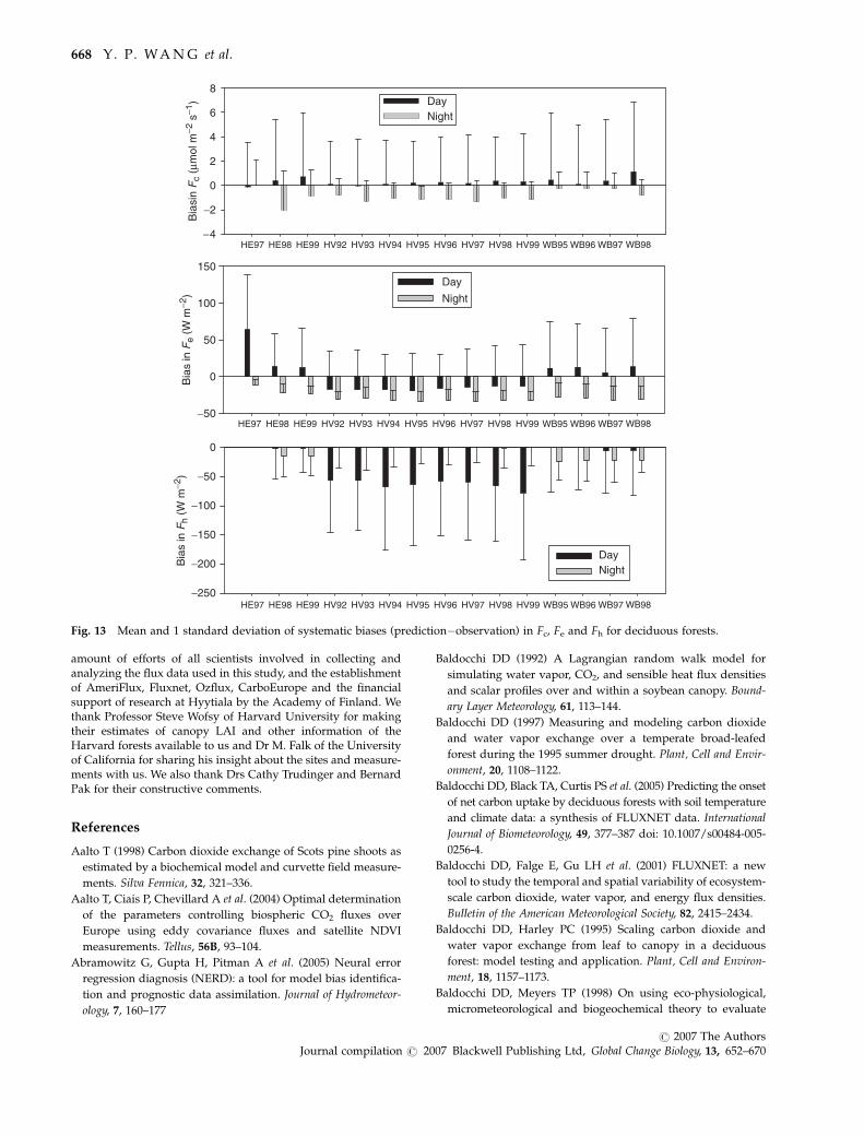
(Figs 12 and 13). For all eight sites, the average daytime

Fc from CBM is �1mmol m�2 s�1 more positive than

the observations but predicted Fc is more negative then

the observations at night. The mean differences in Fc are

less than 1mmol m�2 s�1 except for night time at HE

(1998) and at HV, where the model underestimates

night-time Fc by 1–2 mmol m�2 s�1 (Fig. 13).

Systematic biases in the predicted Fe are rather small

and positive for most site years during day time

(o16 W m�2), and small (o20 W m�2) but consistently

negative during night time for all eight sites except the

savanna site (TZ, Fig. 12). The biases in the predicted

Fe for site TZ are quite large, with means of 39 W m�2

2002 2003 2004

Late

nt h

eat (F

e)

−40

0

40

80

120

2002 2003 2004

Sen

sibl

e he

at (F

h)

−50

0

50

100

150

200

Year

2002 2003 2004

NE

E (F

c)

−8

−4

0

4



−40 0 40 80 120

Mod

elle

d F

e

−40

0

40

80

120

−50 0 50 100 150 200

Mod

elle

d F

h

−50

0

50

100

150

200


−6 −4 −2 0 2

Mod

elle

d F

c−6

−4

−2

0

2

Fig. 10 Left-hand panels: monthly mean fluxes of Fe, Fh and Fc at site TZ as observed ( � ) and predicted by CSIRO biosphere model

(CBM) with model I (black curve) or model II (grey curve) for vx,25 and jx,25. Right-hand panels: comparison of the observed and

predicted monthly mean fluxes using CBM with model I (black circle) or model II (grey circle) for vx,25 and jx,25.



for the day time and �38 W m�2 during night-time,

resulting in only small net bias over 24 h. Biases in the

predicted Fe are negative for both day and night at HV,

suggesting that the model underestimates the net radia-

tion at that site.

The model underestimates mean Fh by 6–64 W m�2

for evergreen forests during daytime and 5–39 W m�2

during night-time for the four evergreen forests and the

savanna site. Systematic biases in the predicted Fh are

quite small for site HE and WB for both day time and

night-time, but at site HV the model consistently under-

estimates Fh by 57–78 W m�2 during daytime, but the

biases are small (o10 W m�2) at night. Significant un-

derestimation of Fh by CBM may result from incorrect

calculation of net radiation due to overestimation of

canopy albedo or underestimation of incoming long-

wave radiation, or the inadequate representation of

canopy turbulence in our model and some other land-

surface models, as demonstrated by Baldocchi (1992)

and Baldocchi & Harley (1995). A study by Hanan et al.

(2005) also found that SiB2 overestimated ground heat

fluxes and underestimated sensible heat fluxes for a

grassland and a wheat crop, but that the net radiation

predicted by SiB2 agreed quite well with measure-

ments. The systematic biases in CBM predictions and

their implications in climate predictions by a global

climate model with our land-surface model are being

investigated (Abramowitz et al., 2005).

Conclusions

Process-based terrestrial ecosystem models have now

been used in global climate modeling and atmospheric

inversion studies (Kaminski et al., 2002). Global vegeta-

tion in these models is typically classified by biome, and

look-up tables are used estimate model parameters for

each biome (e.g. Sellers et al., 1996). The parameters

have generally been derived from small numbers of

measurements at the plant scale or from expert judg-

ment. However, parameters determined at one scale

lead to incorrect predictions at other scales if there is a

nonlinear relationship between model parameters and

predicted fluxes. To overcome this problem at the 100–

1000 m scale, six key parameters in the CBM were

estimated in this study by applying a nonlinear inver-

sion technique to measurements of fluxes of heat, water

vapor and carbon dioxide for eight forest ecosystems.

Estimates of two photosynthetic parameters, vcmax; 25,

jmax, 25 at the canopy scale were somewhat lower than

from leaf gas exchange measurements for an evergreen

broad-leaved forest, oak-grass savanna and two high

latitude evergreen forest. Good agreement was found

for a boreal forest and deciduous forests. More impor-

tantly, vx, 25 and jx, 25 were found to vary seasonally as

leaves develop for the deciduous forests studied. To our

knowledge, seasonal variations of vx, 25 and jx, 25 have

not been taken into account in any land-surface

schemes used in global climate modeling so far. This

may result in systematic bias in the modeled net carbon

fluxes from deciduous forests and predicted seasonal

variation of atmospheric CO2 concentration over the

land surface in the mid-latitudes region. Most global

inversions so far have not considered systematic model

errors separately from measurement errors, any bias in

model predictions will result in bias in the inversion

estimates.

The CBM was able to simulate water vapor and CO2

fluxes quite well, with small systematic and random

error (Table 4, Figs 12 and 13). However, CBM system-

atically underestimated the sensible heat flux for most

of the eight sites studied, even after optimizing six key

model parameters using measured fluxes. This implies

that there may be some structural deficiencies in the

model, possibly in the calculated albedos or net radia-

0 30 60 90 120 150 180 210 240 270 300 330 360

0 30 60 90 120 150 180 210 240 270 300 330 360

Leaf

tem

pera

ture

(°C

)

−100

1020304050

Day of year

f w

0.00.20.40.60.81.01.2

f d

0.00.20.40.60.81.01.2

0 2 4 6 8 10 12

v x, 2

5 f w

(µm

ol m

−2 s

−1)

0

20

40

60

80

100

Fig. 11 Upper panel: variation of hourly canopy temperature.

Middle panel: variation of daily water stress (fw) and soil

temperature on leaf development (fd) as used in modeling

canopy photosynthesis. Lower panel: comparison of the esti-

mates of fwvx, 25 from optimization of CSIRO biosphere model for

year 2002 ( � ), year 2003 ( � ) and estimates from field gas

exchange measurements in 2001 (filled grey circle) by Xu &

Baldocchi (2003).



tion, or that the default values used for the fixed model

parameters were incorrect. These are being actively

investigated (Abramowitz et al., 2005).

Global land-surface models have evolved from sim-

ple tipping-bucket models to the fully interactive mod-

els (Pitman, 2003). Sustained effort has also been made

in comparing different land-surface models with field

observations (Chen et al., 1997; Pitman et al., 1999; and

references at http://www.cic.mq.edu.au/pilps-rice/).

In the development of global land-surface models, one

of the major difficulties is to ensure that the models are

applicable to a wide range of terrestrial ecosystems,

ranging from desert to arctic biomes, under the present

and future climate conditions. Past validation of model

predictions was limited by field observations. With the

establishment of growing number of surface flux towers

and flux-tower-related studies, we need to establish a

systematic framework for calibrating and validating

different land-surface models, therefore, field measure-

ments can be used to improve the parameterization or

identification of systematic errors resulting from model

structure or formulation. This study is a step in that

direction. The framework developed here can also be

used for other land-surface models because the optimi-

zation framework using PEST is independent of land-

surface models and their structure and all site-specific

information is contained in one input file. This study

contributes to the applications of nonlinear optimiza-

tion in improving the predictions of global land-surface

models.

Acknowledgements

We thank the Australian Greenhouse Office and the AustralianAcademy of Sciences for their support of this work. Part of thiswork was completed while the senior author was visiting toUniversity of California, Berkeley and Carnegie Institution ofWashington, Stanford. We are grateful for the tremendous

AB98 AB99 HY97 HY98 NB95 NB96 NB97 NB98 TB02 TB03 TZ02 TZ03



Bia

s in

Fc

(µm

ol m

−2 s

−1)

−2

0

2

4

6

8Day

Night

Day

Night

DayNight

Bia

s in

Fe

(W m

−2)

−80

−40

0

40

80

120

Bia

s in

Fh

(W m

−2)

−160

−120

−80

−40

0

Fig. 12 Mean and 1 standard deviation of systematic biases (prediction�observation) in Fc, Fe and Fh for all evergreen forests and

savanna site.



amount of efforts of all scientists involved in collecting andanalyzing the flux data used in this study, and the establishmentof AmeriFlux, Fluxnet, Ozflux, CarboEurope and the financialsupport of research at Hyytiala by the Academy of Finland. Wethank Professor Steve Wofsy of Harvard University for makingtheir estimates of canopy LAI and other information of theHarvard forests available to us and Dr M. Falk of the Universityof California for sharing his insight about the sites and measure-ments with us. We also thank Drs Cathy Trudinger and BernardPak for their constructive comments.

References

Aalto T (1998) Carbon dioxide exchange of Scots pine shoots as

estimated by a biochemical model and curvette field measure-

ments. Silva Fennica, 32, 321–336.

Aalto T, Ciais P, Chevillard A et al. (2004) Optimal determination

of the parameters controlling biospheric CO2 fluxes over

Europe using eddy covariance fluxes and satellite NDVI

measurements. Tellus, 56B, 93–104.

Abramowitz G, Gupta H, Pitman A et al. (2005) Neural error

regression diagnosis (NERD): a tool for model bias identifica-

tion and prognostic data assimilation. Journal of Hydrometeor-

ology, 7, 160–177

Baldocchi DD (1992) A Lagrangian random walk model for

simulating water vapor, CO2, and sensible heat flux densities

and scalar profiles over and within a soybean canopy. Bound-

ary Layer Meteorology, 61, 113–144.

Baldocchi DD (1997) Measuring and modeling carbon dioxide

and water vapor exchange over a temperate broad-leafed

forest during the 1995 summer drought. Plant, Cell and Envir-

onment, 20, 1108–1122.

Baldocchi DD, Black TA, Curtis PS et al. (2005) Predicting the onset

of net carbon uptake by deciduous forests with soil temperature

and climate data: a synthesis of FLUXNET data. International

Journal of Biometeorology, 49, 377–387 doi: 10.1007/s00484-005-

0256-4.

Baldocchi DD, Falge E, Gu LH et al. (2001) FLUXNET: a new

tool to study the temporal and spatial variability of ecosystem-

scale carbon dioxide, water vapor, and energy flux densities.

Bulletin of the American Meteorological Society, 82, 2415–2434.

Baldocchi DD, Harley PC (1995) Scaling carbon dioxide and

water vapor exchange from leaf to canopy in a deciduous

forest: model testing and application. Plant, Cell and Environ-

ment, 18, 1157–1173.

Baldocchi DD, Meyers TP (1998) On using eco-physiological,

micrometeorological and biogeochemical theory to evaluate

HE97 HE98 HE99 HV92 HV93 HV94 HV95 HV96 HV97 HV98 HV99 WB95 WB96 WB97 WB98



Bia

sin F

c (µ

mol

m−2

s−1

)

−4

−2

0

2

4

6

8DayNight

−50

0

50

100

150Day

Night

Bia

s in

Fh

(W m

−2)

Bia

s in

Fe

(W m

−2)

−250

−200

−150

−100

−50

0

DayNight

Fig. 13 Mean and 1 standard deviation of systematic biases (prediction�observation) in Fc, Fe and Fh for deciduous forests.



carbon dioxide, water vapor and gaseous deposition fluxes

over vegetation. Agricultural and Forest Meteorology, 90, 1–26.

Baldocchi DD, Xu LK, Kiang N (2004) How plant functional-type,

weather, seasonal drought, and soil physical properties alter

water and energy fluxes of an oak-grass savanna and an annual

grassland. Agricultural and Forest Meteorology, 123, 13–39.

Bassow SL, Bazzaz FA (1997) Intra- and inter-specific variation in

canopy photosynthesis in a mixed deciduous forest. Oecologia,

109, 507–515.

Black TA, Den Hartog G, Neumann H et al. (1996) Annual cycle

of water vapour and carbon dioxide fluxes in and above a

boreal aspen forest. Global Change Biology, 2, 219–229.

Braswell B, Sacks WJ, Linder E et al. (2005) Estimating diurnal to

annual ecosystem parameters by synthesis of a carbon flux

model with eddy covariance net ecosystem exchange observa-

tions. Global Change Biology, 11, 335–355.

Chen TH, Henderson-Sellers A, Milley PCD et al. (1997) Cabauw

experiment results from the Project for Intercomparison of

Land Surface parameterization Schemes. Journal of Climate, 10,

1194–1215.

Clapp RB, Hornberger GM (1978) Empirical equations for soil

hydraulic properties. Water Resources Research, 14, 601–604.

Colello GD, Grivet C, Sellers PS et al. (1998) Modeling of energy, water,

and CO2 flux in a temperate grassland ecosystem with SiB2: May–

October 1987. Journal of the Atmospheric Sciences, 55, 1141–1169.

Cowan IR, Farquhar GD (1977) Stomatal function in relation to

leaf metabolism and environment. Symposium of the Society for

Experimental Biology, 31, 471–505.

Dang QL, Margolis HA, Collatz GJ (1998) Parameterization and

testing of a coupled photosynthesis–stomatal conductance

model for boreal trees. Tree Physiology, 18, 141–153.

de Pury DGG, Farquhar GD (1997) Simple scaling of photo-

synthesis from leaves to canopies without the errors of big-leaf

models. Plant, Cell and Environment, 20, 537–557.

Dickinson RE (1983) Land surface processes and climate-surface

albedos and energy balance. Advances in Geophysics, 25, 305–353.

Doherty J (2002) PEST: Model-Independent Parameter Estimation,

4th Edn. Watermark Numerical Computing, Utah, USA.

Falge E, Tenhunen J, Baldocchi DD et al. (2001) Gap-filled

strategies for defensible annual sums of net ecosystem ex-

change. Agricultural and Forest Meteorology, 107, 43–69.

Federer CA (1982) Transpirational supply and demand: plant,

soil, and atmospheric effects evaluated by simulation. Water

Resources Research, 18, 355–362.

Field C (1983) Allocating leaf nitrogen for the maximization of

carbon gain: leaf age as a control on the allocation program.

Oecologia, 56, 341–347.

Field CB, Jackson RB, Mooney HA (1995) Stomatal responses to

increasing CO2: implications from the plant to global scale.

Plant, Cell and Environment, 18, 1214–1225.

Gill DS, Amthor JS, Bormann FH (1998) Leaf phenology, photo-

synthesis, and persistence of samplings and shrubs in a

mature northern hardwood forest. Tree Physiology, 18, 281–289.

Goulden ML, Munger JW, Fan SM et al. (1996) Exchange of

carbon dioxide by a deciduous forest: response to interannual

climate variability. Science, 271, 1576–1578.

Granier A, Ceschia E, Damesin C et al. (2002a) The carbon balance

of a young beech forest. Functional Ecology, 14, 312–325.

Granier A, Pilegaard K, Jensen NO (2002b) Similar net ecosystem

exchange of beech stands located in France and Denmark.

Agricultural and Forest Meteorology, 114, 75–82.

Hanan NP, Berry JA, Verma SB et al. (2005) Testing a model of

CO2, water and energy exchange in Great Plains tallgrass

prairie and wheat ecosystems. Agricultural and Forest Meteor-

ology, 131, 162–179

Jackson RB, Canadell J, Ehleringer JR et al. (1996) A global

analysis of root distributions for terrestrial biomes. Oecologia,

108, 389–411.

Kaminski T, Knorr W, Rayner PJ et al. (2002) Assimilating atmo-

spheric data into a terrestrial biosphere model: a case study of

the seasonal cycle. Global Biogeochemical Cycles, 16, 1066, doi:

10.1029/2001GB001463.

Kelly RH, Parton WJ, Hartman MD et al. (2000) Intra-annual and

interannual variability of ecosystem process in shortgrass

steppe. Journal of Geophysical Research, 105, 20093–20100.

Kirschbaum MUF (1995) The temperature dependence of soil or-

ganic matter decomposition, and effect of global warming on soil

organic matter storage. Soil Biology and Biochemistry, 27, 753–760.

Kowalczyk EA, Garratt JR, Krummel PB (1994) Implementation of

a Soil-Canopy Scheme into the CSIRO GCM – Regional Aspects

of the Model Response. CSIRO, Melbourne (CSIRO Division of

Atmospheric Research technical paper; no. 32).

Kramer K, Leinonen I, Loustau D (2000) The importance of

phenology for evaluation of climate change on growth of

boreal, temperate and Mediterranean forest ecosystems: an

overview. International Journal of Biometeorology, 44, 67–75.

Law BE, Fagle E, Gu L et al. (2002) Environmental controls over

carbon dioxide and water vapor exchange of terrestrial vege-

tation. Agricultural and Forest Meteorology, 113, 97–120.

Leuning R (1995) A critical appraisal of a coupled stomatal–

photosynthesis model for C3 plants. Plant, Cell and Environ-

ment, 18, 339–357.

Leuning R (1997) Scaling to a common temperature improves the

Vcmax. Journal of Experimental Botany, 307, 345–347.

Leuning R (2002) Temperature dependence of two parameters

in a photosynthesis model. Plant, Cell and Environment, 25,

1205–1210.

Leuning R, Cleugh HA, Zegelin SJ et al. (2005) Carbon and Water

Fluxes over a Temperate Eucalyptus Forest and a Tropical

Wet/Dry Savanna in Australia: measurements and compar-

ison with MODIS remote sensing estimates. Agricultural and

Forest Meteorology, 129, 151–173.

Leuning R, Kelliher FM, Depury DGG et al. (1995) Leaf nitrogen,

photosynthesis, conductance and transpiration – scaling

from leaves to canopies. Plant, Cell and Environment, 18,

1183–1200.

Medlyn BE (1996) The optimal allocation of nitrogen within the

C3 photosynthetic system at elevated CO2. Australian Journal

of Plant Physiology, 23, 593–603.

Meir P, Kruijt B, Broadmeadow M et al. (2002) Acclimation of

photosynthetic capacity to irradiance in tree canopies in rela-

tion to leaf nitrogen concentration and leaf mass per unit area.

Plant, Cell and Environment, 25, 343–357.

Moncrieff JB, Malhi Y, Leuning R (1996) The propagation of

errors in long-term measurements of land-atmosphere fluxes

of carbon and water. Global Change Biology, 2, 231–240.



Oechel WC, Ourlitis GL, Hastings SJ et al. (2000) Acclimation of

ecosystem CO2 exchange in the Alaska Artic in response to

decadal climate warming. Nature, 406, 978–981.

Pelkonen P, Hari P (1980) The dependence of springtime recov-

ery of CO2 uptake in Scots pine on temperature and internal

factors. Flora, 169, 398–404.

Pitman AJ (2003) The evolution of, and the revolution in, land

surface schemes designed for climate models. International

Journal of Climatology, 23, 479–510.

Pitman AJ, Henderson-Sellers A, Desborough CE et al. (1999)

Key results and implications from phase 1(c) of the Project for

Intercomparison of Land-Surface Parameterization Schemes.

Climate Dynamics, 15, 673–684.

Raupach MR, Finkele K, Zhang L (1997) SCAM (Soil–Canopy–

Atmosphere Model): description and comparisons with field data.

CSIRO Centre for Environmental Mechanics Technical Report

32, Canberra, Australia.

Rayment MB, Loustau D, Jarvis PG (2002) Photosynthesis and

respiration of black spruce at three organizational scales:

shoot, branch and canopy. Tree Physiology, 22, 219–229.

Reichstein M, Falge E, Baldocchi D et al. (2005) On the separation

of net ecosystem exchange into assimilation and ecosystem

respiration: review and improved algorithm. Global Change

Biology, 11, 1424–1439.

Seibt WA, Brand A, Heimann M et al. (2004) Observations of O2:

CO2 exchange ratios during ecosystem gas exchange. Global

Biogeochemical Cycles, 18, GB4024, doi: 10.1029/2004GB002242.

Sellers PJ, Hall FG, Kelly RD et al. (1997) BOREAS in 1997:

scientific results, overview and future directions. Journal of

Geophysical Research, 102, 28731–28769.

Sellers PJ, Randall DA, Collatz GJ et al. (1996) A revised land

surface parameterization (SiB2) for atmospheric GCMs. Part II:

generation of global fields of terrestrial biophysical parameters

from satellite data. Journal of Climate, 9, 706–737.

Spitters CJT (1986) Separating the diffuse and direct component

of global radiation and its implications for modeling canopy

photosynthesis. Part II: calculation of canopy photosynthesis.

Agricultural and Forest Meteorology, 38, 231–242.

Suni T, Rinne J, Reissell A et al. (2003) Long-term measurements

of surface fluxes above a Scots pine forest in Hyytiala, southern

Finland, 1996–2001. Boreal Environment Research, 8, 287–301.

Tanaka K, Kosugi Y, Nakamura A (2002) Impact of leaf physio-

logical characteristics on seasonal variation in CO2, latent and

sensible heat exchanges over a tree plantation. Agricultural and

Forest Meteorology, 114, 103–122.

Tjoelker MG, Oleksyn J, Reeich PB (2001) Modeling respiration

of vegetation: evidence for a general temperature-dependent

Q10. Global Change Biology, 7, 223–230.

Valentini R, DeAngelis P, Matteucci G et al. (1996) Seasonal net

carbon dioxide exchange of a beach forest with the atmo-

sphere. Global Change Biology, 2, 199–207.

Valentini R, Matteucci G, Dolman AJ et al. (2000) Respiration as

the main determinant of carbon balance in European forests.

Nature, 404, 861–865.

Wang YP (2003) A comparison of three different canopy radia-

tion models commonly used in plant modelling. Functional

Plant Biology, 30, 143–152.

Wang YP, Jarvis PG (1990) Influence of crown structural proper-

ties on PAR absorption, photosynthesis and transpiration in

sitka spruce: application of a model (MAESTRO). Tree Physiol-

ogy, 7, 297–316.

Wang YP, Jarvis PG (1993) Influence of shoot structure on the

photosynthesis of Sitka spruce (picea sitchensis). Functional

Ecology, 7, 433–451.

Wang YP, Leuning R (1998) A two-leaf model for canopy

conductance, photosynthesis and partitioning of available

energy I: model description and comparison with a

multi-layered model. Agricultural and Forest Meteorology, 91,

89–111.

Wang YP, Leuning R, Cleugh HA et al. (2001) Parameter

estimation in surface exchange models using nonlinear inver-

sion: how many parameters can we estimate and which

measurements are most useful. Global Change Biology, 7,

495–510.

Wang Q, Tenhunen J, Falge E et al. (2003) Simulation and scaling

of temporal variation in gross primary production for coniferous

and deciduous temperate forests. Global Change Biology, 10,

37–51.

Willaims M, Scharz PA, Law BE et al. (2005) An improved

analysis of forest carbon dynamics using data assimilation.

Global Change Biology, 11, 89–105.

Williams M, Rastetter EB, Fernandes DN et al. (1996) Modelling

the soil-plant-atmosphere continuum in a Quercus-Acer stand

at Harvard forest: the regulation of stomatal conductance by

light, nitrogen and soil/plant hydraulic properties. Plant, Cell

and Environment, 19, 911–927.

Willmott CJ (1984) On the validation of models. Physical Geogra-

phy, 2, 184–194.

Wilson KB, Baldocchi DD (2000) Seasonal and interannual varia-

bility of energy fluxes over a broadleaved temperate decid-

uous forest in North America. Agricultural and Forest

Meteorology, 100, 1–18.

Wilson KB, Baldocchi DD, Aubinet M et al. (2002) Energy

partitioning between latent and sensible heat flux during the

warm season at FLUXNET sites. Water Resources Research, 38,

1294, doi:10.1029/2001 WR000989.

Wilson KB, Baldocchi DD, Falge E et al. (2003) Diurnal centroid

of ecosystem energy and carbon fluxes at FLUXNET sites.

Journal of Geophysical Research, 108 (D21), 4664, doi: 10.1029/

2001JD001349.

Wilson KB, Baldocchi DD, Hanson PJ (2001) Leaf age affects the

seasonal pattern of photosynthetic capacity and net ecosystem

exchange of carbon in a deciduous forest. Plant, Cell and

Environment, 24, 571–583.

Wofsy SC, Goulden ML, Munger JW et al. (1993) Net exchange of

CO2 in mid-latitude forests. Science, 260, 1314–1317.

Wullschleger SD (1993) Biochemical limitations to carbon

assimilation in C3 plants – a retrospective analysis of the A/Ci

curves from 109 species. Journal of Experimental Botany, 44,

907–920.

Xu LK, Baldocchi DD (2003) Seasonal trends in photosynthetic

parameters and stomatal conductance of blue oak (Quercus

douglasii) under prolonged summer drought and high tem-

perature. Tree Physiology, 23, 865–877.



Documents

Estimating parameters in a land-surface model by applying