Estimating risk premia in money market rates

!"" # #$ !!""" %&

' ($#)*+, -.+ /01(,#2) *+./ 01.34$#)$#/*#356'0 /$ 0) ! 7

5 ) !+87) 9 ) ! 7

!

" #

$ $%&

!

" #

' & ()))

* &+,,---.%/.

0 ()))

' 0 )))%/

!" # $%#&' %(%' %

")*

%*+,"++)+)*!, - $&' %(%' % -

+." /+ 0++)+)123%4 0+)*+)+)

+23%* !", 5

2

%*

"" -

"2',!,+"" 5

Abstract

This paper empirically tests the expectations hypothesis on both daily EONIA swap rates and

monthly EURIBOR rates extended backwards with German LIBOR rates. In addition, we

quantify the size of the risk premia in the money market at maturities of one, three, six and nine

months. Using implied forward and spot rates in a cointegrated VAR model, we find that the

data support the expectations hypothesis in the euro area and in Germany prior to 1999. We find

that risk premia are relatively limited at the shorter maturities but more significant at maturities

of six and nine months. Furthermore, the results on LIBOR/EURIBOR rates tentatively indicate

a downward shift in the structure of the risk premia after the introduction of the euro.

JEL classification: E43,C32

Keywords: Term structure of interest rates; Expectations hypothesis; Cointegrated VAR models

Non-technical summary

The aim of this paper is to estimate the size of the risk premia embedded in the implied forward interest

rates derived from euro area money market interest rates. For this purpose, we estimate a cointegrating

vector autoregressive model (CIVAR) using monthly and daily data for money market interest rates and

implied forward rates.

In order to find estimates of risk premia, we first test whether the expectations hypothesis theory (EH) of

the term structure of interest rates holds true. On German LIBOR data from 1989 until 1998 with monthly

frequency we find that a “weak version” of this theory cannot be rejected on a horizon from one up to

nine months. The weak version of the EH incorporates a constant term premium which increases with

maturity. These estimations suggest risk premia of around 5 basis points at the one-month maturity. The

indicated risk premia increase to around 10 basis points at the three-month maturity, reaching 15 and 27

basis points at the six- and nine-month maturities respectively.

When estimating on a longer sample period, incorporating the period from January 1999 until late 2001

using EURIBOR rates, we no longer find support to the expectations hypothesis. We have two potential

explanations for this. On the one hand, the rejection of the EH may stem from the existence of time-

varying risk premia following the launch of the European single currency. On the other hand, the results

could be explained by a shift in the level of risk premia at different horizons.

We propose to test the latter potential explanation mainly for two reasons. Firstly, according to the

convergence of the different national monetary policies towards the German approach, it would be

surprising that time-varying risk premia should appear with the launch of the European single currency,

given the indications that the risk premia in German money markets before this period were time-

independent. Secondly, according to the results the rejection of the EH seems to be due to only a minor

change in the estimates.

Therefore, we tested for the existence of a structural change in the level of the constant risk premium. We

found that this change probably appeared in January 1999. By re-estimating the models for the whole

sample period, we found that the introduction of EMU has entailed a decrease of risk premia of around 2,

5, 9 and 14 basis points respectively, at the 1-, 3-, 6- and 9-month horizons compared to the estimated risk

premia in German data.

We also tested the expectations hypothesis (using a cointegrating VAR-model) on daily data for the euro

area, using EONIA swap rates. The results seem to support a weak version of the expectations hypothesis

as well, i.e. with a constant term premium. Using two different samples, the estimated risk premia are in

ranges of 0-1, 2, 4-6 and 10-13 basis points at the horizons of one, three, six and nine months

respectively. Although the estimated risk premia for the EONIA market should be interpreted with

caution given the limited sample period, they are fairly close to the results obtained from the analysis on

German LIBOR/EURIBOR data. However, one should keep in mind that the results from the analyses

using EONIA swap rates and LIBOR/EURIBOR rates are not 100 per cent comparable as the credit risks

in EONIA swap rates are lower than in LIBOR/EURIBOR rates.

The empirical evidence from other studies is mixed and few studies give clear indications about the size

of risk premia in money market rates. However, our results seem to be broadly in line with other

comparable studies on European data.

1. IntroductionShort-term interest rates contain information about market participants’ expectations about the stance of

monetary policy in the near future. An assessment of these expectations can prove useful in many ways.

Firstly, knowledge of such expectations helps the central banks to predict whether a particular policy

decision is likely to surprise market participants, and what their short-term response is likely to be to a

given decision. Secondly, measures of interest rate expectations can also be useful to evaluate the central

banks’ communication with financial markets (Goodfriend, 1998 and Fisher, 2001) and, ex post, to assess

whether monetary policy was predictable (Rudebusch, 1995, 1998 and Taylor, 2001).

If there were no uncertainty about the path of future interest rates, forward rates would equal expected

future interest rates. As future interest rates are not known with certainty, risk averse investors will then

require a risk premium to bear this interest risk. Hence, the existence of risk premia, arising from interest

rate risk and investor risk aversion, implies that there will be a wedge between implied forward rates and

the expected future interest rate which normally increases with time. Because the sizes of such risk

premia are unobservable, the "true" market expectations about future interest rates are not known with

certainty.

Forward rates in the euro area can be derived from the term structures of both EONIA swap rates and

EURIBOR rates.1 EURIBOR rates are offered rates on unsecured loans in the interbank market.

Consequently, the forward rates derived from such rates will also include a credit risk premium. The

existence of credit risk premia widens the wedge between the implied forward interest rates and the

expected rates. Just as for term premia, credit risk considerations are likely to increase with maturity.

Credit risk in EONIA swaps is more limited than in EURIBOR since the swaps do not involve an

exchange of principal amounts. The breakdown of risk premia into different categories of risk is beyond

the scope of this analysis, which aims at providing a quantification of the overall risk premia in money

market rates.

In the economic literature, two distinct approaches have been developed for extracting information about

interest rates expectations and risk premia from the term structure of the yield curve. The expectations

hypothesis (EH) theory literature focuses on the time-series properties of interest rates to analyse the

relationship between short and long-term rates.2 The second approach is a market-based “no-arbitrage”

approach, which tries to identify a factor structure affecting the shape of the term structure. This latter

approach assumes stationary stochastic processes for economic fundamentals driving interest rates

1 There exist many other financial instruments from which market expectations can be extracted, for example FRA rates (forward

rate agreements) and EURIBOR futures, see the article "The information content of interest rates and their derivatives formonetary policy" page 37-55 in the ECB Monthly Bulletin of May 2000. See also Svensson and Soderlind (1997) for adetailed description of techniques to extract market expectations from financial instruments and for instance Carlson et al.(1995) for a description of American financial instruments used for this purpose.

5

dynamics, and fundamentals are represented as factors determining the decomposition of interest rates

into expectations and risk premia.3

Following the first approach, the spreads between interest rates at different maturities, or the implied

forward rates extracted from the yield curve, reflect the path of future short-term rates.

To give a sneak preview of our results, the expectations hypothesis was tested in both a single-equation

framework (using the Phillips-Hansen methodology) and a cointegrating vector autoregressive model

(CIVAR). The analysis using a CIVAR-model indicates that the "pure" version of the EH (with no risk

premium) does not hold true in the German-LIBOR market for most of the maturities up to 9 months.

However, the "weak" version of the EH (i.e. with a risk premium constant across time) is supported by

data. The risk premia are found to be increasing with the maturity of the forward rates. Table 1 below

provides a summary of measures of risk premia indicated from this analysis and other studies.

Moreover, adding EURIBOR data from January 1999 to the German LIBOR data implicated that the EH,

using the Phillips-Hansen methodology, was slightly rejected at maturities of three months and beyond.

Among potential explanations, this paper explicitly test the hypothesis of a level shift in the constant risk

premia according to the Gregory and Hansen (1996) methodology. The results suggest that the constant

risk premia decreased for all maturities after the launch of the European single currency in 1999. More

specifically, the risk premia amounted at 2, 5, 9 and 14 basis points respectively for the one-, three-, six-

and nine-months for the whole sample (see Table 1).

Our results are broadly in line with other comparable studies on data for European countries (e.g. Gerlach

et.al., 1997, Cassola et.al., 2001, and Cuthbertson et. al., 2000, Brooke et. al., 2000). However, most

studies focus on whether the expectations hypothesis holds true. The number of other studies quantifying

the size of risk premia in interest rates is relatively limited. Cassola et.al. (2001) find evidence that the

term premium in German interest rates from 1972 to 1998 is around zero basis points for the one-month

maturity, increasing to around 40-50 basis points at the twelve-month maturity. Brooke et. al. (2000)

estimate the size of term premia by comparing implied two-week interbank forward rates derived from

the UK money market instruments with actual outturns of the two-week repo rate. The average biases

suggested that term premia embodied in interbank forward rates are significant beyond a six-month

horizon. They tentatively indicate that the average biases over the period from January 1993 to September

2002 for six-month, one-year and two-year maturities were 23, 45 and 109 basis points respectively. They

2 Among others, see Shiller et al., 1983, and Campbell and Shiller, 1991.3 For more details, see for instance Balduzzi, Das, Foresi and Sundaram, 1996.

-

believe that credit risk considerations may account for 20-25 basis points, on average for these

maturities.4

The note is organised as follows. Section 2 presents briefly the data. In Section 3, we present some other

empirical evidence. In Section 4 we present our empirical results. Section 5 concludes.

Table 1. Indicated risk premia at different maturities (basis points)

Months Ahead 1 month 3 months 6 months 9 months

ESTIMATIONS:

Monthly data (German LIBOR /EURIBOR):

1989.12-1998.12 (Germany) 5 10 15 27

1989.12-2001.8: (Germany and euro area, pre

terrorist attacks)

5 n.a1) n.a1) n.a1)

1989.12-2002.2: (Germany and euro area) 5 n.a1) n.a1) n.a1)

Daily data (EONIA SWAP rates):

Jan. 1999-Sept. 2001: 0 2 6 10

Jan. 1999-June 2002: 1 2 4 13

OTHER STUDIES:

Cassola and Luis (Germany, 1972-1998)2) 0-5 5-10 20-25 25-35

Brooke et. al (UK, 1993-2000)3 23

Gravelle et.al. (Canada, 1988-1998) 6 20 58 100

1) Not available because "expectations hypothesis" is formally rejected

2) Approximate values, see ECB working paper No. 46, page 51.

3) Risk premia embedded in interbank implied forward rates compared with the two-week official monetary policyrepo rate. This study finds that the risk premia are 45 and 109 basis points for the one-year and the two-yearmaturities respectively

4 The credit risk spread stems from the fact that they use interbank forward rates, which contain credit risks, and compare with

the outturns of the official repo rate of the Bank of England, which is given on loans with collateral, thus almost free of creditrisks.

2. Data

Two different data sets are used in our estimations: A daily data set of EONIA swap rates from beginning

1999 to 5 June 2002 and a data set of monthly averages of EURIBOR rates extended backwards with

German LIBOR rates, covering the period between December 1989 and February 2002. EONIA swap

rates are superior to the EURIBOR in providing information about market expectations. However, before

the introduction of the euro money market the national swap markets were not liquid enough to provide as

reliable information as could be derived from the LIBOR markets.

2.1 Daily data - EONIA swap rates

In an EONIA swap, two parties agree to exchange the difference between the interest accrued at an

agreed fixed interest rate for a fixed period on an agreed notional amount and interest accrued on the

same amount by compounding EONIA daily over the term of the swap.5 The ‘fixed leg’ of this agreement

is referred to as the EONIA swap rate. Hence, the EONIA swap rates reflect the expected average EONIA

rate over the maturity of the swap contract. EONIA swap rates are traded for maturities from one to three

weeks and one to twelve monthsplus maturities of 15, 18, 21 and 24 months.

Chart 1: ECB interest rates and the EONIA

(annual percentages, daily data)

Chart 2: EONIA swap rates

(annual percentages, daily data)

Sources: ECB and Reuters

5 It is only possible to roll over investments on workdays. Thus, on working days the EONIA swap rates are based on daily

compounding, while it is treated as a simple rate over weekends.

1.5

2.0

2.5

3.0

3.5

4.0

4.5

5.0

5.5

6.0

Jan99

Jul99

Jan00

Jul00

Jan01

Jul01

Jan02

Jul02

1.5

2.0

2.5

3.0

3.5

4.0

4.5

5.0

5.5

6.0

overnight interest rate (EONIA)

ECB minimum bid rate

1.5

2.0

2.5

3.0

3.5

4.0

4.5

5.0

5.5

6.0

Jan99

Jul99

Jan00

Jul00

Jan01

Jul01

Jan02

Jul02

1.5

2.0

2.5

3.0

3.5

4.0

4.5

5.0

5.5

6.0

1 month 6 month 1 year

The EONIA is computed, by the ECB, as a weighted average of all overnight unsecured lending

transactions made in the euro area interbank market by a panel of primary banks. Normally the EONIA is

traded close to the ECB minimum bid rate in the main refinancing operations, see Chart 1.

The EONIA sometimes differs markedly from the minimum bid rate. Interest rate expectations6 or the

liquidity conditions can usually explain these discrepancies. Calendar effects (at the last business day of

the month, quarter or year) from balance sheet considerations of financial institutions can also affect the

liquidity conditions.

In Chart 2 the EONIA swap rates with maturities of one, six and twelve months show the same pattern as

the EONIA in Chart 1. When the minimum bid rate is expected to increase, as in most of 2000, the

twelve-month swap rates are generally higher than the shorter maturities of one- to six-months due to

higher expected averages of the future EONIA.

The nature of the swap arrangement also limits the credit risk since no principle amounts are exchanged.7

The swap rates therefore provide a more exact indication of the term premium the market adds due to

increasing uncertainty for future interest rates.

Since early 1999 the swaps linked to the EONIA have replaced swaps linked to the EURIBOR as the

main reference swap rate in the euro money market.8 Thus, in the regression analysis for the sample

period from 1 January 1999 onwards we use implied forward rates computed from the term structure of

the EONIA swaps.9

Charts 3 and 4 display the implied one-month forward rate in one and six months and the one-month spot

rate with a one-month and six-month lead respectively. The predictions by the forward rates are quite

accurate on the one-month horizon whereas the difference between actual and predicted rates is somewhat

6 If market participants expect changes in the ECB rates within the reserve maintenance period the liquidity demand is affected in

the direction of the expectations. For example, expectations of an increase in interest rates in the reserve maintenance periodcan lead to higher liquidity demand and drive up the EONIA as market participants expects the cost of lending to be higher inthe following period.

7 The credit risk embedded in EONIA swap rates reflect therefore almost uniquely the credit risk premium on overnighttransactions as included in the EONIA.

8 For further information see Santillan et.al. (2000).9 Implied forward rates can be computed using the following equation:

ijii

ti

jitji

t mmmr

mr

f−

−

+

+=

+

++ 1200

*1

1200*1

1200*1

,

,ji,

Where ft i,j represents the implied forward rate at time t for the i-month interest rate in j months. The rates ri+j,t and ri,t represents

the spot rates with maturity i and i+j at time t, respectively. m refers to the maturity of the EONIA swap.

larger on the six-month horizon, as actual out turns normally are harder to predict the further ahead one

looks.

Chart 3: Implied one-month forward rate in

one month and one-month EONIA swap rates

(with a one-month lead)

(annual percentages, daily)


six months and one-month EONIA swap rates

(with a six-month lead)

(annual percentages, daily)

Sources: Reuters and own calculations.

2.2 Monthly data - GERMAN LIBOR and EURIBOR

The LIBOR and the EURIBOR rates are weighted average interbank offered rates and both are regarded

to be highly representative benchmark rates respectively for Germany until December 1998 and the euro

area thereafter. LIBOR and EURIBOR are interest rates on exchange of uncollateralised short-term

liquidity quoted by primary banks. The unsecured nature of these loans implies that some premium for

credit risk is likely to be embedded in the rates.

We used monthly averages for German LIBOR rates from December 1989 until December 1998 and

EURIBOR rates from 1999 until February 2002. Chart 5 below illustrates the developments of these

monthly data for the one- and nine-month maturities together with the Bundesbank’s official tender rate

spliced with the ECB fixed rate/minimum bid rate from 1999. The LIBOR/EURIBOR rates follow the

refinancing rate set by the central bank closely.

2.0

2.5

3.0

3.5

4.0

4.5

5.0

5.5

Jan99 Jul99 Jan00 Jul00 Jan01 Jul01 Jan02

2.0

2.5

3.0

3.5

4.0

4.5

5.0

5.5

forward spot

2.0

2.5

3.0

3.5

4.0

4.5

5.0

5.5

Jan99 Jul99 Jan00 Jul00 Jan01 Jul01 Jan02

2.0

2.5

3.0

3.5

4.0

4.5

5.0

5.5

forward spot

Chart 5: Central bank reference rate and

interbank offered rate

(annual percentages, monthly averages)

Sources: Bundesbank, ECB, Reuters and BloombergNote: From December 1989 to December 1998 Bundesbank tender rate and German LIBOR rates areused. Since 1999 the ECB minimum bid rate and EURIBOR rates are used.

As for the EONIA swap rates, market expectations are extracted using implied forward rates based on the

LIBOR/EURIBOR money market yield curve. The one-month implied forward rate in one and three

months are presented in Charts 6 and 7 together with the actual one-month spot rate with one and three

months lead. "Predicted" and actual outturns of the interest rates are relatively close for most of the

period. The main exceptions are at the beginning of the sample.10

10 The average historical difference between the one-, three-, six- and nine-month German LIBOR/EURIBOR rates and the

corresponding implied forward rates (i.e. with a lead of one, three, six and nine months) were 4, 7, 5 and 12 basis pointsrespectively in the period between December 1989 to February 2002.

2.0

3.0

4.0

5.0

6.0

7.0

8.0

9.0

10.0

11.0

1989

1990

1991

1992

1993

1994

1995

1996

1997

1998

1999

2000

2001

2

3

4

5

6

7

8

9

10

11

reference rate 1 month 9 month


one-month and one-month LIBOR/EURIBOR

rates (with a one-month lead)

(annual percentages, monthly)


three months and one-month LIBOR /

EURIBOR rates (with a three-month lead)

(annual percentages, monthly)

Sources: Bloomberg, Reuters and own calculations.

2

3

4

5

6

7

8

9

10

11

1989

1990

1991

1992

1993

1994

1995

1996

1997

1998

1999

2000

2001

2

3

4

5

6

7

8

9

10

11

implied forward spot rate

2.0

3.0

4.0

5.0

6.0

7.0

8.0

9.0

10.0

11.0

1989

1990

1991

1992

1993

1994

1995

1996

1997

1998

1999

2000

2001

2

3

4

5

6

7

8

9

10

11

implied forward spot rate

3. Empirical evidence from other studies

In general, most studies test the EH theory by estimating the relationship between actual outturns of

interest rates and the implied forward rates derived from the yield curve:11

(1) R(n)t = α + β f k(n)t-k+ et ,

where f k(n)t-k is the forward rate at time t-k of an n period instrument beginning in k periods, R(n)t is the

spot rate at time t of an n period instrument, and et is the residual. Here, postulating the expectations

hypothesis is the same as assuming that β=1. Thus, if β is significantly different from unity, the EH

theory is rejected. The constant term α can be interpreted as a constant risk premium if β is strictly equal

to one.12 Moreover, the ’strong’ version of the EH theory holds true only if β=1 and at the same time α=0.

The ’weak’ version of the EH theory holds true if the estimated β=1 and at the same time α ≠0.13

The empirical literature on the term structure of interest rates contains disparate pieces of evidence about

the predictive power of the yield curve in the money and the capital market. Most studies seem to agree

on the following "stylized facts": First, whereas the strong version of the EH (the spread between

maturities or the implied forward rates are unbiased predictors of the future spot rate) is rejected in most

cases, the studies, however, suggest that there is an important element of "truth" to the expectations

theory of the term structure. Most studies find that the forward rates have a high predictive power of

actual outturns of spot interest rates, i.e., when regressing implied forward rates on the actual outturns, the

estimated coefficient (the estimated β-value) is typically found to be significantly positive. Secondly, the

EH seems to receive more support in the money market (with maturities up to 12 months) than for longer

maturities. Thirdly, at the very short end of the yield curve (up to 3 months), the weak version of the EH

(with a time-invariant but maturity dependent risk premium) seems to gain support in most studies.

Finally, the predictive content of the yield curve appears to be higher in European countries than in the

United States.

Brooke et.al. (2000) estimate the size of term premia in UK data by comparing implied two-week

interbank forward rates derived from money market instruments with actual outturns of the two-week

11 Some studies normally avoid the possibility of spurious regression by running the regression in Equation (1) in first differences

but the possibility of integrated data gives the opportunity of constructing information tests based on the existence of acointegrating relationship between the ’forecast’ and outturn.

12 See for instance Cuthbertson et al. (2000) and Bhundia et al. (1998).13 The expectations hypothesis is explained in Shiller (1973), Shiller et al. (1983), Engle (1987), Mishkin (1988), Gravelle et al.

(1998) and Jondeau (2001).

6

repo rate. If term premia are broadly stable and if the sample period is sufficiently long, expectational

error should average out to zero. Any remaining bias should then represent the average term premium,

though this method also will pick up differences between the money market instruments used and the

repo rate that are related to liquidity and credit quality. They find that term premia embodied in interbank

forward rates are significant beyond a six-month horizon. They tentatively indicate that the average risk

premia over the period from January 1993 to September 2001 for six-month, one-year and two-year

maturities were 23, 45 and 109 basis points respectively. However, credit risk considerations may account

for 20-25 basis points, on average for these maturities.

Cassola et al. (2001), find that a "two-factor constant volatility"-model on German data quite well

describes the yield curve from 1972 to 1998. Their results indicate that term premia are negligible at the

maturity of one month but increasing to around 40-50 basis points at the twelve-month maturity.

Using a single-equation model and "imposing" that the EH theory holds true, Gravelle et al. (1998) find

on Canadian data that the constant term premium increases with the maturity of the forward rate, going

from 6 to 20, and from 58 to 100 basis points when the maturity increases from 1 to 3, and from 6 to 9

months respectively. In addition, they find that the risk premium is 47 basis points at the maturity of nine

months in the United States. This study is based on FRA interest rates (forward interest rate agreements)

which may include some additional risk premia compared with EONIA swaps and EURIBOR rates, i.e.

higher liquidity and credit risk premia.

Studies using Cointegrating regressions

The empirical literature on the term structure of interest rates received a new impulse from the pioneer

works of Campbell and Shiller (1987, 1991). They were the first to test the EH by testing for a

cointegration relationship between interest rates in a VAR framework, using US money market and

capital market data. Their idea was that, if the EH holds strictly true, then the slope of the yield curve

does only depend on the future fluctuations of the short rates. A necessary (but not sufficient) condition

for the EH to hold true is that, if both the short-term and the long-term interest rates are integrated of the

same order, there must exist a cointegrating relationship between these rates. As a second condition, the

sum of the coefficients inside the cointegrating vector must be equal to zero, i.e. there must be a long term

one-to-one relationship between the interest rates at different maturities (homogeneity of degree 1). The

studies by Campbell and Shiller were followed by several studies using this framework to test the validity

of the EH theory. Some of them are reported in Table 2. In particular, these studies show that nominal

interest rates are characterised as being integrated of order one and that they tend to move together

enabling them to be cointegrated.

Campbell and Shiller (1991) did not find the spread between interest rates of maturities up to 12 months

significant in explaining the developments of the spot rates, except for at the one-month maturity. And

even for the one-month maturity the restriction imposed by the EH theory, i.e. a long-term unit

relationship between yield spreads and future changes in interest rates, was rejected. However, using

different samples and specifications, Jondeau and Ricart (1999) and Jondeau (2001), both on US data,

find that the coefficient for the spread is significantly different from zero but also significantly different

from unity, thus rejecting the EH.

The study from Gravelle et al. primarily tests the EH theory on Canadian data in a VAR model. Using

such model they reject the EH theory. Their evidence suggests that the formal rejection of the EH theory

is due to the existence of a time-varying term premium. The existence of a time-varying risk premium

also gains support in some other studies.14

For studies on European countries, the picture is mixed. While most studies cannot reject the

cointegration hypothesis, Bundhia and Chadha (1998) cannot find evidence that β=1 for the sterling

futures market, i.e the EH theory is rejected. By contrast, the study of Cuthbertson, Hayes and Nitzsche

(2000) cannot reject the EH theory for the German money market. Jondeau (2001) cannot reject the

expectations theory on French and British data. On the other hand, the study suggests that the EH theory

is in most cases rejected on German data.

14 See for example Campbell and Shiller (1987), Engle and Ng (1993), Iyer (1997) and Jondeau (2001).

5

Table 2: Results of testing the EH in the literature using cointegrating regressions

Maturity ofone-period rate β )ˆ.(. βes Sample

periodAuthors

1 month 0.50*1.02*0.99*

0.120.010.01

1952-871984-961976-93

Campbell&Shiller (1991) on US dataBhundia&Chadha (1998) on UK dataCuthbertson, Hayes&Nitzsche (2000) on German data

2 months 0.201.73*1.04*0.99*

0.280.500.020.01

1952-871976-861984-961976-93

Campbell&Shiller (1991) on US dataEngsted&Tanggaard (1995) on Danish dataBhundia&Chadha (1998) on UK dataCuthbertson, Hayes&Nitzsche (2000) on German data

3 months -0.151.59*1.05*0.45*0.71*0.56*0.71*1.03*0.67*0.72*0.60*0.74*

0.200.410.010.160.150.080.230.010.170.230.110.14

1952-871976-861984-961975-971975-971975-971975-971976-931982-971982-971982-971982-97

Campbell&Shiller (1991) on US dataEngsted&Tanggaard (1995) on Danish dataBhundia&Chadha (1998) on UK dataJondeau&Ricart (1999) on US dataJondeau&Ricart (1999) on UK dataJondeau&Ricart (1999) on German dataJondeau&Ricart (1999) on French dataCuthbertson, Hayes&Nitzsche (2000) on German dataJondeau (2001) on US dataJondeau (2001) on UK dataJondeau (2001) on German dataJondeau (2001) on French data

6 months 0.041.13*1.13*0.120.71*0.63*0.82*1.03*0.400.64*0.64*0.69*

0.330.260.080.280.180.130.170.010.240.210.110.20

1952-871976-861984-961975-971975-971975-971975-971976-931982-971982-971982-971982-97


12 months -0.020.84*1.220.55*0.77*0.91*0.72*1.07*0.210.68*0.68*0.73*

0.370.353.750.240.200.210.120.030.300.220.150.21

1952-871976-861984-961975-971975-971975-971975-971976-931982-971982-971982-971982-97


* denotes the estimates of β’s are significantly different from zero. While these studies employ different methodologies fortesting the EH, all of them are based on the assumption that the money market interest rates at different maturities arecointegrated.

-

4. Results from estimating risk premia in a cointegrating vector

autoregressive framework

We first test the EH in a framework using cointegration analysis estimating the long run relationship

between the spot interest rates and the forward rates using the Phillips-Hansen methodology15 (in a single-

equation regression). Second, we will estimate the dynamic relationship between the spot and forward

rates using a cointegrating vector autoregressive model (CIVAR).

While the Phillips-Hansen methodology allows to test explicitly the EH using the long-run equilibrium,

the CIVAR methodology takes into account also the short term dynamics and is useful in determining

forecasts of the expected spot rate in the future. The former methodology corrects for non-normality (and

autocorrelation) in the residuals and is therefore useful as a cross check of the results of the VAR

estimations. Moreover, the VAR methodology will be particularly useful for testing the null hypothesis of

a constant risk premium. It will also give an estimation of the size of the risk premia given that the EH is

not rejected. Both methods take into account the non-stationary feature of the interest rates in levels

which may be useful in order to avoid some bias associated with standard single-equation estimations of

the expectation hypothesis as suggested by Thornton (2001).16

4.1 German LIBOR and EURIBOR rates

The first step in the econometric analysis is to check the existence of cointegration between the spot rates

and the implied forward rates. We computed two tests of cointegration, the Engle-Granger (1987) test and

the Johansen and Juselius (1990) test.17 Table 3 summarizes the results from the Johansen tests. The

results suggest that for all horizons the null hypothesis of cointegration between spot and forward rates is

not rejected. These results are confirmed by the Engle & Granger cointegration tests18 and we therefore

conclude that the one-month spot rate and the one-month implied forward rate with horizons of one to

nine months are cointegrated.19 Subsequently, we tested the EH theory taking into account the non-

stationarity of the money market interest rates as suggested by the cointegration tests.

15 See Phillips et al. (1990).16 We present a demonstration of his argument in Appendix 1.17 See Appendix 2 for more details about the methods for testing cointegration.18 See Appendix 3.19 These results are in line with the results for other countries on monthly data (see for example Engsted, 1999, 2000).

Table 3. Johansen test for cointegration (stochastic matrix test). German LIBOR

Horizon H0 trace-test p-value

cointegrating vector

restriction test1

(p-value)

One month r <= 0 13.349 0.033 * 0.69

(r1mt+1m

- ft1m,1m) r <= 1 0.54702 0.526

Three-month r <= 0 12.348 0.049 * 0.06

(r1mt+3m

- ft1m,3m) r <= 1 0.4831 0.556

six-month r <= 0 9.2972 0.153 0.00 **

(r1mt+6m

- ft1m,6m) r <= 1 0.3891 0.604

Nine-month r <= 0 6.5206 0.377 0.00 **

(r1mt+9m

- ft1m,9m) r <= 1 1.4415 0.269

Note: A number of 12 lags have been used. The test statistics for H(rank≤p) are listed with p-values based onDoornik and Hendry (2001); ** and * mark significance at 95% and 99%. Testing commences at H(rank=0), andstops at the first insignificant statistics. Sample period is 1989.12-1998.12.1) The statistic shown for this test is the p-value of the null hypothesis test that the cointegrating vector β coefficientis equal to 1. ** indicates the rejection of the null hypothesis at a significance level of 1%.

4.1.1 Estimations using the Phillips-Hansen methodology

By using the Phillips-Hansen methodology, we estimated the cointegrating relationship between forward

and spot rates. Three different sample periods were used. Sample A cover the period from December

1989 to December 1998 (i.e. only German data). Sample B covers the period from December 1989 up to

the terrorist attacks in September 2001 and sample C covers the period from December 1989 to February

2002. In sample B and C, monthly observations from the EURIBOR market (from January 1999 to

February 2002) were spliced with data from the German LIBOR market. This allows us to check whether

the observations since the introduction of the euro in January 1999 affect the results. Sample B excludes

the period after the terrorist attacks on 11 September 2001 and the following turmoil in financial markets.

Market participants could not possibly predict the following substantial decrease in money market interest

rates. We therefore suspect that the results for the sample including the observations after these events

could be distorted by significant expectational errors.

The Phillips-Hansen estimator (also called the Fully Modified Ordinary Least Squares (FM-OLS)

estimators method) is appropriate for estimation and inference when there exists a single cointegrating

relationship between a set of I(1) variables.20 This econometric methodology does not follow the standard

20 The methodology is briefly outlined in Appendix 4.

statistical inference. Broadly speaking, Phillips and Hansen (1990) proposed a method that corrects for

both endogeneity in the data and asymptotic bias in the coefficient estimates. As mentioned, this

methodology takes into account problems with autocorrelation and non-normality of the residuals.

Table 4: Phillips-Hansen cointegrating regressions: R(n)t = α + β f k(n)t-k

ExplanatoryVariable

Sampleperiod

Lags ofwindow α β Wald statistic

A 13-.0126(.0603)

.9992(.0093)

.0057[.939]

B 13-.0326(.0489)

1.0019(.0081)

.0574[.811]

1 month

C 13-.0383(.0468)

1.0025(.0078)

.1050[.746]

A 12-.3090(.1569)

1.0473(.0251)

3.546[.060]

B 12-.2861(.1285)

1.0449(.0636)

4.2626[.039]*

3 month

C 12-.2974(.1239)

1.0462(.0211)

4.7471[.029]*

A 13-.5690(.4020)

1.1144(.0509)

3.2310[.072]

B 13-.5459(.3103)

1.1124(.0523)

4.6017[.032]*

6 month

C 13-.5904(.2996)

1.1181(.0510)

5.3562[.021]*

A 11-1.1065(.6094)

1.1901(.0988)

3.6977[.054]

B 11-.9555(.4958)

1.1692(.0851)

3.9545[.047]*

9 month

C 11-1.0039(.4842)

1.1752(.0837)

4.3767[.036]*

Note: Column 3 reports the number of lags used for truncation. Columns 4 and 5 report the value of each coefficientwith their standard errors in parentheses while the last column reports the Wald test statistics for the nullhypothesis β=1 with the p-value between brackets. * denotes rejection at the 5% significance level.

The Phillips-Hansen (1990) fully modified estimators of the cointegrating parameters are shown in Table

4 21. The Phillips-Hansen modified estimator allows a valid test (Wald test) that the cointegrating vector is

(1,-1). This restriction, on a one-month horizon, is not rejected on any sample investigated. Moreover, on

sample A the restriction imposed on the cointegrating vector (1,-1) is not rejected at any maturity. The

results on the German sample are in line with the results in Cuthbertson et al. (2000) who find that

German money market interest rates "appear to conform reasonably closely to the expectations hypothesis

of the term structure with a constant term premium."

However, on sample B and C the restriction tests (Wald statistic) are formally rejected at a 5%

significance level for the three-, six- and nine-month horizons. Strictly interpreted, this means that the

expectations hypothesis is formally rejected when adding EURIBOR data to the German LIBOR dataset

at maturities beyond one-month. Second, the value of the β- coefficient is increasing with maturity.

Moreover, the p-value of the Wald test is smaller on sample B and C than on sample A, which may be

interpreted as a change in the long-run relationship.

These results suggest that, at the very short end of the yield curve in the money market (i.e. at the one-

month horizon), there is not much difference between the samples as the expectations hypothesis seems to

hold true on all of them. From the three-month horizon and onwards, the hypothesis is rejected on the

extended samples B and C, although only slightly. These results may suggest that "something" changes

after January 1999 (see below). A possible explanation could be a different structure of risk premia before

and after January 1999. Finally, the rejection of the test does not seem to be only explained by the

disturbances from the "unexpected" decreases of interest rates following the terrorist attacks, as the EH is

rejected both on sample B (which ends in August 2001) and C (which ends in February 2002).

The recursively estimated coefficient for the forward rates (β-coefficient) for the six-month maturity is

shown in Chart 8. In Appendix 5 similar charts are displayed also for the other maturities investigated.

The conclusions are the same for all maturities: The coefficients are broadly stable.

Chart 8: Recursive estimation of β using the Phillips-Hansen methodology

Coef. of FLI1M6M and its 2 S.E. bands based on recursive OLS

Months

-0.5-1.0-1.5-2.0-2.5

0.00.51.01.52.0

1987M7 1990M1 1992M7 1995M1 1997M7 2000M1 2002M2

21 Note that they use for that the results from Newey and West (1987) which is also the case with the autocorrelation- and

4.1.2 The Cointegrating Vector Autoregressive Estimations (CIVAR)

The VAR framework allows evaluating the potential impact of short-term dynamics on the long-term

relationship. Given the inherent problem of overlapping observations, the chosen number of lags in the

CIVAR was primarily selected to eliminate serial correlation and secondly, the lag structure was selected

to minimise the AIC and HQ information criteria22. The VAR approach also allows to test the empirical

content in the EH theory. A further description of the VAR methodology is presented in Appendix 6.

We estimated the two-equation CIVAR for three sample periods: First, we estimated only for the German

period (i.e. from December 1989 to December 1998). Second, we re-estimated the same model for a

sample period until September 2001 and a period until February 2002. Regarding the sample period

ending in December 1998, we first estimated a cointegration relationship between the one-month money

market interest rate and the one-month implied forward rate at different horizons with an unrestricted

intercept as suggested by Johansen (1990). Inside this framework, we tested the null hypothesis of β=1

which was rejected at the six and nine-month horizon at a 5% significance level, but not rejected for the

one- and three-month horizons (see Table 3).

However, the estimated cointegrating coefficient for the implied forward rates seems to be relatively close

to unity23 at all maturities investigated. The rejection of the second condition of the strict version of the

EH theory (i.e. a cointegrating vector of (1,-1) and without an intercept term) suggests that the forward

rate cannot fully explain the future levels of the money market rates. The interpretation of this result may

be twofold. Either, we can postulate that only a weak version of the EH is supported by the data, i.e. there

exists a ’constant’ term premium,24 or it may mean that there exists a time-varying risk premium. The

latter interpretation has also received support in the literature.

In order to check the existence and size of a constant risk premium, we re-estimated the CIVAR model

imposing the presence of the intercept in the cointegrating space. We then tested the joint hypothesis of

β=1 and α≠0. For all maturities investigated except the three-month, the tests were not rejected, thus

supporting a weak version of the EH theory. Although the restriction test was rejected at the three-month

maturity, we chose to estimate with a constant term also at this maturity. This was because we find it a bit

of a puzzle that there should exist risk premia at the horizons of one, six and nine months, but not for the

three-month horizon. Finally, this results seems to be sensitive to the choice of sample period and by

heteroscedastic-consistent standard errors methods in Hendry and Doornik (2001).

22 The problem of serial correlation is often provided by overlapping observations and can however explain the difficulty toobtain appropriate and reasonable estimation results in a single-equation framework (not reported here).

23 See Appendix 7.24 See Gerlach and Smets (1997) and Hardouvelis (1988).

starting the estimation period later, the restriction test was not rejected, thus suggesting a constant term

premium also for the three-month rate.

Under these circumstances (i.e. β=1) the estimated coefficient for α can be interpreted as a constant term

premium.25 Our findings indicate a constant risk premium that varies from 5 basis points at the one-month

horizon, 10 basis points at the three-month horizon, 15 basis points at the six-month horizon and reaching

27 basis points at the nine-month horizon. However, it should be noted that the estimated standard

deviations of the constant terms were found to be relatively high at the six- and nine-month maturities (17

and 32 basis points respectively), indicating high uncertainty about the "true" levels of risk premia. At the

one- and three-month maturities the standard deviations were smaller: 1 and 6 basis points respectively.

The results are reported in Table 5. The last row of Table 5 reports the LR test of restrictions which

follows a χ2 (1) distribution with the p-value in brackets (see Hendry and Doornik, 2001).

Broadly speaking, the results of the CIVAR estimations broadly confirm the results of the Phillips-

Hansen estimations. The fact that the results from the Phillips-Hansen estimations and the CIVAR are in

line suggests that non-normality in the residuals is not critical for the results from the cointegrating

VAR26.

Regarding the samples that end in September 2001 and February 2002, the results were mixed (see

Appendix 8). This was not surprising given that the Phillips-Hansen estimations indicated that the

restriction β=1 was rejected at maturities beyond one-month. This was broadly confirmed from the VAR

estimations. However, the LR-restriction test in the VAR regressions did not reject the EH theory for the

six-month maturity, where the estimated risk premia were 6 and 9 basis points for the two samples.

Nevertheless, the tests were close to reject the hypothesis at a 5% significance level also at this maturity.

Given that the unit relationship restriction tests were rejected using the Phillips-Hansen fully modified

estimator we chose to not emphasise these particular estimates.

25 Even if normally, as proposed by Johansen (1992), there is no need to have an intercept inside the cointegration relationship,

its inclusion makes sense since the implied forward rates cannot explain alone all the fluctuations of the future spot rates. Inother words, any disparities between interest rates that are not explained by the strict relationship is found in the constantterm which therefore is defined as an excess return (for a detailed definition of excess return, see Chapter 10 of Campbell, Loand MacKinlay, 1997) of the forward rates relative to the spot rates for similar maturity (i.e. a risk premium). Anotherargument for running cointegration analysis with a restricted constant is that we want to eliminate the linear trend from theinterest rate level.

26 The non-normality seems to stem from excess kurtosis, which is less problematic. See Godfrey and Orme (1991).

Table 5: Results and mis-specification tests for the CIVAR(ρ) for the one-, three-, six- and nine-monthshorizon. German Libor market December 1989- December 1998

Note: * and ** denote the rejection of the null hypothesis at 5% and 1% significance levels respectively. ThePortmanteau test follows a χ2 distribution. The critical value of the test is 38.9 and 45.6 respectively at 5% and 1%significance level. See Hamilton (1994) for the critical values. The selection of the number of lags used in theCIVAR is based on two elements: (i) having a sufficient number of lags to remove autocorrelation andheteroscedasticity (ii) the AIC and HQ information criteria.

4.1.3 Testing a level shift in the cointegrated vector autoregressive model

The results of both methods (Phillips and Hansen and the CIVAR) for the larger sample (including the

EURIBOR observations) could be explained either by a time-varying risk premium, or by a change in the

structure of the constant risk premium since the launch of the European single currency. Given the results

of both the cointegrated estimations and the recursive estimations (see Appendix 5), only the latter of the

two explanations are tested here27.

In order to detect the potential shift in the level of the intercept in the long-run relationship and its timing

as well, Durré (2003) follow the methodology proposed in Gregory and Hansen (1996) and Gregory,

Nason and Watt (1996). This methodology proposes a residual-based test where α in Equation (1) is not

exactly considered as time-invariant, but is allowed to shift to a new long-run relationship (i.e. with

another constant risk premium). Moreover, by considering the timing of this shift as unknown, it would

27 See Durré (2003) for further details.

Horizon One-month Three-month Six-month Nine-month

( ft1m,1m - r1m,t

t+1m - (ft

1m,3m - r1m,tt+3m

- ( ft1m,6m - r1m,t

t+6m - ( ft1m,9m - r1m,t

t+9m -

Lags 13 12 13 11

Cointegrating vector 1 - 1 - 0.053 1 - 1 - 0.101 1 - 1 - 0.146 1 - 1 - 0.272S.E. of (0.014) (0.057) (0.167) (0.322)

Portmanteau test (26) spot rate 27.29 29.38 30.28 36.78 forward rate 34.00 22.61 17.55 15.98

ARCH 1-7 spot rate 0.58 0.41 0.24 0.40 forward rate 0.98 0.42 0.78 1.60

Hetero-test spot rate 0.41 0.60 0.47 0.47 forward rate 0.59 0.64 0.72 0.73

Normality -test spot rate 21.81 ** 31.73 ** 36.41 ** 39.09 ** forward rate 28.92 ** 9.70 ** 7.24 ** 0.40

LR test of restrictions 0.02 7.72 ** 1.49 2.82 p-value (0.89) (0.01) (0.22) (0.09)

6

be particularly interesting to check the evolution of the residuals for each equation around the launch of

the European single currency. 28

In order to take into account a potential shift in the intercept, Equation (1) is modified as follows:

(2) R(n)t = α1 +α2ϕtτ+ β f k(n)t-k t

where α1 is the intercept before the shift and α2 represents the change in the intercept at the time of the

shift τ. As previously, f k(n)t-k is the forward rate at time t-k of an n period instrument beginning in k

periods, R(n)t is the spot rate at time t of an n period instrument, and t is the residual which displays a

I(0) process. We then estimate this cointegrating relationship by ordinary least squares (OLS) and an

augmented Dickey-Fuller unit root test is applied to the regression errors. Thereafter the cointegration test

statistic for each possible regime shift τ subsample of all available observations) is

computed. For each τ we estimate equation 2 by OLS, yielding the residual tT (where the subscript τ

denotes the dependance of the residual sequence on the choice of change point τ). As suggested by

Gregory and Hansen (1996), the smallest value (or the largest negative value) of the test statistic is a

signal of a regime shift.29 The results displayed in Figure 1 in Appendix 9 clearly show a structural

change far and near the emergence of the European single currency.

According to these results, we reestimated the VAR systems for the sample covering the period from

December 1989 to August 2001 for the LIBOR/EURIBOR market, by imposing the following

specification for the cointegrating vector for all maturities : X=(1,-1,-αi,-demu)’, in which the first two

variables are the imposed values for respectively the implied forward rate and the spot rate at different

horizons, αi (i=1,3,6 and 9) is the restricted intercept for which we impose the value equal to the one

prevailing during the German period (cfr Table 5) and demu is a dummy variable with value one for the

euro period (i.e. from January 1999 onwards) and zero otherwise. The results are reported in Table 6.

28 The results (not reported here) of the residuals sum of squares of the spot rate and the forward rate equations of the CIVAR

showed indeed a jump around 1999 while the Chow test clearly signals a break in 1999 (see Durré, 2003).29 Gregory and Hansen (1996) propose to choose the subset T=(0.15,0.85).

Table 6: Results and mis-specification tests for the CIVAR(ρ) for the one-, three-, six- and nine-monthhorizon. German Libor and Euribor markets December 1989-August 2001

Horizon One-month

(ft1m,1m,-r1m,t,-α,-demu)

Three-month


Six-month


Nine-month


Lags 13 12 13 11

Cointegrating vector 1, -1, -0.053, 0.0169 1, -1, -0.101, 0.052 1, -1, -0.146, 0.088 1, -1, -0.272, 0.1360

Portmanteau test

- spot rate- forward rate

4.97648.7334

2.97432.8748

3.38162.2145

4.55172.9509

ARCH 1-7


0.72882.8191

0.71801.0778

0.30511.7966

0.84861.7878

Hetero-test


0.87301.4482

0.98090.6903

0.9391.4840

0.97601.0334

Normality-test


22.92**71.91**

38.54**102.2**

36.9411.94

44.12**2.5415**

LR test of restrictionp-value

0.07(0.96)

6.17(0.05)

3.72(0.15)

5.89(0.05)

Note : * and ** denote the rejection of the null hypothesis at 5% and 1% significance levels respectively. The Portmanteau testfollows a χ2 distribution. The critical value of the test is 38.9 and 45.6 respectively at 5% and 1% significance level. SeeHamilton (1994) for the critical values. The selection of the number of lags used in the CIVAR is based on two elements: (i)having a sufficient number of lags to remove autocorrelation and heteroscedasticity (ii) the AIC and HQ information criteria.

The results presented in Table 6 thus confirm the preliminary intuition from the residual-based test from

Gregory and Hansen (1990). Indeed, at most horizons, the restriction tests do not reject the specification

with a level shift from January 1999 onwards. In particular, the estimations of the CIVAR systems seem

to indicate that the introduction of the European single currency has entailed a decrease of the constant

risk premium of an amount 1.7, 5.2, 9 and 13.6 basis points respectively at the 1-, 3-, 6- and 9-month

horizons compared to the estimated risk premiums using the “German” sample period.

5

4.2 Estimating a CIVAR for the EONIA swap market

The CIVAR was estimated on daily EONIA swap data using two different samples. The first sample

spans the period from 199930 to 10 September 2001, while the second sample period includes data until 5

June 2002. The reason for using the sample period ending on 10 September was the significant impact on

money market rates from the terrorist attacks, which of course could not be foreseen. Thus one could

suspect that the results from including the observations following these events would be distorted by large

expectational errors. This is obvious when looking at chart 4, which shows that expected rates three

months ahead were much higher than the actual outturns For these reasons we chose to cross check the

results by using these two sample periods. However, the results from the two different samples were in

fact broadly the same. We note from the outset that an unavoidable problem in studying economic

relationships in the euro area is the fact that the period since the introduction of the euro on January 1

1999 is relatively short. This is particularly relevant considering the use of cointegrating techniques to

evaluate long-term relationships, which normally requires long sample periods. However, one could argue

that the "long-term relationships" are established faster for financial markets data than for other more

typical macroeconomic variables, like money and prices, consumption and income, et cetera. In any case,

such estimations on a limited sample period might give some tentative indications, which need to be

reestimated as more data become available.

30 The exact start date depends on the maturity. This is because the first observations of the spot rates are used to compute

implied forward rates, which are then regressed on the actual outturns of the spot rates. For the one-month regression, thefirst estimation observation is 2 February. For the three-, six- and nine-month horizons the regressions start at 7 June, 2September and 30 November 1999 respectively.

-

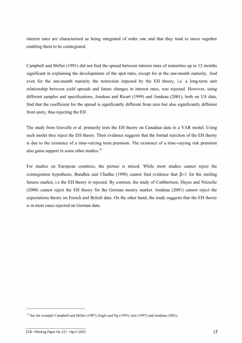
Table 7. Johansen test for cointegration (stochastic matrix test). EONIA swap rates

Note: A number of 21 lags have been used. The test statistics for H(rank≤p) are listed with p-values based onDoornik and Hendry (2001); ** and * mark significance at 95% and 99%. Testing commences at H(rank=0), andstops at the first insignificant statistics. Sample period is 1999 - 10.9 2001.1) The statistic shown for this test is the p-value of the null hypothesis test that the cointegratingvector β coefficient is equal to 1. ** indicates the rejection of the null hypothesis at a significance level of 1%.

We used the same methodology as for the monthly dataset outlined above. I.e., we first estimated a

cointegration relationship between the EONIA swap one-month rate and the one-month implied forward

rate at different horizons with an unrestricted intercept. We tested the null hypothesis of β=1 which was

rejected, except at the one-month horizon (see Table 7). However, the cointegrating coefficient of the

implied forward rates seems to be relatively close to unity at all maturities investigated (see Table 1 in

Appendix 10). Furthermore, we tested the joint hypothesis of β=1 and α≠0 by imposing the presence of

the intercept in the cointegrating space. The results are reported in Table 8. The last row of Table 8

reports the LR-test of restrictions which follows a χ2 (1) distribution with the p-value in brackets.

The results of the mis-specifications tests report basically no autocorrelation or heteroscedasticity (White,

1980, and Kalirajan, 1989) in the residuals. However, the normality test is strongly rejected in all cases.

Nevertheless, as indicated by the charts in Appendix 11, this result does not seem to stem from ’excess

skewness’ but from ’excess kurtosis’, thus, the distribution function of the residuals is symmetric, even if

there is non-normality.

More interestingly, the joint restriction of β=1 and α≠0 is not rejected for the three, six and nine month

maturities. This suggests existence of a constant risk premium at these maturities. The risk premia are

estimated to be 2, 6 and 10 basis points for the three-, six- and nine-month horizons respectively (see

Table 8). For the one-month horizon the estimated risk premium was zero as the restricted presence of a

constant term in the cointegrating space was rejected and therebyconfirms the results from Table 6.


One month r <= 0 78.133 0.000 **

(r1mt+1m

- ft1m,1m) r <= 1 0.31117 0.649 0.311

Three-month r <= 0 14.21 0.023 *

(r1mt+3m

- ft1m,3m) r <= 1 0.81921 0.423 0.000 **

six-month r <= 0 14.819 0.018 *

(r1mt+6m

- ft1m,6m) r <= 1 0.35328 0.624 0.000 **

Nine-month r <= 0 13.151 0.035 *

(r1mt+9m

- ft1m,9m) r <= 1 0.30171 0.655 0.000 **


restriction test1

(p-value)

Also in the case of the EONIA swap rates the standard deviations of the estimated constants were

relatively high. At the three-, six- and nine-month maturities they were 5, 7 and 15 basis points

respectively, about the same size as the point-estimates of the risk premia. This indicates high uncertainty

about the size of risk premia. Consequently, estimations with different sub-samples may result in different

risk premia (see Appendix 12).

Table 8: Results and mis-specification tests for the CIVAR(ρ) for the one- three-, six- and nine-months

horizon. Sample period: 1999 - 10 September 2001 (see also footnote 28). EONIA swap rates

Note: * and ** denote the rejection of the null hypothesis at 5% and 1% significance levels respectively. ThePortmanteau test follows a χ2 distribution with m=21 degrees of freedom. The critical value of the test is 32.7 and38.9 respectively at 5% and 1% significance level. See Hamilton (1994) for the critical values. The selection of thenumber of lags used in the CIVAR is based on two elements: (i) having a sufficient number of lags to removeautocorrelation and heteroskedasticity (ii) the AIC and HQ information criteria.

Extending the sample

As mentioned, we also estimated the model on a longer sample, ending in early June 2002. The estimated

risk premia on this sample are not much different from the results using the shorter sample. Table 9

presents the results from the Johansen cointegration tests and Table 10 presents the results from the

estimated CIVAR. On this sample, the estimated risk premia were 1, 2, 4 and 13 basis points for the

maturities of one-, three-, six- and nine months respectively. The standard deviations of the risk premia

were 1, 5, 9 and 15 basis points respectively. Thus, risk premia seem to be very small at maturities up to

three months, but more significant beyond that horizon. There is high uncertainty about the exact size of

the risk premia at the six- and nine-month maturities.


( ft1m,1m - r1m,t

t+21 - (ft

1m,3m - r1m,tt+63

- ( ft1m,6m - r1m,t

t+126 - ( ft1m,9m - r1m,t

t+189 -

Lags 22 9 14 5



ARCH 1-1 spot rate 33.08 ** 20.63 ** 19.18 ** 15.14 ** forward rate 53.44 ** 16.53 ** 2.00 3.58Hetero-test spot rate 0.76 1.43 1.49 1.31 forward rate 1.32 * 1.41 0.85 1.48

Normality -test spot rate 637.66 ** 347.92 ** 363.07 ** 380.87 ** forward rate 187.69 ** 119.47 ** 39.46 ** 29.38 **

LR test on restrictions 4.21 0.19 0.18 0.05 p-value (0.04) * (0.66) (0.68) (0.83)

Table 9: Johansen test (stochastic matrix) for cointegration

Note: the test statistics for H(rank≤p) are listed with p-values based on Doornik and Hendry (2001); ** and * marksignificance at 95% and 99%. Testing commences at H(rank=0), and stops at the first insignificant statistics.1) The statistic shown for this test is the p-value of the null hypothesis test that the cointegrating vector β coefficientis equal to 1. ** indicates the rejection of the null hypothesis at a critical level of 1%. Sample period is 1.1 1999 -5.6 2002.

Table 10: Results and mis-specification tests for the CIVAR(ρ) for the three-, six- and nine-months

horizon with constant. Sample period: 1999- 5 June 2002 (see also footnote 28). EONIA swap rates

Note: * and ** denote the rejection of the null hypothesis at 5% and 1% significance levels respectively. ThePortmanteau test follows a χ2 distribution with m=21 degrees of freedom. The critical value of the test is 32.7 and38.9 respectively at 5% and 1% significance level. See Hamilton (1994) for the critical values. The selection of thenumber of lags used in the CIVAR is based on two elements: (i) having a sufficient number of lags to removeautocorrelation and heteroskedasticity (ii) the AIC and HQ information criteria.


One month r <= 0 107.93 0.000 **

(r1mt+1m

- ft1m,1m) r <= 1 0.013265 0.946 0.3616

Three-month r <= 0 23.299 0.000 **

(r1mt+3m

- ft1m,3m) r <= 1 0.022347 0.926 0.000 **

six-month r <= 0 13.912 0.026 *

(r1mt+6m

- ft1m,6m) r <= 1 0.017919 0.935 0.000 **

Nine-month r <= 0 11.852 0.059

(r1mt+9m

- ft1m,9m) r <= 1 0.4258 0.584 0.000 **


restriction test1

(p-value)


( ft1m,1m - r1m,t

t+21 - (ft

1m,3m - r1m,tt+63

- ( ft1m,6m - r1m,t

t+126 - ( ft1m,9m - r1m,t

t+189 -

Lags 22 9 14 5



ARCH 1-1 spot rate 32.36 ** 22.96 ** 19.64 ** 13.26 ** forward rate 61.35 ** 23.08 ** 1.73 8.44 **

Hetero-test spot rate 1.08 0.96 1.10 1.40 forward rate 1.84 ** 1.37 0.88 0.93


LR test on restrictions 2.47 0.06 0.01 0.55 p-value (0.12) (0.81) (0.91) (0.46)

5. Conclusions

The expectations hypothesis (EH) was tested on German data for the period December 1989- December

1998. The tests were conducted using the single-equation framework of Phillips-Hansen and in a

cointegrated VAR framework. The results from both methodologies indicated that the weak version of the

EH (i.e. with a constant risk premium) holds true for maturities of up to nine months.

The VAR-estimations on monthly German LIBOR data suggest risk premia of around 5 basis points at

the one-month maturity. The premium increases to around 10 basis points at the three-month maturity,

and reaches 15 and 27 basis points at the six- and nine-month maturities respectively.

When expanding the data by incorporating the period from 1999 until late 2001 using EURIBOR rates,

the results of the estimations suggest that the specification of the cointegrating vector for the German

period is slightly different after the start of EMU, i.e. the null hypothesis that the cointegrating vector

between forward rates and spot rates is (1,-1) was rejected by close margin. These results may have two

potential explanations. On the one hand, the rejection of the EH may come from the existence of time-

varying risk premia following the launch of the European single currency. On the other hand, the results

could be explained by a shift in the level of risk premia at different horizons, in the sense of Gregory and

Hansen (1996).

This paper proposes to test the latter potential explanation mainly for two reasons. First, according to the

convergence of the different national monetary policies towards the German approach, it would be

surprising that time-varying risk premia should appear with the launch of the European single currency,

while the results suggest that time-independent risk premia existed in German money markets before this.

Second, according to the Phillips and Hansen results and the OLS recursive estimations, the rejection of

the EH seems to be due to a change of a limited size. Indeed, the OLS recursive estimations of the

relationship between the spot rate and the implied forward rate appears quite stable over the whole period,

i.e. from December 1989 to August 2001. Therefore, we explicitly tested the existence of a structural

change in the level of the constant risk premium and found that this change probably appeared in January

1999. By reestimating the preliminary models for the whole sample, we found that this last event has

entailed a decrease of risk premia of an amount of 1.7, 5.2, 9 and 13.6 basis points respectively at the 1-,

3- ,6- and 9-month horizons compared to the estimated risk premiums of the German period.

Although the limited number of years for an cointegration analysis, we also estimated a cointegrating

VAR on EONIA swap rates data with daily frequency starting in 1999, using two different samples (the

first sample period ends on 10 September 2001 and the second sample period ends on 5 June 2002). The

results broadly confirmed the level shift in the previous estimations. Indeed, they indicate somewhat

lower term premia than those resulting from the estimations using monthly data on the German Libor

market. More precisely, they tentatively suggest risk premia in ranges of 0-1, 2, 4-6 and 10-13 for the

maturities of one, three, six and nine months respectively. Given the limited sample period, these results

should be interpreted with caution.

The results from the EONIA swap rates and the LIBOR/EURIBOR rates are not 100% comparable. This

is because, as explained in Section 2, credit risk in EONIA swap rates is more limited than for the LIBOR

and EURIBOR rates. As credit risks also could be expected to increase with the maturity, the difference

between risk premia embedded in EONIA swap rates and EURIBOR rates could also be expected to

increase with the maturity. Thus, some of the discrepancy between the estimated term premia from the

two different datasets may be due to different credit risk.

Finally, the results seem to be broadly in line with other comparable empirical evidence. For instance,

Cuthbertson et. al. (2000) find that the expectations hypothesis is compatible with German money market

data for the period from 1976 to 1993. Moreover, the results of Cassola and Luis (2001), using German

data up to 1998, suggest that the risk premium increases with the maturity of the implied forward rates.

References

Andrews, D. W. K., 1991. Heteroskedasticity and Autocorrelation Consistent Covariance Matrix

Estimation, Econometrica, 59, 817-58.

Balduzzi, P., Das, S.R., Foresi, S., Sundaram, R., 1996. A Simple Approach to Three-Factor Affine TermStructure Models. Journal of Fixed Income, December, 43-53.

Brooke, M., Cooper, N., 2000. Inferring Market Interest Rate Expectations from Money Market Rates.Bank of England Quarterly Bulletin, November, 392-402.

Bhundia, A.J., Chadha, J.S., 1998. The Information Content of 3-Month Sterling Futures. EconomicLetters, 61, 209-14.

Campbell, J.Y., Lo, A.W., MacKinlay, A.C., 1997. The Econometrics of Financial Markets. PrincetonUniversity Press.

Campbell, J. Y., Perron, P., 1991. Pitfalls and Opportunities: What Macroeonomists Should Know aboutUnit Roots. NBER Macroeconomics Annual, 6, 141-201.

Campbell, J. Y., Shiller, R. J., 1987. Cointegration and Tests of Present Value Models. Journal ofPolitical Economy, 95, 1062-88.

Campbell, J. Y., Shiller, R. J., 1991. Yield Spreads and Interest Rate Movements: A Bird’s Eye View.Review of Economic Studies, 58, 495-514.

Campbell, R. H., Huang, R. D., 1991. The Impact of the Federal Reserve Bank’s Open MarketOperations. NBER Working Paper, 4663, 1-33.

Carlson, J.B., McIntire, J.M., Thornson, J.B., 1995. Federal Reserve Futures as an Indicator of FutureMonetary Policy: A Primer. Economic Review, Federal Reserve Bank of Cleveland, 20-30.

Cassola, N. Barros, L., 2001. A Two-Factor Model of the German Term Structure of Interest Rates. ECB

Working Paper , 46.

Choi, S., Wohar, M.E., 1995. The Expectations Theory of Interest Rates: Cointegration and FactorDecomposition. International Journal of Forecasting, 11, 253-62.

Clements, M.P., Hendry, D.F., 1995. Macroeconomic Forecasting and Modelling. Economic Journal, 105(431).

Collin-Dufresne, P., Solnik, B., 2001. On the Term Structure of Default Premia in the Swap and LIBORMarkets. Journal of Finance, 56(3), 1095-115.

Cuthbertson, K., Hayes, S., Nitzsche, D., 2000. Are German Money Market Rates Well Behaved?Journal of Economic Dynamics and Control, 24, 347-60.

Dor, E., Durré, A., 1997. Forecasting Economic Indicators: A Comparison of Cointegrated VAR Modelsand Univariate ARIMA Methods, and an Application to Consumer Prices, Real Consumption andInvestment. Labores-CNRS Working Paper, 97-11, 1-54.

Doornik, J.A., Hendry, D.F., 2001. Modelling Dynamic Systems Using PcGive. Volume II. TimberlakeConsultants LTD.

Drudi, F., Violi, R., 1998. Decomposing the Term Structure into Risk Premia and Expectations: Evidencefor the Eurolira Rates. Chapt. 2 in Angeloni, I. and Rovelli, R. (eds), Monetary Policy and Interest Rates,MacMillan Press, London.

Durré, A., 2003. The EH Theory and the Money Market : An Application to the Euro Area. LABORESWorking Paper, 03-01, LABORES (CNRS-URA 362).

ECB, 2000. The Information Content of Interest Rates and their Derivatives for Monetary Policy.Monthly Bulletin, European Central Bank, May 2000, 37-55.

ECB, 2001. The Information Content of the Main Money Market Instruments in the Euro Area. MonthlyBulletin, European Central Bank, June 2001, Box 6, 27-8.

Enders, W., 1995. Applied Econometric Time Series. J. Wiley & Sons.Inc.

Engel, Ch., 1995. The Forward Discount Anomaly and the Risk Premium: A Survey of Recent Evidence.NBER Working Paper, 5312, 1-114.

Engle, R.E., Granger, C.W.J., 1987. Cointegration and Error-Correction: Representation, Estimation andTesting. Econometrica, 55, 251-76.

Engle, R.F., Lilien, D.M., Robins, R.P., 1987. Estimating Time Varying Risk Premia in the TermStructure : The ARCH-M Model. Econometrica, 55 (2), 391-407.

Engle, R.F., Ng., V., 1993. Time Varying Volatility and the Dynamic Behavior of the Term Structure.Journal of Money, Credit, and Banking, 25, 336-49.

Engsted, T., Tanggaard, C., 1995. The Predictive Power of Yield Spreads for Future Interest Rates:Evidence from the Danish Term Structure. Scandinavian Journal of Economics, 97(1), 145-59.

Fama, E.F., 1984. The Information in the Term Structure. Journal of Financial Economics, 13, 509-28.

Favero, C.A., Mosca, F., 2001. Uncertainty on Monetary Policy and the Expectations Model of the TermStructure of Interest Rates. Economics Letters, 71, 369-75.

Fisher, M., 2001. Forces That Shape the Yield Curve. Federal Reserve Bank of Atlanta Economic Review,1st Quarter, 1-15.

Gaspar, V., Perez-Quiros, G. and Sicilia, J., 2001. The ECB Monetary Policy Strategy and the MoneyMarket. Oesterreichische Nationalbank Working Paper, 47, 1-33.

Gerlach, S., Smets, F., 1997. The Term Structure of Euro-Rates: Some Evidence in Support of theExpectations Hypothesis. Journal of International Money and Finance, 16, 305-21.

6

Godfrey, L.G., Orme, C.D., 1991. Testing for Skewness of Regression Disturbances. Economics Letters,37, 31-4.

Goodfriend, M., 1998. Using the Term Structure of Interest Rates for Monetary Policy. Chapt. 10 inAngeloni, I. and Rovelli, R. (eds), Monetary Policy and Interest Rates, MacMillan Press, London.

Gravelle, T., Muller, Ph., Streliski, D., 1998. Towards a New Measure of Interest Rate Expectations inCanada: Estimating a Time-Varying Term Premium. Bank of Canada Internal Paper, 179-216.

Gregory, A.W., Hansen, B.E., 1996. Residual-based Tests for Cointegration in Models with RegimeShifts. Journal of Econometrics, 70, 99-126.

Gregory, A.W., Nason, J.M., Watt, D.G., 1996. Testing for Structural Breaks in CointegratedRelationships. Journal of Econometrics, 71, 321-41.

Hamilton, J.D., 1994. Time Series Analysis. Princeton University Press.

Hardouvelis, G.A., 1988. The Predictive Power of the Term Structure during Recent Monetary Regimes.Journal of Finance, 339-56.

Hardouvelis, G.A., 1994. The Term Structure Spread and Future Changes in Long and Short Rates in theG7 Countries : Is There a Puzzle ? Journal of Monetary Economics, 255-83.

Hendry, D.F., Doornik, J.A., 2001. Modelling Dynamic Systems Using PcGive. Volume I. TimberlakeConsultants LTD.

Iyer, S., 1997. Time-varying Term Premia and the Behaviour of Forward Interest Rate Prediction Errors.The Journal of Financial Research, 4 (Winter), 503-7.

Johansen, S., 1992. Testing Weak Exogeneity and the Order of Cointegration in UK Money Demand.Journal of Policy Modelling, 14, 313-34.

Johansen, S., Juselius, K., 1990. Maximum Likelihood Estimation and Inference on Cointegration – WithApplications to the Demand for Money. Oxford Bulletin of Economics and Statistics, 52(2), 169-210.

Jondeau, E., 2001. La Théorie des anticipations de la structure par terme permet-elle de rendre compte del’évolution des taux d’intérêt sur euro-devise. Annales d’Économie et de Statistique, 62, 139-74.

Jondeau, E., Ricart, R., 1999. The Expectations Hypothesis of the Term Structure: Test on US, German,French, and UK Euro-Rates. Journal of International Money and Finance, 18(5), 725-50.

Jorion, P., Mishkin, F.S., 1991. A Multicountry Comparison of Term-Structure Forecasts at LongHorizons. Journal of Financial Economics, 29, 59-80.

Kalirajan, K.P., 1989. A Test for Heteroscedasticity and Non-Normality of Regression Residuals – APractical Approach. Economics Letters, 30, 133-36.

Kessel, R.A., 1965. The Cyclical Behavior of the Term Structure of Interest Rates. NBER OccasionalPaper, 91.

Lee, S.-S., 1995. Macroeconomic Sources of Time-Varying Risk Premiums in the Term Structure ofInterest Rates. Journal of Money, Credit and Banking, 27(2), 549-69.

MacKinnon, J. G., 1991. Critical Values for Integration Tests. In Engle, R.F. and Granger, C.J.W. (eds.),Long-Run Economic Relationships, Oxford University Press, 267-76. .

Mankiw, G.N., 1986. The Term Structure of Interest Rates Revised. Brookings Papers of EconomicActivity, 53, 61-107.

Meiselman, D., 1962. The Term Structure of Interest Rates. Englewood Cliffs, New Jersey.

Mishkin, F.S., 1988. The Information in the Term Structure: Some Further Results. Journal of AppliedEconometrics, 3, 307-14.

Phillips, P.C.B., Hansen, B.E., 1990. Statistical Inference in Instrumental Variables Regression with I(1)Processes. Review of Economic Studies, 57, 99-125.

Pilegaard, R. 2002. Extracting the risk premium from the euro area money market. Master thesis from theUniversity of Copenhagen October 2002.

Rudebusch, G., 1995. Federal Reserve Interest Rate Targeting, Rational Expectations, and the TermStructure. Journal of Monetary Economics, 35, 245-74.

Rudebusch, G., 1998. Monetary Policy and the Term Structure of Interest Rates: An Overview of SomeRecent Research. Chapt. 9 in Angeloni, I. and Rovelli, R. (eds), Monetary Policy and Interest Rates,MacMillan Press, London.

Santillan, J., M. Bayle and C. Thygesen, 2000. The Impact of the Euro on Money and Bond Markets.ECB Occasional Paper Series, July.

Sims, Ch., 1980. Macroeconomics and Reality. Econometrica, 48, 1-49.

Shiller, R.J., 1973. Rational Expectations and the Term Structure of Interest Rates. Journal of Money,Credit and Banking, 3, 856-60.

Shiller, R.J., 1980. Can the Fed Control Real Interest Rates? In S. Fisher, ed. Rational Expectations andEconomic Policy. Chicago : University of Chicago Press, 117-67.

Shiller, R.J., 1981. Alternative Tests of Rational Expectations Models: The Case of the Term Structure.Journal of Econometrics, 16, 71-87.

Shiller, R.J., Campbell, J.Y., Schoenholtz, K.L., 1983. Forward Rates and Future Policy: Interpreting theTerm Structure of Interest Rates. Brookings Papers on Economic Activity, 1, 173-217.

Shiller, R.J., 1990. The Term Structure of Interest Rates. Chapter 13 in Friedman, B.M. and Han, F.H.(eds), Handbook of Monetary Economics, Volume I, North-Holland, Amsterdam.

Soderlind, P., Svensson, L.E.O., 1997. New Techniques to Extract Market Expectations from FinancialInstruments. Journal of Monetary Economics, 40, 373-429.

5

Svensson, L.E.O., 1994. Estimating and Interpreting Forward Interest Rates: Sweden 1992-1994. CEPRDiscussion Paper, 1051, 1-26.

Svensson, L.E.O., 2001. Comments on ‘The ECB Monetary Policy Strategy and the Money Market’.Oesterreichische Nationalbank Working Paper, 47, 43-6.

Taylor, J. B., 2001. Expectations, Open Market Operations, and Challenges in the Federal Funds Rate.Paper prepared for the Federal Reserve Bank of St. Louis Conference ‘Monetary Policy in Theory andPractice’.

Thornton, D.L., 2001. The Bias in the Conventional Test of the Expectations Theory: Resolving theAnomalies at the Very Short End of the Term Structure. Federal Reserve Bank of St. Louis WorkingPaper, 2000-003B.

Tzavalis, E., Wickens, M.R., 1997. Explaining the Failures of the Term Spread Models of the RationalExpectations Hypothesis of the Term Structure. Journal of Money, Credit and Banking, 29(3), 364-80.

White, H., 1980. A Heteroskedasticity-Consistent Covariance Matrix Estimator and Direct Tests forHeteroskedasticity. Econometrica, 48, 817-38.

-

Appendix 1

Potential bias involved by the conventional test of the Expectations Hypothesis

In his recent study, Thornton (2001) underlines problems that may arise from the conventional test of the

expectations hypothesis, i.e. in which the short-term interest rate appears symmetrically on both sides of

the estimation. By doing this, we test if the spread between interest rates with different maturities is a

good predictor of the future change of the spot rate. The basic point of the argument may be summarized

as follows. Traditionally, when testing the EH theory, we estimate the following relationship:

tmt

nt

mt

k

i

mmit RRRR

kωβα +−+=−∑

−

=+ )(1

1

0

where mtR is the (m-period) short-term interest rate, n

tR is the longer-term interest rate, (k-1) is the period

in the future and tω is an iid white noise error. If the EH theory holds true, the null hypothesis β=1 is not

rejected. In his paper, Thornton argues that this relationship is correctly specified if and only if the EH

holds true. Otherwise, this specification may entail bias in favour of the support the EH theory. Then,

before subtracting the short-term interest on both sides of the equation, he parameterises the relationship

between the long-term and the short-term interest rates according to the expectations theory:

πθ −−= ∑∑−

=+

−

=+

1

0

1

0

11k

imit

nt

k

i

mmit V

kRR

k

where the average weighted short-term interest rate in the future is a function of the actual long-term

interest rate, minus the sum of the white noise errors and a constant term (defined here as a constant term

premium). Now, when subtracting the actual short-term interest rate, mtR , on both sides of the previous

equation, we obtain:

πθ −−−=− ∑∑−

=+

−

=+

1

0

1

0

11k

imit

mt

nt

mt

k

i

mmit V

kRRRR

k

Note that this equation is similar to the first one if we add the expression mt

mt RR θθ − on the left-hand side

of the previous equation. Doing so and using the same notation for the constant and the error terms, we

obtain:

tmt

mt

nt

mt

k

i

mmit RRRRR

kωθθα +−+−+=−∑

−

=+ )1()(1

1

0

which is similar to the first formulation of the EH theory only if θ=1. If not, the third term of the previous

equation does not disappear and then θ cannot be considered as the best estimator of β. Indeed, taking the

expected value of the least squares estimator of β from the first equation, we obtain in this case:

22 )(

)(

)(

)()1(ˆ

mt

nt

tmt

nt

mt

nt

mt

mt

nt

RR

RRE

RR

RRREE

−−

−−

−−+=

∑∑

∑∑ ω

θθβ

where the variables in the fractional expressions denote the adjustment for the mean. Then, if θ≠1, the

limit of β when N→∞ converges to:

+−−−+=∞→ 2,

2

2,

2)1(ˆlim

RmRmRnRn

RmRmRn

NPσσσ

σσθθβ

So, if θ≠1, then β will also be influenced by the second term which is affected itself by the covariance

and the relative variances of each interest rate. In the case where short-term and long-term interest rates

are uncorrelated, i.e. 0, =RmRnσ , the previous equation converges to

+−+

2

21)1(

Rn

Rm

σσθθ and therefore,

when the variance of the (short-term) m-period rate increases and is slightly higher than the variance of

the (long-term) n-period interest rate, it is possible that β is biased toward one. On the other hand, in the

case where RmRnRn ,2 σσ > the terms in brackets become less than one which increases the probability of a

higher value for β . That could explain why in some of our single-equation estimations we obtained

estimated values for β larger than one. Even if long-term and short-terms interest rates are generated

independently (i.e. a random walk process) or by an autoregressive process, the test of the EH in terms of

spreads finds in most cases results in favour of the theory. Indeed, for the latter case, which seems to be

valuable for instance for interest rates in the EONIA market, each interest rate is generated by the

following process:

tmtmm

t RR εϕµ ++= −1

tntnn

t RR γψµ ++= −1

This is indeed the process the EONIA swap rates seems to display using the standard methodology of Box

and Jenkins. We then obtain in this case:

ψϕσ

ψσ

ψσ

ψψψ

ψϕψσσσ

σβγεγε

γ

−−−+−

−−−

−

−−−=∞→1

211

)1(11

11

/*1ˆlim

,

2

2

2

2

2

22,

2k

kNP

kRnRmRmRn

where we see that the estimate of β will be positive in the particular case where 22 / RnRm σσ <1 and ϕ<ψ.

Moreover, the larger the variance of the short-term interest rate is compared to the variance of the long-

term interest rate, the higher the estimate of β will be. If we look for instance at the EONIA market, it

must be quoted that the short-term interest rates display on average higher volatilities than the long-term

interest rates. This is especially the case during September 2001 where the variance of the EONIA spot

rate was 39% higher than the variance of the EONIA one-month swap rate while the latter was only 10%

higher on average than the variance of the implied forward rates of maturity from one month up to one

year. Some explanation of our preliminary results inside the basic single equation (Section 3.2) could

come from these features. Note for example that the estimations on the sample including the observations

after 11 September 2001 display systematically higher values of β compared to the results on the sample

without those observations.

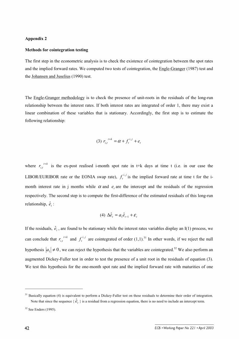
Appendix 2

Methods for cointegration testing

The first step in the econometric analysis is to check the existence of cointegration between the spot rates

and the implied forward rates. We computed two tests of cointegration, the Engle-Granger (1987) test and

the Johansen and Juselius (1990) test.

The Engle-Granger methodology is to check the presence of unit-roots in the residuals of the long-run

relationship between the interest rates. If both interest rates are integrated of order 1, there may exist a

linear combination of these variables that is stationary. Accordingly, the first step is to estimate the

following relationship:

(3) tji

tkt

ti efr ++=+ ,, α

where kt

tir+

, is the ex-post realised i-month spot rate in t+k days at time t (i.e. in our case the

LIBOR/EURIBOR rate or the EONIA swap rate), ji

tf ,is the implied forward rate at time t for the i-

month interest rate in j months while α and te are the intercept and the residuals of the regression

respectively. The second step is to compute the first-difference of the estimated residuals of this long-run

relationship, te :

(4) ttt eae ε+=∆ −11 ˆˆ

If the residuals, te , are found to be stationary while the interest rates variables display an I(1) process, we

can conclude that kt

tir+

, and ji

tf , are cointegrated of order (1,1).31 In other words, if we reject the null

hypothesis 01 ≠a , we can reject the hypothesis that the variables are cointegrated.32 We also perform an

augmented Dickey-Fuller test in order to test the presence of a unit root in the residuals of equation (3).

We test this hypothesis for the one-month spot rate and the implied forward rate with maturities of one

31 Basically equation (4) is equivalent to perform a Dickey-Fuller test on these residuals to determine their order of integration.

Note that since the sequence te is a residual from a regression equation, there is no need to include an intercept term.

32 See Enders (1995).

month, three months, six months and nine months with a number of 21 lags on the daily data and 12 lags

on the monthly data. The results for both data sets are reported in Tables 2 and 3 in Appendix 3.

The DF- and ADF-tests rejected the null hypothesis of non-stationary residuals. We can then conclude

that the one-month spot interest rates and the corresponding implied forward rates are cointegrated of

order (1,1) for both markets/data sets.

We also performed the Johansen test for cointegration. This four-step procedure was performed with an

unrestricted vector autoregressive model using the levels of spot and forward rates, for each relationship

between the spot rate and the implied forward rates. A maximum number of 12 lags for the Libor/Euribor

market and 21 lags for the EONIA market were chosen. The difference in the number of lags is explained

by the frequency used in each case (i.e. monthly and daily frequency respectively). The results are

reported in Table 3 for the LIBOR/EURIBOR data and in Table 6 for the EONIA swaps in Section 4 of

the paper.

Appendix 3

1. Descriptive statistics. LIBOR/EURIBOR market.

Table 1.1. Normality test for the 1-month spot rate

Sample size 173: 10 to 182Mean 5.442775Std.Devn. 2.264577 (using T-1: 2.271151)Skewness 0.616111Excess Kurtosis -1.092024Minimum 2.570000Maximum 9.840000Normality Chi^2(2)= 72.882 [0.0000] **(asymptotic form of normality test: 19.541)

Table 1.2. Normality test for the 1-month implied forward rate








2. LIBOR/EURIBOR market : Unit-root tests 23 to 182 with a maximum of 12 laqs33

Table 2. Test for unit-roots in the residuals of the simple OLS regressions with amaximum of 12 laqs

Level ∆

Residuals of 1 month equation -3.4816** -5.4873**

Residuals of 3 months equation -3.5970** -5.6761**

Residuals of 6 months equation -3.4054* -5.1205**


Source: European Central Bank. ∆ denotes the first difference operator. The data sample covers the period from the January 1987 to February2002. The unit root test used is the univariate augmented Dickey-Fuller for which the critical values are –2.18 and –3.473 at 5% and 1% level ofsignificance, respectively which are marked by * and** (MacKinnon, 1991).

3. EONIA swap market : Unit-root tests

Table 3. Unit-root tests based on ADF test with 21 lags

Level ∆Residuals of 1 month equation -4.836** -7.036**



Residuals of 9 months equation 1.374 -4.568**

Source: European Central Bank. ∆ denotes the first difference operator. The data sample covers

the period from the 4th January to the 10 September2001. The unit root test used is the univariate

augmented Dickey-Fuller for which the critical values are –2.18 and –3.473 at 5% and 1% level of

significance, respectively which are marked by * and** (MacKinnon, 1991).

33 Critical values: 5%=-2.18 1%=-3.472; Constant included. ** and * indicates

respectively the rejection of the null hypothesis at 5% and 1% significance level.

6

Appendix 4

The Phillips-Hansen methodology: A short Explanation

Consider for instance the following linear regression model:

ntuxy tt ,...,2,1,10 =++= ββ

where the k*1 vector of I(1) regressors are not themselves cointegrated. Therefore, xt has a first-

difference stationary process given by

ntvx tt ,...,2,1, =+=∆ µ

in which µ is a k*1 vector of drift parameters and vt is a k*1 vector of I(0), or stationary variables. It is

also assumed that ( )’, ’ttt vu=ξ is strictly stationary with zero mean and a finite positive-definite covariance

matrix, Σ.

The computation of the FM-OLS estimator of β is carried out in two stages. In the first stage, yt is

corrected for the long-run inter-dependence of ut and vt. For this purpose, let ût be the residual vector in

the first equation, and write

ξt=(ût, vt)’, t=2,3,…,n

where vt= ∆xt- µ , for t=2,3,…,n

and

( ) ∑=

− ∆−=n

t

txn2

11µ .

A consistent estimator of the long-run variance of ξt is given by

ΩΩΩΩ

=Λ+Λ+Σ=Ωkkk

k

*1*

*11*1’2221

1211

where

∑=−=Σn

t

ttn 2

’1

1 ξξ

and

( )∑ Γ=Λ sms,ω

∑=Γ−

=+−

sn

tsttns

1’1 ξξ

and ω(s,m) is the lag-window with horizon (or truncation) m.

Now let

[ ]12211211

∆∆∆∆=Λ+Σ=∆

211222221 ΩΩ∆−∆=Ζ −

^1

2212

^* ttt vyy −ΩΩ−=

=+

kkIk

kkD

k*

*10

*)1(

In the second stage the FM-OLS estimator of β is given by

)*’()’(^

1

^

* Ζ−= − nDyWWWβ

where

)’1,...,1,1,1(),,(,)’,...,,,(^*4

^*3

^*2

^*1

^

* === nn XWyyyyy ττ

In general, we use the lag window of Tukey that is defined as

)/cos(12/1),( msms πω += and 0≤ s ≤ m/2

in which the value of m is arbitrary chosen. In the following of the analysis here, we choose a maximum

value of m that not exceed 40, as recommended by Pesaran and Pesaran (1997). Moreover, to be

consistent with the forthcoming analysis, we determine the exact number of lags for each model that is in

line with the selection of the order in the VAR framework. That means a number of lags for truncation

equal to 4, 5, 2 and 11 for the 1, 3, 6 and 9-month horizons respectively.

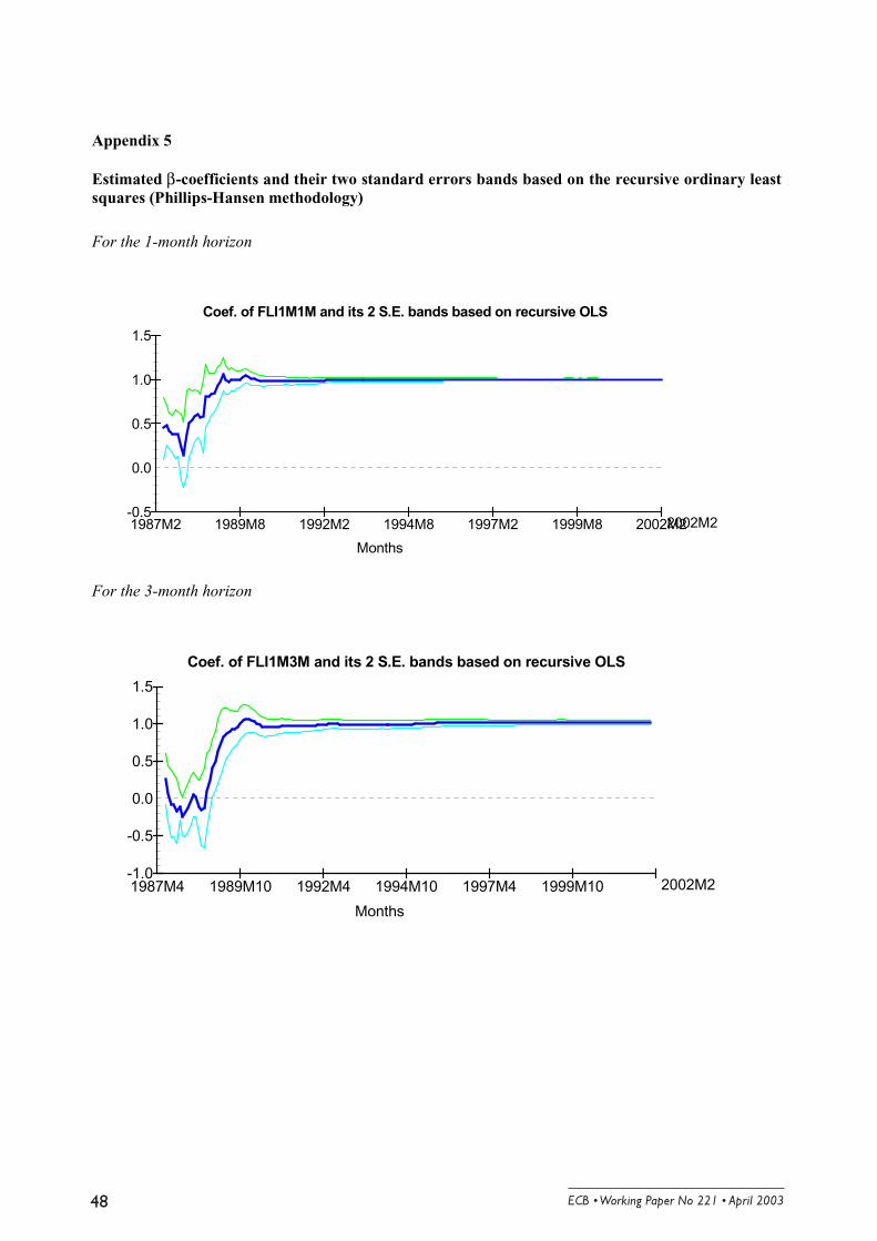
5

Appendix 5

Estimated β-coefficients and their two standard errors bands based on the recursive ordinary leastsquares (Phillips-Hansen methodology)

For the 1-month horizon


Months

-0.5

0.0

0.5

1.0

1.5

1987M2 1989M8 1992M2 1994M8 1997M2 1999M8 2002M22002M2



Months

-0.5

-1.0

0.0

0.5

1.0

1.5

1987M4 1989M10 1992M4 1994M10 1997M4 1999M10 2002M2

-



Months

-0.5-1.0-1.5-2.0-2.5

0.00.51.01.52.0

1987M7 1990M1 1992M7 1995M1 1997M7 2000M1 2002M2



Months

-0.5-1.0-1.5-2.0

0.00.51.01.52.02.5

1987M10 1990M4 1992M10 1995M4 1997M10 2000M4 2002M2

Appendix 6

The VAR methodology

If Xt is an n-sized vector of I(1) variables, the VAR description of the process of Xt can be written :

tlt

p

llt uXX +Φ+= −

=∑

1

µ

where µ is a n-components vector, Φl are n x n matrices and ut a vector of white noise error terms. This

description can be re-parameterised as follows:

tltlt

p

llttt uXXAXXX +−+Φ−=− −−−

−

=−− ∑ )()1( 1

1

111 µ

where

and

∑+=

Φ−=p

ljjlA

1

Unit roots imply that Φ(1) is singular. When the VAR is cointegrated, which means that there exist r

cointegrating vectors, Φ(1) can be written as -αβ’ where α and β are n x r matrices of rank r. β is a matrix

of cointegrating vectors of coefficients and β’Χt-1 is a stationary r-components vector of cointegrating

relations, the fluctuations of which describe short-term departures from the long term relations. α is a

matrix of adjustment coefficients, describing the relation of each I(1) variable to previous short term

departures from each long term relation. As suggested previously by the cointegration tests, r is equal to 1

between the spot rate and the implied forward rates at different maturities. Imposing this restriction, the

cointegrating vector is normalised by constraining the coefficient of the spot rate to 1.34 Clements and

Hendry (1995) show that the estimation of the VAR with this constraint, when true, strongly improves the

forecasts. However, the interpretation of the VAR results on a limited number of years must be

interpreted with caution as suggested by Campbell and Perron (1991).

34 For more details on the methodology, see Dor and Durré (1997) and Jondeau (2001).

∑=

Φ−=Φp

llnI

1

)1(

Appendix 7

Table 1: Results and mis-specification tests for the CIVAR(ρ) for the one-, three-, six- and nine-months

horizon without a constant. German LIBOR market.

Note: * and ** denote the rejection of the null hypothesis at 5% and 1% significance levels respectively. The

Portmanteau test follows a χ2 distribution with m=21 degrees of freedom. The critical value of the test is 32.7 and

38.9 respectively at 5% and 1% significance level. These results were compared to the critical values reported in

Hamilton (1994).

lags 13 12 13 11

Cointegrating vector 1-0.991 1-0.990 1-0.981 1-0.964

portmanteau test (26) spot rate 32.75 29.03 29.70 36.53 forward rate 32.63 22.22 17.60 16.26

ARCH 1-7 spot rate 0.57 0.41 0.23 0.40 forward rate 1.02 0.42 0.77 1.61

Hetero-test spot rate 0.41 0.62 0.49 0.48 forward rate 0.62 0.66 0.74 0.73

Normality -test spot rate 24.245 ** 32.35 ** 36.54 ** 39.16 ** forward rate 24.37 ** 9.66 ** 7.29 * 0.37

One-month Three-month Six-month Nine-month

( ft1m,1m - r1m,t

t+1m ) (ft

1m,3m - r1m,tt+3m

) ( ft1m,6m - r1m,t

t+6m ) ( ft1m,9m - r1m,t

t+9m )

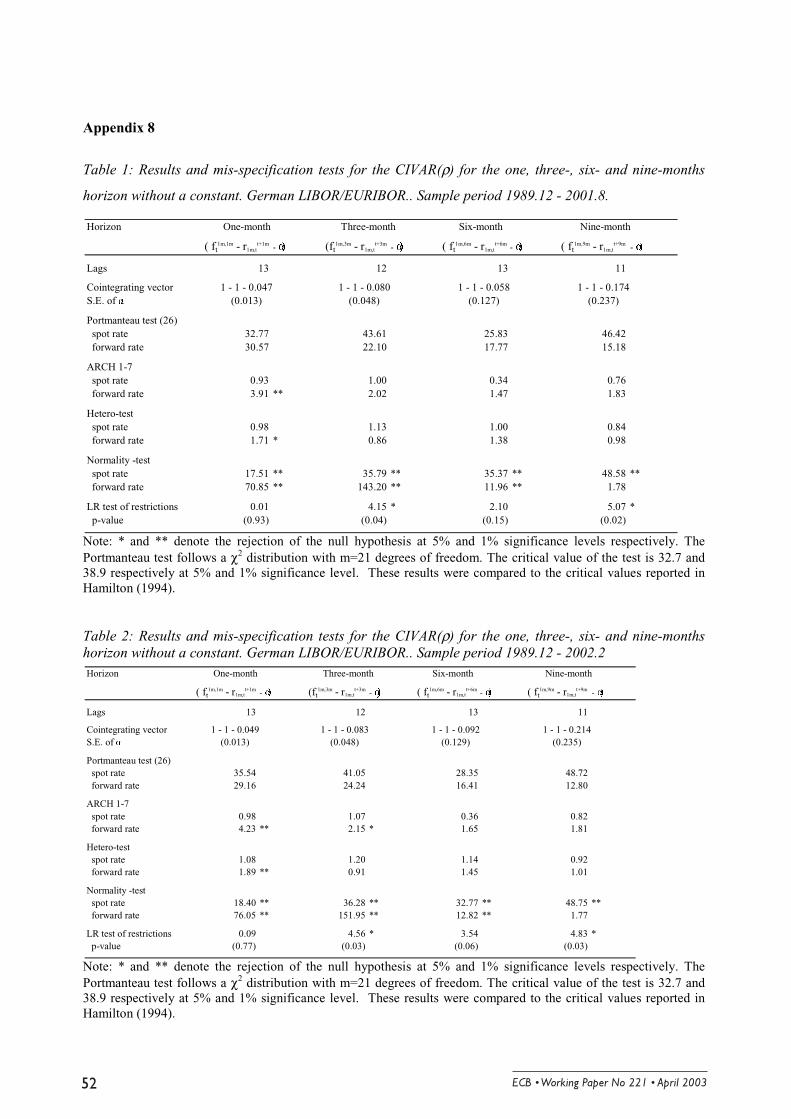
Appendix 8

Table 1: Results and mis-specification tests for the CIVAR(ρ) for the one, three-, six- and nine-months

horizon without a constant. German LIBOR/EURIBOR.. Sample period 1989.12 - 2001.8.

Note: * and ** denote the rejection of the null hypothesis at 5% and 1% significance levels respectively. ThePortmanteau test follows a χ2 distribution with m=21 degrees of freedom. The critical value of the test is 32.7 and38.9 respectively at 5% and 1% significance level. These results were compared to the critical values reported inHamilton (1994).

Table 2: Results and mis-specification tests for the CIVAR(ρ) for the one, three-, six- and nine-monthshorizon without a constant. German LIBOR/EURIBOR.. Sample period 1989.12 - 2002.2



( ft1m,1m - r1m,t

t+1m - (ft

1m,3m - r1m,tt+3m

- ( ft1m,6m - r1m,t

t+6m - ( ft1m,9m - r1m,t

t+9m -

Lags 13 12 13 11



ARCH 1-7 spot rate 0.93 1.00 0.34 0.76 forward rate 3.91 ** 2.02 1.47 1.83

Hetero-test spot rate 0.98 1.13 1.00 0.84 forward rate 1.71 * 0.86 1.38 0.98


LR test of restrictions 0.01 4.15 * 2.10 5.07 * p-value (0.93) (0.04) (0.15) (0.02)


( ft1m,1m - r1m,t

t+1m - (ft

1m,3m - r1m,tt+3m

- ( ft1m,6m - r1m,t

t+6m - ( ft1m,9m - r1m,t

t+9m -

Lags 13 12 13 11



ARCH 1-7 spot rate 0.98 1.07 0.36 0.82 forward rate 4.23 ** 2.15 * 1.65 1.81

Hetero-test spot rate 1.08 1.20 1.14 0.92 forward rate 1.89 ** 0.91 1.45 1.01


LR test of restrictions 0.09 4.56 * 3.54 4.83 * p-value (0.77) (0.03) (0.06) (0.03)

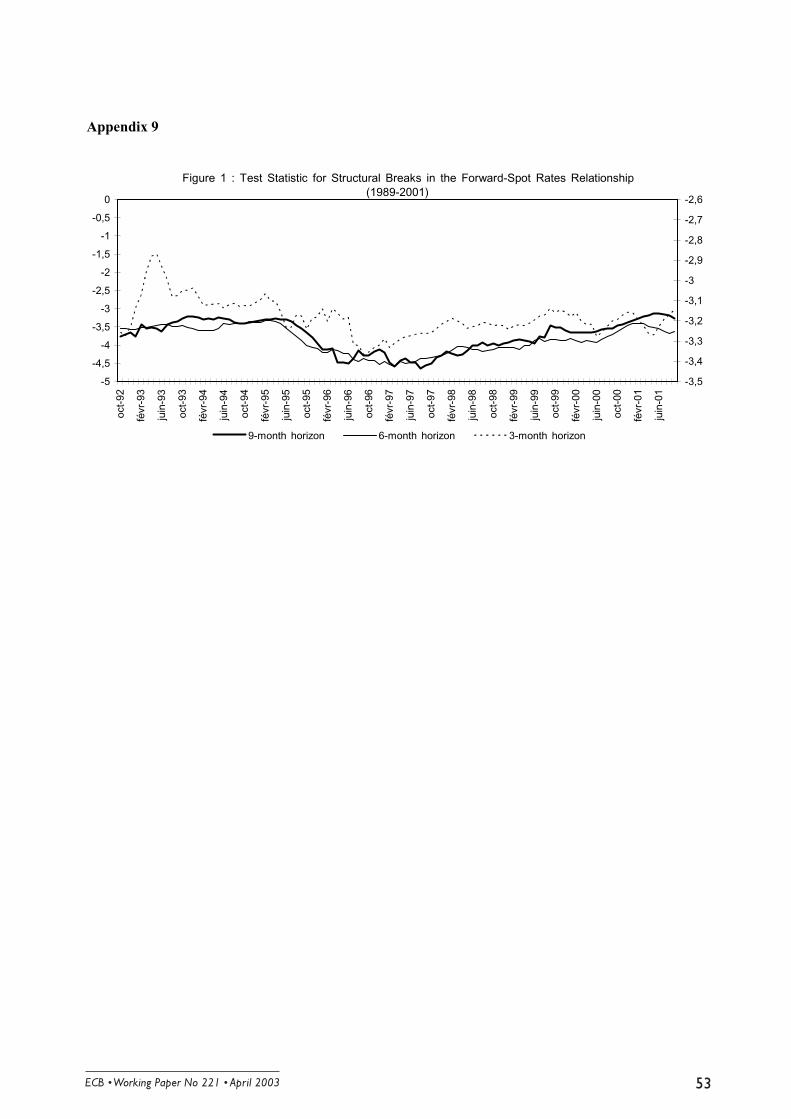
Appendix 9

Figure 1 : Test Statistic for Structural Breaks in the Forward-Spot Rates Relationship(1989-2001)

-5

-4,5

-4

-3,5

-3

-2,5

-2

-1,5

-1

-0,5

0

oct-

92

févr

-93

juin

-93

oct-

93

févr

-94

juin

-94

oct-

94

févr

-95

juin

-95

oct-

95

févr

-96

juin

-96

oct-

96

févr

-97

juin

-97

oct-

97

févr

-98

juin

-98

oct-

98

févr

-99

juin

-99

oct-

99

févr

-00

juin

-00

oct-

00

févr

-01

juin

-01

-3,5

-3,4

-3,3

-3,2

-3,1

-3

-2,9

-2,8

-2,7

-2,6

9-month horizon 6-month horizon 3-month horizon

Appendix 10

Table 1: Results and mis-specification tests for the CIVAR(ρ) for the three-, six- and nine-months horizonwithout a constant. EONIA swap market.

Note: * and ** denote the rejection of the null hypothesis at 5% and 1% significance levels respectively. The

Portmanteau test follows a χ2 distribution with m=21 degrees of freedom. The critical value of the test is 32.7 and

38.9 respectively at 5% and 1% significance level. These results were compared to the critical values reported in

Hamilton (1994).


r1m,tt+21 - ft

1m,1m r1m,tt+63 - ft

1m,3m r1m,tt+126 - ft

1m,6m r1m,tt+189 - ft

1m,9m

lags 22 9 14 5



ARCH 1-1 spot rate 33.25 ** 20.55 ** 19.17 ** 15.12 forward rate 53.65 ** 16.42 ** 1.97 3.57

Hetero-test spot rate 0.76 1.43 1.49 * 1.31 forward rate 1.31 * 1.42 0.85 1.48


Appendix 11

Distribution function of the residuals using a CIVAR(ρ) model – Three-month Horizon

Distribution function of the residuals using a CIVAR(ρ) model – Six-month Horizon

Distribution function of the residuals using a CIVAR(ρ) model – Nine-month Horizon

-10.0 -7.5 -5.0 -2.5 0.0 2.5 5.0 7.5 10.0

0.25

0.50

0.75 Densityr:Fwd1,3m N(0,1)

-5.0 -2.5 0.0 2.5 5.0

0.2

0.4

0.6

Densityr:sw_1m N(0,1)

-10.0 -7.5 -5.0 -2.5 0.0 2.5 5.0

0.2

0.4

0.6

Densityr:Fwd1,6m N(0,1)

-5.0 -2.5 0.0 2.5 5.0

0.25

0.50

0.75 Densityr:sw_1m N(0,1)

-7.5 -5.0 -2.5 0.0 2.5 5.0 7.5

0.25

0.50

0.75

Densityr:Fwd1,9m N(0,1)

-5.0 -2.5 0.0 2.5 5.0

0.25

0.50

0.75

Densityr:sw_1m N(0,1)

6

Appendix 12

Table 1: Estimated constant terms at sub samples, standard errors in parenthesis. EONIA swap market.

Indicated risk premium measured in basis points = Constant term * 100

Observation/Date 3-month maturity 6-month maturity 9-month maturity

650/ 16 Jul. 2001 0.068

(0.058)

0.111

(0.070)

0.170

(0.179)

689/ 10 Sep. 2001 0.016

(0.051)

0.058

(0.068)

0.096

(0.149)

800/ 15 Feb. 2002 0.026

(0.056)

0.109

(0.099)

0.101

(0.163)

874/ 5 Jun. 2002 0.022

(0.052)

0.041

(0.095)

0.128

(0.148)

Appendix 13

Resulting tables when using the sample from 4 January 1999 to 5 June 2002. EONIA swap market.

Table 1: Results and mis-specification tests for the CIVAR(ρ) for the three-, six- and nine-monthshorizon without a constant



lags 22 9 14 5



ARCH 1-1 spot rate 32.45 ** 22.93 ** 19.63 ** 13.23 ** forward rate 61.36 ** 22.95 ** 1.74 8.53 **

Hetero-test spot rate 1.08 0.96 1.11 1.40 forward rate 1.84 * 1.37 0.88 0.93


r1m,tt+21 - ft

1m,1m r1m,tt+63 - ft

1m,3m r1m,tt+126 - ft

1m,6m r1m,tt+189 - ft

1m,9m

5

!"#$%%"""&&'&

(( ) $ *&+&,-&. +/00/&

((1 )2$""3*4&5 5&-&26&7 88+/00/&

((9 )2 $ "*5&:/00(&

((; )<=(>?9(>>?*+&@&-8&+/00/&

(( )@"$" *:& &A +/00/&

((? ) BC $ 4 (>??D(>>?*=&2&7+/00/&

((> )2 *.& &2+/00/&

(/0 ), "*E&@6-&2+/00/&

(/( ). *5&<&&5&/00/&

(// )." "*&A6 <&5 /00/&

(/ )5 *&75&A/00/&

(/1 )2 B*=&& E&@6/00/&

(/9 ) *E&2 /00/&

(/; ): *&2&F/00/&

(/ ) " *E&@6-&2/00/&

(/? ):BD *&E<&/00/&

-

(/> ).D "C *5& D.",&E2/00/&

(0 )@8B$ *&"2/00/&

(( )2@4$""""""3*2&5&&<G8D 8 2/00/&

(/ )4 $)"-* *:&5 &<G8D 8 &72/00/&

( ) ="3*5&22&<2/00/&

(1 )7 . (>>/D(>>>*&+&A 2/00/&

(9 )7 BB*&&7 5 /00/&

(; )< D$" *=&5 /00/&

( )C !*H& 5 /00/&

(? )."* "$"2H 3*&&2 5 /00/&

(> ):*2&85 /00/&

(10 )D *2&2/00/&

(1( )5 *&,&E2/00/&

(1/ )2 B C *5&=&D285&@&.2/00/&

(1 )5D "*4&"2/00/&

(11 )5 $ B*2&E E&@ 2/00/&

(19 )7"" " *2&82&2/00/&

(1; ) I"! 3*& &@2/00/&

6

(1 )7DD "8 2&2/00/&

(1? )7 *A&2/00/&

(1> )7E ED D *5&5& 2/00/&

(90 )C *<&=+&A =&A +/00/&

(9( )= *& +/00/&

(9/ )ED *=&D285&,+/00/&

(9 ) $ *5& +/00/&

(91 )7 $" B B " 3*2&8+/00/&

(99 )J :$ *+&&+&<8D 8 +/00/&

(9; )4 *+&+&8&@+ /00/&

(9 )$ *-&=&.H& 4&5&E + /00/&

(9? )F7 *&E &+& + /00/&

(9> ): *&2+ /00/&

(;0 )2 C B*&5&+&@&2&E+ /00/&

(;( )7 *,&E+ /00/&

(;/ ) $BH*E&-5/00/&

(; )7 ! B$ D *2& =&-5/00/&

(;1 )$ *=&5/00/&

6

(;9 )7 *=&&E5/00/&

(;; )2 D *<&2&&+&@&+5/00/&

(; )4 BCK+&+&@&<&E"+&@&5/00/&

(;? ) :*<&5/00/&

(;> )2 *5&:.& 5/00/&

(0 ) 3*=&2"<&<5/00/&

(( )5 C *&E<&5/00/&

(/ )C D6$ *.&+E/00/&

( ):C *&L&,E/00/&

(1 )4 *5&E E/00/&

(9 )2 *E&= +&:&@ @&-E/00/&

(; )2 *=&,& E/00/&

( )5 *&& E/00/&

(? )4 *&+&&,M8DE E/00/&

(> ): " D *&+&5&7&, E/00/&

(?0 )< $ & *2&5&,& E/00/&

(?( )4 $ HE+*=&A& E/00/&

(?/ )7 D *=&<N E/00/&

6

(? )2 " " *&:/00/&

(?1 ) *&@ +&D&<:/00/&

(?9 )$" 37,5*&E&2&8&&2 :/00/&

(?; )H B & $ (>?>D(>>?=*2&2:/00/&

(? )5 *2&H:/00/&

(?? )E B 3*@&&=N:/00/&

(?> ) *&@+&+&O82&<:/00/&

(>0 )2 8$ "*7&J:/00/&

(>( )7 *,&E&. /00/&

(>/ )4 #HE < ' 3*=&8DF+&E . /00/&

(> )E *+&2G. /00/&

(>1 )E $" *E&2 A&&A. /00/&

(>9 )4D DD $" "3*5&4,&- . /00/&

(>; )" "*E&=P ,&- . /00/&

(> )5 ! " *&". /00/&

(>? )B $ 2*5&&57&/00/&

(>> )7 *7&&H/00/&

6

/00 )4"HE$" 2H3*2&2&8/00/&

/0( ) *.&/00/&

/0/ )5 *5& 82&2C+&E+/00&

/0 )2 C88 *& ,&E+/00&

/01 )5 C*,& <&& -&E+/00&

/09 )< BD DD " *&2+/00&

/0; ) *&=&<+/00&

/0 )5 *&<&N8+/00&

/0? )3 *5&55&2 +/00&

/0> )5" *&L&@&5D.&=8Q 8+/00&

/(0 )5<B $ *E&ED=O2&H+/00&

/(( )E D *&2 +&&A +/00&

/(/ )2 *&= 82&E+/00&

/( )5 *E&+&2/00&

/(1 ): *5&4,&- /00&

/(9 ) *@&= /00&

/(; )7 $ *2&!L8<&5&E/00&

/( )7 *+&22/00&

/(? )78DD B +*=&A& 2/00&

6

/(> )BDBD*&52/00&

//0 )7 $ *2&<5 /00&

//( )*5&OE& 6<& 5 /00&

Documents

Estimating risk premia in money market rates