Embed Size (px)
Citation preview
Mathematical Statistics
Stockholm University
Estimation of Dispersion Parameters inGLMs with and without Random Effects
Meng Ruoyan
Examensarbete 2004:5

Postal address:Mathematical StatisticsDept. of MathematicsStockholm UniversitySE-106 91 StockholmSweden
Internet:http://www.matematik.su.se/matstat
Mathematical StatisticsStockholm UniversityExamensarbete 2004:5,http://www.matematik.su.se/matstat
Estimation of Dispersion Parameters in GLMswith and without Random Effects
Meng Ruoyan∗
January 2004
Abstract
In this paper, we study estimation of dispersion parameters in GLMswith and without random effects with focus on its application in non-life insurance. Three different methods of estimating φ, the dispersionparameter in the GLMs, have been presented, namely maximum like-lihood, Pearson and Deviance methods. We extended the GLMs byintroducing a random effect representing so-called multi-level factor.This introduces an additional dispersion parameter α. We investigatetwo methods that have been suggested for estimating α: the maximumlikelihood method and an alternative method proposed by Ohlsson andJohansson(2003b). We study and compared all the estimation meth-ods partly by empirical studies with data from the non-life insuranceand partly by simulations.
Keywords: Generalized linear models, dispersion parameters, multi-level factors, Tweedie models.
∗E-mail: [email protected]: Esbjorn Ohlsson and Bjorn Johansson.
Contents
1 Non-life Insurance and Generalized Linear Models 31.1 Mathematical Modelling for Non-life Insurance . . . . . . . . . 31.2 Introduction to Generalized Linear Models . . . . . . . . . . . 51.3 GLMs for the Average Claim Amount . . . . . . . . . . . . . . 6
2 Estimation of the Dispersion Parameter φ 72.1 Three Estimation Methods of φ . . . . . . . . . . . . . . . . . 8
2.1.1 Deviance and Pearson Estimation of φ . . . . . . . . . 92.1.2 Maximum Likelihood Estimation of φ . . . . . . . . . . 102.1.3 Comparison of the three Methods . . . . . . . . . . . . 11
2.2 Numerical Examples from Car Insurance . . . . . . . . . . . . 122.2.1 Analysis of car insurance data . . . . . . . . . . . . . . 122.2.2 Analysis of Estimators . . . . . . . . . . . . . . . . . . 132.2.3 Sensitivity of estimates to extreme values . . . . . . . . 16
2.3 Simulation . . . . . . . . . . . . . . . . . . . . . . . . . . . . . 182.3.1 Simulations with Gamma Distributed Claims . . . . . 182.3.2 Simulations with Pareto Distributed Claims . . . . . . 19
3 Estimation of Dispersion parameters in GLMs with RandomEffect 213.1 Introduction to GLMs with Random Effect . . . . . . . . . . . 21
3.1.1 Jewell’s Theorem . . . . . . . . . . . . . . . . . . . . . 223.1.2 Tweedie Models and Random Effects in GLMs . . . . . 23
3.2 Estimation of the α . . . . . . . . . . . . . . . . . . . . . . . . 243.2.1 ML Estimation of α . . . . . . . . . . . . . . . . . . . 243.2.2 An Alternative Estimation Method . . . . . . . . . . . 253.2.3 Estimation Algorithm . . . . . . . . . . . . . . . . . . 26
3.3 Application to Car Insurance . . . . . . . . . . . . . . . . . . 263.3.1 Empirical Study . . . . . . . . . . . . . . . . . . . . . . 263.3.2 Simulation Study . . . . . . . . . . . . . . . . . . . . . 29
4 Conclusion 32
5 Reference 34
6 Appendix A 35
7 Acknowledgement 39
2
1 Non-life Insurance and Generalized Linear
Models
The aim of this paper is to study estimation methods for dispersion pa-
rameters in Generalized Linear Models (GLMs) in the context of non-life
insurance. Before we go into details, we need to give a brief picture of what
GLMs are and how they are used in non-life insurance. In the first part of
this section, we are going to introduce some important definitions concerning
non-life insurance. In the second part an outline of the theory of GLMs will
be presented. Finally, we present more details on how GLMs are applied in
modelling the average claims in non-life insurance.
1.1 Mathematical Modelling for Non-life Insurance
Non-life insurance protects the insured against certain risks, such as financial
loss or property damage liability. The insured is obliged to pay a premium to
the insurer who undertakes to indemnify for the losses. The premium is the
price to insure a specified risk for a specified period of time. An important
task for actuaries is to model the premium so that it reflects differences
between groups of customers. The most important part of the premium is
the risk premium, which is defined as the average claim cost per insured. It
can be expressed in terms of two other quantities, average claim amount and
claim frequency:
Risk premium = claim frequency × average claim amount
where average claim amount equals the total claims cost divided by the
number of claims and claim frequency is the average number of claims per
year. In this paper we shall only consider the problem of modelling the
average claim amount.
3
We seek a model that describes the differences in average claim amount
among various groups of customers. For instance, in the case of car insurance,
large cars may have higher average claims than small ones. To deal with
the problem, insurance companies often define several variables, which are
related to properties of the customers or the insured objects. Such variables
are called rating factors. In car insurance, ages of cars and ages of drivers
are two commonly used rating factors. Rating factors are often discretized
by forming group of adjacent values. For instance, car age can be discretized
by letting cars aged 0-2 years form one group, 3-5 years another and so on.
Customers belonging to the same group with respect to all the rating factors
are said to belong to the same tariff cell. In the model, customers in the
same tariff cell are considered to have the same average claim amount.
In a statistical model, we consider rating factors as regressors for the response
variable, the average claim amount. In this circumstance, the classical re-
gression models are no longer applicable for the following reasons:
1. Classical linear models are additive whilst we prefer a multiplicative
model, because in the context of average claim amount we are more
interested in the relative change against a ’standard level’ rather than
the change in absolute values.
2. In the classical linear models, it is assumed that the response variable
has a Gaussian distribution. This is obviously unreasonable for average
claim amount, which only takes non-negative values and is skewed to
the right.
Hence classical linear models are not the most suitable in this context. We
need to find other models which can solve these problems.
4
1.2 Introduction to Generalized Linear Models
Generalized linear models (GLMs) are an extension of classical linear models.
Firstly, GLMs allow a more extensive distribution family for the response
variable than just the Gaussian distribution. The probability density for the
response variable can be expressed as:
f(y) = exp
{yθ − b(θ)
φ/w+ c(y, φ)
}(1)
where w denotes the weight of the response variable. This distribution family
is known as ’Exponential Dispersion Models’ (EDM). Apart from the Gaus-
sian distribution, there are many other distributions belonging to this family,
such as the binomial, Poisson and gamma distributions.
GLMs are parameterized in terms of the parameters θ and φ. The latter is
called the dispersion parameter. We are going to focus on estimation methods
for this parameter in the next section.
The mean and variance of Y can be written as follows:
µ = E(Y) = b′(θ)
Var(Y) =b′′(θ)φ
w=
V (µ)φ
w(2)
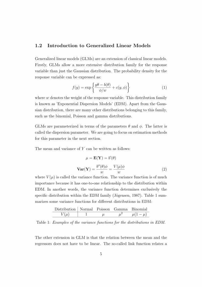
where V (µ) is called the variance function. The variance function is of much
importance because it has one-to-one relationship to the distribution within
EDM. In another words, the variance function determines exclusively the
specific distribution within the EDM family (Jogensen, 1987). Table 1 sum-
marizes some variance functions for different distributions in EDM:
Distribution Normal Poisson Gamma BinomialV (µ) 1 µ µ2 µ(1− µ)
Table 1: Examples of the variance functions for the distributions in EDM.
The other extension in GLM is that the relation between the mean and the
regressors does not have to be linear. The so-called link function relates a
5
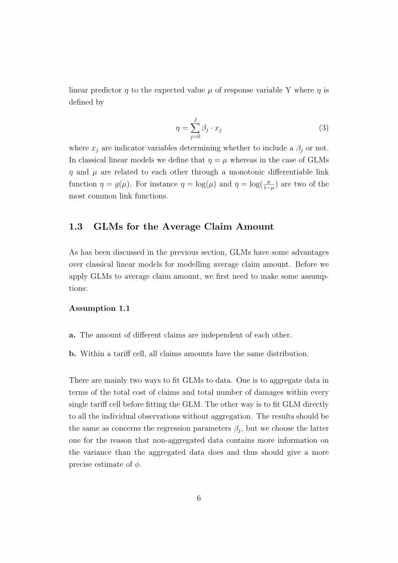
linear predictor η to the expected value µ of response variable Y where η is
defined by
η =J∑
j=0
βj · xj (3)
where xj are indicator variables determining whether to include a βj or not.
In classical linear models we define that η = µ whereas in the case of GLMs
η and µ are related to each other through a monotonic differentiable link
function η = g(µ). For instance η = log(µ) and η = log( µ1−µ
) are two of the
most common link functions.
1.3 GLMs for the Average Claim Amount
As has been discussed in the previous section, GLMs have some advantages
over classical linear models for modelling average claim amount. Before we
apply GLMs to average claim amount, we first need to make some assump-
tions:
Assumption 1.1
a. The amount of different claims are independent of each other.
b. Within a tariff cell, all claims amounts have the same distribution.
There are mainly two ways to fit GLMs to data. One is to aggregate data in
terms of the total cost of claims and total number of damages within every
single tariff cell before fitting the GLM. The other way is to fit GLM directly
to all the individual observations without aggregation. The results should be
the same as concerns the regression parameters βj, but we choose the latter
one for the reason that non-aggregated data contains more information on
the variance than the aggregated data does and thus should give a more
precise estimate of φ.
6
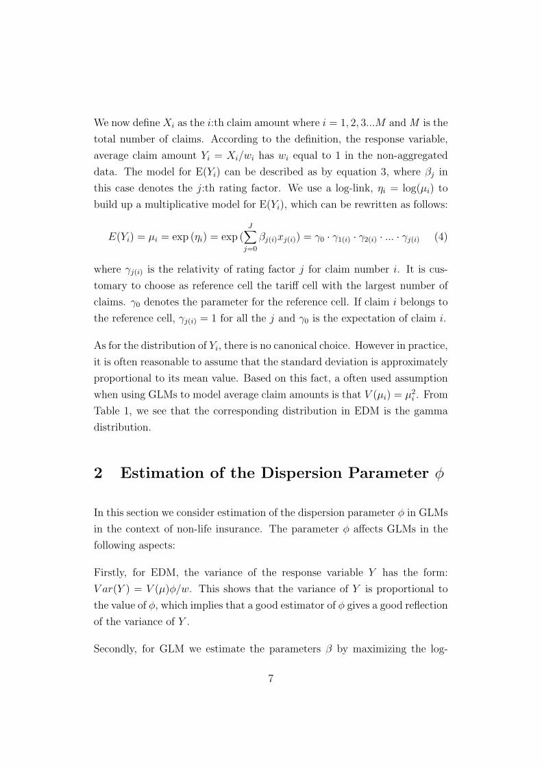
We now define Xi as the i:th claim amount where i = 1, 2, 3...M and M is the
total number of claims. According to the definition, the response variable,
average claim amount Yi = Xi/wi has wi equal to 1 in the non-aggregated
data. The model for E(Yi) can be described as by equation 3, where βj in
this case denotes the j:th rating factor. We use a log-link, ηi = log(µi) to
build up a multiplicative model for E(Yi), which can be rewritten as follows:
E(Yi) = µi = exp (ηi) = exp (J∑
j=0
βj(i)xj(i)) = γ0 · γ1(i) · γ2(i) · ... · γj(i) (4)
where γj(i) is the relativity of rating factor j for claim number i. It is cus-
tomary to choose as reference cell the tariff cell with the largest number of
claims. γ0 denotes the parameter for the reference cell. If claim i belongs to
the reference cell, γj(i) = 1 for all the j and γ0 is the expectation of claim i.
As for the distribution of Yi, there is no canonical choice. However in practice,
it is often reasonable to assume that the standard deviation is approximately
proportional to its mean value. Based on this fact, a often used assumption
when using GLMs to model average claim amounts is that V (µi) = µ2i . From
Table 1, we see that the corresponding distribution in EDM is the gamma
distribution.
2 Estimation of the Dispersion Parameter φ
In this section we consider estimation of the dispersion parameter φ in GLMs
in the context of non-life insurance. The parameter φ affects GLMs in the
following aspects:
Firstly, for EDM, the variance of the response variable Y has the form:
V ar(Y ) = V (µ)φ/w. This shows that the variance of Y is proportional to
the value of φ, which implies that a good estimator of φ gives a good reflection
of the variance of Y .
Secondly, for GLM we estimate the parameters β by maximizing the log-
7
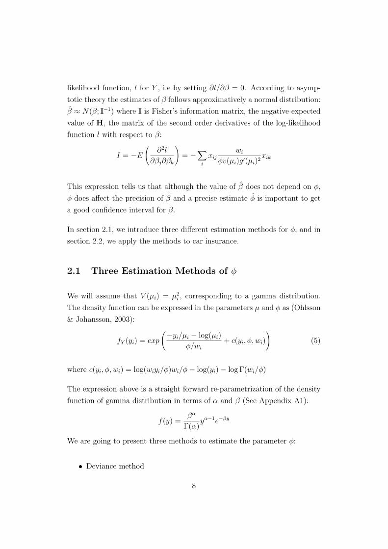
likelihood function, l for Y , i.e by setting ∂l/∂β = 0. According to asymp-
totic theory the estimates of β follows approximatively a normal distribution:
β ≈ N(β; I−1) where I is Fisher’s information matrix, the negative expected
value of H, the matrix of the second order derivatives of the log-likelihood
function l with respect to β:
I = −E
(∂2l
∂βj∂βk
)= −∑
i
xijwi
φv(µi)g′(µi)2xik
This expression tells us that although the value of β does not depend on φ,
φ does affect the precision of β and a precise estimate φ is important to get
a good confidence interval for β.
In section 2.1, we introduce three different estimation methods for φ, and in
section 2.2, we apply the methods to car insurance.
2.1 Three Estimation Methods of φ
We will assume that V (µi) = µ2i , corresponding to a gamma distribution.
The density function can be expressed in the parameters µ and φ as (Ohlsson
& Johansson, 2003):
fY (yi) = exp
(−yi/µi − log(µi)
φ/wi
+ c(yi, φ, wi)
)(5)
where c(yi, φ, wi) = log(wiyi/φ)wi/φ− log(yi)− log Γ(wi/φ)
The expression above is a straight forward re-parametrization of the density
function of gamma distribution in terms of α and β (See Appendix A1):
f(y) =βα
Γ(α)yα−1e−βy
We are going to present three methods to estimate the parameter φ:
• Deviance method
8
• Pearson method
• Maximum Likelihood method
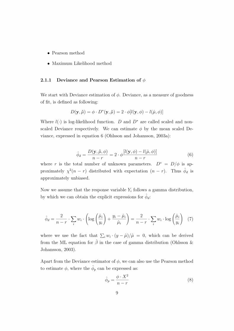
2.1.1 Deviance and Pearson Estimation of φ
We start with Deviance estimation of φ. Deviance, as a measure of goodness
of fit, is defined as following:
D(y, µ) = φ ·D∗(y, µ) = 2 · φ[l(y, φ)− l(µ, φ)]
Where l(·) is log-likelihood function. D and D∗ are called scaled and non-
scaled Deviance respectively. We can estimate φ by the mean scaled De-
viance, expressed in equation 6 (Ohlsson and Johansson, 2003a):
φd =D(y, µ, φ)
n− r= 2 · φ [l(y, φ)− l(µ, φ)]
n− r(6)
where r is the total number of unknown parameters. D∗ = D/φ is ap-
proximately χ2(n − r) distributed with expectation (n − r). Thus φd is
approximately unbiased.
Now we assume that the response variable Yi follows a gamma distribution,
by which we can obtain the explicit expressions for φd:
φd =2
n− r·∑
i
wi ·(
log
(µi
yi
)+
yi − µi
µi
)=
2
n− r·∑
i
wi · log
(µi
yi
)(7)
where we use the fact that∑
i wi · (y − µ)/µ = 0, which can be derived
from the ML equation for β in the case of gamma distribution (Ohlsson &
Johansson, 2003).
Apart from the Deviance estimator of φ, we can also use the Pearson method
to estimate φ, where the φp can be expressed as:
φp =φ ·X2
n− r(8)
9
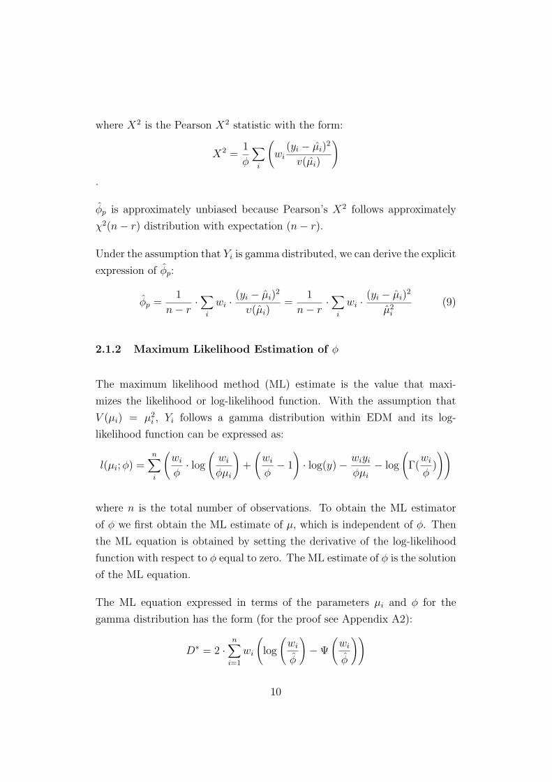
where X2 is the Pearson X2 statistic with the form:
X2 =1
φ
∑
i
(wi
(yi − µi)2
v(µi)
)
.
φp is approximately unbiased because Pearson’s X2 follows approximately
χ2(n− r) distribution with expectation (n− r).
Under the assumption that Yi is gamma distributed, we can derive the explicit
expression of φp:
φp =1
n− r·∑
i
wi · (yi − µi)2
υ(µi)=
1
n− r·∑
i
wi · (yi − µi)2
µ2i
(9)
2.1.2 Maximum Likelihood Estimation of φ
The maximum likelihood method (ML) estimate is the value that maxi-
mizes the likelihood or log-likelihood function. With the assumption that
V (µi) = µ2i , Yi follows a gamma distribution within EDM and its log-
likelihood function can be expressed as:
l(µi; φ) =n∑
i
(wi
φ· log
(wi
φµi
)+
(wi
φ− 1
)· log(y)− wiyi
φµi
− log
(Γ(
wi
φ)
))
where n is the total number of observations. To obtain the ML estimator
of φ we first obtain the ML estimate of µ, which is independent of φ. Then
the ML equation is obtained by setting the derivative of the log-likelihood
function with respect to φ equal to zero. The ML estimate of φ is the solution
of the ML equation.
The ML equation expressed in terms of the parameters µi and φ for the
gamma distribution has the form (for the proof see Appendix A2):
D∗ = 2 ·n∑
i=1
wi
(log
(wi
φ
)−Ψ
(wi
φ
))
10
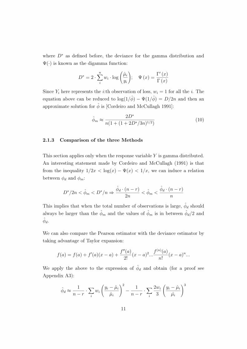
where D∗ as defined before, the deviance for the gamma distribution and
Ψ(·) is known as the digamma function:
D∗ = 2 ·n∑
i
wi · log
(µi
yi
); Ψ (x) =
Γ′ (x)
Γ (x)
Since Yi here represents the i:th observation of loss, wi = 1 for all the i. The
equation above can be reduced to log(1/φ) − Ψ(1/φ) = D/2n and then an
approximate solution for φ is [Cordeiro and McCullagh 1991]:
φm ≈ 2D∗
n(1 + (1 + 2D∗/3n)1/2)(10)
2.1.3 Comparison of the three Methods
This section applies only when the response variable Y is gamma distributed.
An interesting statement made by Cordeiro and McCullagh (1991) is that
from the inequality 1/2x < log(x) − Ψ(x) < 1/x, we can induce a relation
between φd and φm:
D∗/2n < φm < D∗/n ⇒ φd · (n− r)
2n< φm <
φd · (n− r)
n
This implies that when the total number of observations is large, φd should
always be larger than the φm and the values of φm is in between φd/2 and
φd.
We can also compare the Pearson estimator with the deviance estimator by
taking advantage of Taylor expansion:
f(a) = f(a) + f ′(a)(x− a) +f ′′(a)
2!(x− a)2...
f (n)(a)
n!(x− a)n...
We apply the above to the expression of φd and obtain (for a proof see
Appendix A3):
φd ≈ 1
n− r·∑
i
wi
(yi − µi
µi
)2
− 1
n− r·∑
i
2wi
3
(yi − µi
µi
)3
11
We see that φp is the first term of the expression above. The last term, which
can take both positive and negative values can be considered as a measure
of the difference between these two estimators. Thus the φp can be either
larger or smaller than the φd. These two estimators are approximately the
same only when the values of yi are close to the predicted values, i.e. the
GLM has a good fit to the data.
What deserves notice here is that even though the Pearson and Deviance
estimators can be considered as measures of deviations of Yi from µi, they can
come to quite different results. The Pearson estimator to some extent might
exaggerate the deviations by taking the square of the difference between yi
and µi while the Deviance estimator on the opposite might under-estimates
the deviations because it diminishes with the logarithm of the ratio of µi and
yi.
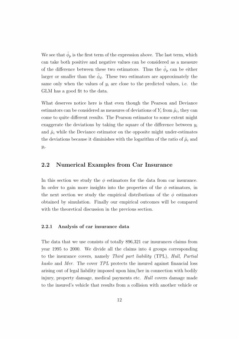
2.2 Numerical Examples from Car Insurance
In this section we study the φ estimators for the data from car insurance.
In order to gain more insights into the properties of the φ estimators, in
the next section we study the empirical distributions of the φ estimators
obtained by simulation. Finally our empirical outcomes will be compared
with the theoretical discussion in the previous section.
2.2.1 Analysis of car insurance data
The data that we use consists of totally 896,321 car insurances claims from
year 1995 to 2000. We divide all the claims into 4 groups corresponding
to the insurance covers, namely Third part liability (TPL), Hull, Partial
kasko and Mer. The cover TPL protects the insured against financial loss
arising out of legal liability imposed upon him/her in connection with bodily
injury, property damage, medical payments etc. Hull covers damage made
to the insured’s vehicle that results from a collision with another vehicle or
12
object or damage incurred when vehicle is transported by boat or train etc.
Partial kasko is a comprehensive cover that protects against losses resulting
from glass damage (Gls), theft (Sto), fire (Bra), salvage (Rad) and machine
(Mas). Mer covers some risks that are not defined in the other risk covers,
e.g. intentional damage.
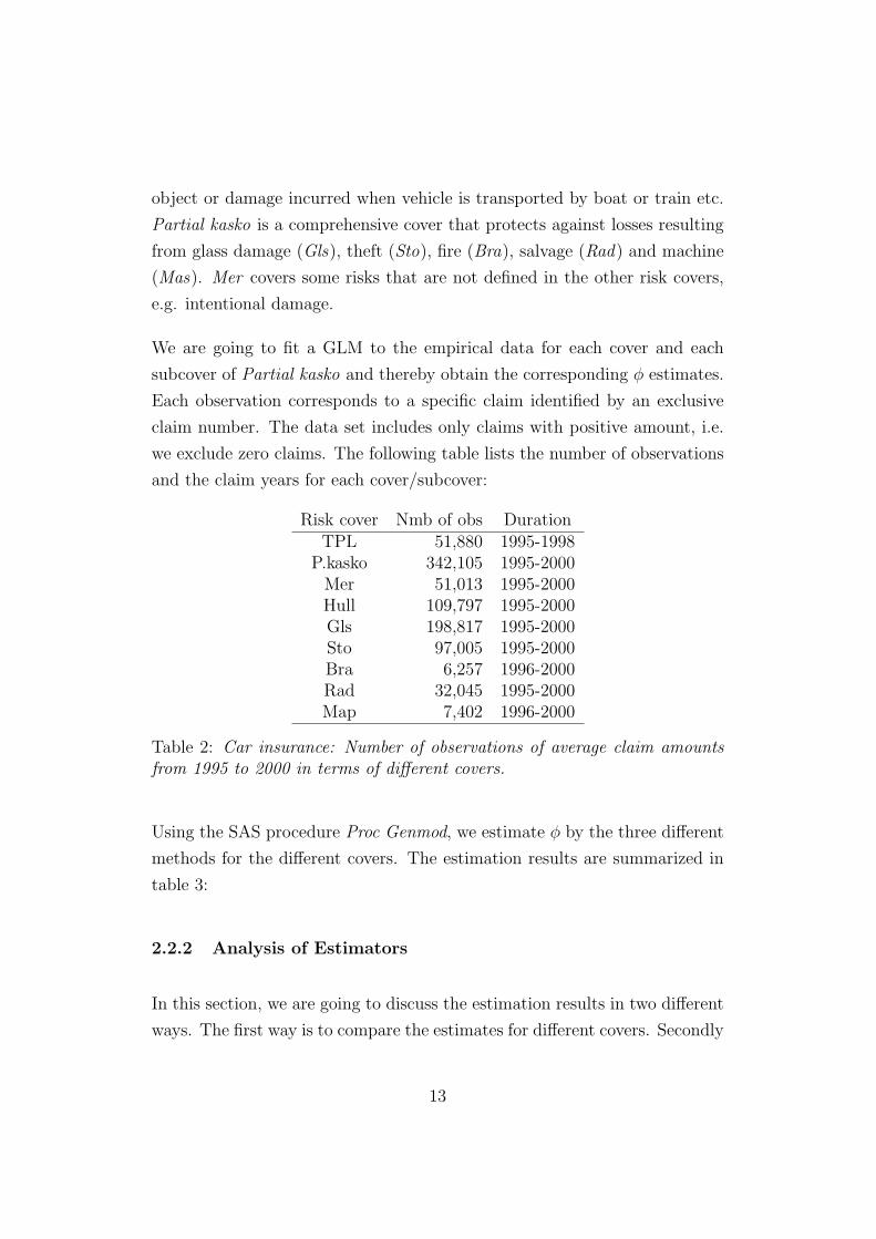
We are going to fit a GLM to the empirical data for each cover and each
subcover of Partial kasko and thereby obtain the corresponding φ estimates.
Each observation corresponds to a specific claim identified by an exclusive
claim number. The data set includes only claims with positive amount, i.e.
we exclude zero claims. The following table lists the number of observations
and the claim years for each cover/subcover:
Risk cover Nmb of obs DurationTPL 51,880 1995-1998
P.kasko 342,105 1995-2000Mer 51,013 1995-2000Hull 109,797 1995-2000Gls 198,817 1995-2000Sto 97,005 1995-2000Bra 6,257 1996-2000Rad 32,045 1995-2000Map 7,402 1996-2000
Table 2: Car insurance: Number of observations of average claim amountsfrom 1995 to 2000 in terms of different covers.
Using the SAS procedure Proc Genmod, we estimate φ by the three different
methods for the different covers. The estimation results are summarized in
table 3:
2.2.2 Analysis of Estimators
In this section, we are going to discuss the estimation results in two different
ways. The first way is to compare the estimates for different covers. Secondly
13
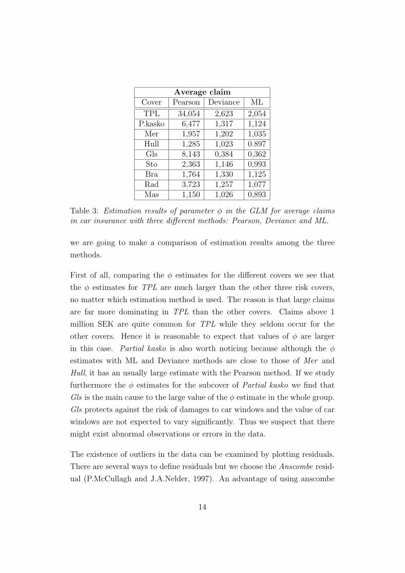
Average claimCover Pearson Deviance ML
TPL 34,054 2,623 2,054P.kasko 6,477 1,317 1,124
Mer 1,957 1,202 1,035Hull 1,285 1,023 0.897Gls 8,143 0,384 0,362Sto 2,363 1,146 0,993Bra 1,764 1,330 1,125Rad 3,723 1,257 1,077Mas 1,150 1,026 0,893
Table 3: Estimation results of parameter φ in the GLM for average claimsin car insurance with three different methods: Pearson, Deviance and ML.
we are going to make a comparison of estimation results among the three
methods.
First of all, comparing the φ estimates for the different covers we see that
the φ estimates for TPL are much larger than the other three risk covers,
no matter which estimation method is used. The reason is that large claims
are far more dominating in TPL than the other covers. Claims above 1
million SEK are quite common for TPL while they seldom occur for the
other covers. Hence it is reasonable to expect that values of φ are larger
in this case. Partial kasko is also worth noticing because although the φ
estimates with ML and Deviance methods are close to those of Mer and
Hull, it has an usually large estimate with the Pearson method. If we study
furthermore the φ estimates for the subcover of Partial kasko we find that
Gls is the main cause to the large value of the φ estimate in the whole group.
Gls protects against the risk of damages to car windows and the value of car
windows are not expected to vary significantly. Thus we suspect that there
might exist abnormal observations or errors in the data.
The existence of outliers in the data can be examined by plotting residuals.
There are several ways to define residuals but we choose the Anscombe resid-
ual (P.McCullagh and J.A.Nelder, 1997). An advantage of using anscombe
14
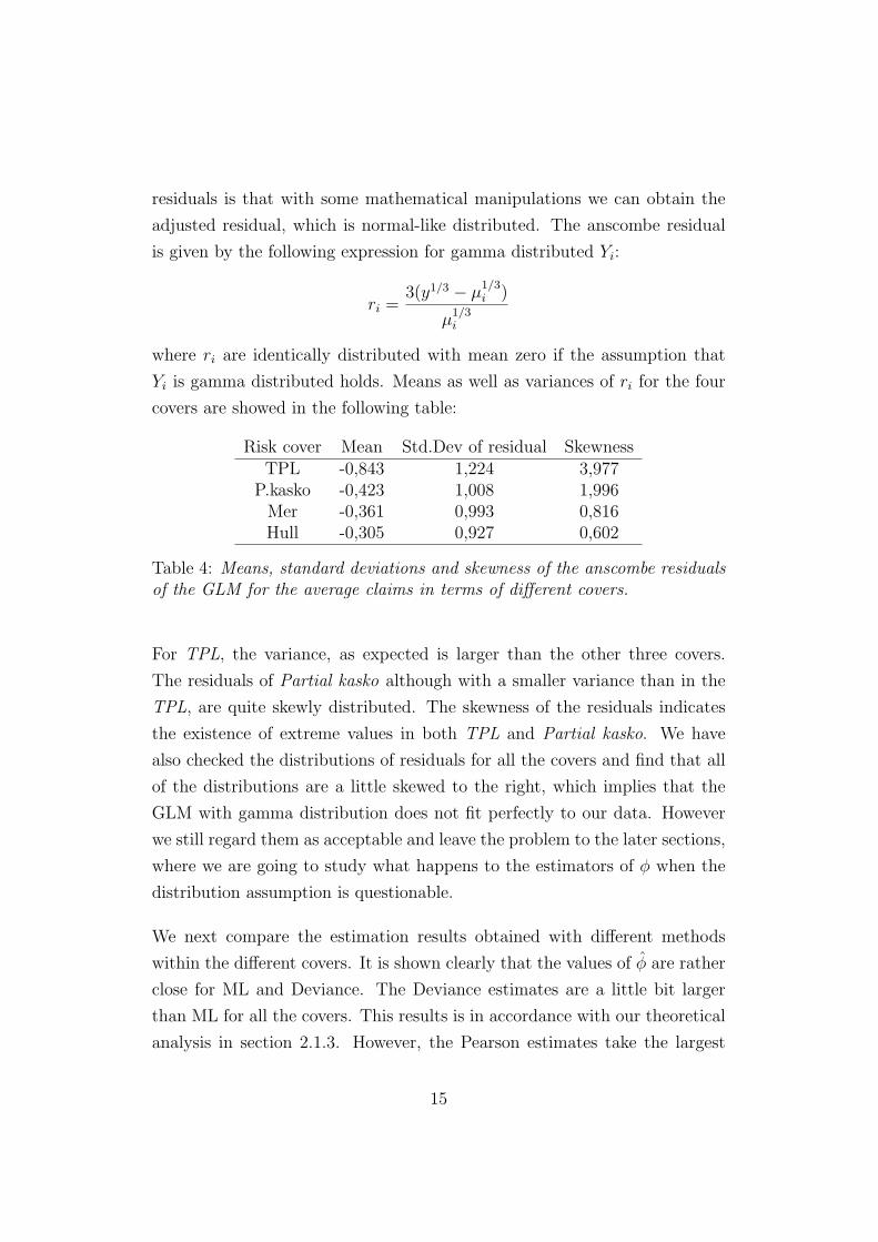
residuals is that with some mathematical manipulations we can obtain the
adjusted residual, which is normal-like distributed. The anscombe residual
is given by the following expression for gamma distributed Yi:
ri =3(y1/3 − µ
1/3i )
µ1/3i
where ri are identically distributed with mean zero if the assumption that
Yi is gamma distributed holds. Means as well as variances of ri for the four
covers are showed in the following table:
Risk cover Mean Std.Dev of residual SkewnessTPL -0,843 1,224 3,977
P.kasko -0,423 1,008 1,996Mer -0,361 0,993 0,816Hull -0,305 0,927 0,602
Table 4: Means, standard deviations and skewness of the anscombe residualsof the GLM for the average claims in terms of different covers.
For TPL, the variance, as expected is larger than the other three covers.
The residuals of Partial kasko although with a smaller variance than in the
TPL, are quite skewly distributed. The skewness of the residuals indicates
the existence of extreme values in both TPL and Partial kasko. We have
also checked the distributions of residuals for all the covers and find that all
of the distributions are a little skewed to the right, which implies that the
GLM with gamma distribution does not fit perfectly to our data. However
we still regard them as acceptable and leave the problem to the later sections,
where we are going to study what happens to the estimators of φ when the
distribution assumption is questionable.
We next compare the estimation results obtained with different methods
within the different covers. It is shown clearly that the values of φ are rather
close for ML and Deviance. The Deviance estimates are a little bit larger
than ML for all the covers. This results is in accordance with our theoretical
analysis in section 2.1.3. However, the Pearson estimates take the largest
15
value compared with the other two, probably due to the existence of extreme
values.
The Pearson estimate for TLP deserves extra attention since it is abnormally
larger than the deviance and the ML estimates. It possibly indicates the
sensitivity of the Pearson estimator to large amounts. For the cover Mer
however, all these three estimates are fairly close to each other. We may
summarize the results as follows:
1. The covers TLP and Partial kasko represent two different phenomena.
TLP has both large variance and skewness in the residuals. In practice
the distribution of TLP claims has fat tails due to the large amounts
in some claims. In this circumstance, the assumption of a gamma
distribution makes less sense than for the other covers. For Partial
kasko variance of the residuals is not very large but the skewness, caused
by outliers, is large. To deal with this kind of data, it is important to
find out the causes for the outliers. It turned out that in this case, the
outliers were caused by defective recording procedures.
2. The Pearson estimates differ greatly from the estimates with the other
two methods especially for the TPL and Partial kasko. It implies that
the Pearson estimator of φ is sensitive to the variance of data and
extreme values, while such values do not have much effect on ML and
deviance estimators.
2.2.3 Sensitivity of estimates to extreme values
In the previous section, we found that estimation results of φ were quite
dependent on which estimation method we employed, particularly for the
covers where extremely large losses occur. This observation motivates us to
study more closely how the φ estimates react to extreme values. In order to
reduce the load of work, we choose the covers TLP as well as Gls as our study
objects, where Gls is one of the subgroups of Partial Kasko and contributes
16
most to the variation in the group.
There are mainly two alternatives when dealing with extreme values. One is
truncation where the claim cost above a certain level is cut away. Truncation
is often used to deal with the problem of large claims in non-life insurance.
The other alternative is to delete all observations defined as ’extreme’. When
the outliers are assumed to be caused by errors, it is natural to use the second
method. After truncation or deletion we obtain a modified data set which
will be used to fit GLMs and estimate the parameter φ. In order to study
the sensitivity of φ to the extreme values we are going to set several levels
at which the data will be truncated or deleted so that we can observe how
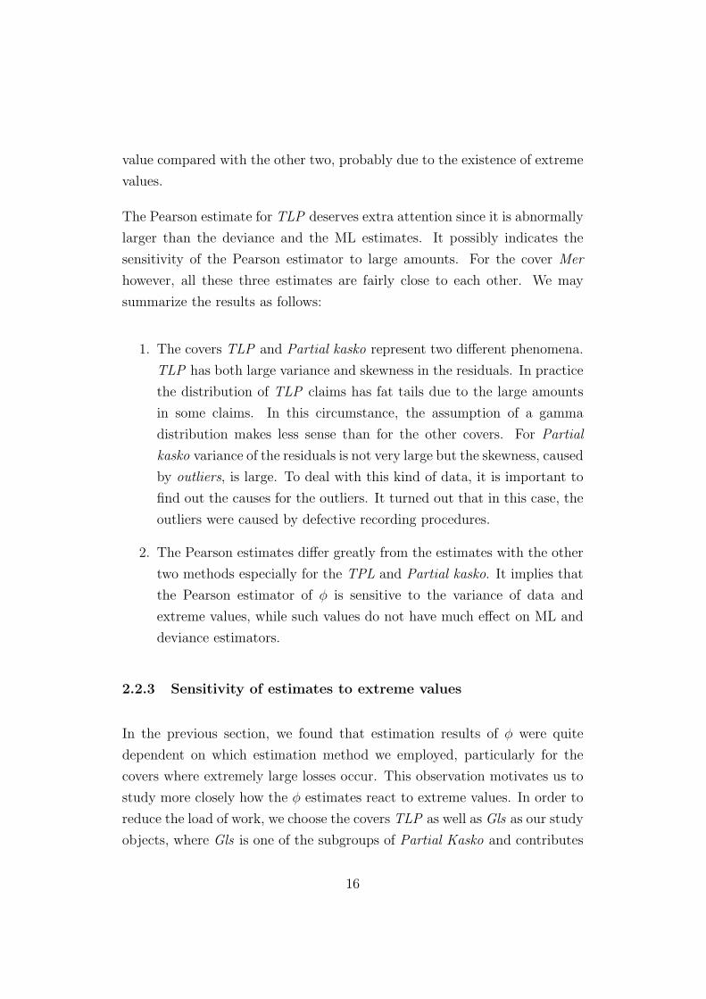
φ estimates change with different levels. We use truncation for risk cover
TLP and deletion for Gls. The results are showed in table 5 and table 6
respectively:
Method Original estimate level1 level2 level3 level4Pearson 34,054 10,194 2,953 1,782 0,640Deviance 2,623 2,124 1,588 1,333 0,801
ML 2,054 1,711 1,326 1,136 0,718
Table 5: Estimations of the parameter φ in the GLM for the cover TLP withtruncations on four different levels (Unit: SEK): level 1 = 1 000 000; level2 = 200 000; level 3 = 100 000; level 4 = 30 000.
Method Original estimate level1 level2 level3 level4Pearson 8.143 1,444 0,286 0,235 0,261Deviance 0.384 0,352 0,335 0,322 0,309
ML 0.362 0,333 0,318 0,306 0,295
Table 6: Estimations of the parameter φ in the GLM for the cover Gls withtruncations on four different levels (Unit: SEK): level 1 = 500 000; level 2= 50 000; level 3 = 4 686 (corresponding to 99% quantile) level 4 = 3 415(corresponding to 95% quantile).
From the table 5 and 6, we find that the Pearson estimates are quite sensitive
to large values while the Deviance and ML estimates are much less affected by
truncation or deletion. Besides, we also notice that after truncation or dele-
17
tion of the extreme values on certain levels, the Pearson estimates decrease
dramatically and become less than the values of the deviance estimate.
2.3 Simulation
From the previous section, we found that in practice, there can be large
differences between the φ estimates. In this section, we are going to study
the properties of the φ estimators when the underlying distribution is known
and try to find out which estimator is the most reliable by a simulation study.
The estimators will be compared in terms of unbiasedness and efficiency. In
order to limit the study, we will only choose two risk covers: TPL and Hull.
Two problems will be of interest in this section. First we are going to study
how the φ estimates behave when the assumption of a gamma distribution is
true. The other interesting problem is what the empirical distributions of φ
look like when the response variable is no longer gamma distributed but the
relationship V (µi) = µ2i still holds. There are many non-EDM distributions
which satisfy the condition above, we choose the Generalized Pareto distri-
bution which has a fat tail. We simulate data out of this distribution and
fit GLMs to it under the false assumption that Y is gamma distributed. We
are interested in studying whether estimators are robust to variation of the
Y distribution.
2.3.1 Simulations with Gamma Distributed Claims
We assume that the claims Yi follow the Gamma distribution where E(Yi) =
µi and V ar(Yi) = φ · µ2i . For the parameter µi, we use the estimated values
for TPL and Hull from the previous sections. We choose the true value of
φ also based on the earlier estimating results so as to make the simulated
data as realistic as possible. Besides, the number of claims per tariff cell
is chosen in accordance with the empirical data. We fitted GLMs to the
simulated data with 10 000 repetitions, each of which contained the same
18
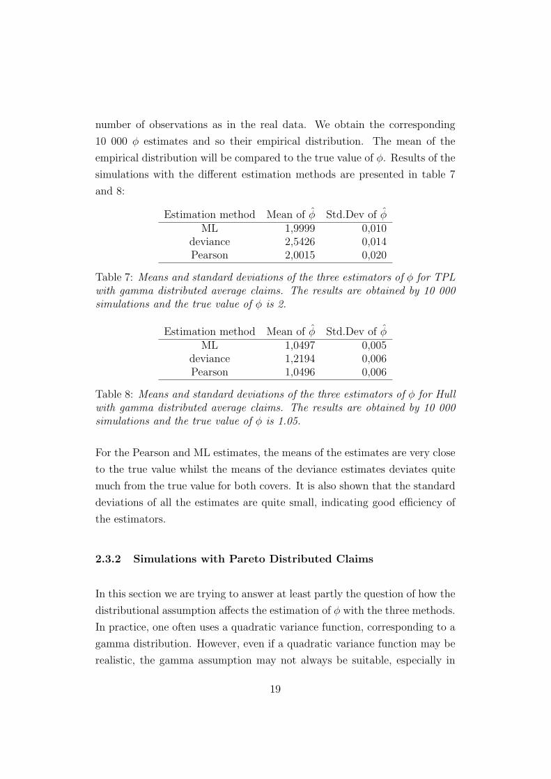
number of observations as in the real data. We obtain the corresponding
10 000 φ estimates and so their empirical distribution. The mean of the
empirical distribution will be compared to the true value of φ. Results of the
simulations with the different estimation methods are presented in table 7
and 8:
Estimation method Mean of φ Std.Dev of φML 1,9999 0,010
deviance 2,5426 0,014Pearson 2,0015 0,020
Table 7: Means and standard deviations of the three estimators of φ for TPLwith gamma distributed average claims. The results are obtained by 10 000simulations and the true value of φ is 2.
Estimation method Mean of φ Std.Dev of φML 1,0497 0,005
deviance 1,2194 0,006Pearson 1,0496 0,006
Table 8: Means and standard deviations of the three estimators of φ for Hullwith gamma distributed average claims. The results are obtained by 10 000simulations and the true value of φ is 1.05.
For the Pearson and ML estimates, the means of the estimates are very close
to the true value whilst the means of the deviance estimates deviates quite
much from the true value for both covers. It is also shown that the standard
deviations of all the estimates are quite small, indicating good efficiency of
the estimators.
2.3.2 Simulations with Pareto Distributed Claims
In this section we are trying to answer at least partly the question of how the
distributional assumption affects the estimation of φ with the three methods.
In practice, one often uses a quadratic variance function, corresponding to a
gamma distribution. However, even if a quadratic variance function may be
realistic, the gamma assumption may not always be suitable, especially in
19
the presence of extreme values. In many cases, distributions with fatter tails
fit better the empirical data, e.g. the log-normal distribution or the gener-
alized Pareto distribution etc. Neither of them belongs to the EDM family.
Therefore we cannot apply these distributions directly in the frame of GLM.
We have studied what happens to the φ estimates if we still assume gamma
distribution though the real data follows a generalized Pareto distribution.
It may be noted that McCullagh and Nelder (1997) recommends using the
Pearson estimator in situations where the gamma assumption is in doubt.
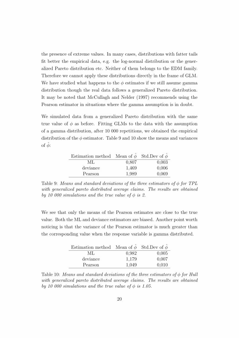
We simulated data from a generalized Pareto distribution with the same
true value of φ as before. Fitting GLMs to the data with the assumption
of a gamma distribution, after 10 000 repetitions, we obtained the empirical
distribution of the φ estimator. Table 9 and 10 show the means and variances
of φ:
Estimation method Mean of φ Std.Dev of φML 0,807 0,003
deviance 1,469 0,006Pearson 1,989 0,069
Table 9: Means and standard deviations of the three estimators of φ for TPLwith generalized pareto distributed average claims. The results are obtainedby 10 000 simulations and the true value of φ is 2.
We see that only the means of the Pearson estimates are close to the true
value. Both the ML and deviance estimators are biased. Another point worth
noticing is that the variance of the Pearson estimator is much greater than
the corresponding value when the response variable is gamma distributed.
Estimation method Mean of φ Std.Dev of φML 0,982 0,005
deviance 1,179 0,007Pearson 1,049 0,010
Table 10: Means and standard deviations of the three estimators of φ for Hullwith generalized pareto distributed average claims. The results are obtainedby 10 000 simulations and the true value of φ is 1.05.
20
3 Estimation of Dispersion parameters in GLMs
with Random Effect
In practice, one is often encountered with the problem of multi-level factors.
A multi-level factor has a large number of classes, many of which with in-
sufficient data for reliable estimates. Car model is a typical example of a
multi-level factor. Nelder & Verral (1997) and Ohlsson & Johansson (2003b)
suggested that multi-level factors can be modelled as random effects in GLMs.
These models include an additional dispersion parameter α and two different
methods of estimating α will be introduced. An empirical study of the three
methods is presented with the same data as we used in the previous section.
The section is ended with a simulation study.
3.1 Introduction to GLMs with Random Effect
According to Ohlsson and Johansson (2003b), GLMs can be extended by
introducing a random effect U in the way that µi(uk) = E(Yi|Uk = uk) = µiuk
for each level k of the random effect and µi = γ0γ1(i)γ2(i)...γj(i), the product
of all the relativities. It is natural to assume that E(Uk) = 1 since Uk can be
interpreted as a random deviation from the mean value given by other rating
factors. This corresponds to assuming mean zero for the random effects in
additive models. The main problem is how we find a suitable predictor for Uk.
According to Ohlsson and Johansson (2003b), the optimal linear predictor
can be expressed as g(Yi) = E(Uk|Yi), which minimizes the mean square
error. In the first part of this section, we are going to give a brief introduction
to Jewell’s Theorem, providing an idea of how to obtain g(Yi) = E(Uk|Yi)
when Yi is an EDM and µi depends on a random effect. Then we will discuss
so-called Tweedie models, where we can obtain an explicit expression for
E(Uk|Yi).
21
3.1.1 Jewell’s Theorem
We assume that conditioning on parameter Θ, the distribution of the response
variable Y is an EDM with density:
fYi|Θ(yi|θ) = exp
(yiθ − b(θ)
φ/wi
+ c(yi, φ, wi)
)(11)
where we have suppressed the index k and defined µ(Θ) = E(Y |Θ). We
assume also that:
Assumption [2]
• Θk are independent and identically distributed random variables for
k = 1, 2...K.
• For k = 1, 2...K, the pairs (Yik, Θk) are independent.
• Conditional on Θk the random variables Y1k,Y2k,...,YIk,k are indepen-
dent.
Given the distribution of the parameter Θ, which functions as prior distribu-
tion, we can get the posterior distribution FΘ|Y (θ|y) with the help of Bayes’
theorem. In Jewell’s theorem, it is assumed that distribution of Θ is of the
form:
fΘ(θ) = exp
(θδ − b(θ)
1/α+ d(δ, α)
)(12)
where:
δ = E(b′(Θ)) = E(µ(Θ)) (13)
and
α =E(b′′(Θ))
V ar(b′(Θ))=
E(V (µ(Θ)))
V ar(µ(Θ))(14)
α is the additional dispersion parameter in the GLMs with random effect.
Equation 14 shows how the dispersion parameter α is related to the variance
22
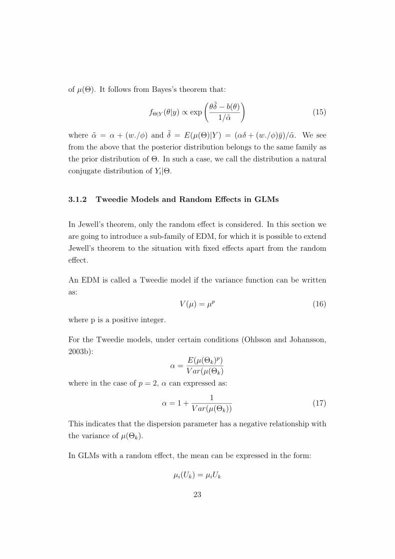
of µ(Θ). It follows from Bayes’s theorem that:
fΘ|Y (θ|y) ∝ exp
(θδ − b(θ)
1/α
)(15)
where α = α + (w./φ) and δ = E(µ(Θ)|Y ) = (αδ + (w./φ)y)/α. We see
from the above that the posterior distribution belongs to the same family as
the prior distribution of Θ. In such a case, we call the distribution a natural
conjugate distribution of Yi|Θ.
3.1.2 Tweedie Models and Random Effects in GLMs
In Jewell’s theorem, only the random effect is considered. In this section we
are going to introduce a sub-family of EDM, for which it is possible to extend
Jewell’s theorem to the situation with fixed effects apart from the random
effect.
An EDM is called a Tweedie model if the variance function can be written
as:
V (µ) = µp (16)
where p is a positive integer.
For the Tweedie models, under certain conditions (Ohlsson and Johansson,
2003b):
α =E(µ(Θk)
p)
V ar(µ(Θk)
where in the case of p = 2, α can expressed as:
α = 1 +1
V ar(µ(Θk))(17)
This indicates that the dispersion parameter has a negative relationship with
the variance of µ(Θk).
In GLMs with a random effect, the mean can be expressed in the form:
µi(Uk) = µiUk
23
where µi is given by the ordinary rating factors and Uk denotes the the
random effect on k:th level. We denote the so called canonical link function by
h(·). Based on the results in the previous section, we can obtain the following
(Ohlsson and Johansson, 2003b): We define the response variable Yik and
E(Yik|Uk) = µiUk. Conditioning on Uk = uk, the Yik follow a Tweedie model
with 1 ≤ p ≤ 2 and Θ = h(Uk) follows the natural conjugate distribution
where α > 0 and δ > 0, then the optimal predictor of Uk is of the form:
uk = E(Uk|Yik), and is given by
uk =
∑i wikyik/µ
p−1i + φα
∑i wikµ
2−pi + φα
(18)
3.2 Estimation of the α
We are interested in the estimation of the dispersion parameters in GLMs
and now focus on the additional dispersion parameter α. In this section, two
methods of estimating α will be presented, starting with maximum likelihood
estimations in the marginal distribution of Yik. Then an alternative method
proposed by Ohlsson and Johansson(2003b) is introduced. We assume that
the response variable Yik|Uk follows a Tweedie model.
3.2.1 ML Estimation of α
For p = 1 or p = 2 in the Tweedie model, it is possible to derive an explicit
expression for the marginal density of Y . The ML estimator can then be
obtained as the solution to the ML equations.
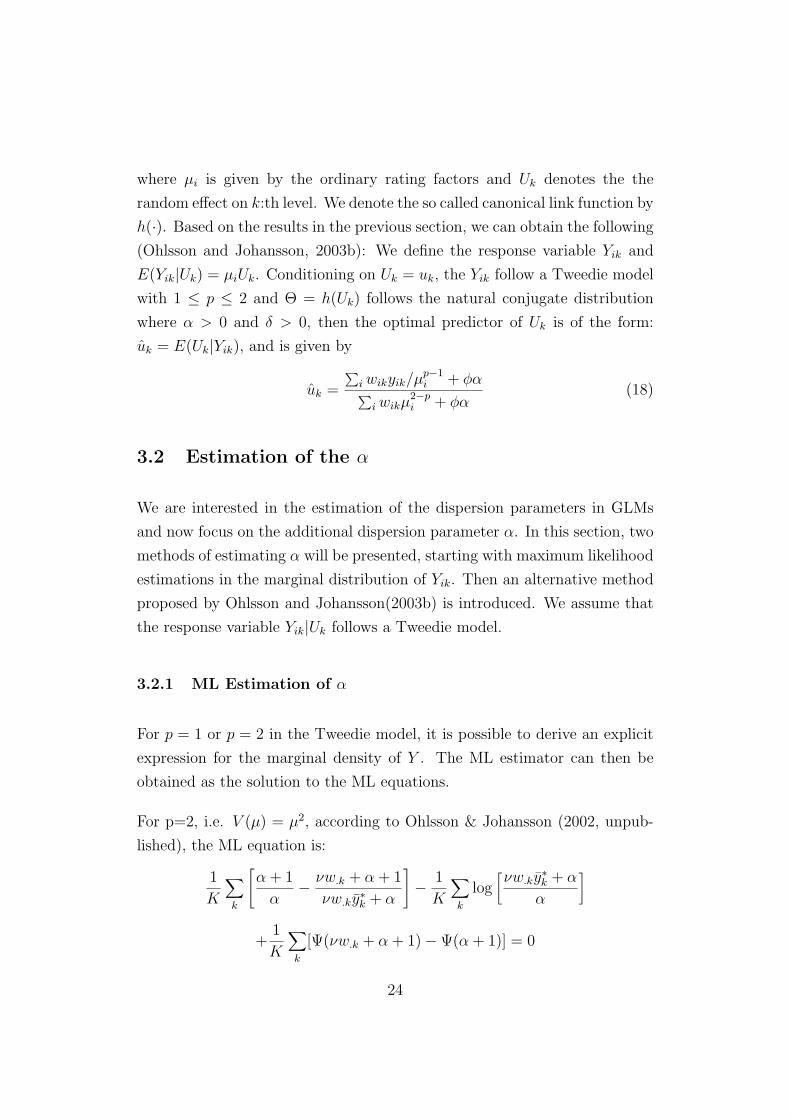
For p=2, i.e. V (µ) = µ2, according to Ohlsson & Johansson (2002, unpub-
lished), the ML equation is:
1
K
∑
k
[α + 1
α− νw.k + α + 1
νw.ky∗k + α
]− 1
K
∑
k
log[νw.ky
∗k + α
α
]
+1
K
∑
k
[Ψ(νw.k + α + 1)−Ψ(α + 1)] = 0
24
where K denotes the total number of classes of the multi-level factor, ν = 1/φ
and yk∗ = yik/µk. Using the estimated α we can then predict the random
effect Uk.
The estimation results of α depends partly on φ, as we can tell from the ex-
pression above. Thus the estimate of φ will affect the quality of the estimate
of α when we use the ML estimator.
3.2.2 An Alternative Estimation Method
According to Ohlsson and Johansson (2003b), under the assumption of Tweedie
models, one can prove that
α =E(µ(Θ)p)
V ar(µ(Θ))
where Θ = h(U). We now consider separate estimation of σ2 = φE(µ(Θ)p)
and σ2Θ = V ar(µ(Θ)), whose ratio is the term φα. From equation 18 we see
that with the αφ we can predict Uk directly. In another words, we do not
need to estimate α and φ separately to obtain Uk.
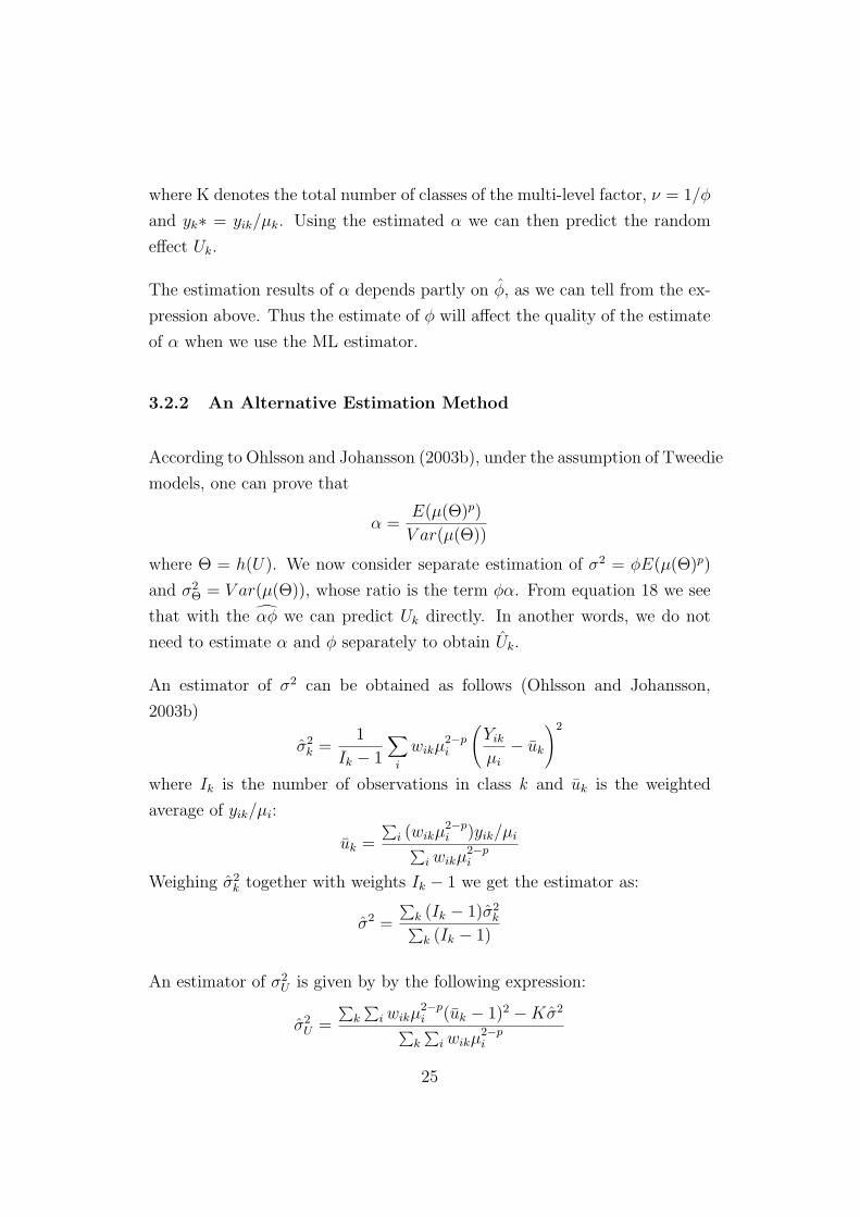
An estimator of σ2 can be obtained as follows (Ohlsson and Johansson,
2003b)
σ2k =
1
Ik − 1
∑
i
wikµ2−pi
(Yik
µi
− uk
)2
where Ik is the number of observations in class k and uk is the weighted
average of yik/µi:
uk =
∑i (wikµ
2−pi )yik/µi∑
i wikµ2−pi
Weighing σ2k together with weights Ik − 1 we get the estimator as:
σ2 =
∑k (Ik − 1)σ2
k∑k (Ik − 1)
An estimator of σ2U is given by by the following expression:
σ2U =
∑k
∑i wikµ
2−pi (uk − 1)2 −Kσ2
∑k
∑i wikµ
2−pi
25
The estimator of αφ can be expressed as: αφ = σ2/σ2U . It can be shown that
given µi, σ2 and σ2U are unbiased estimators of σ2 and σ2
U respectively.
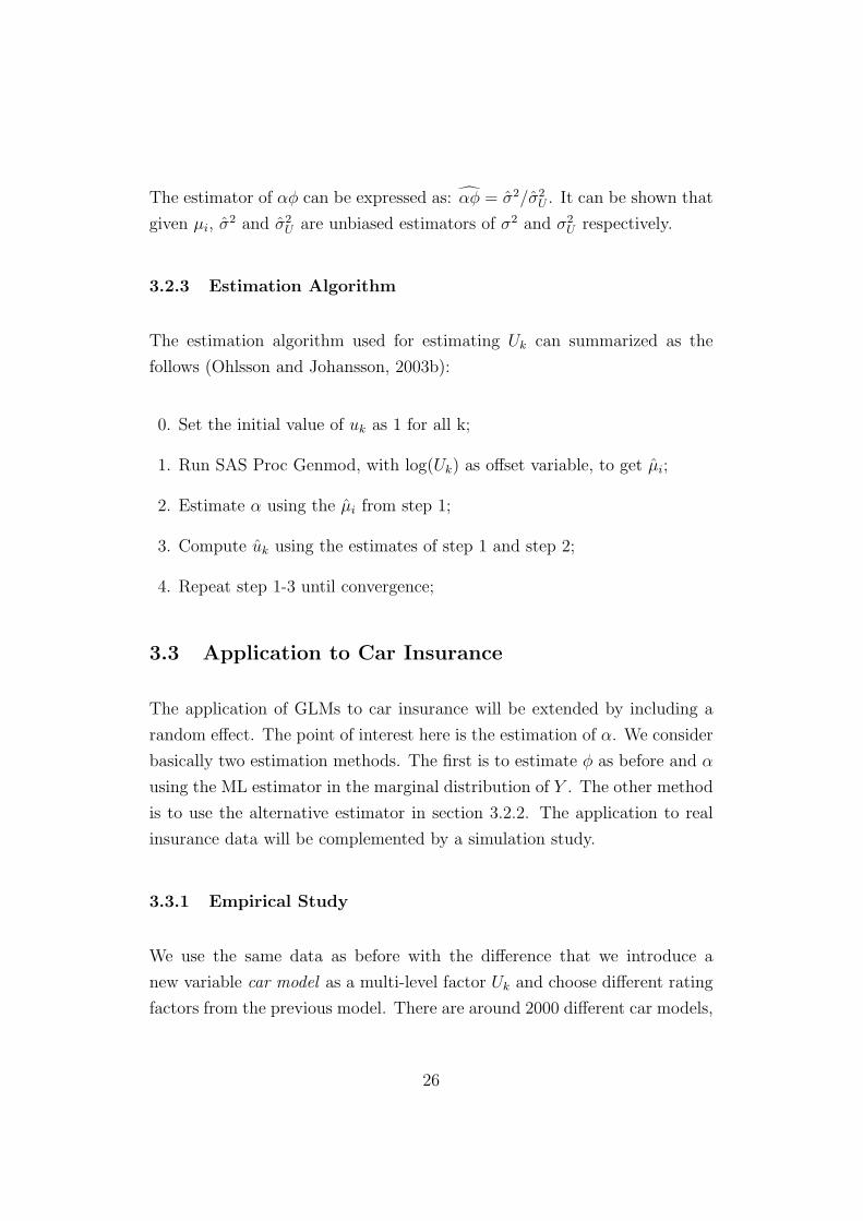
3.2.3 Estimation Algorithm
The estimation algorithm used for estimating Uk can summarized as the
follows (Ohlsson and Johansson, 2003b):
0. Set the initial value of uk as 1 for all k;
1. Run SAS Proc Genmod, with log(Uk) as offset variable, to get µi;
2. Estimate α using the µi from step 1;
3. Compute uk using the estimates of step 1 and step 2;
4. Repeat step 1-3 until convergence;
3.3 Application to Car Insurance
The application of GLMs to car insurance will be extended by including a
random effect. The point of interest here is the estimation of α. We consider
basically two estimation methods. The first is to estimate φ as before and α
using the ML estimator in the marginal distribution of Y . The other method
is to use the alternative estimator in section 3.2.2. The application to real
insurance data will be complemented by a simulation study.
3.3.1 Empirical Study
We use the same data as before with the difference that we introduce a
new variable car model as a multi-level factor Uk and choose different rating
factors from the previous model. There are around 2000 different car models,
26
i.e. Uk has about 2000 classes. The new model can be expressed as follows:
µi(uk) = E(Yi|Uk = uk) = γ0γ1(i)γ2(i)...γj(i)uk
where the parameter γj(i) denotes the relativity for the i:th level with respect
to the j:th rating factor.
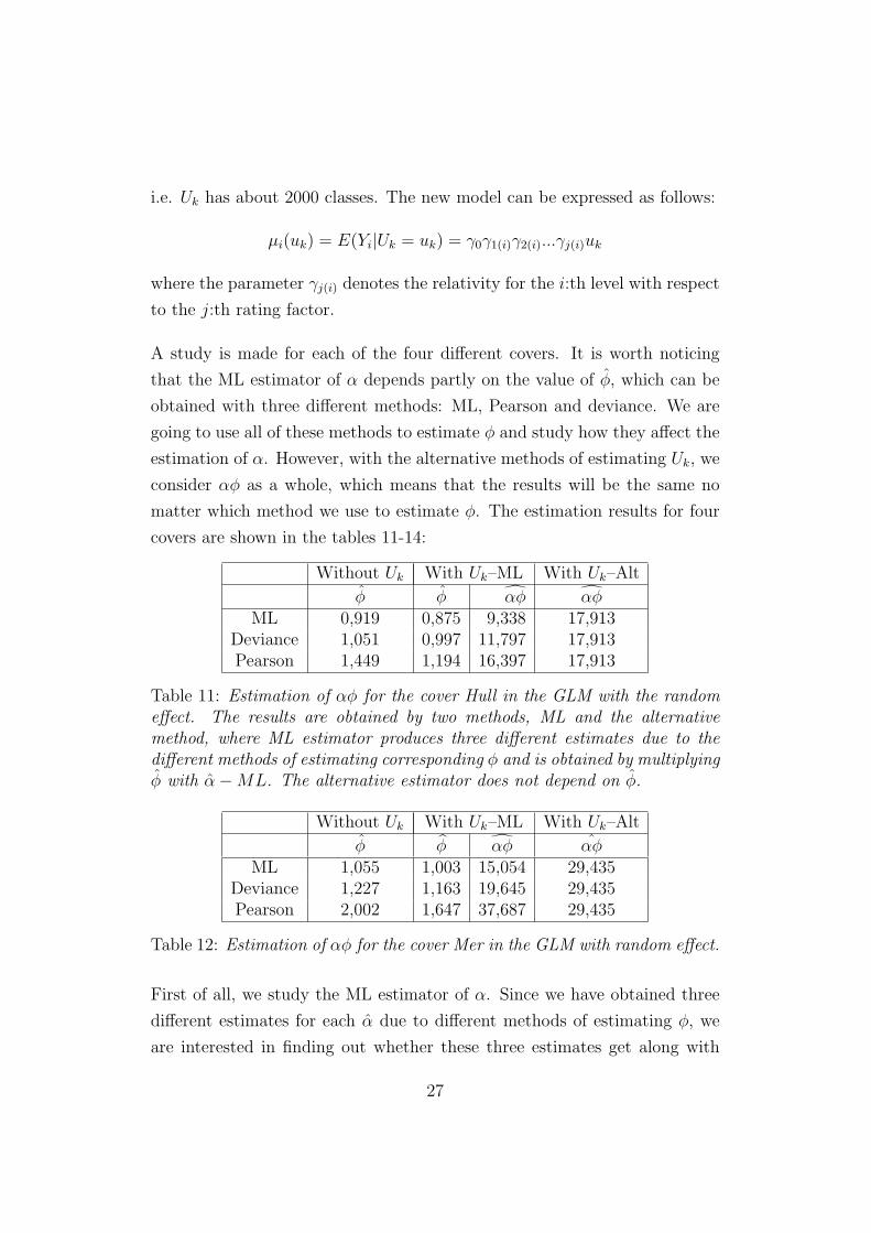
A study is made for each of the four different covers. It is worth noticing
that the ML estimator of α depends partly on the value of φ, which can be
obtained with three different methods: ML, Pearson and deviance. We are
going to use all of these methods to estimate φ and study how they affect the
estimation of α. However, with the alternative methods of estimating Uk, we
consider αφ as a whole, which means that the results will be the same no
matter which method we use to estimate φ. The estimation results for four
covers are shown in the tables 11-14:
Without Uk With Uk–ML With Uk–Alt
φ φ αφ αφML 0,919 0,875 9,338 17,913
Deviance 1,051 0,997 11,797 17,913Pearson 1,449 1,194 16,397 17,913
Table 11: Estimation of αφ for the cover Hull in the GLM with the randomeffect. The results are obtained by two methods, ML and the alternativemethod, where ML estimator produces three different estimates due to thedifferent methods of estimating corresponding φ and is obtained by multiplyingφ with α−ML. The alternative estimator does not depend on φ.
Without Uk With Uk–ML With Uk–Alt
φ φ αφ αφML 1,055 1,003 15,054 29,435
Deviance 1,227 1,163 19,645 29,435Pearson 2,002 1,647 37,687 29,435
Table 12: Estimation of αφ for the cover Mer in the GLM with random effect.
First of all, we study the ML estimator of α. Since we have obtained three
different estimates for each α due to different methods of estimating φ, we
are interested in finding out whether these three estimates get along with
27
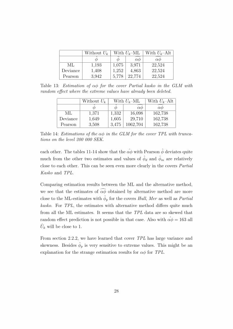
Without Uk With Uk–ML With Uk–Alt
φ φ αφ αφML 1,193 1,075 3,971 22,524
Deviance 1,408 1,252 4,863 22,524Pearson 3,942 5,778 22,774 22,524
Table 13: Estimation of αφ for the cover Partial kasko in the GLM withrandom effect where the extreme values have already been deleted.
Without Uk With Uk–ML With Uk–Alt
φ φ αφ αφML 1,371 1,332 16,098 162,738
Deviance 1,649 1,605 29,710 162,738Pearson 3,508 3,475 1062,704 162,738
Table 14: Estimations of the αφ in the GLM for the cover TPL with trunca-tions on the level 200 000 SEK.
each other. The tables 11-14 show that the αφ with Pearson φ deviates quite
much from the other two estimates and values of φd and φm are relatively
close to each other. This can be seen even more clearly in the covers Partial
Kasko and TPL.
Comparing estimation results between the ML and the alternative method,
we see that the estimates of αφ obtained by alternative method are more
close to the ML-estimates with φp for the covers Hull, Mer as well as Partial
kasko. For TPL, the estimates with alternative method differs quite much
from all the ML estimates. It seems that the TPL data are so skewed that
random effect prediction is not possible in that case. Also with αφ = 163 all
Uk will be close to 1.
From section 2.2.2, we have learned that cover TPL has large variance and
skewness. Besides φp is very sensitive to extreme values. This might be an
explanation for the strange estimation results for αφ for TPL.
28
3.3.2 Simulation Study
In order to give more insight into the properties of the estimators of α, we
performed a simulation study. The main purpose of simulations is to compare
the estimated α with the true value, in which way we can get some idea of
how well different estimation methods work. For the sake of simplicity, we
choose to create a data set with only one fixed effect and one random effect.
To begin with, we assume that
Yi|Uk ∼ Gamma(µiUk, φ)
where E(Yi|Uk) = µiUk. The corresponding natural conjugate distribution
fΘ(θ) is of the form
fΘ(θ) = exp
(θδ + log(−θ)
1/α+ d
)
where the canonical link function can be expressed as Θ = −1/Uk. It can be
shown that Uk ∼ InverseGamma(α + 1, α) (for a proof see the Appendix
A4). To generate the data Yi, we take the following steps:
• Set the true values of the fixed factors µi (See table 15)
• Set the true values of φ = 2 and α = 12
• Simulate variable Uk ∼ InverseGamma(α + 1, α)
• Simulate variable Yi|Uk ∼ Gamma(µiUk, φ)
We suppose that the fixed effect has only five levels, µi for i = 1, 2, 3, 4, 5
that take the following values:
We assume also that the multi-level factors has totally 1110 levels with the
number of observations for each level given by the following table:
Thus we have 6 000 observations on each level i and totally 30 000 obser-
vations. We fit the extended GLMs with the random effect Uk into the
29
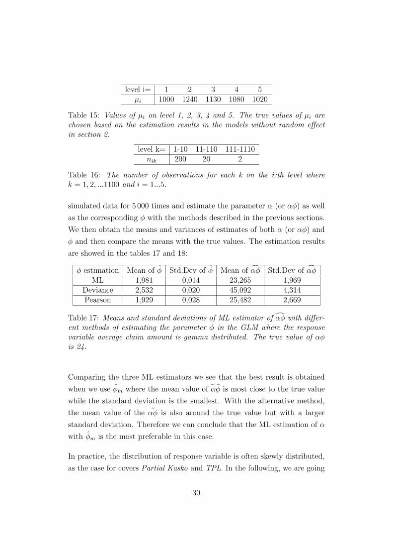
level i= 1 2 3 4 5µi 1000 1240 1130 1080 1020
Table 15: Values of µi on level 1, 2, 3, 4 and 5. The true values of µi arechosen based on the estimation results in the models without random effectin section 2.
level k= 1-10 11-110 111-1110nik 200 20 2
Table 16: The number of observations for each k on the i:th level wherek = 1, 2, ...1100 and i = 1...5.
simulated data for 5 000 times and estimate the parameter α (or αφ) as well
as the corresponding φ with the methods described in the previous sections.
We then obtain the means and variances of estimates of both α (or αφ) and
φ and then compare the means with the true values. The estimation results
are showed in the tables 17 and 18:
φ estimation Mean of φ Std.Dev of φ Mean of αφ Std.Dev of αφML 1,981 0,014 23,265 1,969
Deviance 2,532 0,020 45,092 4,314Pearson 1,929 0,028 25,482 2,669
Table 17: Means and standard deviations of ML estimator of αφ with differ-ent methods of estimating the parameter φ in the GLM where the responsevariable average claim amount is gamma distributed. The true value of αφis 24.
Comparing the three ML estimators we see that the best result is obtained
when we use φm where the mean value of αφ is most close to the true value
while the standard deviation is the smallest. With the alternative method,
the mean value of the αφ is also around the true value but with a larger
standard deviation. Therefore we can conclude that the ML estimation of α
with φm is the most preferable in this case.
In practice, the distribution of response variable is often skewly distributed,
as the case for covers Partial Kasko and TPL. In the following, we are going
30
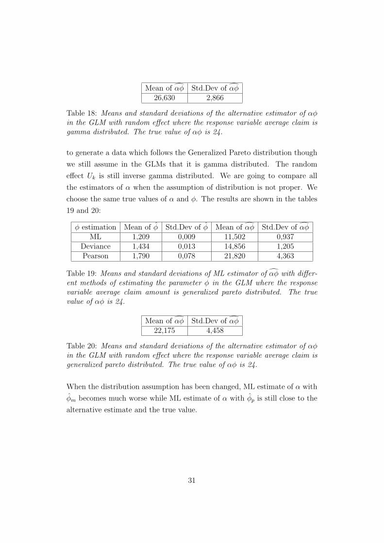
Mean of αφ Std.Dev of αφ26,630 2,866
Table 18: Means and standard deviations of the alternative estimator of αφin the GLM with random effect where the response variable average claim isgamma distributed. The true value of αφ is 24.
to generate a data which follows the Generalized Pareto distribution though
we still assume in the GLMs that it is gamma distributed. The random
effect Uk is still inverse gamma distributed. We are going to compare all
the estimators of α when the assumption of distribution is not proper. We
choose the same true values of α and φ. The results are shown in the tables
19 and 20:
φ estimation Mean of φ Std.Dev of φ Mean of αφ Std.Dev of αφML 1,209 0,009 11,502 0,937
Deviance 1,434 0,013 14,856 1,205Pearson 1,790 0,078 21,820 4,363
Table 19: Means and standard deviations of ML estimator of αφ with differ-ent methods of estimating the parameter φ in the GLM where the responsevariable average claim amount is generalized pareto distributed. The truevalue of αφ is 24.
Mean of αφ Std.Dev of αφ22,175 4,458
Table 20: Means and standard deviations of the alternative estimator of αφin the GLM with random effect where the response variable average claim isgeneralized pareto distributed. The true value of αφ is 24.
When the distribution assumption has been changed, ML estimate of α with
φm becomes much worse while ML estimate of α with φp is still close to the
alternative estimate and the true value.
31
4 Conclusion
In the GLMs without random effect, there is only one dispersion parameter
φ. We have discussed three methods of estimating φ in two different sit-
uations. In the first case, where the GLM fits well to our empirical data,
the ML estimator of φ turns out to be unbiased with 95% confidence. Both
Pearson and Deviance estimators are biased. Meanwhile, the Deviance esti-
mates are always larger than the ML estimates, which has been shown both
theoretically and empirically. The Pearson estimator is pretty good in the
sense that the value of the estimate is quite close to the true value. In the
second case, when the distributional assumption is doubtful, we find that
the ML estimator is no longer unbiased. However, the Pearson estimator
is robust because the estimate does not change much even when the distri-
bution assumption has been changed. Another finding is that the Pearson
estimator is very sensitive to extreme values. When we delete or truncate
the extreme values, the Pearson estimate decreases dramatically as it should.
On the other side, the Deviance and ML estimates do not change much after
deletion or truncation.
In the GLMs with random effect, there is an additional dispersion parameter,
α. In this paper, two estimation methods, ML and the alternative method
have been introduced to estimate the quantity αφ, which can be used directly
to calculate the random effect Uk. The ML estimator is dependent of the φ
estimate. It has been shown that when the distributional assumption is
sensible, all of the ML estimators are biased with 95% confidence. However,
the ML estimates with φm and φp are quite close to the true value while the
ML estimates with φd deviates much from the true value. After we change
the assumption, the estimate with φm becomes worse and its value is close
to the one of ML estimates with φd. The ML estimates with φp is affected
comparatively less and the value of the estimate is still relatively close to
the true value. This is in accordance with the results in the GLMs without
random effects, where the φp is the most robust. Comparing the ML with
the alternative method, we find that except for the cover TPL, the value of
32
the alternative estimate gets along with the ML estimates with φp no matter
whether the distributional assumption is proper or not. This is the case in
both empirical and simulation studies. However, a disadvantage of these two
estimators is that the standard deviations of the estimates are large.
When the value of αφ is large, the uk is convergent to 1, which implies that
the random effect does not affect the model substantially and even can be
ignored. This could possibly explain the abnormal estimations of αφ for TPL
where the random effect car model does not have much importance on the
response variable, average claim amount. In such cases, neither ML nor the
alternative estimators yield sensible estimations.
In summary, we recommend the Pearson estimator for estimating φ with the
reason that it is the most robust against the distributional assumption since
in practice it is often difficult to find a canonical distribution that fits the data
well, particularly when there are large values. Concerning the α estimation
in the model with a random effect, it turns out that the ML estimator with
φp and the alternative estimator are superior to the others, though both are
biased, the estimates are robust and do not deviate much from the true value.
33
5 Reference
• P.McCullagh and J.A.Nelder (1997): ”Generalized Linear Models.”
• Esbjorn Ohlsson and Bjorn Johansson (2003a): ”Prissattning inom
sakforsakring med Generaliserade linjara modeller.”
• Esbjorn Ohlsson and Bjorn Johansson (2003b): ”Credibility theory and
GLM revised”
• Gauss M. Cordeiro and P.McCullagh (1991): ”Bias Correction in Gen-
eralized Linear Models” Journal of the Royal Statistical Society. Series
B, Volume 53, Issue 3 629-643.
• Nelder.J.A and Verrall, R.J. (1997): ”Credibility Theory and General-
ized linear models.” ASTIN Bulletin, Vol 27:1, 71-82.
34
6 Appendix A
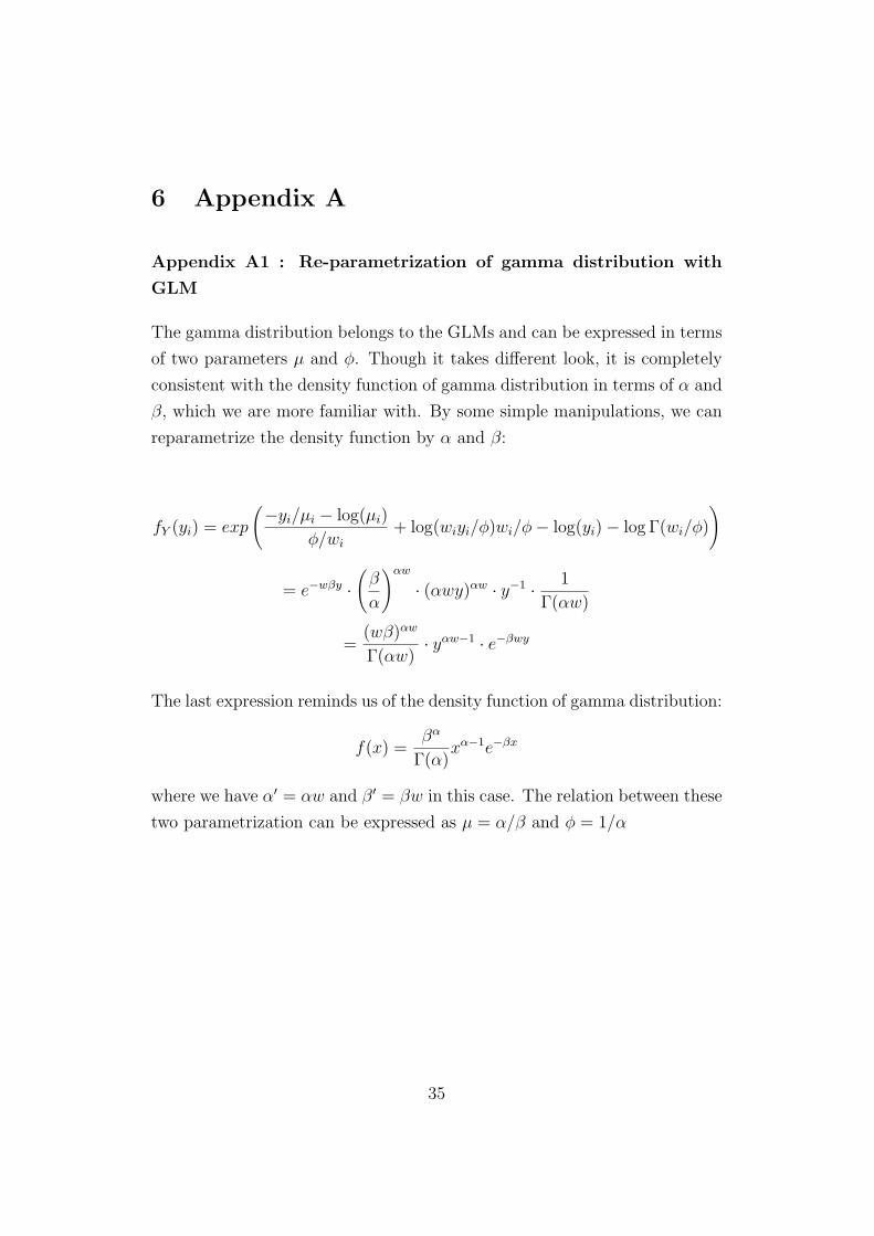
Appendix A1 : Re-parametrization of gamma distribution with
GLM
The gamma distribution belongs to the GLMs and can be expressed in terms
of two parameters µ and φ. Though it takes different look, it is completely
consistent with the density function of gamma distribution in terms of α and
β, which we are more familiar with. By some simple manipulations, we can
reparametrize the density function by α and β:
fY (yi) = exp
(−yi/µi − log(µi)
φ/wi
+ log(wiyi/φ)wi/φ− log(yi)− log Γ(wi/φ)
)
= e−wβy ·(
β
α
)αw
· (αwy)αw · y−1 · 1
Γ(αw)
=(wβ)αw
Γ(αw)· yαw−1 · e−βwy
The last expression reminds us of the density function of gamma distribution:
f(x) =βα
Γ(α)xα−1e−βx
where we have α′ = αw and β′ = βw in this case. The relation between these
two parametrization can be expressed as µ = α/β and φ = 1/α
35
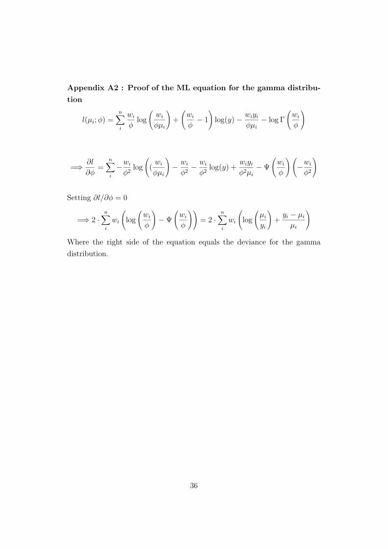
Appendix A2 : Proof of the ML equation for the gamma distribu-
tion
l(µi; φ) =n∑
i
wi
φlog
(wi
φµi
)+
(wi
φ− 1
)log(y)− wiyi
φµi
− log Γ
(wi
φ
)
=⇒ ∂l
∂φ=
n∑
i
−wi
φ2log
((
wi
φµi
)− wi
φ2− wi
φ2log(y) +
wiyi
φ2µi
−Ψ
(wi
φ
) (−wi
φ2
)
Setting ∂l/∂φ = 0
=⇒ 2 ·n∑
i
wi
(log
(wi
φ
)−Ψ
(wi
φ
))= 2 ·
n∑
i
wi
(log
(µi
yi
)+
yi − µi
µi
)
Where the right side of the equation equals the deviance for the gamma
distribution.
36
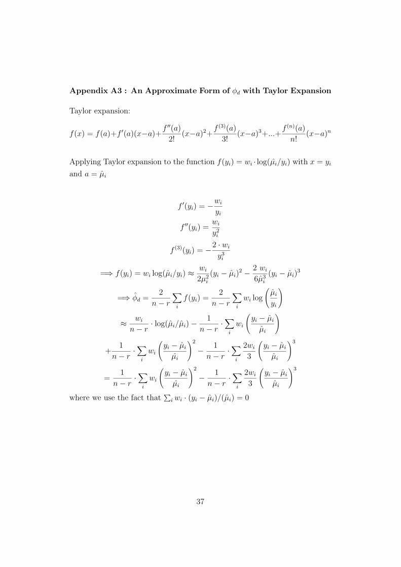
Appendix A3 : An Approximate Form of φd with Taylor Expansion
Taylor expansion:
f(x) = f(a)+f ′(a)(x−a)+f ′′(a)
2!(x−a)2+
f (3)(a)
3!(x−a)3+...+
f (n)(a)
n!(x−a)n
Applying Taylor expansion to the function f(yi) = wi · log(µi/yi) with x = yi
and a = µi
f ′(yi) = −wi
yi
f ′′(yi) =wi
y2i
f (3)(yi) = −2 · wi
y3i
=⇒ f(yi) = wi log(µi/yi) ≈ wi
2µ2i
(yi − µi)2 − 2 wi
6µ3i
(yi − µi)3
=⇒ φd =2
n− r
∑
i
f(yi) =2
n− r
∑
i
wi log
(µi
yi
)
≈ wi
n− r· log(µi/µi)− 1
n− r·∑
i
wi
(yi − µi
µi
)
+1
n− r·∑
i
wi
(yi − µi
µi
)2
− 1
n− r·∑
i
2wi
3
(yi − µi
µi
)3
=1
n− r·∑
i
wi
(yi − µi
µi
)2
− 1
n− r·∑
i
2wi
3
(yi − µi
µi
)3
where we use the fact that∑
i wi · (yi − µi)/(µi) = 0
37
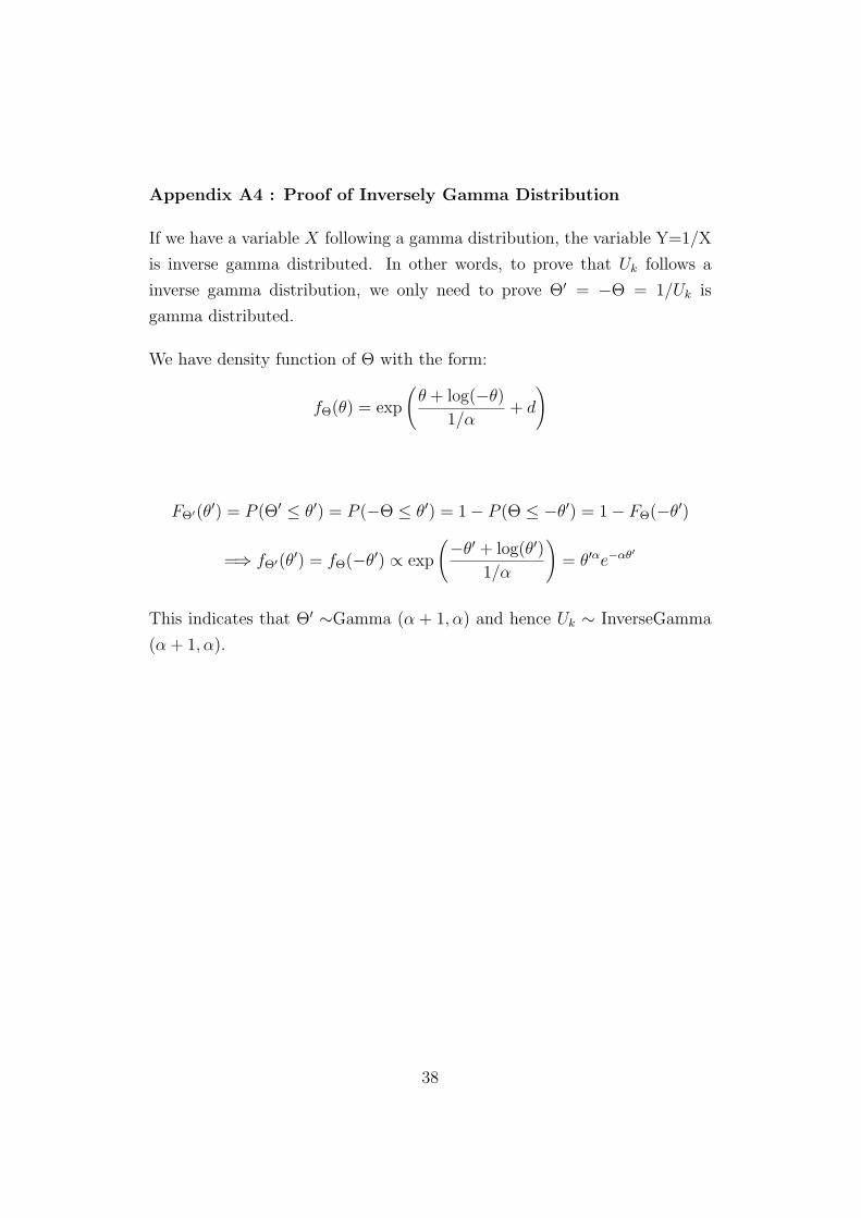
Appendix A4 : Proof of Inversely Gamma Distribution
If we have a variable X following a gamma distribution, the variable Y=1/X
is inverse gamma distributed. In other words, to prove that Uk follows a
inverse gamma distribution, we only need to prove Θ′ = −Θ = 1/Uk is
gamma distributed.
We have density function of Θ with the form:
fΘ(θ) = exp
(θ + log(−θ)
1/α+ d
)
FΘ′(θ′) = P (Θ′ ≤ θ′) = P (−Θ ≤ θ′) = 1− P (Θ ≤ −θ′) = 1− FΘ(−θ′)
=⇒ fΘ′(θ′) = fΘ(−θ′) ∝ exp
(−θ′ + log(θ′)1/α
)= θ′αe−αθ′
This indicates that Θ′ ∼Gamma (α + 1, α) and hence Uk ∼ InverseGamma
(α + 1, α).
38

7 Acknowledgement
I would like to extend my sincere gratitude and appreciation to many people
who make this master thesis possible.
First of all, great thanks are due to my supervisors, Esbjorn Ohlsson and
Bjorn Johansson, who have been providing me with a great many inspiring
ideas and instructions on both content and structure of this thesis. Thanks
to their participance, it has become a fully enjoyable learning process to write
the thesis.
I am highly indebted to Actuary Department at Lansforskringar, Sak, whose
assistance is vital for this thesis work. A sincere thank to the head of Actuary
Department, Eva Blomberg for providing me such a great opportunity and
also special thanks to Gunde Brandin and Fredrik Johansson who have been
generously sharing knowledge and experience with me.
I would also like to acknowledge with great appreciation faculties of Math-
ematical Statistical Institution at Stockholm University. Thanks a lot for
leading and guiding me the journey of exploration of the mathematical and
statistical world, which is extraordinary interesting and challenging.
Last but not the least, I would like to send my most sincere gratitude to my
family: mother Ming Meng, father Yan Hou, sister Nannan Lundin and my
husband Yaohua Yu, who are always supportive to me.
39