Estimation of Generic Subslab Attenuation Factors for

NGWA.org Groundwater Monitoring & Remediation 1

© 2014 The Authors. Groundwater Monitoring & Remediation published by Wiley Periodicals, Inc. on behalf of National Ground Water Association. doi: 10.1111/gwmr.12086

This is an open access article under the terms of the Creative Commons Attribution License, which permits use, distribution and reproduction in any medium, provided the original work is properly cited.

Estimation of Generic Subslab Attenuation Factors for Vapor Intrusion Investigationsby Roger Brewer, Josh Nagashima, Mark Rigby, Martin Schmidt, and Harry O’Neill

IntroductionRisk-based screening levels for soil, groundwater, and

soil gas are often included in vapor intrusion guidance docu-ments. Such screening levels, particularly for groundwater and soil gas, are important tools for rapid identification of potential vapor intrusion risks (VIRs) as well as for expedit-ing the clearance of low-risk sites from additional agency oversight. A key parameter in calculating these screening levels is the indoor air:subslab soil gas attenuation factor (SSAF). This factor reflects the degree of mixing and dilu-tion of intruding soil gas with indoor air (Figure 1) and can be calculated empirically as follows:

SSAF = Concentration in indoor air ____________________________ Concentration in subslab soil gas

. (1)

Subslab soil gas screening levels are generated by selecting a default attenuation factor and indoor air con-centration into this equation and solving for the subslab concentration:

Subslab soil gas screening level

= Indoor air screening level

______________________ SSAF

. (2)

Fate and transport models can be used to develop equiv-alent screening levels for soil and groundwater, based on the target concentration of the volatile organic compound (VOC) in subslab soil gas and the equilibrium partitioning charac-teristics of the targeted chemical (e.g., U.S. Environmental Protection Agency [USEPA] 2004).

This paper evaluates two of the most commonly used approaches for developing default SSAFs for use in vapor intrusion guidance: (1) direct measurement of apparent atten-uation based on empirical databases of paired indoor air and subslab soil gas data and (2) estimation of attenuation fac-tors based on vapor entry rates and indoor air exchange rates (IAERs). In the first case, the SSAF is estimated by divid-ing the measured chemical concentration in indoor air by its subslab soil gas concentration. In the second case, the SSAF is estimated by dividing the vapor entry rate by the IAER in terms of volume per unit of time. The vapor entry rate is referred to as “Q

soil” in United States Environmental Protection

Agency (USEPA) guidance (USEPA 2004), although a more accurate term would be “Q

floor” since vapor flow through the

floor (rather than out of the soil) is the primary parameter of interest. This modification recognizes that the model can also be used for buildings with crawl spaces. The IAER for a building represents the number of times that the total volume of air in the building is replaced with fresh air each hour and

AbstractGeneric indoor air:subslab soil gas attenuation factors (SSAFs) are important for rapid screening of potential vapor intrusion risks in build-

ings that overlie soil and groundwater contaminated with volatile chemicals. Insufficiently conservative SSAFs can allow high-risk sites to be prematurely excluded from further investigation. Excessively conservative SSAFs can lead to costly, time-consuming, and often inconclusive actions at an inordinate number of low-risk sites. This paper reviews two of the most commonly used approaches to develop SSAFs: (1) com-parison of paired, indoor air and subslab soil gas data in empirical databases and (2) comparison of estimated subslab vapor entry rates and indoor air exchange rates (IAERs). Potential error associated with databases includes interference from indoor and outdoor sources, reliance on data from basements, and seasonal variability. Heterogeneity in subsurface vapor plumes combined with uncertainty regarding vapor entry points calls into question the representativeness of limited subslab data and diminishes the technical defensibility of SSAFs extracted from databases. The use of reasonably conservative vapor entry rates and IAERs offers a more technically defensible approach for the development of generic SSAF values for screening. Consideration of seasonal variability in building leakage rates, air exchange rates, and interpolated vapor entry rates allows for the development of generic SSAFs at both local and regional scales. Limitations include applicability of the default IAERs and vapor entry rates to site-specific vapor intrusion investigations and uncertainty regarding applicability of generic SSAFs to assess potential short-term (e.g., intraday) variability of impacts to indoor air.

2 R. Brewer et al./ Groundwater Monitoring & Remediation NGWA.org

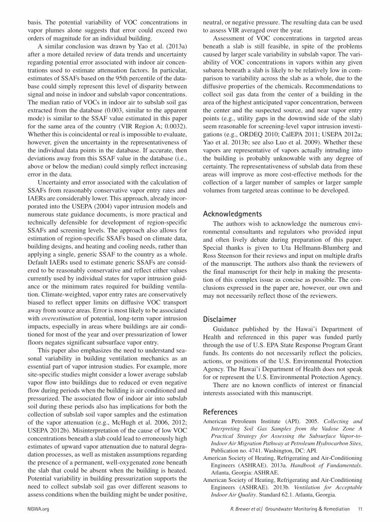
straightforward; that is, the concentration of a volatile mea-sured in indoor air is divided by its subslab concentration (see Equation 1). This approach is used to estimate a sub-slab vapor attenuation factor for more than 1000 buildings included in the USEPA database (USEPA 2012b). The range and frequency of estimated attenuation factors are presented in Figure 2. Different plots on the graph reflect different fil-ters applied to the database, with the purple plot represent-ing data sets where VOCs in subslab soil gas samples were 50 times greater than the anticipated indoor air background. Statistical analysis of this particular set of data is used to generate generic SSAFs for general screening purposes, resulting in a median value of 0.003 and a 95th percentile value of 0.03. (Note that the reported median value also appears to be approximately coincidental with the mode.)

While elegant in its apparent simplicity, this approach requires two important assumptions (see also USEPA 2012a): (1) indoor air data are representative of vapor impacts and (2) subslab soil gas represents intruding vapors associated with those impacts. If these criteria cannot be established within a reasonable degree of accuracy for each data pair, then the estimated SSAF becomes questionable, as does any statistical evaluation of the database as a whole.

Indoor Air DataThe risk posed to building occupants by intruding vapors is

typically assessed in terms of long-term impacts to indoor air. The objective of indoor air sampling is to estimate the asso-ciated long-term average concentration of intrusion-related VOCs in areas of the building that a person regularly occupies. The degree to which the indoor air data included in the USEPA (2012b) vapor intrusion database meets this objective is ham-pered by a number of potential sources of error, including: (1) masking of low-level vapor intrusion impacts by VOCs from indoor and/or outdoor sources, (2) collection of samples from rooms not representative of normally occupied areas, and (3) reliance in most cases on a single sample to characterize this area (refer to Table 1 in the USEPA document).

Note that the reported concentrations of VOCs in indoor air were within the assumed background levels for most of

is traditionally presented in terms of the number of building air exchanges per unit time (e.g., exchanges per hour; USEPA 2004, 2011). An IAER of 1/h, for example, indicates that indoor air is replaced once every hour. A default indoor air volume of 244 m3 for a one-story, single-family residence is recommended in USEPA vapor intrusion guidance (100 m2 floor area and 2.44 m height; USEPA 2004).

Selection of one approach over the other for develop-ing generic SSAFs profoundly affects the assumed VIR. Inadequately conservative attenuation factors can allow high-risk sites to be prematurely excluded from further investigation. Excessively conservative attenuation factors can lead to costly and often inconclusive investigations.

A large database of groundwater, soil gas, and indoor air data has been compiled by the USEPA (2012b) and is the primary source of data being used to develop empiri-cally based attenuation factors. This paper focuses on the paired, subslab, and indoor air data in the database used to derive SSAFs. Concerns highlighted for the technical basis of proposed subslab attenuation factors also likely apply to deeper soil gas and groundwater data (e.g., Yao et al. 2013a). However, the authors consider the subslab data to be most prone to potential errors in decision making, and an important starting point for a more detailed review of the adequacy of the database for the development of technically defensible, attenuation factors in general.

Use of Empirical Databases to Calculate Attenuation FactorsCalculation of SSAFs

Calculation of an SSAF based on indoor air and sub-slab data collected at a building would ideally be very

Figure 1. Simplified conceptual site model of vapor intrusion and attenuation in indoor air: (A) upward diffusion of vapors from the source area through vadose zone soil; (B) advective flow of subslab vapors into depressurized building via cracks, utility gaps, etc., in the floor; (C) exchange of indoor air and outdoor air due to climate-induced leakage and/or mechani-cal ventilation; (D) attenuation of subslab vapors upon mixing with indoor air.

Figure 2. Range and frequency of ratios of indoor air to subslab soil gas data for individual buildings included in the USEPA database, assumed to represent SSAFs for the structures (from USEPA 2012b).

NGWA.org R. Brewer et al./ Groundwater Monitoring & Remediation 3

More than 75% of the indoor air samples included in the database were collected from residential basements. Basements are an important potential source of indoor air contaminants due to the upward flow of air when the lower living area of the house is depressurized with respect to outdoor air, for example when the house is heated (Dodson et al. 2007; USEPA 2007a). The ventilation of basements relative to upper levels is not recorded in the USEPA database, and the representativeness of the samples from upper levels cannot be quantitatively assessed. As dis-cussed subsequently, minimum ventilation standards for regularly occupied areas are required under the building permit (American Society of Heating, Refrigerating and Air-Conditioning Engineers [ASHRAE] 2013a, 2013b). A higher air exchange rate in upper areas of the building would further attenuate vapors due to leakage and ventila-tion, making indoor air data from these areas more repre-sentative of risk to occupants.

Reliance on a single indoor air sample for most of the pairs in the database poses an additional source of potential error. Studies where large numbers of concurrent indoor air samples are collected indicate that VOC concentrations can vary spatially within the same building by up to four orders of magnitude for large commercial buildings and by a factor of three for smaller residential buildings (Otson and Fellin 1992; Eklund et al. 2008; Folkes et al. 2009; USEPA 2011, 2012b). Concentrations of volatiles in indoor air at vapor intrusion sites have also been demonstrated to vary by as much as three orders of magnitude over time (Folkes et al. 2009; Song et al. 2011; Holton et al. 2013).

Spatial variability can be addressed in part by the col-lection of a sample over a longer period that accounts for natural circulation and mixing of indoor air. To meet this objective, 24-h samples are often considered adequate (e.g., California Environmental Protection Agency [CalEPA] 2011). Longer duration samples also take into account diurnal effects of vapor intrusion. However, the duration of sample collection for each subject building is not discussed in the USEPA database report, introducing another potential source of error into the data used to derive the SSAFs.

the samples in the database. Of the samples that exceeded the anticipated background levels, the majority were still within an order of magnitude of these values. This is compensated for in the USEPA (2012b) database report in part by filtering the data with respect to the assumed range of background VOCs in indoor air. Of the original 1231 sets of paired subslab and indoor air data sets, 464 were filtered out in order to address known or suspected indoor sources, concentrations of VOCs in the subslab soil gas sample that are less than that reported for indoor air, and other poten-tially complicating factors. All but 320 sets of paired data were eliminated after screening out indoor air data that fell within the assumed background range of a VOC.

This compromises the representativeness of SSAFs extracted from the database since sites with very low SSAFs and sites where vapor intrusion was not occurring were excluded from further consideration. Contributions from indoor or ambient sources can cause subslab attenuation to be underestimated and can misrepresent cases where vapor intrusion is not occurring. The median, mean, and 95th per-centile attenuation factors presented in the USEPA (2012b) report are, therefore, biased toward cases with less attenua-tion (higher attenuation factors) and do not reflect the data-base population as a whole.

The USEPA (2012b) database assessment includes an alternate filter that focuses on subslab soil gas data greater than various multiples of the anticipated background (e.g., 100; see Figure 2). However, this again does not address uncertainty in the representativeness of the “high source strength” soil gas data in terms of vapors that actu-ally intruded into the structure and impacted indoor air. Variability of vapor concentrations in the subslab could lead to the presence of both “low source strength” and “high source strength” areas under the same slab. Whether impacts to indoor air were tied to a high vs. low source strength would depend on the location of the vapor entry point rather than where the subslab sample was collected. The reliability of an SSAF derived for an apparent “high source strength” data pair would be no more reliable than an SSAF derived for an apparent “low source strength” data pair.

Table 1Weighted Vapor Entry Rates for Designated Vapor Intrusion Risk Regions

VIR Region1

Average Number of Cooling Days per Year2,3

Average Number of Non-Coolingor Heating Days per Year3,4

Weighted Annual-Average Vapor Entry Rate5 (L/min)

Region A (Cold)6 62 303 4.5

Region B (Warm)7 122 243 4.0

Region C (Mediterranean)8 199 166 3.4

Region D (Tropical)9 365 0 2.01Vapor intrusion risk regions (see Figure 4). 2Number of days per year with mean temperature >65 °F in Regions A, B, and D and >55 °F in Region C. 3Based on mean daily temperatures published by NOAA (2013) for the contiguous 48 states and DRI (2013) for Hawaií and Alaska; 15-d period assigned to months when mean daily temperature between different areas of the region were both above and below the target CDD-HDD cutoff.4Number of days per year with mean temperature <65 °F in Regions A, B, and D and <55 °F in Region C.5Weighted vapor entry estimated based on assumed maximum effective entry rate of 2 L/min on cooling days and 5 L/min on non-cooling or heating days per 100 m2 building slab area (see text).6Cold climate region represented by northern and Rocky Mountain states with mean daily temperature >65 °F from at least July through August; includes Alaska (see text).7Warm climate region represented by southern and southwestern states with mean daily temperature >65 °F from at least June through September.8Mediterranean climate region represented by coastal central California with cool summers and mean daily temperature >55 °F from mid-April through October.9Tropical climate region represented by Hawaií, southernmost Florida, Puerto Rico, the United States Virgin Islands, and Guam, with year-round mean daily temperature >65 °F.


previously entered the building. These sources of error can be overlooked only if the concentrations of subslab vapors are relatively homogeneous.

This is highly unlikely. Most guidance documents recog-nize variability of VOC concentrations in subsurface vapor plumes, including the USEPA database document (American Petroleum Institute [API] 2005; New Jersey Department of Environmental Protection [NJDEP] 2013; Interstate Technology & Regulatory Council [ITRC] 2007; USDOD 2009; CalEPA 2012; USEPA 2012a, 2012b). Data for build-ings where large numbers of subslab soil gas samples have been collected suggest that spatial variability of one to sev-eral orders of magnitude in VOC concentrations at the scale of a building slab (i.e., across the slab as a whole) is likely to be the rule rather than the exception (Widdowson et al. 1997; Choi and Smith 2005; McHugh et al. 2007; Luo et al. 2009; Johnson et al. 2012; Lutes et al. 2012; Schmidt 2012; O’Neill 2013; Yao et al. 2013a, 2013b, 2013c; Shen et al. 2013; see also McHugh et al. 2006; Tillman and Weaver 2006; USEPA 2012a). It is reasonable to assume that the reported concen-tration of a VOC in a small (e.g., 1 L) subslab soil gas sam-ple represents the immediate area. However, closely spaced grids of passive soil gas samples in outdoor areas routinely identify order-of-magnitude variability over distances of a few feet (e.g., O’Neill 2013; Whetzel et al. 2009; see also American Society for Testing and Materials [ASTM] 2011). Similar variability has been identified in radon gas studies (e.g., Bunzl et al. 1998; Winkler et al. 2001). Variability in VOC concentrations in subslab soil gas is likely to be great-est when vapors are associated with small, isolated pockets of contaminated soil but can also be considerable for vapors attributed only to contaminated groundwater.

This inherent spatial variability of subslab vapors will have profound effects on the calculation of SSAFs based on empirical data. Figure 3 illustrates one example. The figure summarizes data for total petroleum hydrocarbons (TPH)

The USEPA document acknowledges these sources of potential error for indoor air samples in the database (USEPA 2012b; see also USEPA 2012a). The representativeness of indoor air data is difficult to quantify, and confidence in estimated SSAFs is difficult to ascertain. However, poten-tial error associated with the representativeness of subslab soil gas data in the database likely far outweighs the error associated with the indoor air data.

Subslab Soil Gas DataAssessing the representativeness of subslab data in

the USEPA database is more challenging than for indoor air. Potential sources of error include: (1) uncertainty in the relation between vapors currently under the slab with vapors previously intruded to indoor air; (2) uncertainty in the duration, entry rate, and volume of vapors intruded to indoor air; (3) potential discrepancies between vapor entry points and sample locations; and (4) reliance in most cases on a single subslab sample to characterize all of the vapors beneath a building.

Evaluating the representativeness of soil gas data first requires that the target population be identified, but this is less straightforward than for indoor air. Direct testing of the vapor that impacted the indoor air is, of course, not possible since the two have already mixed. Instead, vapors under the structure are assumed to represent vapors that intruded earlier, which introduces error in the SSAF calculations (USEPA 2012b; see also USEPA 2007b).

Uncertainty in the population of subslab soil vapors to be targeted for characterization introduces additional error into the database. Indoor vapors could be assumed to reflect the volume of vapor that intruded during the previous exchange of indoor air. For example, an IAER of 0.5/h (CalEPA 2011) and a vapor entry rate of 5 L/min (USEPA 2004) equate to a vapor entry rate of 600 L per air exchange (i.e., 2 h) for each 100 m2 of building footprint (USEPA 2012a). Alternately, an assumed time period of 24 h would take into account diur-nal effects (CalEPA 2011). Assuming a vapor entry rate of 5 L/min, this equates to a vapor plume volume of 7200 L.

Another option might be to assume that the volume of vapors immediately beneath the entire slab area represents the population of interest. The volume of air-filled pore spaces in the first 15 cm of soil beneath a 100 m2 slab is approximately 4200 L, assuming an air-filled porosity of 28% (default parameter values are included in the USEPA vapor intrusion model; see USEPA 2004, 2012a). Some guidance documents suggest a source area of vapors beneath slabs as thick as 3 feet (e.g., CalEPA 2011), corresponding to a volume of soil gas of approximately 25,000 L.

A third source of potential error in subslab soil gas data in the USEPA database is the relationship between vapor entry points and sample locations. The specific location of subslab vapor samples in terms of potential vapor entry routes is not recorded in the USEPA database and in most cases is presumably unknown.

The total error associated with these factors alone is dif-ficult or impossible to quantify. Acceptance of the SSAF with any reasonable degree of precision and accuracy requires a leap of faith that the sole subslab sample rep-resents the hundreds or thousands of liters of vapors that

Figure 3. Isoconcentration map of TPH soil gas data beneath a building slab (from Luo et al. 2009).


subsurface is reasonably homogeneous (uniform).” It goes on to provide an alternative, “site-specific” approach for calculating SSAF values based on the use of default vapor entry rates and IAERs. This is discussed in the following section.

The USEPA (2012b, 16) report continues, “Considering this variability, a statistical approach to characterizing the empirical attenuation factors was adopted....” However, this statement is misleading. Statistical evaluation of the database only addresses the variability between individual homes and buildings, not variability and error within a single data point. Any data set, accurate or not, can yield a pattern amenable to statistical analysis. Statistical analy-sis of a database is valid only if the individual data points represent their intended purpose within a quantifiable range of error (Silver 2012). This is clearly not the case for the paired indoor air and subslab soil gas samples in the USEPA (2012b) database.

This variability highlights the perils of applying statisti-cal approaches designed to evaluate databases in which the error associated with individual data points can reasonably be assumed to be minimal (e.g., age, height, weight, etc.) vs. databases in which the reproducibility of individual data points is uncertain (see Silver 2012). The Central Limit Theorem in this case no longer applies, and statistical analy-sis of the database cannot compensate for the unknown error. Although seemingly straightforward, the frequency graph presented in the USEPA database report (see Figure 2) can-not reliably be assumed to reflect the distribution of SSAFs for the individual homes and buildings included in the data-base. Subsequently, there is no technically defensible basis for using the 95th percentile SSAF value of 0.03 extracted from the database (see also McHugh et al. 2007). As dis-cussed in the following section, the reported median ratio of 0.003 is similar to SSAFs calculated as the ratio of vapor flow to indoor air exchange in this paper. Whether this is coincidental or accurately reflects attenuation is uncertain and is not examined in detail.

Use of Indoor Air Exchange Rates and Subsurface Vapor Entry Rates to Estimate SSAFs

Calculation of Subslab Attenuation FactorsAn SSAF for a building can also be calculated from the

ratio of the rate of subsurface vapor intrusion (“vapor entry rate”) to the rate of fresh air entering the building over the same time period, as represented by the IAER:

SSAF = Vapor flow rate ( L ____

min ) ___________________________

Indoor air exchange ratee ( L ____ min

) . (3)

The vapor entry rate is traditionally expressed in terms of a default building floor area of 100 m2 (USEPA 2012a). In this sense, the term might be more appropriately defined as a “flux” rate. The term “entry” is, however, retained for use in this paper with the understanding that the value presented applies to a specific area of floor space. This mass balance approach is indirectly incorporated into the vapor intrusion models published by USEPA (2002, 2004), with the SSAF

in vapors beneath a 210 m2 building slab (after Luo et al. 2009). Note that the concentration of TPH measured in 17 1-L soil gas samples collected beneath the slab of the build-ing ranged from 0 to 145 mg/L (145,000,000 µg/m3). The maximum detected concentration exceeds the published, risk-based screening levels for TPH in subslab soil gas by up to three orders of magnitude (e.g., see Brewer et al. 2013) and suggests potentially significant vapor intrusion concerns. This could be possible if the lower level of the structure was depressurized with respect to the subslab air space, and if upward attenuation was insufficient to reduce TPH concentrations below the levels of concern before the vapors were drawn through entry points in the slab.

As evident in Figure 3, any estimate of an SSAF for the building depends on the location of the subslab sample and could vary by orders of magnitude. As succinctly concluded by Luo et al. (2009, 89): “Random sampling of a few loca-tions might not reveal the true range of concentrations… Even if one had precise knowledge of the subslab soil gas distribution, it is not clear how it would be used to assess pathway significance without knowledge of the vapor entry points to the building and soil gas entry rates through those points.” The concentration of the VOC reported for the sole soil gas sample collected beneath the building could well simply reflect random “noise” in the vapor plume rather than the “signal” directly tied to vapor intrusion, that is, rather than the mean concentration of the VOC in soil gas tied to the measured impacts to indoor air (see also Silver 2012). The potential for multiple vapor entry points from areas under the slab with differing VOC concentrations and different entry rates further compromises the database reli-ability for estimation of the SSAF.

Confidence in USEPA Database SSAFsOf the potential sources of error in the USEPA vapor

intrusion database, spatial variability of VOC concentra-tions in subslab soil gas is likely the most significant, in particular at the scale of a single 1-L sample. The effect of spatial (and temporal) variability on the reliability of atten-uation factors extracted from the database is recognized but perhaps not fully appreciated in the USEPA (2012b, 15) report:

These factors may impart bias when calculating concen-tration ratios, depending on the extent to which the samples accurately represent the spatial and temporal variability of the indoor air concentrations and the subsurface vapor con-centrations affecting the building… The spatial and temporal variability in observed subsurface and indoor air concentra-tions within and among buildings mean that for every site, and every structure (emphasis added) in an area of similar subsurface contamination, a range of empirical attenuation factors would likely be calculated from a series of discrete indoor air and subsurface vapor concentrations measured at different points in space or at different times.

This potential shortcoming of the database is similarly anticipated in vapor intrusion guidance published by the California Department of Toxic Substances Control. This guidance includes a default SSAF of 0.05 derived from earlier versions of the USEPA database (CalEPA 2011, 16): “The default attenuation factors assume [that] …the


IECC Climate Zones and Designation of Vapor Intrusion Risk Regions

A “Climate Zone” approach similar to that used by Murray and Burmaster (1995) combined with the Köppen-Geiger (Peel et al. 2007) and Trewartha (Trewartha and Horn 1980) climate-classification schemes is used in combination with International Energy Conservation Code (IECC) maps (International Code Council [ICC] 2012) to subdivide the country into four, distinct “VIR” regions (Figure 4): (1) Region A (cold), (2) Region B (warm), (3) Region C (Mediterranean), and (4) Region D (tropical). Region B includes the coastal marine areas of northern California, Oregon, and Washington. Other specific areas included in the regions are discussed as follows.

The IECC climate zones characterize different regions of the United States in terms of “heating degree days” (HDD) and “cooling degree days” (CDD). Climate zone boundaries follow county boundary lines (see also U.S. Department of Energy [USDOE] 2010). The climate zones closely approxi-mate climate-classification boundaries designated by the Köppen-Geiger (Peel et al. 2007) and Trewartha schemes (Trewartha and Horn 1980). An HDD value for a given day represents the difference between the average daily tempera-ture and a base temperature of 65°F when the daily average temperature is below 65 °F. For example, if the average tem-perature for a given day is 40 °F, then the HDD value for that day is 25. Individual daily HDD values are summed to gen-erate an annual HDD value for the location. Higher annual HDD values indicate a greater need for heating in compari-son to locations with lower values. A CDD is a measure of how hot a location is over a period of time, relative to a base temperature of 50 °F (65 °F used by some entities). The CDD is the difference between that day’s average temperature and a temperature of 50 °F, if the daily average temperature is

equal to the ratio of the average vapor entry rate into a build-ing (Q

soil) and the Building Ventilation Rate (Q

building) when

vapor flow into the building is dominated by advection (see also Song et al. 2011). This same approach is used to develop generic screening levels by several states (e.g., CalEPA 2008, 2011; Hawaii Department of Health [HDOH] 2011; see also ITRC 2005). Note that the USEPA vapor intrusion mod-els calculate a single “Infinite Source Indoor Attenuation Coefficient (alpha)” that takes into account total attenuation from the source area to indoor air, rather than separate atten-uation factors for the source and subslab vapors and then for the subslab vapors and indoor air.

Calculation of the SSAF requires that the IAER be con-verted to units of volume and time identical to that used for vapor entry, or liters per minute:

IAER ( L ____ min

) = IAER ( Exchanges _________

h ) × 1h ______

60min

× Volune ( m3 _________

Exchanges ) × 1000 ( L ___

m3 ) . (4)

The term “Volume” represents the interior volume of the structure.

As discussed next, the flow of subsurface vapors into homes and buildings has been extensively studied and is reasonably well understood. IAERs are understood within a relatively narrow range of error (refer to supplement). Models and field studies have demonstrated that a build-ing’s ventilation rate and soil gas entry rate are positively correlated (Cavallo et al. 1992; Song et al. 2014; see also Hers et al. 2001). In combination, they offer a technically defensible and more robust approach for estimating region-specific SSAFs that can be used to develop tools for vapor intrusion screening. An example of this approach is pre-sented in the next section.

Figure 4. Example vapor intrusion risk (VIR) regions defined in terms of average building leakage rates and associated IAERs and vapor entry rates (see Tables 1 and 2; after ICC 2012). VIR Region A: Cold (includes Alaska); VIR Region B: Warm with Hot Summers (includes Marine/Oceanic coastal area of northern California, Oregon and Washington); VIR Region C: Mediterranean with Cool Summers (primarily coastal central California); VIR Region D: Tropical (not shown—Puerto Rico, the United States Virgin Islands, Hawai’i, and Guam).


this exchange rate (see Hers et al. 2001; Gilbert et al. 2008; ASHRAE 2013a). Lower IAERs likewise indicate inad-equate ventilation that should be identified and corrected as part of a vapor intrusion investigation.

VIR Region B (“Warm”) Default IAERA default IAER of 0.50/h is assigned to VIR Region B,

including the south, southwest, and the southernmost and Central Valley areas of California (IECC Climate Zones 2, 3, and 4 with the exception of coastal central California; ICC 2012; see Figure 4). This area is characterized by hav-ing less than 5,400 HDD per year. The default IAER again approximates the annual median air exchange rates esti-mated by Murray and Burmaster (1995) for their Climate Regions 3 and 4 (i.e., 0.44/h and 0.65/h, respectively). Yamamoto et al. (2010) similarly estimated that the median air exchange rate for homes in Texas was 0.47/h. Lower IAERs are primarily associated with tighter, newer homes in which air conditioning is used for most of the year (Sherman and Matson 2011). This should be accompanied by a lower to negligible vapor entry rate due to pressuriza-tion of the lower portions of the home (see also McHugh et al. 2012; Song et al. 2014).

California’s climate is highly diverse, with the south-eastern corner of the state characterized by a hot desert-to-steppe climate, the coastal area stretching from the U.S.-Mexico border to just north of Los Angeles character-ized by a Mediterranean climate with hot summers, and the southern half of the Central Valley characterized by a semi-arid steppe climate (Kaufmann 2003). These areas were included in VIR Region B due to the potential for heating during brief but cold winters. Studies specific to California estimate a range of IAERs from 0.5 to 1.5 times per hour (e.g., Wilson et al. 1996). The default IAER of 0.50/h assigned to VIR Region B corresponds to the default IAER recommended for the state as a whole in vapor intrusion guidance by the California Department of Toxic Substances Control (CalEPA 2011).

The Marine West Coast climate of coastal northern California (Humboldt, Trinity, and Del Norte counties) and coastal Oregon and Washington is also included in VIR Region B (Taylor and Hannan 1999; ICC 2012; see Figure 4). This area falls within IECC Climate Zone 4C (3600< HDD <5400; ICC 2012). These areas are classified as Mediterranean under the 1899 Köppen-Geiger scheme (Peel et al. 2007). The areas are more appropriately classified as Temperate Ocean Marine (Trewartha and Horn 1980) and are distinct from the true Mediterranean climate of coastal cen-tral California (see below) by having cooler temperatures and significantly higher rainfall. This can be expected to result in less ventilation from open windows and doors in compari-son to VIR Region C, as well as an increased use of heating, resulting in lower average IAERs and, as discussed in the fol-lowing, a higher annual-average subsurface vapor entry rate.

Residential IAERs in these areas as a whole are some-what higher in comparison to IECC Climate Zones 5 to 8 due in part to increased periods of the year when open win-dows and doors are used for ventilation (refer to the afore-mentioned discussion and Murray and Burmaster 1995). Air exchange rates in the warmest regions, extending from

greater than 50 °F (see ICC 2012). Daily CDD values are summed to generate an annual CDD value for the location. Higher annual CDD values indicate a greater need for cool-ing in comparison to locations with lower values.

The IECC climate zones are useful approximations of variation in regional IAERs. “Building leakage” models can be used to approximate a default, IAER, and vapor entry rate for each VIR region. The ratio of vapor entry rate to the IAER is then used to assign an SSAF to each VIR region.

Indoor Air Exchange Rates

Published StudiesIndoor air exchange takes place through a combina-

tion of three processes: (1) leakage of outdoor air into the structure around windows, doors, and rooflines and through cracks, gaps, and other openings; (2) natural ventilation via open windows, doors, and other openings; and (3) forced or mechanical ventilation driven by fans. IAER can be measured in the field using tracer tests (e.g., ASTM 1990; ASTM 2000; ASHRAE 2002, 2006, 2013a; Batterman et al. 2006; Bennett et al. 2012). Regional variations in IAER can be predicted by models that consider the types and sizes of houses, typical leakage properties, and representative weather conditions (e.g., Sherman and Matson 2011).

A review of published IAERs for different regions of the country is provided in the supplement to this paper. The example IAERs presented in the following section are based on a review of the noted references. Alternatively, less or more conservative IAERs could be applied on a more site-specific basis (e.g., refer to upper- and lower-bound distri-bution of air exchange rates summarized in USEPA 2011). However, coinciding vapor entry rates would require similar adjustment to correspond with the change in overall build-ing leakage. Nonetheless, an assessment of the adequacy of building ventilation should be a fundamental part of all vapor intrusion investigations.

VIR Region A (“Cold”) Default IAERA default IAER of 0.35/h is assigned to VIR Region A,

including the northeastern, north central, and Rocky Mountain areas of the country as well as the inland area of Oregon and Washington and all of Alaska (IECC Climates Zones 5, 6, 7, and 8; ICC 2012). This area is characterized by the need to heat buildings for most of the year, with decreased periods when windows and doors are likely to be left open.

An IAER of 0.35/h corresponds to the minimum ventila-tion rate required for residential structures in the United States (ASHRAE 2013b; see also Lawrence Berkeley National Laboratory [LBNL] 1998; USDOE 2002; Manufactured Housing Research Alliance [MHRA] 2003; ASHRAE 2010; USEPA 2010). The IAER is similar to median, annual air exchange rates estimated by Murray and Burmaster (1995) for colder regions that have more than 5400 HDD per year (i.e., 0.32/h and 0.40/h for Climate Regions 1 and 2, respectively). Lower annual-average IAERs are possible but should be accompanied by proportionally lower vapor entry rates, offsetting the potential VIRs. Impacts to indoor air quality by indoor sources also become increasingly likely to mask and outweigh risks posed by vapor intrusion below


for general screening purposes (i.e., 83 cm3/s or 7200 L/d). This rate is considered to be reasonable for conditions when advection is the dominant mechanism for vapor transport across a foundation. This value is supported both by conser-vative models and through comparison to radon and tracer studies (USEPA 2012a; see also CalEPA 2011). The USEPA (2012a) Conceptual Site Model document for vapor intru-sion clarifies that the entry rate (“soil gas advection rate”) applies to each 100 m2 footprint of a building and must be proportionally corrected for building size.

The USEPA (2012a) Conceptual Site Model document notes that impacts to indoor air are relatively constant for higher vapor entry rates (e.g., >5 L/min per 100 m2 foot-print). Increasing the vapor entry rate will not increase impacts to indoor air. This is because VOC transport into the advective zone is limited by the rate of VOC diffusion away from the source (USEPA 2012a). A vapor entry rate of 5 L/min thus represents a reasonable maximum value.

As is the case for IAERs, annual-average vapor entry rates can be anticipated to vary across seasons and between different climate zones. Song et al. (2014) evaluated sea-sonal changes in vapor entry rates by linking vapor intru-sion models to building leakage models, which are used to assess energy efficiency (see Sherman and Matson 2011). The models generate a worst-case indoor-outdoor pres-sure differential of 40 g/cm-s2 for periods when a home is being heated, identical to the default value incorporated into the USEPA vapor intrusion guidance (USEPA 2004). Significantly lower pressure differentials are calculated for warmer periods of the year, with values approaching zero for summer periods when the home is being cooled.

These day-to-day pressure differentials are entered into the USEPA (2004) vapor intrusion model to estimate daily vapor entry rates. The models suggest a peak vapor entry of approximately 3 to 5 L/min (per 100 m2) during the cold winter months when a structure is being heated (Song et al. 2014). This corresponds well with the default vapor entry rate recommended by the USEPA (2004). However, vapor entry rates in the range of 0 to 2 L/min are characteristic of warm summer months, when the structure is being cooled and the pressure differential between indoor and outdoor air is significantly less. This lower entry rate corresponds well with radon field studies, which indicated a fivefold reduction in radon entry rates when a building is cooled by open windows and doors (Cavallo et al. 1992). The use of air conditioning will typically pressurize a building and largely negate the advective intrusion of subsurface vapor (ASHRAE 2009, 2013a; see also MHRA 2003; USEPA 2010, 2012; Song et al. 2014; refer to supplement). Note that this could result in the outward leakage of indoor air in subslab soils (McHugh et al. 2006, 2012).

Taking these studies into consideration, a default aver-age vapor entry rate of 5 L/min is reasonably conservative for cold periods of the year, when a building is likely to be heated for at least part of the day (e.g., mean daily tempera-ture <65 °F). Similarly, a default vapor entry rate of 2 L/min is reasonable for periods when a building is being cooled (e.g., mean daily temperature less than HDD default of 65 °F). For screening purposes, it is reasonable to apply the more conservative vapor entry rate to intermittent periods

Florida to western Texas, are lower than might be expected due to tighter homes and the use of air conditioning for most of the year, compared to more moderate areas.

VIR Region C (Mediterranean) Default IAERA default annual-average IAER of 1.0/h is assigned to

VIR Region C. This includes the coastal central California and a thin sliver of land along the western edge of the Sierra Mountains, which is characterized by a Mediterranean cli-mate with cool summers (Kauffman 2003; see Figure 4, Sierra area not depicted due to scale). The areas fall into IECC Climate Zone 3C (ICC 2012) and Climate Regions 3 and 4 of Murray and Burmaster (1995).

The area is distinct from Region B in terms of cooling and particularly heating. The selected IAER reflects year-round moderate temperatures and an increased use of win-dows and doors for ventilation, as well as minimal heating requirements during the winter. This is in agreement with the mid-range of IAERs identified for coastal areas (e.g., see Wilson et al. 1996; California Energy Commission [CEC] 2001; and Yamamoto et al. 2010) and is either consistent with or more conservative than peer-reviewed vapor intru-sion guidance published by regulatory agencies located in these areas (e.g., Oakland Environmental Services Division 2000; CalEPA 2008). Natural ventilation is usually preferred to mechanical ventilation in these areas (Sherman 1995; ASHRAE 2013a). The IECC climate zone classification also reflects a reduced use of heating in coastal central California (Climate Zone 3C; HDD <3600) in comparison to interior California (Climate Zone 3B; HDD <5400). This helps to explain the comparatively higher IAERs for this area, even though the mean daily temperature dips slightly below the IECC HDD default of 65 °F for most of the year.

VIR Region D (Tropical) Default IAERAn annual-average IAER of 1.0/h is assigned to VIR

Region D. This area includes southernmost Florida, Hawai’i, Puerto Rico, the United States Virgin Islands, and Guam (see Figure 4; latter areas not depicted) and falls into IECC Climate Zone 1 (ICC 2012). The default air exchange rate corresponds to the value incorporated into vapor intru-sion guidance published by the State of Hawai’i (HDOH 2011). Natural ventilation is generally preferred for venti-lation of residences primarily due to a mean temperature of >65 °F throughout the year (Desert Research Institute [DRI] 2013). Heating is only occasionally used in sparsely populated, high-elevation areas of the islands of Maui and Hawai’i. Although detailed studies of IAERs have not been published for the state, the annual-average IAERs can rea-sonably be assumed to be at least as high as those of coastal central California.

Vapor Entry Rates

Climate-Weighted Vapor Entry RatesAn overview of factors related to building leakage and

vapor intrusion under different climate and ventilation scenarios is included in the supplement to this paper. The USEPA (2004) vapor intrusion guidance recommends a default, subsurface vapor entry rate of 5 L/min into buildings


published by Song et al. (2014) could be used to develop weighted vapor entry rates on a more area-specific basis (see also USDOE 2010).

Application of Method

Estimation of VIR Region SSAFsDefault SSAFs can now be calculated and assigned to

each of the VIR regions in Figure 4. The selected IAERs, vapor entry rates, and associated SSAFs are preliminary and illustrate regional differences in VIRs. A more detailed analysis similar to that of Song et al. (2014) could be carried out for individual regions or subparts of these regions. Note that the SSAF values presented may not reflect the views of regulatory agencies that oversee vapor intrusion investiga-tions in the region, except as specifically referenced.

Region-specific IAERs assigned in terms of IAER must be converted to volume per unit time for comparison to vapor entry rates for a floor area of 100 m2. Assuming a default indoor house volume of 244 m3 or 244,000 L (USEPA 2012a), conversion of the assigned IAERs of 0.35/h (VIR Region A), 0.50/h (VIR Region B), and 1.0/h (VIR Regions C and D) to liters per minute yields default IAERs of 1423, 2033, and 4067 L/min, respectively (Table 2).

Default SSAFs are generated for VIR regions using Equation 4 (Table 2). An SSAF of 0.0032 is calculated for the colder areas of VIR Region A. This agrees well with an annual-average attenuation factor of 0.003 estimated for residential buildings in northeastern states by Song et al. (2014). A slightly lower SSAF of 0.0020 is calculated for the warmer areas of VIR Region B. An SSAF of 0.0008 is calculated for VIR Region C, the Mediterranean climate areas of coastal California with its cool summers. The low-est SSAF of 0.0005 is calculated for VIR Region D, includ-ing the tropical islands of Hawai’i, southernmost Florida, Puerto Rico, the United States Virgin Islands, and Guam.

The range of attenuation factors predicted agrees well with previous estimates of SSAFs based on estimated vapor entry rates and IAERs (e.g., USEPA 2004). The region boundaries depicted in Figure 4 could be evaluated at a more local scale by referring to the IECC Climate Zone database (ICC 2012; see also ASHRAE 2010 and USDOE 2010) and

(e.g., spring and fall) when a building might be either heated or cooled but wind effects and closed doors and windows could depressurize the structure.

Default Vapor Entry Rates for VIR RegionsThis approach allows the calculation of seasonally

weighted vapor entry rates based on the average number of heating days and cooling days per year for a targeted area and an appropriate temperature to approximate the cutoff for that area. Table 1 presents the approximate num-ber of cooling days (i.e., mean daily temperature >65 °F) per year for each of the four designated climate regions. Data for the contiguous 48 states are based on Composite Temperature Plots published by the National Oceanographic and Atmospheric Administration for the years 1994 to 2013 (National Oceanographic and Atmospheric Administration [NOAA] 2013). Estimates of mean daily temperatures for Hawai’i (used as a surrogate for southernmost Florida, Puerto Rico, the United States Virgin Islands, and Guam) and Alaska are based on data published by the Desert Research Institute (DRI 2013).

The IECC cutoff of 65 °F is used to establish CDD and HDD values for Regions A, B, and D. This temperature cutoff is not appropriate for the Mediterranean climate of coastal central California. The number of days for which the mean daily temperature is below 65 °F is similar to the much colder Region A (i.e., 77 °F vs. 62 °F; refer to NOAA 2013), yet the average IAER is significantly higher. The higher IAER suggests that residents continue to keep win-dows open when the temperatures are below 65 °F. Heating is also less likely to be used during this period. Although somewhat subjective, an alternative cutoff of 55 °F is con-sidered to be reasonable for the estimation of CDD vs. HDD values in Region C. As noted in Table 1, this yields a total of 166 d during which homes might be heated during the year.

Assignment of a default vapor entry rate of 2 L/min for “cooling days” and an entry rate of 5 L/min for the remaining parts of the year (i.e., heating or otherwise “non- cooling days”) generates weighted year-average vapor entry rates of 4.5, 4.0, 3.4, and 2.0 L/min for the cold, warm, Mediterranean, and tropical climate regions, respectively (see Table 1). Climate data and models similar to those

Table 2Subslab Attenuation Factors Estimated for Designated Vapor Intrusion Risk Regions

Climate Zone1 Default Vapor Entry Rate2 (L/min)Default Indoor Air Exchange Rate3

(L/min)Subslab Attenuation

Factor4

Region A (Cold)5 4.5 0.35/h 1423 0.0032

Region B (Warm)6 4.0 0.5/h 2033 0.0020

Region C (Mediterranean)7 3.4 1.0/h 4067 0.0008

Region D (Tropical)8 2.0 1.0/h 4067 0.00051Vapor intrusion risk regions (see Figure 4).2Annual-average vapor entry rate (see Table 1).3Reflects assumed interior house volume of 244 m3 and default building slab (or crawl space) area of 100 m2.4Ratio of vapor entry rate to indoor air exchange rate.5Cold climate region represented by northern and Rocky Mountain states with mean daily temperature >65 °F from at least July through August.6Warm climate region represented by southern and southwestern states with mean daily temperature >65 °F from at least June through September.7Mediterranean climate region represented by coastal central California with cool summers and mean daily temperature >55 °F from mid-April through October.8Tropical climate region represented by Hawaií, southernmost Florida, Puerto Rico, the United States Virgin Islands, and Guam, with year-round mean daily temperature >65 °F.


specific vapor intrusion investigation. Vapor entry rates and IAERs, as well as SSAFs, can vary significantly both between and within buildings (see supplement; see also Johnson 2002, 2005). IAERs are well studied but could vary by an order of magnitude, depending on the age and design of the structure; the method being used for heating, cooling, and ventilation; and other factors (refer to supplement). Effective vapor entry rates can vary by wide margins for similar reasons, including the presence or absence of floor cracks and gaps in different areas of an individual building. Site-specific measurement of vapor flow into buildings and IAERs is difficult if not impos-sible for typical vapor intrusion investigations.

However, potential error associated with building-specific variability of IAERs and vapor entry rates does not neces-sarily carry over to estimation of annual-average SSAFs. Long-term vapor entry rates and IAERs are positively cor-related. Although sufficient quantitative field data are still lacking, especially for “Q

soil,” an increase in the vapor entry

rate should be accompanied by an offsetting increase in the IAER (see Cavallo et al. 1992; Song et al. 2014; see also Hers et al. 2001). This relationship and the use of reasonably conservative values for both parameters minimize the risk that the generic SSAFs could significantly underpredict the magnitude of long-term vapor intrusion impacts to indoor air.

The applicability of the generic SSAFs presented in this paper to short-term impacts to indoor air (e.g., intraday) is uncertain. Short-term temporal and/or spatial variability of both IAERs and vapor entry rates could be significant due to sudden changes in weather conditions (e.g., high winds) or changes in building ventilation (e.g., heating or air con-ditioning turned off at night). This could affect short-term SSAFs and lead to temporarily decreased or increased impacts to indoor air. A detailed evaluation of the short-term variability of impacts to indoor air related to vapor intrusion was, however, beyond the scope of this paper.

Summary and ConclusionsThis paper illustrates that the disparity between the two

approaches for estimation of SSAFs is most likely attributable to error associated with individual data points incorporated into the USEPA (2012b) empirical database. Spatial variabil-ity in subslab soil gas, uncertainty in vapor entry points, and the limited number of sample points per structure (typically one) introduces unavoidable and unquantifiable error into the calculated SSAFs. Temporal and spatial variability of VOCs in indoor air, the potential for unrecognized indoor sources of VOCs, and the limited number of sample points (again typically one) per structure introduce additional and unquan-tifiable error. Statistical analysis of the data does not solve this problem and merely assesses the variability between individual homes and buildings rather than the potential error associated with individual building data points.

These irresolvable problems invalidate the use of the USEPA (2012b) vapor intrusion database for development of defensible and reproducible SSAFs within a reasonable degree of accuracy. Error associated with the representative-ness of subslab soil gas data and/or indoor air data in the USEPA VI database is directly carried over into calculation of an SSAF, and it is impossible to assess on a building- specific

Köppen-Geiger and Trewartha climate-classification maps (e.g., Trewartha and Horn 1980; Peel et al. 2007) as well as local building leakage studies. The mean daily temperature across much of the Gulf Coast, for example, exceeds 65 °F during the months of April and October, while temperatures are still well below this level for more northern areas of the “warm” climate region during these months. A lower number of heating days and ultimately a lower SSAF would be warranted for these areas in comparison to the rest of the warm climate region.

Alaska is included in the same climate region as Iowa, even though the mean daily temperature across the majority of Alaska never exceeds 65 °F. The overall SSAF of 0.0032 generated for Region A might, therefore, be insufficiently conservative for this state, but it is close to a maximum SSAF value of 0.0035, due to a vapor entry rate of 5 L/min and an IAER of 0.35/h.

Comparison to Database-Derived SSAFsThe discrepancies between the above-estimated default

SSAFs and those extracted from the USEPA (2012b) empir-ical database (e.g., 95th percentile SSAF) are tied to several factors, including: (1) error in the database associated with spatial (and temporal) subslab vapor heterogeneity, (2) error in the database associated with masking of low but probably typical SSAFs due to interference from indoor air sources of VOCs, and (3) attempts to develop a single IAER, vapor entry rate, and SSAF for the highly variable climate regions of the United States. The conflict is recognized but not fully reconciled in the database report:

Using the median values for residential building vol-ume and air exchange rates (395 m3 and 0.45 air changes per hour, respectively) provided in the Exposure Factors Handbook 2011 Edition … and a central value of 5 L/min for Q

soil in sandy materials … the median value of the sub-

slab soil gas attenuation factor … is expected to be approxi-mately 0.002. (USEPA 2012b, 50)

The CalEPA (2011) vapor intrusion guidance recom-mends a default SSAF of 0.05 for California as a whole, based on earlier interpretation of the USEPA database. This SSAF suffers from the same problems as aforementioned for more recent interpretations of the USEPA (2012b) data-base. The same guidance, however, recommended a default vapor entry rate, house volume, and an IAER of 5 L/min, 244 m3, and 0.5/h, respectively, for a more site-specific evaluation of existing or future residential buildings. This generates a more technically defensible SSAF of 0.0025 and corresponds well to the default SSAF of 0.0020 estimated in this paper for VIR Region B (see Table 2).

Oregon was likewise cautious regarding the seemingly high 95th percentile SSAF of 0.03 proposed for the USEPA (2012b) database. An SSAF of 0.005, closer to the median of the database, was ultimately selected for inclusion in that state’s vapor intrusion guidance (ORDEQ 2010).

LimitationsThe IAERs and vapor entry rates assigned to individual

regions for calculation of generic SSAFs cannot be assumed to be applicable to individual buildings as part of a site-


neutral, or negative pressure. The resulting data can be used to assess VIR averaged over the year.

Assessment of VOC concentrations in targeted areas beneath a slab is still feasible, in spite of the problems caused by larger scale variability in subslab vapor. The vari-ability of VOC concentrations in vapors within any given subarea beneath a slab is likely to be relatively low in com-parison to variability across the slab as a whole, due to the diffusive properties of the chemicals. Recommendations to collect soil gas data from the center of a building in the area of the highest anticipated vapor concentration, between the center and the suspected source, and near vapor entry points (e.g., utility gaps in the downwind side of the slab) seem reasonable for screening-level vapor intrusion investi-gations (e.g., ORDEQ 2010; CalEPA 2011; USEPA 2012a; Yao et al. 2013b; see also Luo et al. 2009). Whether these vapors are representative of vapors actually intruding into the building is probably unknowable with any degree of certainty. The representativeness of subslab data from these areas will improve as more cost-effective methods for the collection of a larger number of samples or larger sample volumes from targeted areas continue to be developed.

AcknowledgmentsThe authors wish to acknowledge the numerous envi-

ronmental consultants and regulators who provided input and often lively debate during preparation of this paper. Special thanks is given to Uta Hellmann-Blumberg and Ross Steenson for their reviews and input on multiple drafts of the manuscript. The authors also thank the reviewers of the final manuscript for their help in making the presenta-tion of this complex issue as concise as possible. The con-clusions expressed in the paper are, however, our own and may not necessarily reflect those of the reviewers.

DisclaimerGuidance published by the Hawai’i Department of

Health and referenced in this paper was funded partly through the use of U.S. EPA State Response Program Grant funds. Its contents do not necessarily reflect the policies, actions, or positions of the U.S. Environmental Protection Agency. The Hawai’i Department of Health does not speak for or represent the U.S. Environmental Protection Agency.

There are no known conflicts of interest or financial interests associated with this manuscript.

ReferencesAmerican Petroleum Institute (API). 2005. Collecting and

Interpreting Soil Gas Samples from the Vadose Zone A Practical Strategy for Assessing the Subsurface Vapor-to-Indoor Air Migration Pathway at Petroleum Hydrocarbon Sites, Publication no. 4741. Washington, DC: API.

American Society of Heating, Refrigerating and Air-Conditioning Engineers (ASHRAE). 2013a. Handbook of Fundamentals. Atlanta, Georgia: ASHRAE.

American Society of Heating, Refrigerating and Air-Conditioning Engineers (ASHRAE). 2013b. Ventilation for Acceptable Indoor Air Quality. Standard 62.1. Atlanta, Georgia.

basis. The potential variability of VOC concentrations in vapor plumes alone suggests that error could exceed two orders of magnitude for an individual building.

A similar conclusion was drawn by Yao et al. (2013a) after a more detailed review of data trends and uncertainty regarding potential error associated with indoor air concen-trations used to estimate attenuation factors. In particular, estimates of SSAFs based on the 95th percentile of the data-base could simply represent this level of disparity between signal and noise in indoor and subslab vapor concentrations. The median ratio of VOCs in indoor air to subslab soil gas extracted from the database (0.003, similar to the apparent mode) is similar to the SSAF value estimated in this paper for the same area of the country (VIR Region A; 0.0032). Whether this is coincidental or real is impossible to evaluate, however, given the uncertainty in the representativeness of the individual data points in the database. If accurate, then deviations away from this SSAF value in the database (i.e., above or below the median) could simply reflect increasing error in the data.

Uncertainty and error associated with the calculation of SSAFs from reasonably conservative vapor entry rates and IAERs are considerably lower. This approach, already incor-porated into the USEPA (2004) vapor intrusion models and numerous state guidance documents, is more practical and technically defensible for development of region- specific SSAFs and screening levels. The approach also allows for estimation of region-specific SSAFs based on climate data, building designs, and heating and cooling needs, rather than applying a single, generic SSAF to the country as a whole. Default IAERs used to estimate generic SSAFs are consid-ered to be reasonably conservative and reflect either values currently used by individual states for vapor intrusion guid-ance or the minimum rates required for building ventila-tion. Climate-weighted, vapor entry rates are conservatively biased to reflect upper limits on diffusive VOC transport away from source areas. Error is most likely to be associated with overestimation of potential, long-term vapor intrusion impacts, especially in areas where buildings are air condi-tioned for most of the year and over pressurization of lower floors negates significant subsurface vapor entry.

This paper also emphasizes the need to understand sea-sonal variability in building ventilation mechanics as an essential part of vapor intrusion studies. For example, more site-specific studies might consider a lower average subslab vapor flow into buildings due to reduced or even negative flow during periods when the building is air conditioned and pressurized. The associated flow of indoor air into subslab soil during these periods also has implications for both the collection of subslab soil vapor samples and the estimation of the vapor attenuation (e.g., McHugh et al. 2006, 2012; USEPA 2012b). Misinterpretation of the cause of low VOC concentrations beneath a slab could lead to erroneously high estimates of upward vapor attenuation due to natural degra-dation processes, as well as mistaken assumptions regarding the presence of a permanent, well-oxygenated zone beneath the slab that could be absent when the building is heated. Potential variability in building pressurization supports the need to collect subslab soil gas over different seasons to assess conditions when the building might be under positive,


Choi, J.W., and J.A. Smith. 2005. Geoenvironmental factors affect-ing organic vapor advection and diffusion fluxes from the unsaturated zone to the atmosphere under natural conditions. Environmental Engineering Science 22: 95–108.

Desert Research Institute (DRI). 2013. Average Statewide Temperature for Western U.S. States. Reno, Nevada: Western Regional Climate Center.

Dodson, R.E., J.I. Levy, J.P. Shine, J.D. Spengler, and D.H. Bennett. 2007. Multi-zonal air flow rates in residences in Boston, Massachusetts. Atmospheric Environment 41: 3722–3727.

Eklund, B.M., S. Burkes, P. Morris, and L. Mosconi. 2008. Spatial and temporal variability in VOC levels within a commercial retail building. Indoor Air 18: 365–374.

Folkes, D., W. Wertz, J. Kurtz, and T. Kuehster. 2009. Observed spatial and temporal distributions of CVOCs at Colorado and New York vapor intrusion sites. Ground Water Monitoring and Remediation 29, no. 1: 70–80.

Gilbert, N.L., M. Guaya, D. Gauvinb, R.N. Dietzc, C.C. Chand, and B. Le´vesque. 2008. Air change rate and concentration of form-aldehyde in residential indoor air. Atmospheric Environment 42: 2424–2428.

Hawaii Department of Health (HDOH), Office of Hazard Evaluation and Emergency Response. 2011. Evaluation of Environmental Hazards at Sites with Contaminated Soil and Groundwater. Honolulu, Hawaii: HDOH.

Hers, I., R. Zapf-Gilje, L. Li, and J. Atwater. 2001. The use of indoor air measurements to evaluate intrusion of subsur-face VOC vapors into buildings. Journal of the Air & Waste Management Association 51: 1318–1331.

Holton, C., H. Luo, P. Dahlen, K. Gorder, E. Dettenmaier, and P.C. Johnson. 2013. Temporal variability of indoor air concen-trations under natural conditions in a house overlying a dilute chlorinated solvent groundwater plume. Environmental Science and Technology 47: 13347–13354.

International Code Council (ICC). 2012. International Energy Conservation Code and Commentary. Washington, DC: ICC.

Interstate Technology & Regulatory Council (ITRC). 2007. Vapor Intrusion Pathway: A Practical Guideline. Washington, DC: ITRC.

Interstate Technology & Regulatory Council (ITRC). 2005. Examination of Risk-Based Screening Values and Approaches of Selected States. Washington, DC: ITRC.

Johnson, P.C. 2005. Identification of application-specific critical inputs for the 1991 Johnson and Ettinger vapor intrusion algo-rithm. Groundwater Monitoring & Remediation 25, no. 1: 63–78.

Johnson, P.C. 2002. Identification of Critical Parameters for the Johnson and Ettinger (1991) Vapour Intrusion Model. American Petroleum Institute Technical Bulletin No. 17. Washington, DC.

Johnson, P.C., H. Luo, C. Holton, D. Dahlen, and Y. Guo. 2012. Integrated Field-Scale, Lab-Scale, and Modeling Studies for Improving the Ability to Assess the Groundwater to Indoor Air Pathway at Chlorinated Solvent-Impacted Groundwater Sites. Alexandria, Virginia: Department of Defense Strategic Environmental Research and Development Program.

Kauffman, E. 2003. Climate and topography. In Atlas of the Biodiversity of California, ed. M. Parisi, 12–15. Sacramento, California: California Department of Fish and Wildlife.

Lawrence Berkeley National Laboratory (LBNL). 1998. Recommended Ventilation Strategies for Energy-Efficient Production Homes. Berkeley, California: Lawrence Berkeley National Laboratory, Energy Analysis Department, Environmental Energy Technologies Division.

Luo, H., P. Dahlen, P.C. Johnson, T. Peargin, and T. Creamer. 2009. Spatial variability of soil-gas concentrations near and beneath

American Society of Heating, Refrigerating and Air-Conditioning Engineers (ASHRAE). 2010. Ventilation and Acceptable Indoor Air Quality in Low-Rise Residential Buildings. Standard 62.2. Atlanta, Georgia.

American Society of Heating, Refrigerating and Air-Conditioning Engineers (ASHRAE). 2009. ASHRAE Handbook - Fundamentals. Atlanta, Georgia: ASHRAE.

American Society of Heating, Refrigerating and Air-Conditioning Engineers (ASHRAE). 2006. A Method of Determining Air Change Rates in Detached Dwellings. Standard 136-1993 (RA 2006). Atlanta, Georgia.

American Society of Heating, Refrigerating and Air-Conditioning Engineers (ASHRAE). 2002. Measuring Air Change Effectiveness. Standard 129-1997 (RA 2002). Atlanta, Georgia.

American Society for Testing and Materials (ASTM). 2011. Standard Practice for Passive Soil Gas Sampling in the Vadose Zone for Source Identification, Spatial Variability Assessment, Monitoring, and Vapor Intrusion Evaluations, ASTM D7758-11. West Conshohocken, Pennsylvania.

American Society for Testing and Materials (ASTM). 2000. Standard Test Method for Determining Air Change in a Single Zone by Means of a Tracer Gas Dilution, ASTM E741-00. West Conshohocken, Pennsylvania.

American Society for Testing and Materials (ASTM). 1990. Tracer gas techniques. Air Change Rate and Air Tightness in Buildings, STP:1067, ed. M.H. Sherman. Philadelphia, Pennsylvania: ASTM.

Batterman, S., C. Jia, G. Hatzivasilis, and C. Godwin. 2006. Simultaneous measurement of ventilation using tracer gas tech-niques and VOC concentrations in homes, garages and vehicles. Journal of Environmental Monitoring 8: 249–256.

Bennett, D.H., W. Fisk, M.G. Apte, X. Wu, A. Trout, D. Faulkner, and D. Sullivan. 2012. Ventilation, temperature, and HVAC characteristics in small and medium commercial buildings in California. Indoor Air 22: 309–320.

Brewer, R., J. Nagashima, M. Kelley, and M. Rigby. 2013. Risk-based evaluation of total petroleum hydrocarbons in vapor intru-sion studies. International Journal of Environmental Research and Public Health 10: 2441–2467.

Bunzl, K., F. Ruckerbauer, and R. Winkler. 1998. Temporal and small-scale spatial variability of 222Rn gas in a soil with a high gravel content. The Science of the Total Environment 220: 157–166.

California Energy Commission (CEC). 2001. Manual for Compliance with the 2001 Energy Efficiency Standards (for Nonresidential Buildings, High-Rise Residential Buildings, and Hotels/Motels), Document No. P400-01-032.

California Environmental Protection Agency (CalEPA), Department of Toxic Substances Control (in conjunction with the California Regional Water Quality Control Board, Los Angeles Region). 2012. Advisory – Active Soil Gas Investigations. Los Angeles, California: CalEPA.

California Environmental Protection Agency (CalEPA), Department of Toxic Substances Control. 2011. Guidance for the Evaluation and Mitigation of Subsurface Vapor Intrusion to Indoor Air. Sacramento, California: CalEPA.

California Environmental Protection Agency (CalEPA), Regional Water Quality Control Board, San Francisco Bay Area Region. 2008. Screening for Environmental Concerns at Sites with Contaminated Soil and Groundwater. Oakland, California: CalEPA.

Cavallo, A., K. Gadsby, T.A. Reddy, and R. Socolow. 1992. The effect of natural ventilation on radon and radon progeny levels in houses. Radiation Protection Dosimetry 45: 569–573.


Sherman, M., and N. Matson. 2011. Residential Ventilation and Energy Characteristics. Berkeley, California: Lawrence Berkeley National Laboratory, Energy Performance of Buildings Group, Energy and Environment Division.

Silver, N. 2012. The Signal and the Noise: Why So Many Predictions Fail—But Some Don’t. New York: The Penguin Press.

Song, S., B.A. Schnorr, and F.C. Ramacciotti. 2014. Quantifying the influence of stack and wind effects on vapor intrusion. Human and Ecological Risk Assessment 20: 1345–1358.

Song, S., F.C. Ramacciotti, B.A. Schnorr, M. Bock, and C.M. Stubbs. 2011. Evaluation of USEPA’s empirical attenuation factor database. Air Waste and Management Association. Emissions Monitoring February 2011: 16–21.

Taylor, G.H., and C. Hannan. 1999. The Climate of Oregon, From Rain Forest to Desert. Corvallis, Oregon: Oregon State University Press.

Tillman, F.D., and J.W. Weaver. 2006. Uncertainty from synergis-tic effects of multiple parameters in the Johnson and Ettinger (1991) vapor intrusion model. Atmospheric Environment 40: 4098–4112.

Trewartha, G.T., and L.H. Horn. 1980. An Introduction to Climate, 5th ed. New York: McGraw-Hill.

U.S. Department of Energy (USDOE), Energy Efficiency and Renewable Energy, Building Technologies Program. 2010. Guide to Determining Climate Regions by County. Washington, DC: USDOE.

U.S. Department of Defense (USDOD), Air Force Institute for Operational Health, Health Risk Assessment Branch. 2009. DoD Vapor Intrusion Handbook. Washington, DC: USDOD.

U.S. Department of Energy (USDOE), Building Technologies Program, Office of Energy Efficiency and Renewable Energy. 2002. Spot Ventilation - Source Control to Improve Indoor Air Quality (Technology Fact Sheet). Washington, DC: USDOE.

U.S. Environmental Protection Agency (USEPA), Office of Solid Waste and Emergency Response. 2012a. Conceptual Model Scenarios for the Vapor Intrusion Pathway. EPA 530-R-10-003. Washington, DC: USEPA.

U.S. Environmental Protection Agency (USEPA), Office of Solid Waste and Emergency Response. 2012b. EPA’s Vapor Intrusion Database: Evaluation and Characterization of Attenuation Factors for Chlorinated Volatile Organic Compounds and Residential Buildings. EPA 530-R-10-002. Washington, DC: USEPA.

U.S. Environmental Protection Agency (USEPA), Office of Research and Development, National Center for Environmental Assessment. 2011. Exposure Factors Handbook. EPA/600/R-090/052F. Washington, DC: USEPA.

U.S. Environmental Protection Agency (USEPA), Office of Radiation and Indoor Air, Indoor Environments Division. 2010. Building Codes and Indoor Air Quality. Washington, DC: USEPA.

U.S. Environmental Protection Agency (USEPA), Indoor Environments Division. 2007a. Exploratory Study of Basement Moisture during Operation of ASD Radon Control Systems (revised March 2008). Washington, DC: USEPA.

U.S. Environmental Protection Agency (USEPA), Office of Research and Development, National Exposure Research Laboratory, Environmental Sciences Division. 2007b. Final Project Report for Investigation of the Influence of Temporal Variation on Active Soil Gas/Vapor Sampling. EPA/600/R-07/141. Las Vegas, Nevada: USEPA.

U.S. Environmental Protection Agency (USEPA), Office of Emergency and Remedial Response. 2004. User’s Guide for

a building overlying shallow petroleum hydrocarbon impacted soils. Groundwater Monitoring & Remediation 29, no. 1: 81–91.

Lutes, C., C. Cosky, R. Uppencamp, L. Abreu, B. Schumacher, J. Zimmerman, R. Truesdale, S.Y. Lin, H. Hayes, and B. Hartman. 2012. Recent observations on spatial and temporal variability in the field. Abstract presented at the Annual Meeting for 22nd Annual International Conference on Soil, Water, Energy, and Air. San Diego, California.

Manufactured Housing Research Alliance (MHRA). 2003. Whole House Ventilation Strategies. New York: MHRA.

McHugh, T.E., L. Beckley, D. Bailey, K. Gorder, E. Dettenmaier, I. Rivera-Duarte, S. Brock, and I.C. MacGregor. 2012. Evaluation of vapor intrusion using controlled building pressure. Environmental Science and Technology 46: 4792−4799.

McHugh, T.E., T.N. Nickels, and S. Brock. 2007. Evaluation of spatial and temporal variability in VOC concentrations at vapor intrusion investigation sites. In Proceedings of Air and Waste Management Association. Vapor Intrusion: Learning from the Challenges, September 26–28, Providence, Rhode Island, 129–142.

McHugh, T.E., P.C. De Blanc, and R.J. Pokluda. 2006. Indoor air as a source of VOC contamination in shallow soils below build-ings. Soil & Sediment Contamination 15: 103–122.

Murray, D.M., and D.E. Burmaster. 1995. Residential air exchange rates in the United States: Empirical and estimated parametric distribution by season and climatic region. Risk Analysis 15, no. 4: 459–465.

National Oceanographic and Atmospheric Administration (NOAA). 2013. Composite Temperature Plots. Washington, DC: NOAA, Earth System Research Laboratory, Physical Sciences Division.

New Jersey Department of Environmental Protection (NJDEP), Site Remediation and Waste Management Program. 2013. Vapor Intrusion Technical Guidance. Trenton, New Jersey.

Oakland Environmental Services Division (OESD). 2000.Technical Background Document. Oakland, California: OESD.

O’Neill, H. 2013. Advanced passive soil gas sampling – Collection of high resolution site characterization data. Abstract presented at the Annual Meeting for CleanUp 2013 – 5th International Contaminated Site Remediation Conference, September 18, Melbourne, Australia.

Oregon Department of Environmental Quality (ORDEQ), Environmental Cleanup Program. 2010. Guidance for Assessing and Remediating Vapor Intrusion in Buildings. Portland, Oregon: ORDEQ.

Otson, R., and P. Fellin. 1992. Volatile organics in the indoor air environment, sources and occurrence. In Gaseous Pollutants, Characterization and Cycling, ed. J.O. Nriagu, 335–421. New York: John Wiley and Sons.

Peel, M.C., Finlayson, B.L., and T.A. McMahon. 2007. Updated world map of the Köppen-Geiger climate classification. Hydrology and Earth System Sciences 11: 1633–1644.

Schmidt, M.A. 2012. Innovative sampling methods for focusing the subslab soil-gas investigation. Paper presented at the Annual Meeting for Air Quality Measurement Methods and Technology, April 24–26, Durham, North Carolina.

Shen, R., Y.J. Yao, K.G. Pennell, and E.M. Suuberg. 2013. Modeling quantification of the influence of soil moisture on subslab vapor concentration. Environmental Science: Processes & Impacts 15: 1444–1451.

Sherman, M.H. 1995. The use of blower door data. Indoor Air 5: 215–224.


Subsurface Vapor Intrusion into Buildings. Washington, DC: USEPA.

U.S. Environmental Protection Agency (USEPA), Office of Solid Waste and Emergency Response. 2002. Draft Guidance for Evaluating the Vapor Intrusion to Indoor Air Pathway from Groundwater and Soils (Subsurface Vapor Intrusion Guidance). Washington, DC: USEPA.

Whetzel, J., H. Anderson, and J. Hodny. 2009. Spatial and temporal variability in vapor intrusion investigations. Abstract presented at the Annual Meeting for USEPA National Forum on Vapor Intrusion, January 12–13, Philadelphia, Pennsylvania, 2009.

Widdowson, M.A., O.R. Haney, H.W. Reeves, C.M. Aelion, and R.P. Ray. 1997. Multiple soil-vapor extraction test for het-erogeneous soil. Journal of Environmental Engineering 123: 160–168.

Wilson, A.L., S.D. Colome, Y. Tian, E.W. Beck, P.E. Baker, D.W. Behrens, I.H. Billick, and C.A. Garrison. 1996. California resi-dential air exchange rates and residence volumes. Journal of Exposure Analysis and Environmental Epidemiology 6, no. 3: 311–326.

Winkler, R., F. Ruckerbauer, and K. Bunzl. 2001. Radon con-centration in soil gas: A comparison of the variability result-ing from different methods, spatial heterogeneity and seasonal fluctuations. The Science of the Total Environment 272: 273–282.

Yamamoto, N., D.G. Shendell, A.M. Winter, and J. Zhang. 2010. Residential air exchange rates in three U.S. metropolitan areas: Results from the relationship among indoor, outdoor, and per-sonal air study 1999–2001. Indoor Air 20: 85–90.

Yao, Y.J., R. Shen, K.G. Pennell, and E.M. Suuberg. 2013a. Examination of the U.S. EPA’s vapor intrusion database

based on models. Environmental Science and Technology 47, 1425−1433.

Yao, Y.J., R. Shen, K.G. Pennell, and E.M. Suuberg. 2013b. Examination of the influence of environmental factors on contaminant vapor concentration attenuation factors using the U.S. EPA’s vapor intrusion database. Environmental Science and Technology 47: 906–91 3.

Yao, Y.J., K.G. Pennell, and E.M. Suuberg. 2013c. Simulating the effect of slab features on vapor intrusion of crack entry. Building and Environment 59: 417–425.

Biographical SketchesRoger Brewer, corresponding author, is at the Hawaii

Department of Health, 919 Ala Moana Blvd., Room 206, Honolulu, HI 96814; +1-808-586-4249; fax +1-808-586-7537; [email protected]

Josh Nagashima is at the Hawaii Department of Health, 919 Ala Moana Blvd., Room 206, Honolulu, HI 96814; [email protected]

Mark Rigby is at Parsons Corporation, 10235 South Jordan Gateway, Suite 300, South Jordan, UT 84095. He may be reached at Marine Science Institute and the Department of Ecology, Evolution, and Marine Biology, University of California, Santa Barbara, CA 93106. [email protected]

Martin Schmidt is at Cox-Colvin and Associates, Inc., 7750 Corporate Blvd, Plain City, OH 43064; [email protected]

Harry O’Neill is at Beacon Environmental Services, Inc., 2203A Commerce Road, Suite 1, Forest Hill, MD 21050; [email protected]

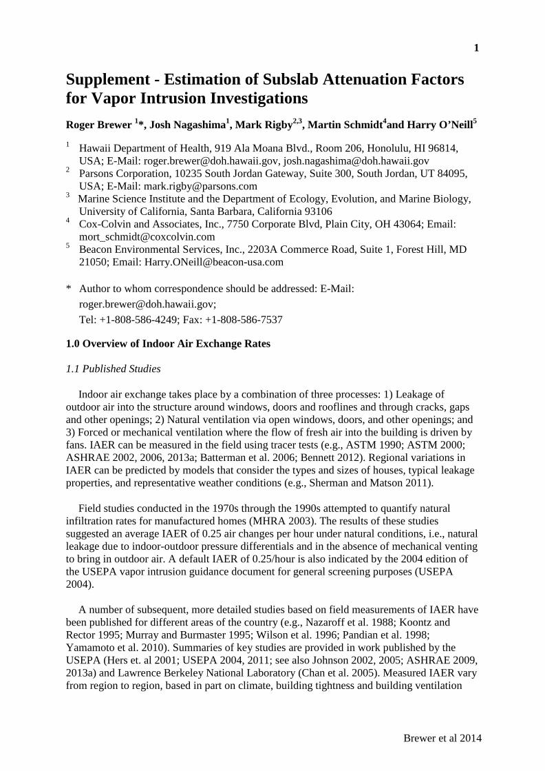
Brewer et al 2014

1

Supplement - Estimation of Subslab Attenuation Factors for Vapor Intrusion Investigations Roger Brewer 1*, Josh Nagashima1, Mark Rigby2,3, Martin Schmidt4and Harry O’Neill5

1 Hawaii Department of Health, 919 Ala Moana Blvd., Room 206, Honolulu, HI 96814, USA; E-Mail: [email protected], [email protected]

2 Parsons Corporation, 10235 South Jordan Gateway, Suite 300, South Jordan, UT 84095, USA; E-Mail: [email protected]

3 Marine Science Institute and the Department of Ecology, Evolution, and Marine Biology, University of California, Santa Barbara, California 93106

4 Cox-Colvin and Associates, Inc., 7750 Corporate Blvd, Plain City, OH 43064; Email: [email protected]

5 Beacon Environmental Services, Inc., 2203A Commerce Road, Suite 1, Forest Hill, MD 21050; Email: [email protected]

* Author to whom correspondence should be addressed: E-Mail: [email protected]; Tel: +1-808-586-4249; Fax: +1-808-586-7537

1.0 Overview of Indoor Air Exchange Rates

1.1 Published Studies

Indoor air exchange takes place by a combination of three processes: 1) Leakage of outdoor air into the structure around windows, doors and rooflines and through cracks, gaps and other openings; 2) Natural ventilation via open windows, doors, and other openings; and 3) Forced or mechanical ventilation where the flow of fresh air into the building is driven by fans. IAER can be measured in the field using tracer tests (e.g., ASTM 1990; ASTM 2000; ASHRAE 2002, 2006, 2013a; Batterman et al. 2006; Bennett 2012). Regional variations in IAER can be predicted by models that consider the types and sizes of houses, typical leakage properties, and representative weather conditions (e.g., Sherman and Matson 2011).

Field studies conducted in the 1970s through the 1990s attempted to quantify natural infiltration rates for manufactured homes (MHRA 2003). The results of these studies suggested an average IAER of 0.25 air changes per hour under natural conditions, i.e., natural leakage due to indoor-outdoor pressure differentials and in the absence of mechanical venting to bring in outdoor air. A default IAER of 0.25/hour is also indicated by the 2004 edition of the USEPA vapor intrusion guidance document for general screening purposes (USEPA 2004).

A number of subsequent, more detailed studies based on field measurements of IAER have been published for different areas of the country (e.g., Nazaroff et al. 1988; Koontz and Rector 1995; Murray and Burmaster 1995; Wilson et al. 1996; Pandian et al. 1998; Yamamoto et al. 2010). Summaries of key studies are provided in work published by the USEPA (Hers et. al 2001; USEPA 2004, 2011; see also Johnson 2002, 2005; ASHRAE 2009, 2013a) and Lawrence Berkeley National Laboratory (Chan et al. 2005). Measured IAER vary from region to region, based in part on climate, building tightness and building ventilation

Brewer et al 2014

2

methods. Murray and Burmaster (1995) estimated regional IAER using contour maps of heating and cooling days used for designing ventilation systems for residential buildings across the country and summarized IAER for each region (see also USEIA 2003, USEPA 2011). Annual, median residential IAERs range from 0.32/hour in the northern, border states and the Rocky Mountain area to 0.65/hour for the deep south and southwest. An annual, median IAER of 0.51/hour was estimated for the US overall with slightly higher mean values.

Differences in regional IAERs were primarily due to variations in heating, air conditioning and open windows and doors throughout the year, as well regional differences in the age, design, and tightness of buildings. The use of open doors and windows for cooling during longer periods of the year can also increase the IAER by a factor of three or more (Wallace et al. 2002; Marr et al. 2012; Bennett et al. 2012). Exhaust fans will depressurize the house and similarly increase leakage of outdoor air and the overall IAER (MHRA 2003; USEPA 2010).

More recent studies suggest that IAERs in the humid southeast may have decreased in the past several decades time due to newer and tighter homes and the increased use of air conditioning (e.g., Chan et al. 2005; Breen et al. 2010; Yamamoto et al. 2010). Over pressurization of houses by air conditioning can reduce fresh air flow into a house. Commercial buildings can similarly be expected to be under positive pressure when air conditioned, as well as requirements for continual fresh air intake (MHRA 20003; USEPA 2012). As discussed below, this should coincide with a significant decrease or even elimination of vapor intrusion into the building.

A decrease in weather-induced leakage for newer homes in warm areas of the country is supported by house-leakage and energy-use models (Sherman and Matson 2011). The models were designed to assess energy efficiency during periods when being mechanically heated and cooled. County-specific, average leakage and air exchange rates for residential homes are estimated based on average house age and design, published leakage data and regional weather conditions. The models do not consider natural ventilation through open doors and windows, since this was not the point of the study. Mechanical ventilation (e.g., attic fans) is likewise not considered, since residential heating and cooling systems are also not typically designed to introduce outdoor air into the home (ASHRAE 2009, 2013a; see also Persily et al. 2010). Predicted air exchange is instead due entirely to leakage around closed doors and windows and other gaps in the walls and roofline.

The Sherman and Matson (2011) study estimates a year-average, nationwide air exchange rate due entirely to building leakage of 1.09/hour. Due to a combination of greater home tightness and expanded use of air conditioning throughout the year, however, the study predicted lower, annual air exchange rates for southeastern areas of the country (<0.8/hour to 1.0/hour) in comparison to the north and the Rocky mountains (1.0/hour to 1.5/hour). A significant, regional variation in leakage-related, air exchange rates for residential homes was not predicted by a similar modeling exercise by Persily et al. (2010), however. That study focused on 19 cities in different areas of the United States. Estimated annual-average air exchange rates ranged from 0.4/hour to 0.5/hour.

Measured IAERs that consider increased ventilation during periods when doors and windows are left open for cooling differ from the model simulations. Natural ventilation can be significant during the spring and fall season in the south and likely explains the higher, year-average IAERs measured for warmer areas of the country than predicted by leakage models. The same inconsistency between simulated and measured air exchange rates noted

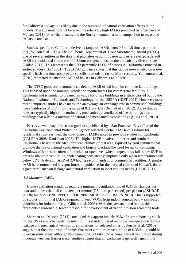
Brewer et al 2014

3

for California and again is likely due to the omission of natural ventilation effects in the models. The apparent conflict between the relatively high IAERs predicted by Sherman and Matson (2011) for northern states and the Rocky mountain area in comparison to measured IAERs is unclear.

Studies specific to California derived a range of IAERs from 0.5 to 1.5 times per hour (e.g., Wilson et al. 1996). The California Department of Toxic Substances Control (DTSC), one of several entities in the state that publishes vapor intrusion guidance, selected a default IAER for residential structures of 0.5/hour for general use in the climatically diverse state (CalPA 2011). This represents the 25th percentile IAER of houses in California estimated in earlier studies (CEC 2001). The DTSC guidance states that this can be re-evaluated on a site-specific basis but does not provide specific methods to do so. More recently, Yamamoto et al. (2010) estimated the median IAER of houses in California at 0.87/hr.

The DTSC guidance recommends a default IAER of 1.0 hour for commercial buildings. This is based upon the minimal ventilation requirements for commercial facilities in California and is similar to the median value for office buildings in a study carried out by the National Institute of Standards and Technology for the USEPA (NIST 2004). However, more recent empirical studies have measured an average air exchange rate in commercial buildings from California of 1.6/hr, with a range of 0.3 to 9.1/hr (Bennett et al. 2012). Air exchange rates are typically higher in continually mechanically-ventilated office buildings than buildings that rely on a mixture of natural and mechanical ventilation (e.g., Jia et al. 2010).

Peer-reviewed, vapor intrusion guidance published by a San Francisco Bay office of the California Environmental Protection Agency selected a default IAER of 1.0/hour for residential structures, near the mid-range of IAERs noted in previous studies for California (CALEPA 2008; Kauffman 2003). The higher IAER relative to interior and southern California is based on the Mediterranean climate of that area, typified by cool summers that promote the use of natural ventilation and largely preclude the need for air conditioning. Windows of homes are often left cracked or open even when temperatures fall below 65ºF in order to maintain ventilation, with heating consistently employed only when temperatures fall below 55ºF. A default IAER of 2.0/hour is recommended for commercial facilities. A similar IAER is recommended in vapor intrusion guidance for the tropical climate of Hawaií, due to a greater reliance on leakage and natural ventilation to meet cooling needs (HDOH 2011).

1.2 Minimum IAERs

Home ventilation standards require a minimum ventilation rate of 0.35 air changes per hour and no less than 15 cubic feet per minute (7.5 liters per second) per person (ASHRAE 2013b; see also LBNL 1998; USDOE 2002; MHRA 2003; USEPA 2010). This is supported by studies of minimal IAERs required to keep VOCs from indoor sources below risk-based guidelines for indoor air (e.g., Gilbert et al. 2008). With the caveats noted below, this represents a reasonable, lower threshold for development of vapor intrusion screening tools.

Sherman and Matson (2011) concluded that approximately 95% of current housing stock for the US as a whole meets the intent of this standard based on house leakage alone. House leakage and mechanical ventilation simulations for selected cities by Persily et al. (2010) suggest that the proportion of homes that meet a minimum ventilation of 0.35/hour could be lower in some areas, although this again does not take into account natural ventilation during moderate weather. Earlier tracer studies suggest that air exchange is generally met in the

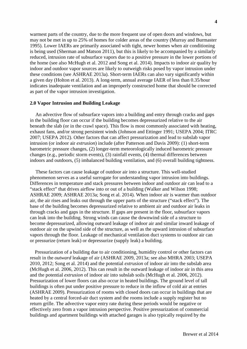
Brewer et al 2014

4

warmest parts of the country, due to the more frequent use of open doors and windows, but may not be met in up to 25% of homes for colder areas of the country (Murray and Burmaster 1995). Lower IAERs are primarily associated with tight, newer homes when air conditioning is being used (Sherman and Matson 2011), but this is likely to be accompanied by a similarly reduced, intrusion rate of subsurface vapors due to a positive pressure in the lower portions of the home (see also McHugh et al. 2012 and Song et al. 2014). Impacts to indoor air quality by indoor and outdoor vapor sources are likely to outweigh risks posed by vapor intrusion under these conditions (see ASHRAE 2013a). Short-term IAERs can also vary significantly within a given day (Holton et al. 2013). A long-term, annual average IAER of less than 0.35/hour indicates inadequate ventilation and an improperly constructed home that should be corrected as part of the vapor intrusion investigation.

2.0 Vapor Intrusion and Building Leakage

An advective flow of subsurface vapors into a building and entry through cracks and gaps in the building floor can occur if the building becomes depressurized relative to the air beneath the slab (or in the crawl space). This flow is most commonly associated with heating, exhaust fans, and/or strong persistent winds (Johnson and Ettinger 1991; USEPA 2004; ITRC 2007; USEPA 2012). Other factors that can affect pressurization and lead to subslab vapor intrusion (or indoor air extrusion) include (after Patterson and Davis 2009): (1) short-term barometric pressure changes, (2) longer-term meteorologically induced barometric pressure changes (e.g., periodic storm events), (3) rainfall events, (4) thermal differences between indoors and outdoors, (5) imbalanced building ventilation, and (6) overall building tightness.

These factors can cause leakage of outdoor air into a structure. This well-studied phenomenon serves as a useful surrogate for understanding vapor intrusion into buildings. Differences in temperature and stack pressures between indoor and outdoor air can lead to a “stack effect” that drives airflow into or out of a building (Walker and Wilson 1998; ASHRAE 2009; ASHRAE 2013a; Song et al. 2014). When indoor air is warmer than outdoor air, the air rises and leaks out through the upper parts of the structure (“stack effect”). The base of the building becomes depressurized relative to ambient air and outdoor air leaks in through cracks and gaps in the structure. If gaps are present in the floor, subsurface vapors can leak into the building. Strong winds can cause the downwind side of a structure to become depressurized, allowing outward leakage of indoor air and similar inward leakage of outdoor air on the upwind side of the structure, as well as the upward intrusion of subsurface vapors through the floor. Leakage of mechanical ventilation duct systems to outdoor air can or pressurize (return leak) or depressurize (supply leak) a building.

Pressurization of a building due to air conditioning, humidity control or other factors can result in the outward leakage of air (ASHRAE 2009, 2013a; see also MHRA 2003; USEPA 2010, 2012; Song et al. 2014) and the potential extrusion of indoor air into the subslab area (McHugh et al. 2006, 2012). This can result in the outward leakage of indoor air in this area and the potential extrusion of indoor air into subslab soils (McHugh et al. 2006, 2012). Pressurization of lower floors can also occur in heated buildings. The ground level of tall buildings is often put under positive pressure to reduce in the inflow of cold air at entries (ASHRAE 2009). Pressurization of rooms with closed doors can occur in buildings that are heated by a central forced-air duct system and the rooms include a supply register but no return grille. The advective vapor entry rate during these periods would be negative or effectively zero from a vapor intrusion perspective. Positive pressurization of commercial buildings and apartment buildings with attached garages is also typically required by the

Brewer et al 2014

5

building permit in order to prevent the infiltration of exhaust (MHRA 2003; USEPA 2010). Wind, barometric pressure changes and other climatic factors can cause daily as well as seasonal pressurization (see McHugh et al. 2006, 2012; Song et al. 2014). Temporary depressurization of buildings normally under positive pressure can, however, be caused by exceptionally high winds or low ambient temperatures.

Open windows and doors can lead to more neutral pressure conditions and, in the absence of wind, reduce or eliminate the effect of subsurface vapor entry into buildings. Radon field studies have demonstrated that reducing building depressurization by opening windows can lower the advective entry of subsurface vapors by as much as a factor of five (Cavallo et al. 1992). These studies suggest that radon flow is a linear function of building depressurization up to a differential pressure of four Pascals or 40 g/cm-s2, the default differential used in the USEPA (2004) vapor intrusion models (see also Song et al. 2014). This was compounded by a doubling of the indoor air exchange rate, for a total ten-fold reduction in measured impacts to indoor air.

References

American Society of Heating, Refrigerating and Air-Conditioning Engineers (ASHRAE). 2002. Measuring Air Change Effectiveness. Standard 129-1997 (RA 2002). Atlanta, GA.

American Society of Heating, Refrigerating and Air-Conditioning Engineers (ASHRAE). 2006. A Method of Determining Air Change Rates in Detached Dwellings. Standard 136-1993 (RA 2006). Atlanta, GA.

American Society of Heating, Refrigerating and Air-Conditioning Engineers (ASHRAE). 2009. ASHRAE Handbook - Fundamentals. Atlanta, GA.

American Society of Heating, Refrigerating and Air-Conditioning Engineers (ASHRAE). 2013a. Handbook of Fundamentals. Atlanta, GA.

American Society of Heating, Refrigerating and Air-Conditioning Engineers (ASHRAE). 2013b. Ventilation for Acceptable Indoor Air Quality. Standard 62.1. Atlanta, GA.

American Society for Testing and Materials (ASTM). 1990. Air Change Rate and Air Tightness in Buildings. Edited by M. H. Sherman. STP:1067. Philadelphia, PA.

American Society for Testing and Materials (ASTM). 2000. Standard Test Method for Determining Air Change in a Single Zone by Means of a Tracer Gas Dilution. ASTM E741-00. West Conshohocken, PA.

Batterman, S., C. Jia, G. Hatzivasilis, and C. Godwin. 2006. Simultaneous measurement of ventilation using tracer gas techniques and VOC concentrations in homes, garages and vehicles. Journal of Environmental Monitoring 8: 249-256.

Bennett, D. H., W. Fisk, M. G. Apte, X. Wu, A. Trout, D. Faulkner and D. Sullivan, 2012. Ventilation, temperature, and HVAC characteristics in small and medium commercial buildings in California. Indoor Air 22: 309–320.

Brewer et al 2014

6

Breen, M., M. Bren, R.W. Williams and B.D. Schultz. 2010. Predicting residential air exchange rates from questionnaires and meteorology: Model evaluation in central North Carolina. Environ. Sci. Technol. 44: 9349–9356.

California Energy Commission (CEC). 2001. Manual for Compliance with the 2001 Energy Efficiency Standards (for Nonresidential Buildings, High-Rise Residential Buildings, and Hotels/Motels), Document No. P400-01-032.

California Environmental Protection Agency (CalEPA), Regional Water Quality Control Board, San Francisco Bay Area Region. 2008. Screening for Environmental Concerns at Sites with Contaminated Soil and Groundwater. May 2008.

California Environmental Protection Agency (CalEPA), Department of Toxic Substances Control. 2011. Guidance for the Evaluation and Mitigation of Subsurface Vapor Intrusion to Indoor Air. October 2011.

Cavallo, A., K. Gadsby, T. A. Reddy, and R. Socolow. 1992. The effect of natural ventilation on radon and radon progeny levels in houses. Radiation Protection Dosimetry 45: 569–573.

Chan, W.R., W.W. Nazaroff, P.N. Price, M.D. Sohn and A.J. Gadgil. 2005. Analyzing a database of residential air leakage in the United States. Atmospheric Environment 39: 3445–3455.

Gilbert, N.L., M. Guaya, D. Gauvinb, R.N. Dietzc, C.C. Chand and B. Le´vesque. 2008. Air change rate and concentration of formaldehyde in residential indoor air. Atmospheric Environment 42: 2424–2428.

Hawaii Department of Health (HDOH), Office of Hazard Evaluation and Emergency Response. 2011. Evaluation of Environmental Hazards at Sites with Contaminated Soil and Groundwater. Fall 2011.

Hers, I., R. Zapf-Gilje, L. Li, and J. Atwater. 2001. The use of indoor air measurements to evaluate intrusion of subsurface VOC vapors into buildings. J. Air & Waste Manage. Assoc. 51: 1318–1331.

Holton, C., H. Luo, P. Dahlen, K. Gorder, E. Dettenmaier and P.C. Johnson. 2013. Temporal variability of indoor air concentrations under natural conditions in a house overlying a dilute chlorinated solvent groundwater plume. Environmental Science and Technology 47: 13347-13354.

Interstate Technology & Regulatory Council (ITRC). 2007. Vapor Intrusion Pathway: A Practical Guideline. Washington, DC.

Jia, C., S. Batterman, C. Godwin, S. Charles and J.Y. Chin. 2012. Sources and migration of volatile organic compounds in mixed-use buildings. Indoor Air 20: 357–369.

Johnson, P.C., and R.A. Ettinger. 1991. Heuristic model for predicting the intrusion rate of contaminant vapors into buildings. Environmental Science Technology 25: 1445–1452.

Brewer et al 2014

7

Johnson, P.C., 2002. Identification of Critical Parameters for the Johnson and Ettinger (1991) Vapour Intrusion Model. American Petroleum Institute Technical Bulletin #17.

Johnson, P.C., 2005. Identification of Application-Specific Critical Inputs for the 1991 Johnson and Ettinger Vapor Intrusion Algorithm. Groundwater Monitoring & Remediation 25, no. 1: 63–78.

Kauffman, E. 2003. “Climate and Topography,” in Atlas of the Biodiversity of California, ed. M. Parisi (Sacramento: California Department of Fish and Wildlife, 2003), 12-15.

Koontz, M.D. and H.E. Rector. 1995. Estimation of distributions for residential air exchange rates. U.S. Environmental Protection Agency. Office of Pollution Prevention and Toxics, Washington, DC.

Lawrence Berkeley National Laboratory (LBNL). 1998. Recommended Ventilation Strategies for Energy-Efficient Production Homes. Berkeley, CA: Lawrence Berkeley National Laboratory, Energy Analysis Department, Environmental Energy Technologies Division.

Manufactured Housing Research Alliance (MHRA). 2003. Whole House Ventilation Strategies. New York, NY.

Marr, D., M. Mason, R. Mosley and X.Y. Liu. 2012. The influence of opening windows and doors on the natural ventilation rate of a residential building. HVAC&R Research 18, no. 1–2: 195–203.

McHugh, T.E., P.C. De Blanc, and R.J. Pokluda. 2006. Indoor air as a source of VOC contamination in shallow soils below buildings. Soil & Sediment Contamination 15: 103–122.

McHugh, T.E., L. Beckley, D. Bailey, K. Gorder, E. Dettenmaier, I. Rivera-Duarte, S. Brock and I.C. MacGregor. 2012. Evaluation of vapor intrusion using controlled building pressure. Environmental Science and Technology 46: 4792−4799.

Murray, D.M. and D.E. Burmaster. 1995. Residential air exchange rates in the United States: empirical and estimated parametric distribution by season and climatic region. Risk Analysis 15, no. 4: 459–465.

Nazaroff, W.W., S.M. Doyle, A.V. Nero, and R.G. Sextro. 1988. Radon entry via potable water. In Radon and its Decay Products in Indoor Air, ed. Nazaroff, W.W. and A.V. Nero, 131-157. New York: Wiley-Interscience.

National Institute of Standards and Technology (NIST). 2004. Analysis of Ventilation Data from the U.S. Environmental Protection Agency Building Assessment Survey and Evaluation (BASE) Study. NISTIR 7145. Gaithersburg, MD.

Pandian, M.D., J.V. Behar, W.R. Ott, L.A. Wallace, A.L. Wilson, S.D. Colome and M. Koontz. 1998. Correcting errors in the nationwide data base of residential air exchange rates. Journal of Exposure Analysis and Environmental Epidemiology 8, no.4: 577–586.

Brewer et al 2014

8

Patterson, B., and G. Davis. 2009. Quantification of vapor intrusion pathways into a slab-on-ground building under varying environmental conditions. Environmental Science and Technology 43: 650–656.

Persily, A., A. Musser and S.J. Emmerich. 2010. Modeled infiltration rate distributions for U.S. housing. Indoor Air 20: 473–485.

Sherman, M. and N. Matson. 2011. Residential Ventilation and Energy Characteristics. Lawrence Berkeley National Laboratory, Energy Performance of Buildings Group, Energy and Environment Division, Berkeley, CA.

Song, S., B.A. Schnorr and F.C. Ramacciotti. 2014. Quantifying the Influence of Stack and Wind Effects on Vapor Intrusion. Human and Ecological Risk Assessment (in press).

U.S. Department of Energy (USDOE), Building Technologies Program, Office of Energy Efficiency and Renewable Energy. 2002. Spot Ventilation - Source control to improve indoor air quality (Technology Fact Sheet). Washington, DC.

U.S. Energy Information Administration (USEIA). 2003. Commercial Buildings Energy Consumption Survey Climate Zones. Washington, DC.

U.S. Environmental Protection Agency (USEPA), Office of Emergency and Remedial Response. 2004. User’s Guide for Subsurface Vapor Intrusion into Buildings. Washington, DC.

U.S. Environmental Protection Agency (USEPA), Office of Radiation and Indoor Air, Indoor Environments Division. 2010. Building Codes and Indoor Air Quality. Washington, DC.

U.S. Environmental Protection Agency (USEPA), Office of Research and Development, National Center for Environmental Assessment. 2011. Exposure Factors Handbook. EPA/600/R-090/052F. Washington, DC.

U.S. Environmental Protection Agency (USEPA), Office of Solid Waste and Emergency Response. 2012. Conceptual Model Scenarios for the Vapor Intrusion Pathway. EPA 530-R-10-003. Washington, DC.

Wallace, L.A., S.J. Emmerich and C. Howard-Reed. 2002. Continuous measurements of air change rates in an occupied house for 1 year: The effect of temperature, wind, fans and windows. Journal of Exposure Analysis and Environmental Epidemiology 12: 296-306.

Walker, I.S., and D.J. Wilson. 1998. Field validation of algebraic equations for stack and wind driven air infiltration calculations. HVAC&R Research Journal 4, no. 2: 119–139.

Wilson, A.L., S.D. Colome, Y. Tian, E.W. Beck, P.E. Baker, D.W. Behrens, I.H. Billick and C.A. Garrison. 1996. California residential air exchange rates and residence volumes. Journal of Exposure Analysis and Environmental Epidemiology 6, no. 3:311–326.

Brewer et al 2014

9

Yamamoto, N., D.G. Shendell, A.M. Winter and J. Zhang, 2010, Residential air exchange rates in three U.S. metropolitan areas: results from the relationship among indoor, outdoor, and personal air study 1999-2001. Indoor Air 20: 85–90.

Documents

Estimation of Generic Subslab Attenuation Factors for