Estimators in simple random sampling: Searls approachrdo.psu.ac.th/sjstweb/journal/35-6/35-6-15.pdf · 2014-12-03 · Original Article Estimators in simple random sampling: Searls

Original Article

Estimators in simple random sampling: Searls approach

Jirawan Jitthavech* and Vichit Lorchirachoonkul

School of Applied Statistics, National Institute of Development Administration,Bang Kapi, Bangkok, 10240 Thailand.

Received 12 March 2013; Accepted 14 August 2013

Abstract

This paper investigates four new estimators in simple random sampling, biased sample mean, ratio estimator, and twolinear regression estimators, using known coefficients of variation of the study variable and auxiliary variable. The propertiesof the new estimators are obtained. Comparisons among the new estimators, three traditional estimators, Searls sample mean,Koyuncu and Kadilar (KK) estimators, Sisodia and Dwivedi (SD) estimator, and Shabbir and Gupta (SG) estimator are under-taken. The analysis shows that the two proposed linear regression estimators are more efficient than the new biased samplemean and at least as efficient as the three traditional estimators and SD estimator. At least one of the proposed linear regressionestimators is always more efficient than the new ratio estimator and Searls sample mean. From the numerical results using twodata sets published in the literature, the proposed linear regression estimators are clearly more efficient than all seven existingestimators.

Keywords: estimator selection criteria, linear regression estimator, bias, MSE, relative efficiency, simple random sampling

Songklanakarin J. Sci. Technol.35 (6), 749-760, Nov. - Dec. 2013

1. Introduction

In simple random sampling where the population sizeis N, and the sample size is n, Searls (1964) proposed a biasedsample mean with a smaller MSE than the traditional samplemean y , obtained by utilizing a known coefficient of varia-tion, yC , without the finite population correction factor

1 1n N . However, in this paper, Searls sample meanusing the finite population correction factor is defined as

2 ,1

wyy

yyC

(1)

The bias and MSE of Searls sample mean, respec-tively, are shown to be

2

2Bias( ) ,1

ywy

y

C Yy

C

(2)

2 2

2MSE( ) ,1

ywy

y

C Yy

C

(3)

It is obvious from Equation 3 that the relative efficiencyof Searls sample mean wyy with respect to the traditionalsample mean y is equal to 2(1 ) 1yC . Without the finitepopulation correction, the results in Equation 1-3 becomethe same results as in the original Searls work (Searls, 1964).However, Searls sample mean should be used under thecondition 2 1yC to avoid a large unacceptable bias inthe estimate.

When we can find an auxiliary variable X which ishighly correlated with the study variable Y, the use of knownauxiliary information in the ratio estimator can reduce theMSE of the sample mean. The traditional combined ratioestimator is defined as

.rXy yx

(4)

The bias and MSE of ry , to first order of approxima-tion, respectively, are given by Cochran (1977)

* Corresponding author.Email address: [email protected]

http://www.sjst.psu.ac.th

J. Jitthavech & V. Lorchirachoonkul / Songklanakarin J. Sci. Technol. 35 (6), 749-760, 2013750

2Bias( ) ,r x y xy Y C C C (5)

2 2 2MSE( ) 2 ,r y x y xy Y C C C C (6)

which is less than MSE( )y if 2 .x yC C Motivated bySearls (1964), several researchers proposed estimators usingthe known coefficient of variation of the auxiliary variable,

xC , for estimating the population mean when the study vari-able is highly correlated with the auxiliary variable, forexample, the Sisodia and Dwivedi (SD) ratio estimator(Sisodia and Dwivedi, 1981), which is defined as:

.xSD

x

X Cy yx C

(7)

The bias and MSE of SDy , to first order of approxi-mation, respectively, are given by

2Bias( ) ,x

SD y xx x

XCXy Y C CX C X C

(8)

22 2MSE( ) 2 .x

SD y y xx x

XCXy Y C C CX C X C

(9)

By Equation 6 and 9, the relative efficiency of SDy with

respect to ry is greater than unity when

1 .2

x

y x

C XC X C

(10)

With respect to y , the relative efficiency of SDy is greaterthan unity when

.2

x

y x

C XC X C

(11)

Gupta and Shabbir (2008) improved the estimation ofpopulation mean by proposing the ratio estimator

1 2 ( ) ,pXy w y w X xx

(12)

where and are either constants or functions of the knownparameters of auxiliary variable, 1w and 2w are constants.The bias and MSE of py , to first order of approximation,

respectively, are given by Koyuncu and Kadilar (2010) (KKestimator)

2 2 21 1 2Bias( ) ( 1) ( ) ,p x y x xy w Y w Y C C C w X C

(13)2 2

2 2 2(1 ) MSE( )MSE( ) ,

(1 ) MSE( )x lr

px lr

C yyC y Y

(14)

where 2 2 2MSE( ) (1 )lr yy Y C (Cochran, 1977), and

1XX

. The values of 1w and 2w , which minimize

MSE( )py are given by

2 21 2 2 2 2

1 ,1 [ (1 ) ]

x

y x

CwC C

(15)

2 2

2 2 2 2 2(1 )( 2 )

.[1 (1 ) ]

x y x

x y x

C C CYwX C C C

(16)

It is clear from Equation 14 that MSE( )py is less thanMSE( )lry . Table 1 gives six values of and as suggestedby Koyuncu and Kadilar (2010), where 2( )x is the kurtosisof the auxiliary variable.

Recently, Shabbir and Gupta (2011) proposed anexponential ratio type estimator (SG estimator)

1 2( ) exp ,(2 1)SG

X xy k y k X xN X x

(17)

where

2

21 2 2

18(1 )

1 (1 )

x

y

CNk

C

and

2 11 1 .

2(1 ) 1y

x

CYk kX N N C

The bias and MSE of SGy , to first order of approxi-mation, respectively. are given by

2 22

1 1 2 23Bias( ) 1 ,

2(1 )8(1 ) 2(1 )y xx x

SGC CC C k Xy Y k k

NN N

(18)

Table 1. Some members of Koyuncu and Kadilar (KK) estimators in simple random sampling.

KK Estimator (0)py (1)py (2)py (3)py (4)py (5)py

0 1 1 1 2 ( )x xC 1 xC 2( )x xC 2 ( )x

751J. Jitthavech & V. Lorchirachoonkul / Songklanakarin J. Sci. Technol. 35 (6), 749-760, 2013

22

222

2 2 2

18(1 )

MSE( ) 1 .4(1 ) 1 (1 )

x

xSG

y

CNC

y YN C

(19)

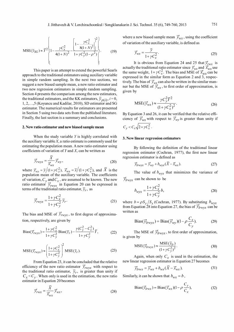
This paper is an attempt to extend the powerful Searlsapproach to the traditional estimators using auxiliary variablein simple random sampling. In the next two sections, wesuggest a new biased sample mean, a new ratio estimator andtwo new regression estimators in simple random sampling.Section 4 presents the comparison among the new estimators,the traditional estimators, and the KK estimators, ( ) ,p iy i = 0,1, 2,…,5 (Koyuncu and Kadilar, 2010), SD estimator and SGestimator. The numerical results for estimators are presentedin Section 5 using two data sets from the published literature.Finally, the last section is a summary and conclusions.

2. New ratio estimator and new biased sample mean

When the study variable Y is highly correlated withthe auxiliary variable X, a ratio estimate is commonly used forestimating the population mean. A new ratio estimator usingcoefficients of variation of Y and X, can be written as

,rwyx wywx

Xy yx

(20)

where 2(1 ),wy yy y C 2(1 ),wx xx x C and X is thepopulation mean of the auxiliary variable. The coefficientsof variation, andy xC C , are assumed to be known. The newratio estimator rwyxy in Equation 20 can be expressed interms of the traditional ratio estimator, ,ry as

2

21 .1

xrwyx r

y

Cy yC

(21)

The bias and MSE of rwyxy , to first degree of approxima-tion, respectively, are given by

2 22

2 2( )1Bias( ) Bias( ) ,

1 1y xx

rwyx ry y

C CCy y YC C

(22)

22

21

MSE( ) MSE( ).1

xrwyx r

y

Cy yC

(23)

From Equation 23, it can be concluded that the relativeefficiency of the new ratio estimator rwyxy with respect tothe traditional ratio estimator, ,ry is greater than unity if

xC < yC . When only is used in the estimation, the new ratioestimator in Equation 20 becomes

,rwx wxwx

Xy yx

(24)

where a new biased sample mean wxy , using the coefficientof variation of the auxiliary variable, is defined as

2 .1

wxx

yyC

(25)

It is obvious from Equation 24 and 25 that rwxy isactually the traditional ratio estimator since wxy and wxx usethe same weight, 21 .xC The bias and MSE of wxx can beexpressed in the similar form as Equation 2 and 3, respec-tively. The bias of wxy can also be written in the similar man-ner but the MSE of wxy , to first order of approximation, isgiven by

2 2

2 2MSE( ) .(1 )

ywx

x

C Yy

C

(26)

By Equation 3 and 26, it can be verified that the relative effi-ciency of wxy with respect to wyy is greater than unity if

22y x xC C C .

3. New linear regression estimators

By following the definition of the traditional linearregression estimator (Cochran, 1977), the first new linearregression estimator is defined as

( ).lrwyx wy wyx wxy y b X x (27)

The value of wyxb that minimizes the variance of

lrwyxy can be shown to be

2

21 ,1

xwyx

y

Cb bC

(28)

where y xb S S (Cochran, 1977). By substituting wyxbfrom Equation 28 into Equation 27, the bias of lrwyxy can bewritten as

Bias( ) Bias( )(1 ).xlrwyx wy

y

Cy yC

(29)

The MSE of lrwyxy , to first order of approximation,is given by

2 2MSE( )MSE( ) .(1 )

lrlrwyx

y

yyC

(30)

Again, when only xC is used in the estimation, thenew linear regression estimator in Equation 27 becomes

( ).lrwx wx wx wxy y b X x (31)

Similarly, it can be shown that wxb b ,

Bias( ) Bias( )(1 ),ylrwx wx

x

Cy y

C (32)


2 2MSE( )

MSE( ) .(1 )

lrlrwx

x

yyC

(33)

From Equation 30 and 33 it can be concluded that both newlinear regression estimators, lrwyxy and lrwxy are alwaysmore efficient than the traditional regression estimator, lry .

4. Estimator comparisons

Four new estimators, ,wxy , ,rwyx lrwyxy y and,lrwxy have been presented in the above sections. The first

part is limited to the relative efficiency comparison amongfour new estimators. The selected new estimators arecompared with the traditional estimators, Searls sample mean,KK estimators, SD estimator, and SG estimator in the secondpart. The relative efficiencies of ,wxy , ,rwyx lrwyxy y and

lrwxy with respect to and are shown in Table 2. The com-parison conditions in Table 2 can be derived directly fromthe MSE formulae in Section 2 and 3. The estimator wxy iseliminated from the future comparison since the relative effi-ciency of wxy with respect to lrwxy is always less than unity..Lemma 1: If 2 2 2(1 ) (1 )x yC C , then lrwxy is moreefficient than rwyxy unless 2 4 2 2(1 ) / (1 )x x y yC C C C .

Otherwise, lrwxy is more efficient than rwyxy providing that

22 4 2 4 2 2 4

2 2 2 2 2 2 2(1 ) (1 ) (1 )

1 1(1 ) (1 ) (1 )

x x x x x

y y y y y

C C C C CC C C C C

,

and as efficient as rwyxy providing that takes on a particu-lar value such as

22 4 2 4 2 2 4

2 2 2 2 2 2 2(1 ) (1 ) (1 )

1 1(1 ) (1 ) (1 )

x x x x x

y y y y y

C C C C CC C C C C

,

which is subject to | | 1 .

Lemma 2: If 2(1 )x x yC C C , then lrwyxy is more efficient

than rwyxy for 0 | | 1 ; otherwise, lrwyxy is as efficient

as rwyxy when 2 2(1 ) .xx

y

C CC

The proofs of Lemma 1 and 2 are shown in Appendix.From Lemma 2, it can be concluded that the relativeefficiency of the linear regression estimator lrwyxy with

Table 2. Relative efficiency comparisons among the proposed estimators: .

Estimators wxy rwyxy lrwyxy

wxy 1

rwyxy2 2 2

2 4(1 )

1 if 12 (1 )

y yx

x y x

C CCC C C

1

lrwyxy22

22

(1 )1 if 1

(1 )y

x

C

C

2

21 if 1xx

y

C CC

1

22 22 221 1 1 1x

x xy

CC yCC

lrwxy 1for 0 | | 1

242

2

11 if

1

x x

y y

C C

C C

1

4 42 2 2

2 22 2 2

1 11 1

1 1

x x x

y y y

C C C

C C C


respect to the ratio estimator rwyxy is not less than unity..Therefore, in this study, only two new estimators, lrwyxy and

lrwxy , are proposed. However, since these two proposed es-timators have been shown to be biased, lrwyxy and lrwxy ,should be used under 2 1Cy and 2 1Cx respectively toavoid the unacceptable large bias.

Next, the two proposed estimators, lrwyxy and lrwxy ,are compared with seven existing estimators consisting of threetraditional estimators, , , ,r lry y y Searls sample mean wyy ,KK estimators ( )py i , SD estimator ,SDy and SG estimator

SGy . It can be concluded from Table 3 that the proposedlinear regression estimators, lrwyxy and lrwxy are always

more efficient than the traditional estimators, y and lry .Again, as shown in Table 3, lrwyxy is always more efficientthan Searls sample mean, wyy .Lemma 3: If 2(1 )x x yC C C , then lrwyxy is more efficientthan ry for 0 | | 1 ; otherwise, lrwyxy is as efficient as

ry when 2 2(1 ) .xx

y

C CC

Lemma 4: If 2(1 )y

xy

CC

C

, then lrwyxy is more efficient

than ry for 0 | | 1 ; otherwise, lrwyxy is as efficient as

ry when 2 2(1 ) .xy

y

C CC

Table 3. Relative efficiencies of proposed estimators with respect to existing estimators.

Proposed Estimators

lrwxy lrwyxy

y 1 for 0 | | 1 1 for 0 | | 1

ry

22 2

22 2 2 2

2

1 if (1 )

(1 ) 1 (1 ) 1

xx

y

xx x

y

C CC

CC C

C

22 2

22 2 2 2

2

1 if (1 )

(1 ) 1 (1 ) 1

xy

y

xy y

y

CC

C

CC C

C

lry 1 for 0 | | 1 1 for 0 | | 1

wyy2 2

22

(1 )1 if 1

1x

y

CC

1 for 0 | | 1

( )py i2

2 2 2 22

1 if 1 (1 )(2 )xx x

y

C C CC

2 2 2 21 if 1 (1 )(2 )x yC C

SDy

22 2

222 2 2 2

2

1 if (1 )

(1 ) 1 (1 ) 1

xx

y x

xx x

xy

C X CC X C

C XC CX CC

22 2

222 2 2 2

2

1 if (1 )

(1 ) 1 (1 ) 1

xy

y x

xy y

xy

C X CC X C

C XC CX CC

SGy

2 2 22 2 2

2 2

4 2 2

4 4

(1 )1 if (1 ) (2 ) 1

4(1 )

(1 )64 (1 )

x xx

y

x x

y

C CCC N

C CC N

2 2 22 2 2

2 2

4 2 2

4 4

(1 )1 if (1 ) 1

4 (1 )

(1 )

64 (1 )

x yy

y

x y

y

C CC

C N

C C

C N

EstimatorsExisting


Lemma 5: If 2

2 22

1

2y

xy

CC

C

, then lrwyxy is more efficient

than KK estimators ( )py i , 0,1, ,5,i for 0 | | 1 .

Otherwise, lrwyxy is more efficient than KK estimators when2 2 2 21 (1 )(2 )x yC C and as efficient as KK estima-

tors when 2 2 2 21 (1 )(2 )x yC C .

Lemma 6: If 2 2 2(1 )(2 )y x x xC C C C , then lrwxy

is more efficient than KK estimators ( )py i , 0,1, ,5,i for

0 | | 1 . Otherwise, lrwxy is more efficient than KK esti-

mators when 2

2 2 2 221 (1 )(2 )x

x xy

C C CC

, and as efficient

as KK estimators when 2

2 2 2 221 (1 )(2 )x

x xy

C C CC

subject to | | 1 .

Lemma 6: If 2 2 2(1 )(2 )y x x xC C C C , then lrwxy

is more efficient than KK estimators ( )py i , 0,1, ,5,i for0 | | 1 . Otherwise, lrwxy is more efficient than KK esti-

mators when 2

2 2 2 221 (1 )(2 )x

x xy

C C CC

, and as efficient

as KK estimators when 2

2 2 2 221 (1 )(2 )x

x xy

C C CC

subject to | | 1 .

Lemma 7: If 2(1 )x x yx

XC C CX C

, then lrwxy is

more efficient than SDy for 0 | | 1 ; otherwise, lrwxy is

as efficient as SDy when 2 2(1 ) .xx

y x

C X CC X C

Lemma 8: If x yx

XC CX C

and 2(1 )y

xx y

CXCX C C

,

then lrwyxy is more efficient than SDy for 0 | | 1 ;otherwise, lrwyxy is as efficient as SDy when =

2 2(1 ) .xy

y x

C X CC X C

Lemma 9: If 22 1

1y

xy

C NC

C

, then lrwyxy in a large popu-

lation is more efficient than SGy for 0 | | 1 .

Lemma 10: If 2 2 2 2 264(1 ) (2 )x y x xC N C C C , then lrwxy

in a large population is more efficient than SGy for0 | | 1 . If 2 2 2(2 )y x xC C C ,then lrwxy in a large popu-

lation is more efficient than SGy when 2 2

22

(2 )1 x x

y

C CC

,

and as efficient as SGy when 2 2

22

(2 )1 x x

y

C CC

.

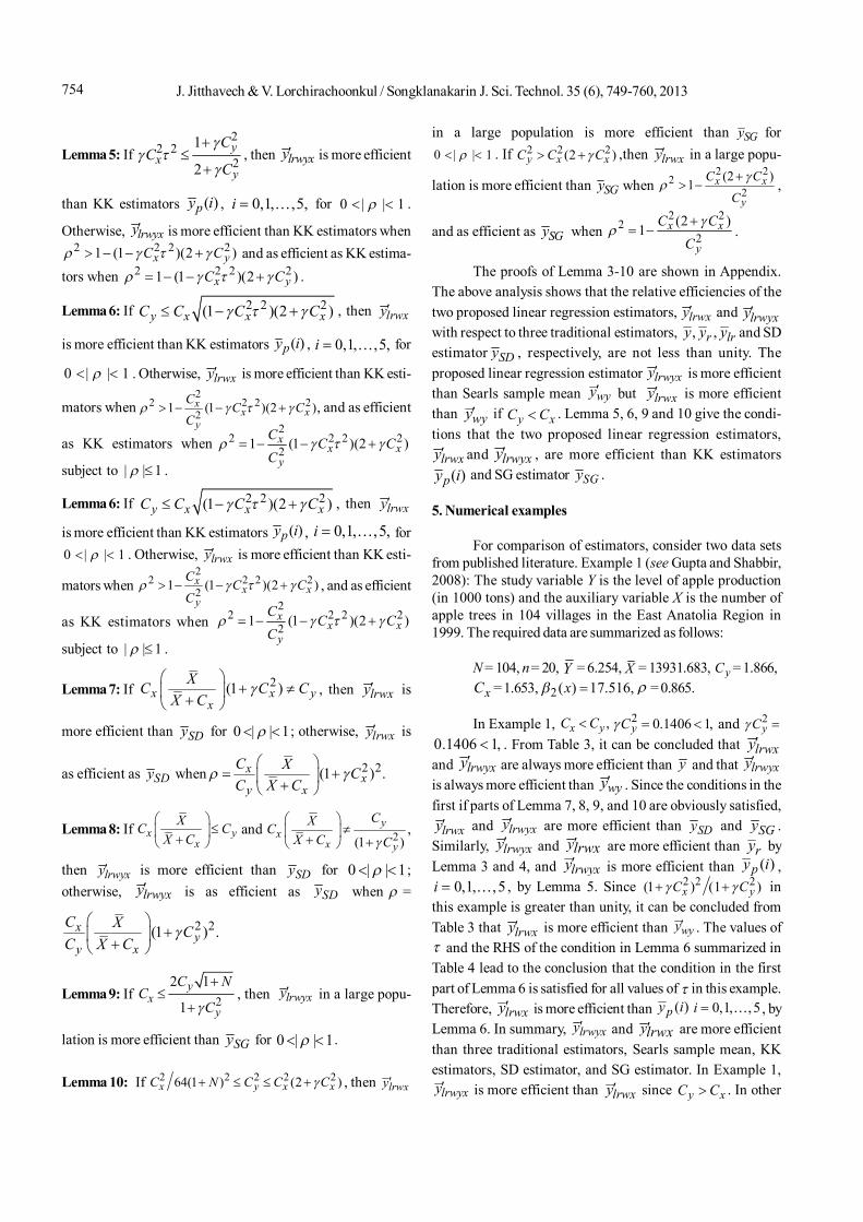
The proofs of Lemma 3-10 are shown in Appendix.The above analysis shows that the relative efficiencies of thetwo proposed linear regression estimators, lrwxy and lrwyxywith respect to three traditional estimators, , ,r lry y y and SDestimator SDy , respectively, are not less than unity. Theproposed linear regression estimator lrwyxy is more efficientthan Searls sample mean wyy but lrwxy is more efficientthan wyy if y xC C . Lemma 5, 6, 9 and 10 give the condi-tions that the two proposed linear regression estimators,

lrwxy and lrwyxy , are more efficient than KK estimators( )py i and SG estimator SGy .

5. Numerical examples

For comparison of estimators, consider two data setsfrom published literature. Example 1 (see Gupta and Shabbir,2008): The study variable Y is the level of apple production(in 1000 tons) and the auxiliary variable X is the number ofapple trees in 104 villages in the East Anatolia Region in1999. The required data are summarized as follows:

N = 104, n = 20, Y = 6.254, X = 13931.683, yC = 1.866,

xC = 1.653, 2( ) 17.516,x = 0.865.

In Example 1, ,x yC C 2 0.1406 1,yC and 2yC

0.1406 1, . From Table 3, it can be concluded that lrwxyand lrwyxy are always more efficient than y and that lrwyxyis always more efficient than wyy . Since the conditions in thefirst if parts of Lemma 7, 8, 9, and 10 are obviously satisfied,

lrwxy and lrwyxy are more efficient than SDy and SGy .Similarly, lrwyxy and ylrwx are more efficient than ry byLemma 3 and 4, and lrwyxy is more efficient than ( )py i ,

0,1, ,5i , by Lemma 5. Since 2 2 2(1 ) (1 )x yC C inthis example is greater than unity, it can be concluded fromTable 3 that lrwxy is more efficient than wyy . The values of and the RHS of the condition in Lemma 6 summarized inTable 4 lead to the conclusion that the condition in the firstpart of Lemma 6 is satisfied for all values of in this example.Therefore, lrwxy is more efficient than ( )py i 0,1, ,5i , byLemma 6. In summary, lrwyxy and ylrwx are more efficientthan three traditional estimators, Searls sample mean, KKestimators, SD estimator, and SG estimator. In Example 1,

lrwyxy is more efficient than lrwxy since y xC C . In other


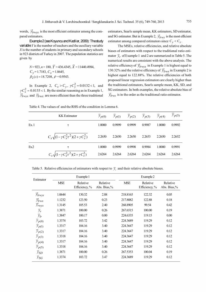
Table 4. The values of and the RHS of the condition in Lemma 6.

KK Estimator (0)py (1)py (2)py (3)py (4)py (5)py

Ex. 1 1.0000 0.9999 0.9999 0.9987 1.0000 0.9992

2 2 2(1 )(2 )x x xC C C 2.2650 2.2650 2.2650 2.2653 2.2650 2.2652

Ex.2 1.0000 0.9999 0.9998 0.9984 1.0000 0.9991

2 2 2(1 )(2 )x x xC C C 2.6264 2.6264 2.6264 2.6264 2.6264 2.6264

Table 5. Relative efficiencies of estimators with respect to ry and their relative absolute biases.

Example 1 Example 2Estimator

MSE Relative Relative MSE Relative RelativeEfficiency, % Abs. Bias,% Efficiency, % Abs. Bias,%

lrwyxy 1.0644 130.32 2.88 218.8165 122.32 0.05

lrwxy 1.1232 123.50 0.23 217.8082 122.88 0.18rwyxy 1.3145 105.53 2.40 268.8905 99.54 0.42

ry 1.3871 100.00 0.26 267.6515 100.00 0.19

lry 1.3847 100.17 0.00 224.6335 119.15 0.00

(0)py 1.3374 103.72 3.42 224.3689 119.29 0.12(1)py 1.3317 104.16 3.40 224.3647 119.29 0.12

(2)py 1.3317 104.16 3.40 224.3647 119.29 0.12(3)py 1.3318 104.16 3.40 224.3647 119.29 0.12

(4)py 1.3317 104.16 3.40 224.3647 119.29 0.12

(5)py 1.3318 104.16 3.40 224.3647 119.29 0.12

SDy 1.3871 100.00 0.26 267.5353 100.04 0.19

SGy 1.3374 103.72 3.47 224.3689 119.29 0.12

words, lrwyxy is the most efficient estimator among the com-pared estimators.

Example 2 (see Koyuncu and Kadilar, 2009): The studyvariable Y is the number of teachers and the auxiliary variableX is the number of students in primary and secondary schoolsin 923 districts of Turkey in 2007. The population statistics aregiven by

N = 923, n = 180, Y = 436.4345, X = 11440.4984,yC = 1.7183, xC = 1.8645,

2 ( ) 18.7208,x = 0.9543.

In Example 2, x yC C , 2 0.0132 1,yC and2 0.0155 1.xC By the similar reasoning as in Example 1,

lrwyxy and ylrwx are more efficient than the three traditional

estimators, Searls sample mean, KK estimators, SD estimator,and SG estimator. But in Example 2, lrwxy is the most efficientestimator among compared estimators since y xC C .

The MSEs, relative efficiencies, and relative absolutebiases of estimators with respect to the traditional ratio esti-mator ry of Example 1 and 2 are summarized in Table 5. Thenumerical results are consistent with the above analysis. Therelative efficiency of lrwyxy in Example 1 is highest equal to130.32% and the relative efficiency of lrwxy in Example 2 ishighest equal to 122.88%. The relative efficiencies of bothproposed linear regression estimators are clearly higher thanthe traditional estimators, Searls sample mean, KK, SD, andSG estimators. In both examples, the relative absolute bias of

lrwxy is in the order as the traditional ratio estimator..


6. Summary and Conclusions

In this paper, the powerful concept of Searls biasedsample mean has been extended to cover the sample mean,the ratio, and linear regression estimators in simple randomsampling. Four new estimators using the coefficient of varia-tion of the auxiliary variable, ,wxy ,rwyxy lrwyxy and lrwxy ,have been investigated and their properties are also obtained.The selection criteria based on relative efficiency amongthese new estimators, , , ,r lry y y ( )py i , i = 0,1,…,5, ,SDyand SGy are shown in Table 2 to 3 and Lemma 1 to 10. In therelative efficiency comparisons, it is found that the newlinear regression estimator lrwxy is more efficient than thenew sample mean wxy . The relative efficiency of lrwyxy withrespect to the new ratio estimator rwyxy is not less than unity..The linear regression estimator lrwyxy is more efficient thananother linear regression estimator lrwxy if C Cy x . Thisleads us to propose only two new linear regression estima-tors. The relative efficiencies of the two proposed linearregression estimators with respect to the three traditionalestimators, y , ry and lry , and SD estimator SDy , respec-tively, are shown to be at least equal to unity. The proposedlinear regression estimator lrwyxy is always more efficientthan Searls sample mean wyy but another linear regressionestimator lrwxy is more efficient than Searls sample mean

wyy if 2 2 2 21 (1 ) (1 )x yC C or Y and X are suffi-ciently high correlated. The estimator selection criteria amongthe proposed estimators, KK estimators ( )py i and SGestimator SGy are given in Lemma 5, 6, 9, and 10.

In two published data sets, the relative efficiencies oflrwyxy and lrwxy are clearly higher than those of other esti-

mators as shown in Table5. The relative biases of lrwyxy andlrwxy are 2.88% and 0.23% in Example1 and 0.05% and

0.18% in Example 2, respectively. There is not much differ-ence between all KK estimators and SG estimator as shownin Table 5.

References

Cochran, W.G. 1977. Sampling Techniques, John Wiley andSons, New York, U.S.A.

Gupta, S. and Shabbir, J. 2008. On Improvement in Estimatingthe Population Mean in Simple Random Sampling.Journal of Applied Statistics. 35, 559-566.

Koyuncu, N. and Kadilar, C. 2009. Efficient Estimators for thePopulation Mean. Hacettepe Journal of Mathematicsand Statistics. 38, 217-225.

Koyuncu, N. and Kadilar, C. 2010. On Improvement in Esti-mating Population Mean in Stratified RandomSampling. Journal of Applied Statistics. 37, 999-1013.

Searls, D.T. 1964. The Utilization of a Known Coefficient ofVariation in the Estimation Procedure. Journal of theAmerican Statistical Association. 59, 1225-1226.

Shabbir, J. and Gupta, S. 2011. On Estimating Finite PopulationMean in Simple and Stratified Sampling. Communica-tions in Statistics - Theory and Methods. 40, 199-212.

Sisodia, B.V.S., and Dwivedi, V.K. 1981. A Modified RatioEstimator using Known Coefficient of Variation ofAuxiliary Variable. Journal of the Indian Society ofAgricultural Statistics, 33, 13-18.


Appendix

Proof of Lemma 1:

From Table 2, lrwxy is at least as efficient as rwyxy if

22 4 2 4 2 2 4

2 2 2 2 2 2 2(1 ) (1 ) (1 )1 1 .(1 ) (1 ) (1 )

x x x x x

y y y y y

C C C C CC C C C C

(A-1)

Consider the first case where 2 2 2(1 ) (1 )x yC C . Under this condition, if 2 2 2(1 ) (1 )x x y yC C C C , then

the RHS in Equation A-1 is negative. It can be concluded that lrwxy is more efficient than rwyxy for 0 | | 1 . If2 2 2(1 ) (1 )x x y yC C C C , then the RHS is equal to zero. From Equation A-1, lrwxy is more efficient than rwyxy unless2 2 2(1 ) (1 )x yC C . When 2 2 2(1 ) (1 )x yC C , lrwxy is as efficient as rwyxy . If 2 2 2(1 ) (1 )x x y yC C C C ,

it is obvious that 2 4 2 2(1 ) (1 )x x y yC C C C .

When 2 4 2 2(1 ) (1 )x x y yC C C C , the minimum of the LHS in Equation A-1 for 0 | | 1 occurs at 1 and

is equal to

min

22 4

1 2 2(1 )

1(1 )

x x

y y

C CLHSC C

.

Consider the difference between min1LHS and the RHS in Equation A-1:

min

22 4 2 2 4 2 4

1 2 2 2 2 2 2 2(1 ) (1 ) (1 )

1 1 1 0.(1 ) (1 ) (1 )

x x x x x

yy y y y

C C C C CLHS

CC C C C

Therefore, if 2 2 2(1 ) (1 )x x y yC C C C , it can be concluded that in Equation A-1, the LHS is greater than theRHS for 0 | | 1 . In other words, if 2 2 2(1 ) (1 ),x x y yC C C C lrwxy is more efficient than rwyxy for 0 | | 1 . Nextconsider the case where 2 2 2(1 ) (1 )x yC C . Under this condition, the RHS in Equation A-1 is equal to zero. FromEquation A-1, it can be concluded that lrwxy is more efficient than rwyxy unless x yC C . When x yC C , lrwxy is asefficient as rwyxy . The final case is 2 2 2(1 ) (1 )x yC C . Under this condition, it follows immediately that 22y x xC C C .In other words, if 2 2 2(1 ) (1 )x yC C , it implies that 2 2 2(1 ) (1 )x x y yC C C C and 2 4 2 2(1 ) (1 )x x y yC C C C .Therefore, from Equation A-1, lrwxy is more efficient than rwyxy if the inequality of Equation A-1 is a strictly inequality andis as efficient as rwyxy if takes on a particular value such that the inequality (A-1) becomes an equality. In summary, if

2 2 2(1 ) (1 )x yC C , then lrwxy is more efficient than rwyxy unless 2 4 2 2(1 ) / (1 )x x y yC C C C . Otherwise, lrwxy ismore efficient than rwyxy provided that Equation A-1 is a strictly inequality and as efficient as rwyxy provided that takeson a particular value such that the inequality of Equation A-1 becomes an equality.

Proof of Lemma 2:

From Table 2, the condition that lrwyxy is at least as efficient as rwyxy can be written as

2 22 2 2 2 2 2

2(1 ) (1 ) 1 (1 ) 1x xx x x

y y

C CC C CC C

. (A-2)


The inequality of Equation A-2 is the same as the inequality of Equation A-1 if the term 2(1 )xC is replaced by the

term 2 2

2(1 )(1 )

x

y

CC

. The proof of Lemma 2 is much simpler than the proof of Lemma 1 since 2(1 )xC is only greater than

zero. It can be shown in the similar manner as in the first part of the proof of Lemma 1 that if 2(1 )x x yC C C , lrwyxy is

more efficient than rwyxy for 0 | | 1 ; otherwise, lrwyxy is as efficient as rwyxy when 2 2(1 ) .xx

y

C CC

Proof of Lemma 3:From Table 3, lrwxy is more efficient than ry if

2 22 2 2 2 2 2

2(1 ) (1 ) 1 (1 ) 1 .x xx x x

y y

C CC C CC C

(A-3)

Since the inequality of Equation A-3 is exactly the same as the inequality of Equation A-2, the conclusion is the sameas Lemma 2.

Proof of Lemma 4:From Table 3, lrwyxy is more efficient than ry if

2 22 2 2 2 2 2

2(1 ) (1 ) 1 (1 ) 1 .x xy y y

y y

C CC C CC C

(A-4)

The inequality of Equation A-4 is in the same form as the inequality of Equation A-2 if the term 21 yC is replaced

by 21 xC . Therefore, it can be concluded that if 2(1 )y

xy

CC

C

, lrwyxy is more efficient than ry for 0 | | 1 ; otherwise,

lrwyxy is as ry when 2 2(1 ) .xy

y

C CC

Proof of Lemma 5:

From Table 3, lrwyxy is at least as efficient as ( )py i if

2 2 2 21 (1 )(2 )x yC C . (A-5)

If 2

2 22

1

2y

xy

CC

C

, it can be shown that the RHS in Equation A-5 is less than or equal to zero. Therefore, it can be

concluded that if 2

2 22

1

2y

xy

CC

C

, lrwyxy is more efficient than KK estimators ( )py i , 0,1, ,5i , for 0 | | 1 .

Otherwise, lrwyxy is more efficient than KK estimators when 2 2 2 21 (1 )(2 ),x yC C and as efficient as KK esti-

mators when 2 2 2 21 (1 )(2 )x yC C .

Proof of Lemma 6:

From Table 3, the condition that lrwxy is at least as efficient as ( )py i is

22 2 2 2

21 (1 )(2 )xx x

y

C C CC

. (A-6)


If 2 2 2(1 )(2 )y x x xC C C C , the RHS in Equation A-6 is either negative or zero. Therefore, lrwxy is more

efficient than KK estimators ( )py i , 0,1, ,5i , for 0 | | 1 . Otherwise, lrwxy is more efficient than KK estimators

when the inequality of Equation A-6 is a strictly inequality and as efficient as KK estimators when the inequality of EquationA-6 becomes an equality.

Proof of Lemma 7:From Table 3, the condition that lrwxy is at least as efficient as SDy is

2 222 2 2 2 2 2

2(1 ) (1 ) 1 (1 ) 1 .x xx x x

y x xy

C CX XC C CC X C X CC

(A-7)

The inequality of Equation A-7 is exactly the same as the inequality of Equation A-2 if the term xx

XCX C

is

replaced by the term xC . It can be shown in the similar manner that if 2(1 )x x yx

XC C CX C

lrwxy is more efficient

than SDy for 0 | | 1 ; otherwise, lrwxy is as efficient as SDy when 2 2(1 ) .xx

y x

C X CC X C

Proof of Lemma 8:Again, from Table 3, the condition that lrwyxy is at least as efficient as SDy is

2 222 2 2 2 2 2

2(1 ) (1 ) 1 (1 ) 1 .x xy y y

y x xy

C CX XC C CC X C X CC

(A-8)

The inequality of Equation A-8 is in the same form as the inequality of Equation A-7 if the term 21 yC is replaced

by 21 xC . Therefore, it can be concluded that if 2(1 )y

xx y

CXCX C C

, lrwyxy is more efficient than SDy for

0 | | 1 ; otherwise, lrwyxy is as efficient as SDy when 2 2(1 ) .xy

y x

C X CC X C

Proof of Lemma 9:

From Table 3, the condition that lrwyxy is at least as efficient as SGy is

2 2 4 2 222 2 2

2 2 4 4(1 ) (1 )

(1 ) 1 .4(1 ) 64 (1 )

y x yxy

y y

C C CCCC N C N

(A-9)

If 2

2 1

1y

xy

C NC

C

, the terms,

2 2 2

2 2(1 )

4 (1 )x y

y

C C

C N

and

2 2 2

2 4(1 )

64 (1 )x y

y

C C

C N

can be approximately equal to zero for large N.


Under such condition and large N, it can be concluded that the LHS in Equation A-9 is greater than zero for 0 | | 1 .

Therefore, lrwyxy in a large population is more efficient than SGy for 0 | | 1 if 22 1

1y

xy

C NC

C

.

Proof of Lemma 10:From Table 3, lrwxy is at least as efficient as SGy if

2 2 2 4 2 22 2 2

2 2 4 4(1 ) (1 )(1 ) (2 ) 14(1 ) 64 (1 )

x x x xx

y y

C C C CCC N C N

. (A-10)

When N is large, the term 2 2 2(1 ) 4(1 )xC N is insignificant when compared with 2. Under this condition,the LHS in Equation A-10 can be approximately reduced to

22 2 2

2(1 ) (2 ) 1xx

y

C CC

, (A–11)

which is greater than zero for 0 | | 1 if 2 2 2(2 )y x xC C C . When N is large, the RHS in Equation A-10 is approximately

equal to zero if 8 (1 )x yC C N . Therefore, if 2 2 2 2 264(1 ) (2 )x y x xC N C C C , then lrwxy in a large population is

more efficient than SGy for 0 | | 1 . When 2 2 2(2 )y x xC C C , the condition 2 2 264(1 )y xC C N is also satisfied for

large N. Therefore, if 2 2 2(2 )y x xC C C , lrwxy in a large population is more efficient than SGy when 2 2

22

(2 )1 x x

y

C CC

,

and as efficient as SG estimator SGy when 2 2

22

(2 )1 x x

y

C CC

.

Documents

Estimators in simple random sampling: Searls approachrdo.psu.ac.th/sjstweb/journal/35-6/35-6-15.pdf · 2014-12-03 · Original Article Estimators in simple random sampling: Searls