On the economics of harvesting age-structuredfish populations*

Olli Tahvonen∗∗

Fishery and Environmental Management Group, FEMUniversity of Helsinki, Department of Biological and Environmental SciencesNovember 2007

Abstract

A generic discrete time age-structured population model is integrated withfishery economics to derive analytical results for maximizing present value re-turns net of effort cost. The simplest case is obtained by assuming two ageclasses. Given knife-edge selectivity and no harvesting cost, the optimal steadystate is a unique (local) saddle point. When fishing gear is nonselective, optimalharvesting may converge toward a stationary cycle that represents pulse fish-ing. Optimal steady states differ from those obtained by the aggregate biomassmodels. This implies that optimal extinction results depend on age structuredinformation. Given a low rate of interest and knife-edge selectivity, the optimalharvesting is shown to converge toward a unique (local) saddle point indepen-dently of the number of age classes.

Keywords: Fishery economics, optimal harvesting, age-structured popula-tions

∗This paper has been presented in International Workshop on StructuredModels in Population and Economics Dynamics, Vienna November, 2007.

∗∗Permanent address: Finnish Forest Research Institute, Unioninkatu 40 A,00170 Helsinki, Finland. E-mail: olli.tahvonen@metla.fi

1

1 Introduction

Optimal harvesting of biologically renewable populations (such as fish andtrees) is among the classical problems of resource economics. One line of researchthat dates back to Baranov (1918) aims to utilize information on the populationage-structure in searching desirable levels of harvesting effort, or as is possiblein some cases, the age class to which the harvesting activity should be targeted.The present study introduces an analytically solvable model for the optimalharvest of age-structured fish populations and suggests that it should be possibleto proceed towards an analytical understanding comparable to that achieved formodels describing the harvestable resource by a single variable for populationbiomass.

During the last forty years or more, mathematicians have analyzedthese questions under continuous age and time structure by applying the Lotka-McKendrik model and its nonlinear generalizations. This setup leads to partialdifferential equations and calls for extended versions of optimal control theory(see e.g. Brokate 1985 or Hritonenko and Yatsenko 2007).

In fishery economics, the problem is approached by age-structured mod-els specified in discrete time. Hannesson (1975) employs the classical Beverton-Holt (1957) multicohort model and shows numerically that for North Atlanticcod optimal harvesting takes the form of pulse fishing. In studies well known inpopulation ecology (Caswell 2001), Horwood and Whittle (1986) and Horwood(1987) study the economics of harvesting age-structured populations applyinga specific linearization technique in numerical computation. Recently, Stage(2006) applies an age-structured model to Namibian linefishing. Many papershave applied age-structured models to various kinds of policy analysis with-out attempting to solve the generic optimization problem (e.g. Sumaila 1997,Steinshamn 1998 and Björndal et al. 2004, Moxnes 2005).

In addition to fishery economics, the discrete time model has been usedin studies concerning various management problems in fishery ecology. A semi-nal paper is Walters (1969) that applies numerical dynamic programming. Muchof this literature is surveyed in Getz and Haight (1989) and Quinn and Deriso(1999). With closer inspection, it becomes evident that the studies in fisheryecology (excluding Walters 1969) solve the model under more or less ad hoctypes of restrictions, such as requiring harvest (or effort) to be constant overtime.

The discrete time approach for the age-structured fishery problem iswell-grounded due to the facts that both reproduction and fishing activitiesmay have clear seasonal characteristics. In addition, age-structured fish pop-ulation models and data are normally given in a discrete time framework andthese models have a long history and numerous management applications inpopulation ecology ( Leslie 1945, Caswell 2001).

Economic research in this field has been almost exclusively based onnumerical computation. The reason for this has been the view that the age-structured fishery problem is analytically intractable (e.g. Wilen 1985, Clark1985, 1990, 2006)1. Compared to the biomass framework commonly applied

2

in fishery economics (Gordon 1954, Plourde 1970), the complication followsbecause of many state variables represented by age classes. In addition, someage-structured specifications commonly applied in fishery ecology and economics(such as the Beverton-Holt 1957 formulation) may not, as such, represent themost fruitful basis for analytical work.

This study formulates the age-structured optimization model as a non-linear programming problem that can be analyzed by standard methods. Inaddition to the analytical approach, numerical computation is used to illustratethe results and to shed light on some questions that are beyond explicit solutions.The population model is in line with generic models applied in fishery ecology(Walters and Martell 2004) and it can be viewed as a direct generalization ofthe traditional "lumped parameter" model applied in fishery economics.

The general multiple age-class harvesting problem is complex, but thereare no obstacles to obtain the necessary optimality conditions using the Kuhn-Tucher theorem. A fruitful setup for a theoretical analysis is obtained by assum-ing only two age classes. Given knife-edge fishing technology, harvesting affectsonly the older age class. In the absence of harvesting cost and under nonlinearutility, the interior steady state is a unique (local) saddle point equilibrium withclear comparative statics properties.

Under linear utility, the optimal solutions are found explicitly for ini-tial states not too far from the steady state. It is shown that the constantescapement policy does not represent optimal solution, similarly to the biomassapproach. Under nonselective fishing gear, it is proved that pulse fishing be-comes the optimal solution. The intuition is that under certain conditions itis possible to avoid catching fish that are too small (i.e. to prevent "growthoverfishing") by harvesting the population cyclically and only at periods whenthe proportion of older age class is high.

Since the age-structured model can be viewed as a generalization ofthe biomass model, it is possible to compare the optimal steady states of thesemodels. The steady states coincide only under zero discounting. Under knifeedge-selectivity, the biomass model yields larger steady state population, whilethe reverse may hold when fishing gear is nonselective. These results implythat the "optimal extinction" outcomes that have been extensively studied inresource economics (e.g. Olson and Roy 1996, 2000) are dependent on whetherthe resource is viewed as an aggregate biomass or as an age-structured system.

Assuming knife-edge selectivity and that only the oldest age class isharvested enables the steady state equation to be obtained without limitingthe number of age classes. It is possible to prove the uniqueness of the steadystate and that it is a saddle point equilibrium under the low rate of interestassumption. Numerical computation suggests that the general model versionexhibits similar smooth harvesting vs. pulse fishing features than does thesimplified model with two age classes.

The literature applying the discrete time age-structured model is almostentirely based on numerical computation. The contribution of this paper is inshowing that there are no obstacles to study the generic age-structured opti-mal harvesting problem analytically. The specific results presented are new in

3

fisheries economic literature. Analytical work in this area helps to fulfil the capbetween fishery ecology and economics literature (cf. Hilborn and Walters 2001,p. 472).2

The paper is organized as follows. Section two presents the model spec-ification and the necessary optimality conditions. Section three considers thespecification with two age classes and presents results for steady states, theirstability and pulse fishing solutions. Section four develops the steady state equa-tions for a model version with unlimited number of age classes and shows thesaddle point feature of this equilibrium. The final section further discusses thediscrete time age-structured model.

2 The age-structured problem and optimality condi-tions

Let xst, s = 1, ..., n, t = 0, 1, ... denote the number of fish in age class s atthe beginning of period t. The number of eggs x0t is given by

x0t =nXs=1

γsxst. (1)

where the constants γs ≥ 0, s = 1, ..., n are fecundity parameters. Therecruits or the age class 1 fish are a function of the number of eggs, i.e.

x1,t+1 = ϕ(x0t), (2)

where ϕ is a recruitment function. Assume ϕ(0) = 0, ϕ0(0) ≤ 1, ϕ0 → 0when x0 → ex0, and that ϕ is strictly concave when x0 ∈ [0, ex0]. As specific exam-ples, this study applies the Beverton-Holt (1957) and Richer (1954) recruitmentfunction given as

ϕBH(x0t) = β1x0t/(1 + β2x0t), (3a)

ϕR(x0t) = β1x0te−β2x0t . (3b)

The Beverton-Holt (1957) recruitment function (3a) is strictly concave, whilethe Richer (1954) specification (3b) is concave for x0 ∈ [0, 2/β2] and convex forx0 ∈ [2/β2,∞). Both are concave when ϕ0 > 0. Denote the number of fishharvested from age class s at the end of periods by hst, s = 1, ..., n, t = 0, 1, ....The development of the age classes s = 2, ..., n are given by

xs+1,t+1 = αsxst − hst, s = 1, ..., n− 2, t = 0, 1, ..., (4a)

xn,t+1 = αn−1xn−1,t − hn−1,t + αnxnt − hnt, t = 0, 1, ..., (4b)

where 0 < αs ≤ 1, s = 1, ..., n are survival parameters. Equation (4a) forthe oldest age class shows that fish remain in this age class if they have survivednatural mortality and fishing. The number of fish harvested from each age classare specified as

4

hst = αsxstqs(Et), s = 1, ..., n, t = 0, 1, ..., (5)

where the age class specific functions qs(Et), s = 1, ..., n, t = 0, 1... givefishing mortality. Assume that the functions qs, s = 1, ..., n are twice andcontinuously differentiable, nondecreasing, concave and qs(0) = 0, qs(E) → bqsas E → bEs, where 0 ≤ bqs ≤ 1 and bEs > 0 for s = 1, ..., n. One example thatsatisfies these assumptions is

hst = αsxstbqs(1− e−σsEt), s = 1, ..., n, t = 0, 1, ..., (6)

where σs, s = 1, ..., n are nonnegative constants.Given the weight of fish of age class s is φs ≥ 0, s = 1, ..., n the total

yield Ht is

Ht =Xn

s=1φshst. (7)

Obviously effort is restricted to be nonnegative, i.e. Et ≥ 0. In addition,there are restrictions to the lower bound number of fish in each age class. Whenbqs = 1, s = 1, ..., n the lower bound restrictions become xs ≥ 0, s = 1, ...n.However, under knife edge selectivity, for example qs(E) = bqs = 0 for somes = 1, ..., j where j < n. More generally, when the maximum fishing mortalityis below one, it is not possible to harvest the given age class to zero. To takethese restrictions into account, the lower bounds are written as (cf. equations2, 4a,b).

x1t ≥ 0, (8a)

xs+1,t+1 ≥ αsxst(1− bqs), s = 1, ..., n− 2, (8b)

xn,t+1 ≥ αn−1xn−1,t(1− bqn−1) + αnxnt(1− bqn). (8c)

Let U denote an increasing and concave function for the utility of total yield,and C an increasing and convex function for fishing effort. A special case ofthe utility function is U(H) = pH, where p is a market price of fish. It isstraightforward to specify an extension where the market price depends on thesize (or age) of fish. Given b = 1/(1+ r) is the discount factor and r the rate ofdiscount, the objective function to be maximized can be given as

maxEt, xst, s=1,...,n, t=0,1,...

V (x0) =X∞

t=0[U(Ht)− C(Et)] b

t. (9)

The optimization problem is now defined by (9) and by the constraints 2,4a,b and 8a-c, where Ht, x0t, and hst, s = 1, ..., n are given by (1), (5) and (7).In this study, this problem will be studied both analytically and numerically.All functions are continuous with continuous first and second order derivativesand it is possible to develop necessary conditions by applying the Kuhn-Tuckertheorem3. These conditions will be used to obtain analytical results. Beyondthis, the conditions are used by applying specific functions and parameter values

5

to obtain additional understanding numerically. Independently of this, the op-timal solutions will be computed by applying gradient-based numerical solutionmethods. For these purposes, this study employes Knitro large scale optimiza-tion software (Byrd et al. 1999, 2006) that includes state-of-the-art interior (orbarrier) and active set methods. By applying numerical methods it is possible toillustrate the analytical results and, in addition, their application enables an ex-amination of the optimal transition dynamics and higher dimensional cases thatare analytically untractable but interesting from the point of view of fisheriesitself.

Let λst, s = 1, ..., n, t = 0, 1, ... denote the Lagrange multipliers for theconstraints (2), (4a,b). The Lagrangian function and the optimality conditionsare

L =X∞

t=0btU [Pn

s=1 φsαsxstqs(Et)]− C(Et)+ (10)

λ1t [ϕ(Pn

s=1 γsxst)− x1,t+1] +Pn−2

s=1 λs+1,tαsxst[1− qs(Et)]

−xs+1,t+1+ λntαn−1xn−1,t[1− qn−1(Et)]+

αnxnt[1− qn(Et)]− xn,t+1,

b−t∂L

∂Et= U 0 [

Pns=1 φsαsxstqs(Et)]

Pns=1 φsαsxstq

0s(Et)− C0(Et)− (11)Pn−1

s=1 λs+1,tαsxstq0s(Et)− λnαnxntq

0n(Et) ≤ 0, t = 0, 1, ...,

b−t∂L

∂EtEt = 0, Et ≥ 0, t = 0, 1, ..., (12)

b−t∂L

∂x1,t+1= bU 0

hXn

s=1φsαsxs,t+1qs(Et+1)

iφ1α1q1(Et+1)− λ1t+

bλ1,t+1ϕ0(Pn

s=1 γsxs,t+1)γ1 + bλ2,t+1α1[1− q1(Et+1)] ≤ 0, (13)

b−t∂L

∂x1,t+1x1,t+1 = 0, x1,t+1 ≥ 0, t = 0, 1, ..., (14)

b−t∂L

∂xs+1,t+1= bU 0

hXn

s=1φsαsxs,t+1qs(Et+1)

iφs+1αs+1qs+1(Et+1)+

bλ1,t+1ϕ0(Pn

s=1 γsxs,t+1)γs+1 − λs+1,t+

bλs+2,t+1αs+1[1− qs+1(Et+1)] ≤ 0, s = 1, ..., n− 2, t = 0, 1, ..., (15)

b−t∂L

∂xs+1,t+1[xs+1,t+1 − αsxst(1− bqs)] = 0, (16a)

xs+1,t+1 − αsxst(1− bqs) ≥ 0, s = 1, ..., n− 2, t = 0, 1, ..., (16b)

6

b−t∂L

∂xn,t+1= bU 0

hXn

s=1φsαsxs,t+1qs(Et+1)

iφnαnqn(Et+1)+ (17)

bλ1,t+1ϕ0(Pn

s=1 γsxs,t+1)γn − λnt+

bλn,t+1αn[1− qn(Et+1)] ≤ 0, t = 0, 1, ...,

b−t∂L

∂xn,t+1[xn,t+1 − αn−1xn−1,t(1− bqn−1)− αnxnt(1− bqn)] = 0, (18a)

xn,t+1 − αn−1xn−1,t(1− bqn−1)− αnxnt(1− bqn) ≥ 0, t = 0, 1, .... (18b)

Next the optimal solutions are studied by proceeding from simple cases towardthe more complex any number of age classes specifications.

3 Simplest case with two age classes

3.1 Steady state analysisGiven n = 2 conditions (11), (13) and (17) take the form:

U 0(Ht)[φ1α1x1tq01(Et) + φ2α2x2tq

02(Et)]− C 0(Et)

−λ2,t[α1x1tq01(Et) + α2x2tq02(Et)] ≤ 0, t = 0, 1, ..., (19)

bU 0(Ht+1)φ1α1q1(Et+1)− λ1t + bλ1,t+1ϕ0(γ1x1,t+1+

γ2x2,t+1)γ1 + bλ2,t+1α1[1− q1(Et+1)] ≤ 0, (20)

bU 0(Ht+1)φ2α2q2(Et+1) + bλ1,t+1ϕ0(γ1x1,t+1 + γ2x2,t+1)γ2−

λ2t + bλ2,t+1α2[1− q2(Et+1)] ≤ 0, t = 0, 1, .... (21)

Assume a steady state where all the variables are constant over time, imply-ing that the time subscripts can be cancelled. In addition, assume an interiorsolution where conditions (19)-(21) hold as equalities. Lagrangian multipliersλ1 and λ2 can be solved by (19) and (20) and eliminated from (21), which forinterpretation purposes can be written in the form

α1x1q01 + α2x2q

02

∂U/∂E

"∂U/∂x2 +

ϕ0γ2∂U/∂x1(1 + r)(1− ϕ0γ1

1+r )

#+

ϕ0γ2α1(1− q1)

(1 + r)(1− ϕ0γ11+r )

+α2(1−q2)−1 = r.

((22))Note that (α1x1tq01 + α2x2tq

02)/(∂U/∂E) = 1/λ2. Equation (22) specifies an

equality between the internal rate of return of a marginal unit of x2 and therate of interest. The fact that the rate of interest exists in both sides of theequation is a consequence of the delays in the the age class structure. The term

7

∂U/∂x2 denotes the return an increase in x2 causes in the harvest of x2. Amarginal increase in x2 causes an increase in recruitment and thus an increasein x1 equal to ϕ0γ2. This increases the utility from harvest of x1 by ϕ0γ2∂U/∂x1.This return must be discounted over one period because of one period delay.In addition, the effect must be normalized by 1/[1 − ϕ0γ1/(1 + r)] because anincrease in x1 causes an increase in recruitment equal to ϕ0γ1 units of x1. Again,this must be discounted over one period due to one period delay. Both termsin the square brackets must be divided by λ2 to obtain the rate of return of x2.Next, the term ϕ0γ2α1(1− q1) reflects the fact that an increase in x2 increasesx1 via recruitment, and this in turn increases x2 by the amount that is leftafter natural and fishing mortality. Again, these effects must be divided by(1+ r)[1−ϕ0γ1/(1+r)] because of the time delay and the recruitment effects ofx1. Finally, the term α2(1−q2) gives the share of one unit of x2 that is left afternatural mortality and fishing. From these effect one must deduct unity becausethe age structured systems gives gross growth. Among other things, this steadystate equation suggests that in age structured models the rate of interest playsa more complicated role than in models based on one single biomass variable.

It is illustrative to analyze the model when it is specified to certaincases instead of studying the most general version that includes all the effectssimultaneously. The simplest possible case follows if juveniles do not belong tospawning stock and do not have direct economic value, i.e. φ1 = 0, γ1 = 0. Inaddition, assume that fishing is costless (C = 0) and that fishing gear has theknife-edge selectivity property in the sense that q1 = 0. Let φ2 = 1. Under theseassumptions, the first term in the LHS of (22) simplifies to α2q2 and equation(22) reduces to

α2 +α1ϕ

0(x2γ2)γ21 + r

− 1 = r. (23a)

Given α2 < 1, it must hold that ϕ0 > 0 at equilibrium. Given ϕ is concavewhen ϕ0 > 0, the steady state is unique. To give a simple intuition for (23a),note that H = α1ϕ(x2γ2) + α2x2 − x2 yields the growth of x2 that can beharvested under sustainability requirements. Thus, ∂H/∂x2 = α1ϕ

0γ2 +α2 − 1is marginal growth. The term α1ϕ

0γ2 is the marginal effect on the next periodlevel of x2 that follows due to increased egg production and recruitment andafter natural mortality of x1. The term α2 gives the share one unit of x2 thatis left after natural mortality.4 From this, one must deduce 1 to obtain themarginal net effect on growth. At an optimal steady state, the marginal growthequals the rate of interest and α1ϕ

0γ2 must be discounted over one period.Given a unique x2 satisfying (23a), the other variables are determined

by

x1 = ϕ(γ2x2), (23b)

q2(E) =α1ϕ(γ2x2)

α2x2+ 1− 1/α2. (23c)

H = α2x2q2(E). (23d)

8

Implicit differentiation shows that increasing the rate of discount decreasesthe levels of x2, x1 and H, but increases the level of fishing mortality q2(E) andthe level of effort E.

Equations (23a-d) specify an interior steady state in the sense that x2 >0. The steady state may exist only if α2+α1ϕ0(0)γ2−1 > r. However, the steadystate is interior also in the sense that q2(E) ≤ 1 in (23c). This implies, forexample, that when the condition α2+α1ϕ

0(0)γ2/(1+ r)−1 > r is violated theonly remaining optimality candidate is not a solution that derives the populationto "extinction".

As specified by restrictions (8b,c), it is possible that there exists somelowest attainable level of x2 that becomes binding. This is most evident underknife-edge selectivity, where technological restrictions may prevent to harvestthe population below some minimum level. For bq2 = 1, equation (23c) yields:

µ(x2) ≡ x2 − α1ϕ(x2γ2) = 0, (24a)

∂µ/∂x2 = 1− α1ϕ0(x2)γ2. (24b)

The equation µ(x2) = 0 has always at least one solution, i.e. x2∞ = 0. If1 − α1ϕ

0(0)γ2 < 0, there exists another solution with some strictly positive x2because ∂µ/∂x2 → 1 when x2 → ex2. This solution is the lowest attainable x2and denote it as x2min. It must hold that α1ϕ0(x2min)γ2 < 1. The question iswhether x2min may be lower than the level of x2 that satisfies (23a). Recallthat the value of x2 that satisfies (23a) is higher the lower is the rate of interest.Assuming r = 0, equation (23a) reads as 1 − α2 − α1ϕ

0(x2)γ2 = 0. Lettingα2 approach zero, yields by strict convexity of ϕ, that x2min is higher thanthe level of x2 that solves (23a) under r = 0.Recall that x2min must satisfyα1ϕ

0(x2min)γ2 < 1. Since the solution to (23a) decreases with the rate ofdiscount the outcome where x2min becomes binding is more likely the higher isthe rate of discount. These findings can be summarized as follows:

Proposition 1. Assume n = 2, φ1 = γ1 = q1 = C = 0, φ2 = 1, bq2 = 1and that the recruitment function ϕ is concave when ϕ0 > 0. The interior steadystate is determined by (23a-d) and is unique. Total harvest and the number offish in both age classes are decreasing and the fishing mortality and effort areincreasing in the rate of interest. If α1ϕ(γ2x2)

α2x2+1−1/α2 > 1, where x2 satisfies

(23a), the steady state is independent of the rate of discount and is determinedby (24a) and x1 = ϕ(x2).

For further interpretation of the boundary steady state given by (24a),recall that this analysis considers the case of knife-edge selectivity (q1 = 0, q2(E) ≥0). In addition, note that harvest occurs after spawning. Thus, recruits cannotbe harvested and the share of recruits that survive as two period old fish spawnbefore they are all harvested. Under the assumption 1−α1ϕ

0(0)γ2 < 0, spawn-ing of those fish that have just reach age class two is enough to maintain thepopulation. The lowest attainable steady state level becomes the optimal steadystate if the rate of discount is high enough. Increasing the rate of discount fur-ther does not affect the steady state. When the lowest attainable steady state

9

exceeds the MSY steady state, the optimal steady state is independent of therate of discount and is determined by the knife edge fishing technology and bi-ological factors only. Compared to biomass models, and especially compared tothe interior steady state given by (22), the role of the rate of interest is nowsmaller.

Assuming Beverton and Holt (1957) recruitment function, x2min is higherthan the solution for (23a), e.g. if r = 0, β1 = 1, β2 = 1/2, α1 = 9/10, α2 =1/5, and γ2 > 25/18. However, if e.g. γ2 ≤ 10/9 (ceteris paribus), it followsthat x2min = 0 and the steady state level for x2 is determined by (23a).

3.2 Stability of steady states under nonlinear utility and no harvesting costTo study the local dynamic properties of the interior steady state, write

equation (4b) for the case n = 2 and q1 = 0 as

x2,t+2 = α1ϕ(x2t) + α2x2,t+1 − α2x2,t+1q2(Et+1), (25)

where it is assumed that γ2 = 1 (without loosing generality). Since C =q1 = 0, it is possible to take q2t as an optimized variable instead of Et. Writeq2t = qt. In addition, assume α1 = α2 = α. Since x1t can be eliminated byx1,t+1 = ϕ(x2t), write x2t as xt for simplicity. By equation (25) it is possible toobtain qt+1 = q(xt, xt+1, xt+2), where ∂q/∂xt = −αϕ0∂q/∂xt+2, ∂q/∂xt+1 =−α(1 − qt+1)∂q/∂xt+2 and ∂q/∂xt+2 = −1/(αxt+1). Next, it is possible toeliminate λ2t and λ2,t+1 by (19) and λ1,t+1 by (20). After these steps, equation(21) takes the form

θ = b2αU 0[αxt+3qt+3(xt+2, xt+3, xt+4)]ϕ0(xt+2)+bαU 0[αxt+2qt+2(xt+1, xt+2, xt+3)]− U 0[αxt+1qt+1(xt, xt+1, xt+2)] = 0. (26)

This is a fourth order nonlinear difference equation. Write its characteristicequation as

w(u) = u4 + w4u3 + w3u

2 + w2u+ w1 = 0, where (27a)

w1 =∂θ/∂xt∂θ/∂xt+4

=1

b2, (27b)

w2 =∂θ/∂xt+1∂θ/∂xt+4

=1

b2ϕ0− α

b, (27c)

w3 =∂θ/∂xt+2∂θ/∂xt+4

= −αϕ0 − U 0ϕ00

U 00ϕ0− α

bϕ0− 1

b2αϕ0, (27d)

w4 =∂θ/∂xt+3∂θ/∂xt+4

=1

bϕ0− α. (27e)

Note first that w(u) → ∞ as u → −∞ or u → ∞. Since w4 > 0 it followsthat w(0) > 0. By the steady state condition (23a):

10

w(1) =−U 0ϕ00U 00ϕ0

< 0,

w(−1) =−U 0ϕ00U 00ϕ0

+(b2αϕ0 − αb− 1)(1 + α− ϕ0α)

b2αϕ0< 0.

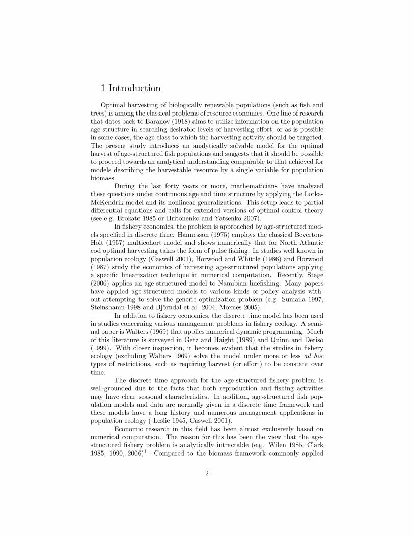
The sign of w(−1) < 0 follows from the concavity of U and ϕ and becauseat any interior steady state it must hold that (b2αϕ0−αb− 1) < 0 and αϕ0 < 1.Thus, all the four roots of the characteristic equation are real and can be givenas: u4 < −1 < u3 < 0 < u2 < 1 < u1. Thus the steady state is a local saddlepoint equilibrium.

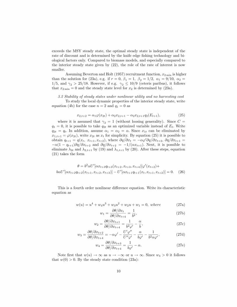
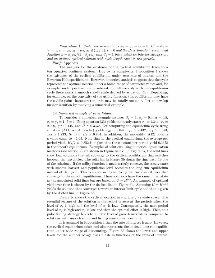
Proposition 2. Given the assumptions of Proposition 1 and a strictlyconcave utility function U, the interior steady state is a local saddle point.

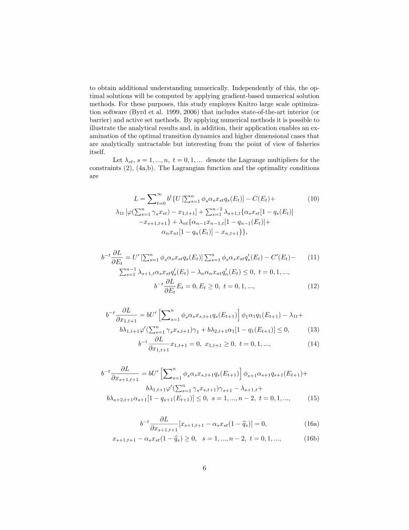
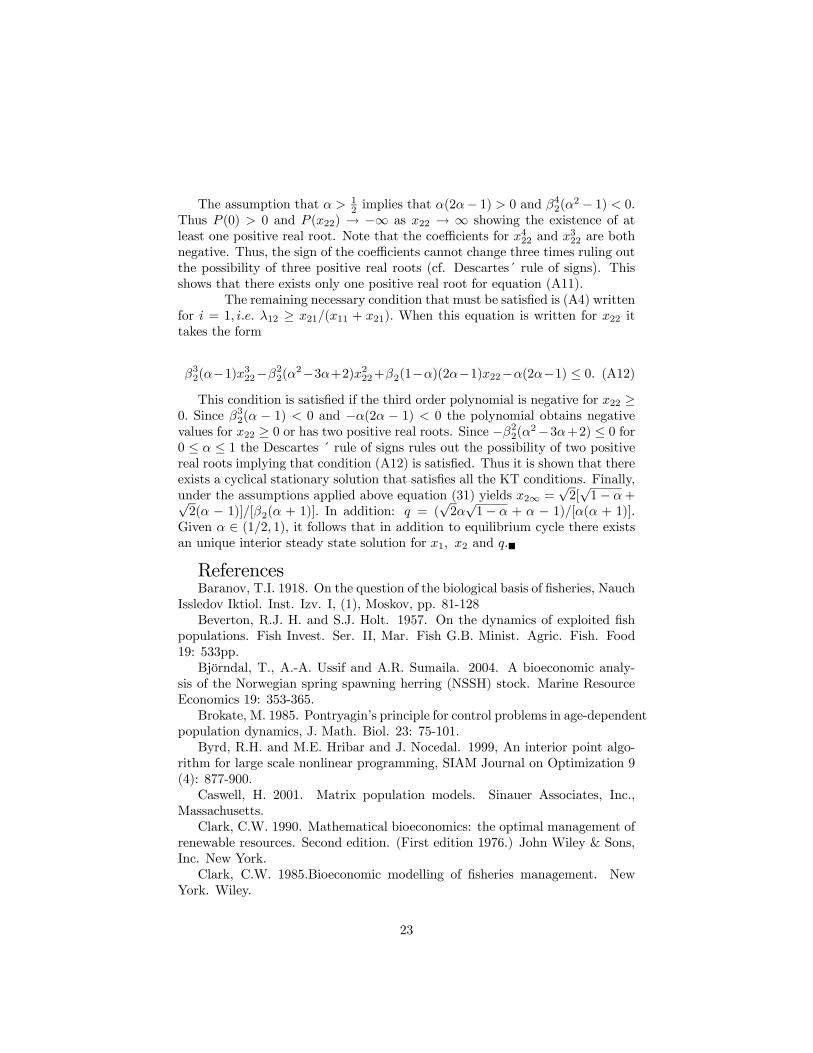
Examples of optimal solutions are shown in Figure 1. Applying theconditions (23a-d) the optimal steady state is x1∞ = 1.2127, x2 = 2.355, H∞ =0.4991 and applying the above derived formulas for characteristic roots implyr1 = −4.87, r2 = −0.207, r3 = 0.791, r4 = 1.277. Figure 1 is produced by thenumerical optimization methods explained in section 2. It shows five examplesof optimal solutions that converge toward the steady state. Excluding the origin,it is likely that the steady state is globally stable for optimal solutions.

3.3 Optimal solution under linear utility and no harvesting costThe steady state defined by (23a-d) is independent of the utility func-

tion. However, it is evident that the same does not hold for optimal ap-proach paths. To study the optimal trasitionary dynamics when the utilityfunction is linear, assume U 0 = 1. For simplicity, maintain the assumptionsγ1 = φ1 = q1 = C = 0, φ2 = γ2 = 1. To find the initial states x10, x20that allow the optimal solution to reach the steady state in one period, assumex11 = x1∞ and x21 = x2∞, where the subscript ∞ refers to the steady state.Since q1 = 0, it is again possible to take q2t as the control variable and denoteq2t = qt. By (2) and (4b) it must hold that

x11 = x1∞ = ϕ(x20), (28)

x21 = x2∞ = α1x10 + α2x20(1− q0). (29)

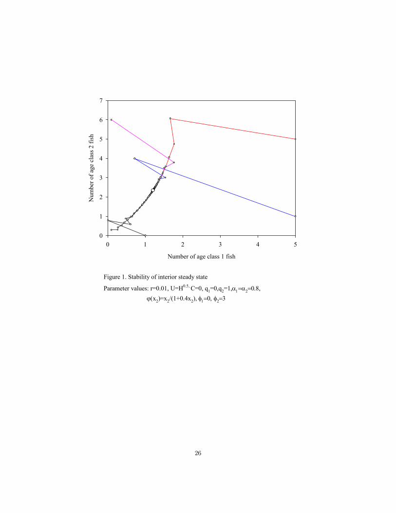
Thus, by (28) it holds that x20 = x2∞. In (29) q0 = 0 implies x10 = x2∞(1−α2)/α1 and q0 = 1 that x10 = x2∞/α1. These are lower and higher bounds forx10. Denote them by x10 and x10. (see Figure 2a). From (29) it follows that thefishing mortality is given as

q0 = 1− (x2∞ − α1x10)

α2x20. (30)

This solution is optimal because it satisfies (19)-(21) as equalities with λ2t =1, t = 0, 1, ...

11

Consider next the possible initial states from which the steady state canbe reached optimally with two steps. Since x11 ∈ [x2∞(1 − α2)/α1, x2∞/α1]must hold after the first step, it follows by x1,t+1 = ϕ(x2t) that the region forx20 is defined by

x2∞/α1 ≤ ϕ(x20) ≤ x2∞(1− α2)/α1. (31)

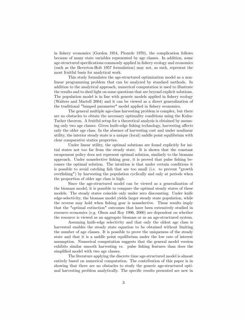
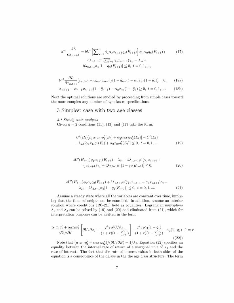
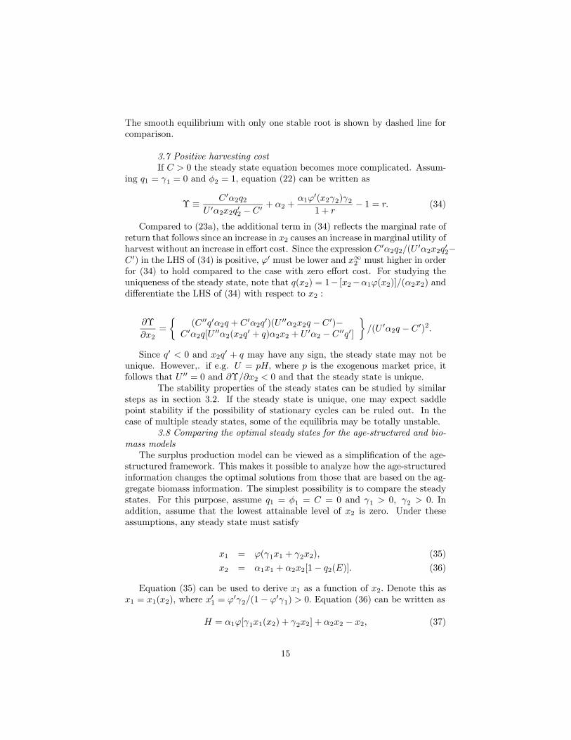
Denote these lower and upper bounds by x20 and x20 accordingly (see Figure1a). To reach the steady state with two steps it must also hold that x21 = x2∞,i.e. that x2∞ = α1x10 + α2x20(1 − q0). The highest possible level for x10 isobtained when q0 = 1, and this level equals x2∞/α1. Finally, the left boundaryof the region is found by setting q0 = 0 implying a boundary x20 = (x2∞ −α1x10)/α2 (Figure 2a). By construction of these boundaries the initial fishingmortality that implies x21 = x2∞, is again given by (30). This solution satisfiesconditions (19)-(21) since x21 = x2∞ and it is possible to set λ2t = 1, t = 0, 1, ....These findings can be summarized as:

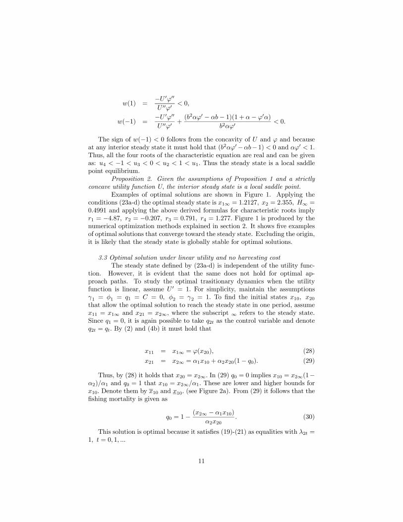
Proposition 3. Given the assumptions of Proposition 1 and that U 0 = 1and that an interior steady state exists, it is optimal to reach the steady statein one period if x20 = x2∞ and x10 ∈ [x2∞(1− α2)/α1, x2∞/α1]. The optimalsolution reaches the steady state in two periods if the initial state satisfies x20 ≥(x2∞ − α1x10)/α2, x2∞/α1 ≤ ϕ(x20) ≤ x2∞(1− α2)/α1 and x20 6= x2∞.

Given the initial state that allows the optimal solution to reach thesteady state in one or two steps, the solution is an example of constant escape-ment policy (see e.g. Spence 1973). Within the constant escapement policy,the population level after the harvest equals to its optimal after harvest steadystate level. Such a policy is optimal for the biomass model under a linear ob-jective and fishery production functions, and given that the beginning of periodbiomass level is not too low. The constant escapement policy means that thesteady state is reached in one step. A similar policy may well be optimal for theage-structured model but with a more restrictive set of initial states. If escape-ment is interpreted to refer to the number of fish in age class 2, escapement isconstant only for those initial states from which x2∞ can be reached optimallywith one step. This is clearly not possible, if x20 > x20 (or x10 > x2∞/α1), forexample. The reason why it takes more periods to reach the steady state is thathigh enough initial x20 implies high x11 and as an implication an excessivelyhigh x22, i.e. x22 > x2∞. Compared to the biomass model, these complicationsare consequences of the age class structure.

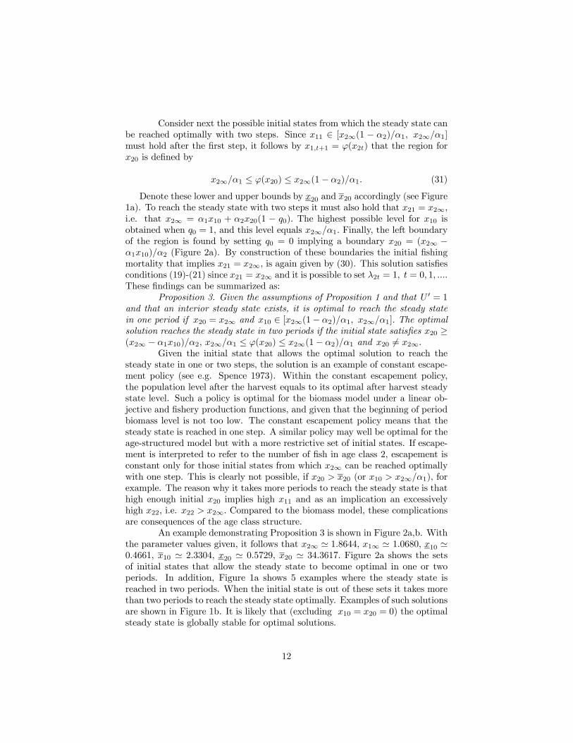
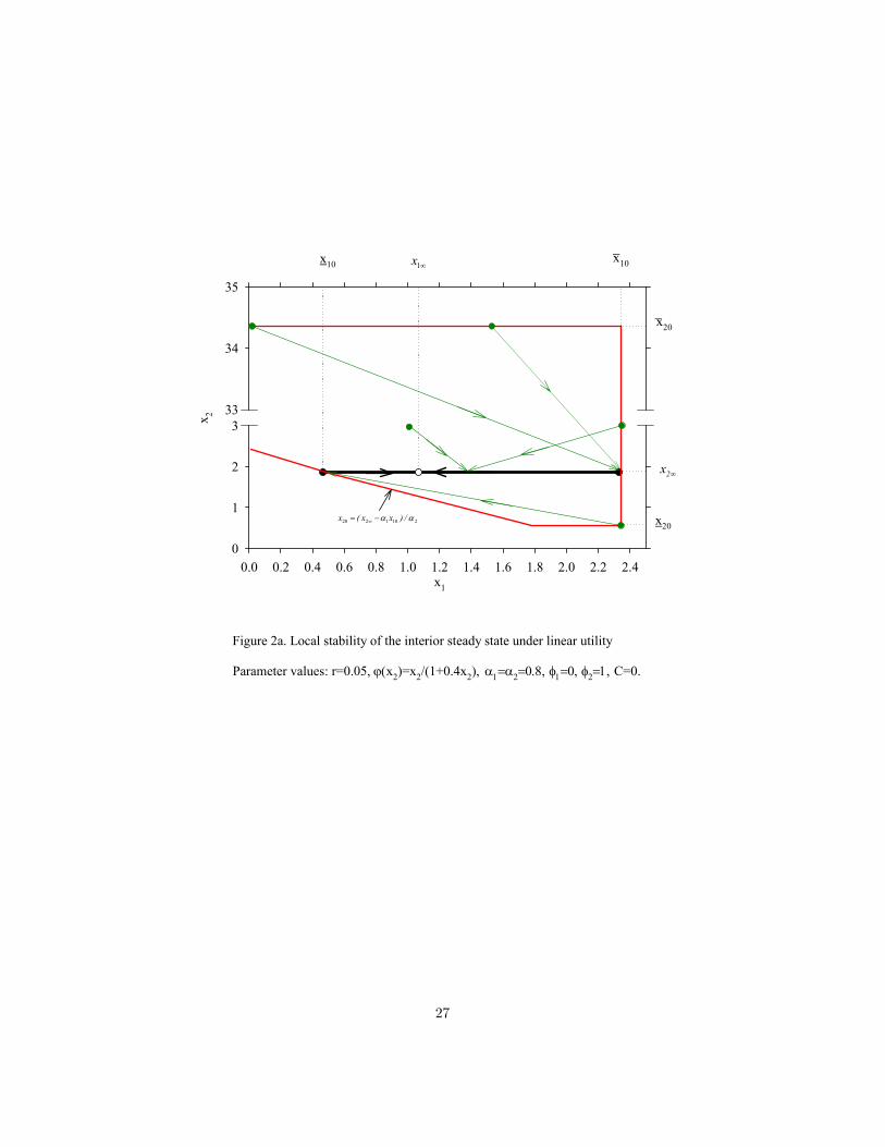
An example demonstrating Proposition 3 is shown in Figure 2a,b. Withthe parameter values given, it follows that x2∞ ' 1.8644, x1∞ ' 1.0680, x10 '0.4661, x10 ' 2.3304, x20 ' 0.5729, x20 ' 34.3617. Figure 2a shows the setsof initial states that allow the steady state to become optimal in one or twoperiods. In addition, Figure 1a shows 5 examples where the steady state isreached in two periods. When the initial state is out of these sets it takes morethan two periods to reach the steady state optimally. Examples of such solutionsare shown in Figure 1b. It is likely that (excluding x10 = x20 = 0) the optimalsteady state is globally stable for optimal solutions.

12

3.4 Steady state under growth overfishingAssume next that q1 > 0 but maintain the assumptions φ1 = γ1 = C =

0, φ2 = 1. Thus, in this case fishing gear is nonselective in spite of the fact thatage class one fish do not have commercial value and do not yet form part of thespawning stock. Fishery ecologists call such harvesting "growth overfishing",since fish are taken to be too small when harvested. Equation (22) for theoptimal steady state obtains the form

q2(E)α1x1q01(E)

x2q02(E)+

α1ϕ0(γ2x2)γ2[1− q1(E)]

1 + r+ α2 − 1 = r, (32)

where E is determined by x2 − α1ϕ(x2)[1 − q1(E)] − α2x2[1 − q2(E)] = 0.The assumption q1(E) = τq2(E), where 0 ≤ τ ≤ 1 and the fact x1 = ϕ(x2)simplifies (32) to

Ψ =α1τq2x2

·ϕ− ϕ0γ2x2

1 + r

¸+

α1ϕ0(γ2x2)γ21 + r

+ α2 − 1 = r, (33)

where q2 = (α1ϕ + x2α2 − x2)/(α1ϕτ + α2x2) and ϕ − ϕ0γ2x2/(1 + r) ispositive by the concavity of ϕ. Since the new expression ·

· [·] not existing in(23a) is positive, the steady state level of x2 must be higher compared to the caseq1 = 0. Differentiation and the concavity of ϕ show that ∂Ψ/∂x2 < 0, implyingthat the optimal steady state is unique. In addition, since ∂τq2/∂τ > 0, itfollows that ∂Ψ/∂τ > 0, implying from the implicit function theorem that thesteady state level of x2 is increasing in τ . In addition, differentiation shows that∂q2/∂τ < 0 and ∂H/∂τ = ∂(α2x2q2)/∂τ < 0. These findings can be summarizedas:

Proposition 4. Given that φ1 = γ1 = C = 0, φ2 = 1 and q1(E) =τq2(E), where 0 ≤ τ ≤ 1,the optimal steady state is unique and the steady statelevels of x1 and x2 are increasing in τ , while the steady state levels of q2 andH are decreasing in τ .

The stability of the steady state can be studied by applying similarsteps as in section 3. However, the expressions will become rather tedious.Numerical computation of the characteristic roots shows that under strictlyconcave utility the steady state may still have the local saddle point property.However, setting τ = 1, specifying U = Hσ and letting σ → 1 finally leads to anoutcome with only one stable root. This follows, for example, if U(H) = Hσ,ϕ(x2) = x2/(1+ 0.4x2), α1 = α2 = 0.8, b = τ = 1 and 0.9315 < σ < 1. In thesecases, it is optimal to reach the steady state only in hairline cases where theinitial state x10, x20 satisfies a specific functional relationship. The next task isto examine other possibilities for the long run equilibria.

3.5 Pulse fishing and cyclical equilibria under growth overfishingInstead of a smooth equilibrium with constant harvest and population

levels over time, another candidate for the long run equilibrium is the stationarycycle. This type of solution is known as pulse fishing (Walters 1969, Hannesson1975) and intuitively it may become optimal due to the problem of growthoverfishing.

13

Proposition 4. Under the assumptions φ1 = γ1 = C = 0, U 0 = φ2 =γ2 = 1, q1 = q2, α1 = α2, α2 ∈ (1/2, 1), r = 0 and the Beverton-Holt recruitmentfunction ϕ = β1x2t/(1+β2x2t) with β1 = 1 there exists an interior steady stateand an optimal cyclical solution with cycle length equal to two periods.Proof: Appendix.

The analysis for the existence of the cyclical equilibrium leads to aten equation nonlinear system. Due to its complexity, Proposition 4 showsthe existence of the cyclical equilibrium under zero rate of interest and theBeverton-Holt specification. However, numerical analysis suggests that the cyclerepresents the optimal solution under a broad range of parameter values and, forexample, under positive rate of interest. Simultaneously with the equilibriumcycle there exists a smooth steady state defined by equation (33). Depending,for example, on the convexity of the utility function, this equilibrium may havethe saddle point characteristics or it may be totally unstable. Let us developfurther intuition by studying a numerical example.

3.6 Numerical example of pulse fishingTo consider a numerical example assume: β1 = 1, β2 = 0.4, α = 0.8,

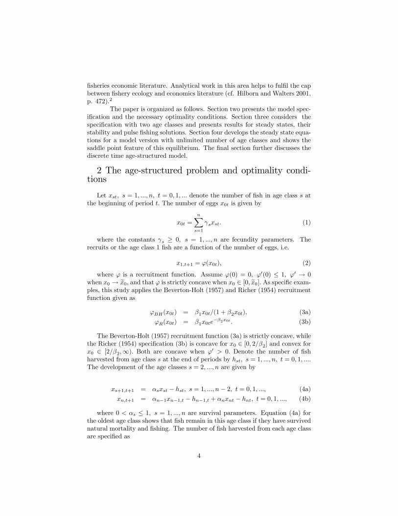
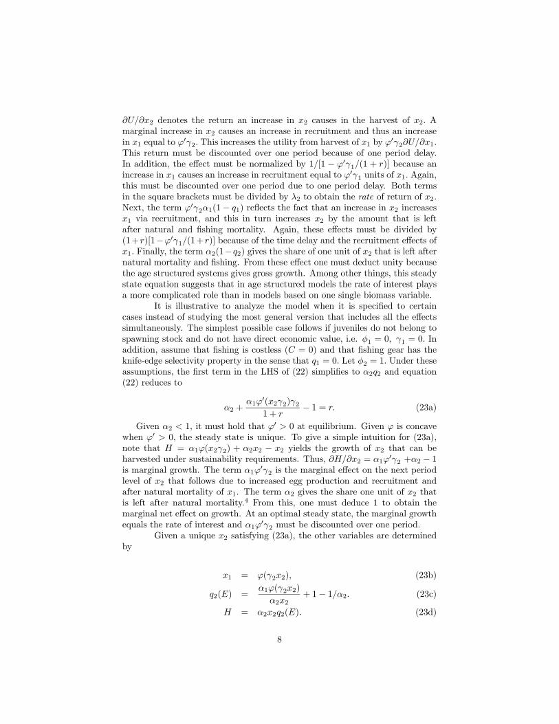
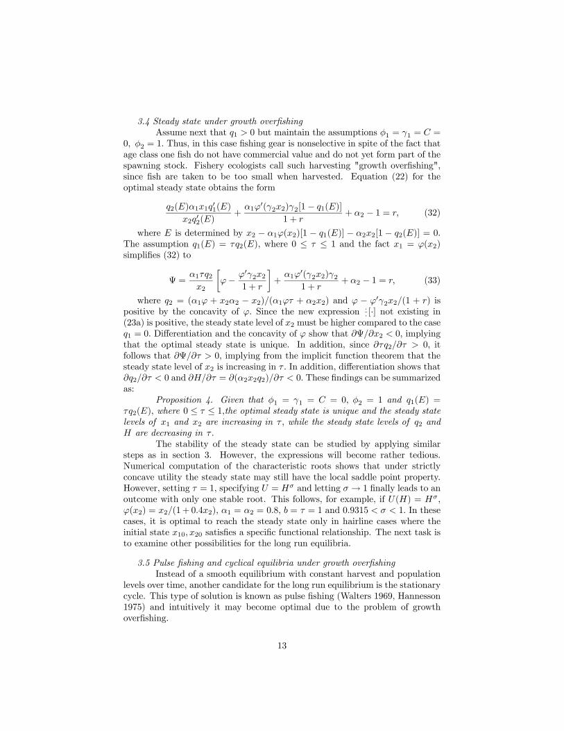
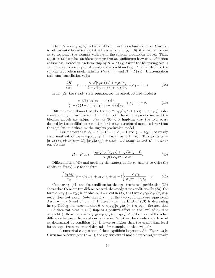
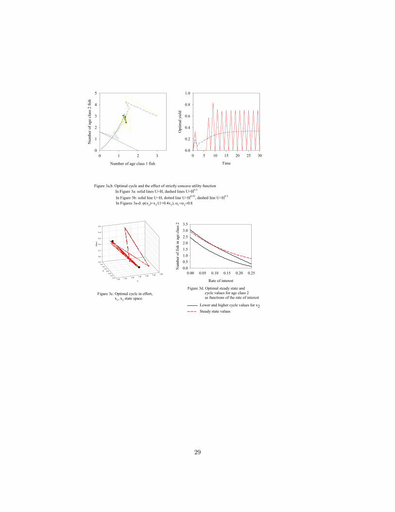
q1 = q2 = 1, b = 1.Using equation (33) yields the steady state: x1 ' 1.344, x2 '2.906, q ' 0.145, and H ' 0.3378. For computing the equilibrium cycle usingequation (A11, see Appendix) yields x22 ' 3.044, x21 ' 2.432, x11 ' 1.373,x12 ' 1.233, H1 ' 0, H2 ' 0.704. In addition, the inequality (A12) obtainsa value equal to −1.05. Note that in the cyclical equilibrium, the average perperiod yield, H2/2 ' 0.352 is higher that the constant per period yield 0.3378in the smooth equilibrium. Examples of solutions using numerical optimizationmethods (see section 2) are shown in Figure 3a,b,c. In Figure 3a, the solid linesshow four solutions that all converge to the cyclical equilibrium that switchesbetween the two circles. The solid line in Figure 3b shows the time path for oneof the solutions. If the utility function is made strictly concave, the steady statewith smooth harvest and population level becomes the long run equilibriuminstead of the cycle. This is shown in Figure 3a by the two dashed lines thatconverge to the smooth equilibrium. These solutions have the same initial stateas the associated solid lines but are based on U = H0.5. An example of optimalyield over time is shown by the dashed line in Figure 3b. Assuming U = H0.93

yields the solution that converges toward an interior limit cycle and that is givenby the dotted line in Figure 3b.

Figure 3c shows the cyclical solution in effort, x1, x2 state space. Theessential feature of the solution is that effort is zero at the periods when thelevel of x1 is high and the level of x2 is low. Consequently, the next periodlevel of x2 is high and x1 is low and then the optimal effort is high. Thus, thispulse fishing strategy leads to a lower level of growth overfishing compared tosolutions with smooth effort and fishing mortalities over time.

It is assumed in Proposition 4 that the rate of interest is zero. However,the cyclical equilibrium exists and also represents the optimal long run equilib-rium under wide range of discounting. Figure 3d shows the lower and upperlevels for the number of age class 2 fish as functions of the rates of interest.

14

The smooth equilibrium with only one stable root is shown by dashed line forcomparison.

3.7 Positive harvesting costIf C > 0 the steady state equation becomes more complicated. Assum-

ing q1 = γ1 = 0 and φ2 = 1, equation (22) can be written as

Υ ≡ C0α2q2U 0α2x2q02 − C 0

+ α2 +α1ϕ

0(x2γ2)γ21 + r

− 1 = r. (34)

Compared to (23a), the additional term in (34) reflects the marginal rate ofreturn that follows since an increase in x2 causes an increase in marginal utility ofharvest without an increase in effort cost. Since the expression C 0α2q2/(U 0α2x2q02−C 0) in the LHS of (34) is positive, ϕ0 must be lower and x∞2 must higher in orderfor (34) to hold compared to the case with zero effort cost. For studying theuniqueness of the steady state, note that q(x2) = 1− [x2−α1ϕ(x2)]/(α2x2) anddifferentiate the LHS of (34) with respect to x2 :

∂Υ

∂x2=

½(C 00q0α2q + C0α2q0)(U 00α2x2q − C 0)−

C 0α2q[U 00α2(x2q0 + q)α2x2 + U 0α2 − C00q0]

¾/(U 0α2q − C 0)2.

Since q0 < 0 and x2q0 + q may have any sign, the steady state may not be

unique. However,. if e.g. U = pH, where p is the exogenous market price, itfollows that U 00 = 0 and ∂Υ/∂x2 < 0 and that the steady state is unique.

The stability properties of the steady states can be studied by similarsteps as in section 3.2. If the steady state is unique, one may expect saddlepoint stability if the possibility of stationary cycles can be ruled out. In thecase of multiple steady states, some of the equilibria may be totally unstable.

3.8 Comparing the optimal steady states for the age-structured and bio-mass modelsThe surplus production model can be viewed as a simplification of the age-

structured framework. This makes it possible to analyze how the age-structuredinformation changes the optimal solutions from those that are based on the ag-gregate biomass information. The simplest possibility is to compare the steadystates. For this purpose, assume q1 = φ1 = C = 0 and γ1 > 0, γ2 > 0. Inaddition, assume that the lowest attainable level of x2 is zero. Under theseassumptions, any steady state must satisfy

x1 = ϕ(γ1x1 + γ2x2), (35)

x2 = α1x1 + α2x2[1− q2(E)]. (36)

Equation (35) can be used to derive x1 as a function of x2. Denote this asx1 = x1(x2), where x01 = ϕ0γ2/(1− ϕ0γ1) > 0. Equation (36) can be written as

H = α1ϕ[γ1x1(x2) + γ2x2] + α2x2 − x2, (37)

15

where H[= α2x2q2(E)] is the equilibrium yield as a function of x2. Since x1is not harvestable and its market value is zero (q1 = φ1 = 0), it is natural to takex2 to represent the biomass variable in the surplus production model. Thus,equation (37) can be considered to represent an equilibrium harvest as a functionas biomass. Denote this relationship by H = F (x2). Given the harvesting cost iszero, the well known optimal steady state condition (e.g. Plourde 1970) for thesurplus production model satisfies F 0(x2) = r and H = F (x2) . Differentiationand some cancellation yields

∂H

∂x2= r =⇒ α1ϕ

0[γ1x1(x2) + γ2x2]γ21− ϕ0[γ1x1(x2) + γ2x2]γ1

+ α2 − 1 = r. (38)

From (22) the steady state equation for the age-structured model is

α1ϕ0[γ1x1(x2) + γ2x2]γ2

(1 + r) 1− bϕ0[γ1x1(x2) + γ2x2] γ1+ α2 − 1 = r. (39)

Differentiation shows that the term η ≡ α1ϕ0γ2/[(1 + r)(1 − bϕ0γ1)] is de-

creasing in x2. Thus, the equilibrium for both the surplus production and thebiomass models are unique. Next ∂η/∂r < 0, implying that the level of x2defined by the equilibrium condition for the age-structured model is lower thanthe equilibrium defined by the surplus production model.

Assume next that φ1 = γ1 = C = 0, φ2 = 1 and q1 = τq2. The steadystate must satisfy x2 = α1ϕ(x2γ2)(1 − τq2)+ α2x2(1 − q2). This yields q2 =[α1ϕ(x2γ2)+ x2(α2− 1)]/[α1ϕ(x2γ2)τ+ α2x2]. By using the fact H = α2x2q2one obtains

H = F (x2) =α2x2α1ϕ(x2γ2) + α2x

22(α2 − 1)

α1ϕ(x2γ2)τ + α2x2. (40)

Differentiation (40) and applying the expression for q2 enables to write thecondition F 0(x2) = r to the form½

α1τq2x2

[ϕ− ϕ0γ2x2] + α1ϕ0γ2 + α2 − 1

¾α2x2

α1ϕτ + α2x2= r. (41)

Comparing (41) and the condition for the age structured specification (33)shows that there are two differences with the steady state conditions. In (33), theterm α1ϕ

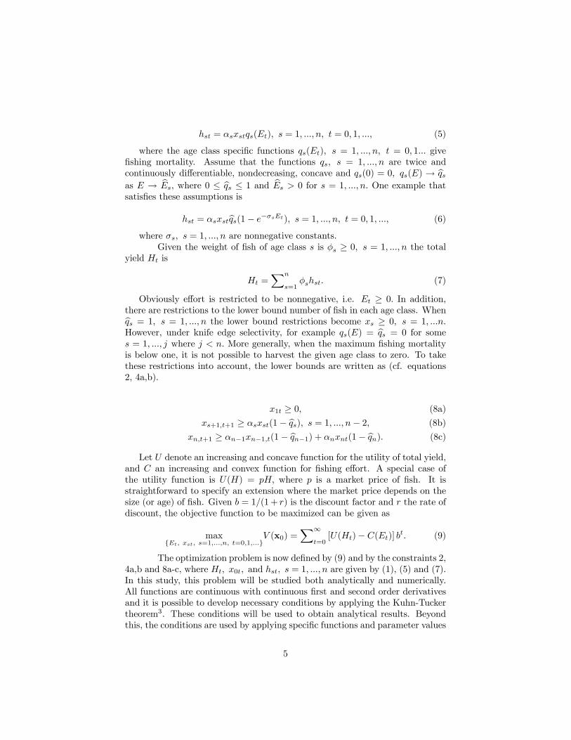
0γ2(1−τq2) is divided by 1+r and in (33) the term α2x2/[α1ϕ(x2)τ +α2x2] does not exist. Note that if r = 0, the two conditions are equivalent.Assume r > 0 and 0 < τ ≤ 1. Recall that the LHS of (33) is decreasingin x2. Taking into account that 0 < α2x2/[α1ϕ(x2)τ + α2x2], the fact that1 + r does not exist in (41) implies a positive effect on the level of x2 thatsolves (41). However, since α2x2/[α1ϕ(x2)τ + α2x2] < 1, the effect of the otherdifference between the equations is reverse. Whether the steady state level ofx2 determined by condition (41) is lower or higher than the equilibrium levelfor the age-structured model depends, for example, on the level of τ .

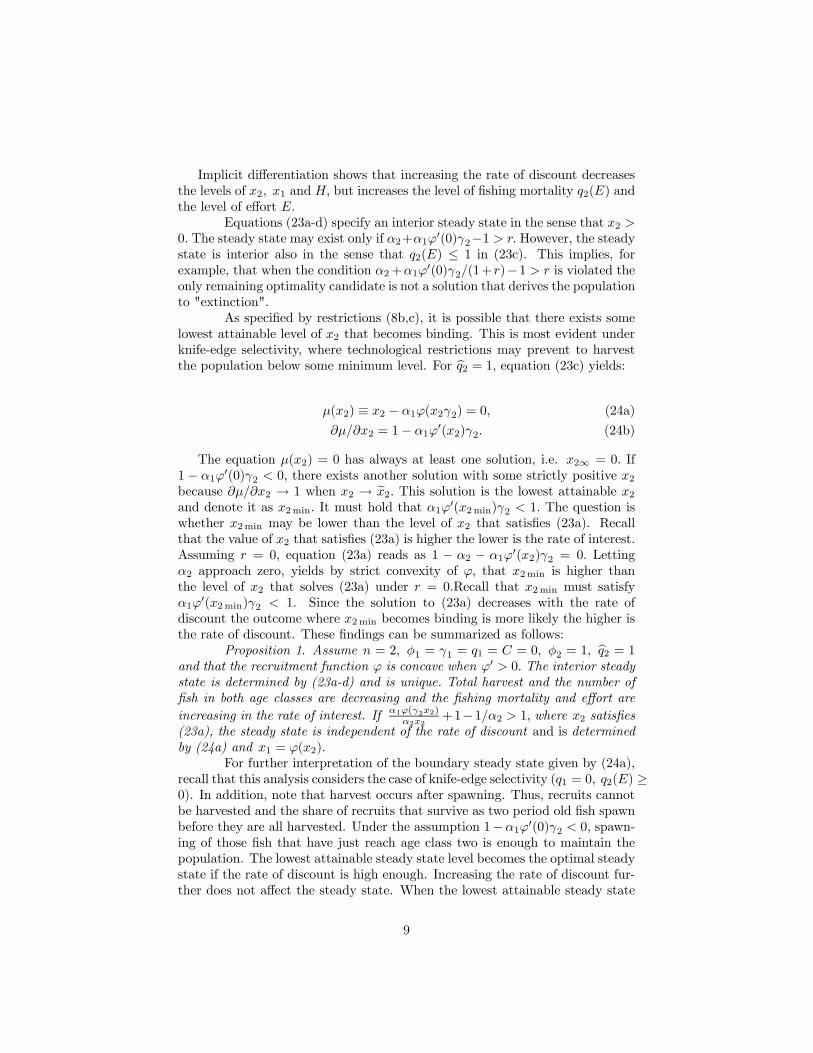
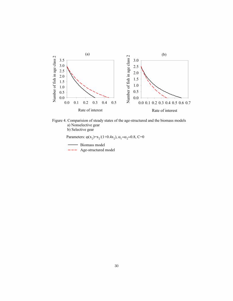
A numerical comparison of these equilibria is presented in Figure 4a,b.Given nonselective gear (τ = 1), the age structured model implies larger steady

16

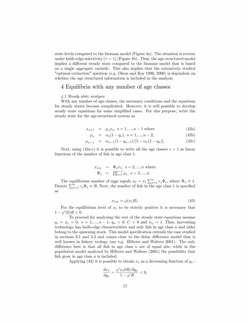
state levels compared to the biomass model (Figure 4a). The situation is reverseunder knife-edge selectivity (τ = 1) (Figure 4b). Thus, the age-structured modelimplies a different steady state compared to the biomass model that is basedon a single aggregate variable. This also implies that the extensively studied"optimal extinction" question (e.g. Olson and Roy 1996, 2000) is dependent onwhether the age structured information is included in the analysis.

4 Equilibria with any number of age classes

4.1 Steady state analysisWith any number of age classes, the necessary conditions and the equations

for steady states become complicated. However, it is still possible to developsteady state equations for some simplified cases. For this purpose, write thesteady state for the age-structured system as

xs+1 = µsxs, s = 1, ..., n− 1 where (42a)

µs = αs(1− qs), s = 1, ..., n− 2, (42b)

µn−1 = αn−1(1− qn−1)/[1− αn(1− qn)]. (42c)

Next, using (42a-c) it is possible to write all the age classes s > 1 as linearfunctions of the number of fish in age class 1:

xs∞ = Φsx1, s = 2, ..., n where

Φs =Qs−1

i=1 µi, s = 2, ..., n.

The equilibrium number of eggs equals x0 = x1Pn

s=1 γsΦs, where Φ1 ≡ 1.Denote

Pns=1 γsΦs ≡ R. Next, the number of fish in the age class 1 is specified

as

x1∞ = ϕ(x1R). (43)

For the equilibrium level of x1 to be strictly positive it is necessary that1− ϕ0(0)R < 0.

To proceed for analyzing the rest of the steady state equations assumeqs = φs = 0, s = 1, ..., n − 1, qn > 0, C > 0 and φn = 1. Thus, harvestingtechnology has knife-edge characteristics and only fish in age class n and olderbelong to the spawning stock. This model specification extends the case studiedin sections 3.1 and 3.2 and comes close to the delay difference model that iswell known in fishery ecology (see e.g. Hilborn and Walters 2001). The onlydifference here is that all fish in age class n are of equal size, while in thepopulation model analyzed by Hilborn and Walters (2001) the possibility thatfish grow in age class n is included.

Applying (43) it is possible to obtain x1 as a decreasing function of qn :

dx1dqn

=ϕ0x1∂R/∂qn1− ϕ0R

< 0,

17

where ∂R/∂qn = −Qn−2

i=1αn−1αn

1−αn(1−qn) < 0. Denote this function by x1 =

x1(qn). The remaining optimality conditions are

U 0αnxnq0n − C 0 − λnαnxnq0n = 0, (44)

−λs + bλ1ϕ0γs + bλs+1αs = 0, s = 1, ..., n− 1, (45)

bU 0αnqn + bλ1ϕ0γn − λn + bλnαn(1− qn) = 0. (46)

Equations (45) can be solved recursively starting from s = n − 1 and pro-ceeding toward s = 1. Each Lagrangian multiplier is then given as a functionof λ1 and λn and finally the equation for s = 1 defines λ1 as a function of λn.Using this result, λ1 can then be eliminated from (46). Dividing (46) by bλnand solving (44) for λn yields:

U 0α2nxnqnq0n

U 0αnxnq0n − C 0+

ϕ0γnbn−1Qn−1

j=1 αn−j

1− ϕ0nPn−1

j=1 bn−1γj

Qj−1k=1 αk−1

o +αn(1− qn) = 1/b. (47)

Equation (47) can be viewed to contain qn as its single variable since all thestate variables, as well as E in C 0, can be given as functions of qn. If C0 = 0, thisequation has a unique solution since the first quotient in the LHS cancels with−αnqn and the remaining part is decreasing in x1 and increasing with qn.

4.2 Stability of the steady stateFor analyzing the stability of the optimal steady state assume that γs =

0, s = 1, ..., n− 1, γn = 1, qs = 0, s = 1, ..., n− 1. In addition, assume C = 0.It is now possible to take qnt directly as the control variable. Denote it qnt ≡ qtfor simplicity. Given an interior solution, the conditions (11)-(18) take the form

U 0(αnxntqt)αnxnt − λntαnxnt = 0, (48)

−λ1t + bλ2,t+1α1 = 0, (49)

−λ2t + bλ3,t+1α1 = 0, (50)

· · ·,λn−1,t + bλn,t+1αn−1 = 0, (51)

bU 0(αnxn,t+1qt+1)αnqt+1 + bλ1,t+1ϕ0(xn,t+1)− λnt + αnbλn,t+1(1− qt+1) = 0.

(52)

Equations (49)-(51) yield λnt = λ1,t−(n−1)/(bn−1Qn−1

i=1 αi) and λ1,t+1 =

λn,t+nσ, where σ = bn−1Qn−1

i=1 αi. In addition, the conditions x1,t+1 = ϕ(xnt),x2,t+1 = x1tα1, ..., xn,t+1 = αn−1xn−1,t+ αnxnt(1− qt) yield

qt = 1− xn,t+1 − σϕ(xn,t−n+1)αnxnt

.

18

Note from (1) that λnt = U 0(αnxntqt). It is now possible to eliminate λ1,t+1,λnt and qt from (52) and obtain the following difference equation for xnt :

Ω = bnϕ0(xt+2)σU 0½αnxt+n+1

·1− xt+n+2 − σϕ(xt+2)

αnxt+n+1

¸¾−U 0

½αnxt+1

·1− xt+2 − σϕ(xt−n+2)

αnxt+1

¸¾+αnbU

0½αnxt+2

·1− xt+3 − σϕ(xt−n+3)

αnxt+2

¸¾,

where xnt = xt for simplicity. This is a nonlinear difference equation of order2n. To form its characteristic equation compute:

w1 =∂Ω/∂xt−n+2∂Ω/xt+n+2

=1

bn,

w2 =∂Ω/∂xt−n+3∂Ω/xt+n+2

= − αnbn−1

,

w3 =∂Ω/∂xt+1∂Ω/xt+n+2

=αn

bnϕ0σ,

w4 =∂Ω/∂xt+2∂Ω/xt+n+2

= − α2nbn−1ϕ0σ

− σϕ0 − 1

bnϕ0σ− ϕ00U 0

ϕ0U 00,

w5 =∂Ω/∂xt+3∂Ω/xt+n+2

=αn

bn−1ϕ0σ,

w6 =∂Ω/∂xt+n+1∂Ω/xt+n+2

= −αn.

The characteristic polynomial can be written as

Φ(u) = u2n + w6u2n−1 + w5u

n+1 + w4un + w3u

n−1 + w2u+ w1 = 0. (53)

Let r = 0, i.e. b = 1. Direct substitution shows that if u is a root of (53)also 1/r is a root of (53). In addition, by direct substitution and the use of thesteady state condition bn−1ϕ0σ + αn − 1/b = 0 it follows that

Φ(1) = −U0ϕ00

U 00ϕ0< 0,

Φ(−1) = −U0ϕ00

U 00ϕ0− 4(ϕ

0σ − 1)24σ

< 0, when n is even

Φ(−1) = U 0ϕ00

U 00ϕ0+(ϕ0σ)2 + 2ϕ0σ(αn + 1) + α2n + 2αn + 1

ϕ0σ> 0.

19

The product of the roots equal 1 (= w1 by Vieta’s formula). The numberof roots is 2n, i.e. even. Since Φ(1) 6= 0 and Φ(−1) 6= 0 it follows that half ofthe roots lie inside the unit circle (centered at the origin) of the complex planeand half of the roots lie outside the unit circle (centered at the origin) of thecomplex plane. Thus, the steady state is a local saddle point when r = 0. SinceΦ is continuously differentiable with respect to r, the saddle point property musthold for positive levels of r that are small enough. This proves the following:Proposition 5. Given qs = φs = 0, s = 1, ..., n − 1, qn > 0, and C = 0 the

steady state is a local saddle point when r ≥ 0 is small enough.The saddle point feature implies that the optimal solution converges

toward the steady state equilibrium at least when the rate of interest is nottoo high and the initial state is not too far from the steady state. Note thatthis specification is a direct extension of the formulation studied in proposition2, where under the assumption n = 2 it was possible to show that the saddlepoint feature holds independently of the rate of discount. Since the steady stateis unique, it is likely that optimal solutions converge toward the equilibriumeven for cases of large deviations from the steady state. Another question isthe nature of optimal solutions when the rate of discount is not small. Both ofthese questions are next studied applying numerical optimization methods.

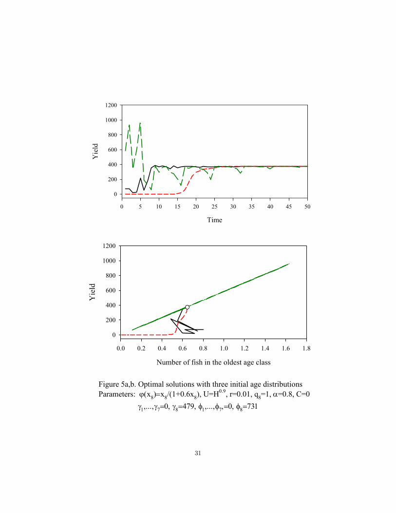
4.3 Numerical examples for populations with any number of age classesProposition 5 shows the local stability properties of the steady state under

low rates of interest. Figure 5a shows the development of three optimal solutionsover time. The solutions differ only because of their different initial age-classstructures. All the solutions converge toward the same equilibrium. Figure5b shows the same solutions in x8,H state space. Both Figures demonstratethe nonmonotonicity of the optimal path. Figure 5b also suggests that theremay be a linear boundary containing the optimal steady state such that theoptimal spawning stock-yield combinations exist below or on this boundary.The solutions exist below the boundary if the number of fish in the age classes1, ..., n − 1 are low, implying that it is optimal to keep the harvest at a lowlevel even if the spawning stock and harvestable age class is near its long runoptimal steady state level. Conversely, if the number of fish in age classess = 1, ..., n− 1 is higher, the optimal yield tends to be an approximately linearfunction of the spawning stock. These solutions reflect the fact that age classess = 1, ..., n−1 contain valuable information on future harvesting possibilities andthat information partly determines the optimal harvest at the present period.

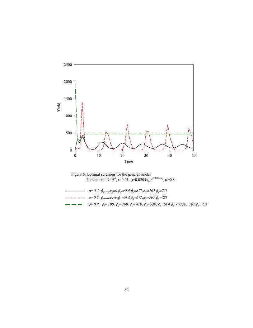
Finally, Figure 6 depicts three optimal solutions for the general modelwithout simplifications. There are eight age classes. The dotted line shows thepulse fishing solution where fishing gear is nonselective and young age classesdo not have commercial value. This outcome is in line with Proposition 4. Ifthe utility function is made more concave, the pulse fishing property becomessomewhat smoother but the solution may still have a limit cycle property (solidline). The solution given by the dashed line shows that the pulse fishing strategycompletely disappears if the young classes are commercially valuable.

20

5 Conclusions

The aim of this paper has been to present analytical results and some nu-merical computation illustrations on optimal harvesting of age-structured fishpopulations. It is shown that the complexity of the multiple age class prob-lem can be reduced by deriving results for model specification with only twoage classes. It may be expected that the results obtained for this simplest caseat least partially carry over to the specifications with higher number of ageclasses.5 The paper takes some steps toward this direction by deriving a steadystate equation and stability analysis for one important special case of the generalmodel. In contrast to some opinions (Wilen 1985, Hilborn and Walters 2001,Clark 1985, 1990, 2006), the age structured model is found to be analyticallytractable.

Some potential extensions are worth noting. The cyclical equilibriumis proved to exist given a zero rate of interest and a recruitment function byBeverton and Holt (1957). Numerical examples suggests that the cyclical equi-librium may be optimal under positive rates of interest and a Richer (1954)recruitment function. Thus, generalizations of the analytical result should bepossible. Given knife-edge selectivity and no harvesting cost, the steady statefor the two age class specification was shown to be a local saddle point indepen-dently of the rate of interest. The analogous result for the any number of ageclasses specification was proved under low rate of interest, but generalizationsshould again be possible. Finally, there should be no obstacles to study theempirically highly relevant case with stochastic recruitment and to derive someanalytical results for the two age classes specification and numerical results formore complex age distributions.

Footnotes:1Wilen (1985) writes: "If we are interested in real-world management prob-

lems, we are inevitably forced to disaggregate and to pick up the more compli-cated features of mixed aged populations. Unfortunately, these appear to bethe most intractable analytically".

2In their extensively used book, Hilborn and Walters (2001) make a sharpdistinction between analytically and numerically solvable models in fishery man-agement. They write that one state variable biomass models are fruitful forelegant analytical solutions but too simple for people working in fisheries man-agement. Models with explicit age structure are considered to be useful forpractical management problems but beyond analytical methods.

3On the use of the Kuhn-Tucker theorem or the Lagrange method for solvingdiscrete time dynamic optimization problems, see e.g. Mercenier and Michel(1994).

4Note that given C = 0, the term −q2α2 cancels out with the direct effectan increase of x2 has on the harvest of x2.

5This is more or less the case in specific class of age structured models inforest economics (cf. Salo and Tahvonen 2002, 2003).

21

Appendix. Proof of Proposition 4.Since q1t = q2t it is possible to take q2t as the optimized variable. Write

q2t = qt for simplicity. The conditions (19)-(21) take the form

αx2t − λ2tα(x1t + x2t) ≤ 0, (A1)

−λ1t + bλ2,t+1α(1− qt+1) ≤ 0, (A2)

b[αqt+1 + λ1,t+1ϕ0(x2,t+1) + λ2,t+1α(1− qt+1)]− λ2t ≤ 0. (A3)

The purpose is to first show that a two period cycle satisfies the necessaryoptimality conditions. For this end set q1 = 0, q2 > 0, x1i, x2i > 0, i = 1, 2(Note that q1 refers to period 1 fishing mortality etc.). This leads to the system

αx2i − λ2iα(x1i + x2i) ≤ 0, i = 1, 2, (A4)

−λ1i + bλ2,i+1α(1− qi+1) = 0, i = 1, 2, (A5)

bαqi+1 + bλ1,i+1ϕ0(x2,i+1) + bλ2,i+1α(1− qi+1)− λ2i = 0, i = 1, 2, (A6)

x1i = ϕ(x2,i+1), i = 1, 2, (A7)

x2i = αx1,i+1 − αx1,i+1qi+1 + αx2,i+1 − αx2,i+1qi+1, i = 1, 2, (A8)

where, due to two period cycle, it is written that q3 = q1, x13 = x11, etc.This is a 10 equations and variables system and the aim is to eliminate allvariables excluding x22 and study the remaining equation (A6) for i = 2.

Eliminating x11, x12, x21 from (A7) and (A8) yields

x22/α− ϕ(x22)− αϕ[x22/α− ϕ(x22)] + x22(1− q) = 0. (A9)

This equation defines q as an decreasing function of x22. Next λ11 and λ12can be eliminated from (A6) using (A5). From (A4) it follows that λ22 =x22/(x21+x22) and λ21 ≥ x21/(x11+x21). After eliminating λ11 from equation(A6) written for i = 1 one obtains an equation for λ21 which can be then beeliminated from (A6) written for i = 2. After these steps equation (A6) for i = 2can be written as

x22ϕ(x21) + x22

½bα(1− q) +

[1− b2α(1− q)ϕ0(x21)][b2αϕ0(x22)− 1]bα

¾+ bαq = 0,

(A10)where x21 = x22/α−ϕ(x22). Since (A9) defines q as a function of x22 equation

(A5) includes x22 as its single variable. The task is to study the existenceand uniqueness of solutions for equation (A10). Under the assumptions ϕ =β1x22/(1 + βx2), β1 = 1, and b = 1 (A10) becomes a fourth order polynomial

P (x22) ≡ β42(α2 − 1)x422 + 4β32(α2 − 1)x322 + β22(6α

2 + 3α− 5)x222+2β2(α

2 + α− 1)x22 + α(2α− 1) = 0. (A11)

22

The assumption that α > 12 implies that α(2α− 1) > 0 and β42(α

2 − 1) < 0.Thus P (0) > 0 and P (x22) → −∞ as x22 → ∞ showing the existence of atleast one positive real root. Note that the coefficients for x422 and x322 are bothnegative. Thus, the sign of the coefficients cannot change three times ruling outthe possibility of three positive real roots (cf. Descartes´ rule of signs). Thisshows that there exists only one positive real root for equation (A11).

The remaining necessary condition that must be satisfied is (A4) writtenfor i = 1, i.e. λ12 ≥ x21/(x11 + x21). When this equation is written for x22 ittakes the form

β32(α−1)x322−β22(α2−3α+2)x222+β2(1−α)(2α−1)x22−α(2α−1) ≤ 0. (A12)This condition is satisfied if the third order polynomial is negative for x22 ≥

0. Since β32(α − 1) < 0 and −α(2α − 1) < 0 the polynomial obtains negativevalues for x22 ≥ 0 or has two positive real roots. Since −β22(α2−3α+2) ≤ 0 for0 ≤ α ≤ 1 the Descartes ´ rule of signs rules out the possibility of two positivereal roots implying that condition (A12) is satisfied. Thus it is shown that thereexists a cyclical stationary solution that satisfies all the KT conditions. Finally,under the assumptions applied above equation (31) yields x2∞ =

√2[√1− α+√

2(α − 1)]/[β2(α + 1)]. In addition: q = (√2α√1− α + α − 1)/[α(α + 1)].

Given α ∈ (1/2, 1), it follows that in addition to equilibrium cycle there existsan unique interior steady state solution for x1, x2 and q.¥

ReferencesBaranov, T.I. 1918. On the question of the biological basis of fisheries, Nauch

Issledov Iktiol. Inst. Izv. I, (1), Moskov, pp. 81-128Beverton, R.J. H. and S.J. Holt. 1957. On the dynamics of exploited fish

populations. Fish Invest. Ser. II, Mar. Fish G.B. Minist. Agric. Fish. Food19: 533pp.Björndal, T., A.-A. Ussif and A.R. Sumaila. 2004. A bioeconomic analy-

sis of the Norwegian spring spawning herring (NSSH) stock. Marine ResourceEconomics 19: 353-365.Brokate, M. 1985. Pontryagin’s principle for control problems in age-dependent

population dynamics, J. Math. Biol. 23: 75-101.Byrd, R.H. and M.E. Hribar and J. Nocedal. 1999, An interior point algo-

rithm for large scale nonlinear programming, SIAM Journal on Optimization 9(4): 877-900.Caswell, H. 2001. Matrix population models. Sinauer Associates, Inc.,

Massachusetts.Clark, C.W. 1990. Mathematical bioeconomics: the optimal management of

renewable resources. Second edition. (First edition 1976.) John Wiley & Sons,Inc. New York.Clark, C.W. 1985.Bioeconomic modelling of fisheries management. New

York. Wiley.

23

Clark, C.W. 2006. The Worldwide Crisis in Fisheries: Economic Models andHuman Behavior. Cambridge Univ. Press, Cambridge, UK.Getz, W.M. and R.G. Haight. 1989. Population harvesting: demographic

models for fish, forest and animal resources. Princeton University Press, N.J.Gordon, H.S. 1954. The economic theory of a common property resource:

the fishery. Journal of Political Economy 62: 124-142.Hannesson, R. 1975. Fishery dynamics: a North Atlantic cod fishery. Cana-

dian Journal of Economics 8: 151-173.Hilborn, R. and C.J. Walters. 2001. Quantitative Fisheries stock assessment:

choice, dynamics and uncertainty. Chapman & Hall, Inc. London.Horwood, J.W. 1987. A calculation of optimal fishing mortalities, J. Cons.

Int. Explor. Mer. 43: 199-208.Horwood, J.W. and P. Whittle. 1986. The optimal harvest from a multi-

cohort stock. IMA Journal of Mathematics Applied in Medicine & Biology 3:143-155.Hritonenko, N. and Y. Yatsenko. 2007. The structure of optimal time- and

age-dependent harvesting in the Lotka-McKendrik population model. Mathe-matical Biosciences 208: 48-62.Leslie, P.H. 1945. On the use of matrices in certain population mathematics,

Biometrica 33: 183-212.Mercenier, J. and P. Michel. 1994. Discrete-time finite horizon approxi-

mations of infinite horizon optimization problems with steady-state invariance,Econometrica 62(3): 635-656.Moxnes, E. 2005. Policy sensitivity analysis. simple versus complex fishery

models. Systems Dynamics Review, 21(2): 123-145.Olson, L. O. and S. Roy. 1996. On Conservation of Renewable Resources

with Stock-Dependent Return and Nonconcave Production, Journal of Eco-nomic Theory, 70 (1): 133-157.Olson, L. O. and S. Roy. 2000. Dynamic Efficiency of Conservation of

Renewable Resources under UncertaintyJournal of Economic Theory, 95(2): 186-214.Plourde, G.C. 1970. A simple model of replenishable resource exploitation,

American Economic Review 60: 518-522.Quinn II, T.J. and R.B. Deriso. 1999. Quantitative fishery dynamics. Ox-

ford University Press, Oxford.Ricker, W.E. 1954. Stock and recruitment.. J. of Fisheries Resource Board

Canada 11: 559-623.Salo, S. and O. Tahvonen. 2002. On equilibrium cycles and normal forests in

optimal harvesting of tree vintages. Journal of Environmental Economics andManagement 44: 1-22.Salo, S. and O. Tahvonen 2003. On the economics of forest vintages. J. of

Economic Dynamics and Control 27: 1411-1435.Spence, M. 1973. Blue whales and applied control theory. Technical Report

No. 108. Stanford University, Institute for Mathematical Studies in the SocialSciences.

24

Stage, J. 2006. Optimal harvesting in an age-class model with age-specificmortalities: an example from Namibian linefishing. Natural Resource Modelling19, 609-631.Steinshamn, S. 1998. Implications of harvesting strategies on population

and profitability in fisheries. Marine Resource Economics 13: 23-36.Sumaila, U.R. 1997. Cooperative and non-cooperative exploitation of the

Arcto_Norwegian cod stock. Environmental and Resource Economics 10: 147-165.Walters, C.J. 1969, A generalized computer simulation model for fish popu-

lation studies. Transactions of the American Fisheries Society 98, 505-512.Walters, C.J. and S.J.D. Martell. 2004. Fisheries ecology and management,

Princeton University Press, Princeton.Walters, C.J. 1986. Adaptive management of renewable resources, Macmil-

lian, New York.Wilen, J.E. 1985. Bioeconomics of renewable resource use, in Handbook of

Natural Resource and Energy Economics, vol.1, A.V. Kneese and J.L. Sweeney(eds.), Elsevier, Amsterdam.

25

Number of age class 1 fish

0 1 2 3 4 5

Num

ber o

f age

cla

ss 2

fish

0

1

2

3

4

5

6

7

Parameter values: r=0.01, U=H0.5, C=0, q1=0,q2=1,α1=α2=0.8,

ϕ(x2)=x2/(1+0.4x2), φ1=0, φ2=3

Figure 1. Stability of interior steady state

26

0.0 0.2 0.4 0.6 0.8 1.0 1.2 1.4 1.6 1.8 2.0 2.2 2.4

x 2

0

1

2

333

34

35

Parameter values: r=0.05, ϕ(x2)=x2/(1+0.4x2), α1=α2=0.8, φ1=0, φ2=1, C=0.

Figure 2a. Local stability of the interior steady state under linear utility

x10 x10

_

x20

x20

_

∞2x

∞1x

2101220 αα /)xx(x −= ∞

x1

27

x1

0.0 0.2 0.4 0.6 0.8 1.0 1.2 1.4 1.6 1.8 2.0 2.2 2.4 2.6 2.8 3.0

x 2

0

1

2

333

34

35

Figure 2b. Examples of solutions that reach the steady state within more than two periods Parameter values: same as in Figure 1a

28

Number of age class 1 fish

0 1 2 3

Num

ber o

f age

cla

ss 2

fish

0

1

2

3

4

5

Time

0 5 10 15 20 25 30

Opt

imal

yie

ld

0.0

0.2

0.4

0.6

0.8

1.0

Figure 3a,b. Optimal cycle and the effect of strictly concave utility functionIn Figure 3a: solid lines U=H, dashed lines U=H0.5

In Figure 3b: solid line U=H, dotted line U=H0.93, dashed line U=H0.5

In Figures 3a-d: ϕ(x2)=x2/(1+0.4x2), α1=α2=0.8

0.0

0.1

0.2

0.3

0.4

0.5

1.20 1.25 1.30 1.35 1.40 1.45 1.50

2.22.4

2.62.8

3.03.2

3.43.6

Effort

x1

x2

Figure 3c. Optimal cycle in effort, x1, x2 state space.

Rate of interest

0.00 0.05 0.10 0.15 0.20 0.25

Num

ber o

f fis

h in

age

cla

ss 2

0.00.51.01.52.02.53.03.5

Lower and higher cycle values for x2Steady state values

Figure 3d. Optimal steady state and cycle values for age class 2 as functions of the rate of interest

29

Rate of interest

0.0 0.1 0.2 0.3 0.4 0.5Num

ber o

f fis

h in

age

cla

ss 2

0.00.51.01.52.02.53.03.5

Biomass modelAge-structured model

Rate of interest

0.0 0.1 0.2 0.3 0.4 0.5 0.6 0.7Num

ber o

f fis

h in

age

cla

ss 2

0.00.51.01.52.02.53.0

Figure 4. Comparision of steady states of the age-structured and the biomass models a) Nonselective gear b) Selective gear

Parameters: ϕ(x2)=x2/(1+0.4x2), α1=α2=0.8, C=0

(a) (b)

30

Number of fish in the oldest age class

0.0 0.2 0.4 0.6 0.8 1.0 1.2 1.4 1.6 1.8

Yie

ld

0

200

400

600

800

1000

1200

Time

0 5 10 15 20 25 30 35 40 45 50

Yie

ld

0

200

400

600

800

1000

1200

Figure 5a,b. Optimal solutions with three initial age distributionsParameters: ϕ(x8)=x8/(1+0.6x8), U=H0.9, r=0.01, q8=1, α=0.8, C=0 γ1,...,γ7=0, γ8=479, φ1,...,φ7,=0, φ8=731

31

0 10 20 30 40 50

Yie

ld

0

500

1000

1500

2000

2500

σ=0.5, φ1,...,φ2=0,φ5=614,φ6=671,φ7=707,φ8=731

σ=0.5, φ1,...,φ2=0,φ5=614,φ6=671,φ7=707,φ8=731 σ=0.9, φ1=100, φ2=260, φ3=410, φ4=530, φ5=614,φ6=671,φ7=707,φ8=731

Figure 6. Optimal solutions for the general model Parameters: U=Hσ, r=0.01, ϕ=0.0205x0te

-0.0024x0t, α=0.8

Time

32