Ethnic and Racial Disparities in Saving Behavior

Mariela Dal Borgo∗

April 15, 2013

Abstract

This study investigates one of the explanations for the ethnic and racial wealth gaps: whether households

with the same income level present differences in saving rates. This question has not been directly addressed

for Hispanics yet, only for African Americans. Using pre-retirement data from the Health and Retirement

Study, I compute saving rates as the ratio of wealth change to income, and distinguish between new flows

of money and capital gains. I find that Mexican as much as African Americans have lower saving rates

than Whites, even after controlling for income and socio-demographic factors. Whereas these differences for

Mexicans are due to lower flows of money into assets, they are explained by lower capital gains for Blacks.

Finally, I explore the role that private transfers play in the accumulation of wealth across races and ethnicities.

Exploiting the panel structure of the data, I estimate models for the decision to save, not on realized transfers,

but on the perceived probabilities of giving/receiving financial help and an inheritance. I find that only the

subjective expectations of leaving an inheritance affect savings negatively for both Mexican Americans and

Whites, so it is unlikely that this accounts for the ethnic gap in wealth accumulation. I conclude that

despite the strong networks that minorities form in their family and community, private transfers within

that network do not seem to play a key role in explaining savings differences.

1 Introduction

Despite their demographic growth in the last decades, Hispanics 1 and Blacks living in the US are particularly

disadvantaged with respect to Whites, not only in terms of income and labor market opportunities, but also in

terms of wealth and readiness for retirement. After the financial crisis of 2007-2008, the wealth gap between

minorities and Whites has climbed to a record level, reaching in 2009 the highest peak of the last 25 years at

least.2 Whereas the consequences of these disparities are well known, their causes and the instruments to reduce

them still need to be better understood.

A natural explanation for wealth disparities across families are differences in income. However, a number

of studies have shown that the Black-White gap persist even within groups with the same permanent income∗Dept. of Economics, University of Warwick. e-mail: M.Dal-Borgo@warwick.ac.uk1In most US surveys Hispanics are considered as an ethnic group, which is a classification determined by culture or origin and

independent of race. Hispanics self-identify mainly as white, mestizo or mulatto descendants, or black. However, most are viewedas of multi-racial origin in the US. In this study I will refer to ‘non-Hispanic Whites’ simply as ‘Whites’ and to ‘non-HispanicBlacks’ as ‘Blacks’.

2“Wealth Gaps Rise to Record Highs Between Whites, Blacks and Hispanics”, Pew Research Center, July 2011.

1

level. This gave rise to a variety of explanations to account for wealth differences that cannot be explained

solely by income (Blau & Graham 1990, Wolff 1992, Oliver & Shapiro 1995, Menchik & Jianakoplos 1997, Hurst

et al. 1998, Barsky et al. 2002, Altonji & Doraszelski 2005). In the case of Hispanics, very few studies address

the issue. Cobb-Clark & Hildebrand (2006) state that most of the ethnic wealth gap stems from differences

in current income levels and background characteristics of households. However, there are reasons to suspect

that Hispanics have different patterns of wealth accumulation than Whites, as the following quotation from The

Wall Street Journal illustrates:

Not only do many Latinos work in low-wage industries, but the idea of accumulating funds for one’s

elder years doesn’t always mesh with a culture that emphasizes individuals taking care of one another.

"Retirement is a foreign concept for many Hispanic workers," [...]. "The focus is on providing for the

extended family, and they expect their family to take care of them when they’re no longer working." ...Even

at the highest income level counted in the Ariel/Hewitt survey—a salary of $120,000 or above—Hispanics

had the least amount saved for retirement: an average of $150,000, compared with $155,000 for African-

Americans, $161,000 for whites and $223,000 for Asians. (Pessin 2011).

According to the standard life-cycle model (Modigliani & Brumberg 1954), one important source of wealth

inequality among households with the same level of income are differences in saving rates.3 Different reasons

were studied in the literature that explains why promoting savings among the poor is seen as a necessary and

fruitful avenue. First, most of the benefits of traditional policies encouraging savings are captured by those

with higher income. Second, this approach seems more promising for economic development and for fighting

against poverty than approaches centered on income. Third, there are certain lumpy investments such as a

house that contribute substantially to increase living standards, but are not affordable to poor people unless

they can accumulate a considerable amount of wealth. Fourth, unexpected events such as a job loss or an illness

require to have accumulated funds to cope with the temporary shock. Fifth, Social Security (S.S.) offers a higher

replacement rate to low-income people and so they may not see the need to save individually for retirement,

which leaves them more vulnerable if the generosity of public funds diminishes. Fifth, the habit of accumulating

a fraction of personal income for the future may help to make people more forward-looking and to extend their

planning horizon. The prevalence of this view has resulted in a shift in the focus of pro-poor policies from

income, education and consumption to tackle directly savings and wealth accumulation.

Despite the evident importance of savings for wealth inequality, the subject has received little attention in the

literature. Most existing studies focus on differences in wealth levels between African Americans and Whites.

Less attention has been paid to the rate of wealth accumulation over time and to the comparison of Hispanics3The other two main sources of inequality beyond income are: i) Inheritances or inter-generational transfers: They may affect

relative wealth positions if Hispanics and Blacks inherit from their parents smaller amounts than Whites. However, Juster et al.(1999) dismiss the importance of bequests since very few American households have received financial inheritances. ii) Ex-postrates of return to capital: The fact that Hispanics and Blacks have a different portfolio composition than Whites (for example, theyare much less likely to hold financial assets) can result in lower ex-post rates of return on their savings. This can also happen ifthere are differences in asset-specific rates of return, i.e. conditional on holding specific assets, minorities face systematically lowerrates of return.

2

and Whites. With the purpose of dealing with these issues, the first goal of this study is to explore whether

there are differences in the savings behavior of Hispanics and Blacks with respect to Whites that could lead

to disparities in wealth.4 In the light of that evidence, my ultimate goal will be to understand the factors

that drive such behavior. Families with lower permanent income have lower saving rates (Dynan et al. 2004).5

So the relevant question is: why could be saving rates lower for minority groups than for Whites, conditional

on income and socio-demographic characteristics? The answer to this question needs to distinguish if savings

differentials arise from active savings decisions made by households or from differences in the evolution of asset

prices.

The hypothesis that I study here is whether lower savings may result from the fact that minorities, and

Mexican Americans in particular, have more extensive family support networks. Strong support networks may

reduce the need of precautionary saving for some individuals, and therefore result in lower accumulated wealth.

Potential transfers to/from family and friends and expected inheritances can affect the individual accumulation

of assets which takes place through an increase in labor supply or a reduction in consumption. Indeed, the

low pension participation rates among Mexican Americans have been attributed to the expectation that when

they get old they will receive support from their children and extended family members (Richman et al. 2012).

Mexican immigrants send significant portions of their salary back to their home countries, which may crowd-out

savings in the US. Remitting funds to help educate children, build homes, and invest in small business is a form

of preserving and strengthening ties abroad6, with the expectation of receiving family support in old age. In

that case, remittances could be viewed as a rational strategy to prepare for retirement and lower savings in the

US would not represent a suboptimal decision.

The contributions of this study are, first, to document the ethnic and racial differences in saving rates. In that

sense, it is close to Gittleman & Wolff (2004) who compare the accumulation patterns of African Americans and

Whites. But I extend their study by incorporating Mexican Americans and Other Hispanics into the analysis,

by including data on S.S. and pensions (the larger component of total wealth that has an equalizing effect),

and by looking at the evolution of savings for a different time period (especially likely to affect capital gains).

Second, this study explores whether the strength of support networks may be affecting the differential saving

patterns by looking at the role of perceived probabilities of transfers and inheritances. This approach, which

has been advocated by Cox & Fafchamps (2008), has not been previously addressed to my knowledge since most

of the data sets only measure actual transfers. McKernan et al. (2011), for example, answer a similar question

but looking at the effect of actual rather than potential transfers. An advantage of the HRS that I can exploit

for this purpose are its direct questions on subjective probabilities. The idea is that what matters for savings

decisions are not realized transfers but the transfers that are expected between family and friends. This may4For the purpose of this analysis, the sample of Hispanics will be split between Mexican Americans and Other Hispanics.5In the simplest version of the life-cycle model savings are proportional to permanent income. However, saving rates are expected

to differ with income in more extended versions of the model that introduce heterogeneity in time preference rates and in interestrates across households, and non-homothetic preferences.

6Amuedo-Dorantes (2006) in “Remittances and their microeconomic impacts: evidence from Latin America” finds that thepercentage of Mexicans reporting that send money back home for asset accumulation purposes is higher than for migrants fromother Latin American countries (48%), where it is more common to remit money for consumption purposes. However, the averagedollar amount remitted home by Mexicans is equal to the average amount remitted home by all the immigrants.

3

have an effect on the precautionary savings of individuals that can rely on external financial help or that are

likely to give that help in case that a particular need arises.

In order to document the differentials in savings rates, I use data from the HRS for the periods 1992-1998

and 1998-2004 and compute total saving rates as the change in wealth divided by income. The choice of years

was based on the availability of S.S. and pension data, which allow me to compare savings rates with and

without those assets. In addition, I distinguish between active savings (exclusive of capital gains) and passive

savings (capital gains or savings due to the change in the price of the asset). By adopting a regression approach,

I find that Mexican Americans have lower saving rates than Whites, even conditioning on income and socio-

demographic factors. What is remarkable is that these differences can be attributed to the direct effects of

accumulation decisions rather than to the effects of asset prices and capital gains. African Americans also

present a gap in unconditional and conditional means and medians. But this is purely reflecting the effect of

lower capital gains during the period considered for the analysis. Including S.S. and pensions, the gap in savings

remains for Mexican American households, but disappears for Black households after controlling for income. I

have not found significant differences in savings between Other Hispanics and Whites.7

The second part of this study evaluates the effect of family transfers and inheritances on the decision to

save. This is done by estimating the effect of subjective probabilities of giving/receiving a transfer and leav-

ing/receiving an inheritance on the decision to save or not rather than on the amount of savings. This requires

to re-estimate the total saving rates for every wave from 1992 to 2008 (excluding S.S. and pensions), and

transform it into an indicator for positive savings. Then I use panel data fixed-effects to see the impact of

"potential" rather than "realized" transfers on savings decisions. The perceived probabilities of transfers may be

endogenous, and so they are instrumented with the lagged subjective probabilities reported, the lagged decision

to give/receive a transfer and household and children income. The results show no effect of financial help on

savings, and the only evidence is for the perceived probability of leaving an inheritance, which is negatively

correlated with savings.

2 Related Literature

The study of the differential in Hispanics and Whites’ saving rates relates to the broad literature on racial and

ethnic inequality. This literature has focused mainly on income; the bulk of studies on wealth differences are

much more recent. Whereas income inequality is a good indicator of discrimination in the labor market, wealth

inequality provides a more complete measure of the relative economic position of minority families. Moreover,

the empirical evidence indicates that the racial gap in wealth is considerably larger than the gap in income.

And among the studies on wealth, most of them seek to explain the gap in wealth levels; just a few look at the

rate of wealth accumulation or savings rate. But only with cross-sectional analysis it is difficult to gain insight

on the causes underlying racial inequalities. By looking at the dynamics of the wealth accumulation process it7Something to consider is that the models of wealth accumulation suffer from higher measurement errors in the dependent

variable and lower explanatory power (as measured by the adjusted R2) than the models in wealth levels. This would require beingmore cautious in the interpretation of their results.

4

is possible to gain a deeper understanding of the reasons behind those wealth disparities.

Most of the initial literature on wealth inequality has focused on the factors that explain the gap between

Black and Whites (see Terrell 1971, Sobol 1979, Blau & Graham 1990, Wolff 1992, Oliver & Shapiro 1995,

Menchik & Jianakoplos 1997, Hurst et al. 1998).8 In their seminal study, Blau & Graham (1990) conduct a

means-coefficient analysis, also known as Blinder-Oaxaca decomposition, that breaks down the differences in

wealth into two components: one explained by differences in household characteristics, such as income, and

another that is unexplained. They find that income is the most important factor to explain wealth differentials.

However, even after accounting for income and other socio-demographic factors, they find that a substantial

portion of the gap remains unexplained. They attempt to resolve the puzzle by evaluating the arguments taken

from the standard life cycle model (Modigliani & Brumberg 1954), which attributes the racial differences in

wealth to: i) inheritances or inter-generational transfers, ii) rates of return, and iii) savings rates. They conclude

that racial differences in inheritances are the most likely of the three to account for most of the wealth gap.

More recent studies, like Altonji & Doraszelski (2005) and Barsky et al. (2002), have risen concerns about

the adequacy of the regression decomposition approach. Barsky et al. (2002) claim that such decompositions

incorrectly assume linearity in the relation between wealth and income. Moreover, the estimates based on such

functional form are used to extrapolate outside the range of the Black income distribution, which is shifted

to the left relative to the White distribution. Thus, they propose a nonparametric method to perform the

decomposition and find that two-thirds of the mean differences in wealth can be attributed to earnings. They

do not consider other factors, but acknowledge that it is fruitful to explore racial differences in preferences

for wealth accumulation as a possible cause of the wealth gap. In comparison with previous studies, Altonji

& Doraszelski (2005) can explain a larger fraction of the racial disparity in wealth holdings with income and

demographic variables, but only if they estimate the wealth model in a sample of Whites. If they use a sample

of Blacks, then they can only explain a small portion. They suggest that this discrepancy in the sensitivity of

wealth holdings to observable characteristics is as important as the differences in income and demographics to

understand the racial wealth gap. They conclude that the discrepancy is not caused by extrapolation out of

sample nor by differences in inter vivos transfers and inheritances, but instead they suspect that it is explained

by differences in savings behavior. This could be the case since, for example, a smaller proportion of Blacks has

access to financial institutions.

Despite the speculations that differences in wealth accumulation can contribute to the racial wealth gap, the

topic has received little attention in the literature. One exception is Gittleman & Wolff (2004), the study more

similar in its approach to this. They divide the change in the value of each asset into capital gains and gross

savings, which are the additional funds invested in that asset. This measure of savings (gross savings minus

inflows from inheritances) is closely related to what in the literature is referred as active savings.9 A wealth8For a survey of the literature on racial differences in wealth see Scholz & Levine (2003).9They point out to difference between their measure of savings and the measure of active savings used by Hurst et al. (1998)

and Juster et al. (1999) among others (including this study). First, Gittleman & Wolff (2004) do not attribute the entire changein net equity of the home (less the value of home improvements) to capital gains. Instead, they divide it into saving (the changein mortgage principal) and capital gains (the change in the value of the house). Second, for assets for which there are not specificquestions about inflows, the active saving approach allocates the entire change in net value to saving. In contrast, Gittleman &Wolff (2004) allocates a fraction to capital gains by applying a rate of return.

5

accounting framework is built to decompose the changes in wealth into savings, capital gains and inheritances or

transfers. They find that racial differences in savings rates are not significant after controlling for income, and

that the rate of return to capital is not greater for Whites than for Blacks, although they acknowledge that the

latter may be period-specific. In counterfactual experiments following Oaxaca & Ransom (1994), they compute

the fraction of the wealth gap that will be reduced if Blacks and Whites had comparable levels of income, had

equalized the unconditional saving rates, had similar portfolio composition, or had inherited similar amounts.

Although the equalization of savings rates would have also increased the wealth ratio, it is remarkable that they

did not find a racial difference in savings behavior after controlling for income.

By the mid-nineties, studies looking at Hispanic wealth were almost nonexistent. Some of the few recent

works that focus on differences in wealth levels are Smith (1995), Even & Macpherson (2003) and Cobb-Clark

& Hildebrand (2006). They reach to different conclusions about the extent to which observable characteristics

are able to explain the ethnic wealth gap. In a multivariate model, Smith (1995) finds that income and, to

a smaller extent, current health are important predictors of racial and ethnic wealth disparities. Even when

a significant amount of the wealth differences can be explained by these and other variables emphasized in

models of asset accumulation, the magnitudes of the differentials remain large. Then he includes pension and

S.S. into his definition of wealth and finds that it has a big impact on reducing racial and ethnic disparities.

This is not surprising, since private pensions and S.S. represent a big fraction of household wealth and S.S.

has an equalizing effect, since it differs very little across race and ethnicity. However, he notes that racial and

ethnic wealth disparities are still larger than what seems justified by differences in permanent income alone,

and concludes that the puzzle of why income minorities save so little remains unresolved.

In contrast, Even & Macpherson (2003) and Cobb-Clark & Hildebrand (2006) arrive to the conclusion that

most of the wealth ethnic gap stems from differences in current income levels and background characteristics

of households, rather than on the way in which households have accumulated wealth in the past (conditional

on their income and characteristics). Even & Macpherson (2003) briefly examine total wealth in multivariate

analysis and find that differences in earnings, education and socio-demographic characteristics account for most

of the racial and ethnic differences in wealth. This result holds independently of whether pension wealth is

included or not in the measure of total wealth (although pension savings do not affect the wealth differentials at

the mean, they do at the lower tail of the distribution since poorer households hold a larger fraction of wealth

in pensions). Cobb-Clark & Hildebrand (2006) analyze the wealth gap using a semi-parametric decomposition

and find that although income differences are important, the main factor explaining the inequality in wealth are

demographic characteristics: Mexican American families have more children and heads that are younger. Low

educational attainment explains part of the wealth gap, even after accounting for differences in income. Note

that the results of these two studies contrast to the explanations given in the literature for the gap in wealth

between Blacks and Whites that originates in the way in which –conditional on their characteristics- wealth is

accumulated.

The ultimate question of whether Hispanics are under-saving for retirement relates to the sizable literature on

the adequacy or optimality of wealth accumulation. A widespread approach followed, for example, by Hubbard

6

et al. (1995) and Engen et al. (1999) is to compare observed behavior against a standard that is obtained

by simulating the expected distribution of wealth from the life cycle model. In the context of that model,

where households are rational optimizers, differences in savings for retirement are attributed to differences in

the rate of time preferences, risk aversion, health status, life expectancy, tastes for goods complementary with

leisure, or Social Security replacement rates. Scholz et al. (2006) use an augmented version of the life cycle

model and find that most HRS households are saving more than their optimal targets, suggesting that they are

financially well-prepared for retirement. Others have assessed savings adequacy by comparing observed data to

financial rules of thumb, for example, Kotlikoff et al. (1982) and Gustman & Steinmeier (1999). And Banks

et al. (1998) and Bernheim et al. (2001) make inferences about the adequacy of retirement savings by looking

at consumption changes before and after retirement. Bernheim et al. (2001) conclude that their findings are

compatible with behavioral theories of wealth accumulation that attribute the differences in wealth accumulation

across households to ‘rule of thumb’, ‘mental accounting’, or ‘hyperbolic discounting’.

Finally, this paper also relates to a growing literature that explores different hypotheses on the differences on

savings and wealth levels across households. Some of these hypotheses attribute differentials in savings and/or

wealth to lifetime income (Dynan et al. 2004), information and learning costs (Lusardi 2005), immigration

condition (Paulson & Singer 2002, Osili & Paulson 2009), cultural effects (Carroll et al. 1994, 1999), and family

size (Banerjee et al. 2010). Dynan et al. (2004) find that high-lifetime income households save a larger fraction

of their income than those who have low-lifetime income. There are psychological and sociological theories that

are consistent with the idea that low-income households save less because they are more impatient, have a higher

SS replacement rate, and have less access to saving vehicles such as private pension plans. They are also more

affected by asset-based, means-tested social insurance programs, which in turn may be distorting their saving

rates. In addition, high information and learning costs can prevent wealth accumulation among minorities.

The hypothesis of cultural effects as an explanation for saving differentials has been proposed by Bosworth

(1993) with the purpose to account for the remarkable differences in savings across countries. The hypothesis

that people from different nationalities have different tastes for savings has been tested by Carroll et al. (1994,

1999) but has not receive empirical support either. Carroll et al. (1994) compares saving patterns of immigrants

to Canada from countries with different saving rates. They find that savings do not vary significantly by place

of origin of the immigrant. Independently of their origin, recent immigrants save less than Canadian-born

people, but with time this difference diminishes. Carroll et al. (1999) answer the same question using data for

the United States, but they do find significant differences on savings across country of origin. In particular,

and consistent with the results found here for Mexican Americans, immigrants from Mexico and Cuba had the

lowest saving rates (along with those from the Philippines and Taiwan). But the immigrants’ saving patterns

do not reflect those observed in aggregate data, i.e. immigrants from countries with high saving rates (such as

Japan, Korea, Taiwan) do not necessarily save more. Thus, they conclude that cultural differences may not be

explaining the differences observed in aggregate data.

Another approach to test the hypothesis on cultural differences is by looking at differences in family support

networks across races and ethnicities, assuming that family support indeed affects savings behavior. In particu-

7

lar, the importance of children and family size in savings decisions has received attention as one explanation for

the fertility transition in the ninetieth and early twentieth century, the process by which Europe and US went

from high to low fertility. The argument is that children are a form of life-cycle savings, where parents invest

on them when they are young and expect to obtain return to child-rearing when they are old (Guinnane 2011).

Children became a less desirable form of savings as a result of the industrialization (the migration from rural

areas to cities resulted in ‘child default’ to their implicit agreement with their parents) and of the introduction

of the social insurance system as means of support in old age (Carter et al. 2004). Also, the demographics

changes in China have converted the country in a unique laboratory to study that hypothesis (Wei & Zhang

2009, Banerjee et al. 2010). Banerjee et al. (2010) note that in China parents depend on children support as

they age, and this dependance is higher from sons than from daughters. They exploit the decline in fertility

from the early 70s caused by family planning programs and corroborates that, as the life-cycle model would

predict, it causes a big increase in household savings driven by parents that have a daughter as a first child.

Beyond those studies looking at the effects of family size, the effects of family support itself in savings behavior

have been recently addressed by McKernan et al. (2011). They find that only large gifts and inheritances matter

to explain the Black-White gap in wealth levels, but there is no role for private transfers in the form of financial

help.

Finally, note that the explanations for differential saving rates across races can also be viewed through the

‘chance’ versus ‘choice’ framework proposed by Venti & Wise (1998). Their purpose is to understand how

much of that wealth dispersion can be attributed to ‘chance’ events, such as inheritances, poor health or other

shocks to wealth, and how much to the conscious ‘choice’ of saving out of available resources. In that context,

Gustman & Steinmeier (2004) estimate a joint structural model of retirement and wealth for groups defined by

race, ethnicity, gender and marital status. They decompose differences in outcomes into those due to differences

in parameters of the preference function and those due to differences in the circumstances (the opportunity set

and factors determining the disutility of work such as health status). What explains the differences in outcomes

among White, Black and Hispanic males are differences in time preferences and in circumstances rather than

preferences for leisure and consumption.

3 Data

In this study I will use data from the Health and Retirement Study (HRS). This choice is based on the

consideration of several advantages that the HRS has over other household surveys collecting wealth data.

First, it provides assets and income data of high quality, with a relatively low rate of item non-response and

abnormally high retention rates compared to other aging studies (Banks et al. 2010). In particular, it provides

the best household survey data available to calculate pension wealth. Since pension wealth is typically the

largest asset on the household balance sheet, its importance for the study of savings is paramount. Second, the

HRS oversamples Blacks and Hispanics at the rate 2:1 relative to Whites, which is extremely helpful for this

8

analysis on racial and ethnic differences.10 Third, this data set collects information on households with at least

one individual over 50 years old, which allows focusing on savings adequacy for retirement. In fact, the HRS is

not appropriate to study savings for the entire age distribution. But the sample selected is the most adequate

for this study because as people get older and approach retirement, they hold more types of assets, own more

wealth and save faster.

Despite these benefits, some data quality issues need to be mentioned (Smith 1995, Venti & Wise 1998). First,

the quality of data on assets and income is lower when they are used in their longitudinal dimension. Indeed,

misreporting of asset balances and the imputation procedures implemented imply that the use of successive

waves of wealth can confound some analyzes. Venti & Wise (1998) points out that “these potential misreports

create ‘spurious’ wave-to-wave changes in assets that are common and typically much larger than ‘legitimate’

wave-to-wave changes.”. Moreover, there is evidence that missing data is not random because those more

reluctant to report are wealthier households (Smith 1995, Banks et al. 2010). In terms of imputation, the

HRS has benefited from the use of bracket questions that allow determining a range in which the values lie

and mitigates the problem of random non-response. However, the imputations of missing values do not rely

on cross-wave information; they only use information from the wave corresponding to the missing data. The

absence of longitudinal imputations also distorts wave-to-wave changes.

Second, Venti & Wise (1998) notes that, even when pension data in the HRS is by far the better collected to

date in a survey; still it suffers from serious measurement errors. These are due mainly to the lack of knowledge

of the respondents about the characteristics of their pension plans. For example, they have trouble classifying

their pension plan as defined-benefit (DB) or defined-contribution (DC). And if they classify their DC pension

plan as DB, then the corresponding balance is zero for that wave. Third, as in most household surveys, the

wealth of very rich families is not accurately captured. It is hard to define the sample frame, and even when

families are interviewed, it could be that they are reluctant to report very large amounts of stock holdings.

Also, it is particularly hard to calculate the net value of certain assets with complex financial structures, such

as business, where the complexity increases with the value of the asset. Unless special sampling frames are

designed to represent high-wealth households, as in the Survey of Consumer Finances (SCF), the full range of

the wealth distribution is not readily captured.

In the light of these issues, income and wealth data are taken from the RAND HRS 2008 Income and Wealth

Imputations11 that deals with missing values by imputing separately each income and wealth component. Unlike

the HRS public release files, the RAND files use an imputation method that is consistent across all waves. In

addition, I follow Smith’s (1995) advice and restrict the analysis to total wealth and a few aggregate wealth

components. He concludes that the more disaggregated the asset, the more cautious a researcher should be

when using the HRS or any household survey. In addition, to deal with the measurement errors, I trim the

sample by excluding households with wealth levels and saving rates at the top and bottom 2 per cent of the10Residents of the State of Florida were the other group oversampled, because it is an area with high density and number of

older populations.11March 2011. See at: http://hrsonline.isr.umich.edu/index.php?p=avail.

9

distribution.12 In this way, I not only get rid of the outliers originated in measurement errors, but also I exclude

the extremely wealthy from the analysis, whose savings behavior is more difficult to model.

The measure of net worth used here includes: i) Real assets: Main home equity, real estate other than home

equity, vehicles and business, and ii) Financial assets: Individual Retirement Accounts (IRAs), stocks, mutual

funds, checking and savings accounts, CDs, savings bonds, treasury bills, bonds, and other assets (money owed

by others, valuable collections, rights in a trust or estate) less other debts (credit card balances, medical debts,

life insurance policy loans, loans from relatives). Note that this measure excludes private pension wealth, social

security wealth, and future earnings. Thus, to account for the latter I use a set of cross-wave data constructed

with information derived from the HRS: the Prospective Social Security Wealth Measures of Pre-Retirees13, the

Imputations for Pension Wealth 1992 and 199814, and the Imputations for Employer-Sponsored Pension Wealth

from Current Jobs in 2004.15

The measure of income corresponds to the last calendar year and is the sum of respondent and spouse earnings,

pensions and annuities, Supplemental Security Income and Social Security disability, Social Security retirement,

unemployment and workers compensation and other government transfers, household capital income, and other

income and lump sums from insurance, pension, and inheritance. To compute saving rates including S.S. and

pensions, it is necessary to adjust the measure of total income and account for employer contributions. Thus,

I adjust total household income by adding the fraction of the respondent and spouse earnings that correspond

to employer contributions to DB and DC plans and to S.S.. This is measured as the cost to employers for DB

and DC plans and for S.S. as percentages of total compensation. The data is taken from the Employer Costs

for Employee Compensation (ECEC), produced by the Bureau of Labor Statistics.

I use household weights for descriptive statistics but not in the regressions. The use of sample weights

in regression analysis is typically required when there is endogenous stratification. In that case, the survey

over-samples a particular population and the oversampling criteria are related to the dependent variable, so the

usual estimators are inconsistent if weights are not used.16 For this study there is purely exogenous stratification

because the HRS stratifies on the regressors only (i.e. race and ethnicity) and not on the savings rate, and so the

usual estimators are still consistent even if the HRS were indirectly oversampling people with low savings. Still

under exogenous stratification one may use weights for a descriptive approach, where the estimated relations

do not necessarily imply causality and attempt to describe characteristics of the whole population and not of

a particular sample. But if one takes a structural or analytical approach, then there is no need to use sample

weights.17

The sample used for this study is restricted to sub-households with the same head and spouse over the

relevant period (1992-1998 or 1998-2004), a common requirement adopted in the literature. By restricting the12This procedure has been applied by Gittleman & Wolff (2004) to the PSID data.13The version 4.0 of the data was prepared by Kandice Kapinos with Charlie Brown, Michael Nolte, Helena Stolyarova,

and David Weir. Survey Research Center, Institute for Social Research, University of Michigan, November 2010. See at:http://hrsonline.isr.umich.edu/index.php?p=avail.

14Final version 2.0, December 2006. See at: http://hrsonline.isr.umich.edu/index.php?p=avail.15Version 1, July 2009. See at: http://hrsonline.isr.umich.edu/index.php?p=avail.16Hill (1992) explains this in the context of the PSID, which over-samples low-income households. Thus, in that case, the

regressions that use income as the dependent variable need to be weighted.17Cameron & Trivedi (2005) gives a good insight into this issue.

10

sample to stable households, one can ensure that wealth changes are not mainly explained by changes in family

composition. I also drop observations for sub-households that were in the sample but were not interviewed in

a particular wave, and for those that have either income or wealth missing. Then I drop households where the

head was below 50 or above 70 years old in 1998 and in 2004 and where the head reports to be retired, where

retirement status is defined through self-reports. Also, I exclude households where the spouses are of a different

race or ethnicity.

3.1 Saving rates

The saving rate is defined as the ratio between savings and the income earned during the relevant period.

The conceptually most appropriate measure of savings is the one obtained as the difference between disposable

personal income and consumer expenditures, where both measures are obtained directly. By defining real income

for household i as the sum of the return on non-human wealth between s − 1 and s (ris−1Wis−1), after-tax

earnings (Eis), and transfers from the government (TRis), household savings can be expressed as:

Yis − Cis = ris−1Wis−1 + Eis + TRis − Cis (1)

where Cis is total consumption and ris−1 is the real after-tax rate of return on non-human wealth between s−1

and s.

However, there are practical difficulties to implement such approach using survey data. In particular, mea-

suring consumption is a very time-consuming process and so it is not typically available in most surveys. The

approach that I will follow here is the one feasible with HRS data and the most commonly adopted in the

empirical literature.18 This consists on computing savings as the difference in net worth between two time

periods (Wis−Wis−1), which is referred as realized savings. Thus, it is straightforward to show the equivalence

of the two definitions of savings if wealth at the end of period s is defined as:

Wis = Wis−1(1 + ris−1) + TRis + Eis − Cis (2)

where Wis−1(1 + ris−1) is net worth (exclusive of human wealth) at the beginning of period s. The equiva-

lence is verified since capital gains are added to income to the extent that they are included in r. The main

disadvantage of this approach is that, as it was explained before, the first difference of wealth will inherit, and

most likely exacerbate, the measurement error that may be already present in the measured net wealth. And

if measurement error is not perfectly correlated across survey waves, changes in wealth will carry significant

amounts of measurement error.

In addition, the HRS allows distinguishing the change in the value of an asset due to: i) ‘active savings’, or

current income that households do not spend but save, and ii) ‘passive savings’, reflecting the change in the price

of the asset or capital gains that household do not realize and spend. The survey contains specific questions

about active savings precisely for those components were capital gains are more important, such as housing,18See Juster et al. (1999) for a detailed description of these approaches.

11

investment in real estate other than the primary residence, business, IRAs, and stocks. For those assets, capital

gains are obtained as a residual –it is the difference between realized and active savings. In the particular case

of housing, active saving is computed as in Juster et al. (2005). For households living in the same house between

two waves, it equals the cost of home improvements plus the change in the mortgage and other home loans if a

family owned a house, and zero otherwise. When a family moves, active saving in housing is computed as the

change in home equity. This implies that when a family does not move the change in house value is imputed to

capital gains. And for families that move between surveys all saving in housing -including the change in house

value- is imputed to active saving.

In addition, note that since both realized and active savings are measured with error, the problem of mea-

surement error becomes even bigger for capital gains, which renders more difficult the estimation of behavioral

functions. Finally, these measures of savings needs to account for net transfers into the households, such as

inheritances and gifts from family and friends, and changes in assets resulting from household members mov-

ing out or into the family. Since the form of these transfers and changes in assets resulting from changes in

family composition is not known, it is not possible to allocate them to particular assets nor to decompose

them between active savings and capital gains. Thus, the net transfers can only be considered when computing

aggregate savings.

Why is it important to distinguish between realized and active savings? Hurst et al. (1998) explain that in

the past the distinction between realized and active savings was not of major importance because the lack of

heterogeneity in savings patterns and the little variability of returns across the population. Since the 1980s

a new view of savings has emerged which acknowledges the existence of liquidity restrictions, the importance

of heterogeneity in savings rates across households, and the dispersion of the ex-post rates of returns. These

factors would contribute to wealth dispersion beyond what is explained by income dispersion. Recent studies

have shown evidence that realized savings –i.e. changes in household wealth-, can differ sharply from active

savings, which exclude capital gains. Eventually, the choice of the most relevant concept of savings depends

on the question of interest. Active savings is more appropriate to analyze the supply of loanable funds for new

investment and therefore is useful to study the effect of a redistribution of income on economic growth (Dynan

et al. 2004). On the other hand, a measure of total savings that includes capital gains is the more appropriate

concept to study the ex-post adequacy of saving for retirement. This is why I will focus in this second measure

when I explore the relations between savings and family transfers.

4 Ethnic Differences in Saving Rates

4.1 Descriptive Analysis

There is a wide gap in wealth levels between Hispanics and Whites, similar to the gap between African Americans

and Whites. This can be seen in Figure 1, where I plot the cumulative distribution of net wealth for each group,

distinguishing between Mexican Americans and the rest of Hispanics. The figure shows that the three minority

12

groups present a cumulative distribution of wealth that looks much more similar than the one corresponding

to Whites. It shows that the median wealth of Mexican Americans of $200 thousand corresponds to the 20th

percentile of the White distribution for 2004. Similarly, the median wealth of Other Hispanics ($163 thousand)

corresponds with approximately the 16th percentile of the White distribution.

Before looking at the patterns of wealth changes, it is useful to have a snapshot of the wealth distribution

by household characteristics at one point in time. In Table 1 I present summary statistics for both mean and

median because of the extreme positive distribution of wealth. Including S.S. and pensions, Mexican Americans

have around half the wealth of Whites, both in terms of mean ($352 vs. $703 thousand) and in terms of median

($243 vs. $569 thousand). A similar gap in means is observed among Other Hispanics (their mean and median

are $398 and $199 thousand respectively). Without retirement assets, the gap widens for Mexican Americans

and their wealth represents only 38% of the White mean and 26% of the median. For Other Hispanics, the

median gap becomes strikingly higher than the mean (8 vs. 63%) reflecting the extreme positive distribution

of wealth for this group when the equalizing effect of S.S. is not accounted for.

As expected, mean and median wealth levels across groups are monotonically increasing with income.19Notice

that the Mexican American wealth gap in means narrows at intermediate income levels, but still it remains at

around 50% at the top and bottom of the income distribution. The gap in medians disappears at the first and

third income quartile, but it remains at the second and fourth. Some of this abrupt changes may be explained

by the small sample size, but still the evidence is consistent with wealth differences at the same income level.

Thus, not all the gap can be attributed to the fact that there is a small portion of Mexican Americans relative

to Whites in the higher income groups. Among Other Hispanics, there is a substantial gap with Whites in mean

and median wealth levels at the lowest income quartile. And there is a jump in their wealth level at the 75th

percentile of income so that they are the more wealthy at higher income levels (their mean wealth is $1,225

thousand, whereas the White wealth is $617 thousand). The Black gap presents less volatility across income

quartiles, possibly due to the higher sample size. It widens at the lowest quantile (in means and medians) and

at the highest income quantile (in medians).

Wealth levels by educational attainment present a similar pattern as income. The wealth gap for Blacks

remains relatively flat across educational levels, it becomes smaller at middle and high levels of education in the

case of Mexican Americans and it declines monotonically with education for Other Hispanics. Wealth levels by

education and income quartiles reveals that the wealth dispersion among Other Hispanics is huge and bigger

than the one observed among other groups. Also notice that Hispanics in general present significant differences

in the wealth gap across educational groups.

Wealth by age of the household head shows that wealth levels are higher for Hispanics aged between 50 and

60 years old than for those aged between 61 and 70. The opposite is true for African Americans and Whites, who

have higher mean and median wealth levels after age 60. As a result, the gap between Hispanics and Whites is

much wider among the older group than among the group below 60. Studies based on more comprehensive data19The exception is the median of Other Hispanics, but the wealth drop observed in the third quartile cannot be considered as

representative of the population due to the small number of observations (five) in that category.

13

sets have shown that wealth accumulation peak in the 45-54 age interval and then experiences a decline, which

is consistent with the prediction of the life-cycle model where individuals save during working years and dissave

during retirement. Since I restrict the sample to non-retired individuals, the observed pattern may reflect the

fact that Hispanics still working at the age of 60 or older do not have the option to retire either because they

have not considered it at all or because they lack the necessary savings to leave the labor market. In contrast,

Whites and Blacks that retire late (that is, after 70) do so as a result of a better-planned strategy and since they

remain in the labor market for longer have more time to accumulate assets. See Appendix C for a discussion of

how self-selection into retirement may affect this sample.

Table 1 also shows that, across all ethnic and racial groups, households where the head is married hold higher

levels of wealth than those where the head is single. But there is not a big difference between the wealth of

Mexican Americans that were born in the US and the one of those born abroad. Among the latter, there is a

small difference depending on the years spent in US since immigration; indeed, early immigrants have slightly

higher mean and median wealth than more recent immigrants. Other Hispanics that were born abroad are

poorer than those who are second or third generation. And among foreign born, the wealth of early immigrants

is higher in means but lower in medians.

Not only there are differences in wealth levels between Whites and minority groups, but also there are wide

disparities in the types of assets where the wealth is invested. This can be seen in Figures 2 and 3, which show

the net wealth composition by ethnicity and race, both in terms of access to individual assets and in terms

of the importance that each asset has in total wealth. The fraction of Mexican Americans that own a house

in 2004 is relatively high (77%), just a bit smaller than the fraction of Whites (86%). But home equity has a

slightly bigger share in Mexicans’ portfolio (19%) than in Whites’ portfolio (18%). The reason is that, even

when a higher fraction of Whites have houses and their houses may have a higher market value, Whites also

have a much more diversified portfolio. Other Hispanics and African Americans have less access to home equity

than Whites and on average it represents a smaller fraction of their total wealth (13 and 12% respectively).

The remaining real assets (other real estate, vehicles and business) have a smaller participation in household

wealth across all groups. What it is remarkable is that, as in the case of the main home, having a vehicle seems

to have much more importance among Mexican Americans than among Other Hispanics and Blacks, since about

80% have at least one (just 10 p.p. less than the proportion of Whites).

Whereas almost all Whites hold financial assets of some form, the proportion of Hispanics with such assets is

much lower (63% Mexican Americans and 71% Other Hispanics), and even lower than the proportion of Blacks

(82%). Moreover, most of the financial wealth held by Hispanics consists on checking and savings accounts,

since very few have stocks, bonds and other savings accounts such as IRAs or Keoghs. Conditional on having

some type of financial asset, its value represent a very small fraction of Hispanics’ total wealth (around 4%),

which is a third of the fraction for Whites.

The smallest gap in wealth holdings is found in Social Security. Around 90% of Mexicans and Whites

and 80% of Other Hispanics and Blacks have S.S. in 2004. But S.S. represents a much higher fraction of total

wealth for Hispanics (57%) and Blacks (55%) than for Whites (42%). The explanation has to do with the lack of

14

diversification of the minorities’ portfolio, since their wealth is concentrated in very few assets. Also, this clearly

puts in evidence their dependence on S.S. to complement their savings. For all groups, private pensions are less

widespread than S.S. Only around 57% of the Whites and between 25 and 31% of the Hispanics have a pension.

Its share in total wealth is similar across groups, oscillating between 24 and 30%. Also, in a decomposition not

shown here, I observe that there is not a big difference in access across groups to defined benefit and defined

contribution plans. However, the former still represents a higher share of total wealth for every racial and ethnic

group, despite the movement in last years from defined benefit to defined contribution pension schemes.

I can now turn to look at the wealth changes over time. Table 2 presents a summary of the income and wealth

levels, both at the beginning and at the end of each period for which the saving rates were computed (excluding

S.S. and pensions). Between 1992 and 1998 the mean wealth of Hispanics declined, whereas the mean wealth

of Blacks and Whites experienced an increase. In the same period, the mean income of Other Hispanics (and

Blacks), but not of Mexican Americans nor Whites, has also declined. In the following 6-year period, there was

an increase in mean wealth and income levels across all ethnic and racial groups, but they were particularly

large for Other Hispanics. Table 2 also shows that the wider gaps between Hispanics and Whites are generally

in the lower percentile of the wealth and income distribution. The gaps tend to narrow when measured for the

highest percentile and for the mean levels of both distributions. And finally, this Table confirms that wealth

dispersion seems to be bigger among Other Hispanics. Indeed, the ratio of 25th wealth percentile over the 50th

percentile is the lowest among all groups, similar only to the one of African Americans. But the ratio of 75th

wealth percentile over the 50th percentile is the highest across all races.

In Table 3 one can compare the unconditional saving rates of both Hispanics groups and of African Americans

with those of Whites. Following the standard practice, mean rates were computed as the ratio between average

savings and average income accumulated over each six-year period. In turn, the saving rates at the 25th, 50th

and 75th percentile are computed for the ratio of savings over income. In 1992-1998, total saving rates were

smaller for Hispanics than for Whites and the differences were in general significant (except for the mean saving

rate of Other Hispanics). When S.S. and pensions are included in the measure of wealth, the Hispanics’ rates

remain smaller and the differences are significant for Mexican Americans and for Other Hispanics only at the

median and the 75th percentile. In 1998-2004, total saving rates increased for all the groups. Simultaneously,

the differences in savings between Whites and Mexican Americans became insignificant except at the median.

Note that after accounting for S.S. and pensions, the gap in total saving rates disappears for Other Hispanics

in this second period and shrinks considerably for Mexican Americans.

To determine whether these differences in total savings are due to money invested into new assets or purely

reflects the effects of asset prices and capital gains, we turn to look at the active and passive saving rates. In

1992-1998 and 1998-2004, the active saving rates of Mexican Americans are negative at the mean (-0.3 and

-5% respectively) and zero at the median, whereas for Whites they are positive and between 3 and 5%. Thus,

the hypothesis that Mexican Americans and Whites have the same active saving rates can be rejected at the

mean and at the median in 1992-1998. For Other Hispanics, it can only be rejected at the median, since their

active saving rate is positive at the mean (4%). In 1998-2004, the difference between Hispanics and Whites is

15

significant at the three percentiles but not at the mean.

Passive savings were significantly smaller for Hispanics than for Whites in 1992-1998, which is expected given

their portfolio choices. But this is no longer true in 1998-2004, when some of the Hispanic rates became actually

higher. Passive savings in the second period may have responded to the evolution of the houses and stock prices.

The sharp increase in housing prices that started in the mid-90s and lasted until their collapse in 2007 has been

steepest in California, Arizona, Nevada and Florida, where there is a higher proportion of Hispanics. Similarly,

the fall in stock prices from 2000 to 2002 would have contributed to deteriorate the passive saving rates of

Whites versus Hispanics since the former have a higher fraction of their wealth in stocks.

For comparison, note that African Americans have smaller saving rates than Whites in both periods, both

including and excluding S.S. and pensions, but the differences are significant mainly at the median and at the

upper quartile of the savings distribution. The same remains true for active and passive saving rates. Note that

the latter are still smaller than those of Whites in the second period, perhaps because Blacks were not affected

by the evolution of the housing market prices as much as Hispanics. Also, this result differs from the findings

in Gittleman & Wolff (2004), who compute higher average rates of return to capital for African Americans

than for Whites during 1984-1994. They attribute this to the path of prices for individual asset categories and

acknowledge that must be period specific.

In order to gain a deeper understanding of the patterns observed at the aggregate level, Table 4 shows a

breakdown of total saving rates by type of asset. Total savings are decomposed into real assets (main home

equity, real estate, vehicles and business), financial assets (IRA/Keogh accounts, stocks, checking and saving

accounts, CDs, government bonds, Treasury bills, bonds, and other savings minus debt), Social Security and

private pensions (defined benefit and defined contribution/combination plans).

Hispanics save less in real assets than Whites in 1992-1998 but slightly more in 1998-2004, at least in means.

As it was explained before, the pattern in the second period is due to Hispanics living in areas where the

boom in house prices was more pronounced. As expected, given minorities’ limited access to financial markets,

saving rates on financial assets are smaller for Hispanics and Blacks than for Whites, both in means and in

medians, and this difference is in general significant. The mean rates of saving in Social Security are in general

modest for all the races and smaller than the median rates due to the importance of the lower tail of the

distribution. The slightly negative rates observed in 1992-1998 may partly reflect measurement errors derived

from the imputations for respondents that could not be matched to S.S. earnings data. Indeed, in my sample, a

higher fraction of imputations are observed among changes in S.S. that are negative than among changes that

are positive. Finally, saving rates on pensions do not seem significantly smaller for Hispanics than for Whites.

In the next section I will turn to multivariate analysis to see if the differences in saving rates noted above

remain after controlling for income and other household characteristics.

16

4.2 Multivariate Analysis

Saving rates depend upon differences in lifetime income. But even among those households with the same

income, saving rates may vary due to differences in risk aversion, rates of time preference, or liquidity constraints.

Thus, to examine ethnic and racial differences in savings in the pre-retirement HRS sample, the regression that

I estimate is:

Saving Ratei = β0 + β1(Mexican American)i + β2(Other Hispanic)i + β3(African American)i (3)

+γIncomei+δXi+εi,

where Mexican Americani, Other Hispanici and African Americani are indicator variables denoting the eth-

nicity or race of the household head; Incomei is the household’s total income; and Xi is a vector of demographic

controls. This vector includes age, a quadratic in the age of the household head, the number of children in

the household, dummies for the head’s educational attainment, marital status and birthplace (U.S. or foreign

born), and region dummies.

An advantage of the HRS is that it provides very good measures of household income for multiple years, and

this allows me to control for the average of total family income from the survey years 1994, 1996 and 1998 for

the saving rate in 1992-1998 and from years 2000, 2002 and 2004 for the saving rate in 1998-2004. The main

concern here is that a spurious negative correlation between saving rates and income may arise if measured

income differs from lifetime income since income also enters as a denominator in the saving rate. This could

be the case if measured income contains transitory components and suffers from measurement error. However,

Dynan et al. (2004) has found in a model similar to this that a simple average of current income eliminates

much of the transitory effects of income and thus could be a good proxy for permanent income. They come to

this conclusion by adopting an IV approach consisting on instrumenting measured, current income with proxies

for permanent income (these instruments are expected to be highly correlated with the permanent component

of current income, but not with its transitory component and the measurement error). Using consumption,

future and lagged earnings and education as instruments they find similar results to those obtained without

instrumenting, the approach adopted here.

The estimation of equation (3) presents a particular challenge derived from the skewness of the distribution

of the saving rates. I deal with this issue in two ways. First, I will trim the outliers observations for the OLS

regressions in order to obtain estimates of the ethnic and racial differences at the means.20 Second, I also

estimate the same specifications using quantile regressions that are less sensitive to the presence of outliers

and can be used on the full samples, without trimmings. They allow to estimate differences in savings at the

medians rather than at the means.20I decided to trim (remove outlier values) rather than winsorize the data (convert the outlier values to the closer data point that

is not an outlier) since the latter puts more weight on the extremes of the distribution. As a consequence, it amplifies the influenceof the values in the tails, and thus, it is a more adequate approach when the data is normally distributed. Since both wealth levelsand saving rates have highly skewed distributions with long tails, I opted for trimming the outliers.

17

For the OLS regressions, I estimate the standard errors using clusters at the family level. In the Appendix

Table A1 I check the robustness of the standard errors to different correction methods. I compare the clustered

standard errors estimated in an OLS model with those obtained from a non-clustered OLS model to gain further

evidence that the clustered and non-clustered estimates are not substantially different. The same is done for

the median regressions, by comparing the conventional with the bootstrapped standard errors.

The first set of results are presented in Table 5, which summarizes the determinants of total savings rates,

including S.S. and pensions. The reported coefficients indicate the difference of each group saving rate with the

one of Whites. Before and after controlling for income the differences between Mexican Americans and Whites

are significantly negative, both in means and in medians. More precisely, Mexican Americans save 11 p.p. less

than Whites on average, and conditioning on income only they save 7.5 p.p. less. In medians the difference is

of 9.4 p.p. for the basic model, and it shrinks to 5.5 p.p. in the model controlling for income. Significant results

are still obtained when additional controls are included such as age of the household head, education, marital

status, birthplace, number of children and region of residence. When these regressions are estimated for the two

periods separately (results not shown here), it becomes evident that this difference arises from lower savings

rates in the first period. Similar results are obtained for African Americans, although the size of the gap with

Whites is smaller and it disappeared after including additional controls. For Other Hispanics the differences in

saving rates are not significant.

Table 6 shows the same regressions as Table 5 but the measures of savings rates exclude S.S. and pensions.

In all specifications, the difference between the savings rates of Mexican Americans and Whites are negative

and significant (Mexican Americans save between 2.9 and 8.2 p.p. less than Whites, depending on the model).

Excluding retirement assets, Blacks also show a negative gap with Whites after controlling for income and

demographic characteristics. Note that even the magnitude of the Black-White gap is close to the one between

Mexican Americans and Whites. Other Hispanics present lower savings than Whites, but the differences are

typically not significant.

In order to understand what is driving the saving differentials with Whites, it is useful to look at the

conditional saving rates decomposed into their active and passive components. Table 7 presents the results for

active saving rates. The models pooling both periods show in general a significant difference in the active saving

rates of Mexican Americans and Whites (7 - 10 p.p. at the mean and 4 p.p. at the median, although the latter is

not significant when income and the full set of controls is included). Other Hispanics do not present significant

differences in active savings. However, if they are estimated for 1992-98 and 1998-2004 separately, one can see

that is the consequence that their lower active savings in the first period, were compensated by higher saving in

the second. On the other hand, African Americans do not present substantial differences in active savings rates

with Whites, except at the mean when no controls are included. This is consistent with Gittleman and Wolff’s

(2004) results, who only find a gap for African Americans before controlling for income. Table 8 closes the story

since it shows that the unconditional differences in passive saving rates are significant in general for the three

groups. However, after adding income and the full set of controls, they become insignificant for Hispanics (in

mean and in medians) and for Blacks (in medians).

18

Finally, we can analyze if the gap in total savings is due to lower accumulation in real assets such as

home equity or in financial assets. The results from the Appendix Table A2 indicate that Mexican Americans

present a lower rate of accumulation in real assets than Whites, although the results are not always significant

after controlling for income and other background characteristics. The same is true for savings in financial

assets (conditioning on income, the difference with Whites is significant for the OLS regressions only). African

Americans have lower savings in real assets (even with the full set of controls) and in financial assets (but not

at the median conditional on income). Since housing has a relatively large share in the portfolio of Mexican and

African Americans (see Figure 3), much larger than the share of financial assets, the dynamics of the former

may be driving the aggregate saving rates (excluding S.S. and pensions). If these results were breakdown for

each period, one can see that the bigger gap in savings in both types of assets are mainly in 1992-1998. Between

1998 and 2004, the gaps have closed since the housing boom has favored the accumulation of real assets among

Hispanics and the fall in stock prices has been more detrimental for Whites’ savings.

In conclusion, what explains lower total saving rates among Mexican Americans (excluding savings in re-

tirement assets) are the decisions to invest money into a new asset rather than purely differentials in capital

gains on assets that they already hold. The opposite argument is true for African Americans: their gap in

total savings (excluding S.S. and pensions) can be attributed mainly to lower capital gains rather than to active

savings. This means that the gap in savings for Mexican Americans results from the decision to consume more

out of income than Whites, whereas the gap for Blacks results from the path of prices followed by the assets in

which they choose to save.

4.3 Oaxaca-Blinder decomposition

Using the Oaxaca-Blinder decomposition one can divide the wealth/saving differential between two groups: a

part that is explained by group differences in observable characteristics, and an unexplained residual resulting

from discrimination or differences in unobserved predictors. Also, I can use this framework to look at the

individual contributions of the single predictors or set of predictors to both the explained and unexplained part

of the differential.

The decomposition output in Appendix Table A3 reports the difference in the mean wealth and saving rate

of Whites minus the ones of Mexican Americans in the first two columns. The wealth gap is USD217 thousands

and the gap in saving rates is 8 p.p.. Differences in characteristics ("endowments") between the two groups

account for 63% of the wealth gap and 30% of the savings gap. The remaining unexplained fraction is usually

attributed to discrimination but also captures the potential effects of differences in unobservable variables. Also

the detailed contributions of the single predictors were included for the explained gap (the total component is

the sum over the individual contributions). I find that income makes the higher contribution to explain the

wealth gap (39%), followed by education (21%) and health (6%). Demographic characteristics (age, age-squared,

number of children, marital status, birthplace) and region of residence do not seem to matter. In the case of

the savings gap, differences in income and health account for about 17% and 21% respectively of the explained

19

part of the savings differences. These results contrast with those of Cobb-Clark & Hildebrand (2006), who

use a semi-parametric decomposition and find that only around 11-12% of the median (rather than mean) gap

remains unexplained. They use a similar set of regressors except that they don’t include health.

The last two columns in Table A3 show that the gap in levels and in rates is similar for African Americans

(USD233 and 8 p.p. respectively) than for Mexicans. Also, a similar fraction (59%) of the wealth gap in levels

but a higher fraction (50%) of the gap in saving rates are explained by differences in characteristics. In that

case, all single predictors matter to explain the gap in wealth, but still income and education are the more

important, while the latter also matters to explain the gap in savings.

The Oaxaca-Blinder decomposition provides support to the hypothesis that a considerable fraction of the

Mexican-White and Black-White gaps in wealth levels cannot be explained by income and other observable

characteristics. Given the evidence from the regression approach that saving rates differ across ethnic and racial

groups, it is natural to suspect that the saving patterns affect the gap in wealth levels. Thus, understanding the

causes of such differences in savings becomes crucial to uncover the ultimate causes of the wealth gap. However,

they have received little attention in the literature and so this is the aim of the analysis in the next section.

5 Determinants of the savings differentials

5.1 Inter vivos transfers and inheritances

The results from Section 4 show that total saving rates are lower for Mexican and African Americans than for

Whites, even conditioning on income and socio-demographic factors. In this section I will consider whether

the beliefs that people held about the probability of giving/receiving financial help and of leaving/receiving

inheritances have any influence on their saving decisions. A priori, one would believe that this factor may be

more relevant to explain the lower saving rates of Mexican Americans than those of Blacks, since family transfers

may have a more direct effect on active savings than in capital gains. In addition, Hispanics are traditionally

believed to have strong family ties, and so financial support within that network, including remittances sent

back home, is a plausible candidate to affect their decisions to hold assets in the US.

Cox & Fafchamps (2008) claim that what determines whether the transfer motive is "operative" are not

realized but potential transfers. The mere expectation of receiving financial support from family and friends in

case of an emergency can crowd-out the accumulation of assets by the household, even if this emergency never

occurs and the transfer doesn’t take place. If minority groups have stronger family networks than Whites, the

potential transfers within that network may affect their need of precautionary savings and result in a different

pattern of wealth accumulation. The HRS allows to measure these operative transfers by asking not only about

the amount of actual transfers but also about the subjective expectations of private transfers. The subjective

expectations are given by responses to the question: "(Using a number from 0-100) What are the chances

that you (and your) (husband\wife\partner) will give financial help totaling $5,000 or more to grown children,

relatives or friends over the next ten years?" (the questions for transfers received and inheritances are phrased

20

in a similar way).

Family support networks can affect wealth accumulation in different directions. First, one would expect

that transfers received from children, relatives or friends have a positive effect on savings if they are added

immediately to wealth. Alternatively, transfers from children to parents can be used to finance consumption

in the event of unexpected needs (e.g. a negative health shock that increases medical expenses or a job loss

that results in a drop in labor earnings). In this case, the most likely to arise among older respondents, the

receipt of transfers will not affect savings. On the other hand, transfers potentially received are likely to act as

precautionary savings and, thus, may have a negative effect in current savings. If families know they can rely

on private transfers to finance their unexpected needs, their savings will be lower on average. The same effects

on savings are likely to arise when distinguishing between actual and potential inheritances received.

Second, transfers given to grown children, relatives or friends can have a negative effect on savings if they

are directly taken out of current savings. However, if such transfers are financed by reducing consumption, then

household’s savings won’t be affected. In contrast, the mere expectation of giving such transfers can have a

positive effect on current savings if parents decide to accumulate more wealth to give such transfers when the

needs arise. For example, parents can save to give financial support to grown children for the down payment

of a house. The same reasoning apply when analyzing the effects of actually leaving an inheritance (sometimes

called a ’gift’ if the person is alive) versus the mere expectation of doing so in the future. The expectation to

leave an inheritance may be a proxy for the desire or importance conferred to bequests and thus may have a

positive effect on savings.

Ultimately, the answer on the effect of realized and potential transfers on savings is an empirical one. To

tackle this question, I re-estimate the saving rates, excluding S.S. and pensions, for each single wave of the HRS.

I use data from wave 1 to wave 9, i.e. from survey years 1992 to 1998. I apply the same sample restrictions

that were described in section 3, the only difference is that now I keep stable households over two years only (at

least) rather than over six years as for the estimates in the previous sections. This results in an increase of the

sample size so that after applying all the restrictions leaves 25,820 households, of which 6 percent are Mexican

Americans, 4 percent are Other Hispanics, 19 percent are Blacks and the remaining 72 percent are Whites.

In Table 9 I summarize the extent of private transfers (both financial help21 and inheritances), by ethnic

and racial group. Financial help from older to younger generations seems to be more prevalent among Whites

than among minority groups ((46 percent of Whites give transfers to children, relatives or friends, versus only

26 of Mexican Americans). But conditional on giving a transfer, Other Hispanics and Blacks give more support

to their children than Whites, whereas the gap still remains for Mexican Americans, who give about half the

amount given by Whites. The reported perceived probability of giving a transfer somewhat replicates the actual

pattern of transfers, since Whites (41 percent) believe on average that their probability of giving a transfer is

higher than the one reported by Mexican Americans (21 percent), Other Hispanics (26 percent), and African

Americans (25 percent). The opposite pattern is observed when looking at transfers received. In that case,21The measure of financial help from the HRS captures giving money, helping pay bills, or covering specific types of costs such as

those for medical care or insurance, schooling, down payment for a home, rent, etc. The financial help can be considered support,a gift or a loan and excludes inheritances, shared housing and shared food.

21

financial help from younger to older generations is more likely to occur among minorities than among Whites.

But conditional on receiving a transfer, my sample does not show substantial differences in the actual amounts

received. The mean perceived probabilities of receiving financial support also reproduce this pattern, although

the gap with Whites is slightly smaller than the one observed in the actual figures (Mexican Americans report

almost the same expectations as Whites).

While the data on actual inheritances left is not available, the HRS also asks about the perceived probability

of such transfer. There is a widespread belief among Whites (74 percent) of leaving a bequest of at least $10,000

over the next 10 years, whereas the probabilities reported by the other groups are smaller and between 40 and

50 percent. This may be reflecting the differences in wealth holdings that make inheritances less affordable

for minorities. Also note the relatively low standard errors, which make these figures the more reliable of

all the measures of subjective probabilities included in Table 9.22 In contrast, receiving an inheritance is a

very infrequent event in this sample, since only 6 percent of Whites and less than one percent of the other

groups report having received one. Conditional on having received an inheritance, the differences in the actual

amounts are not so striking. The higher conditional mean of Other Hispanics, probably reflects the highly

skewed distribution of wealth for this group. Finally, the perceived probability of receiving an inheritance is 28

percent for Whites and less than 10 percent for the other three groups. Also the amount expected, conditioning

on attaching a positive probability to receive an inheritance, is larger for the former.

In Tables 10 and 11 a multivariate framework is used to look at the ethnic differences in actual and potential

transfers, after controlling for income and some other background characteristics. Column 1 in Table 10 shows

the marginal effects estimated from a Probit model for the decision of whether to give a transfer, column 2

corresponds to the marginal effects from a Tobit model for the actual amounts given (this model allows to

account for the large proportion reporting zero transfers) and column 3 shows the Probit marginal effects for

the perceived probabilities of transfers. The dependent variable for column 3 is constructed as a binary indicator

that takes value one if the reported probability (in increments of 10) is larger than 50 percent. Columns 4,

5 and 6 estimates the same models for transfers received. The first thee columns reveal that Hispanics are

less likely than Whites of giving a transfer of $5,000 or more over the next 10 years to children, relatives or

friends, even conditioning on income and demographic characteristics. And among those who give transfers, the

amounts are smaller for Mexican Americans, who give on average $105 thousands less than Whites. Consistent

with that, Hispanics and Blacks hold lower perceived probabilities than Whites of giving a transfer. Also note

that households with a head born in US (not shown here) are significantly less likely to give transfers. This

may be due to the larger remittances sent by foreign born families that keep social ties in their place of birth.

Columns 4 to 6 show that Mexican and African Americans are slightly more likely to receive a transfer than

Whites, although this transfers are smaller for Blacks than for Whites. Other Hispanics and Blacks think that

their likelihood of receiving transfers is higher.22In general, the standard deviations of the perceived probabilities of giving a transfer, either financial help or an inheritance, are

smaller than those corresponding to receiving a transfer. This makes the analysis more reliable for the former than for the latter.In addition, there is evidence that people are likely to under-report actual transfers received because they weight them less thanthe actual transfers given.

22

Table 11 summarizes similar information for inheritances. Other Hispanics and Blacks believe that they are

less likely to leave an inheritance over the period considered. Scholz & Levine (2003) argue that this gap does

not indicate that Whites place a higher importance on leaving a bequest but the fact that they find bequests

more affordable. The three groups are also significantly less likely of receiving an inheritance. But conditional on

receiving an inheritance, Other Hispanics receive substantially more. Similar results (not shown in this Table)

were obtained for retired individuals, but for them the ethnic and racial gaps in transfers and inheritances

received are much larger. In general, the ethnic and racial gaps summarized in Tables 10 and 11 reveal some

consistency between actual and subjective probabilities.

5.2 The effect of transfers and inheritances on savings

Given the significant differences in perceptions about the probability of private transfers and inheritances across

ethnic and racial groups, it is natural to ask next whether they have any influence on households’ savings

decisions. I will tackle this question by estimating a model for the whole sample and each ethnic and racial

group, with the following specification:

Si,t = β0 + β1ExpWki,t−1+β5Xit + αi + ui,t for k = 1, 2, 3, 4 (4)

where the dependent variable is an indicator that take value one if the saving rate of family i between years

t − 1 and t is positive and zero otherwise23; ExpWki,t−1 is the perceived probability of: 1) giving a transfer of

$5,000 or more to grown children, relatives or friends; 2) receiving a transfer of $5,000 or more from children,

relatives or friends; 3) leaving an inheritance of $10,000 or more and 4) receiving any inheritance. All subjective

probabilities corresponds to the reports of family i at time t − 1 for the next 10 years (recoded as a binary

variable, as explained in the previous section). Xi,t represents observed household characteristics at time t

that may affect the preferences for savings (permanent income and its square, age and its square, number

of children, education, whether the household head is married, year and region dummies).24 The term αi

captures the family-level fixed-effects that account for the correlation between the regressors and time-invariant

characteristics.

In the fixed-effects model, the regressors can be correlated with the time-invariant component of the error

(αi) but not with the idiosyncratic error ui,t. If the latter is not correlated with beliefs about the probability of

transfers and inheritances and with the other time-varying controls, then the estimated coefficients will capture

the causal effects of potential transfers on savings. Table 12 presents the results of estimating equation 4 for

the whole sample and for each ethnic and racial group separately using a fixed-effects model. The estimates

imply that a high perceived probability of leaving an inheritance would reduce the probability of saving over

the next two years for the whole sample (5.4 percent), Mexican Americans (8.9) and Whites (6.2). One would

have expected a positive coefficient if the desire to leave a bequest encourages savings. The negative coefficient23For this model specification, the use of a binary indicator as the dependent variable renders more reasonable estimates than

the amount of savings.24Note that some of these variables such as education or the dummy for marital status do present some within variation, and for

this reason they were kept as controls in the FE model.

23

can result if the opposite is true: knowing that they can afford to leave an inheritance of $10,000 or more during

the next 10 years, individuals may prefer to start consuming more of their current income and reduce or even

stop the accumulation of assets. On the other hand, the table shows no effect of holding a higher belief about

the probability of receiving an inheritance on savings.

The coefficients for the perceived probabilities of giving and receiving a transfers are significant for the whole

sample, but have the opposite sign as the ones conjectured in the previous section. The assumption that the

perceived probabilities are uncorrelated with the time-varying component of the error is more reasonable in

the case of inheritances, but less likely for inter vivos transfers that tend to be affected by changes in current

economic conditions. If that assumption does not hold, then the FE estimation becomes inconsistent and one

needs to instrument for perceived probabilities of giving and receiving a transfer. Following the perceptions-

based literature, I will choose the instruments based on the factors that influence individual perceptions about

the probability of private transfers (Lochner 2007).25 One can presume that individuals with strong family

support networks hold beliefs about the probability of giving/receiving financial help, which influence their

decision to save. Household income and whether the household gives/receives transfers affect their subjective

expectations about the probability of giving/receiving transfers in the future. Beliefs may also respond to

expected income of the recipients/givers, i.e., of children, relatives and friends. More formally, a simple rule for

updating beliefs about the probability of giving a transfer can be formulated as:

E(π/Hi,t) = f(E(π/Hi,t−1), Ii,t, Ij,t, TGi,t, Zj,t) (5)

where information is accumulated according to Hi,t = (Hi,t−1, Ii,t, Ij,t, TGi,t, Zi,t), and depends on the giver

and recipient households’ income between t− 1 and t (Ii,t and Ij,t), on the decision to give a transfer between

t − 1 and t (TGi,t), and on any new information about the economic conditions of the giver and recipient

families (Zi,t) (for example, whether the household head gets married, whether the family moves to a new state,

whether a child died, etc.). I will make the following assumptions on the updating equation: i) The current

perceived probability of giving a transfer should be increasing in the previous expected probability (f1 ≥ 0);

ii) The expected probability of giving a transfer should be increasing in household income and decreasing in

recipient’s income (f2 ≥ 0 and f3 ≤ 0); iii) The effect of having given a transfer in the past should increase the

subjective probability of giving a transfer in the future (f4 ≥ 0).

Based on equation (5) that captures the relation between subjective probabilities of giving a transfer,

ExpTGi,t, and E(π/Hi,t), I can estimate the following structure of updating:

ExpTGi,t = γ1ExpTGi,t−1 + γ2Ii,t + γ3Ij,t + γ4TGi,t + γ5Zj,t + ηi,t (6)

Exploiting the panel structure of the data, one can allow for unobserved individual fixed effects ηi,t = νi +εi,t

where νi is a fixed effect. I will assume that only Z variables are strictly exogenous, i.e., that its entire history is25Lochner (2007), for example, looks at the effects of beliefs on crime and shows that individuals update their beliefs rationally:

criminals who avoid arrest perceive a lower probability of arrest, while those who are arrested perceive a higher probability.

24

independent of εi,t. For Ii,t, Ij,t and TGi,t I will make the weaker assumption that they are uncorrelated with the

current shock εi,t and with future errors but are correlated with past errors, that is, they are "predetermined".

This implies that future values of Ii,t, Ij,t and TGi,t will depend on εi,t. This assumption is important because

it allows future income, and therefore future saving rates, to depend on current beliefs about the probability of

giving a transfer. Since one lag of the dependent variable is included as a regressor, the fixed effects should be

eliminated by first-differencing (rather than mean-differencing). In order to obtain consistent estimates in the

presence of lagged regressors, an IV estimation of the parameters is implemented in the FD model. Table 13

presents the result of both the OLS estimation and the IV estimation for the model in first-difference using two-

step GMM, for the whole sample only.26In the last two columns analogous specifications are used to estimate the

perceived probability of receiving a transfer. The results show that the subjective expectations in the previous

period are significantly and positively correlated with current subjective expectations. The same is observed for

actual transfers given/received in the previous period (i.e. between t− 1 and t), which present a high positive

correlation with perceived probabilities reported in the current period. The coefficient on family income has

the expected sign in all cases, but is it only significant for the OLS estimates. Finally, child income also has

the expected sign and is significant but only for the expected probability of giving a transfer estimated with

both the OLS and IV FD model. With a few exceptions, these results indicate that our choice of predictors do

reasonably well to estimate the perceived probabilities.27

Finally, we can re-estimate the relationship between the perceived probability of transfers and the saving

decision. Thus, I will instrument equation 4 but only for the perceived probabilities of giving and receiving a

transfer. I will eliminate the fixed-effects of the model that are correlated with the expected beliefs by first-

differencing equation 4. Thus, I need to instrument for 4ExpWi,t−1, which can be correlated with 4ui,t since

ui,t−1 affects Si,t−1. I will assume that the time-varying component of the error (ui,t) is independent of Xi in

every period (strong exogeneity), of ExpWi,t−1 and its past values, and of all the lagged values of the givers

and recipients’ income and of the lagged decision to give a transfer (weak exogeneity). Thus, if beliefs and past

savings and recipients’ income are predetermined rather than strictly exogenous, I can use ExpWi,t−2, Ij,t−1

and TGi,t−1 as instruments for 4ExpTGi,t−1. I will only drop Ii,t−1 from the set of instruments since this I

am already controlling for a proxy for permanent income (computed as the average of three years income), and

also because in any case its predictive power is weak in the FD IV specifications of Table 13 and in the first

stage estimates of equation 4.

The results for the estimates of the decision to save on the perceived probability of giving a transfer are

presented in Table 14 and of receiving a transfer in Table 15. In both cases, none of the coefficients are

significant after instrumenting the perceived probability reported at the beginning of the period with lagged

subjective probability, children income and past decision to give/receive a transfer respectively. This implies that26In order to improve precision, I use an estimator with better finite sample properties than the Arellano-Bond estimator, which

is based on the assumption that E(ExpTGi,s4εi,t) = 0 for s ≤ t− 2. The estimator I use, known as the Arellano-Bover/Blundell-Bond estimator, assumes additionally that E(4ExpTGi,t−1εi,t) = 0 so that 4ExpTGi,s−1 is used as an instrument and also thefirst-differences of the predetermined variables can be used as instruments.

27The worst fit for the subjective expectation of receiving a transfer may be explained by the larger variance of such probabilities,possibly due to the higher propensity to misreport such transfers.

25

the significant coefficients found in the first two regressions from Table 12 were resulting from an estimation bias.

This leads us to conclude that there is not enough evidence in favor of hypothesis that potential financial help

play an important role to explain the differential in savings decisions. But one cannot rule out that measurement

errors explain the absence of significant effects in my results, at least for the subjective expectation of receiving

a transfer. Only the expectation of leaving an inheritance seems to play a more important role for saving

decisions, but the channel through which this happens remains the subject of further research. Finally, note

that these results are consistent with the findings in the literature for actual transfers as shown in McKernan

et al. (2011), who conclude that inheritances, but not financial support, may have a significant effect on the

wealth gap.

6 Conclusion

While there is a broad literature looking at the reasons for the gap in wealth between Black and White families,

little is known about the gap between Hispanics and Whites. This study attempts to fill this gap by, first,

documenting the ethnic and racial differences in saving rates for families with the same level of income, one

possible explanation for the wealth gap. Second, the role played by strong support networks, more common

among minorities, on the savings differential is analyzed by exploring the effects of potential (i.e. non-realized)

transfers.

Using data from the HRS for the periods 1992-1998 and 1998-2004, I compute total saving rates, both with

and without S.S. and pensions. Controlling for income and other demographic characteristics, I find that total

saving rates for Mexican and African Americans are substantially lower than for Whites when retirement assets

are excluded (the inclusion of S.S. and pensions do not alter substantially the results, despite that they represent

a significant portion of household wealth). Moreover, for Mexican Americans this is due to the direct decision

of investing less money in new assets (active savings), whereas it reflects lower capital gains (passive savings)

in the case of African Americans. Most of the dynamics described for the whole period are driven by the

pattern of savings in 1992-98. In the second period (1998-2004), two factors operated in the opposite direction

and reduced to some extent the savings gap: the distortions in the sub-prime market that made houses more

affordable to low-income people, specially to Hispanics traditionally excluded from the housing market, and the

fall in stock prices that has eroded mainly the capital gains of Whites. Notice that since we are missing the

years of the financial crisis in this first analysis, we do not account for the dramatic drop in savings (particularly

for Hispanics) that took place after 2007.

In the second part of the study, specific questions from the HRS aimed at measuring the perceived probabilities

of giving/receiving a transfer and of leaving/receiving an inheritance were used to guide the analysis. By

instrumenting the subjective probabilities of giving/receiving a transfer with their lagged values, the lagged

values of actual transfers given/received, and children income, I find no effect of those potential financial help

on saving decisions for any group. On the other hand, the expectation of leaving (but not receiving) an

inheritance does have a significant and negative effect on saving decisions of Mexican Americans and Whites.

26

Further research is needed to understand the mechanism through which this expectation operates. In any case,

it seems unlikely that it is contributing to widen the ethnic gap in savings since it also has a large negative

effect on Whites savings decisions. Thus, despite the strong networks that minorities form in their family and

community, the results described imply that private transfers within that network do not seem to play a key

role in explaining savings differences. This is in line with the findings in McKernan et al. (2011), who conclude

that only large gifts and inheritances are important to explain the Black-White gap in wealth, but they do not

find significant effects from private transfers to support families.

The study of the racial and ethnic gaps is justified not only by the intrinsic relevance of the racial aspects

of economic inequality, but also because it is an important step towards understanding the causes of wealth

inequality in a broader sense. By digging deeper into the underlying causes of the savings differential one can

make better conjectures about the optimality/adequacy of their savings behavior. The existence of such gap

in active savings may be a first -although not conclusive- indicator that Mexican Americans are not saving

optimally for retirement.28 If Mexican Americans do not have preferences about inter-generational transfers,

saving too little may be inefficient since their lifetime utility can be increased by reallocating consumption

across time. Moreover if the generosity of Social Security is reduced in the future, then it becomes even more

important to understand if their savings behavior on other assets is indeed optimal.

There are other plausible explanations for the differential in wealth accumulation that were not addressed

in this study and deserve consideration by future research on the determinants of savings. First, Hispanics

and African Americans have high levels of expenses on goods that Whites do not. For example, Charles et al.

(2009) present evidence that Hispanics and Blacks spend relatively more on conspicuous goods than Whites after

controlling for permanent income, as a way to signal status. Moav & Neeman (2012) show that such behavior

leads to an equilibrium where the saving rate is increasing in income, resulting in a poverty trap. Also, ethnic

and racial minorities are likely to pay a larger amount on rent because they lack housing, and on medical goods

due to their poorer health (Perez 1998). Second, differences in rates of time preference, risk aversion, liquidity

constraints and other factors related to preferences, such as time inconsistency, may also have an independent

role to explain racial and ethnic differences in savings. Black and Hispanic households are less willing to take

risks and have significantly shorter planning horizons than do other groups, even after conditioning on income,

age and education (Scholz & Levine 2003). Third, they benefit extensively from asset-tested social insurance

programs that may discourage wealth accumulation. But since this mechanism does not seem to have affected

significantly wealth accumulation among poor households, it is unlikely to play a key role in this context either.

But whatever the answer to this question, it will affect whether the savings differential results from new flows

of money or from pure capital gains. This distinction is important since policy recommendations to encourage

savings may differ in one case and the other. On the one hand, to promote active savings it may be necessary to

target the number of working hours, wages or consumption levels. Direct policies that foster asset accumulation,28Notice that it is not clear either that the typical American household, which has a behavior more similar to Whites, is saving

optimally (Scholz et al. 2006). In order to determine the optimality of households’ savings one would need to make assumptionsabout future consumption and preferences. And to assess the adequacy of savings one needs to make value judgments relating toneeds at older ages.

27

such as those facilitating savings on down payments for houses, may be another effective way to promote active

savings. On the other hand, the equalization of passive savings may require more financial literacy so that

minorities can make more savvy portfolio-choices.

28

References

Altonji, J. G. & Doraszelski, U. (2005), ‘The role of permanent income and demographics in black/white

differences in wealth’, The Journal of Human Resources 40(1), 1–30.

Amuedo-Dorantes, C. & Pozo, S. (2002), ‘Precautionary saving by young immigrants and young natives’,

Southern Economic Journal 69(1), 48–71.

Banerjee, A., Meng, X. & Qian, N. (2010), The life cycle model and household savings: Micro evidence from

urban china. Yale University.

Banks, J., Blundell, R. & Tanner, S. (1998), ‘Is there a retirement-savings puzzle?’, American Economic Review

88(4), 769–788.

Banks, J., Muriel, A. & Smith, J. P. (2010), Attrition and health in ageing studies: Evidence from ELSA and

HRS, IZA Discussion Papers 5161, Institute for the Study of Labor (IZA).

Barsky, R., Bound, J., Charles, K. K. & Lupton, J. P. (2002), ‘Accounting for the black-wealth gap: A non-

parametric approach’, Journal of the American Statistical Association 97(459), 663–673.

Bernheim, B. D., Skinner, J. & Weinberg, S. (2001), ‘What accounts for the variation in retirement wealth

among U.S. households?’, The American Economic Review 91(4), 832–857.

Blau, F. D. & Graham, J. W. (1990), ‘Black-white differences in wealth and asset composition’, The Quarterly

Journal of Economics 105(2), 321–338.

Blinder, A. S. (1973), ‘Wage discrimination: Reduced form and structural estimates’, The Journal of Human

Resources 8(4), 436–455.

Bosworth, B. P. (1993), Saving and Investment in a Global Economy, The Brookings Institution, Washington.

Cameron, A. C. & Trivedi, P. K. (2005), Microeconometrics: Methods and Applications, Cambridge University

Press, New York, NY.

Carroll, C. D., Rhee, B.-K. & Rhee, C. (1994), ‘Are there cultural effects on saving? Some cross-sectional

evidence’, The Quarterly Journal of Economics 109(3), 685–699.

Carroll, C. D., Rhee, B.-K. & Rhee, C. (1999), ‘Does cultural origin affect saving behavior? Evidence from

immigrants’, Economic Development and Cultural Change 48(1), 33–50.

Carter, S. B., Ransom, R. L. & Sutch, R. (2004), Family matters: The life-cycle transition and the antebellum

american fertility decline, in T. W. Guinnane, W. A. Sundstrom & W. Whatley, eds, ‘History Matters: Essays

on Economic Growth, Technology, and Demographic Change’, Stanford University Press, pp. 271–327.

Charles, K. K., Hurst, E. & Roussanov, N. (2009), ‘Conspicuous consumption and race’, The Quarterly Journal

of Economics 124(2), 425–467.

29

Cobb-Clark, D. A. & Hildebrand, V. A. (2006), ‘The wealth of Mexican Americans’, The Journal of Human

Resources 41(4), 841–868.

Cox, D. & Fafchamps, M. (2008), Extended family and kinship networks: Economic insights and evolutionary

directions, in T. P. Schultz & J. Strauss, eds, ‘Handbook of Development Economics’, Vol. 4, Elsevier B.V.

Curtin, R. T., Juster, T. & Morgan, J. N. (1989), Survey estimates of wealth: An assessment of quality, in R. E.

Lipsey & H. S. Tice, eds, ‘The Measurement of Saving, Investment, and Wealth’, NBER Chapters, National

Bureau of Economic Research, Inc, pp. 473–552.

DiNardo, J., Fortin, N. M. & Lemieux, T. (1996), ‘Labor market institutions and the distribution of wages,

1973-1992: A semiparametric approach’, Econometrica 64(5), 1001–1044.

DuMouchel, W. H. & Duncan, G. J. (1983), ‘Using sample survey weights in multiple regression analyses of

stratified samples’, Journal of the American Statistical Association 78(383), 535–543.

Dustmann, C. (1997), ‘Return migration, uncertainty, and precautionary savings’, Journal of Development

Economics 52(2), 295–316.

Dynan, K. E., Skinner, J. & Zeldes, S. P. (2004), ‘Do the rich save more?’, Journal of Political Economy

112(2), 397–444.

Engen, E. M., Gale, W. G. & Uccello, C. E. (1999), ‘The adequacy of household saving’, Brooking Papers on

Economic Activity 1999(2), 65–165.

Even, W. E. & Macpherson, D. A. (2003), Racial and ethnic differences in pension wealth, in S. W. Polachek, ed.,

‘Worker Well-Being and Public Policy’, Vol. 22 of Research in Labor Economics, Emerald Group Publishing

Limited, pp. 203–225.

Gittleman, M. & Wolff, E. N. (2004), ‘Racial differences in patterns of wealth accumulation’, The Journal of

Human Resources 39(1), 193–227.

Guinnane, T. W. (2011), ‘The historical fertility transition: A guide for economists’, Journal of Economic

Literature 49(3), 589–614.

Gustman, A. L., & Steinmeier, T. L. (2005), ‘Imperfect knowledge of Social Security and pensions’, Industrial

Relations 44(2), 373–397.

Gustman, A. L., Mitchell, O. S. & Steinmeier, T. L. (1995), ‘Retirement measures in the Health and Retirement

Study’, The Journal of Human Resources 30(Supplement 1995), S57–S83.

Gustman, A. L. & Steinmeier, T. L. (1999), ‘Effects of pensions on savings: Analysis with data from the health

and retirement study’, 50(1), 271–324.

30

Gustman, A. L. & Steinmeier, T. L. (2004), Understanding patterns of Social Security benefit receipt, pensions

incomes, retirement and saving by race, ethnicity, gender and marital status: A structural approach. Michigan

Retirement Research Center, University of Michigan.

Hill, M. S. (1992), The Panel Study of Income Dynamics: A User’s Guide, Sage, Newbury Park, California.

Hubbard, R. G., Skinner, J. & Zeldes, S. P. (1995), ‘Precautionary saving and social insurance’, Journal of

Political Economy 103(2), 360–399.

Hurst, E., Luoh, M. C. & Stafford, F. P. (1998), ‘The wealth dynamics of American families, 1984-94’, Brookings

Papers on Economic Activity 29(1), 267–338.

Juster, F. T., Lupton, J. P., Smith, J. P. & Stafford, F. (2005), ‘The decline in household saving and the wealth

effect’, The Review of Economics and Statistics 87(4), 20–27.

Juster, F. T., Smith, J. P. & Stafford, F. (1999), ‘The measurement and structure of household wealth’, Labour

Economics 6(2), 253–275.

Kotlikoff, L. J., Spivak, A. & Summers, L. H. (1982), ‘The adequacy of savings’, American Economic Review

72(5), 392–397.

Lochner, L. (2007), ‘Individual perceptions of the criminal justice system’, American Economic Review

97(1), 444–460.

Lusardi, A. (2005), Financial education and the saving behaviour of African-American and Hispanic households.

Department of Economics, Dartmouth College.

McKernan, S.-M., Ratcliffe, C., Simms, M. & Zhang, S. (2011), Private transfers, race and wealth, Technical

report, Urban Institute. Opportunity and Ownership Project.

Menchik, P. L. & Jianakoplos, N. A. (1997), ‘Black-white wealth inequality: Is inheritance the reason?’, Eco-

nomic Inquiry 35(2), 428–442.

Moav, O. & Neeman, Z. (2012), ‘Saving rates and poverty: The role of conspicuous consumption and human

capital’, The Economic Journal 122, 933–956.

Modigliani, F. & Brumberg, R. (1954), Utility Analysis and the Consumption Function: An Interpretation of

the Cross Section Data, Rutgers University Press, New Brunswick, NJ, pp. 388–436.

Moon, M. & Juster, F. T. (1995), ‘Economic status measures in the Health and Retirement Study’, The Journal

of Human Resources 30(Supplement 1995), S138–S157.

Oaxaca, R. L. & Ransom, M. R. (1994), ‘On discrimination and the decomposition of wage differentials’, Journal

of Econometrics 61(1), 5–21.

31

Oliver, M. & Shapiro, T. (1995), Black Wealth / White Wealth: A New Perspective on Racial Inequality,

Routledge, New York.

Osili, U. O. & Paulson, A. L. (2009), Immigrants’ Access to Financial Services and Asset Accumulation, Russell

Sage Foundation Press, New York, pp. 285–317.

Paulson, A. L. & Singer, A. (2002), Savings and settlement: Evidence from Mexican migrants. Federal Reserve

Bank of Chicago.

Perez, S. M. (1998), Efforts to increase retirement savings: Issues for Latino Americans, Technical report,

National Council of La Raza. Working Paper for Senate Special Aging Committee and Employer-Employee

Relations Subcommittee of the Workforce Committee.

Pessin, J. L. (2011), ‘Reaching out to Latinos: Firms factor in Hispanic culture in striving to hit the right note’,

The Wall Street Journal (October 4).

Richman, K., Ghilarducci, T., Knight, R., Jelm, E. & Saad-Lesser, J. (2012), Confianza, saving, and retirement:

A study of mexican immigrants, Technical report, Institute for Latino Studies, University of Notre Dame.

Scholz, J. K. & Levine, K. (2003), U.S. black-white wealth inequality. Department of Economics and Institute

for Research and Poverty, University of Winsconsin-Madison.

Scholz, J. K., Seshadri, A. & Khitatrakun, S. (2006), ‘Are americans saving "optimally" for retirement?’, Journal

of Political Economy 114(4), 607–643.

Smith, J. P. (1995), ‘Racial and ethnic differences in wealth in the Health and Retirement Study’, The Journal

of Human Resources 30(Supplement 1995), S158–S183.

Sobol, M. G. (1979), ‘Factors influencing private capital accumulation on the eve of retirement’, The Review of

Economics and Statistics 61(-4), 585–93.

Terrell, H. S. (1971), ‘Wealth accumulation of black and white families: The empirical evidence’, Journal of

Finance 26(2), 363–377.

Venti, S. (2011), ‘Economic measurement in the Health and Retirement Study’, Forum for Health Economics

& Policy 14(3), 2.

Venti, S. F. & Wise, D. A. (1998), ‘The cause of wealth dispersion at retirement: Choice or chance?’, AEA

Papers and Proceedings 88(2), 185–191.

Wei, S.-J. & Zhang, X. (2009), The competitive saving motive: Evidence from rising sex ratios and savings

rates in china, Working Paper 15093, National Bureau of Economic Research.

Wolff, E. N. (1992), ‘Changing inequality of wealth’, American Economic Review 82(2), 552–58.

32

Figure 1: Cumulative Distribution of Net Wealth by Ethnic Group, 2004

0

.2

.4

.6

.8

1

Cum

ulat

ive

Per

cent

age

of th

e P

opul

atio

n

0 1,000,000 2,000,000 3,000,000Net Wealth

Mexican Americans Other HispanicsAfrican Americans Whites

Note: Sample consists of HRS households whose head was the same between 1998 and 2004 and was not retired during those years.The top and bottom 2 percent of total wealth in 2004 was dropped.

33

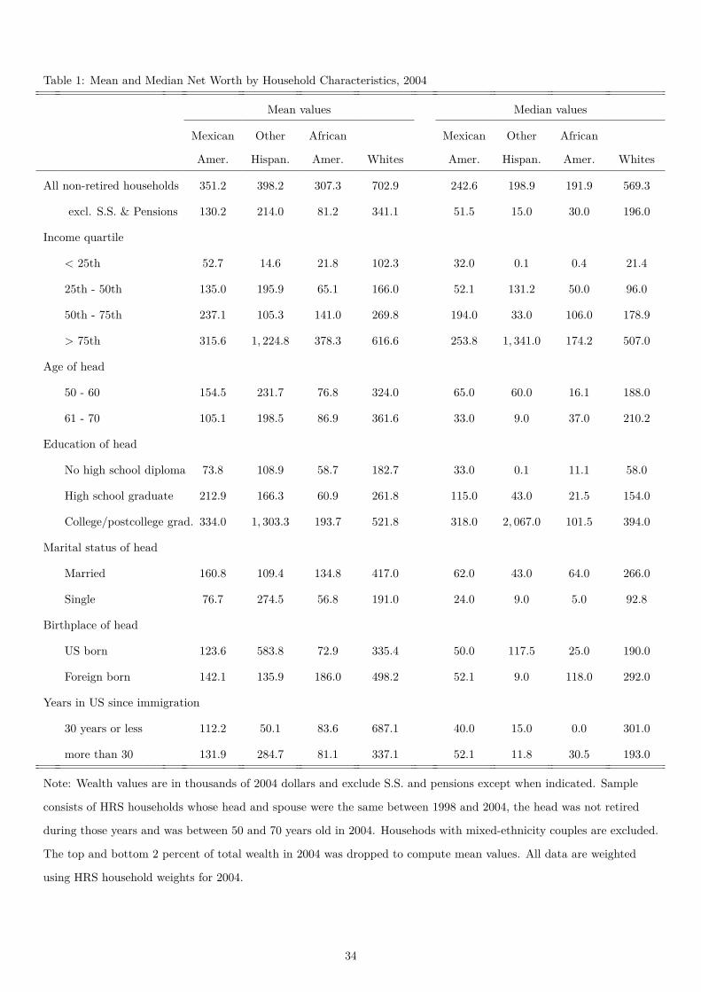
Table 1: Mean and Median Net Worth by Household Characteristics, 2004

Mean values Median values

Mexican

Amer.

Other

Hispan.

African

Amer. Whites

Mexican

Amer.

Other

Hispan.

African

Amer. Whites

All non-retired households 351.2 398.2 307.3 702.9 242.6 198.9 191.9 569.3

excl. S.S. & Pensions 130.2 214.0 81.2 341.1 51.5 15.0 30.0 196.0

Income quartile

< 25th 52.7 14.6 21.8 102.3 32.0 0.1 0.4 21.4

25th - 50th 135.0 195.9 65.1 166.0 52.1 131.2 50.0 96.0

50th - 75th 237.1 105.3 141.0 269.8 194.0 33.0 106.0 178.9

> 75th 315.6 1, 224.8 378.3 616.6 253.8 1, 341.0 174.2 507.0

Age of head

50 - 60 154.5 231.7 76.8 324.0 65.0 60.0 16.1 188.0

61 - 70 105.1 198.5 86.9 361.6 33.0 9.0 37.0 210.2

Education of head

No high school diploma 73.8 108.9 58.7 182.7 33.0 0.1 11.1 58.0

High school graduate 212.9 166.3 60.9 261.8 115.0 43.0 21.5 154.0

College/postcollege grad. 334.0 1, 303.3 193.7 521.8 318.0 2, 067.0 101.5 394.0

Marital status of head

Married 160.8 109.4 134.8 417.0 62.0 43.0 64.0 266.0

Single 76.7 274.5 56.8 191.0 24.0 9.0 5.0 92.8

Birthplace of head

US born 123.6 583.8 72.9 335.4 50.0 117.5 25.0 190.0

Foreign born 142.1 135.9 186.0 498.2 52.1 9.0 118.0 292.0

Years in US since immigration

30 years or less 112.2 50.1 83.6 687.1 40.0 15.0 0.0 301.0

more than 30 131.9 284.7 81.1 337.1 52.1 11.8 30.5 193.0

Note: Wealth values are in thousands of 2004 dollars and exclude S.S. and pensions except when indicated. Sample

consists of HRS households whose head and spouse were the same between 1998 and 2004, the head was not retired

during those years and was between 50 and 70 years old in 2004. Househods with mixed-ethnicity couples are excluded.

The top and bottom 2 percent of total wealth in 2004 was dropped to compute mean values. All data are weighted

using HRS household weights for 2004.

34

Figure 2: Percentage of Households Holding each Type of Asset, 2004

0.0

20.0

40.0

60.0

80.0

100.0

120.0

Main homeequity

Real estate Vehicles Business Net financialassets

Social Security Private pensions

Mexican Americans Other Hispanics African Americans Whites

Figure 3: Percentage of Total Household Wealth, 2004

0.0

10.0

20.0

30.0

40.0

50.0

60.0

70.0

Main homeequity

Real estate Vehicles Business Net financialassets

Social Security Private pensions

Mexican Americans Other Hispanics African Americans Whites

Note: Sample consists of HRS households whose head and spouse were the same between 1998 and 2004, the head was not retiredduring those years and was between 50 and 70 years old in 2004. Households with mixed-ethnicity couples are excluded. Netfinancial assets include IRA/Keogh accounts, stocks, checking and saving accounts, CDs, government bonds, Treasury bills, bonds,and other savings minus debt. The top and bottom 2 percent of each component’s share in total wealth in 1992-1998 (1998-2004)were dropped. All data are weighted using the HRS household weights for 1998 (2004).

35

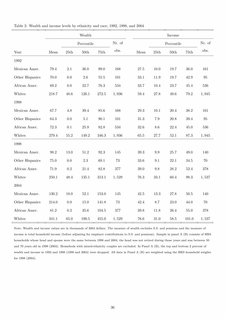
Table 2: Wealth and income levels by ethnicity and race, 1992, 1998, and 2004

Wealth Income

Percentile Nr. of

obs.

Percentile Nr. of

obs.Year Mean 25th 50th 75th Mean 25th 50th 75th

1992

Mexican Amer. 79.4 2.1 36.0 99.0 168 27.5 10.0 19.7 36.0 161

Other Hispanics 70.0 0.0 2.6 55.5 101 33.1 11.9 19.7 42.9 95

African Amer. 69.2 0.0 22.7 76.3 534 33.7 10.4 23.7 45.4 536

Whites 218.7 48.6 126.1 272.5 1, 936 59.4 27.8 49.6 79.2 1, 945

1998

Mexican Amer. 67.7 4.8 39.4 85.6 168 29.3 10.1 20.4 38.2 161

Other Hispanics 64.3 0.0 5.1 90.1 101 31.3 7.9 20.8 39.4 95

African Amer. 72.3 0.1 25.9 82.8 534 32.6 8.6 22.4 45.0 536

Whites 279.4 55.2 149.2 346.3 1, 936 65.5 27.7 52.1 87.3 1, 945

1998

Mexican Amer. 98.2 13.0 51.2 92.3 145 39.3 9.9 25.7 49.0 140

Other Hispanics 75.0 0.0 2.3 69.1 73 33.6 9.1 22.1 34.5 70

African Amer. 71.9 0.2 21.4 82.8 377 39.0 9.8 28.2 52.4 378

Whites 250.1 48.4 135.1 313.1 1, 529 76.3 33.1 60.4 98.3 1, 537

2004

Mexican Amer. 130.2 18.0 52.1 153.0 145 42.5 13.3 27.8 50.5 140

Other Hispanics 214.0 0.0 15.0 141.8 73 42.4 8.7 23.0 44.0 70

African Amer. 81.2 0.2 35.6 104.5 377 39.8 11.8 26.4 55.0 378

Whites 341.1 65.0 190.5 455.0 1, 529 76.6 31.0 58.5 101.0 1, 537

Note: Wealth and income values are in thousands of 2004 dollars. The measure of wealth excludes S.S. and pensions and the measure of

income is total household income (before adjusting for employer contributions to S.S. and pensions). Sample in panel A (B) consists of HRS

households whose head and spouse were the same between 1998 and 2004, the head was not retired during those years and was between 50

and 70 years old in 1998 (2004). Househods with mixed-ethnicity couples are excluded. In Panel A (B), the top and bottom 2 percent of

wealth and income in 1992 and 1998 (1998 and 2004) were dropped. All data in Panel A (B) are weighted using the HRS household weights

for 1998 (2004).

36

Table3:

Saving

Rates

byEt

hnicity

andRace,

1992-1998an

d1998-2004

Mexican

American

sOther

Hisp

anics

African

American

sW

hites

Percentile

Percentile

Percentile

Percentile

Saving

rate

Mean

25th

50th

75th

Mean

25th

50th

75th

Mean

25th

50th

75th

Mean

25th

50th

75th

1992-98

Total

-7.8***

-25.4**

0.0***

14.2***

-1.3

-5.0*

0.0***

6.8***

4.4

-8.6

0.0***

15.7***

15.7

-8.9

6.5

28.5

+SS

,pen

s-7.6***

-48.9***

0.5***

34.7*

11.2

-14.1

7.0*

26.3*

7.0

-27.7*

5.4***

34.9**

17.9

-20.0

13.4

45.1

Active

-0.3*

-7.9

0.0***

12.1

4.4

-6.6

0.0***

11.3

1.3

-4.3

0.4***

10.0***

4.7

-6.1

3.0

14.1

Passive

-7.5***

-19.8

0.0**

12.8***

-5.7**

-12.8

0.0***

10.0***

3.1***

-10.4

0.0***

11.2***

11.0

-10.0

2.6

24.2

1998-04

Total

16.0

-12.1

3.4**

40.1

23.2

0.0***

3.0***

29.7

5.4***

-8.7

0.1*

14.4***

23.2

-6.6

9.2

36.7

+SS

,pen

s24.5

-38.5***

16.5

74.3

50.3

0.0***

30.5***

72.8

22.8

-19.0

16.0

53.7

30.4

-14.8

21.3

58.1

Active

-4.9

-18.1**

0.0***

7.9***

4.9

-3.3*

0.0*

7.3***

-4.3

-6.6

0.0***

7.8***

5.4

-7.1

3.6

15.7

Passive

21.0

-8.9

6.9

44.4

18.4

0.0***

0.0***

31.4

9.6

-7.8

0.0

16.3***

17.8

-6.7

5.9

30.4

Note:

Meansaving

ratesforeach

grou

pequa

lthe

ratioof

meansaving

over

sixtimes

averagean

nual

incomein

thesamepe

riod

.Percentile

saving

ratesarecompu

tedfortheratioof

saving

over

six

times

incomedu

ring

thesamepe

riod

.Activesaving

isthesum

ofnetflo

wsof

mon

eysavedin

individu

alassets.Passive

saving

isthediffe

rencebe

tweentotalc

hang

ein

wealthan

dactive

saving

sover

a

6-year

period

.Sa

mpleconsists

onho

useh

olds

who

sehead

andspou

sewerethesamean

dthehead

was

notretiredin

1992-1998(1998-2004)an

dwas

betw

een50

and70

yearsoldin

1998

(2004).

Hou

seho

dswithmixed-ethnicity

coup

lesareexclud

ed.The

samples

aretrim

med

only

formeanratesby

drop

ping

thetopan

dbo

ttom

2pe

rcentof

totals

avingover

1992-1998(1998-2004)an

dof

averageincomeover

1993-1997(1999-2003).

*,**,*

**diffe

rencewithW

hitessign

ificant

at10,5

and1pe

rcentlevel

37

Table4:

Saving

Rates

byEt

hnicity

andRacean

dTyp

eof

Asset,1

992-1998

and1998-2004

Mexican

American

sOther

Hisp

anics

African

American

sW

hites

Percentile

Percentile

Percentile

Percentile

Asset

Mean

25th

50th

75th

Mean

25th

50th

75th

Mean

25th

50th

75th

Mean

25th

50th

75th

1992-98

Reala

ssets

-9.8**

-17.6

0.0***

8.9

-2.0

-2.0**

0.0***

6.2**

1.7

-6.8

0.0***

7.6**

2.4

-6.9

1.7

12.0

Fina

nc.assets

2.3**

-1.4

0.0***

2.5***

3.3*

-1.6

0.0***

2.2***

4.0**

-1.6

0.0***

3.1***

11-2.5

2.1

14.2

Social

Secu

rity

-2.6**

-5.0

3.3

16.5**

-0.1

-0.9

1.9

10.5

-1.8

-3.3

3.8

10.2***

-0.4

-1.3

3.0

7.4

Pensions

-5.1

-17.8

5.0

21.5

12.6

-7.0

6.4

15.7**

11.4

-10.3

3.8

22.5

9.2

-4.5

6.9

23.6

1998-04

Reala

ssets

15.1***

-9.2

2.0*

2423.0

0.0***

0.0***

20.6

5.7

-2.5

0.0***

9.9***

12.7

-3.2

5.2

21.4

Fina

nc.assets

2.6

-1.2***

0.0***

2.5***

3.6*

-0.3***

0.0***

5.2***

0.0**

-2.8*

0.0***

3.2***

6.0

-4.4

1.4

13.3

Social

Secu

rity

4.6***

-33.5***

11.1

30.3***

9.0

0.0

9.5

24.9

6.5

0.0

13**

25.9***

5.9

0.0

10.2

18.4

Pensions

21.6

-12.5

3.9

16.5

22.8*

6.1

29.4*

46.8

33.2**

-1.1*

17.3**

44.2***

11.9

-6.1

5.6

22.9

Note:

Seetheno

teto

Table3fordefin

itionof

saving

rates.

Reala

ssetscomprisemainho

meequity,r

eale

state,

vehicles

andbu

siness.Finan

cial

assets

includ

eIR

A/K

eogh

accoun

ts,s

tocks,

checking

andsaving

accoun

ts,C

Ds,

governmentbo

nds,

Treasury

bills,b

onds,a

ndothersaving

sminus

debt.So

cial

Security

wealthis

compu

tedassumingclaimingat

age70.Pension

wealthinclud

esDefined

Benefitvalues

atexpe

cted

ageof

retirementan

dDefinedCon

tribution/

Com

bina

tion

accoun

tba

lances.Sa

mpleconsists

onho

useholds

who

sehead

andspou

sewerethesame,

thehead

was

notretiredin

1992-1998(1998-2004)an

dwas

betw

een50

and70

yearsoldin

1998

(2004).Hou

seho

ldswithmixed-ethnicity

coup

lesareexclud

ed.The

samples

aretrim

med

only

formeanratesby

drop

ping

thetop

andbo

ttom

2pe

rcentof

totals

avingover

1992-1998(1998-2004)an

dof

averageincomeover

1993-1997(1999-2003).

*,**,*

**diffe

rencewithW

hitessign

ificant

at10,5

and1pe

rcentlevel

38

Table 5: Total Saving Rates including Social Security and Pensions, 1992-1998 and 1998-2004OLS OLS OLS Median Median Median

Mex. Amer. -.111∗∗ -.075∗ -.110∗∗ -.094∗∗∗ -.055∗ -.082∗∗

(.043) (.044) (.052) (.032) (.032) (.040)

Other Hisp. .030 .060 .042 -.030 -.007 -.007(.051) (.052) (.060) (.042) (.041) (.051)

Afr. Amer. -.072∗∗∗ -.041 -.035 -.071∗∗∗ -.026 .000(.024) (.025) (.027) (.020) (.020) (.022)

98-04’ .160∗∗∗ .153∗∗∗ .211∗∗∗ .092∗∗∗ .078∗∗∗ .120∗∗∗

(.020) (.020) (.021) (.016) (.015) (.017)

Constant .088∗∗∗ .035∗∗ -5.807∗∗∗ .128∗∗∗ .070∗∗∗ -5.841∗∗∗

(.014) (.018) (1.887) (.012) (.014) (1.482)

Other controls No Income Income No Income Income+ others + others

Adj. R-Square .016 .021 .046Pseudo R-Square .004 .007 .019Observations 5,011 5,011 4,928 5,246 5,246 5,159

Notes. The table reports the coefficients from OLS and median regressions of the total saving rate on ethnicity and race dummiesand other controls. The observations for the two periods are pooled and the coefficient on 98-04’ captures the fixed-effects for thesecond period. All specifications that control for income, also control for its square. In addition, specifications in columns (3) and(6) control for age of the head and its square, the number of children in the household, the education of the head and include adummy if the household head is married, a dummy if the head is born in U.S., and region dummies. Robust standard errors(clustered at the family level) and trimmed samples are used for OLS regressions only.

39

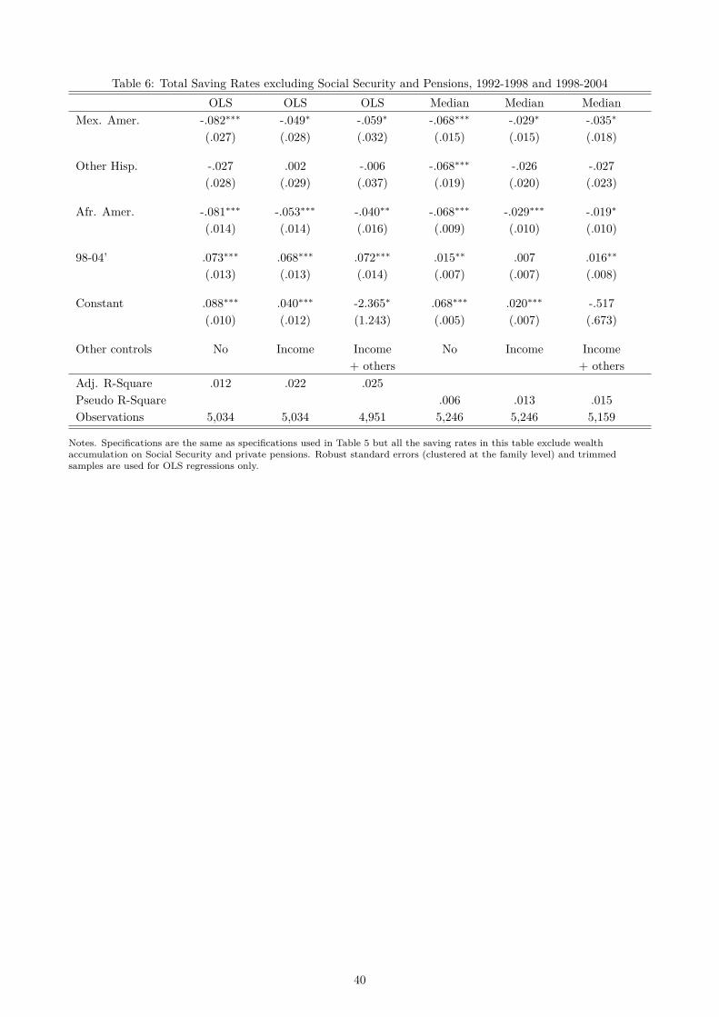
Table 6: Total Saving Rates excluding Social Security and Pensions, 1992-1998 and 1998-2004OLS OLS OLS Median Median Median

Mex. Amer. -.082∗∗∗ -.049∗ -.059∗ -.068∗∗∗ -.029∗ -.035∗

(.027) (.028) (.032) (.015) (.015) (.018)

Other Hisp. -.027 .002 -.006 -.068∗∗∗ -.026 -.027(.028) (.029) (.037) (.019) (.020) (.023)

Afr. Amer. -.081∗∗∗ -.053∗∗∗ -.040∗∗ -.068∗∗∗ -.029∗∗∗ -.019∗

(.014) (.014) (.016) (.009) (.010) (.010)

98-04’ .073∗∗∗ .068∗∗∗ .072∗∗∗ .015∗∗ .007 .016∗∗

(.013) (.013) (.014) (.007) (.007) (.008)

Constant .088∗∗∗ .040∗∗∗ -2.365∗ .068∗∗∗ .020∗∗∗ -.517(.010) (.012) (1.243) (.005) (.007) (.673)

Other controls No Income Income No Income Income+ others + others

Adj. R-Square .012 .022 .025Pseudo R-Square .006 .013 .015Observations 5,034 5,034 4,951 5,246 5,246 5,159

Notes. Specifications are the same as specifications used in Table 5 but all the saving rates in this table exclude wealthaccumulation on Social Security and private pensions. Robust standard errors (clustered at the family level) and trimmedsamples are used for OLS regressions only.

40

Table 7: Active Saving Rates excluding Social Security and Pensions, 1992-1998 and 1998-2004OLS OLS OLS Median Median Median

Mex. Amer. -.082∗∗∗ -.067∗∗ -.096∗∗ -.039∗ -.035 -.041(.032) (.032) (.038) (.022) (.023) (.029)

Other Hisp. .019 .032 .007 -.043 -.039 -.035(.037) (.037) (.042) (.029) (.030) (.037)

Afr. Amer. -.037∗∗ -.024 -.017 -.009 -.008 -.000(.018) (.019) (.020) (.014) (.014) (.016)

98-04’ .092∗∗∗ .090∗∗∗ .138∗∗∗ .081∗∗∗ .080∗∗∗ .106∗∗∗

(.014) (.014) (.015) (.011) (.011) (.012)

Constant .044∗∗∗ .022∗ -5.937∗∗∗ .076∗∗∗ .073∗∗∗ -4.992∗∗∗

(.009) (.012) (1.215) (.008) (.010) (1.072)

Other controls No Income Income No Income Income+ others + others

Adj. R-Square .011 .012 .049Pseudo R-Square .004 .004 .017Observations 5,008 5,008 4,927 5,246 5,246 5,159

Notes. Specifications are the same as specifications used in Table 5. Robust standard errors (clustered at the family level) andtrimmed samples are used for OLS regressions only.

41

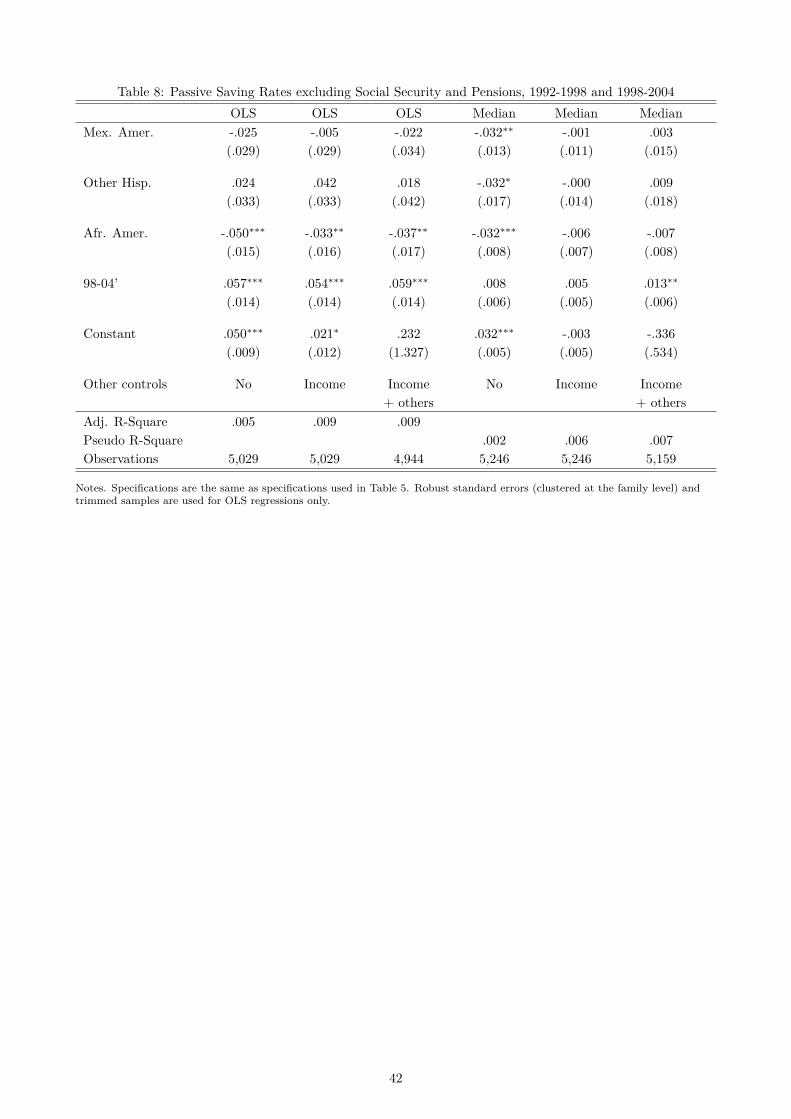
Table 8: Passive Saving Rates excluding Social Security and Pensions, 1992-1998 and 1998-2004OLS OLS OLS Median Median Median

Mex. Amer. -.025 -.005 -.022 -.032∗∗ -.001 .003(.029) (.029) (.034) (.013) (.011) (.015)

Other Hisp. .024 .042 .018 -.032∗ -.000 .009(.033) (.033) (.042) (.017) (.014) (.018)

Afr. Amer. -.050∗∗∗ -.033∗∗ -.037∗∗ -.032∗∗∗ -.006 -.007(.015) (.016) (.017) (.008) (.007) (.008)

98-04’ .057∗∗∗ .054∗∗∗ .059∗∗∗ .008 .005 .013∗∗

(.014) (.014) (.014) (.006) (.005) (.006)

Constant .050∗∗∗ .021∗ .232 .032∗∗∗ -.003 -.336(.009) (.012) (1.327) (.005) (.005) (.534)

Other controls No Income Income No Income Income+ others + others

Adj. R-Square .005 .009 .009Pseudo R-Square .002 .006 .007Observations 5,029 5,029 4,944 5,246 5,246 5,159

Notes. Specifications are the same as specifications used in Table 5. Robust standard errors (clustered at the family level) andtrimmed samples are used for OLS regressions only.

42

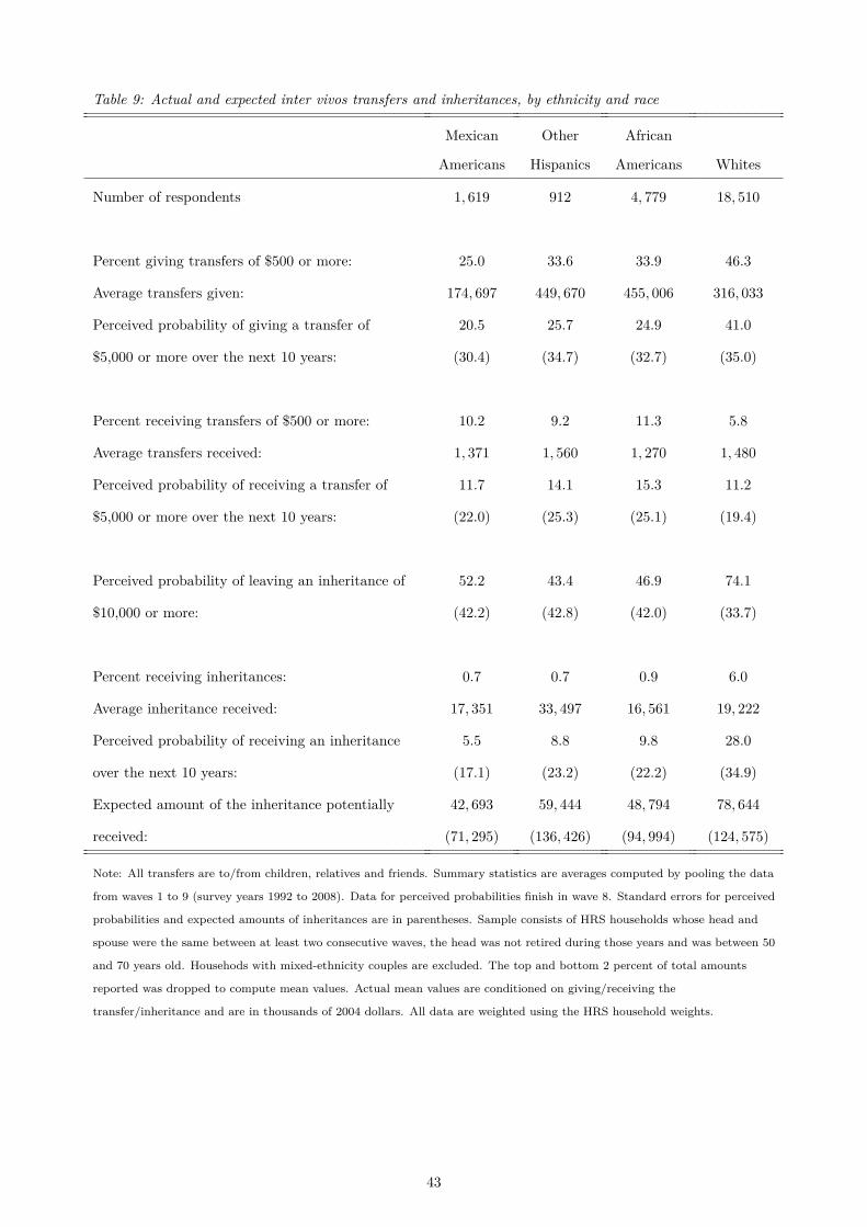
Table 9: Actual and expected inter vivos transfers and inheritances, by ethnicity and race

Mexican

Americans

Other

Hispanics

African

Americans Whites

Number of respondents 1, 619 912 4, 779 18, 510

Percent giving transfers of $500 or more: 25.0 33.6 33.9 46.3

Average transfers given: 174, 697 449, 670 455, 006 316, 033

Perceived probability of giving a transfer of 20.5 25.7 24.9 41.0

$5,000 or more over the next 10 years: (30.4) (34.7) (32.7) (35.0)

Percent receiving transfers of $500 or more: 10.2 9.2 11.3 5.8

Average transfers received: 1, 371 1, 560 1, 270 1, 480

Perceived probability of receiving a transfer of 11.7 14.1 15.3 11.2

$5,000 or more over the next 10 years: (22.0) (25.3) (25.1) (19.4)

Perceived probability of leaving an inheritance of 52.2 43.4 46.9 74.1

$10,000 or more: (42.2) (42.8) (42.0) (33.7)

Percent receiving inheritances: 0.7 0.7 0.9 6.0

Average inheritance received: 17, 351 33, 497 16, 561 19, 222

Perceived probability of receiving an inheritance 5.5 8.8 9.8 28.0

over the next 10 years: (17.1) (23.2) (22.2) (34.9)

Expected amount of the inheritance potentially 42, 693 59, 444 48, 794 78, 644

received: (71, 295) (136, 426) (94, 994) (124, 575)

Note: All transfers are to/from children, relatives and friends. Summary statistics are averages computed by pooling the data

from waves 1 to 9 (survey years 1992 to 2008). Data for perceived probabilities finish in wave 8. Standard errors for perceived

probabilities and expected amounts of inheritances are in parentheses. Sample consists of HRS households whose head and

spouse were the same between at least two consecutive waves, the head was not retired during those years and was between 50

and 70 years old. Househods with mixed-ethnicity couples are excluded. The top and bottom 2 percent of total amounts

reported was dropped to compute mean values. Actual mean values are conditioned on giving/receiving the

transfer/inheritance and are in thousands of 2004 dollars. All data are weighted using the HRS household weights.

43

Table 10: Estimates of actual probabilities and amounts and perceived probabilities of giving/receiving transfersGive a Transfer Receive a Transfer

Percent Amount Perceived Probab. Percent Amount Perceived Probab.Probit Tobit Probit Probit Tobit Probit

Mex. Amer. -.14∗∗∗ -105,306.72∗∗ -.07∗∗∗ .03∗∗∗ -27.56 .01(.03) (49,312.50) (.02) (.01) (134.43) (.01)

Other Hisp. -.12∗∗∗ 30,660.94 -.10∗∗∗ .01 38.80 .02∗

(.03) (86,600.91) (.03) (.01) (170.75) (.01)

Afr. Amer. -.02 34,559.02 -.03∗∗ .03∗∗∗ -104.51∗ .03∗∗∗

(.01) (30,787.97) (.01) (.01) (62.32) (.00)Pseudo R-Square .081 .002 .171 .062 .007 .035Observations 20,755 8,309 18,698 20,760 969 18,189

Notes. The dependent variables in columns 3 and 6 (perceived probability) are binary indicators that take value one if the household reports aprobability of 50 percent or more. Household data on perceived probabilities is the average of the probabilities reported by householdrespondents. All specifications also control for household income and its square, age of the head and its square, the number of children in thehousehold, dummies for education of the head, whether the head was born in the US and whether is married, and state and year fixed-effects.Robust standard errors, clustered at the family level, are in parentheses. Samples exclude wave 9 (survey year 2008) for perceived probabilities.Samples for Tobit regressions are trimmed and limited to households with positive transfers.

Table 11: Estimates of actual probabilities and amounts and perceived probabilities of leaving/receiving inheritancesLeave an Inheritance Receive an InheritancePerceived Probab. Percent Amount Perceived Probab. Expected Amount

Probit Probit Tobit Probit TobitMex. Amer. .01 -.04∗∗∗ 3,148.97 -.17∗∗∗ -10,029.80

(.022) (.009) (4,189.446) (.025) (7,447.400)

Other Hisp. -.17∗∗∗ -.06∗∗∗ 24,909.61∗∗∗ -.11∗∗∗ 7,772.40(.037) (.016) (2,527.787) (.028) (13,572.822)

Afr. Amer. -.12∗∗∗ -.04∗∗∗ -1,592.82 -.13∗∗∗ -7,656.07∗∗∗

(.013) (.004) (2,392.596) (.011) (2,920.059)Pseudo R-Square .231 .089 .013 .140 .006Observations 18,203 20,995 555 18,224 6,094

Notes. See note to Table 10 for description of the ’perceived probability’ indicator. All specifications include the same controls as the onesdescribed in the note to Table 10. Robust standard errors, clustered at the family level, are in parentheses. Samples exclude wave 9 (survey year2008) for perceived probabilities. Samples for Tobit regressions are trimmed and limited to households with positive actual and expectedinheritances.

44

Table 12: Fixed-effect estimates of total saving rates on perceived probabilities

All the

sample

Mexican

Americans

Other

Hispanics

African

Americans Whites

FE FE FE FE FE

Give a Transfer -0.027** -0.073 0.156 -0.004 -0.030**

(.013) (.069) (.111) (.035) (.015)

Adj. R-Squared 0.005 0.011 0.014 0.002 0.008

Observations 20, 225 1, 282 556 3, 590 14, 797

Receive a Transfer 0.046* 0.103 -0.118 0.071 0.035

(.026) (.092) (.157) (.048) (.033)

Adj. R-Squared 0.005 0.003 0.012 0.004 0.007

Observations 19, 806 1, 219 539 3, 437 14, 611

Leave an Inheritance -0.054*** -0.089* -0.095 -0.014 -0.062***

(.015) (.050) (.087) (.035) (.019)

Adj. R-Squared 0.007 0.011 0.011 0.006 0.01

Observations 16, 407 1, 038 452 2, 823 12, 094

Receive an Inheritance 0.021 -0.038 -0.030 -0.006 0.023

(.018) (.170) (.219) (.063) (.019)

Adj. R-Squared 0.006 0.004 0.007 0.004 0.009

Observations 16, 403 1, 042 455 2, 822 12, 084

Notes. All specifications also control for household income and its square, age of the head and its square, the number of children in the

household, dummies for education of the head, whether the head was born in the US and whether is married, and state and year

fixed-effects. Robust standard errors, clustered at the family level, are in parentheses.

45

Table 13: Estimates of belief updating for the perceived probability of giving/receiving a transferGive a Transfer Receive a Transfer

OLS FD IV OLS FD IVGive a Transfer (perc. prob. in t-1) .253∗∗∗ .080∗∗∗

(.009) (.022)

Give a Transfer (actual) .165∗∗∗ .094∗∗∗

(.007) (.014)

Receive a Transfer (perc. prob. in t-1) .184∗∗∗ .072∗∗

(.019) (.031)

Receive a Transfer (actual) .134∗∗∗ .074∗∗∗

(.013) (.022)

Household Income/1,000,000 .416∗∗∗ .081 -.029∗∗ -.034(.077) (.111) (.012) (.033)

Children Income/1,000,000 -.131∗∗∗ -.254∗ -.004 .076(.035) (.136) (.022) (.075)

Constant 1.832∗∗∗ .372 .100 .234(.439) (1.460) (.275) (.765)

Adj. R-Square .277 .067Observations 18,121 11,598 15,794 9,693

Notes. Estimates in columns "FD IV" are obtained using the two-step, Arellano-Bover/Blundell-Bond estimator. See note to Table 10 fordescription of the ’perceived probability’ indicator. Children income was constructed by imputing the median value to the four intervals forwhich it was reported by their parents. All specifications control for age of the head and its square, the number of children in the household, andinclude dummies for the education of the head, whether is married and whether was born in the US. Year and region fixed-effects are alsoincluded. Robust standard errors are in parentheses (this is the Windmeijer (2005) WC-robust estimator for the two step-estimator).

46

Table14:Tw

o-stageleast-squa

resfirst-differen

cedestim

ates

oftotals

avingrates

Allthesample

Mexican

American

sOther

Hisp

anics

African

American

sW

hites

(1)

(2)

(3)

(4)

(5)

D.G

iveaTr

ansfer

(perc.

prob

.in

t-1)

-.014

-.181

.079

.065

-.017

(.049)

(.256)

(.279)

(.116)

(.056)

Con

stan

t.099

∗.215

.078

.207

∗.062

(.052)

(.247)

(.336)

(.126)

(.061)

R-squ

ared

.009

.040

.087

.022

.012

Observatio

ns5,822

300

120

908

4,494

Table15:Tw

o-stageleast-squa

resfirst-differen

cedestim

ates

oftotals

avingrates

Allthesample

Mexican

American

sOther

Hisp

anics

African

American

sW

hites

(1)

(2)

(3)

(4)

(5)

D.R

eceive

aTr

ansfer

(perc.

prob

.in

t-1)

.015

.128

-.374

.239

-.076

(.082)

(.252)

(.524)

(.160)

(.104)

Con

stan

t.096

∗.067

-.045

.275

∗∗.058

(.053)

(.215)

(.314)

(.127)

(.062)

R-Squ

ared

.009

.039

.114

.016

.010

Observatio

ns5,635

282

121

836

4,396

Notes

toTa

bles

14an

d15.Estim

ates

areob

tained

usingthe2S

LSfirst-differencedestimator.The

depe

ndentvariab

leisabina

ryindicatorthat

takesvalueon

eifho

useholdsaving

sbe

tweent-1an

dtarepo

sitive.Seetheno

teto

Table10

fordescriptionof

the’perceived

prob

ability’ind

icator.Allspecification

scontrolfor

perm

anentho

useholdincomean

ditssqua

re,a

geof

thehead

andits

squa

re,a

ndtimean

dregion

fixed-effe

cts.

Rob

uststan

dard

errors,c

lustered

atthefamily

level,arein

parentheses.

47

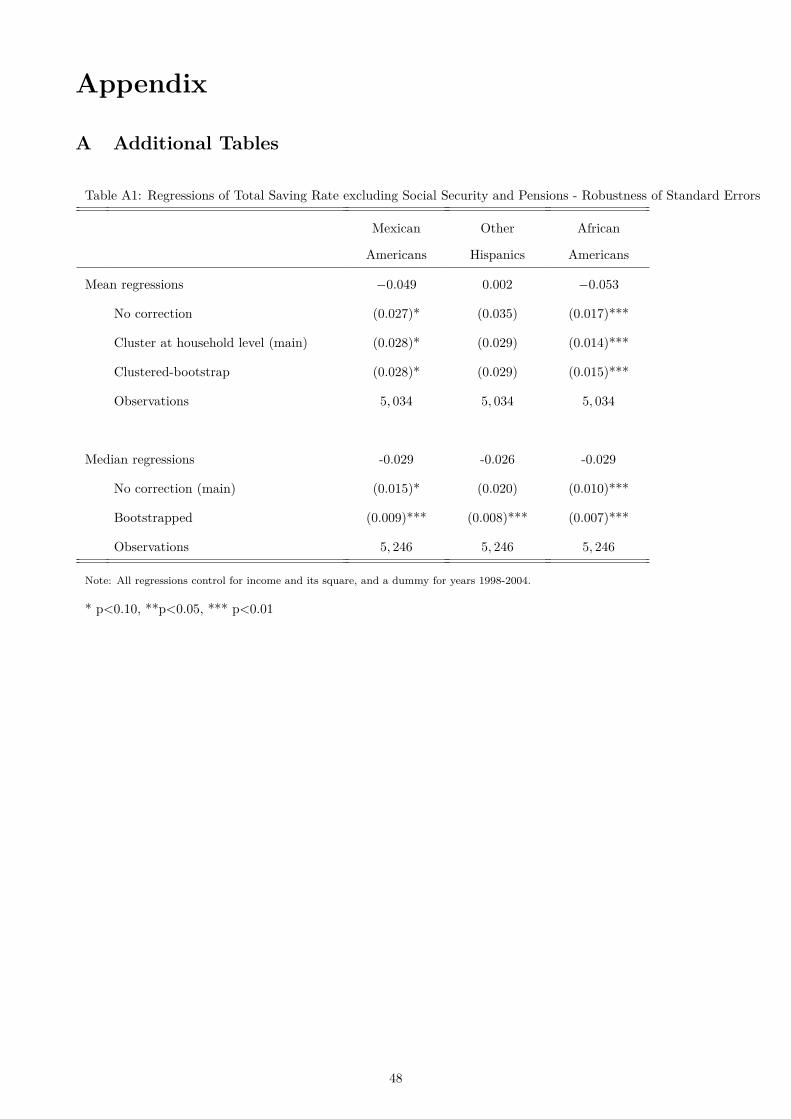
Appendix

A Additional Tables

Table A1: Regressions of Total Saving Rate excluding Social Security and Pensions - Robustness of Standard Errors

Mexican

Americans

Other

Hispanics

African

Americans

Mean regressions −0.049 0.002 −0.053

No correction (0.027)* (0.035) (0.017)***

Cluster at household level (main) (0.028)* (0.029) (0.014)***

Clustered-bootstrap (0.028)* (0.029) (0.015)***

Observations 5, 034 5, 034 5, 034

Median regressions -0.029 -0.026 -0.029

No correction (main) (0.015)* (0.020) (0.010)***

Bootstrapped (0.009)*** (0.008)*** (0.007)***

Observations 5, 246 5, 246 5, 246

Note: All regressions control for income and its square, and a dummy for years 1998-2004.

* p<0.10, **p<0.05, *** p<0.01

48

Table2:

Saving

Rates

onReala

ndFina

ncialA

ssets,

1992-1998an

d1998-2004

Reala

ssets

Fina

nciala

ssets

OLS

OLS

OLS

Med

ian

Median

Med

ian

OLS

OLS

OLS

Med

ian

Med

ian

Med

ian

Mex.Amer.

-.041

∗-.0

30-.0

43∗

-.022

∗∗∗

-.009

-.015

-.045

∗∗∗

-.028

∗∗∗

-.007

-.018

∗∗∗

-.004

-.004

(.021)

(.022)

(.025)

(.008)

(.008)

(.009)

(.008)

(.008)

(.012)

(.005)

(.005)

(.007)

Other

Hisp

..008

.017

.004

-.022

∗∗-.0

09-.0

11-.0

38∗∗

∗-.0

23∗∗

.002

-.018

∗∗∗

-.003

-.001

(.023)

(.023)

(.029)

(.010)

(.010)

(.012)

(.010)

(.010)

(.014)

(.006)

(.007)

(.009)

Afr.Amer.

-.029

∗∗∗

-.019

∗-.0

22∗∗

-.022

∗∗∗

-.010

∗∗-.0

09∗

-.045

∗∗∗

-.030

∗∗∗

-.017

∗∗∗

-.018

∗∗∗

-.005

-.004

(.010)

(.010)

(.011)

(.005)

(.005)

(.005)

(.006)

(.006)

(.007)

(.003)

(.003)

(.004)

98-04’

.093

∗∗∗

.091

∗∗∗

.102

∗∗∗

.018

∗∗∗

.014

∗∗∗

.019

∗∗∗

-.020

∗∗∗

-.022

∗∗∗

-.027

∗∗∗

.000

-.003

-.005

∗

(.009)

(.009)

(.010)

(.004)

(.004)

(.004)

(.006)

(.006)

(.007)

(.002)

(.002)

(.003)

Con

stan

t.015

∗∗-.0

02-1.546

∗.022

∗∗∗

.006

∗-.3

83.064

∗∗∗

.039

∗∗∗

-.521

.018

∗∗∗

.002

.031

(.006)

(.008)

(.834)

(.003)

(.003)

(.341)

(.005)

(.006)

(.577)

(.002)

(.002)

(.250)

Other

controls

No

Income

Income

No

Income

Income

No

Income

Income

No

Income

Income

+othe

rs+

othe

rs+

othe

rs+

othe

rsAdj.R-Squ

are

.022

.024

.027

.010

.024

.028

Pseu

doR-Squ

are

.004

.006

.007

.004

.010

.011

Observatio

ns5,022

5,022

4,937

5,246

5,246

5,159

5,049

5,049

4,964

5,24

65,246

5,159

Notes.Fo

reach

column,

thetophead

ings

indicate

thesaving

measure

used

asdepe

ndentvariab

le.Seetheno

teto

Table3fordefin

itionof

saving

rates.

The

controls

includ

edarethesameas

theon

esinclud

edin

specification

s(3)an

d(6).

Rob

uststan

dard

errors

(clustered

atthefamily

level)an

dtrim

med

samples

areused

forOLS

regression

son

ly.

49

Table A3: Oaxaca-Blinder decomposition

Mexican Americans African Americans

Level of wealth Saving rate Level of wealth Saving rate

Total gap 217,325*** .082*** 232,732*** .080***

(11, 846) (.028) (8, 907) (.014)

Explained gap 136,918*** [63%] 0.025 [30%] 136,571*** [59%] .040*** [50%]

(15, 771) (.019) (8, 391) (.007)

Unexplained gap 80,407*** [37%] .057* [70%] 96,161*** [39%] .040*** [50%]

(16, 320) (.032) (7, 986) (.016)

Contributions to the explained gap by component

Income 85,466*** [39%] .014*** [17%] 75,563*** [32%] .012*** [15%]

(11, 144) (.004) (9, 881) (.004)

Education 45,339*** [21%] 0.012 [15%] 26,092*** [11%] .008* [10%]

(6, 782) (.009) (4, 137) (.005)

Demographic characteristics −2, 169 [1%] -0.009 [-11%] 19,654*** [8%] 0.001 [1%]

(9, 117) (.012) (4, 248) (.005)

Health 12,235*** [6%] .017*** [21%] 8,792*** [4%] .013*** [16%]

(3, 394) (.006) (2, 434) (.004)

Region of residence −3, 953 [-2%] -0.009 [-11%] 6,470** [3%] 0.005 [6%]

(8, 354) (.012) (2, 723) (.003)

Standard errors in parentheses; percent of total variation in brackets.

*p<0.10, **p<0.05, ***p<0.001

50

B Data description

I use household data from the Health and Retirement Study (HRS) for 1992-2004. In this appendix I describe

in detail the construction of the variables used for the analysis.

1) Sample selection: Most of the data are taken from the 1992, 1998 and 2004 HRS waves, but I also

rely on some data from intermediate waves to compute permanent income and active savings. Respondents

in the HRS are defined as the age-eligible individuals (in 1992 the selected birth cohort aged 51-61) and the

spouse, regardless of age, when the respondent is married. Spouses are included because retirement decisions

are often taken jointly by the couple. Thus, at least two observations are present in households with married

or partnered respondents: one for the primary respondent, the individual with more knowledge about assets,

debts and retirement planning, and other for the secondary respondent, i.e. his/her spouse. Following the

standard practice, I will treat the male in the couple, rather than the primary respondent, as the household

head. The reason is that this facilitates comparison with other studies, and also there are more differences in

characteristics affecting earnings behavior between men and women than between the primary and secondary

respondent (Moon & Juster 1995).

Each individual defined as the household head constitutes one observation. The sample selection follows the

typical restrictions adopted in the empirical literature on savings. Thus, I restrict the sample to sub-households

with the same head over the relevant period (1992-1998 or 1998-2004) and to those where the head’s spouse was

the same, in case the head has a partner. This leaves 10,283 observations in 1992-1998 and 11,767 in 1998-2004.

The purpose is to restrict the sample to stable households, where wealth changes are not explained mostly by

changes in family composition. I also drop observations for sub-households that were in the sample but were

not interviewed in a particular wave. This leaves a total of 5,548 observations for the analysis in 1992-1998 and

9,147 observations for 1998-2004. Sub-households that have either income or wealth missing were also dropped

(only 10 households were dropped in 1998-2004). Next, I drop households where the head was below 50 or above

70 years old in 1998 and in 2004 (5,243 observations remaining for 1992-1998 and 4,618 for 1998-2004). Then I

drop households where the head reports to be retired either in the first or in the last year of each period, which

leaves 3,113 and 2,424 observations for 1992-1998 and for 1998-2004 respectively.29Finally, I exclude households

where the spouses are of a different race or ethnicity and so the total number of observations falls to 2,953 in

1992-1998 and to 2,302 in 1998-2004. Finally, the sample was trimmed when necessary by dropping households

in the top and bottom 2 percent of the corresponding distribution (details are given in each table’s notes).

2) Weights: All summary statistics for 1992-1998 were obtained using the household level weights provided

by the HRS for 1998. Results for 1998-2004 use the weights for 2004.

3) Constructed variables:

A. Total Saving: It is obtained as the difference between real net wealth in 1998 (2004) minus real net29Note that retirement status can vary if instead of using self-reports one uses an objective measure such as “no current job”.

Gustman et al. (1995) show that self-reports result in significantly lower number of retirees than the use of objective measures.Thus, as a robustness check one can also define retired households as those where the head has no current job. They also notethat the HRS allows capturing the flows from labor force to retirement and the other way around, resulting from the fact thatretirement is not an absorbing state.

51

wealth in 1992 (1998). That measure can be decomposed into two components: active and passive savings. The

measures of wealth levels (total and individual components) are taken from the RAND HRS 2008 Income and

Wealth Imputations. Total net wealth comprises main home equity (the value of main house minus all mortgages

in the primary residence and other home loans), real estate other than home equity, vehicles, business, Individual

Retirement Accounts (IRAs), stocks, mutual funds, checking and savings accounts, CDs, savings bonds, treasury

bills, bonds, and other assets (money owed by others, valuable collections, rights in a trust or estate) less other

debts (credit card balances, medical debts, life insurance policy loans, loans from relatives). This measure of

total wealth excludes pension and Social Security (S.S.), which are not directly reported in the survey. These

variables were constructed ex-post using information collected in the 1992, 1998 and 2004 waves and it is possible

to access to some of them through the HRS website. Here I use the pension and S.S. wealth measures that are

publicly available and I add them to the measure of wealth in order to compute total wealth.

- Pension wealth: The procedure to construct this variable for 1992 and 1998 is described in the HRS

document ’Imputations for Pension Wealth 1992 and 1998’, and for 2004 in the document ’Imputations for

Employer-Sponsored Pension Wealth from Current Jobs in 2004’. Pension wealth is estimated for current jobs

from both self-reported and employer data. Using the respondent’s self-reported pension plan type, it is possible

to determine which method of wealth estimation to use.

i) If the respondent is covered by at least one DC plan on his current job at the time of the survey (1992,

1998 or 2004), DC wealth is computed from the self-reported account balance. Note that multiple accounts

can be reported from the same job and in that case total DC wealth is the sum of each account balance from

current job.

ii) If the respondent is covered by at least one DB plan at the time of the survey, the HRS Pension Estimation

Program is used to compute wealth for each DB plan. This is done by combining self-reported data and pension

plan rules obtained from the Summary Plan Description. SPDs were obtained by different means such as

by contacting the employers of HRS respondents, by conducting an employer pension provider survey, by

respondents’ requests to their employers, by Internet searches and use of commercial databases. DB values

were calculated at seven different ages: the expected age of retirement, early age of retirement, normal age of

retirement, ages 60, 62, 65 and, only for 2004, age 70. The calculations of the present values from DB plans use

the intermediate future real interest rate (2.9%) and the inflation rate (2.8%) forecast by the Social Security

Administration (SSA). The present values are then discounted back to the survey year, which allows comparison

between DB and DC amounts.

iii) If the respondent is covered by DB and DC plans or a Combination plan, both DB and DC wealth values

are calculated.

Thus, total pension wealth is calculated by adding DB values at a given age of retirement (expected, early,

normal, 60, 62, 65 or 70) and the total value of all the DC/Combination account balances in the corresponding

survey year. Different imputations methods were used when the data needed for these estimates were missing.

Since in 1992 and 1998 DB wealth is discounted back to the survey year only for the expected age of retirement,

this is the only DB value I can use for 2004 as well.

52

- Social Security wealth: The methodology to construct this variable is described in the HRS document

’Prospective Social Security Wealth Measures of Pre-Retirees’. S.S. wealth is calculated for ’pre-retirement’

respondents (i.e. those who are not claiming S.S. benefits as of the wave date) in 1992, 1998 and 2004.30 First,

this involves computing the Average Indexed Monthly Earning (AIME) and Primary Insurance Amount (PIA)

for each respondent using the ANYPIA program (Office of the Actuary, v 2008.1). That program determines

S.S. eligibility and coverage for each individual based on his/her earnings record. AIME is the average of

the individual’s highest indexed earnings over the appropriate number of ’computation years’. The PIA is the

amount payable to the worker at the projected claim date in claim year dollars and it is a function of AIME

and ’bend points’. Annual PIAs are calculated as of three claim ages: age 62, full retirement age (FRA) and age

70. To calculate survival probabilities, they use the SSA life tables by year of birth and sex. And the interest

rates and the inflation rates are taken from the SSA Trustee Reports.

S.S. wealth is calculated on three monthly benefits: i) retirement insurance benefits (or old-age insurance

benefits) are based on lifetime earnings, and are paid to retired workers age 62 or over who are fully insured ii)

incremental auxiliary spouse benefits, is based on the spouse’s life-time earnings and iii) incremental survivor

benefit, is based on the deceased insured worker’s lifetime earnings. Thus, wealth is computed by assuming

that the monthly S.S. benefit comprises i) and ii) if both spouses are alive, whereas it comprises i) and iii) if

one worker is deceased. By definition, ii) and iii) are zero for the higher earner. Adjustments are made on

each period for early or late claiming, and these three components of S.S. wealth are weighted by the survival

probabilities. The resulting wealth values are made comparable across individuals by reporting them in wave

date dollars. Note that benefits are calculated assuming claiming ages that the respondent has not yet attained

by the survey date (age 62, FRA, and age 70). If a respondent is older than a particular age claim or if he has

started claiming benefits, missing values are assigned. Thus, for example, S.S. wealth at FRA is only calculated

for individuals that are 67 or younger.

Thus, the variable measuring household total S.S. wealth, assuming both respondent and spouse claim at

their respective FRA, is the sum of respondent’s retirement insurance wealth, respondent’s incremental auxiliary

spouse benefit wealth, respondent’s incremental survivor benefit wealth, spouse’s incremental retirement insur-

ance benefit wealth, spouse’s incremental auxiliary spouse benefit wealth, and spouse’s incremental survivor

benefit wealth. As in the case of other wealth components, missing values were imputed when possible.

Ideally, to compute total wealth one would like to add S.S. and pension wealth assuming claiming at age 62

or at FRA (also called normal retirement age), which are the assumptions used to compute both pension and

SS wealth for all the three waves. However, I can only use pension wealth at expected age of retirement for

the reasons explained above. Thus, I decided to use S.S. wealth assuming claiming at age 70, since in that way

I can have pension measures for people at older ages (recall that S.S. wealth take value zero when people has

already reached the assumed claiming age, thus if I were using SS assuming claiming at 62 or FRA I will be

underestimating S.S. wealth at older ages).30This is the information in the files publicly available as of August 2012. Access to the S.S. wealth measures for current retirees

has restricted access.

53

B. Active Saving: The specific measures of active savings are taken from the ‘Assets and Income’ and

‘Asset change’ modules, using the corresponding HRS imputations. Active savings using the HRS data can be

defined as the sum of the following components:

. Active savings =

+ change in the value of housing*

+ net amount invested in real estate (excluding main home)*

+ change in the net value of vehicles

+ net amount invested in business*

+ net amount put into IRA or Keogh accounts*

+ net investment into stocks*

+ change in the value of cash assets

+ change in the net value of other assets

− change in the value of other debt

Some of the active savings components were measured by the HRS using explicit questions, such as the cost of

home improvements, investment in real estate other than the primary residence, business, IRAs, and stocks.31

Those questions were added in every wave, and so I added the values reported for each two-year period in order

to get the total active savings between 1992 and 1998 and between 1998 and 2004. The remaining components

were obtained as the difference in wealth between the six-years period, and so for them active savings are

identical to total savings. Among the assets with no specific questions on active savings are S.S. and pensions,

despite that capital gains may be significant especially in DC pension plans. Thus, in this case I opted for

not distinguishing between active and passive savings to avoid overestimating the former. To my knowledge,

this distinction for retirement assets has not been done in other studies of savings either, although one may be

willing to distinguish between the change in wealth resulting from net new money put into these accounts and

the change in wealth resulting from capital gains.

Active saving in housing is computed separately for households living in the same house and households

moving between two consecutive waves, as in Juster et al. (2005). For the first group, active saving equals the

cost of home improvements plus the change in the mortgage and other home loans if a family owned a house,

and zero otherwise. When a family moves between two waves, active saving in housing is computed as the

change in home equity. Thus, when a family does not move, the change in house value is imputed to capital

gains, whereas for families that move between surveys all saving in housing -including the change in house value-

is imputed to active saving.

Finally, note that the HRS also includes questions about net transfers into the household consisting on inflows

and outflows resulting from changes in family composition and inheritances and gifts. In particular, ‘assets and31The components for which there are specific questions about active savings in the HRS are the ones marked with an asterisk.

54

debts brought in’ and ‘assets and debts moved out’ capture the fact that, as individuals join the family, they

may bring assets and debts with them and, as they leave, they may take assets and debts as well. In addition,

active savings include inheritances and gifts from family and friends that are not savings out of income as in

the traditional definition of savings. Since in general we don’t know the type of assets associated to these flows,

i.e. whether the household receives a car or a stock as a result of an inheritance or a new member join in, we

cannot impute them correctly to active or passive savings. Following Juster et al. (2005), I do not include these

net wealth transfers as part of either active nor passive savings.

C. Passive Saving: It only accounts for the capital gains of the assets for which the HRS has specific

questions about active savings. Here I compute the aggregate measure of passive savings as the difference

between the change in total net wealth during 1992-1998 (1998-2004) minus total active savings over the same

period. Since both total and active saving are deflated as described in point 4) below, passive saving obtained

as a residual are also in 2004 dollars.

D. Income: Income variables are taken from the same source as the wealth measures, that is, the RAND

HRS 2008 Income and Wealth Imputations. The measure of total income computed from the HRS corresponds

to the last calendar year and is the sum of respondent and spouse earnings, pensions and annuities, Supple-

mental Security Income and Social Security disability, Social Security retirement, unemployment and workers

compensation and other government transfers, household capital income (includes business or farm income,

self-employment earnings, gross rent, dividend and interest income, and other asset income), and other income

and lump sums from insurance, pension, and inheritance. It was not possible to compute disposable income by

subtracting taxes paid by the household members because the HRS does not collect information on taxes (with

a few exceptions, such as taxes on real estate). Income is calculated for 1993-1997 by averaging data from the

1994, 1996 and 1998 waves, and for 1999-2003 by taking the mean of the following three waves (2000, 2002 and

2004).

In addition, to compute saving rates, it is necessary to adjust the measure of total income and account for

employer contributions to pensions and S.S.. As Dynan et al. (2004) point out, these contributions are part

of pension and SS saving but they are not included in the measure of total income described above. The

HRS only asks about the employer contributions to DC plans. but not about contributions to DB plans nor

to SS. In addition, self-reports on employer contributions are known to be typically measured with error, due

mainly to the lack of knowledge of the respondent. Thus, I opted for using the Employer Costs for Employee

Compensation (ECEC), produced by the Bureau of Labor Statistics. The ECEC measures the average cost to

employers for wages, salaries and benefits, per employee hour worked. In particular, it provides the cost for DB

and DC plans and for S.S. as percentages of total compensation. I use the average for the period 1992-2006

of these measures, computed separately for state and local government workers on the one hand, and private

industry workers on the other. The percentages of total compensation are 6.2% for DB, 0.6% for DC, and

3.6% for SS in the case of workers in the public sector, and 1.5%, 1.6% and 4.8% respectively for the private

sector. Thus, I adjust total household income by adding the fraction of the respondent and spouse earnings

that correspond to employer contributions to DB and DC plans and to S.S..

55

E. Saving Rates: I compute total, active and passive saving rates as the ratio between the corresponding

saving measure over 1992-1998 (1998-2004) and six times the average of total adjusted income over 1993-

1997 (1999-2003).

F. Other variables:

• Age: Age is one of the key eligibility criteria for a household to be part of the HRS sample and so the

unit of observation is the age-eligible respondent. Age of the household head is measured in 1995 for the

period 1992-1998 and in 2001 for the period 1998-2004.

• Education: Education dummies were built by considering the highest degree of education of the house-

hold head. The dummies created are “no high school diploma” if the individual has no degree or a

General Equivalence Degree (GED), “high school graduate” if the individual has a high school diploma

and “college/postcollege graduate” if the individual has at least a two-year college degree.

• Health status: The health indicator is constructed from a question where the respondent is asked to rate

his/her health status as excellent, very good, good, fair, or poor. For each year, I compute an indicator

that takes value one if they rate their health as excellent, very good or good, and zero otherwise. Then,

I add the values coded for each wave, that is, for years 1992, 1994, 1996 and 1998 for the analysis in

1992-1998 and for years 1998, 2000, 2002 and 2004 for the period 1998-2004. Finally, I create a dummy

for good health that takes value one if the sum of the four waves is greater or equal than 3 and zero

otherwise.

4) Deflators: All variables are deflated using the NIPA implicit price deflator for personal consumption ex-

penditures, with the base year adjusted to be 2004. The stock variables such as total wealth and its components

and permanent income are deflated by dividing the correspondent balance by the price index for that year.

Thus, the change in wealth is simply the difference of those variables in real terms. The flow variables used

to compute active savings are deflated using the 2-year harmonic mean of the NIPA implicit price deflator for

personal consumption. Then the real components over each 2-year period are added to obtain the 6-year active

saving measure (for 1992-1998 and 1998-2004 separately).

C Self-selection into retirement

Figures 4 and 5 show that the fraction of non-retired people decrease monotonically with age for Blacks and

Whites. The proportion of Hispanics who are still working at each age and ethnic group is higher than than

the proportion of Whites. Moreover, the pattern of decline is less monotonic than the pattern observed among

Blacks and Whites. The density estimates of working people’s age declines smoothly for whites after 55 years

old in 1995 and after 60 years old in 2001. In contrast, the decline is less smooth for Mexican Americans and

Other Hispanics in both periods. This reveals that there is some self-selection into retirement among Hispanics.

They are more likely to continue working at older ages than Whites.

56

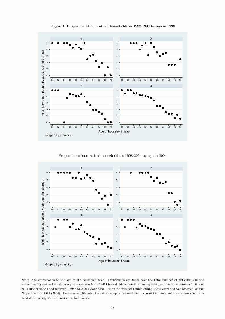
Figure 4: Proportion of non-retired households in 1992-1998 by age in 1998

0.2

.4.6

.81

0.2

.4.6

.81

0.2

.4.6

.81

0.2

.4.6

.81

50 52 54 56 58 60 62 64 66 68 70 50 52 54 56 58 60 62 64 66 68 70

50 52 54 56 58 60 62 64 66 68 70 50 52 54 56 58 60 62 64 66 68 70

1 2

3 4

% o

f non

−re

tired

peo

ple

by a

ge a

nd e

thni

c gr

oup

Age of household headGraphs by ethnicity

Proportion of non-retired households in 1998-2004 by age in 2004

.2.4

.6.8

1

.2.4

.6.8

1

.2.4

.6.8

1

.2.4

.6.8

1

50 52 54 56 58 60 62 64 66 68 70 50 52 54 56 58 60 62 64 66 68 70

50 52 54 56 58 60 62 64 66 68 70 50 52 54 56 58 60 62 64 66 68 70

1 2

3 4

% o

f non

−re

tired

peo

ple

by a

ge a

nd e

thni

c gr

oup

Age of household headGraphs by ethnicity

Note: Age corresponds to the age of the household head. Proportions are taken over the total number of individuals in thecorresponding age and ethnic group. Sample consists of HRS households whose head and spouse were the same between 1998 and2004 (upper panel) and between 1989 and 2004 (lower panel), the head was not retired during those years and was between 50 and70 years old in 1998 (2004). Households with mixed-ethnicity couples are excluded. Non-retired households are those where thehead does not report to be retired in both years.

57

Figure 5: Density estimates of age in 1998 by ethnicity and race

0

.05

.1

.15

Den

sity

50 55 60 65 70Age in 1995

Age Age if working Age if retired

kernel = epanechnikov, bandwidth = 1.1827

Mexican Americans

0

.05

.1

.15

Den

sity

50 55 60 65 70Age in 1995

Age Age if working Age if retired

kernel = epanechnikov, bandwidth = 1.2265

Other Hispanics

0

.05

.1

.15

Den

sity

50 55 60 65 70Age in 1995

Age Age if working Age if retired

kernel = epanechnikov, bandwidth = 0.8194

African Americans

0

.05

.1

.15

Den

sity

50 55 60 65 70Age in 1995

Age Age if working Age if retired

kernel = epanechnikov, bandwidth = 0.6880

Whites

Density estimates of age in 2004 by ethnicity and race

0

.05

.1

.15

.2

Den

sity

50 55 60 65 70Age in 2001

Age Age if working Age if retired

kernel = epanechnikov, bandwidth = 1.1353

Mexican Americans

0

.05

.1

.15

Den

sity

50 55 60 65 70 75Age in 2001

Age Age if working Age if retired

kernel = epanechnikov, bandwidth = 1.3326

Other Hispanics

0

.05

.1

.15

Den

sity

50 55 60 65 70Age in 2001

Age Age if working Age if retired

kernel = epanechnikov, bandwidth = 0.9883

African Americans

0

.05

.1

.15

Den

sity

50 55 60 65 70Age in 2001

Age Age if working Age if retired

kernel = epanechnikov, bandwidth = 0.7613

Whites

Note: Age corresponds to the age of the household head. Sample consists of HRS households whose head and spouse were the samebetween 1998 and 2004 (upper panel) and between 1989 and 2004 (lower panel), the head was not retired during those years andwas between 50 and 70 years old in 1998 (2004). House hods with mixed-ethnicity couples are excluded. Non-retired householdsare those where the head does not report to be retired in both years. Retired households are those where the head reports to beretired in at least one of those two years.

58