Noname manuscript No.(will be inserted by the editor)

Eulerian tour algorithms for data visualization and the PairViz package

C.B. Hurley and R.W. Oldford ?

November 4, 2008

Abstract PairViz is an R package that produces orderings of statistical objects for visualization purposes.

We abstract the ordering problem to one of constructing edge-traversals of (possibly weighted) graphs.

PairViz implements various edge traversal algorithms which are based on Eulerian tours and Hamiltonian

decompositions. We describe these algorithms, their PairViz implementation and discuss their properties and

performance. We illustrate their application to two visualization problems, that of assessing rater agreement,

and model comparison in regression.

1 Introduction

Visualization methods are important in the exploration, analysis and presentation of data. A carefully chosen

graphic creates a visual impression of the overall behaviour of a dataset or a model fit. At a more detailed

level, comparisons become important, for example, comparisons between variables, cases, groups, clusters

or models. A common practice is to lay out the objects in a line and compare them to one another on a

common aligned scale. Unfortunately, as the visual distance between the objects being compared increases,

the accuracy of the pairwise comparison decreases. This simple layout unwittingly favours comparisons

between adjacent objects and so favours n− 1 of the possible`n2

´pairwise comparisons.

In the visualization literature, a number of approaches have been taken to finding informative linear

orderings. These include (i) interactively picking and dropping objects to facilitate comparison (for example

Theus, [20], Yang et al [22]), (ii) sorting the objects on some characteristic (e.g. Cleveland [5], Theus [20],

Hofmann [12]) and (iii) seriating the objects so that nearby objects are similar (for example, Ankerst et al,

[3], Friendly and Kwan [9]) or more generally, where their comparison is “interesting” (Hurley [13]).

In Hurley and Oldford [14] we took a different though complementary approach to the visualization of

comparisons. We constructed visualizations which facilitated all`n2

´comparisons, by constructing sequences

where all pairs of objects appear adjacently. We also described a plethora of applications, ranging from

parallel coordinate displays to star glyphs, multiple comparisons and interaction plots, and our methodology,

which is based on graphs and graph traversal. All of these ideas are implemented in the R package PairViz,

which is the focus of the present paper.

The PairViz package offers functionality for constructing comparison sequences, and some new varieties

of graphics besides. In this paper, we focus on comparison sequences. However, all visualizations presented

in the present paper and in Hurley and Oldford [14] are provided by PairViz.

? Research supported in part by a Discovery Grant from the Natural Sciences and Engineering Research Council ofCanada., and by Research Frontiers Grant from Science Foundation Ireland.

C.B. HurleyDepartment of Mathematics, National University of Ireland, Maynooth, Co. Kildare, IrelandTel.: +353-1-7083792Fax: +353-1-7083913E-mail: catherine.hurley@nuim.ie

R.W. OldfordDepartment of Statistics and Actuarial Science, University of Waterloo, Waterloo, Ontario, Canada.

2

In Section 2 we begin with an introductory example where the goal is to compare and to relate variables.

Section 3 gives a synopsis of the relevant graph theory –[14] gives more details. Section 4 describes and gives

examples of PairViz functions for constructing comparison sequences, which are actually graph traversals.

The following Section 5 compares these functions, and should help in assessing which algorithm is appropriate

for the visualization task at hand. Section 6 explores the use of graph traversal in model selection for

regression, and finally we give concluding remarks in Section 7.

2 An introductory example

We start with a motivating example. The “diagnoses” data (Fleiss [8]) contains psychiatric diagnoses of 30

patients provided by 6 raters. The ratings are D=depression, PD= personality disorder, S= Schizophrenia,

N= Neurosis, O= Other. Figure 1 shows a parallel coordinate display, adapted for categorical data. There is

Rating psychiatric patients

1 2 3 4 5 6

D

PD

S

N

O

Fig. 1 Parallel coordinate plot of ratings. The black bars show each rater’s distribution of ratings.

one parallel axis for each of the six raters. The ratings are assigned nominal values of 1 for depression, 2 for

personality disorder and so on. Then, for each rater, coordinates are spread out vertically in an equispaced

fashion about the nominal value. Also, rather than 0-width axes as is usual in parallel coordinate displays, the

axes are given a small width so that on each axis, observations are represented by horizontal line segments.

The overlaid bars (shown in black) have bar length proportional to frequency and so give the distribution

for each rater. With this representation we can compare raters, and also the ratings given to a patient by

different raters. We see for instance that rater 6 never assigns a rating of “Other”, and he/she diagnoses

many of the patients categorized as “Other” by raters 1-5 as suffering from neurosis.

This adapted parallel coordinate display is similar to parallel sets, as proposed by Bendix et al [4].

Unwin et al [17] alternatively overlay circles with area proportional to frequency on the parallel axes to show

marginal distributions of categorical variables, while Wills [21] overlays marginal summary views on axes for

both categorical and continuous variables.

One problem with the visualization of Figure 1 is that it is clearly easier to assess agreement between

raters who appear on adjacent axes. The main theme of our research and the PairViz package is that

visualizations should facilitate all interesting comparisons. For the diagnoses data, this is achieved with a

parallel coordinate display where all pairs of raters appear adjacently, as shown in Figure 2.

The ordering for the axis was produced using the PairViz function eulerian, which will be described

in Section 4.4. But the main idea should be clear: all pairs of raters appear adjacently, and the pairs are

ordered in such a way that the raters whose agreement is higher tend to appear first. To verify that this is

the case, the barchart in the lower panel of Figure 2 traces the proportion of ratings that are in agreement

between each pair of raters. This display shows that there is good agreement between raters 3, 4 and 5.

Rater 6 has low agreement with all other raters, but especially with rater 1.

3

Rating psychiatric patients

5 4 3 5 2 1 3 2 4 2 6 3 1 4 6 5 1 6

D

PD

S

N

O

0.00.8

Fig. 2 Parallel coordinate plot of ratings, showing all pairs of raters adjacently. The black bars show each rater’sdistribution of ratings. The lower bar chart shows the agreement proportion for each pair of raters.

3 Brief Background

Our setup is as follows. The objects we want to order are identified with nodes of a graph. Undirected

edges are placed between nodes which we wish to compare. Edge weights indicate the importance of the

comparison, the smaller the edge weight the more important the comparison. In many applications we are

interested in all comparisons, in which case the graph is complete. Such a graph is denoted by Kn where n

is the number of nodes. Generally, we are interested in traversing the graph in such a way as to visit every

edge.

A path is called a Hamiltonian path if it visits all vertices of a graph exactly once. A path which contains

all of the edges of a graph, visiting each edge exactly once is called an Eulerian path (or Eulerian trail) and

if the path is closed then the traversal is called an Eulerian tour.

It is well known that if G is a connected graph, G has an Eulerian tour if and only if it is an even graph

(i.e. every vertex has an even number of edges). (This result goes back to Euler in 1763, and his solution to

the Bridges of Konigsberg problem). Furthermore, a connected graph G with exactly two odd nodes has an

open Eulerian trail starting and ending at the odd nodes. The graph K2m+1 is an even graph, and thus has

an Eulerian tour. (In fact , as discussed in Hurley and Oldford [14], it has an immense number of such tours).

Furthermore, it is possible to construct Eulerian tours on K2m+1 which are Hamiltonian decompositions,

that is, composed entirely of edge-distinct Hamiltonian cycles.

The graph K2m is not an even graph, in fact all of its vertices have an odd number of edges. It follows

that K2m does not have an Eulerian path. Any path that visits all of the edges will have to visit some edges

more than once. Our constructions produce edge-traversals on K2m which are “nearly Eulerian” by adding

m− 1 extra edges to K2m in such a way that 2m− 2 of the nodes are even and two are odd. We denote this

extended version of K2m by Ke2m. Then an open euler path exists on Ke

2m, travelling from one odd node to

the other, visiting all edges along the way.

Since K2m is not Eulerian it does not have a decomposition into edge-distinct Hamiltonian cycles.

However, it is possible to decompose K2m into edge-distinct Hamiltonian paths, rather than cycles. Here are

some general results about Hamiltonian cycle or path decompositions on the complete graph. Kn can be

decomposed as follows:

(lw-odd-cycle) For n = 2m + 1, into m Hamiltonian cycles, or

(lw-odd-path) m Hamiltonian paths and an almost-one factor.

(lw-even-path) For n = 2m, into either m Hamiltonian paths, or

(lw-even-cycle) m− 1 Hamiltonian cycles and a one-factor (or perfect matching).

These are known as Lucas-Walecki decompositions (Lucas, [16]; also Alspach, et al [2]).

In the following sections, we will refer to constructing Eulerians on Kn. Strictly speaking, for even

n = 2m the path is only a nearly Eulerian path on K2m but is a proper open Eulerian path on Ke2m.

4

4 Constructing Eulerians

The PairViz package has four functions for constructing Eulerians. The first, hpaths, produces Hamil-

tonian decompositions on complete graphs. The second method, weighted hpaths, produces Hamiltonian

decompositions on weighted complete graphs, where the Hamiltonians are roughly weight increasing. The

third method is a recursive algorithm which produces Eulerians (not based on Hamiltonians) on complete

graphs, and this is implemented in the function eseq. Finally, we describe the function etour, for producing

weight-increasing Eulerians on weighted graphs.

4.1 Hamiltonian decompositions on complete graphs

Lucas-Walecki constructions provide a method for constructing all four varieties of decomposition on Kn

described in the previous section. In [14]we described constructions for the decompositions lw-odd-cycle and

lw-even-path only, but in the PairViz package, all four decompositions are available.

Our basic work horse is the zigzag function. This function yields an n × m matrix with m = dn/2e,where each row is a Hamiltonian on Kn. For example, see the following results:

> zigzag(6)

[,1] [,2] [,3] [,4] [,5] [,6]

[1,] 1 2 6 3 5 4

[2,] 2 3 1 4 6 5

[3,] 3 4 2 5 1 6

> zigzag(7)

[,1] [,2] [,3] [,4] [,5] [,6] [,7]

[1,] 1 2 7 3 6 4 5

[2,] 2 3 1 4 7 5 6

[3,] 3 4 2 5 1 6 7

[4,] 4 5 3 6 2 7 1

Note that when the n vertices are arranged clockwise around a circle, each row follows a zig-zag path starting

with node i. In general zigzag(2m) produces the decomposition lw-even-path, and zigzag(2m + 1) yields

lw-odd-path. Notice for example that the last row of zigzag(7) duplicates edges (4,5), (3,6) and (2,7) from

the first row. The other edges (5,3), (6,2) and (7,1) are the almost-one factor.

We mention one early application of the zig-zag construction in statistical graphics. Wegman [18] pro-

duced m = dn/2e different parallel coordinate displays of n−variable data, where the ith display used the

variable permutation given by the ith row of zigzag(n).

To get a Hamiltonian cycle decomposition, notice zigzag(6) has each of 1, . . . , 6 as endpoints of the

rows. Therefore, binding a column of 7’s to zigzag(6) produces a Hamiltonian cycle decomposition on K7.

Similarly, binding a column of 8’s to zigzag(7), yields 3 edge-disjoint Hamiltonian cycles in the first 3 rows,

with the last row containing a one-factor (perfect matching). In general, cbind(n, zigzag(n-1)) produces

the cycle decompositions lw-odd-cycle and lw-even-cycle. In our implementation, however, we use instead

cbind(1, 1+ zigzag(n-1)) so that all four decompositions start with 1.

The hpaths function produces each of the four decompositions detailed above. Cycles or paths are

requested via the argument cycle. The default behaviour is for hpaths to produce the exact decomposition,

i.e. cycles for odd n and paths for even n. For example, hpaths(7) produces decomposition lw-odd-cycle:

> hpaths(7)

[,1] [,2] [,3] [,4] [,5] [,6] [,7]

[1,] 1 2 3 7 4 6 5

[2,] 1 3 4 2 5 7 6

[3,] 1 4 5 3 6 2 7

When the rows of hpaths(7) are glued together and a final 1 added to close the path, we have an

Eulerian tour on K7. Invoking hpaths with the matrix=FALSE option produces the tour.

> hpaths(7,matrix=FALSE)

[1] 1 2 3 7 4 6 5 1 3 4 2 5 7 6 1 4 5 3 6 2 7 1

5

As described above, hpaths(6) produces the decomposition lw-even-path as given by zigzag(6), and

when the paths, that is the rows, are joined together the joining edges are now visited twice. In fact

hpaths(6,matrix=FALSE) gives an Eulerian path not on K6 but on the amended graph Ke6 . In general

the duplicated edges are (j, j + m− 1), j = 2, . . . , m for the graph K2m.

Other isomorphic decompositions are obtained by supplying the first Hamiltonian as an argument to

hpaths. Then all node labels are rearranged accordingly, as in the following example:

> hpaths(1:7)

[,1] [,2] [,3] [,4] [,5] [,6] [,7]

[1,] 1 2 3 4 5 6 7

[2,] 1 3 5 2 7 4 6

[3,] 1 5 7 3 6 2 4

4.2 Hamiltonian decompositions on weighted complete graphs

For weighted graphs our goal is an ordered Eulerian T where weights tend to increase as the sequence pro-

gresses. In [14] we proposed an algorithm (referred to as WHam) that builds such paths out of Hamiltonians.

In PairViz the WHam algorithm is implemented by the function weighted hpaths. This function takes an

array of Hamiltonians h of size n×m say, such as that produced by hpaths. The weighted hpaths function

attempts to pick the best of various rearrangements of this array. We describe the procedure for a cycle

decomposition, the modifications for path decompositions are given in parentheses.

1. Find the Hamiltonian cycle (path) with the smallest total weight. (Or course, finding the overall best

Hamiltonian is NP hard, so approximate solutions are generally used). The best direction and starting

point of the cycle (direction only for paths) is obtained by using a correlation measure on the weights to

measure their tendency to increase.

2. The optimized Hamiltonian is placed in the first row of h, and node labels in other rows are permuted

using this relabeling.

3. Again using correlation, the best direction is chosen for the cycles (paths) in rows 2, . . . , m of h.

4. Finally, the cycles (paths) are sorted in order of increasing correlation.

An example of the use of weighted hpaths will be given in Section 5.

4.3 Eulerians on complete graphs, a recursive algorithm

Next we describe an algorithm eseq which recursively builds up an Eulerian on Kn. We have not previously

seen this algorithm in the literature, but it has some interesting properties, visiting edges in an “increasing”

order.

Suppose we can construct an Eulerian on Kn−2. Consider the graph K+ with edges (j, n− 1), (j, n) for

j = 1, 2, . . . , n − 2 and n − 1, n. This graph is illustrated in Figure 3 for the n = 7 and n = 6 cases. An

Eulerian on Kn must visit all of the edges of the graph K+ in addition to those visited by the Eulerian on

Kn−2. The eseq construction forms an Eulerian on Kn by appending Eulerians on Kn−2 and K+.

To see how this works, first consider the n odd setting. An Eulerian tour on K1 is trivially eseq(1) = 1.

Suppose now that eseq(n-2) gives an euler tour on Kn−2, starting and ending with 1. Here n is odd and so

the graph K+ is even, as illustrated in first graph shown in Figure 3. We form an Eulerian tour on K+ by

interleaving n− 1 and n consecutively between elements of the sequence 1, 2, . . . , n− 2, and then appending

n − 1, n, 1. That is, Tnew = 1, n − 1, 2, n, 3, n − 1, 4, n, 5, . . . , n − 3, n, n − 2, n − 1, n, 1. This path is joined

on to eseq(n-2), resulting in an Eulerian tour on Kn. (Note that since the last vertex visited by eseq(n-2)

coincides with the first vertex of Tnew, this leading vertex of Tnew is omitted from the Eulerian on Kn). For

example, here are eseq(5) and eseq(7).

> eseq(5)

[1] 1 2 3 1 4 2 5 3 4 5 1

> eseq(7)

[1] 1 2 3 1 4 2 5 3 4 5 1 6 2 7 3 6 4 7 5 6 7 1

6

1 2 3 4 5

6 7

1 2 3 4

5 6

Fig. 3 A graph K+ with edges (n− 1, n) and (j, n− 1), (j, n) for j = 1, 2, . . . , n− 2 illustrated for n = 7 and n = 6.Append Eulerians on Kn−2 and K+ to form a Eulerian on Kn.

For the n even case, the process is initiated with an open Eulerian path on K2, that is, eseq(2) = 1, 2.

Now suppose we have eseq(n-2) which is an Eulerian on Kn−2 starting with 1 and ending with n−2. Here n

is even and so the graph K+ has exactly two odd nodes, namely n−1 and n, as illustrated in the right hand

side graph shown in Figure 3. We form an Eulerian path on K+ with the odd nodes as end points, by starting

with n− 1 and then interleaving n and n− 1 consecutively between elements of the sequence 1, 2, . . . , n− 2,

and then appending n−1, n. That is, join Tnew = n−1, 1, n, 2, n−1, 3, n, 4, . . . , n−3, n, n−2, n−1, n, onto

eseq(n-2) to produce eseq(n). Since the endpoints of eseq(n-2) and Tnew differ, the join implicitly adds

another edge, namely (n−2, n−1), and this edge is visited again in Tnew. Therefore, strictly speaking eseq(n)

forms an open Eulerian path on Ken, where Ke

n is formed by adding additional edges between (j, j + 1), for

j = 2, 4, 6, . . . , n− 2 to the complete graph Kn. Here we illustrate the results for eseq(4) and eseq(6).

>eseq(4)

[1] 1 2 3 1 4 2 3 4

> eseq(6)

[1] 1 2 3 1 4 2 3 4 5 1 6 2 5 3 6 4 5 6

From its construction, we can see that the Eulerian produced by eseq(n) has the following two properties.

Since the constructions are slightly different for the odd and even n cases, we will refer to them as eseq-odd

and eseq-even in the following paragraphs. Proofs are provided in the Appendix.

Property 1 For odd n, eseq-odd(n) has length En =`n2

´+ 1. The first Ek elements gives eseq-odd(k), for

k = 1, 3, 5, . . . , n− 2.

For even n, eseq-even(n) has length En = n2/2. The first Ek elements gives eseq-even(k), for k =

2, 4, . . . , n− 2.

Property 2 Consider two nodes i < j, and an integer k ≥ 1. In most cases the eseq-odd and eseq-even

sequences vist the edge (i− k, j) before (i, j) and the visit to (i, j) preceeds a visit to (i, j + k).

We mention two other possible constructions for the n even case. First, start with any Eulerian on Kn+1

and delete all instances of n + 1. This creates a closed path on Kn with n/2 of the edges visited twice.

Deleting one of these duplicated edges provides an open Eulerian path on Ken.

The second construction starts with any Eulerian on Kn−1 and simply inserts at a visit to node ‘1’ the

detour 1, n, 2, 3, n, 4, 5, . . . , n− 2, n− 1, n. This detour is an open Eulerian path on the graph K+ with edges

(j, n), j = 1, 2, . . . , n− 1, and (j, j + 1), j = 2, 4, . . . , n− 2. (Of course any Eulerian on K+ would do just as

well). The nice feature of this second construction is that when the detour is inserted at the end, duplicated

edges appear only in the last section of the Eulerian. These strategies are implemented in kntour drop and

kntour add. Note that when these functions are applied to the results of eseq, they give the same result.

Below we see the result of kntour add(eseq(5)) which is identical to kntour drop(eseq(7)).

> eseq(5)

[1] 1 2 3 1 4 2 5 3 4 5 1

> kntour_add(eseq(5))

7

[1] 1 2 3 1 4 2 5 3 4 5 1 6 2 3 6 4 5 6

Note that if the detour is inserted into the middle of an Eulerian on Kn−1, the situation is slightly more

complicated. Consider inserting 16235456 at the second occurrence of ‘1’ in eseq(5). The path becomes

12316236456 14253451 where the detour is underlined. Since the detour does not return to ‘1’ the path

breaks between 6 and 1 and is reported as 1425345112316236456.

4.4 Eulerians on general weighted graphs

A classical algorithm for constructing Eulerian tours or open Eulerian paths is due to Hierholzer [11]. In [14]

we described this algorithm and also a modification (referred to as algorithm GrEul) for weighted graphs.

Here we discuss the PairViz implementation.

The standard algorithm for Eulerian tours on even graphs builds up the path by starting from an

arbitrarily chosen node, and following unvisited edges until no further moves are possible, giving a closed

path T . Then starting from a node with unvisited edges, continue to follow unvisited edges, yielding a cycle

which is spliced into T . This step is repeated until all edges are visited once. With the GrEul algorithm

[14] for weighted graphs, the lowest weight available edge is chosen at each stage. The starting node is also

chosen from one of the two nodes adjacent to the lowest weight edge.

In PairViz, the function etour implements the Hierholzer algorithm and its counterpart (GrEul) for

weighted graphs. For this we need a data structure which represents a graph. We use the graphNEL class

from package graph (Gentleman et al [10]).

(As an aside, there are now a number of implementations of graphs available for R. In fact, we used the

igraph package (Csardi [6]) to produce all graph drawings in this paper.)

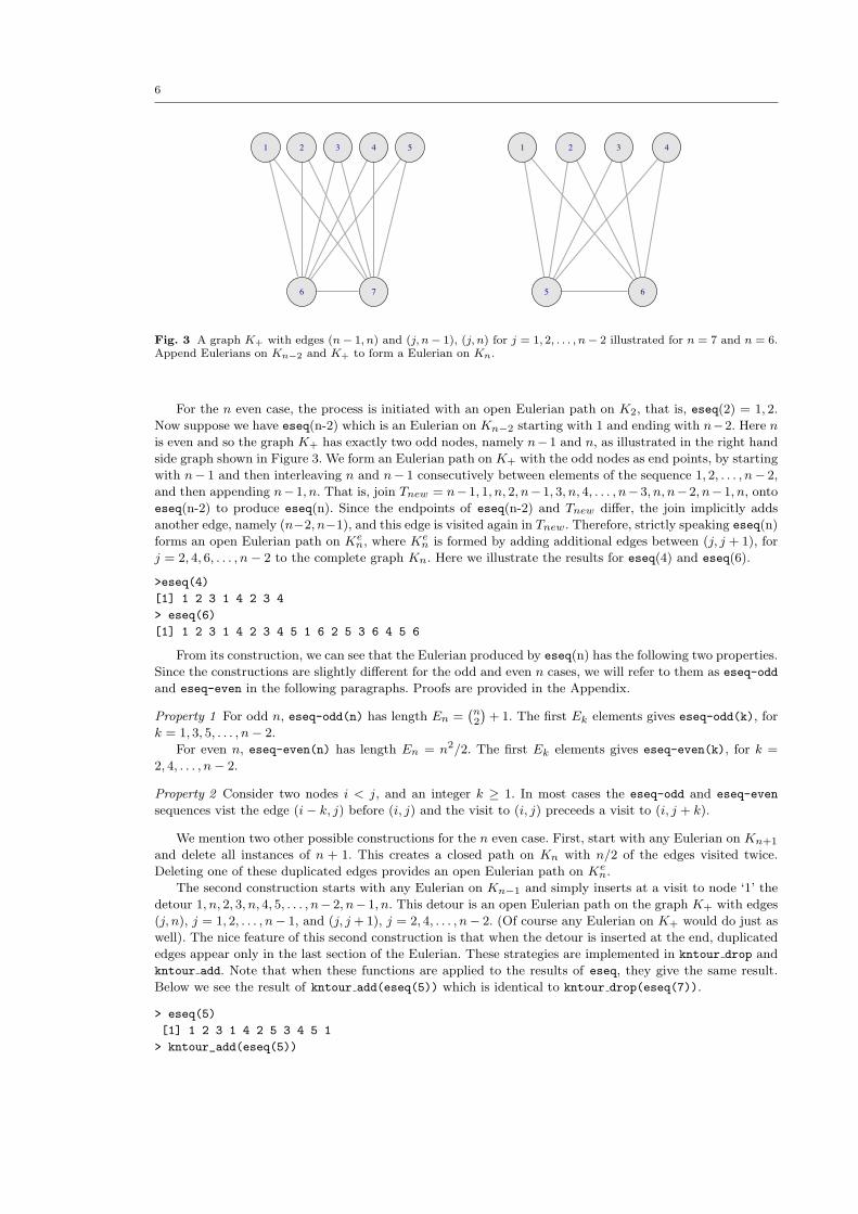
Figure 4 and the adjacent code illustrates the construction of a weighted graph.

> n <- LETTERS[1:5]> g <- new("graphNEL",nodes=n)> g <- addEdge(n[1],n[2:3],g,8:9)> g <- addEdge(n[2],n[3:5],g,5:7)> g <- addEdge(n[4],n[5],g,1)> etour(g,weighted=FALSE)[1] "A" "B" "D" "E" "B" "C" "A"> etour(g)[1] "E" "D" "B" "C" "A" "B" "E"

8

9

5

6 7

1

A

B

C

D E

Fig. 4 A weighted graph which is even.

When etour is invoked with weighted=FALSE, the tour starts at the first node of the graph, and always

visits the first available edge. Therefore nodes are visited in order ABCA, reaching a dead end at the second

visit to node A. The algorithm then restarts from B, the last visited node with unused edges, and visits

BDEB, and this path replaces the B in ABCA, giving ABDEBCA.

With weighted=TRUE (the default), the tour starts with edge ED, which is the lowest weight edge in the

graph. Here E is chosen over D as the starting node because the next lowest weight edge emanating from D

has lower weight than the next lowest weight edge emanating from E. In this case, the algorithm follows the

lowest weight edge at each stage, and manages to visit all edges before reaching the dead end.

For the construction of complete graphs, the PairViz package provides the generic function mk complete graph,

which builds a complete graph from a distance matrix (a dist or a symmetric matrix), or with a specified

number of vertices. The following demonstrates the result of etour on K5.

> etour(mk_complete_graph(5))

[1] "1" "2" "3" "1" "4" "2" "5" "3" "4" "5" "1"

8

In the above example, the nodes are ordered numerically, so the algorithm always visits the lowest numbered

node available.

Now we shift our focus to graphs where all nodes are not even. For graphs with some odd nodes, it is

always possible to form a similar graph which is even. It is a well-known result from graph theory that the

number of odd nodes of a graph is even. Using this fact, it is clear that adding additional dummy edges

between pairs of odd nodes will produce an even graph. An alternative option would be to augment the

graph by adding an extra dummy node with edges to each of the odd nodes, but Eulerian tours from such

a graph would include this dummy node.

PairViz provides a function mk even graph which constructs an even graph from a graphNEL of a con-

nected graph (or a distance matrix, or with a specified number of vertices). by adding extra edges between

pairs of odd nodes. Figure 5 illustrates the process. In this example, the graph has five nodes only one of

A

B C

D

E

A

B C

D

E1 3

44

5

22

6

A

B C

D

E

Fig. 5 In graph(a) C is the only even node. In (b), extra dummy edges (shown in the black dotted line) are (A,E)and (B,D), so the graph is even. In (c), the graph is weighted, and the dummy edges are (A,D) and (B,E).

which (C) has an even number of edges. In Figure 5(b) odd nodes are paired off A with E and B with D

and new edges are added. In the resulting graph, all nodes are now even.

An Eulerian tour on the graph of Figure 5(b) starting from A also ends with A. However, as the edge

(E,A) is the last edge visited by the tour, the etour algorithm recognizes that this edge is one of those

added by mk even graph, and as such does not require a visit. The tour is broken at this edge so the result

is actually an open Eulerian path. Here is the result of etour on the graph gb of Figure 5(b). Note assuming

nodes are in lexicographical order, the first node (here node A) is the default starting point for the Eulerian.

> etour(gb)

[1] "A" "B" "D" "A" "C" "D" "B" "E"

More precisely, the result of etour(gb) is an open Eulerian path on the graph with the dummy edge

(A,E) deleted. While Eulerian tours exist for even graphs only, open Eulerian paths exist for graphs with

exactly two odd nodes. These open paths travel from one odd node to the other, visiting all edges along the

way. The etour algorithm take advantage of this fact. When the start node has a dummy edge, say (start,

target), this edge is ignored by the edge traversal algorithm. The result is an open Eulerian path, traveling

from the start node to the target node.

For the graph of Figure 5(a) the four odd nodes can be paired in three different ways. Figure 5(b)

illustrates our pairing strategy for unweighted graph, that is, pair the first odd node with the last, and the

other odd nodes in consecutive pairs. For complete graphs where the number of nodes n is even, this pairing

strategy adds edges (1,n) and (j, j + 1) for j = 2, 4, . . . , n− 2. Then the default etour path starts at node 1

and ends at node n.

> etour(mk_even_graph(6))

[1] "1" "2" "3" "1" "4" "2" "5" "1" "6" "2" "3" "4" "5" "3" "6" "4" "5" "6"

When the graph is weighted, the goal is Eulerian paths with edge weights tending to increase. So the

pairing process used by mk even graph assists in this goal by pairing the default start node with the odd

node with the highest average weight, which becomes the target node of the Eulerian path. Figure 5(c)

9

illustrates the pairing process for a weighted graph. Here node A is the default starting point for the tour

as it is attached to the lowest weight edge (node A is preferred over node B because the next lowest weight

edge emanating from B has lower weight than the next lowest weight edge emanating from A). Our strategy

pairs A with the odd node with the highest average weight, which is node D in this instance. This leaves

nodes B and E as the other pair. Here we have the results of etour on the graph gc of Figure 5(c).

> etour(gc)

[1] "A" "B" "E" "B" "D" "A" "C" "D"

> etour(gc,start="C")

[1] "C" "A" "B" "E" "B" "D" "A" "D" "C"

When no starting point is specified, A is the default start, which the pairing process partners with node

D. Starting from A, etour forms an open path ending at D. However when C is specified as a starting node,

none of its edges are duplicates, so etour forms a tour beginning and ending at C.

As described above, the function etour produces an Eulerian on even graphs. The generic function

eulerian provides a useful wrapper: it builds an even graph (actually a subclass of graphNEL) from a

graphNEL, distance matrix, or from the complete graph with a specified number of nodes, and invokes etour

on the even graph created.

The strategy of pairing off the odd nodes in order to construct an Eulerian tour is well-known in graph

theory, and arises in the so-called Chinese postman problem (Edmonds and Johnson [7]) . The Chinese

postman problem is to find the shortest tour that visits every edge at least once. For the graph of Figure

5(a), with weights as in (c), an Eulerian tour of the graph shown in (c) is the solution. Other pairings of the

odd nodes would not be allowed, as they add new edges rather than duplicating existing edges. An improved

version of mk even graph would make use of the algorithm of Edmonds and Johnson [7] which solves the

Chinese postman problem.

5 Comparison of algorithms

In the previous sections we described four methods for constructing Eulerians. The first three, hpaths,

weighted hpaths and eseq construct Eulerians on Kn only, while the function eulerian is appropriate for

connected graphs. Table 1 summarizes these properties.

Table 1 Properties of four algorithms

Algorithm Graph Hamiltonians Weights

eseq complete no nohpaths complete yes noweighted hpaths complete yes yeseulerian connected no optional

First, a word about efficiency. Since Kn has O(n2) edges, any Eulerian algorithm on Kn must be at least

O(n2) . In fact all of the algorithms for constructing unweighted Eulerians are O(n2). For weighted hpaths

finding the best Hamiltonian in the first step of the algorithm given in Section 4.2 is the bottleneck. With

the eulerian function on weighted graphs, the cost associated with constructing an ordered Eulerian must

include the cost of an edge sort at each vertex, and so has overall order on Kn of O(n2 log n).

However these bounds are not the full story. In practice eseq is substantially faster than the eulerian

function, even when weights are ignored. For example, on K60 eulerian takes about 30 seconds while eseq

takes 1/1000 of a second on a Mac 2.1 GHz powerbook. It would seem that for this application graphNEL is

not an efficient choice of data structure.

For unweighted complete graphs with n vertices, PairViz offers 3 choices, hpaths(n), eseq(n) or

eulerian(n). The algorithm hpaths produces Hamiltonians, so occurrences of nodes are spread out more or

less uniformly throughout the path. As explained in Section 4.3, eseq visits edges between low order nodes

first, which might be advantageous if there were are a lot of nodes and the low order ones and visits between

them are more important. The sequence produced by eulerian(n) is quite similar to that given by eseq(n).

10

> eseq(7)

[1] 1 2 3 1 4 2 5 3 4 5 1 6 2 7 3 6 4 7 5 6 7 1

> eulerian(7)

[1] 1 2 3 1 4 2 5 1 6 2 7 3 4 5 3 6 4 7 5 6 7 1

The graph-based algorithm (when there are no weights) visits the next available node, which is the lowest-

index available node since the nodes are ordered 1, . . . , n. Essentially, eseq is based on an ordering of edges

while eulerian uses etour which for unweigted graphs is based on an ordering of nodes. This behaviour is

illustrated in Figure 6 which shows time traces of the sequences produced by the three algorithms.

0 5 10 15 20 25 30

12

34

56

78

Eseq 8

x

0 5 10 15 20 25 30

12

34

56

78

Etour 8

x

0 5 10 15 20 25 30

12

34

56

78

Hpaths 8

0 5 10 15 20 25 30 35

24

68

Eseq 9

x

e1

0 5 10 15 20 25 30 35

24

68

Etour 9

x

e2

0 5 10 15 20 25 30 35

24

68

Hpaths 9

e3

Fig. 6 Traces of the Eulerians on K8 and K9 generated by the three functions eseq, hpaths and (un-weighted)eulerian.

For weighted complete graphs PairViz offers a choice between the functions weighted hpaths and

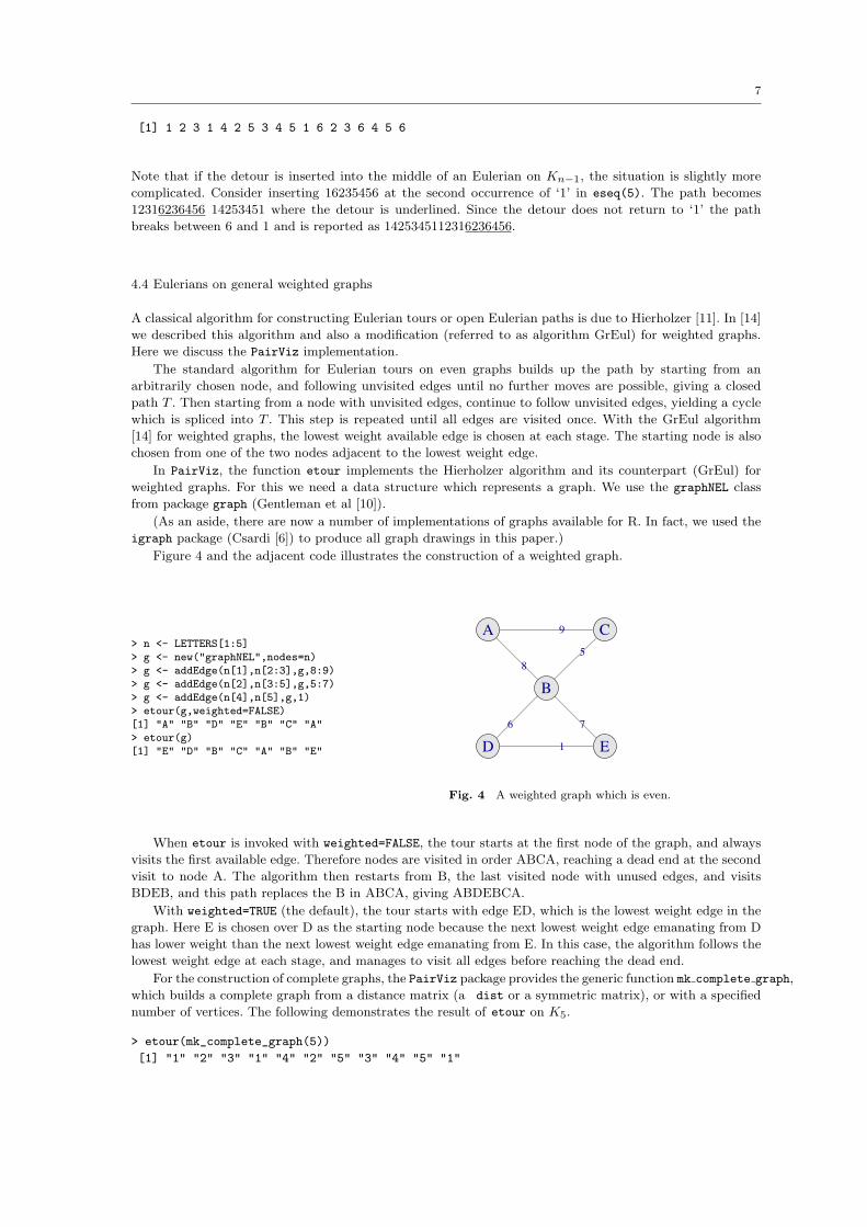
eulerian. Figure 7 shows traces of the distances in eurodist (part of the standard R release) as ordered

by Eulerians on K21 produced by the functions eseq, eulerian and weighted hpaths. As expected the

distances in the first trace show no particular pattern, while those in the weighted Eulerian trace have a

generally increasing pattern. In this setting weighted hpaths is not so successful, but given that eurodist

consists of distances between 21 European cities, this is not so surprising.

6 A model example

In this section we outline the use of Eulerians for regression model comparison.

We will use the well-known sleep data (Allison and Cicchetti [1]), with four predictors A= non dreaming

sleep, B= dreaming sleep, C=log body weight and D=maximum life span and a response of log brain weight

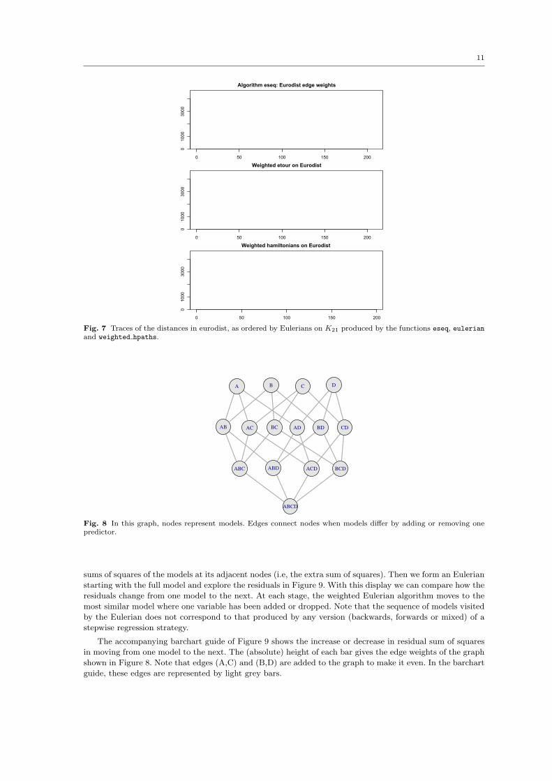
recorded for 45 mammal species. (Species with missing data are omitted). Figure 8 represents model choices

by nodes of a graph. Edges connect nodes whose models differ by adding or removing one predictor. Only

nodes representing single predictor models have an odd number of edges, so just two extra edges are necessary

for an even graph.

Stepwise regression algorithms begin with the full model (or the best single predictor model), and re-

peatedly remove (or add) predictors. The edges in the graph of Figure 8 shows the set of possible moves in

a stepwise regression algorithm. Edge weights (not shown) are given by the absolute difference in residual

11

0 50 100 150 200

01000

3000

Algorithm eseq: Eurodist edge weights

1:length(pw)

0 50 100 150 200

01000

3000

Weighted etour on Eurodist

1:length(pw)

0 50 100 150 200

01000

3000

Weighted hamiltonians on Eurodist

Fig. 7 Traces of the distances in eurodist, as ordered by Eulerians on K21 produced by the functions eseq, eulerianand weighted hpaths.

A B C D

AB AC ADBC BD CD

ABC ABD ACD BCD

ABCD

Fig. 8 In this graph, nodes represent models. Edges connect nodes when models differ by adding or removing onepredictor.

sums of squares of the models at its adjacent nodes (i.e, the extra sum of squares). Then we form an Eulerian

starting with the full model and explore the residuals in Figure 9. With this display we can compare how the

residuals change from one model to the next. At each stage, the weighted Eulerian algorithm moves to the

most similar model where one variable has been added or dropped. Note that the sequence of models visited

by the Eulerian does not correspond to that produced by any version (backwards, forwards or mixed) of a

stepwise regression strategy.

The accompanying barchart guide of Figure 9 shows the increase or decrease in residual sum of squares

in moving from one model to the next. The (absolute) height of each bar gives the edge weights of the graph

shown in Figure 8. Note that edges (A,C) and (B,D) are added to the graph to make it even. In the barchart

guide, these edges are represented by light grey bars.

12

Sleep data: Model residuals.

ABCD ABD AD ACD ABCD BCD CD D BD BCD BC C AC ABC AB A AC ACD CD C A AD D B AB ABD BD B BC ABC ABCD

Fig. 9 Parallel coordinate display of model residuals. Barchart guide shows increase or decrease in residual sum ofsquares in moving from one model to the next. The light gray bars indicate model changes which do not correspondto adding or dropping a predictor.

In Figure 9 we see that the residuals for the first 10 models visited appear to change very little. The first

big increase in the residual sum of squares occurs when model AB is visited. This is the first model visited

which does not include predictor C= body weight, and in fact all models with body weight as a predictor are

included in the first 10 nodes visited. A revised plot which zooms in on the first 10 axes will explore these

models in more detail, or alternatively, one could construct an Eulerian on the graph obtained by removing

nodes whose models do not include predictor C.

Unwin et at [17] demonstrate comprehensively the value of parallel coordinate displays in exploratory

modeling analysis. They use axis orderings which visit all one-predictor models, then all two-predictor models

and so on. Eulerian tours of model space are a useful addition to the model exploration toolkit. With them

we can see precisely how model summaries change as predictors are added or dropped. In this example we

chose residuals and their sum of squares as our model summaries, but other quantities could equally well be

adopted.

7 Concluding remarks

The PairViz package is for pairwise visualization and comparison of statistical objects, using Hamiltonian

decompositions and Eulerian paths. In this paper, we focused on the various algorithms for Hamiltonian

decompositions and Eulerians.

However, this methodology leads to deeper insight of some conventional statistical graphics, and brings

home to the data analyst how the choice of Hamiltonian in a visualization confounds the interpretation. The

raters example in Section 2 illustrates this. Hurley and Oldford [14] give other examples, namely interaction

plots for a two-factor experiment, and the use of star glyphs for visually clustering cases.

Our methodology leads to enhanced versions of conventional statistical displays, specifically, the parallel

coordinate display with accompanying barchart guide, as shown in Figures 2 and 9. This display is available

via the guided pcp function in PairViz. In [14] we use guided pcps to look at scagnostics (Wilkinson et al,

[19]) of pairwise variable displays.

Shifting the focus of a visualization to showing the comparison between objects led us to a new graphical

method for multiple pairwise comparison of treatment groups [14]. This new visualization is available via

the mc plot function in PairViz.

The basic notion that graphs and graph traversals are a useful model for data visualization also suggests

new ways of looking at dynamic graphics (Hurley and Oldford, [15]).

13

8 Appendix

Property 1 For odd n, eseq-odd(n) has length En =`n2

´+ 1. The first Ek elements gives eseq-odd(k),

for k = 1, 3, 5, . . . , n − 2. For even n, eseq-even(n) has length En = n2/2. The first Ek elements gives

eseq-even(k), for k = 2, 4, . . . , n− 2.

Proof For odd n, eseq-odd(n) is by construction an Eulerian on the graph Kn. This graph has`n2

´edges,

all of which are visited exactly once by a sequence of length`n2

´+ 1.

For even n, eseq-even(n) is by construction an Eulerian on the graph Ken. The graph Kn has

`n2

´edges, and Ke

n an additional (n − 2)/2 edges all of which are visited exactly once by a sequence of length`n2

´+ (n− 2)/2 + 1 = n2/2.

Property 2 Consider two nodes i < j, and an integer k ≥ 1. In most cases the eseq-odd and eseq-even

sequences vist the edge (i− k, j) before (i, j) and the visit to (i, j) preceeds a visit to (i, j + k).

Proof First, we consider the eseq-odd sequence.

The edge (i, j) is visited before (i, j + k) when j is odd, and k ≥ 1. This is because (i, j) is an edge in

Kj and so occurs in eseq-odd(j), while (i, j + k) is not an edge in Kj and is visited by an extension of

eseq-odd(j).

Similarly, when j is even, (i, j) occurs in eseq-odd(j+1), while for k ≥ 2, (i, j +k) occurs in an extension

of eseq-odd(j+1). Actually, checking the formulation for Tnew, we can see that for i = 1, or even, (i, j) is

visited before (i, j + 1).

Furthermore, except for the closing ‘1’ at the end of Tnew, the Tnew sequence visits nodes 1, 2, . . . , n− 2

in order, and so edge (i− k, j) is visited before (i, j) for k ≥ 1, except when i− k = 1 and j is odd. In this

j odd case, edge (1, j) is visited after edge (k, j) for k = 2, 3, . . . , j − 1.

Next, we consider the eseq-even sequence.

The edge (i, j) is visited before (i, j + k) when j is even, and k ≥ 1. This is because (i, j) is an edge in

Kj and so occurs in eseq-even(j), while (i, j + k) is not an edge in Kj and is visited by an extension of

eseq-even(j).

Similarly, when j is odd, (i, j) occurs in eseq-even(j+1), while for k ≥ 2, (i, j +k) occurs in an extension

of eseq-even(j+1). However, from the construction of Tnew, we can see that for odd i only, (i, j) is visited

before (i, j + 1).

Again, by inspecting the Tnew sequence, which visits nodes 1, 2, . . . , n− 2 in order, we see that (i− k, j)

is visited before (i, j) for k ≥ 1. However, for odd j, edge (j − 1, j) is visited twice. The first visit is the

joining edge between eseq-even(j-1) and eseq-even(j+1) and this visit occurs before visits to (k, j), for

k = 1, 2, . . . , j − 2.

References

1. Allison, T. and Cicchetti, D. (1976) “Sleep in Mammals: Ecological and Constitutional Correlates”, Science, 194,pp. 732-734.

2. Alspach, B, J.-C. Bermond and D. Sotteau (1990) “Decomposition into cycles I: Hamilton decompositions”, inCycles and Rays (eds. G. Hahn, G, Sabidussi, and R.E. Woodrow), Kluwer Academic Publishers, Boston.

3. Ankerst, M., S. Berchtold and Keim D. A. (1998) “Similarity Clustering of Dimensions for an Enhanced Visual-ization of Multidimensional Data”, Proceedings: IEEE Symposium on Information Visualization, pp. 52-60.

4. Bendix, F., R. Kosara and H. Hauser (2005) “Parallel Sets: Visual Analysis of Categorical Data”, INFOVIS ’05:Proceedings of the Proceedings of the 2005 IEEE Symposium on Information, pp 1-18.

5. Cleveland, W.S. (1995) Visualizing Data, Summit, NJ:Hobart Press.6. Csardi, G. (2008) The igraph package. http://www.r-project.org.7. Edmonds, J. and Johnson, E. L. (1973) “Matching, Euler Tours, and the Chinese Postman.” Mathematical Pro-

gramming, 5, pp. 88-1248. Fleiss, J.L. (1971) “Measuring nominal scale agreement among many raters”, Psychological Bulletin, 76, 378-382.9. Friendly, M. and Kwan, E. (2003) “Effect Ordering for Data Displays”, Computational Statistics and Data Analysis,

43, 509-539.10. Gentleman, R., E. Whalen, W. Huber, S. Falcon (2007) The graph package. http://www.r-project.org.

11. Hierholzer, C. (1873) “Uber die Moglichkeit, einen Linienzug ohne Wiederholung und ohne Unterbrechung zuumfahren”. Math. Annalen, VI, pp. 30-32.

12. Hofmann, H. (2006) “Multivariate categorical data–mosaic plots”, In Graphics of large datasets, visualizing amillion, eds. A. Unwin, M. Theus, H. Hofmann. Springer-Verlag.

13. Hurley, C. (2004) “Clustering Visualizations of Multidimensional Data”, Journal of Computational and GraphicalStatistics, vol. 13, (4), pp 788-806, 2004.

14

14. Hurley, C. and R.W. Oldford (2008) “Pairwise display of high dimensional information via Eulerian tours andHamiltonian decompositions”, submitted.

15. Hurley, C. and R.W. Oldford (2008) “Graphs as navigational infrastructure for high dimensional data spaces”,submitted.

16. Lucas, D.E. (1892) Recreations Mathematiques, Vol. II, Gauthier Villars, Paris.17. Unwin, A, C. Volinsky and S. Winkler (2003) “Parallel coordinates for exploratory modelling analysis”’, Compu-

tational Statistics and Data Analysis, vol 43, pp. 553–564 .18. Wegman, E.J. (1990) “Hyperdimensional data analysis using parallel coordinates”, Journal of the American

Statistical Association, 85, pp. 664-675.19. Wilkinson, L., Anand, A. and Grossman, R. (2005) “Graph-theoretic scagnostics”, Proceedings of the IEEE

Information Visualization 2005, pp. 157-164.20. Theus, M. (2002) “Interactive Data Visualization using Mondrian”,Journal of Statistical Software , vol 7, issue

11.21. Wills, G. (2000) “A good, simple axis”, Statistical computing and statistical graphics newsletter, vol 11, 00 20–25.22. Yang, J.,W. Peng, M.O. Ward and E.A. Rundenmeister, (2003) “Interactive hierarchical dimension ordering, spac-

ing and filtering for exploration of high dimensional datasets”, Proceedings of the IEEE Symposium on InformationVisualization, pp 105–112.