IMPROVED VISUALIZATION ALGORITHMS FOR VERTICAL TWO …

IMPROVED VISUALIZATION ALGORITHMS FOR VERTICAL TWO-PHASE ANNULARFLOW

By

WESLEY WARREN KOKOMOOR

A THESIS PRESENTED TO THE GRADUATE SCHOOLOF THE UNIVERSITY OF FLORIDA IN PARTIAL FULFILLMENT

OF THE REQUIREMENTS FOR THE DEGREE OFMASTER OF SCIENCE

UNIVERSITY OF FLORIDA

2011

I dedicate this to the ashes of the Department of Nuclear and Radiological Engineering.

2

ACKNOWLEDGMENTS

The author gratefully acknowledges the teaching guidance of Dr. DuWayne Schubring,

who has demonstrated a committment to the success of his students and to the overall quality of

thermal hydraulic research.

The author recognizes and appreciates the matching financial support for the NRC Faculty

Development Grant Program from the University of Florida College of Engineering and Depart-

ment of Nuclear and Radiological Engineering. Additional funding for research equipment has

also been graciously provided by the University of Florida Division of Sponsored Research.

3

TABLE OF CONTENTS

page

ACKNOWLEDGMENTS . . . . . . . . . . . . . . . . . . . . . . . . . . . . . . . . . . . . 3

LIST OF TABLES . . . . . . . . . . . . . . . . . . . . . . . . . . . . . . . . . . . . . . . 7

LIST OF FIGURES . . . . . . . . . . . . . . . . . . . . . . . . . . . . . . . . . . . . . . . 8

LIST OF SYMBOLS . . . . . . . . . . . . . . . . . . . . . . . . . . . . . . . . . . . . . . 11

ABSTRACT . . . . . . . . . . . . . . . . . . . . . . . . . . . . . . . . . . . . . . . . . . . 15

CHAPTER

1 INTRODUCTION . . . . . . . . . . . . . . . . . . . . . . . . . . . . . . . . . . . . 16

1.1 Annular Flow Overview . . . . . . . . . . . . . . . . . . . . . . . . . . . . . . . 161.2 Quantitative Visualization . . . . . . . . . . . . . . . . . . . . . . . . . . . . . . 171.3 Objectives . . . . . . . . . . . . . . . . . . . . . . . . . . . . . . . . . . . . . . 18

2 LITERATURE REVIEW . . . . . . . . . . . . . . . . . . . . . . . . . . . . . . . . . 20

2.1 Regime Identification . . . . . . . . . . . . . . . . . . . . . . . . . . . . . . . . 202.2 Flow Visualization . . . . . . . . . . . . . . . . . . . . . . . . . . . . . . . . . 242.3 Annular Flow Modeling . . . . . . . . . . . . . . . . . . . . . . . . . . . . . . . 28

2.3.1 Schubring and Shedd Prediction of Film Thickness . . . . . . . . . . . . 302.3.2 Schubring and Shedd Prediction of Wave Behavior, Entrained Fraction,

and Pressure Gradient . . . . . . . . . . . . . . . . . . . . . . . . . . . . 322.4 Application of Literature . . . . . . . . . . . . . . . . . . . . . . . . . . . . . . 35

3 PLIF EDGE IDENTIFICATION . . . . . . . . . . . . . . . . . . . . . . . . . . . . . 37

3.1 PLIF Optics . . . . . . . . . . . . . . . . . . . . . . . . . . . . . . . . . . . . . 373.2 PLIF Processing . . . . . . . . . . . . . . . . . . . . . . . . . . . . . . . . . . . 38

3.2.1 PLIF Image Processing . . . . . . . . . . . . . . . . . . . . . . . . . . . 393.2.2 Code Modifications . . . . . . . . . . . . . . . . . . . . . . . . . . . . . 423.2.3 PLIF Outlier-Selection GUI . . . . . . . . . . . . . . . . . . . . . . . . . 433.2.4 PLIF Data Processing . . . . . . . . . . . . . . . . . . . . . . . . . . . . 45

3.3 PLIF Results . . . . . . . . . . . . . . . . . . . . . . . . . . . . . . . . . . . . 473.3.1 PLIF Image Comparison . . . . . . . . . . . . . . . . . . . . . . . . . . 473.3.2 PLIF Single-Zone Comparison . . . . . . . . . . . . . . . . . . . . . . . 473.3.3 PLIF Base and Wave Comparison . . . . . . . . . . . . . . . . . . . . . . 55

3.3.3.1 Critical Standard Deviation Multiplier Method . . . . . . . . . 553.3.3.2 Intermittency Input Method . . . . . . . . . . . . . . . . . . . 60

4 PLIF INTERFACE TRACKING . . . . . . . . . . . . . . . . . . . . . . . . . . . . . 66

4.1 PLIF Image Pair Processing . . . . . . . . . . . . . . . . . . . . . . . . . . . . . 66

4

4.1.1 PLIF Image Pair Edge Processing . . . . . . . . . . . . . . . . . . . . . . 684.1.2 PLIF Image Pair Divisions . . . . . . . . . . . . . . . . . . . . . . . . . 684.1.3 PLIF Image Pair Cross-Correlation . . . . . . . . . . . . . . . . . . . . . 684.1.4 PLIF Image Pair Data Processing . . . . . . . . . . . . . . . . . . . . . . 69

4.1.4.1 PLIF Image Pair Outlier Removal . . . . . . . . . . . . . . . . 724.1.4.2 Van Driest Model Data Fitting . . . . . . . . . . . . . . . . . . 72

4.2 PLIF Image Pair Results . . . . . . . . . . . . . . . . . . . . . . . . . . . . . . 73

5 VERTICAL WAVE LENGTH MEASUREMENT . . . . . . . . . . . . . . . . . . . . 77

5.1 Vertical Wave Video Acquisition . . . . . . . . . . . . . . . . . . . . . . . . . . 775.2 Vertical Wave Length Processing . . . . . . . . . . . . . . . . . . . . . . . . . . 795.3 Vertical Wave Length Results . . . . . . . . . . . . . . . . . . . . . . . . . . . . 81

5.3.1 Individual Wave Length Results . . . . . . . . . . . . . . . . . . . . . . 815.3.2 Average Wave Length Results . . . . . . . . . . . . . . . . . . . . . . . . 825.3.3 Wave Correlations . . . . . . . . . . . . . . . . . . . . . . . . . . . . . . 83

6 GLOBAL MODEL APPLICATION . . . . . . . . . . . . . . . . . . . . . . . . . . . 85

6.1 Re-Correlated Film Behavior . . . . . . . . . . . . . . . . . . . . . . . . . . . . 856.1.1 PLIF Observations (FEP Test Section) . . . . . . . . . . . . . . . . . . . 856.1.2 Vertical Wave Observations . . . . . . . . . . . . . . . . . . . . . . . . . 86

6.2 Model Adjustments . . . . . . . . . . . . . . . . . . . . . . . . . . . . . . . . . 876.3 Comparison to Vertical Data (FEP Tube) . . . . . . . . . . . . . . . . . . . . . . 886.4 Comparison to Vertical Data (Quartz Tube) . . . . . . . . . . . . . . . . . . . . 89

7 CONCLUSIONS . . . . . . . . . . . . . . . . . . . . . . . . . . . . . . . . . . . . . 94

7.1 PLIF Conclusions . . . . . . . . . . . . . . . . . . . . . . . . . . . . . . . . . . 947.2 PLIF Image Pair Conclusions . . . . . . . . . . . . . . . . . . . . . . . . . . . . 957.3 Vertical Wave Conclusions . . . . . . . . . . . . . . . . . . . . . . . . . . . . . 967.4 Global Model Conclusions . . . . . . . . . . . . . . . . . . . . . . . . . . . . . 977.5 Overall Conclusions . . . . . . . . . . . . . . . . . . . . . . . . . . . . . . . . . 987.6 Recommended Future Work . . . . . . . . . . . . . . . . . . . . . . . . . . . . 99

APPENDIX

A PLIF DATA . . . . . . . . . . . . . . . . . . . . . . . . . . . . . . . . . . . . . . . . 101

B PLIF HISTOGRAMS: BASE AND WAVE . . . . . . . . . . . . . . . . . . . . . . . . 104

C PLIF HISTOGRAMS: STANDARD DEVIATION MULTIPLIER METHOD . . . . . 107

D PLIF HISTOGRAMS: INTERMITTENCY METHOD . . . . . . . . . . . . . . . . . 115

E PLIF IMAGE PAIR DATA . . . . . . . . . . . . . . . . . . . . . . . . . . . . . . . . 126

F MEAN INTERFACIAL VELOCITY PLOTS . . . . . . . . . . . . . . . . . . . . . . 127

5

G VERTICAL WAVE LENGTH DATA . . . . . . . . . . . . . . . . . . . . . . . . . . . 130

H VERTICAL WAVE LENGTH EXAMPLE IMAGES . . . . . . . . . . . . . . . . . . 132

REFERENCES . . . . . . . . . . . . . . . . . . . . . . . . . . . . . . . . . . . . . . . . . 138

BIOGRAPHICAL SKETCH . . . . . . . . . . . . . . . . . . . . . . . . . . . . . . . . . . 143

6

LIST OF TABLES

Table page

3-1 Initial crop widths for PLIF image processing. . . . . . . . . . . . . . . . . . . . . . . 39

3-2 Error comparison for film thickness relative roughness correlation. . . . . . . . . . . . 55

3-3 Error calculations for base-to-wave ratio correlation. . . . . . . . . . . . . . . . . . . 62

5-1 Frame rates and video lengths for vertical wave videos . . . . . . . . . . . . . . . . . 79

5-2 Performance of vertical-specific wave correlations . . . . . . . . . . . . . . . . . . . . 84

6-1 Performance of present global model for vertical FEP film thickness data. . . . . . . . 88

6-2 Performance of present global model for vertical quartz tube data. . . . . . . . . . . . 89

A-1 Vertical FEP tube data. . . . . . . . . . . . . . . . . . . . . . . . . . . . . . . . . . . 101

A-2 PLIF data using kc method. . . . . . . . . . . . . . . . . . . . . . . . . . . . . . . . . 102

A-3 PLIF data using INTw method. . . . . . . . . . . . . . . . . . . . . . . . . . . . . . . 103

E-1 Flow conditions for PLIF image pair sets. . . . . . . . . . . . . . . . . . . . . . . . . 126

G-1 Vertical quartz tube wave data (1). . . . . . . . . . . . . . . . . . . . . . . . . . . . . 130

G-2 Vertical quartz tube wave data (2). . . . . . . . . . . . . . . . . . . . . . . . . . . . . 131

7

LIST OF FIGURES

Figure page

1-1 PLIF images of base film. . . . . . . . . . . . . . . . . . . . . . . . . . . . . . . . . . 17

1-2 Back-lit images of disturbance waves. . . . . . . . . . . . . . . . . . . . . . . . . . . 18

2-1 Vertical flow regimes, as shown by Hewitt and Hall Taylor. . . . . . . . . . . . . . . . 21

2-2 Schematic illustration of flooding and flow reversal. . . . . . . . . . . . . . . . . . . . 23

3-1 Test section for PLIF measurements. Flow is out of the plane of the page. . . . . . . . 38

3-2 Example rejected PLIF images. . . . . . . . . . . . . . . . . . . . . . . . . . . . . . . 46

3-3 Example processed PLIF images for flow condition 121F. . . . . . . . . . . . . . . . . 48

3-4 Example processed PLIF images for flow condition 162F. . . . . . . . . . . . . . . . . 49

3-5 Histograms of film thickness (base and wave) comparison to original results. . . . . . . 50




3-9 Total film thickness trend comparison. . . . . . . . . . . . . . . . . . . . . . . . . . . 54

3-10 Histograms of base film using kc method for selected flow conditions. . . . . . . . . . 56

3-11 Histograms of base film using kc method for selected flow conditions. . . . . . . . . . 57

3-12 Base film thickness trends using kc method for selected flow conditions. . . . . . . . . 58

3-13 Histograms of wave height using kc method for selected flow conditions. . . . . . . . . 59

3-14 Histograms of wave height using kc method for selected flow conditions. . . . . . . . . 60

3-15 Wave height trends using kc method. . . . . . . . . . . . . . . . . . . . . . . . . . . . 61

3-16 Ratio of wave height to base film using kc method. . . . . . . . . . . . . . . . . . . . 62

3-17 Base film thickness trends, kc method versus INTw method. . . . . . . . . . . . . . . 63

3-18 Wave height trends, kc method versus INTw method. . . . . . . . . . . . . . . . . . . 64

3-19 Ratio of wave height to base film, kc method versus INTw method. . . . . . . . . . . . 65

4-1 Diagram of processing path for PLIF interface tracking. . . . . . . . . . . . . . . . . . 67

4-2 PLIF cross-correlation example graphs. . . . . . . . . . . . . . . . . . . . . . . . . . 70

8

4-3 PLIF cross-correlation example images. . . . . . . . . . . . . . . . . . . . . . . . . . 71

4-4 y+ vs. u+i plots for selected flow conditions . . . . . . . . . . . . . . . . . . . . . . . 74

4-5 y+ vs. u+i plots for selected flow conditions . . . . . . . . . . . . . . . . . . . . . . . 75

4-6 Average y+ vs. u+i , by Usg. . . . . . . . . . . . . . . . . . . . . . . . . . . . . . . . . 75

4-7 PLIF interfacial velocity data (with van Driest model). . . . . . . . . . . . . . . . . . 76

5-1 Schematic of vertical flow loop with quartz test section. . . . . . . . . . . . . . . . . . 78

5-2 Visualization section for vertical waves, including measurement for physical scale. . . 78

5-3 Schematic of vertical wave length measurement techniques. . . . . . . . . . . . . . . . 80

5-4 Example wavelength comparison images for varying gas velocities. . . . . . . . . . . . 82

5-5 Wave length and intermittency trends with comparison of measurement techniques . . 83

5-6 Wave length and intermittency correlation performance. . . . . . . . . . . . . . . . . . 84

6-1 Model results pertaining to film thickness for vertical FEP tube. . . . . . . . . . . . . . 90

6-2 Components of τi from model for vertical FEP tube. . . . . . . . . . . . . . . . . . . . 91

6-3 Performance of model in vertical quartz tube. . . . . . . . . . . . . . . . . . . . . . . 92

6-4 Modeled entrained fraction, Emod, in vertical quartz tube. (Left) By Usl. (Right) By Usg. 93

B-1 Histograms of film thickness (base and wave) for selected flow conditions. . . . . . . . 104



C-1 Histograms of base film thickness using kc method for selected flow conditions. . . . . 107




C-5 Histograms of wave height using kc method for selected flow conditions. . . . . . . . . 111




D-1 Histograms of base film thickness using INTw method for selected flow conditions. . . 116

9





D-6 Histograms of wave height using INTw method for selected flow conditions. . . . . . 121





F-1 PLIF interfacial velocity data plots for selected flow conditions. . . . . . . . . . . . . . 127



H-1 Vertical wave length example images for flow condition 139Q. . . . . . . . . . . . . . 132











10

LIST OF SYMBOLS, NOMENCLATURE, OR ABBREVIATIONS

A area (m2)

Ar function of roughness from Nikuradse equation

avedarki average darkness (axial) in vertical wave video images

avedarkX average, time-independent darkness (axial) in vertical wave video images

base (as subscript) pertains to base film

cB parameter in Hurlburt et al. rough-tube friction factor

Cf (Fanning) friction factor

core (as subscript) pertains to the gas core

crit (as subscript) critical

D diameter (m)

Dh hydraulic diameter (m)

ddarki normalized average darkness (axial) in vertical wave video images

E entrained fraction

fwave wave frequency (s−1)

FEP flourinated ethylene propylene

film (as subscript) pertains to liquid film

fps frames per second (s−1)

fric (as subscript) part due to friction

g acceleration due to gravity

g (as subscript) pertains to gas phase

G mass flux (kg m−1 s−2)

11

HEA (as subscript) pertains to model of Hurlburt et al.

i (as subscript) evaluated at gas-liquid interface

INTw wave intermittency

kc (PLIF) standard deviation multiplier

KEs superficial kinetic energy (dynamic pressure) (J m−3)

l (as subscript) pertains to liquid phase

Lwave length of a disturbance wave (m)

LF linear fraction (from film thickness model)

m mass flow rate (kg s−1)

m+ non-dimensional mass flow rate

mod (as subscript) pertains to a modeled result

nFC number of flow conditions considered

nframes number of frames in a vertical wave video

npairs number of (PLIF) image pairs

nom (as subscript) nominal value

OH (as subscript) pertains to the Owen and Hewitt model

P pressure (Pa)

PLIF planar laser-induced flourescence

Q volumetric flow rate (m3s−1)

Quartz pertains to quartz test section

RD droplet deposition flux (kg m−2 s−1)

Re Reynolds number

12

Re? roughness Reynolds number

rough (as subscript) part due to roughness (as opposed to drag)

Score wave score

Sr Strouhal number

SS (as subscript) pertains to a correlation in the works of Schubring andShedd

t time (general) (s)

tvideo length of high-speed video (s)

trans (as subscript) related to the transition from base film zone to wave zone

u axial velocity (m s−1)

U velocity (general) (m s−1)

U+ non-dimensional velocity (general)

u+ non-dimensional axial velocity

u? liquid friction velocity (m s−1)

UD velocity of depositing droplets (m s−1)

UE velocity of entraining droplets (m s−1)

Us superficial velocity (volume flux) (m s−1)

UV P universal velocity profile

vfric,g gas friction velocity (m s−1)

vwave wave velocity (m s−1)

wave (as subscript) pertains to waves

α void fraction

δ film thickness (m)

13

δ+ wall coordinate film thickness (non-dimensional)

∆t time difference (PLIF image pairs) (s)

ε roughness height (m)

ε non-dimensional roughness height

εeff effective roughness (m)

κ von Karman constant

µ dynamic viscosity (kg m−1)

ν kinematic viscosity (m2 s−1)

φRR parameter in film thickness model

ρ density (kg m−3)

σ surface tension (N m−1)

τ shear (Pa)

14

Abstract of Thesis Presented to the Graduate Schoolof the University of Florida in Partial Fulfillment of the

Requirements for the Degree of Master of Science

IMPROVED VISUALIZATION ALGORITHMS FOR VERTICAL TWO-PHASE ANNULARFLOW

By

Wesley Warren Kokomoor

May 2011

Chair: DuWayne SchubringMajor: Nuclear Engineering Sciences

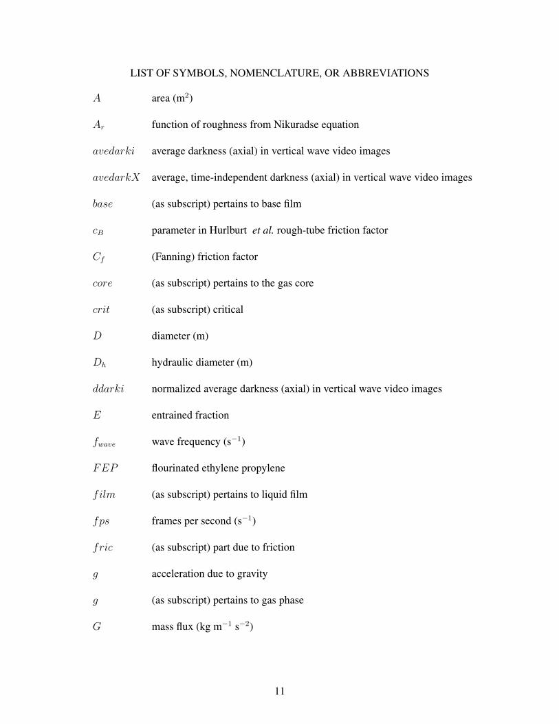
Annular flow is a configuration of gas-liquid two-phase flow characterized by a thin film

of liquid surrounding a core of faster-moving gas. The liquid film is often a site of complex

geometry where liquid mass transport occurs through base film and disturbance waves. Annular

flow occurs in a wide range of industrial heat-transfer equipment, including the top of a BWR

core, in the steam generator of a PWR, and in postulated accident scenarios including critical heat

flux (CHF) by dryout.

The present work focuses on the characterization of individual film behaviors in annular

flow. Quantitative visualization techniques are discussed that provide for large-scale data

collection of multiple, interrelated flow behaviors. The non-trivial data reduction codes for

these techniques have been further developed in the present work to improve measurement

accuracy. Film thickness distribution (base film and wave), disturbance wave length, and wave

intermittency estimates have been updated using modified techniques. A system is also suggested

for measuring the velocity of the gas-liquid interface. Lastly, the present observations have been

applied to a recent two-region (base film and disturbance wave) annular flow model.

15

CHAPTER 1INTRODUCTION

Gas-liquid two-phase flow is common to many industrial applications, especially in

boiling or condensing heat transfer equipment. Nuclear power plants contain two-phase flow in

several systems of light water reactors, including boiling in the core of a BWR and in the steam

generator of a PWR. The core of a PWR may also be the site of saturated boiling in off-normal

conditions or accident scenarios.

The continuing study of two-phase flow is necessary due to the complexity of interactions

at the interfaces between phases. Most descriptions of these interactions begin by recognizing

and categorizing the general arrangement of the two-phases, referred to as a “flow regime.” A

more comprehensive look into flow regime categories, traits, and identification is included in

Section 2.1.

1.1 Annular Flow Overview

The current work focuses on the annular flow regime, characterized by a core of fast-moving

gas surrounded by a liquid film along the channel wall. Annular flow occurs through a wide

range of gas and liquid flow rates. In nuclear systems, annular flow may be observed near the top

of the core in a BWR and in the steam generator of a PWR. This regime is also the final stage in

channel boiling before gas-droplet flow occurs in critical heat flux (CHF) by dryout (postulated

BWR accident scenario).

The liquid film is often a site of complex geometry. The liquid moves slowly relative to the

gas core and may transport a small fraction of the gas as bubbles, which can affect boiling heat

transfer. The remainder of the liquid film can be divided into base film and disturbance waves.

The base film occupies most of the total film area, creating a relatively smooth interface

with the gas core. Some example images of base film are shown in Figure 1-1, taken using a

planar laser-induced flourescence (PLIF) technique and processed using the method discussed in

Chapter 3. Each image has been rotated 90◦ counter-clockwise, so the vertical upflow is shown as

right to left. The gas velocity for the top four images is considerably less than for the top four (46

16

m s−1 vs. 78 m s−1). The images indicate that an increased gas flow rate has a slimming effect on

base film thickness.

Figure 1-1. PLIF images of base film. Usl = 6.3 cm s−1. Usg = (top four) 46 m s−1, (bottom four)78 m s−1.

Disturbance waves travel along top of the base film, exchanging liquid mass with the base

film and traveling at a much higher velocity. Some example backlit wave images, processed

using the method discussed in Chapter 5, are shown in Figure 1-2. The waves in these images

are visible as dark patches because less light is transferred through the thicker film sections,

indicative of wave behavior.

In addition to base film and waves, some liquid is transported through the tube as droplets

entrained in the gas core. The study of liquid entrainment requires difficult and often intrusive

measurements that are not among the present visualization techniques. However, the qualitative

assessment of entrainment is an important aspect of annular flow mechanics; entrained liquid

behavior is closely tied to disturbance wave behavior.

1.2 Quantitative Visualization

Quantitative visualization refers to a family of data acquisition techniques based on

the manipulation and detection of radiation in a flow field. The center of the visualization

process is an experimental apparatus, reconstructing a flow scenario with necessary control and

17

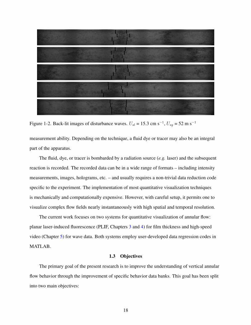
Figure 1-2. Back-lit images of disturbance waves. Usl = 15.3 cm s−1, Usg = 52 m s−1

measurement ability. Depending on the technique, a fluid dye or tracer may also be an integral

part of the apparatus.

The fluid, dye, or tracer is bombarded by a radiation source (e.g. laser) and the subsequent

reaction is recorded. The recorded data can be in a wide range of formats – including intensity

measurements, images, holograms, etc. – and usually requires a non-trivial data reduction code

specific to the experiment. The implementation of most quantitative visualization techniques

is mechanically and computationally expensive. However, with careful setup, it permits one to

visualize complex flow fields nearly instantaneously with high spatial and temporal resolution.

The current work focuses on two systems for quantitative visualization of annular flow:

planar laser-induced fluorescence (PLIF, Chapters 3 and 4) for film thickness and high-speed

video (Chapter 5) for wave data. Both systems employ user-developed data regression codes in

MATLAB.

1.3 Objectives

The primary goal of the present research is to improve the understanding of vertical annular

flow behavior through the improvement of specific behavior data banks. This goal has been split

into two main objectives:

18

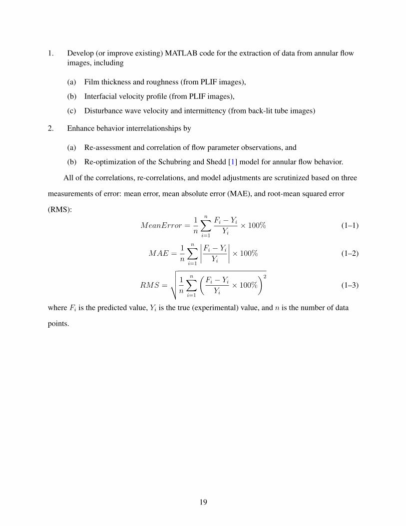
1. Develop (or improve existing) MATLAB code for the extraction of data from annular flowimages, including

(a) Film thickness and roughness (from PLIF images),

(b) Interfacial velocity profile (from PLIF images),

(c) Disturbance wave velocity and intermittency (from back-lit tube images)

2. Enhance behavior interrelationships by

(a) Re-assessment and correlation of flow parameter observations, and

(b) Re-optimization of the Schubring and Shedd [1] model for annular flow behavior.

All of the correlations, re-correlations, and model adjustments are scrutinized based on three

measurements of error: mean error, mean absolute error (MAE), and root-mean squared error

(RMS):

MeanError =1

n

n∑i=1

Fi − YiYi

× 100% (1–1)

MAE =1

n

n∑i=1

∣∣∣∣Fi − YiYi

∣∣∣∣× 100% (1–2)

RMS =

√√√√ 1

n

n∑i=1

(Fi − YiYi

× 100%

)2

(1–3)

where Fi is the predicted value, Yi is the true (experimental) value, and n is the number of data

points.

19

CHAPTER 2LITERATURE REVIEW

This chapter summarizes literature relevent to the present research. Fundamental two-phase

flow behavior and visualization techniques are outlined, followed by literature on the following

annular flow behaviors of interest:

• Base film thickness,

• Disturbance wave velocity, frequency, and length,

• Liquid entrainment.

The behavior interrelationships are discussed using the global

2.1 Regime Identification

The characterization of two-phase flow through a channel has been the subject of research

for many decades due to the complex interactions at the interfaces between phases. The contrast

between single and multi-phase system dynamics is stark, but certain elements are still relevent,

such as turbulence. Single-phase turbulence has been well established in fluid dynamics text (e.g.

Kays et al. [2] and Holman [3]) by use of the dimensionless Reynolds number, ReD:

ReD =ulDh

νl(2–1)

where ul is the average liquid velocity, νl is the liquid kinematic viscosity and Dh is the hydraulic

diameter used to characterize channel geometries. For a given geometry, an upper limit for

laminar behavior can be formed in terms of ReD, above which transitional or fully turbulent

behavior prevail.

In contrast, texts such as Whalley [4] have demonstrated the severe changes in the physical

nature of two-phase gas-liquid flows over a range of flow parameters. The interaction between

phases in a multi-phase channel often becomes very complex, leading to distinct configurations,

or flow regimes, as a function of fluid pressure, gas and liquid flow rates, fluid properties, and

channel geometry. Hewitt and Hall Taylor [5] suggested four basic flow regimes for vertical flow,

20

shown in Figure 2-1: the bubbly regime, where vapor bubbles are evenly dispersed throughout

a continuous liquid phase; slug, where large bubbles (slugs) take up much of the volume; churn,

where the faster moving fluids create complex oscillations; and annular, where a continuous core

of gas is surrounded by a thin film of slower-moving liquid.

Figure 2-1. Vertical flow regimes, as shown by Hewitt and Hall Taylor [5]. From left-to-right:bubbly flow, slug flow, churn flow, and annular flow.

In addition, a wispy-annular regime has been observed (such as by Hewitt and Roberts

[6]) for high gas and high liquid flow, causing a large fraction of liquid to travel through the gas

core as “wisp” structures. One of the characteristics of the wispy-annular regime, as discussed

by Hawkes et al. [7], is the significant fluctuation in pressure gradient. They also developed a

mechanism for predicting the transition into this regime based on conservation equations and the

development of sustained liquid waves in the gas core.

Modeling attempts for two-phase flow are often specific to one of these regimes due to the

differences in phase interactions. The consequences of non regime-specific, or “patternless,”

modeling have been discusses in detail by Thome [8, 9] with a heat transfer perspective. Several

negative effects were discussed by Thome, including:

1. Failure to predict the onset of dryout or the sharp decline in two-phase void fraction duringcertain dryout scenarios.

2. The neglect of proper annular film heat transfer.

21

3. The neglect of proper turbulent and thermal boundary layer theory for heat transfer.

The determination of vertical two-phase regimes based on basic flow parameters has been

addressed from many angles. Several attempts have been made in the literature to plot regime

transitions on specified coordinates. A short summary of this concept, referred to as regime

mapping, has been provided by Whalley [4]. One of the earliest attempts at regime mapping

(Baker [10]) relied on the observation of transitions by the author. The plotting corrdinates for

the Baker map are the mass fluxes of the gas and liquid with corrections for fluid properties. The

usefulness of this map is limited to small tube diameters ( < 0.05 m) and for air/water flows (for

which the map was developed).

The Hewitt and Roberts [6] map was also produced by observation for air/water systems,

this time for vertical flow and with mapping coordinates of momentum flux, calculated from

the mass flux (G) and density (ρ). The inclusion of density in the mapping coordinates creates

some sensitivity to pressure in the flow system. However, the reliance of observation in the

development of the map is still inherently subjective. The work of Taitel et al. [11] was one

attempt to create regime transition criteria from mechanical principles. Many of these theoretical

processes, however, have been under scrutiny due to questionable physical principles (Whalley

[4]). A critique of the Taitel et al. principles has also been provided by Hewitt [12].

Mishima and Ishii [13] have also developed transition criteria based on principles of fluid

mechanics. Of particular interest to the current work is the churn-to-annular transition, which has

been developed in the one-dimensional drift flux model by Hibiki and Ishii [14] and described by

two mechanisms.

The first mechanism relates the onset of annular flow to the absence of flow reversal in the

liquid film section along large bubbles. This is closely related to the concepts of flow reversal and

flooding – the transition between countercurrent and cocurrent flow, shown in Figure 2-2. Fowler

and Lisseter [15] have provided a review of mechanical principles for the onset of cocurrent flow

(flooding) using a two-fluid model. Flooding is analagous to the churn-to-annular transition,

considering countercurrent flow as large bubbles in a slug regime.

22

Figure 2-2. Schematic illustration of flooding and flow reversal, as shown by Fowler and Lisseter[15].

The second annular transition mechanism described by Hibiki and Ishii is the destruction

of liquid slugs or waves by entrainment or deformation. This would occur at a superficial gas

velocity, Usg, sufficient to entrain liquid in the core. Equation 2–2 has been derived by a force

balance between the shearing force of the vapor drag and the surface tension of the liquid. The

application of this model has been limited to tube diameters larger than the criterion shown in

Equation 2–3 (for round tube geometry).

Usg ≥(σg∆ρ

ρ2g

)1/4

N−0.2µf (2–2)

23

D >

√(σ

∆ρg

)N−0.4µf

[(1 − 0.11Co)/Co]2 (2–3)

Nµf = µf

[ρfσ

√(σ

∆ρg

)]−1/2

(2–4)

Co = 1.2 − 0.2

√(ρgρf

)(2–5)

2.2 Flow Visualization

Flow visualization refers to the identification of visible patterns in fluid motion and the sub-

sequent qualitative or quantitative analysis. The present discussion focuses on those techniques

that enhance the understanding of annular two-phase flow.

Perhaps the most basic application of flow visualization is by direct image manipulation and

processing. Ohta et al. [16] has demonstrated early image thresholding methods for determining

velocity flow fields for bubbles. The use of high-speed video and image processing for two-phase

flow has been demonstrated by Rezkallah et al. [17, 18] to determine local gas phase velocities

and instantaneous void fractions. These studies are sensitive to two-phase flow regimes and

provide regime-specific data and early estimations of error.

Recently, Schubring et al. [19] has provided a quantitative, statistical approach to vertical

annular flow wave measurements by image manipulation and processing. The images used in

the study were obtained by high-speed video of a backlit tube. The visualization of disturbance

waves has also been specifically studied by Belt et al. [20] through the use of conductance-based

film thickness sensors. The sensors were applied in an array that facilitated the time-resolved,

three-dimensional visualization of disturbance waves, which is also relevent to the present work

on wave characteristics. The validity of conductance probes as film thickness measurement

devices has been scrutinized by Rodrıguez [21] for a failure to recognize bubbles in the liquid

film. The devices are also often placed into the flow and are thus invasive to the experiment.

Flow visualization methods are constantly adapting to technological advancements, notably

laser capabilities and computational power. A recent and comprehensive review of achievements

24

in the area is provided by Smits and Lim [22]. The ability to obtain and analyze information

on particles in fluid motion has been an extremely powerful advancement over the past three

decades. A review of measurements by fluid particle techniques on the micro and macro scale

has been provided by Sinton [23]. Popular particle-based visualization techniques include laser-

doppler velocimetry (LDV), particle image velocimetry (PIV), and particle tracking velocimetry

(PTV).

Two-beam LDV is one of the earliest laser systems for flow measurement, popular in

practice since the mid 1970s. Macroscale LDV has been successfully applied to two- and three-

dimensional flow patterns, including three-dimensional turbulent boundary layers by Compton

and Eaton [24]. In a general LDV system, a small volume of fluid, seeded with reflective

particles, is exposed to the interference pattern created by the intersection of two lasers. Flow

velocity can then be determined by calculating the Doppler frequency in a given control volume.

The goal for most fluid visualization techniques is to achieve spatial and temporal resolution

fine enough to observe microscale turbulent motion. However, microscale LDV has been

limited technologically by laser diameter, which limits the size of the interference section, and

statistically by reducing the number of particles in the interference section. The work of Compton

and Eaton displays two-dimensional interference sections as small as 35µm× 66µm. Further

advancements have been made by Tieu et al. [25] with LDV velocity measurements as close as

18µm to a channel wall.

Particle image velocimetry (PIV) involves a fundamentally different approach to particle

motion in fluids, adding the ability to track velocity and direction for several locations of

interest at once. The histories of multiple seed particles in a flow are recorded by time-elapsed

photography and are analyzed in a separate process to determine velocity vectors.

General PIV setups allow an area to be instantaneously observed through the use of a

planar illumination source, usually a pulsed laser sheet, and one or more cameras. The work of

Adrian [26] demonstrates the variety of instrumentation techniques under the general theory of

PIV. Several physical limitations exist for a PIV system that must be addressed simultaneously,

25

including size of the control volume, particle density, particle response, and methods for time-

elapsed photography. The optimization of PIV systems for two-pulse imaging and multi-pulse

imaging has also been developed by Keane and Adrian [27, 28].

Another limitation of PIV is the computational power required for statistical image correla-

tion. The extraction of quantitative data from particle images is often the most important step in

PIV measurements, as described by Hinsch [29]. The correlation of multiple particle images is

achieved by autocorrelation or by cross-correlation. Autocorrelation is performed by shifting an

image and correlating with itself, which is used in PIV systems that acquire a single, multiple-

exposed image. Limitations to autocorrelation, including the apparent lack of positive/negative

direction, have been mitigated by Marzouk and Hart [30].

In contrast, cross-correlation requires two separate images and knowledge of the time

between them. The advantage of cross-correlation is the knowledge of direction due to the

independently exposed images. The work Keane and Adrian [31] has shown considerable

advancement in cross-correlation techniques specifically for the use of PIV measurements. The

disadvantages to this method include more expensive instrumentation (camera speed), increased

storage capacity (double the images), and increased computational power (image manipulation).

The usual application of PIV can develop velocity vector fields in two dimensions (2-D)

for a fixed time. Several innovative techniques have been developed to apply PIV to three

dimensions (3-D) to fully understand volumetric fluid motion. A recent review of leading 3-

D PIV techniques has been discussed by Hinsch [32]. The utmost in multi-dimensional flow

visualization involves the resolution of three velocity demensions over three spacial dimensions

with time. The only visualization technique advanced enough to store such a high quantity of

data, to date, is holographic PIV.

The application of PIV to achieve microscale flows is termed as micro-PIV, which is

especially useful for low velocities such as near-wall flows or low Reynolds number flows.

Santiago et al. [33] demonstrate micro-PIV measurements with spatial resolutions that approach

one micron.

26

Also of particular interest is the application of PIV to multiphase gas-liquid flows. The

ability to resolve two phases with micro-PIV has been demonstrated by Hassan [34] for bubbly

air-water flow in a vertical channel. Wavy and wavy-annular flow regimes have also been

successfully characterized by Schubring et al. [35] using micro-PIV.

Particle tracking velocimetry (PTV) attempts to increase resolution by tracking individual

particles rather than locations. The clear advantage over PIV, which requires approximately 20

particles per interrogation area to obtain an accurate velocity vector (Sinton [23]), is that PTV

provides up to 20 individual velocity vectors. In practice, however, individual particle tracking

requires more than two images per correlation set and a fraction of particles are lost in tracking.

To provide enough flow information to accurately track individual particles, PTV theory

has been coupled with PIV correlations, often phrased as “super-resolution” PIV analysis. This

was first accomplished by Keane et al. in 1995 [36], who improved the spacial resolution of

normal PIV measurements by 250%. More recent efforts by Takehara et al. [37] have shown

improvements of over 500% with similar methods.

The advancements in laser power and pulse frequency capabilities have opened up new

realms of flow visualization based on laser-induced fluorescence (LIF) [22]. Most LIF appli-

cations for the two-dimensional visualization of fluid flow are collectively referred to as planer

laser-induced fluorescence (PLIF), which has been studied as early as 1988 by Hanson [38].

PLIF uses a laser at an appropriate frequency to excite the seed molecules in a fluid, which sub-

sequently flouresce. The result is a nearly instantaneous cross-sectional image of a fluid, making

PLIF a very attractive method for high-velocity turbulent flow imaging. Kychakoff et al. [39]

demonstrated the early ability of PLIF to visualize highly turbulent flame gases. The work of

Hanson [40] further demonstrated the use of PLIF for pressurized combustion processes.

The transformation of PLIF images into quantitative data often requires unique, non-trivial

image processing and can be very computationally expensive. Early efforts to understand the

capabilities of PLIF by van Cruyningen et al. [41] for flow through a nozzle emphasized the

resolution and error calculations of measurements. The use of PLIF to study annular flow film

27

thickness is a more recent development by Rodrıguez and Shedd [42], refined by Schubring et

al. [43, 44].

2.3 Annular Flow Modeling

The data analysis in the present work is focused on the characteristics of individual thin-film

mechanisms – liquid film and disturbance wave statistics – and the effects of those mechanisms

on annular flow behavior. In a two-zone model (waves and base film), disturbance waves are

modeled as separate structures than base film or entrained droplets. The two-zone method relies

heavily on accurate characterizations of wave behaviors.

Reviews of wave behavior are provided by Azzopardi in 1989 [45] and again in 1997 as a

part of a larger review of entrainment [46]. For vertical upflow, Nedderman and Shearer [47] and

Hall Taylor et al. [48] observed that wave velocities and frequencies increase with increasing

gas and liquid flow rate. Martin [49] has observed an inverse effect of tube diameter on wave

frequency. An inverse relationship between liquid kinematic viscosity and wave frequency has

also been observed by Mori et al. [50].

Some research, such as that by Mori et al. [51], has suggested the presence of two distinct

wave structures in vertical flow, termed disturbance waves and huge waves. The latter have

greater average velocity and liquid mass. Huge waves are observed closer to the annular-churn

boundary, outside of the range of the present work.

For the estimation of wave velocity, vwave, a mechanistic model and an empirical correlation

have been developed by Pearce [52] that include a dependence on liquid interface velocity, Ul,i.

However, this measurement is more challenging than that of vwave itself. Kumar et al. [53]

developed a vwave prediction based on superficial velocities and Reynolds numbers:

vwave,Kumar =CkumarUsg + Usl

1 + CKumar(2–6)

CKumar = 5.5

(ρgρl

)1/2(RelReg

)1/4

(2–7)

Rel =ml

Dπµl(2–8)

28

Reg =mg

Dπµg(2–9)

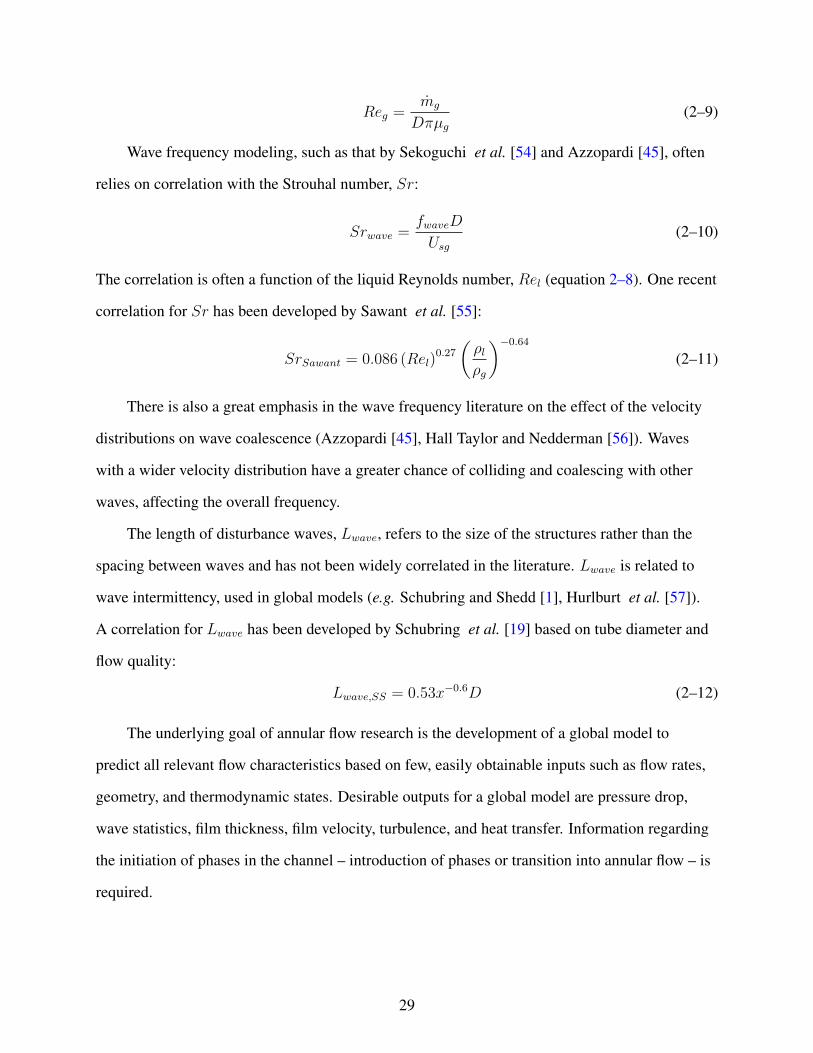
Wave frequency modeling, such as that by Sekoguchi et al. [54] and Azzopardi [45], often

relies on correlation with the Strouhal number, Sr:

Srwave =fwaveD

Usg(2–10)

The correlation is often a function of the liquid Reynolds number, Rel (equation 2–8). One recent

correlation for Sr has been developed by Sawant et al. [55]:

SrSawant = 0.086 (Rel)0.27

(ρlρg

)−0.64

(2–11)

There is also a great emphasis in the wave frequency literature on the effect of the velocity

distributions on wave coalescence (Azzopardi [45], Hall Taylor and Nedderman [56]). Waves

with a wider velocity distribution have a greater chance of colliding and coalescing with other

waves, affecting the overall frequency.

The length of disturbance waves, Lwave, refers to the size of the structures rather than the

spacing between waves and has not been widely correlated in the literature. Lwave is related to

wave intermittency, used in global models (e.g. Schubring and Shedd [1], Hurlburt et al. [57]).

A correlation for Lwave has been developed by Schubring et al. [19] based on tube diameter and

flow quality:

Lwave,SS = 0.53x−0.6D (2–12)

The underlying goal of annular flow research is the development of a global model to

predict all relevant flow characteristics based on few, easily obtainable inputs such as flow rates,

geometry, and thermodynamic states. Desirable outputs for a global model are pressure drop,

wave statistics, film thickness, film velocity, turbulence, and heat transfer. Information regarding

the initiation of phases in the channel – introduction of phases or transition into annular flow – is

required.

29

The global model of Schubring and Shedd [1] has been chosen for further discussion.

Similar to the Hurlburt et al. [57] model, the Schubring and Shedd model employs a two-zone

(base/wave) film roughness concept to link interfacial shear and film thickness. The Hurlburt et

al. model, however, requires film thickness and entrained fraction as inputs. The Schubring and

Shedd model addresses these issues by only requiring flow rates, fluid properties and geometry as

inputs. The outputs of the model include pressure gradient, film thickness (with zone separation),

and disturbance wave velocity. There is a greater emphasis on the behaviors in the liquid film

rather than on modeling entrainment or deposition.

2.3.1 Schubring and Shedd Prediction of Film Thickness

The prediction of film thicknesses originates with the correlation of a friction factor, the

sensitivity of which has been described by the authors as negligible. Two correlations for the

(Fanning) friction factor have been provided. The first is the Blasius relation (Equation 2–14)

increased by a factor φRR, where Recore,base is defined as the Reynolds number of the gas core

over the base film. Experimental data has been used to correlate φRR, shown in Equation 2–16.

Recore,base =ρgUcore,baseDcore,base

µg(2–13)

Cf,i,base = 0.079φRRRe−0.25core,base (2–14)

φRR = 1.9x0.1 (2–15)

The second is the friction factor of Hurlburt et al. [57], who set the empirical constant

cB,base to 0.8:

Cf,i,base = 0.582

[− ln εbase

(εbase − 1)2 − ln cB,base + 1.05 +1

2

εbase + 1

εbase − 1

]−2

(2–16)

The roughness is evaluated using:

εbase = 2 (1 − LFbase) δbase (2–17)

εbase =2εbase

D − δbase(2–18)

30

where LFbase is the fraction of film that follows a linear velocity profile. The remainder of liquid

film is observed as ripples at the gas-liquid interface and is modeled as well-mixed (constant

velocity). The ripple size was related to the standard deviation of base film height, provided

by the experimental data of Schubring et al. [43, 44] as 30% of the average base film. The

remaining 70% is assumed to flow with a linear (viscous) velocity profile (LFbase = 0.7).

The liquid velocity at the interface (Ul,i,base) and film flow rate (mfilm,base) are estimated

through a computation of shear:

τi,base = Cf,i,baseρgU

2core,base

2(2–19)

u?base =

√τi,baseρl

(2–20)

δ+base =

δbaseu?base

νl(2–21)

U+l,i,base = δ+

baseLFbase (2–22)

Ul,i,base = U+l,i,baseu

?base (2–23)

m+film,base =

[LF 2

base

2+ LFbase (1 − LFbase)

] (δ+base

)2 (2–24)

mfilm,base = m+film,baseDµlπ (2–25)

The velocity of the gas core over the base film (Ucore,base) and core velocity (Ug,base) are

computed from the following:

Dcore,base = D − 2δbase (2–26)

Acore,base =πD2

core,base

4(2–27)

Ucore,base = Ug,base − Ul,i,base (2–28)

Ug,base = UsgA

Acore,base(2–29)

Usg =mg

ρgA(2–30)

31

The model is closed with a relation of wave height to base film height. The average wave

height was observed to be approximately double the average base film height:

δwave = 2δbase (2–31)

2.3.2 Schubring and Shedd Prediction of Wave Behavior, Entrained Fraction, andPressure Gradient

The total modeled shear in the wave zone, τi,wave, is separated into two terms (Equation 2–

32). The first, τi,wave,rough, relates to the roughness of waves and is computed in an analogous

manner as the base film roughness. The second, τi,wave,trans, relates to the sudden transitions from

flow over base film to flow over waves. A rough-tube friction factor, Cf,i,wave, is estimated to

compute τi,wave,rough, where cB,wave is an empirical constant set to the value of 2.4 suggested by

Hurlburt et al. [57]:

τi,wave = τi,wave,rough + τi,wave,trans (2–32)

τi,wave,rough = Cf,i,waveρgU

2core,wave

2(2–33)

Cf,i,wave = 0.582

[− ln εbase

(εbase − 1)2 − ln cB,wave + 1.05 +1

2

εbase + 1

εbase − 1

]−2

(2–34)

The Schubring et al. model requires an approximation for wave roughness, which was

calculated as a constant 40% of the mean wave height. Wave roughness is therefore computed

with:

εwave = 0.4δwave (2–35)

εwave =2εwave

D − δwave(2–36)

The sudden transitions between base film and waves have been described by Schubring

and Shedd as similar to an obstacle in the tube. Wave properties are therefore important to the

calculation of gas-to-liquid momentum transfer (proportional to core kinetic energy density for

an obstruction). An empirical correlation, developed by Schubring [58], is used to estimate the

length of the disturbance waves, Lwave, presented in Equation 2–12

32

The characteristic gas velocity at the base-wave transition, Ug,trans, is found using:

Ug,trans = (Ul,i,base − Ul,i,wave) +

√τi,baseρg

√1

δ+g,trans

∫ δ+g,trans

0

[u+ (y+)]2 dy+ (2–37)

δ+g,trans =

δwave − δbaseνg

√τi,baseρg

(2–38)

The non-dimensional distance δ+g,trans represents the penetration of the wave into the boundary

layer formed over the base film. The characteristic velocity considers both the RMS velocity in

the gas obstructed by the film (second term, right hand side) and the change in interfacial velocity

between the wave and base film zones (first term, right hand side).

For turbulent gas and liquid velocity approximations, a universal velocity profile (UVP) is

assumed as presented by Whalley [4], where u+ and y+ are defined as:

u+(y) =u(y)

u?l(2–39)

y+ =yu?lνl

(2–40)

δ+ =δu?lνl

(2–41)

u+ =

y+ if y+ < 5

−3 + 5 ln(y+) if 5 < y+ < 30

5.5 + 2.5 ln(y+) if 30 < y+

(2–42)

The shear from the sharp transition is estimated by the following equation, with the factor of

2 as an empirical parameter:

τi,wave,trans = 2ρcoreUg,trans

2(δwave − δbase)

Lwave(2–43)

For the film in the wave zone, the universal velocity profile is assumed, non-dimensionalized

by wave zone shear, τi,wave. The wave zone gas-liquid interface for the current data is within

the log layer (y+ > 30) of the film, simplifying the velocity profile calculation. The interfacial

velocity of the waves (Ul,i,wave = vwave) and wave zone liquid film flow rate, mfilm,wave, are

33

computed from the following:

U+l,i,wave = 5.5 + 2.5 ln

(δ+wave

)(2–44)

Ul,i,wave = U+l,i,waveu

?wave (2–45)

m+film,wave = −64 + 3δ+

wave + 2.5δ+wave ln

(δ+wave

)(2–46)

mfilm,wave = m+film,waveDµlπ (2–47)

The density of the core (gas and entrained droplets), ρcore, is estimated by mass conservation

in the liquid phase and an assumed homogeneous model in the core:

ml,Ent = ml − ml,film,base (1 − INTw) − ml,film,waveINTw (2–48)

E =ml,Ent

ml

(2–49)

ρcore =ml,Ent + mg

A (Usg + UslE)(2–50)

The wave intermittency, INTw, is estimated by an empirical correlation developed by

Schubring et al. [19]:

INTw,SS = 0.1 +Rel

40000(2–51)

Rel =ρlUslD

µl(2–52)

The droplet deposition flux, RD, is required in the evaluation of pressure drop. The correla-

tion of Ishii and Mishima [59] (Equation 2–53) is used to compute this, which incorporates the

entrained fraction through the use of core density, ρcore.

RD = 0.022 (ρcore − ρg)UsgRe−0.25g

(ρg

ρcore − ρg

)0.26

(2–53)

Reg =ρgUsgD

µg(2–54)

Estimation of average pressure loss is accomplished by independently solving the following

base and wave interfacial shear equations for their respective dP/dz values, as from the work of

Fore et al. [60] (Equations 2–55 and 2–56). The total pressure loss is then calculated using the

34

wave intermittency, INTw:

τi,base = −Dcore,base

4

(1 −

ρcoreU2g,base

Pabs

)dP

dz base(2–55)

−ρcoregDcore,base

4−RD (Ucore,wave − Ul,i,wave)

τi,wave = −Dcore,wave

4

(1 −

ρcoreU2g,wave

Pabs

)dP

dz wave(2–56)

−ρcoregDcore,wave

4−RD (Ucore,wave − Ul,i,wave)

dP

dz= (1 − INTw)

dP

dz base+ INTw

dP

dz wave(2–57)

In a similar fashion, the time-averaged film thickness is computed by:

δ = (1 − INTw) δbase + INTwδwave (2–58)

The final outputs of this model include film height, interfacial velocity (wave velocity for the

wave zone), pressure gradient, and film flow rate. The model performance was evaluated using

annular flow data obtained by Schubring et al. [43, 44]. Outputs for pressure gradient and wave

velocity are reasonable and on par with empirical, single-behavior estimates.

2.4 Application of Literature

The research efforts discussed in this chapter represent only a small fraction of flow

visualization and annular flow literature. The papers selected for this review have been in line

with the goal of the current work – to improve the measurement and modeling of individual

annular flow phenomena. The emphasis on the specific behaviors of annular flow is an important

step to understanding the physics of the flow regime as a whole. The desirable outputs of annular

modeling – pressure gradient and heat transfer – will benefit from the understanding of these

behaviors.

The following chapters focus on the application of two fluid visualization techiniques: PLIF

imaging and high-speed video. Several annular flow observations in the literature are studied

35

and updated using these methods, including base film and wave distributions, interfacial velocity,

disturbance wave lengths, and wave intermittency.

36

CHAPTER 3PLIF EDGE IDENTIFICATION

Film thickness has been described in the literature using a two-zone characterization,

composed of base film and disturbance waves with drastic behavior differences. Due to the

periodic nature of disturbance waves, the measurement of film thickness by most techniques is

preferential to base film. The purpose of this work is to characterize both zones of the liquid film

using PLIF images obtained by Schubring et al. [43]. The current work includes revisions and

improvements to the original algorithm.

3.1 PLIF Optics

A schematic of the test section used for the PLIF image acquisition is shown in Figure 3-1.

The main components in the experimental setup are the flow tube, laser light source, flourescing

dye, digital camera, and lens. Flourinated ethylene propylene (FEP) was selected as the flow tube

material due to the proximity of its refractive index (1.337) to that of water (1.333). This allowed

for accurate near-wall measurements of base film thicknesses, which are generally on the order of

100 µm. The FEP section was encompassed by a square, water-filled chamber and painted black

to reduce ambient light and improve image contrast.

The laser light source was a New Wave Research Solo PIV Nd:YAG that used a commerical

light sheet attachment. The laser sheet entered the enclosure at a 90◦ angle through a viewing

window to avoid refraction at the air-FEP transition. Rhodamine B was used as the flourescing

dye. A Roper-Scientific 1300YHS-DIF camera (1300 by 1030 pixels, inter-line transfer CCD)

was aimed through another viewing window at a 90◦ angle to the laser sheet to view the liquid

cross-section made visible by the flourescing dye.

The current work is based on image sets taken from a lens (Mitutoyo Telecentric Objective

3x, NA = 0.07, nominal working distance 72.5 mm, depth of focus 56 µm) that yielded pixels

3.14 µm in each direction (total axial length: approximately 4 mm). All of the flow conditions

used for the current work are shown in Table A along with gas and liquid superficial velocities.

37

Nd:YAG Laser

CCD Camera

FEP Box

FEP Tube

Viewing Windows

Black Paint

Red Filter

Plane of Focus & Laser Sheet

Figure 3-1. Test section for PLIF measurements. Flow is out of the plane of the page.

3.2 PLIF Processing

PLIF processing uses MATLAB code in three sections: image processing, outlier-removal,

and data processing. The expected shape of the liquid edge is a smooth, continuous, unbroken

line through the length of the image. A metric was developed for the original code, “chaos,” as a

measurement for the lack of continuity in the edge and has been maintained in the current work.

When adjacent axial locations both contain detected edges, the difference in height between the

edge locations is taken to the power of 1.5, with all of these results summed for each image as the

chaos value.

An outlier-removal procedure is performed for the small fraction of PLIF images that are

incorrectly processed. A graphical user interface (GUI) was developed to locate, tag, and purge

poorly processed images. The final data processing section has been developed to quantify film

thickness data and generate figures.

38

3.2.1 PLIF Image Processing

Some obstacles overcome in the liquid edge-finding routine include:

1. Image contrast

2. Single-pixel image noise

3. Bubbles in the gas-liquid interface

4. Out-of-plane features, including droplets near the interface

The image processing is accomplished in the following steps.

Crop. The image is cropped to a specified width to reduce the image processing time and

reduce the impact of droplets at the outer range of the images. The initial crop widths are a

function of the gas flow rates, based on the maximum observed film thickness for each liquid

flow. These values have been presented in Table 3-1.

Table 3-1. Initial crop widths for PLIF image processing.Qg,nom WidthL min−1 µm800 2000

1000 15001200 12501400 11001600 800

Axial Blur. To reduce single-row noise, the image is subjected to a five-pixel blurring

process in the axial direction. The center pixel in the process is a weighted average; the center is

weighted 3, the next adjacent weighted 2, and the ends weighted 1. This process has a negligible

effect on the final edge shape beyond reducing noise-related errors in the edge.

Median Filter. Single-pixel noise in the image is reduced by applying a median filter, found

in the MATLAB image processing toolbox as medfilt2. The filter window is set to 3 pixels in all

directions.

Contrast Adjustment. The raw images are initially too dark for viewing by the human

eye. The pixel range of the images is adjusted using a MATLAB function, imadjust. The main

operation in imadjust is shown in Equation 3–1 where J is the output image, I is the input image,

39

and subscripts min, max, and n represent the minimum, maximum, and current pixel value in

the image, respectively. The exponential weighting factor, γ, has been set to 1.5 and wieghts

the output towards the lower pixel values to help reduce blur in the gas core. This version of the

image, referred to as the adjusted image, is also used later in the process as the user-viewable

version.

Jn = Jmin + (Jmax − Jmin)

[(In − Imin)

(Imax − Imin)

]γ(3–1)

Stretch. The adjusted image is then enhanced a second time by applying a row-by-row

linear stretch of the pixel values, creating a better defined edge for low contrast regions. A

stretching threshold is implemented to ensure that a region is not blurred by this process. A

minimum-to-maximum pixel difference of 74 (out of 255) is required for a row before it is

linearly stretched.

The newly stretched image (Tempstr) is then added to the previous adjusted image

(Adjusted) as in Equation 3–2. The weighting factor for the addition was determined by vi-

sual inspection to reduce the axial noise created by the stretching process.

Stretched = 0.8 × Tempstr + 0.2 × Adjusted (3–2)

Opening / Closing. A morphological opening and closing is applied to the stretched

image with built-in MATLAB functions imopen and imclose to reduce the effects of small-scale

defects in the edge. The first time through the processing, a disk of radius 3 pixels is used as the

morphological structure. All other iterations, which contain edge data and updated image size,

use a variable system of morphological disk radii described in Equation 3–5 (units of pixels).

An image can be subject to three different open/close radii (Roc) depending on the distance

from the channel wall (y) and the array of edge locations (Edge). The parameters C1 and C2 are

distances from the channel wall where the morphological radius changes, and are based on the

height and roughness (standard deviation) of the liquid edge. This system was developed since

higher edge locations (e.g., waves) show more chaotic edge behavior, larger bubbles, and more

40

edge defects. The larger radii are more effective at smoothing this behavior.

C1 = Edge+ 2 × s(Edge) (3–3)

C2 = 1.6C1 (3–4)

Roc(z) =

1 for y(z) ≤ C1

6 for C1 < y(z) ≤ C2

13 for C2 < y(z)

(3–5)

Threshold. The resulting image is cleaned up again using medfilt2 and then subjected

to a film threshold. The threshold value for all data sets is 85 (out of 255). The liquid edge is

represented by a change in the binary value.

Edge Location. The liquid edge is located for each row and recorded into an array. Due to

droplets or other out-of-plane features, there are often multiple possible edge locations. In the

first iteration the edge is recorded as the farthest location from the wall. In subsequent iterations,

the edge is recorded as the edge closest to the wall, which is often the most accurate. This

recording of edge values is compared to the first iteration to find the patches that did not agree

(often corresponding to droplets or bubbles). No edges are recorded within 40 µm of the wall, as

these are generally spurious and do not represent true base film.

Edge Iteration. A system was developed to compare the disagreements in the edge

recordings on the basis of edge continuity. The recorded values that produce a more continuous

liquid edge – not representing entrained droplets or dispersed bubbles – are accepted as the

final values based on local calculations of chaos and standard deviation. The final edge vector

undergoes a one-dimensional median filter (radius of 11 pixels) to remove any remaining pixel

noise.

Bubble Elimination. A bubble reduction algorithm is employed for smaller defects caused

by bubbles in the interface. Any edge perturbation that ranges from 0 to 200 µm in length with

a depression of at least 15 µm is recorded as a defect due to a bubble. Once located, the bubble

section is fixed by linearly interpolating between the outer pixels.

41

Edge Cleaner. An iterative process is performed to eliminate edge locations that are at

least 120 µm from the edge mean (not including edge locations recorded as “zero”) and greater

than 2.4 standard deviations from the mean. This step is more effective at eliminating incorrect

patches of the edge that could not be specifically identified.

Width Iteration. The resulting edge vector is then used to set a new image width and the

entire process is iterated, starting with the crop. The iteration continues until the width of the

image ceases to change (a difference of less than 20µm) or after 10 iterations. This reduction of

image size greatly reduces the required computation of each subsequent iteration and allows for

easier image storage.

Image Storage. To enable a visual inspection, the final edge array is superimposed onto

the adjusted, viewable image as a light blue (cyan) line. The attempts at the iterative edge fixing

method (identified edge points that were not selected) are indicated on the image as green lines.

Bubble removals are indicated by small red lines at the bottom of images. All of the data from

the process is then stored for the following outlier-removal and data processing.

3.2.2 Code Modifications

Many of the features in the current algorithm are similar to the original. The process

described in Section 3.2.1 includes the following changes from the original code.

Initial Crop Width. The original crop widths were determined based on total internal

reflection (TIR) measurements by Schubring [58]. The initial crop widths presented in Table 3-1

have been increased due to larger observed film heights and increased computational power.

Contrast Methods. The use of the γ variable in the MATLAB function imadjust was not

implemented in the original code. This variable weights the images towards the darker pixels and

creates images with better contrast and defined edges.

Stretch Threshold. The stretching threshold was included in the current version to

eliminate issues with noise and blurring from the original process. The final step in this process –

linearly adding the adjusted image to the newly stretched image – was also added to reduce noise.

42

Morphological Radii. The original code only performed the morphological opening and

closing process with one structure and a constant radius (1 pixel). The current variable radius

method uses radii that range from 1 pixel to 13 pixels, depending on the length of the edge. This

is the most computationally expensive operation in the PLIF processing algorithm, doubling the

processing time for each image.

Film Threshold. The binary threshold for the current code has been decreased significantly

from the original due to new contrasting methods. The original image film threshold was 175 (out

of 255) and is now reduced to 85.

Edge Iteration. The concept of edge iteration was introduced in the new code as an

alternative to locating and fixing bubbles. It takes advantage of the iteration that already took

place in the original – centered around reducing the image size.

Bubble Detection. The purpose of the bubble detection in the original algorithm was to find

and eliminate regions of the edge that were perturbed by a bubble, described as a length of edge

150 µm and a mean depression of at least 15 µm relative to the surrounding film height. This

was a constant criteria designed around the average observed bubble at the interface. The current

process detects variable lengths of bubbles, or any similar edge defects, that range from 0 to 200

µm

Image Storage. The edge data from the original algorithm was superimposed onto the

current images at red lines. Example images showing both sets of data are shown in Figure 3-3

and Figure 3-4.

3.2.3 PLIF Outlier Selection GUI

There are certain features of the liquid film that can cause errors in the recorded liquid edge.

Some such issues cause failure in the edge finding routine. It is preferable to locate and reject

such “outlier” images. Any measurement of standard deviation or chaos is not sufficient grounds

for image rejection – highly chaotic edge vectors have occasionally been observed to be accurate.

For this reason, a graphical user interface (GUI) was produced using MATLAB to aid in the

visual identification of outliers.

43

The GUI loads one set of processed flow data at a time and calculates the mean and standard

deviation of all edge values. A list of potential outliers is produced for which the mean of the

edge vector lies outside of a critical range. The default critical range is calculated as 2 standard

deviations away from the mean, but can be modified in the GUI. This criterion primarily locates

edge vectors that are uncharacteristically high. A similar criterion is evaluated using chaos

values, attempting to locate erratic edge vectors. From this list, the user can select an image,

view the image and edge data, and determine whether it qualifies as an outlier. Images were only

rejected if the recorded edge represented the film incorrectly as a result of the following:

Core liquid. Some images show droplets or larger sections of liquid traveling through

the core. This is often much farther from the wall than the liquid film and can skew the data if

detected. However, errors of this kind are generally smaller, as most of the flows tested have low

levels of entrainment. Even if detected, liquid in the core has been observed to affect, at most,

10% of an image. Due to the disparity in the recorded values, any falsely detected liquid in the

core that affects more than 5% of a recorded edge (by visual estimation) is removed.

Out-of-plane features. Some features, unidentifiable as part of the liquid film, show up

in images as large, blurry patches. Some of these issues may be exacerbated by the stretching

routine in the image processing. These sections, much like the core liquid, result in extreme

overestimation of the film. Out-of-plane features also occur in much larger sections, often

affecting over 15% of a recorded edge. All of the images with this type of issue are rejected.

Erratic film sections. Some images show a liquid edge that is extremely erratic and not

well characterized by the image processing. This can be caused by several mechanisms, such

as a large concentration of bubbles at the interface, a large wave with liquid tearing from the

surface, or the rolling/breaking of a large wave. Errors of this type occur at varying levels of

severity (disparity between the recorded edge and the true edge location) and are rejected on a

case-by-case basis.

Some example images that were selected as outliers have been shown in Figure 3-2. The

number of outliers removed for each flow condition (Rej) is shown in the right-hand column of

44

Table A. Typically, between 1% and 5% of the total images in a flow condition are selected as

outliers. An array is created by the GUI that indicates which images were selected, later used in

the data analysis.

3.2.4 PLIF Data Processing

The first step in the data analysis procedure is to convert the results from image processing

to a physical scale, taking into account misalignment from the experimental procedure. The

entire data set was observed to be slightly skewed - the wall location at the top of the image was

found to be 6 pixels (19 µm) to the right of that at the bottom. Each image was linearly adjusted

to compensate for this misalignment.

Film thickness data are then split into two regions using one of two methods. The first is

based on the work of Rodrıguez [21] and uses a critical standard deviation multiplier, kc, to

create the separation criterion. Film height measurements greater than kc standard deviations

from the mean base film height are assumed to be wave measurements. Based on the work of

Schubring [58], a kc value of 2 is used for this analysis. The evaluation of this criterion must be

performed iteratively. The initial assumption for this procedure is that the standard deviation of

the base film is the same as the standard deviation for all film points. This iteration continues

until the base film distribution converges.

An alternate method is to use wave intermittency data as an input for the calculation. Values

for INTw from Chapter 5 have been used as inputs for this method. The main discrepancy

between the INTw and the PLIF data is the use of slightly different tube diameters. There is

also an error associated with the INTw measurements (based on the wave length, velocity and

frequency measurements) that could compound the error for the base/wave division.

After the zone separation, several figures are produced for data analysis. Wave and base

distributions are represented by histograms. The mean and standard deviation of wave and base

film are calculated and plotted as functions of Usg and Usl. Other information is also obtained that

is useful for the optimization of the code, including chaos values for the data set and the number

of points where no edge was detected.

45

Figure 3-2. Example rejected PLIF images for flow conditions (top to bottom) 185F, 166F, 147F,128F, and 109F (constant Usl = 21.1 cm s−1).

46

3.3 PLIF Results

Average film thickness (δ), base film thickness (δbase), and wave height (δwave); their

respective roughnesses (estimated by sample standard deviations); and wave intermittency

(INTw) are shown for all 26 tests in Table A (kc method) and Table A (INTw method).

3.3.1 PLIF Image Comparison

Example processed PLIF images are shown in Figure 3-3 (flow condition 121F) and

Figure 3-4 (flow condition 162F). Each image indicates the edge from the original code (red line)

along with the edge from the current code (blue line) to highlight the code modifications (in the

case of both edge indicators existing in the same space, the red line is visible).

For base film, the difference in edge location is visibly negligible. Most of the differences

are due to larger waves and bubbles, where the interface is not as clearly defined. The images

chosen for this comparison all show structures that the current efforts were directed at improving.

It can be seen from the images that the current code finds slightly higher values at most

locations due to the more aggressive contrasting methods used in the processing. For large waves,

this discrepancy becomes much more apparent, indicating that the original code under-predicted

wave heights. The current code also does a better job at ignoring the structures in the film,

including bubbles.

3.3.2 PLIF Single-Zone Comparison

All of the figures presented for this section include the results of the original code along with

the current results for comparison. Figures 3-5 and 3-6 show film thickness distributions for five

flow conditions with constant liquid flow rate (Usl = 21.1 cm s−1). Figures 3-7 and 3-8 show film

thickness distributions for five flow conditions with constant gas flow rate (Usg = 57 m s−1). All

film thickness distributions are shown in Appendix B.

The main effect of increasing the gas flow rate is a shift of the distribution peak to the

left (lower film thickness). A similar trend is seen in the current results, but the shape of the

distributions are generally taller and narrower. The narrower shape is most apparent in the lowest

47

Figure 3-3. Example processed PLIF images for flow condition 121F. Red line shows originalresults, light blue line shows current results.

48

Figure 3-4. Example processed PLIF images for flow condition 162F. Red line shows originalresults, light blue line shows current results.

49

0 500 1000 15000

1

2

3

4

5

6

7x 10

4

δ [µm]

n pt [−

]

0 500 1000 15000

2

4

6

8

10

12

14x 10

4

δ [µm]

n pt [−

]

0 200 400 600 800 1000 12000

2

4

6

8

10x 10

4

δ [µm]

n pt [−

]

0 200 400 600 800 10000

2

4

6

8

10x 10

4

δ [µm]

n pt [−

]

0 200 400 600 800 10000

1

2

3

4

5

6

7x 10

4

δ [µm]

n pt [−

]

0 200 400 600 800 1000 12000

2

4

6

8

10

12x 10

4

δ [µm]

n pt [−

]

Figure 3-5. Histograms of film thickness (base and wave), original results (left) versus currentresults (right). Flow conditions (top to bottom) 109F, 128F, and 147F (constant Usl =21.1 cm s−1).

50

0 200 400 600 8000

1

2

3

4

5

6

7x 10

4

δ [µm]

n pt [−

]

0 200 400 600 800 10000

2

4

6

8

10x 10

4

δ [µm]

n pt [−

]

0 100 200 300 400 500 6000

1

2

3

4

5

6

7

8x 10

4

δ [µm]

n pt [−

]

0 200 400 600 8000

2

4

6

8

10x 10

4

δ [µm]

n pt [−

]

Figure 3-6. Histograms of film thickness (base and wave), original results (left) versus currentresults (right). Flow conditions (top to bottom) 166F and 185F (constant Usl = 21.1cm s−1).

gas flows (Usg = 36.3 m s−1), indicating that the greatest discrepancy in results occurs at lower

gas flow rates (higher film thicknesses).

Film thickness trends are shown in Figure 3-9 with film roughness, estimated here by a

standard deviation. The average film thickness trends for the new data are similar to those of the

original. The film thickness steadily decreases with increasing gas superficial velocity, with the

decrease slightly steeper than with the original code. The film thickness also tends to increase

with liquid superficial velocity over a larger range than the original (150 µm versus 100 µm).

51

0 200 400 600 800 10000

2

4

6

8

10x 10

4

δ [µm]

n pt [−

]

0 200 400 600 8000

2

4

6

8

10x 10

4

δ [µm]

n pt [−

]

0 200 400 600 800 10000

1

2

3

4

5

6

7x 10

4

δ [µm]

n pt [−

]

0 200 400 600 800 1000 12000

2

4

6

8

10x 10

4

δ [µm]

n pt [−

]

0 200 400 600 800 10000

1

2

3

4

5

6

7x 10

4

δ [µm]

n pt [−

]

0 200 400 600 800 1000 12000

2

4

6

8

10

12x 10

4

δ [µm]

n pt [−

]

Figure 3-7. Histograms of film thickness (base and wave), original results (left) versus currentresults (Right). Flow conditions (top to bottom) 140F, 143F, and 147F (constant Usg =57 m s−1).

52

0 200 400 600 800 10000

2

4

6

8

10x 10

4

δ [µm]

n pt [−

]

0 200 400 600 800 1000 12000

2

4

6

8

10x 10

4

δ [µm]

n pt [−

]

0 200 400 600 800 10000

1

2

3

4

5

6

7x 10

4

δ [µm]

n pt [−

]

0 200 400 600 800 1000 12000

2

4

6

8

10

12x 10

4

δ [µm]

n pt [−

]

Figure 3-8. Histograms of film thickness (base and wave), original results (left) versus currentresults (Right). Flow conditions (top to bottom) 151F and 153F (constant Usg = 57 ms−1).

The average film thickness values are all considerably higher. This has been observed

visually in the image comparisons, as the new code generally detects higher film thickness

values, especially for wave sections.

The film roughness trends are also similar but show a considerable increase in film rough-

ness values. The current code appeared to produce smoother edge results, which indicates that the

higher roughness is another effect of detecting larger waves. The relative roughness is also higher

and appears to be a weak function of gas and liquid superficial velocity. An empirical correlation

was developed using flow quality (x) to express this dependence, shown in Equation 3–6. The

error for this correlation is shown in Table 3-2 along with the error from approximating the

53

0 20 40 60 80 100 1200

50

100

150

200

250

300

Usg

[m s−1]

δ [µ

m]

6.312.721.129.633.8

Usl [cm s−1]

0 20 40 60 80 1000

50

100

150

200

250

300

350

400

Usg

[m s−1]

δ [µ

m]

6.312.721.129.633.8

Usl [cm s−1]

0 20 40 60 80 100 1200

20

40

60

80

100

120

140

Usg

[m s−1]

s(δ)

[µ

m]

6.312.721.129.633.8

Usl [cm s−1]

0 20 40 60 80 1000

50

100

150

200

250

Usg

[m s−1]

s(δ)

[µ

m]

6.312.721.129.633.8

Usl [cm s−1]

0 20 40 60 80 100 1200.0

0.1

0.2

0.3

0.4

0.5

Usg

[m s−1]

s(δ)

/δ [−

]

6.312.721.129.633.8U

sl [cm s−1]

0 20 40 60 80 1000.0

0.2

0.4

0.6

0.8

1.0

Usg

[m s−1]

s(δ)

/δ [−

]

6.312.721.129.633.8

Usl [cm s−1]

Figure 3-9. Total film thickness trends, original results (left) versus current results (right). (Top)Average film thickness, (middle) average film roughness (standard deviation of filmthickness), (bottom) Ratio of film roughness to film thickness.

54

data from the average (0.508). The average value produces a reasonable estimate, indicating

that the relative roughness is near constant. However, the mean absolute error (MAE) and the

root-mean-squared error (RMS) are improved by around 50% with the correlation.

s(δ)

δ= 0.33x−0.33 (3–6)

Table 3-2. Error comparison for film thickness relative roughness correlation.Method Error (%) MAE (%) RMS (%)Average −2.93 14.33 19.15New Corr. −0.74 7.92 9.47

3.3.3 PLIF Base and Wave Comparison

The total film thickness distributions have been divided into base and wave zones using the

two methods described in Section 3.2.4 (critical standard deviation multiplier method, kc, and

intermittency input method, INTw).

3.3.3.1 Critical Standard Deviation Multiplier Method

Figures 3-10 and 3-11 show base film thickness distributions for five flow conditions

(constant liquid flow, Usl = 21.1 cm s−1). The shape of the base film distributions have changed

very little with the new code. The location and magnitude of the peaks are comparable, although

data are extended to the right.

The base film trends, shown in Figure 3-12, support these observations. The magnitudes

and slopes have changed very little for both the average base film thickness and the average

roughness. The relative roughness indicates a constant ratio of base roughness to base height

(0.3), consistent with the modeling effort of Schubring and Shedd [1]. Only a weak dependence

on gas flow rate remains.

Figures 3-13 and 3-14 show wave height distributions for the same flow conditions. All

of the distributions show a more pronounced tail to the right, indicating higher wave height

measurements. For some gas flow rates (e.g. 1400 L min−1) the maximum measured wave height

has been increased by over 200 µm.

55

0 50 100 150 200 250 300 3500

0.5

1

1.5

2

2.5

3x 10

4

δ [µm]

n pt [−

]

0 50 100 150 200 2500

0.5

1

1.5

2

2.5

3x 10

4

δ [µm]

n pt [−

]

0 50 100 150 200 250 3000

0.5

1

1.5

2

2.5

3x 10

4

δ [µm]

n pt [−

]

0 50 100 150 200 2500

0.5

1

1.5

2

2.5

3x 10

4

δ [µm]

n pt [−

]

0 50 100 150 2000

0.5

1

1.5

2

2.5

3x 10

4

δ [µm]

n pt [−

]

0 50 100 150 200 2500

0.5

1

1.5

2

2.5

3x 10

4

δ [µm]

n pt [−

]

Figure 3-10. Histograms of base film using kc method, original results (left) versus current results(right). Flow conditions (top to bottom) 109F, 128F, and 147F (constant Usl = 21.1cm s−1).

56

0 50 100 150 2000

0.5

1

1.5

2

2.5

3x 10

4

δ [µm]

n pt [−

]

0 50 100 150 2000

0.5

1

1.5

2

2.5

3x 10

4

δ [µm]

n pt [−

]

0 50 100 1500

0.5

1

1.5

2x 10

4

δ [µm]

n pt [−

]

0 50 100 1500

0.5

1

1.5

2x 10

4

δ [µm]

n pt [−

]

Figure 3-11. Histograms of base film using kc method, original results (left) versus current results(right). Flow conditions (top to bottom) 166F and 185F (constant Usl = 21.1 cms−1).

The wave height trends, shown in Figure 3-15, show that there has been a dramatic increase

in average wave height values. Wave height also appears as a much stronger function of gas flow

rate as indicated by the steeper slope. The roughness has also increased dramatically, showing

a much higher fluctuation within the wave zone. The relative roughness has increased from

about 0.2 to about 0.3 and shows a new dependence on gas flow rate (although very slight). The

wave-to-base ratios, shown in Figure 3-16, indicate that the new code indeed finds higher waves,

showing an increase in average wave-to-base ratio from about 2 to 2.5.

The remainder of the film thickness distributions generated using the kc method are shown

in Appendix C.

57

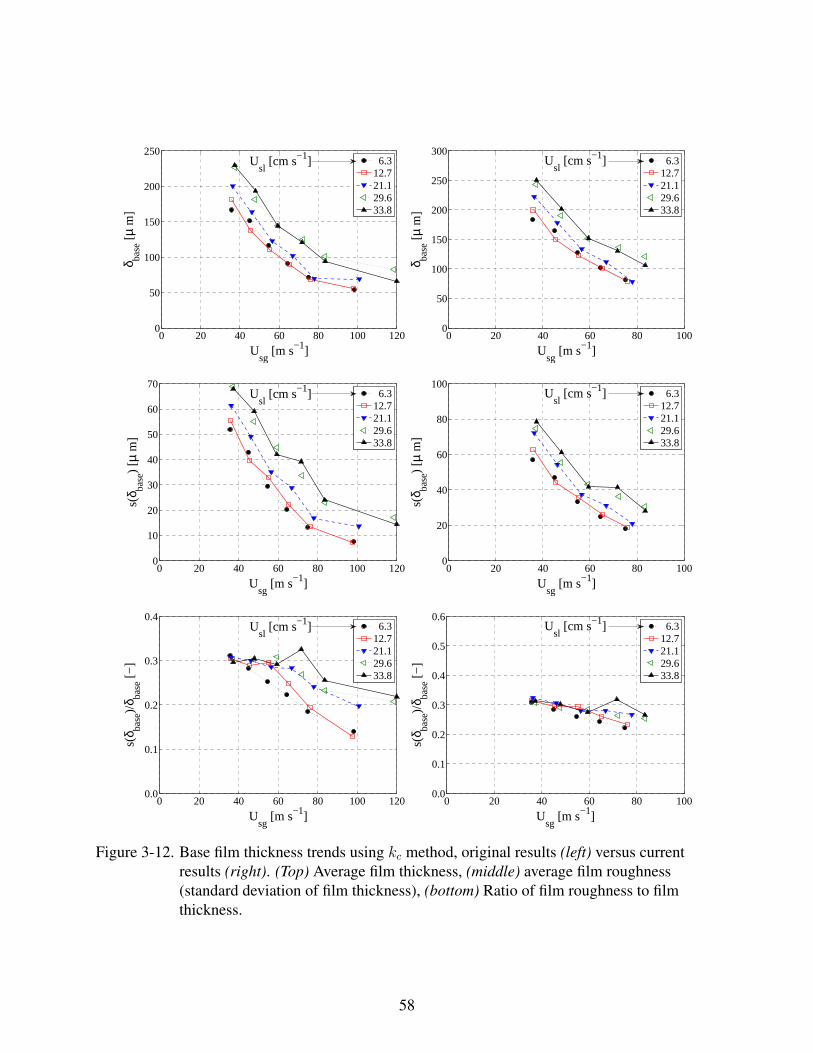
0 20 40 60 80 100 1200

50

100

150

200

250

Usg

[m s−1]

δ base [

µ m

]

6.312.721.129.633.8

Usl [cm s−1]

0 20 40 60 80 1000

50

100

150

200

250

300

Usg

[m s−1]

δ base [

µ m

]

6.312.721.129.633.8

Usl [cm s−1]

0 20 40 60 80 100 1200

10

20

30

40

50

60

70

Usg

[m s−1]

s(δ ba

se)

[µ m

]

6.312.721.129.633.8

Usl [cm s−1]

0 20 40 60 80 1000

20

40

60

80

100

Usg

[m s−1]

s(δ ba

se)

[µ m

]

6.312.721.129.633.8

Usl [cm s−1]

0 20 40 60 80 100 1200.0

0.1

0.2

0.3

0.4

Usg

[m s−1]

s(δ ba

se)/

δ base [−

]

6.312.721.129.633.8

Usl [cm s−1]

0 20 40 60 80 1000.0

0.1

0.2

0.3

0.4

0.5

0.6

Usg

[m s−1]

s(δ ba

se)/

δ base [−

]

6.312.721.129.633.8

Usl [cm s−1]

Figure 3-12. Base film thickness trends using kc method, original results (left) versus currentresults (right). (Top) Average film thickness, (middle) average film roughness(standard deviation of film thickness), (bottom) Ratio of film roughness to filmthickness.

58

0 500 1000 15000

2000

4000

6000

8000

10000

12000

14000

δ [µm]

n pt [−

]

0 500 1000 15000

0.5

1

1.5

2

2.5

3

3.5

4x 10

4

δ [µm]

n pt [−

]

0 200 400 600 800 1000 12000

0.5

1

1.5

2

2.5

3x 10

4

δ [µm]

n pt [−

]

0 200 400 600 800 10000

0.5

1

1.5

2

2.5

3x 10

4

δ [µm]

n pt [−

]

0 200 400 600 800 10000

0.5

1

1.5

2x 10

4

δ [µm]

n pt [−

]

0 200 400 600 800 1000 12000

0.5

1

1.5

2

2.5

3

3.5

4x 10

4

δ [µm]

n pt [−

]

Figure 3-13. Histograms of wave height using kc method, original results (left) versus currentresults (right). Flow conditions (top to bottom) 109F, 128F, and 147F (constant Usl= 21.1 cm s−1).

59

0 200 400 600 8000

0.5

1

1.5

2x 10

4

δ [µm]

n pt [−

]

0 200 400 600 800 10000

0.5

1

1.5

2

2.5

3x 10

4

δ [µm]

n pt [−

]

0 100 200 300 400 500 6000

0.5

1

1.5

2

2.5

3x 10

4

δ [µm]

n pt [−

]

0 200 400 600 8000

0.5

1

1.5

2

2.5

3x 10

4

δ [µm]

n pt [−

]

Figure 3-14. Histograms of wave height using kc method, original results (left) versus currentresults (right). Flow conditions (top to bottom) 166F and 185F (constant Usl = 21.1cm s−1).

3.3.3.2 Intermittency Input Method

The INTw distributions are not compared directly to the original code in the same manner

as the kc distributions. The current data processing uses INTw values from Chapter 5 that differ

from those used in the work of Schubring [58], which would undermine such a comparison.

Instead, the film thickness trends of the kc and INTw methods have been compared to each other

in Figures 3-17 through 3-19. The base and wave distributions generated using this method are

shown in Appendix D.

Average base film trends are shown in Figure 3-17. The values for the INTw method are

generally higher and show a steeper slope, indicating a stronger dependence on gas flow rate. The

60

0 20 40 60 80 100 1200

100

200

300

400

500

Usg

[m s−1]

δ wav

e [µ

m]

6.312.721.129.633.8

Usl [cm s−1]

0 20 40 60 80 1000

100

200

300

400

500

600

700

Usg

[m s−1]

δ wav

e [µ

m]

6.312.721.129.633.8

Usl [cm s−1]

0 20 40 60 80 100 1200

20

40

60

80

100

120

140

Usg

[m s−1]

s(δ w

ave)

[µ m

]

6.312.721.129.633.8

Usl [cm s−1]

0 20 40 60 80 1000

50

100

150

200

250

Usg

[m s−1]

s(δ w

ave)

[µ m

]

6.312.721.129.633.8

Usl [cm s−1]

0 20 40 60 80 100 1200.0

0.1

0.2

0.3

0.4

Usg

[m s−1]

s(δ w

ave)/

δ wav

e [−]

6.312.721.129.633.8U

sl [cm s−1]

0 20 40 60 80 1000.0

0.1

0.2

0.3

0.4

0.5

0.6

Usg

[m s−1]

s(δ w

ave)/

δ wav

e [−]

6.312.721.129.633.8

Usl [cm s−1]

Figure 3-15. Wave height trends using kc method, original results (left) versus current results(right). (Top) Average film thickness, (middle) average film roughness (standarddeviation of film thickness), (bottom) Ratio of film roughness to film thickness.

61

0 20 40 60 80 100 1201.0

1.5

2.0

2.5

3.0

Usg

[m s−1]

δ wav

e/δba

se [−

]

6.312.721.129.633.8

Usl [cm s−1]

0 20 40 60 80 1001.0

1.5

2.0

2.5

3.0

Usg

[m s−1]

δ wav

e/δba

se [−

]

6.312.721.129.633.8

Usl [cm s−1]

Figure 3-16. Ratio of wave height to base film using kc method, original results (left) versuscurrent results (right).

relative roughness has also increased by a few percent. Many of the trends discussed with data

from the kc method are still apparent.

Average wave height trends are shown in Figure 3-18. Similar to the base film, the average

wave height values have increased and the slope has become steeper. This is to be expected if

the INTw method creates a separation criterion higher than the kc method – both averages will

increase. The roughness in the wave zone is consistent between both methods, which creates a

decrease in the relative roughness for INTw by a few percent.

Figure 3-19 shows wave-to-base ratios after the zone separation. The INTw values are

directly related to these ratios, which clearly show functions of both gas and liquid flow rates.

The lower water flow rates, 800 and 1000 L min−1, show very erratic behavior as a function of

gas flow. The wave-to-base ratio has been empirically correlated using flow quality (x), shown in

Equation 3–7. The error for this correlation has also been calculated, shown in Table 3-3.

δwaveδbase

= 1.86x−0.18 (3–7)

Table 3-3. Error calculations for base-to-wave ratio correlation.Error (%) MAE (%) RMS (%)−0.25 6.74 8.13

62

0 20 40 60 80 1000

50

100

150

200

250

300

Usg

[m s−1]

δ base [

µ m

]

6.312.721.129.633.8

Usl [cm s−1]

0 20 40 60 80 1000

50

100

150

200

250

300

Usg

[m s−1]

δ base [

µ m

]

6.312.721.129.633.8

Usl [cm s−1]

0 20 40 60 80 1000

20

40

60

80

100

Usg

[m s−1]

s(δ ba

se)

[µ m

]

6.312.721.129.633.8

Usl [cm s−1]

0 20 40 60 80 1000

20

40

60

80

100

Usg

[m s−1]

s(δ ba

se)

[µ m

]

6.312.721.129.633.8

Usl [cm s−1]

0 20 40 60 80 1000.0

0.1

0.2

0.3

0.4

0.5

0.6

Usg

[m s−1]

s(δ ba

se)/

δ base [−

]

6.312.721.129.633.8

Usl [cm s−1]

0 20 40 60 80 1000.0

0.1

0.2

0.3

0.4

0.5

0.6

Usg

[m s−1]

s(δ ba

se)/

δ base [−

]

6.312.721.129.633.8

Usl [cm s−1]

Figure 3-17. Base film thickness trends, kc method (left) versus INTw method (right). (Top)Average film thickness, (middle) average film roughness (standard deviation of filmthickness), (bottom) Ratio of film roughness to film thickness.

63

0 20 40 60 80 1000

100

200

300

400

500

600

700

Usg

[m s−1]

δ wav

e [µ

m]

6.312.721.129.633.8

Usl [cm s−1]

0 20 40 60 80 1000

50

100

150

200

250

Usg

[m s−1]

s(δ w

ave)

[µ m

]

6.312.721.129.633.8

Usl [cm s−1]

0 20 40 60 80 1000.0

0.1

0.2

0.3

0.4

0.5

0.6

Usg

[m s−1]

s(δ w

ave)/

δ wav

e [−]

6.312.721.129.633.8

Usl [cm s−1]

Figure 3-18. Wave height trends, kc method (left) versus INTw method (right). (Top) Averagefilm thickness, (middle) average film roughness (standard deviation of filmthickness), (bottom) Ratio of film roughness to film thickness.

64

0 20 40 60 80 1001.0

1.5

2.0

2.5

3.0

Usg

[m s−1]

δ wav

e/δba

se [−

]

6.312.721.129.633.8

Usl [cm s−1]

Figure 3-19. Ratio of wave height to base film, kc method (Left) versus INTw method (right).

65

CHAPTER 4PLIF INTERFACE TRACKING

Most of the PLIF images have been taken with a very large time separation to ensure

independent measurements. By taking PLIF images at much shorter time intervals, the movement

of the gas-liquid interface can be observed. Global models require and estimate of this, for

which a linear relationship (Schubring and Shedd [1]) or the UVP (Equation 2–42, Owen and

Hewitt [61]) in the film has been assumed.

The characterization of the gas-liquid interface is highly dependent on disturbance wave

behavior, as demonstrated in the literature (e.g., Azzopardi [45, 46]). PLIF images allow for the

separation of base film and wave behavior, unavailable by other film thickness measurement

techniques.

The raw data for short time delay PLIF pairs was acquired by Schubring [58] with the same

apparatus used in Chapter 3. The time delays for each image set were selected to produce pairs

appropriate for cross-correlation (roughly 50 pixels in distance). The flow conditions tested for

this work, along with the time delay for each set, are shown in Table E-1. The current chapter

includes preliminary findings as well as challenges and suggestions for future work.

4.1 PLIF Image Pair Processing

Four stages of processing are used to transform PLIF image pairs into reviewable trend plots

for interfacial velocity. A diagram of stages 1 through 3 is shown in Figure 4-1.

1. Each image is processed to identify the liquid edge.

2. Each pair is split into sections and individually correlated to identify the appropriate lagdistances.

3. The raw data is processed through outlier removal, conversion to physical scale, andnon-dimensionalization.

4. The processed data is compared to liquid velocity models, including

(a) The universal velocity profile (for individual flow conditions), and

(b) The van Driest model for continuous law of the wall (for multiple flow conditions).

66

Image Processing / Edge Location Image Processing / Edge Location

Raw Image 1 Raw Image 2

Processed Image 1

Processed Image 2

Edge Locations 1

(pixels)

EdgeLocations 2

(pixels)

Cross-Correlation

Images:Combined and Shifted

Pairs

Graph: Correlation vs.

Image LagCorrelation Data

(pixels)Flow Rates and Flow Parameters

Base / Wave Division Criteria

Elapsed Time (Δt)

Data Processing and Fitting

Graph: y+ vs u

i+

(total)

Number ofDivisions (2)

Graph:y+ vs u

i+

(flow condition)

Figure 4-1. Diagram of processing path for PLIF interface tracking.

67

4.1.1 PLIF Image Pair Edge Processing

The work of Schubring [58] discussed some difficulties associated with cross-correlating

PLIF edge vectors. Most of the issues were focused on accurately detecting the liquid edge, often

complicated by bubbles in the interface. Many of these issues have been addressed by adjusting

the PLIF edge finding routine, outlined in Chapter 3. The edge processing for tracking the liquid

interface utilizes the edge processing code developed in Section 3.2. The actual image processing

and edge finding routines are identical except for the film thickness threshold, which needed to be

adjusted due to reduced contrast between gas and liquid for the PLIF image pairs.

The varying level of quality from one image to the next made a constant threshold difficult

to determine. This version of the PLIF edge finding code employs a histogram-based threshold

selection method developed by Otsu [62]. Otsu’s method iteratively determines the most accurate

threshold value based on the reduction of variance in the thresholded section. It has been

observed to create accurate results in a higher range of image qualities by visual inspection.

4.1.2 PLIF Image Pair Divisions

Each image has an axial distance of 1300 pixels, or about 4 mm. As a result, the film

thickness may vary from base to wave within an image. Large bubbles may also obscure

interface. This poses a problem to correlating the image pairs, as different film heights and film

features move at different velocities. This also poses a problem for developing velocity as a

function of distance from the wall if the wall height for an image pair is not clearly defined.

Each image pair is split into two sections, each 650 pixels in length. The remainder of the

image pair processing scheme is performed on each section individually. Other numbers of

sections were considered. However, as the size of the image pairs decreased, the chances of poor

correlation increase due to a lack of features in the liquid edge. Splitting the images into two

sections yielded the most consistent cross-correlation success.

4.1.3 PLIF Image Pair Cross-Correlation

This stage of the processing uses cross-correlation to determine the most accurate distance

lag between the edge vectors. The cross-correlation is performed using a built-in MATLAB

68

function, which takes each edge vector as an input and returns an array of correlation values

(between -1 and 1, termed Xcorr). The values of Xcorr correspond to the distances that the

edge vectors were lagged, termed Lag.

The appropriate correlated distance between an image pair is found as the maximum value

of Xcorr for Lag values between -100 and 600 pixels. A negative value for Lag would represent

a negative velocity, which may be physically accurate in some cases due to local flooding.

However, Lag values less than -100 pixels (-0.3 mm) most often correspond to broken sections of

film or the incorrect correlation of features. High Xcorr values may often occur near the ends of

the edge vectors (Lag > 600). This is generally due to coincidental agreement at the edge ends,

and so any Lag value over 600 pixels (1.9 mm) is ignored.

This stage of the code also outputs figures for verification of the edge finding and correlation

process. A graph of Xcorr versus Lag is produced for each original image pair that includes a

line for each image section. This figure also includes the recorded value of Lag for each image

section. An example correlation graph for each gas flow rate is shown in Figure 4-2.

A combined image is produced for each correlated image pair that includes each edge vector

superimposed on one image, shifted by the recorded Lag value for verification. The compiled

images that correspond to the correlation graphs in Figure 4-2 are shown in Figure 4-3. Each

image has the first image of the pair on top and the second one the bottom. The yellow line is the

liquid edge of the first image, shifted and superimposed on the liquid edge of the second image

(cyan line).

4.1.4 PLIF Image Pair Data Processing

This stage of the image pair processing uses the physical pixel scale of the images and a

priori knowledge of flow conditions to input fluid properties for velocity and distance calculation.

The raw interfacial velocity, ui, is calculated from the physical distance traveled by the film over

the known elapsed time, ∆t. The distance from the wall, y, was calculated as the average of both

edge vectors for an image pair (not including zeros). The non-dimensionalization is performed

69

−600 −400 −200 0 200 400 600−0.5

0

0.5

1

Lag (pixels)

X−

corr

[−]

Section 1 Lag = 77Section 2 Lag = 75

−600 −400 −200 0 200 400 600−0.5

0

0.5

1

Lag (pixels)

X−

corr

[−]


−600 −400 −200 0 200 400 600−0.5

0

0.5

1

Lag (pixels)

X−

corr

[−]


−600 −400 −200 0 200 400 600−0.5

0

0.5

1

Lag (pixels)

X−

corr

[−]


−600 −400 −200 0 200 400 600−0.5

0

0.5

1

Lag (pixels)

X−

corr

[−]


Figure 4-2. PLIF cross-correlation example graphs from flow conditions (top left) 105F, (topright) 126F, (middle left) 143F, (middle right) 164F, (bottom) 181F.

from the following:

u+i =

uiu?

(4–1)

y+ =yu?

νl(4–2)

70

Figure 4-3. PLIF cross-correlation example images, (left) section 1, (right) section 2. Taken fromflow conditions (top to bottom) 105F, 126F, 143F, 164F, and 181F.

u? =

√τi,waveρl

(4–3)

where ui is the measured interfacial velocity, u+i is the dimensionless interfacial velocity, y+ is a

wall unit, and τi,wave is calculated from Equation 2–56.

Each PLIF image pair is marked as wave or base film using intermittency data from

Chapter 5. The division is based on the average film thickness of each correlated pair, not

including zeros in the edge vectors. The total list of film points is then sorted and separated based

71

on the recorded wave intermittency for that flow condition. Data points that represent wave film

are displayed as red dots and base film sections are displayed as blue dots.

4.1.4.1 PLIF Image Pair Outlier Removal

It was demonstrated in Section 3.2.3 that there is an error associated with PLIF processing

that results in poorly identified liquid edges up to 5% of the time. PLIF interface tracking

requires that both images in a pair be correctly processed, which compounds that error. In

addition, the use of cross-correlation is dependent on features of the interface being present and

identified in both images.

An image pair is accepted as a data point if it meets all three of the following criteria:

1. The lag distance must be within three standard deviations away from the mean lag for aflow condition.

2. The maximum Xcorr value must be greater than 0.25.

3. Over half of the edge vector must be recorded as an edge (not a zero).

4.1.4.2 Van Driest Model Data Fitting

The non-dimensionalized data points for the 800 L min−1 and 1200 L min−1 gas flow

rate conditions were combined for a more comprehensive data fit. The Van Driest model for a

continuous law of the wall, described in Kays et al. [2], has been used for this purpose. The

model introduces an empirical constant, A+, and an integral that must be evaluated numerically:∫ u+

u+o

du+ =1

κ

∫ y+

y+o

dy+

y+[1 − exp

(− y+

A+

)] (4–4)

where κ is the von Karman constant (0.41), and u+o and y+

o are the lower bounds of the model.

The van Driest model was developed to extend to the viscous sublayer, eliminating the need for

a buffer layer in the UVP. Therefore, the values below the bounds of the van Driest model are

assumed to obey the viscous sublayer (u+ = y+) and the lower bounds are set equal to eachother.

The value for u+o is then determined by solving the following:

1

κ= u+

o

[1 − exp

(− u+

o

A+

)](4–5)

72

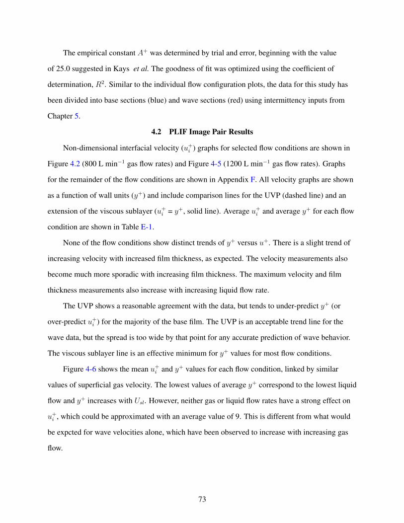
The empirical constant A+ was determined by trial and error, beginning with the value

of 25.0 suggested in Kays et al. The goodness of fit was optimized using the coefficient of

determination, R2. Similar to the individual flow configuration plots, the data for this study has

been divided into base sections (blue) and wave sections (red) using intermittency inputs from

Chapter 5.

4.2 PLIF Image Pair Results

Non-dimensional interfacial velocity (u+i ) graphs for selected flow conditions are shown in

Figure 4.2 (800 L min−1 gas flow rates) and Figure 4-5 (1200 L min−1 gas flow rates). Graphs

for the remainder of the flow conditions are shown in Appendix F. All velocity graphs are shown

as a function of wall units (y+) and include comparison lines for the UVP (dashed line) and an

extension of the viscous sublayer (u+i = y+, solid line). Average u+

i and average y+ for each flow

condition are shown in Table E-1.

None of the flow conditions show distinct trends of y+ versus u+. There is a slight trend of

increasing velocity with increased film thickness, as expected. The velocity measurements also

become much more sporadic with increasing film thickness. The maximum velocity and film

thickness measurements also increase with increasing liquid flow rate.

The UVP shows a reasonable agreement with the data, but tends to under-predict y+ (or

over-predict u+i ) for the majority of the base film. The UVP is an acceptable trend line for the

wave data, but the spread is too wide by that point for any accurate prediction of wave behavior.

The viscous sublayer line is an effective minimum for y+ values for most flow conditions.

Figure 4-6 shows the mean u+i and y+ values for each flow condition, linked by similar

values of superficial gas velocity. The lowest values of average y+ correspond to the lowest liquid

flow and y+ increases with Usl. However, neither gas or liquid flow rates have a strong effect on

u+i , which could be approximated with an average value of 9. This is different from what would

be expcted for wave velocities alone, which have been observed to increase with increasing gas

flow.

73

0 10 20 30 400

10

20

30

40

50

60

70

Ui+ [−]

δ + [−

]

Ui+ Base

Ui+ Wave

UVP

Ui+ = y+

0 10 20 30 400

10

20

30

40

50

60

70

80

Ui+ [−]

δ + [−

]

Ui+ Base

Ui+ Wave

UVP

Ui+ = y+

0 10 20 30 40 500

20

40

60

80

100

Ui+ [−]

δ + [−

]

Ui+ Base

Ui+ Wave

UVP

Ui+ = y+

0 5 10 15 20 25 30 350

20

40

60

80

100

120

140

Ui+ [−]

δ + [−

]

Ui+ Base

Ui+ Wave

UVP

Ui+ = y+

Figure 4-4. y+ vs. u+i plots for flow conditions (top left) 102F, (top right) 105F, (bottom left)

109F, and (bottom right) 113F. (Approximate Usg = 36 m s−1).

The result of the van Driest model data fit is shown in Figure 4-7 using a value of 34.0 for

A+. As with UVP curves for individual flow condtions, this model tends to under-predict the

base film velocity. The model also turns upwards sharply, failing to predict any u+i values much

over 20. However, the wide distribution of film thickness and velocity measurements would make

fitting this data difficult with any model, as evident in the wave section.

74

0 10 20 30 40 500

10

20

30

40

50

Ui+ [−]

δ + [−

]

Ui+ Base

Ui+ Wave

UVP

Ui+ = y+

0 10 20 30 40 500

10

20

30

40

50

60

70

80

Ui+ [−]

δ + [−

]

Ui+ Base

Ui+ Wave

UVP

Ui+ = y+

0 10 20 30 40 500

10

20

30

40

50

60

70

Ui+ [−]

δ + [−

]

Ui+ Base

Ui+ Wave

UVP

Ui+ = y+

0 5 10 15 20 25 30 350

50

100

150

200

Ui+ [−]

δ + [−

]

Ui+ Base

Ui+ Wave

UVP

Ui+ = y+

Figure 4-5. y+ vs. u+i plots for flow conditions (top left) 140F, (top right) 143F, (bottom left)

147F, (bottom right) 151F. (Approximate Usg = 57 m s−1).

0 5 10 15 200

10

20

30

40

50

Ui+ [−]

δ + [−

]

36.145.855.865.976.8

Usg

[m s−1]

Figure 4-6. Average y+ vs. u+i , by Usg.

75

0 10 20 30 40 50 600

20

40

60

80

100

120

Ui+

y+ (m

ean)

Ui+ Base

Ui+ Wave

van Driest

Figure 4-7. PLIF interfacial velocity data (with van Driest model). Flow conditions included:102F, 105F, 109F, 113F, 140F, 143F, 147F, and 151F.

76

CHAPTER 5VERTICAL WAVE LENGTH MEASUREMENT

High-speed videos of many vertical annular flow conditions were acquired and analyzed in

the work of Schubring, Shedd and Hurlburt [19] and in the dissertation of Schubring [58]. The

two major objectives of the studies were to:

• Demonstrate the use of high-speed video to estimate the velocities, lengths, and temporalspacings of individual waves.

• Use these individual wave measurements to develop average velocites, lengths, frequenciesand intermittencies of disturbance waves as functions of gas and liquid flow rates.

The current work is an extension of one aspect of the original vertical wave processing code

– wave length measurement. A new wave length measurement technique has been developed to

address the circumferential asymmetry of disturbance waves traveling through a vertical tube.

All other aspects of the processing are identical including identification, velocity, and frequency

measurements. The goal of the current work is to use the new processing method to study the

effect of circumferential asymmetry on wave behavior.

5.1 Vertical Wave Video Acquisition

A vertical test facility was constructed around a quartz tube with an inner diameter of 0.0234

m (23.4 mm), shown in Figure 5-1. All aspects of this flow loop are identical to that used for

the PLIF measurements (Chapter 3) with the exception of the test section tube material and

diameter. Liquid and gas mass flow rates and superficial velocities were recorded using flow

meters coupled with static pressure measurements. Liquid superficial velocities in the present

work range from 0.04 to 0.39 m/s, with gas superficial velocities between 36 and 82 m/s. Test

section pressures ranged from 100 to 116 kPa.

A 0.303 m long region of the tube was back lit with five lights and imaged with an In-

tegrated Design Tools X-Stream VISION XS-3 high-speed CMOS digital camera in 8-bit

grayscale. Waves appear in the test region as dark patches that pass over each of the five lights

in sequence. The conversion to physical scale was accomplished by also recording video of a

ruler, shown in Figure 5-2. The pixels were 242 µm squares. The total image resolution was 1252

77

(Waves)(P)

(dP)

Separator Exhaust

Air Rotameters(P)

Compressed Air (from lab)

Water Meter

Gear Pump

Copper (below)/Quartz (above) Boundary

Reservoir

Air Flow Straighteners

Figure 5-1. Schematic of vertical flow loop with quartz test section.

pixels (axial length) by 112 or 120 pixels (width). Regions exposed to each light were used as

virtual detectors for the identification and tracking of disturbance waves.

Figure 5-2. Visualization section for vertical waves, including measurement for physical scale.

The frame rate for the video aqcuisition was varied based on the observation that wave

velocity increases with increasing gas flow. The frame rate was increased with increasing gas

velocity as indicated in Table 5-1. The video duration was also altered to maintain a consistent

number of frames for processing. The initial video outputs (saved as .avi files) were separated

into uncompressed .tif images for analysis.

Every aspect of the original vertical high-speed video processing code (MATLAB-based)

has been maintained except for the wave length measurement method. The code begins with

78

Table 5-1. Frame rates and video lengths for vertical wave videosQg,nom [L min−1] fps [s−1] tvideo [s] nframes [-]

800 400 11 44001000 500 10 50001200 600 9 54001400 700 8 56001600 800 7 56001800 900 6 5400

wave identification, accomplished using the score of wave, a metric developed by Schubring

et al. [19] for wave tracking. The score is calculated as a function of the peak-normalized

darkness, summed over three consecutive video frames. The code proceeds with wave tracking

(unchanged), wave verification (unchanged), and wave length measurement (discussed below).

5.2 Vertical Wave Length Processing

Two measurement techniques have been applied to estimate the length of disturbance waves,

a single-section measurement (original code) and a multi-section measurement (current code). A

schematic of the two measurement techniques is shown in Figure 5-3, where L1 represents the

original estimate and L2 is the current estimate. The single-section method proceeds by locating

the center of the wave (darkest section), then scanning in both directions to find the forward

and rear edges of the wave. The wave is then recorded as the difference between the two edge

recordings. A more detailed description of the original processing code is provided by Schubring

et al. [19].

The multi-section method proceeds by identifying the center of the wave in the same manner

as the original code. The image is then split into four equal sections (Img(sec), sec = 1 through

4) along the tube width. Each section is then averaged along its width to produce avedarki(sec),

then normalized by the time-independent average for the entire flow condition (avedarkX) to

produce ddarki(sec), shown in Equation 5–1. All of the elements in Equation 5–1 are arrays

with a pixel length equal to the length of the test section.

ddarki(sec) = Img(sec) − avedarkX (5–1)

79

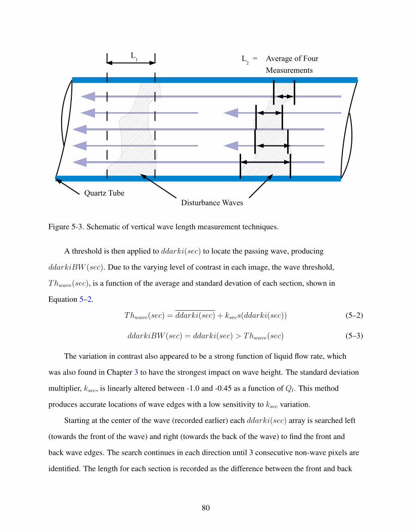
L1 L

2 = Average of Four

Measurements

Quartz TubeDisturbance Waves

Figure 5-3. Schematic of vertical wave length measurement techniques.

A threshold is then applied to ddarki(sec) to locate the passing wave, producing

ddarkiBW (sec). Due to the varying level of contrast in each image, the wave threshold,

Thwave(sec), is a function of the average and standard devation of each section, shown in

Equation 5–2.

Thwave(sec) = ddarki(sec) + ksecs(ddarki(sec)) (5–2)

ddarkiBW (sec) = ddarki(sec) > Thwave(sec) (5–3)

The variation in contrast also appeared to be a strong function of liquid flow rate, which

was also found in Chapter 3 to have the strongest impact on wave height. The standard deviation

multiplier, ksec, is linearly altered between -1.0 and -0.45 as a function of Ql. This method

produces accurate locations of wave edges with a low sensitivity to ksec variation.

Starting at the center of the wave (recorded earlier) each ddarki(sec) array is searched left

(towards the front of the wave) and right (towards the back of the wave) to find the front and

back wave edges. The search continues in each direction until 3 consecutive non-wave pixels are

identified. The length for each section is recorded as the difference between the front and back

80

edges. The wave length for the image (Lwave) is recorded as the average of all four wave section

measurements (Lsec, Equation 5–5) and converted to a physical scale. The wave intermittency for

the flow condition is then calculated from the following:

INTw =Lwavefwavevwave

(5–4)

Lwave =1

4

4∑i=1

Lsec,i (5–5)

The program outputs the original image with all four wave section measurements superim-

posed (as solid lines) and the results of the single-section measurement from the original code (as

dashed lines). Average values of wave length (Lwave), wave frequency (fwave), and wave velocity

(vwave) are calculated for each flow condition.

5.3 Vertical Wave Length Results

Wave length (Lwave) and wave intermittency (INTw) measurements are recorded in

Appendix G for all flow conditions along with gas and liquid superficial velocities.

5.3.1 Individual Wave Length Results

Example images with both wave length measurement techniques are shown in Figure 5-4 for

increasing gas flow, where dashed lines indicate the single-measurement method and solid lines

indicate the multi-measurement method. Additional wave measurement examples are shown in

Appendix H for increasing liquid flow.

Disturbance waves are not always symmetric around the circumference of the tube. A wave

is often observed to be thicker in certain sections or travel with a slant through the tube. The

observation of assymetry in disturbance waves has also been addressed by Belt [20] through the

use of three-dimensional conductance probe measurements.

The single-section measurement technique records all wave edges at the left and right

extremes, and is therefore over-estimating the length of assymetrical features. This can be seen

in Figure 5-4, where the distance between dashed lines is consistently larger than between solid

lines.

81

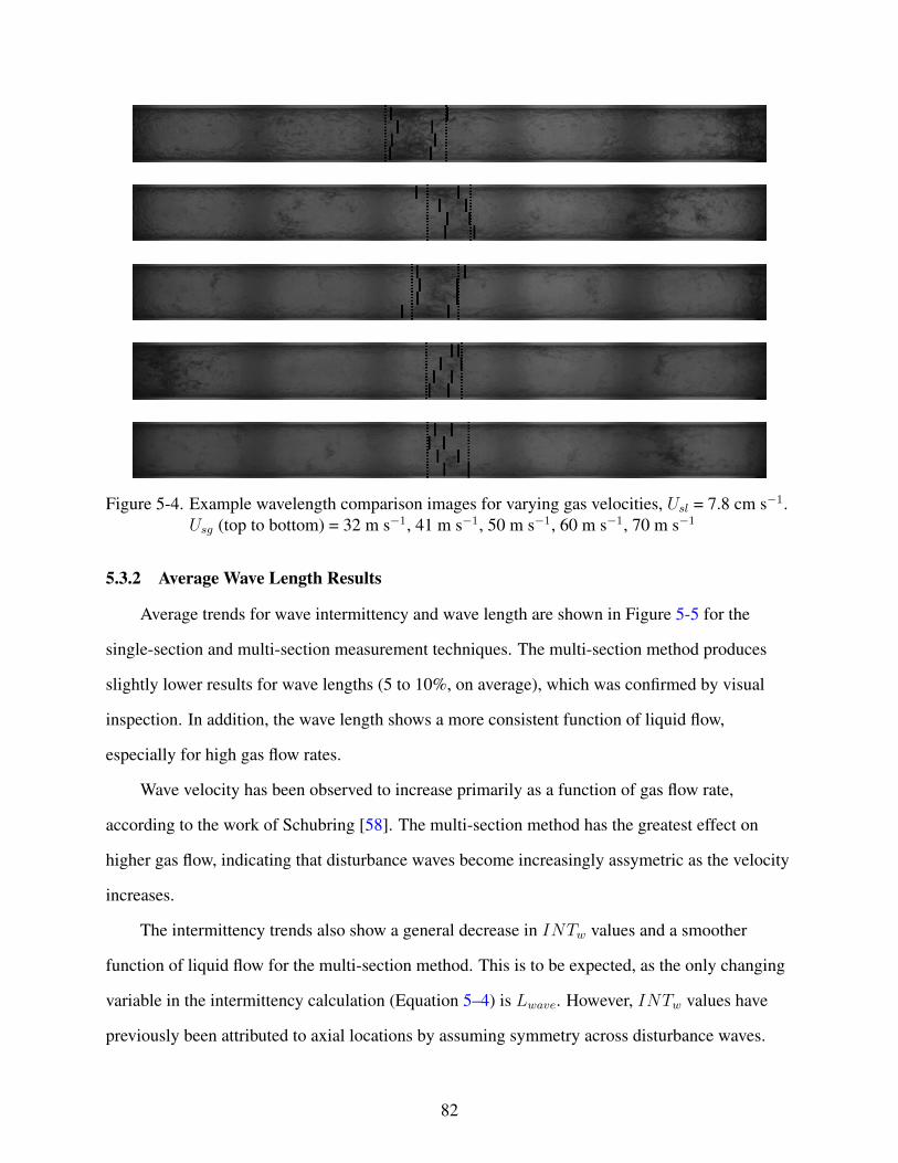
Figure 5-4. Example wavelength comparison images for varying gas velocities, Usl = 7.8 cm s−1.Usg (top to bottom) = 32 m s−1, 41 m s−1, 50 m s−1, 60 m s−1, 70 m s−1

5.3.2 Average Wave Length Results

Average trends for wave intermittency and wave length are shown in Figure 5-5 for the

single-section and multi-section measurement techniques. The multi-section method produces

slightly lower results for wave lengths (5 to 10%, on average), which was confirmed by visual

inspection. In addition, the wave length shows a more consistent function of liquid flow,

especially for high gas flow rates.

Wave velocity has been observed to increase primarily as a function of gas flow rate,

according to the work of Schubring [58]. The multi-section method has the greatest effect on

higher gas flow, indicating that disturbance waves become increasingly assymetric as the velocity

increases.

The intermittency trends also show a general decrease in INTw values and a smoother

function of liquid flow for the multi-section method. This is to be expected, as the only changing

variable in the intermittency calculation (Equation 5–4) is Lwave. However, INTw values have

previously been attributed to axial locations by assuming symmetry across disturbance waves.

82

0 10 20 30 40 500.00

0.01

0.02

0.03

0.04

0.05

0.06

Usl [cm s−1]

Lw

ave [m

]

3443536576

Usg

[m s−1]

0 10 20 30 40 500.00

0.01

0.02

0.03

0.04

0.05

0.06

Usl [cm s−1]

Lw

ave [m

]

3443536576

Usg

[m s−1]

0 10 20 30 40 500.00

0.05

0.10

0.15

0.20

0.25

0.30

Usl [cm s−1]

INT

w [−

]

3443536576

Usg

[m s−1]

0 10 20 30 40 500.00

0.05

0.10

0.15

0.20

0.25

0.30

Usl [cm s−1]

INT

w [−

]

3443536576

Usg

[m s−1]

Figure 5-5. (Top) Lwave vs. Usl, by Usg. (Bottom) INTw vs. Usl, by Usg. (Left) Single-sectionwave length measurement technique. (Right) Multiple-section wave lengthmeasurement technique.

The application of the multi-section method removes the assumption of symmetry, and thereby

relocates wave behavior from an axial location to a location on the liquid film. This change in

location has a direct impact on two-zone modeling efforts, including Hurlburt et al. [57] and

Schubring et al. [1], ans is more consistent with an application of film modeling.

5.3.3 Wave Correlations

Emprical correlations were developed for the single-section data in the work of Schubring [58].

The correlations for Lwave and INTw have been re-optimized for the multi-section data:

Lwave,KS = 0.43D

x0.63(5–6)

INTw,KS = 0.07 +Rel

49000(5–7)

83

These correlations’ performance is shown in Figure 5-6; all vertical-specific correlations are

judged as shown in Table 5-2, based on flows with Qg,nom of 800 to 1600 L min−1 (i.e., those

plotted in this chapter).

Table 5-2. Performance of vertical-specific wave correlationsCorrelated Parameter Mean Error [%] MAE [%] RMS [%]Lwave,KS −1.58 15.91 20.50INTw,KS −1.10 9.47 12.13

0 1 2 3 4 5 60

1

2

3

4

5

6

Lwave

[m]

Lw

ave,

KS [m

]

3443536576± 20%

Usg

[m s−1]

0 1 2 3 4 5 60

1

2

3

4

5

6

Lwave

[m]

Lw

ave,

KS [m

]

3.9 7.815.523.334.9± 20%

Usl [cm s−1]

0.00 0.05 0.10 0.15 0.20 0.25 0.300.00

0.05

0.10

0.15

0.20

0.25

0.30

INTw

[m]

INT

w,K

S [m]

3443536576± 20%

Usg

[m s−1]

0.00 0.05 0.10 0.15 0.20 0.25 0.300.00

0.05

0.10

0.15

0.20

0.25

0.30

INTw

[m]

INT

w,K

S [m]

3.9 7.815.523.334.9± 20%

Usl [cm s−1]

Figure 5-6. Wave correlation performance. Series of constant Usg. (Right) Series of similar Usl.(Top) Lwave,KS . (Bottom) INTw,KS .

84

CHAPTER 6GLOBAL MODEL APPLICATION

The global model of Schubring and Shedd [1] (described in Chapter 2) has been modified

based on the results of Chapters 3 and 5. The optimization of the model proceeds by first

updating the film behavior correlations developed in the current work. The second step is

determining which parameters in the model (empirical and physical) can be adjusted to improve

agreement with data and to more accurately reflect the physics of annular flow.

The metrics of optimization for this work are the errors between correlated parameters

and measured outputs, which vary depending on the measurement test section. For the FEP

test section (used for PLIF film measurement), average film thickness (δ), base film thickness

(δbase), and wave height (δwave) data are available. For the quartz test section, pressure gradient

(dP/dz) and disturbance wave velocity (vwave) data are available. The current model results are

also compared qualitatively to the results of the original model, presented in the dissertation of

Schubring [58].

6.1 Re-Correlated Film Behavior

The updated PLIF measurement technique in Chapter 3 and the updated vertical wave length

measurement technique in Chapter 5 have resulted in changes to film behavior approximations

relevant to the Schubring and Shedd model. The specific contributions of these adjustments to the

global model are described by test section.

6.1.1 PLIF Observations (FEP Test Section)

The Schubring and Shedd model relies on observations of roughness in the base zone,

roughness in the wave zone, and an approximation of wave-to-base film height ratio. The

following observations have been made in the current work that update those observations in the

model:

Base Film Roughness. The base film roughness is calculated in the current work as twice

standard deviation of base film data (same as the original work) and is used two ways in the

model:

85

1. In the roughness friction factor from Hurlburt et al. , shown in Equation 2–16.

2. To approximate the fraction of base film that travels with a linear profile (linear fraction,LFbase).

The original observation agrees well with the current work, demonstrating a constant relative

roughness of 0.6 and a LFbase of 0.7.

Wave Height Roughness. The wave roughness is calculated as the standard deviation of

wave data and is applied in the roughness friction factor shown in Equation 2–34. The roughness

in the wave zone has been observed in the current work as 60% of δwave (an increase from the

original observation of 40%).

Wave-to-Base Ratio. The original work estimated mean wave height as 2 times the mean

base height, which did not explain some low liquid flow behaviors. The current work shows that

the ratio is actually a function of gas and liquid flow rate. An empirical correlation was developed

to express this ratio as a function of flow quality (Equation 3–7), shown again here:

δwaveδbase

= 1.86x−0.18 (6–1)

6.1.2 Vertical Wave Observations

The updated wave length (Lwave) measurement code developed in Chapter 5 resulted in

different observations of wave length and wave intermittency (INTw) than the original work.

Wave Length Observations. The wave length distributions in the current work show

generally shorter values for Lwave than previously observed. The correlation for Lwave developed

by Schubring [19] (Equation 2–12) has been re-optimized to fit the new measurements:

Lwave,KS = 0.43D

x0.63(6–2)

Wave Intermittency Observations. INTw is closely linked to Lwave, and therefore

showed similar departures from the original model. The correlation for INTw developed by

Schubring [19] (Equation 2–51) has been re-optimized to fit the new measurements:

INTw,KS = 0.07 +Rel

49000(6–3)

86

6.2 Model Adjustments

Some parameters in the Schubring and Shedd model are purely empirical. The goal of a

global model is to describe annular flow from physical principles. The calculation of wave shear

from sharp base-wave transitions, τi,wave,trans, is one violation of this goal by employing a purely

empirical factor of 2. This parameter has been removed, effectively lowering the contribution of

transition shear:

τi,wave,trans =ρcoreUg,trans

2(δwave − δbase)

Lwave(6–4)

The base and wave zone sub-models both use the rough tube friction factor suggested by

Hurlburt et al. [57] and employ the empirical constants cB,base and cB,wave. These constants are

observed in the equations as the subjects of a natural logarithm, so by setting them to 1.0 in the

current model they are effectively eliminated:

Cf,i,base = 0.582

[− ln εbase

(εbase − 1)2 + 1.05 +1

2

εbase + 1

εbase − 1

]−2

(6–5)

Cf,i,wave = 0.582

[− ln εwave

(εwave − 1)2 + 1.05 +1

2

εwave + 1

εwave − 1

]−2

(6–6)

The prediction of film thickness (both zones) and velocity is very sensitive to the friction

correlation, including the empirical enhancer, φRR. The equation for φRR has been adjusted from

its original form (Equation 2–15) to the following:

φRR = 2.18x−0.1 (6–7)

The original model observed a poor correlation of wave velocity outputs for series of

constant liquid flow, which increased too quickly with increasing gas flow rate. This can be

attributed to an over-prediction of wave velocity by the universal velocity profile. To remedy this,

the relative roughness of the wave zone is used to predict the fraction of the wave that travels

with the prescribed profile (termed the wave varying fraction, V Fwave) creating the following

87

expression for wave velocity:

U+l,i,wave = 5.5 + 2.5 ln

((1 − V Fwave)δ

+wave

)(6–8)

Ul,i,wave = U+l,i,waveu

?wave (6–9)

V Fwave = 0.3 (6–10)

This assumes that the upper portion of the wave (rough fraction) does not increase the wave

velocity (well-mixed flow). This is in agreement with the preliminary results of PLIF interface

tracking in Chapter 4, which indicates a consistent over-pridiction of wave velocity by the UVP

as a function of wave height.

6.3 Comparison to Vertical Data (FEP Tube)

The original model was developed first with consideration of the vertical FEP tube flow

conditions, used primarily for the PLIF film thickness measurements. The separation between

base and wave zones has been performed using the INTw values from disturbance wave

visualization. Average values for δ, δbase, and δwave are available for each flow condition from

PLIF results and are compared to the model outputs for error estimation.

Table 6-1 shows the accuracy of the predictions for these three results for PLIF flows

investigated with Qg,nom of 1600 L min−1 and below. Flow 189F was imaged twice; both

comparisons are included in the results.

Table 6-1. Performance of present global model for vertical FEP film thickness data.Correlated Parameter Mean Error [%] MAE [%] RMS [%]δ -0.10 8.70 11.11δbase 0.17 8.93 11.49δwave 0.42 9.82 14.31

Figure 6-1 shows the predicted δ, δbase, and δwave with series of liquid flow rate, along with

the performance of the model for film thickness. The current model performs very well for δ

and δbase, with slight inaccuracies in constant liquid series. This observation is consistent with

the original model and is most likely related to the same issues: experimental errors – notably

88

locating the tube wall – that vary with flow rates. The original model also performed very well

for PLIF film thickness data and showed similar trends.

6.4 Comparison to Vertical Data (Quartz Tube)

Flow conditions studied in the quartz tube allow for two direct comparisons of modeled

results and experimental data: pressure gradient and wave velocity. A total of 54 flow conditions

(Qg,nom of 1600 L min−1 and below) are available. The performance of the model with respect to

these two quantities is shown in Table 6-2. The modeled and experimental results are compared

for the quartz tube in Figure 6-3.

Table 6-2. Performance of present global model for vertical quartz tube data.Correlated Parameter Mean Error [%] MAE [%] RMS [%]dP/dz 0.45 17.42 23.22vwave 10.88 19.14 20.99

For pressure loss, the results show similar trends as from the original model. The over-

prediction of dP/dz with high gas and liquid flow appears to be a chronic issue with the model

and these high flow rates. The error estimates are good, and on par with empirical pressure loss

estimators. The wave velocity is also well-predicted in the quartz tube, although the range of

vwave with increasing gas flow rate is somewhat underestimated – as in the original model. The

change applied to the Ul,i,wave calculation shows an improvement for velocity estimates at high

gas flow rates.

The estimate of entrained fraction from the model, Emod, is shown in Figure 6-4 as a

function of gas and liquid flow rate. This estimate is evaluated qualitatively due to the lack of

entrainment data for comparison.

The values for Emod decrease across the board for the new model while maintaining the

same trends. The increases with gas and liquid flow rate are consistent with the original model,

wave videos, and entrainment literature. The increase with liquid flow rate and the sharp drop

towards an entrained fraction of 0 at low Usl are in agreement with the excess liquid concept.

89

0 20 40 60 80 1000

50

100

150

200

250

300

350

400

Usg

[m s−1]

δ mod

[µ

m]

6.312.721.129.633.8

Usl [cm s−1]

0 50 100 150 200 250 300 350 4000

50

100

150

200

250

300

350

400

δexp

[µ m]

δ mod

[µ

m]

6.312.721.129.633.8± 20%

Usl [cm s−1]

0 20 40 60 80 1000

50

100

150

200

250

300

350

Usg

[m s−1]

δ base

,mod [

µ m

]

6.312.721.129.633.8

Usl [cm s−1]

0 50 100 150 200 250 300 3500

50

100

150

200

250

300

350

δbase,exp

[µ m]

δ base

,mod [

µ m

]

6.312.721.129.633.8± 20%

Usl [cm s−1]

0 20 40 60 80 1000

200

400

600

800

Usg

[m s−1]

δ wav

e,m

od [

µ m

]

6.312.721.129.633.8

Usl [cm s−1]

0 200 400 600 8000

200

400

600

800

δwave,exp

[µ m]

δ wav

e,m

od [

µ m

]

6.312.721.129.633.8± 20%

Usl [cm s−1]

Figure 6-1. Model results pertaining to film thickness for vertical FEP tube. (Left) Results forseries of Usl. (Right) Performance comparison. (Top) δ. (Middle) δbase. (Bottom)δwave.

90

0 20 40 60 80 1000

5

10

15

20

25

30

35

40

Usg

[m s−1]

τ i,mod

,bas

e (1

− IN

T w)

[Pa]

6.312.721.129.633.8

Usl [cm s−1]

0 5 10 15 20 25 30 35 400

5

10

15

20

25

30

35

40

Usl [cm s−1]

τ i,mod

,bas

e (1

− IN

T w)

[Pa]

3646576880

Usg

[m s−1]

0 20 40 60 80 1000

5

10

15

20

25

30

35

40

Usg

[m s−1]

τ i,mod

,wav

e,ro

ugh IN

Tw

[Pa]

6.312.721.129.633.8

Usl [cm s−1]

0 5 10 15 20 25 30 35 400

5

10

15

20

25

30

35

40

Usl [cm s−1]

τ i,mod

,wav

e,ro

ugh IN

Tw

[Pa]

3646576880

Usg

[m s−1]

0 20 40 60 80 1000

5

10

15

20

25

30

35

40

Usg

[m s−1]

τ i,mod

,wav

e,tr

ans IN

Tw

[Pa]

6.312.721.129.633.8

Usl [cm s−1]

0 5 10 15 20 25 30 35 400

5

10

15

20

25

30

35

40

Usl [cm s−1]

τ i,mod

,wav

e,tr

ans IN

Tw

[Pa]

3646576880

Usg

[m s−1]

Figure 6-2. Components of τi from model for vertical FEP tube. (Left) By Usl. (Right) By Usg.(Top) Base film roughness, τi,base (1 − INTw). (Middle) Wave roughness,τi,wave,roughINTw. (Bottom) Wave drag, τi,wave,transINTw.

91

0 20 40 60 80 1000

5

10

15

20

25

30

35

Usg

[m s−1]

−dP

/dz m

od [k

Pa

m−1 ]

3.9 7.815.523.334.9

Usl [cm s−1]

0 5 10 15 20 25 30 35 400

5

10

15

20

25

30

35

Usl [cm s−1]

−dP

/dz m

od [k

Pa

m−1 ]

3443536576

Usg

[m s−1]

0 5 10 15 20 25 30 350

5

10

15

20

25

30

35

−dP/dzexp

[kPa m−1]

−dP

/dz m

od [k

Pa

m−1 ]

3.9 7.815.523.334.9± 20%

Usl [cm s−1]

0 5 10 15 20 25 30 350

5

10

15

20

25

30

35

−dP/dzexp

[kPa m−1]

−dP

/dz m

od [k

Pa

m−1 ]

3443536576± 20%

Usg

[m s−1]

0 1 2 3 4 5 6 7 80

1

2

3

4

5

6

7

8

vwave,Quartz

[m s−1]

Ul,i

,mod

,wav

e [m s

−1 ]

3.9 7.815.523.334.9± 20%

Usl [cm s−1]

0 1 2 3 4 5 6 7 80

1

2

3

4

5

6

7

8

vwave,Quartz

[m s−1]

Ul,i

,mod

,wav

e [m s

−1 ]

3443536576± 20%

Usg

[m s−1]

Figure 6-3. Performance of model in vertical quartz tube. (Left) By Usl. (Right) By Usg. (Top)dP/dx predictions. (Middle) dP/dx comparisons. (Bottom) vwave comparisons.

92

0 20 40 60 80 1000.0

0.2

0.4

0.6

0.8

1.0

Usg

[m s−1]

Em

od [−

]

3.9 7.815.523.334.9

Usl [cm s−1]

0 5 10 15 20 25 30 35 400.0

0.2

0.4

0.6

0.8

1.0

Usl [cm s−1]

Em

od [−

]

3443536576U

sg [m s−1]

Figure 6-4. Modeled entrained fraction, Emod, in vertical quartz tube. (Left) By Usl. (Right) ByUsg.

93

CHAPTER 7CONCLUSIONS

The current effort on two-phase modeling is justified by the numerous applications to

industrial heat-exchange equipment, notably in nuclear (BWR and PWR) systems. The annular

regime exists through large range of flow rates and is found in the core of a BWR, the steam

generator of a PWR, and in several postulated accident scenarios (including CHF in a BWR).

Gas-liquid annular flow is characterized by a core of fast-moving gas with entrained

liquid droplets, surrounded by a thin film of liquid, complicated by the presence of disturbance

waves and entrained gas bubbles. The complex features of annular flow are intricately related,

producing fluctuations in pressure loss and heat transfer, which are of particular interest in

industrial applications.

Many features of annular flow have been studied by previous researchers. Several features,

including film thickness distributions, disturbance wave distributions, and film velocity profiles

are integral to the flow mechanics and modeling efforts. Chapter 2 outlines several of these

efforts, culminating with the global modeling efforts of Schubring and Shedd [1]. The goal of the

Schubring and Shedd [1] model is to characterize annular flow through quantitative visualization

of individual flow features.

The conclusions for each chapter in the current work are presented, followed by a brief

summary/conclusion of the total effort and suggestions for future work.

7.1 PLIF Conclusions

The planar laser induced fluorescence (PLIF) annular film measurement technique of

Schubring et al. [43, 44] has been modified in Chapter 3. Many of the figures used to present the

original data have been duplicated and shown for comparison.

The results of the new algorithm have been compared visually to the previous and have

demonstrated more accurate results for edge location. The problems with detecting bubbles in

the interface have been limited, while the measurement of larger, more erratic waves has been

94

improved. An accurate GUI method of locating and eliminating poorly processed images has

been added.

The new algorithm has been compared quantitatively to the previous (by use of the kc

method), demonstrating differences in film thickness distribution. A new correlation has

been presented for film thickness relative roughness as a function of flow quality. A large

impact is also seen on wave height distributions and average wave values, which show a greater

dependency on gas flow rate. Relative roughness for the wave zone is now estimated as 0.3,

based on the interpretation of roughness as standard deviation. This measurement has a direct

impact on the Schubring and Shedd [1] model for predicting friction in the wave zone.

Very little impact on base film thickness distributions or trends is seen. The original code

did not show any problems with base film measurement; the code modifications were directed at

thicker, more erratic sections of the film. The wave-to-base ratio has been affected due to larger

wave measurements, with a correlation presented to predict this behavior as a function of flow

quality. The relative increase in wave height will increase the contribution of the wave zone shear.

The kc method for separating base film from waves, developed by Rodrıguez [21], was

compared to base-wave separations using INTw inputs. The INTw results were comparable

in magnitude, but showed higher average film thickness values for base and wave and stronger

dependence of gas flow rate.

7.2 PLIF Image Pair Conclusions

A MATLAB programming scheme was developed to accept time-elapsed PLIF image

pairs of annular flow and estimate the velocity of the gas-liquid interface (Chapter 4). These

measurements have been used to study the non-dimensional interfacial velocity, u+i , as a function

of wall units, y+. There are still several aspects of this study that require future effort, which may

be justified by the current work. Some issues that need to be addressed include:

PLIF Image Quality. Achieving cross-correlation with a success rate necessary for this

study requires extremely accurate liquid edge measurements. Many of the issues with poorly

95

processed images and bad cross-correlations stem from blurry PLIF images. A vigorous outlier-

removal process is employed to compensate for these problems in the current data, which may

skew the results. More specifically, base film sections are difficult to track due to the lack of

features of base film. Increased image quality would allow more accurate processing and better

overall velocity measurements.

Function Development. Neither the UVP or the linear/viscous approximation show good

agreement with the u+i measurements for individual flow rates. A better universal function for

interfacial velocity needs to be developed with respect to distance from the channel wall. It

has been demonstrated that such a function does exist – albeit weakly – and that superficial

gas velocity has little effect. The use of the van Driest model has not been proven significantly

accurate as a universal approximation of u+i , especially considering the increased empiricism and

computation required. The UVP is also an innaccurate approximation, but is relatively easy to

apply.

The PLIF image pairs have been divided into base and wave zones using intermittency data

from Chapter 5. The two zones have, in some flow conditions, shown different velocity behavior.

The wave zone shows a much wider range of interfacial velocities and film thicknesses. It may

be useful in future efforts to correlate the data in two zones to compensate for the difference in

behavior.

7.3 Vertical Wave Conclusions

The high-speed video processing code for wave length measurement (Lwave) developed

by Schubring et al. [19] has been modified to accommodate asymmetric disturbance waves by

splitting each image into multiple sections (Chapter 5). The two methods, single- and multi-

section, have been compared visually and quantitatively to assess the impact of asymmetry on

Lwave estimation.

The multi-section method produces more accurate wave length measurements for individual

waves and generally shorter estimates for individual and average Lwave values. The wave length

96

trends also appear as smoother functions of gas and liquid flow rates. The wave intermittency

(INTw), calculated as a function of Lwave, shows similar changes.

The assumption of disturbance wave symmetry has been key in the definition of INTw: the

fraction of time that disturbance waves are present at an axial location. The lack of symmetry

implies that wave intermittency is applicable to a location on the liquid film.

7.4 Global Model Conclusions

Several limitations to the original model have been addressed in the current work through

updated measurement techniques and re-correlation of individual parameters (Chapter 6). The

determination of velocity in the base film – using relative roughness to identify a linear fraction

(LFbase) – has been strengthened by an improved agreement with the new measurements.

Performance of the model has been improved for low-liquid flows through the correlation of

wave-to-base ratio, previously assumed constant.

Several limitations of the model still exist in the friction factor correlations and assumed

velocity profiles. The reliance on the universal velocity profile for estimates in the wave zone

has not been verified. In contrast, the current work on interfacial tracking (Chapter 4) shows

preliminary results that question such an assumption. The inclusion of a well-mixed layer on

the wave zone has mitigated some over-prediction in wave velocity, but it is more likely that the

universal velocity profile not suited for Ul,i,wave prediction.

The empirical factor of 2 in Equation 2–43 (transition effect) has been removed and

continues to produce accurate results. A reliance on the universal velocity profile still exists

through the Ui,wave,trans term, which may require future adjustment. A predominant form of

empiricism is the use of sample standard deviation as an estimation of roughness, used in several

calculations of velocity and shear.

The use of the Hurlburt et al. [57] friction factors requires an empirical assignment of the

values for cB. The remainder of the model adjustment has been performed by tweaking φRR, a

purely empirical fit. The model could be improved with a more physical determination of friction

factors, perhaps eliminating the need for such an adjustment parameter.

97

In spite of the continued limitations, the model produces a number of accurate predictions

with reduced empiricism while requiring no information beyond flow rates, tube diameter, and

fluid properties. All predictions are accurate to within 20% (MAE); many are significantly

superior to this. The predictions for film height and wave velocity are accurate to within 10%

and 15% (MAE, respectively), including any differences that may be related to the experimental

facility (FEP vs. quartz tubing). The accuracy of the prediction for vwave is notable, especially

given the lack of direct wave zone velocity profile information.

7.5 Overall Conclusions

The culmination of the current work is the re-correlation of the Schubring and Shedd global

model [1] in Chapter 6. Much of the current effort has been spent updating measurement tech-

niques and data sets for the better understanding of annular flow behavior. The real verification

for these individual behavioral observations relies on their interrelationships and the improved

prediction of annular flow parameters. The Schubring and Shedd model has been used as a metric

for these improvements, showing similar – often improved – observational agreements in output

parameters with reduced empiricism.

One theme of the current work is the application of quantitative visualization for measure-

ments in annular flow. The PLIF measurements have been shown to produce visually accurate

film thickness results (base film and wave) without intrusive instrumentation. The vertical wave

video has demonstrated similar achievements, with the addition of temporal resolution.

One limiting factor to both techniques – and quantitative visualization in general – is the

reliance of measurements on unique data regression code. The current work shows how some

observations can vary based on measurement techniques after the raw data collection. Several

original observations, including base film roughness estimates, have been revised by the new

code. However, the adjustment of wave-to-base ratio and wave intermittency trends has a notable

impact on global model outputs. The objective development of data reduction code, and the

knowledge of all limitations, is key to the accuracy of a measurement.

98

The effort spent on liquid interface tracking (Chapter 4) has not been applied to the global

model in Chapter 6. That effort could be useful to the understanding of interfacial velocity and

shear. The current limitations to interfacial tracking are primarily dependent on image quality.

7.6 Recommended Future Work

The current work has shown improvements in the use of PLIF and high-speed video data

for annular flow, along with improved global modeling. However, several limitation still exist

in pursuit of the overall goal – a completely closed model for industrial annular flow. The

achievement of that goal is well beyond the scope of the current work. The following areas

require further study to achieve this goal.

Time-elapsed PLIF. These data would facilitate the analysis of momentum transfer at

the gas-liquid interface and a better understanding of the film roughness concept. The main

limitation to this measurement is the lack of contrast in PLIF image pairs, limiting the accuracy

of liquid edge identification. A new, comprehensive set of time-elapsed PLIF images is required

for future analysis. The future work for developing interfacial velocity as a function of film

height has also been discussed in Section 7.2.

In addition to the gas-liquid interface, bubbles within the liquid core are often visible with

a possibility of tracking. The reliable identification of bubbles is a much more difficult task, as

bubbles show up through a range of intensities and contrasts. The three-dimensional shape and

location of bubbles also pose problems, as the identification of bubbles outside the laser plane

could result in inaccurate measurements.

Entrainment. Liquid entrainment in the gas core is particularly difficult to describe.

The further development of global models requires a better understanding of entrained liquid

behavior and its complex dependence on gas and liquid velocities. The involvement of complex

entrainment scenarios into the global model may reduce the empiricism in some of these

behaviors.

For future data acquisition, the location and tracking of entrained liquid in annular flow

would be invasive for almost any physical measurement technique. The use of multiple cameras

99

with three-dimensional reconstruction, or other multi-dimensional visualization techniques, may

be applicable.

Property Effects. This work focused on behaviors of an air-water system, rarely seen in

industrial applications. An accurate property-dependent annular flow model is ideal, requiring

multiple fluid pairs and a wide range of fluid properties for comparison. This would improve

the relation of laboratory work to the realms of refrigerants, steam-water systems, and other

condensible gases prevalent in industrial systems. On a smaller scale, more attention could be

focused on correlating parameters to fluid properties such as density, viscosity, or surface tension.

Heat Transfer. While the outputs of the current work have a direct effect on heat transfer

modeling, the coupling of convective heat transfer in the liquid film could enhance the model’s

industrial application. A better understanding of turbulence-enhanced convective heat transfer

may also provide insight to thin-film mechanics.

The scope of the current work has been limited to the raw data available. Advancement of

the Schubring and Shedd [1] global model to a closed, physical engineering design code requires

a great addition of thoughtful experimental work, supplemented with data reduction efforts on a

similar scale.

100

APPENDIX APLIF DATA

Table A-1. Vertical FEP tube data.Flow Qg,nom Ql Usg Usl Total Rej

[L min−1] [L min−1] [m s−1] [cm s−1] [images] [images]102F 800 1.5 35.7 6.3 400 4105F 800 3.0 35.8 12.7 400 5109F 800 5.0 36.3 21.1 400 8113F 800 7.0 37.2 29.6 400 16115F 800 8.0 37.3 33.8 400 18121F 1000 1.5 45.0 6.3 400 5124F 1000 3.0 45.4 12.7 400 3128F 1000 5.0 46.2 21.1 400 6132F 1000 7.0 47.8 29.6 400 12134F 1000 8.0 47.9 33.8 400 13140F 1200 1.5 54.7 6.3 400 1143F 1200 3.0 55.3 12.7 400 4147F 1200 5.0 56.5 21.1 400 2151F 1200 7.0 59.3 29.6 400 15153F 1200 8.0 59.4 33.8 400 5159F 1400 1.5 64.4 6.3 400 2162F 1400 3.0 65.2 12.7 400 4166F 1400 5.0 66.9 21.1 400 2170F 1400 7.0 72.1 29.6 400 17172F 1400 8.0 71.7 33.8 400 6178F 1600 1.5 75.0 6.3 400 1181F 1600 3.0 76.1 12.7 400 0185F 1600 5.0 78.0 21.1 400 3189Fa 1600 7.0 83.5 29.6 400 9189Fb 1600 7.0 83.5 29.6 400 16191F 1600 8.0 83.5 33.8 300 6

101

Table A-2. PLIF data using kc method.Flow δ s(δ) δbase s(δbase) δwave s(δwave)

[µm] [µm] [µm] [µm] [µm] [µm]102F 223.9 116.0 183.8 57.0 412.5 135.5105F 260.8 157.2 199.9 62.6 491.8 190.1109F 294.3 165.4 222.3 72.0 532.9 163.5113F 337.8 205.3 242.8 74.7 608.5 217.9115F 342.7 196.7 250.6 78.6 602.1 197.7121F 187.2 78.0 164.8 47.1 332.7 82.4124F 187.8 107.5 150.5 44.2 357.6 142.2128F 239.7 143.8 177.9 54.4 439.6 160.1132F 262.6 160.8 190.7 55.4 469.1 183.9134F 267.6 148.4 202.0 61.2 473.9 152.8140F 145.0 57.7 127.6 33.2 247.7 64.0143F 153.1 81.5 122.3 35.9 277.7 94.4147F 174.6 94.6 133.7 37.4 304.6 103.4151F 201.5 109.2 151.9 43.1 347.5 113.7153F 206.9 116.0 151.6 41.8 354.9 121.6159F 116.5 43.2 102.0 24.9 190.0 41.4162F 116.6 47.5 100.3 26.1 194.5 49.0166F 146.1 78.2 111.5 31.2 252.9 82.9170F 171.7 83.3 136.1 36.1 293.5 84.2172F 167.9 91.4 130.8 41.6 307.7 92.4178F 91.6 31.2 81.3 18.1 144.9 30.6181F 91.1 33.1 79.4 18.6 145.2 31.6185F 100.0 52.4 78.3 20.9 173.3 59.7189Fa 158.1 73.9 123.7 26.5 250.4 80.9189Fb 152.4 76.5 117.3 34.7 260.8 68.2191F 135.6 65.8 105.8 28.2 231.3 60.4

102

Table A-3. PLIF data using INTw method.Flow δ s(δ) δbase s(δbase) δwave s(δwave)

[µm] [µm] [µm] [µm] [µm] [µm]102F 223.9 116.0 197.1 68.4 496.0 146.3105F 260.8 157.2 219.7 80.4 623.1 198.5109F 294.3 165.4 237.0 84.1 595.6 161.2113F 337.8 205.3 258.4 87.7 677.7 217.7115F 342.7 196.7 261.2 86.9 641.7 198.1121F 187.2 78.0 165.6 47.6 336.7 82.8124F 187.8 107.5 160.1 52.6 432.0 151.2128F 239.7 143.8 193.0 67.3 522.2 159.5132F 262.6 160.8 201.1 63.9 518.2 188.0134F 267.6 148.4 207.2 65.2 494.9 153.2140F 145.0 57.7 131.8 36.8 270.9 68.5143F 153.1 81.5 130.9 43.3 328.4 98.8147F 174.6 94.6 145.0 47.1 359.0 106.5151F 201.5 109.2 162.0 51.3 390.6 114.5153F 206.9 116.0 159.9 48.6 388.6 122.0159F 116.5 43.2 106.1 28.2 208.8 42.9162F 116.6 47.5 104.3 29.4 212.6 52.1166F 146.1 78.2 122.4 40.5 306.2 83.0170F 171.7 83.3 144.1 42.7 330.5 82.6172F 167.9 91.4 132.7 43.1 316.3 92.3178F 91.6 31.2 83.2 19.5 153.0 31.5181F 91.1 33.1 81.7 20.4 154.3 32.6185F 100.0 52.4 83.7 25.5 201.0 62.3189Fa 158.1 73.9 133.2 34.4 292.7 84.0189Fb 152.4 76.5 126.3 42.2 293.0 65.8191F 135.6 65.8 112.5 34.0 260.0 55.6

103

APPENDIX BPLIF HISTOGRAMS: BASE AND WAVE

0 500 1000 1500 20000

2

4

6

8

10x 10

4

δ [µm]

n pt [−

]

0 500 1000 1500 20000

2

4

6

8

10

12x 10

4

δ [µm]

n pt [−

]

0 500 1000 15000

2

4

6

8

10x 10

4

δ [µm]

n pt [−

]

0 200 400 600 800 1000 12000

2

4

6

8

10

12x 10

4

δ [µm]

n pt [−

]

0 200 400 600 800 1000 12000

2

4

6

8

10x 10

4

δ [µm]

n pt [−

]

0 500 1000 15000

2

4

6

8

10

12

14x 10

4

δ [µm]

n pt [−

]

Figure B-1. Histograms of film thickness, base and wave. Flow conditions: (Top Left) 102F. (TopRight) 105F. (Middle Left) 113F. (Middle Right) 115F. (Bottom Left) 121F. (BottomRight) 124F.

104

0 200 400 600 8000

2

4

6

8

10

12x 10

4

δ [µm]

n pt [−

]

0 200 400 600 8000

2

4

6

8

10x 10

4

δ [µm]

n pt [−

]

0 200 400 600 800 10000

2

4

6

8

10x 10

4

δ [µm]

n pt [−

]

0 200 400 600 800 10000

2

4

6

8

10x 10

4

δ [µm]

n pt [−

]

0 200 400 600 800 10000

2

4

6

8

10x 10

4

δ [µm]

n pt [−

]

0 200 400 600 800 10000

2

4

6

8

10x 10

4

δ [µm]

n pt [−

]

Figure B-2. Histograms of film thickness, base and wave. Flow conditions: (Top Left) 132F. (TopRight) 134F. (Middle Left) 159F. (Middle Right) 162F. (Bottom Left) 170F. (BottomRight) 172F.

105

0 200 400 600 8000

2

4

6

8

10

12x 10

4

δ [µm]

n pt [−

]

0 200 400 600 8000

2

4

6

8

10x 10

4

δ [µm]

n pt [−

]

0 200 400 600 8000

2

4

6

8

10

12x 10

4

δ [µm]

n pt [−

]

0 200 400 600 8000

1

2

3

4

5

6

7x 10

4

δ [µm]

n pt [−

]

Figure B-3. Histograms of film thickness, base and wave. Flow conditions: (Top Left) 178F. (TopRight) 181F. (Bottom Left) 189Fa. (Bottom Right) 191F.

106

APPENDIX CPLIF HISTOGRAMS: STANDARD DEVIATION MULTIPLIER METHOD

0 100 200 300 4000

0.5

1

1.5

2

2.5

3x 10

4

δ [µm]

n pt [−

]

0 50 100 150 200 2500

0.5

1

1.5

2

2.5

3x 10

4

δ [µm]

n pt [−

]

0 50 100 150 2000

0.5

1

1.5

2

2.5

3x 10

4

δ [µm]

n pt [−

]

0 50 100 1500

0.5

1

1.5

2

2.5

3x 10

4

δ [µm]

n pt [−

]

0 50 100 1500

0.5

1

1.5

2

2.5

3x 10

4

δ [µm]

n pt [−

]

Figure C-1. Histograms of base film thickness using kc method. Flow conditions: (Top Left)102F. (Top Right) 121F. (Middle Left) 140F. (Middle Right) 159F. (Bottom) 178F.

107

0 100 200 300 4000

0.5

1

1.5

2

2.5

3x 10

4

δ [µm]

n pt [−

]

0 50 100 150 200 2500

0.5

1

1.5

2

2.5

3x 10

4

δ [µm]

n pt [−

]

0 50 100 150 2000

0.5

1

1.5

2

2.5

3x 10

4

δ [µm]

n pt [−

]

0 50 100 150 2000

0.5

1

1.5

2

2.5

3x 10

4

δ [µm]

n pt [−

]

0 50 100 1500

0.5

1

1.5

2

2.5

3x 10

4

δ [µm]

n pt [−

]


108

0 50 100 150 200 250 300 3500

0.5

1

1.5

2

2.5

3x 10

4

δ [µm]

n pt [−

]

0 50 100 1500

0.5

1

1.5

2

2.5

3x 10

4

δ [µm]

n pt [−

]

0 50 100 150 200 2500

0.5

1

1.5

2

2.5

3x 10

4

δ [µm]

n pt [−

]

0 50 100 150 200 2500

0.5

1

1.5

2

2.5

3x 10

4

δ [µm]

n pt [−

]

0 50 100 150 2000

0.5

1

1.5

2

2.5

3x 10

4

δ [µm]

n pt [−

]

Figure C-3. Histograms of base film thickness using kc method. Flow conditions: (Top Left)113F. (Top Right) 132F. (Middle Left) 151F. (Middle Right) 170F. (Bottom) 189aF.

109

0 50 100 150 2000

0.5

1

1.5

2

2.5

3x 10

4

δ [µm]

n pt [−

]

0 50 100 1500

0.5

1

1.5

2

2.5

3x 10

4

δ [µm]

n pt [−

]

0 50 100 150 200 2500

0.5

1

1.5

2

2.5

3x 10

4

δ [µm]

n pt [−

]

0 50 100 150 200 2500

0.5

1

1.5

2

2.5

3x 10

4

δ [µm]

n pt [−

]

0 50 100 150 2000

0.5

1

1.5

2x 10

4

δ [µm]

n pt [−

]


110

0 500 1000 1500 20000

0.5

1

1.5

2

2.5

3x 10

4

δ [µm]

n pt [−

]

0 200 400 600 800 1000 12000

0.5

1

1.5

2

2.5

3

3.5

4x 10

4

δ [µm]

n pt [−

]

0 200 400 600 8000

0.5

1

1.5

2

2.5

3x 10

4

δ [µm]

n pt [−

]

0 200 400 600 800 10000

0.5

1

1.5

2

2.5

3x 10

4

δ [µm]

n pt [−

]

0 200 400 600 8000

0.5

1

1.5

2

2.5

3x 10

4

δ [µm]

n pt [−

]

Figure C-5. Histograms of wave height using kc method. Flow conditions: (Top Left) 102F. (TopRight) 121F. (Middle Left) 140F. (Middle Right) 159F. (Bottom) 178F.

111

0 500 1000 1500 20000

0.5

1

1.5

2

2.5

3

3.5

4x 10

4

δ [µm]

n pt [−

]

0 500 1000 15000

0.5

1

1.5

2

2.5

3

3.5

4x 10

4

δ [µm]

n pt [−

]

0 200 400 600 800 1000 12000

0.5

1

1.5

2

2.5

3x 10

4

δ [µm]

n pt [−

]

0 200 400 600 800 10000

0.5

1

1.5

2

2.5

3x 10

4

δ [µm]

n pt [−

]

0 200 400 600 8000

0.5

1

1.5

2

2.5

3x 10

4

δ [µm]

n pt [−

]


112

0 500 1000 15000

0.5

1

1.5

2

2.5

3x 10

4

δ [µm]

n pt [−

]

0 200 400 600 8000

0.5

1

1.5

2

2.5

3x 10

4

δ [µm]

n pt [−

]

0 200 400 600 800 1000 12000

0.5

1

1.5

2

2.5

3

3.5

4x 10

4

δ [µm]

n pt [−

]

0 200 400 600 800 10000

0.5

1

1.5

2

2.5

3x 10

4

δ [µm]

n pt [−

]

0 200 400 600 8000

0.5

1

1.5

2

2.5

3

3.5

4x 10

4

δ [µm]

n pt [−

]

Figure C-7. Histograms of wave height using kc method. Flow conditions: (Top Left) 113F. (TopRight) 132F. (Middle Left) 151F. (Middle Right) 170F. (Bottom) 189aF.

113

0 200 400 600 800 1000 12000

0.5

1

1.5

2

2.5

3x 10

4

δ [µm]

n pt [−

]

0 200 400 600 8000

0.5

1

1.5

2

2.5

3x 10

4

δ [µm]

n pt [−

]

0 200 400 600 800 1000 12000

0.5

1

1.5

2

2.5

3

3.5

4x 10

4

δ [µm]

n pt [−

]

0 200 400 600 800 10000

0.5

1

1.5

2

2.5

3x 10

4

δ [µm]

n pt [−

]

0 200 400 600 8000

0.5

1

1.5

2x 10

4

δ [µm]

n pt [−

]


114

APPENDIX DPLIF HISTOGRAMS: INTERMITTENCY METHOD

0 100 200 300 4000

0.5

1

1.5

2

2.5

3x 10

4

δ [µm]

n pt [−

]

0 100 200 300 4000

0.5

1

1.5

2

2.5

3

3.5

4x 10

4

δ [µm]

n pt [−

]

0 100 200 300 4000

0.5

1

1.5

2

2.5

3x 10

4

δ [µm]

n pt [−

]

0 100 200 300 4000

0.5

1

1.5

2

2.5

3x 10

4

δ [µm]

n pt [−

]

0 100 200 300 4000

0.5

1

1.5

2

2.5

3x 10

4

δ [µm]

n pt [−

]

Figure D-1. Histograms of base film thickness using INTw method. Flow conditions: (Top Left)102F. (Top Right) 105F. (Middle Left) 109F. (Middle Right) 113F. (Bottom) 115F.

115

0 50 100 150 200 250 3000

0.5

1

1.5

2

2.5

3x 10

4

δ [µm]

n pt [−

]

0 50 100 150 200 250 3000

0.5

1

1.5

2

2.5

3x 10

4

δ [µm]

n pt [−

]

0 50 100 150 200 250 300 3500

0.5

1

1.5

2

2.5

3x 10

4

δ [µm]

n pt [−

]

0 50 100 150 200 250 300 3500

0.5

1

1.5

2

2.5

3x 10

4

δ [µm]

n pt [−

]

0 50 100 150 200 250 300 3500

0.5

1

1.5

2

2.5

3x 10

4

δ [µm]

n pt [−

]


116

0 50 100 150 200 2500

0.5

1

1.5

2

2.5

3x 10

4

δ [µm]

n pt [−

]

0 50 100 150 200 2500

0.5

1

1.5

2

2.5

3x 10

4

δ [µm]

n pt [−

]

0 50 100 150 200 250 3000

0.5

1

1.5

2

2.5

3x 10

4

δ [µm]

n pt [−

]

0 50 100 150 200 250 3000

0.5

1

1.5

2

2.5

3x 10

4

δ [µm]

n pt [−

]

0 50 100 150 200 250 3000

0.5

1

1.5

2

2.5

3x 10

4

δ [µm]

n pt [−

]


117

0 50 100 150 2000

0.5

1

1.5

2

2.5

3x 10

4

δ [µm]

n pt [−

]

0 50 100 150 2000

0.5

1

1.5

2

2.5

3x 10

4

δ [µm]

n pt [−

]

0 50 100 150 200 2500

0.5

1

1.5

2

2.5

3x 10

4

δ [µm]

n pt [−

]

0 50 100 150 200 2500

0.5

1

1.5

2

2.5

3x 10

4

δ [µm]

n pt [−

]

0 50 100 150 200 2500

0.5

1

1.5

2

2.5

3x 10

4

δ [µm]

n pt [−

]


118

0 50 100 1500

0.5

1

1.5

2

2.5

3x 10

4

δ [µm]

n pt [−

]

0 50 100 1500

0.5

1

1.5

2

2.5

3x 10

4

δ [µm]

n pt [−

]

0 50 100 1500

0.5

1

1.5

2

2.5

3x 10

4

δ [µm]

n pt [−

]

0 50 100 150 200 2500

0.5

1

1.5

2

2.5

3x 10

4

δ [µm]

n pt [−

]

0 50 100 150 2000

0.5

1

1.5

2x 10

4

δ [µm]

n pt [−

]

Figure D-5. Histograms of base film thickness using INTw method. Flow conditions: (Top Left)178F. (Top Right) 181F. (Middle Left) 185F. (Middle Right) 189F. (Bottom) 189Fa.

119

0 500 1000 1500 20000

2000

4000

6000

8000

10000

12000

δ [µm]

n pt [−

]

0 500 1000 1500 20000

2000

4000

6000

8000

10000

12000

δ [µm]

n pt [−

]

0 500 1000 1500 20000

5000

10000

15000

δ [µm]

n pt [−

]

0 500 1000 1500 20000

0.5

1

1.5

2

2.5

3x 10

4

δ [µm]

n pt [−

]

0 500 1000 1500 20000

0.5

1

1.5

2

2.5

3x 10

4

δ [µm]

n pt [−

]

Figure D-6. Histograms of wave height using INTw method. Flow conditions: (Top Left) 102F.(Top Right) 105F. (Middle Left) 109F. (Middle Right) 113F. (Bottom) 115F.

120

0 500 1000 15000

0.5

1

1.5

2x 10

4

δ [µm]

n pt [−

]

0 500 1000 15000

2000

4000

6000

8000

10000

12000

14000

δ [µm]

n pt [−

]

0 500 1000 15000

2000

4000

6000

8000

10000

12000

14000

δ [µm]

n pt [−

]

0 500 1000 15000

0.5

1

1.5

2

2.5

3x 10

4

δ [µm]

n pt [−

]

0 500 1000 15000

0.5

1

1.5

2

2.5

3x 10

4

δ [µm]

n pt [−

]


121

0 200 400 600 800 1000 12000

0.5

1

1.5

2x 10

4

δ [µm]

n pt [−

]

0 200 400 600 800 1000 12000

2000

4000

6000

8000

10000

12000

14000

δ [µm]

n pt [−

]

0 200 400 600 800 1000 12000

0.5

1

1.5

2x 10

4

δ [µm]

n pt [−

]

0 200 400 600 800 1000 12000

0.5

1

1.5

2x 10

4

δ [µm]

n pt [−

]

0 200 400 600 800 1000 12000

0.5

1

1.5

2

2.5

3x 10

4

δ [µm]

n pt [−

]


122

0 200 400 600 800 10000

2000

4000

6000

8000

10000

12000

14000

δ [µm]

n pt [−

]

0 200 400 600 800 10000

5000

10000

15000

δ [µm]

n pt [−

]

0 200 400 600 800 10000

2000

4000

6000

8000

10000

12000

δ [µm]

n pt [−

]

0 200 400 600 800 10000

2000

4000

6000

8000

10000

12000

14000

δ [µm]

n pt [−

]

0 200 400 600 800 10000

0.5

1

1.5

2

2.5

3x 10

4

δ [µm]

n pt [−

]


123

0 200 400 600 8000

0.5

1

1.5

2

2.5

3x 10

4

δ [µm]

n pt [−

]

0 200 400 600 8000

0.5

1

1.5

2x 10

4

δ [µm]

n pt [−

]

0 200 400 600 8000

5000

10000

15000

δ [µm]

n pt [−

]

0 200 400 600 8000

0.5

1

1.5

2x 10

4

δ [µm]

n pt [−

]

0 200 400 600 8000

2000

4000

6000

8000

10000

12000

δ [µm]

n pt [−

]

Figure D-10. Histograms of wave height using INTw method. Flow conditions: (Top Left) 178F.(Top Right) 181F. (Middle Left) 185F. (Middle Right) 189F. (Bottom) 189Fa.

124

APPENDIX EPLIF IMAGE PAIR DATA

Table E-1. Flow conditions for PLIF image pair sets.Flow Qg,nom Ql ∆t δ+ u+

i

L min−1 L min−1 ms [-] [-]102F 800 1.5 0.21 25.52 8.53105F 800 3.0 0.17 26.88 8.88109F 800 5.0 0.14 33.56 8.78113F 800 7.0 0.12 41.39 9.54120F 1000 1.0 0.19 19.08 6.86122F 1000 2.0 0.17 19.91 9.15126F 1000 4.0 0.14 25.91 10.4130F 1000 6.0 0.12 32.95 10.5134F 1000 8.0 0.10 43.53 10.16140F 1200 1.5 0.15 16.87 7.28143F 1200 3.0 0.13 20.83 7.42147F 1200 5.0 0.12 21.61 10.5151F 1200 7.0 0.10 32.96 10.56158F 1400 1.0 0.15 14.63 8.23160F 1400 2.0 0.13 14.81 7.27164F 1400 4.0 0.12 19.65 10.3168F 1400 6.0 0.11 24.22 9.9172F 1400 8.0 0.09 34.07 11.62178F 1600 1.5 0.13 14.23 8.35181F 1600 3.0 0.11 15.85 8.05185F 1600 5.0 0.10 21.74 9.51189F 1600 7.0 0.10 25.47 12.05

125

APPENDIX FMEAN INTERFACIAL VELOCITY PLOTS

0 5 10 15 20 25 30 350

10

20

30

40

50

Ui+ [−]

δ + [−

]

Ui+ Base

Ui+ Wave

UVP

Ui+ = y+

0 5 10 15 20 25 30 350

10

20

30

40

50

60

Ui+ [−]

δ + [−

]

Ui+ Base

Ui+ Wave

UVP

Ui+ = y+

0 10 20 30 40 500

10

20

30

40

50

60

70

80

Ui+ [−]

δ + [−

]

Ui+ Base

Ui+ Wave

UVP

Ui+ = y+

0 10 20 30 400

20

40

60

80

100

120

140

Ui+ [−]

δ + [−

]

Ui+ Base

Ui+ Wave

UVP

Ui+ = y+

0 10 20 30 40 500

20

40

60

80

100

120

140

160

Ui+ [−]

δ + [−

]

Ui+ Base

Ui+ Wave

UVP

Ui+ = y+

Figure F-1. PLIF interfacial velocity data plots for flow conditions (top left) 120F, (top right)122F, (middle left) 126F, (middle right) 130F, (bottom) 134F.

126

0 10 20 30 40 500

10

20

30

40

50

Ui+ [−]

δ + [−

]

Ui+ Base

Ui+ Wave

UVP

Ui+ = y+

0 10 20 30 400

10

20

30

40

50

Ui+ [−]

δ + [−

]

Ui+ Base

Ui+ Wave

UVP

Ui+ = y+

0 10 20 30 400

10

20

30

40

50

Ui+ [−]

δ + [−

]

Ui+ Base

Ui+ Wave

UVP

Ui+ = y+

0 5 10 15 20 25 30 350

10

20

30

40

50

60

70

80

Ui+ [−]

δ + [−

]

Ui+ Base

Ui+ Wave

UVP

Ui+ = y+

0 10 20 30 400

20

40

60

80

100

120

140

160

Ui+ [−]

δ + [−

]

Ui+ Base

Ui+ Wave

UVP

Ui+ = y+

Figure F-2. PLIF interfacial velocity data plots for flow conditions (top left) 158F, (top right)160F, (middle left) 164F, (middle right) 168F, (bottom) 172F.

127

0 5 10 15 20 25 30 350

10

20

30

40

50

Ui+ [−]

δ + [−

]

Ui+ Base

Ui+ Wave

UVP

Ui+ = y+

0 10 20 30 40 500

5

10

15

20

25

30

35

40

Ui+ [−]

δ + [−

]

Ui+ Base

Ui+ Wave

UVP

Ui+ = y+

0 10 20 30 40 500

20

40

60

80

100

120

140

160

180

Ui+ [−]

δ + [−

]

Ui+ Base

Ui+ Wave

UVP

Ui+ = y+

0 10 20 30 40 500

20

40

60

80

100

120

140

160

180

Ui+ [−]

δ + [−

]

Ui+ Base

Ui+ Wave

UVP

Ui+ = y+

Figure F-3. PLIF interfacial velocity data plots for flow conditions (top left) 178F, (top right)181F, (bottom left) 185F, (bottom right) 189F.

128

APPENDIX GVERTICAL WAVE LENGTH DATA

Table G-1. Vertical quartz tube wave data (1).Flow Qg,nom Ql Usg Usl Lwave INTw

[L min−1] [L min−1] [m s−1] [cm s−1] [cm] [-]101Q 800 1.0 32.7 3.9 1.92 0.072102Q 800 1.5 32.8 5.8 2.14 0.090103Q 800 2.0 32.4 7.8 2.39 0.086105Q 800 3.0 33.0 11.6 2.74 0.104107Q 800 4.0 33.3 15.5 2.81 0.142109Q 800 5.0 33.6 19.4 3.27 0.163111Q 800 6.0 34.8 23.3 3.45 0.181113Q 800 7.0 34.5 27.1 3.78 0.195117Q 800 9.0 35.4 34.9 4.26 0.208119Q 800 10.0 35.7 38.8 4.97 0.226120Q 1000 1.0 41.4 3.9 1.75 0.073121Q 1000 1.5 41.5 5.8 2.27 0.119122Q 1000 2.0 41.2 7.8 2.20 0.086124Q 1000 3.0 41.9 11.6 2.38 0.107126Q 1000 4.0 42.3 15.5 2.51 0.130128Q 1000 5.0 42.7 19.4 2.77 0.145130Q 1000 6.0 44.8 23.3 2.89 0.174132Q 1000 7.0 44.4 27.1 3.27 0.195134Q 1000 8.0 44.7 31.0 3.71 0.214136Q 1000 9.0 45.5 34.9 3.74 0.222138Q 1000 10.0 45.8 38.8 4.19 0.231139Q 1200 1.0 50.4 3.9 1.79 0.086140Q 1200 1.5 50.5 5.8 2.00 0.097141Q 1200 2.0 50.3 7.8 2.12 0.092143Q 1200 3.0 51.1 11.6 2.29 0.121145Q 1200 4.0 51.7 15.5 2.16 0.124147Q 1200 5.0 52.3 19.4 2.30 0.138149Q 1200 6.0 55.7 23.3 2.66 0.157151Q 1200 7.0 55.3 27.1 2.90 0.177153Q 1200 8.0 55.5 31.0 3.17 0.205155Q 1200 9.0 56.5 34.9 3.48 0.224157Q 1200 10.0 56.6 38.8 3.78 0.242

129

Table G-2. Vertical quartz tube wave data (2).Flow Qg,nom Ql Usg Usl Lwave INTw

[L min−1] [L min−1] [m s−1] [cm s−1] [cm] [-]158Q 1400 1.0 59.6 3.9 1.67 0.122159Q 1400 1.5 59.5 5.8 1.81 0.108160Q 1400 2.0 59.7 7.8 1.86 0.103162Q 1400 3.0 60.4 11.6 1.83 0.121164Q 1400 4.0 61.1 15.5 1.60 0.128166Q 1400 5.0 62.1 19.4 1.51 0.121168Q 1400 6.0 67.2 23.3 1.86 0.139170Q 1400 7.0 67.2 27.1 2.17 0.149172Q 1400 8.0 67.1 31.0 2.69 0.190174Q 1400 9.0 75.7 34.9 2.95 0.217176Q 1400 10.0 76.7 38.8 3.27 0.235177Q 1600 1.0 69.6 3.9 1.19 0.131178Q 1600 1.5 69.5 5.8 1.32 0.123179Q 1600 2.0 69.8 7.8 1.37 0.115181Q 1600 3.0 70.7 11.6 1.42 0.123183Q 1600 4.0 71.4 15.5 1.32 0.129185Q 1600 5.0 72.5 19.4 1.27 0.132187Q 1600 6.0 77.7 23.3 1.54 0.152189Q 1600 7.0 77.9 27.1 1.42 0.140191Q 1600 8.0 78.3 31.0 1.77 0.153193Q 1600 9.0 88.6 34.9 2.40 0.182195Q 1600 10.0 90.5 38.8 2.69 0.226196Q 1800 1.0 80.3 3.9 0.83 0.136197Q 1800 1.5 80.3 5.8 0.90 0.127198Q 1800 2.0 80.5 7.8 0.92 0.119200Q 1800 3.0 81.5 11.6 1.04 0.119202Q 1800 4.0 82.5 15.5 1.13 0.132204Q 1800 5.0 83.3 19.4 1.16 0.132206Q 1800 6.0 88.6 23.3 1.27 0.152208Q 1800 7.0 88.9 27.1 1.30 0.172210Q 1800 8.0 89.6 31.0 1.48 0.158212Q 1800 9.0 101.5 34.9 1.61 0.164214Q 1800 10.0 105.0 38.8 2.38 0.200

130

APPENDIX HVERTICAL WAVE LENGTH EXAMPLE IMAGES

The following figures include example wave images for vertial annular flow for Qg,nom =

1200 L min−1 (approximately Usg = 53 m s−1) and are shown in order of increasing liquid flow

(Usl from 3.9 to 38.8 cm s−1).

Figure H-1. Vertical wave length example images for flow condition 139Q.

131



132



133



134



135



136

REFERENCES

[1] T. S. D. Schubring, “A model for pressure loss, film thickness, and entrained fraction forgas-liquid annular flow,” International Journal of Heat and Fluid Flow, p. Under review.

[2] W. M. Kays, M. E. Crawford, and B. Weigand, Convective Heat and Mass Transfer. NewYork, NY, USA: McGraw Hill, 4th ed., 2005.

[3] J. P. Holman, Viscous Fluid Flow. McGraw-Hill, 2002.

[4] P. B. Whalley, Boiling, Condensation and Gas-Liquid Flow. Oxford, UK: Clarendon Press,1987.

[5] G. F. Hewitt and N. S. Hall Taylor, Annular Two-Phase Flow. Oxford, UK: Pergamon Press,1970.

[6] G. F. Hewitt and D. N. Roberts, “Studies of two-phase flow patterns by simultaneous x-rayand flash photography,” AERE M-2159, 1969.

[7] N. J. Hawkes, C. Lawrence, and G. Hewitt, “Prediction of the transition from annularto wispy-annular flow using linear stability analysis of the gas-droplet core,” ChemicalEngineering Science, vol. 56, pp. 1925–1932, 2001.

[8] J. R. Thome, “Flow boiling in horizontal tubes: a critical assessment of current method-ologies,” in Two-Phase Flow Modelling and Experimentation 1995 (G. P. Celata and R. K.Shah, eds.), vol. 1, (Rome, Italy), pp. 41–52, Edizioni ETS, Pisa, Oct. 1995.

[9] J. R. Thome, “Boiling of new refrigerants: a state-of-the-art review,” International Journalof Refrigeration, vol. 19, no. 7, pp. 435–457, 1996.

[10] O. Baker, “Simultaneous flow of oil and gas,” Oil and Gas Journal, vol. 53, no. 12, pp. 185–190, 1954.

[11] Y. Taitel, D. Barnea, and A. E. Dukler, “Modeling flow pattern transitions for steady upwardgas-liquid flow in vertical tubes,” AIChE Journal, vol. 26, pp. 345–354, 1980.

[12] G. F. Hewitt, “Flow regimes,” in Handbook of Multiphase Systems (G. Hetsroni, ed.),pp. 2–3 – 2–43, New York: McGraw–Hill, 1982.

[13] K. Mishima and M. Ishii, “Flow regime transition criteria for upward two-phase flow invertical tubes,” International Journal of Heat and Mass Transfer, vol. 27, pp. 723–737,1984.

[14] T. Hibiki and M. Ishii, “One-dimensional drift-flux model and constitutive equations forrelative motion between phases in various two-phase flow regimes,” International Journalof Heat and Mass Transfer, vol. 46, no. 25, pp. 4935–4948, 2003.

[15] A. C. Fowler and P. E. Lisseter, “Flooding and flow reversal in annular two-phase flows,”SIAM Journal on Applied Mathematics, vol. 52, pp. 15–33, 1992.

137

[16] J. Ohta, F. Yamamoto, and M. Koukawa, “Visualization and image processing for a gas-liquid two-phase flow,” in Flow Visualization and Image Processing of Multiphase Systems(W. J. Yang, F. Yamamoto, and F. Mayinger, eds.), vol. 209 of The Proceedings of theASME Fluids Engineering Division, (Fukui-shi, Japan), pp. 65–72, The American Societyof Mechanical Engineers, Aug. 1995.

[17] K. S. Rezkallah and P. de Jong, “Measurements if actual gas velocity in two-phase flowusing high-speed video and image processing,” in Proceedings of the Fourth InternationalSymposium on Fluid Control, Measurement and Visualization, (Toulouse), 1994.

[18] K. S. Rezkallah and N. N. Clarke, “Void fraction measurements in gas-liquid flows usingimage processing,” in Flow Visualization and Image Processing of Multiphase Systems(W. J. Yang, F. Yamamoto, and F. Mayinger, eds.), vol. FED-Vol. 209 of The Proceedingsof the ASME Fluids Engineering Division, (Hilton Head, SC), pp. 31–35, The AmericanSociety of Mechanical Engineers, Aug. 1995.

[19] D. Schubring, T. A. Shedd, and E. T. Hurlburt, “Studying disturbance waves in verticalannular flow with high-speed video,” Submitted to the International Journal of MultiphaseFlow, 2009.

[20] R. Belt, J. V. Westende, H. Prasser, and L. Portela, “Time and spacially resolved measure-ments of interfacial waves in vertical annular flow,” IJMF, vol. 36, pp. 570–587, 2010.

[21] D. J. Rodrıguez, Characterization of bubble entrainment, interfacial roughness and thesliding bubble mechanism in horizontal annular flow. PhD thesis, University of Wisconsin-Madison, Madison, WI, USA, 2004.

[22] A. J. Smits and T. T. Lim, Flow Visualization: Techniques and Examples. Imperial CollegePress, 2000.

[23] D. Sinton, “Microscale flow visualization,” Microfluidics and Nanofluidics, vol. 1, no. 1,pp. 2–21, 2004.

[24] D. Compton and L. Eaton, “A high-resolution laser doppler anemometer for three-dimensional turbulent boundary layers,” Experiments in Fluids, vol. 22, pp. 111–117,1996.

[25] A. Tieu, M. Machenzie, and E. Li, “Measurements in microscopic flow with a solid-statelda,” Experiments in Fluids, vol. 19, pp. 293–294, 1995.

[26] R. J. Adrian, “Particle–imaging techniques for experimental fluid mechanics,” AnnualReview of Fluid Mechanics, vol. 23, pp. 261–304, 1991.

[27] R. D. Keane and R. J. Adrian, “Optimization of particle image velocimeters. Part i: Doublepulsed systems,” Measurement Science and Technology, vol. 1, pp. 1202–1215, 1990.

[28] R. D. Keane and R. J. Adrian, “Optimization of particle image velocimeters. Part ii:Multiple pulsed systems,” Measurement Science and Technology, vol. 2, pp. 963–974, 1991.

138

[29] K. Hinsch, “Particle image velocimetry,” in Speckle Metrology (R. Sirohi, ed.), (New York,NY), pp. 235–323, Marcel Dekker, 1993.

[30] Y. Marzouk and D. Hart, “Asymmetric autocorrelation function to resolve directionalambiguity in piv images,” Experiments in Fluids, vol. 25, pp. 401–408, 1998.

[31] R. D. Keane and R. J. Adrian, “Theory of cross-correlation analysis of piv images,” AppliedScientific Research, vol. 49, pp. 191–215, 1992.

[32] K. D. Hinsch, “Three-dimensional particle velocimetry,” Measurement Science andTechnology, vol. 6, pp. 742–753, 1994.

[33] J. G. Santiago, S. T. Wereley, C. D. Meinhart, D. J. Beebe, and R. J. Adrian, “A particleimage velocimetry system for microfluidics,” Experiments in Fluids, vol. 25, pp. 316–319,1998.

[34] Y. Hassan, “Multiphase bubbly flow visualization using particle image velocimetry,” Annalsof the New York Academy of Sciences, vol. 972, pp. 223–228, 2002.

[35] D. Schubring, R. E. Foster, and T. A. Shedd, “Two-zone PIV analysis of wavy and wavy-annular two-phase flow,” in Proceedings of ICONE16, 16th International Conference onNuclear Engineering, (Orlando, FL, USA), ASME, 2008. Paper ICONE16-48111.

[36] R. D. Keane, R. J. Adrian, and Y. Zhang, “Super-resolution particle imaging velocimetry,”Measurement Science and Technology, vol. 6, pp. 754–768, 1995.

[37] K. Takehara, R. Adrian, G. Etoh, and K. Christensen, “A kalman tracker for super-resolutionpiv,” Experiments in Fluids, pp. 34–41, 2000.

[38] R. K. Hanson, “Planar laser-induced flourescence imaging,” J. Quant. Spectrosc. Radiat.Transfer, vol. 40, pp. 343–362, 1988.

[39] G. Kychakoff, K. Knapp, R. D. Howe, and R. K. Hanson, “Flow visualization in combustiongases using nitric oxide flourescence,” AIAA Journal, vol. 20, pp. 153–154, 1984.

[40] R. K. Hanson, “Combustion diagnostics: Planar imaging techniques,” in Proceedings ofthe Twenty-First Symposium (International) on Combustion (P. Dagaut and V. Sick, eds.),(Munich), pp. 1677–1691, The Combustion Institute, 1986.

[41] I. van Cruyningen, A. Lozano, and R. K. Hanson, “Quantitative imaging of concentration byplanar laser-induced flourescence,” Experiments in Fluids, vol. 10, pp. 41–49, 1990.

[42] D. J. Rodrıguez and T. A. Shedd, “Cross-sectional imaging of the liquid film in horizontaltwo-phase annular flow,” in 2004 ASME Heat Transfer/Fluids Engineering SummerConference, (Charlotte, NC), 2004. Paper 56445.

[43] D. Schubring, A. C. Ashwood, T. A. Shedd, and E. T. Hurlburt, “Planar laser-inducedfluorescence (PLIF) measurements of liquid film thickness in annular flow. Part I: Methodsand data,” Submitted to the International Journal of Multiphase Flow, 2009.

139

[44] D. Schubring, T. A. Shedd, and E. T. Hurlburt, “Planar laser-induced fluorescence (PLIF)measurements of liquid film thickness in annular flow. Part II: Interpretation and modeling,”Submitted to the International Journal of Multiphase Flow, 2009.

[45] B. J. Azzopardi, “Disturbance wave frequencies, velocities and spacing in vertical annulartwo-phase flow,” Nuclear Engineering and Design, vol. 92, no. 2, pp. 121–133, 1986.

[46] B. J. Azzopardi, “Drops in annular two-phase flow,” International Journal of MultiphaseFlow, vol. 23, no. Supplement, pp. 1–53, 1997.

[47] R. M. Nedderman and C. J. Shearer, “The motion and frequency of large disturbance wavesin annular two-phase flow of air-water mixtures,” Chemical Engineering Science, vol. 18,pp. 661–670, 1963.

[48] N. S. Hall Taylor, G. F. Hewitt, and P. M. C. Lacey, “The motion and frequency of largedisturbance waves in annular two-phase flow of air-water mixtures,” Chemical EngineeringScience, vol. 18, pp. 537–552, 1963.

[49] C. J. Martin, “Annular two phase flow.” D. Phil Thesis, University of Oxford, UK, 1983.

[50] K. Mori, Y. Kondo, M. Kaji, and T. Yagishita, “Effects of liquid viscosity on characteristicsof waves in gas-liquid two-phase flow (characteristics of huge waves and disturbancewaves),” JSME International Journal Series B-Fluids and Thermal Engineering, vol. 42,no. 4, pp. 658–666, 1999.

[51] K. Mori, M. Kaji, Y. Kondo, and K. Sekoguchi, “Wave venation in downward gas-liquidtwo-phase flow (Part I, Time-spatial behavior chart of interface and analysis of mainwave-vein),” Heat Transfer – Japanese Research, vol. 25, no. 8, pp. 499–510, 1996.

[52] D. L. Pearce, “Film waves in horizontal annular flow: space-time correlator experiments,”CERL Note RD/L/N111/79, 1979.

[53] R. Kumar, M. Gottmann, and K. R. Sridhar, “Film thickness and wave velocity measure-ments in a vertical duct,” Journal of Fluids Engineering, vol. 124, pp. 634–642, Sept.2002.

[54] K. Sekoguchi, M. Takeishi, and T. Ishimatsu, “Interfacial structure in vertical upwardannular flow,” PCH: Physico-Chemical Hydrodynamics, vol. 6, no. 1/2, pp. 239–255, 1985.

[55] P. Sawant, M. Ishii, T. Hazuki, T. Takamasa, and M. Mori, “Properties of disturbancewaves in vertical annular two-phase flow,” Nuclear Engineering and Design, vol. 238,pp. 3528–3541, 2008.

[56] N. S. Hall Taylor and R. M. Nedderman, “The coalescence of disturbance waves in aannular two-phase flow,” Chemical Engineering Science, vol. 23, pp. 551–564, 1968.

[57] E. T. Hurlburt, L. B. Fore, and R. C. Bauer, “A two zone interfacial shear stress and liquidfilm velocity model for vertical annular two-phase flow,” in Proceedings of the ASME Fluids

140

Engineeering Division Summer Meeting 2006, vol. 2, (Miami, FL, USA), pp. 677–684,2006.

[58] D. Schubring, Behavior interrelationships in annular flow. PhD thesis, University ofWisconsin-Madison, Madison, WI, USA, 2009.

[59] M. Ishii and K. Mishima, “Correlation for liquid entrainment in annular two-phase flow oflow viscous fluid,” Argonne National Laboratory Report ANL/RA/LWR 81-2, 1981.

[60] L. B. Fore, S. G. Beus, and R. C. Bauer, “Interfacial friction in gas-liquid annular flow:analogies to full and transition roughness,” International Journal of Multiphase Flow,vol. 26, pp. 1755–1769, 2000.

[61] D. G. Owen and G. F. Hewitt, “An improved annular two-phase flow model,” in 3rdInternational Conference on Multi-Phase Flow, (The Hague, Netherlands), pp. 73–84,1987.

[62] N. Otsu, “A threshold selection method from gray-level histograms,” IEEE Trans. Sys.,Man., Cyber., vol. 9, pp. 62–66, 1979.

141

BIOGRAPHICAL SKETCH

Wesley Warren Kokomoor was born in 1985 as the youngest of three children. He was

born and raised in Englewood, Florida, graduating from Lemon Bay High School in 2004. He

earned his B.S. in Mechanical Engineering from the University of Florida in 2008 with a minor in

Material Sciences Engineering.

Wesley begain his graduate work at the University of Florida Department of Nuclear and

Radiological Engineering in the Fall of 2009 under the guidance of Dr. DuWayne Schubring. His

research has been focused on the computer-aided visualization of two-phase flow phenomena,

specifically vertical annular flow. Upon completion of his M.S. degree, Wesley plans to pursue a

carreer in private industry.

142

Documents

IMPROVED VISUALIZATION ALGORITHMS FOR VERTICAL TWO …