Embed Size (px)
Citation preview
Eurodollar Futures: Interest Rate Market Building Blocks John W. Labuszewski, Managing Director Research & Product Development 312-466-7469, [email protected] Richard Co, Director Research & Product Development 312-930-3227, [email protected] Eurodollar futures have achieved remarkable success since their introduction at CME Group in December 1981. Much of this growth may directly be attributed to the fact that Eurodollar futures represent fundamental building blocks of the interest rate marketplace. Indeed, they have often been characterized as the “Swiss Army knife” of the futures industry to the extent that they may be used in any number of ways to achieve diverse objectives. The scope of this document is to provide an appreciation as to how and why Eurodollar futures may be used to achieve these diverse ends. We begin with some background on the fundamental nature of Eurodollar futures including a discussion of pricing and arbitrage relationships. We move on to an explanation of how Eurodollar futures may be used to take advantage of expectations regarding the changing shape of the yield curve or dynamic credit considerations. Finally, we discuss the symbiotic relationship between Eurodollar futures and over-the-counter (OTC) interest rate swaps. In particular, Eurodollar futures are often used to price and to hedge interest rate swaps with good effect.
The success of the Eurodollar futures market may be attributed to their diverse applications. Indeed, Eurodollar futures have often been characterized as the “Swiss Army knife” of the futures industry.
Eurodollar Futures: Interest Rate Market Building Blocks 2
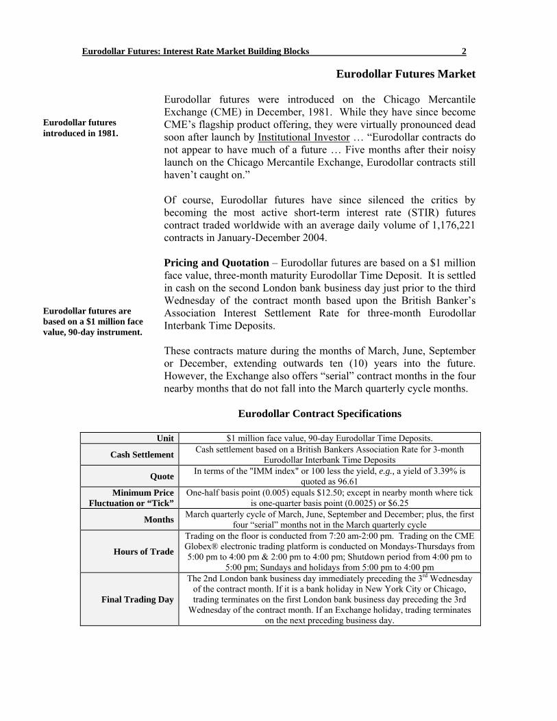
Eurodollar Futures Market Eurodollar futures were introduced on the Chicago Mercantile Exchange (CME) in December, 1981. While they have since become CME’s flagship product offering, they were virtually pronounced dead soon after launch by Institutional Investor … “Eurodollar contracts do not appear to have much of a future … Five months after their noisy launch on the Chicago Mercantile Exchange, Eurodollar contracts still haven’t caught on.”
Of course, Eurodollar futures have since silenced the critics by becoming the most active short-term interest rate (STIR) futures contract traded worldwide with an average daily volume of 1,176,221 contracts in January-December 2004. Pricing and Quotation – Eurodollar futures are based on a $1 million face value, three-month maturity Eurodollar Time Deposit. It is settled in cash on the second London bank business day just prior to the third Wednesday of the contract month based upon the British Banker’s Association Interest Settlement Rate for three-month Eurodollar Interbank Time Deposits. These contracts mature during the months of March, June, September or December, extending outwards ten (10) years into the future. However, the Exchange also offers “serial” contract months in the four nearby months that do not fall into the March quarterly cycle months.
Eurodollar Contract Specifications
Unit $1 million face value, 90-day Eurodollar Time Deposits.
Cash Settlement Cash settlement based on a British Bankers Association Rate for 3-month Eurodollar Interbank Time Deposits
Quote In terms of the "IMM index" or 100 less the yield, e.g., a yield of 3.39% is quoted as 96.61
Minimum Price Fluctuation or “Tick”
One-half basis point (0.005) equals $12.50; except in nearby month where tick is one-quarter basis point (0.0025) or $6.25
Months March quarterly cycle of March, June, September and December; plus, the first four “serial” months not in the March quarterly cycle
Hours of Trade
Trading on the floor is conducted from 7:20 am-2:00 pm. Trading on the CME Globex® electronic trading platform is conducted on Mondays-Thursdays from 5:00 pm to 4:00 pm & 2:00 pm to 4:00 pm; Shutdown period from 4:00 pm to
5:00 pm; Sundays and holidays from 5:00 pm to 4:00 pm
Final Trading Day
The 2nd London bank business day immediately preceding the 3rd Wednesday of the contract month. If it is a bank holiday in New York City or Chicago, trading terminates on the first London bank business day preceding the 3rd
Wednesday of the contract month. If an Exchange holiday, trading terminates on the next preceding business day.
Eurodollar futures introduced in 1981.
Eurodollar futures are based on a $1 million face value, 90-day instrument.
Eurodollar Futures: Interest Rate Market Building Blocks 3
Trading is conducted on the floor of the Exchange using traditional open outcry methods during regular daylight hours and simultaneously on the CME Globex® electronic trading platform virtually around the clock. Increasingly, the market is shifting to trading on an electronic basis such that, as of December 2004, approximately 70% of all Eurodollar volume traded is concluded on the CME Globex platform.
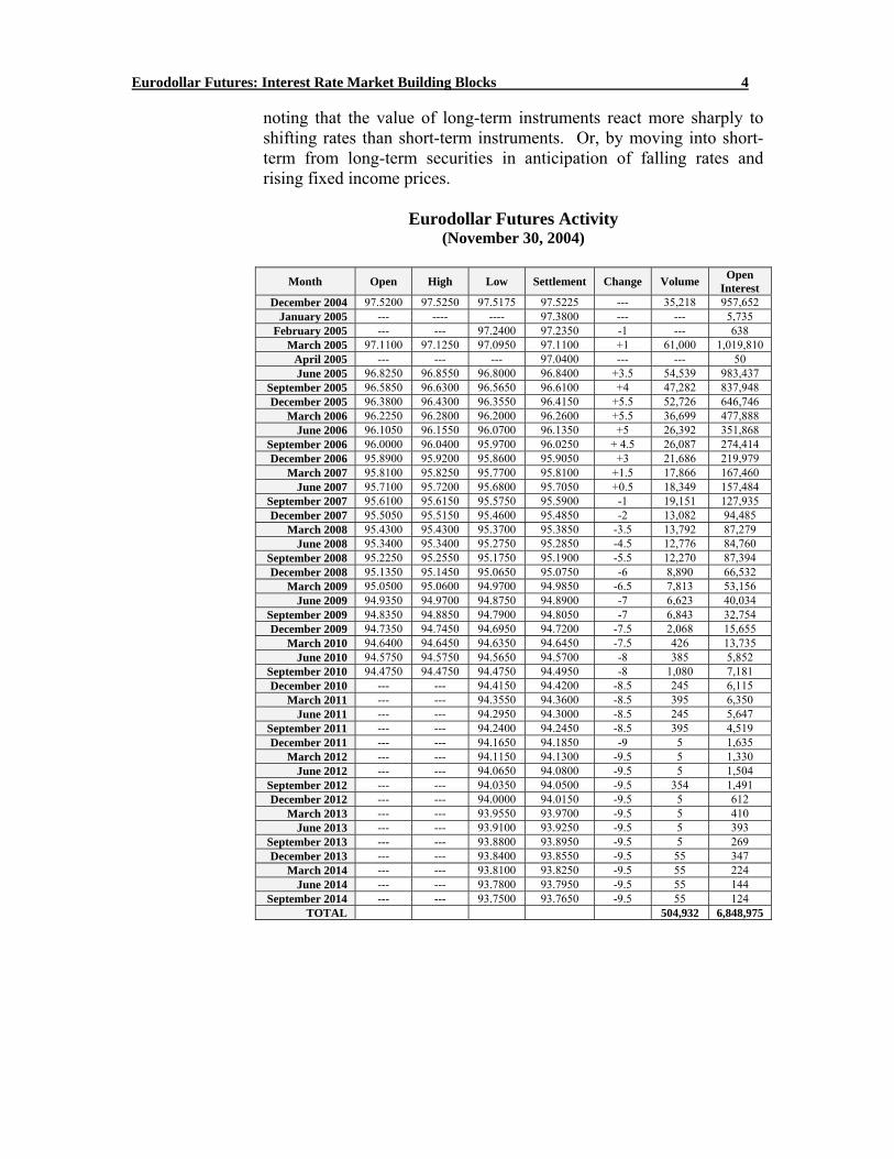
These contracts are quoted in terms of the "IMM index." 1 The IMM index is equal to 100 less the yield on the security, e.g., if the yield equal 3.39%, the index equals 96.61. The minimum price fluctuation generally equals one-half basis point or 0.005%. Based on a $1 million face value 90-day instrument, this equates to $12.50. However, in the nearby expiring contract month, the minimum price fluctuation is set at one-quarter basis point or 0.0025% equating to $6.25 per contract. As seen in the table below, September 2005 futures rose by 6 full basis points to settle the day at a price of 96.61. Noting that each basis point is worth $25 per contract based upon a $1,000,000, 90 day instrument, this implies an increase in value of $150 for the day. Note that the value of a basis point may be computed as $25 = $1,000,000 x (90 days / 360 days) x 0.01%. Shape of the Yield Curve – Pricing patterns in the Eurodollar futures market are very much a reflection or mirror of conditions prevailing in the money markets and moving outwards on the yield curve. But before we explain how Eurodollar futures pricing patterns are kept in lockstep with the yield curve, let us consider that the shape of the yield curve may be interpreted as an indicator of the direction in which the market as a whole believes interest rates may fluctuate. There are three basic theories which are referenced to explain the shape of the yield curve … the expectations hypothesis, the liquidity hypothesis and the segmentation hypothesis. Let’s start with the assumption that the yield curve is flat, i.e., short-term rates and longer–term interest rates are equivalent and investors are expressing no particular preference for securities on the basis of maturity. The expectations hypothesis modifies this assumption with the supposition that rational investors may be expected to alter the composition of their fixed income portfolios to reflect their beliefs with respect to the future direction of interest rates. Thus, investors move into long-term from short-term securities in anticipation of rising rates and falling fixed income security prices,
1 The “IMM” or International Monetary Market was established as a Division of Chicago Mercantile Exchange many years ago … the distinction is seldom made today as CME operates as a unified entity … but references to IMM persist today.
Trading is now mostly electronic.
Quoted as 100 less yield.
Eurodollar futures reflect shape of the yield curve.
Expectations hypothesis suggests investor normally prefer liquidity of S-T over L-T securities.
Eurodollar Futures: Interest Rate Market Building Blocks 4
noting that the value of long-term instruments react more sharply to shifting rates than short-term instruments. Or, by moving into short-term from long-term securities in anticipation of falling rates and rising fixed income prices.
Eurodollar Futures Activity (November 30, 2004)
Month Open High Low Settlement Change Volume Open
Interest December 2004 97.5200 97.5250 97.5175 97.5225 --- 35,218 957,652
January 2005 --- ---- ---- 97.3800 --- --- 5,735 February 2005 --- --- 97.2400 97.2350 -1 --- 638
March 2005 97.1100 97.1250 97.0950 97.1100 +1 61,000 1,019,810 April 2005 --- --- --- 97.0400 --- --- 50 June 2005 96.8250 96.8550 96.8000 96.8400 +3.5 54,539 983,437
September 2005 96.5850 96.6300 96.5650 96.6100 +4 47,282 837,948 December 2005 96.3800 96.4300 96.3550 96.4150 +5.5 52,726 646,746
March 2006 96.2250 96.2800 96.2000 96.2600 +5.5 36,699 477,888 June 2006 96.1050 96.1550 96.0700 96.1350 +5 26,392 351,868
September 2006 96.0000 96.0400 95.9700 96.0250 + 4.5 26,087 274,414 December 2006 95.8900 95.9200 95.8600 95.9050 +3 21,686 219,979
March 2007 95.8100 95.8250 95.7700 95.8100 +1.5 17,866 167,460 June 2007 95.7100 95.7200 95.6800 95.7050 +0.5 18,349 157,484
September 2007 95.6100 95.6150 95.5750 95.5900 -1 19,151 127,935 December 2007 95.5050 95.5150 95.4600 95.4850 -2 13,082 94,485
March 2008 95.4300 95.4300 95.3700 95.3850 -3.5 13,792 87,279 June 2008 95.3400 95.3400 95.2750 95.2850 -4.5 12,776 84,760
September 2008 95.2250 95.2550 95.1750 95.1900 -5.5 12,270 87,394 December 2008 95.1350 95.1450 95.0650 95.0750 -6 8,890 66,532
March 2009 95.0500 95.0600 94.9700 94.9850 -6.5 7,813 53,156 June 2009 94.9350 94.9700 94.8750 94.8900 -7 6,623 40,034
September 2009 94.8350 94.8850 94.7900 94.8050 -7 6,843 32,754 December 2009 94.7350 94.7450 94.6950 94.7200 -7.5 2,068 15,655
March 2010 94.6400 94.6450 94.6350 94.6450 -7.5 426 13,735 June 2010 94.5750 94.5750 94.5650 94.5700 -8 385 5,852
September 2010 94.4750 94.4750 94.4750 94.4950 -8 1,080 7,181 December 2010 --- --- 94.4150 94.4200 -8.5 245 6,115
March 2011 --- --- 94.3550 94.3600 -8.5 395 6,350 June 2011 --- --- 94.2950 94.3000 -8.5 245 5,647
September 2011 --- --- 94.2400 94.2450 -8.5 395 4,519 December 2011 --- --- 94.1650 94.1850 -9 5 1,635
March 2012 --- --- 94.1150 94.1300 -9.5 5 1,330 June 2012 --- --- 94.0650 94.0800 -9.5 5 1,504
September 2012 --- --- 94.0350 94.0500 -9.5 354 1,491 December 2012 --- --- 94.0000 94.0150 -9.5 5 612
March 2013 --- --- 93.9550 93.9700 -9.5 5 410 June 2013 --- --- 93.9100 93.9250 -9.5 5 393
September 2013 --- --- 93.8800 93.8950 -9.5 5 269 December 2013 --- --- 93.8400 93.8550 -9.5 55 347
March 2014 --- --- 93.8100 93.8250 -9.5 55 224 June 2014 --- --- 93.7800 93.7950 -9.5 55 144
September 2014 --- --- 93.7500 93.7650 -9.5 55 124 TOTAL 504,932 6,848,975
Eurodollar Futures: Interest Rate Market Building Blocks 5
In the process of shortening the maturity of one’s portfolio, investors will bid up the price of short-term securities and drive down the price of long-term securities. As a result, short-term yields decline and long-term yields rise … the yield curve steepens. In the process of extending maturities, the opposite occurs and the yield curve flattens or inverts. 2
Yields expected to rise Yield curve is steep
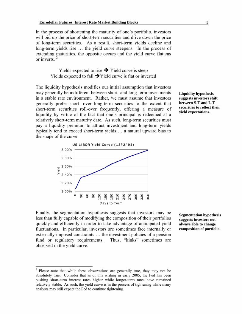
Yields expected to fall Yield curve is flat or inverted The liquidity hypothesis modifies our initial assumption that investors may generally be indifferent between short- and long-term investments in a stable rate environment. Rather, we must assume that investors generally prefer short- over long-term securities to the extent that short-term securities roll-over frequently, offering a measure of liquidity by virtue of the fact that one’s principal is redeemed at a relatively short-term maturity date. As such, long-term securities must pay a liquidity premium to attract investment and long-term yields typically tend to exceed short-term yields … a natural upward bias to the shape of the curve.
US LIBOR Yield Curve (12/2/04)
2.00%
2.20%
2.40%
2.60%
2.80%
3.00%
0
30
60
90
120
150
180
210
240
270
300
330
360
Days to Term
Yie
ld
Finally, the segmentation hypothesis suggests that investors may be less than fully capable of modifying the composition of their portfolios quickly and efficiently in order to take advantage of anticipated yield fluctuations. In particular, investors are sometimes face internally or externally imposed constraints … the investment policies of a pension fund or regulatory requirements. Thus, “kinks” sometimes are observed in the yield curve.
2 Please note that while these observations are generally true, they may not be absolutely true. Consider that as of this writing in early 2005, the Fed has been pushing short-term interest rates higher while longer-term rates have remained relatively stable. As such, the yield curve is in the process of tightening while many analysts may still expect the Fed to continue tightening.
Liquidity hypothesis suggests investors shift between S-T and L-T securities to reflect their yield expectations.
Segmentation hypothesis suggests investors not always able to change composition of portfolio.
Eurodollar Futures: Interest Rate Market Building Blocks 6
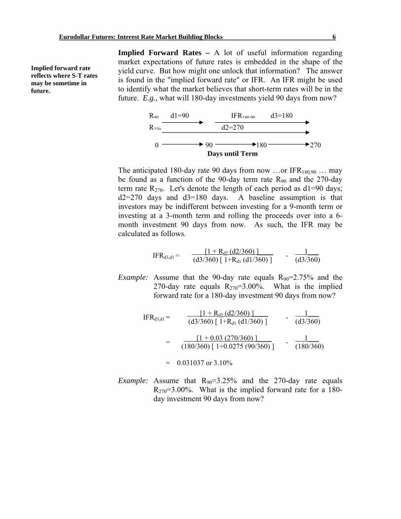
Implied Forward Rates – A lot of useful information regarding market expectations of future rates is embedded in the shape of the yield curve. But how might one unlock that information? The answer is found in the "implied forward rate" or IFR. An IFR might be used to identify what the market believes that short-term rates will be in the future. E.g., what will 180-day investments yield 90 days from now?
The anticipated 180-day rate 90 days from now …or IFR180,90 … may be found as a function of the 90-day term rate R90 and the 270-day term rate R270. Let's denote the length of each period as d1=90 days; d2=270 days and d3=180 days. A baseline assumption is that investors may be indifferent between investing for a 9-month term or investing at a 3-month term and rolling the proceeds over into a 6-month investment 90 days from now. As such, the IFR may be calculated as follows.
IFRd3,d1 = [1 + Rd2 (d2/360) ]____ (d3/360) [ 1+Rd1 (d1/360) ] - 1___
(d3/360) Example: Assume that the 90-day rate equals R90=2.75% and the
270-day rate equals R270=3.00%. What is the implied forward rate for a 180-day investment 90 days from now?
IFRd3,d1 = [1 + Rd2 (d2/360) ]____
(d3/360) [ 1+Rd1 (d1/360) ] - 1___ (d3/360)
= [1 + 0.03 (270/360) ]____ (180/360) [ 1+0.0275 (90/360) ] - 1___
(180/360)
= 0.031037 or 3.10% Example: Assume that R90=3.25% and the 270-day rate equals
R270=3.00%. What is the implied forward rate for a 180-day investment 90 days from now?
0 90 180 270 Days until Term
R270 d2=270 IFR180 90 d3=180 R90 d1=90
Implied forward rate reflects where S-T rates may be sometime in future.
Eurodollar Futures: Interest Rate Market Building Blocks 7
IFRd3,d1 = [1 + Rd2 (d2/360) ]____
(d3/360) [ 1+Rd1 (d1/360) ] - 1___ (d3/360)
= [1 + 0.03 (270/360) ]____ (180/360) [ 1+0.0325 (90/360) ] - 1___
(180/360)
= 0.028518 or 2.85% Example: Assume that R90=3.05% and the 270-day rate equals
R270=3.00%. What is the implied forward rate for a 180-day investment 90 days from now?
IFRd3,d1 = [1 + Rd2 (d2/360) ]____
(d3/360) [ 1+Rd1 (d1/360) ] - 1___ (d3/360)
= [1 + 0.03 (270/360) ]____ (180/360) [ 1+0.03 (90/360) ] - 1___
(180/360)
= 0.029777 or 2.98%
The table below summarizes the results of our examples. As such, a steep yield curve suggests a general market expectation of rising rates. An inverted yield curve suggests a general market expectation of falling rates.
90-Day Rate 270-Day Rate IFR
Steep Yield Curve 2.75% 3.00% 3.10% Inverted Yield Curve 3.25% 3.00% 2.85%
Flat Yield Curve 3.00% 3.00% 2.98% Finally, a flat yield curve suggests that the market expects slight declines in rates. This is consistent with our liquidity hypothesis that suggests that the market will generally favor short- over long-term rates in the absence of expectations of rising or falling rates. It is the slightly inclined yield curve that reflects an expectation of stable rates in the future. This result may further be understood by citing the compounding effect implicit in a roll-over from a 90-day to a 180-day investment. Because the investor recovers the original investment plus interest after the first 90 days, there is somewhat more principle to reinvest over the subsequent 180-day period. Thus, one can afford to invest over the subsequent 180-day period at a rate slightly lower than 3% and still realize a total return of 3% over the entire 270-day term.
Eurodollar Futures: Interest Rate Market Building Blocks 8
Futures as Mirror of Yield Curve – The point to our discussion about IFRs is … Eurodollar futures should price at levels that reflect these IFRs. In other words, Eurodollar futures prices directly reflect, and are a mirror of, the yield curve. This is intuitive if one considers that a Eurodollar futures contract represents a 3-month investment entered into N days in the future. And, if Eurodollar futures did not reflect IFRs, an arbitrage opportunity would present itself. Example: Consider the following interest rate structure in the
Eurodollar (Euro) futures and cash markets. Which is the better investment for the next 6 months … (1) invest for 6 months at the current spot rate of 2.75%; (2) invest for 3 months at the current spot rate of 2.55% and buy March Eurodollar futures, or (3) invest for 9 months at the current spot rate of 2.96% and sell June Euro futures? It is December and let’s assume that these investments have terms of 90 days (0.25 years), 180 days (0.50 years) or 270 days (0.75 years).
Mar. Euro futures 97.00 (3.00%) Jun. Euro futures 96.70 (3.30%) Sep. Euro futures 96.50 (3.50%)
3 month investment offer @ 2.55% 6 month investment offer @ 2.75% 9 month investment offer @ 2.96%
The second investment option implies that you invest at 2.55% for the first 3 months and lock-in a rate of 3.00% by buying March Eurodollar futures for the subsequent 3 months. This implies a return of 2.78% over entire 6 month period.
1+R(.5) = [1 + 0.0255 (.25)][1+0.03(.25)]
R = ([1 + 0.0255 (.25)][1+0.03(.25)]) -1 .5
= 2.78%
The third alternative means that you invest for the next 270 at 2.96% and sell June Eurodollar futures at 3.30%, effectively committing to sell the spot investment 180 days hence when it has 90 days until maturity. This implies a return of 2.77% over the next 6 months.
Action of arbitrageurs ensures that CME Euro-dollar futures will reflect shape of yield curve.
Eurodollar Futures: Interest Rate Market Building Blocks 9
[1+R(.5)] [1+.033(.25)] = [1 + 0.0296(.75)]
R = ([1 + 0.0296(.75)]/[1+.033(.25)]) -1 .5
= 2.77%
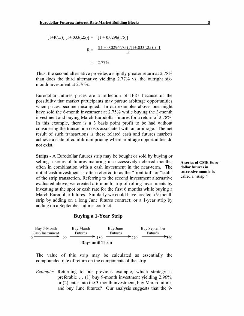
Thus, the second alternative provides a slightly greater return at 2.78% than does the third alternative yielding 2.77% vs. the outright six-month investment at 2.76%. Eurodollar futures prices are a reflection of IFRs because of the possibility that market participants may pursue arbitrage opportunities when prices become misaligned. In our examples above, one might have sold the 6-month investment at 2.75% while buying the 3-month investment and buying March Eurodollar futures for a return of 2.78%. In this example, there is a 3 basis point profit to be had without considering the transaction costs associated with an arbitrage. The net result of such transactions is these related cash and futures markets achieve a state of equilibrium pricing where arbitrage opportunities do not exist. Strips - A Eurodollar futures strip may be bought or sold by buying or selling a series of futures maturing in successively deferred months, often in combination with a cash investment in the near-term. The initial cash investment is often referred to as the “front tail” or “stub” of the strip transaction. Referring to the second investment alternative evaluated above, we created a 6-month strip of rolling investments by investing at the spot or cash rate for the first 6 months while buying a March Eurodollar futures. Similarly we could have created a 9-month strip by adding on a long June futures contract; or a 1-year strip by adding on a September futures contract.
The value of this strip may be calculated as essentially the compounded rate of return on the components of the strip. Example: Returning to our previous example, which strategy is
preferable … (1) buy 9-month investment yielding 2.96%, or (2) enter into the 3-month investment, buy March futures and buy June futures? Our analysis suggests that the 9-
Buying a 1-Year Strip
Buy 3-Month Buy March Buy June Buy September Cash Instrument Futures Futures Futures 0 90 180 270 360 Days until Term
A series of CME Euro-dollar futures in successive months is called a “strip.”
Eurodollar Futures: Interest Rate Market Building Blocks 10
month strip yields 2.97% relative to 2.96% on the 9-month investment.
Mar. Euro futures 97.00 (3.00%) Jun. Euro futures 96.70 (3.30%)
3 month investment offer @ 2.55% 9 month investment offer @ 2.96%
1+R(.75) = [1 + 0.0255 (.25)] [1+0.03(.25)] [1+0.033(.25)]
R = ([1 + 0.0255 (.25)] [1+0.03(.25)] [1+0.033(.25)]) -1 .75
= 2.97%
In our example above, there is no compelling advantage to buy the strip relative to a straight term advantage to the extent that the yields are virtually the same. However, if the rates were sufficiently divergent, one might buy the strip and sell the term investment to finance the strip. Or, sell the strip and buy the term investment. This represents a form of arbitrage that ensures that Eurodollar futures represent a consistent reflection of the curve. Note that, to the extent that Eurodollar futures are listed out ten years into the future, one may create 1-year, 2-year, 3-year, … , up to 10-year strips … that may be compared to comparable term securities. In fact these values are often compared to term Treasury securities and to swap rates as discussed in more detail below. 3 Packs and Bundles – Because strips have proven to be popular trading instruments … and because of the complexities associated with their purchase or sale … the Exchange has developed the concept of “packs” and “bundles” to facilitate strip trading. A pack or bundle may be thought of as the purchase or sale of a series of Eurodollar futures representing a particular segment of the yield curve. Packs and bundles should be thought of a building blocks used to create or liquidate positions along various segments of interest along the yield curve. Packs and bundles may be bought or sold in a single transaction, eliminating the possibility that a multitude of orders in each individual contract goes unfilled. Note that the popularity of these concepts is reflected in Eurodollar open interest patterns where … unlike most futures contracts where 3 Note that for purposes of this exposition, we have simplified our analysis a bit. For example, we have not discussed the fact that compounding of interest implies that one will have more principal to invest upon each roll-over date.
Bundles are pre-packaged strips traded on CME.
Eurodollar Futures: Interest Rate Market Building Blocks 11
virtually all of the volume and open interest is concentrated in the nearby or lead month … Eurodollars have significant volume and open interest in the deferred months going out ten years along the yield curve. The Exchange offers trading in 1-, 2-, 3-, 4-, 5-, 6-, 7-, 8-, 9-, and 10-year bundles. These products may be thought of as Eurodollar futures strips (absent the front tail or stub investment) extending out 1, 2, 3, … , 10 years into the future. For example, one may buy a 1-year bundle by purchasing the first four quarterly expiration Eurodollar futures contracts. Or, one may sell a 3-year bundle by selling the first twelve quarterly expiration Eurodollar futures contracts. The price of a bundle is typically quoted by reference to the average change in the value of all Eurodollar futures contracts in the bundle since the prior day’s settlement price. For example, if the first four quarterly Eurodollar contracts are up 2 basis points for the day and the second four quarterly Eurodollar contracts are up 3 basis points for the day then the 2-year bundle may be quoted as +2.5 basis points. After a trade is concluded at a negotiated price, prices are assigned to each of the various legs, i.e., Eurodollar futures contracts, associated with the bundle. These prices must be within the daily range for at least one of the component contracts of the bundle. This assignment is generally administered through an automated system operated by the Exchange. Packs are similar to bundles in that they represent an aggregation of a number of Eurodollar futures contracts traded simultaneously. But they are constructed to represent a series of four consecutive quarterly Eurodollar futures.
For example, one may buy a pack by buying the March, June, September and December 2006 Eurodollar futures contracts, constituting a pack. Or, sell a pack by selling the March, June, September and December 2007 Eurodollar futures contract, constituting yet another pack. Packs are quoted and prices are assigned to the individual legs in the same manner that one quotes and assigns prices to the legs of a bundle.
A pack is a package of 4 successive Eurodollar futures.
Eurodollar Futures: Interest Rate Market Building Blocks 12
Speculating on Shape of Yield Curve Because Eurodollar futures are a mirror of the yield curve, one may spread these contracts to take a position on the relative yields associated with long- and short-term yields, i.e., to speculate on the shape of the yield curve. If the yield curve is expected to steepen, the recommended strategy is to “buy the curve” by purchasing near-term and selling longer-term or deferred Eurodollar futures. If the opposite is expected to occur, i.e., the yield curve is expected to flatten or invert, the recommended strategy is to “sell the curve” by selling near-term and buying deferred Eurodollar futures.
Expectation Action
Yield curve expected to steepen
“Buy the curve,” i.e., buy nearby and sell deferred futures
Yield curve expected to flatten or invert
“Sell the curve,” i.e., sell nearby and buy deferred futures
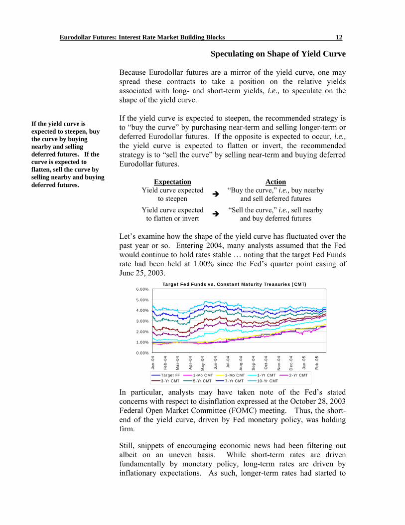
Let’s examine how the shape of the yield curve has fluctuated over the past year or so. Entering 2004, many analysts assumed that the Fed would continue to hold rates stable … noting that the target Fed Funds rate had been held at 1.00% since the Fed’s quarter point easing of June 25, 2003.
Target Fed Funds vs. Constant Maturity Treasuries (CMT)
0.00%
1.00%
2.00%
3.00%
4.00%
5.00%
6.00%
Jan-0
4
Feb-0
4
Mar-
04
Apr-
04
May-0
4
Jun-0
4
Jul-
04
Aug-0
4
Sep-0
4
Oct
-04
Nov-0
4
Dec-
04
Jan-0
5
Feb-0
5
Target FF 1-Mo CMT 3-Mo CMT 1-Yr CMT 2-Yr CMT3-Yr CMT 5-Yr CMT 7-Yr CMT 10-Yr CMT
In particular, analysts may have taken note of the Fed’s stated concerns with respect to disinflation expressed at the October 28, 2003 Federal Open Market Committee (FOMC) meeting. Thus, the short-end of the yield curve, driven by Fed monetary policy, was holding firm.
Still, snippets of encouraging economic news had been filtering out albeit on an uneven basis. While short-term rates are driven fundamentally by monetary policy, long-term rates are driven by inflationary expectations. As such, longer-term rates had started to
If the yield curve is expected to steepen, buy the curve by buying nearby and selling deferred futures. If the curve is expected to flatten, sell the curve by selling nearby and buying deferred futures.
Eurodollar Futures: Interest Rate Market Building Blocks 13
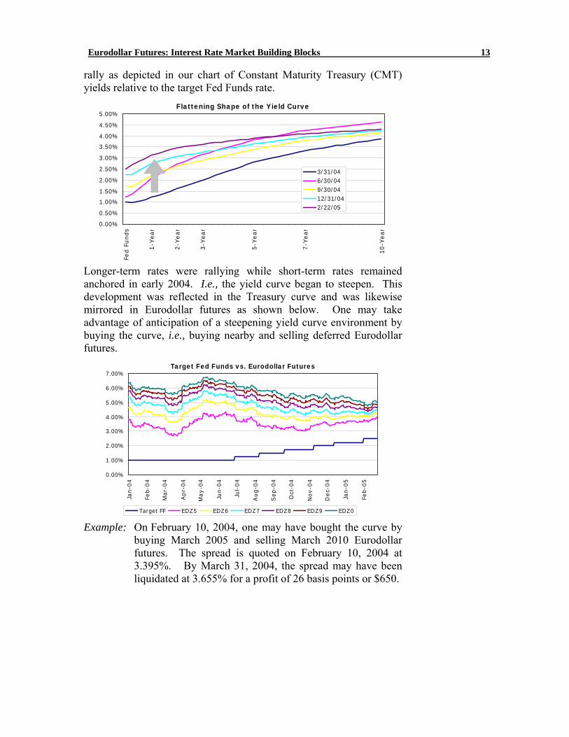
rally as depicted in our chart of Constant Maturity Treasury (CMT) yields relative to the target Fed Funds rate.
Flattening Shape of the Yield Curve
0.00%
0.50%
1.00%
1.50%
2.00%
2.50%
3.00%
3.50%
4.00%
4.50%
5.00%
Fed F
unds
1-Y
ear
2-Y
ear
3-Y
ear
5-Y
ear
7-Y
ear
10-Y
ear
3/31/046/30/049/30/0412/31/042/22/05
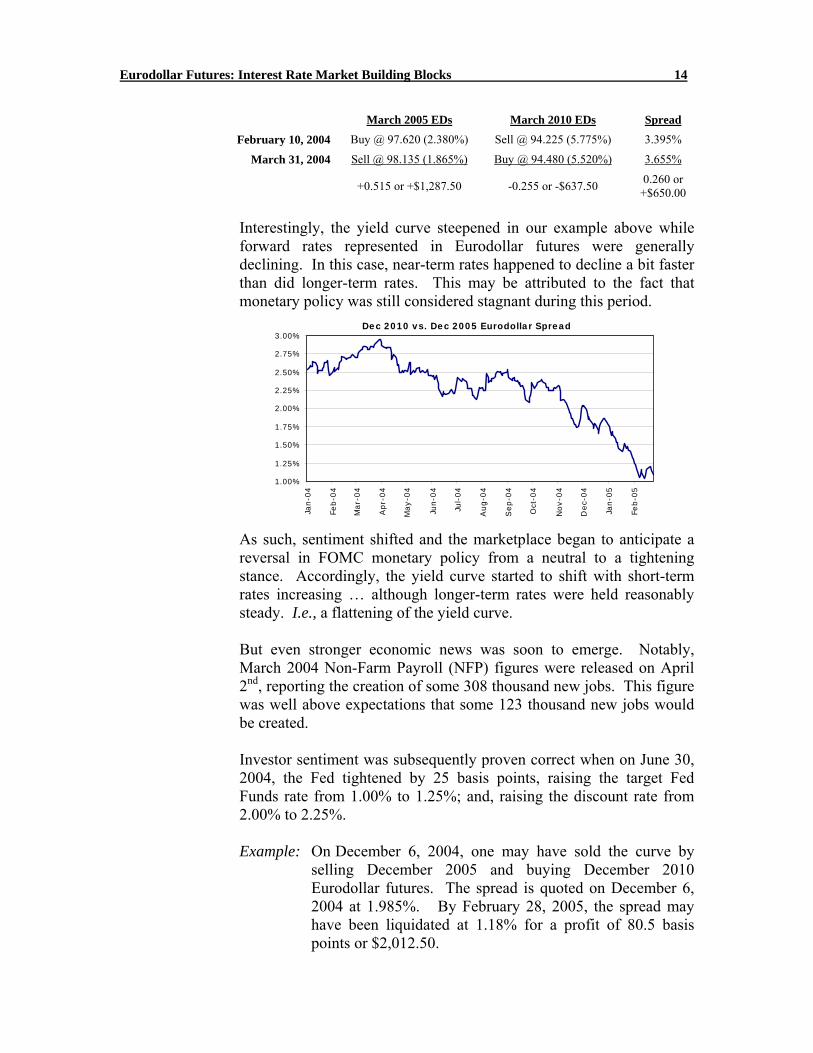
Longer-term rates were rallying while short-term rates remained anchored in early 2004. I.e., the yield curve began to steepen. This development was reflected in the Treasury curve and was likewise mirrored in Eurodollar futures as shown below. One may take advantage of anticipation of a steepening yield curve environment by buying the curve, i.e., buying nearby and selling deferred Eurodollar futures.
Target Fed Funds vs. Eurodollar Futures
0.00%
1.00%
2.00%
3.00%
4.00%
5.00%
6.00%
7.00%
Jan-0
4
Feb-0
4
Mar-
04
Apr-
04
May-0
4
Jun-0
4
Jul-
04
Aug-0
4
Sep-0
4
Oct
-04
Nov-0
4
Dec-
04
Jan-0
5
Feb-0
5
Target FF EDZ5 EDZ6 EDZ7 EDZ8 EDZ9 EDZ0
Example: On February 10, 2004, one may have bought the curve by buying March 2005 and selling March 2010 Eurodollar futures. The spread is quoted on February 10, 2004 at 3.395%. By March 31, 2004, the spread may have been liquidated at 3.655% for a profit of 26 basis points or $650.
Eurodollar Futures: Interest Rate Market Building Blocks 14
March 2005 EDs March 2010 EDs Spread
February 10, 2004 Buy @ 97.620 (2.380%) Sell @ 94.225 (5.775%) 3.395%
March 31, 2004 Sell @ 98.135 (1.865%) Buy @ 94.480 (5.520%) 3.655%
+0.515 or +$1,287.50 -0.255 or -$637.50 0.260 or +$650.00
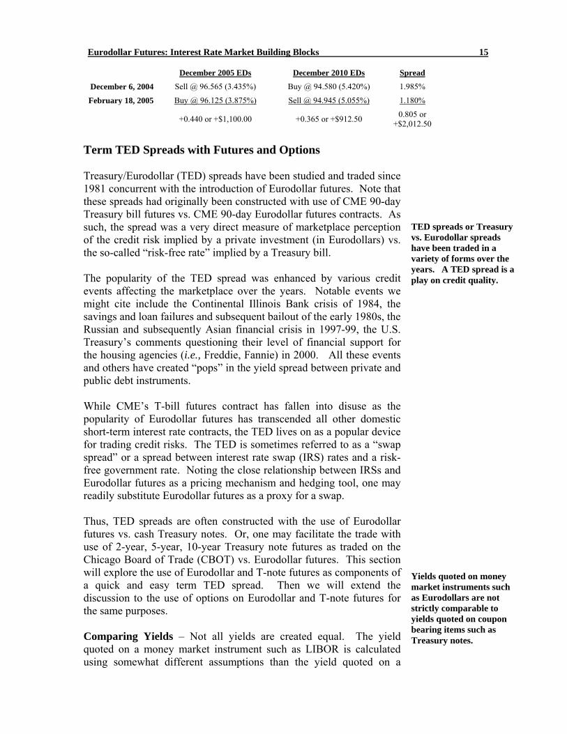
Interestingly, the yield curve steepened in our example above while forward rates represented in Eurodollar futures were generally declining. In this case, near-term rates happened to decline a bit faster than did longer-term rates. This may be attributed to the fact that monetary policy was still considered stagnant during this period.
Dec 2010 vs. Dec 2005 Eurodollar Spread
1.00%
1.25%
1.50%
1.75%
2.00%
2.25%
2.50%
2.75%
3.00%
Jan-0
4
Feb-0
4
Mar-
04
Apr-
04
May-0
4
Jun-0
4
Jul-
04
Aug-0
4
Sep-0
4
Oct
-04
Nov-0
4
Dec-
04
Jan-0
5
Feb-0
5
As such, sentiment shifted and the marketplace began to anticipate a reversal in FOMC monetary policy from a neutral to a tightening stance. Accordingly, the yield curve started to shift with short-term rates increasing … although longer-term rates were held reasonably steady. I.e., a flattening of the yield curve. But even stronger economic news was soon to emerge. Notably, March 2004 Non-Farm Payroll (NFP) figures were released on April 2nd, reporting the creation of some 308 thousand new jobs. This figure was well above expectations that some 123 thousand new jobs would be created. Investor sentiment was subsequently proven correct when on June 30, 2004, the Fed tightened by 25 basis points, raising the target Fed Funds rate from 1.00% to 1.25%; and, raising the discount rate from 2.00% to 2.25%. Example: On December 6, 2004, one may have sold the curve by
selling December 2005 and buying December 2010 Eurodollar futures. The spread is quoted on December 6, 2004 at 1.985%. By February 28, 2005, the spread may have been liquidated at 1.18% for a profit of 80.5 basis points or $2,012.50.
Eurodollar Futures: Interest Rate Market Building Blocks 15
December 2005 EDs December 2010 EDs Spread
December 6, 2004 Sell @ 96.565 (3.435%) Buy @ 94.580 (5.420%) 1.985%
February 18, 2005 Buy @ 96.125 (3.875%) Sell @ 94.945 (5.055%) 1.180%
+0.440 or +$1,100.00 +0.365 or +$912.50 0.805 or +$2,012.50
Term TED Spreads with Futures and Options Treasury/Eurodollar (TED) spreads have been studied and traded since 1981 concurrent with the introduction of Eurodollar futures. Note that these spreads had originally been constructed with use of CME 90-day Treasury bill futures vs. CME 90-day Eurodollar futures contracts. As such, the spread was a very direct measure of marketplace perception of the credit risk implied by a private investment (in Eurodollars) vs. the so-called “risk-free rate” implied by a Treasury bill. The popularity of the TED spread was enhanced by various credit events affecting the marketplace over the years. Notable events we might cite include the Continental Illinois Bank crisis of 1984, the savings and loan failures and subsequent bailout of the early 1980s, the Russian and subsequently Asian financial crisis in 1997-99, the U.S. Treasury’s comments questioning their level of financial support for the housing agencies (i.e., Freddie, Fannie) in 2000. All these events and others have created “pops” in the yield spread between private and public debt instruments. While CME’s T-bill futures contract has fallen into disuse as the popularity of Eurodollar futures has transcended all other domestic short-term interest rate contracts, the TED lives on as a popular device for trading credit risks. The TED is sometimes referred to as a “swap spread” or a spread between interest rate swap (IRS) rates and a risk-free government rate. Noting the close relationship between IRSs and Eurodollar futures as a pricing mechanism and hedging tool, one may readily substitute Eurodollar futures as a proxy for a swap. Thus, TED spreads are often constructed with the use of Eurodollar futures vs. cash Treasury notes. Or, one may facilitate the trade with use of 2-year, 5-year, 10-year Treasury note futures as traded on the Chicago Board of Trade (CBOT) vs. Eurodollar futures. This section will explore the use of Eurodollar and T-note futures as components of a quick and easy term TED spread. Then we will extend the discussion to the use of options on Eurodollar and T-note futures for the same purposes. Comparing Yields – Not all yields are created equal. The yield quoted on a money market instrument such as LIBOR is calculated using somewhat different assumptions than the yield quoted on a
TED spreads or Treasury vs. Eurodollar spreads have been traded in a variety of forms over the years. A TED spread is a play on credit quality.
Yields quoted on money market instruments such as Eurodollars are not strictly comparable to yields quoted on coupon bearing items such as Treasury notes.
Eurodollar Futures: Interest Rate Market Building Blocks 16
coupon bearing instrument such as a Treasury note. Fixed income traders need be careful to assure that they are comparing “apples with apples.” Yields associated with Eurodollar or LIBOR quotes are known as money market yields (MMY). Note that Eurodollars are so-called “add-on” instruments where one invests the stated face value and received the original investment plus interest at term. Thus, one’s interest may be calculated as a simple function of the face value (FV), rate (R) and days to maturity (d) …
Interest = FV [R x (d/360)] Example: If one were to purchase a $1 million face value unit of 270-
day Euros with MMY=3.00%, one would receive the original $1 million face value (FV) investment plus interest (i) of $7,833 at the conclusion of 94 days.
Interest = $1,000,000 [0.03 x (270/360)]
= $22,500 MMYs suffer from the mistaken assumption that there are but 360 days in a year (a “money-market” year!). As such, MMYs are not completely comparable to the bond equivalent yield (BEY) quoted on Treasury notes that imply periodic coupon payments. The following adjustment may be made to render the two quotes comparable …
BEY = MMY x (365/360) Example: Assume you have a 90-day money market instrument
yielding 3.00%. Let’s convert that figure to a bond-equivalent yield. Note that the BEY of 3.0417% slightly exceeds the MMY.
3.0417% = 3.00% x (365/360)
Complicating the calculation is the fact that notes and bonds offer semi-annual coupon payments. Thus, money market instruments that require the investor to wait until maturity for any return do not permit interim compounding. This means that the formula provided above is only valid for instruments with less than 6-months (183-days) to term. If there are 183 or more days until term, use the following formula where P=price or original investment and i=interest.
But we can use formulae to find bond equivalent yields (BEY).
Eurodollar Futures: Interest Rate Market Building Blocks 17
BEY = (-d/365) + √ ([d/365]2 – [(2d/365)-1][1-((FV+i)/FV)]) [(d/365)-0.5]
Example: Let’s return to our example of a 270-day Euro investment
quoted at a MMY=3.00%. Note from our example above that the interest accrued on a $1 million investment would be $22,500. The BEY may be calculated as 3.027% and slightly higher than the MMY=3.00%.
BEY = (-270/365) + √ ([270/365]2 – [(2x270/365)-1][1-(($1,000,000+$22,500)/$1,000,000)])
[(d/365)-0.5] = 3.027%
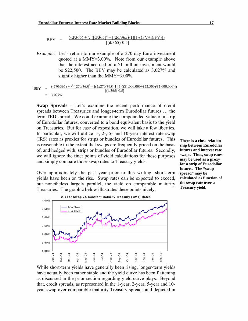
Swap Spreads – Let’s examine the recent performance of credit spreads between Treasuries and longer-term Eurodollar futures … the term TED spread. We could examine the compounded value of a strip of Eurodollar futures, converted to a bond equivalent basis to the yield on Treasuries. But for ease of exposition, we will take a few liberties. In particular, we will utilize 1-, 2-, 5- and 10-year interest rate swap (IRS) rates as proxies for strips or bundles of Eurodollar futures. This is reasonable to the extent that swaps are frequently priced on the basis of, and hedged with, strips or bundles of Eurodollar futures. Secondly, we will ignore the finer points of yield calculations for these purposes and simply compare those swap rates to Treasury yields. Over approximately the past year prior to this writing, short-term yields have been on the rise. Swap rates can be expected to exceed, but nonetheless largely parallel, the yield on comparable maturity Treasuries. The graphic below illustrates these points nicely.
2-Year Swap vs. Constant Maturity Treasury (CMT) Rates
1.00%
1.50%
2.00%
2.50%
3.00%
3.50%
4.00%
Jan-0
4
Feb-0
4
Mar-
04
Apr-
04
May-0
4
Jun-0
4
Jul-
04
Aug-0
4
Sep-0
4
Oct
-04
Nov-0
4
Dec-
04
Jan-0
5
Feb-0
5
2-Yr Swap2-Yr CMT
While short-term yields have generally been rising, longer-term yields have actually been rather stable and the yield curve has been flattening as discussed in the prior section regarding yield curve plays. Beyond that, credit spreads, as represented in the 1-year, 2-year, 5-year and 10-year swap over comparable maturity Treasury spreads and depicted in
There is a close relation-ship between Eurodollar futures and interest rate swaps. Thus, swap rates may be used as a proxy for a strip of Eurodollar futures. The “swap spread” may be calculated as function of the swap rate over a Treasury yield.
Eurodollar Futures: Interest Rate Market Building Blocks 18
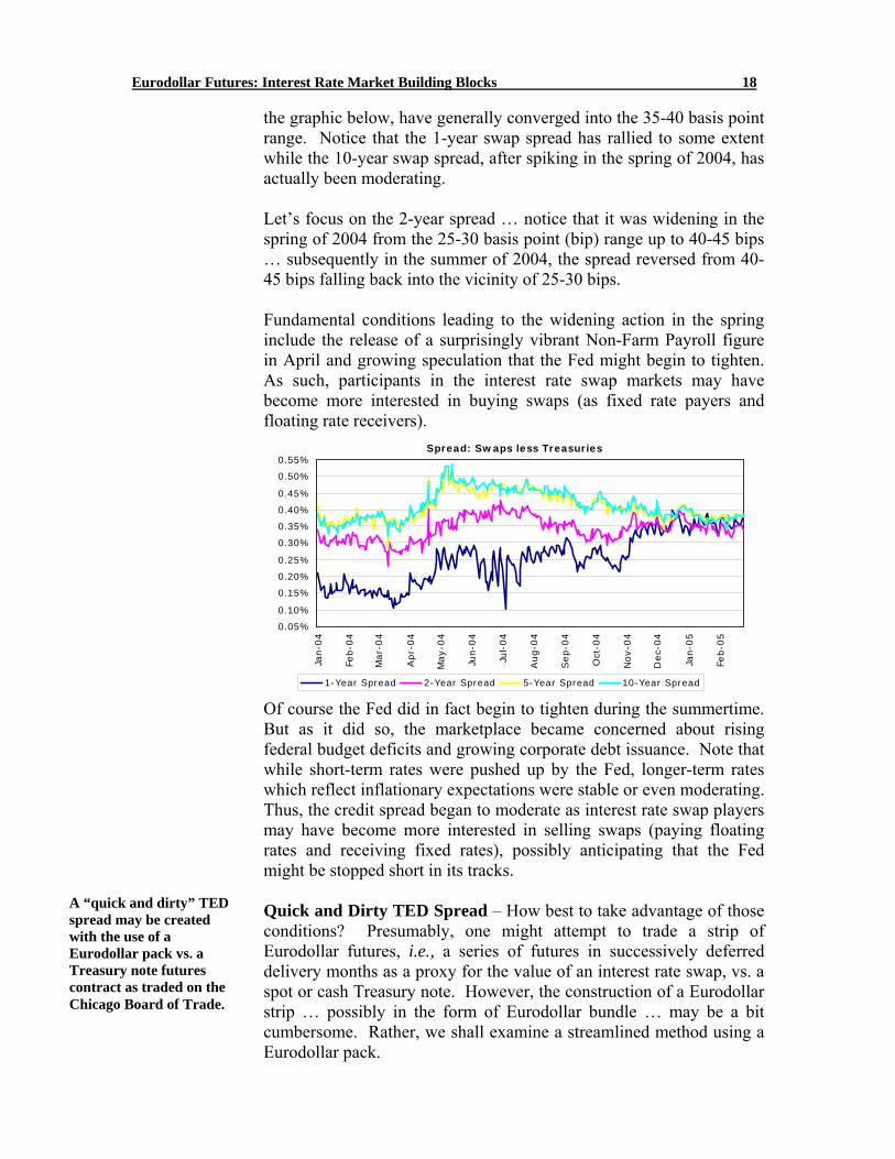
the graphic below, have generally converged into the 35-40 basis point range. Notice that the 1-year swap spread has rallied to some extent while the 10-year swap spread, after spiking in the spring of 2004, has actually been moderating. Let’s focus on the 2-year spread … notice that it was widening in the spring of 2004 from the 25-30 basis point (bip) range up to 40-45 bips … subsequently in the summer of 2004, the spread reversed from 40-45 bips falling back into the vicinity of 25-30 bips. Fundamental conditions leading to the widening action in the spring include the release of a surprisingly vibrant Non-Farm Payroll figure in April and growing speculation that the Fed might begin to tighten. As such, participants in the interest rate swap markets may have become more interested in buying swaps (as fixed rate payers and floating rate receivers).
Spread: Swaps less Treasuries
0.05%
0.10%
0.15%
0.20%
0.25%
0.30%
0.35%
0.40%
0.45%
0.50%
0.55%
Jan-0
4
Feb-0
4
Mar-
04
Apr-
04
May-0
4
Jun-0
4
Jul-
04
Aug-0
4
Sep-0
4
Oct
-04
Nov-0
4
Dec-
04
Jan-0
5
Feb-0
5
1-Year Spread 2-Year Spread 5-Year Spread 10-Year Spread
Of course the Fed did in fact begin to tighten during the summertime. But as it did so, the marketplace became concerned about rising federal budget deficits and growing corporate debt issuance. Note that while short-term rates were pushed up by the Fed, longer-term rates which reflect inflationary expectations were stable or even moderating. Thus, the credit spread began to moderate as interest rate swap players may have become more interested in selling swaps (paying floating rates and receiving fixed rates), possibly anticipating that the Fed might be stopped short in its tracks. Quick and Dirty TED Spread – How best to take advantage of those conditions? Presumably, one might attempt to trade a strip of Eurodollar futures, i.e., a series of futures in successively deferred delivery months as a proxy for the value of an interest rate swap, vs. a spot or cash Treasury note. However, the construction of a Eurodollar strip … possibly in the form of Eurodollar bundle … may be a bit cumbersome. Rather, we shall examine a streamlined method using a Eurodollar pack.
A “quick and dirty” TED spread may be created with the use of a Eurodollar pack vs. a Treasury note futures contract as traded on the Chicago Board of Trade.
Eurodollar Futures: Interest Rate Market Building Blocks 19
A Eurodollar futures pack represents an aggregation of four quarterly expiration Eurodollar futures in consecutive months traded simultaneously. For example, one may buy a pack by buying the March, June, September and December 2006 Eurodollar futures contracts, constituting a pack. Or, sell a pack by selling the March, June, September and December 2007 Eurodollar futures contract, constituting yet another pack. Packs are often referred to by color designations. The “white pack” refers to the first four quarterly expiration Eurodollar futures; the “red pack” is the subsequent four futures; the “green pack” is the next four futures, …, a “gold pack” represents four quarterly Eurodollar futures going out five years on the curve. Just as it may be cumbersome to utilize a strip of Eurodollar futures in the context of a TED spread, it may likewise be cumbersome to utilize cash Treasury securities. In particular, CBOT Treasury note futures are available and may conveniently be spread against a Eurodollar pack. Note that CME and CBOT futures are cleared through a common clearing link which allows one to avail special spread margins that reflect the risk of the combination of the two partially offsetting legs of the spread. In other words, let’s utilize Eurodollar packs as a proxy for interest rate swap rates and CBOT 2-year T-note futures as a proxy for cash or spot Treasury securities. One might buy the credit spread (buy T-Note futures/sell Eurodollar futures) in anticipation of a widening TED spread. Or, one may sell the TED spread (sell T-Note futures/buy Eurodollar futures) in anticipation of a narrowing credit spread. This is the essence of our “quick and dirty TED spread.” 4
Long the TED Spread Buy CBOT T-Note Futures & Sell Eurodollar Pack
Short the TED Spread Sell CBOT T-Note Futures & Buy Eurodollar Pack
Weighting the Spread – In order to assure that the “quick and dirty” TED spread will really reflect the relative credit risks implied by the private vs. public debt sectors, it will become necessary to weight the spread. Thus, we must endeavor to match the risk exposure associated with the two instruments given an assumption that the yields on pair move in a
4 The concept of a “quick and dirty TED spread” was pioneered by Mr. Frederick Sturm of the Chicago Board of Trade.
A Eurodollar pack represents a pre-packaged unit of four Eurodollar futures contracts in successively deferred months.
Buy or go long a TED spread by buying T-note futures and selling Euro-dollar packs. Sell or go short a TED spread by selling T-note futures and buying Eurodollar packs.
Eurodollar Futures: Interest Rate Market Building Blocks 20
parallel manner. I.e., balance the risk associated with T-Note futures with an appropriately offsetting number of Eurodollar packs … to balance any change (Δ) in the value of the T-note futures with an opposite change in the value of the Eurodollar pack … given an equivalent shift in yields.
Δ Value of T-Note Futures ≈ Δ Value of Eurodollar Pack But we can’t manage what we can’t measure. Basis point value (BPV) measures the monetary change in the value of an instrument in response to a one basis point (0.01%) change in yield as follows. BPVs may be utilized as a proxy for the more abstract concept of change such that BPV≈Δ.
The BPV for a money market instrument such as those represented by Eurodollar futures may be calculated as follows where FV=face value of instrument and d=days to maturity.
BPVED = FV x (d/360) x 0.01% Example: Find the basis point value (BPV) of a $1 million face value
90-day exposure as represented by one Eurodollar futures contract. By plugging these values into our equation as shown above, we may calculate the basis point value associated with one $1 million face value 90-day Eurodollar futures contract (BPVED) as $25.00 (BPVED = $25.00).
BPVED = FV x (d/360) x 0.01%
= $1,000,000 x (90/360) x 0.01%
= $25.00 The BPV associated with a money market instrument such as a LIBOR investment may be found by as a simple linear function to the face value (FV) and the term in days (d) of the instrument. Thus, the basis point value of a pack of four Eurodollar futures (BPVpack) is simply $100 (BPVpack = 4 x $25). Likewise, we must find the BPV associated with a CBOT T-note futures contract. However, the calculations are a bit more complex. Note that 2-year T-note futures permit the delivery of $200,000 face value of U.S. Treasury notes with an original maturity no greater than 5 years, 3 months and a remaining term until maturity between 1 years, 9 months and 2 years, regardless of coupon. At any given time, there
TED spreads should be weighted such that no gain or loss is realized in the event of a parallel shift in the yield curve. The proper hedge ratio (HR) is found by reference to basis point values (BPVs).
Basis point value represents the dollar change in the value of a fixed income instrument in response to a one basis point (0.01%) change in yield.
Eurodollar Futures: Interest Rate Market Building Blocks 21
will be a number of T-notes which will eligible for delivery or deliverable. 5
The CBOT conversion factor (CF) invoicing system is (theoretically) designed to render equally economic the delivery of any eligible for delivery T-note. In practice, however, a single security stands out as most economic or cheapest to deliver (CTD) in light of the difference between cash values and the invoice price a buyer would pay to seller upon delivery calculated as a function of the futures price multiplied by the conversion factor … Invoice Price = Futures Settlement x CF … plus any accrued interest.
The point is that it is necessary to identify the CTD security and its basis point value (BPVctd). The effective basis point value of a T-note futures contract (BPVt-note) is equal to the basis point value of the CTD security divided by the conversion factor … BPVt-note = BPVctd ÷ CFctd. Once the CTD security is identified, we must identify its basis point value (BPVctd) and divide by its conversion factor (CFctd) to find the futures basis point value (BPVt-note) 6
BPVt-note = BPVctd ÷ CFctd
Example: On April 16, 2004, the cheapest to deliver 2-year T-note
was the 2-1/4% of April 2006. It had a BPV of $34.66 per $200,000 face value and a conversion factor for delivery into the June 2004 2-year futures contract of 0.9358.7 Thus, the effective BPV of the futures contract may be calculated as $37.04.
BPVt-note = BPVctd ÷ CFctd
= $34.66 ÷ 0.9358
= $37.04 Armed with the information above, we may identify the appropriate Hedge Ratio (HR) which would balance a TED spread constructed
5 Note that T-note futures are quoted in 32nds or fractions of a 32nd. One thirty-second of the $200,000 face value unit deliverable against a 2-year T-note futures contract equals $62.50. Quotation devices may show a quote of 106 percent of par plus 16 thirty-seconds as 106-16. If you add 1/64th, the quote may appear as 106-16+ or as 106-165. Add a 1/128th and the quote may appear as 106-162 … add 3/128ths and the quote may appear as 106-167. In the two latter cases, the trailing “5” is typically truncated. 6 Commercially available quotation devices such as the Bloomberg system may be referenced as a convenient way of identifying the CTD security at any given time, as well as its BPV. 7 Note that the CBOT 2-year T-note futures contract is based upon a $200,000 face value delivery unit.
The BPV of a Eurodollar futures contract is simply $25. The BPV of a T-note futures contract must be found by reference to the cheapest-to-deliver cash security and its conversion factor.
Eurodollar Futures: Interest Rate Market Building Blocks 22
using Eurodollar packs vs. 2-year T-note futures. The HR that indicates the appropriate number of T-note futures to trade vs. Eurodollar packs may be calculated as follows.
HR = BPVpack ÷ BPVt-note
Example: How many September 2-year T-note futures must be traded to balance a single Eurodollar pack? In our previous discussion, we had calculated a BPVpack=$100.00 and a BPVt-note=$37.04. Plugging this information into our formula, we calculate a ratio of 2.7 or roughly twenty-seven (27) 2-year T-note futures for every ten packs.
HR = BPVpack ÷ BPVt-note
= $100.00 ÷ $37.04
= 2.699 or ∼27 2-year T-note futures vs. 10 packs Term TEDs with Futures – Now that we know how to weight the spread, let’s look at some examples of how the spread may have been applied in 2004. Note once again that the 2-year swap spread was rallying in the spring only to decline in the summer months. Example: TED spreads were rallying in the spring of 2004. On April
16, 2004, one may have gone long or bought the 2-year term TED spread by buying 27 CBOT September 2-year T-note futures at 106-01/32nds; and, selling ten red packs comprised of the June 2005, September 2005, December 2005 and March 2006.8 The four legs of the pack were priced at 97.23, 96.85, 96.51 and 96.225, respectively, for an average price of 96.705 (3.295%). Note that the 2-year swap spread was at 30.1 basis points.
By July 15, 2004, the 2-year swap spread was seen at 39.7
basis points … an advance of 9.6 basis points. September 2-year T-notes were down 15/32nds to 105-18/32nds for a loss of $25,312.50 on the 27-lot long position. The four legs of the Eurodollar pack were priced at 96.83, 96.49, 96.18 and 95.955, respectively, for an average price of
8 In this example, we are using September 2-year T-notes. However, we are applying the hedge ratio calculated based upon a June 2004 2-year T-Note delivery. We have taken this liberty in keeping with the spirit of our “quick and dirty” approach and in light of the fact that the 2-1/4% T-note of April 2006 was in fact not eligible for delivery against the September 2004 futures contract as it would have slipped out of the 1-3/4 to 2 year maturity delivery window. In fact, a different security ultimately was cheapest to deliver against the September contract but that was unknown in April. Note that the BPV of the T-note futures contract can and will change in response to shifts in the CTD, possibly necessitating an adjustment of the Hedge Ratio.
We can trade term TED spreads with Eurodollar futures and CBOT T-note futures.
Eurodollar Futures: Interest Rate Market Building Blocks 23
96.36375 (3.63625%). The 10 short packs could have been covered at a profit of $38,675.00 while the 27 long T-note futures generated a loss of $25,312.50. Adding it all up, this spread generated a profit of $13,362.50.
Sept 2004 CBOT 2-Year
T-Note Futures Red Eurodollar Pack Swap Spread
April 16, 2004 Buy 27 @ 106-01/32nds (2.875%) Sell 10 @ 96.7050 (3.2950%) 0.301%
July 15, 2004 Sell 27 @ 105-18/32nds (3.110%) Buy 10 @ 96.36375 (3.63625%) 0.397%
-15/32nds or -$25,312.50 +0.38675 or +$38,675.00 +$13,362.50 The spread between 2-year T-note futures and the Eurodollar packs operated as a reasonable proxy for the 2-year swap spread … the spread between the implicit yield on the pack and 2-year note futures moved from 42 bips (=3.295%-2.875%) up to 52.6 bips (=3.63625%-3.11%) for an advance of 10.6 bips … approximately equal to the 9.6 bip movement in the 2-year swap spread. Note that this example had us put on 10 packs or 40 Eurodollar futures at $25 per basis point … thus, the spread had an implicit BPV=$1,000. The spread, by whatever reference, moved approximately 10 bips and resulted in a profit of approximately $10,000 at $1,000/bip (actually $13,362.50). Example: TED spreads were starting to slip by the summer months of
2004. On July 15, 2004, one may have gone short or sold the 2-year term TED spread by selling 25 CBOT December 2-year T-note futures at 105-045/32nds; and, selling ten red packs comprised of the September 2005, December 2005, March 2006 and June 2006 contracts.9 The four legs of the pack were priced at 96.49, 96.18, 95.955 and 95.765, respectively, for an average price of 96.0975 (3.9025%). Note that the 2-year swap spread was at 39.7 basis points.
Dec 2004 CBOT 2-Year
T-Note Futures Red Eurodollar Pack Spread
July 15, 2004 Sell 25 @ 105-045/32nds (3.322%) Buy 10 @ 96.0975 (3.9025%) 0.397%
September 30, 2004 Buy 25 @ 105-197/32nds (3.082%) Sell 10 @ 96.66 (3.34%) 0.312%
-152/32nds or -$23,828.12 +0.5625 or +$56,250.00 +$32,421.87 By September 30, 2004, the 2-year swap spread was seen at
31.2 basis points … a decline of 8.5 basis points.
9 The Hedge Ratio has changed to the extent that the CTD has shifted. In July 2004, the 2-3/4% note of June 2006 was CTD. It had a BPV=$38.10 per $200,000 face value and a CF=0.9467 for delivery into September 2005 futures (noting that it was not ultimately deliverable against December 2005 futures). Thus, the BPVt-note = $40.24 which suggests a HR = 2.48 or 25 2-year T-note futures for every pack (=$100÷$40.24).
Eurodollar Futures: Interest Rate Market Building Blocks 24
September 2-year T-notes were down 152/32nds to 105-197/32nds for a loss of $23,828.12 on the 25-lot short position. The four legs of the Eurodollar pack were priced at 96.99, 96.75, 96.54 and 96.36, respectively, for an average price of 96.66 (3.34%). The 10 long packs could have been liquidated at a profit of $56,250. Adding it all up, this spread generated a profit of $32,421.87.
Note that in this case, our quick and dirty term TED was a not a particularly accurate tracker of the 2-year swap spread. The spread between the implicit yield on the pack and 2-year note futures moved from 58 bips (=3.9025%-3.322%) down to 26 bips (=3.34%-3.082%) for a decline of 32 bips … much larger than the 8.5 bip decline in the 2-year swap spread. It might be argued that futures traders had perhaps overestimated the Fed’s aggression in pursuing a tightening policy by July, only to moderate perceptions by September.
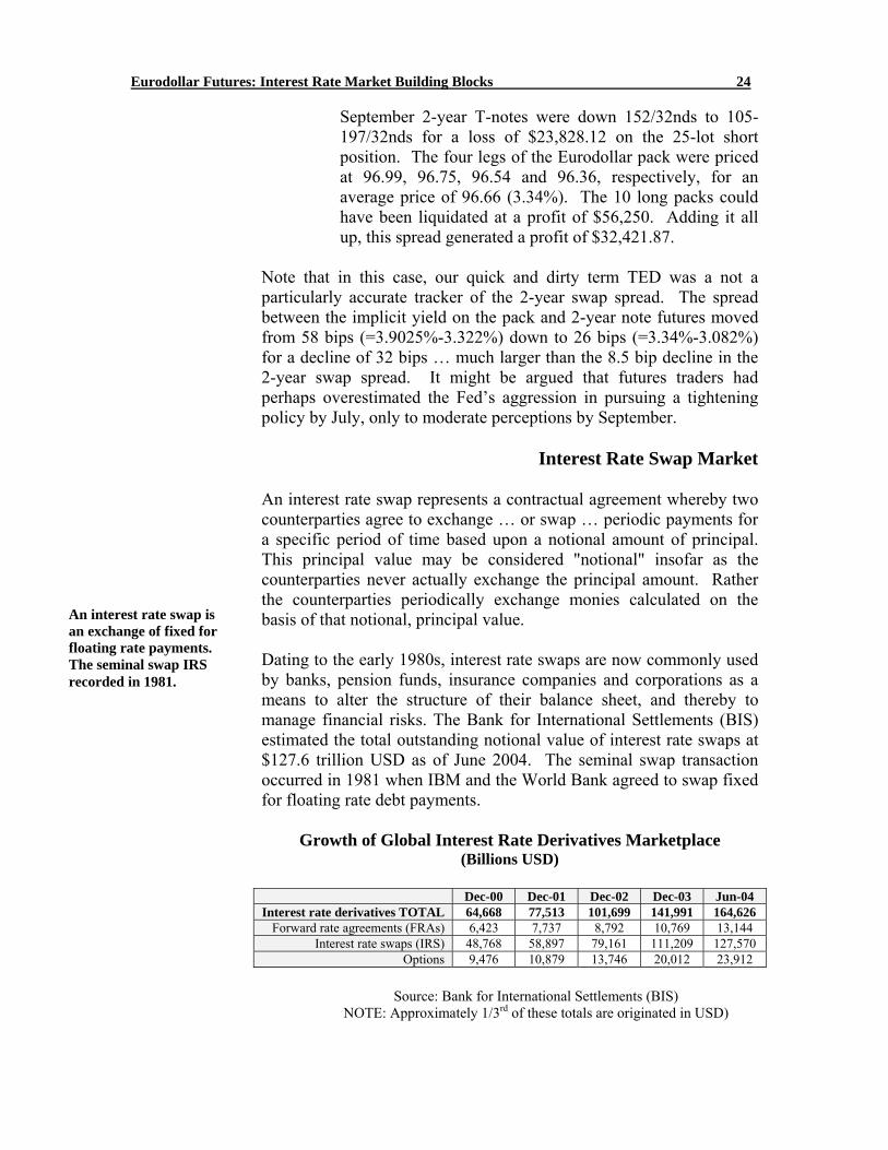
Interest Rate Swap Market An interest rate swap represents a contractual agreement whereby two counterparties agree to exchange … or swap … periodic payments for a specific period of time based upon a notional amount of principal. This principal value may be considered "notional" insofar as the counterparties never actually exchange the principal amount. Rather the counterparties periodically exchange monies calculated on the basis of that notional, principal value. Dating to the early 1980s, interest rate swaps are now commonly used by banks, pension funds, insurance companies and corporations as a means to alter the structure of their balance sheet, and thereby to manage financial risks. The Bank for International Settlements (BIS) estimated the total outstanding notional value of interest rate swaps at $127.6 trillion USD as of June 2004. The seminal swap transaction occurred in 1981 when IBM and the World Bank agreed to swap fixed for floating rate debt payments.
Growth of Global Interest Rate Derivatives Marketplace (Billions USD)
Dec-00 Dec-01 Dec-02 Dec-03 Jun-04
Interest rate derivatives TOTAL 64,668 77,513 101,699 141,991 164,626 Forward rate agreements (FRAs) 6,423 7,737 8,792 10,769 13,144
Interest rate swaps (IRS) 48,768 58,897 79,161 111,209 127,570 Options 9,476 10,879 13,746 20,012 23,912
Source: Bank for International Settlements (BIS)
NOTE: Approximately 1/3rd of these totals are originated in USD)
An interest rate swap is an exchange of fixed for floating rate payments. The seminal swap IRS recorded in 1981.
Eurodollar Futures: Interest Rate Market Building Blocks 25
While that transaction was completed directly between the two principal counterparties, most swaps are transacted through swap dealers … typically large banks or other financial institutions that show bids and offers to buy or sell swaps. This practice mitigates credit risk on the part of the counterparties who may be unfamiliar with the other’s credit stature.
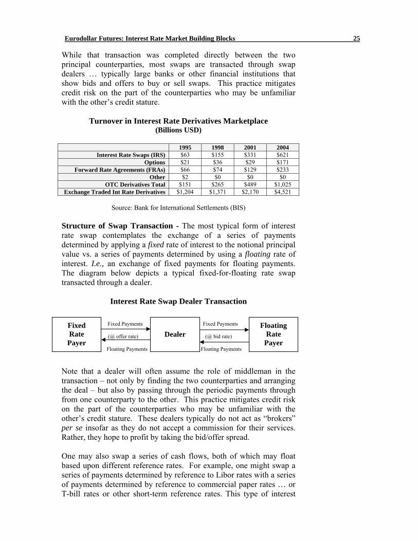
Turnover in Interest Rate Derivatives Marketplace
(Billions USD)
1995 1998 2001 2004 Interest Rate Swaps (IRS) $63 $155 $331 $621
Options $21 $36 $29 $171 Forward Rate Agreements (FRAs) $66 $74 $129 $233
Other $2 $0 $0 $0 OTC Derivatives Total $151 $265 $489 $1,025
Exchange Traded Int Rate Derivatives $1,204 $1,371 $2,170 $4,521
Source: Bank for International Settlements (BIS) Structure of Swap Transaction - The most typical form of interest rate swap contemplates the exchange of a series of payments determined by applying a fixed rate of interest to the notional principal value vs. a series of payments determined by using a floating rate of interest. I.e., an exchange of fixed payments for floating payments. The diagram below depicts a typical fixed-for-floating rate swap transacted through a dealer.
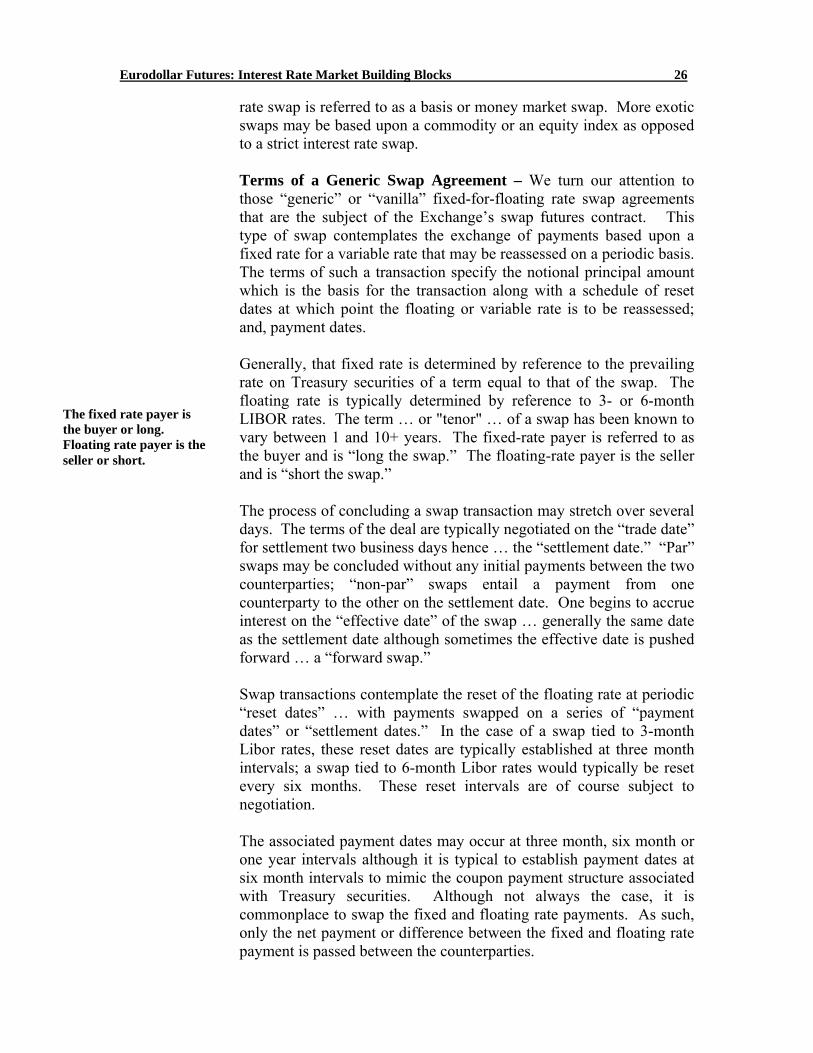
Interest Rate Swap Dealer Transaction Fixed Payments Fixed Payments (@ offer rate) (@ bid rate) Floating Payments Floating Payments Note that a dealer will often assume the role of middleman in the transaction – not only by finding the two counterparties and arranging the deal – but also by passing through the periodic payments through from one counterparty to the other. This practice mitigates credit risk on the part of the counterparties who may be unfamiliar with the other’s credit stature. These dealers typically do not act as “brokers” per se insofar as they do not accept a commission for their services. Rather, they hope to profit by taking the bid/offer spread. One may also swap a series of cash flows, both of which may float based upon different reference rates. For example, one might swap a series of payments determined by reference to Libor rates with a series of payments determined by reference to commercial paper rates … or T-bill rates or other short-term reference rates. This type of interest
Floating Rate
Payer
Dealer
Fixed Rate
Payer
Eurodollar Futures: Interest Rate Market Building Blocks 26
rate swap is referred to as a basis or money market swap. More exotic swaps may be based upon a commodity or an equity index as opposed to a strict interest rate swap. Terms of a Generic Swap Agreement – We turn our attention to those “generic” or “vanilla” fixed-for-floating rate swap agreements that are the subject of the Exchange’s swap futures contract. This type of swap contemplates the exchange of payments based upon a fixed rate for a variable rate that may be reassessed on a periodic basis. The terms of such a transaction specify the notional principal amount which is the basis for the transaction along with a schedule of reset dates at which point the floating or variable rate is to be reassessed; and, payment dates. Generally, that fixed rate is determined by reference to the prevailing rate on Treasury securities of a term equal to that of the swap. The floating rate is typically determined by reference to 3- or 6-month LIBOR rates. The term … or "tenor" … of a swap has been known to vary between 1 and 10+ years. The fixed-rate payer is referred to as the buyer and is “long the swap.” The floating-rate payer is the seller and is “short the swap.”
The process of concluding a swap transaction may stretch over several days. The terms of the deal are typically negotiated on the “trade date” for settlement two business days hence … the “settlement date.” “Par” swaps may be concluded without any initial payments between the two counterparties; “non-par” swaps entail a payment from one counterparty to the other on the settlement date. One begins to accrue interest on the “effective date” of the swap … generally the same date as the settlement date although sometimes the effective date is pushed forward … a “forward swap.” Swap transactions contemplate the reset of the floating rate at periodic “reset dates” … with payments swapped on a series of “payment dates” or “settlement dates.” In the case of a swap tied to 3-month Libor rates, these reset dates are typically established at three month intervals; a swap tied to 6-month Libor rates would typically be reset every six months. These reset intervals are of course subject to negotiation.
The associated payment dates may occur at three month, six month or one year intervals although it is typical to establish payment dates at six month intervals to mimic the coupon payment structure associated with Treasury securities. Although not always the case, it is commonplace to swap the fixed and floating rate payments. As such, only the net payment or difference between the fixed and floating rate payment is passed between the counterparties.
The fixed rate payer is the buyer or long. Floating rate payer is the seller or short.
Eurodollar Futures: Interest Rate Market Building Blocks 27
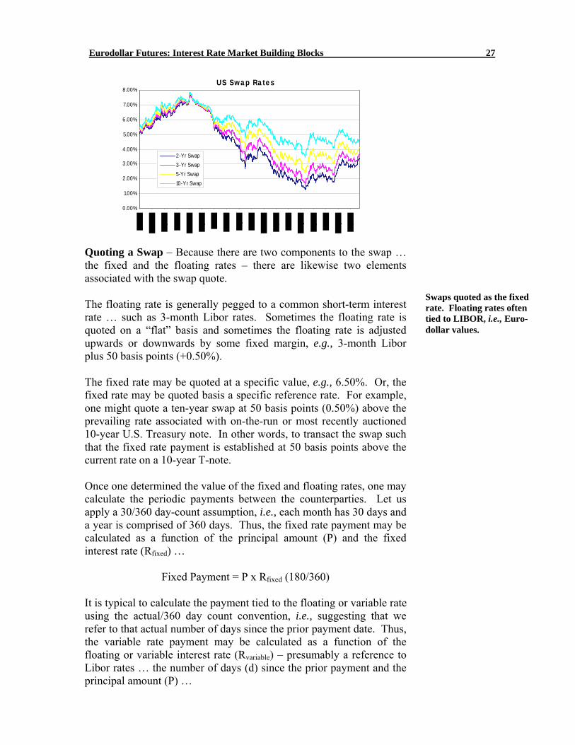
US Swap Rates
0.00%
1.00%
2.00%
3.00%
4.00%
5.00%
6.00%
7.00%
8.00%
2-Yr Swap3-Yr Swap5-Yr Swap10-Yr Swap
Quoting a Swap – Because there are two components to the swap … the fixed and the floating rates – there are likewise two elements associated with the swap quote. The floating rate is generally pegged to a common short-term interest rate … such as 3-month Libor rates. Sometimes the floating rate is quoted on a “flat” basis and sometimes the floating rate is adjusted upwards or downwards by some fixed margin, e.g., 3-month Libor plus 50 basis points (+0.50%). The fixed rate may be quoted at a specific value, e.g., 6.50%. Or, the fixed rate may be quoted basis a specific reference rate. For example, one might quote a ten-year swap at 50 basis points (0.50%) above the prevailing rate associated with on-the-run or most recently auctioned 10-year U.S. Treasury note. In other words, to transact the swap such that the fixed rate payment is established at 50 basis points above the current rate on a 10-year T-note. Once one determined the value of the fixed and floating rates, one may calculate the periodic payments between the counterparties. Let us apply a 30/360 day-count assumption, i.e., each month has 30 days and a year is comprised of 360 days. Thus, the fixed rate payment may be calculated as a function of the principal amount (P) and the fixed interest rate (Rfixed) …
Fixed Payment = P x Rfixed (180/360)
It is typical to calculate the payment tied to the floating or variable rate using the actual/360 day count convention, i.e., suggesting that we refer to that actual number of days since the prior payment date. Thus, the variable rate payment may be calculated as a function of the floating or variable interest rate (Rvariable) – presumably a reference to Libor rates … the number of days (d) since the prior payment and the principal amount (P) …
Swaps quoted as the fixed rate. Floating rates often tied to LIBOR, i.e., Euro-dollar values.
Eurodollar Futures: Interest Rate Market Building Blocks 28
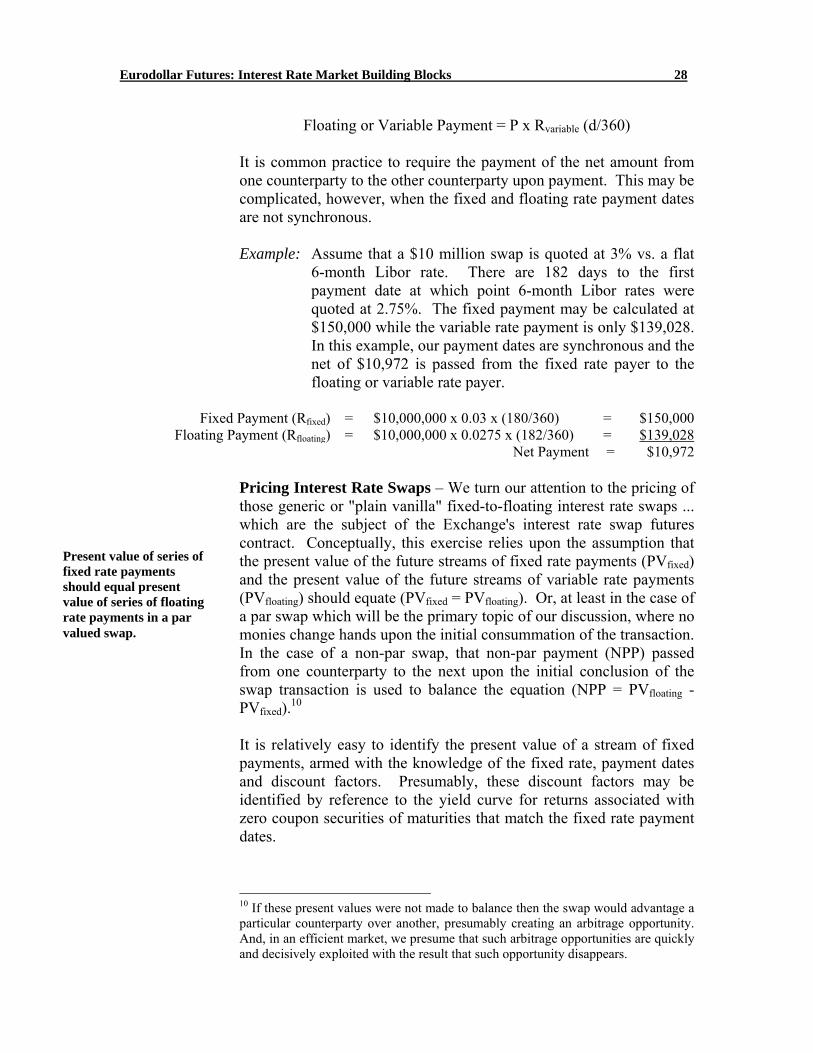
Floating or Variable Payment = P x Rvariable (d/360)
It is common practice to require the payment of the net amount from one counterparty to the other counterparty upon payment. This may be complicated, however, when the fixed and floating rate payment dates are not synchronous. Example: Assume that a $10 million swap is quoted at 3% vs. a flat
6-month Libor rate. There are 182 days to the first payment date at which point 6-month Libor rates were quoted at 2.75%. The fixed payment may be calculated at $150,000 while the variable rate payment is only $139,028. In this example, our payment dates are synchronous and the net of $10,972 is passed from the fixed rate payer to the floating or variable rate payer.
Fixed Payment (Rfixed) = $10,000,000 x 0.03 x (180/360) = $150,000
Floating Payment (Rfloating) = $10,000,000 x 0.0275 x (182/360) = $139,028 Net Payment = $10,972
Pricing Interest Rate Swaps – We turn our attention to the pricing of those generic or "plain vanilla" fixed-to-floating interest rate swaps ... which are the subject of the Exchange's interest rate swap futures contract. Conceptually, this exercise relies upon the assumption that the present value of the future streams of fixed rate payments (PVfixed) and the present value of the future streams of variable rate payments (PVfloating) should equate (PVfixed = PVfloating). Or, at least in the case of a par swap which will be the primary topic of our discussion, where no monies change hands upon the initial consummation of the transaction. In the case of a non-par swap, that non-par payment (NPP) passed from one counterparty to the next upon the initial conclusion of the swap transaction is used to balance the equation (NPP = PVfloating - PVfixed).10 It is relatively easy to identify the present value of a stream of fixed payments, armed with the knowledge of the fixed rate, payment dates and discount factors. Presumably, these discount factors may be identified by reference to the yield curve for returns associated with zero coupon securities of maturities that match the fixed rate payment dates.
10 If these present values were not made to balance then the swap would advantage a particular counterparty over another, presumably creating an arbitrage opportunity. And, in an efficient market, we presume that such arbitrage opportunities are quickly and decisively exploited with the result that such opportunity disappears.
Present value of series of fixed rate payments should equal present value of series of floating rate payments in a par valued swap.
Eurodollar Futures: Interest Rate Market Building Blocks 29
It is, however, a bit more difficult to assess the present value of those future streams of variable rates payments. We cannot know what those variable payments will be. Still, the marketplace offers much information regarding interest rates that may be used to impute these future income streams and, in turn, to assess the value of a swap transaction.
In particular, one may study the yield curve to glean valuable information regarding the market’s implicit assessment of future interest rates … or “implied forward rates” (IFRs). An IFR may be imputed if one can identify the term rate associated with the inception and conclusion of a loan. For example, if one has information regarding the term 6-month rate and the one-year rate, one may impute the IFR for a six-month rate six-months hence. This calculation is based upon the assumption that an investor will be indifferent between a one-year term investment and a six-month investment rolled over into another subsequent six-month investment, aggregating to a one-year term. These IFRs may be used as a proxy to calculate the variable rate payments on future payment dates. Actually, IFRs of a sort are available by direct reference to the Exchange’s Eurodollar futures market that lists contracts extending out ten years into the future. The rate implied in the Eurodollar futures quote effectively represents an IFR itself. As such, swap traders frequently reference Eurodollar pricing as a proxy for those future variable rates and in turn utilize swap rates as a benchmark for other fixed income securities. Thus, it is possible to assess the present value of the futures streams of both fixed and variable rate payments. And, as discussed above, to identify the value of the swap as the difference in the two sums. In a par swap, that difference is zero … no monies change changes when the swap is initially concluded. However, the value of a swap represented in the difference between these net present values is expected to fluctuate over time as a function of market conditions. For example, if yields are generally rising, this will result in advancing IFRs. Thus, the present value of the variable rate payments will advance … noting that the fixed payments are, of course, fixed. This advantages the fixed rate payer.
We can expect that the performance of an interest rate swap will reflect the performance of a coupon-bearing security with a maturity equal to the term of the swap less the term of the rate to which the variable payments are tied. For example, a ten-year swap tied to 6-month Libor may perform akin to a 10-year term security … depending on how close one is to the next variable rate reset date.
Swaps often priced by reference to implied forward rates or CME Eurodollar futures prices.
Eurodollar Futures: Interest Rate Market Building Blocks 30
If one seeks to terminate a swap agreement prematurely … presumably with one’s dealer … this implies either a profit or loss and a concluding receipt or payment of monies represented by the updated difference in the present values. As such, non-par swap transactions are often used prematurely to terminate a previous swap transaction … whether the original transaction was concluded at par or otherwise. In any event, the initial pricing of a par swap reduces to the question: what fixed rate will cause the two streams of future income to balance? Essentially, that is the rate represented when one references the ISDA benchmark rates associated with par swaps of any particular term. Credit Risk Considerations – Credit risk is implied in a swap insofar as the two counterparties are obligated periodically to swap monies … often for considerable term into the future. But because there is no exchange of the principal or nominal amount up front … and because those payments are typically netted so that only the difference between the fixed and variable rate payment is actually exchanged … credit risks are reduced relative to a typical debt obligation. In other words, what is at risk in the event of a default on a swap agreement is the difference between the original cost of the swap and the current cost of a swap with a term equal to the remaining term of the original. The practice of netting is a significant convenience in this process. As the swap market developed and matured from the early 1980s, swap dealers found that they were frequently conducting business with the same counterparties. This led to the accumulation of large books of outstanding swaps. Rather than administer each one of these swap transactions separately, these dealers’ backoffices wrote contracts that permitted them to consolidate all outstanding swaps, netting all payments between the dealer and a particular counterparty. A default in any one swap agreement would give the aggrieved counterparty the option to cancel all outstanding swaps. Eventually, the International Swap and Derivatives Association (ISDA) developed and made available standardized master agreements of this kind that are in near universal use today. Of course, swap dealers … many of which are banks and are, therefore, accustomed to assessing credit risks … identify a poor credit quality counterparty, they may attempt to manage credit risk through the imposition of performance bond requirements. These requirements may be administered in a manner not dissimilar from the way in which futures margins are administered … although mark-to-market adjustments would likely be required less frequently than daily.
Swaps are typically bi-lateral transactions where the counterparties accept each other’s credit risk.
Eurodollar Futures: Interest Rate Market Building Blocks 31
Utility of Interest Rate Swaps – Interest rate swaps have been actively utilized by a wide variety of financial institutions … including pension funds, mutual funds, insurance companies, banks … and corporations … both domestic and abroad … and government entities. Swaps have been used to manage risk exposures, to reduce the cost of funding or increase the return on an investment and for speculative purposes. Interest rate swaps are used because they convey important financial benefits. Broadly speaking, these transactions convey value because they allow market participants to: (1) exploit situations where they have a comparative advantage, (2) exploit information advantages or asymmetries; and (3) avoid prepayment “penalties” implicit in the structure of many debt instruments. The theory of comparative advantage suggests that various fixed income market participants may enjoy the ability to borrow or lend at advantageous terms in particular markets. A swap provides the means to convey those benefits from one counterparty to the other … in return perhaps for a similar favor. Consider, for example, the possibility that credit spreads … or the difference in loan rates paid by less creditworthy borrowers vs. more creditworthy borrowers … may be steeper with regard to fixed rate as opposed to floating rate loans … and may rise as a function of the loan’s term. Thus, a company with a relatively low credit rating may seek to borrow in the credit markets at a floating rate … where the company has a comparative advantage … but hedge the risk of rising rates by entering a swap transaction as the fixed rate payer. Some critics have sought to punch holes in the theory of comparative advantage. In particular, such critics suggest that arbitrage activity in the capital markets may serve to do away with such comparative advantages … detracting thereby from the utility of swap transactions. While there is some validity in this criticism, it is not clear that capital markets are completely efficient in this sense or that the theory of comparative advantage does not at least partially explain the utility of swaps. A second explanation for the utility of swap transactions may be identified as informational advantages. An example of such informational advantages might be found in a situation where a firm had information not generally available suggesting that its credit rating may deteriorate. As such, a firm may seek to fund its activities with floating rate debt but hedge the risk of rising funding costs by entering a swap transaction as the fixed rate payer. Or, a firm may enter into
Eurodollar Futures: Interest Rate Market Building Blocks 32
the same transaction simply because it anticipates rising short-term rates in the future. A third explanation for the popularity of swaps might be found by examining the structure of most fixed rate debt obligations. Often, fixed rate debt is issued with a callable provision. A corporation may, for example, issue a note that is callable at par at the discretion of the corporation. This provision protects the borrower against the possibility that rates will fall and the borrower will be saddled with high-rate debt for an extended period of time. But such protection comes at a cost. In particular, the borrower will offer somewhat elevated rates to attract interest in such an obligation than would otherwise be the case. By contrast, there is no such prepayment penalty or premium associated with a swap transaction. A swap may, however, be terminated prior to maturity by payment of the current value of the swap … reflecting the present value of the differential payment stream reflected in the original vs. the current swap rate.
Growing Up Together
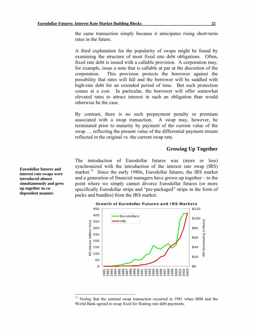
The introduction of Eurodollar futures was (more or less) synchronized with the introduction of the interest rate swap (IRS) market.11 Since the early 1980s, Eurodollar futures, the IRS market and a generation of financial managers have grown up together – to the point where we simply cannot divorce Eurodollar futures (or more specifically Eurodollar strips and “pre-packaged” strips in the form of packs and bundles) from the IRS market.
Growth of Eurodollar Futures and IRS Markets
0
50
100
150
200
250
300
350
400
450
1981
1982
1983
1984
1985
1986
1987
1988
1989
1990
1991
1992
1993
1994
1995
1996
1997
1998
1999
2000
2001
2002
2003
ED V
olum
e (M
illio
n C
nts
)
$0
$20
$40
$60
$80
$100
$120
IRS O
uts
tandin
g (tr
illio
ns)
Eurodollars
IRS
11 Noting that the seminal swap transaction occurred in 1981 when IBM and the World Bank agreed to swap fixed for floating rate debt payments.
Eurodollar futures and interest rate swaps were introduced almost simultaneously and grew up together in co-dependent manner.
Eurodollar Futures: Interest Rate Market Building Blocks 33
And, Eurodollar futures have grown with the growth and development of the interest rate swap marketplace. The tables below depict the growth in notional value outstanding (~open interest) and turnover (~volume) in over-the-counter and exchange traded interest rate derivatives. While the notional value outstanding in Eurodollar futures is dwarfed by the OTC markets – futures nonetheless take the lead in terms of volume. A&L vs. Swap Applications – Actually, initial institutional use of Eurodollar futures was limited largely to asset & liability management and general speculative applications. These A&L applications involve hedging asset/liability mismatches within an institution’s book. In the early 1980s, most banks and savings institutions applied the “risk bucket” approach where assets and liabilities were categorized and compared by maturity. Risk was incumbent wherever a mismatch between assets and liabilities within any particular bucket was identified. Eurodollar futures became handy tools to balance these mismatches and allay risks. In subsequent years, with the advent of cheap computing power and generalized appreciation for more sophisticated financial modeling techniques including duration, VAR, etc., the risk bucket method of analysis was largely supplanted. Nonetheless, Eurodollar futures remain an important tool for A&L managers.
IRS Applications - Swap traders routinely reference Eurodollar pricing as a proxy for future variable rates and in turn utilize swap rates as a benchmark for other fixed income securities.
“The interest-rate swap curve – a series of rates across the maturity spectrum, which are pegged to the Chicago Mercantile Exchange’s Eurodollar futures – has established itself as an emerging alternative to Treasurys as a benchmark for measuring the relative value of other debt classes ... The swap curve is becoming ‘more influential, and we’re certainly interested in swap movement as it relates to the corporates, asset-backed and mortgage-backed securities that we own,’ said Tom Marthaler, a portfolio manager with Chicago Trust Co.” 12
Consider that OTC derivatives are marketed actively by derivatives dealers to insurance companies, hedge funds and corporations. These dealers in turn manage their books with the use of futures. In other words, OTC derivatives dealers effectively package or re-package risks for sale to their customers that are managed with the use of Eurodollar futures. 12 “Interest-Rate Swap Curve is Emerging as Alternative to Treasurys Benchmark,” Wall Street Journal, February 22, 2000.
Eurodollar futures originally sold as means to manage asset/liability mismatches of banking institutions.
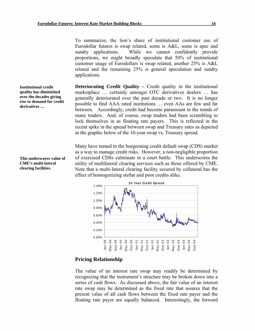
Eurodollar Futures: Interest Rate Market Building Blocks 34
To summarize, the lion’s share of institutional customer use of Eurodollar futures is swap related, some is A&L, some is spec and sundry applications. While we cannot confidently provide proportions, we might broadly speculate that 50% of institutional customer usage of Eurodollars is swap related, another 25% is A&L related and the remaining 25% is general speculation and sundry applications.
Deteriorating Credit Quality – Credit quality in the institutional marketplace … certainly amongst OTC derivatives dealers … has generally deteriorated over the past decade or two. It is no longer possible to find AAA rated institutions … even AAs are few and far between. Accordingly, credit had become paramount in the minds of many traders. And, of course, swap traders had been scrambling to lock themselves in as floating rate payers. This is reflected in the recent spike in the spread between swap and Treasury rates as depicted in the graphic below of the 10-year swap vs. Treasury spread. Many have turned to the burgeoning credit default swap (CDS) market as a way to manage credit risks. However, a non-negligible proportion of exercised CDSs culminate in a court battle. This underscores the utility of multilateral clearing services such as those offered by CME. Note that a multi-lateral clearing facility secured by collateral has the effect of homogenizing stellar and poor credits alike.
10-Year Credit Spread
0.00%
0.20%
0.40%
0.60%
0.80%
1.00%
1.20%
1.40%
Jan
-99
Ma
y-9
9
Se
p-9
9
Jan
-00
Ma
y-0
0
Se
p-0
0
Jan
-01
Ma
y-0
1
Se
p-0
1
Jan
-02
Ma
y-0
2
Se
p-0
2
Jan
-03
Ma
y-0
3
Se
p-0
3
Jan
-04
Ma
y-0
4
Se
p-0
4
Pricing Relationship The value of an interest rate swap may readily be determined by recognizing that the instrument’s structure may be broken down into a series of cash flows. As discussed above, the fair value of an interest rate swap may be determined as the fixed rate that assures that the present value of all cash flows between the fixed rate payer and the floating rate payer are equally balanced. Interestingly, the forward
Institutional credit quality has diminished over the decades giving rise to demand for credit derivatives …
This underscores value of CME’s multi-lateral clearing facilities.
Eurodollar Futures: Interest Rate Market Building Blocks 35
rates implied in Eurodollar futures prices may be used as a significant reference in these calculations. Let us consider the structure of a so-called “IMM dated” interest rate swap. An IMM swap is constructed such that the periodic rate fixing dates fall on the maturation dates for Eurodollar futures contracts and the floating rate is pegged to current 3-month LIBOR rates. Further, let us apply an “actual/360” day count convention for both legs of the swap transaction. There are other swap structures that we may discussion … but this is a particularly convenient structure to price and hedge and will serve as the basis for our illustrations. Let the principal or notional value of the transaction be denoted as “P,” the present value of $1 received i days (“di”) in the future is denoted as “PVi,” the variable or floating 3-month LIBOR rates expected to be prevailing di days in the future are denoted at “Ri.”
We are of course interested in pricing the swap as the fixed rate Rfixed that assures that the net prevent value of all fixed rate payments equates to the expected values of all floating rate payments, i.e., the non-par payment of the swap equals zero (NPP=$0.00). The generalized solution to our problem may be found as follows.
n Σ PVi (Rfixed/4) P
i=1 =
n Σ PVi Ri (di /360) P i=1
Solving for Rfixed …
Rfixed = n n 4 Σ PVi Ri (di /360) / Σ PVi i=1 i=1
Conveniently, the specific numbers we will require to solve for Rfixed will largely be supplied by reference to the Eurodollar futures market. As discussed above, Eurodollar futures prices represent the implied forward rate, i.e., the market’s expectation regarding rates that may prevail in the future. Thus, we may reference those rates as an indication for the 3-month LIBOR rates at which the variable payments may be established or Ri. The appropriate present value discount factor (PVi) may likewise be found in the Eurodollar futures market structure. Specifically, the reciprocal of the compounded value of a Eurodollar futures strip is comparable to the value of a zero coupon bond and may be used as the discounting factor PVi or the present value of $1 received i days in the future. Example: Let’s find the value of a two-year IMM-dated swap with a
$10 million notional or principal amount. Assume that the
Many swaps are reset on Eurodollar maturity dates (IMM) dates … these swaps are simple to price using Eurodollar futures prices.
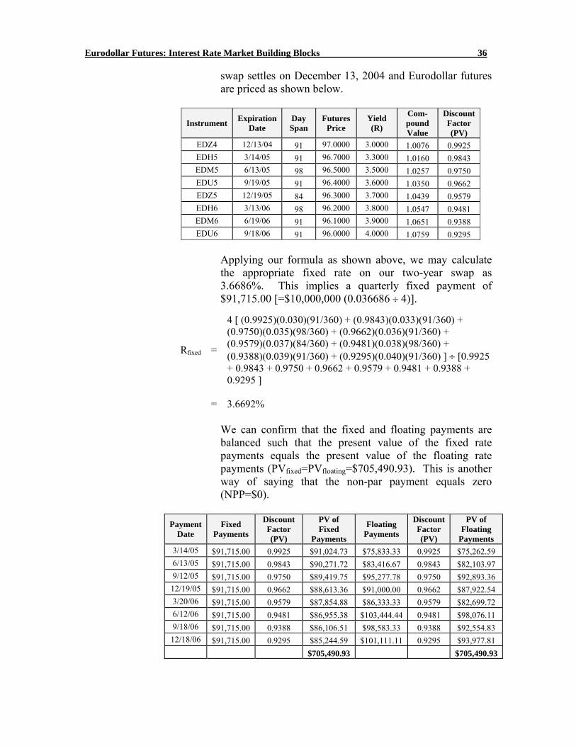
Eurodollar Futures: Interest Rate Market Building Blocks 36
swap settles on December 13, 2004 and Eurodollar futures are priced as shown below.
Instrument Expiration Date
Day Span
Futures Price
Yield (R)
Com-pound Value
Discount Factor (PV)
EDZ4 12/13/04 91 97.0000 3.0000 1.0076 0.9925 EDH5 3/14/05 91 96.7000 3.3000 1.0160 0.9843 EDM5 6/13/05 98 96.5000 3.5000 1.0257 0.9750 EDU5 9/19/05 91 96.4000 3.6000 1.0350 0.9662 EDZ5 12/19/05 84 96.3000 3.7000 1.0439 0.9579 EDH6 3/13/06 98 96.2000 3.8000 1.0547 0.9481 EDM6 6/19/06 91 96.1000 3.9000 1.0651 0.9388 EDU6 9/18/06 91 96.0000 4.0000 1.0759 0.9295
Applying our formula as shown above, we may calculate
the appropriate fixed rate on our two-year swap as 3.6686%. This implies a quarterly fixed payment of $91,715.00 [=$10,000,000 (0.036686 ÷ 4)].
Rfixed =
4 [ (0.9925)(0.030)(91/360) + (0.9843)(0.033)(91/360) + (0.9750)(0.035)(98/360) + (0.9662)(0.036)(91/360) + (0.9579)(0.037)(84/360) + (0.9481)(0.038)(98/360) + (0.9388)(0.039)(91/360) + (0.9295)(0.040)(91/360) ] ÷ [0.9925 + 0.9843 + 0.9750 + 0.9662 + 0.9579 + 0.9481 + 0.9388 + 0.9295 ]
= 3.6692%
We can confirm that the fixed and floating payments are
balanced such that the present value of the fixed rate payments equals the present value of the floating rate payments (PVfixed=PVfloating=$705,490.93). This is another way of saying that the non-par payment equals zero (NPP=$0).
Payment
Date Fixed
Payments
Discount Factor (PV)
PV of Fixed
Payments
Floating Payments
Discount Factor (PV)
PV of Floating
Payments 3/14/05 $91,715.00 0.9925 $91,024.73 $75,833.33 0.9925 $75,262.59 6/13/05 $91,715.00 0.9843 $90,271.72 $83,416.67 0.9843 $82,103.97 9/12/05 $91,715.00 0.9750 $89,419.75 $95,277.78 0.9750 $92,893.36 12/19/05 $91,715.00 0.9662 $88,613.36 $91,000.00 0.9662 $87,922.54 3/20/06 $91,715.00 0.9579 $87,854.88 $86,333.33 0.9579 $82,699.72 6/12/06 $91,715.00 0.9481 $86,955.38 $103,444.44 0.9481 $98,076.11 9/18/06 $91,715.00 0.9388 $86,106.51 $98,583.33 0.9388 $92,554.83 12/18/06 $91,715.00 0.9295 $85,244.59 $101,111.11 0.9295 $93,977.81
$705,490.93 $705,490.93
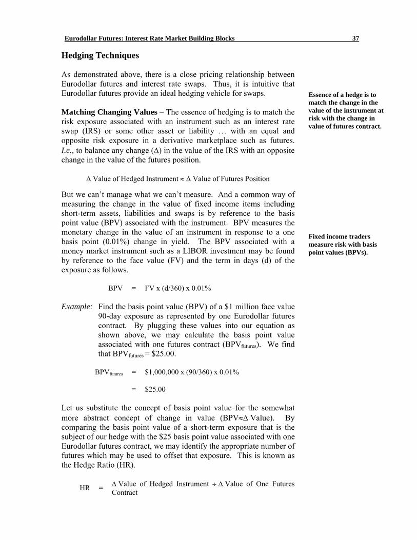
Eurodollar Futures: Interest Rate Market Building Blocks 37
Hedging Techniques As demonstrated above, there is a close pricing relationship between Eurodollar futures and interest rate swaps. Thus, it is intuitive that Eurodollar futures provide an ideal hedging vehicle for swaps. Matching Changing Values – The essence of hedging is to match the risk exposure associated with an instrument such as an interest rate swap (IRS) or some other asset or liability … with an equal and opposite risk exposure in a derivative marketplace such as futures. I.e., to balance any change (Δ) in the value of the IRS with an opposite change in the value of the futures position.
Δ Value of Hedged Instrument ≈ Δ Value of Futures Position But we can’t manage what we can’t measure. And a common way of measuring the change in the value of fixed income items including short-term assets, liabilities and swaps is by reference to the basis point value (BPV) associated with the instrument. BPV measures the monetary change in the value of an instrument in response to a one basis point (0.01%) change in yield. The BPV associated with a money market instrument such as a LIBOR investment may be found by reference to the face value (FV) and the term in days (d) of the exposure as follows.
BPV = FV x (d/360) x 0.01% Example: Find the basis point value (BPV) of a $1 million face value
90-day exposure as represented by one Eurodollar futures contract. By plugging these values into our equation as shown above, we may calculate the basis point value associated with one futures contract (BPVfutures). We find that BPVfutures = $25.00.
BPVfutures = $1,000,000 x (90/360) x 0.01%
= $25.00
Let us substitute the concept of basis point value for the somewhat more abstract concept of change in value (BPV≈Δ Value). By comparing the basis point value of a short-term exposure that is the subject of our hedge with the $25 basis point value associated with one Eurodollar futures contract, we may identify the appropriate number of futures which may be used to offset that exposure. This is known as the Hedge Ratio (HR).
HR = Δ Value of Hedged Instrument ÷ Δ Value of One Futures Contract
Essence of a hedge is to match the change in the value of the instrument at risk with the change in value of futures contract.
Fixed income traders measure risk with basis point values (BPVs).
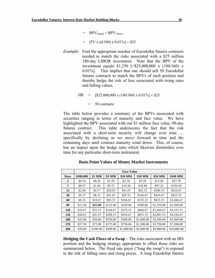
Eurodollar Futures: Interest Rate Market Building Blocks 38
= BPVhedged ÷ BPV futures = [FV x (d/360) x 0.01%] ÷ $25 Example: Find the appropriate number of Eurodollar futures contracts
needed to match the risks associated with a $25 million 180-day LIBOR investment. Note that the BPV of the investment equals $1,250 [=$25,000,000 x (180/360) x 0.01%]. This implies that one should sell 50 Eurodollar futures contracts to match the BPVs of each position and thereby hedge the risk of loss associated with rising rates and falling values.
HR = [$25,000,000 x (180/360) x 0.01%] ÷ $25
= 50 contracts
The table below provides a summary of the BPVs associated with securities ranging in terms of maturity and face value. We have highlighted the BPV associated with our $1 million face value, 90-day futures contract. This table underscores the fact that the risk associated with a short-term security will change over time … specifically by declining as we move forward in time and the remaining days until contract maturity wind down. This, of course, has an impact upon the hedge ratio which likewise diminishes over time for any particular short-term instrument.
Basis Point Values of Money Market Instruments
Face Value Days $500,000 $1 MM $5 MM $10 MM $20 MM $50 MM $100 MM
1 $0.14 $0.28 $1.39 $2.78 $5.56 $13.89 $27.78 7 $0.97 $1.94 $9.72 $19.44 $38.89 $97.22 $194.44 15 $2.08 $4.17 $20.83 $41.67 $83.33 $208.33 $416.67 30 $4.17 $8.33 $41.67 $83.33 $166.67 $416.67 $833.33 60 $8.33 $16.67 $83.33 $166.67 $333.33 $833.33 $1,666.67 90 $12.50 $25.00 $125.00 $250.00 $500.00 $1,250.00 $2,500.00
120 $16.67 $33.33 $166.67 $333.33 $666.67 $1,666.67 $3,333.33 150 $20.83 $41.67 $208.33 $416.67 $833.33 $2,083.33 $4,166.67 180 $25.00 $50.00 $250.00 $500.00 $1,000.00 $2,500.00 $5,000.00 270 $37.50 $75.00 $375.00 $750.00 $1,500.00 $3,750.00 $7,500.00 360 $50.00 $100.00 $500.00 $1,000.00 $2,000.00 $5,000.00 $10,000.00
Hedging the Cash Flows of a Swap – The risks associated with an IRS position and the hedging strategy appropriate to offset those risks are summarized below. The fixed rate payer (“long the swap”) is exposed to the risk of falling rates and rising prices. A long Eurodollar futures
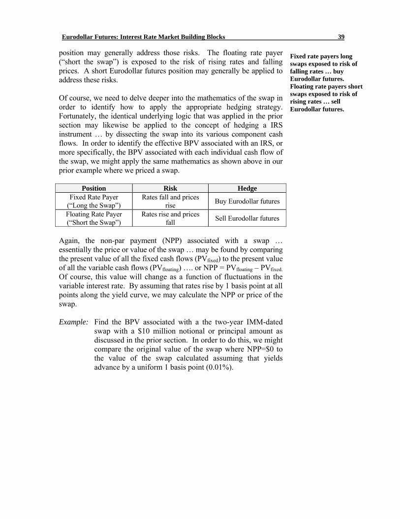
Eurodollar Futures: Interest Rate Market Building Blocks 39
position may generally address those risks. The floating rate payer (“short the swap”) is exposed to the risk of rising rates and falling prices. A short Eurodollar futures position may generally be applied to address these risks.
Of course, we need to delve deeper into the mathematics of the swap in order to identify how to apply the appropriate hedging strategy. Fortunately, the identical underlying logic that was applied in the prior section may likewise be applied to the concept of hedging a IRS instrument … by dissecting the swap into its various component cash flows. In order to identify the effective BPV associated with an IRS, or more specifically, the BPV associated with each individual cash flow of the swap, we might apply the same mathematics as shown above in our prior example where we priced a swap.
Position Risk Hedge Fixed Rate Payer
(“Long the Swap”) Rates fall and prices
rise Buy Eurodollar futures
Floating Rate Payer (“Short the Swap”)
Rates rise and prices fall Sell Eurodollar futures
Again, the non-par payment (NPP) associated with a swap … essentially the price or value of the swap … may be found by comparing the present value of all the fixed cash flows (PVfixed) to the present value of all the variable cash flows (PVfloating) …. or NPP = PVfloating – PVfixed. Of course, this value will change as a function of fluctuations in the variable interest rate. By assuming that rates rise by 1 basis point at all points along the yield curve, we may calculate the NPP or price of the swap. Example: Find the BPV associated with a the two-year IMM-dated
swap with a $10 million notional or principal amount as discussed in the prior section. In order to do this, we might compare the original value of the swap where NPP=$0 to the value of the swap calculated assuming that yields advance by a uniform 1 basis point (0.01%).
Fixed rate payers long swaps exposed to risk of falling rates … buy Eurodollar futures. Floating rate payers short swaps exposed to risk of rising rates … sell Eurodollar futures.
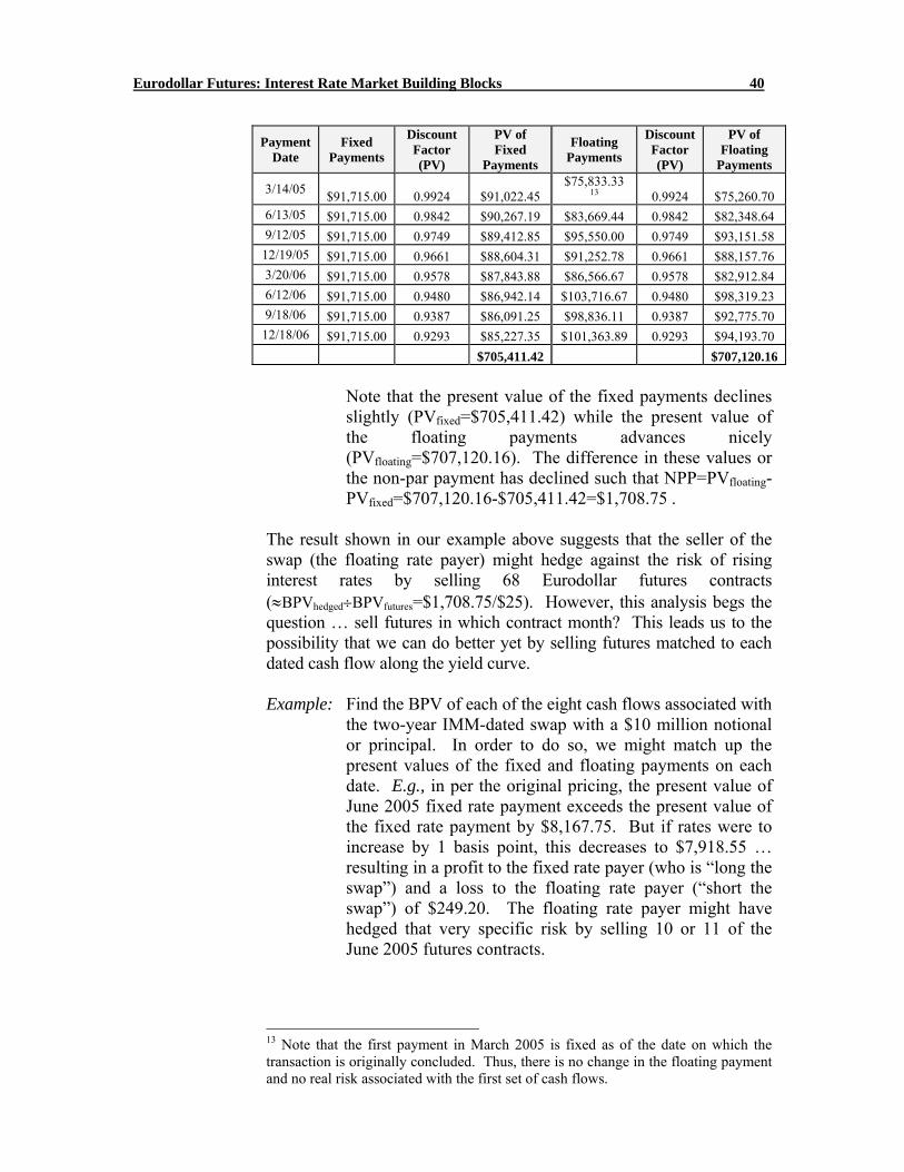
Eurodollar Futures: Interest Rate Market Building Blocks 40
Payment Date
Fixed Payments
Discount Factor (PV)
PV of Fixed
Payments
Floating Payments
Discount Factor (PV)
PV of Floating
Payments
3/14/05 $91,715.00 0.9924 $91,022.45 $75,833.33
13 0.9924 $75,260.70 6/13/05 $91,715.00 0.9842 $90,267.19 $83,669.44 0.9842 $82,348.64 9/12/05 $91,715.00 0.9749 $89,412.85 $95,550.00 0.9749 $93,151.58 12/19/05 $91,715.00 0.9661 $88,604.31 $91,252.78 0.9661 $88,157.76 3/20/06 $91,715.00 0.9578 $87,843.88 $86,566.67 0.9578 $82,912.84 6/12/06 $91,715.00 0.9480 $86,942.14 $103,716.67 0.9480 $98,319.23 9/18/06 $91,715.00 0.9387 $86,091.25 $98,836.11 0.9387 $92,775.70 12/18/06 $91,715.00 0.9293 $85,227.35 $101,363.89 0.9293 $94,193.70
$705,411.42 $707,120.16
Note that the present value of the fixed payments declines slightly (PVfixed=$705,411.42) while the present value of the floating payments advances nicely (PVfloating=$707,120.16). The difference in these values or the non-par payment has declined such that NPP=PVfloating-PVfixed=$707,120.16-$705,411.42=$1,708.75 .
The result shown in our example above suggests that the seller of the swap (the floating rate payer) might hedge against the risk of rising interest rates by selling 68 Eurodollar futures contracts (≈BPVhedged÷BPVfutures=$1,708.75/$25). However, this analysis begs the question … sell futures in which contract month? This leads us to the possibility that we can do better yet by selling futures matched to each dated cash flow along the yield curve. Example: Find the BPV of each of the eight cash flows associated with
the two-year IMM-dated swap with a $10 million notional or principal. In order to do so, we might match up the present values of the fixed and floating payments on each date. E.g., in per the original pricing, the present value of June 2005 fixed rate payment exceeds the present value of the fixed rate payment by $8,167.75. But if rates were to increase by 1 basis point, this decreases to $7,918.55 … resulting in a profit to the fixed rate payer (who is “long the swap”) and a loss to the floating rate payer (“short the swap”) of $249.20. The floating rate payer might have hedged that very specific risk by selling 10 or 11 of the June 2005 futures contracts.
13 Note that the first payment in March 2005 is fixed as of the date on which the transaction is originally concluded. Thus, there is no change in the floating payment and no real risk associated with the first set of cash flows.
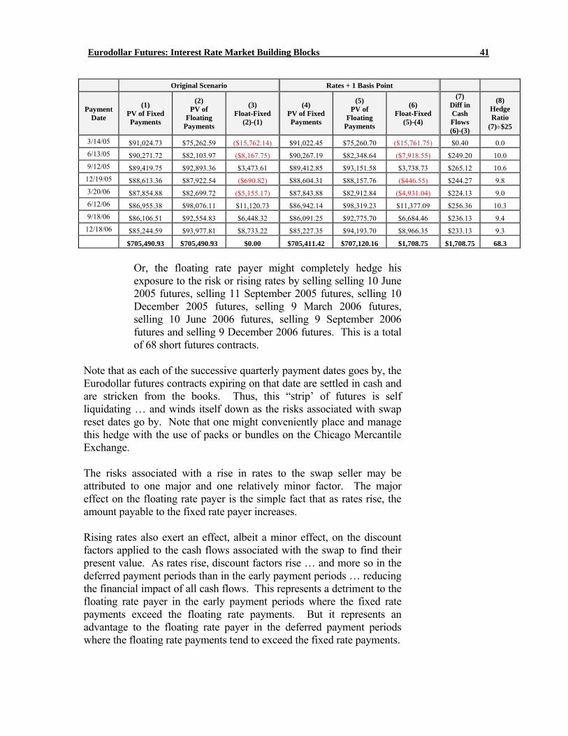
Eurodollar Futures: Interest Rate Market Building Blocks 41
Original Scenario Rates + 1 Basis Point
Payment Date
(1) PV of Fixed Payments
(2) PV of
Floating Payments
(3) Float-Fixed
(2)-(1)
(4) PV of Fixed Payments
(5) PV of
Floating Payments
(6) Float-Fixed
(5)-(4)
(7) Diff in Cash Flows (6)-(3)
(8) Hedge Ratio
(7)÷$25
3/14/05 $91,024.73 $75,262.59 ($15,762.14) $91,022.45 $75,260.70 ($15,761.75) $0.40 0.0 6/13/05 $90,271.72 $82,103.97 ($8,167.75) $90,267.19 $82,348.64 ($7,918.55) $249.20 10.0 9/12/05 $89,419.75 $92,893.36 $3,473.61 $89,412.85 $93,151.58 $3,738.73 $265.12 10.6 12/19/05 $88,613.36 $87,922.54 ($690.82) $88,604.31 $88,157.76 ($446.55) $244.27 9.8 3/20/06 $87,854.88 $82,699.72 ($5,155.17) $87,843.88 $82,912.84 ($4,931.04) $224.13 9.0 6/12/06 $86,955.38 $98,076.11 $11,120.73 $86,942.14 $98,319.23 $11,377.09 $256.36 10.3 9/18/06 $86,106.51 $92,554.83 $6,448.32 $86,091.25 $92,775.70 $6,684.46 $236.13 9.4 12/18/06 $85,244.59 $93,977.81 $8,733.22 $85,227.35 $94,193.70 $8,966.35 $233.13 9.3
$705,490.93 $705,490.93 $0.00 $705,411.42 $707,120.16 $1,708.75 $1,708.75 68.3
Or, the floating rate payer might completely hedge his exposure to the risk or rising rates by selling selling 10 June 2005 futures, selling 11 September 2005 futures, selling 10 December 2005 futures, selling 9 March 2006 futures, selling 10 June 2006 futures, selling 9 September 2006 futures and selling 9 December 2006 futures. This is a total of 68 short futures contracts.
Note that as each of the successive quarterly payment dates goes by, the Eurodollar futures contracts expiring on that date are settled in cash and are stricken from the books. Thus, this “strip’ of futures is self liquidating … and winds itself down as the risks associated with swap reset dates go by. Note that one might conveniently place and manage this hedge with the use of packs or bundles on the Chicago Mercantile Exchange. The risks associated with a rise in rates to the swap seller may be attributed to one major and one relatively minor factor. The major effect on the floating rate payer is the simple fact that as rates rise, the amount payable to the fixed rate payer increases. Rising rates also exert an effect, albeit a minor effect, on the discount factors applied to the cash flows associated with the swap to find their present value. As rates rise, discount factors rise … and more so in the deferred payment periods than in the early payment periods … reducing the financial impact of all cash flows. This represents a detriment to the floating rate payer in the early payment periods where the fixed rate payments exceed the floating rate payments. But it represents an advantage to the floating rate payer in the deferred payment periods where the floating rate payments tend to exceed the fixed rate payments.
Eurodollar Futures: Interest Rate Market Building Blocks 42
Convexity – Unfortunately, our hedger’s tasks are not necessarily complete once the hedge is placed. While the BPV associated with Eurodollar futures contracts remain static such that BPVf=$25.00, the BPV associated with the swap that is the subject of our hedge (BPVhedged) is dynamic. This is illustrated in the table below where we have calculated the non-par payment (NPP) or price of the swap given a range of movement in interest rates. Note that the span or change in the value of the swap is in fact NOT constant. This table illustrates the concept of “convexity.” Convexity is a property embedded in the pricing structure of many interest rate instruments including interest rate swaps. And, as we may see from our illustration, it implies that the swap becomes more sensitive to changing rates as rates fall and less sensitive to changing rates as rates rise. This further implies that more futures contracts are needed to maintain a balanced hedge in a falling rate environment while fewer futures contracts are needed in a rising rate environment. I.e., hedge ratios increase as rates fall and decrease when rates rise. This phenomenon may tend to benefit the floating rate payer who is short the swap and hedged with a short futures position. Specifically, this implies that he may become “overhedged” when rates rise … he is losing value in the swap at a decelerating pace but more than offsetting it with his short futures hedge. He becomes “underhedged” when rates fall … the swap is gaining value at an accelerating pace … the futures hedge position is losing value at a constant pace relative to the general change in rates. By contrast, this phenomenon may work to the detriment of the fixed rate payer who is long the swap and hedged with a long futures position. As rates rise, the swap is gaining value at a decelerating pace while the value of the long futures position is declining at a constant pace relative to the general change in interest rates … he is becoming “overhedged.” As rates decline, the swap is losing value at an accelerating rate while the value of the short futures position is advancing at a constant pace relative to the general change in interest rates … he is becoming “underhedged.”
Convexity is a relatively subtle effect … but potentially quite significant when the size of one’s positions becomes large. Thus, hedgers frequently attempt to manage the size of the futures hedge position on a dynamic basis in response to realized and anticipated market trends.
Value of interest rate swaps subject to convexity while Eurodollar futures imply no convexity. Thus, one must manage the hedge.
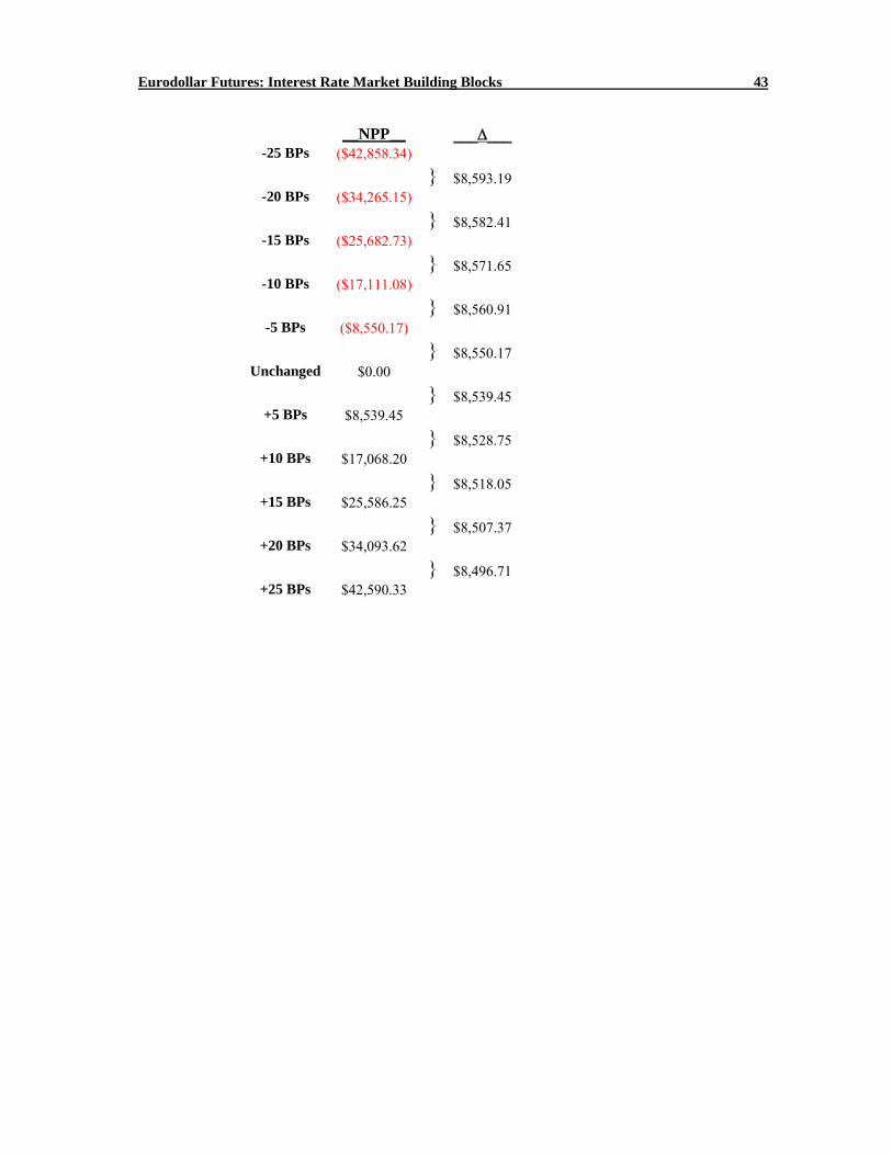
Eurodollar Futures: Interest Rate Market Building Blocks 43
__NPP__ ___Δ___
-25 BPs ($42,858.34) } $8,593.19
-20 BPs ($34,265.15) } $8,582.41
-15 BPs ($25,682.73) } $8,571.65
-10 BPs ($17,111.08) } $8,560.91
-5 BPs ($8,550.17) } $8,550.17
Unchanged $0.00 } $8,539.45
+5 BPs $8,539.45 } $8,528.75
+10 BPs $17,068.20 } $8,518.05
+15 BPs $25,586.25 } $8,507.37
+20 BPs $34,093.62 } $8,496.71
+25 BPs $42,590.33
Eurodollar Futures: Interest Rate Market Building Blocks 44
Technical Appendix – Complications and Shortcuts for Pricing and Hedging Swaps
For expositional clarity, some practical aspects of pricing and hedging interest rate swaps are suppressed in the text above. While covering all relevant details is impossible, we nonetheless intend to highlight some important complications that arise in practice and outline some shortcuts for addressing those issues. Pricing by Anticipated Cashflow vs. Back-to-back Notes - We illustrated the pricing of interest rate swap, i.e., determining the fixed coupon rate of the swap, by considering the anticipated net cash flow of the swap and setting the total net present value of the cash flow to zero using the Eurodollar curve for discounting purpose. While this is a perfectly legitimate way of pricing swaps, the method suffers from poor flexibility. This deficiency becomes very evident as the complexity of the structure of the swap grows, e.g., different basis, different day count convention, different payment frequency, etc. An elegant alternative for the pricing exists by recognizing the nature of swaps as back-to-back notes, i.e. the “receive-fix” party in the swap is simultaneously long a fixed coupon note and short a floating coupon note with the same notional amount. Thus, at the inception of the swap, the net present value of the two notes must be one and the same since no cash changes hands. Further, the floating coupon note with the coupon set at the current market interest rate, e.g. 3-Month LIBOR, must possess a net present value equaling the face value. Thus, the fixed coupon rate is nothing more than the current market coupon rate for a bullet note issue with maturity coinciding with the tenure of the swap. As such, we have reduced the problem to a very manageable one, even when more complexities are piled onto the swap structure. A further benefit for utilizing the back-to-back notes approach will be very evident when we discuss hedging interest rate swaps using Eurodollar futures. With a back-to-back notes structure, the hedges for the fixed and floating coupon notes are determined separately. Netting the hedges will give us the correct hedging strategy for the swap. We will demonstrate with an illustration in a later section. Interpolating Eurodollar Curve - For simplicity, examples of swaps in this article are deliberately chosen to have a start date14 coinciding with a particular Eurodollar futures contract. This situation occurs once every three months. For the rest of the days, one would inevitably need to account for the discrepancy. In this appendix, we illustrate a method based on log-linear interpolation of the discount 14 More precisely, the value date of the swap coincides with the value date of a 3-Month LIBOR Eurodollar Deposit corresponding to a Eurodollar futures contract.
Non-vanilla swaps require more rigorous pricing methodologies. Back-to-back note pricing more robust than cash-flow method discussed above.
Eurodollar Futures: Interest Rate Market Building Blocks 45
factors. There are various advantages in interpolation based on discount factors:
1. Discount factors have a physical interpretation … it is, in fact,
the price of a zero coupon note with a face value of one dollar. E.g., at a 3-month LIBOR of 2.50%, assuming a count of 90 days for the 3-month period, the corresponding discount factor is simply 1 / [1 + 2.5% x (90/360)] = 0.993789. Indeed, a three-month zero-coupon note with face value of $1 is worth exactly $0.993789. Discount factors and zero coupon prices are equivalent concepts.
2. Discount factors (zero coupon prices) are well behaved. As a
function of time, discount factor will always be between one and zero and decreases with time/maturity, starting with a value of one at the current value date15. I.e., discount factor for a payment 3 months from now will always be greater than that for a payment 3 months and 2 days from now.
3. Given discount factors associated with any two days, the
(forward) rate between the two days can be easily determined. This has been illustrated in the article already.
Given the prices of all the traded instruments, e.g., Eurodollar futures of various expirations, cash LIBOR deposits, etc., only so many points on the discount factor curve can be determined unambiguously. For the intervening points on the curve, some estimation or interpolation is required. Given the well-behaved nature of the curve, i.e. always between zero and one and is decreasing, there are many possible choices of interpolation techniques – among them linear and log-linear interpolation. We choose log-linear interpolation for the following reasons … (1) it preserves the convex nature16 of the discount factor curve, and (2) it provides a tractable hedging calculation with a tidy day-count based hedging formula for non-IMM dated swaps. Having mentioned these considerations, however, the readers are free to choose any curve interpolation method. With the advances in the capabilities of the computers, a closed-form hedging formula is not a necessity.
15 LIBOR/Swap market observes a T+2 arrangement. Thus, the discount factor associated with the current value date is one. 16 Since the discount factor curve originates with a value one, is decreasing but never falls to zero, the curve is necessarily convex if the curve is continuous, i.e. the value of the curve at any point is lower than corresponding point on the chord linking points to either side of the point. Choosing log-linear interpolation preserves this feature.
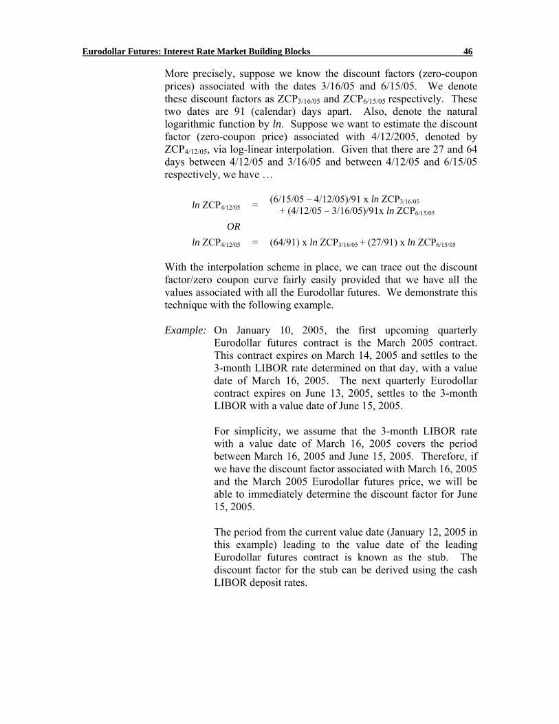
Eurodollar Futures: Interest Rate Market Building Blocks 46
More precisely, suppose we know the discount factors (zero-coupon prices) associated with the dates 3/16/05 and 6/15/05. We denote these discount factors as ZCP3/16/05 and ZCP6/15/05 respectively. These two dates are 91 (calendar) days apart. Also, denote the natural logarithmic function by ln. Suppose we want to estimate the discount factor (zero-coupon price) associated with 4/12/2005, denoted by ZCP4/12/05, via log-linear interpolation. Given that there are 27 and 64 days between 4/12/05 and 3/16/05 and between 4/12/05 and 6/15/05 respectively, we have …
ln ZCP4/12/05 = (6/15/05 – 4/12/05)/91 x ln ZCP3/16/05
+ (4/12/05 – 3/16/05)/91x ln ZCP6/15/05
OR
ln ZCP4/12/05 = (64/91) x ln ZCP3/16/05 + (27/91) x ln ZCP6/15/05 With the interpolation scheme in place, we can trace out the discount factor/zero coupon curve fairly easily provided that we have all the values associated with all the Eurodollar futures. We demonstrate this technique with the following example. Example: On January 10, 2005, the first upcoming quarterly
Eurodollar futures contract is the March 2005 contract. This contract expires on March 14, 2005 and settles to the 3-month LIBOR rate determined on that day, with a value date of March 16, 2005. The next quarterly Eurodollar contract expires on June 13, 2005, settles to the 3-month LIBOR with a value date of June 15, 2005.
For simplicity, we assume that the 3-month LIBOR rate with a value date of March 16, 2005 covers the period between March 16, 2005 and June 15, 2005. Therefore, if we have the discount factor associated with March 16, 2005 and the March 2005 Eurodollar futures price, we will be able to immediately determine the discount factor for June 15, 2005. The period from the current value date (January 12, 2005 in this example) leading to the value date of the leading Eurodollar futures contract is known as the stub. The discount factor for the stub can be derived using the cash LIBOR deposit rates.
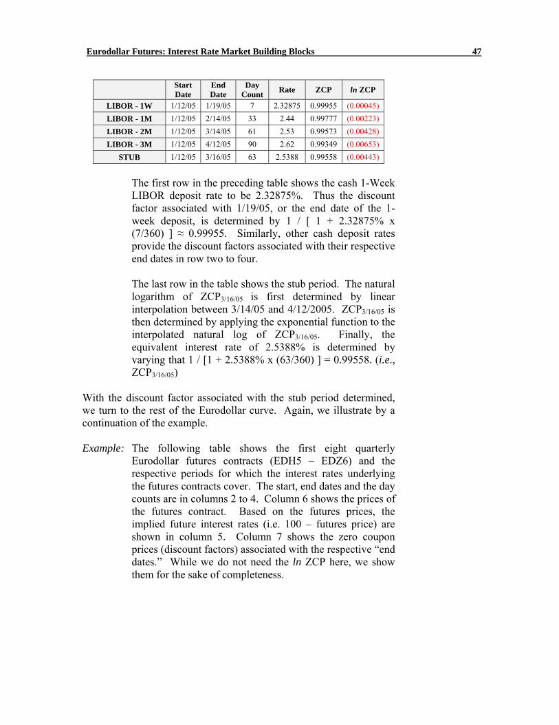
Eurodollar Futures: Interest Rate Market Building Blocks 47
Start
Date End Date
Day Count Rate ZCP ln ZCP
LIBOR - 1W 1/12/05 1/19/05 7 2.32875 0.99955 (0.00045) LIBOR - 1M 1/12/05 2/14/05 33 2.44 0.99777 (0.00223) LIBOR - 2M 1/12/05 3/14/05 61 2.53 0.99573 (0.00428) LIBOR - 3M 1/12/05 4/12/05 90 2.62 0.99349 (0.00653)
STUB 1/12/05 3/16/05 63 2.5388 0.99558 (0.00443)
The first row in the preceding table shows the cash 1-Week LIBOR deposit rate to be 2.32875%. Thus the discount factor associated with 1/19/05, or the end date of the 1-week deposit, is determined by 1 / [ 1 + 2.32875% x (7/360) ] ≈ 0.99955. Similarly, other cash deposit rates provide the discount factors associated with their respective end dates in row two to four. The last row in the table shows the stub period. The natural logarithm of ZCP3/16/05 is first determined by linear interpolation between 3/14/05 and 4/12/2005. ZCP3/16/05 is then determined by applying the exponential function to the interpolated natural log of ZCP3/16/05. Finally, the equivalent interest rate of 2.5388% is determined by varying that 1 / [1 + 2.5388% x (63/360) ] = 0.99558. (i.e., ZCP3/16/05)
With the discount factor associated with the stub period determined, we turn to the rest of the Eurodollar curve. Again, we illustrate by a continuation of the example. Example: The following table shows the first eight quarterly
Eurodollar futures contracts (EDH5 – EDZ6) and the respective periods for which the interest rates underlying the futures contracts cover. The start, end dates and the day counts are in columns 2 to 4. Column 6 shows the prices of the futures contract. Based on the futures prices, the implied future interest rates (i.e. 100 – futures price) are shown in column 5. Column 7 shows the zero coupon prices (discount factors) associated with the respective “end dates.” While we do not need the ln ZCP here, we show them for the sake of completeness.
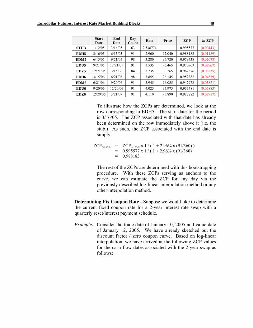
Eurodollar Futures: Interest Rate Market Building Blocks 48
Start
Date End Date
Day Count Rate Price ZCP ln ZCP
STUB 1/12/05 3/16/05 63 2.538774 0.995577 (0.00443) EDH5 3/16/05 6/15/05 91 2.960 97.040 0.988183 (0.01189) EDM5 6/15/05 9/21/05 98 3.280 96.720 0.979438 (0.02078) EDU5 9/21/05 12/21/05 91 3.535 96.465 0.970763 (0.02967) EDZ5 12/21/05 3/15/06 84 3.735 96.265 0.962376 (0.03835) EDH6 3/15/06 6/21/06 98 3.855 96.145 0.952382 (0.04879) EDM6 6/21/06 9/20/06 91 3.945 96.055 0.942978 (0.05871) EDU6 9/20/06 12/20/06 91 4.025 95.975 0.933481 (0.06883) EDZ6 12/20/06 3/21/07 91 4.110 95.890 0.923882 (0.07917)
To illustrate how the ZCPs are determined, we look at the row corresponding to EDH5. The start date for the period is 3/16/05. The ZCP associated with that date has already been determined on the row immediately above it (i.e. the stub.) As such, the ZCP associated with the end date is simply:
ZCP6/15/05 = ZCP3/16/05 x 1 / ( 1 + 2.96% x (91/360) )
= 0.995577 x 1 / ( 1 + 2.96% x (91/360) = 0.988183
The rest of the ZCPs are determined with this bootstrapping procedure. With these ZCPs serving as anchors to the curve, we can estimate the ZCP for any day via the previously described log-linear interpolation method or any other interpolation method.
Determining Fix Coupon Rate - Suppose we would like to determine the current fixed coupon rate for a 2-year interest rate swap with a quarterly reset/interest payment schedule. Example: Consider the trade date of January 10, 2005 and value date
of January 12, 2005. We have already sketched out the discount factor / zero coupon curve. Based on log-linear interpolation, we have arrived at the following ZCP values for the cash flow dates associated with the 2-year swap as follows:
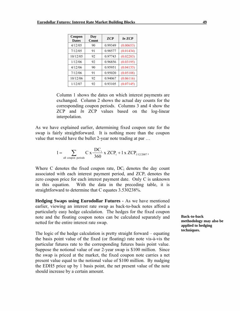
Eurodollar Futures: Interest Rate Market Building Blocks 49
Coupon Dates
Day Count ZCP ln ZCP
4/12/05 90 0.99349 (0.00653) 7/12/05 91 0.98577 (0.01434)
10/12/05 92 0.97743 (0.02283) 1/12/06 92 0.96856 (0.03195) 4/12/06 90 0.95951 (0.04133) 7/12/06 91 0.95020 (0.05108)
10/12/06 92 0.94067 (0.06116) 1/12/07 92 0.93105 (0.07145)
Column 1 shows the dates on which interest payments are exchanged. Column 2 shows the actual day counts for the corresponding coupon periods. Columns 3 and 4 show the ZCP and ln ZCP values based on the log-linear interpolation.
As we have explained earlier, determining fixed coupon rate for the swap is fairly straightforward. It is nothing more than the coupon value that would have the bullet 2-year note trading at par …
1/12/2007iperiodscoupon all
i x ZCP1 x ZCP360DC xC1 += ∑ ,
Where C denotes the fixed coupon rate, DCi denotes the day count associated with each interest payment period, and ZCPi denotes the zero coupon price for each interest payment date. Only C is unknown in this equation. With the data in the preceding table, it is straightforward to determine that C equates 3.530238%. Hedging Swaps using Eurodollar Futures - As we have mentioned earlier, viewing an interest rate swap as back-to-back notes afford a particularly easy hedge calculation. The hedges for the fixed coupon note and the floating coupon notes can be calculated separately and netted for the entire interest rate swap. The logic of the hedge calculation is pretty straight forward – equating the basis point value of the fixed (or floating) rate note vis-à-vis the particular futures rate to the corresponding futures basis point value. Suppose the notional value of our 2-year swap is $100 million. Since the swap is priced at the market, the fixed coupon note carries a net present value equal to the notional value of $100 million. By nudging the EDH5 price up by 1 basis point, the net present value of the note should increase by a certain amount.
Back-to-back methodology may also be applied to hedging techniques.
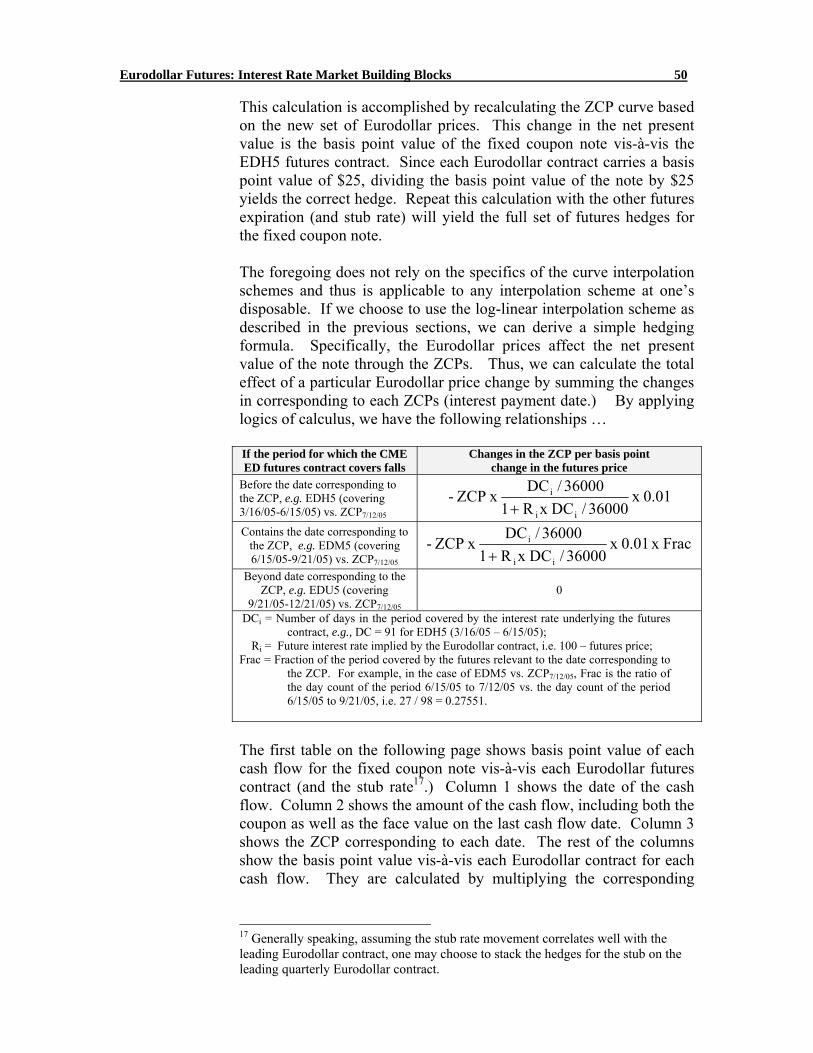
Eurodollar Futures: Interest Rate Market Building Blocks 50
This calculation is accomplished by recalculating the ZCP curve based on the new set of Eurodollar prices. This change in the net present value is the basis point value of the fixed coupon note vis-à-vis the EDH5 futures contract. Since each Eurodollar contract carries a basis point value of $25, dividing the basis point value of the note by $25 yields the correct hedge. Repeat this calculation with the other futures expiration (and stub rate) will yield the full set of futures hedges for the fixed coupon note. The foregoing does not rely on the specifics of the curve interpolation schemes and thus is applicable to any interpolation scheme at one’s disposable. If we choose to use the log-linear interpolation scheme as described in the previous sections, we can derive a simple hedging formula. Specifically, the Eurodollar prices affect the net present value of the note through the ZCPs. Thus, we can calculate the total effect of a particular Eurodollar price change by summing the changes in corresponding to each ZCPs (interest payment date.) By applying logics of calculus, we have the following relationships … If the period for which the CME ED futures contract covers falls
Changes in the ZCP per basis point change in the futures price
Before the date corresponding to the ZCP, e.g. EDH5 (covering 3/16/05-6/15/05) vs. ZCP7/12/05
0.01x 36000/DCx R1
36000/DC x ZCP-ii
i
+
Contains the date corresponding to the ZCP, e.g. EDM5 (covering 6/15/05-9/21/05) vs. ZCP7/12/05
Frac x 0.01x 36000/DCx R1
36000/DC x ZCP-ii
i
+
Beyond date corresponding to the ZCP, e.g. EDU5 (covering
9/21/05-12/21/05) vs. ZCP7/12/05
0
DCi = Number of days in the period covered by the interest rate underlying the futures contract, e.g., DC = 91 for EDH5 (3/16/05 – 6/15/05);
Ri = Future interest rate implied by the Eurodollar contract, i.e. 100 – futures price; Frac = Fraction of the period covered by the futures relevant to the date corresponding to
the ZCP. For example, in the case of EDM5 vs. ZCP7/12/05, Frac is the ratio of the day count of the period 6/15/05 to 7/12/05 vs. the day count of the period 6/15/05 to 9/21/05, i.e. 27 / 98 = 0.27551.
The first table on the following page shows basis point value of each cash flow for the fixed coupon note vis-à-vis each Eurodollar futures contract (and the stub rate17.) Column 1 shows the date of the cash flow. Column 2 shows the amount of the cash flow, including both the coupon as well as the face value on the last cash flow date. Column 3 shows the ZCP corresponding to each date. The rest of the columns show the basis point value vis-à-vis each Eurodollar contract for each cash flow. They are calculated by multiplying the corresponding
17 Generally speaking, assuming the stub rate movement correlates well with the leading Eurodollar contract, one may choose to stack the hedges for the stub on the leading quarterly Eurodollar contract.
Eurodollar Futures: Interest Rate Market Building Blocks 51
cashflow to the changes in the ZCP per basis point as determined by the formulae in the above table. Summing up the basis point value across all the cash flow vis-à-vis each futures expiration provide a total basis point value. Dividing the basis point value by the basis point value per Eurodollar contract ($25) provides the correct number of contracts for delta-hedging the fixed coupon note. The same exercise is applied to the floating rate note. Observe that at the next reset, the floating rate note will carry the then-market rate. Thus, the market value of the note will be at par at the next reset. Thus, the total “cash-flow” of the note at the next reset is the sum of the coupon payment (the current 3-month LIBOR, which has been determined already) plus face value. The second table on the page below illustrates the corresponding hedge calculations for the floating rate note. Netting the fixed coupon note against the floating rate note provides the net futures hedge for the interest rate swap. Before moving on to the next topic… one can observe that while we have a self-contained formula for the calculation of basis point value, it is not necessarily easy to implement. Given the possibility of the “perturbation” method and the enormous computing power at the user’s disposal, one may elect to abandon these formulae in favor of the more computationally intensive method. Executing the Hedge - Inspecting the hedging strategy prescribed by the hedge calculation, one can readily conclude that the tailored hedge may be very hard to execute in practice. It involves different number of contracts for each contract month. Simultaneous order execution on eight quarterly contracts is very hard to manage, with the markets in different contract months possessing different liquidity. Various strategies are available for simplifying the execution of the hedging strategy. Depending on your confidence of the correlation amongst various contract months, one may elect to …
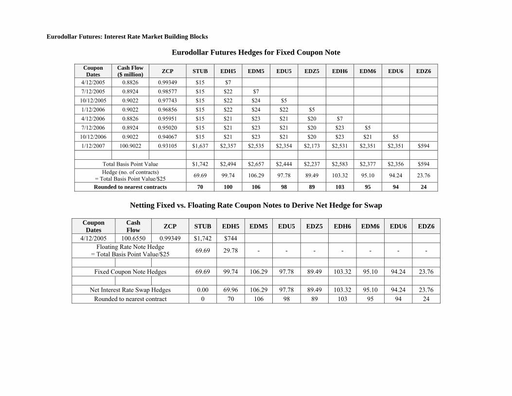
Eurodollar Futures: Interest Rate Market Building Blocks
Eurodollar Futures Hedges for Fixed Coupon Note
Coupon Dates
Cash Flow ($ million) ZCP STUB EDH5 EDM5 EDU5 EDZ5 EDH6 EDM6 EDU6 EDZ6
4/12/2005 0.8826 0.99349 $15 $7 7/12/2005 0.8924 0.98577 $15 $22 $7
10/12/2005 0.9022 0.97743 $15 $22 $24 $5 1/12/2006 0.9022 0.96856 $15 $22 $24 $22 $5 4/12/2006 0.8826 0.95951 $15 $21 $23 $21 $20 $7 7/12/2006 0.8924 0.95020 $15 $21 $23 $21 $20 $23 $5
10/12/2006 0.9022 0.94067 $15 $21 $23 $21 $20 $23 $21 $5 1/12/2007 100.9022 0.93105 $1,637 $2,357 $2,535 $2,354 $2,173 $2,531 $2,351 $2,351 $594
Total Basis Point Value $1,742 $2,494 $2,657 $2,444 $2,237 $2,583 $2,377 $2,356 $594 Hedge (no. of contracts)
= Total Basis Point Value/$25 69.69 99.74 106.29 97.78 89.49 103.32 95.10 94.24 23.76
Rounded to nearest contracts 70 100 106 98 89 103 95 94 24
Netting Fixed vs. Floating Rate Coupon Notes to Derive Net Hedge for Swap
Coupon
Dates Cash Flow ZCP STUB EDH5 EDM5 EDU5 EDZ5 EDH6 EDM6 EDU6 EDZ6
4/12/2005 100.6550 0.99349 $1,742 $744 Floating Rate Note Hedge
= Total Basis Point Value/$25 69.69 29.78 - - - - - - -
Fixed Coupon Note Hedges 69.69 99.74 106.29 97.78 89.49 103.32 95.10 94.24 23.76
Net Interest Rate Swap Hedges 0.00 69.96 106.29 97.78 89.49 103.32 95.10 94.24 23.76 Rounded to nearest contract 0 70 106 98 89 103 95 94 24
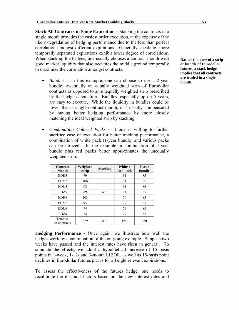
Eurodollar Futures: Interest Rate Market Building Blocks 53
Stack All Contracts in Same Expiration – Stacking the contracts in a single month provides the easiest order execution, at the expense of the likely degradation of hedging performance due to the less than perfect correlation amongst different expirations. Generally speaking, more temporally separated expirations exhibit lower degree of correlations. When stacking the hedges, one usually chooses a contract month with good market liquidity that also occupies the middle ground temporally to maximize the correlation amongst contracts.
• Bundles – in this example, one can choose to use a 2-year bundle, essentially an equally weighted strip of Eurodollar contracts as opposed to an unequally weighted strip prescribed by the hedge calculation. Bundles, especially up on 5 years, are easy to execute. While the liquidity in bundles could be lower than a single contract month, it is usually compensated by having better hedging performance by more closely matching the ideal weighted strip by stacking.
• Combination Colored Packs – if one is willing to further
sacrifice ease of execution for better tracking performance, a combination of white pack (1-year bundle) and various packs can be utilized. In the example, a combination of 1-year bundle plus red packs better approximates the unequally weighted strip.
Contract Month
Weighted Strip Stacking White +
Red Pack 2-year Bundle
EDH5 70 91 85 EDM5 106 91 85 EDU5 98 91 85 EDZ5 89 679 91 85 EDH6 103 79 85 EDM6 95 79 85 EDU6 94 79 85 EDZ6 24 79 85
Total no. of contracts 679 679 680 680
Hedging Performance - Once again, we illustrate how well the hedges work by a continuation of the on-going example. Suppose two weeks have passed and the interest rates have risen in general. To simulate the effects, we adopt a hypothetical increase of 15 basis points in 1-week, 1-, 2- and 3-month LIBOR, as well as 15-basis point declines in Eurodollar futures prices for all eight relevant expirations. To assess the effectiveness of the futures hedge, one needs to recalibrate the discount factors based on the new interest rates and
Rather than use of a strip or bundle of Eurodollar futures, a stack hedge implies that all contracts are traded in a single month.
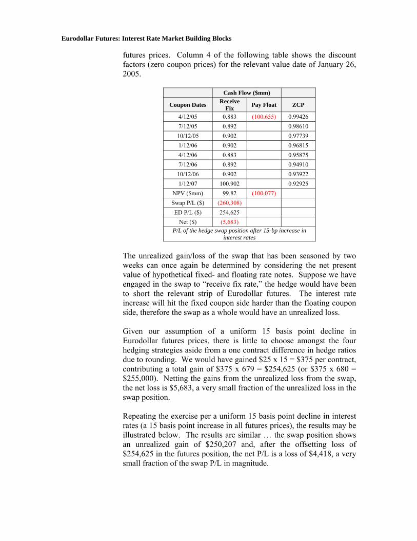
Eurodollar Futures: Interest Rate Market Building Blocks
futures prices. Column 4 of the following table shows the discount factors (zero coupon prices) for the relevant value date of January 26, 2005.
Cash Flow ($mm)
Coupon Dates Receive Fix Pay Float ZCP
4/12/05 0.883 (100.655) 0.99426 7/12/05 0.892 0.98610
10/12/05 0.902 0.97739 1/12/06 0.902 0.96815 4/12/06 0.883 0.95875 7/12/06 0.892 0.94910
10/12/06 0.902 0.93922 1/12/07 100.902 0.92925
NPV ($mm) 99.82 (100.077) Swap P/L ($) (260,308) ED P/L ($) 254,625
Net ($) (5,683) P/L of the hedge swap position after 15-bp increase in
interest rates
The unrealized gain/loss of the swap that has been seasoned by two weeks can once again be determined by considering the net present value of hypothetical fixed- and floating rate notes. Suppose we have engaged in the swap to “receive fix rate,” the hedge would have been to short the relevant strip of Eurodollar futures. The interest rate increase will hit the fixed coupon side harder than the floating coupon side, therefore the swap as a whole would have an unrealized loss.
Given our assumption of a uniform 15 basis point decline in Eurodollar futures prices, there is little to choose amongst the four hedging strategies aside from a one contract difference in hedge ratios due to rounding. We would have gained $25 x 15 = $375 per contract, contributing a total gain of $375 x 679 = $254,625 (or $375 x 680 = $255,000). Netting the gains from the unrealized loss from the swap, the net loss is $5,683, a very small fraction of the unrealized loss in the swap position.
Repeating the exercise per a uniform 15 basis point decline in interest rates (a 15 basis point increase in all futures prices), the results may be illustrated below. The results are similar … the swap position shows an unrealized gain of $250,207 and, after the offsetting loss of $254,625 in the futures position, the net P/L is a loss of $4,418, a very small fraction of the swap P/L in magnitude.
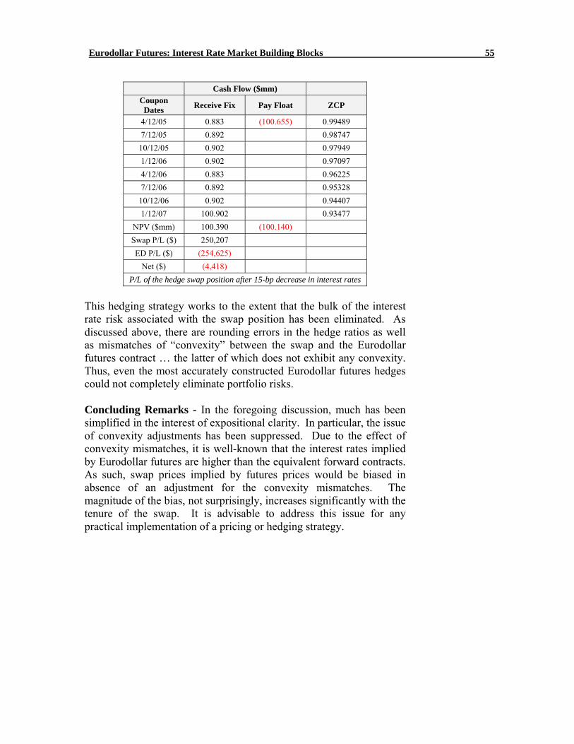
Eurodollar Futures: Interest Rate Market Building Blocks 55
Cash Flow ($mm)
Coupon Dates Receive Fix Pay Float ZCP
4/12/05 0.883 (100.655) 0.99489 7/12/05 0.892 0.98747
10/12/05 0.902 0.97949 1/12/06 0.902 0.97097 4/12/06 0.883 0.96225 7/12/06 0.892 0.95328
10/12/06 0.902 0.94407 1/12/07 100.902 0.93477
NPV ($mm) 100.390 (100.140) Swap P/L ($) 250,207 ED P/L ($) (254,625)
Net ($) (4,418) P/L of the hedge swap position after 15-bp decrease in interest rates
This hedging strategy works to the extent that the bulk of the interest rate risk associated with the swap position has been eliminated. As discussed above, there are rounding errors in the hedge ratios as well as mismatches of “convexity” between the swap and the Eurodollar futures contract … the latter of which does not exhibit any convexity. Thus, even the most accurately constructed Eurodollar futures hedges could not completely eliminate portfolio risks. Concluding Remarks - In the foregoing discussion, much has been simplified in the interest of expositional clarity. In particular, the issue of convexity adjustments has been suppressed. Due to the effect of convexity mismatches, it is well-known that the interest rates implied by Eurodollar futures are higher than the equivalent forward contracts. As such, swap prices implied by futures prices would be biased in absence of an adjustment for the convexity mismatches. The magnitude of the bias, not surprisingly, increases significantly with the tenure of the swap. It is advisable to address this issue for any practical implementation of a pricing or hedging strategy.