EUROPEAN ORGANIZATION FOR NUCLEAR RESEARCH European ... · EUROPEAN ORGANIZATION FOR NUCLEAR RESEARCH European Laboratory for Particle Physics Internal NOTE ALICE Reference Number

EUROPEAN ORGANIZATION FOR NUCLEAR RESEARCH

European Laboratory for Particle Physics

Internal NOTEALICE Reference Number

2009-035date of last change

November 19, 2009

Alignment of the ALICE Inner Tracking System with cosmic-ray tracks

C. Bombonati a,b, C. Cheshkov b, A. Dainese c,1), C.E. Garcia Trapaga d,e,R. Grosso a, A. Jacholkowski f , M. Lunardon a, M. Masera g, S. Moretto a,F. Prino e, A. Rossi h, R. Shahoyan b, M. van Leeuwen i, and N. Vermeer i

a Universita degli Studi di Padova and INFN, Padova, Italyb CERN, Geneva, Switzerland

c INFN - Sezione di Padova, Padova, Italyd InSTEC, Havana, Cuba

e INFN - Sezione di Torino, Torino, Italyf Universita di Catania, Catania, Italy

g Universita di Torino and INFN, Torino, Italyh Universita di Trieste and INFN, Trieste, Italyi Universiteit Utrecht, Utrecht, the Netherlands

Abstract

The ALICE Inner Tracking System (ITS) consists of six cylindrical layers of silicondetectors with three different technologies; in the outward direction: two pixel, twodrift and two strip layers. The number of parameters to be determined in the spatialalignment of the 2198 sensor modules of the ITS is about 13,000. The target align-ment precision is well below 10 µm in some cases (pixels). The sources of alignmentinformation are the survey measurements and the reconstructed tracks from cosmicrays and from proton–proton collisions. The main track-based alignment methoduses the Millepede global approach. An iterative local method was developed andused as well. We present the results obtained for the ITS alignment using about105 charged tracks from cosmic rays that have been collected during summer 2008,with the ALICE solenoidal magnetic field switched off.

1) e-mail: [email protected]

1 Introduction

The ALICE experiment [1] will study nucleus–nucleus, proton–proton and proton–nucleuscollisions at the CERN Large Hadron Collider (LHC). The main physics goal of theexperiment is to investigate the properties of strongly-interacting matter in the conditionsof high energy density (> 10 GeV/fm3) and high temperature ( >

∼ 0.2 GeV), expected to bereached in central Pb–Pb collisions at

√sNN = 5.5 TeV. Under these conditions, according

to lattice QCD calculations, quark confinement into colourless hadrons should be removedand a deconfined Quark–Gluon Plasma should be formed [2]. In the past two decades,experiments at CERN-SPS (

√sNN = 17.3 GeV) and BNL-RHIC (

√sNN = 200 GeV) have

gathered ample evidence for the formation of this state of matter [3].The ALICE experimental apparatus consists of two main components: the central

barrel and the forward muon spectrometer. The coverage of the central barrel detectorsallows the tracking of particles emitted on a pseudo-rapidity range |η| < 0.9 over the fullazimuth. These detectors are embedded in the large L3 magnet that provides a solenoidalfield B = 0.5 T.

The Inner Tracking System (ITS) is a barrel-type silicon tracker that surroundsthe interaction region. It consists of six cylindrical layers, with radii between 3.9 cm and43.0 cm, covering the pseudo-rapidity range |η| < 0.9. The two innermost layers areequipped with Silicon Pixel Detectors (SPD), the two intermediate layers are made ofSilicon Drift Detectors (SDD), while Silicon Strip Detectors (SSD) are mounted on thetwo outermost layers. The main task of the ITS is to provide precise track and vertexreconstruction close to the interaction point. In particular, the ITS was designed with theaim to improve the position, angle, and momentum resolution for tracks reconstructed inthe Time Projection Chamber (TPC), to identify the secondary vertices from the decay ofhyperons and heavy flavoured hadrons, to reconstruct the interaction vertex with a resolu-tion better than 100 µm, and to recover particles that are missed by the TPC (due to eitherdead regions or low-momentum cut-off). The measurement of charm and beauty hadronproduction in Pb–Pb collisions at the LHC is one of the main items of the ALICE physicsprogram, because it will allow to investigate the mechanisms of heavy-quark propagationand hadronization in the hot and dense medium formed in high-energy heavy-ion collisionsand it will serve as a reference for the study of the medium effects on quarkonia [4]. Theseparation, from the interaction vertex, of the decay vertices of heavy flavoured hadrons,which have mean proper decay lengths cτ ∼ 100–500 µm, requires a resolution on thetrack impact parameter (distance of closest approach to the vertex) well-below 100 µm.This requirement is met by the ITS. According to the design parameters, the positionresolution at the primary vertex in the plane transverse to the beam-line for charged-piontracks reconstructed in the TPC and in the ITS is expected to be approximately, in µm,10+53/(pt

√sin θ), where pt is the transverse momentum in GeV/c and θ is the polar angle

with respect to the beam-line [4]. However, when considering the real detector, as installedin the experiment, the resolution is in general significantly degraded by the misalignment.The ITS is made of thousands of separate modules, whose positions are displaced, withrespect to the ideal case, during the assembly and the integration of the different compo-nents. These displacements, if not taken into account, degrade the tracking performanceof the detector, thus the physics performance. Therefore, it is mandatory to align thedetector, that is, to measure the displacements (translations and rotations), so that theycan be properly taken into account during track reconstruction. The ITS alignment pro-cedure starts from the positioning survey measurements performed during the assembly,and is refined using tracks from cosmic-ray muons and from particles produced in LHC pp

1

SPD

SDD

SSD

87

.2 c

m

x

y

z

locz

locy

locx

locφ

locθ

locψ

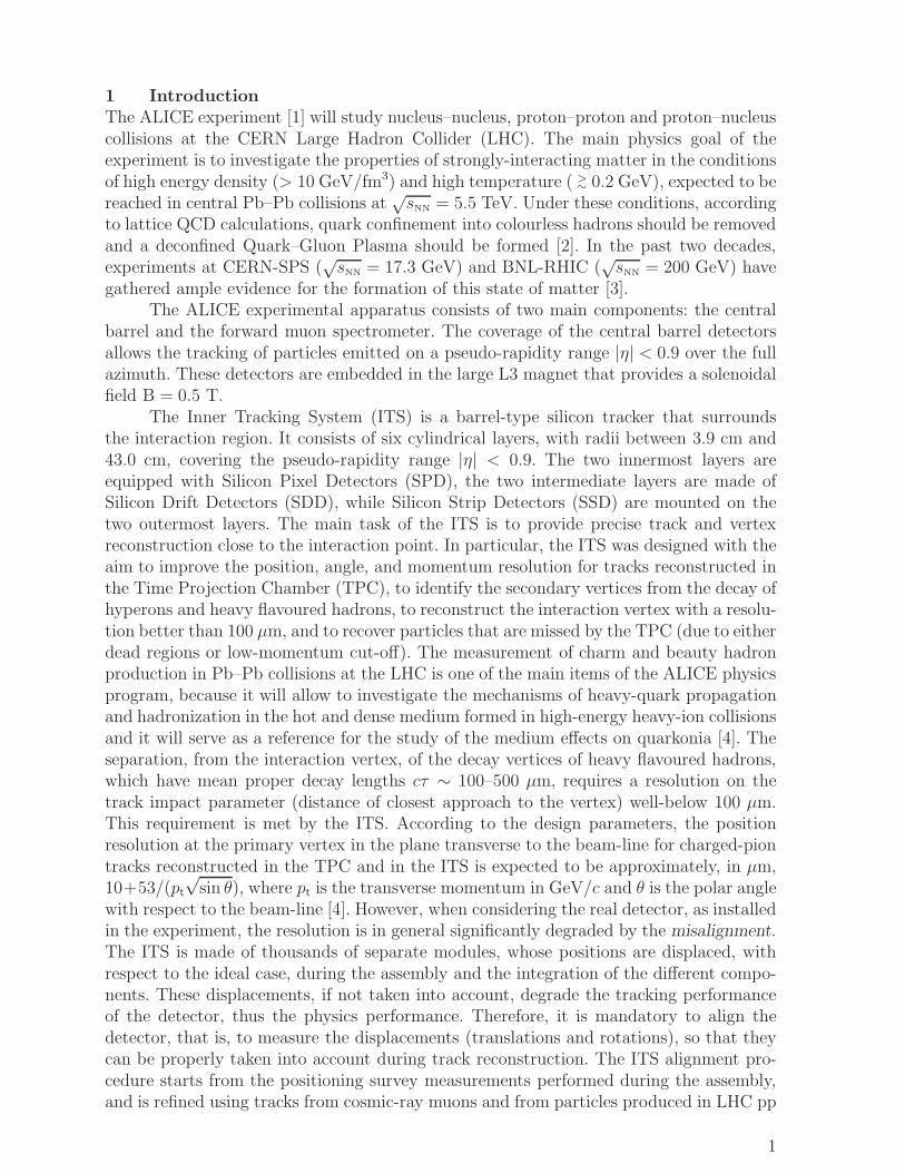
Figure 1: Layout of the ITS and definition of the ALICE global (left) and ITS-modulelocal (right) reference systems.

collisions. Two independent methods, based on tracks-to-measured-points residuals mini-mization, are considered. The first method uses the Millepede approach [5], where a globalfit to all residuals is performed, extracting all the alignment parameters simultaneously.The second method performs a (local) minimization for each single module and accountsfor correlations between modules by iterating the procedure until convergence is reached.

In this report, we present the alignment methods for the ITS and the results obtainedusing the cosmic-data sample collected during summer 2008 with B = 0 (a small data setwith B = ±0.5 T was also collected; we used it for a few specific validation checks). Insection 2 we describe in detail the ITS detector layout and in section 3 we discuss thestrategy adopted for the alignment. In section 4 we describe the 2008 sample of cosmic-muon data. These data were used to validate the available survey measurements (section 5)and to apply the track-based alignment algorithms: the Millepede method (section 6) anda local method that we are developing (section 7). We draw conclusions in section 8.

2 ITS detector layout

The geometrical layout of the ITS layers is shown in the left-hand panel of Fig. 1, asit is implemented in the ALICE simulation and reconstruction software framework (Ali-Root [6]). The ALICE global reference system has the z axis on the beam-line, the xaxis in the LHC (horizontal) plane, pointing to the centre of the accelerator, and the yaxis pointing upward. The axis of the ITS barrel coincides with the z axis. The modulelocal reference system (Fig. 1, right) is defined with the xloc and zloc axes on the sensorplane and the zloc axis in the same direction as the global z axis. The local x directionis approximately equivalent to the global rϕ. The alignment degrees of freedom of themodule are translations in xloc, yloc, zloc, and rotations by angles ψloc, θloc, ϕloc, about thexloc, yloc, zloc axes, respectively1).

The ITS geometry in AliRoot is described in full detail, down the level of all me-chanical structures and single electronic components, using the ROOT [7] geometrical

1) The alignment transformation can be expressed equivalently in terms of the local or global coordinates.

2

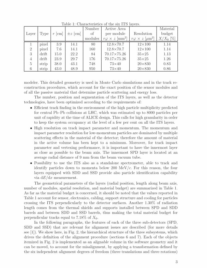
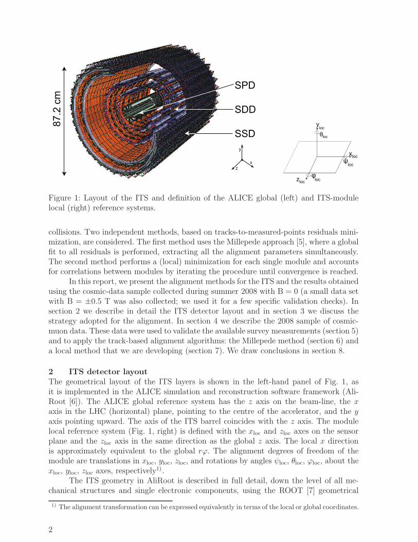
Table 1: Characteristics of the six ITS layers.Number Active Area Material

Layer Type r [cm] ±z [cm] of per module Resolution budgetmodules rϕ × z [mm2] rϕ × z [µm2] X/X0 [%]

1 pixel 3.9 14.1 80 12.8×70.7 12×100 1.142 pixel 7.6 14.1 160 12.8×70.7 12×100 1.143 drift 15.0 22.2 84 70.17×75.26 35×25 1.134 drift 23.9 29.7 176 70.17×75.26 35×25 1.265 strip 38.0 43.1 748 73×40 20×830 0.836 strip 43.0 48.9 950 73×40 20×830 0.86

modeler. This detailed geometry is used in Monte Carlo simulations and in the track re-construction procedures, which account for the exact position of the sensor modules andof all the passive material that determine particle scattering and energy loss.

The number, position and segmentation of the ITS layers, as well as the detectortechnologies, have been optimized according to the requirements of:

• Efficient track finding in the environment of the high particle multiplicity predictedfor central Pb–Pb collisions at LHC, which was estimated up to 8000 particles perunit of rapidity at the time of ALICE design. This calls for high granularity in orderto keep the system occupancy at the level of a few per cent on all the ITS layers.

• High resolution on track impact parameter and momentum. The momentum andimpact parameter resolution for low-momentum particles are dominated by multiplescattering effects in the material of the detector; therefore the amount of materialin the active volume has been kept to a minimum. Moreover, for track impactparameter and vertexing performance, it is important to have the innermost layeras close as possible to the beam axis. The innermost SPD layer is located at anaverage radial distance of 9 mm from the beam vacuum tube.

• Possibility to use the ITS also as a standalone spectrometer, able to track andidentify particles down to momenta below 200 MeV/c. For this reason, the fourlayers equipped with SDD and SSD provide also particle identification capabilityvia dE/dx measurement.

The geometrical parameters of the layers (radial position, length along beam axis,number of modules, spatial resolution, and material budget) are summarized in Table 1.As far as the material budget is concerned, it should be noted that the values reported inTable 1 account for sensor, electronics, cabling, support structure and cooling for particlescrossing the ITS perpendicularly to the detector surfaces. Another 1.30% of radiationlength comes from the thermal shields and supports installed between SPD and SDDbarrels and between SDD and SSD barrels, thus making the total material budget forperpendicular tracks equal to 7.18% of X0.

In the following paragraphs, the features of each of the three sub-detectors (SPD,SDD and SSD) that are relevant for alignment issues are described (for more detailssee [1]). We show here, in Fig. 2, the hierarchical structure of the three subsystems, whichdrives the definition of the alignment procedure (sections 6 and 7). Each of the objectsitemized in Fig. 2 is implemented as an alignable volume in the software geometry and itcan be moved, to account for the misalignment, by applying a transformation defined bythe six independent alignment degrees of freedom (three translations and three rotations)

3

ITS barrel

SPD barrel

Sectors (10)

Half-staves(4 on inner, 8 on outer layer)

Modules (2)

SDD-SSD barrel

SDD barrel SSD barel

Layers (2)

Ladders(14 on inner, 22 on outer layer)

Modules(6 on inner, 8 on outer ladders)

Layers (2)

Ladders(34 on inner, 38 on outer layer)

Modules(22 on inner, 25 on outer ladders)

Figure 2: Schematic description of the hierarchical structure of the ITS.

of the volume [8].

2.1 Silicon Pixel Detector

The basic building block of the ALICE SPD is a module consisting of a two-dimensionalsensor matrix of reverse-biased silicon detector diodes bump-bonded to 5 front-end chips.The sensor matrix consists of 256 × 160 cells, each measuring 50 µm (rϕ) by 425 µm (z).The active area of each module is 12.8 mm (rϕ) × 70.7 mm (z), the thickness of the sensoris 200 µm, while the readout chip is 150 µm thick. Two modules are mounted togetheralong the z direction to form a 141.6 mm long half-stave. Two half-staves are attachedhead-to-head along the z direction to a carbon-fibre support sector, which provides alsocooling. Each sector (see Fig. 3) supports six staves: two on the inner layer and four onthe outer layer. The assembly of half-staves on sectors provides an overlap of about 2% ofthe sensitive areas along rϕ, while there is no sensor overlap along z, where instead thereis a small gap between the two half-staves. Five sectors are then mounted together toform an half-barrel and finally the two (top and bottom) half-barrels are mounted around

z

y

x

Figure 3: SPD drawings. Left: the SPD barrel and the beam pipe (radius in mm). Right:a Carbon Fibre Support Sector.

4

the beam pipe to close the full barrel, which is actually composed of 10 sectors. In total,the SPD includes 60 staves, consisting of 240 modules with 1200 readout chips for a totalof 9.8 × 106 cells.

The spatial precision of the SPD sensor is determined by the pixel cell size andby the track incidence angle on the detector, as well as by the threshold applied in thereadout electronics. The values of resolution along rϕ and z extracted from beam testsare 12 and 100 µm, respectively.

During the summer 2008 data taking, 212 out of 240 SPD modules were active.A typical threshold value was about 2800 electrons. Noisy pixels, corresponding to lessthan 0.15%, were masked out and the information was stored in the Offline ConditionsDataBase (OCDB) to be used in the offline reconstruction.

2.2 Silicon Drift Detector

The basic building block of the ALICE SDD is a module with a sensitive area of 70.17(rϕ)× 75.26(z) mm2, divided into two drift regions where electrons move in opposite directionsunder a drift field of ≈ 500 V/cm (see Fig. 4, right). The SDD modules are mounted onlinear structures called ladders. There are 14 ladders with six modules each on the innerSDD layer (layer 3), and 22 ladders with eight modules each on the outer SDD layer(layer 4). Modules and ladders are assembled to have an overlap of the sensitive areaslarger than 580 µm in the both rϕ and z directions, so as to provide full angular coverage(Fig. 4, left).

The modules are attached with ryton pins to the ladder space frame, which is alightweight truss made of Carbon-Fibre Reinforced Plastic (CFRP) with a protectivecoating against humidity absorption, and have their anode rows parallel to the ladderaxis (z). During the assembling phase, the positions of the detectors were measured withrespect to reference ruby spheres, glued to the ladder feet. The ladders are mounted on aCFRP structure made of a cylinder, two cones and four support rings. The cones providethe links to the outer SSD barrel and have windows for the passage of the SDD services.The support rings are mechanically fixed to the cones and bear reference ruby spheres for

MOS injectors

Highest Voltage CathodeDri

ftD

rift

Figure 4: Left: scheme of the SDD layers. Right: scheme of an SDD module. Units aremillimeters.

5

the ladder positioning.The z coordinate is reconstructed from the centroid of the collected charge along the

anodes. The position along the drift coordinate (xloc ≈ rϕ) is reconstructed starting fromthe measured drift time with respect to the trigger time. An unbiased reconstructionof the xloc coordinate requires therefore to know with good precision the drift speedand the time-zero (t0), which is the measured drift time for particles with zero driftdistance. The drift speed depends on temperature (as T−2.4) and it is therefore sensitiveto temperature gradients in the SDD volume and to temperature variations with time.Hence, it is important to calibrate frequently this parameter during the data taking. Forthis reason, in each of the two drift regions of an SDD module, 3 rows of 33 MOS chargeinjectors are implanted at known distances from the collection anodes [10], as sketched inFig. 4 (right): when a dedicated calibration trigger is received, the injector matrix providesa measurement of the drift speed in 33 positions along the anode coordinate for each SDDdrift region. Finally, a correction for non-uniformity of the drift field (due to non-linearitiesin the voltage divider and, for a few modules, also due to significant inhomogeneitiesin dopant concentration) has to be applied: it is extracted from measurements of thesystematic deviations between charge injection position and reconstructed coordinatesthat was performed on all the 260 SDD modules with an infrared laser [11].

The space precision of the SDD detectors, as obtained during beam tests of full-sizeprototypes, is on average 35 µm along the drift direction xloc and 25 µm for the anodecoordinate zloc.

During summer 2008, 246 out of 260 SDD modules participated in data acquisition.The baseline, gain and noise for each of the 133,000 anodes were measured every ≈24 hours by means of dedicated calibration runs that allowed us also to tag noisy (≈0.5%) and dead (≈ 1%) channels. The drift speeds were measured with dedicated injectorruns collected every ≈ 6 hours and stored in the OCDB and successively used in thereconstruction.

2.3 Silicon Strip Detector

The basic building block of the ALICE SSD is a module composed of one double-sided strip detector connected to two hybrids hosting the front-end electronics. The sensorsare 300 µm thick and have an active area of 73×40 mm2 along z and rϕ directions,respectively. Each sensor has 768 strips on each side with a pitch of 95 µm. The stereoangle is 35 mrad, which is a compromise between stereo view and reduction of ambiguitiesresulting from high particle densities. The strips are almost parallel to the beam axis (z-direction), to provide the best resolution in the rϕ direction. The angle of the strips withrespect to the beam axis is +7.5 mrad on one side and −27.5 mrad on the other side. Asa result, each strip crosses about 14 strips on the other detector side.

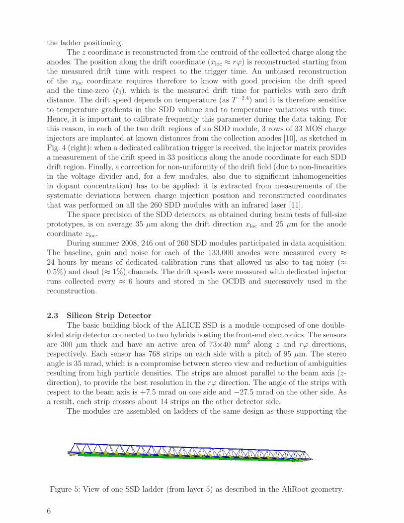
The modules are assembled on ladders of the same design as those supporting the

Figure 5: View of one SSD ladder (from layer 5) as described in the AliRoot geometry.

6

SDD (see Fig. 5). The innermost SSD layer (layer 5) is composed of 34 ladders, each ofthem being a linear array of 22 modules along the beam direction. Layer 6 (the outermostITS layer) consists of 38 ladders, each made of 25 modules. In order to obtain full pseudo-rapidity coverage, the modules are mounted on the ladders with small overlaps betweensuccessive modules, that are 600 µm apart in the radial direction. The 72 ladders, carryinga total of 1698 modules, are mounted on Carbon Fibre Composite support cones in twocylinders. Carbon fiber is lightweight (to minimize the interactions) and at the same time itis a stiff material allowing to minimize the bending due to gravity. The ladders are 120 cmlong, but the sensitive area on layer 5 amounts 88 cm and on layer 6 it amounts 100 cm.For each layer, the ladders are mounted at two slightly different radii (∆r = 6 mm) suchthat full azimuthal coverage is obtained. The acceptance overlaps, present both along zand rϕ, amount to 2% of the SSD sensor surface. The positions of the sensors with respectto reference points on the ladder were measured during the detector construction phase,as well as the ones of the ladders with respect to the support cones.

The spatial resolution of the SSD system is determined by the 95 µm pitch of thesensor readout strips and the charge-sharing between those strips. Without making useof the analogue information the r.m.s spatial resolution is 27 µm. Beam tests have shownthat a spatial resolution of better than 20 µm in the rϕ direction can be obtained byanalyzing the charge distribution within each cluster. In the direction along the beam,the spatial resolution is of about 830 µm.

During the 2008 cosmic run, 1477 out of 1698 SSD modules took data. The fractionof bad strips was ≈1.5%. The SSD gain calibration has two components: overall calibrationof ADC values to energy loss and relative calibration of the P and N sides. This chargematching is a strong point of double sided silicon sensors and helps to remove fake clusters.Both calibrations relied on cosmics. The resulting normalized difference in P- and N-chargehas a FWHM of 11%. The gains have proved to be stable during the data taking. In anycase, since the signal-to-noise ratio is larger than 20, the detecting efficiency does notdepend much on the details of the gain calibration.

3 Alignment target and strategy

For silicon tracking detectors, the ‘standard’ target of the alignment procedures is theachievement a level of precision and accuracy such that the resolution on the reconstructedtrack parameters (in particular, the impact parameter and the curvature, which measuresthe transverse momentum) is degraded by at most 20% with respect to the resolutionexpected in case of the ideal geometry without misalignment. This standard is adoptedby all four LHC experiments.

The resolutions on the track impact parameter and curvature are both propor-tional to the space point resolution, in the limit of negligible multiple scattering effect(large momentum). If the residual misalignment is assumed to be equivalent to randomgaussian spreads in the six alignment parameters of the sensor modules, on which spacepoints are measured, a 20% degradation in the effective space point resolution (hence20% degradation of the track parameters in the large momentum limit) is obtained whenthe misalignment spread in a given direction is

√120%2 − 100%2 ≈ 70% of the intrinsic

sensor resolution along that direction. With reference to the intrinsic precisions listed inTable 1, the target residual misalignment spreads in the local coordinates on the sensorplane are: for SPD, 8 µm in xloc and 70 µm in zloc; for SDD, 25 µm in xloc and 18 µmin zloc; for SSD, 14 µm in xloc and 500 µm in zloc. Since also the misalignment in theθloc angle (rotation about the axis normal to the sensor plane) impacts directly on the

7

effective spatial precision, the numbers given above should be taken as effective spreadsincluding also the effect of the θloc rotation. In any case, these target numbers are onlyan indication of the precision that is requested from the alignment procedures.

The other alignment parameters (yloc, ψloc, ϕloc) describe movements of the modulesmainly in the radial direction. These have a small impact on the effective resolution, fortracks with a small angle with respect to the normal to the module plane, a typicalcase for tracks coming from the interaction region. However, they are related to the so-called weak modes: correlated misalignments of the different modules that do not affectthe reconstructed tracks fit quality (χ2), but bias systematically the track parameters.A typical example is radial expansion or compression of all the layers, which biases themeasured track curvature, hence the momentum estimate. Correlated misalignments forthe parameters on the sensor plane (xloc, zloc, θloc) can determine weak modes as well.These misalignments are, by definition, difficult to determine with tracks from collisions,but can be tackled using physical observables [12] (e.g. looking for shift in invariant massesof reconstructed decay particles) and cosmic-ray tracks. These offer a unique possibilityto correlate modules that are never correlated in case of tracks from the interactionregion, and they offer a broad range of track-to-module-plane incidence angles that helpto constrain also the yloc, ψloc and ϕloc parameters, thus improving the sensitivity to weakmodes.

As already mentioned in the introduction, the sources of alignment information thatwe use are the survey measurements and the reconstructed space points from cosmic-rayand collision particles. These points are the input for the software alignment methods,based on global or local minimization of the residuals. The strategy for the ITS firstalignment is outlined as follows:

1. Validation of the SSD survey measurements with cosmic-ray tracks.2. Alignment of SPD and SSD with cosmic-ray tracks, without magnetic field. The

initial alignment is more robust if performed with straight tracks (no field), whichhelp to avoid possible biases that can be introduced when working with curvedtracks (e.g. radial layer compression/expansion).

3. Use of the already aligned SPD and SSD to confirm and refine the initial time-zerocalibration of SDD, obtained with SDD standalone methods.

4. Validation of the SDD survey measurements with cosmic-ray tracks.5. Alignment of the full detector (SPD, SDD, SSD) with cosmic-ray tracks, including

also data collected with magnetic field B = 0.5 T. These data are extremely usefulalso to study the track quality and precision as a function of the measured track mo-mentum, which allows to separate the detector resolution and residual misalignmentfrom the multiple scattering effect.

6. Alignment with tracks from pp collisions, with both B = 0 and B = 0.5 T. Cosmic-ray tracks have a dominant vertical component and the sides of the barrel layershave limited statistics. In addition, most of the tracks crossing the side modules,which are close to vertical, have small incidence angles with respect to the moduleplane. We reject tracks with incidence angle below 30◦, because the precision ofthe corresponding space points is much worse than for other tracks and it is quitedifficult to evaluate and account for. For this reason, tracks from pp collisions areessential to complete the alignment of the full detector. They will also be used toroutinely monitor the quality of the alignment during data taking, and refine thecorrections if needed.

7. Relative alignment of the ITS and the TPC, when both detectors are already inter-

8

nally aligned and calibrated. This relative alignment will be performed using tracksfrom pp collisions. Relative movements of the two detectors are monitored by adedicated system based on lasers, mirrors and cameras [13].This report covers the steps 1 and 2, with an outlook on step 3.

4 Cosmic-ray run 2008: data taking and reconstruction

During the 2008 cosmic run, extending from June to October, about 105 events withreconstructed tracks in the ITS have been collected. In order to simplify the first alignmentround, the solenoidal magnetic field was switched off during most of this data takingperiod. Two types of cosmic triggers were available in 2008: a trigger provided by theACORDE detector (dedicated to the cosmic ray studies), and a trigger provided by theSPD. ACORDE [1] is a large surface scintillator array, covering about 10% (20 m2) of thethree upper octants of the ALICE magnet, which provides a relatively high (≈ 100 Hz)cosmic trigger rate. This trigger is useful for the main tracking detector, the TPC, whosegeometrical dimension matches well that of ACORDE. On the other hand, for a smallinner detector like the ITS, this trigger has a low purity level (below 1%) in terms ofthe number of events with tracks crossing all its layers. For these reasons, using the SPDtrigger (described in the following) was much more convenient for the purpose of collectingevents for the ITS alignment, and the ACORDE triggered events were not used. The SPDFastOR trigger [1] is based on a programmable hit pattern recognition system (on FPGA)at the level of individual readout chips (1200 in total, each reading a sensor area of about1.4 × 1.4 cm2). This trigger system enables a flexible selection of events of interest, forexample high-multiplicity proton–proton collisions, foreseen to be studied in the scopeof the ALICE physics program. For the 2008 cosmic run, the trigger logic consisted inselecting events with at least one hit on the upper half of the outer SPD layer (r ≈ 7 cm)and at least one on the lower half of the same layer. This trigger condition enhancessignificantly the probability of selecting events in which a cosmic muon, coming fromabove (the dominant component of the cosmic-ray particles reaching the ALICE cavernplaced below ≈ 30 m of molasse), traverses the full ITS detector. This FastOR triggeris very efficient (more than 99%) and has purity (fraction of events with a reconstructedtrack having points in both SPD layers) reaching about 30–40%, limited mainly by theradius of the inner layer (≈ 4 cm) because the trigger assures only the passage of a particlethrough the outer layer (≈ 7 cm). For the FastOR trigger, typically 77% of the chips (i.e.about 90% of the active modules) could be configured and used. The trigger rate wasabout 0.18 Hz. The average SPD FastOR trigger rate scales geometrically quite well withthe ACORDE trigger rate and is also in agreement with the known cosmic-muon flux inALICE, as measured by the L3 experiment [14] at LEP, that was installed in the samecavern.

The following procedure, fully integrated in the AliRoot framework [6], is used fortrack reconstruction:

• the event reconstruction starts from the cluster finding in the ITS (hereafter, wewill refer to the clusters as “points”);

• a pseudo primary vertex is created using the reconstructed points in the two SPDlayers; this is done by searching for a set of at least three points lying on a straightline and defining as vertex the middle point of the segment between the two pointsthat belong to the same layer; in this way the rest of reconstruction can proceedin a similar way as for interactions occurring inside the beam pipe; if there are lessthan the required three points in SPD, also the SDD and SSD points can be used

9

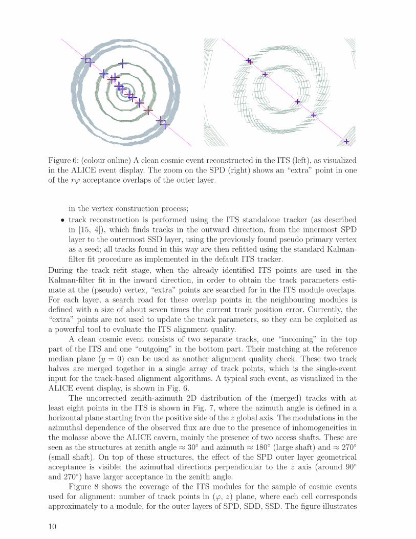
Figure 6: (colour online) A clean cosmic event reconstructed in the ITS (left), as visualizedin the ALICE event display. The zoom on the SPD (right) shows an “extra” point in oneof the rϕ acceptance overlaps of the outer layer.

in the vertex construction process;

• track reconstruction is performed using the ITS standalone tracker (as describedin [15, 4]), which finds tracks in the outward direction, from the innermost SPDlayer to the outermost SSD layer, using the previously found pseudo primary vertexas a seed; all tracks found in this way are then refitted using the standard Kalman-filter fit procedure as implemented in the default ITS tracker.

During the track refit stage, when the already identified ITS points are used in theKalman-filter fit in the inward direction, in order to obtain the track parameters esti-mate at the (pseudo) vertex, “extra” points are searched for in the ITS module overlaps.For each layer, a search road for these overlap points in the neighbouring modules isdefined with a size of about seven times the current track position error. Currently, the“extra” points are not used to update the track parameters, so they can be exploited asa powerful tool to evaluate the ITS alignment quality.

A clean cosmic event consists of two separate tracks, one “incoming” in the toppart of the ITS and one “outgoing” in the bottom part. Their matching at the referencemedian plane (y = 0) can be used as another alignment quality check. These two trackhalves are merged together in a single array of track points, which is the single-eventinput for the track-based alignment algorithms. A typical such event, as visualized in theALICE event display, is shown in Fig. 6.

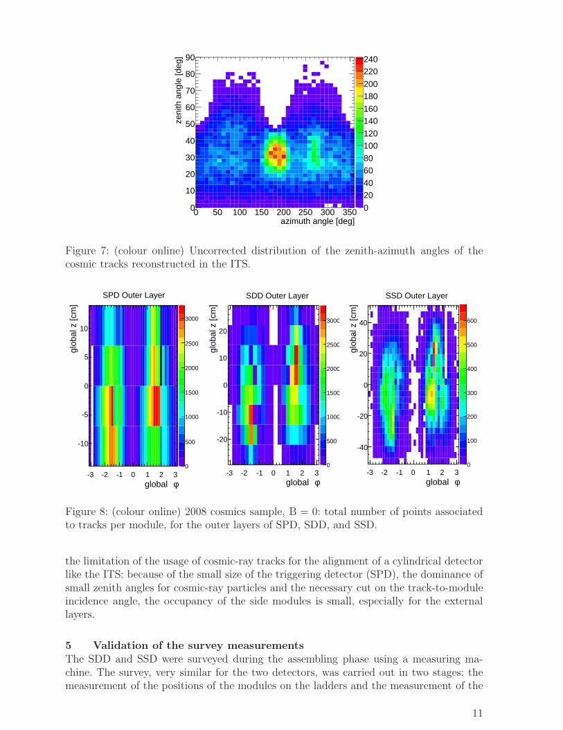
The uncorrected zenith-azimuth 2D distribution of the (merged) tracks with atleast eight points in the ITS is shown in Fig. 7, where the azimuth angle is defined in ahorizontal plane starting from the positive side of the z global axis. The modulations in theazimuthal dependence of the observed flux are due to the presence of inhomogeneities inthe molasse above the ALICE cavern, mainly the presence of two access shafts. These areseen as the structures at zenith angle ≈ 30◦ and azimuth ≈ 180◦ (large shaft) and ≈ 270◦

(small shaft). On top of these structures, the effect of the SPD outer layer geometricalacceptance is visible: the azimuthal directions perpendicular to the z axis (around 90◦

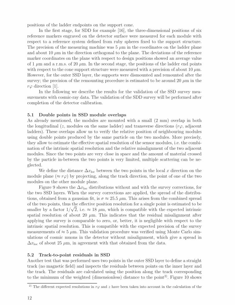
and 270◦) have larger acceptance in the zenith angle.Figure 8 shows the coverage of the ITS modules for the sample of cosmic events

used for alignment: number of track points in (ϕ, z) plane, where each cell correspondsapproximately to a module, for the outer layers of SPD, SDD, SSD. The figure illustrates

10

azimuth angle [deg]0 50 100 150 200 250 300 350

zeni

th a

ngle

[deg

]

0

10

20

30

40

50

60

70

80

90

0

2040

6080

100120

140160

180200

220240

Figure 7: (colour online) Uncorrected distribution of the zenith-azimuth angles of thecosmic tracks reconstructed in the ITS.

φglobal -3 -2 -1 0 1 2 3

glob

al z

[cm

]

-10

-5

0

5

10

0

500

1000

1500

2000

2500

3000

SPD Outer Layer

φglobal -3 -2 -1 0 1 2 3

glob

al z

[cm

]

-20

-10

0

10

20

0

500

1000

1500

2000

2500

3000

SDD Outer Layer

φglobal -3 -2 -1 0 1 2 3

glob

al z

[cm

]

-40

-20

0

20

40

0

100

200

300

400

500

600

SSD Outer Layer

Figure 8: (colour online) 2008 cosmics sample, B = 0: total number of points associatedto tracks per module, for the outer layers of SPD, SDD, and SSD.

the limitation of the usage of cosmic-ray tracks for the alignment of a cylindrical detectorlike the ITS: because of the small size of the triggering detector (SPD), the dominance ofsmall zenith angles for cosmic-ray particles and the necessary cut on the track-to-moduleincidence angle, the occupancy of the side modules is small, especially for the externallayers.

5 Validation of the survey measurements

The SDD and SSD were surveyed during the assembling phase using a measuring ma-chine. The survey, very similar for the two detectors, was carried out in two stages: themeasurement of the positions of the modules on the ladders and the measurement of the

11

positions of the ladder endpoints on the support cone.In the first stage, for SDD for example [16], the three-dimensional positions of six

reference markers engraved on the detector surface were measured for each module withrespect to a reference system defined from ruby spheres fixed to the support structure.The precision of the measuring machine was 5 µm in the coordinates on the ladder planeand about 10 µm in the direction orthogonal to the plane. The deviations of the referencemarker coordinates on the plane with respect to design positions showed an average valueof 1 µm and a r.m.s. of 20 µm. In the second stage, the positions of the ladder end pointswith respect to the cone support structure were measured with a precision of about 10 µm.However, for the outer SSD layer, the supports were dismounted and remounted after thesurvey; the precision of the remounting procedure is estimated to be around 20 µm in therϕ direction [1].

In the following we describe the results for the validation of the SSD survey mea-surements with cosmic-ray data. The validation of the SDD survey will be performed aftercompletion of the detector calibration.

5.1 Double points in SSD module overlaps

As already mentioned, the modules are mounted with a small (2 mm) overlap in boththe longitudinal (z, modules on the same ladder) and transverse directions (rϕ, adjacentladders). These overlaps allow us to verify the relative position of neighbouring modulesusing double points produced by the same particle on the two modules. More precisely,they allow to estimate the effective spatial resolution of the sensor modules, i.e. the combi-nation of the intrinsic spatial resolution and the relative misalignment of the two adjacentmodules. Since the two points are very close in space and the amount of material crossedby the particle in-between the two points is very limited, multiple scattering can be ne-glected.

We define the distance ∆xloc between the two points in the local x direction on themodule plane (≈ rϕ) by projecting, along the track direction, the point of one of the twomodules on the other module plane.

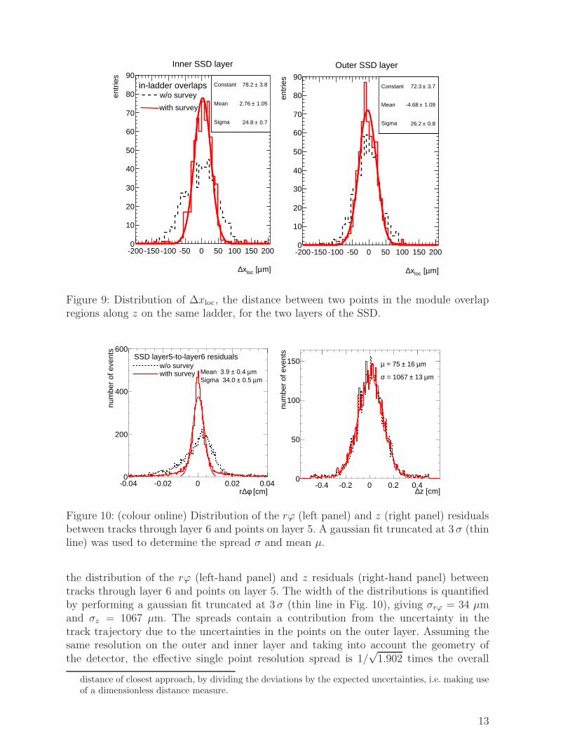
Figure 9 shows the ∆xloc distributions without and with the survey corrections, forthe two SSD layers. When the survey corrections are applied, the spread of the distribu-tions, obtained from a gaussian fit, is σ ≈ 25.5 µm. This arises from the combined spreadof the two points, thus the effective position resolution for a single point is estimated to besmaller by a factor 1/

√2, i.e. ≈ 18 µm, which is compatible with the expected intrinsic

spatial resolution of about 20 µm. This indicates that the residual misalignment afterapplying the survey is comparable to zero, or, better, it is negligible with respect to theintrinsic spatial resolution. This is compatible with the expected precision of the surveymeasurements of ≈ 5 µm. This validation procedure was verified using Monte Carlo sim-ulations of cosmic muons in the detector without misalignment, which give a spread in∆xloc of about 25 µm, in agreement with that obtained from the data.

5.2 Track-to-point residuals in SSD

Another test that was performed uses two points in the outer SSD layer to define a straighttrack (no magnetic field) and inspects the residuals between points on the inner layer andthe track. The residuals are calculated using the position along the track correspondingto the minimum of the weighted (dimensionless) distance to the point2). Figure 10 shows

2) The different expected resolutions in rϕ and z have been taken into account in the calculation of the

12

m]µ [locx∆

-200-150 -100 -50 0 50 100 150 200

ent

ries

0

10

20

30

40

50

60

70

80

90Constant 3.8± 78.2

Mean 1.05± 2.76

Sigma 0.7± 24.8

Constant 3.8± 78.2

Mean 1.05± 2.76

Sigma 0.7± 24.8

Inner SSD layer

Constant 3.8± 78.2

Mean 1.05± 2.76

Sigma 0.7± 24.8

Constant 3.8± 78.2

Mean 1.05± 2.76

Sigma 0.7± 24.8

w/o survey

with survey

in-ladder overlaps

m]µ [locx∆

-200-150 -100 -50 0 50 100 150 200

ent

ries

0

10

20

30

40

50

60

70

80

90Constant 3.7± 72.3

Mean 1.09± -4.68

Sigma 0.8± 26.2

Constant 3.7± 72.3

Mean 1.09± -4.68

Sigma 0.8± 26.2

Outer SSD layer

Constant 3.7± 72.3

Mean 1.09± -4.68

Sigma 0.8± 26.2

Constant 3.7± 72.3

Mean 1.09± -4.68

Sigma 0.8± 26.2

Figure 9: Distribution of ∆xloc, the distance between two points in the module overlapregions along z on the same ladder, for the two layers of the SSD.

[cm]φ∆r-0.04 -0.02 0 0.02 0.04

num

ber

of e

vent

s

0

200

400

600

mµ 0.5 ±Sigma 34.0 mµ 0.4 ±Mean 3.9

w/o surveywith survey

SSD layer5-to-layer6 residuals

z [cm]∆-0.4 -0.2 0 0.2 0.4

num

ber

of e

vent

s

0

50

100

150

mµ 13 ± = 1067 σ

mµ 16 ± = 75 µ

Figure 10: (colour online) Distribution of the rϕ (left panel) and z (right panel) residualsbetween tracks through layer 6 and points on layer 5. A gaussian fit truncated at 3 σ (thinline) was used to determine the spread σ and mean µ.

the distribution of the rϕ (left-hand panel) and z residuals (right-hand panel) betweentracks through layer 6 and points on layer 5. The width of the distributions is quantifiedby performing a gaussian fit truncated at 3 σ (thin line in Fig. 10), giving σrϕ = 34 µmand σz = 1067 µm. The spreads contain a contribution from the uncertainty in thetrack trajectory due to the uncertainties in the points on the outer layer. Assuming thesame resolution on the outer and inner layer and taking into account the geometry ofthe detector, the effective single point resolution spread is 1/

√1.902 times the overall

distance of closest approach, by dividing the deviations by the expected uncertainties, i.e. making useof a dimensionless distance measure.

13

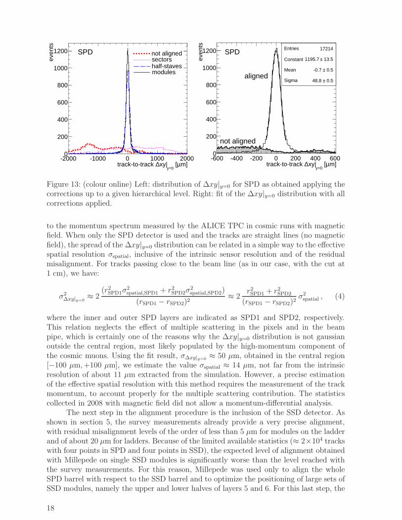
spread [17], so 25 µm and 778 µm in rϕ and z, respectively.The effective resolution of the points in z is well within the expected uncertainty,

indicating that no significant additional misalignment is present. For the rϕ direction,the obtained spread of 25 µm is larger than the intrinsic resolution of 20 µm. Multiplescattering of low-momentum tracks is expected to contribute to the broadening of thedistribution, but no quantitative estimate of this effect was carried out. We can thereforenot rule out that additional misalignments with an r.m.s. up to about 20 µm are present inthe SSD. The mean residual is also non-zero, (3.9± 0.4) µm, which suggests that residualshifts at the 5–10 µm level could be present. These misalignments would have to be at theladder level to be compatible with the result from the study with sensor module overlaps.

A third method that was used to verify the SSD survey consisted in performingtracking with pairs of points (2 points on layer 5 and two points on layer 6 or two setsof points on layer 5 and 6), and comparing the track parameters of both track segments.The conclusion from this method is consistent with the results from the track-to-pointmethod. For details see [17].

6 ITS alignment with Millepede

In general, the task of track-based alignment algorithms is the determination of the setof geometry parameters that minimize the global χ2 of the track-to-point residuals:

χ2global =

∑

modules, tracks

~δTt,p V−1

t,p~δt,p . (1)

In this expression, the sum runs over all the detector modules and all the tracks in agiven dataset; ~δt,p = ~rt − ~rp is the residual between the data point ~rp and the recon-structed track extrapolation ~rt to the module plane; Vt,p is the covariance matrix of theresidual. Note that, in general, the reconstructed tracks themselves depend on the assumedgeometry parameters. This section describes how this minimization problem is treated byMillepede [5, 18] —the main algorithm used for ITS alignment— and presents the firstalignment results obtained with cosmic-ray data.

6.1 General principles of the Millepede algorithm

Millepede belongs to the global least-squares minimization type of algorithms, which aimat determining simultaneously all the parameters that minimize the global χ2 in Eq. (1).It assumes that, for each of the local coordinates, the residual of a given track t to aspecific measured point p can be represented in a linearized form as δt,p = ~a · ∂δt,p/∂~a +~αt · ∂δt,p/∂ ~αt, where ~a are the global parameters describing the alignment of the detector(three translations and three rotations per module) and ~αt are the local parameters of thetrack. The corresponding χ2

global equation for n tracks with ν local parameters per trackand for m modules with 6 global parameters (N = 6m total global parameters) leads toa huge set of N + ν n normal equations. These can be written in the following partitionedmatrix equation form:

C G1 . . . . . . Gn

GT1 Γ1 0 . . . 0

......

...... 0

GTn 0 . . . 0 Γn

~a~α1...~αn

=

~b~β1...~βn

(2)

14

The sub-matrices C involve the derivatives of the residuals only over the global pa-rameters (in the local frame of the sensor, where the covariance matrix is diagonal,Cij =

∑

t,p σ−2p ∂δt,p/∂ai ∂δt,p/∂aj), Γt depends only on the track t parameters (Γt,ij =

∑

p σ−2p ∂δt,p/∂αt,i ∂δt,p/∂αt,j) and Gt is for the local parameters of the track t and the

global parameters (Gt,ij =∑

p σ−2p ∂δt,p/∂ai ∂δt,p/∂αt,j). Similarly, the right-hand side of

Eq. (2) is grouped to bi =∑

t,p σ−2p δt,p ∂δt,p/∂ai and βt,i =

∑

p σ−2p δt,p ∂δt,p/∂αt,i.

The idea behind the Millepede method is to consider the local ~α parameters as nui-sance parameters that are eliminated using the Banachiewicz identity [19] for partitionedmatrices:

(

C11 C12

C12 C22

)−1

=

(

B −BC12C−122

−C−122 CT

12B C−122 + C−1

22 CT12BC12C

−122

)

(3)

with B =(

C11 − C12C222C

T12

)−1. In fact, the full matrix of all the N+νn parameters is not

built explicitly: using Eq. (3) the set of N normal equations for the global parameters is

constructed by subtracting from C and~b the contributions related to the local parameters.If needed, linear constraints on the global parameters can be added using the Lagrangemultipliers. Historically, two versions, Millepede and Millepede II, were released. The firstone, written in Fortran, was performing the calculation of the residuals, the derivativesand the final matrix elements as well as the extraction of the exact solution in one singlestep, keeping all necessary information in computer memory. The large memory and CPUtime needed to extract the exact solution of a N ×N matrix equation effectively limitedits use to N < 10, 000 global (alignment) parameters. This limitation was removed in thesecond version, Millepede II. Software-wise the algorithm is split in two parts: the firstone (available in C and Fortran) stores in an intermediate file the residuals, derivativesand constraints provided by the user, while the second one (in Fortran) processes thesedata, builds the necessary matrices (optionally in sparse format, to save memory space)and solves them using advanced iterative methods, much faster than the exact methods.

6.2 Millepede for the ALICE ITS

Following the development of Millepede, ALICE had its own implementation ofboth versions, hereafter indicated as MP and MPII, within the AliRoot framework [6].Both consist of a detector independent solver class, responsible for building and solvingthe matrix equations, and a class interfacing the former to specific detectors3). While MPclosely follows the original algorithm [5], MPII has a number of extensions. In addition tothe MinRes matrix equation solution algorithm offered by the original Millepede II, themore general FGMRES [21] method was added, as well as the powerful ILU(k) matrixpreconditioners [22]. All the results shown in this work are obtained with MPII.

The track-to-point residuals, used to construct the global χ2, are calculated usinga parametric straight line ~r(t) = ~a+~b t or helix ~r(t) = {ax + r cos(t+ ϕ0), ay + r sin(t+ϕ0), az + bz t} track model, depending on the presence of the magnetic field. The full errormatrix of the measured points is accounted for in the track fit, while multiple scatteringis ignored, since it has no systematic effect on the residuals.

Special attention was paid to the possibility to account for the complex hierarchy ofthe alignable volumes of the ITS, shown in Fig. 2, in general leading to better description

3) MP was originally implemented for the Muon Arm alignment and has been later interfaced to ITS,while MPII is currently interfaced to ITS only.

15

m]µ residuals [locSPD x-1000 -500 0 500 1000

entr

ies

0

10000

20000

30000

40000

50000 not alignedaligned

m]µ residuals [locSPD z-1000 -500 0 500 1000

entr

ies

0

2000

4000

6000

8000

Figure 11: Example of Millepede residuals in the local reference frame of the SPD modulesbefore and after the alignment.

of the material budget distribution after alignment. This is achieved by defining explicitparent–daughter relationships between the volumes corresponding to mechanical degreesof freedom in the ITS. The alignment is performed simultaneously for the volumes onall levels of the hierarchy, e.g. for the SPD the corrections are obtained in a single stepfor the sectors, the half-staves within the sectors and the modules within the half-staves.Obviously, this leads to a degeneracy of the possible solutions, which should be removedby an appropriate set of constraints. We implemented the possibility to constrain eitherthe mean or the median of the corrections for the daughter volumes of any parent volume.While the former can be applied via Lagrange multipliers directly at the minimizationstage, the latter, being non-analytical, is applied a posteriori in a dedicated afterburner.The relative movement δ of volumes for which the survey data is available (e.g. SDDand SSD modules) can be restricted to be within the declared survey precision σsurvey byadding a set of gaussian constraints δ2/σ2

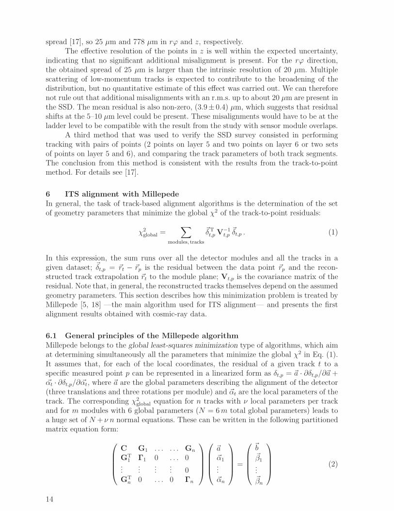
survey to the global χ2.We report here a few example figures to illustrate the bare output results from

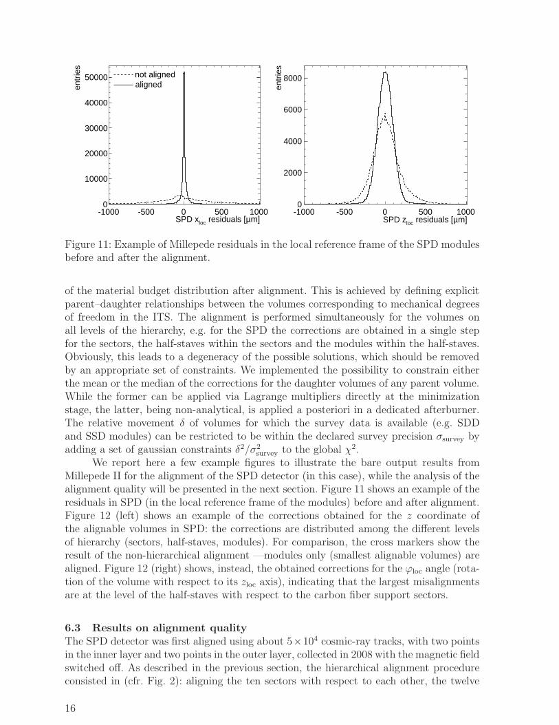
Millepede II for the alignment of the SPD detector (in this case), while the analysis of thealignment quality will be presented in the next section. Figure 11 shows an example of theresiduals in SPD (in the local reference frame of the modules) before and after alignment.Figure 12 (left) shows an example of the corrections obtained for the z coordinate ofthe alignable volumes in SPD: the corrections are distributed among the different levelsof hierarchy (sectors, half-staves, modules). For comparison, the cross markers show theresult of the non-hierarchical alignment —modules only (smallest alignable volumes) arealigned. Figure 12 (right) shows, instead, the obtained corrections for the ϕloc angle (rota-tion of the volume with respect to its zloc axis), indicating that the largest misalignmentsare at the level of the half-staves with respect to the carbon fiber support sectors.

6.3 Results on alignment quality

The SPD detector was first aligned using about 5×104 cosmic-ray tracks, with two pointsin the inner layer and two points in the outer layer, collected in 2008 with the magnetic fieldswitched off. As described in the previous section, the hierarchical alignment procedureconsisted in (cfr. Fig. 2): aligning the ten sectors with respect to each other, the twelve

16

Sector number0 1 2 3 4 5 6 7 8 9

m]

µz

[∆

-800

-600

-400

-200

0

200

400

600

800

Sectors Half-staves Modules

ModulesNon-hierarchical:

Hierarchical:

Sectors Half-staves Modules

[deg

]lo

cφ∆

-4

-2

0

2

4

Figure 12: (colour online) Example of hierarchical SPD alignment. Left: corrections forthe z coordinate of the SPD volumes as a function of the sector number. Crosses: resultsfrom the alignment with all misalignments attributed to the module degrees of freedom.Hierarchical alignment resolves the corrections in contributions from sectors (squares),half-staves (triangles) and module (circles) misalignments. Right: corrections to the ϕloc

angle obtained in the hierarchical alignment.

half-staves of each sector with respect to the sector, and the two modules of each half-stavewith respect to the half-stave.

Mainly, the following two observables are used to check the quality of the obtainedalignment: the top half-track to bottom half-track matching at the plane y = 0, and thetrack-to-point distance for the “extra” points in the acceptance overlaps.

For the first observable, the cosmic-ray track is split into the two track segments thatcross the upper (y > 0) and lower (y < 0) halves of the ITS barrel, and the parametersof the two segments are compared at y = 0. The main variable is ∆xy|y=0, the track-to-track distance at y = 0 in the (x, y) plane transverse to beam-line. This observable, thatis accessible only with cosmic-ray tracks, provides a direct measurement of the resolutionon the track transverse impact parameter d0; namely: σ∆xy|y=0

(pt) =√

2σd0(pt). Since the

data used for the current analysis were collected without magnetic field, they do not allowus to directly assess the d0 resolution (this will be the subject of a future work). However,also without a momentum measurement, ∆xy|y=0 is a powerful indicator of the alignmentquality, as we show in the following.

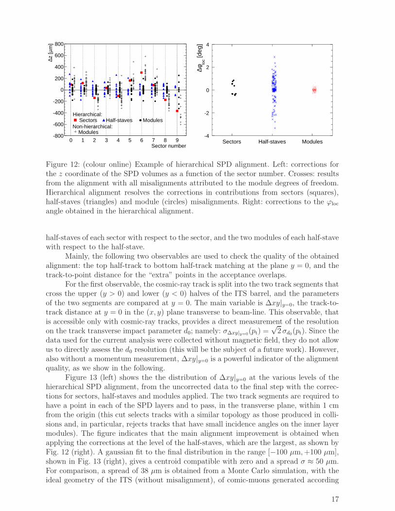
Figure 13 (left) shows the the distribution of ∆xy|y=0 at the various levels of thehierarchical SPD alignment, from the uncorrected data to the final step with the correc-tions for sectors, half-staves and modules applied. The two track segments are required tohave a point in each of the SPD layers and to pass, in the transverse plane, within 1 cmfrom the origin (this cut selects tracks with a similar topology as those produced in colli-sions and, in particular, rejects tracks that have small incidence angles on the inner layermodules). The figure indicates that the main alignment improvement is obtained whenapplying the corrections at the level of the half-staves, which are the largest, as shown byFig. 12 (right). A gaussian fit to the final distribution in the range [−100 µm,+100 µm],shown in Fig. 13 (right), gives a centroid compatible with zero and a spread σ ≈ 50 µm.For comparison, a spread of 38 µm is obtained from a Monte Carlo simulation, with theideal geometry of the ITS (without misalignment), of comic-muons generated according

17

m]µ [y=0

xy|∆track-to-track -2000 -1000 0 1000 2000

even

ts

0

200

400

600

800

1000

1200 not alignedsectorshalf-stavesmodules

SPDEntries 17214

Constant 13.5± 1195.7

Mean 0.5± -0.7

Sigma 0.5± 48.8

m]µ [y=0

xy|∆track-to-track -600 -400 -200 0 200 400 600

even

ts

0

200

400

600

800

1000

1200 Entries 17214

Constant 13.5± 1195.7

Mean 0.5± -0.7

Sigma 0.5± 48.8

not aligned

aligned

SPD

Figure 13: (colour online) Left: distribution of ∆xy|y=0 for SPD as obtained applying thecorrections up to a given hierarchical level. Right: fit of the ∆xy|y=0 distribution with allcorrections applied.

to the momentum spectrum measured by the ALICE TPC in cosmic runs with magneticfield. When only the SPD detector is used and the tracks are straight lines (no magneticfield), the spread of the ∆xy|y=0 distribution can be related in a simple way to the effectivespatial resolution σspatial, inclusive of the intrinsic sensor resolution and of the residualmisalignment. For tracks passing close to the beam line (as in our case, with the cut at1 cm), we have:

σ2∆xy|y=0

≈ 2(r2

SPD1σ2spatial,SPD1 + r2

SPD2σ2spatial,SPD2)

(rSPD1 − rSPD2)2≈ 2

r2SPD1 + r2

SPD2

(rSPD1 − rSPD2)2σ2

spatial , (4)

where the inner and outer SPD layers are indicated as SPD1 and SPD2, respectively.This relation neglects the effect of multiple scattering in the pixels and in the beampipe, which is certainly one of the reasons why the ∆xy|y=0 distribution is not gaussianoutside the central region, most likely populated by the high-momentum component ofthe cosmic muons. Using the fit result, σ∆xy|y=0

≈ 50 µm, obtained in the central region[−100 µm,+100 µm], we estimate the value σspatial ≈ 14 µm, not far from the intrinsicresolution of about 11 µm extracted from the simulation. However, a precise estimationof the effective spatial resolution with this method requires the measurement of the trackmomentum, to account properly for the multiple scattering contribution. The statisticscollected in 2008 with magnetic field did not allow a momentum-differential analysis.

The next step in the alignment procedure is the inclusion of the SSD detector. Asshown in section 5, the survey measurements already provide a very precise alignment,with residual misalignment levels of the order of less than 5 µm for modules on the ladderand of about 20 µm for ladders. Because of the limited available statistics (≈ 2×104 trackswith four points in SPD and four points in SSD), the expected level of alignment obtainedwith Millepede on single SSD modules is significantly worse than the level reached withthe survey measurements. For this reason, Millepede was used only to align the wholeSPD barrel with respect to the SSD barrel and to optimize the positioning of large sets ofSSD modules, namely the upper and lower halves of layers 5 and 6. For this last step, the

18

Entries 12273

Mean 0.005348

RMS 89.45

m]µ [y=0

xy|∆track-to-track -400 -300 -200 -100 0 100 200 300 400

even

ts

0

100

200

300

400

500

600

700 Entries 12273

Mean 0.005348

RMS 89.45

SPD+SSD

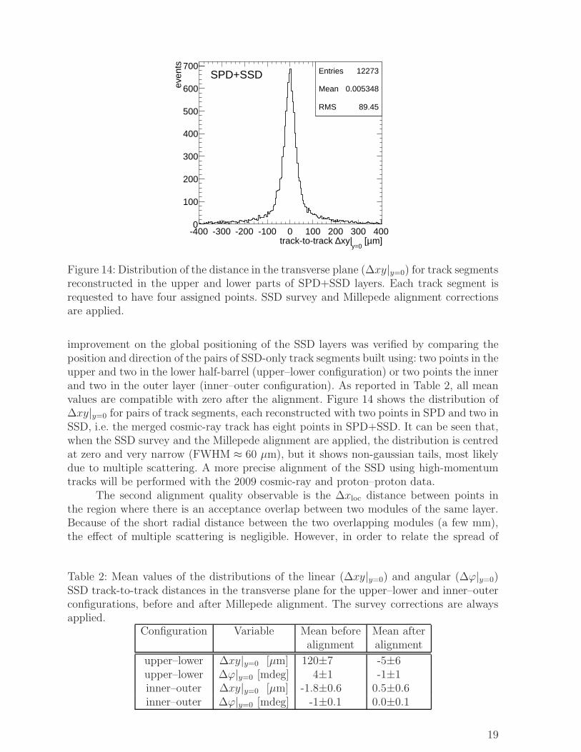
Figure 14: Distribution of the distance in the transverse plane (∆xy|y=0) for track segmentsreconstructed in the upper and lower parts of SPD+SSD layers. Each track segment isrequested to have four assigned points. SSD survey and Millepede alignment correctionsare applied.

improvement on the global positioning of the SSD layers was verified by comparing theposition and direction of the pairs of SSD-only track segments built using: two points in theupper and two in the lower half-barrel (upper–lower configuration) or two points the innerand two in the outer layer (inner–outer configuration). As reported in Table 2, all meanvalues are compatible with zero after the alignment. Figure 14 shows the distribution of∆xy|y=0 for pairs of track segments, each reconstructed with two points in SPD and two inSSD, i.e. the merged cosmic-ray track has eight points in SPD+SSD. It can be seen that,when the SSD survey and the Millepede alignment are applied, the distribution is centredat zero and very narrow (FWHM ≈ 60 µm), but it shows non-gaussian tails, most likelydue to multiple scattering. A more precise alignment of the SSD using high-momentumtracks will be performed with the 2009 cosmic-ray and proton–proton data.

The second alignment quality observable is the ∆xloc distance between points inthe region where there is an acceptance overlap between two modules of the same layer.Because of the short radial distance between the two overlapping modules (a few mm),the effect of multiple scattering is negligible. However, in order to relate the spread of

Table 2: Mean values of the distributions of the linear (∆xy|y=0) and angular (∆ϕ|y=0)SSD track-to-track distances in the transverse plane for the upper–lower and inner–outerconfigurations, before and after Millepede alignment. The survey corrections are alwaysapplied.

Configuration Variable Mean before Mean afteralignment alignment

upper–lower ∆xy|y=0 [µm] 120±7 -5±6upper–lower ∆ϕ|y=0 [mdeg] 4±1 -1±1inner–outer ∆xy|y=0 [µm] -1.8±0.6 0.5±0.6inner–outer ∆ϕ|y=0 [mdeg] -1±0.1 0.0±0.1

19

Entries 1784

Constant 2.3± 70.7

Mean 0.505± 0.785

Sigma 0.5± 18.3

m]µ [locx∆track-to-point -300 -200 -100 0 100 200 300

entr

ies

0

10

20

30

40

50

60

70

80Entries 1784

Constant 2.3± 70.7

Mean 0.505± 0.785

Sigma 0.5± 18.3 aligned

not aligned

SPD overlaps

) [deg]2α+1αsum of incidence angles (10 20 30 40 50 60 70 80 90

m]

µ2

r.m

.s. [

±)

fit in

lo

cx∆(σ

0

5

10

15

20

25

30

datasimulation (no misalignment)

mµ = 10 σm (3 seeds)µ = 7 σ

simulation (random gaussian misal.):

SPD overlaps

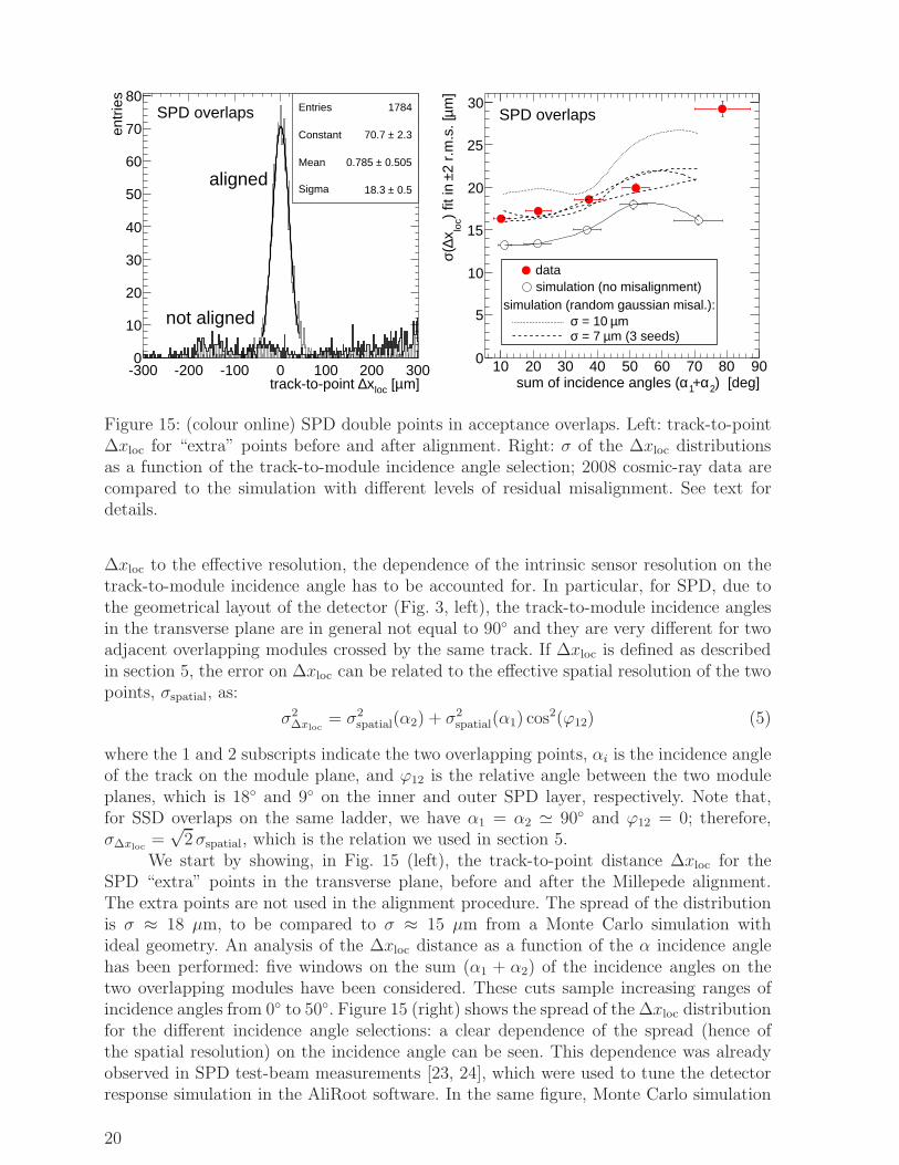
Figure 15: (colour online) SPD double points in acceptance overlaps. Left: track-to-point∆xloc for “extra” points before and after alignment. Right: σ of the ∆xloc distributionsas a function of the track-to-module incidence angle selection; 2008 cosmic-ray data arecompared to the simulation with different levels of residual misalignment. See text fordetails.

∆xloc to the effective resolution, the dependence of the intrinsic sensor resolution on thetrack-to-module incidence angle has to be accounted for. In particular, for SPD, due tothe geometrical layout of the detector (Fig. 3, left), the track-to-module incidence anglesin the transverse plane are in general not equal to 90◦ and they are very different for twoadjacent overlapping modules crossed by the same track. If ∆xloc is defined as describedin section 5, the error on ∆xloc can be related to the effective spatial resolution of the twopoints, σspatial, as:

σ2∆xloc

= σ2spatial(α2) + σ2

spatial(α1) cos2(ϕ12) (5)

where the 1 and 2 subscripts indicate the two overlapping points, αi is the incidence angleof the track on the module plane, and ϕ12 is the relative angle between the two moduleplanes, which is 18◦ and 9◦ on the inner and outer SPD layer, respectively. Note that,for SSD overlaps on the same ladder, we have α1 = α2 ≃ 90◦ and ϕ12 = 0; therefore,σ∆xloc

=√

2σspatial, which is the relation we used in section 5.We start by showing, in Fig. 15 (left), the track-to-point distance ∆xloc for the

SPD “extra” points in the transverse plane, before and after the Millepede alignment.The extra points are not used in the alignment procedure. The spread of the distributionis σ ≈ 18 µm, to be compared to σ ≈ 15 µm from a Monte Carlo simulation withideal geometry. An analysis of the ∆xloc distance as a function of the α incidence anglehas been performed: five windows on the sum (α1 + α2) of the incidence angles on thetwo overlapping modules have been considered. These cuts sample increasing ranges ofincidence angles from 0◦ to 50◦. Figure 15 (right) shows the spread of the ∆xloc distributionfor the different incidence angle selections: a clear dependence of the spread (hence ofthe spatial resolution) on the incidence angle can be seen. This dependence was alreadyobserved in SPD test-beam measurements [23, 24], which were used to tune the detectorresponse simulation in the AliRoot software. In the same figure, Monte Carlo simulation

20

Entries 7448

Constant 7.1± 417.8

Mean 0.7± -1.0

Sigma 0.7± 48.8

m]µ [y=0

xy|∆track-to-track -600 -400 -200 0 200 400 600

even

-num

ber

even

ts

0

50

100

150

200

250

300

350

400

450Entries 7448


Mean 0.7± -1.0

Sigma 0.7± 48.8

SPD

aligned withodd-number events

m]µ [y=0

xy|∆track-to-track -600 -400 -200 0 200 400 600

even

ts

0

50

100

150

200

250

300 sub-sample 1Entries 5172

Mean 0.873± 0.475

Sigma 0.9± 50.8

sub-sample 1Entries 5172

Mean 0.873± 0.475

Sigma 0.9± 50.8


Mean 0.85± -2.58

Sigma 0.8± 48.2


Mean 0.85± -2.58

Sigma 0.8± 48.2


Mean 0.80± 3.29 Sigma 0.8± 46.8


Mean 0.80± 3.29 Sigma 0.8± 46.8

SPDaligned with full sample

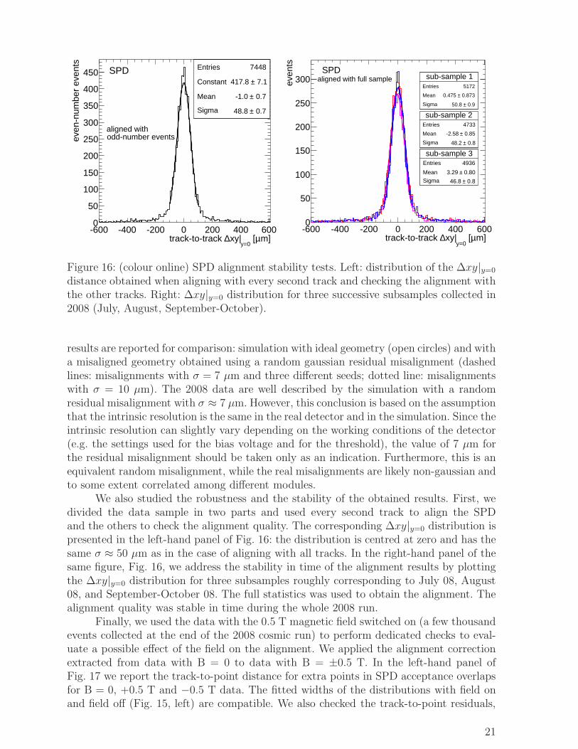
Figure 16: (colour online) SPD alignment stability tests. Left: distribution of the ∆xy|y=0

distance obtained when aligning with every second track and checking the alignment withthe other tracks. Right: ∆xy|y=0 distribution for three successive subsamples collected in2008 (July, August, September-October).

results are reported for comparison: simulation with ideal geometry (open circles) and witha misaligned geometry obtained using a random gaussian residual misalignment (dashedlines: misalignments with σ = 7 µm and three different seeds; dotted line: misalignmentswith σ = 10 µm). The 2008 data are well described by the simulation with a randomresidual misalignment with σ ≈ 7 µm. However, this conclusion is based on the assumptionthat the intrinsic resolution is the same in the real detector and in the simulation. Since theintrinsic resolution can slightly vary depending on the working conditions of the detector(e.g. the settings used for the bias voltage and for the threshold), the value of 7 µm forthe residual misalignment should be taken only as an indication. Furthermore, this is anequivalent random misalignment, while the real misalignments are likely non-gaussian andto some extent correlated among different modules.

We also studied the robustness and the stability of the obtained results. First, wedivided the data sample in two parts and used every second track to align the SPDand the others to check the alignment quality. The corresponding ∆xy|y=0 distribution ispresented in the left-hand panel of Fig. 16: the distribution is centred at zero and has thesame σ ≈ 50 µm as in the case of aligning with all tracks. In the right-hand panel of thesame figure, Fig. 16, we address the stability in time of the alignment results by plottingthe ∆xy|y=0 distribution for three subsamples roughly corresponding to July 08, August08, and September-October 08. The full statistics was used to obtain the alignment. Thealignment quality was stable in time during the whole 2008 run.

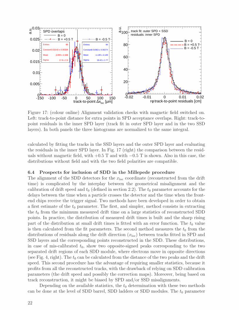
Finally, we used the data with the 0.5 T magnetic field switched on (a few thousandevents collected at the end of the 2008 cosmic run) to perform dedicated checks to eval-uate a possible effect of the field on the alignment. We applied the alignment correctionextracted from data with B = 0 to data with B = ±0.5 T. In the left-hand panel ofFig. 17 we report the track-to-point distance for extra points in SPD acceptance overlapsfor B = 0, +0.5 T and −0.5 T data. The fitted widths of the distributions with field onand field off (Fig. 15, left) are compatible. We also checked the track-to-point residuals,

21

hdxyovl2


a.u.

0

0.005

0.01

0.015

0.02

0.025

0.03

hdxyovl2Entries 88

Constant 0.00329± 0.02142

Mean 2.326± 2.009

Sigma 2.3± 17.8

Entries 88

Constant 0.00329± 0.02142

Mean 2.326± 2.009

Sigma 2.3± 17.8

Entries 94

Constant 0.00274± 0.01963

Mean 2.140± -1.138

Sigma 1.77± 18.42

Entries 94

Constant 0.00274± 0.01963

Mean 2.140± -1.138

Sigma 1.77± 18.42

Entries 88

Constant 0.00329± 0.02142

Mean 2.326± 2.009

Sigma 2.3± 17.8

Entries 88

Constant 0.00329± 0.02142

Mean 2.326± 2.009

Sigma 2.3± 17.8

Entries 94

Constant 0.00274± 0.01963

Mean 2.140± -1.138

Sigma 1.77± 18.42

Entries 94

Constant 0.00274± 0.01963

Mean 2.140± -1.138

Sigma 1.77± 18.42

Entries 88

Constant 0.00329± 0.02142

Mean 2.326± 2.009

Sigma 2.3± 17.8

Entries 88

Constant 0.00329± 0.02142

Mean 2.326± 2.009

Sigma 2.3± 17.8

B = 0B = +0.5 T B = -0.5 T

SPD overlaps

track-to-point residuals [cm]φr-0.02 -0.01 0 0.01 0.02

a.u.

0

20

40

60

80

100

B = 0B = +0.5 TB = -0.5 T

track fit: outer SPD + SSDresiduals: inner SPD

Figure 17: (colour online) Alignment validation checks with magnetic field switched on.Left: track-to-point distance for extra points in SPD acceptance overlaps. Right: track-to-point residuals in the inner SPD layer (track fit in outer SPD layer and in the two SSDlayers). In both panels the three histograms are normalized to the same integral.

calculated by fitting the tracks in the SSD layers and the outer SPD layer and evaluatingthe residuals in the inner SPD layer. In Fig. 17 (right) the comparison between the resid-uals without magnetic field, with +0.5 T and with −0.5 T is shown. Also in this case, thedistributions without field and with the two field polarities are compatible.

6.4 Prospects for inclusion of SDD in the Millepede procedure

The alignment of the SDD detectors for the xloc coordinate (reconstructed from the drifttime) is complicated by the interplay between the geometrical misalignment and thecalibration of drift speed and t0 (defined in section 2.2). The t0 parameter accounts for thedelays between the time when a particle crosses the detector and the time when the front-end chips receive the trigger signal. Two methods have been developed in order to obtaina first estimate of the t0 parameter. The first, and simpler, method consists in extractingthe t0 from the minimum measured drift time on a large statistics of reconstructed SDDpoints. In practice, the distribution of measured drift times is built and the sharp risingpart of the distribution at small drift times is fitted with an error function. The t0 valueis then calculated from the fit parameters. The second method measures the t0 from thedistributions of residuals along the drift direction (xloc) between tracks fitted in SPD andSSD layers and the corresponding points reconstructed in the SDD. These distributions,in case of mis-calibrated t0, show two opposite-signed peaks corresponding to the twoseparated drift regions of each SDD module, where electrons move in opposite directions(see Fig. 4, right). The t0 can be calculated from the distance of the two peaks and the driftspeed. This second procedure has the advantage of requiring smaller statistics, because itprofits from all the reconstructed tracks, with the drawback of relying on SDD calibrationparameters (the drift speed and possibly the correction maps). Moreover, being based ontrack reconstruction, it might be biased by SPD and/or SSD misalignments.

Depending on the available statistics, the t0 determination with these two methodscan be done at the level of SDD barrel, SDD ladders or SDD modules. The t0 parameter

22

Entries 2760


Mean 0.00068± -0.04974

Sigma 0.00059± 0.03271

[cm]loc

track-to-point residuals in x-0.4 -0.2 0 0.2 0.4

even

ts

0

20

40

60

80

100

120

140Entries 2760


Mean 0.00068± -0.04974

Sigma 0.00059± 0.03271

SDDLayer 4 side C

Drift regions: Left

Entries 2527


Mean 0.00067± 0.05994

Sigma 0.00057± 0.03138

[cm]loc

track-to-point residuals in x-0.4 -0.2 0 0.2 0.4

even

ts

0

20

40

60

80

100

120Entries 2527


Mean 0.00067± 0.05994

Sigma 0.00057± 0.03138

SDDLayer 4 side C

Drift regions: Right

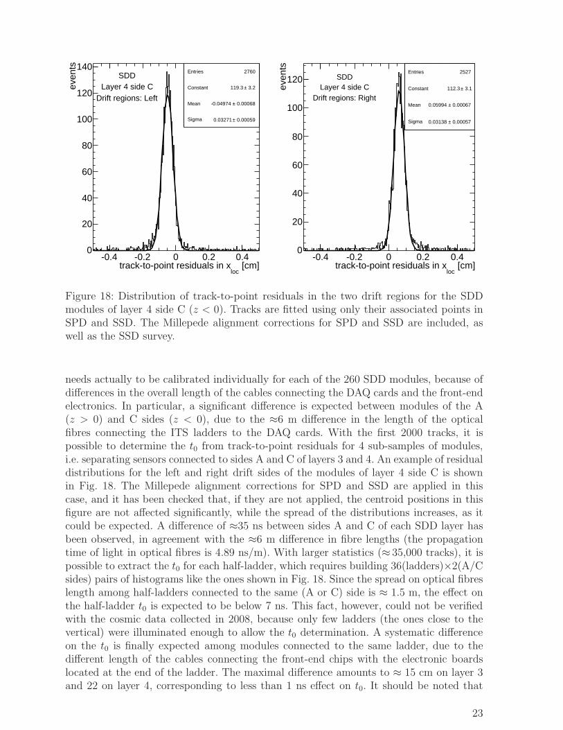
Figure 18: Distribution of track-to-point residuals in the two drift regions for the SDDmodules of layer 4 side C (z < 0). Tracks are fitted using only their associated points inSPD and SSD. The Millepede alignment corrections for SPD and SSD are included, aswell as the SSD survey.

needs actually to be calibrated individually for each of the 260 SDD modules, because ofdifferences in the overall length of the cables connecting the DAQ cards and the front-endelectronics. In particular, a significant difference is expected between modules of the A(z > 0) and C sides (z < 0), due to the ≈6 m difference in the length of the opticalfibres connecting the ITS ladders to the DAQ cards. With the first 2000 tracks, it ispossible to determine the t0 from track-to-point residuals for 4 sub-samples of modules,i.e. separating sensors connected to sides A and C of layers 3 and 4. An example of residualdistributions for the left and right drift sides of the modules of layer 4 side C is shownin Fig. 18. The Millepede alignment corrections for SPD and SSD are applied in thiscase, and it has been checked that, if they are not applied, the centroid positions in thisfigure are not affected significantly, while the spread of the distributions increases, as itcould be expected. A difference of ≈35 ns between sides A and C of each SDD layer hasbeen observed, in agreement with the ≈6 m difference in fibre lengths (the propagationtime of light in optical fibres is 4.89 ns/m). With larger statistics (≈ 35,000 tracks), it ispossible to extract the t0 for each half-ladder, which requires building 36(ladders)×2(A/Csides) pairs of histograms like the ones shown in Fig. 18. Since the spread on optical fibreslength among half-ladders connected to the same (A or C) side is ≈ 1.5 m, the effect onthe half-ladder t0 is expected to be below 7 ns. This fact, however, could not be verifiedwith the cosmic data collected in 2008, because only few ladders (the ones close to thevertical) were illuminated enough to allow the t0 determination. A systematic differenceon the t0 is finally expected among modules connected to the same ladder, due to thedifferent length of the cables connecting the front-end chips with the electronic boardslocated at the end of the ladder. The maximal difference amounts to ≈ 15 cm on layer 3and 22 on layer 4, corresponding to less than 1 ns effect on t0. It should be noted that

23

[cm]locdrift coordinate x-3 -2 -1 0 1 2 3

res

idua

ls [m

m]

loc

x

-0.15

-0.1

-0.05

0

0.05

0.1

0.15SDD module 266

with geometrical parameters

[cm]locdrift coordinate x-3 -2 -1 0 1 2 3

res

idua

ls [m

m]

loc

x

-0.15

-0.1

-0.05

0

0.05

0.1

0.15

with geometrical+calibration parameters

SDD module 266

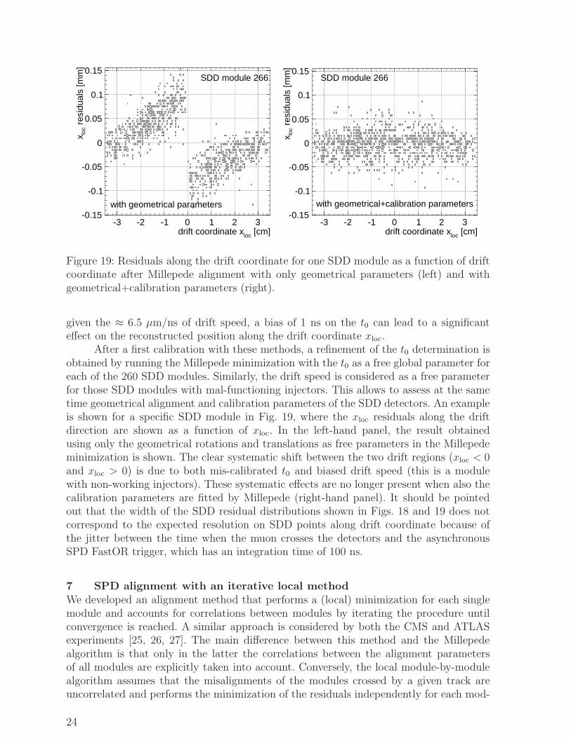
Figure 19: Residuals along the drift coordinate for one SDD module as a function of driftcoordinate after Millepede alignment with only geometrical parameters (left) and withgeometrical+calibration parameters (right).

given the ≈ 6.5 µm/ns of drift speed, a bias of 1 ns on the t0 can lead to a significanteffect on the reconstructed position along the drift coordinate xloc.

After a first calibration with these methods, a refinement of the t0 determination isobtained by running the Millepede minimization with the t0 as a free global parameter foreach of the 260 SDD modules. Similarly, the drift speed is considered as a free parameterfor those SDD modules with mal-functioning injectors. This allows to assess at the sametime geometrical alignment and calibration parameters of the SDD detectors. An exampleis shown for a specific SDD module in Fig. 19, where the xloc residuals along the driftdirection are shown as a function of xloc. In the left-hand panel, the result obtainedusing only the geometrical rotations and translations as free parameters in the Millepedeminimization is shown. The clear systematic shift between the two drift regions (xloc < 0and xloc > 0) is due to both mis-calibrated t0 and biased drift speed (this is a modulewith non-working injectors). These systematic effects are no longer present when also thecalibration parameters are fitted by Millepede (right-hand panel). It should be pointedout that the width of the SDD residual distributions shown in Figs. 18 and 19 does notcorrespond to the expected resolution on SDD points along drift coordinate because ofthe jitter between the time when the muon crosses the detectors and the asynchronousSPD FastOR trigger, which has an integration time of 100 ns.

7 SPD alignment with an iterative local method

We developed an alignment method that performs a (local) minimization for each singlemodule and accounts for correlations between modules by iterating the procedure untilconvergence is reached. A similar approach is considered by both the CMS and ATLASexperiments [25, 26, 27]. The main difference between this method and the Millepedealgorithm is that only in the latter the correlations between the alignment parametersof all modules are explicitly taken into account. Conversely, the local module-by-modulealgorithm assumes that the misalignments of the modules crossed by a given track areuncorrelated and performs the minimization of the residuals independently for each mod-

24

N iteration0 2 4 6 8 10 12 14 16 18 20

mµ

-10

-5

0

5

10

15

20

25

local x

N iteration0 2 4 6 8 10 12 14 16 18 20

mµ

-20

0

20

40

60

80

100

120

local y

N iteration0 2 4 6 8 10 12 14 16 18 20

mµ

0

10

20

30

40

50

60

70

local z

meansigma

N iteration0 2 4 6 8 10 12 14 16 18 20

mde

g

-20

0

20

40

60

80

100

ψlocal

N iteration0 2 4 6 8 10 12 14 16 18 20

mde

g

-10

0

10

20

30

40

50θlocal

N iteration0 2 4 6 8 10 12 14 16 18 20

mde

g

-40

-20

0

20

40

60

80

100

120

φlocal

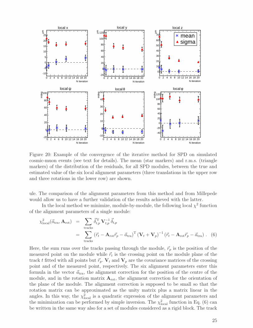
Figure 20: Example of the convergence of the iterative method for SPD on simulatedcosmic-muon events (see text for details). The mean (star markers) and r.m.s. (trianglemarkers) of the distribution of the residuals, for all SPD modules, between the true andestimated value of the six local alignment parameters (three translations in the upper rowand three rotations in the lower row) are shown.

ule. The comparison of the alignment parameters from this method and from Millepedewould allow us to have a further validation of the results achieved with the latter.

In the local method we minimize, module-by-module, the following local χ2 functionof the alignment parameters of a single module:

χ2local(~atra,Arot) =

∑

tracks

~δTt,p V−1

t,p~δt,p

=∑

tracks

(~rt −Arot~rp − ~atra)T (Vt + Vp)

−1 (~rt − Arot~rp − ~atra) . (6)

Here, the sum runs over the tracks passing through the module, ~rp is the position of themeasured point on the module while ~rt is the crossing point on the module plane of thetrack t fitted with all points but ~rp. Vt and Vp are the covariance matrices of the crossingpoint and of the measured point, respectively. The six alignment parameters enter thisformula in the vector ~atra, the alignment correction for the position of the centre of themodule, and in the rotation matrix Arot, the alignment correction for the orientation ofthe plane of the module. The alignment correction is supposed to be small so that therotation matrix can be approximated as the unity matrix plus a matrix linear in theangles. In this way, the χ2

local is a quadratic expression of the alignment parameters andthe minimization can be performed by simple inversion. The χ2

local function in Eq. (6) canbe written in the same way also for a set of modules considered as a rigid block. The track

25

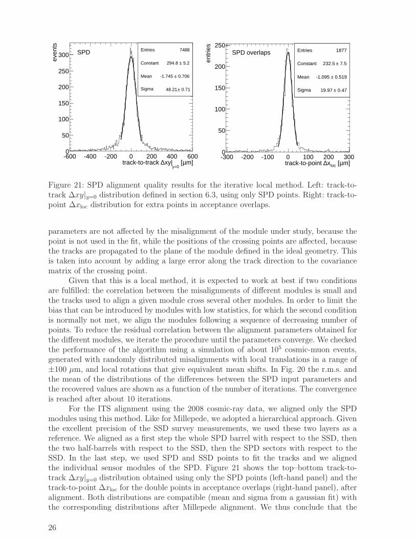
Entries 7488


Mean 0.706± -1.745

Sigma 0.71± 48.21

m]µ [y=0

xy|∆track-to-track -600 -400 -200 0 200 400 600

even

ts

0

50

100

150

200

250

300Entries 7488


Mean 0.706± -1.745

Sigma 0.71± 48.21

SPD Entries 1877


Mean 0.519± -1.095

Sigma 0.47± 19.97


entr

ies

0

50

100

150

200

250Entries 1877


Mean 0.519± -1.095

Sigma 0.47± 19.97

SPD overlaps

Figure 21: SPD alignment quality results for the iterative local method. Left: track-to-track ∆xy|y=0 distribution defined in section 6.3, using only SPD points. Right: track-to-point ∆xloc distribution for extra points in acceptance overlaps.

parameters are not affected by the misalignment of the module under study, because thepoint is not used in the fit, while the positions of the crossing points are affected, becausethe tracks are propagated to the plane of the module defined in the ideal geometry. Thisis taken into account by adding a large error along the track direction to the covariancematrix of the crossing point.

Given that this is a local method, it is expected to work at best if two conditionsare fulfilled: the correlation between the misalignments of different modules is small andthe tracks used to align a given module cross several other modules. In order to limit thebias that can be introduced by modules with low statistics, for which the second conditionis normally not met, we align the modules following a sequence of decreasing number ofpoints. To reduce the residual correlation between the alignment parameters obtained forthe different modules, we iterate the procedure until the parameters converge. We checkedthe performance of the algorithm using a simulation of about 105 cosmic-muon events,generated with randomly distributed misalignments with local translations in a range of±100 µm, and local rotations that give equivalent mean shifts. In Fig. 20 the r.m.s. andthe mean of the distributions of the differences between the SPD input parameters andthe recovered values are shown as a function of the number of iterations. The convergenceis reached after about 10 iterations.

For the ITS alignment using the 2008 cosmic-ray data, we aligned only the SPDmodules using this method. Like for Millepede, we adopted a hierarchical approach. Giventhe excellent precision of the SSD survey measurements, we used these two layers as areference. We aligned as a first step the whole SPD barrel with respect to the SSD, thenthe two half-barrels with respect to the SSD, then the SPD sectors with respect to theSSD. In the last step, we used SPD and SSD points to fit the tracks and we alignedthe individual sensor modules of the SPD. Figure 21 shows the top–bottom track-to-track ∆xy|y=0 distribution obtained using only the SPD points (left-hand panel) and thetrack-to-point ∆xloc for the double points in acceptance overlaps (right-hand panel), afteralignment. Both distributions are compatible (mean and sigma from a gaussian fit) withthe corresponding distributions after Millepede alignment. We thus conclude that the

26

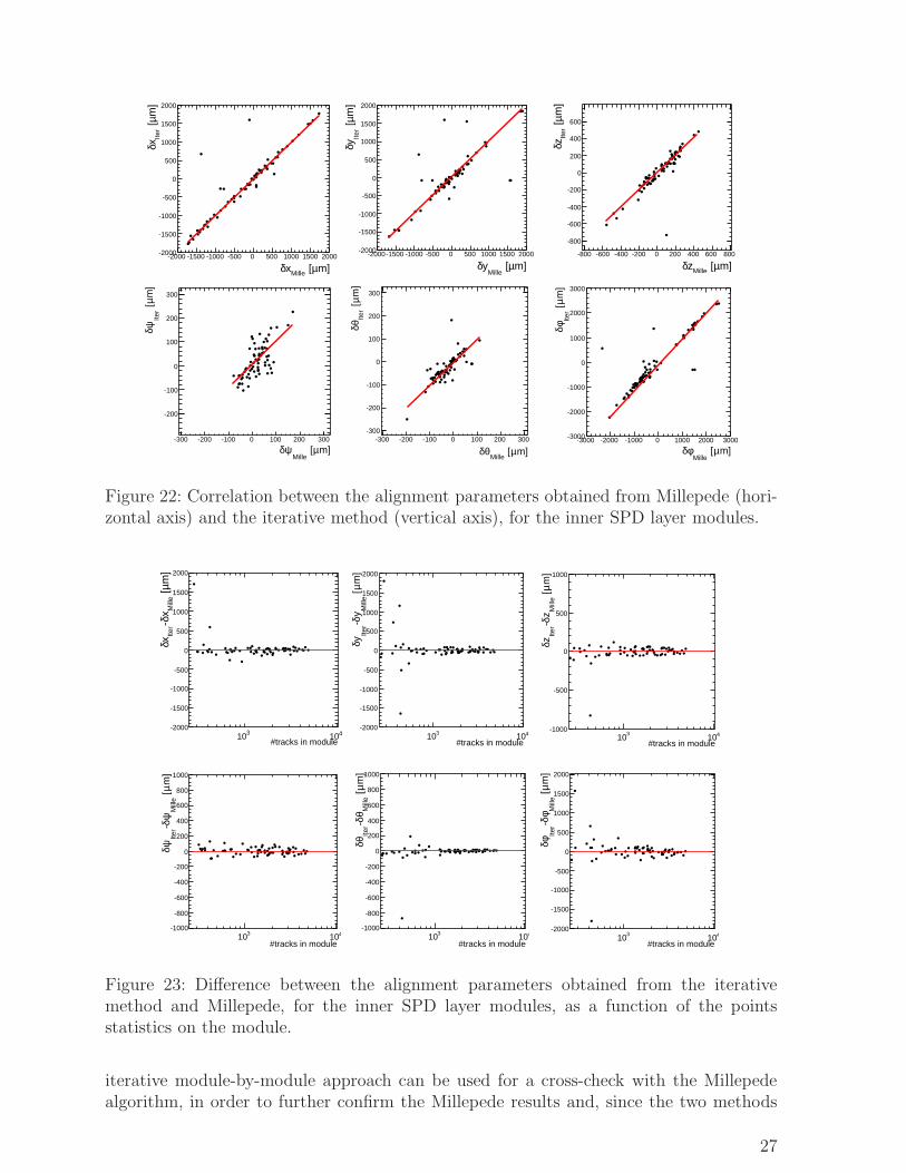
m]µ [Millexδ-2000 -1500 -1000 -500 0 500 1000 1500 2000

m]

µ [Ite

rxδ

-2000

-1500

-1000

-500

0

500

1000

1500

2000

m]µ [Mille

yδ-2000-1500 -1000 -500 0 500 1000 1500 2000

m]

µ [Ite

ryδ

-2000

-1500

-1000

-500

0

500

1000

1500

2000

m]µ [Millezδ-800 -600 -400 -200 0 200 400 600 800

m]

µ [Ite

rzδ

-800

-600

-400

-200

0

200

400

600

m]µ [Mille

ψδ-300 -200 -100 0 100 200 300

m]

µ [

Iter

ψδ

-200

-100

0

100

200

300

m]µ [Mille

θδ-300 -200 -100 0 100 200 300

m]

µ [

Iter

θδ

-300

-200

-100

0

100

200

300

m]µ [Mille

φδ-3000 -2000 -1000 0 1000 2000 3000

m]

µ [

Iter

φδ

-3000

-2000

-1000

0

1000

2000

3000

Figure 22: Correlation between the alignment parameters obtained from Millepede (hori-zontal axis) and the iterative method (vertical axis), for the inner SPD layer modules.

#tracks in module310 410

m]

µ [M

ille

xδ-Ite

rxδ

-2000

-1500

-1000

-500

0

500

1000

1500

2000


m]

µ [

Mill

eyδ-

Iter

yδ

-2000

-1500

-1000

-500

0

500

1000

1500

2000


m]

µ [

Mill

ezδ-

Iter

zδ

-1000

-500

0

500

1000


m]

µ [

Mill

eψδ-

Iter

ψδ

-1000

-800

-600

-400

-200

0

200

400

600

800

1000


m]

µ [

Mill

eθδ-

Iter

θδ

-1000

-800

-600

-400

-200

0

200

400

600

800

1000


m]

µ [

Mill

eφδ-

Iter

φδ

-2000

-1500

-1000

-500

0

500

1000

1500

2000

Figure 23: Difference between the alignment parameters obtained from the iterativemethod and Millepede, for the inner SPD layer modules, as a function of the pointsstatistics on the module.

iterative module-by-module approach can be used for a cross-check with the Millepedealgorithm, in order to further confirm the Millepede results and, since the two methods

27

are in many aspects independent, to check the presence of possible systematic trends inthe extracted alignment parameters. In Fig. 22 the values of the parameters obtainedwith the iterative method are plotted as a function of those obtained with Millepede.A correction was applied to account for a possible global roto-translation of the wholeITS, which does not affect the quality of the alignment and can be different for the twomethods. Most of the modules are clustered along the diagonal lines, that correspond tothe situation in which the parameters from the two methods are exactly the same. Thereare some outlier modules, that are far from the ideal result. However, the plots of thedifference between the two parameter values as a function of the statistics on the module(Fig. 23) show that the outliers mostly correspond to modules with low statistics (sidesof the SPD barrel).

8 Conclusions

The results on the first alignment of the ALICE Inner Tracking System with cosmic-raytracks, collected in 2008 in the absence of magnetic field, have been presented.

The initial step of the alignment procedure consisted in the validation of the surveymeasurements for the Silicon Strip Detector (SSD). The three methods applied to thispurpose indicate that the residual misalignment for modules on ladders is within 5 µm,i.e. negligible with respect to the intrinsic resolution of this detector in the most precisedirection, while the residual misalignment for the ladders with respect to the supportcones amounts to about 20 µm.

The procedure continues with track-based software alignment performing residualsminimization. We presented the results obtained with a sample of about 105 cosmic-raytracks, reconstructed in events selected by the FastOR trigger of the Silicon Pixel Detector(SPD). We mainly use the Millepede algorithm, which minimizes a global χ2 of residualsfor all alignable volumes and a large set of tracks.

We start from the SPD, which is aligned in a hierarchical approach, from the largestmechanical structures (10 support sectors) to the 240 single sensor modules. About 90%of the latter were active during the 2008 cosmic run, and about 85% had enough spacepoints (> 50) to allow the alignment. Then, we align the SPD barrel with respect to theSSD barrel. The SSD coverage provided by the cosmic-ray tracks is insufficient to alignthe SSD at the level of ladders, especially for the ladders close to the horizontal planey = 0. Therefore, for the time being we only align the SSD at the level of large sets ofladders. The two intermediate ITS layers, the Silicon Drift Detectors (SDD), representa special case, because the reconstruction of one of the two local coordinates requiresdedicated calibration procedures (drift velocity and drift time zero extraction), whichare to some extent related to the alignment. Indeed, one of the approaches that we aredeveloping for the time zero calibration is based on the analysis of track residuals in astandalone procedure, initially, and then directly within the Millepede algorithm. Oncethese procedure will become stable and robust, the SDD will be included in the standardalignment chain. For all six layers, the completion of the alignment for all modules willrequire tracks from proton–proton collisions; a few 106 events (collected in a few days)should allow us to reach a uniform alignment level, close to the target, over the entiredetector.

We use mainly two observables to assess the quality of the obtained alignment: thematching of the two half-tracks produced by a cosmic-ray particle in the upper and lowerhalves of the ITS barrel, and the residuals between double points produced in the geo-metrical overlaps between adjacent modules. For the SPD, both observables indicate an

28

effective space point resolution of about 14 µm in the most precise direction, to be com-pared to about 11 µm extracted from the Monte Carlo simulation without misalignments.This difference of ≈ 25% (from 11 to 14 µm) is already quite close the 20%, which isthe final target of the alignment. In addition, the measured incidence angle dependenceof the spread of the double points residuals is well reproduced by Monte Carlo simula-tions that include random residual misalignments with a gaussian sigma of about 7 µm.Further confidence on the robustness of the results is provided, to some extent, by thecross-checks we performed using a small data set with magnetic field switched on and,mainly, by the comparison of the Millepede results to those from a second, independent,alignment method. This second method, which iteratively minimizes a set of local module-by-module χ2 functions, yields, compared to Millepede, a similar alignment quality anda quite compatible set of alignment corrections.

Using the present data set with magnetic field off, since the track momenta arenot known, the multiple scattering effect, which is certainly not negligible, cannot bedisentangled from the residual misalignment effect. Therefore, a more conclusive statementon the SPD residual misalignment will be possible only after the analysis of cosmic-raydata collected with magnetic field switched on. The same applies for combined trackingwith SPD, SDD and SSD points: in this case, the momentum-differential analysis of thetransverse distance between the two half-tracks (upper and lower half-barrels) will allow usto measure the track transverse impact parameter resolution, which is a key performancefigure in view of the ALICE heavy flavour physics program.

Acknowledgements

We thank F. Antinori, I. Belikov, P. Giubellino, G. Martinez, V. Manzari, G. Nooren andF. Tosello for fruitful discussions and comments on the manuscript, R. Dima, B. Giraudoand J.-F. Grosse Oetringhaus for providing some of the detector drawings shown in Sec-tion 2. The results presented in this note were obtained using the data collected duringthe 2008 cosmic-ray global run of ALICE. We are grateful to the ALICE Collaboratorsinvolved in the ITS detector construction and commissioning and in the online and offlineactivities related to the collection and reconstruction of the data. A shorter version ofthis manuscript will be proposed to the ALICE Editorial Board for publication in a sci-entific journal, and it will be signed by all the ALICE Collaborators directly or indirectlyinvolved.

References

[1] K. Aamodt et al. [ALICE Collaboration], JINST 3 (2008) S08002.[2] F. Carminati et al. [ALICE Collaboration], J. Phys. G 30 (2003) 1517, chapter 1 and

references therein.[3] U. Heinz and M. Jacob, arXiv:nucl-th/0002042, and references therein;

I. Arsene et al. [BRAHMS Collaboration], Nucl. Phys. A757 (2005) 1;K. Adkox et al. [PHENIX Collaboration], Nucl. Phys. A757 (2005) 184;B.B. Back et al. [PHOBOS Collaboration], Nucl. Phys. A757 (2005) 28;J. Adams et al. [STAR Collaboration], Nucl. Phys. A757 (2005) 102.

[4] B. Alessandro et al. [ALICE Collaboration], J. Phys. G 32 (2006) 1295.[5] V. Blobel and C. Kleinwort, contribution to the Conference on Advanced Statistical

Techniques in Particle Physics, Durham, March, 18–22, 2002.[6] ALICE Off-line framework, AliRoot, http://aliceinfo.cern.ch/Offline[7] ROOT, http://root.cern.ch

29

[8] R. Grosso, in “Proceedings of the first LHC detector alignment workshop”, CERN,September 4–6, 2006, CERN-2007-004.

[9] S. Beole et al., Nucl. Inst. and Meth. A582 (2007) 733.[10] A. Rashevsky et al., Nucl. Inst. and Meth. A572 (2007) 125.[11] G. Batigne et al., JINST 3 (2008) P06004.[12] S. Blusk, et al. “Proceedings of the first LHC detector alignment workshop”, CERN,

September 4–6, 2006, CERN-2007-004.[13] B.S. Nilsen et al., Nucl. Inst. and Meth. A599 (2009) 176.[14] M. Chemarin et al. [L3 Collaboration], Nucl. Phys. Proc. Suppl. 85 (2000) 361.[15] E. Crescio et al., ALICE Internal Note in preparation.[16] M.G. Poghosyan et al., ALICE Internal Note in preparation.[17] A. Dainese et al., ALICE Internal Note in preparation.[18] V. Blobel, in “Proceedings of the first LHC detector alignment workshop”, CERN,

September 4–6, 2006, CERN-2007-004.[19] R.A. Frazer, W.J. Duncan and A.R. Collar. Elementary Matrices and Some Appli-

cations to Dynamics and Differential Equations, Cambridge University Press, Cam-bridge (1938).

[20] C. Paige and M. Saunders, SIAM J. Numer. Anal. 12 (1975) 617.[21] Y. Saad and M.H. Schultz, SIAM J. Sci. Stat. Comput., 7 (1986) 856.[22] I.S. Duff, A.M. Erisman and J.K. Reid, Direct methods for sparse matrices, Oxford

University Press, London (1986).[23] G.E. Bruno et al., ALICE Internal Note 2005-011 (2005).[24] G.E. Bruno et al., ALICE Internal Note 2005-022 (2005).[25] P. Bruckman de Renstrom, in “Proceedings of the first LHC detector alignment

workshop”, CERN, September 4–6, 2006, CERN-2007-004.[26] F.-P. Schilling, in “Proceedings of the first LHC detector alignment workshop”,

CERN, September 4–6, 2006, CERN-2007-004.[27] V. Karimaki et al., CMS Note 2006/008 (2006).

30

Documents

EUROPEAN ORGANIZATION FOR NUCLEAR RESEARCH European ... · EUROPEAN ORGANIZATION FOR NUCLEAR RESEARCH European Laboratory for Particle Physics Internal NOTE ALICE Reference Number