Evolutionary Algorithms for Constrained Parameter

Optimization Problems

Zbigniew Michalewicz� and Marc Schoenauery

Abstract

Evolutionary computation techniques have received a lot of attention regarding their potentialas optimization techniques for complex numerical functions. However, they have not produceda signi�cant breakthrough in the area of nonlinear programming due to the fact that they havenot addressed the issue of constraints in a systematic way. Only recently several methods havebeen proposed for handling nonlinear constraints by evolutionary algorithms for numerical opti-mization problems; however, these methods have several drawbacks and the experimental resultson many test cases have been disappointing.

In this paper we (1) discuss di�culties connected with solving the general nonlinear pro-gramming problem, (2) survey several approaches which have emerged in the evolutionary com-putation community, and (3) provide a set of eleven interesting test cases, which may serve asa handy reference for future methods.

1 Introduction

The general nonlinear programming (NLP) problem is to �nd ~x so as to

optimize f(~x), ~x = (x1; : : : ; xn) 2 IRn,

where ~x 2 F � S. The objective function f is de�ned on the search space S � IRn and theset F � S de�nes the feasible region. Usually, the search space S is de�ned as a n-dimensionalrectangle in IRn (domains of variables de�ned by their lower and upper bounds):

�Department of Computer Science, University of North Carolina, Charlotte, NC 28223, USA; e-mail:zbyszek@uncc.edu and Institute of Computer Science, Polish Academy of Sciences, ul. Ordona 21, 01-237Warsaw, Poland; e-mail: zbyszek@ipipan.waw.pl.

yCMAP { URA CNRS 756, Ecole Polytechnique, Palaiseau 91128, France, e-mail:marc.schoenauer@polytechnique.fr.

l(i) � xi � u(i); 1 � i � n,

whereas the feasible region F � S is de�ned by a set of m additional constraints (m � 0):

gj(~x) � 0, for j = 1; : : : ; q, and hj(~x) = 0, for j = q + 1; : : : ;m.

At any point ~x 2 F , the constraints gk that satisfy gk(~x) = 0 are called the active constraintsat ~x. By extension, equality constraints hj are also called active at all points of S.

The NLP problem, in general, is intractable. If the objective function f and functions gj 'sand hj's expressing constraints are arbitrary, then there is little choice apart from methodsbased on exhaustive search. This is the reason for identifying several special cases of the NLP.One of the studied cases is the one where all functions gj's and hj 's are linear; such problemsare called linearly constrained optimization problems. If, additionally, the objective function fis polynomial at most quadratic, the problem is called quadratic programming problem. Thebest known special case of quadratic programming is where the objective function f is linearas well; this problem is called linear programming problem. There is also an important specialcase, called unconstrained optimization, where there are no constraints at all, i.e., m = 0 andF = S.

One of the main di�culties in solving NLP is the problem of local optima; a feasible point~x0 2 F is a local optimum for the objective function f i� there exist � > 0 such that for all ~xin the �-neighborhood of ~x0 in F , f(~x) > f( ~x0).1 Local optima just satisfy the mathematicalrequirements on the derivatives of the functions and many optimization techniques based ongradient methods aim at local optimization only.

In general, it is impossible to develop a deterministic method for the NLP in the globaloptimization category, which would be better than the exhaustive search. As stated by Gregory(1995):

\It's unrealistic to expect to �nd one general NLP code that's going to work forevery kind of nonlinear model. Instead, you should try to select a code that �tsthe problem you are solving. If your problem doesn't �t in any category except`general', or if you insist on a globally optimal solution (except when there is nochance of encountering multiple local optima), you should be prepared to have touse a method that boils down to exhaustive search, i.e., you have an intractableproblem."

Evolutionary algorithms are global methods, which aim at complex objective functions (e.g.,non di�erentiable or discontinuous). However, most research on applications of evolutionarycomputation techniques to nonlinear programming problems has been concerned with complexobjective functions but no constraints (F = S). Many of the test functions used by various re-searchers during the last 20 years did not include any constraints (apart from speci�ed domains

1For minimization problems.

2

of variables); this was the case with �ve test functions F1{F5 proposed by De Jong (1975), aswell as with many other test cases proposed since then (Eshelman and Scha�er, 1993; Fogeland Stayton, 1994; Wright, 1991). Only recently several approaches have emerged which aimat general nonlinear programming problems.

It seems worthwhile to extend evolutionary techniques by some constraint-handling meth-ods. It is also important to gain some experimental feedback on merits and drawbacks of thesemethods. The ultimate goal is to create a useful evolutionary toolbox for the general NLPproblem!

The paper is organized as follows. The following section surveys brie y several opera-tors which has been developed for evolutionary algorithms with oating-point representation.Section 3 presents several constraint-handling techniques for numerical optimization problemswhich have emerged in evolutionary computation techniques over the years. Most methodsare enlightened by an example of how they behave on a speci�c NLP problem. Section 4summarizes all methods and indicates some directions for future research.

2 Numerical Optimization and Operators

Most evolutionary algorithms for numerical optimization problems use vectors of oating pointnumbers for their chromosomal representations. For such representations, many operators havebeen proposed during the last 30 years. Several constraint-handling methods are discussedin the following section; some of these methods (e.g., Genocop, section 3.1.1) require a set ofspeci�c operators. For that reason, we discuss brie y these operators in turn.

2.1 Mutation operators

The most popular mutation operator is Gaussian mutation, which modi�ed all components ofthe solution vector ~x = hx1; : : : ; xni by adding a random noise:

~xt+1 = ~xt +N(0; ~�),

where N(0; ~�) is a vector of independent random Gaussian numbers with a mean of zero andstandard deviations ~�. Such a mutation is used in evolution strategies (B�ack et al., 1991)and evolutionary programming (Fogel, 1995). (One of the historical di�erences between thesetechniques lies in adjusting vector of standard deviations ~�).

Other types of mutations include non-uniform mutation, where

xt+1k =

(xtk +4(t; r(k)� xk) if a random binary digit is 0xtk �4(t; xk � l(k)) if a random binary digit is 1

for k = 1; : : : ; n. The function4(t; y) returns a value in the range [0; y] such that the probabilityof 4(t; y) being close to 0 increases as t increases (t is the generation number). This property

3

causes this operator to search the space uniformly initially (when t is small), and very locallyat later stages. In experiments reported by Michalewicz et al. (1994), the following functionwas used:

4(t; y) = y � r � (1 � t

T)b;

where r is a random number from [0::1], T is the maximal generation number, and b is a systemparameter determining the degree of non{uniformity.

It is also possible to experiment with a uniform mutation, which changes a single componentof the solution vector; e.g., if ~xt = (x1; : : : ; xk; : : : ; xn), then ~xt+1 = (x1; : : : ; x0k; : : : ; xn), wherex0k is a random value (uniform probability distribution) from the domain of variable xk. Aspecial case of uniform mutation is boundary mutation, where x0k is either left of right boundaryof the domain of xk.

2.2 Crossover operators

There are several interesting types of crossover operators. The �rst family is directly designedfrom the well-known bitstring crossover operators (known also as \discrete recombination"operators): 1-point, 2-point and uniform crossover, except that the \genes" exchanged betweenthe two parents are real-valued coordinates. For instance, uniform crossover, works as follows.Two parents, ~x = hx1; : : : ; xni and ~y = hy1; : : : ; yni, produce an o�spring, ~z = hz1; : : : ; zni,where zi = xi or zi = yi with equal probability for all i = 1; : : : ; n (the second o�spring iscreated by reversing decisions for all components).

Some multi-parents versions of these operators have also been designed. M�uhlenbein andVoigt (1995) investigated the properties of a recombination operator called gene pool recombi-nation (default recombination mechanism in evolution strategies (Schwefel, 1981), where thegenes are randomly picked from the gene pool de�ned by the selected parents. A similar multi-parent crossover was also investigated also by Eiben et al. (1994) in the context of combinatorialoptimization.

Another possibility is arithmetical crossover. Here two vectors, ~x and ~y produce two o�-spring, ~p and ~q, which are linear combinations of their parents, i.e.,

~p = a � ~x+ (1 � a) � ~y and ~q = (1 � a) � ~x+ a � ~y.

This operator has also been called guaranteed average crossover (Davis, 1989) (when a = 1=2),and intermediate crossover (Schwefel, 1981).

It is possible to generalize arithmetical crossover into multi-parent operator; parents ~x1; ~x2;: : : ; ~xr may produce a family of o�spring:

~y = a1 ~x1 + a2 ~x2 + : : :+ ar ~xr,

4

for any choice of (ai) 2 [0; 1]r such that a1 + a2 + : : :+ ar = 1.

The simplex crossover operator proposed by Renders and Bersini (1994) for numerical opti-mization problems can also be viewed as another generalization of arithmetical crossover; thiscrossover operator involves computing the centroid of group of parents and moving from theworst individual beyond the centroid point. More precisely, the operator selects k > 2 par-ents (set J), determines the best and the worst individual within the selected group (~b and ~w,respectively), computes the centroid ~c of the selected group with removed worst individual:

~c =P

~xi2J�~w ~xi=(k � 1),

and computes the `re ected point' ~y (i.e., the o�spring) obtained from the worst one:

~y = ~c+ (~c� ~w).

(This operator includes also a few extra options, which are based on the outcome of comparisons

between the values of f(~y), f(~w), and f(~b); for details, see Renders and Bersini, 1994).

Some of these ideas were embodied earlier in the evolutionary procedure called scatter search(Glover, 1977). The process generates initial populations by screening good solutions producedby heuristics. The points used as parents are then joined by linear combinations with context-dependent weights, where such combinations may apply to multiple parents simultaneously.The linear combination operators are further modi�ed by adaptive rounding processes to handlecomponents required to take discrete values. (The vectors operated on may contain both realand integer components, as opposed to strictly binary components.) Finally, preferred outcomesare selected and again subjected to heuristics, whereupon the process repeats. The approach hasbeen found useful for mixed integer and combinatorial optimization problems. (For backgroundand recent developments see, e.g., (Glover, 1994)).

An interesting variation along this line is the heuristic crossover operator proposed byWright (1991); this crossover uses values of the objective function in determining the directionof the search, and it produces only one o�spring. The operator generates a single o�spring ~zfrom two parents, ~x and ~y according to the following rule:

~z = r � (~x� ~y) + ~x,

where r is a random number between 0 and 1, and the parent ~x is not worse than ~y, i.e.,f(~x) � f(~y) for maximization problems and f(~x) � f(~y) for minimization problems.

Recently, some results of experiments with a geometrical crossover operator were reported(Michalewicz et al., 1996). Geometrical crossover can only be applied to problems where eachvariable takes nonnegative values only, i.e., 0 � l(i) � xi � u(i), so its use is quite restrictedin comparison with other types of crossovers (e.g., arithmetical crossover). However, for manyengineering problems, all problem variables are positive; moreover, it is always possible toreplace variable xi 2 hl(i); u(i)i which can take negative values (i.e., where l(i) < 0) with a newvariable yi = xi � l(i).

5

The geometrical crossover operator takes two parents and produces a single o�spring; forparents ~x and ~y the o�spring is ~z = hpx1y1; : : : ;pxnyni. Also it is possible to generalize thisoperator to include several parents:

~y = h(x1;1)�1(x1;2)�2 : : : (x1;r)�r ; : : : ; (xn;1)�1(xn;2)�2 : : : (xn;r)�ri,

where �1 + : : :+ �r = 1 and 0 � �i � 1 for all 1 � i � r.

3 Constraint-handling methods

During the last few years several methods were proposed for handling constraints by geneticalgorithms for parameter optimization problems; this section discusses them in turn. It is usefulto group these methods into four categories:

1. methods based on preserving feasibility of solutions,

2. methods based on penalty functions,

3. methods which make a clear distinction between feasible and infeasible solutions, and

4. other hybrid methods.

The subsequent four subsections 3.1{3.4 describe methods of these categories, respectively.Also, for most methods we provide with a test case and the results of the method on this testcase. We do not di�erentiate between minimization and maximization problems (we presenttest cases of both categories); note that

min ff(~x)g is equivalent to max f�f(~x)g, for ~x 2 F .

3.1 Methods based on preserving feasibility of solutions

There are two methods which fall into this category; we discuss them in turn.

3.1.1 Use of specialized operators

The Genocop (for GEnetic algorithm for Numerical Optimization of COnstrained Problems)system was developed by Michalewicz and Janikow (1991). The idea behind the system isbased on specialized operators which transform feasible individuals into feasible individuals, i.e.,operators, which are closed on the feasible part F of the search space. The method assumeslinear constraints only and a feasible starting point (or feasible initial population). Linearequations are used to eliminate some variables; they are replaced as a linear combination of

6

remaining variables. Linear inequalities are updated accordingly. A closed set of operatorsmaintains feasibility of solutions. For example, when a particular component xi of a solutionvector ~x is mutated, the system determines its current domain dom(xi) (which is a functionof linear constraints and remaining values of the solution vector ~x) and the new value of xi istaken from this domain (either with at probability distribution for uniform mutation, or otherprobability distributions for non-uniform and boundary mutations). In any case the o�springsolution vector is always feasible. Similarly, arithmetic crossover, a~x+ (1� a)~y, of two feasiblesolution vectors ~x and ~y yields always a feasible solution (for 0 � a � 1) in convex search spaces(the system assumes linear constraints only which imply convexity of the feasible search spaceF). The heuristic crossover described in section 2.2 generates a single o�spring ~z (note that anadditional feasibility check is required in such a case) from two parents.

Genocop proved its usefulness for linearly constrained optimization problems; it gave sur-prisingly good performance on many test functions (Michalewicz et al., 1994; Michalewicz,1996). For example, let us consider the following problem (Floudas and Pardalos, 1987) tominimize a function:

G1(~x) = 5x1 + 5x2 + 5x3 + 5x4 � 5P4

i=1 x2i �

P13i=5 xi,

subject to the following constraints:

2x1 + 2x2 + x10 + x11 � 10, 2x1 + 2x3 + x10 + x12 � 10, 2x2 + 2x3 + x11 + x12 � 10,�8x1 + x10 � 0, �8x2 + x11 � 0, �8x3 + x12 � 0,�2x4 � x5 + x10 � 0, �2x6 � x7 + x11 � 0, �2x8 � x9 + x12 � 0,

and bounds 0 � xi � 1, i = 1; : : : ; 9, 0 � xi � 100, i = 10; 11; 12, 0 � x13 � 1.

The problem has 13 variables and 9 linear constraints; the function G1 is quadratic with itsglobal minimum at

~x� = (1; 1; 1; 1; 1; 1; 1; 1; 1; 3; 3; 3; 1),

where G1(~x�) = �15. Six (out of nine) constraints are active at the global optimum (all exceptthe following three: �8x1 + x10 � 0, �8x2 + x11 � 0, �8x3 + x12 � 0).

Genocop requires less than 1,000 generations to arrive at the global solution.

Note that the linear constraints imply convexity of the feasible search space, which usuallyrequire smaller e�ort of the search process than non convex ones, where the feasible parts ofthe search space can be disjoint and irregular. Note also, that the method can be generalizedto handle nonlinear constraints provided that the resulting feasible search space F is convex.But the weakness of the method lies in its inability to deal with non convex search spaces (i.e,to deal with nonlinear constraints in general).

7

3.1.2 Searching the boundary of feasible region

One of the main reasons that lie behind di�culties in locating the global solution is the inabilityof evolutionary systems to search precisely the boundary area between feasible and infeasibleregions of the search space. This ability can be quite important in the case of optimizationproblems with nonlinear equality constraints or with active nonlinear constraints at the targetoptimum.

Some other heuristic methods recognized the need for searching areas close to the boundaryof the feasible region. For example, one of the most recently developed approach for constrainedoptimization is strategic oscillation. Strategic oscillation was originally proposed in accompa-niment with the strategy of scatter search (Glover, 1977), and more recently has been appliedto a variety of problem settings in combinatorial and nonlinear optimization (see, for example,the review of Glover and Kochenberger (1995)). The approach is based on identifying a criticallevel, which represents a boundary between feasibility and infeasibility. The basic strategy is toapproach and cross the feasibility boundary, by a design that is implemented either by adaptivepenalties and inducements (which are progressively relaxed or tightened according to whetherthe current direction of search is to move deeper into a particular region or to move back towardthe boundary) or by simply employing modi�ed gradients or sub-gradients to progress in thedesired direction.

Evolutionary computation techniques have a huge potential in incorporating specializedoperators which search the boundary of feasible and infeasible regions in an e�cient way.This might be quite signi�cant: it is a common situation for many constrained optimizationproblems that some constraints are active at the target global optimum. This optimum thus lieson the boundary of the feasible space. One the other hand, it is commonly acknowledged thatrestricting the size of the search space in evolutionary algorithms (as in most search algorithms)is generally bene�cial. Hence, it seems natural in the context of constrained optimization torestrict the search of the solution to the boundary of the feasible part of the space. We providetwo examples of a such approach; for more details the reader is referred to (Schoenauer andMichalewicz, 1996).

An interesting constrained numerical optimization test case emerged recently; the problem(Keane, 1994) is to maximize a function:

G2(~x) = jP

n

i=1cos4(xi)�2

Qn

i=1cos2(xi)pP

n

i=1ix2

i

j;

subject to

Qni=1 xi � 0:75 ,

Pni=1 xi � 7:5n , and bounds 0 � xi � 10 for 1 � i � n.

Function G2 is nonlinear and its global maximum is unknown, lying somewhere near theorigin. The problem has one nonlinear constraint and one linear constraint; the latter one isinactive around the origin and will be forgotten in the following.

8

020

4060

80100

0

20

40

60

80

1000

0.2

0.4

0.6

0.8

1

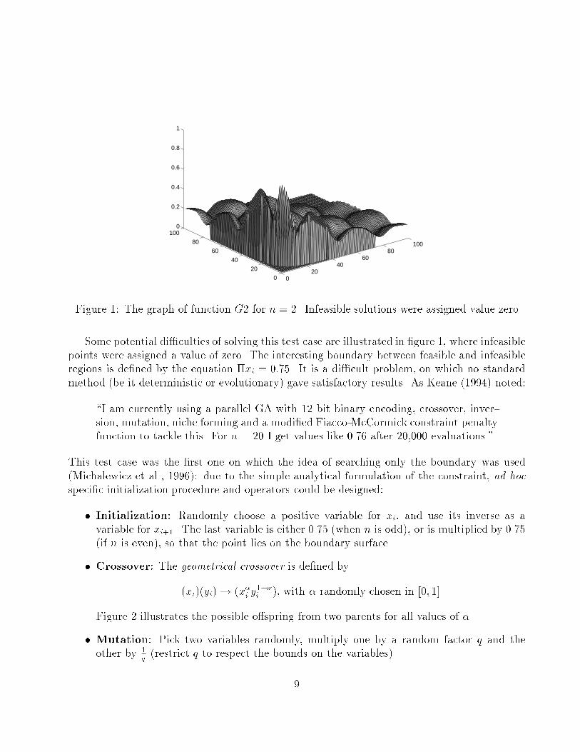
Figure 1: The graph of function G2 for n = 2. Infeasible solutions were assigned value zero

Some potential di�culties of solving this test case are illustrated in �gure 1, where infeasiblepoints were assigned a value of zero. The interesting boundary between feasible and infeasibleregions is de�ned by the equation �xi = 0:75. It is a di�cult problem, on which no standardmethod (be it deterministic or evolutionary) gave satisfactory results. As Keane (1994) noted:

\I am currently using a parallel GA with 12 bit binary encoding, crossover, inver-sion, mutation, niche forming and a modi�ed Fiacco-McCormick constraint penaltyfunction to tackle this. For n = 20 I get values like 0.76 after 20,000 evaluations."

This test case was the �rst one on which the idea of searching only the boundary was used(Michalewicz et al., 1996): due to the simple analytical formulation of the constraint, ad hocspeci�c initialization procedure and operators could be designed:

� Initialization: Randomly choose a positive variable for xi, and use its inverse as avariable for xi+1. The last variable is either 0.75 (when n is odd), or is multiplied by 0.75(if n is even), so that the point lies on the boundary surface.

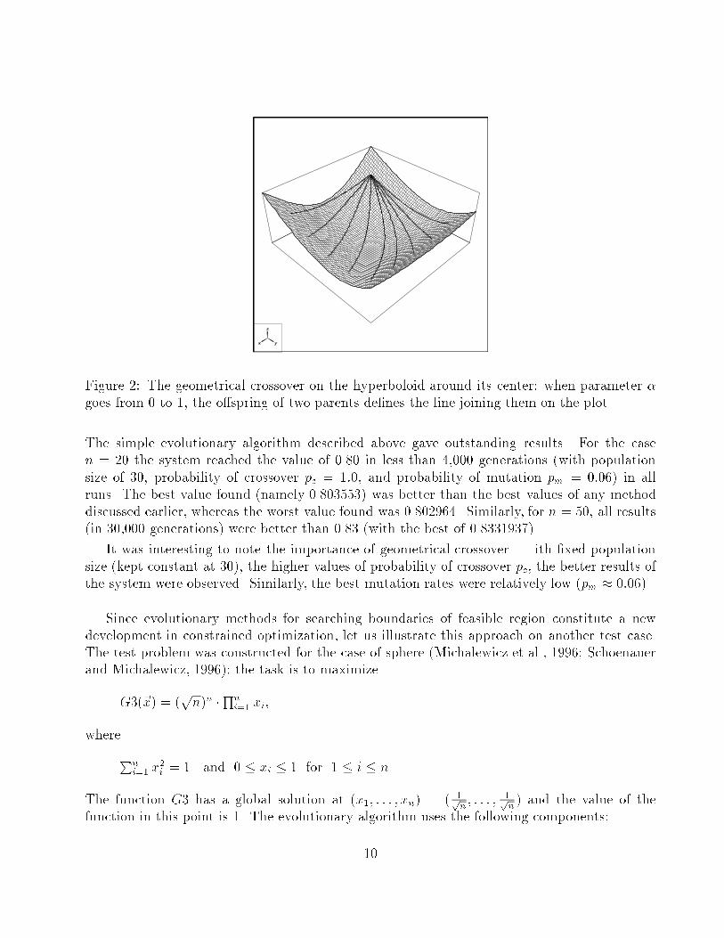
� Crossover: The geometrical crossover is de�ned by

(xi)(yi)! (x�i y1��i ), with � randomly chosen in [0; 1]

Figure 2 illustrates the possible o�spring from two parents for all values of �.

� Mutation: Pick two variables randomly, multiply one by a random factor q and theother by 1

q(restrict q to respect the bounds on the variables).

9

x y

z

Figure 2: The geometrical crossover on the hyperboloid around its center: when parameter �goes from 0 to 1, the o�spring of two parents de�nes the line joining them on the plot.

The simple evolutionary algorithm described above gave outstanding results. For the casen = 20 the system reached the value of 0.80 in less than 4,000 generations (with populationsize of 30, probability of crossover pc = 1:0, and probability of mutation pm = 0:06) in allruns. The best value found (namely 0.803553) was better than the best values of any methoddiscussed earlier, whereas the worst value found was 0.802964. Similarly, for n = 50, all results(in 30,000 generations) were better than 0.83 (with the best of 0.8331937).

It was interesting to note the importance of geometrical crossover. With �xed populationsize (kept constant at 30), the higher values of probability of crossover pc, the better results ofthe system were observed. Similarly, the best mutation rates were relatively low (pm � 0:06).

Since evolutionary methods for searching boundaries of feasible region constitute a newdevelopment in constrained optimization, let us illustrate this approach on another test case.The test problem was constructed for the case of sphere (Michalewicz et al., 1996; Schoenauerand Michalewicz, 1996); the task is to maximize

G3(~x) = (pn)n �Qn

i=1 xi,

where

Pni=1 x

2i = 1 and 0 � xi � 1 for 1 � i � n.

The function G3 has a global solution at (x1; : : : ; xn) = ( 1pn; : : : ; 1p

n) and the value of the

function in this point is 1. The evolutionary algorithm uses the following components:

10

� Initialization: Randomly generate n variables yi, calculate s =Pn

i=1 y2i , and initialize

an individual (xi) by x = yi=s for i 2 [1; n].

� Crossover: The sphere crossover produces one o�spring (zi) from two parents (xi) and(yi) by:

zi =q�x2i + (1 � �)y2i i 2 [1; n], with � randomly chosen in [0; 1]:

� Mutation: Similarly, the problem-speci�c mutation transforms (xi) by selecting twoindices i 6= j and a random number p in h0; 1i, and setting:

xi ! p � xi and xj ! q � xj;where q =s(xixj)2(1 � p2) + 1:

The simple evolutionary algorithm described above gave very good results. For the case n = 20the system reached the value of 0.99 in less than 6,000 generations (with population size of 30,probability of crossover pc = 1:0, and probability of mutation pm = 0:06) in all runs. The bestvalue found in 10,000 generations was 0.999866.

3.2 Methods based on penalty functions

In Evolutionary Computation as in many other �elds of optimization, most of the constraint-handling methods are based on the concept of (exterior) penalty functions, which penalizeinfeasible solutions, i.e. try to solve an unconstrained problem (on F) using the modi�ed�tness function:

eval(~x) =

(f(~x); if ~x 2 Ff(~x) + penalty(~x); otherwise;

where penalty(~x) is zero, if no violation occurs, and is positive, otherwise. Usually, the penaltyfunction is based on the distance of a solution from the feasible region F , or on the e�ort to\repair" the solution, i.e., to force it into F . The former case is the most popular one; in manymethods a set of functions fj (1 � j � m) is used to construct the penalty, where the functionfj measures the violation of the j-th constraint in the following way:

fj(~x) =

(maxf0; gj(~x)g; if 1 � j � qjhj(~x)j; if q + 1 � j � m:

However, these methods di�er in many important details, how the penalty function is designedand applied to infeasible solutions. In the following subsections we discuss all known methodsin turn.

11

3.2.1 Method of static penalties

The method was proposed by Homaifar, Lai, and Qi (1994); it assumes that for every constraintwe establish a family of intervals which determine appropriate penalty coe�cient. It works asfollows:

� for each constraint, create several (`) levels of violation,

� for each level of violation and for each constraint, create a penalty coe�cient Rij (i =1; 2; : : : ; `, j = 1; 2; : : : ;m); higher levels of violation require larger values of this coe�-cient.

� start with a random population of individuals (feasible or infeasible),

� evolve the population; evaluate individuals using the following formula

eval(~x) = f(~x) +Pm

j=1Rijf2j (~x).

The weakness of the method is in the number of parameters. For m constraints the methodrequires m(2`+1) parameters in total: m parameters to establish number of intervals for eachconstraint, ` parameters for each constraint, de�ning the boundaries of the intervals (levels ofviolation), and ` parameters for each constraint representing the penalty coe�cients Rij . Inparticular, for m = 5 constraints and ` = 4 levels of violation, we need to set 45 parameters!Clearly, the results are parameter dependent. It is quite likely that for a given problem thereexist one optimal set of parameters for which the system returns feasible near-optimum solution,however, it might be quite hard to �nd it.

A limited set of experiments reported by Michalewicz (1995a) indicates that the method canprovide good results if violation levels and penalty coe�cients Rij are tuned to the problem.For example, Homaifar et al. (1994) experimented with the following problem (Himmelblau,1992). Minimize a function of 5 variables:

G4(~x) = 5:3578547x23 + 0:8356891x1x5 + 37:293239x1 � 40792:141,

subject to three double inequalities:

0 � 85:334407 + 0:0056858x2x5 + 0:00026x1x4 � 0:0022053x3x5 � 9290 � 80:51249 + 0:0071317x2x5 + 0:0029955x1x2 + 0:0021813x23 � 11020 � 9:300961 + 0:0047026x3x5 + 0:0012547x1x3 + 0:0019085x3x4 � 25,

and bounds:

78 � x1 � 102, 33 � x2 � 45, 27 � xi � 45 for i = 3; 4; 5.

The best solution obtained in 10 runs (Homaifar et al., 1994) was

12

~x = (80:49; 35:07; 32:05; 40:33; 33:34)

with G4(~x) = �30005:7, whereas the optimum solution (Himmelblau, 1992) is

~x� = (78:0; 33:0; 29:995; 45:0; 36:776),

with G4(~x�) = �30665:5. Two constraints (upper bound of the �rst inequality and the lowerbound of the third inequality) are active at the optimum.

However, the importance of proper values for penalty coe�cients should be emphasized.For example, Homaifar et al. (1994) reported a value 50 for such penalty coe�cient for theviolation of the lower boundary of the �rst constraint and the value of 2.5 for the violationof the upper boundary of the �rst constraints, without any comments on the source for thesevalues.

3.2.2 Method of dynamic penalties

The method was proposed by Joines and Houck (1994). As opposed to the previous method,the authors assumed dynamic penalties. Individuals are evaluated (at the iteration t) by thefollowing formula:

eval(~x) = f(~x) + (C � t)�Pm

j=1 f�j (~x),

where C, � and � are constants. A reasonable choice for these parameters, reported by Joinesand Houck (1994), is C = 0:5, � = � = 2. The method requires much smaller number(independent of the number of constraints) of parameters than the �rst method. Also, insteadof de�ning several levels of violation, the pressure on infeasible solutions is increased due to the(C � t)� component of the penalty term: towards the end of the process (for high values of thegeneration number t), this component assumes large values.

One of the problems (Hock and Schittkowski, 1981) experimented by Joines and Houck(1994) was to minimize a function

G5(~x) = 3x1 + 0:000001x31 + 2x2 + 0:000002=3x32

subject to

x4 � x3 + 0:55 � 0, x3 � x4 + 0:55 � 0,1000 sin(�x3 � 0:25) + 1000 sin(�x4 � 0:25) + 894:8 � x1 = 01000 sin(x3 � 0:25) + 1000 sin(x3 � x4 � 0:25) + 894:8 � x2 = 01000 sin(x4 � 0:25) + 1000 sin(x4 � x3 � 0:25) + 1294:8 = 00 � xi � 1200, i = 1; 2, and �0:55 � xi � 0:55, i = 3; 4.

The best known solution is

13

~x� = (679:9453; 1026:067; 0:1188764;�0:3962336),

and G5(~x�) = 5126:4981.

The best result of experiments reported by Joines and Houck (1994) (many runs, variousvalues of � and �) gave a value of 5126.6653 of the objective function. No solution was fullyfeasible due to the three equality constraints, but the sum of the violated constraints was quitesmall (10�4). On the other hand, the method seems to provide too strong penalties: often thefactor (C � t)� grows too fast to be useful. The system has little chances to escape from localoptima: in most experiments reported by Michalewicz (1995a) the best individual was foundin early generations. The method gave very good results for test cases where the objectivefunctions were quadratic.

3.2.3 Method of annealing penalties

This method, called Genocop II, is also based on dynamic penalties and was described byMichalewicz and Attia (1994) and Michalewicz (1996). Its modi�ed version works as follows:

� divide all constraints into four subsets: linear equations, linear inequalities, nonlinearequations, and nonlinear inequalities,

� select a random single point as a starting point (the initial population consists of copiesof this single individual). This initial point satis�es linear constraints,

� set the initial temperature � = �0,

� evolve the population using the following formula:

eval(~x; � ) = f(~x) + 12�

Pmj=1 f

2j (~x),

� if � < �f , stop, otherwise

{ decrease temperature � ,

{ the best solution serves as a starting point of the next iteration,

{ repeat the previous step of the algorithm.

This is the only method we are aware of (except Genocop III, section 3.3.3) which distin-guishes between linear and nonlinear constraints. The algorithm maintains feasibility of alllinear constraints using a set of closed operators, which convert a feasible solution (feasible interms of linear constraints only) into another feasible solution. At every iteration the algorithmconsiders active constraints only, the pressure on infeasible solutions is increased due to thedecreasing values of temperature � .

14

The method has an additional unique feature: it starts from a single point.2 Consequently,it is relatively easy to compare this method with other classical optimization methods whoseperformance are tested (for a given problem) from some starting point.

The method requires a starting and `freezing' temperatures, �0 and �f , respectively, andthe cooling scheme to decrease temperature � . Standard values (reported by Michalewicz andAttia (1994)) are �0 = 1, �i+1 = 0:1 � �i, with �f = 0:000001.

One of the test problems (Floudas and Pardalos, 1987) experimented by Michalewicz andAttia (1994) was:

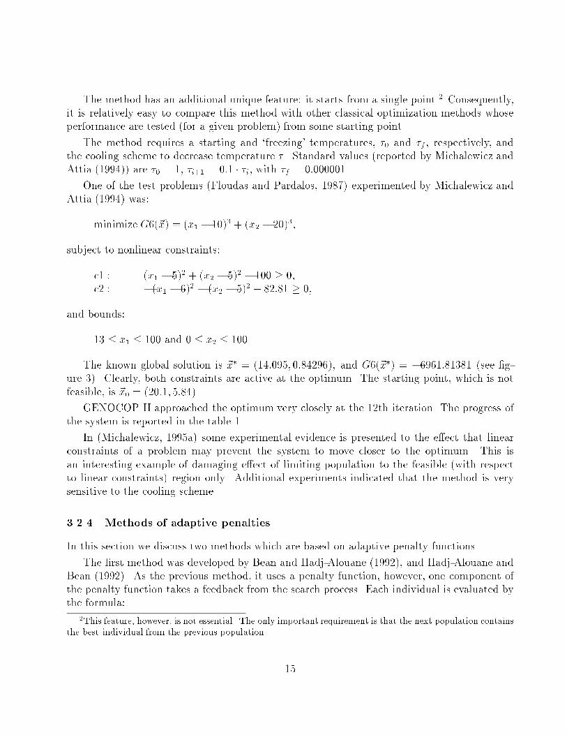
minimize G6(~x) = (x1 � 10)3 + (x2 � 20)3,

subject to nonlinear constraints:

c1 : (x1 � 5)2 + (x2 � 5)2 � 100 � 0,c2 : �(x1 � 6)2 � (x2 � 5)2 + 82:81 � 0,

and bounds:

13 � x1 � 100 and 0 � x2 � 100.

The known global solution is ~x� = (14:095; 0:84296), and G6(~x�) = �6961:81381 (see �g-ure 3). Clearly, both constraints are active at the optimum. The starting point, which is notfeasible, is ~x0 = (20:1; 5:84).

GENOCOP II approached the optimum very closely at the 12th iteration. The progress ofthe system is reported in the table 1.

In (Michalewicz, 1995a) some experimental evidence is presented to the e�ect that linearconstraints of a problem may prevent the system to move closer to the optimum. This isan interesting example of damaging e�ect of limiting population to the feasible (with respectto linear constraints) region only. Additional experiments indicated that the method is verysensitive to the cooling scheme.

3.2.4 Methods of adaptive penalties

In this section we discuss two methods which are based on adaptive penalty functions.

The �rst method was developed by Bean and Hadj-Alouane (1992), and Hadj-Alouane andBean (1992). As the previous method, it uses a penalty function, however, one component ofthe penalty function takes a feedback from the search process. Each individual is evaluated bythe formula:

2This feature, however, is not essential. The only important requirement is that the next population containsthe best individual from the previous population.

15

feasiblespace

optimum

(14.095, 0.84296)

Figure 3: A feasible space for test case of G6

eval(~x) = f(~x) + �(t)Pm

j=1 f2j (~x),

where �(t) is updated every generation t in the following way:

�(t+ 1) =

8>><>>:

(1=�1) � �(t); if ~bi 2 F for all t� k + 1 � i � t

�2 � �(t); if ~bi 2 S �F for all t� k + 1 � i � t�(t); otherwise;

where ~bi denotes the best individual, in terms of function eval, in generation i, �1; �2 > 1 and�1 6= �2 (to avoid cycling). In other words, the method (1) decreases the penalty component�(t + 1) for the generation t + 1, if all best individuals in the last k generations were feasible,and (2) increases penalties, if all best individuals in the last k generations were infeasible. Ifthere are some feasible and infeasible individuals as best individuals in the last k generations,�(t+ 1) remains without change.

The method introduces three additional parameters, �1, �2, and the time horizon, k. Itseems that there is an interesting analogy between this method and the method used in earlyevolution strategies to optimize the convergence rate, where a \1/5 success rule" was proposed(Rechenberg, 1973; B�ack et al., 1991):

The ratio ' of successful mutations to all mutations should be 1/5. Increase thevariance of the mutation operator, if ' is greater than 1/5; otherwise, decrease it.

The 1/5 success rule emerged as a conclusion of the process of optimizing convergence rates oftwo functions (the so-called corridor model and sphere model). The rule was applied every k

16

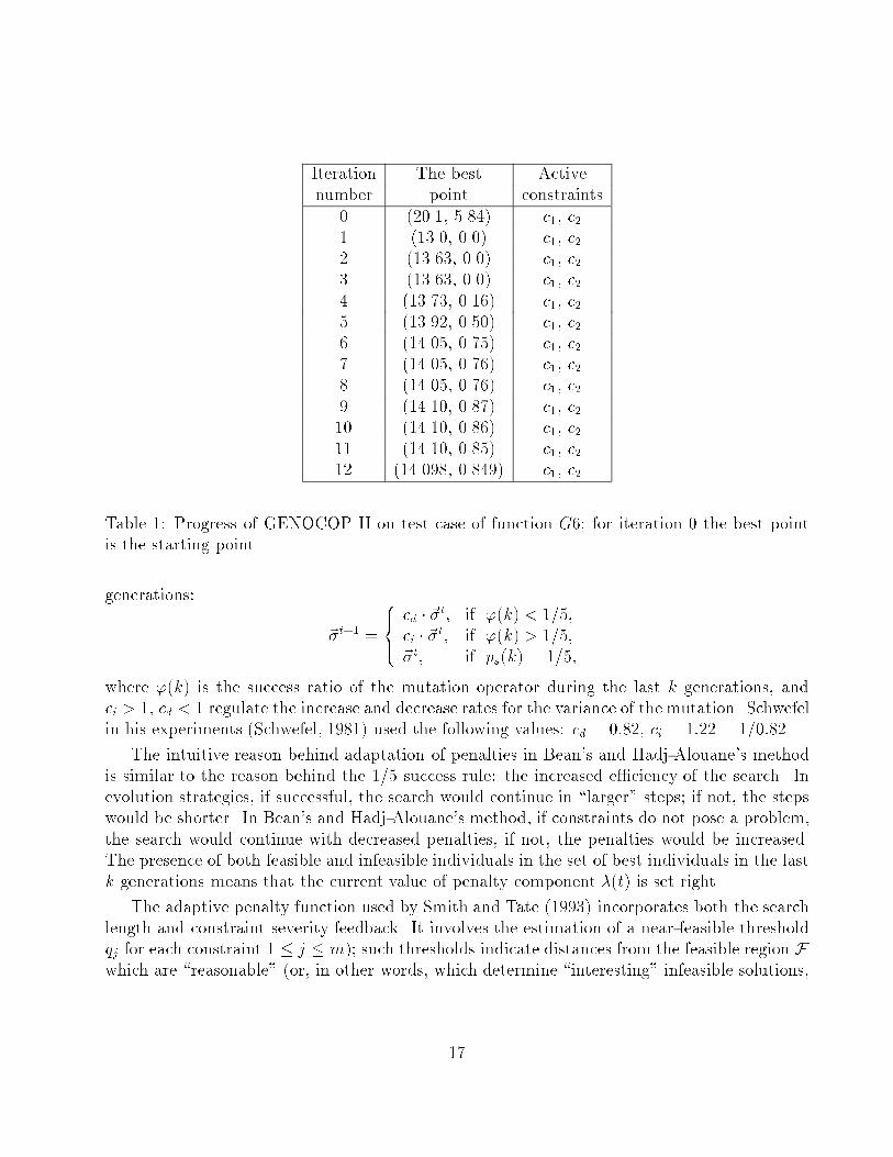
Iteration The best Activenumber point constraints

0 (20.1, 5.84) c1, c21 (13.0, 0.0) c1, c22 (13.63, 0.0) c1, c23 (13.63, 0.0) c1, c24 (13.73, 0.16) c1, c25 (13.92, 0.50) c1, c26 (14.05, 0.75) c1, c27 (14.05, 0.76) c1, c28 (14.05, 0.76) c1, c29 (14.10, 0.87) c1, c210 (14.10, 0.86) c1, c211 (14.10, 0.85) c1, c212 (14.098, 0.849) c1, c2

Table 1: Progress of GENOCOP II on test case of function G6; for iteration 0 the best pointis the starting point.

generations:

~�t+1 =

8><>:

cd � ~�t; if '(k) < 1=5;ci � ~�t; if '(k) > 1=5;~�t; if ps(k) = 1=5;

where '(k) is the success ratio of the mutation operator during the last k generations, andci > 1, cd < 1 regulate the increase and decrease rates for the variance of the mutation. Schwefelin his experiments (Schwefel, 1981) used the following values: cd = 0:82, ci = 1:22 = 1=0:82.

The intuitive reason behind adaptation of penalties in Bean's and Hadj-Alouane's methodis similar to the reason behind the 1/5 success rule: the increased e�ciency of the search. Inevolution strategies, if successful, the search would continue in \larger" steps; if not, the stepswould be shorter. In Bean's and Hadj-Alouane's method, if constraints do not pose a problem,the search would continue with decreased penalties, if not, the penalties would be increased.The presence of both feasible and infeasible individuals in the set of best individuals in the lastk generations means that the current value of penalty component �(t) is set right.

The adaptive penalty function used by Smith and Tate (1993) incorporates both the searchlength and constraint severity feedback. It involves the estimation of a near-feasible thresholdqj for each constraint 1 � j � m); such thresholds indicate distances from the feasible region Fwhich are \reasonable" (or, in other words, which determine \interesting" infeasible solutions,

17

i.e., solutions relatively close to the feasible region). Thus the evaluation function is de�ned as

eval(~x; t) = f(~x) + Ffeas(t)� Fall(t)mXj=1

(fj(~x)=qj(t))k;

where Fall(t) denotes the unpenalized value of the best solution yet found (up to generation t),Ffeas(t) denotes the value of the best feasible solution yet found (up to generation t), and kis a constant. Note, that the near-feasible thresholds qj(t) are dynamic, i.e., they are adjustedduring the search (for example, it is possible to de�ne qj(t) = qj(0)=(1 + �jt) thus resulting inincreasing the penalty component over time).

To the best of our knowledge, neither of the adaptive methods described in this subsectionhas been applied to continuous nonlinear programming problems.

3.2.5 Death penalty method

This method just rejects infeasible individuals (death penalty); the method has been used byevolution strategies (B�ack et al., 1991) and simulated annealing. For some problems, this simplemethod provides quality results.

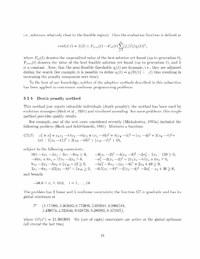
For example, one of the test cases considered recently (Michalewicz, 1995a) included thefollowing problem (Hock and Schittkowski, 1981). Minimize a function:

G7(~x) = x21 + x22 + x1x2 � 14x1 � 16x2 + (x3 � 10)2 + 4(x4 � 5)2 + (x5 � 3)2 + 2(x6 � 1)2+5x27 + 7(x8 � 11)2 + 2(x9 � 10)2 + (x10 � 7)2 + 45,

subject to the following constraints:

105 � 4x1 � 5x2 + 3x7 � 9x8 � 0, �3(x1 � 2)2 � 4(x2 � 3)2 � 2x23 + 7x4 + 120 � 0,�10x1 + 8x2 + 17x7 � 2x8 � 0, �x21 � 2(x2 � 2)2 + 2x1x2 � 14x5 + 6x6 � 0,8x1 � 2x2 � 5x9 + 2x10 + 12 � 0, �5x21 � 8x2 � (x3 � 6)2 + 2x4 + 40 � 0,3x1 � 6x2 � 12(x9 � 8)2 + 7x10 � 0, �0:5(x1 � 8)2 � 2(x2 � 4)2 � 3x25 + x6 + 30 � 0,

and bounds

�10:0 � xi � 10:0, i = 1; : : : ; 10.

The problem has 3 linear and 5 nonlinear constraints; the function G7 is quadratic and has itsglobal minimum at

~x� = (2:171996; 2:363683; 8:773926; 5:095984; 0:9906548;1:430574; 1:321644; 9:828726; 8:280092; 8:375927),

where G7(~x�) = 24:3062091. Six (out of eight) constraints are active at the global optimum(all except the last two).

18

The \death penalty" method provided with respectable solutions the best of which hadthe value of 25.653. To evaluate this method it is necessary to initialize a population byfeasible solutions. This di�erent initialization scheme makes the comparison of all the methodseven harder. However, in experiments reported in (Michalewicz, 1995a), an interesting patternemerged: the method generally gave a quite poor performance. Also, the method was not asstable as other methods; the standard deviation of returned solutions was relatively high.

3.2.6 Segregated genetic algorithm

The method of so-called segregated genetic algorithm was proposed by Le Riche et al. (1995)as yet another way to handle the problem of the robustness of the penalty level (see section3.2). The tuning of the penalty level encounters the following dilemma: a too small penaltylevel leads to solutions which are infeasible (some penalized points still exhibit higher penalized�tness than the best feasible point); a too high penalty level restricts the search inside thefeasible region, forbidding any shot-cut across the infeasible region, and thus eventually failingto converge to the optimal solution.

The idea is to design two di�erent penalized �tness functions with static penalty terms p1and p2 (see section 3.2): penalty p1 is purposely too small, while penalty p2 is hopefully toohigh. All individuals of the current population undergo crossover and mutation. The valuesof the two �tness functions fi(~x) = f(~x) + pi(~x), i = 1; 2, are computed for each resultingo�spring (at no extra cost in term of objective function evaluation), and two ranked lists arecreated according to the values of the �tnesses of all individuals (parents plus o�spring) foreach one of the �tnesses. The selection of the parents of next generation is then achieved bypicking up alternatively the best individual from each list (and removing this individual fromboth lists afterwards). The main idea is that such a selection scheme will result roughly inmaintaining two subpopulations: the individuals selected on the basis of f1 will more likelylie in the infeasible region while the ones selected on the basis of f2 will probably stay in thefeasible region; the overall process is thus allowed to reach the feasible optimum from both sidesof the boundary of the feasible region.

This method gave excellent results in the domain of Laminated Design Optimization (LeRiche et al., 1995), but has not yet, to the best of our knowledge, been applied to continuousnonlinear programming problems.

3.3 Methods based on a search for feasible solutions

There are a few methods which emphasize the distinction between feasible and infeasible so-lutions in the search space S. One method considers the problem constraints in a sequence; aswitch from one constraint to another is made upon arrival of a su�cient number of feasibleindividuals in the population. The second method is based on an assumption, that any feasible

19

solution is better than any infeasible one. The third method repairs infeasible individuals. Wediscuss these methods in turn.

3.3.1 Behavioral memory method

The method was proposed by Schoenauer and Xanthakis (1993); the authors called this methoda \behavioral memory" approach. It works as follows:

� start with a random population of individuals (feasible or infeasible),

� set j = 1 (j is a constraint counter),

� evolve this population with eval(~x) = fj(~x), until a given percentage of the population(so-called ip threshold �) is feasible for this constraint,3

� set j = j + 1,

� the current population is the starting point for the next phase of the evolution, whereeval(~x) = fj(~x) (de�ned in the section 3.2). During this phase, points that do not satisfyone of the 1st, 2nd, ..., or (j � 1)-th constraint are eliminated from the population.The stop criterion is again the satisfaction of the j-th constraint by the ip thresholdpercentage � of the population.

� if j < m, repeat the last two steps, otherwise (j = m) optimize the objective function,i.e., eval(~x) = f(~x), rejecting infeasible individuals.

The method requires a linear order of all constraints which are processed in turn. It is unclearwhat is the in uence of the order of constraints on the results of the algorithm; our experimentsindicated that di�erent orders provide di�erent results (di�erent in the sense of the total runningtime and precision).

In total, the method requires three parameters: the sharing factor �, the ip threshold �,and a particular order of constraints. The method is very di�erent to the other methods, and,in general, is di�erent than other penalty approaches, since it considers only one constraint atthe time. Also, in the last step of the algorithm the method optimizes the objective function fitself with a death penalty.

The method was evaluated by Schoenauer and Xanthakis (1993) on the following problem:

Maximize the function

G8(~x) = sin3(2�x1)�sin(2�x2)x3�(x1+x2)

,

subject to the following constraints:

3The method suggests the use of a sharing scheme to maintain diversity of the population.

20

c1(~x) = x21 � x2 + 1 � 0,c2(~x) = 1� x1 + (x2 � 4)2 � 0

and bounds:

0 � x1 � 10 and 0 � x2 � 10.

0

1

2

3

4

0

10

5

0

1

2

3

4

0

1

2

3

4

0

1

2

3

4

0

10

5

x y

z

Function G8

0

1

2

3

4

-10

0

10

-5

5

0

12

3

4

0

12

3

4

0

1

2

3

4

-10

0

10

-5

5

x y

z

Penalty factor = 1

0

1

2

3

4

-10

0

10

-5

5

0

12

3

4

0

12

3

4

0

1

2

3

4

-10

0

10

-5

5

x y

z

Penalty factor = 50

Figure 4: Function G8 together with two �tness landscapes corresponding to two di�erentpenalization parameters �: a small value of � leaves the highest peaks outside the feasibleregion, while a large value of � makes the feasible region look like a needle in a haystack (allplots are truncated between �10 and 10 for the sake of visibility)

Function G8 has many local optima, the highest peaks are located along the x axis (e.g.,G8(0:00015; 0:0225) > 1540). In the feasible region, however, G8 has two maxima of almostequal �tness of value of 0.1. Figures 4 show the penalized �tness landscape for di�erent penaltyparameters (i.e., plots of the function G8(~x) � �(c1(~x)+ + c1(~x)+) for di�erent values of �).All values of the penalized function are truncated at �10 and 10 to allow values in the feasibleregion (around 0) to be distinguishable.

This situation makes any attempt to use penalty parameters a di�cult task: small penaltyparameters leave the feasible region hidden among much higher peaks of the penalized �tness(Figure 4-b) while penalty parameters large enough to allow the feasible region to really out-stand in the penalized-�tness landscape imply vertical slopes of that region (Figure 4-c): thepartial credit principle, allowing the evolutionary algorithm to gently climb such slopes is notvalid, and the discovery of the global maximum of the penalized �tness thus relies on a luckymove from the huge and at low-�tness region.

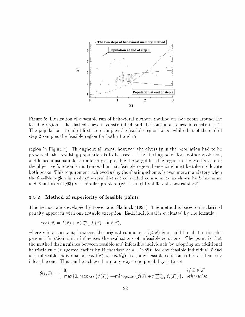
On the other hand, the behavioral memory method has no di�culty in localizing 80% ofthe population �rst into the feasible region for constraint c1 (step 1), then into the feasibleregion for both constraints (step 2), as can be seen on Figure 5. The optimization of G8itself in that region is then straightforward (see the smooth bimodal �tness landscape in that

21

X1

X2

0 1 2 3

1

3

5

7

9

The two steps of behavioral memory method

Population at end of step 1

Population at end of step 2

Figure 5: Illustration of a sample run of behavioral memory method on G8: zoom around thefeasible region. The dashed curve is constraint c1 and the continuous curve is constraint c2.The population at end of �rst step samples the feasible region for c1 while that of the end ofstep 2 samples the feasible region for both c1 and c2

region in Figure 4). Throughout all steps, however, the diversity in the population had to bepreserved: the resulting population is to be used as the starting point for another evolution,and hence must sample as uniformly as possible the target feasible region in the two �rst steps;the objective function is multi-modal in that feasible region, hence care must be taken to locateboth peaks. This requirement, achieved using the sharing scheme, is evenmore mandatory whenthe feasible region is made of several distinct connected components, as shown by Schoenauerand Xanthakis (1993) on a similar problem (with a slightly di�erent constraint c2).

3.3.2 Method of superiority of feasible points

The method was developed by Powell and Skolnick (1993). The method is based on a classicalpenalty approach with one notable exception. Each individual is evaluated by the formula:

eval(~x) = f(~x) + rPm

j=1 fj(~x) + �(t; ~x),

where r is a constant; however, the original component �(t; ~x) is an additional iteration de-pendent function which in uences the evaluations of infeasible solutions. The point is thatthe method distinguishes between feasible and infeasible individuals by adopting an additionalheuristic rule (suggested earlier by Richardson et al., 1989): for any feasible individual ~x andany infeasible individual ~y: eval(~x) < eval(~y), i.e., any feasible solution is better than anyinfeasible one. This can be achieved in many ways; one possibility is to set

�(t; ~x) =

(0; if ~x 2 Fmaxf0;max~x2Fff(~x)g �min~x2S�Fff(~x) + r

Pmj=1 fj(~x)gg; otherwise:

22

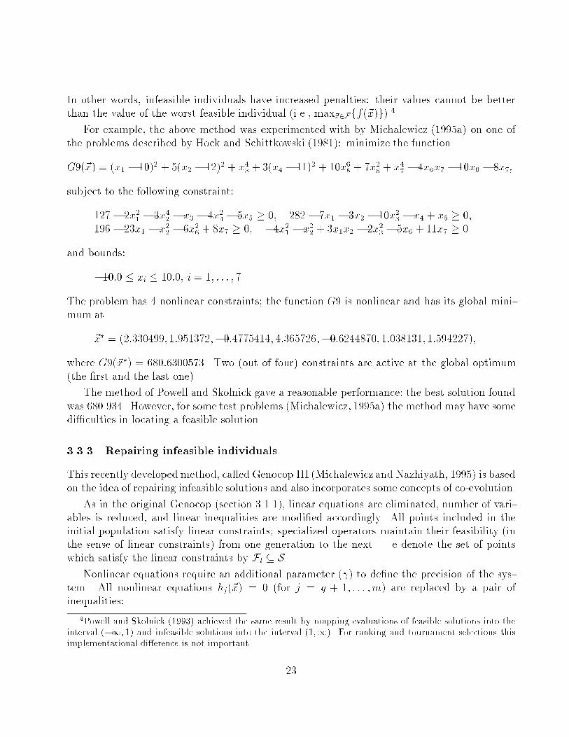
In other words, infeasible individuals have increased penalties: their values cannot be betterthan the value of the worst feasible individual (i.e., max~x2Fff(~x)g).4

For example, the above method was experimented with by Michalewicz (1995a) on one ofthe problems described by Hock and Schittkowski (1981): minimize the function

G9(~x) = (x1 � 10)2 + 5(x2 � 12)2 + x43 + 3(x4 � 11)2 + 10x65 + 7x26 + x47 � 4x6x7 � 10x6 � 8x7,

subject to the following constraint:

127 � 2x21 � 3x42 � x3 � 4x24 � 5x5 � 0, 282 � 7x1 � 3x2 � 10x23 � x4 + x5 � 0,196 � 23x1 � x22 � 6x26 + 8x7 � 0, �4x21 � x22 + 3x1x2 � 2x23 � 5x6 + 11x7 � 0

and bounds:

�10:0 � xi � 10:0, i = 1; : : : ; 7.

The problem has 4 nonlinear constraints; the function G9 is nonlinear and has its global mini-mum at

~x� = (2:330499; 1:951372;�0:4775414; 4:365726;�0:6244870; 1:038131; 1:594227),

where G9(~x�) = 680:6300573. Two (out of four) constraints are active at the global optimum(the �rst and the last one).

The method of Powell and Skolnick gave a reasonable performance; the best solution foundwas 680.934. However, for some test problems (Michalewicz, 1995a) the method may have somedi�culties in locating a feasible solution.

3.3.3 Repairing infeasible individuals

This recently developed method, called Genocop III (Michalewicz and Nazhiyath, 1995) is basedon the idea of repairing infeasible solutions and also incorporates some concepts of co-evolution.

As in the original Genocop (section 3.1.1), linear equations are eliminated, number of vari-ables is reduced, and linear inequalities are modi�ed accordingly. All points included in theinitial population satisfy linear constraints; specialized operators maintain their feasibility (inthe sense of linear constraints) from one generation to the next. We denote the set of pointswhich satisfy the linear constraints by Fl � S.

Nonlinear equations require an additional parameter ( ) to de�ne the precision of the sys-tem. All nonlinear equations hj(~x) = 0 (for j = q + 1; : : : ;m) are replaced by a pair ofinequalities:

4Powell and Skolnick (1993) achieved the same result by mapping evaluations of feasible solutions into theinterval (�1; 1) and infeasible solutions into the interval (1;1). For ranking and tournament selections thisimplementational di�erence is not important.

23

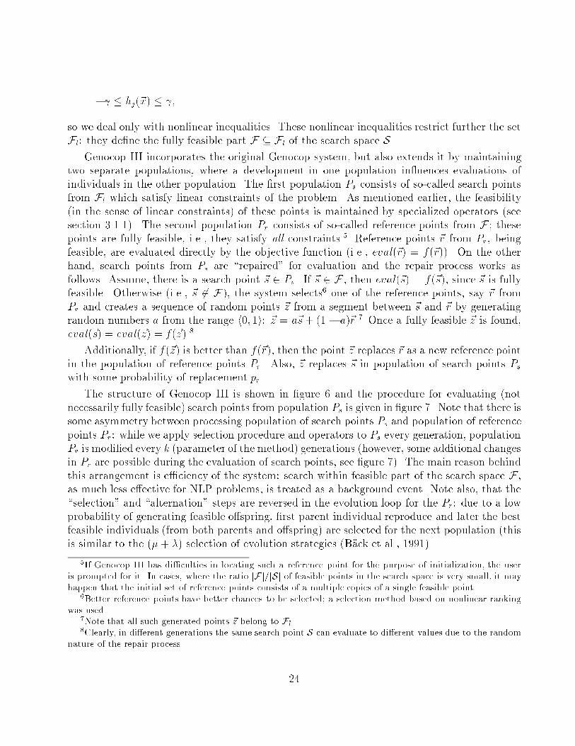
� � hj(~x) � ,

so we deal only with nonlinear inequalities. These nonlinear inequalities restrict further the setFl: they de�ne the fully feasible part F � Fl of the search space S.

Genocop III incorporates the original Genocop system, but also extends it by maintainingtwo separate populations, where a development in one population in uences evaluations ofindividuals in the other population. The �rst population Ps consists of so-called search pointsfrom Fl which satisfy linear constraints of the problem. As mentioned earlier, the feasibility(in the sense of linear constraints) of these points is maintained by specialized operators (seesection 3.1.1). The second population Pr consists of so-called reference points from F ; thesepoints are fully feasible, i.e., they satisfy all constraints.5 Reference points ~r from Pr, beingfeasible, are evaluated directly by the objective function (i.e., eval(~r) = f(~r)). On the otherhand, search points from Ps are \repaired" for evaluation and the repair process works asfollows. Assume, there is a search point ~s 2 Ps. If ~s 2 F , then eval(~s) = f(~s), since ~s is fullyfeasible. Otherwise (i.e., ~s 62 F), the system selects6 one of the reference points, say ~r fromPr and creates a sequence of random points ~z from a segment between ~s and ~r by generatingrandom numbers a from the range h0; 1i: ~z = a~s+ (1 � a)~r.7 Once a fully feasible ~z is found,eval(~s) = eval(~z) = f(~z).8

Additionally, if f(~z) is better than f(~r), then the point ~z replaces ~r as a new reference pointin the population of reference points Pr. Also, ~z replaces ~s in population of search points Ps

with some probability of replacement pr.

The structure of Genocop III is shown in �gure 6 and the procedure for evaluating (notnecessarily fully feasible) search points from population Ps is given in �gure 7. Note that there issome asymmetry between processing population of search points Ps and population of referencepoints Pr: while we apply selection procedure and operators to Ps every generation, populationPr is modi�ed every k (parameter of the method) generations (however, some additional changesin Pr are possible during the evaluation of search points, see �gure 7). The main reason behindthis arrangement is e�ciency of the system: search within feasible part of the search space F ,as much less e�ective for NLP problems, is treated as a background event. Note also, that the\selection" and \alternation" steps are reversed in the evolution loop for the Pr: due to a lowprobability of generating feasible o�spring, �rst parent individual reproduce and later the bestfeasible individuals (from both parents and o�spring) are selected for the next population (thisis similar to the (�+ �) selection of evolution strategies (B�ack et al., 1991).

5If Genocop III has di�culties in locating such a reference point for the purpose of initialization, the useris prompted for it. In cases, where the ratio jFj=jSj of feasible points in the search space is very small, it mayhappen that the initial set of reference points consists of a multiple copies of a single feasible point.

6Better reference points have better chances to be selected; a selection method based on nonlinear rankingwas used.

7Note that all such generated points ~z belong to Fl.8Clearly, in di�erent generations the same search point S can evaluate to di�erent values due to the random

nature of the repair process.

24

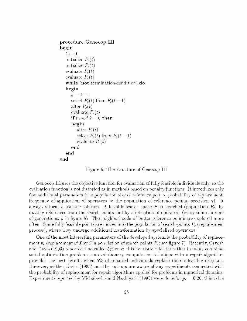
procedure Genocop III

begin

t 0initialize Ps(t)initialize Pr(t)evaluate Ps(t)evaluate Pr(t)while (not termination-condition) dobegin

t t+ 1select Ps(t) from Ps(t� 1)alter Ps(t)evaluate Ps(t)if t mod k = 0 thenbegin

alter Pr(t)select Pr(t) from Pr(t� 1)evaluate Pr(t)

end

end

end

Figure 6: The structure of Genocop III

Genocop III uses the objective function for evaluation of fully feasible individuals only, so theevaluation function is not distorted as in methods based on penalty functions. It introduces onlyfew additional parameters (the population size of reference points, probability of replacement,frequency of application of operators to the population of reference points, precision ). Italways returns a feasible solution. A feasible search space F is searched (population Pr) bymaking references from the search points and by application of operators (every some numberof generations, k in �gure 6). The neighborhoods of better reference points are explored moreoften. Some fully feasible points are moved into the population of search-points Ps (replacementprocess), where they undergo additional transformation by specialized operators.

One of the most interesting parameters of the developed system is the probability of replace-ment pr (replacement of ~s by ~z in population of search points Ps; see �gure 7). Recently, Orvoshand Davis (1993) reported a so-called 5%-rule: this heuristic rule states that in many combina-torial optimization problems, an evolutionary computation technique with a repair algorithmprovides the best results when 5% of repaired individuals replace their infeasible originals.However, neither Davis (1995) nor the authors are aware of any experiments connected withthe probability of replacement for repair algorithms applied for problems in numerical domains.Experiments reported by Michalewicz and Nazhiyath (1995) were done for pr = 0:20; this value

25

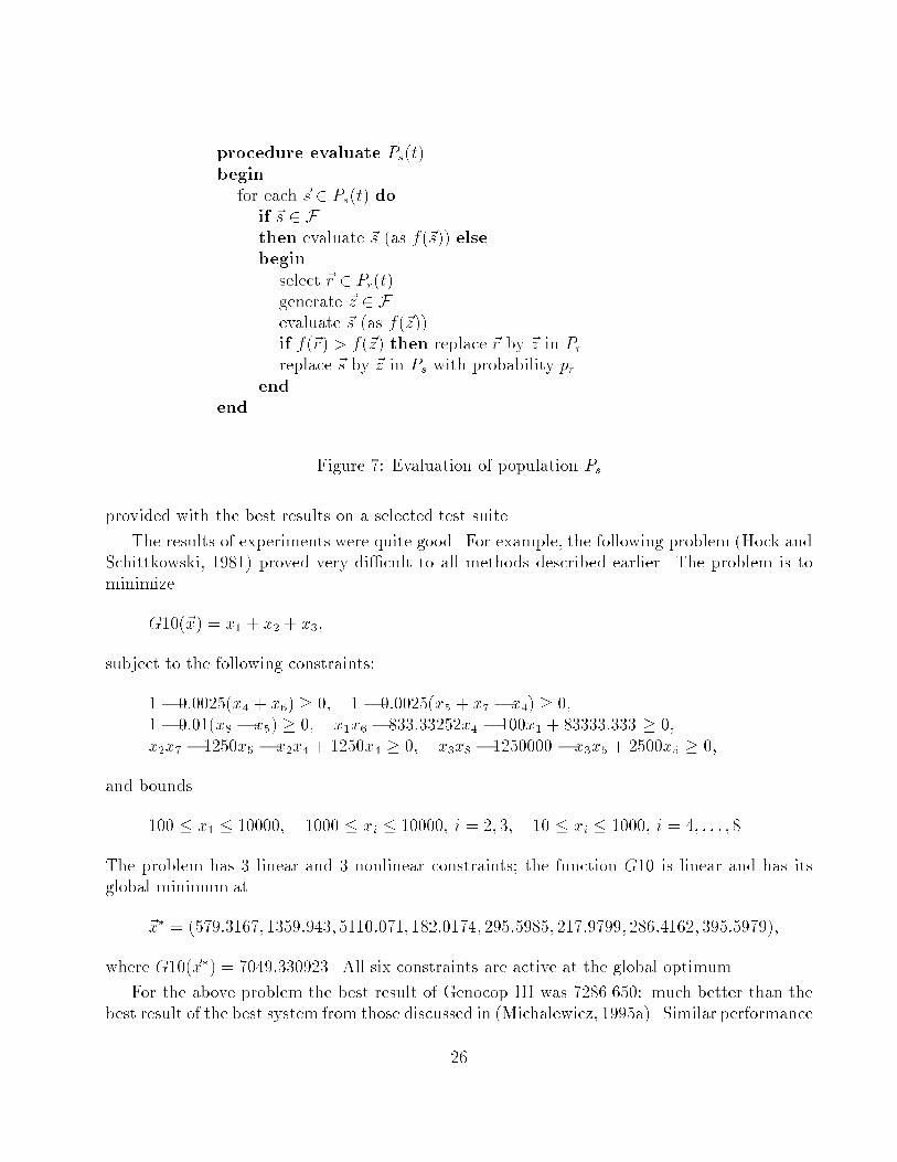
procedure evaluate Ps(t)begin

for each ~s 2 Ps(t) doif ~s 2 Fthen evaluate ~s (as f(~s)) elsebegin

select ~r 2 Pr(t)generate ~z 2 Fevaluate ~s (as f(~z))if f(~r) > f(~z) then replace ~r by ~z in Pr

replace ~s by ~z in Ps with probability prend

end

Figure 7: Evaluation of population Ps

provided with the best results on a selected test suite.

The results of experiments were quite good. For example, the following problem (Hock andSchittkowski, 1981) proved very di�cult to all methods described earlier. The problem is tominimize

G10(~x) = x1 + x2 + x3,

subject to the following constraints:

1� 0:0025(x4 + x6) � 0, 1 � 0:0025(x5 + x7 � x4) � 0,1� 0:01(x8 � x5) � 0, x1x6 � 833:33252x4 � 100x1 + 83333:333 � 0,x2x7 � 1250x5 � x2x4 + 1250x4 � 0, x3x8 � 1250000 � x3x5 + 2500x5 � 0,

and bounds

100 � x1 � 10000, 1000 � xi � 10000, i = 2; 3, 10 � xi � 1000, i = 4; : : : ; 8.

The problem has 3 linear and 3 nonlinear constraints; the function G10 is linear and has itsglobal minimum at

~x� = (579:3167; 1359:943; 5110:071; 182:0174; 295:5985; 217:9799; 286:4162; 395:5979),

where G10(~x�) = 7049:330923. All six constraints are active at the global optimum.

For the above problem the best result of Genocop III was 7286.650: much better than thebest result of the best system from those discussed in (Michalewicz, 1995a). Similar performance

26

was observed on two other problems, G9 (with 680.640) and G7 (with 25.883). Additionalinteresting observation was connected with stability of the system. Genocop III had a very lowstandard deviation of results. For example, for problem G9, all results were between 680.640and 680.889; on the other hand, other systems produced variety of results (between 680.642and 689.660, see Michalewicz (1995a)).

Of course, all resulting points ~x were feasible, which was not the case with other systems(e.g., Genocop II produced a value of 18.917 for the problem G7, the systems based on themethods of Homaifar, Lai, and Qi (section 3.2.1) and Powell and Skolnick (section 3.3.2) gaveresults of 2282.723 and 2101.367, respectively, for the problem G10, and these solutions werenot feasible).

3.4 Hybrid methods

It is relatively easy to develop hybrid methods which combine evolutionary computation tech-niques with deterministic procedures for numerical optimization problems. Waagen et al.(1992) combined evolutionary programming technique (with oating point representation, Fo-gel, 1995) with the direction set method of Hooke-Jeeves; this hybrid method was tested onthree (unconstrained) test functions. Myung et al. (1995) considered a similar approach, butthey experimented with constrained problems. Again, they combined oating-point evolution-ary programming technique with some other method|developed by Maa and Shanblatt (1992).However, while the method of Waagen et al. (1992) incorporated the direction set algorithmas a problem-speci�c operator of his evolutionary technique, Myung et al. (1995) divided thewhole optimization process into two separate phases. During the �rst phase, evolutionaryalgorithm optimizes the function

eval(~x) = f(~x) +s

2

0@ mX

j=1

f2j (~x)

1A ;

where s is a constant. After the termination of this phase, the second phase of the optimizationalgorithm of Maa and Shanblatt (1992) was applied to the best solution found during the �rstphase; this phase iterates until the system

~x0 = �5 f(~x)�24 mXj=1

5fj(~x)(sfj(~x) + �j)

35 ;

is in equilibrium, where the Lagrange multipliers are updated as �0j = �sfj for a small positiveconstant �.

This hybrid method was successfully applied to a few test cases; for example, one of thetest cases was to minimize

G11(~x) = x21 + (x2 � 1)2,

27

subject to a nonlinear constraint:

x2 � x21 = 0,

and bounds:

�1 � xi � 1, i = 1; 2.

The known global solutions are ~x� = (�0:70711; 0:5), and G11(~x�) = 0:75000455.

For this problem, the �rst phase of the evolutionary process converges quickly in 100 gen-erations to (�0:70711; 0:5), and the second phase drives the system to the global solution.However, the method was not tested for problems of higher dimensions.

Several other constraint handling methods deserve also some attention. For example, somemethods use of the values of objective function f and penalties fj (j = 1; : : : ;m) as elementsof a vector and apply multi-objective techniques to minimize all components of the vector. Forexample, Scha�er's (1985) Vector Evaluated Genetic Algorithm (VEGA) selects 1=(m + 1) ofthe population based on each of the objectives. Such an approach was incorporated by Parmeeand Purchase (1994) in the development of techniques for constrained design spaces. On theother hand, in the approach by Surry et al. (1995), all members of the population are ranked onthe basis of constraint violation. Such rank r, together with the value of the objective functionf , leads to the two-objective optimization problem. This approach gave a good performanceon optimization of gas supply networks (Surry et al., 1995).

Also, an interesting approach was reported by Paredis (1994). The method (described inthe context of constraint satisfaction problems) is based on a co-evolutionary model, where apopulation of potential solutions co-evolves with a population of constraints: �tter solutionssatisfy more constraints, whereas �tter constraints are violated by more solutions. There issome development connected with generalizing the concept of \ant colonies" (Colorni et al.,1991) (which were originally proposed for order-based problems) to numerical domains (Bilchevand Parmee, 1995); �rst experiments on some test problems (from Table 3) gave very goodresults (Bilchev, 1995). It is also possible to incorporate the knowledge of the constraints of theproblem into the belief space of cultural algorithms (Reynolds, 1994); such algorithms providea possibility of conducting an e�cient search of the feasible search space (Reynolds et al.,1995). Recently, Kelly and Laguna (1996) developed a new procedure for di�cult constrainedoptimization problems, which

\...has succeeded in generating optimal and near-optimal solutions in minutes tocomplex nonlinear problems that otherwise have required days of computer timein order to verify optimal solutions. These problems include nonconvex, nondi�er-entiable and mixed discrete functions over constrained regions. The feasible spaceexplicitly incorporates linear and integer programming constraints and implicitly in-corporates other nonlinear constraints by penalty functions. The objective functions

28

to be optimized may have no `mathematically speci�able' representation, and caneven require simulations to generate. Due to this exibility, the approach appliesalso to optimization under uncertainty (which increases its relevance to practicalapplications)."

The method combines evolutionary processes with (1) scatter search, (2) with procedures ofmixed integer optimization, and (3) with adaptive memory strategies of tabu search.

However, all the above methods are on early stages of their development, or they have notbeen applied yet to the general NLP, so we do not discuss them any further.

4 Conclusions and Future Work

It is di�cult to compare the constraint-handling methods which were discussed in the previoussection of this paper. The main reason is that the original formulations of these methods arebased on di�erent representations (binary or oat), and consequently they use di�erent opera-tors. For example, the method of static penalties (section 3.2.1) was proposed for a standardGA with binary representation, standard crossover and mutation. Genocop (section 3.1.1) uses oating point representation with seven specialized operators. The method of superiority offeasible points (section 3.3.2) was also developed for oating point representation. However,their operators were di�erent to those of Genocop. Bean and Hadj-Alouane adapted penalties(section 3.2.4) for integer programming problems and used binary representation to code inte-gers. Death penalty methods (section 3.2.5) were mainly used by evolution strategies ( oatingpoint representation with Gaussian mutation and adaptation of control parameters), and thesegregated GAs (section 3.2.6) has not been applied yet to the NLP. For these reasons we donot provide numerical results of the above methods on all test cases de�ned in the previoussection. The only general observation we can make at this stage is that for constrained numer-ical optimization problems, the oating point representation provides with much better results(some of experiments on comparisons between binary and oating point representations forunconstrained problems were reported in Michalewicz, 1996, chapter 5).

Some partial comparisons of several constraint-handling methods were reported (Michalewicz,1995a), where a modi�ed version of Genocop system was used for all experiments; the code wasupdated accordingly for each considered method. The results of these comparisons are givenin Table 2.

It is not clear what characteristics of a constrained problem make it di�cult for an evo-lutionary technique. It seems that no single parameter (number of linear, nonlinear, activeconstraints, the ratio � = jFj=jSj of feasible points in S, type of the function, number ofvariables) proved to be signi�cant as a major measure of di�culty of the problem. For exam-ple, many methods approached the optimum quite closely for the test cases G1 and G7 (with� = 0:0111% and � = 0:0003%, respectively), whereas most of the methods experienced di�-culties for the test case G10 (with � = 0:0010%). Two quadratic functions (the test cases G1

29

Test Exact Method Method Method Method Method Method MethodCase opt. of section of section of section of section of section of section of section

3.2.1 3.2.2 3.3.1 3.2.3 3.3.2 3.2.5 3.2.5(f)b �15:002 �15:000 �15:000 �15:000 �15:000 �15:000

G1 �15:000 m �15:002 �15:000 �15:000 �15:000 �15:000 | �14:999w �15:001 �14:999 �14:998 �15:000 �14:999 �13:616c 0, 0, 4 0, 0, 0 0, 0, 0 0, 0, 0 0, 0, 0 0, 0, 0b 2282.723 3117.242 7485.667 7377.976 2101.367 7872.948

G10 7049.331 m 2449.798 4213.497 8271.292 8206.151 2101.411 | 8559.423w 2756.679 6056.211 8752.412 9652.901 2101.551 8668.648c 0, 3, 0 0, 3, 0 0, 0, 0 0, 0, 0 1, 2, 0 0, 0, 0b 680.771 680.787 680.836 680.642 680.805 680.934 680.847

G9 680.630 m 681.262 681.111 681.175 680.718 682.682 681.771 681.826w 689.660 682.798 685.640 680.955 685.738 689.442 689.417c 0, 0, 1 0, 0, 0 0, 0, 0 0, 0, 0 0, 0, 0 0, 0, 0 0, 0, 0b 24.690 25.486 18.917 17.388 25.653

G7 24.306 m 29.258 26.905 | 24.418 22.932 | 27.116w 36.060 42.358 44.302 48.866 32.477c 0, 1, 1 0, 0, 0 0, 1, 0 1, 0, 0 0, 0, 0

Table 2: Experimental results. For some methods, the best (b), median (m), and the worst(w) result (out of 10 independent runs) are reported together with the number (c) of violatedconstraints at the median solution: the sequence of three numbers indicate the number ofviolations by more than 1.0, more than 0.1, and more than 0.001, respectively. The symbol `|'stands for `the results were not meaningful'. The results for method of section 3.2.5 report alsothe results of experiments (case 3.2.5(f)) where the initial population was feasible.

and G7) with a similar number of constraints (9 and 8, respectively) and an identical number(6) of active constraints at the optimum, gave a di�erent challenge to most of these methods.Also, several methods were quite sensitive to the presence of a feasible solution in the initialpopulation (e.g., method of section 3.2.5; see table 2).

All test cases are summarized in table 3; for each test case we list number n of variables,type of the function f , the relative size of the feasible region in the search space given by theratio �, the number of constraints of each category (linear inequalities LI, nonlinear equationsNE and inequalities NI), and the number a of active constraints at the optimum (includingequality constraints).

Despite some obvious weaknesses of the method of static penalties (section 3.2.1), this basicmethod, which requires �xed user-supplied penalty parameters, remains the most popular oneto handle constraints for evolutionary algorithms and many other optimization frameworks.The main reason for that popularity is that it certainly is the simplest technique to implement:it requires only a straightforward modi�cation of the objective function. Moreover, it is fair tosay that it gives quite reasonable results in many cases. Nevertheless, as emphasized in some of

30

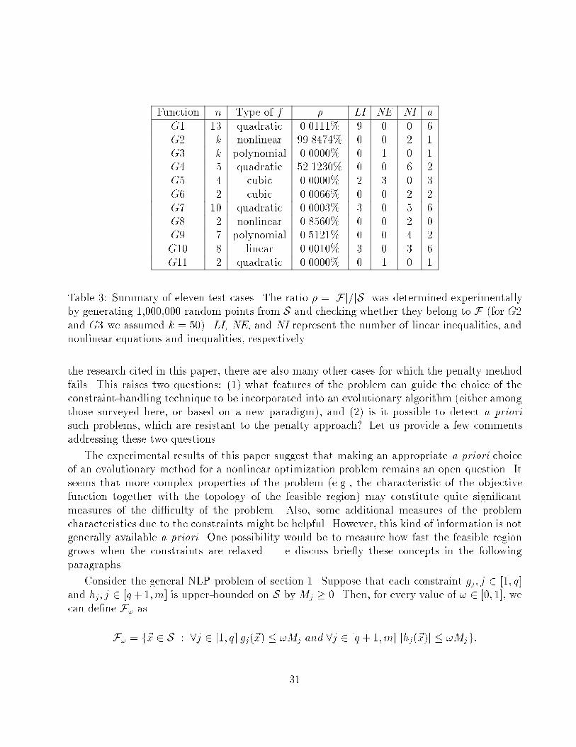
Function n Type of f � LI NE NI a

G1 13 quadratic 0.0111% 9 0 0 6G2 k nonlinear 99.8474% 0 0 2 1G3 k polynomial 0.0000% 0 1 0 1G4 5 quadratic 52.1230% 0 0 6 2G5 4 cubic 0.0000% 2 3 0 3G6 2 cubic 0.0066% 0 0 2 2G7 10 quadratic 0.0003% 3 0 5 6G8 2 nonlinear 0.8560% 0 0 2 0G9 7 polynomial 0.5121% 0 0 4 2G10 8 linear 0.0010% 3 0 3 6G11 2 quadratic 0.0000% 0 1 0 1

Table 3: Summary of eleven test cases. The ratio � = jFj=jSj was determined experimentallyby generating 1,000,000 random points from S and checking whether they belong to F (for G2and G3 we assumed k = 50). LI, NE, and NI represent the number of linear inequalities, andnonlinear equations and inequalities, respectively

the research cited in this paper, there are also many other cases for which the penalty methodfails. This raises two questions: (1) what features of the problem can guide the choice of theconstraint-handling technique to be incorporated into an evolutionary algorithm (either amongthose surveyed here, or based on a new paradigm), and (2) is it possible to detect a priorisuch problems, which are resistant to the penalty approach? Let us provide a few commentsaddressing these two questions.

The experimental results of this paper suggest that making an appropriate a priori choiceof an evolutionary method for a nonlinear optimization problem remains an open question. Itseems that more complex properties of the problem (e.g., the characteristic of the objectivefunction together with the topology of the feasible region) may constitute quite signi�cantmeasures of the di�culty of the problem. Also, some additional measures of the problemcharacteristics due to the constraints might be helpful. However, this kind of information is notgenerally available a priori. One possibility would be to measure how fast the feasible regiongrows when the constraints are relaxed. We discuss brie y these concepts in the followingparagraphs.

Consider the general NLP problem of section 1. Suppose that each constraint gj; j 2 [1; q]and hj; j 2 [q+1;m] is upper-bounded on S by Mj � 0. Then, for every value of ! 2 [0; 1], wecan de�ne F! as

F! = f~x 2 S : 8j 2 [1; q] gj(~x) � !Mj and 8j 2 [q + 1;m] jhj(~x)j � !Mjg:

31

It is interesting to observe that F0 = F and F1 = S. The way �! = jF!j=jSj behavesaround ! = 0 | measured, for instance, by the value

�! =d�!d!j!=0;

can serve as an indicator of \how fast" the feasible region expands around its boundary.

Of course, the di�culty of the NLP also heavily depends on the objective function f itself.So one possible measure of di�culty of the constrained problem is an evaluation of the optimumof the objective function f with relaxed constraints. The following formula,9

'! =max~x2F!

f(~x)

max~x2F f(~x);

can serve as a such measure. Unfortunately, this ratio can only be estimated a posteriori bysolving a large number of NLPs, all as di�cult as the original one.

In general, there are three possible sources of di�culties of the NLP. These di�culties canarise from the objective function itself, from the de�nition of the feasible region (i.e., from theconstraints alone), or from the coupling between the objective function and the constraints.Hence the following features should be taken into account when trying to characterize di�erentNLPs:

� The ruggedness of the unconstrained �tness landscape certainly is the �rst importantcharacteristic in uencing the overall problem di�culty; for instance, linear or convexobjective functions will always result in easier constrained problems than almost-chaoticfunctions, for the same set of constraints; however, this characteristic can hardly beestimated a priori.

� The sparseness of the feasible region indeed is a crucial factor of di�culty: in someproblems, �nding a single feasible point is the major di�culty. Moreover, a high slope ofthe constraints on the border of the feasible region is another way by which a constrainedproblem can resist the penalty method; some hints have been given above (the factors �and �! can be numerically estimated a priori).

� A high ratio between the highest global optima of the objective function (on the wholedomain where it is de�ned) and of the optima of the constrained function (e.g., the localoptima of the objective function in the feasible region), as well as a small distance betweenthese global optima and the feasible region can make the constrained optimization problemalmost intractable for penalty methods; unfortunately, it is almost impossible to estimatethis factor a priori. However, some useful a posteriori informations about the behaviorof di�erent methods might be obtained at the cost of heavy computations by comparingtheir respective performances on gradually relaxed hard NLPs.

9For maximization problems. The objective function f takes non-negative values.

32

� The number of active constraints at the optimum is of course of importance: the moreconstraints that are active at the optimum, the more likely to succeed are algorithmssearching close to the boundary of the feasible region; the extreme case being that de-scribed in section 3.1.2. But here again it is very di�cult to predict such a number apriori.

It seems that the most promising approach at this stage of research is experimental, involvingthe design of a scalable test suite of constrained optimization problems, in which many of thesefeatures could be easily tuned. Then it should be possible to test new methods with respect tothe corpus of all available methods.

Such experimental suite should contain:

� Convex problems (for validation only, as any gradient-bassed method will outperform anystochastic algorithm by several orders of magnitude on such problems);

� Convex objective function and non-convex constraints (from easy to di�cult in slope,number of connected components, etc.);

� Non-convex objective function (with multiple optima) with convex constraints;

� Non-convex objective function (with numerous multiple optima) and highly non-convexsteep constraints (with F consisting of possibly disjoint regions).

Such an experimental test suite is currently under construction.

Acknowledgments:

This material is based upon work supported by the National Science Foundation underGrant IRI-9322400. The authors would to thank Ken De Jong for his suggestions which madethe article more readable.

References

B�ack, T., F. Ho�meister, and H.-P. Schwefel (1991). A survey of evolution strategies. In R. K.Belew and L. B. Booker (Eds.), Proceedings of the 4th International Conference on GeneticAlgorithms, pp. 2{9. Morgan Kaufmann.

Bean, J. C. and A. B. Hadj-Alouane (1992). A dual genetic algorithm for bounded integer pro-grams. Technical Report TR 92-53, Department of Industrial and Operations Engineering,The University of Michigan.

Bilchev, G. (1995). Private communication.

Bilchev, G. and I. Parmee (1995). Ant colony search vs. genetic algorithms. Technical report,Plymouth Engineering Design Centre, University of Plymouth.

33

Colorni, A., M. Dorigo, and V. Maniezzo (1991). Distributed optimization by ant colonies. InProceedings of the First European Conference on Arti�cial Life, Paris. MIT Press/BradfordBook.

Davis, L. (1989). Adapting operator probabilities in genetic algorithms. In J. D. Scha�er (Ed.),Proceedings of the 3rd International Conference on Genetic Algorithms, pp. 61{69. MorganKaufmann.

Davis, L. (1995). Private communication.

DeJong, K. (1975). The Analysis of the Behavior of a Class of Genetic Adaptive Systems. Ph.D. thesis, University of Michigan, Ann Harbor. Dissertation Abstract International, 36(10),5140B. (University Micro�lms No 76-9381).

Eiben, A., P.-E. Raue, and Z. Ruttkay (1994). Genetic algorithms with multi-parent recombina-tion. In Y. Davidor, H.-P. Schwefel, and R. Manner (Eds.), Proceedings of the 3rd Conferenceon Parallel Problems Solving from Nature, Number 866 in LNCS, pp. 78{87. Springer Verlag.

Eshelman, L. and J. D. Scha�er (1993). Real-coded genetic algorithms and interval-schemata.In L. D. Whitley (Ed.), Foundations of Genetic Algorithms 2, Los Altos, CA, pp. 187{202.Morgan Kaufmann.

Floudas, C. and P. Pardalos (1987). A Collection of Test Problems for Constrained GlobalOptimization Algorithms, Volume 455 of LNCS. Berlin: Springer Verlag.

Fogel, D. and L. Stayton (1994). On the e�ectiveness of crossover in simulated evolutionaryoptimization. BioSystems 32, 171{182.

Fogel, D. B. (1995). Evolutionary Computation. Toward a New Philosophy of Machine Intelli-gence. Piscataway, NJ: IEEE Press.

Glover, F. (1977). Heuristics for integer programming using surrogate constraints. DecisionSciences 8 (1), 156{166.

Glover, F. (1994). Genetic algorithms and scatter search: Unsuspected potentials. Statistics,and Computing 4, 131{140.

Glover, F. and G. Kochenberger (1995). Critical event tabu search for multidimensional knap-sack problems. In Proceedings of the International Conference on Metaheuristics for Opti-mization, pp. 113{133. Kluwer Publishing.

Gregory, J. (1995). Nonlinear Programming FAQ, Usenet sci.answers. Available atftp://rtfm.mit.edu/pub/usenet/sci.answers/nonlinear-programming-faq.

Hadj-Alouane, A. B. and J. C. Bean (1992). A genetic algorithm for the multiple-choice integerprogram. Technical Report TR 92-50, Department of Industrial and Operations Engineering,The University of Michigan.

Himmelblau, D. (1992). Applied Nonlinear Programming. McGraw-Hill.

34

Hock, W. and K. Schittkowski (1981). Test Examples for Nonlinear Programming Codes, Vol-ume 187 of Lecture Notes in Economics and Mathematical Systems. Springer Verlag.

Homaifar, A., S. H.-Y. Lai, and X. Qi (1994). Constrained optimization via genetic algorithms.Simulation 62 (4), 242{254.

Joines, J. and C. Houck (1994). On the use of non-stationary penalty functions to solve non-linear constrained optimization problems with gas. In Z. Michalewicz, J. D. Scha�er, H.-P.Schwefel, D. B. Fogel, and H. Kitano (Eds.), Proceedings of the First IEEE InternationalConference on Evolutionary Computation, pp. 579{584. IEEE Press.

Keane, A. (1994, May 19). Genetic Algorithms Digest. V8n16.

Kelly, J. and M. Laguna (1996, April 8). Genetic Algorithms Digest. V10n16.

Leriche, R. G., C. Knopf-Lenoir, and R. T. Haftka (1995). A segragated genetic algorithmfor constrained structural optimization. In L. J. Eshelman (Ed.), Proceedings of the 6th

International Conference on Genetic Algorithms, pp. 558{565.

Maa, C. and M. Shanblatt (1992). A two-phase optimization neural network. IEEE Transactionson Neural Networks 3 (6), 1003{1009.

Michalewicz, Z. (1995a). Genetic algorithms, numerical optimization and constraints. In L. J.Eshelman (Ed.), Proceedings of the 6th International Conference on Genetic Algorithms, pp.151{158. Morgan Kaufmann.

Michalewicz, Z. (1995b). Heuristic methods for evolutionary computation techniques. Journalof Heuristics 1 (2), 177{206.

Michalewicz, Z. (1996). Genetic Algorithms+Data Structures=Evolution Programs. New-York:Springer Verlag. 3rd edition.

Michalewicz, Z. and N. Attia (1994). Evolutionary optimization of constrained problems. InProceedings of the 3rd Annual Conference on Evolutionary Programming, pp. 98{108. WorldScienti�c.

Michalewicz, Z. and C. Z. Janikow (1991). Handling constraints in genetic algorithms. In R. K.Belew and L. B. Booker (Eds.), Proceedings of the 4th International Conference on GeneticAlgorithms, pp. 151{157. Morgan Kaufmann.

Michalewicz, Z., T. Logan, and S. Swaminathan (1994). Evolutionary operators for continuousconvex parameter spaces. In Proceedings of the 3rd Annual Conference on EvolutionaryProgramming, pp. 84{97. World Scienti�c.

Michalewicz, Z. and G. Nazhiyath (1995). Genocop III: A co-evolutionary algorithm for nu-merical optimization problems with nonlinear constraints. In D. B. Fogel (Ed.), Proceedingsof the Second IEEE International Conference on Evolutionary Computation, pp. 647{651.IEEE Press.

35

Michalewicz, Z., G. Nazhiyath, and M. Michalewicz (1996). A note on usefulness of geomet-rical crossover for numerical optimization problems. In P. J. Angeline and T. B�ack (Eds.),Proceedings of the 5th Annual Conference on Evolutionary Programming. To appear.

M�uhlenbein, H. and H.-M. Voigt (1995). Gene poool recombination for the breeder geneticalgorithm. In Proceedings of the Metaheuristics International Conference, pp. 19{25.

Myung, H., J.-H. Kim, and D. Fogel (1995). Preliminary investigation into a two-stage methodof evolutionary optimization on constrained problems. In J. R. McDonnell, R. G. Reynolds,and D. B. Fogel (Eds.), Proceedings of the 4th Annual Conference on Evolutionary Program-ming, pp. 449{463. MIT Press.

Orvosh, D. and L. Davis (1993). Shall we repair? Genetic algorithms, combinatorial optimiza-tion, and feasibility constraints. In S. Forrest (Ed.), Proceedings of the 5th InternationalConference on Genetic Algorithms, pp. 650. Morgan Kaufmann.

Paredis, J. (1994). Coevolutionary constraint satisfaction. In Y. Davidor, H.-P. Schwefel, andR. Manner (Eds.), Proceedings of the 3rd Conference on Parallel Problems Solving fromNature, pp. 46{55. Springer Verlag.

Parmee, I. and G. Purchase (1994). The development of directed genetic search technique forheavily constrained design spaces. In Proceedings of the Conference on Adaptive Computingin Engineering Design and Control, pp. 97{102. University of Plymouth.

Powell, D. and M. M. Skolnick (1993). Using genetic algorithms in engineering design optimiza-tion with non-linear constraints. In S. Forrest (Ed.), Proceedings of the 5th InternationalConference on Genetic Algorithms, pp. 424{430. Morgan Kaufmann.

Rechenberg, I. (1973). Evolutionstrategie: Optimierung Technisher Systeme nach Prinzipiendes Biologischen Evolution. Stuttgart: Fromman-Holzboog Verlag.

Renders, J.-M. and H. Bersini (1994). Hybridizing genetic algorithms with hill-climbing meth-ods for global optimization: Two possible ways. In Z. Michalewicz, J. D. Scha�er, H.-P.Schwefel, D. B. Fogel, and H. Kitano (Eds.), Proceedings of the First IEEE InternationalConference on Evolutionary Computation, pp. 312{317. IEEE Press.

Reynolds, R. (1994). An introduction to cultural algorithms. In Proceedings of the 3rd AnnualConference on Evolutionary Programming, pp. 131{139. World Scienti�c.

Reynolds, R., Z. Michalewicz, and M. Cavaretta (1995). Using cultural algorithms for con-straint handling in Genocop. In J. R. McDonnell, R. G. Reynolds, and D. B. Fogel (Eds.),Proceedings of the 4th Annual Conference on Evolutionary Programming, pp. 298{305. MITPress.

Richardson, J. T., M. R. Palmer, G. Liepins, and M. Hilliard (1989). Some guidelines forgenetic algorithms with penalty functions. In J. D. Scha�er (Ed.), Proceedings of the 3rd

International Conference on Genetic Algorithms, pp. 191{197. Morgan Kaufmann.

36

Scha�er, D. (1985). Multiple objective optimization with vector evaluated genetic algorithms.In J. J. Grefenstette (Ed.), Proceedings of the 1st International Conference on GeneticAlgorithms. Laurence Erlbaum Associates.

Schoenauer, M. and Z. Michalewicz (1996). Evolutionary computation at the edge of feasibility.W. Ebeling, and H.-M. Voigt (Eds.), Proceedings of the 4th Conference on Parallel ProblemsSolving from Nature, Springer Verlag.

Schoenauer, M. and S. Xanthakis (1993). Constrained GA optimization. In S. Forrest (Ed.),Proceedings of the 5th International Conference on Genetic Algorithms, pp. 573{580. MorganKaufmann.

Schwefel, H.-P. (1981). Numerical Optimization of Computer Models. New-York: John Wiley& Sons. 1995 { 2nd edition.

Smith, A. and D. Tate (1993). Genetic optimization using a penalty function. In S. Forrest(Ed.), Proceedings of the 5th International Conference on Genetic Algorithms, pp. 499{503.Morgan Kaufmann.

Surry, P., N. Radcli�e, and I. Boyd (1995). A multi-objective approach to constrained opti-mization of gas supply networks. In T. Fogarty (Ed.), Proceedings of the AISB-95 Workshopon Evolutionary Computing, Volume 993, pp. 166{180. Springer Verlag.

Waagen, D., P. Diercks, and J. McDonnell (1992). The stochastic direction set algorithm: Ahybrid technique for �nding function extrema. In D. B. Fogel and W. Atmar (Eds.), Proceed-ings of the 1st Annual Conference on Evolutionary Programming, pp. 35{42. EvolutionaryProgramming Society.

Wright, A. (1991). Genetic algorithms for real parameter optimization. In J. G. Rawlins (Ed.),Foundations of Genetic Algorithms, pp. 205{218. Morgan Kaufmann.

37