Embed Size (px)
Citation preview
University of KentuckyUKnowledge
University of Kentucky Master's Theses Graduate School
2011
EVALUATING THE EFFECTIVENESS OFPEAK POWER TRACKING TECHNOLOGIESFOR SOLAR ARRAYS ON SMALLSPACECRAFTDaniel Martin ErbUniversity of Kentucky, [email protected]
Click here to let us know how access to this document benefits you.
This Thesis is brought to you for free and open access by the Graduate School at UKnowledge. It has been accepted for inclusion in University ofKentucky Master's Theses by an authorized administrator of UKnowledge. For more information, please contact [email protected].
Recommended CitationErb, Daniel Martin, "EVALUATING THE EFFECTIVENESS OF PEAK POWER TRACKING TECHNOLOGIES FOR SOLARARRAYS ON SMALL SPACECRAFT" (2011). University of Kentucky Master's Theses. 656.https://uknowledge.uky.edu/gradschool_theses/656

STUDENT AGREEMENT:
I represent that my thesis or dissertation and abstract are my original work. Proper attribution has beengiven to all outside sources. I understand that I am solely responsible for obtaining any needed copyrightpermissions. I have obtained and attached hereto needed written permission statements(s) from theowner(s) of each third-party copyrighted matter to be included in my work, allowing electronicdistribution (if such use is not permitted by the fair use doctrine).
I hereby grant to The University of Kentucky and its agents the non-exclusive license to archive and makeaccessible my work in whole or in part in all forms of media, now or hereafter known. I agree that thedocument mentioned above may be made available immediately for worldwide access unless apreapproved embargo applies.
I retain all other ownership rights to the copyright of my work. I also retain the right to use in futureworks (such as articles or books) all or part of my work. I understand that I am free to register thecopyright to my work.
REVIEW, APPROVAL AND ACCEPTANCE
The document mentioned above has been reviewed and accepted by the student’s advisor, on behalf ofthe advisory committee, and by the Director of Graduate Studies (DGS), on behalf of the program; weverify that this is the final, approved version of the student’s dissertation including all changes requiredby the advisory committee. The undersigned agree to abide by the statements above.
Daniel Martin Erb, Student
Dr. James E. Lumpp, Major Professor
Dr. Zhi David Chen, Director of Graduate Studies
EVALUATING THE EFFECTIVENESS OF PEAK POWER TRACKING TECHNOLOGIES FOR SOLAR ARRAYS ON SMALL SPACECRAFT
THESIS
A thesis submitted in partial fulfillment of the requirements for the degree of Master of Science in Electrical Engineering in the
College of Engineering at the University of Kentucky
By
Daniel Martin Erb
Lexington, Kentucky
Director: Dr. James E. Lumpp, Professor of Electrical and
Computer Engineering
Lexington, Kentucky
2011
Copyright © Daniel Martin Erb 2011
ABSTRACT OF THESIS
EVALUATING THE EFFECTIVENESS OF PEAK POWER TRACKING TECHNOLOGIES FOR SOLAR ARRAY ON SMALL SPACECRAFT
The unique environment of CubeSat and small satellite missions allows certain
accepted paradigms of the larger satellite world to be investigated in order to trade performance for simplicity, mass, and volume. Peak Power Tracking technologies for solar arrays are generally implemented in order to meet the End-of-Life power requirements for satellite missions given radiation degradation over time. The short lifetime of the generic satellite mission removes the need to compensate for this degradation. While Peak Power Tracking implementations can give increased power by taking advantage and compensating for the temperature cycles that solar cells experience, this comes at the expense of system complexity and, given smart system design, this increased performance is negligible and possibly detrimental. This thesis investigates different Peak Power Tracking implementations and compares them to two Fixed Point implementations as well as a Direct Energy Transfer system in terms of performance and system complexity using computer simulation. This work demonstrates that, though Peak Power Tracking systems work as designed, under most circumstances Direct Energy Transfer systems should be used in small satellite applications as it gives the same or better performance with less complexity. KEYWORDS: Small Satellites, Power Systems, Solar Arrays, Peak Power Tracking, Direct
Energy Transfer
___________Daniel Erb____________
___________09/13/2011___________
Dr. James E. Lumpp
EVALUATING THE EFFECTIVENESS OF PEAK POWER TRACKING TECHNOLOGIES FOR SOLAR ARRAY ON SMALL SPACECRAFT
By
Daniel Martin Erb
Director of Thesis
Director of Graduate Studies
Dr. Zhi David Chen
9/13/2011

iii
ACKNOWLEDGEMENTS
I would like to acknowledge the support of Kentucky Space, the Kentucky Space
Grant Consortium, the Kentucky Science and Technology Corporation, and the Space
Systems Lab at the University of Kentucky. I would like to thank Dr. James Lumpp for his
support and mentorship during my graduate studies. I would like to thank my parents
for always nodding understandingly when I told them that I was almost done. Finally, I
would like to thank Lindsey for getting her Master’s degree before me and making me
call her master until I finished mine.
iv
TABLE OF CONTENTS
LIST OF TABLES .................................................................................................................... vi
LIST OF FIGURES ................................................................................................................. vii
1.0 Introduction ............................................................................................................. 1
2.0 Background .............................................................................................................. 2
2.1 Small Satellite Definition ...................................................................................... 2
2.2 Solar Cell Behavior................................................................................................ 4
2.3 LEO Environment and Solar Cell Effects ............................................................... 9
2.3.1 Incidence Angle ........................................................................................... 10
2.3.2 Temperature ............................................................................................... 13
2.3.3 Radiation ..................................................................................................... 14
2.4 Solar Array Interface .......................................................................................... 17
3.0 Modeling ................................................................................................................ 18
3.1 Simulink® Based Model ...................................................................................... 19
3.2 Orbital Parameters ............................................................................................. 19
3.2.1 Rotation Rates ............................................................................................. 20
3.2.2 Temperature ............................................................................................... 21
3.3 Solar Cell Model ................................................................................................. 24
3.4 Battery Charge Regulator Model ....................................................................... 25
3.5 Solar Array Interface Models ............................................................................. 26
3.5.1 MPPT ........................................................................................................... 27
3.5.1.1 Fractional Voltage ................................................................................ 27
3.5.1.2 Perturb and Observe ........................................................................... 30
3.5.1.3 dP/dV ................................................................................................... 32
3.5.2 Non-MPPT ................................................................................................... 34
3.5.2.1 Fixed Voltage ....................................................................................... 34
3.5.2.2 Temperature Compensated Fixed Voltage .......................................... 35
3.5.3 Direct Energy Transfer ................................................................................ 36
3.5.3.1 Battery Model ...................................................................................... 39
3.5.3.1 System Load Model ............................................................................. 41
4.0 Evaluation and Comparison ................................................................................... 43
4.1 Ideal .................................................................................................................... 44
4.2 Fractional Voltage .............................................................................................. 44
4.3 Perturb and Observe .......................................................................................... 46
4.4 dP/dV .................................................................................................................. 47
4.5 Fixed Voltage ...................................................................................................... 47
4.6 Temperature Compensated Fixed Voltage ........................................................ 48
4.7 Direct Energy Transfer ........................................................................................ 49
v
5.0 Conclusions ............................................................................................................ 50
5.1 Battery Charge Regulator Efficiency .................................................................. 51
5.2 Effect of Rotation Rate ....................................................................................... 52
5.3 Effect of Solar Cell Damage ................................................................................ 53
5.3.1 Radiation ..................................................................................................... 54
5.3.2 Single Cell Damage ...................................................................................... 56
5.4 Discussion ........................................................................................................... 56
6.0 Bibliography ........................................................................................................... 60
7.0 Vita ......................................................................................................................... 64
vi
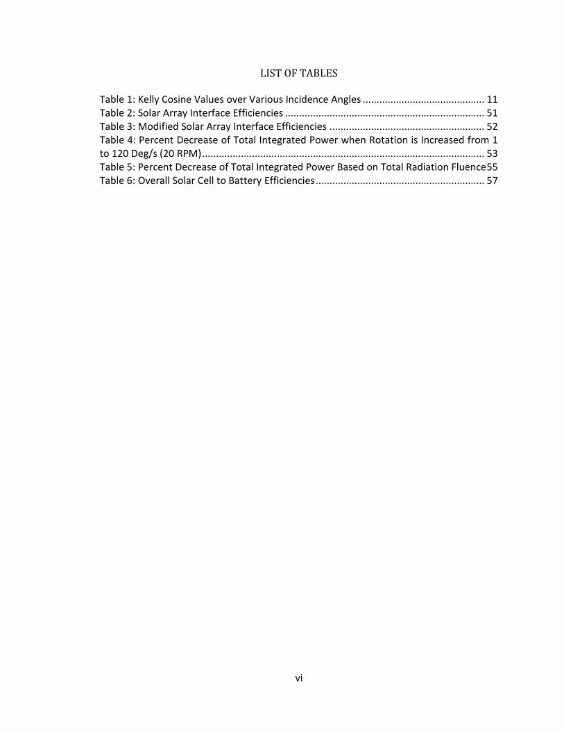
LIST OF TABLES
Table 1: Kelly Cosine Values over Various Incidence Angles ............................................ 11
Table 2: Solar Array Interface Efficiencies ........................................................................ 51
Table 3: Modified Solar Array Interface Efficiencies ........................................................ 52
Table 4: Percent Decrease of Total Integrated Power when Rotation is Increased from 1 to 120 Deg/s (20 RPM) ...................................................................................................... 53
Table 5: Percent Decrease of Total Integrated Power Based on Total Radiation Fluence 55
Table 6: Overall Solar Cell to Battery Efficiencies ............................................................. 57
vii
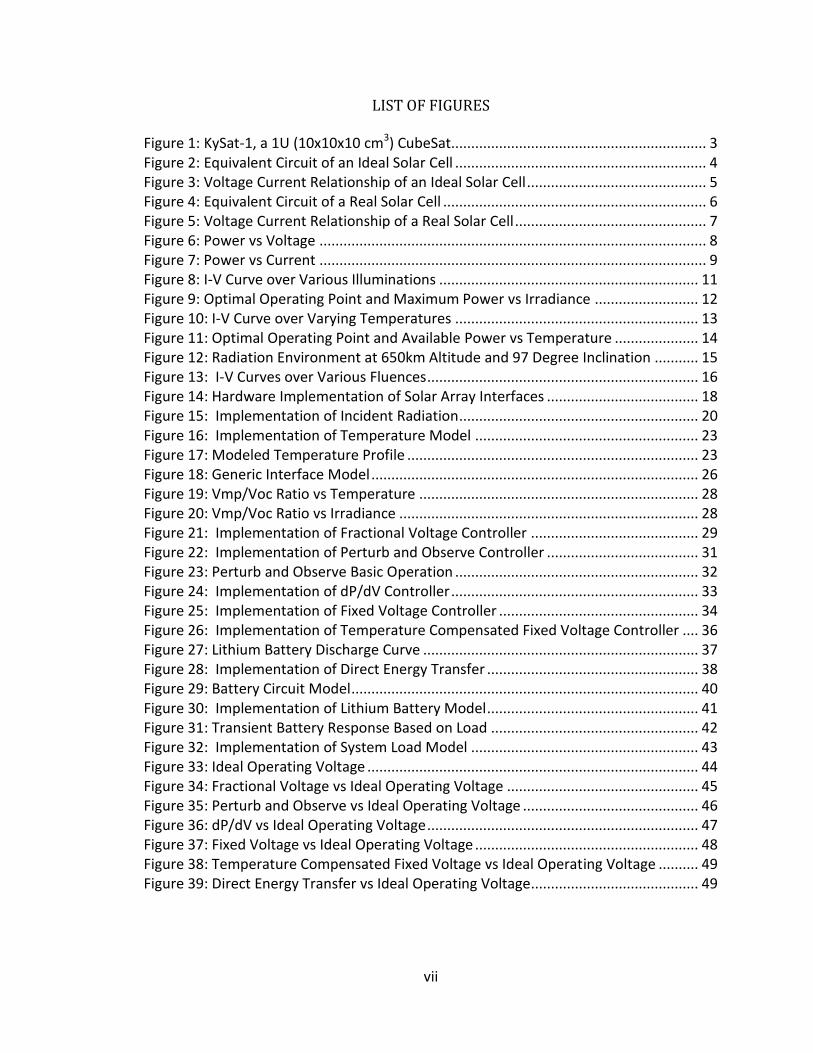
LIST OF FIGURES
Figure 1: KySat-1, a 1U (10x10x10 cm3) CubeSat................................................................ 3
Figure 2: Equivalent Circuit of an Ideal Solar Cell ............................................................... 4
Figure 3: Voltage Current Relationship of an Ideal Solar Cell ............................................. 5
Figure 4: Equivalent Circuit of a Real Solar Cell .................................................................. 6
Figure 5: Voltage Current Relationship of a Real Solar Cell ................................................ 7
Figure 6: Power vs Voltage ................................................................................................. 8
Figure 7: Power vs Current ................................................................................................. 9
Figure 8: I-V Curve over Various Illuminations ................................................................. 11
Figure 9: Optimal Operating Point and Maximum Power vs Irradiance .......................... 12
Figure 10: I-V Curve over Varying Temperatures ............................................................. 13
Figure 11: Optimal Operating Point and Available Power vs Temperature ..................... 14
Figure 12: Radiation Environment at 650km Altitude and 97 Degree Inclination ........... 15
Figure 13: I-V Curves over Various Fluences .................................................................... 16
Figure 14: Hardware Implementation of Solar Array Interfaces ...................................... 18
Figure 15: Implementation of Incident Radiation ............................................................ 20
Figure 16: Implementation of Temperature Model ........................................................ 23
Figure 17: Modeled Temperature Profile ......................................................................... 23
Figure 18: Generic Interface Model .................................................................................. 26
Figure 19: Vmp/Voc Ratio vs Temperature ...................................................................... 28
Figure 20: Vmp/Voc Ratio vs Irradiance ........................................................................... 28
Figure 21: Implementation of Fractional Voltage Controller .......................................... 29
Figure 22: Implementation of Perturb and Observe Controller ...................................... 31
Figure 23: Perturb and Observe Basic Operation ............................................................. 32
Figure 24: Implementation of dP/dV Controller .............................................................. 33
Figure 25: Implementation of Fixed Voltage Controller .................................................. 34
Figure 26: Implementation of Temperature Compensated Fixed Voltage Controller .... 36
Figure 27: Lithium Battery Discharge Curve ..................................................................... 37
Figure 28: Implementation of Direct Energy Transfer ..................................................... 38
Figure 29: Battery Circuit Model ....................................................................................... 40
Figure 30: Implementation of Lithium Battery Model ..................................................... 41
Figure 31: Transient Battery Response Based on Load .................................................... 42
Figure 32: Implementation of System Load Model ......................................................... 43
Figure 33: Ideal Operating Voltage ................................................................................... 44
Figure 34: Fractional Voltage vs Ideal Operating Voltage ................................................ 45
Figure 35: Perturb and Observe vs Ideal Operating Voltage ............................................ 46
Figure 36: dP/dV vs Ideal Operating Voltage .................................................................... 47
Figure 37: Fixed Voltage vs Ideal Operating Voltage ........................................................ 48
Figure 38: Temperature Compensated Fixed Voltage vs Ideal Operating Voltage .......... 49
Figure 39: Direct Energy Transfer vs Ideal Operating Voltage.......................................... 49
1
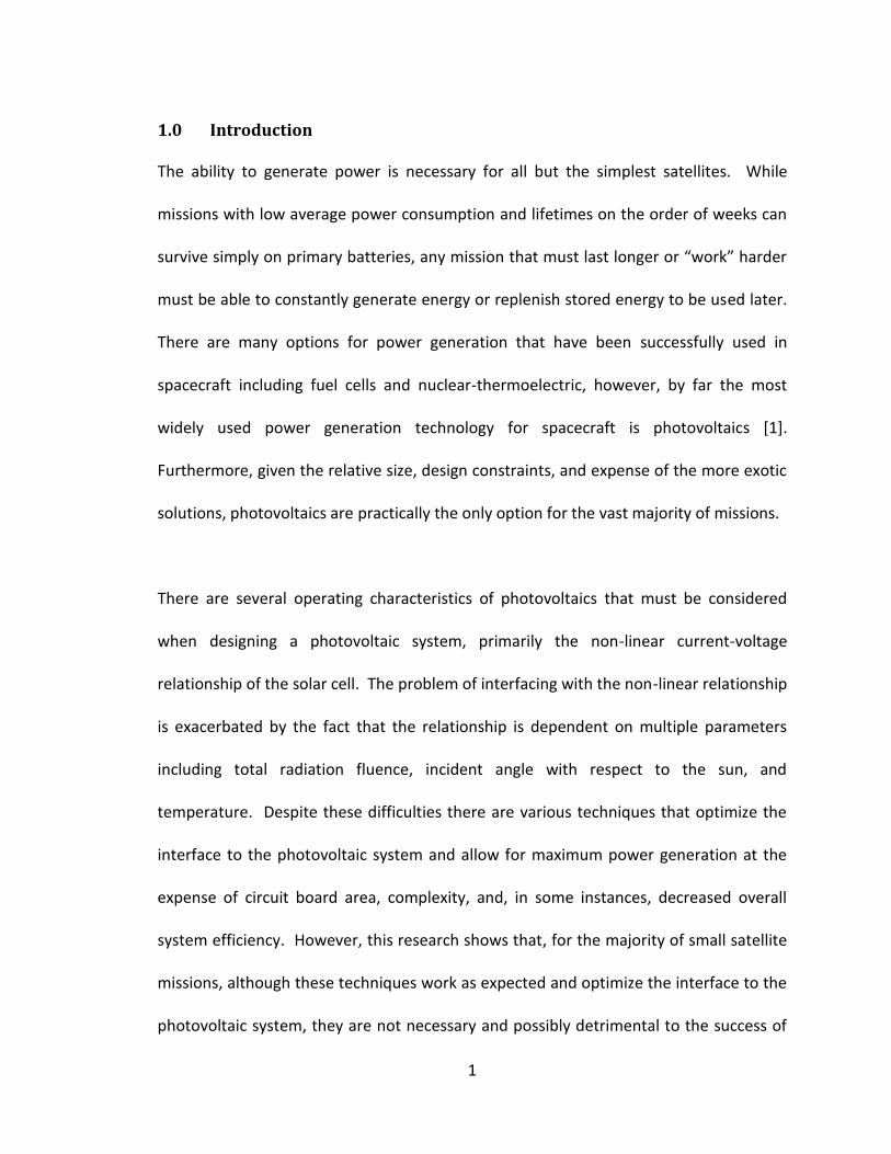
1.0 Introduction
The ability to generate power is necessary for all but the simplest satellites. While
missions with low average power consumption and lifetimes on the order of weeks can
survive simply on primary batteries, any mission that must last longer or “work” harder
must be able to constantly generate energy or replenish stored energy to be used later.
There are many options for power generation that have been successfully used in
spacecraft including fuel cells and nuclear-thermoelectric, however, by far the most
widely used power generation technology for spacecraft is photovoltaics [1].
Furthermore, given the relative size, design constraints, and expense of the more exotic
solutions, photovoltaics are practically the only option for the vast majority of missions.
There are several operating characteristics of photovoltaics that must be considered
when designing a photovoltaic system, primarily the non-linear current-voltage
relationship of the solar cell. The problem of interfacing with the non-linear relationship
is exacerbated by the fact that the relationship is dependent on multiple parameters
including total radiation fluence, incident angle with respect to the sun, and
temperature. Despite these difficulties there are various techniques that optimize the
interface to the photovoltaic system and allow for maximum power generation at the
expense of circuit board area, complexity, and, in some instances, decreased overall
system efficiency. However, this research shows that, for the majority of small satellite
missions, although these techniques work as expected and optimize the interface to the
photovoltaic system, they are not necessary and possibly detrimental to the success of
2
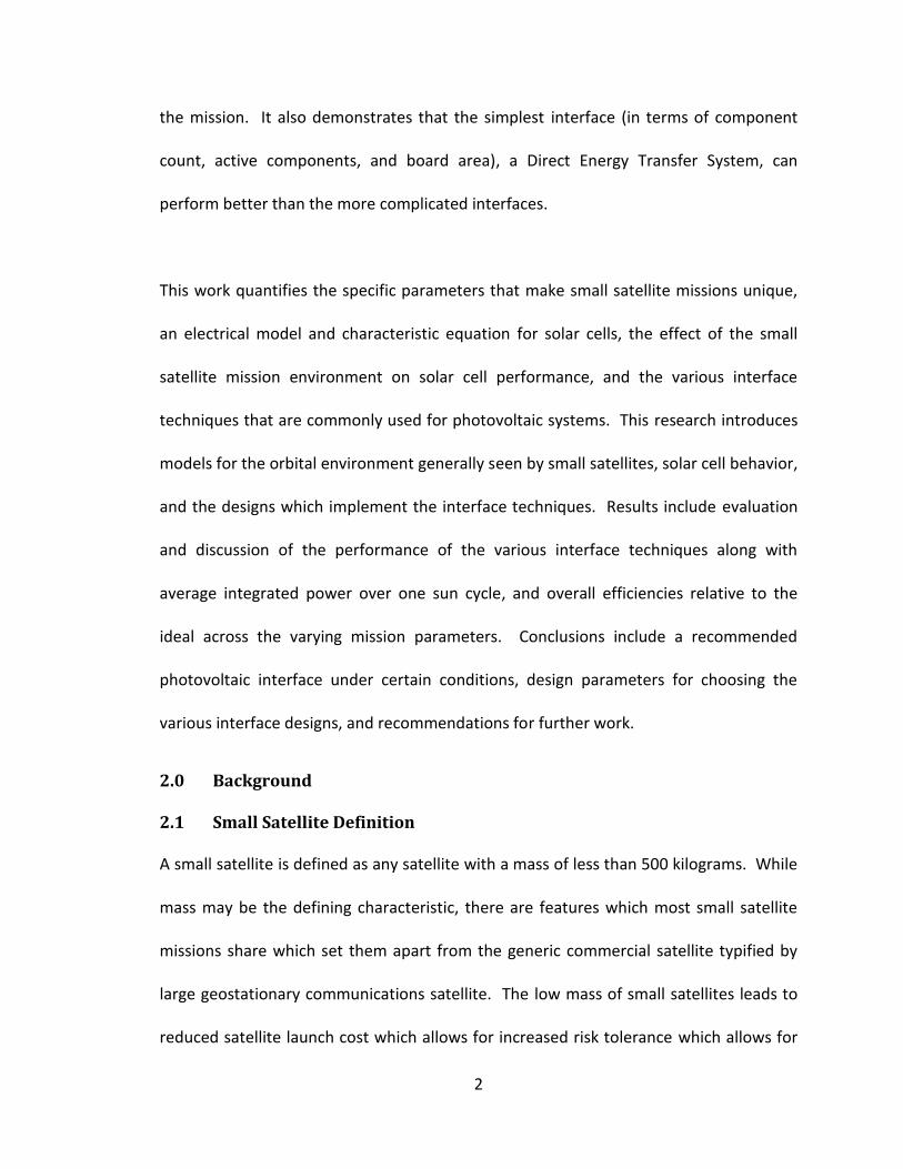
the mission. It also demonstrates that the simplest interface (in terms of component
count, active components, and board area), a Direct Energy Transfer System, can
perform better than the more complicated interfaces.
This work quantifies the specific parameters that make small satellite missions unique,
an electrical model and characteristic equation for solar cells, the effect of the small
satellite mission environment on solar cell performance, and the various interface
techniques that are commonly used for photovoltaic systems. This research introduces
models for the orbital environment generally seen by small satellites, solar cell behavior,
and the designs which implement the interface techniques. Results include evaluation
and discussion of the performance of the various interface techniques along with
average integrated power over one sun cycle, and overall efficiencies relative to the
ideal across the varying mission parameters. Conclusions include a recommended
photovoltaic interface under certain conditions, design parameters for choosing the
various interface designs, and recommendations for further work.
2.0 Background
2.1 Small Satellite Definition
A small satellite is defined as any satellite with a mass of less than 500 kilograms. While
mass may be the defining characteristic, there are features which most small satellite
missions share which set them apart from the generic commercial satellite typified by
large geostationary communications satellite. The low mass of small satellites leads to
reduced satellite launch cost which allows for increased risk tolerance which allows for
3
less redundancy in satellite subsystems. Furthermore, small satellites generally have a
one to two year primary mission timeline and are injected into low earth orbit both of
which lowers the risk of system failure due to shorter exposure to the space
environment; radiation, micrometeorites, etc and due to lower overall radiaton
environment of low earth orbit as opposed to higher orbits.
Increased risk tolerance allows modern technologies to be used in small satellites which
lead to further reduced mass and volume. This trend of miniaturization has allowed
fully capable satellites to be developed which have a mass of less than one kilogram. An
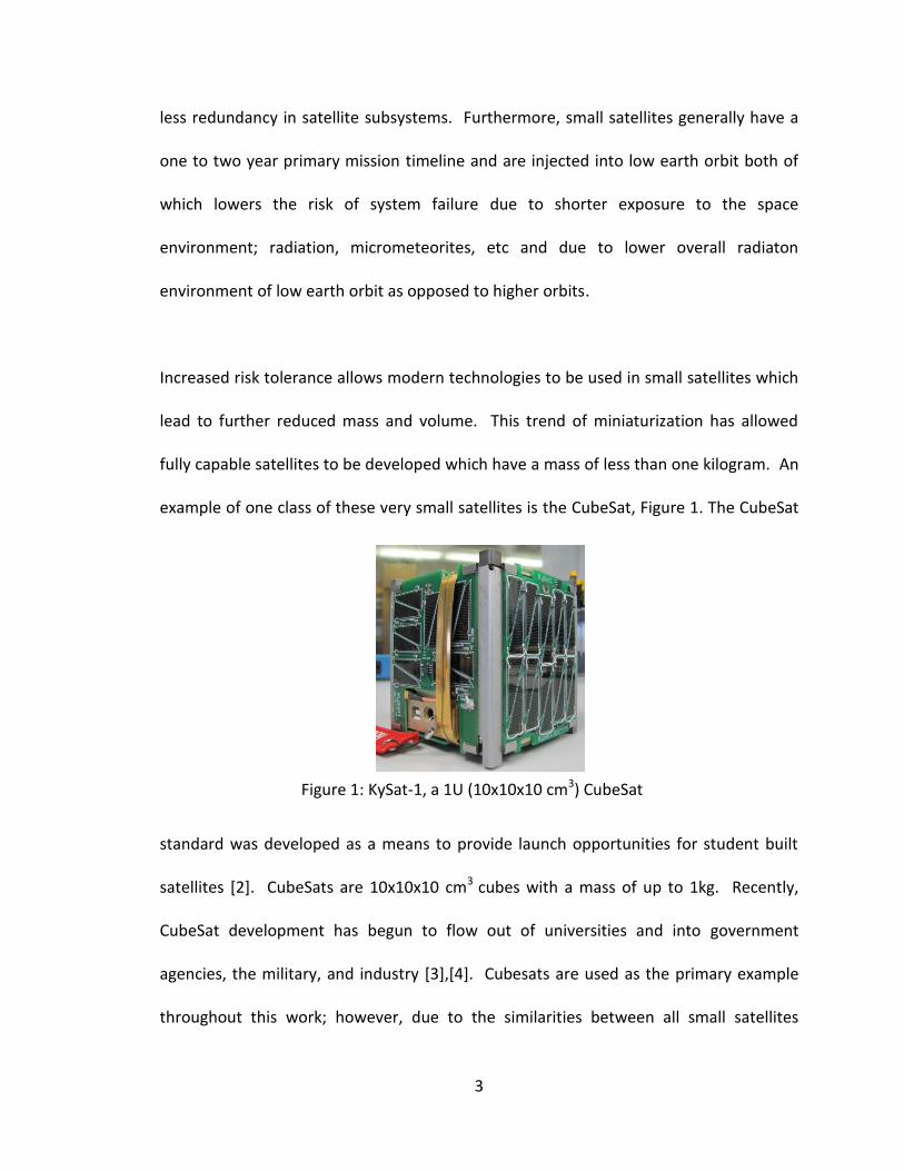
example of one class of these very small satellites is the CubeSat, Figure 1. The CubeSat
standard was developed as a means to provide launch opportunities for student built
satellites [2]. CubeSats are 10x10x10 cm3 cubes with a mass of up to 1kg. Recently,
CubeSat development has begun to flow out of universities and into government
agencies, the military, and industry [3],[4]. Cubesats are used as the primary example
throughout this work; however, due to the similarities between all small satellites
Figure 1: KySat-1, a 1U (10x10x10 cm3) CubeSat
4
missions, the conclusions drawn are directly applicable to many small satellites
programs.
2.2 Solar Cell Behavior
Solar cells work by converting electromagnetic radiation, in the form of optical
wavelength photons, into electrical energy. They do this by using what is known as the
photovoltaic effect, in which a photon transfers its energy to a valence electron which is
then able to roam around the lattice of a semiconductor, along with the hole it left
behind. The movement of electrons and holes generates an electric current in the
semiconductor [5].
While it is important to understand the underlying physics of solar cell operation, that
level of detail is not necessary to analyze a cells performance under varying condtions.
An equivalent circuit model is a convenient and widely used method for evaluating the
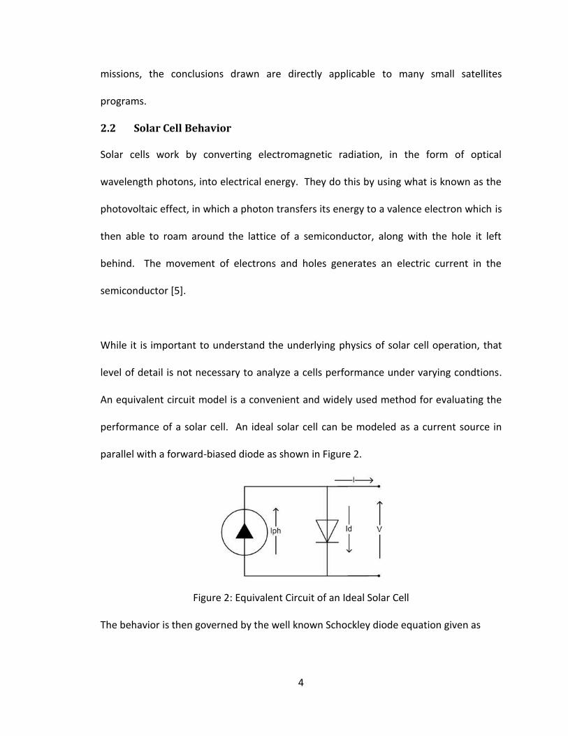
performance of a solar cell. An ideal solar cell can be modeled as a current source in
parallel with a forward-biased diode as shown in Figure 2.
Figure 2: Equivalent Circuit of an Ideal Solar Cell
The behavior is then governed by the well known Schockley diode equation given as
5
)1()/( TD nVV
oD eII (1)
Where ID is the current through the diode, IO is the reverse saturation current, VD is the
voltage across the diode, n is the quality factor and VT is the thermal voltage, which
equals k*T/q where q is the fundamental charge of an electron in coulombs, k is the
Boltzmann constant in Joules per Kelvin, and T is the temperature in Kelvin. Circuit
analysis gives the behavior of the solar cell as
Dph III (2)
Where I is the current out of the solar cell and Iph is the photogenerated current using
the process described above. Combining (1) and (2) gives the characteristic equation of
an ideal solar cell
)1()/( TnVV
oph eIII (3)
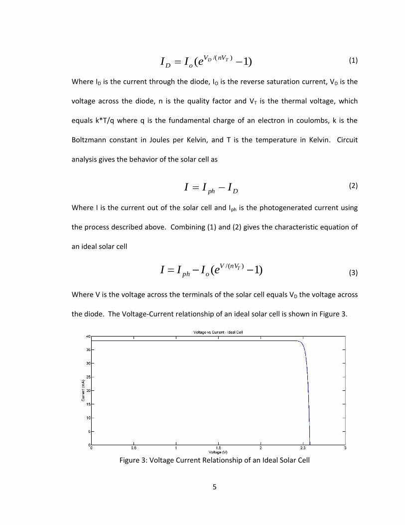
Where V is the voltage across the terminals of the solar cell equals VD the voltage across
the diode. The Voltage-Current relationship of an ideal solar cell is shown in Figure 3.
Figure 3: Voltage Current Relationship of an Ideal Solar Cell
6
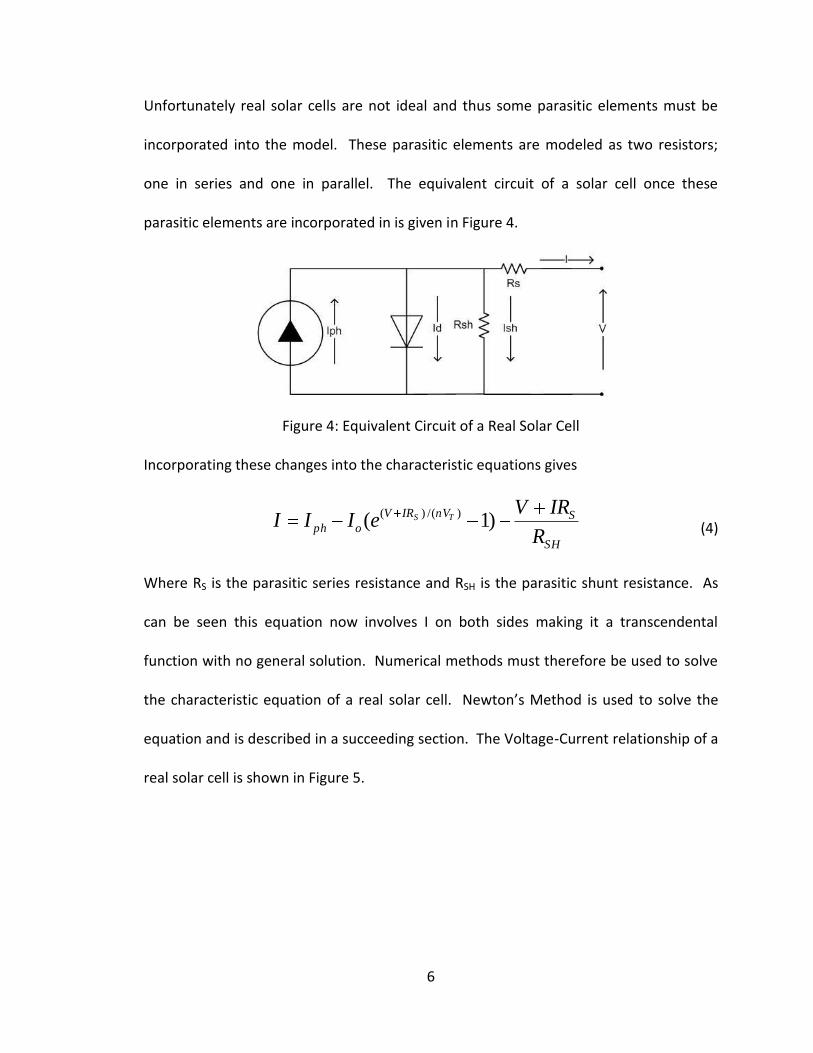
Unfortunately real solar cells are not ideal and thus some parasitic elements must be
incorporated into the model. These parasitic elements are modeled as two resistors;
one in series and one in parallel. The equivalent circuit of a solar cell once these
parasitic elements are incorporated in is given in Figure 4.
Figure 4: Equivalent Circuit of a Real Solar Cell
Incorporating these changes into the characteristic equations gives
SH
SnVIRV
ophR
IRVeIII TS )1(
)/()(
(4)
Where RS is the parasitic series resistance and RSH is the parasitic shunt resistance. As
can be seen this equation now involves I on both sides making it a transcendental
function with no general solution. Numerical methods must therefore be used to solve
the characteristic equation of a real solar cell. Newton’s Method is used to solve the
equation and is described in a succeeding section. The Voltage-Current relationship of a
real solar cell is shown in Figure 5.
7
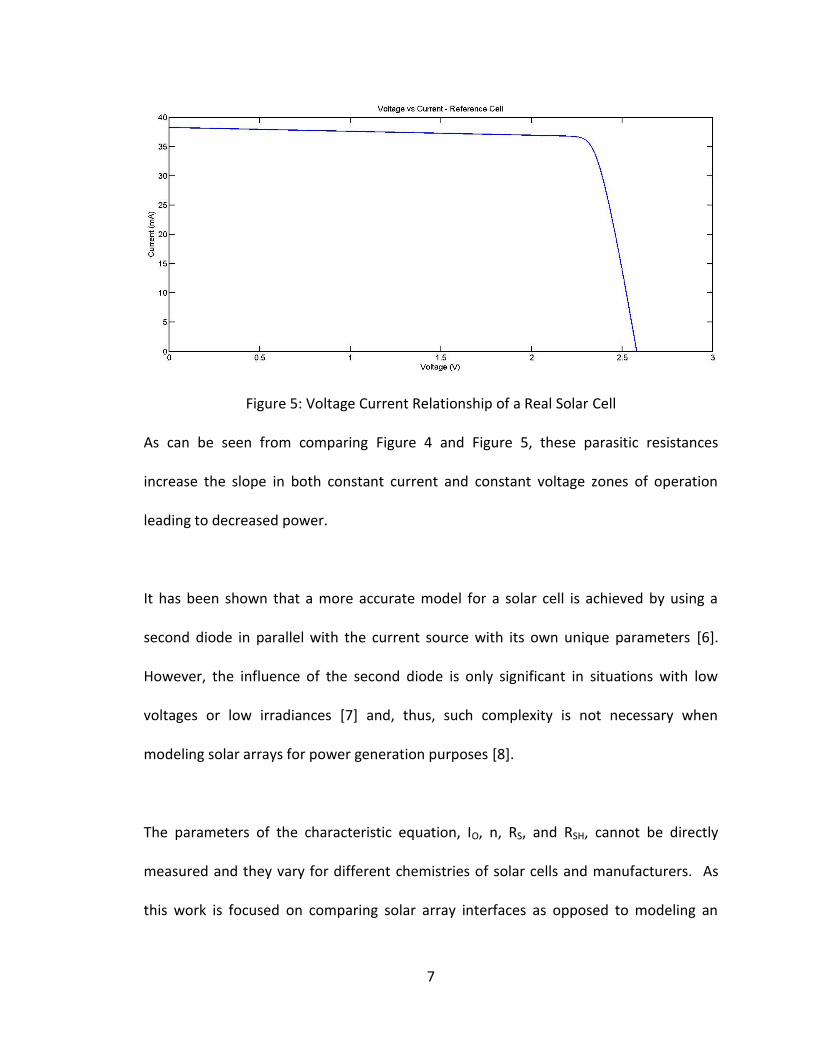
Figure 5: Voltage Current Relationship of a Real Solar Cell
As can be seen from comparing Figure 4 and Figure 5, these parasitic resistances
increase the slope in both constant current and constant voltage zones of operation
leading to decreased power.
It has been shown that a more accurate model for a solar cell is achieved by using a
second diode in parallel with the current source with its own unique parameters [6].
However, the influence of the second diode is only significant in situations with low
voltages or low irradiances [7] and, thus, such complexity is not necessary when
modeling solar arrays for power generation purposes [8].
The parameters of the characteristic equation, IO, n, RS, and RSH, cannot be directly
measured and they vary for different chemistries of solar cells and manufacturers. As
this work is focused on comparing solar array interfaces as opposed to modeling an
8
actual system, the parameters used in the solar cell model constructed were based on
manufacturers specifications and not empirically determined; there are, however,
various methods for extraction using empirical methods [9], [10].
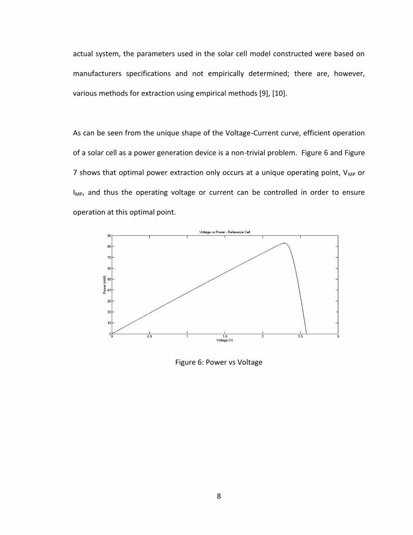
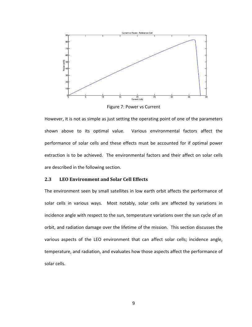
As can be seen from the unique shape of the Voltage-Current curve, efficient operation
of a solar cell as a power generation device is a non-trivial problem. Figure 6 and Figure
7 shows that optimal power extraction only occurs at a unique operating point, VMP or
IMP, and thus the operating voltage or current can be controlled in order to ensure
operation at this optimal point.
Figure 6: Power vs Voltage
9
Figure 7: Power vs Current
However, it is not as simple as just setting the operating point of one of the parameters
shown above to its optimal value. Various environmental factors affect the
performance of solar cells and these effects must be accounted for if optimal power
extraction is to be achieved. The environmental factors and their affect on solar cells
are described in the following section.
2.3 LEO Environment and Solar Cell Effects
The environment seen by small satellites in low earth orbit affects the performance of
solar cells in various ways. Most notably, solar cells are affected by variations in
incidence angle with respect to the sun, temperature variations over the sun cycle of an
orbit, and radiation damage over the lifetime of the mission. This section discusses the
various aspects of the LEO environment that can affect solar cells; incidence angle,
temperature, and radiation, and evaluates how those aspects affect the performance of
solar cells.
10
2.3.1 Incidence Angle
The incidence angle, defined as the angle between the a light source and solar cell
normal, affects the performance of solar cells by effectively lowering the total
irradiance, equivalent power density of the light source in W/m2, projected onto the
solar cell. The relationship between incidence angle and output current follows the
cosine law given by
)cos(OS EE (5)
Where ES is the irradiance projected onto the solar cell, θ is the incidence angle between
the solar cell and the light source, and EO is the solar constant. The solar constant is the
power density produced by the sun measured once it reaches earth; it has been
measured to vary from 1331 to 1423 W/m2[1]. Lowering the irradiance projected onto
the solar cell has the effect of lowering the output current of the solar cell. The effect of
this reduced irradiance can be seen in Figure 8.
11
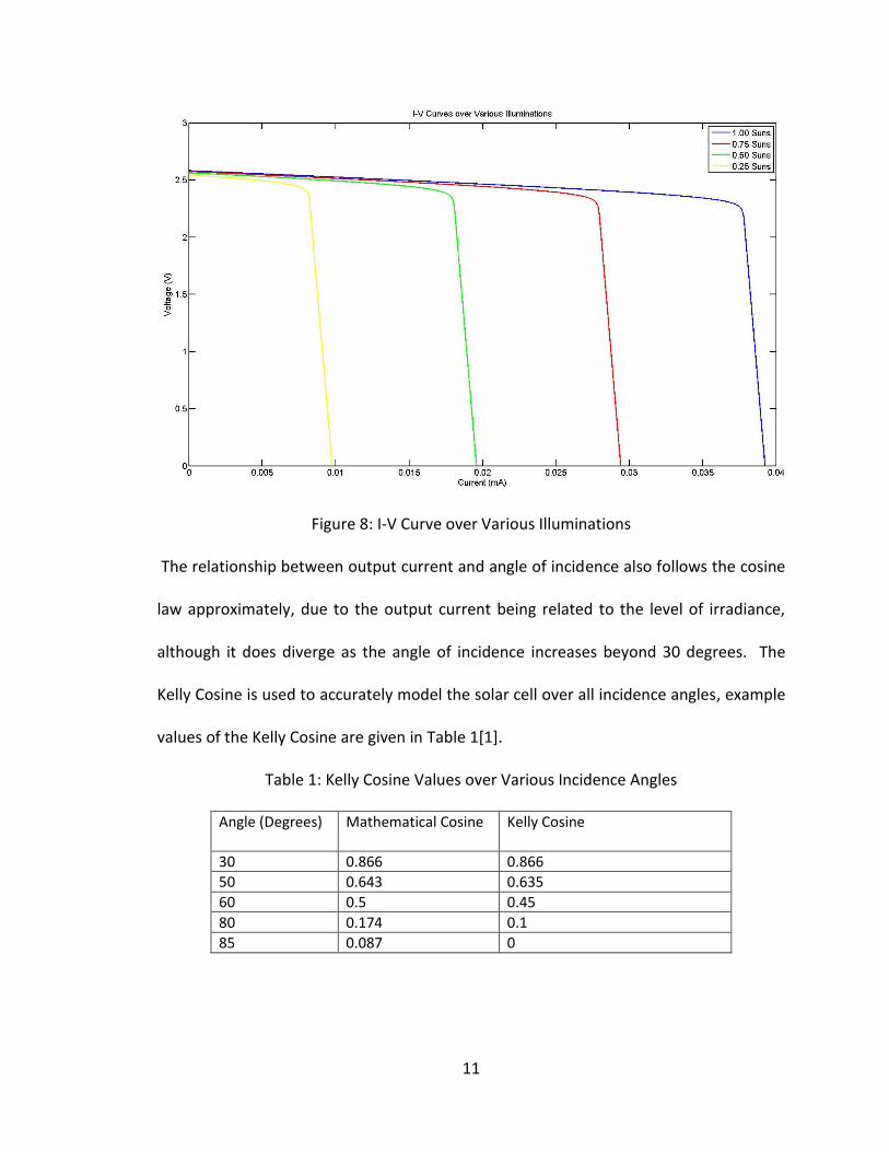
Figure 8: I-V Curve over Various Illuminations
The relationship between output current and angle of incidence also follows the cosine
law approximately, due to the output current being related to the level of irradiance,
although it does diverge as the angle of incidence increases beyond 30 degrees. The
Kelly Cosine is used to accurately model the solar cell over all incidence angles, example
values of the Kelly Cosine are given in Table 1[1].
Table 1: Kelly Cosine Values over Various Incidence Angles
Angle (Degrees) Mathematical Cosine Kelly Cosine
30 0.866 0.866
50 0.643 0.635
60 0.5 0.45
80 0.174 0.1
85 0.087 0
12
It can be seen in Figure 8 that over the various illuminations the amount of current
available from the solar cell decreases dramatically but the open circuit voltage, the
voltage which corresponds to zero current flow, VOC, of the solar cell is only slightly
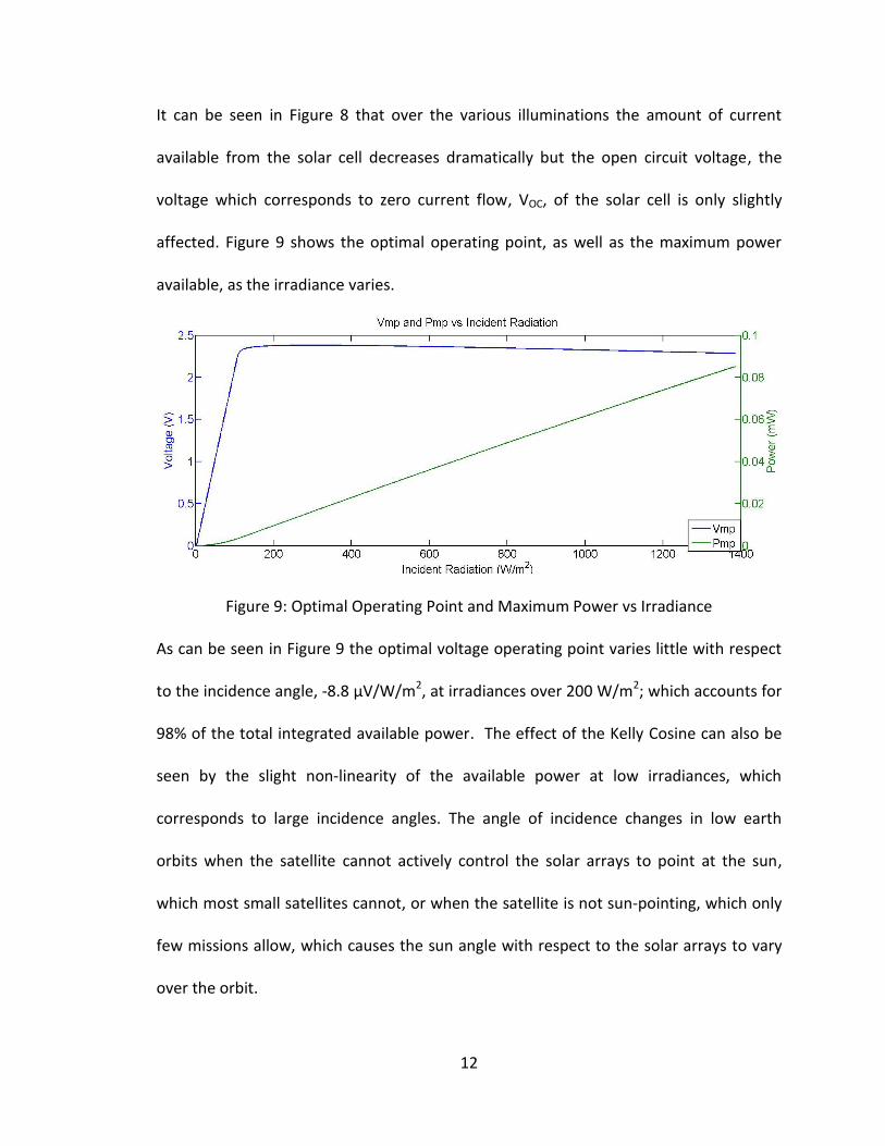
affected. Figure 9 shows the optimal operating point, as well as the maximum power
available, as the irradiance varies.
Figure 9: Optimal Operating Point and Maximum Power vs Irradiance
As can be seen in Figure 9 the optimal voltage operating point varies little with respect
to the incidence angle, -8.8 μV/W/m2, at irradiances over 200 W/m2; which accounts for
98% of the total integrated available power. The effect of the Kelly Cosine can also be
seen by the slight non-linearity of the available power at low irradiances, which
corresponds to large incidence angles. The angle of incidence changes in low earth
orbits when the satellite cannot actively control the solar arrays to point at the sun,
which most small satellites cannot, or when the satellite is not sun-pointing, which only
few missions allow, which causes the sun angle with respect to the solar arrays to vary
over the orbit.
13
2.3.2 Temperature
With no atmosphere to hold onto heat there are large temperature swings over
relatively short periods in low earth orbit. Standard expected temperature in Low Earth
orbit vary from -30 to 50 C over one orbit, a period of approximately 100 minutes [11].
The effect of temperature on solar cells can be directly seen in the characteristic
equation of a solar cell, (4), in the thermal voltage. But the more dramatic effect comes
from changes in the reverse saturation current. However the exact mechanism that
causes temperature to change the behavior of solar cells in not important for this study
as this study only needs to model one solar cell to evaluate multiple solar array
interfaces. Therefore, the effect of temperature has been modeled to correspond to
the solar cell manufacturers specification of a change in the optimal voltage operating
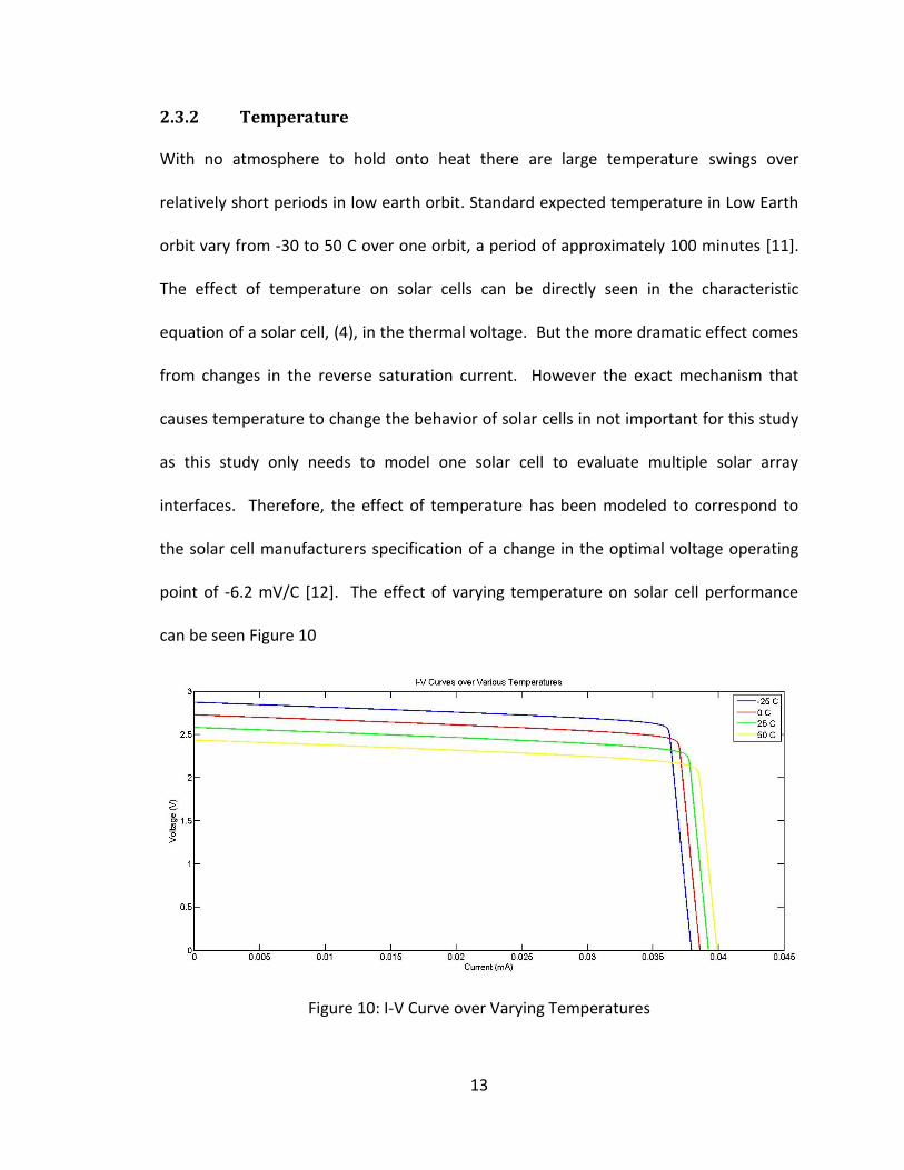
point of -6.2 mV/C [12]. The effect of varying temperature on solar cell performance
can be seen Figure 10
Figure 10: I-V Curve over Varying Temperatures
14
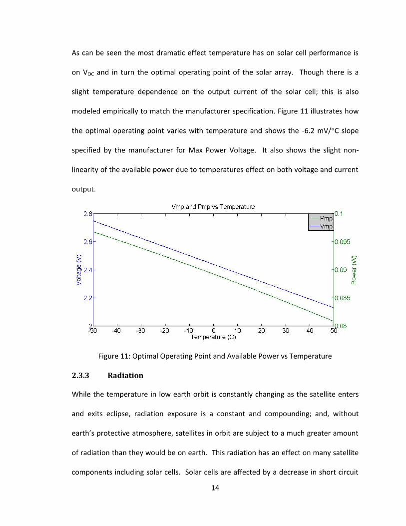
As can be seen the most dramatic effect temperature has on solar cell performance is
on VOC and in turn the optimal operating point of the solar array. Though there is a
slight temperature dependence on the output current of the solar cell; this is also
modeled empirically to match the manufacturer specification. Figure 11 illustrates how
the optimal operating point varies with temperature and shows the -6.2 mV/°C slope
specified by the manufacturer for Max Power Voltage. It also shows the slight non-
linearity of the available power due to temperatures effect on both voltage and current
output.
Figure 11: Optimal Operating Point and Available Power vs Temperature
2.3.3 Radiation
While the temperature in low earth orbit is constantly changing as the satellite enters
and exits eclipse, radiation exposure is a constant and compounding; and, without
earth’s protective atmosphere, satellites in orbit are subject to a much greater amount
of radiation than they would be on earth. This radiation has an effect on many satellite
components including solar cells. Solar cells are affected by a decrease in short circuit
15
current, defined as the amount current generated at zero volts, due to changes in the
diffusion length as well as a decrease in VOC due to increases of the reverse saturation
current and quality factor [13].
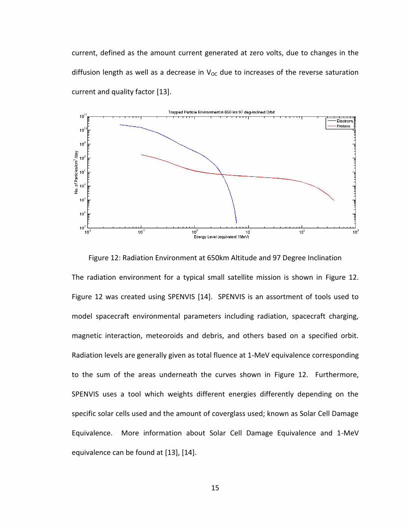
Figure 12: Radiation Environment at 650km Altitude and 97 Degree Inclination
The radiation environment for a typical small satellite mission is shown in Figure 12.
Figure 12 was created using SPENVIS [14]. SPENVIS is an assortment of tools used to
model spacecraft environmental parameters including radiation, spacecraft charging,
magnetic interaction, meteoroids and debris, and others based on a specified orbit.
Radiation levels are generally given as total fluence at 1-MeV equivalence corresponding
to the sum of the areas underneath the curves shown in Figure 12. Furthermore,
SPENVIS uses a tool which weights different energies differently depending on the
specific solar cells used and the amount of coverglass used; known as Solar Cell Damage
Equivalence. More information about Solar Cell Damage Equivalence and 1-MeV
equivalence can be found at [13], [14].
16
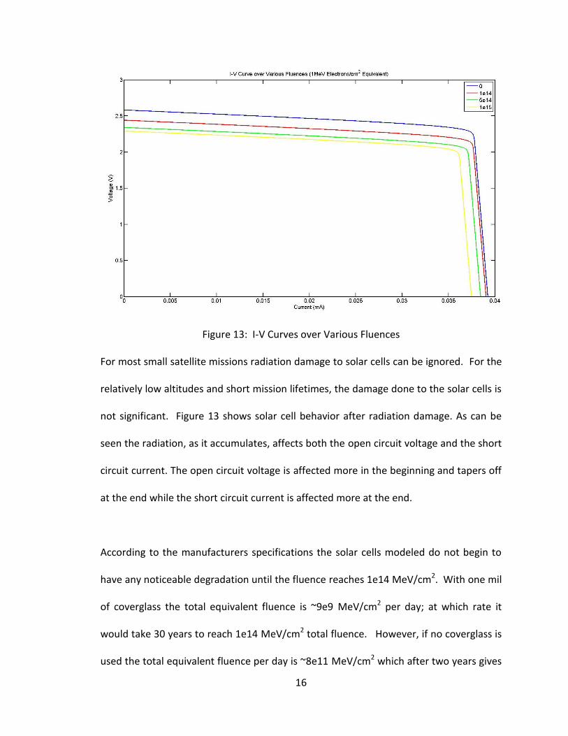
Figure 13: I-V Curves over Various Fluences
For most small satellite missions radiation damage to solar cells can be ignored. For the
relatively low altitudes and short mission lifetimes, the damage done to the solar cells is
not significant. Figure 13 shows solar cell behavior after radiation damage. As can be
seen the radiation, as it accumulates, affects both the open circuit voltage and the short
circuit current. The open circuit voltage is affected more in the beginning and tapers off
at the end while the short circuit current is affected more at the end.
According to the manufacturers specifications the solar cells modeled do not begin to
have any noticeable degradation until the fluence reaches 1e14 MeV/cm2. With one mil
of coverglass the total equivalent fluence is ~9e9 MeV/cm2 per day; at which rate it
would take 30 years to reach 1e14 MeV/cm2 total fluence. However, if no coverglass is
used the total equivalent fluence per day is ~8e11 MeV/cm2 which after two years gives
17
a total fluence of 5.8e14 MeV/cm2, which would lead to a significant change in solar cell
performance. Also, if the orbit varies greatly from that described above, the radiation
environment could be vastly different. Therefore, a discussion is included in the results
section on how each solar array interface responds to a radiation damaged solar cell.
2.4 Solar Array Interface
As discussed above there are many factors in low earth orbit which affect the
performance of a solar cell. Temperature and incidence angle are constantly changing
throughout an orbit while radiation causes a constant slow decline. Therefore, in order
to optimally generate power from solar cells they must be operated carefully. To reach
that end, various control schemes have been designed, called Maximum Power Point
Trackers (MPPT), which manipulate either operating voltage or current of the solar
array. MPPT’s manipulate the operating point of the solar array by controlling the
operation of a switching converter situated between the solar arrays and load. The
switching converter acts as a load transformer causing the solar array to always “see” an
ideal load no matter the state of the actual load. A battery, or other energy storage
device, is then placed in parallel to account for load transients. An MPPT also adjusts
the ideal load to account for changes in solar cell performance due to environmental
factors such as those described above and shown in Figure 8, Figure 10, and Figure 13.
Furthermore, the use of a switching converter between the solar arrays and the rest of
system decouples the two designs allowing the solar arrays and the battery/load to be
designed with little regard to each other.
18
3.0 Modeling
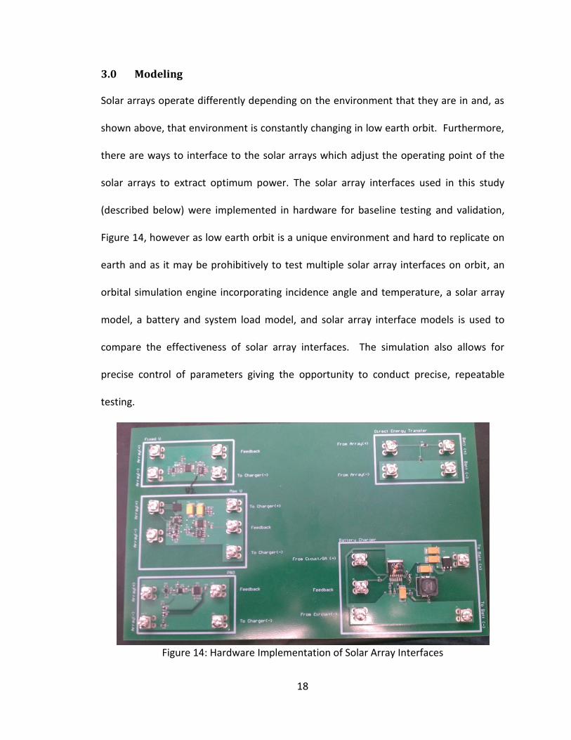
Solar arrays operate differently depending on the environment that they are in and, as
shown above, that environment is constantly changing in low earth orbit. Furthermore,
there are ways to interface to the solar arrays which adjust the operating point of the
solar arrays to extract optimum power. The solar array interfaces used in this study
(described below) were implemented in hardware for baseline testing and validation,
Figure 14, however as low earth orbit is a unique environment and hard to replicate on
earth and as it may be prohibitively to test multiple solar array interfaces on orbit, an
orbital simulation engine incorporating incidence angle and temperature, a solar array
model, a battery and system load model, and solar array interface models is used to
compare the effectiveness of solar array interfaces. The simulation also allows for
precise control of parameters giving the opportunity to conduct precise, repeatable
testing.
Figure 14: Hardware Implementation of Solar Array Interfaces

19
3.1 Simulink® Based Model
The solar array interfaces described above, as well as other orbital parameters, were
implemented in Simulink® in order to model their behavior in an orbital environment
and compare their behavior against each other. Simulink® is MATLAB-based tool for
graphical modeling and simulation of time-varying dynamic systems. It is used here as a
convenient tool for developing differential models and implementing controller designs
while combining all of these different elements quickly which eases development and
debugging. As Simulink® is, in essence, a differential equation solver it gives the option
of using different solvers which can trade accuracy for speed, etc. As used here, all the
designs were tested over multiple solvers to ensure stability and accuracy while the
same solver, ode45 Dormand-Prince Method, is used for comparisons. More
information can be found in the Simulink® documentation [15].
3.2 Orbital Parameters
The orbit used for the simulations is a 650 km orbit at 97 degree inclination. This gives
an orbital period of 97.73 minutes with a maximum eclipse of 35.38 minutes [16]. This
orbital period is similar for all low earth orbiting satellites; for this simulation it primarily
affects the temperature range experienced by the satellite. It is also used to model the
radiation environment. The effects of radiation are discussed in the conclusion. The
rotation rate is standard for passively stabilized CubeSats, though the effect of faster
rotation rates is discussed in the conclusion.
20
3.2.1 Rotation Rates
Cubesats generally utilized body mounted solar cells to generate power. This means
that the incidence angle between the solar cells and the sun is dependent on the
attitude of the entire spacecraft. As most CubeSats use only passive attitude control, as
opposed to spin stabilized or three-axis control, a slight rotation is modeled for the solar
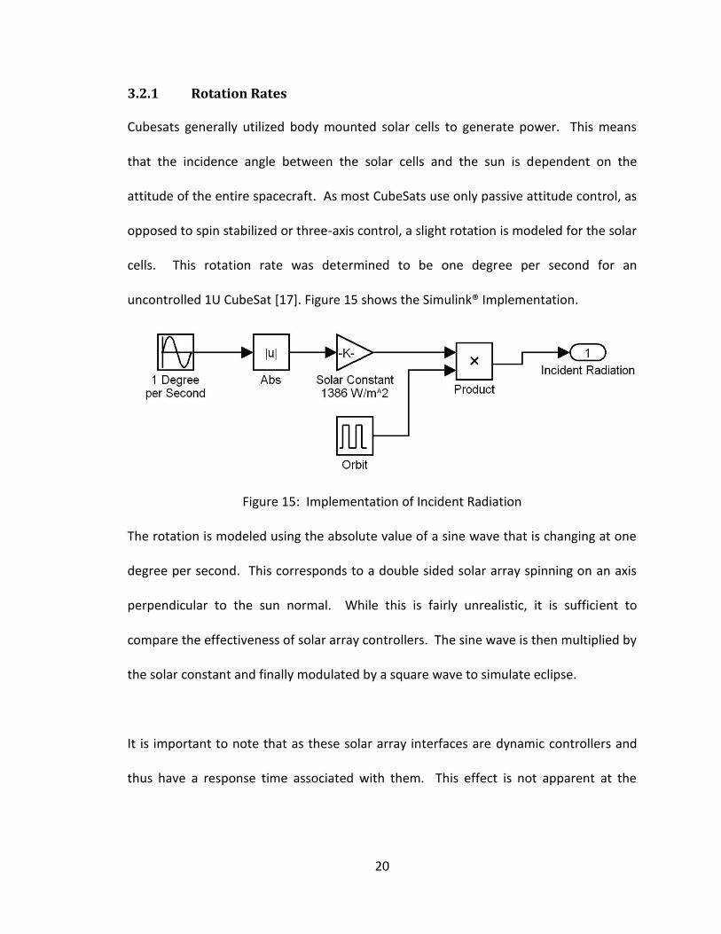
cells. This rotation rate was determined to be one degree per second for an
uncontrolled 1U CubeSat [17]. Figure 15 shows the Simulink® Implementation.
Figure 15: Implementation of Incident Radiation
The rotation is modeled using the absolute value of a sine wave that is changing at one
degree per second. This corresponds to a double sided solar array spinning on an axis
perpendicular to the sun normal. While this is fairly unrealistic, it is sufficient to
compare the effectiveness of solar array controllers. The sine wave is then multiplied by
the solar constant and finally modulated by a square wave to simulate eclipse.
It is important to note that as these solar array interfaces are dynamic controllers and
thus have a response time associated with them. This effect is not apparent at the
21
moderate rotation rate used here but must be taken into account for faster rotations.
Further discussion of this effect can be found in the Conclusions section of this thesis.
3.2.2 Temperature
As stated above, a CubeSat in low earth orbit has been shown to vary from -30 to +50
degrees C but, due to the unique environment of low earth orbit, this variance is not
linear and therefore must be modeled. Several assumptions are used in the
development of the temperature model including: infinite conductivity, zero Kelvin sink
temperature, and constant absorptivity, emissivity, and specific heat capacity. The
temperature model is created by first calculating the net thermal power of the system
given as:
4TAVFAqAPGAPDP Snet (6)
Where Pnet is the net power in watts, APD is the average power dissipated, APG is the
average power generated, qS is the incident radiation in W/m2, α is the absorptivity, A is
the total area in m2, VF is the view factor, ε is the emissivity, σ is the Stefan – Boltzmann
constant, and T is the temperature in Kelvin. Of course this equation is different
depending on whether or not the satellite is in eclipse. While in the sun qS is the sum of
the Earth’s infrared radiation, solar radiation, and solar radiation reflected off the Earth
known an albedo. While in eclipse qS is equal to only Earth’s infrared radiation and APG
is equal to zero.
The net power is then integrated with respect to time to determine the total thermal
energy of the system in joules.
22
dtPE
t
t
net
o
(7)
Where E is the total thermal energy of the system and t-to is the fundamental time step
of the system. The total energy is then used to determine the system temperature
using the specific heat capacity as follows:
mc
ET (8)
Where m is the mass of the system and c is the weighted average specific heat of the
system given as:
TotalMass
nMassnatSpecificHeMassatSpecificHec
)()(...)1()1( (9)
The temperature calculated in (8) is then fed back into (6) for the next net thermal
power calculation.
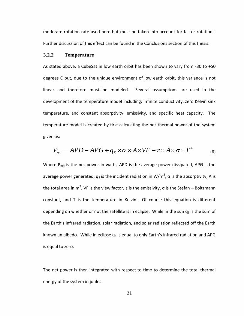
The implementation designed for this model, Figure 16, uses a function to determine
the net thermal power and to factor in the mass and weighted specific heat. This value
is then integrated to give the overall temperature in Kelvin. This reversal of (7) and (8) is
valid as the mass and specific heat are considered constant and thus can move into the
integral in (7) without any problems. Finally, the temperature is converted into degrees
Celsius. The square wave, labeled orbit, is used to determine when the satellite is in
eclipse. The integrator is set to an initial value representing the temperature of the
satellite just as it leaves eclipse. This was determined by choosing a reasonable guess
23
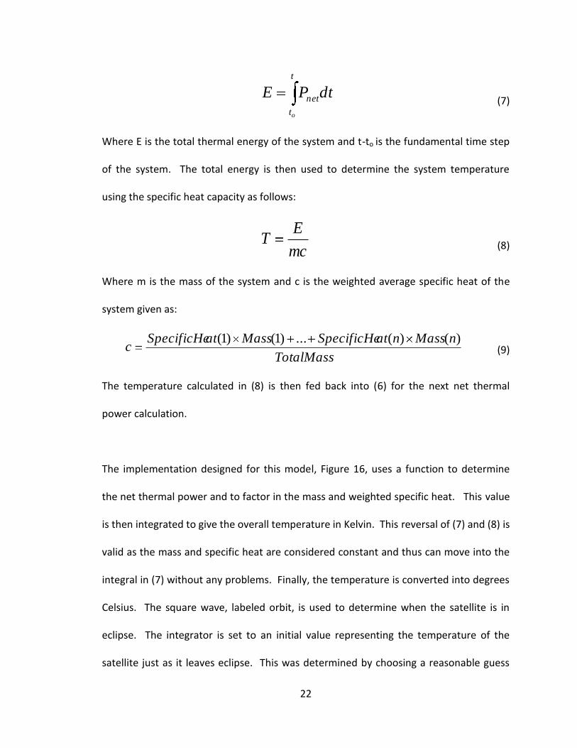
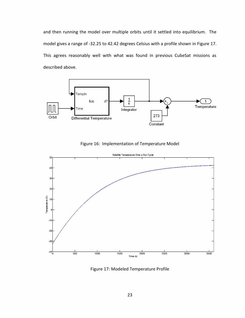
and then running the model over multiple orbits until it settled into equilibrium. The
model gives a range of -32.25 to 42.42 degrees Celsius with a profile shown in Figure 17.
This agrees reasonably well with what was found in previous CubeSat missions as
described above.
Figure 16: Implementation of Temperature Model
Figure 17: Modeled Temperature Profile
24
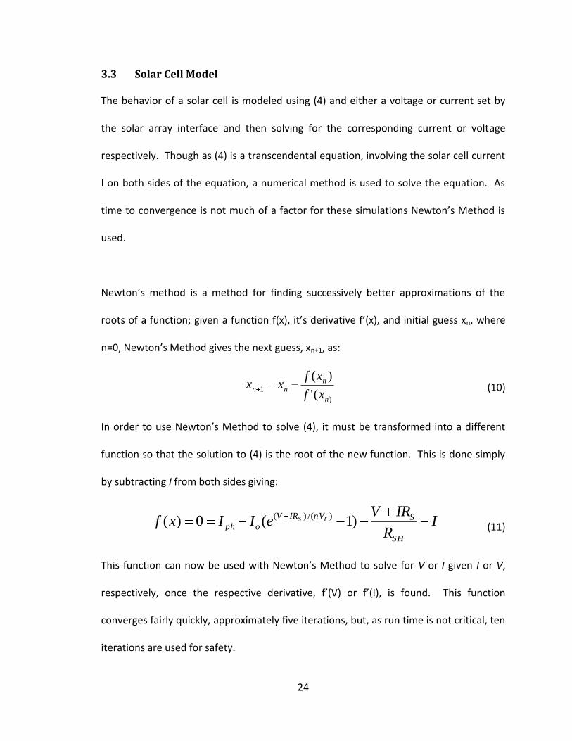
3.3 Solar Cell Model
The behavior of a solar cell is modeled using (4) and either a voltage or current set by
the solar array interface and then solving for the corresponding current or voltage
respectively. Though as (4) is a transcendental equation, involving the solar cell current
I on both sides of the equation, a numerical method is used to solve the equation. As
time to convergence is not much of a factor for these simulations Newton’s Method is
used.
Newton’s method is a method for finding successively better approximations of the
roots of a function; given a function f(x), it’s derivative f’(x), and initial guess xn, where
n=0, Newton’s Method gives the next guess, xn+1, as:
)
1('
)(
n
nnn
xf
xfxx (10)
In order to use Newton’s Method to solve (4), it must be transformed into a different
function so that the solution to (4) is the root of the new function. This is done simply
by subtracting I from both sides giving:
IR
IRVeIIxf
SH
SnVIRV
ophTS )1(0)(
)/()(
(11)
This function can now be used with Newton’s Method to solve for V or I given I or V,
respectively, once the respective derivative, f’(V) or f’(I), is found. This function
converges fairly quickly, approximately five iterations, but, as run time is not critical, ten
iterations are used for safety.
25
Real solar cells, as part of a full mission simulation, would have to be modeled using the
operating parameters, RS, RSH, IO, and n, would have to be empirically determined;
however, as this research is concerned with comparing solar array interfaces as opposed
to modeling a real system the parameters RS, RSH, IO, and n were not determined
empirically using a physical solar cell. They were, however, determined to closely match
a manufacturer’s specification of Improved Triple Junction Solar Cells.
A MATLAB function, seen in Figure 18 as the Solar Cell Model block, is the solar cell
model in the simulation which takes the requested voltage or current, temperature, and
incident radiation as inputs and outputs the solar array current and voltage.
3.4 Battery Charge Regulator Model
A battery charge regulator is, as its name implies, a power regulator, either switching or
linear, which conditions incoming power to charge a battery with a certain profile
specified by the battery chemistry. The battery charge regulator modeled is a current
mode switcher which allows for input current programming. This means that the
regulator operation is determined by the input current which can be adjusted by an
external circuit. This is modeled, as seen in several figures below, as a single gain
labeled as Vfb -> Ireq, which translates the solar array interface control signal into the
input current of the battery charge regulator and thus the output current of the solar
cell.
26
3.5 Solar Array Interface Models
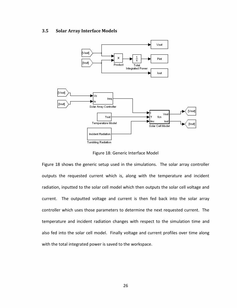
Figure 18: Generic Interface Model
Figure 18 shows the generic setup used in the simulations. The solar array controller
outputs the requested current which is, along with the temperature and incident
radiation, inputted to the solar cell model which then outputs the solar cell voltage and
current. The outputted voltage and current is then fed back into the solar array
controller which uses those parameters to determine the next requested current. The
temperature and incident radiation changes with respect to the simulation time and
also fed into the solar cell model. Finally voltage and current profiles over time along
with the total integrated power is saved to the workspace.
27
3.5.1 MPPT
While there are many MPPT controllers there are only a few major designs with the rest
being derivatives off of those; this study only looks at the major designs but more can be
found in [18]. The MPPT controllers described, modeled and compared for this work are
known as: Fractional Voltage, Perturb and Observe, and dP/dV. For comparison, a
Fixed-Point and Temperature-Compensated Fixed-Point controller are developed and
modeled. Finally these are all compared to the simplest solar array interface,
connecting the solar arrays directly, with diode protection, to a battery known as Direct
Energy Transfer.
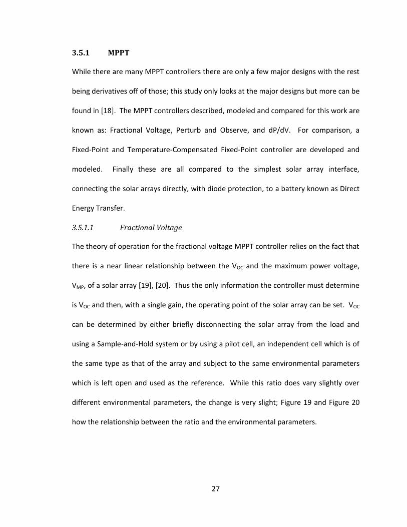
3.5.1.1 Fractional Voltage
The theory of operation for the fractional voltage MPPT controller relies on the fact that
there is a near linear relationship between the VOC and the maximum power voltage,
VMP, of a solar array [19], [20]. Thus the only information the controller must determine
is VOC and then, with a single gain, the operating point of the solar array can be set. VOC
can be determined by either briefly disconnecting the solar array from the load and
using a Sample-and-Hold system or by using a pilot cell, an independent cell which is of
the same type as that of the array and subject to the same environmental parameters
which is left open and used as the reference. While this ratio does vary slightly over
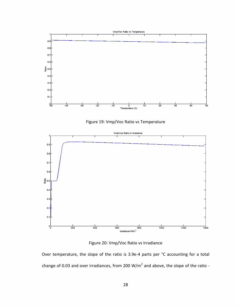
different environmental parameters, the change is very slight; Figure 19 and Figure 20
how the relationship between the ratio and the environmental parameters.
28
Figure 19: Vmp/Voc Ratio vs Temperature
Figure 20: Vmp/Voc Ratio vs Irradiance
Over temperature, the slope of the ratio is 3.9e-4 parts per °C accounting for a total
change of 0.03 and over irradiances, from 200 W/m2 and above, the slope of the ratio -
29
3.9e-5 parts per W/m2 accounting for a total change of 0.04. While these numbers are
applicable only for the particular solar cell modeled, the general idea remains the same.
Herein, though, lies one of the weaknesses of the fractional voltage method; the
optimal ratio is solar cell dependent. Therefore, each array must be independently
characterized to set the optimal ratio which ensures optimal performance. Also, as this
is not a “true” MPPT controller, mistakes in characterization have a direct impact on
power generation.
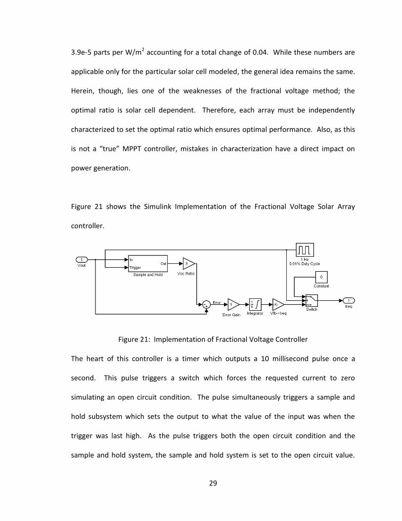
Figure 21 shows the Simulink Implementation of the Fractional Voltage Solar Array
controller.
Figure 21: Implementation of Fractional Voltage Controller
The heart of this controller is a timer which outputs a 10 millisecond pulse once a
second. This pulse triggers a switch which forces the requested current to zero
simulating an open circuit condition. The pulse simultaneously triggers a sample and
hold subsystem which sets the output to what the value of the input was when the
trigger was last high. As the pulse triggers both the open circuit condition and the
sample and hold system, the sample and hold system is set to the open circuit value.
30
The open circuit value is then passed through a gain equal to an optimal, empirically
determined ratio which relates the open circuit voltage to the maximum power voltage.
Finally an error integrator forces the difference between the operating voltage and the
determined operating voltage to zero by adjusting the control value which is input to
the Battery Charge Regulator model as described above.
3.5.1.2 Perturb and Observe
A Perturb and Observe (P&O) controller works by coupling a perturbating signal onto
the solar cell voltage which induces a change in the current. The phase of the perturbed
power signal is compared to that of the perturbing signal and this phase difference
determines the position of the operating voltage with respect to VMP[21]. If they are in
phase, the operating voltage is too low, as an increase in operating voltage leads to an
increase in power, and, similarly, if they are out of phase the operating voltage is too
high, as an increase in operating voltage leads to a decrease in power. A similar
method, known as Climb the Hill, puts the perturbing signal on the control voltage as
opposed to directly on the solar cell voltage which, in practice, accomplishes the same
thing and so, for this research, these techniques are considered to be the same. A P&O
controller is a “true” MPPT controller and, thus, can be used as generic controller
without regard to solar cell type and mistakes in characterization.
Figure 22 shows the Simulink Implementation of the Perturb and Observe Solar Array
Controller.
31
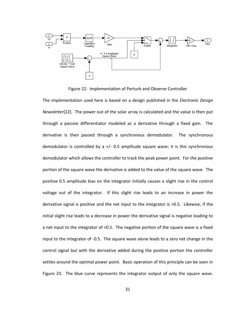
Figure 22: Implementation of Perturb and Observe Controller
The implementation used here is based on a design published in the Electronic Design
Newsletter[22]. The power out of the solar array is calculated and the value is then put
through a passive differentiator modeled as a derivative through a fixed gain. The
derivative is then passed through a synchronous demodulator. The synchronous
demodulator is controlled by a +/- 0.5 amplitude square wave; it is this synchronous
demodulator which allows the controller to track the peak power point. For the positive
portion of the square wave the derivative is added to the value of the square wave. The
positive 0.5 amplitude bias on the integrator initially causes a slight rise in the control
voltage out of the integrator. If this slight rise leads to an increase in power the
derivative signal is positive and the net input to the integrator is >0.5. Likewise, if the
initial slight rise leads to a decrease in power the derivative signal is negative leading to
a net input to the integrator of <0.5. The negative portion of the square wave is a fixed
input to the integrator of -0.5. The square wave alone leads to a zero net change in the
control signal but with the derivative added during the positive portion the controller
settles around the optimal power point. Basic operation of this principle can be seen in
Figure 23. The blue curve represents the integrator output of only the square wave.
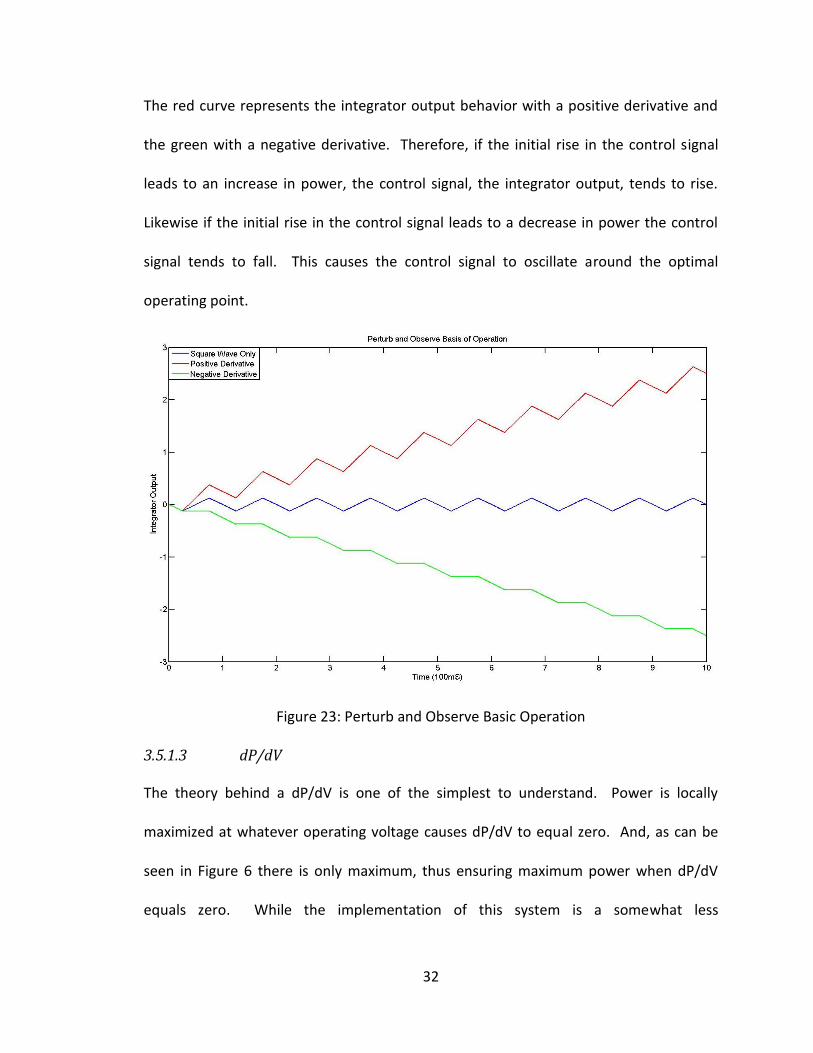
32
The red curve represents the integrator output behavior with a positive derivative and
the green with a negative derivative. Therefore, if the initial rise in the control signal
leads to an increase in power, the control signal, the integrator output, tends to rise.
Likewise if the initial rise in the control signal leads to a decrease in power the control
signal tends to fall. This causes the control signal to oscillate around the optimal
operating point.
Figure 23: Perturb and Observe Basic Operation
3.5.1.3 dP/dV
The theory behind a dP/dV is one of the simplest to understand. Power is locally
maximized at whatever operating voltage causes dP/dV to equal zero. And, as can be
seen in Figure 6 there is only maximum, thus ensuring maximum power when dP/dV
equals zero. While the implementation of this system is a somewhat less
33
straightforward, the design used for this work is described below, though there are
others [23], [24]. A dP/dV controller is also a “true” MPPT controller and, thus, can be
used as generic controller without regard to solar cell type and mistakes in
characterization.
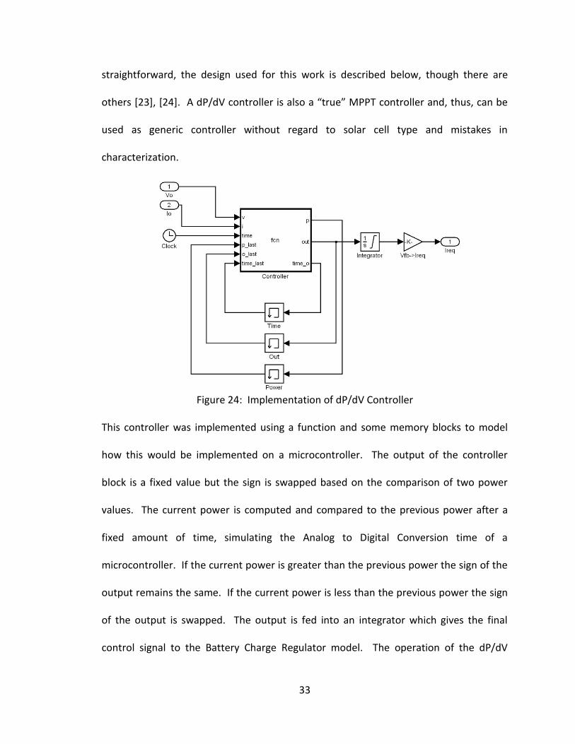
Figure 24: Implementation of dP/dV Controller
This controller was implemented using a function and some memory blocks to model
how this would be implemented on a microcontroller. The output of the controller
block is a fixed value but the sign is swapped based on the comparison of two power
values. The current power is computed and compared to the previous power after a
fixed amount of time, simulating the Analog to Digital Conversion time of a
microcontroller. If the current power is greater than the previous power the sign of the
output remains the same. If the current power is less than the previous power the sign
of the output is swapped. The output is fed into an integrator which gives the final
control signal to the Battery Charge Regulator model. The operation of the dP/dV
34
controller is similar to the operation of the Perturb and Observe controller in that it
causes the control signal to oscillate around the optimal point.
3.5.2 Non-MPPT
The following solar array interfaces are not MPPT, or pseudo-MPPT, controllers,
however, they do allow an optimal operating point to be set. They also decouple the
solar array and battery/load designs.
3.5.2.1 Fixed Voltage
As the name implies, a Fixed Point controller sets the operating point based on a static
voltage reference. This operating point must be empirically determined and, as such,
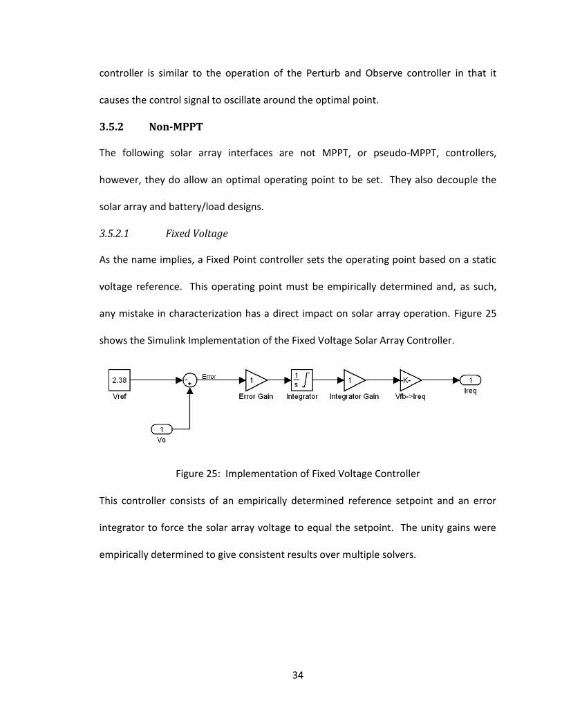
any mistake in characterization has a direct impact on solar array operation. Figure 25
shows the Simulink Implementation of the Fixed Voltage Solar Array Controller.
Figure 25: Implementation of Fixed Voltage Controller
This controller consists of an empirically determined reference setpoint and an error
integrator to force the solar array voltage to equal the setpoint. The unity gains were
empirically determined to give consistent results over multiple solvers.
35
3.5.2.2 Temperature Compensated Fixed Voltage
A Temperature Compensated Fixed Point controller operates just like the Fixed Point
Controller except that the voltage reference is set in such a way that it changes with
temperature. As can be seen by comparing Figure 9 and Figure 11, temperature has the
greater impact on the solar array operating point and so, by compensating for
temperature, the optimal operating point can be estimated. The nominal operating
point as well as the relationship between the temperature and the optimal operating
point must, again, be empirically determined and, again, any mistake in characterization
has a direct impact on solar array operation. The model described below uses a static
voltage reference modulated through a voltage divider which utilizes a Resistive
Temperature Detector (RTD) as the temperature transducer. There have been other
studies which yielded promising results using a p-n junction diode, under the same
temperature conditions as the solar cells, as both the reference voltage and
temperature transducer [25]. Figure 26 shows the Simulink Implementation of the
Temperature Compensated Fixed Voltage Solar Array Controller.
36
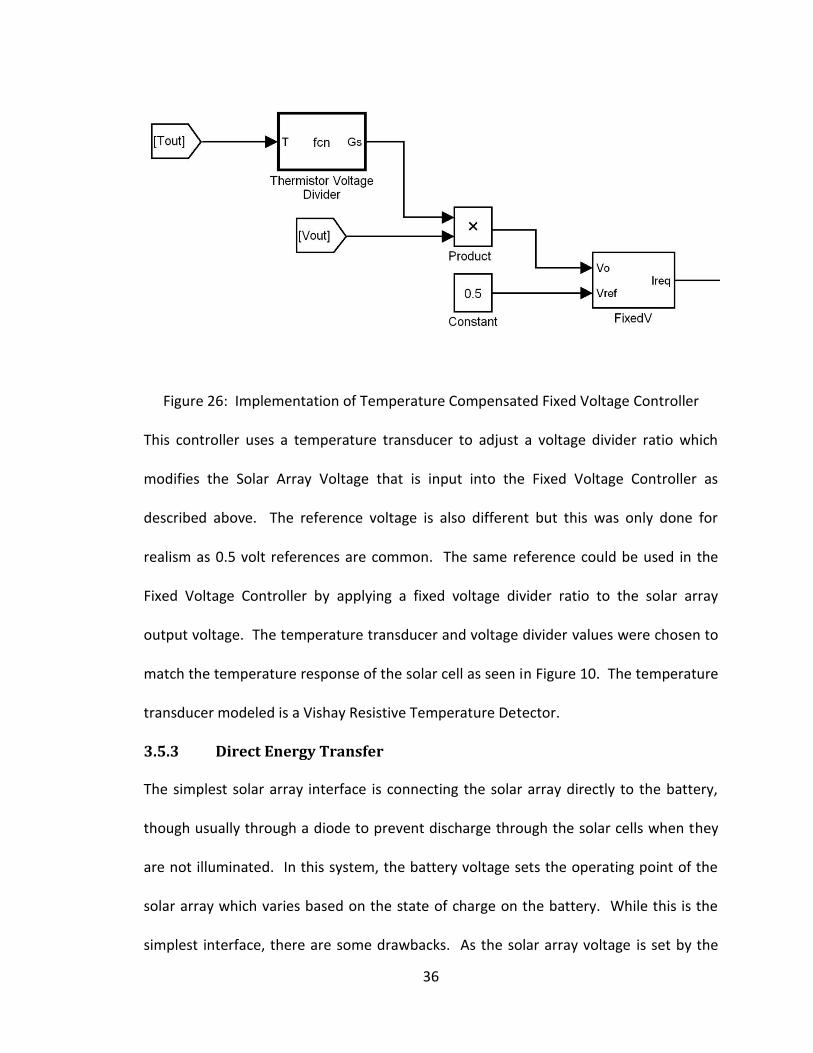
Figure 26: Implementation of Temperature Compensated Fixed Voltage Controller
This controller uses a temperature transducer to adjust a voltage divider ratio which
modifies the Solar Array Voltage that is input into the Fixed Voltage Controller as
described above. The reference voltage is also different but this was only done for
realism as 0.5 volt references are common. The same reference could be used in the
Fixed Voltage Controller by applying a fixed voltage divider ratio to the solar array
output voltage. The temperature transducer and voltage divider values were chosen to
match the temperature response of the solar cell as seen in Figure 10. The temperature
transducer modeled is a Vishay Resistive Temperature Detector.
3.5.3 Direct Energy Transfer
The simplest solar array interface is connecting the solar array directly to the battery,
though usually through a diode to prevent discharge through the solar cells when they
are not illuminated. In this system, the battery voltage sets the operating point of the
solar array which varies based on the state of charge on the battery. While this is the
simplest interface, there are some drawbacks. As the solar array voltage is set by the
37
battery voltage the solar array will not operate at its optimal point at all times. Also, as
the battery voltage changes based on state of charge, the operating point varies with it.
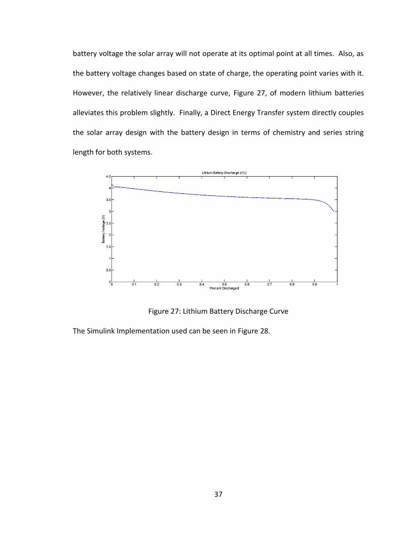
However, the relatively linear discharge curve, Figure 27, of modern lithium batteries
alleviates this problem slightly. Finally, a Direct Energy Transfer system directly couples
the solar array design with the battery design in terms of chemistry and series string
length for both systems.
Figure 27: Lithium Battery Discharge Curve
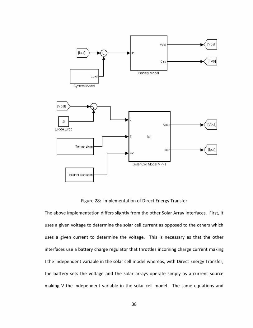
The Simulink Implementation used can be seen in Figure 28.
38
Figure 28: Implementation of Direct Energy Transfer
The above implementation differs slightly from the other Solar Array Interfaces. First, it
uses a given voltage to determine the solar cell current as opposed to the others which
uses a given current to determine the voltage. This is necessary as that the other
interfaces use a battery charge regulator that throttles incoming charge current making
I the independent variable in the solar cell model whereas, with Direct Energy Transfer,
the battery sets the voltage and the solar arrays operate simply as a current source
making V the independent variable in the solar cell model. The same equations and
39
methods were used, the only difference is using Newtons Method to solve for I as
opposed to V. This was tested and verified to give very similar results. The added
protection diode is modeled as a constant voltage added to the battery voltage which
sets the solar array operating voltage as:
( 12)
Where VS is the solar array operating voltage, VBat is the battery voltage, and VD is the
forward voltage drop of the diode. Finally, the power calculation is made using the solar
cell current and the battery voltage, as opposed to the solar array voltage, so as to not
include the forward voltage of the diode which would overestimate the amount of
power available to the satellite system.
As seen in (12), the operating point of the solar arrays depend on the battery voltage
and, as seen in Figure 27, the battery voltage, while relatively linear, is dependent on
the state-of-charge of the battery. The battery behavior must therefore be modeled to
accurately reflect the behavior of the solar arrays during a real mission.
3.5.3.1 Battery Model
The battery model used is based on [26] which develops a model capable of simulating
the dynamic behavior of lithium batteries at runtime. The equivalent circuit used to
model a lithium battery, developed in [26], can be seen in Figure 29. Runtime behavior
is modeled using parameters based on the current state-of-charge of the battery,
determined by the integrated current into and out of the battery. The parameters used
are the open-circuit voltage, the series resistance, and two RC networks, one
DBatS VVV
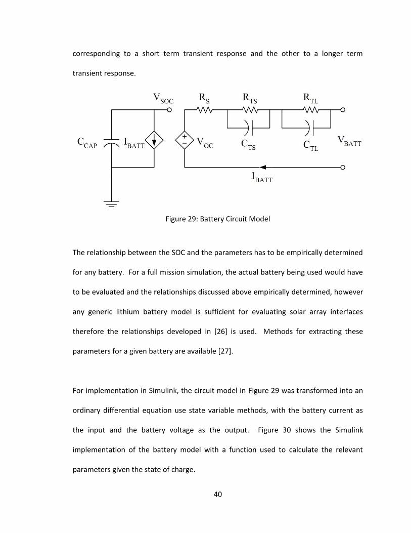
40
corresponding to a short term transient response and the other to a longer term
transient response.
Figure 29: Battery Circuit Model
The relationship between the SOC and the parameters has to be empirically determined
for any battery. For a full mission simulation, the actual battery being used would have
to be evaluated and the relationships discussed above empirically determined, however
any generic lithium battery model is sufficient for evaluating solar array interfaces
therefore the relationships developed in [26] is used. Methods for extracting these
parameters for a given battery are available [27].
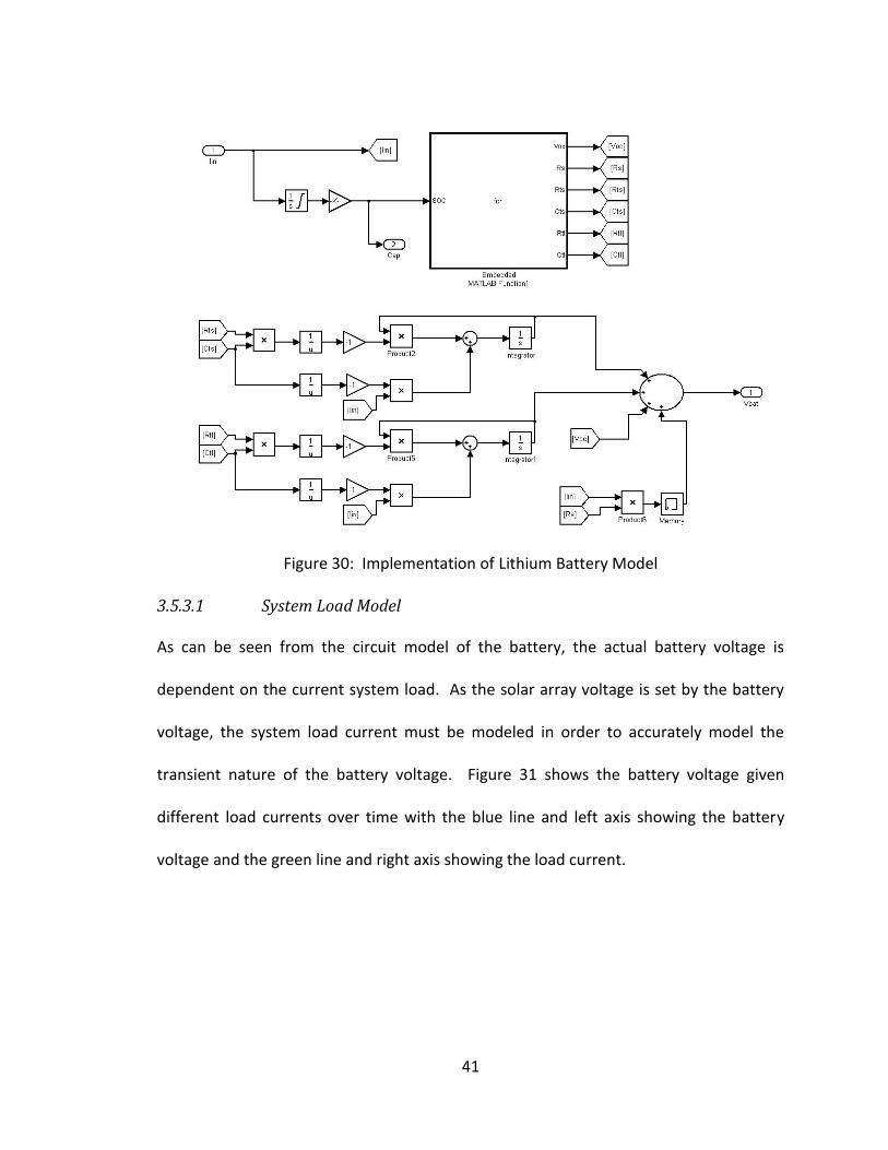
For implementation in Simulink, the circuit model in Figure 29 was transformed into an
ordinary differential equation use state variable methods, with the battery current as
the input and the battery voltage as the output. Figure 30 shows the Simulink
implementation of the battery model with a function used to calculate the relevant
parameters given the state of charge.
41
Figure 30: Implementation of Lithium Battery Model
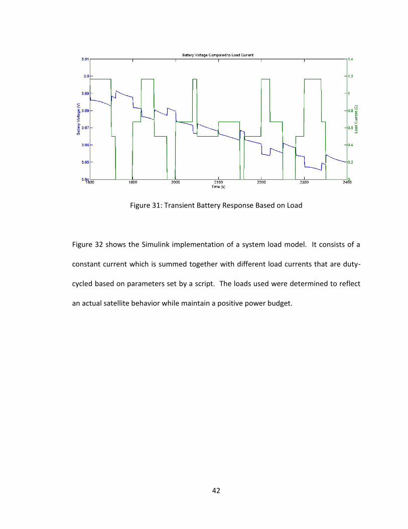
3.5.3.1 System Load Model
As can be seen from the circuit model of the battery, the actual battery voltage is
dependent on the current system load. As the solar array voltage is set by the battery
voltage, the system load current must be modeled in order to accurately model the
transient nature of the battery voltage. Figure 31 shows the battery voltage given
different load currents over time with the blue line and left axis showing the battery
voltage and the green line and right axis showing the load current.
42
Figure 31: Transient Battery Response Based on Load
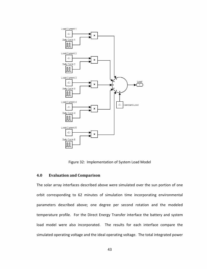
Figure 32 shows the Simulink implementation of a system load model. It consists of a
constant current which is summed together with different load currents that are duty-
cycled based on parameters set by a script. The loads used were determined to reflect
an actual satellite behavior while maintain a positive power budget.
43
Figure 32: Implementation of System Load Model
4.0 Evaluation and Comparison
The solar array interfaces described above were simulated over the sun portion of one
orbit corresponding to 62 minutes of simulation time incorporating environmental
parameters described above; one degree per second rotation and the modeled
temperature profile. For the Direct Energy Transfer interface the battery and system
load model were also incorporated. The results for each interface compare the
simulated operating voltage and the ideal operating voltage. The total integrated power
44
for each interface is also given along with the matching efficiency; calculated as the total
integrated power divided by the ideal total integrated power.
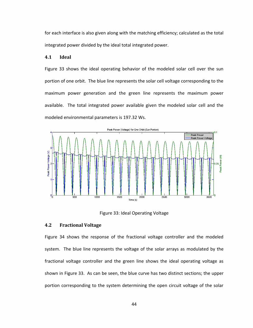
4.1 Ideal
Figure 33 shows the ideal operating behavior of the modeled solar cell over the sun
portion of one orbit. The blue line represents the solar cell voltage corresponding to the
maximum power generation and the green line represents the maximum power
available. The total integrated power available given the modeled solar cell and the
modeled environmental parameters is 197.32 Ws.
Figure 33: Ideal Operating Voltage
4.2 Fractional Voltage
Figure 34 shows the response of the fractional voltage controller and the modeled
system. The blue line represents the voltage of the solar arrays as modulated by the
fractional voltage controller and the green line shows the ideal operating voltage as
shown in Figure 33. As can be seen, the blue curve has two distinct sections; the upper
portion corresponding to the system determining the open circuit voltage of the solar
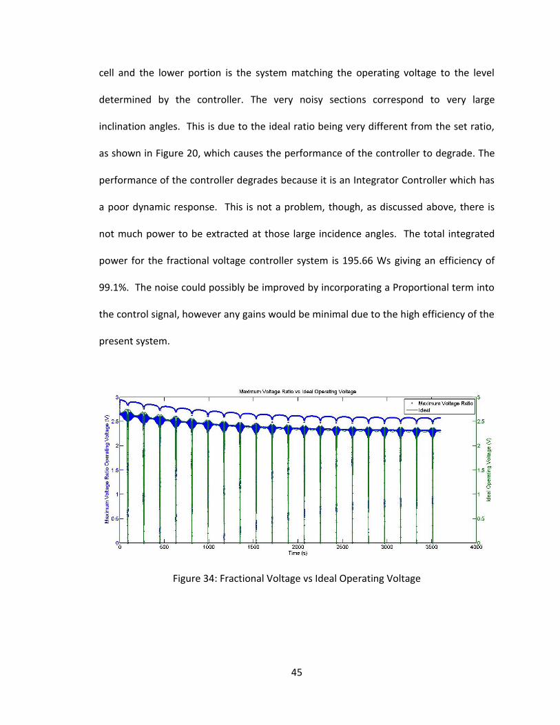
45
cell and the lower portion is the system matching the operating voltage to the level
determined by the controller. The very noisy sections correspond to very large
inclination angles. This is due to the ideal ratio being very different from the set ratio,
as shown in Figure 20, which causes the performance of the controller to degrade. The
performance of the controller degrades because it is an Integrator Controller which has
a poor dynamic response. This is not a problem, though, as discussed above, there is
not much power to be extracted at those large incidence angles. The total integrated
power for the fractional voltage controller system is 195.66 Ws giving an efficiency of
99.1%. The noise could possibly be improved by incorporating a Proportional term into
the control signal, however any gains would be minimal due to the high efficiency of the
present system.
Figure 34: Fractional Voltage vs Ideal Operating Voltage
46
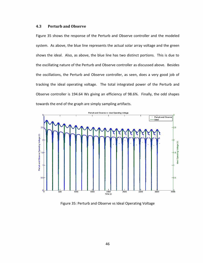
4.3 Perturb and Observe
Figure 35 shows the response of the Perturb and Observe controller and the modeled
system. As above, the blue line represents the actual solar array voltage and the green
shows the ideal. Also, as above, the blue line has two distinct portions. This is due to
the oscillating nature of the Perturb and Observe controller as discussed above. Besides
the oscillations, the Perturb and Observe controller, as seen, does a very good job of
tracking the ideal operating voltage. The total integrated power of the Perturb and
Observe controller is 194.64 Ws giving an efficiency of 98.6%. Finally, the odd shapes
towards the end of the graph are simply sampling artifacts.
Figure 35: Perturb and Observe vs Ideal Operating Voltage
47
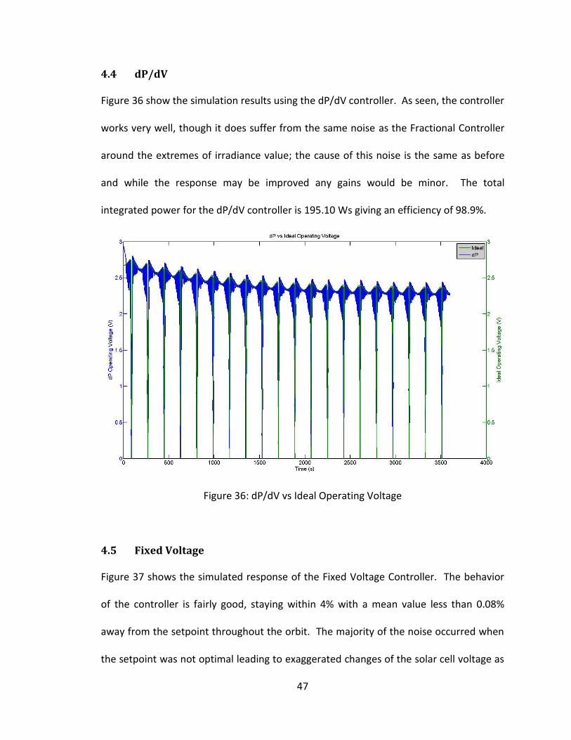
4.4 dP/dV
Figure 36 show the simulation results using the dP/dV controller. As seen, the controller
works very well, though it does suffer from the same noise as the Fractional Controller
around the extremes of irradiance value; the cause of this noise is the same as before
and while the response may be improved any gains would be minor. The total
integrated power for the dP/dV controller is 195.10 Ws giving an efficiency of 98.9%.
Figure 36: dP/dV vs Ideal Operating Voltage
4.5 Fixed Voltage
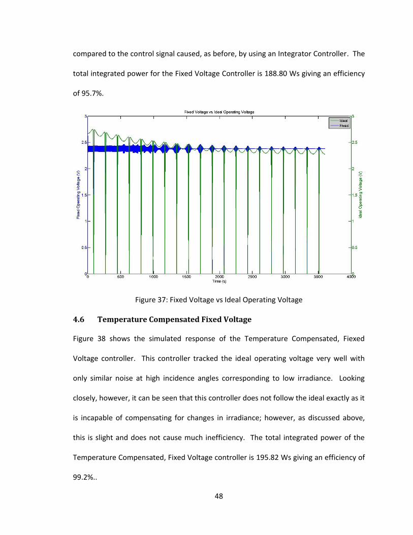
Figure 37 shows the simulated response of the Fixed Voltage Controller. The behavior
of the controller is fairly good, staying within 4% with a mean value less than 0.08%
away from the setpoint throughout the orbit. The majority of the noise occurred when
the setpoint was not optimal leading to exaggerated changes of the solar cell voltage as
48
compared to the control signal caused, as before, by using an Integrator Controller. The
total integrated power for the Fixed Voltage Controller is 188.80 Ws giving an efficiency
of 95.7%.
Figure 37: Fixed Voltage vs Ideal Operating Voltage
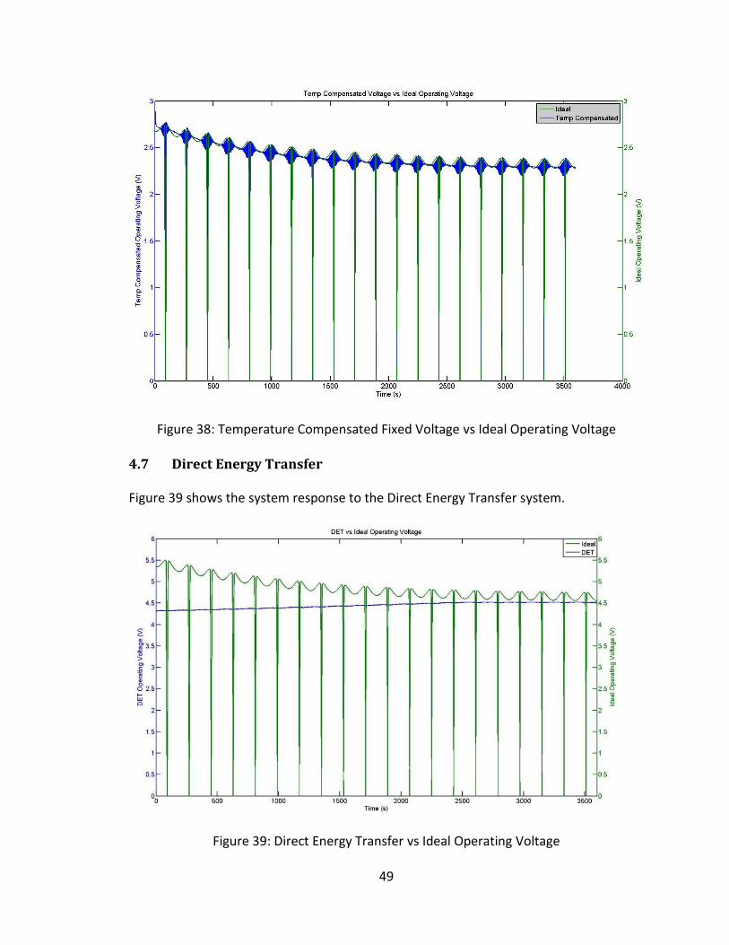
4.6 Temperature Compensated Fixed Voltage
Figure 38 shows the simulated response of the Temperature Compensated, Fiexed
Voltage controller. This controller tracked the ideal operating voltage very well with
only similar noise at high incidence angles corresponding to low irradiance. Looking
closely, however, it can be seen that this controller does not follow the ideal exactly as it
is incapable of compensating for changes in irradiance; however, as discussed above,
this is slight and does not cause much inefficiency. The total integrated power of the
Temperature Compensated, Fixed Voltage controller is 195.82 Ws giving an efficiency of
99.2%..
49
Figure 38: Temperature Compensated Fixed Voltage vs Ideal Operating Voltage
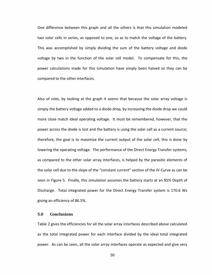
4.7 Direct Energy Transfer
Figure 39 shows the system response to the Direct Energy Transfer system.
Figure 39: Direct Energy Transfer vs Ideal Operating Voltage
50
One difference between this graph and all the others is that this simulation modeled
two solar cells in series, as opposed to one, so as to match the voltage of the battery.
This was accomplished by simply dividing the sum of the battery voltage and diode
voltage by two in the function of the solar cell model. To compensate for this, the
power calculations made for this simulation have simply been halved so they can be
compared to the other interfaces.
Also of note, by looking at the graph it seems that because the solar array voltage is
simply the battery voltage added to a diode drop, by increasing the diode drop we could
more close match ideal operating voltage. It must be remembered, however, that the
power across the diode is lost and the battery is using the solar cell as a current source;
therefore, the goal is to maximize the current output of the solar cell, this is done by
lowering the operating voltage. The performance of the Direct Energy Transfer systems,
as compared to the other solar array interfaces, is helped by the parasitic elements of
the solar cell due to the slope of the “constant current” section of the IV-Curve as can be
seen in Figure 5. Finally, this simulation assumes the battery starts at an 85% Depth of
Discharge. Total integrated power for the Direct Energy Transfer system is 170.6 Ws
giving an efficiency of 86.5%.
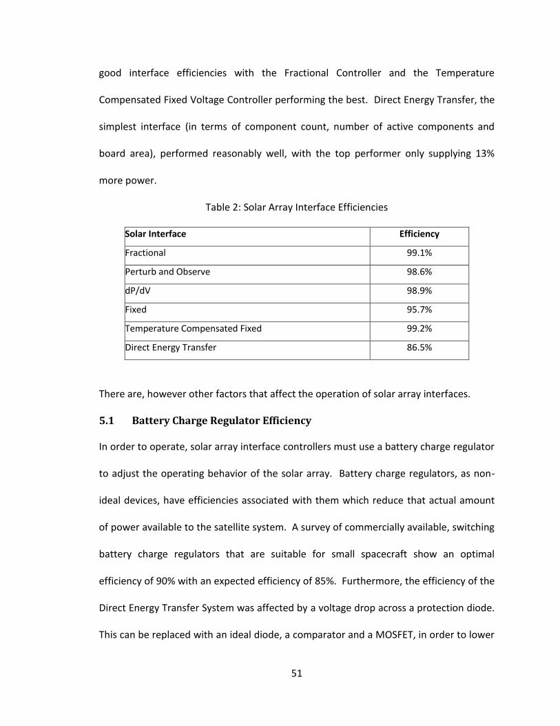
5.0 Conclusions
Table 2 gives the efficiencies for all the solar array interfaces described above calculated
as the total integrated power for each interface divided by the ideal total integrated
power. As can be seen, all the solar array interfaces operate as expected and give very
51
good interface efficiencies with the Fractional Controller and the Temperature
Compensated Fixed Voltage Controller performing the best. Direct Energy Transfer, the
simplest interface (in terms of component count, number of active components and
board area), performed reasonably well, with the top performer only supplying 13%
more power.
Table 2: Solar Array Interface Efficiencies
Solar Interface Efficiency
Fractional 99.1%
Perturb and Observe 98.6%
dP/dV 98.9%
Fixed 95.7%
Temperature Compensated Fixed 99.2%
Direct Energy Transfer 86.5%
There are, however other factors that affect the operation of solar array interfaces.
5.1 Battery Charge Regulator Efficiency
In order to operate, solar array interface controllers must use a battery charge regulator
to adjust the operating behavior of the solar array. Battery charge regulators, as non-
ideal devices, have efficiencies associated with them which reduce that actual amount
of power available to the satellite system. A survey of commercially available, switching
battery charge regulators that are suitable for small spacecraft show an optimal
efficiency of 90% with an expected efficiency of 85%. Furthermore, the efficiency of the
Direct Energy Transfer System was affected by a voltage drop across a protection diode.
This can be replaced with an ideal diode, a comparator and a MOSFET, in order to lower
52
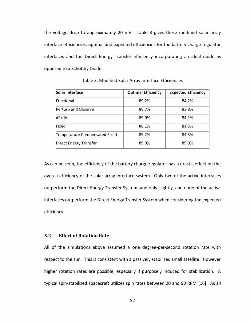
the voltage drop to approximately 20 mV. Table 3 gives these modified solar array
interface efficiencies; optimal and expected efficiencies for the battery charge regulator
interfaces and the Direct Energy Transfer efficiency incorporating an ideal diode as
opposed to a Schottky Diode.
Table 3: Modified Solar Array Interface Efficiencies
Solar Interface Optimal Efficiency Expected Efficiency
Fractional 89.2% 84.2%
Perturb and Observe 88.7% 83.8%
dP/dV 89.0% 84.1%
Fixed 86.1% 81.3%
Temperature Compensated Fixed 89.2% 84.3%
Direct Energy Transfer 89.0% 89.0%
As can be seen, the efficiency of the battery charge regulator has a drastic effect on the
overall efficiency of the solar array interface system. Only two of the active interfaces
outperform the Direct Energy Transfer System, and only slightly, and none of the active
interfaces outperform the Direct Energy Transfer System when considering the expected
efficiency.
5.2 Effect of Rotation Rate
All of the simulations above assumed a one degree-per-second rotation rate with
respect to the sun. This is consistent with a passively stabilized small satellite. However
higher rotation rates are possible, especially if purposely induced for stabilization. A
typical spin-stabilized spacecraft utilizes spin rates between 20 and 90 RPM [16]. As all
53
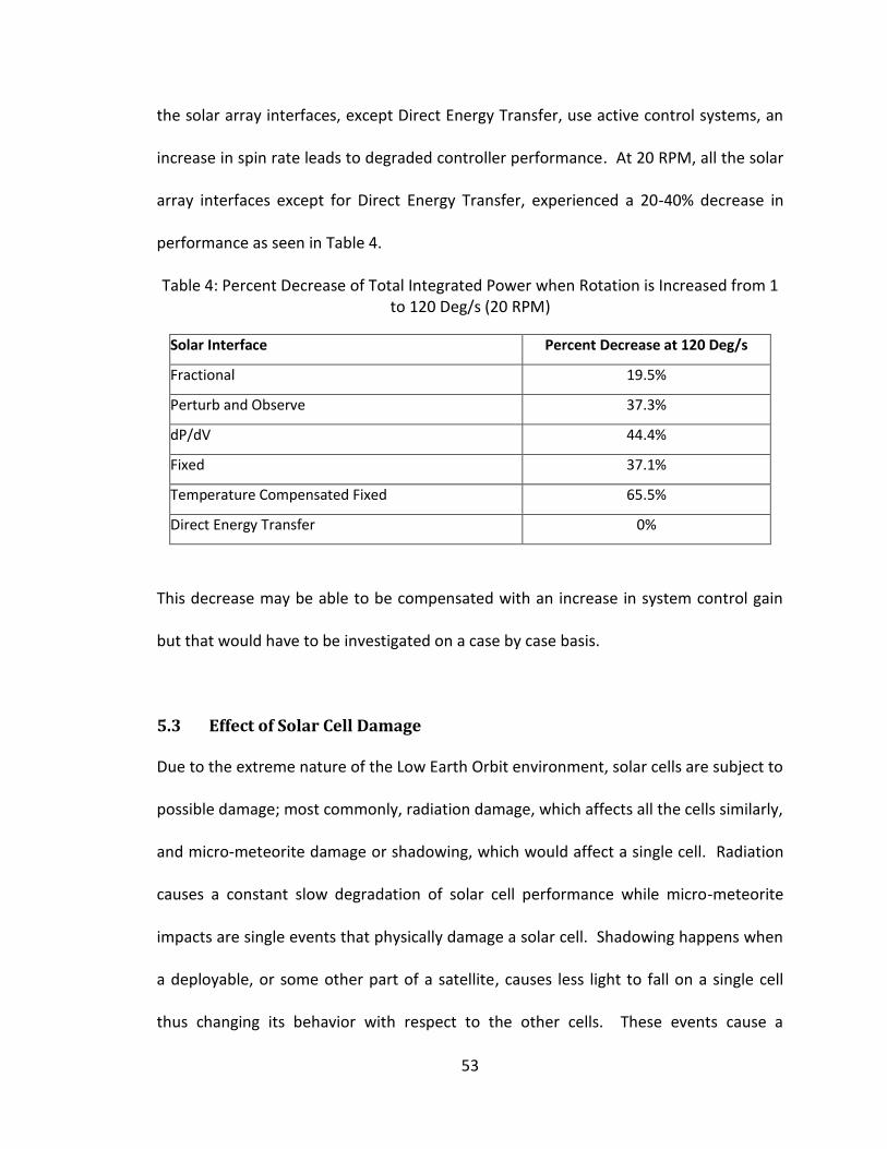
the solar array interfaces, except Direct Energy Transfer, use active control systems, an
increase in spin rate leads to degraded controller performance. At 20 RPM, all the solar
array interfaces except for Direct Energy Transfer, experienced a 20-40% decrease in
performance as seen in Table 4.
Table 4: Percent Decrease of Total Integrated Power when Rotation is Increased from 1 to 120 Deg/s (20 RPM)
Solar Interface Percent Decrease at 120 Deg/s
Fractional 19.5%
Perturb and Observe 37.3%
dP/dV 44.4%
Fixed 37.1%
Temperature Compensated Fixed 65.5%
Direct Energy Transfer 0%
This decrease may be able to be compensated with an increase in system control gain
but that would have to be investigated on a case by case basis.
5.3 Effect of Solar Cell Damage
Due to the extreme nature of the Low Earth Orbit environment, solar cells are subject to
possible damage; most commonly, radiation damage, which affects all the cells similarly,
and micro-meteorite damage or shadowing, which would affect a single cell. Radiation
causes a constant slow degradation of solar cell performance while micro-meteorite
impacts are single events that physically damage a solar cell. Shadowing happens when
a deployable, or some other part of a satellite, causes less light to fall on a single cell
thus changing its behavior with respect to the other cells. These events cause a
54
permanent change to the solar cells negatively affecting their performance. The
probability of damage increases with increased mission time, therefore most of these
effects can be discounted for short mission times. However, to ensure mission success,
the possible consequences of radiation or single cell damage must be investigated.
5.3.1 Radiation
Figure 13 shows the behavior of solar cells after being damaged by differing amounts of
radiation. As can be seen, radiation damage affects all aspects of the solar cell behavior,
open circuit voltage, max power voltage, short circuit current, and max power current.
True MPPT interfaces, dP/dV and P&O, continue to operate normally as they are able to
compensate and do not rely on accurate solar array parameters to operate. Fractional
Voltage solar array interfaces also operate fairly well after radiation damage as both the
open circuit voltage and max power voltage are reduced relatively equally. However,
Fixed Point solar array interfaces, both temperature compensated and not, can be
detrimentally affected by solar array damage.
As can be seen in Figure 13 if the fixed operating point chosen corresponds to the
optimal operating point before radiation damage occurs, it will not be long before that
point is above the open circuit voltage of the solar arrays. The controller would then be
attempting to force the solar array to operate above its open circuit voltage leading to a
power output of zero. To compensate, the operating point must be set to non-optimal
point to prevent radiation damage from catastrophically affecting power generation.
55
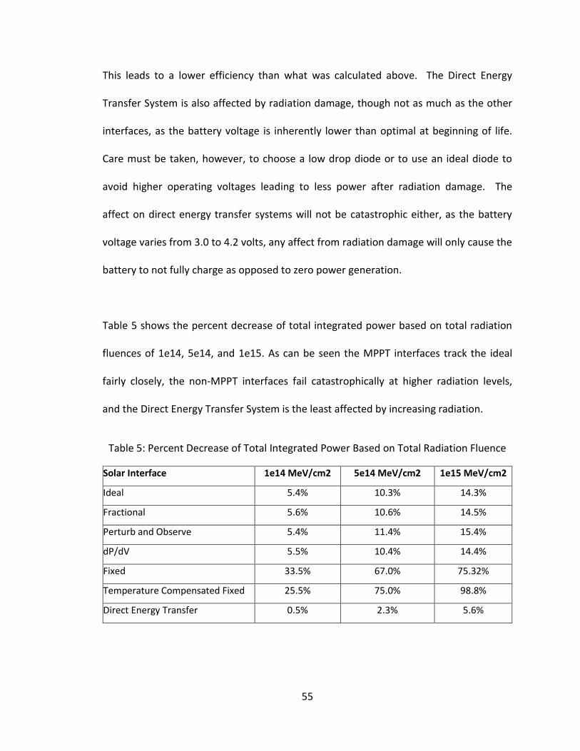
This leads to a lower efficiency than what was calculated above. The Direct Energy
Transfer System is also affected by radiation damage, though not as much as the other
interfaces, as the battery voltage is inherently lower than optimal at beginning of life.
Care must be taken, however, to choose a low drop diode or to use an ideal diode to
avoid higher operating voltages leading to less power after radiation damage. The
affect on direct energy transfer systems will not be catastrophic either, as the battery
voltage varies from 3.0 to 4.2 volts, any affect from radiation damage will only cause the
battery to not fully charge as opposed to zero power generation.
Table 5 shows the percent decrease of total integrated power based on total radiation
fluences of 1e14, 5e14, and 1e15. As can be seen the MPPT interfaces track the ideal
fairly closely, the non-MPPT interfaces fail catastrophically at higher radiation levels,
and the Direct Energy Transfer System is the least affected by increasing radiation.
Table 5: Percent Decrease of Total Integrated Power Based on Total Radiation Fluence
Solar Interface 1e14 MeV/cm2 5e14 MeV/cm2 1e15 MeV/cm2
Ideal 5.4% 10.3% 14.3%
Fractional 5.6% 10.6% 14.5%
Perturb and Observe 5.4% 11.4% 15.4%
dP/dV 5.5% 10.4% 14.4%
Fixed 33.5% 67.0% 75.32%
Temperature Compensated Fixed 25.5% 75.0% 98.8%
Direct Energy Transfer 0.5% 2.3% 5.6%
56
5.3.2 Single Cell Damage
Solar arrays can also be affected by single events, such as localized damage or shading
due to offgassing, that cause one cell in a string to not operate or to operate poorly. All
the MPPT Interfaces can compensate for this and the only affect will be the loss of
power from the single cell. However, with non-MPPT interfaces, this will cause the
power from the entire string of cells to be lost. There are two ways to compensate for
this, oversizing solar cell strings and using lots of small strings as opposed to a few long
strings. As these single events should be rare, oversizing solar cell strings is not practical
or efficient for small spacecraft, therefore the best method for compensating against
single events while still maintaining a high efficiency is to use the smallest string length
and the maximum number of strings possible.
5.4 Discussion
As demonstrated above, a Direct Energy Transfer system, the simplest solar array
interface (in terms of component count, the number of active components, and board
area), performs as well, and in some cases better, than the more complex Maximum
Peak Power Tracking interfaces. Even when the optimal efficiency of a Battery Charge
Regulator (90%) is taken into consideration the best MPPT had a solar array matching
efficiency of 89.2%. A Direct Energy Transfer System, using an ideal diode (the optimal
solution for Direct Energy Transfer), has a solar array matching efficiency of 89.0%.
Given the increased complexity and relatively low gains, as well as how MPPT’s are
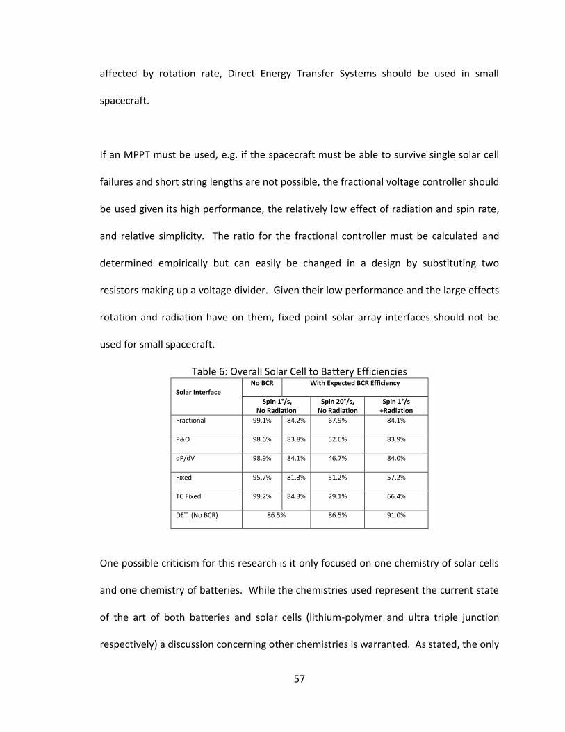
57
affected by rotation rate, Direct Energy Transfer Systems should be used in small
spacecraft.
If an MPPT must be used, e.g. if the spacecraft must be able to survive single solar cell
failures and short string lengths are not possible, the fractional voltage controller should
be used given its high performance, the relatively low effect of radiation and spin rate,
and relative simplicity. The ratio for the fractional controller must be calculated and
determined empirically but can easily be changed in a design by substituting two
resistors making up a voltage divider. Given their low performance and the large effects
rotation and radiation have on them, fixed point solar array interfaces should not be
used for small spacecraft.
Table 6: Overall Solar Cell to Battery Efficiencies
Solar Interface No BCR With Expected BCR Efficiency
Spin 1°/s, No Radiation
Spin 20°/s, No Radiation
Spin 1°/s +Radiation
Fractional 99.1% 84.2% 67.9% 84.1%
P&O 98.6% 83.8% 52.6% 83.9%
dP/dV 98.9% 84.1% 46.7% 84.0%
Fixed 95.7% 81.3% 51.2% 57.2%
TC Fixed 99.2% 84.3% 29.1% 66.4%
DET (No BCR) 86.5% 86.5% 91.0%
One possible criticism for this research is it only focused on one chemistry of solar cells
and one chemistry of batteries. While the chemistries used represent the current state
of the art of both batteries and solar cells (lithium-polymer and ultra triple junction
respectively) a discussion concerning other chemistries is warranted. As stated, the only
58
requirement for Direct Energy Transfer systems to work is that the battery voltage and
the solar array voltage be matched. The technologies modeled not only represent
current state of the art but also the highest current nominal voltages; lithium batteries
at 3.7v nominal, 4.2v max and triple junction solar cells at ~2.3v @ max power.
Therefore, if legacy technologies are used, all that must be considered is if their nominal
voltage is a close multiple of the technologies modeled. Commonly used batteries for
small spacecraft, besides lithium chemistries, are Nickel-Cadmium and Nickel Metal-
Hydride. The voltages for both of these chemistries are 1.2v nominal and 1.4v max
which means that a series string of three of these batteries will give 3.6v nominal and
4.2v max which matches very closely to the batteries modeled. The discharge curve for
these batteries are different than the lithium technologes modeled, however the
difference is slight enough that it should not matter.
Two commonly used solar cell chemistries for small spacecraft are multi-junction and
silicon solar cells. Multi-junction (double- and triple-junction, the latter of which was
modeled for this work) have similar performance characteristics as described above.
Silicon solar cells have a max power voltage of a little less than 0.5 volts which, when
arranged in a series string of 5 cells gives a max power voltage of 2.5v which
approximately matches the multi-junction performance; if arranged in a series string of
9 cells gives a max power voltage of 4.5v which is a good match for lithium batteries.
Given the smaller nominal voltages of silicon solar cells and nickel-based batteries
arranging them to match each other or the other technologies modeled is a semi-trivial

59
task. As an example the CubeSat mission mentioned before that achieved a 90%
matching efficiency used Lithium-Ion batteries and Double-Junction solar cells.
Another possible criticism is that only one cell or two cells in series were modeled as
opposed to modeling full arrays. However, while there may be some differences due to
individual characteristics of actual solar cells (which can be mitigated by careful
selection of cells) there is no inherent reason that arrays should behave any differently
than single cells, besides the increase in voltage or current due to series or parallel
strings respectively, given proper blocking and bypass diode protection is used. As
discussed above, the only thing necessary when using arrays as opposed to single cells is
to still match the battery and solar cell voltages. Finally, it must be noted that when
combining chemistries and array sizes in order to match battery and solar array voltages
the error should be on the side of greater solar cell voltage. When using Direct Energy
Transfer the solar cells serve as a current source for the batteries and, given the IV-curve
of solar cells, if the batteries are sized 0.1v (for example) above the solar array voltage
the power loss will be fairly severe when compared to the power loss from sizing the
solar array voltage 0.1v above the batteries.
60
6.0 Bibliography
[1] M. Patel, Spacecraft Power Systems. Boca Raton, USA: CRC Press, 2005.
[2] H. Heidt, J. Puig-Sauri, A. Moore, S. Nakasuka, and R. Twiggs, "CubeSat: A New
Generation of Picosatellite for Education and Industry Low-Cost Space
Experimentation," in Proceedings of the 14th Annual AIAA/USU Conference on
Small Satellites, Logan, 2000.
[3] E. Caday-Eames, "Small Box, Big Potential," Boeing Frontiers, p. 20, Oct. 2006.
[4] C. Galliand, "Study of the Small: Potential for Operational Military Use of CubeSats,"
in Proceedings of the 24th Annual Conference on Small Satellite, Logan, UT, 2010.
[5] G. Aruajo, "The Solar Cell," in Solar Electricity: Engineering of Photovoltaic Systems.
Sevilla : Inst. of Solar Energy, Polytechnic Univ. of Madrid, 1994, ch. 2.
[6] M. Wolf, G. T. Nowl, and R. J. Stirn, "Investigation of the double exponential in the
current—Voltage characteristics of silicon solar cells," Electron Devices, IEEE
Transactions on, vol. 24, no. 4, pp. 419-428, Apr. 1977.
[7] D. S. H. Chan and J. C. H. Phang, "Analytical methods for the extraction of solar-cell
single- and double-diode model parameters from I-V characteristics," Electron
Devices, IEEE Transactions on, vol. 34, no. 2, pp. 286-293, Feb. 1987.
[8] M. A. de Blas, J. L. Torres, E. Prieto, and A. Garcia, "Selecting a suitable model for
characterizing photovoltaic devices," Renewable Energy, vol. 25, no. 3, pp. 371-380,
Mar. 2002.
61
[9] M. C. Z. Ouennoughi, "A simpler method for extracting solar cell parameters using
the conductance method," Solid-State Electronics, vol. 43, no. 11, pp. 1985-1988,
Nov. 1999.
[10] M. Chegaar, G. Azzouzi, and P. Mialhe, "Simple parameter extraction method for
illuminated solar cells," Solid-State Electronics, vol. 50, no. 7-8, pp. 1234-1237, Jul.
2006.
[11] J. Foley and A. Williams, "PolySat: Building on Success," in Cubesat Developers
Workshop, Logan, UT, 2008.
[12] "26.8% Improved Triple Junction (ITJ) Solar Cells," SpectroLab Product Data Sheet.
[13] H. Y. Tada, J. R. J. Carter, and B. E. Anspaugh, "Solar Cell Radiation Handbook," Jet
Propulsion Lab, Pasadena, Technical Report, 1982.
[14] (2010, Dec.) SPENVIS: The Space Environment Information System. [Online].
http://www.spenvis.oma.be/
[15] Mathworks, "Choosing a solver," Technical Documentation, 2007.
[16] W. J. Larson and J. R. Wertz, Eds., Space Mission Analysis and Design, 7th ed. El
Segundo, CA, USA: Microcosm Press, 2005.
[17] S. Rawashdeh, "Passive Attitude Stabilization For Small Satellites," Masters Thesis,
University of Kentucky, Lexington, 2009.
[18] T. Esram and P. L. Chapman, "Comparison of Photovoltaic Array Maximum Power
Point Tracking Techniques," Energy Conversion, IEEE Transactions on, vol. 22, no. 2,
pp. 439-449, Jun. 2007.
62
[19] J. J. Schoeman and J. D. van Wyk, "A Simplified Maximal Power Controller for
Terrestrial Photovoltaic Panel Arrays," in 13th Annual IEEE Power Electron
Specialists Conference, 1982, pp. 361-367.
[20] G. W. Hart, H. M. Branz, and C. H. C. III, "Experimental tests of open-loop maximum-
power-point tracking techniques for photovoltaic arrays," Solar Cells, vol. 13, no. 2,
pp. 185-195, Dec. 1984.
[21] N. Femia, G. Petrone, G. Spagnuolo, and M. Vitelli, "Optimization of perturb and
observe maximum power point tracking method," Power Electronics, IEEE
Transactions on, vol. 20, no. 4, pp. 963-973, Jul. 2005.
[22] W. S. Woodward, "Solar-array controller needs no multiplier to maximize power,"
Electronic Design Newsletter, pp. 51-52, Dec. 2008.
[23] E. Koutroulis, K. Kalaitzakis, and N. C. Voulgaris, "Development of a microcontroller-
based, photovoltaic maximum power point tracking control system," Power
Electronics, IEEE Transactions on, vol. 16, no. 1, pp. 46-54, Jan. 2001.
[24] J. N. Avaritsiotis, "The efficient exploitation of photovoltaic electricity," Solar Cells,
vol. 14, no. 3, pp. 261-279, Jul. 1985.
[25] K. Kobayashi, H. Matsuo, and Y. Sekine, "A Novel Optimum Operating Point Tracker
of the Solar Cell Power Supply System," in Power Electronics Specialists Conference,
2004. PESC 04. 2004 IEEE 35th Annual, 2004, pp. 2147-2151.
[26] M. Chen and G. A. Rincon-Mora, "Accurate electrical battery model capable of
predicting runtime and I-V performance," Energy Conversion, IEEE Transactions on,
63
vol. 21, no. 2, pp. 504-511, Jun. 2006.
[27] S. Abu-Sharkh and D. Doerffel, "Rapid test and non-linear model characterisation of
solid-state lithium-ion batteries," Journal of Power Sources, vol. 130, no. 1-2, pp.
266-274, May 2004.
64
7.0 Vita
Daniel Martin Erb
Born June 26, 1983 in Alton, IL
Bachelor of Science in Engineering Physics from Murray State University
Positions Held o Associate Engineer – University of Kentucky o Space Systems Engineer – Kentucky Space
Publications o D. Erb, et al., “Evaluation of Solar Array Peak Power Tracking
Technologies for CubeSats”, 25th Annual AIAA/USU Conference on Small Satellites, Logan, UT, March 2011
o D. Erb, et al., “Kentucky Space: A Multi-University Small Satellite Enterprise”, 2009 Small Satellite Conference, August 2009.
o S. Rawashdeh, et al., “Aerodynamic Attitude Stabilization for a Ram-Facing CubeSat” AAS 32nd Annual Guidance and Control Conference, Breckenridge, Colorado, Jan 2009
o J. Lumpp, et al., “SOCEM: Sub-Orbital CubeSat Experimental Mission”, 31st IEEE Aerospace Conference, Big Sky, Montana, United States, March 2010
o G. Chandler, et al., “Development of an Off-the-Shelf Bus for Small Satellites,” IEEEAC paper #1365, IEEE Aerospace Conference, Big Sky, Montana. March 2007