Evaluating the Financial Performance of Bank Branches

Jesús T. Pastor C. A. Knox Lovell Henry Tulkens

Centro deInvestigaciónOperativa

D e p a r t m e n t o fEconomics

CORE

Universidad MiguelHernández

University of Georgia Voie du Roman Pays, 34

0 3 2 0 2 E l c h e(Alicante), SPAIN

Athens, GA 30602,USA

B-1348 Louvain-la-Neuve, BELGIUM

jtpastor@umh.es knox@terry.uga.edu tulkens@core.ucl.ac.be

Abstract

In this paper we evaluate the financial performance of virtually all ofthe branch offices of a large European savings bank for a recent six-monthaccounting period. We employ a complementary pair of nonparametrictechniques to evaluate their financial performance, in terms of their abilityto conserve on the expenses they incur in the process of building theircustomer bases and providing customer services valued by the bank. Wefind substantial variation in the ability of branch offices to perform this task,and substantial agreement on the identity of the branches at the bottom ofthe performance distribution. We then employ parametric techniques todetermine that the list of indicators on which their financial performance iscurrently evaluated can be substantially reduced without statisticallysignificant loss of information to bank management. Both findings suggestways in which the bank can increase the profitability of its branch network.

Keywords: banking, performance indicators, efficiency

JEL codes: D20, G21, C60

1

1

CONTENTS

1. INTRODUCTION ............................................................................................ 2

2. THE BRANCH OFFICE FINANCIAL PERFORMANCE DATA.............. 5

3. THE ANALYTICAL TECHNIQUES............................................................. 6

3.1 DEA AND FDH............................................................................................ 6

3.2 EVALUATING THE INFORMATION CONTENT OF THE DATA SET ..................... 10

3.3. THE CURSE OF DIMENSIONALITY ................................................................ 12

4. EMPIRICAL FINDINGS............................................................................... 12

4.1 INITIAL DEA RESULTS................................................................................ 13

4.2 VARIABLE DELETION TEST RESULTS .......................................................... 13

4.3 DEA AND FDH EVALUATIONS OF OVERALL FINANCIAL PERFORMANCE ...... 17

5. SUMMARY AND CONCLUSIONS............................................................. 19

FOOTNOTES...................................................................................................... 26

REFERENCES ................................................................................................... 29

2

2

1. Introduction

We examine the performance of a large European savings bank

that currently operates a network of approximately 600 branch offices.

Bank management collects and analyzes information on several expense,

revenue and customer indicators from each branch office on a regular

basis. Management’s objective is to evaluate the overall financial

performance of each branch office, by monitoring branch office expenses,

revenues and customer bases with an eye toward maximizing the profit

the branch network returns to the bank.

Management has provided us with data covering over 20 expense,

revenue and customer indicators for each branch office in its network for a

recent six-month accounting period. Our objectives are to build a

consistent data base consisting of several expense and service indicators,

to evaluate the overall financial performance of each branch office, and to

evaluate the information content of the data base itself.

The value of having an independent evaluation of the overall

financial performance of branch offices is that our approach is model-

based, in contrast to the descriptive approach adopted by bank

management. Our model-based approach enables us to identify branch

offices that excel, and those that are less successful, at conserving on

expenses while generating revenues. Identifying branch offices at the top

and the bottom of the overall financial performance distribution is an

essential first step in a process of improving the overall performance of the

branch network. Branch offices appearing at the bottom of the distribution,

or branch offices whose overall financial performance fails to meet a

predetermined minimum standard, may be candidates for remedial action,

or perhaps closure. Bonuses may be assigned to branch offices at the top

of the distribution, or to branch offices whose overall financial performance

surpasses a predetermined standard. In addition, high-performing branch

3

3

offices may serve as instructive role models for low-performing branch

offices.

The value of having an independent evaluation of the data base

itself is that it may be possible to characterize the information content of

each indicator that management currently uses to evaluate the overall

financial performance of branch offices. Some indicators are inevitably

influential, and should be retained, while others may be superfluous, and

are candidates for deletion. By conducting a series of statistical tests, we

are able to characterize individual indicators as being influential or

superfluous. This enables us to suggest ways in which the magnitude of

the data base can be reduced, without sacrificing or distorting information

that would be useful to bank management. If it is possible to reduce the

number of indicators on which the branch office performance evaluation is

based, bank profit is doubly enhanced, through reduced bank monitoring

costs and also through reduced branch office compliance costs.

Our empirical analysis of the overall financial performance of

branch offices is based on a complementary pair of nonparametric

mathematical programming techniques. Both have been used to analyze

the performance of financial institutions, including bank branches, although

never before in tandem. Data envelopment analysis (DEA) (Charnes et al.

(1978)) is a linear programming technique developed specifically for the

purpose of evaluating and comparing the performance of a collection of

comparable organizations. Free disposal hull (FDH) analysis (Deprins et

al. (1984)) is a closely related mixed integer programming technique

developed for the same purpose.1 Both techniques have the ability to

evaluate and compare the performance of organizations that use several

resources to provide several services; this makes them particularly useful

in a financial services context, since branch offices incur a variety of

expenses in the provision of a wide range of financial services. Neither

technique requires information on the prices of the resources

4

4

organizations consume or of the services they provide; this is also useful

in a financial services context, since it is difficult to derive prices of all the

services branch offices offer their customers.2 Using a pair of

complementary analytical techniques is useful for two reasons. First, it is

always desirable to have a supplementary technique (in our case FDH) to

provide a validation check on the results provided by the primary

technique (in our case DEA). To the extent that primary findings are

confirmed by supplementary findings, the confidence of bank management

in the validity of the findings is enhanced.3 Second, DEA and FDH have

complementary strengths that will be discussed below.

The paper is organized as follows. In Section 2 we discuss the data

base we have constructed from the data originally provided to us by bank

management. Our data base consists of four expense indicators, three

revenue indicators, three customer base indicators, and a pair of

conventional financial ratios, for 573 branch offices for a recent six-month

accounting period. In Section 3 we discuss the two analytical techniques

we use to analyze the overall financial performance of the branch offices.

We also discuss the statistical techniques we use to analyze the

information content of the data base itself. In Section 4 we present and

discuss our empirical findings. Our first finding is that the complete list of

indicators on which the branch office performance evaluation is initially

based can be reduced considerably, with no statistically significant loss of

information to bank management. Our second finding is that considerable

variation in overall financial performance exists among the bank’s branch

offices, and that reducing this variation by improving the performance of

the weakest branch offices would return increased profit to the bank.

Section 5 concludes with a summary of our findings and some suggestions

for future work.

5

5

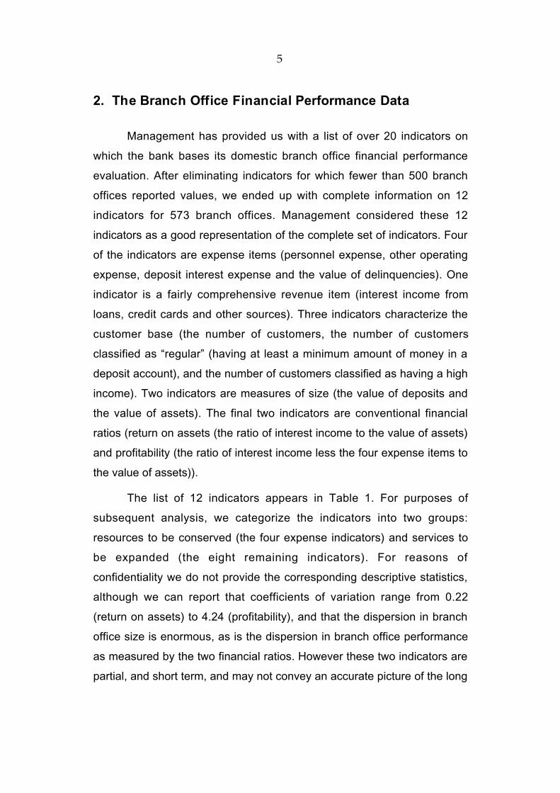
2. The Branch Office Financial Performance Data

Management has provided us with a list of over 20 indicators on

which the bank bases its domestic branch office financial performance

evaluation. After eliminating indicators for which fewer than 500 branch

offices reported values, we ended up with complete information on 12

indicators for 573 branch offices. Management considered these 12

indicators as a good representation of the complete set of indicators. Four

of the indicators are expense items (personnel expense, other operating

expense, deposit interest expense and the value of delinquencies). One

indicator is a fairly comprehensive revenue item (interest income from

loans, credit cards and other sources). Three indicators characterize the

customer base (the number of customers, the number of customers

classified as “regular” (having at least a minimum amount of money in a

deposit account), and the number of customers classified as having a high

income). Two indicators are measures of size (the value of deposits and

the value of assets). The final two indicators are conventional financial

ratios (return on assets (the ratio of interest income to the value of assets)

and profitability (the ratio of interest income less the four expense items to

the value of assets)).

The list of 12 indicators appears in Table 1. For purposes of

subsequent analysis, we categorize the indicators into two groups:

resources to be conserved (the four expense indicators) and services to

be expanded (the eight remaining indicators). For reasons of

confidentiality we do not provide the corresponding descriptive statistics,

although we can report that coefficients of variation range from 0.22

(return on assets) to 4.24 (profitability), and that the dispersion in branch

office size is enormous, as is the dispersion in branch office performance

as measured by the two financial ratios. However these two indicators are

partial, and short term, and may not convey an accurate picture of the long

6

6

term financial viability of the branch offices. What is needed is a picture of

the overall financial performance of branch offices, as measured by their

ability to convert the resources at their disposal into services valued by

bank management, and this is not provided by the usual variable-by-

variable information. An overall picture of the financial performance of

branch offices requires that the information contained in the indicators

listed in Table 1 be aggregated into a single comprehensive performance

indicator. A pair of comprehensive performance indicators is developed in

the next Section.

3. The Analytical Techniques

In this Section we describe the analytical techniques we use to

evaluate the overall financial performance of the branch offices, and to

evaluate the information content of the underlying data base. We begin

with a description of the analytical techniques we use to evaluate the

overall financial performance of the branch offices.

3.1 DEA and FDH

We refer to the list of indicators discussed in Section 2 and

summarized in Table 1. Our objective is to aggregate the 12 financial

indicators in such a way that we generate an overall performance

evaluation for each branch office. DEA generates such a performance

evaluation, as does FDH. The two techniques do not generally assign the

same performance evaluation to each branch office, but if the two

performance rankings are generally consistent, this provides a measure of

confidence in each ranking.

7

7

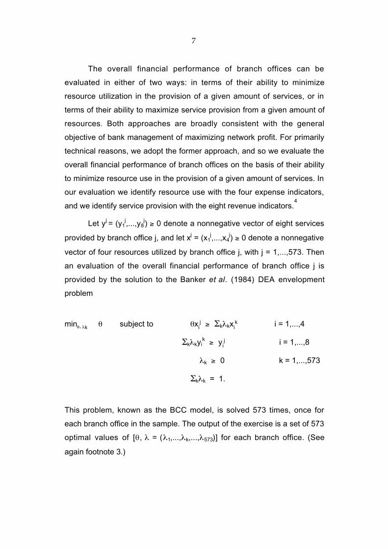
The overall financial performance of branch offices can be

evaluated in either of two ways: in terms of their ability to minimize

resource utilization in the provision of a given amount of services, or in

terms of their ability to maximize service provision from a given amount of

resources. Both approaches are broadly consistent with the general

objective of bank management of maximizing network profit. For primarily

technical reasons, we adopt the former approach, and so we evaluate the

overall financial performance of branch offices on the basis of their ability

to minimize resource use in the provision of a given amount of services. In

our evaluation we identify resource use with the four expense indicators,

and we identify service provision with the eight revenue indicators.4

Let yj = (y1j,...,y8

j) ≥ 0 denote a nonnegative vector of eight services

provided by branch office j, and let xj = (x1j,...,x4

j) ≥ 0 denote a nonnegative

vector of four resources utilized by branch office j, with j = 1,...,573. Then

an evaluation of the overall financial performance of branch office j is

provided by the solution to the Banker et al. (1984) DEA envelopment

problem

minθ, λk θ subject to θxij ≥ Σkλkxi

k i = 1,...,4

Σkλkyik ≥ yi

j i = 1,...,8

λk ≥ 0 k = 1,...,573

Σkλk = 1.

This problem, known as the BCC model, is solved 573 times, once for

each branch office in the sample. The output of the exercise is a set of 573

optimal values of [θ, λ = (λ1,...,λk,...,λ573)] for each branch office. (See

again footnote 3.)

8

8

The objective in the problem is to radially contract the resource

vector utilized by branch office j as much as possible. The constraints of

the problem limit the potential contraction by requiring that (θxj,yj) not

outperform best practice observed in the sample of 573 branch offices.

The optimal value of θ ∈ (0,1] provides an overall financial performance

indicator, incorporating performance across all 12 indicators. Optimal θ = 1

suggests that branch office j is operating at best practice, since it is not

possible to contract its resource vector without violating best practice

standards in the sample.5 Optimal θ < 1 suggests that branch office j is

operating at less than best practice, since it is possible to contract its

resource vector equiproportionately to θxj, or by 100• (1 - θ)%, without

violating best practice standards in the sample. The smaller the value of

optimal θ, the less efficient a branch office is in conserving expenses in the

generation of revenues, and the more room it has for improvement.

The nonzero optimal values of λk, k = 1,...,573, identify the best

practice branch offices to which branch office j is compared. If more than

one optimal λk > 0, the performance of branch office j is evaluated relative

to the performance of an unobserved convex combination of these best

practice branch offices. It is also possible to evaluate the performance of

branch office j relative to that of a single best practice branch office, by

adding to the DEA constraint set the additional requirement that λk ∈ {0,1},

k = 1,...,573. This converts the DEA performance evaluation problem to an

FDH performance evaluation problem. Together with the DEA

requirements that λk ≥ 0, k = 1,...,573, and that Σ kλk = 1, the FDH

constraint λk ∈ {0,1}, k = 1,...,573, forces exactly one optimal value of λk to

be positive, and to attain a value of unity, with all other optimal values λm =

0, m≠k. This leads to the evaluation of the performance of branch office j

relative to that of exactly one best practice branch office, the one having a

service mix most similar to that of branch office j. Like the DEA exercise,

9

9

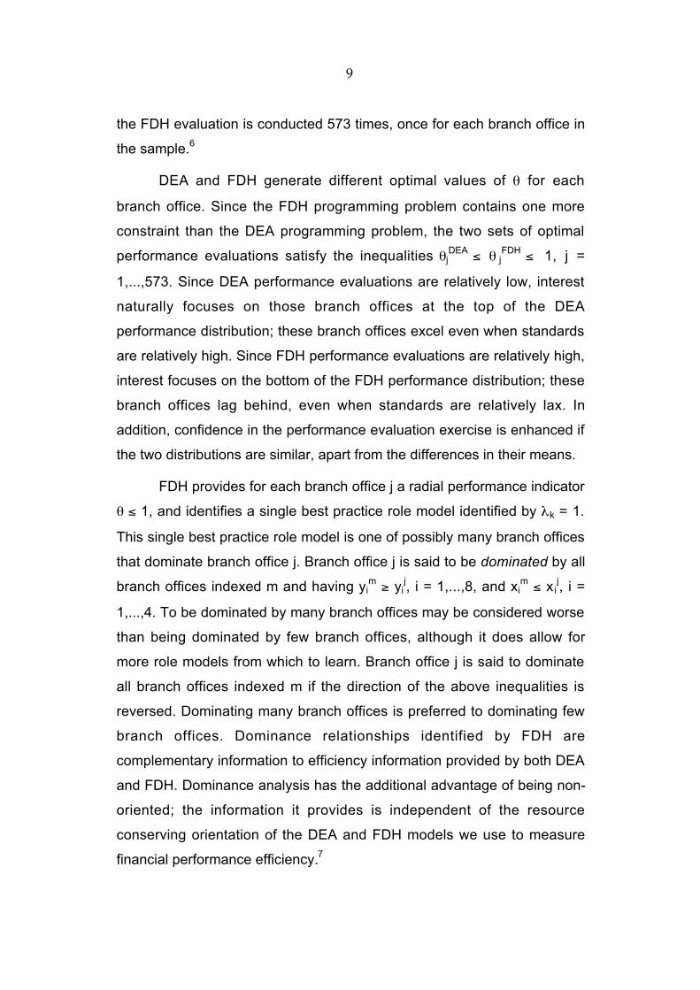
the FDH evaluation is conducted 573 times, once for each branch office in

the sample.6

DEA and FDH generate different optimal values of θ for each

branch office. Since the FDH programming problem contains one more

constraint than the DEA programming problem, the two sets of optimal

performance evaluations satisfy the inequalities θjDEA ≤ θ j

FDH ≤ 1, j =

1,...,573. Since DEA performance evaluations are relatively low, interest

naturally focuses on those branch offices at the top of the DEA

performance distribution; these branch offices excel even when standards

are relatively high. Since FDH performance evaluations are relatively high,

interest focuses on the bottom of the FDH performance distribution; these

branch offices lag behind, even when standards are relatively lax. In

addition, confidence in the performance evaluation exercise is enhanced if

the two distributions are similar, apart from the differences in their means.

FDH provides for each branch office j a radial performance indicator

θ ≤ 1, and identifies a single best practice role model identified by λk = 1.

This single best practice role model is one of possibly many branch offices

that dominate branch office j. Branch office j is said to be dominated by all

branch offices indexed m and having yim ≥ yi

j, i = 1,...,8, and xim ≤ xi

j, i =

1,...,4. To be dominated by many branch offices may be considered worse

than being dominated by few branch offices, although it does allow for

more role models from which to learn. Branch office j is said to dominate

all branch offices indexed m if the direction of the above inequalities is

reversed. Dominating many branch offices is preferred to dominating few

branch offices. Dominance relationships identified by FDH are

complementary information to efficiency information provided by both DEA

and FDH. Dominance analysis has the additional advantage of being non-

oriented; the information it provides is independent of the resource

conserving orientation of the DEA and FDH models we use to measure

financial performance efficiency.7

10

10

3.2 Evaluating the Information Content of the Data Set

Thus far the strategy for developing an overall financial

performance evaluation of branch offices has been predicated on the

assumption that all 12 expense and revenue indicators are included in the

analysis. However it is possible that not all 12 indicators have the same

information content. Some may be influential, in the sense that deleting

any one of them would result in a significantly different performance

distribution. Others may be superfluous, in the sense that deleting any one

of them would generate essentially the same performance distribution. The

objective of this Section is to determine the minimal subset of influential

indicators upon which to base the overall financial performance evaluation

of the branch offices. To that end we summarize a variable deletion

procedure developed by Pastor et al. (2002).

We begin with a DEA performance analysis of all 573 branch offices

based on all 12 resource and service indicators, DEA being our primary

performance evaluation technique. We then ask if the performance of

some branch offices, as measured by their optimal values of θ, declines

more dramatically than that of other branch offices when a particular

indicator (or set of indicators) is deleted. If it does, the performance

distribution is distorted by the deletion of that indicator, a significant

amount of managerially useful information would be lost, the candidate

indicator for deletion is deemed “influential,” and it is not deleted. If the

performance distribution does not change in a substantial way, an

insignificant amount of managerially useful information would be

sacrificed, the candidate indicator for deletion is deemed “superfluous” and

deleted, and potentially large resource savings can be realized. This

procedure continues until no indicator (or set of indicators) can be found

whose deletion would not seriously distort the performance distribution.

11

11

The surviving indicators then form the basis for a second DEA

performance evaluation, and an initial FDH performance evaluation.

Somewhat more formally, let 0 < ρ j = θjr /θj

t ≤ 1, j = 1,...,573, be a

vector of ratios of efficiency scores obtained from a reduced set of r < 12

indicators to the efficiency scores obtained from the full set of t = 12

indicators, for each of 573 branch offices. The values of ρ j constitute a

sample drawn from a distribution Ψ = (Ψ1,...,Ψ j,...,Ψ573). We want to

determine if values of Ψ that differ from unity in a sufficiently large

magnitude are likely enough to assert that the deleted indicator (or set of

indicators) is influential. We can solve this problem by determining whether

there exists sufficient statistical evidence to assert that P[Ψ < ρo] > po, ρo

being a preassigned value (say, 0.95) and po being some satisfactory level

of probability (say, 5%). A test of the hypothesis is based on the binomial

distribution B(572, po). The reason for considering 572 instead of 573 is

that at least one of the efficient units in the model with all the indicators will

remain efficient in all models with fewer indicators. The statistic we

consider is T = number of units with ρ < ρo. The null hypothesis, which

states that the set of efficiency scores of the initial and the reduced model

are indistinguishable, is rejected if the p-value of the binomial distribution

corresponding to T is high (or, equivalently, if T is a large number). In that

case, we conclude that the candidate indicator (or set of indicators) is

influential, because the reduced set of indicators explains less than ρo% of

the total efficiency for more than po% of the branch offices. If the

hypothesis can be rejected, we conclude that the candidate indicator (or

set of indicators) is superfluous, because the reduced set of indicators

explains more than ρo% of the total efficiency for more than (1 - po)% of

the branch offices. One final point is worth mentioning. The binomial test is

applied to a sample that is not i.i.d., and the two parameters are fixed at

(ρo,po). However by means of a Monte Carlo simulation study Sirvent et al.

(2001) have determined that the test performs reasonably well for specific

12

12

pairs of values of the parameters, outperforming the power of other known

tests.

3.3. The Curse of Dimensionality

In the introduction we noted that the elimination of superfluous

indicators would enable bank management to reduce the monitoring and

compliance costs associated with the branch office performance

evaluation exercise. As Simar and Wilson (2001) note, there also is a

compelling technical reason for doing so. The DEA and FDH efficiency

estimators are biased, although they are consistent. However their rates of

convergence vary inversely with the number of indicators included in the

performance evaluation; this is the curse of dimensionality that plagues

nonparametric estimators.8 Confidence in the performance evaluation

would thereby be enhanced not just by concordance of the DEA and FDH

efficiency rankings, but also by increased rates of convergence brought

about by the elimination of superfluous indicators.

4. Empirical Findings

We begin with a discussion of the results of applying our primary

analytical technique, DEA, to the entire list of 12 indicators. We use these

results as a benchmark against which to compare subsequent results

obtained from shorter lists of indicators. We continue by discussing the

results of applying the variable deletion test to the 12 indicator data set,

using the DEA efficiency scores. Finally, when we have obtained a

minimal fully informative list of indicators, we recalculate DEA efficiency

scores, and we calculate FDH efficiency scores and dominance

relationships. Our evaluation of the overall financial performance of the

13

13

branch offices is based on the DEA and FDH results applied to the

reduced list of indicators.

4.1 Initial DEA Results

We have run the DEA linear programming problem for 573 branch

offices, using the complete list of indicators containing four resources and

eight services. Results are summarized by the frequency distribution of

DEA efficiency scores which appears in the first column of Table 2.

Roughly 28% (158 of 573) of all branch offices are best practice offices,

being incapable of a radial contraction of their expenditure vectors without

violating best practice observed in the sample.9 The remaining 72% of

branch offices have financial performance efficiencies ranging down to

0.546, implying that the least efficient offices are capable of a 45%

reduction in their expenditures without sacrificing service provision. The

bottom decile of the performance distribution is capable, on average, of a

37% reduction in expenditure without sacrificing service provision.

4.2 Variable Deletion Test Results

Bank management has classified the eight service indicators into

three categories. The service category deemed most important consists of

the primary revenue indicator (interest income from loans, credit cards and

other sources) and the two size indicators (the value of deposits and the

value of assets). A somewhat less important service category consists of

the three indicators characterizing the customer base (the number of

customers, the number of regular customers, and the number of high-

income customers). A third, still less important, service category consists

of the two financial ratios (return on assets and profitability).

14

14

Referring back to the variable deletion procedure discussed in

Section 3.2, we wish to test the hypothesis that an evaluation of the overall

financial performance of branch offices based on a reduced number of

service categories provides essentially the same information as an

evaluation based on all three service categories. Testing this hypothesis

requires solving the DEA linear programming problem for all 573 branch

offices several times. We have already solved the problem using all three

service categories. The next step is to solve the same problem using only

the first two service categories, after which we solve the same problem

using only the first and third service categories. Then we conduct two tests

of the hypothesis that either the second service category or the third

service category can be deleted without statistically significant loss of

information. If we reject both hypotheses, the performance evaluation is

based on all three service categories, because all three service categories

turn out to be influential. If we fail to reject both hypotheses, the

performance evaluation is based on just the first service category,

because the second and third service categories are deemed superfluous.

If we reject one hypothesis and fail to reject the other, the performance

evaluation is based on two influential service categories, the first service

category and one of the two remaining service categories. Finally, once we

are down to a minimal number of influential service categories, we repeat

the procedure in an effort to eliminate superfluous resources, and

superfluous services within each service category. Whatever the outcome

of the hypothesis testing procedure, we are confident that the final

financial performance evaluation is based on the smallest number of

resources and services which can be used without statistically significant

loss of managerially useful information.

We begin by testing the hypothesis that the third service category is

superfluous, on the grounds that the two financial ratios are

consequences, rather than determinants, of the overall financial

15

15

performance of branch offices. We are unable to reject this hypothesis; the

two frequency distributions of branch office financial performance

efficiencies are virtually identical, and statistically indistinguishable. The

evaluation of overall financial performance based on all three service

categories generates 158 efficient branch offices, with the efficiencies of

the remaining 415 branch offices contained in the range [1, 0.546]. The

evaluation of overall financial performance based on the first two service

categories generates 150 efficient branch offices, with the remaining 423

branch offices contained in the range [1, 0.546]. Only three branch offices

have ρj = θj10/θj

12 < ρo = 0.95. We conclude that the two financial ratios are

superfluous to an evaluation of the overall financial efficiency of branch

offices.10

We next test the hypothesis that the second service category is

superfluous, on the grounds that customer characteristics are not direct

indicators of financial performance. We are able to reject this hypothesis;

deleting customer characteristics alters the frequency distribution of

branch office financial performance efficiencies to a statistically significant

degree. 190 branch offices have ρj = θj7/θj

10 < ρo = 0.95. Since elimination

of the three customer characteristics indicators would result in a significant

loss of managerially useful information, this service category is not

deleted. At this point in the hypothesis testing procedure, we have

succeeded in reducing the list of indicators from 12 to 10.11

We next test the hypothesis that any single resource, or any single

remaining service, can be deleted without statistically significant loss of

information. We are unable to delete any of the four resources; deleting

any resource would significantly alter the frequency distribution of branch

office financial performance efficiencies, thereby leading to a loss of

managerially useful information.12 We are, however, able to delete two

services, one from each remaining service category, without statistically

significant loss of information. The two services we are able to delete are

16

16

interest income (from the first category), and the number of regular clients

(from the second category).13 We were rather surprised when we

discovered that it was practically equivalent to delete the number of clients

instead of the number of regular clients. In any DEA model formulated as a

linear program, two outputs are equivalent if either one of them can be

expressed as an affine combination of the other with positive scale factor.

A linear regression with the number of clients as the independent variable

and the number of regular clients as dependent yields a positive slope

(0.83) and an adjusted R2=0.996. In fact management preferred to delete

from the analysis the number of clients instead of the number of regular

clients, considering that the latter variable is more representative of the

activity of the bank.

After completing the variable deletion test procedure, we have

succeeded in reducing the number of service indicators from eight to four,

because we have found the four deleted service indicators to be

superfluous, containing no independent information of their own. We have

been unable to reduce the number of resource indicators, since each of

them is influential. A complete list of surviving influential indicators and

deleted superfluous indicators appears in Table 3.

The frequency distribution of branch office overall financial

performance efficiencies based on the four influential services appears in

the second column of Table 2. There is no statistically significant

difference between this distribution and that based on the complete set of

eight services appearing in the first column. The simpler model generates

slightly fewer efficient branch offices, as it must mathematically, but it

generates the same range of branch office financial performance efficiency

scores. The mean is also marginally lower, but both means imply that, on

average, branch offices are capable of a 13% reduction in their expenses

without a compensating reduction in their financial and customer base

characteristics. Otherwise the two frequency distributions appear to be

17

17

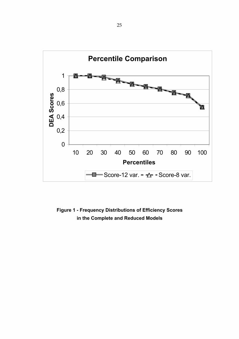
virtually identical. The similarity of the two frequency distributions is

illustrated in Figure 1. Underlying Figure 1 is the fact that 304 branch

offices have exactly the same overall financial performance efficiency in

the two models, an additional 180 branches experience a less than 1%

decrease in efficiency in the final model, and only seven branch offices

experience an decrease in efficiency in excess of 5% in the final model.

The fact that deletion of four revenue indicators affected the overall

financial performance evaluation of 85% of branch offices by less than 1%

attests to the superfluous nature of the four deleted indicators.

4.3 DEA and FDH Evaluations of Overall Financial Performance

We are now prepared to conduct an evaluation of the overall

financial performance of the branch offices. Although we base our

evaluation on the reduced list of indicators containing eight influential

indicators, we are assured by the statistical tests conducted in Section 4.2

that essentially the same evaluation would result from the complete list of

indicators.

We are interested in extracting maximum information from the DEA

and FDH financial performance evaluations, since they provide

complementary insights. Since DEA is relatively demanding, its most

useful information identifies high-performing branch offices. Since FDH is

relatively generous, its most useful information identifies low-performing

branch offices. In addition, FDH provides dominance information that

complements both financial performance distributions.

The DEA results have already been discussed; they are

summarized in the second column of Table 2 and illustrated in Figure 1.

We conducted the FDH analysis with the complete model and with the

reduced model. The results of the two models are even more similar than

18

18

in the DEA case. In the complete model there are only 30 units with an

efficiency score less than 1, while in the reduced model we found 40.

Nevertheless the range of variation of the inefficiency scores was exactly

the same for both models. Moreover, 29 of 30 inefficient offices from the

complete model received exactly the same efficiency score in the reduced

model. Consequently results of the variable deletion test, which was

applied only in the DEA case, were validated by the FDH models.14 FDH

efficiency scores are not summarized by a frequency distribution in Table

2 because FDH assigns an efficiency score of unity to 93% (533 of 573)

branch offices. The scores of the 40 radially inefficient branch offices are

contained in the range [0.998, 0.713], with a mean of 0.902.

As we indicated in Section 3.1, the generosity of FDH encourages

us to examine the bottom of the performance distribution. In Table 4 we list

the bottom 25 branch offices, according to two criteria. In the first three

columns we list the bottom 25 branch offices as revealed by their FDH

efficiency scores, and we compare their FDH and DEA efficiency score

ranks. In the next three columns we list the 25 most frequently dominated

branch offices according to FDH, and we compare their FDH and DEA

efficiency score ranks. Although FDH assigns consistently higher

performance scores than DEA does, it is abundantly clear from Table 4

that the two techniques are in substantial agreement on the identity of the

worst-performing branch offices. Nearly half (11 of 25) of the branch

offices receiving the lowest FDH efficiency scores also receive the lowest

DEA efficiency scores, and over a third (9 of 25) of the most frequently

dominated branch offices according to FDH receive the lowest DEA

efficiency scores.

In light of the concordance between the DEA and the FDH

performance rankings, it is relatively easy to identify the 15 branch offices

most in need of bank management attention. These branch offices have ID

numbers 911, 102, 832, 840, 802, 272, 818, 110, 336, 310, 260, 320, 186,

19

19

188 and 338. Each is among the 25 most frequently dominated branch

offices, and most of them are at the bottom of both efficiency score

rankings.

5. Summary and Conclusions

In this paper we have evaluated the financial performance of the

vast majority of the branch offices of a large European savings bank. Our

evaluation has been based on a list of indicators currently used by the

bank for the same general purpose. The indicators include four expense

items, an inclusive revenue item, two size indicators, three customer base

characteristics, and a pair of financial ratios. We have used a pair of

complementary methodologies, DEA and FDH, to evaluate financial

performance, and we have used a pair of complementary criteria,

efficiency analysis and dominance analysis, to implement the evaluation.

Our first finding concerns the financial performance of branch

offices. Our primary analytical technique, DEA, revealed a wide range of

performance variation, with worst performance capable of a 45% reduction

in resource consumption without any offsetting reduction in service

provision. This range holds for the initial 12 variable model and for the final

eight variable model. The implication of this finding is that efficiency

improvement at the worst-performing branch offices can generate a

substantial increase in profit for the bank.15

Our second finding is that the list of 12 indicators (which is smaller

than the list used by the bank) is unnecessarily, and expensively, large.

We have found the four expense indicators to be influential, and so we are

unable to delete any of them without statistically significant loss of

information to bank management. However we have also demonstrated

that four of the eight service indicators are superfluous, and contain no

20

20

independent information of their own concerning the financial performance

of branch offices. The four superfluous service indicators can be deleted

from the financial performance evaluation exercise with no statistically

significant loss of information to bank management. Stated somewhat

differently, when these four service indicators are deleted from the variable

list, only 89 of 573 branch offices incurred more than a 1% decline in their

performance rating, and only five branch offices incurred more than a 5%

decline. Since the two performance rankings are statistically

indistinguishable, the bank has the potential to conserve on monitoring

and compliance costs by reducing the number of indicators on which it

bases its performance evaluation, once again pointing to the feasibility of a

streamlining of the bank’s branch office evaluation procedures.

Perhaps the most useful information we can provide bank

management is the identities of the worst performing branch offices in its

network. Our third finding is that our primary analytical technique, DEA,

and our secondary technique, FDH, as well as our two performance

criteria, efficiency and dominance, identify essentially the same low-

performing branch offices. This is reassuring, because it generates

confidence in our findings, and it is also of considerable value to bank

management, because it identifies problem branch offices in need of

remedial action.

Our financial performance evaluation has been based on detailed

branch office information provided to us by bank management. The

variable list has benefited from frequent discussions with bank

management. Nonetheless, potentially useful information has been

unavailable to us. This information concerns the characteristics of the

operating environment in which branch offices seek to minimize the

expenses required to provide revenue-generating services to their

customers. Information on operating environment characteristics, such as

the population in the surrounding area of each branch, the age of each

21

21

branch, the degree of competition in each branch’s neighborhood, and so

on, would prove useful in levelling the playing field prior to conducting the

financial performance evaluation. Techniques for incorporating such

characteristics into the analysis have been developed by Daraio and Simar

(2003) and Simar and Wilson (2003).

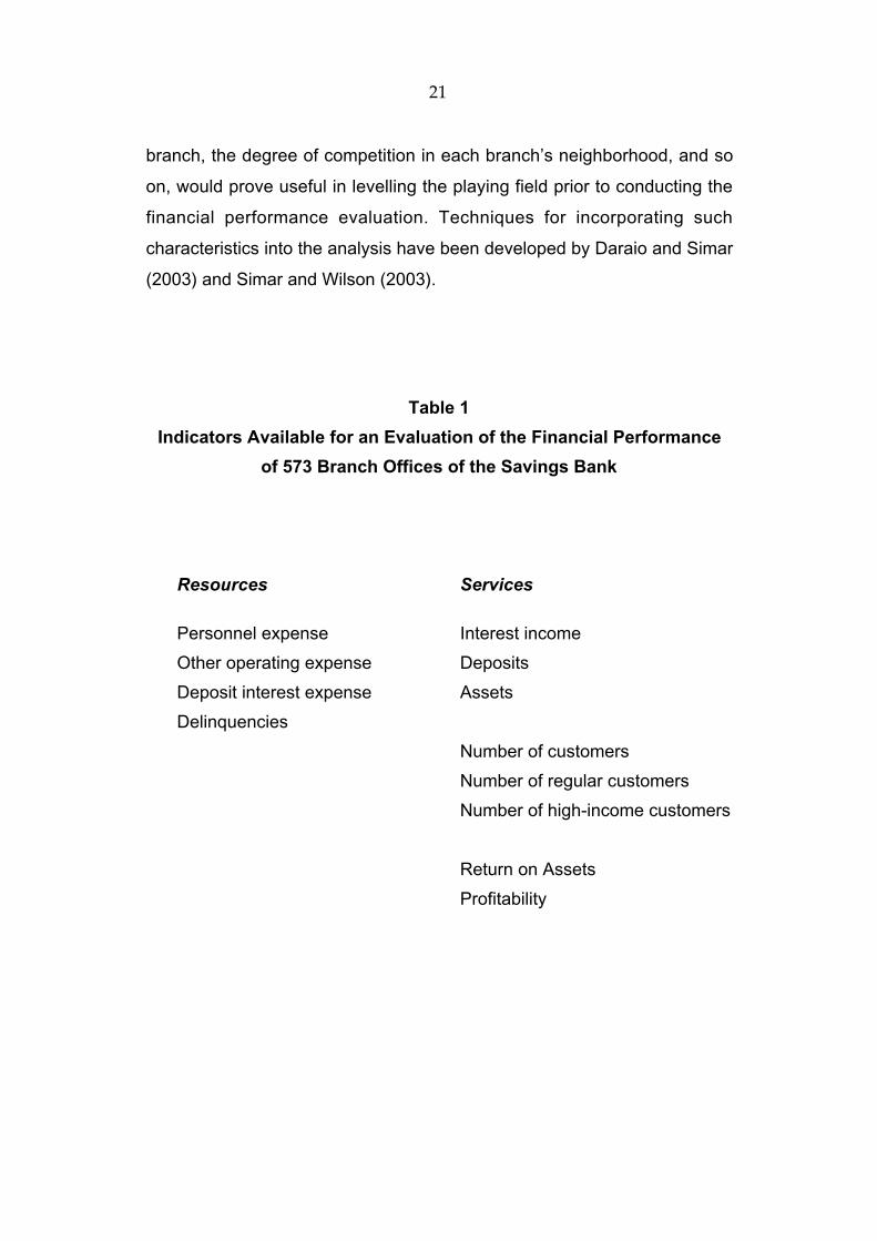
Table 1

Indicators Available for an Evaluation of the Financial Performance

of 573 Branch Offices of the Savings Bank

Resources Services

Personnel expense Interest income

Other operating expense Deposits

Deposit interest expense Assets

Delinquencies

Number of customers

Number of regular customers

Number of high-income customers

Return on Assets

Profitability

22

22

Table 2

Distribution of Branch Office Financial Performance Efficiencies, byPercentile

Efficiency Scores

Percentile 12 Indicator Model 8 Indicator Model

(4 Resources, 8 Services) (4 Resources, 4 Services)

10 1.000 1.000

20 1.000 1.000

30 0.982 0.973

40 0.933 0.922

50 0.883 0.877

60 0.846 0.841

70 0.809 0.804

80 0.759 0.752

90 0.715 0.713

100 0.546 0.546

Number of Efficient Branch Offices (%) 158 (27.6%) 147 (25.7%)

Mean Efficiency Score 0.873 0.868

23

23

Table 3

Influential and Superfluous Financial Performance Indicators

Influential Indicators Superfluous Indicators

Personnel expense

Other operating expense

Deposit interest expense

Delinquencies

Interest income

Deposits

Assets

Number of regular customers

Number of customers

Number of high income customers

Return on assets

Profitability

24

24

Table 4

The Worst Performing Branch Offices, by FDH and by DEA

Ranked by FDH Efficiency Score Ranked by FDH Dominance

Branch Office ID# - FDH Rank - DEA Rank Branch Office ID# - FDH Rank - DEA Rank

102 573 573 911 572 563

911 572 563 102 573 573

832 571 553 832 571 553

840 570 561 840 570 561

818 569 570 802 563 571

260 568 544 272 551 518

924 567 529 818 569 570

944 566 485 110 533 542

333 565 527 336 552 540

186 564 566 310 540 536

802 563 571 260 568 544

789 562 944 566 485

175 561 560 760 560

760 560 320 553 552

240 559 508 993 549 515

410 558 538 164 538

460 557 550 206 531 567

400 556 488 186 564 566

174 555 524 188 554 568

188 554 568 768 547 492

320 553 552 338 546 559

926 552 510 781 545

272 551 518 826 539 496

989 550

993 549 515

25

25

Figure 1 - Frequency Distributions of Efficiency Scores

in the Complete and Reduced Models

Percentile Comparison

0

0,2

0,4

0,6

0,8

1

10 20 30 40 50 60 70 80 90 100

Percentiles

DE

A S

core

s

Score-12 var. Score-8 var.

26

26

Footnotes

1. An identical formulation of FDH, called MED, a measure of efficiencydominance, was proposed at the same time by Bowlin et al. (1984).

2. Numerous studies have used DEA to examine bank branch operatingperformance, including Oral and Yolalan (1990), Vassiloglou andGiokas (1990), Giokas (1991), Drake and Howcroft (1994), Parkan(1994), Boufounou (1995), Haag and Jaska (1995), Sherman andLadino (1995), Athanassopoulos et al. (1996), Nash and Sterna-Karwat (1996), Athanassopoulos (1997), Lovell and Pastor (1997),Schaffnit et al. (1997), Athanassopoulos (1998), Camanho and Dyson(1999), Soteriou and Zenios (1999a, 1999b), Xue and Harker (1999),Golany and Storbeck (1999), Kantor and Maital (1999), Soteriou et al.(1999), Athanassopoulos (2000), Athanassopoulos and Giokas (2000),Dekker and Post (2001), Hartman et al. (2001), and Portela et al.(2003). A handful of studies have used FDH for the same purpose,including Respaut (1989), Tulkens (1993), and Tulkens and Malnero(1996).

3. An excellent illustration of the use of alternative empiricalmethodologies for cross-validation purposes is provided by Charnes etal. (1988), who used DEA and goal programming to providecomplementary analyses of the breakup of AT&T in the US.

4. The technical reason we choose a resource conserving orientation isthat one of the services, profitability, attains negative values for 161branch offices. This variable must be translated, so that all values arenonnegative. Lovell and Pastor (1995) have shown that a radialoutput-oriented linear programming model of performance evaluationis not invariant with respect to translation of services, but that a radialinput-oriented linear programming model is invariant with respect totranslation of services. An economic argument in support of a resourceconserving orientation is that services are more likely to be exogenousto branch office management than resources.

5. The phrase “suggests that” means “is necessary but not sufficient for,”since optimal θ = 1 is necessary and sufficient for radial efficiency, butis not sufficient for overall efficiency, since slacks may be present. Inour empirical exercise we have found slacks to be neither large norsystematic.

27

27

6. Adding the constraint λk ∈ {0,1}, k = 1,…,573, converts the DEA linearprogramming problem to an FDH mixed integer programming problem.A simple minimax solution algorithm is described in Tulkens (1993).

7. Dominance analysis is an under-utilized performance evaluationtechnique, although it has been used by Fried et al. (1993, 1995),Lovell (1995) and Tulkens and Malnero (1996).

8. Kneip et al. (1998) show that the rates of convergence of the DEA andFDH estimators are given by θDEA - θ = Op(J

-2/M+N+1) and θFDH - θ =Op(J

-1/M+N), where J is the sample size and M and N are the number ofoutputs and inputs. Simar and Wilson (2001) propose several teststatistics for superfluous variables, one of which corresponds to ourstatistic ρj = θj

r/θjt, j=1,…,J. However rather than imposing a parametric

distribution on this statistic, they employ bootstrapping techniques.

9. DEA allows producers freedom to choose the weights they attach toinputs and outputs in order to maximize their efficiency. This leads to amultiplicity of efficient producers and allows only a partial ranking ofproducers, and can be considered another curse of dimensionality.The curse is even worse with FDH. An attempt to create a completeranking by using a super-efficiency DEA model to break ties at the topis provided by Xue and Harker (2002).

10. The p-value associated with T=3 is 0.000000453, and consequentlythe null hypothesis cannot be rejected. The two efficiency distributionsare statistically indistinguishable and the two financial ratios can bedeleted.

11. The p-value associated with T=190 is 1 (with an error less than0.00000001. Hence the null hypothesis is rejected.

12. The test statistic associated with the deletion of each of the fourservice indicators from the original 12 indicator model are: T=187 forpersonnel expense, T=104 for other operating expense, T=407 fordeposit interest expense, and T=153 for delinquencies. The p-valueassociated with T=104 is 1 (with an error less than 0.00000001) andtherefore all the remaining p-values are also 1 (with an error less than0.00000001). In each of the four cases the null hypothesis is rejected.Since the deletion of an indicator after others have already been

28

28

deleted gives a larger value of T (see Pastor et al. (1997)), we aresure that, after deleting the two financial ratios, we are unable todelete any single resource.

13. The test statistic when comparing the complete model with thereduced model with only eight indicators is T=5, with a correspondingp-value of 0.00000299. Hence the null hypothesis cannot be rejected.

14. The variable deletion test can also be applied directly to an FDHmodel, as explained in Pastor et al. (2002).

15. The DEA results indicate that elimination of branch office inefficiencywithin the bottom decile only would result in a cost saving to the bankof an amount which exceeds the average branch office expense by afactor of 23.

29

29

References

Athanassopoulos, A. D. (1997), “Service Quality and Operating EfficiencySynergies for Management Control in the Provision of FinancialServices: Evidence from Greek Bank Branches,” European Journal ofOperational Research 98, 300-13.

Athanassopoulos, A. D. (1998), “Non-Parametric Frontier Models forAssessing the Market and Cost Efficiency of Large-Scale Bank BranchNetworks,” Journal of Money, Credit and Banking 30, 172-92.

Athanassopoulos, A. D. (2000), “An Optimization Framework of the Triad:Source Capabilities, Customer Satisfaction, and Performance,” Chapter9 in P. T. Harker and S. A. Zenios, eds., Performance of FinancialInstitutions: Efficiency, Innovation, Regulation. New York: CambridgeUniversity Press.

Athanassopoulos, A. D., and D. Giokas (2000), “The Use of DataEnvelopment Analysis in Banking Institutions: Evidence from theCommercial Bank of Greece,” Interfaces 30:2 (March/April), 81-95.

Athanassopoulos, A. D., A. C. Soteriou and S. A. Zenios (1996),“Disentangling Within- and Between-Country Efficiency Differences ofBank Branches,” Chapter 10 in P. T. Harker and S. A. Zenios, eds.,Performance of Financial Institutions: Efficiency, Innovation, Regulation.New York: Cambridge University Press.

Banker, R. D., A. Charnes and W. W. Cooper (1984), “Some Models forEstimating Technical and Scale Inefficiencies in Data EnvelopmentAnalysis,” Management Science 30:9 (September), 1078-92.

Boufounou, P. V. (1995), “Evaluating Bank Branch Location andPerformance: A Case Study,” European Journal of OperationalResearch 87, 389-402.

Bowlin, W. F., J. Brennan, A. Charnes, W. W. Cooper and T. Sueyoshi(1984), “A Model for Measuring Amounts of Efficiency Dominance,”Research Report, Graduate School of Business, University of Texas,Austin, TX 78712, USA.

30

30

Camanho, A. S., and R. G. Dyson (1999), “Efficiency, Size, Benchmarksand Targets for Bank Branches: An Application of Data EnvelopmentAnalysis,” Journal of the Operational Research Society 50:9, 903-15.

Charnes, A., W. W. Cooper and E. Rhodes (1978), “Measuring theEfficiency of Decision Making Units,” European Journal of OperationalResearch 2, 429-44.

Charnes, A., W. W. Cooper and T. Sueyoshi (1988), “A Goal Programming/ Constrained Regression Review of the Bell System Breakup,”Management Science 34:1 (January), 1-26.

Daraio, C., and L. Simar (2003), “Introducing Environmental Variables inNonparametric Frontier Models: A Probabilistic Approach,” DiscusiónPaper 0313, Institut de Statistique, Université Catholique de Louvain,Louvain-la-Neuve, Belgium.

Dekker, D., and T. Post (2001), “A Quasi-Concave DEA Model with anApplication for Bank Branch Performance Evaluation,” EuropeanJournal of Operational Research 132, 296-311.

Deprins, D., L. Simar and H. Tulkens (1984), “Measuring Labor-Efficiencyin Post Offices,” in M. Marchand, P. Pestieau and H. Tulkens, eds., ThePerformance of Public Enterprises: Concepts and Measurement.Ámsterdam: North-Holland.

Drake, L., and B. Howcroft (1994), “Relative Efficiency in the BranchNetwork of a UK Bank: An Empirical Study,” Omega 22:1, 83-90.

Fried, H. O., C. A. K. Lovell and P. Vanden Eeckaut (1993), “Evaluatingthe Performance of US Credit Unions,” Journal of Banking and Finance17:2-3 (April), 251-65.

Fried, H. O., C. A. K. Lovell and P. Vanden Eeckaut (1995), “ServiceProductivity in US Credit Unions,” Chapter 13 in P. T. Harker, ed., TheService Productivity and Quality Challenge. Boston: Kluwer AcademicPublishers.

31

31

Giokas, D. (1991), “Bank Branch Operating Efficiency: A ComparativeApplication of DEA and the Log-Linear Model,” Omega 19:6, 549-57.

Golany, B., and J. E. Storbeck (1999), “A Data Envelopment Análisis ofthe Operational Efficiency of Bank Branches,” Interfaces 29:3(May/June), 14-26.

Haag, S. E., and P. V. Jaska (1995), “Interpreting Efficiency Ratings: AnApplication of Bank Branch Operating Efficiencies,” Managerial andDecisión Economics 16:1 (January-February), 7-14.

Hartman, T. E., J. E. Storbeck and P. Byrnes (2001), “Allocative Efficiencyin Branch Banking,” European Journal of Operational Research 134,232-42.

Kantor, J., and S. Maital (1999), “Measuring Efficiency by Product Group:Integrating DEA with Activity-Based Accounting in a Large MideastBank,” Interfaces 29:3 (May/June), 27-36.

Kneip, A., B. U. Park and L. Simar (1998), “A Note on the Convergence ofNonparametric DEA Estimators for Production Efficiency Scores,”Econometric Theory 14, 783-93.

Lovell, C. A. K. (1995), “Measuring the Macroeconomic Performance ofthe Taiwanese Economy,” International Journal of ProductionEconomics 39, 165-78.

Lovell, C. A. K., and J. T. Pastor (1995), “Units Invariant and TranslationInvariant DEA Models,” Operations Research Letters 18:3, 147-51.

Lovell, C. A. K., and J. T. Pastor (1997), ”Target Setting: An Application toa Bank Branch Network,” European Journal of Operational Research98, 290-99.

Nash, D., and A. Sterna-Karwat (1996), “An Application of DEA toMeasure Branch Cross Selling Efficiency,” Computers & OperationsResearch 23:4 (April), 385-92.

32

32

Oral, M., and R. Yolalan (1990), “An Empirical Study on MeasuringOperating Efficiency and Profitability of Bank Branches,” EuropeanJournal of Operational Research 46, 282-94.

Parkan, C. (1994), “Operational Competitiveness Ratings of ProductionUnits,” Managerial and Decision Economics 15:3 (May-June), 201-21.

Pastor, J. T., J. L. Ruiz and I. Sirvent (1997), “Procedures for ProgressiveSelection of Variables in DEA,” Working Paper, Departamento deEstadistica e Investigación Operativa, Universidad de Alicante, 03071Alicante, Spain.

Pastor, J. T., J. L. Ruiz and I. Sirvent (2002), “A Statistical Test for NestedRadial DEA Models,” Operations Research 50:4 (July-August), 728-35.

Respaut, B. (1989), “Mesures de l’efficacité productive des 911 agencesd’une banque privée belge,” Chapter 3 in H. Tulkens, ed., Efficacite etManagement. Charleroi, Belgium: CIFOP.

Schaffnit, C., D. Rosen and J. C. Paradi (1997), “Best Practice Analysis ofBank Branches: An Application of DEA in a Large Canadian Bank,”European Journal of Operational Research 98, 269-89.

Sherman, H. D., and G. Ladino (1995), “Managing Bank Productivity UsingData Envelopment Analysis,” Interfaces 25:2 (March-April), 60-73.

Silva Portela, M. C. A., P. C. Borges and E. Thanassoulis (2003), “FindingClosest Targets in Non-Oriented DEA Models: The Case of Convex andNon-Convex Technologies,” Journal of Productivity Analysis 19:2/3(April), 251-69.

Simar, L., and P. W. Wilson (2001), “Testing Restrictions in NonparametricEfficiency Models,” Communications in Statistics 30:1, 159-84.

Simar, L., and P. W. Wilson (2003), “Estimation and Inference in Two-Stage, Semi-Parametric Models of Production Processes,” DiscussionPaper 0307, Institut de Statistique, Université Catholique de Louvain,Louvain-la-Neuve, Belgium.

33

33

Sirvent, I., J. L. Ruiz, F. Borras and J. T. Pastor (2001), “A Monte CarloEvaluation of Some Tests of Model Specification in DEA,” Trabajos I+D,#I-2001-13, Centro de Investigación Operativa, Universidad MiguelHernández, Spain.

Soteriou, A. C., C. V. Zenios, K. Agathocleous and S. A. Zenios (1999),“Benchmarks of the Efficiency of Bank Branches,” Interfaces 29:3(May/June), 37-51.

Soteriou, A. C., and S. A. Zenios (1999a), “Using Data EnvelopmentAnalysis for Costing Bank Products,” European Journal of OperationalResearch 114, 234-48.

Soteriou, A., and S. A. Zenios (1999b), “Operations, Quality, andProfitability in the Provision of Banking Services,” Management Science45:9 (September), 1221-38.

Tulkens, H. (1993), “On FDH Analysis: Some Methodological Issues andApplications to Retail Banking, Courts and Urban Transit,” Journal ofProductivity Analysis 4:1 (June), 183-210.

Tulkens, H., and A. Malnero (1996), “Nonparametric Approaches to theAssessment of the Relative Efficiency of Bank Branches,” Chapter 10 inD. G. Mayes, ed., Sources of Productivity Growth . New York:Cambridge University Press.

Tulkens, H., and P. Vanden Eeckaut (1995), “Non-Parametric Efficiency,Progress and Regress Measures for Panel Data: MethodologicalAspects,” European Journal of Operational Research 80, 474-99.

Vassiloglou, M., and D. Giokas (1990), “A Study of the Relative Efficiencyof Bank Branches: An Application of Data Envelopment Analysis,”Journal of the Operational Research Society 41:7, 591-97.

Xue, M., and P.T. Harker (2002), “Note: Ranking DMUs with InfeasibleSuper Efficiency in DEA Models,” Management Science 48:5 (May),705-10.