Embed Size (px)
Citation preview
Evaluating the performance of aggregate production planning
strategies under uncertainty
A thesis submitted to The University of Manchester for the degree of Doctor of Philosophy
in the Faculty of Humanities
2017
Aboozar Jamalnia
Alliance Manchester Business School
1
The University of Manchester
Aboozar Jamalnia
Degree: Doctor of Philosophy
Thesis title: Evaluating the performance of aggregate production planning strategies
under uncertainty
Date: 10/05/2017 Abstract: The thesis is presented in three papers format. Paper 1 presents the first bibliometric literature survey of its kind on aggregate production planning (APP) in presence of uncertainty. It surveys a wide range of the literatures which employ operations research/management science methodologies to deal with APP in presence of uncertainty by classifying them into six main categories such as stochastic mathematical programming, fuzzy mathematical programming and simulation. After a preliminary literature analysis, e.g. with regard to number of publications by journal and publication frequency by country, the literature about each of these categories is shortly reviewed. Then, a more detailed statistical analysis of the surveyed research, with respect to the source of uncertainty, number of publications trend over time, adopted APP strategies, applied management science methodologies and their sub-categories, and so on, is presented. Finally, possible future research paths are discussed on the basis of identified research trends and research gaps. The second paper proposes a novel decision model to APP decision making problem based on mixed chase and level strategy under uncertainty where the market demand acts as the main source of uncertainty. By taking into account the novel features, the constructed model turns out
to be stochastic, nonlinear, multi-stage and multi-objective. APP in practice entails multiple-objectivity. Therefore, the model involves multiple objectives such as total revenue, total production costs, total labour productivity costs, optimum utilisation of production resources and capacity and customer satisfaction, and is validated on the basis of real world data from beverage manufacturing industry. Applying the recourse approach in stochastic programming leads to empty feasible space, and therefore the wait and see approach is used instead. After solving the model using the real-world industrial data, sensitivity analysis and several forms of trade-off analysis are conducted by changing different parameters/coefficients of the constructed model, and by analysing the compromise between objectives respectively. Finally, possible future research directions, with regard to the limitations of present study, are discussed. The third paper is to appraise the performance of different APP strategies in presence of uncertainty. The relevant models for various APP strategies including the pure chase, the pure level, the modified chase and the modified level strategies are derived from the fundamental model developed for the mixed chase and level strategy in paper 2. The same procedure, which is used in paper 2, follows to solve the models constructed for these strategies with respect to the aforementioned objectives/criteria in order to provide business and managerial insights to operations managers about the effectiveness and practicality of these APP policies under uncertainty. Multiple criteria decision making (MCDM) methods such as additive value function (AVF), the technique for order of preference by similarity to ideal solution (TOPSIS) and VIKOR are also used besides multi-objective optimisation to assess the overall performance of each APP strategy.

2
DECLARATION No portion of the work referred to in the thesis has been submitted in support of an application for another degree or qualification of this or any other university or other institute of learning.
3
COPYRIGHT STATEMENT
i. The author of this thesis (including any appendices and/or schedules to this thesis) owns certain copyright or related rights in it (the “Copyright”) and s/he has given The University of Manchester certain rights to use such Copyright, including for administrative purposes.
ii. Copies of this thesis, either in full or in extracts and whether in hard or electronic copy, may be made only in accordance with the Copyright, Designs and Patents Act 1988 (as amended) and regulations issued under it or, where appropriate, in accordance with licensing agreements which the University has from time to time. This page must form part of any such copies made.
iii. The ownership of certain Copyright, patents, designs, trade marks and other intellectual property (the “Intellectual Property”) and any reproductions of copyright works in the thesis, for example graphs and tables (“Reproductions”), which may be described in this thesis, may not be owned by the author and may be owned by third parties. Such Intellectual Property and Reproductions cannot and must not be made available for use without the prior written permission of the owner(s) of the relevant Intellectual Property and/or Reproductions.
iv. Further information on the conditions under which disclosure, publication and commercialisation of this thesis, the Copyright and any Intellectual Property University IP Policy (see http://documents.manchester.ac.uk/display.aspx?DocID=24420), in any relevant Thesis restriction declarations deposited in the University Library, The University Library’s regulations (see http://www.library.manchester.ac.uk/about/regulations/) and in The University’s policy on Presentation of Theses.
4
List of Contents
Preface……………………………………………………………………………………………………………………………………………..10 PAPER 1
Page Aggregate production planning under uncertainty: a bibliometric literature survey and future research directions ………………………………………..………….…..13
Abstract………………………………………………………………………………………………………………………………..…………..13 1.1. Introduction…………………………………………………………………………………………………………………………..…..13 1.2. The need for bibliometric literature survey on APP under uncertainty…………………………………..….18 1.3. Preliminary analysis of the literature………………………………………………………………………………………...19 1.4. Classification scheme……………………………………………………………………………………………………………..….21 1.5. Elaborate review of the literature on APP subject to uncertainty…………………………………………...…23 1.5.1. Fuzzy mathematical programming…………………………………………………………………………………..……..23 1.5.1.1. Fuzzy multi-objective optimisation…………………………………………………………………………..……….….23 1.5.1.2. Fuzzy goal programming……………………………………………………………………………………………..……….24 1.5.1.3. Fuzzy linear programming………………………………………………………………………………………..………….25 1.5.1.4. Fuzzy nonlinear programming……………………………………………………………………………………..….…..25 1.5.1.5. Other fuzzy mathematical programming approaches…………………………………………………..….….26 1.5.2. Stochastic mathematical programming…………………………………………………………………………..…..…26 1.5.2.1. Stochastic linear programming……………………………………………………………………………………..…….26 1.5.2.2. Stochastic multi-objective optimisation…………………………………………………………………….…...…...27 1.5.2.3. Stochastic nonlinear programming……………………………………………………………………………….….….27 1.5.2.4. Robust optimisation…………………………………………………………………………………………………..…...…..28 1.5.2.5. Stochastic control………………………………………………………………………………………………………..…...…29 1.5.2.6. Other stochastic mathematical programming methodologies………………………………………..…..29 1.5.3. Simulation…………………………………………………………………………………………………………………………...…29 1.5.3.1. Common discrete-event simulation………………………………………………………………………………..…..30 1.5.3.2. Other simulation modelling techniques……………………………………………………………………………....30
5
1.5.4. Metaheuristics………………………………………………………………………………………………………….…………..31 1.5.4.1. Genetic algorithms…………………………………………………………………………………………………………….31 1.5.4.2. Tabu search……………………………………………………………………………………………………………………….31 1.5.4.3. Other metaheuristic approaches…………………………………………………………………………..…………..31 1.5.5. Possibilistic programming…………………………………………………………………………………………………….32 1.5.5.1. Ordinary possibilistic programming…………………………………………………………………………………..32 1.5.5.2. Interactive possibilistic programming……………………………………………………………………………….32 1.5.6. Evidential reasoning……………………………………………………………………………………………….……………33 1.6. Further detailed analysis of the literature………………………………………………………………………………33 1.6.1. Source of uncertainty in APP models…………………………………………………………………………………..33 1.6.2. Trends for frequency of published research regarding each main category of the methodologies…………………………………………………………………………………………….34 1.6.3. Frequency of published research with regard to each sub-category of the methodologies………………………………………………………………………………………………37 1.6.4. The most cited research on APP under uncertainty…………………………………………………………….40 1.6.5. Literature with respect to the applied APP strategy……………………………………………………………41 1.7. Conclusions and future research directions……………………………………………………………………………42 References……………………………………………………………………………………………………………………………………44 PAPER 2 A novel decision model based on mixed chase and level strategy to aggregate production planning in presence of uncertainty ………………….……………………………………..51 Abstract…………………………………………………………………………………………………………………………………….…51 2.1. Introduction……………………………………………………………………….…………………………………………………51 2.1.1. General overview……………………………………………………………………………………………………….….….51 2.1.2. Fundamental APP policies and options………………………………………………………………………….…..52 2.1.3. Problem statement……………………………………………………………………………………………….…………..54 2.2. Literature review……………………………………………………………………………………………………………….…55 2.2.1. Stochastic multi-objective optimisation…………………………………………………………………………….55 2.2.2. Stochastic nonlinear programming……………………………………………………………………………….…..56 2.2.3. Stochastic linear programming…………………………………………………………………………………………56
6
2.3. Model development………………………………………………………………………………………………………….…57 2.3.1. Methodological remarks…………………………………………………………………………………………………..57 2.3.2. Stochastic nonlinear multi-objective optimisation model of APP under uncertainty for the mixed chase and level strategy………………………………………………………….60 2.3.2.1. Notations………………………………………………………….…………………………………………………….……..60 2.3.2.1.1. Decision variables……………………………………………………………………………………………………….60
2.3.2.1.2. Parameters/constants………………………………………………………………………………………….……..60 2.3.2.2. Objectives……………………………………………………………………….…………………………………….……….62 2.3.2.3. Constraints…………………………………………………………………….……………………………………….……..65 2.4. Case study……………………………………………………………………………………………………………………….…..72 2.5. Further experiments with the model……………………………………………………………………………….….77 2.5.1. Scenario 1: construct pay-off table…………………………………………………………………………….….…77 2.5.2. Scenario 2: consider minimisation/maximisation objectives separately……………………..…..78 2.5.3. Scenario 3: conduct trade-off analysis……………………………………………………………………….…...78 2.5.4. Scenario 4: conduct sensitivity analysis……………………………………………………………………….….79 2.6. Conclusions and future research directions……………………………………………………………………….82 References……………………………………………………..……………………………………………………………………..…85 PAPER 3 Evaluating the performance of aggregate production planning strategies under uncertainty…………………………………………………………………………………………………………….….……88 Abstract……………………………………………………………………………………………………………………………….…...88 3.1. Introduction……………………………………………………………………………………………………………………..…88 3.1.1. General overview…………………………………………………………………………………………………………….88 3.1.2. Common APP options and strategies……………………………………………………………………………….91 3.1.3. Problem statement……………………………………………………………………………………………….…………91 3.2. Literature review………………………………………………………………………………………………………..…..…92 3.2.1. Literature on appraising APP policies………………………………………………………………………..….…92 3.2.2. Research gaps in the literature…………………………………………………………………………………..…..93 3.3. Model development for the fundamental mixed chase and level strategy………………………..95
7
3.4. Examining the performance of other APP strategies………………………………………………..……….95
3.4.1. The pure chase strategy…………………………………………………………………………………………………96 3.4.2. The modified chase strategy…………………………………………………………………………………….…...99 3.4.3. The pure level strategy………………………………………………………………………………………….…….100 3.4.4. The modified level strategy…………………………………………………………………………………….…..102
3.5. Further analysis of the results……………………………………….…………………………………………..…..104 3.5.1. Assessing the performance of APP strategies based on single criterion………………………104 3.5.2. Assessing the performance of APP strategies using MCDM methods………………………….105 3.5.3. Sensitivity analysis of the rankings…………………………………………………………………………..…107 3.5.4. Comparing the results of different studies on evaluating the APP policies………………...110 3.6. Conclusions and directions for future research…………………………………………………….………110 References………………………………………………………………………………………………………………..….….…113 Conclusions and future research paths……………………………………………………………………………….114
8
Lists of tables and figures PAPER 1
Page
Table 1.1: The details of the surveyed literature………………………………………………………………….....................20 Table 1.2: Top ten countries in terms of number of publications on APP under uncertainty…………………...21 Table 1.3: Classification of the methodologies applied to study APP subject to uncertainty……………….…...21 Table 1.4: The source of uncertainty in APP models in presence of uncertainty……………………………………….33 Table 1.5: The number of publications on APP under uncertainty over time……………………….……………….….35 Table 1.6: The frequencies of studies regarding each sub-category of the methodologies applied to APP under uncertainty…………………………………………………………………………………...39 Table 1.6: (Continued)……………………………………………………………………………………………………………………………..40 Table 1.7: The most cited research on APP under uncertainty…………………………………………………………….…..41 Table 1.8: Comparing the research on APP in presence of uncertainty with respect to utilised APP strategy……………………………………………………………………………………………………………………….……...41 Fig. 1.1: The diagram which shows APP relationships with other types of production planning and control activities………………………………………………………………………………………….….14 Fig. 1.2: APP literature map……………………………………………………………………………………………………………………17 Fig.1.3: The share of each methodology from literature on APP under uncertainty…………………………….…36 Fig.1.4-a: Trend analysis plot for the number of studies on fuzzy mathematical programming to APP……………………………………………………………………………………………………………………………..36 Fig.1.4-b: Trend analysis plot for the number of studies on stochastic mathematical programming to APP………………………………………………………………………………………………………………………….….36 Fig.1.4-c: Trend analysis plot for the number of studies on metaheuristics to APP………………………………..37 Fig.1.4-d: Trend analysis plot for the number of studies on possibilistic programming to APP……………...37 Fig.1.4-e: Trend analysis plot for the number of studies on simulation modelling to APP……………………..37 PAPER 2 Table 2.1: Comparison between existing stochastic mathematical programming models of APP……………………………………………………………………………………………………………………………………..59 Table 2.2: Unadjusted forecasted product demand (in bottles)………………………………………………….…….…73 Table 2.3: Cost figures (in GBP)…………………………………………………………………………………………………………..73 Table 2.3: (Continued)…………………………………………………………………………………………………………………………74
9
Table 2.4: The input data…………………………………………………………………………………………………………………….74 Table 2.4: (Continued)…………………………………………………………………………………………………………………………74 Table 2.4: (Continued)…………………………………………………………………………………………………………………………74 Table 2.4: (Continued)…………………………………………………………………………………………..…………………………….75 Table 2.5: The solutions for objectives………………………………………………………………………..………………………75 Table 2.6: Table 2.6: The solutions for decision variables with regard to the average demand scenario………………………………………………………..……………………………………………………………………………………76 Table 2.6: (Continued)………………………………………………………………………………………………………………………..77 Table 2.6: (Continued)…………………………………………………………………………………………………………………….….77 Table 2.7: Pay-off table with regard to scenario 1………..…………………………………………………………………….77 Table 2.8: The outcome of scenario 2………………………………………………………………………………………….….…78 Table 2.9: The implementation data of scenario 3……………………………………………………………………….….…79 Table 2.10: Trade-off analysis with regard to the conditions of scenario 3…………………………………………79 Table 2.11: The implementation data of scenario 4……………………………………………………………………………80 Table 2.12: Sensitivity analysis with regard to scenario 4…………………………………………………………….…….80 Fig. 2.1: Pay-off with regard to scenario 1………………………………………………………………………………….……...78 Fig. 2.2: Trade-off analysis with respect to the conditions of scenario 3…………………………………….………79 Fig. 2.3-a-Fig. 2.3-d: Sensitivity analysis results with regard to scenario 4 conditions………………….……..81 PAPER 3 Table 3.1: Comparison between the studies on evaluation of the APP strategies…..……………….…..…...95 Table 3.2: The solutions obtained for the pure chase strategy………………………………………….……….….….97 Table 3.3: The solutions obtained for the modified chase strategy……………………………………….……..…100 Table 3.4: The solutions obtained for the pure level strategy……………………………………………………….…102 Table 3.5: The solutions obtained for the modified level strategy……………………………………………..…...103 Table 3.6: APP strategy rankings.…………………………………………………………………………………………….……..106 Table 3.7: The aggregation of APP strategy rankings …………………………………………………..………….……..106 Table 3.8: The sensitivity analysis results………………………………………………………………………………………..109 Fig. 3.1: The diagram which shows APP relationships with other types of production planning and control activities………………………………………………………………………………………………………………………..90
10
Preface
Aggregate production planning (APP) is a medium term production and employment planning that
typically covers a time horizon which ranges from 3 to 18 months, and is concerned with
determining the optimum production volumes, hiring and lay off rates, work force and
inventory levels, backordering and subcontracting quantities, and so on for each time period
within the planning horizon with respect to the limitation of production resources.
The present research proposes a novel decision model to APP under uncertainty. By taking into
account the novel features, the constructed model turns out to be stochastic, nonlinear, multi-
stage and multi-objective. The model evaluates the performance of five APP strategies with
regard to 7 objectives/criteria. The research gaps and novel features of the proposed APP model
are discussed in detail in relevant parts of the thesis. The present study is the first attempt of its
kind that systematically appraise the performance of a comprehensive range of APP strategies
after detailed analysis of existing literature and by building upon the author’s previous experience
on developing APP decision models.
The thesis is presented in three papers style instead of the traditional thesis format for several
reasons. From the personal evaluation of many PhD theses, the author found out that only about
one-third of the average 80000-85000 words content of the traditional thesis format is original
contribution. That is, great portion of their content is about reviewing existing concepts and
methodologies. As such, the novel parts of a thesis could be presented in the papers structure,
which makes it much easier for other researchers to read the research results and findings
presented in a more concise form. Accordingly, it also facilitates searching among published
research outputs. Furthermore, many PhD graduates normally extract papers from their
traditional thesis framework to submit to the relevant journals for publication. Therefore, by
providing the thesis in three papers style directly, many redundancies will be eliminated. Finally,
the author has already published several papers in different journals. Hence, regarding this
experience, he believes it would be more convenient for him to present his research in alternative
format, three papers format, efficiently.
As already detailed in Abstract section, the paper 1, as the first literature survey paper on APP
models under uncertainty, conducts an in-depth bibliometric literature survey on quantitative
APP models in presence of uncertainty, which is accompanied by detailed statistical analysis of
the surveyed literature and recommendations on possible future research paths.
In paper 2, a new, stochastic, nonlinear, multi-objective optimisation model with novel features
including elaborated pricing, advertising, demand management mechanisms and workforce

11
productivity measurement is developed to deal with APP subject to uncertainty regarding the
mixed chase and level strategy to give a holistic picture of APP. A comprehensive set of seven
objectives such as total profit, customer satisfaction, utilisation of production resources and
workforce productivity costs are considered. The model is then implemented in a beverage
manufacturing company.
In paper 3, four extra mathematical models are derived from the model developed in paper 2, for
the mixed chase and level policy, to model other APP strategies including the pure chase, the pure
level, the modified chase and the modified level strategies. The performance of APP strategies is
compared with each other’s on the basis of abovementioned objectives/criteria.

12
PAPER 1
Title: Aggregate production planning under uncertainty: a bibliometric literature survey and future research directions
PAGE: 12
13
Aggregate production planning under uncertainty: a bibliometric literature survey and future research directions
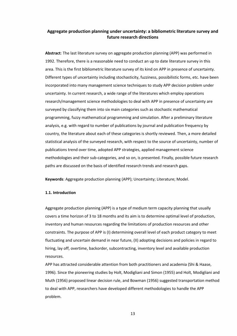
Abstract: The last literature survey on aggregate production planning (APP) was performed in
1992. Therefore, there is a reasonable need to conduct an up to date literature survey in this
area. This is the first bibliometric literature survey of its kind on APP in presence of uncertainty.
Different types of uncertainty including stochasticity, fuzziness, possibilistic forms, etc. have been
incorporated into many management science techniques to study APP decision problem under
uncertainty. In current research, a wide range of the literatures which employ operations
research/management science methodologies to deal with APP in presence of uncertainty are
surveyed by classifying them into six main categories such as stochastic mathematical
programming, fuzzy mathematical programming and simulation. After a preliminary literature
analysis, e.g. with regard to number of publications by journal and publication frequency by
country, the literature about each of these categories is shortly reviewed. Then, a more detailed
statistical analysis of the surveyed research, with respect to the source of uncertainty, number of
publications trend over time, adopted APP strategies, applied management science
methodologies and their sub-categories, and so on, is presented. Finally, possible future research
paths are discussed on the basis of identified research trends and research gaps.
Keywords: Aggregate production planning (APP); Uncertainty; Literature; Model.
1.1. Introduction
Aggregate production planning (APP) is a type of medium term capacity planning that usually
covers a time horizon of 3 to 18 months and its aim is to determine optimal level of production,
inventory and human resources regarding the limitations of production resources and other
constraints. The purpose of APP is (I) determining overall level of each product category to meet
fluctuating and uncertain demand in near future, (II) adopting decisions and policies in regard to
hiring, lay off, overtime, backorder, subcontracting, inventory level and available production
resources.
APP has attracted considerable attention from both practitioners and academia (Shi & Haase,
1996). Since the pioneering studies by Holt, Modigliani and Simon (1955) and Holt, Modigliani and
Muth (1956) proposed linear decision rule, and Bowman (1956) suggested transportation method
to deal with APP, researchers have developed different methodologies to handle the APP
problem.
14
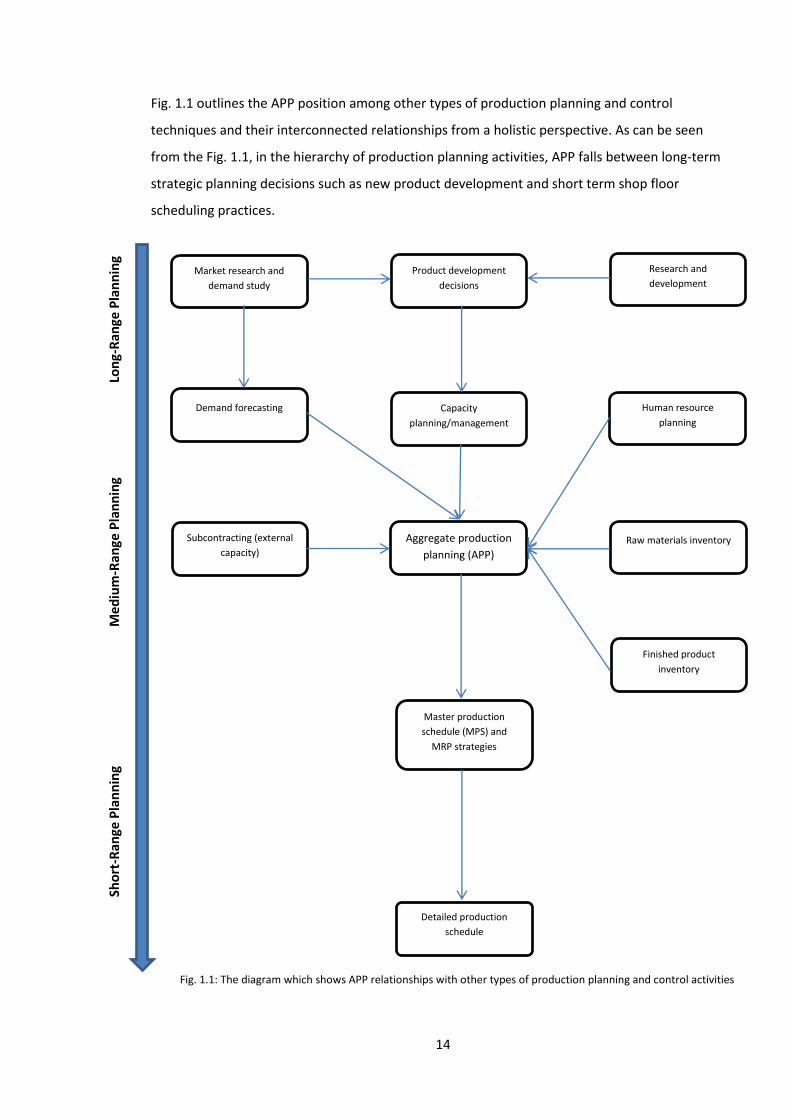
Fig. 1.1 outlines the APP position among other types of production planning and control
techniques and their interconnected relationships from a holistic perspective. As can be seen
from the Fig. 1.1, in the hierarchy of production planning activities, APP falls between long-term
strategic planning decisions such as new product development and short term shop floor
scheduling practices.
Market research and
demand study
Demand forecasting
Product development
decisions
Research and
development
Capacity
planning/management
Human resource
planning
Aggregate production
planning (APP)
Raw materials inventory
Finished product
inventory
Subcontracting (external
capacity)
Master production
schedule (MPS) and
MRP strategies
Detailed production
schedule
Lon
g-R
ange
Pla
nn
ing
M
ed
ium
-Ran
ge P
lan
nin
g Sh
ort
-Ran
ge P
lan
nin
g
Fig. 1.1: The diagram which shows APP relationships with other types of production planning and control activities
15
Uncertainty is described by Funtowicz and Ravetz (1990) as a situation of inadequate information,
which can be present in three forms: inexactness, unreliability, and border with ignorance. Walker
et al. (2003) adopt a general definition of uncertainty as being any departure from the
unachievable ideal of complete determinism.
A large portion of the existing research studies the deterministic state of APP and ignores its
inherent uncertain nature. This assumption may be valid in several APP decision making problems
where product demand exhibits a smooth pattern, i.e. demand has low coefficient of variation
and workforce market, materials price and availability and other related factors show a rather
consistent state.
However, in practical business environments, products usually have shorter life cycles, demand is
uncertain and variable, customers' preferences are changing, production capacity is limited,
workforce market condition is unstable, subcontracting may impose higher costs and has its own
difficulties, raw materials supply is uncertain and increase in backorders leads to customers’
dissatisfaction and makes them change their purchasing source. These all display the dynamic and
uncertain characteristics of APP, and the need to incorporate these uncertainties into the APP
decision models. Therefore, the utilisation of traditional deterministic methodologies may lead to
considerable errors and imprecise decisions.
A significant number of studies have been devoted to APP subject to uncertainty by considering
different forms of uncertainty including stochasticity, possibilistic forms, fuzziness and
randomness.
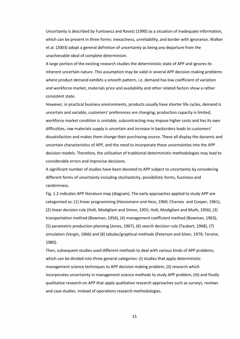
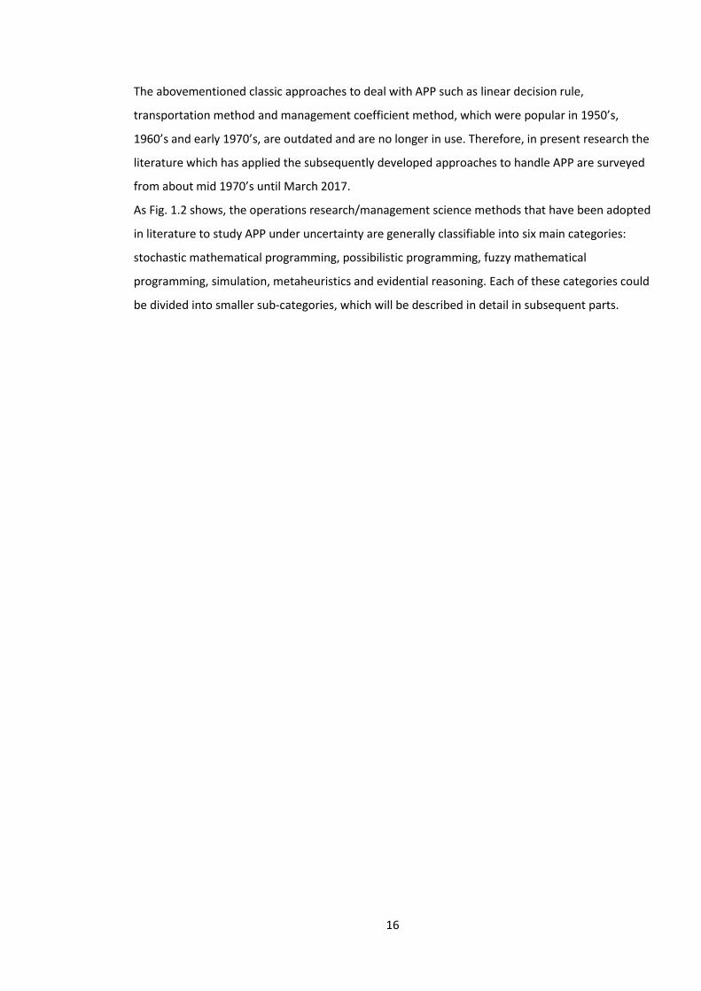
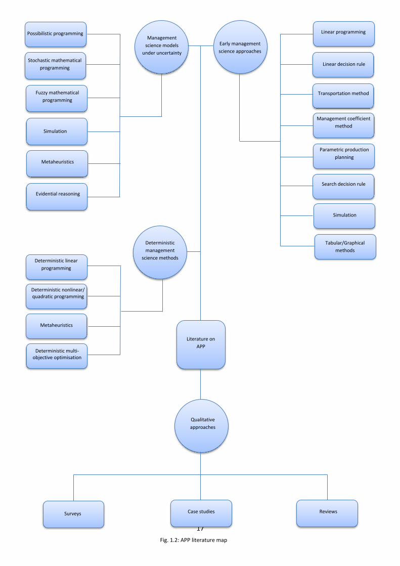
Fig. 1.2 indicates APP literature map (diagram). The early approaches applied to study APP are
categorised as: (1) linear programming (Hanssmann and Hess, 1960; Charnes and Cooper, 1961),
(2) linear decision rule (Holt, Modigliani and Simon, 1955; Holt, Modigliani and Muth, 1956), (3)
transportation method (Bowman, 1956), (4) management coefficient method (Bowman, 1963),
(5) parametric production planning (Jones, 1967), (6) search decision rule (Taubert, 1968), (7)
simulation (Vergin, 1966) and (8) tabular/graphical methods (Peterson and Silver, 1979; Tersine,
1980).
Then, subsequent studies used different methods to deal with various kinds of APP problems,
which can be divided into three general categories: (I) studies that apply deterministic
management science techniques to APP decision making problem, (II) research which
incorporates uncertainty in management science methods to study APP problem, (III) and finally
qualitative research on APP that apply qualitative research approaches such as surveys, reviews
and case studies. instead of operations research methodologies.
16
The abovementioned classic approaches to deal with APP such as linear decision rule,
transportation method and management coefficient method, which were popular in 1950’s,
1960’s and early 1970’s, are outdated and are no longer in use. Therefore, in present research the
literature which has applied the subsequently developed approaches to handle APP are surveyed
from about mid 1970’s until March 2017.
As Fig. 1.2 shows, the operations research/management science methods that have been adopted
in literature to study APP under uncertainty are generally classifiable into six main categories:
stochastic mathematical programming, possibilistic programming, fuzzy mathematical
programming, simulation, metaheuristics and evidential reasoning. Each of these categories could
be divided into smaller sub-categories, which will be described in detail in subsequent parts.
17
Qualitative
approaches
Management
science models
under uncertainty
Early management
science approaches
Deterministic
management
science methods
Management coefficient
method
Transportation method
Parametric production
planning
Search decision rule
Simulation
Tabular/Graphical
methods
Deterministic linear
programming
Deterministic nonlinear/ quadratic programming
Deterministic multi- objective optimisation
Metaheuristics
Stochastic mathematical
programming
Possibilistic programming
Fuzzy mathematical
programming
Simulation
Metaheuristics
Evidential reasoning
Fig. 1.2: APP literature map
Linear decision rule
Linear programming
Literature on
APP
Surveys
Case studies
Reviews
18
The paper is further organised as follows. The need for a bibliometric literature survey on APP
under uncertainty is justified in the next part. Section 1.3 gives a preliminary literature
analysis. The classification plan is presented in Section 1.4. In Section 1.5, the literature on APP
under uncertainty is reviewed elaborately. Section 1.6 goes through a more detailed statistical
analysis of the surveyed literature. In Section 1.7, conclusions are drawn and possible future
research directions are discussed.
1.2. The need for bibliometric literature survey on APP under uncertainty
The last literature survey on APP was conducted by Nam and Logendran (1992). Therefore, an
up to date literature survey in this area is required.
This is the first bibliometric-based literature survey of its kind on APP under uncertainty. The
authors decided to consider APP, as a central activity in production planning and control which
was depicted in Fig. 1.1, instead of general production planning in order to provide an in-depth
and focused literature analysis.
The researchers have been incorporating uncertainty in APP to make decision models which
better represent the present day turbulent industrial environments. The research on APP in
presence of uncertainty has been growing constantly over the recent decades.
Current study considers the existing research on APP under uncertainty as a crucial and
constantly growing part of the research about APP. The research on deterministic APP decision
models would require a separate literature survey, again, to present another in-depth and
specialised literature analysis.
The detailed statistical/numerical analysis of literature regarding journal contributions,
publication frequencies over time, methodologies applied to study APP under uncertainty, etc.
provides research insights about recent research trends and research gaps for interested
researchers. The recommendations on future research directions which are drawn based on
recent research trends and existing research gaps will provide a basis for other researchers to
make their own research agenda.
19
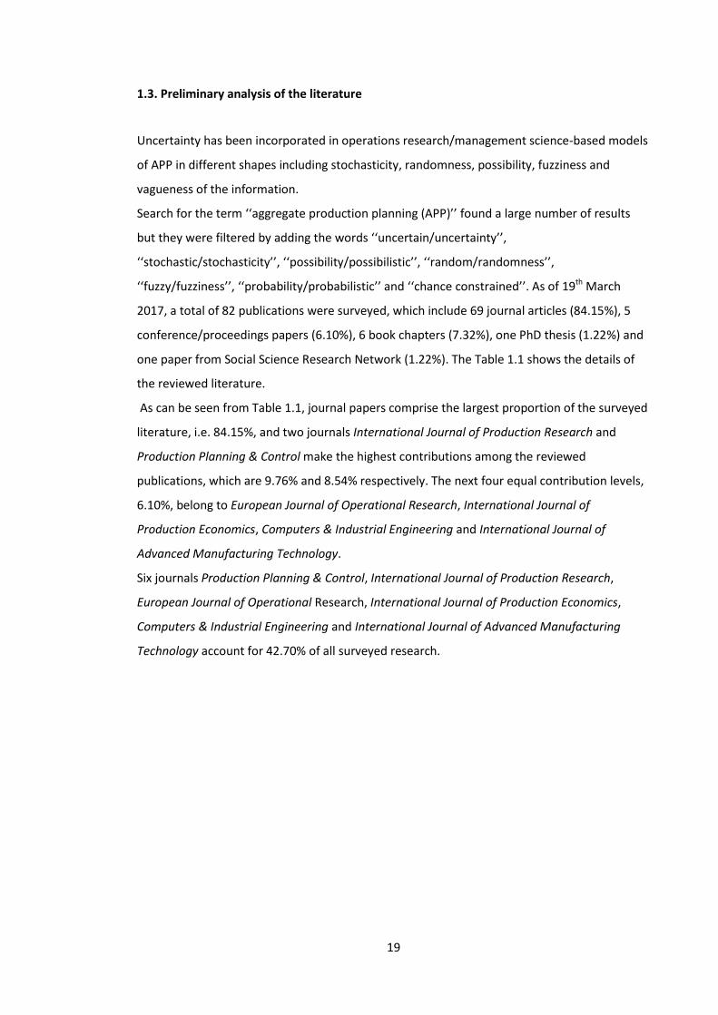
1.3. Preliminary analysis of the literature
Uncertainty has been incorporated in operations research/management science-based models
of APP in different shapes including stochasticity, randomness, possibility, fuzziness and
vagueness of the information.
Search for the term ‘‘aggregate production planning (APP)’’ found a large number of results
but they were filtered by adding the words ‘‘uncertain/uncertainty’’,
‘‘stochastic/stochasticity’’, ‘‘possibility/possibilistic’’, ‘‘random/randomness’’,
‘‘fuzzy/fuzziness’’, ‘‘probability/probabilistic’’ and ‘‘chance constrained’’. As of 19th March
2017, a total of 82 publications were surveyed, which include 69 journal articles (84.15%), 5
conference/proceedings papers (6.10%), 6 book chapters (7.32%), one PhD thesis (1.22%) and
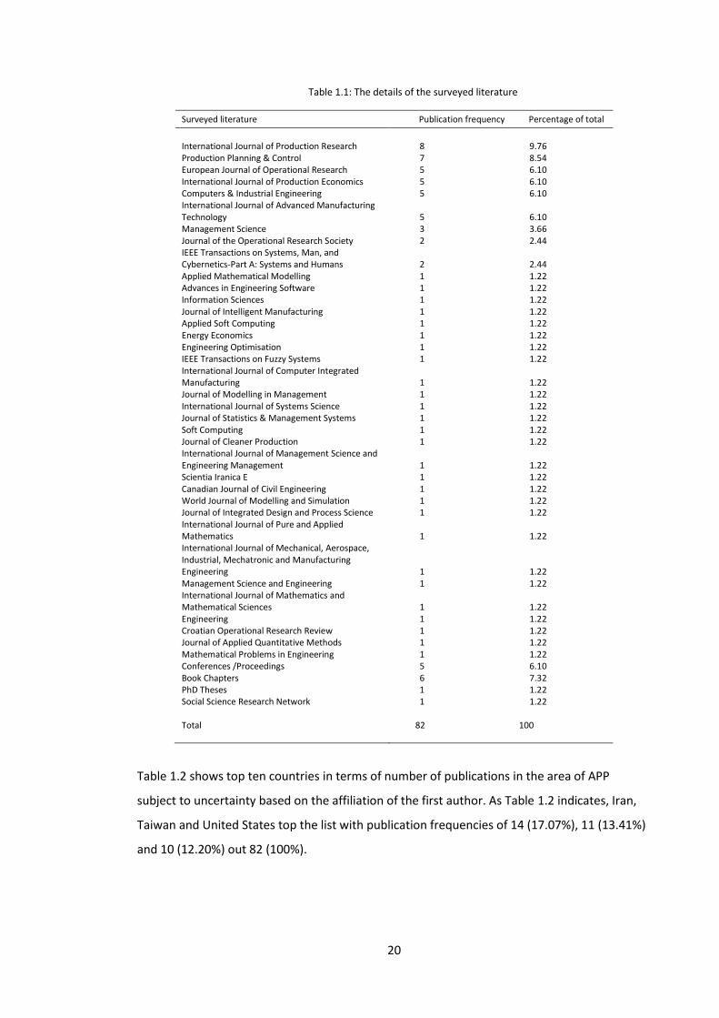
one paper from Social Science Research Network (1.22%). The Table 1.1 shows the details of
the reviewed literature.
As can be seen from Table 1.1, journal papers comprise the largest proportion of the surveyed
literature, i.e. 84.15%, and two journals International Journal of Production Research and
Production Planning & Control make the highest contributions among the reviewed
publications, which are 9.76% and 8.54% respectively. The next four equal contribution levels,
6.10%, belong to European Journal of Operational Research, International Journal of
Production Economics, Computers & Industrial Engineering and International Journal of
Advanced Manufacturing Technology.
Six journals Production Planning & Control, International Journal of Production Research,
European Journal of Operational Research, International Journal of Production Economics,
Computers & Industrial Engineering and International Journal of Advanced Manufacturing
Technology account for 42.70% of all surveyed research.
20
Surveyed literature Publication frequency Percentage of total
International Journal of Production Research Production Planning & Control European Journal of Operational Research International Journal of Production Economics Computers & Industrial Engineering International Journal of Advanced Manufacturing Technology Management Science Journal of the Operational Research Society IEEE Transactions on Systems, Man, and Cybernetics-Part A: Systems and Humans Applied Mathematical Modelling Advances in Engineering Software Information Sciences Journal of Intelligent Manufacturing Applied Soft Computing Energy Economics Engineering Optimisation IEEE Transactions on Fuzzy Systems International Journal of Computer Integrated Manufacturing Journal of Modelling in Management International Journal of Systems Science Journal of Statistics & Management Systems Soft Computing Journal of Cleaner Production International Journal of Management Science and Engineering Management Scientia Iranica E Canadian Journal of Civil Engineering World Journal of Modelling and Simulation Journal of Integrated Design and Process Science International Journal of Pure and Applied Mathematics International Journal of Mechanical, Aerospace, Industrial, Mechatronic and Manufacturing Engineering Management Science and Engineering International Journal of Mathematics and Mathematical Sciences Engineering Croatian Operational Research Review Journal of Applied Quantitative Methods Mathematical Problems in Engineering Conferences /Proceedings Book Chapters PhD Theses Social Science Research Network Total
8 9.76 7 8.54 5 6.10 5 6.10 5 6.10 5 6.10 3 3.66 2 2.44 2 2.44 1 1.22 1 1.22 1 1.22 1 1.22 1 1.22 1 1.22 1 1.22 1 1.22 1 1.22 1 1.22 1 1.22 1 1.22 1 1.22 1 1.22 1 1.22 1 1.22 1 1.22 1 1.22 1 1.22 1 1.22 1 1.22 1 1.22 1 1.22 1 1.22 1 1.22 1 1.22 1 1.22 5 6.10 6 7.32 1 1.22 1 1.22 82 100
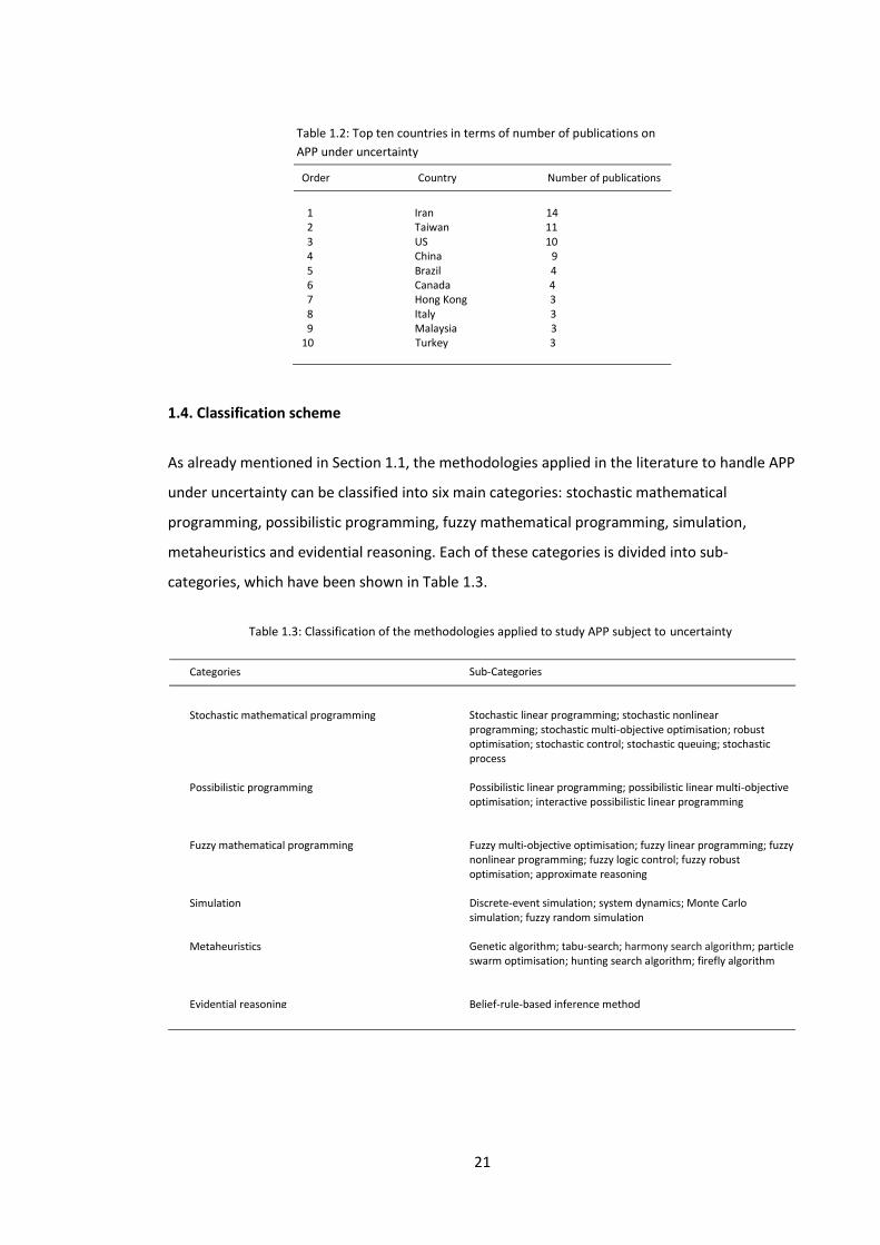
Table 1.2 shows top ten countries in terms of number of publications in the area of APP
subject to uncertainty based on the affiliation of the first author. As Table 1.2 indicates, Iran,
Taiwan and United States top the list with publication frequencies of 14 (17.07%), 11 (13.41%)
and 10 (12.20%) out 82 (100%).
Table 1.1: The details of the surveyed literature
21
Order Country Number of publications
1 Iran 14 2 Taiwan 11 3 US 10 4 China 9 5 Brazil 4 6 Canada 4 7 Hong Kong 3 8 Italy 3 9 Malaysia 3 10 Turkey 3
1.4. Classification scheme
As already mentioned in Section 1.1, the methodologies applied in the literature to handle APP
under uncertainty can be classified into six main categories: stochastic mathematical
programming, possibilistic programming, fuzzy mathematical programming, simulation,
metaheuristics and evidential reasoning. Each of these categories is divided into sub-
categories, which have been shown in Table 1.3.
Table 1.3: Classification of the methodologies applied to study APP subject to uncertainty
Table 1.2: Top ten countries in terms of number of publications on
APP under uncertainty
Categories Stochastic mathematical programming Possibilistic programming Fuzzy mathematical programming Simulation Metaheuristics Evidential reasoning
Sub-Categories Stochastic linear programming; stochastic nonlinear programming; stochastic multi-objective optimisation; robust optimisation; stochastic control; stochastic queuing; stochastic process Possibilistic linear programming; possibilistic linear multi-objective optimisation; interactive possibilistic linear programming Fuzzy multi-objective optimisation; fuzzy linear programming; fuzzy nonlinear programming; fuzzy logic control; fuzzy robust optimisation; approximate reasoning Discrete-event simulation; system dynamics; Monte Carlo simulation; fuzzy random simulation Genetic algorithm; tabu-search; harmony search algorithm; particle swarm optimisation; hunting search algorithm; firefly algorithm Belief-rule-based inference method
22
In short, these categories and sub-categories are described as follows:
Stochastic mathematical programming: It includes mathematical models for APP under
uncertainty that apply stochastic linear programming, stochastic nonlinear programming,
stochastic multi-objective optimisation, and so on where demand for products, constants and
coefficients of the mathematical programming models and decision variables are of
stochastic/random nature. This group also includes mathematical programming models with
probabilistic constraints or chance constrained models.
Possibilistic programming: Possibilistic linear programming and possibilistic linear multi-
objective optimisation methods belong to this category. In general, the possibilistic
programming models to deal with APP is recommended when the information about the
forecasted demand, parameters and coefficients of the constructed mathematical
programming models and objective function/goal values are imprecise in essence.
Fuzzy mathematical programming: This class of models for APP in presence of uncertainty
covers a wide range of mathematical programming models in fuzzy environment such as fuzzy
linear programming, fuzzy nonlinear programming and fuzzy multi-objective optimisation. In
this set of models, uncertainty is present in the form of fuzziness, which involves market
demand, objective/goal values, constants, coefficients and constraints of the developed
management science models.
Simulation: Discrete-event simulation, system dynamics, Monte Carlo simulation, etc. are
among the simulation methodologies that have been proposed to run APP decision problem so
that forecasted demand, objective/goal values, parameters/coefficients and constraints are
supposed to be uncertain in their nature.
Metaheuristics: Due to the nonlinearity, combinatorial and large scale nature of APP
problems, metaheuristics have proved to be efficient techniques to solve APP problems with
uncertain characteristics. In this group of APP models, uncertainty is present in decision
variables, customer demand, objective function/goal values, constraints, constants and
coefficients of the constructed operations research models.
Evidential reasoning: At present, to the best of the authors’ knowledge, just one paper on
evidential reasoning to APP has been published, which employs a belief-rule-based inference
method to handle APP decision making problem with uncertain demand.
The APP literature that applies each of the abovementioned methodologies will be reviewed in
the next part.
23
1.5. Elaborate review of the literature on APP subject to uncertainty
In following sections the literature about quantitative APP models under uncertainty is
reviewed regarding different methodologies that it employs. The studies have been reviewed
in chronological order within each category.
1.5.1. Fuzzy mathematical programming
The literature on application of fuzzy mathematical programming approaches in the APP
context can be classified into studies which apply I) fuzzy multi-objective optimisation, II) fuzzy
goal programming, III) fuzzy linear programming, IV) fuzzy nonlinear programming, V) fuzzy
logic control, VI) fuzzy robust optimisation and VII) approximate reasoning techniques.
As an explanation, although the fuzzy goal programming could be considered as a subset of
fuzzy multi-objective optimisation but due to the significant number of publications that apply
fuzzy goal programming to APP, it has been presented as a separate sub-division to show a
clearer picture of the literature.
1.5.1.1. Fuzzy multi-objective optimisation
Since APP problem always involves several criteria (objectives) and due to the vagueness of the
acquired information, fuzzy multi-objective programming has been widely used in this area.
Lee (1990), Gen, Tsujimura and Ida (1992), Wang and Fang (2001), Wang and Liang (2004),
Ghasemy Yaghin, Torabi and Fatemi Ghomi (2012), Madadi and Wong (2014), Gholamian et al.
(2015), Gholamian, Mahdavi and Tavakkoli-Moghaddam (2016), Kalaf et al. (2015), Sisca,
Fiasché and Taisch (2015) and Fiasché et al. (2016) utilised various kinds of fuzzy multi-
objective optimisation models to study APP under uncertainty.
Lee (1990) recommended fuzzy linear programming and fuzzy multi-objective linear
programming approaches to handle APP problem under fuzziness with fuzzy objective values,
fuzzy demand, etc. Gen, Tsujimura and Ida (1992) presented an interactive fuzzy linear multi-
objective programming method for APP such that all coefficients/parameters are regarded as
triangular fuzzy numbers. Wang and Fang (2001) proposed a fuzzy linear multi-objective
optimisation approach to APP decision making problem where product price, subcontracting
cost, production capacity, and so forth are all characterised as fuzzy variables.
Wang and Liang (2004) developed a fuzzy linear multi-objective optimisation model to deal
with APP decision problem, which tries to minimise total production costs, inventory holding
and backordering costs and costs of changes in the workforce level. In their model, objective
24
functions are of fuzzy nature. A hybrid fuzzy multi-objective APP decision model in a two
echelon supply chain with both quantitative and qualitative objectives and constraints was
recommended by Ghasemy Yaghin, Torabi and Fatemi Ghomi (2012) where cost parameters,
warehouse space, etc. are assumed to be fuzzy variables. A multi-objective fuzzy APP model
with qualitative and quantitative objectives was proposed by Madadi and Wong (2014). In
their model, forecasted demand, production costs, and so on are regarded as fuzzy numbers.
Gholamian et al. (2015) and Gholamian, Mahdavi and Tavakkoli-Moghaddam (2016) developed
a fuzzy multi-site multi-objective mixed integer nonlinear APP model in a supply chain under
uncertainty with fuzzy demand, fuzzy cost parameters, etc. A modified fuzzy multi-objective
linear programming method to APP that minimises total production costs and total labour
costs is proposed by Kalaf et al. (2015), which involves fuzzy aspiration levels of the objectives
and fuzzy tolerance levels. Sisca, Fiasché and Taisch (2015) constructed a fuzzy multi-objective
linear programming model for APP in a reconfigurable assembly unit for optoelectronics where
product price, inventory cost, etc. are supposed to be fuzzy variables.
Fiasché et al. (2016) developed a fuzzy linear multi-objective optimisation model of APP in
fuzzy environment where the product price, unit cost of not utilising the resources, etc. are of
fuzzy nature.
1.5.1.2. Fuzzy goal programming
Da Silva and Marins (2004), Wang and Liang (2005b), Tavakkoli-Moghaddam et al. (2007),
Jamalnia and Soukhakian (2009), Belmokaddem, Mekidiche and Sahed (2009), and Sadeghi,
Razavi Hajiagha and Hashemi (2013) developed a variety of fuzzy goal programming models to
tackle APP problem in presence of uncertainty.
Da Silva and Marins (2004) developed a fuzzy goal programming model for APP in a Brazilian
sugar mill. In their study, the goal values are presented as triangular and trapezoidal fuzzy
numbers. Wang and Liang (2005b) presented an interactive fuzzy multi-objective linear
programming approach for APP decision problem with fuzzy goal values. Tavakkoli-
Moghaddam et al. (2007) suggested a fuzzy mixed-integer goal programming model to run APP
problem, which includes fuzzy goal values, fuzzy technological coefficients, fuzzy constraints
upper bounds and fuzzy demand. Jamalnia and Soukhakian (2009) proposed a hybrid fuzzy
goal programming approach that includes both quantitative and qualitative objectives with
fuzzy aspiration levels.
Belmokaddem, Mekidiche and Sahed (2009) applied a fuzzy goal programming method with
different goal priorities to APP where the goal values are of fuzzy nature. Sadeghi, Razavi
25
Hajiagha and Hashemi (2013) proposed a fuzzy goal programming model of APP with fuzzy
aspiration levels where coefficients and parameters of the model are assumed to be grey
numbers.
1.5.1.3. Fuzzy linear programming
The literature on applying fuzzy linear programming approach to APP includes studies
performed by Dai, Fan and Sun (2003), Liang et al. (2011), Pathak and Sarkar (2011), Omar,
Jusoh and Omar (2012), Wang and Zheng (2013), Iris and Cevikcan (2014) and Chen and Huang
(2014).
Dai et al. (2003) presented a fuzzy linear programming methodology to deal with APP in
condition of imprecise information and fuzzy constraints. Liang et al. (2011) constructed a
fuzzy linear programming model of APP, which attempts to minimise total production cost
subject to constraints on inventory levels, workforce levels, etc. where objective function and
its coefficients and constraints’ upper/lower bounds are assumed to be fuzzy variables. A fuzzy
mixed-integer linear programming model for APP with fuzzy demand, fuzzy warehouse space,
fuzzy cost parameters, and so forth in a multi-echelon multi item supply chain network was
developed by Pathak and Sarkar (2011).
Omar, Jusoh and Omar (2012) investigated the benefits of applying fuzzy mathematical
programming in APP context by developing a fuzzy mixed-integer linear programming model
to APP with fuzzy demand, fuzzy cost parameters, etc. in a resin manufacturing plant, which
considers both fuzzy and possibilistic uncertainties. Wang and Zheng (2013) proposed a fuzzy
linear programming method to APP in a refinery industry in Taiwan, which aims at maximising
total profit so that market demand and cost items are characterised as fuzzy numbers.
A fuzzy linear programming model of APP with imprecise data which involves fuzzy demand
and fuzzy cost items was suggested by Iris and Cevikcan (2014). Chen and Huang (2014)
proposed the extension principle to solve the developed fuzzy linear programming model for
APP where the forecasted demand, maximum available labour, and so on are of fuzzy nature.
1.5.1.4. Fuzzy nonlinear programming
Fuzzy nonlinear programming approaches applications to APP in regard to uncertainty include
researches conducted by Tang, Wang and Fung (2000), Fung, Tang and Wang (2003), Chen and
Huang (2010) and Chen and Sarker (2015).
Tang, Wang and Fung (2000) proposed a fuzzy nonlinear programming model of APP with
quadratic objective function, which is to minimise total production and inventory costs where
26
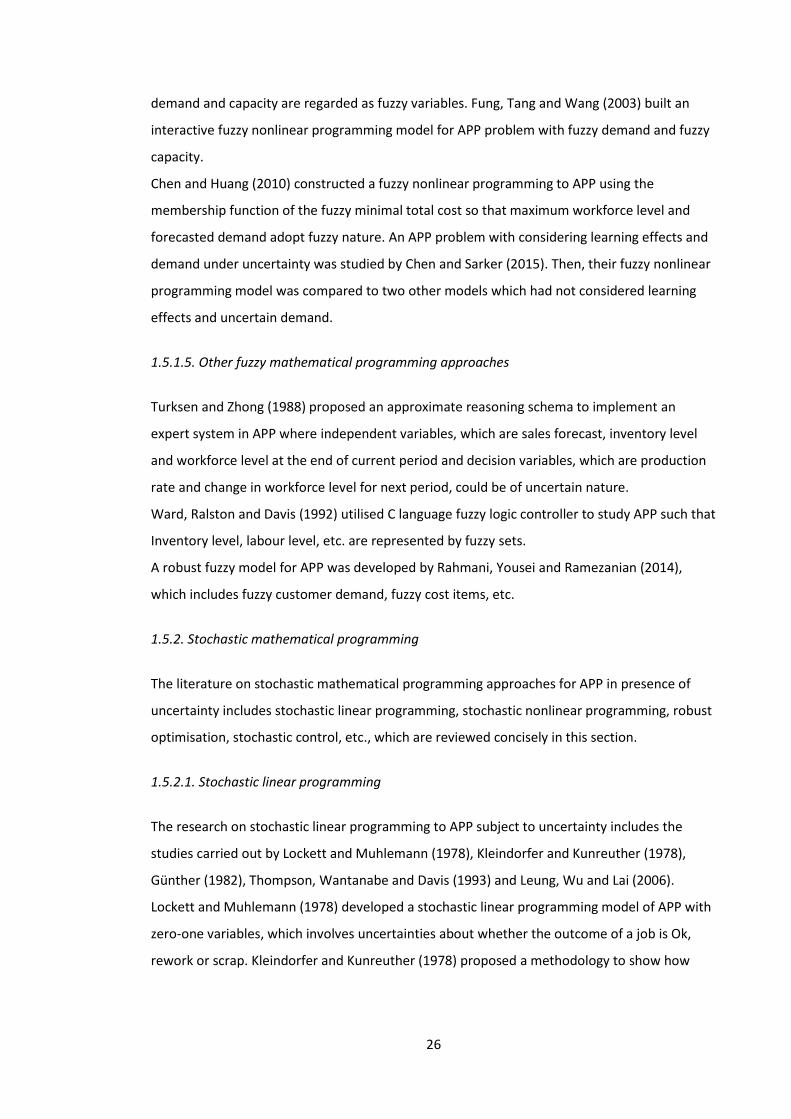
demand and capacity are regarded as fuzzy variables. Fung, Tang and Wang (2003) built an
interactive fuzzy nonlinear programming model for APP problem with fuzzy demand and fuzzy
capacity.
Chen and Huang (2010) constructed a fuzzy nonlinear programming to APP using the
membership function of the fuzzy minimal total cost so that maximum workforce level and
forecasted demand adopt fuzzy nature. An APP problem with considering learning effects and
demand under uncertainty was studied by Chen and Sarker (2015). Then, their fuzzy nonlinear
programming model was compared to two other models which had not considered learning
effects and uncertain demand.
1.5.1.5. Other fuzzy mathematical programming approaches
Turksen and Zhong (1988) proposed an approximate reasoning schema to implement an
expert system in APP where independent variables, which are sales forecast, inventory level
and workforce level at the end of current period and decision variables, which are production
rate and change in workforce level for next period, could be of uncertain nature.
Ward, Ralston and Davis (1992) utilised C language fuzzy logic controller to study APP such that
Inventory level, labour level, etc. are represented by fuzzy sets.
A robust fuzzy model for APP was developed by Rahmani, Yousei and Ramezanian (2014),
which includes fuzzy customer demand, fuzzy cost items, etc.
1.5.2. Stochastic mathematical programming
The literature on stochastic mathematical programming approaches for APP in presence of
uncertainty includes stochastic linear programming, stochastic nonlinear programming, robust
optimisation, stochastic control, etc., which are reviewed concisely in this section.
1.5.2.1. Stochastic linear programming
The research on stochastic linear programming to APP subject to uncertainty includes the
studies carried out by Lockett and Muhlemann (1978), Kleindorfer and Kunreuther (1978),
Günther (1982), Thompson, Wantanabe and Davis (1993) and Leung, Wu and Lai (2006).
Lockett and Muhlemann (1978) developed a stochastic linear programming model of APP with
zero-one variables, which involves uncertainties about whether the outcome of a job is Ok,
rework or scrap. Kleindorfer and Kunreuther (1978) proposed a methodology to show how
27
forecast horizons for stochastic aggregate planning problems with uncertain demand relate to
the planning procedures and the information system within the organisation.
Günther (1982) presented a stochastic linear programming approach to deal with APP problem
under demand uncertainty. Thompson, Wantanabe and Davis (1993) developed linear
programming frameworks to evaluate several APP policies where customer demand, most of
the coefficients of the linear programming model and some parameters were presented with
probability distributions to reflect the uncertainty in APP environment. A stochastic linear
programming method to handle APP with stochastic demand and stochastic cost parameters
was proposed by Leung, Wu and Lai (2006).
1.5.2.2. Stochastic multi-objective optimisation
Rakes, Franz and Wynne (1984), Chen and Liao (2003) and Nowak (2013) utilised stochastic
multi-objective optimisation techniques to consider APP under uncertainty.
Rakes, Franz and Wynne (1984) applied a chance-constrained goal programming approach to
APP. In their model, the product demands, time required for inspection and products testing
and so forth are random variables. Chen and Liao (2003) adopted a multi-attribute decision
making approach to select the most efficient APP strategy such that selling price, market
demand, cost coefficients, etc. are assumed to be stochastic variables. Nowak (2013)
presented a procedure which combines linear multi-objective programming, simulation and an
interactive approach to model APP with uncertain demand.
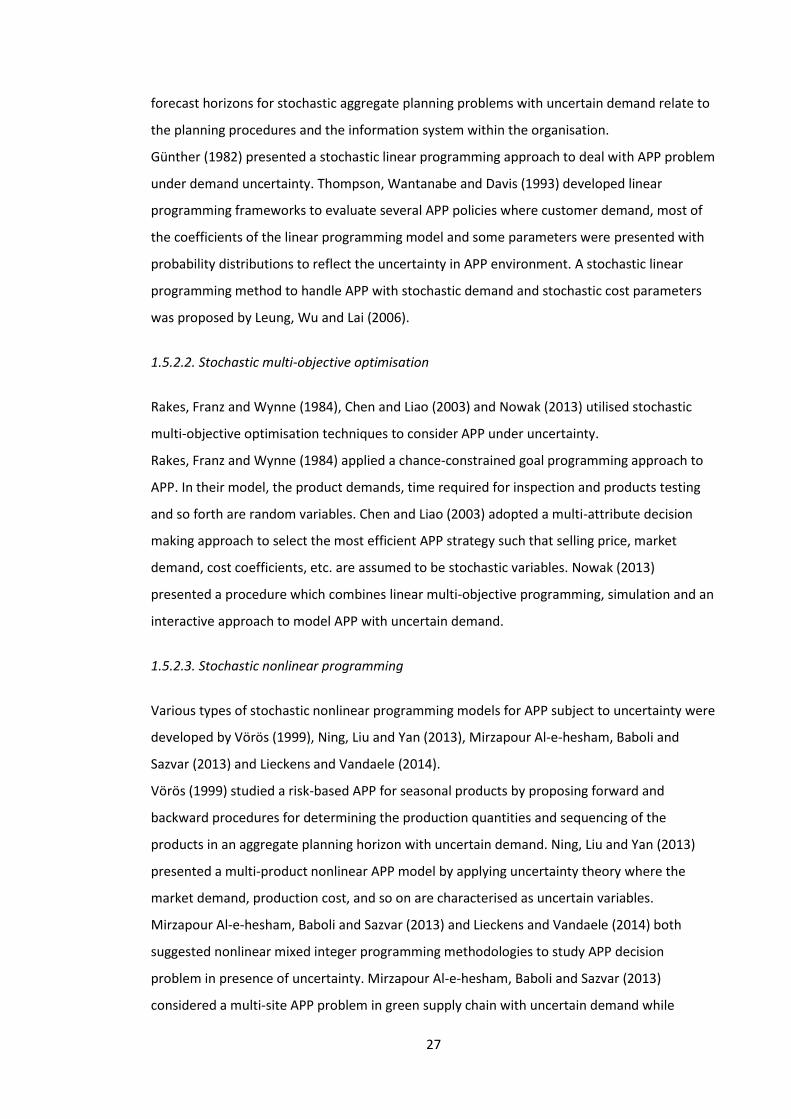
1.5.2.3. Stochastic nonlinear programming
Various types of stochastic nonlinear programming models for APP subject to uncertainty were
developed by Vörös (1999), Ning, Liu and Yan (2013), Mirzapour Al-e-hesham, Baboli and
Sazvar (2013) and Lieckens and Vandaele (2014).
Vörös (1999) studied a risk-based APP for seasonal products by proposing forward and
backward procedures for determining the production quantities and sequencing of the
products in an aggregate planning horizon with uncertain demand. Ning, Liu and Yan (2013)
presented a multi-product nonlinear APP model by applying uncertainty theory where the
market demand, production cost, and so on are characterised as uncertain variables.
Mirzapour Al-e-hesham, Baboli and Sazvar (2013) and Lieckens and Vandaele (2014) both
suggested nonlinear mixed integer programming methodologies to study APP decision
problem in presence of uncertainty. Mirzapour Al-e-hesham, Baboli and Sazvar (2013)
considered a multi-site APP problem in green supply chain with uncertain demand while
28
Lieckens and Vandaele (2014) developed a multi-product, multi routing model where a routing
consists of a sequence of operations on different resources so that the uncertainty is
associated with the stochastic nature of the both demand patterns and production lead times.
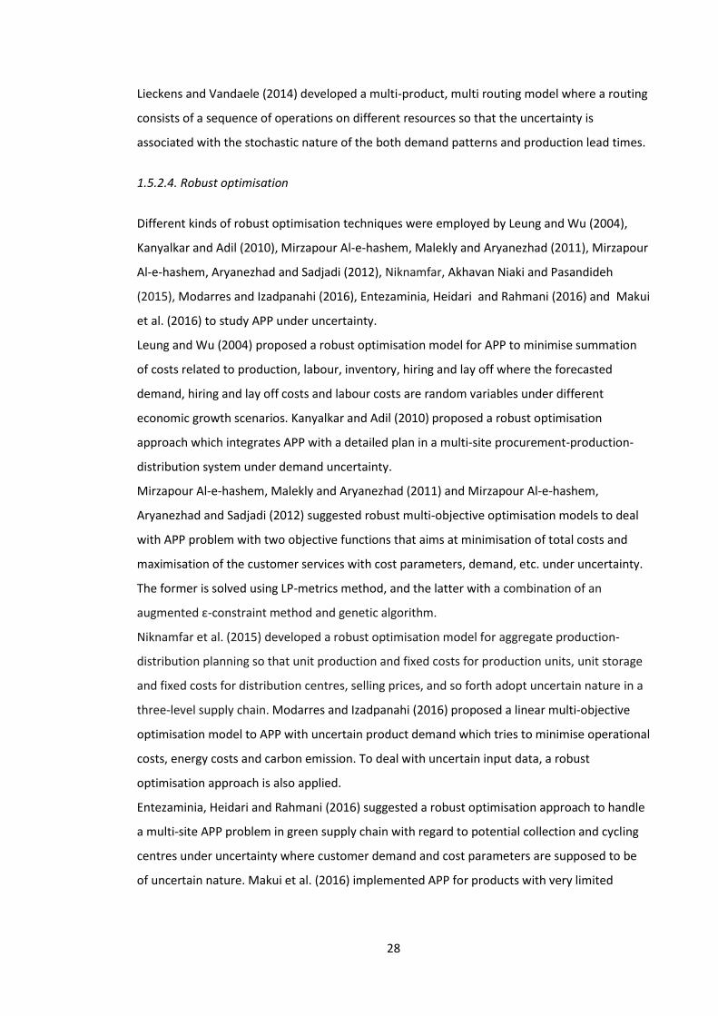
1.5.2.4. Robust optimisation
Different kinds of robust optimisation techniques were employed by Leung and Wu (2004),
Kanyalkar and Adil (2010), Mirzapour Al-e-hashem, Malekly and Aryanezhad (2011), Mirzapour
Al-e-hashem, Aryanezhad and Sadjadi (2012), Niknamfar, Akhavan Niaki and Pasandideh
(2015), Modarres and Izadpanahi (2016), Entezaminia, Heidari and Rahmani (2016) and Makui
et al. (2016) to study APP under uncertainty.
Leung and Wu (2004) proposed a robust optimisation model for APP to minimise summation
of costs related to production, labour, inventory, hiring and lay off where the forecasted
demand, hiring and lay off costs and labour costs are random variables under different
economic growth scenarios. Kanyalkar and Adil (2010) proposed a robust optimisation
approach which integrates APP with a detailed plan in a multi-site procurement-production-
distribution system under demand uncertainty.
Mirzapour Al-e-hashem, Malekly and Aryanezhad (2011) and Mirzapour Al-e-hashem,
Aryanezhad and Sadjadi (2012) suggested robust multi-objective optimisation models to deal
with APP problem with two objective functions that aims at minimisation of total costs and
maximisation of the customer services with cost parameters, demand, etc. under uncertainty.
The former is solved using LP-metrics method, and the latter with a combination of an
augmented ε-constraint method and genetic algorithm.
Niknamfar et al. (2015) developed a robust optimisation model for aggregate production-
distribution planning so that unit production and fixed costs for production units, unit storage
and fixed costs for distribution centres, selling prices, and so forth adopt uncertain nature in a
three-level supply chain. Modarres and Izadpanahi (2016) proposed a linear multi-objective
optimisation model to APP with uncertain product demand which tries to minimise operational
costs, energy costs and carbon emission. To deal with uncertain input data, a robust
optimisation approach is also applied.
Entezaminia, Heidari and Rahmani (2016) suggested a robust optimisation approach to handle
a multi-site APP problem in green supply chain with regard to potential collection and cycling
centres under uncertainty where customer demand and cost parameters are supposed to be
of uncertain nature. Makui et al. (2016) implemented APP for products with very limited
29
expiration dates. A robust optimisation method is also used due to inherent uncertainty of
parameters of the constructed APP model.
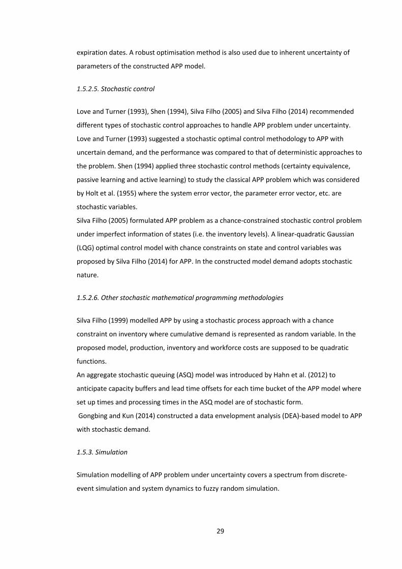
1.5.2.5. Stochastic control
Love and Turner (1993), Shen (1994), Silva Filho (2005) and Silva Filho (2014) recommended
different types of stochastic control approaches to handle APP problem under uncertainty.
Love and Turner (1993) suggested a stochastic optimal control methodology to APP with
uncertain demand, and the performance was compared to that of deterministic approaches to
the problem. Shen (1994) applied three stochastic control methods (certainty equivalence,
passive learning and active learning) to study the classical APP problem which was considered
by Holt et al. (1955) where the system error vector, the parameter error vector, etc. are
stochastic variables.
Silva Filho (2005) formulated APP problem as a chance-constrained stochastic control problem
under imperfect information of states (i.e. the inventory levels). A linear-quadratic Gaussian
(LQG) optimal control model with chance constraints on state and control variables was
proposed by Silva Filho (2014) for APP. In the constructed model demand adopts stochastic
nature.
1.5.2.6. Other stochastic mathematical programming methodologies
Silva Filho (1999) modelled APP by using a stochastic process approach with a chance
constraint on inventory where cumulative demand is represented as random variable. In the
proposed model, production, inventory and workforce costs are supposed to be quadratic
functions.
An aggregate stochastic queuing (ASQ) model was introduced by Hahn et al. (2012) to
anticipate capacity buffers and lead time offsets for each time bucket of the APP model where
set up times and processing times in the ASQ model are of stochastic form.
Gongbing and Kun (2014) constructed a data envelopment analysis (DEA)-based model to APP
with stochastic demand.
1.5.3. Simulation
Simulation modelling of APP problem under uncertainty covers a spectrum from discrete-
event simulation and system dynamics to fuzzy random simulation.
30
Lee and Khumawala (1974), McClain and Thomas (1977), Lee, Steinberg and Khumawala
(1983), Khouja (1998), Tang, Fung and Yung (2003), Ning, Wansheng and Zhao (2006), Tian,
Mohamed and AbouRizk (2010), Jamalnia and Feili (2013), Gansterer (2015) and Altendorfer,
Felberbauer and Jodlbauer (2016) proposed various types of simulation models to study APP
subject to uncertainty.
1.5.3.1. Common discrete-event simulation
Lee and Khumawala (1974) assessed the performance of four different APP policies under
demand uncertainty by simulating the activities of an operating firm. McClain and Thomas
(1977) utilised both simulation and linear programming techniques to evaluate the horizon
effects in APP with seasonal demand where in simulation case, the demand was supposed to
be random normal variable. Lee, Steinberg and Khumawala (1983) compared the effectiveness
of the aggregate-disaggregate and material requirements planning approaches to production
planning in a simulation environment such that demand was generated by using stochastic
functions. Their research applied linear decision rule as the optimal aggregate technique in the
aggregate-disaggregate approach.
Tang, Fung and Yung (2003) conducted a simulation analysis for multi-product APP problem
under fuzziness of demand and capacities. Tian, Mohamed and AbouRizk (2010) applied a
simulation-based approach to aggregate planning of a batch plant which produces concrete
and asphalts so that fluctuating demand could be generated by using a statistical distribution,
e.g. uniform, normal, etc. Gansterer (2015) investigated the impact of APP with demand under
uncertainty in a make-to-order environment utilising a discrete-event simulation method
within a comprehensive hierarchical production planning framework.
Altendorfer, Felberbauer and Jodlbauer (2016) evaluated the effect of long term forecast error
on optimal planned utilisation factor for a production system with stochastic customer
demand. Simulation is used to determine overall costs like capacity, backorder and inventory
costs.
1.5.3.2. Other simulation modelling techniques
Khouja (1998) developed an APP framework to evaluate volume flexibility using Monte Carlo
simulation with normally distributed demand.
Ning, Wansheng and Zhao (2006) constructed a fuzzy random model for APP in which market
demand, production cost, etc. are all assumed to be fuzzy random variables. Then, the
proposed model is solved employing hybrid optimization algorithm combining fuzzy random
31
simulation, genetic algorithm, neural network and simultaneous perturbation stochastic
approximation algorithm.
By employing an integrated system dynamics and discrete-event simulation, Jamalnia and Feili
(2013) evaluated effectiveness and practicality of different APP strategies regarding total profit
criterion where the forecasted demand was represented as random normal distribution.
1.5.4. Metaheuristics
Different kinds of metaheuristics were proposed by Wang and Fang (1997), Fichera et al.
(1999), Baykasoğlu and Göçken (2006), Aliev et al. (2007), Baykasoglu and Gocken (2010),
Aungkulanon, Phruksaphanrat and Luangpaiboon (2012), Luangpaiboon and Aungkulanon
(2013) and Chakrabortty et al. (2015) for APP in condition of uncertainty.
1.5.4.1. Genetic algorithms
Wang and Fang (1997) presented an inexact approach which imitates the human decision
making process by generating a family of inexact solutions to a fuzzy linear programming with
fuzzy objective values and fuzzy constraints using a genetics-based algorithm within an
acceptable level as candidates for a decision maker to consider further. Fichera et al. (1999)
suggested possibilistic linear programming and genetic algorithm as a decision support system
for APP to assist decision makers in APP decisions in a vague environment where the
constraint on balance equation for production, inventory and demand and total production
capacity are of possibilistic form. An interactive fuzzy-genetic methodology to solve aggregate
production-distribution planning in supply chain subject to the fuzziness of total profit, total
expenses, etc. was developed by Aliev et al. (2007).
1.5.4.2. Tabu search
Baykasoğlu and Göçken (2006) proposed a tabu-search method to solve a fuzzy goal
programming model of APP with fuzzy goal values. Baykasoglu and Gocken (2010) proposed a
multi-objective APP with fuzzy parameters, and solved the model by employing fuzzy numbers
ranking methods and tabu search.
1.5.4.3. Other metaheuristic approaches
Aungkulanon, Phruksaphanrat and Luangpaiboon (2012) applied a harmony search algorithm
with different evolutionary elements to solve a fuzzy multi-objective linear programming
32
model for APP with fuzzy objectives. Luangpaiboon and Aungkulanon (2013) presented a
multi-objective linear programming decision making model for APP with inventory under
uncertainty. Their proposed model was solved by applying hybrid metaheuristics of the
hunting search (HuSIHSA) and firefly (FAIHSA) mechanisms on the improved harmony search
algorithm.
Chakrabortty et al. (2015) solved an integer linear programming model of APP with imprecise
operating costs, demand and capacity related data by employing a particle swarm optimisation
approach.
1.5.5. Possibilistic programming
The literature on possibilistic programming approaches that utilised to study APP subject to
uncertainty ranges from regular possibilistic programming methods to interactive possibilistic
programming approaches.
1.5.5.1. Ordinary possibilistic programming
Hsieh and Wu (2000) and Sakallı et al. (2010) proposed various forms of possibilistic
programming approaches to study APP with imprecise information.
Hsieh and Wu (2000) proposed a possibilistic linear multi-objective optimisation approach to
consider APP decision making problem with imprecise demand and cost coefficients, which
take triangular possibility distribution functions. Sakallı, Baykoç and Birgören (2010) presented
a possibilistic linear programming model for APP in brass casting industry. In the constructed
model, demand quantities, percentages of the ingredient in some raw materials, etc. have
imprecise nature, and adopt triangular possibility distributions.
1.5.5.2. Interactive possibilistic programming
Wang and Liang (2005a), Liang (2007) and Liang (2007) developed interactive possibilistic
programming models for APP problem with imprecise information.
Wang and Liang (2005a) presented a novel interactive possibilistic linear programming (i-PLP)
approach, which considers APP with imprecise forecasted demand, related operating costs,
and capacity. Their model tries to minimise total costs regarding the constraints on inventory
levels, labour levels, overtime, etc. A multi-objective APP problem with imprecise demand,
cost coefficients, available resources and capacity was studied by Liang (2007) with applying an
33
interactive linear multi-objective possibilistic programming model. The proposed model
minimises total production costs and oscillations in work-force level.
Liang (2007) presented an i-PLP method to solve APP problems where the objective function,
forecasted demand, related capacities and operating costs adopt imprecise nature. The study
aims at minimising total manufacturing costs subject to bounds on inventory, labour, overtime,
and so on for each operating cost category.
1.5.6. Evidential reasoning
Li et al. (2013) presented a belief-rule-based inference methodology for APP under demand
uncertainty. The proposed model was implemented by using a paint factory example to
conduct a comparative study and sensitivity analysis.
1.6. Further detailed analysis of the literature
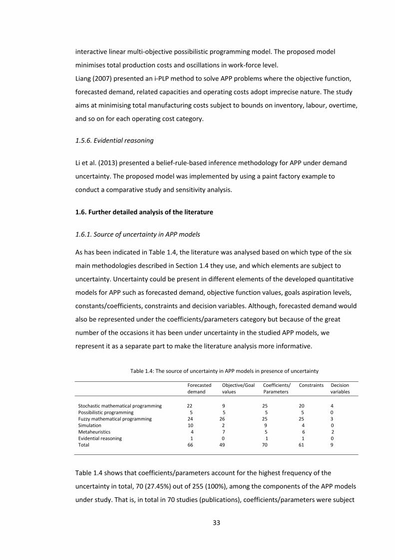
1.6.1. Source of uncertainty in APP models As has been indicated in Table 1.4, the literature was analysed based on which type of the six
main methodologies described in Section 1.4 they use, and which elements are subject to
uncertainty. Uncertainty could be present in different elements of the developed quantitative
models for APP such as forecasted demand, objective function values, goals aspiration levels,
constants/coefficients, constraints and decision variables. Although, forecasted demand would
also be represented under the coefficients/parameters category but because of the great
number of the occasions it has been under uncertainty in the studied APP models, we
represent it as a separate part to make the literature analysis more informative.
Table 1.4 shows that coefficients/parameters account for the highest frequency of the
uncertainty in total, 70 (27.45%) out of 255 (100%), among the components of the APP models
under study. That is, in total in 70 studies (publications), coefficients/parameters were subject
Forecasted Objective/Goal Coefficients/ Constraints Decision demand values Parameters variables
Stochastic mathematical programming 22 9 25 20 4 Possibilistic programming 5 5 5 5 0 Fuzzy mathematical programming 24 26 25 25 3 Simulation 10 2 9 4 0 Metaheuristics 4 7 5 6 2 Evidential reasoning 1 0 1 1 0 Total 66 49 70 61 9
Table 1.4: The source of uncertainty in APP models in presence of uncertainty
34
to a form of uncertainty. Two of the equally highest frequencies of the coefficients/parameters
under uncertainty, i.e. 25 (35.71%) out of 70 (100%), belong to the studies that apply fuzzy
mathematical programming and stochastic mathematical programming methods. The third tier
is represented by the literature that employs simulation techniques which contributes to 9
(12.86%) out of 70 (100%) occasions of the coefficients and parameters uncertainty that is a
sharp decrease compared to the first two highest frequencies.
Forecasted market demand comes in the second place among the elements of the surveyed
APP models under uncertainty in terms of frequency of being uncertain, which adds up to 66
(25.88%) out of 255 (100%) in total. Similar to the coefficients/parameters case, fuzzy
mathematical programming, stochastic mathematical programming and simulation modelling
methodologies top the list for the number of occasions that forecasted demand characterised
as uncertain in the reviewed literature with corresponding frequencies 24 (36.36%), 22
(33.33%) and 10 (15.15%) out of 66 (100%) respectively.
Constraints represent the third level of the uncertainty frequencies among the elements of the
reviewed APP models in presence of uncertainty with total frequency of 61 (23.92%) out of
255 (100%). Again, similar to the two previously analysed APP model components, fuzzy
mathematical programming and stochastic mathematical programming techniques make the
highest contributions in terms of number of occasions that the surveyed research studies
include uncertain constraints, which are 25 (40.98%) and 20 (32.79%) out of 61 (100%)
respectively. But, unlike the two previously analysed elements of the APP models, now
metaheuristics come in the third place with respect to the number of occasions that the
surveyed literature includes uncertain constraints, i.e. 6 (9.84%) out of 61 (100%).
Finally, objective/goal values and decision variables come in the fourth and fifth places in
terms of the total occasions that these APP model components are subject to uncertainty with
corresponding frequencies of 49 (19.22%) and 9 (3.53%) out of 255 (100%).
More details about the frequencies regarding each of these components and the relevant
methodologies are presented in Table 1.4.
1.6.2. Trends for frequency of published research regarding each main category of the
methodologies
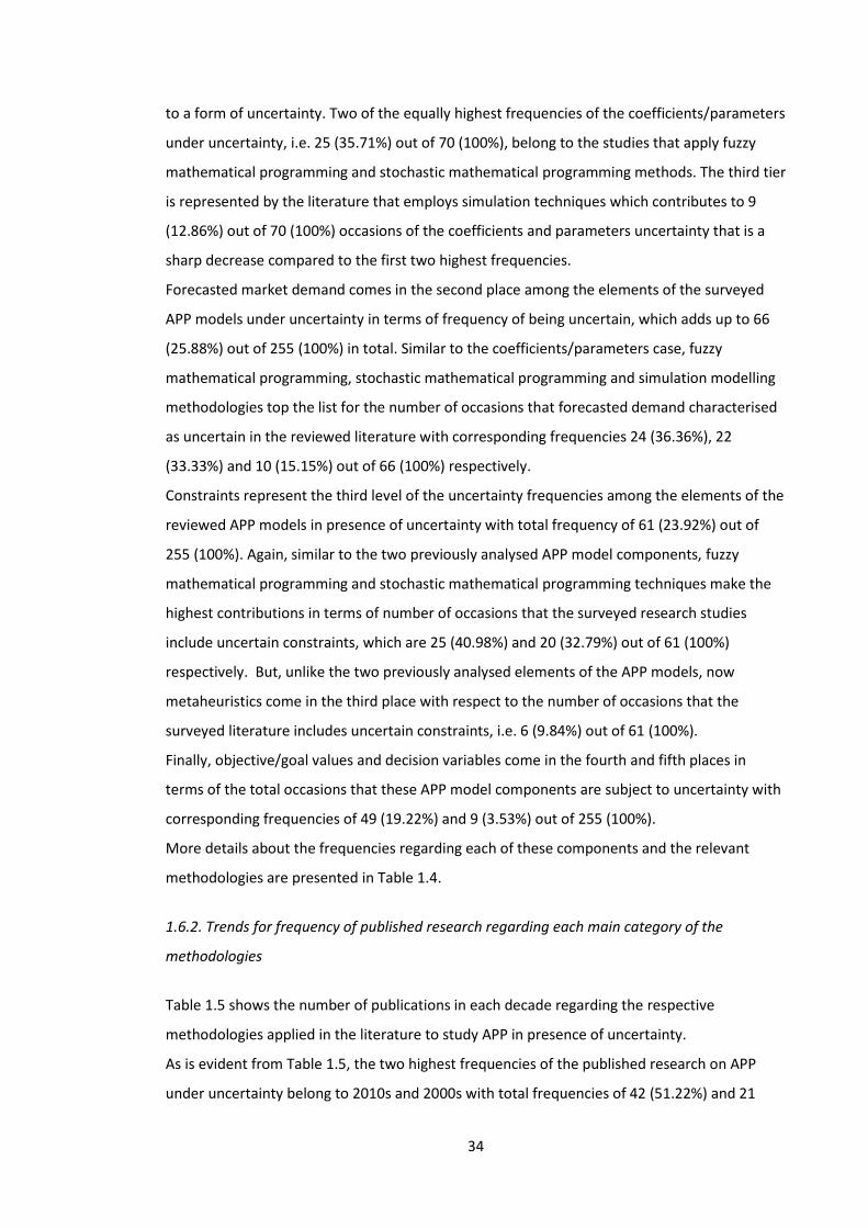
Table 1.5 shows the number of publications in each decade regarding the respective
methodologies applied in the literature to study APP in presence of uncertainty.
As is evident from Table 1.5, the two highest frequencies of the published research on APP
under uncertainty belong to 2010s and 2000s with total frequencies of 42 (51.22%) and 21
35
(25.61%) out of 82 (100%) respectively. 1990s come in the third place with total number of 11
(13.41%) publications out of 82 (100%). The number of the studies in other decades with
respect to relevant methodologies has been presented in Table 1.5. Generally, the total
number of literature about APP subject to uncertainty has been increasing constantly from
1970s until 2010s.
1970-1979 1980-1989 1990-1999 2000-2009 2010-2016 Total
Stochastic mathematical Programming 2 2 5 4 14 27 Possibilistic programming 4 1 5 Fuzzy mathematical Programming 1 3 9 18 31 Simulation 2 1 1 2 4 10 Metaheuristics 2 2 4 8 Evidential reasoning 1 1 Total 4 4 11 21 42 82
In 2010s, the research that applies fuzzy mathematical programming and stochastic
mathematical programming techniques accounts for 18 (42.86%) and 14 (33.33%) out of total
publications number, i.e. 42 (100%), which put them in the first and second orders
respectively. The studies that utilise simulation and metaheuristics methods jointly come in
the third place with equal frequencies of 4 (9.52%) out of 42 (100%).
For the decade starting in 2000, of 21 studies (100%) the highest number, 9 (42.86%), goes to
the literature which applies fuzzy mathematical programming to APP. Possibilistic
programming and stochastic mathematical programming methods come in the next place with
equal contribution of 4 (19.05%) out of 21 (100%).
In the time period 1990-1999, three of the highest frequencies of the studies about APP under
uncertainty, belong to stochastic mathematical programming, fuzzy mathematical
programming and metaheuristics-based methodologies with corresponding frequencies of 5
(45%), 3 (27.27%) and 2 (18.18%) out of 11 (100%).
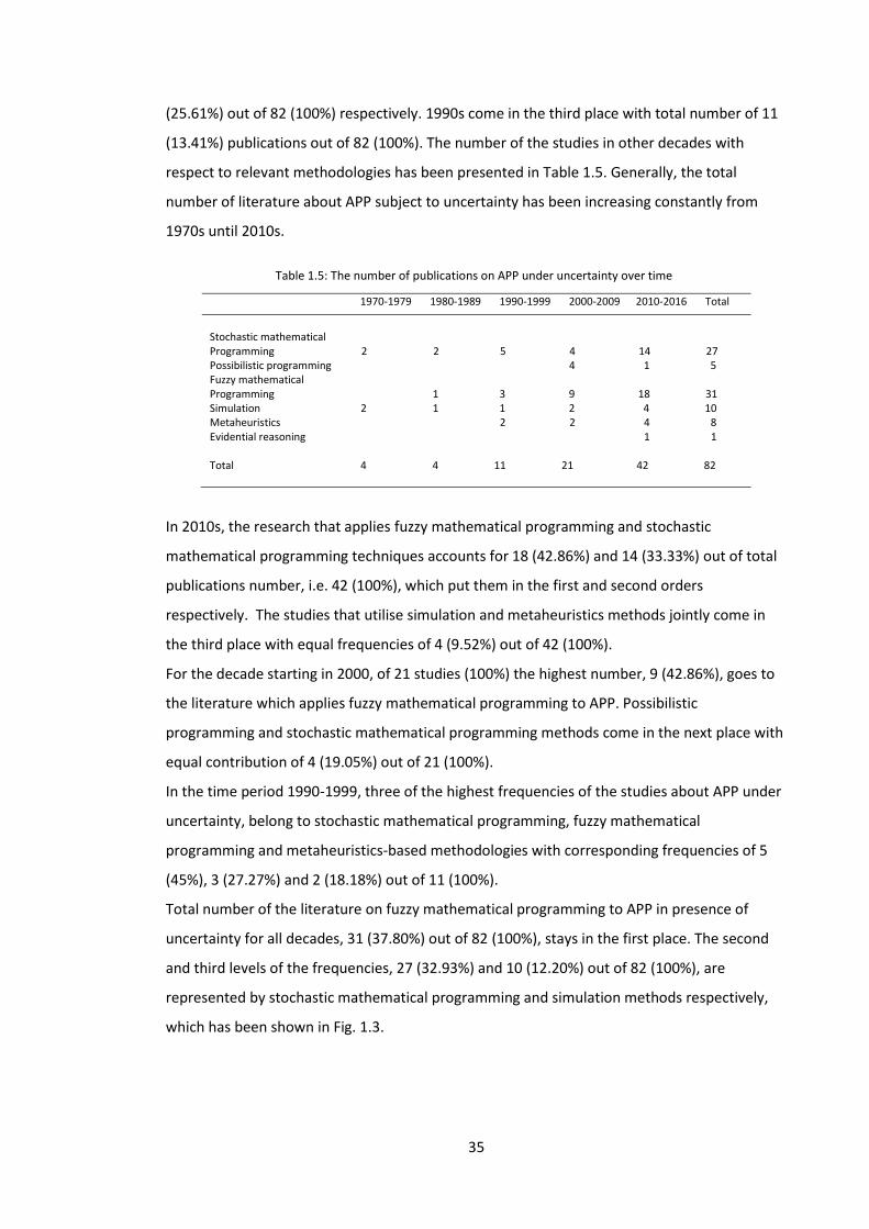
Total number of the literature on fuzzy mathematical programming to APP in presence of
uncertainty for all decades, 31 (37.80%) out of 82 (100%), stays in the first place. The second
and third levels of the frequencies, 27 (32.93%) and 10 (12.20%) out of 82 (100%), are
represented by stochastic mathematical programming and simulation methods respectively,
which has been shown in Fig. 1.3.
Table 1.5: The number of publications on APP under uncertainty over time
36
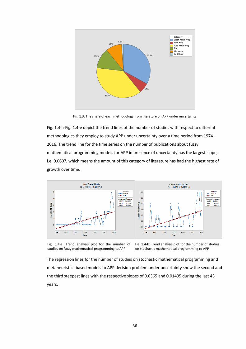
Fig. 1.4-a-Fig. 1.4-e depict the trend lines of the number of studies with respect to different
methodologies they employ to study APP under uncertainty over a time period from 1974-
2016. The trend line for the time series on the number of publications about fuzzy
mathematical programming models for APP in presence of uncertainty has the largest slope,
i.e. 0.0607, which means the amount of this category of literature has had the highest rate of
growth over time.
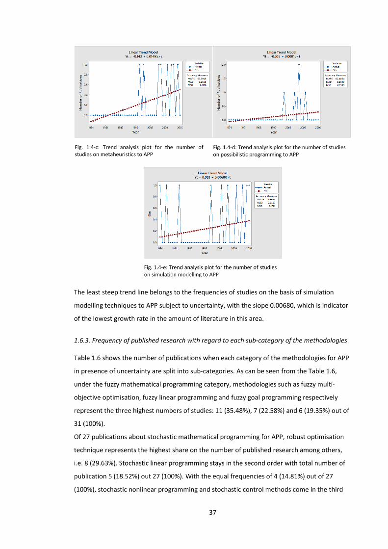
The regression lines for the number of studies on stochastic mathematical programming and
metaheuristics-based models to APP decision problem under uncertainty show the second and
the third steepest lines with the respective slopes of 0.0365 and 0.01495 during the last 43
years.
Stoch Math Prog
Poss Prog
Fuzz Math Prog
Sim
Metaheur
Evid Reas
Category
1.2%9.8%
12.2%
37.8%
6.1%
32.9%
Fig. 1.3: The share of each methodology from literature on APP under uncertainty
Fig. 1.4-a: Trend analysis plot for the number of studies on fuzzy mathematical programming to APP
Fig. 1.4-b: Trend analysis plot for the number of studies on stochastic mathematical programming to APP
37
The least steep trend line belongs to the frequencies of studies on the basis of simulation
modelling techniques to APP subject to uncertainty, with the slope 0.00680, which is indicator
of the lowest growth rate in the amount of literature in this area.
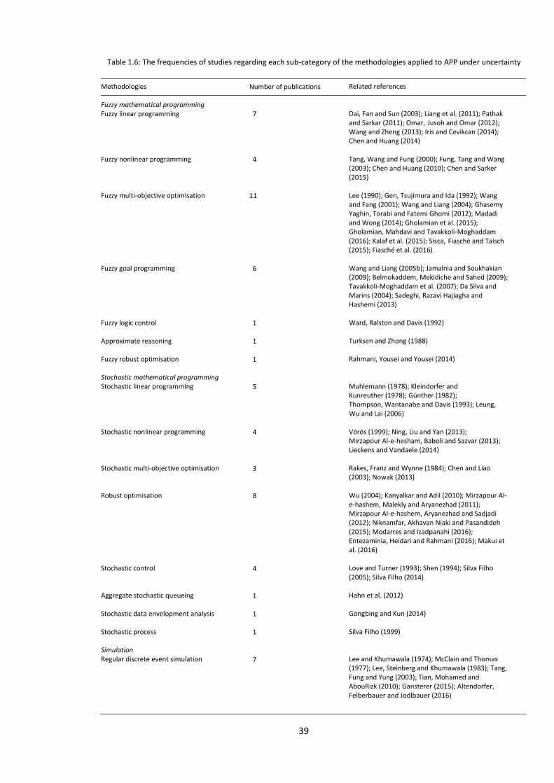
1.6.3. Frequency of published research with regard to each sub-category of the methodologies Table 1.6 shows the number of publications when each category of the methodologies for APP
in presence of uncertainty are split into sub-categories. As can be seen from the Table 1.6,
under the fuzzy mathematical programming category, methodologies such as fuzzy multi-
objective optimisation, fuzzy linear programming and fuzzy goal programming respectively
represent the three highest numbers of studies: 11 (35.48%), 7 (22.58%) and 6 (19.35%) out of
31 (100%).
Of 27 publications about stochastic mathematical programming for APP, robust optimisation
technique represents the highest share on the number of published research among others,
i.e. 8 (29.63%). Stochastic linear programming stays in the second order with total number of
publication 5 (18.52%) out 27 (100%). With the equal frequencies of 4 (14.81%) out of 27
(100%), stochastic nonlinear programming and stochastic control methods come in the third
Fig. 1.4-c: Trend analysis plot for the number of studies on metaheuristics to APP
Fig. 1.4-d: Trend analysis plot for the number of studies on possibilistic programming to APP
Fig. 1.4-e: Trend analysis plot for the number of studies on simulation modelling to APP

38
place. Frequency of 3 (11.11%) out of 27 (100%) puts stochastic multi-objective optimisation in
the fourth place.
Common discrete-event simulation as a subset of the simulation methodology in general, has
been utilised in research on APP in presence of uncertainty in 7 occasions (70%) out of 10
(100%), which is the greatest contribution among other simulation methods. Monte Carlo
simulation, system dynamics and fuzzy random simulation all with equal frequencies, 1 (10%)
out of 10 (100%), stay in the second place.
The number of published studies for other main categories of the methodologies and the
corresponding sub-categories can be seen from Table 1.6.
39
Methodologies Fuzzy mathematical programming Fuzzy linear programming Fuzzy nonlinear programming Fuzzy multi-objective optimisation Fuzzy goal programming Fuzzy logic control Approximate reasoning Fuzzy robust optimisation Stochastic mathematical programming Stochastic linear programming Stochastic nonlinear programming Stochastic multi-objective optimisation Robust optimisation Stochastic control Aggregate stochastic queueing Stochastic data envelopment analysis Stochastic process Simulation Regular discrete event simulation
Number of publications 7 4 11 6 1 1 1 5 4 3 8 4 1 1 1 7
Related references Dai, Fan and Sun (2003); Liang et al. (2011); Pathak and Sarkar (2011); Omar, Jusoh and Omar (2012); Wang and Zheng (2013); Iris and Cevikcan (2014); Chen and Huang (2014) Tang, Wang and Fung (2000); Fung, Tang and Wang (2003); Chen and Huang (2010); Chen and Sarker (2015) Lee (1990); Gen, Tsujimura and Ida (1992); Wang and Fang (2001); Wang and Liang (2004); Ghasemy Yaghin, Torabi and Fatemi Ghomi (2012); Madadi and Wong (2014); Gholamian et al. (2015); Gholamian, Mahdavi and Tavakkoli-Moghaddam (2016); Kalaf et al. (2015); Sisca, Fiasché and Taisch (2015); Fiasché et al. (2016) Wang and Liang (2005b); Jamalnia and Soukhakian (2009); Belmokaddem, Mekidiche and Sahed (2009); Tavakkoli-Moghaddam et al. (2007); Da Silva and Marins (2004); Sadeghi, Razavi Hajiagha and Hashemi (2013) Ward, Ralston and Davis (1992) Turksen and Zhong (1988) Rahmani, Yousei and Yousei (2014) Muhlemann (1978); Kleindorfer and Kunreuther (1978); Günther (1982); Thompson, Wantanabe and Davis (1993); Leung, Wu and Lai (2006) Vörös (1999); Ning, Liu and Yan (2013); Mirzapour Al-e-hesham, Baboli and Sazvar (2013); Lieckens and Vandaele (2014) Rakes, Franz and Wynne (1984); Chen and Liao (2003); Nowak (2013) Wu (2004); Kanyalkar and Adil (2010); Mirzapour Al-e-hashem, Malekly and Aryanezhad (2011); Mirzapour Al-e-hashem, Aryanezhad and Sadjadi (2012); Niknamfar, Akhavan Niaki and Pasandideh (2015); Modarres and Izadpanahi (2016); Entezaminia, Heidari and Rahmani (2016); Makui et al. (2016) Love and Turner (1993); Shen (1994); Silva Filho (2005); Silva Filho (2014) Hahn et al. (2012) Gongbing and Kun (2014) Silva Filho (1999) Lee and Khumawala (1974); McClain and Thomas (1977); Lee, Steinberg and Khumawala (1983); Tang, Fung and Yung (2003); Tian, Mohamed and AbouRizk (2010); Gansterer (2015); Altendorfer, Felberbauer and Jodlbauer (2016)
Table 1.6: The frequencies of studies regarding each sub-category of the methodologies applied to APP under uncertainty
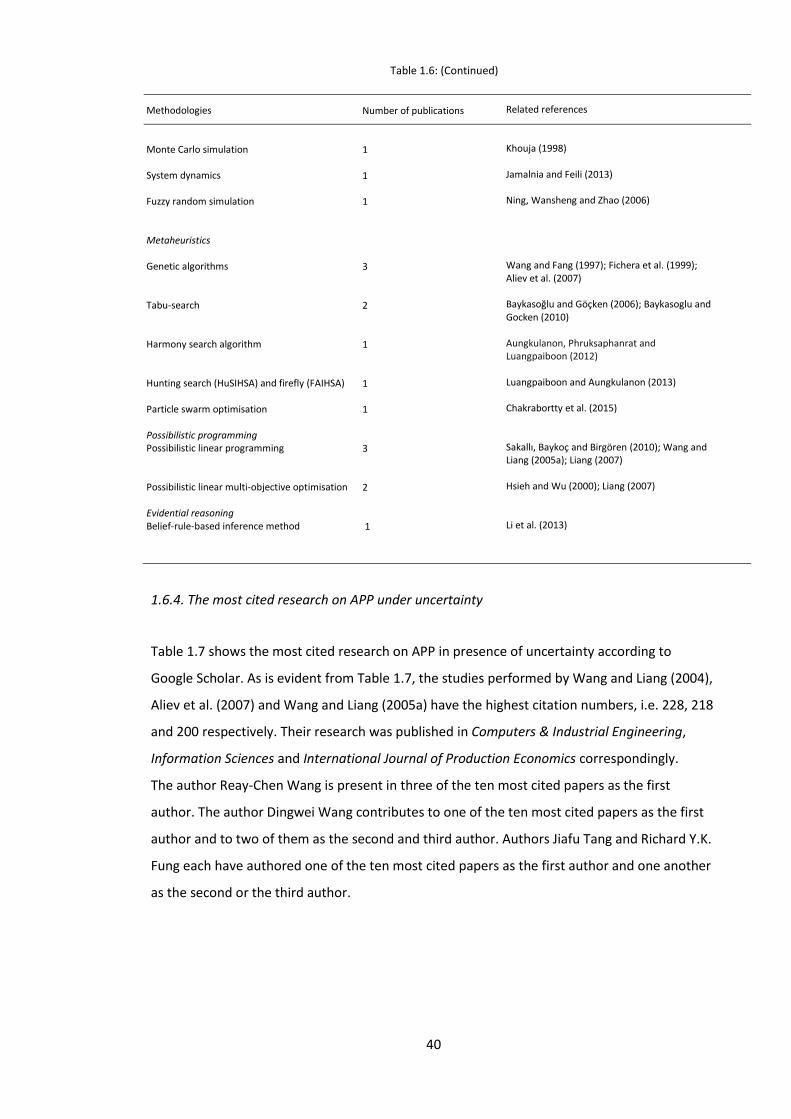
40
1.6.4. The most cited research on APP under uncertainty
Table 1.7 shows the most cited research on APP in presence of uncertainty according to
Google Scholar. As is evident from Table 1.7, the studies performed by Wang and Liang (2004),
Aliev et al. (2007) and Wang and Liang (2005a) have the highest citation numbers, i.e. 228, 218
and 200 respectively. Their research was published in Computers & Industrial Engineering,
Information Sciences and International Journal of Production Economics correspondingly.
The author Reay-Chen Wang is present in three of the ten most cited papers as the first
author. The author Dingwei Wang contributes to one of the ten most cited papers as the first
author and to two of them as the second and third author. Authors Jiafu Tang and Richard Y.K.
Fung each have authored one of the ten most cited papers as the first author and one another
as the second or the third author.
Methodologies Monte Carlo simulation System dynamics Fuzzy random simulation Metaheuristics Genetic algorithms Tabu-search Harmony search algorithm Hunting search (HuSIHSA) and firefly (FAIHSA) Particle swarm optimisation Possibilistic programming Possibilistic linear programming Possibilistic linear multi-objective optimisation Evidential reasoning Belief-rule-based inference method
Number of publications 1 1 1 3 2 1 1 1 3 2 1
Related references Khouja (1998) Jamalnia and Feili (2013) Ning, Wansheng and Zhao (2006) Wang and Fang (1997); Fichera et al. (1999); Aliev et al. (2007) Baykasoğlu and Göçken (2006); Baykasoglu and Gocken (2010) Aungkulanon, Phruksaphanrat and Luangpaiboon (2012) Luangpaiboon and Aungkulanon (2013) Chakrabortty et al. (2015) Sakallı, Baykoç and Birgören (2010); Wang and Liang (2005a); Liang (2007) Hsieh and Wu (2000); Liang (2007) Li et al. (2013)
Table 1.6: (Continued)
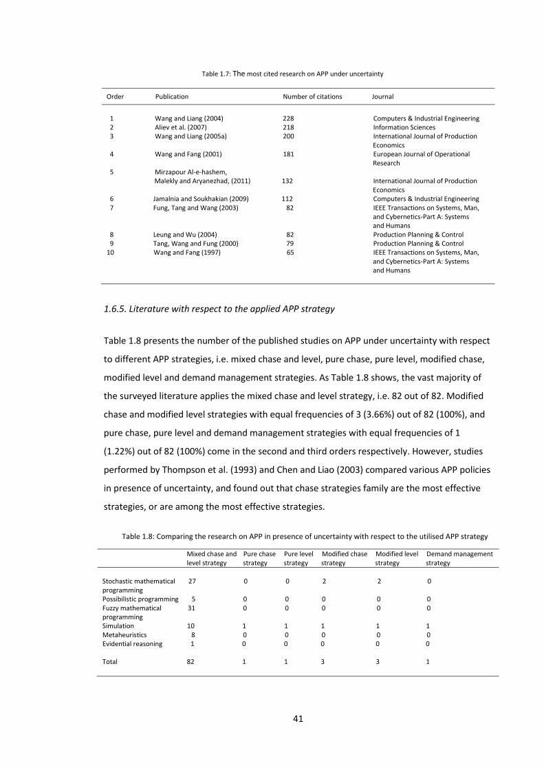
41
Order Publication Number of citations Journal
1 Wang and Liang (2004) 228 Computers & Industrial Engineering 2 Aliev et al. (2007) 218 Information Sciences
3 Wang and Liang (2005a) 200 International Journal of Production Economics 4 Wang and Fang (2001) 181 European Journal of Operational Research 5 Mirzapour Al-e-hashem, Malekly and Aryanezhad, (2011) 132 International Journal of Production Economics 6 Jamalnia and Soukhakian (2009) 112 Computers & Industrial Engineering 7 Fung, Tang and Wang (2003) 82 IEEE Transactions on Systems, Man, and Cybernetics-Part A: Systems and Humans 8 Leung and Wu (2004) 82 Production Planning & Control 9 Tang, Wang and Fung (2000) 79 Production Planning & Control 10 Wang and Fang (1997) 65 IEEE Transactions on Systems, Man, and Cybernetics-Part A: Systems and Humans
1.6.5. Literature with respect to the applied APP strategy
Table 1.8 presents the number of the published studies on APP under uncertainty with respect
to different APP strategies, i.e. mixed chase and level, pure chase, pure level, modified chase,
modified level and demand management strategies. As Table 1.8 shows, the vast majority of
the surveyed literature applies the mixed chase and level strategy, i.e. 82 out of 82. Modified
chase and modified level strategies with equal frequencies of 3 (3.66%) out of 82 (100%), and
pure chase, pure level and demand management strategies with equal frequencies of 1
(1.22%) out of 82 (100%) come in the second and third orders respectively. However, studies
performed by Thompson et al. (1993) and Chen and Liao (2003) compared various APP policies
in presence of uncertainty, and found out that chase strategies family are the most effective
strategies, or are among the most effective strategies.
Mixed chase and Pure chase Pure level Modified chase Modified level Demand management level strategy strategy strategy strategy strategy strategy
Stochastic mathematical 27 0 0 2 2 0 programming Possibilistic programming 5 0 0 0 0 0 Fuzzy mathematical 31 0 0 0 0 0 programming Simulation 10 1 1 1 1 1 Metaheuristics 8 0 0 0 0 0 Evidential reasoning 1 0 0 0 0 0 Total 82 1 1 3 3 1
Table 1.7: The most cited research on APP under uncertainty
Table 1.8: Comparing the research on APP in presence of uncertainty with respect to the utilised APP strategy
42
1.7. Conclusions and future research directions
In this research, a wide scope of literature on APP under uncertainty was analysed. This
literature includes journal papers, book chapters, conference/proceedings papers and PhD
theses which were classified into six main categories on the basis of applied methodologies.
The uncertainties present in the constructed management science models are of sorts like
stochasticity, fuzziness and impreciseness of the information. First, the relevant literature
about each of abovementioned methods was reviewed concisely, and then a more detailed
statistical analysis of the surveyed research was followed.
Two journals, International Journal of Production Research and Production Planning & Control,
make the highest contributions in terms of number of publications among the reviewed
literature. Total numbers of studies which apply fuzzy mathematical programming and
stochastic mathematical programming to APP in presence of uncertainty come in the first and
second places respectively. The trend lines for the frequency of studies on fuzzy mathematical
programming and stochastic mathematical programming to APP under uncertainty show the
highest slopes.
Possible future research directions according to in-depth literature survey in present study are
recommended as follows:
As already was shown in Table 1.8, the absolutely prevalent APP strategy in the
literature about APP in presence of uncertainty (and even in the literature on
deterministic APP models) is the mixed chase and level strategy. However, the surveys
conducted by Buxey (1990, 1995, 2003, 2005) revealed that the most popular APP
policy among operations managers is the chase strategy, which shows a gap between
APP in academia and APP in practice. This also indicates an intense gap related to the
lack of the studies about quantitative APP models under uncertainty based on other
APP strategies such as chase strategy, level strategy and the demand management
strategy.
Several relative advantages of the simulation techniques over mathematical
programming methods, e.g. coping with dynamic or transient effects, addressing
interactions between different components, the ability of providing a sufficient basis
for developing explanatory and predictive models of operational processes, and so
forth have been stated in the literature. Therefore, the relatively low share of the
literature which apply simulation modelling to study APP subject to uncertainty
(12.20%), and the least steep trend line of the frequency of the number of published

43
research in this area over recent decades recommend the need to do extra research in
this field to compensate the unfairly narrow share of the simulation methods.
To the best of our knowledge, only a single journal paper has been published on
evidential reasoning (ER) to APP in both uncertain and deterministic manners. So,
regarding the capabilities of the ER in handling the uncertainty, this could act as a
foundation stone to drive more research in this area.
Regarding the dynamic nature of APP in practice which is highly dependent on initial
conditions, e.g. finished product inventory level and workforce level in the beginning,
and considering the nonlinear and complex feature of many APP models, the chaos
theory would be a suitable methodology to study APP system’s behaviour in unstable
industrial environments.
APP under uncertainty in manufacturing environments that follow the principles of the
productions systems like just in time (JIT), lean production and flexible manufacturing
system (FMS) with regard to specific requirements for each of these production
philosophies can be fertile areas of the future research.
44
References Aliev, R.A., Fazlollahi, B., Guirimov, B.G. and Aliev, R.R. (2007). ‘Fuzzy genetic approach to aggregate production–distribution planning in supply chain management’, Information Sciences, 177(20), pp. 4241–4255.
Altendorfer, K., Felberbauer, T. and Jodlbauer, H. (2016). ‘Effects of forecast errors on optimal
utilisation in aggregate production planning with stochastic customer demand’, International
Journal of Production Research, 54(12), pp. 3718-3735.
Aungkulanon, P., Phruksaphanrat, B. and Luangpaiboon, P. (2012). Harmony Search
Algorithm with Various Evolutionary Elements for Fuzzy Aggregate Production Planning, in
Ao, S.I., Castillo, O. and Huang, X. (eds.) Intelligent Control and Innovative Computing. US:
Springer Science+Business Media, pp. 189-201. Baykasoğlu, A. and Göçken, T. (2006). ‘A tabu search approach to fuzzy goal programs and an application to aggregate production planning’, Engineering Optimization, 38(2), pp. 155-177. Baykasoglu, A. and Gocken, T. (2010). ‘Multi-objective aggregate production planning with fuzzy parameters’, Advances in Engineering Software, 41(9), pp. 1124–1131. Belmokaddem, M., Mekidiche, M. and Sahed, A. (2009). ‘Application of a fuzzy goal
programming approach with different importance and priorities to aggregate production
planning’, Journal of Applied Quantitative Methods, 4(3), pp. 317-331.
Bowman, E.H. (1956). ‘Production scheduling by the transportation method of linear programming’, Operations Research, 4(1), pp. 100-103. Bowman, E.H. (1963). ‘Consistency and optimality in managerial decision making’, Management Science, 9(2), pp. 310-321. Buxey, G. (1990). ‘The myth of aggregate planning’, Production Planning & Control, 1 (4), pp.222-234. Buxey, G. (1995). ‘A managerial perspective on aggregate planning’, International Journal of Production Economics, 41 (1-3), pp. 127–133. Buxey, G. (2003). ‘Strategy not tactics drives aggregate planning’, International Journal of Production Economics, 85(3), pp. 331–346. Buxey, G. (2005). ‘Aggregate planning for seasonal demand: reconciling theory with practice’, International Journal of Operations and Production Management, 25 (11), pp. 1083–1100. Chakrabortty, R.K., Hasin, M.A.A., Sarker, R.A. and Essam, D.L. (2015). ‘A possibilistic environment based particle swarm optimization for aggregate production planning’, Computers & Industrial Engineering, 88, pp. 366–377. Charnes, A. and Cooper, W.W. (1961). Management models and industrial applications of linear programming. New York: John Wiley and Sons. Chen, Y.K. and Liao, H.C. (2003). ‘An investigation on selection of simplified aggregate production planning strategies using MADM approaches’, International Journal of Production Research, 41(14), pp. 3359–3374. Chen, S.P. and Huang, W.L. (2010). ’A membership function approach for aggregate production planning problems in fuzzy environments’, International Journal of Production Research, 48(23), pp. 7003-7023. Chen, S.P. and Huang, W.L. (2014). ‘Solving fuzzy multiproduct aggregate production planning problems based on extension principle’, International Journal of Mathematics and Mathematical Sciences, 2014(2014), pp. 1-18. Chen, Z. and Sarker, B.R. (2015). ‘Aggregate production planning with learning effect and uncertain demand’, Journal of Modelling in Management, 10(3), pp. 296 – 324. Da Silva, A.F. and Silva Marins, F.A. (2014). ‘A Fuzzy Goal Programming model for solving aggregate production-planning problems under uncertainty: A case study in a Brazilian sugar mill’, Energy Economics, 45, pp. 196–204.
45
Dai, L., Fan, L. and Sun, L. (2003). ‘Aggregate production planning utilising a fuzzy linear programming’, Journal of Integrated Design & Process Science, 7(4), pp. 81-95. Entezaminia, A., Heidari, M. and Rahmani, D. (2016). ‘Robust aggregate production planning in a green supply chain under uncertainty considering reverse logistics: a case study’, The International Journal of Advanced Manufacturing Technology, DOI: 10.1007/s00170-016-9459-6. Fiasché, M., Ripamonti, G., Sisca, F.G., Taisch, M. and Tavola, G. (2016). A Novel hybrid fuzzy multi-objective linear programming method of aggregate production planning, in Bassis, S., Esposito, A., Carlo Morabito, F. and Pasero, E. (eds.) Advances in Neural Networks. Switzerland: Springer International Publishing, pp. 489-501. Fichera, S., La Spada, A., Perrone, G., Grasso, V. and La Commare, U. (1999). Possibilistic Programming and Gas for Aggregate Production Planning under Vague Information, in Kuljanic, E. (eds.) Advanced Manufacturing Systems and Technology. Wien New York: Springer Verlag, pp. 485-492. Fung, R.Y.K., Tang, J. and Wang, D. (2003). ‘Multiproduct aggregate production planning with fuzzy demands and fuzzy capacities’, IEEE Transactions on Systems, Man, and Cybernetics-Part A: Systems and Humans, 33(3), pp. 302-313. Funtowicz, S.O. and Ravetz, J.R. (1990). Uncertainty and Quality in Science for Policy. Dordrecht: Kluwer Academic Publishers. Gansterer, M. (2015). ‘Aggregate planning and forecasting in make-to-order production systems’, International Journal of Production Economics, 170(Part B), pp. 521-528. Gen, M., Tsujimura, Y. and Ida, K. (1992). ‘Method for Solving Multi-objective Aggregate Production Planning Problem with Fuzzy Parameters’, Computers and Industrial Engineering, 23(I-4), pp. 117-120. Ghasemy Yaghin, R., Torabi, S.A. and Fatemi Ghomi, S.M.T. (2012). ‘Integrated markdown pricing and aggregate production planning in a two echelon supply chain: A hybrid fuzzy multiple objective approach’, Applied Mathematical Modelling, 36(12), pp. 6011-6030. Gholamian, N., Mahdavi,I, Tavakkoli-Moghaddam, R. and Mahdavi-Amiri, N. (2015). ‘Comprehensive fuzzy multi-objective multi-product multi-site aggregate production planning decisions in a supply chain under uncertainty’, Applied Soft Computing, 37(2015), pp. 585–607. Gholamian, N., Mahdavi, I. and Tavakkoli-Moghaddam, R. (2016). ‘Multiobjective multi-product multi-site aggregate production planning in a supply chain under uncertainty: fuzzy multi-objective optimisation’, International Journal of Computer Integrated Manufacturing, 29(2), pp. 149-165. Gongbing, B.I. and Kun, X. (2014). ‘Aggregate Planning Based on Stochastic Demand DEA Model with an Application in Production Planning’, Management Science and Engineering, 8(4), pp. 1-6. Günther, H.O. (1982). ‘A comparison of two classes of aggregate production planning models under stochastic demand’, Engineering Costs and Production Economics, 6(1), pp. 89-97. Hahn, G.J., Kaiser, C., Kuhn, H., Perdu, L. and Vandaele, N.J. (2012). Enhancing aggregate production planning with an integrated stochastic queuing model, in Klatte, D., Luthi, H.J. and Schmedders, K. (eds.) Operations Research Proceedings 2011. Berlin Heidelberg: Springer-Verlag, pp. 451-456. Hanssmann, F. and Hess, S.W. (1960). ‘A linear programming approach to production and employment scheduling’, Management Science, 1(1), pp. 46-51. Holt, C.C., Modigliani, F. and Simon, H.A. (1955). ‘Linear decision rule for production and employment scheduling’, Management Science, 2(1), pp. 1-30. Holt, C.C., Modigliani, F. and Muth, J.F. (1956). ‘Derivation of a linear decision rule for production and employment’, Management Science, 2(2), pp. 159-177.
46
Hsieh, S. and Wu, M.S. (2000). ‘Demand and cost forecast error sensitivity analyses in aggregate production planning by possibilistic linear programming models’, Journal of Intelligent Manufacturing, 11(4), pp. 355-364. Iris, C. and Cevikcan, E. (2014). A fuzzy linear programming approach for aggregate production planning, in Kahraman, C. and Öztayşi, B. (eds.) Supply Chain Management Under Fuzziness. Berlin Heidelberg: Springer-Verlag, pp. 355-374. Jamalnia, A. and Soukhakian, M.A. (2009). ‘A hybrid fuzzy goal programming approach with different goal priorities to aggregate production planning’, Computers & Industrial Engineering, 56(4), pp. 1474–1486. Jamalnia, A. and Feili, A. (2013). ‘A simulation testing and analysis of aggregate production planning strategies’, Production Planning & Control, 24(6), pp. 423-448. Jones, C.H. (1967). ‘Parametric production planning’, Management Science, 13(11), pp. 843–866. Kalaf, B.A., Abu Bakar, R., Soon, L.L., Bin Monsi, M., Bakheet, A.J.K. and Abbas, I.T. (2015). ‘A modified fuzzy multi-objective linear programming to solve aggregate production planning’, International Journal of Pure and Applied Mathematics, 104(3), pp. 339-352. Kanyalkar, A.P. and Adil, G.K. (2010). ‘A robust optimisation model for aggregate and detailed planning of a multi-site procurement-production-distribution system’, International Journal of Production Research, 48(3), pp. 635-656. Khouja, M. (1998). ‘An aggregate production planning framework for the evaluation of volume flexibility’, Production Planning & Control, 9(2), pp. 127-137. Kleindorfer, P. and Kunreuther, H. (1978). ‘Stochastic Horizons for the Aggregate Planning Problem’, Management Science, 24(5), pp. 485-497. Lee, W.B. and Khumawala, B.M. (1974). ‘Simulation Testing of Aggregate Production Planning Models in an Implementation Methodology’, Management Science, 20(6), pp. 903-911. Lee, W.B., Steinberg, B. and Khumawala, B.M. (1983). ‘Aggregate versus disaggregate production planning: a simulated experiment using LDR and MRP’, International Journal of Production Research, 21(6), pp. 797-811. Lee, Y.Y. (1990). Fuzzy sets theory approach to aggregate production planning and inventory control. PhD. Kansas State University. Leung, S.C.H. and Wu, Y. (2004). ‘A robust optimization model for stochastic aggregate production planning’, Production Planning & Control, 15(5), pp. 502-514. Leung, S.C.H., Wu, Y. and Lai, K.K. (2006). ‘A stochastic programming approach for multi-site aggregate production planning’, Journal of the Operational Research Society, 57(2), pp. 123-132. Li, B., Wang, H., Yang, J.B., Guo, M and Qi, C. (2013). ‘A belief-rule-based inference method for aggregate production planning under uncertainty’, International Journal of Production Research, 51(1), pp. 83-105. Liang, T.F. (2007). ‘Imprecise aggregate production planning decisions using interactive possibilistic linear programming’, Journal of Statistics and Management Systems, 10(3), pp. 451-472. Liang, T.F. (2007). ‘Application of interactive possibilistic linear programming to aggregate production planning with multiple imprecise objectives’, Production Planning & Control, 18(7), pp. 548-560. Liang, T.F., Cheng, H.W., Chen, P.Y. and Shen, K.H. (2011). ‘Application of fuzzy sets to aggregate production planning with multiproducts and multitime periods’, IEEE Transactions of Fuzzy Systems, 19(3), pp. 465-477. Lieckens, K. and Vandaele, N. (2014). A decision support system for the stochastic aggregate planning problem: March 28 2014. Available at: http://ssrn.com/abstract=2419376 (Accessed 20 March 2016).
47
Lockett, A.G. and Muhlemann, A.P. (1978). ‘A stochastic programming model for aggregate production planning’, European Journal of Operational Research, 2(5), pp. 350-356. Love, C.E. and Turner, M. (1993). ‘Note on utilizing stochastic optimal control in aggregate production planning’, European Journal of Operational Research, 65(2), pp. 199-206. Luangpaiboon, P. and Aungkulanon, P. (2013). ‘Integrated approaches to enhance aggregate production planning with inventory uncertainty based on improved harmony search algorithm’, International Journal of Mechanical, Aerospace, Industrial, Mechatronic and Manufacturing Engineering, 7(1), pp. 33-38. Madadi, N. and Wong, K.Y. (2014). ‘A multi-objective fuzzy aggregate production planning model considering real capacity and quality of products’, Mathematical Problems in Engineering, 2014(2014), pp. 1-15. Makui, A., Heydari, M., Aazami, A. and Dehghani, E. (2016). ‘Accelerating Benders decomposition approach for robust aggregate production planning of products with a very limited expiration date’, Computers & Industrial Engineering, 100 (2016), pp. 34-51. McClain, J.O. and Thomas, J. (1977). ‘Horizon effects in aggregate production planning with seasonal demand’, Management Science, 23(7), pp. 728-736. Mirzapour Al-e-hashem, S.M.J., Malekly, H. and Aryanezhad, M.B. (2011). ‘A multi-objective robust optimization model for multi-product multi-site aggregate production planning in a supply chain under uncertainty’, International Journal of Production Economics, 134(1), pp. 28-42. Mirzapour Al-e-hashem, S.M.J., Aryanezhad, M.B. and Sadjadi, S.J. (2012). ‘An efficient algorithm to solve a multi-objective robust aggregate production planning in an uncertain environment’, The International Journal of Advanced Manufacturing Technology, 58(5), pp. 765-782. Mirzapour Al-e-hashem, S.M.J., Baboli, A. and Sazvar, Z. (2013). ‘A stochastic aggregate production planning model in a green supply chain: Considering flexible lead times, nonlinear purchase and shortage cost functions’, European Journal of Operational Research, 230(1), pp. 26-41. Modarres, M. and Izadpanahi, E. (2016). ‘Aggregate production planning by focusing on energy saving: A robust optimization approach’, Journal of Cleaner Production, 133 (2016), pp. 1074-1085. Nam, S.J. and Logendran, R. (1992). ‘Aggregate production planning - A survey of models and methodologies’, European Journal of Operational Research, 61(3), pp. 255-272. Niknamfar, A.H., Akhavan Niaki, S.T. and Pasandideh, S.H.R. (2015). ‘Robust optimization approach for an aggregate production–distribution planning in a three-level supply chain’, The International Journal of Advanced Manufacturing Technology, 76(1), pp. 623-634. Ning, Y., Wansheng, T. and Zhao, R. (2006). ‘Multiproduct aggregate production planning in fuzzy random environments', World Journal of Modelling and Simulation, 2(5), pp. 312-321. Ning, Y., Liu, J. and Yan, L. (2013). ‘Uncertain aggregate production planning’, Soft Computing, 17(4), pp. 617-624. Nowak, M. (2013). ‘An interactive procedure for aggregate production planning’, Croatian Operational Research Review, 4(1), pp. 247-57. Omar, M.K., Jusoh, M.M. and Omar, M. (2012). Investigating the benefits of fuzzy mathematical programming approach for solving aggregate production planning, WCCI 2012 IEEE World Congress on Computational Intelligence, Brisbane, Australia. 10-15 June 2012. pp. 1-6. Pathak, S. and Sarkar (Mondal), S. (2012). ‘A fuzzy optimization model to the aggregate production/distribution planning decision in a multi-item supply chain network’, International Journal of Management Science and Engineering Management, 7(3), pp. 163-173. Peterson, R. and Silver, E.A. (1979). Decision systems for inventory management and production planning. New York: John Wiley and Sons.
48
Rahmani, D., Yousei, A. and Ramezanian, R. (2014). ‘A new robust fuzzy approach for aggregate production planning’, Scientia Iranica E, 21(6), pp. 2307-2314. Rakes, T.R., Franz, L.S. and Wynne, A.J. (1984). ‘Aggregate production planning using chance-constrained goal programming’, International Journal of Production Research, 22(4), pp. 673-684. Sadeghi, M., Razavi Hajiagha, S.H. and Hashemi, S.S. (2013). ‘A fuzzy grey goal programming approach for aggregate production planning’, The International Journal of Advanced Manufacturing Technology, 64(9), pp. 1715-1727. Sakallı, U.S., Baykoç, O.F. and Birgören, B. (2010). ‘A possibilistic aggregate production planning model for brass casting industry’, Production Planning & Control, 21(3), pp. 319-338. Shen, R.F.C. (1994). ‘Aggregate production planning by stochastic control’, European Journal of
Operational Research, 73(2), pp. 346-359.
Shi, Y. and Haase, C. (1996). ‘Optimal trade-offs of aggregate production planning with multiple objective and multi-capacity demand levels’, International Journal of Operations and Quantitative Management, 2(2), pp. 127–143. Silva Filho, O.S. (1999). ‘An aggregate production planning model with demand under uncertainty’, Production Planning & Control, 10(8), pp.745-756.
Silva Filho, O.S. (2005). A constrained stochastic production planning problem with imperfect
information of inventory, Proceedings of the 16th IFAC World Congress, Czech Republic. pp.
1503-1503.
Silva Filho, O.S. (2014). ‘Optimal Aggregate Production Plans via a Constrained LQG Model’, Engineering, 6(12), pp. 773-788. Sisca, F.G., Fiasché, M. and Taisch, M. (2015). A novel hybrid modelling for aggregate production planning in a reconfigurable assembly unit for optoelectronics, in Arik, S., Huang, T., Lai, W.K. and Liu, Q. (eds.) National Information Processing. Switzerland: Springer International Publishing, pp. 571–582. Tang , J., Wang, D. and Fung, R.Y.K. (2000). ‘Fuzzy formulation for multi-product aggregate production planning’, Production Planning & Control, 11(7), pp. 670-676. Tang , J., Fung, R.Y.K. and Yung, K.L. (2003). ‘Fuzzy modelling and simulation for aggregate production planning’, International Journal of Systems Science, 34(12-13), pp. 661-673. Taubert, W.H. (1968). ‘A search decision rule for aggregate scheduling problem’, Management Science, 14(6), pp.343-359. Tavakkoli-Moghaddam, R., Rabbani, M., Gharehgozli, A.H. and Zaerpour, N. (2007). A fuzzy aggregate production planning model for make-to-stock environments, 2007 IEEE International Conference on Industrial Engineering and Engineering Management, Singapore. 2-4 December 2007. pp. 1609 – 1613. Tersine, R.J. (1980). Productions/operations management: concepts, structures and analysis. New York: North Holland Publishing Company. Tian, X., Mohamed, Y. and AbouRizk, S. (2010). ‘Simulation-based aggregate planning of batch plant operations’, Canadian Journal of Civil Engineering, 37(10), pp. 1277-1288. Thompson, S.D., Wantanabe, D.T. and Davis, W.J. (1993). ‘A comparative study of aggregate production planning strategies under conditions of uncertainty and cyclic product demands’, International Journal of Production Research, 31(8), pp. 1957–1979. Turksen, I.B. and Zhong, Z. (1988). An approximate reasoning approach for the implementation of an expert system in aggregate production planning, Proceedings of the 1988 IEEE International Conference on Systems, Man, and Cybernetics, Beijing, China. 8-12 August 1988. pp. 173-176. Vergin, R.C. (1966). ‘Production scheduling under seasonal demand’, Journal of Industrial Engineering, 17(5), pp. 260-266. Vörös, J. (1999). ‘On the risk-based aggregate planning for seasonal products’, International Journal of Production Economics, 59(1-3), pp. 195-201.
49
Walker, W.E., Harremoës, P., Rotmans, J., Van Der Sluijs, J.P., Van Asselt, M.B.A., Janssen, P. and Krayer Von Krauss, M.P. (2003). ‘Defining uncertainty: a conceptual basis for uncertainty management in model-based decision support’, Integrated Assessment, 4(1), pp. 5-17. Wang, D. and Fang, S.C. (1997). ‘A genetics-based approach for aggregated production planning in a fuzzy environment’, IEEE Transactions on Systems, Man, and Cybernetics-Part A: Systems and Humans, 27(5), pp. 636-645. Wang, R.C. and Fang, H.H. (2001). ‘Aggregate production planning with multiple objectives in a fuzzy environment’, European Journal of Operational Research, 133(3), pp.521-536. Wang, R.C. and Liang, T.F. (2004). ‘Application of fuzzy multi-objective linear programming to aggregate production planning’, Computers & Industrial Engineering, 46(1), pp. 17–41. Wang, R.C. and Liang, T.F. (2005a). ‘Applying possibilistic linear programming to aggregate production planning’, International Journal of Production Economics, 98(3), pp. 328-341. Wang, R.C. and Liang, T.F. (2005b). ‘Aggregate production planning with multiple fuzzy goals’, The International Journal of Advanced Manufacturing Technology, 25(5), pp. 589–597. Wang, H.F. and Zheng, K.W. (2013). ‘Application of fuzzy linear programming to aggregate production plan of a refinery industry in Taiwan’, Journal of the Operational Research Society, 64(2), pp. 169–184. Ward, T.L., Ralston, P.A.S and Davis, J.A. (1992). ‘Fuzzy logic control of aggregate production
planning’, Computers & Industrial Engineering, 23(1-4), pp. 137-140.

50
PAPER 2
Title: A novel decision model based on mixed chase and level strategy to aggregate
production planning in presence of uncertainty
PAGE: 50
51
A novel decision model based on mixed chase and level strategy to aggregate production planning in presence of uncertainty
Abstract: The present study proposes a novel decision model to aggregate production
planning (APP) decision making problem based on mixed chase and level strategy under
uncertainty where the market demand acts as the main source of uncertainty. By taking into
account the novel features, the constructed model turns out to be stochastic, nonlinear, multi-
stage and multi-objective. APP in practice entails multiple-objectivity. Therefore, the model
involves multiple objectives such as total revenue, total production costs, total labour
productivity costs, optimum utilisation of production resources and capacity and customer
satisfaction, and is validated on the basis of real world data from beverage manufacturing
industry. Applying the recourse approach in stochastic programming leads to empty feasible
space, and therefore the wait and see approach is used instead. After solving the model using
the real-world industrial data, sensitivity analysis and several forms of trade-off analysis are
conducted by changing different parameters/coefficients of the constructed model, and by
analysing the compromise between objectives respectively. Finally, possible future research
directions, with regard to the limitations of current study, are discussed.
Keywords: Aggregate production planning (APP); Uncertainty; Stochastic nonlinear multi-
objective optimisation.
2.1. Introduction 2.1.1. General overview Aggregate production planning (APP) is a medium term production and employment planning
that typically covers a time horizon which ranges from 3 to 18 months, and is concerned with
determining optimal production volumes, hiring and lay off rates, workforce and inventory
levels, backordering and subcontracting quantities, and so on with respect to the limitations of
production resources for each time period within the planning horizon. This planning
technique usually involves one product or a family of similar products, i.e. with similarities in
production process, skills required, raw materials needed, etc. despite small differences so
that considering the problem from an aggregated viewpoint is still credible.
In the hierarchy of production planning, APP falls between long-term strategic planning
decisions such as new product development and short term production scheduling activities.
52
Similar to other production planning family members, APP also involves several
objectives/criteria in practice. Due to the dynamic nature of APP and instable state of real
world industrial environments, deterministic models for APP would lead to un-robust
decisions. This implies that uncertainties need to be incorporated into the APP decision
models.
Current study proposes a novel decision making model to APP which takes into account
dynamicity (stochasticity), nonlinearity and multiple objectivity simultaneously. The model
turns out to be stochastic, nonlinear, multi-stage and multi-objective, and includes objectives
such as total revenue, total production costs, total labour productivity costs, total costs of the
changes in workforce level and customer satisfaction subject to bounds on inventory,
backorder, subcontracting, workforce level, and so forth under uncertainty. The proposed
approach models APP problem under the primary mixed strategy which integrates chase and
level strategies to provide a holistic view of the APP.
The WWW-NIMBUS software (Miettinen and Mäkelä, 2006) will be used to solve the
constructed stochastic, nonlinear, non-smooth, nonconvex, non-differentiable multi-objective
optimisation model for the APP problem.
The paper is further organised as follows. The regular APP policies and options are explained in
the next subsection, and then the problem under study is described in Section 2.1.3. The
relevant literature is reviewed in Section 2.2. The proposed APP model is presented in Section
2.3 with comprehensive details. The constructed model is implemented by utilising real world
industrial data in Section 2.4. Further experiments with the model are performed by trade-off
analysis and sensitivity analysis in Section 2.5. Conclusion is drawn, and recommendations on
possible future research directions are provided in final section.
2.1.2. Fundamental APP policies and options
Aggregate production planners are concerned with matching production capacity and demand
when total expected demand and the available production capacity show significant
discrepancy. Even if the cumulative demand and the cumulative supply/production are roughly
equal over the planning horizon, dealing with unsmooth demand would still be a challenging
task. The forecasted demand may exceed or fall below the planned capacity. In APP process,
operations managers’ task is achieving an approximate equality (balance) between production
capacity and projected demand within the planning horizon.
The basic demand management options are as follows (Heizer and Render, 2001; Reid and
Sanders, 2002; Schroeder, 2003; Stevenson, 2005; Slack et al. 2007):
53
(1) pricing;
(2) promotion (advertising);
(3) backorders or reservations; and
(4) development of complementary products.
The options listed below are the basic capacity management alternatives (Heizer and Render,
2001; Reid and Sanders, 2002; Schroeder, 2003; Stevenson, 2005; Slack et al. 2007):
(1) varying workforce size by hiring and lay-offs;
(2) overtime/slack time and extra shifts;
(3) using part time or temporary labour;
(4) subcontracting; and
(5) changing inventory levels.
Three basic operations strategies can be used in APP, along with many combinations in
between, to meet the fluctuating demand over time. One basic strategy is to level the
workforce; the other is to chase demand with the workforce. With a perfectly level strategy,
the rate of regular time output will be constant. Any variations in demand must then be
absorbed using inventories, overtime, temporary workers, subcontracting, backorders or any
of the demand-influencing options. With the pure chase strategy, the workforce level is
changed to meet, or chase, demand. In this case, it is not necessary to carry inventory or to use
any of the other variables available for APP; the workforce absorbs all the changes in demand
(Reid and Sanders, 2002; Schroeder, 2003). The third strategy, the pure demand management
strategy, is an approach that attempts to change or influence demand to fit available capacity
by employing options such as pricing, advertising and developing alternative products and
services (Slack et al., 2007).
Normally, the pure demand management policy is always considered as part of the level
strategy. The present research also regards the demand management policy as a subset of the
level strategy.
Each of the two pure plans is applied only where its advantages strongly outweigh its
disadvantages. For many organisations, however, these pure approaches do not match their
required combination of competitive and operational objectives. Most operations managers
are required simultaneously to reduce costs and inventory, to minimise capital investment and
yet to provide a responsive and costumer-oriented approach at all times. For this reason, most
organisations choose to follow a mixture of the two approaches (Slack et al., 2007).
54
2.1.3. Problem statement
The operations/manufacturing data was collected from ZamZam Group as a major soft drink
producing company in West Asia. The company used to be the former subsidiary of PepsiCo in
Iran but then it changed its brand name to ZamZam, and was extended from one plant to
seventeen plants throughout the country and abroad. Over one hundred products which range
from beverages to beers and mineral waters are produced by ZamZam Group.
Normally, the company is operating in two 8 hour shifts. The first shift basically ends at 4pm
every day, and then the second shift begins which are respectively called regular shift and
extra shift by the operations management department of the company. The shifts are
considered separately because of costs differences, e.g. wage costs in extra shift are higher.
The subcontracting is usually produced by ZamZam Isfahan, another branch of the ZamZam
Group in city of Isfahan, Iran.
Backorders should be met by the next time period at the latest. The product demand follows a
seasonal pattern, i.e. in spring and summer demand rises, and in autumn and winter demand
declines.
The company hires and lays off the workers, mostly lower skilled workers, according to
changes in demand level. The newly hired workers go through a short training process.
The production planners implement APP mainly by using linear programming and simulation
methods alongside their experience.
The seasonality of the demand for drink products and co-production by the plants in ZamZam
Group (which makes options such as subcontracting practically possible) renders the Company
a suitable case study for present research.
As already mentioned in Section 2.1.1, the APP is done for a family of similar products. As such,
this study considers carbonated soft drinks in 300ml bottles in three flavours cola, orange and
lemonade as a family of products in order to conduct APP process. This multiproduct APP
decision making problem covers a time horizon of 12 months which includes 4 time periods,
i.e. 4 seasons to reflect the seasonal oscillations of the product demands.
The customer demand is supposed to be the main source of uncertainty, and is presented in
terms of three demand level scenarios: high demand, average demand and low demand with
associated probabilities which are abbreviated as H, A and L respectively throughout the study.
The forecasted demand acts as the driving force of the APP system. Seasonal demand patterns
and unpredictability inherent in quantity and timing of received orders makes the whole APP
system uncertain which in turn recommends utilising a decision modelling tool that takes
account of these uncertainties.
55
Based on our discussion with marketing and sales managers of the company, we found out
that when demand grows or declines, it will normally endure for several consecutive time
periods while maintaining the seasonality pattern. Therefore, in this study, we assumed that
the demand volume scenarios will be the same in all consecutive time periods in planning
horizon.
The primary objective of the current research is to find the optimal values of the production in
day shift and night shift, backorder, inventory, subcontracting, workforce hired and laid off in
day shift and night shift, product prices, etc. over the planning horizon for the company under
study in presence of uncertainty.
2.2. Literature review
The methodologies applied in the literature to deal with APP under uncertainty can be
classified into six main categories: stochastic mathematical programming, possibilistic
programming, fuzzy mathematical programming, simulation modelling, metaheuristics, and
evidential reasoning. In present study, the most relevant category, i.e. the existing research on
stochastic mathematical programming to APP which in turn comprises sub-categories such as
stochastic linear programming, stochastic nonlinear programming and stochastic multi-
objective optimisation models of APP, is concisely reviewed in following subsections.
2.2.1. Stochastic multi-objective optimisation
Rakes et al. (1984), Chen and Liao (2003) and Nowak (2013) utilised stochastic multi-objective
optimisation techniques to consider APP under uncertainty.
Rakes et al. (1984) applied a chance-constrained goal programming approach to APP. In their
model, the product demands, time required for inspection and products testing and so forth
are random variables. Chen and Liao (2003) adopted a multi-attribute decision making
approach to select the most efficient APP strategy such that selling price, market demand, cost
coefficients, etc. are assumed to be stochastic variables. Nowak (2013) presented a procedure
which combines linear multi-objective programming, simulation and an interactive approach
with uncertain demand.
56
2.2.2. Stochastic nonlinear programming
Various types of stochastic nonlinear programming models for APP subject to uncertainty were
developed by Vörös (1999), Ning et al. (2013), Mirzapour Al-e-hesham et al. (2013) and
Lieckens and Vandaele (2014).
Vörös (1999) studied a risk-based APP for seasonal products by proposing forward and
backward procedures for determining the production quantities and sequencing of the
products in an aggregate planning horizon with uncertain demand. Ning et al. (2013)
presented a multi-product, nonlinear APP model by applying uncertainty theory where the
market demand, production cost, and so on are characterised as uncertain variables.
Mirzapour Al-e-hesham et al. (2013) and Lieckens and Vandaele (2014) both suggested
nonlinear, mixed integer programming methodologies to study APP decision problem in
presence of uncertainty. Mirzapour Al-e-hesham et al. (2013) considered a multi-site APP
problem in green supply chain with uncertain demand. Lieckens and Vandaele (2014)
developed a multi-product, multi routing model where a routing consists of a sequence of
operations on different resources. The uncertainty is associated with the stochastic nature of
the both demand patterns and production lead times.
2.2.3. Stochastic linear programming
The research on stochastic linear programming to APP subject to uncertainty includes the
studies carried out by Lockett and Muhlemann (1978), Kleindorfer and Kunreuther (1978),
Günther (1982), Thompson et al. (1993) and Leung et al. (2006).
Lockett and Muhlemann (1978) developed a stochastic linear programming model of APP with
zero-one variables, which involves uncertainties about whether the outcome of a job is Ok,
rework or scrap. Kleindorfer and Kunreuther (1978) proposed a methodology to show how
forecast horizons for stochastic aggregate planning problems with uncertain demand relate to
the planning procedures and the information system within the organisation.
Günther (1982) presented a stochastic linear programming approach to deal with APP problem
under demand uncertainty. Thompson et al. (1993) developed linear programming
frameworks to evaluate several APP policies where customer demand, most of the coefficients
of the linear programming model and some parameters were presented with probability
distributions to reflect the uncertainty in APP environment. A stochastic linear programming
method to handle APP with stochastic demand and stochastic cost parameters was proposed
by Leung et al. (2006).
57
2.3. Model development
2.3.1. Methodological remarks
There are main features that distinguish the proposed decision making model in present study
from the existing analytical models for APP in the literature, notably:
Despite the popularity of various chase strategies of aggregate planning among
operations managers (Buxey, 1990, 1995, 2003, 2005), the options included in these
strategies such as the frequent hiring and lay-offs, working overtime and multiple shift
operations are always major causes of productivity losses. Some literature treats the
hiring process as a source of productivity loss. It is generally accepted that new
workers need a certain period to adapt and to reach the same productivity as
experienced workers. It is well known that lay-offs affect labour productivity not only
in the short term, but also over longer horizons. Even seasonal fluctuations in
employment can have an impact on productivity (Piper and Vachon, 2001). Hayes and
Clark (1985) demonstrated that frequent lay-offs are associated with instability and
confusion, which in turn have a negative impact on labour productivity. Frequent lay-
offs and rehiring contributes to the depreciation of knowledge (Li and Rajagopalan,
1998) and increase the likelihood of forgetting prior learning when rehiring (Kher et al.,
1999). Lay-offs can also have a negative effect on the workforce’s morale (Thomas and
McClain, 1993) and affect the motivation level of the employees, which has also been
proven to impact negatively on productivity (Huselin, 1998).
For the first time, the proposed APP decision making model in current research takes
into account the productivity declines associated with chase policies of APP due to I)
the frequent hiring and, thus the time required to learn the necessary skills and reach
the same productivity as experienced labour, and II) workers’ motivation decline as a
result of frequent lay-offs.
In their previous research, the authors modelled demand management strategy of APP
for the first time through a system dynamics simulation technique by considering the
pricing and advertising options (see Jamalnia and Feili, 2013). Current study improves
the previous study’s demand management strategy framework fundamentally to take
into account the stochastic nature of APP problem. Therefore, this is the first study of
its kind that systematically considers the demand management policy in a
mathematical programming model developed for APP by utilising pricing and
58
advertising alternatives, which act based on precise mechanisms, that will be detailed
in subsequent sections.
In the hierarchy of production planning activities, capacity planning, as a long-range
decision, is regarded as input to APP as a medium-range decision. The existing APP
literature usually ignores the production capacity decisions or at best assumes the
production capacity as a subjectively estimated fixed amount. Since the workforce
level, as a major factor in determining the production capacity, oscillates constantly
because of regular hiring and firing, supposing the production capacity for each
product as a fixed value could lead to inaccurate decisions. Perhaps, an effective way
in assigning the production capacity for each product would be determining the long-
term/strategic capacity decisions in interaction with the medium-term APP decisions.
In the proposed multi-stage, stochastic mathematical programming model of APP, the
production capacities for different products are regarded as the first stage decision
variables, i.e. deterministic decision variables that their values need to be determined
dynamically in interaction with the stochastic part of the model at the beginning of
planning horizon, and before the uncertainty is revealed.
Furthermore, a novel rational objective function is developed to minimise unutilised
available production resources and manufacturing capacities.
APP in practice involves stochasticity, nonlinearity and multi-objectivity. Stochasticity
may arise from uncertainty present in constants/parameters of APP models such as
demand, cost coefficients and product price. In addition to the constants/parameters,
decision variables in APP models also can be of stochastic nature. Several factors from
quadratic cost functions and stepwise product price function (if product price is no
longer supposed to be a constant) to taking into account the learning curve effect can
make the APP decision models nonlinear. The need for taking into account the
multiple criteria associated with APP in real world, e.g. total revenue, total production
costs, customer satisfaction, and so on and the need for trade-off analysis between
these objectives necessitates multi-objective optimisation. The existing APP literature
includes one or two of these features for the sake of simplicity.
This study represents the first APP model that deals with these three attribute all
together under the same framework.
In present research, since the demand volume is hardly predictable, it makes the
demand uncertain, and thus a stochastic variable. Mathematical operations related to
embedding the demand management mechanism in the developed model via pricing
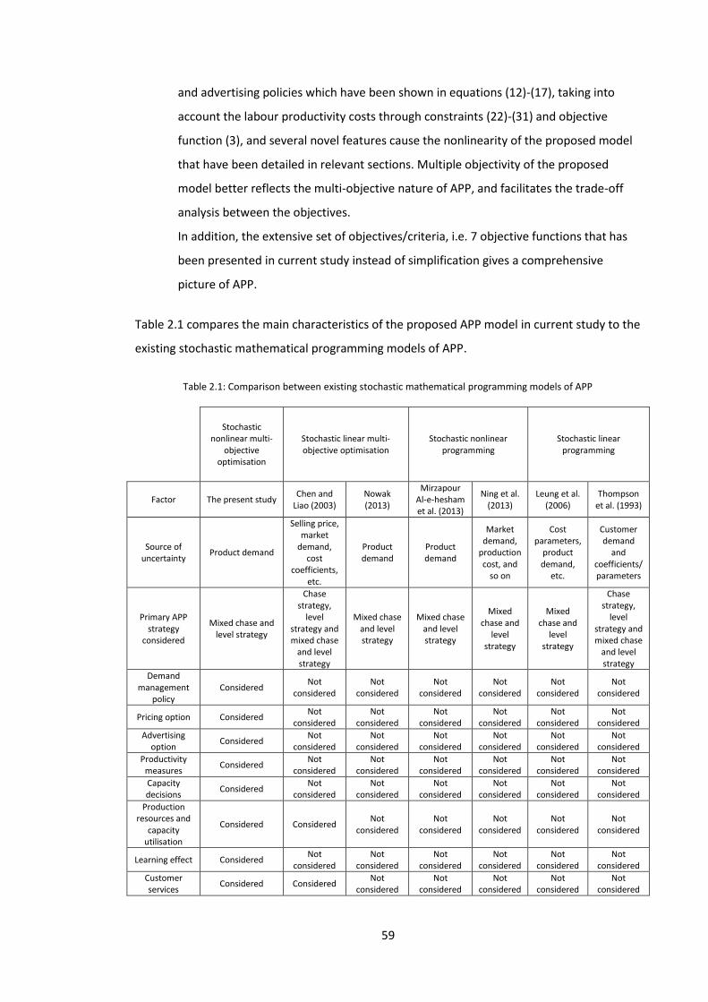
59
and advertising policies which have been shown in equations (12)-(17), taking into
account the labour productivity costs through constraints (22)-(31) and objective
function (3), and several novel features cause the nonlinearity of the proposed model
that have been detailed in relevant sections. Multiple objectivity of the proposed
model better reflects the multi-objective nature of APP, and facilitates the trade-off
analysis between the objectives.
In addition, the extensive set of objectives/criteria, i.e. 7 objective functions that has
been presented in current study instead of simplification gives a comprehensive
picture of APP.
Table 2.1 compares the main characteristics of the proposed APP model in current study to the
existing stochastic mathematical programming models of APP.
Stochastic nonlinear multi-
objective optimisation
Stochastic linear multi-objective optimisation
Stochastic nonlinear programming
Stochastic linear programming
Factor The present study Chen and
Liao (2003) Nowak (2013)
Mirzapour Al-e-hesham et al. (2013)
Ning et al. (2013)
Leung et al. (2006)
Thompson et al. (1993)
Source of uncertainty
Product demand
Selling price, market
demand, cost
coefficients, etc.
Product demand
Product demand
Market demand,
production cost, and
so on
Cost parameters,
product demand,
etc.
Customer demand
and coefficients/ parameters
Primary APP strategy
considered
Mixed chase and level strategy
Chase strategy,
level strategy and mixed chase
and level strategy
Mixed chase and level strategy
Mixed chase and level strategy
Mixed chase and
level strategy
Mixed chase and
level strategy
Chase strategy,
level strategy and mixed chase
and level strategy
Demand management
policy Considered
Not considered
Not considered
Not considered
Not considered
Not considered
Not considered
Pricing option Considered Not
considered Not
considered Not
considered Not
considered Not
considered Not
considered
Advertising option
Considered Not
considered Not
considered Not
considered Not
considered Not
considered Not
considered
Productivity measures
Considered Not
considered Not
considered Not
considered Not
considered Not
considered Not
considered
Capacity decisions
Considered Not
considered Not
considered Not
considered Not
considered Not
considered Not
considered
Production resources and
capacity utilisation
Considered Considered Not
considered Not
considered Not
considered Not
considered Not
considered
Learning effect Considered Not
considered Not
considered Not
considered Not
considered Not
considered Not
considered
Customer services
Considered Considered Not
considered Not
considered Not
considered Not
considered Not
considered
Table 2.1: Comparison between existing stochastic mathematical programming models of APP
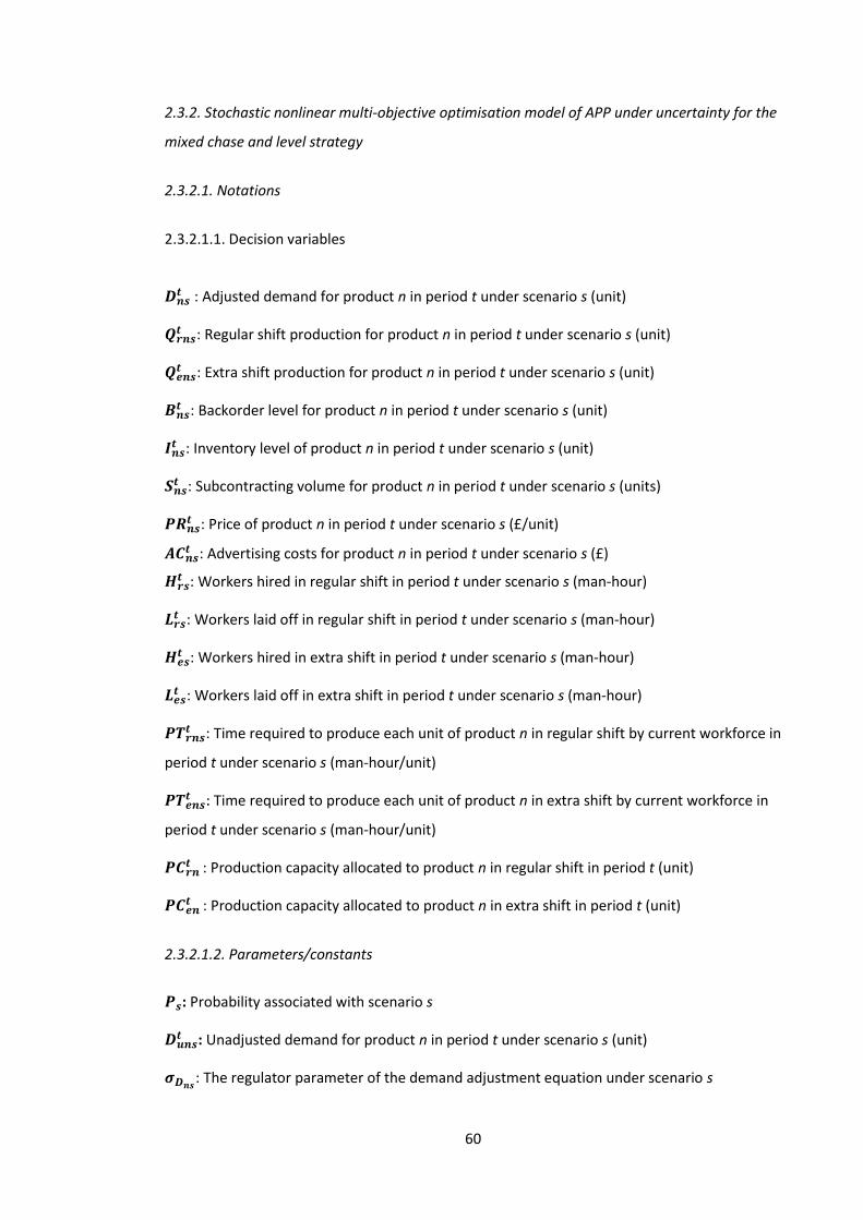
60
2.3.2. Stochastic nonlinear multi-objective optimisation model of APP under uncertainty for the
mixed chase and level strategy
2.3.2.1. Notations
2.3.2.1.1. Decision variables
𝑫𝒏𝒔𝒕 : Adjusted demand for product n in period t under scenario s (unit)
𝑸𝒓𝒏𝒔𝒕 : Regular shift production for product n in period t under scenario s (unit)
𝑸𝒆𝒏𝒔𝒕 : Extra shift production for product n in period t under scenario s (unit)
𝑩𝒏𝒔𝒕 : Backorder level for product n in period t under scenario s (unit)
𝑰𝒏𝒔𝒕 : Inventory level of product n in period t under scenario s (unit)
𝑺𝒏𝒔𝒕 : Subcontracting volume for product n in period t under scenario s (units)
𝑷𝑹𝒏𝒔𝒕 : Price of product n in period t under scenario s (£/unit)
𝑨𝑪𝒏𝒔𝒕 : Advertising costs for product n in period t under scenario s (£)
𝑯𝒓𝒔𝒕 : Workers hired in regular shift in period t under scenario s (man-hour)
𝑳𝒓𝒔𝒕 : Workers laid off in regular shift in period t under scenario s (man-hour)
𝑯𝒆𝒔𝒕 : Workers hired in extra shift in period t under scenario s (man-hour)
𝑳𝒆𝒔𝒕 : Workers laid off in extra shift in period t under scenario s (man-hour)
𝑷𝑻𝒓𝒏𝒔𝒕 : Time required to produce each unit of product n in regular shift by current workforce in
period t under scenario s (man-hour/unit)
𝑷𝑻𝒆𝒏𝒔𝒕 : Time required to produce each unit of product n in extra shift by current workforce in
period t under scenario s (man-hour/unit)
𝑷𝑪𝒓𝒏 𝒕 : Production capacity allocated to product n in regular shift in period t (unit)
𝑷𝑪𝒆𝒏 𝒕 : Production capacity allocated to product n in extra shift in period t (unit)
2.3.2.1.2. Parameters/constants
𝑷𝒔: Probability associated with scenario s
𝑫𝒖𝒏𝒔𝒕 : Unadjusted demand for product n in period t under scenario s (unit)
𝝈𝑫𝒏𝒔: The regulator parameter of the demand adjustment equation under scenario s
61
𝑪𝑷𝑹𝒏: The coefficient in the equation which stands for the price of product n (£/unit*unit)
𝑷𝑷𝑹𝒏: The parameter/constant term in the equation which stands for the price of product n
(£/unit)
𝑭𝑷𝑹𝒏𝒔𝒕 : Fixed price for product n in period t under scenario s (£/unit)
𝑭𝑨𝑪𝒏𝒔𝒕 : Fixed advertising costs for product n in period t under scenario s (£)
𝒂𝑨𝑪𝒏 , 𝒃𝑨𝑪𝒏 and 𝒄𝑨𝑪𝒏: The constant terms of the equation which represents the advertising
costs of product n (the unit for the first and the third terms is £ and the unit for the second
term is £*£)
𝝈𝑨𝑪𝒏: The regulator parameter of the equation which represents the advertising costs of
product n (£/unit)
𝑪𝒑𝒏𝒕 : All production costs including materials cost, machines operations cost, salary paid to
managers, professionals, administrative staff, etc. except costs incurred as salary paid to
workers to produce product n in period t (£/unit)
𝑺𝑷𝑻𝒓𝒏: Standard time required to produce each unit of product n in regular shift (man-
hour/unit)
𝑺𝑷𝑻𝒆𝒏: Standard time required to produce each unit of product n in extra shift (man-
hour/unit)
𝒂𝑷𝑻𝒓𝒏, 𝒃𝑷𝑻𝒓𝒏and 𝒄𝑷𝑻𝒓𝒏: The constant terms of the equation which stands for the production
time of product n in regular shift (the unit for the first and the third terms is man-hour/unit
and the unit for the second term is 1/unit)
𝒂𝑷𝑻𝒆𝒏, 𝒃𝑷𝑻𝒆𝒏and 𝒄𝑷𝑻𝒆𝒏: The constant terms of the equation which stands for the production
time of product n in extra shift (the unit for the first and the third terms is man-hour/unit and
the unit for the second term is 1/unit)
𝑭𝒓𝒏: Time required to produce the first unit of product n in regular shift by newly hired
workforce (man-hour/unit)
𝑭𝒆𝒏: Time required to produce the first unit of product n in extra shift by newly hired
workforce (man-hour/unit)
𝑪𝒓𝒘𝒏𝒕 : Regular shift worker salary cost for product n in period t (£/man-hour)
𝑪𝒆𝒘𝒏𝒕 : Extra shift worker salary cost for product n in period t (£/man-hour)
62
𝒃𝒓or 𝒃𝒆: Factor used to calculate cumulative average time to produce units in regular shift and
extra shift respectively. The value of 𝑏𝑟 or 𝑏𝑒is calculated as:
𝒃𝒓or 𝒃𝒆 =𝑳𝒏(𝒍𝒆𝒂𝒓𝒏𝒊𝒏𝒈 𝒄𝒖𝒓𝒗𝒆 % 𝒊𝒏 𝒅𝒆𝒄𝒊𝒎𝒂𝒍 𝒇𝒐𝒓𝒎)
𝑳𝒏𝟐
𝑪𝒔𝒏𝒕 : Subcontracting cost per unit of product n in period t (£/unit)
𝑪𝒊𝒏𝒕 : Inventory carrying cost per unit of product n in period t (£/unit)
𝑪𝒃𝒏𝒕 : Backorder cost per unit of product n in period t (£/unit)
𝑪𝒓𝒉𝒕 : Cost to hire one worker in regular shift in period t (£/man-hour)
𝑪𝒓𝒍𝒕 : Cost to lay off one worker in regular shift in period t (£/man-hour)
𝑪𝒆𝒉𝒕 : Cost to hire one worker in extra shift in period t (£/man-hour)
𝑪𝒆𝒍𝒕 : Cost to lay off one worker in extra shift in period t (£/man-hour)
𝑻𝑷𝑪: Total production capacity allocated to all products over the planning horizon T (unit)
𝑴𝑼𝒏: Hours of machine usage per unit of product n (machine-hour/unit)
𝝂𝒏: Warehouse space needed per unit of product n (𝑚3/unit)
𝑾𝒓𝒔 𝒎𝒂𝒙𝒕 : Maximum workers level available in regular shift in period t under scenario s (man-
hour)
𝑾𝒆𝒔 𝒎𝒂𝒙𝒕 : Maximum workers level available in extra shift in period t under scenario s (man-
hour)
𝑴𝑪𝒎𝒂𝒙𝒕 : Maximum machine capacity available in period t (machine- hour)
𝑽𝒎𝒂𝒙𝒕 : Maximum warehouse space available in period t (𝑚3)
𝑺𝒏𝒔 𝒎𝒂𝒙𝒕 : Maximum subcontracting allowed for product n in period t under scenario s (unit)
𝑩𝒏𝒔 𝒎𝒂𝒙𝒕 : Maximum backorder allowed for product n in period t under scenario s (unit)
𝑨𝑪𝒏𝒔 𝒎𝒂𝒙𝒕 : Maximum advertising costs for product n in period t under scenario s (£)
2.3.2.2. Objectives
Since the wait and see method of stochastic programming is applied in present research, the
objective functions need to be optimised for each demand quantity scenario subject to the
constraints related to that specific scenario. Then, the expected value for each objective will be
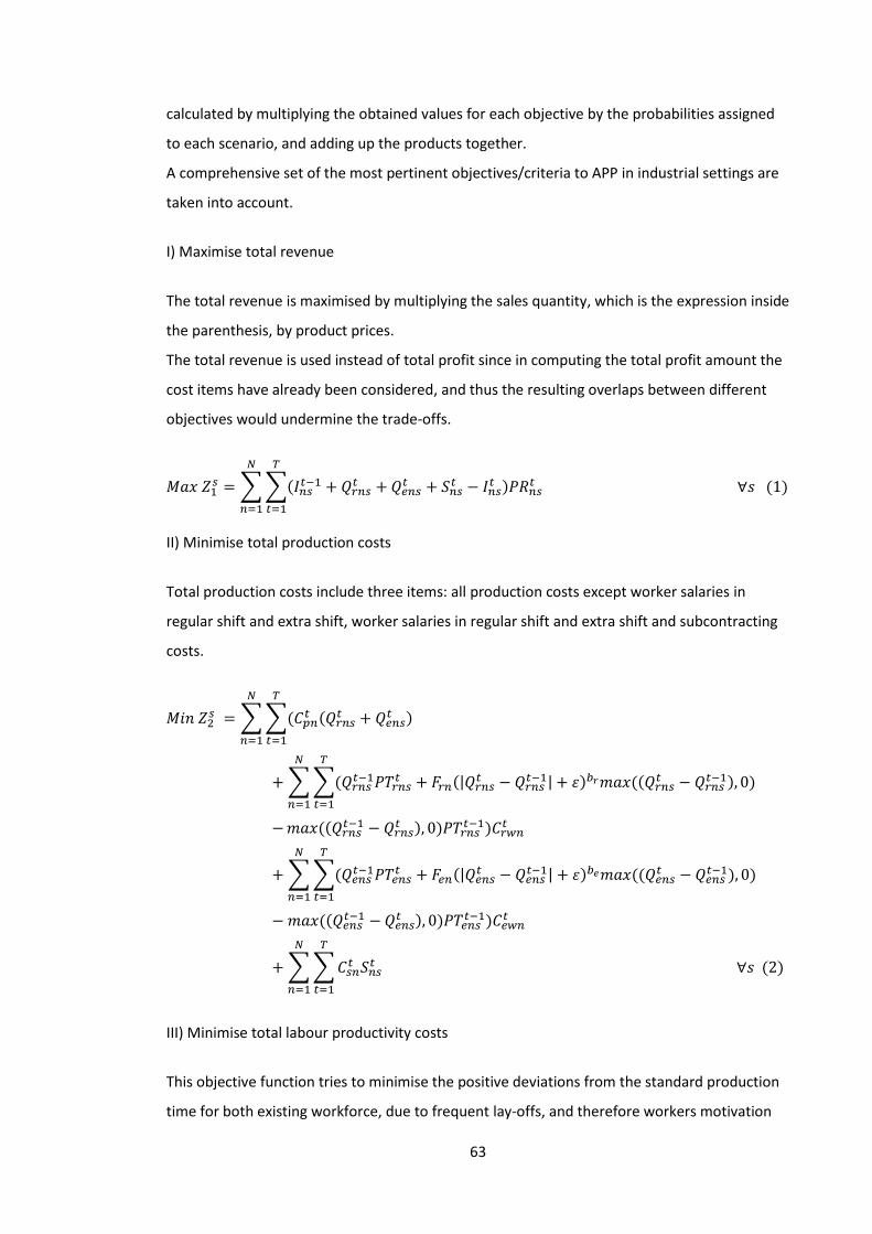
63
calculated by multiplying the obtained values for each objective by the probabilities assigned
to each scenario, and adding up the products together.
A comprehensive set of the most pertinent objectives/criteria to APP in industrial settings are
taken into account.
I) Maximise total revenue
The total revenue is maximised by multiplying the sales quantity, which is the expression inside
the parenthesis, by product prices.
The total revenue is used instead of total profit since in computing the total profit amount the
cost items have already been considered, and thus the resulting overlaps between different
objectives would undermine the trade-offs.
𝑀𝑎𝑥 𝑍1𝑠 = ∑∑(𝐼𝑛𝑠
𝑡−1 + 𝑄𝑟𝑛𝑠𝑡 +𝑄𝑒𝑛𝑠
𝑡 + 𝑆𝑛𝑠𝑡 − 𝐼𝑛𝑠
𝑡 )𝑃𝑅𝑛𝑠𝑡
𝑇
𝑡=1
𝑁
𝑛=1
∀𝑠 (1)
II) Minimise total production costs
Total production costs include three items: all production costs except worker salaries in
regular shift and extra shift, worker salaries in regular shift and extra shift and subcontracting
costs.
𝑀𝑖𝑛 𝑍2𝑠 = ∑∑(𝐶𝑝𝑛
𝑡 (𝑄𝑟𝑛𝑠𝑡 + 𝑄𝑒𝑛𝑠
𝑡 )
𝑇
𝑡=1
𝑁
𝑛=1
+∑∑(𝑄𝑟𝑛𝑠𝑡−1𝑃𝑇𝑟𝑛𝑠
𝑡 + 𝐹𝑟𝑛(|𝑄𝑟𝑛𝑠𝑡 − 𝑄𝑟𝑛𝑠
𝑡−1| + 𝜀)𝑏𝑟𝑚𝑎𝑥 ((𝑄𝑟𝑛𝑠𝑡 − 𝑄𝑟𝑛𝑠
𝑡−1), 0)
𝑇
𝑡=1
𝑁
𝑛=1
−𝑚𝑎𝑥 ((𝑄𝑟𝑛𝑠𝑡−1 − 𝑄𝑟𝑛𝑠
𝑡 ), 0)𝑃𝑇𝑟𝑛𝑠𝑡−1)𝐶𝑟𝑤𝑛
𝑡
+∑∑(𝑄𝑒𝑛𝑠𝑡−1𝑃𝑇𝑒𝑛𝑠
𝑡 + 𝐹𝑒𝑛(|𝑄𝑒𝑛𝑠𝑡 − 𝑄𝑒𝑛𝑠
𝑡−1| + 𝜀)𝑏𝑒𝑚𝑎𝑥 ((𝑄𝑒𝑛𝑠𝑡 − 𝑄𝑒𝑛𝑠
𝑡−1), 0)
𝑇
𝑡=1
𝑁
𝑛=1
−𝑚𝑎𝑥 ((𝑄𝑒𝑛𝑠𝑡−1 −𝑄𝑒𝑛𝑠
𝑡 ), 0)𝑃𝑇𝑒𝑛𝑠𝑡−1)𝐶𝑒𝑤𝑛
𝑡
+∑∑𝐶𝑠𝑛𝑡 𝑆𝑛𝑠
𝑡
𝑇
𝑡=1
𝑁
𝑛=1
∀𝑠 (2)
III) Minimise total labour productivity costs
This objective function tries to minimise the positive deviations from the standard production
time for both existing workforce, due to frequent lay-offs, and therefore workers motivation
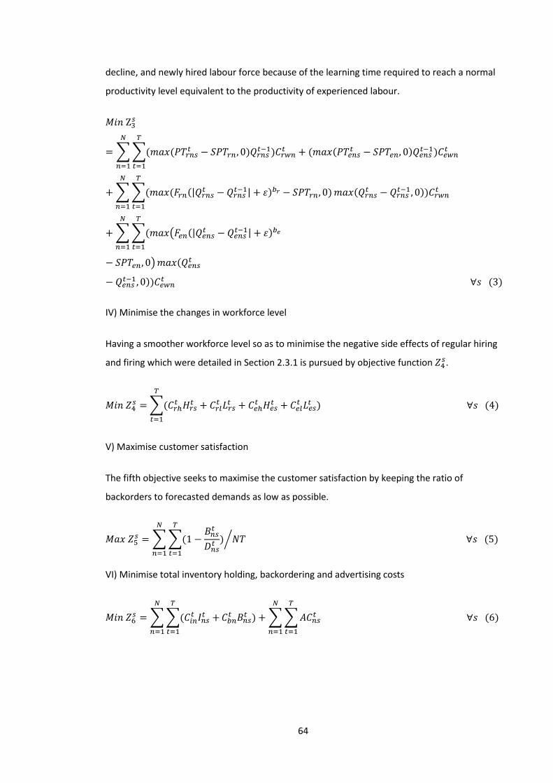
64
decline, and newly hired labour force because of the learning time required to reach a normal
productivity level equivalent to the productivity of experienced labour.
𝑀𝑖𝑛 Z3
𝑠
= ∑∑(𝑚𝑎𝑥(𝑃𝑇𝑟𝑛𝑠𝑡 − 𝑆𝑃𝑇𝑟𝑛, 0)𝑄𝑟𝑛𝑠
𝑡−1
𝑇
𝑡=1
𝑁
𝑛=1
)𝐶𝑟𝑤𝑛𝑡 + (𝑚𝑎𝑥(𝑃𝑇𝑒𝑛𝑠
𝑡 − 𝑆𝑃𝑇𝑒𝑛, 0)𝑄𝑒𝑛𝑠𝑡−1)𝐶𝑒𝑤𝑛
𝑡
+∑∑(𝑚𝑎𝑥 (𝐹𝑟𝑛(|𝑄𝑟𝑛𝑠𝑡 − 𝑄𝑟𝑛𝑠
𝑡−1| + 𝜀)𝑏𝑟 − 𝑆𝑃𝑇𝑟𝑛, 0)𝑚𝑎𝑥(𝑄𝑟𝑛𝑠𝑡 − 𝑄𝑟𝑛𝑠
𝑡−1, 0))𝐶𝑟𝑤𝑛𝑡
𝑇
𝑡=1
𝑁
𝑛=1
+∑∑(𝑚𝑎𝑥(𝐹𝑒𝑛(|𝑄𝑒𝑛𝑠𝑡 − 𝑄𝑒𝑛𝑠
𝑡−1| + 𝜀)𝑏𝑒
𝑇
𝑡=1
𝑁
𝑛=1
− 𝑆𝑃𝑇𝑒𝑛, 0)𝑚𝑎𝑥(𝑄𝑒𝑛𝑠𝑡
− 𝑄𝑒𝑛𝑠𝑡−1, 0))𝐶𝑒𝑤𝑛
𝑡 ∀𝑠 (3)
IV) Minimise the changes in workforce level
Having a smoother workforce level so as to minimise the negative side effects of regular hiring
and firing which were detailed in Section 2.3.1 is pursued by objective function 𝑍4𝑠.
𝑀𝑖𝑛 𝑍4𝑠 =∑(𝐶𝑟ℎ
𝑡 𝐻𝑟𝑠𝑡 + 𝐶𝑟𝑙
𝑡 𝐿𝑟𝑠𝑡 + 𝐶𝑒ℎ
𝑡 𝐻𝑒𝑠𝑡 + 𝐶𝑒𝑙
𝑡 𝐿𝑒𝑠𝑡 )
𝑇
𝑡=1
∀𝑠 (4)
V) Maximise customer satisfaction
The fifth objective seeks to maximise the customer satisfaction by keeping the ratio of
backorders to forecasted demands as low as possible.
𝑀𝑎𝑥 𝑍5𝑠 = ∑∑(1 −
𝐵𝑛𝑠𝑡
𝐷𝑛𝑠𝑡 )
𝑇
𝑡=1
𝑁
𝑛=1
𝑁𝑇⁄ ∀𝑠 (5)
VI) Minimise total inventory holding, backordering and advertising costs
𝑀𝑖𝑛 𝑍6𝑠 = ∑∑(𝐶𝑖𝑛
𝑡 𝐼𝑛𝑠𝑡 +
𝑇
𝑡=1
𝑁
𝑛=1
𝐶𝑏𝑛𝑡 𝐵𝑛𝑠
𝑡 ) +∑∑𝐴𝐶𝑛𝑠𝑡
𝑇
𝑡=1
𝑁
𝑛=1
∀𝑠 (6)
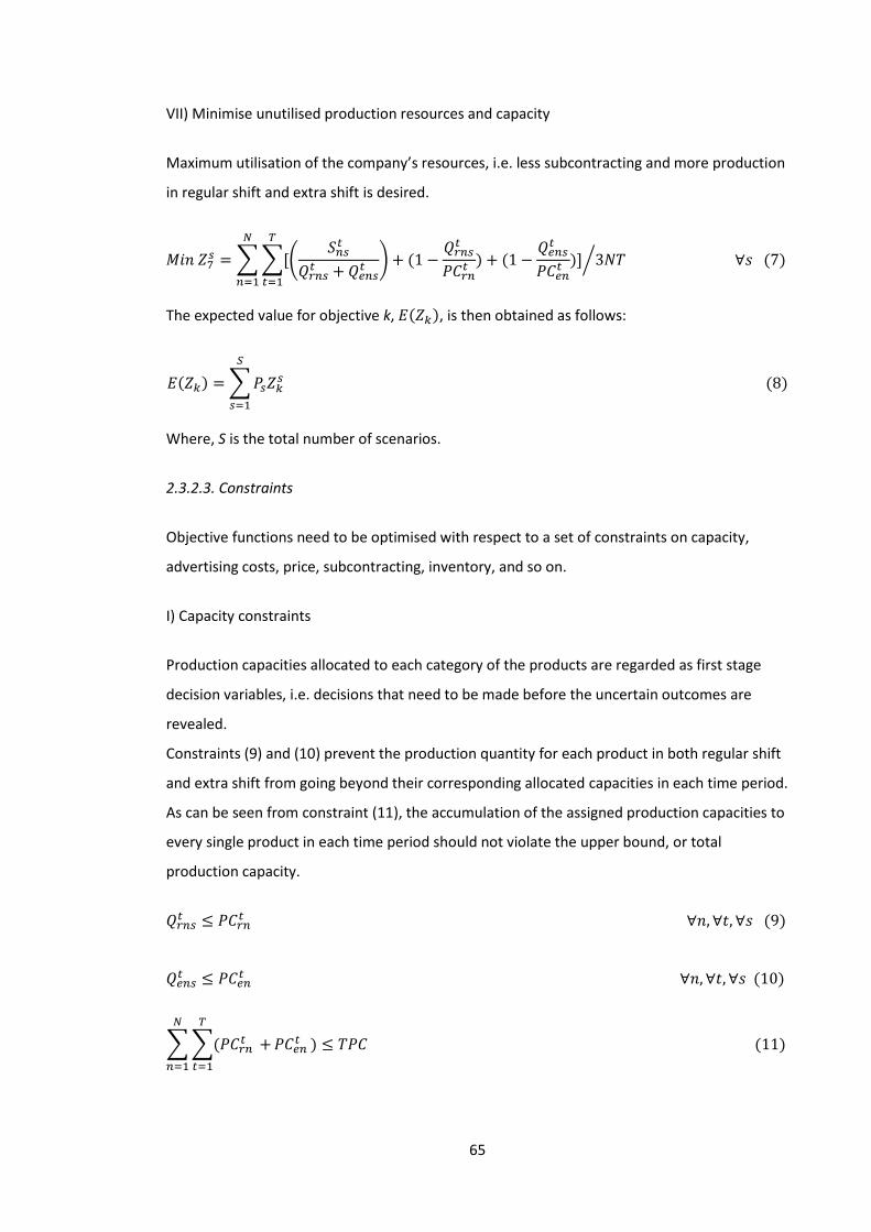
65
VII) Minimise unutilised production resources and capacity
Maximum utilisation of the company’s resources, i.e. less subcontracting and more production
in regular shift and extra shift is desired.
𝑀𝑖𝑛 𝑍7𝑠 = ∑∑[(
𝑆𝑛𝑠𝑡
𝑄𝑟𝑛𝑠𝑡 + 𝑄𝑒𝑛𝑠
𝑡 ) + (1 −𝑄𝑟𝑛𝑠𝑡
𝑃𝐶𝑟𝑛𝑡
𝑇
𝑡=1
𝑁
𝑛=1
) + (1 −𝑄𝑒𝑛𝑠𝑡
𝑃𝐶𝑒𝑛𝑡 )] 3𝑁𝑇⁄ ∀𝑠 (7)
The expected value for objective k, 𝐸(𝑍𝑘), is then obtained as follows:
𝐸(𝑍𝑘) =∑𝑃𝑠𝑍𝑘𝑠
𝑆
𝑠=1
(8)
Where, S is the total number of scenarios.
2.3.2.3. Constraints
Objective functions need to be optimised with respect to a set of constraints on capacity,
advertising costs, price, subcontracting, inventory, and so on.
I) Capacity constraints
Production capacities allocated to each category of the products are regarded as first stage
decision variables, i.e. decisions that need to be made before the uncertain outcomes are
revealed.
Constraints (9) and (10) prevent the production quantity for each product in both regular shift
and extra shift from going beyond their corresponding allocated capacities in each time period.
As can be seen from constraint (11), the accumulation of the assigned production capacities to
every single product in each time period should not violate the upper bound, or total
production capacity.
𝑄𝑟𝑛𝑠𝑡 ≤ 𝑃𝐶𝑟𝑛
𝑡 ∀𝑛, ∀𝑡, ∀𝑠 (9)
𝑄𝑒𝑛𝑠𝑡 ≤ 𝑃𝐶𝑒𝑛
𝑡 ∀𝑛, ∀𝑡, ∀𝑠 (10)
∑∑(𝑃𝐶𝑟𝑛 𝑡 +
𝑇
𝑡=1
𝑁
𝑛=1
𝑃𝐶𝑒𝑛 𝑡 ) ≤ 𝑇𝑃𝐶 (11)
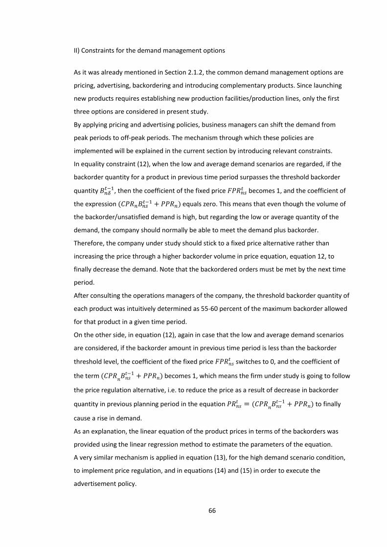
66
II) Constraints for the demand management options
As it was already mentioned in Section 2.1.2, the common demand management options are
pricing, advertising, backordering and introducing complementary products. Since launching
new products requires establishing new production facilities/production lines, only the first
three options are considered in present study.
By applying pricing and advertising policies, business managers can shift the demand from
peak periods to off-peak periods. The mechanism through which these policies are
implemented will be explained in the current section by introducing relevant constraints.
In equality constraint (12), when the low and average demand scenarios are regarded, if the
backorder quantity for a product in previous time period surpasses the threshold backorder
quantity 𝐵𝑛𝛿𝑡−1, then the coefficient of the fixed price 𝐹𝑃𝑅𝑛𝑠
𝑡 becomes 1, and the coefficient of
the expression (𝐶𝑃𝑅𝑛𝐵𝑛𝑠𝑡−1 + 𝑃𝑃𝑅𝑛) equals zero. This means that even though the volume of
the backorder/unsatisfied demand is high, but regarding the low or average quantity of the
demand, the company should normally be able to meet the demand plus backorder.
Therefore, the company under study should stick to a fixed price alternative rather than
increasing the price through a higher backorder volume in price equation, equation 12, to
finally decrease the demand. Note that the backordered orders must be met by the next time
period.
After consulting the operations managers of the company, the threshold backorder quantity of
each product was intuitively determined as 55-60 percent of the maximum backorder allowed
for that product in a given time period.
On the other side, in equation (12), again in case that the low and average demand scenarios
are considered, if the backorder amount in previous time period is less than the backorder
threshold level, the coefficient of the fixed price 𝐹𝑃𝑅𝑛𝑠𝑡 switches to 0, and the coefficient of
the term (𝐶𝑃𝑅𝑛𝐵𝑛𝑠𝑡−1 + 𝑃𝑃𝑅𝑛) becomes 1, which means the firm under study is going to follow
the price regulation alternative, i.e. to reduce the price as a result of decrease in backorder
quantity in previous planning period in the equation 𝑃𝑅𝑛𝑠𝑡 = (𝐶𝑃𝑅
𝑛𝐵𝑛𝑠𝑡−1 + 𝑃𝑃𝑅𝑛) to finally
cause a rise in demand.
As an explanation, the linear equation of the product prices in terms of the backorders was
provided using the linear regression method to estimate the parameters of the equation.
A very similar mechanism is applied in equation (13), for the high demand scenario condition,
to implement price regulation, and in equations (14) and (15) in order to execute the
advertisement policy.
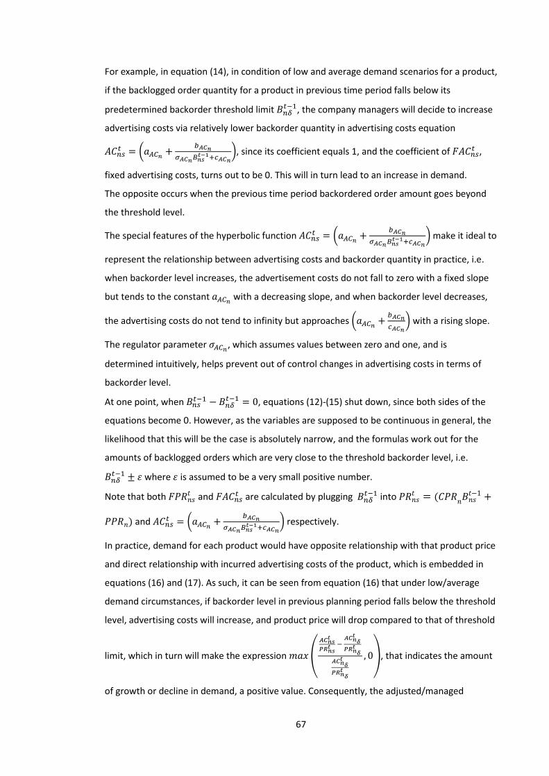
67
For example, in equation (14), in condition of low and average demand scenarios for a product,
if the backlogged order quantity for a product in previous time period falls below its
predetermined backorder threshold limit 𝐵𝑛𝛿𝑡−1, the company managers will decide to increase
advertising costs via relatively lower backorder quantity in advertising costs equation
𝐴𝐶𝑛𝑠𝑡 = (𝑎𝐴𝐶𝑛 +
𝑏𝐴𝐶𝑛𝜎𝐴𝐶𝑛𝐵𝑛𝑠
𝑡−1+𝑐𝐴𝐶𝑛), since its coefficient equals 1, and the coefficient of 𝐹𝐴𝐶𝑛𝑠
𝑡 ,
fixed advertising costs, turns out to be 0. This will in turn lead to an increase in demand.
The opposite occurs when the previous time period backordered order amount goes beyond
the threshold level.
The special features of the hyperbolic function 𝐴𝐶𝑛𝑠𝑡 = (𝑎𝐴𝐶𝑛 +
𝑏𝐴𝐶𝑛𝜎𝐴𝐶𝑛𝐵𝑛𝑠
𝑡−1+𝑐𝐴𝐶𝑛) make it ideal to
represent the relationship between advertising costs and backorder quantity in practice, i.e.
when backorder level increases, the advertisement costs do not fall to zero with a fixed slope
but tends to the constant 𝑎𝐴𝐶𝑛 with a decreasing slope, and when backorder level decreases,
the advertising costs do not tend to infinity but approaches (𝑎𝐴𝐶𝑛 +𝑏𝐴𝐶𝑛𝑐𝐴𝐶𝑛
) with a rising slope.
The regulator parameter 𝜎𝐴𝐶𝑛, which assumes values between zero and one, and is
determined intuitively, helps prevent out of control changes in advertising costs in terms of
backorder level.
At one point, when 𝐵𝑛𝑠𝑡−1 −𝐵𝑛𝛿
𝑡−1 = 0, equations (12)-(15) shut down, since both sides of the
equations become 0. However, as the variables are supposed to be continuous in general, the
likelihood that this will be the case is absolutely narrow, and the formulas work out for the
amounts of backlogged orders which are very close to the threshold backorder level, i.e.
𝐵𝑛𝛿𝑡−1 ± 𝜀 where 𝜀 is assumed to be a very small positive number.
Note that both 𝐹𝑃𝑅𝑛𝑠𝑡 and 𝐹𝐴𝐶𝑛𝑠
𝑡 are calculated by plugging 𝐵𝑛𝛿𝑡−1 into 𝑃𝑅𝑛𝑠
𝑡 = (𝐶𝑃𝑅𝑛𝐵𝑛𝑠𝑡−1 +
𝑃𝑃𝑅𝑛) and 𝐴𝐶𝑛𝑠𝑡 = (𝑎𝐴𝐶𝑛 +
𝑏𝐴𝐶𝑛𝜎𝐴𝐶𝑛𝐵𝑛𝑠
𝑡−1+𝑐𝐴𝐶𝑛) respectively.
In practice, demand for each product would have opposite relationship with that product price
and direct relationship with incurred advertising costs of the product, which is embedded in
equations (16) and (17). As such, it can be seen from equation (16) that under low/average
demand circumstances, if backorder level in previous planning period falls below the threshold
level, advertising costs will increase, and product price will drop compared to that of threshold
limit, which in turn will make the expression 𝑚𝑎𝑥(
𝐴𝐶𝑛𝑠𝑡
𝑃𝑅𝑛𝑠𝑡 −
𝐴𝐶𝑛𝛿𝑡
𝑃𝑅𝑛𝛿𝑡
𝐴𝐶𝑛𝛿𝑡
𝑃𝑅𝑛𝛿𝑡
, 0), that indicates the amount
of growth or decline in demand, a positive value. Consequently, the adjusted/managed
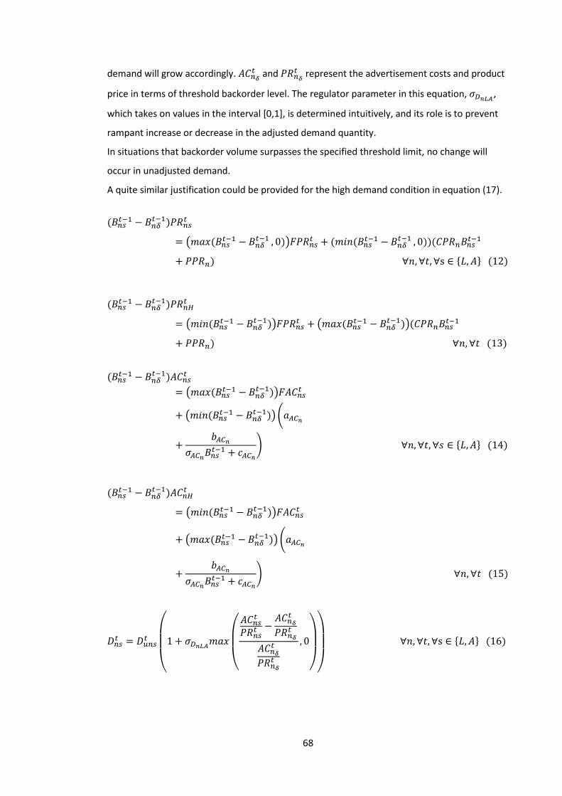
68
demand will grow accordingly. 𝐴𝐶𝑛𝛿𝑡 and 𝑃𝑅𝑛𝛿
𝑡 represent the advertisement costs and product
price in terms of threshold backorder level. The regulator parameter in this equation, 𝜎𝐷𝑛𝐿𝐴 ,
which takes on values in the interval [0,1], is determined intuitively, and its role is to prevent
rampant increase or decrease in the adjusted demand quantity.
In situations that backorder volume surpasses the specified threshold limit, no change will
occur in unadjusted demand.
A quite similar justification could be provided for the high demand condition in equation (17).
(𝐵𝑛𝑠𝑡−1 − 𝐵𝑛𝛿
𝑡−1)𝑃𝑅𝑛𝑠𝑡
= (𝑚𝑎𝑥(𝐵𝑛𝑠𝑡−1 − 𝐵𝑛𝛿
𝑡−1 , 0))𝐹𝑃𝑅𝑛𝑠𝑡 + (𝑚𝑖𝑛(𝐵𝑛𝑠
𝑡−1 − 𝐵𝑛𝛿𝑡−1 , 0))(𝐶𝑃𝑅𝑛𝐵𝑛𝑠
𝑡−1
+ 𝑃𝑃𝑅𝑛) ∀𝑛, ∀𝑡, ∀s ∈ {𝐿, 𝐴} (12)
(𝐵𝑛𝑠𝑡−1 − 𝐵𝑛𝛿
𝑡−1)𝑃𝑅𝑛𝐻𝑡
= (𝑚𝑖𝑛(𝐵𝑛𝑠𝑡−1 − 𝐵𝑛𝛿
𝑡−1))𝐹𝑃𝑅𝑛𝑠𝑡 + (𝑚𝑎𝑥(𝐵𝑛𝑠
𝑡−1 − 𝐵𝑛𝛿𝑡−1))(𝐶𝑃𝑅𝑛𝐵𝑛𝑠
𝑡−1
+ 𝑃𝑃𝑅𝑛) ∀𝑛, ∀𝑡 (13)
(𝐵𝑛𝑠𝑡−1 − 𝐵𝑛𝛿
𝑡−1)𝐴𝐶𝑛𝑠𝑡
= (𝑚𝑎𝑥(𝐵𝑛𝑠𝑡−1 − 𝐵𝑛𝛿
𝑡−1))𝐹𝐴𝐶𝑛𝑠𝑡
+ (𝑚𝑖𝑛(𝐵𝑛𝑠𝑡−1 − 𝐵𝑛𝛿
𝑡−1))(𝑎𝐴𝐶𝑛
+𝑏𝐴𝐶𝑛
𝜎𝐴𝐶𝑛𝐵𝑛𝑠𝑡−1 + 𝑐𝐴𝐶𝑛
) ∀𝑛, ∀𝑡, ∀𝑠 ∈ {𝐿, 𝐴} (14)
(𝐵𝑛𝑠𝑡−1 − 𝐵𝑛𝛿
𝑡−1)𝐴𝐶𝑛𝐻𝑡
= (𝑚𝑖𝑛(𝐵𝑛𝑠𝑡−1 − 𝐵𝑛𝛿
𝑡−1))𝐹𝐴𝐶𝑛𝑠𝑡
+ (𝑚𝑎𝑥(𝐵𝑛𝑠𝑡−1 −𝐵𝑛𝛿
𝑡−1)) (𝑎𝐴𝐶𝑛
+𝑏𝐴𝐶𝑛
𝜎𝐴𝐶𝑛𝐵𝑛𝑠𝑡−1 + 𝑐𝐴𝐶𝑛
) ∀𝑛, ∀𝑡 (15)
𝐷𝑛𝑠𝑡 = 𝐷𝑢𝑛𝑠
𝑡
(
1+ 𝜎𝐷𝑛𝐿𝐴𝑚𝑎𝑥
(
𝐴𝐶𝑛𝑠𝑡
𝑃𝑅𝑛𝑠𝑡 −
𝐴𝐶𝑛𝛿𝑡
𝑃𝑅𝑛𝛿𝑡
𝐴𝐶𝑛𝛿𝑡
𝑃𝑅𝑛𝛿𝑡
, 0
)
)
∀𝑛, ∀𝑡, ∀s ∈ {𝐿, 𝐴} (16)
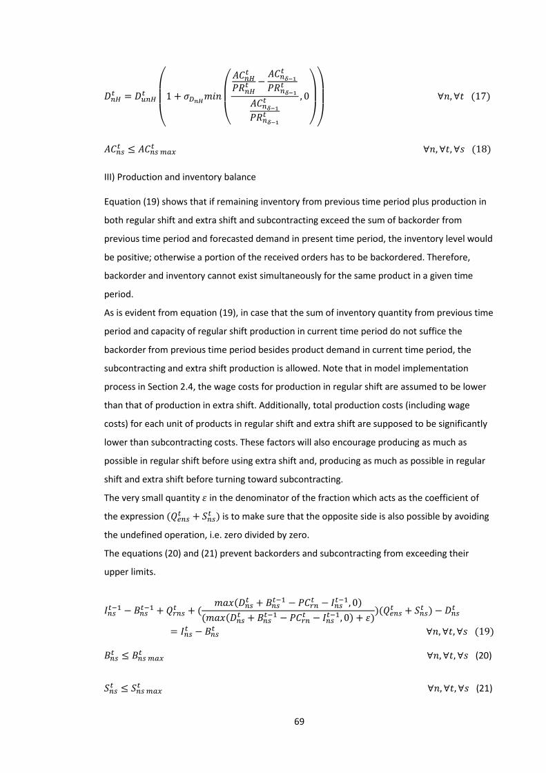
69
𝐷𝑛𝐻𝑡 = 𝐷𝑢𝑛𝐻
𝑡
(
1 + 𝜎𝐷𝑛𝐻𝑚𝑖𝑛
(
𝐴𝐶𝑛𝐻𝑡
𝑃𝑅𝑛𝐻𝑡 −
𝐴𝐶𝑛𝛿−1𝑡
𝑃𝑅𝑛𝛿−1𝑡
𝐴𝐶𝑛𝛿−1𝑡
𝑃𝑅𝑛𝛿−1𝑡
, 0
)
)
∀𝑛, ∀𝑡 (17)
𝐴𝐶𝑛𝑠𝑡 ≤ 𝐴𝐶𝑛𝑠 𝑚𝑎𝑥
𝑡 ∀𝑛, ∀𝑡, ∀𝑠 (18)
III) Production and inventory balance Equation (19) shows that if remaining inventory from previous time period plus production in
both regular shift and extra shift and subcontracting exceed the sum of backorder from
previous time period and forecasted demand in present time period, the inventory level would
be positive; otherwise a portion of the received orders has to be backordered. Therefore,
backorder and inventory cannot exist simultaneously for the same product in a given time
period.
As is evident from equation (19), in case that the sum of inventory quantity from previous time
period and capacity of regular shift production in current time period do not suffice the
backorder from previous time period besides product demand in current time period, the
subcontracting and extra shift production is allowed. Note that in model implementation
process in Section 2.4, the wage costs for production in regular shift are assumed to be lower
than that of production in extra shift. Additionally, total production costs (including wage
costs) for each unit of products in regular shift and extra shift are supposed to be significantly
lower than subcontracting costs. These factors will also encourage producing as much as
possible in regular shift before using extra shift and, producing as much as possible in regular
shift and extra shift before turning toward subcontracting.
The very small quantity 𝜀 in the denominator of the fraction which acts as the coefficient of
the expression (𝑄𝑒𝑛𝑠𝑡 + 𝑆𝑛𝑠
𝑡 ) is to make sure that the opposite side is also possible by avoiding
the undefined operation, i.e. zero divided by zero.
The equations (20) and (21) prevent backorders and subcontracting from exceeding their
upper limits.
𝐼𝑛𝑠𝑡−1 − 𝐵𝑛𝑠
𝑡−1 + 𝑄𝑟𝑛𝑠𝑡 + (
𝑚𝑎𝑥(𝐷𝑛𝑠𝑡 + 𝐵𝑛𝑠
𝑡−1 − 𝑃𝐶𝑟𝑛𝑡 − 𝐼𝑛𝑠
𝑡−1, 0)
(𝑚𝑎𝑥(𝐷𝑛𝑠𝑡 + 𝐵𝑛𝑠
𝑡−1 − 𝑃𝐶𝑟𝑛𝑡 − 𝐼𝑛𝑠
𝑡−1, 0) + 𝜀))(𝑄𝑒𝑛𝑠
𝑡 + 𝑆𝑛𝑠𝑡 ) − 𝐷𝑛𝑠
𝑡
= 𝐼𝑛𝑠𝑡 − 𝐵𝑛𝑠
𝑡 ∀𝑛, ∀𝑡, ∀𝑠 (19)
𝐵𝑛𝑠𝑡 ≤ 𝐵𝑛𝑠 𝑚𝑎𝑥
𝑡 ∀𝑛, ∀𝑡, ∀𝑠 (20)
𝑆𝑛𝑠𝑡 ≤ 𝑆𝑛𝑠 𝑚𝑎𝑥
𝑡 ∀𝑛, ∀𝑡, ∀𝑠 (21)
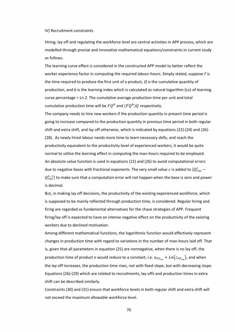
70
IV) Recruitment constraints
Hiring, lay off and regulating the workforce level are central activities in APP process, which are
modelled through precise and innovative mathematical equations/constraints in current study
as follows.
The learning curve effect is considered in the constructed APP model to better reflect the
worker experience factor in computing the required labour-hours. Simply stated, suppose F is
the time required to produce the first unit of a product, Q is the cumulative quantity of
production, and b is the learning index which is calculated as natural logarithm (Ln) of learning
curve percentage ÷ Ln 2. The cumulative average production time per unit and total
cumulative production time will be 𝐹𝑄𝑏 and (𝐹𝑄𝑏)𝑄 respectively.
The company needs to hire new workers if the production quantity in present time period is
going to increase compared to the production quantity in previous time period in both regular
shift and extra shift, and lay off otherwise, which is indicated by equations (22)-(24) and (26)-
(28). As newly hired labour needs more time to learn necessary skills, and reach the
productivity equivalent to the productivity level of experienced workers, it would be quite
normal to utilise the learning effect in computing the man-hours required to be employed.
An absolute value function is used in equations (22) and (26) to avoid computational errors
due to negative bases with fractional exponents. The very small value 𝜀 is added to |𝑄𝑟𝑛𝑠𝑡 −
𝑄𝑟𝑛𝑠𝑡−1| to make sure that a computation error will not happen when the base is zero and power
is decimal.
But, in making lay off decisions, the productivity of the existing experienced workforce, which
is supposed to be mainly reflected through production time, is considered. Regular hiring and
firing are regarded as fundamental alternatives for the chase strategies of APP. Frequent
firing/lay off is expected to have an intense negative effect on the productivity of the existing
workers due to declined motivation.
Among different mathematical functions, the logarithmic function would effectively represent
changes in production time with regard to variations in the number of man-hours laid off. That
is, given that all parameters in equation (25) are nonnegative, when there is no lay off, the
production time of product n would reduce to a constant, i.e. 𝑎𝑃𝑇𝑟𝑛 + 𝐿𝑛(𝑐𝑃𝑇𝑟𝑛), and when
the lay off increases, the production time rises, not with fixed slope, but with decreasing slope.
Equations (26)-(29) which are related to recruitments, lay-offs and production times in extra
shift can be described similarly.
Constraints (30) and (31) ensure that workforce levels in both regular shift and extra shift will
not exceed the maximum allowable workforce level.
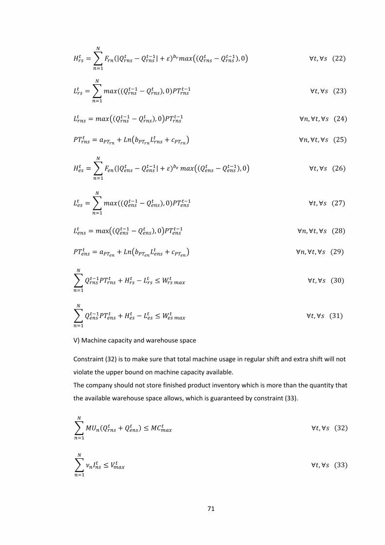
71
𝐻𝑟𝑠𝑡 = ∑𝐹𝑟𝑛(|𝑄𝑟𝑛𝑠
𝑡 − 𝑄𝑟𝑛𝑠𝑡−1| + 𝜀)𝑏𝑟𝑚𝑎𝑥((𝑄𝑟𝑛𝑠
𝑡 −𝑄𝑟𝑛𝑠𝑡−1), 0) ∀𝑡, ∀𝑠 (22)
𝑁
𝑛=1
𝐿𝑟𝑠𝑡 = ∑𝑚𝑎𝑥((𝑄𝑟𝑛𝑠
𝑡−1 − 𝑄𝑟𝑛𝑠𝑡
𝑁
𝑛=1
), 0)𝑃𝑇𝑟𝑛𝑠𝑡−1 ∀𝑡, ∀𝑠 (23)
𝐿𝑟𝑛𝑠𝑡 = 𝑚𝑎𝑥((𝑄𝑟𝑛𝑠
𝑡−1 − 𝑄𝑟𝑛𝑠𝑡 ), 0)𝑃𝑇𝑟𝑛𝑠
𝑡−1 ∀𝑛, ∀𝑡, ∀𝑠 (24)
𝑃𝑇𝑟𝑛𝑠𝑡 = 𝑎𝑃𝑇𝑟𝑛 + 𝐿𝑛(𝑏𝑃𝑇𝑟𝑛𝐿𝑟𝑛𝑠
𝑡 + 𝑐𝑃𝑇𝑟𝑛) ∀𝑛, ∀𝑡, ∀𝑠 (25)
𝐻𝑒𝑠𝑡 = ∑𝐹𝑒𝑛(|𝑄𝑒𝑛𝑠
𝑡 − 𝑄𝑒𝑛𝑠𝑡−1| + 𝜀)𝑏𝑒
𝑁
𝑛=1
𝑚𝑎𝑥((𝑄𝑒𝑛𝑠𝑡 −𝑄𝑒𝑛𝑠
𝑡−1), 0) ∀𝑡, ∀𝑠 (26)
𝐿𝑒𝑠𝑡 = ∑𝑚𝑎𝑥 ((𝑄𝑒𝑛𝑠
𝑡−1 − 𝑄𝑒𝑛𝑠𝑡
𝑁
𝑛=1
), 0)𝑃𝑇𝑒𝑛𝑠𝑡−1 ∀𝑡, ∀𝑠 (27)
𝐿𝑒𝑛𝑠𝑡 = 𝑚𝑎x((𝑄𝑒𝑛𝑠
𝑡−1 −𝑄𝑒𝑛𝑠𝑡 ), 0)𝑃𝑇𝑒𝑛𝑠
𝑡−1 ∀𝑛, ∀𝑡, ∀𝑠 (28)
𝑃𝑇𝑒𝑛𝑠𝑡 = 𝑎𝑃𝑇𝑒𝑛 + 𝐿𝑛(𝑏𝑃𝑇𝑒𝑛𝐿𝑒𝑛𝑠
𝑡 + 𝑐𝑃𝑇𝑒𝑛) ∀𝑛, ∀𝑡, ∀𝑠 (29)
∑𝑄𝑟𝑛𝑠𝑡−1𝑃𝑇𝑟𝑛𝑠
𝑡 +𝐻𝑟𝑠𝑡 − 𝐿𝑟𝑠
𝑡
𝑁
𝑛=1
≤ 𝑊𝑟𝑠 𝑚𝑎𝑥𝑡 ∀𝑡, ∀𝑠 (30)
∑𝑄𝑒𝑛𝑠𝑡−1𝑃𝑇𝑒𝑛𝑠
𝑡 +𝐻𝑒𝑠𝑡 − 𝐿𝑒𝑠
𝑡
𝑁
𝑛=1
≤ 𝑊𝑒𝑠 𝑚𝑎𝑥𝑡 ∀𝑡, ∀𝑠 (31)
V) Machine capacity and warehouse space
Constraint (32) is to make sure that total machine usage in regular shift and extra shift will not
violate the upper bound on machine capacity available.
The company should not store finished product inventory which is more than the quantity that
the available warehouse space allows, which is guaranteed by constraint (33).
∑𝑀𝑈𝑛(𝑄𝑟𝑛𝑠𝑡 + 𝑄𝑒𝑛𝑠
𝑡 ) ≤ 𝑀𝐶𝑚𝑎𝑥𝑡
𝑁
𝑛=1
∀𝑡, ∀𝑠 (32)
∑𝜈𝑛𝐼𝑛𝑠𝑡 ≤ 𝑉𝑚𝑎𝑥
𝑡
𝑁
𝑛=1
∀𝑡, ∀𝑠 (33)
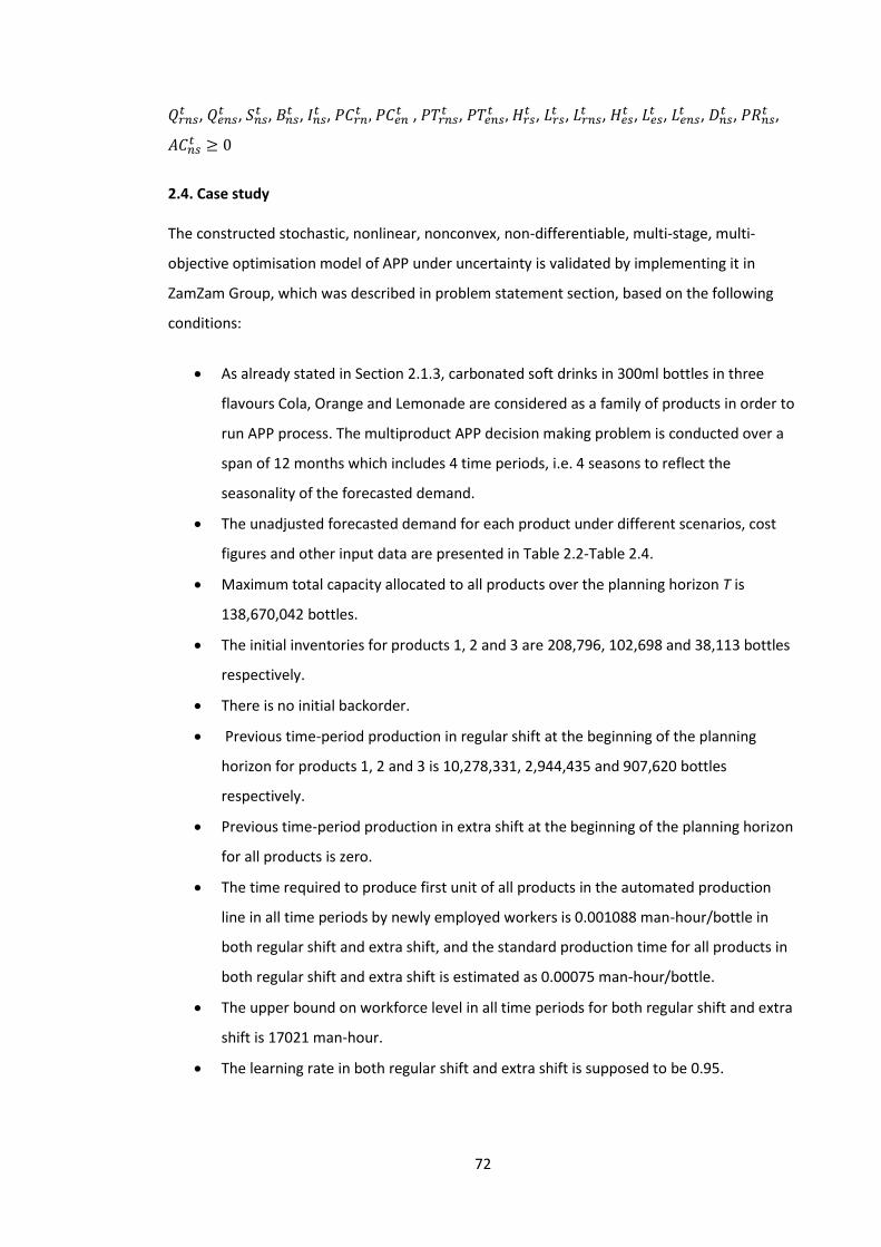
72
𝑄𝑟𝑛𝑠𝑡 , 𝑄𝑒𝑛𝑠
𝑡 , 𝑆𝑛𝑠𝑡 , 𝐵𝑛𝑠
𝑡 , 𝐼𝑛𝑠𝑡 , 𝑃𝐶𝑟𝑛
𝑡 , 𝑃𝐶𝑒𝑛𝑡 , 𝑃𝑇𝑟𝑛𝑠
𝑡 , 𝑃𝑇𝑒𝑛𝑠𝑡 , 𝐻𝑟𝑠
𝑡 , 𝐿𝑟𝑠𝑡 , 𝐿𝑟𝑛𝑠
𝑡 , 𝐻𝑒𝑠𝑡 , 𝐿𝑒𝑠
𝑡 , 𝐿𝑒𝑛𝑠𝑡 , 𝐷𝑛𝑠
𝑡 , 𝑃𝑅𝑛𝑠𝑡 ,
𝐴𝐶𝑛𝑠𝑡 ≥ 0
2.4. Case study The constructed stochastic, nonlinear, nonconvex, non-differentiable, multi-stage, multi-
objective optimisation model of APP under uncertainty is validated by implementing it in
ZamZam Group, which was described in problem statement section, based on the following
conditions:
As already stated in Section 2.1.3, carbonated soft drinks in 300ml bottles in three
flavours Cola, Orange and Lemonade are considered as a family of products in order to
run APP process. The multiproduct APP decision making problem is conducted over a
span of 12 months which includes 4 time periods, i.e. 4 seasons to reflect the
seasonality of the forecasted demand.
The unadjusted forecasted demand for each product under different scenarios, cost
figures and other input data are presented in Table 2.2-Table 2.4.
Maximum total capacity allocated to all products over the planning horizon T is
138,670,042 bottles.
The initial inventories for products 1, 2 and 3 are 208,796, 102,698 and 38,113 bottles
respectively.
There is no initial backorder.
Previous time-period production in regular shift at the beginning of the planning
horizon for products 1, 2 and 3 is 10,278,331, 2,944,435 and 907,620 bottles
respectively.
Previous time-period production in extra shift at the beginning of the planning horizon
for all products is zero.
The time required to produce first unit of all products in the automated production
line in all time periods by newly employed workers is 0.001088 man-hour/bottle in
both regular shift and extra shift, and the standard production time for all products in
both regular shift and extra shift is estimated as 0.00075 man-hour/bottle.
The upper bound on workforce level in all time periods for both regular shift and extra
shift is 17021 man-hour.
The learning rate in both regular shift and extra shift is supposed to be 0.95.
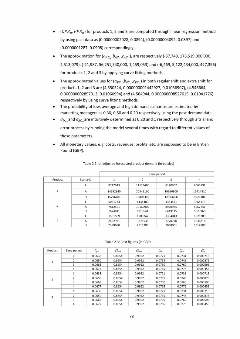
73
(𝐶𝑃𝑅𝑛, 𝑃𝑃𝑅𝑛) for products 1, 2 and 3 are computed through linear regression method
by using past data as (0.00000002028, 0.0894), (0.00000004092, 0.0897) and
(0.0000001287, 0.0908) correspondingly.
The approximation for (𝑎𝐴𝐶𝑛,𝑏𝐴𝐶𝑛,𝑐𝐴𝐶𝑛), are respectively (-37,749, 178,519,000,000,
2,513,079), (-21,987, 56,251,340,000, 1,459,053) and (-6,469, 5,122,434,000, 427,396)
for products 1, 2 and 3 by applying curve fitting methods.
The approximated values for (𝑎𝑃𝑇𝑛,𝑏𝑃𝑇𝑛,𝑐𝑃𝑇𝑛) in both regular shift and extra shift for
products 1, 2 and 3 are (4.550524, 0.000000001442927, 0.01056907), (4.546664,
0.000000002897013, 0.01060994) and (4.564944, 0.000000008527615, 0.01041776)
respectively by using curve fitting methods.
The probability of low, average and high demand scenarios are estimated by
marketing managers as 0.30, 0.50 and 0.20 respectively using the past demand data.
𝜎𝐷𝑛𝑠and 𝜎𝐴𝐶𝑛are intuitively determined as 0.20 and 1 respectively through a trial and
error process by running the model several times with regard to different values of
these parameters.
All monetary values, e.g. costs, revenues, profits, etc. are supposed to be in British
Pound (GBP).
Time period
Product Scenario 1 2 3 4
1
L 9747943 11123480 8120967 6065191
A 14982840 20343160 16926800 11414810
H 15296181 18803319 12973106 9525384
2
L 5021774 6134489 4343471 3264113
A 7812561 10169900 8920985 5967746
H 7674811 8310541 6449115 5029168
3
L 1561509 1909242 1354043 1021289
A 2452971 3271535 2770720 1836216
H 2388680 2915203 2038001 1512800
Product Time period 𝐶𝑝𝑛𝑡 𝐶𝑟𝑤𝑛
𝑡 𝐶𝑒𝑤𝑛𝑡 𝐶𝑠𝑛
𝑡 𝐶𝑏𝑛𝑡 𝐶𝑖𝑛
𝑡
1
1 0.0638 0.8654 0.9952 0.0721 0.0731 0.000715
2 0.0650 0.8654 0.9952 0.0735 0.0745 0.000875
3 0.0663 0.8654 0.9952 0.0750 0.0760 0.000595
4 0.0677 0.8654 0.9952 0.0765 0.0775 0.000455
2
1 0.0638 0.8654 0.9952 0.0721 0.0731 0.000715
2 0.0650 0.8654 0.9952 0.0735 0.0745 0.000875
3 0.0663 0.8654 0.9952 0.0750 0.0760 0.000595
4 0.0677 0.8654 0.9952 0.0765 0.0775 0.000455
3
1 0.0638 0.8654 0.9952 0.0721 0.0731 0.000715
2 0.0650 0.8654 0.9952 0.0735 0.0745 0.000875
3 0.0663 0.8654 0.9952 0.0750 0.0760 0.000595
4 0.0677 0.8654 0.9952 0.0765 0.0775 0.000455
Table 2.2: Unadjusted forecasted product demand (in bottles)
Table 2.3: Cost figures (in GBP)
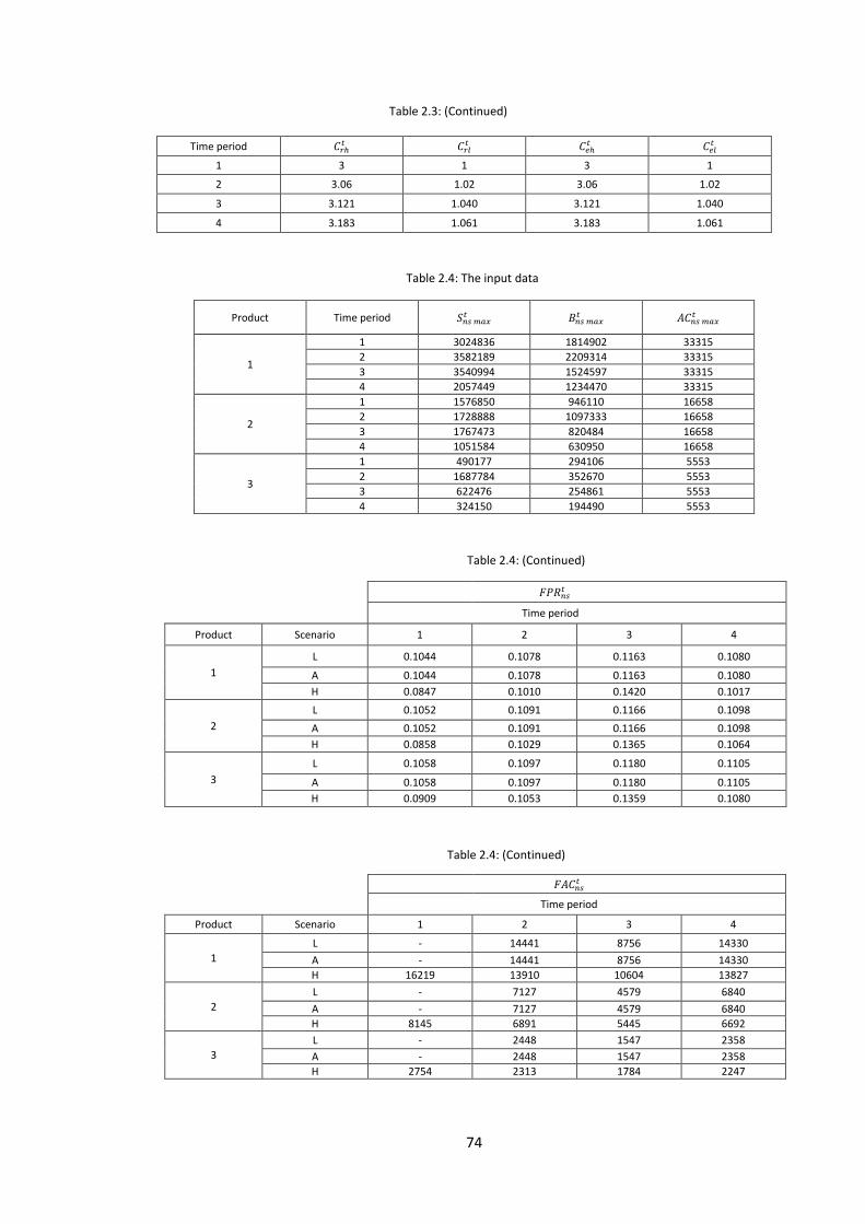
74
Product Time period 𝑆𝑛𝑠 𝑚𝑎𝑥𝑡 𝐵𝑛𝑠 𝑚𝑎𝑥
𝑡 𝐴𝐶𝑛𝑠 𝑚𝑎𝑥𝑡
1
1 3024836 1814902 33315
2 3582189 2209314 33315
3 3540994 1524597 33315
4 2057449 1234470 33315
2
1 1576850 946110 16658
2 1728888 1097333 16658
3 1767473 820484 16658
4 1051584 630950 16658
3
1 490177 294106 5553
2 1687784 352670 5553
3 622476 254861 5553
4 324150 194490 5553
𝐹𝑃𝑅𝑛𝑠
𝑡
Time period
Product Scenario 1 2 3 4
1
L 0.1044 0.1078 0.1163 0.1080
A 0.1044 0.1078 0.1163 0.1080
H 0.0847 0.1010 0.1420 0.1017
2
L 0.1052 0.1091 0.1166 0.1098
A 0.1052 0.1091 0.1166 0.1098
H 0.0858 0.1029 0.1365 0.1064
3
L 0.1058 0.1097 0.1180 0.1105
A 0.1058 0.1097 0.1180 0.1105
H 0.0909 0.1053 0.1359 0.1080
𝐹𝐴𝐶𝑛𝑠
𝑡
Time period
Product Scenario 1 2 3 4
1
L - 14441 8756 14330
A - 14441 8756 14330
H 16219 13910 10604 13827
2
L - 7127 4579 6840
A - 7127 4579 6840
H 8145 6891 5445 6692
3
L - 2448 1547 2358
A - 2448 1547 2358
H 2754 2313 1784 2247
Time period 𝐶𝑟ℎ𝑡 𝐶𝑟𝑙
𝑡 𝐶𝑒ℎ𝑡 𝐶𝑒𝑙
𝑡
1 3 1 3 1
2 3.06 1.02 3.06 1.02
3 3.121 1.040 3.121 1.040
4 3.183 1.061 3.183 1.061
Table 2.3: (Continued)
Table 2.4: The input data
Table 2.4: (Continued)
Table 2.4: (Continued)
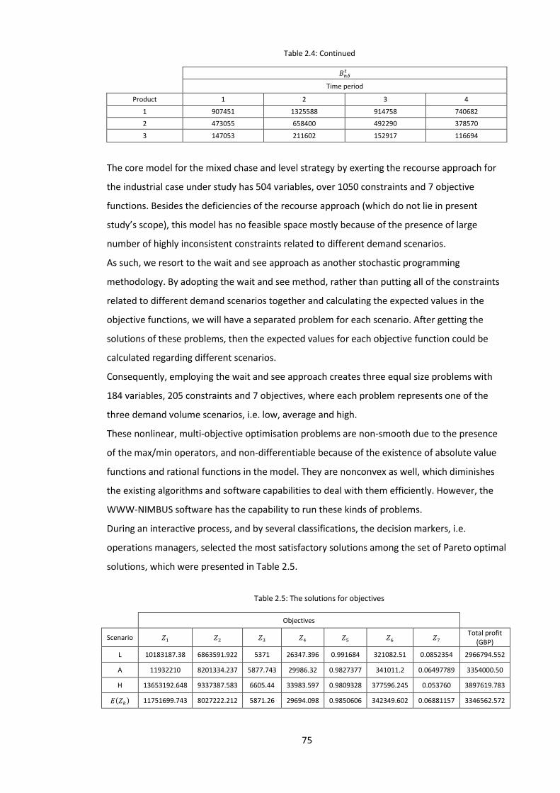
75
𝐵𝑛𝛿𝑡
Time period
Product 1 2 3 4
1 907451 1325588 914758 740682
2 473055 658400 492290 378570
3 147053 211602 152917 116694
The core model for the mixed chase and level strategy by exerting the recourse approach for
the industrial case under study has 504 variables, over 1050 constraints and 7 objective
functions. Besides the deficiencies of the recourse approach (which do not lie in present
study’s scope), this model has no feasible space mostly because of the presence of large
number of highly inconsistent constraints related to different demand scenarios.
As such, we resort to the wait and see approach as another stochastic programming
methodology. By adopting the wait and see method, rather than putting all of the constraints
related to different demand scenarios together and calculating the expected values in the
objective functions, we will have a separated problem for each scenario. After getting the
solutions of these problems, then the expected values for each objective function could be
calculated regarding different scenarios.
Consequently, employing the wait and see approach creates three equal size problems with
184 variables, 205 constraints and 7 objectives, where each problem represents one of the
three demand volume scenarios, i.e. low, average and high.
These nonlinear, multi-objective optimisation problems are non-smooth due to the presence
of the max/min operators, and non-differentiable because of the existence of absolute value
functions and rational functions in the model. They are nonconvex as well, which diminishes
the existing algorithms and software capabilities to deal with them efficiently. However, the
WWW-NIMBUS software has the capability to run these kinds of problems.
During an interactive process, and by several classifications, the decision markers, i.e.
operations managers, selected the most satisfactory solutions among the set of Pareto optimal
solutions, which were presented in Table 2.5.
Objectives
Scenario 𝑍1 𝑍2 𝑍3 𝑍4 𝑍5 𝑍6 𝑍7 Total profit
(GBP)
L 10183187.38 6863591.922 5371 26347.396 0.991684 321082.51 0.0852354 2966794.552
A 11932210 8201334.237 5877.743 29986.32 0.9827377 341011.2 0.06497789 3354000.50
H 13653192.648 9337387.583 6605.44 33983.597 0.9809328 377596.245 0.053760 3897619.783
𝐸(𝑍𝑘) 11751699.743 8027222.212 5871.26 29694.098 0.9850606 342349.602 0.06881157 3346562.572
Table 2.4: Continued
Table 2.5: The solutions for objectives
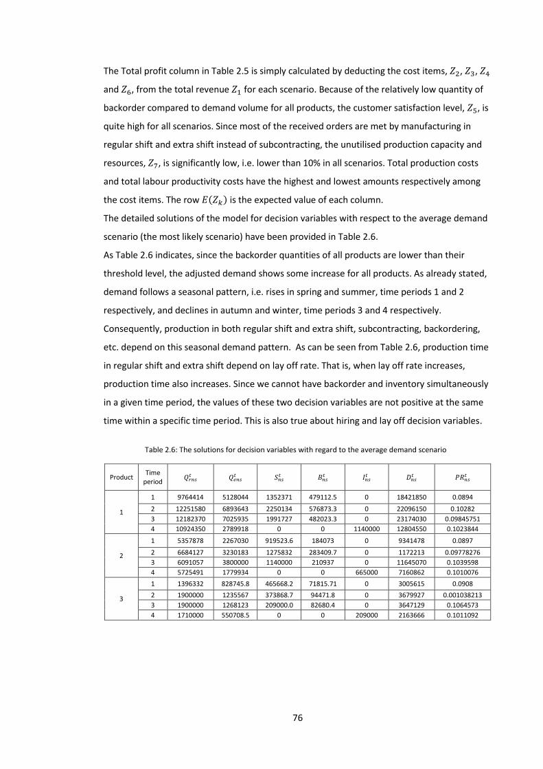
76
The Total profit column in Table 2.5 is simply calculated by deducting the cost items, 𝑍2, 𝑍3, 𝑍4
and 𝑍6, from the total revenue 𝑍1 for each scenario. Because of the relatively low quantity of
backorder compared to demand volume for all products, the customer satisfaction level, 𝑍5, is
quite high for all scenarios. Since most of the received orders are met by manufacturing in
regular shift and extra shift instead of subcontracting, the unutilised production capacity and
resources, 𝑍7, is significantly low, i.e. lower than 10% in all scenarios. Total production costs
and total labour productivity costs have the highest and lowest amounts respectively among
the cost items. The row 𝐸(𝑍𝑘) is the expected value of each column.
The detailed solutions of the model for decision variables with respect to the average demand
scenario (the most likely scenario) have been provided in Table 2.6.
As Table 2.6 indicates, since the backorder quantities of all products are lower than their
threshold level, the adjusted demand shows some increase for all products. As already stated,
demand follows a seasonal pattern, i.e. rises in spring and summer, time periods 1 and 2
respectively, and declines in autumn and winter, time periods 3 and 4 respectively.
Consequently, production in both regular shift and extra shift, subcontracting, backordering,
etc. depend on this seasonal demand pattern. As can be seen from Table 2.6, production time
in regular shift and extra shift depend on lay off rate. That is, when lay off rate increases,
production time also increases. Since we cannot have backorder and inventory simultaneously
in a given time period, the values of these two decision variables are not positive at the same
time within a specific time period. This is also true about hiring and lay off decision variables.
Product Time
period 𝑄𝑟𝑛𝑠𝑡 𝑄𝑒𝑛𝑠
𝑡 𝑆𝑛𝑠𝑡 𝐵𝑛𝑠
𝑡 𝐼𝑛𝑠𝑡 𝐷𝑛𝑠
𝑡 𝑃𝑅𝑛𝑠𝑡
1
1 9764414 5128044 1352371 479112.5 0 18421850 0.0894
2 12251580 6893643 2250134 576873.3 0 22096150 0.10282
3 12182370 7025935 1991727 482023.3 0 23174030 0.09845751
4 10924350 2789918 0 0 1140000 12804550 0.1023844
2
1 5357878 2267030 919523.6 184073 0 9341478 0.0897
2 6684127 3230183 1275832 283409.7 0 1172213 0.09778276
3 6091057 3800000 1140000 210937 0 11645070 0.1039598
4 5725491 1779934 0 0 665000 7160862 0.1010076
3
1 1396332 828745.8 465668.2 71815.71 0 3005615 0.0908
2 1900000 1235567 373868.7 94471.8 0 3679927 0.001038213
3 1900000 1268123 209000.0 82680.4 0 3647129 0.1064573
4 1710000 550708.5 0 0 209000 2163666 0.1011092
Table 2.6: The solutions for decision variables with regard to the average demand scenario
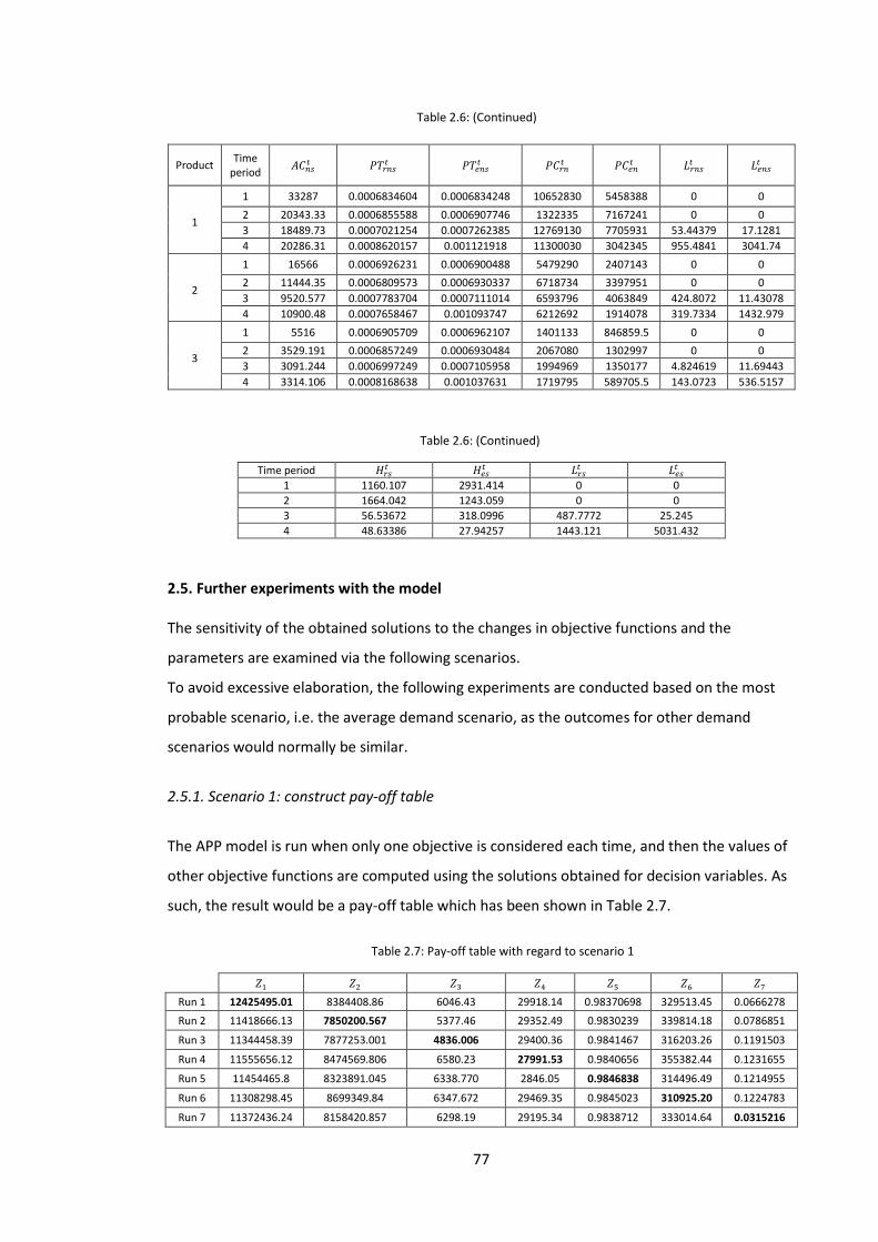
77
Product Time
period 𝐴𝐶𝑛𝑠
𝑡 𝑃𝑇𝑟𝑛𝑠𝑡 𝑃𝑇𝑒𝑛𝑠
𝑡 𝑃𝐶𝑟𝑛𝑡 𝑃𝐶𝑒𝑛
𝑡 𝐿𝑟𝑛𝑠𝑡 𝐿𝑒𝑛𝑠
𝑡
1
1 33287 0.0006834604 0.0006834248 10652830 5458388 0 0
2 20343.33 0.0006855588 0.0006907746 1322335 7167241 0 0
3 18489.73 0.0007021254 0.0007262385 12769130 7705931 53.44379 17.1281
4 20286.31 0.0008620157 0.001121918 11300030 3042345 955.4841 3041.74
2
1 16566 0.0006926231 0.0006900488 5479290 2407143 0 0
2 11444.35 0.0006809573 0.0006930337 6718734 3397951 0 0
3 9520.577 0.0007783704 0.0007111014 6593796 4063849 424.8072 11.43078
4 10900.48 0.0007658467 0.001093747 6212692 1914078 319.7334 1432.979
3
1 5516 0.0006905709 0.0006962107 1401133 846859.5 0 0
2 3529.191 0.0006857249 0.0006930484 2067080 1302997 0 0
3 3091.244 0.0006997249 0.0007105958 1994969 1350177 4.824619 11.69443
4 3314.106 0.0008168638 0.001037631 1719795 589705.5 143.0723 536.5157
Time period 𝐻𝑟𝑠
𝑡 𝐻𝑒𝑠𝑡 𝐿𝑟𝑠
𝑡 𝐿𝑒𝑠𝑡
1 1160.107 2931.414 0 0
2 1664.042 1243.059 0 0
3 56.53672 318.0996 487.7772 25.245
4 48.63386 27.94257 1443.121 5031.432
2.5. Further experiments with the model The sensitivity of the obtained solutions to the changes in objective functions and the
parameters are examined via the following scenarios.
To avoid excessive elaboration, the following experiments are conducted based on the most
probable scenario, i.e. the average demand scenario, as the outcomes for other demand
scenarios would normally be similar.
2.5.1. Scenario 1: construct pay-off table
The APP model is run when only one objective is considered each time, and then the values of
other objective functions are computed using the solutions obtained for decision variables. As
such, the result would be a pay-off table which has been shown in Table 2.7.
𝑍1 𝑍2 𝑍3 𝑍4 𝑍5 𝑍6 𝑍7
Run 1 12425495.01 8384408.86 6046.43 29918.14 0.98370698 329513.45 0.0666278
Run 2 11418666.13 7850200.567 5377.46 29352.49 0.9830239 339814.18 0.0786851
Run 3 11344458.39 7877253.001 4836.006 29400.36 0.9841467 316203.26 0.1191503
Run 4 11555656.12 8474569.806 6580.23 27991.53 0.9840656 355382.44 0.1231655
Run 5 11454465.8 8323891.045 6338.770 2846.05 0.9846838 314496.49 0.1214955
Run 6 11308298.45 8699349.84 6347.672 29469.35 0.9845023 310925.20 0.1224783
Run 7 11372436.24 8158420.857 6298.19 29195.34 0.9838712 333014.64 0.0315216
Table 2.6: (Continued)
Table 2.6: (Continued)
Table 2.7: Pay-off table with regard to scenario 1
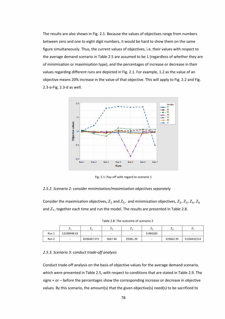
78
The results are also shown in Fig. 2.1. Because the values of objectives range from numbers
between zero and one to eight digit numbers, it would be hard to show them on the same
figure simultaneously. Thus, the current values of objectives, i.e. their values with respect to
the average demand scenario in Table 2.5 are assumed to be 1 (regardless of whether they are
of minimisation or maximisation type), and the percentages of increase or decrease in their
values regarding different runs are depicted in Fig. 2.1. For example, 1.2 as the value of an
objective means 20% increase in the value of that objective. This will apply to Fig. 2.2 and Fig.
2.3-a-Fig. 2.3-d as well.
2.5.2. Scenario 2: consider minimisation/maximisation objectives separately
Consider the maximisation objectives, 𝑍1 and 𝑍5, and minimisation objectives, 𝑍2, 𝑍3, 𝑍4, 𝑍6
and 𝑍7, together each time and run the model. The results are presented in Table 2.8.
𝑍1 𝑍2 𝑍3 𝑍4 𝑍5 𝑍6 𝑍7
Run 1 12248948.63 - - - 0.984265 - -
Run 2 - 8106467.071 5667.46 29381.39 - 319662.95 0.036432214
2.5.3. Scenario 3: conduct trade-off analysis
Conduct trade-off analysis on the basis of objective values for the average demand scenario,
which were presented in Table 2.5, with respect to conditions that are stated in Table 2.9. The
signs + or – before the percentages show the corresponding increase or decrease in objective
values. By this scenario, the amount(s) that the given objective(s) need(s) to be sacrificed to
Table 2.8: The outcome of scenario 2
Fig. 2.1: Pay-off with regard to scenario 1
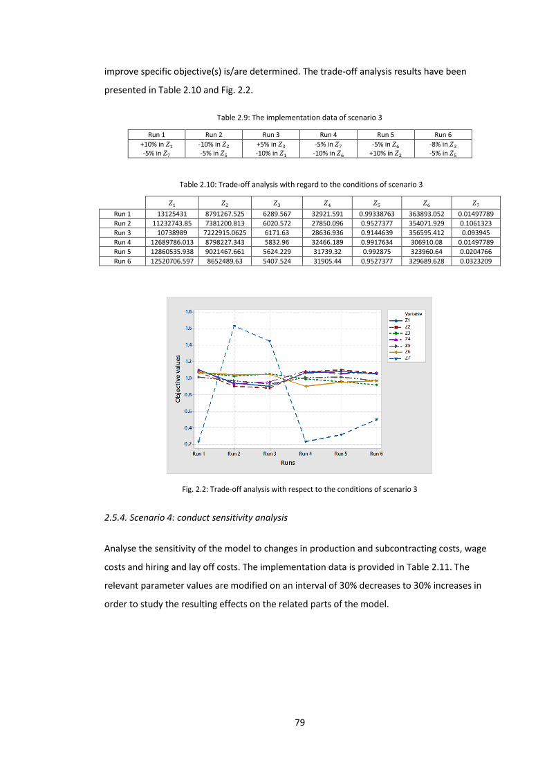
79
improve specific objective(s) is/are determined. The trade-off analysis results have been
presented in Table 2.10 and Fig. 2.2.
Run 1 Run 2 Run 3 Run 4 Run 5 Run 6
+10% in 𝑍1 -5% in 𝑍7
-10% in 𝑍2 -5% in 𝑍5
+5% in 𝑍3 -10% in 𝑍1
-5% in 𝑍7 -10% in 𝑍6
-5% in 𝑍6 +10% in 𝑍2
-8% in 𝑍3 -5% in 𝑍5
𝑍1 𝑍2 𝑍3 𝑍4 𝑍5 𝑍6 𝑍7
Run 1 13125431 8791267.525 6289.567 32921.591 0.99338763 363893.052 0.01497789
Run 2 11232743.85 7381200.813 6020.572 27850.096 0.9527377 354071.929 0.1061323
Run 3 10738989 7222915.0625 6171.63 28636.936 0.9144639 356595.412 0.093945
Run 4 12689786.013 8798227.343 5832.96 32466.189 0.9917634 306910.08 0.01497789
Run 5 12860535.938 9021467.661 5624.229 31739.32 0.992875 323960.64 0.0204766
Run 6 12520706.597 8652489.63 5407.524 31905.44 0.9527377 329689.628 0.0323209
2.5.4. Scenario 4: conduct sensitivity analysis
Analyse the sensitivity of the model to changes in production and subcontracting costs, wage
costs and hiring and lay off costs. The implementation data is provided in Table 2.11. The
relevant parameter values are modified on an interval of 30% decreases to 30% increases in
order to study the resulting effects on the related parts of the model.
Table 2.9: The implementation data of scenario 3
Table 2.10: Trade-off analysis with regard to the conditions of scenario 3
Fig. 2.2: Trade-off analysis with respect to the conditions of scenario 3
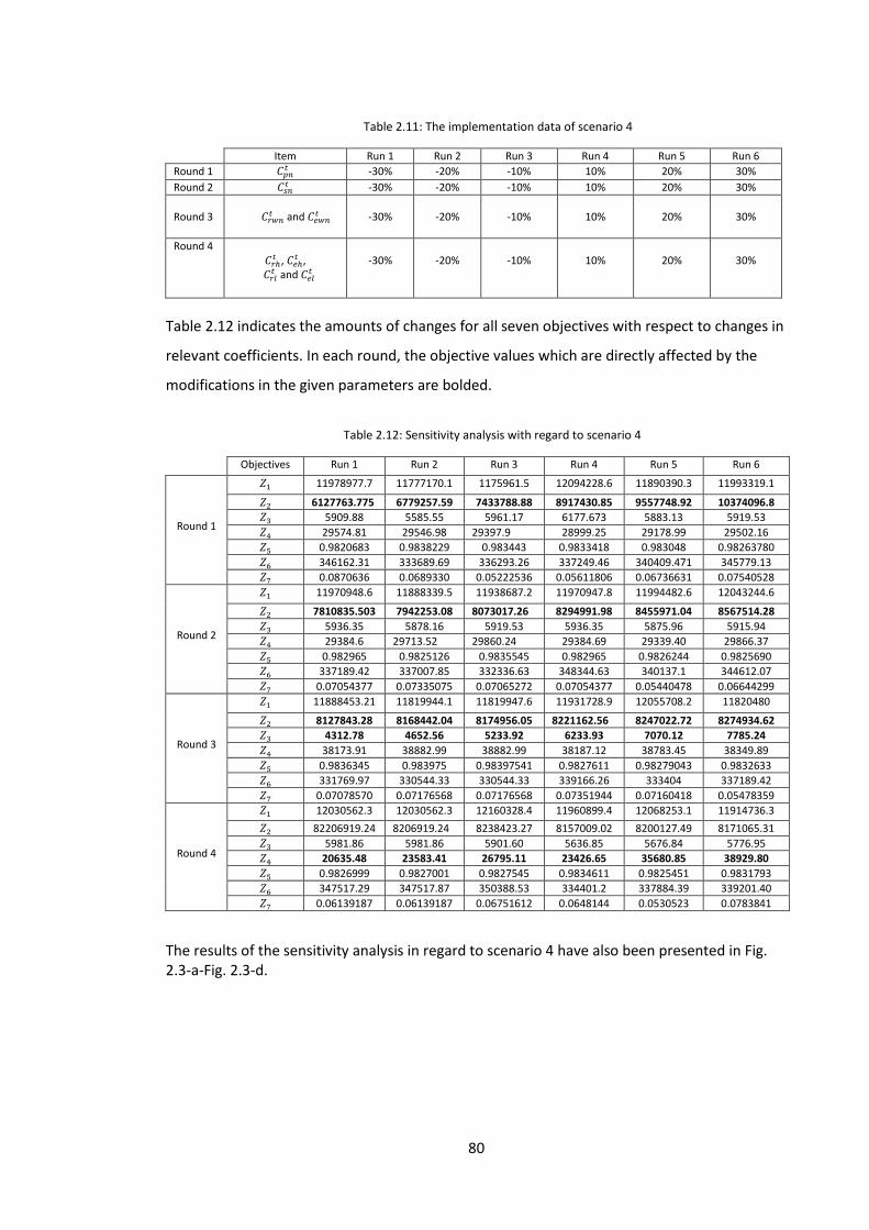
80
Item Run 1 Run 2 Run 3 Run 4 Run 5 Run 6
Round 1 𝐶𝑝𝑛𝑡 -30% -20% -10% 10% 20% 30%
Round 2 𝐶𝑠𝑛𝑡 -30% -20% -10% 10% 20% 30%
Round 3
𝐶𝑟𝑤𝑛
𝑡 and 𝐶𝑒𝑤𝑛𝑡
-30%
-20%
-10%
10%
20%
30%
Round 4 𝐶𝑟ℎ𝑡 , 𝐶𝑒ℎ
𝑡 , 𝐶𝑟𝑙
𝑡 and 𝐶𝑒𝑙𝑡
-30%
-20%
-10%
10%
20%
30%
Table 2.12 indicates the amounts of changes for all seven objectives with respect to changes in
relevant coefficients. In each round, the objective values which are directly affected by the
modifications in the given parameters are bolded.
Objectives Run 1 Run 2 Run 3 Run 4 Run 5 Run 6
Round 1
𝑍1 11978977.7 11777170.1 1175961.5 12094228.6 11890390.3 11993319.1
𝑍2 6127763.775 6779257.59 7433788.88 8917430.85 9557748.92 10374096.8
𝑍3 5909.88 5585.55 5961.17 6177.673 5883.13 5919.53
𝑍4 29574.81 29546.98 29397.9 28999.25 29178.99 29502.16
𝑍5 0.9820683 0.9838229 0.983443 0.9833418 0.983048 0.98263780
𝑍6 346162.31 333689.69 336293.26 337249.46 340409.471 345779.13
𝑍7 0.0870636 0.0689330 0.05222536 0.05611806 0.06736631 0.07540528
Round 2
𝑍1 11970948.6 11888339.5 11938687.2 11970947.8 11994482.6 12043244.6
𝑍2 7810835.503 7942253.08 8073017.26 8294991.98 8455971.04 8567514.28
𝑍3 5936.35 5878.16 5919.53 5936.35 5875.96 5915.94
𝑍4 29384.6 29713.52 29860.24 29384.69 29339.40 29866.37
𝑍5 0.982965 0.9825126 0.9835545 0.982965 0.9826244 0.9825690
𝑍6 337189.42 337007.85 332336.63 348344.63 340137.1 344612.07
𝑍7 0.07054377 0.07335075 0.07065272 0.07054377 0.05440478 0.06644299
Round 3
𝑍1 11888453.21 11819944.1 11819947.6 11931728.9 12055708.2 11820480
𝑍2 8127843.28 8168442.04 8174956.05 8221162.56 8247022.72 8274934.62
𝑍3 4312.78 4652.56 5233.92 6233.93 7070.12 7785.24
𝑍4 38173.91 38882.99 38882.99 38187.12 38783.45 38349.89
𝑍5 0.9836345 0.983975 0.98397541 0.9827611 0.98279043 0.9832633
𝑍6 331769.97 330544.33 330544.33 339166.26 333404 337189.42
𝑍7 0.07078570 0.07176568 0.07176568 0.07351944 0.07160418 0.05478359
Round 4
𝑍1 12030562.3 12030562.3 12160328.4 11960899.4 12068253.1 11914736.3
𝑍2 82206919.24 8206919.24 8238423.27 8157009.02 8200127.49 8171065.31
𝑍3 5981.86 5981.86 5901.60 5636.85 5676.84 5776.95
𝑍4 20635.48 23583.41 26795.11 23426.65 35680.85 38929.80
𝑍5 0.9826999 0.9827001 0.9827545 0.9834611 0.9825451 0.9831793
𝑍6 347517.29 347517.87 350388.53 334401.2 337884.39 339201.40
𝑍7 0.06139187 0.06139187 0.06751612 0.0648144 0.0530523 0.0783841
The results of the sensitivity analysis in regard to scenario 4 have also been presented in Fig. 2.3-a-Fig. 2.3-d.
Table 2.11: The implementation data of scenario 4
Table 2.12: Sensitivity analysis with regard to scenario 4
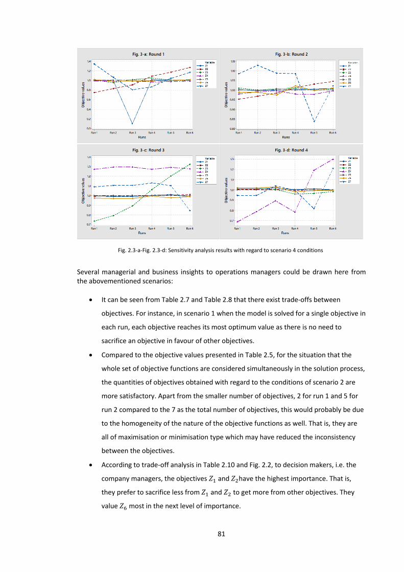
81
Several managerial and business insights to operations managers could be drawn here from the abovementioned scenarios:
It can be seen from Table 2.7 and Table 2.8 that there exist trade-offs between
objectives. For instance, in scenario 1 when the model is solved for a single objective in
each run, each objective reaches its most optimum value as there is no need to
sacrifice an objective in favour of other objectives.
Compared to the objective values presented in Table 2.5, for the situation that the
whole set of objective functions are considered simultaneously in the solution process,
the quantities of objectives obtained with regard to the conditions of scenario 2 are
more satisfactory. Apart from the smaller number of objectives, 2 for run 1 and 5 for
run 2 compared to the 7 as the total number of objectives, this would probably be due
to the homogeneity of the nature of the objective functions as well. That is, they are
all of maximisation or minimisation type which may have reduced the inconsistency
between the objectives.
According to trade-off analysis in Table 2.10 and Fig. 2.2, to decision makers, i.e. the
company managers, the objectives 𝑍1 and 𝑍2have the highest importance. That is,
they prefer to sacrifice less from 𝑍1 and 𝑍2 to get more from other objectives. They
value 𝑍6 most in the next level of importance.
Fig. 2.3-a-Fig. 2.3-d: Sensitivity analysis results with regard to scenario 4 conditions
82
As is evident from Table 2.12, the developed APP model is most sensitive to changes in
production costs 𝐶𝑝𝑛𝑡 , since the total production costs shows the biggest relative
changes from each run to another run accordingly.
Changes in subcontracting cost are also expected to have an impact on total
production costs with similar intensity compared to that of production costs. Due to
the relatively small quantity of the subcontracted orders, however, the magnitude of
the respective fluctuations in total production costs, as result of increase/decrease in
subcontracting costs, turns out to be much lower.
Variations in wage rates paid to workers in both regular shift and extra shift, 𝐶𝑟𝑤𝑛𝑡 and
𝐶𝑒𝑤𝑛𝑡 , correspondingly affect 𝑍2 and 𝑍3, i.e. total production costs and total labour
productivity costs. Although the values of the objective functions are chosen among a
set of Pareto-optimal solutions by the decision makers during several classifications, a
proportionate increase or decrease in their quantities are observed in response to
increase/decrease in wage rates.
A similar trend is seen for round 4 where fluctuations in costs of changes in workforce
level occur in accordance with variations in hiring and lay off costs, which have been
provided in detail in Table 2.12.
2.6. Conclusions and future research directions
This study proposed a novel stochastic, nonlinear, multi-stage, multi-objective decision making
model to APP based on mixed chase and level strategy which considers multiple objectives
such as total revenue, total production costs, total labour productivity costs, total costs of the
changes in workforce level and customer satisfaction subject to constraints on inventories,
backorders, subcontracting, workforce level, and so forth where the forecasted demand acts
as the main source of uncertainty.
The recourse approach of stochastic programming led to infeasible space due to the large
number of highly inconsistent constraints related to different demand scenarios. The wait and
see method, as another stochastic programming approach, was used instead.
The constructed stochastic, nonlinear, nonconvex, non-differentiable, multi-objective
optimisation model for the APP problem was solved using WWW-NIMBUS software. The
solution determined the optimal values of the production in regular shift and extra shift,
backorder, inventory, subcontracting, workforce hired and laid off in regular shift and extra
shift, product price, etc. over the planning horizon for the company under study in presence of
uncertainty.
83
Further experiments with the model were performed by sensitivity analysis via changing
different parameters of the model, and by different forms of trade-off analysis.
Several future research directions are recommended for APP, especially by utilising the
management science techniques:
i. Recourse approach as one of major stochastic programming approaches has a serious
drawback. The main shortcoming of this approach is that it considers all constraints
relating to different scenarios with equal probability (with certainty or P=1, where P
stands for the probability of associated scenarios) in constraints section of the
stochastic mathematical programming. In other words, it puts all the constraints
relating to different scenarios together, and solves the problem where the objective
function is the expected value regarding different scenarios. This does not sound true,
since when all constraints relating to different scenarios are put together in one
mathematical programming problem, it looks like all scenarios happen at the same
time with equal probabilities (with P=1 or certainty). A suitable methodology needs to
be developed to resolve this shortcoming.
ii. In this study, we assumed that the demand volume scenarios will be the same in all
consecutive time periods. That is, if, for example, demand quantity is high in first time
period, it will also be high in all future time periods. We made this assumption based
on our discussion with the company’s managers, where according to their long term
experience with customer demand in the company under study, they approved that
demand normally has similar mood in several consecutive time periods while
maintaining the seasonality pattern. However, this assumption could be invalid in
different cases, and needs to be taken into account in relevant APP models.
iii. APP problems modelled by multi-stage stochastic programming techniques, e.g.
Markov decision process would normally need to deal with the curse of dimensionality
due to rather large scale of real world APP decision problems. One of the efficient
methods to handle this issue can be Monte Carlo methods employed within the
reinforcement learning structure to find the optimal actions in each stage by
maximising the reward (profit).
iv. Aggregate production planners have traditionally been doing APP for the sake of
maximising profit without properly taking into account the sustainability aspects, e.g.
workers mental and physical health regarding workloads as the result of operating in
overtime and multiple shifts, increased workplace incidents/injuries due to excessive
overtime and nightshifts, negative psychological effects of frequent hiring and lay off
84
on employees, greenhouse gas emissions, declined customer satisfaction level because
of regular backordering, and so forth. Very little research has been conducted on APP
with regard to sustainability factors. Therefore, these sustainability dimensions need
to be systematically incorporated into analytical models of APP, e.g. simulation
models, mathematical models, etc. in order to develop a decision making framework
which is more consistent with contemporary operations management requirements.
v. The outlook for Big Data driven approaches to APP particularly in larger manufacturing
corporations, e.g. big car producing companies, airplane manufacturing corporations,
etc. in order to provide decision support systems which have specific utilities in
production planning and control activities, would be a promising area of research.
85
References Buxey, G. (1990). ‘The myth of aggregate planning’, Production Planning & Control, 1 (4), pp.222-234. Buxey, G. (1995). ‘A managerial perspective on aggregate planning’, International Journal of Production Economics, 41 (1-3), pp. 127–133. Buxey, G. (2003). ‘Strategy not tactics drives aggregate planning’, International Journal of Production Economics, 85(3), pp. 331–346. Buxey, G. (2005). ‘Aggregate planning for seasonal demand: reconciling theory with practice’, International Journal of Operations and Production Management, 25 (11), pp. 1083–1100. Chen, Y.K. and Liao, H.C. (2003). ‘An investigation on selection of simplified aggregate production planning strategies using MADM approaches’, International Journal of Production Research, 41(14), pp. 3359–3374. Günther, H.O. (1982). ‘A comparison of two classes of aggregate production planning models under stochastic demand’, Engineering Costs and Production Economics, 6(1), pp. 89-97. Heizer, J. and Render, B. (2001). Production and operations management: strategic and tactical decisions. Upper Saddle River, NJ: Prentice Hall. Huselin, M.A. (1998). The impact of human resource management practices on turnover, productivity, and corporate financial performance, in Mabey, C., Salaman, G. and Storey, J. (eds.) Strategic human resource management: a reader. London: Sage, pp. 104–127. Jamalnia, A. and Feili, A. (2013). ‘A simulation testing and analysis of aggregate production planning strategies’, Production Planning & Control, 24(6), pp. 423-448. Kher, H.V., Malhotra, M.K., Philipoom, P.R. and Fry, T.D. (1999). ‘Modelling simultaneous worker learning and forgetting in dual recourse constrained systems’, European Journal of Operational Research, 115(1), pp. 158–172. Kleindorfer, P. and Kunreuther, H. (1978). ‘Stochastic Horizons for the Aggregate Planning Problem’, Management Science, 24(5), pp. 485-497. Leung, S.C.H., Wu, Y. and Lai, K.K. (2006). ‘A stochastic programming approach for multi-site aggregate production planning’, Journal of the Operational Research Society, 57(2), pp. 123-132. Li, G. and Rajagopalan, S. (1998). ‘A learning curve model with knowledge depreciation’, European Journal of Operational Research, 105(1), pp. 143–154. Lieckens, K. and Vandaele, N. (2014). A decision support system for the stochastic aggregate planning problem: March 28 2014. Available at: http://ssrn.com/abstract=2419376 (Accessed 20 March 2016). Lockett, A.G. and Muhlemann, A.P. (1978). ‘A stochastic programming model for aggregate production planning’, European Journal of Operational Research, 2(5), pp. 350-356. Miettinen, K. and Mäkelä, M.M. (2006). ‘Synchronous Approach in Interactive Multi-objective Optimization’, European Journal of Operational Research, 170(3), pp. 909-922. Mirzapour Al-e-hashem, S.M.J., Baboli, A. and Sazvar, Z. (2013). ‘A stochastic aggregate production planning model in a green supply chain: Considering flexible lead times, nonlinear purchase and shortage cost functions’, European Journal of Operational Research, 230(1), pp. 26-41. Ning, Y., Liu, J. and Yan, L. (2013). ‘Uncertain aggregate production planning’, Soft Computing, 17(4), pp. 617-624. Nowak, M. (2013). ‘An interactive procedure for aggregate production planning’, Croatian Operational Research Review, 4(1), pp. 247-57. Piper, C.J. and Vachon, S. (2001). ‘Accounting for productivity losses in aggregate planning’, International Journal of Production Research, 39 (17), pp. 4001–4012.
86
Rakes, T.R., Franz, L.S. and Wynne, A.J. (1984). ‘Aggregate production planning using chance-constrained goal programming’, International Journal of Production Research, 22(4), pp. 673-684. Reid, R.D. and Sanders., N.R. (2002). Operations management. New York: John Wiley and Sons. Schroeder, R.G. (2003). Operations management, contemporary concepts and cases. New York: McGraw-Hill. Slack, N., Chambers, S. and Johnston, R. (2007). Operations management. Essex: FT Prentice Hall. Stevenson, W.J. (2005). Operations Management. New York: McGraw-Hill. Thomas, L.J. and McClain, J.O. (1993). An overview of production planning, in Grave, S.G., Rinnooy Kan, A.H.G. and Zipkin, P.H. (eds.) Logistics of production and inventory. Amsterdam: North-Holland, pp. 333–370. Thompson, S.D., Wantanabe, D.T. and Davis, W.J. (1993). ‘A comparative study of aggregate production planning strategies under conditions of uncertainty and cyclic product demands’, International Journal of Production Research, 31(8), pp. 1957–1979. Vörös, J. (1999). ‘On the risk-based aggregate planning for seasonal products’, International Journal of Production Economics, 59(1-3), pp. 195-201.

87
PAPER 3
Title: Evaluating the performance of aggregate production planning strategies under uncertainty
PAGE: 87
88
Evaluating the performance of aggregate production planning strategies under uncertainty
Abstract: The current study builds upon the paper 2 by developing four extra aggregate
production planning (APP) models to different APP strategies other than the mixed chase and
level strategy. These models are derived from the fundamental APP model that was proposed
for the mixed chase and level strategy in paper 2. Therefore, the relevant models for APP
strategies including the pure chase, the pure level, the modified chase and the modified level
strategies are taken from the basic model developed for the mixed chase and level strategy.
The same procedure, as described in paper 2, follows to solve the models constructed for
these strategies with respect to the corresponding objectives/criteria in order to provide
business insights to operations managers about the effectiveness and practicality of various
APP policies in presence of uncertainty.
Multiple criteria decision making (MCDM) methods such as additive value function (AVF), the
technique for order of preference by similarity to ideal solution (TOPSIS) and VIKOR are also
used besides multi-objective optimisation to assess the overall performance of each APP
strategy. The pure chase and the modified chase strategies show the best performance in
general, followed by the pure level strategy.
A detailed sensitivity analysis is also conducted by changing the weights assigned to different
criteria in abovementioned MCDM methods to evaluate the impacts that these weight
changes can have on the final rank of each APP strategy.
Keywords: Aggregate production planning (APP); Strategy; Uncertainty; Model.
3.1. Introduction
3.1.1. General overview
Aggregate production planning (APP) is a medium range production and employment planning
that normally spans a time horizon which ranges from 3 to 18 months and is about
determining the optimum production quantities, hiring and lay off rates, work force and
inventory levels, backordering and subcontracting volumes, and so on for each time period
within the planning horizon subject to the limitations of available production resources. Such
planning technique typically involves one product or a family of similar products, i.e. products
with similarities in production process, skills required, materials needed, etc. despite minor
differences so that considering the problem from an aggregated viewpoint is still valid.
89
APP has attracted considerable attention from both practitioners and academia (Shi & Haase,
1996). Since 1955 that the pioneering studies by Holt et al. (1955) and Holt et al. (1956)
proposed linear decision rule, and Bowman (1956) suggested transportation method to deal
with APP, researchers have developed different methodologies to handle the APP problem.
Fig. 3.1, as already presented in paper 1, outlines the APP position among other types of
production planning and control techniques, and their interconnected relationships from a
holistic perspective. As can be seen from the Fig. 3.1, in the hierarchy of production planning
activities, APP falls between long-term strategic planning decisions such as new product
development and short term shop floor scheduling practices.
The forecasted demand acts as the driving force of the APP system. Seasonal demand patterns
together with unpredictability inherent in quantity and timing of received orders makes the
whole APP system uncertain, which in turn recommends utilising a decision modelling tool that
takes account of these uncertainties.
As such, due to the dynamic nature of APP and instable states of real world industrial
environments, the deterministic models for APP would lead to unrobust decisions.
Moreover, similar to other production planning family members, APP also involves several
objectives/criteria in practice.
Therefore, the present study utilises a novel stochastic, nonlinear, multi-stage, multi-objective
decision making model of APP which considers multiple objectives such as total revenue, total
production costs, total labour productivity costs, total costs of the changes in workforce level
and customer satisfaction subject to bounds on inventory, backorder, subcontracting,
workforce level, and so forth under uncertainty.
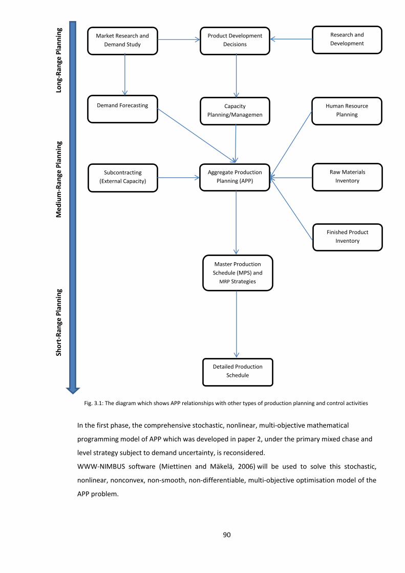
90
In the first phase, the comprehensive stochastic, nonlinear, multi-objective mathematical
programming model of APP which was developed in paper 2, under the primary mixed chase and
level strategy subject to demand uncertainty, is reconsidered.
WWW-NIMBUS software (Miettinen and Mäkelä, 2006) will be used to solve this stochastic,
nonlinear, nonconvex, non-smooth, non-differentiable, multi-objective optimisation model of the
APP problem.
Market Research and
Demand Study
Demand Forecasting
Product Development
Decisions
Research and
Development
Capacity
Planning/Managemen
t
Human Resource
Planning
Aggregate Production
Planning (APP)
Raw Materials
Inventory
Finished Product
Inventory
Subcontracting
(External Capacity)
Master Production
Schedule (MPS) and
MRP Strategies
Detailed Production
Schedule
Lon
g-R
ange
Pla
nn
ing
M
ediu
m-R
ange
Pla
nn
ing
Sho
rt-R
ange
Pla
nn
ing
Fig. 3.1: The diagram which shows APP relationships with other types of production planning and control activities
91
Then, the relevant models for other APP strategies including the pure chase, the pure level, the
modified chase and the modified level are derived from the fundamental model developed for the
mixed chase and level strategy. The same procedure, as described above, follows to solve the
models constructed for these strategies with respect to the aforementioned objectives/criteria to
provide managerial and business insights for operations managers about the effectiveness and
usefulness of various APP policies.
Additive value function (AVF), the technique for order of preference by similarity to ideal solution
(TOPSIS) and VIKOR, as multiple criteria decision making (MCDM) methods, are also utilised in
addition to multi-objective optimisation to evaluate the overall performance of each APP plan.
The paper is further organised as follows. In next two parts the regular APP options and policies
are explained, and then the problem under study is described. Section 3.2 briefly reviews the
most relevant literature; the research gaps are also considered in this section. Model
development together with the notations is presented in Section 3.3. In Section 3.4, models are
developed, and run for various APP strategies. In Section 3.5, APP strategies are analysed in detail
by applying MCDM methods, and finally the conclusions and possible future research extensions
are presented in Section 3.6.
3.1.2. Common APP options and strategies
The common APP options and policies were already detailed in Section 2.1.2 in paper 2.
3.1.3. Problem statement
The problem under study was fully described in Section 2.1.3 in paper 2.
The present research objective is to appraise different APP strategies’ performance under
uncertainty. Main research questions are:
Which APP strategies are more effective and useful with regard to relevant criteria under
uncertainty?
What are the advantages/disadvantages of different kinds of APP policies? In which
conditions these strategies perform optimally?
With regard to each APP strategy, what are the optimal values of the production in
regular shift and extra shift, backorder and inventory level, subcontracting, workforce
hired and laid off in regular shift and extra shift, product price, and so forth over the
planning horizon for the company under study in presence of uncertainty?
92
3.2. Literature review
The literature on stochastic mathematical programming methods to APP was reviewed in detail in
part 2.2 of paper 2, and thus the research about appraising APP policies is shortly overviewed in
this section.
3.2.1. Literature on appraising APP policies
The studies on evaluating the relevant APP policies which range from surveys to quantitative
management science-based methods include Lee and Khumawala (1974), Dubois and Oliff (1991),
Buxey (1990, 1995, 2003, 2005), Thompson et al. (1993), Chen and Liao (2003), Gulsun et al.
(2009) and Jamalnia and Feili ( 2013).
Through simulating the activities of an operating firm, Lee and Khumawala (1974) assessed the
performance of four different APP policies under demand uncertainty. Dubois and Oliff (1991)
surveyed a cross section of manufacturers about present practices of APP. Using input from
practitioners and academicians a questionnaire was developed to examine strategies that the firm
uses to deal with short range and long range demand fluctuations, major inputs to APP decisions,
etc.
Buxey (1990, 1995, 2003, 2005) conducted surveys in groups of Australian firms in different
industries to find out which APP policies are the most widely used in practice.
Thompson et al. (1993) developed linear programming frameworks to evaluate several APP
policies where customer demand, most of the coefficients of the linear programming model and
some parameters were presented with probability distributions to reflect the uncertainty in APP
environment. Chen and Liao (2003) adopted a multi-attribute decision making approach to select
the most efficient APP strategy such that selling price, market demand, cost coefficients, etc. are
assumed to be stochastic variables
Gulsun et al. (2009) developed a deterministic multi-objective optimisation model for APP which
is used as a basis to select the most appropriate APP strategy. Jamalnia and Feili (2013) employed
an integrated system dynamics and discrete-event simulation approach in order to evaluate the
effectiveness and practicality of different APP strategies on the basis of total profit measure,
where the market demand was regarded as random variable.
93
3.2.3. Research gaps in the literature
The research gaps in existing literature on examining the effectiveness and usefulness of different
APP strategies are discussed chronologically in this section, together with the motives behind
doing the present research:
a) The APP methods examined in the study performed by Lee and Khumawala (1974), used
to be among the very early methodologies proposed to deal with APP, but they are
currently regarded as conventional approaches to handle APP decision process that are
no longer in use. The newer trends in the past decades on developing novel approaches
and methodologies to deal with APP demand utilising corresponding state of the art APP
policies.
b) Studies conducted by Buxey (1990, 1995, 2003, 2005) and Dubois and Oliff (1991) have
drawbacks in common.
First, these studies were surveys in specific geographical areas, and their results only
represent the popularity of using relevant APP policies/strategies from the respondents’
viewpoints, e.g. from operations managers viewpoints in those geographical locations,
while the APP strategies employed by the industry managers may not necessarily be the
optimal ones.
Second, these categories of studies provide results that can hardly be generalised for
other geographical locations.
And third, the results have not been achieved by using an efficient analytical method
based on suitable criteria, and only presents managers’ responses on most widely used
APP policies.
c) Researches performed by Thompson et al. (1993) and Chen and Liao (2003) have several
major shortcomings in common that cast serious doubts on the accuracy of the obtained
results.
The option of varying the workforce level to meet the fluctuating demand is not
considered in their constructed mathematical programming model at all, and using the
overtime is considered as the only way to make changes in production capacity, whereas
changing the labour force level has always been regarded as a fundamental alternative to
the chase strategy in operations management literature.
94
Furthermore, the subcontracting option, as one of key options for level strategy, is totally
ignored in their proposed mathematical programming model.
In addition, the six APP strategies which were assessed in their study, to some extent, fall
into the pure chase and the pure level strategies scopes in current research, and
therefore do not match other three popular APP strategies.
Finally, the descriptions and characteristics of the APP strategies examined in
aforementioned studies seem quite inconsistent with common definitions and natures of
those APP strategies, and are conceptually and technically inaccurate. For example, in
mathematical equations defined for the chase strategies, they put the production volume
(in regular time and overtime) equal to demand volume but as mentioned above, the
hiring and lay off, as fundamental options in chase strategies, are not allowed in their
models. Apart from conceptual inaccuracy, regarding the limitations of production in
overtime by current workforce, this would make the model infeasible since by common
definition of chase strategies, backorder and inventory, as options to meet the demand,
are not permitted, or very limited quantities of backorder and inventory are permitted.
d) The research conducted by Gulsun et al. (2009) which is extension of the research
performed by Chen and Liao (2003) also contains similar flaws which were detailed above
in the last two paragraphs of section c. Furthermore, they define an objective function to
represent the workers motivation decline due to hiring and lay off but that objective does
not connect the hiring and lay off to workers motivation decline at all, and more
resembles total costs of hiring and lay off.
e) Jamalnia and Feili (2013) previously compared the effectiveness of various APP strategies
by applying a simulation modelling approach. But, to avoid the excessive complexity of
the model, they made the comparison between different APP strategies on the basis of a
single criterion, i.e. total profit.
Taking into account other criteria like workforce productivity costs, costs of changes in
workforce level, utilisation of production resources and capacity and customer
satisfaction besides total profit would present a wide-ranging appraisal of APP strategies.
The current study will provide a comprehensive evaluation of APP strategies performance by
overcoming the limitations discussed above.
Table 3.1 presents the comparison between existing researches on appraising the APP policies.
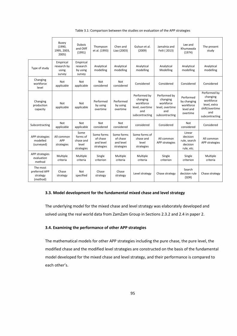
95
Table 3.1: Comparison between the studies on evaluation of the APP strategies
Buxey (1990,
1995, 2003, 2005)
Dubois and Oliff (1991)
Thompson et al. (1993)
Chen and Liao (2003)
Gulsun et al. (2009)
Jamalnia and Feili ( 2013)
Lee and Khumawala
(1974)
The present study
Type of study
Empirical research by
using survey
Empirical research by using survey
Analytical modelling
Analytical modelling
Analytical modelling
Analytical Modelling
Analytical modelling
Analytical modelling
Changing workforce
level
Not applicable
Not applicable
Not considered
Not considered
Considered Considered Considered Considered
Changing production
capacity
Not applicable
Not applicable
Performed by using overtime
Performed by using overtime
Performed by changing
workforce level, overtime
and subcontracting
Performed by changing
workforce level, overtime
and subcontracting
Performed by changing workforce level and overtime
Performed by changing
workforce level, extra
shift/overtime and
subcontracting
Subcontracting Not
applicable Not
applicable Not
considered Not
considered considered Considered
Not considered
Considered
APP strategies modelled (surveyed)
All common APP
strategies
Some forms of
chase and level
strategies
Some forms of chase and level strategies
Some forms of chase and level strategies
Some forms of chase and
level strategies
All common APP strategies
Linear decision
rule, search decision rule, etc.
All common APP strategies
APP strategies evaluation
method
Multiple criteria
Multiple criteria
Single criterion
Multiple criteria
Multiple criteria
Single criterion
Single criterion
Multiple criteria
The most preferred APP
strategy (method)
Chase strategy
Not specified
Chase strategy
Chase strategy
Level strategy Chase strategy Search
decision rule (SDR)
Chase strategy
3.3. Model development for the fundamental mixed chase and level strategy
The underlying model for the mixed chase and level strategy was elaborately developed and
solved using the real world data from ZamZam Group in Sections 2.3.2 and 2.4 in paper 2.
3.4. Examining the performance of other APP strategies
The mathematical models for other APP strategies including the pure chase, the pure level, the
modified chase and the modified level strategies are constructed on the basis of the fundamental
model developed for the mixed chase and level strategy, and their performance is compared to
each other’s.
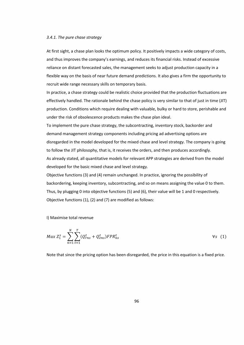
96
3.4.1. The pure chase strategy
At first sight, a chase plan looks the optimum policy. It positively impacts a wide category of costs,
and thus improves the company’s earnings, and reduces its financial risks. Instead of excessive
reliance on distant forecasted sales, the management seeks to adjust production capacity in a
flexible way on the basis of near future demand predictions. It also gives a firm the opportunity to
recruit wide range necessary skills on temporary basis.
In practice, a chase strategy could be realistic choice provided that the production fluctuations are
effectively handled. The rationale behind the chase policy is very similar to that of just in time (JIT)
production. Conditions which require dealing with valuable, bulky or hard to store, perishable and
under the risk of obsolescence products makes the chase plan ideal.
To implement the pure chase strategy, the subcontracting, inventory stock, backorder and
demand management strategy components including pricing ad advertising options are
disregarded in the model developed for the mixed chase and level strategy. The company is going
to follow the JIT philosophy, that is, it receives the orders, and then produces accordingly.
As already stated, all quantitative models for relevant APP strategies are derived from the model
developed for the basic mixed chase and level strategy.
Objective functions (3) and (4) remain unchanged. In practice, ignoring the possibility of
backordering, keeping inventory, subcontracting, and so on means assigning the value 0 to them.
Thus, by plugging 0 into objective functions (5) and (6), their value will be 1 and 0 respectively.
Objective functions (1), (2) and (7) are modified as follows:
I) Maximise total revenue
𝑀𝑎𝑥 𝑍1𝑠 = ∑∑(𝑄𝑟𝑛𝑠
𝑡 + 𝑄𝑒𝑛𝑠𝑡 )𝐹𝑃𝑅𝑛𝑠
𝑡
𝑇
𝑡=1
𝑁
𝑛=1
∀𝑠 (1)
Note that since the pricing option has been disregarded, the price in this equation is a fixed price.
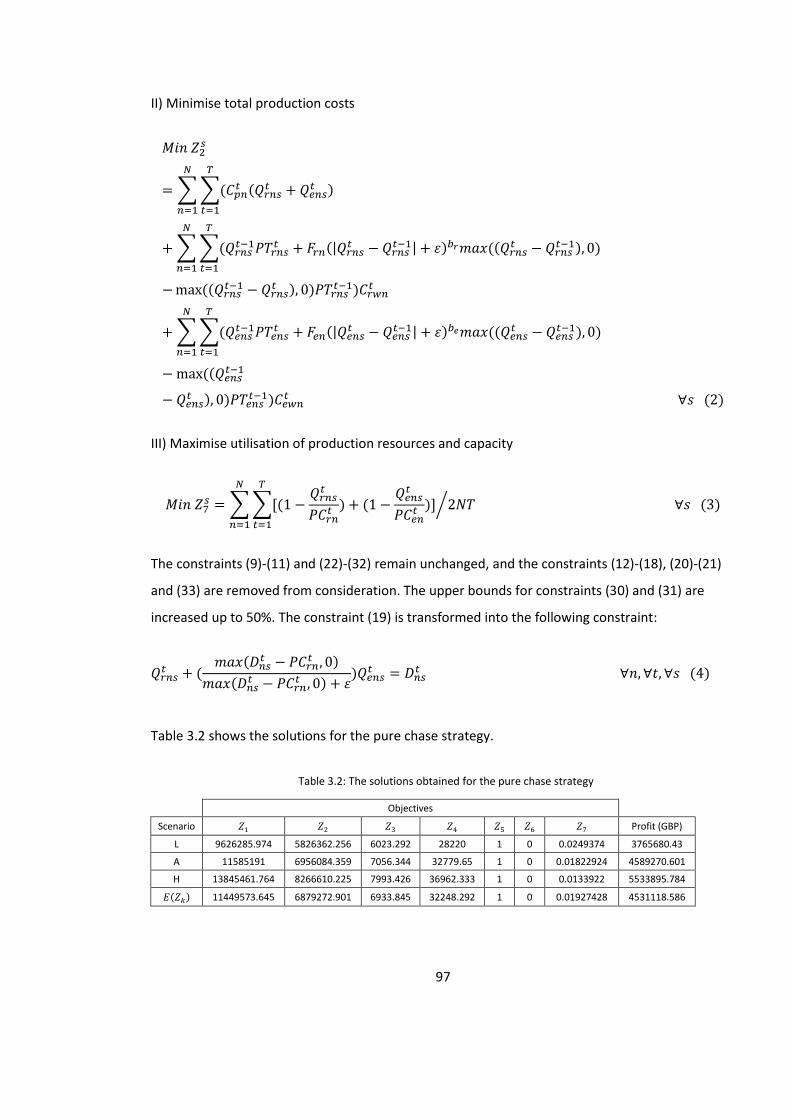
97
II) Minimise total production costs
𝑀𝑖𝑛 𝑍2
𝑠
= ∑∑(𝐶𝑝𝑛𝑡 (𝑄𝑟𝑛𝑠
𝑡 + 𝑄𝑒𝑛𝑠𝑡 )
𝑇
𝑡=1
𝑁
𝑛=1
+∑∑(𝑄𝑟𝑛𝑠𝑡−1𝑃𝑇𝑟𝑛𝑠
𝑡 + 𝐹𝑟𝑛(|𝑄𝑟𝑛𝑠𝑡 − 𝑄𝑟𝑛𝑠
𝑡−1| + 𝜀)𝑏𝑟𝑚𝑎𝑥 ((𝑄𝑟𝑛𝑠𝑡 − 𝑄𝑟𝑛𝑠
𝑡−1), 0)
𝑇
𝑡=1
𝑁
𝑛=1
−max ((𝑄𝑟𝑛𝑠𝑡−1 − 𝑄𝑟𝑛𝑠
𝑡 ), 0)𝑃𝑇𝑟𝑛𝑠𝑡−1)𝐶𝑟𝑤𝑛
𝑡
+∑∑(𝑄𝑒𝑛𝑠𝑡−1𝑃𝑇𝑒𝑛𝑠
𝑡 + 𝐹𝑒𝑛(|𝑄𝑒𝑛𝑠𝑡 − 𝑄𝑒𝑛𝑠
𝑡−1| + 𝜀)𝑏𝑒𝑚𝑎𝑥 ((𝑄𝑒𝑛𝑠𝑡 − 𝑄𝑒𝑛𝑠
𝑡−1), 0)
𝑇
𝑡=1
𝑁
𝑛=1
−max ((𝑄𝑒𝑛𝑠𝑡−1
− 𝑄𝑒𝑛𝑠𝑡 ), 0)𝑃𝑇𝑒𝑛𝑠
𝑡−1)𝐶𝑒𝑤𝑛𝑡 ∀𝑠 (2)
III) Maximise utilisation of production resources and capacity
𝑀𝑖𝑛 𝑍7𝑠 = ∑∑[(1 −
𝑄𝑟𝑛𝑠𝑡
𝑃𝐶𝑟𝑛𝑡
𝑇
𝑡=1
𝑁
𝑛=1
) + (1 −𝑄𝑒𝑛𝑠𝑡
𝑃𝐶𝑒𝑛𝑡 )] 2𝑁𝑇⁄ ∀𝑠 (3)
The constraints (9)-(11) and (22)-(32) remain unchanged, and the constraints (12)-(18), (20)-(21)
and (33) are removed from consideration. The upper bounds for constraints (30) and (31) are
increased up to 50%. The constraint (19) is transformed into the following constraint:
𝑄𝑟𝑛𝑠𝑡 + (
𝑚𝑎𝑥(𝐷𝑛𝑠𝑡 − 𝑃𝐶𝑟𝑛
𝑡 , 0)
𝑚𝑎𝑥(𝐷𝑛𝑠𝑡 − 𝑃𝐶𝑟𝑛
𝑡 , 0) + 𝜀)𝑄𝑒𝑛𝑠
𝑡 = 𝐷𝑛𝑠𝑡 ∀𝑛, ∀𝑡, ∀𝑠 (4)
Table 3.2 shows the solutions for the pure chase strategy.
Objectives
Scenario 𝑍1 𝑍2 𝑍3 𝑍4 𝑍5 𝑍6 𝑍7 Profit (GBP)
L 9626285.974 5826362.256 6023.292 28220 1 0 0.0249374 3765680.43
A 11585191 6956084.359 7056.344 32779.65 1 0 0.01822924 4589270.601
H 13845461.764 8266610.225 7993.426 36962.333 1 0 0.0133922 5533895.784
𝐸(𝑍𝑘) 11449573.645 6879272.901 6933.845 32248.292 1 0 0.01927428 4531118.586
Table 3.2: The solutions obtained for the pure chase strategy
98
As can be seen from Table 3.2, total expected revenue and total expected production costs, 𝐸(𝑍1)
and 𝐸(𝑍2) respectively, are lower than that of mixed chase and level strategy because the
demand management policy embedded in the mixed chase and level strategy causes an increase
in adjusted demand quantity, and therefore increase in the sales quantity and total production
costs accordingly. But, the lesser decrease in total expected revenue, 2.57%, compared to the
expected proportionate decrease which is seen in total expected production costs, 14.30%, is due
to the lowered prices in the mixed chase and level strategy case that are lower than the fixed
prices, 𝐹𝑃𝑅𝑛𝑠𝑡 , as result of applying the pricing policy. A part of the decrease in total production
costs would also be attributed to the lower costs of producing in regular shift and extra shift
compared to subcontracting costs which has been discarded in current operations strategy.
As is expected, the pure chase strategy has resulted in higher costs of changes in labour force
level and costs related to human resource productivity and their corresponding expected values,
i.e. 𝐸(𝑍3) and 𝐸(𝑍4). However, the amount of this rise might not be as much as expected
because the demand adjustment mechanism applied with the mixed chase and level strategy
would have a contribution in unsmoothing the demand level which in turn will cause higher rates
of hiring and lay off.
Pure chase strategy tries to meet the market demand solely by producing in regular shift and
extra shift, and adjusting the manufacturing capacity by varying the workforce level. Therefore, it
has much better performance in utilising the company’s production capacity and resources, which
is approved by very small percentage of unutilised production resources/capacities in 𝐸(𝑍7).
The pure chase plan presents a significantly higher expected profit in comparison with the basic
mixed strategy.
Although, the mixed chase and level strategy contributes to revenue/sales growth but as stated
above, at the same time the price reductions due to the lower volumes of the backorders
neutralise a portion of sales growth impact on total revenue. On the other side, the increase in
demand causes a corresponding increase in production, and thus total production costs. In
addition to these factors, ignoring the 𝑍6, total inventory carrying, backordering and advertising
costs, explains the higher total profit for the pure chase strategy despite the slight increases in 𝑍3
and 𝑍4.
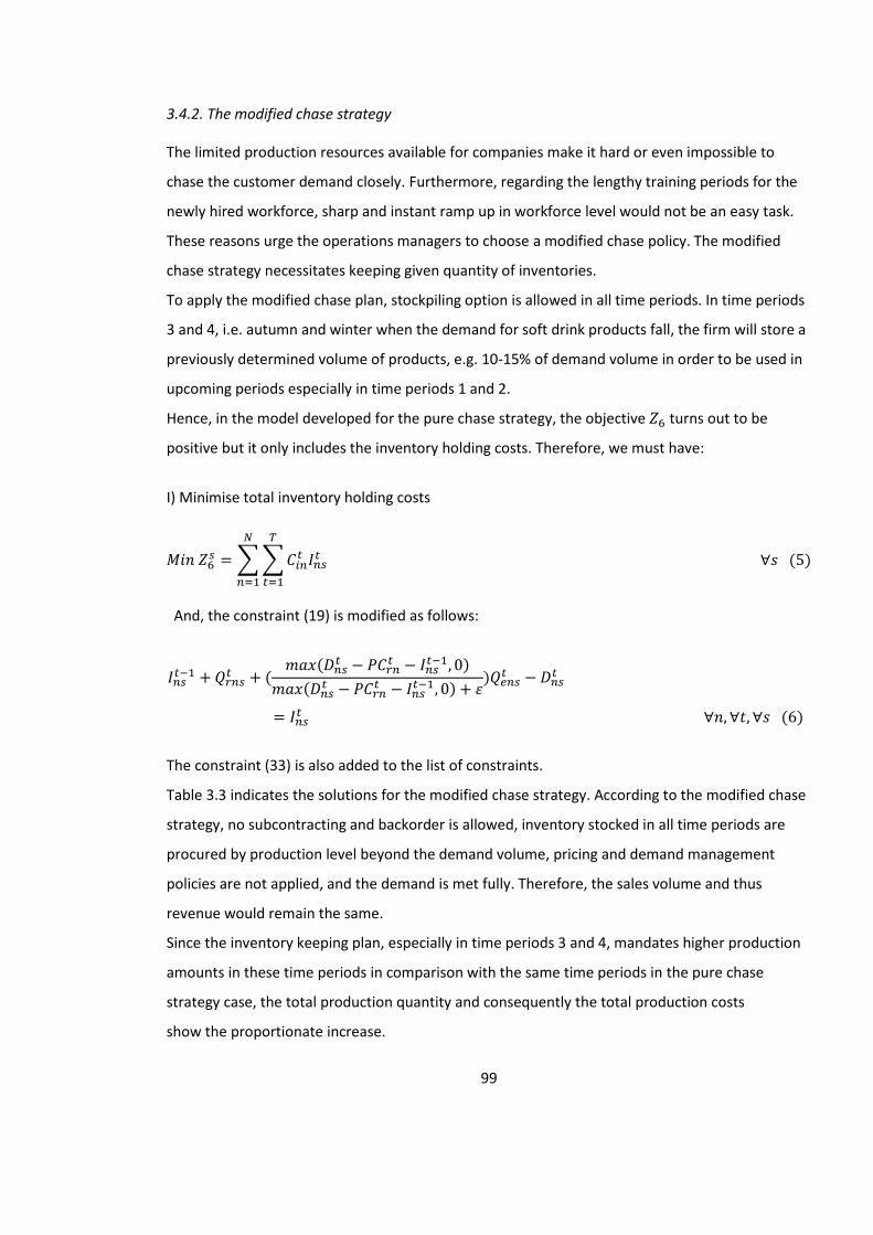
99
3.4.2. The modified chase strategy The limited production resources available for companies make it hard or even impossible to
chase the customer demand closely. Furthermore, regarding the lengthy training periods for the
newly hired workforce, sharp and instant ramp up in workforce level would not be an easy task.
These reasons urge the operations managers to choose a modified chase policy. The modified
chase strategy necessitates keeping given quantity of inventories.
To apply the modified chase plan, stockpiling option is allowed in all time periods. In time periods
3 and 4, i.e. autumn and winter when the demand for soft drink products fall, the firm will store a
previously determined volume of products, e.g. 10-15% of demand volume in order to be used in
upcoming periods especially in time periods 1 and 2.
Hence, in the model developed for the pure chase strategy, the objective 𝑍6 turns out to be
positive but it only includes the inventory holding costs. Therefore, we must have:
I) Minimise total inventory holding costs
𝑀𝑖𝑛 𝑍6𝑠 = ∑∑𝐶𝑖𝑛
𝑡 𝐼𝑛𝑠𝑡
𝑇
𝑡=1
𝑁
𝑛=1
∀𝑠 (5)
And, the constraint (19) is modified as follows:
𝐼𝑛𝑠𝑡−1 +𝑄𝑟𝑛𝑠
𝑡 + (𝑚𝑎𝑥(𝐷𝑛𝑠
𝑡 − 𝑃𝐶𝑟𝑛𝑡 − 𝐼𝑛𝑠
𝑡−1, 0)
𝑚𝑎𝑥(𝐷𝑛𝑠𝑡 − 𝑃𝐶𝑟𝑛
𝑡 − 𝐼𝑛𝑠𝑡−1, 0) + 𝜀
)𝑄𝑒𝑛𝑠𝑡 − 𝐷𝑛𝑠
𝑡
= 𝐼𝑛𝑠𝑡 ∀𝑛, ∀𝑡, ∀𝑠 (6)
The constraint (33) is also added to the list of constraints.
Table 3.3 indicates the solutions for the modified chase strategy. According to the modified chase
strategy, no subcontracting and backorder is allowed, inventory stocked in all time periods are
procured by production level beyond the demand volume, pricing and demand management
policies are not applied, and the demand is met fully. Therefore, the sales volume and thus
revenue would remain the same.
Since the inventory keeping plan, especially in time periods 3 and 4, mandates higher production
amounts in these time periods in comparison with the same time periods in the pure chase
strategy case, the total production quantity and consequently the total production costs
show the proportionate increase.
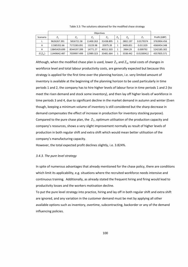
100
Objectives
Scenario 𝑍1 𝑍2 𝑍3 𝑍4 𝑍5 𝑍6 𝑍7 Profit (GBP)
L 9626267.391 5816721.58 11400.263 31438.895 1 2802.197 0.0179374 3763904.456
A 11585352.66 7172283.091 13229.98 35975.39 1 3409.851 0.011329 4360454.348
H 13845429.699 8544197.399 14771.27 40311.503 1 3964.29 0.009792 5242185.302
𝐸(𝑍𝑘) 11449642.487 7039997.499 12989.323 35481.664 1 3338.442 0.01300412 4357835.571
Although, when the modified chase plan is used, lower 𝑍3 and 𝑍4, total costs of changes in
workforce level and total labour productivity costs, are generally expected but because this
strategy is applied for the first time over the planning horizon, i.e. very limited amount of
inventory is available at the beginning of the planning horizon to be used particularly in time
periods 1 and 2, the company has to hire higher levels of labour force in time periods 1 and 2 (to
meet the risen demand and stock some inventory), and then lay off higher levels of workforce in
time periods 3 and 4, due to significant decline in the market demand in autumn and winter (Even
though, keeping a minimum volume of inventory is still considered but the sharp decrease in
demand compensates the effect of increase in production for inventory stocking purpose).
Compared to the pure chase plan, the 𝑍7, optimum utilisation of the production capacity and
company’s resources, shows a very slight improvement normally as result of higher levels of
production in both regular shift and extra shift which would mean better utilisation of the
company’s manufacturing capacity.
However, the total expected profit declines slightly, i.e. 3.824%.
3.4.3. The pure level strategy
In spite of numerous advantages that already mentioned for the chase policy, there are conditions
which limit its applicability, e.g. situations where the recruited workforce needs intensive and
continuous training. Additionally, as already stated the frequent hiring and firing would lead to
productivity losses and the workers motivation decline.
To put the pure level strategy into practice, hiring and lay off in both regular shift and extra shift
are ignored, and any variation in the customer demand must be met by applying all other
available options such as inventory, overtime, subcontracting, backorder or any of the demand
influencing policies.
Table 3.3: The solutions obtained for the modified chase strategy
101
The maximum 3 hour overtime besides the normal 8 hour regular shift is performed by the
current workforce. The upper bound of the subcontracting is increased to 30% of the adjusted
demand in each time period.
Ignoring hiring and lay-off options means their corresponding decision variables take on the value
0, and therefore the objectives 𝑍3 and 𝑍4 also assume the value 0. All other objective functions
except objective function (2) remain unchanged.
The new objective function (2) will be as follows:
I) Total production costs
𝑀𝑖𝑛 𝑍2𝑠 = ∑∑𝐶𝑝𝑛
𝑡 (𝑄𝑟𝑛𝑠𝑡 + 𝑄𝑒𝑛𝑠
𝑡 )
𝑇
𝑡=1
𝑁
𝑛=1
+∑∑𝐶𝑟𝑤𝑛𝑡 (𝑄𝑟𝑛𝑠
𝑡 𝑃𝑇𝑛) + 𝐶𝑒𝑤𝑛𝑡 (𝑄𝑒𝑛𝑠
𝑡 𝑃𝑇𝑛)
𝑇
𝑡=1
𝑁
𝑛=1
+∑∑𝐶𝑠𝑛𝑡 𝑆𝑛𝑠
𝑡
𝑇
𝑡=1
𝑁
𝑛=1
∀𝑠 (7)
Where 𝑃𝑇𝑛 represents the normal production time, when there is no hiring and lay off, regardless
of demand scenarios, operating in regular shift or overtime, etc. 𝑄𝑒𝑛𝑠𝑡 shows production quantity
in overtime.
Constraints (9)-(21), (32) and (33) remain unchanged. Constraints (22)-(29) are lifted.
Constraints (30) and (31), workforce level constraints, are transformed into a single constraint as
below:
∑(𝑄𝑟𝑛𝑠𝑡 + 𝑄𝑒𝑛𝑠
𝑡 )𝑃𝑇𝑛
𝑁
𝑛=1
≤ 𝑊 𝑠 𝑚𝑎𝑥𝑡 ∀𝑡, ∀𝑠 (8)
Because the existing workforce carries out the overtime as well, the upper limit of the labour
force, 𝑊 𝑠 𝑚𝑎𝑥𝑡 , has no notation of operating in regular shift or overtime but the maximum 3 hour
overtime is added to the 8 hour regular shift working hours to calculate this upper bound.
As can be seen from Table 3.4, in comparison with the mixed chase and level plan, total expected
revenue, 𝐸(𝑍1), has declined about 23.044% mainly for two reasons: I) the backorder quantities
for all products in all time periods go beyond the threshold level, and in two occasions of the
three occasions, i.e. when the product demand turns out to be low and average, the demand
adjustment mechanism, which would have led to an increase in demand, is turned off. Moreover,
in case high demand scenario occurs, again because backorder volume has exceeded the
threshold level, the demand management policy causes a proportionate decrease in the demand.
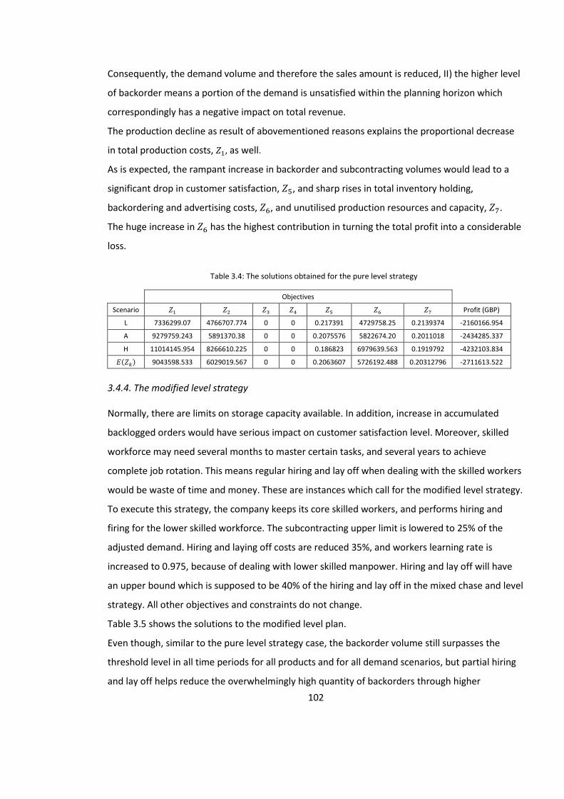
102
Consequently, the demand volume and therefore the sales amount is reduced, II) the higher level
of backorder means a portion of the demand is unsatisfied within the planning horizon which
correspondingly has a negative impact on total revenue.
The production decline as result of abovementioned reasons explains the proportional decrease
in total production costs, 𝑍1, as well.
As is expected, the rampant increase in backorder and subcontracting volumes would lead to a
significant drop in customer satisfaction, 𝑍5, and sharp rises in total inventory holding,
backordering and advertising costs, 𝑍6, and unutilised production resources and capacity, 𝑍7.
The huge increase in 𝑍6 has the highest contribution in turning the total profit into a considerable
loss.
Objectives
Scenario 𝑍1 𝑍2 𝑍3 𝑍4 𝑍5 𝑍6 𝑍7 Profit (GBP)
L 7336299.07 4766707.774 0 0 0.217391 4729758.25 0.2139374 -2160166.954
A 9279759.243 5891370.38 0 0 0.2075576 5822674.20 0.2011018 -2434285.337
H 11014145.954 8266610.225 0 0 0.186823 6979639.563 0.1919792 -4232103.834
𝐸(𝑍𝑘) 9043598.533 6029019.567 0 0 0.2063607 5726192.488 0.20312796 -2711613.522
3.4.4. The modified level strategy Normally, there are limits on storage capacity available. In addition, increase in accumulated
backlogged orders would have serious impact on customer satisfaction level. Moreover, skilled
workforce may need several months to master certain tasks, and several years to achieve
complete job rotation. This means regular hiring and lay off when dealing with the skilled workers
would be waste of time and money. These are instances which call for the modified level strategy.
To execute this strategy, the company keeps its core skilled workers, and performs hiring and
firing for the lower skilled workforce. The subcontracting upper limit is lowered to 25% of the
adjusted demand. Hiring and laying off costs are reduced 35%, and workers learning rate is
increased to 0.975, because of dealing with lower skilled manpower. Hiring and lay off will have
an upper bound which is supposed to be 40% of the hiring and lay off in the mixed chase and level
strategy. All other objectives and constraints do not change.
Table 3.5 shows the solutions to the modified level plan.
Even though, similar to the pure level strategy case, the backorder volume still surpasses the
threshold level in all time periods for all products and for all demand scenarios, but partial hiring
and lay off helps reduce the overwhelmingly high quantity of backorders through higher
Table 3.4: The solutions obtained for the pure level strategy
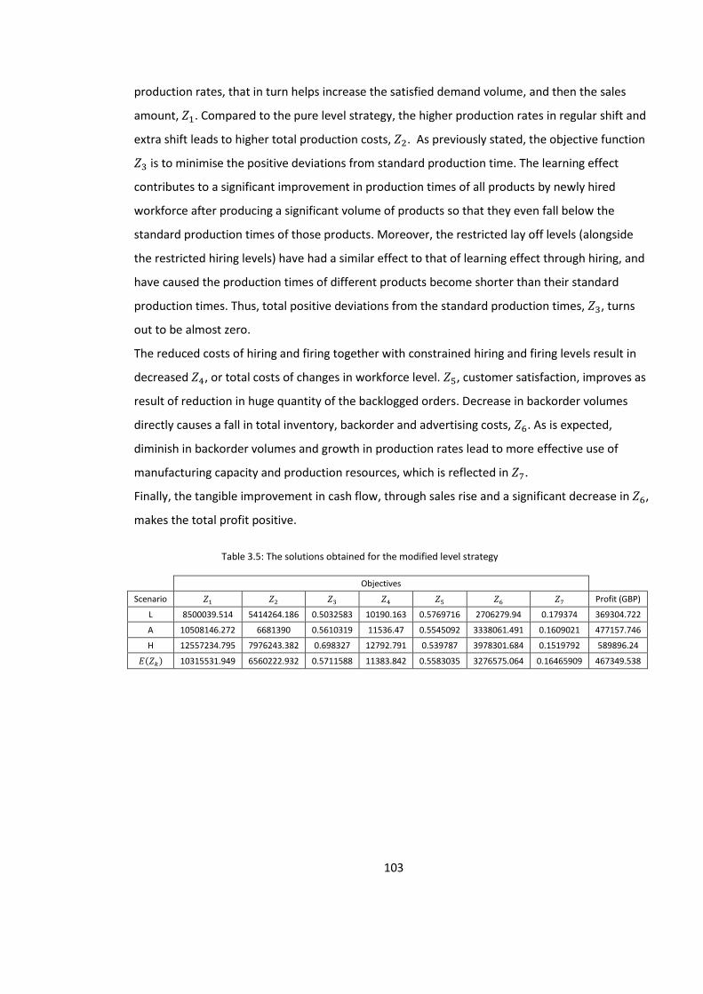
103
production rates, that in turn helps increase the satisfied demand volume, and then the sales
amount, 𝑍1. Compared to the pure level strategy, the higher production rates in regular shift and
extra shift leads to higher total production costs, 𝑍2. As previously stated, the objective function
𝑍3 is to minimise the positive deviations from standard production time. The learning effect
contributes to a significant improvement in production times of all products by newly hired
workforce after producing a significant volume of products so that they even fall below the
standard production times of those products. Moreover, the restricted lay off levels (alongside
the restricted hiring levels) have had a similar effect to that of learning effect through hiring, and
have caused the production times of different products become shorter than their standard
production times. Thus, total positive deviations from the standard production times, 𝑍3, turns
out to be almost zero.
The reduced costs of hiring and firing together with constrained hiring and firing levels result in
decreased 𝑍4, or total costs of changes in workforce level. 𝑍5, customer satisfaction, improves as
result of reduction in huge quantity of the backlogged orders. Decrease in backorder volumes
directly causes a fall in total inventory, backorder and advertising costs, 𝑍6. As is expected,
diminish in backorder volumes and growth in production rates lead to more effective use of
manufacturing capacity and production resources, which is reflected in 𝑍7.
Finally, the tangible improvement in cash flow, through sales rise and a significant decrease in 𝑍6,
makes the total profit positive.
Objectives
Scenario 𝑍1 𝑍2 𝑍3 𝑍4 𝑍5 𝑍6 𝑍7 Profit (GBP)
L 8500039.514 5414264.186 0.5032583 10190.163 0.5769716 2706279.94 0.179374 369304.722
A 10508146.272 6681390 0.5610319 11536.47 0.5545092 3338061.491 0.1609021 477157.746
H 12557234.795 7976243.382 0.698327 12792.791 0.539787 3978301.684 0.1519792 589896.24
𝐸(𝑍𝑘) 10315531.949 6560222.932 0.5711588 11383.842 0.5583035 3276575.064 0.16465909 467349.538
Table 3.5: The solutions obtained for the modified level strategy
104
3.5. Further analysis of the results
3.5.1. Assessing the performance of APP strategies based on single criterion
The aforementioned APP strategies are ranked based on each of the eight criteria mentioned
above as follows:
I) Based on total expected revenue, 𝐸(𝑍1)
Mixed chase and level strategy ≻ the pure chase strategy ≈ the modified chase strategy ≻ the
modified level strategy ≻ the pure level strategy
Where ≻ means an alternative is preferred over another and ≈ means the alternatives are
equivalent.
II) Based on total expected production costs, 𝐸(𝑍2)
The pure level strategy ≻ the modified level strategy ≻ the pure chase strategy ≻ the modified
chase strategy ≻ mixed chase and level strategy
III) Based on total expected labour productivity costs, 𝐸(𝑍3)
The pure level strategy ≻ the modified level strategy ≻ mixed chase and level strategy ≻ the pure
chase strategy ≻ the modified chase strategy
IV) Based on total expected costs of changes in workforce level, 𝐸(𝑍4)
The pure level strategy ≻ the modified level strategy ≻ mixed chase and level strategy ≻ the pure
chase strategy ≻ the modified chase strategy
V) Based on expected customer satisfaction degree, 𝐸(𝑍5)
The pure chase strategy ≈ the modified chase strategy ≻ mixed chase and level strategy ≻ the
modified level strategy ≻ the pure level strategy
105
VI) Based on total expected inventory holding, backordering and advertising costs, 𝐸(𝑍6)
The pure chase strategy ≻ the modified chase strategy ≻ mixed chase and level strategy ≻ the
modified level strategy ≻ the pure level strategy
VII) Based on expected unutilised production resources and capacity, 𝐸(𝑍7)
The modified chase strategy ≻ the pure chase strategy ≻ mixed chase and level strategy ≻ the
modified level strategy ≻ the pure level strategy
VII) Based on total expected profit
The pure chase strategy ≻ the modified chase strategy ≻ mixed chase and level strategy ≻ the
modified level strategy ≻ the pure level strategy.
3.5.2. Assessing the performance of APP strategies using MCDM methods
The MCDM techniques, AVF, TOPSIS and VIKOR, are used to assess the overall performance of
different APP strategies by taking all of the criteria mentioned above into account except total
profit, again to avoid the significant overlaps between criteria.
First, the criteria are assigned weights by employing the analytic hierarchy process (AHP), and
then these weights are utilised in the process of aggregation used by the aforementioned
methods. The weights of the attributes 𝑍1-𝑍7 are correspondingly determined as: 0.3203, 0.2219,
0.0624, 0.0781, 0.1339, 0.1379 and 0.0453. Table 3.6 shows the overall rankings of the APP
strategies together with total aggregated scores regarding each strategy.
As Table 3.6 indicates, the APP strategies from the chase family dominate in rankings performed
by AVF and VIKOR but the level strategies top the list of TOPSIS ranking. In AVF ranking, the pure
level strategy stays just behind chase strategies, and outperforms both mixed chase and level and
the modified level polices with slightly higher overall score. In the ranking conducted by the VIKOR
method, the modified level plan stays next to the mixed chase and level strategy, and the pure
level strategy is at the bottom of the list.
The TOPSIS ranking puts the pure chase plan in third place, which is followed by the mixed chase
and level and the modified chase strategies respectively with very close scores.
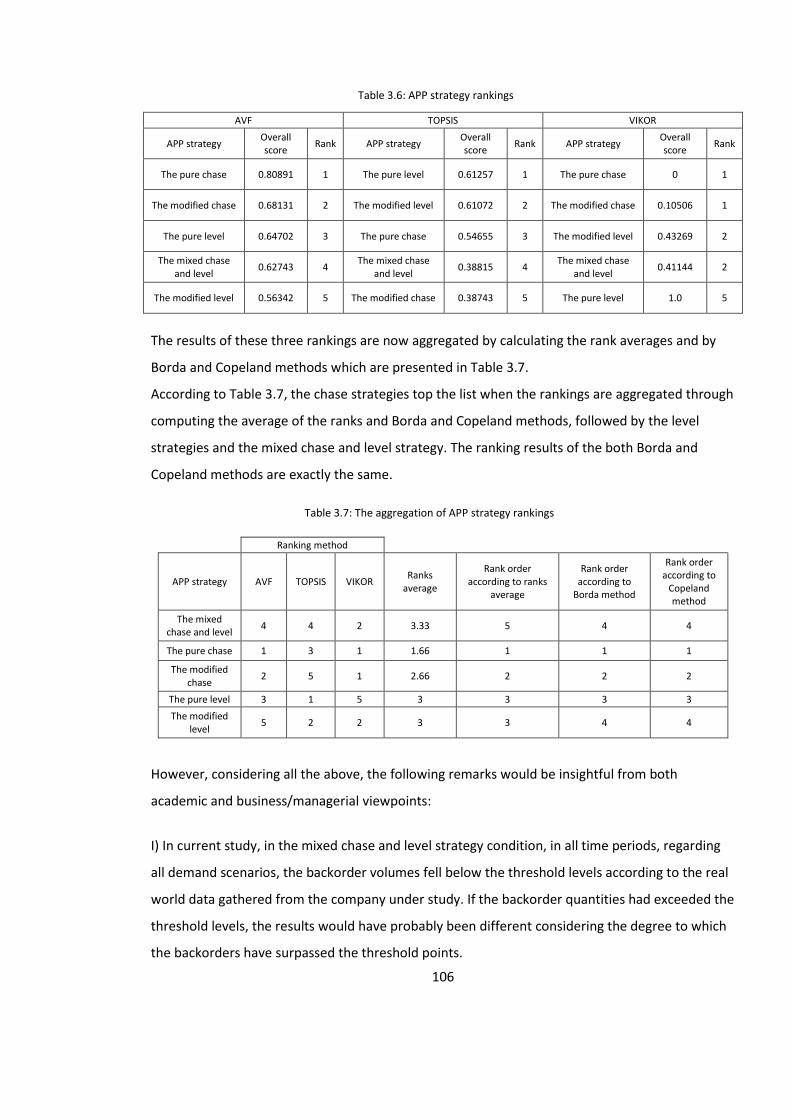
106
AVF TOPSIS VIKOR
APP strategy Overall score
Rank APP strategy Overall score
Rank APP strategy Overall score
Rank
The pure chase 0.80891 1 The pure level 0.61257 1 The pure chase 0 1
The modified chase 0.68131 2 The modified level 0.61072 2 The modified chase 0.10506 1
The pure level 0.64702 3 The pure chase 0.54655 3 The modified level 0.43269 2
The mixed chase and level
0.62743 4 The mixed chase
and level 0.38815 4
The mixed chase and level
0.41144 2
The modified level 0.56342 5 The modified chase 0.38743 5 The pure level 1.0 5
The results of these three rankings are now aggregated by calculating the rank averages and by
Borda and Copeland methods which are presented in Table 3.7.
According to Table 3.7, the chase strategies top the list when the rankings are aggregated through
computing the average of the ranks and Borda and Copeland methods, followed by the level
strategies and the mixed chase and level strategy. The ranking results of the both Borda and
Copeland methods are exactly the same.
Ranking method
APP strategy AVF TOPSIS VIKOR Ranks
average
Rank order according to ranks
average
Rank order according to
Borda method
Rank order according to
Copeland method
The mixed chase and level
4 4 2 3.33 5 4 4
The pure chase 1 3 1 1.66 1 1 1
The modified chase
2 5 1 2.66 2 2 2
The pure level 3 1 5 3 3 3 3
The modified level
5 2 2 3 3 4 4
However, considering all the above, the following remarks would be insightful from both
academic and business/managerial viewpoints:
I) In current study, in the mixed chase and level strategy condition, in all time periods, regarding
all demand scenarios, the backorder volumes fell below the threshold levels according to the real
world data gathered from the company under study. If the backorder quantities had exceeded the
threshold levels, the results would have probably been different considering the degree to which
the backorders have surpassed the threshold points.
Table 3.6: APP strategy rankings
Table 3.7: The aggregation of APP strategy rankings
107
II) With regard to the extent to which a production process is capital-intensive or labour-intensive,
it might be questionable that to what degree increasing the workforce level by recruiting the
workers would necessarily mean a corresponding increase in production rate. However, ZamZam
Company has already been operating with significant idle production capacity as it lost a portion
of its market share to the newly established Pepsi and Coca Cola companies’ branches throughout
the country in recent years. This implies that regular hiring could effectively help increase the
production volume in the corporation under study.
III) A moderate rate of hiring and lay off and wage costs were considered in present research.
However, higher rates of these cost items besides the higher weights for 𝑍3 and 𝑍4, total labour
productivity costs and total costs of changes in workforce level, might have considerable effect on
APP strategy ranks.
3.5.3. Sensitivity analysis of the rankings
In this part, the sensitivity of the ranking results to changes in the weights assigned to each
criterion is examined. The sensitivity analysis is conducted by changing the present weights of the
criteria, (𝑊1, 𝑊2, 𝑊3, 𝑊4, 𝑊5, 𝑊6, 𝑊7) = (0.3203, 0.2219, 0.0624, 0.0781, 0.1339, 0.1379, 0.0453),
as follows:
Scenario 1: Put new weights= (0.3803, 0.1819, 0.0824, 0.0981, 0.1239, 0.0879, 0.0453). The
outcome is presented in Table 3.8. As can be seen from Table 3.8, the rankings of APP strategies
according to AVF and TOPSIS have not changed. However, in AVF ranking, the pure level strategy
stays in the third place with slightly lower score compared to that of the pure chase strategy
which is most probably because of reducing the weight of 𝑍7 where the pure level strategy has
the worst performance. VIKOR ranking shows a slight change, i.e. now, the mixed chase and level
and the modified level strategies are in the third and fourth orders respectively instead of being in
the same level. This is normally due to increasing the weight of 𝑍1 in which the mixed chase and
level strategy has the best performance, and reducing the weight of 𝑍2 where the mixed chase
and level strategy does much worse in comparison with the modified level strategy.
Scenario 2: Put new weights= (0.3503, 0.1019, 0.0624, 0.0781, 0.1339, 0.2579, 0.0153). Based on
this scenario, in all rankings the pure chase strategy is still the best. The modified chase strategy
still stays in the second order in AVF ranking but it is ranked number one together with the pure
chase strategy in VIKOR ranking. Although lowering the weights of 𝑍2 and 𝑍7 where the chase
108
strategies perform pretty well has a negative impact on their ranks, increasing the weights of 𝑍1
and 𝑍6 compensates these negative effects. The mixed chase and level strategy is ranked best by
VIKOR, and the second best by TOPSIS as result of increasing the weight of 𝑍1 in which the mixed
chase and level strategy has the best performance, and decreasing the weights of 𝑍2 and 𝑍7
where the mixed chase and level strategy proves to be relatively inefficient.
Scenario 3: Put new weights= (0.3203, 0.0419, 0.1624, 0.1781, 0.0339, 0.0379, 0.2253). According
to the new set of weights, the pure level strategy gets the highest scores as the best policy in AVF
and TOPSIS rankings. The modified level strategy is ranked as the second best by TOPSIS. This is
mostly because of assigning higher weights to 𝑍3 and 𝑍4where the chase strategies have poor
performance, and lower weights to 𝑍5 and 𝑍6 where the level strategies prove to be relatively
weak. These results are obtained despite assigning lower weight to 𝑍2in which the level strategies
present the best performance, and higher weight to 𝑍7 in which the level strategies present the
poorest performance.
As different methods use different procedures in their ranking process, the ranking obtained by
VIKOR is completely different. It puts the mixed chase and level, the pure chase and the modified
chase strategies in the first level. In mixed chase and level case, the reason for the improved
VIKOR ranking is a sharp decrease in weight of 𝑍2 where the mixed chase and level strategy is the
least efficient, and increase in the weights of 𝑍3 and 𝑍4where this strategy performs relatively
better. Likewise, a sharp increase in the weight assigned to 𝑍7 where the chase strategies proved
to be the most effective, and a significant reduction in the weight assigned to 𝑍2 where the level
strategies are more effective than pure strategies explain the improvement in rankings of the
pure chase and the modified chase strategies.
Scenario 4: Put new weights= (0.0703, 0.0519, 0.1724, 0.2281, 0.3039, 0.0979, 0.0753). On the
basis of scenario 4 conditions, all of the three ranking methods rank a strategy from the level
strategies family as the most efficient, i.e. the pure level strategy is ranked number one by AVF
and TOPSIS; and in VIKOR ranking, the modified level strategy comes in the first place. Despite
assigning significantly higher weight to 𝑍2 in which the chase strategies present the best
performance, a sharp decrease in the weight of 𝑍1in which the level strategies are the least
efficient, and a sharp increase in the weights of 𝑍3 and 𝑍4 where the chase strategies have the
poorest performance put the pure or the modified level strategies ahead of chase strategies.
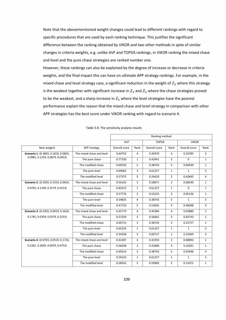
109
Note that the abovementioned weight changes could lead to different rankings with regard to
specific procedures that are used by each ranking technique. This justifies the significant
difference between the ranking obtained by VIKOR and two other methods in spite of similar
changes in criteria weights, e.g. unlike AVF and TOPSIS rankings, in VIKOR ranking the mixed chase
and level and the pure chase strategies are ranked number one.
However, these rankings can also be explained by the degree of increase or decrease in criteria
weights, and the final impact this can have on ultimate APP strategy rankings. For example, in the
mixed chase and level strategy case, a significant reduction in the weight of 𝑍2 where this strategy
is the weakest together with significant increase in 𝑍3 and 𝑍4 where the chase strategies proved
to be the weakest, and a sharp increase in 𝑍5 where the level strategies have the poorest
performance explain the reason that the mixed chase and level strategy in comparison with other
APP strategies has the best score under VIKOR ranking with regard to scenario 4.
Ranking method
AVF TOPSIS VIKOR
New weights APP strategy Overall score Rank Overall score Rank Overall score Rank
Scenario 1: (0.3803, 0.1819, 0.0824, 0.0981, 0.1239, 0.0879, 0.0453)
The mixed chase and level 0.64753 4 0.39470 4 0.24785 3
The pure chase 0.77230 1 0.42941 3 0 1
The modified chase 0.69550 2 0.38743 5 0.09439 1
The pure level 0.69062 3 0.61257 1 1 5
The modified level 0.57375 5 0.59429 2 0.43845 4
Scenario 2: (0.3503, 0.1019, 0.0624,
0.0781, 0.1339, 0.2579, 0.0153)
The mixed chase and level 0.56163 3 0.58071 2 0.08240 1
The pure chase 0.83272 1 0.61257 1 0 1
The modified chase 0.57776 2 0.53225 3 0.05136 1
The pure level 0.54825 4 0.38743 5 1 5
The modified level 0.47710 5 0.52835 4 0.46048 4
Scenario 3: (0.3203, 0.0419, 0.1624,
0.1781, 0.0339, 0.0379, 0.2253)
The mixed chase and level 0.42774 4 0.44384 4 0.03880 1
The pure chase 0.57259 3 0.56661 3 0.03743 1
The modified chase 0.60715 2 0.38743 5 0.22757 1
The pure level 0.65224 1 0.61257 1 1 5
The modified level 0.35638 5 0.60727 2 0.33369 4
Scenario 4: (0.0703, 0.0519, 0.1724,
0.2281, 0.3039, 0.0979, 0.0753)
The mixed chase and level 0.42287 4 0.41950 3 0.08893 1
The pure chase 0.56658 2 0.41890 4 0.10291 1
The modified chase 0.49214 3 0.38743 5 0.42696 4
The pure level 0.59143 1 0.61257 1 1 5
The modified level 0.28502 5 0.59983 2 0.21072 1
Table 3.8: The sensitivity analysis results
110
3.5.4. Comparing the results of different studies on evaluating the APP policies
The present study by taking into account multiple criteria concludes that the most effective APP
strategies are from chase family, which approves the results of existing research about evaluating
APP policies which were presented in Table 3.1. The current research considered criteria that take
into account the labour productivity costs and costs of changes in workforce level due to frequent
hiring and lay off, which is common in chase strategies, to have a comprehensive evaluation of
various APP strategies.
The findings of the present research are also consistent with the findings of surveys conducted by
Buxey (1990, 1995, 2003, 2005) where they all found out that the most prevalent APP strategies
in Australian industries are different versions of chase strategies. However, modelling APP
problems solely on the basis of mixed chase and level strategy is quite dominant in APP literature.
This does not only show the gap between APP literature and APP in practice but also indicates the
need to do more research on APP by utilising strategies other than the mixed chase and level.
3.6. Conclusions and directions for future research The present study proposed a framework based on a set of stochastic, nonlinear, multi-objective
optimisation models to evaluate the performance of various APP strategies under uncertainty,
where the customer demand was regarded as the main source of uncertainty. In the first stage, a
novel, precise, stochastic, nonlinear, multi-objective optimisation decision making model was
constructed for APP based on the mixed chase and level strategy to consider APP from a holistic
view. Then, the relevant models for other APP strategies such as pure chase, pure level, modified
chase and modified level were derived from the model that was developed for the mixed chase
and level strategy. Different APP strategies were compared with regard to criteria/objectives like
total profit, total revenue, total production costs and total labour productivity costs.
The MCDM methods AVF, TOPSIS and VIKOR were used to rank various APP strategies regarding
different criteria, and then the rankings of different methods were aggregated by computing the
average of the ranks and by Borda and Copeland methods. On the whole, the pure chase and the
modified chase strategies had the best performance after aggregating the rankings of different
methods, followed by the pure level strategy.
The research can be extended in several directions in the future, mainly:
111
I. The present study was conducted in an industry which combines both capital-
intensiveness and labour-intensiveness features. Case studies from more labour-intensive
industries, especially in chase strategy cases, would produce more informative
results/findings.
II. The interface between operations management and marketing management has been a
growing area of research. To the best of the authors’ knowledge, there is no published
work on evaluating APP strategies from marketing management viewpoint. This is
especially true regarding the fact that the demand management mechanisms embedded
in level strategies act by applying pricing and advertising options that normally are
considered as marketing mechanisms as well.
III. The existing research on assessing APP strategies with respect to productivity measures,
although very few, has always done this using analytical management science-based
methodologies. As already stated throughout the paper, frequent hiring and lay off,
excessive usage of overtime, extra shifts, etc., which are regarded as the integral parts of
chase strategies, impact the workers productivity via psychological factors. Therefore,
there is a need for qualitative research to address these issues from behavioural
perspective too.
IV. As discussed in Section 3.5.4, multiple consecutive surveys by Buxey (1990, 1995, 2003,
2005) revealed that chase strategies are the most popular APP strategies in Australian
firms while as can be seen from Table 1.8 (in paper 1), the mixed chase and level strategy
is the most frequently used strategy in research which utilises analytical models of APP.
This does not only show the big gap between APP literature and APP in real world
industrial environments but also indicates the need for more research on analytical
decision models of APP based on strategies other than the mixed chase and level strategy.
V. APP includes a chain of interrelated decisions in different time periods, and these
decisions are influenced by/influencing other decisions and policies adopted in previous
and next time periods within the planned time horizon. This means APP problem can be
formulated as a dynamic programming model. For instance, regular shift production,
extra shift production and subcontracting are impacted by inventory level in previous
time period, and impact the inventory level in the next time period. As such, in each stage
(time period), the state would be inventory level remaining from previous time period,
and the decision variables are production in regular shift, production in extra shift,

112
subcontracting and backordering at current time period. As detailed in Section 3.1, APP is
inherently uncertain decision making problem. Thus, integrating uncertainty into the
developed dynamic programming model of APP to build a stochastic dynamic
programming model could help improve the quality of the decision model.
However, APP problems in practice tend to be of large scale which arises the curse of
dimensionality that needs to be managed effectively. Fortunately, there exists numerous
ways to handle this issue, including the decomposition/partitioning techniques and
scenario reduction methods.
113
References
Buxey, G. (1990). ‘The myth of aggregate planning’, Production Planning & Control, 1 (4), pp.222-234. Buxey, G. (1995). ‘A managerial perspective on aggregate planning’, International Journal of Production Economics, 41 (1-3), pp. 127–133. Buxey, G. (2003). ‘Strategy not tactics drives aggregate planning’, International Journal of Production Economics, 85(3), pp. 331–346. Buxey, G. (2005). ‘Aggregate planning for seasonal demand: reconciling theory with practice’, International Journal of Operations and Production Management, 25 (11), pp. 1083–1100. Bowman, E.H. (1956). ‘Production scheduling by the transportation method of linear programming’, Operations Research, 4(1), pp. 100-103. Chen, Y.K. and Liao, H.C. (2003). ‘An investigation on selection of simplified aggregate production planning strategies using MADM approaches’, International Journal of Production Research, 41(14), pp. 3359–3374. Dubois, F.L. and Oliff, M.D. (1991). ‘Aggregate production planning in practice’, Production and Inventory Management Journal, 32 (3), pp. 26–30. Gulsun, B., Tuzkaya, G., Tuzkaya, U.R., and Onut, S. (2009). ‘An Aggregate Production Planning Strategy Selection Methodology based on Linear Physical Programming’, International Journal of Industrial Engineering, 16 (2), pp. 135-146. Holt, C.C., Modigliani,F. and Simon, H.A. (1955). ‘Linear decision rule for production and employment scheduling’, Management Science, 2(1), pp. 1-30. Holt, C.C., Modigliani,F. and Muth, J.F. (1956). ‘Derivation of a linear decision rule for production and employment’, Management Science, 2(2), pp. 159-177. Jamalnia, A. and Feili, A. (2013). ‘A simulation testing and analysis of aggregate production planning strategies’, Production Planning & Control, 24(6), pp. 423-448. Lee, W.B. and Khumawala, B.M. (1974). ‘Simulation Testing of Aggregate Production Planning Models in an Implementation Methodology’, Management Science, 20(6), pp. 903-911. Miettinen, K. and Mäkelä, M.M. (2006). ‘Synchronous Approach in Interactive Multi-objective Optimization’, European Journal of Operational Research, 170(3), pp. 909-922. Shi, Y. and Haase, C. (1996). ‘Optimal trade-offs of aggregate production planning with multiple objective and multi-capacity demand levels’, International Journal of Operations and Quantitative Management, 2(2), pp. 127–143. Thompson, S.D., Wantanabe, D.T. and Davis, W.J. (1993). ‘A comparative study of aggregate production planning strategies under conditions of uncertainty and cyclic product demands’, International Journal of Production Research, 31(8), pp. 1957–1979.
114
Conclusions and future research paths
The thesis was presented in three papers format.
In first paper, a wide scope of literature on APP under uncertainty was surveyed from bibliometric
viewpoint. The uncertainties present in the constructed management science models of APP in
the literature are of sorts like stochasticity, fuzziness and impreciseness of the information. This
literature includes journal papers, book chapters, conference/proceedings papers and PhD theses
which were classified into six main categories on the basis of the methodologies applied, e.g.
stochastic mathematical programming, possibilistic programming, etc. First, the relevant
literature about each of abovementioned methods was reviewed concisely, and then a more
detailed statistical analysis of the surveyed research was followed.
Paper 2 proposed a novel decision model to aggregate production planning (APP) decision making
problem based on mixed chase and level strategy under uncertainty where the market demand
acts as the main source of uncertainty. By taking into account the novel features, the constructed
model turned out to be stochastic, nonlinear, multi-stage and multi-objective. APP in practice
entails multiple-objectivity. Therefore, the model involves multiple objectives such as total
revenue, total production costs, total labour productivity costs, optimum utilisation of production
resources and capacity and customer satisfaction, and was validated on the basis of real world
data from beverage manufacturing industry. Applying the recourse approach in stochastic
programming led to empty feasible space, and therefore the wait and see approach was used
instead. After solving the model using the real-world industrial data, sensitivity analysis and
several forms of trade-off analysis were conducted by changing different parameters/coefficients
of the constructed model, and by analysing the compromise between objectives respectively.
The paper 3 built upon the paper 2 by developing four extra aggregate production planning (APP)
models to different APP strategies other than the mixed chase and level strategy. These models
were derived from the fundamental APP model that was proposed for the mixed chase and level
strategy in paper 2. Therefore, the relevant models for APP strategies including the pure chase,
the pure level, the modified chase and the modified level strategies were taken from the basic
model developed for the mixed chase and level strategy.
The same procedure, as described in paper 2, was followed to solve the models constructed for
these strategies with respect to the corresponding objectives/criteria in order to provide business
insights to operations managers about the effectiveness and practicality of various APP policies in
presence of uncertainty.
115
Multiple criteria decision making (MCDM) methods such as additive value function (AVF), the
technique for order of preference by similarity to ideal solution (TOPSIS) and VIKOR were also
used besides multi-objective optimisation to assess the overall performance of each APP strategy.
The pure chase and the modified chase strategies showed the best performance in general,
followed by the pure level strategy.
A detailed sensitivity analysis was also conducted by changing the weights assigned to different
criteria in abovementioned MCDM methods to evaluate the impacts that these weight changes
can have on the final rank of each APP strategy.
The present research could be extended in several directions as follows:
As already was shown in Table 1.8, the absolutely prevalent APP strategy in the literature
about APP in presence of uncertainty (and even in the literature on deterministic APP
models) is the mixed chase and level strategy. However, the surveys conducted by Buxey
(1990, 1995, 2003, 2005) revealed that the most popular APP policy among operations
managers is the chase strategy, which shows a gap between APP in academia and APP in
practice. This also indicates an intense gap related to the lack of the studies about
quantitative APP models under uncertainty based on other APP strategies such as chase
strategy, level strategy and the demand management strategy.
Several relative advantages of the simulation techniques over mathematical programming
methods, e.g. coping with dynamic or transient effects, addressing interactions between
different components, the ability of providing a sufficient basis for developing explanatory
and predictive models of operational processes, and so forth have been stated in the
literature. Therefore, the relatively low share of the literature which apply simulation
modelling to study APP subject to uncertainty (12.20%), and the least steep trend line of
the frequency of the number of published research in this area over recent decades
recommend the need to do extra research in this field to compensate the unfairly narrow
share of the simulation methods.
Recourse approach as one of major stochastic programming approaches has a serious
drawback. The main shortcoming of this approach is that it considers all constraints
relating to different scenarios with equal probability (with certainty or P=1, where P
stands for the probability of associated scenarios) in constraints section of the stochastic
mathematical programming. In other words, it puts all the constraints relating to different
116
scenarios together, and solves the problem where the objective function is the expected
value regarding different scenarios. This does not sound true, since when all constraints
relating to different scenarios are put together in one mathematical programming
problem, it looks like all scenarios happen at the same time with equal probabilities (with
P=1 or certainty). A suitable methodology needs to be developed to resolve this
shortcoming.
In this study, we assumed that the demand volume scenarios will be the same in all
consecutive time periods. That is, if, for example, demand quantity is high in first time
period, it will also be high in all future time periods. We made this assumption based on
our discussion with the company’s managers, where according to their long term
experience with customer demand in the company under study, they approved that
demand normally has similar mood in several consecutive time periods while maintaining
the seasonality pattern. However, this assumption could be invalid in different cases, and
needs to be taken into account in relevant APP models.
The present study was conducted in an industry which combines both capital-
intensiveness and labour-intensiveness features. Case studies from more labour-intensive
industries, especially in chase strategy cases, would produce more informative
results/findings.
The interface between operations management and marketing management has been a
growing area of research. To the best of the authors’ knowledge, there is no published
work on evaluating APP strategies from marketing management viewpoint. This is
especially true regarding the fact that the demand management mechanisms embedded
in level strategies act by applying pricing and advertising options that normally are
considered as marketing mechanisms as well.
The existing research on assessing APP strategies with respect to productivity measures,
although very few, has always done this using analytical management science-based
methodologies. As already stated throughout the paper, frequent hiring and lay off,
excessive usage of overtime, extra shifts, etc., which are regarded as the integral parts of
chase strategies, impact the workers productivity via psychological factors. Therefore,
there is a need for qualitative research to address these issues from behavioural
perspective too.
![[PPT]Production and Operations Management: …sureten/(aggregate planning)5.ppt · Web viewDisaggregating the Aggregate Plan Aggregate Planning Aggregate planning Intermediate-range](https://img.pdfslide.net/doc/110x75/5aec86827f8b9ab24d902697/pptproduction-and-operations-management-suretenaggregate-planning5pptweb.jpg)