Evaluating the role of transportation system tin the com-

munity resilience assessment

Kairui Fenga, Guanjie Houa and Quanwang Lia

aDepartment of Civil Engineering, Tsinghua University

Introduction

Natural hazards, such as earthquake and hurricanes, impose great risk to the residents in com-

munities of all sizes, and impair the normal function of built environment. Consequently, in-

creasing attention has been cast on the emergency capacity of communities and the rapidity of

their recovery process following a hazard event. The concept of community resilience has been

raised, accepted and valued by researchers and policy makers and significant efforts have been

conducted to define and quantify the community resilience [2,7,9,14,16]. The gist of commu-

nity resilience is reflected by four characters: robustness, rapidity, redundancy and resourceful-

ness [2], as shown in Figure 1.

.

Figure 1: Schematic representation of community resilience Figure 2: Map of Beijing city

Abstract: The performance of transportation system has significant impact on the

recovery rapidity of damaged communities after the occurrence of hazard events,

because most of the necessary materials, machines and workmanship are shipped by

transportation system from the suppliers to the building site. This paper analyses the

supporting of transportation system to the recovery process of built environment,

and proposes an indicator for evaluating this effect, which relates the capacity of

transportation system to the recovery speed of built environment. The approach is

demonstrated through the performance evaluation of the simplified transportation

system of Beijing city, and the effects of retrofitting transportation system on im-

proving the resilience of built environment are analysed.

Key words: Community resilience; Transportation system; Built environment; Ret-

rofit strategy; Recovery; Earthquake.

Resilience is often regarded as an attribute of communities rather than a property of individual

infrastructure components or systems [13,16]. A resilient community requires a resilient built

environment that consists of different building sectors, such as residential, commercial,

education, government, etc., which are interdependent in their functionalities in maintaining the

well-being of a community. Hence, it becomes meaningful to account for the interdependency

between building sectors in the resilience assessment of the whole community [8].

Following a hazard events, the resilient of a community depends not only on the robustness of

building sectors but also on the performance of transportation system, which affects

significantly the rapidity of recovery process. From the view point of system and network, the

performance of transportation system following hazard events has been discussed in terms of

the connectivity and travel time, and several case studies have been presented [5,10,15].

However, none of the existing literature analyzes the supporting role of transportation system

for the recovery of damaged buildings, which is, however, a key issue because the repairing of

damaged buildings needs the delivery of resources by transportation system, including

materials, machines and workmanship.

Firstly, the paper introduces the measurement for community functionality considering the

inter-dependency among building sectors, which is then illustrated using a simplified model of

Beijing city. Secondly, an indicator for the performance of transportation system following

hazard events is defined, and the network flow algorithm is introduced to find the optimal

logistics plan and rapidest recovery process of the community functionality. Finally, a case

study is carried out to demonstrate the application of the proposed method and evaluate the

supporting effect of transportation system to the recovery of built environment after an

earthquake.

Community functionality and retrofit optimization

2.1 Measurement for community functionality

The measure of community functionality, as seen in Fig. 1, is required to quantify the

community resilience. Conceptually, the community functionality can be defined by the

probability of an ‘undesired outcome’. In light of this, the degree of population out-migration

following a hazard event is chosen as an overall community resilience metric. The occurrence

of population out-migration highly depends on the damage conditions of different building

sectors, and certain community functionality should be maintained to avoid it [3].

Four essential community functions are considered including housing, business, education and

public service, and the buildings supporting each of these four essential community functions

are respectively referred as residential building sector (RBS), business building sector (BBS),

education building sector (EBS) and public service building sector (PBS). The community

functionality, FC, is defined as [8]:

𝐹𝐶 = 1 − 𝐿𝐶 = 1 − 𝐈1×4[𝑫𝑨𝑴]{𝐥}4×1 (1)

in which 𝐹𝐶 and 𝐿𝐶are the overall community functionality and its loss, ranging from 0 to 1;

𝑙𝑖is the percentage of buildings in sector i becoming unoccupiable; The [DAM] is Damage

Augmentation Matrix accounting for the interdependency among the essential functionality

provided by the four buildings sectors, which is

[𝐷𝐴𝑀] = [

𝑎11 𝑎12𝑙1 𝑎13𝑙1 𝑎14𝑙1

𝑎21𝑙2 𝑎22 𝑎23𝑙2 𝑎24𝑙2

𝑎31𝑙3

𝑎41𝑙4

𝑎32𝑙3

𝑎42𝑙4

𝑎33 𝑎43𝑙4

𝑎34𝑙3

𝑎44

] = [

0.13 0.30𝑙1 0.37𝑙1 0.27𝑙1

0.30𝑙2 0.04 0.28𝑙2 0.10𝑙2

0.37𝑙3

0.27𝑙4

0.28𝑙3

0.10𝑙4

0.13 0.28𝑙4

0.28𝑙3

0.05

] (2)

The threshold value for acceptable functionality, FC, is 0.87. The detailed derivation for the

[DAM] and the threshold of FC can be found elsewhere [8].

2.2 Seismic response and retrofit optimization strategy

The relationship between structural response, , and seismic intensity, IM, can be expressed in

a power-law form[6,11].

𝜃 = 𝑎 ⋅ 𝐼𝑀𝑏 ⋅ 𝜀 (3)

where a and b are parameters determined by regression analysis and the logarithmic standard

deviation 𝜀 is the error associate with the power-law form. For building sector i as a whole, the

ratio of buildings that are not safe to occupy (li) can be written as:

𝑙𝑖 = 1 − 𝛷 (𝑙𝑛(𝜃𝑐𝑟,𝑖) − 𝜆𝜃,𝑖

𝜉𝜃,𝑖

) (4)

where 𝜆𝜃,𝑖 and 𝜉𝜃,𝑖 can be obtained through simulation-based methods introduced in [12] pro-

vided that fragility information on individual buildings in the sector are available. And 𝑓𝑖 =

1 − 𝑙𝑖 is the functionality index of building sector i.

The retrofit cost for sector i, ci, depending on building characteristics, site conditions and retrofit

options, can be determined by a hyperbolic function of retrofitted resistance.

𝐶𝑖 = ∑ 𝐶0𝑖 ⋅ 𝑘𝑖 ⋅ (𝜇𝜃,𝑖

∗

𝜇𝜃,𝑖

− 1)

𝑛𝑖

𝑖=1

(5)

in which 𝐶0𝑖 is the individual building replacement cost; coefficient 𝑘𝑖 is associated with the

building construction type and site conditions; 𝜇𝜃,𝑖∗ and 𝜇𝜃,𝑖 are the post- and pre-retrofit mean

seismic performance of the building.

The Cost Efficiency, 𝑍𝑖 , of retrofitting sector i to enhance the overall functionality of the

community as a whole is:

𝑍𝑖 =𝜕𝐹𝐶

𝜕𝑓𝑖

∙𝑑𝑓𝑖

𝑑𝐶𝑖

(6)

where

𝜕𝐹𝐶

𝜕𝑓𝑖

= 𝑎𝑖𝑖 + ∑ (𝑎𝑖𝑗 + 𝑎𝑗𝑖)𝑙𝑗 (7)𝑚

𝑗=1,𝑗≠𝑖

𝑑𝑓𝑖

𝜕𝐶𝑖

=𝑑𝑓𝑖

𝑑𝜆𝜃,𝑖

⋅𝑑𝜆𝜃,𝑖

𝑑𝜇𝜃,𝑖

⋅𝑑𝜇𝜃,𝑖

𝑑𝐶𝑖

(8)

𝑍𝑖 is a key parameter to determine the retrofit strategy, and the building sector associated with

the largest value of Zi, i = 1,..4, has the highest priority for retrofitting.

2.3 Illustration of retrofit optimization of built environment

A simplified model of Beijing City shown in Fig.2 is established to demonstrate the application

of the approach, in which four building sectors are considered. Each building sector includes

three building categories designed for different seismic intensity levels1 (SIL), i.e. SIL6, SIL 7

or SIL 8, corresponding to PGAs of 0.06g,0.13g and 0.25g, respectively. The number of

buildings, the seismic response parameters and the basic retrofit costs are shown in Table 1.

Table 1: Building sectors and their seismic behaviors

Building Sector

Building Category

Number of

Buildings

a Design Seismic Intensity Level

(SIL)

Retrofit cost per building, C0 k

(million RMB)

Residential building

R6 40 0.040 6 (0.07g) 1.72 R7 50 0.024 7 (0.13g) 1.89 R8 10 0.013 8 (0.25g) 2.06

Business buildings

B6 8 0.046 6 (0.07g) 5.15 B7 10 0.026 7 (0.13g) 5.66 B8 2 0.015 8 (0.25g) 6.17

Education buildings

E6 2 0.036 6 (0.07g) 2.57 E7 2 0.021 7 (0.13g) 2.92 E8 1 0.012 8 (0.25g) 3.26

Public service

buildings

P6 10 0.044 6 (0.07g) 0.86

P7 10 0.025 7 (0.13g) 1.03

P8 5 0.014 8 (0.25g) 1.20

The overall community functionality as a function of seismic intensity expressed by PGA, is

plotted in Fig. 3. The community functionality, FC, decreases with increase in the PGA intensity,

reaching 0.87 (the threshold of the acceptable functionality) as the PGA reaches 0.15g.

Figure 3: Community functionality as a function of seismic intensity Figure 4: Transportation network of Beijing

To achieve the target community functionality of 0.87 under seismic intensity level of 8 (PGA

= 0.25g), the optimum retrofit strategy is acquired using the proposed method based on cost

efficiency, and shown in Table 2.

The optimum retrofit strategy mainly enhances education buildings and public service buildings,

because these buildings are fewer in numbers and retrofit costs, resulting higher cost

efficiencies (Z) than those of the residential buildings and business buildings. We can also find

that many, but not necessarily all, buildings have a seismic capacity matching the considered

seismic intensity following retrofit.

Table 2: Optimum retrofit strategy under seismic intensity level 8

Building Sector Building category and No. of buildings

Retrofit strategy Cost (million)

Residential buildings R6, R7, R8 100 Not retrofitted 0.00

Business buildings B6 8 All are retrofitted to seismic level 7 30.96

B7, B8 12 Not retrofitted 0.00

Education buildings E6 2 All are retrofitted to seismic level 8 10.95 E7 2 All are retrofitted to seismic level 8 4.71 E8 1 retrofitted to seismic level of 9 3.43

Public service buildings P6 10 5 buildings are retrofitted to level 8 12.44 P7 10 all are retrofitted to level 8 8.21 P8 5 Not retrofitted 0.00

Support effect of transportation system to recovery of buildings

Transportation system represents a critical component of society’s infrastructure systems, and

is needed for the welfare of the public. After an earthquake, the transportation system is respon-

sible for the transportation of search/rescue and medical team, the passing of injured to hospitals

during the first few hours; and later, it is required for the delivery of repairing materials, ma-

chines and workmanship to the damaged building sites to support the recovery of built environ-

ment [4,18]. In this section, our research focuses on the role of transportation system to

facilitate the repairing/restoration of buildings, and proposes a method to evaluate the support-

ing effect of transportation system to the recovery of damaged buildings.

3.1 Transportation network and bridge fragilities

The transporting network in Beijing city is considered in this section, and the study is limited

to the 4 ring roads and 10 linking roads, as shown in Fig. 4. This network model consists of 37

nodes and 56 links, and the total number of bridges is 36. The network is defined in terms of

nodes and links. A node is at the location where two or more highways intersect (usually inter-

changes). A link is defined by a line between two nodes with no other nodes in between.

(a) bridges in 2nd and 3rd rings (b) bridges in 4th and 5th rings

Figure 5: Fragility curves of Beijing’s bridge

City transportation system comprises numerous structural components; among them, bridges

are the most vulnerable components under earthquake excitations. Similar to the buildings, the

bridges of Beijing city were also designed and constructed according to 3 seismic intensity

levels. In the previous study [10,17], bridge fragility information was expressed as a function

of peak ground acceleration (PGA), and it was assumed that the curves be expressed in the form

of two parameter lognormal distribution function. The fragility curves of bridges of Beijing city

is shown in Fig. 5, in which the damage state is classified into 5 categories, i.e., none, slight,

moderate, severe and collapse. Once the bridge is damaged, Table 3 shows the loss of traffic

capacity depending on the degree of damage.

Table 3 Loss in road capacity once the bridge is damaged

Damage state None Slight Moderate Severe Collapse

Capacity loss 0 20% 50% 100% 100%

3.2 Methodology

Damaged by the earthquake, the capacity and topology of the transportation network are

changed. Thus, a network flow model specialized in managing material flow demand and road

capacity is chosen to account for this change.

In the network flow model, a key issue is to solve the min-cost max-traffic problem between

two nodes. The flow network is defined as a graph G(V,E). V is the set of all nodes and E is

the set of all edges. It is required that the flow network has a single source and a single sink,

and suppose node s is the source of transportation demand in the network, node t is the sink of

transportation demand [1].

The flow network holds the following properties:

1) Every edge (u, v) ∈ 𝐄 holds a non-negative capacity c(u, v) ≥ 0.

2) Between (u, v) ∈ 𝐄 ,the real traffic flow f(u, v) is restricted in 0 ≤ f(u, v) ≤ c(u, v)

3) ∀v ∈ 𝐕 − {𝒔, 𝒕}, the in-flow is equal to out-flow, which means ∑ f(u, v) =(u,v)∈𝐄

∑ f(v, w) (v,w)∈𝐄 .

4) ∀(u, v) ∈ 𝐄 holds a cost b(u, v), and each unit flow passing by it will be punished by

b(u, v).

Under the constraint of maximum total traffic flow, the network flow method can minimize the

total cost brought by the traffic action.

𝐶𝑜𝑠𝑡 = ∑ 𝑏(𝑢, 𝑣)𝑓(𝑢, 𝑣)(𝑢,𝑣)∈𝑬

(9)

According to the topology of Beijing city, the graph G(V,E) was first established, as seen in

Fig. 4. The source node s is an assumed node linked to all the nodes on the 5th ring, where

receives all the resources shipped from other cities to Beijing. The sink node t is an assumed

node linked to all the nodes in the network. The capacity of each edge, c(u,v), is controlled by

the mean travel speed, number of lanes and road condition. The normalized daily capacities are

shown in Fig.4. The needed resources to repair/restore the damage buildings at each node are

around 200.

The damage of bridges is assumed to be statistically independent, and capacity c(u, v) is

determined by the damage state according to Table 3.

The received resources at each node can be simulated as the following

1) Simulate the damage state of bridges and the damage state of buildings, and then

determine the capacity matrix of the road system.

2) Establish the flow network G(V,E) and add the source node s and sink node t into set V,

and then calculate the cost at each node.

3) Allocate the shipped resources according to the optimal solution of network flow

method, and then update the damage state of each building, update the cost at each

node, and repeat step 3 for the next day analysis, so that we obtain one sample of the

recovery process of the city.

3.3 Resource supply rate and analysis results

To evaluate the supporting effect of transportation system to the recovery of built environment,

resource supply rate is proposed in this section. For an individual building, the resource supply

rate, rind, is defined as:

𝑟𝑖𝑛𝑑 =𝛱𝑠

𝛱𝑛

(10)

in which 𝛱𝑛 denotes the demanding resources daily for the full speed recovery of the concerned

building, 𝛱𝑠 denotes the supplied resources daily to the building through the transportation

system. As for the whole community, the resource supply rate, r, is defined as a weighted

average of rind of all buildings in the community

𝑟 =∑ ∑ 𝑤𝑖𝑗𝑖

4𝑗=1 𝑟𝑖𝑛𝑑,𝑖𝑗

∑ ∑ 𝑤𝑖𝑗𝑖4𝑗=1

(11)

in which rind,ij is the resource supply rate for the ith building in the jth building sector, 𝑤ij is the

weighting factor, which is determined by:

𝑤𝑖𝑗 =𝜕𝐹𝐶

𝜕𝑓𝑗

⋅𝑑 𝑓𝑗

𝑑 𝛱𝑖𝑗

(12)

In which 𝜕𝐹𝐶

𝜕𝑓𝑗 distinguishes the importance of different building sector to the functionality

assessment of the whole community, and 𝑑 𝑓𝑗

𝑑 𝛱𝑖𝑗 reflects the difference in cost efficiency of

repairing different individual building in a building sector.

Suppose an earthquake occurs with a PGA of 0.25g, which causes the damage of buildings and

bridges. 1000 simulations of damaged conditions of Beijing city were performed. The 1000

samples of recovery trajectory were obtained, and some of them are shown in Fig.6. In which

the mean recovery trajectory shows that, on average, the community functionality is restored to

an acceptable level (FC = 0.87) 3 months later. But the recovery process has great uncertainty,

the cases associated with 10 percentile and 90 percentile are also shown in the Figure.

The resource supply rate is also calculated using the simulated results, its probability

distribution can be found in Fig. 7, labelled ‘current‘, where 7(a) corresponds to the case

immediately after the earthquake, 7(b) is for that one month later. It can be seen that the resource

supply rate provided by transportation system has large uncertainty, and the transportation

system can only ship averagely 57% of resources needed for the full speed recovery

immediately after the earthquake. The resource supply rate gets larger one month later,

increases from 0.57 to 0.82 averagely, because the needed resources decrease as more damaged

buildings have been repaired.

Figure 6: Sampled recovery trajectories

(a) Immediately after earthquake (b) 1 month after earthquake

Figure 7: Comparison between probabilistic distribtuions of resource supply rate

Suppose all the bridges are retrofitted to a higher seismic intensity level, their seismic fragility

curves are shown in Fig. 8. Repeating the analyses above, the simulated recovery trajectories

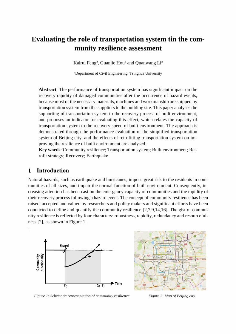
are shown in Fig.9. It can be seen that the time for the built environment back to the acceptable

level decreases to 2 months on average, and the variability of the recovery process is

significantly reduced compared with Fig. 6, demonstrating the improvement in the supporting

effect of transportation system to the recovery of damaged buildings after the transportation

network is retrofitted.

The resource supply rate is also analyzed for the retrofitted transportation system. Its probability

distributions are also shown in Fig. 7, labelled ‘retrofitted‘. The mean resource supply rate

increases from 0.57 to 0.70 immediately after earthquake, 0.82 to 0.92 one month after the

0.45

0.5

0.55

0.6

0.65

0.7

0.75

0.8

0.85

0.9

0.95

0 1 2 3 4

Co

mm

un

ity

Fun

ctio

nal

ity

Recovery time (month)

90 percentile

Mean

10 percentile

0.02 0.06

0.12

0.18 0.22

0.25

0.12

0.02 0.01 0.03

0.07

0.24

0.49

0.10 0.07

Current

retrofitted

0.00 0.01 0.02 0.04 0.09

0.17

0.29 0.29

0.09

0.01

0.16

0.80

0.03

current

retrofitted

earthquake, when the transportation system is retrofitted. It can be seen that the resource supply

rate is a meaningful indicator to evaluate the capacity of transportation system in the aspect of

supporting the recovery process of damaged buildings following a hazard event.

Figure 8: Fragility curves after retrofitting Figure 9: Sampled recovery trajectories aftter retrofitting

Summary

This paper introduces a measurement for community functionality of built environment, and

then proposes an indicator to evaluate the capacity of existing transportation system in support-

ing the recovery process of damaged built environment following a hazard event. Examples are

provided to illustrate the applications of both the measurement for community functionality and

the proposed indicator, resource supply rate of transportation network. It is demonstrated that

the proposed indicator is meaningful to evaluate the supporting effect of the transportation sys-

tem on the recovery process of built environment.

Acknowledgement

The research described in this paper was supported by the National Key Research and Devel-

opment Program of China (2016YFC0701404). This support is acknowledged. Zhewei Huang

and Jiayuan Mao gave useful advices on the network modeling, their help is also gratefully

acknowledged.

References

[1] Ahuja, K. et al.. Network flows: theory, algorithms, and applications. Prentice Hall, 1993.

[2] Bruneau, M. et al.. A framework to quantitatively assess and enhance the seismic

resilience of communities. Earthquake Spectra, 2003, 19 (4), 733–752.

[3] Bruneau, M. & Reinhorn, A.. Exploring the concept of seismic resilience for acute care

facilities. Earthquake Spectra, 2007, 23(1), 41–62.

[4] Chang, L. et al.. Post-earthquake modelling of transportation networks. Structure and

Infrastructure Engineering, 2012, 8(10), 893–911.

0.45

0.5

0.55

0.6

0.65

0.7

0.75

0.8

0.85

0.9

0.95

0 1 2 3 4C

om

mu

nit

y Fu

nct

ion

alit

y

Reconvery time (month)

90 percentile

Mean

10 percentile

[5] Chilan, P.. Structuring a definition of resilience for the freight frans- portation fystem.

Transportation Research Record Journal of the Transportation Research Board, 2097.

2009, pp. 19–25.

[6] Cornell C. et al.. Probabilistic basis for 2000 SAC federal emergency management agency

steel moment frame guidelines. Journal of Structural Engineering, ASCE, 2002, 128(4),

526-533.

[7] Cutter, S. et al.. Disaster resilience indictor for benchmarking baseline conditions. J.

Homeland Security and Emergency Management, 2010, 7(1): Article 51

[8] Feng, K. et al.. Measuring and enhancing resilience of building portfolios considering the

functional interdependence among community sectors. conditionally accepted by

Structural Safety, 2017

[9] Francis, R., et al.. A metric and frameworks for resilience analysis of engineered and

infrastructure systems. Reliability Engineering & System Safety, 2017, 121, 90-103.

[10] Frangopol, D. and Bocchini, P.. Bridge network performance, maintenance and opti-

misation under uncertainty: accomplishments and challenges. Structure Infrastruc- ture

Engineering (2012), 8(4), pp. 341–356

[11] Li, Q. and Ellingwood, B. Structural response and damage assessment by enhanced

uncoupled modal response history analysis. Journal of Earthquake Engineering, 2005,

9(5): 719-737

[12] Lin, P. et al.. A risk de-aggregation framework that relates community resilience goals to

building performance objectives. Sustainable & Resilient Infrastructure 2016, 1(1):1-13.

[13] McAllister, T.. Developing Guidelines and Standards for Disaster Resilience of the Built

Environment: A Research Needs Assessment ,National Institute of Standards and

Technology (NIST) Technical Note 1795, 2013.

[14] Miles, S. and Chang, S.. Modeling community recovery from earthquakes. Earthquake

Spectra, 2006, 22(2): 439–458.

[15] Miller, M. and Baker, J.. Coupling mode-destination accessibility with seismic risk

assessment to identify at-risk communities. Reliability Engineering & System Safety,

2016, 147: 60-71.

[16] NIST.. Community resilience planning guide for buildings and infrastructure systems.

Volume 1 and Volume 2. National Institute of Standards and Technology, Gaithersburg,

MD 20899 USA, 2015.

[17] Shinozuka M, et al.. Performance of highway network systems under earthquake damage,

Proceedings of the Second International Workshop on Mitigation of Seismic Effects on

Transportation Structures, Taiwan, Sep. 13-15, pp.303-317, 2000.

[18] Yan, S., & Shih, Y. L.. Optimal scheduling of emergency roadway repair and subsequent

relief distribution. Computers and Operations Research, 2009, 36(6), 2049–2065