Evaluating the Unemployment Insurance

Modernization Provisions of the American

Recovery and Reinvestment Act

by

Zachary Bleemer

Prof. Walter Nicholson, Advisor

Prof. Stanislav Rabinovich, Advisor

Submitted to the Department of Economics

at Amherst College in partial fulfillment of the requirements

for the degree of Bachelor of Arts with honors.

April 17, 2013

ii

ABSTRACT

Despite the high current unemployment rate and the corresponding importance of the

American unemployment insurance (UI) system, scholarship on UI examines only a few

aspects of UI policy—such as optimal benefit levels and extended duration—and has

largely failed to address critical policy issues pertaining to UI eligibility and utilization. I

measure the increase in UI utilization and total UI benefit receipts caused by the

implementation of the Unemployment Insurance Modernization Provisions, which were

incentivized by the American Recovery and Reinvestment Act of 2009 through

categorical grants totaling $4.4 billion. I compile and analyze a large state-level panel

dataset containing information on state implementation decisions and unemployment

utilization rates. Because a non-random selection of states implements these provisions, I

account for sample selection bias using a modified control function approach. I find that

implementing the eligibility modernizations resulted in more than 1,500,000 people

receiving UI benefits between 2009 and 2011. Moreover, I find that those people

received approximately $8.0 billion in total UI benefits, which is nearly double the

federal government’s cost for incentivization. My findings suggest that the ARRA’s

modernizations were an effective tool for broadening UI eligibility and a substantial

advancement in the U.S. unemployment insurance system.

iii

Acknowledgements

First, I thank Professor Stanislav Rabinovich, without whose acumen and attention I

could never brought this project to an appropriate end.

I thank Professor Jessica Reyes for her dedication to thesis writing at Amherst and her

important lessons in organization, clarity, and rhetoric.

I thank Professor Jun Ishii for insightful econometric education and assistance throughout

this process, and for the economic intuition with which he infuses every discussion.

My study of Unemployment Insurance began when Professor Walter Nicholson

announced, just before walking out of our Microeconomics class, that he was seeking an

assistant to work on one of his research projects. Despite my obvious ill-preparedness,

Professor Nicholson took me on and has led me through a marvelous process of

economic discovery through the lens of UI. I thank him for his faith, his encouragement,

and his economic wisdom.

I thank the Dean of the Faculty’s Office at Amherst College and Mathematica Policy

Institute for providing funding to complete portions of this project.

All those listed above have provided comments on this paper, for which I thank them

again. Any errors or inadequacies that remain are my responsibility alone.

To my family, and to Julia.

iv

TABLE OF CONTENTS

1. Introduction ................................................................................................................... 1

2. Background ................................................................................................................... 3

2.1 Legal History ....................................................................................................................................... 3

2.2 Literature Review ............................................................................................................................... 4

3. Data ................................................................................................................................ 7

4. Theoretical Framework ................................................................................................ 8

4.1 UI Utilization ....................................................................................................................................... 8

4.2 Generosity Model .............................................................................................................................. 10

5. Empirical Methodology .............................................................................................. 11

5.1 Identification ..................................................................................................................................... 11

5.1.1 UI Utilization ............................................................................................................................. 12

5.1.2 UI Benefit Generosity ............................................................................................................... 14

5.2 Econometric Methodology ............................................................................................................... 16

5.2.1 Sample Selection Bias ............................................................................................................... 16

5.2.2 Autocorrelation and Heteroskedasticity ................................................................................. 24

5.3 Policy Evaluation .............................................................................................................................. 25

6. Results .......................................................................................................................... 28

6.1 Selection Equation ............................................................................................................................ 28

6.2 Substantive Equations ...................................................................................................................... 30

6.3 Policy Evaluation .............................................................................................................................. 34

7. Robustness ................................................................................................................... 35

7.1 Control Variables ............................................................................................................................. 36

7.2 Control Function Polynomials ......................................................................................................... 38

7.3 Standard Errors ................................................................................................................................ 40

8. Conclusion ................................................................................................................... 41

9. Appendices ................................................................................................................... 43

9.1 Appendix 1: Data Structure ............................................................................................................. 43

9.2 Appendix 2: Control Functions ....................................................................................................... 44

10. Bibliography .............................................................................................................. 45

1

1. INTRODUCTION

Unemployment is one of the central concerns of contemporary labor economics,

and today’s high unemployment rate makes it one of the central concerns of any

American citizen. As a consequence, the design of unemployment insurance (UI) is a key

policy issue, receiving substantial attention in both policy debates and academic research.

However, while there is a wealth of research on the effects of the level and the duration

of unemployment benefits, questions related to the third aspect of UI, eligibility, have not

been adequately addressed.1 This paper helps to fills that gap in the literature by

examining the effects of key recent changes in UI eligibility policy.

The American Recovery and Reinvestment Act of 2009 engineered a major UI

eligibility reform with its Unemployment Compensation Modernization Incentive

Payments provision, which I refer to as the MIP Act. The MIP Act offered states

categorical grants of up to a total of $7 billion (divided proportionally by population) in

return for those states implementing designated UI modernizations, each of which

increases either UI eligibility or UI benefit generosity (targeting low-income job-losers).2

Evaluating the effects of the MIP Act is important for at least two reasons. First,

the MIP Act was a large-scale policy which was intended to expand UI eligibility. A

natural question, therefore, is whether implementing the modernization provisions of

ARRA did in fact increase UI utilization. The answer to this question sheds light on

which groups should be targeted, and what kinds of policies should be adopted, by state

governments seeking to expand UI coverage. Second, by increasing UI eligibility, the

1 Nicholson (1997) notes that “there has been comparatively little quantitative research on the effect of UI eligibility

provisions…this seems like a very promising area for future research” (106). In the policy context, Kletzer and Rosen

(2006) point out that state governments have not significantly altered their UI eligibility requirements since the

policies’ inception, despite substantial changes in the composition of the unemployment pool. 2 See the American Recovery and Reinvestment Act of 2009 (§2003).

2

modernization provisions were thought to improve consumption smoothing possibilities

for unemployed individuals, thereby stimulating their spending and stabilizing the

American economy.3

Understanding the result of these modernizations is thus an

important step in comparing and evaluating the effectiveness of stimulus programs.

This paper studies the effects of three of the designated modernizations on UI

utilization and total UI benefits. In particular, I study the Alternative Base Period (ABP),

the Part-Time Work Provision (PTW), and the Compelling Family Reasons Provision

(CFP), the three modernizations that directly affect UI eligibility. I answer two questions

about each modernization: (1) how many people collected UI because of it, and (2) how

much money in benefits those individuals received.

Estimation of these effects is complicated by two issues. The first is data

availability. The lack of individual-level data prevents me from directly estimating the

effect of the modernizations on affected individuals. Moreover, available data does not

include all the relevant variables that determine UI utilization. Consequently, I must use

proxy variables. The second issue is sample selection: a non-random selection of states

implemented modernizations. My empirical strategy addresses these issues.

I employ a difference-in-differences framework using a state-level panel dataset

to estimate the increase in UI utilization and total UI benefits caused by each of three of

the modernizations. I propose a theoretical framework and provide a host of proxy

variables to control for extraneous variation in both dependent variables of interest. I then

present an econometric strategy that accounts for sample selection bias using a modified

control function approach motivated by Heckman (1979) and Heckman and Navarro-

Lozano (2004).

3 For evidence of this individual consumption-smoothing behavior induced by UI, see Gruber (1997).

3

I find that the ABP increases UI utilization by 14% in implementing states, while

PTW and CFP increase utilization by 10% and 5.4%, respectively. Moreover, I show that

individuals collecting UI under these newly implemented modernizations received $8.0

billion in benefits between 2009 and 2011, nearly twice the $4.4 billion paid by the

federal government to incentivize UI modernization. My findings imply that the

modernizations were successful in considerably expanding UI eligibility.

Section 2 provides background on the MIP Act and related scholarship. Section 3

presents my data sources, and Section 4 states my theoretical framework. Section 5

discusses my empirical methods, focusing on identification and sample selection bias.

Section 6 presents my results, and Section 7 discusses robustness. Section 8 concludes.

2. BACKGROUND

2.1 LEGAL HISTORY

Each US state maintains its own UI system funded by a combination of state and

federal taxes. Individuals are typically eligible for up to 26 weeks of UI benefits (which

are proportional to their former wage) upon losing their employment at no fault of their

own, if they meet certain monetary and non-monetary eligibility criteria. US states are

natural grounds for experimentation in all sorts of UI policy, with each state

implementing its own policies.1 The MIP Act incentivized states to implement five of

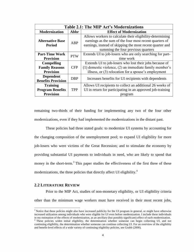
those policies, described in Table 2.1. I study the policies that expand UI eligibility,

which are the first three modernizations in that Table.2 States received one-third of their

designated MIP Act funding for implementing the Alternative Base Period, and the

1 For instance, in January 2005, 17 states had already implemented the ABP, and 6 states had already implemented

PTW. 2 For an evaluation of a similar UI job-training provision, see LaLonde (1995), who argues the negative net benefits of

such programs. I do not evaluate this modernization here.

4

remaining two-thirds of their funding for implementing any two of the four other

modernizations, even if they had implemented the modernizations in the distant past.

These policies had three stated goals: to modernize UI systems by accounting for

the changing composition of the unemployment pool; to expand UI eligibility for more

job-losers who were victims of the Great Recession; and to stimulate the economy by

providing substantial UI payments to individuals in need, who are likely to spend that

money in the short-term.3 This paper studies the effectiveness of the first three of these

modernizations, the three policies that directly affect UI eligibility.4

2.2 LITERATURE REVIEW

Prior to the MIP Act, studies of non-monetary eligibility, or UI eligibility criteria

other than the minimum wage workers must have received in their most recent jobs,

3 Notice that these policies might also have increased publicity for the UI program in general, or might have otherwise

increased utilization among individuals who were eligible for UI even before modernization. I include these individuals

in my estimation of the effects of modernization, as an ancillary (but possibly significant) effect of each modernization. 4 These policies widen initial eligibility, the determination whether someone can begin collecting UI, and not

continuing eligibility, the determination whether someone can continue collecting UI. For an overview of the eligibility

and benefit-level effects of a wide variety of continuing eligibility policies, see Grubb (2000).

Table 2.1: The MIP Act’s Modernizations

Modernization Abbr Effect of Modernization

Alternative Base

Period ABP

Allows workers to calculate their eligibility-determining

earnings as the sum of the four most recent quarters of

earnings, instead of skipping the most recent quarter and

summing the four previous quarters

Part-Time Work

Provision PTW

Extends UI to job-losers who are only searching for part-

time work

Compelling

Family Reasons

Provision

CFP

Extends UI to job-losers who lost their jobs because of

(1) domestic violence, (2) an immediate family member’s

illness, or (3) relocation for a spouse’s employment

Dependent

Benefits Provision DBP Increases benefits for UI recipients with dependents

Training

Program Benefits

Provision

TPP

Allows UI recipients to collect an additional 26 weeks of

UI in return for participating in an approved job-training

program

5

largely focused on the ABP.5 Vroman (1995) uses administrative data from the six states

that had implemented the ABP at that time to show that between 6% and 8% of

applicants collected UI under the ABP. Stettner, Boushey, and Wenger (2005) use SIPP

(Survey of Income and Program Participation) survey data of the unemployed to predict

that a nationwide ABP would increase eligibility by 7.2%. My finding of a 14% increase

caused by the ABP is higher than these authors’ estimates; the fact that I correct for

sample selection bias, along with the evolving labor market and the labor activity leading

up to and occurring during the Great Recession likely account for this difference.

O’Leary (2011) presents a case study of all of the modernizations. O’Leary uses

administrative data to measure the cost of each of the ARRA modernizations to the state

of Kentucky by examining rejected UI applicants, calculating what fraction would have

been accepted had each modernization been in place. Using this methodology, O’Leary

calculates that eligibility increases by 2.82% from ABP, 0.6% from PTW, and 0.6% from

CFR. However, O’Leary’s values are lower bounds on the effects of each of these laws,

because he does not account for any increase in UI claims from newly eligible workers

after the modernizations’ implementation.

Lindner and Nichols (2012) use SIPP data from 1996-2008 to estimate the effect

of each modernization on national UI eligibility. They find that ABP increases eligibility

by 3.9% and CFP by 6.0%, but that PTW increases eligibility by 23.9%. The authors

assume that all job-losers who lost part-time jobs can only collect UI under PTW;

however, part-time workers can collect UI in most states (so long as they seek full-time

work). The authors thus attribute many low-wage workers who would be eligible under

5 For a summary of early research on non-monetary eligibility, see Nicholson (1997); however, the author shows that

very little analysis on any UI initial eligibility policies had been completed.

6

ABP to the expected effect of PTW, leading to an over-estimation of the effect of PTW at

the expense of ABP. If this were corrected, our findings would likely be very similar.

Scholarship on non-monetary UI eligibility, then, largely uses individual-level

data. Administrative data is copious, but only includes UI applicants (and thus cannot

predict increases in UI eligibility caused by new applications). Survey data has smaller

sample sizes (especially at the state level) and may have misreporting and participation

biases, but is representative of all of the unemployed. Neither indicates whether an

individual could only collect UI due to the implementation of one of the modernizations.

I take a macro approach to the evaluation of non-monetary UI eligibility by investigating

it at the state level. Because so many states implemented the modernizations between

2009 and 2011, there is sufficient variation at the state level to estimate the real effect of

policies on eligibility and benefit levels instead of their predicted or expected effects.

In addition to the particular difficulties of each of these studies, they estimate

vastly different effects of the modernizations in question, and they do not measure the

total benefits provided to UI recipients under each policy. My state-level panel approach

is thus an important addition to the literature.

More broadly, this paper contributes to an already large literature studying the

effects of UI. Most of this literature has focused on other aspects of UI policy, such as

benefit levels and the expiration and extension of benefits (see Moffitt (1985) and Meyer

(1990) for seminal studies, Krueger and Meyer (2002) for a survey, and Rothstein (2011),

Valetta and Kuang (2010), and Fujita (2010) for studies on the Great Recession). As

shown above, there is comparatively little research on the third key aspect of UI—

eligibility. This paper fills that gap.

7

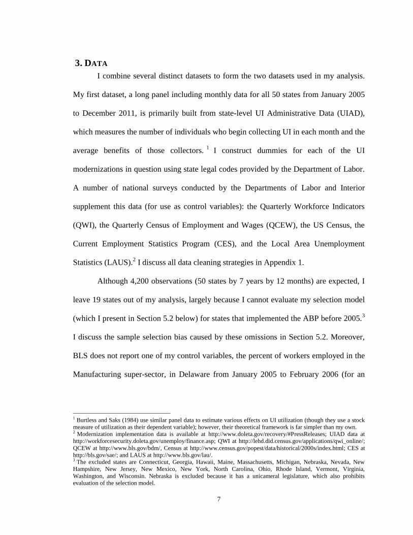
3. DATA

I combine several distinct datasets to form the two datasets used in my analysis.

My first dataset, a long panel including monthly data for all 50 states from January 2005

to December 2011, is primarily built from state-level UI Administrative Data (UIAD),

which measures the number of individuals who begin collecting UI in each month and the

average benefits of those collectors.1

I construct dummies for each of the UI

modernizations in question using state legal codes provided by the Department of Labor.

A number of national surveys conducted by the Departments of Labor and Interior

supplement this data (for use as control variables): the Quarterly Workforce Indicators

(QWI), the Quarterly Census of Employment and Wages (QCEW), the US Census, the

Current Employment Statistics Program (CES), and the Local Area Unemployment

Statistics (LAUS).2 I discuss all data cleaning strategies in Appendix 1.

Although 4,200 observations (50 states by 7 years by 12 months) are expected, I

leave 19 states out of my analysis, largely because I cannot evaluate my selection model

(which I present in Section 5.2 below) for states that implemented the ABP before 2005.3

I discuss the sample selection bias caused by these omissions in Section 5.2. Moreover,

BLS does not report one of my control variables, the percent of workers employed in the

Manufacturing super-sector, in Delaware from January 2005 to February 2006 (for an

1 Burtless and Saks (1984) use similar panel data to estimate various effects on UI utilization (though they use a stock

measure of utilization as their dependent variable); however, their theoretical framework is far simpler than my own. 2 Modernization implementation data is available at http://www.doleta.gov/recovery/#PressReleases; UIAD data at

http://workforcesecurity.doleta.gov/unemploy/finance.asp; QWI at http://lehd.did.census.gov/applications/qwi_online/;

QCEW at http://www.bls.gov/bdm/, Census at http://www.census.gov/popest/data/historical/2000s/index.html; CES at

http://bls.gov/sae/; and LAUS at http://www.bls.gov/lau/. 3 The excluded states are Connecticut, Georgia, Hawaii, Maine, Massachusetts, Michigan, Nebraska, Nevada, New

Hampshire, New Jersey, New Mexico, New York, North Carolina, Ohio, Rhode Island, Vermont, Virginia,

Washington, and Wisconsin. Nebraska is excluded because it has a unicameral legislature, which also prohibits

evaluation of the selection model.

8

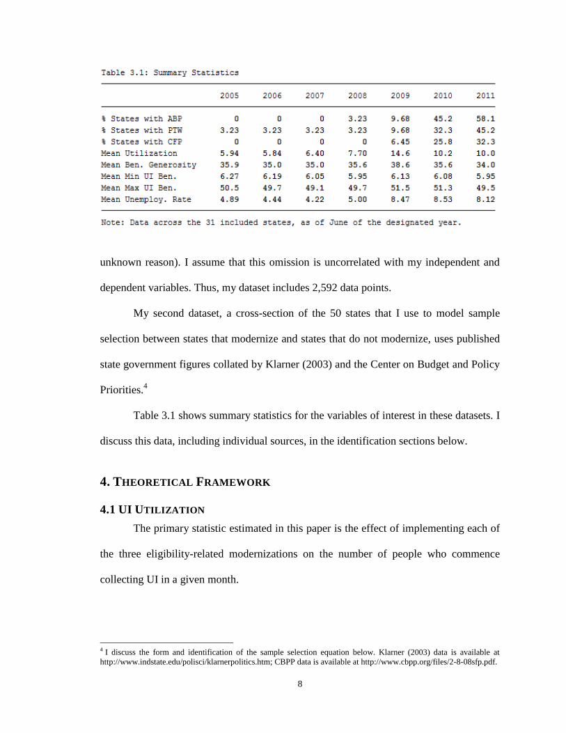
unknown reason). I assume that this omission is uncorrelated with my independent and

dependent variables. Thus, my dataset includes 2,592 data points.

My second dataset, a cross-section of the 50 states that I use to model sample

selection between states that modernize and states that do not modernize, uses published

state government figures collated by Klarner (2003) and the Center on Budget and Policy

Priorities.4

Table 3.1 shows summary statistics for the variables of interest in these datasets. I

discuss this data, including individual sources, in the identification sections below.

4. THEORETICAL FRAMEWORK

4.1 UI UTILIZATION

The primary statistic estimated in this paper is the effect of implementing each of

the three eligibility-related modernizations on the number of people who commence

collecting UI in a given month.

4 I discuss the form and identification of the sample selection equation below. Klarner (2003) data is available at

http://www.indstate.edu/polisci/klarnerpolitics.htm; CBPP data is available at http://www.cbpp.org/files/2-8-08sfp.pdf.

9

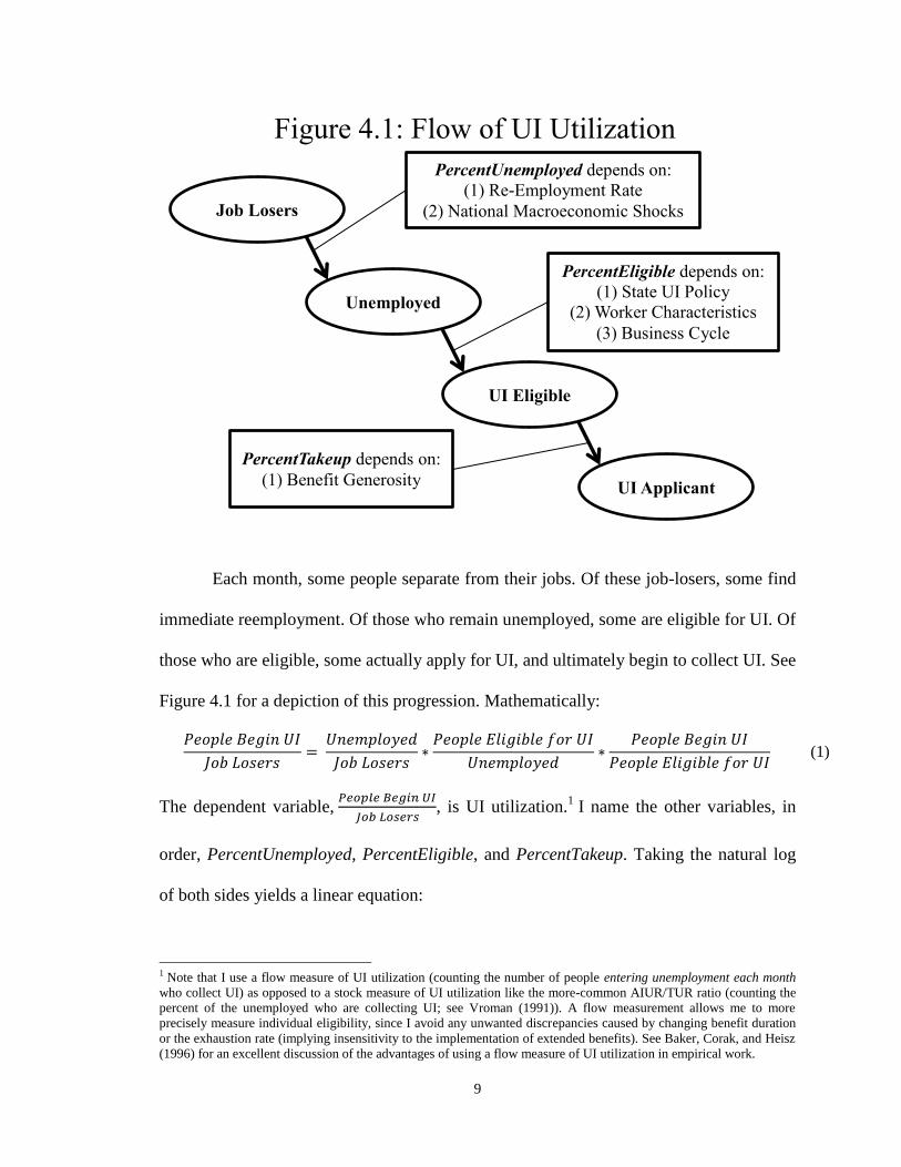
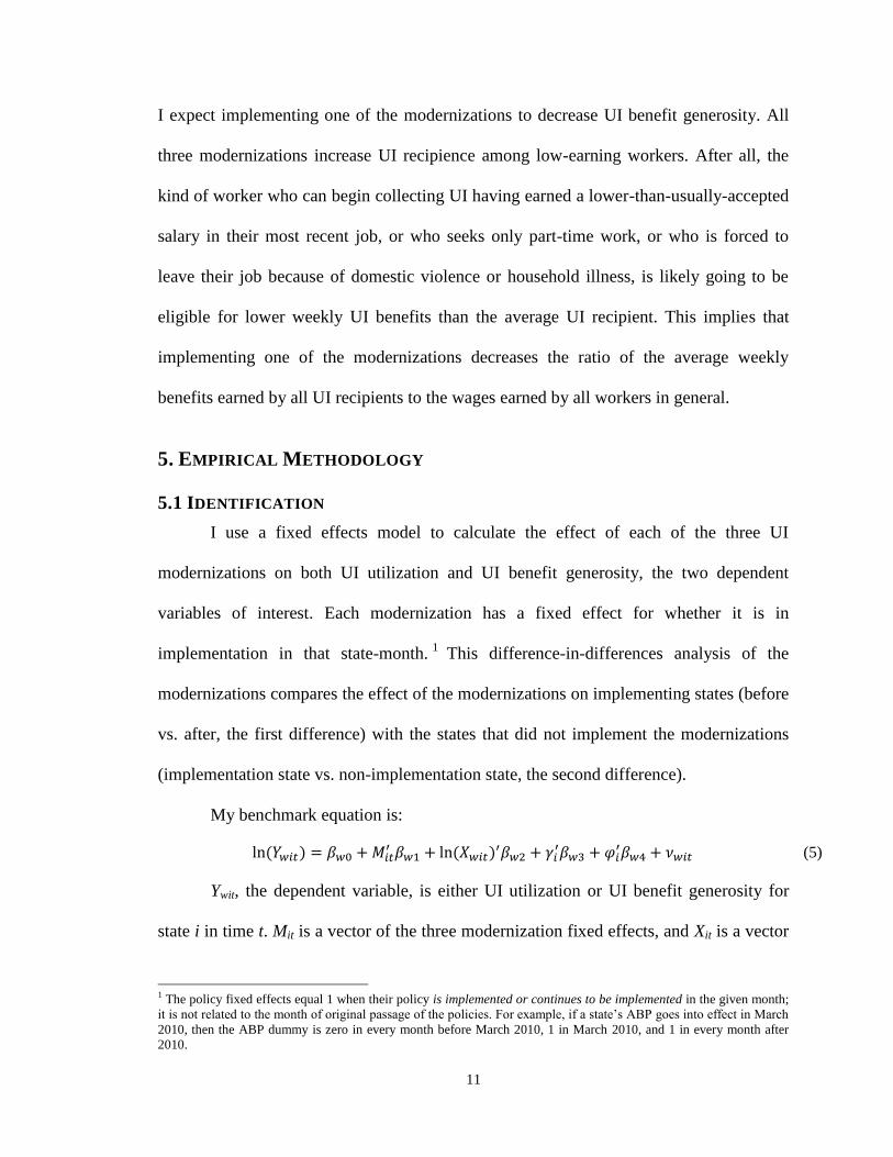
Each month, some people separate from their jobs. Of these job-losers, some find

immediate reemployment. Of those who remain unemployed, some are eligible for UI. Of

those who are eligible, some actually apply for UI, and ultimately begin to collect UI. See

Figure 4.1 for a depiction of this progression. Mathematically:

(1)

The dependent variable,

, is UI utilization.

1 I name the other variables, in

order, PercentUnemployed, PercentEligible, and PercentTakeup. Taking the natural log

of both sides yields a linear equation:

1 Note that I use a flow measure of UI utilization (counting the number of people entering unemployment each month

who collect UI) as opposed to a stock measure of UI utilization like the more-common AIUR/TUR ratio (counting the

percent of the unemployed who are collecting UI; see Vroman (1991)). A flow measurement allows me to more

precisely measure individual eligibility, since I avoid any unwanted discrepancies caused by changing benefit duration

or the exhaustion rate (implying insensitivity to the implementation of extended benefits). See Baker, Corak, and Heisz

(1996) for an excellent discussion of the advantages of using a flow measure of UI utilization in empirical work.

Unemployed

UI Eligible

PercentUnemployed depends on:

(1) Re-Employment Rate

(2) National Macroeconomic Shocks

PercentEligible depends on:

(1) State UI Policy

(2) Worker Characteristics

(3) Business Cycle

PercentTakeup depends on:

(1) Benefit Generosity

Job Losers

UI Applicant

Figure 4.1: Flow of UI Utilization

10

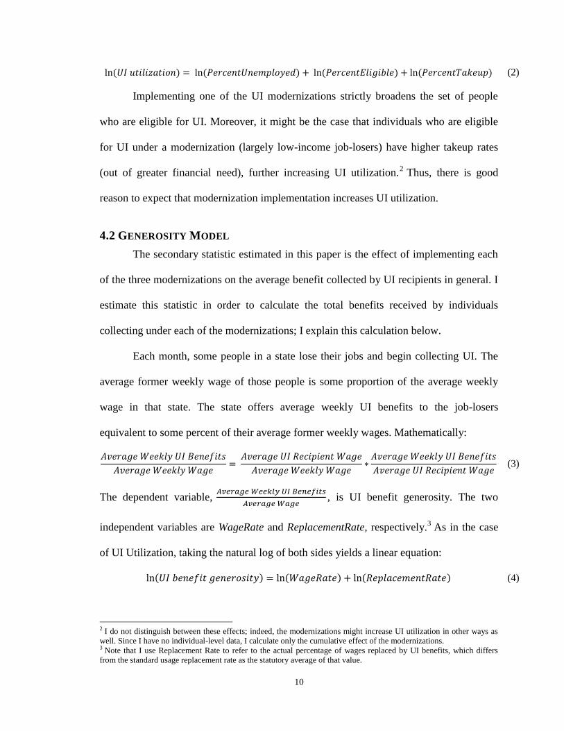
(2)

Implementing one of the UI modernizations strictly broadens the set of people

who are eligible for UI. Moreover, it might be the case that individuals who are eligible

for UI under a modernization (largely low-income job-losers) have higher takeup rates

(out of greater financial need), further increasing UI utilization.2 Thus, there is good

reason to expect that modernization implementation increases UI utilization.

4.2 GENEROSITY MODEL

The secondary statistic estimated in this paper is the effect of implementing each

of the three modernizations on the average benefit collected by UI recipients in general. I

estimate this statistic in order to calculate the total benefits received by individuals

collecting under each of the modernizations; I explain this calculation below.

Each month, some people in a state lose their jobs and begin collecting UI. The

average former weekly wage of those people is some proportion of the average weekly

wage in that state. The state offers average weekly UI benefits to the job-losers

equivalent to some percent of their average former weekly wages. Mathematically:

(3)

The dependent variable,

, is UI benefit generosity. The two

independent variables are WageRate and ReplacementRate, respectively.3 As in the case

of UI Utilization, taking the natural log of both sides yields a linear equation:

(4)

2 I do not distinguish between these effects; indeed, the modernizations might increase UI utilization in other ways as

well. Since I have no individual-level data, I calculate only the cumulative effect of the modernizations. 3 Note that I use Replacement Rate to refer to the actual percentage of wages replaced by UI benefits, which differs

from the standard usage replacement rate as the statutory average of that value.

11

I expect implementing one of the modernizations to decrease UI benefit generosity. All

three modernizations increase UI recipience among low-earning workers. After all, the

kind of worker who can begin collecting UI having earned a lower-than-usually-accepted

salary in their most recent job, or who seeks only part-time work, or who is forced to

leave their job because of domestic violence or household illness, is likely going to be

eligible for lower weekly UI benefits than the average UI recipient. This implies that

implementing one of the modernizations decreases the ratio of the average weekly

benefits earned by all UI recipients to the wages earned by all workers in general.

5. EMPIRICAL METHODOLOGY

5.1 IDENTIFICATION

I use a fixed effects model to calculate the effect of each of the three UI

modernizations on both UI utilization and UI benefit generosity, the two dependent

variables of interest. Each modernization has a fixed effect for whether it is in

implementation in that state-month.1

This difference-in-differences analysis of the

modernizations compares the effect of the modernizations on implementing states (before

vs. after, the first difference) with the states that did not implement the modernizations

(implementation state vs. non-implementation state, the second difference).

My benchmark equation is:

(5)

Ywit, the dependent variable, is either UI utilization or UI benefit generosity for

state i in time t. Mit is a vector of the three modernization fixed effects, and Xit is a vector

1 The policy fixed effects equal 1 when their policy is implemented or continues to be implemented in the given month;

it is not related to the month of original passage of the policies. For example, if a state’s ABP goes into effect in March

2010, then the ABP dummy is zero in every month before March 2010, 1 in March 2010, and 1 in every month after

2010.

12

of variables proxying for PercentUnemployed, PercentEligible, and PercentTakeup in the

first case and WageRate and ReplacementRate in the second. are state fixed effects and

are time fixed effects (for each period). Since the control variables are proxied, I include a

measurement error term .

5.1.1 UI UTILIZATION

UI utilization is the ratio of the number of people who receive first UI payments

to the number of job-losers, both of which I observe.2

I do not observe

PercentUnemployed, PercentEligible, or PercentTakeup, each of which I proxy using the

dependences listed in Figure 4.1. Consider each of these in turn.

PercentUnemployed is the percent of job-losers who actually enter unemployment

(as opposed to immediately beginning a new job or leaving the labor market).

PercentUnemployed has both state-level and national-level components: better state

hiring conditions might lead to higher immediate reemployment, and better national

macroeconomic conditions (like changes to the tax code) might lead to people moving to

other states in order to find employment or better entrepreneurial opportunities. Thus, I

proxy PercentUnemployed with both state-level hiring rates and national time dummies. I

calculate the hiring rate by finding the ratio between the total hires in a state-month3 and

the population of the state in that month.4 National time dummies capture the effect of

any national macroeconomic shocks, like the Great Recession.

PercentEligible, the percent of unemployed people who are eligible for UI, varies

in at least three dimensions. First, specific states’ UI eligibility policies differ in myriad

2 First payments data is from UAID; separations data is from QWI. I lag forward first payments by one month in order

to account for the timing between job loss and UI first payment; see Appendix 1. 3 Data from the Bureau of Labor Statistics’ Quarterly Census of Employment and Wages. Hiring data is quarterly,

which leads to some degree of measurement error. However, there is no reason to expect that the failure to include

monthly wage information biases the regression, and instead only results in attenuation error in the β coefficient on

PercentUnemployment (which is acceptable given that it is not the variable of interest). 4 Hiring data is from QCEW; population data is from the Census.

13

ways, from differing monetary eligibility and hourly work requirements to special

treatment for members of the armed forces or people with temporary disabilities.5 These

policies lead to great variation in which workers are eligible for UI. Second, states have

workers with different demographic distributions, which correspond with differing

distributions of job-loser demographics.6 For example, some states have relatively more

workers in the financial industry, which may imply that many workers in those states will

have been long-employed and well paid before losing their jobs. Even if two states had

identical UI eligibility policies, it may appear that one has more flexible eligibility

policies than another merely because the former state has job-losers with different

demographics than those of the latter state. Third, fluctuations in the business cycle might

affect the kind of worker entering unemployment; during recessions, for instance, firms

might have to lay off longer-term employees who are more likely to by insured by UI.7

I proxy for each of these dimensions. First, I include state dummy variables to

control for differences in eligibility policy, assuming that the modernizations were the

only substantial changes to UI eligibility during the Recession.8 They also account for

differences in administrative effectiveness and eligibility determination.9

Second, I

include two sets of demographic variables: industry control variables measuring the

percent of individuals who work in each of the 11 CES super sectors and in the

government, and age control variables measuring the percent of individuals collecting UI

5 See DOL ETA’s Comparison of State Unemployment Laws (2012), under both Monetary Entitlement and

Nonmonetary Eligibility, for an enumeration of the variety of differences among state eligibility laws. 6 For example, McMurrer and Chasanov (1995) show a positive association between both larger unionized industries

and a larger manufacturing industry and higher UI utilization. 7 Gordon (2009) argues for the counter-cyclicality of UI, both in first claims and first payments. 8 See Lancaster (2005-2011) for yearly evidence that the only significant changes to nonmonetary eligibility policy

during the time covered in this dataset were the modernizations. 9 See Corson, Hershey, and Kerachsky (1986) for a discussion of eligibility determination. They find, unsurprisingly,

that well-defined administrative policy at the state level causes higher levels of correct eligibility determination.

14

who are within each of seven age brackets.10

By including a set of age control variables

instead of only an average, I allow for a piecewise-linear relationship between age and UI

eligibility instead of a merely linear relationship. Third, I include the Total

Unemployment Rate (TUR) to allow for cyclicality in eligibility.11

Finally, I proxy PercentTakeup with two UI statutory generosity variables. The

implicit assumption is that the significant determinant of applying to UI is how valuable

that insurance is; the more money available from UI, the more likely an eligible

individual is to apply for UI.12

In particular, I include the minimum and maximum

weekly benefits available through UI.13

Since wage levels differ across states, I normalize

these UI policy generosity variables by dividing them by the average (median) weekly

wage in the state, so that higher UI policy generosity implies not a higher cost of living,

but the greater value of the UI benefits.14

Most control variables are included in logarithmic form. Of course, I do not take

logarithms of state and time dummies. I also do not take the log of the age distribution

variables, since they are percentages constructed to sum to one in order to determine a

piecewise-linear relationship, and they would lose this distinctive quality in log form.

5.1.2 UI BENEFIT GENEROSITY

UI benefit generosity is ratio of the average weekly UI benefit to the average

wage, both of which I observe. I use this ratio to account for differences in salaries and

10 Industry data is from CES, which combines hundreds of jobs types into 11 super sectors: National Resources and

Mining; Construction; Manufacturing; Trade, Transportation, and Utilities; Information; Financial Activities;

Professional and Business Services; Education and Health Services; Leisure and Hospitality; Other Services; and

Public Administration. For my industry control variables, I take the ratio of the number of individuals working in the

private sector in each super sector to the total number of individuals working in the private sector. Age data is from

UIAD. I modify the data by dividing by the percent of people who report their ages (almost exclusively over 90%), to

correct for any bias in non-reporting (assuming the same distribution of reported and non-reported ages). The age

brackets used are <22, 22-24, 25-34, 35-44, 45-54, 55-59, 60-64, and >65 years old. 11 TUR data is from LAUS. 12 For evidence of this strong positive relationship, see Anderson and Meyer (1997), who find an elasticity between the

takeup rate and UI benefits of between 0.39 and 0.59. 13 Data from Loryn Lancaster’s yearly reports on the subject; see Lancaster (2005-2011) 14 Data is from QCEW.

15

average costs of living between states. I do not observe ReplacementRate or WageRate,

each of which I proxy. Consider each of these in turn.

WageRate is the ratio of the wage of the average new UI recipient to the average

wage in the state. I proxy the Wage Rate using demographic composition and time

dummies. I include the industry and age distribution variables (along with the percent of

workers employed by the government) to account for demographic differences across

states, since those differences likely lead to different distributions of UI recipients, which

manifests itself in higher or lower benefits-to-wages ratios. I include time dummies for

each state-month in order to capture two effects. First, there are seasonal effects of low-

or high-wage workers regularly collecting UI with more frequency during certain months,

across states (for instance, many symphony employees work nine months each year and

collect low UI during the off-quarter). Second, Benefit Generosity is sensitive both to

changes in average benefit levels and to average wage levels, and the latter might be

sensitive to national macroeconomic shocks that discourage regular wage increases.15

ReplacementRate is the ratio of average UI benefits to the wage of an average UI

recipient. I proxy ReplacementRate with state-level policy variables that determine the

monetary generosity of each state’s UI system. I use state dummies to distinguish states’

UI eligibility policies, and include the same measures of UI statutory generosity as above

(minimum and maximum available weekly benefits) to control for changes in benefit

levels. In addition, although only the three modernizations studied in this paper directly

affect UI Utilization, a fourth modernization (which increases benefit levels for job-losers

15 A relative decrease in the average wage would likely manifest itself in average benefit levels, since benefits are a

function of the wages of job-losers. However, there might be a delay in that relationship (because the workers whose

wages fail to increase are not necessarily the same workers who lose their jobs in that month), and so long as that delay

is similar across states (and there is no reason to think otherwise), time dummies capture its effects.

16

with children or other dependents) might increase the Replacement Rate in states that

implement it, so I include a dummy for the Dependent Benefits modernization.

I include only the logarithm of any variable that is not either a dummy or one of

the members of the age distribution.

5.2 ECONOMETRIC METHODOLOGY

I state my benchmark equations above as Equations 5. However, I cannot estimate

this equation directly because sample selection bias, caused by a non-random selection of

states that implement the modernizations, violates the Gauss-Markov linearity condition.

This section discusses my solution to sample selection bias in the stated substantial

equations, which uses a control function framework with the propensity score

approximated by the hazard rates of a duration model. Following sample selection bias, I

also discuss the violation of spherical errors.

5.2.1 SAMPLE SELECTION BIAS

If a non-random selection of states implemented modernizations (e.g. if the states’

selection mechanisms correlate with the effects of the modernizations), then βw1 would

estimate the combination of two different effects: the effect of the implementation of the

modernization, and the effect of being the kind of state that implements that

modernization, the two of which might be correlated. Although part of this latter effect is

absorbed by the control variables described above, those control variables cannot account

for correlation between the implementation of modernizations and UI utilization. This

study is interested in the actual effect of the modernizations’ implementation, but sample

selection bias confounds those results through omitted variable bias.

Analysis of sample selection bias usually makes use of a linear selection equation

that would model which states are included in the sample using state-level characteristics.

17

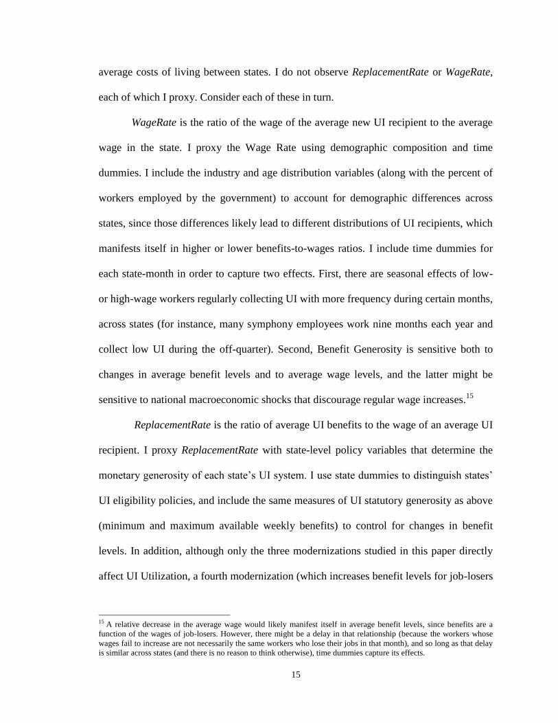
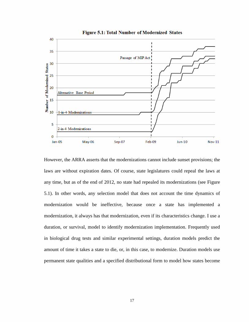
However, the ARRA asserts that the modernizations cannot include sunset provisions; the

laws are without expiration dates. Of course, state legislatures could repeal the laws at

any time, but as of the end of 2012, no state had repealed its modernizations (see Figure

5.1). In other words, any selection model that does not account the time dynamics of

modernization would be ineffective, because once a state has implemented a

modernization, it always has that modernization, even if its characteristics change. I use a

duration, or survival, model to identify modernization implementation. Frequently used

in biological drug tests and similar experimental settings, duration models predict the

amount of time it takes a state to die, or, in this case, to modernize. Duration models use

permanent state qualities and a specified distributional form to model how states become

18

modernization states over time.16

Thus, this model form prohibits states to move from

being modernized to being not modernized.

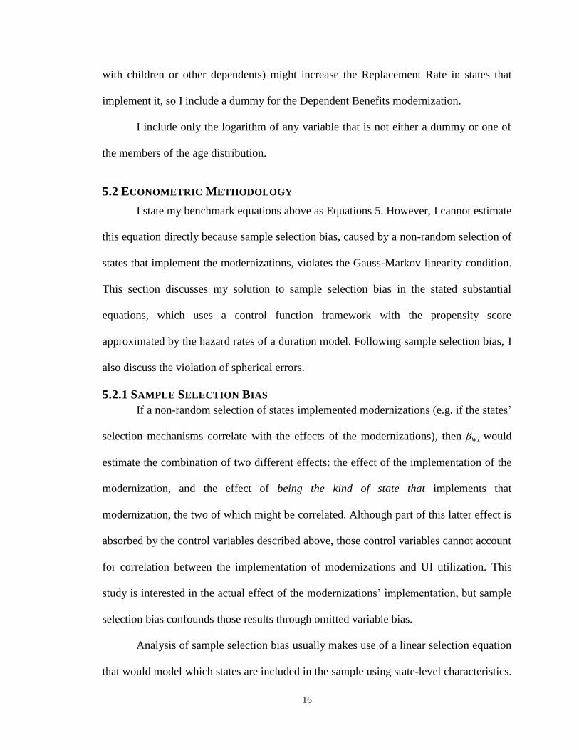
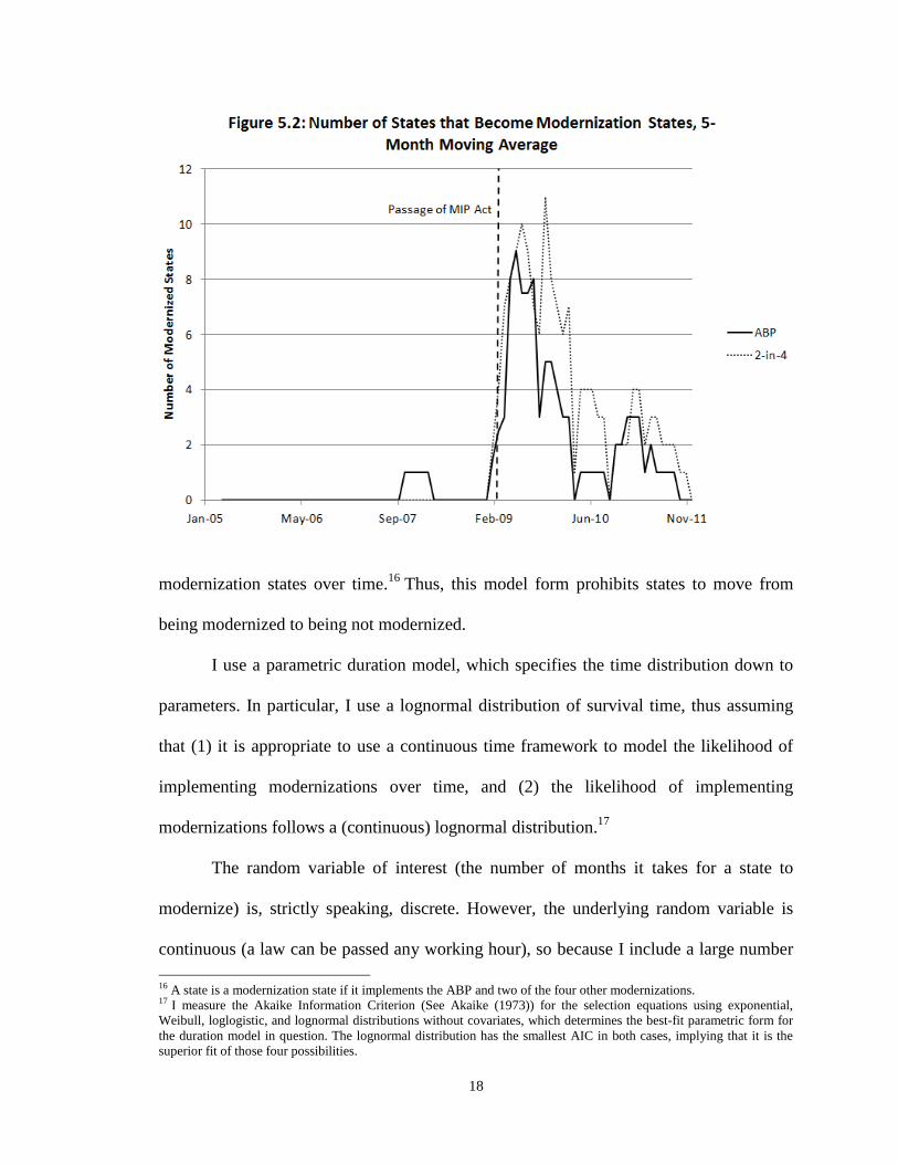
I use a parametric duration model, which specifies the time distribution down to

parameters. In particular, I use a lognormal distribution of survival time, thus assuming

that (1) it is appropriate to use a continuous time framework to model the likelihood of

implementing modernizations over time, and (2) the likelihood of implementing

modernizations follows a (continuous) lognormal distribution.17

The random variable of interest (the number of months it takes for a state to

modernize) is, strictly speaking, discrete. However, the underlying random variable is

continuous (a law can be passed any working hour), so because I include a large number

16 A state is a modernization state if it implements the ABP and two of the four other modernizations. 17 I measure the Akaike Information Criterion (See Akaike (1973)) for the selection equations using exponential,

Weibull, loglogistic, and lognormal distributions without covariates, which determines the best-fit parametric form for

the duration model in question. The lognormal distribution has the smallest AIC in both cases, implying that it is the

superior fit of those four possibilities.

19

of periods (84 for each state), I approximate that discrete distribution with the continuous

lognormal distribution. The greatest concern with the lognormal form is that the passage

of ARRA appears to be a discontinuity in the time distribution; after all, many states

implement modernizations just after the passage of ARRA. However, the lognormal form

allows for this jump with its asymmetrical form, swiftly reaching a peak but flexible

about how quickly the instantaneous probability of modernization returns to zero. In

addition, state legislatures have been long aware of the ARRA modernizations, because

an identical Unemployment Insurance Modernization Act had been introduced in both the

House and the Senate more than two years earlier.18

The assumption of rational

expectations of state legislatures implies a continuous increase rather than a

discontinuous spike in the likelihood of modernization implementation.19

Flexible in

multiple mean parameters as well as the curve’s standard error, the lognormal distribution

is a good parametric fit for a duration model of state modernization implementation.

Figure 5.2 shows the distribution of modernization implementation across states, strongly

suggesting a lognormal distribution.

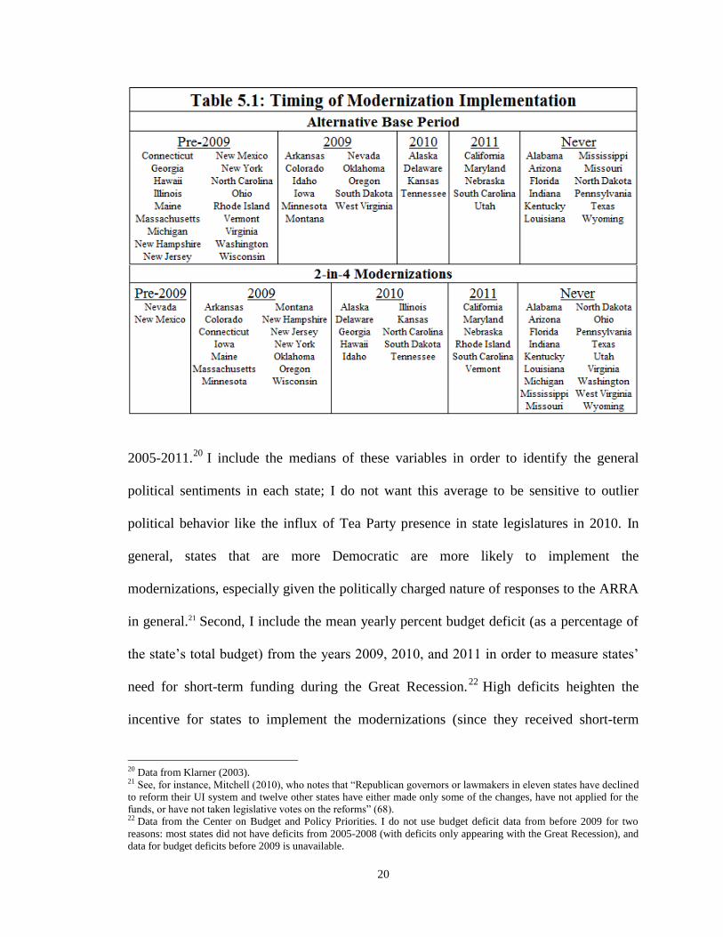
Table 5.1 shows if and when states became ABP states and 2-in-4-modernization

states. I use two kinds of covariates to model the transition probability of state i to

modernize. First, I include variables measuring the median Democratic control of the

state House of Representatives, the Senate, and the Governorship over every month from

18 See S. 1871 and H.R. 3920, Section 402. The bill was passed in the House of Representatives, but died in Senate

committee before it was placed into the ARRA. 19 Strictly speaking, on this interpretation one would expect a discontinuous spike in the probability of implementing

modernizations when the law was originally announced, two years before the passage of the ARRA. However, at that

time the probability of the modernization incentivization funding actually being implemented by Congress was very

small, and compounded with future-discounting would result in a very small discontinuity that I assume to be

insignificant. Therefore, prior expectations of the passage of the incentivization contained in the ARRA are adequate to

eliminate any significant discontinuities in the modernizaiton implementation distribution.

20

2005-2011.20

I include the medians of these variables in order to identify the general

political sentiments in each state; I do not want this average to be sensitive to outlier

political behavior like the influx of Tea Party presence in state legislatures in 2010. In

general, states that are more Democratic are more likely to implement the

modernizations, especially given the politically charged nature of responses to the ARRA

in general.21 Second, I include the mean yearly percent budget deficit (as a percentage of

the state’s total budget) from the years 2009, 2010, and 2011 in order to measure states’

need for short-term funding during the Great Recession.22

High deficits heighten the

incentive for states to implement the modernizations (since they received short-term

20 Data from Klarner (2003). 21 See, for instance, Mitchell (2010), who notes that “Republican governors or lawmakers in eleven states have declined

to reform their UI system and twelve other states have either made only some of the changes, have not applied for the

funds, or have not taken legislative votes on the reforms” (68). 22 Data from the Center on Budget and Policy Priorities. I do not use budget deficit data from before 2009 for two

reasons: most states did not have deficits from 2005-2008 (with deficits only appearing with the Great Recession), and

data for budget deficits before 2009 is unavailable.

21

funding in return for long-term liability). According to my model, then, these four

variables identify the state decision to become ABP and 2-in-4-modernization states

(states that implement two of the four additional modernizations)

I model the expected time in which state i becomes an ABP state (Ai) and

becomes a 2-in-4-modernization state (Ti) using two distinct duration models, each of

which separates states into two groups: modernized and unmodernized. Mathematically:

[

] {

(6)

[

] {

(7)

where is a vector of the selection covariates described above, are the estimated

coefficients, and is an error term caused by measurement error of . Modernization

states (at time t) are states for which zit = 1; non-modernization states (at time t) are states

for which zit = 0.

I estimate these first-step equations using a duration maximum likelihood

framework. States may be of two types: either they become modernization states during

the time of my dataset (2005-2011), or they never become modernization states (in my

timeframe). In the case of states that never become modernization states, I maximize their

survival rate , or the chance that the state has not modernized by t:

(

) (8)

In the case of states that modernize, on the other hand, I maximize their hazard rate λ(t),

or the chance that the state modernizes in time conditional on their not having yet

modernized:

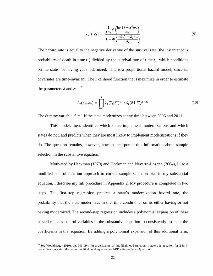
22

(

)

(

)

(9)

The hazard rate is equal to the negative derivative of the survival rate (the instantaneous

probability of death in time ) divided by the survival rate of time , which conditions

on the state not having yet modernized. This is a proportional hazard model, since its

covariates are time-invariant. The likelihood function that I maximize in order to estimate

the parameters β and σ is:23

∏

(10)

The dummy variable di = 1 if the state modernizes at any time between 2005 and 2011.

This model, then, identifies which states implement modernizations and which

states do not, and predicts when they are most likely to implement modernizations if they

do. The question remains, however, how to incorporate this information about sample

selection in the substantive equation.

Motivated by Heckman (1979) and Heckman and Navarro-Lozano (2004), I use a

modified control function approach to correct sample selection bias in my substantial

equation. I describe my full procedure in Appendix 2. My procedure is completed in two

steps. The first-step regression predicts a state’s modernization hazard rate, the

probability that the state modernizes in that time conditional on its either having or not

having modernized. The second-step regression includes a polynomial expansion of these

hazard rates as control variables in the substantive equation to consistently estimate the

coefficients in that equation. By adding a polynomial expansion of this additional term,

23 See Wooldridge (2010), pp. 993-994, for a derivation of this likelihood function. I state this equation for 2-in-4-

modernization states; the respective likelihood equation for ABP states replaces Ti with Ai.

23

the substantive equation separately calculates the effects of the modernizations and the

effect of being the kind of state that implements modernizations, and therefore

consistently estimates the effect of the modernizations alone. 24

As I describe in Appendix

2, because I assume that the error terms of the selection models are uncorrelated, I do not

include cross-polynomials between the two hazard rates in my regressions, though I do

present those results in the Robustness section below.

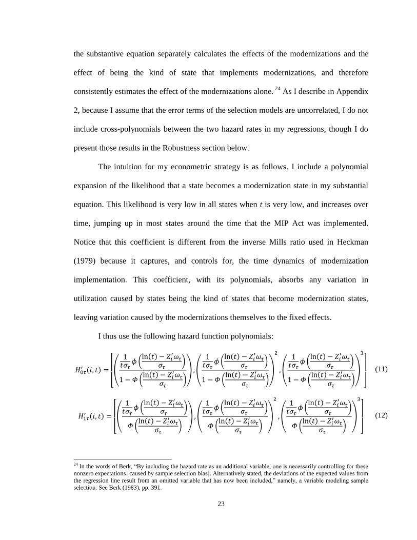
The intuition for my econometric strategy is as follows. I include a polynomial

expansion of the likelihood that a state becomes a modernization state in my substantial

equation. This likelihood is very low in all states when t is very low, and increases over

time, jumping up in most states around the time that the MIP Act was implemented.

Notice that this coefficient is different from the inverse Mills ratio used in Heckman

(1979) because it captures, and controls for, the time dynamics of modernization

implementation. This coefficient, with its polynomials, absorbs any variation in

utilization caused by states being the kind of states that become modernization states,

leaving variation caused by the modernizations themselves to the fixed effects.

I thus use the following hazard function polynomials:

[

(

(

)

(

)

) (

(

)

(

)

)

(

(

)

(

)

)

]

(11)

[

(

(

)

(

)

) (

(

)

(

)

)

(

(

)

(

)

)

]

(12)

24 In the words of Berk, “By including the hazard rate as an additional variable, one is necessarily controlling for these

nonzero expectations [caused by sample selection bias]. Alternatively stated, the deviations of the expected values from

the regression line result from an omitted variable that has now been included,” namely, a variable modeling sample

selection. See Berk (1983), pp. 391.

24

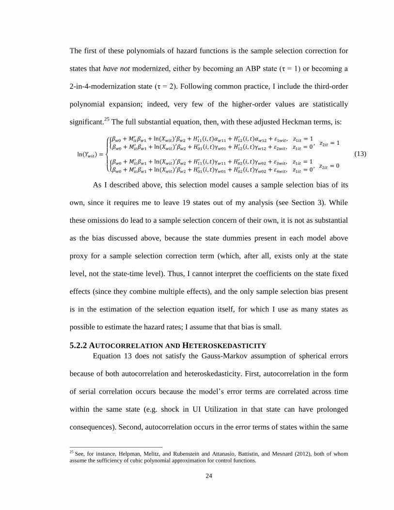
The first of these polynomials of hazard functions is the sample selection correction for

states that have not modernized, either by becoming an ABP state (τ = 1) or becoming a

2-in-4-modernization state (τ = 2). Following common practice, I include the third-order

polynomial expansion; indeed, very few of the higher-order values are statistically

significant.25

The full substantial equation, then, with these adjusted Heckman terms, is:

{

{

{

(13)

As I described above, this selection model causes a sample selection bias of its

own, since it requires me to leave 19 states out of my analysis (see Section 3). While

these omissions do lead to a sample selection concern of their own, it is not as substantial

as the bias discussed above, because the state dummies present in each model above

proxy for a sample selection correction term (which, after all, exists only at the state

level, not the state-time level). Thus, I cannot interpret the coefficients on the state fixed

effects (since they combine multiple effects), and the only sample selection bias present

is in the estimation of the selection equation itself, for which I use as many states as

possible to estimate the hazard rates; I assume that that bias is small.

5.2.2 AUTOCORRELATION AND HETEROSKEDASTICITY

Equation 13 does not satisfy the Gauss-Markov assumption of spherical errors

because of both autocorrelation and heteroskedasticity. First, autocorrelation in the form

of serial correlation occurs because the model’s error terms are correlated across time

within the same state (e.g. shock in UI Utilization in that state can have prolonged

consequences). Second, autocorrelation occurs in the error terms of states within the same

25 See, for instance, Helpman, Melitz, and Rubenstein and Attanasio, Battistin, and Mesnard (2012), both of whom

assume the sufficiency of cubic polynomial approximation for control functions.

25

time (e.g. some national shocks affect all (or most) states’ UI Utilization similarly).

Third, heteroskedasticity occurs in the error term; there is no reason to expect different

times and states having the same variance levels in their error terms.

My dataset is a ‘long’ panel dataset in that it allows for a large-T asymptotic

assumption (assume T→∞) in addition to large-dataset asymptotic assumption (assume

N→∞). Thus, in order to account for all three variance concerns, I use the variance

estimator developed by Driscoll and Kraay (1998).26

Driscoll-Kraay error terms are

asymptotically valid given a large-T asymptotic assumption, independent of the size of S

(number of states).27

Like the Newey-West estimator, the Driscoll-Kraay estimator

requires the specification of an economically determined order of autocorrelation, which I

set at three years (36 months), based on the assumption that the effects of shocks to UI

Utilization might be sustained for up to that length of time. The estimator uses linearly

decaying Bartlett weights such that the serial correlation between terms decreases as

those terms grow further apart.28

I compare these Driscoll-Kraay variances with other

variance estimations in the Robustness section below.

5.3 POLICY EVALUATION

So far, I have discussed how to estimate the effect of each of the three

modernizations on both UI Utilization and UI Benefit Generosity, where the first is

26 Robust standard errors (White (1980)) use a large-N assumption to consistently account for heteroskedasticity, but

not autocorrelation. Both clustered standard errors and Newey-West (1987) standard errors use a large-N assumption to

allow for serial correlation (complete in the former case and limited in the latter case), but neither allows for cross-

sectional autocorrelation. Finally, panel-corrected standard errors (Beck and Katz (1995)) consistently account for

heteroskedasticity and contemporaneous cross-sectional autocorrelation, but can only account for serial autocorrelation

by assuming an AR(1) process in the error terms, which would invalidate the control function approach defined above.

Moreover, panel-corrected standard errors require a small-S/T assumption, which is not the case in my dataset. 27 Note also that Driscoll-Kraay standard errors, as a generalization of Newey-West standard errors, allay any concerns

with serial correlation in the independent variables of interest, as shown through Monte Carlo simulation in Bertrand,

Duflo, and Mullainathan (2004), pp. 271. The authors’ two caveats are that this procedure is not effective if S, the

number of states, is small (6-10 states) or the order of autocorrelation is small, but my cross-section is large and I

specify a large order of autocorrelation. 28 See Hoechle (2007), pp. 287-288, for the specific Driscoll-Kraay covariance matrix and estimation procedure.

26

and the second is

. Since the models are both

evaluated using the logarithm of these values, following standard practice (since both

values are small) I interpret coefficients β1 and α1 as the percent change in UI Utilization

and UI Benefit Generosity caused by the modernizations, respectively. I assume that a

state’s implementing a modernization has no effect on either the number of job losers in

that state or the average wage in that state; my model includes no moral hazard on the

part of employers, and there is no obvious reason that these laws affect anything except

the kinds of people who collect UI. Therefore, I interpret β1 as the percent change in the

number of people who begin collecting UI benefits because of the modernizations, and α1

as the percent change in the average level of benefits because of the modernizations (each

the numerator of the respective variable).

Let M be one of the three modernizations, and let βM and αM be the respective

fixed effect coefficients for M. Let t be an arbitrary time in state i such that i has

implemented M on or before time t. Finally, let xit be the total number of people who

begin collecting UI, and let yit be the average benefits of all UI recipients. I calculate the

number of people who begin collecting benefits only because of the implementation of M

(nMit), and the average weekly benefit collected by those people (bMit), using:29

( (

) ) (14)

Following these equations, the total benefits paid out to individuals who are only eligible

for UI because the state has implemented M, in their first week of benefits (since

eligibility measures UI first payments and the benefit level measures weekly benefits), is

29 The first equation in Equation 14 is the definition of discussed above. The second equation comes from the

identity ( )( )

, which averages the benefit levels for each of the two groups (those who

collect UI only because of M and those who can collect otherwise), and results in the current benefit level under M.

27

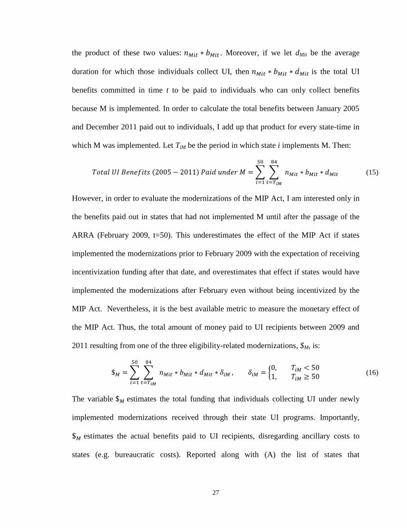
the product of these two values: . Moreover, if we let dMit be the average

duration for which those individuals collect UI, then is the total UI

benefits committed in time t to be paid to individuals who can only collect benefits

because M is implemented. In order to calculate the total benefits between January 2005

and December 2011 paid out to individuals, I add up that product for every state-time in

which M was implemented. Let TiM be the period in which state i implements M. Then:

∑ ∑

(15)

However, in order to evaluate the modernizations of the MIP Act, I am interested only in

the benefits paid out in states that had not implemented M until after the passage of the

ARRA (February 2009, t=50). This underestimates the effect of the MIP Act if states

implemented the modernizations prior to February 2009 with the expectation of receiving

incentivization funding after that date, and overestimates that effect if states would have

implemented the modernizations after February even without being incentivized by the

MIP Act. Nevertheless, it is the best available metric to measure the monetary effect of

the MIP Act. Thus, the total amount of money paid to UI recipients between 2009 and

2011 resulting from one of the three eligibility-related modernizations, $M, is:

∑ ∑

{

(16)

The variable estimates the total funding that individuals collecting UI under newly

implemented modernizations received through their state UI programs. Importantly,

estimates the actual benefits paid to UI recipients, disregarding ancillary costs to

states (e.g. bureaucratic costs). Reported along with (A) the list of states that

28

implemented modernizations and (B) the number of people who received UI benefits

under the MIP Act, $M is an important metric in evaluating the effectiveness of that Act.

I calculate a lower bound variance of $M. I do so by first repeatedly resampling

my data and evaluating Equation 13 (for both utilization and benefit generosity) to

bootstrap [ ] . Since these coefficients are estimated separately, I

cannot directly calculate this variance; however, bootstrapping provides an

asymptotically valid variance estimation.30

I then must assume that the covariances of

across state and time are negligibly small, an assumption that, while

necessary (as I cannot calculate those covariances), implies that there is no serial

correlation or contemporary cross-sectional correlation in UI benefits (from M). Finally,

since I do not estimate the average duration of UI collection by individuals collecting UI

under M (which is a topic for future research), I assume that individuals collecting under

M collect UI on average for the same duration as all UI recipients; because that data is

available in UIAD, dMit is given (and thus has no variance). The somewhat tenuous nature

of these assumptions implies that the reported error terms are lower bounds on the true

error terms. Nevertheless, given these assumptions and well-known rules of variances:

[ ] ∑ ∑ [ ]

(17)

6. RESULTS

6.1 SELECTION EQUATION

Table 6.1 shows the regression results from the first-step selection equation.

There are two modeled equations: Equation 6 (Column 1) and Equation 7 (Column 2). I

30 For the efficiency, validity, and procedure of bootstrapping, see Wooldridge (2010), pp. 438-442. I draw 10,000

samples (with replacement) to calculate the variances.

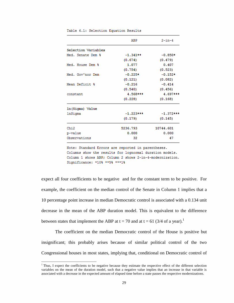
29

expect all four coefficients to be negative and for the constant term to be positive. For

example, the coefficient on the median control of the Senate in Column 1 implies that a

10 percentage point increase in median Democratic control is associated with a 0.134 unit

decrease in the mean of the ABP duration model. This is equivalent to the difference

between states that implement the ABP at t = 70 and at t = 61 (3/4 of a year).1

The coefficient on the median Democratic control of the House is positive but

insignificant; this probably arises because of similar political control of the two

Congressional houses in most states, implying that, conditional on Democratic control of

1 Thus, I expect the coefficients to be negative because they estimate the respective effect of the different selection

variables on the mean of the duration model, such that a negative value implies that an increase in that variable is

associated with a decrease in the expected amount of elapsed time before a state passes the respective modernizations.

30

the Senate, the effect of Democratic control of the House is statistically no different from

zero. The coefficients on mean state budget deficits during the Great Recession are

negative but insignificantly non-zero, which provides no evidence of a negative effect

between budget deficits and duration until modernization. However, in both models

Democratic control of the Senate and of the Governorship corresponds with significantly

lower duration until modernization at the 10% level.

The natural log of the variances in both models ( and

) are -1.223

and -1.372, with the 2-in-4-modernizations model having a slightly lower variance than

the ABP model. A of -1.372 implies a variance in the duration model of 0.0643,

which for a state expected to modernize at t=70 implies a 95% confidence interval of

modernizing between t=42 and t=115.

The χ2 test statistic evaluates the null hypothesis that all of the coefficients on the

independent variables are equal to zero (i.e. there is no association between the

independent variables and the mean of the duration model). The p-value in both

regressions is 0.000, implying that the specified selection models are strongly predictive.

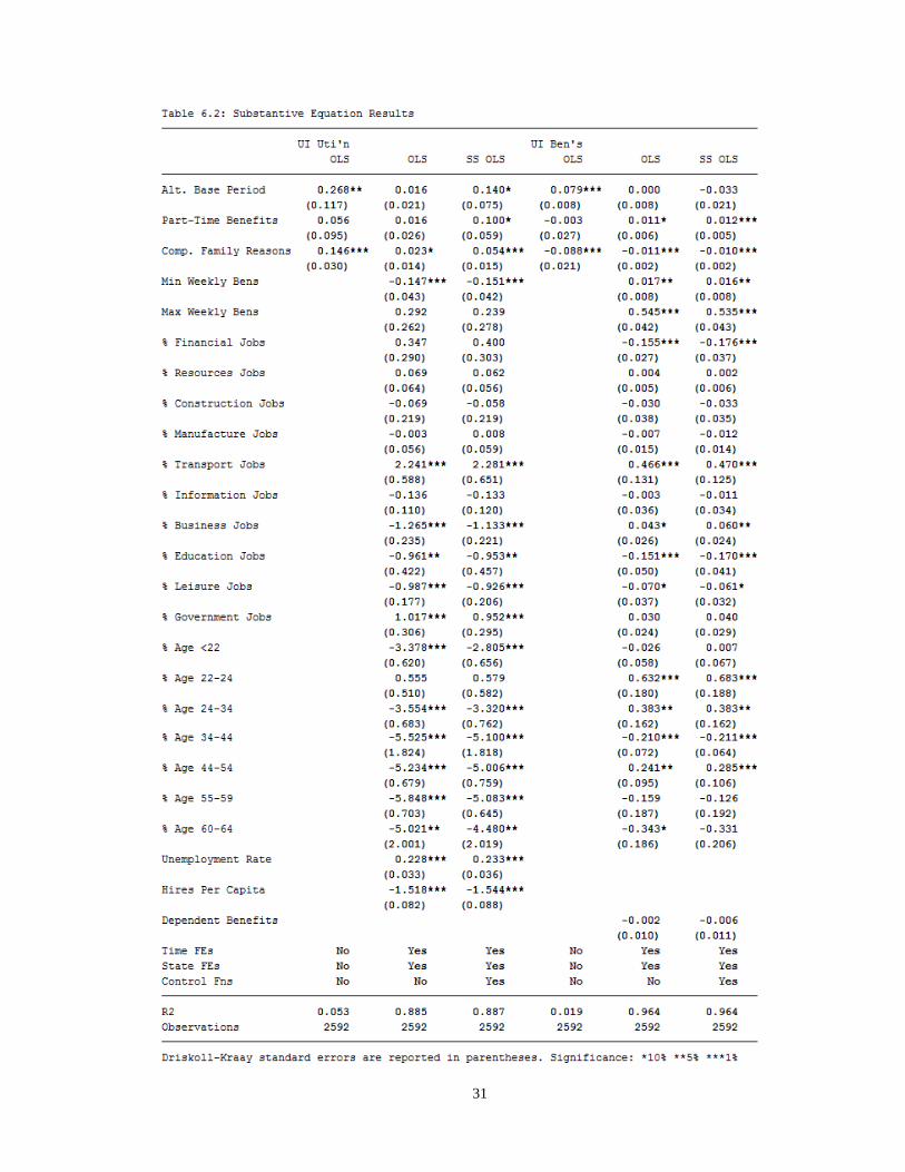
6.2 SUBSTANTIVE EQUATIONS

Table 6.2 shows the coefficient estimates for Equation 13, with columns 1-3

showing the estimates for UI utilization and 4-6 show the results for UI benefit

generosity. Columns 1 and 4 show OLS results without any control variables; Columns 2

and 5 show results with controls but without correcting for sample selection; and columns

3 and 6 show results including the control function polynomials. Driskoll-Kraay error

terms are displayed with all six models.

31

32

The shift from Column 2 to Column 3, which controls for sample selection bias

using the modified control function approach discussed above, marks a substantial

increase in the estimated effect of all three modernizations. Indeed, as I show in the

Robustness section below, there is a strong negative correlation between being the kind

of state that modernizes and UI utilization. Remember that my sample selection

correction is dynamic; this result implies that states that are likely to modernize early

according to my model, but fail to do so, have far lower UI utilization. This is an

unsurprising result: if a state is highly Democratic but modernizes late, then it is likely

that there are unobserved factors that cause the state to not modernize (e.g. a powerful

Republican senator) that also cause an unobserved decrease in UI utilization.

The rest of this section only discusses the results in Columns 3 and 6, which

display my main results. The first three rows show the fixed effects of the three

modernizations. I find that all three modernizations studied in this paper had significant

positive effects on Utilization at the 10% level. The largest effect, as expected, was from

the ABP, which increased eligibility by about 14.0% (percent, not percentage points).

PTW and CFP increased eligibility by about 10.0% and 5.4%, respectively. Moreover, I

find a significant and negative change in Benefit Generosity from CFP at the 1% level,

implying that UI recipients under that provision collected significantly lower average

weekly benefits than those otherwise available for UI. Surprisingly, I also find a

significantly positive (though small) coefficient in Benefit Generosity on PTW, which

implies that job-losers collecting UI under that provision obtain higher-than-average

benefits. I discuss the policy implications of these coefficients below.

33

The other control variables largely have the expected sign and have reasonable

coefficient values. I find that states with higher maximum UI benefits have higher benefit

generosity (e.g., a doubled maximum UI benefit is associated with a 54% increase in

average weekly benefits). States with higher minimum UI benefits have slightly higher

benefit generosity but lower utilization (implying that generous states actually have lower

minimum UI benefits, as this increases the number of workers eligible for UI). I find that

the unemployment rate is positively associated with utilization, with a coefficient that

estimates that an increase in the TUR from 5% to 8% would imply an increase in

utilization from 30.0% to 33.8%, because longer-term more-eligible workers are laid off

during high-unemployment spells. I find that a higher hiring rate implies lower

utilization, suggesting that job-losers are more likely to find a new job quickly (instead of

applying for UI) in states with more hiring; moving from the 50th

to the 75th

percentile of

hiring (7% to 8.5%) is associated with a decrease in utilization from 30.0% to 22.0%.

I find that large Transportation and Government sectors are positively associated

with UI utilization, which might reflect a high unionization rate (which increases

awareness and eligibility for UI) or high employment turnover rates.2 One surprising

result is that states with larger finance industries have significantly lower-than-average

benefit generosity; this might be because states with larger finance industries are more

urban, and urban areas in general have lower benefit generosity because of the

availability and turnover of low-wage jobs. For the age control variables, Age 65+ is

omitted out of multicolinearity, so the coefficients measure effects relative to those of

Age 65+. I find that states with high percentages of young workers (below 24) and old

2 Burtless and Saks (1984) and McMurrer and Chasanov (1995) show a positive association between larger unionized

industries and higher UI utilization.

34

workers (65+) collecting UI have relatively higher utilization, while the rest of the

distribution is flat. Moreover, states with high percentages workers below 34 or between

44 and 54 collecting UI have relatively higher benefit generosity. The age variables are

included without logarithm, so while the industry coefficients are interpreted as percent-

percent increases, the age coefficients are interpreted as percentage -percent increases.

6.3 POLICY EVALUATION

After the passage of ARRA, 19 states implemented the ABP, 18 implemented

PTW, and 19 implemented CFP. Table 6.3 shows the Policy Evaluation results from the

regression analysis above, as explained in Section 5.3, with bootstrapped 95% confidence

intervals; however, as explained above, these intervals are lower bounds (I do not account

for covariance between state-months). Note that the results in Table 6.4 include the

increase in utilization and total benefits only in states that implemented modernizations

after the passage of ARRA, which I attribute to the MIP Act’s incentivization.

29,204,000 individuals collected UI between February 2009 and the end of 2011.

My analysis shows that about 2,300,000 of those individuals collected UI strictly under

the ABP, 520,000 of whom collected UI in states that did not have the ABP when the

ARRA incentivized ABP implementation. Similarly, about 1,200,000 individuals

collected UI under PTW, 580,000 of whom were in newly implementing states, and about

500,000 collected under CFP, nearly all of whom (480,000) collected in newly

Table 6.3: Policy Evaluation Results

Utilization 95% Total Benefits (bill.) 95% (bill.)

ABP 517,227 ± 6,205 $2.182 ± $3.668

PTW 581,460 ± 11,905 $3.464 ± $6.997

CFP 475,370 ± 14,556 $2.321 ± $8.982

35

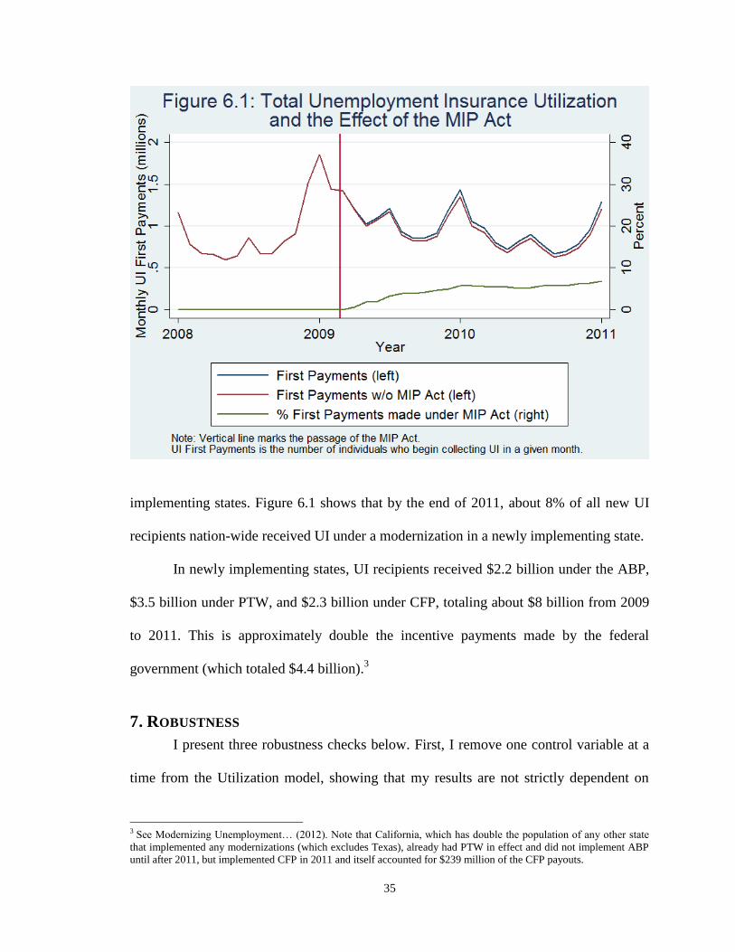
implementing states. Figure 6.1 shows that by the end of 2011, about 8% of all new UI

recipients nation-wide received UI under a modernization in a newly implementing state.

In newly implementing states, UI recipients received $2.2 billion under the ABP,

$3.5 billion under PTW, and $2.3 billion under CFP, totaling about $8 billion from 2009

to 2011. This is approximately double the incentive payments made by the federal

government (which totaled $4.4 billion).3

7. ROBUSTNESS

I present three robustness checks below. First, I remove one control variable at a

time from the Utilization model, showing that my results are not strictly dependent on

3 See Modernizing Unemployment… (2012). Note that California, which has double the population of any other state

that implemented any modernizations (which excludes Texas), already had PTW in effect and did not implement ABP

until after 2011, but implemented CFP in 2011 and itself accounted for $239 million of the CFP payouts.

36

any one. Second, I vary the polynomial expansion of my control function to show the

importance of selection bias and my exclusion of the cross-polynomial terms. Third, I

present the standard errors derived from other variance estimation procedures, showing

that my choice of Driscoll-Kraay errors is appropriate and unremarkable.

7.1 CONTROL VARIABLES

Table 7.1 shows the results of the UI Utilization model evaluated without each set

of proxied control variables.1 The only set that I do not remove is the set of state dummy

variables, since they stand in as the sample selection correction for leaving some states

out of my regression (as described above), and thus cannot be removed without incurring

not only omitted variable bias but also (likely significant) sample selection bias.

Although there is variation in the magnitude and positive significance of all three

coefficients of interest, in most cases all three coefficients are within about one standard

error away from the fully identified coefficients, which are shown in Column 1. Two of

the largest deviations occur in Column 7, which shows that omitting the time dummy

variables increases the purported effect of the ABP to 21.6% while decreasing the

purported effect of PTW to 4.7%. Remember that the time dummies have at least three

roles in this model. First, they account for seasonality. Second, they account for national

Utilization shocks (which may be the result of national macroeconomic conditions).

Third, they nationally smooth the jumps in quarterly- and yearly-reported independent

variables (for instance, controlling for the sudden national increase in population each

January, when the yearly Census data updates). Moreover, there is good reason to expect

1 I do not provide this robustness check for the Benefit Generosity model, both because that model is less well-

developed (since because its interpretation is less informative) and because of the space required to discuss such a

robustness check; I discuss control-omissions only from the Utilization model.

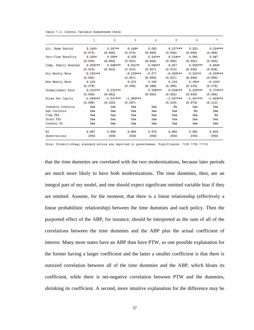
37

that the time dummies are correlated with the two modernizations, because later periods

are much more likely to have both modernizations. The time dummies, then, are an

integral part of my model, and one should expect significant omitted variable bias if they

are omitted. Assume, for the moment, that there is a linear relationship (effectively a

linear probabilistic relationship) between the time dummies and each policy. Then the

purported effect of the ABP, for instance, should be interpreted as the sum of all of the

correlations between the time dummies and the ABP plus the actual coefficient of

interest. Many more states have an ABP than have PTW, so one possible explanation for

the former having a larger coefficient and the latter a smaller coefficient is that there is

outsized correlation between all of the time dummies and the ABP, which bloats its

coefficient, while there is net-negative correlation between PTW and the dummies,

shrinking its coefficient. A second, more intuitive explanation for the difference may be

38

that there was a positive Utilization shock before the Great Recession (perhaps resulting

from national regulatory policy), and then during that recession, after controlling for

cyclicality, there was a negative shock (perhaps national Tea Party dissuasion from

accepting governmental payouts). Since many more states had the ABP than had PTW

before the Great Recession, the ABP coefficient might capture that earlier shock, while

the PTW coefficient might capture the later shock.

One other large deviation from the fully identified coefficients occurs in Column

5, which shows that omitting the industry control variables decreases the purported effect

of CFP to 1.7%. Further examination shows that this purported decrease in the coefficient

results from the omission of only two of the industry control variables: the Transportation

industry and the Leisure industry (indeed, omitting all of the other industries, but

maintaining these two, yields a coefficient of 5.3%, almost the same as the fully

identified result). This implies a large negative correlation between CFP and the

Transportation industry and a large positive correlation between CFP and the Leisure

industry, and indeed those correlations are the case (both have magnitude above 0.2).

Intuitively, the CFP coefficient in the omitted-variables model appears to be smaller than

the coefficient in the fully identified model, but this is only because the coefficient is not

only measuring the effect of the CFP, but is also proxying for states with large

transportation and small leisure industries. Including these variables is appropriate to fix

this omitted variables problem and obtain an unbiased estimate of the effect of CFP.

7.2 CONTROL FUNCTION POLYNOMIALS

The first four columns of Table 7.2 show the results of the UI Utilization regression with

the first three orders of control functions included, with the fourth column showing my

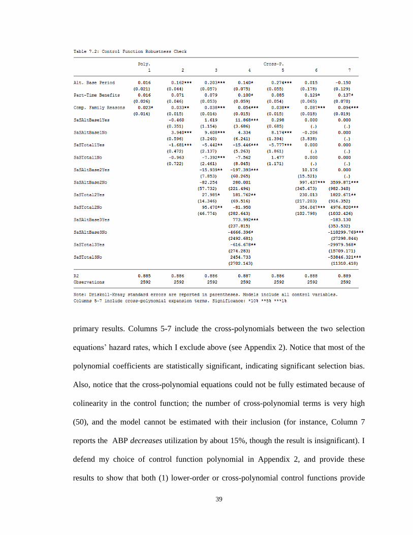
39

primary results. Columns 5-7 include the cross-polynomials between the two selection

equations’ hazard rates, which I exclude above (see Appendix 2). Notice that most of the

polynomial coefficients are statistically significant, indicating significant selection bias.

Also, notice that the cross-polynomial equations could not be fully estimated because of

colinearity in the control function; the number of cross-polynomial terms is very high

(50), and the model cannot be estimated with their inclusion (for instance, Column 7

reports the ABP decreases utilization by about 15%, though the result is insignificant). I

defend my choice of control function polynomial in Appendix 2, and provide these

results to show that both (1) lower-order or cross-polynomial control functions provide

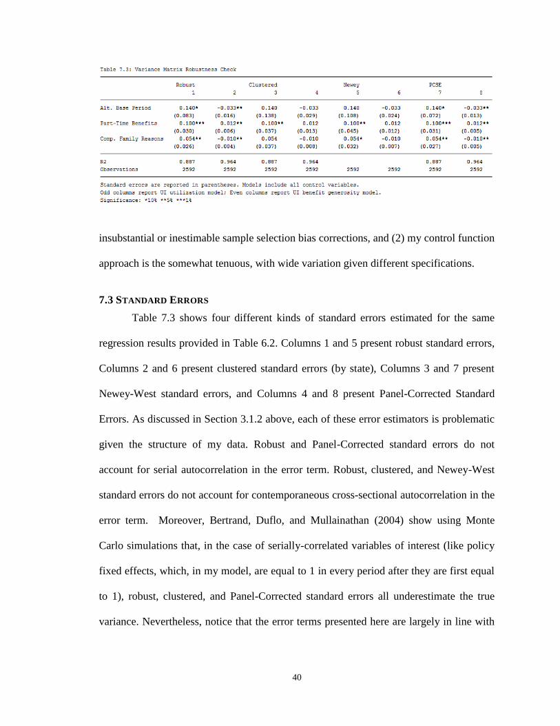
40

insubstantial or inestimable sample selection bias corrections, and (2) my control function

approach is the somewhat tenuous, with wide variation given different specifications.

7.3 STANDARD ERRORS

Table 7.3 shows four different kinds of standard errors estimated for the same

regression results provided in Table 6.2. Columns 1 and 5 present robust standard errors,

Columns 2 and 6 present clustered standard errors (by state), Columns 3 and 7 present

Newey-West standard errors, and Columns 4 and 8 present Panel-Corrected Standard

Errors. As discussed in Section 3.1.2 above, each of these error estimators is problematic

given the structure of my data. Robust and Panel-Corrected standard errors do not

account for serial autocorrelation in the error term. Robust, clustered, and Newey-West

standard errors do not account for contemporaneous cross-sectional autocorrelation in the

error term. Moreover, Bertrand, Duflo, and Mullainathan (2004) show using Monte

Carlo simulations that, in the case of serially-correlated variables of interest (like policy

fixed effects, which, in my model, are equal to 1 in every period after they are first equal

to 1), robust, clustered, and Panel-Corrected standard errors all underestimate the true

variance. Nevertheless, notice that the error terms presented here are largely in line with

41

those estimated above using the Driskoll-Kraay procedure, and that most of the

coefficients of interest are similarly statistically significant (different from 0).

8. CONCLUSION

The American Recovery and Reinvestment Act of 2009 designated $7 billion to

incentivize states to modernize their UI systems, through a provision that I call the MIP

Act. The stated intention of the ARRA was to stimulate the American economy, with the

MIP Act providing money to largely low-income job-losers who were likely to spend the

money quickly (through consumption smoothing). The MIP Act was also intended to

incentivize states to permanently modernize their UI systems, largely by expanding UI

eligibility to workers who, for one reason or another, have been excluded from their

state’s UI eligibility provisions. I provide answers to two questions: (1) how many people

ultimately collected UI because of states’ modernizing their UI programs under the MIP

Act, and (2) how much money in benefits those individuals received.

I present a state-level difference-in-difference approach to answer these questions,

developing an identification strategy and using a modified control function approach to

correct for sample selection bias. I find that the Alternative Base Period, the Part-Time

Work Provision, and the Compelling Family Reasons Provision (the three eligibility-

related MIP Act modernizations) increased eligibility by 14%, 10%, and 5.4%,

respectively, each of which is statistically different from zero at the 10% level. In total,

my results show that an additional 1,580,000 job-losers collected unemployment

insurance during the Great Recession in states that had not implemented the respective

modernization until after the passage of the MIP Act, a 5.4% increase in UI utilization

nationwide.

42

In addition to these eligibility values, I also estimate total UI benefits paid out to

individuals collecting UI under each modernization, which the literature not previously

estimated. I find that benefits received under the ABP, PTW, and CFP total $2.2 billion,

$3.5 billion, and $2.3 billion respectively, totaling about $8.0 billion (between February

2009 and the end of 2011). These total benefits are far higher than the $4.4 billion

distributed by the federal government to modernization states.1 This estimate suggests

that the MIP Act was an effective use of federal stimulus dollars, providing significant

funding to low-income job-losers who were likely spend that money in the short term.

One shortcoming of my state-level two-step approach is low efficiency, which

results in large errors. Efficiency could be improved in two ways. First, future research

could benefit greatly from strong individual-level data, which is currently unavailable

because no data source captures whether people collect UI under any specific eligibility

policy. Second, future research could implement a one-step maximum likelihood strategy

instead of my two-step strategy, which, though time-consuming, would provide a more

efficient estimation, especially in correcting for sample selection bias.

My research suggests a number of possible topics for further study. First, I have

assumed that the modernizations’ effects are independent of modernizing states’

demographics; using interaction terms might result in a better understanding of these

effects. Second, although the above analysis corrects for sample selection bias between

states that are or are not ABP states and those that are or are not 2-in-4-modernization

states, I do not correct for potential sample selection bias between the four secondary

modernizations, which would require modeling how states choose which policy to adopt.

1 My results thus confirm O’Leary’s (2011) worry that the federal incentive payments would cover less than three years

of the increased UI benefits caused by the modernizations (the remaining costs come from state treasuries).

43

Third, my results show a number of strong relationships between UI Utilization and

several industry and age variables that researchers have not investigated. Investigating

these relationships further appears to be a fruitful avenue for future research.

9. APPENDICES

9.1 APPENDIX 1: DATA STRUCTURE

I define UI utilization as the ratio of the number of people who begin collecting UI in

the next state-month to the number of job-losers the current state-month. The numerator

is lagged forward by one month to account for three factors: any delay in the job-loser’s

application for UI, any processing delay at state UI administrative offices, and any

statutory waiting period (found in most states) that require the job-loser to wait

approximately two weeks before beginning to collect UI (which commences on receiving

a first payment). Although the numerator (UI First Payments, from UIAD) is reported for

every state-month, the total number of job-losers (Separations1, from QWI) is only

reported every quarter. In order to calculate a monthly UI Utilization rate, then, I multiply

quarterly separations by the proportion of that quarter’s UI First Claims (which counts

the number of people who apply for UI for the first time after losing their employment)

that occur in that month.

I claim that the distribution of separations across months in a quarter is the same as

that of first claims, which follows from two assumptions: (1) the proportion of job-losers

who apply for UI stays constant in the three months of each quarter, and (2) little (or no)

time elapses between job-loss and UI application. Notice that the first assumption does

not imply a constant PercentTakeup over the quarter (which would assume away the need

to control for that value), since PercentTakeup measures the percent of people eligible for

UI who apply for UI, not the percent of job-losers in general. If the error in the ratio of

first claims to job-losers is mean-zero and independent of the independent variables in the

regression, then the violation of the first assumption merely suggests measurement error

in the dependent variable, which does not result in biased β coefficients. Many people

who apply for UI are not eligible, as evidenced by first claims figures that are

significantly higher than first payments figures, and I assume that, when restricted to

looking within a single quarter, the specific state or time is independent of the

relationship between separations and claims.2

The second assumption is more

1 The separations data has two flaws, each working in opposite directions. On the one hand, if an individual loses more

than one job within a quarter, Separations data counts their situation as a single job loss, leading to an underestimation

of Separations. On the other hand, if an individual leaves one job in order to take another job, or is fired from their job,

or leaves in order to commence self-employment, or leaves the labor force altogether, then these situations are counted

as Separations, although none of these individuals are eligible for UI. This leads to an over-estimation of Separations.

Indeed, summary statistics show that median UI Utilization stands at about 8% in my data, lower than expected.

However, I assume that the over-estimation of Separations leads only to measurement error in the dependent variable,

which does not imply bias of any kind. In addition, this value of separations is significantly better than either a stock

measure of total Unemployed or any other available measure of job loss. 2 Notice, then, that I assume that the first of the three delays described above to explain the lagged dependent variable

is insignificant; I assume that there is very little time for most UI-collecting job-losers between job loss and first claim.

44

problematic, since its negation implies that the ratio of claims to separations might be

artificially high or low just because of the time that people wait between the separation

and the first claim. Imagine if all workers wait exactly one month after losing their jobs

to apply for UI, and that separations are high in the second month of a quarter but low in

the third month; in this case, my procedure assigns too many separations to the third

month in the quarter, which might bias the regression results. I know of no researcher

who has examined the timing of UI claims after separations, and I leave that as a question

for future research. However, I think that assuming almost no lag between claims and

separations is the best alternative, and assume that any lag ends up merely contributing to

measurement error in the dependent variable.

Several independent variables in both substantial equations are reported on an

irregular basis: total hires (quarterly), state population (yearly), statutory generosity

(yearly), and average wage (quarterly).3 However, there is no reason to expect that the

failure to include monthly wage information biases the regression, and instead results

only in attenuation error in the respective coefficients (which is acceptable given that

they are not the variables of interest). In addition, since I include national time dummies,

I do not expect any significant time-discontinuities caused by the variables’ jumps every

three months or every year, as those jumps are likely at the national level.

9.2 APPENDIX 2: CONTROL FUNCTIONS

Notice that, in Equation 5: [ ]

[

] (18)

Pioneering work on sample selection bias, like Heckman (1979), directly estimates

this expected value of a truncated error term by assuming bivariate normality between the

two error terms. However, is not normally distributed in my model, which prohibits

using Heckman’s procedure. Instead, I use the control function approach discussed in

Heckman and Navarro-Lozano (2004). Those authors show that, assuming that the two

error terms are independent of and Xit:

[

] [ ] (

) (19)

where P is defined as the propensity score, or the probability that a state takes treatment

conditional on the available covariates, and is some function that can be estimated by

a Taylor expansion of P.

Heckman and Navarro-Lozano’s (2004) propensity score is determined independent

of the state of the subject in previous periods; however, I cannot estimate such a

propensity score using a duration model, which necessarily controls on having not

modernized in previous periods. Thus, although Heckman and Navarro-Lozano use a

single propensity score term to absorb all selection bias, I use two such terms,

conditioning on whether or not the state has modernized before that time. I include these

terms separately, estimated with different coefficients, in order to provide more flexibility

to my approach. Thus, I only approximate Heckman and Navarro-Lozano’s method, and

do not instance it. The intuition behind both methods is the same.

This question is, to my knowledge, unresearched. However, the lag in Separations is still justified by administrative

delays and state-mandated waiting periods. 3 Note that average wage is also used as the denominator of the dependent variable in the benefit generosity model;

however, measurement error in the dependent variable does not bias the coefficients of interest.

45

According to the assumptions of a duration model, it is only possible to move from

the non-treated group to the treated group, and not vice-versa. However, selection bias

clearly exists in both cases; I observe the UI Utilization of non-modernization states only

in certain cases, and similarly I observe the UI Utilization of modernization states only in

certain cases. Notice that Heckman and Navarro’s definition of propensity score does not

imply . To the contrary, the probability that a state takes treatment conditional on

the available covariates has merely changed from the hazard rate stated in Equation 9 to

that same hazard rate without the “1-” term in the denominator, which conditions the

hazard rate on having been selected instead of conditioning it on having not been

selected.4 Consider the intuition of this approximation: the modernization-state control

function polynomials control for any variance in utilization in states that are more the

kind of state that would be a modernization state, conditional on their being such a state.

Despite my selection model being such that treated states cannot choose to become

untreated states, the two-step estimation procedure remains essentially the same.

Vella (1998) shows that in the multivariate-normal case, if and are

uncorrelated, then their resulting control function is additively separable.5 Consider that

assumption given my model. I assume that certain states become ABP states, and other

people become 2-of-4-modernization states for the same reasons (i.e. because of

underlying politics and fiscal need), but that knowledge about a state’s passage of ABP

(for instance), conditional on state politics and fiscal need, offers no insight into when (or

if) the state will become a 2-in-4-modernization state. In other words, the only knowledge

you get about a state’s likelihood to become a 2-in-4-modernization state given when it

becomes an ABP state is knowledge about its politics and fiscal need, which only

indirectly relates to becoming a 2-in-4-modernization state. In general, states become 2-

in-4-modernization states after they become ABP states, but I assume this is because the

distribution of states becoming 2-in-4-modernization states peaks at a later time than that

of ABP states, and is explained fully by politics and need.6 Thus, motivated by Vella, I

make this assumption that follows from the relationship between the three error terms:

[ ] (

) (

) (

) (20)

where Pθτ is the propensity score of state i in time t if and can be estimated

by a polynomial expansion of Pθτ. Thus, I do not include cross-polynomial terms in my

regression.

10. BIBLIOGRAPHY

Akaike, H. (1973). Information theory and an extension of the maximum likelihood principle.

In B.N. Petrov & F. Csaki (eds.), Second International Symposium on Information

Theory (267-281). Budapest, Hungary: Akademiai Kiado.

Amemiya, T. (1984). Tobit Models: A Survey. Journal of Econometrics 24(1), 3-61.

American Recovery and Reinvestment Act of 2009 §2003. 327-329.

Anderson, P. & Meyer, B. (1997). Unemployment Insurance Takeup Rates and the After-Tax

Value of Benefits. The Quarterly Journal of Economics 112(3), 913-937.

4 See Lee (1978), who develops this idea in the bivariate-normal case. 5 Notice that Vella’s model is one instance of Amemiya’s Type 4 Tobit model; See Amemiya (1984). 6 This assumption implies that some states might become 2-in-4-modernizations states before becoming ABP states.

Indeed, four states became 2-in-4-modernization states before becoming ABP states: Arkansas (by 3 months),

California (by 12 months), Nevada (by 51 months), and Oregon (by 1 month).

46

Attanasio, O., Battinstin, E., & Mesnard, A. Food and Cash Transfers: Evidence from Colombia.

The Economic Journal 122(559), 92-124.

Baker, M., Corak, M., & Heisz, A. (1996). Unemployment in the Stock and Flow (No. 97).

Ottowa, CAN: Statistics Canada.

Beck, N., & Katz, J. (1995). What to do (and not to do) with Time-Series Cross-Sectional Data.

The American Political Science Review 89(3), 634-647.

Berk, R. (1983). An Introduction to Sample Selection Bias in Sociological Data. American

Sociological Review 48(3), 386-398.

Bertrand, M., Duflo, E., and Mullainathan, S. (2004). How Much Should We Trust Differences-

In-Differences Estimates?. The Quarterly Journal of Economics 119(1), 249-275.

Burtless, G., & Saks, D. (1984). The Decline in Insured Unemployment During the 1980s.

Washington, DC: The Brookings Institution.

Comparison of State Unemployment Laws. (2012). Washington, DC: Employment and Training

Administration, US Department of Labor.

Corson, W., Hershey, A., & Kerachsky, S. (1986). Nonmonetary Eligibility in State

Unemployment Insurance Programs: Law and Practice. Kalamazoo, MI: W.E. Upjohn

Institute for Employment Research.

Driscoll, J., & Kraay, A. (1998). Consistent Covariance Matrix Estimation with Spatially

Dependent Panel Data. Review of Economics and Statistics 80(4), 549-560.

Fujita, S. (2010). Effects of the UI Benefit Extensions: Evidence from the CPS (Working Paper

10-35). Philadelphia, PA: Federal Reserve Bank of Philadelphia.

Grubb, D. (2000). Eligibility Criteria for Unemployment Benefits. In Labour Market Policies and

the Public Employment Service (217-240). Paris, FR: Organisation for Economic Co-

Operation and Development.

Gruber, J. (1997). The Consumption Smoothing Benefits of Unemployment Insurance. The

American Economic Review (87(1), 192-205.

Gordon, R. (2009). Green Shoot or Dead Twig: Can Unemployment Claims Predict the End of

the American Recession? Vox. London, UK: Centre for Economic Policy Research.

Heckman, J. (1979). Sample Selection Bias as a Specification Error. Econometrica 47(1), 153-

161.

Heckman, J., & Robb, R. (1985). Alternative Methods for Estimating the Impact of Interventions.

In J. Heckman & B. Singer (Eds.), Longitudinal Analysis of Labor Market Data (156-

246). Cambridge, UK: Cambridge University Press.

Heckman, J., & Navarro-Lozano, S. (2004). Using Matching, Instrumental Variables, and Control

Functions to Estimate Economic Choice Models. The Review of Economics and Statistics

86(1), 30-57.

Helpman, E., Melitz, M., & Rubenstein, Y. (2008). Estimating Trade Flows: Trading Partners and

Trading Volumes. The Quarterly Journal of Economics 123(2), 441-487.

Hoechle, D. (2007). Robust Standard Errors for Panel Regressions with Cross-Sectional

Dependence. The Stata Journal 7(3), 281-312.

H.R. 3920—110th Congress: Unemployment Insurance Modernization Act. (2007).

Klarner, C. (2003). The Measurement of the Partisan Balance of State Government. State Politics

and Policy Quarterly 3(3), 309-319.

Kletzer, L., & Rosen, H. (2006). Reforming Unemployment Insurance for the Twenty-First-

Century Workforce. In J. Furman & J. Bordoff (Eds.), Path to Prosperity: Hamilton

Project Ideas on Income Security, Education, and Taxes (63-92). Washington, DC: The

Brookings Institution.

Krueger, A., & Meyer, B. (2002). Labor Supply Effects of Social Insurance. In A. J. Auerbach &

M. Feldstein (Eds.), Handbook of Public Economics, vol. 4 (2327-2392). Amsterdam:

Elsevier.

47

LaLonde, R. The Promise of Public Sector-Sponsored Training Programs. The Journal of

Economic Perspectives 9(2), 149-168.

Lancaster, L. (2009). Changes in State Unemployment Insurance Legislation in 2008. Monthly

Labor Review January 2009, 28-37.

-----. (2010). Changes in State Unemployment Insurance Legislation in 2009. Monthly Labor

Review January 2010, 37-58.

-----. (2011). Changes in State Unemployment Insurance Legislation in 2010. Monthly Labor

Review January 2011, 38-56.

Lee, L. (1978). Unionism and Wage Rates: A Simultaneous Equations Model with Qualitative

and Limited Dependent Variables. International Economic Review 19(2), 415-433.

Lindner, S., & Nichols, A. (2012). How Do Unemployment Insurance Modernization Laws

Affect the Number and Composition of Eligible Workers? Washington, DC: The Urban

Institute.

McMurrer, D., & Chasanov, A. Trends in Unemployment Insurance Benefits. Monthly Labor

Review 118(9), 30-39.

Meyer, B. (1990). Unemployment Insurance and Unemployment Spells. Econometrica 58(4),

757-782.

Modernizing Unemployment Insurance: Federal Incentives Pave the Way for State Reforms.

(2012). New York, NY: National Employment Law Project Briefing Paper.

Moffitt, R. (1985). Unemployment Insurance and the Distribution of Unemployment Spells.

Journal of Econometrics 28(1), 85-101.

Mitchell, M. (2010). Gender and Unemployment Insurance: Why Women Receive

Unemployment Benefits at Lower Rates than Men and Will Unemployment Insurance

Reform Close the Gender Gap. Texas Journal of Women and the Law (20:1), 55-74.

Newey, W., & West, W. (1987). A Simple, Positive Semi-Definite, Heteroskedasticity and

Autocorrelation Consistent Covariance Matrix. Econometrica 55(3), 703-708.

Nicholson, W. (1997). Initial Eligibility for Unemployment Compensation. In C. O’Leary & S.

Wandner (Eds.), Unemployment Insurance in the United States: Analysis of Policy Issues

(91-124). Kalamazoo, MI: W.E. Upjohn Institute for Employment Research.

O’Leary, C. (2011). Benefit Payment Costs of Unemployment Insurance Modernization:

Estimates Based on Kentucky Administrative Data (Working Paper No. 11-172).

Kalamazoo, MI: Upjohn Institute.

Rothstein, J. (2011). Unemployment Insurance and Job Search in the Great Recession (Working

Paper No. 17534). Cambridge, MA: National Bureau of Economic Research.

S. 1871—110th Congress: Unemployment Insurance Modernization Act. (2007).

Stettner, A., Boushet, H., & Wenger, J. (2005). Clearing the Path to Unemployment Insurance for

Low-Wage Workers: An Analysis of Alternative Base Period Implementation.

Washington, DC: Center for Economic and Policy Research.

Valletta, R., & Kuang, K. (2010). Extended Unemployment and UI Benefits (Economic Letter

No. 2010-12). San Francisco, CA: Federal Reserve Bank of San Francisco.

Vella, F. (1998). Estimating Models with Sample Selection Bias: A Survey. The Journal of

Human Resources 33(1), 127-169.

Vroman, W. (1991). Analysis: Why the Decline in Unemployment Insurance Claims? Challenge

34(5), 55-58.

-----. (1995). The Alternative Base Period in Unemployment Insurance: Final Report

(Unemployment Insurance Occasional Paper 1995-3). Washington, DC: United States

Department of Labor, Employment and Training Administration.

White, H. (1980). A Heteroskedasticity-Consistent Covariance Matrix Estimator and a Direct

Test for Heteroskedasticity. Econometrica 48, 817-838.

Wooldridge, J. (2010). Econometric Analysis of Cross Section and Panel Data. Cambridge, MA:

The MIT Press.