Embed Size (px)
Citation preview

HAL Id: tel-03137600https://tel.archives-ouvertes.fr/tel-03137600
Submitted on 10 Feb 2021
HAL is a multi-disciplinary open accessarchive for the deposit and dissemination of sci-entific research documents, whether they are pub-lished or not. The documents may come fromteaching and research institutions in France orabroad, or from public or private research centers.
L’archive ouverte pluridisciplinaire HAL, estdestinée au dépôt et à la diffusion de documentsscientifiques de niveau recherche, publiés ou non,émanant des établissements d’enseignement et derecherche français ou étrangers, des laboratoirespublics ou privés.
Evaluation of energy efficiency in mobile cellularnetworks using a fluid modeling framework
Yanqiao Hou
To cite this version:Yanqiao Hou. Evaluation of energy efficiency in mobile cellular networks using a fluid modeling frame-work. Modeling and Simulation. Université Paris-Saclay, 2020. English. �NNT : 2020UPASG032�.�tel-03137600�

Evaluation of energy efficiency
in mobile cellular networks
using a fluid modeling framework
Thèse de doctorat de l'université Paris-Saclay
École doctorale n°580 : Sciences et Technologies de l'Information et de
la Communication (STIC)
Spécialité de doctorat : Réseaux, Information et Communications
Unité de recherche : Université Paris-Saclay, CNRS, CentraleSupélec,
Laboratoire des signaux et systèmes, 91190, Gif-sur-Yvette, France
Référent : Faculté des sciences d’Orsay
Thèse présentée et soutenue en visioconférence totale, le
26 novembre 2020, par
Yanqiao HOU
Composition du Jury
Hind CASTEL-TALEB
Professeur, Télécom SudParis, IPP Présidente
Marceau COUPECHOUX
Professeur, Télécom Paris, IPP Rapporteur & Examinateur
Tadeusz CZACHORSKI
Professeur, IITIS PAN Poland Rapporteur & Examinateur
André-Luc BEYLOT
Professeur, ENSEEIHT, Université de
Toulouse
Examinateur
Joanna TOMASIK
Professeur, CentraleSupélec, Université
Paris-Saclay Examinatrice
Véronique VÈQUE
Professeur, Université Paris-Saclay Directrice de thèse
Lynda ZITOUNE
Maître de Conférences, ESIEE Paris Co-encadrante
Jean-Marc KELIF
Ingénieur de recherche, Orange Labs Invité
Th
èse
de d
oct
ora
t
NN
T : 2
020U
PA
SG
032


Acknowledgements
I wish to express my sincere appreciation to my supervisor Dr. Véronique Vèque, a full
professor in the Electrical Engineering Department of University Paris-Sud, and the head
of Telecommunications and Networking group at the Laboratory of Signal and Systems
(L2S–UMR 8506), for leading me to the telecommunication area. My research view gets
widely broadened during the PhD years which should thanks to communication opportuni-
ties strongly supported by Dr. Vèque. This appreciation is also for many helps and cares on
my private life.
I also would like to give my many thanks to my co-supervisor Dr. Lynda Zitoune, an
associate professor in École Supérieure d’Ingénieurs en Électrotechnique et Électronique
(ESIEE), Paris, for smart suggestion and deep discussion on the research direction, technical
details and paper manuscripts.
I would further like to thank all my colleagues at the Lab, where they provide me great
advices on my work and share their great minds with me. In particular, I would like to
thank Dr. Djibrilla Adamou Incha, Mr Melek Charfi and Dr. João Alberto Ferreira, who
saved me a lot from language problems and took care of me a lot during my pregnancy. I
thank them a lot for the precious friendships.
Special thanks to my Chinese friends, namely Peipei Ran, Xiaoxia Zhang, Jian Song,
Chen Kang, Li Wang, Yanpei Liu, Zhan Wang, Chao Zhang and Caifang Cai. They have
accompanied me and brought me happiness and help in these three years.
I wish to express my gratitude to Dr Dominique Lesselier, for his assistance during my
PhD.
I would like to thank Dr. CASTEL-TALEB Hind, Dr. BEYLOT André-Luc and Dr. TOMASIK
Joanna as my jury members, Dr. COUPECHOUX Marceau and Professor CZACHORSKI
Tadeusz as referees, Dr. KELIF Jean-Marc as invited member.
I also would like to show my sincere gratitude and deep thanks to my husband and my
daughter. Their support, encouragement, smile, and countless sacrifice are the basis of my
continuing personal development.
Last but not least, I am grateful to my parents, my brother and my sisters, who are
always loving and supporting me all through my PhD.


Abstract
English:The design target of energy efficiency for 5G networks is at least 1000-fold than the
currently available 4G system, while offering higher data transmission rate and very low
latency. To evaluate the performance of large representative cellular networks and capture
the main factors involved in the energy consumption process, representative and accurate
models must be developed.
To develop tractable and efficient models, we use the spatial fluid modeling framework
and compute the energy efficiency metric. Our model consists of a downlink transmission
of an OFDMA cellular network, composed of several base stations and multiple user
equipments randomly distributed over the area. An analytical expression of energy efficiency
is then derived to study the impact of the major factors involved in the energy consumption
process such as fading and shadowing attenuation, cellular coverage type and quality.
Extensive numerical simulations were run to compare the results obtained by Monte Carlo
simulations and demonstrate the effectiveness and accuracy of the fluid modeling for large
cellular networks. The numerical results indicate that user density does not affect energy
efficiency. Besides, energy efficiency is more important in suburban environments than in
urban environments where the shadowing effect is great, regardless of the cellular coverage
type. However, and more generally, micro-cellular networks’ deployment offers better
energy efficiency than the conventional macro-cellular ones.
Besides, we evaluated the effect of the promising Joint Transmission Coordinated
MultiPoint (JT-CoMP) technique on energy efficiency, which is significantly improved as
the number of coordinated BSs increases. On the other hand, coordination between base
stations is only effective for user equipment that is remote from their base station.
To resume, our numerical results illustrate the effectiveness and accuracy of fluid
modeling, which can be considered as a mathematical tool by operators to benchmark
cellular networks’ energy efficiency.
Keywords: energy efficiency, mobile networks, JT-CoMP, performance evaluation, fluid
modeling

vi Abstract
Français:La conception des systèmes de communication dits 5G cible une efficacité énergétique
ambitieuse, au moins 1000 fois supérieure à celle du système 4G actuellement disponible,
tout en offrant un débit de transmission de données supérieur et un temps de latence très
faible. Il est donc nécessaire de développer des modèles représentatifs et précis des grands
réseaux cellulaires afin d’évaluer leur performance et d’identifier les principaux facteurs
impliqués dans la consommation d’énergie comme l’atténuation de signal, le type et la
qualité de la couverture cellulaire radio.
Nous avons utilisé la modélisation fluide spatiale pour développer des modèles représen-
tatifs et calculables afin de calculer la métrique d’efficacité énergétique. Notre modèle
considère un réseau composé de plusieurs cellules opérant en OFDMA sur les liens descen-
dants, et de multiples équipements utilisateurs répartis aléatoirement. Une expression
analytique de l’efficacité énergétique a été dérivée pour prendre en compte les principaux
facteurs liés à la communication : coefficient d’atténuation de signal, probabilité de couver-
ture, type du réseau. Des simulations numériques ont permis de comparer les résultats avec
ceux obtenus par les simulations Monte Carlo et ainsi, montrer l’efficacité et la précision
de la modélisation fluide pour de grands réseaux cellulaires. Les résultats numériques
montrent que l’efficacité énergétique est indépendante de la densité des équipements util-
isateurs. Par ailleurs, l’efficacité énergétique est plus importante dans les environnements
suburbains que dans les milieux urbains où l’effet de shadowing est grand et ce, quel que
soit le type de réseaux (macro, micro ou femto). Cependant, et d’une façon plus générale,
le déploiement de petits réseaux (small cells) offre une meilleure efficacité énergétique
comparée au réseau macro classique.
En outre, nous avons évalué l’effet de la technique de transmission conjointe multipoint
(JT-CoMP) sur l’efficacité énergétique, qui est considérablement améliorée lorsque le nombre
de stations de base coordonnées augmente. En revanche, la coordination entre les stations
de base n’est efficace que pour les équipements utilisateurs éloignés de leur station de base.
En résumé, nos résultats numériques mettent en évidence l’efficacité et la précision
de la modélisation fluide qui peut être considérée comme un outil mathématique par les
opérateurs pour évaluer l’efficacité énergétique des réseaux cellulaires.
Mots clés: efficacité énergétique, réseaux mobiles, JT-CoMP, évaluation des perfor-
mances, modélisation fluide

Overview of the manuscript
The 5G network design aims to offer more capacities and less latency and fulfill the in-
creasing data traffic, leading to higher energy consumption. From the view point of
environmental responsibility, radio communication is a large proportion of information and
communications technologies (ICT) related to carbon dioxide (CO2) emissions. During
the last decades, Energy Efficiency (EE) has received a lot of attention in wireless com-
munications and is very important, from the viewpoints of both economic benefits and
environmental responsibility. The investigation of EE, in wireless networks, is driven using
either system-level simulations or stochastic geometry to consider the spatial distribution
of nodes (base stations and user terminals) when describing the topological model of the
networks. However, since today’s wireless communication networks are denser and denser
due to the increasing number of base stations (BSs) and user terminals, simulation-based
approaches have become a painful task and resource-intensive. On the other hand, stochas-
tic geometry-based studies assume, in most cases, a Poisson point process to describe the
locations of nodes, which allows us to derive a closed-form formula of the energy efficiency
metrics. Nevertheless, when non-Poisson point processes are considered, eg., perturbed
lattice, β-Ginibre point process, and Matérn point process, the performance models are
not analytically tractable due to the non-independent nature of points. Therefore, either
approximations or simulations are conducted to prove the model accuracy.
Spatial fluid modeling has recently been developed to evaluate network performance,
like the signal-to-interference-plus-noise ratio (SINR) and outage probability through
analytical expressions. However, an investigation of EE based on fluid modeling in wireless
networks is still missing. Additionally, the advanced technique of Joint Transmission
Coordinated MultiPoint (JT-CoMP) has been designed to improve such parameters as SINR,
capacity, and quality of service. Nevertheless, this technology brings additional energy
power consumption for transmitting backhauling information. Hence, while utilizing
the JT-CoMP scheme, how to compute EE based on fluid modeling is still an open issue.
Performance of JT-CoMP has been studied by simulations or with stochastic geometry but
not using fluid modeling. Therefore, our objective is to evaluate EE for the cellular networks

viii Overview of the manuscript
based on the fluid modeling, while considering JT-CoMP and non JT-CoMP schemes, in order
to develop an accurate and tractable model and to show the efficiency of fluid modeling.
The PhD thesis is divided into six chapters and it is organized as follows:
In chapter 1, we first outline the background information on energy efficiency (EE) in
the information and communications technologies. Then the cellular network concept and
its energy consumption are presented. Furthermore, advanced technologies developed
to increase spectral efficiency in 4G systems are introduced, as they have the potential to
improve EE. Finally, we discuss some survey papers focusing on EE by taking advantage of
the advanced technologies.
In chapter 2, we first list some EE models from the perspective of its definition. Then,
as the critical components of the EE model, the power consumption models and the
throughput models are introduced. Finally, we classify some literature papers on EE from
the perspectives of both EE-evaluation and EE-optimization, according to some advanced
technologies to illustrate the impact of these technologies on EE.
The chapter 3 is an introduction to the model common to the whole thesis. We first
survey main scientific papers published on fluid modeling. Then, we present the cellular
system we use in our work. Afterward, the concept of fluid modeling is introduced and
the mathematical expressions of SINR and interference factor based on this model are
presented. Finally, some numerical results of SINR are shown to validate the accuracy of
fluid modeling.
Chapter 4 illustrates a tractable model of EE without considering the impact of shadow-
ing and analyzes the joint effect of shadowing and path-loss exponent on EE based on the
spatial fluid modeling in the macro- and femto- cellular networks, respectively. After having
developed the associated EE model, the data rate computation is discussed without and
with considering the impact of shadowing. In the case of non-shadowing, we develop three
data rate models for three scenarios, depending on the network’s size. Whereas, in the case
of shadowing, we make a brief recall of the signal quality, the mean and standard deviation
of interference factor using fluid modeling, and then present a closed-form expression of
the signal quality threshold, which is depending on the user equipments’ location while
considering a fixed coverage probability. Finally, based on the above work, we assess the
EE for both macro- and femto- cellular networks in non-shadowing and shadowing cases
through simulation results.
In chapter 5, we develop a tractable and efficient EE model based on the spatial
fluid modeling framework when JT-CoMP is applied. After reviewing the literature on
JT-CoMP technology, we introduce the corresponding system model, including the refined
power consumption model and energy efficiency metrics. Then, the data rate computation

ix
and the backhauling traffic computation are presented. Moreover, we investigate the EE
enhancement in both macro- (MCN) and femto- (FCN) cellular networks, compared to
the baseline case where no coordination is applied. Finally, we show that the EE metrics
computed for a femto-cellular system increase depending on some parameters, such as
path-loss exponent, network area, and the number of coordinated base stations, when
varying the backhauling power cost depending on the data rate requirement. We further
reveal the impact of the distance threshold, which corresponds to the predefined threshold
of SIR, on EE per cell, thus verifying the effectiveness of JT-CoMP.
Finally, chapter 6 summarizes the thesis and sets some perspectives for the future
work. Appendices provides supplementary materials, including the published/submitted
contributions.


Vue d’ensemble du manuscrit
La conception du réseau 5G vise à offrir plus de capacités et moins de latence et à répondre
à l’augmentation du trafic de données, entraînant une consommation d’énergie plus élevée.
Du point de vue de la responsabilité environnementale, les radiocommunications constituent
une part importante des technologies de l’information et des communications (TIC) liées
aux émissions de gaz carbonique (CO2). Au cours des dernières décennies, l’efficacité
énergétique (EE) a été l’objet de beaucoup d’attention dans les communications sans
fil et est très importante, tant du point de vue des avantages économiques que de la
responsabilité environnementale. L’étude de l’EE, dans les réseaux sans fil, est conduite
à l’aide de simulations au niveau du système ou de géométrie stochastique pour prendre
en compte la distribution spatiale des nœuds (stations de base et terminaux d’utilisateurs)
lors de la description du modèle topologique des réseaux. Cependant, comme les réseaux
de communication sans fil d’aujourd’hui sont de plus en plus denses en raison du nombre
croissant de stations de base (BS) et de terminaux utilisateurs, les approches basées sur
la simulation sont devenues une tâche pénible et gourmande en ressources. D’autre part,
les études basées sur la géométrie stochastique supposent, dans la plupart des cas, un
processus ponctuel de Poisson pour décrire les emplacements des nœuds, ce qui nous
permet de dériver une formule en forme fermée des métriques d’efficacité énergétique.
Néanmoins, lorsque des processus ponctuels non-Poisson sont considérés, par exemple, un
réseau perturbé, un processus ponctuel β -Ginibre et un processus ponctuel de Matérn, les
modèles de performance ne sont pas analysables en raison de la nature non indépendante
des points. Par conséquent, des approximations ou des simulations sont effectuées afin de
prouver la précision du modèle.
La modélisation des fluides spatiaux a récemment été développée dans le but d’évaluer
les performances du réseau, comme le rapport signal/brouillage et bruit (SINR) et la
probabilité de panne au moyen d’expressions analytiques. Cependant, une enquête sur l’EE
basée sur la modélisation des fluides dans les réseaux sans fil fait toujours défaut. De plus,
la technique avancée dite « Joint Transmission Coordinated MultiPoint » (JT-CoMP) a été
conçue pour améliorer des paramètres tels que le SINR, la capacité et la qualité de service.

xii Vue d’ensemble du manuscrit
Néanmoins, cette technologie conduit à une consommation d’énergie supplémentaire pour
la transmission des informations de « back-hauling ». Par conséquent, tout en utilisant
le schéma JT-CoMP, comment calculer l’EE basée sur la modélisation des fluides reste un
problème en suspens. Les performances de JT-CoMP ont été étudiées par des simulations
ou avec une géométrie stochastique mais pas en utilisant la modélisation des fluides. Par
conséquent, notre objectif est d’évaluer l’EE pour les réseaux cellulaires sur la base de la
modélisation des fluides, tout en considérant les schémas JT-CoMP et non JT-CoMP, afin de
développer un modèle précis et traitable et de montrer l’efficacité de la modélisation des
fluides.
La thèse de doctorat est divisée en six chapitres et est organisée comme suit:
Au chapitre 1, nous présentons d’abord les informations générales sur l’efficacité én-
ergétique (EE) dans les technologies de l’information et de la communication. Ensuite, le
concept de réseau cellulaire et sa consommation d’énergie sont introduits. En outre, des
technologies avancées développées dans le but d’augmenter l’efficacité spectrale des sys-
tèmes 4G sont considérées, car elles ont le potentiel d’améliorer l’EE. Enfin, nous discutons
de certains articles de revue axés sur l’EE en tirant parti des technologies de pointe.
Au chapitre 2, nous énumérons d’abord quelques modèles d’EE du point de vue de
leur définition. Ensuite, en tant que composants critiques du modèle EE, les modèles
de consommation d’énergie et les modèles de débit sont introduits. Enfin, nous classons
certains articles de la littérature sur l’EE du point de vue à la fois de l’évaluation de l’EE et
de l’optimisation de l’EE, selon certaines technologies avancées pour illustrer l’impact de
ces technologies sur l’EE.
Le chapitre 3 est une introduction au modèle commun à l’ensemble de la thèse. Nous
examinons d’abord les principaux articles scientifiques publiés sur la modélisation des
fluides. Ensuite, nous présentons le système cellulaire que nous utilisons dans notre travail.
Puis le concept de modélisation des fluides est introduit et les expressions mathématiques
du SINR et du facteur d’interférence basées sur ce modèle sont présentées. Enfin, certains
résultats numériques du SINR sont donnés pour valider la précision de la modélisation des
fluides.
Le chapitre 4 illustre un modèle traitable d’EE sans tenir compte de l’impact de l’ombrage
et analyse l’effet conjoint de l’ombrage et de l’exposant de perte de chemin sur l’EE basé
sur la modélisation des fluides spatiaux dans les réseaux macro et femto-cellulaires, respec-
tivement. Après avoir développé le modèle EE associé, le calcul du débit est discuté sans et
avec la prise en compte de l’impact de l’observation. Dans un cas de non-ombrage, nous
développons trois modèles de débit de données pour trois scénarios, en fonction de la taille
du réseau. Dans le cas de l’ombrage, nous faisons un bref rappel de la qualité du signal, la

xiii
moyenne et l’écart type du facteur d’interférence en utilisant la modélisation de fluide, puis
nous présentons une expression de forme fermée du seuil de qualité du signal, qui dépend
de l’emplacement des équipements de l’utilisateur, tout en considérant une probabilité de
couverture fixe. Enfin, sur la base des travaux ci-dessus, nous évaluons l’EE pour les deux
réseaux macro-cellulaires et femto-cellulaires dans les cas de non-ombrage et d’ombrage
grâce aux résultats de simulation.
Dans le chapitre 5, nous développons un modèle d’EE traitable et efficace basé sur
le cadre de modélisation des fluides spatiaux lorsque JT-CoMP est appliqué. Après avoir
examiné la littérature sur la technologie JT-CoMP, nous présentons le modèle de système
correspondant, y compris le modèle de consommation d’énergie raffiné et les mesures
d’efficacité énergétique. Ensuite, le calcul du débit de données et le calcul du trafic
de backhauling sont présentés. En sus, nous étudions l’amélioration de l’EE dans les
réseaux cellulaires macro- (MCN) et femto- (FCN), par rapport au cas de base où aucune
coordination n’est appliquée. Enfin, nous montrons que les métriques d’EE calculées pour un
système femto-cellulaire augmentent en fonction de certains paramètres, tels que l’exposant
de perte de chemin, la zone de réseau et le nombre de stations de base coordonnées, en
faisant varier le coût de la puissance de retour en fonction du débit de données exigé. Nous
révélons en outre l’impact du seuil de distance, qui correspond au seuil prédéfini de SIR,
sur l’EE par cellule, vérifiant ainsi l’efficacité du JT-CoMP.
Le chapitre 6 résume la thèse et présente quelques perspectives de travaux futurs. Les
annexes fournissent des documents supplémentaires, y compris les contributions publiées
ou soumises.


Table of contents
Abstract v
Overview of the manuscript vii
Vue d’ensemble du manuscrit xi
List of figures xix
List of tables xxiii
1 Related work on advanced techniques in 5G 1
1.1 Introduction . . . . . . . . . . . . . . . . . . . . . . . . . . . . . . . . . . . . . . . 2
1.2 Energy efficiency (EE) in ICT . . . . . . . . . . . . . . . . . . . . . . . . . . . . . 3
1.2.1 Environmental and 5G usage aspects . . . . . . . . . . . . . . . . . . . 3
1.2.2 Operators and users viewpoints . . . . . . . . . . . . . . . . . . . . . . . 4
1.3 Cellular network concept . . . . . . . . . . . . . . . . . . . . . . . . . . . . . . . 5
1.4 SE-EE relationship . . . . . . . . . . . . . . . . . . . . . . . . . . . . . . . . . . . 6
1.4.1 Spectral efficiency (SE) . . . . . . . . . . . . . . . . . . . . . . . . . . . . 6
1.4.2 Energy efficiency (EE) . . . . . . . . . . . . . . . . . . . . . . . . . . . . . 7
1.4.3 SE-EE relationship . . . . . . . . . . . . . . . . . . . . . . . . . . . . . . . 7
1.5 Promising key 5G technologies . . . . . . . . . . . . . . . . . . . . . . . . . . . . 8
1.5.1 Multiple-Input Multiple-Output (MIMO) . . . . . . . . . . . . . . . . . 8
1.5.2 Coordination Multipoint (CoMP) . . . . . . . . . . . . . . . . . . . . . . 10
1.5.3 Heterogeneous cellular network (HetNet) . . . . . . . . . . . . . . . . 11
1.5.4 Relay transmission . . . . . . . . . . . . . . . . . . . . . . . . . . . . . . . 12
1.5.5 BS on/off strategy . . . . . . . . . . . . . . . . . . . . . . . . . . . . . . . 13
1.5.6 Cloud radio access network (Cloud-RAN) . . . . . . . . . . . . . . . . . 14
1.6 EE-related surveys . . . . . . . . . . . . . . . . . . . . . . . . . . . . . . . . . . . . 15
1.7 Conclusion . . . . . . . . . . . . . . . . . . . . . . . . . . . . . . . . . . . . . . . . 18

xvi Table of contents
2 Models for EE 19
2.1 Introduction . . . . . . . . . . . . . . . . . . . . . . . . . . . . . . . . . . . . . . . 20
2.2 EE models . . . . . . . . . . . . . . . . . . . . . . . . . . . . . . . . . . . . . . . . . 20
2.2.1 Input/output power related EE model . . . . . . . . . . . . . . . . . . . 21
2.2.2 Cell power consumption and cell area related EE model . . . . . . . . 22
2.2.3 Transmitting power and data rate related EE model . . . . . . . . . . 23
2.2.4 SE and power cost related EE model . . . . . . . . . . . . . . . . . . . . 23
2.2.5 Overall data rate and power cost related EE model . . . . . . . . . . . 24
2.3 Power consumption models (PCM) . . . . . . . . . . . . . . . . . . . . . . . . . 24
2.3.1 Ideal load dependent PCM . . . . . . . . . . . . . . . . . . . . . . . . . . 25
2.3.2 Linear PCM . . . . . . . . . . . . . . . . . . . . . . . . . . . . . . . . . . . 25
2.3.3 PCM with sleep mode . . . . . . . . . . . . . . . . . . . . . . . . . . . . . 26
2.3.4 PCM with backhauling cost . . . . . . . . . . . . . . . . . . . . . . . . . 26
2.3.5 PCM considering non-empty buffer . . . . . . . . . . . . . . . . . . . . . 27
2.3.6 PCM with transmitting antennas . . . . . . . . . . . . . . . . . . . . . . 27
2.3.7 A refined double linear PCM . . . . . . . . . . . . . . . . . . . . . . . . . 28
2.4 Throughput models . . . . . . . . . . . . . . . . . . . . . . . . . . . . . . . . . . . 28
2.5 Classification of EE models . . . . . . . . . . . . . . . . . . . . . . . . . . . . . . 30
2.5.1 Evaluation-based related work . . . . . . . . . . . . . . . . . . . . . . . 30
2.5.2 Optimization-based related work . . . . . . . . . . . . . . . . . . . . . . 36
2.6 Conclusion . . . . . . . . . . . . . . . . . . . . . . . . . . . . . . . . . . . . . . . . 44
3 System model 47
3.1 Introduction . . . . . . . . . . . . . . . . . . . . . . . . . . . . . . . . . . . . . . . 47
3.2 System model for the thesis . . . . . . . . . . . . . . . . . . . . . . . . . . . . . . 48
3.2.1 Energy efficiency definition . . . . . . . . . . . . . . . . . . . . . . . . . 49
3.2.2 Power consumption model . . . . . . . . . . . . . . . . . . . . . . . . . . 50
3.2.3 Data rate (Darea) over a network area . . . . . . . . . . . . . . . . . . . 50
3.3 Overview of fluid modeling . . . . . . . . . . . . . . . . . . . . . . . . . . . . . . 51
3.3.1 Notations . . . . . . . . . . . . . . . . . . . . . . . . . . . . . . . . . . . . 51
3.3.2 SINR in the hexagonal network . . . . . . . . . . . . . . . . . . . . . . . 52
3.3.3 SINR in fluid network model . . . . . . . . . . . . . . . . . . . . . . . . 53
3.4 Accuracy of fluid model . . . . . . . . . . . . . . . . . . . . . . . . . . . . . . . . 54
3.4.1 Simulation process . . . . . . . . . . . . . . . . . . . . . . . . . . . . . . . 54
3.4.2 Discussion of results . . . . . . . . . . . . . . . . . . . . . . . . . . . . . . 55
3.4.3 CDF results . . . . . . . . . . . . . . . . . . . . . . . . . . . . . . . . . . . 57
3.4.4 SIR vs network range . . . . . . . . . . . . . . . . . . . . . . . . . . . . . 58

Table of contents xvii
3.5 Conclusion . . . . . . . . . . . . . . . . . . . . . . . . . . . . . . . . . . . . . . . . 59
4 Fluid modeling of EE and effect of shadowing on EE 61
4.1 Introduction . . . . . . . . . . . . . . . . . . . . . . . . . . . . . . . . . . . . . . . 62
4.2 Energy efficiency definition . . . . . . . . . . . . . . . . . . . . . . . . . . . . . . 63
4.3 Data rate computation . . . . . . . . . . . . . . . . . . . . . . . . . . . . . . . . . 64
4.3.1 Data rate within the central hexagon . . . . . . . . . . . . . . . . . . . 65
4.3.2 Data rate over a first ring . . . . . . . . . . . . . . . . . . . . . . . . . . . 65
4.3.3 Data rate over a large network . . . . . . . . . . . . . . . . . . . . . . . 66
4.4 Data rate with shadowing consideration . . . . . . . . . . . . . . . . . . . . . . 70
4.4.1 Signal quality . . . . . . . . . . . . . . . . . . . . . . . . . . . . . . . . . . 71
4.4.2 Data rate . . . . . . . . . . . . . . . . . . . . . . . . . . . . . . . . . . . . . 72
4.4.3 Coverage probability . . . . . . . . . . . . . . . . . . . . . . . . . . . . . 73
4.5 Model evaluation: non-shadowing case . . . . . . . . . . . . . . . . . . . . . . 74
4.5.1 Simulation setup . . . . . . . . . . . . . . . . . . . . . . . . . . . . . . . . 74
4.5.2 Model accuracy . . . . . . . . . . . . . . . . . . . . . . . . . . . . . . . . . 75
4.5.3 EE variation vs cell network types . . . . . . . . . . . . . . . . . . . . . 76
4.5.4 Impacts of user’s density on EE . . . . . . . . . . . . . . . . . . . . . . . 78
4.5.5 EE vs path-loss exponent . . . . . . . . . . . . . . . . . . . . . . . . . . . 78
4.5.6 EE variation over a first ring . . . . . . . . . . . . . . . . . . . . . . . . . 79
4.5.7 EE variation over a large network . . . . . . . . . . . . . . . . . . . . . 80
4.6 Model evaluation: shadowing case . . . . . . . . . . . . . . . . . . . . . . . . . 82
4.6.1 Simulation setup . . . . . . . . . . . . . . . . . . . . . . . . . . . . . . . . 83
4.6.2 Relationship between Γth and r . . . . . . . . . . . . . . . . . . . . . . . 84
4.6.3 Energy efficiency discussion . . . . . . . . . . . . . . . . . . . . . . . . . 86
4.6.4 EE model accuracy . . . . . . . . . . . . . . . . . . . . . . . . . . . . . . . 88
4.7 Conclusion . . . . . . . . . . . . . . . . . . . . . . . . . . . . . . . . . . . . . . . . 89
5 EE analysis of JT-CoMP scheme in macro/femto cellular networks 91
5.1 Introduction . . . . . . . . . . . . . . . . . . . . . . . . . . . . . . . . . . . . . . . 92
5.2 JT-CoMP scheme . . . . . . . . . . . . . . . . . . . . . . . . . . . . . . . . . . . . . 93
5.3 JT-CoMP performance evaluation . . . . . . . . . . . . . . . . . . . . . . . . . . 94
5.4 System model . . . . . . . . . . . . . . . . . . . . . . . . . . . . . . . . . . . . . . 96
5.4.1 Energy efficiency model with JT-CoMP scheme . . . . . . . . . . . . . 97
5.4.2 Power consumption model with JT-CoMP scheme . . . . . . . . . . . . 97
5.4.3 SINR calculation: case of JT-CoMP . . . . . . . . . . . . . . . . . . . . . 98
5.5 Data rate computation . . . . . . . . . . . . . . . . . . . . . . . . . . . . . . . . . 100
xviii Table of contents
5.5.1 Non-CoMP scenario . . . . . . . . . . . . . . . . . . . . . . . . . . . . . . 102
5.5.2 AllUEs-CoMP scenario . . . . . . . . . . . . . . . . . . . . . . . . . . . . . 103
5.5.3 CoMP scenario . . . . . . . . . . . . . . . . . . . . . . . . . . . . . . . . . 103
5.6 Backhauling traffic computation: Cbh . . . . . . . . . . . . . . . . . . . . . . . . 104
5.7 Simulation and results . . . . . . . . . . . . . . . . . . . . . . . . . . . . . . . . . 104
5.7.1 Date rate vs the network radius . . . . . . . . . . . . . . . . . . . . . . . 105
5.7.2 EE vs radius Ra in scenario AllUEs-CoMP . . . . . . . . . . . . . . . . . 107
5.7.3 Impact of distance threshold dth on cell EE EEcel l in CoMP scenario . 111
5.7.4 EE gain vs BSs number . . . . . . . . . . . . . . . . . . . . . . . . . . . . 112
5.7.5 Backhauling power cost vs BSs number . . . . . . . . . . . . . . . . . . 114
5.8 Conclusion . . . . . . . . . . . . . . . . . . . . . . . . . . . . . . . . . . . . . . . . 116
6 Conclusion and Perspective 119
6.1 Conclusion . . . . . . . . . . . . . . . . . . . . . . . . . . . . . . . . . . . . . . . . 119
6.2 Future work . . . . . . . . . . . . . . . . . . . . . . . . . . . . . . . . . . . . . . . 121
6.2.1 Other bandwidth scheduling approach . . . . . . . . . . . . . . . . . . 122
6.2.2 EE in heterogeneous networks . . . . . . . . . . . . . . . . . . . . . . . 122
6.2.3 EE-evaluation for uplink system . . . . . . . . . . . . . . . . . . . . . . . 123
6.2.4 EE mobility model . . . . . . . . . . . . . . . . . . . . . . . . . . . . . . . 123
Appendix A Computation of data rate in remaining part 125
A.1 Basic functions and application on example 1 . . . . . . . . . . . . . . . . . . . 125
A.2 Data rate for the remaining part for a disc area with any size . . . . . . . . . 127
References 131

List of figures
1.1 An example of cellular network . . . . . . . . . . . . . . . . . . . . . . . . . . . 5
1.2 Breakdown of energy consumption in cellular network . . . . . . . . . . . . . 6
1.3 Sketch of EE-SE tradeoff: (a) in ideal case (b) under practical concerns . . . 8
1.4 Diagrams of MIMO schemes . . . . . . . . . . . . . . . . . . . . . . . . . . . . . 9
1.5 CoMP schemes: (a) CB/CS (b) JP/JT . . . . . . . . . . . . . . . . . . . . . . . . 10
1.6 A scenario of heterogeneous wireless network (HetNet) . . . . . . . . . . . . 11
1.7 Two scenarios of relay systems . . . . . . . . . . . . . . . . . . . . . . . . . . . . 12
1.8 The average daily traffic demand a residential area . . . . . . . . . . . . . . . 13
1.9 Cloud-RAN architecture for mobile networks . . . . . . . . . . . . . . . . . . . 14
2.1 Percentage of power consumption by different components of a large-cell BS 25
3.1 Cellular network with an integer frequency reuse (IFR) 1 scheme . . . . . . 49
3.2 Network area of radius Ra (0< Ra ≤ Re). . . . . . . . . . . . . . . . . . . . . . 51
3.3 Network model in hexagonal case and main parameters . . . . . . . . . . . . 52
3.4 Network model in fluid case and some parameters . . . . . . . . . . . . . . . . 53
3.5 SINR vs the distance to the BS in a macro cellular network. . . . . . . . . . . 55
3.6 SINR vs the distance to the BS in a femto cellular network. . . . . . . . . . . 56
3.7 CDF of SIR values in a macro cellular network . . . . . . . . . . . . . . . . . . 57
3.8 CDF of SIR values in a femto cellular network . . . . . . . . . . . . . . . . . . 57
3.9 SIR vs the number of network rings in a macro cellular network . . . . . . . 58
3.10 SIR vs the number of network rings in a femto cellular network . . . . . . . 59
4.1 Scenario 1: network area with radius Ra (0< Ra ≤ Re) . . . . . . . . . . . . 65
4.2 Scenario 2: network area with radius Ra (Re < Ra ≤ 2Rc) . . . . . . . . . . . 66
4.3 Scenario 3: network area with radius Ra (0< Ra ≤ Rnw) . . . . . . . . . . . . 67
4.4 Homogeneous network with a various radius Ra/a . . . . . . . . . . . . . . . 68
4.5 Two examples for the decomposition of the network area. . . . . . . . . . . . 69
4.6 EE difference vs network radius Ra . . . . . . . . . . . . . . . . . . . . . . . . . 76

xx List of figures
4.7 EE variation vs network radius Ra for different network types. . . . . . . . . 77
4.8 EE variation vs network radius, Ra, with R= 1Km, Nu = 500 . . . . . . . . . 78
4.9 EE vs path loss exponent in macro and femto cellular network . . . . . . . . 79
4.10 EE variation vs network radius in a first ring . . . . . . . . . . . . . . . . . . . 80
4.11 EE vs network radius Ra . . . . . . . . . . . . . . . . . . . . . . . . . . . . . . . . 81
4.12 EE error vs network radius Ra . . . . . . . . . . . . . . . . . . . . . . . . . . . . 81
4.13 Average EE vs network radius Ra . . . . . . . . . . . . . . . . . . . . . . . . . . . 82
4.14 Coverage probability vs SINR threshold for fixed UEs . . . . . . . . . . . . . . 84
4.15 SINR threshold Γ t h vs UE distance to the BS; Between fluid model and
polynomial curve fitting (PCF) . . . . . . . . . . . . . . . . . . . . . . . . . . . . 85
4.16 EE variation vs network radius Ra in femto cellular network . . . . . . . . . . 87
4.17 EE variation vs network radius Ra in macro cellular network . . . . . . . . . 88
4.18 EE error vs network radius Ra in cellular networks . . . . . . . . . . . . . . . . 89
5.1 JT-CoMP scheme . . . . . . . . . . . . . . . . . . . . . . . . . . . . . . . . . . . . . 93
5.2 Hexagonal network and main parameters. . . . . . . . . . . . . . . . . . . . . . 97
5.3 JT-CoMP in hexagonal model . . . . . . . . . . . . . . . . . . . . . . . . . . . . . 99
5.4 JT-CoMP in fluid model with n(= 1) coordinated BSs . . . . . . . . . . . . . . 99
5.5 Area of interest with various radius Ra (0< Ra ≤ Re) . . . . . . . . . . . . . . 100
5.6 JT-CoMP strategy defined by distance threshold dth . . . . . . . . . . . . . . . 101
5.7 Darea vs radius of the MCN, R = 1000m, KCoM P = 50W , n = 1, AllUEs-CoMP
scenario . . . . . . . . . . . . . . . . . . . . . . . . . . . . . . . . . . . . . . . . . . 106
5.8 Darea vs radius of the FCN, R= 50m, KCoM P = 30mW , n= 1, AllUEs-CoMP
scenario . . . . . . . . . . . . . . . . . . . . . . . . . . . . . . . . . . . . . . . . . . 106
5.9 EE vs radius of the network area in a FCN, KCoM P = 30mW , AllUEs-CoMP
scenario, n= 1 . . . . . . . . . . . . . . . . . . . . . . . . . . . . . . . . . . . . . 107
5.10 EE vs radius of the network area in a FCN, KCoM P = 30mW , AllUEs-CoMP
scenario, n= 3 . . . . . . . . . . . . . . . . . . . . . . . . . . . . . . . . . . . . . 108
5.11 EE vs radius of the network area in a MCN, R = 1000m, KCoM P = 50W ,
AllUEs-CoMP scenario, n= 1 . . . . . . . . . . . . . . . . . . . . . . . . . . . . 108
5.12 EE vs radius of the network area in a MCN, R = 1000m, KCoM P = 50W ,
AllUEs-CoMP scenario, n= 3 . . . . . . . . . . . . . . . . . . . . . . . . . . . . 109
5.13 EE per cell vs dth, various KCoM P , η= 2.6 and n= 1 in a FCN . . . . . . . . . 111
5.14 SIR versus distance to the BS in Non-CoMP mode, simulated by fluid model
with η= 2.6 in a FCN . . . . . . . . . . . . . . . . . . . . . . . . . . . . . . . . . 112
5.15 EE improvement in a MCN, R= 1000m, η= 2.6, KCoM P = 50W for AllUEs-
CoMP scenario . . . . . . . . . . . . . . . . . . . . . . . . . . . . . . . . . . . . . 113

List of figures xxi
5.16 EE improvement in a FCN, R = 50m, η = 2.6, KCoM P = 30mW for AllUEs-
CoMP scenario . . . . . . . . . . . . . . . . . . . . . . . . . . . . . . . . . . . . . 113
5.17 KCoM P vs the number of coordinated BSs n in a MCN, AllUEs-CoMP scenario 114
5.18 KCoM P vs the number of coordinated BSs n in a FCN, AllUEs-CoMP scenario 115
A.1 Decomposition of the remaining region for example 1. . . . . . . . . . . . . . 125
A.2 Fluid model: small integral triangular region (shaded area) and main pa-
rameters . . . . . . . . . . . . . . . . . . . . . . . . . . . . . . . . . . . . . . . . . 126
A.3 Fluid model: integral basin region (shaded area) and main parameters . . 126
A.4 Decomposition of the interested area with any size for the computation of
data rate. . . . . . . . . . . . . . . . . . . . . . . . . . . . . . . . . . . . . . . . . . 127
A.5 Four types of subregions in the decomposition of interested area. . . . . . . 128

List of tables
2.1 Main symbols on EE model . . . . . . . . . . . . . . . . . . . . . . . . . . . . . . 22
2.2 Classification of evaluation-based related work . . . . . . . . . . . . . . . . . . 35
2.3 Classification of optimization-based related work . . . . . . . . . . . . . . . . 43
3.1 Values of double linear PCM . . . . . . . . . . . . . . . . . . . . . . . . . . . . . 50
3.2 Simulation parameter value . . . . . . . . . . . . . . . . . . . . . . . . . . . . . . 55
4.1 Common parameters in a large network . . . . . . . . . . . . . . . . . . . . . . 68
4.2 Simulation Parameter Value . . . . . . . . . . . . . . . . . . . . . . . . . . . . . . 75
4.3 Simulation Parameter Value . . . . . . . . . . . . . . . . . . . . . . . . . . . . . . 83
4.4 Γ t h fitting error between fluid and PCF, with Prcov = 90%, R= 50m, η= 3 . 86
5.1 Simulation Parameter Value . . . . . . . . . . . . . . . . . . . . . . . . . . . . . . 105
5.2 EE results (K bits/Joule) of a FCN in different scenarios: Non-CoMP and
AllUEs-CoMP . . . . . . . . . . . . . . . . . . . . . . . . . . . . . . . . . . . . . . . 110
5.3 Numerical results of EEcel l and EE25 measured by Kbits/Joule . . . . . . . . . 114
5.4 Numerical Results of EEcel l measured by Kbits/Joule in the FCN for fixed
KCoM P and various KCoM P with η= 2.6 . . . . . . . . . . . . . . . . . . . . . . . 115
5.5 Numerical Results of EEcel l measured by bits/Joule in the MCN for fixed
KCoM P and various KCoM P with η= 2.6 . . . . . . . . . . . . . . . . . . . . . . . 115


Chapter 1
Related work on advanced techniques in
5G
Contents
1.1 Introduction . . . . . . . . . . . . . . . . . . . . . . . . . . . . . . . . . . . . . . . 2
1.2 Energy efficiency (EE) in ICT . . . . . . . . . . . . . . . . . . . . . . . . . . . . . 3
1.2.1 Environmental and 5G usage aspects . . . . . . . . . . . . . . . . . . . 3
1.2.2 Operators and users viewpoints . . . . . . . . . . . . . . . . . . . . . . . 4
1.3 Cellular network concept . . . . . . . . . . . . . . . . . . . . . . . . . . . . . . . 5
1.4 SE-EE relationship . . . . . . . . . . . . . . . . . . . . . . . . . . . . . . . . . . . 6
1.4.1 Spectral efficiency (SE) . . . . . . . . . . . . . . . . . . . . . . . . . . . . 6
1.4.2 Energy efficiency (EE) . . . . . . . . . . . . . . . . . . . . . . . . . . . . . 7
1.4.3 SE-EE relationship . . . . . . . . . . . . . . . . . . . . . . . . . . . . . . . 7
1.5 Promising key 5G technologies . . . . . . . . . . . . . . . . . . . . . . . . . . . . 8
1.5.1 Multiple-Input Multiple-Output (MIMO) . . . . . . . . . . . . . . . . . 8
1.5.2 Coordination Multipoint (CoMP) . . . . . . . . . . . . . . . . . . . . . . 10
1.5.3 Heterogeneous cellular network (HetNet) . . . . . . . . . . . . . . . . 11
1.5.4 Relay transmission . . . . . . . . . . . . . . . . . . . . . . . . . . . . . . . 12
1.5.5 BS on/off strategy . . . . . . . . . . . . . . . . . . . . . . . . . . . . . . . 13
1.5.6 Cloud radio access network (Cloud-RAN) . . . . . . . . . . . . . . . . . 14
1.6 EE-related surveys . . . . . . . . . . . . . . . . . . . . . . . . . . . . . . . . . . . . 15
1.7 Conclusion . . . . . . . . . . . . . . . . . . . . . . . . . . . . . . . . . . . . . . . . 18

2 Related work on advanced techniques in 5G
1.1 Introduction
As far as we know, the fourth generation of the wireless communication systems has
been evaluated in terms of spectral efficiency (SE), defined as the throughput per unit
of bandwidth. It is an indication of how much traffic a limited frequency spectrum can
carry. However, SE can not offer any insight on how efficient the energy consumption
is, i.e., the energy required to handle the traffic. Therefore, energy efficiency (EE) has
attracted much interest in recent years as one of the key performance indicators to design
the energy-efficient 5G wireless networks. A most widely-applied definition of EE is the
ratio between SE and the total power consumption [1]. According to the above definition,
it is obvious that EE has a close relationship with SE. Hence, many studies have now been
conducted to improve EE through improving SE.
From the perspectives of both increasing bandwidth and improving the signal-to-
interference-plus-noise ratio at the users, several key and advanced technologies have
been developed to improve the SE of advanced 4G wireless networks, like: multiple-input
multiple-output (MIMO), base stations (BSs) cooperation, small cells, relay transmission,
on-off switching policy of BSs [2], cloud radio access networks (Cloud-RAN), carrier ag-
gregation and millimeter-wave (mmWave) communications. Given the above definition
of EE, denoted by SE, these technologies can be considered as promising candidates for
5G mobile cellular systems to improve EE. Additionally, we have found that most of the
studied work on the investigation of the energy efficiency (EE) in wireless networks, are
conducted with the purpose either to evaluate the impact of some advanced techniques
on EE, or to define/design the technical parameters in order to optimize the EE factor.
Accordingly, introducing these advanced technologies is very necessary for the reader’s
better understanding how they enable the dramatic increase of SE and EE.
This chapter aims to identify several technologies, which are crucial and can improve
capacity, coverage, or energy efficiency (EE) in the 5G wireless radio networks. Additionally,
this thesis is focusing on EE model design for the 5G cellular networks and specifically inves-
tigates the effect of coordinated BSs and shadowing on the performance of EE. Therefore,
presenting these advanced technologies is helpful to understand our thesis work. Mention
that the carrier aggregation and millimeter-wave (mmWave) communications mainly focus
on the efficient utilization of spectrum bandwidth, which is beyond the scope of discussion
of this thesis. Hence, the two technologies will not be discussed in this chapter.
In this chapter, we first outline the background information on energy efficiency in the
information and communications technologies (ICT). Then the concept of cellular network
and its energy consumption are presented. Furthermore, the advanced technologies are

1.2 Energy efficiency (EE) in ICT 3
introduced, which have the potential to improve EE. Finally, we discuss some survey papers
which are focusing on EE through taking advantage of the advanced technologies so as to
illustrate the impact of these techniques on EE.
1.2 Energy efficiency (EE) in ICT
With the advent of the fifth generation of wireless networks, with millions more base
stations (BSs) and billions of connected devices, energy efficiency (EE) has been proposed
as one of key performance indicators for the design of energy-efficient wireless networks.
The EE of a communication link can be defined as a ratio of the achievable sum rate to
the total power consumed and is given in bits/Joule [3]. Energy consumption for wireless
systems has become a more and more important issue in the world due to its impact on the
environment and the operation cost. For example, carbon emissions of energy sources have
great negative impact on the environment, and the price of energy is increasing day by day.
Hence, it is very important to study EE in information and communications technologies
(ICT).
1.2.1 Environmental and 5G usage aspects
Information and communications technologies (ICT), powered by traditional carbon-based
energy sources, are playing a more and more substantial role in global greenhouse gas
emissions since the amount of energy for ICT increases dramatically with the rapidly growth
of the number of connected devices. Presently, the CO2 generated by ICT accounts for 5%
of the global emission [2, 4] and the percentage is increasing briskly due to the explosive
growth of service requirements in the near future. Meanwhile, as some parts of ICT systems,
infrastructures of cellular mobile networks, wired communication networks and Internet
consume more than 14% of the worldwide electric energy nowadays [5, 6]. It is anticipated
that 75% of the ICT district will be the radio access communication by 2020 [7]. The truth
hints that wireless communications should be highly concerned considering its key role in
diminishing ICT-related CO2 emissions.
However, reducing ICT-related energy consumption and CO2 emissions is challenging
considering the tremendous deployment of telecommunication devices and the requirement
of high communication quality. Currently, people foresee the mobile traffic to grow by a
factor of 1000 by the year of 2020, and 10 to 100-fold for the number of connected users.
In 5G networks, billions of devices (50 billion by the year of 2020) [8], are served to
provide ubiquitous connectivity and innovative and rate-demanding services. For example,

4 Related work on advanced techniques in 5G
multiple devices (including smartphone, laptop, PC, tablets) would be owned by each person
along with human communications and machine correspondence. One of the advantages
of 5G is its ability to build a universal and connected communication environment where
cars, robots, drones, smart city devices, medical devices, sensors and wearable devices
use radio access networks to associate with each other, interacting with users to provide
a series of innovative services such as smart grids, smart homes, smart cities, smart cars,
telesurgery, and advanced security [9]. Apparently, for the sake of serving such an extensive
amount of terminals and comparing to current standards, the provided capacity will have to
exponentially increase in the prospect networks. It is estimated that the traffic volume in 5G
networks is demanded to reach tens of Exabytes (1018 Bytes) per month. Correspondingly,
the capacity provided in 5G networks is required to be 1000 times higher than that in 4G
networks. Additionally, some applications require a lower latency. For example, the latency
of 5G networks is expected to be lower than 1ms in autonomous vehicles [10].It is impossible to achieve the above ambitious goals based on the architecture and
infrastructure of current 4G networks by scaling up the transmitting powers considering
factors like the limited energy resources on the earth, greenhouse gas emissions, electro-
magnetic pollution, and the slow progress of battery technology and application. According
to the energy crunch, the design of 5G wireless communication systems thus necessarily
have to consider the energy efficiency (EE) as one of the objectives from the perspective of
operators and users.
1.2.2 Operators and users viewpoints
From the operators’ point of view, the energy consumption in the wireless access network
mainly comes from the base station (BS) [11], accounting for more than 57% of the total
energy consumption [11–13]. In total, 4.5 GWatt of power is consumed by approximately
3 million BSs in the world [14]. Meanwhile, the financial cost for energy consumption
occupies a great proportion of annual operating expenses for service provider [15, 16].From literatures, one finds the electricity bills cost about 18% (in mature markets of Europe)
and 32% (in India) of their operational expenditure (OPEX) [17–19]. The percentage can
increase up to 50% for the radio access networks [20, 21]. Thus energy efficiency is of
high interest and urgent to be considered for operators since the financial benefits can be
expected for a well designed cellular networks.
Energy-efficient wireless communication is also crucial from users’ perspective. Around
3 billion mobile terminals (MTs) are in use in the world with power consumption ranging
from 0.2 to 0.4 GWatt [22]. The high energy expenditure of wireless access networks has
drawn concerns from mobile users in terms of economy and quality-of-experience (QoE).

1.3 Cellular network concept 5
According to J. D. Power and Associates Reports [23] on the study of wireless smartphone
customer satisfaction, superior comments are given to iPhone except for the battery life.
In the report of [24], the same problem was found. About 60% of mobile users suffer
from the limited battery capacity [25] and the time cost for charging battery in a MT has
become a significant factor to value the quality-of-service (QoS) [26]. What’s worse, the
gap between energy demand and battery capacity offered by MTs is exponentially enlarging
[27]. Hence, without a breakthrough in battery technology, the battery life of terminal sets
will be the main limitation for the development of energy-hungry applications (e.g., video
games, mobile P2P, interactive video, video monitors, streaming multimedia, mobile TV, 3D
services, and video sharing) [18].In the next section, we will show the concept of a cellular network and introduce the
power consumption in radio communication system.
1.3 Cellular network concept
A wireless cellular network is a mobile network, where a large number of base stations
(BSs) with limited power are deployed and provide services. Each BS covers a limited
area, called a cell. These cells together provide network coverage over larger geographical
areas, where the voice, data, and other types of content can be transmitted via BSs. Even,
mobile users are able to communicate with each other while they are moving through cells
during transmission. A BS typically uses a different set of frequencies from neighboring
BSs, to avoid interference and provide guaranteed service quality within each cell. A simple
example of cellular network is shown in Fig. 1.1.
Fig. 1.1 An example of cellular network
The design objectives for cellular networks are to maximize the throughput, spectral
efficiency (SE), defined as the throughput per unit of bandwidth while meeting quality-

6 Related work on advanced techniques in 5G
of-service (QoS) requirements. However, the energy consumption was not be considered
at the initial design of the cellular network. The typical power consumption of different
elements of a current wireless network [12] is shown in Fig. 1.2. It is clearly shown that
Fig. 1.2 Breakdown of energy consumption in cellular network [12]
BSs consume the highest proportion of energy in cellular networks. Typically, the increase
of the number of BSs inevitably leads to the raise of the overall energy consumption in the
network. Therefore, from BSs’ perspective, one can deploy efficient BSs to decrease the
energy consumption in the cellular network and then to obtain a energy-efficient cellular
network.
1.4 SE-EE relationship
1.4.1 Spectral efficiency (SE)
The efficiency of a communication system has traditionally been measured in terms of
spectral efficiency (SE) for a point-to-point transmission, where both the transmitter and
receiver are equipped with only one antenna. SE refers to the ability of a given channel
encoding method to utilize bandwidth efficiently. It is defined as the transmission rate per
unit of bandwidth [1, 13, 28]. SE is measured in bits per second per hertz. Let BW be the
system bandwidth, Puse as the given useful transmitting power, N0 as the power spectral
density of additional white Gaussian noise (AWGN). Correspondingly, the signal-to-noise
ratio (SNR) at the receiver can be defined as in [13], displayed by,
SNR=Puse
N0 · BW. (1.1)

1.4 SE-EE relationship 7
Via Shannon’s formula, then SE can be denoted as
SE = log2(1+ SNR) (1.2)
The SE metric indicates how efficiently a limited frequency spectrum is utilized.
1.4.2 Energy efficiency (EE)
Energy efficiency (EE) has been proposed as a metric to evaluate the energy consumption
for the network framework. Various EE metrics have been defined in the literatures [29].Except the widely used bit-per-Joule capacity [30, 31], the energy-per-bit to noise power
spectral density ratio [30, 32–34], the rate per energy [35] or the Joule-per-bit [36] also
can be used as an EE metric. The detailed formulas of these EE metrics will be discussed in
the next chapter. Bit-per-Joule is expected as the popular EE metric for 4G cellular systems
and beyond. Since it not only considers the features and properties of capacity, but also the
energy consumption of the whole networks. Taking advantage of the popular EE metric
of bit-per-Joule, EE is defined as a ratio of the total transferred bits to the total power
consumption. Let Pex p,total be the total consumed power for transmitting data rate in a
point-to-point transmission system, the EE can be expressed as
EE =BW · (log2(1+Puse
N0 · BW))/Pex p,total
=BW · SE/Pex p,total .(1.3)
1.4.3 SE-EE relationship
For simplification, in most of the theoretical work related to the EE-SE trade-off, Pex p,total =Puse for a point-to-point transmission system. According to Eq. (1.2), we derive BW
Puse=
1N0(2SE−1) . Through combining Eq. (1.2) and Eq. (1.3), we can obtain the relationship
between SE and EE, as in [13],
EE =BW · SE
Puse=
SEN0(2SE − 1)
(1.4)
From the above expression, EE converges to a constant, 1/(N0 · ln2) when SE approaches
zero. On the contrary, EE approaches zero when SE tends to infinity. The fundamental
tradeoff between EE and SE is shown in Fig. 1.3 (a). This EE-SE relationship is for point-
to-point communication not for network. However, in the practical systems, the EE-SE
relation is not as simple as the above formula and this relationship has been influenced by

8 Related work on advanced techniques in 5G
several hardware constraints, such as circuit power, power amplifier [27]. More precisely,
if circuit power is considered, the relationship curve will turn to a bell shape, as illustrated
in Fig. 1.3 (b).
Fig. 1.3 Sketch of EE-SE tradeoff: (a) in ideal case (b) under practical concerns [13]
According to the relationship between EE and SE in Fig. 1.3 (b), we observe that EE can
be improved with the increase of SE in the low-SE regime. Since in the low-SE regime, the
circuit and transmitting power of the BS site will not increase obviously with the increase
of SE, which leads to an increase in EE. Therefore, for the purpose of improvement of EE,
some advanced technologies have been widely and popularly used to improve SE, as we
list in the following section.
1.5 Promising key 5G technologies
In the last ten years, many studies have investigated the spectral efficiency for different
types of networks using some advanced radio communication technologies, e.g., multiple-
input multiple-output (MIMO), coordination multipoint (CoMP) scheme, heterogeneous
cellular networks, relay transmission, the on-off switching policy of base station (BS), and
cloud radio access network (cloud-RAN). A brief introduction is given to these technologies
in the below part, which helps the understanding of the underlying EE models.
1.5.1 Multiple-Input Multiple-Output (MIMO)
MIMO technique has been widely adopted in wireless networks nowadays to transfer and
receive more data at the same time by equipping BS or user equipments (UEs) with multiple
antennas [6]. A diagram of MIMO is given as in Fig. 1.4. Single-input single-output
(SISO), single-input multiple-output (SIMO), and multiple-input single-output (MISO) are
regarded as special cases of MIMO. In detail, SISO is a conventional radio system where the
transmitter and the receiver have only a single antenna, respectively. SIMO is the special

1.5 Promising key 5G technologies 9
case when the transmitter has a single antenna and the receiver has multiple antennas.
MISO is the contrary. MIMO can also be used with single user or multiple users to form
single-user MIMO (SU-MIMO) and multi-user MIMO (MU-MIMO), as shown in the figure.
Fig. 1.4 Diagrams of MIMO schemes [6]
MIMO increases the spatial diversity. The array gain is achieved by sending signals
that carry the same information through different paths between transmitting antennas
and receiver antennas. The variety of paths available in MIMO system can be used to
provide additional robustness to the radio link by improving the signal to noise ratio, or by
increasing the link data capacity. As a result of the use multiple antennas, MIMO wireless
technology is able to considerably increase the SE while still obeying Shannon’s law. The
transmission using multiple antennas also leads to higher network throughput. Due to the
configuration of multiple antennas, MIMO is shown as an effective technology to improve
the network capacity, spectral efficiency (SE). Based on the relationship between SE and
EE, thereby MIMO is regarded as a method to improve the network energy efficiency.
Recently, massive MIMO technology, one of the key enablers for 5G, is emerged where
BSs are equipped with a number of antennas to achieve multiple orders of spectral and
energy efficiency gains over current LTE networks [37, 38]. However, more antenna devices
will consume more circuit power as wells as more signaling overhead in MIMO systems.
For example, in order to obtain good performance, channel state information (CSI) is
required at the receiver or at both the transmitter and the receiver. Some symbols need to
be sent before the data transmission with the purpose of estimating the CSI, which leads to
additional signaling overhead. Therefore, the energy efficiency (EE) of MIMO systems is
still an open issue if the circuit power consumption and the signal overhead are considered.

10 Related work on advanced techniques in 5G
1.5.2 Coordination Multipoint (CoMP)
CoMP technique has been proposed in 3GPP LTE-Advanced as a tool to improve coverage,
cell-edge throughput and system efficiency [39]. In CoMP transmission, several BSs are
cooperated to transmit and receive data from multiple UEs based on the shared information
between BSs [40]. The cooperation techniques aim to avoid or exploit interference in order
to improve the data rates and spectral efficiency of cell edge UEs [41].CoMP in radio access networks can be applied either in the downlink of the radio
systems, namely a transmission coordination, or in the uplink, namely a reception coor-
dination [42]. In general, CoMP includes two main families coordination methods, joint
processing/transmission (JP/JT) and coordinated beamforming/coordinated scheduling
(CB/CS). JP/JT scheme means that a single UE receives multiple copies of the useful data
from different BSs in the coordinated set (the set of BSs that are coordinated). This scheme
of JP/JT is aimed at improving the received signal quality of the target UE and/or cancel
the interference from the BSs outside the coordinated set. The BSs in coordinated set
share the required data via high-speed wired link since the amount of control data to be
exchanged is large, e.g., channel knowledge and computed transmission weights. JP/JT in
a downlink system is illustrated in Fig. 1.5 (b). However, CB/CS scheme means that data
to a single UE is instantaneously transmitted from one of BSs in the CoMP set, and that
scheduling decisions and/or generated beams are coordinated transmitted between BSs in
order to control the created interference. CB/CS is illustrated in Fig. 1.5 (a).
Fig. 1.5 CoMP schemes: (a) CB/CS (b) JP/JT [42]
A JT-CoMP scheme in the downlink system is shown in Fig. 1.5 (b). Each of the UEs
are associated with the two closed BSs and receives the useful information from them.
Since the transmission power resources of multiple BSs can be used through coherent

1.5 Promising key 5G technologies 11
transmissions, the maximum received signal powers for the cell-edge UEs are obtained,
and the interference from neighboring BSs is significantly mitigated. Thereby, the SINR
and SE of the cell-edge UEs are improved significantly [40]. Due to JT-CoMP, cell edge UEs
experience lower interference, higher receiving SE and throughput, hence requiring less
transmission power from both BSs. Given that the EE is related to throughput and power
consumption, thus, JT-CoMP can be regarded as a promising technology to improve the EE
for 5G wireless networks.
CoMP technology has been already included in LTE-A standard [43] and it plays an
important role in 5G networks due to the advantages of reducing interference and improving
SE. Motivated by these advantages, some studies have been investigated on JT-CoMP for
the energy efficiency in wireless networks. However, most of the current work is based on
intractable models, which needs a lot of time and huge resources to conduct simulations.
Therefore, how to develop an accurate and tractable model for EE-evaluation is still an
interesting issue while considering the JT-CoMP approach, which provides a research
direction for our thesis work.
1.5.3 Heterogeneous cellular network (HetNet)
Fig. 1.6 A scenario of heterogeneous wireless network (HetNet) [44]
Heterogeneous networks have been introduced in the LTE-Advanced standardization
[45]. A heterogeneous network (HetNet) is one kind of wireless network composed by a
mixture types of BSs (macro-, micro-, pico-, and femto- BSs) with different transmission
powers and coverage, as shown in Fig. 1.6. In recent years, HetNets are widely deployed
in 5G wireless networks so as to enhance the capacity/coverage and to save energy con-

12 Related work on advanced techniques in 5G
sumption [46]. Through the deployment of multi-tier BSs, the area spectral efficiency (SE)
is increased, while transmitting power is reduced due to the decreased propagation loss
between nodes [47]. Although the coverage and throughput can be enhanced by deploying
dense small cells, a tremendous escalation of energy consumption cannot be avoided, due
to the massive small connections in pico cell than the macro cell. The dense and random
deployment of small cells and their uncoordinated operation raise important questions
about the implication of energy efficiency (EE) in such multi-tier networks [16]. Improving
EE can help the operators reduce the operational expenditure as energy constitutes a
significant part of their expenditure. As a result, energy efficiency has been evolved as one
of the major concerns for network operators to design the HetNet.
1.5.4 Relay transmission
Fig. 1.7 Two scenarios of relay systems [6]
Relaying is an important technology for increasing the coverage and capacity of the
network. Relay node (RN) is a kind of BS which covers smaller area than a macro cell and
used to collect signals from a BS and resend an amplified or revised version to the target
UE. Two kinds of relay systems are taken into account in [6, 48], pure relay systems and
cooperative relay systems, as shown in Fig. 1.7. The function of the relay nodes in the
pure relay system is only to help the source node to transmit data. However, all the nodes
act as information sources as well as relays in the cooperative relay systems. Specially, a
micro/femto/pico BS can be regarded as a RN in a HetNet. If a BS is used as a RN, it is not
1.5 Promising key 5G technologies 13
only a source node to send its own signal, but it can also be as a received node to resend
the collected information.
Typically, relaying splits the transmission into smaller hops and better channel quality is
provided between base stations and relay nodes, compared to the direct transmission from
the base station to users. Therefore, the spectral efficiency can be increased. Furthermore,
since the distance between transmitter and receivers is decreased compared with the direct
transmission, the transmitting power can be reduced, which lead to the improvement of
energy efficiency. Therefore, RN is more efficient in communication due to the lower energy
consumption and different fading channels/links. As a consequence, RN is considered as a
promising solution to increase the energy efficiency in 5G network.
1.5.5 BS on/off strategy
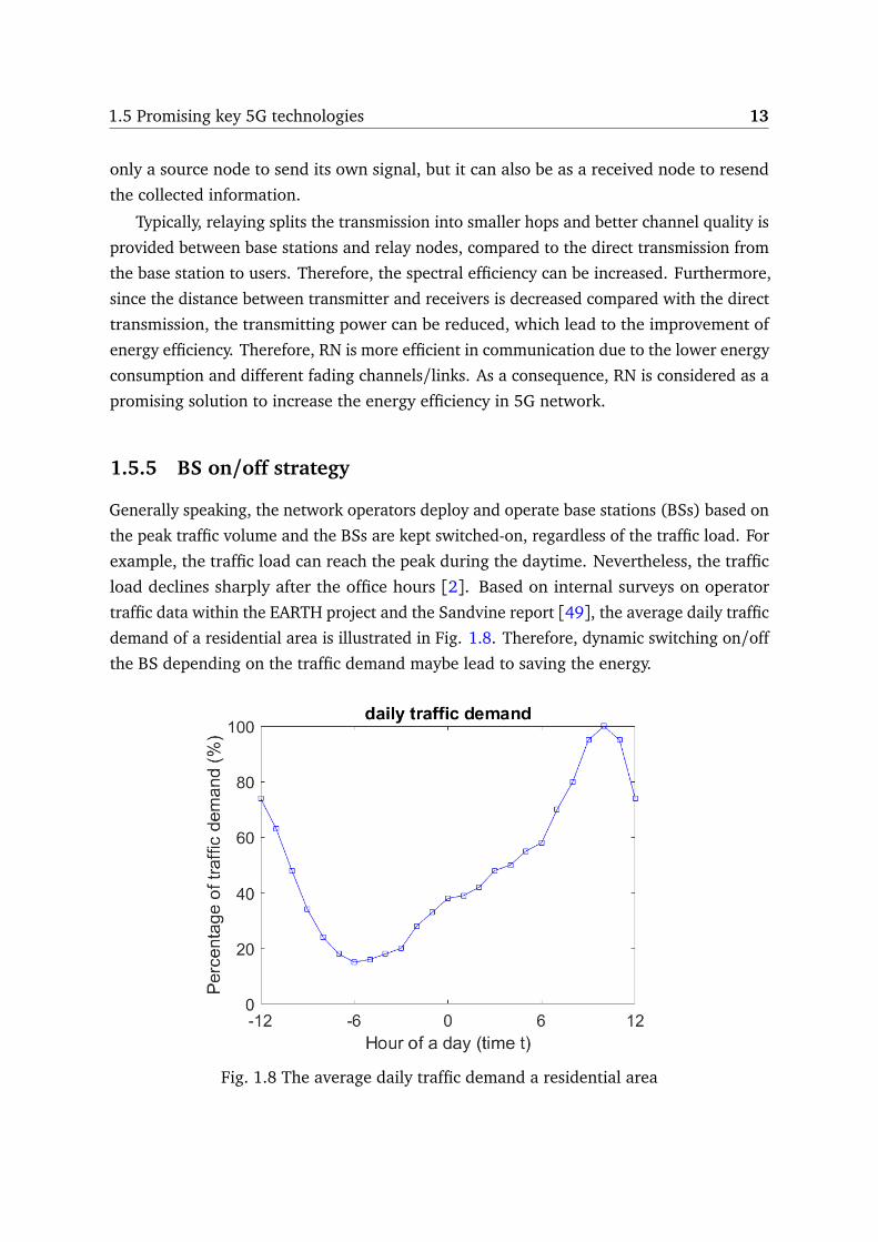
Generally speaking, the network operators deploy and operate base stations (BSs) based on
the peak traffic volume and the BSs are kept switched-on, regardless of the traffic load. For
example, the traffic load can reach the peak during the daytime. Nevertheless, the traffic
load declines sharply after the office hours [2]. Based on internal surveys on operator
traffic data within the EARTH project and the Sandvine report [49], the average daily traffic
demand of a residential area is illustrated in Fig. 1.8. Therefore, dynamic switching on/off
the BS depending on the traffic demand maybe lead to saving the energy.
Fig. 1.8 The average daily traffic demand a residential area

14 Related work on advanced techniques in 5G
BS switching on/off is proposed as a technique to save operating energy through
adjusting the transmission strategy of network according to the traffic demand. Operators
switch off unnecessary infrastructure nodes or elements while satisfying constraints such as
coverage and data rate requirements [9]. In detail, the users in switching-off BS coverage
can be served by neighboring active BSs in order to maintain the user throughput and
the reliability performance. Given that EE is defined as a ratio of throughput over the
power consumption, EE increases with the decrease of the power consumption while the
throughput remains the same. Therefore, this technique is expected to be utilized to
meet the energy saving requirement for dense and ultra-dense deployments in future 5G
networks.
1.5.6 Cloud radio access network (Cloud-RAN)
Spurred by the impressive spread of cloud computing, cloud radio access network (Cloud-
RAN) is a network architecture where baseband resources are pooled to a remote data-center,
named baseband units (BBU) pool, so that they can be shared between BSs. This can be
implemented via software [50]. Fig. 1.9 gives an overview of the overall Cloud-RAN
architecture (RRH: remote radio head, BBU: baseband units). In more detail, only the
radio frequency (RF) chain and the baseband-to-RF conversion stages are presented by the
BSs and the BSs are connected through high-capacity links to the data-center, where all the
baseband processing and the resource allocation algorithms are run [9].
Fig. 1.9 Cloud-RAN architecture for mobile networks [50]

1.6 EE-related surveys 15
Cloud-RAN is a network architecture that shows significant promises in improving
both the spectrum efficiency and the energy efficiency of wireless networks [51]. It brings
these benefits based on the below four folds [52, 53]. Firstly, a centralized BBU pool
allows for the joint precoding of user messages for interference mitigation. Therefore, the
transmitting power of BSs can be reduced with the less interference generated. Secondly,
the cooperative BS with distributed antenna equipped by radio remote head (RRH) provides
higher spectrum efficiency [51]. Thirdly, most of the baseband signal are proceed by the
BBU pool under the Cloud-RAN architecture. Then, the conventional highcost high-power
BSs can be replaced by low-cost low-power radio remote heads (RRHs). Fourthly, the
central processor can perform joint resource allocation among the BSs to allocate resources
according to the users’ traffic demand, and put idle BSs into sleep mode during non-peak
time for energy saving. Based on the advantages of reduction deployment costs in Cloud-
RAN, Cloud-RAN is another key technology instrumental to making 5G networks more
energy-efficient.
1.6 EE-related surveys
The tremendous growth of wireless communication systems leads to challenges in efficiently
utilizing limited network resources to meet the high QoS requirements. Higher capacity
wireless links are expected but suffer from increasing power consumption and associated
financial cost. Meanwhile, the battery capacity of the smartphones limits the improvement of
QoS. Additionally, the slow development of related technologies in battery also enlarges the
gap between energy demand and battery capacity offered by mobile terminals. Therefore,
energy efficiency is becoming more and more important for wireless system design.
Most of the surveys available in the literature theoretically discussed the energy efficiency
in 5G wireless networks from the perspective of the state-of-the-art technologies. Some
surveys of current literature on energy efficiency will be presented in the following part.
Surveys in [6, 46, 54, 55] discussed how to design the EE wireless communication from
the technical methods. For example, the work in [6] summarizes the advanced techniques
of MIMO and relay transmission, resource allocation between signaling and data symbols
in order to design EE networks. Those advanced technologies are only analyzed to improve
the SE from the view point of information-theoretic analysis. Moreover, the authors in [46]mainly discussed the trade-off between EE and SE, QoS for 5G wireless communication,
based on a system framework of green HetNets along with some techniques, such as network
dynamic cooperative transmission and dynamic resource allocation. However, they studied
EE from the network architecture and cross-layer design perspectives, which mainly focus
16 Related work on advanced techniques in 5G
on the design principle. The detailed and precise equation of EE is not discussed in that
literature.
Alternatively, the enabling technologies (massive MIMO, millimeter waves and small
cells) for 5G green networks are investigated in [54]. Specially, the authors identified
the achievable capacity/throughput gains from both theoretical and practical perspectives
according to some references, for example, the system capacity of a massive MIMO system
can be increased by factors of 3 to 6.7 for a base station with 64 antennas serving 15
clients simultaneously. Moreover, an overview description of mobile access and several
new concepts for 5G networks are demonstrated in [55], where some key performance
indicators, the trends of EE and the evolutionary technologies of Massive MIMO, relay
transmission, cloud-RAN and small cell are illustrated for 5G networks.
The four mentioned surveys only focused on the discussion of the advanced technologies
so as to improve SE, whereas none of them are studied the EE and limited to quantify the
improvement of EE.
On the other hand, the papers in [9, 18, 19] discussed the energy saving from the
perspective of the radio resource management. For example, the survey in [9] provides
an investigation on the energy-efficient design and operation of 5G networks from the
domains of resource allocation and network planning and deployment. Different other
surveys focusing on the traditional electrical energy, the energy harvesting and transfer and
hardware solutions for energy efficient 5G networks are first proposed in that literature.
Some open issues are also addressed in [9], such as how to combine all energy-efficient
techniques to optimize EE, how to use random matrix theory, stochastic geometry and
learning techniques in order to deal with randomness of the deployed devices and user
equipments and thereby to maximize EE.
Moreover, from the perspectives of radio resource management and network deployment
strategies, the authors in [18] overview the energy-efficient technologies of various relay
and cooperative communications in wireless networks. Specially, the most popular EE
metric of bit-per-Joule is discussed there, which is defined as the system throughput for
unit-energy consumption. Considering that daily traffic loads at BSs vary widely over time
and space as shown in Fig. 1.8, thus, a lot of energy is wasted when the traffic load is
low. Accordingly, these energy-efficient technologies proposed in [18] are mainly discussed
under low-traffic loads.
Alternatively, from the perspectives of network operators and mobile users, the literature
in [19] elaborates a brief survey on energy-efficient techniques and solutions in order to
design and improve the efficiency usage of energy. A unified-treatment way of energy
efficient solutions is adopted for network operators and mobile users. For instance, the

1.6 EE-related surveys 17
green solutions of switching on-off radio devices and radio resource scheduling are mainly
emphasized according to the low/high call traffic load conditions. However, it mainly
focuses on direct communications (i.e., no multi-hop or relaying techniques) for licensed
networks and users.
Specially, some work highlight the energy efficient 5G wireless network based on out-
standing technology, like Massive MIMO in [37] and switching on-off BSs in [56]. The work
in [37] discusses an overview of massive MIMO technology, a realistic power consumption
models in MIMO systems and some outstanding techniques for EE-maximization. The
survey pointed out that EE-maximization of a Massive MIMO system can be achieved
using the Massive MIMO technique through minimizing power amplifier (PA) power loss,
scaling the number of BS antennas and reducing radio frequency requirements at BS. The
simulation results show that the sum EE of all users can be improved by increasing the
number of BS antennas and it exists a maximum achievable sum EE. Furthermore, the
results also reveal that the optimal number of antennas increases from 63 to 92 and the
peak EE increases from 3.6 to 9.2 M bits/Joule with the raise of the number of users from
6 to 50 in the system.
Authors in [56] emphasize that the switching on/off BSs technology in order to improve
the EE in 5G dense and ultra-dense networks. They present that switching-off unnecessary
network elements can be as one of tools for decoupling the scaling of networks from the
growth of operating power, which is aimed at adjusting the network capacity according
to the demand in order to save operating energy. They mainly emphasize and devise an
energy-saving algorithm based on a majorization-minimization approach for turning-off
some unnecessary BSs. However, the quantitative improvement of EE is missing from
discussion.
Unlike most of the surveys that discussed the EE in the physical layer while some
advanced technologies are exploited, the survey in [28] presents an overview of different
EE trade-off mechanisms of green communications with respect to each protocol layer,
such as physical, media access control (MAC), network, transport and application layer,
respectively. Specially, the technologies of sleeping mode, cell breathing, cell zooming are
investigated in terms of the EE trade-offs. However, the quantitative improvement of EE
are limited in their investigation.
All survey papers discussed above illustrate that a energy-efficient wireless network
can be designed through taking advantage of the 5G technologies candidates. Moreover,
they also indicated that the 5G technologies candidates can be used to evaluate EE or to
study the problem of EE optimization. Nevertheless, these conclusions are drawn from the

18 Related work on advanced techniques in 5G
perspectives of theoretical and design principle. In the next chapter, we will present some
literatures to show the advanced technologies on EE through some simulation results.
1.7 Conclusion
This chapter provides the background information and some related work on advanced
techniques, beneficial to improve EE for 5G wireless networks. We first introduce research
motivation on EE in ICT and the cellular network concept. Then the relationship between SE
and EE is presented, which is helpful to understand our thesis work. Moreover, the typical
approaches and techniques to reduce the system energy consumption and to improve
the SE are presented, such as MIMO technique, coordination multipoint transmission,
heterogeneous cellular network, relay transmission, BS switching off and Cloud-RAN,
which are promising to be exploited in 5G networks. Finally, we discussed some surveys
which are focusing on the green communication.
To investigate the impact of the network parameters on EE, and to capture the major
factors involved in the energy consumption process, representative and accurate models
are needed. Therefore, in the next chapter, we will present the EE models which have been
utilized in some literatures.

Chapter 2
Models for EE
Contents
2.1 Introduction . . . . . . . . . . . . . . . . . . . . . . . . . . . . . . . . . . . . . . . 20
2.2 EE models . . . . . . . . . . . . . . . . . . . . . . . . . . . . . . . . . . . . . . . . . 20
2.2.1 Input/output power related EE model . . . . . . . . . . . . . . . . . . . 21
2.2.2 Cell power consumption and cell area related EE model . . . . . . . . 22
2.2.3 Transmitting power and data rate related EE model . . . . . . . . . . 23
2.2.4 SE and power cost related EE model . . . . . . . . . . . . . . . . . . . . 23
2.2.5 Overall data rate and power cost related EE model . . . . . . . . . . . 24
2.3 Power consumption models (PCM) . . . . . . . . . . . . . . . . . . . . . . . . . 24
2.3.1 Ideal load dependent PCM . . . . . . . . . . . . . . . . . . . . . . . . . . 25
2.3.2 Linear PCM . . . . . . . . . . . . . . . . . . . . . . . . . . . . . . . . . . . 25
2.3.3 PCM with sleep mode . . . . . . . . . . . . . . . . . . . . . . . . . . . . . 26
2.3.4 PCM with backhauling cost . . . . . . . . . . . . . . . . . . . . . . . . . 26
2.3.5 PCM considering non-empty buffer . . . . . . . . . . . . . . . . . . . . . 27
2.3.6 PCM with transmitting antennas . . . . . . . . . . . . . . . . . . . . . . 27
2.3.7 A refined double linear PCM . . . . . . . . . . . . . . . . . . . . . . . . . 28
2.4 Throughput models . . . . . . . . . . . . . . . . . . . . . . . . . . . . . . . . . . . 28
2.5 Classification of EE models . . . . . . . . . . . . . . . . . . . . . . . . . . . . . . 30
2.5.1 Evaluation-based related work . . . . . . . . . . . . . . . . . . . . . . . 30
2.5.2 Optimization-based related work . . . . . . . . . . . . . . . . . . . . . . 36
2.6 Conclusion . . . . . . . . . . . . . . . . . . . . . . . . . . . . . . . . . . . . . . . . 44

20 Models for EE
2.1 Introduction
As illustrated in the previous chapter, energy efficiency (EE), as one of key performance
indicators, becomes an important concern while designing a 5G wireless network, not only
because of the increasing energy price but also because of the environmental requirement
of a lower CO2 emission of communication networks. Hence, EE has received much
attention by both academia and industry through utilizing the different network model
tools, such as system-level simulations and stochastic geometry. Much efforts have been
done to investigate the problems of EE evaluation and EE optimization through using
some advanced technologies, such as multiple-input multiple-output (MIMO), coordination
multipoint (CoMP) scheme, heterogeneous cellular networks (HetNets), relay transmission
and the on-off switching policy of base station (BS). However, an appropriate definition of
EE is the fundamental to study the EE performance for the network.
Various EE models have been proposed in both academia and industry from the mea-
surement level of power amplifier, antenna, base stations (BSs), user equipments (UEs) and
the network. Among these models, some are proposed for simplicity, and the others are
proposed while considering the network performance such as spectral efficiency, throughput
and capacity. One can choose the EE model according to the measurement level as well as
the network performance. In this regards, it is very important to understand the detailed
definitions of EE metric in different literatures.
Throughout this chapter, we aim to present some EE models according to the different EE
definitions, and to classify the literatures on EE according to these promising technologies so
as to investigate the impact of these technologies on EE, which will be useful to understand
our thesis work.
In this chapter, we first list some EE models from the view point of EE definition. As
the important components of the EE model, then the power consumption models and the
throughput models are introduced. Furthermore, we classify some literatures on EE from
view points of both EE evaluation and EE optimization. The further classification of the
categories are based on the advanced technologies, since they have great impact on EE.
Afterwards, we summarize the impact of these techniques on EE through comparing the
simulation results in the literatures.
2.2 EE models
Various models have been proposed by both academia and industry to evaluate the EE
performance. In general, from the perspective of measurement level, most of the proposed
2.2 EE models 21
EE models are on three different levels in mobile cellular networks so as to obtain the
network performance. The three different levels are as follows:
• Hardware component level (for wireless equipment subsystems e.g. power amplifier,
antenna, etc.)
• Node level (e.g. BSs and user terminals)
• System or network level (for a group of equipments that form a network).
Additionally, we also found that there are two ways of defining energy efficiency metrics.
First, EE is defined as the ratio between the energy output and the energy input, which is the
oldest model on EE. Secondly, considering the network performance of QoS parameters such
as throughput and capacity, EE is defined as the ratio between a given network performance
and the energy consumed [57].
Therefore, according to the measurement level and the various definitions of EE, a
review of the EE models used in wireless communication networks is carried out. Table
2.1 summarized the related variables and symbols of EE, capacity and throughput used
throughout our discussion.
2.2.1 Input/output power related EE model
At the system level, a simple definition of the energy efficiency is defined by the operators
is the ratio between the network output power (energy) and the total input power (energy)
[21]. This model is the oldest model. Denoting the network output power (i.e., the power
of the radio frequency (RF) transmitted signal) and the input power (consumed), as Po
and Pi, respectively, the energy efficiency EEs ys for the network is given by
EEs ys =Po
Pi(2.1)
According to the above definition, we observe EEs ys has no unit. Generally, the deployment
of cellular networks is typically optimized for ubiquitous radio access of mobile users. This
implies that a significant portion of base stations (BSs) are primarily providing coverage.
Eq. (2.1) shows that it is not necessary to achieve the full traffic load for the network, since
the users ask for the low service during the off-peak traffic hours. Therefore, this equation
can be used when the coverage of a cellular network is required to be greater than a given
value, i.e., to reach an acceptable coverage probability.

22 Models for EE
Table 2.1 Main symbols on EE model
Notation DefinitionEEs ys system or network EEAPC area power consumption (ratio of cell power consumption to cell area)EC I energy consumption index (ratio of power cost and data rate)EE energy efficiencyEEu EE of a user uPo network output powerPi network input powerPex p,cel l total power consumption in a cellAarea cell areaEex p the network energy consumption during the observation periodNbi t the number of correctly delivered bits during the observation periodPex p,ave the average network powerRave the average data rateSEarea the area spectral efficiencyPex p,u the total transmitting power of user uRu the achievable data rate of user uCn the maximum data rate of the networkThtotal the sum achievable data rate of the networkPCtotal the total power consumption of the network
2.2.2 Cell power consumption and cell area related EE model
To assess the EE for networks having different coverage areas, the area power consumption
is introduced, defined as the ratio between the average power consumption per cell and
the corresponding cell area [58]. Denoting Pex p,cel l as the total power consumption in the
cell and Aarea as the cell area, the area power consumption APC is given as
APC =Pex p,cel l
Aarea[W/Km2] (2.2)
measured in W/Km2. This EE model can be used at the node level (e.g. BSs) and the
system level, respectively. Since the cell area can not only refer to the coverage of a certain
BS but also the coverage of the whole network. Accordingly, Pex p,cel l can be the total power
consumption of a certain BS or the total power consumption of the whole network, from
the perspectives of both the node level and the system level, respectively. Moreover, the
coverage area can reflect the area power consumption from a deployment perspective.
Additionally, this equation can be used to compare the power consumption in HetNets while
varying the number of micro BSs in one cell so as to investigate the impact of deployment

2.2 EE models 23
stratigies on the power consumption. However, this model needs to be used in conjunction
with other performance metrics as it cannot be used to successfully access the EE of two
networks having different capacity or throughput.
2.2.3 Transmitting power and data rate related EE model
Another EE model on the node level is the energy consumption index (ECI) or energy per
bit, proposed in the "Energy Aware Radio and neTworking tecHnologies (EARTH)" project
[59]. The energy per bit is measured in J/bit. The energy per bit metric is defined as a
ratio of the network energy consumption (EC) during the observation period (T) to the
total number of bits (B) that were correctly delivered in the network during the same time
period. Since the network energy consumption is simply the (average) power multiplied
by the observation period, this metric could be equivalently described as the ratio between
(average) network power (Pex p,ave) and the (average) data rate (Rave) and expressed in
W/bps. Denoting Eex p as the network energy consumption and Nbi t as the amount of data
correctly delivered in the network, the definition of ECI is given by
EC I =Eex p
Nbi t=
Pex p,ave
Rave[J/bi t or W/bps]. (2.3)
The ECI focuses on the amount of energy spent per delivered bit and hence is an
indicator of network bit delivery EE. This may be especially important in the scenario of
high traffic loads. Furthermore, ECI approaches infinity with traffic load close to zero,
since the network energy consumption Eex p does not typically go to zero for low traffic
loads. ECI is commonly used in the literature, especially for theoretical studies and single
link evaluations. Nevertheless, for the low traffic load scenario, the traffic demands of the
mobile terminals do not always require BSs at the full power. Specially, the energy cost for
the error reception of data is not considered in this model.
2.2.4 SE and power cost related EE model
For the sake of reflecting the achieved network coverage, the authors in [16, 60] define
the EE as the ratio between the area SE and the average network power consumption.
Denoting Pex p,ave as the average network power consumption and SEarea as the area SE,
the network EE, denoted EEs ys, can be displayed as
EEs ys =SEarea
Pex p,ave(bi t/J/Hz) (2.4)

24 Models for EE
EEs ys is measured in bi t/J/Hz. The objective of this definition is to increase the number
of transmitted information bits per unit energy, which has been widely used in various
publications. This model can be used to evaluate the EE at the component, node and system
levels. Moreover, it can also be applicable for the low service demands scenario, where
a reasonable network coverage should be guaranteed while considering the strategy of
switching off BSs. Specially, the area is a constant for evaluating the system EE.
2.2.5 Overall data rate and power cost related EE model
A classical and most widely-applied model to evaluate the EE for the telecommunication
networks is the Bit-per-Joule metric. It is defined as a ratio of total volume of data transferred
to the energy consumed within a given time interval, expressed by
EE =overal l date rate
total power comsumption(bi ts/J or bi ts/s/wat t) (2.5)
The system capacity, Cn, is the maximum total number of bits that the network can deliver
per Joule of energy by one/multiple BSs. The overall network throughput, Thtotal , is the
sum of the data rates that are successfully delivered to all the terminals in a network,
composed by one/multiple cells. Denoting PCtotal as the total power consumption, EE also
can be expressed as EE = Cn/PCtotal or EE = Thtotal/PCtotal .
Depending on the specific area of interest, this EE model can be covered on component,
node and system levels in wireless cellular networks. For example, EE becomes EEu (the
energy efficiency of one user) at the user’s level and EEs ys at the network or system level,
respectively. Considering the simplicity of this EE model, it has been applied in many
literatures for 4G networks and beyond.
Given that the most used definition of energy efficiency is related to the throughput
or capacity and to the power consumption, here we will briefly present some power
consumption models (PCMs) and throughput models, which are popular and most used in
literatures.
2.3 Power consumption models (PCM)
In [12, 14, 21, 61], the percentage of power consumption by different components of a
large-cell base station (BS) is reported, as shown in Fig. 2.1. We observe that the power
amplifier and feeder cost about 65.6% of the total power. Moreover, the power cost by
signal processing overhead, battery backup and power supply loss, cooling loss, power

2.3 Power consumption models (PCM) 25
amplifier loss also can not be ignored. Therefore, a model to quantity the component
cost is necessary. Nowadays, various power consumption models have been proposed in
literatures for the BS. A summary of different models to calculate power consumption is
presented as follows. Here, the power consumption for the BS b is denoted as Pex p,b.
Fig. 2.1 Percentage of power consumption by different components of a large-cell BS [14].
2.3.1 Ideal load dependent PCM
The authors in [62] introduce an ideal load dependent power model with the assumption
that the power cost by base station (BS) is proportional to the BS utilization (or loads).
In other words, when a BS is utilized, it includes power consumption for transmitting
antennas, power amplifiers, cooling equipment and so on. However, there is no power
consumption for the BS in an idle state. Let ϕb denote the BS utilization and Pt x stands for
the BS transmitting power. The equation of power consumption can be displayed as
Pex p,b = ϕbPt x . (2.6)
This is a relatively old model to quantify the power consumption of one BS, which assumes
Pex p,b depending on the utilization of BS, ϕb. However, such a model is not realistic since
the power consumption does not matter with BS utilization, as illustrated in Fig. 2.1.
2.3.2 Linear PCM
In [63], a linear/canonical power consumption model is employed as
Pex p,b = ζPt x + Pcircui t , (2.7)

26 Models for EE
where ζ is an inverse of the drain efficiency of transmitting amplifier and Pcircui t is the total
circuit power expenditure by radio frequency (RF) chain components (filters, mixers, and
synthesizers) and baseband operations (digital up/down conversion, precoding, receiver
combining, channel coding/decoding and channel estimation). The energy consumption of
power amplifier is excluded in Pcircui t , which is independent of the transmission state.
However, Eq. (2.7) tends to overestimate the system power consumption because
they assume that the transmitting buffer is never empty during the whole transmission
frame, which is not true since the transmitter has the idle state. Furthermore, given
the consideration of Rayleigh fading scenario, where a signal will randomly vary or fade
according to a Rayleigh distribution, it is not possible to have a deterministic estimation
when the buffer becomes empty during the frame transmission.
2.3.3 PCM with sleep mode
When the traffic requirement of users is zero, it means there is no traffic load for the BS
and the BS can be in sleep mode. However, the BS still uses some power. Therefore, [2]proposed a new power consumption model of one BS, expressed as
Pex p,b =
ρload Pt x + Pact ive, if 0< Pt x ≤ Pt x ,max
Psleep, if Pt x = 0(2.8)
where ρload denotes a constant coefficient depending on the traffic load, Pt x is the trans-
mitting power of BS, Pact ive is the minimum power required to support BS with non-zero
transmitting power, Pt x ,max is the BS transmitting power at the maximum load and Psleep
accounts for the power consumption of the BS in sleep mode. Normally, Psleep < Pact ive
so that this power model is popular to be used while the switching on/off technology is
adopted.
2.3.4 PCM with backhauling cost
In order to capture backhauling energy needs, the authors in [64] propose a general power
consumption model,
Pex p,b = a · Pt x + b · Psp + c · Pbh (2.9)
where Pex p,b, Pt x , Psp and Pbh denote the average consumed energy per BS, the radiated
power per BS, the signal processing power per BS, and the power due to backhauling,
respectively. The coefficients a, b, and c denote the scale with respect to the corresponding

2.3 Power consumption models (PCM) 27
power type amplifier and feeder losses, cooling, or battery backup. The three coefficients
can be computed according to the parameters in [65]. This model assumes that all BSs are
under full load, i.e., the energy consumption for an idle BS is not considered.
2.3.5 PCM considering non-empty buffer
A new average power consumption model is introduced in [66] which fully accounts for the
non-empty buffer probability (NBP) and jointly optimizes both the transmitting power and
the quality-of-service (QoS) exponent for the data link layer in a wireless point-to-point
system, which is damaged by complex additive white Gaussian noise and block fading (the
channel state is independent from one to another). The new power consumption model is
thus formulated as:
Pex p,b(Pt x) = ζ · Prob · Pt x + Pcircui t =Rmax ,arri
Eγ[log(1+ Pt xγ)]︸ ︷︷ ︸
Prob
· ζ · Pt x + Pcircui t (2.10)
where Prob is the probability of non-empty buffer, ζ is an inverse of the drain efficiency of
transmitting amplifier, Rmax ,arri is the maximum constant arrival data at the physical layer
of the transmitter, Pt x is the transmitting power and γ is the exponential random variable
modeling the Rayleigh fading channel. This model is applicable for Rayleigh fading channel
and data link layer regardless of the noise impact.
2.3.6 PCM with transmitting antennas
When considering the effect of the number of transmitting antennas, a novel linear model
is presented in [65] as
Pex p,b = Nant · (ζPt x ,PA+ LSP) · (1+ LC) · (1+ LPSBB), (2.11)
where Nant denotes the number of antennas in the system, Pt x ,PA refers to the transmitting
power per power amplifier (PA), ζ is an inverse of the power amplifier efficiency, LSP ,
LC , LPSBB are the signal processing overhead, cooling loss, and battery backup and power
supply loss, respectively. While the power consumption for direct current to analog current
converters is neglected, this model gives an upper bound on the power consumption of a
BS equipped with transmitting antennas.
In [59, 67], this model has been refined so that the power consumption of the other
BS components, e.g., direct current (DC) and analog current (AC) converters, are also

28 Models for EE
included. Denoting Nant as the number of antennas per BS, Pt x as the transmitting power
per BS, ζ as an inverse of the power amplifier efficiency, Pf i xed as the non-transmission
power consumption including baseband processing, battery backup, cooling, etc, the power
consumption model is given as
Pex p,b = ζPt x + Nant Pcircui t + Pf i xed . (2.12)
Even though this model takes into account the non-linearity of the power amplifier (PA),
it has been illustrated that the relation between the relative radio frequency (RF) output
power and the BS power consumption is nearly-linear. The given results show that the
power consumption of components like DC-DC/AC-DC converter and cooling unit will not
grow linearly with the number of antennas.
2.3.7 A refined double linear PCM
The refined double linear power consumption model (PCM) [68] is given by:
Pex p,b = Nant · (∆P · Pt x ,PA + P0) + P1 (2.13)
where ∆P = (1+ LC) · (1+ LPSBB)/µPA, µPA being power amplifier efficiency, P0 = LSP · (1+LC) · (1+ LPSBB), and P1 is a fixed part accounting for the direct current (DC) and analog
current (AC) converters.
2.4 Throughput models
In the below part, we will present some concepts like the network capacity Cn, the overall
network throughput Thtotal , area spectral efficiency SEarea, and the user achieved data rate
Ru.
The network capacity, Cn, is defined as the maximum amount of data that may be
transferred by one or multiple BSs. Additionally, the overall network throughput, Thtotal ,
is defined as the sum of the data rates that are successfully delivered to all the terminals in
a network. Particularly, Thtotal equals Cn while Shannon formula is used, since Shannon
formula is applied to compute the highest number of binary digits per second during the
transmission.
In a MIMO uplink system, the authors in [69] define system network capacity Cn
(measured by bits per second) based on Shannon capacity, which is related to the total

2.4 Throughput models 29
bandwidth of the network BWn and network channel information, as given by
Cn = BWn log2 det(I + PHH†), (2.14)
where H stands for the channel matrix between BSs and user terminals, I is the identity
matrix and P represents the transmission power of each user terminal, and † is the trans-
position operation. The matrix H characterizes the MIMO channel, where the fast fading,
noise and interference are considered in the wireless communication. Specially, in the
classical network without MIMO technology, the channel matrix H is a 1× 1 matrix.
The area spectral efficiency SEarea (measured over a unit area) is popularly used for
the energy efficiency expression [16] in a low traffic demand case, as displayed by
SEarea = λnPn(Γth) log2(1+ Γth), (2.15)
where λn denotes the BS density, Γth is a certain signal quality-of-service (QoS) threshold
and Pn stands for the coverage probability. The area spectral efficiency, SEarea, actually
measures the network throughput, Thtotal , while considering the coverage probability. The
coverage probability Pn can be computed by averaging the success probability over the
distance to the nearest node. Specially, success probability is defined as P(γx→u > Γth) when
the signal-to-noise ratio (SNR) γ of the transmitting signal from the BS at x to the mobile
terminal at u is above the threshold Γth.
Based on the knowledge of the instantaneous channel state information (CSI) [70, 71],the achieved data rate Ru by the user u is related to the allocated bandwidth Bu and to the
received SNR, SNRu at user u, displayed as
Ru = Bu log2(1+SNRu
Γ) (2.16)
where Γ is the SNR gap between the channel capacity and a practical coding and modulation
scheme. Specially, Γ equals 1 in Shannon formula.
Given that the feedback of the instantaneous CSI between each user and its serving
base station is needed, a lot of expenses have to be paid by the operators and users. For this
case, the statistical CSI is utilized and the achieved data rate Ru is rewritten in a statistical
average sense [72], as
Ru = EH[Bu log2(1+SNRu
Γ)], (2.17)
where EH stands for the expectation over the channel matrix H. Ru in Eq. (2.16) and Eq.
(2.17) is measured in bits per second.

30 Models for EE
Based on the models of energy efficiency (EE), power consumption and throughput
discussed before, much work have been studied on the EE performance in some literatures.
According to the published papers, we found that most of the work on the energy efficiency
(EE) investigation in wireless networks are conducted with the purpose either to evaluate
the impact of some advanced techniques on the EE, or to define/design the parameters of
these advanced techniques in order to optimize the EE. Therefore, a classification of the
literatures on EE performance will be presented in the following section, according to these
two objectives: EE evaluation and EE optimization.
2.5 Classification of EE models
As discussed in chapter 1, these advanced technologies are promising to be utilized so as to
improve the network EE for the future radio communication networks, such as multiple-
input multiple-output (MIMO), coordination multipoint (CoMP) scheme, heterogeneous
cellular networks (HetNets), relay transmission and the on-off switching policy of base
station (BS). Hence, we further categorize the evaluation-based related work and the
optimization-based related work of EE according to these advanced technologies, in order
to investigate the impact of these technologies on EE.
2.5.1 Evaluation-based related work
In this subsection, we further investigate the impact of these technologies, e.g., MIMO,
CoMP, HetNets, Relay and BS switching on/off, on EE through the simulation results in
some evaluation-based related work. Moreover, considering that most of the EE models are
proposed at the hardware component level, the node level and the system or network level,
we also discuss the evaluation-based related work according to the measurement levels.
– MIMO system
Many literatures focus on the investigation of the impact of MIMO technique on EE owing
to the improvement of spectral efficiency brought by this technique. As an example, Ngo
et al. [3] investigated the trade-off between EE and SE for a very large single-cell/multi-
cell multiuser MIMO uplink system, where EE is defined as a ratio of the sum of data
rates transmitted per user terminal over the transmitting power consumption of each user.
The system EE, EEs ys, can be expressed as EEs ys =∑
u Ru
Pex p,ubi ts/J , where Ru denotes the
achieved data rate of user u equipped with single antenna, computed by Eq. (2.17), and
Pex p,u is the total transmitting power consumption of user u, computed by Eq. (2.6). The

2.5 Classification of EE models 31
numerical results reveal the EE and SE can be improved through taking advantage of large
antenna arrays with lower transmitting power regime, compared to a single-antenna system.
However, the circuit power consumption in the power consumption model (PCM) is not
taken into account. Additionally, when a realistic PCM is considered, Fabien Heliot et al.[68] presented a novel and generic closed-form approximation of the trade-off between
EE and SE over a MIMO Rayleigh fading channel, where EE-SE trade-off can be regarded
as a problem of expressing EE by SE. Based on the energy consumption index (ECI), as
defined in Eq. (2.3), and a more realistic PCM, as defined in Eq. (2.13), the approximation
accuracy is assessed. Through a comparison of EE gain between in MIMO and SISO systems
over Rayleigh fading channel, the simulation results show that EE is not always improved
with the increase of SE and the number of antennas. Indeed, MIMO system will consume
more circuit power and more signaling overhead with numerous antenna configurations,
resulting that the practical EE gain decreases with the number of transmitting antennas.
In a nutshell, for the purpose of increasing EE, it is very important to choose an
appropriate number of antennas in the future MIMO system.
– CoMP system
Fabien Heliot et al. [73] analyzed the EE of both uplink and downlink in a idealistic CoMP
communication system, through assuming perfect backhaul links between each BS and an
idealistic cooperative processing. EE is defined as a ratio of the channel capacity, as defined
in Eq. (2.14), to the system consumed power, defined in Eq. (2.11). Numerical results
demonstrate that multi-BS cooperation can improve the EE when the link quality between
the BSs and MSs is weak, e.g., cell-edge communication, and that the backhauling and
cooperative processing power should be kept low in order to provide EE gain. However,
in that paper, the numerical results are obtained based on the assumption that the power
consumption required for backhaulings and cooperative multiple BSs is regarded as a
constant, which is not realistic.
In contrast, considering the realistic backhauling power consumption model, the work
in [74] investigated the EE for a Beyond-LTE cellular network through taking advantage
of the cell switch-off scheme and JT-CoMP transmission technology. EE is defined as the
ratio between the received capacity of one user, defined in Eq. (2.14), and the total access
network power consumption, defined in Eq. (2.9). Through simulations with realistic
parameters, the results show that the CoMP scheme used jointly with the cell switch off
schemes is more energy efficient in the access networks. Specially, setting a proper number
of coordinated BSs, namely CoMP set degree, is very important in terms of energy efficiency.
A higher CoMP set degree may cause a decrease in energy efficiency performance due to
32 Models for EE
signaling and backhauling overhead in the network. Meanwhile, taking advantage of the
CoMP scheme, the authors in [64] also evaluated the EE for a cellular network and the
numerical results indicate that CoMP technique can not bring benefit to the energy efficiency
when CoMP set degree is above three, due to the additionally required backhauling power
for the cooperative set.
Unlike the conventional cellular networks powered by on-grid energy, Abu Jahid et al.[75] proposed a novel network model to evaluate EE for a downlink LTE-A cellular hybrid
system, powered by both on-grid energy and solar energy. The EE is defined as the ratio of
aggregate throughput of the network, defined in Eq. (2.16), to the total power required
for running the network, defined in Eq. (2.12). This model is utilized in two scenarios: 1)
SINR-based JT-CoMP and 2) distance-based JT-CoMP. In SINR-based JT-CoMP technique,
the best two BSs offering maximum SINR are serving a user and in distance-based JT-CoMP
one, two closest BSs are intended to serve a user. Simulation results illustrate that the
proposed SINR-based JT-CoMP scheme achieves a superior EE performance compared to
the distance based JT-CoMP hybrid model.
Overall, CoMP technology can be used to improve the EE for the future wireless com-
munication networks, through setting an appropriate number of coordinated BSs for the
cooperative set.
– HetNet
From the BS deployment point of view, the EE evaluation is investigated in a cellular
network [58], in an interference-limited heterogeneous cellular mobile radio networks
[76], in a 5G wireless network [77] and in an ultra dense HetNets [78], respectively, so as
to illustrate the impact of different types of BSs deployment on EE.
The authors in [58] studied the impact of deployment strategies on the area power
consumption, through deploying varying numbers of micro BSs in a macro cell. The area
power consumption (APC) is defined as the ratio between the average power consumption
per cell, formulated in Eq. (2.7), and the corresponding cell area. The definition of area
spectral efficiency, as the achievable data rate in a network per unit bandwidth per unit
area, measured in bit per second per Hertz per square kilometer, is also demonstrated so
as to find the minimum area power consumption. The numerical results reveal that the
area spectral efficiency can be increased through improvement of the density of micro BSs,
whereas the area power consumption is moderate with the raise of the number of micro
BSs in the full traffic load scenario. Since the deployment of additional micro BSs per cell
increases the average power consumption per cell, resulting the increase of the area power
consumption.
2.5 Classification of EE models 33
Additionally, with random micro BSs deployment and ‘bits/J’ as the EE metric, Henrik
Klessig et al. [76] investigated the EE of a heterogeneous OFDM-based mobile network
while taking into account the co-channel interference by varying traffic demand per area.
The EE is defined as the ratio between the actual throughput of the reference area, defined
in Eq. (2.16), and the total power consumption, defined in Eq. (2.7). The simulation results
indicate that a EE gain of about 20% can be achieved through increasing deployment density
of micro BSs, since the area spectral efficiency is enhanced and the transmitting power
of macro BSs is reduced with the micro BSs deployment, while still providing coverage.
Comparing to the work in [58] for the full traffic load scenario, this network EE model can
be applied in both non-full load scenario and hot spot scenario.
Unlike the work in [58, 76]with micro BSs deployment in macro, Safdar Rizvi et al. [77]investigated the EE of a 5G HetNet when small BSs (pico, femto) are deployed in the macro
cells. The EE is defined as a ratio of the maximum data rate of the network, defined in Eq.
(2.16), over the total power consumption, defined in Eq. (2.7). The numerical analysis
have confirmed that EE is enhanced in 5G HetNet when the number of small BSs, i.e., pico
and femto, is increased in a rational manner. Additionally, [78] investigates the impact
of BS deployment on EE using the stochastic geometry theory and derives a closed-form
EE with respect to the BS deployment in an ultra dense HetNet where the pico BSs are
deployed in the macro cells. The network EE is defined as the ratio between the minimum
achievable throughput, defined in (2.15), and the total power consumption of the whole
network, defined in Eq. (2.6). Numerical results show that with the increasing number
of pico BSs, EE first increases and then decreases due to the rise of power consumption
caused by the increment of pico BSs.
Overall, in the HetNets, the density of small cell BSs should be designed carefully in
order to obtain the maximum network EE.
– Relay system
The energy consumption in relay systems is also investigated. Roberto Fantini et al. [79]presented an analysis of the energy efficiency (EE) from the view points of two relay
schemes: two hop scheme and the multicast cooperative scheme. The division of the two
schemes is based on whether the relay node (RN) creates cell of its own or not. According
to the observed numerical results in terms of energy consumption index, energy can be
saved up to 15.6% in the two-hop relay scheme. RN can be as an effective tool to reduce
the energy consumption in telecommunication networks and achieve a great improvement
on the capacity.

34 Models for EE
– BS on/off
Taking into account the BS on/off strategy, Chang Li et al. [67] investigated the effect
of the BS density and number of transmitting antennas on the network throughput and
energy efficiency in a random cellular network where all BSs are micro-BSs equipped with
multiple antennas. According to whether the BSs have users to serve, the BSs can be
divided into active BSs and inactive BSs. The inactive BSs do not transmit any signals. The
network EE, measured in bi t/J/Hz, is defined as the the network throughput to the power
consumption per unit area, defined in Eq. (2.12). Specially, the power consumption per
unit area includes the power consumption from both the active and inactive BSs, constituted
by the transmitting power, the circuit power of the corresponding radio frequency chain and
the non-transmission power consumption, including baseband processing, battery backup,
cooling, etc. The simulation results show that 1). EE first increases and then decreases with
the increase of BS density when the ratio of non-transmission power cost to the total BS
power consumption is smaller than a given value. Otherwise, EE decreases as BS density
increases. 2). EE first increases and then decreases with the increase of the number of BS
antennas, when the non-transmission power consumption is smaller than a given threshold
value. Otherwise, EE of a single-antenna system is better that of a multi-antenna system.
Therefore, the different components of BS power consumption play a critical role in the
EE when the technology of BS switching on/off is applied.
– MIMO + CoMP
However, with increasingly demanding of EE, only utilizing an advanced technology is not
enough to satisfy the energy-efficient design. Therefore, some existing publications have
investigated the EE through taking advantage of multiple advanced technologies.
The work in [80] derived a closed-form approximation (CFA) of the EE-SE trade-off for
the uplink of a CoMP system with MIMO Rayleigh fading channel. The network EE, EEs ys,
is defined as a ratio of the sum rate of all UEs, defined in Eq. (2.17), over the total power
consumption, defined in Eq. (2.9), given as EEs ys =∑
u Ru∑
u Pex p,ubi ts/J . Ru and Pex p,u denote
the achieved data rate and the total transmitting power consumption of user u, equipped
with multiple antennas. The simulation results show that in a realistic PCM, CoMP system
is more energy efficient than a non-cooperative system due to the improvement in SE
and mainly for cell-edge communication. However, EE decreases with the increase of the
number of cooperating BSs, since the backhaulling and processing power consumption
brought by CoMP technique is increased.

2.5 Classification of EE models 35
All the literatures discussed above validate that the advanced technologies can increase
the network capacity and improving system EE for the wireless network through theoretical
analysis and simulation results. Table 2.2 summarizes the classification discussed above
according to the advanced technologies. More general and comprehensive information can
be found in that table.
Table 2.2 Classification of evaluation-based related work
Tech. Model Measure.level
Up/Down-link
Comments
MIMO Bit-per-Joule [3],Energy consump-tion index (ECI)[68]
Node up,down
MIMO can improve EE withoutconsidering circuit power con-sumption by antennas [3]; MIMOcan not improve EE with ultra-multiple antenna configurationsand a realistic PCM [68]
CoMP Bit-per-Joule [64,73–75]
System,system,node,system
both,both,down,down
All work indicate the improvementof EE with CoMP. However, a con-stant backhauling power cost is as-sumed [73]; the power consump-tion of solar energy is included[75]; [64, 74] illustrates the size ofcooperative set above three can’timprove EE
HetNet Area power con-sumption (APC)[58], Bit-per-Joule [76–78]
System down All work illustrate that HetNet de-ployment can improve EE. How-ever, deployment of micro, macroBSs [58, 76]; pico, femto andmacro BSs [77]; pico, macro BSs[78]
Relay ECI [79] Node down Rely can reduce energy consump-tion and a two-hop scheme is moreefficient
BSon/off
Bit-per-Joule-Hz[67]
System down EE increases with the raise of BSdensity and the number of BS an-tennas when the power consump-tion of BS component satisfy cer-tain conditions
MIMO+CoMP
Bit-per-Joule [80] System up Discussed EE-SE trade-off problemand appropriate number of cooper-ating BSs can lead EE improvement

36 Models for EE
2.5.2 Optimization-based related work
Appropriate performance EE models are of primary importance for the design of green
wireless communication networks, because they are directly related to the choice of the
optimization objectives and the constraints of the corresponding optimization problems.
Based on the throughput models, power consumption models (PCMs) and the EE models
discussed before, we found the existing literatures investigate the optimization of EE either
from a power minimization perspective or data rate maximization perspective. Therefore,
an overview of EE maximization is presented below regarding these two perspectives.
Considering that all EE-optimization problems are proposed based on some advanced
technologies, such as HetNet, BS switching on/off strategy, CoMP, MIMO, and relay, in this
subsection, we further classify the optimization-based related work on EE according to
these advanced technologies.
– Power optimization
From the power perspective, the EE maximization problem can be transfered to minimize
the total power cost, expressed as
min Ptotal
s.t. γk ≥ γD, Pt x ≤ Pt x ,max
(2.18)
where Ptotal , Pt x , Pt x ,max represent the overall power consumption, the transmitting power
per BS and the maximum transmitting power per BS, respectively, γk, γD is respectively the
achievable data rate of the kth UE and the fixed quality-of-service (QoS) target for every
user. Taking advantage of these advanced technologies and based on the Eq. (2.18), we
present some related work of EE optimization in the below part and introduce the specific
concepts of the total power consumption in different literatures.
i). HetNet
An investigation of the impact of BS’s density and the transmitting power on the
network energy consumption is presented in [81] for both homogeneous and hetero-
geneous networks. The total power consumption Ptotal is computed as λmacron Pmacro
ex p,b +λmicro
n Pmicroex p,b , where λmacro
n and λmicron account for the density of macro and micro BSs,
respectively, Pmacroex p,b and Pmicro
ex p,b are the total power consumption of macro and micro
BSs, as defined in Eq. (2.7). The numerical results show that the heterogeneous
deployment is one of advanced technology to improve the network EE.

2.5 Classification of EE models 37
ii). HetNet + BS on/off
Taking advantage of some dynamic sleeping strategies of BSs and the tool of stochastic
geometry, the optimization problem of network EE is investigated for dense cellular
networks [82] and for a 5G HetNet [83]. Unlike the conventional HetNets, the
HetNet architecture in the two literatures is separated into the control and data
planes, where a macro BS manages control signal and low data rate traffic and small
BSs, e.g., pico, micro and femto BSs, manage only the high data rate traffic. The
optimization objective Ptotal , in the two literatures are given as Ptotal =∑
Pex p,bλn
and Ptotal = Pmacroex p,b + P small
ex p,b + Pswitching , respectively, where λn denotes the spatial
density of BSs, P smallex p,b is total power cost by small cell BSs, Pswitching is the power
cost owing to switching states of BSs and Pex p,b is computed by Eq. (2.8). The
numerical results in [82] and [83] reveal that the separated network architecture is
a better energy-efficient solution compared to the conventional HetNet architecture.
However, the difference between [82] and [83] is that the former only considered
the constraints of power control and quality-of-service (QoS) at UEs, while the latter
also covers the delay constraint.
iii). MIMO + HetNet
In [84], a combination of two densification approaches, massive MIMO BS and small-
cell access points (SCAs), is considered to minimize the total power consumption,
including dynamic emitted power and static hardware power, while satisfying quality-
of-service (QoS) constraints for the users and power constraints for the BS and
SCAs. The power consumption model is calculated by Eq. (2.7). Nevertheless,
the beamforming vectors is regarded as optimization variables in that work. The
simulation results show that the network EE can be improved by employing massive
MIMO at the BSs or deploying some small cells. However, EE can reach a saturation
point by combining massive MIMO and small cells due to the additional power
consumption coming from the extra hardware.
iv). CoMP + BS on/off
The study in [85] designed energy-aware cooperation strategies for green cellular
networks in order to ensure the system energy-saving while satisfying UE traffic
demands. Specially, a heuristic algorithm is proposed to cope with sleep-mode of BSs
and cooperate among active BSs. The power consumption is computed by Eq. (2.12),
which includes the dynamic serving power consumption of a BS, corresponding to
the number of downlink channel resource blocks allocated to each UE served by this
BS. Compared to the conventional system where all BSs are on, the simulation results
38 Models for EE
demonstrate that the heuristic algorithm is outperformed under any kinds of traffic
loads, for instance, energy can be saved about 60% in low-load scenario and about
30% in high-load scenario.
In fact, Eq. (2.18) only reflects the minimization of power consumption in the system
and the total volume of data transferred by this power is not presented apparently. Therefore,
in what follows, we present some literatures which investigate the EE maximization problem
from the perspective of data rate.
– Data rate optimization
Regardless of the technology used in the wireless network, the most widely-used EE model
for the optimization problem is Bit-per-Joule. While satisfying the constraints of power
control and data rate, the general formula for the energy optimization problem is expressed
as
max EEs ys =Rtotal
Ptotal
s.t. 0≤ Pt x ≤ Pt x ,max , Rtotal ≥ Rth
(2.19)
where Ptotal denotes the overall power consumption in the system, Pt x , Pt x ,max represent
the transmitting power per BS and the maximum transmitting power per BS, respectively,
Rtotal is the maximum amount of data, Rth accounts for the data rate requirement. Through
taking advantage of the common optimization formula of Eq. (2.19), in the following
part, an overview of the optimization-based related work is present according to some
advanced technologies in order to investigate their impact on EE. We also explain the
different concepts of the optimization goal in literatures.
i). MIMO
The EE maximization problem is investigated for a uplink multi-user MIMO system
[70], for a downlink multicell multiuser multiple-input single-output (MU-MISO)
system [86] and for a uplink and downlink of single-cell multi-user MIMO system
[38], respectively. In [70], the total data rate and the power cost are computed
by Eqs. (2.16) and (2.7), respectively. Based on the knowledge of instantaneous
CSI, the EE maximization can be achieved through a low-complexity optimal power
allocation algorithm. The numerical results demonstrate that EE of MU-MIMO can
be improved with a circuit management strategy where users can choose to turn
off electronic circuit operations when some antennas are not utilized. In particular,
both electronic circuit and radio frequency (RF) transmission power consumption
are taken into account in the single cell environment. However, the priority of UEs is

2.5 Classification of EE models 39
not considered. Through introducing a weight coefficient characterized the priority
of UEs in [86], the EE is defined as the ratio between the weighted sum data rate of
all users, defined in Eq. (2.14), and the system overall power consumption, defined
in Eq. (2.12). A two-layer optimization scheme is proposed to solve the non-convex
fractional problem of EE optimization. Numerical results illustrate that the proposed
scheme has a fast convergence and can achieve near-optimal EE.
However, the total EE for the uplink and downlink system in [38] is defined as a
ratio of the average sum rate, defined in Eq. (2.14), to the average overall power
consumption of the system, defined in Eq. (2.7). The optimal solution of EE is
obtained through selecting the appropriate optimization variables, e.g., the number
of BS antennas, the number of active user equipments, and the achievable rate
per user in a single-cell scenario with perfect channel state information (CSI). The
numerical results show that massive MIMO technology (deploying large number of
low-power antennas at BSs) is an effective method to achieve the EE maximization.
Typically, different from the normal linear PCM, the circuit power cost includes the
power consumption of the channel estimation process, power consumption of the
channel coding and decoding unit, and power consumption of the linear processing
by one BS. Unlike the previous work, the authors also analyzed the EE optimization in
the single-cell scenario with imperfect CSI and in the multi-cell scenario with perfect
CSI.
ii). MIMO + HetNet
Taking advantage of the tool of stochastic geometry, the work in [60] discussed
the uplink EE maximization problem for a dense heterogeneous MIMO cellular
network, where BSs configured with massive antennas are distributed according to a
homogeneous Poisson point processes (PPP) and UEs equipped with single antenna
are uniformly distributed. The EE model of Bit-per-Joule-Hz, as defined in Eq. (2.4),
is utilized to replace Bit-per-Joule metric in Eq. (2.19). The Eqs. (2.14) and (2.12)
are used to compute the data rate and the system power consumption, respectively.
The numerical results show that the maximum of EE can be achieved through adding
extra BS antennas, such as a massive MIMO setup with 91 antennas per BS and
10 UEs. Typically, the area power consumption includes the power cost of radiated
amplifier antenna, of BS transceiver chains, of the signal processing, coding and
decoding of UEs.
iii). MIMO + CoMP + Relay
Unlike most previous related works, in [87], a unified framework of power allocation

40 Models for EE
policies is proposed to maximize the global energy efficiency (GEE), defined as
the ratio between the sum achievable rate and the total consumed power, as well
as to minimize the weighted EE for users in a 5G uplink wireless network while
taking advantage of the emerging techniques of OFDMA, MIMO, CoMP and relay
transmission. The total data rate and the power cost are computed by Eqs. (2.16)
and (2.7), respectively. The numerical results analyze the impact of minimum-rate
constraints on the algorithm, which is proposed to guarantee GEE convergence.
However, they assume that one or more resource blocks are exploited for data
transmission.
iv). CoMP
Based on the tool of Poisson point process (PPP), EE maximization is investigated
for a downlink coherent JT-CoMP network [88] while considering the circuit power
and non-ideal power amplifiers (PAs), and for a downlink CoMP network [89] while
exploiting the power efficient cache hardware at BSs. Specially, in [88], EE is defined
as the ratio between the number of overall data bits transmitted, defined in Eq. (2.16),
and the total energy consumed by all nodes, defined in Eq. (2.12). The numerical
results show that EE can be promoted by the application of power allocation. Unlike
other PCM where the power consumption is only devoted to the BSs, the total power
consumption in [88] comes from both of BSs and UEs.
Moreover, the network EE in [89] is defined as the ratio between the average network
throughput Rave, defined in Eq. (2.16), and the average total power consumption
Pex p,ave, defined in Eq. (2.9). The numerical results show EE maximum can be ob-
tained through optimizing cache capacity of each BS. In particular, the total power
consumption includes the power cost at BS for transmitting, for operating the base-
band and radio frequency circuits, for caching and backhauling, and for cooling and
power supply.
Additionally, a distributed power optimization scheme based on max-min weighted
EE in [90] is proposed with quality-of-service (QoS) constraint in a downlink CoMP
system, which is based on limited intercell coordination. The authors convert the
optimization problem to a standard form of max-min fractional problem and Eq.
(2.16) is used to compute data rate. Simulation results show that the proposed
scheme can significantly improve the minimum EE. Typically, unlike the common
PCM of Eq. (2.9), the power cost is computed by Pt x + Pcircui t + Pbh, where the
additional backhauling power cost Pbh for supporting CoMP is regarded as a constant.
2.5 Classification of EE models 41
v). CoMP + HetNet
In [91, 92], authors investigate the problem of EE optimization in an OFDMA downlink
HetNet using CoMP transmission while applying a realistic power consumption model
and considering the quality-of-service (QoS) constraint. The network EE is defined
as a ratio of total system throughput, defined in Eq. (2.16), to the total power
consumption, defined in Eq. (2.12). Unlike the general HetNet, the authors define
a novel HetNet CoMP system, which is composed of many HetNet cell. Each of
HetNet cell includes one centralized macro BS, several small BSs and many UEs. The
centralized macro BS can cooperates with multiple small BSs in the same HetNet
cell as well as other macro BSs located at different HetNet cells. Simulations results
illustrate that there is a tradeoff between EE and SE. Typically, the power consumption
of backhaul links is considered.
Moreover, unlike the above HetNet, the authors in [93] design a JT-CoMP precoder
for the purpose of EE maximization while guaranteeing the data rate requirement
of each UE in a HetNet, where several pico-BSs are located in the coverage of a
macro-BS and the two kinds of BSs jointly serve multiple UEs with the same time
frequency resource. The network EE can be defined as a ratio of the total achievable
data rate of all UEs, obtained by Eq. (2.16), over the total power consumption of the
HetNet, defined in Eq. (2.7). The simulation results show that the optimal EE can
be achieved through the proposed JT-CoMP precoder scheme. However, the power
consumption for backhauling links between the macro-BS and the pico-BSs, and the
interference among the pico-cells is ignored in that literature.
vi). CoMP + BS on/off
Based on the stochastic geometry, the work in [94] investigated one network per-
formance metric, named energy-spectral efficiency (ESE), for the dense large-scale
cellular networks through taking advantage of the advanced technologies of CoMP
transmission and BS switching on/off scheme. Additionally, a closed-form expression
of ESE is proposed with some network parameters, e.g., CoMP activation factor,
BS-density, mobile-traffic intensity, system bandwidth and average data rate require-
ment. Numerical results show that the maximization of ESE is obtained through
jointly optimizing the CoMP activation factor and the BS density while considering
the constraint of users’ outage probability. Typically, unlike the previous EE model,
the network ESE is measured by bit/Hz/Joule, and defined as a ratio of the total
throughput of users per unit area to the overall power consumption Ptotal,b multiplied
by the system bandwidth BWn, expressed by ESE = ρu×RuPtotal,b×BWn
, where ρu is the density
of users.

42 Models for EE
vii). HetNet + BS on/off
Based on the tool of stochastic geometry, the optimization of EE is proposed in [95]for a HetNet employing two sleep strategies for the small cell BSs, namely random
sleeping policy and strategic sleeping policy. In the random sleeping policy, the
small cell BSs are divided into four modes with some probability, i.e., on, off, sleep
and standby. Instead of randomly operating small cell BSs, BSs are chosen to sleep
according to traffic load in the strategic sleeping policy. The EE metric is defined as
the ratio between the overall throughput per unit area, defined in Eq. (2.16), and
the total power consumption of BSs. Power consumption model (PCM) is given as
Pt x + PM P + PRF + PF PGA, where Pt x accounts the transmitting power of BSs, PRF is the
power cost of the amplifier and radio frequency transmitter, PM P denotes the power
cost of a microprocessor for the purpose of managing the standardized radio protocols
and associated baseband, PF PGA is the power consumption of the field-programmable
gate array (FPGA) with other integrated circuitry in order to support a range of
functions, including data encryption, hardware authentication, and network time
protocol. The simulation results show that there are about 30% improvement in EE
with random sleeping policy and about 15% improvement with a strategic sleeping
policy. Different from the common EE metric in Eq. (2.19), the transmitting power is
assumed as a constant proportion of the total power consumption, which neglects
the instantaneous transmitting power varying with the instantaneous traffic load.
Moreover, the authors in [16] also investigated the optimization of EE and the
power consumption minimization in HetNets through the deployment of different
sleeping policies and small cells. The EE is defined as a ratio of the area spectral
efficiency, defined in Eq. (2.15), over the average network power consumption,
Pave,ex p, computed by Pave,ex p = λnPex p,b. λn is the density of macro BS. The numerical
results illustrate that the EE improvement is related to the sleeping strategy used and
that the deployment of small cells generally leads to higher EE but this gain saturates
as the density of small cells increases.
All these optimization-based related work validated that EE improvement can be
achieved through using some advanced technologies. Alternatively, according to these
related work, we also find that even if the same technology is used in the wireless networks,
different EE model can be chosen while considering some constraints, such as power control,
quality-of-service (QoS) of UEs and delay constraint. The key is to develop an effective
and low-complexity algorithm or scheme so as to obtain the optimal solution of EE. A
classification of EE optimization problem proposed in literatures is presented in Table 2.3,
according to these advanced technologies mentioned before.

2.5 Classification of EE models 43
Table 2.3 Classification of optimization-based related work
Power
Technique Up/Down-link
ConstraintsPower,QoS,delay
Comments
HetNet [81] down Power,QoS
Minimize the APC through joint BSdensity and BS transmission poweroptimization strategy [81]
HetNet+BS on/off[82, 83]
down Power,QoS;Power,QoS, delay
Improving EE with a separated Het-Net in [82, 83]. Power cost relatedto BSs’ density [82] and coveringpower cost for switching states ofBSs [83]
MIMO+ Het-Net [84]
down Power,QoS
Achieving high EE with beamform-ing variable [84]
CoMP+ BSon/off [85]
down Power Using a strategy of changing thenumber of coordinated BSs accord-ing to traffic demands
Datarate
MIMO[38, 70, 86]
up,down,both
QoS;Power;Power
Considering power cost of chan-nel coding and decoding unit [38];Turning-off UEs electronic circuit[70]; Considering priority of servingUEs [86]
MIMO + Het-Net [60]
up Power,QoS
Using Bit-per-Joule-Hz model
MIMO +CoMP +Relay [87]
up Power,QoS
To maximize the globle EE and mini-mize individual EE per UE
CoMP [88–90]
down Power,QoS;–;Power
Power cost devoted by BSs and UEs[88], by BS caching [89]. Backhaul-ing power cost as a constant [90]
CoMP + Het-Net [91–93]
down Qos; Qos;Power,QoS
Considering backhauling power cost[91, 92]. Ignoring pico BSs inter-ference and backhauling power cost[93]
CoMP + BSon/off [94]
down QoS Proposing a novel energy-spectral ef-ficiency (ESE) model
HetNet +BS on/off[16, 95]
down QoS,delay;QoS
Total power cost related to densityof BSs [16]; Including power cost ofFPGA [95]

44 Models for EE
2.6 Conclusion
According to the related work on EE evaluation and EE optimization in the above section,
it can be found that different EE models can be used in wireless communication networks.
Moreover, different PCM and throughput models can be selected to compute the network
EE even if the same network is set up and the same EE metric is used in different literatures.
Typically, we found that the Bit-per-Joule metric is the most widely-used EE model, since it
reflects the energy required to handle the traffic and it can be applied at the different mea-
surement levels, such as at the component, node and system levels. Therefore, considering
its simplicity and popularity of the Bit-per-Joule metric, we will use this metric throughout
the PhD thesis.
Alternatively, through comparing the numerical results between these related work, we
also find that those 5G technologies candidates of MIMO, CoMP, HetNets, relay and BS
switching on/off strategy can enhance the network EE, which is consistent with the theoret-
ical discussion on technologies, as mentioned in chapter 1. Nevertheless, these technologies
must satisfy certain conditions so that they can improve the system EE. For instance, 1)
MIMO technique can bring EE improvement with using the appropriate number of antenna
configuration, since the excessive number of antennas may bring additional circuit power
consumption. 2) CoMP technique can improve EE when the number of coordinated BSs
does not exceed three, since the additional power consumption for backhauling increases
as the raise of the number of coordinated BSs. 3) While utilizing the HetNet technique, it
is very important to choose the appropriate density of small cell BSs so as to obtain the
maximum of EE. 4) For achieving the optimal EE in the system, it is the key to develop a
suitable sleeping policy for BSs and to chose the appropriate density of BSs, while the BS
switching on/off technique is applied.
The basic concepts of EE, PCM and throughput models discussed in the related work
provide the background and fundamental knowledge of EE, which helps us to propose our
own EE model. Additionally, we find that most of the above related work on EE for the
CoMP system is based on intractable models, which needs a lot of time and huge resources
to conduct simulations. Hence, how to develop an accurate and tractable model for EE
evaluation is still an interesting issue with considering the CoMP technique. Furthermore,
some works have shown that a tractable network model, namely fluid modeling, can be used
to evaluate performance of JT-CoMP. Motivated by that work, how to develop a tractable
EE model based on this fluid modeling and Bit-per-Joule metric is also an open issue. In
this regards, the main objective of the present thesis is to develop a tractable EE model

2.6 Conclusion 45
based on the fluid modeling and to investigate the joint impact of shadowing and path-loss
exponent on EE in a wireless cellular network and in a CoMP system.
Finally, we summarize this chapter. This chapter provides an overview of the EE models
which are exploited in most of the literatures. We first listed some EE models based on
different EE definitions. Given that the EE models are closely related to the throughput and
power consumption models, then we introduced the power consumption models and the
throughput models. Moreover, based on EE-evaluation and EE-optimization, a catalog of
the EE-related work is presented, which illustrates that different EE models can be used in
the various networks and that the 5G promising technologies and their technical parameters
have an important impact on EE.
In the next chapter, we will present the system model and our EE model based on the
aforementioned PCM and EE metric in order to analyze the network performance.


Chapter 3
System model
Contents
3.1 Introduction . . . . . . . . . . . . . . . . . . . . . . . . . . . . . . . . . . . . . . . 47
3.2 System model for the thesis . . . . . . . . . . . . . . . . . . . . . . . . . . . . . . 48
3.2.1 Energy efficiency definition . . . . . . . . . . . . . . . . . . . . . . . . . 49
3.2.2 Power consumption model . . . . . . . . . . . . . . . . . . . . . . . . . . 50
3.2.3 Data rate (Darea) over a network area . . . . . . . . . . . . . . . . . . . 50
3.3 Overview of fluid modeling . . . . . . . . . . . . . . . . . . . . . . . . . . . . . . 51
3.3.1 Notations . . . . . . . . . . . . . . . . . . . . . . . . . . . . . . . . . . . . 51
3.3.2 SINR in the hexagonal network . . . . . . . . . . . . . . . . . . . . . . . 52
3.3.3 SINR in fluid network model . . . . . . . . . . . . . . . . . . . . . . . . 53
3.4 Accuracy of fluid model . . . . . . . . . . . . . . . . . . . . . . . . . . . . . . . . 54
3.4.1 Simulation process . . . . . . . . . . . . . . . . . . . . . . . . . . . . . . . 54
3.4.2 Discussion of results . . . . . . . . . . . . . . . . . . . . . . . . . . . . . . 55
3.4.3 CDF results . . . . . . . . . . . . . . . . . . . . . . . . . . . . . . . . . . . 57
3.4.4 SIR vs network range . . . . . . . . . . . . . . . . . . . . . . . . . . . . . 58
3.5 Conclusion . . . . . . . . . . . . . . . . . . . . . . . . . . . . . . . . . . . . . . . . 59
3.1 Introduction
With the progress towards 5G wireless network, energy efficiency (EE) has become one
of the key design criterion for future wireless communications. As shown in the previous
chapter, the EE models are utilized to evaluate and optimize this metric. It is observed that
the Bit-per-Joule metric is the most popular model for evaluating EE due to its definition of

48 System model
a ratio between the throughput or capacity and the power consumption. Therefore, taking
advantage of this EE definition, the purpose of our work is to propose a mathematical
framework for a downlink transmission network in order to evaluate the network EE based
on a so-called fluid modeling.
The spatial fluid modeling is an approximation approach for networks, where the
interfering BSs are replaced by a continuum of infinitesimal interferers [96]. Unlike a
Poisson network model where the distribution of all BSs is assumed following a Poisson
point processes distribution with a BSs density, the fluid modeling is tractable due to the
below assumption. Given the inter site distance (ISD) between two BSs, the interfering
BSs, consisted by a given finite number of BSs, are regarded as a continuum of transmitters
with a BSs density, which can be denoted using ISD. This means that the transmitted
interference power is considered as a continuous field over the entire network. Then,
the total interference power of a UE with fixed distance to its serving BS can be easily
calculated by integrating. Based on this model, Kelif et al. proposed analytical formulas for
the signal-to-interference-plus-noise ratio (SINR) in HetNets [97] and in a Poisson wireless
network [98], and for outage probability in cellular networks [96]. Furthermore, taking
advantage of this model, the paper [99] investigated the impact of coordination between
BSs in a dense area. In addition, authors in [100] also developed a tractable expression of
the total cell data rate and investigated its variations considering various frequency reuse
and scheduling schemes in an OFDMA cellular network. All these work highlighted the
benefits of this modeling method as it reduces considerably the analysis complexity and
provides a macroscopic evaluation of the network performance.
Spurred by the tractable advantages of spatial fluid modeling, the goal in this chapter is
to develop a tractable analytical expression of EE-evaluation based on this fluid framework.
This expression will be used throughout all the thesis work. First, system model is introduced
to provide the main network environment under consideration. In particular, we discuss in
detail the EE definition and the power consumption model we used. Further, we illustrate
how to compute the SINR in the hexagonal network and in the fluid one, respectively, since
SINR is the basic parameter to compute the data rate and EE. Finally, we discuss some
simulation results in order to prove the accuracy of fluid modeling.
3.2 System model for the thesis
In this thesis, we consider a downlink transmission of an OFDMA cellular network, composed
of NBS base stations (BSs) and Nu user equipments (UEs) randomly distributed over the
network. Since the radio resources of each BS are divided into many parallel and orthogonal
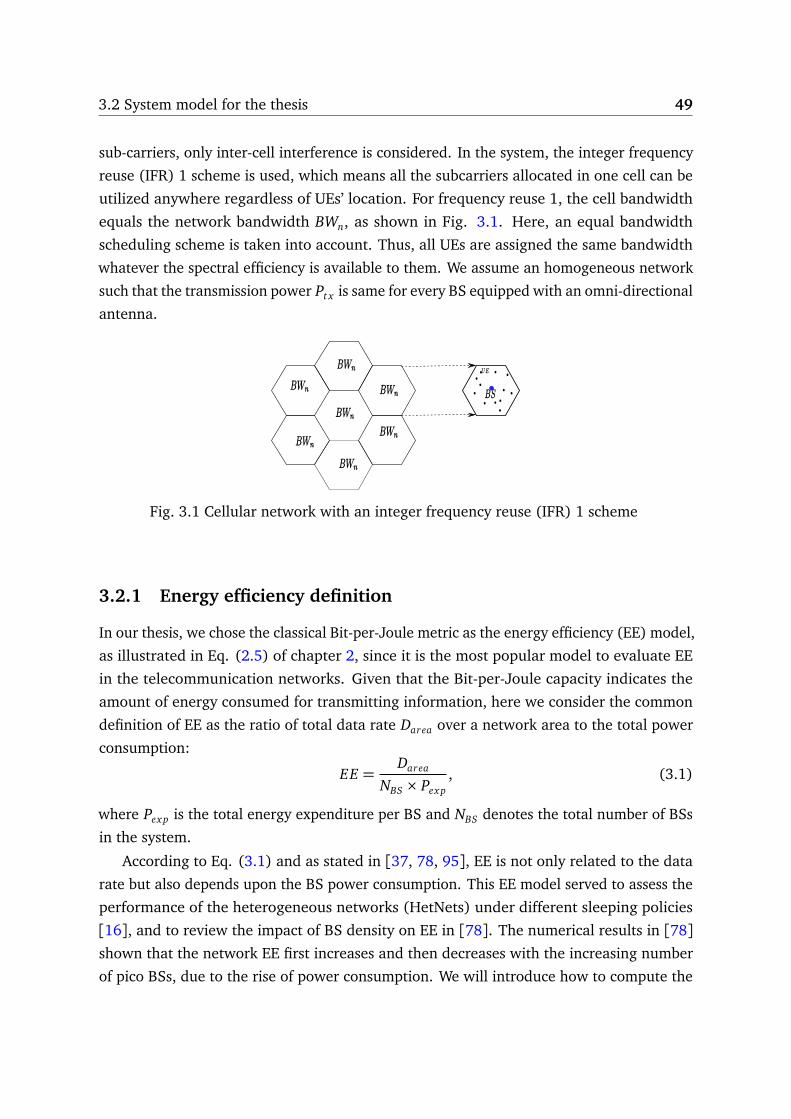
3.2 System model for the thesis 49
sub-carriers, only inter-cell interference is considered. In the system, the integer frequency
reuse (IFR) 1 scheme is used, which means all the subcarriers allocated in one cell can be
utilized anywhere regardless of UEs’ location. For frequency reuse 1, the cell bandwidth
equals the network bandwidth BWn, as shown in Fig. 3.1. Here, an equal bandwidth
scheduling scheme is taken into account. Thus, all UEs are assigned the same bandwidth
whatever the spectral efficiency is available to them. We assume an homogeneous network
such that the transmission power Pt x is same for every BS equipped with an omni-directional
antenna.
Fig. 3.1 Cellular network with an integer frequency reuse (IFR) 1 scheme
3.2.1 Energy efficiency definition
In our thesis, we chose the classical Bit-per-Joule metric as the energy efficiency (EE) model,
as illustrated in Eq. (2.5) of chapter 2, since it is the most popular model to evaluate EE
in the telecommunication networks. Given that the Bit-per-Joule capacity indicates the
amount of energy consumed for transmitting information, here we consider the common
definition of EE as the ratio of total data rate Darea over a network area to the total power
consumption:
EE =Darea
NBS × Pex p, (3.1)
where Pex p is the total energy expenditure per BS and NBS denotes the total number of BSs
in the system.
According to Eq. (3.1) and as stated in [37, 78, 95], EE is not only related to the data
rate but also depends upon the BS power consumption. This EE model served to assess the
performance of the heterogeneous networks (HetNets) under different sleeping policies
[16], and to review the impact of BS density on EE in [78]. The numerical results in [78]shown that the network EE first increases and then decreases with the increasing number
of pico BSs, due to the rise of power consumption. We will introduce how to compute the

50 System model
power consumption Pex p per BS and the total data rate Darea based on the fluid modeling
in the below part.
3.2.2 Power consumption model
Here, we consider a realistic double linear power consumption model (PCM) [68], as
defined in Eq. (2.13) (already been introduced in the second chapter). Since, this PCM
covers the most of the energy consumption in the system, such as the power cost by the
transmitting antenna, the baseband processing, the cooling system, the battery backup, the
power supply and the direct current (DC)-DC and analog current (AC)-DC converters.
The double linear PCM is defined as
Pex p = Nant(∆P Pt x + P0) + P1, (3.2)
where Nant is the number of transmitting antennas per BS, Pt x is the transmitting power
per power amplifier (PA), P1 is the fixed part accounting for the direct current (DC) and
alternating current (AC) converters. ∆P and P0 denote some circuit power consumption
which includes the signal processing overhead LSP , cooling loss LC and battery backup and
power supply loss LPSBB, respectively, characterized by ∆P = (1+ LC)(1+ LPSBB)/µPA and
P0 = LSP(1+ LC)(1+ LPSBB), µPA being the power amplifier (PA) efficiency.
This model shows that the BS power consumption increases with the number of antennas,
Nant , and the transmitting power, Pt x . However, the power consumption of components like
DC-DC/AC-DC converters and cooling unit will not grow linearly with Nant . The numerical
values of Pt x , ∆P , P0, P1 for different types of BSs, like macro, micro and femto BSs, are
given in Table 3.1 as in [68].
Table 3.1 Values of double linear PCM [68]
Parameters Pt x(W ) ∆P P0 P1
macro BSs 80 7.25 244 255
micro BSs 6.31 3.14 35 34
pico or femto BSs 0.25 4.4 6.1 2.6
3.2.3 Data rate (Darea) over a network area
We focus on evaluating the data rate Darea of the network area with radius Ra. For example,
when 0 < Ra ≤ Re, the area of interest is a small part of the central cell, as shown in Fig.
3.2. According to Shannon’s formula, we can compute the achievable data rate of one UE

3.3 Overview of fluid modeling 51
Fig. 3.2 Network area of radius Ra (0< Ra ≤ Re).
and the total data rate Darea over the network area of interest. Since the EE is computed
based on the Darea and Pex p, the detailed information on the computation of the data rate
Darea will be presented in the next chapter.
Based on the aforementioned EE model, power consumption model and data rate
expression, we can evaluate the network EE. Since the data rate is related to the SINR
expression, the basic thing is to explain how to compute SINR based on the fluid modeling.
In the following subsection, we shortly recall the fluid network modeling and present the
SINR expression and interference factor expression using the spatial fluid modeling.
3.3 Overview of fluid modeling
In an OFDMA network, radio resources of a BS are divided into many parallel and orthogonal
subcarriers and inner-cell interferences are neglected. The spatial fluid modeling is to
approximate a hexagonal network of several rings around a central cell. Here, only downlink
communications are considered and the shadowing effects are neglected. The network is
homogeneous and all base stations (BSs) have the same transmitting power.
3.3.1 Notations
The sketch of the hexagonal network is given in Fig. 3.3. The network is homogeneous.
Every hexagon has the same cell radii R. Rc and Rnw denote the half distance between two
adjacent BSs and the network range, respectively. Re is defined as the equivalent radius of
a circle whose area is identical to the hexagonal cell, i,e., Re = aRc where a =Æ
2p
3/π.
The network environment consists of NBS BSs and Nu UEs per cell. Assuming a uniform
distribution for the BSs and the UEs, the density of BSs is ρBS = 1/(2p
3R2c) and the density
of UEs is ρu = Nu/(2p
3R2c).

52 System model
Fig. 3.3 Network model in hexagonal case and main parameters
In the following, we introduce the computation of signal-to-noise-plus-interference ratio
(SINR) γu for a UE u in the hexagonal network and in the proposed fluid network modeling,
respectively.
3.3.2 SINR in the hexagonal network
Regarding the propagation model, the useful power pb,u received by UE u from BS b is
written as pb,u = Pt x Kr−ηu , where K is a constant, η (> 2) is the path-loss exponent, ru
denotes the distance between the UE and the serving BS. The total external signal power
(interference) pex t,u received at u equals∑
j ̸=b Pt x Kr−ηu, j , where ru, j is the distance between
u and the BS j. Given the above notations, the SINR γu for a given UE u is given by
γu =Pt x Kr−ηu∑
j ̸=b Pt x Kr−ηu, j + N0
=r−ηu∑
j ̸=b r−ηu, j +σ
(3.3)
where σ = N0/(KPt x) and N0 denotes the received power from additional white Gaussian
noise.
As introduced in [96], the other-cell-interference-factor (OCIF) y f (r,η), for a fixed UE
at distance r, is defined as a ratio between the total external interference power from other
cells and the useful power, displayed as
y f (r,η) =pex t,u
pb,u
=
∑
j ̸=b r−ηu, j
r−ηu
(3.4)

3.3 Overview of fluid modeling 53
3.3.3 SINR in fluid network model
In the spatial fluid model introduced in [96, 98, 99], a network (constituted by a finite
number of BSs) is regarded as an equivalent continuum of transmitters which are uniformly
distributed in the spatial domain. Considering that the distance between interfering BSs
is 2Rc, the set of transmitting power by interfering BSs in the network is also treated as a
continuous field over the entire system.
Fig. 3.4 Network model in fluid case and some parameters
For a given UE located in the central cell, we consider a circular shaped network
around this central cell with radius Rnw, as shown in Fig. 3.4. The interfering area is
the shaded region limited over the rings with radii 2Rc − ru and Rnw − ru, respectively,
centered at the UE’s position. For each elementary surface ds = zdzdθ at a distance zwhich contains ρBSds BSs, the corresponding interference power equals ρBSzdzdθ Pt x Kz−η.The integration over all the interfering area, gives the total amount of external interference
power pex t,u, approximated as in [96], by
pex t,u =
2π∫
0
Rnw−ru∫
2Rc−ru
ρBS Pt x Kz−ηzdzdθ
=2πρBS Pt x Kη− 2
[(2Rc − ru)2−η − (Rnw − ru)
2−η].
(3.5)
Therefore, the SINR γu in the fluid modeling can be expressed as
γu =Pt x Kr−ηu
2πρBS Pt x Kη−2 [(2Rc − ru)2−η − (Rnw − ru)2−η] + N0
. (3.6)

54 System model
As a consequence, the other-cell-interference-factor (OCIF), y f (r,η), for a UE at distance
r, can be approximated as in [96],
y f (r,η) =2πρBS rη
η− 2[(2Rc − r)2−η − (Rnw − r)2−η]. (3.7)
When Rnw is much larger than ru (Rnw≫ ru) and neglecting the thermal noise σ (e.g.,
in urban environments), Eq. (3.6) can be further simplified into
γu =(η− 2)r−ηu
2πρBS(2Rc − ru)2−η. (3.8)
The substitution of ρBS = 1/(2p
3R2c) into Eq. (3.8) and the introduction of the normalized
distance x = ru/Rc, the above equation can be rewritten into
γu(x) =p
3π(η− 2)x−η(2− x)2−η, (3.9)
from which one finds the γu for UE u only depends upon the relative distance to the serving
BS, ru/Rc, and the path-loss exponent, η.
The analytically tractable expression of γu of Eq. (3.8) can be easily used to compute the
data rate over a network area of interest, Darea. In the following section, some numerical
results will be presented to validate the accuracy of the fluid modeling.
3.4 Accuracy of fluid model
In this section, we show some numerical results of the SINR and its cumulative distribu-
tion function (CDF), which are obtained by fluid modeling and Monte Carlo simulations,
respectively. Simulations are carried out on MATLAB. For the simplification purpose, the
noise, the effect of shadowing and fast fading are ignored in all the simulation process.
Therefore, the SINR is equal to the SIR in this section.
3.4.1 Simulation process
For Monte Carlo (MC) simulations, we consider 15 rings of hexagonal cells around a central
hexagon such that Rnw = 31Rc. Nu UEs are generated uniformly in the central hexagon and
we assume that they are attached to the BS located at the center of a hexagon. We sort
all these UEs depending upon the distance to their serving BS, and we average the SINR,
γu, for all UEs at the same distance. The results presented here are obtained by averaging
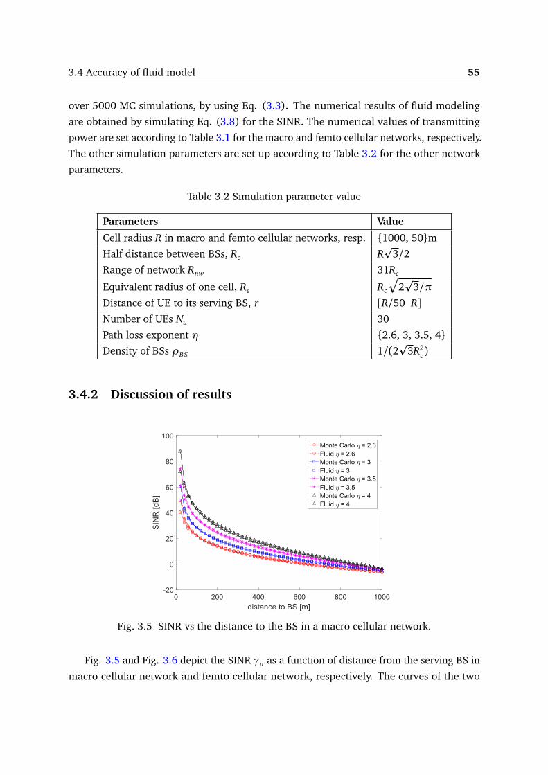
3.4 Accuracy of fluid model 55
over 5000 MC simulations, by using Eq. (3.3). The numerical results of fluid modeling
are obtained by simulating Eq. (3.8) for the SINR. The numerical values of transmitting
power are set according to Table 3.1 for the macro and femto cellular networks, respectively.
The other simulation parameters are set up according to Table 3.2 for the other network
parameters.
Table 3.2 Simulation parameter value
Parameters Value
Cell radius R in macro and femto cellular networks, resp. {1000, 50}mHalf distance between BSs, Rc R
p3/2
Range of network Rnw 31Rc
Equivalent radius of one cell, Re Rc
Æ
2p
3/π
Distance of UE to its serving BS, r [R/50 R]Number of UEs Nu 30
Path loss exponent η {2.6, 3, 3.5, 4}Density of BSs ρBS 1/(2
p3R2
c)
3.4.2 Discussion of results
Fig. 3.5 SINR vs the distance to the BS in a macro cellular network.
Fig. 3.5 and Fig. 3.6 depict the SINR γu as a function of distance from the serving BS in
macro cellular network and femto cellular network, respectively. The curves of the two

56 System model
figures prove the accuracy of the fluid modeling towards the hexagonal lattice one. We
also notice that there is a slight difference between fluid and hexagonal models, mainly for
the UEs located closer to the serving BS. The difference is related to the circular shaped
form considered in fluid model. Indeed, whatever the position of UEs in the inner circle,
the average of the external power of all neighboring BSs is the same. However, in the
hexagonal model, this assumption is no longer true, since we consider the real distance
from neighboring BSs.
Fig. 3.6 SINR vs the distance to the BS in a femto cellular network.
Furthermore, for the accuracy purpose, we compare the numerical results in Fig. 3.5
with the ones developed in [100] while considering the same system parameters values
for a macro cellular network. We observe that for a given distance, the numerical values
of SINR obtained by fluid modeling in Fig. 3.5 and the ones in [100] are the same with
the identical path-loss exponent η, which illustrates the accuracy of our code. However,
focusing on the results obtained by Monte Carlo simulations in Fig. 3.5 and in [100],we also observe that there is a little difference in a short area around the BS, due to the
randomness of the locations of UEs.
Moreover, we observe that the SINR of UEs, near the serving BS, is larger than the
ones located at the edge. For example, for η= 3.5 in Fig. 3.5, the SINR reaches 50.3dB
at 40m from the serving BS, and about -3.1dB at 960m further. We also observe that
values of the SINR for UEs, which is far from their serving BS, are same obtained by fluid
and Monte Carlo simulation. Since for the UEs located at the cell edge, the principal

3.4 Accuracy of fluid model 57
received power is the interference power coming from other external BSs. The SINR, γu,
decreases exponentially with the distance whatever the path-loss exponent values, η, and
it is proportional to the path-loss exponent value, i.e., γu is higher for a larger path-loss
exponent η = 4. We conclude that the values of SINR are larger in suburban area (η in
{3.5, 4}) than the ones in the urban area (η in {2.6, 3}). Additionally, we can also observe
the same conclusion in the femto cellular network, as shown in Fig. 3.6.
3.4.3 CDF results
Fig. 3.7 CDF of SIR values in a macro cellular network
Fig. 3.8 CDF of SIR values in a femto cellular network

58 System model
For further verification of the accuracy of the spatial fluid modeling, we also investigate
the cumulative distribution function (CDF) of SINR. Fig. 3.7 and Fig. 3.8 describe the CDF
along with various SINR threshold for η= 2.5 in the macro and femto cellular networks,
respectively. The numerical values in both two figures show that the analytical results match
well with Monte Carlo ones, which reveals the accuracy of the fluid modeling, despite the
small difference. For example, the error is about 0.05 in the range [−5 15] dB. In addition,
we observe that the mean value of SIR is about 0dB (1bps) in both two figures. In other
words, due to the uniform distribution of UEs, the SIR of half of the UEs are greater than
0dB (1bps).
3.4.4 SIR vs network range
For illustrating the impact of network range on SIR, we investigate the SIR of fixed UEs
varies with the number of network rings. Fig. 3.9 and Fig. 3.10 depict the SIR variation
depending on the number of network rings in two types of cellular networks, macro and
femto, respectively, for η = 3. The distances, ru, of UE are set as {300m, 500m, 800m} and
{20m, 25m, 40m} in macro and femto celluar networks, respectively. The numerical results
of SIR are obtained based on Eq. (3.6) with considering network range, Rnw, and Eq. (3.8)
with neglecting Rnw. Focusing on Fig. 3.9, we observe that the numerical values of SIR are
almost the identical when the number of network rings is larger than 15, whatever the
values of ru. In other words, when the network range Rnw ≥ 31Rc, we can use the simplified
Eq. (3.8) to compute data rate and EE in a fluid modeling. Thus, we set the network range
is 31Rc in the simulation section. The same conclusion can be found in the femto cellular
networks.
0 2 4 6 8 10 12 14 16 18Numer of network rings
0
1
2
3
4
5
6
7
SIR
(dB)
of fix
ed U
E
ru=0.3Km no Rnw,
ru=0.5Km no Rnw,
ru=0.8Km no Rnw ,
with Rnw
with Rnw
with Rnw
Fig. 3.9 SIR vs the number of network rings in a macro cellular network

3.5 Conclusion 59
0 2 4 6 8 10 12 14 16 18Numer of network rings
0
1
2
3
4
5
SIR
(dB)
of fixe
d U
E
ru=20m no Rnw
,
ru=25m no Rnw
,
ru=40m no Rnw
,
with Rnw
with Rnw
with Rnw
Fig. 3.10 SIR vs the number of network rings in a femto cellular network
3.5 Conclusion
In this chapter, we developed a tractable analytical expression of EE-evaluation based on
this fluid framework, which will be used in the following chapters. First, we presented the
system model for evaluating network energy efficiency, including the expression of EE and
power consumption model. Then, we presented the expression of SIR in fluid modeling,
which is tractable. Furthermore, we discussed the simulation results of SIR and CDF of SIR.
The observations point out that the analytical results obtained by fluid model are similar
to the ones established by Monte Carlo simulations, which shown the accuracy of fluid
modeling.
In the next chapter, we will present the computation of data rate based on this system
model in detail and the work using this system model to evaluate EE for the large cellular
networks so as to investigate the impact of shadowing on EE.

Chapter 4
Fluid modeling of EE and effect of
shadowing on EE
Contents
4.1 Introduction . . . . . . . . . . . . . . . . . . . . . . . . . . . . . . . . . . . . . . . 62
4.2 Energy efficiency definition . . . . . . . . . . . . . . . . . . . . . . . . . . . . . . 63
4.3 Data rate computation . . . . . . . . . . . . . . . . . . . . . . . . . . . . . . . . . 64
4.3.1 Data rate within the central hexagon . . . . . . . . . . . . . . . . . . . 65
4.3.2 Data rate over a first ring . . . . . . . . . . . . . . . . . . . . . . . . . . . 65
4.3.3 Data rate over a large network . . . . . . . . . . . . . . . . . . . . . . . 66
4.4 Data rate with shadowing consideration . . . . . . . . . . . . . . . . . . . . . . 70
4.4.1 Signal quality . . . . . . . . . . . . . . . . . . . . . . . . . . . . . . . . . . 71
4.4.2 Data rate . . . . . . . . . . . . . . . . . . . . . . . . . . . . . . . . . . . . . 72
4.4.3 Coverage probability . . . . . . . . . . . . . . . . . . . . . . . . . . . . . 73
4.5 Model evaluation: non-shadowing case . . . . . . . . . . . . . . . . . . . . . . 74
4.5.1 Simulation setup . . . . . . . . . . . . . . . . . . . . . . . . . . . . . . . . 74
4.5.2 Model accuracy . . . . . . . . . . . . . . . . . . . . . . . . . . . . . . . . . 75
4.5.3 EE variation vs cell network types . . . . . . . . . . . . . . . . . . . . . 76
4.5.4 Impacts of user’s density on EE . . . . . . . . . . . . . . . . . . . . . . . 78
4.5.5 EE vs path-loss exponent . . . . . . . . . . . . . . . . . . . . . . . . . . . 78
4.5.6 EE variation over a first ring . . . . . . . . . . . . . . . . . . . . . . . . . 79
4.5.7 EE variation over a large network . . . . . . . . . . . . . . . . . . . . . 80
4.6 Model evaluation: shadowing case . . . . . . . . . . . . . . . . . . . . . . . . . 82
4.6.1 Simulation setup . . . . . . . . . . . . . . . . . . . . . . . . . . . . . . . . 83
4.6.2 Relationship between Γth and r . . . . . . . . . . . . . . . . . . . . . . . 84

62 Fluid modeling of EE and effect of shadowing on EE
4.6.3 Energy efficiency discussion . . . . . . . . . . . . . . . . . . . . . . . . . 86
4.6.4 EE model accuracy . . . . . . . . . . . . . . . . . . . . . . . . . . . . . . . 88
4.7 Conclusion . . . . . . . . . . . . . . . . . . . . . . . . . . . . . . . . . . . . . . . . 89
4.1 Introduction
To support the requirement of x1000 traffic increase in 5G networks, the EE has to be
improved dramatically x1000 at least in the next 5 years time-frame [10, 101]. However,
the goal is not easy to achieve considering so many factors, such as the environmental, eco-
nomical and operational concerns [102]. In particular, from the operators perspective, EE is
urgent to be considered for designing the cellular networks due to that a high EE reduces the
commercial expenditure of operators. In addition, several EU-funded research projects have
been carried out to develop more energy-efficient wireless communications, e.g., Energy
Aware Radio and neTwork tecHnologies (EARTH) [103], Towards Real Energy-efficient
Network Design (TREND) [104] and Mobile and wireless communications Enablers for
Twenty-twenty (2020) Information Society (METIS) [105]. On the other hand, several col-
laborative initiatives, such as the GreenTouch consortium [106], and the 5G Infrastructure
Public Private Partnership (5G PPP) [107], have also focused on analyzing the energy-
efficient wireless networks through utilizing some promising techniques. In these work, the
proposed solutions are achieved using system-level simulations, or stochastic geometry to
describe network model (mainly the nodes locations and the propagation models) and to
derive consequently the EE performance model. Nevertheless, since today’s networks are
more and more dense due to the increase number of BSs, simulation-based approaches have
become a hard task and resource-intensive. Moreover, stochastic geometry-based studies
assume in most cases a Poisson point process to describe the nodes locations which allows
to derive a closed-form formula of the energy metric. However, when non-Poisson point
processes are considered, eg., perturbed lattice, β -Ginibre point process, and Matérn point
process, the performance models are not analytically tractable due to the non-independent
nature of points [108]. Therefore, representative, tractable and accurate models are needed
to evaluate the EE performance of the cellular networks in the energy consumption process,
which motivates this work.
In addition, shadowing is used to model random variations of the received power
signals on the path loss due to the encountered obstacles like buildings, trees, terrain
conditions [109, 110], during the transmission of signal in wireless channel. In detail, the
obstacles make the signal change at random, resulting a random variation of the received

4.2 Energy efficiency definition 63
signal power for the UEs, with the same distance to the transmitter whereas in different
locations. Commonly, shadow fading is modeled using the log-normal distribution in the
radio propagation process, thus it is also called as lognormal fading. Some research efforts
are made to illustrate the impact of shadowing fading. The authors in [111] derived some
closed-form expressions for the interference factor’s mean and standard deviation, as well
as the outage probability while taking into account the impact of the path-loss exponent and
the shadowing. The authors in [112] show that shadowing increases outage probability in
cellular radio networks. Additionally, the work of [113] shows that the coverage probability
is severely reduced by shadowing in a Poisson small cell network. The above work illustrates
that the effect of shadowing is significant and should not be neglected while characterizing
the performance of cellular networks, i.e., coverage probability and outage probability.
Nevertheless, the influence of shadowing on the EE is still an open issue while the fluid
modeling is utilized.
Hence, our objective in this chapter is to develop a tractable EE model for cellular
networks based on the spatial fluid modeling without considering the shadowing effect,
and to investigate the impact of shadowing on EE. We first present a tractable and effective
EE model for an OFDMA cellular network based on the spatial fluid modeling, which
reduces the analysis complexity. Then, we present how to compute the data rate while the
impact of shadowing is neglected. Furthermore, we develop a closed-form expression of
the signal-quality threshold using the Polynomial Curve Fitting (PCF) approach so as to
compute the data rate with taking into account the shadowing effect. Finally, we discuss
the simulation performance to prove the effectiveness and accuracy of the proposed model
through a comparison between fluid modeling and Monte Carlo simulations.
4.2 Energy efficiency definition
We consider the common definition of EE as the ratio of total data rate Darea in a network
area over the total power consumption, i.e., EE = DareaNBS×Pex p
, as defined in Eq. (3.1). Metric
EE is measured in terms of bits/Joule, which is the maximum amount of bits that can be
reliably delivered by the system per Joule of energy. NBS denotes the overall number of
BSs in the system, and Pex p accounts for the total energy expenditure per BS. Pex p can be
calculated according to the Eq. (3.2).
Since the definition of EE is not only related to the data rate, but also related to the
power consumption of the system, we present how to compute the total data rate Darea
without/with considering the effect of shadowing during the transmission of signal in the
radio system.

64 Fluid modeling of EE and effect of shadowing on EE
4.3 Data rate computation
In a cellular system, both the signal and interference strength decay super-linearly with
distance [114]. Therefore, the distance between the BS and mobile users is a key element to
quantify the fundamental network performance metrics and to estimate the system capacity
and the energy efficiency, which are critical indicators for the network deployment. Much
work on EE and data rates has been investigated focusing on the central cell. However, in a
practical scenario, the statistical distance of UEs to the origin is changing due to UEs’s life
activity, either inside or outside the central cell, or any point of the system network. As a
result, the data rate and energy consumption exist outside the central cell. Therefore, it is
an interesting issue to investigate the data rate over a disc region, not only limited to the
central cell.
The objective is to compute the total data rate, Darea, over a disc region with radius of
Ra. Let the center of a central hexagon be the origin. The radius of Ra is also called the
statistical distance. Based on the different size of Ra, in this chapter, we consider three
scenarios, i.e., 0< Ra ≤ Re, Re < Ra ≤ 2Rc and 0< Ra ≤ Rnw. Re is the radius of a disk with
a surface equivalent to the central hexagonal cell, such that Re = aRc =Æ
2p
3/πRc with
a =Æ
2p
3/π. Rc is the half distance between two BSs and Rnw is the network range.
According to the Shannon’s formula, the spectral efficiency (SE), measured by bps/Hz,
for a UE u is a function of signal quality γu as
SEu(r) = log2(1+ γu(r)). (4.1)
The maximum of achievable data rate Du(r) for user u at distance r is the multiplication of
the user’s bandwidth Bu and SEu, i.e.,
Du(r) = Bu × SEu(r). (4.2)
Since the user’s density ρu is invariant, users are assigned with the same bandwidth, and
the total data rate Darea over the area is closely related to the SINR γu(r) of users, Darea
can be written as the integration of Du over the interested area. Mention that γu(r) has
been given as γu =(η−2)r−ηu
2πρBS(2Rc−ru)2−η, as defined in Eq. (3.8).
Therefore, in the following subsection we focus on evaluating the data rate Darea of
interested area in different scenarios through Eqs. (3.8), (4.1) and (4.2).

4.3 Data rate computation 65
Fig. 4.1 Scenario 1: network area with radius Ra (0< Ra ≤ Re)
4.3.1 Data rate within the central hexagon
Fig. 4.1 depicts the scenario when the interested area is one part of the central cell, i.e.
(0 < Ra ≤ Re). Since the UEs are uniformly distributed in every cell, the density ρu
is a constant. Therefore, the number of users N ′u over the area of interest is given as
N ′u = (NuR2a)/(a
2R2c), where Nu is the number of users per cell.
Considering an equal bandwidth sharing among UEs, Bu = BWn/Nu where BWn is the
total bandwidth. Based on Eqs. (3.8), (4.1) and (4.2), replacing ρu = Nu/(2p
3R2c), the
total data rate Darea can be written as
Darea =
∫ 2π
0
∫ Ra
0
Buρulog2(1+ γu(r))rdrdθ
=BWnπp
3R2c
∫ Ra
0
r log2(1+ γu(r))dr.
(4.3)
A worthwhile observation is that the Eq. (4.3) neither depends on the number of UEs
deployed per cell nor upon the value of ρu. When Ra = Re, the above equation is evolved
to compute the total cell data rate, Dcel l , as in [100].
4.3.2 Data rate over a first ring
Actually, when a user moves from one cell to its adjacent cell, the BS located at the adjacent
cell becomes its new serving BS for the user. In this case, the SINR and data rate for the
user maybe change due to changes in relative distance between the user and its new serving
BS. Thus, to investigate the data rate over a first ring is also an interesting issue.
Beyond the central cell, we explain here how to compute the total data rate. Assume a
user m, located outside the central cell at distances r, rm from the central cell BS O0 and
its serving BS B, respectively, as shown in Fig. 4.2. According to the law of cosines, the
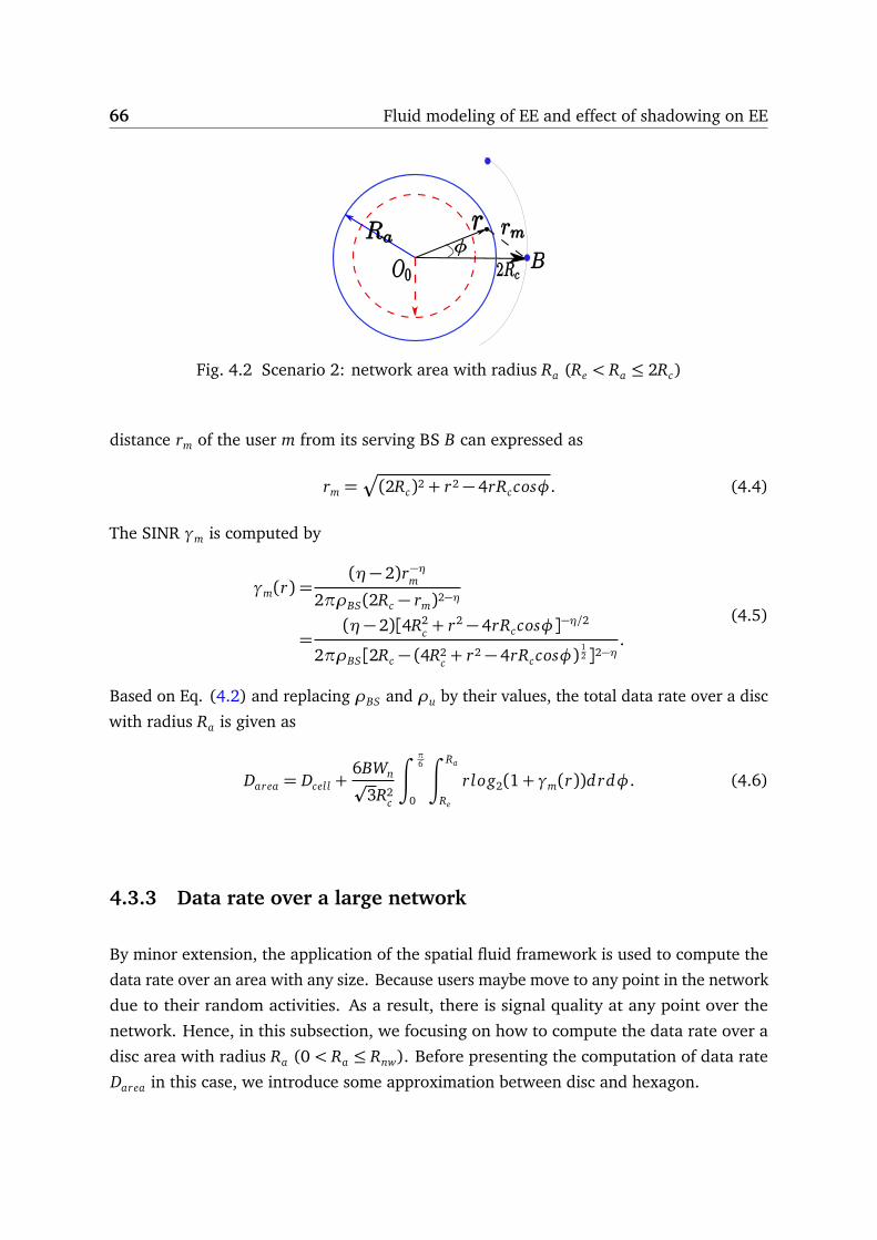
66 Fluid modeling of EE and effect of shadowing on EE
Fig. 4.2 Scenario 2: network area with radius Ra (Re < Ra ≤ 2Rc)
distance rm of the user m from its serving BS B can expressed as
rm =Æ
(2Rc)2 + r2 − 4rRccosφ. (4.4)
The SINR γm is computed by
γm(r) =(η− 2)r−ηm
2πρBS(2Rc − rm)2−η
=(η− 2)[4R2
c + r2 − 4rRccosφ]−η/2
2πρBS[2Rc − (4R2c + r2 − 4rRccosφ)
12 ]2−η
.(4.5)
Based on Eq. (4.2) and replacing ρBS and ρu by their values, the total data rate over a disc
with radius Ra is given as
Darea = Dcel l +6BWnp
3R2c
∫π6
0
∫ Ra
Re
r log2(1+ γm(r))drdφ. (4.6)
4.3.3 Data rate over a large network
By minor extension, the application of the spatial fluid framework is used to compute the
data rate over an area with any size. Because users maybe move to any point in the network
due to their random activities. As a result, there is signal quality at any point over the
network. Hence, in this subsection, we focusing on how to compute the data rate over a
disc area with radius Ra (0< Ra ≤ Rnw). Before presenting the computation of data rate
Darea in this case, we introduce some approximation between disc and hexagon.

4.3 Data rate computation 67
Approximation between disc and hexagon
Setting the origin of the global coordinate system at the central BS, as shown in Fig. 4.3,
the disc region with radius of Ra is of interest and denoted by Sdisc. The objective here is to
compute total data rate Darea over Sdisc based on Eq. (3.8).
Fig. 4.3 Scenario 3: network area with radius Ra (0< Ra ≤ Rnw)
For simplicity, some literatures took into account the hexagonal cell as a circular cell
with equal area to investigate the network performances, such as other-cell interference
[115] and the received power at a BS [116]. These work shown that the circular cell and
the hexagonal cell can be transformed into each other where the locations of all UEs are
the same. Hence, in this subsection we made the following approximations.
(1) The interested circular region Sdisc has the same area as the equivalent hexagon Shex ,
such as Sdisc = Shex .
(2) The date rate over a circular region is equal to the data rate over an equivalent
hexagonal region. Because UEs’ position remains unchanged whatever in the disc
region or in the equivalent hexagonal area.
(3) Using the symmetric property of a hexagon, the hexagon can be divided into 12 small
triangles.
Based on the above approximation, the total data rate Darea over an interested disc region
Sdisc is equal to the total data rate over an equivalent hexagon area Shex . As a result,
Darea =
∫∫
Sdisc
ρuBulog2(1+ γu(r))ds
=
∫∫
Shex
ρuBulog2(1+ γu(r))ds
=12× Dt r ihex ,
(4.7)

68 Fluid modeling of EE and effect of shadowing on EE
where Dt r ihex is the data rate of the shaded triangular region, as shown in Fig. 4.3. Therefore,
we present how to compute the total data rate of the shaded triangular region, Dt r ihex , in the
following part.
The notations used in this subsection are summarized in Table 4.1.
Table 4.1 Common parameters in a large network
Parameter DescriptionSdisc surface area of a disc region with radius Ra
Darea data rate over Sdisc
Shex surface area of an equivalent hexagonDt r i
hex data rate over an area, i.e., twelfth of Shex
Dcel l data rate per hexagonal cell△O0S2S1
surface area of a triangleD△ data rate over the triangle area, △O0S2S1
(D△ =3Dcel l
4 )□S1S2S3S4
surface area of a squareD□ data rate over the square area □S1S2S3S4
(D□ = Dcel l)Dre data rate over the remaining areant the number of D△k the number of D□
Computation of data rate Dt r ihex
According to the approximation of the disc area by a hexagon, the network area is enclosed
by two axes, for example, the x-axis represents the value of Ra/a, as shown in Fig. 4.4. Dt r ihex
is decomposed as repeated blocks of the highlighted triangles, rectangle with vertices S1,
S2, S3, S4, and some remaining part. Two examples are given in the following to explain
the law of geometric decomposition.
Fig. 4.4 Homogeneous network with a various radius Ra/a

4.3 Data rate computation 69
The first example shows the case when 3Rc < Ra/a < 5Rc, so that Dt r ihex is the data rate
over the triangle with vertices O0, A1 and B1. The corresponding decomposition scheme is
sketched by Fig. 4.5(a). Hence, the data rate Dt r ihex is a summation of D△ (data rate over
a triangle) and data rate over the remaining part which is a trapezoid with vertices S1,
S2, A1 and B1. For the evaluation of data rate, D△, with the knowledge that the data rate
is only related to the distances from the serving BS and UEs, it is not difficult to derive
that D△ = 3Dcel l/4. The computation of the data rate over the remaining part is given in
Appendix A.
(a) example 1
(b) example 2
Fig. 4.5 Two examples for the decomposition of the network area.
The second example illustrates the case when 6Rc < Ra/a < 7Rc. Dt r ihex is the data rate
over the surface area with vertices O0, A2 and B2, as shown in Fig. 4.5(b). Let D□, Dcel l
denote the data rate over the square area □S1S2S3S4and data rate over a hexagonal cell,
respectively. Following similar analysis as the first example and based on the geometry
property of a hexagon, Dt r ihex is decomposed as two D△, one D□, and the data rate over the
remaining part, where D□ = Dcel l . Appendix A presents the approach to compute the data
rate over the remaining region, as for the first example.
As seen from the above two examples, the data rate with any value of Ra/a is a
summation of multiple D△, D□, and the data rate over the remaining part, i.e.,
Dt r ihex = nt D△ + kD□ + Dre, (4.8)
where nt , k are non-negative integers and denote the number of repeated parts of D△and D□, respectively. Dre denotes the data rate over the remaining area. With any given

70 Fluid modeling of EE and effect of shadowing on EE
value of Ra/a, the computation of the data rate for the remaining part, i.e., Dre, follows the
approach described in Appendix A. We here present how to compute nt and k.
Taking advantage of the symmetry pattern of a hexagon, we observe that the number of
△O0S2S1appears with a period 3Rc and that the number of □S1S2S3S4
appears with a period
2Rc along the Ra/a axis. Hence, the number of D△, nt , can be defined as
nt =�
Ra
a, 3Rc
�
, (4.9)
where [·, ·] is the quotient operator. Additionally, we observe that D□ appears at the right
(towards to positive direction of the axis of Ra/a) and □S1S2S3S4depends on Ra/a and nt .
Hence, the number of D□, k, is given by
k =nt∑
n=1
max
�
0,�
Ra
a− 3nRc, 2Rc
�
�
. (4.10)
Eqs. (4.9) and (4.10) are obtained based on the geometric characteristic of a hexagon.
A detailed example is given to better understand the above two equations. Assuming
6Rc < Ra/a < 7Rc as in example 2 and according to Eq. (4.9), nt is calculated, i.e., nt = 2,
which illustrates that there are two D△. With nt = 2 and following Eq. (4.10), the value
of k is a summation, which yields to the value of 1, i.e., k = 1. That shows that there is
one D□. In one word, according to Eqs. (4.9) and (4.10), we obtain nt = 2 and k = 1 for
6Rc < Ra/a < 7Rc, which is in accordance with the truth, as shown in Fig. 4.5(b). That
illustrates the accuracy of Eqs. (4.9) and (4.10).
Therefore, for a given value of Ra, using Eqs. (4.9), (4.10) and the computed Dre in
Appendix A, Dt r ihex over a triangle area can be easily computed. Then replacing Dt r i
hex in Eq.
(4.7), we can obtain the data rate Darea over a disc region with radius of Ra.
As a result, we can easily compute the EE metric in Eq. (3.1) by replacing Pex p with Eq.
(3.2), replacing Darea with Eq. (4.3) or Eq. (4.6) or Eq. (4.7).
4.4 Data rate with shadowing consideration
In this section, we recall first the SINR expression of a user equipment u located at a
distance r from its serving BS b, taking the path-loss exponent and the shadowing impact
into account. Then, to calculate the data rate over a network area Darea, we rely on the
proposed fluid model to present a formula of the coverage probability. Especially, in the case
of a fixed coverage probability, we further drive a closed-form expression between SINR

4.4 Data rate with shadowing consideration 71
threshold Γ th(r) and UE’s distance r through a polynomial curve fitting method, which is
compared with the fluid modeling.
4.4.1 Signal quality
Regarding the propagation model, the received power pb at the UE u, located at a distance
r from its serving BS, b, can be written as,
pb = Pt x Kr−ηAb, (4.11)
where Ab = 10ξb10 denotes the shadowing effect. The lognormal random variable Ab charac-
terizes the random variations of the received power around a mean value. ξb stands for
a normal distributed random variable (RV), with zero mean and standard deviation, σ,
which is between 0 and 8 dB. Pt x Kr−η represents the mean value of received power from
BS b, at UE u, where K is a constant and η(> 2) is the path-loss exponent. The interference
received power, pex t , at u from the external BSs is:
pex t =∑
j ̸=b
Pt x Kr−ηj A j. (4.12)
Given the above notations, the SINR γu of a given UE u is
γu =Pt x Kr−ηb Ab∑
j ̸=b Pt x Kr−ηj A j + N0
, (4.13)
where N0 is the Gaussian noise. Neglecting the noise power because of the urban area and
considering same transmission power of BSs, Pt x , the SINR can be rewritten as
γu =r−ηAb∑
j ̸=b r−ηj A j
. (4.14)
Let γu = 1/A f with
A f =
∑
j ̸=b r−ηj A j
r−ηAb, (4.15)
where A f can be approximated by a lognormal RV with mean value, m f , and standard
deviation, s f [117–119]. According to the definition of [119], the terms m f and s f can be

72 Fluid modeling of EE and effect of shadowing on EE
calculated as
m f =1a
ln[y f (r,η)H(r,σ)]
s2f =2[σ2 −
1a2
ln(H(r,σ))]
y f (r,η) =
∑
j ̸=b r−ηj
r−η
H(r,σ) =ea2σ2/2[G(r,η)(ea2σ2−1) + 1]1/2
G(r,η) =
∑
j ̸=b r−2ηj
(∑
j ̸=b r−ηj )2
a =ln1010
(4.16)
where m f is measured in dB. The term y f (r,η), considered as the interference factor
since it stands for the A f factor without shadowing. Specially, in the fluid modeling, the
interference factor, y f (r,η), for a fixed UE at distance r can be computed by y f (r,η) =2πρBS rη
η−2 [(2Rc − r)2−η − (Rnw − r)2−η], as displayed in Eq. (3.7). The factor G(r,η) can also
be rewritten as
G(r,η) =y f (r, 2η)
[y f (r,η)]2. (4.17)
4.4.2 Data rate
The data rate over a network area, as shown in Fig. 4.1, is computed while taking the
impact of shadowing into account.
As shown in [16, 19], the spectral efficiency of a given UE can be measured while con-
sidering the coverage probability. According to Shannon’s formula, the average achievable
throughput, for a UE u at the distance r, is given as
Du(r) = BuPrcov log2(1+ Γ t h(r)), (4.18)
where Prcov = P(γu > Γ t h(r)) is the coverage probability [120], and Bu is the UE’s bandwidth.
Hence, the total data rate Darea over a network area of radius Ra, can be computed as
Darea =
∫ 2π
0
∫ Ra
0
BuρuPrcov log2(1+ Γ t h(r))rdrdθ , (4.19)
where ρu is the UE’s density.

4.4 Data rate with shadowing consideration 73
Therefore, to compute the data rate, Darea, we first define the coverage probability based
on the other-cell-interference-factor (OCIF), y f (r,η) =2πρBS rη
η−2 [(2Rc − r)2−η− (Rnw− r)2−η],as shown in Eq. (3.7), Eqs. (4.14), (4.16) and (4.17). Then, we derive a closed-form
formula of the SINR threshold, Γ t h, in the case of a fixed coverage probability using the
Polynomial Curve Fitting (PCF) method.
4.4.3 Coverage probability
In the propagation channels, often coverage probability is used as a metric to assess the
performance of the communication system [121]. The coverage probability, Prcov, is defined
in [121, 122] as the probability for the signal quality SINR, γu, of a UE u to be larger than
a threshold value Γ t h and can be expressed as,
Prcov = P(γu > Γ t h). (4.20)
Based on Eqs. (4.14), (4.15), (4.16), as in [111, 119], we have,
Prcov =P(γu > Γ t h)
=P(1Γ t h>
1γu)
=P(1Γ t h> A f (m f , s f ))
=P(10log10(1Γ t h)> 10log10(A f ))
=1−Q[10log10(
1Γ t h)−m f
s f],
(4.21)
where Q is the error function, denoted as Q(x) = 12π
∫ +∞x
e−t22 d t. For a given r, we can
compute the corresponding Γ t h according to Eqs. (3.7), (4.16), (4.17) and (4.21) in the
case of a known Prcov and a fixed path-loss exponent η. Furthermore, we can plot the
variation of Γ t h depending on the UE’s distance r based on the fluid framework. Then,
using the Polynomial Curve Fitting (PCF), we can set up an accurate fitting of an analytical
function relying Γ t h to r. Γ t h can be expressed by a third degree polynomial of r, as,
Γ t h(r) = w0 +w1r +w2r2 +w3r3, (4.22)
where the coefficients w0, w1, w2 and w3 can be obtained through the least-square fitting.
For example, w0 = 25.6483, w1 = −1.3220, w2 = 0.0222 and w3 = −0.0002 for η= 2.6

74 Fluid modeling of EE and effect of shadowing on EE
and σ = 3dB. The coverage probability should be high enough to overcome the rapid
degradation of signal quality caused by the obstacles effect. Normally, Prcov should follow
the relationship Prcov ≥ C0, 70% ≤ C0 ≤ 95%, as shown in [123]. Here, we set Pr
cov = 0.9
whatever the distance r for all UEs [111], in order to guarantee the signal quality for all
UEs and to achieve a high coverage probability.
Replacing Γ t h(r) of Eq. (4.22) and ρu = Nu/(2p
3R2c) in Eq. (4.19), the total data rate
Darea is expressed as
Darea =BWnπPr
covp3R2
c
∫ Ra
0
r log2(1+w0 +w1r +w2r2 +w3r3)dr. (4.23)
For simplify purposes, an equal bandwidth sharing among UEs is considered here Bu =BWn/Nu (BWn is the total bandwidth), as well as a constant coverage probability Pr
cov.
To compare with the case of a network without shadowing effect σ = 0, the data rate is
computed by Eq. (4.3) with γu(r) =(η−2)r−ηu
2πρBS[(2Rc−ru)2−η−(Rnw−ru)2−η].
Simulations are performed to assess the performance of the proposed fluid modeling in
two cases: non-shadowing and shadowing impact in the network.
4.5 Model evaluation: non-shadowing case
In this section, the differences of the data rate per cell obtained by fluid modeling and Monte
Carlo simulations are first presented. Then, we estimate the EE of a small area constrained
by 0< Ra ≤ Re and with different kinds of cellular networks. After, the investigation on the
impact of the user density and the path-loss exponent on the cell EE for various cellular
networks is studied. At the end, we evaluate the performance of EE over the first ring
(Re < Ra ≤ 2Rc) and the large cellular networks (0 < Ra ≤ Rnw), in order to validate the
corresponding fluid models.
4.5.1 Simulation setup
Three values of the cell radius are considered as R ∈ {1000, 200, 50}m and stand for the
macro, micro and femto cellular networks, respectively. We consider 15 rings of hexagonal
cells around a central hexagon such that Rnw = 31Rc. Nu users are generated uniformly
in the central hexagon and we assume that they are attached to the BS located at the
center of the hexagon. To indicate the effect of pathloss, Erceg model [124] is utilized with
A= (4πζ f )2/(cζη/2)2, ζ= 100 m, f = 2.5 GHz, η= {2.6, 2.8} and c is the speed of light
in air. Here, thermal noise density = −174 dBm/Hz.

4.5 Model evaluation: non-shadowing case 75
For Monte Carlo (MC) simulations, the results presented here are obtained by averaging
over 3000 MC simulations. The main idea of Monte Carlo trails is as follows. First, we
initial the number of iterations and the number of UEs. Then, we create the location of
all BSs and UEs, and compute the γu for every UE in every iteration. Based on the γu, we
compute the total data rate of all UEs located at a disc region with radius Ra. Next, we
update the iteration and repeat the above process until finishing all the iterations. After
that, we average the total data rate over the number of iterations and obtain the averaged
data rate. We also compute the total power consumption for the networks. Finally, using
the definition of EE in Eq. (3.1), we compute EE with the average data rate and the total
power cost.
The numerical results of fluid modeling are obtained by simulating Darea using Eq.(4.3)
for the first scenario, Eq. (4.6) for the second scenario and Eq. (4.7) for the third scenario,
after replacing them in EE definition, as shown in Eq. (3.1). The other simulation parame-
ters are set up according to Table 3.1 for the power consumption model as defined in [68],and Table 4.2 for the other network parameters.
Table 4.2 Simulation Parameter Value
Parameters ValueSystem bandwidth BWn 10MHzCarrier frequency 2GHzCell radius R {1000, 200, 50}m for macro, micro and femto resp.Half distance between BSs, Rc R
p3/2
Range of network Rnw 31Rc
Radius of interested area Ra [R/20 2Rc]Equivalent radius of one cell, Re Rc
Æ
2p
3/πNumber of antennas Nant 1Number of users Nu {100, 500}Path loss exponent η {2.6, 2.8}Density of BSs ρBS 1/(2
p3R2
c)Density of users ρu Nu/(2
p3R2
c)
4.5.2 Model accuracy
In order to validate the accuracy of our model, we compute the difference of EE obtained
by fluid modeling and Monte Carlo simulations, considering the same Ra, η, BWn, Nu ={100, 500} in a macro cellular network. The difference is plotted in Fig. 4.6 and computed
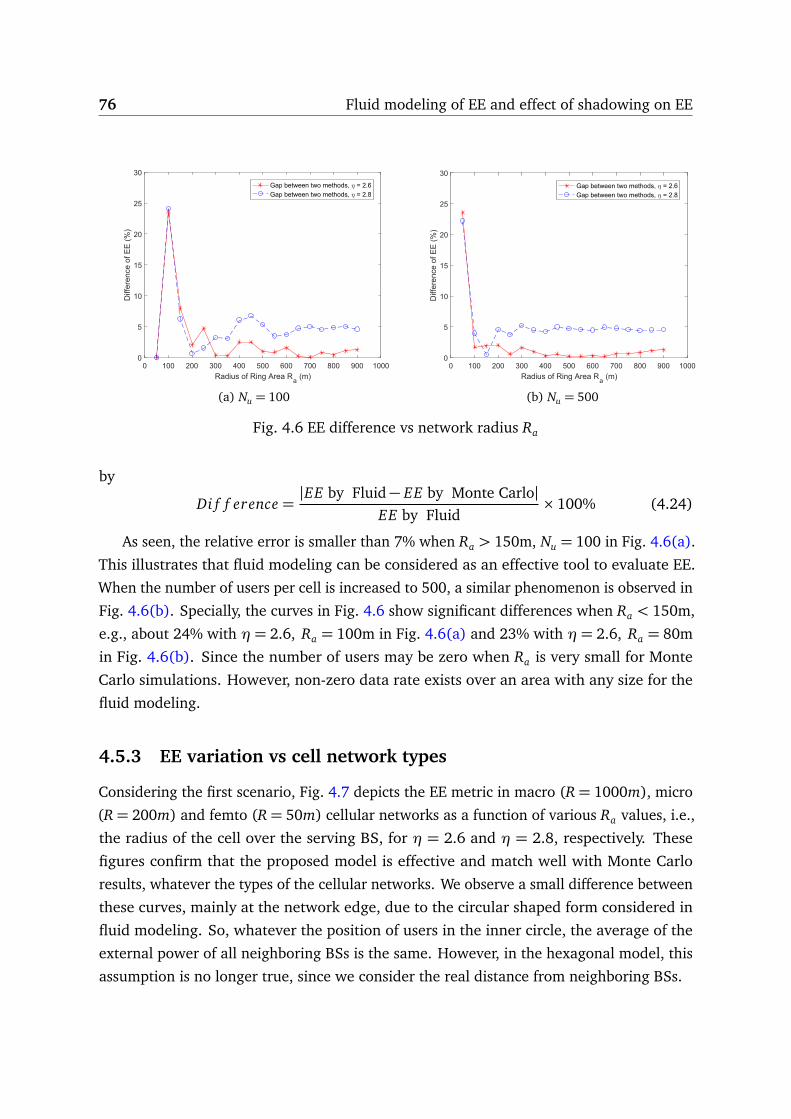
76 Fluid modeling of EE and effect of shadowing on EE
(a) Nu = 100 (b) Nu = 500
Fig. 4.6 EE difference vs network radius Ra
by
Di f f erence =|EE by Fluid− EE by Monte Carlo|
EE by Fluid× 100% (4.24)
As seen, the relative error is smaller than 7% when Ra > 150m, Nu = 100 in Fig. 4.6(a).
This illustrates that fluid modeling can be considered as an effective tool to evaluate EE.
When the number of users per cell is increased to 500, a similar phenomenon is observed in
Fig. 4.6(b). Specially, the curves in Fig. 4.6 show significant differences when Ra < 150m,
e.g., about 24% with η= 2.6, Ra = 100m in Fig. 4.6(a) and 23% with η= 2.6, Ra = 80m
in Fig. 4.6(b). Since the number of users may be zero when Ra is very small for Monte
Carlo simulations. However, non-zero data rate exists over an area with any size for the
fluid modeling.
4.5.3 EE variation vs cell network types
Considering the first scenario, Fig. 4.7 depicts the EE metric in macro (R= 1000m), micro
(R = 200m) and femto (R = 50m) cellular networks as a function of various Ra values, i.e.,
the radius of the cell over the serving BS, for η = 2.6 and η = 2.8, respectively. These
figures confirm that the proposed model is effective and match well with Monte Carlo
results, whatever the types of the cellular networks. We observe a small difference between
these curves, mainly at the network edge, due to the circular shaped form considered in
fluid modeling. So, whatever the position of users in the inner circle, the average of the
external power of all neighboring BSs is the same. However, in the hexagonal model, this
assumption is no longer true, since we consider the real distance from neighboring BSs.

4.5 Model evaluation: non-shadowing case 77
(a) macro-cell, R= 1000m, Nu = 100 (b) micro-cell, R= 200m, Nu = 100
(c) femto-cell, R= 50m, Nu = 100
Fig. 4.7 EE variation vs network radius Ra for different network types.
Moreover, we observe that EE is improved with the increase of Ra. Surprisingly, EE
is less effective closer to the BS, even though the SIR is high. Indeed, the total power
consumption overall the network is much higher than the total data rate of a network with
radius Ra. However, in this case, EE raises fast, due to the ratio between the cell area of
radius Ra and the total network area of radius Rnw. For example, in Fig. 4.7(a), EE raises
quickly for Ra ∈ [0,600] and EE increases slightly for Ra ∈ [600, Re], since the SIR for a
given user far from its serving BS is small in this case.
Furthermore, results show that EE is about 24bi ts/Joule for the macro-cell network in
Fig. 4.7(a) for η = 2.8 and Ra = Re. EE values are, respectively, near 260bi ts/Joule for
a micro-cell network in Fig. 4.7(b), and about 2.5K bits/Joule for a femto-cell network

78 Fluid modeling of EE and effect of shadowing on EE
in Fig. 4.7(c). However, the transmitting power per BS decreases from 80W to 0.25W . It
means that small-cell networks can save a lot of energy during the transmission due to
their lower energy dissipation and attenuation compared to the macro cellular networks.
Therefore, the small-cell network is more efficient than a macro-cell one and a micro-cell
one, which is consistent with findings in [82].
4.5.4 Impacts of user’s density on EE
Fig. 4.8 depicts the EE performance in a macro cellular network as a function of various Ra
values, i.e., the size of the cell over the serving BS, with Nu = 500, η = 2.6 and η = 2.8
respectively. In this case, the numerical values show the accuracy of the fluid modeling for
EE evaluation. While comparing Fig. 4.8 and Fig. 4.7(a) with Nu = 500, we observe that
the numerical values of EE are identical, for example, for Ra = Re and η= 2.6, the energy
efficiency is about EE = 18.16bi ts/Joule, regardless the number of users Nu. Indeed, the
data rate over the network area is not related to ρu and Nu, as defined in Eq. (4.3).
Fig. 4.8 EE variation vs network radius, Ra, with R= 1Km, Nu = 500
4.5.5 EE vs path-loss exponent
While considering the thermal noise N0 = −174dBm/Hz and Nu = 100, Fig. 4.9 shows
the variation of EE over the cell (Ra = Re) depending on different path loss exponents η
in case of macro and femto cellular networks, i.e., R= 1000m and R= 50m, respectively.
The results show that EE increases with the growth of η in both types of cellular networks.

4.5 Model evaluation: non-shadowing case 79
2.6 2.8 3 3.2 3.4 3.6 3.8 40
2000
4000
Path Loss Exponent η
EE
(bits/Joule)per
cell
0
10
20
30
40
EE
(bits/Joule)per
cell
Fluid in macrocellFluid in femtocell
Fig. 4.9 EE vs path loss exponent in macro and femto cellular network
Interestingly, when η ranges from 2 to 3, i.e., from the free space to suburban environment,
the dissipation of transmitting power becomes great. However, in this case the SIR for a
fixed user increases leading to the EE improvement. Moreover, we observe that there is
an obvious increase of EE in femto cellular one, owing to that the power expenditure for
femto-BS is very small. Therefore, deployment of femto cells is more efficient to satisfy the
5G requirements.
4.5.6 EE variation over a first ring
In a practical case, with the movement of UEs from the central cell to the adjacent cell, the
data rate of UEs will changes. As a result, the total data rate and the EE over a network area
will be changed. Therefore, it is interesting to investigate the EE variation over the first ring
(not limited one central cell). Fig. 4.10 depicts the EE variation depending on the radius of
the network area of interest Ra, in case of the second scenario, Re < Ra ≤ 2Rc, for different
types of cellular networks. We observe that EE values increase fast when Re < Ra ≤ 2Rc w.r.t
those of one cell, since the total data rate grows quickly for users close to their serving BS.
Furthermore, results show that the EE is about 72bi ts/Joule for the macro-cell network
in Fig. 4.10(a) for η= 2.8 and Ra = 2Rc, and it is about 7.9K bits/Joule for a femto-cell
network in Fig. 4.10(c). It turns out that the small-cell network is more efficiency than a
macro-cell one.

80 Fluid modeling of EE and effect of shadowing on EE
(a) macro-cell, R= 1000m (b) micro-cell, R= 200m
(c) femto-cell, R= 50m
Fig. 4.10 EE variation vs network radius in a first ring
4.5.7 EE variation over a large network
Finally, we assess the EE over a macro cellular network and a femto cellular network in
case of the third scenario, 0< Ra ≤ Rnw. Fig. 4.11 depicts the EE variation depending on
the radius of the network area, with path-loss exponent η= 2.6, the number of users per
cell Nu = 100 and Nu = 50, respectively, in both types of cellular networks. We observe
that the results obtained by the proposed model match well with the ones achieved by
Monte Carlo simulations, which shows that the proposed model is accurate. This accuracy
is further illustrated in Fig. 4.12, where the related relative error is given. The results show
that all error values are below 2.5% in the macro cellular network and are below 5% in the

4.5 Model evaluation: non-shadowing case 81
(a) macro-cell, R= 1000m, Nu = 100 (b) femto-cell, R= 50m, Nu = 50
Fig. 4.11 EE vs network radius Ra
femto cellular network. Thus, it illustrates that the proposed approach is an efficient and
accurate tool to evaluate EE for any size of networks.
(a) macro-cell (b) femto-cell
Fig. 4.12 EE error vs network radius Ra
Using the tool of fluid modeling, we also compute the average EE over a macro cellular
network and a femto cellular network, considering the same η = 2.6, BWn = 10MHz,
Nu = {100, 50}. The average EE, Average EE, is plotted in Fig. 4.13 and computed by
Average EE =Darea
ρBS × Sarea × Pex p(4.25)
where Darea is the total data rate over a network area with radius Ra, Sarea is the corre-
sponding area of the network, and ρBS denotes the density of BSs over the entire network,
respectively.

82 Fluid modeling of EE and effect of shadowing on EE
As seen from Fig. 4.13, we observe that the average EE values first decrease, then
increase, and finally converge to a constant value, while varying Ra. Indeed, as the network
is homogeneous, fluid modeling considers that the transmitting power over any subsurface
area of the network is same, which causes the same power consumption over any subsurface
area. Therefore, the average EE decreases, for Rc/2< Ra ≤ 1.3Rc, due to the slow increase
of data rate Darea as well as the higher power cost. For 1.3Rc/2 < Ra ≤ 2Rc, the average
EE values increase, since the data rate Darea contains more UEs, which are close to their
serving BSs and have higher SIR. In particular, for Ra > 4Rc, we can observe that the
average EE over a very large network, is the same as the average EE over one cell in
both two figures. For example, for a macro cellular network, the average EE converges to
13.3K bits/Joule and for a femto cellular network, it converges to 1.5M bits/Joule. Since
a large homogeneous network is actually composed of many identical cells and every cell
has the same UEs distribution and same transmitting power. According to the convergence
law of large numbers in probability theory, i.e., the average of the whole observed samples
gets close to the average of an observed sample, the large network can be regarded as the
sum of all cells, resulting the average EE over the entire network equals the individual
average EE.
(a) macro-cell, R= 1000m, Nu = 100 (b) femto-cell, R= 50m, Nu = 50
Fig. 4.13 Average EE vs network radius Ra
4.6 Model evaluation: shadowing case
The aim of this section is threefold. First, we intend to show the relationship between the
SINR threshold Γ t h and the UE’s distance r in the case of a fixed coverage probability and

4.6 Model evaluation: shadowing case 83
a known path-loss exponent. The closed-form expression is obtained through a polynomial
curve fitting (PCF), and compared to the results obtained by the fluid modeling. Then,
taking advantage of this above expression, we show the accuracy of the EE formula proposed
by comparing the simulation results to those of Monte Carlo simulations over an equivalent
hexagonal network while considering the impact of shadowing. Finally, we investigate the
EE error between the fluid framework and Monte Carlo simulations, with the consideration
of the same parameters values of path-loss exponent and standard deviation of shadowing.
4.6.1 Simulation setup
The numerical results of fluid modeling are obtained by the simulations based on Eqs.
(3.7), (4.17), and (4.23). We compute the coverage probability for every ru according to
Eqs. (4.16) and (4.21) in Monte Carlo simulations (sim.). The results of EE are obtained
through averaging over 3000 independent iterations of Monte Carlo simulations. Here,
we set Prcov = {0.7, 0.9} since the Pr
cov is required to be large enough to make sure good
signal quality for all UEs [123]. According to Table 3.1 and Table 4.3, we set the other
simulation parameters.
Table 4.3 Simulation Parameter Value
Parameters ValueSystem bandwidth, BWn 10MHzUEs minimum distance to BS, Dmin 10mHalf distance between BSs, Rc {50, 1000}mCell radius, R 2Rc/
p3
Range of network, Rnw 15Rc
Equivalent radius of one cell, Re Rc
Æ
2p
3/πRadius of interested area, Ra [R/30 Re]Number of antennas, Nant 1Number of users, Nu {50, 100}Path loss exponent, η {2.6, 3}Density of BSs, ρBS 1/(2
p3R2
c)Density of users, ρu Nu/(2
p3R2
c)Shadowing standard deviation, σ {3, 6, 8} dBCoverage probability, Pr
cov {0.9, 0.7}
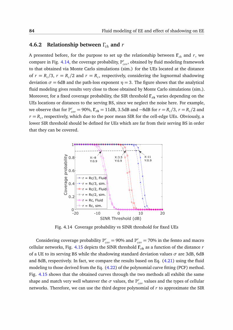
84 Fluid modeling of EE and effect of shadowing on EE
4.6.2 Relationship between Γth and r
A presented before, for the purpose to set up the relationship between Γ th and r, we
compare in Fig. 4.14, the coverage probability, Prcov, obtained by fluid modeling framework
to that obtained via Monte Carlo simulations (sim.) for the UEs located at the distance
of r = Rc/3, r = Rc/2 and r = Rc, respectively, considering the lognormal shadowing
deviation σ = 6dB and the path-loss exponent η= 3. The figure shows that the analytical
fluid modeling gives results very close to those obtained by Monte Carlo simulations (sim.).
Moreover, for a fixed coverage probability, the SIR threshold Γ t h varies depending on the
UEs locations or distances to the serving BS, since we neglect the noise here. For example,
we observe that for Prcov = 90%, Γ t h = 11dB, 3.5dB and −8dB for r = Rc/3, r = Rc/2 and
r = Rc, respectively, which due to the poor mean SIR for the cell-edge UEs. Obviously, a
lower SIR threshold should be defined for UEs which are far from their serving BS in order
that they can be covered.
-20 -10 0 10 20SINR Threshold (dB)
0
0.2
0.4
0.6
0.8
1
Cov
erag
epro
bab
ility
r = Rc/3, Fluid
r = Rc/3, sim.
r = Rc/2, Fluid
r = Rc/2, sim.
r = Rc, Fluid
r = Rc, sim.
X:-8Y:0.9
X:3.5Y:0.9
X:11Y:0.9
Fig. 4.14 Coverage probability vs SINR threshold for fixed UEs
Considering coverage probability Prcov = 90% and Pr
cov = 70% in the femto and macro
cellular networks, Fig. 4.15 depicts the SINR threshold Γ t h as a function of the distance rof a UE to its serving BS while the shadowing standard deviation values σ are 3dB, 6dB
and 8dB, respectively. In fact, we compare the results based on Eq. (4.21) using the fluid
modeling to those derived from the Eq. (4.22) of the polynomial curve fitting (PCF) method.
Fig. 4.15 shows that the obtained curves through the two methods all exhibit the same
shape and match very well whatever the σ values, the Prcov values and the types of cellular
networks. Therefore, we can use the third degree polynomial of r to approximate the SIR
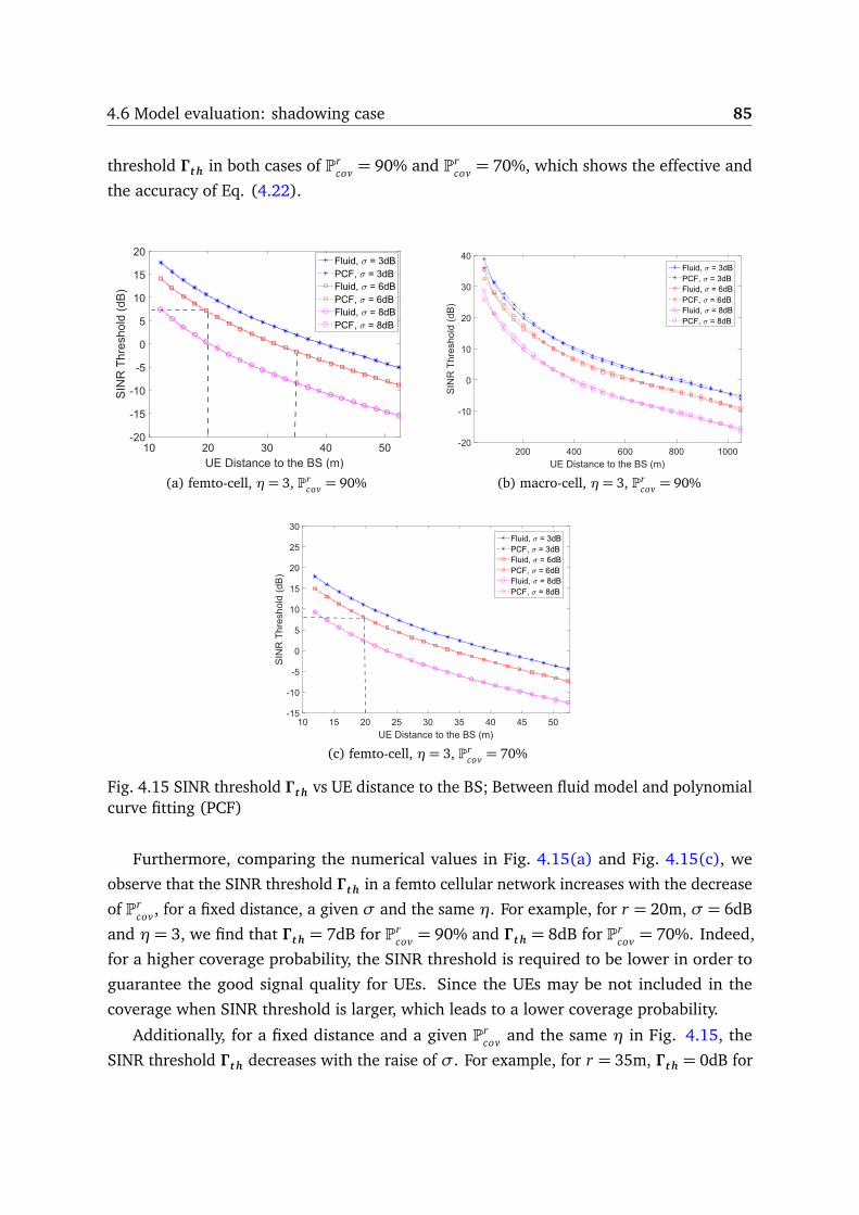
4.6 Model evaluation: shadowing case 85
threshold Γ t h in both cases of Prcov = 90% and Pr
cov = 70%, which shows the effective and
the accuracy of Eq. (4.22).
(a) femto-cell, η= 3, Prcov = 90% (b) macro-cell, η= 3, Pr
cov = 90%
(c) femto-cell, η= 3, Prcov = 70%
Fig. 4.15 SINR threshold Γ t h vs UE distance to the BS; Between fluid model and polynomialcurve fitting (PCF)
Furthermore, comparing the numerical values in Fig. 4.15(a) and Fig. 4.15(c), we
observe that the SINR threshold Γ t h in a femto cellular network increases with the decrease
of Prcov, for a fixed distance, a given σ and the same η. For example, for r = 20m, σ = 6dB
and η= 3, we find that Γ t h = 7dB for Prcov = 90% and Γ t h = 8dB for Pr
cov = 70%. Indeed,
for a higher coverage probability, the SINR threshold is required to be lower in order to
guarantee the good signal quality for UEs. Since the UEs may be not included in the
coverage when SINR threshold is larger, which leads to a lower coverage probability.
Additionally, for a fixed distance and a given Prcov and the same η in Fig. 4.15, the
SINR threshold Γ t h decreases with the raise of σ. For example, for r = 35m, Γ t h = 0dB for

86 Fluid modeling of EE and effect of shadowing on EE
σ = 6dB and Γ t h = −6dB for σ = 8dB in Fig. 4.15(a). The reason is that the higher value
of σ leads to more serious shadow fading and then a lower SINR at a certain distance. This
observation has been already demonstrated in [113], that is the shadowing significantly
impacts on the coverage performance especially when the SINR thresholds are small.
For further illustrating the accuracy of polynomial curve fitting (PCF) method, we
compute the Γ t h fitting error as the difference between the fluid modeling and the PCF
in a femto cellular network with η = 3 and coverage probability Prcov = 90%, as shown
numerically in Table 4.4. We observe that the error does not exceed 0.2, which validate
the accuracy of PCF. Therefore, this method can be used to compute data rate and energy
efficiency in the below part.
Table 4.4 Γ t h fitting error between fluid and PCF, with Prcov = 90%, R= 50m, η= 3
𝒓𝒖 (m)
11.9 15.8 19.6 25.4 29.3 35 40.8 44.6 50.4 52.3=𝑹𝒆
σ=3 0.1802 0.1035 0.0902 0.0339 0.0764 0.0463 0.0404 0.0745 0.0154 0.1059
σ=6 0.1803 0.1036 0.0903 0.0339 0.0764 0.0465 0.0404 0.0746 0.0154 0.1062
σ=8 0.1814 0.104 0.0911 0.0339 0.077 0.0471 0.0406 0.0754 0.0154 0.1076
According to the polynomial expression of Γ t h, in the following part we will show some
results of energy efficiency (EE) based on Eq. (3.1), when replacing the data rate Darea
with Eq. (4.23).
4.6.3 Energy efficiency discussion
Fig. 4.16 and Fig. 4.17 depict the EE variations in a femto cellular network and in a macro
cellular network depending on Ra, i.e., the size of the ring over the serving BS. Both figures
are obtained using the analytical model we proposed and Monte Carlo simulations (sim.)
for three cases, depending on the standard deviation value σ = 0dB (without shadowing),
σ = 6dB and σ = 8dB. The coverage probability is set Prcov = 90% or Pr
cov = 70%. Both of
two figures confirm that the proposed model is effective and matches well with the Monte
Carlo results, whatever the value of the path-loss exponent (η = 3 or η = 2.6). In addition,
we observe a small difference between these curves due to the circular shape considered
in the fluid modeling. Since in fluid modeling, the average interference factor y f (r,η)without shadowing based on Eq. (3.7) is the same, resulting the same SINR threshold value

4.6 Model evaluation: shadowing case 87
(a) femto-cell, η= 3, Prcov = 90% (b) femto-cell, η= 2.6, Pr
cov = 90%
(c) femto-cell, η= 3, Prcov = 70%
Fig. 4.16 EE variation vs network radius Ra in femto cellular network
according to Eq. (4.21). However, in the hexagonal modeling, the y f (r,η) is calculated
according to the real UEs’ distances from neighboring BSs.
Furthermore, while comparing Fig. 4.16(a) and Fig. 4.16(c) with Prcov = 90% and
Prcov = 70%, respectively, we observe that the numerical values of EE, obtained by fluid
modeling, decrease with the reduction of Prcov for same values of Ra, η and σ. For example,
the EE is about 5.57K bits/Joule for η= 3, σ = 6dB and , at the cell edge (Ra = Re) and
Prcov = 90%, whereas the EE is about 4.99K bits/Joule when Pr
cov = 70%. Since a higher
coverage rate can lead to a larger data rate, and thus a larger EE can be obtained.
Moreover, focusing on Fig. 4.16(a), we observe that the values of EE decreases in a
femto cellular network with the increase ofσ for a fixed value of Ra. For example, in the case
of Ra = 30m, EE is about 3.85K bits/Joule for σ = 6dB, and it is about 1.65K bits/Joule

88 Fluid modeling of EE and effect of shadowing on EE
(a) macro-cell, η= 3, Prcov = 90% (b) macro-cell, η= 2.6, Pr
cov = 90%
Fig. 4.17 EE variation vs network radius Ra in macro cellular network
for σ = 8dB. In fact, the larger the shadowing, the lower the achieved throughput of UEs.
The similar conclusion can be found in other figures of Fig. 4.16 and in Fig. 4.17.
In addition, while comparing Fig. 4.16(a) and Fig. 4.16(b) in a femto cellular network
with Prcov = 90%, we observe that the numerical values of EE, obtained by fluid modeling,
decrease with the reduction of η for same values of Ra and σ. For example, the EE is about
5.57K bits/Joule for η = 3, at the cell edge (Ra = Re) and σ = 6dB, whereas the EE is
about 3.73K bits/Joule when η = 2.6. When η ranges from 3 to 2, i.e., from the suburban
environment to the free space, the dissipation of the transmission power reduces. However,
in this case the SIR at a fixed distance decreases, which further leads to the EE decline.
Therefore, EE decreases as η reduces. Comparing Fig. 4.17(a) and Fig. 4.17(b) in a macro
cellular network with Prcov = 90%, we can find the same conclusion.
4.6.4 EE model accuracy
For the accuracy purpose, in Fig. 4.18 we compute the EE error between the proposed
fluid modeling and Monte Carlo simulations, depending on the network radius Ra of a
femto cellular network and a macro cellular network, respectively, with η = 2.6 and
Prcov = 90%. In Fig. 4.18(a), we observe that the error is less than 20% for Ra > 17m
in a femto cellular network, whatever the values of σ. Meanwhile, the results in Fig.
4.18(b) also show a error of less than 20% for Ra > 100m in a macro cellular network.
Those numerical results illustrate the accuracy of fluid modeling as a tool for performance
evaluation while considering the impact of shadowing. However, the EE error is less than
30% for 10< Ra < 17m in a femto cellular network, since the fitting error of Γ t h between
fluid and PCF is larger for 10< Ra < 17m, as shown in Table 4.4.

4.7 Conclusion 89
(a) femto-cell, η= 2.6, Prcov = 90% (b) macro-cell, η= 2.6, Pr
cov = 90%
Fig. 4.18 EE error vs network radius Ra in cellular networks
4.7 Conclusion
In this chapter, we propose a tractable expression of EE based on fluid modeling in an
OFDMA cellular network. The model is proposed for a network area within the central
cell and is extended to compute the EE for network area, with any size. The proposed EE
model is assessed under the two conditions of non-shadowing and shadowing.
While neglecting the impact of shadowing, we assess the EE in three types of cellular
networks including macro, micro and femto cellular networks. The model accuracy of the
obtained EE model is shown through a comparison with Monte Carlo trials. Additionally,
the results also exhibit that: 1) the density of users per cell has no impact on the EE, since
the analysis is considered only in downlink transmissions, 2) EE is independent from the
users’ density but proportional to the path-loss exponent, 3) a femto cellular network is
more efficient than the macro one, and 4) the proposed EE model over the network area
with any size is accurate.
While taking the impact of shadowing and the path-loss exponent into account, we
first developed a closed-form polynomial formula between UEs’ location and the signal
quality threshold using polynomial curve fitting (PCF) for a fixed coverage probability.
Then taking advantage of this formula, we evaluated the energy efficiency (EE) based on
the fluid modeling in an OFDMA femto and a macro cellular network. Finally, we shown
the accuracy of the obtained EE models through a comparison with Monte Carlo trials. The
results shown the effective of fluid modeling as a mathematical tool to evaluate the EE with
the consideration of shadowing impact. The numerical results also illustrated the impact of

90 Fluid modeling of EE and effect of shadowing on EE
shadowing on EE, i.e., EE decreased with the raise of the lognormal shadowing standard
deviation value of σ.
The results of this chapter provide adequate insights into that fluid modeling can be
considered as an accuracy tool to evaluate the network EE with/without considering the
effect of shadowing. Accordingly, in the following chapter, we derive an energy efficiency
model for a cellular network based on the fluid modeling while using the joint transmission
coordinated multipoint(JT-CoMP) scheme. Since the application of JT-CoMP brings the
power consumption due to the more channel estimation operation, more overhead to
deploy the coordinated cooperative base stations.

Chapter 5
EE analysis of JT-CoMP scheme in
macro/femto cellular networks
Contents
5.1 Introduction . . . . . . . . . . . . . . . . . . . . . . . . . . . . . . . . . . . . . . . 92
5.2 JT-CoMP scheme . . . . . . . . . . . . . . . . . . . . . . . . . . . . . . . . . . . . . 93
5.3 JT-CoMP performance evaluation . . . . . . . . . . . . . . . . . . . . . . . . . . 94
5.4 System model . . . . . . . . . . . . . . . . . . . . . . . . . . . . . . . . . . . . . . 96
5.4.1 Energy efficiency model with JT-CoMP scheme . . . . . . . . . . . . . 97
5.4.2 Power consumption model with JT-CoMP scheme . . . . . . . . . . . . 97
5.4.3 SINR calculation: case of JT-CoMP . . . . . . . . . . . . . . . . . . . . . 98
5.5 Data rate computation . . . . . . . . . . . . . . . . . . . . . . . . . . . . . . . . . 100
5.5.1 Non-CoMP scenario . . . . . . . . . . . . . . . . . . . . . . . . . . . . . . 102
5.5.2 AllUEs-CoMP scenario . . . . . . . . . . . . . . . . . . . . . . . . . . . . . 103
5.5.3 CoMP scenario . . . . . . . . . . . . . . . . . . . . . . . . . . . . . . . . . 103
5.6 Backhauling traffic computation: Cbh . . . . . . . . . . . . . . . . . . . . . . . . 104
5.7 Simulation and results . . . . . . . . . . . . . . . . . . . . . . . . . . . . . . . . . 104
5.7.1 Date rate vs the network radius . . . . . . . . . . . . . . . . . . . . . . . 105
5.7.2 EE vs radius Ra in scenario AllUEs-CoMP . . . . . . . . . . . . . . . . . 107
5.7.3 Impact of distance threshold dth on cell EE EEcel l in CoMP scenario . 111
5.7.4 EE gain vs BSs number . . . . . . . . . . . . . . . . . . . . . . . . . . . . 112
5.7.5 Backhauling power cost vs BSs number . . . . . . . . . . . . . . . . . . 114
5.8 Conclusion . . . . . . . . . . . . . . . . . . . . . . . . . . . . . . . . . . . . . . . . 116
92 EE analysis of JT-CoMP scheme in macro/femto cellular networks
5.1 Introduction
5G wireless networks are expected to increase substantially data rates and quality-of-service
(QoS) for users, at a similar or a lower power consumption as today’s 4G networks. As
discussed in chapter 1, Joint Transmission Coordinated Multipoint (JT-CoMP) transmission
is a promising technology to improve the network energy efficiency (EE) and to fulfill
upcoming communication demands [125], through turning the inter-cell interference
into useful signals, especially for the cell-edge user equipments (UEs). Through taking
advantage of the JT-CoMP technique, information is transmitted to a UE simultaneously
from different coordinated BSs in order to improve the received signal quality and strength
[47] as well as to enhance the spectral efficiency. However, this technology in practice also
brings some additional energy consumption for transmitting the resource information, i.e.,
backhauling information. Additionally, while JT-CoMP approach is applied, the performance
evaluation of energy efficiency (EE) becomes a hard task in terms of time expense to
conduct simulations. Therefore, it is still an open issue to develop an accurate model for
EE-evaluation while the JT-CoMP transmission is applied.
As illustrated in the results section of the previous chapter, fluid modeling can be
considered as an effective and accuracy tool to evaluate EE for the cellular networks
with/without taking the impact of shadowing into account. Since this modeling can reduce
the analysis complexity and provide a macroscopic evaluation of the network performance.
Therefore, spurred by the above advantages of fluid modeling, our objective in this chapter
is to design a tractable model for evaluating EE based on the fluid modeling while JT-CoMP
approach is considered in a network system.
In this chapter, we first introduce the concept of JT-CoMP in detail. Then, we discuss
the JT-CoMP models and the numerical results in some literatures. Furthermore, combing
our previous work in chapter 4, we derive a closed-form expression of EE based on the fluid
modeling while the JT-CoMP approach is applied, which reduces the analysis complexity.
Given that the definition of EE is related to the data rate and power consumption, we redefine
a new power consumption model with considering the backhauling power consumption for
the JT-CoMP system. Afterwards, depending on the JT-CoMP scheme, we consider three
scenarios to compute the total data rate of the network area and the backhauling traffic.
Finally, we discuss the simulation performance to prove the effectiveness and accuracy
of our proposed model through a comparison between fluid modeling and Monte Carlo
simulations.

5.2 JT-CoMP scheme 93
5.2 JT-CoMP scheme
Before introducing the concept of JT-CoMP, we first recall the concept of CoMP since JT-
CoMP is one of the main families coordination method of CoMP. As discussed in chapter 1,
CoMP refers to a system where the transmission and/or reception at multiple, geographically
separated antenna sites is dynamically coordinated in order to improve the coverage, cell-
edge throughput and system efficiency. In a CoMP transmission system, several BSs are
cooperated to transmit and receive data from multiple UEs based on the shared information
between BSs so as to mitigate intercell interference and hence improve spectral efficiency.
The set of several coordinated BSs is called as CoMP cooperative set, where the data is
available at each BS. In the CoMP cooperative set, the BSs directly or indirectly participate
in data transmission to UEs [126]. Hence, CoMP has been considered by 3GPP as a tool to
provide a significant gain in terms of capacity and cell edge throughput.
Joint Transmission Coordinated Multipoint (JT-CoMP) is outlined by 3GPP [126], which
is one of key strategies of CoMP. In JT-CoMP, data intended for a particular UE, comes jointly
from multiple coordinated BSs (part of or entire CoMP cooperative set) at the same time
and thus to improve the received signal quality as well as the spectral efficiency (SE) [75].Fig. 5.1 illustrates the JT-CoMP scheme [40]. User 2 associates with BS 2 while user 1
associates with BS 1. Instead of serving their associated users independently, BSs 1 and 2
cooperatively transmit useful information to their users. For instance, if both BSs apply
time-division multiple access (TDMA) in the first time slot, both BSs 1 and 2 transmit the
same information to user 2. The user combines the signals from both BSs to decode the
information. In the second time slot, the BSs cooperatively serve user 1. Due to JT, cell
edge users experience higher receiving signal strength and lower interference, resulting
the higher coverage and larger cell-edge throughput.
Fig. 5.1 JT-CoMP scheme [40]

94 EE analysis of JT-CoMP scheme in macro/femto cellular networks
According to the coordination way, JT-CoMP can be further classified into distance-based
JT-CoMP technique and SINR-based one. In detail, in the former, several nearest BSs are
intended to serve a UE, whereas in the SINR-based JT-CoMP technique, the best several
BSs offering maximum SINR are selected to serve a UE.
5.3 JT-CoMP performance evaluation
EE evaluation is investigated in [75] for a downlink LTE-Advanced cellular system with
using JT-CoMP scheme. Two JT-CoMP approaches are considered in that system, such
as SINR-based JT-CoMP and distance-based JT-CoMP. Based on system-level simulations,
simulation results illustrate that the SINR-based JT-CoMP scheme can achieve a superior
EE performance compared to the distance-based JT-CoMP scheme.
In [91], authors investigate the problem of EE optimization in an OFDMA downlink
heterogeneous network (HetNet) using a JT-CoMP transmission. The HetNet system is
composed of several HetNet cells and they are coordinated via fiber backhauling, which
can be called interbackhaul. Each of cell consists of one macro-BS, several low-power
femto-BSs, and some uniformly distributed UEs. These femto-BSs are backhauled through
fiber/microwave to the macro-BS in the one HetNet cell, which can be termed intrabackhaul.
In particular, JT-CoMP is applied in the system when the received SINR at the UE is lower
than 3dB. Using system-level simulations, simulation and analysis of results show that the
EE first increases with respect to the SE and then decreases when the SE exceeds some
value.
Additionally, the author in [125] investigated the outage probability and effective
throughput of the system through taking advantage of the JT-CoMP technology. The JT-
CoMP model is introduced as follows. A cellular network is considered, where each BS is
located at the center of a hexagonal cell and all UEs are assumed to be distributed uniformly
over a cell. Each cell is divided into the center zone, with a setting radius, and the edge
zone. Accordingly, the distance-based JT-CoMP technique is only available for UEs, located
at the edge zone over a downlink transmission so as to improve cell-edge performance.
Based on this system model, analytical expressions of cumulative distribution function
(CDF) of the SIR, outage probability and throughput are derived based on 2-dimensional
Markov chain analysis, since the call arrival process is assumed to follow a Poisson process.
The simulation results show that the system performance mainly depends on the center
zone size and the offered load. Moreover, compared with the dynamic point selection
scheme (one scheme dynamically switches the serving BS based on the UE’s channel and
the cell loading conditions), JT-CoMP scheme can achieve a lower outage probability.

5.3 JT-CoMP performance evaluation 95
Additionally, simulations in [41] show that JT-CoMP transmission and reception schemes
have a significant effect in terms of improving the throughput of the cell-edge users based
on the LTE-Advanced simulation conditions.
Moreover, a tractable model for Non-Coherent Joint-Transmission (NC-JT) cooperation
is proposed in [127] while user-centric clustering and channel-dependent cooperation
activation are taken into account. The user-centric clustering is defined such as, the cluster
of cooperative BSs is formed around a typical user and the channel-dependent cooperation
activation is defined such as, JT is adopted according to whether the channel to a cooperative
BS is in deep fading. A single-tier OFDMA-based cellular system is considered, which is
formed according to a stationary Poisson point process. The definitions of cooperative set
and active cooperative set are introduced. The cooperative set is defined such as, if the
received signal strength at a BS in the uplink is larger than a threshold, then this BS is
grouped into the cooperative set. While, the active cooperative set is defined such as, if
the signal received at the typical user is greater than a cooperation activation threshold,
then this BS joints the cooperative transmission. The CDF of SINR of a typical user is
characterized in the case of user-centric BS clustering. Simulation results show that when
the NC-JT CoMP is used, increasing the BS density can improve the SINR, and that the
average spectral efficiency is saturated at a cluster size of around 7 BSs with imperfect CSI
at the receiver.
Until now, much leading work with JT-CoMP techniques is carried out either using
system-level simulations or based on stochastic geometry. However, stochastic geometry
framework yields to intractable models when non-Poisson point processes, eg., perturbed
lattice, β -Ginibre point process, and Matérn point process, are considered to describe, in a
more realistic way, the nodes’ locations. In this case, either approximations or simulations
are conducted to prove the model accuracy. In the other side, simulation-based models
become resource-intensive when considering large networks, with a high number of base
stations (BSs) and user equipments (UEs). As a result, an approximation-based is necessary
to evaluate the network performance.
As mentioned before, spatial fluid modeling can be used to evaluate the network
performance of cellular networks, such as SINR, outage probability, and energy efficiency
through analytical expressions. In [99], the authors use this mathematical framework
to study the SINR enhancement depending on the number of coordinated BSs and other
network-related parameters in dense areas. The notation of the cooperation field is proposed
to compute the power of coordinated BSs by integration. Depending on the number of
coordinated BSs, three scenarios are considered. As a matter of fact, we use this tractable
model to benchmark the EE variation depending on the network parameters, such as its size

96 EE analysis of JT-CoMP scheme in macro/femto cellular networks
and its type (macro, femto), the number of coordinated BSs, and the path-loss exponent as
it reflects the network environment, while JT-CoMP is applied.
We combine here our previous work done in the last chapter to develop an EE model
in the case of JT-CoMP. We first extend the fluid modeling with JT-CoMP to compute the
total data rate over a network area. Then, we derive the closed-form expression of EE for
the JT-CoMP downlink transmission, which is tractable and quite simple to compute. The
effectiveness and the accuracy of the underlying model are shown for both types of cellular
networks, macrocells and femtocells, by comparing the results to those of Monte Carlo
(MC) simulations while considering several path-loss exponents and varying the number
of cooperating BSs, in the case of a constant backhauling power cost. Furthermore, we
investigate the EE improvement with the variation of the backhauling power cost, depending
on some parameters, like the network area radius and the number of coordinated BSs.
Actually, JT-CoMP is used to improve the signal quality of UEs far from their serving BS.
Here, we define a distance threshold as well as the associated SIR threshold making JT-
CoMP approach more efficient in terms of EE. We also discuss the impact of these thresholds
in the case of variable backhauling power costs depending on the data rate requirement.
5.4 System model
To meet these objectives cited before, we consider the downlink channel of an OFDMA
network with JT-CoMP approach, where the UE receives the useful signal from its serving
BS and the cooperative BSs. Interference is only generated by the outer BSs, i.e., ones
outside the cooperative set. The obtained model can be utilized as an efficient tool by an
operator to benchmark the energy efficiency of its network even if some additional BSs are
needed to boost the services.
Here, we describe the EE model when JT-CoMP is used through the network, mainly
within the closest BSs, i.e., those belonging to the first ring as shown in Fig. 5.2. In the
cellular system, only one BS is selected for data transmission to the UE. In contrast, when
the coordination is used, multiple BSs in the coordination set send data together to the UE.
Since interference mainly comes from neighbors in the first ring, we limit the coordination
set of BSs on this ring, so that the total number of coordinated BSs, Mco = 2, ..., 7. The
system model presented here is quite similar to the one in chapter 3. It concerns an OFDMA
cellular network, composed of NBS base stations (BSs) and Nu user equipments (UEs)
randomly distributed over the network. Mco BSs are able to jointly transmit data in order to
improve the signal quality at the UE located at the distance ru from its serving BS (central
cell in Fig. 5.2). We assume that the radio resources of each BS are divided into many

5.4 System model 97
parallel and orthogonal sub-carriers, only inter-cell interference is considered. The network
is supposed homogeneous, such that the transmission power Pt x is the same for every BS.
Fig. 5.2 Hexagonal network and main parameters.
Since we introduce the JT-CoMP scheme, the energy efficiency model is refined in this
chapter and presented below.
5.4.1 Energy efficiency model with JT-CoMP scheme
In order to capture the energy-efficiency of that network with JT-CoMP, we use the common
Eq. (5.1) as in [37, 78]:
EE =Darea
Mco × PCoM Pex p + (NBS −Mco)× Pex p
. (5.1)
The EE is computed as the ratio of total data rate over a network area Darea, to the total
power consumption. Here, PCoM Pex p and Pex p are respectively the total energy expenditure
per coordinated BS and per BS.
5.4.2 Power consumption model with JT-CoMP scheme
The power consumption of a coordinated BS, PCoM Pex p in Eq. (5.2), is defined depending on
the number of transmitting antennas Nant , the transmitting power Pt x and the backhauling
power cost KCoM P . The fixed part, P1, accounts for the direct current/alternating current
(DC/AC) converters. ∆P and P0 denote some circuit power consumption.
PCoM Pex p = Nant(∆P Pt x + P0) + P1 + KCoM P . (5.2)
Backhauling power consumption KCoM P is the power cost due to the backhauling and
data sharing for every BS. Fehske et al., in [64] have investigated the impact of a microwave
98 EE analysis of JT-CoMP scheme in macro/femto cellular networks
backhauling in most cellular networks with a CoMP approach. They model the backhauling
as a set of wireless micro wave links. KCoM P can be a constant for simplification, or be
calculated as in [64]:
KCoM P =P0
bhCbh
C0bh
= αbhCbh, (5.3)
where P0bh denotes the power consumed by the backhaul equipment when supporting the
maximum data rate C0bh, αbh = P0
bh/C0bh is the power coefficient of backhaul equipment,
and Cbh is the backhauling traffic for every BS, i.e., the accumulated data rate of several
UEs served by one cooperating BS [89]. Therefore, KCoM P is linearly proportional to the
backhauling requirement Cbh. The calculation of Cbh will be presented in the below sections.
In particular, αbh = 5 × 10⁻⁷Joules/bi t [64, 89] for a macro BS and αbh = 4 ×10⁻⁸Joules/bi t for a femto BS [89, 128, 129].
Obviously, the power consumption of a common BS, i.e., without coordination, also
can be computed using the Eq. (5.2), without the KCoM P part. In other words, in Non-
CoMP mode, Cbh and KCoM P are zero. Therefore, the total energy expenditure per BS
with Non-CoMP is given by Pex p = Nant(∆P PT x + P0) + P1 and the EE equation is reduced
to EE = DareaNBS×Pex p
. The numerical values of each part in Eq. (5.2) are listed in Table 3.1,
regarding the BSs types (macro, micro, femto).
Before presenting how to compute the total data rate Darea, we give the SINR calculation
with fluid modeling in the case of JT-CoMP.
5.4.3 SINR calculation: case of JT-CoMP
Basically, without any coordination and neglecting the noise, the SINR Γu at u in this basic
case, as we denote it Non-CoMP mode, is displayed by
Γu =(η− 2)r−ηu
2πρBS[(2Rc − ru)2−η − (Rnw − ru)2−η]. (5.4)
The above equation is obtained by fluid framework, which can be seen more details in
chapter 3.
Usually, BSs cooperate to transmit and receive data from multiple UEs in different cells
to improve the coverage and especially, to enhance cell-edge throughput. As in [99], a UE
u is served by the central BS b, and receives data from coordinated BSs as shown in Fig.
5.3. The UE experiences a SINR Γ CoM Pu as
Γ CoM Pu =
pb,u + pu,CoM P
pex t,u − pu,CoM P. (5.5)

5.4 System model 99
pu,CoM P denotes the received power at u from the BSs which are in the coordinated set
together with the serving BS. It defines the received power improvement by means of
the coordination. pb,u = Pt x Kr−ηu is the received power from its serving BS b, pex t,u =2πρBS Pt x Kη−2 [(2Rc − ru)2−η − (Rnw − ru)2−η] is the total external or interference power coming
from others BSs without cooperation.
Fig. 5.3 JT-CoMP in hexagonal model
As the first ring is composed of six BSs around the serving BS, as shown in Fig. 5.3,
the homogeneous network we consider is divided into six equal parts. Therefore, there
are n BSs, such that n= {1, ..., 6}, in the first ring to cooperatively transmit data with the
central BS. Hence, the JT coordination area can be delimited over a ring of radii between
[2Rc − ru, 4Rc − ru] and the angle of nπ/6 (see [99] for more details). For example, the
red area in Fig. 5.4 is the cooperative region between serving BS and one coordinated BS
(n= 1).
Fig. 5.4 JT-CoMP in fluid model with n(= 1) coordinated BSs

100 EE analysis of JT-CoMP scheme in macro/femto cellular networks
Therefore, for a given UE u with n (n= {1, ..., 6}) BSs in the coordinated set to jointly
transmit data with its serving BS, the improvement of the received power or the coordinated
power can be written as
pu,CoM P =
∫nπ3
0
∫ 4Rc−ru
2Rc−ru
ρBS Pt x Kz−ηzdzdθ
=nπ3ρBS Pt x Kη− 2
[(2Rc − ru)2−η − (4Rc − ru)
2−η].
(5.6)
Consequently, we can compute the SINR Γ CoM Pu in Eq. (5.5) at u, by replacing pb,u =
Pt x Kr−ηu , pex t,u =2πρBS Pt x Kη−2 [(2Rc − ru)2−η− (Rnw− ru)2−η] and pu,CoM P as defined in Eq (5.6),
displayed as
Γ CoM Pu =
3(η− 2)r−ηu + nπρBS[(2Rc − ru)2−η − (4Rc − ru)2−η]
6πρBS[(2Rc − ru)2−η − (Rnw − ru)2−η] + nπρBS[(2Rc − ru)2−η − (4Rc − ru)2−η].
(5.7)
The analytically tractable expressions of Γu in Eq. (5.4) and Γ CoM Pu in Eq. (5.7) can be
easily exploited to compute data rate over a network area, since the two equations only
depend on the density of BS, ρBS, the radius of the cell, Rc, the range of the network, Rnw,
the path-loss exponent, η, the distance of a UE to its serving BS, ru, and the number of
coordinated BS, n, in the first ring.
Therefore, taking advantage of the expressions of Γu and Γ CoM Pu , we will present the
computation of data rate Darea in the following section.
5.5 Data rate computation
Fig. 5.5 Area of interest with various radius Ra (0< Ra ≤ Re)

5.5 Data rate computation 101
This section presents the evaluation of data rate over a network area of radius Ra, such
that Ra varies in [0, Re], as shown in Fig. 5.5. Note that Re is the radius of a disk with a
surface equivalent to the hexagonal central cell, such that Re =Æ
2p
3/πRc.
We claim that JT-CoMP is not as much efficient for UEs with a greater Γu, and even can
reduce EE performance of the network. To investigate this hypothesis, we consider the
cell divided into two parts: inner region and outer region based on the signal quality Γu at
UE u, as displayed in Fig. 5.6. Indeed, UEs located in the inner region, do not need the
improvement of their SINR, since they are close to their serving BS. Hence, the inner region
is regarded as Non-CoMP mode. In return, the outer region is defined as CoMP mode, due
to the worst SINR experienced there. For example, a cell-edge UE u is in a CoMP mode
since
Γu ≤ Γthreshold , (5.8)
where Γthreshold is a predefined threshold in dB, related to a distance, called the distance
threshold dth. Hence, we aim to define these thresholds in order to set up the network
conditions ensuring a greatest JT-CoMP performance. Thus, we can further obtain the
higher EE.
Fig. 5.6 JT-CoMP strategy defined by distance threshold dth
Depending on different values of dth, we define three scenarios to resolve the problem.
• Non-CoMP scenario when dth = Re. Here, there is no need to use JT-CoMP, since the
overall cell falls in the inner region. In other words, all UEs are in Non-CoMP mode,
and their Γu can be calculated by Eq. (5.4). Although it is not realistic, this scenario
serves as a baseline or a reference to evaluate and to compare the gain of EE when
JT-CoMP is applied.
• AllUEs-CoMP scenario when dth = 0. It is the worst case, where all UEs in the cell
are in the outer region and choose JT-CoMP whatever their locations. Γ CoM Pu can be
computed by Eq. (5.7).

102 EE analysis of JT-CoMP scheme in macro/femto cellular networks
The results analysis of the latter scenario together with Non-CoMP scenario results,
allow to define the dth threshold and thereby define adequately the inner and the
outer regions. Moreover, we can investigate the boundary of the EE using fluid
approximation.
• CoMP scenario is the common and the more realistic scenario, since the cell is com-
posed of two regions: inner region and outer region depending on the distance
threshold dth. In the inner, UEs do not use JT-CoMP scheme, whereas the UEs whose
distances are larger than dth choose JT-CoMP scheme. Using this scenario, we can
evaluate the effectiveness of JT-CoMP depending on the coordinated BSs number, the
distance threshold dth, and the network size Ra such that 0< Ra ≤ Re.
Regarding the three scenarios described above, we detail how to compute the data rate
in the following paragraphs.
5.5.1 Non-CoMP scenario
In this scenario, we aim at evaluating the data rate Darea over a network area with the
condition of dth = Re. To do so, we focus on a network area with a radius Ra, such as
(0< Ra ≤ Re), i.e., one part of the central cell, as depicted in Fig. 5.5. Since the UEs are
uniformly distributed in space, the density ρu is constant. Therefore, the number of users
N ′u over the area of interest, of radius Ra, is given as N ′u = (NuR2a)/R
2e , where Nu is the total
number of UEs.
According to Shannon’s formula, the spectral efficiency (SE), measured in bps/Hz,
for a UE u located at the distance r depends on its signal quality Γu and is given as
SEu(r) = log2(1+ Γu(r)). The maximum theoretical achievable data rate Du(r) of UE u can
be computed as Du(r) = Bu × SEu(r), where Bu is the UE’s bandwidth. Hence, the total
data rate Darea over a network area of radius Ra, can be written by
Darea =
∫ 2π
0
∫ Ra
0
Buρulog2(1+ Γu(r))rdrdθ . (5.9)
Considering an equal bandwidth sharing among UEs, Bu = BWn/Nu where BWn is the total
bandwidth. Replacing ρu = Nu/(2p
3R2c), the total data rate is rewritten as
Darea =BWnπp
3R2c
∫ Ra
0
r log2(1+ Γu(r))dr. (5.10)

5.5 Data rate computation 103
A worthwhile observation is that Eq. (5.10) neither depends on the number of UEs
deployed per cell, nor upon their density ρu. When Ra = Re, the above equation is evolved
to compute the total cell data rate, D̃.
5.5.2 AllUEs-CoMP scenario
In this scenario, whatever the location of UEs in the cell, all of them use JT-CoMP to
receive signal from both the serving BS and the coordinated BSs deployed in the first ring.
Therefore, in this case, the total data rate Darea over a network area with radius Ra can be
expressed as
Darea =BWnπp
3R2c
∫ Ra
0
r log2(1+ ΓCoM Pu (r))dr. (5.11)
When Ra = Re, the above equation is evolved to compute the total cell data rate, DCoM Pcel l .
5.5.3 CoMP scenario
CoMP Scheme is used for a fixed value of dth, where only UEs with lower signal quality
compared to Γthreshold adopt JT-CoMP. The rest of UEs are in Non-CoMP mode. As same as
the previous scenarios, the aim is to compute total data rate Darea over a network area with
radius Ra. Therefore, depending on the network radius Ra, we can have two possibilities:
1. For Ra ≤ dth, the area of interest is one part of inner region and Darea can be computed
with the same Eq. (5.10).
2. For dth < Ra ≤ Re, the area of interest has two parts: inner region, i.e., a disk of
radius dth, and a ring part with inner radius dth and outer radius Ra. The data rate
over the inner region, Dinner , is computed by Dinner =BWnπp
3R2c
∫ dth
0r log2(1+ Γu(r))dr.
The data rate over the ring between inner radius dth and outer radius Ra, Douter is
computed as Douter =BWnπp
3R2c
∫ Ra
dthr log2(1+ Γ CoM P
u (r))dr.
Therefore, the data rate Darea in CoMP scenario can be expressed as
Darea =
BWnπp3R2
c
Ra∫
0
r log2(1+ Γu(r))dr, Ra ≤ dth
Dinner + Douter , dth < Ra ≤ Re
(5.12)
According to the above definition of data rate, we find that Darea is mainly related to the
distance threshold dth and the radius Ra. The accuracy of Eqs. (5.10), (5.11) and (5.12) is
verified in the simulation section through a comparison with Monte Carlo simulations.
104 EE analysis of JT-CoMP scheme in macro/femto cellular networks
The bit-per-joule capacity indicates the amount of energy consumed for transmitting
information. In fact, the last parameter to define for the EE model concerns the power
consumption which must take into account not only the power consumed at each BS, but
also the relative backhauling power used to share data between cooperative BSs. In the
subsequent section we introduce the definition of energy efficiency expression depending
on these powers and the total data rate formulated above.
5.6 Backhauling traffic computation: Cbh
Regarding the last section, when JT-CoMP is applied, we suppose that KCoM P is related to
total data rate over the shaded region with CoMP, as shown in Fig. 5.6. So we consider
different equations of Cbh depending on the scenarios of CoMP approach, for example,
• AllUEs-CoMP: Cbh = DCoM Pcel l ,
• CoMP scenario: Cbh = DCoM Pshade ,
where DCoM Pshade =
BWnπp3R2
c
∫ Re
dthr log2(1+ Γ CoM P
u (r))dr. Meanwhile, in Non-CoMP mode, Cbh and
KCoM P are zero.
5.7 Simulation and results
In this section, we evaluate the proposed EE models through simulations and several
purposes are exposed as follows. First, we show some numerical results of the data rate
Darea over both macro cellular networks (denoted MCN) and femto cellular networks
(denoted FCN). Then, we present the accuracy of the EE expressions proposed in the last
section by comparing the simulation results to those of Monte Carlo (MC) simulations
of a hexagonal network. Additionally, we investigate the suitable value of SIR threshold,
Γthreshold and its corresponding distance threshold dth in order to define the inner and outer
regions. Finally, we show the impact of the number of coordinated BSs, n, variable path-loss
exponent, η, on the energy efficiency improvement and investigate the variation of the
backhauling power consumption, as mentioned in chapter 2. Simulations are carried out
on MATLAB.
For MC simulations, we consider 7 rings of hexagonal cells around a central hexagon
such that Rnw = 15Rc. Nu UEs are generated uniformly in the central hexagon and we
assume that they are attached to the BS located at the center of a hexagon. We compute
the Γu (without JT-CoMP case), Γ CoM Pu (in case of JT-CoMP), for each UE in the area and

5.7 Simulation and results 105
Table 5.1 Simulation Parameter Value
Parameters ValueSystem bandwidth B 10MHzCell radius R: macro, femto, resp. {1000, 50}mHalf distance between BSs, Rc R
p3/2
Range of network Rnw 15Rc
Radius of interested area Ra [R/20 Re]Equivalent radius of one cell, Re Rc
Æ
2p
3/πNumber of antennas Nant 1Number of users Nu: macro, femto, resp. {300, 100}Power coefficient of backhaul equipmentαbh: macro, femto, resp.
{5× 10⁻⁷Joules/bi t,4× 10−8Joules/bi t}
Path loss exponent η {2.6, 3, 3.5, 4}Density of BSs ρBS 1/(2
p3R2
c)Density of users ρu Nu/(2
p3R2
c)
then sum the achievable data rate for all UEs depending on Du = Bu × log2(1 + Γu) or
Du = Bu × log2(1 + Γ CoM Pu ), related to two cases above respectively. Finally, we obtain
the total data rate Darea in the area. We use the Eq. (5.1) to plot the EE variation. The
results presented here are obtained by averaging over 5000 independent iterations of MC
simulations. The other simulation parameters are set up according to Table 3.1 for the
power consumption model, and Table 5.1 for the other network parameters.
5.7.1 Date rate vs the network radius
Fig. 5.7 and Fig. 5.8 depict the data rate Darea as a function of the network radius Ra for
two path-loss exponent η= 2.6 or η= 3.5 in the MCN and FCN, respectively. The results
confirm that the proposed model is effective and match well with MC results for the case
of JT-CoMP, whatever the type of the cellular network and the values of η. Moreover, the
results in both figures show that the theoretical Darea increases with the size of the network
area Ra when the JT-CoMP is applied. Indeed, the data rate over the network area is related
to Ra, as defined in Eq. (5.11). Alternatively, while comparing Fig. 5.7 and Fig. 5.8, we
observe that the numerical values of Darea are identical. For example, for Ra = Re (the
whole cell) and η= 2.6, the data rate is constant Darea = 17.85M bps. Therefore, the data
rate enhancement is the same, regardless of the type of cellular networks. In fact, if we
introduce the normalized distance x = ru/Rc, and considering Rnw = 15Rc, ΓCoM Pu (ru) can
be rewritten as Eq. (5.13).

106 EE analysis of JT-CoMP scheme in macro/femto cellular networks
Fig. 5.7 Darea vs radius of the MCN, R = 1000m, KCoM P = 50W , n = 1, AllUEs-CoMPscenario
Fig. 5.8 Darea vs radius of the FCN, R = 50m, KCoM P = 30mW , n = 1, AllUEs-CoMPscenario
Γ CoM Pu (x) =
x−η + nπ6p
3(η−2)[(2− x)2−η − (4− x)2−η]
πp3(η−2)
[(2− x)2−η − (15− x)2−η] + nπ6p
3(η−2)[(2− x)2−η − (4− x)2−η]
(5.13)

5.7 Simulation and results 107
With Ra = kRc, then the total data rate Darea over a network area of radius of Ra can be
rewritten as:
Darea =BWnπp
3R2c
∫ Ra
0
r log2(1+ ΓCoM Pu (r))dr
=BWnπp
3
∫ k
0
x log2(1+ ΓCoM Pu (x))d x
(5.14)
As a result, Darea does not depend on Rc and Rnw, but is related to the ratios of Ra/Rc,
Rnw/Rc and η. In other words, we can obtain same data rate in the MCN and the FCN,
if the same path-loss exponent and the same bandwidth are set together with the same
distance ratios of Ra/Rc and Rnw/Rc.
5.7.2 EE vs radius Ra in scenario AllUEs-CoMP
Fig. 5.9 EE vs radius of the network area in a FCN, KCoM P = 30mW , AllUEs-CoMP scenario,n= 1
The simulation results of energy efficiency for a FCN obtained through fluid model and
MCS are shown in Figs. 5.9 and 5.10 along with various Ra, and considering different
network parameters, such as the path-loss exponent η and the number of cooperative BSs
n. Figs. 5.11 and 5.12 depict the EE performance as a function of Ra values in a MCN. The
results in the four figures are obtained for the AllUEs-CoMP scenario. Here, we consider
the number of coordinated BSs, n = {1, 3}. Additionally, we set the backhauling power
cost KCoM P as a constant, i.e., KCoM P = 50W for a MCN and KCoM P = 30mW for a FCN as
in [90].

108 EE analysis of JT-CoMP scheme in macro/femto cellular networks
Fig. 5.10 EE vs radius of the network area in a FCN, KCoM P = 30mW , AllUEs-CoMPscenario, n= 3
Fig. 5.9 describes EE along with various Ra for 4 different values of η and one coor-
dinated BS, n= 1. Fig. 5.10 depicts the EE along with various Ra for 3 coordinated BSs,
n= 3. In both cases, we observe that EE values increase with the growth of η for a fixed
Ra, whatever the value of n, which is due to the improvement of SIR for a fixed UE along
with the raise of η. We conclude that EE gain in suburban area (η ∈ {3.5, 4}) is more
attractive than the one in the urban area (η ∈ {2, 6, 3}). However, BSs coordination is still
more important in such environment than in the suburban area.
Fig. 5.11 EE vs radius of the network area in a MCN, R= 1000m, KCoM P = 50W , AllUEs-CoMP scenario, n= 1

5.7 Simulation and results 109
Moreover, the numerical values in Figs. 5.9 and 5.10 show that the analytical results
match well with Monte Carlo ones, whatever the values of η, as in [130], which reveals
the proposed model is effective and accurate, despite the small gap we observe in Fig. 5.10
when 35m < Ra < Re. Indeed, as the network is homogeneous, the approximated fluid
modeling considers that the impact of the 6 cooperative BSs located in the first ring on the
UE is same, which causes the same SIR improvement for the cell-edge UEs whatever its
position to the coordinated BSs. However, this assumption is no longer true in hexagonal
model, since the real distances from a UE to its serving BS, and to the coordinated BSs
are considered, which leads to a higher SIR and a greater EE for cell-edge UEs than the
analytical fluid results.
Fig. 5.12 EE vs radius of the network area in a MCN, R= 1000m, KCoM P = 50W , AllUEs-CoMP scenario, n= 3
Figs. 5.11 and 5.12 depict the EE performance as a function of various Ra values in
a MCN. We observe that the numerical results of EE are improved with JT-CoMP scheme
compared to those without JT-CoMP, in both two figures. Especially, while comparing the
numerical values in Figs. 5.11 and 5.12 for η= 3.5, we observe that the EE improvement
is more important when 3 coordinated BSs are used than the case where only one BS is
considered (n= 1). Hence, increasing the number of cooperating BSs improves the data
rate over the network area in the case of fixed backhauling power consumption.
In addition, for convenient presentation purpose, the EE numerical values of a FCN
based on fluid modeling are presented in Table 5.2 for two scenarios: Non-CoMP and AllUEs-CoMP, while considering a constant backhauling power cost KCoM P = 30mW , cooperation
with 1 and 3 BSs n = {1, 3} and various path loss exponent η = {2.6, 3, 4}. We observe
that EE is improved when the number of coordinated BSs increases. Moreover, compared

110 EE analysis of JT-CoMP scheme in macro/femto cellular networks
to the baseline case of Non-CoMP where no coordination is considered, the EE gain varies
within the interval of [0.12 2.89]K bits/Joule in the urban area, whereas it changes within
the interval of [0.21 4.84]K bits/Joule in the suburban area, depending on the distance to
the serving BS.
Table 5.2 EE results (K bits/Joule) of a FCN in different scenarios: Non-CoMPand AllUEs-CoMP. KCoM P = 30mW , n = [1, 3], η = [2.6, 3, 4] and Ra =[10, 15,20,25, 30,35, 40, Re] (m)
𝑹𝒂 (m)
10 15 20 25 30 35 40 45.5=𝑹𝒆
η=2.6
Non-CoMP 1.99 3.47 4.93 6.26 7.42 8.4 9.2 9.91
AllUEs-CoMP (𝒏 = 𝟏) 2.03 3.56 5.08 6.5 7.77 8.88 9.85 10.77
AllUEs-CoMP (𝒏 = 𝟑) 2.11 3.75 5.43 7.06 8.59 10.03 11.38 12.8
η=3
Non-CoMP 2.55 4.55 6.58 8.49 10.16 11.56 12.7 13.66
AllUEs-CoMP (𝒏 = 𝟏) 2.59 4.65 6.76 8.77 10.58 12.15 13.48 14.69
AllUEs-CoMP (𝒏 = 𝟑) 2.7 4.89 7.2 9.47 11.6 13.57 15.38 17.21
η=4
Non-CoMP 3.88 7.1 10.54 13.89 16.92 19.47 21.47 23.02
AllUEs-CoMP (𝒏 = 𝟏) 3.94 7.24 10.78 14.27 17.47 20.24 22.48 24.35
AllUEs-CoMP (𝒏 = 𝟑) 4.09 7.58 11.4 15.25 18.92 22.24 25.14 27.86
Furthermore, we observe that the EE gain exceeds 3K bits/Joule for Ra ≥ 25m when
3 BSs jointly transmit the signal to the UE, which shows that the coordination is enough
important. However, the EE improvement is not as expected for Ra < 25m. In fact, it is not
very interesting to coordinated transmission for UEs with a great signal quality, i.e., those
UEs close to the serving BS. Coordination for closer UEs does not bring any improvement
on their SIR, quite the opposite, it increases the backhauling cost and impacts the energy
efficiency. Therefore, in the following, we present some results to analyze the EE gain
depending on the number of coordinated BSs, n, mainly when Ra > 25m. But, prior to
that, we need to fix the distance threshold dth, even so we can suppose it equal to 25m as
observed in the last result.
Since the CoMP approach has slight impact on UEs, in particular those far from their
serving BS in the case of a constant KCoM P about 30mW . Therefore, it is necessary in the
following part, to show the impact of distance threshold dth on EEcel l , considering the CoMPscenario with variable KCoM P , depending on data rate requirement Cbh.

5.7 Simulation and results 111
5.7.3 Impact of distance threshold dth on cell EE EEcel l in CoMP sce-
nario
Considering the slight effect of coordinated BSs on the UEs close to their serving BS, we
aim to define the distance threshold dth, and investigate its impact on the cell EE, EEcel l .
To do so, we consider the third scenario, the realistic one as detailed earlier in section
5.5, i.e., CoMP scenario (0 < dth < Re). By varying dth, we evaluate the EE gain in a
FCN with variable KCoM P depending on Cbh, the backhauling requirement as in Eq. (5.3).
By this experiment we capture the network parameters/environment together with the
backhauling constraints.
Fig. 5.13 EE per cell vs dth, various KCoM P , η= 2.6 and n= 1 in a FCN
Fig. 5.13 shows the obtained result and compares the EEcel l of a FCN between the
proposed framework and Monte Carlo simulations taking into account η= 2.6 and n= 1.
Once again, Fig. 5.13 shows a slight error, below 4%, when compared with Monte Carlo
results, which validate the accuracy of the proposed model for evaluating EE. Furthermore,
we can clearly see from this figure, that the distance threshold dth makes a significant
impact on EEcel l . If we focus on fluid modeling result (the red curve), we observe that
the EEcel l values are almost constant for dth < 25m, and decrease when beyond. Indeed,
in this scenario, the outer region becomes smaller with the raise of dth, which leads to
lower data rate as well as higher power cost for backhauling brought by CoMP technique.
Interestingly, we can observe the analytical value of EEcel l (the red line) in scenario AllUEs-CoMP is the same with the one for dth = 25m, i.e., EEcel l = 10.38K bits/Joule. In other
words, unnecessary use of CoMP for inner-region UEs with ru < 25m can cause high energy
consumption and low inefficiency, due to excess signaling transmission for cooperative BSs.

112 EE analysis of JT-CoMP scheme in macro/femto cellular networks
Therefore, the distance threshold dth can be set as 25m, which is reasonable in our work.
Moreover, regarding the Fig. 5.14, where we plot quite simply the SIR depending on UE’s
distance to the serving BS in Non-CoMP mode, we observe that the UEs located beyond
25m experience a SIR ≤ 3dB. We emphasize that 3dB is considered as a standard reference
threshold beyond which a cell-edge UE makes use of joint transmission to increase signal
strength as set up previously in several references, as in [74, 92, 131].
Fig. 5.14 SIR versus distance to the BS in Non-CoMP mode, simulated by fluid model withη= 2.6 in a FCN
To further analyze the impact of n on EE when Ra > 25m, we present some numerical
results of EE in case of two scenarios, AllUEs-CoMP and CoMP, considering both constant
KCoM P and varying KCoM P as defined in Eq. (5.3). Here, constant KCoM P is set as 30mWrather than computed by Eq. (5.3). Since adding a new BS in the coordination set produces
a slight change in the backhauling power cost KCoM P , which will be shown in the following
parts.
5.7.4 EE gain vs BSs number
Figs. 5.15 and 5.16 show the numerical values of EE for various number of coordinated BSs
n and η= 2.6 for R/2 < Ra < Re, in a MCN and a FCN, respectively. In both two figures,
we observe that EE is improved as the growth of n for a fixed Ra. In fact, for a fixed Ra,
the data rate Darea increases with the raise of coordinated BSs number n, regarding the
fixed backhauling power cost. In the MCN, the EE enhancement reaches 66bi ts/Joulewhen 6 BSs are used to jointly transmit data, against 26bi ts/Joule in case of 3 BSs. The

5.7 Simulation and results 113
EE improvement is more substantial in a FCN, since it is about 2.9K bits/Joule when 3 BSs
are considered and reaches 7.3K bits/Joule in case of 6 coordinated BSs.
500 600 700 800 900 1000Radius of Ring Area Ra (m)
40
60
80
100
120
140
160
EE (
bits/
Joule
)no-CoMPCoMP n = 1CoMP n = 2CoMP n = 3CoMP n = 4CoMP n = 5CoMP n = 6
Fig. 5.15 EE improvement in a MCN, R = 1000m, η = 2.6, KCoM P = 50W for AllUEs-CoMPscenario
25 30 35 40 45 50Radius of Ring Area Ra (m)
6
8
10
12
14
16
18
EE (
Kbits/
Joule
)
no-CoMPCoMP n = 1CoMP n = 2CoMP n = 3CoMP n = 4CoMP n = 5CoMP n = 6
Fig. 5.16 EE improvement in a FCN, R= 50m, η= 2.6, KCoM P = 30mW for AllUEs-CoMPscenario
For convenient presentation purpose, the fluid-based numerical values of EE per cell
(denoted as EEcel l for Ra = Re) and EE (denoted as EE25 for Ra = 25m ) in Fig. 5.16 are
presented respectively in Table 5.3 while considering constant backhauling power cost
KCoM P = 30mW . We observe that the EE25 gain is less than 2K bits/Joule whatever the
value of n. Once again, it demonstrates that the EE improvement is not very important for

114 EE analysis of JT-CoMP scheme in macro/femto cellular networks
Ra < 25m, as in Table 5.2. Therefore, the numerical results of EE in Fig. 5.16 is presented
only for 25m< Ra < 50m.
Table 5.3 Numerical results of EEcel l and EE25 measured by Kbits/Joule in Fig. 5.16 whenη= 2.6 for Ra = Re, Ra = 25, respectively, in a FCN
Non-CoMP CoMP Moden= 1 n= 2 n= 3 n= 4 n= 5 n= 6
EEcel l 9.91 10.77 11.73 12.8 14.03 15.46 17.17EE25 6.26 6.5 6.77 7.06 7.4 7.77 8.22
Additionally, comparing Figs. 5.10 and 5.12 for η= 3.5 and n= 3, we observe that EE
is improved about 38bi ts/Joule at the edge of a MCN, whereas it is about 4.3K bits/Joulein a FCN. This means that the JT-CoMP is more effective and brings higher improvement in
small cellular networks. Although the same data rate Darea is observed in the MCN and the
FCN, the EE improvement is higher in the FCN than in MCN, thanks to the smaller fixed
backhauling power cost in the FCN.
5.7.5 Backhauling power cost vs BSs number
Fig. 5.17 KCoM P vs the number of coordinated BSs n in a MCN, AllUEs-CoMP scenario
When a new cooperative BS is added in the system, some additional energy is needed
due to the additional power consumption for transmitting the backhauling traffic. Therefore,
based on Eq. (5.3), Figs. 5.17 and 5.18 show some numerical results of the backhauling
power consumption, KCoM P , along with the various number of coordinated BSs n in a MCN
and a FCN, for η= 2.6 and 3.5. We observe that the values of KCoM P in a FCN increases

5.7 Simulation and results 115
Fig. 5.18 KCoM P vs the number of coordinated BSs n in a FCN, AllUEs-CoMP scenario
slightly with the raise of n whatever the values of η. Regarding the macrocell case, the
additional energy cost for transmitting the backhauling capacity between BSs while adding
the new coordinated BS is more significant. Specially, the results show that KCoM P is about
26W for η = 3.5 and n = 6 in a MCN, as shown in Fig. 5.17 , and it is about 2W for a FCN
in Fig. 5.18. For η = 3.5 and n = 3, KCoM P = 18.8W in a MCN and KCoM P = 1.5W in a
FCN. Since the FCN has lower power dissipation compared to the MCN, which causes the
smaller KCoM P in FCN.
Table 5.4 Numerical Results of EEcel l measured by Kbits/Joule in the FCN for fixed KCoM P
and various KCoM P with η= 2.6
Non-CoMP
CoMP Mode
n= 1 n= 2 n= 3 n= 4 n= 5 n= 6
EEcel l (Fixed KCoM P) 9.91 10.77 11.73 12.8 14.03 15.46 17.17EEcel l (VariousKCoM P)
9.91 10.74 11.69 12.76 13.98 15.4 17.1
Table 5.5 Numerical Results of EEcel l measured by bits/Joule in the MCN for fixed KCoM P
and various KCoM P with η= 2.6
no-CoMP CoMP Mode
n= 1 n= 2 n= 3 n= 4 n= 5 n= 6
EEcel l (Fixed KCoM P) 90.05 97.68 106.34 116.07 127.19 140.15 155.71
EEcel l (Various
KCoM P)
90.05 97.83 106.5 116.25 127.38 140.35 155.92

116 EE analysis of JT-CoMP scheme in macro/femto cellular networks
For a convenient presentation purpose, we compare in Table. 5.4, the numerical values
of EE per cell (denoted as EEcel l when Ra = Re) obtained from fluid model in a FCN regarding
of the two cases: a constant backhauling power cost KCoM P = 30mW and variable KCoM P ,
calculated by Eq. (5.3). As presented previously, we observe that EEcel l increases with the
growth of n in the two cases, which is due to the higher data rate improvement brought
by JT-CoMP. Moreover, the results show that EEcel l gain is about 1.8K bits/Joule when
there are 2 coordinated BSs in the first ring. EEcel l gain is around 2.8K bits/Joule when 3
coordinated BSs are utilized regardless of the cases of KCoM P . Moreover, it is to emphasize
that EEcel l are quite similar in both two cases. Therefore, considering KCoM P = 30mW is
reasonable choice, it does not compromise the first results presented above. The same
observations are verified in case of a MCN with KCoM P = 50W , as shown in Table. 5.5.
In conclusion, the obtained results emphasize the JT-CoMP scheme in small cells as
opposed to macrocells. It is a very interesting result that matches very well with the
5G scenario characterized by high density and more short-range communication such as
Internet-of-Things (IoT).
5.8 Conclusion
In this chapter, we proposed a tractable expression of the energy efficiency (EE) performance
based on fluid modeling for the downlink transmission system while considering the JT-
CoMP approach. The expression of EE is a function of the total received data rate and the
total power consumption. Regarding the power consumption while JT-CoMP is applied in
the system, we consider the backhauling power cost in two cases: i) a constant backhauling
power cost, and ii) variable backhauling power cost depending on the data rate requirement.
Then, we investigate the impact of the path-loss exponent, the number of coordinated
BSs, and the radius of interest on the EE metric in both types of cellular networks: macro
(MCN) and femto (FCN) and its gain for three scenarios, which are divided according to the
different values of distance threshold dth. The numerical results show the model accuracy
of EE through a comparison with Monte Carlo trials. Moreover, the results exhibit that the
data rate is the same for both types of cellular networks, whereas the energy efficiency in a
FCN is larger than the one in a MCN. In both networks, the EE is improved with the raise
of the number of coordinated BSs n for the two cases: fixed backhauling power cost KCoM P
and variable KCoM P , since the total data rate of the area increases when n increases. For
various KCoM P values, we observe that dth set as 25m, is reasonable, which is corresponding
to the 3dB threshold value as defined in most of papers. The backhauling power cost
also increases with the growth of n, due to the additional energy cost for transmitting the

5.8 Conclusion 117
additional backhauling capacity between macro BSs. However, in the FCN, adding a new
BS in the coordination set, produces a slight change in the backhauling power cost KCoM P .
Consequently, the proposed EE model with JT-CoMP is tractable and allow the study of
network energy efficiency through the main parameters of the network, which may provide
some insights on the design of future network.


Chapter 6
Conclusion and Perspective
Contents
6.1 Conclusion . . . . . . . . . . . . . . . . . . . . . . . . . . . . . . . . . . . . . . . . 119
6.2 Future work . . . . . . . . . . . . . . . . . . . . . . . . . . . . . . . . . . . . . . . 121
6.2.1 Other bandwidth scheduling approach . . . . . . . . . . . . . . . . . . 122
6.2.2 EE in heterogeneous networks . . . . . . . . . . . . . . . . . . . . . . . 122
6.2.3 EE-evaluation for uplink system . . . . . . . . . . . . . . . . . . . . . . . 123
6.2.4 EE mobility model . . . . . . . . . . . . . . . . . . . . . . . . . . . . . . . 123
In this chapter, the main results obtained in this thesis will be first summarized. Then
we will give some possible and interesting ideas for the further work that may extend these
results.
6.1 Conclusion
The advent of the fifth generation of wireless networks requires an incredible increase in
throughput, simultaneous connections number and, low latency to provide the full set of
capabilities. However, this unprecedented increase in capacity are expected not leading to
an energy crunch. Therefore, 5G requirements specify it must be achieved at similar or
lower power consumption as todays’ networks. The energy efficiency (EE) becomes one
of the key performance indicators in 5G wireless communication network. To evaluate
the performance of large representative cellular networks, investigate the impact of the
environmental parameters on EE, and capture the significant factors involved in the energy
consumption process, representative and accurate models are needed.

120 Conclusion and Perspective
Furthermore, the advanced technology of Joint Transmission Coordinated MultiPoint
(JT-CoMP) is a promising scheme to enhance throughput and increase the capacity by
reducing the interference, especially for cell-edge users. Nevertheless, some additional
energy for hardware circuit and resource information is consumed by this technology.
Hence, a tractable model for the performance evaluation of EE in dense networks with
JT-CoMP approach is needed in terms of time expense to conduct simulations.
Fluid modeling is an approximation approach for the network evaluation, assuming
that a given finite number of transmitters are regarded as an equivalent continuum of
transmitters with a certain density. Then, the total interference power over the continuous
field can be easily calculated by integrating. Unlike other network models, SINR, outage
probability and data rate can be calculated easily based on this fluid modeling. Hence,
fluid modeling has the potential to be used for the energy efficiency evaluation, since it
reduces the analysis complexity and provides a macroscopic evaluation of the network
performance.
The objective of this thesis is to design and model the dense cellular network based on a
tractable and efficient fluid modeling in order to evaluate the network EE and to investigate
the impact of shadowing and JT-CoMP scheme on EE. With these objectives, we summarize
the key findings of our chapters.
Taking advantage of the proposed system model in chapter 3, chapter 4 evaluated the
network EE without and with considering the impact of shadowing on EE.
In the non-shadowing case, a tractable and efficient model based on spatial fluid modeling
has been developed for the investigation of network EE, whatever its size. Furthermore,
the effectiveness and accuracy of the proposed model have been verified in both macro-
and femto- cellular networks, through a comparison of the results obtained by Monte
Carlo simulations. Moreover, the EE variation has also been analyzed while considering
different network parameters, such as network size, network types, users’ density and the
path-loss exponent. The simulation results have shown that the proposed EE model over
the network area with any size is accurate and that the femto-cellular network is more
efficient than the macro-cellular one due to the lower energy dissipation and attenuation in
the femeto-cellular network. More interestingly, the simulation results have also exhibited
that the users’ density has no effect on EE and that EE increases as the path-loss exponent
increases.
In the case of shadowing, we have studied the joint impact of shadowing and path-loss
exponent on EE for both the macro- and femto- cellular networks, based on the tractable
fluid modeling. Using a polynomial curve fitting method, we first developed a closed-form
expression of SINR threshold, which is related to the users’ location. Based on the above

6.2 Future work 121
expression and the spatial fluid modeling, we then established a tractable and efficient
EE model for both macro- and femto- cellular networks while considering the network
parameter of coverage probability. In addition, the effectiveness and accuracy of the
proposed model have been validated through a comparison with the results obtained by
Monte Carlo simulations. The simulation results have exhibited that EE increases as the
path-loss exponent and coverage probability increase and that EE decreases as the standard
deviation values of lognormal shadowing increases.
While the JT-CoMP approach is applied, in chapter 5 we proposed a tractable expression
of EE performance based on fluid modeling for a downlink transmission system. We
considered two cases of backhauling power cost, a constant backhauling power cost, and
variable backhauling power cost depending on the data rate requirement. We first defined
three scenarios according to the application of JT-CoMP. For example, in the first one,
we computed the EE expression without considering the coordination between BSs. The
second scenario is the worst case, where joint transmission is applied whatever the positions
of UEs in the cell. The third scenario is the realistic one, such that the coordination is
applied when necessary, at the cell edge or more precisely at a certain distance from the
serving BS. Regarding the three scenarios, we confirmed the accuracy of the proposed EE
model for both macro- (MCN) and femto- (FCN) cellular networks through comparing the
simulation results with the ones obtained by Monte Carlo trials. The simulation results
have been exhibited that the data rate is same in both types of cellular networks, whereas
the EE in a FCN was larger than the one in a MCN. The simulation results have also
shown that EE increases with the raise of the network area, path-loss exponent and the
coordinated BSs number in both cases of a constant backhauling power cost and variable
backhauling power cost. More interestingly, the simulation results have also demonstrated
that SINR threshold of 3dB is reasonable for the JT-CoMP system in the scenario of variable
backhauling power cost. Additionally, the simulation results have also pointed out that
adding a new coordinated BS in the FCN, compared with the MCN, produces a slighter
change to the backhauling power cost, illustrating that JT-CoMP is more efficient in the
small cellular network due to the short range transmissions.
6.2 Future work
This thesis concentrates on how to design and model the energy efficiency metrics based on
the spatial fluid modeling and the proposed model shows the effective and accuracy of the
fluid modeling, as a mathematical tool to benchmark the energy efficiency for the cellular
networks. However, there are other scenarios and test cases which could be reflected on as

122 Conclusion and Perspective
future work. Some of the potential extensions of our work done in this thesis are listed in
the below subsections.
6.2.1 Other bandwidth scheduling approach
For the investigation of EE based on the bandwidth scheduling approach, all the results in
this thesis have been obtained based on the equal bandwidth scheduling scheme, which
represents all users are assigned the same bandwidth whatever the spectral efficiency
is available to them. However, the user at the cell-edge experiences a lower signal-to-
interference-plus-noise ratio (SINR) due to the long distance and fast attenuation. If we
assign the same bandwidth to the cell-edge user, it has difficulties to get enough resource
for the communication and the requirement of quality of services can not be guaranteed.
Therefore, a resource allocation scheme is necessary to balance the bandwidth among
users in order to meet the users’ demand and improve the network performance. Thus, the
EE-evaluation through a new bandwidth scheduling scheme can be considered as a further
work of this thesis.
6.2.2 EE in heterogeneous networks
For the sake of simplicity, we have made some assumptions in this thesis that all the studied
cellular networks are homogeneous, i.e., the transmitting power of each base station is the
same. However, in most practical applications, the networks are heterogeneous to meet
the network flexibility and the increasing data rate requirements. Thus, heterogeneous
network deployment has been an advanced technology to improve the network coverage and
enhance the network energy efficiency in the view of operators, as cited in the first chapter.
The dense deployment of multi-tier small cells will incur a tremendous escalation of energy
consumption, which is one of the significant concerns faced by cellular networks. And some
work on EE has been done mainly depending on simulation analysis. However, it needs
massive computation and is not tractable. Additionally, the work in [97] demonstrated that
the spatial fluid modeling can be utilized to evaluate the signal-to-interference-plus-noise
ratio (SINR) of users in a heterogeneous cellular network, composed of macro- and femto-
cells. Therefore, it would be worthwhile to investigate the EE model, based on the fluid
modeling, for a 2-tier heterogeneous cellular network, which is composed by macro and
femto cells.

6.2 Future work 123
6.2.3 EE-evaluation for uplink system
Due to the fact that limitations of downlink transmission speed are currently considered
the more important bottleneck of cellular communications, the work in this thesis only
focuses on evaluating the energy efficiency for the downlink system, from the operators’
view. However, from the users’ perspective, energy-efficient wireless communication is
also crucial. Since the high energy expenditure of wireless access networks has facilitated
quickly economic concerns and quality-of-experience (QoE) considerations for mobile users.
Additionally, the slow advances in battery technologies, as mentioned in chapter 1, also set a
limitation of energy demand for mobile multimedia services. For battery-constrained mobile
terminals, uplink power consumption dominates the power budget for data transmission.
Therefore, it is also interesting to evaluate the energy efficiency in the uplink scenario.
Additionally, the authors in [132] have already studied the effect of interference factor
based on the spatial fluid modeling for an uplink system, where the given fixed finite number
of mobile users are regarded as an equivalent continuum of mobile users distributed at
a certain density. That work illustrated that the fluid modeling also can be used for the
uplink system. But so far, there is no work on EE evaluation for the uplink system through
taking advantage of the spatial fluid modeling. Hence, following an analogue way as the
downlink one, how to model and design an effective and tractable EE model for the uplink
system, based on the spatial fluid modeling, is still an open issue.
6.2.4 EE mobility model
Our model is proposed without considering the constraints of quality of service for users
and under the assumption that the users are stationary during the transmission process.
However, for a given deployment scenario of wireless network, we know the average daily
traffic at a certain time of one day is changing with the hours of a day. For example,
the traffic demand during the evening is very low, since not all users are always active,
which leads to low energy consumption. However, the traffic demand increases as raise of
the number of active subscribers between busy and off-peak hours, as shown in Fig. 1.8.
Therefore, it is important to identify the spatial and temporal variation of EE in the wireless
network with the consideration of various traffic demand. Alternatively, when we consider
a deployed system where has many fixed users transmitting the signals, one user may move
from one cell to another as time passes. In this case, the network energy efficiency may
change. In addition, new users may appear on the deployed wireless cellular networks as
time passes and they request to communicate and allocate new channels. This leads to
changes in channel access and network energy efficiency. Therefore, in such scenarios, how

124 Conclusion and Perspective
to model the spatial-temporal change of EE becomes a critical issue in the wireless cellular
networks.

Appendix A
Computation of data rate in remaining
part
A.1 Basic functions and application on example 1
Fig. A.1 Decomposition of the remaining region for example 1.
This appendix illustrates the computation approach of the data rate of the remaining
part in Chapter 4. The illustration is based on the example 1, the remaining part of which
is shown in Fig. A.1. The corresponding data rate can be decomposed as data rate of
subregions as
Dre = DS1T1T6T7+ DT1S2T3T6
+ DS2T2T3+ DT3T2A1T4
+ DT6T3T4T5+ DT7T6T5B1
, (A.1)
where the subscript of the summand denotes the vertices of the decomposed subregions.
Since the data rate is only related with the relative distance between the serving base station
(BS) and the user, it is no hard to conclude that DS1T1T6T7, DT1S2T3T6
= Dcel l/4, DS2T2T3=

126 Computation of data rate in remaining part
Dcel l/12 and DT3T2A1T4= DT6T3T4T5
, Dcel l being the date rate for one cell. Thus, Eq. (A.1) is
rewritten as
Dre = 7Dcel l/12+ 2DT3T2A1T4+ DT7T6T5B1
. (A.2)
The solution to DT3T2A1T4and DT7T6T5B1
is obtained based on the introduced basic functions.
Fig. A.2 Fluid model: small integral triangular region (shaded area) and main parameters
Two basic functions are used to compute the data rate of the decomposed subregions.
The first is the function Γ int computing the data rate over a small triangular shaded region,
as shown in Fig. A.2. For a user u having the distance r to its serving base station, the data
rate = Bu log2(1+ γu(r)), where γu(r) denotes the signal-to-interference-plus-noise ratio
(SINR) and computed with Eq. (3.8). When the user density ρu is known, the number of
users in an infinitesimal area equals ρurdrdθ and the data rate Γ int over the shaded area is
computed by the integration
Γ int (d0) =
π6∫
0
d0cosθ∫
0
Bu log2(1+ γu(r))ρurdrdθ , (A.3)
where 0< d0 ≤ Rc. In particular, when d0 = Rc,
Γ int (Rc) = Dcel l/12. (A.4)
Fig. A.3 Fluid model: integral basin region (shaded area) and main parameters

A.2 Data rate for the remaining part for a disc area with any size 127
The second basic function Γbas computes the data rate over a trapezoid region, which is
shown as the shaded area in Fig. A.3. With the value of d1, 0< d1 ≤ Rc, the involved angle
φ = arctan Rc+d1p3(Rc−d1)
and θmin =π3 −φ. Then, the total data rate over the shaded region
follows the integration
Γbas(d1) =Dcel l
6−
φ∫
0
Rc−d1cosθ∫
0
Bu log2(1+ γu(r))ρurdrdθ −
θmin∫
0
Rccosθ∫
0
Bu log2(1+ γu(r))ρurdrdθ
(A.5)
The solution to DT3T2A1T4and DT7T6T5B1
can be expressed according to Γbas as DT3T2A1T4=
Γbas(Ra/a− 4Rc), DT7T6T5B1= Dcel l/4− Γbas(5Rc − Ra/a).
A.2 Data rate for the remaining part for a disc area with
any size
Fig. A.4 Decomposition of the interested area with any size for the computation of datarate.
As described in Chapter 4, with the decomposition of the interested space into repeated
D△, D□, and the remaining region, the total data rate is computed by
Dt r ihex = nt D△ + kD□ + Dre, (A.6)

128 Computation of data rate in remaining part
with D△ = 3Dcel l/4, D□ = Dcel l , nt =�
Raa , 3Rc
�
, k =∑nt
n=1 maxn
0,�
Raa − 3nRc, 2Rc
�o
, [·, ·]being the quotient operator. The computation of Dre needs further decomposition of the
remaining region, as sketched in Fig. A.4.
Fig. A.5 Four types of subregions in the decomposition of interested area.
When 0< Ra/a ≤ 3Rc, three cases need to be considered as shown by the line segments
X 11 Y 1
1 , X 12 Y 1
2 , X 13 Y 1
3 , which stand for the case of 0 < Ra/a ≤ Rc, Rc < Ra/a ≤ 2Rc, 2Rc <
Ra/a ≤ 3Rc, respectively. One summarizes that four types of subregions shown in Fig. A.5
are the basic units of the decomposition. Defining DA, DB, DC , DF as the data rate for the
corresponding region with the parameter d, we have
Dt r ihex =
DC(Ra/a) , 0< Ra/a ≤ Rc
Dcel l/12+ DB(Ra/a− Rc) , Rc < Ra/a ≤ 2Rc
Dcel l/3+ DA(Ra/a− 2Rc) + DF(Ra/a− 2Rc) , 2Rc < Ra/a ≤ 3Rc
(A.7)
The solution to DA, DB, DC , DF as a function of d is not hard to be represented based on the
function Γ int and Γbas as DA(d) = Dcel l/4− Γbas(Rc − d), DB(d) = Γbas(d), DC(d) = Γ in
t (d),DF(d) = Γbas(d)− (Dcel l/12− Γ in
t (Rc − d)). To simply the illustration below, new notations
are defined as D1(d) = DC(d), D2(d) = Dcel l/12+ DB(d), D3(d) = Dcel l/3+ DA(d) + DF(d).The parameter d equals (Ra/a)mod Rc.
When 6Rc ≤ Ra/a < 9Rc, nt = 2, mod being the reminder operator. When 6Rc ≤ Ra/a <7Rc (corresponding with the line segment X 3
1 Y 31 ), Dre = D1(d)+ Dcel l/2+2(DA(d)+ DB(d)),
where Dcel l/2 is due to [Ra/a− 3Rc − 2Rc, Rc] = 1 for the bottom layer of decomposition
in Fig. A.4. The multiplied number 2 for (DA(d) + DB(d)) equals nt . Following similar
analysis, when 7Rc ≤ Ra/a < 8Rc (corresponding with the line segment X 32 Y 3
2 ), since
[Ra/a − 3Rc − 2Rc, Rc] = 0 for the bottom layer and [Ra/a − 2 × 3Rc − 0 × 2Rc, Rc] = 1
for the second layer, Dre = D2(d) + Dcel l/2 + 2(DA(d) + DB(d)). For the line segment
X 33 Y 3
3 , Dre = D3(d) + Dcel l/2+ 2(DA(d) + DB(d)), where the summand Dcel l/2 is due to that
[Ra/a− 3Rc − 2× 2Rc, Rc] = 1 for the bottom layer.

A.2 Data rate for the remaining part for a disc area with any size 129
From the above analysis, the formula to compute Dre for any value of Ra/a is written as
Dre(Ra) = D1,2, or3(d) + vDcel l/2+ nt(DA(d) + DB(d)), (A.8)
where
v =nt∑
n=1
(Ra/a− 3nRc − 2knRc)mod Rc (A.9)
and
kn =max
�
0,�
Ra
a− 3nRc, 2Rc
�
�
. (A.10)


References
[1] L. Deng, Y. Rui, P. Cheng, J. Zhang, Q. Zhang, and M. Li, “A unified energy efficiency
and spectral efficiency tradeoff metric in wireless networks,” IEEE CommunicationsLetters, vol. 17, no. 1, pp. 55–58, 2012.
[2] G. Auer, V. Giannini, C. Desset, I. Godor, P. Skillermark, M. Olsson, M. A. Imran,
D. Sabella, M. J. Gonzalez, O. Blume, et al., “How much energy is needed to run a
wireless network?,” IEEE Wireless Communications, vol. 18, no. 5, 2011.
[3] H. Q. Ngo, E. G. Larsson, and T. L. Marzetta, “Energy and spectral efficiency of very
large multiuser MIMO systems,” IEEE Transactions on Communications, vol. 61, no. 4,
pp. 1436–1449, 2013.
[4] A. Fehske, G. Fettweis, J. Malmodin, and G. Biczok, “The global footprint of mobile
communications: The ecological and economic perspective,” IEEE CommunicationsMagazine, vol. 49, no. 8, 2011.
[5] M. A. Matin, Handbook of Research on Progressive Trends in Wireless Communicationsand Networking. IGI Global, 2014.
[6] G. Y. Li, Z. Xu, C. Xiong, C. Yang, S. Zhang, Y. Chen, and S. Xu, “Energy-efficient
wireless communications: tutorial, survey, and open issues,” IEEE Wireless Commu-nications, vol. 18, no. 6, 2011.
[7] “Why the EU is betting big on 5G,” Res. EU Focus Mag, vol. 15, no. 1977-4036, 2015.
[8] E. W. Paper, “More than 50 billion connected devices,” Ericsson, Tech. Rep., pp. 284
353–354 Uen, Feb. 2011.
[9] S. Buzzi, I. Chih-Lin, T. E. Klein, H. V. Poor, C. Yang, and A. Zappone, “A survey of
energy-efficient techniques for 5G networks and challenges ahead,” IEEE Journal onSelected Areas in Communications, vol. 34, no. 4, pp. 697–709, 2016.

132 References
[10] I. Vision, “Framework and overall objectives of the future development of IMT
for 2020 and beyond,” International Telecommunication Union (ITU), Document,Radiocommunication Study Groups, 2015.
[11] T. Chen, Y. Yang, H. Zhang, H. Kim, and K. Horneman, “Network energy saving
technologies for green wireless access networks,” IEEE Wireless Communications,vol. 18, no. 5, 2011.
[12] C. Han, T. Harrold, S. Armour, I. Krikidis, S. Videv, P. M. Grant, H. Haas, J. S.
Thompson, I. Ku, C.-X. Wang, et al., “Green radio: radio techniques to enable
energy-efficient wireless networks,” IEEE communications magazine, vol. 49, no. 6,
2011.
[13] Y. Chen, S. Zhang, S. Xu, and G. Y. Li, “Fundamental trade-offs on green wireless
networks,” IEEE Communications Magazine, vol. 49, no. 6, 2011.
[14] H. Bogucka and A. Conti, “Degrees of freedom for energy savings in practical adaptive
wireless systems,” IEEE Communications Magazine, vol. 49, no. 6, 2011.
[15] E. Oh, B. Krishnamachari, X. Liu, and Z. Niu, “Toward dynamic energy-efficient
operation of cellular network infrastructure,” IEEE Communications Magazine, vol. 49,
no. 6, 2011.
[16] Y. S. Soh, T. Q. Quek, M. Kountouris, and H. Shin, “Energy efficient heterogeneous
cellular networks,” IEEE Journal on Selected Areas in Communications, vol. 31, no. 5,
pp. 840–850, 2013.
[17] I. Humar, X. Ge, L. Xiang, M. Jo, M. Chen, and J. Zhang, “Rethinking energy efficiency
models of cellular networks with embodied energy,” IEEE Network, vol. 25, no. 2,
2011.
[18] D. Feng, C. Jiang, G. Lim, L. J. Cimini, G. Feng, and G. Y. Li, “A survey of energy-
efficient wireless communications,” IEEE Communications Surveys & Tutorials, vol. 15,
no. 1, pp. 167–178, 2013.
[19] M. Ismail, W. Zhuang, E. Serpedin, and K. Qaraqe, “A survey on green mobile
networking: From the perspectives of network operators and mobile users,” IEEECommunications Surveys & Tutorials, vol. 17, no. 3, pp. 1535–1556, 2015.
[20] S. Tombaz, A. Vastberg, and J. Zander, “Energy-and cost-efficient ultra-high-capacity
wireless access,” IEEE wireless Communications, vol. 18, no. 5, 2011.
References 133
[21] L. M. Correia, D. Zeller, O. Blume, D. Ferling, Y. Jading, I. Gódor, G. Auer, and L. Van
Der Perre, “Challenges and enabling technologies for energy aware mobile radio
networks,” IEEE Communications Magazine, vol. 48, no. 11, 2010.
[22] S. Mclaughlin, P. M. Grant, J. S. Thompson, H. Haas, D. I. Laurenson, C. Khirallah,
Y. Hou, and R. Wang, “Techniques for improving cellular radio base station energy
efficiency,” IEEE Wireless Communications, vol. 18, no. 5, 2011.
[23] “2010 wireless smartphone customer satisfaction study,” J.D. Power and Associates,2010.
[24] “2010 China nokia mobile phone user research report,” 2010.
[25] X. Ma, M. Sheng, Y. Zhang, and X. Wang, “Concurrent transmission for energy
efficiency in heterogeneous wireless networks,” IEEE Transaction on Wireless Com-munnications.
[26] M. Ismail, W. Zhuang, and S. Elhedhli, “Energy and content aware multi-homing
video transmission in heterogeneous networks,” IEEE Transactions on Wireless Com-munications, vol. 12, no. 7, pp. 3600–3610, 2013.
[27] G. Miao, N. Himayat, Y. G. Li, and A. Swami, “Cross-layer optimization for energy-
efficient wireless communications: a survey,” Wireless Communications and MobileComputing, vol. 9, no. 4, pp. 529–542, 2009.
[28] R. Mahapatra, Y. Nijsure, G. Kaddoum, N. U. Hassan, and C. Yuen, “Energy effi-
ciency tradeoff mechanism towards wireless green communication: A survey.,” IEEECommunications Surveys and Tutorials, vol. 18, no. 1, pp. 686–705, 2016.
[29] T. Chen, H. Kim, and Y. Yang, “Energy efficiency metrics for green wireless com-
munications,” 2010 International Conference on Wireless Communications & SignalProcessing (WCSP), pp. 1–6, 2010.
[30] H. Kwon and T. Birdsall, “Channel capacity in bits per joule,” IEEE Journal of OceanicEngineering, vol. 11, no. 1, pp. 97–99, 1986.
[31] V. Rodoplu and T. H. Meng, “Bits-per-joule capacity of energy-limited wireless net-
works,” IEEE Transactions on Wireless Communications, vol. 6, no. 3, pp. 857–865,
2007.
[32] S. Verdú, “Spectral efficiency in the wideband regime,” IEEE Transactions on Infor-mation Theory, vol. 48, no. 6, pp. 1319–1343, 2002.

134 References
[33] A. Lozano, A. M. Tulino, and S. Verdú, “Multiple-antenna capacity in the low-power
regime,” IEEE Transactions on Information Theory, vol. 49, no. 10, pp. 2527–2544,
2003.
[34] O. Oyman and A. J. Paulraj, “Spectral efficiency of relay networks in the power limited
regime,” 2004 IEEE 42th Annual Allerton Conference on Communcation, Control andComputing, Allerton, USA, 2004.
[35] J. Gómez-Vilardebó, A. I. Pérez-Neira, and M. Nájar, “Energy efficient communica-
tions over the awgn relay channel,” IEEE Transactions on Wireless Communications,vol. 9, no. 1, pp. 32–37, 2010.
[36] C. Bae and W. E. Stark, “Energy and bandwidth efficiency in wireless networks,”
2006 International Conference on Communications, Circuits and Systems, vol. 2,
pp. 1297–1302, 2006.
[37] K. N. R. S. V. Prasad, E. Hossain, and V. K. Bhargava, “Energy efficiency in massive
mimo-based 5g networks: Opportunities and challenges,” IEEE Wireless Communica-tions, vol. 24, no. 3, pp. 86–94, 2017.
[38] E. Björnson, L. Sanguinetti, J. Hoydis, and M. Debbah, “Optimal design of energy-
efficient multi-user MIMO systems: Is massive MIMO the answer?,” IEEE Transactionson Wireless Communications, vol. 14, no. 6, pp. 3059–3075, 2015.
[39] R. Irmer, H. Droste, P. Marsch, M. Grieger, G. Fettweis, S. Brueck, H.-P. Mayer,
L. Thiele, and V. Jungnickel, “Coordinated multipoint: Concepts, performance, and
field trial results,” IEEE Communications Magazine, vol. 49, no. 2, pp. 102–111, 2011.
[40] T. Han and N. Ansari, “On greening cellular networks via multicell cooperation,”
IEEE Wireless Communications, vol. 20, no. 1, pp. 82–89, 2013.
[41] S. Singh, A. Kumar, S. S. Khurmi, and T. Singh, “Coordinated multipoint (CoMP)
reception and transmission for LTE-Advanced/4G 1,” 2012.
[42] M. O. E. H. Mauro Renato Boldi, Antti Tölli, “Coordinated multipoint (CoMP) sys-
tems,” Mobile and Wireless Communications for IMT-Advanced and Beyond, pp. 121–
155, 2011.
[43] 3GPP TR 36.814, LTE, “Technical specification group radio access network; evolved
universal terrestrial radio access (e-utra); further advancements for e-utra physical
layer aspects (release 9),” 3GPP, Tech. Rep., 9.0.0, 3 2010.

References 135
[44] J. Wu, S. Jin, L. Jiang, and G. Wang, “Dynamic switching off algorithms for pico
base stations in heterogeneous cellular networks,” EURASIP Journal on WirelessCommunications and Networking, vol. 2015, no. 1, p. 117, 2015.
[45] A. Ghosh, N. Mangalvedhe, R. Ratasuk, B. Mondal, M. Cudak, E. Visotsky, T. Thomas,
J. Andrews, P. Xia, H.-S. Jo, H. Dhillon, and T. Novlan, “Heterogeneous cellular
networks: From theory to practice,” IEEE Communications Magazine, vol. 50, pp. 54–
64, 06 2012.
[46] Hu, Rose Qingyang and Qian, Yi, “An energy efficient and spectrum efficient wireless
heterogeneous network framework for 5G systems,” IEEE Communications Magazine,
vol. 52, no. 5, pp. 94–101, 2014.
[47] Z. Hasan, H. Boostanimehr, and V. K. Bhargava, “Green cellular networks: A survey,
some research issues and challenges,” IEEE Communications surveys & tutorials,vol. 13, no. 4, pp. 524–540, 2011.
[48] Y. Yang, H. Hu, J. Xu, and G. Mao, “Relay technologies for WiMAX and LTE-advanced
mobile systems,” IEEE Communications Magazine, vol. 47, no. 10, pp. 100–105,
2009.
[49] S. ULC, “Sandvine global internet phenomena report-1h2012,” tech. rep., Technical
report, 2012.
[50] A. Checko, H. L. Christiansen, Y. Yan, L. Scolari, G. Kardaras, M. S. Berger, and
L. Dittmann, “Cloud RAN for mobile networks-a technology overview,” IEEE Commu-nications surveys & tutorials, vol. 17, no. 1, pp. 405–426, 2014.
[51] “C-RAN: the road towards green ran, ver. 3.0,” White Paper, China Mobile, Dec. 2013.
[52] B. Dai and W. Yu, “Energy efficiency of downlink transmission strategies for cloud
radio access networks,” IEEE Journal on Selected Areas in Communications, vol. 34,
no. 4, pp. 1037–1050, 2016.
[53] D. Pompili, A. Hajisami, and T. X. Tran, “Elastic resource utilization framework for
high capacity and energy efficiency in cloud RAN,” IEEE Communications Magazine,
vol. 54, no. 1, pp. 26–32, 2016.
[54] M. Sinaie, A. Zappone, E. A. Jorswieck, and P. Azmi, “5G green networking: Enabling
technologies, potentials, and challenges,” 2016 IEEE 17th Annual Conference onWireless and Microwave Technology (WAMICON), pp. 1–6, 2016.

136 References
[55] A. Mämmelä, “Energy efficiency in 5G mobile networks,” 2015 IEEE 14th IFIPNetworking Conference, Toulouse, France, 2015.
[56] R. L. Cavalcante, S. Stanczak, M. Schubert, A. Eisenblätter, and U. Türke, “Toward
energy-efficient 5G wireless communications technologies: Tools for decoupling the
scaling of networks from the growth of operating power,” IEEE Signal ProcessingMagazine, vol. 31, no. 6, pp. 24–34, 2014.
[57] A. A. Ibrahim, K. P. Kpochi, and E. J. Smith, “Energy consumption assessment of
mobile cellular networks,” American Journal of Engineering Research (AJER), vol. 7,
pp. 96–101, 2018.
[58] F. Richter, A. J. Fehske, and G. P. Fettweis, “Energy efficiency aspects of base station
deployment strategies for cellular networks,” 2009 IEEE 70th Vehicular TechnologyConference Fall (VTC 2009-Fall), pp. 1–5, 2009.
[59] G. Auer, O. Blume, V. Giannini, I. Godor, M. Imran, Y. Jading, E. Katranaras, M. Olsson,
D. Sabella, P. Skillermark, et al., “D2. 3: Energy efficiency analysis of the reference
systems, areas of improvements and target breakdown,” INFSO-ICT-247733 EARTH,
pp. 1–69, 2012.
[60] E. Björnson, L. Sanguinetti, and M. Kountouris, “Deploying dense networks for
maximal energy efficiency: Small cells meet massive MIMO,” IEEE Journal on SelectedAreas in Communications, vol. 34, no. 4, pp. 832–847, 2016.
[61] I. Ashraf, F. Boccardi, and L. Ho, “Sleep mode techniques for small cell deployments,”
IEEE Communications Magazine, vol. 49, no. 8, pp. 72–79, 2011.
[62] K. Son, H. Kim, Y. Yi, and B. Krishnamachari, “Base station operation and user
association mechanisms for energy-delay tradeoffs in green cellular networks,” IEEEjournal on selected areas in communications, vol. 29, no. 8, pp. 1525–1536, 2011.
[63] W. Cheng, X. Zhang, and H. Zhang, “Joint spectrum and power efficiencies optimiza-
tion for statistical QoS provisionings over SISO/MIMO wireless networks,” IEEEJournal on Selected Areas in Communications, vol. 31, no. 5, pp. 903–915, 2013.
[64] A. J. Fehske, P. Marsch, and G. P. Fettweis, “Bit per joule efficiency of cooperating
base stations in cellular networks,” 2010 IEEE Globecom Workshops (GCWkshps ’10),
pp. 1406–1411, 2010.

References 137
[65] O. Arnold, F. Richter, G. Fettweis, and O. Blume, “Power consumption modeling
of different base station types in heterogeneous cellular networks,” 2010 FutureNetwork Mobile Summit, pp. 1–8, 2010.
[66] M. Sinaie, A. Zappone, E. A. Jorswieck, and P. Azmi, “A novel power consumption
model for effective energy efficiency in wireless networks,” IEEE Wireless Communi-cations Letters, vol. 5, no. 2, pp. 152–155, 2016.
[67] C. Li, J. Zhang, and K. B. Letaief, “Throughput and energy efficiency analysis of
small cell networks with multi-antenna base stations,” IEEE Transactions on WirelessCommunications, vol. 13, no. 5, pp. 2505–2517, 2014.
[68] F. Héliot, M. A. Imran, and R. Tafazolli, “On the energy efficiency-spectral efficiency
trade-off over the MIMO rayleigh fading channel,” IEEE Transactions on Communica-tions, vol. 60, no. 5, pp. 1345–1356, 2012.
[69] D. Gesbert, S. Hanly, H. Huang, S. S. Shitz, O. Simeone, and W. Yu, “Multi-cell MIMO
cooperative networks: A new look at interference,” IEEE Journal on Selected Areas inCommunications, vol. 28, pp. 1380–1408, dec 2010.
[70] G. Miao, “Energy-efficient uplink multi-user MIMO,” IEEE Transactions on wirelesscommunications, vol. 12, no. 5, pp. 2302–2313, 2013.
[71] G. Miao, N. Himayat, and G. Y. Li, “Energy-efficient link adaptation in frequency-
selective channels,” IEEE Transactions on communications, vol. 58, no. 2, 2010.
[72] Y. Rui, Q. Zhang, L. Deng, P. Cheng, and M. Li, “Mode selection and power optimiza-
tion for energy efficiency in uplink virtual MIMO systems,” IEEE Journal on SelectedAreas in Communications, vol. 31, no. 5, pp. 926–936, 2013.
[73] F. Héliot, M. A. Imran, and R. Tafazolli, “Energy efficiency analysis of idealized
coordinated multi-point communication system,” pp. 1–5, IEEE, 2011.
[74] G. Cili, H. Yanikomeroglu, and F. R. Yu, “Cell switch off technique combined with
coordinated multi-point (CoMP) transmission for energy efficiency in beyond-LTE
cellular networks,” 2012 IEEE International Conference on Communications (ICC),
pp. 5931–5935, 2012.
[75] A. Jahid, A. B. Shams, and M. F. Hossain, “Energy efficiency of JT-CoMP based
green powered LTE-A cellular networks,” 2017 International Conference on Wireless

138 References
Communications, Signal Processing and Networking (WiSPNET), pp. 1739–1745,
2017.
[76] H. Klessig, A. J. Fehske, and G. P. Fettweis, “Energy efficiency gains in interference-
limited heterogeneous cellular mobile radio networks with random micro site de-
ployment,” 2011 IEEE 34th Sarnoff Symposium, pp. 1–6, 2011.
[77] S. Rizvi, A. Aziz, M. T. Jilani, N. Armi, G. Muhammad, and S. H. Butt, “An investigation
of energy efficiency in 5G wireless networks,” 2017 International Conference onCircuits, System and Simulation (ICCSS), pp. 142–145, 2017.
[78] T. Zhang, J. Zhao, L. An, and D. Liu, “Energy efficiency of base station deployment in
ultra dense HetNets: A stochastic geometry analysis,” IEEE Wireless CommunicationsLetters, vol. 5, no. 2, pp. 184–187, 2016.
[79] R. Fantini, D. Sabella, and M. Caretti, “Energy efficiency in LTE-advanced networks
with relay nodes,” 2011 IEEE 73rd Vehicular Technology Conference (VTC Spring),
pp. 1–5, 2011.
[80] O. Onireti, F. Héliot, and M. A. Imran, “On the energy efficiency-spectral efficiency
trade-off in the uplink of comp system,” IEEE Transactions on Wireless Communica-tions, vol. 11, no. 2, pp. 556–561, 2012.
[81] J. Peng, P. Hong, and K. Xue, “Energy-aware cellular deployment strategy under
coverage performance constraints,” IEEE Transactions on Wireless Communications,vol. 14, no. 1, pp. 69–80, 2014.
[82] A. Shojaeifard, K.-K. Wong, K. A. Hamdi, E. Alsusa, D. K. So, and J. Tang, “Stochastic
geometric analysis of energy-efficient dense cellular networks,” IEEE Access, vol. 5,
pp. 455–469, 2017.
[83] M. W. Kang and Y. W. Chung, “An efficient energy saving scheme for base stations in 5G
networks with separated data and control planes using particle swarm optimization,”
Energies, vol. 10, no. 9, p. 1417, 2017.
[84] E. Bjornson, M. Kountouris, and M. Debbah, “Massive MIMO and small cells: Im-
proving energy efficiency by optimal soft-cell coordination,” pp. 1–5, 2013.
[85] P.-H. Huang, S.-S. Sun, and W. Liao, “GreenCoMP: energy-aware cooperation for
green cellular networks,” IEEE Transactions on Mobile Computing, vol. 16, no. 1,
pp. 143–157, 2017.

References 139
[86] S. He, Y. Huang, S. Jin, and L. Yang, “Coordinated beamforming for energy efficient
transmission in multicell multiuser systems,” IEEE Transactions on Communications,vol. 61, no. 12, pp. 4961–4971, 2013.
[87] A. Zappone, L. Sanguinetti, G. Bacci, E. Jorswieck, and M. Debbah, “Energy-efficient
power control: A look at 5G wireless technologies,” IEEE Transactions on SignalProcessing, vol. 64, no. 7, pp. 1668–1683, 2016.
[88] Y. Zhang, Q. Cui, and N. Wang, “Energy efficiency maximization for CoMP joint
transmission with non-ideal power amplifiers,” 2017 IEEE 28th Annual InternationalSymposium on Personal, Indoor, and Mobile Radio Communications (PIMRC), pp. 1–6,
2017.
[89] D. Liu and C. Yang, “Energy efficiency of downlink networks with caching at base
stations,” IEEE Journal on Selected Areas in Communications, vol. 34, no. 4, pp. 907–
922, 2016.
[90] B. Du, C. Pan, W. Zhang, and M. Chen, “Distributed energy-efficient power optimiza-
tion for CoMP systems with max-min fairness,” IEEE Communications Letters, vol. 18,
no. 6, pp. 999–1002, 2014.
[91] K. M. S. Huq, S. Mumtaz, J. Bachmatiuk, J. Rodriguez, X. Wang, and R. L. Aguiar,
“Green HetNet CoMP: Energy efficiency analysis and optimization,” IEEE Transactionson vehicular technology, vol. 64, no. 10, pp. 4670–4683, 2015.
[92] K. M. S. Huq, S. Mumtaz, and J. Rodriguez, “QoS aware energy-efficient resource
scheduling for HetNet CoMP,” 2015 IEEE International Conference on Communications(ICC), pp. 5954–5960, 2015.
[93] Z. Xu, C. Yang, G. Y. Li, Y. Liu, and S. Xu, “Energy-efficient CoMP precoding in
heterogeneous networks,” IEEE Transactions on Signal Processing, vol. 62, no. 4,
pp. 1005–1017, 2014.
[94] G. Zhao, S. Chen, L. Zhao, and L. Hanzo, “Joint energy-spectral-efficiency optimiza-
tion of COMP and BS deployment in dense large-scale cellular networks,” IEEETransactions on Wireless Communications, vol. 16, no. 7, pp. 4832–4847, 2017.
[95] C. Liu, B. Natarajan, and H. Xia, “Small cell base station sleep strategies for energy
efficiency,” IEEE Transactions on Vehicular Technology, vol. 65, no. 3, pp. 1652–1661,
2016.

140 References
[96] J.-M. Kelif, M. Coupechoux, and P. Godlewski, “A fluid model for performance analysis
in cellular networks,” EURASIP Journal on Wireless Communications and Networking,
vol. 2010, no. 1, p. 435189, 2010.
[97] J.-M. Kelif, W. Diego, and S. Senecal, “Impact of transmitting power on femto cells
performance and coverage in heterogeneous wireless networks,” 2012 IEEE WirelessCommunications and Networking Conference (WCNC), pp. 2996–3001, 2012.
[98] J.-M. Kelif, S. Senecal, C. Bridon, and M. Coupechoux, “Quality of service and
performance evaluation: A fluid approach for poisson wireless networks,” 2014 IEEEInternational Conference and Workshop on the Network of Future (NOF), pp. 1–5,
2014.
[99] L. Zitoune, S. Cerovic, D. Cerovic, V. Vèque, and J.-M. Kelif, “Performance evaluation
of JT CoMP approach: Tractable model using spatial fluid modeling,” 2016 IEEEIFIP Networking Conference, pp. 198–206, 2016.
[100] M. Maqbool, P. Godlewski, M. Coupechoux, and J.-M. Kélif, “Analytical performance
evaluation of various frequency reuse and scheduling schemes in cellular OFDMA
networks,” Performance Evaluation, vol. 67, no. 4, pp. 318–337, 2010.
[101] Alliance, “5G white paper,” Next generation mobile networks (NGMN), White Paper,February 2015.
[102] S. C. V. N. Index., “Global mobile data traffic forecast update,” White Paper, pp. 2015–
2020, February 2016.
[103] D. D. EARTH, “Energy efficiency analysis of the reference systems, areas of improve-
ments and target breakdown,” version 2.0, January 2012.
[104] “Final trend workshop,” Brussels, October 2013.
[105] A. Osseiran, F. Boccardi, V. Braun, K. Kusume, P. Marsch, M. Maternia, O. Queseth,
M. Schellmann, H. Schotten, H. Taoka, et al., “Scenarios for 5G mobile and wireless
communications: the vision of the metis project,” IEEE Communications Magazine,
vol. 52, no. 5, pp. 26–35, 2014.
[106] “https://green-touch.org/,”
[107] G. V. 5G PPP, “The 5G infrastructure public private partnership, the next generation
of communication networks and services,” IEEE Wireless Communications Letters,February 2015.

References 141
[108] H. Wei, N. Deng, W. Zhou, and M. Haenggi, “Approximate SIR analysis in general
heterogeneous cellular networks,” IEEE Transactions on Communications, vol. 64,
no. 3, pp. 1259–1273, 2016.
[109] R. Hekmat and P. Van Mieghem, “Connectivity in wireless ad-hoc networks with a log-
normal radio model,” Mobile networks and applications, vol. 11, no. 3, pp. 351–360,
2006.
[110] Y. Tian, Y. Ou, G. You, and Z. Wang, “A coverage configuration scheme of wireless
sensor networks base on collaborative sensing in shadow fading,” 2017 IEEE 29thChinese Control And Decision Conference (CCDC), pp. 5993–5997, 2017.
[111] D. B. Cheikh, J.-M. Kelif, M. Coupechoux, and P. Godlewski, “SIR distribution analysis
in cellular networks considering the joint impact of path-loss, shadowing and fast
fading,” EURASIP Journal on Wireless Communications and Networking, vol. 2011,
no. 1, p. 137, 2011.
[112] J.-M. Kelif and M. Coupechoux, “Impact of topology and shadowing on the outage
probability of cellular networks,” 2009 IEEE International Conference on Communica-tions(ICC), pp. 1–6, 2009.
[113] J. Chen, L.-C. Wang, and C.-H. Liu, “Coverage probability of small cell networks with
composite fading and shadowing,” 2014 IEEE 25th Annual International Symposiumon Personal, Indoor, and Mobile Radio Communication (PIMRC), pp. 1965–1969,
2014.
[114] Y. Zhuang, Y. Luo, L. Cai, and J. Pan, “A geometric probability model for capacity
analysis and interference estimation in wireless mobile cellular systems,” 2011 IEEEGlobal Telecommunications Conference - GLOBECOM 2011, pp. 1–6, 2011.
[115] Z. Lei, D. Goodman, and N. Mandayam, “Location-dependent other-cell interference
and its effect on the uplink capacity of a cellular cdma system,” IEEE VTS 50th onVehicular Technology, vol. 3, pp. 2164 – 2168, August 1999.
[116] M. Jansen and R. Prasad, “Capacity, throughput, and delay analysis of a cellular
ds cdma system with imperfect power control and imperfect sectorization,” IEEETransactions on Vehicular Technology, vol. 44, pp. 67 – 75, march 1995.
[117] G. L. Stüber, Principles of mobile communication, vol. 2. Springer, 1996.

142 References
[118] L. Fenton, “The sum of log-normal probability distributions in scatter transmission
systems,” IRE Transactions on Communications Systems, vol. 8, no. 1, pp. 57–67,
1960.
[119] J.-M. Kelif, S. Senecal, M. Coupechoux, and C. Bridon, “Analytical performance
model for Poisson wireless networks with pathloss and shadowing propagation,”
2014 IEEE Globecom Workshops (GC Wkshps), pp. 1528–1532, 2014.
[120] Y. Gu and S. Aissa, “RF-based energy harvesting in decode-and-forward relaying sys-
tems: Ergodic and outage capacities,” IEEE Transactions on Wireless Communications,vol. 14, no. 11, pp. 6425–6434, 2015.
[121] J. G. Andrews, F. Baccelli, and R. K. Ganti, “A tractable approach to coverage and
rate in cellular networks,” IEEE Transactions on communications, vol. 59, no. 11,
pp. 3122–3134, 2011.
[122] R. F. Guiazon, K.-K. Wong, and M. Fitch, “Coverage probability of cellular networks
using interference alignment under imperfect CSI,” Digital Communications andNetworks, vol. 2, no. 4, pp. 162–166, 2016.
[123] G. Koutitas, “Green network planning of single frequency networks,” IEEE transac-tions on broadcasting, vol. 56, no. 4, pp. 541–550, 2010.
[124] V. Erceg, L. J. Greenstein, S. Y. Tjandra, S. R. Parkoff, A. Gupta, B. Kulic, A. A.
Julius, and R. Bianchi, “An empirically based path loss model for wireless channels in
suburban environments,” IEEE Journal on selected areas in communications, vol. 17,
no. 7, pp. 1205–1211, 1999.
[125] S.-Y. Kim and C.-H. Cho, “Call blocking probability and effective throughput for
call admission control of CoMP joint transmission,” IEEE Transactions on VehicularTechnology, vol. 66, no. 1, pp. 622–634, 2017.
[126] 3GPP TR 36.913, LTE, “Requirements for further advancements for evolved universal
terrestrial radio access (E-UTRA)(LTE-advanced)(release 10),” evolved universal
terrestrial radio access (E-UTRA), 3GPP, Tech. Rep., version 10.0.0, 2011.
[127] R. Tanbourgi, S. Singh, J. G. Andrews, and F. K. Jondral, “A tractable model for
noncoherent joint-transmission base station cooperation,” IEEE Transactions onWireless Communications, vol. 13, no. 9, pp. 4959–4973, 2014.
References 143
[128] Y. Xu, Y. Li, Z. Wang, T. Lin, G. Zhang, and S. Ci, “Coordinated caching model for
minimizing energy consumption in radio access network,” pp. 2406–2411, 2014.
[129] N. Choi, K. Guan, D. C. Kilper, and G. Atkinson, “In-network caching effect on
optimal energy consumption in content-centric networking,” pp. 2889–2894, 2012.
[130] Y. Hou, L. Zitoune, and V. Vèque, “Fluid modeling of energy efficiency in large cellular
networks,” 2018 IEEE 29th Annual International Symposium on Personal, Indoor andMobile Radio Communications (PIMRC), pp. 1–5, 2018.
[131] M. Sawahashi, Y. Kishiyama, A. Morimoto, D. Nishikawa, and M. Tanno, “Coordinated
multipoint transmission/reception techniques for LTE-advanced [Coordinated and
Distributed MIMO],” IEEE Wireless Communications, vol. 17, no. 3, 2010.
[132] J.-M. Kelif, “Admission control on fluid cdma networks,” 2006 IEEE 4th InternationalSymposium on Modeling and Optimization in Mobile, Ad Hoc and Wireless Networks,pp. 1–7, 2006.


Publications
JOURNAL PAPERS
——————————————————
Published
Y. Hou, L. Zitoune, and V. Vèque, “Fluid-based Energy Efficiency Analysis of JT-CoMP Scheme
in Femto Cellular Networks”, IEEE Transactions on Green Communications and Networking,
pp. 1-1, 2020. doi: 10.1109/TGCN.2020.3036903.
CONFERENCE PAPERS
——————————————————
Published
Y. Hou, L. Zitoune, and V. Vèque, “Analysis of the energy efficiency of JT-CoMP in macro/femto
cellular networks”, Francophone Meetings on Protocol Design, Performance Assessment andExperimentation of Communication Networks (CORES2020), Lyon, France, 2020.
Y. Hou, L. Zitoune, and V. Vèque, “Energy Efficiency Analysis of JT-CoMP Scheme in
Macro/Femto Cellular Networks”, 2019 IEEE Global Communications Conference (GLOBE-COM), Waikoloa, HI, USA, pp. 1-6, 2019. doi: 10.1109/GLOBECOM38437.2019.9013282.
Y. Hou, L. Zitoune, and V. Vèque, “Effect of Shadowing on Energy Efficiency in Small Cellular
Networks”, 2019 IEEE 27th International Symposium on Modeling, Analysis, and Simulationof Computer and Telecommunication Systems (MASCOTS), Rennes, FR, pp. 221-227, 2019.

doi: 10.1109/MASCOTS.2019.00031.
Y. Hou, L. Zitoune, and V. Vèque, “Fluid modeling of energy efficiency in large cellular net-
works”, 2018 IEEE 29th Annual International Symposium on Personal, Indoor and Mobile Ra-dio Communications (PIMRC), Bologna, pp. 1-5, 2018. doi: 10.1109/PIMRC.2018.8580879.
Poster Presentations
Y. Hou, L. Zitoune, and V. Vèque, “Journée Des Doctorants”, Laboratoire des Signaux etSystèmes (L2S), CentraleSupélec, Paris, 27 June 2018.
Y. Hou, L. Zitoune, and V. Vèque, “Journée Doctorants ESIEE”, École Supérieure d’Ingénieursen Électrotechnique et Électronique (ESIEE), Paris, 21 June 2018.
Y. Hou, L. Zitoune, and V. Vèque, “Journées Non-thématiques DU GDR RSD”, École nationalesupérieure d’électrotechnique, d’électronique, d’informatique, d’hydraulique et des télécommu-nications (ENSEEIHT), Toulouse, 18-19 Jan. 2018.
Y. Hou, L. Zitoune, and V. Vèque, “Seminar in the Research Team", Laboratoire des Signauxet Systèmes (L2S), CentraleSupélec, Paris, 11 July 2017.

Université Paris-Saclay Espace Technologique / Immeuble Discovery Route de l’Orme aux Merisiers RD 128 / 91190 Saint-Aubin, France
Titre : Évaluation de l'efficacité énergétique dans les réseaux cellulaires mobiles à l'aide de la modélisation
fluide
Mots clés : efficacité énergétique, réseaux mobiles, JT-CoMP, évaluation des performances, modélisation
fluide
Résumé : La conception des systèmes de
communication dits 5G cible une efficacité
énergétique ambitieuse, au moins 1000 fois
supérieure à celle du système 4G actuellement
disponible, tout en offrant un débit de transmission
de données supérieur et un temps de latence très
faible. Il est donc nécessaire de développer des
modèles représentatifs et précis des grands réseaux
cellulaires afin d’évaluer leur performance et
d’identifier les principaux facteurs impliqués dans la
consommation d'énergie comme l’atténuation de
signal, le type et la qualité de la couverture cellulaire
radio.
Nous avons utilisé la modélisation fluide spatiale
pour développer des modèles représentatifs et
calculables afin de calculer la métrique d'efficacité
énergétique. Notre modèle considère un réseau
composé de plusieurs cellules opérant en OFDMA sur
les liens descendants, et de multiples équipements
utilisateurs répartis aléatoirement. Une expression
analytique de l'efficacité énergétique a été dérivée
pour prendre en compte les principaux facteurs liés à
la communication : coefficient d’atténuation de
signal, probabilité de couverture, type du réseau. Des
simulations numériques ont permis de comparer les
résultats avec ceux obtenus par les simulations
Monte Carlo et ainsi, montrer l'efficacité et la
précision de la modélisation fluide pour de grands
réseaux cellulaires. Les résultats numériques
montrent que l'efficacité énergétique est
indépendante de la densité des équipements
utilisateurs. Par ailleurs, l'efficacité énergétique est
plus importante dans les environnements
suburbains que dans les milieux urbains où l'effet
de shadowing est grand et ce, quel que soit le type
de réseaux (macro, micro ou femto). Cependant, et
d’une façon plus générale, le déploiement de petits
réseaux (small cells) offre une meilleure efficacité
énergétique comparée au réseau macro classique.
En outre, nous avons évalué l'effet de la technique
de transmission conjointe multipoint (JT-CoMP)
sur l'efficacité énergétique, qui est
considérablement améliorée lorsque le nombre de
stations de base coordonnées augmente. En
revanche, la coordination entre les stations de base
n ’ est efficace que pour les équipements
utilisateurs éloignés de leur station de base. En
résumé, nos résultats numériques mettent en
évidence l'efficacité et la précision de la
modélisation fluide qui peut être considérée
comme un outil mathématique par les opérateurs
pour évaluer l'efficacité énergétique des réseaux
cellulaires.

Université Paris-Saclay Espace Technologique / Immeuble Discovery Route de l’Orme aux Merisiers RD 128 / 91190 Saint-Aubin, France
Title : Evaluation of energy efficiency in mobile cellular networks using a fluid modeling framework
Keywords : energy efficiency, mobile networks, JT-CoMP, performance evaluation, fluid modeling
Abstract : The design target of energy efficiency for
5G networks is at least 1000-fold than the currently
available 4G system, while offering higher data
transmission rate and very low latency. To evaluate
the performance of large representative cellular
networks and capture the main factors involved in
the energy consumption process, representative and
accurate models must be developed.
To develop tractable and efficient models, we use the
spatial fluid modeling framework and compute the
energy efficiency metric. Our model consists of a
downlink transmission of an OFDMA cellular
network, composed of several base stations and
multiple user equipments randomly distributed over
the area. An analytical expression of energy efficiency
is then derived to study the impact of the major
factors involved in the energy consumption process
such as fading and shadowing attenuation, cellular
coverage type and quality. Extensive numerical
simulations were run to compare the results obtained
by Monte Carlo simulations and demonstrate the
effectiveness and accuracy of the fluid modeling for
large cellular networks. The numerical results
indicate that user density does not affect energy
efficiency. Besides, energy efficiency is more
important in suburban environments than in urban
environments where the shadowing effect is great,
regardless of the cellular coverage type. However,
and more generally, micro-cellular networks ’
deployment offers better energy efficiency than the
conventional macro-cellular ones.
Besides, we evaluated the effect of the promising
Joint Transmission Coordinated MultiPoint (JT-
CoMP) technique on energy efficiency, which is
significantly improved as the number of
coordinated BSs increases. On the other hand,
coordination between base stations is only
effective for user equipment that is remote from
their base station.
To resume, our numerical results illustrate the
effectiveness and accuracy of fluid modeling, which
can be considered as a mathematical tool by
operators to benchmark cellular networks’ energy
efficiency.