Embed Size (px)
Citation preview

University of New MexicoUNM Digital Repository
Nuclear Engineering ETDs Engineering ETDs
Fall 11-14-2017
Evaluation of Energy Released from NuclearCriticality Excursions in Process SolutionsCorey Michael SkinnerUniversity of New Mexico
Follow this and additional works at: https://digitalrepository.unm.edu/ne_etds
Part of the Nuclear Engineering Commons
This Thesis is brought to you for free and open access by the Engineering ETDs at UNM Digital Repository. It has been accepted for inclusion inNuclear Engineering ETDs by an authorized administrator of UNM Digital Repository. For more information, please contact [email protected].
Recommended CitationSkinner, Corey Michael. "Evaluation of Energy Released from Nuclear Criticality Excursions in Process Solutions." (2017).https://digitalrepository.unm.edu/ne_etds/65

Corey Michael Skinner Candidate
Nuclear Engineering
Department
This thesis is approved, and it is acceptable in quality and form for publication:
Approved by the Thesis Committee:
Dr. Robert D. Busch , Chairperson
Dr. Cassiano R.E. de Oliveira
Dr. David L.Y. Louie

Evaluation of Energy Released from
Nuclear Criticality Excursions
in Process Solutions
by
Corey Michael Skinner
B.S., Nuclear Engineering, University of New Mexico, 2016
THESIS
Submitted in Partial Fulfillment of the
Requirements for the Degree of
Master of Science
Nuclear Engineering
The University of New Mexico
Albuquerque, New Mexico
December, 2017

iii
©2017, Corey Michael Skinner

iv
ACKNOWLEDGEMENTS
I would like to thank my advisor, Dr. Robert D. Busch, for his support, patience, and
mentorship. I would also like to thank Dr. Cassiano R.E. de Oliveira for his knowledge
and assistance with physical modeling and simulation techniques, as well as Dr. David
L.Y. Louie of Sandia National Laboratories for his understanding of the problem domain
and applications. Additionally, I want to thank Dr. Louis F. Restrepo of Atkins Global
NS for his foundational work and his guidance. Finally, I would like to express
appreciation to Dr. Alan Levin and Patrick Frias of DOE-HSS (AU-30) for overseeing
this research. This work is supported by the DOE Health, Safety and Security Nuclear
Safety Research and Development Program under WAS Project No. 2016HS201601210.

v
Evaluation of Energy Released from Nuclear Criticality Excursions in
Process Solutions
by
Corey Michael Skinner
B.S. Nuclear Engineering, University of New Mexico, 2016
M.S. Nuclear Engineering, University of New Mexico, 2017
ABSTRACT
Typically, the staff of a nonreactor nuclear facility or a processing facility involving
nuclear material are not expected to have a strong technical background in nuclear
criticality physics, as that is not the purpose of these sites, yet handle material with the
potential to undergo a criticality excursion. Such excursions have occurred 22 times in
the past, 21 of which involved an aqueous solution material. Therefore, it would be useful
to have a general model capable of providing a quick estimation of the consequences of a
criticality excursion in a processing plant. To this end, correlations developed utilizing
experimental data from previous tests were analyzed, from which it was determined that
two bounding empirical correlations are applicable to such a system with a relatively high
degree of accuracy. Additionally, a computational model was adapted using Monte Carlo
nuclear physics and a time- and volume-element discretization scheme. This model was
used to predict the evolution and estimate the consequences of first-pulse excursions from
both a SILENE experimental excursion and the historical Wood River Junction accident.

vi
The model was able to predict the power peak and total energy from the SILENE
experiment when a pressure gradient damping factor was applied. Further work is needed
to adequately account for the reactivity feedback from volume changes and balance the
pressure effects with the density effects.

vii
Contents
List of Figures .................................................................................................................... ix
List of Tables .................................................................................................................... xii
Chapter 1 – Introduction ......................................................................................................1
Nuclear Criticality Excursions ............................................................................. 1
Definition of Criticality ........................................................................................ 3
Characteristics of a Solution Criticality Excursion .............................................. 4
Open and Closed Systems .................................................................................... 8
General Bounds and Estimation ........................................................................... 9
Chapter 2 – Summary of Literature Review ......................................................................11
Criticality Accidents and Studies ....................................................................... 11
Fission Yield Estimations .................................................................................. 14
Excursion Modeling ........................................................................................... 21
Conclusions of Literature Review ...................................................................... 24
Chapter 3 – Estimation of Fission Yield ............................................................................25
Empirical Models ............................................................................................... 25
3.1.1 Olsen’s Model ............................................................................................. 29
3.1.2 Tuck’s Model .............................................................................................. 33
3.1.3 Barbry’s Model ........................................................................................... 40
3.1.4 Nomura’s Model ......................................................................................... 43

viii
Summary of Empirical Models .......................................................................... 49
Chapter 4 – Computational Model .....................................................................................53
Calculation Details ............................................................................................. 54
Computational Constants and Settings ............................................................... 72
Chapter 5 – Computational Results ...................................................................................75
SILENE S4-346.................................................................................................. 75
Wood River Junction .......................................................................................... 85
Limiting Acceleration ........................................................................................ 94
Chapter 6 – Concluding Remarks ....................................................................................101
Appendices: Computational Model Source Code ............................................................105
Appendix A – Driver Script File: transientmodel.py .................................................. 107
Appendix B – File Operations Library: tm_fileops.py ............................................... 111
Appendix C – Volume and Material Discretization: tm_material.py ......................... 114
Appendix D – Calculational Parameters: tm_constants.py ......................................... 118
Nomenclature and Acronyms ..........................................................................................120
References ........................................................................................................................122

ix
List of Figures
Figure 1-1: Typical Solution System Criticality Excursion ................................................ 7
Figure 2-1: Specific Fission Yields in Experiments at CRAC and SILENE (Barbry, 1987)
........................................................................................................................................... 19
Figure 3-1: Olsen’s Model – Chronological (With Outlier Data)..................................... 31
Figure 3-2: Olsen’s Model – Chronological ..................................................................... 32
Figure 3-3: Olsen’s Model – Yield-Ordered (With Outlier Data) .................................... 32
Figure 3-4: Olsen’s Model – Yield-Ordered ..................................................................... 33
Figure 3-5: Tuck’s General Solution Model – Chronological (With Outlier Data) ......... 36
Figure 3-6: Tuck’s General Solution Model – Chronological .......................................... 36
Figure 3-7: Tuck’s General Solution Model – Yield-Ordered (With Outlier Data) ......... 37
Figure 3-8: Tuck’s General Solution Model – Yield-Ordered .......................................... 37
Figure 3-9: Tuck’s Uranium Model – Chronological (With Outlier Data) ...................... 38
Figure 3-10: Tuck’s Uranium Model – Chronological ..................................................... 38
Figure 3-11: Tuck’s Uranium Model – Yield-Ordered (With Outlier Data) .................... 39
Figure 3-12: Tuck’s Uranium Model – Yield-Ordered..................................................... 39
Figure 3-13: Barbry’s Model – Chronological (With Outlier Data) ................................. 41
Figure 3-14: Barbry’s Model – Chronological ................................................................. 42
Figure 3-15: Barbry’s Model – Yield-Ordered (With Outlier Data) ................................ 42
Figure 3-16: Barbry’s Model – Yield-Ordered ................................................................. 43
Figure 3-17: Nomura’s Non-Boiling Model – Chronological (With Outlier Data).......... 45
Figure 3-18: Nomura’s Non-Boiling Model – Chronological .......................................... 46
Figure 3-19: Nomura’s Non-Boiling Model – Yield-Ordered (With Outlier Data) ......... 46

x
Figure 3-20: Nomura’s Non-Boiling Model – Yield-Ordered .......................................... 47
Figure 3-21: Nomura’s Boiling Model – Chronological (With Outlier Data) .................. 47
Figure 3-22: Nomura’s Boiling Model – Chronological .................................................. 48
Figure 3-23: Nomura’s Boiling Model – Yield-Ordered (With Outlier Data) ................. 48
Figure 3-24: Nomura’s Boiling Model – Yield-Ordered .................................................. 49
Figure 3-25: Bounded Fission Yield Ratio – Chronological (With Outlier Data) ............ 50
Figure 3-26: Bounded Fission Yield Ratio – Chronological ............................................ 50
Figure 3-27: Bounded Fission Yield Ratio – Yield-Ordered (With Outlier Data) ........... 51
Figure 3-28: Bounded Fission Yield Ratio – Yield-Ordered ............................................ 52
Figure 4-1: Computational Model Flowchart ................................................................... 55
Figure 4-2: Cylindrical Discretization .............................................................................. 56
Figure 4-3: Annular Discretization ................................................................................... 57
Figure 4-4: Radial Discretization ...................................................................................... 57
Figure 5-1: Experimental Results of SILENE Excursion S4-346 (Barbry et al., 2009) ... 76
Figure 5-2: SILENE S4-346 Base Power Profile ............................................................. 79
Figure 5-3: SILENE S4-346 Base Energy Profile ............................................................ 80
Figure 5-4: SILENE S4-346 Base Neutron Multiplication Factor Profile ....................... 80
Figure 5-5: SILENE S4-346 Axial Profile at 0 ms, Solution Height = 45.5 cm .............. 82
Figure 5-6: SILENE S4-346 Base Axial Profile at 4.3 ms, Solution Height = 56.07 cm . 82
Figure 5-7: SILENE S4-346 Damped Power Profile ........................................................ 83
Figure 5-8: SILENE S4-346 Damped Energy Profile ...................................................... 83
Figure 5-9: SILENE S4-346 Damped Neutron Multiplication Factor Profile .................. 84

xi
Figure 5-10: SILENE S4-346 Damped Axial Profile at 7.7 ms, Solution Height = 52.5 cm
........................................................................................................................................... 85
Figure 5-11: Wood River Junction Base Power Profile.................................................... 88
Figure 5-12: Wood River Junction Base Energy Profile .................................................. 89
Figure 5-13: Wood River Junction Base Multiplication Factor Profile ............................ 89
Figure 5-14: Wood River Junction Axial Profile at 0 ms, Solution Height = 23.5 cm..... 90
Figure 5-15: Wood River Junction Base Axial Profile at 1.0 ms, Solution Height = 28.7
cm ...................................................................................................................................... 90
Figure 5-16: Wood River Junction Damped Power Profile .............................................. 91
Figure 5-17: Wood River Junction Damped Energy Profile ............................................ 92
Figure 5-18: Wood River Junction Damped Multiplication Factor Profile ...................... 92
Figure 5-19: Wood River Junction Damped Axial Profile at 3.5 ms, Solution Height =
28.6 cm .............................................................................................................................. 93
Figure 5-20: SILENE S4-346 Limited Power Profile....................................................... 95
Figure 5-21: SILENE S4-346 Limited Energy Profile ..................................................... 95
Figure 5-22: SILENE S4-346 Limited Multiplication Factor Profile ............................... 96
Figure 5-23: SILENE S4-346 Limited Axial Profile at 12.2 ms, Solution Height = 51.9
cm ...................................................................................................................................... 97
Figure 5-24: Wood River Junction Limited Power Profile ............................................... 98
Figure 5-25: Wood River Junction Limited Energy Profile ............................................. 98
Figure 5-26: Wood River Junction Limited Multiplication Factor Profile ....................... 99
Figure 5-27: Wood River Junction Limited Axial Profile at 9.4 ms, Solution Height =
28.3 cm ............................................................................................................................ 100

xii
List of Tables
Table 2-1: Criticality Accident Fission Yields (T. P. McLaughlin, 1991) ....................... 13
Table 3-1: Accidents Analyzed via Empirical Models ..................................................... 26
Table 3-2: Physical Parameters for Empirical Models ..................................................... 28
Table 3-3: Results of Olsen’s Model ................................................................................ 31
Table 3-6: Results of Tuck’s Model ................................................................................. 34
Table 3-7: Results of Barbry’s Model .............................................................................. 40
Table 3-8: Results of Nomura’s Model ............................................................................ 44
Table 4-1: Constants of Computational Model ................................................................. 73
Table 5-1: Summary of Properties for SILENE Excursion S4-346 .................................. 76
Table 5-2: Initial SILENE Material Definitions ............................................................... 77
Table 5-3: Initial Wood River Junction Material Definitions ........................................... 87

1
Chapter 1 – Introduction
Nuclear Criticality Excursions
Substantial amounts of nuclear material are involved in the operations of nuclear facilities
that process fissionable materials, which include spent fuel processing, high enrichment
fuel processing, as well as other nonreactor applications. This nuclear fuel can take the
form of aqueous acid solutions containing fissile materials, which have an inherent
danger of achieving nuclear criticality under certain conditions. Such fissile materials are
primarily considered to be those containing plutonium or uranium-235 at various levels
of concentration and enrichment.
Accidental criticality excursions have occurred in solutions processing situations
previously, and all known historical examples of these events have been characterized in
a report from Los Alamos National Laboratory (T. McLaughlin et al., 2000). These
events have had consequences ranging from an interruption of work due to evacuation
procedures, to the direct contribution to the fatality of workers either working directly
with or nearby the accidental excursion.
The potential severity of these events has led to the development of safety guidelines and
site assessments, and strict regulations involving the use and handling of fissile materials.
There is a wealth of experimental data available for criticality excursions in solution
systems, including data gathered from the historical accidents. Additionally, several
experimental facilities have previously operated, such as the CRAC and SILENE solution
reactor experiments at Valduc in France (Barbry, Fouillaud, Grivot, & Reverdy, 2009), as

2
well as the KEWB experiments at Santa Susana Field Laboratory in California during the
1950’s.
While the analysis of a nuclear excursion evolution of a solution criticality event is useful
and should be performed in the hopes of developing some easier rule-of-thumb style
estimations, a somewhat recent report by McLaughlin includes the statement that “For
operations with significant quantities of fissile materials in solution form, there are
significant reported experimental data, and more being generated. Practically all site- and
process-specific criticality accident characterizations and evaluations should be able to be
performed by the direct use of these data. The absence of computer codes and software
models of physical processes such as bubble generation does not appear to be an
impediment to the implementation of well-founded emergency plans and procedures. On
the contrary, it is always preferable to solve issues with directly applicable experimental
data, and such data appear to be largely available for solution criticality accidents” (T. P.
McLaughlin, 2003).
Indeed, there are many guidelines and regulations in place to prevent the occurrence of an
accidental criticality excursion. All sites should be specifically evaluated for conditions
pertaining to that site, and a safety analysis report constructed. However, the existence of
a more general model for quick and rapid estimations of the consequences of a nuclear
criticality excursion resulting from solution materials would be useful in emergency
planning. It’s with such an application in mind that the work documented within this
thesis was completed.
3
Previous models have been developed in an attempt to predict the consequences of a
criticality event in a solution system. This thesis attempts to document those models and
analyze the effectiveness and implications of them when compared to both historical and
experimental data. Simple empirical models for the estimation of fission yields as well as
a more complicated computational model for the evolution of an accident are analyzed,
and the applicability of these models is determined. More modern approaches are
explored in terms of computational power achievable and information available on the
physical properties and parameters involved.
Definition of Criticality
A system of fissile material may undergo an excursion when both geometric and material
conditions allow for a state of criticality, where the number of neutrons removed from the
system are equivalent to the number of neutrons generated in the system. This implies
that the fission rate and the number of neutrons present in the system at any given time
remain steady and unchanging.
Three general states of criticality are typically discussed, those being subcritical, critical,
and supercritical. A subcritical system is one in which the neutron generation intrinsic to
the system does not exceed the neutron losses, and so the net effect is one of decreasing
neutron population and therefore decreasing energy generation. A critical system is the
balance of neutron gains within the system equating the neutron losses, which preserves
the power of the system and results in a steady-state energy generation. Finally, a
supercritical system is defined as the production of neutrons out-competing the loss of
neutrons, with the net effect of increasing neutron population and energy generation.

4
A supercritical system is further separated into delayed and prompt supercriticality. When
a nucleus undergoes a fission event, neutrons that are immediately released are termed
prompt neutrons, and those that are emitted as part of a decay process from the generated
fission fragment are termed delayed neutrons. Delayed neutrons are generated between
milliseconds to minutes after the generating fission event, and a delayed supercritical
system is used as a control mechanism for standard nuclear reactor operations, because
this is a transitional state at which the system can be responded to and reasonably
controlled while changing the net energy production. The more extreme case of
supercriticality is one in which the system is considered supercritical in response to only
prompt neutrons generated by the fission process, known as prompt supercriticality. A
prompt supercritical system is a generally uncontrolled excursion that rapidly increases in
energy and neutron population, and changes made at this scale are very quickly
propagated into system at a rate that is difficult or impossible to react to.
When referring to the state of criticality of a system, a common term used is the effective
neutron multiplication factor, also known as 𝑘𝑒𝑓𝑓. This factor is the resulting eigenvalue
from reactor kinetics models, but can be thought of on a high-level approximation as the
ratio of neutrons in one instant to the ratio of neutrons in the next. Thus, with a 𝑘𝑒𝑓𝑓
equal to unity, the system is deemed critical. If 𝑘𝑒𝑓𝑓 is less than one, the system is
subcritical, and if 𝑘𝑒𝑓𝑓 is greater than one, it is supercritical.
Characteristics of a Solution Criticality Excursion
Criticality excursions in a solution system have different properties from those in a solid
metal or reactor system. While neutronics parameters are initially calculated similarly

5
under a point reactor kinetics model, the material properties and evolution of the
excursion are quite different (T. McLaughlin et al., 2000).
A criticality excursion in a solution system imparts energy directly into the solution
material, typically an aqueous acid medium containing some fraction of enriched uranium
or plutonium material for a fuel processing or nonreactor facility. The energy deposited
into the solution by the fission events of a nuclear criticality can have several different
effects on the evolution of the excursion.
Criticality events can result in an increase in temperature of the solution material, which
may eventually lead to boiling or chemical dissociation of the materials present within
the system. Solution boiling may be a terminating effect of criticality, as material is
removed from the system in a gaseous or vapor state, as well as the overall density of the
solution system changing to accommodate voids produced by the nucleation process of
boiling. The density change from boiling will impact the material properties of the critical
solution, causing a negative reactivity coefficient. The rising action of boiling bubbles
may also be a terminating effect, pushing the fissile material upwards or away, or causing
a mixing action of the involved materials, which may induce negative reactivity feedback
and terminate the excursion.
Additionally, ionizing radiation produced by the criticality event may cause the
production of radiolytic gas within the solution system (Spiegler, Bumpus, & Norman,
1962), specifically involving the radiolysis of hydrogen and oxygen for aqueous
solutions. During a slow transient, radiolytic gases are continually removed in the form of
gas bubbles, which nucleate at physical sites such as container walls or cooling coils.

6
During a fast transient such as that caused by prompt supercriticality, however, this gas
cannot diffuse to a nucleation site at a fast enough rate to allow for surface nucleation to
be an effective formation mechanism. The alternative is that radiolytic effects due to
ionizing energy deposition will eventually overcome the chemical recombination effects,
and radiolytic gas will nucleate away from surfaces within the solution at a high enough
concentration (Forehand, 1981). Similar to boiling, this gas nucleation has the properties
of decreasing reactivity both through overall density reduction, mixing action of solution
components, or through physical motion or removal of fissile material.
For extremely rapid reactivity insertions caused by a large amount of material motion or a
dramatic geometry change, energy deposition through criticality builds up very rapidly.
This can cause a disproportionately large amount of pressure to accumulate within the
solution container, causing a pressure-gradient driven expulsion of solution material (T.
McLaughlin et al., 2000). This type of event is typically terminated through a
combination of density changes and geometry changes caused by splashing and ejection.
In the event that fissile material is not removed from a solution system by the first pulse,
a “sloshing” effect can develop that results in repeated criticality events, or multiple
pulses of an excursion. As the solution is continually pushed upwards from fission energy
deposition having a criticality-termination effect, gravity returns it to a critical geometry
and induces a re-criticality. This type of oscillating event normalizes to a plateau of
energy deposition, where the rapid transient is overcome and the solution system
undergoes a general energy production phase, which typically leads to boiling (Barbry,
1994).
7
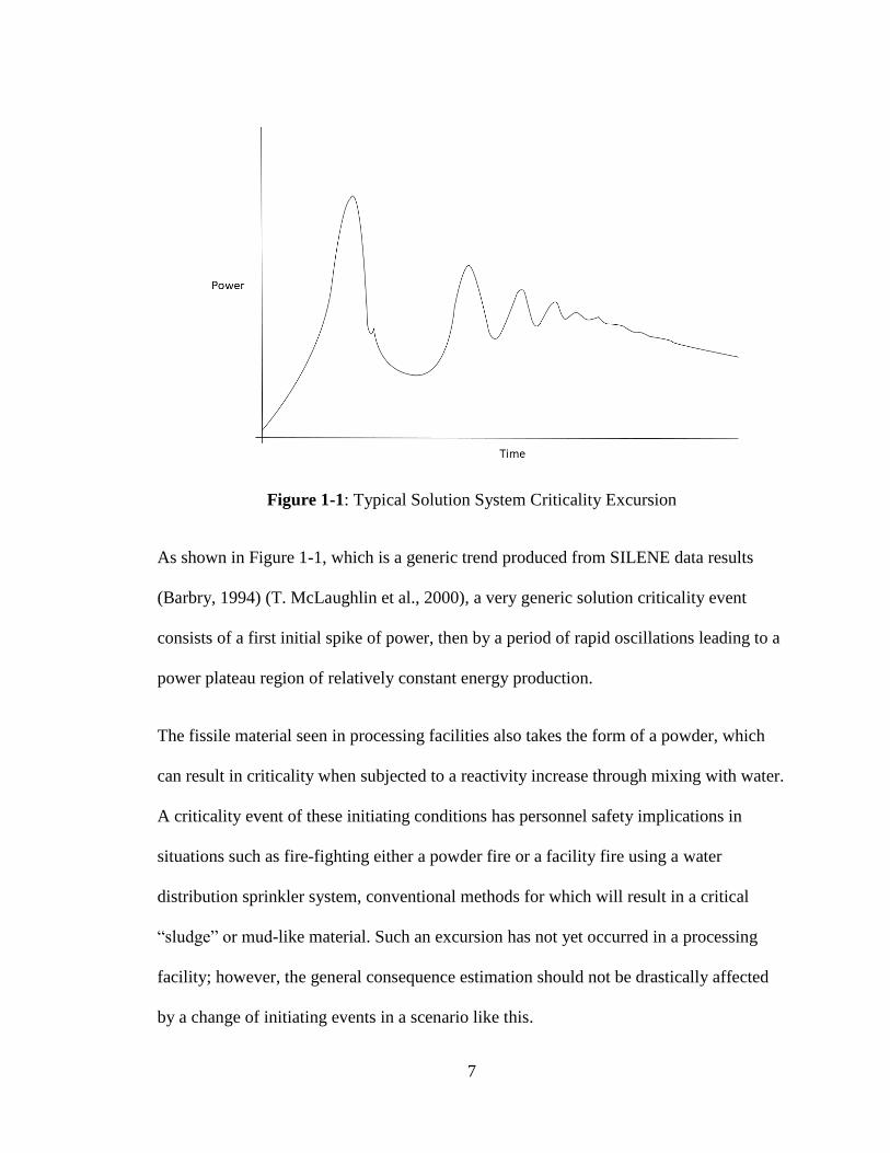
Figure 1-1: Typical Solution System Criticality Excursion
As shown in Figure 1-1, which is a generic trend produced from SILENE data results
(Barbry, 1994) (T. McLaughlin et al., 2000), a very generic solution criticality event
consists of a first initial spike of power, then by a period of rapid oscillations leading to a
power plateau region of relatively constant energy production.
The fissile material seen in processing facilities also takes the form of a powder, which
can result in criticality when subjected to a reactivity increase through mixing with water.
A criticality event of these initiating conditions has personnel safety implications in
situations such as fire-fighting either a powder fire or a facility fire using a water
distribution sprinkler system, conventional methods for which will result in a critical
“sludge” or mud-like material. Such an excursion has not yet occurred in a processing
facility; however, the general consequence estimation should not be drastically affected
by a change of initiating events in a scenario like this.

8
Open and Closed Systems
A criticality event in a solution-based system can be characterized overall by whether the
structure containing the fissile media is considered an open or a closed system. An open
system provides an easy avenue for the expulsion or removal of the fissile material from
the geometry, either by ejection from the container into the atmosphere or into a separate
container configuration of the processing system, such as a feed pipe. A closed system
allows no such avenue for material removal, and so the solution system is typically
terminated by material changes rather than by geometry changes (DOE, 1994), such as
dilution, mixing, evaporation, or human intervention.
An open system tends to be showcased by a single-pulse excursion, and is typically
rapidly terminating. The single burst induces a large pressure gradient on the solution
material, pushing it away from the system. Historical examples of this effect can be found
in the criticality accidents that occurred on July 24, 1964 at the United Nuclear Fuels
Recovery Plant in Wood River Junction, Rhode Island; as well as that which occurred on
December 10, 1968 at the Mayak Production Association near Chelyabinsk, Russia (T.
McLaughlin et al., 2000). An open system or system with connected piping generally has
a single-pulse criticality with total fissions not numbering much higher than 1x10¹⁵
fissions per liter of fissile solution in the container (Barbry, 1987).
A closed system promotes multiple criticality pulses and a longer-lasting nuclear
excursion. A historical example of a criticality event being terminated by solution boiling
can be seen in the accident that occurred at the Idaho Chemical Processing Plant on
October 16, 1959, which terminated after 15 to 20 minutes of boiling following multiple
excursions (T. McLaughlin et al., 2000). A closed system tends to have an upper bound

9
of approximately 1.6x10¹⁶ fissions generated per liter based on results from solution
criticality experiments (Barbry, 1987).
Additionally, extreme examples of criticality excursions in solution materials taking
place over an extended period of many hours can be seen in the accidents that occurred at
Hanford Works on April 7, 1662; the Novosibirsk Chemical Concentration Plant on May
15, 1997; and the JCO Fuel Fabrication Plant in Tokai-Mura, Japan on September 30,
1999 (T. McLaughlin et al., 2000). These accidents are governed by extenuating
environmental circumstances external to the intrinsic solution evolution properties. For
example, the JCO Fuel Fabrication Plant accident involved a uranyl nitrate solution that
was enclosed in a precipitation vessel and subjected to heat removal via a cooling jacket,
which allowed for an extended duration of criticality and a lengthy excursion evolution
over the course of 19 hours and 40 minutes.
General Bounds and Estimation
Solution criticality excursions are bounded by an upper energy release developed by an
integrated fission yield of 4x10¹⁹ total fissions in the case of the excursion that occurred
at the Idaho Chemical Processing Plant in October 16, 1959; and by a lower energy
release developed by an integrated fission yield of 1x10¹⁵ total fissions in the case of the
accident at Windscale Works in England on August 24, 1970. For a single pulse
excursion, the lowest pulse yield from a historical accident in a solution system is 1x10¹⁶
total fissions, which occurred at the Hanford site on April 7, 1962 as well as at Y-12 in
Oak Ridge on June 16, 1958. The highest single pulse yield from a solution accident was
approximately 2x10¹⁷ fissions from the accident at the Mayak Production Association on
January 2, 1958 (T. McLaughlin et al., 2000).

10
Within the bounds of known data, the existence of a general model for estimating the
consequences of a criticality excursion in a solution material would be useful for the
safety analysis of such a system, and having the ability to quickly estimate the
consequences of a criticality excursion could lead to more informed design choices and
procedure plans. This thesis is an attempt at both a collection of known analysis
techniques for a solution criticality system, as well as an analysis of those techniques. To
that end, a literature review consisting of readily-available relevant information was
conducted. From this literature review, empirical models developed from experimental
data were selected and analyzed for fitness to parameters from historical accidents.
Additionally, a computational model was developed and tested against known parameters
for these excursions.

11
Chapter 2 – Summary of Literature Review
To provide a more complete picture of the physics and state of solutions criticality
modeling available to the general researcher or personnel safety worker at the time of this
writing, a literature review was conducted, the results of which are included within this
section. The literature review primarily concerns the energy deposition of criticality
excursions, the methods and models used for calculation, and the historical records and
precedence for criticality excursions in both accident scenarios and experiments
conducted. Many reports and documents were sourced, the most relevant of which are
listed here.
Criticality Accidents and Studies
A Review of Criticality Accidents 2000 Revision (T. McLaughlin et al., 2000)
This 2000 report from Los Alamos National Laboratory is both a technical introduction
to the science of a criticality excursion and the evolution thereof, as well as a review of
the historical accidents that have occurred. Much of the data for the known accidents was
obtained from this document, and it was treated as the primary source of information in
the event of conflicting information such as accident fission yield, due to both its
thorough documentation and its relative modernity in reporting the information to date.
Specifically, accident geometries, fission yields, and durations were obtained from this
document, as well as the implications and damage produced by the accidents. The first
segment of this report covers processing accidents and solution excursions in detail,
while the remaining sections discuss reactor accidents and critical assembly excursions
that have occurred at various facilities in the past.

12
It should be noted that this document is considered to be the most current version of a
chain of documents pertaining to the chronicling of criticality accidents as of the time of
this writing, beginning with “A Review of Criticality Accidents” by William Stratton
(Stratton, 1967), which was later revised by David Smith (D. Smith & Stratton, 1989).
The current version includes additional information not known at the time of Smith’s
revision pertaining to one Japanese accident and 19 Russian accidents.
Process Criticality Accident Likelihoods, Consequences, and Emergency Planning
(T. P. McLaughlin, 1991)
McLaughlin describes criticality accidents in several configurations and material types,
as well as uses the evolution of CRAC experiment 19 as an example of the typical
evolution expected from a criticality excursion in a solution system. No guiding models
or analysis techniques for a solution excursion are discussed, but an argument is made for
a case-specific analysis for an incidental criticality event rather than adopting simplistic
values such as those tabulated within the document. However, tabulated values for the
expected fission yields of various systems are included for reference, and are reported
here in Table 2-1.

13
Table 2-1: Criticality Accident Fission Yields (T. P. McLaughlin, 1991)
System Description Burst Yield
(fissions)
Total Yield
(fissions)
Solutions under 100 gallons 1 × 10¹⁷ 3 × 10¹⁸
Solutions over 100 gallons 1 × 10¹⁸ 3 × 10¹⁹
Liquid/Powder 3 × 10²⁰ 3 × 10²⁰
Liquid/Metal Pieces 3 × 10¹⁸ 1 × 10¹⁹
Solid Uranium 3 × 10¹⁹ 3 × 10¹⁹
Solid Plutonium 1 × 10¹⁸ 1 × 10¹⁸
Large Storage Arrays (< Prompt
Critical) − 1 × 10¹⁹
Large Storage Array (> Prompt
Critical) 3 × 10²² 3 × 10²²
SILENE Reactor Results of Selected Typical Experiment (Barbry, 1994)
This document specifically pertains to the evaluation of data from experiments conducted
at the SILENE facilities. Much of the technical data for the SILENE reactors, including
material composition, geometry, and expected yields are contained within this document.
This document is primarily a summary and data report for the SILENE reactor
experiments, with an emphasis on developing commonalities between the conducted
experiments to develop a “typical” excursion from the solution reactor.
Review of the CRAC and SILENE Criticality Accident Studies (Barbry et al., 2009)
Barbry’s 2009 report revisits much of the information learned during the CRAC and
SILENE experimental studies conducted in France. This report showcases the evolution
of a solution excursion under experimental conditions, and reports on the neutronic
parameters such as reactivity insertion and period of evolution, as well as the thermal-
hydraulic parameters such as pressure increase and duration of evolution.
Process Criticality Accident Likelihoods, Magnitudes, and Emergency Planning – A
Focus on Solution Accidents (T. P. McLaughlin, 2003)

14
This conference paper presents an argument for the redesign of emergency planning for
criticality accidents based on the then-recent publication of previously unreported
criticality accidents, primarily those occurring in Russia. The same model as previously
covered in Barbry’s work (Barbry, 1987) is presented, further details of which can be
found in the Empirical Models section of this document.
Fission Yield Estimations
Nuclear Criticality Safety – Estimation of the Number of Fissions of a Postulated
Criticality Accident (ISO, 2011)
This document contains a tabulated summary of criticality accidents that have occurred,
which has been verified against the data present in the 2000 report of historical criticality
accidents (T. McLaughlin et al., 2000). Also contained within are details on the primary
features of experimental solution facilities, experimental metal facilities, and
experimental heterogeneous facilities. These are very basic overviews of these facilities,
and details on individual experiments performed are not given.
Many simplified formulae are also listed, including those seen in previously reviewed
documents and those contained in the Empirical Models section of this document.
Between listed boundaries on fission yields for experimental facilities and the given
simplified correlations, this document has a wealth of information for fission yield
determination, both in terms of the simple duration and volume based empirical models,
and more complicated models involving further parameters of the accident characteristics
and geometries.

15
Simplified Methods of Estimating the Results of Accidental Solution Excursions
(Tuck, 1974)
Tuck makes use of the data from six solution criticality accidents that have occurred and
from the KEWB and CRAC experiments to posit models for the characterization of
solution accidents, one of which pertains to the number of fissions in any five-second
interval for a uranium-specific solution, and one of which pertains to the total number of
fissions for both uranium and plutonium solutions. These models are shown in the
Empirical Models section of this report.
Tuck validates these models against a simplified code system named EXCUR developed
at Rocky Flats, which is used to compute the variation of power during the first spike of a
solution excursion based on calculated shutdown coefficients, as well as using data from
both the CRAC and KEWB experiments to model the evolution of an excursion.
Empirical Method for Estimating the Total Number of Fissions from Accidental
Criticality in Uranium and Plutonium Systems (Olsen, Hooper, Uotinen, & Brown,
1974)
Olsen posits several models for estimation of the accident fission yield within this
document. The first model presented is based on data from the CRAC experiments in
France, and contains an estimate for the total fission yield in the plateau region of a
criticality excursion evolution, and in the burst region. The total yield of the overall
excursion can be calculated by the summation of those two values. This model is
explored further in the Empirical Models section of this report.

16
Olsen also notes that the models contained within this document may be applied to a
plutonium system, but the predicted fission yield values will be conservatively high due
to the presence of Pu-240, which undergoes spontaneous fission. The same conservatism
should be expected for a slightly enriched uranium solution system, due to the higher
concentration of U-238.
United States Nuclear Regulatory Commission Regulatory Guides 3.33, 3.34, and
3.35 (USNRC, 1977), (USNRC, 1979a), (USNRC, 1979b)
Several US NRC Regulatory Guides were also sourced for the purposes of establishing a
reasonable estimation on how to evaluate solution criticality within a nonreactor facility.
It must be noted that at the time of this writing, these reports have been officially
withdrawn beginning in December of 1997, with the intention of being superseded by
Regulatory Guide 3.71. However, Regulatory Guide 3.71, as of Revision 2 to that
document, contains no further mention of the foundational hypothetical accident scenario
as described in these regulatory guides. As of the time of Revision 2 to Regulatory Guide
3.71, the accident scenarios are now based on information described in Appendix C of
ANSI/ANS standard number 8.23 (ANS, 2007).
The hypothetical accident described within these documents and used as an establishing
parameter for a regulatory position is based on the following stipulations:
• Ventilated cell with shielding equivalent to 5 feet of concrete of 142 pounds per
cubic foot density
• Initial burst of 1 × 10¹⁸ fissions in 0.5 seconds, followed by 47 bursts of
1.9 × 10¹⁷ fissions at ten-minute intervals for eight hours

17
• Termination by evaporation of 100 liters of a solution containing 400 grams per
liter of uranium at less than 5% enrichment
• Concentrations of fission products and transuranics in the solution corresponding
to irradiated fuel assuming 100% dilution, plus those produced within the incident
• Noble gases are assumed to be removed prior to the incident
Based on comparisons with the known parameters and evolution characteristics for
historical and experimental excursions, this hypothetical system is believed to be
unsuitable for analysis, and non-representative of a typical solution excursion system.
The incredible hypothetical accident in combination with the supersession of these
reports should be taken into account for any analysis purposes.
Airborne Release Fractions/Rates and Respirable Fractions for Nonreactor Nuclear
Facilities (DOE, 1994)
The originating document for this project was a proposed revision to Chapter 6 of this
DOE handbook. Chapter 6 specifically refers to the existence of respirable fractions and
radiological releases pertaining to criticality excursions, consisting of both metallic and
solution systems. This document details the evidence of respirable fractions and airborne
release of material from these accidents, and contains simplified data on the estimation of
fission yields from given accidents.
Model to Estimate the Maximum Fission Yield in Accidental Solution Excursions
(Barbry, 1987)

18
This document was produced by Francis Barbry from the CEA de Valduc (Valduc Center
for Nuclear Studies) in France, following his work with the CRAC and SILENE
experiments. Barbry promotes the utility of a simple model for estimation of the effective
fission yield of a criticality excursion in a solution system, and based on CRAC and
SILENE data, posits a relationship dependent on the volume of the solution and on the
duration of the excursion. This relationship is presented in more detail within the
Empirical Models section of this report.
Within this document, Barbry also posits the existence of a boiling threshold that occurs
at approximately 1 × 10¹⁶ fissions per liter. Once this value is reached within an
excursion evolution, boiling of the solution begins, which leads to a decrease in the
overall density and can contribute to criticality termination. The figure developed by
Barbry provides the accident evolution model and the boiling threshold is included in this

19
document as Figure 2-1 for reference purposes.
Figure 2-1: Specific Fission Yields in Experiments at CRAC and SILENE (Barbry,
1987)
Simplified Evaluation Models for Total Fission Number in a Criticality Accident
(Nomura & Okuno, 1995)
Nomura and Okuno develop a thermal property analysis of CRAC experiments and ten
processing accidents to showcase a reliance on solution boiling for the overall fission
yield expected from a criticality excursion in a solution system. A model for both a
boiling and for a non-boiling solution are developed that are dependent only on solution
volume, which are detailed in the Empirical Models section of this report.

20
Additionally, models for the characterization of a fuel-rod water system accident are
developed using similar liquid boiling properties, which are validated against
experimental data from SPERT, a low-enriched pressurized water reactor.
Applicability of Simplified Methods to Evaluate Consequences of Criticality
Accident Using Past Accident Data (Nakajima, 2003)
Nakajima develops a tabulated listing of criticality accidents that have occurred in
nuclear fuel processing plants known at the time of writing. This includes 13 accidents
from Russia, seven from the USA, one from the UK, and one from Japan. Using these
data, Nakajima provides a comparison between simplified fission yield correlations
established by Tuck, Olsen, Barbry, and Nomura.
Nakajima concludes that Nomura’s formula and Barbry’s formula with infinitive duration
agreed fairly well with known data for solution accidents as a function of solution
volume. Olsen’s formula and Barbry’s formula as a function of duration reproduce the
upper envelope with the exception of the Idaho Chemical Processing Plant accident in
October of 1959 and the Tokai-Mura accident in September of 1999. The conclusion is
made that because the Tokai-Mura accident underwent a solution cooling process that
produced a large amount of power for a long time, a new formula would be required that
takes this into account.
21
Excursion Modeling
A Review of the SILENE Criticality Excursions Experiments (Barbry, 1993)
This report is a fairly detailed, though non-exhaustive account of the data seen in the
SILENE experiments. The first table in the report contains first peak and total fission
values for select experiments, as well as other information such as duration, volume,
doubling time, pressure change, total potential reactivity addition, and temperature
change.
Using the maximum energies measured during the CRAC and SILENE excursions for up
to a seven dollar reactivity insertion, an empirical equation in terms of the specific total
number of fissions and the excursion duration is given, which is the same model
developed by Barbry as detailed in the Empirical Models section of this report.
Barbry reports that the volume of radiolytic gas formed during the course of a solution
excursion is proportional to the number of fissions, reaching ~1.1 × 10⁻¹³ cubic
centimeters per fission (i.e., 110 liters of gas for 1018 fissions). The threshold for the
formation of radiolysis bubbles is estimated at 1.5 × 10¹⁵ fissions per liter of fissile
solution. The solution is assumed to be brought to a boiling point at a released energy
level of about 0.33 Megajoules per liter, or ~1.1 × 10¹⁶ fissions per liter. The level of
the boiling pseudo-plateau described in the paper is marked as dependent on the amount
of excess reactivity present in the system.
Production of Void and Pressure by Fission Track Nucleation of Radiolytic Gas
Bubbles During Power Bursts in a Solution Reactor (Spiegler et al., 1962)
22
This report contains a lot of information on the development of radiolytic gas generation
models, primarily based on data from the KEWB experiments. Reactivity coefficients
and feedback models for void production in solution criticality systems are discussed
within this document, and several values for gas production coefficients are provided for
both spherical cores and cylindrical cores in the form of volume of gas produced per unit
of energy deposited into the system.
The fluid dynamics of the gas bubbles in the solution system are discussed, as well as
assumptions involving the uniform radius of radiolytic gas bubbles and that the bubbles
are in equilibrium with both the dissolved gas concentration and the solution properties.
Many of these assumptions were accounted for in the Computational Model section of
this document.
Nuclear Excursions in Aqueous Solutions of Fissile Materials (Hetrick & Smith,
1987)
This conference paper is a short summary of work performed by David Hetrick and
Adrienne Smith, a more complete picture of which can be found within Smith’s
published master’s thesis (A. Smith, 1989). This model is based on a simple axial
discretization of a cylindrical solution reactor, where the volume is governed by
equations of state derived from quasi-steady state thermodynamics related to the isobaric
and isothermal compressibility factors.
Hetrick and Smith rely on the usage of neutronics models to calculate changing reactivity
with a changing cylindrical height and diameter, and so the system is propagated via a
displacement scheme, which alters the overall feedback of the system. Additional

23
information is provided for the radiolytic gas models, the majority of the details of which
can be found in the Computational Model section of this document.
Estimating Maximum Pulse Yields for Solution Criticality Accidents (Hetrick &
McLaughlin, 1993)
Hetrick and McLaughlin present a reactivity calculation based on the Nordheim-Fuchs
model of point reactor kinetics and the inhour equation of neutron population to
determine the evolution of a solution-based criticality accident. Being a short document
from conference proceedings, little is given in the form of calculational details, but the
principles of the Nordheim-Fuchs model were used for the Computational Model section
of this document.
The Code CRITEX to Simulate Transient Criticality in Fissile Solutions (Bickley,
Mather, & Shaw, 1987)
An overview of the calculational capability of the CRITEX code is provided within this
conference paper. CRITEX as described takes a known power profile as input and relies
on numerical integration of reactivity feedback due to radiolytic gas generation and the
Doppler effect of nuclear cross-section evolution with temperature. CRITEX is also
described as allowing for the mixing of gas and averaging of temperature, as well as for
the water vapor production via boiling of the solution.
Simulation of Criticality Accident Transients in Uranyl Nitrate Solution with
COMSOL Multiphysics (Hurt, Pevey, & Angelo, 2012)

24
This conference paper by Hurt, Pevey, and Angelo describes a coupled solver using
COMSOL multiphysics models along with MCNP to allow for the adjustment of
reactivity due to temperature feedback and radiolytic gas generation effects. The
computational model is analyzed against experimental results for a 50 cent reactivity
insertion in the SILENE core.
Conclusions of Literature Review
While many empirical models have been developed based on experimental values, the
state of a Monte Carlo applicable computational modeling system useable by a safety
worker or the general public could not be directly ascertained. For the most part, such
code systems are developed as part of a contract with either specific applications in mind,
or as a general research experiment for the purposes of emulating a known power profile
to be used as an input parameter for those simulations. A code system that is able to
dynamically evolve an excursion based solely on material properties that can be
determined from the solution in use at a generic processing facility is not readily
available.

25
Chapter 3 – Estimation of Fission Yield
Several avenues of analysis for the evolution and expected yield of solution criticalities
were evaluated in the process of this work. Empirical models that have been proposed as
the results of previous work performed on experimental data were applied to known
accident scenarios, and two accurate models can be assumed to be bounding: the model
provided by Barbry being a generally accurate conservative estimate of the fission yield
and the uranium model provided by Tuck being a generally accurate under-estimation of
the fission yield.
Empirical Models
Several examples of simplified models for criticality fission yield determination can be
found in the ISO Standard 16117 (ISO, 2011). Only the models involving simple, easily
determined quantities such as volume, mass, and duration were considered useful for
analysis purposes, as it’s less likely that a processing facility or other host facility of a
fissile solution media will know quantities such as reactivity insertion rate at the time of a
criticality excursion. Most of the models described within the ISO Standard 16117 were
discarded for reasons of complexity when describing a typical solution processing
accident.
The models discussed were fit to the historical accident data, and compared for accuracy.
The accidents used in this analysis (T. McLaughlin et al., 2000) are shown in Table 3-1.

26
Table 3-1: Accidents Analyzed via Empirical Models
Location Date Chronological
Number
Fissile
Media
Approximate
Total Fission
Yield
Mayak Production
Association
3/15/1953 1 Pu 2.0 × 10¹⁷
Mayak Production
Association
4/21/1957 2 U(90) 1.0 × 10¹⁷
Mayak Production
Association
1/2/1958 3 U(90) 2.0 × 10¹⁷
Oak Ridge Y-12 Plant 6/16/1958 4 U(93) 1.3 × 10¹⁸
Los Alamos Scientific
Laboratory
12/30/1958 5 Pu 1.5 × 10¹⁷
Idaho Chemical Processing
Plant
12/30/1958 6 U(91) 4.0 × 10¹⁹
Mayak Production
Association
12/5/1960 7 Pu 2.5 × 10¹⁷
Idaho Chemical Processing
Plant
1/25/1961 8 U(90) 6.0 × 10¹⁷
Siberian Chemical
Combine, Tomsk
7/14/1961 9 U(22.6) 1.2 × 10¹⁵
Hanford Works 4/7/1962 10 Pu 8.0 × 10¹⁷
Mayak Production
Association
9/7/1962 11 Pu 2.0 × 10¹⁷
Siberian Chemical
Combine, Tomsk
1/30/1963 12 U(90) 7.9 × 10¹⁷
Siberian Chemical
Combine, Tomsk
12/2/1963 13 U(90) 1.6 × 10¹⁶
Wood River Junction,
Rhode Island
7/24/1964 14 U(93) 1.3 × 10¹⁷
Electrostal Machine
Building Plant
11/3/1965 15 U(6.5) 1.0 × 10¹⁶
Mayak Production
Association
12/16/1965 16 U(90) 5.5 × 10¹⁷
Mayak Production
Association
12/10/1968 17 Pu 1.3 × 10¹⁷
Windscale Works 8/24/1970 18 Pu 1.0 × 10¹⁵
Idaho Chemical Processing
Plant
10/17/1978 19 U(82) 2.7 × 10¹⁸
Siberian Chemical
Combine, Tomsk
12/13/1978 20 Pu metal 3.0 × 10¹⁵
Novosibirsk Chemical
Concentration Plant
5/15/1997 21 U(70) 5.5 × 10¹⁵
JCO Fuel Fabrication Plant 9/30/1999 22 U(18.8) 2.5 × 10¹⁸

27
Within this document, these accidents will be referred to by their chronological number.
It is also important to note that accident Number 21, occurring at the Novosibirsk
Chemical Concentration Plant on May 15, 1997, has an unknown volume and fissile
composition. The implication is that while accident Number 21 is a historic accident
involving solutions processing of a fissile material, it is not able to be correctly modeled
using any of the empirical methods following due to a lack of relevant information. It is
assumed that any current or future processing facility will have knowledge of the solution
volume and relevant instrumentation for determination of the excursion duration. Also of
import is that accident Number 20, occurring at the Siberian Chemical Combine in
Tomsk on December 13, 1978 is a plutonium metal ingot accident and does not involve a
solution system. Accident 20 is the only accident involving a metal system, and as such is
not included in the analysis process for these models, as other metal system accidents that
have historically occurred are either critical assemblies for experimentation or moderated
reactor systems.
The empirical formulae analyzed are primarily based upon physical parameters of the
accidents, specifically the volume of the fissile solution in liters and duration of the
excursion in seconds if known. These parameters are detailed in Table 3-2, along with the
fissile density for characterization purposes (T. McLaughlin et al., 2000). For those
accidents where the excursion duration is limited to less than one minute, a value of 10
seconds is substituted for the models that rely upon excursion duration, as this provides a
reasonable estimation of the fission yields as well as being a reasonable estimation time
for the evolution of a burst excursion (T. McLaughlin et al., 2000). Also included in
Table 3-2 is the ranking of the accident by a fission yield number in increasing order,

28
with the accidents having the largest fission yield being higher numbered than those with
a lower fission yield.
Table 3-2: Physical Parameters for Empirical Models
Accident
Number
Solution
Volume (L)
Fissile
Density (g/L)
Duration
(s)
Yield
Number
Approximate
Total Fission
Yield
1 31 26.1 < 1 min 13 2.0 × 10¹⁷
2 30 102 600 7 1.0 × 10¹⁷
3 58.4 376.7 < 1 min 12 2.0 × 10¹⁷
4 56 37.5 1200 19 1.3 × 10¹⁸
5 160 18.4 < 1 min 10 1.5 × 10¹⁷
6 800 38.6 1200 22 4.0 × 10¹⁹
7 19 44.7 6600 14 2.5 × 10¹⁷
8 40 180 180 16 6.0 × 10¹⁷
9 42.9 39.2 < 1 min 2 1.2 × 10¹⁵
10 45 28.7 135000 18 8.0 × 10¹⁷
11 80 15.8 6000 11 2.0 × 10¹⁷
12 35.5 63.9 37200 17 7.9 × 10¹⁷
13 64.8 29.8 57600 6 1.6 × 10¹⁶
14 41 50.5 5400 9 1.3 × 10¹⁷
15 100 36.5 < 1 min 5 1.0 × 10¹⁶
16 28.6 69.2 25200 15 5.5 × 10¹⁷
17 28.8 52.1 900 8 1.3 × 10¹⁷
18 40 51.8 10 1 1.0 × 10¹⁵
19 345.5 19.3 7200 21 2.7 × 10¹⁸
20 0.54 18700 < 1 min 3 3.0 × 10¹⁵
21 unknown unknown 97500 4 5.5 × 10¹⁵
22 45 69.3 70800 20 2.5 × 10¹⁸
It is also important to note that accidents 9, 13, 15, and 18 are considered general outliers
for all tested models, due to a relatively small number of fissions in comparison to values
for other accidents. The characterization of these accidents as outliers is considered to
lend conservatism to the models discussed, and relative model accuracy will be analyzed
without taking into account the reported fission yields of these accidents. For the tables of
results shown for each model, these outlier accidents will be highlighted. Because these

29
accidents have a low yield of fissions, neglecting them from analysis is considered a
conservative approach to maintaining relative accuracy for each model.
For each model analyzed, a visualization of the data both with and without the outlier
accidents specific to that model is presented. These visualizations are presented on a
semi-logarithmic plot area where the y-axis is a ratio of the calculated fission yield to the
expected fission yield. For ease of use in reading these figures, a line is drawn through
the point of perfect accuracy, or through the points where the y-axis aligns to y = 1 x 100
= 1.0, showing that all points with values above this line are overpredicted by the model
in question, and all points with values below this line are underpredicted by the model.
This allows for a rough visualization of the conservatism for each model analyzed.
The models analyzed are presented in chronological order, where the results can be seen
from Olsen’s Model (1974), Tuck’s Model (1974), Barbry’s Model (1987), and
Nomura’s Model (1995) in the following sections.
3.1.1 Olsen’s Model
Olsen, Hooper, Uotinen, and Brown developed a model of measuring both the burst and
plateau fission yield for an excursion involving a uranium or plutonium solution (Olsen et
al., 1974). The burst fissions are represented by 𝑁𝐵 and the plateau fissions are
represented as 𝑁𝑃 in Equations 3.1 and 3.2. As is the case with other models analyzed, 𝑉
is the volume of the solution in liters and 𝑡 is the duration of the excursion in seconds.
For this model, the duration of the burst yield is considered to be negligible, whereas the
full duration of the accident is used for the plateau

30
definition.
𝑁𝐵 = 2.95 × 10¹⁵ ⋅ 𝑉0.82 (3.1)
𝑁𝑃 = 3.2 × 1018 ⋅ (1 − 𝑡−0.15) (3.2)
The total fission yield 𝑁𝑓 of the excursion is then represented by the sum of the burst and
plateau yields, as shown in Equation 3.3.
𝑁𝑓 = 𝑁𝐵 + 𝑁𝑃 (3.3)
The approximate results of this model are shown in Table 3-4. Because the burst fission
yield is not known for all historical accidents, the percent difference is calculated with
respect to the total yield of the accident for comparison purposes.
The average percent yield of the total fission yield as estimated by Olsen’s model is 599
%. This shows a trend of over prediction with a high degree of conservatism with
exception to very large yields like that posed by Number 6, but is not considered to be a
particularly accurate estimation.
For comparison, graphical representations of the results of Olsen’s model are included as
Figures 3-1 and 3-2, as a ratio of the calculated fission yield to the reported fission yield
with respect to the chronological ordering of the accidents. Figures 3-3 and 3-4 contain
the data with the accidents ordered by the reported fission yield.

31
Table 3-3: Results of Olsen’s Model
Accident
Number
Burst
Percent
Difference
Plateau
Percent
Difference
Total
Percent
Difference
1 -75 634 658
2 -52 1874 1922
3 -58 634 675
4 -93 61 67
5 26 878 1005
6 -98 -94 -92
7 -86 837 851
8 -89 188 198
9 5261 122273 127634
10 -91 232 240
11 -46 1066 1119
12 -93 221 228
13 463 16036 16600
14 -52 1683 1731
15 1187 14584 15872
16 -91 354 362
17 -64 1474 1509
18 5974 93357 99431
19 -87 -12 -1
22 -97 4 6
Figure 3-1: Olsen’s Model – Chronological (With Outlier Data)
0.01
0.1
1
10
100
1000
1 4 7 10 13 16 19 22
Exp
ecte
d t
o R
epo
rted
Fis
sio
n Y
ield
Rat
io
Accident No.

32
Figure 3-2: Olsen’s Model – Chronological
Figure 3-3: Olsen’s Model – Yield-Ordered (With Outlier Data)
0.01
0.1
1
10
100
1 4 7 10 13 16 19 22
Exp
ecte
d t
o R
epo
rted
Fis
sio
n Y
ield
Rat
io
Accident No.
0.01
0.1
1
10
100
1000
1E+15 1E+16 1E+17 1E+18 1E+19
Exp
ecte
d t
o R
epo
rted
Fis
sio
n Y
ield
Rat
io
Reported Fission Yield.
33
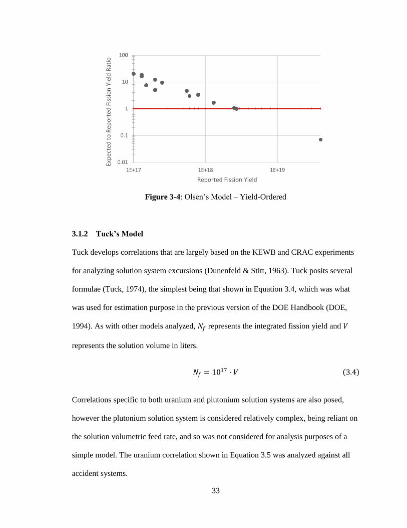
Figure 3-4: Olsen’s Model – Yield-Ordered
3.1.2 Tuck’s Model
Tuck develops correlations that are largely based on the KEWB and CRAC experiments
for analyzing solution system excursions (Dunenfeld & Stitt, 1963). Tuck posits several
formulae (Tuck, 1974), the simplest being that shown in Equation 3.4, which was what
was used for estimation purpose in the previous version of the DOE Handbook (DOE,
1994). As with other models analyzed, 𝑁𝑓 represents the integrated fission yield and 𝑉
represents the solution volume in liters.
𝑁𝑓 = 1017 ⋅ 𝑉 (3.4)
Correlations specific to both uranium and plutonium solution systems are also posed,
however the plutonium solution system is considered relatively complex, being reliant on
the solution volumetric feed rate, and so was not considered for analysis purposes of a
simple model. The uranium correlation shown in Equation 3.5 was analyzed against all
accident systems.
0.01
0.1
1
10
100
1E+17 1E+18 1E+19
Exp
ecte
d t
o R
epo
rted
Fis
sio
n Y
ield
Rat
io
Reported Fission Yield
34
𝑁𝑓 = 2.4 × 10¹⁵ ⋅ 𝑉 (3.5)
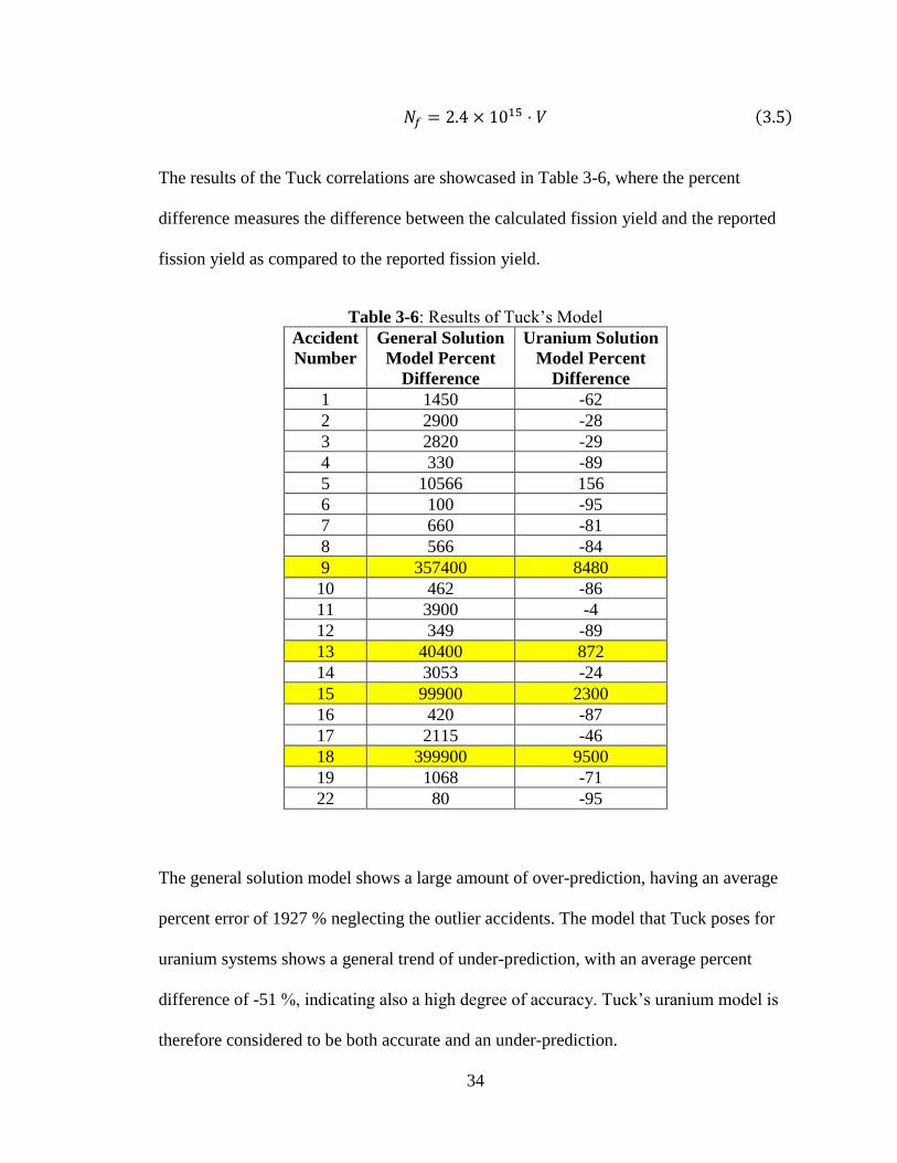
The results of the Tuck correlations are showcased in Table 3-6, where the percent
difference measures the difference between the calculated fission yield and the reported
fission yield as compared to the reported fission yield.
Table 3-6: Results of Tuck’s Model
Accident
Number
General Solution
Model Percent
Difference
Uranium Solution
Model Percent
Difference
1 1450 -62
2 2900 -28
3 2820 -29
4 330 -89
5 10566 156
6 100 -95
7 660 -81
8 566 -84
9 357400 8480
10 462 -86
11 3900 -4
12 349 -89
13 40400 872
14 3053 -24
15 99900 2300
16 420 -87
17 2115 -46
18 399900 9500
19 1068 -71
22 80 -95
The general solution model shows a large amount of over-prediction, having an average
percent error of 1927 % neglecting the outlier accidents. The model that Tuck poses for
uranium systems shows a general trend of under-prediction, with an average percent
difference of -51 %, indicating also a high degree of accuracy. Tuck’s uranium model is
therefore considered to be both accurate and an under-prediction.
35
For both of these models, accident Number 5 is shown as a general over-estimate.
Because these models are dependent on the volume of the system, and accident Number 5
is an organic plutonium solution occurring at the Los Alamos Scientific Laboratory on
December 30, 1958 with an exceptionally large fissile volume, this is considered
somewhat atypical for an accident scenario modeled in these parameters. The general
criticality excursion in a solution would be considered to occur without the use of a
multi-layered solution and induced via stirring. For such conditions, an alternative
bounding model should be considered.
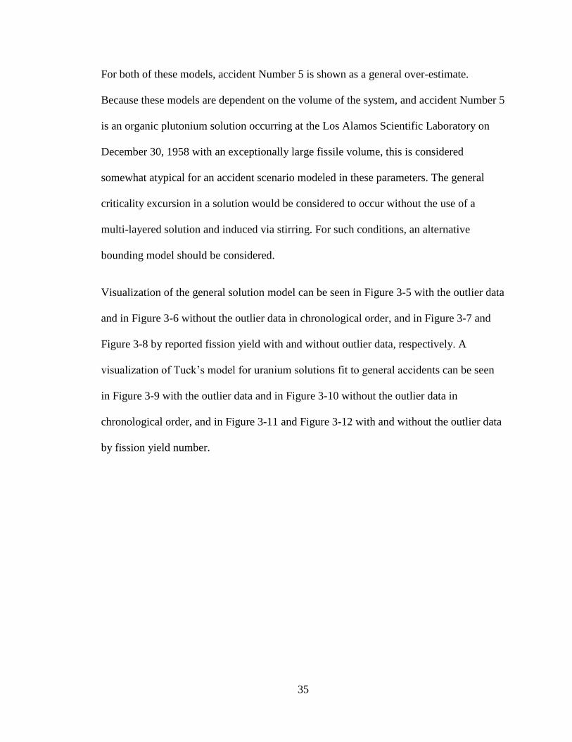
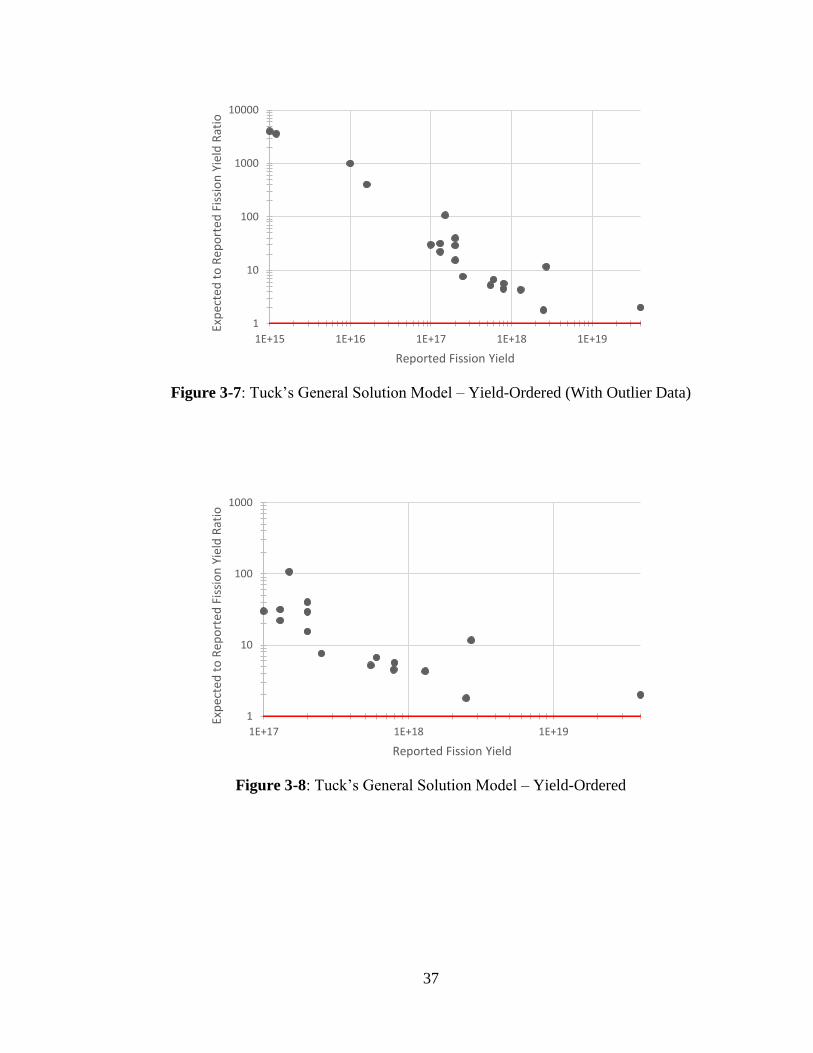
Visualization of the general solution model can be seen in Figure 3-5 with the outlier data
and in Figure 3-6 without the outlier data in chronological order, and in Figure 3-7 and
Figure 3-8 by reported fission yield with and without outlier data, respectively. A
visualization of Tuck’s model for uranium solutions fit to general accidents can be seen
in Figure 3-9 with the outlier data and in Figure 3-10 without the outlier data in
chronological order, and in Figure 3-11 and Figure 3-12 with and without the outlier data
by fission yield number.

36
Figure 3-5: Tuck’s General Solution Model – Chronological (With Outlier Data)
Figure 3-6: Tuck’s General Solution Model – Chronological
1
10
100
1000
10000
1 4 7 10 13 16 19 22
Exp
ecte
d t
o R
epo
rted
Fis
sio
n Y
ield
Rat
io
Accident No.
1
10
100
1000
1 4 7 10 13 16 19 22
Exp
ecte
d t
o R
epo
rted
Fis
sio
n Y
ield
Rat
io
Accident No.
37
Figure 3-7: Tuck’s General Solution Model – Yield-Ordered (With Outlier Data)
Figure 3-8: Tuck’s General Solution Model – Yield-Ordered
1
10
100
1000
10000
1E+15 1E+16 1E+17 1E+18 1E+19
Exp
ecte
d t
o R
epo
rted
Fis
sio
n Y
ield
Rat
io
Reported Fission Yield
1
10
100
1000
1E+17 1E+18 1E+19
Exp
ecte
d t
o R
epo
rted
Fis
sio
n Y
ield
Rat
io
Reported Fission Yield

38
Figure 3-9: Tuck’s Uranium Model – Chronological (With Outlier Data)
Figure 3-10: Tuck’s Uranium Model – Chronological
0.01
0.1
1
10
100
1 4 7 10 13 16 19 22
Exp
ecte
d t
o R
epo
rted
Fis
sio
n Y
ield
Rat
io
Accident No.
0.01
0.1
1
10
1 4 7 10 13 16 19 22
Exp
ecte
d t
o R
epo
rted
Fis
sio
n Y
ield
Rat
io
Accident No.

39
Figure 3-11: Tuck’s Uranium Model – Yield-Ordered (With Outlier Data)
Figure 3-12: Tuck’s Uranium Model – Yield-Ordered
0.01
0.1
1
10
100
1E+15 1E+16 1E+17 1E+18 1E+19
Exp
ecte
d t
o R
epo
rted
Fis
sio
n Y
ield
Rat
io
Reported Fission Yield
0.01
0.1
1
10
1E+17 1E+18 1E+19
Exp
ecte
d t
o R
epo
rted
Fis
sio
n Y
ield
Rat
io
Reported Fission Yield

40
3.1.3 Barbry’s Model
One of the four simple models analyzed was that presented in “Model to Estimate the
Maximum Fission Yield in Accidental Solution Excursions” by Francis Barbry (Barbry,
1987). Based on the CRAC and SILENE experiments, Barbry provides the empirical
model shown in Equation 3.6, where 𝑁𝑓 is the total fission yield, 𝑡 is the duration of the
excursion in seconds, and 𝑉 is the volume of the solution in liters.
𝑁𝑓(𝑡) =𝑡
3.55 × 10⁻¹⁵ + 6.38 × 10⁻¹⁷ ⋅ 𝑡⋅ 𝑉 (3.6)
This equation for the total fission yield provides the results showcased in Table 3-7.
Table 3-7: Results of Barbry’s Model
Accident
Number
Percent
Difference
1 26
2 330
3 137
4 -35
5 767
6 -70
7 18
8 -20
9 28972
10 -11
11 521
12 -29
13 6241
14 389
15 8032
16 -18
17 227
18 9451
19 81
22 -71

41
Neglecting the small-yield outlier accidents 9, 13, 15, and 18, the average percent
difference of this formula is 85 %, showing a general trend of overestimation of reported
yields, with the underestimation values being relatively small. This formula is therefore
believed to be the closest approximation of both conservatism and accuracy.
The graphical representation of Barbry’s formula applied to the chronological accidents
can be seen in Figures 3-13 and 3-14. These data are plotted on a semi-logarithmic scale
where the y-axis is the ratio of calculated fission yield to reported fission yield, such that
any values above y = 1 x 100 = 1.0, are overpredicted, and any values below 1.0 are
underpredicted. The data both with and without the outliers is shown. Barbry’s formula
ordered by the reported fission yield value is shown in Figure 3-15 and 3-16, with and
without the outliers, respectively.
Figure 3-13: Barbry’s Model – Chronological (With Outlier Data)
0.1
1
10
100
1 4 7 10 13 16 19 22
Exp
ecte
d t
o R
epo
rted
Fis
sio
n Y
ield
Rat
io
Accident No.

42
Figure 3-14: Barbry’s Model – Chronological
Figure 3-15: Barbry’s Model – Yield-Ordered (With Outlier Data)
0.1
1
10
1 4 7 10 13 16 19 22
Exp
ecte
d t
o R
epo
rted
Fis
sio
n Y
ield
Rat
io
Accident No.
0.1
1
10
100
1E+17 1E+18 1E+19
Exp
ecte
d t
o R
epo
rted
Fis
sio
n Y
ield
Rat
io
Reported Fission Yield

43
Figure 3-16: Barbry’s Model – Yield-Ordered
3.1.4 Nomura’s Model
Nomura and Okuno pose two potential models for the estimation of the total fission yield
from a solution criticality accident (Nomura & Okuno, 1995). Their models are
differentiated based on excursions that result in boiling versus excursions that do not
result in boiling. The estimation for the fission yield 𝑁𝑓 in a solution without boiling is
given by Equation 3.7, and the fission yield 𝑁𝑓 in a solution with boiling is given by
Equation 3.8, where in both cases 𝑉 represents the solution volume in liters.
𝑁𝑓 = 2.6 × 10¹⁶ ⋅ 𝑉 (3.7)
𝑁𝑓 = 6 × 10¹⁶ ⋅ 𝑉 (3.8)
These correlations give rise to the data presented in Table 3-8, where the accidents
known to involve a period of boiling are also denoted. Both the non-boiling model and
the boiling model were compared with the reported fission yield for all accidents,
however, in the interest of establishing an overall fitness of model.
0.1
1
10
1E+17 1E+18 1E+19
Exp
ecte
d t
o R
epo
rted
Fis
sio
n Y
ield
Rat
io
Reported Fission Yield

44
The average percent difference for the non-boiling model neglecting the outlier accidents
9, 13, 15, and 18 is 427 %. The boiling model without the outlier accidents provides an
average percent difference of 1116%. It should be noted that the non-boiling model
predicts closer results for the accidents that are known to involve or potentially involve
boiling, with the exception of accident number 6, which occurred at the Idaho Chemical
Processing Plant on October 16, 1959. This accident is the only accident that would fall
under the assumptions made by Nomura in the development of his model, involving
enough boiling of the solution material to cause a material loss. For simple estimation
purposes using Nomura’s methods, it is probably most effective to use the non-boiling
approximation unless boiling is explicitly noted to have occurred.
Table 3-8: Results of Nomura’s Model
Accident
Number
Involved
Boiling
Non-Boiling
Model Percent
Difference
Boiling Model
Percent
Difference
1 Maybe 303 830
2 Maybe 680 1700
3 Maybe 659 1652
4 Yes 12 158
5 No 2673 6300
6 Yes -48 20
7 No 97 356
8 No 73 300
9 No 92850 214400
10 No 46 237
11 No 940 2300
12 No 16 169
13 No 10430 24200
14 No 720 1792
15 No 25900 59900
16 Maybe 35 212
17 No 476 1229
18 No 103900 239900
19 No 203 601
22 No -53 8

45
For visualization purposes, plots of the ratio of calculated fission yield to reported fission
yield for the non-boiling model with and without the outlier accidents are included in
Figures 3-17 and 3-18 in chronological order and in Figures 3-19 and 3-20 in order of
ranking by reported fission yield; and for the boiling model in Figures 3-21 and 3-22 in
chronological order and in Figures 3-23 and 3-24 in order of ranking by the reported
fission yield. As with other models analyzed, the data points above a value of 1.0 are
overestimated by the model, and the data points below a value of 1.0 are underestimated.
Figure 3-17: Nomura’s Non-Boiling Model – Chronological (With Outlier Data)
0.1
1
10
100
1000
10000
1 4 7 10 13 16 19 22
Exp
ecte
d t
o R
epo
rted
Fis
sio
n Y
ield
Rat
io
Accident No.

46
Figure 3-18: Nomura’s Non-Boiling Model – Chronological
Figure 3-19: Nomura’s Non-Boiling Model – Yield-Ordered (With Outlier Data)
0.1
1
10
100
1 4 7 10 13 16 19 22
Exp
ecte
d t
o R
epo
rted
Fis
sio
n Y
ield
Rat
io
Accident No.
0.1
1
10
100
1000
10000
1E+15 1E+16 1E+17 1E+18 1E+19
Exp
ecte
d t
o R
epo
rted
Fis
sio
n Y
ield
Rat
io
Reported Fission Yield

47
Figure 3-20: Nomura’s Non-Boiling Model – Yield-Ordered
Figure 3-21: Nomura’s Boiling Model – Chronological (With Outlier Data)
0.1
1
10
100
1E+17 1E+18 1E+19
Exp
ecte
d t
o R
epo
rted
Fis
sio
n Y
ield
Rat
io
Reported Fission Yield
1
10
100
1000
10000
1 4 7 10 13 16 19 22
Exp
ecte
d t
o R
epo
rted
Fis
sio
n Y
ield
Rat
io
Accident No.

48
Figure 3-22: Nomura’s Boiling Model – Chronological
Figure 3-23: Nomura’s Boiling Model – Yield-Ordered (With Outlier Data)
1
10
100
1 4 7 10 13 16 19 22
Exp
ecte
d t
o R
epo
rted
Fis
sio
n Y
ield
Rat
io
Accident No.
1
10
100
1000
10000
1E+15 1E+16 1E+17 1E+18 1E+19
Exp
ecte
d t
o R
epo
rted
Fis
sio
n Y
ield
Rat
io
Reported Fission Yield

49
Figure 3-24: Nomura’s Boiling Model – Yield-Ordered
Summary of Empirical Models
The two models that have the closest accuracy are Barbry’s model and Tuck’s model for
uranium solutions. Barbry’s model has a tendency to overestimate the fission yields when
outliers are neglected, while Tuck’s uranium model has a tendency to underestimate the
fission yields when outliers are neglected. Because Barbry’s model is dependent on the
duration of the excursion involved, it is important to note that for those excursions with a
reported duration of less than one minute, typically the single-burst excursions, a value of
10 seconds was substituted for the duration term.
Combined, these two models can reasonably be assumed to be bounding estimates for a
typical accident scenario. While not a perfect estimate, the general trend as shown in
Figure 3-25 is that Barbry’s model and Tuck’s model bound the reported yields while
maintaining general accuracy. Neglecting the established outlier data of accidents 9, 13,
15, and 18 as shown in Figure 3-26, the bounded value is typically not more than one
order of magnitude away from the reported yield of the accident. On both Figure 3-27
1
10
100
1E+17 1E+18 1E+19
Exp
ecte
d t
o R
epo
rted
Fis
sio
n Y
ield
Rat
io
Reported Fission Yield

50
and Figure 3-28, the line representing unity is defined, showing where the true value of
the reported yield would occur, and providing an indication of the relative accuracy of
both bounding models.
Figure 3-25: Bounded Fission Yield Ratio – Chronological (With Outlier Data)
Figure 3-26: Bounded Fission Yield Ratio – Chronological
0.01
0.1
1
10
100
1 4 7 10 13 16 19 22
Exp
ecte
d t
o R
epo
rted
Fis
sio
n Y
ield
Rat
io
Accident No.
Barbry's Model
Tuck's Model
Unity
0.01
0.1
1
10
1 4 7 10 13 16 19 22
Exp
ecte
d t
o R
epo
rted
Fis
sio
n Y
ield
Rat
io
Accident No.
Fission Ratio - Bounded
Barbry's Model
Tuck's Model
Unity

51
When the accidents are ordered by reported fission yield, a trend of general over-
prediction to general under-prediction is made apparent, as shown in Figures 3-27 and 3-
28. While still within an order of magnitude of accuracy, the implication is that for
excursions with a larger predicted fission yield, the bounding correlations should be
assumed to be less conservative than for excursions or accidents with smaller predicted
fission yields. The scale change that occurs on each subsequent set of figures should be
noted, as the outlier accidents being neglected does increase the overall accuracy of the
models involved.
Figure 3-27: Bounded Fission Yield Ratio – Yield-Ordered (With Outlier Data)
0.01
0.1
1
10
100
1E+15 1E+16 1E+17 1E+18 1E+19
Exp
ecte
d t
o R
epo
rted
Fis
sio
n Y
ield
Rat
io
Reported Fission Yield
Barbry's Model
Tuck's Model
Unity

52
Figure 3-28: Bounded Fission Yield Ratio – Yield-Ordered
This is considered to be a reasonable bounding approximation for a typical solution
accident at a processing facility, as these correlations are not dependent on any data other
than solution volume and the excursion duration, which should be parameters easily
determined for most situations. If a conservative estimate is required, Barbry’s model
should serve as a reasonable approximation without sacrificing accuracy. Note that the
volumes analyzed ranged from 19 liters to 800 liters and the durations from 10 seconds to
37.5 hours. For more accurate assessments specific to a facility or for a situation where
uncommon features or elements may impact a criticality excursion that occurs, a full
criticality safety evaluation should be performed for the site in question.
0.01
0.1
1
10
1E+17 1E+18 1E+19Ex
pec
ted
to
Rep
ort
ed F
issi
on
Yie
ld R
atio
Reported Fission Yield
Barbry's Model
Tuck's Model
Unity

53
Chapter 4 – Computational Model
A computational model was developed to simulate the evolution of the initial spike in a
criticality excursion in a solution system. This model utilizes both a time and volumetric
discretization approach, and makes use of Python 3.6.3 and the SERPENT 1.1.7 Monte
Carlo particle transport code with a specific focus on volumetric expansion as a
termination effect. This computational model uses various correlations and empirical
equations of state to evolve the solution system between neutronics calculations
performed by SERPENT, resulting in a series of input files and output files written that
can be used for analysis purposes.
The evolution of a criticality excursion is typically considered to have a large initial burst
of fissions, followed by some series of re-criticality excursions and a plateau region. This
is largely dependent on whether the solution is an open or closed system.
An open solution system will have a large initial fission spike that shifts the material and
results in an overall negative reactivity insertion due to the density decrease. Following
that, the solution is either splashed out as a termination effect or falls back into the
container for a re-criticality event, eventually stabilizing in density for the plateau region
and leading to boiling and radiolytic gas generation.
A closed solution system is considered to have an extended criticality punctuated by
reactivity changes caused by ripples or waves in the solution due to splashing effects.
This configuration is likely to result in boiling unless an avenue is provided for solution
ejection to termination (i.e., into a pipe system or drain).

54
Both an open system and a closed system will have a large burst excursion or fission
spike in the initial moments of the reaction, where a large number of fissions occur over a
small period of time. An attempt was made at modeling this event using the SERPENT
Monte Carlo program (Leppänen, Pusa, Viitanen, Valtavirta, & Kaltiasenaho, 2015), as
well as the Python programming language, version 3.6.3.
An object-oriented approach was taken in Python, where the volumetric regions of a
cylindrical solution material were discretized into both radial and axial components, and
the neutronics parameters of the event are obtained from SERPENT. Using SERPENT
flux tallies for each discretized volume, a neutron flux profile is obtained and used for
subsequent thermal calculations.
Calculation Details
A large amount of work was performed by Adrienne Bobbette Smith in her 1989 thesis
for the University of Arizona, “Nuclear Excursions in Aqueous Solutions of Fissile
Materials” (A. Smith, 1989). Smith’s work formed the basis of the modeling technique
used herein, and was expanded upon and modified for this work. Smith’s model was
constructed for use with the DARE P Continuous System Simulation Language
developed at the University of Arizona, a compiler for which is at present difficult to
find, so the analysis that follows is an attempt at modernization of both the model and a
means to execute the model on what is considered a modern and relatively open
computational platform as of the time of this writing. If it is desired to faithfully
reproduce the work found in Smith’s original thesis, the DARE P language was found to
be related to various other analog system simulation languages that have fallen out of
general use (Korn, 1989).

55
For the constructed simulation, four core Python modules were constructed, with the
titles “transientmodel.py”, “tm_constants.py”, “tm_material.py”, and “tm_fileops.py”.
The driver script file that contains the main function is transientmodel.py, and so this is
what would be executed while running the program. The global calculational parameters
are contained within tm_constants.py, and so this file is effectively the settings for the
program that get imported into the other modules. The framework for volumetric
discretizations is contained within tm_material.py, and so all evolution of each individual
system occurs within this file. The file tm_fileops.py contains the interface with
SERPENT by means of input and output files, as well as the methods for appending to an
output file. A general flowchart of the program structure can be seen in Figure 4-1.
Figure 4-1: Computational Model Flowchart
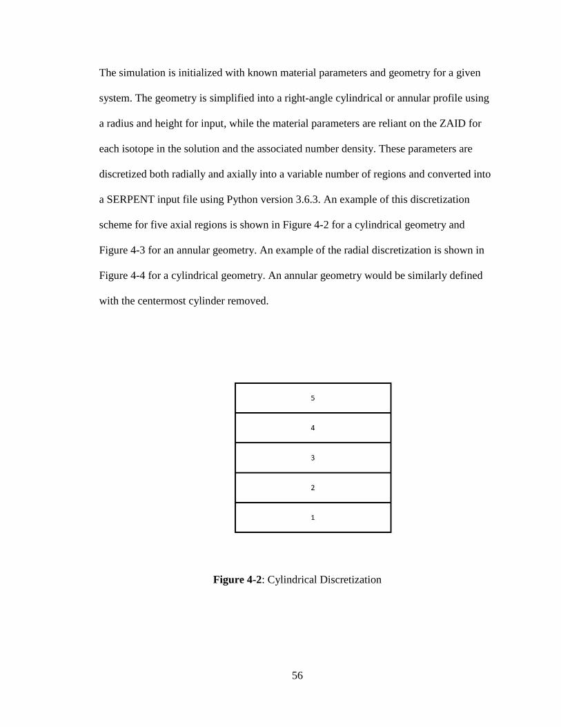
56
The simulation is initialized with known material parameters and geometry for a given
system. The geometry is simplified into a right-angle cylindrical or annular profile using
a radius and height for input, while the material parameters are reliant on the ZAID for
each isotope in the solution and the associated number density. These parameters are
discretized both radially and axially into a variable number of regions and converted into
a SERPENT input file using Python version 3.6.3. An example of this discretization
scheme for five axial regions is shown in Figure 4-2 for a cylindrical geometry and
Figure 4-3 for an annular geometry. An example of the radial discretization is shown in
Figure 4-4 for a cylindrical geometry. An annular geometry would be similarly defined
with the centermost cylinder removed.
Figure 4-2: Cylindrical Discretization
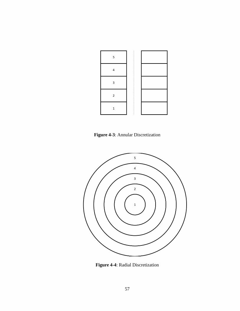
57
Figure 4-3: Annular Discretization
Figure 4-4: Radial Discretization

58
After developing an initial profile of volumetric discretization based on the framework
contained in tm_material.py, the main method will then call the SERPENT 1.1.7 program
using GNU Bash version 4.3.11 on the Linux Subsystem for Windows environment.
Small modifications would need to be made to this portion of the program for an
alternative environment or operating system to be used, but such modifications are not
out of the question, and should be fairly straightforward to implement.
SERPENT performs Monte Carlo neutronics calculations to search for a multiplication
eigenvalue 𝑘𝑒𝑓𝑓 (Leppänen et al., 2015), and prints an output file containing various
parameters and calculational results. Of import in these results are the neutron lifetime 𝑙,
the multiplication value 𝑘𝑒𝑓𝑓, and the average number of neutrons emitted per fission �̅�.
Note that SERPENT calculates both an “implicit” and an “analog” value for 𝑘𝑒𝑓𝑓 and 𝑙,
where the implicit value is defined for the given universe and the analog value is defined
for the whole geometry. Based on the structure of the generic SERPENT input file that
was used, the analog value was selected for these parameters.
Volumetric neutron tallies are also given as parameters to the SERPENT program for
each material in the input file, and those tallies are read from an output file and used as a
representation for the number of fissions and the general flux profile within the system.
Detector responses in SERPENT are normalized to a full-geometry detector count,
resulting in a fractional fission profile for the system. An initiating integrated system
power is chosen for the excursion in units of fissions per second, generally of a high
magnitude to facilitate the expansion of the material, such that Monte Carlo calculations
do not take up much time in the linear evolution period of a solution excursion.

59
From the neutron profile obtained from SERPENT, the true number of fissions 𝑁𝑖 in each
volume segment 𝑖 is calculated by the use of Equation 4.1, where 𝑓𝑖 is the fraction of total
fission events that occur in volume segment 𝑖, 𝑊 is the total power production of the
system in units of fissions per second, and Δ𝑡 is the discretized duration in time in units
of seconds.
𝑁𝑖 = 𝑊 ⋅ 𝑓𝑖 ⋅ Δ𝑡 (4.1)
The assumption is made that on average, 180 MeV of energy is deposited into the
solution material per fission event, which allows for an equation of state to be used. Prior
to that, however, an acceleration is calculated for the center of mass of each volumetric
discretization to allow for a volumetric expansion. The center of mass acceleration is
calculated simply by means of a pressure balance, accounting for gravitational effects on
the material producing both hydrostatic pressure and a negative acceleration. This
calculation is shown in Equation 4.2, where 𝐶𝑖 is the height of the center of mass of
volume element 𝑖 in the z-direction of a cylindrical coordinate system, 𝐴𝑖 is the cross-
sectional area of the base of volume element 𝑖, 𝑃𝑖 is the gauge pressure at the top of
volume element 𝑖, and 𝑚𝑖 is the mass of the solution contained within volume element 𝑖.
𝑑2𝐶𝑖
𝑑𝑡2=
𝐴𝑖
𝑚𝑖⋅ (𝑃𝑖−1 − 𝑃𝑖) − Λ ⋅ 𝑣𝐶𝑂𝑀𝑖
− 𝑔 (4.2)
For these calculations, the pressure at the top of the cylindrical material is assumed to be
at an atmospheric gauge pressure of zero, and the initial pressures are calculated based on
simple gravitational acceleration and solution density throughout the material. An
example of this is shown in Equation 4.3, where 𝑃(𝑖−1)0 is the initial pressure at the

60
bottom of element 𝑖 due to the hydrostatic effects of gravity, 𝑃(𝑖)0 is the pressure at the
top of volume element 𝑖, which is assumed to be zero at the top-most element, 𝑔 is the
gravitational acceleration acting on the fluid, 𝑑 is the fluid density, which is constant over
the initial state of the solution, and ℎ𝑖 is the height of solution present on top of volume
element 𝑖. The center of mass is assumed to be the geometric center of the volume
element 𝑖 in question, because the density is assumed to be consistent throughout the
element. All elements initially start with the same density, while the mass would be
determined from the volume of the element. All axial elements of the same radial
discretization are considered to have the same mass, as the units are discretized evenly
based on length.
𝑃(𝑖−1)0= 𝑃(𝑖)0
+ 𝑑 ⋅ 𝑔 ⋅ ℎ𝑖 (4.3)
The Λ in Equation 4.2 represents a dissipation term, which is a factor that attempts to
account for the damping effect of friction and deformation of the walls of the tank (A.
Smith, 1989). This value is on the order of 3000-4400 per second. This is applied only for
the volume regions in the outermost radial discretizations, where the fluid would be in
contact with the boundaries of the tank. This term is multiplied by the current velocity of
the center of mass of volume region 𝑖, represented as 𝑣𝐶𝑂𝑀𝑖, which is initially zero at the
start of the excursion. The value for gravitational acceleration constant 𝑔 in the negative
z-direction of a cylindrical coordinate system is assumed to be 9.80665 meters per second
squared.
Each value for the center of mass acceleration is then used to expand the solution axially
from the bottom upwards. It is assumed that the container the solution is in does not
61
expand in the radial direction or in the negative z-direction and fixes the solution
geometrically. That is, for any open system or closed system with a venting opening, the
pressure at the top of the solution is always atmospheric, which allows for an easier
vector for expansion in the positive z-direction as the path of least resistance, and
splashing and expansion in the radial directions is completely negated by the material of
the solution container.
The solution is expanded upwards starting from the lowest base because the base of the
container is a fixed point in space, at a z-coordinate of zero in a cylindrical coordinate
system. This allows for the acceleration to be accounted for in this region, and the height
adjusted accordingly based on the principle that the center of mass in a volume element is
the geometric center of that volume element, as each volume element is assumed to have
a uniform density within itself during the course of the expansion process. The height of
the volume element is then adjusted, and the volume element immediately above is
shifted upwards before the center of mass acceleration is applied. This shifting technique
prevents the material from being “locked” in space about the initial center of mass and
allows for a natural expansion vector, as the surrounding solution pressures are the
primary drivers of volumetric expansion.
The principles of an incompressible fluid are applied here to prevent the system from
being solely driven by pressure in terms of compression and expansion. If the volume
element would be compressed to such a point that the fluid density is below the original
starting density of that volume element, then the compression is simply limited to the
original volume of the element, and the velocity of the center of mass at that point in time
is set to be zero. This prevents a solution from compressing to unphysical quantities due

62
to a pressure balance equation, and the incompressibility of the aqueous fluid is
preserved. For an expanding fluid, the density is adjusted, as it is assumed that the fluid is
being intermixed with atmosphere via a splashing or aerosolization effect to fill the voids
while preserving mass.
The center of mass is adjusted based on classical kinematics involving acceleration,
where 𝑣𝐶𝑂𝑀𝑖𝑛𝑖𝑡𝑖𝑎𝑙 is the initial center of mass velocity at the current time-step, and
𝑣𝐶𝑂𝑀𝑓𝑖𝑛𝑎𝑙 is the final center of mass velocity for that time-step, which can be calculated
as in Equation 4.4, where 𝐶 is the position of the center of mass on the z-axis from the
bottom of the solution container at a z-coordinate of zero, and Δ𝑡 is the discretized time-
step of the overall excursion evolution.
𝑣𝐶𝑂𝑀𝑓𝑖𝑛𝑎𝑙= 𝑣𝐶𝑂𝑀𝑖𝑛𝑖𝑡𝑖𝑎𝑙
+𝑑2𝐶
𝑑𝑡2⋅ Δ𝑡 (4.4)
This allows for a change in the center of mass position Δ𝐶 to be calculated as shown in
Equation 4.5, where the new position of the center of mass 𝐶 can then be calculated
simply by adding the value for Δ𝐶.
Δ𝐶 = 𝑣𝐶𝑂𝑀𝑖𝑛𝑖𝑡𝑖𝑎𝑙⋅ Δ𝑡 +
1
2⋅
𝑑2𝐶
𝑑𝑡2⋅ Δ𝑡2 (4.5)
Knowing the center of mass position and the position of the bottom of the volume
element accounting for the shift from acceleration of the elements below allows for the
position of the height of the element to be calculated, which is then used for the shift of
the elements above this volume element. The height 𝐻𝑖 of the volume element 𝑖 is
calculated as shown in Equation 4.6, where 𝐵𝑖 is the base height of volume element 𝑖.

63
Both the height of the top of the element 𝐻 and the height of the base of the element 𝐵
are measured from the base of the total solution system at the z-coordinate of zero. As
previously stated, the assumption made here is that each volume element 𝑖 has a constant
density, and so the center of mass of the volume element is always in the geometric
center of that volume element.
𝐻𝑖 = 𝐵𝑖 + 2 ⋅ (𝐶𝑖 − 𝐵𝑖) (4.6)
After expanding the volume based on current pressures, but before executing neutronic
calculations for the next time-step, an equation of state is applied to each volume
element. The isobaric expansion coefficient 𝛽0 and the isothermal compressibility 𝜅0 for
the pure liquid is obtained using a Python wrapper for the CoolProp library (Bell,
Wronski, Quoilin, & Lemort, 2014) assuming that the intensive thermophysical
properties for the aqueous solution material do not diverge drastically from those of water
(Barbry, 1994).
The isobaric expansion coefficient and isothermal compressibility for the pure liquid are
adjusted to account for the addition of radiological gas produced by the excursion as
shown in Equations 4.7 and 4.8 to get an overall isobaric expansion coefficient 𝛽 and an
overall isothermal compressibility 𝜅. The volume element is considered to produce
radiological gas if the number of fissions per liter exceeds a threshold value. The value
used for this threshold is 1.5 x 10¹⁵ fissions per liter, a value obtained from experimental
analysis of the SILENE experiments (Barbry, 1993) that does not diverge drastically
from previous work performed (Spiegler et al., 1962). So long as the volumetric fission
yield does not exceed this value, it is assumed that the radiolytic gas produced is of a low
64
enough density that chemical recombination effects of the gas exceed the gaseous
nucleation effects, preventing vapor bubbles from forming. Pertaining to the radiological
gas production within the system, the surface tension of the liquid is represented by 𝜎,
and is also obtained from the CoolProp calculational reference library (Bell et al., 2014).
The volume fraction of radiologic gas in the system is represented as 𝑓𝑒. The radius of the
radiolytic gas bubbles that are nucleated 𝑟𝑏 is assumed to be a constant value of 5 x 10⁻⁸
meters (Kimpland, 1993), independent of temperature, liquid pressure, surface tension,
dissolved gas concentration, and uranium concentration (Spiegler et al., 1962).
𝜅 = 𝜅0 ⋅ (1 − 𝑓𝑒) +𝑓𝑒
𝑃 +4 ⋅ 𝜎3 ⋅ 𝑟𝑏
(4.7)
𝛽 = 𝛽0 ⋅ (1 − 𝑓𝑒) +𝑓𝑒
𝑇⋅
(𝑃 +2 ⋅ 𝜎
𝑟𝑏)
(𝑃 +4 ⋅ 𝜎3 ⋅ 𝑟𝑏
)(4.8)
The volume fraction of radiolytic gas in the system is calculated as derived from the ideal
gas law involving temperature 𝑇, pressure 𝑃, and volume 𝑉 (A. Smith, 1989); as shown
in Equation 4.9. This equation is dependent on the assumption that the mass fraction of
gas in the system is a function only of the mass of the solution present, and that the
solution mass does not appreciably deplete by means of radiolytic gas production. That
is, even with a relatively higher-order integrated fission yield of 1 x 10¹⁹ total fissions for
a solution system, any alteration to the mass content of the overall solution present is
almost completely negligible. Therefore, the mass of the solution times the mass fraction
of gas to the overall solution results in only the term for the mass of the gas present in the
solution, 𝑚𝑔𝑎𝑠. Note that 𝑅𝑔𝑎𝑠 is the representation for the specific ideal gas constant for

65
the hydrogen-1 nuclide, which is the only gas being accounted for in an aqueous nitrate
system. This is due to the effects of a fast transient excursion, where diffusion of gas
from the fuel to nucleation sites is too slow for surface nucleation to be effective, so the
hydrogen gas concentration increases until the solution effectively behaves like a gas
bubble chamber at a critical concentration of gas production (Spiegler et al., 1962).
𝑓𝑒 =𝑚𝑔𝑎𝑠 ⋅ 𝑅𝑔𝑎𝑠 ⋅ 𝑇
𝑉 ⋅ (𝑃 +2 ⋅ 𝜎
𝑟𝑏)
(4.9)
The fission gas produced once the reaction reaches the given threshold value of 1.5 x
1015fissions per liter (Barbry, 1993) is dependent upon a radiolytic yield term for the gas
in question, in this case hydrogen. The yield term is a function of energy deposition via
fission events, and based on analysis of the KEWB and CRAC experiments (Forehand,
1981) is considered to be approximated as 2.3 x 10⁻⁴ kilograms of H2 gas produced per
MegaJoule of energy deposited into the system.
The temperature change Δ𝑇 of the volume element is then calculated as shown in
Equation 4.10, where the mass-specific constant volume heat capacity 𝑐𝑣 of the aqueous
solution is again assumed to not diverge drastically from the value for water and therefore
is obtained from the CoolProp library (Bell et al., 2014). Because the heat capacity is
determined as an intensive property of the fluid, the mass of the solution present 𝑚 must
be accounted for. The amount of energy deposited into the solution contained in the
volume element in question by means of fission events within time-step of length Δ𝑡 is
represented as Δ𝐸. The volume difference through pressure-based expansion as
previously calculated for this time-step is represented as Δ𝑉.

66
Δ𝑇 =1
𝑐𝑣 ⋅ 𝑚⋅ (Δ𝐸 −
𝛽 ⋅ 𝑇
𝜅⋅ Δ𝑉) (4.10)
Knowing the change in temperature and the change in volume, the compressibility
equations can be used to calculate the change in the average pressure of the volume
element, as shown in Equation 4.11, which is reliant on the current volume of the
element.
Δ𝑃 =𝛽
𝜅⋅ Δ𝑇 −
1
𝜅 ⋅ 𝑉⋅ Δ𝑉 (4.11)
It is important to note that these equations have negative terms as a function of the
change in volume, Δ𝑉. An account is made for this by performing the calculation without
the inclusion of these negative terms to get an overall pressure at each discretized time
step, and then expanding the solution volume element based on that pressure. After
expansion, the temperature and pressure are then reduced based on the Δ𝑉 term in the
equation, which prevents any unrealistic pressure accumulation by not taking the effects
of volumetric expansion into account. These volumetric terms are a limiting factor on the
expansion of the material, and the effect of taking them into account is realized in
subsequent time-steps of the calculation.
The pressure change calculated is applied to the volume element as a change to the
average pressure of that element. For each element, the pressure is assumed to be linearly
defined according to a hydrostatic model as in the initial conditions of the solution, such
that only gravitational effects and height affect the pressure as shown in Equation 4.3,
where ℎ𝑖 is the distance measured in the negative z-direction on a cylindrical coordinate
axis of solution existing on top of the point of measurement 𝑖.

67
Because the average pressure of the volume element is at the center of mass position due
to the constant density assumption for each volume element, the pressure at the top of the
volume element is linearized with the average pressure to obtain the pressure at the
bottom of the volume element. For reference, the pressure calculations are shown in
Equation 4.12, from which Equation 4.13 may be determined through simple algebra,
where 𝑃�̅� represents the average pressure, or the pressure at the point of the center of
mass, of volume element 𝑖.
𝑃�̅� =(𝑃𝑖 + 𝑃𝑖−1)
2(4.12)
𝑃𝑖−1 = 2 ⋅ 𝑃�̅� − 𝑃𝑖 (4.13)
Because the top of the solution system is known to be at a fixed atmospheric pressure, the
bottom-most or maximum pressure calculations begin from the top of the solution system
discretizations, contrary to the volumetric expansion calculations, which begin from the
bottom of the solution system discretizations. A continuity of pressure is maintained by
asserting that the top-most pressure value of one element is equivalent to the bottom-most
pressure value of the element directly above it.
Once the solution volume elements are expanded and have their intensive thermophysical
properties and state values updated, the neutronic calculations are run for the next time-
step. At each time-step calculation, an output file for the calculation is appended to with
values for the current time elapsed, the number of fissions that occurred during that time-
step, the total integrated number of fissions at that point in time, the maximum
temperature within the solution, and neutronics parameters including the neutron lifetime,

68
the effective multiplication factor 𝑘𝑒𝑓𝑓, and the uncertainty 𝜎𝑒𝑓𝑓 associated with the
effective multiplication factor in the form of 𝑘𝑒𝑓𝑓 + 2 ⋅ 𝜎𝑒𝑓𝑓, which provides a
conservative 95% confidence interval to the multiplication factor.
Using the neutronic parameters obtained from SERPENT Monte Carlo calculations, the
total system power at the next time-step 𝑊 is then propagated based on a point-reactor
kinetics model that relies on the total system power at the previous time-step 𝑊0 as
shown in Equation 4.14, where 𝑘𝑒𝑓𝑓 is the effective multiplication factor, Λ𝑝 is the
prompt neutron generation time, 𝛽𝑑 is the delayed neutron production fraction, and Δ𝑡 is
the time-step duration. This propagation equation is based on the principles of a prompt
supercriticality event, where the evolution of the accident happens on a small time-scale.
The prompt neutron generation time Λ𝑝 is given by simply dividing the prompt neutron
lifetime given by the SERPENT Monte Carlo calculations by the effective multiplication
factor. The expression for reactivity 𝜌 is defined in Equation 4.15.
𝑊 = 𝑊0 ⋅ exp (𝜌 − βd
Λp⋅ Δ𝑡) (4.14)
𝜌 =𝑘𝑒𝑓𝑓 − 1
𝑘𝑒𝑓𝑓
(4.15)
As detailed, the overall system power in fissions per second is then assigned to a power
in each discretized volume element based on the fission fraction profile obtained from the
SERPENT tallies, and the calculation then propagates until the multiplication factor falls
below a determined number and the solution is assumed to be subcritical. The limit on the
multiplication factor 𝑘𝑒𝑓𝑓 for termination used in this thesis is 0.98, which is conservative
69
given the probabilistic nature of Monte Carlo calculations, but other values may be
substituted fairly easily.
The multiplication factor is governed both by material properties and by geometry
properties. After each evolution of the solution system, the new volumes are converted
into a SERPENT-compatible input file format using the surface and universe-based
system of establishing geometry (Leppänen et al., 2015).
The material properties are also adjusted at each time-step analyzed. The density of the
system is recalculated for each discretized volume element based on the assumption that
there are not enough fissions in each volume element occurring during an excursion to
reasonably affect the mass of the system. So, the initial mass of that volume element is
divided by the new volume after the expansion stage, which results in a new density. Due
to the conservation of mass principles of recalculating a new density upon expansion, the
homogenized voids in the solution are considered to be a result of marginal aerosolization
due to the splashing effect of expansion. This phenomenon likely has additional
considerations to take into account in terms of interactions with the physical properties of
the expansion mechanism that are outside the scope of this simple model.
Material properties are also dependent on the temperature of the material, which affects
the neutronic cross-sections for absorption and scattering, which can in turn drastically
influence the value for the multiplication factor. SERPENT utilizes a temperature-
interpolation method for adjusting cross-sections based on temperature, where the
libraries for temperature of each nuclide are adjusted every 300 degrees Celsius starting
from a value of 300 Kelvin. The cross-section library to use for each material is

70
determined by rounding the temperature value of each volume element to the nearest
applicable SERPENT cross-section library specific to that temperature. The thermal
scattering kernel for light water is also updated, as hydrogen to oxygen bonds affect the
neutron scattering cross-section in aqueous solutions. This kernel is assigned to each
material and is adjusted every 50 degrees Celsius starting from 300 Kelvin. The thermal
scattering kernel for light water of each volume element is adjusted by rounding the
temperature of that volume element to the closest appropriate value of a SERPENT
thermal scattering kernel library to use for that element.
With respect to the initial event, the initial energy deposition of the system due to the
excursion fission events prior to the point of the calculational starting power is calculated.
This is based on the assumption that the energy build-up of the system during the
beginning stages of evolution of the excursion does not appreciably contribute to a
pressure gradient driven acceleration prior to the starting power value, to the extent of
being negligible with respect to hydrostatic pressure. The overall energy deposition is
applied to the temperature value of each volumetric element under the assumption that
the prior geometric fission profile during the initial stages of the first-spike excursion
evolution does not differ in an appreciable way from the initial geometric fission profile
provided by the first Monte Carlo calculation performed by SERPENT.
The initial energy deposition to the system is calculated by integrating the power
equation with respect to time. Because a Nordheim-Fuchs model is used for the power
evolution, the evolution period 𝜏 is calculated as seen in Equation 4.16 based on the
initial neutronic parameters determined from the first SERPENT calculation.

71
𝜏 =Λ𝑝
(𝜌 − 𝛽𝑑)(4.16)
Knowing the period, the estimated time of evolution of the excursion 𝑇𝑒 in seconds from
a point of power of 1 fission per second can be calculated as in Equation 4.17, where the
initial power was selected as an appreciably low value, seeing as how the Nordheim-
Fuchs model asymptotically approaches zero, and a limit must be set on the excursion
evolution time. The value for 𝑃𝑐𝑎𝑙𝑐 in this equation is the power at which the evolution
calculations begin at a computational time of zero.
𝑇𝑒 = ln (𝑃𝑐𝑎𝑙𝑐
1) ⋅ 𝜏 (4.17)
This allows for the number of fissions 𝑁𝑒 that occurred during the excursion prior to the
initiation of the calculations to be determined from Equation 4.18, again assuming that
the initial power of the event was 1 fission per second.
𝑁𝑒 = exp (𝑇𝑒
𝜏− 1) ⋅ 1 (4.18)
Additionally, this model was set to match experimental parameters via the inclusion of an
inertial pressure gradient damping factor of 0.1, with Kimpland and Smith stating that the
acceleration of the center of mass caused by the Newtonian pressure balance on the
system should be reduced by an order of magnitude to account for various inadequacies
in the model (Hetrick & Smith, 1987). These inadequacies are considered to be a result of
the crude pressure gradient in a single region and of the preselected input power shapes
used for Smith’s model (A. Smith, 1989). The results of the use of this factor are included
in this report, but despite not using a pre-selected power shape for the reaction, the model

72
was still evolving faster than experimental results. This could be due to the initial
complaint about the simplified pressure gradient in a single region, as well as any other
material factors caused by turbulence within the solution, atmosphere mixing with the
solution to cause an appreciable density decrease, and an insufficient discretization for a
potentially unstable model as the thermodynamic evolution equations are applied in an
explicit fashion of dependence on previously calculated values, rather than in an implicit
numerical fashion. Also note that because the system is assumed to be physically
bounded by the container it is in, there are no interactions between elements in the radial
discretization regions being taken into account with the exception of a fission power
profile, with all expansion assumed to be taking place in the positive z-direction of a
cylindrical coordinate system.
Computational Constants and Settings
The use and settings for the Python calculational tool including many of the equation
constants are primarily contained within the file tm_constants.py. For general use, the
constants of the defined models are listed in Table 4-1 organized by the discretization
parameters (parameters that are used for the overall discretization of both the volume and
the time-step size), the calculational parameters (parameters used for the equation of state
and radiolytic production), and neutronic parameters (parameters used as input settings
for the SERPENT calculation pertaining to neutronics data).
All modules of the Python 3.6.3 code written for this project make an attempt to follow
the PEP 8 style guide for Python code (van Rossum, Warsaw, & Coghlan, 2001), and
should be easy to reference and utilize. The full code listing is included in this thesis in
the form of Appendices, along with specific implementation details and general

73
instructions for modification and use. Any person with a working version of the
SERPENT executable should be able to easily modify this code for their own personal
use for any given cylindrical system of fissionable material under a variable value for
axial, radial, and time discretization size.
Table 4-1: Constants of Computational Model
Parameter Variable – Code
Representation
Value Units
Discretization Parameters
Constant time-step
size as a magnitude:
power of 10𝑥
TIMESTEP_MAGNITUDE -4 s
Number of axial
discretizations NUM_AXIAL 5 None
Number of radial
discretizations NUM_RADIAL 3 None
Calculational Parameters
Initiating power level
at which to start the
calculations
INIT_POWER 1 × 10¹⁸ fissions
s
Threshold for
production of
radiolytic gas
THRESHOLD 1.5 × 10¹⁵ fissions
l
Radius of radiolytic
gas bubbles upon
nucleation
RAD_GAS_BUBBLE 5.0 × 10⁻⁸ m
Gravitational
acceleration constant GRAV 9.80665
m
s2
Specific ideal gas
constant for diatomic
hydrogen-1 nuclides
RH2 4.12497× 10⁶
m3⋅Pa
kg⋅K
Generation constant
for radiolytic
hydrogen-1
RADIOLYTIC_G 2.30 × 10⁻⁴ kg
MJ
Dissipation term –
accounts for friction
and material
resistance during
expansion
DISSIPATION 4400 s-1
Value of 𝑘𝑒𝑓𝑓 at
which the solution is
considered subcritical
SUBCRITICAL_LIMIT 0.98 None

74
Table 4-1: Constants of Computational Model (Continued)
Neutronics Parameters
Number of particle
histories per Monte
Carlo calculation
NUM_PARTICLES 10000 neutrons
Number of Monte
Carlo calculations
to perform for
convergence
NUM_CYCLES 500 cycles
Number of Monte
Carlo cycles to drop
for Shannon
entropy
convergence
NUM_DROPS 50 cycles
Additionally, it should be noted that the SERPENT Monte Carlo program includes an
option for the analysis of unresolved resonance probability tables for the neutronic-cross
sections (Leppänen et al., 2015). Within the code listings included in this report, and for
the results generated from these calculations, the unresolved resonance probability peak
calculations were not utilized. This was primarily to facilitate the rapid development and
testing of the model, and because for a highly enriched homogenous solution the overall
effect of an unresolved resonance is largely negligible.
Because the net result of performing these unresolved resonances is a self-shielding effect
that has to be carried out during tracking, the transport cycle of the code slows down
quite considerably (Leppänen et al., 2015). Subsequent users should make the judgment
call on whether to include unresolved resonance probability calculations, as the net self-
shielding effect is greater for more complicated geometries, material profiles, and lower
fissile enrichments.

75
Chapter 5 – Computational Results
The computational model was utilized for the simulation of two well-characterized
scenarios based on historical and experimental data. Experimental data is in the form of a
SILENE excursion, while the historical model is provided by the Wood River Junction,
Rhode Island accident, which occurred on July 24, 1964 (Nakache, Shapiro, Soodak,
Marotta, & Schamberger, 1964).
SILENE S4-346
The SILENE reaction selected for analysis was the S4-346 experiment, consisting of an
approximate three dollar rapid reactivity insertion, accomplished by means of a neutron-
absorbing poison rod situated in the center of the annular core (Barbry et al., 2009). The
general configuration of the SILENE reactor is an annular cylinder with an 18.0
centimeter outer radius and a 3.8 centimeter inner radius for containing the solution
material inside.
SILENE S4-346 contained 40.2 liters of a 93% enriched uranyl nitrate solution at a
concentration of 70.9 grams of uranium per liter of solution. The reactor experienced
evolution at a reciprocal period of 428 per second to a peak power of 2.40 x 10¹⁹ fissions
per second for an integrated yield of 1.50 x 10¹⁷ fissions due to an inserted reactivity of
2.96 dollars (Barbry et al., 2009). As shown in Figure 5-1, the S4-346 excursion had a
first spike evolution to termination that occurred on a time scale of tens of milliseconds.
The approximate properties of the SILENE S4-346 excursion are detailed in Table 5-1.

76
Figure 5-1: Experimental Results of SILENE Excursion S4-346 (Barbry et al., 2009)
Table 5-1: Summary of Properties for SILENE Excursion S4-346
Property Value
Initial Inverse Period 428 s-1
Peak Power 2.40 × 10¹⁹ fissions/s
Total Energy Deposition 1.50 × 10¹⁷ fissions
Time of Evolution from ~6 × 10¹⁶
fissions/s to Point of Peak Power
~0.02 s
Change in Temperature 60 °C, majority after
termination
Peak Pressure 7 bar
The neutronics aspect of the calculation performed by SERPENT requires material
definitions to perform Monte Carlo analysis on tracked particles. These definitions are
given in terms of a volumetric concentration of each isotope, referred to as a number

77
density. The composition of a typical SILENE composition developed by Barbry was
used for these calculations (Barbry, 1994) and can be seen in Table 5-2, where the
number density provided to SERPENT is in units of atoms per barn-centimeter. As a
note, a barn is defined as 1 x 10-24 square centimeters, meaning number density is in
terms of atoms per unit volume. In the words of Barbry’s data report, this “is a mean
composition used as reference in the calculations, since it is obvious that the value of
these parameters must have varied during the experiments, reprocessing and various
adjustments” (Barbry, 1994).
Because the density of the solution material changes in time over the course of the
accident evolution, these values are initial definitions only, and are adjusted based on the
new calculated density of the solution after each volumetric expansion stage. The typical
SILENE material definitions used are based on an initial mass density of the solution of
1.161 grams per cubic centimeter at a total uranium concentration of 70 grams of
uranium per liter of solution. The general U-235 enrichment is 92.7%.
Table 5-2: Initial SILENE Material Definitions
Isotope ZAID Number Density
(atoms
b-cm)
Hydrogen 1001 6.258 × 10⁻²
Nitrogen 7014 1.569 × 10⁻³
Oxygen 8016 3.576 × 10⁻²
Uranium-234 92234 1.060 × 10⁻⁶
Uranium-235 92235 1.686 × 10⁻⁴
Uranium-236 92236 4.350 × 10⁻⁷
Uranium-238 92238 1.170 × 10⁻⁵
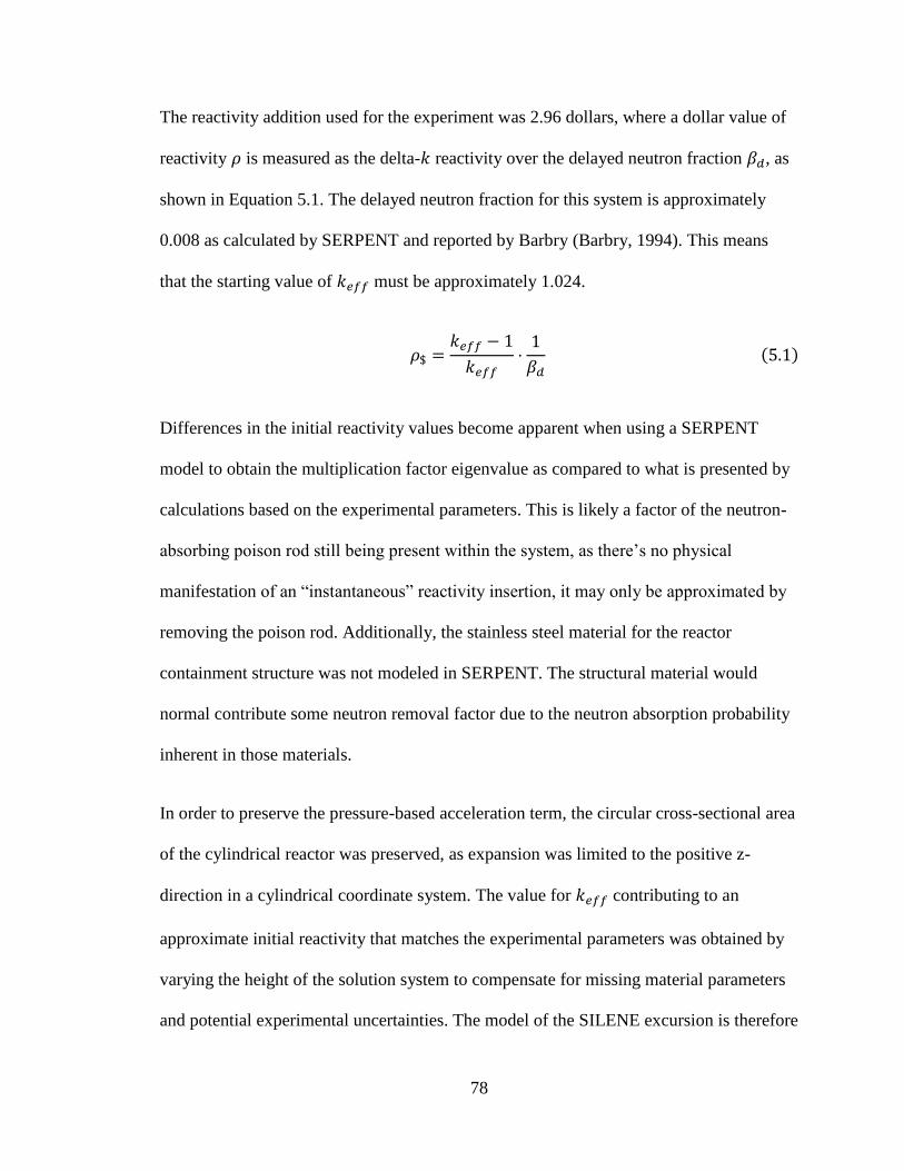
78
The reactivity addition used for the experiment was 2.96 dollars, where a dollar value of
reactivity 𝜌 is measured as the delta-𝑘 reactivity over the delayed neutron fraction 𝛽𝑑, as
shown in Equation 5.1. The delayed neutron fraction for this system is approximately
0.008 as calculated by SERPENT and reported by Barbry (Barbry, 1994). This means
that the starting value of 𝑘𝑒𝑓𝑓 must be approximately 1.024.
𝜌$ =𝑘𝑒𝑓𝑓 − 1
𝑘𝑒𝑓𝑓⋅
1
𝛽𝑑
(5.1)
Differences in the initial reactivity values become apparent when using a SERPENT
model to obtain the multiplication factor eigenvalue as compared to what is presented by
calculations based on the experimental parameters. This is likely a factor of the neutron-
absorbing poison rod still being present within the system, as there’s no physical
manifestation of an “instantaneous” reactivity insertion, it may only be approximated by
removing the poison rod. Additionally, the stainless steel material for the reactor
containment structure was not modeled in SERPENT. The structural material would
normal contribute some neutron removal factor due to the neutron absorption probability
inherent in those materials.
In order to preserve the pressure-based acceleration term, the circular cross-sectional area
of the cylindrical reactor was preserved, as expansion was limited to the positive z-
direction in a cylindrical coordinate system. The value for 𝑘𝑒𝑓𝑓 contributing to an
approximate initial reactivity that matches the experimental parameters was obtained by
varying the height of the solution system to compensate for missing material parameters
and potential experimental uncertainties. The model of the SILENE excursion is therefore

79
geometrically represented by an outer radius of 18.0 centimeters, an inner radius of 3.8
centimeters, and a height of 45.5 centimeters. This is considered a reasonable
approximation to make, as reactivity drives the excursion evolution, while the discretized
calculation of pressure is applied to a fractional profile of the height. The expansion of
the system is the terminating factor, so preserving the base cross-sectional area is of
greater import to the system integrity than preserving the height of the system. The
criticality excursion is considered to be terminated upon reaching a value of 0.98 for the
multiplication factor 𝑘𝑒𝑓𝑓.
The SILENE excursion was initially calculated with the base model, meaning without the
pressure gradient damping factor used by Hetrick and Smith to match physical values
(Hetrick & Smith, 1987). Such a calculation will be referred to as a “base calculation”,
while a run involving the damping factor will be referred to as a “damped calculation”.
This provides a power profile for the accident shown in Figure 5-2, and an overall energy
production shown in Figure 5-3.
Figure 5-2: SILENE S4-346 Base Power Profile
1E+17
1E+18
1E+19
0 0.001 0.002 0.003 0.004 0.005
Po
wer
(fi
ssio
ns/
s)
Time (s)
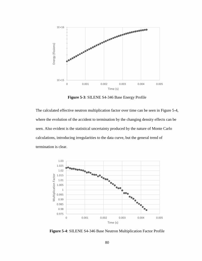
80
Figure 5-3: SILENE S4-346 Base Energy Profile
The calculated effective neutron multiplication factor over time can be seen in Figure 5-4,
where the evolution of the accident to termination by the changing density effects can be
seen. Also evident is the statistical uncertainty produced by the nature of Monte Carlo
calculations, introducing irregularities to the data curve, but the general trend of
termination is clear.
Figure 5-4: SILENE S4-346 Base Neutron Multiplication Factor Profile
1E+15
1E+16
0 0.001 0.002 0.003 0.004 0.005
Ener
gy (
fiss
ion
s)
Time (s)
0.975
0.98
0.985
0.99
0.995
1
1.005
1.01
1.015
1.02
1.025
1.03
0 0.001 0.002 0.003 0.004 0.005
Mu
ltip
licat
ion
Fac
tor
Time (s)

81
As can be seen in comparison to the experimental data, this accident terminates on a
much faster time-scale and at a lower power than would be expected, resulting in a lower
overall energy yield by approximately an order of magnitude. A reasonable deduction to
make would be that a limiting factor makes sense to apply to this system, to closer match
those experimental values.
It is possible to produce a pictorial representation of the material and geometric profile
within SERPENT. The initial state and the final state of the solution discretization in the
form of an axial cross-sectional view are presented in Figures 5-5 and 5-6, to provide a
graphical representation of the evolution of the volumetric profile. Note that SERPENT
1.1.7 does not allow for specific colors to be assigned to materials, and so each material
is represented by a randomly-selected color with the exception of atmospheric void
material, which is black. Additionally, the profile is normalized to a 1000 by 1000 pixel
image size, and so axial aspect ratio cannot be preserved. However, the relative geometric
locations of each material discretization should be fairly straightforward to determine.

82
Figure 5-5: SILENE S4-346 Axial Profile at 0 ms, Solution Height = 45.5 cm
Figure 5-6: SILENE S4-346 Base Axial Profile at 4.3 ms, Solution Height = 56.07 cm
As evidenced in the geometric profile pictures of the axial cross-section of the SILENE
reactor, the use of an atmospheric boundary condition at the top of the reactor results in a
large expansion of the materials located towards the top. The bottom-most materials
remain in their non-aerosolized liquid state.

83
Introduction of a pressure gradient damping factor of 0.1 multiplied to the calculated
acceleration term produces the damped profiles seen in Figures 5-7, 5-8, and 5-9 for the
power, energy, and neutron multiplication factor respectively.
Figure 5-7: SILENE S4-346 Damped Power Profile
Figure 5-8: SILENE S4-346 Damped Energy Profile
1E+18
1E+19
0 0.001 0.002 0.003 0.004 0.005 0.006 0.007 0.008 0.009
Po
wer
(fi
ssio
ns/
s)
Time (s)
1E+15
1E+16
1E+17
0 0.001 0.002 0.003 0.004 0.005 0.006 0.007 0.008 0.009
Ener
gy (
fiss
ion
s)
Time (s)

84
Figure 5-9: SILENE S4-346 Damped Neutron Multiplication Factor Profile
As seen, even with the damping factor used by Hetrick and Smith, this interpretation of
the model still results in a much faster termination of criticality than what is seen by
experimental results. While the initial geometric profile remains the same as that shown
in Figure 5-5, the axial cross-section of the material for the final calculated step of the
damped evolution can be seen in Figure 5-10.
0.975
0.98
0.985
0.99
0.995
1
1.005
1.01
1.015
1.02
1.025
1.03
0 0.001 0.002 0.003 0.004 0.005 0.006 0.007 0.008 0.009
Mu
ltip
licat
ion
Fac
tor
TIme (s)

85
Figure 5-10: SILENE S4-346 Damped Axial Profile at 7.7 ms, Solution Height = 52.5
cm
Within this profile, it can be seen that the central volumetric region did not expand as
quickly relative to the undamped profile. Because of the dissipation constant utilized on
the material regions adjacent to walls of the solution container, the base profile was able
to build up in center of mass velocity at a much quicker rate, and so the solution height
reached a larger value before the criticality was terminated. While with the pressure
gradient damping factor applied to overall acceleration, the central region for the damped
calculations was able to more closely match the dissipated expansion of the boundary
regions, and the solution expanded with a much more uniform profile. Again, expansion
was primarily seen towards the top of the solution container, where the atmospheric
boundary condition is set.
Wood River Junction
The historical excursion that was seen at Wood River Junction is of a very similar
material composition to that seen in the SILENE experiments, being comprised of a 93%

86
enriched uranyl nitrate solution in a carbonate reagent makeup vessel. This accident has a
reported two excursions with two different initiating events (T. McLaughlin et al., 2000),
however only the first pulse of this accident will be subject to analysis by the
computational model developed.
The exact material composition of the solution involved in the Wood River Junction
accident is not known, but it is known that the 93% enriched uranyl nitrate solution
involved was contained in a reagent makeup vessel along with an amount of sodium
carbonate. The chemical stoichiometry of sodium carbonate is Na2CO3. While carbon has
an appreciable scattering cross section for neutrons, it is not believed to have been
present in a high enough concentration to adversely affect the energy spectrum of the
involved neutrons in a prompt critical pulse scenario, and so both carbon and oxygen are
neglected from the overall solution. However, sodium has an appreciable nuclear neutron
absorption cross-section, and an analysis was performed to obtain the sodium to uranium
ratio present within the system, determined to be a value of 0.358 (Nakache et al., 1964).
Based on the assumption that the overall density of the uranyl nitrate solution was largely
unaffected, the additional sodium concentration to be accounted for in the materials data
was added to the general uranyl nitrate solution used for the SILENE analysis, and then
renormalized to the same overall density, providing the values shown in Table 5-3 for a
material definition to use in the SERPENT Monte Carlo analysis.

87
Table 5-3: Initial Wood River Junction Material Definitions
Isotope ZAID Number Density
(atoms
b-cm)
Hydrogen 1001 6.254 × 10⁻²
Nitrogen 7014 1.568 × 10⁻³
Oxygen 8016 3.574 × 10⁻²
Uranium-
234
92234 1.059 × 10⁻⁶
Uranium-
235
92235 1.685 × 10⁻⁴
Uranium-
236
92236 4.347 × 10⁻⁷
Uranium-
238
92238 1.169 × 10⁻⁵
Sodium 11023 6.504 × 10⁻⁵
The first pulse of the excursion is reported to have a yield of approximately 1 x 10¹⁷
fissions, caused by an initial reactivity of about 1.7 dollars present in the system, which is
deemed achievable by the known contents involved (Nakache et al., 1964). Because the
materials involved are very similar, again the approximate value for 𝛽𝑑 is 8 x 10⁻³, which
provides a value for the initial neutron multiplication factor 𝑘𝑒𝑓𝑓 of the system of about
1.014.
The geometry of the Wood River Junction vessel is a right-angle cylinder with a 22.9
centimeter radius that contains 41.0 liters of the uranyl nitrate plus sodium carbonate
solution. Again, because reactivity controls the evolution of the accident, the initial
multiplication vector of the system was controlled through adjustments made to the
solution height, which was set at 23.5 centimeters to meet reactivity requirements. Note
that this excursion was also reported to have ejected about 20% of the solution, and so the
density terminating effect via material loss is highly evident in this system.

88
An exact profile of the evolution of this system is not available, so the time-scale of the
excursion evolution cannot be compared to experimental values, which is why the
SILENE S4-346 reactor experiment is a useful parameter comparison. However, knowing
that the Wood River Junction accident involved 1.7 dollars of initial reactivity and the
first pulse was terminated at approximately 1 x 10¹⁷ fissions provides some avenues for
comparison. The results of the base calculation proceeded without the pressure gradient
damping factor are presented in Figures 5-11, 5-12, and 5-13.
Figure 5-11: Wood River Junction Base Power Profile
1E+17
1E+18
1E+19
0 0.0002 0.0004 0.0006 0.0008 0.001 0.0012
Po
wer
(fi
ssio
ns/
s)
Time (s)

89
Figure 5-12: Wood River Junction Base Energy Profile
Figure 5-13: Wood River Junction Base Multiplication Factor Profile
As with the SILENE model, it can be seen that the base calculation excursion evolves
extremely rapidly, and terminates with a developed integrated fission yield approximately
an order of magnitude below the predicted value. The axial cross-sectional profiles
generated by the SERPENT program are shown in Figures 5-14 and 5-15.
1E+15
1E+16
0 0.0002 0.0004 0.0006 0.0008 0.001 0.0012
Ener
gy (
fiss
ion
s)
Time (s)
0.975
0.98
0.985
0.99
0.995
1
1.005
1.01
1.015
0 0.0002 0.0004 0.0006 0.0008 0.001 0.0012
Mu
ltip
licat
ion
Fac
tor
Time (s)

90
Figure 5-14: Wood River Junction Axial Profile at 0 ms, Solution Height = 23.5 cm
Figure 5-15: Wood River Junction Base Axial Profile at 1.0 ms, Solution Height = 28.7
cm
From these geometric profiles, it can be seen that the solution volume evolution happens
at a large scale in the central regions of the container, and again the expansion is most
evident towards the top of the assembly, where the atmospheric boundary condition
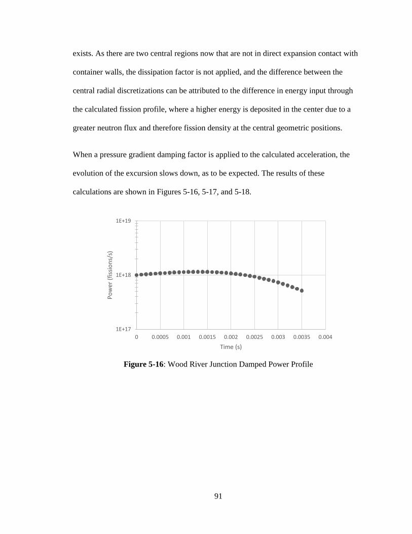
91
exists. As there are two central regions now that are not in direct expansion contact with
container walls, the dissipation factor is not applied, and the difference between the
central radial discretizations can be attributed to the difference in energy input through
the calculated fission profile, where a higher energy is deposited in the center due to a
greater neutron flux and therefore fission density at the central geometric positions.
When a pressure gradient damping factor is applied to the calculated acceleration, the
evolution of the excursion slows down, as to be expected. The results of these
calculations are shown in Figures 5-16, 5-17, and 5-18.
Figure 5-16: Wood River Junction Damped Power Profile
1E+17
1E+18
1E+19
0 0.0005 0.001 0.0015 0.002 0.0025 0.003 0.0035 0.004
Po
wer
(fi
ssio
ns/
s)
Time (s)

92
Figure 5-17: Wood River Junction Damped Energy Profile
Figure 5-18: Wood River Junction Damped Multiplication Factor Profile
1E+15
1E+16
0 0.0005 0.001 0.0015 0.002 0.0025 0.003 0.0035 0.004
Ener
gy (
fiss
ion
s)
Time (s)
0.975
0.98
0.985
0.99
0.995
1
1.005
1.01
1.015
1.02
0 0.0005 0.001 0.0015 0.002 0.0025 0.003 0.0035 0.004
Mu
ltip
licat
ion
Fac
tor
Time (s)

93
As can be seen, the evolution of this excursion slows down to 3.5 milliseconds prior to
termination, and the integrated fission yield increases as a result. However, this fission
yield still does not match the reported yield of 1 x 10¹⁷ fissions for the first spike
(Nakache et al., 1964), and is once again off by approximately an order of magnitude in
the damped calculation.
The geometric axial profiles of the solution system should look the same at the initial
time step shown in Figure 5-14, but the profile at the point of termination is shown in
Figure 5-19.
Figure 5-19: Wood River Junction Damped Axial Profile at 3.5 ms, Solution Height =
28.6 cm
As evident from the geometric material profile, the solution expands in a very similar
fashion even when damped. In contrast to the SILENE models, the Wood River Junction
models only have an outer wall with which to apply the dissipation effects to the
acceleration term, and so again the damping factor can be seen to be providing enough
94
time prior to termination for the outermost radial discretizations to expand slightly before
the criticality is terminated due to inertial effects.
Limiting Acceleration
Overall results indicate a clear trend of aerosolization and splashing that occurs as a result
of this model, which leads to a termination of criticality. Even with a pressure gradient
damping factor of effectively an order of magnitude decrease applied to the center of
mass acceleration term, the approximations made to volumetric expansion are still
overpredictors of the actual physical evolution of a solution excursion. It may be the case
that a smaller pressure gradient damping coefficient is required to obtain a more accurate
evolution profile. With these results in mind, a pressure gradient damping factor of 0.01
was applied to the calculations of both the SILENE and Wood River Junction systems,
and as expected the excursion evolution slowed down even further. The excursion
evolution calculations performed with a pressure gradient damping factor of 0.01 are
referred to as “limited” excursions.
When a damping factor of 0.01 is applied to the SILENE S4-346 experiment, the
resulting peak power is calculated to be 2.34 x 10¹⁹ fissions per second, which very
closely approximates the expected value of 2.40 x 10¹⁹ fissions per second for the power
of this excursion, the profile for which can be seen in Figure 5-20. The total energy
deposition is calculated as being 1.44 x 10¹⁷ fissions, which again very closely
approximates the expected value of this excursion, given as 1.50 x 10¹⁷ total fissions. The
profile for the energy deposition of the excursion can be seen in Figure 5-21. As before,
the excursion is fairly stable in terms of multiplication factor, and shows a clear trend
towards termination, seen in Figure 5-22.
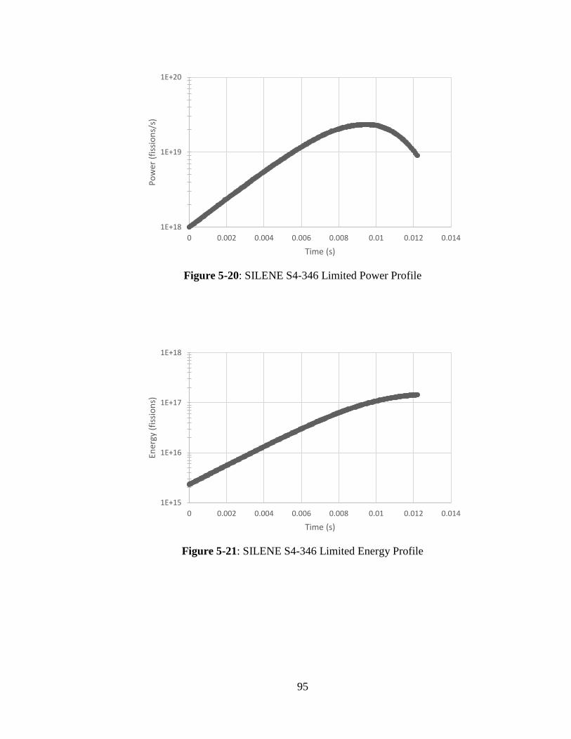
95
Figure 5-20: SILENE S4-346 Limited Power Profile
Figure 5-21: SILENE S4-346 Limited Energy Profile
1E+18
1E+19
1E+20
0 0.002 0.004 0.006 0.008 0.01 0.012 0.014
Po
wer
(fi
ssio
ns/
s)
Time (s)
1E+15
1E+16
1E+17
1E+18
0 0.002 0.004 0.006 0.008 0.01 0.012 0.014
Ener
gy (
fiss
ion
s)
Time (s)
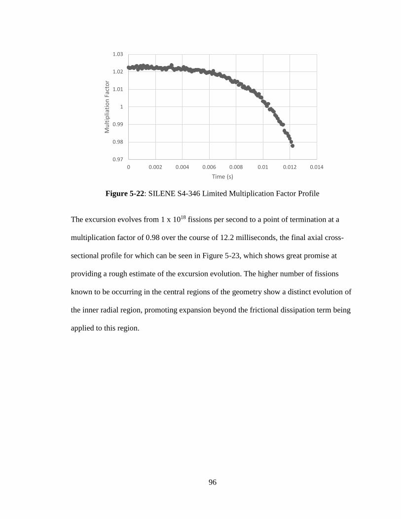
96
Figure 5-22: SILENE S4-346 Limited Multiplication Factor Profile
The excursion evolves from 1 x 10¹⁸ fissions per second to a point of termination at a
multiplication factor of 0.98 over the course of 12.2 milliseconds, the final axial cross-
sectional profile for which can be seen in Figure 5-23, which shows great promise at
providing a rough estimate of the excursion evolution. The higher number of fissions
known to be occurring in the central regions of the geometry show a distinct evolution of
the inner radial region, promoting expansion beyond the frictional dissipation term being
applied to this region.
0.97
0.98
0.99
1
1.01
1.02
1.03
0 0.002 0.004 0.006 0.008 0.01 0.012 0.014
Mu
ltip
liati
on
Fac
tor
Time (s)

97
.
Figure 5-23: SILENE S4-346 Limited Axial Profile at 12.2 ms, Solution Height = 51.9
cm
However, when the same damping factor of 0.01 is applied to the Wood River Junction
accidental excursion, the results are slightly further from the expected values. The peak
power is estimated as being 1.52 x 10¹⁸ fissions per second, as shown in Figure 5-24.
This provides a total energy deposition of 1.62 x 10¹⁶ fissions, the profile for which is
shown in Figure 5-25. While the accident still shows a distinct termination effect as
shown in Figure 5-26, the expected yield of this accident is approximately 1 x 10¹⁷
fissions of energy deposition, and so the calculated value is still an underprediction.

98
Figure 5-24: Wood River Junction Limited Power Profile
Figure 5-25: Wood River Junction Limited Energy Profile
1E+17
1E+18
1E+19
0 0.002 0.004 0.006 0.008 0.01
Po
wer
(fi
ssio
ns/
s)
Time (s)
1E+15
1E+16
1E+17
0 0.002 0.004 0.006 0.008 0.01
Ener
gy (
fiss
ion
s)
Time (s)

99
Figure 5-26: Wood River Junction Limited Multiplication Factor Profile
Possible reasons for this underpredicted value are varied, including experimental errors
on the side of conservatism when approximating the fission yield in the post-accident
analysis at Wood River Junction, as this was not an instrumented, fully-characterized
excursion event. An overall damping effect may be present due to fluid turbulence and
mixing that was effectively approximated by the two wall frictional dissipation terms
seen in the SILENE S4-346 models that doesn’t come into effect in the Wood River
Junction models, the ending profile for which is shown in Figure 5-27, clearly displaying
a large central volumetric expansion of the system. Additionally, the initial power
generation of 1 x 10¹⁸ fissions per second used as a starting point for the excursion
evolution may be too high, and limited the effect of the evolution at Wood River
Junction. It should also be mentioned that the Wood River Junction accident was a stirred
tank, which would have an additional mechanical energy input that does not get
accounted for by this model.
0.975
0.98
0.985
0.99
0.995
1
1.005
1.01
1.015
1.02
0 0.002 0.004 0.006 0.008 0.01
Mu
ltip
licat
ion
Fac
tor
Time (s)

100
Figure 5-27: Wood River Junction Limited Axial Profile at 9.4 ms, Solution Height =
28.3 cm
While any number of reasons could be the cause of an over-prediction term at the Wood
River Junction site, the very close approximation of the SILENE excursion yield is
promising. The overall conclusion is that a value of 0.01 pressure gradient damping term
is a close approximation of a mechanically terminated excursion, but a smaller value
should be used to err on the side of conservatism when approximating the results of an
excursion. A lower initial power than 1 x 10¹⁸ fissions per second for the excursion
evolution calculations could also be desired to more closely approximate the evolution.
It should also be noted that the use of a value of 0.01 for the pressure gradient damping
factor resulted in a large amount of pressure build-up within the system via the equations
of state. Because the pressure is increased primarily through energy deposition via
fissions and decreased through expansion of the material by volumetric change, limiting
the volumetric change also limited the loss of pressure from the system.

101
Chapter 6 – Concluding Remarks
While the safety aspects of an accidental criticality involving a fissile solution system are
well-accounted for by the existence of standards and regulations involving site-specific
analysis, the existence of general rule-of-thumb evaluations for a solution criticality is
still a worthwhile endeavor to allow for quick estimations of expected yield and accident
evolution parameters.
Within the known parameters of historical accidents involving solution systems that have
occurred, a bounding trend is evident between the usage of Barbry’s model (Barbry,
1987) and Tuck’s model (Tuck, 1974) that encompasses most of the expected yield
values within a relatively high degree of accuracy in comparison to similar such
evaluations that have been attempted. Barbry’s model tends to over-predict the integrated
fission yield of a solution system, while Tuck’s model tends to under-predict. In general,
both models have a high degree of over-estimation for a relatively low fission yield on
the order of 1 x 10¹⁵ total fissions to 1 x 10¹⁷ total fissions, and the estimated value for an
integrated fission yield begins to drop slightly below the reported value at yields larger
than approximately 5 x 10¹⁷, a trend that is common to most simple empirical models. It
is suggested that should these models be used to calculate a bounding fission yield, this
over-estimation to under-estimation trend be taken into account.
The existence of a simple, openly available computational model to evaluate the
evolution of a solution-based criticality excursion that includes modern Monte Carlo
computational methods and accounts for termination effects by means of a pressure-
based acceleration term is largely still unresolved, although it is the hope that such a
102
model can be generated with a relatively small amount of additional analysis. The use of
a multiplying factor by Hetrick and Smith (Hetrick & Smith, 1987) to affect the pressure
gradient acceleration term is a concept that could be explored and refined, although using
a value of 0.01 for this factor had positive results when applied to the experimental
excursion. This factor could be further decreased to allow for conservatism and to more
accurately predict the evolution of a less well-defined excursion, but time spent on
analysis of this factor would most likely be better spent on an improvement of the
solution expansion models, because decreasing the calculated acceleration term by more
than two orders of magnitude most probably shows the effects of a very crude model
rather than simply an inaccurate term. Additionally, the implementation of this factor
produced system pressures of an unexpectedly high magnitude, meaning that further
decreasing this value would likely result in a more unrealistic model.
Most minor discrepancies between the Monte Carlo calculated parameters and the
empirically calculated values used for the neutronic evolution can likely be attributed
both to experimental error and the statistical nature inherent in a Monte Carlo analysis
technique, as well as the crude geometries utilized while modeling, such as no
atmosphere, container walls, or reflective surroundings (e.g., a concrete floor). For the
most part, however, the values returned from Monte Carlo analysis matched the
experimental values very accurately where such values are known (Barbry, 1994).
The model used to represent the volumetric expansion mechanisms of the solution system
is overall very simplified, and a very rough discretization method was imposed over it for
the calculations presented herein. There are additional fluid properties that may be
considered for a more refined model in terms of aerosolization, splashing models, and

103
turbulence effects on solution friction. Treating each volumetric element as a unit of
constant properties is considered to be a crude pressure gradient calculation of just a
single region, and the current numerical approximation is applied in an explicit fashion,
which is subject to instabilities (Hetrick & Smith, 1987).
The model originally developed by Smith and Hetrick that used these thermodynamic
profiles and Newtonian mechanics for volumetric acceleration was used with an input of
a predetermined power profile (Hetrick & Smith, 1987). Dynamically evolving the power
profile through the use of a neutronics code required slight alterations in the order of
equation of state calculations performed to reduce the number of instabilities in the
model, which is likely the cause of a rapid termination even with the damping factor. The
use of a more refined model that solves the issue of extreme pressure development upon
limiting the volumetric expansion should be a high priority for future work.
However, the results clearly indicate potential applications of a model of similar
construction that could be used to rapidly test and determine the effects of a solution
criticality. The model presented herein is meant to include very simple technologies that
are easily obtained, and openly available to anyone to either continue research, improve,
or utilize for other purposes.
The overall goal of this thesis was to present a collection and analysis of the current state
of solution criticality modeling as is available within common avenues of research and
publications. It is the sincerest hope of the author that this thesis is useful as an
approximation and summary, as well as in laying the groundwork of models for use in the

104
construction of better-informed decisions by a safety operator, facility worker, or the
layperson outside of a closed-source environment.

105
Appendices: Computational Model Source Code
List of Appendices:
• Appendix A: Driver Script File: transientmodel.py
• Appendix B: File Operations Library: tm_fileops.py
• Appendix C: Volume and Material Discretization: tm_material.py
• Appendix D: Calculational Parameters: tm_constants.py
The Python 3.6.3 code used for analysis purposes is included within this section. Any
person should be able to utilize this code for their own purposes, as long as they have
both a version of SERPENT compatible with the input files for 1.1.7 and a Python
interpreter able to recognize the 3.6.3 dialect of the Python programming language.
Usage is simply a matter of running the transientmodel.py script file from any terminal
emulator, and entering the prompted file name to use for the SERPENT input and output
files. Minor modifications may need to be made to transientmodel.py to accommodate
calling the SERPENT “sss” executable through a medium other than the Windows
Subsystem for Linux framework, but this should be straightforward to implement.
Calling the SERPENT executable is the only example of such an interaction, and so the
modifications required are very limited.
Additional library dependencies used for the Python calculational tool at the time of
writing are as follows:
• NumPy version 1.13.3
• RE version 2.2.1

106
• CoolProp version 6.0.0

107
Appendix A – Driver Script File: transientmodel.py
This is the main driver, and should be called from a terminal emulator. The purpose of
this script is to import all relevant files within the same directory, then proceed with the
calculations. Volume elements are created based on the values in tm_constants.py, an
initial SERPENT input file is created, and the initial neutronics parameters are obtained
from the SERPENT output file. For each volume element, the fission power profile
generated by SERPENT is used to evolve the element forwards in time based on energy
deposition. SERPENT is called after each evolution until a value for the neutronic
multiplication parameter 𝑘𝑒𝑓𝑓 falls below 0.98, with the results of each time-step being
written to a generic comma-separated-value format output file named “results.txt”.
#!/usr/bin/env python3 # -*- coding: utf-8 -*- # transientmodel.py ''' A transient model for critical solution systems. By Corey Skinner. Dependencies: re for regular expression pattern matching in output files os for calling the sss and bash processes via command interface, file existence for debug numpy for arrays and mathematical methods CoolProp for water properties (assuming aqueous mixture is approximated by water) - Imported in module file "tm_material" ''' # External from os import system, path import re import numpy as np # Shared from tm_material import Material # Requires CoolProp import tm_constants as c import tm_fileops as fo def set_materials(elems, ndens, tot_height, tot_radius, **kwargs): '''Return a list of materials and geometries, radial columns dominant''' mat_counter = 1 # Materials begin with number 1 materials = [] # Two dimensional list of materials for return inner_radius = 0 # cm # All materials should start out with the same initial density dens = [0.0] * len(elems) # g/cm^3 for ind, nden in enumerate(ndens): dens[ind] = nden / 6.022e23 * 1e24 * c.AWEIGHT[ind] # g/cm^3 den = sum(dens) # g/cm^3

108
# Initial pressures are assumed to be linear, based on rho-g-h model # All pressures are absolute, not gauge for ind, radius in enumerate(calc_radii(tot_radius)): base_height = 0.0 # cm, start at planar origin r_list = [] # Second dimension empty list for appending # From bottom to top, heights being added half_height = 0.0 # m, placeholder for height in calc_heights(tot_height): # The half_height value is calculated for the initial value from base if half_height == 0.0: half_height = height / 2 av_height = (tot_height - height + half_height) / 100 # m av_pres = den * c.GRAV * av_height / 1000 * 100**3 / 1e6 + c.ATM # MPa # Equivalent to the height of the center of mass: com_height = tot_height - av_height * 100 # cm if (ind == 0 and c.INNER_RAD > 0.0) or (ind == c.NUM_RADIAL - 1): dissipate = 1 else: dissipate = 0 if 'temp' in kwargs: temperature = kwargs['temp'][mat_counter - 1] # K r_list.append(Material(mat_counter, elems, ndens, den, height, base_height, radius, inner_radius, com_height, dissipate, av_pres, temperature)) else: r_list.append(Material(mat_counter, elems, ndens, den, height, base_height, radius, inner_radius, com_height, dissipate, av_pres)) mat_counter += 1 base_height = height # cm materials.append(r_list) inner_radius = radius # cm return materials def propagate_power(k_eff, lifetime, beta_eff, power): '''Propagate the number of neutrons over delta-t''' reactivity = (k_eff - 1) / k_eff prompt_gen_time = lifetime / k_eff # s return power * np.exp((reactivity - beta_eff) / prompt_gen_time * c.DELTA_T) # fis/s def energy_dep_init(k_eff, lifetime, beta_eff): '''Calculate the initial energy deposition at the start of the reaction''' reactivity = (k_eff - 1) / k_eff prompt_gen_time = lifetime / k_eff # s period = prompt_gen_time / (reactivity - beta_eff) # s # Assuming an initiating accident of 1 fission per second at time t=0 # NOTE: np.log() is the natural logarithm time = np.log(c.INIT_POWER / 1) * period # s return period * (np.exp(time / period) - 1) * 1 # fissions def calc_heights(tot_height): '''Returns a list of the ranges of height based on total''' height_diff = tot_height / c.NUM_AXIAL # cm heights = list(map(lambda ind: ind * height_diff, range(1, c.NUM_AXIAL + 1))) # cm return heights # cm def calc_radii(tot_rad): '''Returns a list of the ranges of radii based on total''' rad_diff = (tot_rad - c.INNER_RAD) / c.NUM_RADIAL # cm radii = list(map(lambda ind: ind * rad_diff + c.INNER_RAD, range(1, c.NUM_RADIAL + 1))) # cm return radii # cm def update_material_states(materials, fissions, tot_height, initial=False): '''Updates the state of all materials in profile''' counter = 0 # Two inner loops prevent use of enumerate() temperatures = [] # K pressures = [] # MPa heights = [] # cm top_pressure = c.ATM # MPa
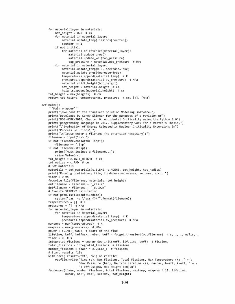
109
for material_layer in materials: bot_height = 0.0 # cm for material in material_layer: material.update_temp(fissions[counter]) counter += 1 if not initial: for material in reversed(material_layer): material.update_pres() material.update_vol(top_pressure) top_pressure = material.bot_pressure # MPa for material in material_layer: material.update_temp(0.0, decrease=True) material.update_pres(decrease=True) temperatures.append(material.temp) # K pressures.append(material.av_pressure) # MPa material.shift_height(bot_height) bot_height = material.height # cm heights.append(material.height) # cm tot_height = max(heights) # cm return tot_height, temperatures, pressures # cm, [K], [MPa] def main(): '''Main wrapper''' print("\nWelcome to the Transient Solution Modeling software.") print("Developed by Corey Skinner for the purposes of a revision of") print("DOE-HDBK-3010, Chapter 6: Accidental Criticality using the Python 3.6") print("programming language in 2017. Supplementary work for a Master's Thesis,") print("\"Evaluation of Energy Released in Nuclear Criticality Excursions in") print("Process Solutions\"") print("\nPlease enter a filename (no extension necessary):") filename = input(">>> ") if not filename.endswith(".inp"): filename += ".inp" if not filename.strip(): print("Must include a filename...") raise ValueError tot_height = c.INIT_HEIGHT # cm tot_radius = c.RAD # cm # Set materials materials = set_materials(c.ELEMS, c.NDENS, tot_height, tot_radius) print("Running preliminary file, to determine masses, volumes, etc...") timer = 0 #s fo.write_file(filename, materials, tot_height) outfilename = filename + "_res.m" detfilename = filename + "_det0.m" # Execute SERPENT calculation if not path.isfile(outfilename): system("bash -c \"sss {}\"".format(filename)) temperatures = [] # K pressures = [] # MPa for material_layer in materials: for material in material_layer: temperatures.append(material.temp) # K pressures.append(material.av_pressure) # MPa maxtemp = max(temperatures) # K maxpres = max(pressures) # MPa power = c.INIT_POWER # Start of the flux lifetime, keff, keffmax, nubar, beff = fo.get_transient(outfilename) # s, _, _, n/fis, _ timer = 0 # s integrated_fissions = energy_dep_init(keff, lifetime, beff) # fissions total_fissions = integrated_fissions # fissions number_fissions = power * c.DELTA_T # fissions # Start results file with open('results.txt', 'w') as resfile: resfile.write("Time (s), Num Fissions, Total Fissions, Max Temperature (K), " + \ "Max Pressure (bar), Neutron Lifetime (s), nu-bar, b-eff, k-eff, " + \ "k-eff+2sigma, Max Height (cm)\n") fo.record(timer, number_fissions, total_fissions, maxtemp, maxpres * 10, lifetime, nubar, beff, keff, keffmax, tot_height)

110
initial = True # Flag to calculate integrated energy deposition with initial profile # Material addition loop print("Beginning main calculation...") # # Material expansion loop print("Now expanding system by temperature...") while keff > c.SUBCRITICAL_LIMIT: # Proceed in time timer += c.DELTA_T # s # Read previous output file for information and calculate new changes fission_profile = fo.count_fissions(detfilename) power = propagate_power(keff, lifetime, beff, power) # fissions/s # Correlation between flux profile and fission density number_fissions = power * c.DELTA_T # fissions fissions = [frac * number_fissions for frac in fission_profile] # fissions total_fissions += number_fissions # fissions # Assume that initiating fission profile does not change from the initial calculation if initial: initial = False # Only calculate one time integrated_dist = [frac * integrated_fissions for frac in fission_profile] # fissions _, _, _ = update_material_states(materials, integrated_dist, tot_height, initial) # cm, [K], [MPa] # Begin total expansion of material #if c.EXPANSION: # update_pressures(materials) # update_heights(materials) tot_height, temperatures, pressures = update_material_states(materials, fissions, tot_height) # cm, [K], [MPa] maxtemp = max(temperatures) # K maxpres = max(pressures) # MPa timer_string = f"{round(timer, abs(c.TIMESTEP_MAGNITUDE)):.6f}" filename = re.sub(r'\d', r'', filename[:filename.rfind(".inp")]).replace('.', '') \ + timer_string + ".inp" outfilename = filename + "_res.m" detfilename = filename + "_det0.m" # Do not need to recalculate masses (thus volumes) for materials at this stage fo.write_file(filename, materials, tot_height) # NOTE: Conditional should be "outfilename", but can be "filename" for debugging purposes if not path.isfile(outfilename): system("bash -c \"sss {}\"".format(filename)) lifetime, keff, keffmax, nubar, beff = fo.get_transient(outfilename) fo.record(timer, number_fissions, total_fissions, maxtemp, maxpres * 10, lifetime, nubar, beff, keff, keffmax, tot_height) print("Current time: {} s".format(round(timer, abs(c.TIMESTEP_MAGNITUDE) + 1))) print("Current k-eff: {}".format(keff)) print("Maximum k-eff: {}".format(keffmax)) print("Number of fissions: {0:E}".format(sum(fissions))) print("Maximum temperature: {}".format(maxtemp)) if __name__ == '__main__': try: main() finally: print("\nProgram terminated\n")

111
Appendix B – File Operations Library: tm_fileops.py
This is a library of functions used for file input and output. These functions include
writing a SERPENT input file, reading relevant neutronics parameters from a SERPENT
output file, and appending to a results file. This file is imported into the
transientmodel.py script.
# -*- coding: utf-8 -*- # tm_fileops.py ''' Import only module. Contains operations on input and output files from SERPENT, primarily writing input files and reading detector output files and parameter output files. Also contains functionality for writing overall results file. ''' import re import tm_constants as c def count_fissions(filename): '''Read an output file to determine the fission (flux) distribution''' pat = re.compile(r'(\s+1)\1+\s+(\S+)') profile = [] counter = 0 with open(filename, mode='r') as detfile: for line in detfile: if re.match(pat, line): matches = re.findall(pat, line) if counter != 0: profile.append(float(matches[0][1])) counter += 1 return profile def get_transient(filename): ''' Read an output file to determine the transient point-reactor kinetics parameters Returns tuple of lifetime, k-eff, maximum k-eff, nu-bar, and beta-eff ''' ltpat = re.compile(r'ANA_PROMPT_LIFETIME\s+\(idx,\s\[1:\s+2\]\)\s=\s\[\s+(\S+)\s\S+\s\];') kepat = re.compile(r'ANA_KEFF\s+\(idx,\s\[1:\s+2\]\)\s=\s\[\s+(\S+)\s(\S+)\s\];') nbpat = re.compile(r'NUBAR\s+\(idx,\s\S+\s+\S+\)\s=\s\[\s+(\S+).+;') bepat = re.compile(r'BETA_EFF\s+\(idx,\s\S+\s+\S+\)\s=\s\[\s+(\S+).+;') with open(filename, mode='r') as ofile: for line in ofile: if re.match(ltpat, line): matches = re.findall(ltpat, line) lifetime = float(matches[0]) # s if re.match(kepat, line): matches = re.findall(kepat, line) keff = float(matches[0][0]) maxkeff = round(keff + 2 * float(matches[0][1]), 5) if re.match(nbpat, line): matches = re.findall(nbpat, line) nubar = float(matches[0]) # n/fis if re.match(bepat, line): matches = re.findall(bepat, line) beff = float(matches[0])
112
return (lifetime, keff, maxkeff, nubar, beff) # s, _, _, n/fis def write_file(filename, materials, tot_height): '''Function to create the series of input files''' with open(filename, mode='w', newline='\n') as fhan: fhan.write("% Serpent Input File\n") fhan.write("set title \"{}\"\n\n".format(filename[:filename.rfind(".inp")])) # Material data fhan.write("\n% Materials\n") for material_level in materials: for material in material_level: fhan.write(str(material)) # Surface data fhan.write("\n% Surfaces\n") # Axial distributions occur on order nx, where n is the material number # and x is the plane number (1 for bottom and 2 for top) # Radial distributions read as n, where n is increasing to NUM_RADIAL if c.INNER_RAD > 0.0: fhan.write("surf 0 cyl 0 0 {}\n".format(c.INNER_RAD)) for rad_ind, material_level in enumerate(materials): fhan.write("surf {0} cyl 0 0 ".format(rad_ind + 1)) for mat_ind, material in enumerate(material_level): if mat_ind == 0: fhan.write("{}\n".format(material.radius)) fhan.write("surf {0}0 pz {1}\n".format(rad_ind + 1, material.base_height)) fhan.write("surf {0}{1} pz {2}\n".format(rad_ind + 1, mat_ind + 1, material.height)) # Overall boundaries fhan.write("surf 1001 pz 0\n") fhan.write("surf 1002 pz {}\n\n".format(tot_height)) # Cell data fhan.write("\n% Cells\n") # Cells are numbered by n, where n is the material number for rad_ind, material_level in enumerate(materials): # Void super-radials are marked with 10n, where n is the radial number # Void sub-radials are marked with 11n, where n is the radial number fhan.write("cell 10{0} {0} void {0}\n".format(rad_ind + 1)) if rad_ind > 0: fhan.write("cell 11{0} {0} void -{1}\n".format(rad_ind + 1, rad_ind)) elif c.INNER_RAD > 0.0: fhan.write("cell 11{0} {0} void -0\n".format(rad_ind + 1)) # Void sub-axials are marked with 12n, where n is the radial number for mat_ind, material in enumerate(material_level): if mat_ind == 0: fhan.write("cell 12{0} {0} void -{0}0\n".format(rad_ind + 1)) fhan.write("cell {0} {1} solution{0} {1}{2} -{1}{3} -{1}" .format(material.matnum, rad_ind + 1, mat_ind, mat_ind + 1)) if rad_ind > 0: fhan.write(" {}".format(rad_ind)) elif c.INNER_RAD > 0.0: fhan.write(" 0") fhan.write("\n") # Void super-axials are marked with 13n, where n is the radial number fhan.write("cell 13{0} {0} void {0}{1}\n".format(rad_ind + 1, c.NUM_AXIAL)) fhan.write("\n") # Global universe cells, marked with 100n, where n is the radial number if c.INNER_RAD > 0.0: fhan.write("cell 1000 0 void 1001 -1002 -0\n") for radial_num in range(1, c.NUM_RADIAL + 1): fhan.write("cell 100{0} 0 fill {0} 1001 -1002 -{0}".format(radial_num)) if radial_num > 1: fhan.write(" {}".format(radial_num - 1)) elif c.INNER_RAD > 0.0: fhan.write(" 0") fhan.write("\n") # Now mark global outside, still of form 100n, but with n > radial number fhan.write("cell 100{0} 0 outside -1001 -{1}\n".format(c.NUM_RADIAL + 1, c.NUM_RADIAL)) fhan.write("cell 100{0} 0 outside 1002 -{1}\n".format(c.NUM_RADIAL + 2, c.NUM_RADIAL)) fhan.write("cell 100{0} 0 outside {1}\n".format(c.NUM_RADIAL + 3, c.NUM_RADIAL))

113
fhan.write("\n") # Thermal scattering S(a,b) fhan.write("\n% Thermal scattering library\n") for material_level in materials: for material in material_level: fhan.write("therm lwtr{0} lwe7.{1}\n".format(material.matnum, material.sab_tag)) fhan.write("\n") # Cross-section library fhan.write("\n% Cross-section library\n") fhan.write("set acelib \"/xs/sss_endfb7u.xsdata\"\n\n") # Criticality parameters fhan.write("\n% Criticality parameters\n") # Leave a guess of 1.0 for k-eff fhan.write("set pop {0} {1} {2} 1.0\n\n" .format(c.NUM_PARTICLES, c.NUM_CYCLES, c.NUM_DROPS)) # Include unresolved resonance probability tables fhan.write("\n% Unresolved resonance probability calculations\n") fhan.write("set ures 0\n\n") # Geometry plot fhan.write("\n% Geometry plot\n") fhan.write("plot 1 1000 1000 0 -{0} {0} -1 {1}\n\n".format(c.RAD + 1, tot_height + 1)) # Flux detectors fhan.write("\n% Flux detectors\n") # Total detector of fissions fhan.write("det 100 du 0 dr -6 void\n") for material_level in materials: for material in material_level: fhan.write("det {0} dc {0} dr -6 void dt 3 100\n".format(material.matnum)) def record(time, numfissions, totfissions, maxt, maxp, lifetime, nubar, beff, keff, keffmax, maxheight): '''Record current step to a results file''' with open("results.txt", 'a') as appfile: appfile.write("{0}, {1:E}, {2:E}, {3}, {4}, {5}, {6}, {7}, {8}, {9}, {10}\n" .format(round(time, abs(c.TIMESTEP_MAGNITUDE) + 1), numfissions, totfissions, maxt, maxp, lifetime, nubar, beff, keff, keffmax, maxheight))

114
Appendix C – Volume and Material Discretization: tm_material.py
This is a class definition used for each volume-discretized element in the analysis. This
file is used as an import to transientmodel.py as the framework for discretization objects
that are created, and allows for those objects to maintain their own states, such as
temperature, pressure, density, geometric position, and so on. This file also allows each
object to propagate itself forward in one time-step based on energy deposition, including
expansion in space and production of radiolytic gas. Such propagation calculations are
explicitly called by transientmodel.py, where the height shift and pressure balances with
respect to atmosphere can be accounted for on an overall scale not achievable by these
discretized elements. These volume objects also have their string representations
overloaded to be compatible with SERPENT input files for material definitions, allowing
for number densities of each volume object to be dynamically stored as specified by this
class definition.
# -*- coding: utf-8 -*- # tm_material.py ''' Import only module. Material definition for transient model, defined as a discretized segment of overall solution volume. Dependencies: CoolProp for material properties numpy for mathematical constants (should be included as part of main file import already) ''' # External from CoolProp.CoolProp import PropsSI # Assuming that the solution is approximated by water import numpy as np # Bring pi into namespace for cylindrical volume calculations # Shared import tm_constants as c # Required for the included tag dictionaries class Material(): '''Generic class for the material in question, and associated geometry''' def __init__(self, matnum, elems, ndens, dens, height, base_height, radius, inner_radius, com_height, dissipate, pres=c.ATM, temp=300): self.dissipate = dissipate # Governs if the material is decelerated due to friction self.matnum = matnum self.elems = elems self.ndens = ndens # a/b-cm self.temp = temp # K self.height = height # cm, note that this is the ABSOLUTE HEIGHT of the material from 0

115
self.base_height = base_height # cm self.radius = radius # cm self.inner_radius = inner_radius # cm self.dens = dens # g/cm^3 self.init_dens = dens # g/cm^3 self.mass = 0.0 # g, placeholder until calculated self.volume = 0.0 # cm^3, placeholder until calculated self.base = 0.0 # cm^2, placeholder until calculated self.kappa = 0.0 # 1/Pa, isothermal compressibility, placeholder until needed self.beta = 0.0 # 1/K, isobaric compressibility, placeholder until needed self.delta_temp = 0.0 # K, initially zero upon definition self.delta_pres = 0.0 # Pa, initially zero upon definition self.atoms = [0.0] * len(ndens) # _, placeholder until calculated self.volfrac_gas = 0.0 # _, initially no radiolytic gas in solution self.mass_h2 = 0.0 # g, initially no radiolytic gas in solution # Pressure: Assume atmospheric conditions (allow for expansion of fluid) self.av_pressure = pres # MPa, gauge value self.calc_bottom_pressure() # MPa, calculate from average pressure input self.com_height = com_height # cm self.com_accel = 0.0 # cm/s^2, initially not in motion self.com_vel = 0.0 # cm/s, initially not in motion self.delta_com = 0.0 # cm, placeholder, no initial delta self.delta_vol = 0.0 # cm^3, placeholder, no initial delta self.xs_tag = "03c" self.sab_tag = "00t" self.gas_production_flag = False # Once radiolytic gas is produced, keep producing it if temp != 300: # K self.__update_xs_tag() self.__update_sab_tag() self.__calc_init() def shift_height(self, baseheight): '''Shift each segment upwards by a set distance''' shift = baseheight - self.base_height # cm self.base_height = baseheight # cm self.height += shift # cm self.com_height += shift # cm def update_temp(self, fissions, decrease=False): '''Update temperature of the solution based on energy input''' # Assume that the system properties do not diverge greatly from those for water spec_heat = PropsSI('O', 'T', self.temp, 'Q', 0.0, 'WATER') # J/kg-K # Assume that 180 MeV is deposited in the solution per fission event if not decrease: self.delta_temp = (fissions * 180 * 1.6022e-13) / spec_heat / (self.mass / 1000) # K else: beta_0 = PropsSI('ISOBARIC_EXPANSION_COEFFICIENT', 'T', self.temp, 'Q', 0.0, 'WATER') # 1/K kappa_0 = PropsSI('ISOTHERMAL_COMPRESSIBILITY', 'T', self.temp, 'Q', 0.0, 'WATER') * 1e6 # 1/MPa surf_tens = PropsSI('I', 'T', self.temp, 'Q', 0.0, 'WATER') * 1e-6 # MN/m self.beta = beta_0 * (1 - self.volfrac_gas) + self.volfrac_gas / self.temp \ * (self.av_pressure + 2 * surf_tens / c.RAD_GAS_BUBBLE) \ / (self.av_pressure + 4 * surf_tens / 3 / c.RAD_GAS_BUBBLE) # 1/K self.kappa = kappa_0 * (1 - self.volfrac_gas) + self.volfrac_gas \ / (self.av_pressure + 4 * surf_tens / 3 / c.RAD_GAS_BUBBLE) # 1/MPa self.delta_temp = -(self.beta * self.temp / (self.kappa * 1e-6) \ * (self.delta_vol / 100**3)) / spec_heat / (self.mass / 1000) # K self.temp += self.delta_temp # K def update_vol(self, top_pres): '''Update center of mass acceleration, and volume''' self.calc_bottom_pressure(top_pres) self.com_accel = (self.base / 100**2) / (self.mass / 1000) \ * (self.bot_pressure - top_pres) * 1e6 * 100 - c.GRAV * 100 # cm/s^2 dissipation = self.dissipate * c.DISSIPATION * self.com_vel # cm/s^2 if np.abs(self.com_accel) < dissipation: self.com_accel = 0 # cm/s^2 else:

116
self.com_accel -= np.abs(dissipation) * np.sign(self.com_accel) # cm/s^2 # Pressure gradient dampening factor self.com_accel *= c.DAMPING_FACTOR # cm/s^2 com_vel_i = self.com_vel # cm/s com_vel_f = com_vel_i + self.com_accel * c.DELTA_T # cm/s self.com_vel = com_vel_f # cm/s, update information for next snapshot self.delta_com = com_vel_i * c.DELTA_T + 1 / 2 * self.com_accel * c.DELTA_T**2 # cm self.com_height += self.delta_com # cm half_height = self.com_height - self.base_height # cm self.height = self.base_height + 2 * half_height # cm old_vol = self.volume # cm^3 self.volume = self.base * (self.height - self.base_height) # cm^3 self.dens = self.mass / self.volume # g/cm^3 # Restrict material by density to disallow compression, allow expansion if self.dens > self.init_dens: self.dens = self.init_dens # g/cm^3 self.volume = self.init_vol # cm^3 self.height = self.volume / self.base + self.base_height # cm self.com_vel = 0.0 # cm/s self.com_accel = 0.0 # cm/s^2 self.com_height = (self.base_height + self.height) / 2 # cm self.delta_vol = self.volume - old_vol # cm^3 self.ndens = [atom * 1e-24 / self.volume for atom in self.atoms] # a/b-cm def update_pres(self, decrease=False): '''Update pressure of the solution system based on intensive properties''' beta_0 = PropsSI('ISOBARIC_EXPANSION_COEFFICIENT', 'T', self.temp, 'Q', 0.0, 'WATER') # 1/K kappa_0 = PropsSI('ISOTHERMAL_COMPRESSIBILITY', 'T', self.temp, 'Q', 0.0, 'WATER') * 1e6 # 1/MPa surf_tens = PropsSI('I', 'T', self.temp, 'Q', 0.0, 'WATER') * 1e-6 # MN/m self.beta = beta_0 * (1 - self.volfrac_gas) + self.volfrac_gas / self.temp \ * (self.av_pressure + 2 * surf_tens / c.RAD_GAS_BUBBLE) \ / (self.av_pressure + 4 * surf_tens / 3 / c.RAD_GAS_BUBBLE) # 1/K self.kappa = kappa_0 * (1 - self.volfrac_gas) + self.volfrac_gas \ / (self.av_pressure + 4 * surf_tens / 3 / c.RAD_GAS_BUBBLE) # 1/MPa if not decrease: self.delta_pres = self.beta / self.kappa * self.delta_temp # MPa else: self.delta_pres = -(self.delta_vol / 100**3) / self.kappa * (self.volume / 100**3) # MPa self.av_pressure += self.delta_pres # MPa def calc_bottom_pressure(self, top_pres=None): '''Called to calculate bottom pressure, overloaded with top pressure if known''' if top_pres is None: self.bot_pressure = self.av_pressure + self.dens * c.GRAV \ * (self.height - self.base_height) / 2 * 100**2 / 1000 / 1e6 # MPa else: self.bot_pressure = 2 * self.av_pressure - top_pres # MPa def __update_xs_tag(self): '''Update the materials cross-section tag; called when new temperature calculated''' round_value = 300 # technically K rounded_temp = int(round_value * round(self.temp / round_value)) self.xs_tag = c.XS_TEMP.get(rounded_temp, "18c") def __update_sab_tag(self): '''Update the thermal scattering correction tag; called when new temperature calculated''' round_value = 50 # technically K rounded_temp = int(round_value * round(self.temp / round_value)) self.sab_tag = c.SAB_TEMP.get(rounded_temp, "18t") def __produce_gas(self, fissions): '''Produce a mass of radiolytic gas in the solution; called from self.update_pressure()''' # 180 MeV deposited in solution per fission event energydep = fissions * 180 * 1.6022e-19 # MJ self.mass_h2 += c.RADIOLYTIC_G * energydep * 1000 # g

117
self.__update_volfrac_gas() def __update_volfrac_gas(self): '''Update the volume fraction of gas, f_e; called from self.produce_gas()''' # Surface tension is re-called for program clarity (prevents multiple function passes) self.volfrac_gas = self.mass_h2 / 1000 * c.RH2 * self.temp \ / (self.volume / 100**3 * (self.av_pressure * 1e6 + 2 \ * PropsSI('I', 'T', self.temp, 'Q', 0.0, 'WATER') / c.RAD_GAS_BUBBLE)) def __calc_init(self): '''Self-called method to calculate some constants after initial file run''' # Ideally only called ONE time after each material definition self.base = np.pi * (self.radius**2 - self.inner_radius**2) # cm^2 self.volume = self.base * (self.height - self.base_height) # cm^3 self.init_vol = self.volume # cm^3 self.atoms = [nden * 1e24 * self.volume for nden in self.ndens] # a self.mass = self.dens * self.volume # g def __str__(self): # Material representation, overload built-in string definition #round_value = 300 # K #rounded_temp = int(round_value * round(self.temp / round_value)) # K ret = "mat solution{0} sum moder lwtr{0} 1001 tmp {1}\n".format(self.matnum, self.temp) template = "{0}.{1} {2}\n" for ind, elem in enumerate(self.elems): ret += template.format(elem, self.xs_tag, self.ndens[ind]) return ret + "\n" # str

118
Appendix D – Calculational Parameters: tm_constants.py
This can simply be thought of as a listing of settings and constants for the calculations.
Most unit conversions are hard-coded into the relevant equations, and so changing the
constants to different units is not recommended without requiring a refactoring of the
overall code, but routines are in place to allow for changes such as the number of
discretizations in either the axial or radial direction, the geometry of the system, material
definitions, and time-step magnitude. Any change made to this file is contributed to the
overall calculational tool, with the intention of having an easily modifiable tool for use
with any given cylindrical system of fissionable material.
# -*- coding: utf-8 -*- # tm_constants.py ''' Import only module. Contains constants for the Python calculations of solution criticality excursions. ''' # SILENE annular geometry #RAD = 18.0 # cm #INNER_RAD = 3.8 # cm #INIT_HEIGHT = 45.5 # cm # Wood River geometry RAD = 22.9 # cm INNER_RAD = 0.0 # cm INIT_HEIGHT = 23.5 # cm # Calculation parameters EXPANSION = True # Allow for material to be expanded TEMPERATURE = True # Allow for temperature to be increased DAMPING_FACTOR = 0.01 # Multiplier on the center of mass acceleration TIMESTEP_MAGNITUDE = -4 DELTA_T = 10**TIMESTEP_MAGNITUDE # s NUM_AXIAL = 5 # Currently limited to < 10 by Serpent definitions NUM_RADIAL = 3 # Currently limited to < 10 by Serpent definitions NUM_MATERIALS = NUM_AXIAL * NUM_RADIAL # Equivalent to the number of regions in the model # Calculated as a threshold value, 1e15 fissions per liter before radiolytic nucleation THRESHOLD = 1.5e17 # fissions/liter SUBCRITICAL_LIMIT = 0.98 # Limit for k_eff at which the excursion is considered terminated # Equation of state # Wood River uses 1e16, Silene uses 1e18 INIT_POWER = 1e18 # fis/s, small initiating fission accident source -> Flux build-up GRAV = 9.80665 # m/s^2 #GRAV = 0.0 # m/s^2 ATM_ABS = 0.101325 # MPa, atmospheric value ATM = 0.0 # MPa, calculated with gauge pressures instead of absolute # Radius of radiolytic gas bubbles, from Forehand dissertation, 1981 # -> Independent of pressure, temperature, surface tension, gas and fissile concentration RAD_GAS_BUBBLE = 5e-6 / 100 # m

119
# Specific ideal gas constant for diatomic H-1 RH2 = 8.3145 / (1.0078250321 * 2) * 100**3 # m^3-Pa/kg-K # Radiolytic gas constant from Forehand dissertation # -> (rough average of KEWB Core 5, CRAC 05, and CRAC 08) RADIOLYTIC_G = 2.30e-4 # kg/MJ DISSIPATION = 4400 # 1/s # SILENE uranyl nitrate #ELEMS = ["1001", "7014", "8016", "92234", "92235", "92236", "92238"] #NDENS = [6.258e-2, 1.569e-3, 3.576e-2, 1.060e-6, 1.686e-4, 4.350e-7, 1.170e-5] # a/b-cm #AWEIGHT = [1.0078250321, 14.003074005, 15.9949146196, 234.040952, 235.043930, # 236.045568, 238.050788] # g/mol # Wood River uranyl nitrate ELEMS = ["1001", "7014", "8016", "92234", "92235", "92236", "92238", "11023"] NDENS = [6.254e-2, 1.568e-3, 3.574e-2, 1.059e-6, 1.685e-4, 4.347e-7, 1.169e-5, 6.504e-5] # a/b-cm AWEIGHT = [1.0078250321, 14.003074005, 15.9949146196, 234.040952, 235.043930, 236.045568, 238.050788, 22.989769] # g/mol # Convergence and entropy constants NUM_PARTICLES = 10000 # Neutrons per cycle NUM_CYCLES = 500 # Calculation cycles NUM_DROPS = 50 # Initial cycles to drop from k-convergence # Thermal scattering cross section for light water SAB_TEMP = { 300: "00t", 350: "02t", 400: "04t", 450: "06t", 500: "08t", 550: "10t", 600: "12t", 650: "14t", 800: "18t" } # Cross section temperatures XS_TEMP = { 300: "03c", 600: "06c", 900: "09c", 1200: "12c", 1500: "15c", 1800: "18c" }

120
Nomenclature and Acronyms
Nomenclature
𝑨𝒊 Circular cross-sectional area of volume element 𝒊 – cm2
𝑩𝒊 Height of the base of volume element 𝑖 measured from the system base – cm
𝚫𝑪 Change in the z-coordinate position of the center of mass – cm
𝑪𝒊 Position of the center of mass of volume element 𝑖 from the system base – cm
𝒄𝒗 Constant volume mass-specific heat capacity – MJ/°C-kg
𝒅 Solution density – g/cm3
𝚫𝑬 Energy deposition in a given timestep – MJ
𝒇𝒆 Volume fraction of radiolytic gas present in system
𝒇𝒊 Fraction of total fissions that occur in volume element 𝑖 𝒈 Gravitational constant of acceleration – m/s2
𝑯𝒊 Height of the top of volume element 𝑖 measured from the system base – cm
𝒉𝒊 Height of solution above the base of volume element 𝑖 – cm
𝒌𝒆𝒇𝒇 Neutron multiplication factor
𝒍 Prompt neutron lifetime – s
𝒎 Mass of solution system – kg
𝒎𝒈𝒂𝒔 Mass of radiolytic gas present in system - kg
𝑵𝑩 Total number of fissions in initial burst
𝑵𝒆 Number of fissions that occurred prior to start of excursion evolution
𝑵𝒇 Total number of fissions
𝑵𝒊 Number of fissions in volume element 𝑖 𝑵𝑷 Total number of fissions in plateau region
𝑷 System pressure – MPa
�̅�𝒊 Average pressure of volume element 𝑖 – MPa
𝑷𝒊 Pressure at the top of volume element 𝑖 – MPa
𝑹𝒈𝒂𝒔 Specific ideal gas constant – m3-Pa/kg-°C
𝒓𝒃 Radius of bubble of radiolytic gas – m
𝑻 System temperature – °C
𝚫𝑻 Change in temperature – °C
𝑻𝒆 Time elapsed prior to start of excursion evolution – s
𝒕 Excursion duration – s
𝚫𝒕 Timestep length – s
𝑽 Solution volume – l
𝚫𝑽 Change in volume due to expansion – cm3
𝒗𝑪𝑶𝑴𝒊 Velocity of the center of mass of volume element 𝑖 – cm/s
𝑾 Total number of fissions per second occurring in the system
𝑾𝟎 Initial number of fissions per second that occurred in the system
𝜷 Effective isobaric expansion coefficient – °C-1
𝜷𝟎 Isobaric expansion coefficient of liquid – °C-1

121
𝜷𝒅 Delayed neutron fraction of total neutrons produced
𝜿 Effective isothermal compressibility coefficient – MPa-1
𝜿𝟎 Isothermal compressibility coefficient of liquid – MPa-1
𝚲 Dissipation constant of acceleration – s-1
𝚲𝒑 Prompt neutron generation time – s
�̅� Average number of neutrons emitted per fission
𝝆 Neutronic reactivity of the system
𝝆$ Neutronic reactivity of the system expressed in terms of prompt criticality – $
𝝈 Surface tension of liquid
𝝉 Neutronic period – s
Acronyms
ANS American Nuclear Society
CEA Commissariat à l'énergie atomique et aux énergies alternatives
CRAC Consequences Radiologiques d’un Accident de Criticite
DOE Department of Energy
ISO International Organization for Standardization
JCO Japan Nuclear Fuel Conversion Company
KEWB Kinetic Experiments on Water Boilers
SERPENT Three-dimensional continuous-energy Monte Carlo particle transport
code
SILENE Critical experiment facility at Valduc Laboratory in France
ZAID Nuclide identification number consisting of Z (number of protons) and A
(total number of nucleons) used in Monte Carlo particle transport codes
122
References
ANS. (2007). Nuclear Criticality Accident Emergency Planning and Response (No.
ANSI/ANS-8.23-2007 (R2012)). American Nuclear Society.
Barbry, F. (1987). Model to Estimate the Maximum Fission Yield in Accidental Solution
Excursions. Transactions of the American Nuclear Society, 55, 412.
Barbry, F. (1993). A Review of the SILENE Criticality Excursions Experiments (No.
Rapport SRSC 93). Commissariat à l’Energie Atomique: IPSN.
Barbry, F. (1994). SILENE Reactor Results of Selected Typical Experiment (No. SRSC-
223).
Barbry, F., Fouillaud, P., Grivot, P., & Reverdy, L. (2009). Review of the CRAC and
SILENE Criticality Accident Studies. Nuclear Science and Engineering, (161),
160–187.
Bell, I., Wronski, J., Quoilin, S., & Lemort, V. (2014). Pure and Pseudo-pure Fluid
Thermophysical Property Evaluation and the Open-Source Thermophysical
Property Library CoolProp. Industrial & Engineering Chemistry Research, 53(6),
2498–2508.
Bickley, A., Mather, D. J., & Shaw, P. M. (1987). The Code CRITEX to Simulate
Transient Criticality in Fissile Solutions. Transactions of the American Nuclear
Society, 55, 406–407.
DOE. (1994). Airborne Release Fractions/Rates and Respirable Fractions for
Nonreactor Nuclear Facilities (DOE Handbook No. DOE-HDBK-3010-94).
Washington, D.C. 20585: U.S. Department of Energy.
123
Dunenfeld, M. S., & Stitt, R. K. (1963). Summary Review of the Kinetics Experiments on
Water Boilers (No. NAA-SR-7087). Canoga Park, California: Atomics
International.
Forehand, H. (1981, March 18). Effect of Radiolytic Gas on Nuclear Excursions in
Aqueous Solutions (Dissertation). The University of Arizona.
Hetrick, D. L., & McLaughlin, T. P. (1993). Estimating Maximum Pulse Yields for
Solution Criticality Accidents. Transactions of the American Nuclear Society, 69,
249–250.
Hetrick, D. L., & Smith, A. B. (1987). Nuclear Excursions in Aqueous Solutions of
Fissile Materials. Transactions of the American Nuclear Society, 55, 407–408.
Hurt, C. J., Pevey, R. E., & Angelo, P. L. (2012). Simulation of Criticality Accident
Transients in Uranyl Nitrate Solution with COMSOL Multiphysics. Transactions
of the American Nuclear Society, 107.
ISO. (2011). Nuclear Criticality Safety - Estimation of the Number of Fissions of a
Postulated Criticality Accident (No. ISO/DIS 16117). International Organization
for Standardization.
Kimpland, R. (1993, August 9). A Multi-Region Computer Model for Predicting Nuclear
Excursions in Aqueous Homogeneous Solution Assemblies (Dissertation). The
University of Arizona.
Korn, G. A. (1989). Interactive Dynamic System Simulation. McGraw-Hill Book
Company.
124
Leppänen, J., Pusa, M., Viitanen, T., Valtavirta, V., & Kaltiasenaho, T. (2015). The
Serpent Monte Carlo Code: Status, Development, and Applications in 2013.
Annals of Nuclear Energy, 82, 142–150.
McLaughlin, T., Monahan, S., Pruvost, N., Frolov, V., Ryazanov, B., & Sviridov, V.
(2000). A Review of Criticality Accidents (No. LA-13638). Los Alamos, New
Mexico 87545: Los Alamos National Laboratory.
McLaughlin, T. P. (1991). Process Criticality Accident Likelihoods, Consequences, and
Emergency Planning (No. LA-UR-91-2325). Los Alamos, New Mexico 87545:
Los Alamos National Laboratory.
McLaughlin, T. P. (2003). Process Criticality Accident Likelihoods, Magnitudes and
Emergency Planning - A Focus on Solution Accidents (Vol. 19, pp. 831–836).
Presented at the Japan Atomic Energy Research Institute Conference.
Nakache, F. R., Shapiro, M. M., Soodak, H., Marotta, C., & Schamberger, R. (1964). The
Nuclear Aspects of the Accidental Criticality at Wood River Junction, Rhode
Island. United Nuclear Corporation.
Nakajima, K. (2003). Applicability of Simplified Methods to Evaluate Consequences of
Criticality Accident Using Past Accident Data. In Proceedings of the 7th
International Conference on Criticality Safety (Vol. 19, pp. 746–751). Tokai,
Japan.
Nomura, Y., & Okuno, H. (1995). Simplified Evaluation Models for Total Fission
Number in a Criticality Accident. Nuclear Technology, 109, 142–152.
Olsen, A. R., Hooper, R. L., Uotinen, V. O., & Brown, C. L. (1974). Empirical Method
for Estimating the Total Number of Fissions from Accidental Criticality in

125
Uranium and Plutonium Systems (No. BNWL-1840). Richland, Washington:
Pacific Northwest Laboratory.
Smith, A. (1989, October 20). Nuclear Excursions in Aqueous Solutions of Fissile
Materials (Master’s Thesis). The University of Arizona.
Smith, D., & Stratton, W. (1989). A Review of Criticality Accidents (Nuclear Criticality
Technology No. DOE/NCT-04). Nuclear Criticality Information System, U.S.
Department of Energy Office of Safety Appraisals.
Spiegler, P., Bumpus, C. F. J., & Norman, A. (1962). Production of Void and Pressure by
Fission Track Nucleation of Radiolytic Gas Bubbles During Power Bursts in a
Solution Reactor (No. NAA-SR-7086). Canoga Park, CA: Atomics International.
Div. of North American Avaition, Inc.
Stratton, W. (1967). A Review of Criticality Accidents (No. LA-3611). Los Alamos
Scientific Laboratory of the University of California.
Tuck, G. (1974). Simplified Methods of Estimating the Results of Accidental Solution
Excursions. Nuclear Technology, 23, 177–188.
USNRC. (1977). Assumptions Used for Evaluating the Potential Radiological
Consequences of Accidental Nuclear Criticality in a Fuel Reprocessing Plant
(No. US NRC Regulatory Guide 3.33). Nuclear Regulatory Commission.
USNRC. (1979a). Assumptions Used for Evaluating the Potential Radiological
Consequences of Accidental Nuclear Criticality in a Plutonium Processing and
Fuel Fabrication Plant (No. US NRC Regulatory Guide 3.35). Nuclear
Regulatory Commission.
126
USNRC. (1979b). Assumptions Used for Evaluating the Potential Radiological
Consequences of Accidental Nuclear Criticality in a Uranium Fuel Fabrication
Plant (No. US NRC Regulatory Guide 3.34). Nuclear Regulatory Commission.
van Rossum, G., Warsaw, B., & Coghlan, N. (2001). Style Guide for Python Code (No.
PEP 8).