Embed Size (px)
Citation preview
EVALUATION OF
NETWORK RELIABILITY
CALCULATION METHODS
(White Paper)
L. E. Miller, December 2004
Extracted from
L. E. Miller, J. J. Kelleher, and L. Wong, "Assessment of Network Reliability CalculationMethods," J. S. Lee Associates, Inc. report JC-2097-FF under contract DAAL02-92-C-0045,
January 1993.

BLANK PAGE
Abstract
iii
EVALUATION OF NETWORK RELIABILITY CALCULATION METHODS
ABSTRACT
This report is extracted from [13], a 1993 report with limited distribution. Someabridgement and all references to specific military systems or applications have beenremoved to produce this extract.
The majority of this report is concerned with the development of improved methodsfor the truncation ( , early termination) of algorithms for calculating networki. e.reliability that are of the “equivalent link" class, which are based on partitioning the setof possible network success and failure events in an efficient manner. Generally thetruncation methods involve detecting when lower and upper bounds on the reliabilityhave converged to a certain degree of closeness. For the convenience of the reader, areview of the mathematical notation associated with this subject is first presented,followed by descriptions of algorithmic approaches and of issues related to algorithmtruncation.
In addition to the development of improvements to equivalent-links algorithms, thereport summarizes evaluations of network reliability algorithms that are based onapplication of the factoring theorem in conjunction with techniques for simplifying orreducing the network topology in such a way that accelerates the computations, includingone recently published algorithm that is a hybrid of factoring/reduction and ofpartitioning concepts. As part of this work, advanced techniques were developed formaking the reduction class of algorithm compute approximations that are upper andlower bounds on the reliability, thereby shortening the computation time further, andthese improvements are documented in this report as well.
On the basis of the numerical results produced by this study, the following wasconcluded in [13]: The concept of using cutsets instead of paths when calculating the upperìbound on - reliability is effective in improving the convergence of the upper bound, but= >only for smaller networks or for large networks with relatively high link reliabilities. Forlarger networks, at some point, usually when the link reliabilities are not high, the eventsgenerated by processing cutset failure events become both numerous and quite small inprobability, requiring excessive computational time.
While a program combining cutsets and paths performed reasonably well, ofìthe partitioning class of algorithms, the original equivalent-links algorithm (ELA) (withpathfinding only) seems to work the best in terms of both speed and accuracy.
A new algorithm combining partitioning and network reduction techniques,ìmodified to include adaptive probability thresholds in order to calculate bounds, showspotential for calculating - reliabilities faster than the ELA. However, this new= >approach does not include a convenient mechanism for stipulating a limit on the lengthsof paths, nor one for trading off the prescribed accuracy with the run time, which areimportant considerations in modeling actual networks.
Contents
iv
EVALUATION OF NETWORK RELIABILITY CALCULATION METHODS
TABLE OF CONTENTS
pageABSTRACT .................................................................................................................... iiiLists of Figures and Tables ............................................................................................. vi
1. INTRODUCTION .................................................................................................. 1 1.1 Background and Notation ............................................................................. 1 1.1.1 Network Representation ..................................................................... 1 1.1.2 The Equivalent-Links Algorithm ........................................................ 5 1.1.3 Connectivities in Terms of Event Probabilities .................................. 9 1.2 ELA2: A Cutset Appproach .......................................................................... 9 1.2.1 Operation of ELA2 ............................................................................. 10 1.2.2 Cutset Search Method ......................................................................... 12 1.2.3 An Observation ................................................................................... 15 1.3 Truncation Issues .......................................................................................... 16 1.3.1 Bound Convergence ............................................................................ 16 1.3.2 Estimates Based on the Bounds .......................................................... 16 1.3.1 Quick Lower Bound ............................................................................ 18
2. ALGORITHM DEVELOPMENT .......................................................................... 19 2.1 Network Examples ........................................................................................ 19 2.1.1 3 3 Grid Network Example ............................................................. 19‚ 2.1.2 15-Node Network Example ................................................................ 20 2.1.3 34-Node Network Example ................................................................ 20 2.2 Algorithm Implementation ............................................................................ 28 2.2.1 Common Program Structure ............................................................... 28 2.2.2 Programs Based on Partitioning ......................................................... 31 2.2.2.1 Program with Pathfinding (ELA) ........................................... 31 2.2.2.2 Program with Cutsets (ELA2) ............................................... 36 2.2.2.3 Program Combining Pathfinding and Cutsets ........................ 39 2.2.2.4 Program Selecting Pathfinding or Cutsets ............................. 39 2.2.3 Programs Based on Factoring ............................................................. 42 2.2.3.1 Program Implementing the Theologou-Carlier Algorithm .... 46 2.2.3.2 Program Implementing the TCA with Bounds ..................... 50 2.2.4 A Program with Combined Partitioning and Factoring ...................... 50 2.3 Algorithm Performances ............................................................................... 52 2.3.1 Comparisons of Exact Calculations .................................................... 53 2.3.2 Comparisons of Bound Calculations .................................................. 53 2.3.2.1 The Programs That Are Compared ........................................ 53 2.3.2.2 Tests for the 15-Node Example Network .............................. 56 2.3.2.3 Tests for the 34-Node Example Network .............................. 59 2.4 Conclusions and Recommendations ............................................................. 68
APPENDICES
Contents
v
A. Example of a Probability Calculation for a 3 3 Network Using the‚ Equivalent-Links Method (Origin 1, Destination 2) ........ 69œ œ A.1 Finding the Success and Failure Events ....................................................... 69 A.2 Accounting for the Node Reliabilities .......................................................... 77B. Example of a Probability Calculation for a 3 3 Network Using the‚ Cutset Method (Origin 1, Destination 2) ......................... 78œ œC. Example of a Probability Calculation for a 3 3 Network Using the‚ Cutpath Method (Origin 1, Destination 2) ....................... 85œ œD. Program Listings ..................................................................................................... 91 D.1 Implementation of the ELA .......................................................................... 91 D.1.1 Program EQLNKTST ......................................................................... 91 D.1.2 Unit EQLINKS ................................................................................... 93 D.2 Implementation of the ELA2 ........................................................................ 97 D.2.1 Program EL2ONLY ............................................................................ 97 D.2.2 Unit CUTONLY ................................................................................. 99 D.3 Implementation of Combined ELA and ELA2 .............................................101 D.3.1 Program EL1&2 ..................................................................................101 D.3.2 Unit CUTSET ..................................................................................... 102 D.4 Implementation of Algorithm Selection ....................................................... 106 D.4.1 Program ELCUTPAT ......................................................................... 106 D.4.2 Unit CUTPATH .................................................................................. 107 D.5 Unit NETSET ................................................................................................110 D.6 Implementation of the TCA .......................................................................... 130 D.6.1 Program TCPTR ................................................................................. 130 D.6.2 Unit TCUPTR ..................................................................................... 134 D.7 Implementation of the TCA with Bounds .....................................................143 D.7.1 Program TCPTRBND .........................................................................143 D.7.2 Probability Functions with Bounds .....................................................146 D.8 Implementation of the Reduction and Partition Algorithm .......................... 152 D.8.1 Program REDNPART and Units RDNPARTU and COMMGRAF .................................................................... 152 D.8.2 Program RNPBOUND and Unit RNPULUNT ...................................164E. Algorithm Tests ...................................................................................................... 170 E.1 Preliminary Tests .......................................................................................... 170 E.1.1 Results for the 3 3 Example Network ............................................. 170‚ E.1.2 Results for the 15-Node Example Network ........................................172 E.1.3 Results for the 34-Node Example Network ........................................172 E.2 Parametric Tests ............................................................................................173 E.2.1 Algorithm Performance Comparisons ................................................ 173 E.2.2 Comparison of Reliability Estimates .................................................. 179 E.2.3 Effects of Variations in the Path Search Method ................................181 E.2.4 Effects of Variations in the Cutset Search Method .............................185
References .......................................................................................................................192
Contents
vi
LIST OF FIGURES
Figure # Page #1-1 Example Network Representation .................................................................... 21-2 Flow Diagram for the Equivalent-Links Algorithm ......................................... 61-3 Flow Diagram for the ELA2 ............................................................................. 111-4 Flow Diagram for Cutset Search ....................................................................... 141-5 4 4 Example Network ................................................................................... 17‚1-6 ELA and ELA2 Bounds .................................................................................... 171-7 Errors in Estimates Based on Bounds ............................................................... 182-1 15-Node Network Example .............................................................................. 212-2 34-Node Network Example .............................................................................. 232-3 Common Structure of Computer Programs ...................................................... 292-4 Sample SNR File Contents ............................................................................... 302-5 Sample Link Budget Parameter Summary ........................................................ 312-6 Flow for the ELA Implementation .................................................................... 342-7 Flow for the ELA2 Implementation .................................................................. 372-8 Flow for Selecting Paths or Cutsets .................................................................. 402-9 Comparison of Bounds with Cutpath Bounds .................................................. 412-10 Comparison of Errors with Cutpath Error ........................................................ 422-11 Pruning Techniques That Can Be Used to Simplify a Network Analysis Problem .................................................... 442-12 Network Reduction Techniques Used by the Page-Perry Algorithm ............... 452-13 Flow Implementing the Function ( ) ........................................................ 49Prob 12-14 Bounds for 15-Node Network Example vs. Threshold ..................................... 572-15 15-Node Execution Time vs. Threshold ........................................................... 582-16 15-Node Bound Tightness vs. Threshold ......................................................... 602-17 ELA Bounds for 34-Node Example vs. Threshold ........................................... 602-18 ELA Execution Time for 34-Nodes vs. Threshold ........................................... 622-19 ELA Events for 34-Nodes vs. Threshold .......................................................... 632-20 ELA Bound Tightness for 34-Nodes vs. Threshold ......................................... 642-21 Comparison of Bounds ..................................................................................... 652-22 Comparison of Execution Times for 34 Nodes ................................................. 652-23 Comparison of Accuracies for 34 Nodes .......................................................... 67A-1 Example 3 3 Network ................................................................................... 70‚E-1 Comparison of Execution Times ...................................................................... 177E-2 Exanded View of Figure E-1 ............................................................................ 178E-3 Comparison of Accuracies ................................................................................178E-4 Comparison of Times for 0.1 .....................................................................180% œE-5 Comparison of Estimates for 0.1 ............................................................... 181% œE-6 Effect of Path Search Method on Time .............................................................184E-7 Effect of Path Search Method on Events .......................................................... 184E-8 Effect of Optimization on ELA Program Time ................................................ 186E-9 Effect of Variations on EL1&2 Program Time .................................................187E-10 Effect of Variations on EL1&2 Success Events ............................................... 188E-11 Effect of Variations on EL1&2 Failure Events ................................................ 189
Contents
vii
E-12 Effect of Optimization on EL1&2 Time ...........................................................190E-13 Effect of Optimization on ELCUTPAT Time .................................................. 191
LIST OF TABLESTable # Page #2-1 Link Reliabilities for 3 3 Example Network ................................................. 22‚2-2 Link Reliabilities for 15-Node Example Network ............................................ 222-3 Link Reliabilities for 34-Node Example Network ............................................ 242-4 Distribution of Hop Distances .......................................................................... 262-5 Node Pairs Enumerated Using the Truncation Rules ....................................... 272-6 Links Up vs. Threshold ..................................................................................... 582-7 Links Up vs. Threshold ..................................................................................... 61E-1 First Set of Results for 3 3 Example ............................................................. 170‚E-2 Second Set of Results for 3 3 Example .........................................................171‚E-3 Results for 15-Node Example ...........................................................................172E-4 Results for 34-Node Example, (3, 11) .............................................................. 174E-5 Results for 34-Node Example, (18, 25) ............................................................ 174E-6 Results for 34-Node Example, (25, 20) ............................................................ 174

Contents
viii
BLANK PAGE
Introduction
1
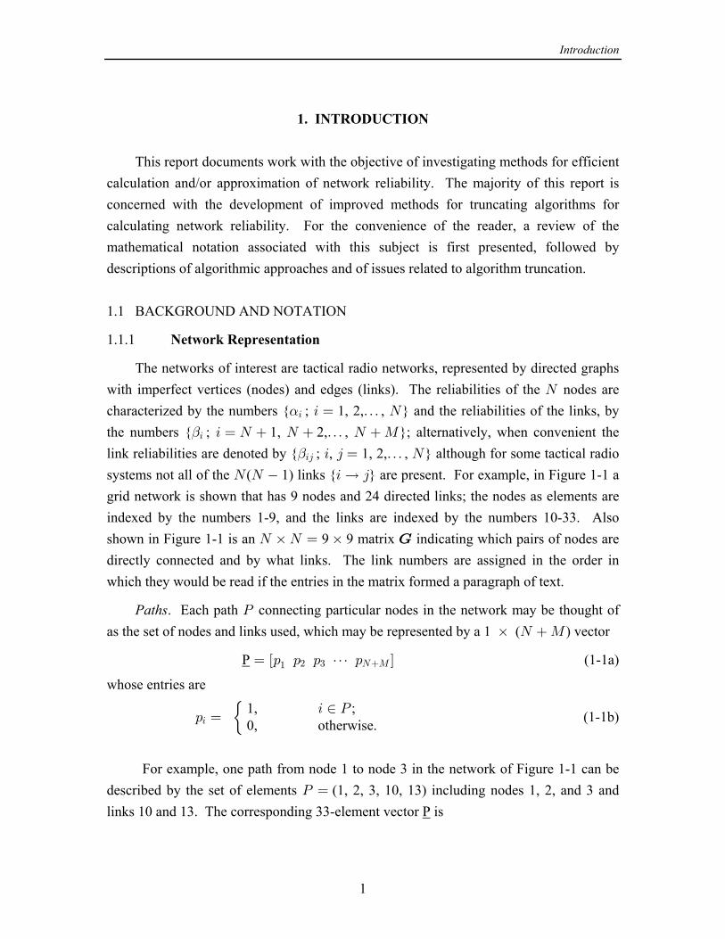
1. INTRODUCTION
This report documents work with the objective of investigating methods for efficientcalculation and/or approximation of network reliability. The majority of this report isconcerned with the development of improved methods for truncating algorithms forcalculating network reliability. For the convenience of the reader, a review of themathematical notation associated with this subject is first presented, followed bydescriptions of algorithmic approaches and of issues related to algorithm truncation.
1.1 BACKGROUND AND NOTATION
1.1.1 Network Representation
The networks of interest are tactical radio networks, represented by directed graphswith imperfect vertices (nodes) and edges (links). The reliabilities of the nodes areR
characterized by the numbers { ; 1, 2, , } and the reliabilities of the links, by!3 3 œ á R
the numbers { ; 1, 2, , }; alternatively, when convenient the"3 3 œ R R á R Q
link reliabilities are denoted by { ; , 1, 2, , } although for some tactical radio"34 3 4 œ á R
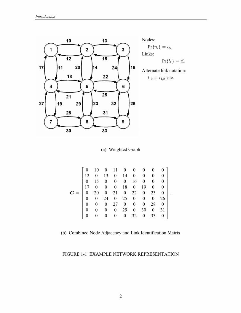
systems not all of the ( 1) links { } are present. For example, in Figure 1-1 aR R 3 Ä 4
grid network is shown that has 9 nodes and 24 directed links; the nodes as elements areindexed by the numbers 1-9, and the links are indexed by the numbers 10-33. Alsoshown in Figure 1-1 is an 9 9 matrix indicating which pairs of nodes areR ‚R œ ‚ K
directly connected and by what links. The link numbers are assigned in the order inwhich they would be read if the entries in the matrix formed a paragraph of text.
. Each path connecting particular nodes in the network may be thought ofPaths T
as the set of nodes and links used, which may be represented by a 1 ( ) vector‚ R Q
(1-1a)P œ : : : â :c d " # $ RQ
whose entries are
(1-1b) 1, ; 0, otherwise. œ:
3 − T3 œ
For example, one path from node 1 to node 3 in the network of Figure 1-1 can bedescribed by the set of elements (1, 2, 3, 10, 13) including nodes 1, 2, and 3 andT œ
links 10 and 13. The corresponding 33-element vector isP
Introduction
2
Nodes: Pr{ }8 œ3 3!
Links: Pr{ }6 œ5 5"
Alternate link notation: etc.6 ´ 6"! "ß#
(a) Weighted Graph
K œ
Ô ×Ö ÙÖ ÙÖ ÙÖ ÙÖ ÙÖ ÙÖ ÙÖ ÙÖ ÙÖ ÙÖ ÙÖ ÙÕ Ø
0 10 0 11 0 0 0 0 012 0 13 0 14 0 0 0 00 15 0 0 0 16 0 0 017 0 0 0 18 0 19 0 00 20 0 21 0 22 0 23 00 0 24 0 25 0 0 0 260 0 0 27 0 0 0 28 00 0 0 0 29 0 30 0 310 0 0 0 0 32 0 33 0
.
(b) Combined Node Adjacency and Link Identification Matrix
FIGURE 1-1 EXAMPLE NETWORK REPRESENTATION
Introduction
3
P œ c d 1 1 1 0 0 0 0 0 0 1 0 0 1 0 0 0 0 0 0 0 0 0 0 0 0 0 0 0 0 0 0 0 0 . (1-1c)
In a particular realization of the probabilistic network, a given element mayEvents.or may not be operable. Let the indicator variable denote the operability of the th\ 33
element, where
(1-2) 1, element operable; 1, element not operable. œ\
3 33 œ
An ( ) is defined to be one of the 2 particular realizations of theelementary event / RQ
network, i.e. a specification of the operational status of each weighted element. Theelementary event may be represented as a 1 ( ) vector,‚ R Q
e , (1-3)œ \ \ â \c d " # RQ
where all the entries equal +1 or 1. Another way to describe an elementary event is as
the logical expression formed by the intersection of logical variables (or their comple-ments) representing the status of each of the elements. Note that elementaryR Q
events are mutually exclusive (disjoint).
A is the union of certain elementary events , , , . Thegeneral event I / / á /" # 8
general event is represented by a 1 ( ) vectorI ‚ R Q
E (1-4)œ âc d0 0 0" RQ#
where
(1-5) 1, 1 for all , 1, 2, , ;
1, 1 for all , 1, 2, , ; 0, otherwise.
œ\ œ / − I 4 œ á 8
\ œ / − I 4 œ á 8033 4
3 4
ÚÛÜ
In other words, if the status of element is the same for all , then encodes that3 / − I \4 3
status ( 1); if the status of element is 1 in some and 1 for some other„ 3 / − I 4
/ − I \ œ3 3, then 0.
A vector E does not uniquely code all possible events. Of all events with the samevector representation, we define a as the one with the greatest number offull eventelementary events. For this analysis, only full events need be considered; hence an eventI D with zeros in its representation is assumed to include the union of 2 elementaryD
events. Note that a path may be interpreted as an event, and the representation of T Pgiven in (1-1c) properly represents the event.
The universal event is defined as the union of all elementary events. Note that theM
event is represented in the above notation by the all-zeros vector.M
Introduction
4
For a more compact notation, can also be written as a list of the nonzero entries inI
E, with an overbar denoting which entries are 1. For example, for
E 1 0 0 1 1 0 0 (1-6a)œ âc dwhere the ellipsis represents all zeros, can also be written
{1 4 5} (1-6b)œI
or alternatively (1, 4, 5). (1-6c)œI
In Boolean logic notation, the “full" events as described above can be considered tobe the joint occurrence of logic variables or their complements. For example, the eventspecified by (1-6a) requires that the events “element 1 is operative" and “element 5 isoperative" be , and that the event “element 4 is operative" be . The status ofTRUE FALSE
all other elements is irrelevant (the condition). Thus in Boolean notation,DON'T CARE
using to denote a status for a particular network element, the equivalent toB DON'T CARE
(1-6a) would be
1 0 1 . (1-6d)œ BB BâBE
The intersection of two events and with vectors A [ ] andE F œ + + â +" # RQ
B [ ] is defined as follows. If for any , both and are nonzero ( 1)œ , , â , 3 + , „" # RQ 3 3
but do not agree, then their intersection does not exist, that is, , theI œ E F œ g
empty set; otherwise, each term of the vector E for is given by the ruleI œ E F
(1-7) , 0 and 0 or ;
, 0 and 0 or ; 0, 0.
œ/+ + Á , œ , œ +, , Á + œ + œ ,
+ œ , œ3
3 3 3 3 3
3 3 3 3 3
3 3
ÚÛÜ
Note that if 0, then both of the first two cases of (1-7) yield the same result and+ œ , Á3 3
there is no ambiguity in the definition (remember that if and are both nonzero and+ ,3 3
unequal, then ).I œ E F œ g
Two classes of events are of particular interest inSuccess and Failure Collections.analyzing the network. For a given node pair ( , ), an event ( , ) is a success event if= > W = >4
for every elementary event the realization of the network corresponding to / − W /3 4 3
contains at least one s-t path. An event ( , ) is a failure event if for every theJ = > / − J4 3 4
realization of the network corresponding to contains no s-t paths./3
Further, two of events may be defined. For a given node pair ( , ), acollections = >
disjoint exhaustive success collection ( , ) is a collection of disjoint success events,f = > R=
Introduction
5
{ , , , } (1-8)œ W W á Wf " # R=
such that if the network realization corresponding to the elementary event contains an/
s-t path, then for one and only one . Furthermore, there are no elementary/ − W W −4 4 f
events which produce a successful s-t path that are not included in a success event in .fSimilarly, a disjoint exhaustive failure collection ( , ) is a collectionY = >
{ , , , } (1-9)œ J J á JY " # R0
such that if the network realization corresponding to contains no s-t paths, then / / − J4
for one and only one , and there are no elementary events failing to produce an s-tJ −4 Y
path that are not included in one of the failure events in . The significance of theseY
exhaustive collections of events is that the s-t reliability, , is the sum of the#=>
probabilities of the success events, which also equals one minus the sum of theR=
probabilities of the failure events.R0
. In order to discuss an algorithm forPartitioning of the complement of an eventgenerating and , we need one more result. Let be an event specified by a vectorf Y \
with nonzero elements, and further, without loss of generality, let these elements beO
elements 1, 2, , . Then the complement of , denoted by , can be partitioned asá O \ \
{1} {1 2} {1 2 3} {1 2 3 } (1-10a)œ â â O\where {1} [ 1 0 0 0], {1 2} [ 1 1 0 0], etc. (1-10b)œ â œ â
The terms on the right hand side of (1-10a) represent disjoint sets, and hence Pr{ } is\
the sum of their individual probabilities.
1.1.2 The Equivalent Links Algorithm
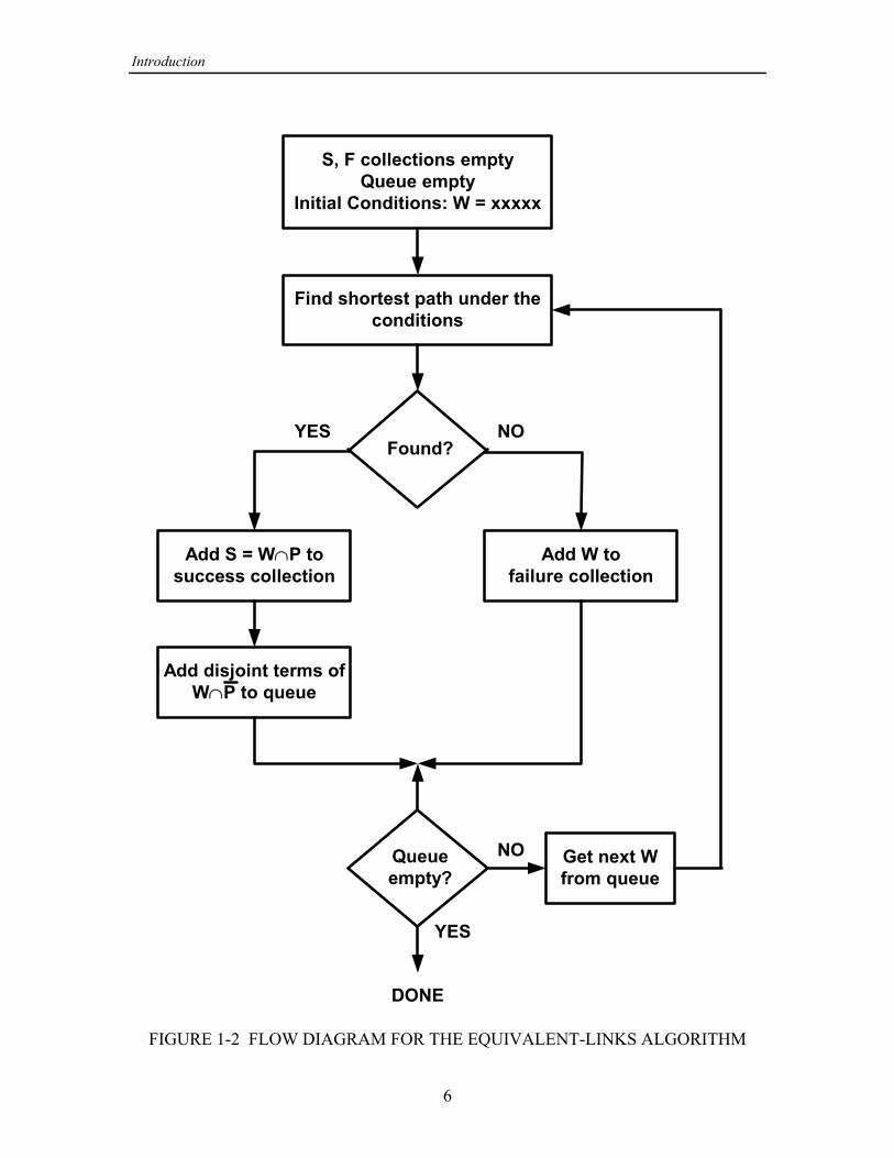
Fundamentally, the ELA or equivalent-links algorithm ([1], [2]) is a method forgenerating success and failure events for a given node pair, plus a method ofdisjointaccounting for node failures efficiently. The event-generation portion of the ELA isrelated to Dotson's method [3]. With reference to Figure 1-2, the way that the ELAworks may be explained as follows:
(a) Events are dimensioned 1 , as if there were no possibility ofInitialization. ‚Q
node failures. The particular node pair ( , ) is specified, and the success and failure= >
collections and (lists of success and failure event vectors stored in computerf Y
Introduction
6
S, F collections emptyQueue empty
Initial Conditions: W = xxxxx
Find shortest path under theconditions
Found?
Add W tofailure collection
Add S = W∩P tosuccess collection
Add disjoint terms ofW∩P to queue
Queueempty?
Get next Wfrom queue
YES
YES
NO
NO
DONE
FIGURE 1-2 FLOW DIAGRAM FOR THE EQUIVALENT-LINKS ALGORITHM
Introduction
7
memory), are emptied. In addition to and there is a first-in-first-out queue, denotedf Y
j, whose purpose is to buffer network events that are to be tested to see whether theyare success or failure events; this queue is initialized to contain one event, the universalevent. Recall that the universal event is the set which is union of all possiblecombinations of network element conditions; its vector representation contains onlyzeros. In Boolean notation, the logical function representing the universal event is
; (1-11)œ BBBBBBBâBBBBI
all the logic variables are specified to be in the state.DON'T CARE
(b) The algorithm takes the first event from the queue andEvent classification. [
uses a pathfinding algorithm to determine if there is a successful connection from to .= >
If no path can be found, the event is declared to be a failure and it is added to the[
failure collection. If a path is found, then the event is declared to be a successT [ T
event and is added to the success collection.
(c) After a success event has been found, theDisjoint event generation. [ T
disjoint events generated by the terms of are put into the queue. As shown in (1-[ T
10), if there are hops in the path , then there are disjoint terms of . These give8 T 8 T
rise to as many as “next events" to be put into the queue for classification; quite often8
there are fewer than next events because the intersection of a term or terms of with8 T
[ is empty. It is shown in Appendix A.2 of [1] that it is desirable to order the elementsof , and consequently of , in the sequence of links traversed from to in order toT T = >
avoid generating events for which successive nodes in the path are operating but areunconnected because of link failures.
(d) The algorithm terminates by itself when the queue becomesTermination.empty, that is, when there are no more next events to be classified as either successes orfailures. It is possible also to terminate the algorithm early (methods for doing so are asubject of the investigations summarized in this report).
In Appendix A.1 of this report, an example of the operation of the ELA in findingsuccess and failure events for a particular network model is given in detail.
The success and failure vectors {S } and {F } which represent the contents of the3 3
sets { } and { } in the implementation of the ELA have the dimension 1 ,f Yœ W J ‚Q3 3
where is the number of links (edges). The components of a particular S vector, forQ Q
example, take the values 1, if the network element is required to be working; 1, if the
network element is required not to be working; or 0, if it doesn't matter what the status of
Introduction
8
the element is. Each S corresponds to a term in the polynomial expression for thereliability of the connection between the given source and terminal nodes in the case thatall the nodes are perfectly reliable ( 1.0 for 1 to ); the 1's indicate those links!3 œ 3 œ R
whose probabilities of working (reliabilities) are factors in the term, and the 1's"
indicate those whose complementary probabilities 1 are factors. The total expression "
for the reliability when the nodes do not fail is thens-t
( , , , )œ á# # " " "=> => R" R# RQ
Pr{ ( , )} (1-12a)œ !4œ"
R=
S s t4
{ : S ( ; , ) 1} {1 : S ( ; , ) 1}, (1-12b)œ < = > œ < = > œ !# #4œ"
R
< << 4 < 4
=
" "
in which S ( ; , ) denotes the th component of the vector representing ( , ).4 4< = > < W = >
To account for node failures, the node reliabilities are “backfitted" into the ex-pression according to the concept of “equivalent links," in which the network links arethought of as being lumped together with the nodes on which they terminate; to thefailure set generated by this method must be added the failure corresponding to theJ!
failure of the source node, , since none of the links used for the ( , ) connection= = >
terminate on . The formula for factoring in the node reliabilities [2] is based the=
observation that
( , )} Pr{ ( , )}, (1-13)Pr{ œ W = >W = >4 = 488
! #where indexes the nodes and ( , ) is the subset of ( , ) which lists the linksn W = > W = >48 4
terminating on node that must be either working or not working. Let denote then R48
number of links required not to be working and the number required to be working,O48
as determined by the algorithm described above. Then the equivalent-link formulas are,assuming that the links are renumbered for convenience [2],
( , )} 1, 0; (1-14a)Pr{ œ R œ O œW = >48 48 48
, 0, 0; (1-14b) œ R œ O ! "8 < 48 48<œ"
O#48
1 (1 ) , 0, 0; (1-14c) œ R O œ! ! "8 8 < 48 48<œ"
R#48
(1 ), 0, 0. (1-14d) œ R O R O
! " "8 < < 48 48<œ"
O
<œO "
48 48# #48
48
Introduction
9
In Appendix A.2 of this report, the formulas in (1-14) are applied to success eventsfound by the ELA in a particular case.
1.1.3 Connectivities in Terms of Event Probabilities
As already noted, the disjoint success and failure events generated by the ELA relatedirectly to the connectivity between pairs of network nodes. The probability that theflood search succeeds in finding a path from origin to terminal (or the s-t reliability),= >
in terms of a disjoint exhaustive link success events collection { , , , },f œ W W á W" # R=
can be written as
Pr{ } (1-15a)œ W#=> 3
R
3œ"
!=
where the link states associated with the event are represented by the vectorW3
S , (1-15b)œ \ \ â \3 3" 3# 3Qc dand the probability of the events is computed using (1-14). An alternative formulation interms of an exhaustive link failure event collection { , , , } isY œ J J á J" # R0
1 Pr{ } Pr{ } Pr{ } (1-16a)œ J J œ J# !=> 3 ! = 3
R R
3œ" 3œ"
! !0 0
where is the source node failure event and the link states associated with the event J J! 3
are represented by the vector
F . (1-16b)œ \ \ â \3 3" 3# 3Qc d Furthermore, suppose exhaustive collections and cannot be found due to com-f Y
puter time and/or memory limitations. If partial collections { , , }, f w" O =œ W á W O R
and { , , }, can be found, there are the boundsY w" P 0œ J á J P R
Pr{ } Pr{ }, (1-17)Ÿ Ÿ JW" !O
3œ"
3 => = 3
P
3œ"
# !
since all the terms of the summations in (1-15a) and (1-16a) are positive.
1.2 ELA2: A CUTSET APPROACH
It was noted in [1] that, because it is based on pathfinding, the ELA tends to find themajority of success events earlier in its operation, and the majority of failure events, later.A consequence of this behavior is that the convergence of the bounds in (1-17) is uneven,requiring the algorithm to be run longer for the same accuracy than it would have to if the

Introduction
10
bounds converged at the same rate. In [4], the concept of basing the event generation onfinding cutsets instead of paths is put forth with the idea of finding failure events earlier,thus improving the convergence of the upper bound and perhaps allowing for an earliertermination of the algorithm with the same accuracy. For convenience, the equivalent-links algorithm modified to use a cutset-finding approach shall be referred to as “ELA2."
1.2.1 Operation of ELA2
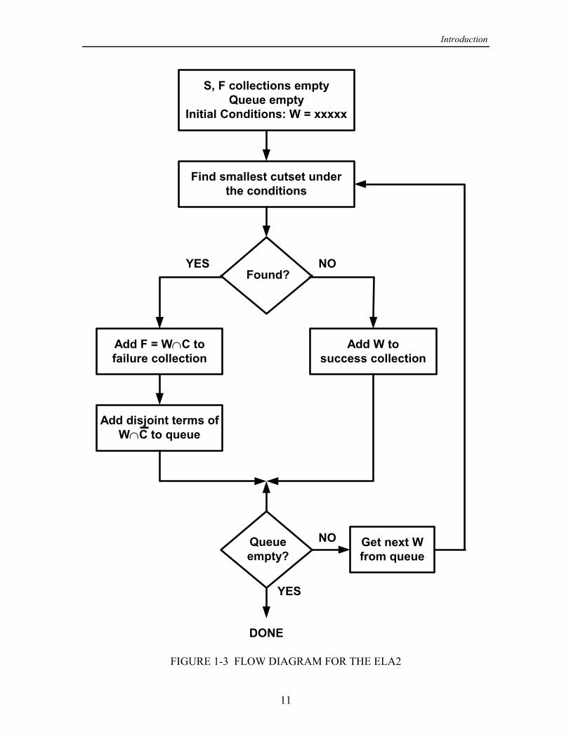
A flow diagram for the ELA2 is shown in Figure 1-3. The way that the ELA2 worksmay be explained as follows:
(a) Events are dimensioned 1 , as if there were no possibility ofInitialization. ‚Q
node failures. The particular node pair ( , ) is specified, and the success and failure= >
collections and are emptied. In addition to and there is a first-in-first-outf Y f Y
queue, denoted , whose purpose is to buffer network events that are to be tested to seej
whether they are success or failure events; this queue is initialized to contain one event,the universal event.
(b) The algorithm takes the first event from the queue andEvent classification. [
uses a cutset-finding algorithm to determine if there is a set of link outages that precludesa successful connection from to . If no cutset can be found, it is because among the= >
links specified as UP in the event , one or more form an - path; in the case of no[ = >
cutset, is declared to be a success and it is added to the success collection without[
further processing. If a cutset
{ , , , } (1-18)œ 6 6 6 áG + , -
is found, then the event is declared to be a failure event and is added to the[ G
failure collection.
(c) After a failure event has been found, theDisjoint event generation. [ G
disjoint events generated by the terms of are put into the queue. If there are [ G 8
link outages in the cutset , then there are disjoint terms of . These give rise to G 8 G 8
“next events" to be put into the queue for classification, of the form
( ). (1-19)œ [ 6 6 6 6 6 6 â[ G + + , + , -
(d) The algorithm terminates by itself when the queue becomesTermination.empty, that is, when there are no more next events to be classified as either successes orfailures. The algorithm can also be terminated early according to a stopping criterion.
Introduction
11
S, F collections emptyQueue empty
Initial Conditions: W = xxxxx
Find smallest cutset underthe conditions
Found?
Add W tosuccess collection
Add F = W∩C tofailure collection
Add disjoint terms ofW∩C to queue
Queueempty?
Get next Wfrom queue
YES
YES
NO
NO
DONE
FIGURE 1-3 FLOW DIAGRAM FOR THE ELA2
Introduction
12
In Appendix B, an example of the operation of the ELA2 in finding success andfailure events for a particular network model is given in detail.
By comparing Figure 1-3 with the flow diagram for the ELA that is given in Figure1-2, it may be observed that the ELA2 is in some sense a dual to the ELA:
Whereas the ELA is based on finding - paths (sets of links that form an ì = > = Ä >
connection), the ELA2 is based on finding - cutsets (sets of link outages that preclude= >
an connection).= Ä >
Whereas the ELA forms success events when a path is found by determiningì T
the intersection , the ELA2 forms failure events when a cutset is found byW œ [ T G
determining the intersection .J œ [ G
Whereas the ELA forms next events after a success event has been determinedì
by determining the disjoint terms of the intersection , the ELA2 forms next events[ T
after a failure event has been determined by determining the disjoint terms of theintersection .[ G
Whereas the ELA after classifying an event as a failure ( ) does notì J œ [
process that event further, the ELA2 after classifying an event as a success ( )W œ [
does not process that event further.
A difference in the operation of ELA and ELA2 that may be observed is that, whilethe order in which the disjoint terms of are generated is significant in the ELA, theT
order in which the disjoint terms of are generated is not significant in the ELA2.G
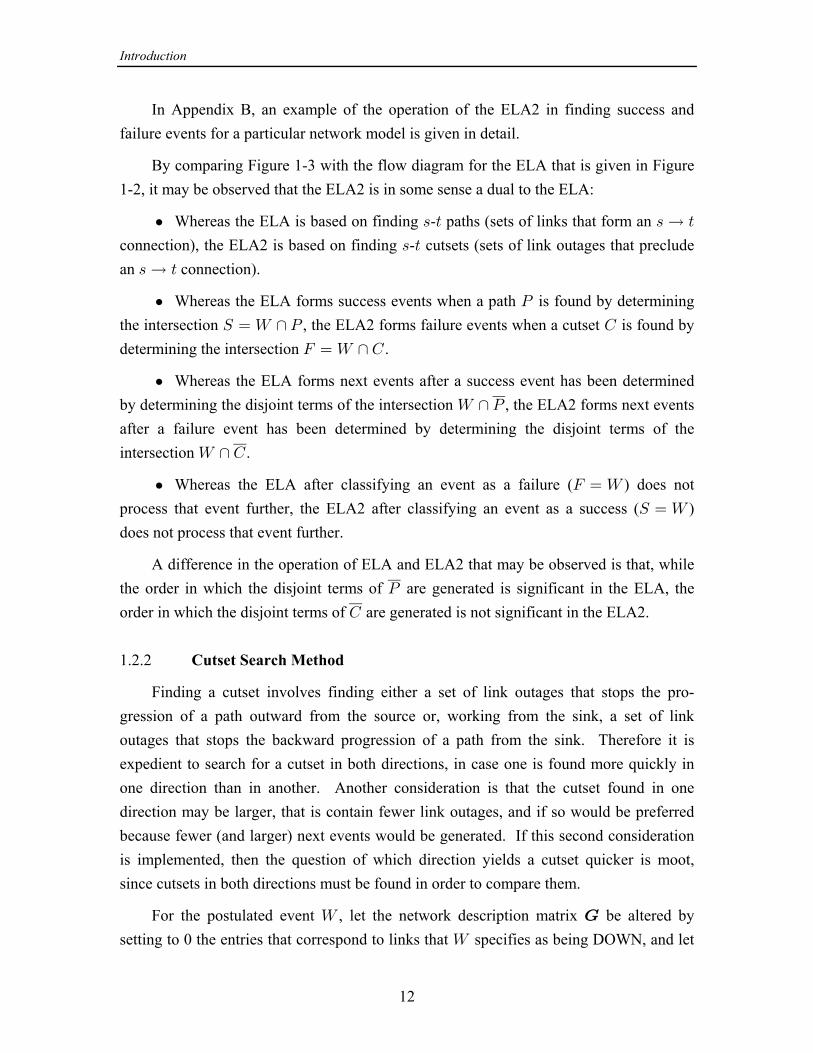
1.2.2 Cutset Search Method
Finding a cutset involves finding either a set of link outages that stops the pro-gression of a path outward from the source or, working from the sink, a set of linkoutages that stops the backward progression of a path from the sink. Therefore it isexpedient to search for a cutset in both directions, in case one is found more quickly inone direction than in another. Another consideration is that the cutset found in onedirection may be larger, that is contain fewer link outages, and if so would be preferredbecause fewer (and larger) next events would be generated. If this second considerationis implemented, then the question of which direction yields a cutset quicker is moot,since cutsets in both directions must be found in order to compare them.
For the postulated event , let the network description matrix be altered by[ K
setting to 0 the entries that correspond to links that specifies as being DOWN, and let[

Introduction
13
Y [ VJ be set of links that are specified in as being UP. Also, let denote the set of3
nodes reached on the th hop outward from the source node. As suggested in [4], a cutset3
in the forward direction may be found by forming a set of failable links according theGJ
following procedure:
(1) Initialize to include the failable links (if any) in the th row of the G =J K
matrix—those links that are in the th row but not in , and therefore were not specified= Y
by as being either UP or DOWN. In order to preclude a path outward from , these[ =
links must fail; therefore, they belong in the cutset. If all of the links in the th row are=
failable, then a cutset has been found and the search is stopped.
(2) If one or more of the links in the th row of are in , indicating unfailed= YK
connections to other nodes, add those nodes to and check whether , that is,VJ > − VJ" "
whether the node has been reached in one hop by a link specified by to be UP. If so,> [
there is no cutset, and the search is stopped.
(3) For the nodes ( ) in , say nodes and , add to the cutset the failableÁ > VJ < <" " #
links used on the second hop, those in the rows indexed by those nodes (row and row<"
< Y#). If none of the links in these rows is in , then a cutset has been found and the searchis stopped. Otherwise, add the nodes reached by the links in to the set , and checkY VJ#
to see if was reached on the second hop using two links specified in to be UP; if not,> [
proceed with the cutset search.
(4) Continue for hop by examining the rows corresponding to the nodes in the set3
VJ G VJ3" J 3, adding failable links in those rows to and stopping with a found cutset if is empty, or stopping with no cutset found if .> − VJ3
A flow diagram for the forward cutset search is included in Figure 1-4 (left side).The search in the reverse direction for a cutset proceeds similarly, using toG VVV 3
denote the set of nodes reached by links in on the th hop backward from the sink:Y 3
(1) Initialize to include the failable links (if any) in the th column of the G >V K
matrix—those links that are in the th column but not in ; if all of the links in the th> Y >
column are failable, then a cutset has been found and the search is stopped.
(2) If one or more of the links in the th column of are in , indicating unfailed> YK
connections from other nodes, add those nodes to and check whether . IfVV = − VV" "
so, node is reachable from node in one hop using a link specified by as being UP,> = [
there is no cutset, and the search is stopped.
Introduction
14
W --> U (set of good links) --> G (network state)RF0, RR0 emptyCf, Cr empty, i = k = 0
Search Direction
Increment iCf = Cf + links in rows of G for nodes in RFi-1 and not in URFi = nodes reached by good links on hop i
Increment kCr = Cr + links in columns of G for nodes in RRk-1RRk = nodes reached by good links on hop k
RFiempty
?
RRkempty
?
t in RFi?
s in RRk?
EXIT (no cutset)
ForwardCutsetFound
ReverseCutsetFound
RFi ∩RRkempty?
Foundboth
cutsets?
Choose larger
NO
NO
NO NO
NONO
YES
YES YES
YES
YES
YES
FIGURE 1-4 FLOW DIAGRAM FOR CUTSET SEARCH
Introduction
15
(3) For the nodes ( ) in , say nodes and , add to the cutset the failableÁ = VV - -" " #
links in the columns indexed by those nodes (column and column ). If none of the- -" #
links in these columns is in , then a cutset has been found and the search is stopped.Y
Otherwise, add the nodes reached by the links in to the set .Y VV#
(4) Continue for hop by examining the columns corresponding to the nodes in the3
set , adding failable links in those columns to and stopping with a found cutsetVV G3" V
if is empty.VV3
A flow diagram for the reverse cutset search is included in Figure 1-4 (right side).Note that if the forward and backward searches are conducted in alternating progressionsfrom the source and sink, respectively, if there is an path comprised of links in = Ä > Y
this fact can be detected efficiently by an nonempty intersection of and forVJ VV5 6
some and . This strategy is incorporated in the flow diagram of Figure 1-4, as is the5 6
concept of selecting the larger of the forward and reverse cutsets.
In the tests of program implementations discussed later in this report, a comparisonis given of the execution times incurred by using two different cutset search strategies:(1) selecting the larger of the forward and reverse cutsets, and (2) selecting the first cutsetfound.
1.2.3 An Observation
At any point during the execution of the ELA or the ELA2, the collection jconsists of events that completely describe the remaining possibilities for the state of[
the network links. Moreover, the s are disjoint, as are the new (smaller) s that are[ [
created by removing one of the s from and processing it—whether by searching for[ j
paths or searching for cutsets.
It follows from this observation that there is no reason why a particular to be[
examined cannot be arbitrarily examined by the pathfinding method or by theeithercutset-finding method. For example, the methods employed could be alternated, orperhaps an attempt could be made to minimize the total number of success and failureevents by selecting the method based on which one creates fewer new s.[
In Section 2, tests are made of various algorithms that combine the features of theELA and the ELA2, in addition to tests of these algorithms in their “pure" form.
Introduction
16
1.3 TRUNCATION ISSUES
The work documented by this report was motivated by a desire to improve, ifpossible, the performance of the ELA in terms of the truncation issues discussed in thefollowing paragraphs.
1.3.1 Bound Convergence
In [1] it was demonstrated that typically the ELA generates success events earlier inthe processing than it generates failure events. For this reason the lower bound on the -= >
reliability, which is the accumulated probability of success, converges faster than theupper bound, which is the complement of the accumulated probability of failure.
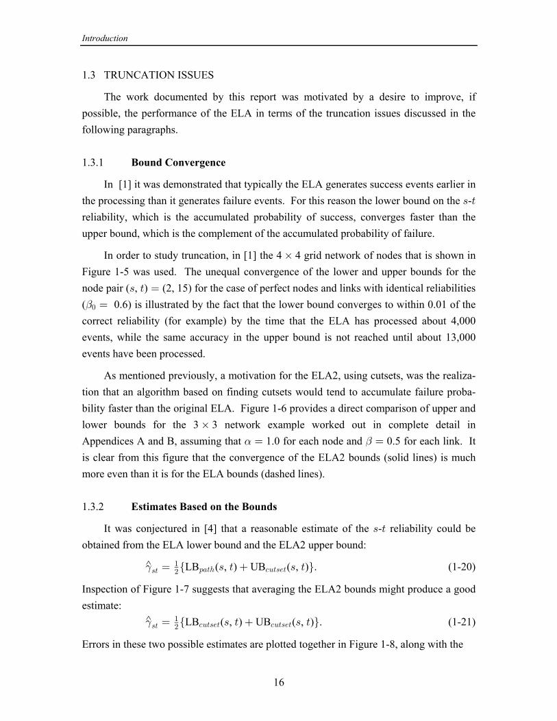
In order to study truncation, in [1] the 4 4 grid network of nodes that is shown in‚
Figure 1-5 was used. The unequal convergence of the lower and upper bounds for thenode pair ( , ) (2, 15) for the case of perfect nodes and links with identical reliabilities= > œ
( 0.6) is illustrated by the fact that the lower bound converges to within 0.01 of the"! œ
correct reliability (for example) by the time that the ELA has processed about 4,000events, while the same accuracy in the upper bound is not reached until about 13,000events have been processed.
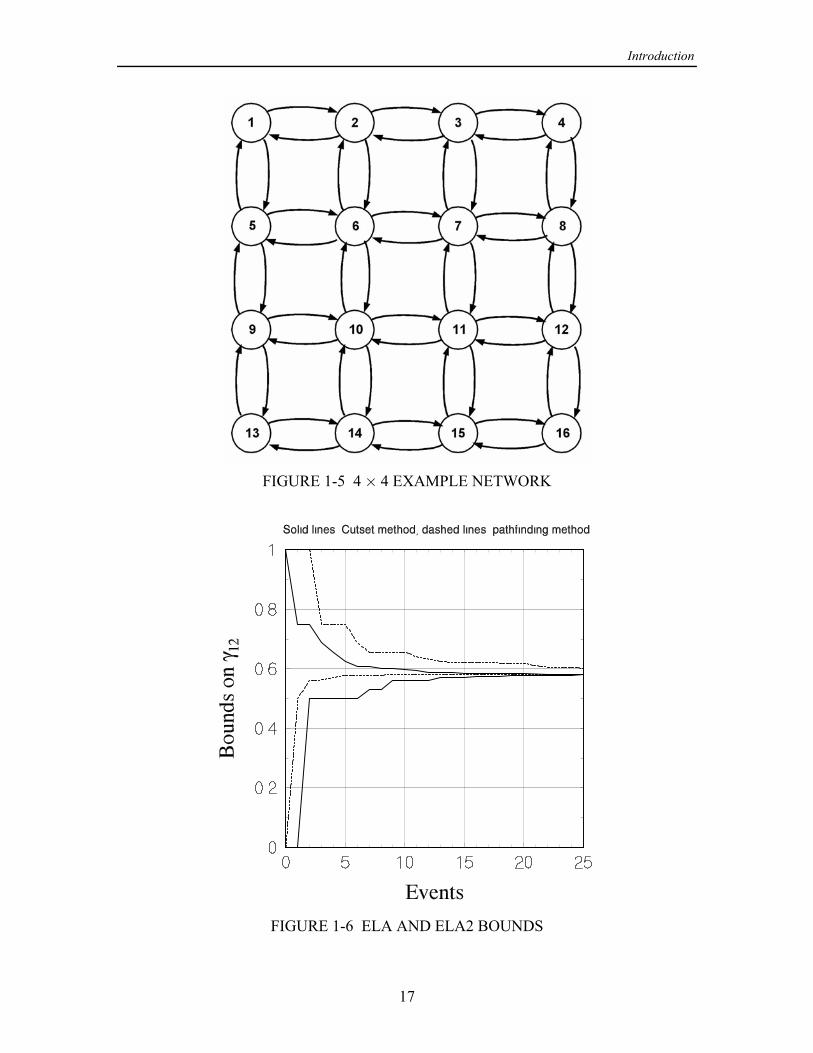
As mentioned previously, a motivation for the ELA2, using cutsets, was the realiza-tion that an algorithm based on finding cutsets would tend to accumulate failure proba-bility faster than the original ELA. Figure 1-6 provides a direct comparison of upper andlower bounds for the 3 3 network example worked out in complete detail in‚
Appendices A and B, assuming that 1.0 for each node and 0.5 for each link. It! "œ œ
is clear from this figure that the convergence of the ELA2 bounds (solid lines) is muchmore even than it is for the ELA bounds (dashed lines).
1.3.2 Estimates Based on the Bounds
It was conjectured in [4] that a reasonable estimate of the - reliability could be= >
obtained from the ELA lower bound and the ELA2 upper bound:
LB ( , ) UB ( , ) . (1-20)^ œ = > = >#=>"# :+>2 -?>=/>e f
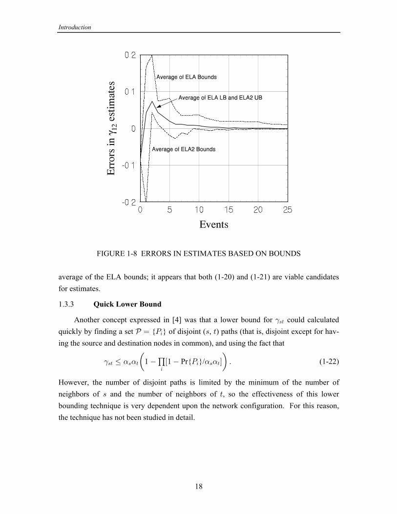
Inspection of Figure 1-7 suggests that averaging the ELA2 bounds might produce a goodestimate: LB ( , ) UB ( , ) . (1-21)^ œ = > = >#=>
"# -?>=/> -?>=/>e f
Errors in these two possible estimates are plotted together in Figure 1-8, along with the
Introduction
17
FIGURE 1-5 4 4 EXAMPLE NETWORK‚
FIGURE 1-6 ELA AND ELA2 BOUNDS
Introduction
18
FIGURE 1-8 ERRORS IN ESTIMATES BASED ON BOUNDS
average of the ELA bounds; it appears that both (1-20) and (1-21) are viable candidatesfor estimates.
1.3.3 Quick Lower Bound
Another concept expressed in [4] was that a lower bound for could calculated#=>
quickly by finding a set { } of disjoint ( , ) paths (that is, disjoint except for hav-c œ T = >3
ing the source and destination nodes in common), and using the fact that
1 1 Pr{ }/ . (1-22)Ÿ T# ! ! ! !=> = > 3 = >3
Π#c d
However, the number of disjoint paths is limited by the minimum of the number ofneighbors of and the number of neighbors of , so the effectiveness of this lower= >
bounding technique is very dependent upon the network configuration. For this reason,the technique has not been studied in detail.
Algorithm Development
19
2. ALGORITHM DEVELOPMENT
In this section, assessment is made of the relative merits of implementations of theELA and the ELA2 - reliability algorithms and for certain variations on them. The= >
assessment is based on numerical evaluations that are preceded by descriptions of theimplementations and by documentation of several network examples that were used forstudy, in order to introduce the computer file structures that the programs are designed toprocess.
2.1 NETWORK EXAMPLES
During the development and testing of the - reliability algorithms, one or more= >
example networks were used. These example networks are described in the followingparagraphs.
2.1.1 3 3 Grid Network Example‚
This network, shown previously in Figure 1-1, has been used extensively for devel-opment because completely worked-out manual solutions have been maintained for thiscase throughout the project for the case of ( , ) (1, 2). Appendices A and B of this= > œ
report contain manual solutions for the ELA and for the ELA2, respectively. The network has 9 nodes and 24 links; there are fewer than the 72 possible linksbecause the network models an area coverage grid in which each of the radios has highlydirectional antennas aimed at particular other radios. In order to provide numerical datafor algorithm testing, a fictional laydown of a jammer and the 9 nodes was created andprocessed by the program LINKSNRS described in [5]. That program calculates SNRsfor every possible link, based on user-supplied link parameters, and writes them to diskfile. Nominal parameters not necessarily realistic in terms of any particular radio systemwere used, and the disk file was edited by deleting the links not shown in Figure 1-1 toproduce the file MESH1000.SNR.1
A list of the links and link reliabilities for this example is given in Table 2-1 at theend of subsection 2.1.4, and was calculated assuming
P P , (2-1)œ œ"34 K KŠ ‹ Š ‹SNR Margin34 34
P P
.5 5
1The format of the disk files is discussed in detail below.
Algorithm Development
20
where P ( ) is the Gaussian cumulative distribution function, is the system's SNRK † .
threshold criterion in dB, and is a standard deviation for the SNR in dB. As suggested5P
in [6], is taken to be 10 dB, while the value of is system-dependent; for the data in5 .P
Table 2-1 and unless otherwise noted, a value of zero dB is assumed. For this report,. 2
network examples were selected in which generally the links all have a positive margin,since the focus of the study is on the operation of network analysis algorithms when alarge number of links are viable. Since a link is DOWN for SNR , the analysis34 .
programs treat links with 0.5 as being absent; this treatment has the effect of"34
defining to have zero value for SNR , as far as - reliability is concerned." .34 34 = >
However, the actual values of link reliability are preserved so that they can be retrievedindividually if desired.
2.1.2 15-Node Network Example
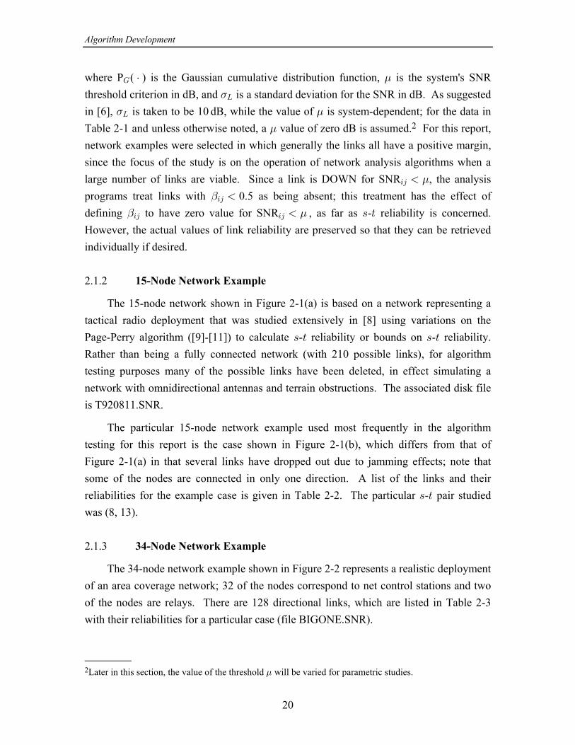
The 15-node network shown in Figure 2-1(a) is based on a network representing atactical radio deployment that was studied extensively in [8] using variations on thePage-Perry algorithm ([9]-[11]) to calculate - reliability or bounds on - reliability.= > = >
Rather than being a fully connected network (with 210 possible links), for algorithmtesting purposes many of the possible links have been deleted, in effect simulating anetwork with omnidirectional antennas and terrain obstructions. The associated disk fileis T920811.SNR.
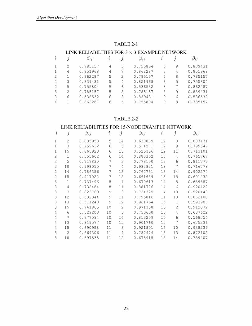
The particular 15-node network example used most frequently in the algorithmtesting for this report is the case shown in Figure 2-1(b), which differs from that ofFigure 2-1(a) in that several links have dropped out due to jamming effects; note thatsome of the nodes are connected in only one direction. A list of the links and theirreliabilities for the example case is given in Table 2-2. The particular - pair studied= >
was (8, 13).
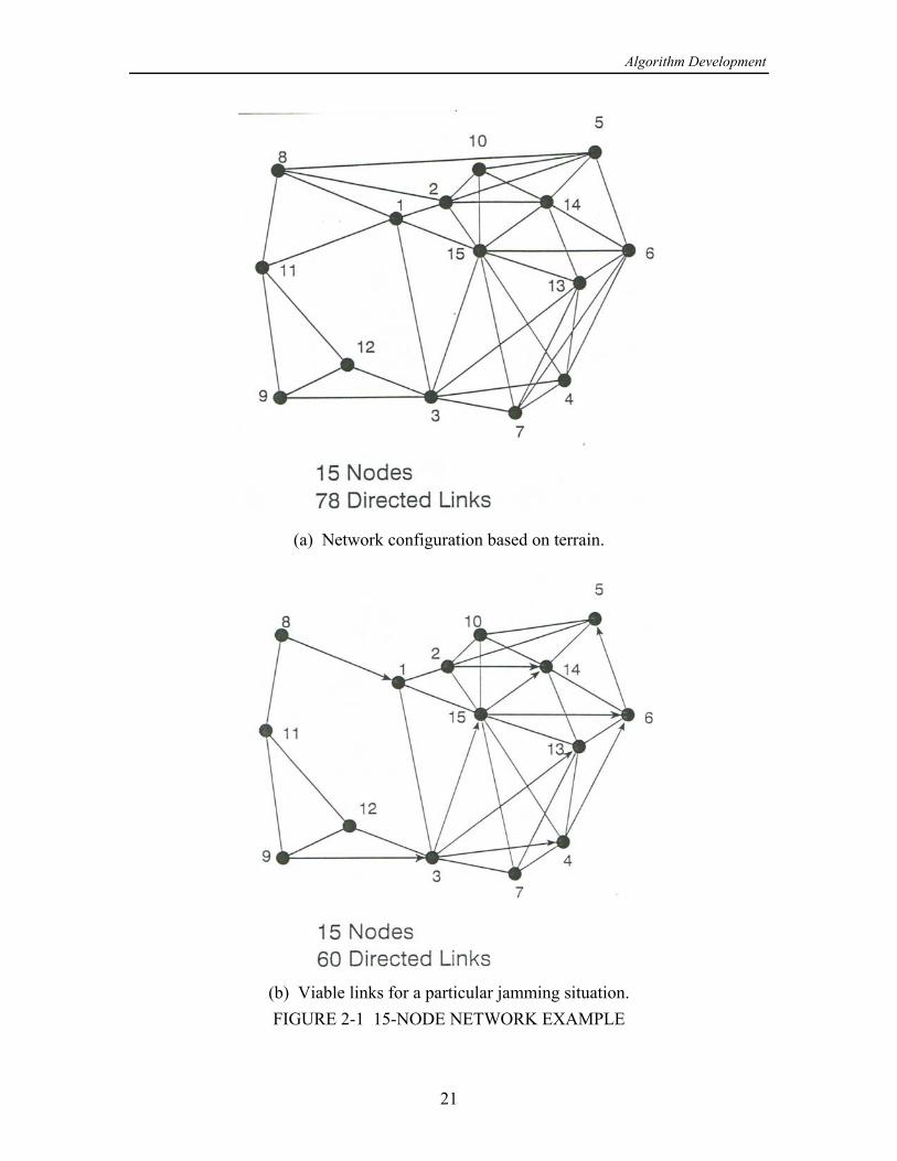
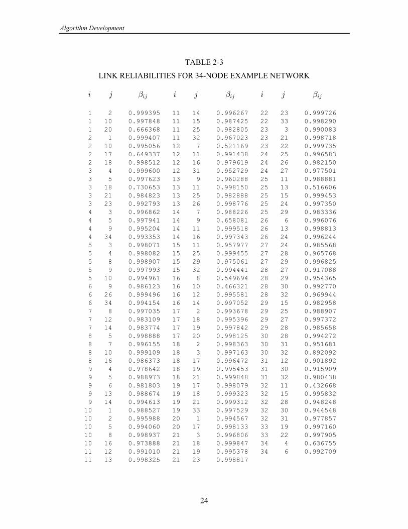
2.1.3 34-Node Network Example
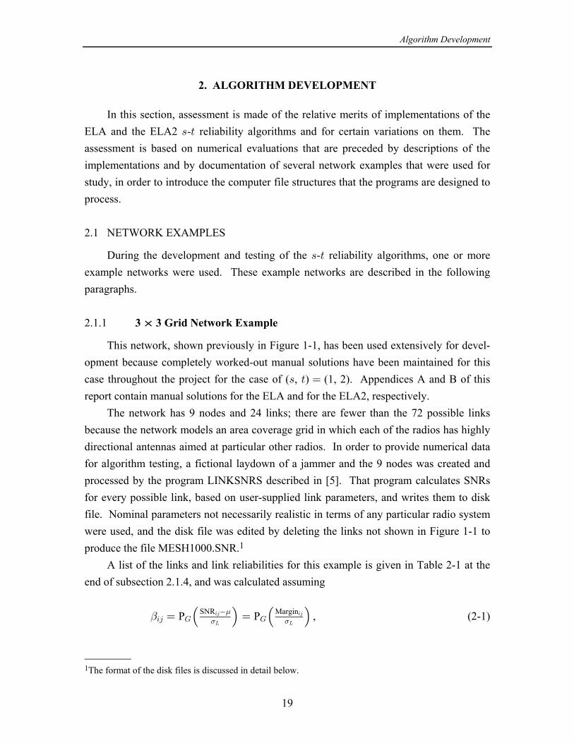
The 34-node network example shown in Figure 2-2 represents a realistic deploymentof an area coverage network; 32 of the nodes correspond to net control stations and twoof the nodes are relays. There are 128 directional links, which are listed in Table 2-3with their reliabilities for a particular case (file BIGONE.SNR).
2Later in this section, the value of the threshold will be varied for parametric studies..
Algorithm Development
21
(a) Network configuration based on terrain.
(b) Viable links for a particular jamming situation.FIGURE 2-1 15-NODE NETWORK EXAMPLE
Algorithm Development
22
TABLE 2-1
LINK RELIABILITIES FOR 3 3 EXAMPLE NETWORK‚ 3 4 3 4 3 4" " "34 34 34
1 2 0.785157 4 5 0.755804 6 9 0.839431 1 4 0.851968 4 7 0.862287 7 4 0.851968 2 1 0.862287 5 2 0.785157 7 8 0.785157 2 3 0.839431 5 4 0.851968 8 5 0.755804 2 5 0.755804 5 6 0.536532 8 7 0.862287 3 2 0.785157 5 8 0.785157 8 9 0.839431 3 6 0.536532 6 3 0.839431 9 6 0.536532 4 1 0.862287 6 5 0.755804 9 8 0.785157
TABLE 2-2
LINK RELIABILITIES FOR 15-NODE EXAMPLE NETWORK 3 4 3 4 3 4" " "34 34 34
1 2 0.835958 5 14 0.630889 12 3 0.887471 1 3 0.752632 6 5 0.511271 12 9 0.799649 1 15 0.865923 6 13 0.525386 12 11 0.713101 2 1 0.555662 6 14 0.883352 13 4 0.765767 2 5 0.717830 7 3 0.778150 13 6 0.811777 2 10 0.998010 7 4 0.982821 13 7 0.716778 2 14 0.786356 7 13 0.762751 13 14 0.902274 2 15 0.917022 7 15 0.661659 13 15 0.601432 3 1 0.737496 8 1 0.670613 14 5 0.639387 3 4 0.732484 8 11 0.881726 14 6 0.920422 3 7 0.822769 9 3 0.721325 14 10 0.520149 3 12 0.632344 9 11 0.795816 14 13 0.862100 3 13 0.511243 9 12 0.961764 15 1 0.593906 3 15 0.741865 10 2 0.971308 15 2 0.912072 4 6 0.529203 10 5 0.750600 15 4 0.687622 4 7 0.877594 10 14 0.812209 15 6 0.568354 4 13 0.819577 10 15 0.901760 15 7 0.675236 4 15 0.690958 11 8 0.921801 15 10 0.938239 5 2 0.669306 11 9 0.787474 15 13 0.872102 5 10 0.697838 11 12 0.678915 15 14 0.759407

Algorithm Development
23
FIGURE 2-2 34-NODE NETWORK EXAMPLE
Algorithm Development
24
TABLE 2-3
LINK RELIABILITIES FOR 34-NODE EXAMPLE NETWORK
3 4 3 4 3 4" " "34 34 34
1 2 0.999395 11 14 0.996267 22 23 0.999726 1 10 0.997848 11 15 0.987425 22 33 0.998290 1 20 0.666368 11 25 0.982805 23 3 0.990083 2 1 0.999407 11 32 0.967023 23 21 0.998718 2 10 0.995056 12 7 0.521169 23 22 0.999735 2 17 0.649337 12 11 0.991438 24 25 0.996583 2 18 0.998512 12 16 0.979619 24 26 0.982150 3 4 0.999600 12 31 0.952729 24 27 0.977501 3 5 0.997623 13 9 0.960288 25 11 0.988881 3 18 0.730653 13 11 0.998150 25 13 0.516606 3 21 0.984823 13 25 0.982888 25 15 0.999453 3 23 0.992793 13 26 0.998776 25 24 0.997350 4 3 0.996862 14 7 0.988226 25 29 0.983336 4 5 0.997941 14 9 0.658081 26 6 0.996076 4 9 0.995204 14 11 0.999518 26 13 0.998813 4 34 0.993353 14 16 0.997343 26 24 0.996244 5 3 0.998071 15 11 0.957977 27 24 0.985568 5 4 0.998082 15 25 0.999455 27 28 0.965768 5 8 0.998907 15 29 0.975061 27 29 0.996825 5 9 0.997993 15 32 0.994441 28 27 0.917088 5 10 0.994961 16 8 0.549694 28 29 0.954365 6 9 0.986123 16 10 0.466321 28 30 0.992770 6 26 0.999496 16 12 0.995581 28 32 0.969944 6 34 0.994154 16 14 0.997052 29 15 0.982958 7 8 0.997035 17 2 0.993678 29 25 0.988907 7 12 0.983109 17 18 0.995396 29 27 0.997372 7 14 0.983774 17 19 0.997842 29 28 0.985658 8 5 0.998888 17 20 0.998125 30 28 0.994272 8 7 0.996155 18 2 0.998363 30 31 0.951681 8 10 0.999109 18 3 0.997163 30 32 0.892092 8 16 0.986373 18 17 0.996472 31 12 0.901892 9 4 0.978642 18 19 0.995453 31 30 0.915909 9 5 0.988973 18 21 0.999848 31 32 0.980438 9 6 0.981803 19 17 0.998079 32 11 0.432668 9 13 0.988674 19 18 0.999323 32 15 0.995832 9 14 0.994613 19 21 0.999312 32 28 0.948248 10 1 0.988527 19 33 0.997529 32 30 0.944548 10 2 0.995988 20 1 0.994567 32 31 0.977857 10 5 0.994060 20 17 0.998133 33 19 0.997160 10 8 0.998937 21 3 0.996806 33 22 0.997905 10 16 0.973888 21 18 0.999847 34 4 0.636755 11 12 0.991010 21 19 0.995378 34 6 0.992709 11 13 0.998325 21 23 0.998817
Algorithm Development
25
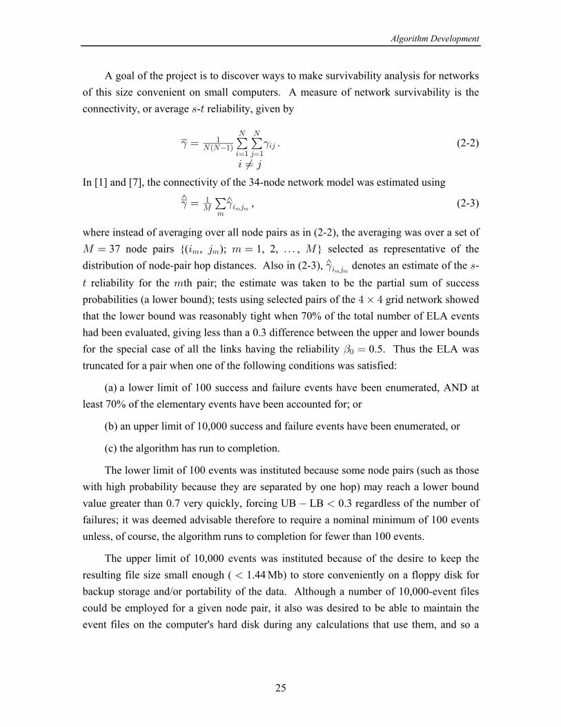
A goal of the project is to discover ways to make survivability analysis for networksof this size convenient on small computers. A measure of network survivability is theconnectivity, or average - reliability, given by= >
. (2-2)œ
3 Á 4
# #"RÐR"Ñ
3œ" 4œ"
R R
34! !
In [1] and [7], the connectivity of the 34-node network model was estimated using
, (2-3)^ ^œ# #"Q
73 4
!7 7
where instead of averaging over all node pairs as in (2-2), the averaging was over a set ofQ œ 3 4 7 œ á Q37 node pairs {( , ); 1, 2, , } selected as representative of the7 7
distribution of node-pair hop distances. Also in (2-3), denotes an estimate of the -#̂3 47 7=
> 7 reliability for the th pair; the estimate was taken to be the partial sum of successprobabilities (a lower bound); tests using selected pairs of the grid network showed% ‚ %
that the lower bound was reasonably tight when 70% of the total number of ELA eventshad been evaluated, giving less than a 0.3 difference between the upper and lower boundsfor the special case of all the links having the reliability 0.5. Thus the ELA was"! œ
truncated for a pair when one of the following conditions was satisfied:
(a) a lower limit of 100 success and failure events have been enumerated, AND atleast 70% of the elementary events have been accounted for; or
(b) an upper limit of 10,000 success and failure events have been enumerated, or
(c) the algorithm has run to completion.
The lower limit of 100 events was instituted because some node pairs (such as thosewith high probability because they are separated by one hop) may reach a lower boundvalue greater than 0.7 very quickly, forcing UB LB 0.3 regardless of the number of
failures; it was deemed advisable therefore to require a nominal minimum of 100 eventsunless, of course, the algorithm runs to completion for fewer than 100 events.
The upper limit of 10,000 events was instituted because of the desire to keep theresulting file size small enough ( 1.44 Mb) to store conveniently on a floppy disk for
backup storage and/or portability of the data. Although a number of 10,000-event filescould be employed for a given node pair, it also was desired to be able to maintain theevent files on the computer's hard disk during any calculations that use them, and so a
Algorithm Development
26
10,000-event limit was selected as a reasonable compromise to allow a number of node-pair event files to reside in the available disk space simultaneously.
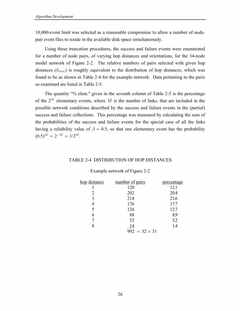
Using these truncation procedures, the success and failure events were enumeratedfor a number of node pairs, of varying hop distances and orientations, for the 34-nodemodel network of Figure 2-2. The relative numbers of pairs selected with given hopdistances ( ) is roughly equivalent to the distribution of hop distances, which was2738
found to be as shown in Table 2-4 for the example network. Data pertaining to the pairsso examined are listed in Table 2-5.
The quantity “% elem." given in the seventh column of Table 2-5 is the percentageof the 2 elementary events, where is the number of links, that are included in theQ Q
possible network conditions described by the success and failure events in the (partial)success and failure collections. This percentage was measured by calculating the sum ofthe probabilities of the success and failure events for the special case of all the linkshaving a reliability value of 0.5, so that one elementary event has the probability" œ
(0.5) 2 1/2 .Q Q Qœ œ
TABLE 2-4 DISTRIBUTION OF HOP DISTANCES
Example network of Figure 2-2
hop distance number of pairs percentage 1 .1120 12 2 .4202 20 3 .6214 21 4 .7176 17 5 .7126 12 6 .988 8 7 .252 5 8 .4 14 1 32 31992 œ ‚

Algorithm Development
27
TABLE 2-5NODE PAIRS ENUMERATED USING THE TRUNCATION RULES
Network model: 34-node network of Figure 2-29-hop limit on paths
“% elem." percentage of elementary events analyzed´
( , ) #events #success #failure % elem. truncation rule= > 2738
(1, 2) 1 100 events1 100 80 20 93 (5, 9) 1 100 events2 102 100 2 77 (17, 19) 1 100 events3 101 77 24 88 (26, 13) 1 100 events4 101 89 12 89 (14, 16) 1 100 events5 101 95 6 80 (31, 32) 1 100 events6 100 87 13 92 (14, 15) 2 70% elem. ev.7 906 844 62 70 (22, 21) 2 100 events8 100 75 25 96 (17, 10) 2 70% elem. ev.9 187 175 12 71 (25, 27) 2 70% elem. ev.10 203 177 26 70 (18, 4) 2 70% elem. ev.11 782 678 104 70 (13, 14) 2 70% elem. ev.12 195 183 12 70 (5, 16) 2 70% elem. ev.13 357 344 13 70 (6, 7) 3 70% elem. ev.14 2,857 2,505 352 70 (1, 3) 3 70% elem. ev.15 201 193 8 70 (24, 30) 3 70% elem. ev.16 982 858 124 70 (3, 6) 3 70% elem. ev.17 1,950 1,243 707 70 (16, 25) 3 70% elem. ev.18 6,848 6,291 557 70 (9, 32) 3 10,000 events19 10,000 8,968 1,032 69 Ÿ (13, 8) 3 70% elem. ev.20 5,460 4,853 607 70 (3, 11) 4 10,000 events21 10,000 8,724 1,276 69 Ÿ (2, 22) 4 70% elem.ev.22 2,196 1,418 776 70 (12, 27) 4 10,000 events23 10,000 8,065 1,935 68 Ÿ (8, 30) 4 10,000 events24 10,000 8,686 1,314 66 Ÿ (18, 14) 4 10,000 events25 10,000 9,078 922 65 Ÿ (6, 15) 4 70% elem. ev.26 735 697 38 70 (18, 25) 5 10,000 events27 10,000 9,731 269 44 Ÿ (12, 19) 5 10,000 events28 10,000 8,882 1,118 57 Ÿ (8, 29) 5 10,000 events29 10,000 9,515 485 55 Ÿ (13, 17) 5 10,000 events30 10,000 9,223 777 51 Ÿ (21, 32) 6 10,000 events31 10,000 9,637 363 46 Ÿ (30, 3) 6 10,000 events32 10,000 9,002 998 47 Ÿ (25, 20) 6 10,000 events33 10,000 8,478 1,522 31 Ÿ (19, 29) 7 10,000 events34 10,000 9,455 545 36 Ÿ (27, 1) 7 10,000 events35 10,000 8,838 1,162 40 Ÿ (20, 27) 8 70% elem. ev.36 1,366 1,202 104 70 (30, 22) 8 70% elem. ev.37 6,129 3,427 2,702 70
184,789

Algorithm Development
28
2.2 ALGORITHM IMPLEMENTATION
In this subsection the computer program implementations of various - reliability= >
calculation algorithms are described. All of the programs are written in TurboPascal andwere compiled in the Borland TurboPascal 6.0 environment.
2.2.1 Common Program Structure
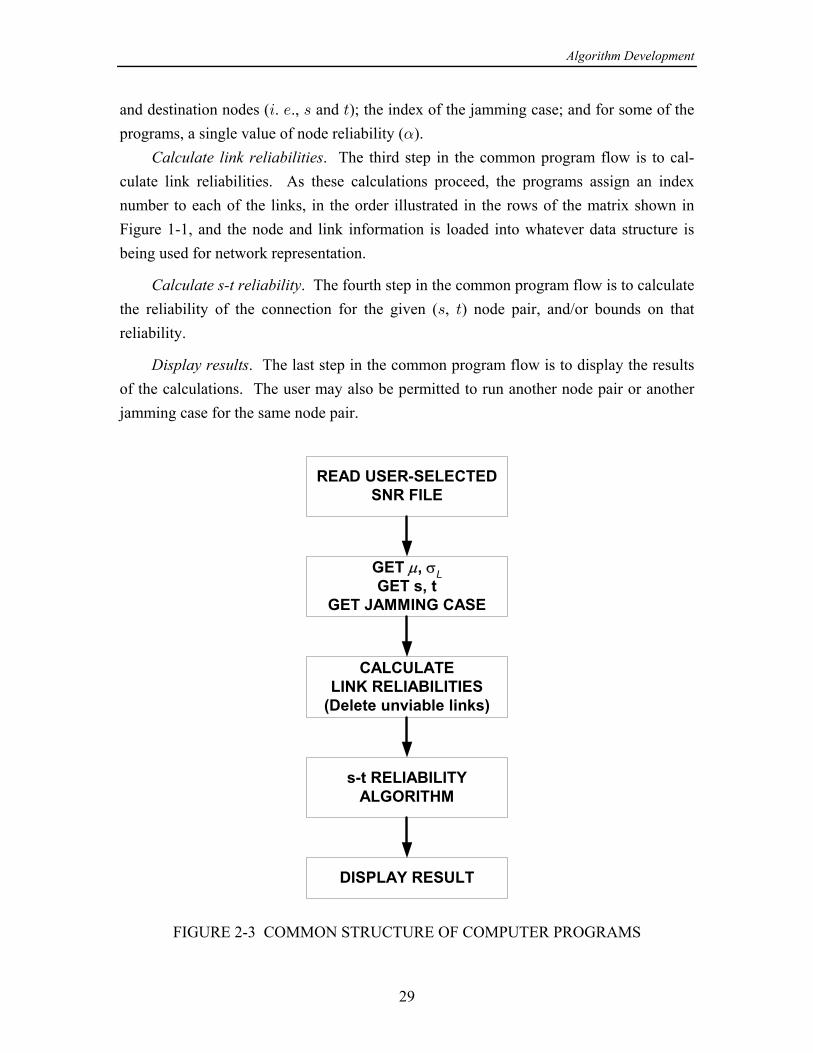
Since all of the programs have the same purpose, there is a common programstructure, which can be understood from the flow diagram in Figure 2-3. In the followingparagraphs, the steps in the common program flow are explained.
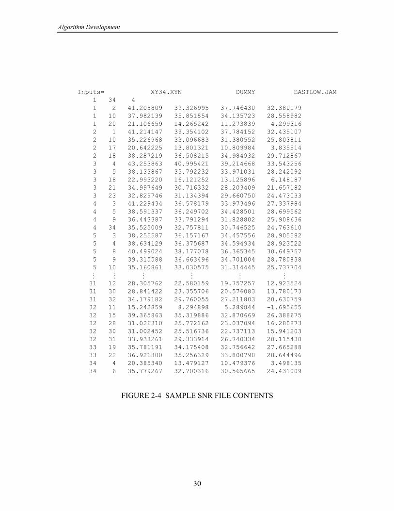
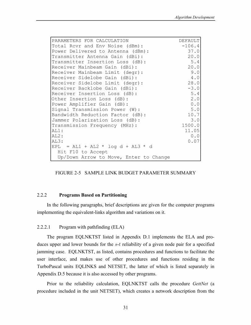
. The programs are set up to read a file describing the network inRead SNR Fileterms of the SNRs at the receivers on given directed links for a particular scenario. Asample SNR file is shown in Figure 2-4. It was generated using the utility programLINKSNRS that is documented in [5] and has the format shown.
The first line of the file gives the names of the files describing the network nodepositions (*.XYN) and the jammer positions, orientations, and powers (*.JAM).LINKSNRS uses the information in these files, plus link budget information supplied bythe user, to calculate jammed SNRs and to write them to a file with a .SNR extension. Asample of the LINKSNRS summary of parameters is given in Figure 2-5.
The second line of the file has the number 1 followed by the number of nodes andthe number of jammer cases (one of which may be selected); the sample SNR file inFigure 2-4 is the source of the link reliability data in Table 2-3 in which there are 34nodes, and jammer case 4 was used.
The third and subsequent lines of an SNR file list the links in terms of the numbersassigned to the transmitter and receiver nodes, in that order, and then, on the same line,the SNRs at the receiver on the link for as many jammer cases as there were specified onthe second line of the file. Note that the fact that nodes have been declared does notR
imply anything about the number of links listed in the file; not all ordered node pairshave to appear in the file. However, LINKSNRS generates numbers for all node pairs,and lines in the file can be deleted, as they were in Figure 2-4, to indicate the absence ofa link due the use of directional antennas, terrain obstructions, etc.
. The second step in the common program flow is to obtain from theGet parametersuser certain parameters needed to perform the - reliability calculation. These include = > .
and for calculating link reliabilities according to (2-1); numbers indexing the source5P
Algorithm Development
29
and destination nodes ( . ., and ); the index of the jamming case; and for some of the3 / = >
programs, a single value of node reliability ( ).!
. The third step in the common program flow is to cal-Calculate link reliabilitiesculate link reliabilities. As these calculations proceed, the programs assign an indexnumber to each of the links, in the order illustrated in the rows of the matrix shown inFigure 1-1, and the node and link information is loaded into whatever data structure isbeing used for network representation.
. The fourth step in the common program flow is to calculateCalculate s-t reliabilitythe reliability of the connection for the given ( , ) node pair, and/or bounds on that= >
reliability.
. The last step in the common program flow is to display the resultsDisplay resultsof the calculations. The user may also be permitted to run another node pair or anotherjamming case for the same node pair.
READ USER-SELECTEDSNR FILE
GET µ, σLGET s, t
GET JAMMING CASE
CALCULATELINK RELIABILITIES
(Delete unviable links)
s-t RELIABILITYALGORITHM
DISPLAY RESULT
FIGURE 2-3 COMMON STRUCTURE OF COMPUTER PROGRAMS
Algorithm Development
30
Inputs= XY34.XYN DUMMY EASTLOW.JAM 1 34 4 1 2 41.205809 39.326995 37.746430 32.380179 1 10 37.982139 35.851854 34.135723 28.558982 1 20 21.106659 14.265242 11.273839 4.299316 2 1 41.214147 39.354102 37.784152 32.435107 2 10 35.226968 33.096683 31.380552 25.803811 2 17 20.642225 13.801321 10.809984 3.835514 2 18 38.287219 36.508215 34.984932 29.712867 3 4 43.253863 40.995421 39.214668 33.543256 3 5 38.133867 35.792232 33.971031 28.242092 3 18 22.993220 16.121252 13.125896 6.148187 3 21 34.997649 30.716332 28.203409 21.657182 3 23 32.829746 31.134394 29.660750 24.473033 4 3 41.229434 36.578179 33.973496 27.337984 4 5 38.591337 36.249702 34.428501 28.699562 4 9 36.443387 33.791294 31.828802 25.908636 4 34 35.525009 32.757811 30.746525 24.763610 5 3 38.255587 36.157167 34.457556 28.905582 5 4 38.634129 36.375687 34.594934 28.923522 5 8 40.499024 38.177078 36.365345 30.649757 5 9 39.315588 36.663496 34.701004 28.780838 5 10 35.160861 33.030575 31.314445 25.737704 ã ã ã ã ã ã 31 12 28.305762 22.580159 19.757257 12.923524 31 30 28.841422 23.355706 20.576083 13.780173 31 32 34.179182 29.760055 27.211803 20.630759 32 11 15.242859 8.294898 5.289844 -1.695655 32 15 39.365863 35.319886 32.870669 26.388675 32 28 31.026310 25.772162 23.037094 16.280873 32 30 31.002452 25.516736 22.737113 15.941203 32 31 33.938261 29.333914 26.740334 20.115430 33 19 35.781191 34.175408 32.756642 27.665288 33 22 36.921800 35.256329 33.800790 28.644496 34 4 20.385340 13.479127 10.479376 3.498135 34 6 35.779267 32.700316 30.565665 24.431009
FIGURE 2-4 SAMPLE SNR FILE CONTENTS
Algorithm Development
31
PARAMETERS FOR CALCULATION DEFAULTTotal Rcvr and Env Noise (dBm): -106.4Power Delivered to Antenna (dBm): 37.0Transmitter Antenna Gain (dBi): 20.0Transmitter Insertion Loss (dB): 5.4Receiver Mainbeam Gain (dBi): 20.0Receiver Mainbeam Limit (degr): 9.0Receiver Sidelobe Gain (dBi): 4.0Receiver Sidelobe Limit (degr): 28.0Receiver Backlobe Gain (dBi): -3.0Receiver Insertion Loss (dB): 5.4Other Insertion Loss (dB): 2.0Power Amplifier Gain (dB): 0.0Signal Transmission Power (W): 5.0Bandwidth Reduction Factor (dB): 10.7Jammer Polarization Loss (dB): 3.0Transmission Frequency (MHz): 1500.0AL1: 11.05AL2: 0.0AL3: 0.07EPL = AL1 + AL2 * log d + AL3 * d Hit F10 to Accept Up/Down Arrow to Move, Enter to Change
FIGURE 2-5 SAMPLE LINK BUDGET PARAMETER SUMMARY
2.2.2 Programs Based on Partitioning
In the following paragraphs, brief descriptions are given for the computer programsimplementing the equivalent-links algorithm and variations on it.
2.2.2.1 Program with pathfinding (ELA)
The program EQLNKTST listed in Appendix D.1 implements the ELA and pro-duces upper and lower bounds for the - reliability of a given node pair for a specified= >
jamming case. EQLNKTST, as listed, contains procedures and functions to facilitate theuser interface, and makes use of other procedures and functions residing in theTurboPascal units EQLINKS and NETSET, the latter of which is listed separately inAppendix D.5 because it is also accessed by other programs.
Prior to the reliability calculation, EQLNKTST calls the procedure (aGettNetprocedure included in the unit NETSET), which creates a network description from the
Algorithm Development
32
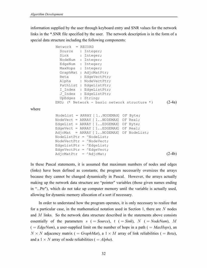
information supplied by the user through keyboard entry and SNR values for the networklinks in the *.SNR file specified by the user. The network description is in the form of aspecial data structure including the following components:
Network = RECORD Source : Integer; Sink : Integer; NodeNum : Integer; EdgeNum : Integer; MaxHops : Integer; GraphMat : AdjcMatPtr; Beta : EdgeVectPtr; Alpha : NodeVectPtr; PathList : EdgeListPtr; I_Index : EdgeListPtr; J_Index : EdgeListPtr; UpEdges : String; END; (* Network - basic network structure *) (2-4a)
where NodeList = ARRAY [1..NODEMAX] OF Byte; NodeVect = ARRAY [1..NODEMAX] OF Real; EdgeList = ARRAY [1..EDGEMAX] OF Byte; EdgeVect = ARRAY [1..EDGEMAX] OF Real; AdjcMat = ARRAY [1..NODEMAX] OF NodeList; NodeListPtr = ^NodeList; NodeVectPtr = ^NodeVect; EdgeListPtr = ^EdgeList; EdgeVectPtr = ^EdgeVect; AdjcMatPtr = ^AdjcMat; (2-4b)
In these Pascal statements, it is assumed that maximum numbers of nodes and edges(links) have been defined as constants; the program necessarily oversizes the arraysbecause they cannot be changed dynamically in Pascal. However, the arrays actuallymaking up the network data structure are “pointer" variables (those given names endingin “...Ptr"), which do not take up computer memory until the variable is actually used,allowing for dynamic memory allocation of a sort if necessary.
In order to understand how the program operates, it is only necessary to realize thatfor a particular case, in the mathematical notation used in Section 1, there are nodesR
and links. So the network data structure described in the statements above consistsQ
essentially of the parameters ( ), ( ), ( ), = œ > œ R œ QSource Sink NodeNum( ), a user-supplied limit on the number of hops in a path ( ), anœ œEdgeNum MaxHopsR ‚R œ ‚Q œ adjacency matrix ( ), a 1 array of link reliabilities ( ),GraphMat Betaand a 1 array of node reliabilities ( ).‚R œ Alpha
Algorithm Development
33
Also associated with the network description in the Pascal statements are a 1 ‚Q
array ( ) reserved for listing (in order) the links used by an path, a stringPathList = Ä >
variable ( ) used to indicate which links are used by a path irrespective of pathUpEdgesorder, and two 1 arrays giving the starting nodes ( ) and stopping nodes‚Q I_Index( ) for each link.J_Index
The procedure examines the SNRs for all ( 1) possible links andGettNet R R
skips possible links that are considered to be unviable—those with SNRs belowthreshold. The viable links ( ) are assigned numbers as they are entered into the ( ,3 Ä 4 3
4) positions of the adjacency matrix, as illustrated in Figure 1-1. In effect, the adjacencymatrix is a table that can be quickly consulted to determine whether two nodes aredirectly connected, and if so, by what link. After assigning a number to a viable link5
connecting node to node , for convenience as a cross-reference the program records the3 4
facts that ( ) and ( ) .I_Index J_Index5 œ 3 5 œ 4
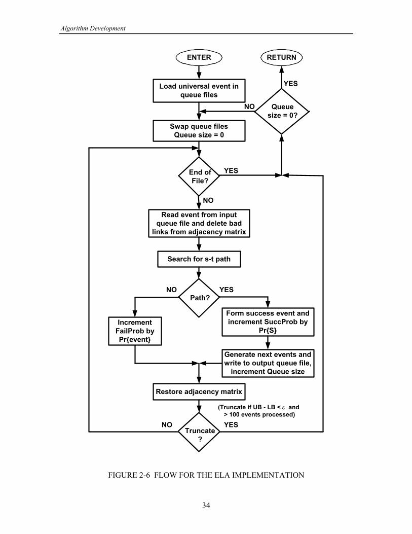
Having “loaded" the network description information, the calling program EQLNK-TST then activates the procedure , which returns upper and lower bounds on theELReliab= >- reliability. This procedure is part of the EQLINKS unit, utilizes procedures andfunctions in EQLINKS and in NETSET, and may be diagrammed as shown in Figure 2-6.That figure is intended to be self-explanatory, but to aid in comprehending it thefollowing remarks are made:
Two sequentially accessed hard-disk files are used for queues , one opened for3
input—having been filled with network events to be tested for success or failure—andone opened for output, to be filled with new events that result when the ELA finds that anevent it has tested gives rise to a success. Two files are used—even though conceptuallyonly one queue is required—because it is the most practical way to implement the queue.For example, taking an event from the queue involves it from the queue; whileremovingit is a simple matter to read an event from a file, there is no practical way then to deletethat single event from the file. The programs simply process all of the events containedin a “read" or input file, the results being put into a “write" or output file; then the inputfile is erased (overwritten, actually) and the former output file becomes the input file.Thus when all of the events in one file have been tested, the program “swaps" files andcontinues testing events; this process is terminated when there are no more new events
3Hard-disk files are used for queues because the amount of memory needed can be a megabyte or more; theI/O to access these files affects the speed of the program considerably.
Algorithm Development
34
Load universal event inqueue files
Swap queue filesQueue size = 0
End ofFile?
Read event from inputqueue file and delete bad
links from adjacency matrix
Search for s-t path
Form success event andincrement SuccProb by
Pr{S}
YES
NO
ENTER
Queuesize = 0?
RETURN
YES
NO
Path?YESNO
Generate next events andwrite to output queue file,
increment Queue size
IncrementFailProb byPr{event}
Restore adjacency matrix
Truncate?
NO YES
(Truncate if UB - LB < ε and > 100 events processed)
FIGURE 2-6 FLOW FOR THE ELA IMPLEMENTATION
Algorithm Development
35
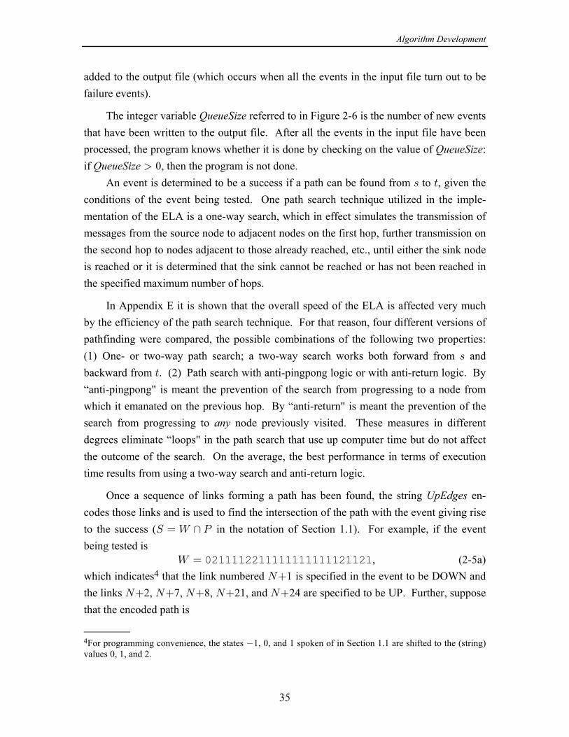
added to the output file (which occurs when all the events in the input file turn out to befailure events).
The integer variable referred to in Figure 2-6 is the number of new eventsQueueSizethat have been written to the output file. After all the events in the input file have beenprocessed, the program knows whether it is done by checking on the value of :QueueSizeif 0, then the program is not done.QueueSize
An event is determined to be a success if a path can be found from to , given the= >
conditions of the event being tested. One path search technique utilized in the imple-mentation of the ELA is a one-way search, which in effect simulates the transmission ofmessages from the source node to adjacent nodes on the first hop, further transmission onthe second hop to nodes adjacent to those already reached, etc., until either the sink nodeis reached or it is determined that the sink cannot be reached or has not been reached inthe specified maximum number of hops.
In Appendix E it is shown that the overall speed of the ELA is affected very muchby the efficiency of the path search technique. For that reason, four different versions ofpathfinding were compared, the possible combinations of the following two properties:(1) One- or two-way path search; a two-way search works both forward from and=
backward from . (2) Path search with anti-pingpong logic or with anti-return logic. By>
“anti-pingpong" is meant the prevention of the search from progressing to a node fromwhich it emanated on the previous hop. By “anti-return" is meant the prevention of thesearch from progressing to node previously visited. These measures in differentanydegrees eliminate “loops" in the path search that use up computer time but do not affectthe outcome of the search. On the average, the best performance in terms of executiontime results from using a two-way search and anti-return logic.
Once a sequence of links forming a path has been found, the string en-UpEdgescodes those links and is used to find the intersection of the path with the event giving riseto the success ( in the notation of Section 1.1). For example, if the eventW œ [ T
being tested is , (2-5a)œ[ 0211112211111111111121121
which indicates that the link numbered 1 is specified in the event to be DOWN and4 R
the links 2, 7, 8, 21, and 24 are specified to be UP. Further, supposeR R R R R
that the encoded path is
4For programming convenience, the states 1, 0, and 1 spoken of in Section 1.1 are shifted to the (string)values 0, 1, and 2.

Algorithm Development
36
, (2-5b)œUpEdges 1211121111111111121111111
which indicates that the path consists of the successes of links 2, 6, and 18.R R R
Then the success event is determined by the procedure in EQLINKS to beSuccess
. (2-5c)œW 0211122211111111121121121
The order of the sequence is preserved in the array and used to generate newPathListevents; it was shown in [1] that preserving this order generates fewer events to be tested.Note that in the example of (2-5), the successes of links 6 and 18 are newR R
conditions, while that of link 2 is not; therefore, although there are three links in theR
path, only two new events are generated.
The process is terminated early (truncated) when the lower bound, which is the sumof the probabilities for the success events found so far, is within of the upper bound,%
which is one minus the sum of the probabilities for the failure events found so far,provided that at least 100 events have been tested. The criterion is a constant that is%
“hard-wired" into the program code, nominally with the value 0.01.% œ
2.2.2.2 Program with cutsets (ELA2)
The program EL2ONLY listed in Appendix D.2 implements the ELA2 usingfunctions and procedures in the unit CUTONLY and in the unit NETSET. In a manneranalogous to the implementation of the ELA, the program EL2ONLY acts as the userinterface and calling program, while the unit CUTONLY provides ELA2-specificroutines and the unit NETSET provides routines that are common to several programs.The data structure used for representing the network and the method for loading it areidentical with that for the implementation of the ELA, as described in Section 2.2.2.1.
Having loaded the network description information, the calling program EL2ONLYthen activates the procedure , which returns upper and lower bounds on the -ELReliab = >
reliability. Though it has the same name as the procedure used to implement the ELA,this procedure, which is part of the unit CUTONLY, in processing queued eventsoperates in a completely complementary fashion, as diagrammed in Figure 2-7.
In place of the search for a path, the implementation of the ELA2 searches for acutset. The search is done in two directions, as discussed in Section 1.2.2. An event isdetermined to be a failure if a cutset of hypothethically failed links can be found thatprecludes a path from to , given the conditions of the event being tested. If a cutset= >
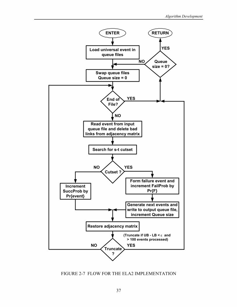
Algorithm Development
37
Load universal event inqueue files
Swap queue filesQueue size = 0
End ofFile?
Read event from inputqueue file and delete bad
links from adjacency matrix
Search for s-t cutset
Form failure event andincrement FailProb by
Pr{F}
YES
NO
ENTER
Queuesize = 0?
RETURN
YES
NO
Cutset ?YESNO
Generate next events andwrite to output queue file,
increment Queue size
IncrementSuccProb by
Pr{event}
Restore adjacency matrix
Truncate?
NO YES
(Truncate if UB - LB < ε and > 100 events processed)
FIGURE 2-7 FLOW FOR THE ELA2 IMPLEMENTATION

Algorithm Development
38
cannot be found, it is because there is an path consisting entirely of links that are= Ä >
specified to be UP.
Once a cutset of link failures has been found, the string encodes thoseUpEdgeslinks (positively) and the array is used as a means to list the links whose failuresPathListare included in the cutset. That is, suppose that the event is represented by the string
, (2-6a)œ[ 0211112211111111111121121
which indicates that the link numbered 1 is specified in the event to be DOWN andR
the links 2, 7, 8, 21, and 24 are specified to be UP. Further, supposeR R R R R
that the encoded cutset is , (2-6b)œUpEdges 1111121111111111121111111
which indicates that the cutset consists of the failures of links 6 and 18. Then theR R
failure event is determined by the procedure in CUTONLY to beCutFail
(2-6c)œJ 0211102211111111101121121.
Unlike the link sequence order for paths, the order of the listing of the links whosefailures are in the cutset has not been found to be significant in affecting the number ofnext events, so they are entered into in their lexicographical order. AnotherPathListaspect of the processing of cutsets that is different from that of pathfinding is that thenumber of new events is always equal to the number of links listed in , since byPathListdefinition any link specified in the event to be DOWN will not be in the cutset.
The - reliability calculation in EL2ONLY is truncated in the same manner as that= >
in EQLNKTST.
2.2.2.3 Program combining pathfinding and cutsets
In order to exploit the fact that the upper bound converges faster than the lowerbound for the ELA2, while the opposite is true for the ELA, the program EL1&2 that islisted in Appendix D.3 was developed, using procedures and functions in the unitNETSET and in the unit CUTSET (which also is listed in Appendix D.3).
Essentially, EL1&2 implements the ELA and the ELA2, using two sets ofbothqueues, with the truncation based on the convergence of the lower bound from thepathfinding method and the upper bound from the cutset-finding method. The two partsof the program operate as described in Sections 2.2.2.1 and 2.2.2.2.

Algorithm Development
39
2.2.2.4 Program selecting pathfinding or cutsets
It was noted in Section 1.2.3 that the partitioning of events can alternate between thepathfinding method and the cutset-finding method. The program ELCUTPAT that islisted in Appendix D.4 (along with its supporting unit, CUTPATH) was written tocombine features of the ELA and the ELA2. Like the other programs for calculating -= >
reliability, it utilizes procedures and functions in the unit NETSET.
In ELCUTPAT, a single pair of queues is used, and the overall design philosophy ofthe program is to minimize the number of new events that are generated, by choosingeither the pathfinding or the cutset-finding approach. As illustrated by the partial flowdiagram in Figure 2-8, after reading an event to be tested the program first seeks an= Ä > path. If one is not found, the event is definitely a failure, which does not generatea new event; the event is therefore processed as an ELA failure event and the next eventto be tested is read from the input queue.
If a path is found, a determination is made of , the number of new eventsNewCountthat would be generated if the event is processed as an ELA success event. If NewCountis 0, then no new events will be generated because all the links in the path were specifiedas being UP in the event being tested; this value of is possible if the eventNewCountbeing tested was previously generated using the cutset approach. If is 1, thenNewCounta cutset exists but it cannot produce any fewer new events. Therefore, if 2,NewCount preference is given to pathfinding: the event is processed as an ELA success event.
If 2, then there is a cutset, possibly with the number of linkNewCount CutCount
failures in it such that , giving rise to fewer new events if theCutCount NewCount
cutset approach is used. To test for this condition, a cutset is found. If CutCount NewCount, the event being tested is processed as an ELA success event; otherwise, it isprocessed as an ELA2 failure event.
It is demonstrated in Appendix C for an example network that this methodology yields atotal of 30 events into which the probability space is partititioned (11 successes and 19failures). When the same example network was analyzed using the ELA, a total of 38events were found (11 successes and 27 failures); using the ELA2, a total of 33 eventswere found (14 successes and 19 failures). For this example, the “cutpath" method did aswell as the ELA in obtaining relatively large success partitions and as well as the ELA2in obtaining relatively large failure partitions.
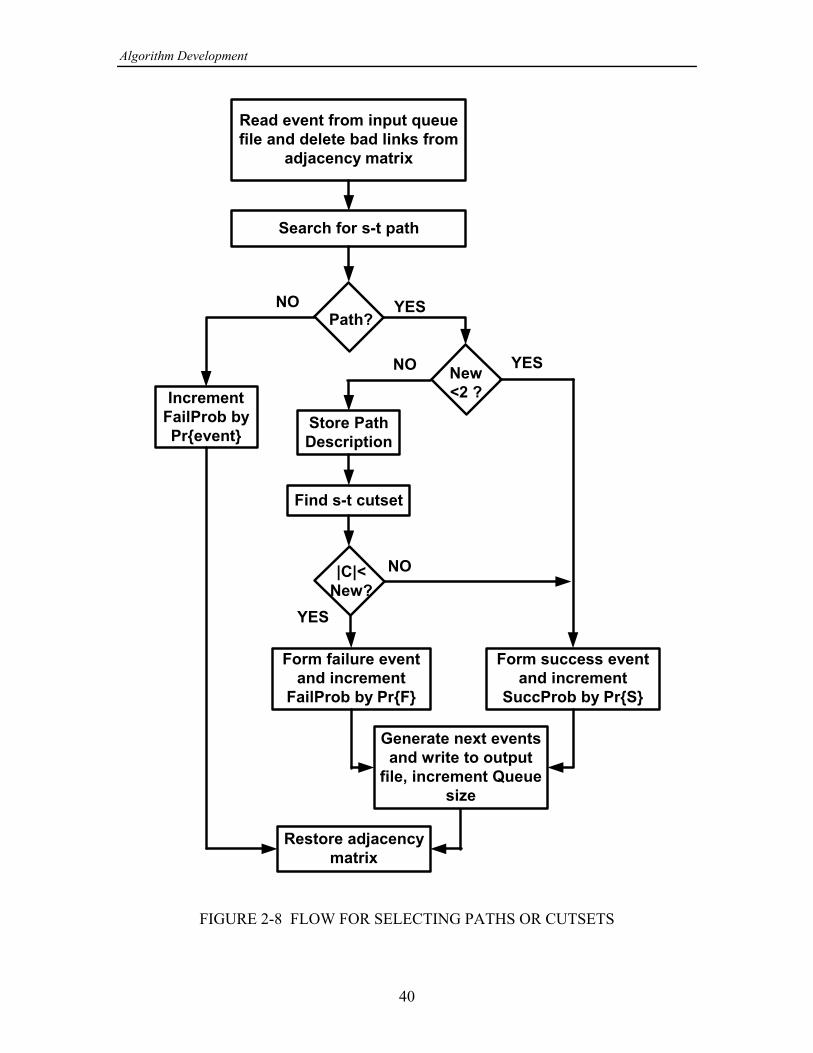
Algorithm Development
40
Read event from input queuefile and delete bad links from
adjacency matrix
Search for s-t path
Path?
Find s-t cutset
IncrementFailProb byPr{event}
Store PathDescription
Form failure eventand increment
FailProb by Pr{F}
YES
YES
NO
NO
New<2 ?
YESNO
|C|<New?
Form success eventand increment
SuccProb by Pr{S}
Generate next eventsand write to output
file, increment Queuesize
Restore adjacencymatrix
FIGURE 2-8 FLOW FOR SELECTING PATHS OR CUTSETS
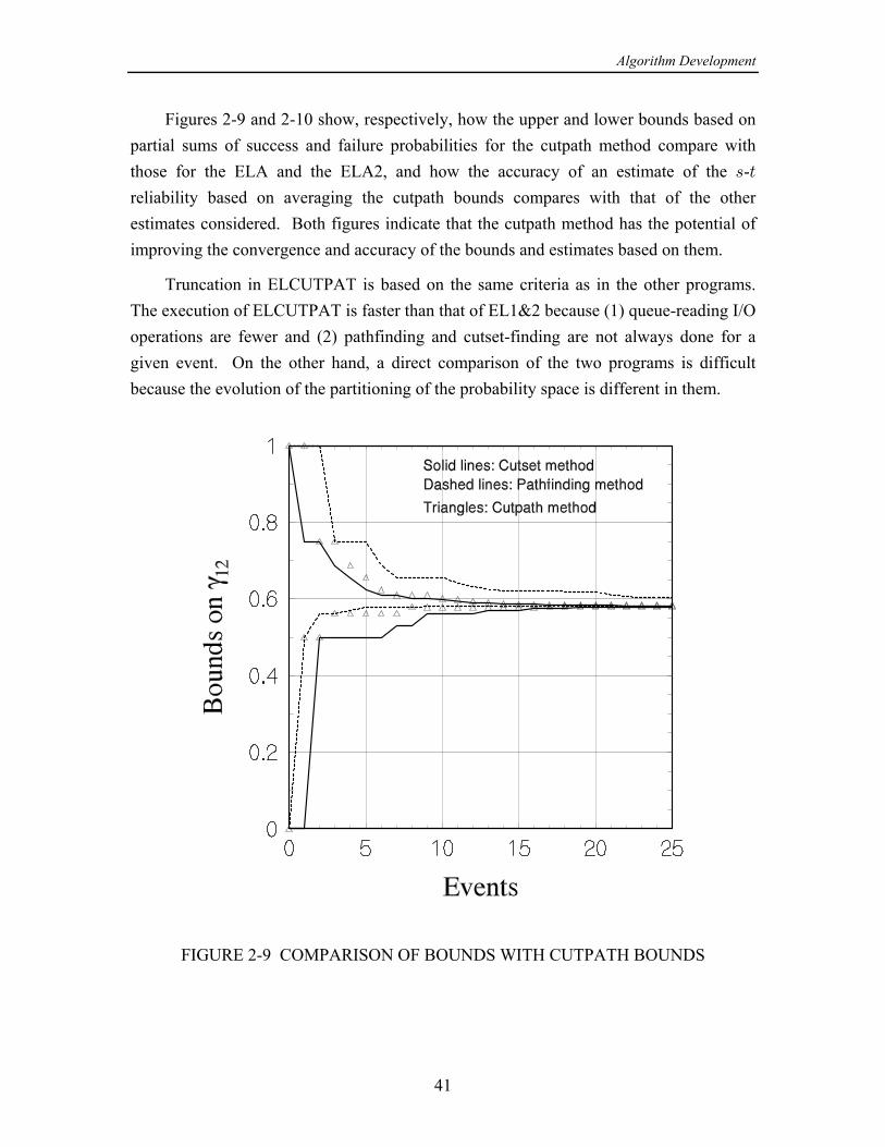
Algorithm Development
41
Figures 2-9 and 2-10 show, respectively, how the upper and lower bounds based onpartial sums of success and failure probabilities for the cutpath method compare withthose for the ELA and the ELA2, and how the accuracy of an estimate of the -= >
reliability based on averaging the cutpath bounds compares with that of the otherestimates considered. Both figures indicate that the cutpath method has the potential ofimproving the convergence and accuracy of the bounds and estimates based on them.
Truncation in ELCUTPAT is based on the same criteria as in the other programs.The execution of ELCUTPAT is faster than that of EL1&2 because (1) queue-reading I/Ooperations are fewer and (2) pathfinding and cutset-finding are not always done for agiven event. On the other hand, a direct comparison of the two programs is difficultbecause the evolution of the partitioning of the probability space is different in them.
FIGURE 2-9 COMPARISON OF BOUNDS WITH CUTPATH BOUNDS
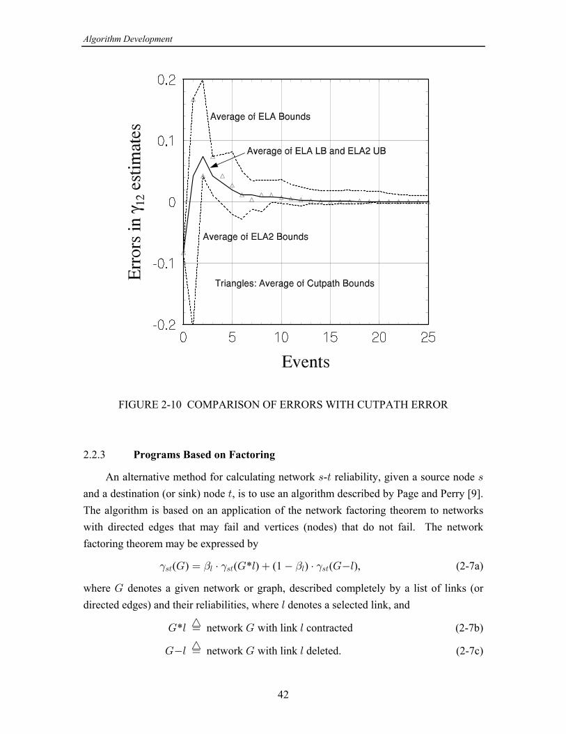
Algorithm Development
42
FIGURE 2-10 COMPARISON OF ERRORS WITH CUTPATH ERROR
2.2.3 Programs Based on Factoring
An alternative method for calculating network - reliability, given a source node = > =
and a destination (or sink) node , is to use an algorithm described by Page and Perry [9].>
The algorithm is based on an application of the network factoring theorem to networkswith directed edges that may fail and vertices (nodes) that do not fail. The networkfactoring theorem may be expressed by
( ) ( * ) (1 ) ( ), (2-7a)œ † K 6 † K6K# " # " #=> 6 => 6 =>
where denotes a given network or graph, described completely by a list of links (orK
directed edges) and their reliabilities, where denotes a selected link, and6
* network with link contracted (2-7b)œ K 6˜K 6
network with link deleted. (2-7c)œ K 6˜K6
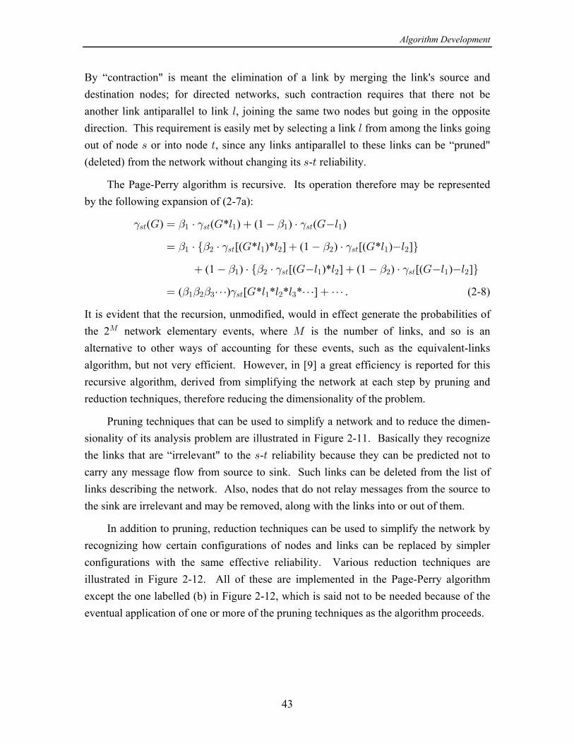
Algorithm Development
43
By “contraction" is meant the elimination of a link by merging the link's source anddestination nodes; for directed networks, such contraction requires that there not beanother link antiparallel to link , joining the same two nodes but going in the opposite6
direction. This requirement is easily met by selecting a link from among the links going6
out of node or into node , since any links antiparallel to these links can be “pruned"= >
(deleted) from the network without changing its - reliability.= >
The Page-Perry algorithm is recursive. Its operation therefore may be representedby the following expansion of (2-7a):
( ) ( * ) (1 ) ( )œ † K 6 † K6K# " # " #=> " => " " => "
[( * )* ] (1 ) [( * ) ]œ † † K 6 6 † K 6 6" " # " #" # => " # # => " #e f (1 ) [( )* ] (1 ) [( ) ] † † K6 6 † K6 6" " # " #" # => " # # => " #e f ( ) [ * * * * ] . (2-8)œ â K 6 6 6 â â" " " #" # $ => " # $
It is evident that the recursion, unmodified, would in effect generate the probabilities ofthe 2 network elementary events, where is the number of links, and so is anQ Q
alternative to other ways of accounting for these events, such as the equivalent-linksalgorithm, but not very efficient. However, in [9] a great efficiency is reported for thisrecursive algorithm, derived from simplifying the network at each step by pruning andreduction techniques, therefore reducing the dimensionality of the problem.
Pruning techniques that can be used to simplify a network and to reduce the dimen-sionality of its analysis problem are illustrated in Figure 2-11. Basically they recognizethe links that are “irrelevant" to the - reliability because they can be predicted not to= >
carry any message flow from source to sink. Such links can be deleted from the list oflinks describing the network. Also, nodes that do not relay messages from the source tothe sink are irrelevant and may be removed, along with the links into or out of them.
In addition to pruning, reduction techniques can be used to simplify the network byrecognizing how certain configurations of nodes and links can be replaced by simplerconfigurations with the same effective reliability. Various reduction techniques areillustrated in Figure 2-12. All of these are implemented in the Page-Perry algorithmexcept the one labelled (b) in Figure 2-12, which is said not to be needed because of theeventual application of one or more of the pruning techniques as the algorithm proceeds.
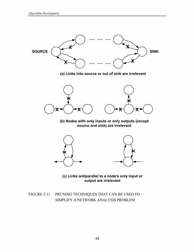
Algorithm Development
44
X
X
X
XSOURCE SINK
(a) Links into source or out of sink are irrelevant
X
X X
X
X X
(b) Nodes with only inputs or only outputs (exceptsource and sink) are irrelevant
X
(c) Links antiparallel to a node's only input oroutput are irrelevant
X
FIGURE 2-11 PRUNING TECHNIQUES THAT CAN BE USED TO SIMPLIFY A NETWORK ANALYSIS PROBLEM
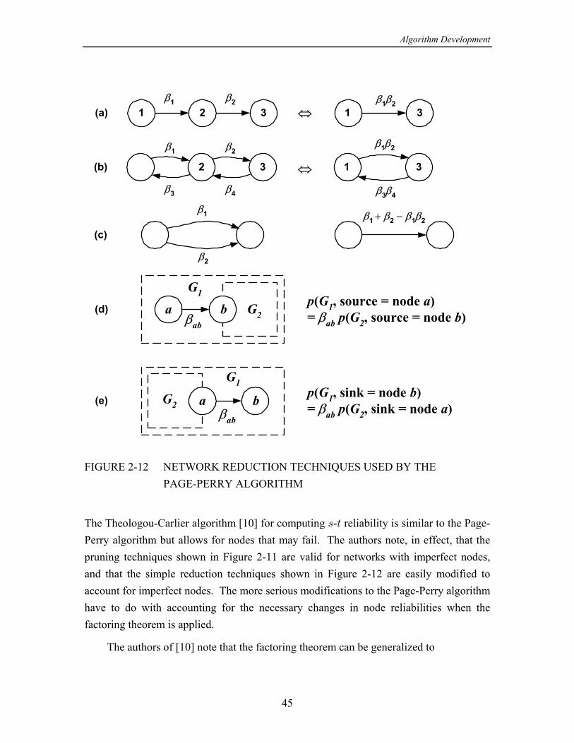
Algorithm Development
45
1
p(G1, source = node a)= βab p(G2, source = node b)
β1 β2 β1β22 3 31(a)
1
β1 β2β1β2
2 3 3
a
β3 β4 β3β4
(b)
⇔
⇔
β1
β2
β1 + β2 − β1β2
(c)
b G2
G1
(d)
p(G1, sink = node b)= βab p(G2, sink = node a)a bG2
G1
(e)
βab
βab
FIGURE 2-12 NETWORK REDUCTION TECHNIQUES USED BY THE PAGE-PERRY ALGORITHM
The Theologou-Carlier algorithm [10] for computing - reliability is similar to the Page-= >
Perry algorithm but allows for nodes that may fail. The authors note, in effect, that thepruning techniques shown in Figure 2-11 are valid for networks with imperfect nodes,and that the simple reduction techniques shown in Figure 2-12 are easily modified toaccount for imperfect nodes. The more serious modifications to the Page-Perry algorithmhave to do with accounting for the necessary changes in node reliabilities when thefactoring theorem is applied.
The authors of [10] note that the factoring theorem can be generalized to
Algorithm Development
46
( ) ( * ) (1 ) ( ), (2-9)œ : † K 6 : † K6K# # #=> 6 => 6 =>
where now represents successful transmission between two failable nodes over a fail-6
able link. Let the nodes and the link be labelled , , and , respectively. Since ? @ / 6
working implies that all three of , , and are working (with probability ),? @ / : œ6 ? / @! " !
then “ * " denotes the graph with contracted and the combined node - havingK 6 / ? @
reliability 1. Since not working implies one or more of , , and not working (with6 ? @ /
probability 1 1 ), then “ " denotes the graph with deleted and : œ K 6 /6 ? / @! " !
with and remaining, with modified reliabilities? @ but
and . (2-10)œ œ! !? @w
w! " ! ! " !
! " ! ! " !? / @ @ / ?
? / @ ? / @
(1 ) (1 )1 1
Note that, in the graph , failures of the nodes and are no longer independent.K 6 ? @
This difficulty is circumvented by taking note of the facts that (1) the - reliability of = > K
is times the - reliability of when it is assumed that 1; and (2) if node! ! ! != > = >= > K œ œ
? / œ @, the source of , does not fail ( 1) then the modified reliability of node in (2-10)!?
no longer depends on the reliability of node :?
. (2-11)œ!@w
! "
" !@ /
/ @
(1 )1
These facts taken together suggest an iterative procedure for finding the - reliability= >
(with factored out) in which the first edge to be factored on is one of the edges out of!=
the source node, or (with factored out) in which the first edge to be factored on is one!>
of the edges out of the sink node. The pruning and reductions as the iterations of (2-9)proceed are entirely equivalent to those of Page and Perry, with the slight additionalcomplexity of modifying the node reliabilities appropriately in the manner we haveshown above.
2.2.3.1 Program implementing the Theologou-Carlier algorithm
The program TCPTR listed in Appendix D.6 implements the Theologou-Carlieralgorithm (TCA) for calculating - reliability. As listed, the program contains pro-= >
cedures and functions to facilitate the user interface, and makes use of other proceduresand functions residing in the TurboPascal unit TCUPTR, which also is listed in AppendixD.6.
Algorithm Development
47
Prior to the reliability calculation, TCPTR calls the procedure , whichBuildGraphcreates a network description from the information supplied by the user through keyboardentry and SNR values for the network links in the *.SNR file specified by the user. Thenetwork description is in the form of a special data structure including the followingcomponents: Graph = RECORD {Describes a graph} Vert : GraphSet; {Set of graph vertices} Source, {Source vertex} Sink : Integer; {Sink vertex} InDegree, {In degree of each vertex} OutDegree : DegreeType; {Out degree of each vertex} nb : ARRAY[1..NODEMAX] OF GraphSet; {Edge(i,j) puts j in nb[i]} NumEdges : Integer; {No. of edges in the graph} NumNodes : Integer; {Largest-numbered vertex} e : ARRAY[1..EDGEMAX] OF Edge; {Describes edges in graph} Alpha : ARRAY[1..NODEMAX] OF Real; {Node reliabilities} END; { Graph } (2-12a)
where DegreeType = ARRAY[1..NODEMAX] OF Integer;
{List of vertex degrees} GraphSet = SET OF 1..NODEMAX; {Set of vertices} Edge = RECORD {Edge in a graph} Start, {Start vertex} Stop : 1..NODEMAX; {Stop vertex } Beta : Real {Edge reliabilities} END; { Edge } (2-12b)
In these Pascal statements, it is assumed that maximum numbers of vertices (nodes) andedges (links) have been defined as constants; the program necessarily oversizes the arraysbecause they cannot be changed dynamically in Pascal.
In order to understand how the program operates, it is only necessary to realize thatfor a particular case, in the mathematical notation used in Section 1, there are nodesR
and links. So the network data structure described in the statements above consistsQ
essentially of a set ( ) containing the numbers (labels) of the links in the network;œ Vert= œ > œ œ ( ); ( ); a list of the number of links entering each node (Source SinkInDegree OutDegree); a list of the number of links leaving each node ( ); a collectionœ
of sets ( ) containing the numbers (labels) of the other nodes to which each nodeR œ nbis connected by a link leaving that node; ( ); ( ); a list ofQ œ R œNumEdges NumNodes
Algorithm Development
48
node reliabilities ( ); and a list ( ) of the start node, stop node, and reliabilityœ œ /Alphafor each link.
The procedure examines the SNRs for all ( 1) possible links andBuildGraph R R
skips links that practically speaking don't exist, that is, those for which the link margin isless than zero, giving rise to a that is less than P (0) 0.5. Those links with"34 K œ
"34 0.5 are considered viable and are entered into the data structure: each is numbered(labelled); its start node, stop node, and reliability are entered into an record; theedgenodes associated with the edge are added to the set and the maximum node numberVertNumNodes is updated, if necessary; and the number (label) of the edge's ending node isadded to the set of nodes reached by the edge's starting node.
Having embedded the information on the network in this directed graph datastructure referenced by the variable name , the program finds the input and output1
degrees of each node and computes the - reliability as= >
( ). (2-12)œ 1#=> Prob
The function ( ) has the flow diagrammed in Figure 2-13. Upon initiation of theProb 1
function, with the variable passed to it as the argument, various pruning and reduction1
procedures are applied to in order to simplify the graph. Then the source and sink node1
reliabilities are factored out, leaving a graph whose source and sink nodes do not fail.This factoring permits application of the Theologou-Carlier version of the networkfactoring theorem stated above in (2-9) and (2-11), using an edge into the sink. Theprogram finds such an edge ( ) and the node from which it originates ( ), and implements6 ;
the expression
( ) * ; 1 (1 ) ; œ 1 6 œ 1 6 œ1Prob Prob Prob! ! " ! ! " ! != > 6 ; 6 ;w w w w
; ;
"’ “ˆ ‰ Š ‹! "" !
; 6
6 ;
(1 )
(2-13)in which denotes the graph after pruning and reduction. Note in (2-13) that the1 1w
function is recursive. Each time is called from within itself, copies of the variablesProbinvolved in the calculation using the call have to be stored; if the depth of recursion is toogreat, the computer can run out of “stack" memory. For that reason, the Pascal codeimplementing uses pointer variables to reference the graph data structure, allowingProbthe memory to be used as needed (not from the stack, but from the larger portion of thecomputer's memory allocated to the “heap") and released when not needed.
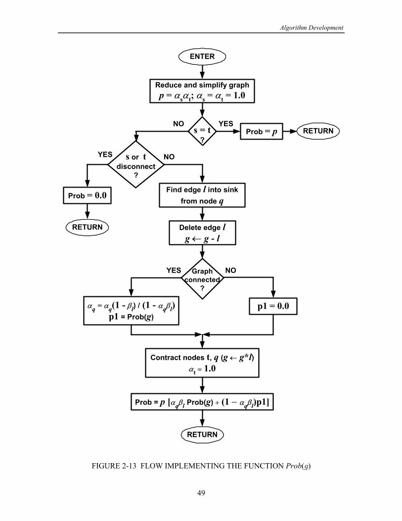
Algorithm Development
49
Reduce and simplify graphp = αsαt; αs = αt = 1.0
s = t?
Find edge l into sinkfrom node q
Delete edge lg ← g - l
YES
NO
ENTER
s or tdisconnect
?
RETURN
YES
NO
Graphconnected
?
YES NO
Contract nodes t, q (g ← g*l)αt = 1.0
αq = αq(1 - βl) / (1 - αqβl)p1 = Prob(g)
Prob = p [αqβl Prob(g) + (1 − αqβl)p1]
Prob = p
Prob = 0.0
RETURN
p1 = 0.0
RETURN
FIGURE 2-13 FLOW IMPLEMENTING THE FUNCTION ( ) Prob 1
Algorithm Development
50
2.2.3.2 Program implementing the TCA with bounds
For relatively large networks, the program TCPTR implementing the TCA can takean excessively long time to execute. For that reason, modifications to the algorithm weredeveloped that permit the fast computation of upper and lower bounds, and these boundshave been implemented in the program TCPTRBND that is listed in Appendix D.7,supported by the unit TCUPTRUL.
In the notation of (2-9), the upper bound is based on the observation that
( ) ( * ) (1 ) ( )œ : † K 6 : † K6K# # #=> 6 => 6 =>
( with 1.0) 1.0 ( * ) (1 1.0) ( ),-14a)(2Ÿ K : œ œ ‚ K 6 ‚ K6# # #=> 6 => =>
or ( ) ( * ). (2-14b)Ÿ K 6K# #=> =>
This bound results in a calculation with potentially much fewer recursions, and is usedwhen the program finds that , the reliability of the link [in the notation of (2-13)], is"6 6
greater than a probability threshold ; the higher the value of that threshold, the tighter the5
bound. A lower bound may be computed similarly from the relationship6
( ) ( * ) 0 ( ) : † K 6 † K6K# # #=> 6 => =>
or ( ) ( * ), (2-15) : † K 6K# #=> 6 =>
ignoring terms of the form (1 ) Pr{subgraph} when a particular link reliability is : ‚6
close to unity. The tightness of this bound, invoked when exceeds a probability"6
threshold, depends upon the value of that threshold.
2.2.4 A Program with Combined Partitioning and Factoring
In a recent paper in the [11], an algorithm wasIEEE Transactions on Reliabilityintroduced that makes uses of both factoring (including reductions and simplifications ofthe network) and the partitioning concepts employed by the ELA. Given the nodes and=
> = Ä >, plus an path consisting of the sequence of links
( , , , , ), (2-16)œ 6 6 6 á 6T " # $ O
the factoring theorem expressed generally above in (2-8) can be put into the followingform by grouping terms:
5A discussion of the heuristic probability thresholds that are used is given later in this report, in connectionwith the numerical results.6Another, simple lower bound is , the reliability of the direct path .! ! "= > => = Ä >
Algorithm Development
51
(1 ) ( ) ( * )( ) œ † K6 † K 6K# " # " #=> " => " " => "
(1 ) ( ) {(1 ) [( * ) ] ( * * )}œ † K6 † K 6 6 † K 6 6" # " " # " #" => " " # => " # # => " #
(1 ) ( ) (1 ) [( * ) ]œ † K6 † † K 6 6" # " " #" => " " # => " #
{(1 ) [( * * ) ] ( * * * )} † K 6 6 6 † K 6 6 6" " " # " #" # $ => " # $ $ => " # $
(1 ) ( ) (1 ) [( * ) ]œ † K6 † † K 6 6" # " " #" => " " # => " #
(1 ) [( * * ) ] † K 6 6 6" " " #" # $ => " # $
ã (1 ) [( * * * * * ) ] â † K 6 6 6 â 6 6" " " " " #" # $ O" O => " # $ O" O
( * * * * * * ) . (2-17) â † K 6 6 6 â 6 6
œ "
" " " " " #" # $ O" O => " # $ O" OðóóóóóóóóóóóóóñóóóóóóóóóóóóóòThe terms in the last equation above correspond to partitioning the 2 elementary eventsQ
into the 1 disjoint eventsO
or 0 (2 elem. events) 6 B B BâBB"
Q"èëëëéëëëêlinks 1
áO
BBâBO"áQèéê
or 1 0 (2 elem. events)6 6 B BâBB BBâB" #Q#
or 1 1 0 (2 elem. events)6 6 6 BâBB BBâB" # $Q$
(2-18)ã ã
or 1 1 1 1 0 (2 elem. events)6 6 6 â6 6 â B BBâB" # $ O# O"QO"
or 1 1 1 1 1 0 (2 elem. events) 6 6 6 â6 6 6 â BBâB" # $ O# O" OQO
or 1 1 1 1 1 1 (2 elem. events) . 6 6 6 â6 6 6 â BBâB" # $ O# O" OQO
The probability of the last subgraph in (2-17) is 1 because all the links in the path areT
postulated to be UP.
As written, (2-17) is simply one of many ways to group the 2 terms of (2-8) intoQ
O †1 terms, since it is understood that each use of the recursive function ( )#=>
involves an expansion and further recursions (after network reductions and simplifica-tions). However, there is an advantage to the grouping shown in (2-18): as noted in [11],each subgraph has at least one less path than the original graph because one of the= Ä >
links in is postulated to have failed. Another insight comes from noting that for eachT
successive subgraph, there is at least one less link and one less node, since contracting alink merges two nodes. In [11] it was reported that this “reduce and partition" algorithmtypically computes in about half the time that is required by the original factoring#=>
algorithm with reduction [9] that was discussed in Section 2.2.3.
Algorithm Development
52
The program REDNPART that is listed in Appendix D.8.1 implements the reduceand partition algorithm as a modification to the Theologou-Carlier algorithm for com-puting the exact - reliability with nodes that can fail. The program RNPBOUND that is= >
listed in Appendix D.8.2 utilizes the same kind of bounding approach that was discussedin Section 2.2.3.2 in order to obtain upper and lower bounds for the reliability.
2.3 ALGORITHM PERFORMANCES
In this subsection, the performances of the various - reliability algorithms de-= >
scribed above are presented. Algorithm performance is given both in terms of accuracyand of time required to compute either exact reliabilities or bounds for selected examplenetworks.
Side-by-side tests of the algorithms were performed in several stages. The initialtests were used to establish a general ranking of algorithm performance for a variety ofnetwork sizes. Certain tests, summarized in Appendix E, were conducted to developrefinements to the more promising algorithms. In addition to showing the degree ofimprovement that can be achieved by efficient programming, these tests established thatthe best performance of the partitioning class of algorithms in terms of execution timegenerally is experienced for two-way pathfinding with anti-return logic; the time is notsignificantly affected by the choice between the cutset search methods using the firstcutset found or using the larger cutset found. The studies summarized in Appendix Ealso revealed that the EL2ONLY program, which uses only cutsets to develop reliabilityevents, requires an excessive amount of program execution time for large networks.Therefore, this program was eliminated from the comparisons presented in thissubsection.
The algorithms were tested using the following *.SNR files:
MESH1000.SNR. (Used for the tests reported in Appendix E only.) This fileì
contains SNRs for the links of the 3 3 example network shown in Figure 1-1 and‚
discussed in Section 2.1.1, with the particular ( , ) pair being (1, 2). The link= >
reliabilities for this case are listed in Table 2-1. In addition to being an example forwhich there is an analytical solution (see Appendices A, B, and C), this case runs veryquickly for any algorithm.
T920811.SNR. This file contains SNRs for the links of the 15-node exampleì
network shown in Figure 2-1 and discussed in Section 2.1.2, with the particular ( , ) pair= >
being (8, 13). The link reliabilities for this case are listed in Table 2-2. This case repre-
Algorithm Development
53
sents a moderately challenging network example in which there is no one-hop = Ä >
path.
BIGONE.SNR. This file contains SNRs for the links of the 34-node exampleì
network shown in Figure 2-2 and discussed in Section 2.1.3, with a focus on theparticular ( , ) pair (25, 20), which has a minimum hop distance of 6. This example= >
represents a realistic-sized MSE network, and was studied in [1].
2.3.1 Comparisons of Exact Calculations
The two programs implementing exact calculations of - reliability are TCPTR,= >
which uses the Theologou-Carlier (factoring) approach discussed in Section 2.2.3.1, andREDNPART, which uses the combined reduction and partition approach discussed inSection 2.2.4. The results of the calculations are as follows:
Case Result Time, TCPTR Time, REDNPART3 , (1, 2) .93133093 1 s 1 s ‚ $ ¥ ¥
15-node, (8, 13) .92982718 49 s 24 s 34-node, (25, 20) ----------- 14 hrs 14 hrs ¦ ¦
The exact answer for the 34-node example network was not available using either algo-rithm after having run for 14 hours.
The small time for the 3 3 example network is not surprising. It is perhaps‚
surprising that the run time for the 15-node example network, though not excessive, is somuch greater than that for the 3 3 network. The difference is only partially accounted‚
for by the size of the networks: the 15-node network has 60 links, whereas the 3 3 has‚
24 links; (49) 4.7 s would be the case for the 3 3 network, assuming an#%Î'! œ ‚
exponential dependence of the time of the TCPTR program upon the number of links.The “reducibility" of the examples undoubtedly has something to do with the relativetimes, but an independent measure of such a characteristic is not available—rather, thetimes themselves would seem to be indicators that could be used to develop a measure ofreducibility.
2.3.2 Comparisons of Bound Calculations
2.3.2.1 The programs that are compared
Five different programs were used to calculate upper and lower bounds on the -= >
reliability for the example cases.
Algorithm Development
54
The three equivalent-links programs (EQLNKTST, EL1&2, and ELCUTPAT) arebased on partitioning, and utilize a stopping criterion that “tracks" the convergence of thebounds: the program is terminated when UB LB 0.01 and at least 98 events have
been processed, unless the calculation is exact for fewer events processed. In addition,EL1&2 stops if either the ELA or the ELA2 portion finds the exact - reliability before= >
the bounds converge. The baseline configuration of these algorithms for the resultspresented includes the following choices of search techniques:
Pathfinding: two-way flood search with prevention of return to any search-ì
propagating node (anti-return logic). When the search at a given stage (hop) reaches aparticular node from two or more previously reached nodes, an arbitrary preference isgiven to the previously reached node having the lowest number (label). For all the resultsin this report, a 10-hop path limit was imposed. In Appendix E, a study is made of theeffect of other pathfinding approaches on the performances of the programs.
Cutset Search: two-way cutset search with selection of the first cutset that isì
found. In Appendix E, it is shown that the selection of the larger cutset, as discussed inSection 1.2.2, is neither uniformly better nor worse in terms of execution time.
Of the other two programs, TCPTRBND is based on reduction and factoring whileRNPBOUND is based on a combination of reduction and partitioning; both of these algo-rithms do not track bound convergence, and therefore could be termed “open-loop."These programs implement new concepts for obtaining upper and lower bounds on the -=> reliability that were not included in the original algorithms. For the results presented inthis section, adaptive probability thresholds were used to implement the boundingtechniques explained in Section 2.2.3.2, as discussed below. Also, the lower and upperbound calculations were combined using one exercise of the basic Theologou-Carlieralgorithm for each subgraph to avoid duplicate calculations.
The adaptive threshold used may be expressed by
, (2-19a)œ 5 †:>2 7+B" $
where ( )/min{100(1.01 ), 26} (2-19b)œ $ " " "7+B
is an adaptive step size and where is an integer indexing the depth of recursion. The5
smaller the value of , the more likely it is that the program will use an approximation:>2
for the probability of the subgraph, thereby running faster. Note that as increases, the5
probability threshold decreases gradually from to . For 0.75, decreases to" " "7+B >2 :
Algorithm Development
55
" " relatively quickly, in 10 to 26 recursions. Otherwise decreases to relatively:>2
slowly, in 26 recursions.
When the program first calls the probability calculation procedure, the depth ofrecursion is 0; each time that procedure calls itself to carry out the network factor-5 œ
ing, is incremented, causing the probability threshold to decrease. This thresholding5
scheme, used for both the lower and upper bound calculations, forces at least one recur-sion since for 0 none of the link reliabilities exceed the threshold. For 0,5 œ 5
factoring on a link with high reliability can result in an approximation—leading either toan upper bound or to a lower bound, as discussed in Section 2.2.3.2, by neglecting theprobability of the subgraph with the factored link deleted. As the depth of the recursionincreases, it is more likely that an approximation is used. By this heuristic method, thedepth of recursion is made self-limiting and the overall execution time of the algorithm iscontained. Developmental tests of the TCPTRBND program revealed that the lower bound (2-15) developed by the Theologou-Carlier type of algorithm tends to be loose; thistendency is especially pronounced for SNR conditions giving rise to sets of relatively lowlink reliability values. The reason for the looseness is that the neglected term has beenneglected on the basis that it is multiplied by (1 ), which is small for 1. How- : : ¸6 6
ever, for low SNR conditions, is not close to 1. Therefore, in addition to implementing:6
the adaptive threshold given in (2-19), the versions of RNPBOUND and TCPTRBND7
used for the parametric performance results that follow employs an additional heuristic:the lower bound is computed as
( ) ( * ) (1 ) Pr{shorðóóóóóóóóóñóóóóóóóóóò ðóóóóóóóóóóóóóóóóóóóóóóñóóóóóóóóóóóóóóóóóóóóóóò : † K 6 : †K# #=> 6 => 6
LB as expressed previously
test path for } . (2-20)= Ä > K 6
additional term to tighten LB
Tests of algorithm performance were made using the files T920811.SNR andBIGONE.SNR for the 15-node and 34-node example networks, respectively, in order toshow the parametric variation in the performances of the algorithms as a function of theSNR conditions. As discussed in Section 2.2.1, the first task performed by each of theprograms implementing the - reliability algorithms is to calculate link reliabilities using= >
the selected link SNR data. In order to generate sets of performance results parametric in
7In Appendix E, fixed link probability thresholds of 0.9 and 0.96, respectively, are used for calculating theTCPTRBND upper and lower bounds as given by (2-14) and (2-15). A higher threshold value was used tocalculate the lower bound because this bound was found to be looser than the upper bound for the samevalue of threshold. Also, lower and upper bounds were calculated by two separate exercises of the basicTheologou-Carlier algorithm.
Algorithm Development
56
the stress conditions affecting the networks, it therefore was expedient to vary the valueof SNR threshold entered from the keyboard, simulating the variation of the SNR for afixed threshold. Mathematically, this simulation can be expressed by
( ) P P , (2-21)œ œ8"34 K K” • ” •SNR ( ) (SNR )34 ! 34 !
P P
8 8 3 3
5 5
in which P ( ) denotes the Gaussian cumulative probability distribution function, isK P† 5
the standard deviation of the SNR (taken to be 10 dB), and incrementing the SNR5P œ
threshold by dB is seen to be equivalent to decrementing the SNR by dB. The3! 8 8
value 0 dB is used throughout this study, giving a link reliability of 0.50 when there3! œ
is a link margin of zero dB.
2.3.2.2 Tests for the 15-node example network
Parametric calculations were made for the 15-node example network with ( , )= > œ
(8, 13). Tests for the 34-node example network are discussed in Section 2.3.2.3.
Figure 2-14 shows the upper and lower bounds calculated by five programs:EQLNKTST, EL1&2, ELCUTPAT, TCPTRBND, and RNPBOUND. All of the upperbounds are plotted with a solid line, and all of the lower bounds, with a dashed line. Inthis case, since the 10-hop limit on paths did not significantly constrain the probabilitythat was calculated using the equivalent-links programs, there is close agreement with thebounds calculated by the recursive programs. Also, by chance (since there is nomechanism to control their accuracy) the recursive programs' bounds are at least as tightas those calculated by the equivalent-links programs (see Figure 2-17, below).
The steep drop in the value of the probability in going from a threshold of 4 dB toone of 5 dB is due to the fact that one of the two links emanating from the source node(node 8) goes from an UP to a DOWN status and is eliminated as its reliability becomesless than 0.5.
In terms of execution time, Figure 2-15 shows the relative performances of the fiveprograms; note the logarithmic scale, necessary because of the wide range in times. Asthe threshold is increased, changing the connectivity, the speed ranking of the four pro-grams changes, but overall the programs based on factoring and reduction tend to be thefastest for this example. Note that the EL1&2 program is much slower than the ELA forthis example, while ELCUTPAT is at most slower by a factor of two.
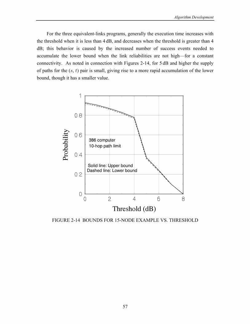
Algorithm Development
57
For the three equivalent-links programs, generally the execution time increases withthe threshold when it is less than 4 dB, and decreases when the threshold is greater than 4dB; this behavior is caused by the increased number of success events needed toaccumulate the lower bound when the link reliabilities are not high—for a constantconnectivity. As noted in connection with Figures 2-14, for 5 dB and higher the supplyof paths for the ( , ) pair is small, giving rise to a more rapid accumulation of the lower= >
bound, though it has a smaller value.
FIGURE 2-14 BOUNDS FOR 15-NODE EXAMPLE VS. THRESHOLD
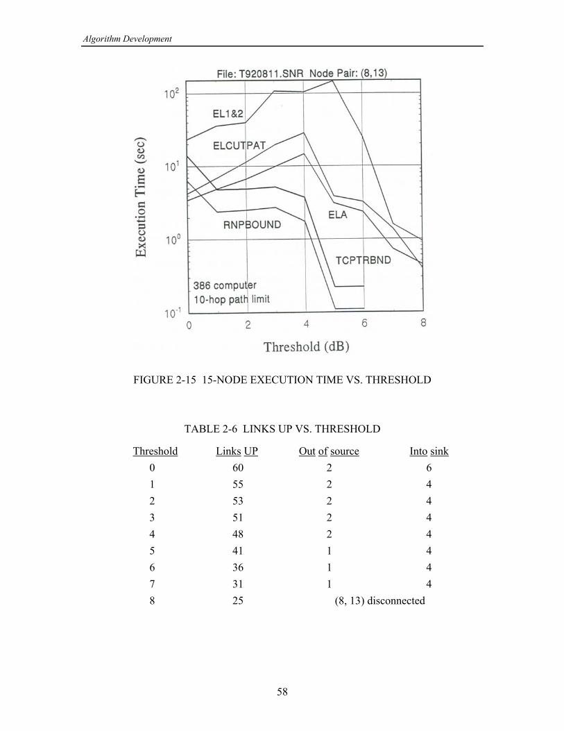
Algorithm Development
58
FIGURE 2-15 15-NODE EXECUTION TIME VS. THRESHOLD
TABLE 2-6 LINKS UP VS. THRESHOLD
Threshold Links UP Out of source Into sink 0 60 2 6 1 55 2 4 2 53 2 4 3 51 2 4 4 48 2 4 5 41 1 4 6 36 1 4 7 31 1 4 8 25 (8, 13) disconnected
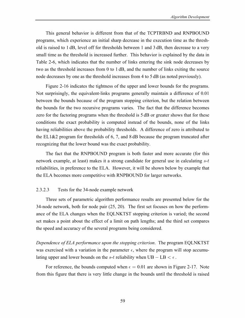
Algorithm Development
59
This general behavior is different from that of the TCPTRBND and RNPBOUNDprograms, which experience an initial sharp decrease in the execution time as the thresh-old is raised to 1 dB, level off for thresholds between 1 and 3 dB, then decrease to a verysmall time as the threshold is increased further. This behavior is explained by the data inTable 2-6, which indicates that the number of links entering the sink node decreases bytwo as the threshold increases from 0 to 1 dB, and the number of links exiting the sourcenode decreases by one as the threshold increases from 4 to 5 dB (as noted previously).
Figure 2-16 indicates the tightness of the upper and lower bounds for the programs.Not surprisingly, the equivalent-links programs generally maintain a difference of 0.01between the bounds because of the program stopping criterion, but the relation betweenthe bounds for the two recursive programs varies. The fact that the difference becomeszero for the factoring programs when the threshold is 5 dB or greater shows that for theseconditions the exact probability is computed instead of the bounds, none of the linkshaving reliabilities above the probability thresholds. A difference of zero is attributed tothe EL1&2 program for thresholds of 6, 7, and 8 dB because the program truncated afterrecognizing that the lower bound was the exact probability.
The fact that the RNPBOUND program is both faster and more accurate (for thisnetwork example, at least) makes it a strong candidate for general use in calculating -= >
reliabilities, in preference to the ELA. However, it will be shown below by example thatthe ELA becomes more competitive with RNPBOUND for larger networks.
2.3.2.3 Tests for the 34-node example network
Three sets of parametric algorithm performance results are presented below for the34-node network, both for node pair (25, 20). The first set focuses on how the perform-ance of the ELA changes when the EQLNKTST stopping criterion is varied; the secondset makes a point about the effect of a limit on path lengths; and the third set comparesthe speed and accuracy of the several programs being considered.
Dependence of ELA performance upon the stopping criterion. The program EQLNKTSTwas exercised with a variation in the parameter , where the program will stop accumu-%
lating upper and lower bounds on the - reliability when UB LB .= > %
For reference, the bounds computed when 0.01 are shown in Figure 2-17. Note% œ
from this figure that there is very little change in the bounds until the threshold is raised
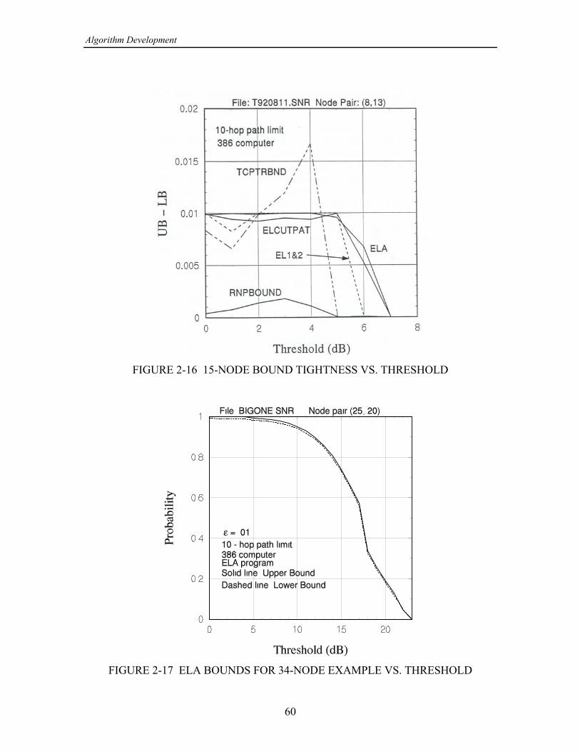
Algorithm Development
60
FIGURE 2-16 15-NODE BOUND TIGHTNESS VS. THRESHOLD
FIGURE 2-17 ELA BOUNDS FOR 34-NODE EXAMPLE VS. THRESHOLD
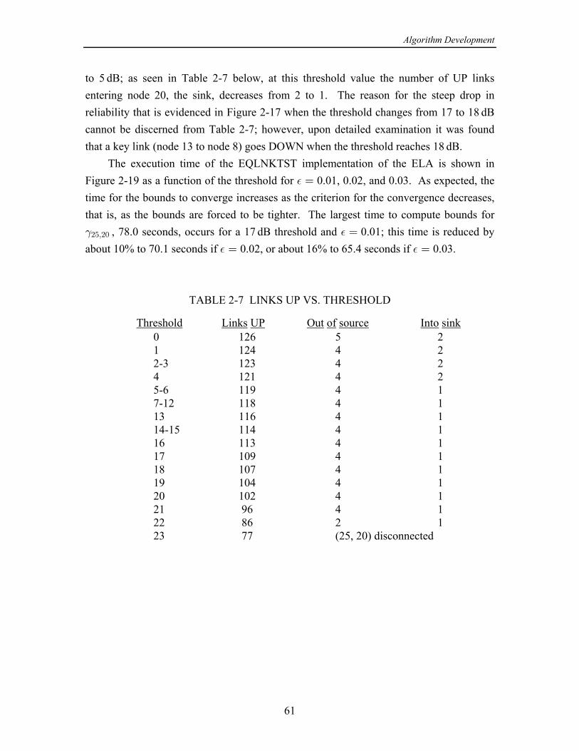
Algorithm Development
61
to 5 dB; as seen in Table 2-7 below, at this threshold value the number of UP linksentering node 20, the sink, decreases from 2 to 1. The reason for the steep drop inreliability that is evidenced in Figure 2-17 when the threshold changes from 17 to 18 dBcannot be discerned from Table 2-7; however, upon detailed examination it was foundthat a key link (node 13 to node 8) goes DOWN when the threshold reaches 18 dB. The execution time of the EQLNKTST implementation of the ELA is shown inFigure 2-19 as a function of the threshold for 0.01, 0.02, and 0.03. As expected, the% œ
time for the bounds to converge increases as the criterion for the convergence decreases,that is, as the bounds are forced to be tighter. The largest time to compute bounds for# %#&ß#! , 78.0 seconds, occurs for a 17 dB threshold and 0.01; this time is reduced byœ
about 10% to 70.1 seconds if 0.02, or about 16% to 65.4 seconds if 0.03.% %œ œ
TABLE 2-7 LINKS UP VS. THRESHOLD
Threshold Links UP Out of source Into sink 0 126 5 2 1 124 4 2 2-3 123 4 2 4 121 4 2 5-6 119 4 1 7-12 118 4 1 13 116 4 1 14-15 114 4 1 16 113 4 1 17 109 4 1 18 107 4 1 19 104 4 1 20 102 4 1 21 96 4 1 22 86 2 1 23 77 (25, 20) disconnected
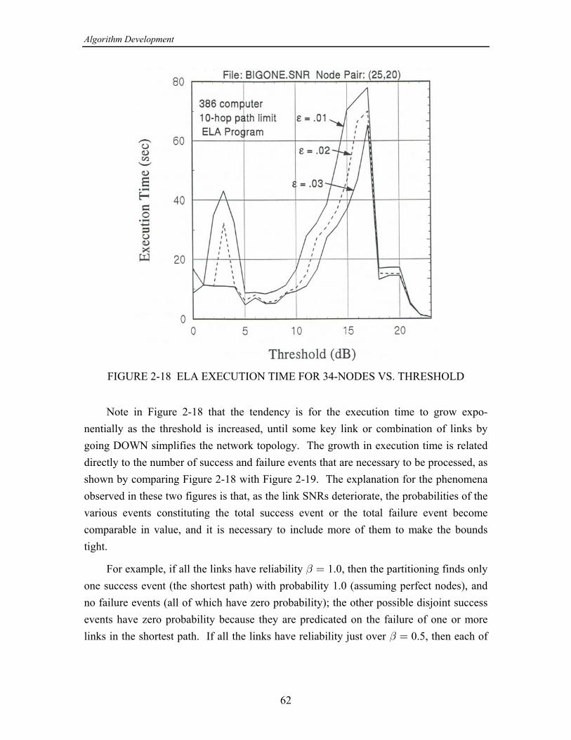
Algorithm Development
62
FIGURE 2-18 ELA EXECUTION TIME FOR 34-NODES VS. THRESHOLD
Note in Figure 2-18 that the tendency is for the execution time to grow expo-nentially as the threshold is increased, until some key link or combination of links bygoing DOWN simplifies the network topology. The growth in execution time is relateddirectly to the number of success and failure events that are necessary to be processed, asshown by comparing Figure 2-18 with Figure 2-19. The explanation for the phenomenaobserved in these two figures is that, as the link SNRs deteriorate, the probabilities of thevarious events constituting the total success event or the total failure event becomecomparable in value, and it is necessary to include more of them to make the boundstight.
For example, if all the links have reliability 1.0, then the partitioning finds only" œ
one success event (the shortest path) with probability 1.0 (assuming perfect nodes), andno failure events (all of which have zero probability); the other possible disjoint successevents have zero probability because they are predicated on the failure of one or morelinks in the shortest path. If all the links have reliability just over 0.5, then each of" œ
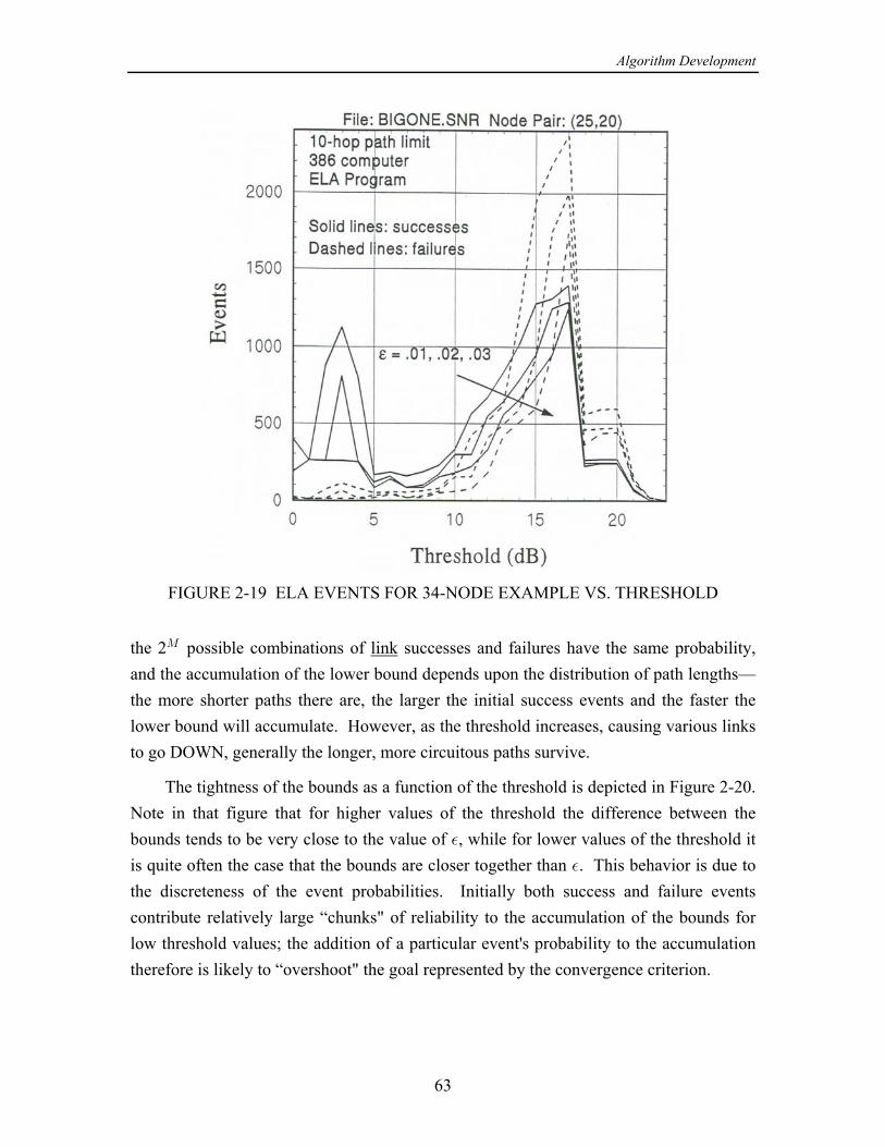
Algorithm Development
63
FIGURE 2-19 ELA EVENTS FOR 34-NODE EXAMPLE VS. THRESHOLD
the 2 possible combinations of successes and failures have the same probability,Q linkand the accumulation of the lower bound depends upon the distribution of path lengths—the more shorter paths there are, the larger the initial success events and the faster thelower bound will accumulate. However, as the threshold increases, causing various linksto go DOWN, generally the longer, more circuitous paths survive.
The tightness of the bounds as a function of the threshold is depicted in Figure 2-20.Note in that figure that for higher values of the threshold the difference between thebounds tends to be very close to the value of , while for lower values of the threshold it%
is quite often the case that the bounds are closer together than . This behavior is due to%
the discreteness of the event probabilities. Initially both success and failure eventscontribute relatively large “chunks" of reliability to the accumulation of the bounds forlow threshold values; the addition of a particular event's probability to the accumulationtherefore is likely to “overshoot" the goal represented by the convergence criterion.
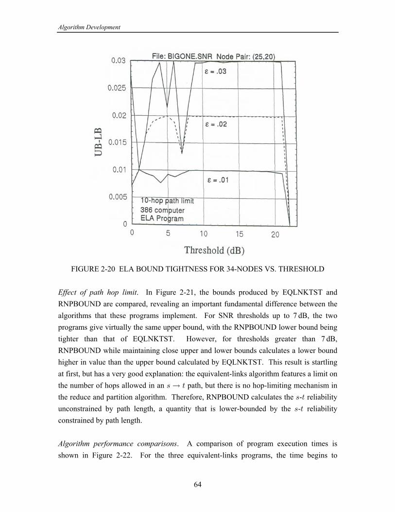
Algorithm Development
64
FIGURE 2-20 ELA BOUND TIGHTNESS FOR 34-NODES VS. THRESHOLD
Effect of path hop limit. In Figure 2-21, the bounds produced by EQLNKTST andRNPBOUND are compared, revealing an important fundamental difference between thealgorithms that these programs implement. For SNR thresholds up to 7 dB, the twoprograms give virtually the same upper bound, with the RNPBOUND lower bound beingtighter than that of EQLNKTST. However, for thresholds greater than 7 dB,RNPBOUND while maintaining close upper and lower bounds calculates a lower boundhigher in value than the upper bound calculated by EQLNKTST. This result is startlingat first, but has a very good explanation: the equivalent-links algorithm features a limit onthe number of hops allowed in an path, but there is no hop-limiting mechanism in= Ä >
the reduce and partition algorithm. Therefore, RNPBOUND calculates the - reliability= >
unconstrained by path length, a quantity that is lower-bounded by the - reliability= >
constrained by path length.
Algorithm performance comparisons. A comparison of program execution times isshown in Figure 2-22. For the three equivalent-links programs, the time begins to
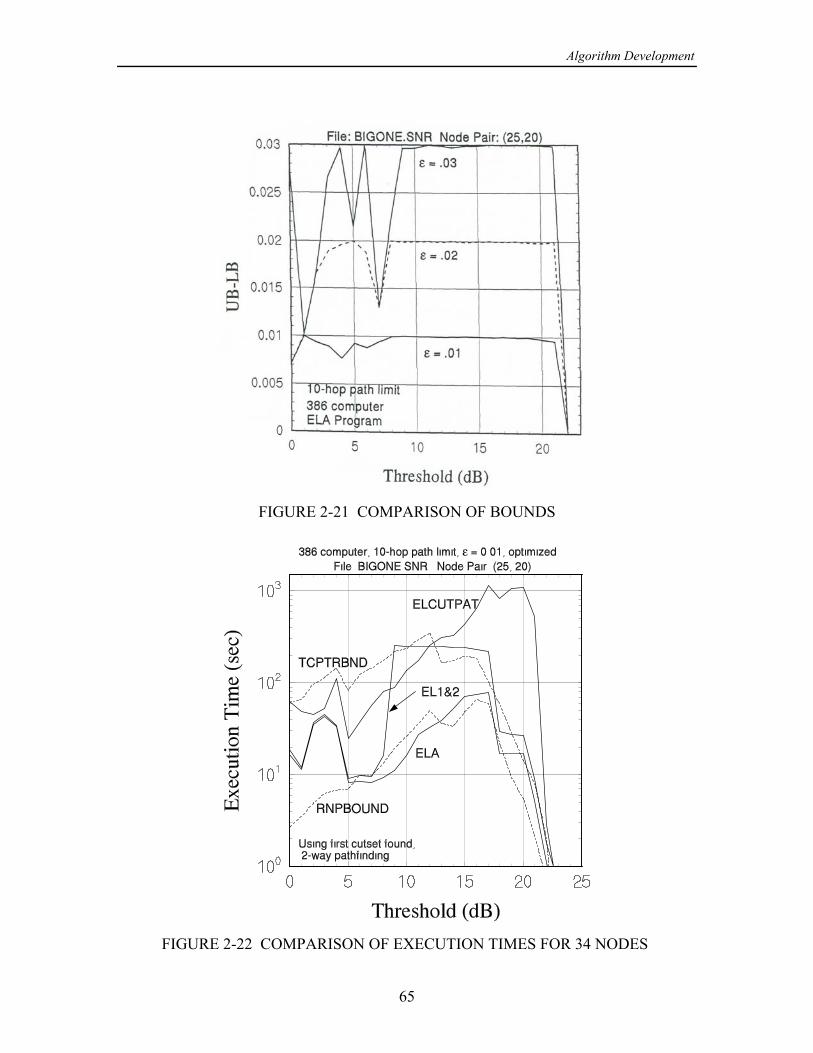
Algorithm Development
65
FIGURE 2-21 COMPARISON OF BOUNDS
FIGURE 2-22 COMPARISON OF EXECUTION TIMES FOR 34 NODES
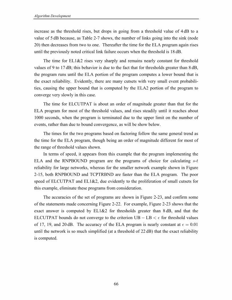
Algorithm Development
66
increase as the threshold rises, but drops in going from a threshold value of 4 dB to avalue of 5 dB because, as Table 2-7 shows, the number of links going into the sink (node20) then decreases from two to one. Thereafter the time for the ELA program again risesuntil the previously noted critical link failure occurs when the threshold is 18 dB.
The time for EL1&2 rises very sharply and remains nearly constant for thresholdvalues of 9 to 17 dB; this behavior is due to the fact that for thresholds greater than 8 dB,the program runs until the ELA portion of the program computes a lower bound that isthe exact reliability. Evidently, there are many cutsets with very small event probabili-ties, causing the upper bound that is computed by the ELA2 portion of the program toconverge very slowly in this case.
The time for ELCUTPAT is about an order of magnitude greater than that for theELA program for most of the threshold values, and rises steadily until it reaches about1000 seconds, when the program is terminated due to the upper limit on the number ofevents, rather than due to bound convergence, as will be show below.
The times for the two programs based on factoring follow the same general trend asthe time for the ELA program, though being an order of magnitude different for most ofthe range of threshold values shown. In terms of speed, it appears from this example that the program implementing theELA and the RNPBOUND program are the programs of choice for calculating -= >
reliability for large networks, whereas for the smaller network example shown in Figure2-15, both RNPBOUND and TCPTRBND are faster than the ELA program. The poorspeed of ELCUTPAT and EL1&2, due evidently to the proliferation of small cutsets forthis example, eliminate these programs from consideration.
The accuracies of the set of programs are shown in Figure 2-23, and confirm someof the statements made concerning Figure 2-22. For example, Figure 2-23 shows that theexact answer is computed by EL1&2 for thresholds greater than 8 dB, and that theELCUTPAT bounds do not converge to the criterion UB LB for threshold values %
of 17, 19, and 20 dB. The accuracy of the ELA program is nearly constant at 0.01% œ
until the network is so much simplified (at a threshold of 22 dB) that the exact reliabilityis computed.
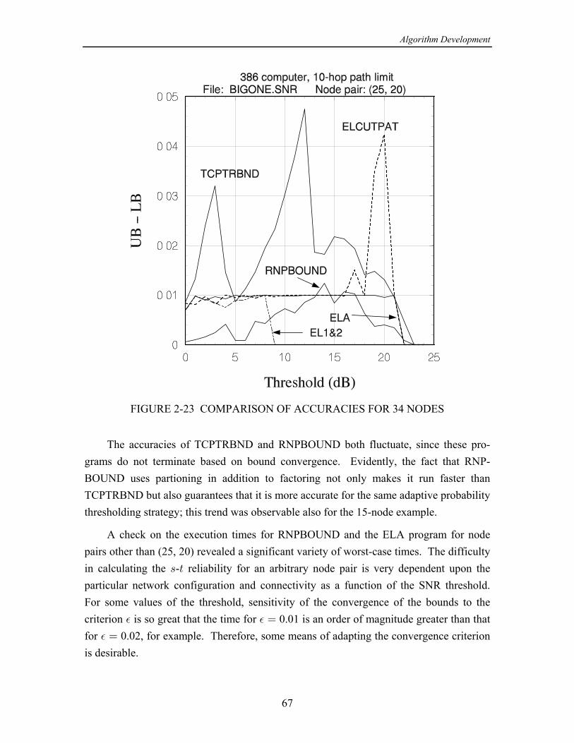
Algorithm Development
67
FIGURE 2-23 COMPARISON OF ACCURACIES FOR 34 NODES
The accuracies of TCPTRBND and RNPBOUND both fluctuate, since these pro-grams do not terminate based on bound convergence. Evidently, the fact that RNP-BOUND uses partioning in addition to factoring not only makes it run faster thanTCPTRBND but also guarantees that it is more accurate for the same adaptive probabilitythresholding strategy; this trend was observable also for the 15-node example.
A check on the execution times for RNPBOUND and the ELA program for nodepairs other than (25, 20) revealed a significant variety of worst-case times. The difficultyin calculating the - reliability for an arbitrary node pair is very dependent upon the= >
particular network configuration and connectivity as a function of the SNR threshold.For some values of the threshold, sensitivity of the convergence of the bounds to thecriterion is so great that the time for 0.01 is an order of magnitude greater than that% % œ
for 0.02, for example. Therefore, some means of adapting the convergence criterion% œ
is desirable.
Algorithm Development
68
2.4 CONCLUSIONS AND RECOMMENDATIONS
On the basis of the numerical results produced by this study, the following wasconcluded in [13]: The concept of using cutsets instead of paths when calculating the upperì
bound on - reliability does work, but only for smaller networks or for large networks= >
with relatively high link reliabilities. For larger networks, at some point, usually whenthe link reliabilities are not high, the events generated by processing cutset failure eventsbecome both numerous and quite small in probability, requiring excessive computationaltime.
While a program combining cutsets and paths performed reasonably well, ofì
the partitioning class of algorithms the original equivalent-links algorithm (with path-finding only) seems to work the best in terms of both speed and accuracy. A new algorithm combining partitioning and network reduction techniques,ì
modified to include adaptive heuristic probability thresholds in order to calculate bounds,shows potential for calculating - reliabilities faster than the ELA. However, this new= > 8
approach does not include a convenient mechanism for stipulating a limit on the lengthsof paths, nor one for trading off the prescribed accuracy with the run time, which areimportant considerations in modelling actual networks. It also, unlike the equivalent-links program, does not truncate on the basis of the tightness of the bounds, and cannotbe used to store a file of events for later calculation.
On the basis of these conclusions and observations, the algorithm of choice is theequivalent-links algorithm.
If further studies are to be conducted in this area, it is recommended that attention begiven to (1) further development of the equivalent-links algorithm, with emphasis onadapting the bound convergence criterion to render a better tradeoff between accuracyand speed, and (2) further development of the reduction and partition algorithm withadaptive probability thresholding, with emphasis on the adaptation technique and onmethods of accounting for a path hop limit.
8The ELA implementation that was tested computed the success and failure probabilities using only linkreliabilities; the procedure for including node reliabilities was not used. When node failures areBackFittaken into account by the ELA, it can be expected that its execution time will increase slightly. TheRNPBOUND program that was tested did take into account node failures.

Example of ELA
69
APPENDIX A
EXAMPLE OF APROBABILITY CALCULATION FOR A 3 3 NETWORK‚
USING THE EQUIVALENT-LINKS ALGORITHM(ORIGIN 1, DESTINATION 2)œ œ
As an example of the operation of the equivalent-links algorithm for includingnodes in the s-t reliability calculation, we consider the problem of finding the probabilitythat, in the 3 3 network of Figure A-1 , the flood search succeeds in finding a path‚ 9
from node 1 to node 2. New events are assumed to be generated using path descriptionsthat give the links used in the order in which they are used.
A.1 FINDING THE SUCCESS AND FAILURE EVENTS
Initially, { [0 0 0 0]}, the universal event. Using an unspecifiedj œ œ âW"
pathfinding algorithm, we proceed as follows. The source is 1 and the terminal iss œ
t œ 2. The first (shortest) completed path is found to be the set of elements
(10) (A-1)œP
which includes, in this instance, the link which directly connects and . Since we have= >
successfully found a path, we add to :W P" f
(10) (A-2)œS"
and add the complement, to :W P" l10
(10) (A-3)œY"
The initial working set is now exhausted. Since | | 1, we are not done. Wej l œ
set , i.e. setj lÃ
(10) (A-4)œW"
and then set . (A-5)œ gl
On the second cycle through the algorithm, we have | | 1 and therefore mustj œ
9The numbering of the links in Figure A-1 is slightly different than that in Figure 1-1 of the text.
10 Only one first-in-first-out queue is required. For ease of presentation we speak of the collection ofjevents being read from the queue, and the collection of events being added to the queue.l
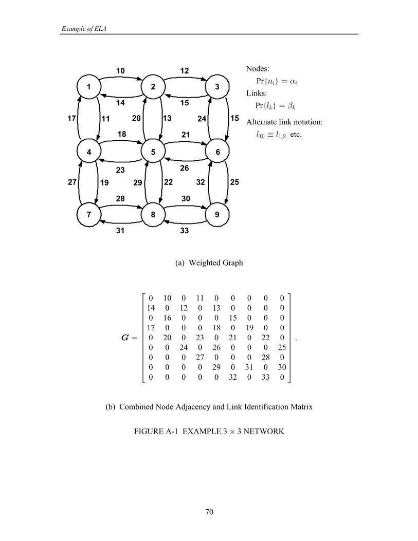
Example of ELA
70
1 2 3
654
7 8 9
10 12
14
17 11 20 13
15
24 15
18 21
23 26
27 19 29 22 32 25
28 30
31 33
Nodes: Pr{ }8 œ3 3!
Links:Pr{ }6 œ5 5"
Alternate link notation: etc.6 ´ 6"! "ß#
(a) Weighted Graph
K œ
Ô ×Ö ÙÖ ÙÖ ÙÖ ÙÖ ÙÖ ÙÖ ÙÖ ÙÖ ÙÖ ÙÖ ÙÖ ÙÕ Ø
0 10 0 11 0 0 0 0 014 0 12 0 13 0 0 0 00 16 0 0 0 15 0 0 017 0 0 0 18 0 19 0 00 20 0 23 0 21 0 22 00 0 24 0 26 0 0 0 250 0 0 27 0 0 0 28 00 0 0 0 29 0 31 0 300 0 0 0 0 32 0 33 0
.
(b) Combined Node Adjacency and Link Identification Matrix
FIGURE A-1 EXAMPLE 3 3 NETWORK‚

Example of ELA
71
examine one event. Now we examine , seeking a short path from 1 to 2 and[ = œ > œ"
find the path using the node sequence 1, 4, 5, 2:
(11, 18, 20). (A-6)œT
Note that in (A-6), the links have been listed in the order of the sequence of links used bythe path that was found; in this instance, the order is the same as the arbitrary order inwhich the links were numbered. Since we have successfully found a path, we appendW P" to ,f (10, 11, 18, 20), (A-7)œS#
and add the partitioned form of the complement, , to :W P" l
(10, 11) (A-8a)œY"
(10, 11, 18) (A-8b)œY#
(10, 11, 18, 20). (A-8c)œY$
We have now exhausted the working set . Since | | 3 0, we must performj l œ
another cycle through the algorithm. We set , clear , and repeat thej l là à g
process. The new working set is obtained by setting equal to the temporary collectionj
l as given in (A-8): (10, 11) (A-9a)œW"
(10, 11, 18) (A-9b)œW#
(10, 11, 18, 20). (A-9c)œW$
and clearing . We begin the next cycle through the algorithm by examining .l œ g W"
With the failure of both links 10 and 11, there is no operable link out of node 1, and asearch for a short path fails quickly. is appended to the failure collection :W" Y
(10, 11) (A-10)œF"
We now examine of (A-9b). We seek a short path from 1 to 2, and find theW#
path using the node sequence 1, 4, 7, 8, 5, 2:
(11, 19, 28, 29, 20). (A-11)œP
Intersecting the path of (A-11) with of (A-9b) gives a new member of theP W#
success collection: (10, 11, 18, 19, 20, 28, 29). (A-12)œS$
Intersecting with adds to the new temporary collection P W# l

Example of ELA
72
(10, 11, 18 ,19) (A-13a)œY"
(10, 11, 18, 19, 28) (A-13b)œY#
(10, 11, 18, 19, 28, 29) (A-13c)œY$
(10, 11, 18, 19, 20, 28, 29) (A-13d)œY%
We now examine given by (A-9c). The path search finds the ordered pathW$
using the node sequence 1, 4, 5, 6, 3, 2:
(11, 18, 21, 24, 16). (A-14)œP
We intersect given by (A-14) with given by (A-9c) to obtainP W$
(10, 11, 16, 18, 20, 21, 24) (A-15)œS%
and append the partitioned complement of intersected with to the temporary collec-P W$
tion :l (10, 11, 18, 20, 21) (A-16a)œY&
(10, 11, 18, 20, 21, 24) (A-16b)œY'
(10, 11, 16, 18, 20, 21, 24). (A-16c)œY(
This exhausts the working collection (A-9). Since | | 0, we must performl
another pass through the algorithm with the new working set given by the set of terms in(A-13) and (A-16).
We examine given by (A-13a). The pathfinding routine returns failure and weW"
append to the failure collection :W" Y
(10, 11, 18, 19). (A-17)œF#
Examination of given by (A-13b) also results in failure and is added to :[ [# # Y
(10, 11, 18, 19, 28) (A-18)œF$
We then examine given by (A-13c). The search results in finding the pathW$
using the node sequence 1, 4, 7, 8, 9, 6, 3, 2:
(11, 19, 28, 30, 32, 24, 16). (A-19)œP
We append the intersection of and the path to the success collection W P$ f
(10, 11, 16, 18, 19, 24, 28, 29, 30, 32), (A-20)œS&
and we append the partitioned complement, , to the temporary collection :W P$ l
(10, 11, 18, 19, 28, 29, 30) (A-21a)œY"

Example of ELA
73
(10, 11, 18, 19, 28, 29, 30, 32) (A-21b)œY#
(10, 11, 18, 19, 24, 28, 29, 30, 32) (A-21c)œY$
(10, 11, 16, 18, 19, 24, 28, 29, 30, 32) (A-21d)œY%
We examine given by (A-13d). The search finds the path using the nodeW%
sequence 1, 4, 7, 8, 5, 6, 3, 2:
(11, 19, 28, 29, 21, 24, 16). (A-22)œP
We append the intersection of with the path to the success collection :W P% f
(10, 11, 16, 18, 19, 20, 21, 24, 28, 29) (A-23)œS'
and append the partitioned complement to the temporary collection :W P% l
(10, 11, 18, 19, 20, 21, 28, 29) (A-24a)œY&
(10, 11, 18, 19, 20, 21, 24, 28, 29) (A-24b)œY'
(10, 11, 16, 18, 19, 20, 21, 24, 28, 29). (A-24c)œY(
We examine given by (A-16a). The search finds the path using the nodeW&
sequence 1, 4, 5, 8, 9, 6, 3, 2:
(11, 18, 22, 30, 32, 24, 16). (A-25)œP
We append the intersection of with the path to the success collection :W P& f
(10, 11, 16, 18, 20, 21, 22, 24, 30, 32) (A-26)œS(
and append the partitioned complement to the temporary collection :W P& l
(10, 11, 18, 20, 21, 22) (A-27a)œY)
(10, 11, 18, 20, 21, 22, 30) (A-27b)œY*
(10, 11, 18, 20, 21, 22, 30, 32) (A-27c)œY"!
(10, 11, 18, 20, 21, 22, 24, 30, 32) (A-27d)œY""
(10, 11, 16, 18, 20, 21, 22, 24, 30, 32). (A-27e)œY"#
We find that and given by (A-16b) and (A-16c), respectively, fail to find a[ [' (
path reaching the destination. We append and to the failure collection :W' ([ Y
(10, 11, 18, 20, 21, 24) (A-28a)œF%
(10, 11, 16, 18, 20, 21, 24). (A-28b)œF&

Example of ELA
74
This exhausts the working set given by (A-13) and (A-16). The temporaryj
collection given by (A-21), (A-24), and (A-27) has cardinality greater than zero.l
Therefore we must make another pass through the algorithm with the new workingcollection given by (A-21), (A-24), and (A-27) and .l à g
We first examine given by (A-21a). The search fails to find a path to theW"
destination and we append to :W" Y
(10, 11, 18, 19, 28, 29, 30). (A-29)œF'
Next we examine given by (A-21b). The search fails to find a path to theW#
destination and we append to :W# Y
(10, 11, 18, 19, 28, 29, 30, 32). (A-30)œF(
We examine given by (A-21c). The path-finding algorithm finds the path usingW$
the node sequence 1, 4, 7, 8, 9, 6, 5, 2:
(11, 19, 28, 30, 32, 26, 20). (A-31)œP
We append the intersection of with to the success collection :W P$ f
(10, 11, 18, 19, 20, 24, 26, 28, 29, 30, 32) (A-32)œS)
and append the partitioned form of the intersection to :W P$ l
(10, 11, 18, 19, 24, 26, 28, 29, 30, 32) (A-33a)œY"
(10, 11, 18, 19, 20, 24, 26, 28, 29, 30, 32). (A-33b)œY#
We examine given by (A-21d). The pathfinding algorithm finds the path usingW%
the node sequence 1, 4, 7, 8, 9, 6, 5, 2:
(11, 19, 28, 30, 32, 26, 20). (A-34)œP
We append the intersection of and the path to the success collection :W P% f
(10, 11, 16, 18, 19, 20, 24, 26, 28, 29, 30, 32) (A-35)œS*
and we append the partitioned form of to the temporary collection :W P% l
(10, 11, 16, 18, 19, 24, 26, 28, 29, 30, 32) (A-36a)œY$
(10, 11, 16, 18, 19, 20, 24, 26, 28, 29, 30, 32) (A-36b)œY%
We examine given by (A-24a). The pathfinding algorithm finds the path usingW&
the node sequence 1, 4, 7, 8, 9, 6, 3, 2:
(11, 19, 28, 30, 32, 24, 16). (A-37)œP
Example of ELA
75
We take the intersection of with the path and append the intersection to the successW P&
collection :f (10, 11, 16, 18, 19, 20, 21, 24, 28, 29, 30, 32) (A-38)œS"!
and append the partitioned form of to the temporary collection :W P& l
(10, 11, 18, 19, 20, 21, 28, 29, 30) (A-39a)œY&
(10, 11, 18, 19, 20, 21, 28, 29, 30, 32) (A-39b)œY'
(10, 11, 18, 19, 20, 21, 24, 28, 29, 30, 32) (A-39c)œY(
(10, 11, 16, 18, 19, 20, 21, 24, 28, 29, 30, 32). (A-39d)œY)
We examine given by (A-24b). The pathfinding algorithm does not find a path,W'
so is added to the failure collection :[' Y
(10, 11, 18, 19, 20, 21, 24, 28, 29). (A-40)œF)
We then examine given by (A-24c). The pathfinding algorithm does not find a[(
path, so we add to :[( Y
(10, 11, 16, 18, 19, 20, 21, 24, 28, 29). (A-41)œF*
Examination of given by (A-27a) results in finding the path using the node[)
sequence 1, 4, 7, 8, 9, 6, 3, 2:
(11, 19, 28, 30, 32, 24, 16). (A-42)œP
We form the intersection of and the path and append that intersection to the successW P)
collection :f (10, 11, 16, 18, 19, 20, 21, 22, 24, 28, 30, 32). (A-43)œS""
Also, we append the intersection , in partitioned form, to the temporary collectionW P)
l: (10, 11, 18, 19, 20, 21, 22) (A-44a)œY*
(10, 11, 18, 19, 20, 21, 22, 28) (A-44b)œY"!
(10, 11, 18, 19, 20, 21, 22, 28, 30) (A-44c)œY""
(10, 11, 18, 19, 20, 21, 22, 28, 30, 32) (A-44d)œY"#
(10, 11, 18, 19, 20, 21, 22, 24, 28, 30, 32) (A-44e)œY"$
(10, 11, 16, 18, 19, 20, 21, 22, 24, 28, 30, 32). (A-44f)œY"%
Example of ELA
76
We examine through given by (A-27b) to (A-27e). The search in eachW* "#[
case fails to find a path to the destination, so we append through to the failure[* ""Wcollection :Y (10, 11, 18, 20, 21, 22, 30) (A-45a)œF"!
(10, 11, 18, 20, 21, 22, 30, 32) (A-45b)œF""
(10, 11, 18, 20, 21, 22, 24, 30, 32) (A-45c)œF"#
(10, 11, 16, 18, 20, 21, 22, 24, 30, 32). (A-45d)œF"$
This exhausts the working set given by (A-21), (A-24), and (A-27). Thej
temporary collection given by (A-33), (A-36), (A-39), and (A-44) is not empty.l
Therefore we must make another pass through the algorithm with the new workingcollection given by , then set .j j l là à g
Each of the s given by (A-33), (A-36), (A-39), and (A-44) results in the failure[
of the pathfinding algorithm to find a path from node 1 to node 2. Thus to the failurecollection we add
(10, 11, 18, 19, 24, 26, 28, 29, 30, 32) (A-46a)œF"%
(10, 11, 18, 19, 20, 24, 26, 28, 29, 30, 32) (A-46b)œF"&
(10, 11, 16, 18, 19, 24, 26, 28, 29, 30, 32) (A-46c)œF"'
(10, 11, 16, 18, 19, 20, 24, 26, 28, 29, 30, 32) (A-46d)œF"(
(10, 11, 18, 19, 20, 21, 28, 29, 30) (A-46e)œF")
(10, 11, 18, 19, 20, 21, 28, 29, 30, 32) (A-46f)œF"*
(10, 11, 18, 19, 20, 21, 24, 28, 29, 30, 32) (A-46g)œF#!
(10, 11, 16, 18, 19, 20, 21, 24, 28, 29, 30, 32) (A-46h)œF#"
(10, 11, 18, 19, 20, 21, 22) (A-46i)œF##
(10, 11, 18, 19, 20, 21, 22, 28) (A-46j)œF#$
(10, 11, 18, 19, 20, 21, 22, 28, 30) (A-46k)œF#%
(10, 11, 18, 19, 20, 21, 22, 28, 30, 32) (A-46l)œF#&
(10, 11, 18, 19, 20, 21, 22, 24, 28, 30, 32) (A-46m)œF#'
(10, 11, 16, 18, 19, 20, 21, 22, 24, 28, 30, 32). (A-46n)œF#(
Example of ELA
77
This exhausts the working set . The temporary collection , so we arej l œ g
done! The collection is now an exhaustive success collection and the collection isf Y
an exhaustive failure collection. The probability of successfully routing a call fromsource 1 to destination 2 (s-t reliability with s 1 and t 2) may be computed usingœ œ
either or .f Y
A.2 ACCOUNTING FOR THE NODE RELIABILITIES
According the formulas given in the text as (1-14), the evaluation of the - relia-= >
bility for this example, including node reliabilities, is accomplished by summing thefollowing success probabilities:
Pr{ } [ ] (A-47a)œW" " # "!! ! "
Pr{ } [ (1 ) ][ ][ ] (A-47b)œ W# " # "! #! % "" & ")! ! " " ! " ! "
Pr{ } [ (1 ) ][ ][ (1 ) ][ ][ ] (A-47c)œ W$ " # "! #! % "" & ") #* ( "* ) #)! ! " " ! " ! " " ! " ! "
Pr{ } [ (1 ) (1 )][ ][ ][ ][ ] (A-47d)œ W% " # "! "' #! $ #% % "" & ") ' #"! ! " " " ! " ! " ! " ! "
Pr{ } [ (1 ) ][ ][ ][ (1 )(1 ) 1 ]œ W& " # "! "' $ #% % "" & ") #* &! ! " " ! " ! " ! " " !
[ ][ ][ ][ ] (A-47e)‚ ! " ! " ! " ! "' $# ( "* ) #) * $!
Pr{ } [ (1 ) (1 )][ ][ ][ (1 ) ]œ W' " # "! "' #! $ #% % "" & ") #*! ! " " " ! " ! " ! " "
[ ][ ][ ] (A-47f)‚ ! " ! " ! "' #" ( "* ) #)
Pr{ } [ (1 ) (1 )][ ][ ][ ][ (1 )]œ W( " # "! "' #! $ #% % "" & ") ' $# #"! ! " " " ! " ! " ! " ! " "
[ ][ ] (A-47g)‚ ! " ! ") ## * $!
œ WPr{ } [ (1 ) )][ (1 ) 1 ][ ][ (1 ) (1 )]) " # "! #! $ #% $ % "" & ") #' #*! ! " " ! " ! ! " ! " " "
[ ][ ][ ][ ] (A-47h)‚ ! " ! " ! " ! "' $# ( "* ) #) * $!
Pr{ } [ (1 )(1 ) ][ ][ ][ (1 ) (1 )]œ W* " # "! "' #! $ #% % "" & ") #' #*! ! " " " ! " ! " ! " " "
[ ][ ][ ][ ] (A-47i)‚ ! " ! " ! " ! "' $# ( "* ) #) * $!
Pr{ } [ (1 ) (1 )][ ][ ][ (1 ) ]œ W"! " # "! "' #! $ #% % "" & ") #*! ! " " " ! " ! " ! " "
[ (1 ) ][ ][ ][ ] (A-47j)‚ ! " " ! " ! " ! "' #" $# ( "* ) #) * $!
Pr{ } [ (1 ) (1 )][ ][ ][ ][ (1 ) ]œ W"" " # "! "' #! $ #% % "" & ") ' #" $#! ! " " " ! " ! " ! " ! " "
[ ][ (1 ) ][ ] (A-47k)‚ ! " ! " " ! "( "* ) ## #) * $!
Example of Cutset Method
78
APPENDIX B
EXAMPLE OF APROBABILITY CALCULATION FOR A 3 3 NETWORK‚
USING THE CUTSET METHOD(ORIGIN 1, DESTINATION 2)œ œ
As an example of the operation of the cutset method for the s-t reliabilitycalculation, we consider the problem of finding the probability that, in the 3 3 network‚
of Figure A-1, the flood search succeeds in finding a path from node 1 to node 2. This isthe same example worked in Appendix A for the equivalent-links algorithm.
We begin with { [0 0 0 0]}, the universal event. We seek a smallj œ œ âW"
cutset of DOWN links that precludes a path from node 1 to node 2. Using an unspecifiedminimum cutset algorithm that works both forward from the source and backward fromthe sink—and giving preferences to a cutset found in a forward search in case of a tie inthe size of the cutsets found—we proceed as follows. The source is 1 and thes œ
terminal is 2. In the forward direction the smallest cutset is (10, 11); that is, there ist œno path out from the source if links 10 and 11 are DOWN. In the reverse direction thesmallest cutset is (10, 16, 20); that is, there is no path into the sink if links 10, 16, and 20are DOWN. Thus the selection is
(10, 11) (B-1)œG
which includes, in this instance, the link which directly connects and . Since we have= >
successfully found a cutset, we add to :W" G Y
(10, 11) (B-2)œJ"
and add the complement, to :W" G l11
(10) (B-3a)œ]"
(10, 11). (B-3b)œ]#
The initial working set is now exhausted. Since | | 2, we are not done. Wej l œ
set , i.e. setj lÃ
(10) (B-4a)œ["
(10, 11) (B-4b)œ[#
and then set
11Only one first-in-first-out queue is required. For ease of presentation we speak of the collection ofjevents being read from the queue, and the collection of events being added to the queue.l
Example of Cutset Method
79
. (B-5)œ gl
On the second cycle through the algorithm, we have | | 2 and therefore mustj œ
examine two events. Now we examine , seeking a short cutset to preclude a path fromW"
s tœ œ = >1 to 2 and find that there is none, since link 10 directly connects to and ispostulated to be UP. Thus we have found
(10), (B-6)œW"
and no further processing of is required.["
With (10, 11) postulated as the status of the network, the forward cutset is[ œ#
(18, 19) and the reverse cutset is (16, 20). Giving preference to the former, we havefound a failure event, and append to :[ G# Y
(10, 11, 18, 19), (B-7)œJ#
The partitioned form of the complement, , is added to :[ G# l
(10, 11, 18) (B-8a)œY"
(10, 11, 18, 19). (B-8b)œY#
We have now exhausted the working set . Since | | 2 0, we must performj l œ
another cycle through the algorithm. We set , clear , and repeat thej l là à g
process. The new working set is obtained by setting equal to the temporary collectionj
l as given in (B-8): (10, 11, 18) (B-9a)œ["
(10, 11, 18, 19). (B-9b)œ[#
and clearing . We begin the next cycle through the algorithm by examining . Inl œ g W"
the forward direction, links 19, 20, 21, and 22 must simultaneously be DOWN topreclude a path from node 1 to node 2; in the reverse direction, links 16 and 20 must beDOWN to preclude a path into node 2 from node 1. Therefore, the selected cutset is (16,20), giving rise to
(10, 11, 16, 18, 20) (B-10)œF$
and (10, 11, 16, 18) (B-11a)œ]"
(10, 11, 16, 18, 20). (B-11b)œ]#
We now examine given by (B-9b). The forward cutset involves links only oneW#
link, link 28, and therefore is the preferred cutset, giving rise to
Example of Cutset Method
80
(10, 11, 18, 19, 28) (B-12)œF%
and (10, 11, 18, 19, 28). (B-13)œ]$
This exhausts the working collection (B-9). Since | | 0, we must performl
another pass through the algorithm with the new working set given by the set of events in(B-11) and (B-13).
We examine given by (B-11a). In the forward direction, links 19, 20, 21, andW"
22 must be DOWN to preclude a path; working backwards from the sink we find thatlinks 20 and 24 must be DOWN. Therefore the selected cutset is (20, 24), giving rise to
(10, 11, 16, 18, 20, 24) (B-14)œJ&
and (10, 11, 16, 18, 20) (B-15a)œ]"
(10, 11, 16, 18, 20, 24). (B-15b)œ]#
We then examine given by (B-11b). There is a path entirely of links that areW#
postulated to be UP, so there is no cutset and
(10, 11, 16, 18, 20). (B-16)œW#
We examine given by (B-13). The forward search for a cutset finds that linksW$
29 and 30 must be DOWN, while the reverse search finds that links 16 and 20 must beDOWN. The selected cutset is (29, 30), giving rise to
(10, 11, 18, 19, 28, 29, 30) (B-17)œJ'
and (10, 11, 18, 19, 28, 29) (B-18a)œ]$
(10, 11, 18, 19, 28, 29, 30). (B-18b)œ]%
This exhausts the working set given by (B-11) and (B-13). The temporaryj
collection given by (B-15) and (B-18) has cardinality greater than zero. Therefore, wel
must make another pass through the algorithm with the new working collection given by(B-15) and (B-18) and .l à g
We first examine given by (B-15a). The fact that links 11, 18, and 20 are["
postulated to be UP simultaneously guarantees a path, so
(10, 11, 16, 18, 20). (B-19)œW$
Example of Cutset Method
81
Next we examine given by (B-15b). Links 19, 21, and 22 must be DOWN to[#
preclude a path, as determined by working forward from the source; the reverse cutsetsearch finds that links 21 and 32 must be DOWN. Therefore, the selected cutset is (21,32), which gives rise to
(10, 11, 16, 18, 20, 21, 24, 32) (B-20)œJ(
and (10, 11, 16, 18, 20, 21, 24) (B-21a)œ]"
(10, 11, 16, 18, 20, 21, 24, 32). (B-21b)œ]#
We examine given by (B-18a). The candidates for cutset are (20, 21, 30) from[$
the forward search and (16, 20) from the reverse search. Selecting the latter, we find thefailure event (10, 11, 16, 18, 19, 20, 28, 29) (B-22)œJ)
and the temporary events
(10, 11, 16, 18, 19, 28, 29) (B-23a)œ]$
(10, 11, 16, 18, 19, 20, 28, 29). (B-23b)œ]%
We examine given by (B-18b). The selected cutset (in the forward direction) is[%
(32), so to the failure collection we add
(10, 11, 18, 19, 28, 29, 30, 32) (B-24)œJ*
and to the temporary collection we add
(10, 11, 18, 19, 28, 29, 30, 32). (B-25)œ]&
This exhausts the working set given by (B-15) and (B-18). The temporaryj
collection given by (B-21), (B-23), and (B-25) is not empty. Therefore we must makel
another pass through the algorithm with the new working collection given byj
j l là à g, then set .
The set of good links postulated by given by (B-21a) forms a path from node 1["
to node 2. Therefore, is a success event:["
(10, 11, 16, 18, 20, 21, 24). (B-26)œW%
Next we examine given by (B-21b). The smallest cutset (found in the reverse[#
direction) is (30), giving rise to
(10, 11, 16, 18, 20, 21, 24, 30, 32) (B-27)œJ"!
and
Example of Cutset Method
82
(10, 11, 16, 18, 20, 21, 24, 30, 32). (B-28)œ]"
The event given by (B-23a) cannot produce a path if either links 20, 21, and 30[$
are DOWN or links 20 and 24 are down. Selecting the latter (found by the reversesearch) gives rise to
(10, 11, 16, 18, 19, 20, 24, 28, 29) (B-29)œJ""
and (10, 11, 16, 18, 19, 20, 28, 29) (B-30a)œ]#
(10, 11, 16, 18, 19, 20, 24, 28, 29). (B-30b)œ]$
Examining given by (B-23b), the conditions postulated guarantee a path:[%
(10, 11, 16, 18, 19, 20, 28, 29). (B-31)œW&
Next we examine givien by (B-25). Either links 24 and 26 must be DOWN, as[&
determined by a forward search, or links 16 and 20, as determined by a reverse search.Selecting the first alternative gives rise to
(10, 11, 18, 19, 24, 26, 28, 29, 30, 32) (B-32)œJ"#
and (10, 11, 18, 19, 24, 28, 29, 30, 32) (B-33a)œ]%
(10, 11, 18, 19, 24, 26, 28, 29, 30, 32). (B-33b)œ]&
This exhausts the working set , with nonempty so that another iteration isj l
required, using as the contents of the events given by (B-28), (B-30), and (B-33).j
Considering given by (B-28), we find that in either search direction two links are["
required to be DOWN in order to preclude a path. Selecting the forward alternative, thecutset (19, 22) gives rise to
(10, 11, 16, 18, 19, 20, 21, 22, 24, 30, 32) (B-34)œJ"$
and (10, 11, 16, 18, 19, 20, 21, 24, 30, 32) (B-35a)œ]"
(10, 11, 16, 18, 19, 20, 21, 22, 24, 30, 32). (B-35b)œ]#
The event given by (B-30a) supports a path of good links:[#
(10, 11, 16, 18, 19, 20, 28, 29). (B-36)œW'
The event given by (B-30b), results in the cutset (21, 30) for the forward search.[$
Thus
(10, 11, 16, 18, 19, 20, 21, 24, 28, 29, 30) (B-37)œJ"%

Example of Cutset Method
83
and (10, 11, 16, 18, 19, 20, 21, 24, 28, 29) (B-38a)œ]$
(10, 11, 16, 18, 19, 20, 21, 24, 28, 29, 30). (B-38b)œ]%
The event given by (B-33a) results in the cutset (16, 26) for a search in either[%
direction. Thus
(10, 11, 16, 18, 19, 24, 26, 28, 29, 30, 32) (B-39)œJ"&
and (10, 11, 16, 18, 19, 24, 28, 29, 30, 32) (B-40a)œ]&
(10, 11, 16, 18, 19, 24, 26, 28, 29, 30, 32). (B-40b)œ]'
Next we examine given by (B-33b). The cutset is (20), leading to[&
(10, 11, 18, 19, 20, 24, 26, 28, 29, 30, 32) (B-41)œJ"'
and (10, 11, 18, 19, 20, 24, 26, 28, 29, 30, 32). (B-42)œ](
This exhausts the working set and another iteration is required to examine thej
events given by (B-35), (B-38), (B-40) and (B-42). The event given by (B-35a) for a["
search in either direction results in the cutset (22, 28), giving rise to
(10, 11, 16, 18, 19, 20, 21, 22, 24, 28, 30, 32) (B-43)œJ"(
and (10, 11, 16, 18, 19, 20, 21, 22, 24, 30, 32) (B-44a)œ]"
(10, 11, 16, 18, 19, 20, 21, 22, 24, 28, 30, 32). (B-44b)œ]#
The good links specified in events and given by (B-35b) and (B-38a), re-[ [# $
spectively, form complete paths:
(10, 11, 16, 18, 19, 20, 21, 22, 24, 30, 32) (B-45a)œW(
(10, 11, 16, 18, 19, 20, 21, 24, 28, 29). (B-45b)œW)
Next we examine given by (B-38b) and find that the cutset is (32), leading to[%
(10, 11, 16, 18, 19, 20, 21, 24, 28, 29, 30, 32) (B-46)œJ")
and (10, 11, 16, 18, 19, 20, 21, 24, 28, 29, 30, 32). (B-47)œ]$
There is no cutset for the event given by (B-40a), giving rise to[&
(10, 11, 16, 18, 19, 24, 28, 29, 30, 32). (B-48)œW*
Example of Cutset Method
84
The event given by (B-40b) has the cutset (20), giving rise to['
(10, 11, 16, 18, 19, 20, 24, 26, 28, 29, 30, 32) (B-49)œJ"*
and (10, 11, 16, 18, 19, 20, 24, 26, 28, 29, 30, 32). (B-50)œ]%
The good links in the event given by (B-42) form a path, so that[(
(10, 11, 18, 19, 20, 24, 26, 28, 29, 30, 32). (B-51)œW"!
A final iteration to examine the events in (B-44), (B-47), and (B-50) reveals thatthey are all success events:
(10, 11, 16, 18, 19, 20, 21, 22, 24, 30, 32) (B-52a)œW""
(10, 11, 16, 18, 19, 20, 21, 22, 24, 28, 30, 32) (B-52b)œW"#
(10, 11, 16, 18, 19, 20, 21, 24, 28, 29, 30, 32) (B-52c)œW"$
(10, 11, 16, 18, 19, 20, 24, 26, 28, 29, 30, 32). (B-52d)œW"%
Both and the temporary collection are empty, so we are done! The collectionj l
f Y is now an exhaustive success collection and the collection is an exhaustive failurecollection. The probability of successfully routing a call from source 1 to destination 2(s-t reliability with s 1 and t 2) may be computed using either or .œ œ f Y

Example of CutPath Method
85
APPENDIX C
EXAMPLE OF APROBABILITY CALCULATION FOR A 3 3 NETWORK‚
USING THE CUTPATH METHOD(ORIGIN 1, DESTINATION 2)œ œ
In this appendix an example is provided of the operation of the method for the -= >
reliability calculation in which a selection is made of either a path or cutset, dependingupon which will generate the fewer number of new events. The problem considered isthat of finding the probability that, in the 3 3 network of Figure A-1, the flood search‚
succeeds in finding a path from node 1 to node 2. This is the same example worked forthe equivalent-links algorithm with pathfinding in Appendix A and using cutsets inAppendix B.
The processing begins by setting { [0 0 0 0]}, the universal event.j œ œ âW"
In accordance with the flow diagram of Figure 2-9, first a short path from node 1 to node2 is sought. Using an unspecified pathfinding algorithm and an unspecified minimumcutset algorithm that works both forward from the source and backward from the sink—and giving preference to a cutset found in a forward search in case of a tie in the size ofthe cutsets found—the problem proceeds as follows, assuming that in the case of a tie inthe number of new events to be generated, a path is preferred.
The source is 1 and the terminal is 2. In the forward direction the smallests tœ œ
path is (10) and the smallest cutset is (10, 11); that is, there is no path out from the sourceif links 10 and 11 are DOWN. In the reverse direction the smallest cutset is (10, 16, 20);that is, there is no path into the sink if links 10, 16, and 20 are DOWN. Thus theselection is pathfinding, with
(10) (C-1)œT
which includes, in this instance, the link which directly connects and . Since we have= >
successfully found a path, we add to :W" T f
(10) (C-2)œW"
and add the complement, to :W" W l12
(10). (C-3)œ]"
12Only one first-in-first-out queue is required. For ease of presentation we speak of the collection ofjevents being read from the queue, and the collection of events being added to the queuel .

Example of CutPath Method
86
The initial working set is now exhausted. Since | | 1, the problem is notj l œ
done. Therefore the queues are exchanged by setting , , by settingj là i. e.
(10) (C-4)œ["
and then setting . (C-5)œ gl
On the second cycle through the algorithm, | | 1, so one there is one event to bej œ
examined. Examining , it is found that the shortest path requires three links: (11,W" T œ
18, 20), which would eventuate in the generation of three new events to be examined. Insearch of a short cutset, it is found that, given that link 10 is DOWN, only link 11 has tobe down to preclude a path from 1 to 2. Thus the cutset method is selected, withs tœ œ
(11), (C-6)œG
giving rise to the failure event , or[ G"
(10, 11), (C-7)œJ"
which is appended to , and the next event , orY [ G"
(10, 11). (C-8)œ]"
The working set is now exhausted. Since | | 1 0, another cycle throughj l œ
the algorithm is needed. The new working set is obtained by setting equal to thej
temporary collection as given in (C-8):l
(10, 11). (C-9)œ["
The next cycle through the algorithm begins by examining . Again, (11, 18, 20)W" T œ
is the shortest path; this time the pathfinding method would generate two new events,since only links 18 and 20 are not specified to be UP in . In the forward direction,["
links 18 and 19 must be DOWN to preclude a path from node 1 to node 2, and links 16and 20 in the reverse direction. Therefore, the selected method is to use pathfinding,giving rise to (10, 11, 18, 20) (C-10)œW#
and (10, 11, 18) (C-11a)œ]"
(10, 11, 18, 20). (C-11b)œ]#
On the next pass through the algorithm, given by (C-11a) is examined. WithW"
link 18 DOWN, the shortest path is (11, 19, 28, 29, 20), involving four links notT œ
Example of CutPath Method
87
specified to be UP in . The forward cutset involves links only one link, link 19, and["
therefore is the preferred cutset, giving rise to
(10, 11, 18, 19) (C-12)œF#
and (10, 11, 18, 19). (C-13)œ]"
Examination of given by (C-11b) determines that the least number of new events[#
is generated using the cutset (16), giving rise toG œ
(10, 11, 16, 18, 20) (C-14)œF$
and (10, 11, 16, 18, 20). (C-15)œ]#
This exhausts the working collection (C-11). Since | | 0, another pass throughl
the algorithm is needed with the new working set given by the events in (C-13) and (C-15).
On examination of given by (C-13), it is found that in the forward direction,W"
only link 28 must be DOWN to preclude a path. Therefore the selected cutset is (28),giving rise to (10, 11, 18, 19, 28) (C-16)œJ%
and (10, 11, 18, 19, 28). (C-17)œ]"
given by (C-15). Similarly, there is no path if only one link is down, link 24.W#
Thus (10, 11, 16, 18, 20, 24) (C-18)œJ&
and (10, 11, 16, 18, 20, 24). (C-19)œ]#
This exhausts the working set given by (C-13) and (C-15). The temporaryj
collection given by (C-17) and (C-19) has cardinality greater than zero. Therefore,l
another pass through the algorithm is required, with the new working collection given by(C-17) and (C-19) and .l à g
Examining given by (C-17) determines that the shortest path (11, 19, 28,[ T œ"
29, 20) would generate two new events, as would the smallest cutset, (16, 20).G œ
Therefore the choice is pathfinding, giving
(10, 11, 18, 19, 20, 28, 29) (C-20)œW$
with

Example of CutPath Method
88
(10, 11, 18, 19, 28, 29) (C-21a)œ]"
(10, 11, 18, 19, 20, 28, 29). (C-21b)œ]#
Next given by (C-19) is examined. The path (11, 18, 21, 24, 16) only[ T œ#
generates one new event, so it is not necessary to find a cutset. The ELA success eventprocessing gives (10, 11, 16, 18, 20, 21, 24) (C-22)œW%
and (10, 11, 16, 18, 20, 21, 24). (C-23)œ]$
This exhausts the working set given by (C-17) and (C-19). The temporaryj
collection given by (C-21) and (C-23) is not empty. Therefore another pass throughl
the algorithm is required.
The shortest path under the network condition postulated by given by (C-21a)["
would add four new events, while (30) is a cutset. Therefore, is an ELA2G œ ["
failure event: (10, 11, 18, 19, 28, 29, 30), (C-24)œJ'
giving rise to
(10, 11, 18, 19, 28, 29, 30). (C-25)œ]"
The shortest path for given by (C-21b) would use three links not said to UP in[#
[#. The smallest cutset (found in the reverse direction) is (16), giving rise to
(10, 11, 16, 18, 19, 20, 28, 29) (C-26)œJ(
and (10, 11, 16, 18, 19, 20, 28, 29). (C-27)œ]#
The event given by (C-23) cannot produce a path if either links 19 and 22 are[$
DOWN or link 32 is down. Selecting the latter (found by the reverse search) gives
(10, 11, 16, 18, 20, 21, 24, 32) (C-28)œJ)
and (10, 11, 16, 18, 20, 21, 24, 32). (C-29)œ]$
This exhausts the working set , with nonempty so that another iteration isj l
required, using as the contents of the events given by (C-25), (C-27), and (C-29).j
Considering given by (C-25), the shortest path adds three new links, while the cutset["
G œ (32) is found, giving rise to
(10, 11, 18, 19, 28, 29, 30, 32) (C-30)œJ*

Example of CutPath Method
89
and (10, 11, 18, 19, 28, 29, 30, 32). (C-31)œ]"
The event given by (C-27) will not support a path (the shortest of which[#
involves two new links) if link 24 is DOWN, so there are developed
(10, 11, 16, 18, 19, 20, 24, 28, 29) (C-32)œJ"!
and (10, 11, 16, 18, 19, 20, 24, 28, 29). (C-33)œ]#
The event given by (C-29) results in selection of the cutset (30) from the reverse[$
search. Thus
(10, 11, 16, 18, 20, 21, 24, 30, 32) (C-34)œJ""
and (10, 11, 16, 18, 20, 21, 24, 30, 32). (C-35)œ]$
Once again the working set is exhausted and another iteration is required toj
examine the events given by (C-31), (C-33), and (C-35). The event given by (C-31)["
for a cutset search in either direction would generate two new events, the same number ofnew events for the path (11, 19, 28, 30, 32, 24, 16). Thus pathfinding is preferred,T œ
giving (10, 11, 16, 18, 19, 24, 28, 29, 30, 32) (C-36)œW&
and (10, 11, 18, 19, 24, 28, 29, 30, 32) (C-37a)œ]"
(10, 11, 16, 18, 19, 24, 28, 29, 30, 32). (C-37b)œ]#
Next examined is given by (C-33), for which the shortest path is found to add[#
only new event, involving link 21. It therefore is not necessary to search for a cutset.The success event and the new event generated are
(10, 11, 16, 18, 19, 20, 21, 24, 28, 29) (C-38)œW'
and (10, 11, 16, 18, 19, 20, 21, 24, 28, 29). (C-39)œ]$
Similarly, only link 22 is new for the path found for given by (C-35), giving[$
(10, 11, 16, 18, 20, 21, 22, 24, 30, 32) (C-40)œW(
and (10, 11, 16, 18, 20, 21, 22, 24, 30, 32). (C-41)œ]%
Example of CutPath Method
90
Another iteration is needed to examine the events in (C-37), (C-39), and (C-41). Ineach case, a cutset of only one link failure is found giving rise to the ELA2 failure events (10, 11, 18, 19, 20, 24, 28, 29, 30, 32) (C-42a)œJ"#
(10, 11, 16, 18, 19, 20, 24, 28, 29, 30, 32) (C-42b)œJ"$
(10, 11, 16, 18, 19, 20, 21, 24, 28, 29, 30) (C-42c)œJ"%
(10, 11, 16, 18, 19, 20, 21, 22, 24, 30, 32) (C-42d)œJ"&
and the next events
(10, 11, 18, 19, 20, 24, 28, 29, 30, 32) (C-43a)œ]"
(10, 11, 16, 18, 19, 20, 24, 28, 29, 30, 32) (C-43b)œ]#
(10, 11, 16, 18, 19, 20, 21, 24, 28, 29, 30) (C-43c)œ]$
(10, 11, 16, 18, 19, 20, 21, 22, 24, 30, 32). (C-43d)œ]%
The next pass of the algorithm uses (C-43) as . All the events examined lead toj
paths with just one new link, so the ELA success event processing is used, giving rise to
(10, 11, 18, 19, 20, 24, 26, 28, 29, 30, 32) (C-44a)œW)
(10, 11, 16, 18, 19, 20, 24, 26, 28, 29, 30, 32) (C-44b)œW*
(10, 11, 16, 18, 19, 20, 21, 24, 28, 29, 30, 32) (C-44c)œW"!
(10, 11, 16, 18, 19, 20, 21, 22, 24, 28, 30, 32) (C-44d)œW""
and four new events which on the final pass of the algorithm, determined to be ELAfailure events (no paths):
(10, 11, 18, 19, 20, 24, 26, 28, 29, 30, 32) (C-45a)œJ"'
(10, 11, 16, 18, 19, 20, 24, 26, 28, 29, 30, 32) (C-45b)œJ"(
(10, 11, 16, 18, 19, 20, 21, 24, 28, 29, 30, 32) (C-45c)œJ")
(10, 11, 16, 18, 19, 20, 21, 22, 24, 28, 30, 32). (C-45d)œJ"*
The collection is now an exhaustive success collection and the collection is anf Y
exhaustive failure collection. The probability of successfully routing a call from source 1to destination 2 ( - reliability with 1 and 2) may be computed using either or= > = œ > œ f
Y .
Program Listings
91
APPENDIX D
COMPUTER PROGRAM LISTINGS
In this appendix the major programs referred to in the text are listed in order todocument the project. All programs are in Turbo-Pascal and were developed in theTurbo-Pascal version 6.0 programming environment.
D.1 IMPLEMENTATION OF THE ELA
D.1.1 Program EQLNKTST.PASPROGRAM EQLNKTST;USES Crt, Dos, Eqlinks, PopMenus, Dir_Menu, Strings, Keyboard, FileChck, Netset;VAR NW : Network; NumNodes, NumJams, kj, hopmax : integer; Thr, Sig : real;(* ------------------------------------------------------------------ *)PROCEDURE InitializeSINR(VAR SINR : ThreeDarray);CONST BIGNEG = -99.9;VAR i, j, k : Integer;BEGIN FOR i := 1 TO maxv DO FOR j := 1 TO maxv DO FOR k := 1 TO maxv DO SINR[i,j,k] := BIGNEG;END; (* InitializeSINR *)(* ------------------------------------------------------------------ *)PROCEDURE GetSNRs(VAR SINR : ThreeDarray);LABEL READ_ERROR;VAR Msg, s, FileSpec, FileStr, ExtStr, SNRStr, DirSpec : String; SNRFile : Text; i, j, k : integer;BEGIN InitializeSINR(SINR); FileSpec := '*.SNR'; DirSpec := ''; Msg := ' << SNRFile Selection (F1 for HELP)'; SNRStr := DirectoryMenu(DirSpec, FileSpec, Msg); MakeStrUpper(SNRStr); {$V-} Fsplit(SNRStr, DirSpec, FileStr, ExtStr); {$V+} IF NOT CheckOldFile(SNRFile, SNRStr) THEN GoTo READ_ERROR; {$I-} Readln(SNRFile, s); {$I+} IF (IOResult <> 0) OR (ExitCode <> 0) THEN GoTO READ_ERROR; {$I-} Readln(SNRFile, i, NumNodes, NumJams); {$I+} WHILE NOT EOF(SNRFile) DO BEGIN {$I-} Read(SNRFile, i, j); {$I+} IF NumJams = 1 THEN
Program Listings
92
{$I-} Readln(SNRFile, SINR[i,j,1]) {$I+} ELSE BEGIN FOR k := 1 to NumJams - 1 DO {$I-} Read(SNRFile, SINR[i,j,k]); {$I+} {$I-} Readln(SNRFile, SINR[i,j,NumJams]); {$I+} END; END; (* WHILE *) Close(SNRFile); Exit;READ_ERROR: Close(SNRFile);END; (* GetSNRs *)(* ------------------------------------------------------------------ *)PROCEDURE GetData;BEGIN ClrScr; QuickPopUp(20, 5, 60, 15, 2, White, Blue, ''); Writeln; Write(' Enter threshold value in dB (0): '); Readln(Threshold); Writeln; Write(' Enter propagation sigma in dB (10) : '); Readln(SigmaL); ClosePopUp;END; (* GetData *)(* ------------------------------------------------------------------ *)PROCEDURE Testbeta(VAR SINR : ThreeDarray);VAR s, More : String; i, j, k : integer;BEGIN More := 'Y'; WHILE More = 'Y' DO BEGIN ClrScr; QuickPopUp(20, 5, 60, 15, 2, Black, Cyan, ''); Writeln; Write(' Calculate a link reliability (Y/N) ? '); Readln(s); MakeStrUpper(s); More := s; IF More = 'Y' THEN BEGIN Writeln; Write(' Enter index of source node (1-',NumNodes,'): '); Readln(i); Writeln; Write(' Enter index of destination node : '); Readln(j); Writeln; Write(' Enter jammer case (1-',NumJams,') : '); Readln(k); Writeln; Writeln(' Beta equals ', Pfunction((SINR[i,j,k]-Threshold)/SigmaL)); Writeln; Pause(' Press any key to continue...'); END; ClosePopUp;

Program Listings
93
END; (* WHILE *)END; (* Testbeta *)(* ----------------------------------------------------------------- *)PROCEDURE TestSTRel(VAR NW : Network);VAR s, More : String; PL, PU : Real;BEGIN More := 'Y'; WHILE More = 'Y' DO BEGIN ClrScr; QuickPopUp(20, 5, 60, 18, 2, Black, Yellow, ''); Writeln; Write(' Calculate an ST Reliability (Y/N) ? '); Readln(s); MakeStrUpper(s); More := s; IF More = 'Y' THEN BEGIN Writeln; Write(' Enter index of source node (1-',NumNodes,'): '); Readln(orig); Writeln; Write(' Enter index of destination node : '); Readln(dest); Writeln; Write(' Enter maximum no. of hops (10) : '); Readln(hopmax); Writeln; Write(' Enter jammer case (1-',NumJams,') : '); Readln(kj); GetNett(NW, NumNodes, kj, hopmax, Threshold, SigmaL); ELReliabil(NW, PL, PU); Writeln; Writeln(' Lower bound: ', PL); Writeln; Writeln(' Upper bound: ', PU); Writeln; Pause(' Press a key to continue...'); END; ClosePopUp; END; (* WHILE *)END; (* TestSTRel *)(* ---------------------- Main Program ------------------------------ *)BEGIN ClrScr; GetSNRs(SINR); GetData; Testbeta(SINR); OpenNetwork(NW); TestSTRel(NW); CloseNetwork(NW);END. (* Main Program *)
D.1.2 Unit EQLINKS.PAS
UNIT EQLINKS;
Program Listings
94
INTERFACEUSES Netset;CONST maxv = 15; {Maximum number of vertices in the graph}13 maxe = 225; {Maximum number of edges} maxjam = 10; {Maximum number of jammers}TYPE Vectj = array[1..maxjam] of real; Matrxi = array[1..maxv] of Vectj; ThreeDarray = array[1..maxv] of Matrxi;VAR SINR, BetaAll : ThreeDarray; Threshold, SigmaL : Real; Orig, Dest : integer;FUNCTION Pfunction(z : real) : real;PROCEDURE SwapFiles(VAR OldQ, NewQ : Text);PROCEDURE SetParam(NW : Network);PROCEDURE Success(VAR NW : Network; s : String; VAR NewCount : integer);PROCEDURE Failure(VAR NW : Network; s : String);PROCEDURE ProcessQ(VAR NW : Network);PROCEDURE Cleanup(VAR NW : Network);PROCEDURE GetNett(VAR NW : Network; NumNodes, kj, hopmax : integer; threshold, sigmaL : real);PROCEDURE ELReliabil(VAR NW : Network; VAR PL, PU : real);(* ---------------------------------------------------------------------*)IMPLEMENTATIONUSES Crt, DOS, FileChck;CONST EVENTMIN = 98; EVENTMAX = 39998; EPSILON = 1.0E-2;VAR NW : Network; {Network graph} origin, destination, hopmax : integer; NumNodes : integer; {maximum node index used} OldQ, NewQ : Text; ReadStr, WriteStr : string; QueueSize, TotCount, SuccCount, FailCount : LongInt; SuccProb, FailProb : real;(* ---------------------------------------------------------------------*)FUNCTION Pfunction(z : real) : real;VAR t, temp : real;BEGIN t := 1.0/(1.0 + 0.33267*abs(z)); temp := 0.4361836*t - 0.1201676*sqr(t) + 0.937298*t*sqr(t); IF abs(z) > 20.0 THEN temp := 0.0 ELSE temp := temp * exp(-0.5*sqr(z))/Sqrt(2.0*pi); IF z >= 0.0 THEN Pfunction := 1.0 - temp ELSE
13These limits can be changed as appropriate when running the program from TurboPascal.
Program Listings
95
Pfunction := temp;END; (* Pfunction *)
(* ---------------------------------------------------------------------*)PROCEDURE SetParam(NW : Network);VAR Event : string; Happen : boolean;BEGIN TotCount := 0; SuccCount := 0; FailCount := 0; QueueSize := 1; SuccProb := 0.0; FailProb := 0.0; ReadStr := 'DATA2.TMP'; WriteStr := 'DATA1.TMP'; happen := CheckNewFile(NewQ, WriteStr); happen := CheckNewFile(OldQ, ReadStr); WITH NW DO BEGIN InitialEvent(Event, '1', EdgeNum); SaveEvent(NewQ, NW, Event); SwapFiles(OldQ, NewQ); SaveEvent(NewQ, NW, Event); END; (* WITH *)END; (* SetParam *)(* ---------------------------------------------------------------------*)PROCEDURE SwapFiles(VAR OldQ, NewQ : Text);VAR s : string; happen : boolean;BEGIN Close(NewQ); Close(OldQ); s := ReadStr; ReadStr := WriteStr; WriteStr := s; happen := CheckOldFile(OldQ, ReadStr); happen := CheckNewFile(NewQ, WriteStr);END; (* SwapFiles *)(* ---------------------------------------------------------------------*)PROCEDURE Success(VAR NW : Network; s : string; VAR NewCount : integer);VAR SuccEvent : string; i : integer;BEGIN WITH NW DO BEGIN NewCount := 0; SuccEvent[0] := Char(EdgeNum); FOR i := 1 TO EdgeNum DO BEGIN IF UpEdges[i] = '1' THEN SuccEvent[i] := s[i] ELSE SuccEvent[i] := UpEdges[i];
Program Listings
96
IF (s[i] = '1') AND (UpEdges[i] <> '1') THEN Inc(NewCount); END; (* FOR *) END; (* WITH *) SuccProb := SuccProb + ProbEvent(NW, SuccEvent); Inc(SuccCount); Inc(TotCount);END; (* Success *)(* ---------------------------------------------------------------------*)PROCEDURE Failure(VAR NW : Network; s: string);BEGIN FailProb := FailProb + ProbEvent(NW, s); Inc(FailCount); Inc(TotCount);END; (* Failure *)(* ---------------------------------------------------------------------*)PROCEDURE ProcessQ(VAR NW : Network);VAR Event : String; PathLen, NewCount : Integer;BEGIN QueueSize := 0; SwapFiles(OldQ, NewQ); WHILE NOT EOF(OldQ) DO BEGIN ReadEvent(OldQ, Event); SetEventLinks(NW, Event); IF TwoWaySearch(NW, PathLen) THEN BEGIN (* Path found *) Success(NW, Event, NewCount); ComplementEvent(NewQ, NW, Event, NewCount); Inc(QueueSize, NewCount); END (* Path found *) ELSE Failure(NW, Event); RestoreEventLinks(NW); IF TotCount > EVENTMAX THEN Exit; IF ((1.0 - (SuccProb + FailProb)) < EPSILON) AND (TotCount > EVENTMIN) THEN Exit; END; (* WHILE *)END; (* ProcessQ *)(* ---------------------------------------------------------------------*)PROCEDURE Cleanup(VAR NW : Network);BEGIN Close(NewQ); Close(OldQ); Erase(NewQ); Erase(OldQ);END; (* Cleanup *)(* ---------------------------------------------------------------------*)PROCEDURE GetNett(VAR NW : Network; NumNodes, kj, hopmax : integer; Threshold, SigmaL : real); {Initialize the network NW from SNRs supplied in array SINR.}VAR k, n, nv, sv, tv : integer; arg : real;
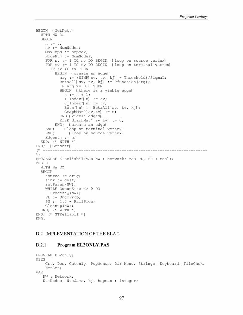
Program Listings
97
BEGIN {GetNett} WITH NW DO BEGIN n := 0; nv := NumNodes; MaxHops := hopmax; NodeNum := NumNodes; FOR sv := 1 TO nv DO BEGIN {loop on source vertex} FOR tv := 1 TO nv DO BEGIN {loop on terminal vertex} IF sv <> tv THEN BEGIN {create an edge} arg := (SINR[sv, tv, kj] - Threshold)/SigmaL; BetaAll[sv, tv, kj] := Pfunction(arg); IF arg >= 0.0 THEN BEGIN {there is a viable edge} n := n + 1; I_Index^[n] := sv; J_Index^[n] := tv; Beta^[n] := BetaAll[sv, tv, kj]; GraphMat^[sv,tv] := n; END {Viable edges} ELSE GraphMat^[sv,tv] := 0; END; {create an edge} END; {loop on terminal vertex} END; {loop on source vertex} Edgenum := n; END; (* WITH *)END; {GetNett}(* ---------------------------------------------------------------------*)PROCEDURE ELReliabil(VAR NW : Network; VAR PL, PU : real);BEGIN WITH NW DO BEGIN source := orig; sink := dest; SetParam(NW); WHILE QueueSize <> 0 DO ProcessQ(NW); PL := SuccProb; PU := 1.0 - FailProb; Cleanup(NW); END; (* WITH *)END; (* STReliabil *)END.
D.2 IMPLEMENTATION OF THE ELA 2
D.2.1 Program EL2ONLY.PAS
PROGRAM EL2only;USES Crt, Dos, Cutonly, PopMenus, Dir_Menu, Strings, Keyboard, FileChck, NetSet;VAR NW : Network; NumNodes, NumJams, kj, hopmax : integer;
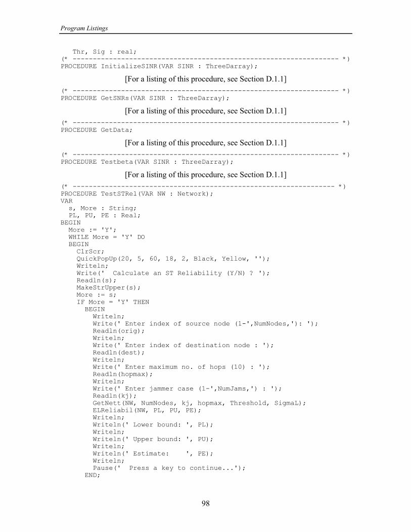
Program Listings
98
Thr, Sig : real;(* ------------------------------------------------------------------ *)PROCEDURE InitializeSINR(VAR SINR : ThreeDarray);
[For a listing of this procedure, see Section D.1.1](* ------------------------------------------------------------------ *)PROCEDURE GetSNRs(VAR SINR : ThreeDarray);
[For a listing of this procedure, see Section D.1.1](* ------------------------------------------------------------------ *)PROCEDURE GetData;
[For a listing of this procedure, see Section D.1.1](* ------------------------------------------------------------------ *)PROCEDURE Testbeta(VAR SINR : ThreeDarray);
[For a listing of this procedure, see Section D.1.1](* ----------------------------------------------------------------- *)PROCEDURE TestSTRel(VAR NW : Network);VAR s, More : String; PL, PU, PE : Real;BEGIN More := 'Y'; WHILE More = 'Y' DO BEGIN ClrScr; QuickPopUp(20, 5, 60, 18, 2, Black, Yellow, ''); Writeln; Write(' Calculate an ST Reliability (Y/N) ? '); Readln(s); MakeStrUpper(s); More := s; IF More = 'Y' THEN BEGIN Writeln; Write(' Enter index of source node (1-',NumNodes,'): '); Readln(orig); Writeln; Write(' Enter index of destination node : '); Readln(dest); Writeln; Write(' Enter maximum no. of hops (10) : '); Readln(hopmax); Writeln; Write(' Enter jammer case (1-',NumJams,') : '); Readln(kj); GetNett(NW, NumNodes, kj, hopmax, Threshold, SigmaL); ELReliabil(NW, PL, PU, PE); Writeln; Writeln(' Lower bound: ', PL); Writeln; Writeln(' Upper bound: ', PU); Writeln; Writeln(' Estimate: ', PE); Writeln; Pause(' Press a key to continue...'); END;
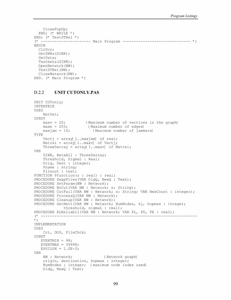
Program Listings
99
ClosePopUp; END; (* WHILE *)END; (* TestSTRel *)(* ---------------------- Main Program ------------------------------ *)BEGIN ClrScr; GetSNRs(SINR); GetData; Testbeta(SINR); OpenNetwork(NW); TestSTRel(NW); CloseNetwork(NW);END. (* Main Program *)
D.2.2 UNIT CUTONLY.PAS
UNIT CUTonly;INTERFACEUSES NetSet;CONST maxv = 20; {Maximum number of vertices in the graph} maxe = 255; {Maximum number of edges} maxjam = 10; {Maximum number of jammers}TYPE Vectj = array[1..maxjam] of real; Matrxi = array[1..maxv] of Vectj; ThreeDarray = array[1..maxv] of Matrxi;VAR SINR, BetaAll : ThreeDarray; Threshold, SigmaL : Real; Orig, Dest : integer; Fname : string; Fileout : text;FUNCTION Pfunction(z : real) : real;PROCEDURE SwapFiles(VAR OldQ, NewQ : Text);PROCEDURE SetParam(NW : Network);PROCEDURE NoCut(VAR NW : Network; s: String);PROCEDURE CutFail(VAR NW : Network; s: String; VAR NewCount : integer);PROCEDURE ProcessQ(VAR NW : Network);PROCEDURE Cleanup(VAR NW : Network);PROCEDURE GetNett(VAR NW : Network; NumNodes, kj, hopmax : integer; threshold, sigmaL : real);PROCEDURE ELReliabil(VAR NW : Network; VAR PL, PU, PE : real);(* ---------------------------------------------------------------------*)IMPLEMENTATIONUSES Crt, DOS, FileChck;CONST EVENTMIN = 98; EVENTMAX = 39998; EPSILON = 1.0E-2;VAR NW : Network; {Network graph} origin, destination, hopmax : integer; NumNodes : integer; {maximum node index used} OldQ, NewQ : Text;
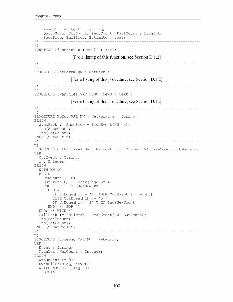
Program Listings
100
ReadStr, WriteStr : string; QueueSize, TotCount, SuccCount, FailCount : LongInt; SuccProb, FailProb, Estimate : real;(* ---------------------------------------------------------------------*)FUNCTION Pfunction(z : real) : real;
[For a listing of this function, see Section D.1.2](* ---------------------------------------------------------------------*)PROCEDURE SetParam(NW : Network);
[For a listing of this procedure, see Section D.1.2](* ---------------------------------------------------------------------*)PROCEDURE SwapFiles(VAR OldQ, NewQ : Text);
[For a listing of this procedure, see Section D.1.2](* ---------------------------------------------------------------------*)PROCEDURE NoCut(VAR NW : Network; s : String);BEGIN SuccProb := SuccProb + ProbEvent(NW, s); Inc(SuccCount); Inc(TotCount);END; (* NoCut *)(* ---------------------------------------------------------------------*)PROCEDURE CutFail(VAR NW : Network; s : String; VAR NewCount : Integer);VAR CutEvent : String; i : Integer;BEGIN WITH NW DO BEGIN NewCount := 0; CutEvent[0] := Char(EdgeNum); FOR i := 1 TO EdgeNum DO BEGIN IF UpEdges[i] = '1' THEN CutEvent[i] := s[i] ELSE CutEvent[i] := '0'; IF UpEdges[i]<>'1' THEN Inc(NewCount); END; (* FOR *) END; (* WITH *) FailProb := FailProb + ProbEvent(NW, CutEvent); Inc(FailCount); Inc(TotCount);END; (* CutFail *)(* ---------------------------------------------------------------------*)PROCEDURE ProcessQ(VAR NW : Network);VAR Event : String; PathLen, NewCount : Integer;BEGIN QueueSize := 0; SwapFiles(OldQ, NewQ); WHILE NOT EOF(OldQ) DO BEGIN
Program Listings
101
ReadEvent(OldQ, Event); SetEventLinks(NW, Event); IF CutSetSearch(NW, Event) THEN BEGIN (* Cut Set found *) CutFail(NW, Event, NewCount); AddEvents(NewQ, NW, Event, NewCount); Inc(QueueSize, NewCount); { Estimate := 0.5*(1.0 + SuccProb - FailProb); Writeln(fileout, totcount:5,succprob:9:6, (1.0-failprob):9:6, estimate:9:6);} END (* Cut Set found *) ELSE NoCut(NW, Event); RestoreEventLinks(NW); IF TotCount > EVENTMAX THEN Exit; IF ((1.0 - (SuccProb + FailProb)) < EPSILON) AND (succcount + failcount > EVENTMIN) THEN Exit; END; (* WHILE *)END; (* ProcessQ *)(* ---------------------------------------------------------------------*)PROCEDURE Cleanup(VAR NW : Network);
[For a listing of this procedure, see Section D.1.2](* ---------------------------------------------------------------------*)PROCEDURE GetNett(VAR NW : Network; NumNodes, kj, hopmax : integer; Threshold, SigmaL : real);
[For a listing of this procedure, see Section D.1.2](* ---------------------------------------------------------------------*)PROCEDURE ELReliabil(VAR NW : Network; VAR PL, PU, PE : real);BEGIN WITH NW DO BEGIN source := orig; sink := dest; SetParam(NW); WHILE (QueueSize <> 0) DO ProcessQ(NW); PL := SuccProb; PU := 1.0 - FailProb; PE := 0.5*(PL + PU); Cleanup(NW); END; (* WITH *)END; (* ELReliabil *)END.
D.3 IMPLEMENTATION OF COMBINED ELA AND ELA2
D.3.1 Program EL1&2.PAS
PROGRAM EL1and2;USES
Program Listings
102
Crt, Dos, CutSet, PopMenus, Dir_Menu, Strings, Keyboard, FileChck, NetSet;VAR NW : Network; NumNodes, NumJams, kj, hopmax : integer; Thr, Sig : real;(* ------------------------------------------------------------------ *)PROCEDURE InitializeSINR(VAR SINR : ThreeDarray);
[For a listing of this procedure, see Section D.1.1](* ------------------------------------------------------------------ *)PROCEDURE GetSNRs(VAR SINR : ThreeDarray);
[For a listing of this procedure, see Section D.1.1](* ------------------------------------------------------------------ *)PROCEDURE GetData;
[For a listing of this procedure, see Section D.1.1](* ------------------------------------------------------------------ *)PROCEDURE Testbeta(VAR SINR : ThreeDarray);
[For a listing of this procedure, see Section D.1.1](* ----------------------------------------------------------------- *)PROCEDURE TestSTRel(VAR NW : Network);
[For a listing of this procedure, see Section D.2.1](* ---------------------- Main Program ------------------------------ *)BEGIN ClrScr; GetSNRs(SINR); GetData; Testbeta(SINR); OpenNetwork(NW); TestSTRel(NW); CloseNetwork(NW);END. (* Main Program *)
D.3.2 Unit CUTSET.PAS
UNIT CUTSET;INTERFACEUSES NetSet;CONST maxv = 35; {Maximum number of vertices in the graph} maxe = 127; {Maximum number of edges} maxjam = 4; {Maximum number of jammers}TYPE Vectj = array[1..maxjam] of real; Matrxi = array[1..maxv] of Vectj; ThreeDarray = array[1..maxv] of Matrxi;VAR SINR, BetaAll : ThreeDarray; Threshold, SigmaL : Real; Orig, Dest : integer; Fname : string;
Program Listings
103
Fileout : text;FUNCTION Pfunction(z : real) : real;PROCEDURE SwapFiles(VAR OldQ, NewQ, OldQC, NewQC : Text);PROCEDURE SetParam(NW : Network);PROCEDURE Success(VAR NW : Network; s : String; VAR NewCount : integer);PROCEDURE Failure(VAR NW : Network; s : String);PROCEDURE NoCut(VAR NW : Network; s: String);PROCEDURE CutFail(VAR NW : Network; s: String; VAR NewCount : integer);PROCEDURE ProcessQ(VAR NW : Network);PROCEDURE Cleanup(VAR NW : Network);PROCEDURE GetNett(VAR NW : Network; NumNodes, kj, hopmax : integer; threshold, sigmaL : real);PROCEDURE ELReliabil(VAR NW : Network; VAR PL, PU, PE : real);(* ---------------------------------------------------------------------*)IMPLEMENTATIONUSES Crt, DOS, FileChck;CONST EVENTMIN = 98; EVENTMAX = 39998; EPSILON = 1.0E-2;VAR NW : Network; {Network graph} origin, destination, hopmax : integer; NumNodes : integer; {maximum node index used} OldQ, NewQ, OldQC, NewQC : Text; ReadStr, WriteStr, ReadStrC, WriteStrC : string; OQS, QueueSize, TotCount, SuccCount, FailCount : LongInt; OQSC, QSizeC, TotCCount, SuccCCount, FailCCount : LongInt; SuccProb, FailProb, SuccPrC, FailPrC, Estimate : real; Exitflag : Boolean;(* ---------------------------------------------------------------------*)FUNCTION Pfunction(z : real) : real;
[For a listing of this function, see Section D.1.2](* ---------------------------------------------------------------------*)PROCEDURE SetParam(NW : Network);VAR Event : string; Happen : boolean;BEGIN TotCount := 0; TotCCount := 0; SuccCount := 0; SuccCCount := 0; FailCount := 0; FailCCount := 0; QueueSize := 1; QSizeC := 1; SuccProb := 0.0; SuccPrC := 0.0; FailProb := 0.0; FailPrC := 0.0; ReadStr := 'DATA2.TMP'; ReadStrC := 'DATA4.TMP'; WriteStr := 'DATA1.TMP';
Program Listings
104
WriteStrC := 'DATA3.TMP'; happen := CheckNewFile(NewQ, WriteStr); happen := CheckNewFile(NewQC, WriteStrC); happen := CheckNewFile(OldQ, ReadStr); happen := CheckNewFile(OldQC, ReadStrC); WITH NW DO BEGIN InitialEvent(Event, '1', EdgeNum); SaveEvent(NewQ, NW, Event); SaveEvent(NewQC, NW, Event); SwapFiles(OldQ, NewQ, OldQC, NewQC); SaveEvent(NewQ, NW, Event); SaveEvent(NewQC, NW, Event); END; (* WITH *)END; (* SetParam *)(* ---------------------------------------------------------------------*)PROCEDURE SwapFiles(VAR OldQ, NewQ, OldQC, NewQC : Text);VAR s : string; happen : boolean;BEGIN Close(NewQ); Close(NewQC); Close(OldQ); Close(OldQC); s := ReadStr; ReadStr := WriteStr; WriteStr := s; s := ReadStrC; ReadStrC := WriteStrC; WriteStrC := s; happen := CheckOldFile(OldQ, ReadStr); happen := CheckOldFile(OldQC, ReadStrC); happen := CheckNewFile(NewQ, WriteStr); happen := CheckNewFile(NewQC, WriteStrC);END; (* SwapFiles *)(* ---------------------------------------------------------------------*)PROCEDURE Success(VAR NW : Network; s : string; VAR NewCount : integer);
[For a listing of this procedure, see Section D.1.2](* ---------------------------------------------------------------------*)PROCEDURE NoCut(VAR NW : Network; s : String);
[For a listing of this procedure, see Section D.2.2](* ---------------------------------------------------------------------*)PROCEDURE Failure(VAR NW : Network; s: string);
[For a listing of this procedure, see Section D.1.2](* ---------------------------------------------------------------------*)PROCEDURE CutFail(VAR NW : Network; s : String; VAR NewCount : Integer);
[For a listing of this procedure, see Section D.2.2]
Program Listings
105
(* ---------------------------------------------------------------------*)PROCEDURE ProcessQ(VAR NW : Network);VAR Event : String; PathLen, NewCount : Integer;BEGIN OQS := QueueSize; OQSC := QSizeC; Exitflag := FALSE; QueueSize := 0; SwapFiles(OldQ, NewQ, OldQC, NewQC); WHILE NOT EOF(OldQ) DO BEGIN ReadEvent(OldQ, Event); SetEventLinks(NW, Event); IF TwoWaySearch(NW, PathLen) THEN BEGIN (* Path found *) Success(NW, Event, NewCount); ComplementEvent(NewQ, NW, Event, NewCount); Inc(QueueSize, NewCount); END; (* Path found *) RestoreEventLinks(NW); Estimate := 0.5*(1.0 + SuccProb - FailPrC); IF TotCount > EVENTMAX THEN Exit; IF ((1.0 - (SuccProb + FailPrC)) < EPSILON) AND (succcount+failccount>eventmin) THEN BEGIN Exitflag := TRUE; Exit; END; END; (* OldQ *) IF (QueueSize = 0) THEN Exit; QSizeC := 0; WHILE NOT EOF(OldQC) DO BEGIN ReadEvent(OldQC, Event); SetEventLinks(NW, Event); IF CutSetSearch(NW, Event) THEN BEGIN (* Cut Set found *) CutFail(NW, Event, NewCount); AddEvents(NewQC, NW, Event, NewCount); Inc(QSizeC, NewCount); END; (* Cut Set found *) RestoreEventLinks(NW); IF TotCCount > EVENTMAX THEN Exit; IF ((1.0 - (SuccProb + FailPrC)) < EPSILON) AND (succcount+failccount>eventmin) THEN BEGIN Exitflag := TRUE; Exit; END; END; (* OldQC *)END; (* ProcessQ *)(* ---------------------------------------------------------------------*)PROCEDURE Cleanup(VAR NW : Network);BEGIN Close(NewQ); Close(OldQ);
Program Listings
106
Erase(NewQ); Erase(OldQ); Close(NewQC); Close(OldQC); Erase(NewQC); Erase(OldQC);END; (* Cleanup *)(* ---------------------------------------------------------------------*)
PROCEDURE GetNett(VAR NW : Network; NumNodes, kj, hopmax : integer; Threshold, SigmaL : real);
[For a listing of this procedure, see Section D.1.2](* ---------------------------------------------------------------------*)PROCEDURE ELReliabil(VAR NW : Network; VAR PL, PU, PE : real);BEGIN WITH NW DO BEGIN source := orig; sink := dest; SetParam(NW); WHILE (QueueSize <> 0) AND (QSizeC <> 0) DO ProcessQ(NW); PL := SuccProb; PU := 1.0 - FailPrC; PE := 0.5*(PL + PU); IF (QueueSize = 0) AND NOT Exitflag THEN PE := PL ELSE IF (QSize = 0) AND NOT Exitflag THEN PE := PU; Cleanup(NW); END; (* WITH *)END; (* ELReliabil *)END.
D.4 IMPLEMENTATION OF ALGORITHM SELECTION
D.4.1 Program ELCUTPAT.PAS
PROGRAM ELCutPat;USES Crt, Dos, CutPath, PopMenus, Dir_Menu, Strings, Keyboard, FileChck, NetSet;VAR NW : Network; NumNodes, NumJams, kj, hopmax : integer; Thr, Sig : real;(* ------------------------------------------------------------------ *)PROCEDURE InitializeSINR(VAR SINR : ThreeDarray);
[For a listing of this procedure, see Section D.1.1](* ------------------------------------------------------------------ *)PROCEDURE GetSNRs(VAR SINR : ThreeDarray);
[For a listing of this procedure, see Section D.1.1](* ------------------------------------------------------------------ *)
Program Listings
107
PROCEDURE GetData;
[For a listing of this procedure, see Section D.1.1](* ------------------------------------------------------------------ *)PROCEDURE Testbeta(VAR SINR : ThreeDarray);
[For a listing of this procedure, see Section D.1.1](* ----------------------------------------------------------------- *)PROCEDURE TestSTRel(VAR NW : Network);
[For a listing of this procedure, see Section D.2.1](* ---------------------- Main Program ------------------------------ *)BEGIN ClrScr; GetSNRs(SINR); GetData; Testbeta(SINR); OpenNetwork(NW); TestSTRel(NW); CloseNetwork(NW);END. (* Main Program *)
D.4.2 Unit CUTPATH.PAS
UNIT CUTPATH;INTERFACEUSES NetSet;CONST maxv = 20; {Maximum number of vertices in the graph} maxe = 135; {Maximum number of edges} maxjam = 10; {Maximum number of jammers}TYPE Vectj = array[1..maxjam] of real; Matrxi = array[1..maxv] of Vectj; ThreeDarray = array[1..maxv] of Matrxi;VAR SINR, BetaAll : ThreeDarray; Threshold, SigmaL : Real; Orig, Dest : integer; Fname : string; Fileout : text;FUNCTION Pfunction(z : real) : real;PROCEDURE SwapFiles(VAR OldQ, NewQ : Text);PROCEDURE SetParam(NW : Network);PROCEDURE Success(VAR NW : Network; s : String; VAR NewCount : integer);PROCEDURE Failure(VAR NW : Network; s : String);PROCEDURE NoCut(VAR NW : Network; s: String);PROCEDURE CutFail(VAR NW : Network; s: String; VAR NewCount : integer);PROCEDURE ProcessQ(VAR NW : Network);PROCEDURE Cleanup(VAR NW : Network);PROCEDURE GetNett(VAR NW : Network; NumNodes, kj, hopmax : integer; threshold, sigmaL : real);PROCEDURE ELReliabil(VAR NW : Network; VAR PL, PU, PE : real);(* ---------------------------------------------------------------------*)IMPLEMENTATION
Program Listings
108
USES Crt, DOS, FileChck;CONST EVENTMIN = 98; EVENTMAX = 39998; EPSILON = 1.0E-2;VAR NW : Network; {Network graph} origin, destination, hopmax : integer; NumNodes : integer; {maximum node index used} OldQ, NewQ : Text; ReadStr, WriteStr : string; QueueSize, TotCount, SuccCount, FailCount : LongInt; SuccProb, FailProb, Estimate : real;(* ---------------------------------------------------------------------*)FUNCTION Pfunction(z : real) : real;
[For a listing of this function, see Section D.1.2](* ---------------------------------------------------------------------*)PROCEDURE SetParam(NW : Network);
[For a listing of this procedure, see Section D.1.2](* ---------------------------------------------------------------------*)PROCEDURE SwapFiles(VAR OldQ, NewQ : Text);
[For a listing of this procedure, see Section D.1.2](* ---------------------------------------------------------------------*)PROCEDURE Success(VAR NW : Network; s : string; VAR NewCount : integer);
[For a listing of this procedure, see Section D.1.2](* ---------------------------------------------------------------------*)PROCEDURE GetNew(VAR NW : Network; s : string; VAR NewCount : integer);VAR i : integer;BEGIN WITH NW DO BEGIN NewCount := 0; FOR i := 1 TO EdgeNum DO IF (s[i] = '1') AND (UpEdges[i] <> '1') THEN Inc(NewCount); END; (* WITH *)END; (* GetNew *)(* ---------------------------------------------------------------------*)PROCEDURE NoCut(VAR NW : Network; s : String);
[For a listing of this procedure, see Section D.2.2](* ---------------------------------------------------------------------*)PROCEDURE Failure(VAR NW : Network; s: string);
[For a listing of this procedure, see Section D.1.2]
Program Listings
109
(* ---------------------------------------------------------------------*)PROCEDURE CutFail(VAR NW : Network; s : String; VAR NewCount : Integer);
[For a listing of this procedure, see Section D.2.2](* ---------------------------------------------------------------------*)PROCEDURE ProcessQ(VAR NW : Network);VAR Event, EdgesUp : String; PathLen, NewCount, CutCount : Integer; ListPath : EdgeList; happen : Boolean; i : integer;LABEL DONE;BEGIN QueueSize := 0; SwapFiles(OldQ, NewQ); WHILE NOT EOF(OldQ) DO BEGIN ReadEvent(OldQ, Event); SetEventLinks(NW, Event); IF NOT TwoWaySearch(NW, PathLen) THEN BEGIN (* Definite failure *) Failure(NW, Event); GOTO DONE; END; (* Definite failure *) GetNew(NW, Event, NewCount); IF (NewCount < 2) THEN BEGIN (* Definite success or short addition *) Success(NW, Event, NewCount); IF (NewCount > 0) THEN ComplementEvent(NewQ, NW, Event, NewCount); Inc(QueueSize, NewCount); GOTO DONE; END; (* Definite success or short addition *) EdgesUp := NW.UpEdges; FOR i := 1 TO NW.EdgeNum DO ListPath[i] := NW.PathList^[i]; happen := CutSetSearch(NW, Event); GetNew(NW, Event, CutCount); IF (CutCount < NewCount) THEN BEGIN (* Cutset preferred *) CutFail(NW, Event, CutCount); AddEvents(NewQ, NW, Event, CutCount); Inc(QueueSize, CutCount); END (* Cutset preferred *) ELSE BEGIN (* Path preferred *) NW.UpEdges := EdgesUp; FOR i := 1 TO NW.EdgeNum DO NW.PathList^[i] := ListPath[i]; Success(NW, Event, NewCount); ComplementEvent(NewQ, NW, Event, NewCount); Inc(QueueSize, NewCount); END; (* Path preferred *)DONE: RestoreEventLinks(NW);
Program Listings
110
Estimate := 0.5*(1.0 + SuccProb - FailProb); IF TotCount > EVENTMAX THEN Exit; IF ((1.0 - (SuccProb + FailProb)) < EPSILON) AND (TotCount > EVENTMIN) THEN Exit; END; (* WHILE *)END; (* ProcessQ *)(* ---------------------------------------------------------------------*)PROCEDURE Cleanup(VAR NW : Network);
[For a listing of this procedure, see Section D.1.2](* --------------------------------------------------------------------- *)PROCEDURE GetNett(VAR NW : Network; NumNodes, kj, hopmax : integer; Threshold, SigmaL : real);
[For a listing of this procedure, see Section D.1.2](* ---------------------------------------------------------------------*)PROCEDURE ELReliabil(VAR NW : Network; VAR PL, PU, PE : real);
[For a listing of this procedure, see Section D.2.2]END.
D.5 UNIT NETSET.PAS
Note that many of the procedures and functions in this unit are not used by the programsstudied in this report.
UNIT NETSET;(* Dotson unit NETSET.PAS (includes cutsets w/o path search) This unit defines the structure of a network in terms of the adjacency matrix and its edge probability vector. In addition, various edge vectors and also a path string are included in the structure, principally to facilitate the operation of Dotson's algorithm. Other elements are the number of vertices and edges as well as the source and sink nodes, and the hop maximum. Two path search routines are provided, a forward only and a two-way search procedure. The data file formats used are implicit here, as described in an earlier memorandum. EdgeFile - Input: description of network configuration EventFile - Output: collection of success/failure events NewQueue, OldQueue - Temporary: files for event storage The calling programs must control file management for this data. *)INTERFACECONST OK = 0; NODEMAX = 40; EDGEMAX = 255; FORMAT_ERROR = 1; DATA_ERROR = 2; INDEX_ERROR = 3;TYPE NodeList = ARRAY [1..NODEMAX] OF Byte; NodeVect = ARRAY [1..NODEMAX] OF Real; NodeMat = Array [1..NODEMAX] OF NodeVect; EdgeList = ARRAY [1..EDGEMAX] OF Byte; EdgeVect = ARRAY [1..EDGEMAX] OF Real; EdgeMat = Array [1..NODEMAX] OF EdgeVect;

Program Listings
111
AdjcMat = ARRAY [1..NODEMAX] OF NodeList; PathMat = ARRAY [0..NODEMAX + 1] OF NodeList; NodeListPtr = ^NodeList; NodeVectPtr = ^NodeVect; NodeMatPtr = ^NodeMat; EdgeListPtr = ^EdgeList; EdgeVectPtr = ^EdgeVect; EdgeMatPtr = ^EdgeMat; AdjcMatPtr = ^AdjcMat; LinkSet = SET OF 1..EdgeMax; NodeSet = SET OF 1..NodeMax; Network = RECORD Source : Integer; Sink : Integer; NodeNum : Integer; EdgeNum : Integer; MaxHops : Integer; GraphMat : AdjcMatPtr; Beta : EdgeVectPtr; Alpha : NodeVectPtr; PathList : EdgeListPtr; I_Index : EdgeListPtr; J_Index : EdgeListPtr; UpEdges : String; EdgeStr : String; EdgeFile : Text; END; (* Network - basic network structure for Dotson method *)TYPE NodeData = RECORD EdgeMat : AdjcMatPtr; EdgesOn : EdgeListPtr; EdgesOff : EdgeListPtr; Gamma : EdgeVectPtr; MaxDegree : Integer; NumOn : Integer; NumOff : Integer; END; (* NodeData - node structure for equivalent links method *)(*----------------------------------------------------------------------------- PUBLIC FUNCTIONS AND PROCEDURES -----------------------------------------------------------------------------------------------*)PROCEDURE OpenNetwork(VAR NW : Network);PROCEDURE CloseNetwork(VAR NW : Network);PROCEDURE SetNetworkNodes(VAR NW : Network);PROCEDURE RestoreEventLinks(VAR NW : Network);FUNCTION ReadEdgeFile(VAR NW : Network) : Integer;FUNCTION ProbEvent(VAR NW : Network; Event : String) : Real;PROCEDURE SetEventLinks(VAR NW : Network; Event : String);PROCEDURE ReadEvent(VAR OldQueue : Text; VAR Event : String);PROCEDURE InitialEvent(VAR Event : String; Value : Char; n : Integer);PROCEDURE SaveEvent(VAR NewQueue : Text; VAR NW : Network; Event : String);FUNCTION OneWaySearch(VAR NW : Network; VAR PathLen : Integer) : Boolean;FUNCTION TwoWaySearch(VAR NW : Network;
Program Listings
112
VAR PathLen : Integer) : Boolean;PROCEDURE ComplementEvent(VAR NewQueue : Text; VAR NW : Network; Event : String; Count : Integer);FUNCTION SuccessEvent(VAR EventFile : Text; VAR NW : Network; Event : String; VAR NewCount : Integer; Flag : Integer) : Real;FUNCTION FailureEvent(VAR EventFile : Text; VAR NW : Network; Event : String; Flag : Integer) : Real;FUNCTION PathCheck(NW : Network; Event : String) : Boolean;FUNCTION CutSetSearch(VAR NW : Network; Event : String) : Boolean;PROCEDURE AddEvents(VAR NewQC : Text; VAR NW : Network; Event : String; NewCount : Integer);PROCEDURE CloseNodeData(VAR ND : NodeData);PROCEDURE OpenNodeData(VAR NW : Network; VAR ND : NodeData);FUNCTION BackFitNodes(VAR NW : Network; VAR ND : NodeData; Event : String) : Real;PROCEDURE EdgeFileError(s : String);PROCEDURE EventFileError(s : String);PROCEDURE AlphaFileError(s : String);PROCEDURE DataIndexError(s0, s1 : String);PROCEDURE DataConflictError(VAR NW : Network; s : String; m, n : Integer);(*-------------------------------------------------------------------*)IMPLEMENTATIONUSES Crt, Keyboard, Strings, TextScrn, PopMenus;(*----------------------------------------------------------------------------- FUNCTIONS AND PROCEDURES PRIVATE TO THIS UNIT ---------------------------------------------------------------------------------PROCEDURE SetAdjacencyMat(MatPtr : AdjcMatPtr);FUNCTION CheckEdgeFileData(NW : Network) : Boolean;PROCEDURE SetLinkMat(VAR NW : Network; VAR pm : PathMat);PROCEDURE SetNodeList(VAR nl : NodeList; Value : Byte);PROCEDURE SetEdgeList(VAR ElPtr : EdgeListPtr; Value : Byte);PROCEDURE SetEdgeVect(ProbPtr : EdgeVectPtr; Value : Real);PROCEDURE SetNodeVect(ProbPtr : NodeVectPtr; Value : Real);PROCEDURE WriteEvent(VAR EventFile : Text; NW : Network; Event : String; Flag : Integer);FUNCTION OneWayPath(VAR NW : Network; VAR pm : PathMat; VAR PathLen : Integer) : Boolean;FUNCTION ForwardSearch(VAR NW : Network; VAR pm : PathMat; VAR kf : Integer
Program Listings
113
VAR FCount: Integer) : Boolean;FUNCTION BackwardSearch(VAR NW : Network; VAR pm : PathMat; VAR kr : Integer VAR BCount: Integer) : Boolean;FUNCTION TwoWayPath(VAR NW : Network; VAR pm : PathMat; VAR pl, rn, kf, kr : Integer) : Boolean;PROCEDURE SetWorkingEdges( Event : String; VAR ND : NodeData);FUNCTION BackFitProb( Up : EdgeList; Down : EdgeList; VAR ND : NodeData; Prob : Real) : Real;---------------------------------------------------------------------*)
(*-------------------------------------------------------------------*)PROCEDURE OpenNetwork(VAR NW : Network);(* Set up network pointers on the heap - no initialization *)BEGIN WITH NW DO BEGIN New(GraphMat); New(I_Index); New(J_Index); New(PathList); New(Alpha); New(Beta); END; (* WITH *)END; (* OpenNetwork *)(*---------------------------------------------------------------------*)PROCEDURE CloseNetwork(VAR NW : Network);(* Restore network pointers to the pre-network heap status *)BEGIN WITH NW DO BEGIN Dispose(Beta); Dispose(Alpha); Dispose(PathList); Dispose(J_Index); Dispose(I_Index); Dispose(GraphMat); END; (* WITH *)END; (* CloseNetwork *)(*---------------------------------------------------------------------*)PROCEDURE SaveEvent(VAR NewQueue: Text; VAR NW : Network; Event : String);(* Save the edge event to the temporary file - i.e., to the next queue*)BEGIN Event[0] := Chr(NW.EdgeNum); Writeln(NewQueue, Event);END; (* SaveEvent *)(*----------------------------------------------------------------------*)PROCEDURE ReadEvent(VAR OldQueue : Text; VAR Event : String);
Program Listings
114
(* Read an edge event from the temporary file - i.e., the current queue*)BEGIN Readln(OldQueue, Event); DropLeadingBlanks(Event);END; (* ReadEvent *)(*---------------------------------------------------------------------*)PROCEDURE WriteEvent(VAR EventFile : Text; NW : Network; Event : String; Flag : Integer);(* Write success or failure edge event with the associated integer flag*)BEGIN Event[0] := Chr(NW.EdgeNum); Write(EventFile, Flag : 3, ' '); Writeln(EventFile, Event);END; (* WriteEvent *)(*---------------------------------------------------------------------*)FUNCTION CheckEdgeFileData(NW : Network) : Boolean;(* Check EdgeFile data against maximum allowable size - show any error*)BEGIN CheckEdgeFileData := TRUE; IF (NW.NodeNum > NODEMAX) OR (NW.EdgeNum > EDGEMAX) THEN BEGIN CursorOff; CheckEdgeFileData := FALSE; QuickPopUp(10, 4, 70, 9, 2, Yellow, Red, ''); Writeln(' ERROR'); Writeln(Bell); IF NW.NodeNum > NODEMAX THEN Writeln(' Maximum number of nodes (', NODEMAX, ')exceeded'); IF NW.EdgeNum > EDGEMAX THEN Writeln(' Maximum number of edges (', EDGEMAX, ')exceeded'); Writeln; Pause(' Press any key to continue... '); ClosePopUp; CursorOn; Exit; END;END; (* CheckEdgeFileData *)(*-------------------------------------------------------------------*)PROCEDURE SetEdgeList(VAR ElPtr : EdgeListPtr; Value : Byte);(* Initialize an EdgeListPtr - all of its entries set to given value *)VAR i : Integer;BEGIN FOR i := 1 TO EDGEMAX DO ElPtr^[i] := Value;END; (* SetEdgeList *)(*--------------------------------------------------------------------*)PROCEDURE SetNodeList(VAR nl : NodeList; Value : Byte);(* Initialize an NodeList - all of its entries are set to given value *)
Program Listings
115
VAR i : Integer;BEGIN FOR i := 1 TO NODEMAX DO nl[i] := Value;END; (* SetNodeList *)(*---------------------------------------------------------------------*)PROCEDURE SetAdjacencyMat(MatPtr : AdjcMatPtr);(* Initialize network adjacency matrix - all its entries equal to zero*)VAR i : Integer;BEGIN FOR i := 1 TO NODEMAX DO SetNodeList(MatPtr^[i], 0);END; (* SetAdjacencyMat *)(*---------------------------------------------------------------------*)PROCEDURE SetEdgeVect(ProbPtr : EdgeVectPtr; Value : Real);(* Initialize edge vector - set all edge probabilities to given value *)VAR i : Integer;BEGIN FOR i := 1 TO EDGEMAX DO ProbPtr^[i] := Value;END; (* SetEdgeVect *)(*---------------------------------------------------------------------*)PROCEDURE SetNodeVect(ProbPtr : NodeVectPtr; Value : Real);(* Initialize node vector - set all node probabilities to given value *)VAR i : Integer;BEGIN FOR i := 1 TO NODEMAX DO ProbPtr^[i] := Value;END; (* SetNodeVect *)(*---------------------------------------------------------------------*)FUNCTION ProbEvent(VAR NW : Network; Event : String) : Real;(* Use edge probabilities, return probability of the edge string event*)VAR Prob : Real; i : Integer;BEGIN WITH NW DO BEGIN Prob := 1.0; FOR i := 1 TO EdgeNum DO BEGIN IF Event[i] = '2' THEN Prob := Prob * Beta^[i] ELSE IF Event[i] = '0' THEN Prob := Prob * (1.0 - Beta^[i]); END; END; (* WITH *)
Program Listings
116
ProbEvent := ProbEND; (* ProbEvent *)(*---------------------------------------------------------------------*)PROCEDURE InitialEvent(VAR Event : String; Value : Char; n : Integer);(* Initialize event string of length n - all entries equal given value*)BEGIN FillChar(Event, Sizeof(String), Value); Event[0] := Chr(n);END; (* InitialEvent *)(*---------------------------------------------------------------------*)PROCEDURE SetNetworkNodes(VAR NW : Network);(* Get source and sink nodes and hop number for network from keyboard *)VAR i : Integer;BEGIN WITH NW DO BEGIN Writeln(' ', EdgeStr); Writeln(' Make Node Selections: '); Write(' Source Node ? ________ '); IF(0 = StringToInt(PosIntegerInp(''), i)) THEN Source := i ELSE Source := 1; IF (Source < 1) OR (Source > NodeNum) THEN Source := 1; Writeln; Write(' Terminal Node ? ______ '); IF (0 = StringToInt(PosIntegerInp(''), i)) THEN Sink := i ELSE Sink := NodeNum; IF (Sink < 1) OR (Sink > NodeNum) THEN Sink := NodeNum; Writeln; Write(' Hop Maximum ? ________ '); IF (0 = StringToInt(PosIntegerInp(''), i)) THEN MaxHops := i ELSE MaxHops := NodeNum - 1; Writeln; IF (MaxHops < 1) OR (MaxHops >= NodeNum) THEN MaxHops := NodeNum - 1; IF Source = Sink THEN BEGIN CursorOff; QuickPopUp(20, 16, 70, 17, 2, Yellow, Red, ' NOTE - Source and sink are not distinct '); Writeln(#7); Pause(' Press any key to continue...'); MaxHops := 0; CursorOn; ClosePopUp; END; END; (* WITH *)
Program Listings
117
END; (* SetNetworkNodes *)(*---------------------------------------------------------------------*)PROCEDURE SetEventLinks(VAR NW : Network; Event : String);(* Turn off links according to failed connections in edge string Event*)VAR i : Integer;BEGIN WITH NW DO BEGIN InitialEvent(UpEdges, '1', EdgeNum); SetEdgeList(PathList, 0); FOR i := 1 TO EdgeNum DO IF Event[i] = '0' THEN GraphMat^[I_Index^[i], J_Index^[i]] := 0; FOR i := 1 TO NodeNum DO BEGIN GraphMat^[i, source] := 0; GraphMat^[sink, i] := 0; END; END; (* WITH *)END; (* SetEventLinks *)(*--------------------------------------------------------------------*)PROCEDURE RestoreEventLinks(VAR NW : Network);(* Restore all links for the original adjacency matrix of the network *)VAR k : Integer;BEGIN WITH NW DO BEGIN FOR k := 1 TO EdgeNum DO GraphMat^[I_Index^[k], J_Index^[k]] := k; FOR k := 1 TO NodeNum DO GraphMat^[k,k] := 0; END; (* WITH *)END; (* RestoreEventLinks *)(*--------------------------------------------------------------------*)PROCEDURE ComplementEvent(VAR NewQueue : Text; VAR NW : Network; Event : String; Count : Integer);(* Get complementary edge events and save them to the next queue file *)VAR i, j, k : Integer; CompEvent : String;BEGIN WITH NW DO BEGIN j := 0; FOR k := 1 TO Count DO BEGIN CompEvent := Event; REPEAT Inc(j); UNTIL (Event[PathList^[j]] <> '2'); FOR i := 1 TO j - 1 DO CompEvent[PathList^[i]] := '2'; CompEvent[PathList^[j]] := '0';
Program Listings
118
SaveEvent(NewQueue, NW, CompEvent); END; END; (* WITH *)END; (* ComplementEvent *)(*---------------------------------------------------------------------*)PROCEDURE AddEvents(VAR NewQC : Text; VAR NW : Network; Event : String; NewCount : Integer);VAR j, k : Integer; CompEvent : String;BEGIN WITH NW DO BEGIN FOR k := 1 TO NewCount DO BEGIN CompEvent := Event; CompEvent[PathList^[k]] := '2'; IF k>1 THEN FOR j := 1 TO k-1 DO CompEvent[PathList^[j]] := '0'; SaveEvent(NewQC, NW, CompEvent); END; (* FOR *) END; (* WITH *)END; (* Add Events *)(*---------------------------------------------------------------------*)FUNCTION SuccessEvent(VAR EventFile : Text; VAR NW : Network; Event : String; VAR NewCount : Integer; Flag : Integer) : Real;(* Process the success event and write it to the output event file *)(* This event has positive length - return probability of the event *)VAR SuccEvent : String; i : Integer;BEGIN WITH NW DO BEGIN NewCount := 0; SuccEvent[0] := Char(EdgeNum); FOR i := 1 TO EdgeNum DO BEGIN IF UpEdges[i] = '1' THEN SuccEvent[i] := Event[i] ELSE SuccEvent[i] := UpEdges[i]; IF (Event[i] = '1') AND (UpEdges[i] <> '1') THEN Inc(NewCount); END; END; (* WITH *) WriteEvent(EventFile, NW, SuccEvent, Flag); SuccessEvent := ProbEvent(NW, SuccEvent);END; (* SuccessEvent *)(*---------------------------------------------------------------------*)FUNCTION FailureEvent(VAR EventFile : Text; VAR NW : Network; Event : String;
Program Listings
119
Flag : Integer) : Real;(* Process the failure event and write it to the output event file *)(* This event has negative length - return probability of the event *)BEGIN WriteEvent(EventFile, NW, Event, -Flag); FailureEvent := ProbEvent(NW, Event);END; (* FailureEvent *)(*--------------------------------------------------------------------*)FUNCTION ReadEdgeFile(VAR NW : Network) : Integer;(* Read EdgeFile data and build the adjacency matrix for the network *)LABEL GRAPH_ERROR;VAR t : Real; i, j, k : Integer;BEGIN ReadEdgeFile := OK; WITH NW DO BEGIN {$I-} Readln(EdgeFile, Source, Sink, NodeNum, EdgeNum); {$I+} IF (IOResult <> 0) OR (ExitCode <> 0) THEN GoTo GRAPH_ERROR; IF NOT CheckEdgeFileData(NW) THEN BEGIN ReadEdgeFile := DATA_ERROR; Exit; END; SetAdjacencyMat(GraphMat); FOR k := 1 TO EdgeNum DO BEGIN {$I-} Readln(EdgeFile, i, j, t); {$I+} IF (IOResult <> 0) OR (ExitCode <> 0) THEN GoTo GRAPH_ERROR; I_Index^[k] := i; J_Index^[k] := j; GraphMat^[i,j] := k; Beta^[k] := t; END; END; (* WITH *) Exit; GRAPH_ERROR: ReadEdgeFile := FORMAT_ERROR;END; (* ReadEdgeFile *)(*-----------------------------------------------------------------------*)FUNCTION OneWayPath(VAR NW : Network; VAR pm : PathMat; VAR PathLen : Integer) : Boolean;(* Is there a path from Source to Sink using current adjacency matrix ?*)(* Use forward flood searches to find path - no backward search is used*)VAR i, j, k : Integer; Path, Chk : Boolean;BEGIN WITH NW DO BEGIN SetNodeList(pm[NodeNum+1], 0); Move(pm[NodeNum+1], pm[0], NodeNum*SizeOf(Byte));
Program Listings
120
pm[1] := GraphMat^[Source]; pm[0, Source] := 1; Path := FALSE; OneWayPath := FALSE; FOR k := 1 TO MaxHops DO BEGIN (* Main Loop *) Chk := FALSE; Move(pm[NodeNum+1], pm[k+1], NodeNum*SizeOf(Byte)); FOR i := 1 TO NodeNum DO BEGIN IF pm[k,i] > 0 THEN BEGIN Chk := TRUE; IF i = Sink THEN BEGIN OneWayPath := TRUE; Path := TRUE; PathLen := k; Exit; END; FOR j := 1 TO NodeNum DO IF (GraphMat^[i,j]>0) AND NOT (pm[0,j]> 0) THEN BEGIN pm[k + 1,j] := GraphMat^[i,j]; pm[0,j] := 1; END; END; (* IF *) END; (* i-Loop *) IF Path THEN Exit; IF NOT Chk THEN BEGIN PathLen := k - 1; Exit; END; END; (* k-Loop *) PathLen := k; END; (* WITH *)END; (* OneWayPath *)(*---------------------------------------------------------------------*)FUNCTION OneWaySearch(VAR NW : Network; VAR PathLen : Integer) : Boolean;(* If an st-path is found, set up the path links used and return TRUE*)VAR LinkMat : PathMat; k, Nback , Link : Integer;BEGIN WITH NW DO BEGIN OneWaySearch := FALSE; IF NOT OneWayPath(NW, LinkMat, PathLen) THEN Exit; InitialEvent(UpEdges, '1', EdgeNum); SetEdgeList(PathList, 0); Nback := Sink; FOR k := 1 TO PathLen DO BEGIN Link := LinkMat[PathLen - k + 1, Nback];
Program Listings
121
UpEdges[Link] := '2'; PathList^[PathLen - k + 1] := Link; Nback := I_Index^[Link]; END; OneWaySearch := TRUE; END; (* WITH *)END; (* OneWaySearch *)(*-------------------------------------------------------------------*)PROCEDURE SetLinkMat(VAR NW : Network; VAR pm : PathMat);(* Initialize the link matrix before beginning a two_way path search *)VAR i : Integer;BEGIN WITH NW DO BEGIN FOR i := 0 TO NodeNum + 1 DO SetNodeList(pm[i], 0); pm[0, Source] := 1; pm[NodeNum + 1, Sink] := 1; pm[1] := GraphMat^[Source]; FOR i := 1 TO NodeNum DO pm[NodeNum, i] := GraphMat^[i, Sink]; END; (* WITH *)END; (* SetLinkMat *)(*---------------------------------------------------------------------*)FUNCTION ForwardSearch(VAR NW : Network; VAR pm : PathMat; VAR kf : Integer VAR FCount : Integer) : Boolean;(* Extend the path search one hop forward - i.e., away from the source*)VAR i, j, Count : Integer;BEGIN WITH NW DO BEGIN Count := FCount; FOR i := 1 TO NodeNum DO IF pm[kf,i] > 0 THEN FOR j := 1 TO NodeNum DO IF (GraphMat^[i,j]>0) AND NOT (pm[0,j]>0) THEN BEGIN pm[kf + 1, j] := GraphMat^[i,j]; pm[0, j] := 1; Inc(FCount); END; IF Count <> FCount THEN ForwardSearch := TRUE ELSE ForwardSearch := FALSE; Inc(kf); END; (* WITH *)END; (* ForwardSearch *)(*--------------------------------------------------------------------*)FUNCTION BackwardSearch(VAR NW : Network; VAR pm : PathMat; VAR kr : Integer VAR BCount: Integer) : Boolean;(* Extend the path search one hop backward - i.e., away from the sink *)VAR
Program Listings
122
i, j, Count : Integer;BEGIN WITH NW DO BEGIN Count := BCount; FOR i := 1 TO NodeNum DO IF pm[NodeNum + 1 - kr, i] > 0 THEN FOR j := 1 TO NodeNum DO IF (GraphMat^[j,i]>0) AND NOT (pm[NodeNum+1, j]>0) THEN BEGIN pm[NodeNum - kr, j] := GraphMat^[j,i]; pm[NodeNum + 1, j] := 1; Inc(BCount); END; Inc(kr); IF (Count <> BCount) THEN BackwardSearch := TRUE ELSE BackwardSearch := FALSE; END; (* WITH *)END; (* BackwardSearch *)(*-----------------------------------------------------------------------*)FUNCTION TwoWayPath(VAR NW : Network; VAR pm : PathMat; VAR pl, rn, kf, kr : Integer) : Boolean;(* Is there an st-path using the current network adjacency matrix ? *)(* Use alterating forward and backward flood searches to find path *)VAR j, BCount, FCount : Integer; Toggle, Check : Boolean;BEGIN WITH NW DO BEGIN kf := 1; kr := 1; FCount := 1; BCount := 1; FOR j := 1 TO NodeNum DO BEGIN IF (pm[1,j] > 0) THEN Inc(FCount); IF (pm[NodeNum,j] > 0) THEN Inc(BCount); END; Toggle := FALSE; TwoWayPath := FALSE; Check := FALSE; REPEAT pl := kf + kr; FOR j := 1 TO NodeNum DO BEGIN IF (pm[kf, j] > 0) AND (pm[NodeNum + 1 - kr, j] > 0) THEN BEGIN rn := j; TwoWayPath := TRUE; Exit; END; END; Toggle := NOT Toggle; { alternate forward and backward step } IF Toggle THEN Check := ForwardSearch(NW, pm, kf, FCount) ELSE Check := BackwardSearch(NW, pm, kr, BCount);
Program Listings
123
UNTIL (NOT Check) OR (kf+kr > MaxHops); END; (* WITH *)END; (* TwoWayPath *)(*---------------------------------------------------------------------*)FUNCTION TwoWaySearch(VAR NW : Network; VAR PathLen : Integer) : Boolean;(* If an st-path is found, set up the path links used and return TRUE*)VAR LinkMat : PathMat; Nfor, Nback, Link : Integer; j, k, kf, kr, RowNo : Integer;BEGIN WITH NW DO BEGIN Link := GraphMat^[Source, Sink]; IF Link > 0 THEN BEGIN PathLen := 1; PathList^[1] := Link; UpEdges[Link] := '2'; TwoWaySearch := TRUE; Exit; END; TwoWaySearch := FALSE; SetLinkMat(NW, LinkMat); IF NOT TwoWayPath(NW, LinkMat, PathLen, RowNo, kf, kr) THEN Exit; InitialEvent(UpEdges, '1', EdgeNum); SetEdgeList(PathList, 0); Nback := RowNo; FOR k := 1 TO kf DO BEGIN Link := LinkMat[kf - k + 1, Nback]; UpEdges[Link] := '2'; PathList^[kf - k + 1] := Link; Nback := I_Index^[Link]; END; Nfor := RowNo; FOR k := 1 TO kr DO BEGIN Link := LinkMat[NodeNum - kr + k, Nfor]; UpEdges[Link] := '2'; PathList^[kf + k] := Link; Nfor := J_Index^[Link]; END; TwoWaySearch := TRUE; END; (* WITH *)END; (* TwoWaySearch *)(*------------------------------------------------------------------*)PROCEDURE AddSetF(NW : Network; VAR Links : PathMat; k : integer; VAR EventSet : LinkSet; VAR Cut : LinkSet; VAR Check : Boolean);VAR i, j : integer;BEGIN WITH NW DO BEGIN Check := FALSE;
Program Listings
124
FOR i := 1 TO NodeNum DO (* sending node *) IF (Links[k-1,i] > 0) THEN (* entry in event *) FOR j := 1 TO NodeNum DO (* receiving node *) IF (GraphMat^[i,j] IN EventSet) AND NOT (Links[0,j]>0) THEN BEGIN (* Propagate *) IF Links[k,j] = 0 THEN BEGIN Links[k,j] := GraphMat^[i,j]; Check := TRUE; Links[0,j] := 1; END; END (* Propagate *) ELSE IF (GraphMat^[i,j]>0) AND NOT (Links[0,j]>0) THEN Cut := Cut + [GraphMat^[i,j]]; END; (* WITH *)END; (* AddSetF *)(*------------------------------------------------------------------*)PROCEDURE AddSetR(NW : Network; VAR Links : PathMat; k : integer; VAR EventSet : LinkSet; VAR Cut : LinkSet; VAR Check : Boolean);VAR i, j : integer;BEGIN WITH NW DO BEGIN Check := FALSE; FOR i := 1 TO NodeNum DO (* receiving node *) IF (Links[k+1,i] > 0) THEN (* entry in event *) FOR j := 1 TO NodeNum DO (* sending node *) IF (GraphMat^[j,i] IN EventSet) AND NOT (Links[NodeNum+1,j]>0) THEN BEGIN (* Propagate *) IF Links[k,j] = 0 THEN BEGIN Links[k,j] := GraphMat^[j,i]; Check := TRUE; Links[NodeNum+1,j] := 1; END; END (* Propagate *) ELSE IF (GraphMat^[j,i]>0) AND NOT (Links[NodeNum+1,j]>0) THEN Cut := Cut + [GraphMat^[j,i]]; END; (* WITH *)END; (* AddSetR *)(*------------------------------------------------------------------*)FUNCTION PathCheck(NW : Network; Event : String) : Boolean;VAR LinkMat : PathMat; i, k : integer;BEGIN WITH NW DO BEGIN PathCheck := FALSE; FOR i := 1 TO EdgeNum DO IF Event[i]<>'2' THEN GraphMat^[I_index^[i],J_index^[i]] := 0; SetNodeList(LinkMat[0], 0); LinkMat[0, Source] := 1; LinkMat[1] := GraphMat^[Source]; IF OneWayPath(NW, LinkMat, k) THEN PathCheck := TRUE; END; (* WITH *)
Program Listings
125
END; (* PathCheck *)(*------------------------------------------------------------------*)PROCEDURE CutPath(VAR NW : Network; SetCut : LinkSet; Count : integer);VAR i,j : integer;BEGIN WITH NW DO BEGIN alpha^[NodeNum+1] := Count; j := 1; FOR i := 1 TO EdgeNum DO IF i IN SetCut THEN BEGIN UpEdges[i] := '2'; PathList^[j] := i; Inc(j); END; END; (* WITH *)END; (* CutPath *)(*------------------------------------------------------------------*)FUNCTION CutSetSearch(VAR NW : Network; Event : String) : Boolean;VAR LinkMatF, LinkMatR : PathMat; ForCut, RevCut, EventSet : LinkSet; i, kf, kr, Rcount, Fcount : integer; CheckF, CheckR : Boolean;BEGIN ForCut := []; RevCut := []; EventSet := []; kf := 0; WITH NW DO BEGIN kr := NodeNum + 1; CutSetSearch := FALSE; FOR i := 1 TO EdgeNum DO IF Event[i] = '2' THEN EventSet := EventSet + [i]; SetNodeList(LinkMatF[0], 0); FOR i := kf TO kr DO BEGIN Move(LinkMatF[0], LinkMatF[i], NodeNum*SizeOf(Byte)); Move(LinkMatF[0], LinkMatR[i], NodeNum*SizeOf(Byte)); END; LinkMatF[kf,source] := 1; LinkMatR[kr,sink] := 1; CheckF := TRUE; CheckR := TRUE; REPEAT IF CheckF THEN BEGIN Inc(kf); AddSetF(NW,LinkMatF,kf,EventSet,ForCut,CheckF); IF (LinkMatF[0,sink] > 0) THEN Exit; END; (* Cutset--forward *) IF CheckR THEN BEGIN Dec(kr); AddSetR(NW,LinkMatR,kr,EventSet,RevCut,CheckR); IF (LinkMatR[NodeNum+1,source] > 0) THEN Exit;
Program Listings
126
END; (* Cutset--reverse *) FOR i := 1 TO NodeNum DO IF (LinkMatF[0,i]>0) AND (LinkMatR[NodeNum+1,i]>0) THEN Exit; UNTIL (NOT CheckF) AND (NOT CheckR); CutSetSearch := TRUE; InitialEvent(UpEdges, '1', EdgeNum); SetEdgeList(PathList, 0); RCount := 0; FCount := 0; FOR i := 1 TO EdgeNum DO BEGIN IF i IN ForCut THEN Inc(FCount); IF i IN RevCut THEN Inc(RCount); END; IF (NOT CheckF) AND (NOT CheckR) THEN BEGIN IF FCount <= RCount THEN CutPath(NW, ForCut, FCount) ELSE CutPath(NW, RevCut, FCount); END ELSE BEGIN IF (NOT CheckF) THEN CutPath(NW, ForCut, FCount); IF (NOT CheckR) THEN CutPath(NW, RevCut, RCount); END; END; (* WITH *)END; (* CutSetSearch *)(*------------------------------------------------------------------*)PROCEDURE OpenNodeData(VAR NW : Network; VAR ND : NodeData);(* Set up node data pointers on the heap - initialize the edge matrix *)VAR i, j, k : Integer;BEGIN WITH NW, ND DO BEGIN New(EdgeMat); New(EdgesOn); New(EdgesOff); New(Gamma); MaxDegree := 1; SetAdjacencyMat(EdgeMat); FOR i := 1 TO NodeNum DO BEGIN k := 1; FOR j := 1 TO NodeNum DO IF GraphMat^[j,i] <> 0 THEN BEGIN EdgeMat^[i,k] := GraphMat^[j,i]; IF MaxDegree < k THEN MaxDegree := k; Inc(k); END; END; END; (* WITH *)END; (* OpenNodeData *)(*------------------------------------------------------------------*)PROCEDURE CloseNodeData(VAR ND : NodeData);(* Restore node data pointers to the pre-nodedata heap status *)BEGIN WITH ND DO
Program Listings
127
BEGIN Dispose(Gamma); Dispose(EdgesOff); Dispose(EdgesOn); Dispose(EdgeMat); END; (* WITH *)END; (* CloseNodeData *)(*-------------------------------------------------------------------*)PROCEDURE SetWorkingEdges( Event : String; VAR ND : NodeData);(* Before backfitting, constructs On and Off edgelists for the event *)VAR i : Integer;BEGIN WITH ND DO BEGIN SetEdgeList(EdgesOn, 0); SetEdgeList(EdgesOff, 0); FOR i := 1 TO Length(Event) DO BEGIN IF Event[i] = '2' THEN EdgesOn^[i] := 1 ELSE IF Event[i] = '0' THEN EdgesOff^[i] := 1; END; END; (* WITH *)END; (* SetWorkingEdges *)(*------------------------------------------------------------------*)FUNCTION BackFitProb( Up : EdgeList; Down : EdgeList; VAR ND : NodeData; Prob : Real) : Real;(* Calculate backfitted probability for the specified node sub-event *)VAR Prob0 : Real; i : Integer;BEGIN Prob0 := Prob; WITH ND DO BEGIN IF (NumOn = 0) AND (NumOff = 0) THEN BEGIN BackFitProb := 1.0; Exit; END; FOR i := 1 TO MaxDegree DO BEGIN IF Up[i] = 1 THEN Prob0 := Prob0 * Gamma^[i]; IF Down[i] = 1 THEN Prob0 := Prob0 * (1.0 - Gamma^[i]); END; IF NumOn = 0 THEN BackFitProb := 1.0 + Prob0 - Prob ELSE BackFitProb := Prob0; END; (* WITH *)END; (* BackFitProb *)(*------------------------------------------------------------------*)FUNCTION BackFitNodes(VAR NW : Network;
Program Listings
128
VAR ND : NodeData; Event : String) : Real;(* Calculate probability of current event backfitted over all nodes *)VAR Prob0, Prob : Real; i, j, k : Integer; Up, Down : EdgeList;BEGIN SetWorkingEdges(Event, ND); WITH NW, ND DO BEGIN Prob := Alpha^[Source]; SetEdgeVect(Gamma, 0); FOR i := 1 TO NodeNum DO BEGIN Prob0 := Alpha^[i]; NumOff := 0; NumOn := 0; FOR j := 1 TO MaxDegree DO BEGIN Up[j] := 0; Down[j] := 0; k := EdgeMat^[i,j]; IF k > 0 THEN BEGIN Gamma^[j] := Beta^[k]; Up[j] := EdgesOn^[k]; Down[j] := EdgesOff^[k]; Inc(NumOn, Up[j]); Inc(NumOff, Down[j]); END; END; Prob := Prob * BackFitProb(Up, Down, ND, Prob0); END; BackFitNodes := Prob; END; (* WITH *)END; (* BackFitNodes *)(* ------------------------------------------------------------- *)PROCEDURE AlphaFileError(s : String);(* Indicate desired format of node probabilities in an AlphaFile *)BEGIN CursorOff; QuickPopUp(10, 4, 70, 23, 2, Yellow, Red, ''); Writeln(Bell); Writeln(' ERROR - INCORRECT DATA IN ALPHA FILE'); Writeln(' ' + s); Writeln; Writeln(' File should contain node data in ASCII form.'); Writeln(' First line: NumNodes (1 integer)'); Writeln(' Later lines: Specifications for individual edges'); Writeln(' NodeNumber Reliability'); Writeln(' Example:'); Writeln(' '); Writeln(' 4 NOTE: There are'); Writeln(' 1 0.925 exactly NumNodes'); Writeln(' 2 0.853 (4) later lines'); Writeln(' 3 0.274 after the header'); Writeln(' 4 0.992 (the first line)'); Writeln(' '); Pause(' Press any key to continue...');
Program Listings
129
CursorOn; ClosePopUp;END; (* AlphaFileError *)(* ------------------------------------------------------------- *)
PROCEDURE EdgeFileError(s : String);(* Indicate desired format of the network data in an EdgeFile *)BEGIN CursorOff; QuickPopUp(10, 4, 70, 23, 2, Yellow, Red, ''); Writeln(Bell); Writeln(' ERROR - INCORRECT DATA IN EDGE FILE'); Writeln(' ' + s); Writeln; Writeln(' File should contain edge data in ASCII form.'); Writeln(' First line: Network information (4 integers)'); Writeln(' Source Sink NumNodes NumEdges'); Writeln(' Later lines: Specifications for individual edges'); Writeln(' StartNode EndNode Reliability'); Writeln(' Example:'); Writeln(' '); Writeln(' 1 4 4 5 NOTE: There are'); Writeln(' 1 2 0.925 exactly NumEdges'); Writeln(' 1 3 0.853 (5) later lines'); Writeln(' 2 3 0.274 after the header'); Writeln(' 2 4 0.992 (the first line)'); Writeln(' 3 4 0.806 for this network'); Writeln(' '); Pause(' Press any key to continue...'); ClosePopUp; CursorOn;END; (* EdgeFileError *)(* ----------------------------------------------------------------- *)PROCEDURE DataIndexError(s0, s1 : String);(* Indexing error between otherwise compatible EdgeFile and BetaFile *)BEGIN CursorOff; QuickPopUp(10, 4, 70, 12, 2, Yellow, Red, ''); Writeln(Bell); Writeln(' ERROR - INCOMPATABLE DATA IN FILES'); Writeln(' ' + s0); Writeln(' and'); Writeln(' ' + s1); Writeln(' The graph size data is in agreement but'); Writeln(' the indexing arrangements are different'); Pause(' Press any key to continue...'); ClosePopUp; CursorOn;END; (* DataIndexError *)(* ------------------------------------------------------------- *)PROCEDURE DataConflictError(VAR NW : Network; s : String; m, n : Integer);(* Incompatible files - differences in the reported network size *)BEGIN CursorOff; QuickPopUp(10, 4, 70, 12, 2, Yellow, Red, ''); Writeln(Bell); Writeln(' ERROR - INCOMPATABLE DATA IN FILE'); Writeln(' ' + s);
Program Listings
130
Writeln; WITH NW DO BEGIN IF m <> NodeNum THEN Writeln(m : 12 , ' nodes reported: should be ', NodeNum); IF n <> EdgeNum THEN Writeln(n : 12 , ' edges reported: should be ', EdgeNum); END; (* WITH *) Writeln; Pause(' Press any key to continue...'); ClosePopUp; CursorOn;END; (* DataConflictError *)(* --------------------------------------------------------------- *)PROCEDURE EventFileError(s : String);(* Indicate the desired format of the st-path data in an EventFile *)BEGIN CursorOff; QuickPopUp(10, 4, 70, 23, 2, Yellow, Red, ''); Writeln(Bell); Writeln(' ERROR - INVALID DATA FORMAT IN EVENT FILE' + Bell); Writeln(' FILE: - ', s); Writeln(' File should contain edge event data in ASCII form.'); Writeln(' First line: Network information (5 integers)'); Writeln(' Source Sink NumNodes NumEdges MaxHops'); Writeln(' Later lines: Success/Failure events'); Writeln(' SF_Flag Event_String (length = NumEdges),'); Writeln(' Example:'); Writeln(' '); Writeln(' 1 2 4 12 3 '); Writeln(' 1 111112111111 '); Writeln(' 2 111110212111 NOTE: Each string'); Writeln(' . length is exactly'); Writeln(' . NumEdges (here 12)'); Writeln(' in this example. '); Writeln(' -3 110110210211 '); Writeln(' '); Writeln(Bell); Pause(' Press any key to continue...'); ClosePopUp; CursorOn;END; (* EventFileError *)(* ----- No initialization ----- *)END.
D.6 IMPLEMENTATION OF THE TCA
D.6.1 Program TCPTR.PAS{$X+}{$S+}{$M 65520,0,655360}PROGRAM TCPTR;(* ------------------------------------------------------------- Driver program for Theologou-Carlier network analysis unit ------------------------------------------------------------- Program implementing the Theologou-Carlier algorithm in IEEE Transactions on Reliability, Vol 40 (June, 1991), pp 210-217.
Program Listings
131
This is a test of the TCUPTR.PAS unit, including the data structures for jamming and hidden links. From jamming data the graph structure is calculated with its link reliabilities (Betas). This is shown for any user-supplied source-sink selection, with an option to estimate the st-reliability for this selected source-sink pair. This portion requests a value of the node reliability (Alpha, a constant), and calculates the exact value of the st-reliability. Stack overflow is avoided by using pointer variables. ------------------------------------------------------------- Note that in the unit it is not required that the node failure Alpha be a constant. Alpha can very from node to node, although in this test program the node failure rate is a constant. -------------------------------------------------------------*)USES Crt, Dos, TCUptr, PopMenus, Dir_Menu, Strings, Keyboard, FileChck;VAR g : Graph; NumJams : Integer; Hidden : EdgeSet; SINR : TriplePointer; Threshold, SigmaL : Real;(* ---------------------------------------------------------------------*)PROCEDURE BuildGraph(VAR g : Graph; VAR h : EdgeSet; kj : Integer; Thresh, Sigma : Real);{ Initialize the graph g from SNRs supplied in array SINR. This procedure also does the hidden edges for the graph.}VAR Temp, arg : Real; k, n, nv, sv, tv : Integer;BEGIN {BuildGraph} WITH g DO BEGIN n := 0; h.n := 0; Vert := []; nv := NumNodes; FOR sv := 1 TO nv DO {loop on source vertex} FOR tv := 1 TO nv DO {loop on terminal vertex} IF sv <> tv THEN BEGIN {create an edge} arg := (SINR^[sv, tv, kj] - Thresh) / Sigma; Temp := Pfunction(arg); IF arg >= -3.0 THEN BEGIN {there is a viable edge} IF arg >= 0.0 THEN BEGIN {unhidden edge} Inc(n); e[n].Start := sv; e[n].Stop := tv; e[n].Beta := Temp; IF e[n].Start > NumNodes THEN NumNodes := e[n].Start; IF e[n].Stop > NumNodes THEN NumNodes := e[n].Stop; Vert := Vert + [e[n].Start, e[n].Stop]; nb[e[n].Start] := nb[e[n].Start] + [e[n].Stop];
Program Listings
132
END; {Unhidden edge} IF arg < 0.0 THEN BEGIN {hidden edge} Inc(h.n); h.e[h.n].Start := sv; h.e[h.n].Stop := tv; h.e[h.n].Beta := Temp; END; {Hidden edge} END; {there is a viable edges} END; {create an edge} NumEdges := n; END; (* WITH *)END; {BuildGraph}(* ------------------------------------------------------------------ *)PROCEDURE ReadTripleData(TripPtr : TriplePointer; VAR g : Graph);LABEL READ_ERROR;VAR SNRFile : Text; i, j, k : Integer; Msg, s, FileSpec, FileStr, ExtStr, SNRStr, DirSpec : String;BEGIN FileSpec := '*.SNR'; DirSpec := ''; Msg := ' << SNRFile Selection (F1 for HELP)'; SNRStr := DirectoryMenu(DirSpec, FileSpec, Msg); MakeStrUpper(SNRStr); {$V-} Fsplit(SNRStr, DirSpec, FileStr, ExtStr); {$V+} IF NOT CheckOldFile(SNRFile, SNRStr) THEN GoTo READ_ERROR; {$I-} Readln(SNRFile, s); {$I+} IF (IOResult <> 0) OR (ExitCode <> 0) THEN GoTo READ_ERROR; {$I-} Readln(SNRFile, i, g.NumNodes, NumJams); {$I+} WHILE NOT EOF(SNRFile) DO BEGIN {$I-} Read(SNRFile, i, j); {$I+} IF NumJams = 1 THEN {$I-} Readln(SNRFile, TripPtr^[i,j,1]) {$I+} ELSE BEGIN FOR k := 1 to NumJams - 1 DO {$I-} Read(SNRFile, TripPtr^[i,j,k]); {$I+} {$I-} Readln(SNRFile, TripPtr^[i,j,NumJams]); {$I+} END; END; (* WHILE *) Close(SNRFile); Exit;READ_ERROR: Close(SNRFile);END; (* ReadTripleData *)(* ------------------------------------------------------------------ *)PROCEDURE GetSignalData(VAR Threshold, SigmaL : Real);VAR Ch : Char; CursorX, CursorY : Byte;BEGIN QuickPopUp(10, 5, 70, 20, 2, White, Blue, ''); Writeln; Writeln(' PARAMETERS:');
Program Listings
133
Writeln; Writeln(' SNR Threshold value in dB: ', Threshold : 10 : 4); Writeln(' Propagation sigma (S+J) in dB: ', SigmaL : 10 : 4); Writeln; CursorX := WhereX; CursorY := WhereY; Write(' Accept these parameters (Y/N) ? '); Ch := UpCase(GetKey); IF Ch = 'Y' THEN BEGIN ClosePopUp; Exit; END; GoToXY(CursorX, CursorY); Writeln(' Enter new data (just Enter to leave an item unchanged)'); Writeln; GetRealNo( ' Enter threshold value (dB):________ ', Threshold); GetRealNo( ' Enter propagation sigma (dB):______ ', SigmaL); ClosePopUp;END; (* GetSignalData *)(* ----------------------------------------------------------------- *)PROCEDURE TestSTRel(VAR g : Graph; VAR h: EdgeSet);VAR k, JamID, temp : Integer; arg, t, Alpha0 : Real; s1, s2, Again, More : String;BEGIN Again := 'Y'; Str(g.NumNodes, s1); Str(NumJams, s2); QuickPopUp(10, 4, 70, 20, 2, White, Blue, ''); WHILE Again <> 'N' DO BEGIN ClrScr; Writeln; Writeln(' Enter source and sink nodes'); Writeln; GetPosInt(' Source node (1-' + s1 + ')_____ ', temp); if temp > g.NumNodes then g.source := 1 else g.source := temp; GetPosInt(' Sink node (1-' + s1 + ')_______ ', temp); if temp > g.NumNodes then g.Sink := g.numNodes else g.Sink :=temp; GetPosInt(' Jammer case (1-' + s2 + ')______ ', JamID); Writeln; arg := SINR^[g.Source, g.Sink, JamID]; t := BetaQ(arg, Threshold, SigmaL); Writeln(' Link reliability (Beta): ', t : 12 : 8); Writeln; Write(' Calculate the st-reliability (Y/N) ? '); More := UpCase(GetKey); Writeln(More); IF More = 'Y' THEN BEGIN Writeln; GetRealNo(' Node reliability (Alpha) << ? ', Alpha0); CursorOff; FOR k := 1 TO NODEMAX DO BEGIN g.Alpha[k] := Alpha0; g.nb[k] := [];
Program Listings
134
END; BuildGraph(g, h, JamID, Threshold, SigmaL); Writeln(' ST-reliability: ', TCSTReliabilU(g, h) : 12 : 8); END; CursorOn; Writeln; Write(' Another node pair (Y/N) ? '); Again := UpCase(GetKey); END; (* WHILE *) ClosePopUp;END; (* TestSTRel *)(* ---------------------------------------------------------------- *)PROCEDURE initializeSNRData( var RHO : triplePointer);(* Initialize SNR data to large negative number *)const bigNeg = -99.9;var i, j, k : integer;begin for i := 1 to NodeMax do for j := 1 to nodeMax do for k := 1 to maxJam do RHO^[i, j, k] := bigNeg;end;
(* ---------------------- Main Program ------------------------------ *)BEGIN ClrScr; New(SINR); initializeSNRData( SINR); Threshold := 0.0; SigmaL := 10.0; ReadTripleData(SINR, g); GetSignalData(Threshold, SigmaL); TestSTRel(g, Hidden); Dispose(SINR);END. (* Main Program *)
D.6.2 Unit TCUPTR.PAS
UNIT TCUPTR;(* -------------------------------------------------------------------- Unit for Theologu-Carlier network analysis - node failures OK -------------------------------------------------------------------- Graph description using pointers to save stack space -------------------------------------------------------------------- Exact calculation -------------------------------------------------------------------- Unit for graph reduction functions implementing the Theologou-Carlier algorithm in IEEE Transactions on Reliability, Vol 40 (June, 1991), pp 210-217. Includes data structures for jamming and hidden links --------------------------------------------------------------------*)INTERFACECONST MAXJAM = 10; {Maximum number of jammers} NODEMAX = 15; {Maximum number of nodes}
Program Listings
135
EDGEMAX = 225; {Maximum number of edges}TYPE DegreeType = ARRAY[1..NODEMAX] OF Integer; {List of vertex degrees} GraphSet = SET OF 1..NODEMAX; {Set of vertices} Edge = RECORD {Edge in a graph} Start, {Start vertex} Stop : 1..NODEMAX; {Stop vertex } Beta : Real {Edge reliabilities} END; { Edge } EdgeSet = RECORD e : ARRAY[1..EDGEMAX] OF Edge; n : Integer; END; (* EdgeSet *) pGraph = ^Graph; Graph = RECORD {Describes a graph} Vert : GraphSet; {Set of graph vertices} Source, {Source vertex} Sink : Integer; {Sink vertex} InDegree, {In degree of each vertex} OutDegree : DegreeType; {Out degree of each vertex} nb : ARRAY[1..NODEMAX] OF GraphSet; {Edge(i,j) puts j in nb[i]} NumEdges : Integer; {Number of edges in the graph} NumNodes : Integer; {Largest numbered vertex in the graph} e : ARRAY[1..EDGEMAX] OF Edge; {Describes all edges in the graph} Alpha : ARRAY[1..NODEMAX] OF Real; {Node reliabilities} END; { Graph } Vectj = ARRAY[1..MAXJAM] OF Real; Matrxi = ARRAY[1..NODEMAX] OF Vectj; TripleArray = ARRAY[1..NODEMAX] OF Matrxi; TriplePointer = ^TripleArray;FUNCTION Pfunction(z : Real) : Real;FUNCTION BetaQ(RhodB, MargindB, SigmadB : Real) : Real;FUNCTION Connected( VAR g : Graph) : Boolean;FUNCTION TCSTReliabilU(VAR g : Graph; VAR h: EdgeSet) : Real;(* ------------------------------------------------------------------ *)IMPLEMENTATION(* ------------------------------------------------------------------- Most of the graph processing functions below are modifications of the earlier Page-Perry procedures for network reduction and factorization, but rewritten according to Theologu-Carlier in order to account for the possibility of node failures. Data structures for jamming and hidden links are used in the calculation. -------------------------------------------------------------------*)USES Crt, Dos, KeyBoard, TextScrn, Strings, PopMenus, FileChck;(* ------------------------------------------------------------------ *)FUNCTION Pfunction(z : Real) : Real;
[For a listing of this function, see Section D.1.2](* ------------------------------------------------------------------ *)FUNCTION BetaQ(RhodB, MargindB, SigmadB : Real) : Real;VAR Temp : Real;BEGIN Temp := (RhodB - MargindB) / SigmadB; BetaQ := Pfunction(Temp);END; (* BetaQ *)(*--------------------------------------------------------------------*)PROCEDURE FindDegree (VAR g : Graph);
Program Listings
136
{ Determine the degree of each vertex in the graph }VAR i : Integer; {Edge number}BEGIN {FindDegree} WITH g DO BEGIN FOR i := 1 TO NumNodes DO BEGIN InDegree[i] := 0; OutDegree[i] := 0; END; FOR i := 1 TO NumEdges DO BEGIN Inc(OutDegree[e[i].Start]); Inc(InDegree[e[i].Stop]); END; END; (* WITH *)END; {FindDegree}(*--------------------------------------------------------------------*)PROCEDURE Delete (VAR g : Graph; n : Integer);{ Deletes edge n from the graph g. Degrees and neighbors are changed.}VAR j: Integer; u, v : Integer; {Endpoints of the deleted edge}BEGIN {Delete} WITH g DO BEGIN u := e[n].Start; v := e[n].Stop; nb[u] := nb[u] - [v]; Dec(InDegree[v]); Dec(OutDegree[u]); FOR j := n TO NumEdges - 1 DO e[j] := e[j + 1]; Dec(NumEdges); END; (* WITH *)END; {Delete}(*--------------------------------------------------------------------*)PROCEDURE CleanSink (VAR g : Graph);{ Remove all edges in g that have the sink as starting vertex.}VAR j : Integer;BEGIN {CleanSink} WITH g DO BEGIN FOR j := NumEdges DOWNTO 1 DO IF e[j].Start = Sink THEN Delete(g, j); END; (* WITH *)END; {CleanSink}(*--------------------------------------------------------------------*)PROCEDURE CleanSource (VAR g : Graph);{ Remove all edges in g that have the source as terminating vertex.}VAR j : Integer;BEGIN {CleanSource} WITH g DO BEGIN FOR j := NumEdges DOWNTO 1 DO IF e[j].Stop = Source THEN
Program Listings
137
Delete(g, j); END; (* WITH *)END; {CleanSource}(*--------------------------------------------------------------------*)PROCEDURE CleanUp (VAR g : Graph);{ Eliminates all dead end and false start vertices in g.}VAR j, u : Integer; Reduced : Boolean; {Set false if a dead end or false start vertexfound}BEGIN {CleanUp} CleanSource(g); CleanSink(g); WITH g DO BEGIN REPEAT Reduced := TRUE; FOR u := 1 TO NumNodes DO IF (u <> Source) AND (u <> Sink) THEN IF (InDegree[u] = 0) or (OutDegree[u] = 0) THEN IF (u IN Vert) THEN BEGIN {eliminate vertex u} Reduced := FALSE; FOR j := NumEdges DOWNTO 1 DO IF (e[j].Start = u) or (e[j].Stop = u) THEN Delete(g, j); Vert := Vert - [u] END; {eliminate vertex u} UNTIL Reduced END; (* WITH *)END; {CleanUp}(*--------------------------------------------------------------------*)PROCEDURE ForwardSimplify (VAR g : Graph; VAR Simplified : Boolean);{ If one exists, eliminates a nonnecessary edge coming into a vertex and sets Simplified to TRUE.}VAR j : Integer; v : Integer; {Initial vertex for an edge} w : Integer; {Terminal vertex of edge out of v}BEGIN {ForwardSimplify} WITH g DO BEGIN FOR v := 1 TO NumNodes DO IF (OutDegree[v] = 1) THEN BEGIN {Look for edge antiparallel to the edge out of v.} FOR j := 1 TO NumEdges DO IF (e[j].Start = v) THEN w := e[j].Stop; FOR j := NumEdges DOWNTO 1 DO IF (e[j].Stop = v) AND (e[j].Start = w) THEN BEGIN {Delete the antiparallel edge.} Delete(g, j); Simplified := TRUE END {Delete the antiparallel edge.} END {Look for edge antiparallel to the edge out of v.} END; (* WITH *)END; {ForwardSimplify}(*--------------------------------------------------------------*)PROCEDURE BackSimplify (VAR g : Graph; VAR Simplified : Boolean);{ If one exists, eliminates a nonnecessary edge coming
Program Listings
138
out of a vertex and sets Simplified to TRUE.}VAR j : Integer; v : Integer; {Terminal vertex for an edge} w : Integer; {Initial vertex of edge out of v}BEGIN {BackSimplify}; WITH g DO BEGIN FOR v := 1 TO NumNodes DO IF InDegree[v] = 1 THEN BEGIN {Look for edge antiparallel to the edge into v.} FOR j := 1 TO NumEdges DO IF (e[j].Stop = v) THEN w := e[j].Start; FOR j := NumEdges DOWNTO 1 DO IF (e[j].Start = v) AND (e[j].Stop = w) THEN BEGIN {Delete the antiparallel edge.} Delete(g, j); Simplified := TRUE END {Delete the antiparallel edge.} END {Look for edge antiparallel to the edge into v.} END; (* WITH *)END; {BackSimplify}(*--------------------------------------------------------------------*)PROCEDURE SourceSinkRed(VAR g:Graph; VAR Found:Boolean; VAR Factor :Real);{ If the sink of graph g has in-degree 1, then it is merged into its neighbor and the resulting sink is cleaned of out-edges. If the soucehas out-degree 1, then the parallel result occurs. Factor is returned asthe appropriate multiplying factor for the graph.}VAR j : Integer; {Possible edge incident to source or sink} OldSink : Integer; {Original sink vertex} OldSource : Integer; {Original source vertex} IntoSink : Integer; {Edge Into the sink} OutOfSource : Integer; {Edge out of the source}BEGIN {SourceSinkRed} WITH g DO BEGIN Found := FALSE; IF InDegree[Sink] = 1 THEN BEGIN {Merge the sink Into its adjacent vertex.} Found := TRUE; FOR j := 1 TO NumEdges DO IF e[j].Stop = Sink THEN IntoSink := j; OldSink := Sink; Sink := e[IntoSink].Start; Factor := Factor * e[IntoSink].Beta * Alpha[Sink]; Alpha[sink] := 1.0; Delete(g,IntoSink); Vert := Vert - [OldSink]; CleanSink(g); END; {Merge the sink into its adjacent vertex.} IF (OutDegree[Source] = 1) AND (Source <> Sink) THEN BEGIN {Merge the source Into its adjacent vertex.} Found := TRUE; FOR j := 1 TO NumEdges DO

Program Listings
139
IF e[j].Start = Source THEN OutOfSource := j; OldSource := Source; Source := e[OutOfSource].Stop; Factor := e[OutOfSource].Beta * Factor * Alpha[Source]; Alpha[Source] := 1.0; Delete(g, OutOfSource); Vert := Vert - [OldSource]; CleanSource(g); END; {Merge the source into its adjacent vertex.} END; (* WITH *)END; {SourceSinkRed}(*--------------------------------------------------------------------*)PROCEDURE InOutDeg1Red (VAR g : Graph; VAR Found : Boolean);{ G is scanned to find a vertex with in-degree and out-degree 1. If sucha vertex is found, it it removed and the resulting graph is simplified.}VAR j : Integer; {Graph edge} u : Integer; {Graph vertex (with possible in/out degree 1)} InRel : Real; {Reliability of edge into u} OutRel : Real; {Reliability of edge out of u} DoubleRel : Real; {Reliability of both edges in sequence} InitV : Integer; {Initial vertex of edge into u} TermV : Integer; {Terminal vertex of edge out of u}BEGIN {InOutDeg1Red} WITH g DO BEGIN FOR u := 1 TO NumNodes DO IF (InDegree[u] = 1) AND (OutDegree[u] = 1) THEN BEGIN {Vertex u has in- and out-degree 1. Eliminate it.} Found := TRUE; FOR j := NumEdges DOWNTO 1 DO IF e[j].Stop = u THEN BEGIN {This is the edge into u.} InitV := e[j].Start; InRel := e[j].Beta; Delete(g, j) END; {This is the edge into u.} FOR j := NumEdges DOWNTO 1 DO IF e[j].Start = u THEN BEGIN {This is the edge out of u.} TermV := e[j].Stop; OutRel := e[j].Beta; Delete(g, j); END; {This is the edge out of u.} DoubleRel := InRel * OutRel * Alpha[u]; Vert := Vert - [u]; IF TermV <> InitV THEN IF TermV IN nb[InitV] THEN BEGIN {Redo reliability of edge from InitV to TermV.} FOR j := 1 TO NumEdges DO IF (e[j].Start = InitV) AND (e[j].Stop = TermV) THEN e[j].Beta := e[j].Beta * (1 - DoubleRel) +DoubleRel; END {Redo reliability of edge from InitV to TermV.} ELSE BEGIN {Construct a new edge from InitV to TermV} NumEdges := NumEdges + 1; e[NumEdges].Start := InitV;
Program Listings
140
e[NumEdges].Stop := TermV; e[NumEdges].Beta := DoubleRel; nb[InitV] := nb[InitV] + [TermV]; Inc(InDegree[TermV]); Inc(OutDegree[InitV]); END; {Construct a new edge from InitV to TermV} Exit; END; {Vertex u has in- and out-degree 1. Eliminate it.} END; (* WITH *)END; {DegTwoRed}(*--------------------------------------------------------------------*)PROCEDURE Contract (VAR g : Graph; NewSink : Integer);{ Contracts the sink of graph g into the vertex NewSink.}VAR v : Integer; {Graph vertex} j : Integer; {Graph edge} InSink : Integer; {Edge from v into the old sink} InNewSink : Integer;{Edge from v into the new sink} Parallel : Boolean; {True if an edge go from v to the NewSink}BEGIN {Contract} WITH g DO BEGIN FOR v := 1 TO NumNodes DO IF (Sink IN nb[v]) THEN BEGIN {There is an edge from v to the sink. Change it.} Parallel := FALSE; FOR j := 1 TO NumEdges DO IF (e[j].Start = v) AND (e[j].Stop = Sink) THEN InSink := j ELSE IF (e[j].Start = v) AND (e[j].Stop = NewSink) THEN BEGIN {There is also an edge from v to the NewSink.} Parallel := TRUE; InNewSink := j; END; {There is also an edge from v to the NewSink.} IF Parallel THEN BEGIN {Eliminate edge (v,sink). Change reliability of (v,NewSink)} e[InNewSink].Beta := e[InNewSink].Beta * (1 - e[InSink].Beta) + e[InSink].Beta; Delete(g, InSink) END {Eliminate edge InSink. Change reliability of InNewSink.} ELSE BEGIN {Change edge InSink to have terminal vertex NewSink.} e[InSink].Stop := NewSink; Inc(InDegree[NewSink]); Dec(InDegree[Sink]); END; nb[v] := (nb[v] + [NewSink]) - [Sink]; END; Vert := Vert - [Sink]; Sink := NewSink; CleanSink(g); END; (* WITH *)END; {Contract}(* ------------------------------------------------------------------- *)FUNCTION findEdge( var g : Graph; i, j : integer) : integer;VAR k, l : integer;BEGIN WITH g DO FOR k := 1 TO numEdges DO
Program Listings
141
IF (e[k].start = i) AND (e[k].stop = j) THEN l := k; findEdge := l;END;(*--------------------------------------------------------------------*)FUNCTION Connected ( VAR g : Graph) : Boolean;{ Determine if the sink can be reached from the source }{ Combined with sinkEdge to find the edge on the shortest path }VAR comp : GraphSet; {Vertices so far reachable from the source} u : Integer; {Possible vertex in comp} OldSet : GraphSet; {Comp on the last pass through the graph} Changed : Boolean; {True when a new vertex is added to comp}BEGIN {BFS} WITH g DO BEGIN comp := [Source]; REPEAT OldSet := comp; Changed := FALSE; FOR u := 1 TO NumNodes DO if u in comp then comp := comp + nb[u]; IF comp <> OldSet THEN Changed := TRUE; UNTIL (NOT Changed); Connected := Sink IN comp END; (* WITH *)END; {BFS}(*----------------------------------------------------------------------*)PROCEDURE SinkEdge(VAR g : Graph; VAR k : Integer; VAR InitVert :Integer);{ Find an edge k into the sink. Initial vertex is InitVert.}VAR j : Integer; {Edge number}BEGIN {SinkEdge} WITH g DO BEGIN FOR j := 1 TO NumEdges DO IF (e[j].Stop = Sink) THEN BEGIN k := j; InitVert := e[j].Start END; END; (* WITH *)END; {SinkEdge}(* ------------------------------------------------------------------ *)
FUNCTION UpperProb(pg : pGraph) : Real;{ Returns the reliability of the graph g.}VAR Reducible : Boolean; {True if the graph was just reduced} p : Real; {Factor for probability of the reduced graph} MarkedEdge : Integer; {Edge used for factoring} ProbEdge : Real; {Probability of edge used for factoring} InitVert : Integer; {Endpoint of factored edge} p1 : Real; {Probability of g with edge removed} pLink : Real; alphaInit : Real; pLocalGraph : pGraph;BEGIN {UpperProb} pLocalGraph := new( pGraph); pLocalGraph^ := pg^; { Copy the graph into local variable }
Program Listings
142
WITH pLocalGraph^ DO BEGIN p := 1.0; REPEAT Reducible := FALSE; CleanUp( pLocalGraph^ ); IF (Source <> Sink) AND (InDegree[Sink] > 0) AND (OutDegree[Source] > 0) THEN BEGIN SourceSinkRed( pLocalGraph^, Reducible, p); IF NOT Reducible THEN BEGIN {No source or sink reduction was possible} BackSimplify( pLocalGraph^, Reducible); ForwardSimplify( pLocalGraph^, Reducible); InOutDeg1Red( pLocalGraph^, Reducible); END END UNTIL NOT Reducible; p := p * Alpha[Sink] * alpha[source]; Alpha[Sink] := 1.0; alpha[source] := 1.0; IF (Source = Sink) THEN UpperProb := p ELSE IF (InDegree[Sink] = 0) OR (OutDegree[Source] = 0) THEN UpperProb := 0 ELSE BEGIN { Factor the graph -- no more reductions are possible} SinkEdge( pLocalGraph^, MarkedEdge, InitVert); alphaInit := alpha[initVert]; ProbEdge := e[MarkedEdge].Beta; pLink := ProbEdge * AlphaInit; { Alpha of terminal is 1 } Delete( pLocalGraph^, MarkedEdge); IF NOT Connected( pLocalGraph^) THEN p1 := 0 ELSE BEGIN {alpha of sink is 1, after deletion of the edge, alpha atthe other end of the deleted edge is calculated as thefollowing} alpha[initVert] := alphaInit * (1 - probEdge) / (1 - probEdge * alphaInit); { alpha of sink still 1 } p1 := UpperProb( pLocalGraph); END; contract( pLocalGraph^, initVert); alpha[sink] := 1.0; upperProb := p * ( pLink * upperProb( pLocalGraph) + (1 - pLink) * p1 ); END {Factor the graph -- no more reductions are possible} END; (* WITH *) dispose( pLocalGraph);END; {UpperProb}(* ------------------------------------------------------------------ *)FUNCTION HiddenProb(VAR g : Graph; VAR h: EdgeSet) : Real;VAR i : Integer; t : Real;BEGIN WITH g DO BEGIN
Program Listings
143
t := 0.0; FOR i := 1 TO h.n DO IF (h.e[i].Start = Source) AND (h.e[i].Stop = Sink) THEN t := h.e[i].Beta; HiddenProb := t; END; (* WITH *)END; (* HiddenProb *)(* ------------------------------------------------------------------ *)FUNCTION TCSTReliabilU(VAR g : Graph; VAR h: EdgeSet) : Real;VAR pa : Real;BEGIN WITH g DO BEGIN FindDegree(g); pa := HiddenProb(g, h) * Alpha[Source] * Alpha[Sink]; TCSTReliabilU := pa + (1 - pa) * UpperProb( @g); END; (* WITH *)END; (* TCSTReliabilU *)(*---------------- No Initialization ---------------------*)END.
D.7 IMPLEMENTATION OF THE TCA WITH BOUNDS
D.7.1 Program TCPTRBND.PAS
{$X+}{$S+}{$M 65520,0,655360}PROGRAM TCPTRBND;(* ------------------------------------------------------------- Driver program for Theologou-Carlier network analysis unit ------------------------------------------------------------- Program implementing the Theologou-Carlier algorithm in IEEE Transactions on Reliability, Vol 40 (June, 1991), pp 210-217. This is a test of the TCUPTRUL.PAS unit, including the data structures for jamming and hidden links. From jamming data the graph structure is calculated with its link reliabilities (Betas). This is shown for any user-supplied source-sink selection, with an option to estimate the st-reliability for this selected source-sink pair. This portion requests a value of the node reliability (Alpha, a constant), and attempts to calculate upper and lower bounds on the st-reliability. ------------------------------------------------------------- Note that in the unit it is not required that the node failure Alpha be a constant. Alpha can very from node to node, although in this test program the node failure rate is a constant. ------------------------------------------------------------- Graph descriptions using pointer arrays to save stack memory. *)USES Crt, Dos, TCptrUL, PopMenus, Dir_Menu, Strings, Keyboard, FileChck, timer, commGraf;VAR g : Graph; NumJams : Integer; Hidden : EdgeSet; Threshold, SigmaL : Real;(* ------------------------------------------------------------------ *)
Program Listings
144
PROCEDURE BuildGraph(VAR g : Graph; VAR h : EdgeSet; kj : Integer; Thresh, Sigma : Real);{ Initialize the graph g from SNRs supplied in unit commGraf. This procedure also does the hidden edges for the graph. This version also calculates the link statistics -- pAverage, pMax }VAR Temp, arg : Real; k, n, nv, sv, tv : Integer;BEGIN {BuildGraph} WITH g DO BEGIN pAverage := 0.0; pMax := 0.0; n := 0; h.n := 0; Vert := []; FOR sv := 1 TO g.numNodes DO {loop on source vertex} FOR tv := 1 TO g.numNodes DO {loop on terminal vertex} IF sv <> tv THEN BEGIN {create an edge} arg := (getSNRvalue(sv, tv, kj) - Thresh) / Sigma; Temp := Pfunction(arg); IF arg >= -3.0 THEN BEGIN {there is a viable edge} IF arg >= 0.0 THEN BEGIN {unhidden edge} Inc(n); e[n].Start := sv; e[n].Stop := tv; e[n].Beta := Temp; Vert := Vert + [e[n].Start, e[n].Stop]; nb[sv] := nb[sv] + [tv]; if temp > pMax then pMax := temp; pAverage := pAverage + temp; END; {Unhidden edge} IF arg < 0.0 THEN BEGIN {hidden edge} Inc(h.n); h.e[h.n].Start := sv; h.e[h.n].Stop := tv; h.e[h.n].Beta := Temp; END; {Hidden edge} END; {there is a viable edges} END; {create an edge} NumEdges := n; pAverage := pAverage / n; END; (* WITH *)END; {BuildGraph}(* ------------------------------------------------------------------ *)PROCEDURE ReadData;VAR SNRFile : Text; Msg, s, FileSpec, FileStr, ExtStr, SNRStr, DirSpec : String;BEGIN FileSpec := '*.SNR'; DirSpec := ''; Msg := ' << SNRFile Selection (F1 for HELP)'; SNRStr := DirectoryMenu(DirSpec, FileSpec, Msg); MakeStrUpper(SNRStr);
Program Listings
145
{$V-} Fsplit(SNRStr, DirSpec, FileStr, ExtStr); {$V+} IF CheckOldFile(SNRFile, SNRStr) THEN readSNRfile( SNRFile); Close(SNRFile); g.numNodes := getNumNodes; numJams := getNumJams;END; (* ReadTripleData *)(* ------------------------------------------------------------------ *)PROCEDURE GetSignalData(VAR Threshold, SigmaL : Real);
[For a listing of this procedure, see Section D.6.1](* ----------------------------------------------------------------- *)PROCEDURE TestSTRel(VAR g : Graph; VAR h: EdgeSet);const rFileName : pathStr = 'c:\tp\test\result.txt';VAR k, JamID, temp : Integer; arg, t, Alpha0 : Real; s1, s2, Again, More : String; i : integer; resultFile : text; tu, tl : real;BEGIN Again := 'Y'; Str(g.NumNodes, s1); Str(NumJams, s2); QuickPopUp(10, 4, 70, 20, 2, White, Blue, ''); WHILE Again <> 'N' DO BEGIN ClrScr; Writeln; Writeln(' Enter source and sink nodes'); Writeln; GetPosInt(' Source node (1-' + s1 + ')_____ ', temp); if temp > g.NumNodes then g.source := 1 else g.source := temp; GetPosInt(' Sink node (1-' + s1 + ')_______ ', temp); if temp > g.NumNodes then g.Sink := g.numNodes else g.Sink :=temp; GetPosInt(' Jammer case (1-' + s2 + ')______ ', JamID); Writeln; arg := getSNRvalue(g.Source, g.Sink, JamID); t := BetaQ(arg, Threshold, SigmaL); Writeln(' Link reliability (Beta): ', t : 12 : 8); Writeln; Write(' Calculate the st-reliability (Y/N) ? '); More := UpCase(GetKey); Writeln(More); IF More = 'Y' THEN BEGIN assign( resultFile, rFileName); rewrite( resultFile); Writeln; GetRealNo(' Node reliability (Alpha) << ? ', Alpha0); CursorOff; for i := 0 to 8 do begin threshold := i; FOR k := 1 TO g.numNodes DO BEGIN
Program Listings
146
g.Alpha[k] := Alpha0; g.nb[k] := []; END; BuildGraph(g, h, JamID, Threshold, SigmaL); writeln( ' Calculating for threshold = ', threshold:3:1); startTimer; TCSTReliabil(g, h, tU, tL); stopTimer; Writeln( resultFile, ' Threshold: ', threshold : 4 : 1, ' Upper Bound: ', tu: 10 : 8); writeln( resultFile, ' Time: ', getElapSeconds:8:3, ' Lower Bound: ', tL: 10 : 8); Writeln( resultFile); end; close( resultFile); END; CursorOn; Writeln; Write(' Another node pair (Y/N) ? '); Again := UpCase(GetKey); END; (* WHILE *) ClosePopUp;END; (* TestSTRel *)(* ---------------------- Main Program ------------------------------ *)BEGIN ClrScr; Threshold := 0.0; SigmaL := 10.0; ReadData; GetSignalData(Threshold, SigmaL); TestSTRel(g, Hidden);END. (* Main Program *)
D.7.2 Unit TCUPTRUL.PAS
UNIT TCUPTRUL;(* ------------------------------------------------------------------ Unit for Theologu-Carlier network analysis - node failures OK -------------------------------------------------------------------- Graph description using pointers to save stack space -------------------------------------------------------------------- Unit for graph reduction functions implementing the Theologou-Carlier algorithm in IEEE Transactions on Reliability, Vol 40 (June, 1991), pp 210-217. Includes data structures for jamming and hidden links -------------------------------------------------------------------*)INTERFACEUSES commGraf;TYPE DegreeType = ARRAY[1..MAXNODE] OF Integer; {List of vertex degrees} GraphSet = SET OF 1..MAXNODE; {Set of vertices} Edge = RECORD {Edge in a graph} Start, {Start vertex} Stop : 1..MAXNODE; {Stop vertex } Beta : Real {Edge reliabilities} END; { Edge } EdgeSet = RECORD e : ARRAY[1..MAXEDGE] OF Edge; n : Integer; END; (* EdgeSet *)
Program Listings
147
pGraph = ^Graph; Graph = RECORD {Describes a graph} Vert : GraphSet; {Set of graph vertices} Source, {Source vertex} Sink : Integer; {Sink vertex} InDegree, {In degree of each vertex} OutDegree : DegreeType; {Out degree of each vertex} nb : ARRAY[1..MAXNODE] OF GraphSet; {Edge(i,j) puts j in nb[i]} NumEdges : Integer; {Number of edges in the graph} NumNodes : Integer; {Largest numbered vertex in the graph} e : ARRAY[1..MAXEDGE] OF Edge; {Describes all edges in the graph} Alpha : ARRAY[1..MAXNODE] OF Real; {Node reliabilities} END; { Graph } edgeList = ARRAY [1..MAXNODE] OF byte; PathMat = ARRAY [0..MAXNODE] OF edgeList;VAR pAverage : real; { Average link success probability } pMax : real; { Maximum link success probability }FUNCTION Pfunction(z : Real) : Real;FUNCTION BetaQ(RhodB, MargindB, SigmadB : Real) : Real;PROCEDURE TCSTReliabil( VAR g : Graph; VAR h: EdgeSet; VAR upperRel, lowerRel : real);(* ------------------------------------------------------------------ *)IMPLEMENTATIONUSES Crt;VAR count : word; { Used these } percentComplete : real; { three variables to } modify : real; { inform user about the progress } delta : real; { modifier of threshold }(* ------------------------------------------------------------------ *)FUNCTION Pfunction(z : Real) : Real;
[For a listing of this function, see Section D.1.2](* ------------------------------------------------------------------ *)FUNCTION BetaQ(RhodB, MargindB, SigmadB : Real) : Real;
[For a listing of this function, see Section D.6.2](*--------------------------------------------------------------------*)PROCEDURE FindDegree (VAR g : Graph);
[For a listing of this procedure, see Section D.6.2](*--------------------------------------------------------------------*)PROCEDURE Delete (VAR g : Graph; n : Integer);
[For a listing of this procedure, see Section D.6.2](*--------------------------------------------------------------------*)PROCEDURE CleanSink (VAR g : Graph);
[For a listing of this procedure, see Section D.6.2](*--------------------------------------------------------------------*)PROCEDURE CleanSource (VAR g : Graph);
[For a listing of this procedure, see Section D.6.2](*---------------------------------------------------------------------*)
Program Listings
148
PROCEDURE CleanUp (VAR g : Graph);
[For a listing of this procedure, see Section D.6.2](*--------------------------------------------------------------------*)PROCEDURE ForwardSimplify (VAR g : Graph; VAR Simplified : Boolean);
[For a listing of this procedure, see Section D.6.2](*--------------------------------------------------------------------*)PROCEDURE BackSimplify (VAR g : Graph; VAR Simplified : Boolean);
[For a listing of this procedure, see Section D.6.2](*--------------------------------------------------------------------*)PROCEDURE SourceSinkRed (VAR g:Graph; VAR Found:Boolean; VARFactor:Real);
[For a listing of this procedure, see Section D.6.2](*--------------------------------------------------------------------*)PROCEDURE InOutDeg1Red (VAR g : Graph; VAR Found : Boolean);
[For a listing of this procedure, see Section D.6.2](*--------------------------------------------------------------------*)PROCEDURE Contract (VAR g : Graph; NewSink : Integer);
[For a listing of this procedure, see Section D.6.2](*--------------------------------------------------------------------*)FUNCTION Connected ( VAR g : Graph) : Boolean;
[For a listing of this function, see Section D.6.2](*--------------------------------------------------------------------*)PROCEDURE SinkEdge(VAR g : Graph; VAR k : Integer; VAR InitVert :Integer);
[For a listing of this procedure, see Section D.6.2](* ------------------------------------------------------------------ *)FUNCTION findEdge( var g : graph; sc, sk : integer) : integer;VAR i : integer;BEGIN WITH g DO FOR i := 1 to numEdges DO IF (e[i].start = sc) and (e[i].stop = sk) then BEGIN findEdge := i; exit; END;END;(* ------------------------------------------------------------------ *)FUNCTION minP( g : Graph) : real;VAR LinkMat : PathMat; i, j, l, Nback : Integer; result : real; r : boolean;BEGIN WITH g DO BEGIN
Program Listings
149
FOR i := 1 to maxNode DO LinkMat[numNodes, i] := 0; Move( linkMat[numNodes], linkMat[0], maxNode); Inc( linkMat[0, source]); Move( linkMat[numNodes], linkMat[1], maxNode); FOR j := 1 to numEdges DO { j indexing edges } IF e[j].start = source THEN BEGIN linkMat[1, e[j].stop] := j; Inc( linkMat[0, e[j].stop]); END; l := 1; r := true; WHILE r and (linkMat[0, sink] = 0) DO BEGIN r := false; move( linkMat[numNodes], linkMat[l+1], maxNode); FOR i := 1 to maxNode DO IF linkMat[l, i] <> 0 THEN FOR j := 1 to maxNode DO IF (j in nb[i]) and (linkMat[0, j] = 0) THEN BEGIN linkMat[l+1, j] := findEdge( g, i, j); inc( linkMat[0, j]); r := true; END; inc(l); END; IF (linkMat[0, sink] <> 0) THEN BEGIN result := 1.0; nBack := sink; FOR i := l downto 1 DO BEGIN result := result * alpha[nBack] *e[linkMat[i,nback]].beta; Nback := e[linkMat[l, nBack]].start; END; minP := result * alpha[source]; END ELSE minP := 0.0; END;END;(* ------------------------------------------------------------------ *)PROCEDURE informUser;BEGIN IF lo( count) = 0 then BEGIN write( 100*percentComplete:2:0, '%'); IF (hi( count) mod 25) = 0 then BEGIN write( ' '); gotoXY( whereX-29, whereY); END ELSE BEGIN gotoXY( whereX+( hi( count) mod 25), whereY); write( '.'); gotoXY( whereX-4-( hi( count) mod 25), whereY); END;
Program Listings
150
END; inc( count);END;
(* ------------------------------------------------------------------ *)PROCEDURE STRel( pg : pGraph; p_Thresh : real; var upperBnd, lowerBnd : real);{ Returns upper and lower bound on the reliability of the graph pg }VAR Reducible : Boolean; {True if the graph was just reduced} p: Real; {Factor for probability of the reduced graph} MarkedEdge : Integer; {Edge used for factoring} ProbEdge : Real; {Probability of edge used for factoring} InitVert : Integer; {starting point of factored edge} pLink : Real; cUpper, cLower, dUpper, dLower : real; { contracted upper and lower and deleted upper and lower } alphaInit : Real; pLocalGraph : pGraph; oldModify, oldPercent : real;BEGIN {UpperProb} oldModify := modify; oldPercent := percentComplete; informUser; pLocalGraph := new( pGraph); pLocalGraph^ := pg^; { Copy the graph into local variable } WITH pLocalGraph^ DO BEGIN p := 1.0; REPEAT Reducible := FALSE; CleanUp( pLocalGraph^ ); IF (Source <> Sink) AND (InDegree[Sink] > 0) AND (OutDegree[Source] > 0) THEN BEGIN SourceSinkRed( pLocalGraph^, Reducible, p); IF NOT Reducible THEN BEGIN {No source or sink reduction was possible} BackSimplify( pLocalGraph^, Reducible); ForwardSimplify( pLocalGraph^, Reducible); InOutDeg1Red( pLocalGraph^, Reducible); END END UNTIL NOT Reducible; IF (Source = Sink) THEN BEGIN lowerBnd := p; UpperBnd := p; END ELSE IF (InDegree[Sink] = 0) OR (OutDegree[Source] = 0) OR (NOT connected( pLocalGraph^)) THEN BEGIN UpperBnd := 0; lowerBnd := 0; END ELSE BEGIN { Factor the graph -- no more reductions are possible} SinkEdge( pLocalGraph^, MarkedEdge, InitVert); alphaInit := alpha[initVert]; ProbEdge := e[MarkedEdge].Beta;
Program Listings
151
pLink := ProbEdge * AlphaInit; { Alpha of sink is always 1 } Delete( pLocalGraph^, MarkedEdge); IF (ProbEdge > P_THRESH) THEN BEGIN dLower := minP( pLocalGraph^); Contract(pLocalGraph^, InitVert); STRel( pLocalGraph, p_Thresh+delta, cUpper, cLower); upperBnd := p * cUpper; lowerBnd := p * ( pLink * cLower + (1-pLink) * dLower); END ELSE BEGIN modify := oldModify /2; alpha[initVert] := alphaInit * (1 - probEdge)/(1 - pLink); STRel( pLocalGraph, p_Thresh-delta, dUpper, dLower); modify := oldModify /2; contract( pLocalGraph^, initVert); STRel( pLocalGraph, p_Thresh-delta, cUpper, cLower); upperBnd := p * ( pLink * (cUpper - dUpper) + dUpper); lowerBnd := p * ( pLink * (cLower - dLower) + dLower); END END {Factor the graph -- no more reductions are possible} END; (* WITH *) percentComplete := oldpercent + oldmodify; dispose( pLocalGraph);END; {UpperProb}(* ------------------------------------------------------------------ *)FUNCTION HiddenProb(VAR g : Graph; VAR h: EdgeSet) : Real;
[For a listing of this function, see Section D.6.2](* ------------------------------------------------------------------ *)FUNCTION lower( r1,r2 : real) : real;BEGIN IF r1 < r2 THEN lower := r1 ELSE lower := r2;END;(* ------------------------------------------------------------------ *)PROCEDURE TCSTReliabil( VAR g : Graph; VAR h: EdgeSet; var upperRel, lowerRel : Real);VAR pa, f : Real; tU, tL : real;BEGIN WITH g DO BEGIN FindDegree(g); f := alpha[source] * alpha[sink]; alpha[source] := 1; alpha[sink] := 1; pa := HiddenProb(g, h) * f; modify := 1.0; percentComplete := 0.0; count := 0; delta := (pMax - pAverage) / lower(((1.01 - pAverage) * 100), 26); STRel( @g, pMax, tU, tL); upperRel := pa + (1 - pa) * f * tU; lowerRel := pa + (1 - pa) * f * tL; END; (* WITH *)
Program Listings
152
END; (* TCSTReliabil *)(*---------------- No Initialization ---------------------*)END.
D.8 IMPLEMENTATION OF THE REDUCTION & PARTITION ALGORITHM
D.8.1 Program REDNPART.PAS and units RDNPARTU.PAS and COMMGRAF.PAS{$X+}{$S+}{$M 65520,0,655360}PROGRAM REDNPART;(* ------------------------------------------------------------- Driver program for Theologou-Carlier network analysis unit ------------------------------------------------------------- Program implementing the Reduction and Partition algorithm in IEEE Transactions on Reliability, Vol 41 (June, 1992), pp 201-209. This is a test of the RDNPARTU.PAS unit which implements the network with adjacency matrix and adaptive thresholds. From jamming data the graph structure is calculated with its link reliabilities (Betas). This is shown for any user-supplied source-sink selection, with an option to estimate the st-reliability for this selected source-sink pair. This portion requests a value of the node reliability (Alpha, a constant), and attempts to calculate upper and lower bounds on the st-reliability. ------------------------------------------------------------- Note that in the unit it is not required that the node failure Alpha be a constant. Alpha can very from node to node, although in this test program the node failure rate is a constsnt. ------------------------------------------------------------- *)USES Crt, Dos, RDNPARTU, PopMenus, Dir_Menu, Strings, Keyboard, FileChck, timer, COMMGRAF;TYPE SNRS = array[1..maxJam, 1..edgeMax] OF Real; Matrix = ARRAY[1..NODEMAX, 1..nodeMax] OF byte;VAR g : Graph; Hidden : EdgeSet; Threshold, SigmaL : Real;(* ------------------------------------------------------------------ *)PROCEDURE BuildGraph(VAR g : Graph; VAR h : EdgeSet; kj : Integer; Thresh, Sigma : Real);
[For a listing of this procedure, see Section D.6.1](* ------------------------------------------------------------------ *)PROCEDURE readSNRs;LABEL READ_ERROR;VAR Msg, s, FileSpec, FileStr, ExtStr, SNRStr, DirSpec : String; SNRFile : Text; i, j, k : integer;BEGIN FileSpec := '*.SNR'; DirSpec := '';
Program Listings
153
Msg := ' << SNRFile Selection (F1 for HELP)'; SNRStr := DirectoryMenu(DirSpec, FileSpec, Msg); MakeStrUpper(SNRStr); {$V-} Fsplit(SNRStr, DirSpec, FileStr, ExtStr); {$V+} IF CheckOldFile(SNRFile, SNRStr) THEN readSNRfile( snrFile); Close(SNRFile);END; (* GetSNRs *)(* ------------------------------------------------------------------ *)PROCEDURE GetSignalData;
[For a listing of this procedure, see Section D.6.1](* ----------------------------------------------------------------- *)PROCEDURE TestSTRel(VAR g : Graph; VAR h: EdgeSet);
[For a listing of this procedure, see Section D.6.1](* ---------------------- Main Program ------------------------------ *)BEGIN ClrScr; Threshold := 0.0; SigmaL := 10.0; ReadSNRs; GetSignalData; TestSTRel(g, Hidden);END. (* Main Program *)
UNIT RDNPARTU;(* ------------------------------------------------------------------ Unit for Theologu-Carlier network analysis - node failures OK -------------------------------------------------------------------- Unit for graph reduction functions implementing the Reducion and Partition Algorithm in IEEE Transactions on Reliability, Vol 41 (June, 1992), pp 201-209. -------------------------------------------------------------------*)INTERFACEUSES COMMGRAF;CONST MAXJAM = 9; {Maximum number of jammers} NODEMAX = 35; {Maximum number of nodes} EDGEMAX = 225; {Maximum number of edges}TYPE nodeType = byte; betaType = real; alphaType = real; DegreeType = ARRAY[1..NODEMAX] OF byte; {List of vertex degrees} Edge = RECORD {Edge in a graph} Start, {Start vertex} Stop : 1..NODEMAX; {Stop vertex } Beta : betaType; {Edge reliabilities} END; { Edge } EdgeSet = RECORD e : ARRAY[1..EDGEMAX] OF Edge; n : Integer; END; (* EdgeSet *) pGraph = ^Graph; Graph = RECORD {Describes a graph} net : array[1..nodeMax, 1..nodeMax] of byte; Source, {Source vertex}
Program Listings
154
Sink : nodeType; {Sink vertex} InDegree, {In degree of each vertex} OutDegree : DegreeType; {Out degree of each vertex} numNodes : byte; {number of nodes in the graph} nodeSet : array[1..nodeMax] of nodeType; e : ARRAY[1..EDGEMAX] OF betaType;{Beta of all edges in the graph} Alpha : ARRAY[1..NODEMAX] OF alphaType; {Node reliabilities} END; { Graph } NodeList = ARRAY [1..NODEMAX] OF nodeType; PathMat = ARRAY [0..NODEMAX + 1] OF NodeList; pathType = array [1..nodeMax] of byte; { shortest path from s to t }FUNCTION Pfunction(z : Real) : Real;FUNCTION BetaQ(RhodB, MargindB, SigmadB : Real) : Real;FUNCTION TCSTReliabil(var g : Graph; VAR h: EdgeSet) : Real;PROCEDURE initializeGraph( var g : graph; nn : byte);(* ------------------------------------------------------------------ *)IMPLEMENTATION(* ------------------------------------------------------------------ Most of the graph processing functions below are modifications of the earlier Page-Perry procedures for network reduction and factorization, but rewritten according to Theologu-Carlier in order to account for the possibility of node failures. Adjency matrix is used to represent the network as oppose to the original set representation. --------------------------------------------------------------------*)USES Crt, Dos, KeyBoard, TextScrn, Strings, PopMenus, FileChck;VAR delta : real;(* ------------------------------------------------------------------ *)PROCEDURE initializeGraph( var g : graph; nn : byte);VAR i : byte;BEGIN WITH g DO BEGIN numNodes := nn; FOR i := 1 TO nn DO net[1, i] := 0; FOR i := 2 TO nn DO move( net[1], net[i], nn); move( net[1], inDegree, nn); move( net[1], outDegree, nn); FOR i := 1 TO nn DO nodeSet[i] := i; source := 1; sink := nn; END;END;(* ------------------------------------------------------------------ *)FUNCTION Pfunction(z : Real) : Real;
[For a listing of this function, see Section D.1.2](* ------------------------------------------------------------------ *)FUNCTION BetaQ(RhodB, MargindB, SigmadB : Real) : Real;
[For a listing of this function, see Section D.6.2](*--------------------------------------------------------------------*)
Program Listings
155
PROCEDURE Delete (VAR g : Graph; sv, tv : nodeType);BEGIN WITH g DO BEGIN Net[sv,tv] := 0; Dec(inDegree[tv]); Dec(outDegree[sv]); END; (* WITH *)END;(*--------------------------------------------------------------------*)PROCEDURE CleanSink (VAR g : Graph);VAR i : byte;BEGIN i := 0; WITH g DO WHILE outDegree[sink] > 0 DO BEGIN REPEAT Inc(i) UNTIL net[sink, nodeSet[i]] <> 0; Delete(g, sink, nodeSet[i]); END;END; (* CleanSink *)(*--------------------------------------------------------------------*)PROCEDURE CleanSource (VAR g : Graph);VAR j : byte;BEGIN j := 0; WITH g DO WHILE inDegree[source] > 0 DO BEGIN REPEAT Inc(j) UNTIL net[nodeSet[j], Source] <> 0; Delete(g, nodeSet[j], source); END;END; (* CleanSource *)(* ------------------------------------------------------------------ *)PROCEDURE eleminateNode( var g : graph; n : nodeType); { make sure there is no link either in or out of this node before calling this procedure }VAR i : byte;BEGIN WITH g DO BEGIN i := 0; REPEAT inc(i); UNTIL nodeSet[i] = n; move( nodeSet[i+1], nodeSet[i], numNodes-i); dec(numNodes); END;END;(*--------------------------------------------------------------------*)PROCEDURE CleanUp (VAR g : Graph);VAR i, j, k, l : nodeType; Reduced : Boolean; {Set false if dead end or false start vertex found}
Program Listings
156
BEGIN CleanSource(g); CleanSink(g); WITH g DO REPEAT Reduced := TRUE; FOR k := numNodes DOWNTO 1 DO BEGIN j := nodeSet[k]; IF (InDegree[j] = 0) OR (OutDegree[j] = 0) THEN IF (j <> Source) AND (j <> Sink) THEN BEGIN FOR l := 1 TO numNodes DO BEGIN i := nodeSet[l]; IF net[j,j] <> 0 THEN delete(g, j, i); END; eleminatenode(g, j); Reduced := FALSE; END; UNTIL ReducedEND;(*--------------------------------------------------------------------*)PROCEDURE ForwardSimplify (VAR g : Graph; VAR Simplified : Boolean);{ If one exists, eliminates a nonnecessary edge coming into a vertex and sets Simplified to TRUE.}VAR i, j : nodeType; v : nodeType; {Initial vertex for an edge}BEGIN {ForwardSimplify} WITH g DO FOR j := 1 TO numNodes DO IF (OutDegree[nodeSet[j]] = 1) THEN BEGIN v := nodeSet[j]; FOR i := 1 TO numNodes DO IF (net[v, nodeSet[i]] <> 0) and (net[nodeSet[i], v] <> 0) THEN BEGIN delete( g, nodeSet[i], v); Simplified := TRUE; END; END; {Delete the antiparallel edge.}END; {ForwardSimplify}(*--------------------------------------------------------------------*)PROCEDURE BackSimplify (VAR g : Graph; VAR Simplified : Boolean);{ If one exists, eliminates a nonnecessary edge coming out of a vertex and sets Simplified to TRUE.}VAR i, j : nodeType; v : nodeType; {Terminal vertex for an edge}BEGIN {BackSimplify}; WITH g DO FOR j := 1 TO numNodes DO IF (InDegree[nodeSet[j]] = 1) THEN BEGIN v := nodeSet[j]; FOR i := 1 TO numNodes DO IF (net[nodeSet[i],v] <> 0) AND (net[v,nodeSet[i]] <> 0)THEN BEGIN
Program Listings
157
delete( g, v, nodeSet[i]); Simplified := TRUE; END; END; {Delete the antiparallel edge.}END; {BackSimplify}(*--------------------------------------------------------------------*)PROCEDURE SourceSinkRed( VAR g : Graph; VAR Found : Boolean; VAR Factor : Real);{ If the sink of graph g has in-degree 1, then it is merged into its neighbor and the resulting sink is cleaned of out-edges. If the source has out-degree 1, then the parallel result occurs. Alpha of the original source or sink are assumed to be 1.0. Factor is returned as the appropriate multiplying factor for the graph.}VAR j : nodeType; {Possible neighbor of source or sink} OldNode : nodeType; {Original source or sink vertex}BEGIN {SourceSinkRed} WITH g DO BEGIN IF InDegree[Sink] = 1 THEN BEGIN {Merge the sink Into its adjacent vertex.} Found := TRUE; OldNode := Sink; FOR j := 1 TO numNodes DO IF (net[nodeSet[j], oldNode] <> 0) THEN Sink := nodeSet[j]; Factor := Factor * e[net[sink,oldNode]] * alpha[Sink]; alpha[sink] := 1.0; Delete(g, sink, oldNode); eleminateNode( g, oldNode); CleanSink(g); END; {Merge the sink into its adjacent vertex.} IF (OutDegree[Source] = 1) AND (Source <> Sink) THEN BEGIN {Merge the source Into its adjacent vertex.} Found := TRUE; OldNode := Source; FOR j := 1 TO numNodes DO IF (net[oldNode,nodeSet[j]] <> 0) THEN Source := nodeSet[j]; Factor := e[net[oldNode,source]] * Factor * Alpha[Source]; alpha[Source] := 1.0; Delete(g, oldNode, Source); eleminateNode( g, oldNode); CleanSource(g); END; {Merge the source into its adjacent vertex.} END; (* WITH *)END; {SourceSinkRed}(*--------------------------------------------------------------------*)PROCEDURE InOutDeg1Red (VAR g : Graph; VAR Found : Boolean);{ G is scanned to find a vertex with in-degree and out-degree 1. If such a vertex is found, it it removed and the resulting graph simplified.}VAR i, j : nodeType; {Graph edge} u : nodeType; {Graph vertex (with possible in/out degree 1)} edgeNumber : byte; {edge number of one of the elimiated edge} DoubleRel : Real; {Reliability of both edges in sequence} InitV : nodeType; {Initial vertex with edge into u} TermV : nodeType; {Terminal vertex with edge out of u}BEGIN {InOutDeg1Red} WITH g DO FOR j := 1 TO numNodes DO IF (InDegree[nodeSet[j]] = 1) AND (OutDegree[nodeSet[j]] = 1) THEN
Program Listings
158
BEGIN {Vertex u has in- and out-degree 1. Eliminate it.} u := nodeSet[j]; Found := TRUE; FOR i := 1 TO numNodes DO IF net[nodeSet[i], u] <> 0 THEN initV := nodeSet[i]; FOR i := 1 TO numNodes DO IF net[u, nodeSet[i]] <> 0 THEN termV := nodeSet[i]; edgeNumber := net[initV, u]; doubleRel := e[edgeNumber] * e[net[u,termV]]* alpha[u]; Delete(g, initV, u); delete(g, u, termV); IF net[initV, termV] <> 0 THEN e[net[initV,termV]] := e[net[initV,termV]] * (1 - DoubleRel) + DoubleRel ELSE BEGIN {Reuse elimated edge to Construct a new edge} net[initV, termV] := edgeNumber; e[edgeNumber] := doubleRel; Inc(InDegree[TermV]); Inc(OutDegree[InitV]); END; {Construct a new edge from InitV to TermV} eleminateNode( g, u); Exit; END; {Vertex u has in- and out-degree 1. Eliminate it.}END; {DegTwoRed}(*--------------------------------------------------------------------*)PROCEDURE ContractToSource (VAR g : Graph; newSource : nodeType);{ Contracts the sink of graph g into the vertex NewSink.}VAR u, v, oldSource : nodeType; {Graph vertex}BEGIN {Contract} WITH g DO BEGIN u := 0; WHILE outDegree[source] <> 0 DO BEGIN REPEAT inc(u) UNTIL net[source, nodeSet[u]] <> 0; v := nodeSet[u]; IF net[newSource,v] <> 0 THEN { Parallel edge } e[net[NewSource,v]] := e[net[newSource,v]] * (1 - e[net[Source,v]]) + e[net[Source,v]] ELSE BEGIN { Change edge outSource} net[newSource,v] := net[Source,v]; Inc(outDegree[NewSource]); inc(inDegree[v]); END; delete( g, source, v); END; oldSource := source; Source := NewSource; eleminateNode(g, oldSource); CleanSource(g); END; (* WITH *)END; {Contract}(*---------------------------------------------------------------------*)
Program Listings
159
PROCEDURE PATH3( VAR g : Graph; VAR r : boolean; VAR pth : pathType; var l : integer);(* If st-path is found, set up the path links used and return TRUE *)(* Use forward flood searches to find path--no backward search used *)(* use linkMat[0] to keep track of the visited nodes so the procedure *)(*will not stuck in a loop *)VAR LinkMat : PathMat; lastNode : nodeType; i, j, Nback : Integer;BEGIN WITH g DO BEGIN lastNode := nodeSet[numNodes]; FOR j := 1 TO lastNode DO LinkMat[nodeMax, j] := 0; move( linkMat[nodeMax], linkMat[0], lastNode); linkMat[0, source] := 1; move( linkMat[nodeMax], linkMat[1], lastNode); FOR j := 1 TO numNodes DO IF net[source,nodeSet[j]] <> 0 THEN BEGIN linkMat[1, nodeSet[j]] := source; inc(linkMat[0, nodeSet[j]]); END; l := 1; r := true; WHILE r AND (linkMat[0, sink] = 0) do BEGIN r := false; move( linkMat[nodeMax], linkMat[l+1], lastNode); FOR i := 1 TO lastNode DO IF linkMat[l, i] <> 0 THEN FOR j := 1 TO numNodes DO IF (linkMat[0, nodeSet[j]] = 0) AND (net[i,nodeSet[j]] <> 0) THEN BEGIN linkMat[l+1, nodeSet[j]] := i; inc( linkMat[0, nodeSet[j]]); r := true; END; inc(l); END; r := (linkMat[0, sink] <> 0); IF r THEN BEGIN nBack := sink; FOR i := 1 TO l DO BEGIN pth[l-i+1] := nBack; Nback := linkMat[l-i+1, nBack]; END; END; END;END;(* ------------------------------------------------------------------ *)FUNCTION minP( var g : graph) : real;VAR i : integer; found : boolean; path : pathType;
Program Listings
160
r : real;BEGIN path3( g, found, path, i); IF found THEN WITH g DO BEGIN r := 1.0; WHILE i > 1 DO BEGIN r := alpha[path[i]] * e[net[path[i-1], path[i]]]; dec(i); END; r := r * alpha[source]*e[net[source, path[1]]]; minP := r; END ELSE minP := 0;END;(* ------------------------------------------------------------------ *)FUNCTION RedNPart(pg : pGraph) : Real;VAR Reducible : Boolean; {True if the graph was just reduced} p : Real; {Factor for probability of the reduced graph} ProbEdge : Real; {Probability of edge used for factoring} endVert : nodeType; {Endpoint of factored edge} r : Real; {Probability of g with edge removed} pLink : Real; pLocalGraph : pGraph; found : boolean; path : pathType; i, length : integer; temp : real;BEGIN pLocalGraph := new( pGraph); pLocalGraph^ := pg^; { Copy the graph into local variable } WITH pLocalGraph^ DO BEGIN p := 1.0; REPEAT Reducible := FALSE; CleanUp( pLocalGraph^ ); IF (Source <> Sink) AND (InDegree[Sink] > 0) AND (OutDegree[Source] > 0) THEN BEGIN SourceSinkRed( pLocalGraph^, Reducible, p); IF NOT Reducible THEN BEGIN {No source or sink reduction was possible} BackSimplify( pLocalGraph^, Reducible); ForwardSimplify( pLocalGraph^, Reducible); InOutDeg1Red( pLocalGraph^, Reducible); END END UNTIL NOT Reducible; IF (Source = Sink) THEN redNPart := p ELSE BEGIN Path3( pLocalGraph^, found, path, length); IF found THEN BEGIN r := 0.0; FOR i := 1 TO length DO
Program Listings
161
BEGIN endVert := path[i]; ProbEdge := e[net[source,endVert]]; pLink := ProbEdge * alpha[endVert]; Delete( pLocalGraph^, source, endVert); temp := p * pLink; IF pLink < 1.0 THEN alpha[endVert] := (alpha[endVert] - pLink) / (1 - pLink); r := r + (p - temp) * redNPart( pLocalGraph); p := temp; IF i < length THEN BEGIN contractToSource( pLocalGraph^, endVert); alpha[source] := 1.0; END; END; redNPart := r + p; END ELSE redNPart := 0.0; END; END; (* WITH *) dispose( pLocalGraph);END;(* ------------------------------------------------------------------ *)FUNCTION HiddenProb(VAR g : Graph; VAR h: EdgeSet) : Real;
[For a listing of this function, see Section D.6.2](* ------------------------------------------------------------------ *)FUNCTION TCSTReliabil(var g : Graph; VAR h: EdgeSet) : Real;VAR p : Real;BEGIN WITH g DO BEGIN p := Alpha[Source] * Alpha[Sink]; alpha[source] := 1.0; alpha[sink] := 1.0; TCSTReliabil := p * redNPart( @g); END; (* WITH *)END;(*---------------- No Initialization ---------------------*)END.
UNIT commGraf; {****************************************************************** This unit implements a 'standard' SNR network by reading in the data in an SNR file. The following functions pertinent to the SNR network are provided. PROCEDURE initializeSNRs; This procedure allocates memory for the SNR network and initialize the network to empty. PROCEDURE readSNRFile( var snrFile : text); This procedure fills in the network with the data in the file snrFile. Note: snrFile is not a string but an opened text file. FUNCTION getSNRValue( sourceNode, terminalNode : integer;
Program Listings
162
jamCase: integer) : real; This function returns the SNR value from sourceNode to terminalNode with jamCase active; FUNCTION getNumNodes : integer; This function returns the number of nodes in the network. FUNCTION getNumJams : integer; This function returns the number of jammers in the network. PROCEDURE clearSNRS; This procedure deallocates the memory and it should be called before the program terminates. ******************************************************************* }INTERFACEUSES dos;CONST maxNode = 35; maxJam = 9; maxEdge = 255;TYPE graphMat = array[1..maxNode, 1..maxNode] of byte; edges = array[1..maxEdge] of real;VAR ioError : boolean;PROCEDURE initializeSNRs;PROCEDURE readSNRFile( var snrFile : text);FUNCTION getSNRValue( sourceNode, terminalNode : integer; jamCase: integer) : real;FUNCTION getNumNodes : integer;FUNCTION getNumJams : integer;PROCEDURE clearSNRS;
IMPLEMENTATIONTYPE snrMat = array[1..maxJam] of edges; pSnrMat = ^snrMat; pGrafMat = ^graphMat;VAR nodeNum, jamNum : byte; g : pGrafMat; e : pSnrMat; initialized : boolean;
PROCEDURE initializeSNRs;VAR i : byte;BEGIN IF NOT initialized THEN BEGIN g := new(pGrafMat); e := new(pSnrMat); for i := 1 to maxNode do g^[1, i] := 0; for i := 2 to maxNode do move( g^[1], g^[i], maxNode); nodeNum := 0; jamNum := 0; initialized := true; END;END;
PROCEDURE readSNRFile( var snrFile : text);VAR i, j, k : integer;
Program Listings
163
s : string; edgeCount : byte;BEGIN initializeSNRS; {$I-} Readln(SNRFile, s); {$I+} IF (IOResult = 0) AND (ExitCode = 0) THEN BEGIN {$I-} Readln(SNRFile, i, nodeNum, jamNum); {$I+} initialized := false; edgeCount := 0; WHILE NOT EOF(SNRFile) DO BEGIN inc(edgeCount); {$I-} Read(SNRFile, i, j); {$I+} G^[i,j] := edgeCount; FOR k := 1 to jamNum DO {$I-} Read(SNRFile, e^[k, edgeCount]); {$I+} {$I-} Readln(SNRFILE); {$I+} END; (* WHILE *) END ELSE ioError := true;END;
FUNCTION getSNRValue( sourceNode, terminalNode : integer; jamCase: integer) : real;CONST bigNeg = -99.9;BEGIN IF g^[sourceNode, terminalNode] <> 0 THEN getSNRValue := e^[jamCase, g^[sourceNode, terminalNode]] else getSNRValue := bigNeg;END;
FUNCTION getNumNodes : integer;BEGIN getNumNodes := nodeNum;END;
FUNCTION getNumJams : integer;BEGIN getNumJams := jamNum;END;
PROCEDURE clearSNRS;BEGIN IF initialized THEN BEGIN dispose(g); dispose(e); initialized := false; END;END;BEGIN initialized := false; initializeSNRS;END.
Program Listings
164
D.8.2 Program RNPBOUND.PAS and unit RNPULUNT.PAS
{$X+}{$S+}{$M 65520,0,655360}PROGRAM RNPBOUND;(* ------------------------------------------------------------- Driver program for Theologou-Carlier network analysis unit ------------------------------------------------------------- Program implementing the Reduction and Partition algorithm in IEEE Transactions on Reliability, Vol 41 (June, 1992), pp 201-209. This is a test of the RNPULUNT.PAS unit which implement the network with adjacency matrix and calculate the st-Reliability to within an upper and lower bound. ------------------------------------------------------------- Note that in the unit it is not required that the node failure Alpha be a constant. Alpha can very from node to node, although in this test program the node failure rate is a constsnt. ------------------------------------------------------------- *)USES Crt, Dos, rnpulunt, commGraf, PopMenus, Dir_Menu, Strings, Keyboard, FileChck, timer;VAR g : Graph; Hidden : EdgeSet; Threshold, SigmaL : Real;(* ------------------------------------------------------------------ *)PROCEDURE BuildGraph(VAR g : Graph; VAR h : EdgeSet; kj : integer);
[For a listing of this procedure, see Section D.6.1](* ------------------------------------------------------------------ *)PROCEDURE ReadTripleData;
[For a listing of this procedure, see Section D.6.1](* ------------------------------------------------------------------ *)PROCEDURE GetSignalData;
[For a listing of this procedure, see Section D.6.1](* ----------------------------------------------------------------- *)PROCEDURE TestSTRel(VAR g : Graph; VAR h: EdgeSet);
[For a listing of this procedure, see Section D.6.1](* ---------------------- Main Program ------------------------------ *)BEGIN setcBreak( true); ClrScr; Threshold := 0.0; SigmaL := 10.0; ReadTripleData; GetSignalData; TestSTRel(g, Hidden);END. (* Main Program *)
UNIT rnpulunt;

Program Listings
165
(* ------------------------------------------------------------------ Unit for Theologu-Carlier network analysis - node failures OK -------------------------------------------------------------------- Unit for graph reduction functions implementing the Reduction and Partition Algorithm in IEEE Transactions on Reliability, Vol 41 (June, 1992), pp 201-209. -------------------------------------------------------------------*)INTERFACEUSES commGraf;VAR pMax, pAverage : real;TYPE nodeType = byte; betaType = real; alphaType = real; DegreeType = ARRAY[1..MAXNODE] OF byte; {List of vertex degrees} Edge = RECORD {Edge in a graph} Start, {Start vertex} Stop : 1..MAXNODE; {Stop vertex } Beta : betaType; {Edge reliabilities} END; { Edge } EdgeSet = RECORD e : ARRAY[1..MAXEDGE] OF Edge; n : Integer; END; (* EdgeSet *) pGraph = ^Graph; Graph = RECORD {Describes a graph} net : array[1..MaxNode, 1..MaxNode] of byte; Source, {Source vertex} Sink : nodeType; {Sink vertex} InDegree, {In degree of each vertex} OutDegree : DegreeType; {Out degree of each vertex} numNodes : byte; {number of nodes in the graph} nodeSet : array[1..MaxNode] of nodeType; e : ARRAY[1..MAXEDGE] OF betaType; {Beta of all edges in the graph} Alpha : ARRAY[1..MAXNODE] OF alphaType; {Node reliabilities} END; { Graph }
NodeList = ARRAY [1..MAXNODE] OF nodeType; PathMat = ARRAY [0..MAXNODE + 1] OF NodeList; pathType = array [1..MaxNode] of byte; { shortest path from s to t}FUNCTION Pfunction(z : Real) : Real;FUNCTION BetaQ(RhodB, MargindB, SigmadB : Real) : Real;PROCEDURE TCSTReliabil(VAR g : Graph; var h : edgeSet; var UB, LB :Real);PROCEDURE initializeGraph( var g : graph; nn : byte);(* ------------------------------------------------------------------ *)IMPLEMENTATION(* ------------------------------------------------------------------- Most of the graph processing functions below are modifications of the earlier Page-Perry procedures for network reduction andfactorization, but rewritten according to Theologu-Carlier in order to account forthe possibility of node failures. Adjency matrix is used to representthe network as oppose to the original set representation. The recursion trunction process applies when the threshold value P_THRESH (set to 0.9 above) is exceeded.
Program Listings
166
Data structures for jamming and hidden links are used in thecalculation. -------------------------------------------------------------------*)USES Crt, Dos, KeyBoard, TextScrn, Strings, PopMenus, FileChck;VAR delta : real;(* ------------------------------------------------------------------ *)PROCEDURE initializeGraph( var g : graph; nn : byte);
[For a listing of this procedure, see Section D.8.1](* ------------------------------------------------------------------ *)FUNCTION Pfunction(z : Real) : Real;
[For a listing of this function, see Section D.1.2](* ------------------------------------------------------------------ *)FUNCTION BetaQ(RhodB, MargindB, SigmadB : Real) : Real;
[For a listing of this function, see Section D.6.2](*--------------------------------------------------------------------*)PROCEDURE Delete (VAR g : Graph; sv, tv : nodeType);
[For a listing of this procedure, see Section D.8.1](*--------------------------------------------------------------------*)PROCEDURE CleanSink (VAR g : Graph);
[For a listing of this procedure, see Section D.8.1](*--------------------------------------------------------------------*)PROCEDURE CleanSource (VAR g : Graph);
[For a listing of this procedure, see Section D.8.1](* ------------------------------------------------------------------ *)PROCEDURE eleminateNode( var g : graph; n : nodeType);
[For a listing of this procedure, see Section D.8.1](*--------------------------------------------------------------------*)PROCEDURE CleanUp (VAR g : Graph);
[For a listing of this procedure, see Section D.8.1](*--------------------------------------------------------------------*)PROCEDURE ForwardSimplify (VAR g : Graph; VAR Simplified : Boolean);
[For a listing of this procedure, see Section D.8.1](*--------------------------------------------------------------------*)PROCEDURE BackSimplify (VAR g : Graph; VAR Simplified : Boolean);
[For a listing of this procedure, see Section D.8.1](*--------------------------------------------------------------------*)PROCEDURE SourceSinkRed( VAR g : Graph; VAR Found : Boolean;
[For a listing of this procedure, see Section D.8.1](*--------------------------------------------------------------------*)PROCEDURE InOutDeg1Red (VAR g : Graph; VAR Found : Boolean);
[For a listing of this procedure, see Section D.8.1]
Program Listings
167
(*--------------------------------------------------------------------*)PROCEDURE ContractToSource (VAR g : Graph; newSource : nodeType);
[For a listing of this procedure, see Section D.8.1](*--------------------------------------------------------------------*)PROCEDURE PATH3( VAR g : Graph; VAR r : boolean; VAR pth : pathType; var l : integer);
[For a listing of this procedure, see Section D.8.1](* ------------------------------------------------------------------ *)FUNCTION minP( var g : graph) : real;VAR i : integer; found : boolean; path : pathType; r : real;BEGIN path3( g, found, path, i); IF found THEN WITH g DO BEGIN r := 1.0; WHILE i > 1 DO BEGIN r := alpha[path[i]] * e[net[path[i-1], path[i]]]; dec(i); END; r := r * alpha[source]*e[net[source, path[1]]]; minP := r; END ELSE minP := 0;END;(* ------------------------------------------------------------------ *)PROCEDURE RedNPartUL( pg : pGraph; pThresh : real; var lower, upper : real);VAR Reducible : Boolean; {True if the graph was just reduced} p, pL, pU : Real; {Factor for probability of the reducedgraph} ProbEdge : Real; {Probability of edge used for factoring} endVert : nodeType; {Endpoint of factored edge} rL, rU : Real; {Probability of g with edge removed} pLink : Real; pLocalGraph : pGraph; found : boolean; path : pathType; i, length : integer; tl, tu : real; tempL, tempU : real;BEGIN pLocalGraph := new( pGraph); pLocalGraph^ := pg^; { Copy the graph into local variable } WITH pLocalGraph^ DO BEGIN p := 1.0; REPEAT Reducible := FALSE; CleanUp( pLocalGraph^ ); IF (Source <> Sink) AND (InDegree[Sink] > 0) AND (OutDegree[Source] > 0) THEN
Program Listings
168
BEGIN SourceSinkRed( pLocalGraph^, Reducible, p); IF NOT Reducible THEN BEGIN { No source or sink reduction was possible } BackSimplify( pLocalGraph^, Reducible); ForwardSimplify( pLocalGraph^, Reducible); InOutDeg1Red( pLocalGraph^, Reducible); END END UNTIL NOT Reducible; IF (Source = Sink) THEN BEGIN upper := p; lower := p; END ELSE BEGIN Path3( pLocalGraph^, found, path, length); IF found THEN BEGIN rL := 0.0; rU := 0.0; pL := p; pU := p; FOR i := 1 TO length DO BEGIN endVert := path[i]; ProbEdge := e[net[source,endVert]]; pLink := ProbEdge * alpha[endVert]; Delete( pLocalGraph^, source, endVert); tl := pL * pLink; IF (probEdge <= pThresh) { or ( i = 1)} THEN BEGIN pThresh := pThresh - delta; tu := pU * pLink; alpha[endVert] := (alpha[endVert] - pLink) / (1 - pLink); redNPartUL( pLocalGraph, pThresh, tempL, tempU); rL := rL + (pL - tl) * tempL; rU := rU + (pU - tu) * tempU; pU := tu; END ELSE BEGIN rL := rL + (pL - tL) * minP( pLocalGraph^); pThresh := pThresh + delta; END; pl := tl; IF i <> length THEN contractToSource( pLocalGraph^, endVert); alpha[source] := 1.0; END; upper := ru + pu; lower := rl + pl; END ELSE BEGIN upper := 0.0; lower := 0.0; END; END; END; (* WITH *) dispose( pLocalGraph);
Program Listings
169
END;(* ------------------------------------------------------------------ *)FUNCTION HiddenProb(VAR g : Graph; VAR h: EdgeSet) : Real;
[For a listing of this procedure, see Section D.6.2](* ------------------------------------------------------------------ *)FUNCTION lower( r1 , r2 : real) : real;BEGIN IF r1 > r2 THEN lower := r2 ELSE lower := r1;END;(* ------------------------------------------------------------------ *)PROCEDURE TCSTReliabil(VAR g : Graph; var h : edgeSet; var UB, LB :Real);VAR p : Real;BEGIN delta := (pMax - pAverage) / lower(((1.01 - pAverage) * 100), 26); WITH g DO BEGIN p := Alpha[Source] * Alpha[Sink]; alpha[source] := 1.0; alpha[sink] := 1.0; redNPartUL( @g, pMax, LB, UB); UB := p * UB; LB := p * LB; END; (* WITH *)END;(*---------------- No Initialization ---------------------*)END.
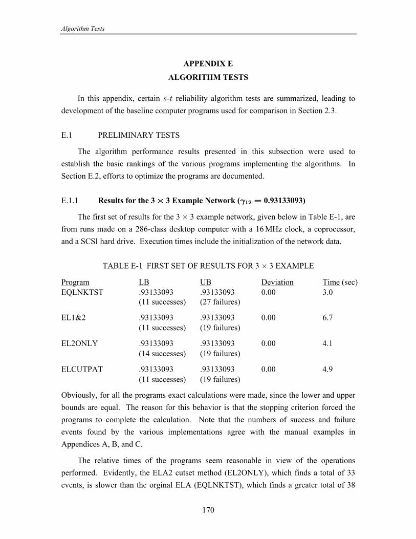
Algorithm Tests
170
APPENDIX E
ALGORITHM TESTS
In this appendix, certain - reliability algorithm tests are summarized, leading to= >
development of the baseline computer programs used for comparison in Section 2.3.
E.1 PRELIMINARY TESTS
The algorithm performance results presented in this subsection were used toestablish the basic rankings of the various programs implementing the algorithms. InSection E.2, efforts to optimize the programs are documented.
E.1.1 Results for the 3 3 Example Network ( 0.93133093)‚ œ#"#
The first set of results for the 3 3 example network, given below in Table E-1, are‚
from runs made on a 286-class desktop computer with a 16 MHz clock, a coprocessor,and a SCSI hard drive. Execution times include the initialization of the network data.
TABLE E-1 FIRST SET OF RESULTS FOR 3 3 EXAMPLE‚
Program LB UB Deviation Time (sec)EQLNKTST .93133093 .93133093 0.00 3.0 (11 successes) (27 failures)
EL1&2 .93133093 .93133093 0.00 6.7 (11 successes) (19 failures)
EL2ONLY .93133093 .93133093 0.00 4.1 (14 successes) (19 failures)
ELCUTPAT .93133093 .93133093 0.00 4.9 (11 successes) (19 failures)
Obviously, for all the programs exact calculations were made, since the lower and upperbounds are equal. The reason for this behavior is that the stopping criterion forced theprograms to complete the calculation. Note that the numbers of success and failureevents found by the various implementations agree with the manual examples inAppendices A, B, and C.
The relative times of the programs seem reasonable in view of the operationsperformed. Evidently, the ELA2 cutset method (EL2ONLY), which finds a total of 33events, is slower than the orginal ELA (EQLNKTST), which finds a greater total of 38
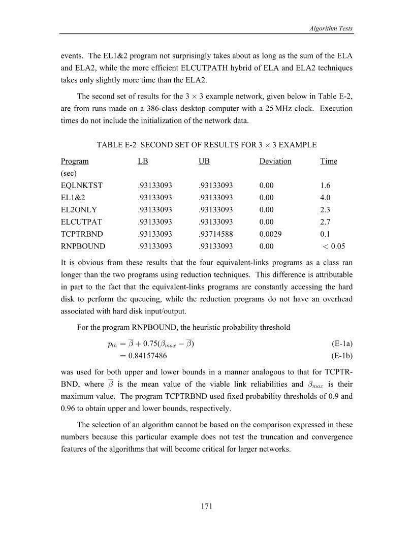
Algorithm Tests
171
events. The EL1&2 program not surprisingly takes about as long as the sum of the ELAand ELA2, while the more efficient ELCUTPATH hybrid of ELA and ELA2 techniquestakes only slightly more time than the ELA2.
The second set of results for the 3 3 example network, given below in Table E-2,‚
are from runs made on a 386-class desktop computer with a 25 MHz clock. Executiontimes do not include the initialization of the network data.
TABLE E-2 SECOND SET OF RESULTS FOR 3 3 EXAMPLE‚
Program LB UB Deviation Time(sec)EQLNKTST .93133093 .93133093 0.00 1.6 EL1&2 .93133093 .93133093 0.00 4.0 EL2ONLY .93133093 .93133093 0.00 2.3 ELCUTPAT .93133093 .93133093 0.00 2.7 TCPTRBND .93133093 .93714588 0.0029 0.1 RNPBOUND .93133093 .93133093 0.00 0.05
It is obvious from these results that the four equivalent-links programs as a class ranlonger than the two programs using reduction techniques. This difference is attributablein part to the fact that the equivalent-links programs are constantly accessing the harddisk to perform the queueing, while the reduction programs do not have an overheadassociated with hard disk input/output.
For the program RNPBOUND, the heuristic probability threshold
0.75( ) (E-1a)œ :>2 7+B" " "
0.84157486 (E-1b)œ
was used for both upper and lower bounds in a manner analogous to that for TCPTR-BND, where is the mean value of the viable link reliabilities and is their" "7+B
maximum value. The program TCPTRBND used fixed probability thresholds of 0.9 and0.96 to obtain upper and lower bounds, respectively.
The selection of an algorithm cannot be based on the comparison expressed in thesenumbers because this particular example does not test the truncation and convergencefeatures of the algorithms that will become critical for larger networks.
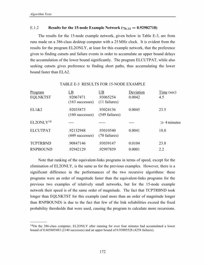
Algorithm Tests
172
E.1.2 Results for the 15-node Example Network ( 0.92982718)#)ß"$ œ
The results for the 15-node example network, given below in Table E-3, are fromruns made on a 386-class desktop computer with a 25 MHz clock. It is evident from theresults for the program EL2ONLY, at least for this example network, that the preferencegiven to finding cutsets and failure events in order to accumulate an upper bound delaysthe accumulation of the lower bound significantly. The program ELCUTPAT, while alsoseeking cutsets gives preference to finding short paths, thus accumulating the lowerbound faster than ELA2.
TABLE E-3 RESULTS FOR 15-NODE EXAMPLE
Program LB UB Deviation Time (sec)EQLNKTST .92067471 .93065254 0.0042 4.5 (163 successes) (11 failures)
EL1&2 .92035873 .93024136 0.0045 23.5 (160 successes) (549 failures)
EL2ONLY ---- ----- ---- 4 minutes 14 ¦
ELCUTPAT .92132948 .93010540 0.0041 18.0 (449 successes) (70 failures)
TCPTRBND .90847146 .93039147 0.0104 23.8 RNPBOUND .92942129 .92997859 0.0001 2.2 Note that ranking of the equivalent-links programs in terms of speed, except for theelimination of EL2ONLY, is the same as for the previous examples. However, there is asignificant difference in the performances of the two recursive algorithms: theseprograms were an order of magnitude faster than the equivalent-links programs for theprevious two examples of relatively small networks, but for the 15-node examplenetwork their speed is of the same order of magnitude. The fact that TCPTRBND tooklonger than EQLNKTST for this example (and more than an order of magnitude longerthan RNPBOUND) is due to the fact that few of the link reliabilities exceed the fixedprobability thresholds that were used, causing the program to calculate more recursions.
14On the 286-class computer, EL2ONLY after running for over four minutes had accumulated a lowerbound of 0.665605483 (2140 successes) and an upper bound of 0.93005528 (4258 failures).
Algorithm Tests
173
Note from Table E-1 that the exact calculation for this example took the TCPTR program49 seconds.
E.1.3 Results for the 34-node Example Network
The results for the 34-node example network, given below in Tables E-4 to E-6, arefrom runs made on a 386-class desktop computer with a 25 MHz clock. For theequivalent-links programs, a 10-hop path limit was used. The only conclusive observa-tions that can be made using the data in these tables is that the EL2ONLY program isdefinitely too time-consuming to be considered for calculation of the - reliabilities of= >
large networks, and that the recursive algorithms definitely should be considered. Thelink reliabilities in these examples generally are too high (yielding 0.99) to give an#=>
adequate picture of the relative performances of the algorithms. The stopping criterion ofUB LB 0.01 for the equivalent-links programs obviously does not operate in the
intended manner when 0.99, and it appears that the criterion for stopping was the#=>
requirement to process 100 events, in the case of node pairs (3, 11) and (18, 25), whilefor node pair (25, 20) the algorithms stopped when the lower bound exceeded 0.99.Interestingly, the most accurate program for (25, 20) for this case was RNPBOUND,which features an adaptive probability threshold.
In order to obtain a better comparison of the algorithm performances for largenetworks, additional tests were conducted using the data for the 15- and 34-node examplenetworks, modified to simulate the degradation of the link SNRs in 1 dB steps. Theresults of those tests are reported in the following subsection.
E.2 PARAMETRIC TESTS
Additional tests of algorithm performance were made using the file BIGONE.SNRfor the 34-node example network and node pair (25, 20). The SNRs in these files for afixed jamming situation were made into a simulated parametric variation of jammerpower by the method explained in Section 2.3.2.1 of the text.
E.2.1 Algorithm Performance Comparisons
Having eliminated the program EL2ONLY from consideration, as well as the pro-grams that compute the exact value of - reliability, runs were made on a 386 computer= >
to compare the performances of the following five algorithms in calculating for the##&ß#!
34-node example network:

Algorithm Tests
174
TABLE E-4 RESULTS FOR 34-NODE EXAMPLE, (3, 11)
Program LB UB UB LB Time (sec)EQLNKTST .99999991 1.00000000 0.00 6.1 (98 successes) (2 failures)
EL1&2 .99999990 1.00000000 0.00 7.2 (64 successes) (36 failures)
EL2ONLY ---- ----- ---- 4 minutes ¦
ELCUTPAT .99999928 1.00000000 0.00 9.3 (83 successes) (23 failures)
TCPTRBND .91294729 1.00000000 0.0871 0.5 RNPBOUND .99998869 1.00000000 0.00 1
TABLE E-5 RESULTS FOR 34-NODE EXAMPLE, (18, 25)
Program LB UB UB LB Time (sec)EQLNKTST .99995848 1.00000000 0.00 7 (100 successes) (1 failure)
EL1&2 .99995646 1.00000000 0.00 7.7 (72 successes) (28 failures)
EL2ONLY ---- ----- ---- 4 minutes ¦
ELCUTPAT .99882084 1.00000000 0.0012 11.7 (42 successes) (72 failures) TCPTRBND .93830301 1.00000000 0.0617 3.5 RNPBOUND .99999791 1.00000000 0.00 3.5
TABLE E-6 RESULTS FOR 34-NODE EXAMPLE, (25, 20)
Program LB UB UB LB Time (sec)EQLNKTST .99250576 0.99952630 0.0070 22.7 (351 successes) (18 failures)
EL1&2 .99250576 0.99937379 0.0069 25.6 (351 successes) (34 failures)
EL2ONLY ---- ----- ---- 4 minutes ¦
ELCUTPAT .99098649 0.99936825 0.0084 115 (883 successes) (616 failures) TCPTRBND .92678123 1.00000000 0.0732 1 RNPBOUND .99897902 0.99937369 0.0004 10
Algorithm Tests
175
Program Algorithm implemented
EQLNKTST Original ELA, with 0.01 and 1-way pathfinding using % œ anti-pingpong (one-hop return prevention logic)
EL1&2 Both ELA and ELA2, using the lower bound from ELA and the upper bound from ELA2, using 0.01,% œ 1-way pathfinding with anti-pingpong, and the selection of the larger of forward and reverse cutsets
ELCUTPAT An algorithm that finds a path or a cutset, depending upon which generates the fewer new events, using 0.01, 1-way pathfinding with anti-pingpong, and% œ selection of the larger of forward and reverse cutsets
TCPTRBND Theologou-Carlier algorithm run twice: once to obtain an upper bound with the link reliability threshold : œ>2
0.9, and once to obtain a lower bound with 0.96: œ>2
RNPBOUND Reduction and Partition algorithm with Theologou- Carlier approach to handle imperfect nodes; run with adaptive threshold once to obtain both upper and lower bounds.
The operation of these programs has been discussed previously, except for the particularheuristic adaptive link probability threshold in RNPBOUND that was used for this set ofresults. The adaptive threshold used may be expressed by
( )/15 , (E-2)œ 5 † :>2 7+B 7+B" " "
where is an integer indexing the depth of recursion. That is, when the program first5
calls the probability calculation procedure, 0; each time that procedure calls itself in5 œ
order to carry out the network factoring, is incremented, causing the probability thresh-5
old to decrease. This thresholding scheme, used for both the lower and upper boundcalculations, forces at least one recursion since for 0 none of the link reliabilities5 œ
exceeds the threshold. For 0, factoring on a link with high reliability can result in an5
approximation—leading either to an upper bound or to a lower bound, as discussed inSection 2.2.3.2, by neglecting the probability of the subgraph with the factored linkdeleted. As the depth of the recursion increases, it is more likely that an approximation isused. By this heuristic method, the depth of recursion is made self-limiting and theoverall execution time of the algorithm is contained.
It has been noted above in connection with the TCPTRBND program that the lowerbound developed by the Theologou-Carlier type of algorithm tends to be loose; thistendency is especially pronounced for SNR conditions giving rise to sets of relatively low
Algorithm Tests
176
link reliability values. The reason for the looseness is that the neglected term has beenneglected on the basis that it is multiplied by (1 ), which is small for 1. : : ¸6 6
However, for low SNR conditions, is not close to 1. Therefore, in addition to:6
implementing the adaptive threshold given in (E-2), the version of RNPBOUND used forthe parametric performance results that follow employs an additional heuristic: the lowerbound is computed as
( ) ( * ) (1 ) Pr{shortest pðóóóóóóóóóñóóóóóóóóóò ðóóóóóóóóóóóóóóóóñóóóóóóóóóóóóóóóóò : † K 6 : † = Ä >K# #=> 6 => 6
LB as expressed previously
ath} (E-3)additional term to tighten LB
Due to excessive run times experienced with the EL1&2 program, a 2400-second(40-minute) limit was implemented in the version of the program that was used to obtainthe comparisons that follow.
Figure E-1 shows the execution time of the several programs as a function of theSNR threshold. Perhaps the most striking feature of the figure is the obvious time-limited behavior of the EL1&2 program for threshold values 9 to 12, despite the fact thatthis program has the lowest time for lower thresholds. It is difficult to understand how a1 dB change could affect the performance of the program so drastically, yet these resultsappear to be correct. A close inspection of the operation of the program for a 9 dBthreshold seemed to indicate that the program spent a disproportionate share of time inthe earlier part of the calculation on servicing the queue containing events generated bythe pathfinding or ELA portion of the algorithm; because of the relatively large hopdistance for the selected ( , ) pair, each path that is found generates a relatively large= >
number of next events that are put into the queue. The cutsets during the early part of therun, however, are relatively large (have few link outages), and the queue of next eventsgenerated by the ELA2 portion of the algorithm is smaller at first. However,accumulation of the upper bound is postponed until after the events contributing to thelower bound have been processed. Evidently, when the threshold is 8 dB, the programfortuitously achieves convergence before the queue sizes have become large.
In this light, it is interesting that the ELCUTPAT results (labelled “Cut Path" inFigure E-1) exhibit a more continuous increase in execution time for thresholds less than18 dB, the point at which the topology of the surviving links in the network begins tosimplify. Besides being faster than EL1&2 by virtue of maintaining one instead of twoqueues, ELCUTPAT seems to have a better performance by virtue of its event-minimizing strategy. However, as Figure E-1 shows, neither EL1&2 or ELCUTPAT iseven close to the efficiency of the other three programs.
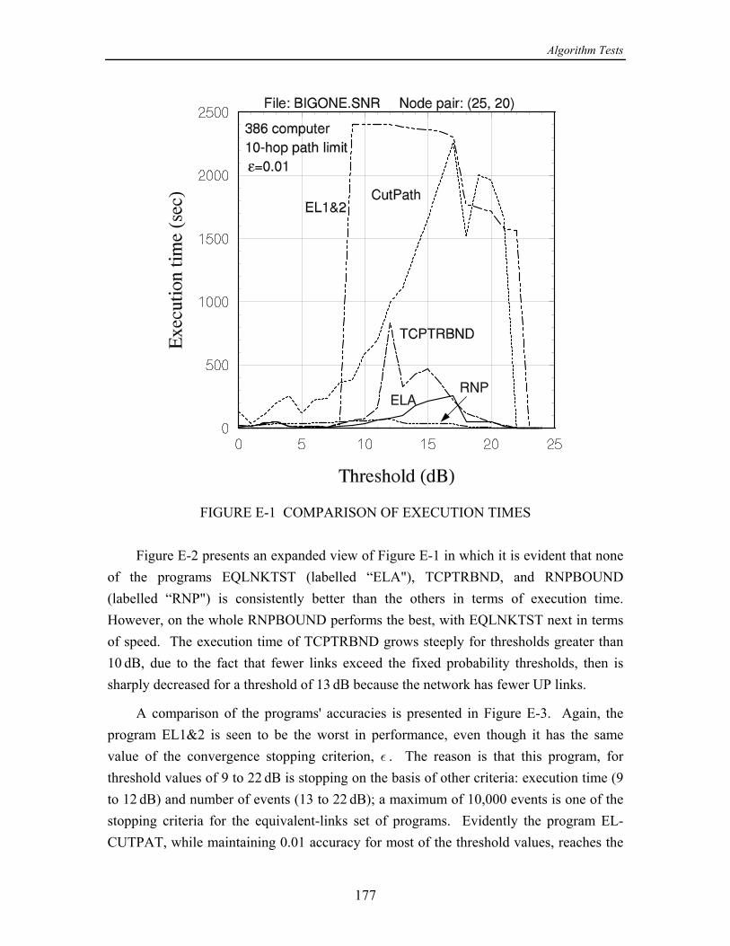
Algorithm Tests
177
FIGURE E-1 COMPARISON OF EXECUTION TIMES
Figure E-2 presents an expanded view of Figure E-1 in which it is evident that noneof the programs EQLNKTST (labelled “ELA"), TCPTRBND, and RNPBOUND(labelled “RNP") is consistently better than the others in terms of execution time.However, on the whole RNPBOUND performs the best, with EQLNKTST next in termsof speed. The execution time of TCPTRBND grows steeply for thresholds greater than10 dB, due to the fact that fewer links exceed the fixed probability thresholds, then issharply decreased for a threshold of 13 dB because the network has fewer UP links.
A comparison of the programs' accuracies is presented in Figure E-3. Again, theprogram EL1&2 is seen to be the worst in performance, even though it has the samevalue of the convergence stopping criterion, . The reason is that this program, for%
threshold values of 9 to 22 dB is stopping on the basis of other criteria: execution time (9to 12 dB) and number of events (13 to 22 dB); a maximum of 10,000 events is one of thestopping criteria for the equivalent-links set of programs. Evidently the program EL-CUTPAT, while maintaining 0.01 accuracy for most of the threshold values, reaches the
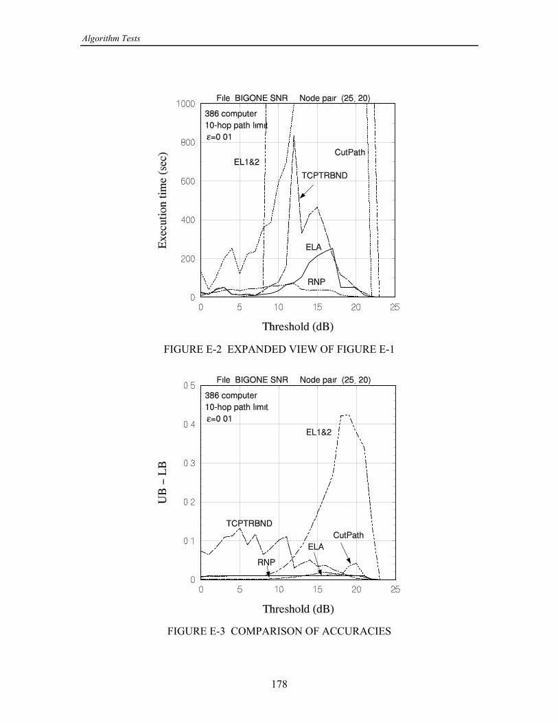
Algorithm Tests
178
FIGURE E-2 EXPANDED VIEW OF FIGURE E-1
FIGURE E-3 COMPARISON OF ACCURACIES
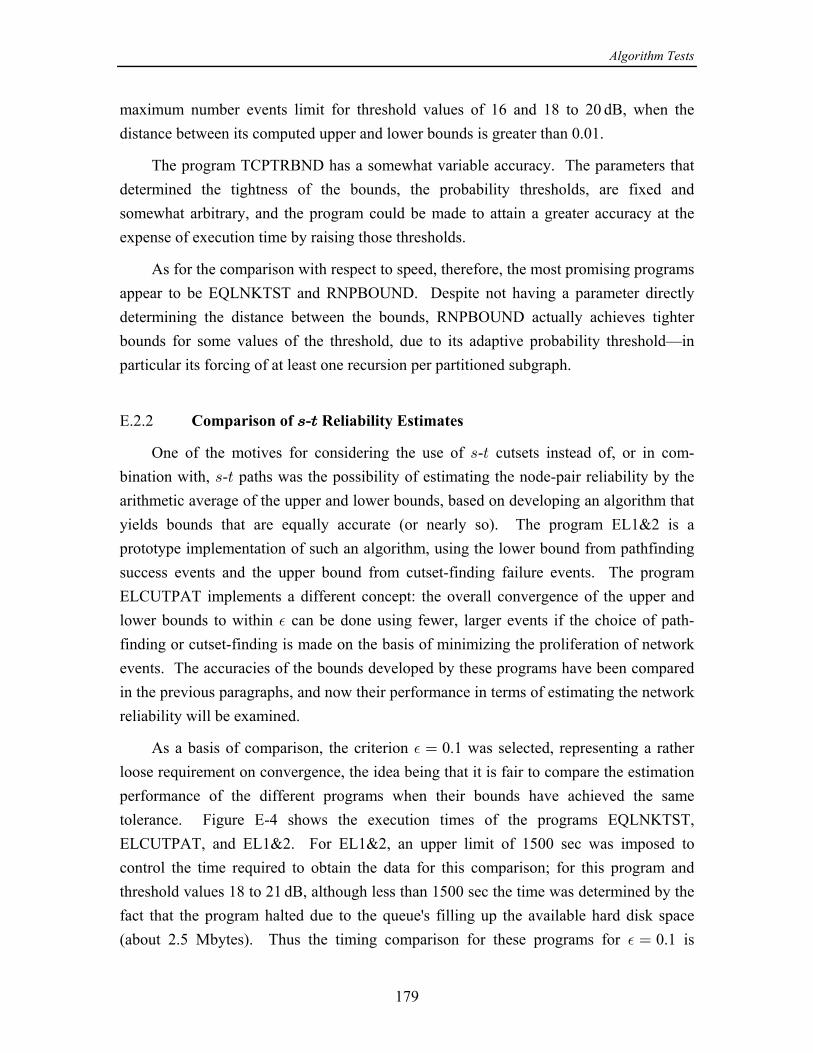
Algorithm Tests
179
maximum number events limit for threshold values of 16 and 18 to 20 dB, when thedistance between its computed upper and lower bounds is greater than 0.01.
The program TCPTRBND has a somewhat variable accuracy. The parameters thatdetermined the tightness of the bounds, the probability thresholds, are fixed andsomewhat arbitrary, and the program could be made to attain a greater accuracy at theexpense of execution time by raising those thresholds.
As for the comparison with respect to speed, therefore, the most promising programsappear to be EQLNKTST and RNPBOUND. Despite not having a parameter directlydetermining the distance between the bounds, RNPBOUND actually achieves tighterbounds for some values of the threshold, due to its adaptive probability threshold—inparticular its forcing of at least one recursion per partitioned subgraph.
E.2.2 Comparison of - Reliability Estimates= >
One of the motives for considering the use of - cutsets instead of, or in com-= >
bination with, - paths was the possibility of estimating the node-pair reliability by the= >
arithmetic average of the upper and lower bounds, based on developing an algorithm thatyields bounds that are equally accurate (or nearly so). The program EL1&2 is aprototype implementation of such an algorithm, using the lower bound from pathfindingsuccess events and the upper bound from cutset-finding failure events. The programELCUTPAT implements a different concept: the overall convergence of the upper andlower bounds to within can be done using fewer, larger events if the choice of path-%
finding or cutset-finding is made on the basis of minimizing the proliferation of networkevents. The accuracies of the bounds developed by these programs have been comparedin the previous paragraphs, and now their performance in terms of estimating the networkreliability will be examined.
As a basis of comparison, the criterion 0.1 was selected, representing a rather% œ
loose requirement on convergence, the idea being that it is fair to compare the estimationperformance of the different programs when their bounds have achieved the sametolerance. Figure E-4 shows the execution times of the programs EQLNKTST,ELCUTPAT, and EL1&2. For EL1&2, an upper limit of 1500 sec was imposed tocontrol the time required to obtain the data for this comparison; for this program andthreshold values 18 to 21 dB, although less than 1500 sec the time was determined by thefact that the program halted due to the queue's filling up the available hard disk space(about 2.5 Mbytes). Thus the timing comparison for these programs for 0.1 is% œ
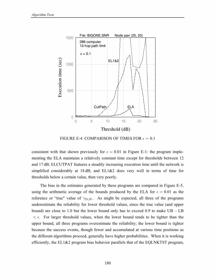
Algorithm Tests
180
FIGURE E-4 COMPARISON OF TIMES FOR 0.1% œ
consistent with that shown previously for 0.01 in Figure E-1: the program imple-% œ
menting the ELA maintains a relatively constant time except for thresholds between 12and 17 dB; ELCUTPAT features a steadily increasing execution time until the network issimplified considerably at 18 dB; and EL1&2 does very well in terms of time forthresholds below a certain value, then very poorly.
The bias in the estimates generated by these programs are compared in Figure E-5,using the arithmetic average of the bounds produced by the ELA for 0.01 as the% œ
reference or “true" value of . As might be expected, all three of the programs##&ß#!
underestimate the reliability for lower threshold values, since the true value (and upperbound) are close to 1.0 but the lower bound only has to exceed 0.9 to make UB LB
%. For larger threshold values, when the lower bound tends to be tighter than theupper bound, all three programs overestimate the reliability; the lower bound is tighterbecause the success events, though fewer and accumulated at various time positions asthe different algorithms proceed, generally have higher probabilities. When it is workingefficiently, the EL1&2 program bias behavior parallels that of the EQLNKTST program,
Algorithm Tests
181
FIGURE E-5 COMPARISON OF ESTIMATES FOR 0.1% œ
and seems to produce as good or better an estimate, but the ELCUTPAT has a differentbias behavior altogether.
Additional data was collected for EL1&2 and ELCUTPAT with an execution timelimit of 160 seconds, the maximum value experienced by the EQLNKTST program, tosee if somehow the intermediate values of the bounds produced by these programs have asmaller bias. Thus time-limited runs were made for ELCUTPAT for 10 to 21 dBthresholds, with the result that the new bias values were generally greater in magnitude;there was a smaller bias for 15 and 16 dB, where the bias is changing from negative topositive. Time-limited runs for the EL1&2 program for 14 to 22 dB thresholds yieldedthe same results: a slightly smaller bias for 15 and 16 dB, but a larger bias otherwise.
E.2.3 Effects of variations in the path search method
Using insights gained from the results described above, further parametric tests ofthe - reliability programs were conducted for the case of the 34-node example network.= >
These tests were designed (1) to determine the effect on execution time of variations in
Algorithm Tests
182
the path and cutset search methods used by the ELA family of algorithms, and (2) todetermine the performance of the TCPTRBND program when it is modified to use thesame adaptive threshold techniques as the RNPBOUND program. In order to study the effect of variations in the path search method, networkreliability calculations using the ELA (program EQLNKTST and modifications to it)were made on the 286 computer for the four possible combinations of the following twopath search techniques: the search propagation technique and the search redundancycontrol technique. In addition, a concentrated effort was made to optimize the programfor the search in terms of execution time. : previous runs utilized a one-way “flooding"ì Search propagation techniqueforward from the source node ( ) in search of the destination node ( ). That is, in steps= >
corresponding to transmission hops, information on the links emanating from the nodesso far reached on step is used to determine the nodes that would be reached on hop3
3 >1. The search stops when is reached, or when the maximum number of hops have15
been used without reaching . An alternative search propagation method is to alternate>
between flooding forward from and backward from ; in this manner a path (if one= >
exists) is discovered if the set of nodes reached in the forward direction has a node incommon with the set of nodes in the backward direction. Although it takes additional16
logic to implement the two-way search, there is a potential for reductions on the order of50% in the search time for cases in which and are widely separated.= >
The basis of this advantage may be explained intuitively as follows: the flood searchmay be thought of as having a radius in terms of the number of hops from the source ofthe search. Thus a one-way search from to that finds a path of length hops covers= > P
an “area" with radius hops. A two-way search presumably would stop after forwardP
and backward searches had each covered areas with radius /2 hops. The number ofP
nodes included in a given hop radius obviously depends upon the properties of thenetwork—for a fully connected network, all the network nodes are included in a one-hopradius from any node, while for an infinite mesh network, there are 4 ( 1) nodes in aP P
radius of hops. Thus the ratio of the number of nodes reached by a two-way pathP
search to that reached by a one-way search can be modelled for a mesh network by
15The convention used by the program for a search in a given direction is that the first time that a node isreach on a given hop, the connection thus established is not replaced by subsequent connections that arefound to be possible for the hop as the program executes its “loops" using the node number (label) as anindex. That is, preference is given to the “lexicographically first" connection.16The “lexicographically first" connections in the half of the path search performed by the backward searchare sometimes different from those that are found by a one-way search, giving rise to the finding ofdifferent paths—sometimes more advantageous to the execution time, sometimes not.
Algorithm Tests
183
. (E-4)2 # nodes in radius /2
# nodes in radius œ œ
‚ P
P8( /2)( /2 1)
4 ( 1) 1/2 1P P
P P PP
For large , obviously the ratio approaches 1/2.P
: the path search method employed to ob-ì Search redundancy control techniquetain the results presented in this report so far featured what was called “anti-pingpong"logic to prevent the propagation of the search to a node visited on the previous hop. Forexample, propagation from the nodes reached on the first hop forward from are not=
allowed to propagate backwards to on the second hop. This logic helps to prevent the=
waste of computation time that would result if the flood search continually regenerateditself by going in loops. However, although this logic prevents the return to a previouslyvisited node two hops later, it does not prevent the return to a previously visited node inmore any than two hops later. Therefore, “anti-return" logic was developed to prevent returns to previously visited nodes, simply by remembering the nodes so far reached bythe search and by not permitting the search to propagate to any of them.
The effects of these variations in the path search technique on the program execu-tion time and on the numbers of events are demonstrated in Figures E-6 and E-7,respectively. It may be observed from Figure E-6 that an overall reduction in the time ofmore than 50% is experienced for certain threshold values, and that generally going fromanti-pingpong logic to anti-return logic reduces the time more than going from a one-waysearch to a two-way search. The time is seen to be very dependent upon the numbers ofsuccess and failure events that are processed, which are different for the two searchpropagation techniques, as illustrated in Figure E-7, due to a necessarily differentlexicographical ordering of preferred paths in the subroutine that implements the two-way search. Evidently in this example the labelling of the nodes and links in conjunctionwith the order in which the links fail as the threshold increases is such that the one-waysearch had a lexicographical advantage for low values of the threshold, but had adisadvantage for higher values.
Algorithm Tests
184
FIGURE E-6 EFFECT OF PATH SEARCH METHOD ON TIME
FIGURE E-7 EFFECT OF PATH SEARCH METHOD ON EVENTS
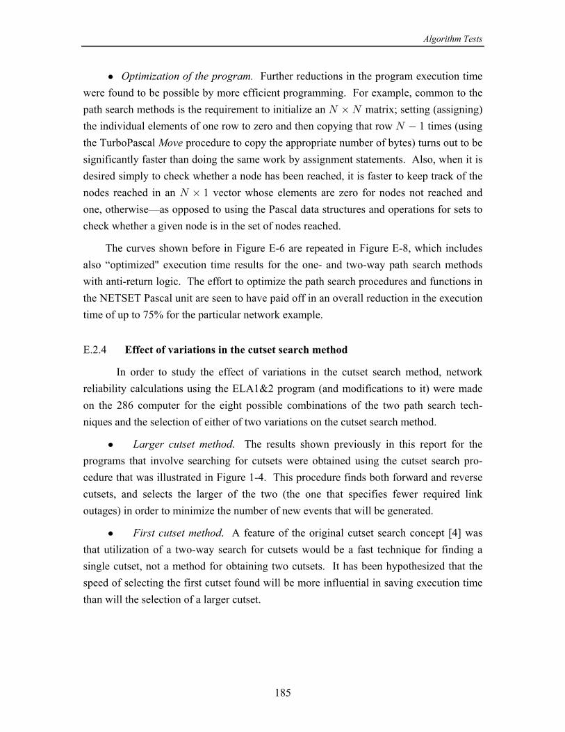
Algorithm Tests
185
Further reductions in the program execution timeì Optimization of the program.were found to be possible by more efficient programming. For example, common to thepath search methods is the requirement to initialize an matrix; setting (assigning)R ‚R
the individual elements of one row to zero and then copying that row 1 times (usingR
the TurboPascal procedure to copy the appropriate number of bytes) turns out to beMovesignificantly faster than doing the same work by assignment statements. Also, when it isdesired simply to check whether a node has been reached, it is faster to keep track of thenodes reached in an 1 vector whose elements are zero for nodes not reached andR ‚
one, otherwise—as opposed to using the Pascal data structures and operations for sets tocheck whether a given node is in the set of nodes reached.
The curves shown before in Figure E-6 are repeated in Figure E-8, which includesalso “optimized" execution time results for the one- and two-way path search methodswith anti-return logic. The effort to optimize the path search procedures and functions inthe NETSET Pascal unit are seen to have paid off in an overall reduction in the executiontime of up to 75% for the particular network example.
E.2.4 Effect of variations in the cutset search method
In order to study the effect of variations in the cutset search method, networkreliability calculations using the ELA1&2 program (and modifications to it) were madeon the 286 computer for the eight possible combinations of the two path search tech-niques and the selection of either of two variations on the cutset search method.
. The results shown previously in this report for theì Larger cutset methodprograms that involve searching for cutsets were obtained using the cutset search pro-cedure that was illustrated in Figure 1-4. This procedure finds both forward and reversecutsets, and selects the larger of the two (the one that specifies fewer required linkoutages) in order to minimize the number of new events that will be generated.
. A feature of the original cutset search concept [4] wasì First cutset methodthat utilization of a two-way search for cutsets would be a fast technique for finding asingle cutset, not a method for obtaining two cutsets. It has been hypothesized that thespeed of selecting the first cutset found will be more influential in saving execution timethan will the selection of a larger cutset.
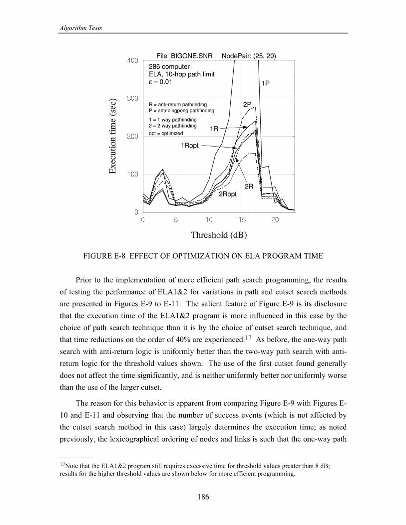
Algorithm Tests
186
FIGURE E-8 EFFECT OF OPTIMIZATION ON ELA PROGRAM TIME
Prior to the implementation of more efficient path search programming, the resultsof testing the performance of ELA1&2 for variations in path and cutset search methodsare presented in Figures E-9 to E-11. The salient feature of Figure E-9 is its disclosurethat the execution time of the ELA1&2 program is more influenced in this case by thechoice of path search technique than it is by the choice of cutset search technique, andthat time reductions on the order of 40% are experienced. As before, the one-way path17
search with anti-return logic is uniformly better than the two-way path search with anti-return logic for the threshold values shown. The use of the first cutset found generallydoes not affect the time significantly, and is neither uniformly better nor uniformly worsethan the use of the larger cutset.
The reason for this behavior is apparent from comparing Figure E-9 with Figures E-10 and E-11 and observing that the number of success events (which is not affected bythe cutset search method in this case) largely determines the execution time; as notedpreviously, the lexicographical ordering of nodes and links is such that the one-way path
17Note that the ELA1&2 program still requires excessive time for threshold values greater than 8 dB;results for the higher threshold values are shown below for more efficient programming.
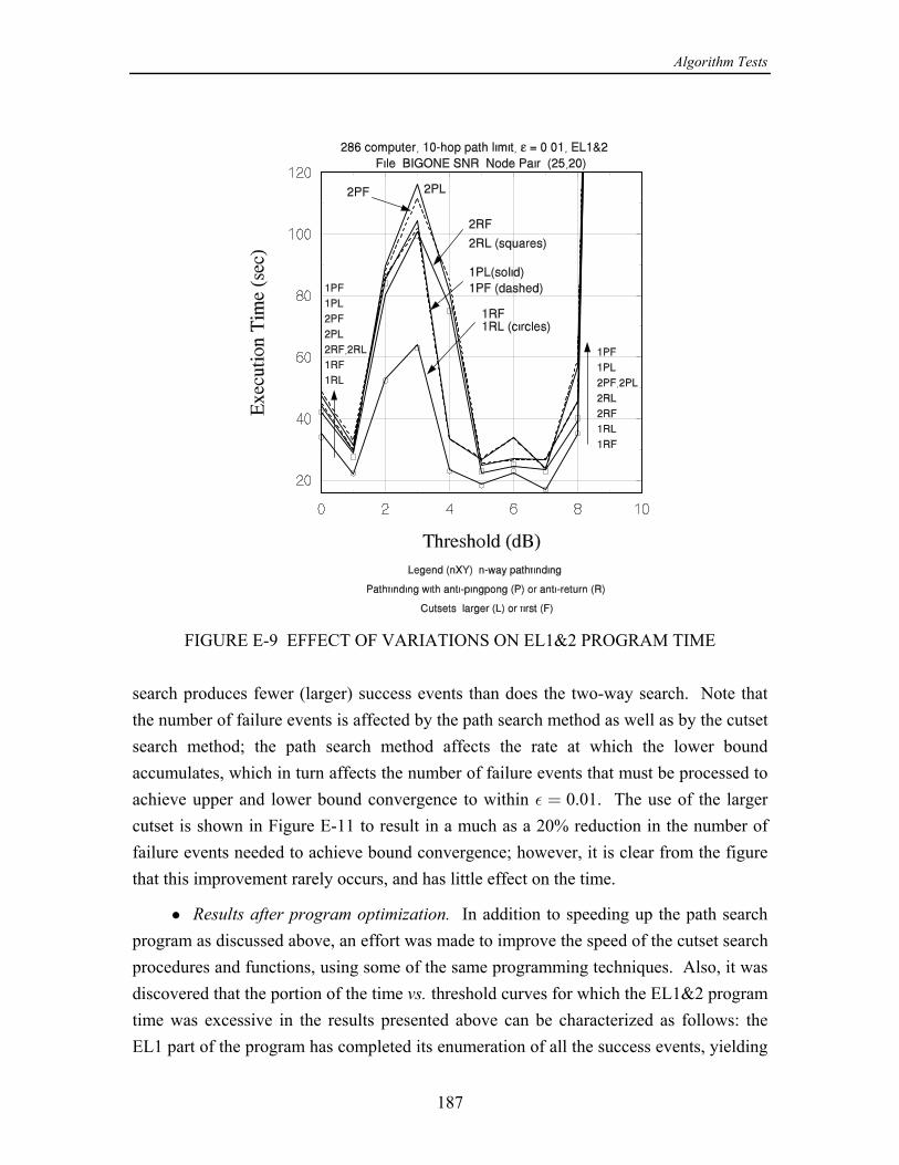
Algorithm Tests
187
FIGURE E-9 EFFECT OF VARIATIONS ON EL1&2 PROGRAM TIME
search produces fewer (larger) success events than does the two-way search. Note thatthe number of failure events is affected by the path search method as well as by the cutsetsearch method; the path search method affects the rate at which the lower boundaccumulates, which in turn affects the number of failure events that must be processed toachieve upper and lower bound convergence to within 0.01. The use of the larger% œ
cutset is shown in Figure E-11 to result in a much as a 20% reduction in the number offailure events needed to achieve bound convergence; however, it is clear from the figurethat this improvement rarely occurs, and has little effect on the time.
In addition to speeding up the path searchì Results after program optimization.program as discussed above, an effort was made to improve the speed of the cutset searchprocedures and functions, using some of the same programming techniques. Also, it wasdiscovered that the portion of the time threshold curves for which the EL1&2 programvs.time was excessive in the results presented above can be characterized as follows: theEL1 part of the program has completed its enumeration of all the success events, yielding
Algorithm Tests
188
FIGURE E-10 EFFECT OF VARIATIONS ON EL1&2 SUCCESS EVENTS
a lower bound that is actually an exact computation of the - reliability, while the EL2= >
part of the program is still processing the thousands of cutset-generated events that areassociated with the particular network example. Based on this discovery, the logic of theprocedures in the CUTSET Pascal unit was modified to accomplish the followingobjectives: (1) Detect when either part of the program has found the exact answer (by notingwhen the queue is not added to), and stop the program at that point. (2) In this eventuality, cause the estimate to be set equal to the exact answer insteadof the average of the upper and lower bounds.
The optimized EL1&2 program produced the results illustrated in Figure E-12,which includes the optimized results for the ELA as well. This figure may be compareddirectly with Figures E-1 and E-2, rather than with Figure E-9, since the 386 computerwas used to obtain them. Note that the various improvements in the EL1&2 programhave reduced the worst-case execution time by almost an order of magnitude. Note also
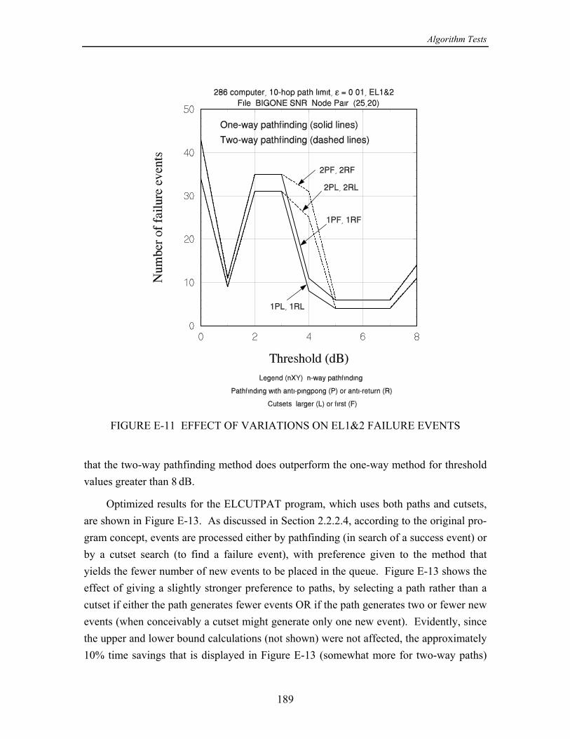
Algorithm Tests
189
FIGURE E-11 EFFECT OF VARIATIONS ON EL1&2 FAILURE EVENTS
that the two-way pathfinding method does outperform the one-way method for thresholdvalues greater than 8 dB.
Optimized results for the ELCUTPAT program, which uses both paths and cutsets,are shown in Figure E-13. As discussed in Section 2.2.2.4, according to the original pro-gram concept, events are processed either by pathfinding (in search of a success event) orby a cutset search (to find a failure event), with preference given to the method thatyields the fewer number of new events to be placed in the queue. Figure E-13 shows theeffect of giving a slightly stronger preference to paths, by selecting a path rather than acutset if either the path generates fewer events OR if the path generates two or fewer newevents (when conceivably a cutset might generate only one new event). Evidently, sincethe upper and lower bound calculations (not shown) were not affected, the approximately10% time savings that is displayed in Figure E-13 (somewhat more for two-way paths)
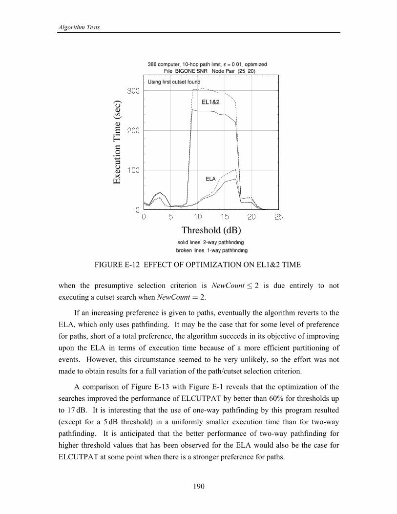
Algorithm Tests
190
FIGURE E-12 EFFECT OF OPTIMIZATION ON EL1&2 TIME
when the presumptive selection criterion is 2 is due entirely to notNewCount Ÿexecuting a cutset search when 2.NewCount œ
If an increasing preference is given to paths, eventually the algorithm reverts to theELA, which only uses pathfinding. It may be the case that for some level of preferencefor paths, short of a total preference, the algorithm succeeds in its objective of improvingupon the ELA in terms of execution time because of a more efficient partitioning ofevents. However, this circumstance seemed to be very unlikely, so the effort was notmade to obtain results for a full variation of the path/cutset selection criterion.
A comparison of Figure E-13 with Figure E-1 reveals that the optimization of thesearches improved the performance of ELCUTPAT by better than 60% for thresholds upto 17 dB. It is interesting that the use of one-way pathfinding by this program resulted(except for a 5 dB threshold) in a uniformly smaller execution time than for two-waypathfinding. It is anticipated that the better performance of two-way pathfinding forhigher threshold values that has been observed for the ELA would also be the case forELCUTPAT at some point when there is a stronger preference for paths.
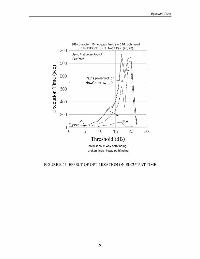
Algorithm Tests
191
FIGURE E-13 EFFECT OF OPTIMIZATION ON ELCUTPAT TIME
References
192
REFERENCES
[1] L. E. Miller and J. J. Kelleher, “Analysis Models for MSE Network SurvivabilityPerformance in the Tactical Environment," J. S. Lee Associates, Inc. report JC-2091-7-FF, March 1992 (DTIC accession number AD-B164578).
[2] D. J. Torrieri, “An Efficient Algorithm for the Calculation of Node-Pair Reliability,"Proc. IEEE 1991 Milit. Comm. Conf. (MILCOM '91), McLean, VA, 4-7 November,pp. 0187-0192.
[3] W. P. Dotson and J. O. Gobien, “A New Analysis Technique for ProbabilisticGraphs," , vol. 26, pp. 855-865, October 1979.IEEE Trans. on Circuits and Syst.
[4] D. J. Torrieri, “New Algorithm for Large Networks," notes dated 6 April 1992.
[5] L. E. Miller, L. Wong, and J. J. Kelleher, “Net Survivability Analysis SoftwareTools," J. S. Lee Associates, Inc. report JC-2092-3-F under contract DAAL02-89-C-0040, August 1992.
[6] L. E. Miller, “Propagation Model Sensitivity Study," J. S. Lee Associates, Inc.report JC-2092-1-FF, July 1992 (DTIC accession number AD-B166479).
[7] L. E. Miller, J. J. Kelleher, and J. S. Lee, “Analysis of the Survivability of LargeMSE Networks by a Truncated Equivalent-Links Methodology," Proc. IEEE 1992Milit. Comm. Conf. (MILCOM '92), San Diego, CA, 12-14 October, pp. 0487-0491.
[8] L. E. Miller, “Army JTIDS Communications Survivability Modelling and JammedConnectivity Assessment (U)" (Secret report), J. S. Lee Associates, Inc. report JC-2091-6-FF under contract DAAL02-89-C-0040, July 1992.
[9] L. B. Page and J. E. Perry, “Reliability of Directed Networks Using the FactoringTheorem," , vol. R-38, pp. 556-562, December 1989.IEEE Trans. on Reliability
[10] O. R. Theologou and J. G. Carlier, “Factoring and Reductions for Networks withImperfect Vertices," , vol. 40, pp. 210-217, June 1991.IEEE Trans. on Reliability
[11] N. Deo and M. Medidi, “Parallel Algorithms for Terminal-Pair Reliability," IEEETrans. on Reliability, vol. 41, pp. 201-209, June 1992.
[12] J. M. Wilson, “An Improved Minimizing Algorithm for Sum of Disjoint Products,"IEEE Trans. on Reliability, vol. 39, pp. 42-45, April 1990.
[13] L. E. Miller, J. J. Kelleher, and L. Wong, "Assessment of Network Reliability Cal-culation Methods," J. S. Lee Associates, Inc. report JC-2097-FF under contractDAALo2-92-C-0045, January 1994 ( DTIC accession number AD-B170336).