Embed Size (px)
Citation preview

Evaluation of Road Weather Messages on DMS Based on Roadside Pavement Sensors
Skylar Knickerbocker, Principal InvestigatorInstitute for TransportationIowa State University
NOVEMBER 2021
Research Report Final Report 2021-25
Office of Research & Innovation • mndot.gov/research

To request this document in an alternative format, such as braille or large print, call 651-366-4718 or 1-800-657-3774 (Greater Minnesota) or email your request to [email protected]. Please request at least one week in advance.

Technical Report Documentation Page 1. Report No. 2. 3. Recipients Accession No.
MN 2021-25
4. Title and Subtitle 5. Report Date
Evaluation of Road Weather Messages on DMS Based on November 2021
Roadside Pavement Sensors 6.
7. Author(s) 8. Performing Organization Report No.
Skylar Knickerbocker, Alireza Sassani, and Zach Hans 9. Performing Organization Name and Address 10. Project/Task/Work Unit No.
Institute for Transportation Iowa State University 11. Contract (C) or Grant (G) No. 2711 South Loop Drive, Ames, IA 50010
(c) 1036216 12. Sponsoring Organization Name and Address 13. Type of Report and Period Covered
Minnesota Department of Transportation Office of Research & Innovation
Final Report 14. Sponsoring Agency Code
395 John Ireland Boulevard, MS 330 St. Paul, Minnesota 55155-1899 15. Supplementary Notes
https://www.mndot.gov/research/reports/2021/202125.pdf 16. Abstract (Limit: 250 words)
Winter weather and its corresponding surface conditions impact the safety and mobility of thousands of motorists
annually. Highway agencies spend millions of dollars in resources and personnel in an effort to ensure safe and efficient
travel. One such strategy is to use dynamic message signs (DMS) that have been deployed across the state to alert
drivers of conditions ahead based on data from roadside sensors. This type of advisory system can provide real-time
information, allowing drivers to adjust their driving behavior to the conditions ahead.
The objective of this project was to analyze traffic behavior along a specially instrumented portion of the US 12 corridor
under various winter weather conditions when advisory messages triggered by roadside pavement sensors were
provided via DMSs between Delano and Maple Plain, Minnesota. Temporary traffic sensor data upstream and
downstream of the DMS are used to evaluate traffic flow metrics during winter weather conditions as compared to
baseline conditions.
In the eastbound direction, statistically significant reductions in mean and 85th percentile speeds of 3.5 mph and 2.9
mph, respectively, were identified. The westbound direction experienced mixed results, with a mixture of statistically
insignificant changes as well as statistically significant increases and decreases in speeds. It is assumed that other
factors were influencing driver behavior in this westbound direction. There were indications of positive effects on
vehicle gaps when evaluating all events combined that were statistically significant but not when evaluating individual
winter weather events.
17. Document Analysis/Descriptors 18. Availability Statement Variable message signs, Highway safety, Friction, Roadside, No restrictions. Document available from:
Cold weather, Sensors
National Technical Information Services,
Alexandria, Virginia 22312 19. Security Class (this report) 20. Security Class (this page) 21. No. of Pages 22. Price
Unclassified Unclassified 91

Evaluation of Road Weather Messages on DMS Based on Roadside
Pavement Sensors
FINAL REPORT
Prepared by:
Skylar Knickerbocker
Alireza Sassani
Zach Hans
Institute for Transportation
Iowa State University
November 2021
Published by:
Minnesota Department of Transportation
Office of Research & Innovation
395 John Ireland Boulevard, MS 330
St. Paul, Minnesota 55155-1899
This report represents the results of research conducted by the authors and does not necessarily represent the views or policies
of the Minnesota Department of Transportation or the Institute for Transportation at Iowa State University]. This report does
not contain a standard or specified technique.
The authors, the Minnesota Department of Transportation, and the Institute for Transportation at Iowa State University do not
endorse products or manufacturers. Trade or manufacturers’ names appear herein solely because they are considered essential
to this report.
ACKNOWLEDGMENTS
The authors would like to thank the Minnesota Department of Transportation (MnDOT) for sponsoring
this research. The team thanks members of the technical advisory panel (TAP) for their feedback and
guidance throughout the research effort, including Garrett Schreiner, Ralph Adair, Lars Impola, Brian
Kary, Peter Morey, Aaron Tag, Adam Wellner, and Eric Lauer-Hunt. The TAP was instrumental in
supporting this research by providing the resources to deploy additional temporary sensors to allow for
a more thorough analysis to identify the effects of winter weather messaging on driver behavior.
The research team is appreciative of and thankful for the TAP’s technical lead, Garrett Schreiner, who
provided access to the data and systems needed for a successful research project. Finally, the authors
would like to thank David Glyer for serving as the project coordinator and keeping the project moving
forward and organized.

TABLE OF CONTENTS
CHAPTER 1: Introduction ...................................................................................................................... 1
1.1 Background ......................................................................................................................................... 1
1.2 Research Significance ......................................................................................................................... 1
1.3 Project Objective and Approach ......................................................................................................... 3
1.4 Remaining Report Content ................................................................................................................. 4
CHAPTER 2: Literature Review ............................................................................................................. 5
2.1 Overview ............................................................................................................................................. 5
2.2 Influence on Driver Behavior .............................................................................................................. 6
2.3 Metrics and Data Sources to Evaluate SMS Effectiveness .................................................................. 9
2.3.1 Speed ........................................................................................................................................... 9
2.3.2 Car Following Behavior .............................................................................................................. 10
2.3.3 Impacts on Traffic Flow Characteristics .................................................................................... 10
2.3.4 Capability to Attract Attention and Convey Information .......................................................... 10
2.3.5 Safety Impacts ........................................................................................................................... 10
2.4 Data Analysis and Interpretation Approaches .................................................................................. 10
2.4.1 Statistical Analysis ..................................................................................................................... 11
2.4.2 Data Interpretation to Evaluate Sign Effectiveness and Driver Compliance ............................. 12
2.5 Other Metrics and Methods of Analysis ........................................................................................... 18
2.5.1 Traffic Flow Characteristics as an Indicator of Sign Effectiveness ............................................ 18
2.5.2 Accounting for Weather-Related Factors.................................................................................. 18
2.5.3 Surveys: Stated Preference, Revealed Preference, and Reported Driver Behavior .................. 19
2.5.4 Traffic Microsimulation ............................................................................................................. 19
2.5.5 Driving Simulators ..................................................................................................................... 19

CHAPTER 3: Study Methodology ........................................................................................................ 20
3.1 Data Metrics ..................................................................................................................................... 20
3.2 Data Sources and Data Collection .................................................................................................... 20
3.2.1 Traffic Sensors ........................................................................................................................... 20
3.2.2 Dynamic Message Signs ............................................................................................................ 22
3.2.3 Cameras ..................................................................................................................................... 22
3.2.4 Friction Sensors ......................................................................................................................... 23
3.2.5 RWIS Sensors ............................................................................................................................. 24
3.2.6 Probe Data ................................................................................................................................. 24
3.3 Winter Weather Events .................................................................................................................... 24
3.4 Analysis Approach ............................................................................................................................ 26
3.4.1 Data Analysis ............................................................................................................................. 27
CHAPTER 4: Data Analysis .................................................................................................................. 30
4.1 Introduction ...................................................................................................................................... 30
4.2 Winter Weather Event 3 ................................................................................................................... 30
4.2.1 Description of Event 3 ............................................................................................................... 30
4.2.2 Sensor Data Analysis for Event 3 ............................................................................................... 32
4.3 Winter Weather Event 9 ................................................................................................................... 34
4.3.1 Description of Event 9 ............................................................................................................... 34
4.3.2 Sensor Data Analysis for Event 9 ............................................................................................... 35
4.4 Winter Weather Event 11 ................................................................................................................. 37
4.4.1 Description of Event 11 ............................................................................................................. 37
4.4.2 Sensor Data Analysis for Event 11 ............................................................................................. 38
4.5 Overall Analysis ................................................................................................................................. 40
4.5.1 Summary of All Individual Events .............................................................................................. 40

4.5.2 Summary for All Events Combined ............................................................................................ 44
4.6 Discussion ......................................................................................................................................... 48
CHAPTER 5: Conclusions and Future Studies ....................................................................................... 55
References ......................................................................................................................................... 58
APPENDIX A: Summary of Individual Events ......................................................................................... 1
APPENDIX B: Summary of Weather Impacts ......................................................................................... 1
LIST OF FIGURES
Figure 1.1. Advisory messaging and warning flashers for the study ............................................................ 3
Figure 2.1. Compliance with static and variable speed limit signs represented by hourly average
speed ........................................................................................................................................................... 14
Figure 2.2. Driver compliance with variable advisory speed DMS on OR 217: (a) driving speed, (b)
displayed speed, and (c) compliance .......................................................................................................... 15
Figure 2.3. Driver compliance with variable advisory speed DMS northbound on OR 217 based on
one-day data ............................................................................................................................................... 16
Figure 2.4. Layout of the advisory speed limit sign system used by Kwon et al. ........................................ 16
Figure 2.5. Average maximum speed difference comparison .................................................................... 17
Figure 2.6. On-screen and full-scale driving simulators .............................................................................. 19
Figure 3.1. Existing and proposed temporary devices along the US 12 corridor........................................ 21
Figure 3.2. DMS locations along US 12 corridor ......................................................................................... 22
Figure 3.3. Locations of camera images displayed in image snapshot composite image .......................... 23
Figure 3.4. Example showing the calculations for calculating speed difference ........................................ 28
Figure 3.5. Summary of statistical analysis changes in differential comparison ........................................ 29
Figure 4.1. Event 3 at the start of the event (left) and end of the event (right) ........................................ 31
Figure 4.2. Friction data during Event 3 ...................................................................................................... 31
Figure 4.3. Event 3 significant distributions for eastbound mean speed difference (left) and
westbound 85th percentile speed difference (right) .................................................................................. 33

Figure 4.4. Average five-minute speeds during control and winter weather Event 3 ................................ 33
Figure 4.5. Event 9 at start of event (left) and end of event (right) ........................................................... 34
Figure 4.6. Crash that occurred at 11:55 a.m. and was cleared after ~30 minutes.................................... 34
Figure 4.7. Friction data during Event 9 ...................................................................................................... 35
Figure 4.8. Event 9 significant distributions for eastbound mean speed difference (left) and
westbound mean speed difference (right) ................................................................................................. 36
Figure 4.9. Average five minute speeds during control and winter weather Event 9 ................................ 37
Figure 4.10. Event 11 at the start of the event (left) and end of the event (right) .................................... 38
Figure 4.11. Friction data during Event 16 .................................................................................................. 38
Figure 4.12. Event 11 significant distributions for eastbound standard deviation difference ................... 39
Figure 4.13. Average five minute speeds during control and winter weather Event 11 ............................ 40
Figure 4.14. Shifts in the downstream-upstream mean-speed difference during the events ................... 41
Figure 4.15. Shifts in the downstream-upstream 85th-percentile-speed difference during the
events .......................................................................................................................................................... 42
Figure 4.16. Shifts in the downstream-upstream difference of speed standard deviation during the
events .......................................................................................................................................................... 43
Figure 4.17. Shifts in the downstream-upstream gap difference during the events .................................. 44
Figure 4.18. Speed difference distributions for the control and study time periods in the
eastbound direction .................................................................................................................................... 47
Figure 4.19. Speed difference distributions for the control and study time periods in the
westbound direction ................................................................................................................................... 47
Figure 4.20. Eastbound mean speed shifts in different precipitation and accumulation conditions ......... 50
Figure 4.21. Westbound mean speed shifts in different precipitation and accumulation conditions ....... 50
Figure 4.22. Eastbound 85th percentile speed shifts in different precipitation and accumulation
conditions .................................................................................................................................................... 51
Figure 4.23. Westbound 85th percentile speed shifts in different precipitation and accumulation
conditions .................................................................................................................................................... 52
Figure 4.24. Eastbound standard deviation shifts in different precipitation and accumulation
conditions .................................................................................................................................................... 52

Figure 4.25. Westbound standard deviation shifts in different precipitation and accumulation
conditions .................................................................................................................................................... 53
Figure 4.26. Eastbound gap shifts in different precipitation and accumulation conditions ....................... 53
Figure 4.27. Westbound gap shifts in different precipitation and accumulation conditions ..................... 54
Figure B.1. Precipitation accumulation (left) and presence (right) for Event 1 ............................................ 1
Figure B.2. Precipitation accumulation (left) and presence (right) for Event 2 ............................................ 1
Figure B.3. Precipitation accumulation (left) and presence (right) for Event 3 ............................................ 1
Figure B.4. Precipitation accumulation (left) and presence (right) for Event 4 ............................................ 1
Figure B.5. Precipitation accumulation (left) and presence (right) for Event 5 ............................................ 2
Figure B.6. Precipitation accumulation (left) and presence (right) for Event 7 ............................................ 2
Figure B.7. Precipitation accumulation (left) and presence (right) for Event 8 ............................................ 2
Figure B.8. Precipitation accumulation (left) and presence (right) for Event 9 ............................................ 2
Figure B.9. Precipitation accumulation (left) and presence (right) for Event 10 .......................................... 3
Figure B.10. Precipitation accumulation (left) and presence (right) for Event 11 ........................................ 3
Figure B.11. Precipitation accumulation (left) and presence (right) for Event 12 ........................................ 3
Figure B.12. Precipitation accumulation (left) and presence (right) for Event 13 ........................................ 3
Figure B.13. Precipitation accumulation (left) and presence (right) for Event 14 ........................................ 4
Figure B.14. Precipitation accumulation (left) and presence (right) for Event 15 ........................................ 4
Figure B.15. Precipitation accumulation (left) and presence (right) for Event 16 ........................................ 4
LIST OF TABLES
Table 2.1. Driver compliance evaluation based on the average difference of observed and posted
speeds ......................................................................................................................................................... 14
Table 3.1. Summary of winter weather events with messaging ................................................................. 24
Table 3.2. Sample DMS messaging gaps ..................................................................................................... 25
Table 3.3. Summary of control time periods for winter weather events ................................................... 26

Table 4.1. Summary of the statistical analysis results for Event 3 .............................................................. 32
Table 4.2. Summary of the statistical analysis results for Event 9 .............................................................. 36
Table 4.3. Summary of the statistical analysis results for Event 11 ............................................................ 39
Table 4.4. Summary of the data analysis results for all events combined ................................................. 45
Table 4.5. Traffic volumes during the events for upstream and downstream locations ............................ 49
Table A.1. Detailed mean speed summary statistics for Event 1 to 9 in eastbound direction ..................... 1
Table A.2. Detailed mean speed summary statistics for Event 10 to 16 in eastbound direction ................. 1
Table A.3. Detailed mean speed summary statistics for Event 1 to 9 in westbound direction .................... 2
Table A.4. Detailed mean speed summary statistics for Event 10 to 16 in westbound direction ................ 2
Table A.5. Detailed 85th percentile speed summary statistics for Event 1 to 9 in eastbound
direction ........................................................................................................................................................ 3
Table A.6. Detailed 85th percentile speed summary statistics for Event 10 to 16 in eastbound
direction ........................................................................................................................................................ 3
Table A.7. Detailed 85th percentile speed summary statistics for Event 1 to 9 in westbound
direction ........................................................................................................................................................ 4
Table A.8. Detailed 85th percentile speed summary statistics for Event 10 to 16 in westbound
direction ........................................................................................................................................................ 4
Table A.9. Detailed standard deviation summary statistics for Event 1 to 9 in eastbound direction .......... 5
Table A.10. Detailed standard deviation summary statistics for Event 10 to 16 in eastbound
direction ........................................................................................................................................................ 5
Table A.11. Detailed standard deviation summary statistics for Event 1 to 9 in westbound
direction ........................................................................................................................................................ 6
Table A.12. Detailed standard deviation summary statistics for Event 10 to 16 in westbound
direction ........................................................................................................................................................ 6
Table A.13. Detailed gap summary statistics for Event 1 to 9 in eastbound direction ................................. 7
Table A.14. Detailed gap summary statistics for Event 10 to 16 in eastbound direction ............................. 7
Table A.15. Detailed gap summary statistics for Event 1 to 9 in westbound direction ................................ 8
Table A.16. Detailed gap summary statistics for Event 10 to 16 in westbound direction ............................ 8

EXECUTIVE SUMMARY
The Minnesota Department of Transportation (MnDOT) deployed a real-time, weather-controlled
dynamic message sign (DMS) system along the US 12 corridor between Delano and Maple Plain,
Minnesota with the expectation that the system would exert a significant effect on traffic. The deployed
DMS system provided road users with real-time information of potential unexpected weather conditions
and/or weather-induced road conditions.
Drivers who are exposed to the DMS messaging and comply with it are better informed, and thus less
likely to be surprised by changes in environmental road conditions. This should result in lower frequency
and severity of crashes and, consequently, improve driver safety and mobility along the corridor.
While providing weather-related information to drivers has promising benefits, the challenge of low
driver compliance still prevails. Drivers do not necessarily adjust their driving behavior according to the
information they are provided. Therefore, it is imperative to maximize driver compliance by using
optimally effective information-delivering media. Agencies should evaluate the DMS systems within
their jurisdiction to make sure they serve the intended purpose with acceptable efficacy and do not
exert any negative side effects.
Key aspects of DMS operation that should be thoroughly evaluated include the following: achieved
driver compliance rate, impact on traffic flow, impact on road safety, and extent of impact beyond the
equipped corridor. The degree of effectiveness and type of influence of DMS on driver behavior depends
on many design and operational factors.
The objective of this project was to analyze traffic behavior along a specially instrumented portion of the
US 12 corridor between Delano and Maple Plain, Minnesota, under various winter weather conditions
when advisory messages triggered by roadside pavement sensors were provided via the DMS. Traffic
sensors were the primary source of data for the analyses along the study corridor.
The data from the sensors were used to compare the performance metrics upstream and downstream
of the dynamic message signs along the corridor. The upstream sensors served as the control location
with no DMS messaging, while the downstream sensors were placed at a location potentially influenced
by DMS winter weather messaging. To evaluate the effectiveness of the system to change driving
behavior, multiple performance measures were established, including changes in mean and 85th
percentile speeds, standard deviation in speeds, and following distance or gap between vehicles.
Temporary sensors were placed to avoid any influence from the urban areas before and after Delano
and Maple Plain. Major assumptions with this approach were that similar traffic would be collected at
both sensors and the effects of the DMS would be present once vehicles returned to rural driving speeds
after traveling through the urban areas. These assumptions aligned with the intention of the system to
affect driver behavior through the corridor outside of the urban areas.
Assessing the influence of the DMS on driving behavior entailed winter weather events where the DMS
was active as well as a baseline period, which represented normal conditions. The baseline periods were

used to account for natural differences in speed upstream and downstream that could not be accounted
for otherwise due to distance and other factors between the sensors. The effect of the DMS during each
period manifested in the change of metrics from upstream to downstream.
Comparing the effect between the winter weather and baseline periods can provide details as to
whether the DMS winter weather messaging exerted a statistically significant influence on driving
behavior. Therefore, study variables were defined that investigated changes in metrics both spatially
(i.e., from upstream to downstream) and temporally (i.e., event and baseline periods) using the same
data sets.
In total, 16 winter weather events were initially analyzed during the 2020–21 winter season, while two
of the events were later excluded from the final analysis due to the short duration of one event and a
high number of blank messages for the other event. The results for three individual events, which
represented a cross section of the various winter weather impacts experienced along the corridor, are
presented in detail in this report. The first event (Event 3) showed the impact of a winter weather event
that had minimal impact and no precipitation accumulation; the second event (Event 9) showed a typical
winter weather event with precipitation accumulation; and the final event (Event 11) showed a
significant winter weather event with a large amount of snow accumulation.
The results were analyzed for all events by direction of travel. The eastbound direction represented the
best study layout because of the placement of the DMS on the outside edge of town with no major
influences on speed or traffic before the downstream sensor, which was used as the measure of
effectiveness. Overall, the DMS showed better, more consistent performance in the eastbound
direction. The results aligned with the expectations that providing drivers winter weather messaging
would impact driver decisions and reduce speed.
When evaluating the individual events, the eastbound direction had 12 of the 14 events with statistically
significant decreases in speed with an average decrease of 3.5 mph. This indicated that speeds
decreased from upstream to downstream during the winter weather event. In addition to the mean
speed, 13 of the 14 events had a statistically significant decrease in the 85th percentile speed with an
average decrease of 2.9 mph.
In addition to the individual events, a combined analysis was completed that aggregated the results of
all events. The results for the mean speed and 85th percentile speed aligned with the results for the
individual events, with the eastbound direction showing reduced speed downstream when accounting
for the control time. The combined analysis showed the mean speed downstream was reduced by 1.5
mph and the 85th percentile speed was reduced by 2.0 mph. The results indicated that the winter
weather messaging appears to influence driver behavior in reducing the mean and 85th percentile
speeds and was statistically significant for a majority of the events in the eastbound direction.
For the westbound direction, three events had a decrease in mean speed, while seven events showed an
increase in mean speed with an average increase of 2.5 mph. The westbound speed shifts were primarily
positive, indicating that the downstream speed increased relative to the upstream speed. The 85th
percentile speed showed mixed results as well, with one event showing desirable decreases in the 85th

percentile speed difference and eight events with an increase. Five of the events had no statistically
significant change in the 85th percentile speed difference.
With a majority of events resulting in an increase, this indicated that westbound speeds were higher
downstream, which was not the desired outcome of the winter weather messaging. For the westbound
direction, the combined event results also aligned with a majority of the individual events, showing
mean and 85th percentile speeds increased downstream when accounting for the control period. The
mean speed increased by 1.45 mph while the 85th percentile speed increased by 2.2 mph, and both
were statistically significant.
These westbound results differed from what was expected, as it was anticipated that drivers would
reduce speed after the display of winter weather messaging. Unlike the eastbound direction, which had
little external influence between the DMS and traffic sensor downstream, the westbound direction had
the DMS located within the city of Maple Plain.
Additional, external factors could account for the results in the westbound direction. These external
factors could include the placement of the DMS within an urban environment, multiple intersections
between the DMS and the downstream sensor, the change in maintenance district boundaries between
the sensors, as well as other external factors that could not be controlled in the analysis.
The MnDOT maintenance boundaries changed between the DMS and downstream traffic sensor in the
westbound direction, which could partially explain the increase in speed. Because the upstream and
downstream traffic sensors were under different maintenance districts, the road conditions may not be
the same when precipitation is accumulating. If the road conditions are poorer at the upstream sensor
than downstream, it would be expected that speeds would increase downstream as drivers have already
navigated poor conditions, and the improved road conditions could have a greater impact on driver
behavior than the winter weather messaging.
The potential impact of maintenance aligns with another assumption from the research team that could
be further explored in a future analysis. Specifically, the severe weather events could cause the winter
weather messaging to be less effective due to the likely awareness by the driver of the conditions, which
they have already accounted for in their driving behavior. Although limited, the most severe winter
weather event (in terms of accumulation) was the only event that did not have a statistically significant
change in mean and 85th percentile speed.
Alternatively, events with no accumulation or precipitation can lead to more effective winter weather
messaging due to drivers reacting to the message because they are less aware of the impacting
condition. Although limited in the number of events, to fully support this conclusion, all events in both
directions that had no accumulation and no precipitation did show statistically significant decreases. If
this is expanded to all no-accumulation events, which may still have precipitation, six of the events by
direction had statistically significant decreases. One event had no statistically significant change, and
one event had a statistically significant increase, both in the westbound direction. Due to the low
number of sample events, the results did not show any indication of certain types of events having
greater impact or correlation with mean or 85th percentile speeds.

A future study could build on this analysis by developing models to understand the various elements
that can impact the results that are anecdotally highlighted in this report, including the effects of
precipitation type and accumulation. The models could validate these findings as well as determine
whether there is any correlation with the severity of the event and the impact that the winter weather
messaging has on driver behavior.
Overall, the results from the eastbound direction of travel indicate that the DMS winter weather
messaging along the US 12 corridor may have positive effects on driver behavior by decreasing the mean
and 85th percentile speeds. There were indications of statistically significant positive effects on vehicle
gaps when evaluating all events combined but not when evaluating individual winter weather events. In
the westbound direction, mixed results were found for the mean and 85th percentile changes in speed.
As described previously, the results indicate that other, uncontrollable external factors at this location
may have contributed to the inconclusive findings.

1
CHAPTER 1: INTRODUCTION
1.1 BACKGROUND
Winter weather and its corresponding surface conditions impact the safety and mobility of thousands of
motorists annually. Highway agencies spend millions of dollars (in resources and personnel) in an effort
to ensure safe and efficient travel. However, regardless of maintenance investment and activities, other
factors, and particularly driver behavior during imperfect conditions, can significantly impact mobility.
Other innovative, cost-effective strategies may be necessary at targeted locations to better inform
motorists of conditions and influence their behavior.
The Minnesota Department of Transportation (MnDOT) has deployed a real-time weather-controlled
dynamic message sign (DMS) system along US 12, which is intended to affect driver behavior along the
corridor. The deployed DMS system provides road users with real-time information on unexpected
weather conditions and/or weather-induced road conditions. The system is anticipated to have multiple
safety benefits, including reducing the risk of crashes and reducing the road user cost.
Drivers who are exposed to the DMS alert and comply with it are better informed and thus less likely to
be surprised by changes in environmental road conditions. This should result in lower frequency and
severity of crashes and, consequently, improve driver safety and mobility along the corridor.
This project aimed to evaluate the effectiveness of this DMS system in influencing driver behavior. The
epicenter of the investigations under this project involved a location-based study of changes in driver
behavior and traffic characteristics to investigate how these changes are influenced by the DMS system.
Due to the wide variety of information that can be conveyed to road users by means of DMS systems,
DMSs have found extensive application in various aspects of traffic management. Most common DMS
use cases include traffic-flow control during congestion, variable speed limits, providing route guidance,
addressing driver needs at critical spots such as pedestrian crossings, and providing information about
road conditions. Road condition information typically consists of information about weather-induced
conditions, crashes, work zones, and route closures (Rämä 2001). Weather-driven DMS are increasingly
being used by transportation agencies to improve road safety and mobility by adopting dynamic traffic
management approaches tailored in real-time to continuously changing weather and road conditions.
1.2 RESEARCH SIGNIFICANCE
Safety of driving is primarily governed by the three core elements: driver behavior, road environment,
and vehicle. The key to safe driving under adverse weather/road conditions is that driver behavior and
vehicle performance harmoniously adapt to the road environment conditions (Rämä 2001, Unrau and
Andrey 2006). However, given non-autonomous vehicles with acceptable performance, drivers cannot
easily detect all weather-induced, adverse road conditions and are often not aware of shortly expected
inclement weather. This leads to drivers being surprised by the road/weather conditions they face or
2
changes in traffic conditions, such as speed reductions or stopped vehicles. Being surprised can result in
drivers being left with inadequate time to make safe driving decisions.
It is expected that providing road users with real-time information about weather and/or surface
conditions will improve safety and mobility by enabling drivers to adjust their behavior, allowing them to
make informed decisions in a timely manner. This will weaken or, ideally, eliminate the factor of surprise
when driving under adverse road conditions, which may already be challenging to a fully informed
driver, and help drivers better adapt to the changing conditions. Conveying real-time road condition
information to motorists can also improve mobility during inclement weather events by reducing speed
variation and conflicts between vehicles present on the road. Reduced traffic conflicts and improved
safety leads to fewer injuries and lower property-damage costs and the economic impacts incurred by
road users and transportation agencies alike.
While providing weather-related information to drivers has promising benefits, the challenge of low
driver compliance still prevails. Drivers do not necessarily adjust their driving behavior according to the
information that they are provided. Therefore, it is imperative to maximize driver compliance by using
optimally effective information delivering media. DMS systems are considerably more effective than
static/traditional signs and thus offer a desirable alternative that is more effective and, unlike static
signs, capable of informing motorists about real-time road and weather conditions (Sui and Young
2014). DMS are indispensable elements of the intelligent transportation system (ITS) in that they offer
numerous advantages over traditional static message signs.
Two important advantages of DMS are securing a higher level of driver compliance compared to static
signs and enabling real-time information provision (Penttinen et al. 1997). Maximum effectiveness of
road warning signs has been conditioned to possess four features: inclusion of a signal word, description
of hazard, warning of consequences, and directions or instructions (Wogalter 2003). Most static signs
cannot satisfy all these criteria at the same time, while dynamic signs are capable of readily
accommodating all four requirements. As a result, DMS significantly outperform static signs with respect
to persuasiveness for drivers.
For example, while most drivers tend to violate static speed limit signs by more than 10 miles per hour
(mph) (Mannering 2007), research has revealed that DMS can encourage drivers to select a speed that is
lower than what they perceive is appropriate (Hogema and Van Der Horst 1997). Due to the ability of
DMS to earn a higher compliance rate, DMS systems provide an opportunity to regulate driver behavior
more effectively. Under adverse road conditions, the smallest improvement in the effectiveness of the
road information system can exert a huge impact on safety.
Agencies need to evaluate the DMS systems within their jurisdiction to ensure that they serve the
intended purpose with acceptable efficacy and do not exert any negative side effects. Key aspects of
DMS operations that need to be thoroughly evaluated include the following: achieved driver compliance
rate, impact on traffic flow, impact on road safety, and extent of impact beyond the equipped corridor.
The degree of effectiveness and type of influence of DMS on driver behavior depends on many design
3
and operational factors. As a result, DMS used for the same purpose in different settings may not show
the same effectiveness.
The effectiveness of DMS has been found to be extremely dependent on factors such as driver
compliance, DMS operation strategies, traffic conditions, and level of enforcement (Abdel-Aty et al.
2008). As such, evaluating the effectiveness of DMS for a certain application, e.g., the weather-
information provision on a given route, is instrumental in optimizing sign operation and can be used to
refine the system’s effectiveness (Riggins et al. 2016). Providing road users with information about
weather and road conditions is not enough, per se; rather, it needs to be accompanied by strategies that
cater to maximizing the effectiveness of the information provided. Determining the degree of
effectiveness is a starting point for optimizing DMS system performance.
1.3 PROJECT OBJECTIVE AND APPROACH
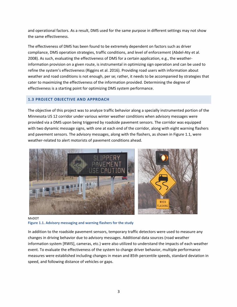
The objective of this project was to analyze traffic behavior along a specially instrumented portion of the
Minnesota US 12 corridor under various winter weather conditions when advisory messages were
provided via a DMS upon being triggered by roadside pavement sensors. The corridor was equipped
with two dynamic message signs, with one at each end of the corridor, along with eight warning flashers
and pavement sensors. The advisory messages, along with the flashers, as shown in Figure 1.1, were
weather-related to alert motorists of pavement conditions ahead.
MnDOT
Figure 1.1. Advisory messaging and warning flashers for the study
In addition to the roadside pavement sensors, temporary traffic detectors were used to measure any
changes in driving behavior due to advisory messages. Additional data sources (road weather
information system [RWIS], cameras, etc.) were also utilized to understand the impacts of each weather
event. To evaluate the effectiveness of the system to change driver behavior, multiple performance
measures were established including changes in mean and 85th percentile speeds, standard deviation in
speed, and following distance of vehicles or gaps.

4
The methodological approach of this project was based on monitoring driver behavior and traffic
performance upstream and within the study corridor. This allowed the researchers to compare driving
behavior metrics, e.g., speed and headway before and after drivers’ exposure to advisory messaging.
Data obtained by this method can be used to quantify changes in driving behavior.
The metrics were then compared during a winter weather event to a baseline condition to isolate
weather-related changes of traffic parameters from the changes caused by other factors such as
roadway geometry. This approach allowed the researchers to account for any natural changes in traffic
parameters, such as speed and volume, and distinguish such changes from those caused by adverse
weather. With this method, the driving behavior of informed and uninformed drivers could be studied
and compared with respect to weather-induced driving decisions.
1.4 REMAINING REPORT CONTENT
The remainder of this report includes four additional chapters before the References and two
appendices after that, as follows:
Chapter 2: Literature Review
Chapter 3: Study Methodology
Chapter 4: Data Analysis
Chapter 5: Conclusions and Future Studies
Appendix A: Summary of Individual Events
Appendix B: Summary of Weather Impacts

5
CHAPTER 2: LITERATURE REVIEW
2.1 OVERVIEW
DMS are one of the most common elements in active traffic management systems that are utilized for
dynamic road traffic management (Boateng et al. 2019). Maximum effectiveness of road warning signs
should possess four features: inclusion of a signal word, description of hazard, warning of consequences,
and directions or instructions (Wogalter 2003). Static signs most often cannot satisfy all of these criteria,
while DMS have the capability of readily accommodating all four features. DMS can be used to convey a
variety of information to road users, including the following:
Local and frequently updated information about inclement weather that may include information
about a small segment of the road or a large area (Rämä 2001).
Information about road and/or traffic conditions such as slippery road, lane closure, road work,
heavy traffic, loose gravel, etc.
Travel information such as distance-time, travel time, and route guidance.
Advisory or regulatory signs/messages that suit the prevailing road and/or weather conditions. For
example, minimum headway, variable speed limits (VLSs) (which are regulatory), and variable
advisory speed (VAS) (Rämä 2001, Boateng et al. 2019, Riggins et al. 2016).
Weather-controlled DMS are being increasingly used by transportation agencies to improve road safety
and mobility by adopting dynamic traffic management approaches tailored in real-time to continuously
changing weather and road conditions. Safety benefits of DMS application, especially under adverse
weather/road conditions, are proven, but the extent of the benefit depends on the degree of driver
compliance with the signs (Boateng et al. 2019). There is a general consensus, driven by evidence from
the existing literature (e.g., Allaby et al. 2006, Abdel-Aty et al. 2008, Hellinga and Mandelzys 2011), that
DMS-enabled messages such as variable speed limits enhance road safety (Hellinga and Mandelzys
2011).
A study for the Finnish National Roads Administration (FinnRA) (Heinijoki 1994) showed that only 14% of
drivers had an accurate perception of road slipperiness, and even a smaller fraction of drivers manage to
maintain safe, sufficiently low speed and proper headway under adverse road conditions (Rämä 2001).
The effectiveness of DMS has been found extremely dependent on factors such as driver compliance,
DMS operation strategies, traffic conditions, and level of enforcement (Abdel-Aty et al. 2008). As such,
evaluating the effectiveness of DMS for a certain application, e.g., the weather-information provision on
a given route, is instrumental in optimizing sign operation. Providing road users with information about
weather and road conditions may not be enough; rather, it is important to maximize the effectiveness of
the information provided. Determining the degree of effectiveness is a starting point for optimizing DMS
performance.
There are numerous current sources of data to investigate traffic performance and evaluate the
effectiveness or influence of DMS (Rämä 2001). Available traffic data sources such as traffic

6
management centers (TMCs), RWISs, vast sensor networks controlled by transportation agencies,
numerous active vendors for traffic data collection, and a variety of commercially available sensors
enable researchers by providing access to large volumes of data. ITS technologies have provided more
effective tools for this purpose and have opened doors to a more promising horizon in information-
enabled road safety improvements (Rämä 2001).
A targeted literature review was performed to identify available performance metrics, data sources, and
data analysis methods to evaluate DMS effectiveness in influencing driver behavior. To this end, the
literature review is organized in the following format:
Influence on Driver Behavior: To successfully evaluate DMS effectiveness, one needs to understand
how DMS influence driver behavior and what factors are involved in the process. This section looks
into existing literature for key factors that should be considered in this regard.
Metrics and data sources to evaluate DMS effectiveness: In this section, performance metrics most
used in the evaluation of DMS and the raw data used for deriving these metrics are identified based
on previous studies.
Data analysis and interpretation approaches: This section describes how to analyze raw data to
derive the metrics and, subsequently, interpret metrics to assess DMS performance. Basing its
discussions on the findings of previous studies, this section also points out important observations,
caveats, practical points, and noteworthy findings pertaining to the application of described
methods and metrics.
Other methods of analysis: For reference purposes, a summary of additional methods that have
been used to evaluate effectiveness are included but were not considered given they do not align
with the scope of this study to evaluate the DMS on US 12.
2.2 INFLUENCE ON DRIVER BEHAVIOR
Three basic elements of driving are driver behavior, road environment, and the vehicle. Safe driving is
achieved when the driver’s behavior and the vehicle, interacting with each other, effectively adapt to
the conditions of the road environment (Rämä 2001, Unrau and Andrey 2006). The fundamental goal of
a DMS is to influence driver behavior by providing real-time information. However, drivers do not
necessarily adjust their driving behavior according to the information they are provided. Assuming
acceptable vehicle performance and a compliant driver, primary reasons why drivers fail to alter their
behavior to the road environment are as follows (Rämä 2001):
Drivers deprioritize safety for other goals
A DMS gives insufficient information
A DMS shows obscure or ineffective information
Drivers receive delayed, insufficient, or no feedback/consequence for their driving behavior
Inadequacies of driving behavior models used for decision making in traffic management

7
Evaluating driver compliance with DMS and how driver behavior is influenced by the sign is an important
part of investigating its effectiveness. On the other hand, optimally designing and operating DMS to
achieve the intended influence on driver behavior requires knowledge about the driver’s perception of
the signs (Banerjee et al. 2020).
Low driver compliance is a major challenge in traffic management and causes an additional source of
uncertainty in road safety analysis. A study on the influence of static speed limit signs on driver behavior
on interstate highways found that the majority of drivers exceeded the speed limit by 8–11 mph, and
35% of drivers who participated in a survey responded that they did not feel safety risk until their speed
exceeds the limit by more than 20 mph (Mannering 2007).
Research has shown higher compliance of drivers to a DMS compared to static signs (Penttinen et al.
1997). It was found that compliance with a DMS can even overshadow drivers’ perception of
appropriate speed. For example, in a study in the Netherlands, a variable speed limit sign displayed on a
DMS displayed a higher speed under foggy road conditions than what drivers would typically choose,
and it was observed that the mean speed increased compared to the same road under similar traffic and
environmental conditions but without the DMS (Hogema and Van Der Horst 1997).
DMS provide an opportunity to impact driver behavior and possibly improve compliance by warning
drivers about adverse road conditions. Rämä (2001) reported a decrease in mean speed by .62–1.24
mph (1–2 km/h) and a smaller standard deviation of speed as a result of displaying slippery road
conditions on a DMS. This study also reported a decrease in the frequency of short headways when a
minimum headway sign was displayed compared to an earlier study on the same test section with only a
variable speed limit sign and slippery road warning sign, where Rämä (1999) had shown no remarkable
influence on headways.
The influence of DMS on driving speed can extend beyond the equipped route onto adjacent routes and
thus affect traffic performance over a large segment of the network. Rämä (1999) observed that
weather-controlled variable speed limit and slippery road condition signs resulted in the reduction of
mean speed on the roads that were accessed via exits within the DMS-equipped section. Rämä (2001),
however, recommended that slippery road condition signs be used with caution and be limited to
critical spots while suggesting that variable speed limits can be used over relatively long road sections.
While DMS have desirable effects on driver behavior and, consequently, on traffic performance and
safety, the degree of effectiveness and type of influence on driver behavior depends on many design
and operational factors. As a result, DMS used for the same purpose in different settings may not show
the same effectiveness. Signs with different types of messages possess different levels of effectiveness
on different groups of drivers and under different conditions (Wang and Cao 2005). Banerjee et al.
(2020) observed this effect in a comprehensive driving simulation study where different types of
messages showed different levels of effectiveness.
Research has found that the necessity of the information shown on a DMS affects how drivers are
influenced by it. In other words, DMS-provided information is more effective when it could not be easily
perceived by drivers on their own.
8
For instance, a case study in Finland (Rämä 2001) found that drivers showed more compliance with a
DMS given information about weather-induced poor road conditions when the conditions were not
obvious. In other words, drivers paid more attention to inclement weather and road condition messages
when they challenged their perception. In agreement with this finding were the results of Zhao et al.’s
survey study (2019), where drivers expressed less favor for DMSs displaying apparent causes of
congestion.
Various design features of the signs are among the factors that influence their effectiveness on driver
behavior. In a study by Rahman et al. (2017), sign content and placement were found not to affect
compliance, while sign frame refresh rate was found to be a significant influencing factor.
Contrary to Rahman et al. (2017), numerous studies (Dudek and Ullman 2002, Ullman et al. 2007, Wang
and Cao 2005, Banerjee et al. 2020) have reported a direct relationship between DMS design
characteristics and sign effectiveness in gaining compliance. Also, the design and color of the messages
influence the DMS’s capability to draw drivers’ attention and affects how drivers perceive or recall the
signs.
For example, a study by Zhao et al. (2019) on driver preference under foggy road conditions suggested
that amber-colored text messages on a black background, white graphs on a blue background, and
single-line route guidance messages were more effective, while text-only messages shown in red or
green on a black background were the least attractive for drivers. It should be noted that this study was
performed at a specific location in China under specific road conditions, while different results may be
obtained in different locations and circumstances.
Based on measured speed-compliance data and a driver-preference survey, Huang and Bai (2019)
suggested that graphics-aided DMSs at work zones were more effective in reducing driver speed, and
that the signs were preferred by drivers. Tay and Choi (2009) found that pictograms may be difficult to
comprehend under certain circumstances, like when incident information is displayed. Rämä (2001),
Luoma and Rämä (1999), and Rämä et al. (1999) suggested that fiber-optic DMS systems were more
effective than electromechanical types, especially when weather information is to be displayed.
Experimental investigations in northern Virginia by Boateng et al. (2019) determined driver compliance
with a VSL sign as 37% and 40% in the downstream and upstream, respectively. Forty-seven percent of
downstream and 51% of upstream interval speeds exceeded the posted speed limit by more than 5 mph
(2.23 m/s). Drivers showed relatively higher compliance when the spacing of signs was smaller. In
agreement with this finding, other research works (Strawderman et al. 2015) have also suggested that
the accumulation of too many consecutive signs related to the same information might reduce sign
effectiveness.
Boateng et al. further concluded that drivers showed higher compliance rates with lower posted speed
limits and attributed it to the restriction of possible speed by the flow of traffic. Higher driver
compliance with lower posted VSLs was also reported in another study (Riggins et al. 2016), where
drivers showed almost full compliance with speed limits of 30 and 35 mph, whereas drivers exceeded
the speed limit by an average of 10 mph when the speed limit was increased to 40, 45, and 50 mph.

9
Driver response to DMS varies by driver familiarity with the sign and the length of time the sign has been
operational in a particular area. This is related to adaptation and novelty effects (Rämä and Kulmala
2000). Drivers who frequent a given route have the chance to adapt to the new signing system, and it
may affect their response to the sign. Also, if a DMS technology is new at the beginning of the
experiment, the effect may change over time as drivers become more familiar with the technology.
Therefore, evaluation results may slightly change over time.
Such variation between the results of experiments in two consecutive years was reported by Rämä and
Kulmala (2000), who observed slightly less effectiveness of a weather-controlled DMS during the second
winter that it was in use. In Fudala and Fontaine’s study (2010) that investigated the impacts of VSLs on
traffic performance, data collection started one month after VSL activation to ensure driver acclamation
with the system.
2.3 METRICS AND DATA SOURCES TO EVALUATE SMS EFFECTIVENESS
All various effects of a DMS on traffic performance and safety depend on its influence on driver behavior
as DMS manage traffic by impacting the driver’s decision-making process. Numerous parameters reflect
the success of a DMS in achieving the intended influence on driver behavior. Due to the extreme
sophistication of human behavioral patterns, the effect of traffic signs on driver behavior is not easily
captured through direct parameters. Therefore, the effectiveness of traffic signs is predominantly
evaluated by investigating the outcomes of the signs’ influence on driver behavior as reflected through a
series of surrogate metrics. Principal categories of metrics and their related parameters to be
investigated in evaluating DMS effectiveness follow. The level of driver compliance with a DMS can be
evaluated using a variety of metrics that are applicable to all different types of signs, including a
regulatory or advisory DMS. Discussions of the most commonly used metrics used for this purpose in the
existing literature follow.
2.3.1 Speed
Speed data provide the primary and most significant metric for evaluating the influence of a DMS on
driver behavior and traffic performance. Various derivatives of speed data such as mean speed over a
segment, lane-based or point-based mean speed, variation of speed among drivers (commonly
represented by the standard deviation of speed), and variation of speeds selected by single drivers may
be used as performance indicators in a DMS-equipped traffic system (Rämä 2001, Hogema and Van Der
Horst 1997, Rämä and Kulmala 2000, Unrau and Andrey 2006, Strawderman et al. 2015).
Speed variation among drivers can have an even more remarkable safety effect than the absolute value
of speed, as speed variation is a major parameter influencing the likelihood of crashes (Unrau and
Andrey 2006, Padget et al. 2001). Variation of speeds selected by single drivers facing a particular
condition, such as a sign, can be used as a variable representative of compliance (Strawderman et al.
2015). Similar to other traffic analysis studies, once sufficient data are collected, descriptive statistics
such as lower and upper quartiles, median, 15th percentile, 85th percentile, etc., are also used as speed
data representatives. The 85th percentile vehicle speed is a very common metric in traffic investigations.

10
2.3.2 Car Following Behavior
Frequency of short headways (Rämä 2001, Rämä and Kulmala 2000), or average physical time gap
between vehicles, can be derived from other traffic characteristic variables that include traffic flow
(volume), average speed, density (occupancy), and vehicle length (or average vehicle length) (Unrau and
Andrey 2006).
2.3.3 Impacts on Traffic Flow Characteristics
The changes made to traffic characteristics such as throughput, congestion, volume, lane occupancy,
and travel time by DMS can be monitored and related to the performance level of a sign (Hellinga and
Mandelzys 2011, Kwon et al. 2007, Unrau and Andrey 2006, Bertini et al. 2015, Papageorgiou et al.
2008).
2.3.4 Capability to Attract Attention and Convey Information
Subjective/qualitative parameters can be collected, including recall, recognition, conception, and
interpretation of signs by drivers (Peeta et al. 2000, Rämä et al. 1999, Rämä and Luoma 1997, Luoma
and Rämä 1999). This information is obtained through reported driver behavior/stated preference.
Objective/quantitative parameters can also be used, such as driver eye movement and its relationship to
measurable driver behavior (e.g., speed compliance). This is especially useful for examining the design
characteristics and placement of a sign.
2.3.5 Safety Impacts
Although not included in this analysis, safety measures can be used to determine the effectiveness of a
DMS, including the frequency of crashes (Kockelman et al. 2006, Strawderman et al. 2015, Bertini et al.
2015) and the severity of crashes (Kockelman et al. 2006). Surrogate safety measures (SSMs) can also be
used in the absence of sufficient crash data. In the case of crashes caused by fog, for example (Peng et
al. 2017), surrogate measures obtained from the data directly measured in a road segment of interest or
using microsimulation software can be used to assess the safety of road facility (Gettman and Head
2003, Savolainen et al. 2010, Bared 2008, Peng et al. 2017). Time to collision (TTC), which estimates the
expected time for two successive vehicles to collide (Tak et al. 2018), is probably the most commonly
used SSM in traffic safety studies, and its correlation with headway and speed variance (Peng et al.
2017) makes it an ideal parameter in DMS evaluation.
2.4 DATA ANALYSIS AND INTERPRETATION APPROACHES
As noted previously, the influence of DMS systems on driver behavior and traffic dynamics can be
studied in a variety of ways, including surveys, traffic modeling, and traffic monitoring at the corridor,
road section, or network levels (Chatterjee et al. 2002). The first step in evaluating the effectiveness of a
DMS or array of them along a given route is to define the hypothesis or hypotheses behind the
motivation of using the system.

11
For example, one may hypothesize that a variable speed limit sign during freezing road conditions
results in higher safety. Then, the parameters for testing the hypothesis/hypotheses are determined and
measured or monitored. In this case/example, two categories of metrics can be studied: resulting road
safety, which can be represented by crash frequency, fatality rate, and severity of injuries, and driver
behavior with respect to safe driving that is referred to as “driver compliance” and can be investigated
by “reported driver behavior” through surveys or indirectly represented by driving metrics such as mean
speed, speed standard deviation, and headway.
Most studies in this regard are before-after experiments (e.g., Rämä and Kulmala 2000, Bertini et al.
2015, Riggins et al. 2016) that monitor the change in certain selected parameters as a result of using the
DMS (Rämä 2001). In adopting a before-after approach, evaluating the effect of a DMS on driver
behavior and traffic calls for either availability of data from before-installation traffic conditions or
conducting measurements over a long enough period of time before operation of the DMS (Hellinga and
Mandelzys 2011).
2.4.1 Statistical Analysis
Statistical analysis of the available data provides insight into the traffic performance and how it is
affected by DMS operation. Speed data are the most important element in investigations pertaining to
traffic signs. A common approach to evaluating the effectiveness of regulatory or advisory signs is
making conclusions based on statistical summaries and inferential statistics drawn from the analysis of
speed data. Depending on the data, different statistical measures can be used to show speed
distribution, e.g., percentage exceeding the speed limit, percentage exceeding the speed limit by certain
values that will be defined based on the data, and different percentiles such as 85th percentile, 50th
percentile, and 25th percentile. The 85th percentile is especially important to evaluate speed variations,
as shown in some previous publications (Vadeby and Forsman 2017).
While descriptive statistics can help understand the data better, evaluating the influence of DMS on
driving behavior and traffic performance requires using inferential statistics and related techniques.
Most commonly used techniques include simple statistical models such as linear regression, t-tests,
ANOVA, and MANOVA; but more advanced techniques such as Bayesian methods, the Tobit [regression]
model, and classification and regression trees may also be used for speed data interpretation (Rämä
1999, Unrau and Andrey 2006, Rahman et al. 2017, Huang and Bai 2019, Kolisetty et al. 2006, Sui and
Young 2014, Debnath et al. 2014).
Different studies have used different inferential statistical methods to investigate the influence of signs
on traffic performance. For example, McMurtry et al. (2009) utilized the F-test and t-test to evaluate the
statistical significance of changes made by VSLs on driving speed through a work zone. The researchers
adopted the average speed and speed variation around the average speed as performance metrics, and
the average speed was preferred as the reference metric over 85th percentile speed because the
average speed was found to be closer to the posted speed.
Brewer et al. (2006) investigated driver compliance with speed limit signs in the work zone by just
considering very basic descriptive statistics, i.e., mean, 85th percentile, and standard deviation of speed.

12
Bai and Li (2011) used ANOVA and two-sample t-tests to evaluate the influence of emergency flasher
traffic control devices on driving speed. In another study, Bai et al. (2010) again used only descriptive
statistics of the speed data and UNIANOVA tests to investigate the degree of effectiveness of temporary
speed-limit signs in work zones.
On the other hand, there are many examples of studies using more advanced analytical methods to
examine speed data. Allpress and Leland (2010) evaluated the effectiveness of obstructive perceptual
countermeasures in reducing speed around work zones by analyzing free-flow speed using one-way
ANOVA and Tukey's range test. Benekohal et al. (2010) utilized multiple statistical analytical methods,
i.e., t-tests, Chi-Square, Kolmogorov-Smirnov tests, and least significant difference in the analysis of
speed data to assess the effectiveness of surveillance-enforced speed limits at work zones. Wang et al.
(2003) analyzed speed data by t-test, Bartlett’s test, ANOVA, and Tukey’s range test. Debnath et al.
(2014) used the Tobit regression technique in analyzing speed data to account for both magnitude and
probability of non-compliance. The objective of speed data analysis is to assess either traffic
performance or driver compliance; in either case, there are generally no limits on using any analytical
method that serves the purpose.
2.4.2 Data Interpretation to Evaluate Sign Effectiveness and Driver Compliance
2.4.2.1 Mean Speed and Short Headway Frequency as Performance Indicators
Driver behavior, especially at the road section level, is typically monitored before and after signs by
establishing an adequate number of upstream and downstream measurement stations. An after-
installation driver behavior investigation was used by Rämä and Kulmala (2000) where three loop
detector traffic monitoring stations measuring speed and headway were used. The first loop detector
was placed upstream of the messaging and the two additional loop detectors were placed downstream.
With this approach taken by Rämä and Kulmala (2000), signs were installed so that they were seen by
drivers in only one traffic direction and the other direction was assumed as the control section. In
addition, driver behavior at the upstream station was considered as baseline behavior where the
difference from downstream driving behavior represented the effect from the DMS. Integrating the
factors of location, direction, and DMS existence, the researchers compared the speeds in the
experimental direction with the difference in speed in the control direction. The difference represented
the change in mean speed for the experimental direction. The value was compared before and after the
DMS was installed to obtain the DMS effectiveness on changing mean speed.
Note that if mean speed is obtained through data aggregation, mean values should be weighted based
on the number of observations during each respective data collection session. When mean speeds are
measured continuously over a given period, there is no need for weighting the results.
In the same study (Rämä and Kulmala 2000), short headways were considered as headways shorter or
equal to 1.5 seconds, and instead of all headways, only the headways equal to or smaller than 5 seconds
were considered in calculations. They used the proportion of short headways, i.e., those equal to or
smaller than 1.5 seconds, in a log-linear model to theorize the effect of the DMS on driver-following
behavior.

13
In this study, statistical analyses were used to assess the distribution of measurements and significance
of effects, and p-values obtained from the t-test were used to evaluate the significance of effects with a
95% confidence interval.
2.4.2.2 Quantifying and Formulating Driver Compliance Using Speed Data
A study evaluating the effect of VSLs on driver behavior was performed on I-66 in northern Virginia. In
this project, Boateng et al. (2019) studied driver compliance with VSLs shown on DMSs by measuring
traffic speeds in 28 segments, referred to as traffic message channels, along I-66. Each DMS was located
between two traffic message channels, with one upstream and one downstream. Data obtained from
any segment between two consecutive DMSs that was shorter than 0.2 miles were excluded from the
analysis.
As noted for this study, when average speed is measured along a segment of the road, the length of the
segment should be long enough to make sure that the results are not affected by highly localized effects
of road geometry and features such as exit ramps. Additionally, when speed data are collected through
discrete measurement points (i.e., data from point sensors) it is advisable not to use one measurement
station. In any case, whether one or more stations are used, the location of the measurement stations
should be selected with caution.
Boateng et al. (2019) collected both probe and roadside radar sensor (point sensor) data for DMS
performance evaluation and reported some daunting problems when using point sensor data. The radar
sensors in this study considerably undercounted traffic volume during congestion. As a result, the traffic
speed-flow curves developed with point sensor data were unrealistic and did not represent the real
characteristics of the traffic. Due to this problem, the sensor data could not be used for traffic speed-
flow analysis, and Boateng et al. gave priority to probe data. The main parameters derived from the
speed data were as follows:
Distribution of observed average speed viz-a-viz posted speeds
Percentage of observed speeds lower than posted speed
Average difference between posted and observed speed
These parameters were used to evaluate the level of driver compliance with VSL, as with the example
shown in Table 2.1.

14
Table 2.1. Driver compliance evaluation based on the average difference of observed and posted speeds
Seg
men
t
Location
of VSL
Distance
(mph)
Posted Variable Speed Limits
(mph) Legend
35.0–
39.9
40.0–
44.9
45.0–
49.9 50
VSL3 0.39 -14.1 -7.4 5.1 10.5 -17.4 Higher Compliance
Level
VSL4 0.39 -5.1 2.1 11.5 11.3 -14.5
VSL1 0.52 -1.1 2 5.6 8.4 -11.6
VSL5 0.74 -9.8 -5.3 5 7.4 -8.7
VSL6 0.93 -7 -1.2 0.8 7 -5.8
VSL7 1.04 -8.3 -4.9 2.5 4.9 -2.9
VSL8 1.05 6.2 8.3 6.5 7.3 0
Highest
Non Compliance
VSL9 1.13 -4.3 1.9 5.5 7.6 2.9
VSL10 1.19 -3.7 -2 0.6 2.9 5.8
VSL11 1.27 4.5 3 2.9 2.9 8.7
VSL2 1.38 -8.7 -6.5 -0.9 5.4 11.6
Source: Boateng et al. 2019
As seen in the study, the different variables that are derived from the difference between driving speed
and posted speed can be used to represent driver compliance with speed-related regulatory or advisory
signs. Many studies, such as Boateng et al. (2019), Riggins et al. (2016), Strawderman et al. (2015),
Bertini et al. (2015), McMurtry et al. (2009), and Buddemeyer (2009), have used this type of variable to
quantify driver compliance.
In a study in Western Australia to evaluate driver compliance with static speed limit signs (Giles 2004),
point sensor data from more than three million free-flow vehicles were collected and driver compliance
was quantified in a very simple way by calculating percentage of drivers above the posted speed limit. A
similar approach was adopted by McMurtry et al. (2009) to quantify driver compliance levels secured by
static and variable speed limit signs, as shown in Figure 2.1.
McMurtry et al. 2009
Figure 2.1. Compliance with static and variable speed limit signs represented by hourly average speed

15
Riggins et al. (2016) used the arithmetic difference between posted speed and driving speed as the sole
variable quantifying driver compliance, as shown in Figure 2.2.
© 2016 Riggins et al. 2016
Figure 2.2. Driver compliance with variable advisory speed DMS on OR 217: (a) driving speed, (b) displayed speed, and (c) compliance
Figure 2.2 presents an analysis of the speed data collected northbound on Oregon Route (OR) 217 in a
single day. As seen in the figure, the approach adopted by Riggins et al. (2016) developed a time-space-

16
speed plot, in which the difference between posted VAS and driving speed was visualized using color
coding.
In Figure 2.2 (a) and (b), colors show the value of driving and posted speed, respectively. Figure 2.2 (c)
shows driver compliance with VAS, calculated as the arithmetic difference between driving speed and
posted speed. According to this definition, drivers have complied with the sign when the driving speed is
less than the posted speed. As simple as this definition sounds, it is a very useful tool for evaluating and
visualizing the effectiveness of the signs, i.e., driver compliance, for example, through compliance
histograms, as shown in Figure 2.3.
© 2016 Riggins et al. 2016
Figure 2.3. Driver compliance with variable advisory speed DMS northbound on OR 217 based on one-day data
Kwon et al. (2007) provided a notable speed-based formulation of driver compliance with speed limit
signs. The study evaluated the effectiveness of a two-sign speed-limit system consisting of a static and a
dynamic advisory speed limit sign for improving safety at a work zone as illustrated in Figure 2.4.
Kwon et al. 2007
Figure 2.4. Layout of the advisory speed limit sign system used by Kwon et al.

17
In this approach, actual driving speed is measured by point sensors in the upstream and downstream of
the DMS.
Based on the approach used by Kwon et al. and assuming there is some level of compliance with signs
(i.e., downstream speed < upstream speed), driver compliance level with a given advisory or regulatory
speed limit sign can be defined as follows:
𝐶𝑜𝑚𝑝𝑙𝑖𝑎𝑛𝑐𝑒 𝐿𝑒𝑣𝑒𝑙 = |𝐷𝑜𝑤𝑛𝑠𝑡𝑟𝑒𝑎𝑚 𝑆𝑝𝑒𝑒𝑑 − 𝑃𝑜𝑠𝑡𝑒𝑑 𝑆𝑝𝑒𝑒𝑑
𝑈𝑝𝑠𝑡𝑟𝑒𝑎𝑚 𝑆𝑝𝑒𝑒𝑑 − 𝑃𝑜𝑠𝑡𝑒𝑑 𝑆𝑝𝑒𝑒𝑑| , 𝑈𝑝𝑠𝑡𝑟𝑒𝑎𝑚 𝑆𝑝𝑒𝑒𝑑 ≠ Posted Speed
2.4.2.3 Speed Variation as an Indicator of Safety Performance
Speed variation across drivers is a more important parameter in safety-related studies because crashes,
especially in inclement weather, are primarily driven by the speed difference between vehicles (Unrau
and Andrey 2006, Padget et al. 2001). Rämä and Kulmala (2000) recorded a decrease in mean speed as a
result of a slippery road condition sign (displayed on a DMS) that was .62–1.24 mph (1–2 km/h) more
than the speed decrease by inclement weather in the absence of the DMS.
In another study, by Kwon et al. (2007), speed variation was used as a metric of the effectiveness of VAS
shown on a DMS within a work zone. Kwon et al. derived speed variation patterns determining the
maximum speed difference within the work zone during the morning peak periods on selected days
before and after activation of the DMS. For this purpose, the researchers analyzed all speed
measurements collected by detectors within the work zone during the peak hour (6:00–7:00 a.m.). A
maximum speed difference was calculated for each one-minute interval during the peak hour of each
day, and the average of these one-minute maximum differences was presented as the average max
speed difference of the day, as shown in Figure 2.5.
Data from March 16th was discarded because of adverse weather conditions Kwon et al. 2007
Figure 2.5. Average maximum speed difference comparison

18
It is apparent from the figure that the average maximum speed difference was reduced after the
activation of the DMS.
In addition to speed variation across vehicles in the same road segment, the speed difference between
the upstream and downstream of a given sign has significant safety importance (Mekker et al. 2016).
Therefore, it is strongly recommended that this parameter is in some way accounted for in data
collection activities associated with evaluating a DMS. This can involve, for instance, collecting speed
data from both upstream and downstream at all studied time intervals.
2.5 OTHER METRICS AND METHODS OF ANALYSIS
The literature documents various other methods for evaluating the impacts of DMS messaging that were
not considered as part of this evaluation. This included using driving and traffic simulators, tracking the
activities of driver’s vision, and driver surveys.
2.5.1 Traffic Flow Characteristics as an Indicator of Sign Effectiveness
Traffic flow characteristics such as vehicle count over a given time interval (e.g., 20 seconds) (Unrau and
Andrey 2006), flow-occupancy (Papageorgiou 2008), travel time (average travel time), travel time
reliability (especially during peak hours) (Bertini et al. 2015), bottleneck pattern (Bertini et al. 2015), by-
lane traffic volume, and total route volume throughput are parameters that can be used to investigate
the influence of signs on traffic performance (Hellinga and Mandelzys 2011, Kwon et al. 2007). These are
primarily aligned with DMS with route guidance and variable speed limits.
2.5.2 Accounting for Weather-Related Factors
Studies have investigated the influence and optimal design of different types of DMSs on driver behavior
and traffic performance under adverse weather conditions (Downey and Bertini 2015, Hassan et al.
2012, Allaby et al. 2006, Riggins et al. 2016, Zhao et al. 2019, Kolisetty et al. 2006, Rämä and Kulmala
2000). The general approach has been to measure traffic performance parameters such as traffic flow,
accident frequency, driving speed, speed variation, and driver compliance under inclement weather or
road conditions in a before-after study scheme and to develop a model to account for those impacts.
According to Downey and Bertini (2015), precipitation was a sole representative of weather conditions
and divided the data into two categories of wet and dry days. The findings from this study highlights the
need to consider weather conditions as one of the study variables and evaluate sign effectiveness in
influencing driver behavior in relation to weather-defining parameters.
One of the comprehensive studies in this regard was performed by Sui and Young (2014) to evaluate the
performance of a DMS system operated by the Wyoming DOT (WYDOT) along a rural segment of I-80 in
southeastern Wyoming. This study stands out in that it examined DMS influence under variable weather
conditions, unlike preceding studies that mainly focused on more predictable, binary weather scenarios.
In that, Sui and Young (2014) introduced three variables, DMS message, weather, and vehicle speed,

19
into the analyses and isolated DMS speed reduction effects from natural slowing due to weather
conditions.
2.5.3 Surveys: Stated Preference, Revealed Preference, and Reported Driver Behavior
Surveys are a very common way of evaluating DMS characteristics and investigating the influence of
DMSs on driver behavior. Such studies can provide subjective information about the effectiveness of the
DMS and are typically used when technology is relatively new and in its early stages of deployment.
Surveys are an excellent and dominant source of information to support the process of designing DMSs
(Chatterjee et al. 2002).
2.5.4 Traffic Microsimulation
Traffic modeling offers a higher degree of flexibility with respect to transferring data across stations and
defining baseline behavior/performance (Chatterjee et al. 2002). Early studies on model-based VMS
performance evaluation based their models on the CONTRAM dynamic traffic assignment model
developed by Leonard et al. (1989). Examples are MCONTRAM (White et al. 1994) and RGCONTRAM
models (McDonald et al. 1995). At present, new high-fidelity traffic simulation software such as VISSIM,
PARAMICS, AIMSUN, SUMO, TEXAS, CORSIM, MovSim, TraffSim, and PointQ are available that can be
used to investigate the influence of DMSs on traffic flow and safety.
2.5.5 Driving Simulators
High-fidelity driving simulator software, especially when coupled with the appropriate hardware, can be
used to evaluate the effectiveness or driver acceptance of DMS with different structures and message
types under different road and traffic conditions (Banerjee et al. 2020). In driving simulator settings, in
addition to driving performance parameters such as speed selection, route selection, lane change, and
car-following behaviors, physical and physiological reactions of the driver such as eye movement, heart
rate, sleepiness, and attention can be readily measured and recorded (Kolisetty et al. 2006). Driving
simulators may be on-screen, such as that shown in Figure 2.6 (left) (Banerjee et al. 2020, Zhao et al.
1995) or full-scale, such as the Missouri Science and Technology (S&T) driving simulator (Bham et al.
2014) (Figure 2.6 (right)).
Banerjee et al. 2020 (left) and Bham 2014 (right)
Figure 2.6. On-screen and full-scale driving simulators

20
CHAPTER 3: STUDY METHODOLOGY
3.1 DATA METRICS
After a thorough literature review, the research team proposed the following data metrics for analysis of
the impacts that the US 12 DMS system had on driver behavior during 2020–21 winter weather events.
Considering the data availability and the intended application of this project, not all of the metrics, as
identified in Section 2.5, were applicable to this project or would serve the purpose of this study. The
metrics used for evaluating the performance of weather-based DMS messaging along the US 12 corridor
between Delano and Maple Plain, Minnesota, follow.
Speed: The speed data were collected by deploying temporary sensors upstream and downstream of
the dynamic message signs, providing the capability to collect individual vehicle speeds. The individual
vehicle speed data were aggregated every five minutes to calculate the mean speed, 85th percentile
speed, and standard deviation.
Vehicle following behavior: Data for each individual vehicle collected also included the headway, i.e.,
gap between the following vehicle and the rear of the leading vehicle. Similar to speed data, the
headway data were aggregated every five minutes to calculate the average gap as well as the
percentage of vehicles with a gap less than 1.5 seconds and less than 10 seconds. Unlike speed, the
vehicle-following performance metric is only valid for vehicles that were following another vehicle and
had the driver adjust their driving behavior to increase or decrease the gap between their vehicles
during a winter weather event. Data for any vehicle not following another vehicle was removed to avoid
influencing the intent of this metric. Given this, data for any vehicle with a gap greater than 10 seconds
was removed from the average gap calculations.
Traffic flow characteristics: Traffic sensors were used to collect the vehicle counts to calculate traffic
flow parameters.
3.2 DATA SOURCES AND DATA COLLECTION
3.2.1 Traffic Sensors
Traffic sensors were the primary source of data for the analyses along the study corridor. The data from
the sensors were used to compare the performance metrics upstream and downstream of the DMS
along the corridor. The upstream sensors served as the control location with no DMS messaging, while
the downstream sensors were placed at a location potentially influenced by DMS messaging. Figure 3.1
shows the locations of the temporary traffic sensors as well as all other devices included in the analysis
along the US 12 corridor.

21
Map image © 2021 ESRI
Figure 3.1. Existing and proposed temporary devices along the US 12 corridor
The markers on the map include permanent devices (DMS and friction sensors) along with the locations
of the temporary sensors that were used to collect individual vehicle data.
Five permanent sensors were available along the corridor but were not used in the analysis because of
the lack of an upstream sensor. Additionally, the aggregation of the data every one minute limited the
performance metrics that could be utilized from the permanent sensors. Alternatively, temporary
sensors were installed to collect individual vehicle data.
The temporary sensor locations were selected to represent similar roadway characteristics as much as
possible upstream and downstream of the DMS. The temporary sensors were placed to avoid any
influence from the urban areas before and after the cities of Delano and Maple Plain. A major
assumption with this approach was that similar traffic data would be collected at both sensors, and the
effects of the DMS would be present once vehicles returned to rural driving speeds after traveling
through the urban areas. This assumption aligned with the intention of the system to affect driver
behavior through the corridor outside of the urban areas.
The green sensor icons in Figure 3.1 represent the upstream sensors receiving no winter weather
messages from the DMS. The upstream sensor was 2.9 miles before the DMS in the eastbound direction
and 1.9 miles before the DMS in the westbound direction. The orange sensor icons represent the
downstream sensors, which were 1.2 miles downstream from the eastbound DMS and 2.0 miles
downstream from the westbound DMS.
Although there was a significant distance between the downstream sensor and DMS, it was assumed
that all vehicles at the downstream sensor viewed the winter weather messaging. Of note at this
location is that the downstream sensor is a considerable distance after the DMS. Multiple intersections

22
and centerline/median barriers are also present along this portion of the corridor that may affect vehicle
speeds.
In the eastbound direction, there are no major side roads generating traffic, which means all vehicles
should have passed the DMS. In the westbound direction, the DMS was located before the signalized
intersection of County Road (CR) 83 in Maple Plain and then also passes CR 90 before the traffic sensor.
Both of these intersections are located within the urban area of Maple Plain and may add additional
vehicles at the downstream sensor that did not pass the DMS and, thus, did not have drivers who
observed the message. Of note, the drivers from these two intersections would have observed the
flashing beacons shown previously in Figure 1.1 before passing the downstream sensor.
3.2.2 Dynamic Message Signs
The two DMSs used for winter weather messaging were located at each end of the corridor and in urban
environments in close proximity to an intersection, as shown in Figure 3.2.
Map image © 2021 ESRI
Figure 3.2. DMS locations along US 12 corridor
This study setup does not represent ideal conditions given multiple other influences in the urban area,
including intersections, roadway geometry, barriers, etc. The research team attempted to minimize or at
least identify the effects of non-DMS and non-weather factors in the final conclusions as much as
possible using appropriate measures in the data analysis.
To identify the messaging being displayed to drivers, the research team utilized the DMS archive. These
data include the message posted on each DMS and the start and end times when the message was
active. The DMS in Maple Plain displayed messaging for westbound traffic, while the DMS at the east of
Delano provided messaging for eastbound traffic.
3.2.3 Cameras
In addition to the sensors, traffic cameras were also utilized to visually confirm the winter weather and
control events. The cameras were used to identify any crashes or other impacts to traffic that should be
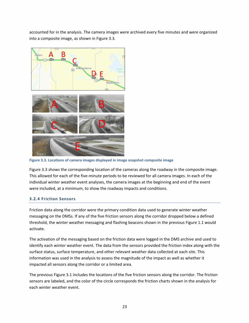
23
accounted for in the analysis. The camera images were archived every five minutes and were organized
into a composite image, as shown in Figure 3.3.
Figure 3.3. Locations of camera images displayed in image snapshot composite image
Figure 3.3 shows the corresponding location of the cameras along the roadway in the composite image.
This allowed for each of the five-minute periods to be reviewed for all camera images. In each of the
individual winter weather event analyses, the camera images at the beginning and end of the event
were included, at a minimum, to show the roadway impacts and conditions.
3.2.4 Friction Sensors
Friction data along the corridor were the primary condition data used to generate winter weather
messaging on the DMSs. If any of the five friction sensors along the corridor dropped below a defined
threshold, the winter weather messaging and flashing beacons shown in the previous Figure 1.1 would
activate.
The activation of the messaging based on the friction data were logged in the DMS archive and used to
identify each winter weather event. The data from the sensors provided the friction index along with the
surface status, surface temperature, and other relevant weather data collected at each site. This
information was used in the analysis to assess the magnitude of the impact as well as whether it
impacted all sensors along the corridor or a limited area.
The previous Figure 3.1 includes the locations of the five friction sensors along the corridor. The friction
sensors are labeled, and the color of the circle corresponds the friction charts shown in the analysis for
each winter weather event.

24
3.2.5 RWIS Sensors
RWIS data were used in the analysis as confirmation of the winter weather event as well as to
understand the meteorological conditions leading up to and during the winter weather event. The
nearest RWIS site was TH 7 @ MP 167.1 (Mayer) (330022), which is located about 12 miles southwest of
the study corridor. This RWIS site was utilized for several reasons, including its proximity to the study
corridor, its variety of sensors, and the corresponding reporting intervals of the sensors.
It was assumed that the conditions at this RWIS site would be generally similar to those along the study
corridor due to the close proximity, although times and precipitation intensities, for example, may differ.
The primary metrics used from the RWIS site included one-hour precipitation accumulation,
precipitation presence, wind speed, and temperature.
3.2.6 Probe Data
Probe data were another valuable data source that could be utilized for understanding the impacts that
the winter weather messaging had on vehicle speeds along the corridor. MnDOT uses HERE for their
probe data provider and the Iteris ClearGuide analytics platform to access the probe data. Using Iteris
ClearGuide, individual routes could be selected to identify segments before and after the DMSs.
Probe data were considered as an auxiliary to the sensor data on a limited basis because only speed-
related performance metrics could be accessed. However, after initial analyses, it was decided not to
use the probe data in the final analysis primarily because the probe data were sparse and did not
provide statistically meaningful results. Furthermore, the number of vehicles used to collect the probe
data was unknown, which introduces uncertainty compared to the sensor data collection of individual
vehicle data.
3.3 WINTER WEATHER EVENTS
Winter weather events were identified based on the activation of the DMS messaging. Because the two
DMSs at each end of the corridor used the same logic, the messaging was comparable with the
exception of manual messages that were posted by MnDOT staff about amber alerts or maintenance
activities.
The start of an event was identified based on when the first winter weather message was posted, and
the end of the event was identified when the winter weather message was removed. The duration of
winter weather messaging ranged from 214 minutes to 7,026 minutes (~6.7 days). In total, 16 winter
weather events were analyzed during the 2020–21 winter season, while two of the events were later
excluded from the final analysis. A list of winter weather events analyzed is shown in Table 3.1.
Table 3.1. Summary of winter weather events with messaging
Event Event Start Event End Duration (minutes)
1 12/13/2020 12:51 12/13/2020 17:12 270
2 12/23/2020 11:57 12/28/2020 9:03 7,026
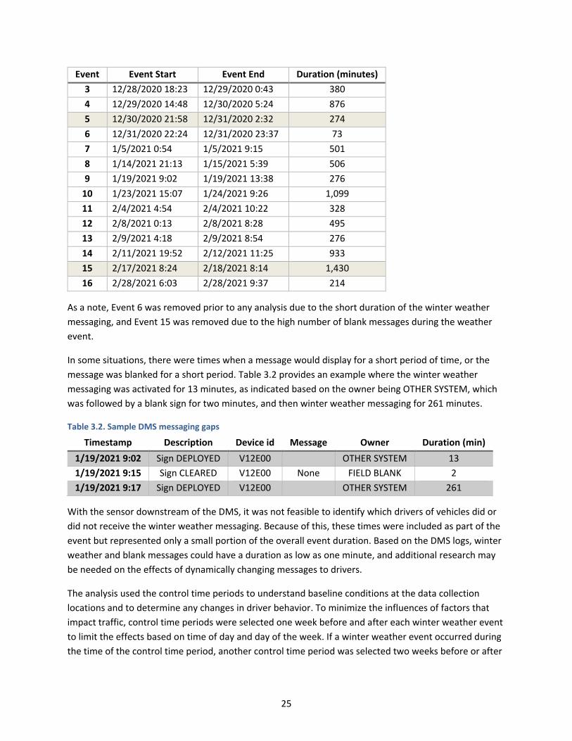
25
Event Event Start Event End Duration (minutes)
3 12/28/2020 18:23 12/29/2020 0:43 380
4 12/29/2020 14:48 12/30/2020 5:24 876
5 12/30/2020 21:58 12/31/2020 2:32 274
6 12/31/2020 22:24 12/31/2020 23:37 73
7 1/5/2021 0:54 1/5/2021 9:15 501
8 1/14/2021 21:13 1/15/2021 5:39 506
9 1/19/2021 9:02 1/19/2021 13:38 276
10 1/23/2021 15:07 1/24/2021 9:26 1,099
11 2/4/2021 4:54 2/4/2021 10:22 328
12 2/8/2021 0:13 2/8/2021 8:28 495
13 2/9/2021 4:18 2/9/2021 8:54 276
14 2/11/2021 19:52 2/12/2021 11:25 933
15 2/17/2021 8:24 2/18/2021 8:14 1,430
16 2/28/2021 6:03 2/28/2021 9:37 214
As a note, Event 6 was removed prior to any analysis due to the short duration of the winter weather
messaging, and Event 15 was removed due to the high number of blank messages during the weather
event.
In some situations, there were times when a message would display for a short period of time, or the
message was blanked for a short period. Table 3.2 provides an example where the winter weather
messaging was activated for 13 minutes, as indicated based on the owner being OTHER SYSTEM, which
was followed by a blank sign for two minutes, and then winter weather messaging for 261 minutes.
Table 3.2. Sample DMS messaging gaps
Timestamp Description Device id Message Owner Duration (min)
1/19/2021 9:02 Sign DEPLOYED V12E00
OTHER SYSTEM 13
1/19/2021 9:15 Sign CLEARED V12E00 None FIELD BLANK 2
1/19/2021 9:17 Sign DEPLOYED V12E00
OTHER SYSTEM 261
With the sensor downstream of the DMS, it was not feasible to identify which drivers of vehicles did or
did not receive the winter weather messaging. Because of this, these times were included as part of the
event but represented only a small portion of the overall event duration. Based on the DMS logs, winter
weather and blank messages could have a duration as low as one minute, and additional research may
be needed on the effects of dynamically changing messages to drivers.
The analysis used the control time periods to understand baseline conditions at the data collection
locations and to determine any changes in driver behavior. To minimize the influences of factors that
impact traffic, control time periods were selected one week before and after each winter weather event
to limit the effects based on time of day and day of the week. If a winter weather event occurred during
the time of the control time period, another control time period was selected two weeks before or after

26
the winter weather event. All of the corresponding control time periods for the winter weather events
are shown in Table 3.3.
Table 3.3. Summary of control time periods for winter weather events
Event Control Start Control End Duration (minutes)
1 12/20/2020 12:51 12/20/2020 17:12 270
2 12/9/2020 11:57 12/9/2020 23:57 720
2 12/16/2020 11:57 12/21/2020 9:03 7,026
3 12/14/2020 18:23 12/15/2020 0:43 380
3 12/21/2020 18:23 12/22/2020 0:43 380
4 12/15/2020 14:48 12/16/2020 5:24 876
4 12/22/2020 14:48 12/23/2020 5:24 876
5 12/16/2020 21:58 12/17/2020 2:32 274
5 1/6/2021 21:58 1/7/2021 2:32 274
7 12/22/2020 0:54 12/22/2020 9:15 501
7 1/12/2021 0:54 1/12/2021 9:15 501
7 1/26/2021 0:54 1/26/2021 9:15 501
8 1/7/2021 21:13 1/8/2021 5:39 506
8 1/21/2021 21:13 1/22/2021 5:39 506
9 1/12/2021 9:02 1/12/2021 13:38 276
9 1/26/2021 9:02 1/26/2021 13:38 276
10 1/16/2021 15:07 1/17/2021 9:26 1,099
10 1/30/2021 15:07 1/31/2021 9:26 1,099
11 1/21/2021 4:54 1/21/2021 10:22 328
11 1/28/2021 4:54 1/28/2021 10:22 328
12 2/1/2021 0:13 2/1/2021 8:28 495
12 2/15/2021 0:13 2/15/2021 8:28 495
13 2/2/2021 4:18 2/2/2021 8:54 276
13 2/16/2021 4:18 2/16/2021 8:54 276
14 2/18/2021 19:52 2/19/2021 11:25 933
14 2/25/2021 19:52 2/26/2021 11:25 933
15 3/3/2021 8:24 3/4/2021 8:14 1,430
15 2/24/2021 8:24 2/25/2021 8:14 1,430
16 3/14/2021 6:03 3/14/2021 9:37 214
16 3/7/2021 6:03 3/7/2021 9:37 214
3.4 ANALYSIS APPROACH
To analyze the effectiveness of the DMS on changing driver behavior, the aforementioned metrics were
evaluated for individual winter weather events by direction of travel, comparing the data from the
sensor upstream of the DMS with the sensor downstream of the DMS. After analyzing each event, an

27
overall analysis was completed combining all events together for each direction of travel. The upstream
sensor served as the control condition where drivers were not provided with any weather-related
messaging, while at the downstream sensor, drivers were provided with winter weather-related
messaging from the DMS. In addition to the winter weather event, control time periods were also
utilized to determine the baseline differences in speed between the downstream and upstream sensors
where no winter weather messaging was provided at either location. To this end, a representative time
period before and after each event was selected as the baseline period for the respective event as
described in the previous section.
The same process of data collection and metric calculation was conducted for the control time periods,
which represent similar traffic characteristics when no winter weather events occurred. As noted
previously, the locations of the sensors were selected to control for roadway characteristics. However,
due to the distance between the sensors and slight changes in roadway characteristics, the performance
measures were not exactly the same during non-winter weather events, which is why a baseline was
needed. Having this baseline allowed for statistical differences in the performance metrics to be
identified, and specifically whether they were statistically different from the control conditions with no
winter weather.
The data from both sensors were filtered to only include times when a message was displayed on the
DMS. Additionally, any times with anomalies, such as a crash, were removed to avoid external influences
beyond the DMS. These filtered and cleaned data were then used to extract the metrics at both
upstream and downstream locations during comparable road conditions.
Descriptive statistics were derived, and statistical tests were conducted to determine any changes at the
downstream sensor that might be attributed to the DMS messaging received by the drivers. The data
from each direction (eastbound and westbound) were treated and analyzed to compare the difference
between the upstream and downstream metrics every five minutes, and then compared to the results
between the baseline time period and the winter weather event time period.
3.4.1 Data Analysis
The differential data analysis compared the difference in the parameters during each time period by
aggregating the data every five minutes and calculating the difference between the upstream and
downstream sensor for each respective time period. The difference between the upstream and
downstream was then compared between the time periods to determine any statistically significant
changes in metrics.
Assessing the influence of each DMS on driving behavior involves the winter weather event as well as
the baseline periods. The effect of the DMS during each time period is manifested in the change of
metrics from upstream to downstream. Comparing this effect between the study and control periods
can indicate whether the DMS exerted a statistically significant influence on driving behavior. Therefore,
the study variables were defined such that they allowed investigation of the changes of metrics on both
spatial (i.e., from upstream to downstream) and temporal (i.e., event and baseline period) bases, using

28
the same data sets. To this end, the aforementioned metrics were calculated for each five-minute
aggregation at both the upstream and downstream sensors.
For each metric of interest (Xagg), i.e., mean speed, the standard deviation of speed, 85th percentile
speed, and gap, two separate data sets were built that contained the five-minute-aggregated values of
that metric at upstream and downstream locations, denoted by Xaggup and Xagg
dwn,, respectively. Then, an
auxiliary variable was defined as Va= (Xaggdwn - Xagg
up) to quantify the change of each given metric from
upstream to downstream.
In defining Va, it was assumed that similar drivers were present both upstream and downstream during
each of the five-minute aggregations. The difference between downstream and upstream metrics was
calculated for each individual five-minute aggregation to determine any changes in the metrics from the
DMS messaging. For example, if the average speed for a five-minute period was 57 mph upstream and
53 mph downstream, the mean speed difference for that time period would be -4 mph given the
downstream sensor showed 4 mph lower than the upstream sensor. This example is visually shown in
Figure 3.4.
Figure 3.4. Example showing the calculations for calculating speed difference
Variable Va was calculated once for the study period (i.e., during DMS operation) and once for the
control period (i.e., the baseline), giving us two versions of Va, denoted by V1 and V2, as follows:
V1=(Va)Study
V2=(Va)Control
Using V1 and V2, another variable, V3, was defined to quantify how the winter weather time period
differed from the control period with respect to the metric change regime from upstream to
downstream, as follows:
V3 = V2-V1

29
In evaluating the data, the distribution of the differences between the downstream and upstream
aggregations during the study and control time periods were compared. Changes in the distribution
could indicate whether the DMS messaging had an impact on driver behavior, i.e., if the study
distribution shifted in comparison to that for the control time periods. Figure 3.5 shows a summary of
the four metrics and the desired shift in study time period distribution as compared to the control time
periods.
Figure 3.5. Summary of statistical analysis changes in differential comparison
A shift to the left in the distribution of the mean speed difference, 85th percentile speed difference, and
standard deviation difference between downstream and upstream during the winter weather study
period indicated that speeds were slower or the standard deviation was lower, resulting in uniform
speeds, which were desirable results for the winter weather messaging. A shift to the right in the
distribution of the average vehicle gap difference during the study period indicated that gaps were
increasing, which would be a desirable result for the winter weather messaging.
>= 0 < 0 >= 0 < 0
Undesirable change in speed regime Desirable change in speed regime
Undesirable change in speed regime Desirable change in speed regime
Undesirable change in Speed variation
(Stdev)
Desirable change in Speed variation
(Stdev)
Desirable change in Gap acceptance Undesirable change in Gap acceptance
85th Percentile
Speed
V1 and V2 V3
Gap
Speed increased or
unchanged from
upstream to
downstream
Speed Reduced from
upstream to
downstream
Speed increased or
unchanged from
upstream to
downstream
Speed Reduced from
upstream to
downstream
Speed variation (Stdev)
increased or
unchanged from
upstream to
downstream
Speed variation
(Stdev) Reduced from
upstream to
downstream
Gap increased or
unchanged from
upstream to
downstream
Gap reduced from
upstream to
downstream
Standard
Deviation
Change of Driving Behavior
from Upstream to Downstream Significance tests and charts
Xagg
Speed
control Study
5-min average speed
Study Control
5-min average speed
Study Control
85th percentile speed
control Study
85th percentile speed
control Study
Stdev. of speed
Study Control
Stdev. of speed
control Study
Gap
Study
Gap

30
CHAPTER 4: DATA ANALYSIS
4.1 INTRODUCTION
The data items and analysis approach described in Chapter 3 were employed to analyze 14 winter
weather events during the 2020–21 winter season. The initial analyses were performed on 16 events,
but it was later decided to exclude Event 6 and 15 from the analysis to maintain data consistency and
reliability; therefore, the final conclusions were made based on the analyses from 14 events. Event 6
was excluded because of its short duration and data sparsity during the event. Event 15 was excluded
because there were too many DMS blank messaging periods during the event.
Sections 4.2 through 4.4 of this chapter present the detailed analysis results obtained from the two
approaches described in Chapter 3 (Section 3.4) for three selected individual events: 3, 9, and 11. The
three individual events represent a sampling of the individual event analysis and a cross section of the
various winter weather impacts experienced along the corridor.
In the sensor data analysis summary tables for these events, different types of changes (or effects) are
highlighted with different colors. The green shading indicates a statistically significant and desirable
change, the yellow shading indicates statistically non-significant changes, and the red shading indicates
statistically significant but undesirable changes.
The first event (Event 3) shows the impact of a winter weather event that had minimal impacts and no
accumulation of precipitation; the second event (Event 9) shows a typical winter weather event with
precipitation accumulation; and the final event (Event 11) shows a significant winter weather event with
a large amount of snow accumulation. The remaining individual event analysis summary tables are
available in Appendix A.
Section 4.5 contains the analysis results for all studied events in comparative and combined manners.
Section 4.6 provides additional discussion on the analysis results.
4.2 WINTER WEATHER EVENT 3
4.2.1 Description of Event 3
Winter weather Event 3 lasted 380 minutes, starting on December 28, 2020. This event represents a
minor winter weather event where no precipitation was indicated by the RWIS and only minimal
impacts were seen to the friction triggering the winter weather messaging. The winter weather
messaging on the DMS did have 39 minutes where the message was blank, primarily at the end of the
event. Over the last hour of the event, the message was blanked nine different times for between one
to eight minutes. Figure 4.1 shows the traffic camera images at the beginning and end of the event.

31
Figure 4.1. Event 3 at the start of the event (left) and end of the event (right)
Reviewing the camera images found no additional impacts to traffic. Two control time periods were
selected one and two weeks before the winter weather event. The control time period camera images
were also reviewed with no impacts on traffic identified.
Friction data in Figure 4.2 correspond to the friction locations shown in the previous Figure 3.1.
Figure 4.2. Friction data during Event 3
For reference, the friction sensor number starts from the east and moves west with 0-US 12 E of CR 90
representing the first sensor on the east end of the corridor and 4-US 12 @ County Line Road
representing the first sensor on the west end of the corridor. The friction data in Figure 4.2 is consistent
with the DMS messaging showing an impact only at the western sensor of 4-US 12 @ County Line Road.
The friction data during the control time period showed no impact to the roadway. For this event and
subsequent events, additional weather data from the nearest RWIS site (TH 7 @ MP 167.1 (Mayer)) was
summarized to verify the event and identify the impacts on the roadway. Additional weather data are
summarized in Appendix B to verify the event and identify the impacts on the roadway. No precipitation
was observed at the nearest RWIS within two hours prior to the message or during the message.

32
Average wind speeds and gusts were generally calm. Precipitation data alone did not provide a clear
indication of the conditions that prompted the message display.
4.2.2 Sensor Data Analysis for Event 3
Table 4.1 shows the statistical analysis for the four performance metrics used to determine the impacts
that the DMS winter weather message may have had on driver behavior.
Table 4.1. Summary of the statistical analysis results for Event 3
Performance Metric
Eastbound Westbound
Study Control Study Control
Downstream Total Volume 449 523/382* 868 1017/829*
Mean Speed Difference (mph) -1.57 3.44 -3.08 -1.35
Speed Difference Standard Deviation (mph) 5.39 4.64 3.22 3.19
Mean Speed Difference Shift (mph) -5.01 -1.73
Mean Speed Difference Significance Significant Significant
Mean 85th Percentile Difference (mph) -2.99 0.95 -2.85 -1.78
Mean 85th Percentile Difference Shift (mph) -3.94 -1.07
Mean 85th Percentile Difference Significance Significant Significant
Mean Standard Deviation Difference (mph) -2.56 -2.77 0.24 -0.08
Mean Standard Deviation Difference Shift (mph) 0.21 0.32
Mean Standard Deviation Difference Significance)
Not significant Not significant
Mean Gap Difference (seconds) -0.01 -0.57 0.26 0.03
Mean Gap Difference Shift (seconds) 0.56 0.23
Mean Gap Difference Significance Not significant Not significant
*Total volume for both control time periods
To interpret the data, the change in mean speed in the eastbound direction can be used as an example.
The data in the table shows that the study time period had a mean speed difference of -1.57 mph with
the speeds downstream being lower than upstream. During the control time periods, the mean speed
difference was 3.44 mph, showing the speeds downstream were greater than upstream. This resulted in
an overall statistically significant shift in the mean speed of -5.01 mph, indicating the downstream
sensor showed greater decreases in mean speed compared to those at the upstream sensor (which had
no winter weather messaging). The remaining metrics can be interpreted similarly with the shift
indicating the overall change.
Both directions of travel showed significant reductions in the mean speed and 85th percentile speed.
The changes in speed were negative, indicating the speeds at the downstream sensor, which

33
experienced the winter weather messaging, were lower than the speeds upstream, which had no
messaging.
When comparing the directions of travel, the eastbound direction showed greater reductions in speed
with a 5.0 mph change in mean speed and 3.9 mph change in 85th percentile speed. Neither direction of
travel had significant changes in either the standard deviation or vehicle gap. Figure 4.3 shows the left
shift in the distribution during the winter weather event for the eastbound mean speed difference and
the westbound 85th percentile speed difference.
Figure 4.3. Event 3 significant distributions for eastbound mean speed difference (left) and westbound 85th percentile speed difference (right)
Figure 4.4 shows the average speed aggregated every five minutes at the downstream and upstream
sensors during the winter weather event as well as during the control event.
Figure 4.4. Average five-minute speeds during control and winter weather Event 3

34
In the eastbound direction for the control time periods, the red line indicating the downstream sensor
speeds is consistently higher than the blue line indicating the upstream sensor speeds. During the winter
weather event, the downstream sensor speeds were comparable or slightly lower than those at the
upstream sensor in the eastbound direction, confirming the changes in speed previously described. In
the westbound direction, the control time periods showed similar speeds upstream and downstream,
but, during the study time period, a more pronounced shift in downstream speeds was found.
4.3 WINTER WEATHER EVENT 9
4.3.1 Description of Event 9
Winter weather Event 9 lasted 276 minutes on January 19, 2021. Two minutes near the beginning of the
event, the DMS message was blanked, but it remained active for all other times of the event. This event
represents a winter weather event that would be described as somewhat typical with some snow
accumulation. Figure 4.5 shows the traffic camera images at the beginning and end of the event.
Figure 4.5. Event 9 at start of event (left) and end of event (right)
When reviewing the camera images, a crash was found at 11:55 a.m. and was cleared by 12:30 p.m. as
shown in Figure 4.6.
Figure 4.6. Crash that occurred at 11:55 a.m. and was cleared after ~30 minutes

35
The crash was located between the westbound DMS and the downstream westbound sensor and likely
would have an impact on driver behavior. This time period was removed from the analysis. Two control
time periods were selected one week before and after the winter weather event. The control time
period camera images were also reviewed with no impacts on traffic identified.
The friction data in Figure 4.7 is consistent with the DMS messaging showing an impact on all sensors.
Figure 4.7. Friction data during Event 9
The friction data during the control time period showed no impact to the roadway. The two eastern
sensors, 0-US 12 E of CR 90 and 1-US 12 W of CR 90, showed lower impacts for Event 9, which is
consistent for all events analyzed. The lower friction data for those two sensors may suggest that an
investigation by MnDOT may be warranted to determine if the readings are accurate or if the sensors
need recalibrated.
Additional weather data were summarized in Appendix B to verify the event and identify the impacts on
the roadway. Accumulating precipitation was recorded at the nearest RWIS more than two hours prior
to the message. Precipitation continued throughout the message, with hourly accumulation reported
during more than half of the message display.
4.3.2 Sensor Data Analysis for Event 9
Table 4.2 shows the statistical analysis for the four performance metrics used to determine the impacts
that the DMS winter weather message may have had on driver behavior.

36
Table 4.2. Summary of the statistical analysis results for Event 9
Performance Metric
Eastbound Westbound
Study Control Study Study
Downstream Total Volume 1197 1379/1326* 1103 1310/1201*
Mean Speed Difference (mph) -2.38 0.30 -0.69 -2.62
Speed Difference Standard Deviation (mph) 3.51 1.98 3.26 2.06
Mean Speed Difference Shift (mph) -2.68 1.94
Mean Speed Difference Significance Significant Significant
Mean 85th Percentile Difference (mph) -2.62 0.06 -1.24 -3.48
Mean 85th Percentile Difference Shift (mph) -2.68 2.24
Mean 85th Percentile Difference Significance Significant Significant
Mean Standard Deviation Difference (mph) -1.10 -0.77 -0.65 -0.21
Mean Standard Deviation Difference Shift (mph) -0.33 -0.44
Mean Standard Deviation Difference Significance) Not significant Not significant
Mean Gap Difference (seconds) -0.10 -0.21 0.23 0.35
Mean Gap Difference Shift (seconds) 0.11 -0.12
Mean Gap Difference Significance Not significant Not significant
*Total volume for both control time periods
For this event, the mean and 85th percentile speeds showed significant decreases in the eastbound
direction but increases in the westbound direction. The eastbound direction impacts were desirable
showing reductions in speeds downstream, which were provided the winter weather messaging. The
westbound direction showed increases downstream after the winter weather messaging. A potential
explanation for this increase is further conveyed in the combined analysis section later in this report.
Neither direction showed significant change in the standard deviation or vehicle gaps. Figure 4.8 shows
the shift in distribution for the mean speeds in the eastbound (left image) and westbound (right image),
which both support the statistically significant changes.
Figure 4.8. Event 9 significant distributions for eastbound mean speed difference (left) and westbound mean speed difference (right)

37
Figure 4.9 shows the average speed aggregated every five minutes at the downstream and upstream
sensors during the winter weather event as well as during the control event.
Figure 4.9. Average five minute speeds during control and winter weather Event 9
Both directions of travel showed only minor decreases in speed during the winter weather event with 2–
5 mph decreases in average speeds. In the eastbound direction, a significant reduction in speed is shown
at the beginning of the event for the downstream sensors. During the control time periods, for the
eastbound direction, the speeds at both sensors were comparable. In the westbound direction, the
downstream speeds were consistently lower than those at the upstream sensor during the control time
periods but showed more consistent speeds at both locations during the winter weather event. This
indicates that speeds had larger reductions upstream and supports the significant increase in speed in
the westbound direction previously described.
4.4 WINTER WEATHER EVENT 11
4.4.1 Description of Event 11
Winter weather Event 11 lasted 328 minutes, starting on February 2, 2021. The DMS at both ends of the
corridor activated for the entire duration of the event with no blank messages displayed. This event
represents one of two major snowfall events that occurred along the corridor during the 2021–22 winter
season. Figure 4.10 shows the traffic camera images at the beginning and end of the event.

38
Figure 4.10. Event 11 at the start of the event (left) and end of the event (right)
Reviewing the camera images found no additional impacts to traffic. Two control time periods were
selected one and two weeks before the winter weather event. The control time period camera images
were also reviewed with no impacts on traffic identified.
The friction data in Figure 4.11 is consistent with the DMS messaging showing an impact on all sensors.
Figure 4.11. Friction data during Event 16
The friction data during the control time period showed no impact to the roadway. Additional weather
data were summarized in Appendix B to verify the event and identify the impacts on the roadway. The
nearest RWIS recorded precipitation more than two hours before the message, continuing for more
than four additional hours after initial message display. Hourly accumulation was first reported about 15
minutes before the message and was last reported four hours after the message.
4.4.2 Sensor Data Analysis for Event 11
Table 4.3 shows the statistical analysis for the four performance metrics used to determine the impacts
that the DMS winter weather message may have had on driver behavior.

39
Table 4.3. Summary of the statistical analysis results for Event 11
Performance Metric
Eastbound Westbound
Study Control Study Study
Downstream Total Volume 2586 3099/3098* 947 1129/1186*
Mean Speed Difference (mph) 0.76 0.95 1.33 -2.01
Speed Difference Standard Deviation (mph) 4.12 2.02 5.75 2.74
Mean Speed Difference Shift (mph) -0.19 3.35
Mean Speed Difference Significance Not significant Significant
Mean 85th Percentile Difference (mph) 0.93 0.39 0.87 -2.56
Mean 85th Percentile Difference Shift (mph) 0.55 3.43
Mean 85th Percentile Difference Significance Not significant Significant
Mean Standard Deviation Difference (mph) -0.02 -0.87 0.38 -0.44
Mean Standard Deviation Difference Shift (mph) 0.85 0.82
Mean Standard Deviation Difference Significance) Significant Significant
Mean Gap Difference (seconds) 0.28 -0.23 -0.05 0.38
Mean Gap Difference Shift (seconds) 0.51 -0.43
Mean Gap Difference Significance Significant Significant
*Total volume for both control time periods
The eastbound direction showed no significant difference in mean or 85th percentile speed but did have
an increase in the standard deviation indicating greater ranges in vehicle speeds downstream. The
distribution of the standard deviation differences between downstream and upstream is shown in
Figure 4.12.
Figure 4.12. Event 11 significant distributions for eastbound standard deviation difference

40
The westbound direction had significant increases in mean speed, 85th percentile speed, and standard
deviation. Both directions had significant differences in the vehicles gaps with the eastbound direction
increasing, which was a desirable result, and the westbound direction decreasing.
Figure 4.13 shows the average speed aggregated every five minutes at the downstream and upstream
sensors during the winter weather event as well as during the control event.
Figure 4.13. Average five minute speeds during control and winter weather Event 11
The winter weather event had a significant impact on speeds for both directions of travel as compared
to the control time period. The eastbound direction appeared to have similar differences in speeds
between the upstream and downstream sensors during the winter weather event and control time
periods. The upstream and downstream sensors in the westbound direction appear to have comparable
speeds during the winter weather event but consistently lower downstream speeds during the control
time period.
4.5 OVERALL ANALYSIS
4.5.1 Summary of All Individual Events
The previous three sections described the individual analyses for three winter weather events during the
2020–21 winter season. The detailed summary statistics are included in Appendix A for all winter
weather events, with the charts in this section summarizing those results.
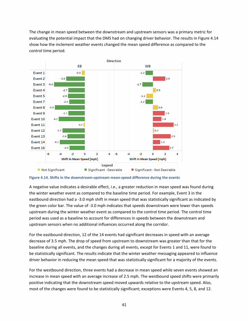
41
The change in mean speed between the downstream and upstream sensors was a primary metric for
evaluating the potential impact that the DMS had on changing driver behavior. The results in Figure 4.14
show how the inclement weather events changed the mean speed difference as compared to the
control time period.
Figure 4.14. Shifts in the downstream-upstream mean-speed difference during the events
A negative value indicates a desirable effect, i.e., a greater reduction in mean speed was found during
the winter weather event as compared to the baseline time period. For example, Event 3 in the
eastbound direction had a -3.0 mph shift in mean speed that was statistically significant as indicated by
the green color bar. The value of -3.0 mph indicates that speeds downstream were lower than speeds
upstream during the winter weather event as compared to the control time period. The control time
period was used as a baseline to account for differences in speeds between the downstream and
upstream sensors when no additional influences occurred along the corridor.
For the eastbound direction, 12 of the 14 events had significant decreases in speed with an average
decrease of 3.5 mph. The drop of speed from upstream to downstream was greater than that for the
baseline during all events, and the changes during all events, except for Events 1 and 11, were found to
be statistically significant. The results indicate that the winter weather messaging appeared to influence
driver behavior in reducing the mean speed that was statistically significant for a majority of the events.
For the westbound direction, three events had a decrease in mean speed while seven events showed an
increase in mean speed with an average increase of 2.5 mph. The westbound speed shifts were primarily
positive indicating that the downstream speed moved upwards relative to the upstream speed. Also,
most of the changes were found to be statistically significant; exceptions were Events 4, 5, 8, and 12.

42
Only Events 1, 3, and 7 in the westbound direction showed a reduction of downstream speed relative to
the upstream speed. The results in the westbound direction are discussed in further detail later in the
report. However, it is assumed that other factors influenced driver behavior in this direction,
contributing to the increase in mean speed.
The results for the change in 85th-percentile-speed in Figure 4.15 followed a similar trend as the mean
speed. The results can be interpreted similar to the mean speed, with a negative value indicating a
desirable effect where the 85th percentile speed downstream is lower as compared to the upstream
sensor after accounting for the control time period.
Figure 4.15. Shifts in the downstream-upstream 85th-percentile-speed difference during the events
Overall, in the eastbound direction, the upstream-downstream speed difference shifted toward negative
values during the DMS-display period. Of the events, 13 of the 14 events had a statically significant
decrease in the 85th percentile with an average decrease of 2.9 mph. Only Event 1 differed from the
mean speed, which had a -1.9 difference in 85th percentile speed during the winter weather event that
was significant, as compared to a non-significant change in mean speed. The results in the eastbound
direction indicated that the winter weather messaging appeared to influence driver behavior by
reducing the 85th percentile speed.
The westbound direction showed mixed results again with one event showing a desirable decrease in
the 85th percentile speed difference and eight events with an increase. Five of the events had no
statistically significant change in the 85th percentile speed difference. A majority of the events resulted
in an increase, or speeds were higher downstream, which was not the desired outcome of the winter
weather messaging. As mentioned for the mean speed, it is assumed that other factors may have been

43
influencing the results in the westbound direction and are described in more detail in the Discussion
section that follows (Section 4.6).
Figure 4.16 shows the results for the shift in standard deviation for each of the individual winter
weather events.
Figure 4.16. Shifts in the downstream-upstream difference of speed standard deviation during the events
The results can be interpreted similar to the mean and 85th percentile speeds in that a negative value is
a desirable effect, indicating that the standard deviation is lower downstream as compared to that for
the upstream sensor after accounting for the control time period. If the standard deviation is lower
downstream, this indicates that the winter weather messaging may alter driver behavior by harmonizing
vehicle speeds in relation to the mean speed.
These standard deviation results may be an indication of the different compliance levels of the drivers
with the DMS or different levels of caution when driving in inclement weather conditions. Literature has
shown that the compliance level correlates to whether poor weather conditions are observed or
perceived (Rämä 2001). In other words, the level of compliance is different when drivers can see the
poor road conditions (through precipitation or accumulation) and when they cannot. Therefore, there
may be some correlation between the standard deviation and precipitation/accumulation, which is
outlined further in the Discussion that follows (Section 4.6).
For both directions of travel, half of the events had no statistically significant change in the standard
deviation as compared to that for the control time period. This indicates that the standard deviation of
vehicle speeds may not be impacted by the winter weather messaging displayed to the drivers.
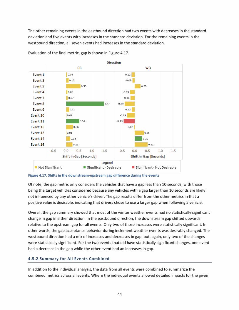
44
The other remaining events in the eastbound direction had two events with decreases in the standard
deviation and five events with increases in the standard deviation. For the remaining events in the
westbound direction, all seven events had increases in the standard deviation.
Evaluation of the final metric, gap is shown in Figure 4.17.
Figure 4.17. Shifts in the downstream-upstream gap difference during the events
Of note, the gap metric only considers the vehicles that have a gap less than 10 seconds, with those
being the target vehicles considered because any vehicles with a gap larger than 10 seconds are likely
not influenced by any other vehicle’s driver. The gap results differ from the other metrics in that a
positive value is desirable, indicating that drivers chose to use a larger gap when following a vehicle.
Overall, the gap summary showed that most of the winter weather events had no statistically significant
change in gap in either direction. In the eastbound direction, the downstream gap shifted upwards
relative to the upstream gap for all events. Only two of those increases were statistically significant. In
other words, the gap acceptance behavior during inclement weather events was desirably changed. The
westbound direction had a mix of increases and decreases in gap, but, again, only two of the changes
were statistically significant. For the two events that did have statistically significant changes, one event
had a decrease in the gap while the other event had an increases in gap.
4.5.2 Summary for All Events Combined
In addition to the individual analysis, the data from all events were combined to summarize the
combined metrics across all events. Where the individual events allowed detailed impacts for the given

45
event, the combined metrics provide an overall measure of the effectiveness for the events analyzed
during the entire 2020–21 winter season. Table 4.4 shows the statistical analysis for the four
performance metrics used to determine the impacts that the DMS winter weather messages may have
had on driver behavior.
Table 4.4. Summary of the data analysis results for all events combined
Performance Metric
Eastbound Westbound
Study Control Study Study
Mean Speed Difference (mph) -1.50 1.28 -0.57 -2.02
Speed Difference Standard Deviation (mph) 5.97 3.79 6.04 3.65
Mean Speed Difference Shift (mph) -2.78 1.45
Mean Speed Difference Significance Significant Significant
Mean 85th Percentile Difference (mph) -2.01 0.62 -0.52 2.71
Mean 85th Percentile Difference Shift (mph) -2.63 2.19
Mean 85th Percentile Difference Significance Significant Significant
Mean Standard Deviation Difference (mph) -1.02 -1.15 0.17 -0.43
Mean Standard Deviation Difference Shift (mph) 0.13 0.60
Mean Standard Deviation Difference Significance) Not significant Significant
Mean Gap Difference (seconds) -0.12 -0.26 0.14 0.20
Mean Gap Difference Shift (seconds) 0.14 -0.07
Mean Gap Difference Significance Significant Not significant
*Total Volume for both control time periods
The results for the mean speed and 85th percentile speed align with the results for the individual events
with the eastbound direction showing reduced speed downstream when accounting for the control time
period and the westbound direction showing increased speeds. In the eastbound direction for all events,
mean speeds downstream were reduced by 1.50 mph, and the 85th percentile speeds were reduced by -
2.01 mph. During the control time period, the mean speeds upstream were greater than downstream by
1.28 mph as well as 0.62 mph for the 85th percentile speeds. After accounting for the control time
period, the eastbound direction showed lower mean speed downstream of 2.78 mph along with
reductions in 85th percentile speeds of 2.63 mph. Both of these results were statistically significant,
indicating that the winter weather messaging may impact driver behavior by reducing vehicle speeds.
For the westbound direction, the results also aligned with a majority of the individual events showing
mean and 85th percentile speeds increased downstream when accounting for the control time period.
The mean speeds increased by 1.45 mph while the 85th percentile speeds increased by 2.19 mph, both
of which were statistically significant. These results differ from what is expected, as it is anticipated that
drivers would reduce speeds after the display of winter weather messaging. However, unlike the
eastbound direction, which had little external influence between the DMS and the traffic sensor
downstream, the westbound direction had the DMS located within the city of Maple Plain. Drivers

46
passed multiple intersections, a centerline concrete barrier, and urban roadways before reaching the
downstream sensor. It is assumed that additional external factors (not accounted for in the study) may
have influenced these speeds.
It should also be noted that the DOT maintenance boundaries changed between the DMS and the
downstream traffic sensor in the westbound direction, which may also help explain the increase in
speeds. Because the upstream and downstream traffic sensors are under different maintenance
districts, the road conditions may not be the same when precipitation is accumulating. If the road
conditions at the upstream sensor are poorer, it would be expected that speeds would increase
downstream as drivers have already navigated poor conditions and the improved road conditions may
have a greater impact on driver behavior than the winter weather messaging. This assumption is further
expanded on in the Discussion section (Section 4.6).
For the individual events, the standard deviation and gap metrics showed mixed results for both the
eastbound and westbound directions. Table 4.4 does show that the eastbound standard deviation and
westbound gap had no statistically significant changes as compared to the control time period. The
westbound direction, on the other hand, did have a shift in the standard deviation of 0.6 that was
statistically significant. This indicated that there was a larger spread in vehicle speeds downstream as
compared to those at the upstream sensor. This result is not necessarily ideal, as more harmonized
speeds should result in reduced conflicts between vehicles. For the individual events, the westbound
standard deviation had statistically significant increases in half of the events, with all other events
except one showing increases that were not statistically significant.
In the eastbound direction, although only two individual events had statistically significant increases in
gap, the combined analysis showed a very minor increase in gap of 0.14 seconds that was statistically
significant. The increase is desirable as this indicates that drivers are choosing larger gaps when
following vehicles giving them more time to react given the uncertain conditions of the winter weather
event. Although 12 of the individual events did not have statistically significant changes in the
eastbound direction, all events did see increases in the gap, which likely resulted in the statistically
significant changes for the combined analysis.
To confirm the assumptions of the statistical analysis, the distribution of each of the metrics were
plotted to confirm the data had normal distribution. Figures 4.18 and 4.19 show the distribution charts
for the mean speeds in the eastbound and westbound directions, respectively.

47
Figure 4.18. Speed difference distributions for the control and study time periods in the eastbound direction
Figure 4.19. Speed difference distributions for the control and study time periods in the westbound direction
The top chart for the eastbound direction shows the shift to the left in the speed difference between
downstream and upstream sensors, indicating larger decreases in speed between the sensors during the
study time period when drivers were shown the winter weather messaging. As previously described, this
is a desirable change as it indicates that speeds were lower downstream after being shown the winter
weather messaging.
The westbound distribution shows a smaller shift in the mean speed difference. The shift to the right for
the distribution indicates that speeds downstream were increased as compared to those at the
upstream sensor during the winter weather event when accounting for the control time period.

48
4.6 DISCUSSION
As noted in previous sections, road conditions, traffic volume, and precipitation/accumulation
conditions may have an impact on the studied metrics and may explain some of the differences between
the eastbound and westbound DMS performance results. Overall, the DMS showed better, more
consistent performance in the eastbound direction. The results aligned with the expectations that
providing drivers with winter weather messaging would impact driver behavior and reduce speed. For a
majority of the events, as well as in the overall analysis, statistically significant changes in mean speed
and 85th percentile speed were documented. The speed reductions show that drivers reduced their
speeds with winter weather messaging, as compared to those at the upstream sensor, which received
no messaging and the control time period.
The results also showed that little effect on the standard deviation of speeds and possible
improvements in gap when evaluating all events combined together. As described in the sensor
placement assumptions, the eastbound direction represented the best study layout due to the
placement of the DMS on the outside edge of town and on no major influences on speed or traffic
before the downstream sensor. The results at this location indicate that the winter weather messaging
likely has a positive influence on driver behavior, which is further explored in this section.
At the same time, the variation of metrics in the westbound direction was less uniform and less
desirable. The findings described in the previous sections showed that the DMS performed satisfactorily
in improving driver behavior during inclement weather in the eastbound study area. However, the same
conclusions cannot necessarily be made for the westbound direction due to irregularities and
undesirable metric variations. That said, the westbound performance may still be deemed acceptable or
even desirable during many events.
Possible explanations for the irregular results in the westbound direction include the placement of the
DMS within an urban environment, multiple intersections between the DMS and the downstream
sensor, the change in maintenance district boundaries between the sensors, and other external factors
that could not be controlled in the analysis. This section investigates whether the difference between
the two directions and the westbound irregularities should be attributed to inadequate DMS
performance or the inherent directional characteristics of the corridor.
First and foremost, the road conditions during snow-accumulating events in the westbound direction
likely varied between the upstream and downstream sensor. As previously mentioned, the upstream
and downstream locations of the sensors used in the westbound direction were maintained by separate
DOT maintenance districts. Because of practical and logistical reasons, the westbound downstream and
upstream locations are likely plowed at different times, possibly resulting in somewhat different road
conditions that may have greater influence on driving behavior. If the downstream location is plowed
sooner than the upstream location, drivers would likely face a change in road conditions when driving in
the westbound direction along this corridor. As a result, many drivers would see the DMS but also see
improved road conditions, as compared to upstream, and increase their vehicle speeds.

49
Another notable factor that can impact metrics is traffic volume. Table 4.5 shows the volume and its
change from upstream to downstream for both directions during the different events.
Table 4.5. Traffic volumes during the events for upstream and downstream locations
Event Eastbound Westbound
Upstream Downstream Volume Change
Upstream Downstream Volume Change
1 1,370 1,283 -87 1,693 1,383 -310
2 18,638 18,745 107 2,2758 2,0246 -2512
3 514 449 -65 1,075 868 -207
4 1,598 1,401 -197 3,190 2,871 -319
5 110 138 28 262 221 -41
7 2,502 2,751 249 1,164 892 -272
8 713 327 -386 302 342 40
9 1,147 1,197 50 1,384 1,103 -281
10 1,665 1,739 74 2,500 2,045 -455
11 2,336 2,586 250 1,233 947 -286
12 2,235 2,336 101 780 651 -129
13 2,346 2,478 132 890 685 -205
14 3,337 3,445 108 2,486 1,956 -530
16 333 339 6 412 363 -49
Green cells and yellow cells in the table show a reduction and increase, respectively, in total traffic
volume during the event from upstream to downstream. The westbound upstream traffic volume was
greater than the downstream in almost all events, except for Event 8. Whereas, during most events,
except for 1, 3, 4, and 8, the eastbound upstream traffic volume was less than the downstream. In the
eastbound direction, a majority of events had less than a 10% change in traffic volume with only two
events having a change greater than 15%, indicating comparable traffic volume. To note, based on the
placement of the DMS and downstream sensor, it may be assumed that most, if not all, vehicles passed
the winter weather messaging on the DMS.
Whereas, in the westbound direction, a majority of the events had a 10 to 20% change in traffic volume.
As previously mentioned, additional traffic generators and other influences between the westbound
DMS and the downstream sensor provide less confidence in the assumption that all vehicles passed the
winter weather messaging on the DMS. Flashing beacons were located directly before the downstream
sensors, so most, if not all, vehicles would have received some notification of winter weather conditions.
However, based on this information, the traffic volume difference is a possible factor for the seemingly
less desirable DMS performance in the westbound direction.
As mentioned in a previous section, drivers are more likely to comply with DMS when they cannot
observe or perceive the poor weather or surface conditions themselves. In other words, the presence of
precipitation and accumulation during an event may cause drivers to put more faith in their personal

50
judgment than the DMS information. Figures 4.20 and 4.21 show how the shift in mean speed was
influenced by the type of precipitation and whether any precipitation had accumulated during the
winter weather event.
Figure 4.20. Eastbound mean speed shifts in different precipitation and accumulation conditions
Figure 4.21. Westbound mean speed shifts in different precipitation and accumulation conditions
The color of the bars in this chart, as well as all similar charts, are based on the statistical analysis with
green indicating a statistically significant and desirable change, yellow indicating statistically non-
significant changes, and red indicating statistically significant but undesirable changes.
As seen in Figure 4.20, the only two non-significant influences in the eastbound direction occurred
during Events 1 and 11 when there was both precipitation and accumulation. Event 11 was the most
severe winter weather event with respect to snow accumulation. On the other hand, as seen in Figure

51
4.21, two of the three desirable speed shifts that were significant in the westbound direction occurred
when there was no accumulation. Only one of the significant, non-desirable speed shifts (positive shift)
in the westbound direction happened when there was no accumulation (during Event 14). A possible
explanation is that severe weather events may result in the winter weather messaging being less
effective, likely due to the awareness by drivers of conditions. Conversely, events with no accumulation
or no/isolated precipitation may lead to more effective winter weather messaging due to drivers
trusting the message, because they are less aware of the impacting condition.
Although limited in the number of events to fully support this conclusion, all events in both directions
that had no accumulation and no precipitation did show statistically significant decreases. If this is
expanded to all no accumulation events, but events that may have precipitation, six of the events by
direction combination had statistically significant decreases, while one event had no statistically
significant change (Event 5 – Westbound), and one event had a statistically significant increase (Event 14
– Westbound). Due to the limited number of sample events, the results did not show any indication of
certain types of events having greater impact on mean speeds.
The 85th percentile speed shift is displayed in a similar manner based on precipitation type and
accumulation for both directions of travel in Figures 4.22 and 4.23.
Figure 4.22. Eastbound 85th percentile speed shifts in different precipitation and accumulation conditions

52
Figure 4.23. Westbound 85th percentile speed shifts in different precipitation and accumulation conditions
The results show similar trends to the mean speed. The only event in the eastbound direction that did
not have a statistically significant change was Event 11, which was the most severe winter weather
event in terms of accumulation. This follows the assumption that more severe events may have less
impact from the winter weather messaging. For the events with no accumulation and no precipitation,
three of the four events had statistically significant decreases, with the fourth event in the westbound
direction showing a non-significant decrease. Due to the limited number of sample events, the results
did not show any indication of certain types of events having greater impact on 85th percentile speeds.
Figures 4.24 and 4.25 show the mixed results for standard deviation, based on the precipitation type
and accumulation.
Figure 4.24. Eastbound standard deviation shifts in different precipitation and accumulation conditions
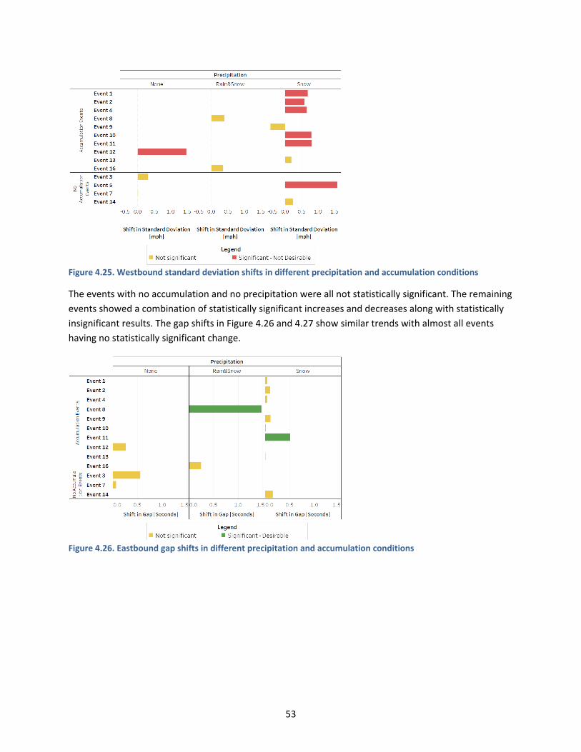
53
Figure 4.25. Westbound standard deviation shifts in different precipitation and accumulation conditions
The events with no accumulation and no precipitation were all not statistically significant. The remaining
events showed a combination of statistically significant increases and decreases along with statistically
insignificant results. The gap shifts in Figure 4.26 and 4.27 show similar trends with almost all events
having no statistically significant change.
Figure 4.26. Eastbound gap shifts in different precipitation and accumulation conditions

54
Figure 4.27. Westbound gap shifts in different precipitation and accumulation conditions

55
CHAPTER 5: CONCLUSIONS AND FUTURE STUDIES
MnDOT deployed a real-time weather-controlled dynamic message sign system along the US 12 corridor
with the expectation that the system would exert a significant effect on traffic along the corridor
between Delano and Maple Plain. The deployed DMS system provided road users with real-time
information on unexpected weather conditions and/or weather-induced road conditions. Drivers who
were exposed to the DMS alert and complied with it were better informed, and thus less likely to be
surprised by changes in road environment conditions. This should have resulted in lower frequency and
severity of crashes, consequently improving driving safety and mobility along the corridor.
While providing weather-related information to drivers has promising benefits, the challenge of low
driver compliance still prevails. Drivers do not necessarily adjust their driving behavior according to the
information they are provided. Therefore, it is imperative to maximize driver compliance by using
optimally effective information-delivering media. Agencies should evaluate the DMS systems within
their jurisdictions to make sure they serve the intended purpose with acceptable efficacy and do not
exert any negative side effects. Key aspects of DMS operations that should be thoroughly evaluated
include achieved driver compliance rate, impact on traffic flow, impact on road safety, and extent of
impact beyond the equipped corridor. The degree of effectiveness and type of influence of DMS on
driver behavior depends on many design and operational factors.
In total, 16 winter weather events were initially analyzed during the 2020–21 winter season, while two
of the events were later excluded from the final analysis due to the short duration of one event and a
high number of blank messages for the other event.
The eastbound direction represented the best study layout due to the placement of the DMS on the
outside edge of town and no major influences on speed or traffic before the downstream sensor.
Overall, the DMS showed better, more consistent performance in the eastbound direction. The results
aligned with expectations that providing drivers with winter weather messaging would impact driver
behavior and reduce speeds. When evaluating the individual events, the eastbound direction had 12 of
the 14 events with significant decreases in speed and an average decrease of 3.5 mph. This indicated
that speeds decreased from upstream to downstream during a winter weather event. In addition to the
mean speed, 13 of the 14 events had a statically significant decrease in the 85th percentile speed with
an average decrease of 2.9 mph. Only Event 1 differed from the mean speed, which had a -1.9
difference in the 85th percentile speed during the winter weather event that was significant compared
to a not significant change in mean speed.
In addition to the individual events, a combined analysis was completed that aggregated the results for
all events. The results for the mean speed and 85th percentile speed aligned with the results for the
individual events with the eastbound direction showing reduced speeds downstream when accounting
for the control period and the westbound direction showing increased speeds. The combined analysis
showed mean speeds downstream were reduced by 1.50 mph, and 85th percentile speeds were
reduced by 2.01 mph. The results indicated that the winter weather messaging appeared to influence

56
driver behavior in reducing the mean and 85th percentile speeds and were statistically significant for a
majority of the events.
For the westbound direction, three events had a decrease in mean speed while seven events showed an
increase in mean speed with an average increase of 2.5 mph. The westbound speed shifts were primarily
positive, indicating that the downstream speed increased relative to the upstream speed. The 85th
percentile speed showed mixed results as well with one event showing desirable decreases in the 85th
percentile speed difference and eight events with an increase. Five of the events had no statistically
significant change in the 85th percentile speed difference. With a majority of events resulting in an
increase, this indicated that speeds were higher downstream, which was not the desired outcome of the
winter weather messaging.
For the westbound direction, the results also aligned with a majority of individual events showing mean
and 85th percentile speeds increased downstream when accounting for the control period. The mean
speeds increased by 1.45 mph while the 85th percentile speed increased by 2.19 mph, both of which
were statistically significant. These results differed from what was expected given it was anticipated that
drivers would reduce their speeds after seeing the display of winter weather messaging. Unlike the
eastbound direction, which had little external influence between the DMS and the traffic sensor
downstream, the westbound direction had the DMS located within the city of Maple Plain. Drivers
passed multiple intersections, a center concrete barrier, and urban roadways before reaching the
downstream sensor.
Additional external factors could account for the results in the westbound direction. These factors
included the placement of the DMS within an urban environment, multiple intersections between the
DMS and downstream sensor, the change in maintenance district boundaries between the sensors, and
other external factors that could not be controlled in the analysis.
The MnDOT maintenance boundaries changed between the DMS and downstream traffic sensor in the
westbound direction, which could partially explain the increase in speed. Because the upstream and
downstream traffic sensors are under different maintenance districts, the road conditions may differ
when precipitation is accumulating. If the road conditions are poorer at the upstream sensor, the speeds
may increase downstream as drivers have already navigated poor conditions. In this case, improved
road conditions may have a greater impact on driver behavior than the winter weather messaging.
The potential impact of maintenance aligns with another area that could be further explored in a future
analysis. Severe weather events may cause the winter weather messaging to be less effective due to
increased driver awareness of the conditions and changes in behavior resulting from these conditions.
Although limited, the most severe winter weather events in terms of accumulation were the only events
that did not have a statistically significant change in the mean or 85th percentile speeds. Conversely,
events with no accumulation or precipitation may have led to more effective winter weather messaging,
as drivers may have been more accepting of the messaging when they were less aware of the impacting
conditions themselves. Although limited in the number of events, all events in both directions that had
no accumulation and no precipitation did show statistically significant speed decreases.

57
When expanding this to all of the no-accumulation events that may have had precipitation, six of the
events by direction had statistically significant speed decreases while one had no statistically significant
changes and one had a statistically significant increase, with both of the increases that occurred being in
the westbound direction. However, due to the limited number of sample events, the results did not
show any indication of certain types of events having greater impact on mean speeds.
A future study could build on this analysis by developing models to understand the various elements
potentially impacting the results that were anecdotally highlighted in this report, including the effects of
precipitation type and accumulation. The models could validate these findings as well as determine
whether there is any correlation between the severity of the event and the impact that the winter
weather messaging has on driver behavior.
Additionally, a future study may be warranted regarding the placement of the DMS with respect to the
desired influence area of the messaging. Such a study could include identifying how far downstream an
advisory message can influence driver behavior as well the influence other factors have in conveying a
message to drivers similar to what was experienced in Maple Plain for the westbound direction of travel.
Overall, the results from the eastbound direction of travel indicated that the DMS winter weather
messaging along the US 12 corridor could have positive effects on driver behavior by decreasing the
mean and 85th percentile speeds. There were also indications of positive effects on vehicle gaps when
evaluating all events combined that were statistically significant but not when evaluating the individual
winter weather events. In the westbound direction, mixed results were found for the mean and 85th
percentile changes in speed. As previously described, the results indicated that other external and
uncontrollable factors with this location could contribute to the inconclusive findings.

58
REFERENCES
Abdel-Aty, M., R. J. Cunningham, V. V. Gayah, and L. Hsia. 2008. Dynamic Variable Speed Limit Strategies
for Real-Time Crash Risk Reduction on Freeways. Transportation Research Record: Journal of the
Transportation Research Board, No. 2078, pp. 108–116.
Allaby, P., B. Hellinga, and M. Bullock. 2006. Variable Speed Limits: Safety and Operational Impacts of a
Candidate Control Strategy for an Urban Freeway. IEEE Conference on Intelligent Transportation
Systems, Vol. 8, pp. 897–902.
Allpress, J. A., and L. S. Leland. 2010. Reducing Traffic Speed within Roadwork Sites Using Obtrusive
Perceptual Countermeasures. Accident Analysis and Prevention, Vol. 42, No. 2, pp. 377–383.
Bai, Y. and Y. Li. 2011. Determining the Drivers’ Acceptance of EFTCD in Highway Work Zones. Accident
Analysis and Prevention, Vol. 43, No. 3, pp. 762–768.
Bai, Y., Finger, K., and Li, Y., “Analyzing Motorist’s Responses to Temporary Signage in Highway Work
Zones,” Safety Science, Elsevier, Vol. 48, No. 2, February 2010, pp. 215-221.
Banerjee, S., M. Jeihani, D. D. Brown, and S. Ahangari. 2020. Comprehensive Analysis of Dynamic
Message Sign Impact on Driver Behavior: A Random Forest Approach. Urban Science, Vol. 4, No. 4,
pp.1–20.
Benekohal, R. F., A. Hajbabaie, J. C. Medina, M. Wang, and M. V. Chitturi. 2010. Speed Photo-Radar
Enforcement Evaluation in Illinois Work Zones. Illinois Center for Transportation, University of
Illinois, Urbana, IL.
M. Downey, and Bertini, R. L.. 2015. Evaluation of a Traffic and Weather Responsive Variable Advisory
Speed System in Portland, Oregon. 94th Annual Meeting of the Transportation Research Board,
January 11–15, Washington, DC.
Boateng, R. A., M. D. Fontaine, and Z. H. Khattak. 2019. Driver Response to Variable Speed Limits on I-66
in Northern Virginia. Journal of Transportation Engineering Part A: Systems, Vol. 145, No. 6, Article
no. 04019021.
Brewer, M. A, G. Pesti, and W. Schneider. 2006. Improving Compliance with Work Zone Speed Limits:
Effectiveness of Selected. Transportation Research Record: Journal of the Transportation Research
Board, No. 1948, pp. 67–76.
Buddemeyer, J. L. 2009. Variable Speed Limit Decision Support System for the Elk Mountain Corridor
Phase 1. Master’s thesis. University of Wyoming, Laramie, WY.
Chatterjee, K., N. B. Hounsell, P. E. Firmin, and P. W. Bonsall. 2002. Driver Response to Variable Message
Sign Information in London. Transportation Research Part C: Emerging Technologies, Vol. 10, No. 2,
pp. 149–169.

59
Debnath, A. K., R. Blackman, and N. Haworth. 2014. A Tobit Model for Analyzing Speed Limit Compliance
in Work Zones. Safety Science, Vol. 70, pp. 367–377.
Dudek, C. L. and G. L. Ullman. 2002. Flashing Messages, Flashing Lines, and Alternating One Line on
Changeable Message Signs. Transportation Research Record: Journal of the Transportation Research
Board, No. 1803, pp. 94–101.
Fudala, N. J. and M. D. Fontaine. 2010. Work Zone Variable Speed Limit Systems: Effectiveness and
System Design Issues. Virginia Transportation Research Council, Charlottesville, VA.
Gettman D. and L. Head. 2003. Surrogate Safety Measures from Traffic Simulation Models.
Transportation Research Record: Journal of the Transportation Research Board, No.1840, pp.
104–115.
Gettman, D., L. Pu, T. Sayed, and S. Shelby. 2008. Surrogate Safety Assessment Model and Validation
:Final Report. FHWA-HRT-08-051. Turner-Fairbank Highway Research Center, Federal Highway
Administration, McLean, VA.
Giles, M. J. 2004. Driver Speed Compliance in Western Australia: A Multivariate Analysis. Transport
Policy, Vol. 11, No. 3, pp. 227–235.
Hassan, H. M., M. A. Abdel-Aty, K. Choi, and S. A. Algadhi. 2012. Driver Behavior and Preferences for
Changeable Message Signs and Variable Speed Limits in Reduced Visibility Conditions. Journal of
Intelligent Transportation Systems: Technology, Planning, and Operations, Vol. 16, No. 3, pp. 132–
146.
Heinijoki, H. 1994. FinnRA Reports 190: Influence of the Type and Condition of Tyres and Drivers’
Perceptions of Road Conditions on Driving Speed. Finnish National Road Association, Helsinki,
Finland.
Hellinga, B. and M. Mandelzys. 2011. Impact of Driver Compliance on the Safety and Operational
Impacts of Freeway Variable Speed Limit Systems. Journal of Transportation Engineering, Vol. 137,
No. 4, pp. 260–268.
Hogema, J. H. and R. Van Der Horst. 1997. Evaluation of A16 Motorway Fog-Signaling System with
Respect to Driving Behavior. Transportation Research Record: Journal of the Transportation
Research Board, No. 1573, pp. 63–67.
Huang, Y. and Y. Bai. 2019. Driver Responses to Graphic-Aided Portable Changeable Message Signs in
Highway Work Zones. Journal of Transportation Safety and Security, Vol. 11, No. 6, pp. 661–682.
Kockelman, K., J. Bottom, Y. J. Kweon, J. Ma, and X. Wang. 2006. NCHRP Web-Only Document 90 (Project
17-23): Safety Impacts and Other Implications of Raised Speed Limits on High-Speed Roads. National
Cooperative Highway Research Program, Washington, DC.

60
Kolisetty, V. G. B., T. Iryo, Y. Asakura, and K. Kuroda. 2006. Effect of Variable Message Signs on Driver
Speed Behavior on a Section of Expressway under Adverse Fog Conditions-A Driving Simulator
Approach. Journal of Advanced Transportation, Vol. 40, No. 1, pp. 47–74.
Kwon, E., D. Brannan, K. Shouman, C. Isackson, and B. Arseneau. 2007. Development and Field
Evaluation of Variable Advisory Speed Limit System for Work Zones. Transportation Research
Record: Journal of the Transportation Research Board, No. 2015, pp. 12–18.
Leonard, D. R., P. Gower, and N. B. Taylor. 1989. CONTRAM: Structure of the Model. Transport and Road
Research Laboratory (TRRL), Wokingham, Berkshire, UK.
Luoma, J. and P. Rämä. 1999. Effects of Variable Speed Limit Signs on Speed Behavior and Recall of
Signs. Traffic Engineering and Control, Vol. 39, pp. 234–237.
Mannering, F. 2007. The Effects of Interstate Speed Limits on Driving Speeds: Some New Evidence. 86th
Annual Meeting of the Transportation Research Board, January 21–25, Washington, DC.
McDonald, M., N. B. Hounsell, and S. R. Njoze. 1995. Strategies for Route Guidance Systems Taking
Account of Driver Response. Pacific Rim TransTech Conference, Vehicle Navigation and Information
Systems Conference Proceedings, 6th International VNIS. A Ride into the Future. July 30–August 2,
Seattle, WA, pp. 328–333.
McMurtry, T., M. Saito, M. Iffkin, and S. Heath. 2009. Variable Speed Limits Signs: Effects on Speed and
Speed Variation in Work Zones. 88th Annual Meeting of the Transportation Research Board, January
11–15, Washington, DC.
Mekker, M. M., S. M. Remias, W. A. Bunnell, D. W. Krohn, E. D. Cox, and D. M. Bullock. 2016. Variable
Speed Limit Study Upstream of an Indiana Work Zone with Vehicle Matching. Transportation
Research Record: Journal of the Transportation Research Board, No. 2555, pp. 53–64.
Padget, E. D., K. K. Knapp, and G. B. Thomas. 2001. Investigation of Winter-Weather Speed Variability in
Sport Utility Vehicles, Pickup Trucks, and Passenger Cars. Transportation Research Record: Journal of
the Transportation Research Board, No. 1779, pp. 116–124.
Papageorgiou, M., E. Kosmatopoulos, and L. Papamichail. 2008. Effects of Variable Speed Limits on
Motorway Traffic Flow. Transportation Research Record: Journal of the Transportation Research
Board, No. 2047, pp. 37–48.
Peeta, S., J. L. Ramos, and R. Pasupathy. 2000. Content of Variable Message Signs and On-Line Driver
Behavior. Transportation Research Record: Journal of the Transportation Research Board, No. 1725,
pp. 102–108.
Peng, Y., M. Abdel-Aty, Q. Shi, and R. Yu. 2017. Assessing the Impact of Reduced Visibility on Traffic
Crash Risk Using Microscopic Data and Surrogate Safety Measures. Transportation Research Part C:
Emerging Technologies, Vol. 74, pp. 295–305.

61
Penttinen, M., J. Luoma, and P. Rämä. 1997. Information Needs of Finnish Drivers. Mobility for Everyone:
4th World Congress on Intelligent Transport Systems, October 21–27, Berlin, Germany.
Rahman, M. M., L. Strawderman, T. Garrison, D. Eakin, and C. C. Williams. 2017. Work Zone Sign Design
for Increased Driver Compliance and Worker Safety. Accident Analysis and Prevention, Vol. 106, pp.
67–75.
Rämä, P. 1999. Effects of Weather-Controlled Variable Speed Limits and Warning Signs on Driver
Behavior. Transportation Research Record: Journal of the Transportation Research Board, No. 1689,
pp. 53–59.
Rämä, P. 2001. Effects of Weather-Controlled Variable Message Signing on Driver Behavior. VTT
Publications, Helsinki University of Technology, Helsinki, Finland.
Rämä, P. and R. Kulmala. 2000. Effects of Variable Message Signs for Slippery Road Conditions on Driving
Speed and Headways. Transportation Research Part F: Traffic Psychology and Behavior, Vol. 3, No. 2,
pp. 85–94.
Rämä, P. and J. Luoma. 1997. Driver Acceptance of Weather-Controlled Road Signs and Displays.
Transportation Research Record: Journal of the Transportation Research Board, No. 1573, pp. 72–75.
Rämä, P., J. Luoma, and V. Harjula. 1999. Distraction Due to Variable Speed Limits. Traffic Engineering
and Control, Vol. 40, No. 9, pp. 428–430.
Riggins, G., R. Bertini, W. Ackaah, and M. Margreiter. 2016. Evaluation of Driver Compliance to Displayed
Variable Advisory Speed Limit Systems: Comparison between Germany and the U.S. Transportation
Research Procedia, Vol. 15, pp. 640–651.
Savolainen, P. T., T. K. Datta, I. Ghosh, and T. J. Gates. 2010. Effects of Dynamically Activated Emergency
Vehicle Warning Sign on Driver Behavior at Urban Intersections. Transportation Research Record:
Journal of the Transportation Research Board, No. 2149, pp. 77–83.
Strawderman, L., M. M. Rahman, Y. Huang, and A. Nandi. 2015. Driver Behavior and Accident Frequency
in School Zones: Assessing the Impact of Sign Saturation. Accident Analysis and Prevention, Vol. 82,
pp. 118–125.
Sui, Y. and R, Young. 2014. Impact of Dynamic Message Signs on Speeds Observed on a Rural Interstate.
Journal of Transportation Engineering, Vol. 140, No. 6, pp. 1–7.
Tak, S., S. Kim, D. Lee, and H. Yeo. 2018. A Comparison Analysis of Surrogate Safety Measures with Car-
Following Perspectives for Advanced Driver Assistance System. Journal of Advanced Transportation,
Vol. 2018, Article no. 8040815, pp. 1–14.
Tay, R. and J, Choi. 2009. Evaluation of Pictograms in Dynamic Lane Control Systems in the Republic of
Korea. Journal of Transportation Systems Engineering and Information Technology, Vol. 9, No. 2, pp.
56–61.

62
Ullman, B. R., G. L. Ullman, C. L. Dudek, and A. A. Williams. 2007. Driver Understanding of Sequential
Portable Changeable Message Signs in Work Zones. Transportation Research Record: Journal of the
Transportation Research Board, No. 2015, pp. 28–35.
Unrau, D. and J. Andrey. 2006. Driver Response to Rainfall on Urban Expressways. Transportation
Research Record: Journal of the Transportation Research Board, No. 1980, pp. 24–30.
Vadeby, A. and Åa Forsman. 2017. Changes in Speed Distribution: Applying Aggregated Safety Effect
Models to Individual Vehicle Speeds. Accident Analysis and Prevention, Vol. 103, pp. 20–28.
Bham, G. H., Leu, M. C. Venkat, B. K., and Mohammadi, M. A. 2014. A Driving Simulator Study to
Evaluate the Impact of Portable Changeable Message Signs (PCMS) on Drivers’ Speed Characteristics
in Work Zones. Midwest Smart Work Zone Deployment Initiative. Ames, IA 50010
Wang, C., K. K. Dixon, and D. Jared. 2003. Evaluation of Speed Reduction Strategies for Highway Work
Zones. Transportation Research Record: Journal of the Transportation Research Board, No. 1824, pp.
44–53.
Wang, J.-h. and Y. Cao. 2005. Assessing Message Display Formats of Portable Variable Message Signs.
Transportation Research Record: Journal of the Transportation Research Board, No. 1937, pp. 113–
119.
White, C., N. Taylor, and N. B. Hounsell. 1994. CONTRAM–A Computer Suite for Modelling Road
Congestion. Traffic Technology International, Vol. 94, pp. 106–110.
Wogalter, M. S. 2003. Factors Influencing the Effectiveness of Warnings. In Visual Information for
Everyday Use: Design and Research Perspectives. CRC Press, Philadelphia, PA, pp. 93–110.
Zhao, S. C., Y. Marumachi, N. Harata, and K. Ohta. 1995. An SP Model for Route Choice Behavior in
Response to Travel Time Information with Marginal Error. World Conference on Transport Research,
July 16–21, Sydney, New South Wales, Australia.
Zhao, W., M. Quddus, H. Huang, J. Lee, and Z. Ma. 2019. Analyzing Drivers’ Preferences and Choices for
the Content and Format of Variable Message Signs (VMS). Transportation Research Part C: Emerging
Technologies, Vol. 100, pp. 1–14.

APPENDIX A: SUMMARY OF INDIVIDUAL EVENTS
This appendix includes the detailed performance metric summaries for all studied events. The
different types of changes (or effects) are shown with different colors as follows: green shading
indicates a statistically significant and desirable change, yellow shading indicates statistically
non-significant changes, and red shading indicates statistically significant but undesirable
changes.

A-1
Table A.1. Detailed mean speed summary statistics for Event 1 to 9 in eastbound direction
1 EVENT 2 EVENT 3 EVENT EVENT 4 EVENT 5 EVENT 7 EVENT 8
Study Control Study Control Study Control Study Control Study Control Study Control Study Control
Mean 1.41 1.89 -0.95 2.09 -1.57 3.44 -0.90 1.78 -0.86 1.90 -0.73 1.81 -4.17 0.73 Standard Error 0.48 0.25 0.17 0.11 0.64 0.40 0.54 0.22 0.91 0.70 0.57 0.24 1.05 0.55
Median 1.97 1.76 -1.00 1.79 -1.75 2.86 -0.87 1.58 -0.67 2.03 -1.45 1.80 -3.50 0.50 Standard Deviation 3.47 1.83 6.04 4.19 5.39 4.64 6.85 3.92 5.58 6.09 5.46 3.93 7.38 5.08
Sample Variance 12.03 3.34 36.47 17.58 29.09 21.51 46.99 15.35 31.19 37.10 29.81 15.41 54.47 25.82 Skewness -0.71 0.79 0.29 2.02 -0.14 1.18 0.20 1.68 -0.15 -0.40 3.06 1.28 -1.21 0.87
Range 16.19 9.84 71.50 54.78 28.25 29.83 49.30 43.67 24.67 32.33 47.20 52.00 38.39 33.67 Minimum -9.71 -1.69 -33.50 -20.00 -17.00 -7.33 -23.30 -13.67 -13.33 -18.00 -14.20 -20.00 -30.83 -12.00 Maximum 6.48 8.15 38.00 34.78 11.25 22.50 26.00 30.00 11.33 14.33 33.00 32.00 7.56 21.67
Count 53.00 53.00 1275.00 1462.00 71.00 135.00 159.00 313.00 38.00 76.00 91.00 267.00 49.00 85.00
Shift Direction Negative Negative Negative Negative Negative Negative Negative magnitude of shift -0.48 -3.04 -5.01 -2.67 -2.76 -2.55 -4.90
t Stat -0.89 -15.09 -6.64 -4.55 -2.41 -4.10 -4.12 P(T<=t) one-tail 0.19 0.00 0.00 0.00 0.01 0.00 0.00
t Critical one-tail 1.66 1.65 1.66 1.65 1.66 1.66 1.67 P(T<=t) two-tail 0.38 0.00 0.00 0.00 0.02 0.00 0.00
t Critical two-tail 1.99 1.96 1.98 1.97 1.99 1.98 1.99
Significance Not significant Significant Significant Significant Significant Significant Significant
Table A.2. Detailed mean speed summary statistics for Event 10 to 16 in eastbound direction
EVENT 9 EVENT 10 EVENT 11 EVENT 12 EVENT 13 EVENT 14 EVENT 16
Study Control Study Control Study Control Study Control Study Control Study Control Study Control
Mean -2.38 0.30 -3.15 1.10 0.76 0.95 -3.51 0.14 -2.71 0.11 -4.80 -0.71 -2.59 -0.10 Standard Error 0.46 0.19 0.44 0.24 0.50 0.17 0.71 0.38 0.33 0.18 0.38 0.21 1.14 0.34
Median -2.28 0.21 -3.00 1.01 -0.06 0.99 -2.63 -0.16 -2.90 0.38 -4.73 -0.57 -1.78 -0.01 Standard Deviation 3.51 1.98 6.39 4.79 4.12 2.02 6.38 4.77 2.49 1.91 4.91 3.84 7.01 3.09
Sample Variance 12.31 3.92 40.86 22.95 16.98 4.07 40.74 22.71 6.19 3.65 24.08 14.74 49.16 9.54 Skewness -0.12 0.15 0.61 0.04 0.24 -0.13 -1.56 2.67 -0.05 -0.27 -1.08 -0.68 -0.98 -0.12
Range 20.15 12.76 50.90 51.50 18.29 9.82 40.50 52.33 10.28 8.10 39.50 31.83 33.42 16.60 Minimum -12.12 -5.85 -21.90 -22.50 -8.32 -4.07 -32.00 -17.00 -8.02 -4.07 -30.00 -21.83 -24.00 -9.10 Maximum 8.04 6.91 29.00 29.00 9.97 5.75 8.50 35.33 2.26 4.03 9.50 10.00 9.42 7.50
Count 57.00 114.00 207.0
0 388.00 67.00 134.00 81.00 160.00 56.00 112.00 171.00 340.00 38.00 85.00
Shift Direction Negative Negative Negative Negative Negative Negative Negative magnitude of shift -2.68 -4.25 -0.19 -3.65 -2.83 -4.08 -2.48
t Stat -5.36 -8.39 -0.35 -4.55 -7.47 -9.52 -2.09 P(T<=t) one-tail 0.00 0.00 0.36 0.00 0.00 0.00 0.02
t Critical one-tail 1.67 1.65 1.66 1.66 1.66 1.65 1.68 P(T<=t) two-tail 0.00 0.00 0.72 0.00 0.00 0.00 0.04
t Critical two-tail 1.99 1.97 1.99 1.98 1.99 1.97 2.02
Significance Significant Significant Not significant Significant Significant Significant Significant

A-2
Table A.3. Detailed mean speed summary statistics for Event 1 to 9 in westbound direction
EVENT 1 EVENT 2 EVENT 3 EVENT 4 EVENT 5 EVENT 7 EVENT 8
Study Control Study Control Study Control Study Control Study Control Study Control Study Control
Mean -4.30 -3.09 0.03 -2.01 -3.08 -1.35 -0.98 -1.47 -2.62 -1.55 -3.02 -1.83 0.19 -0.63 Standard Error 0.55 0.32 0.17 0.09 0.37 0.26 0.46 0.20 0.67 0.47 0.53 0.28 0.97 0.45
Median -4.08 -2.95 -0.41 -2.03 -3.56 -1.39 -1.53 -1.67 -2.62 -1.74 -2.97 -1.81 0.00 -0.67 Standard Deviation 3.99 2.37 6.11 3.30 3.22 3.19 5.79 3.68 4.55 4.54 4.84 4.38 6.66 4.16
Sample Variance 15.88 5.60 37.30 10.86 10.36 10.17 33.56 13.56 20.68 20.57 23.41 19.17 44.38 17.28 Skewness -0.46 -0.52 0.31 0.17 0.70 0.06 0.09 0.44 -0.14 0.29 -0.54 -0.13 -0.18 0.01
Range 22.95 11.67 52.00 33.50 16.83 18.25 41.75 37.00 23.00 28.00 30.40 30.17 38.00 24.23 Minimum -17.28 -9.41 -24.50 -17.50 -9.68 -9.75 -22.75 -19.33 -15.00 -14.00 -19.00 -17.67 -19.00 -12.83 Maximum 5.67 2.26 27.50 16.00 7.15 8.50 19.00 17.67 8.00 14.00 11.40 12.50 19.00 11.40
Count 53.00 53.00 1253.00 1459.00 76.00 152.00 160.00 330.00 46.00 95.00 84.00 250.00 47.00 86.00
Shift Direction Negative Positive Negative Positive Negative Negative Positive magnitude of shift -1.20 2.04 -1.73 0.49 -1.07 -1.19 0.83
t Stat -1.89 10.59 -3.84 0.97 -1.31 -2.00 0.77 P(T<=t) one-tail 0.03 0.00 0.00 0.17 0.10 0.02 0.22 t Critical one-tail 1.66 1.65 1.66 1.65 1.66 1.66 1.67 P(T<=t) two-tail 0.06 0.00 0.00 0.33 0.19 0.05 0.44 t Critical two-tail 1.99 1.96 1.98 1.97 1.99 1.98 2.00
Significance Significant Significant Significant Not significant Not significant Significant Not significant
Table A.4. Detailed mean speed summary statistics for Event 10 to 16 in westbound direction
EVENT 9 EVENT 10 EVENT 11 EVENT 12 EVENT 13 EVENT 14 EVENT 16
Study Control Study Control Study Control Study Control Study Control Study Control Study Control
Mean -0.69 -2.62 -0.40 -1.81 1.33 -2.01 -1.88 -2.06 0.19 -2.72 -1.27 -2.48 -1.84 -4.50 Standard Error 0.43 0.19 0.52 0.22 0.71 0.24 0.78 0.38 0.76 0.46 0.40 0.23 1.04 0.42
Median -0.63 -2.55 -0.92 -2.06 1.51 -2.22 -1.52 -2.73 0.00 -2.79 -1.52 -2.67 0.09 -4.48 Standard Deviation 3.26 2.06 7.19 4.30 5.75 2.74 6.78 4.75 5.63 4.84 5.26 4.40 6.64 3.81
Sample Variance 10.65 4.22 51.67 18.49 33.09 7.49 45.92 22.53 31.68 23.40 27.62 19.34 44.15 14.48 Skewness -0.01 -0.11 1.68 0.96 0.55 -0.12 -0.46 1.02 0.33 0.86 0.32 0.64 -1.72 0.56
Range 14.86 12.60 59.89 42.33 35.35 16.88 34.33 33.50 32.33 46.75 32.75 42.73 29.37 22.18 Minimum -8.89 -8.81 -18.89 -17.00 -11.83 -11.01 -20.33 -14.00 -14.50 -22.25 -14.75 -21.73 -23.50 -11.98 Maximum 5.96 3.79 41.00 25.33 23.51 5.87 14.00 19.50 17.83 24.50 18.00 21.00 5.87 10.20
Count 57.00 114.00 190.0
0 395.00 65.00 134.00 75.00 152.00 55.00 109.00 173.00 365.00 41.00 82.00
Shift Direction Positive Positive Positive Positive Positive Positive Positive magnitude of shift 1.94 1.41 3.35 0.18 2.91 1.20 2.66
t Stat 4.10 2.49 4.45 0.21 3.27 2.61 2.38 P(T<=t) one-tail 0.00 0.01 0.00 0.42 0.00 0.00 0.01 t Critical one-tail 1.66 1.65 1.66 1.66 1.66 1.65 1.67 P(T<=t) two-tail 0.00 0.01 0.00 0.84 0.00 0.01 0.02 t Critical two-tail 1.99 1.97 1.99 1.98 1.99 1.97 2.01
Significance Significant Significant Significant Not significant Significant Significant Significant

A-3
Table A.5. Detailed 85th percentile speed summary statistics for Event 1 to 9 in eastbound direction
EVENT 1 EVENT 2 EVENT 3 EVENT 4 EVENT 5 EVENT 7 EVENT 8
Study Control Study Control Study Control Study Control Study Control Study Control Study Control
Mean -0.76 1.13 -1.92 1.29 -2.99 0.95 -0.69 1.09 -0.57 1.29 -1.07 0.32 -4.83 0.79 Standard Error 0.53 0.30 0.17 0.11 0.65 0.41 0.48 0.20 0.84 0.71 0.38 0.24 1.27 0.44
Median -0.05 1.00 -1.70 0.90 -3.15 0.93 -1.20 0.75 -1.45 0.65 -0.85 0.00 -4.00 0.33 Standard Deviation 3.83 2.17 5.99 4.31 5.52 4.90 6.10 3.61 5.32 6.23 3.56 3.89 8.74 3.94
Sample Variance 14.65 4.69 35.91 18.58 30.52 23.99 37.23 13.06 28.31 38.87 12.68 15.15 76.35 15.52 Skewness -0.96 0.44 0.25 1.71 -0.12 -0.10 0.38 0.53 0.21 0.08 -0.11 1.29 -1.20 0.58
Range 21.65 9.70 74.10 52.90 27.00 31.90 36.15 31.65 22.45 42.80 26.25 51.85 39.75 24.00 Minimum -14.70 -3.65 -35.05 -18.90 -15.70 -17.40 -16.75 -13.25 -12.60 -19.80 -13.55 -19.85 -32.80 -8.00 Maximum 6.95 6.05 39.05 34.00 11.30 14.50 19.40 18.40 9.85 23.00 12.70 32.00 6.95 16.00
Count 53.00 53.00 1278.00 1455.00 73.00 144.00 165.00 318.00 40.00 77.00 90.00 268.00 47.00 80.00
Shift Direction Negative Negative Negative Negative Negative Negative Negative magnitude of shift -1.89 -3.20 -3.94 -1.78 -1.86 -1.39 -5.61
P(T<=t) one-tail 0.00 0.00 0.00 0.00 0.05 0.00 0.00 P(T<=t) two-tail 0.00 0.00 0.00 0.00 0.09 0.00 0.00
Significance Significant Significant Significant Significant Significant Significant Significant
Table A.6. Detailed 85th percentile speed summary statistics for Event 10 to 16 in eastbound direction
EVENT 9 EVENT 10 EVENT 11 EVENT 12 EVENT 13 EVENT 14 EVENT 16
Study Control Study Control Study Control Study Control Study Control Study Control Study Control
Mean -2.62 0.06 -2.29 0.00 0.93 0.39 -2.82 0.18 -2.90 -0.06 -3.67 -0.45 -3.34 0.10 Standard Error 0.37 0.14 0.45 0.24 0.48 0.12 0.53 0.26 0.33 0.15 0.38 0.23 1.51 0.32
Median -2.35 0.00 -2.40 0.00 0.15 0.00 -2.03 0.00 -3.20 0.00 -3.85 0.00 -1.13 0.05 Standard Deviation 2.81 1.48 6.51 4.71 3.92 1.43 4.73 3.28 2.47 1.59 4.99 4.22 9.31 3.02
Sample Variance 7.91 2.19 42.41 22.15 15.37 2.04 22.37 10.78 6.10 2.53 24.94 17.77 86.73 9.11 Skewness 0.22 0.10 0.67 -0.54 0.57 0.24 -1.26 0.87 0.02 -0.89 -1.01 2.78 -1.58 -0.58
Range 11.40 10.55 62.20 58.10 21.20 10.60 36.00 24.20 11.20 9.15 38.90 57.00 49.00 16.70 Minimum -7.10 -5.30 -29.20 -29.10 -8.70 -5.40 -25.40 -9.20 -8.40 -5.00 -27.90 -15.00 -35.00 -10.00 Maximum 4.30 5.25 33.00 29.00 12.50 5.20 10.60 15.00 2.80 4.15 11.00 42.00 14.00 6.70
Count 57.00 114.00 206.00 393.00 68.00 136.00 80.00 164.00 57.00 114.00 170.00 338.00 38.00 87.00
Shift Direction Negative Negative Positive Negative Negative Negative Negative magnitude of shift -2.68 -2.30 0.55 -3.00 -2.84 -3.22 -3.44
P(T<=t) one-tail 0.00 0.00 0.13 0.00 0.00 0.00 0.02 P(T<=t) two-tail 0.00 0.00 0.27 0.00 0.00 0.00 0.03
Significance Significant Significant Not significant Significant Significant Significant Significant

A-4
Table A.7. Detailed 85th percentile speed summary statistics for Event 1 to 9 in westbound direction
EVENT 1 EVENT 2 EVENT 3 EVENT 4 EVENT 5 EVENT 7 EVENT 8
Study Control Study Control Study Control Study Control Study Control Study Control Study Control
Mean -3.89 -4.11 0.11 -2.89 -2.85 -1.78 -0.81 -2.39 -1.51 -2.42 -2.77 -2.11 0.15 -1.18 Standard Error 0.44 0.26 0.18 0.10 0.42 0.32 0.44 0.22 0.72 0.52 0.52 0.28 1.15 0.55
Median -4.00 -4.95 0.00 -4.00 -2.85 -2.40 -1.05 -3.00 -1.98 -3.00 -3.10 -3.00 -0.30 -0.78 Standard Deviation 3.21 1.88 6.34 3.68 3.70 3.97 5.56 4.08 5.11 5.14 4.90 4.51 7.91 5.24
Sample Variance 10.30 3.53 40.16 13.53 13.69 15.74 30.90 16.63 26.07 26.44 24.04 20.34 62.52 27.49 Skewness -1.15 0.87 0.20 0.62 0.01 0.41 0.33 0.34 0.80 -0.15 -0.74 0.39 0.13 -0.03
Range 18.00 9.85 46.90 38.50 19.10 28.80 30.55 32.05 23.85 35.00 26.00 30.00 34.45 27.30 Minimum -16.00 -9.00 -21.75 -22.50 -11.10 -13.00 -13.30 -18.05 -10.25 -21.00 -19.00 -15.00 -16.85 -14.40 Maximum 2.00 0.85 25.15 16.00 8.00 15.80 17.25 14.00 13.60 14.00 7.00 15.00 17.60 12.90
Count 53.00 53.00 1255.00 1461.00 77.00 155.00 162.00 335.00 50.00 97.00 89.00 254.00 47.00 92.00
Shift Direction Positive Positive Negative Positive Positive Negative Positive magnitude of shift 0.22 3.00 -1.07 1.59 0.91 -0.66 1.33
P(T<=t) one-tail 0.34 0.00 0.02 0.00 0.16 0.13 0.15 P(T<=t) two-tail 0.67 0.00 0.05 0.00 0.31 0.27 0.30
Significance Not significant Significant Significant Significant Not significant Not significant Not significant
Table A.8. Detailed 85th percentile speed summary statistics for Event 10 to 16 in westbound direction
EVENT 9 EVENT 10 EVENT 11 EVENT 12 EVENT 13 EVENT 14 EVENT 16
Study Control Study Control Study Control Study Control Study Control Study Control Study Control
Mean -1.24 -3.48 -0.37 -2.40 0.87 -2.56 -1.31 -2.34 -0.78 -3.34 -1.33 -3.22 -1.38 -5.35 Standard Error 0.37 0.19 0.51 0.22 0.74 0.26 0.79 0.49 0.70 0.44 0.47 0.24 1.02 0.50
Median -0.90 -4.00 -0.93 -2.83 1.00 -3.35 0.00 -2.48 -1.40 -4.15 -1.60 -3.80 -1.35 -5.43 Standard Deviation 2.82 2.01 7.04 4.33 6.02 3.05 6.95 6.22 5.23 4.55 6.30 4.45 6.46 4.64
Sample Variance 7.96 4.03 49.57 18.76 36.20 9.29 48.34 38.70 27.34 20.75 39.73 19.78 41.70 21.57 Skewness -0.23 0.95 0.97 -0.15 -0.25 0.01 -0.95 0.24 0.37 -0.03 -0.11 0.44 -0.33 -0.03
Range 16.65 9.10 49.50 34.20 32.75 18.75 41.60 41.70 26.20 28.20 58.10 42.60 40.00 22.85 Minimum -9.85 -7.10 -17.00 -21.20 -14.90 -13.55 -29.20 -23.00 -11.80 -19.70 -32.10 -21.60 -23.15 -16.65 Maximum 6.80 2.00 32.50 13.00 17.85 5.20 12.40 18.70 14.40 8.50 26.00 21.00 16.85 6.20
Count 57.00 114.00 192.00 386.00 66.00 135.00 77.00 158.00 56.00 109.00 177.00 355.00 40.00 86.00
Shift Direction Positive Positive Positive Positive Positive Positive Positive magnitude of shift 2.24 2.03 3.43 1.03 2.56 1.89 3.97
P(T<=t) one-tail 0.00 0.00 0.00 0.14 0.00 0.00 0.00 P(T<=t) two-tail 0.00 0.00 0.00 0.27 0.00 0.00 0.00
Significance Significant Significant Significant Not significant Significant Significant Significant

A-5
Table A.9. Detailed standard deviation summary statistics for Event 1 to 9 in eastbound direction
EVENT 1 EVENT 2 EVENT 3 EVENT 4 EVENT 5 EVENT 7 EVENT 8
Study Control Study Control Study Control Study Control Study Control Study Control Study Control
Mean -3.41 -1.39 -1.69 -1.22 -2.56 -2.77 -0.93 -1.08 -0.35 -1.91 -1.41 -2.06 0.44 -0.36 Standard Error 0.28 0.23 0.10 0.07 0.62 0.36 0.30 0.18 1.03 0.67 0.39 0.20 0.73 0.71
Median -3.56 -1.37 -1.49 -1.12 -2.29 -2.67 -0.70 -0.76 0.28 -2.05 -1.18 -1.90 0.26 -0.03 Standard Deviation 2.05 1.69 3.46 2.46 4.82 4.04 3.46 3.05 5.02 3.87 3.46 2.96 4.59 5.09
Sample Variance 4.22 2.84 11.99 6.07 23.27 16.29 11.96 9.33 25.22 14.94 12.00 8.76 21.10 25.93 Skewness -0.27 -0.34 -0.45 -0.19 -1.23 -0.18 -0.07 -0.02 -1.31 -0.43 -3.49 -1.90 -0.66 -0.47
Range 8.56 7.63 29.02 21.50 28.91 21.21 23.12 22.41 23.64 15.93 24.99 34.69 23.03 24.63 Minimum -8.31 -5.79 -18.99 -11.34 -21.92 -14.85 -11.76 -11.31 -16.38 -11.56 -19.81 -24.20 -14.58 -15.44 Maximum 0.26 1.83 10.03 10.16 6.99 6.36 11.36 11.09 7.26 4.37 5.18 10.49 8.46 9.19
Count 53.00 53.00 1139.00 1327.00 60.00 125.00 134.00 276.00 24.00 33.00 77.00 230.00 40.00 52.00
Shift Direction Negative Negative Positive Positive Positive Positive Positive magnitude of shift -2.02 -0.47 0.21 0.14 1.56 0.65 0.80
P(T<=t) one-tail 0.00 0.00 0.39 0.34 0.11 0.07 0.22 P(T<=t) two-tail 0.00 0.00 0.77 0.68 0.21 0.14 0.43
Significance Significant Significant Not significant Not significant Not significant Not significant Not significant
Table A.10. Detailed standard deviation summary statistics for Event 10 to 16 in eastbound direction
EVENT 9 EVENT 10 EVENT 11 EVENT 12 EVENT 13 EVENT 14 EVENT 16
Study Control Study Control Study Control Study Control Study Control Study Control Study Control
Mean -1.10 -0.77 0.80 -1.64 -0.02 -0.87 0.44 -0.71 0.09 -0.53 1.38 -0.24 -0.24 0.05 Standard Error 0.27 0.17 0.29 0.18 0.31 0.15 0.51 0.27 0.28 0.19 0.25 0.18 0.72 0.28
Median -1.15 -0.78 0.57 -1.52 0.13 -0.96 -0.11 -0.67 0.37 -0.48 1.25 -0.18 -0.75 -0.07 Standard Deviation 2.04 1.85 3.90 3.31 2.56 1.73 4.16 3.07 2.08 2.02 3.06 3.05 4.22 2.57
Sample Variance 4.16 3.41 15.19 10.94 6.53 2.99 17.27 9.44 4.31 4.07 9.34 9.28 17.81 6.63 Skewness 0.44 -0.72 0.18 -0.67 0.27 0.63 2.42 -1.22 -0.62 -0.17 0.40 -0.49 1.44 0.58
Range 11.16 13.30 20.15 28.49 15.49 10.79 28.33 29.51 14.81 10.60 20.74 30.41 22.09 17.21 Minimum -6.17 -8.81 -8.83 -19.74 -7.22 -4.16 -9.70 -19.09 -8.17 -6.26 -7.87 -17.17 -6.72 -6.98 Maximum 4.99 4.50 11.31 8.75 8.27 6.63 18.63 10.42 6.64 4.34 12.88 13.24 15.37 10.24
Count 57.00 114.00 178.00 329.00 67.00 136.00 66.00 133.00 56.00 114.00 149.00 296.00 34.00 84.00
Shift Direction Negative Positive Positive Positive Positive Positive Negative magnitude of shift -0.33 2.43 0.85 1.15 0.62 1.63 -0.29
P(T<=t) one-tail 0.15 0.00 0.01 0.02 0.03 0.00 0.36 P(T<=t) two-tail 0.30 0.00 0.02 0.05 0.07 0.00 0.71
Significance Not significant Significant Significant Significant Significant Significant Not significant
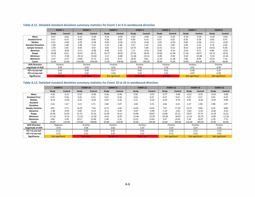
A-6
Table A.11. Detailed standard deviation summary statistics for Event 1 to 9 in westbound direction
EVENT 1 EVENT 2 EVENT 3 EVENT 4 EVENT 5 EVENT 7 EVENT 8
Study Control Study Control Study Control Study Control Study Control Study Control Study Control
Mean 0.07 -0.62 0.22 -0.38 0.24 -0.08 0.20 -0.46 1.26 -0.33 -0.19 -0.20 -0.24 -0.64 Standard Error 0.27 0.23 0.09 0.06 0.26 0.20 0.30 0.14 0.57 0.35 0.35 0.18 0.62 0.37
Median 0.31 -0.49 0.29 -0.38 0.04 -0.36 -0.23 -0.46 1.03 -0.29 0.06 -0.26 -0.11 -0.39 Standard Deviation 1.94 1.68 2.90 2.10 2.19 2.48 3.57 2.42 3.54 3.05 2.89 2.52 3.74 3.04
Sample Variance 3.78 2.83 8.43 4.42 4.81 6.14 12.75 5.84 12.51 9.32 8.34 6.34 14.02 9.26 Skewness -0.42 -0.83 -0.72 -0.48 0.40 0.33 1.17 -0.05 0.58 -0.14 -0.43 0.11 0.84 -0.93
Range 10.08 8.31 33.97 26.75 10.77 18.04 27.54 18.94 19.00 21.38 17.18 18.57 22.75 19.50 Minimum -5.71 -5.58 -19.12 -14.60 -4.17 -9.88 -11.28 -10.14 -6.90 -9.90 -9.32 -10.08 -9.19 -12.34 Maximum 4.37 2.73 14.85 12.15 6.61 8.17 16.26 8.81 12.10 11.48 7.86 8.49 13.56 7.16
Count 53.00 53.00 1103.00 1344.00 71.00 149.00 139.00 295.00 38.00 75.00 70.00 205.00 37.00 68.00
Shift Direction Positive Positive Positive Positive Positive Positive Positive magnitude of shift 0.69 0.60 0.32 0.66 1.59 0.01 0.40
P(T<=t) one-tail 0.03 0.00 0.17 0.02 0.01 0.48 0.29 P(T<=t) two-tail 0.05 0.00 0.34 0.05 0.02 0.97 0.58
Significance Significant Significant Not significant Significant Significant Not significant Not significant
Table A.12. Detailed standard deviation summary statistics for Event 10 to 16 in westbound direction
EVENT 9 EVENT 10 EVENT 11 EVENT 12 EVENT 13 EVENT 14 EVENT 16
Study Control Study Control Study Control Study Control Study Control Study Control Study Control
Mean -0.65 -0.21 0.52 -0.28 0.38 -0.44 0.92 -0.55 -0.77 -0.96 -0.31 -0.55 -0.45 -0.82 Standard Error 0.35 0.16 0.25 0.15 0.32 0.18 0.52 0.37 0.37 0.41 0.27 0.17 0.35 0.33
Median -0.14 -0.26 0.32 -0.26 0.34 -0.42 0.71 -0.29 -0.55 -0.74 0.01 -0.34 -0.39 -0.84 Standard Deviation
2.63 1.67 3.21 2.71 2.60 2.07 3.83 3.74 2.66 4.15 3.27 2.98 2.08 2.97
Sample Variance 6.91 2.77 10.33 7.34 6.75 4.30 14.65 14.01 7.07 17.24 10.72 8.90 4.33 8.80 Skewness -1.48 -0.50 0.06 -0.14 -0.11 -0.44 -0.07 -0.48 -1.34 -2.65 -0.62 -2.33 -0.46 -0.25
Range 15.96 13.54 21.37 27.42 12.09 14.12 24.96 28.87 13.86 37.32 19.07 37.72 11.59 19.22 Minimum -11.16 -8.14 -11.20 -15.36 -6.61 -8.95 -11.44 -15.05 -10.38 -26.87 -11.53 -26.75 -6.80 -11.50 Maximum 4.80 5.40 10.17 12.06 5.48 5.16 13.51 13.82 3.47 10.45 7.54 10.97 4.78 7.72
Count 56.00 114.00 172.00 328.00 65.00 133.00 55.00 105.00 52.00 104.00 152.00 305.00 35.00 82.00
Shift Direction Negative Positive Positive Positive Positive Positive Positive magnitude of shift -0.44 0.80 0.82 1.47 0.19 0.24 0.36
P(T<=t) one-tail 0.13 0.00 0.01 0.01 0.36 0.22 0.23 P(T<=t) two-tail 0.25 0.01 0.03 0.02 0.73 0.45 0.45
Significance Not significant Significant Significant Significant Not significant Not significant Not significant

A-7
Table A.13. Detailed gap summary statistics for Event 1 to 9 in eastbound direction
Event 1 Event 2 Event 3 Event 4 Event 5 Event 7 Event 8
Study Control Study Control Study Control Study Control Study Control Study Control Study Control
Mean -0.13 -0.18 -0.18 -0.28 -0.01 -0.57 -0.13 -0.18 N/A N/A -0.08 -0.15 0.59 -0.88 Standard Error 0.15 0.13 0.05 0.05 0.41 0.34 0.22 0.13 N/A N/A 0.14 0.09 0.38 0.51
Median 0.10 -0.21 -0.11 -0.26 0.04 -0.72 0.13 -0.31 N/A N/A -0.18 -0.21 0.47 -0.66 Standard Deviation 1.11 0.92 1.63 1.61 2.24 2.64 2.04 1.84 N/A N/A 1.13 0.99 2.08 2.61
Sample Variance 1.22 0.85 2.67 2.59 5.02 6.97 4.16 3.39 N/A N/A 1.28 0.99 4.33 6.84 Skewness -0.34 -0.20 -0.53 -0.20 0.12 0.26 -0.86 0.27 N/A N/A 1.22 -0.70 0.19 -0.84
Range 5.18 3.40 13.76 15.42 10.42 12.01 12.69 12.58 N/A N/A 7.97 10.57 10.37 11.82 Minimum -3.06 -1.97 -7.93 -7.85 -4.92 -6.68 -7.87 -6.80 N/A N/A -3.28 -6.17 -4.17 -7.71 Maximum 2.11 1.43 5.83 7.57 5.50 5.33 4.82 5.78 N/A N/A 4.69 4.40 6.20 4.12
Count 53.00 53.00 903.00 980.00 30.00 62.00 85.00 202.00 N/A N/A 64.00 129.00 30.00 26.00
Shift Direction Positive Positive Positive Positive N/A Positive Positive magnitude of shift 0.04 0.10 0.56 0.05 N/A 0.07 1.47
P(T<=t) one-tail 0.41 0.09 0.15 0.43 N/A 0.35 0.01 P(T<=t) two-tail 0.83 0.18 0.29 0.85 N/A 0.69 0.03
Significance Not significant Not significant Not significant Not significant N/A Not significant Significant
Table A.14. Detailed gap summary statistics for Event 10 to 16 in eastbound direction
Event 9 Event 10 Event 11 Event 12 Event 13 Event 14 Event 16
Study Control Study Control Study Control Study Control Study Control Study Control Study Control
Mean -0.10 -0.21 -0.23 -0.25 0.28 -0.23 0.05 -0.21 -0.07 -0.08 -0.16 -0.32 -0.02 -0.27 Standard Error 0.16 0.09 0.20 0.16 0.10 0.06 0.12 0.12 0.13 0.09 0.19 0.09 0.48 0.25
Median 0.00 -0.18 -0.16 -0.31 0.27 -0.27 0.10 -0.18 -0.10 -0.08 -0.20 -0.24 0.08 0.02 Standard Deviation 1.22 1.00 2.03 2.30 0.86 0.72 0.89 1.24 0.94 0.90 2.02 1.33 2.20 2.09
Sample Variance 1.48 0.99 4.12 5.28 0.74 0.52 0.79 1.53 0.89 0.81 4.06 1.78 4.82 4.35 Skewness 0.03 0.02 -0.76 0.29 1.88 0.12 1.58 -0.18 0.29 0.86 0.23 -0.40 -0.67 -0.38
Range 6.52 4.53 11.45 14.97 7.52 4.46 6.52 10.67 6.17 6.36 17.42 11.27 9.47 11.10 Minimum -2.92 -2.49 -6.80 -6.87 -2.49 -2.50 -2.30 -5.21 -3.13 -2.31 -9.04 -5.59 -5.83 -6.98 Maximum 3.60 2.04 4.64 8.10 5.03 1.96 4.21 5.47 3.03 4.04 8.38 5.68 3.64 4.12
Count 57.00 114.00 108.00 218.00 68.00 134.00 53.00 108.00 56.00 111.00 117.00 215.00 21.00 72.00
Shift Direction Positive Positive Positive Positive Positive Positive Positive magnitude of shift 0.11 0.02 0.51 0.26 0.01 0.16 0.25
P(T<=t) one-tail 0.27 0.47 0.00 0.06 0.47 0.22 0.32 P(T<=t) two-tail 0.55 0.94 0.00 0.13 0.95 0.44 0.65
Significance Not significant Not significant Significant Not significant Not significant Not significant Not significant

A-8
Table A.15. Detailed gap summary statistics for Event 1 to 9 in westbound direction
Event 1 Event 2 Event 3 Event 4 Event 5 Event 7 Event 8
Study Control Study Control Study Control Study Control Study Control Study Control Study Control
Mean 0.15 0.27 0.11 0.20 0.26 0.03 0.01 0.19 N/A N/A 0.20 0.36 -0.39 0.00 Standard Error 0.12 0.11 0.05 0.04 0.23 0.18 0.14 0.11 N/A N/A 0.20 0.19 0.44 0.37
Median 0.06 0.09 0.04 0.16 0.13 0.03 -0.04 0.17 N/A N/A 0.25 0.43 -0.13 -0.08 Standard Deviation 0.88 0.82 1.46 1.43 1.69 1.88 1.39 1.60 N/A N/A 1.44 1.95 2.13 2.12
Sample Variance 0.77 0.67 2.13 2.04 2.86 3.52 1.92 2.57 N/A N/A 2.08 3.80 4.52 4.50 Skewness 0.19 1.90 0.43 -0.03 0.78 -0.03 -0.29 0.20 N/A N/A -0.24 0.48 -0.50 0.70
Range 3.32 4.72 14.02 16.92 9.79 12.69 9.83 13.38 N/A N/A 8.93 14.09 8.98 10.31 Minimum -1.55 -0.83 -6.57 -8.87 -3.51 -6.47 -5.54 -6.51 N/A N/A -4.32 -6.03 -5.49 -4.37 Maximum 1.77 3.89 7.45 8.05 6.28 6.21 4.29 6.87 N/A N/A 4.61 8.06 3.49 5.94
Count 53.00 53.00 912.00 1064.00 55.00 113.00 93.00 225.00 N/A N/A 52.00 101.00 23.00 33.00
Shift Direction Negative Negative Positive Negative N/A Negative Negative magnitude of shift -0.12 -0.09 0.23 -0.19 N/A -0.16 -0.39
P(T<=t) one-tail 0.24 0.09 0.21 0.15 N/A 0.29 0.25 P(T<=t) two-tail 0.47 0.18 0.42 0.30 N/A 0.58 0.50
Significance Not significant Not significant Not significant Not significant N/A Not significant Not significant
Table A.16. Detailed gap summary statistics for Event 10 to 16 in westbound direction
Event 9 Event 10 Event 11 Event 12 Event 13 Event 14 Event 16
Study Control Study Control Study Control Study Control Study Control Study Control Study Control
Mean 0.23 0.35 0.05 0.34 -0.05 0.38 0.21 0.23 0.52 0.17 0.26 -0.04 0.73 0.22 Standard Error 0.10 0.09 0.17 0.12 0.17 0.11 0.25 0.20 0.27 0.19 0.14 0.10 0.31 0.25
Median 0.19 0.17 0.27 0.23 -0.22 0.31 0.10 -0.12 0.36 0.11 0.20 0.04 0.67 0.09 Standard Deviation 0.79 0.96 1.88 1.88 1.33 1.26 1.50 1.71 1.70 1.82 1.50 1.59 1.63 1.99
Sample Variance 0.62 0.92 3.53 3.53 1.76 1.58 2.24 2.91 2.89 3.33 2.26 2.54 2.65 3.97 Skewness 0.17 2.13 -0.55 0.33 -0.02 0.47 -0.02 1.00 2.57 1.02 0.73 -0.56 0.57 -0.30
Range 4.44 7.67 10.89 13.29 7.21 7.21 8.32 10.18 9.93 12.95 11.12 12.95 7.65 10.68 Minimum -1.92 -1.49 -6.42 -6.59 -3.89 -3.12 -4.33 -3.73 -1.63 -4.47 -4.03 -6.97 -2.43 -6.25 Maximum 2.52 6.18 4.47 6.70 3.32 4.09 3.99 6.45 8.31 8.48 7.09 5.97 5.22 4.42
Count 56.00 114.00 126.00 255.00 62.00 123.00 36.00 73.00 39.00 89.00 118.00 231.00 27.00 62.00
Shift Direction Negative Negative Negative Negative Positive Positive Positive magnitude of shift -0.12 -0.29 -0.43 -0.02 0.35 0.30 0.51
P(T<=t) one-tail 0.20 0.08 0.02 0.47 0.15 0.04 0.11 P(T<=t) two-tail 0.39 0.16 0.04 0.95 0.29 0.09 0.21
Significance Not significant Not significant Significant Not significant Not significant Significant Not significant

APPENDIX B: SUMMARY OF WEATHER IMPACTS
This appendix includes a summary of the nearest RWIS site, TH 7 @ MP 167.1 (Mayer) (330022). The
figures include the hourly precipitation as well as precipitation presence but additional data were
reviewed at each site including the atmospheric conditions, wind speed, and weather immediately
before each event.

B-1
Figure B.1. Precipitation accumulation (left) and presence (right) for Event 1
Figure B.2. Precipitation accumulation (left) and presence (right) for Event 2
Figure B.3. Precipitation accumulation (left) and presence (right) for Event 3
Figure B.4. Precipitation accumulation (left) and presence (right) for Event 4

B-2
Figure B.5. Precipitation accumulation (left) and presence (right) for Event 5
Figure B.6. Precipitation accumulation (left) and presence (right) for Event 7
Figure B.7. Precipitation accumulation (left) and presence (right) for Event 8
Figure B.8. Precipitation accumulation (left) and presence (right) for Event 9

B-3
Figure B.9. Precipitation accumulation (left) and presence (right) for Event 10
Figure B.10. Precipitation accumulation (left) and presence (right) for Event 11
Figure B.11. Precipitation accumulation (left) and presence (right) for Event 12
Figure B.12. Precipitation accumulation (left) and presence (right) for Event 13

B-4
Figure B.13. Precipitation accumulation (left) and presence (right) for Event 14
Figure B.14. Precipitation accumulation (left) and presence (right) for Event 15
Figure B.15. Precipitation accumulation (left) and presence (right) for Event 16